DESY 10-091HU-EP-10-33SFB/CPP-10-60

– HATHOR –

HAdronic Top andHeavy quarks crOss section calculatoR

M. Aliev a, H. Lackera, U. Langenfelda, S. Mochb,

P. Uwera and M. Wiedermanna

aHumboldt-Universität zu Berlin, Institut für PhysikNewtonstraße 15, D-12489 Berlin, Germany

bDeutsches Elektronensynchrotron DESYPlatanenallee 6, D–15735 Zeuthen, Germany

Abstract

We present a program to calculate the total cross section fortop-quark pair productionin hadronic collisions. The program takes into account recent theoretical developmentssuch as approximate next-to-next-to-leading order perturbative QCD corrections and itallows for studies of the theoretical uncertainty by separate variations of the factoriza-tion and renormalization scales. In addition it offers the possibility to obtain the crosssection as a function of the running top-quark mass. The program can also be appliedto a hypothetical fourth quark family provided the QCD couplings are standard.

Program summary

Title of program: Hathor

Version: 1.0

Catalogue number:

Program summary URL: http://www.physik.hu-berlin.de/pep/tools

http://www-zeuthen.desy.de/˜moch/hathor

E-mail: sven-olaf.moch@desy.de, peter.uwer@physik.hu-berlin.de

License: GNU Public License

Computers: Standard PCs (x86, x86_64 processors)

Operating system: Linux

Program language: C++, fortran, Java

Memory required to execute: 256 MB

Other programs called: None.

External files needed: Interface to LHAPDF for the user’s choice of parton distributionfunctions, seehttp://projects.hepforge.org/lhapdf/.

Keywords: Top-quarks, total cross section, QCD, radiative corrections, run-ning mass.

Nature of the physical problem: Computation of total cross section in perturbative QCD.

Method of solution: Numerical integration of hard parton cross section convolutedwith parton distribution functions.

Restrictions on complexity of theproblem:

None

Typical running time: A few seconds to a few minutes on standard desktop PCs or note-books, depending on the chosen options.

1

1 Introduction

The top-quark is the heaviest elementary particle in naturediscovered so far. As a consequence ofits large mass close to the scale of the electroweak symmetrybreaking it has remarkable propertiesmaking it a distinct research object. For example the short lifetime does not allow the formationof hadronic bound-states. Rather, the top-quark decays before it hadronizes, a fact often referredto colloquially as the top-quark behaving like a quasi-freequark. Non-perturbative effects are thusessentially cut-off by the short lifetime and, as an important consequence, the polarization of top-quarks can be studied through the parity violating decay into aW-boson and a bottom quark. Thetop-quark also provides an interesting environment for precision tests of the Standard Model (SM)and possible extensions, e.g., by constraining the allowedrange for the Higgs mass.A mandatory ingredient for top-quark physics at hadron colliders are precise theoretical predictionsto compare with. Current Tevatron measurements and the perspectives at LHC, i.e., a measurementof the top-quark pair cross section with an uncertainty of the order of 5% only set the target for the-oretical predictions of the production process. Clearly such an accuracy needs to include quantumcorrections.Within Quantum Chromodynamics (QCD) radiative corrections were calculated some time agoto next-to-leading order (NLO) first considering unpolarized top-quark production [1, 2] and laterincluding spin information [3]. In the former case, also completely analytical results have recentlybeen provided [4]. Beyond the NLO accuracy in QCD various sources of possible improvementshave been identified. Large logarithmic corrections due to soft gluon emission were investigatedand resummed at the next-to-leading-logarithmic (NLL) accuracy [5, 6] and recently improvedto include also the next-to-next-to-leading-logarithmic(NNLL) corrections [7–9]. Alternatively,resummation has also provided the means to construct parts of the full next-to-next-to-leading(NNLO) fixed order results [7, 10, 11], which can be supplemented by including all Coulombtype corrections [11] and also the full scale dependence at NNLO accuracy [7, 12]. With a targetprecision for the total cross section at the few per cent level also bound state effects from theresummation of Coulomb type corrections [13,14] as well as electro-weak radiative corrections atNLO [15–17] need to be considered.The compilation of all these results is in principle straight forward given the extensive literatureon the subject. However, no publicly available program exists so far which contains the latesttheoretical developments. The “modus operandi” of the pastwas that predictions were updated bytheorists from time to time taking into account new theoretical improvements and/or new sets ofparton distribution functions (PDFs). The aim of the present paper is to provide a program for thecomputation of the top-quark pair cross section including state of the art theory. As such it canserve as a reference for future cross section calculations.The program Hathor includes perturbativeQCD corrections at higher orders in the different approximations along with options allowing alsoa detailed study of the theoretical uncertainties. Moreover, it provides the possibility to computethe total cross section not only in the commonly adapted polemass scheme but also in terms oftheMS mass a choice recently employed for top-quark pair production in hadronic collisions forthe first time [12, 18]. Finally, the aim of this publication is not only to provide a tool for crosssection calculations but also to facilitate experimental analyses. To that end the package containsin addition to the stand alone program also a small library that can be easily integrated into existingcode.The outline of the article is a follows. In the next Section webriefly discuss the theoretical foun-dations as well as the procedure to convert to theMS mass. Sections 3 and 4 contain installationdetails and the program description while usage and examples are given in Section 5. We end with

2

conclusions in Section 6. All formulae as implemented in Hathor are collected in the Appendices Aand B.

2 Methods

The hadronic cross section for top-quark pair production isobtained from the convolution of thefactorized partonic cross section ˆσi j with the parton luminositiesLi j :

σh1h2→ttX(S,mt) =∑

i, j

S∫

4m2t

dsLi j (s,S,µ f ) σi j (s,mt,αs(µr ),µ f ) , (1)

Li j (s,S,µ f ) =1S

S∫

s

dss

fi/h1

(

sS,µ f

)

f j/h2

( ss,µ f

)

. (2)

HereS denotes the hadronic center-of-mass energy squared,µr , (µ f ) denotes the renormalization(factorization) scale and the functionsfi/h1,2(x,µ f ) are the PDFs describing the probability to finda parton of typei with a momentum fraction betweenx and x+ dx in the hadronhk. The QCDcoupling constantαs(µr ) is evaluated at the scaleµr . In the following we useαs in the schemewith nf light flavors. For top-quark production, the running is thusdetermined by the five lightflavorsu,d,c, s,b which we treat as massless. The top-quark massmt appearing in Eq. (1) is themass renormalized in the on-shell (pole-mass) scheme.In perturbative QCD the partonic cross section ˆσi j (s,mt,αs,µ f ) is expanded in the QCD couplingconstant up to NNLO:

σi j = a2s σ

(0)i j (s,mt)+a3

s σ(1)i j (s,mt,µr ,µ f )+a4

s σ(2)i j (s,mt,µr ,µ f ) + O(a5

s) , (3)

with as= αs/π.In leading-order (LO) only the parton channelsqq andggcontribute and the respective Born crosssections are given by:

σ(0)qq =

4π3

271sβ(3−β2), (4)

σ(0)gg =

π3

481s

{

(33−18β2+β4) ln

(

1+β1−β

)

−59β+31β3}

, (5)

with β =√

1−ρ andρ = 4m2t /s. Starting from NLO also thegq andgq channels contribute. In

Ref. [1] (and in many subsequent publications) an alternative decomposition was used in terms ofso-called scaling functionsfi j :

σi j =αs

2

m2t

{

f (0)i j (ρ)+4παs f (1)

i j (ρ,µ f /mt,µr/µ f )+ (4παs)2 f (2)

i j (ρ,µ f /mt,µr/µ f ) + O(αs3)}

. (6)

Since the scaling functions are dimensionless they depend only on ρ and the ratiosµ f /mt andµr/µ f . The full renormalization and factorization scheme dependence can be constructed usingthe renormalization group equation, the standard evolution equations of the PDFs and information

3

about lower orders, i.e., up to NNLO knowledge off (0)i j (ρ) and f (1)

i j (ρ,1,1) is sufficient. The generalstructure can be written in the following form

f (1)i j (ρ,µ f /mt,µr/mt) = f (10)

i j +LM f (11)i j +2β0LR f (0)

i j , (7)

f (2)i j (ρ,µ f /mt,µr/mt) = f (20)

i j +LM f (21)i j +L2

M f (22)i j +3β0LR f (10)

i j +3β0LRLM f (11)i j

+2β1LR f (0)i j +3β2

0L2R f (0)

i j , (8)

with i j = {qq,gg} and we abbreviateLM = ln(µ2f /m

2t ) andLR = ln(µ2

r /µ2f ). The scale dependence

in thegq (gq) channel can be easily derived from the above realizing thatf (0)gq = 0 so some terms

in Eqs. (7) and (8) are simplify absent. In the conventions used here the coefficients of the beta-functionβ0,β1 are given by

β0 =1

(4π)2

(

11−23

nf

)

, β1 =1

(4π)4

(

102−383

nf

)

. (9)

The Born contributions have been presented in Eqs. (4), (5) and at present also the complete NLOcorrections are known, i.e., the functionsf (10)

i j and f (11)i j in Eq. (7). A complete NNLO calculation

for the total cross section is not yet available, sincef (2)i j (ρ,µ f /mt,µr/mt) in Eq. (8) is missing the

contribution f (20)i j while f (21)

i j and f (22)i j have been obtained from renormalization group arguments

as mentioned above. However, exact expressions forf (20)i j in the limit ρ→ 1 based on soft-gluon

resummation have been derived and provide the foundation for approximate NNLO results ofσh1h2→ttX.The central physics questions to be addressed can be phrasedas follows:

• How large is the total cross sectionσh1h2→ttX at a given order in perturbation theory ?

• Given a computation of the total cross section according to Eq. (1) what is the associatedtheoretical uncertainty ?

In order to address these issues the package Hathor has different production models implementedwhich are accessible to the user as options. In the followingwe briefly describe these options as faras the underlying physics is concerned. To be self-consistent and for easier reference all necessarytheory input, e.g., the scaling functions has been collected in Appendix B. For details of how toaccess these options when running Hathor we refer to the nextSections 4 and 5.

Option LO

The optionLO provides a rough estimate although with large theoretical uncertainties which willreceive sizable corrections at higher orders. This option uses the Born cross sections of Eqs. (4), (5)(see also Eqs. (B.1)–(B.3)).

Option NLO

The optionNLO is the first instance where a meaningful theoretical uncertainty can be quoted inperturbation theory. This option employs the complete NLO QCD corrections [1, 2]. All scalingfunctions f (10)

i j are given as accurate fits [12] based on the recently published analytic results [4],(see also Eqs. (B.4)–(B.6)).

4

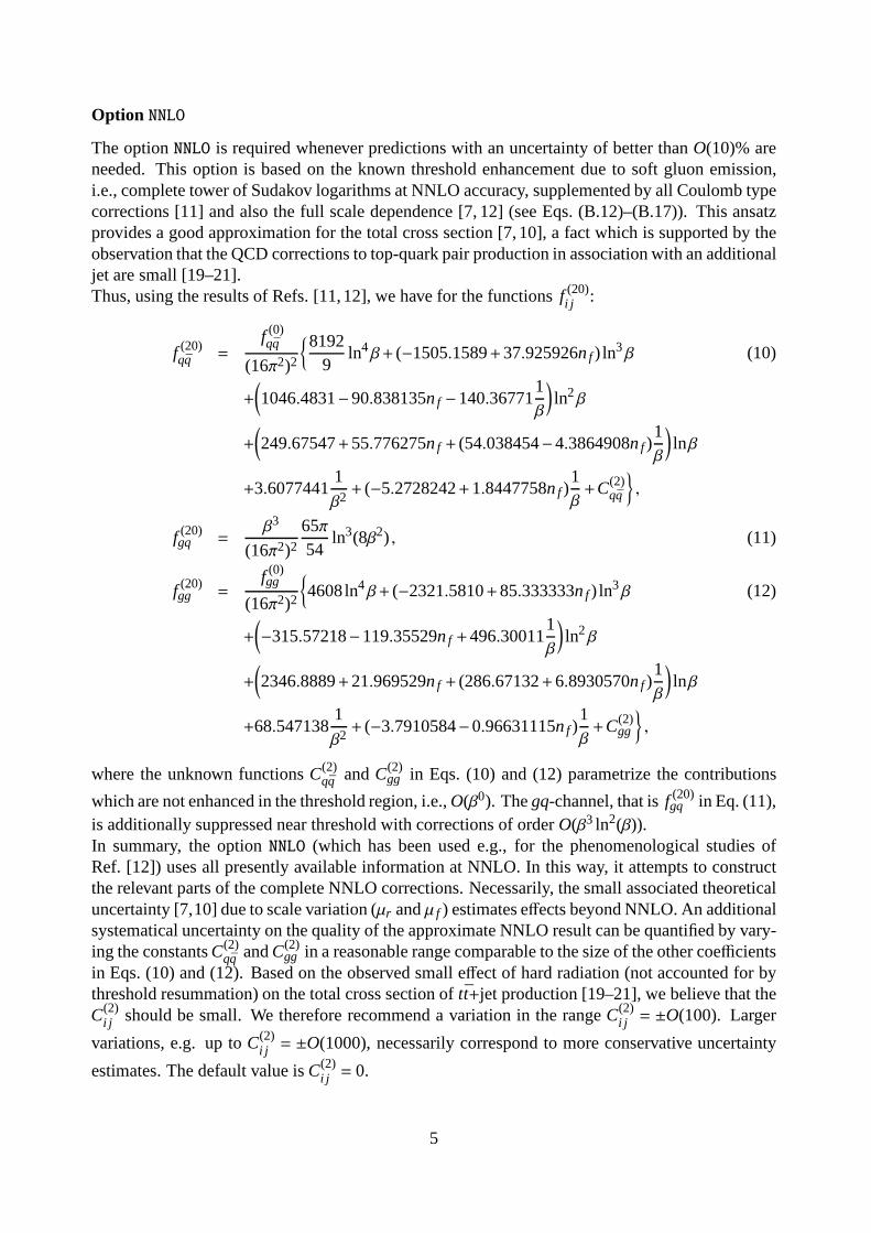
Option NNLO

The optionNNLO is required whenever predictions with an uncertainty of better thanO(10)% areneeded. This option is based on the known threshold enhancement due to soft gluon emission,i.e., complete tower of Sudakov logarithms at NNLO accuracy, supplemented by all Coulomb typecorrections [11] and also the full scale dependence [7, 12] (see Eqs. (B.12)–(B.17)). This ansatzprovides a good approximation for the total cross section [7, 10], a fact which is supported by theobservation that the QCD corrections to top-quark pair production in association with an additionaljet are small [19–21].Thus, using the results of Refs. [11,12], we have for the functions f (20)

i j :

f (20)qq =

f (0)qq

(16π2)2

{81929

ln4β+ (−1505.1589+37.925926nf ) ln3β (10)

+

(

1046.4831−90.838135nf −140.367711β

)

ln2β

+

(

249.67547+55.776275nf + (54.038454−4.3864908nf )1β

)

lnβ

+3.60774411

β2+ (−5.2728242+1.8447758nf )

1β+C(2)

qq

}

,

f (20)gq =

β3

(16π2)2

65π54

ln3(8β2) , (11)

f (20)gg =

f (0)gg

(16π2)2

{

4608ln4β+ (−2321.5810+85.333333nf ) ln3β (12)

+

(

−315.57218−119.35529nf +496.300111β

)

ln2β

+

(

2346.8889+21.969529nf + (286.67132+6.8930570nf )1β

)

lnβ

+68.5471381

β2+ (−3.7910584−0.96631115nf )

1β+C(2)

gg

}

,

where the unknown functionsC(2)qq andC(2)

gg in Eqs. (10) and (12) parametrize the contributions

which are not enhanced in the threshold region, i.e.,O(β0). Thegq-channel, that isf (20)gq in Eq. (11),

is additionally suppressed near threshold with corrections of orderO(β3 ln2(β)).In summary, the optionNNLO (which has been used e.g., for the phenomenological studiesofRef. [12]) uses all presently available information at NNLO. In this way, it attempts to constructthe relevant parts of the complete NNLO corrections. Necessarily, the small associated theoreticaluncertainty [7,10] due to scale variation (µr andµ f ) estimates effects beyond NNLO. An additionalsystematical uncertainty on the quality of the approximateNNLO result can be quantified by vary-ing the constantsC(2)

qq andC(2)gg in a reasonable range comparable to the size of the other coefficients

in Eqs. (10) and (12). Based on the observed small effect of hard radiation (not accounted for bythreshold resummation) on the total cross section oftt+jet production [19–21], we believe that theC(2)

i j should be small. We therefore recommend a variation in the rangeC(2)i j = ±O(100). Larger

variations, e.g. up toC(2)i j = ±O(1000), necessarily correspond to more conservative uncertainty

estimates. The default value isC(2)i j = 0.

5

Option LOG_ONLY

The optionLOG_ONLY is also motivated by the idea of soft gluon enhancement near threshold.It emerged as a conservative definition of the theoretical uncertainty in a comparison of differ-ent approaches to incorporate dominant terms beyond NLO to acertain logarithmic accuracy. Inparticular threshold resummation at NLL accuracy, performed as in Refs. [6, 22] which typicallyproceeds in Mellin-space, see Eq. (13), has been tested against an expansion in powers of lnk(β) inmomentum space as advocated in Ref. [7,10]. This comparisonhas yielded satisfactory agreement,because resummation beyond NLL, i.e., at NNLL accuracy has only a minor effect [7].The optionLOG_ONLY as discussed below is based on work with CCMMMNU [23]. It is a genuineNLO approach with logarithmic improvement near threshold and scale variations inµr andµ f (witha constraint on the ratio ofµr/µ f ) estimate effects beyond NLO. Being a conservative approach theresulting theoretical uncertainty is necessarily larger than in the optionNNLO.Let us briefly mention the essential technical points. In Refs. [6, 22] the logarithmic enhancementis constructed from the ln(N) terms in Mellin space where the resummation is usually performed.The transformation from momentum (ρ−) space to Mellin (N-) space is given by

σ(N) =∫ 1

0dρρN−1σ(ρ) , (13)

whereρ = 4m2t /s. The important feature of Eq. (13) to realize is that beyond logarithmic accuracy

the momentum space and the Mellin-space expressions do differ by terms which are not enhancedin β or, respectively power-suppressed in 1/N. Any difference could be included in a choice ofC(2)

i jin Eqs. (10), (12).OptionLOG_ONLY has to be used with the OptionNNLO and it is implemented in the following way(see [23] for further details): Beyond NLO the functionsf (0)

i j are truncated everywhere to theirleading term inβ (cf. Eqs. (4), (5)) and, This applies in particular to Eqs. (10) and (12) wheref (0)i j appear as overall factors, but we still keep the complete curly brackets in Eqs. (10) and (12),

i.e. we include also all Coulomb corrections∼ 1/β2 and∼ 1/β. For consistency, though, thegq-channel beyond NLO is neglected (f (20)

gq and Eqs. (B.14) and (B.15)). Also for the scale dependentpart, the optionLOG_ONLY keeps only terms which are logarithmically enhanced in the thresholdregion. In this case the functionsf (21)

i j and f (22)i j in Eqs. (B.12)–(B.17)) are truncated to logarithmic

accuracy. Again, one could also vary the constantsC(2)qq andC(2)

gg in a rangeC(2)i j = ±O(100) to test

for additional systematical uncertainties. The default value isC(2)i j = 0.

Option MS_MASS

The optionMS_MASS allows for the computation of the total cross sections as a functions of therunning mass in theMS scheme. In a nut-shell this is based on the replacementmt →m(m) (seeEq. (A.1)) in the expression forσh1h2→ttX in Eq. (1). The optionMS_MASS can be applied togetherwith optionsLO, NLO andNNLO.Let us briefly discuss the main motivation for this option. Sofar the mass used in all formulae isgiven as the so-called on-shell or pole-mass which is definedas the location of pole of the quarkpropagator calculated order-by-order in perturbation theory. It is well known that the pole-mass isnot a well defined concept in QCD since quarks do not appear as asymptotic states in the quantumfield theoretical description of the strong interaction owing to confinement. In other words, the

6

quark propagator does not have a pole in full QCD. A more quantitative analysis leads to theconclusion that the pole-mass is intrinsically uncertain of the order ofΛQCD (see e.g. [24, 25]).Since in perturbation theory the pole-mass can be expressedin terms of a short distance mass likefor example the running mass which is free from non-perturbative effects it is advantageous totranslate the cross section predictions from the on-shell scheme to theMS mass scheme. As abenefit, the convergence of the perturbative series is significantly improved when the running massis used and the extracted numerical value of the top-quark mass is very stable under higher ordercorrections. These observations were first pointed out in Ref. [12].In the Hathor program the conversionσh1h2→ttX(S,mt) → σh1h2→ttX(S,m(m)) has been realizednow in an easy way allowing a direct evaluation of the cross section using the running mass (seealso [18]). All details are deferred to Appendix A.

Option PDF_SCAN

The optionPDF_SCAN allows for the automated computation of PDF uncertainties.In the defaultsetting of the Hathor package the PDFs can be accessed with the LHAPDF library [26, 27]. Aprerequisite for this option is, of course, that the respective PDF provides a set of error PDFs.There are, however, different conventions with respect to PDF uncertainties.For instance, there exists the convention of asymmetric uncertainties, a choice adopted by e.g.MSTW [28] and CTEQ [29]. Here the error PDFs come innPDF pairs (σk,+,σk,−), where the firstelement of the pair describes the error of the correspondingparameter in the ’+’-direction, thesecond the one in the ’−’-direction. Then, for a given PDF set with a central fit resulting in a crosssectionσ0 the systematic uncertainty∆σ± is estimated by (see e.g. [30]),

∆σ± =12

√

∑

k=1,nPDF

(max(0,±σk,+∓σ0,±σk,−∓σ0))2 . (14)

Eq. (14) is the default of the Hathor package when using the optionPDF_SCAN. Following standardconventions the PDF uncertainty should be linearly added tothe theoretical uncertainty from scalevariations (parameterizing uncalculated higher orders).Other PDF sets, e.g. ABKM [31], employ the convention of symmetric uncertainties, where thenPDF elements each describe the (symmetric) ’±’-variation. In this case, the quadratic uncertainty∆σ± is obtained by adding the individual errors quadratically in the standard manner,

∆σ± =

√

∑

k=1,nPDF

(σk−σ0)2 , (15)

and the optionPDF_SCAN has to be combined with the additional optionPDF_SYM_ERR.Finally, there exist PDF sets, e.g. [32, 33] which simply return a numbernPDF of best fits, wheretypically nPDF ≃ O(100). Then, the PDF uncertainty of the cross sectionσ is estimated by com-puting it with each of the best fits and taking the standard statistical average. In such cases, theoptionPDF_SCAN cannot be used for an automated computation of the PDF uncertainty. WithinHathor, it of course, always possible for the user to provideown code for the evaluation of the PDFuncertainty.If, however, a PDF set provides different values of the strong couplingαs for different error PDFs,this is automatically taken into account.

7

Before continuing with the description of the Hathor program, let us mention that the packageoffers the possibility for several extensions in the future. With an experimental precision of 5%as envisaged at LHC the electro-weak radiative correctionsat NLO [15–17] have to be taken intoaccount. While for the Tevatron they turn out to be small (less than 1%) they are of the order of2% at LHC with a slight dependence on the Higgs mass. Electro-weak NLO corrections can beincluded in a similar manner as the higher order QCD corrections, i.e., with the help of accuratefits.Also the treatment of QCD radiative corrections leaves roomfor improvement, e.g. by incorpo-rating bound state effects from the resummation of Coulomb type corrections [13, 14]. Finally,the design of the Hathor package can in principle also accommodate related approaches for thecomputation of the total top-quark pair cross section beyond NLO, for instance those based on softgluon enhancement in differential kinematics [34,35] (see Ref. [36] for earlier work). Such extrap-olations of large logarithms from soft gluon emission in a differential variable (e.g. the top-quarkpair-invariant mass) to the full partonic phase space introduce systematic uncertainties and requirea detailed comparison to an inclusive approach such as in Eqs. (10)–(12).

3 Installation

In the default setting the Hathor package is based on the LHAPDF library [26] to access the PDFs.The Hathor package has been tested with the most recent version lhapdf-5.8.3 which can be ob-tained fromhttp://projects.hepforge.org/lhapdf. Please follow the instructions in theLHAPDF package to install the LHAPDF library. To build and use Hathor first unpack the pack-age usingtar xvfz Hathor.tar.gz at the location where one wants to install the package. Thiswill create a directory Hathor-1.0. Please create a symbolic link lhapdf inside this directory tothe location of ones LHAPDF installation. The contents oflhapdf should contain the LHAPDFinstallation with the directories:bin include lib lib64 share. Then use make to build theHathor package. Make will build the Hathor (static) librarylibHathor.a which can be used inother applications. In addition an example programmain.exe is built. For details concerning theexample program we refer to Section 5. Note that the compilation is done using the GNU com-pilers gcc, gfortran and g++. The package is known to work also with the Intel compiler. Infactwe recommend the usage of the Intel compiler since this results in a much better performance.However, given that it is not everywhere available Hathor uses the GNU compiler by default.1

To run the example one has to tell the system where the dynamiclibraries for LHAPDF can befound. This is conveniently done using the environment variableLD_LIBRARY_PATH. Using theC-shell the statement would be:setenv LD_LIBRARY_PATH <path_to_lhapdf_installation>/lib/

In addition, one probably needs to specify the location where the grid files for the LHAPDF libraryare stored. Again using the C-shell, the statement would be of the form:setenv LHAPATH <path_to_lhapdf_installation>/lhapdf/share/lhapdf/PDFsets

For a detailed description concerning the paths required bythe LHAPDF library, we refer to theLHAPDF manual. As concluding remarks with respect to the PDFlibraries we would like to pointout that Hathor does not try to handle errors from the LHAPDF library. This is not possible sinceLHAPDF does not provide a detailed error handling. Also notethat since LHAPDF is not threadsafe the same is true for Hathor.

1For the Intel compiler the user has to adapt themakefile.

8

Hathor is also equipped with a graphical user interface (GUI) written in Java. The GUI makesuse of dynamic libraries to access the Hathor library withinJava.2 The dynamic library is builtwith the commandCreateJavaGui.csh which is included in the Hathor package. The commandCreateJavaGui.csh creates the dynamic librarylibHathor4Java.so and writes the executablefile xhathor which is used to start the GUI. Please note thatxhathor sets up various paths: i.e.the environment variableLHAPATH is set to./lhapdf/share/lhapdf if it has not been set yet. Inaddition the dynamic librarieslibLHAPDF.so andlibgfortran.so on which the Hathor libraryrelies are preloaded. This step is platform dependent and not alway easy to achieve in a universalway. If the graphical interface does not start withxhathor the correct setting of the paths is alikely source of potential errors. In that case we recommendto set the necessary paths directly inxhathor or to consult the authors for support.

4 Description

The entire cross section is calculated inside the class Hathor. This is done in order to avoid anypossible problem with names used in already existing codes.Inside this class, a two dimensionalnumerical integration is performed in which the PDFs are convoluted with the hard scattering crosssection. As a numerical integration procedure we use the Vegas algorithm [37].3 Since Vegas isa Monte Carlo integration we need to provide random numbers.Those are obtained by using theRanlux algorithm [38] and we use the implementation available from Ref. [39].The Hathor class takes as constructor argument a reference to the PDF which should be used inthe current cross section calculation. In the following we list the publically available function callsand option choices together with a short description.

• Hathor(Pdf & pdf)

Constructor to build one instance of the Hathor class. The argument is an instance of thePDF. In case that LHAPDF is used the corresponding definitionwould be:Lhapdf pdf("MSTW2008nnlo68cl");

to use theMSTW2008nnlo68cl set.At first sight it might appear strange that we use an additional “wrapper class” as interfaceto LHAPDF. The idea behind this is to give the user the possibility to become independentfrom LHAPDF. This is achieved by inheriting the classLhapdf from the base classPdf. Byinhering its own class from the base class the user can thus easily implement its own wrapperto whatever PDF set he wants to use. As an example theclass MSTW has been supplied,which gives direct access to the MSTW set [28]. (Note that in the MSTW case theαs valueis set to 1 since the library does not provide a function to evaluate it. The user has thusprovide its ownαs.) We have observed that in some cases the original code provided withthe PDF sets is faster than what is provided by LHAPDF. Since the evaluation of the PDFsrepresents a significant part of the calculation the usage ofthe original PDFs may speed upthe entire calculation significantly.

• void printOptions()

Use this function to print the options currently selected via the routinesetScheme();

2The same technology can be used to access the Hathor library from Mathematica or Maple. The authors mayprovide the respective interfaces in a future update on demand.

3Hathor uses Vegas code which is a C port of the original fortran version [37].

9

• void setScheme(unsigned int newscheme)

Sets the specific scheme in particular perturbative order and renormalization schemes. Pos-sible options are:

– Hathor::LO to switch on the leading-order contribution.

– Hathor::NLO to switch on the individual NLO contribution.

– Hathor::NNLO to switch on the individual NNLO contribution (see Section 2).

Please also note that for the computation of the total cross section up to e.g. NNLO accuracy,it is necessary to combine the options as insetScheme(Hathor::LO | Hathor::NLO | Hathor::NNLO);

Other possible options are:

– Hathor::MS_MASS to use the mass renormalized in theMS scheme (see Section 2).

– Hathor::LOG_ONLY to keep only the logarithmically enhanced terms (see Section 2).Please note that this option requires alsoHathor::NNLO to be set.

– Hathor::PDF_SCAN to switch on the evaluation of the PDF uncertainties. That istosay, the error PDFs are also integrated along with the central value. To save comput-ing time one may set the accuracy withXS.setPrecision(Hathor::LOW) to LOWin this case. Care has to be taken, though, by the user to ensure that the default PDFuncertainty estimate as implemented in Hathor (asymmetricerror) complies with theconventions of the respective PDF set, as e.g. some PDF sets provide only a symmetricerror. In this case, the additional optionHathor::PDF_SYM_ERR needs to be set. Seealso the discussion in Section 2.

– Hathor::PDF_SYM_ERR invokes symmetric PDF error, if foreseen by the conventionof the PDF set.

Please note, that these options can again be combined, e.g. as insetScheme(Hathor::LO | Hathor::NLO | Hathor::MS_MASS);

• void setColliderType( COLLIDERTYPE type)

Sets the hadronic initial state. UseHathor::PP to select proton–proton collisions andHathor::PPBAR for proton–anti-proton collisions. The collider energiesare set to the de-fault values: 7 TeV in case of proton–proton collisions and 1960 GeV in case of proton–anti-proton collisions. If this is inappropriate the values can be changed using the commandvoid setSqrtShad(double ecms), where the center of mass energy is provided in GeV.

• void setSqrtShad(double ecms)

Sets the center-of-mass energy in GeV.

• void setNf(int nf)

Sets the number of massless flavors tonf. For top-quark physics the default setting isnf =

5 and should not be changed. This function may be used when thecross section for ahypothetical heavy quark of a fourth family is computed, as Hathor includes the fullnf

dependence of the hard scattering cross section, i.e. it features the formulae for generalnf .However, please note that the PDFs usually provideαs in thenf = 5 flavor scheme. So theuser should be careful with this option (and the interpretation of the results).

10

• void setCqq(double tmp)

Can be used to set the constant defined in Eq. (10) to a specific value (see Section 2). Thedefault isCqq = 0.

• void setCgg(double tmp)

Can be used to set the constant defined in Eq. (12) to a specific value (see Section 2). Thedefault isCgg = 0

• void setPrecision(int n)

Can be used to define the accuracy of the numerical integration performed by the Hathorpackage. It sets the number of function evaluations used in the Monte Carlo integration. Inprinciple, the user can provide any reasonable integer value.

Pre-defined values are:Hathor::LOW, Hathor::MEDIUM, Hathor::HIGH. We recommendLOW for the PDF scan andMEDIUM for the central value. This should be sufficient for mostapplications. Please note thatHathor::LOW should give already an accuracy at the percentlevel. For detailed comparisons of theoretical resultsHIGH may be used.

• double getAlphas(double mur)

Returns the QCD coupling constant at the renormalization scale mur as provided by the(central) PDF.

• double getXsection(double m, double mur, double muf)

This function starts the cross section calculation for a given top-quark mass and the factoriza-tion/renormalization scales provided as arguments. Unless a specific scheme is set throughsetScheme the default setting is used:Hathor::LO | Hathor::NLO | Hathor::NNLO

The cross section for the central PDF is returned. More information can be obtained throughgetResult.

• void getResult(int pdfset, double & integral, double & err)

This function is used to obtain additional information after the cross section has been cal-culated for a specific setting of the renormalization/factorization scale usinggetXsection.The integer valuepdfset specifies the respective PDF: 0 for the central value, and 1 togetPdfNumber() for the respective error PDF. The result for the central value and the nu-merical error from the numerical integration are returned throughintegral anderr. Notethaterr should always be negligible. If this is not the case the precision of the numericalintegration should be increased throughsetPrecision.

• void getPdfErr(double & up, double \& down)

This function returns the PDF uncertainty, if the optionHathor::PDF_SCAN has been used.By default, Hathor assumes an asymmetric PDF error convention. In case of a symmetricone, the optionPDF_SCAN has to be combined with the optionPDF_SYM_ERR (see Section 2and the discussion above).

• int getPdfNumber()

Returns the number of error PDFs currently in use. If 0 is returned the optionPDF_SCAN isnot switched on or the PDF set does not support error PDFs. E.g., in case of the PDF setmstw2008nnlo.68cl the return value would be 40.

11

• void sethc2(double)

Can be used to change the value for (hc)2 which is used by Hathor to convert the crosssections from GeV−2 to pico barn. The default used by Hathor is:0.389379323e+9.

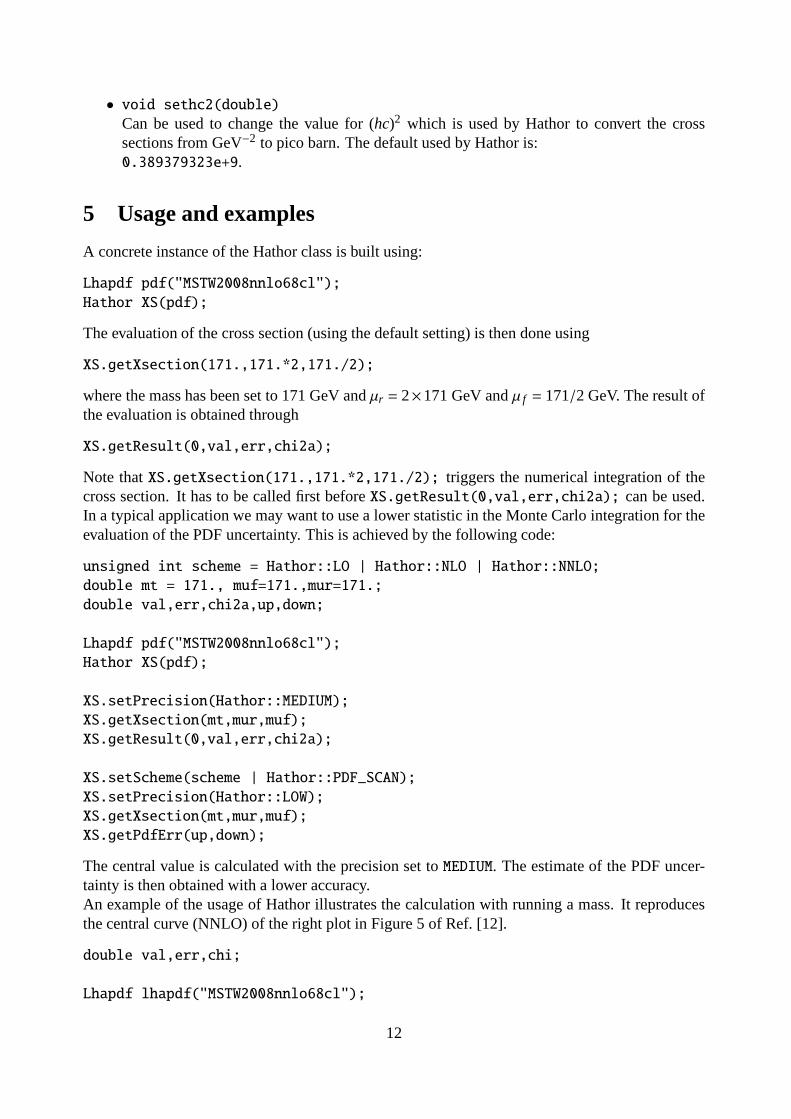
5 Usage and examples

A concrete instance of the Hathor class is built using:

Lhapdf pdf("MSTW2008nnlo68cl");

Hathor XS(pdf);

The evaluation of the cross section (using the default setting) is then done using

XS.getXsection(171.,171.*2,171./2);

where the mass has been set to 171 GeV andµr = 2×171 GeV andµ f = 171/2 GeV. The result ofthe evaluation is obtained through

XS.getResult(0,val,err,chi2a);

Note thatXS.getXsection(171.,171.*2,171./2); triggers the numerical integration of thecross section. It has to be called first beforeXS.getResult(0,val,err,chi2a); can be used.In a typical application we may want to use a lower statistic in the Monte Carlo integration for theevaluation of the PDF uncertainty. This is achieved by the following code:

unsigned int scheme = Hathor::LO | Hathor::NLO | Hathor::NNLO;

double mt = 171., muf=171.,mur=171.;

double val,err,chi2a,up,down;

Lhapdf pdf("MSTW2008nnlo68cl");

Hathor XS(pdf);

XS.setPrecision(Hathor::MEDIUM);

XS.getXsection(mt,mur,muf);

XS.getResult(0,val,err,chi2a);

XS.setScheme(scheme | Hathor::PDF_SCAN);

XS.setPrecision(Hathor::LOW);

XS.getXsection(mt,mur,muf);

XS.getPdfErr(up,down);

The central value is calculated with the precision set toMEDIUM. The estimate of the PDF uncer-tainty is then obtained with a lower accuracy.An example of the usage of Hathor illustrates the calculation with running a mass. It reproducesthe central curve (NNLO) of the right plot in Figure 5 of Ref. [12].

double val,err,chi;

Lhapdf lhapdf("MSTW2008nnlo68cl");

12

Hathor XS(lhapdf);

XS.setColliderType(Hathor::PPBAR);

XS.setScheme(Hathor::LO | Hathor::NLO | Hathor::NNLO | Hathor::MS_MASS );

XS.setPrecision(Hathor::LOW);

for(double mt = 140; mt < 181.; mt++ ){

XS.getXsection(mt,mt,mt);

XS.getResult(0,val,err,chi);

cout << mt << " " << XS.getAlphas(mt) <<" "<< val << " " << err << endl;

}

The typical runtimes for these examples range between seconds and a few minutes and also de-pend on the chosen compilers. E.g. on an Intel 3.00GHz QuadCore PC we have obtained with theoptionsNNLO, PDF_SCAN (PDF setMSTW2008nnlo68cl) andXS.setPrecision(Hathor::LOW)the result for the cross section after 64 seconds using the gfortran compiler, and, 41 seconds re-spectively, using Intel’s ifort compiler.

The Java GUI is invoked by the commandxhathor (see the discussion in Sec. 3 for the installa-tion). A screenshot is displayed in Fig. 1 and the input is self-explanatory with the help of Sec. 4for the description of all options.

Figure 1:Screen shot of the Java graphical user interface for Hathor.

6 Conclusions

Top-quark production at hadron colliders is at the edge of becoming a precision measurementrequiring accurate theory predictions. Hathor is a fast andflexible program for the computationof the total cross section of hadronic heavy-quark pair-production. It takes into account the latest

13

theoretical developments through a variety of options, it allows for separate variations of all scalesand can be used with a large number of PDFs through the LHAPDF interface. As a novelty,Hathor offers predictions in different renormalization schemes for the heavy-quark mass (pole andMS) and it can also be applied to a hypothetical fourth quark family assuming standard QCDcouplings. Thus, with these functionalities Hathor can serve as a reference for future cross sectioncalculations.Hathor typically runs in a few seconds up to a few minutes (depending on the chosen options, e.g.extensive PDF scans) on standard desktop or notebook PCs. The Hathor package can either beused as a stand alone program or, as a small library, it can be easily integrated into existing code,e.g. for experimental analyses.

Hathor is publicly available for download from [40] or from the authors upon request.

Acknowledgments

We acknowledge useful discussions with S. Alekhin and U. Husemann. This work is supportedin part by the Deutsche Forschungsgemeinschaft in Sonderforschungsbereich/Transregio 9 and theHelmholtz Gemeinschaft under contract VH-NG-105 and contract VH-HA-101 (Alliance“Physicsat the Terascale”).

A Total cross section with a running mass

The starting point is the relation between the on-shell massand theMS mass:

mt =m(µr )(

1+asd1+a2sd2

)

, (A.1)

with as= αs/π. If the decouplingαsnf=6→ αs

nf=5 is performed atm(µr ) the coefficients are givenby

d1 =43+ ℓ , (A.2)

d2 =30732+2ζ2+

23ζ2 ln2−

16ζ3+

50972ℓ+

4724ℓ2 (A.3)

−

(

71144+

13ζ2+

1336ℓ+

112ℓ2

)

nf +43

∑

l

∆(ml/mt) ,

which are known from Refs. [41–43] andℓ = ln(µr2/m(µr )

2). Note that the coefficientsdi dependin general on the renormalization scale. Usingm(m) instead ofm(µr ) the formulae simplify signifi-cantly. The full renormalization scale dependence can be restored at the end using renormalizationgroup arguments.∆(mi/mt) accounts for all massive quarksmi lighter than the top-quark. For alllight quarks we setml = 0 so the sum in Eq. (A.3) vanishes.To convert the cross section to theMS mass scheme we start from the hadronic cross sectionexpanded inαs:

σh1h2→ttX(S,mt) = a2sσ

(0)(S,mt)+a3sσ

(1)(S,mt)+a4sσ

(2)(S,mt)+O(a5s) . (A.4)

Expressingmt in terms ofm(m) and expanding inαs we obtain

σh1h2→ttX = a2sσ

(0)(S,m(m))+a3sσ

(1)(S,m(m))+a4sσ

(2)(S,m(m)) (A.5)

14

+a3sd1m(m)

dσ(0)(mt)dmt

∣

∣

∣

∣

∣

∣

mt=m(m)+a4

s

m(m)d2dσ(0)(mt)

dmt

∣

∣

∣

∣

∣

∣

mt=m(m)

+m(m)d1dσ(1)(mt)

dmt

∣

∣

∣

∣

∣

∣

mt=m(m)+

12

m(m)2d21

d2σ(0)(mt)

dmt2

∣

∣

∣

∣

∣

∣

mt=m(m)

.

The derivatives of the LO cross sections with respect to the mass can be written in the followingform:

dσ(0)(mt)dmt

∣

∣

∣

∣

∣

∣

mt=m(m)=

2m(m)

∫ S

4m(m)2ds

(

sddsLi j (s,S,µ f )

)

σ(0)i j (s,m(m)) , (A.6)

and

d2σ(0)

dm2t

∣

∣

∣

∣

∣

∣

mt=m(m)

= −2

m(m)2

∫ S

4m(m)2ds

(

sddsLi j (s,S,µ f )

)

σ(0)i j (s,m(m)) (A.7)

+2

m(m)

∫ S

4m(m)2ds

(

sddsLi j (s,S,µ f )

) dσ(0)i j

dmt

∣

∣

∣

∣

∣

∣

∣

∣

mt=m(m)

,

where a summation over the contributing parton channels is understood. Note that in Eqs. (A.5), (A.6)and (A.7) the renormalization scale is set toµr =m(m). The required derivatives of the LO partoniccross sections with respect to the mass are easily obtained from Eqs. (4), (5):

mtdσqq

dmt= −

1

m2t

19παs

2ρ3

β, (A.8)

mtdσgg

dmt=

1192παs

2 1

m2t

ρ

β

(

β(36−40β2+4β4) ln

(

1+β1−β

)

−7−116β2+91β4)

. (A.9)

For the first derivative ofσ(1) we obtain a similar result:

dσ(1)

dmt

∣

∣

∣

∣

∣

∣

mt=m(m)= −

∫ S

4m(m)2dsLi j (s,S,µ f )

1m(m)

σ(1)i j (s,m(m)) (A.10)

+2

m(m)

∫ S

4m(m)2ds

(

sddsLi j (s,S,µ f )

)

σ(i)(

s,m(m),µ f

m(m),1

)

,

with

σ(1)i j (s,m(m)) = µ f

∂

∂µ fσ

(1)i j

(

s,m(m),µ f

m(m),1

)

. (A.11)

Using Eq. (6) the contribution ˜σ(1)i j (s,m(m)) can be written as

a2sσ

(1)i j = 8

αs2(m(m))

m(m)2f (11)i j . (A.12)

Since the luminosities are only known numerically the derivatives are evaluated using

ddsLi j (s,S,µ f ) =

12δ

(

Li j (s+δ,S,µ f )−Li j (s−δ,S,µ f ))

+O(δ2) . (A.13)

The results presented so far are only valid forµr =m(m). Using

as(m(m)) = as(µr )(

1+4π2as(µr )LRβ0+ (4π2)2as(µr )2(β1LR+β

20L2

R))

, (A.14)

with LR= ln(µr2/m(m)2) it is easy to restore the complete renormalization scale dependence inas.

15

B Scaling functions

Here we present the expressions for the scaling functions asimplemented in the program Hathor.At Born level,

f (0)qq =

πβρ

27[2+ρ] , (B.1)

f (0)gq = 0, (B.2)

f (0)gg =

πβρ

192

[1β

(ρ2+16ρ+16) ln(1+β1−β

)

−28−31ρ]

, (B.3)

whereβ =√

1−ρ andρ = 4m2t /s. At NLO the functionsf (10)

i j have been described through preciseparametrizations with per mil accuracy and the following ansatz [12]:

f (10)qq =

ρβ

36π

[323

ln2β+

(

32ln2−823

)

lnβ−112π2

β

]

+βρaqq0 +h(β,a1, . . . ,a17) (B.4)

+1

8π2(nf −4) f (0)

qq

[43

ln2−23

lnρ−109

]

,

f (10)gq =

116πβ3

[59

lnβ+56

ln2−73108

]

+h(a)gq(β,a1, . . . ,a15) , (B.5)

f (10)gg =

7β768π

[

24ln2β+

(

72ln2−3667

)

lnβ+1184π2

β

]

+βagg0 +h(β,a1, . . . ,a17) (B.6)

+(nf −4)ρ2

1024π

[

ln(1+β1−β

)

−2β]

,

wherenf denotes the number of light quarks and the completenf -dependence has been kept

manifest. The constantsai j0 readaqq

0 = 0.03294734 andagg0 = 0.01875287 and the fit functions

h(β,a1, . . . ,a17) andh(a)gq(β,a1, . . . ,a15) are given in Eqs. (B.18), (B.19) together with a list of all

parameters in Tabs. 1–3. The exact expressions for scale dependent functionsf (11)i j have already

compact analytical form containing at most dilogarithms. They read [1]

f (11)qq =

1

8π2

[

16π81ρ ln

(

1+β1−β

)

+19

f (0)qq (ρ)

(

127−6nf +48ln

(

ρ

4β2

))]

, (B.7)

f (11)gq =

1

8π2

π

192

[

49ρ(

14ρ2+27ρ−136)

ln

(

1+β1−β

)

(B.8)

−323ρ (2−ρ)h1(β)−

8135β(

1319ρ2−3468ρ+724)

]

,

f (11)gg =

1

8π2

[

π

192

{

2ρ(

59ρ2+198ρ−288)

ln

(

1+β1−β

)

(B.9)

+12ρ(

ρ2+16ρ+16)

h2(β)−6ρ(

ρ2−16ρ+32)

h1(β)

−415β(

7449ρ2−3328ρ+724)

}

+12f (0)gg (ρ) ln

(

ρ

4β2

)]

,

with the auxiliary functions containing the standard dilogarithm Li2(x) = −∫ x0

dtt ln(1− t),

h1(β) = ln2(

1+β2

)

− ln2(

1−β2

)

+2Li2

(

1+β2

)

−2Li2

(

1−β2

)

, (B.10)

16

h2(β) = Li2

(

2β1+β

)

−Li2

(

−2β1−β

)

. (B.11)

At NNLO the functionsf (21)i j and f (22)

i j are known exactly [12]. The fits to the scaling functionsgenerally have per mil accuracy with exceptions in regions close to zero, where an accuracy betterthan one percent is kept.

f (21)qq =

1

(16π2)2f (0)qq

[

−8192

9ln3β+

(129283−

327689

ln2)

ln2β (B.12)

+

(

−840.51065+70.1838541β

)

lnβ−82.2467031β+467.90402

]

+nf

(16π2)2f (0)qq

[

−2563

ln2β+

(26089−

28169

ln2)

lnβ+6.57973631β−64.614276

]

+h(β,bi +nf ci)−4nf

2

(16π2)2f (0)qq

[

43

ln2−23

lnρ−109

]

,

f (22)qq =

1

(16π2)2f (0)qq

[20489

ln2β+

(

−7840

9+

40969

ln2)

lnβ+270.89724]

(B.13)

+nf

(16π2)2f (0)qq

[3209

lnβ−5969+

3209

ln2]

+h(β,bi +nf ci)+4nf

2

3(16π2)2f (0)qq ,

f (21)gq = −

π

(16π2)2β3

[77027

ln2β+

(

−680581+

616081

ln2)

lnβ+0.137077841β

(B.14)

+0.22068868]

−πnf

81(16π2)2β3

[

46lnβ−1633+76ln2

]

+h(b)gq(β,bi +nf ci)

f (22)gq =

π

(16π2)2β3

[38581

lnβ−1540243+

38581

ln2]

+h(b)gq(β,bi +nf ci) , (B.15)

f (21)gg =

1

(16π2)2f (0)gg

[

−4608ln3β+

(1099207−18432ln2

)

ln2β (B.16)

+

(

69.647185−248.150051β

)

lnβ+56.8677211β+17.010070

]

+nf

(16π2)2f (0)gg

[

−64ln2β+

(404821−192ln2

)

lnβ−3.44652851β−37.602004

]

+h(β,bi +nf ci) ,

f (22)gg =

1

(16π2)2f (0)gg

[

1152ln2β+ (−2568+2304ln2) lnβ−79.74312140]

(B.17)

+nf

(16π2)2f (0)gg

[

16lnβ−16+16ln2]

+h(β,bi +nf ci) ,

with the fit functionsh(β,a1, . . . ,a17) andh(b)gq(β,a1, . . . ,a18) (see Tabs. 1–3 for a list of all parame-

ters),

h(β,a1, . . . ,a17) = a1β2+a2β

3+a3β4+a4β

5 (B.18)

+a5β2 lnβ+a6β

3 lnβ+a7β4 lnβ+a8β

5 lnβ

+a9β2 ln2β+a10β

3 ln2β+a11β lnρ+a12β ln2ρ+a13β2 lnρ

+a14β2 ln2ρ+a15β

3 lnρ+a16β3 ln2ρ+a17β

4 lnρ ,

h(a)gq(β,a1, . . . ,a15) = a1β

4+a2β5+a3β

6 (B.19)

17

+a4β4 lnβ+a5β

5 lnβ+a6β6 lnβ

+a7β2ρ lnρ+a8β

2ρ ln2ρ+a9β3ρ lnρ

+a10β3ρ ln2ρ+a11β

4ρ lnρ

+a12β4ρ ln2ρ+a13β

2ρ ln3ρ+a14β2ρ ln4ρ+a15β

2ρ ln5ρ ,

h(b)gq(β,a1, . . . ,a18) = a1β

3+a2β4+a3β

5+a4β6+a5β

7 (B.20)

+a6β4 lnβ+a7β

5 lnβ+a8β6 lnβ+a9β

7 lnβ

+a10β3 lnρ+a11β

3 ln2ρ+a12β4 lnρ+a13β

4 ln2ρ

+a14β5 lnρ+a15β

5 ln2ρ+a16β6 lnρ+a17β

6 ln2ρ+a18β7 lnρ .

f (10)qq f (21)

qq f (22)qq

i ai bi ci bi ci

1 0.07120603 −0.15388765 −0.07960658 0.37947056 −0.00224114

2 −1.27169999 4.85226571 0.50111294 −4.25138041 0.02685576

3 1.24099536 −7.06602840 −0.09496432 2.91716094 −0.01777126

4 −0.04050443 2.36935255 −0.32590203 0.94994470 −0.00626121

5 0.02053737 −0.03634651 −0.02229012 0.10537529 −0.00062062

6 −0.31763337 1.25860837 0.23397666 −1.69689874 0.00980999

7 −0.71439686 2.75441901 0.30223487 −2.60977181 0.01631175

8 0.01170002 −1.26571709 0.13113818 −0.27215567 0.00182500

9 0.00148918 −0.00230536 −0.00162603 0.00787855 −0.00004627

10 −0.14451497 0.15633927 0.08378465 −0.47933827 0.00286176

11 −0.13906364 1.79535231 −0.09147804 −0.18217132 0.00111459

12 0.01076756 0.36960437 −0.01581518 −0.04067972 0.00017425

13 0.49397845 −5.45794874 0.26834309 0.54147194 −0.00359593

14 −0.00567381 −0.76651636 0.03251642 0.08404406 −0.00035339

15 −0.53741901 5.35350436 −0.25679483 −0.51918414 0.00363300

16 −0.00509378 0.39690927 −0.01670122 −0.04336452 0.00017915

17 0.18250366 −1.68935685 0.07993054 0.15957988 −0.00115164

Table 1:Coefficients for fits of theqq scaling functions.

18

f (10)gq f (21)

gq f (22)gq

i ai bi ci bi ci

1 −0.26103970 −0.00120532 0.00003257 −0.00022247 0.00001789

2 0.30192672 −0.04906353 0.00014276 0.00050422 0.00000071

3 −0.01505487 −0.20885725 −0.00402017 −0.02945504 −0.00020581

4 −0.00142150 −13.73137224 0.06329831 0.34340412 0.00108759

5 −0.04660699 14.01818840 −0.05952825 −0.31894917 −0.00086284

6 −0.15089038 −0.00930488 0.00002694 0.00009213 0.00000010

7 −0.25397761 −0.52223668 0.00159804 0.00690402 0.00001638

8 −0.00999129 −4.68440515 0.01522672 0.07847233 0.00022730

9 0.39878717 −7.61046166 0.02869438 0.16042051 0.00045698

10 −0.02444172 1.36687743 −0.00875589 −0.05186974 −0.00025620

11 −0.14178346 1.84698291 −0.00800271 −0.03861021 −0.00016026

12 0.01867287 −7.26265988 0.04043479 0.21650362 0.00070713

13 0.00238656 −4.89364026 0.01965878 0.10137656 0.00034937

14 −0.00003399 11.04566784 −0.05262293 −0.28056264 −0.00072547

15 −0.00000089 4.13660190 −0.01457395 −0.08090469 −0.00025525

16 0.00000000 −6.33477051 0.02314616 0.13077889 0.00034015

17 0.00000000 −1.08995440 0.00291792 0.01813862 0.00006613

18 0.00000000 1.19010561 −0.00220115 −0.01585757 −0.00006562

Table 2:Coefficients for fits of thegqscaling functions.

19

f (10)gg f (21)

gg f (22)gg

i ai bi ci bi ci

1 −8.92563222 −4.18931464 0.12306772 0.01222783 −0.00380386

2 149.90572830 82.35066406 −2.75808806 −0.77856184 0.08757766

3 −140.55601420 −87.87311969 3.19739272 1.33955698 −0.10742267

4 −0.34115615 9.80259328 −0.56233045 −0.59108409 0.02382706

5 −2.41049833 −1.12268550 0.03240048 0.00248333 −0.00099760

6 54.73381889 29.51830225 −0.92541788 −0.23827213 0.02932941

7 90.91548015 48.36110694 −1.57154712 −0.38868910 0.04906147

8 −4.88401008 −7.06261770 0.35109760 0.28342153 −0.01373734

9 −0.17466779 −0.08025226 0.00227936 0.00010876 −0.00006986

10 13.47033628 7.01493779 −0.21030153 −0.03383862 0.00658371

11 22.66482710 15.00588140 −0.63688407 −0.29071016 0.02089321

12 4.60726682 3.84142441 −0.12959776 −0.11473654 0.00495414

13 −67.62342328 −47.02161789 1.91690216 0.98929369 −0.06553459

14 −9.70391427 −8.05583379 0.26755747 0.24899069 −0.01046635

15 65.08050888 47.02740535 −1.86154423 −1.06096321 0.06559130

16 5.09663260 4.21438052 −0.13795865 −0.13425338 0.00551218

17 −20.12225341 −14.99599732 0.58155056 0.35935660 −0.02095059

Table 3:Coefficients for fits of theggscaling functions.

20

References[1] P. Nason, S. Dawson, and R. K. Ellis, Nucl. Phys.B303, 607 (1988).

[2] W. Beenakker, H. Kuijf, W. L. van Neerven, and J. Smith, Phys. Rev.D40, 54 (1989).

[3] W. Bernreuther, A. Brandenburg, Z. G. Si, and P. Uwer, Nucl. Phys.B690, 81 (2004), arXiv:hep-ph/0403035.

[4] M. Czakon and A. Mitov, Nucl. Phys.B824, 111 (2010), arXiv:0811.4119.

[5] N. Kidonakis and G. Sterman, Nucl. Phys.B505, 321 (1997), arXiv:hep-ph/9705234.

[6] R. Bonciani, S. Catani, M. L. Mangano, and P. Nason, Nucl.Phys.B529, 424 (1998), arXiv:hep-ph/9801375.

[7] S. Moch and P. Uwer, Phys. Rev.D78, 034003 (2008), arXiv:0804.1476.

[8] M. Czakon, A. Mitov, and G. Sterman, Phys. Rev.D80, 074017 (2009), arXiv:0907.1790.

[9] M. Beneke, P. Falgari, and C. Schwinn, Nucl. Phys.B828, 69 (2010), arXiv:0907.1443.

[10] S. Moch and P. Uwer, Nucl. Phys. Proc. Suppl.183, 75 (2008), arXiv:0807.2794.

[11] M. Beneke, M. Czakon, P. Falgari, A. Mitov, and C. Schwinn, (2009), arXiv:0911.5166.

[12] U. Langenfeld, S. Moch, and P. Uwer, Phys. Rev.D80, 054009 (2009), arXiv:0906.5273.

[13] K. Hagiwara, Y. Sumino, and H. Yokoya, Phys. Lett.B666, 71 (2008), arXiv:0804.1014.

[14] Y. Kiyo, J. H. Kühn, S. Moch, M. Steinhauser, and P. Uwer,Eur. Phys. J.C60, 375 (2009), arXiv:0812.0919.

[15] W. Beenakker, A. Denner, W. Hollik, R. Mertig, T. Sack, and D. Wackeroth, Nucl. Phys.B411, 343 (1994).

[16] W. Bernreuther, M. Fücker, and Z.-G. Si, Phys. Rev.D74, 113005 (2006), arXiv:hep-ph/0610334.

[17] J. H. Kühn, A. Scharf, and P. Uwer, Eur. Phys. J.C51, 37 (2007), arXiv:hep-ph/0610335.

[18] S. Moch, U. Langenfeld, and P. Uwer, (2010), arXiv:1001.3987.

[19] S. Dittmaier, P. Uwer, and S. Weinzierl, Phys. Rev. Lett. 98, 262002 (2007), hep-ph/0703120.

[20] S. Dittmaier, P. Uwer, and S. Weinzierl, Eur. Phys. J.C59, 625 (2009), arXiv:0810.0452.

[21] K. Melnikov and M. Schulze, JHEP0908, 049 (2009), arXiv:arXiv:0907.3090.

[22] M. Cacciari, S. Frixione, M. L. Mangano, P. Nason, and G.Ridolfi, JHEP09, 127 (2008), arXiv:0804.2800.

[23] M. Cacciari, M. Czakon, M. L. Mangano, A. Mitov, S. Moch,P. Nason, and P. Uwer, (2010), to appear.

[24] I. I. Bigi, M. A. Shifman, N. Uraltsev, and A. Vainshtein, Phys.Rev.D50, 2234 (1994), arXiv:hep-ph/9402360.

[25] M. C. Smith and S. S. Willenbrock, Phys.Rev.Lett.79, 3825 (1997), arXiv:hep-ph/9612329.

[26] M. R. Whalley, D. Bourilkov, and R. C. Group, (2005), hep-ph/0508110.

[27] CEDAR HepForge, LHAPDF data base,http://projects.hepforge.org/lhapdf/.

[28] A. D. Martin, W. J. Stirling, R. S. Thorne, and G. Watt, Eur. Phys. J.C63, 189 (2009), arXiv:0901.0002.

[29] P. M. Nadolskyet al., Phys. Rev.D78, 013004 (2008), arXiv:0802.0007.

[30] J. M. Campbell, J. Huston, and W. Stirling, Rept.Prog.Phys.70, 89 (2007), arXiv:hep-ph/0611148.

[31] S. Alekhin, J. Blümlein, S. Klein, and S. Moch, Phys. Rev. D81, 014032 (2010), arXiv:0908.2766.

[32] S. I. Alekhin, Phys.Rev.D63, 094022 (2001), arXiv:hep-ph/0011002.

[33] R. D. Ballet al., (2010), arXiv:arXiv:1002.4407.

[34] N. Kidonakis and R. Vogt, Phys. Rev.D78, 074005 (2008), arXiv:0805.3844.

[35] V. Ahrens, A. Ferroglia, M. Neubert, B. D. Pecjak, and L.L. Yang, (2010), arXiv:1003.5827.

[36] N. Kidonakis, E. Laenen, S. Moch, and R. Vogt, Phys. Rev.D64, 114001 (2001), arXiv:hep-ph/0105041.

[37] G. P. Lepage, J. Comp. Phys.27, 192 (1978).

21

[38] M. Lüscher, Comput. Phys. Commun.79, 100 (1994), arXiv:hep-lat/9309020.

[39] M. Lüscher, Ranlux,http://luscher.web.cern.ch/luscher/ranlux/index.html (GNU license).

[40] Hathor, http://www.physik.hu-berlin.de/pep/tools/ orhttp://www-zeuthen.desy.de/˜moch/hathor .

[41] N. Gray, D. J. Broadhurst, W. Gräfe, and K. Schilcher, Z.Phys.C48, 673 (1990).

[42] K. Chetyrkin and M. Steinhauser, Nucl.Phys.B573, 617 (2000), arXiv:hep-ph/9911434.

[43] K. Melnikov and T. v. Ritbergen, Phys.Lett.B482, 99 (2000), arXiv:hep-ph/9912391.

22