EUROPEAN ORGANISATION FOR NUCLEAR RESEARCH

CERN-PPE/95-1123 January 1995

Electroweak Measurements using

Heavy Quarks at LEP

T.Behnke

Universit�at Hamburg/DESY, II Institut f�ur Experimental Physik, Notkestrasse 85,D-22607 Hamburg, Germany

D.G.Charlton

Royal Society University Research Fellow,School of Physics and Space Research, University of Birmingham, Birmingham B15 2TT,

United Kingdom,and

PPE Division, CERN, CH-1211 Geneva 23, Switzerland

Abstract

Electroweak measurements at the LEP electron-positron collider have been made bothfor di�erent lepton and quark avours. The measurements in the heavy quark sector,speci�cally of the partial widths for Z0 decays to bb and cc and the forward-backwardb and c quark production asymmetries, are reviewed. Combined values from the LEPmeasurements are derived of �bb=�had = 0:2207� 0:0022, �cc=�had = 0:153� 0:011, and forthe asymmetries at

ps = 91:26 GeV, Ab

FB = 0:0902� 0:0045 and AcFB = 0:070� 0:012. In

the framework of the standard model, a value of �bb=�had = 0:2189� 0:0020 is obtained(for �cc=�had = 0:171). The b asymmetry is used to measure the e�ective electroweakmixing angle sin2 �e�W = 0:2328� 0:0008.

(Submitted to Physica Scripta)

1 Introduction

The LEP electron-positron collider at CERN started operation in 1989 with the goal of studyingthe properties of the intermediate vector boson of the weak neutral current, the Z0. Precisemeasurements have been made of the Z0 mass, its width and leptonic couplings using leptonicand inclusive hadronic decays of the Z0 [1]. With the large statistics now available from the�rst few years of LEP operation, the reach of high precision physics has been extended intothe investigation of heavy quarks. In particular the couplings of individual quark avourshave become the subject of increasing interest. They are measured via the partial width fora Z0 decay into a pair of quarks of a speci�c avour, and from forward-backward productionasymmetries.

In this paper the current status of these measurements is reviewed. The motivation forthe investigations are discussed in the next section, followed by a detailed presentation of thetechniques currently in use. Particular emphasis is given in section 3 to methods of preparingsamples of bottom, b, and charm, c, quarks. The results obtained by the LEP experimentsare reviewed in sections 4-6, and combined and compared with standard model predictions insection 7. Measurements of light quark electroweak observables are relatively limited, but arebrie y reviewed in section 8. Future prospects for the heavy quark measurements are discussedin section 9.

2 Motivations

One of the principal physics goals of the LEP collider is to measure accurately the couplingsof the Z0 to quarks and leptons. Measurements of the Z0 cross-section as a function of energy,the lineshape, the total hadronic decay width, �had, the leptonic partial widths, the forward-backward asymmetries of decays to leptons, and of the polarisation of � leptons produced inZ0 decays, have all contributed to the current extremely precise knowledge of the couplings ofthe Z0 to each avour of lepton. In the quark sector measurements are harder to make becauseof the di�culty in distinguishing between the di�erent primary quark avours produced inZ0 decays. Heavy quarks, however, provide a powerful insight into this sector, because theirlarge masses mean that they are only rarely produced in the hadronisation process, rather thandirectly from Z0 decay. The large masses and detectable lifetimes of hadrons containing heavyquarks further mean that it is possible to separate events containing them from light-quarkbackgrounds.

At LEP, the neutral current couplings of heavy quarks can be probed by measuring thepartial Z0 decay widths to bb and cc (denoted �bb and �cc respectively), and the angulardistribution of the produced heavy quarks relative to the beam axis. These quantities arepredicted by the standard model of the electroweak interaction. However, since only �ve of thesix quark avours are experimentally well established, and since no direct evidence for the Higgsboson exists as yet, numerical predictions can only be made as a function of the unknown massesof the top quark and the Higgs boson, denoted mtop and mHiggs, respectively. Most electroweakobservables depend on these parameters through radiative corrections involving a virtual topquark or Higgs boson.

In the lowest-order Born approximation, the partial Z0 decay width to a fermion-antifermion

1

pair ff, �ff, is expressed as a function of the coupling constants:

�ff =G�m

3Z

2�p2

�3� �2

2(gfV)

2 + �3(gfA)2

!: (1)

Here � is the velocity of the produced fermion f in the Z0 rest frame, G� the Fermi decayconstant, mZ the Z0 mass, and gfV; g

fA the vector and axial-vector electroweak neutral current

coupling constants. These latter are expressible:

gfV = I3;Lf � 2Qf sin2 �W (2)

gfA = I3;Lf ; (3)

where I3;Lf is the third component of weak isospin, taking values I3;Lf = 12;�1

2, for c and b

quarks, respectively, and Qf is the fermion charge, Qf = 23;�1

3, for c and b. The quantity

sin2 �W, the electroweak mixing angle, is de�ned by

sin2 �W � 1 �m2W=m

2Z : (4)

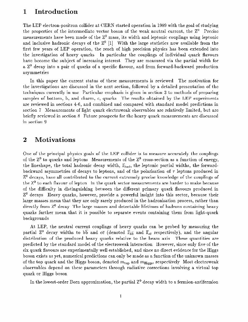
This lowest-order formalism is, however, insu�ciently accurate for precise electroweak measure-ments made at LEP: the radiative corrections have to be taken into account.

e-

e+Z

W

t–

tb

b–

e-

e+Z t

W

W b

b–

Figure 1: Two Feynman diagrams which contribute to the Z0-bb-speci�c vertex corrections. Suchdiagrams are unimportant for �nal dd and ss avours because the d and s quarks lie in di�erent weakisospin doublets to the top quark.

The Z0-bb vertex is particularly interesting in this context. Radiative corrections a�ect thisvertex di�erently to those of other lighter fermion avours because the b quark is in the sameweak isospin doublet as the top quark. This means that loop diagrams involving top quarks,such as those shown in �gure 1, contribute quite di�erently to this vertex than to the others.The other important graphs in this context are corrections to the Z0 propagator, which a�ect all

2

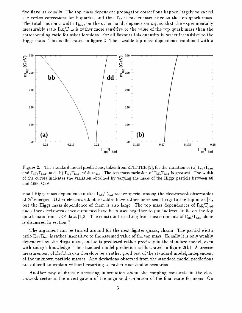
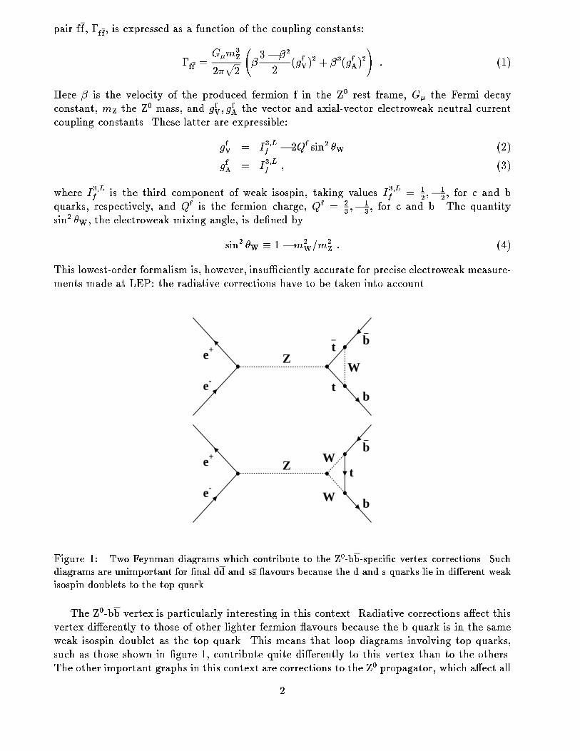
�ve avours equally. The top mass dependent propagator corrections happen largely to cancelthe vertex corrections for b-quarks, and thus �bb is rather insensitive to the top quark mass.The total hadronic width �had, on the other hand, depends on mt, so that the experimentallymeasurable ratio �bb=�had is rather more sensitive to the value of the top quark mass than thecorresponding ratio for other fermions. For all avours this quantity is rather insensitive to theHiggs mass. This is illustrated in �gure 2. The sizeable top mass dependence combined with a

Γqq–/Γhad

mto

p (G

eV)

bb–

dd–

(a)0.21 0.215 0.22

50

100

150

200

250

300

Γcc–/Γhad

mto

p (G

eV)

(b)0.165 0.17 0.175 0.18

50

100

150

200

250

300

Figure 2: The standard model predictions, taken from ZFITTER [2], for the variation of (a) �bb=�hadand �dd=�had, and (b) �cc=�had, with mtop. The top mass variation of �bb=�had is greatest. The widthof the curves indicates the variation obtained by varying the mass of the Higgs particle between 60and 1000 GeV.

small Higgs mass dependence makes �bb=�had rather special among the electroweak observablesat Z0 energies. Other electroweak observables have rather more sensitivity to the top mass [3],but the Higgs mass dependence of them is also large. The top mass dependences of �bb=�hadand other electroweak measurements have been used together to put indirect limits on the topquark mass from LEP data [1,3]. The constraint resulting from measurements of �bb=�had aloneis discussed in section 7.

The argument can be turned around for the next lighter quark, charm. The partial widthratio �cc=�had is rather insensitive to the assumed value of the top mass. Equally it is only weaklydependent on the Higgs mass, and so is predicted rather precisely in the standard model, evenwith today's knowledge. The standard model prediction is illustrated in �gure 2(b). A precisemeasurement of �cc=�had can therefore be a rather good test of the standard model, independentof the unknown particle masses. Any deviations observed from the standard model predictionsare di�cult to explain without resorting to rather unorthodox scenarios.

Another way of directly accessing information about the coupling constants in the elec-troweak sector is the investigation of the angular distribution of the �nal state fermions. On

3

the pole of the Z0 resonance the vector and the axial-vector components of the neutral currentinterfere and result in an asymmetry relative to the direction of the initial state fermion. Inter-ference also occurs between the electromagnetic and neutral weak currents. On the peak thisinterference vanishes, but it becomes more and more important at energies away from the Z0

pole.

The forward-backward asymmetry, AfFB, for the process e

+e� ! Z0 ! ff, is de�ned:

AfFB �

�F � �B

�F + �B; (5)

where �F/�B are the cross-sections for the fermion f to be produced in the forward/backwardhemisphere, respectively, and where the forward hemisphere refers to cos � > 0, where � isthe polar angle at which the outgoing fermion is produced relative to the e� beam direction.In the standard model to lowest order, for centre-of-mass energies close to the Z0 mass, thedistribution in cos � can be written:

d�

d cos �/ 1 + cos2 � +

8

3AfFB cos � : (6)

On the pole of the Z0 resonance for heavy quark avour Q, AQ;0FB , the forward-backward asym-

metry, can again be expressed as a function of the electroweak coupling constants gfV and gfA:

AQ;0FB =

3

4AeAQ ; (7)

where Ae and AQ are given by:

Af =2gfVg

fA

(gfV)2 + (gfA)

2=

2(1� 4jQfj sin2 �W)1 + (1 � 4jQf j sin2 �W)2

: (8)

Note that heavy quark asymmetry measurements at LEP can only measure the product AeAQ.However, AQ can be measured directly if signi�cant longitudinal polarization is present in theelectron or positron beams. In this case AQ can be derived by measuring the left-right forward-backward asymmetry. This is currently only possible at the SLC electron-positron collider atSLAC. The SLC results are brie y presented in section 7.

Electroweak radiative corrections modify these formulae only slightly. The corrections areconventionally absorbed by modifying equation (2) to contain an e�ective mixing angle sin2 �e�W ,instead of the sin2 �W de�ned by equation (4).

Measuring the asymmetry on the pole of the Z0 therefore probes quite directly the weakneutral current couplings or, alternatively, sin2 �W. Repeating the asymmetry measurementsat energies away from the pole, even within the small centre-of-mass energy range investigatedat LEP-I, gives sensitivity to -Z0 interference and tests the combined electroweak predictionof the standard model.

In practice the situation is modi�ed by the e�ects of photon radiation and photon-exchangediagrams, which mean that the measured Af

FB di�ers from the pole asymmetry, Af;0FB, that

would be obtained with pure on-mass-shell Z0 decays. This and other small corrections neededto correct from the measured to the pole asymmetry are discussed in section 6.4.

4

Measurements of the Z0 lineshape together with lower energy neutrino-scattering measure-ments indicate that sin2 �W � 0:23, predicting:

Ae � 0:14

Ab � 0:94 ; Ab;0FB � 0:10

Ac � 0:67 ; Ac;0FB � 0:07

The di�erent fermion asymmetries have di�erent sensitivities to sin2 �W:

�(sin2 �W) � �1

6�(Ab;0

FB) (9)

�(sin2 �W) � �1

4�(Ac;0

FB) (10)

These sensitivities are greater than for Z0 decays to charged lepton pairs `+`�, where:

�(sin2 �W) � �1

2�(A`;0

FB) : (11)

To understand the properties of the data, it is often necessary to use Monte Carlo simulationprograms. The JETSET Monte Carlo program [4], tuned to agree with LEP and lower energydata, is usually employed to model the Z0 decay and the hadronisation process. Each of theLEP experiments has its own special detector simulation program through which Monte Carloevents are passed. These detector simulation packages produce event structures similar to thoseof the real data, so that the same analysis programs can be used for either type of event.

3 Heavy Quark Tagging Techniques

At LEP, Z0's are produced essentially at rest in the four detectors, ALEPH, DELPHI, L3and OPAL. All four have a similar construction, with charged particle tracking chambers,calorimetry, and muon detection over almost the entire solid angle [5]. The detectors arebuilt with approximately cylindrical geometries, with a uniform magnetic �eld parallel to thebeam inside the tracking volumes. Particularly important for heavy avour physics are thehigh precision silicon microvertex detectors of the experiments { these have been added by allfour collaborations since LEP started. Results using these precise vertex detectors have beenpublished by ALEPH, DELPHI and OPAL, and analyses from L3, whose microvertex detectorwas installed last, are in progress.

The experimental method of measuring heavy quark partial widths and asymmetries pro-ceeds by �rst isolating a pure sample of hadronic Z0 decays. Events containing heavy quarksare selected using various tagging techniques. A good understanding of these tagging methodsis essential for precise electroweak measurements, and the techniques are therefore discussedin detail in this section. The partial width ratios �QQ=�had, where Q is b or c, can be derivedstraightforwardly from the number of tagged events and the total number of hadronic events,if the e�ciencies are known. A more sophisticated technique, \double-tagging", allows theheavy quark tagging e�ciency also to be derived from the data, and is described in section 4.Forward-backward asymmetry measurements, on the other hand, also require that the axisof the Z0 decay to quark-antiquark pair be identi�ed, and that the quark and antiquark bedistinguished, in practice achieved using a charge measure.

5

Hadronic Z0 decays can easily be identi�ed at LEP. Backgrounds from Z0 decays to lep-ton pairs are rejected by cutting on the charged track or electromagnetic cluster multiplicities.Backgrounds, from cosmic rays, detector noise, beam-gas interactions, and two-photon pro-cesses, can be rejected by requiring a high visible energy in the event as expected from Z0

decay, that several tracks come from the interaction point, and that the momentum ow in theevent is approximately balanced. The selection e�ciencies for hadronic Z0 decays are typicallybetween 95% and 99%, and are known to the 0.5% level or better. Residual background comesmostly from Z0 decays to �+��, and is typically at the level of 0.1-0.5%. The quality of thehadronic event selection procedure is su�cient to ensure that consequent errors on the heavyquark electroweak measurements are negligible.

The four heavy quark tagging techniques employed are discussed in the following subsec-tions. At present, lifetime and lepton tags are most powerful for Z0 ! bb events, lepton andreconstructed particle tags for Z0 ! cc events. The decaying quark charge can be estimatedfrom the charges of leptons and reconstructed particles, when they are used as tags. For othertag types, such as vertex tags, a special technique is needed. This is provided by \hemispherecharge" estimators, as discussed in section 3.5.

The ight direction of a heavy quark needs to be estimated for two purposes. For the asym-metry measurement, the axis of the Z0 ! QQ decay must be estimated { this is customarilytaken to be the event thrust axis. Most of the tagging techniques use the kinematic propertiesof heavy hadron decays, such as their large mass, to identify them. These approaches bene�tgreatly from a good estimate of the ight direction of the heavy hadron being tagged. Thissecond type of direction estimate, of the decaying heavy hadron rather than the Z0 decay axis, isusually obtained using a jet-�nding algorithm, identifying jet directions with quark ight direc-tions. The details of jet reconstruction vary from analysis to analysis, but a similar algorithmis used throughout.

The jet-�nding algorithm takes as input a set of energy-momentum four-vectors, and clustersthem into jets. The input four-vectors supplied approximate the individual �nal-state particles.ALEPH, DELPHI and OPAL use calorimeter energy deposits and reconstructed tracks to givethe input four-vectors, removing energy matched with tracks to avoid double counting. L3use calorimeter energy alone, as that performs just as well. These input \particles" are thenclustered according to the jet-�nding algorithm. Practically all analyses use an algorithm �rstproposed by the JADE collaboration [6]. This proceeds by considering all pairs of particles, iand j, and calculating the invariant-mass-squared of each pair, M2

ij , de�ned by:

M2ij = 2EiEj(1� cos�ij) (12)

where Ei, Ej are the energies of the two particles, and �ij is the angle between them. Thepair with the lowest mass are merged into a single \pseudo-particle" with four-momentumequal to the sum of the four-momenta of the two constituents. The procedure is repeated untilthe masses of all particle and pseudo-particle pairs are greater than a cut-o� threshold. Thetwo most common variants of the scheme either apply a �xed mass-squared cut-o�, xmin, or a�xed cut-o�, ycut, on the mass-squared scaled by the visible energy in the event. These twoschemes give similar performance, and the typical cut-o�s used for heavy quark measurementsare xmin = 36-49 GeV2, or alternatively ycut = 0:01-0:02. In Z0 ! bb events, such jet-�ndingschemes give estimates of the b hadron direction with a typical resolution of about 70 mrad,improving to about 50 mrad for jet energies above 10 GeV.

6

In the discussions that follow in this section, it should be understood that the variousheavy avour tags can be applied to complete events, event hemispheres, or other restrictedparts of events. For simplicity the tags are frequently discussed as applying to events { thisshould not be taken to imply any loss of generality. In practice, tags are often applied to eventthrust hemispheres, de�ned as being separated by the plane through the interaction pointperpendicular to the event thrust axis.

3.1 Lifetime Tagging Techniques

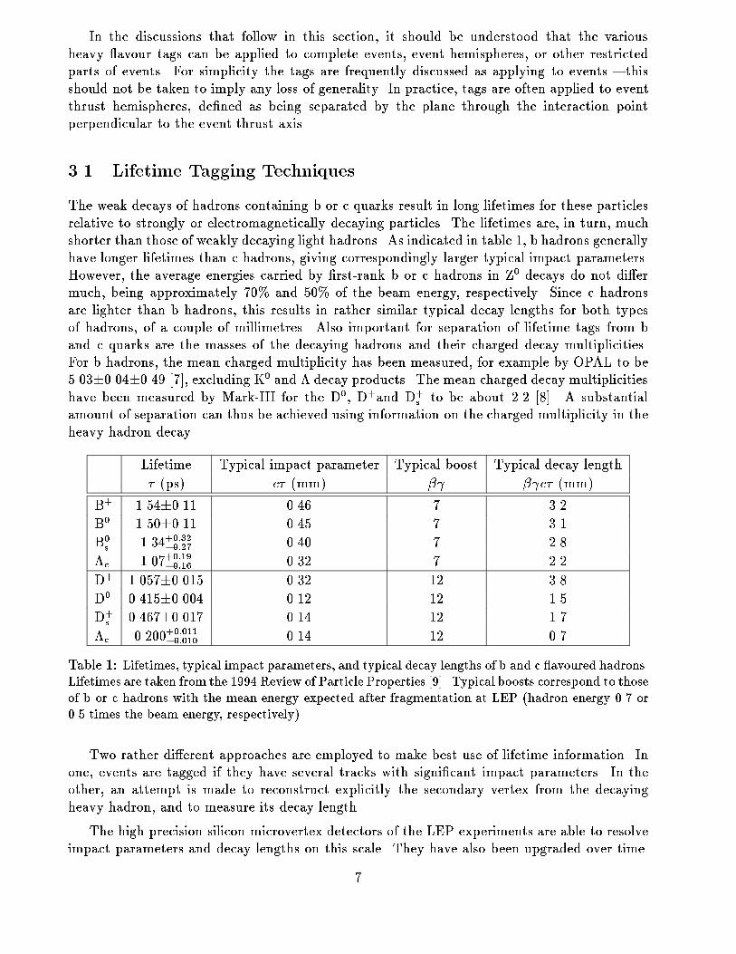
The weak decays of hadrons containing b or c quarks result in long lifetimes for these particlesrelative to strongly or electromagnetically decaying particles. The lifetimes are, in turn, muchshorter than those of weakly decaying light hadrons. As indicated in table 1, b hadrons generallyhave longer lifetimes than c hadrons, giving correspondingly larger typical impact parameters.However, the average energies carried by �rst-rank b or c hadrons in Z0 decays do not di�ermuch, being approximately 70% and 50% of the beam energy, respectively. Since c hadronsare lighter than b hadrons, this results in rather similar typical decay lengths for both typesof hadrons, of a couple of millimetres. Also important for separation of lifetime tags from band c quarks are the masses of the decaying hadrons and their charged decay multiplicities.For b hadrons, the mean charged multiplicity has been measured, for example by OPAL to be5.03�0.04�0.49 [7], excluding K0 and � decay products. The mean charged decay multiplicitieshave been measured by Mark-III for the D0, D+and D+

s to be about 2.2 [8]. A substantialamount of separation can thus be achieved using information on the charged multiplicity in theheavy hadron decay.

Lifetime Typical impact parameter Typical boost Typical decay length

� (ps) c� (mm) � � c� (mm)

B+ 1.54�0.11 0.46 7 3.2

B0 1.50�0.11 0.45 7 3.1

B0s 1.34+0:32�0:27 0.40 7 2.8

�c 1.07+0:19�0:16 0.32 7 2.2

D+ 1.057�0.015 0.32 12 3.8

D0 0.415�0.004 0.12 12 1.5

D+s 0.467�0.017 0.14 12 1.7

�c 0.200+0:011�0:010 0.14 12 0.7

Table 1: Lifetimes, typical impact parameters, and typical decay lengths of b and c avoured hadrons.Lifetimes are taken from the 1994 Review of Particle Properties [9]. Typical boosts correspond to thoseof b or c hadrons with the mean energy expected after fragmentation at LEP (hadron energy 0.7 or0.5 times the beam energy, respectively).

Two rather di�erent approaches are employed to make best use of lifetime information. Inone, events are tagged if they have several tracks with signi�cant impact parameters. In theother, an attempt is made to reconstruct explicitly the secondary vertex from the decayingheavy hadron, and to measure its decay length.

The high precision silicon microvertex detectors of the LEP experiments are able to resolveimpact parameters and decay lengths on this scale. They have also been upgraded over time.

7

In some analyses high precision microvertex information is available in three dimensions, inothers only in the plane perpendicular to the beam axis. When this is the case, lifetime tagalgorithms use impact parameters (or decay lengths) projected into this plane. This two-dimensional problem is relatively straightforward, the full three-dimensional problem is rathermore complex.

A common requirement in all the lifetime tag methods is for a precise estimate of the primaryvertex position. This is obtained event by event by �tting reconstructed tracks to a commonprimary vertex point, discarding those which are inconsistent with coming from the primary.Tracks from heavy avour decays will often be included in this primary vertex determination,leading to a mis-determined primary vertex. Such e�ects have to be considered in lifetime taganalyses, either explicitly, or by modifying the primary vertex position �t to make it insensitiveto such tracks. The position and size of the LEP beam spot are usually included as constraintsin the event-by-event primary vertex �t. The size and position of the beam spot are themselvesdetermined by averaging over many events the primary vertex position found without the beam-spot constraint. The spot position varies with time, and the size changes if the LEP machineoptics are changed. The position is measured with a typical precision of 10�m in the planetransverse to the beam. The beam spot shape is highly elliptical in this plane, being around5-10 �m vertically and 100 �m horizontally. The beam spot is typically 1 cm long.

In many of the analyses, it is necessary to use Monte Carlo simulated data to evaluatethe performance of tagging algorithms. Much e�ort has been invested to ensure that theuncertainties so introduced do not dominate errors on results. For lifetime tags, use of simulateddata is particularly important. Corrections are commonly applied to the simulated data toimprove agreement with data, and it is customary to vary the size of these corrections toestimate detector resolution uncertainties.

3.1.1 Impact Parameter Lifetime Tags

The simplest lifetime tagging method is to require that there be some minimum number oftracks with impact parameter above a threshold. However, impact parameter resolution errorsare sometimes comparable with the impact parameters being measured, so it is preferable tocut on the \impact parameter signi�cance", S, de�ned as the impact parameter divided by itsmeasurement error.

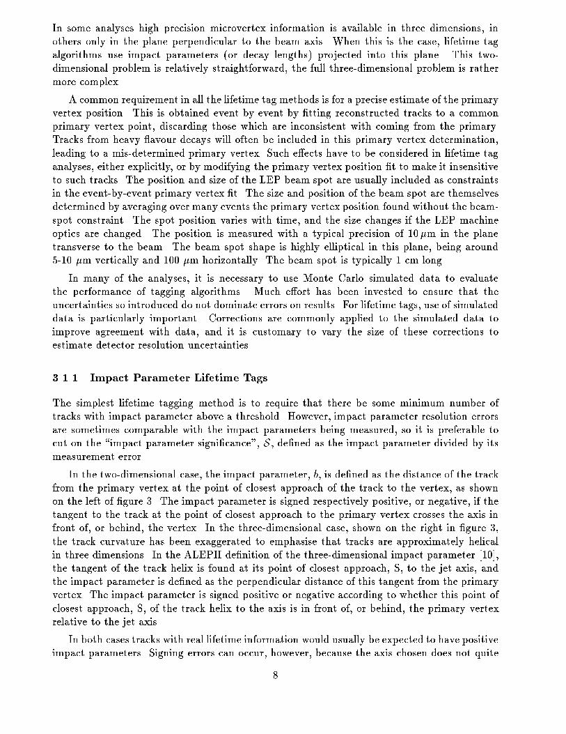
In the two-dimensional case, the impact parameter, b, is de�ned as the distance of the trackfrom the primary vertex at the point of closest approach of the track to the vertex, as shownon the left of �gure 3. The impact parameter is signed respectively positive, or negative, if thetangent to the track at the point of closest approach to the primary vertex crosses the axis infront of, or behind, the vertex. In the three-dimensional case, shown on the right in �gure 3,the track curvature has been exaggerated to emphasise that tracks are approximately helicalin three dimensions. In the ALEPH de�nition of the three-dimensional impact parameter [10],the tangent of the track helix is found at its point of closest approach, S, to the jet axis, andthe impact parameter is de�ned as the perpendicular distance of this tangent from the primaryvertex. The impact parameter is signed positive or negative according to whether this point ofclosest approach, S, of the track helix to the axis is in front of, or behind, the primary vertexrelative to the jet axis.

In both cases tracks with real lifetime information would usually be expected to have positiveimpact parameters. Signing errors can occur, however, because the axis chosen does not quite

8

Jet a

xis

trac

k 1

trac

k 2

b1

b2 Primary vertex

2-d impact parameter

Jet a

xistrac

k 1

track

2

b1

b2

S1

S2

3-d impact parameter

b1 < 0b2 > 0

Figure 3: Impact parameter signing conventions. In the two-dimensional case the tracks are repre-sented by their tangents at the point of closest approach to the vertex. In both cases shown, track 1has a negative signed impact parameter, b1 < 0, and track 2 a positive value, b2 > 0.

correspond to the true decaying particle direction. Such signing errors have the undesirablefeature of introducing an exponential lifetime component into the negative impact parametersigni�cance distribution.

The typical impact parameter resolution obtained for tracks with microvertex detector in-formation is 15-25 �m for 45 GeV tracks. At lower momentum the resolution decreases becauseof multiple scattering in material around the beam-pipe, typically to around 70 �m at 2 GeV.

The number of tracks with signed impact parameter signi�cance, S, greater than some giventhreshold is termed the \forward multiplicity". Forward multiplicity was �rst used for b taggingin Z0 decays by Mark-II [11], and has also been used by OPAL to measure �bb=�had [12].

A more sophisticated way of using impact parameter information has been devised byALEPH [10]. This proceeds by estimating the probability, PT , that each track with a pos-itive signed impact parameter signi�cance, S > 0, is actually a track from the primary vertex.The measure PT is de�ned by

PT =Z1

S

R(x)dx

where R is the probability density function for S, resulting entirely from resolution e�ects.By construction PT should have a at probability distribution between 0 and 1 for tracksgenuinely produced at the primary vertex. The PT values of all selected tracks in the event,event hemisphere, or jet (as appropriate for the analysis considered) are then combined to forma joint probability, PN , for that group of tracks. The quantity PN is de�ned as

PN � �N�1Xj=0

(� ln �)j

j!

9

where

� �NYi=1

(PT )i

The quantity � is just the product over the N tracks of the probabilities that each originatesfrom the primary vertex. This quantity itself contains the information required about the no-lifetime likelihood of the particular set of impact parameter signi�cances observed, but it is not avery useful variable as its distribution depends strongly on the number of tracks N contributing.To avoid such problems, PN is constructed as the probability of �nding the particular set ofimpact parameter signi�cances obtained, or any equally or less likely con�guration, for thisparticular value of N . In this way a variable is constructed which, in the case of no lifetime, is at between 0 and 1 for each value of N separately. For events with lifetime information PN isclose to zero. Of course, there is lifetime information even in light quark events from K0 and �decays. This is reduced by rejecting identi�ed photon conversion, K0 and � decay candidates.

For ALEPH, this technique is found to provide a very powerful tagging algorithm. Thepower of the technique lies in the low probability that large impact parameter signi�cances cancome from tracks actually originating from the primary vertex { so it is critical that the tailsof the resolution function for the impact parameter signi�cance are kept small, and are wellunderstood. Since the product of probabilities is taken over several tracks, and the value of PT

for a given track varies directly with the size of these tails, small reductions in the size of thetails can give signi�cant improvements in the tagging performance. Careful study is thereforenecessary to reduce as far as possible poorly-measured or badly reconstructed tracks. The sizeof the resolution tails can be measured from the data using negative signed impact parametertracks, allowing this source of systematic uncertainty to be reasonably well controlled. Thee�ects of impact parameter signing errors mean that care has to be taken to ensure the reallifetime contamination in this backward distribution is not too high. The performance of thistype of algorithm varies signi�cantly from one LEP detector to another. DELPHI have alsoadopted this impact parameter tagging algorithm [13,14].

3.1.2 Reconstructed Secondary Vertex Tags

OPAL have used a di�erent type of lifetime tagging algorithm, based on secondary vertex re-construction [15]. This algorithm is relatively insensitive to resolution tails in impact parameterdistributions, as several tracks are needed to form the secondary vertex, and they must all bereasonably consistent with coming from that common secondary vertex. Published analyseshave so far been restricted to vertex reconstruction in the plane perpendicular to the beam.

The algorithm used by OPAL is a \tear-down" vertex �nder, operating on tracks which havebeen clustered into jets. Track quality cuts are applied to reduce contamination from poorlymeasured tracks, and tracks from K0 and � decays. Selected tracks in the jet are �tted to acommon vertex point, and the �2 of the vertex �t is evaluated. The change in this �2, ��2, isevaluated when each track in the vertex is dropped in turn. If any track contributes ��2 > 4the track giving the largest ��2 is dropped, and the �t repeated. The process is iterated untilno tracks contribute ��2 > 4, or until fewer than four charged tracks remain, in which case novertex is found.

The decay length, L, is de�ned as the distance from the reconstructed secondary vertexposition to the primary vertex, constrained by the direction of the jet (or by the direction of

10

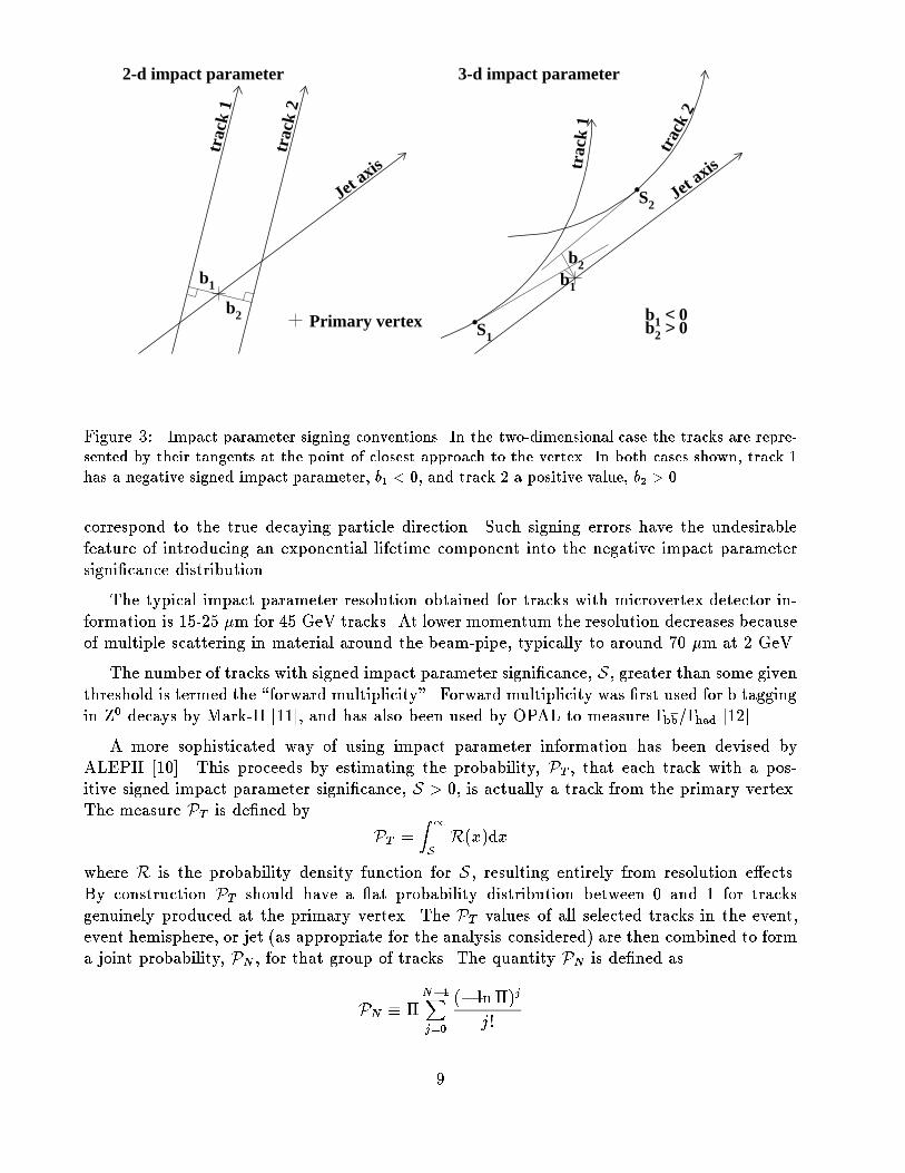
Figure 4: Decay length signi�cance, L=�L, distribution for OPAL data and Monte Carlo simulation.

summed momentum vectors of the particles associated with the secondary vertex). The decaylength is signed positive if the secondary vertex is displaced in front of the primary vertexrelative to the constraining direction, negative otherwise. The error, �L, on the decay lengthincludes the errors from both the primary and secondary vertex reconstruction uncertainties.To reduce the e�ect of poorly measured vertices, the \decay length signi�cance", L=�L, is usedas the lifetime tag discriminant, typically requiring L=�L > 8 for a b tag.

This secondary-vertex reconstruction algorithm has the desirable property that it gives asymmetric decay length signi�cance distribution for events with no lifetime information. Asecond useful feature is that small shifts in the direction constraint used to sign the decaylength cannot give rise to decay length signing errors { rather they just degrade the decaylength signi�cance resolution somewhat.

The distribution of L=�L obtained by OPAL is shown in �gure 4. The lifetime information inthe forward direction coming from b decays is clearly visible. The agreement between simulationand data in the backward direction, dominated by resolution e�ects, is seen to be reasonablefor decay length signi�cances L=�L < �5. A simple way of reducing the e�ects of resolutionuncertainties coming from background with no lifetime component is to subtract the backwardtags observed in the data from the forward tags at the same value of jL=�Lj. This works well,but is only appropriate in a subset of analyses, due to its statistical nature.

11

3.1.3 Lifetime Tag Performance

b e�ciency "b (%) b purity (%)

ALEPH [10] 26 96

DELPHI [13] 24 89

OPAL [15] 19 95

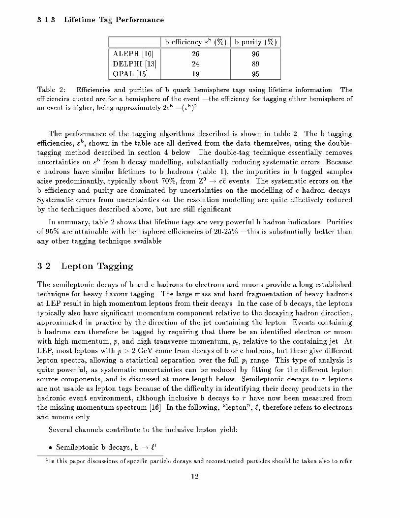
Table 2: E�ciencies and purities of b quark hemisphere tags using lifetime information. Thee�ciencies quoted are for a hemisphere of the event { the e�ciency for tagging either hemisphere ofan event is higher, being approximately 2"b � ("b)2.

The performance of the tagging algorithms described is shown in table 2. The b tagginge�ciencies, "b, shown in the table are all derived from the data themselves, using the double-tagging method described in section 4 below. The double-tag technique essentially removesuncertainties on "b from b decay modelling, substantially reducing systematic errors. Becausec hadrons have similar lifetimes to b hadrons (table 1), the impurities in b tagged samplesarise predominantly, typically about 70%, from Z0 ! cc events. The systematic errors on theb e�ciency and purity are dominated by uncertainties on the modelling of c hadron decays.Systematic errors from uncertainties on the resolution modelling are quite e�ectively reducedby the techniques described above, but are still signi�cant.

In summary, table 2 shows that lifetime tags are very powerful b hadron indicators. Puritiesof 95% are attainable with hemisphere e�ciencies of 20-25% { this is substantially better thanany other tagging technique available.

3.2 Lepton Tagging

The semileptonic decays of b and c hadrons to electrons and muons provide a long-establishedtechnique for heavy avour tagging. The large mass and hard fragmentation of heavy hadronsat LEP result in high momentum leptons from their decays. In the case of b decays, the leptonstypically also have signi�cant momentum component relative to the decaying hadron direction,approximated in practice by the direction of the jet containing the lepton. Events containingb hadrons can therefore be tagged by requiring that there be an identi�ed electron or muonwith high momentum, p, and high transverse momentum, pt, relative to the containing jet. AtLEP, most leptons with p > 2 GeV come from decays of b or c hadrons, but these give di�erentlepton spectra, allowing a statistical separation over the full pt range. This type of analysis isquite powerful, as systematic uncertainties can be reduced by �tting for the di�erent leptonsource components, and is discussed at more length below. Semileptonic decays to � leptonsare not usable as lepton tags because of the di�culty in identifying their decay products in thehadronic event environment, although inclusive b decays to � have now been measured fromthe missing momentum spectrum [16]. In the following, \lepton", `, therefore refers to electronsand muons only.

Several channels contribute to the inclusive lepton yield:

� Semileptonic b decays, b! `1

1In this paper discussions of speci�c particle decays and reconstructed particles should be taken also to refer

12

� \Cascade" b decays, b! c! ` and b! c! `

� Decays of b hadrons to leptonically decaying J= mesons, b! J= ! `

� Decays of b hadrons to a leptonically decaying � , b! � ! `

� Semileptonic c decays, c! `

� \Instrumental" backgrounds, from photon conversions to e+e�, decays in ight of � andK to muons, hadrons faking lepton signatures, and so on.

The �rst �ve sources are together known as \prompt" lepton sources. Semileptonic b andc decays together with cascade decays produce the large majority of prompt leptons in thesample. Instrumental background sources are mostly concentrated at low p and pt.

pt (GeV)p (GeV)

pt (GeV)p (GeV)

pt (GeV)p (GeV)

(a) b→l (b) b→c→l (c) c→l

01

2

0510

1520

2530

0200400600800

10001200

01

2

0510

1520

2530

0500

10001500200025003000350040004500

01

2

0510

1520

2530

0500

1000150020002500

Figure 5: Distributions of p vs. pt, predicted by the JETSET Monte Carlo [4], for leptons from (a)semileptonic b decays; (b) cascade decays; and (c) semileptonic c decays in Z0 to cc decay events. Themomenta are de�ned in the experimental frame, and pt is measured relative to the decaying b hadrondirection (for (a) and (b)) or relative to the decaying c hadron direction (for (c)). The vertical scaleis arbitrary.

The possibility of avour separation using lepton p and pt distributions is illustrated in�gure 5. Leptons directly from semileptonic b decays have harder p and pt distributions thanthose from cascade and semileptonic c decays. In turn, leptons from semileptonic c decays inZ0 ! cc events have a harder p spectrum than those from cascade decays. The reconstructed pand pt distributions for identi�ed muons in the L3 detector are shown in �gure 6. Backgroundleptons are only a small component for pt > 1 GeV. For this L3 analysis, the pt of the lepton iscalculated relative to its containing jet, excluding the lepton momentum when calculating thejet direction.

Fitting the inclusive lepton spectrum can provide some information about electroweak pa-rameters, but much can be gained if events with two identi�ed leptons (\dileptons") are also

to the corresponding charge-conjugated process or particles.

13

DataMC: u,d,s,c backgr.MC: c → µ onlyMC: b backgr.MC: b → c → µ onlyMC: b → µ only

L3

P (GeV)

Num

ber

of m

uons

0

500

1000

1500

2000

2500

3000

3500

5 10 15 20 25 30

L3

PT (GeV)

Num

ber

of m

uons

0

1000

2000

3000

4000

5000

1 2 3 4 5 6

Figure 6: Distributions of p and pt for muons reconstructed in the L3 detector [17], comparedto Monte Carlo (MC) predictions. Over ow entries are shown in the rightmost bins. Predictedbackground lepton candidates are shown separately for bb and non-bb events.

used. By �tting both the lepton and dilepton spectra together, more quantities can be mea-sured simultaneously. If instrumental backgrounds are neglected (or �rst subtracted from thedata), the inclusive di�erential cross-section in p and pt for prompt leptons has the form:

d2�`dpdpt

/Xi

B(i)"i(p; pt)�bb�had

fi(p; pt) +B(c! `)"c!`(p; pt)�cc�had

fc!`(p; pt) (13)

where the sum over i runs over the �rst four lepton source channels listed above, B(i) representsthe decay branching ratio for source i, "i(p; pt) refers to the e�ciency of detecting a lepton fromsource i, and fi(p; pt) represents the p, pt distribution of the leptons from source i. For dileptons,if it is assumed that the two leptons originate in di�erent heavy quark decays, and the e�ciencycorrelation between the two leptons is neglected, the di�erential cross-section takes the form:

d4�`dp1dpt;1dp2dpt;2

/Xi;j

B(i)B(j)"i(p1; pt;1)"j(p2; pt;2)�bb�had

fi(p1; pt;1)fj(p2; pt;2) +

B(c! `)2"c!`(p1; pt;1)"c!`(p2; pt;2)�cc�had

fc!`(p1; pt;1)fc!`(p2; pt;2) (14)

where now the p1=2 and pt;1=2 of both leptons (1/2) appear. The identi�cation e�ciencies "are known from simulation, and are checked with control samples of data. The momentumdistributions f are also known from a combination of lower energy experimental measurementsand Monte Carlo simulation. Using the inclusive lepton distribution (equation (13)) alone, itis not possible to measure both the branching ratios and Z0 decay widths { a measurementof �bb=�had requires that the branching ratio B(b ! `) is known. This branching ratio is notknown very precisely from lower energy data, so the systematic error on �bb=�had from such anapproach would be too big to be interesting. If, however, the single lepton and dilepton spectra

14

are �tted together, the most important branching ratios can be determined from the data whilesimultaneously determining �bb=�had and �cc=�had.

Such �ts to the single lepton and dilepton spectra are performed by all four LEP collab-orations [14, 17{19]. By extending the �t to include the cos � variation of the cross-section,the four electroweak heavy quark avour parameters �bb=�had, �cc=�had, A

bFB and Ac

FB can, inprinciple, all be measured simultaneously. In practice only ALEPH have published such a mea-surement [19] to date. The average b mixing parameter �, and the b fragmentation, may alsobe determined in these �ts. The choice of exactly which parameters to measure, and which totake from external sources, such as lower energy measurements, is a balance which depends onthe statistics used in the �t and the details of the approach used. The approaches adopted bythe four collaborations di�er { ALEPH prefer a combined �t of all parameters, whereas theother experiments have separate �ts for smaller sets of parameters.

The major sources of systematic errors in lepton analyses come from semileptonic decayproperties. The large uncertainties which would arise from knowledge of the b semileptonicbranching ratio are removed by �tting for it, but the momentum spectrum of the lepton fromthe decay must still be assumed. Phenomenological models [20, 21] are used to predict thespectrum. The models have been tuned to reproduce the momentum spectrum of leptonsfrom decays of slow B mesons, produced in �(4S) decays observed by the CLEO detector [22].Additional systematic errors accrue because of the admixture of unmeasured semileptonic B0

s

and �c decays. Errors arise in a similar way for semileptonic c decays, where the most usefullower energy measurements come from DELCO and MARK-III [23,24].

Experimental systematic errors arise from knowledge of the lepton identi�cation e�ciencies,and the contamination by instrumental backgrounds. Lepton identi�cation e�ciencies aregenerally very well known at LEP, typically at the level of �2%, and do not give rise tosigni�cant uncertainties. Instrumental backgrounds, on the other hand, are pervasive andrelatively di�cult to estimate. Conversion background can be measured, and partially excluded,by reconstruction of the other electron track from the converting photon. Control samples ofhadron tracks can be used to measure the modelling of hadronic backgrounds, but relativeuncertainties remain at the level of �10%.

The overall performance of lepton tags is limited by the low semileptonic branching ratios,of approximately 10% for both b and c semileptonic decays. Clean identi�cation means thatonly leptons with p > 2 or 3 GeV can be used { a cut at 3 GeV removes approximately 25%and 40% of leptons from primary b and c semileptonic decay, respectively. In this momentumrange lepton identi�cation e�ciencies lie typically in the range 70{80%. A close to 90% pure btag requires typically an additional pt cut of about 1.2 GeV, which imposes a further e�ciencyloss of around 50%, giving overall hemisphere tagging e�ciencies of around 6%, for a combinedelectron and muon tag.

3.3 Flavour Separation using Event Shapes

The high mass and hard fragmentation of the b quark is exploited by another separation tech-nique. Very little energy is lost by gluon radiation in the hadronisation process of b quarks, sothat the b hadron and, subsequently, its decay products, carry a large fraction of the primaryquark energy. In contrast, in light quark events most particles are produced in gluon frag-mentation with a rather soft momentum spectrum. Similarly, the b decay products can have

15

a relatively large transverse momentum with respect to the b quark direction, since the largemass of the b hadron increases the available transverse phase-space signi�cantly. This resultsin broader jets in bb events compared to light quark events.

Even without completely reconstructing the b decay products, quantities can be devisedwhich carry some of this information. The hard b fragmentation means that most informationis carried by a small number of tracks with high momentum and high transverse momentum,measured relative to the jet direction. Many of the separating variables constructed are there-fore restricted to a few of the most energetic tracks in a jet. ALEPH [25, 26] and OPAL [27]use very similar variables, constructed mostly from the momenta of tracks. The L3 collabo-ration [28] perform an equivalent analysis based entirely on calorimeter information. Typicalquantities used are:

� Bjet: The boosted sphericity of the jet. The tracks of a jet are boosted into a new frame,such that the sphericity of b decay products is isotropically distributed. Non-b jets,boosted into an equivalent frame, show di�erent distributions.

� Quantities constructed from the momenta (or energies) of all tracks and of the mostenergetic ones, measured both transverse and longitudinally to the jet direction.

� D123;M123, the directed sphericity and invariant mass of the three most energetic particlesin the jet;

� L3 includes the energy di�erence between the highest and the fourth highest energeticcluster, Egap.

� ALEPH has constructed two additional variables which use all tracks in a hemisphere,rather than in a jet. They are constructed from the product of momenta of di�erenttracks, and from the invariant masses assuming the pion mass for each track, calculatedin the rest frame of all particles in the hemisphere.

Distributions of some of these quantities are shown in �gure 7. The measured distributionsare compared to the predicted behaviour of bb and cc events, with appropriate normalisation.None of these quantities by itself provides a very good separation between bb and non-bbevents. In addition the variables are highly correlated, further complicating the analysis. Toexploit fully the information available, and still take the correlations properly into account, anarti�cial neural net [29] is used to combine the variables into a single discriminating quantity.This is constructed such that, given perfect separation between avours, it would be one for bbevents, zero for cc events. The output distribution of such a network is shown in �gure 8(a),and compared with simulated bb, cc and light avour events. The performance possible withsuch a net is illustrated in �gure 8(b), showing the e�ciency versus purity curve obtained byL3 with a net using 11 variables per event.

DELPHI [30] have extended this method to attempt to separate b, c and uds events intothree categories. To improve the separation power of the network, lifetime information isincluded in the form of impact parameters of leading tracks in the jet. The sensitivity to ccevents is improved by using information typical for the decay of a charged D�+ meson into aD0 and a pion, of which the transverse momentum relative to the jet direction is expected tobe very small.

16

Bjet (pt,tot )2

pll p

tl

pltnorm D123

M123

databottom events (MC)charm events (MC)sum

OPAL

Fra

ctio

n of

tota

l ent

ries

per

bin

0

0.05

0.1

0.15

0.2

0 0.2 0.4 0.6 0.8 10

0.1

0.2

0 2 4 6 8

0

0.1

0.2

0 5 10 15 200

0.05

0.1

0.15

0.2

0 0.5 1 1.5 2

0

0.1

0.2

0 1 2 30

0.1

0.2

0.3

0.4

0 0.2 0.4 0.6 0.8 1

0

0.1

0.2

0 1 2 3 4

0

0.05

0.1

0.15

0.2

0 0.2 0.4 0.6 0.8 10

0.1

0.2

0 2 4 6 8

0

0.1

0.2

0 5 10 15 200

0.05

0.1

0.15

0.2

0 0.5 1 1.5 2

0

0.1

0.2

0 1 2 30

0.1

0.2

0.3

0.4

0 0.2 0.4 0.6 0.8 1

0

0.1

0.2

0 1 2 3 4

0

0.05

0.1

0.15

0.2

0 0.2 0.4 0.6 0.8 10

0.1

0.2

0 2 4 6 8

0

0.1

0.2

0 5 10 15 200

0.05

0.1

0.15

0.2

0 0.5 1 1.5 2

0

0.1

0.2

0 1 2 30

0.1

0.2

0.3

0.4

0 0.2 0.4 0.6 0.8 1

0

0.1

0.2

0 1 2 3 4

0

0.05

0.1

0.15

0.2

0 0.2 0.4 0.6 0.8 10

0.1

0.2

0 2 4 6 8

0

0.1

0.2

0 5 10 15 200

0.05

0.1

0.15

0.2

0 0.5 1 1.5 2

0

0.1

0.2

0 1 2 30

0.1

0.2

0.3

0.4

0 0.2 0.4 0.6 0.8 1

0

0.1

0.2

0 1 2 3 4

Figure 7: Distributions of the seven jet shape variables used by OPAL, for events with an exclusivelyreconstructed D�+ in the other hemisphere. Shown are data (points with error bars), Monte Carlo bbevents (dashed line) and cc events (dotted line). Light avour background has already been subtracted.

17

0

0.01

0.02

0.03

0 0.2 0.4 0.6 0.8 1

b eventsnon-b eventsc events

Fc

Frac

tion

of E

vent

s (a)

L3

0

0.25

0.5

0.75

1

0 0.2 0.4 0.6 0.8 1

Efficiency

Pur

ity

(b)L3

Figure 8: (a) Output distribution of the neural net used by the L3 collaboration [28] to identify bbevents. The solid line is the distribution of bb events predicted by Monte Carlo, the dashed line thatof non-b events, and the dotted line the that of cc events. (b) E�ciency vs. purity curve for the samenet.

The network identi�cation probabilities need to be well known for this approach to beuseful. To minimise dependence on Monte Carlo modelling, attempts are made to measurethese probabilities from the data, or to verify the probabilities found in the Monte Carlo. Theresponse to bb events can be tested with lepton tagged samples. Large lepton samples existwith high purities and small systematic uncertainties, and are used to check the net response(ALEPH, DELPHI, L3) or to train the network (ALEPH, OPAL). ALEPH have developed amethod of determining the network identi�cation probabilities from the simultaneous detectionof leptons in the opposite hemisphere [26].

Estimation of the network tagging rates is considerably more di�cult for other avours,since no unbiased pure data samples of charm or light avour events exist. Therefore MonteCarlo has to be used to calculate the network response. The dependence of the results on thesimulation is potentially one of the more important sources of systematic errors.

It is seen from �gure 8(b) that it is not possible to prepare very pure samples of a single avour with an event shape tag. For bb events, purities of around 70% can be obtained with anevent e�ciency of about 20%. The strength of the method lies in the relatively high e�ciencyobtainable with this type of tag, and, potentially, in its extension to include avours other thanbottom.

18

3.4 Reconstructed Particle Tags

Reconstructed particles are a powerful tool for tagging the avour of an event. In principle suchtags could be designed for all �ve avours. The idea is to use mesons or baryons2 which containthe avour investigated, or which are the immediate decay products of particles containing this avour. It is comparatively easy to tag cc and bb events because of the low production rateof these quarks in the fragmentation process. In many cases in such events the mesons soughtcontain the primary quark avour, and so tag it. Although similar tags could be devised forthe lighter avours, interpretation of the measured particle rates in terms of the primary event avours is di�cult because a substantial fraction of such mesons would be produced in thehadronisation process.

Signals from fully reconstructed decays are usually fairly clean, so providing reasonably puretags. However, in most cases analyses are limited by the small branching ratios into the identi-�able channels, typically of the order of one percent. This, together with �nite reconstructione�ciencies, restricts the precision obtainable in analyses based on fully reconstructed particles.

At LEP reconstructed particle tags are most important for charm tagging, although, since bhadrons nearly always decay to c hadrons, reconstructed c- avoured particles can also be usedto tag bb events. However, lifetime and lepton tags are much more powerful b tagging toolsthan reconstructed particles. When used as a charm tag, reconstructed particles from bb eventsare a background source which must be understood. Separation of the bb and cc componentsin the samples is discussed in more detail below.

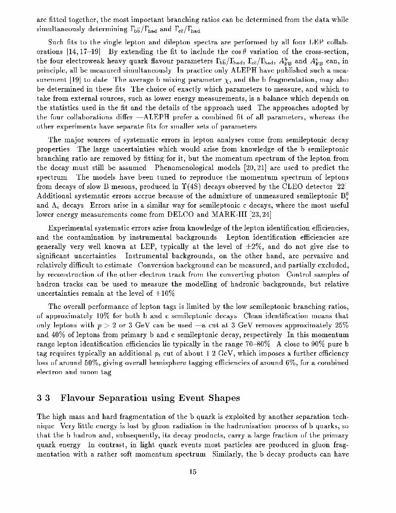
The main decay channels used for electroweak analyses at LEP are listed in table 3. Thebranching ratios of each decay, and the expected number of mesons per hadronic Z0 decay ineach channel, are also shown. Analyses using D�+ mesons are most advanced of those exploitingexclusive decay reconstruction, and so D�+ reconstruction techniques are emphasised in thefollowing discussion.

decay mode branching ratio (%) decays per Z0

D�++ ! D0�+ 68:1�1:3 0.1496�! K��+ 2:73�0:11 0.0032�! K��+�0 9:40�0:70 0.0111�! K��+���+ 5:52�0:36 0.0065

D0 ! K��+ 4:01�0:14 0.0040

D+ ! K��+�+ 9:1�0:6 0.0091

Table 3: Table of D meson decays most commonly used as avour tags at LEP. All branching ratiosare taken from the 1994 Review of Particle Properties [9]. For the number of decays per hadronic Z0,the predictions of the JETSET Monte Carlo program [4] are used for the partial widths and for thehadronisation fraction for a D to be produced, together with the branching ratios given.

2The following discussion is restricted to mesons, but is equally well applicable to baryons.

19

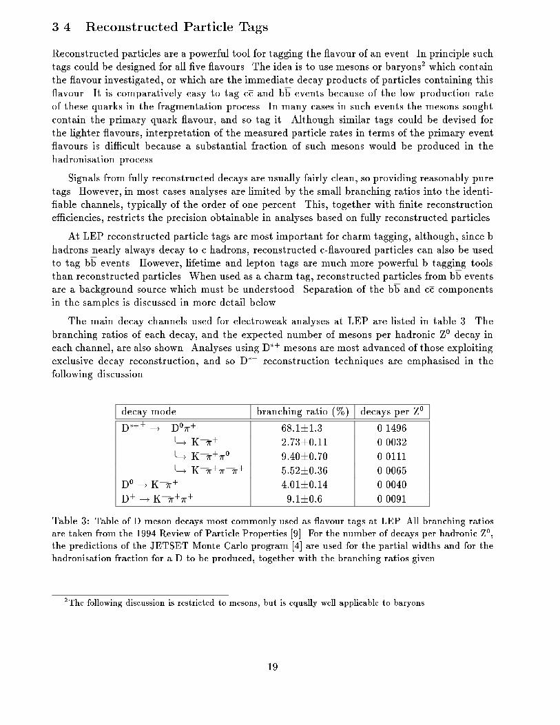
Figure 9: Distribution of the di�erence in invariant mass between a D�+ and a D0 candidate asreconstructed with the ALEPH detector [25]. Only candidates with a scaled energy larger than 25%of the beam energy are included in the plot.

3.4.1 Reconstruction of D Mesons

A large number of di�erent D states have been observed at LEP. The only ones currentlyinteresting for use as tags for primary avours are the D�+, and, to a lesser extent, the Dmeson ground states D+ and D0. Analyses involving the D�+ meson have been published byALEPH [25], OPAL [27] and DELPHI [31] . The D�+ is particularly noteworthy, because italways decays into a ground state D meson, D+ or D0, with emission of either a pion or aphoton. The masses of the D�+ and D0 di�er only by 145:5 MeV, severely limiting the phase-space available to the decay products; in the D�+ rest-frame 40 MeV are available in the decayD�+ ! D0�+. A very clean way of reconstructing this decay is to look at the mass di�erencebetween the D�+ and the D0 candidates. True D�+ decays show up in this plot as a narrowpeak at 145:5 MeV, very close to the kinematic limit of 139:6 MeV, the pion mass. Such a massdi�erence plot is shown in �gure 9, as reconstructed in the ALEPH detector. Clearly visible isthe peak at �M = 145:5 MeV, over very little background.

Other D meson decays do not pro�t from such a kinematical coincidence. Background levels,for example in the direct reconstruction of D+ or D0 mesons, are therefore signi�cantly higher.

The technical aspects of reconstructing a D�+ meson are well established, and are verysimilar amongst the di�erent collaborations. After selecting hadronic events and good qualitycharged tracks, the D�+ reconstruction proceeds by �rst identifying a D0 candidate, then com-bining this candidate with a pion candidate to form the �nal D�+ candidate. Since all D0 decays

20

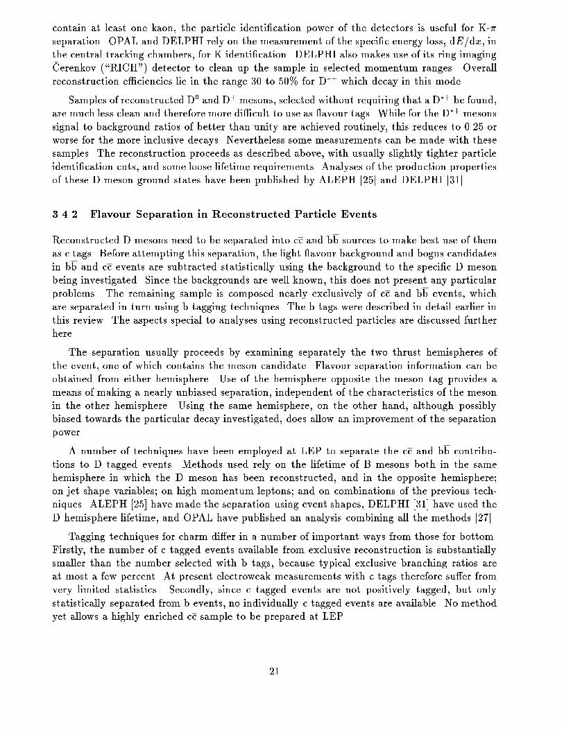
contain at least one kaon, the particle identi�cation power of the detectors is useful for K-�separation. OPAL and DELPHI rely on the measurement of the speci�c energy loss, dE=dx, inthe central tracking chambers, for K identi�cation. DELPHI also makes use of its ring imaging�Cerenkov (\RICH") detector to clean up the sample in selected momentum ranges. Overallreconstruction e�ciencies lie in the range 30 to 50% for D�+ which decay in this mode.

Samples of reconstructed D0 and D+ mesons, selected without requiring that a D�+ be found,are much less clean and therefore more di�cult to use as avour tags. While for the D�+ mesonssignal to background ratios of better than unity are achieved routinely, this reduces to 0.25 orworse for the more inclusive decays. Nevertheless some measurements can be made with thesesamples. The reconstruction proceeds as described above, with usually slightly tighter particleidenti�cation cuts, and some loose lifetime requirements. Analyses of the production propertiesof these D meson ground states have been published by ALEPH [25] and DELPHI [31].

3.4.2 Flavour Separation in Reconstructed Particle Events

Reconstructed D mesons need to be separated into cc and bb sources to make best use of themas c tags. Before attempting this separation, the light avour background and bogus candidatesin bb and cc events are subtracted statistically using the background to the speci�c D mesonbeing investigated. Since the backgrounds are well known, this does not present any particularproblems. The remaining sample is composed nearly exclusively of cc and bb events, whichare separated in turn using b tagging techniques. The b tags were described in detail earlier inthis review. The aspects special to analyses using reconstructed particles are discussed furtherhere.

The separation usually proceeds by examining separately the two thrust hemispheres ofthe event, one of which contains the meson candidate. Flavour separation information can beobtained from either hemisphere. Use of the hemisphere opposite the meson tag provides ameans of making a nearly unbiased separation, independent of the characteristics of the mesonin the other hemisphere. Using the same hemisphere, on the other hand, although possiblybiased towards the particular decay investigated, does allow an improvement of the separationpower.

A number of techniques have been employed at LEP to separate the cc and bb contribu-tions to D tagged events. Methods used rely on the lifetime of B mesons both in the samehemisphere in which the D meson has been reconstructed, and in the opposite hemisphere;on jet shape variables; on high momentum leptons; and on combinations of the previous tech-niques. ALEPH [25] have made the separation using event shapes, DELPHI [31] have used theD hemisphere lifetime, and OPAL have published an analysis combining all the methods [27].

Tagging techniques for charm di�er in a number of important ways from those for bottom.Firstly, the number of c tagged events available from exclusive reconstruction is substantiallysmaller than the number selected with b tags, because typical exclusive branching ratios areat most a few percent. At present electroweak measurements with c tags therefore su�er fromvery limited statistics. Secondly, since c tagged events are not positively tagged, but onlystatistically separated from b events, no individually c tagged events are available. No methodyet allows a highly enriched cc sample to be prepared at LEP.

21

3.5 Hemisphere Charge Techniques for Estimating the Heavy Quark

Charge

While D�+ and lepton tags yield rather directly charge information about the decaying heavyquark from the charges of the identi�ed particles, lifetime tags do not. In principle, the chargesof the tracks associated to a reconstructed secondary vertex could be used to estimate thedecaying hadron charge. Some progress has recently been reported on such a technique [32],but a problem remains that it is relatively rarely that exactly the correct tracks are associatedwith the secondary vertex. The impact parameter probability method of lifetime tagging alsodoes not itself give any information about the decaying hadron charge.

To try to circumvent these di�culties, \jet charge" measures are used to estimate theprimary quark charge from a weighted sum of the charges of several tracks in, for example, athrust hemisphere. Jet charge de�nitions vary slightly, but the most commonly employed is:

Qhem =�iqijplij��ijplij�

;

where the sum over i runs over the tracks in the hemisphere, qi is the charge of track i, and pli isthe component of its momentum along the thrust axis direction. The parameter � is chosen togive optimal charge sensitivity, typical values being � = 0:5 or � = 0:7. This type of hemispherecharge measure has been used in several analyses at LEP. So far the application to measurementsof heavy avour electroweak observables has been limited to the forward-backward asymmetryfor lifetime-tagged Z0 ! bb events (section 6) [14,33].

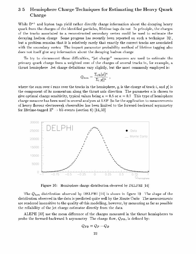
Figure 10: Hemisphere charge distribution observed by DELPHI [14]

The Qhem distribution observed by DELPHI [14] is shown in �gure 10. The shape of thedistribution observed in the data is predicted quite well by the Monte Carlo. The measurementsare rendered insensitive to the quality of this modelling, however, by measuring as far as possiblethe reliability of the jet charge estimator directly from the data.

ALEPH [33] use the mean di�erence of the charges measured in the thrust hemispheres toprobe the forward-backward b asymmetry. The charge ow, QFB, is de�ned by:

QFB � QF �QB

22

where QF and QB are the jet charges of the forward and backward thrust hemispheres, respec-tively. The distribution of the charge sum, Q, is also used:

Q � QF +QB :

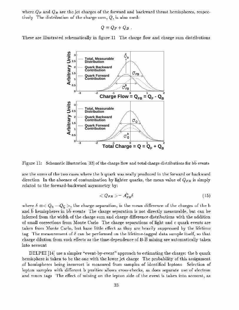
These are illustrated schematically in �gure 11. The charge ow and charge sum distributions

0

0.5

1

1.5

2

2.5

3

-3 -2 -1 0 1 2Charge Flow = Q FB = QF - QB

Arb

itrar

y U

nits Total, Measurable

Distribution

Quark BackwardContribution

Quark ForwardContribution

0

0.5

1

1.5

2

2.5

3

-3 -2 -1 0 1 2Total Charge = Q = Q F + QB

Arb

itrar

y U

nits Total, Measurable

Distribution

Quark BackwardContribution

Quark ForwardContribution

Figure 11: Schematic illustration [33] of the charge ow and total charge distributions for bb events.

are the sums of the two cases where the b quark was really produced in the forward or backwarddirection. In the absence of contamination by lighter quarks, the mean value of QFB is simplyrelated to the forward-backward asymmetry by:

< QFB >= AbFB� (15)

where � �< Qb �Qb >, the charge separation, is the mean di�erence of the charges of the band b hemispheres in bb events. The charge separation is not directly measurable, but can beinferred from the width of the charge sum and charge di�erence distributions with the additionof small corrections from Monte Carlo. The charge separations of light and c quark events aretaken from Monte Carlo, but have little e�ect as they are heavily suppressed by the lifetimetag. The measurement of � can be performed on the lifetime-tagged data sample itself, so thatcharge dilution from such e�ects as the time-dependence of B-B mixing are automatically takeninto account.

DELPHI [14] use a simpler \event-by-event" approach to estimating the charge: the b quarkhemisphere is taken to be the one with the lower jet charge. The probability of this assignmentof hemispheres being incorrect is measured from samples of identi�ed leptons. Selection oflepton samples with di�erent b purities allows cross-checks, as does separate use of electronand muon tags. The e�ect of mixing on the lepton side of the event is taken into account, as

23

is the possible e�ect of time-dependent mixing on the lifetime-tagged side. The probability ofcorrectly assigning the b quark and antiquark hemispheres is found to be (67.3�1.2)% [14],where the error includes a �0.5% contribution from the mixing uncertainty. As for the ALEPHmethod, the charge separations of light and c quark events are taken from Monte Carlo.

4 Measurements of �bb=�had

The �rst measurements of �bb=�had from LEP primarily used \single-tag" techniques: i.e. eventswere examined, and if any tag were found in the event, the event was classi�ed as tagged. Thenumber of tagged events, Ntag, is then given by:

Ntag = Nhad("b �bb�had

+ "c�cc�had

+ "u�uu�had

+ "d�dd�had

+ "s�ss�had

) (16)

where "q is the probability of tagging an event where the Z0 has decayed to qq. For the tagsused to date, the tagging e�ciencies for uu, dd, and ss events are almost identical. De�ning"uds to be the average tagging e�ciency for these liqht quark events, and using the constraint

�bb�had

+�cc�had

+�uu�had

+�dd�had

+�ss�had

= 1 ; (17)

equation (16) can be reformulated:

Ntag = Nhad("b �bb�had

+ "c�cc�had

+ "uds(1� �bb�had

� �cc�had

)) ; (18)

giving for �bb=�had:

�bb�had

=

Ntag

Nhad� ("c � "uds)

�cc

�had� "uds

"b � "uds : (19)

Since "uds and "c are arranged to be much smaller than "b, this reduces approximately to:

�bb�had

� Ntag

"bNhad

: (20)

In the single-tagging methods, "b is taken from a priori knowledge, via Monte Carlo anddetector simulation programs. The statistical accuracy of this approach is limited by Ntag, andthe systematic precision by how well "b is known. For typical event tagging e�ciencies, "b, oforder 10%, with order �10% relative uncertainty, this approach becomes systematics limitedwith only about 10 000 hadronic Z0 decays.

Recent measurements of �bb=�had have, therefore, used a di�erent approach which does notrequire a priori knowledge of the b tagging e�ciency { instead it is determined from the datathemselves. This is achieved with the \double-tagging" approach. In this technique, the eventis divided into two thrust hemispheres, and tagging algorithms are applied independently toeach hemisphere in turn. The number of tagged hemispheres and the number of double-taggedevents together allow both the b tagging e�ciency and �bb=�had to be measured from the data.

24

The number of tagged hemispheres, Nt, can be written:

Nt = 2Nhad("b �bb�had

+ "c�cc�had

+ "uds(1 � �bb�had

� �cc�had

)) (21)

where it is assumed, as in equation (18), that the uu, dd and ss e�ciencies are the same, andthat the Z0 hadronic decays are saturated by decays to the usual �ve quark avours. Thetagging e�ciencies "b, "c and "uds are here the hemispheric tagging probabilities. The numberof double-tagged events, Ntt, is then

Ntt = Nhad(Cb("b)2

�bb�had

+ Cc("c)2

�cc�had

+ Cuds("uds)2(1� �bb

�had� �cc�had

)) (22)

where the correlation parameters, Cq, are introduced to take into account possible e�ciencycorrelations between the two hemispheres. Equations (21) and (22) can be solved algebraicallyfor �bb=�had and "b if the other quantities are known from the data and simulation studies.Neglecting for clarity the background terms involving "c and "uds, the solutions:

�bb�had

� CbN2t

4NttNhad

(23)

"b � 2Ntt

CbNt

(24)

are obtained. The statistical disadvantage of the double-tagging method can be seen in theseformulae: the statistical error on �bb=�had is dominated by Ntt, the number of double-taggedevents. The main systematic uncertainties in the double tag approach come from knowledge ofthe correlation coe�cient Cb and the background tagging e�ciencies "c and "uds.

The correlation coe�cient uncertainty is potentially rather serious, given the form of equa-tion (23). The correlations arise from both physical and detector-related e�ects. Hard gluonradiation can give rise to correlations. In some cases, the gluon is very hard and recoils againstthe b and b jets, which are found in the same thrust hemisphere. If the gluon is softer it can stillgive rise to b and b momenta which are both lower than usual, giving lower tagging e�ciencyin the two hemispheres. On the detector side, tagging e�ciencies which are not uniform overthe geometrical acceptance of the detector can give rise to correlations in tagging e�ciency.For lifetime tags, hemispheric correlations can also arise from the primary vertex position infor-mation, which is shared between the two hemispheres. In general, the e�ect of the correlationuncertainties is kept small by arranging the event selection so as to keep the correlating e�ectsthemselves small. Nonetheless, they give rise to a signi�cant source of systematic uncertainty,as discussed below.

The background tagging e�ciency uncertainties are the largest source of systematic error inthe most precise �bb=�had measurements available. Charmed hadron decay properties are mostimportant, since c decays form the main background to b decays in all the tagging techniques.Detector resolution uncertainties also a�ect "c (and "uds) and have to be treated carefully. Indouble lifetime tag measurements, the dominant background systematic errors come from theuncertainties on the c hadron mixtures, and on the mean c hadron charged decay multiplicity. Alarge uncertainty comes also from the relatively poorly-measured �cc=�had, unless the frameworkof the standard model is assumed, when the uncertainty is negligible since �cc=�had is quiteprecisely predicted.

25

The measured value of �bb=�had depends on the amount of gluon splitting to bb and cc pairsin the hadronisation process, because it can lead to b tags in light quark events. The levelof gluon splitting has been calculated in perturbative QCD [34], with an estimated accuracyof �25-30%. The analyses presented here take these heavy quarks from gluon splitting intoaccount using the level predicted by the JETSET Monte Carlo, which is found to agree within30% with the calculations. The errors quoted in table 4 correspond to varying the heavy quarkproduction rate from gluon splitting by �50%.

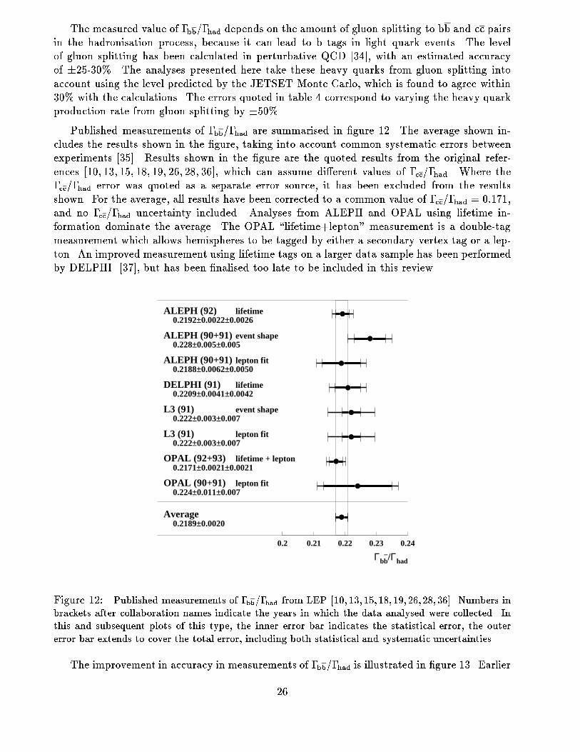
Published measurements of �bb=�had are summarised in �gure 12. The average shown in-cludes the results shown in the �gure, taking into account common systematic errors betweenexperiments [35]. Results shown in the �gure are the quoted results from the original refer-ences [10, 13, 15, 18, 19, 26, 28, 36], which can assume di�erent values of �cc=�had. Where the�cc=�had error was quoted as a separate error source, it has been excluded from the resultsshown. For the average, all results have been corrected to a common value of �cc=�had = 0:171,and no �cc=�had uncertainty included. Analyses from ALEPH and OPAL using lifetime in-formation dominate the average. The OPAL \lifetime+lepton" measurement is a double-tagmeasurement which allows hemispheres to be tagged by either a secondary vertex tag or a lep-ton. An improved measurement using lifetime tags on a larger data sample has been performedby DELPHI [37], but has been �nalised too late to be included in this review.

Γbb–/Γhad

ALEPH (92) lifetime0.2192±0.0022±0.0026

ALEPH (90+91) event shape0.228±0.005±0.005

ALEPH (90+91) lepton fit0.2188±0.0062±0.0050

DELPHI (91) lifetime0.2209±0.0041±0.0042

L3 (91) event shape0.222±0.003±0.007

L3 (91) lepton fit0.222±0.003±0.007

OPAL (92+93) lifetime + lepton0.2171±0.0021±0.0021

OPAL (90+91) lepton fit0.224±0.011±0.007

Average0.2189±0.0020

0.2 0.21 0.22 0.23 0.24

Figure 12: Published measurements of �bb=�had from LEP [10, 13, 15,18,19, 26,28,36]. Numbers inbrackets after collaboration names indicate the years in which the data analysed were collected. Inthis and subsequent plots of this type, the inner error bar indicates the statistical error, the outererror bar extends to cover the total error, including both statistical and systematic uncertainties.

The improvement in accuracy in measurements of �bb=�had is illustrated in �gure 13. Earlier

26

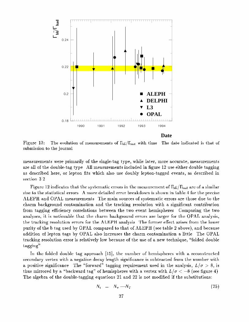
Date

Γ bb– /

Γ had

ALEPHDELPHIL3OPAL

Figure 13: The evolution of measurements of �bb=�had with time. The date indicated is that ofsubmission to the journal.

measurements were primarily of the single-tag type, while later, more accurate, measurementsare all of the double-tag type. All measurements included in �gure 12 use either double taggingas described here, or lepton �ts which also use doubly lepton-tagged events, as described insection 3.2.

Figure 12 indicates that the systematic errors in the measurement of �bb=�had are of a similarsize to the statistical errors. A more detailed error breakdown is shown in table 4 for the preciseALEPH and OPAL measurements. The main sources of systematic errors are those due to thecharm background contamination and the tracking resolution with a signi�cant contributionfrom tagging e�ciency correlations between the two event hemispheres. Comparing the twoanalyses, it is noticeable that the charm background errors are larger for the OPAL analysis,the tracking resolution errors for the ALEPH analysis. The former e�ect arises from the lowerpurity of the b tag used by OPAL compared to that of ALEPH (see table 2 above), and becauseaddition of lepton tags by OPAL also increases the charm contamination a little. The OPALtracking resolution error is relatively low because of the use of a new technique, \folded doubletagging".

In the folded double tag approach [15], the number of hemispheres with a reconstructedsecondary vertex with a negative decay length signi�cance is subtracted from the number witha positive signi�cance. The \forward" tagging requirement used in the analysis, L=� > 8, isthus mirrored by a \backward tag" of hemispheres with a vertex with L=� < �8 (see �gure 4).The algebra of the double-tagging equations 21 and 22 is not modi�ed if the substitutions:

Nt = Nv �Nv (25)

27

Error Source ALEPH [10] OPAL [15]

Detector/Simulation E�ects

Tracking resolution 0.0014 0.0007

Lepton e�ciency and backgrounds { 0.0006

Monte Carlo statistics 0.0014 0.0005

Event selection avour bias 0.0003 0.0003

Charm Background

c hadron production fractions 0.0009 0.0009

c hadron lifetimes 0.0005 0.0004

c hadron decay properties 0.0006 0.0010

c fragmentation 0.0001 0.0007

Light Quark Background

g ! cc=bb 0.0004 0.0005

K0, hyperon production rates 0.0003 0.0003

Hemisphere Correlations 0.0009 0.0007

Total systematical 0.0026 0.0021

Statistical 0.0022 0.0021

Table 4: Breakdown of error sources for the two currently most precise measurements of �bb=�had.

Ntt = Nvv �Nvv +Nvv (26)

are made, where Nv is the number of forward tagged hemispheres, Nv the number of backwardtagged hemispheres, Nvv the number of events with both hemispheres forward tagged, Nvv thenumber of events with one forward and one backward tagged hemisphere, and Nvv the numberwith both hemispheres backward tagged. This statistical subtraction reduces signi�cantly thesensitivity of the result to resolution uncertainties, at the cost of an increase in statistical error.In practice, the number of backward tagged hemispheres is approximately 4% of the numberof forward tagged hemispheres, so the loss in statistical precision is unimportant.

The fraction of hadronic Z0 decays to bb pairs is not expected to vary by more than 1% overthe centre-of-mass energy range probed so far at LEP (88-95 GeV). Since the majority of thedata are collected at the peak energy and very little are collected at the extreme energies, thee�ect on the measurements can be expected to be very small. Several �bb=�had measurementstacitly assume this, since they average data from the di�erent energy points, while others useonly data taken at the peak energy. OPAL [15] and DELPHI [13] have explicitly checked thatno variation is observed, although the precision of the test is at the 3-5% level.

Combining the individual �bb=�had measurements in �gure 12, taking into account commonsystematic errors between the di�erent measurements as discussed in section 7 below, an averageLEP value of

�bb�had

= 0:2189 � 0:0020

is obtained, for �cc=�had = 0:171, where the total error quoted includes both statistical andsystematic errors. The dependence of this result on �cc=�had, and its consistency with thestandard model, is discussed in section 7. The prospects for improving the measurement infuture are discussed in section 9. The ratio �bb=�had has also been measured at the SLC linear

28

collider. The most precise published measurement from SLC [11] is �bb=�had = 0:251� 0:049�0:030, consistent with, but much less precise than, the LEP average.

5 Measurements of �cc=�had

The number of tagged cc events available at LEP is signi�cantly smaller than the number ofbb events. Therefore measurements of the partial width �cc=�had are considerably less precisethan equivalent measurements in the b sector, with measurements still relying on the single tagtechnique.

Measurements of �cc=�had have been performed for a number of di�erent c tagging methods.The �rst measurements of �cc=�had used an inclusive lepton tag in a manner equivalent tothe b tagging method [38], but to measure c quark properties. When �tting the p and ptspectra of the lepton candidates, both b and c components are allowed to oat, resulting in asimultaneous measurement of �bb=�had and �cc=�had. Relatively large systematic uncertaintiesarise for �cc=�had. Since the rate of c quark production is derived from the shape of the p and ptspectra, and since charm and background leptons have similar distributions, the result dependsrather critically on the assumed spectral shapes. In addition these analyses are targeted more atmeasuring �bb=�had, so the c sensitivity is not optimal. Nevertheless competitive measurementshave been made using this method.

Another early analysis at LEP was published in 1990 [39] and used the small momentumavailable to the transition pion in the decay D�+ ! D0� as an inclusive tag for charm. Lookingat the transverse momentum spectrum of all tracks in a hemisphere, a peak is expected andobserved for cc events at very low values of pt. Very few processes exist which can produce anexcess at these low transverse momentum values. However the background from fragmentationtracks is very large. This measurement therefore su�ers from di�cult systematic errors, andhas not been repeated.

Attempts have been made to measure �cc=�had using the jet-shape variables discussed above.The DELPHI collaboration [30] has published such an analysis, with, however, large systematicerrors from the modelling of the network response by the Monte Carlo.

Several measurements employ D mesons as reconstructed particle tags, including the mostprecise single measurement to date. DELPHI [31] have presented results using D0 and D�

rates. Both the D0 ! K�� and the D+ ! K��+�+ decays are identi�ed, and are separatedinto components from charm and from bottom using lifetime information, so allowing theproduct �cc=�hadPc to be determined. Here Pc is the product branching ratio that a charm quarkfragments into the D meson investigated and then decays in the channel in question. Pc is takenfrom lower energy measurements, to derive �cc=�had. Since all D mesons eventually decay intoone of these ground state mesons, this method does not depend severely on assumptions aboutthe relative production fraction of a particular D meson in charm fragmentation. OPAL [27],on the other hand, rely on the assumption that the D�+ meson is produced in the same way atLEP energies as it is in lower energy e+e� collisions. This allows the determination of �cc=�hadfrom the measured rate of D�+ production, which has been measured with a smaller error thanthe D0 or D+ production rate. Again lower energy measurements are used to determine a valuefor the product branching ratio B(c! D�+X)B(D�+ ! K��).

The currently available results for �cc=�had are summarised in �gure 14. Combining all,

29

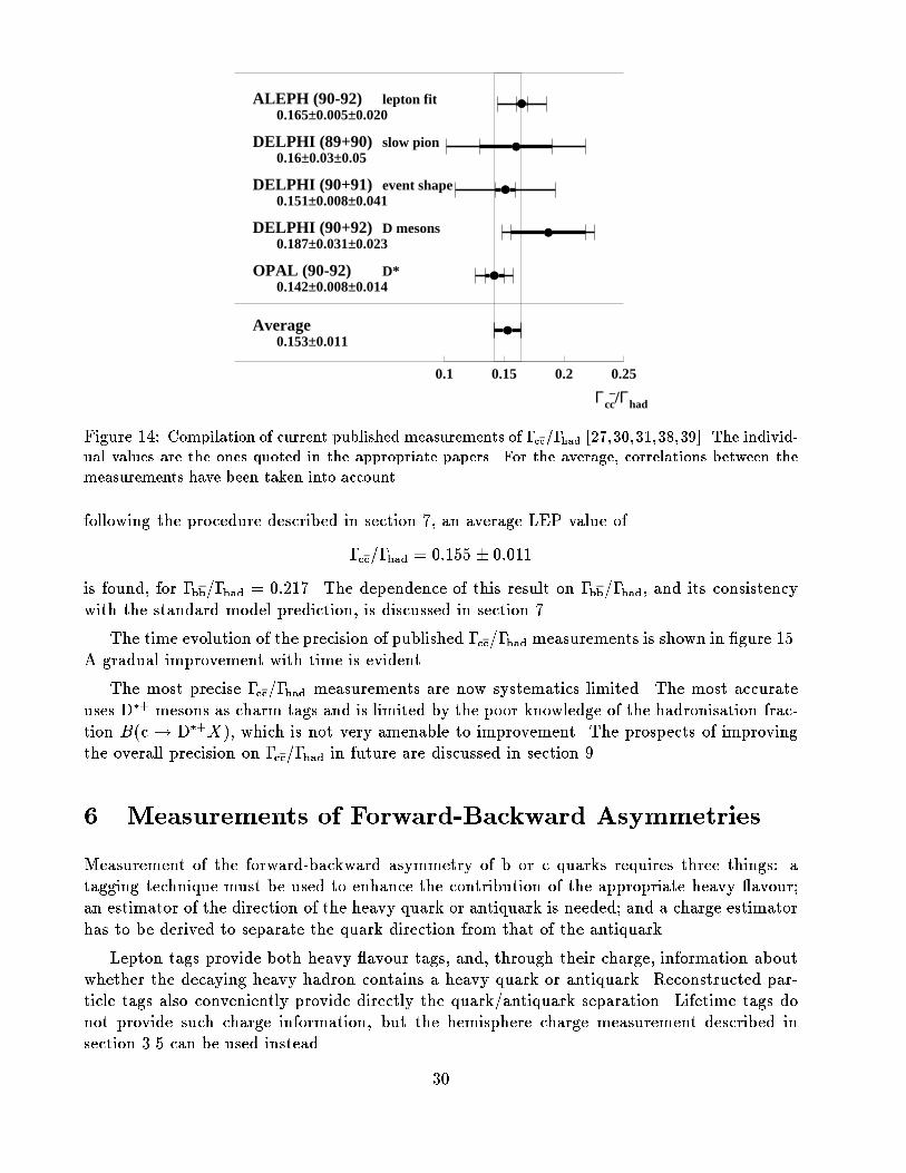
Γcc–/Γhad

ALEPH (90-92) lepton fit0.165±0.005±0.020

DELPHI (89+90) slow pion0.16±0.03±0.05

DELPHI (90+91) event shape0.151±0.008±0.041

DELPHI (90+92) D mesons0.187±0.031±0.023

OPAL (90-92) D*0.142±0.008±0.014

Average0.153±0.011

0.1 0.15 0.2 0.25

Figure 14: Compilation of current published measurements of �cc=�had [27,30,31,38,39]. The individ-ual values are the ones quoted in the appropriate papers. For the average, correlations between themeasurements have been taken into account.

following the procedure described in section 7, an average LEP value of

�cc=�had = 0:155 � 0:011

is found, for �bb=�had = 0:217. The dependence of this result on �bb=�had, and its consistencywith the standard model prediction, is discussed in section 7.

The time evolution of the precision of published �cc=�had measurements is shown in �gure 15.A gradual improvement with time is evident.

The most precise �cc=�had measurements are now systematics limited. The most accurateuses D�+ mesons as charm tags and is limited by the poor knowledge of the hadronisation frac-tion B(c ! D�+X), which is not very amenable to improvement. The prospects of improvingthe overall precision on �cc=�had in future are discussed in section 9.

6 Measurements of Forward-Backward Asymmetries

Measurement of the forward-backward asymmetry of b or c quarks requires three things: atagging technique must be used to enhance the contribution of the appropriate heavy avour;an estimator of the direction of the heavy quark or antiquark is needed; and a charge estimatorhas to be derived to separate the quark direction from that of the antiquark.

Lepton tags provide both heavy avour tags, and, through their charge, information aboutwhether the decaying heavy hadron contains a heavy quark or antiquark. Reconstructed par-ticle tags also conveniently provide directly the quark/antiquark separation. Lifetime tags donot provide such charge information, but the hemisphere charge measurement described insection 3.5 can be used instead.

30

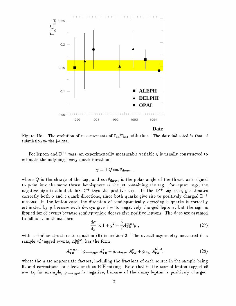
Date

Γ cc– /Γ ha

d

ALEPHDELPHIOPAL

Figure 15: The evolution of measurements of �cc=�had with time. The date indicated is that ofsubmission to the journal.

For lepton and D�+ tags, an experimentally measurable variable y is usually constructed toestimate the outgoing heavy quark direction:

y � �Q cos �thrust ;

where Q is the charge of the tag, and cos �thrust is the polar angle of the thrust axis signedto point into the same thrust hemisphere as the jet containing the tag. For lepton tags, thenegative sign is adopted, for D�+ tags the positive sign. In the D�+ tag case, y estimatescorrectly both b and c quark directions, since both quarks give rise to positively charged D�+

mesons. In the lepton case, the direction of semileptonically decaying b quarks is correctlyestimated by y because such decays give rise to negatively charged leptons, but the sign is ipped for cc events because semileptonic c decays give positive leptons. The data are assumedto follow a functional form

d�

dy/ 1 + y2 +

8

3AmeasFB y ; (27)

with a similar structure to equation (6) in section 2. The overall asymmetry measured in asample of tagged events, Ameas

FB , has the form

AmeasFB = gb�taggedA

bFB + gc�taggedA

cFB + gbkgdA

bkgdFB ; (28)

where the g are appropriate factors, including the fractions of each source in the sample being�t and corrections for e�ects such as B-B mixing. Note that in the case of lepton tagged ccevents, for example, gc�tagged is negative, because of the decay lepton is positively charged.

31

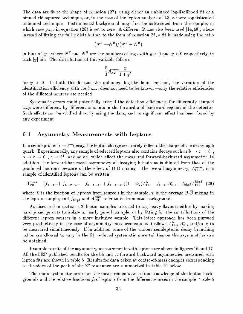
The data are �t to the shape of equation (27), using either an unbinned log-likelihood �t or abinned chi-squared technique, or, in the case of the lepton analysis of L3, a more sophisticatedunbinned technique. Instrumental background may �rst be subtracted from the sample, inwhich case gbkgd in equation (28) is set to zero. A di�erent �t has also been used [14,40], whereinstead of �tting the full y distribution to the form of equation 27, a �t is made using the ratio

(NF �NB)=(NF +NB)

in bins of jyj, where NF and NB are the numbers of tags with y > 0 and y < 0 respectively, ineach jyj bin. The distribution of this variable follows

8

3AmeasFB

y

1 + y2

for y > 0. In both this �t and the unbinned log-likelihood method, the variation of theidenti�cation e�ciency with cos �thrust does not need to be known { only the relative e�cienciesof the di�erent sources are needed.

Systematic errors could potentially arise if the detection e�ciencies for di�erently chargedtags were di�erent, by di�erent amounts in the forward and backward regions of the detector.Such e�ects can be studied directly using the data, and no signi�cant e�ect has been found byany experiment.

6.1 Asymmetry Measurements with Leptons

In a semileptonic b! `� decay, the lepton charge accurately re ects the charge of the decaying bquark. Experimentally, any sample of selected leptons also contains decays such as b! c! `+,b ! c! `�, c ! `+, and so on, which a�ect the measured forward-backward asymmetry. Inaddition, the forward-backward asymmetry of decaying b hadrons is diluted from that of theproduced hadrons because of the e�ect of B-B mixing. The overall asymmetry, Ameas

FB , in asample of identi�ed leptons can be written:

AmeasFB = (fb!`� + fb!�!`� � fb!c!`+ + fb!c!`�)(1 � 2�)Ab

FB � fc!`+AcFB + fbkgdA

bkgdFB (29)

where fi is the fraction of leptons from source i in the sample, � is the average B-B mixing inthe lepton sample, and fbkgd and A

bkgdFB refer to instrumental backgrounds.

As discussed in section 3.2, lepton samples are used to tag heavy avours either by makinghard p and pt cuts to isolate a nearly pure b sample, or by �tting for the contributions of thedi�erent lepton sources in a more inclusive sample. This latter approach has been pursuedvery productively in the case of asymmetry measurements as it allows Ab

FB, AcFB and/or � to

be measured simultaneously. If in addition some of the various semileptonic decay branchingratios are allowed to vary in the �t, reduced systematic uncertainties on the asymmetries canbe obtained.

Example results of the asymmetry measurements with leptons are shown in �gures 16 and 17.All the LEP published results for the bb and cc forward-backward asymmetries measured withlepton �ts are shown in table 5. Results for data taken at centre-of-mass energies correspondingto the sides of the peak of the Z0 resonance are summarised in table 10 below.

The main systematic errors on the measurements arise from knowledge of the lepton back-grounds and the relative fractions fi of leptons from the di�erent sources in the sample. Table 5

32

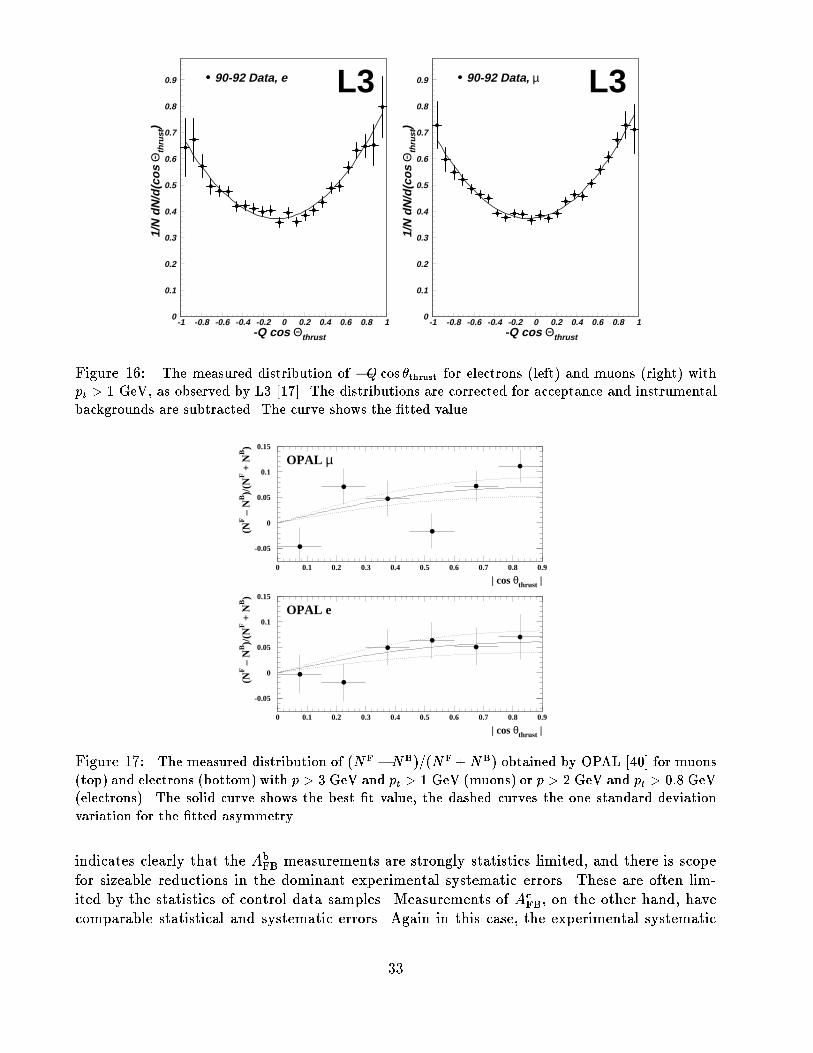
90-92 Data, e L3

-Q cos Θthrust

1/N

dN

/d(c

os Θ

thru

st)

0

0.1

0.2

0.3

0.4

0.5

0.6

0.7

0.8

0.9

-1 -0.8 -0.6 -0.4 -0.2 0 0.2 0.4 0.6 0.8 1

90-92 Data, µ L3

-Q cos Θthrust

1/N

dN

/d(c

os Θ

thru

st)

0

0.1

0.2

0.3

0.4

0.5

0.6

0.7

0.8

0.9

-1 -0.8 -0.6 -0.4 -0.2 0 0.2 0.4 0.6 0.8 1

Figure 16: The measured distribution of �Q cos �thrust for electrons (left) and muons (right) withpt > 1 GeV, as observed by L3 [17]. The distributions are corrected for acceptance and instrumentalbackgrounds are subtracted. The curve shows the �tted value.

-0.05

0

0.05

0.1

0.15

0 0.1 0.2 0.3 0.4 0.5 0.6 0.7 0.8 0.9

| cos θthrust |

(NF –

NB)/

(NF +

NB)

-0.05

0

0.05

0.1

0.15

0 0.1 0.2 0.3 0.4 0.5 0.6 0.7 0.8 0.9

| cos θthrust |

(NF –

NB)/

(NF +

NB)

OPAL µ

OPAL e

Figure 17: The measured distribution of (NF �NB)=(NF +NB) obtained by OPAL [40] for muons(top) and electrons (bottom) with p > 3 GeV and pt > 1 GeV (muons) or p > 2 GeV and pt > 0:8 GeV(electrons). The solid curve shows the best �t value, the dashed curves the one standard deviationvariation for the �tted asymmetry.

indicates clearly that the AbFB measurements are strongly statistics limited, and there is scope

for sizeable reductions in the dominant experimental systematic errors. These are often lim-ited by the statistics of control data samples. Measurements of Ac

FB, on the other hand, havecomparable statistical and systematic errors. Again in this case, the experimental systematic

33

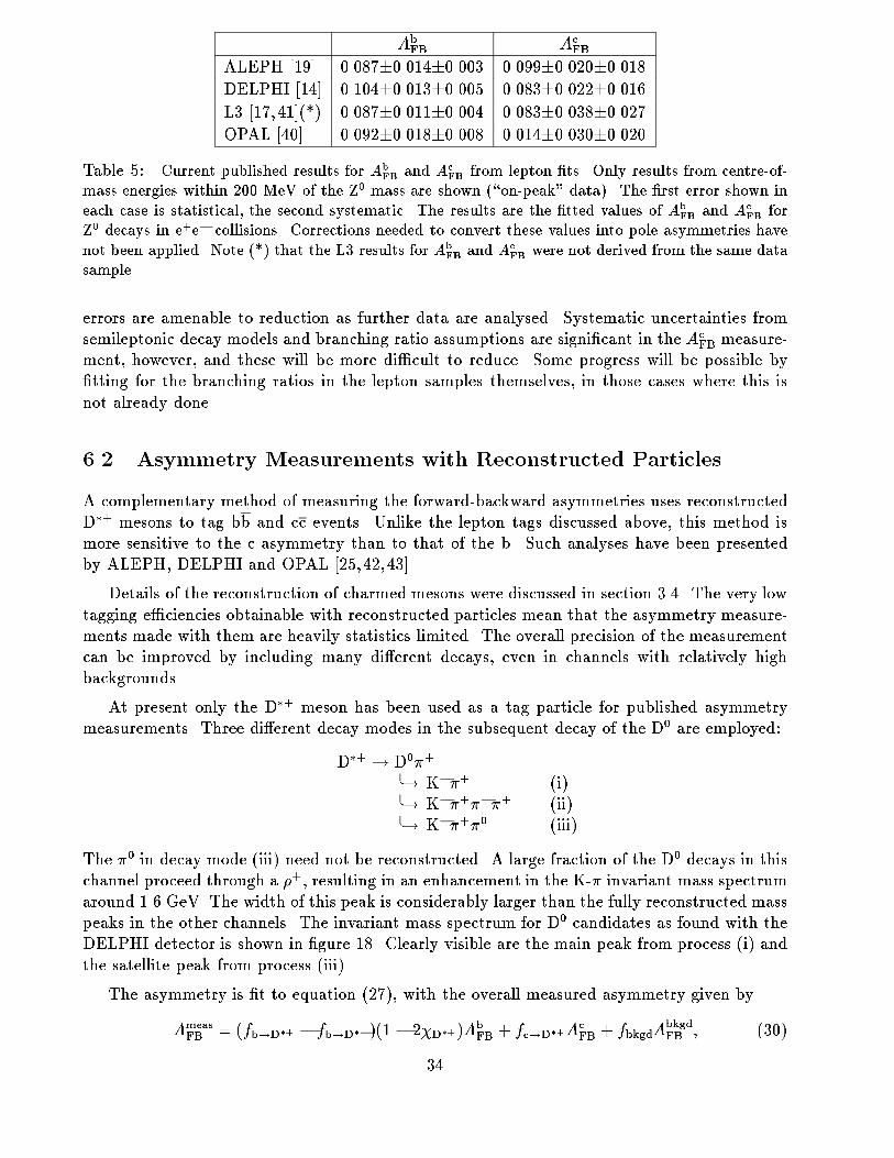
AbFB Ac

FB

ALEPH [19] 0.087�0.014�0.003 0.099�0.020�0.018DELPHI [14] 0.104�0.013�0.005 0.083�0.022�0.016L3 [17,41](*) 0.087�0.011�0.004 0.083�0.038�0.027OPAL [40] 0.092�0.018�0.008 0.014�0.030�0.020

Table 5: Current published results for AbFB and Ac

FB from lepton �ts. Only results from centre-of-mass energies within 200 MeV of the Z0 mass are shown (\on-peak" data). The �rst error shown ineach case is statistical, the second systematic. The results are the �tted values of Ab

FB and AcFB for

Z0 decays in e+e� collisions. Corrections needed to convert these values into pole asymmetries havenot been applied. Note (*) that the L3 results for Ab

FB and AcFB were not derived from the same data

sample.

errors are amenable to reduction as further data are analysed. Systematic uncertainties fromsemileptonic decay models and branching ratio assumptions are signi�cant in the Ac

FB measure-ment, however, and these will be more di�cult to reduce. Some progress will be possible by�tting for the branching ratios in the lepton samples themselves, in those cases where this isnot already done.

6.2 Asymmetry Measurements with Reconstructed Particles

A complementary method of measuring the forward-backward asymmetries uses reconstructedD�+ mesons to tag bb and cc events. Unlike the lepton tags discussed above, this method ismore sensitive to the c asymmetry than to that of the b. Such analyses have been presentedby ALEPH, DELPHI and OPAL [25,42,43].

Details of the reconstruction of charmed mesons were discussed in section 3.4. The very lowtagging e�ciencies obtainable with reconstructed particles mean that the asymmetry measure-ments made with them are heavily statistics limited. The overall precision of the measurementcan be improved by including many di�erent decays, even in channels with relatively highbackgrounds.

At present only the D�+ meson has been used as a tag particle for published asymmetrymeasurements. Three di�erent decay modes in the subsequent decay of the D0 are employed:

D�+ ! D0�+

�! K��+ (i)�! K��+���+ (ii)�! K��+�0 (iii) .

The �0 in decay mode (iii) need not be reconstructed. A large fraction of the D0 decays in thischannel proceed through a �+, resulting in an enhancement in the K-� invariant mass spectrumaround 1.6 GeV. The width of this peak is considerably larger than the fully reconstructed masspeaks in the other channels. The invariant mass spectrum for D0 candidates as found with theDELPHI detector is shown in �gure 18. Clearly visible are the main peak from process (i) andthe satellite peak from process (iii).

The asymmetry is �t to equation (27), with the overall measured asymmetry given by

AmeasFB = (fb!D�+ � fb!D��)(1 � 2�D�+)A

bFB + fc!D�+A

cFB + fbkgdA

bkgdFB ; (30)

34

0

50

100

150

200

250

300

350

400

450

1.3 1.4 1.5 1.6 1.7 1.8 1.9 2 2.1 2.2

mKπ [GeV/c2]

even

ts

DELPHIXE > 0.2data

D*+ decays

reflections

background

πsl + X

Figure 18: Invariant mass spectrum of D0 candidates reconstructed in the DELPHI detector. Thesecond broader peak visible around 1.6 GeV is due to the decay D0 ! K��0, with the �0 not recon-structed.

with the de�nitions of the fi, �D�+ and AbkgdFB equivalent to those of equation (29). The B-B

mixing parameter, �D�+, is that appropriate to the sample of D�+ mesons, which include mostly

neutral B mesons and a small fraction of charged B mesons. \Wrongly" charged D�� mesonscan be produced in b-decays via the suppressed production of a c quark in the process b! ccs.This component is estimated to be less than 1% from Monte Carlo studies and theoreticalconsiderations [44]. To ensure that Abkgd

FB = 0, partially reconstructed D mesons, present in thetagged samples at a signi�cant level, must be counted as part of the signal. They are handledin di�erent ways by the di�erent collaborations, and are most often corrected for using MonteCarlo models. OPAL use a special estimator constructed from the data.

A distribution of Q cos � of identi�ed candidates, corrected for acceptance, is shown in�gure 19. The sensitivity of these tags is largest for charm, and it can be improved by combina-tion with the asymmetries obtained from the lepton measurements discussed above, taking thecorrelations between the measurements into account. As an example, table 6 shows the corre-lation matrix between the OPAL asymmetry measurement using leptons and that using D�+

mesons [43]. Note that the largest correlations are between the b and c asymmetries measuredwithin each analysis, but that these correlations have opposite signs in the two cases. Averagingthe results therefore gives both an improved accuracy and a reduced correlation between themeasured b and c asymmetries. A full combination of all the asymmetry results is discussed insection 7.

The results from the di�erent asymmetry measurements with reconstructed particles arelisted in table 7. These measurements are dominated by statistical errors, and are likely toremain so for some time in future.

35

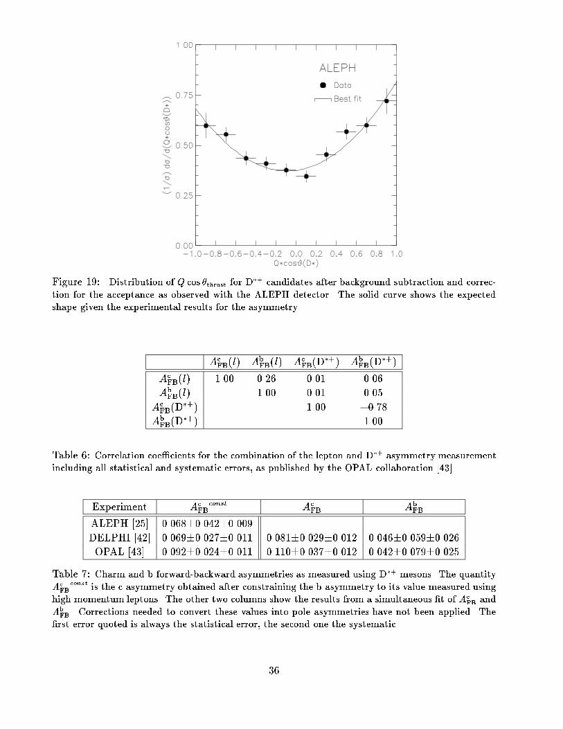
Figure 19: Distribution of Q cos �thrust for D�+ candidates after background subtraction and correc-tion for the acceptance as observed with the ALEPH detector. The solid curve shows the expectedshape given the experimental results for the asymmetry.

AcFB(l) Ab

FB(l) AcFB(D

�+) AbFB(D

�+)

AcFB(l) 1.00 0.26 0.01 0.06

AbFB(l) 1.00 0.01 0.05

AcFB(D

�+) 1.00 �0.78AbFB(D

�+) 1.00

Table 6: Correlation coe�cients for the combination of the lepton and D�+ asymmetry measurementincluding all statistical and systematic errors, as published by the OPAL collaboration [43].

Experiment AcFB

const AcFB Ab

FB

ALEPH [25] 0.068�0.042�0.009DELPHI [42] 0.069�0.027�0.011 0.081�0.029�0.012 0.046�0.059�0.026OPAL [43] 0.092�0.024�0.011 0.110�0.037�0.012 0.042�0.079�0.025

Table 7: Charm and b forward-backward asymmetries as measured using D�+ mesons. The quantityAcFB

const is the c asymmetry obtained after constraining the b asymmetry to its value measured usinghigh momentum leptons. The other two columns show the results from a simultaneous �t of Ac

FB andAbFB. Corrections needed to convert these values into pole asymmetries have not been applied. The

�rst error quoted is always the statistical error, the second one the systematic.

36

6.3 Asymmetry Measurements with Lifetime Tagged Events

As discussed in section 3.5 above, the primary quark charge in a lifetime-tagged b hemispherecan be estimated using the jet-charge technique. ALEPH [33] and DELPHI [14] have publishedanalyses using such an approach. Precise silicon vertex detectors only cover the central partof the acceptance for data analysed so far, to approximately j cos � j = 0:75-0:8. The lifetimetagging performance is thus signi�cantly degraded outside this region, so the thrust axis isrequired to lie within this acceptance. ALEPH use a cut at j cos �thrustj = 0:8, DELPHI one atj cos �thrustj = 0:7. Both analyses measure the b quark tagging e�ciency of the lifetime tag fromthe data using the double-tagging approach described in section 4. Some details of the ALEPHand DELPHI approaches are quite di�erent { ALEPH use the statistical separation power ofthe hemisphere charge measure, DELPHI use an event-by-event charge tag and exploit leptonsto measure its reliability.

ALEPH measure the forward-backward asymmetry using the relationship (section 3.5 andequation (15)):

< QFB >�< QF �QB >' �bAbFB

where �b is the value of � for b quarks. No binning in cos �thrust is used, and �b is determinedfrom the data, with only small corrections from Monte Carlo. The residual lighter quarkbackground in the sample also gives a contribution to the overall asymmetry: ALEPH chooseto take the standard model predictions for the dependence of all �ve quark avour asymmetrieson sin2 �e�W , and they then �t for the single parameter sin2 �e�W . This is then converted back,using the standard model relationship, into the value of Ab

FB at the Z0 peak.

DELPHI measure the forward-backward asymmetry using a chi-squared �t to the distri-bution of cos �thrust of the tagged sample, taking the charge assignment according to whichhemisphere has the lower measured charge. Corrections are applied for the lighter quark back-ground, assuming that Ab

FB = AsFB = Ad

FB and AcFB = Au

FB as predicted approximately by thestandard model, and taking Ac

FB = �AbFB, where the scale factor � is taken to have its standard

model value.

The �nal results obtained in the two analyses are shown in table 8. It can be seen from

AbFB

ALEPH [33] 0.0992�0.0084�0.0046DELPHI [14] 0.115�0.017�0.010

Table 8: Current published results for AbFB using lifetime tags and hemisphere charge measures.

Corrections needed to convert these values into pole asymmetries have not been applied. The �rsterror shown in each case is statistical, the second systematic.

the table that the measurements are statistically limited. The dominant sources of systematicerror in both ALEPH and DELPHI analyses come from knowledge of how well the chargeidenti�cation performs, and the purity of the b tag. Both of these are determined largely fromthe data, and so they will shrink as the data volume increases, giving promise that this type ofanalysis will continue to be statistically limited.

37

6.4 Corrections and Theoretical Uncertainties

The forward-backward asymmetry measurements described almost all assume that the di�er-ential cross-section can be written (equation (6)):

d�

d cos �/ 1 + cos2 � +

8

3AfFB cos �

and that the quark direction is well approximated by the thrust axis direction. Conversion ofthese measured asymmetries, Ab

FB and AcFB, to the pole asymmetries, A

b;0FB and Ac;0

FB, thereforerequires some small corrections to account for these assumptions. In addition, radiation ofphotons by the incoming electron and positron is not included in the de�nition of the poleasymmetries, but is present in the data. These corrections needed to convert the measuredasymmetries to the pole asymmetries are listed in table 9.

Source Shift in AbFB Shift in Ac

FB

QED corrections +0.0041 +0.0104

QCD corrections +0.0027�0.0010 +0.0022�0.0005Photon exchange �0.0003 �0.0008Centre-of-mass energy �0.0013 �0.0034Overall +0.0052�0.0010 +0.0084�0.0005

Table 9: Corrections needing to be applied to the measured b and c quark asymmetries [2,3,45]. Theshifts shown are added to the measured asymmetries to obtain the corrected values. The uncertaintyon the QCD correction is much larger than those on the other corrections.

QED corrections include primarily the e�ects of initial state radiation. This correction isparticularly important because the forward-backward asymmetry varies quite strongly withcentre-of-mass energy. The QCD correction for using the thrust axis to approximate the quarkdirection has been calculated for massless quarks, and a modi�cation of the correction for themassive quark case has been estimated by Lampe et al. [45]. In addition, e+e� annihilationthrough the photon instead of the Z0 also a�ects the asymmetry slightly, and a further smallcorrection needs to be applied to correct from the centre-of-mass energy at which LEP hasoperated to the nearby Z0 mass.

6.5 Combined Results

The results of the on-peak asymmetry measurements using the di�erent techniques areshown in �gures 20 and 21. The averages shown are derived taking into account the full cor-relations between measurements, discussed in the following section. The averages have beenderived for a centre-of-mass energy,

ps, of 91.26 GeV. For the b asymmetry, lepton and jet

charge measurements contribute approximately equally. Measurements using reconstructedparticles are not shown in �gure 20 because they do not contribute signi�cantly to the b asym-metry measurement. For the c asymmetry, lepton and reconstructed particle measurementscontribute similarly.

Measurements of the b and c asymmetry at energies at the sides of the peak of the Z0

resonance are listed in table 10. The b asymmetry has been measured using leptons by a

38

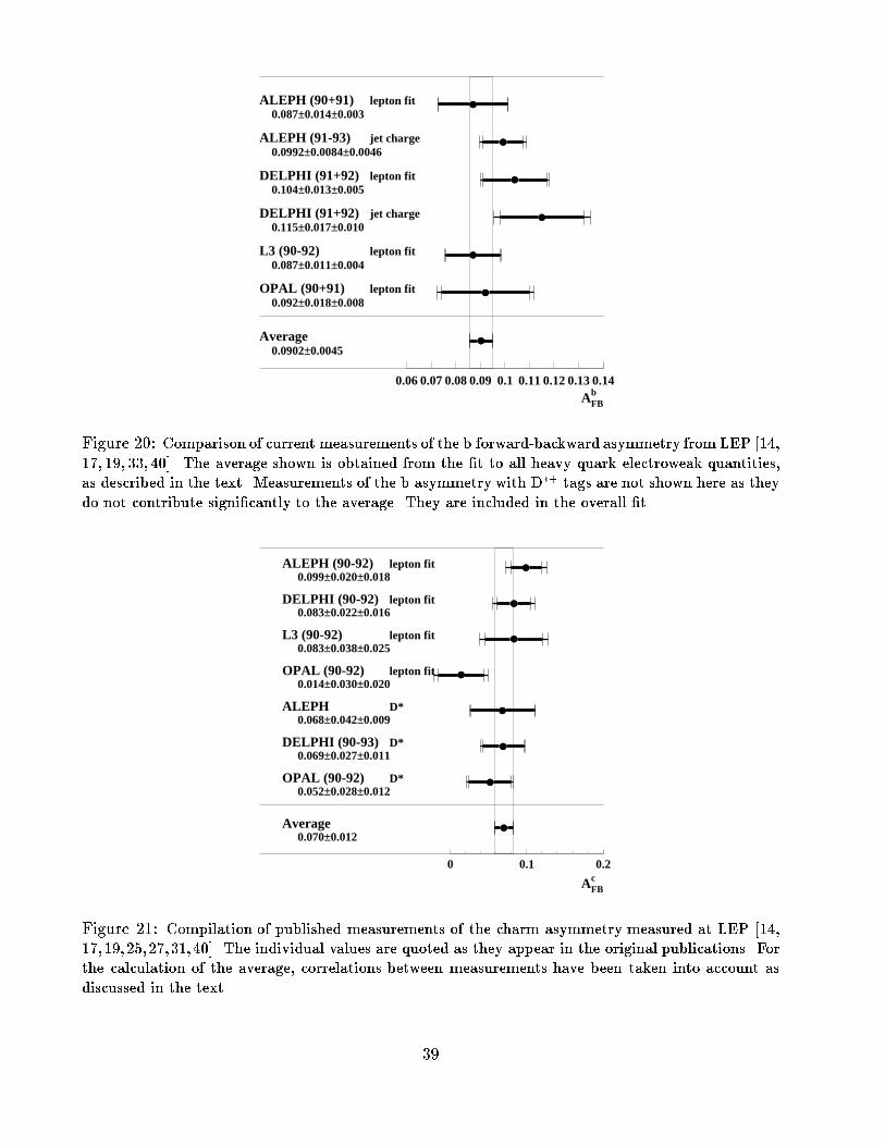
AFBb

ALEPH (90+91) lepton fit0.087±0.014±0.003

ALEPH (91-93) jet charge0.0992±0.0084±0.0046

DELPHI (91+92) lepton fit0.104±0.013±0.005

DELPHI (91+92) jet charge0.115±0.017±0.010

L3 (90-92) lepton fit0.087±0.011±0.004

OPAL (90+91) lepton fit0.092±0.018±0.008

Average0.0902±0.0045

0.06 0.07 0.08 0.09 0.1 0.11 0.12 0.13 0.14

Figure 20: Comparison of current measurements of the b forward-backward asymmetry from LEP [14,17, 19, 33, 40]. The average shown is obtained from the �t to all heavy quark electroweak quantities,as described in the text. Measurements of the b asymmetry with D�+ tags are not shown here as theydo not contribute signi�cantly to the average. They are included in the overall �t.

AFBc

ALEPH (90-92) lepton fit0.099±0.020±0.018

DELPHI (90-92) lepton fit0.083±0.022±0.016

L3 (90-92) lepton fit0.083±0.038±0.025

OPAL (90-92) lepton fit0.014±0.030±0.020

ALEPH D*0.068±0.042±0.009

DELPHI (90-93) D*0.069±0.027±0.011

OPAL (90-92) D*0.052±0.028±0.012

Average0.070±0.012

0 0.1 0.2

Figure 21: Compilation of published measurements of the charm asymmetry measured at LEP [14,17,19,25,27,31,40]. The individual values are quoted as they appear in the original publications. Forthe calculation of the average, correlations between measurements have been taken into account asdiscussed in the text.

39

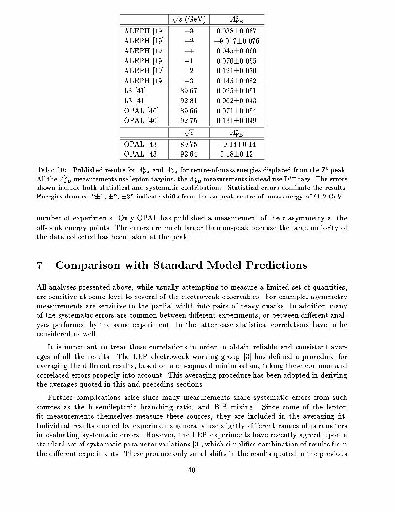
ps (GeV) Ab

FB

ALEPH [19] �3 0.038�0.067ALEPH [19] �2 �0.017�0.076ALEPH [19] �1 0.045�0.060ALEPH [19] +1 0.070�0.055ALEPH [19] +2 0.121�0.070ALEPH [19] +3 0.145�0.082L3 [41] 89.67 0.025�0.051L3 [41] 92.81 0.062�0.043OPAL [40] 89.66 0.071�0.054OPAL [40] 92.75 0.131�0.049

ps Ac

FB

OPAL [43] 89.75 �0.14�0.14OPAL [43] 92.64 0.18�0.12

Table 10: Published results for AbFB and Ac

FB for centre-of-mass energies displaced from the Z0 peak.All the Ab

FB measurements use lepton tagging, the AcFB measurements instead use D�+ tags. The errors

shown include both statistical and systematic contributions. Statistical errors dominate the results.Energies denoted \�1, �2, �3" indicate shifts from the on-peak centre-of-mass energy of 91.2 GeV.

number of experiments. Only OPAL has published a measurement of the c asymmetry at theo�-peak energy points. The errors are much larger than on-peak because the large majority ofthe data collected has been taken at the peak.

7 Comparison with Standard Model Predictions

All analyses presented above, while usually attempting to measure a limited set of quantities,are sensitive at some level to several of the electroweak observables. For example, asymmetrymeasurements are sensitive to the partial width into pairs of heavy quarks. In addition manyof the systematic errors are common between di�erent experiments, or between di�erent anal-yses performed by the same experiment. In the latter case statistical correlations have to beconsidered as well.

It is important to treat these correlations in order to obtain reliable and consistent aver-ages of all the results. The LEP electroweak working group [3] has de�ned a procedure foraveraging the di�erent results, based on a chi-squared minimisation, taking these common andcorrelated errors properly into account. This averaging procedure has been adopted in derivingthe averages quoted in this and preceding sections.

Further complications arise since many measurements share systematic errors from suchsources as the b semileptonic branching ratio, and B-B mixing. Since some of the lepton�t measurements themselves measure these sources, they are included in the averaging �t.Individual results quoted by experiments generally use slightly di�erent ranges of parametersin evaluating systematic errors. However, the LEP experiments have recently agreed upon astandard set of systematic parameter variations [3], which simpli�es combination of results fromthe di�erent experiments. These produce only small shifts in the results quoted in the previous

40

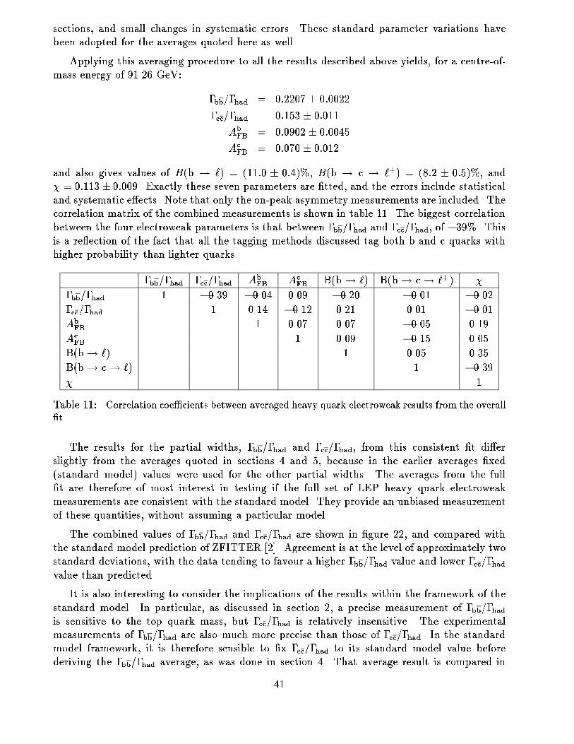
sections, and small changes in systematic errors. These standard parameter variations havebeen adopted for the averages quoted here as well.

Applying this averaging procedure to all the results described above yields, for a centre-of-mass energy of 91.26 GeV:

�bb=�had = 0:2207 � 0:0022

�cc=�had = 0:153 � 0:011

AbFB = 0:0902 � 0:0045

AcFB = 0:070 � 0:012

and also gives values of B(b ! `) = (11:0 � 0:4)%, B(b ! c ! `+) = (8:2 � 0:5)%, and� = 0:113� 0:009. Exactly these seven parameters are �tted, and the errors include statisticaland systematic e�ects. Note that only the on-peak asymmetry measurements are included. Thecorrelation matrix of the combined measurements is shown in table 11. The biggest correlationbetween the four electroweak parameters is that between �bb=�had and �cc=�had, of �39%. Thisis a re ection of the fact that all the tagging methods discussed tag both b and c quarks withhigher probability than lighter quarks.

�bb=�had �cc=�had AbFB Ac

FB B(b! `) B(b! c! `+) �

�bb=�had 1 �0.39 �0.04 0.09 �0.20 �0.01 �0.02�cc=�had 1 0.14 �0.12 0.21 0.01 �0.01AbFB 1 0.07 0.07 �0.05 0.19

AcFB 1 0.09 �0.15 0.05

B(b! `) 1 0.05 0.35

B(b! c! `) 1 �0.39� 1

Table 11: Correlation coe�cients between averaged heavy quark electroweak results from the overall�t.

The results for the partial widths, �bb=�had and �cc=�had, from this consistent �t di�erslightly from the averages quoted in sections 4 and 5, because in the earlier averages �xed(standard model) values were used for the other partial widths. The averages from the full�t are therefore of most interest in testing if the full set of LEP heavy quark electroweakmeasurements are consistent with the standard model. They provide an unbiased measurementof these quantities, without assuming a particular model.

The combined values of �bb=�had and �cc=�had are shown in �gure 22, and compared withthe standard model prediction of ZFITTER [2]. Agreement is at the level of approximately twostandard deviations, with the data tending to favour a higher �bb=�had value and lower �cc=�hadvalue than predicted.

It is also interesting to consider the implications of the results within the framework of thestandard model. In particular, as discussed in section 2, a precise measurement of �bb=�hadis sensitive to the top quark mass, but �cc=�had is relatively insensitive. The experimentalmeasurements of �bb=�had are also much more precise than those of �cc=�had. In the standardmodel framework, it is therefore sensible to �x �cc=�had to its standard model value beforederiving the �bb=�had average, as was done in section 4. That average result is compared in

41

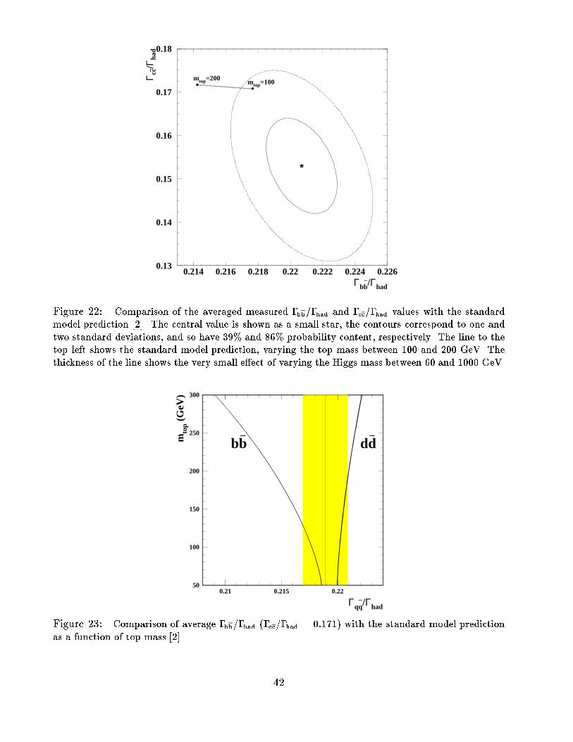
mtop=100mtop=200

Γbb–/Γhad

Γ cc– /

Γ had

0.13

0.14

0.15

0.16

0.17

0.18

0.214 0.216 0.218 0.22 0.222 0.224 0.226

Figure 22: Comparison of the averaged measured �bb=�had and �cc=�had values with the standardmodel prediction [2]. The central value is shown as a small star, the contours correspond to one andtwo standard deviations, and so have 39% and 86% probability content, respectively. The line to thetop left shows the standard model prediction, varying the top mass between 100 and 200 GeV. Thethickness of the line shows the very small e�ect of varying the Higgs mass between 60 and 1000 GeV.

Γqq–/Γhad

mto

p (G

eV)

bb–

dd–

0.21 0.215 0.2250

100

150

200

250

300

Figure 23: Comparison of average �bb=�had (�cc=�had = 0:171) with the standard model predictionas a function of top mass [2].

42

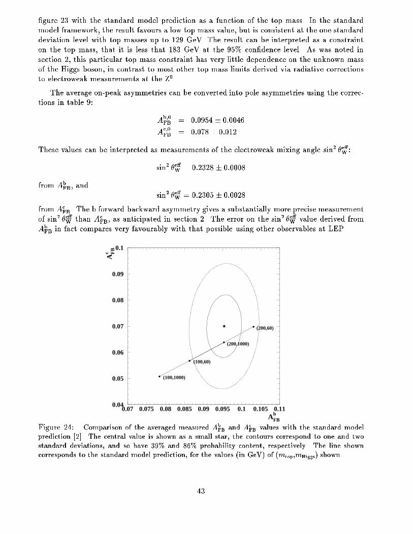
�gure 23 with the standard model prediction as a function of the top mass. In the standardmodel framework, the result favours a low top mass value, but is consistent at the one standarddeviation level with top masses up to 129 GeV. The result can be interpreted as a constrainton the top mass, that it is less that 183 GeV at the 95% con�dence level. As was noted insection 2, this particular top mass constraint has very little dependence on the unknown massof the Higgs boson, in contrast to most other top mass limits derived via radiative correctionsto electroweak measurements at the Z0.

The average on-peak asymmetries can be converted into pole asymmetries using the correc-tions in table 9:

Ab;0FB = 0:0954 � 0:0046

Ac;0FB = 0:078 � 0:012

These values can be interpreted as measurements of the electroweak mixing angle sin2 �e�W :

sin2 �e�W = 0:2328 � 0:0008

from AbFB, and

sin2 �e�W = 0:2305 � 0:0028

from AcFB. The b forward-backward asymmetry gives a substantially more precise measurement

of sin2 �e�W than AcFB, as anticipated in section 2. The error on the sin2 �e�W value derived from

AbFB in fact compares very favourably with that possible using other observables at LEP.

(100,1000)

(200,1000)

(100,60)

(200,60)

AFBb

AF

Bc

0.04

0.05

0.06

0.07

0.08

0.09

0.1

0.07 0.075 0.08 0.085 0.09 0.095 0.1 0.105 0.11

Figure 24: Comparison of the averaged measured AbFB and Ac

FB values with the standard modelprediction [2]. The central value is shown as a small star, the contours correspond to one and twostandard deviations, and so have 39% and 86% probability content, respectively. The line showncorresponds to the standard model prediction, for the values (in GeV) of (mtop,mHiggs) shown.

43

Centre-of-mass energy (GeV)

AF

Bb

88 89 90 91 92 93 94-0.1

-0.05

0

0.05

0.1

0.15

0.2

Centre-of-mass energy (GeV)

AF

Bc

88 89 90 91 92 93 94-0.4

-0.3

-0.2

-0.1

0

0.1

0.2

0.3

0.4

Figure 25: Averaged measurements of the b and c asymmetries at energies on and around the poleof the Z0 resonance. The curve shown is the prediction of the standard model for a Higgs mass of300 GeV and a top mass of 175 GeV.

The measured asymmetry values are compared in �gure 24 with the standard model pre-diction of ZFITTER [2]. Agreement is good.

The averaged values measured for the b and c asymmetries above and below the Z0 peak areshown in �gure 25 together with the average on-peak asymmetry. The averages were performedusing the same chi-squared minimisation technique as used for the main combined average,assuming that the partial widths, semileptonic branching ratios, and � mixing parameter canbe taken from the on-peak measurements. The curves show the standard model predictions,from ZFITTER [2].

Recently the SLD collaboration, working with polarised electron beams at the SLC linearcollider, have reported measurements of the b and c quark forward-backward left-right asym-metries [46], which probe directly the coupling constants Ab and Ac. They �nd:

Ab = 0:89� 0:09 � 0:06

Ac = 0:37� 0:23 � 0:21 ;

where the �rst error shown is statistical, the second systematic. The results are in agreementwith the predictions of the standard model of Ab � 0:94, Ac � 0:67 (see section 2), and withthe LEP measurements presented here.

8 Light Quark Properties

An interesting extension of the measurements discussed in this review is the determination ofthe partial widths and the asymmetries in the light quark sector. Such measurements alsoprovide tests of the universality of the couplings in the standard model.

44

Undi�erentiated average \up-like" and \down-like" partial widths have been determinedusing events with a �nal state photon [47] together with the precisely measured total Z0 hadronicdecay width, �had, and are measured at the 10%-20% level. Similarily the asymmetries of allhadrons have been measured by all four LEP experiments, without distinguishing betweenprimary event avours, using momentum weighted event charge techniques. They are used toderive values for sin2 �e�W [48].

Recently techniques for tagging light avour events using high momentum stable particleshave been developed [49,50]. A �rst measurement of the asymmetry of strange quarks at LEPhas been presented by the DELPHI collaboration [50]. Fast charged kaons, and �0 baryonsdecaying into p��, are used as tags for strange quarks. Unlike the analyses using heavy quarks, asigni�cant fraction of these particles are produced in the fragmentation process or from decaysof b and c quarks. A measurement of the apparent asymmetry of the kaon is therefore nottrivially related to the corresponding strange quark asymmetry. Rather involved hadronisationcorrections have to be applied, which are currently based on Monte Carlo studies. Using inaddition only the assumption that the unmeasured u and d quark asymmetries are respectivelyequal to the c and b quark asymmetries leads to

AsFB = 0:131 � 0:025 � 0:054 ;

where the �rst error is statistical, the second systematic. The systematic error is dominatedby modelling errors in the Monte Carlo, in particular of the charm fragmentation and theprobability of producing ss pairs in the hadronisation process.

The result is consistent with the b asymmetry measurements presented above, illustratingthe avour independence of the couplings in the standard model, at the current level of precision.

9 Future Prospects

Year Million hadronic Z0 decays

1989 (scan) 0.03

1990 (scan) 0.15

1991 (scan) 0.3

1992 0.7

1993 (scan) 0.7

1994 1.6

Table 12: Data accumulated per LEP experiment. The counts from the di�erent experiments areequal to within 10-15%. A centre-of-mass energy scan around the Z0 peak was performed in the yearsmarked \scan". In 1992 and 1994 all data were collected on the top of the Z0 peak.

The approximate numbers of hadronic Z0 decays collected by the LEP experiments are given intable 12. High-resolution microvertex detectors, very important for high precision electroweakmeasurements in the heavy avour sector, were installed and commissioned by ALEPH, DEL-PHI and OPAL in 1990 and 1991, and by L3 in 1993-1994. As a result, 1.5 to 3 million hadronicZ0 decays are available per experiment, with largely uniformly good data quality. Many of theresults reviewed in this paper do not yet include the data collected in 1993, and none yet include

45

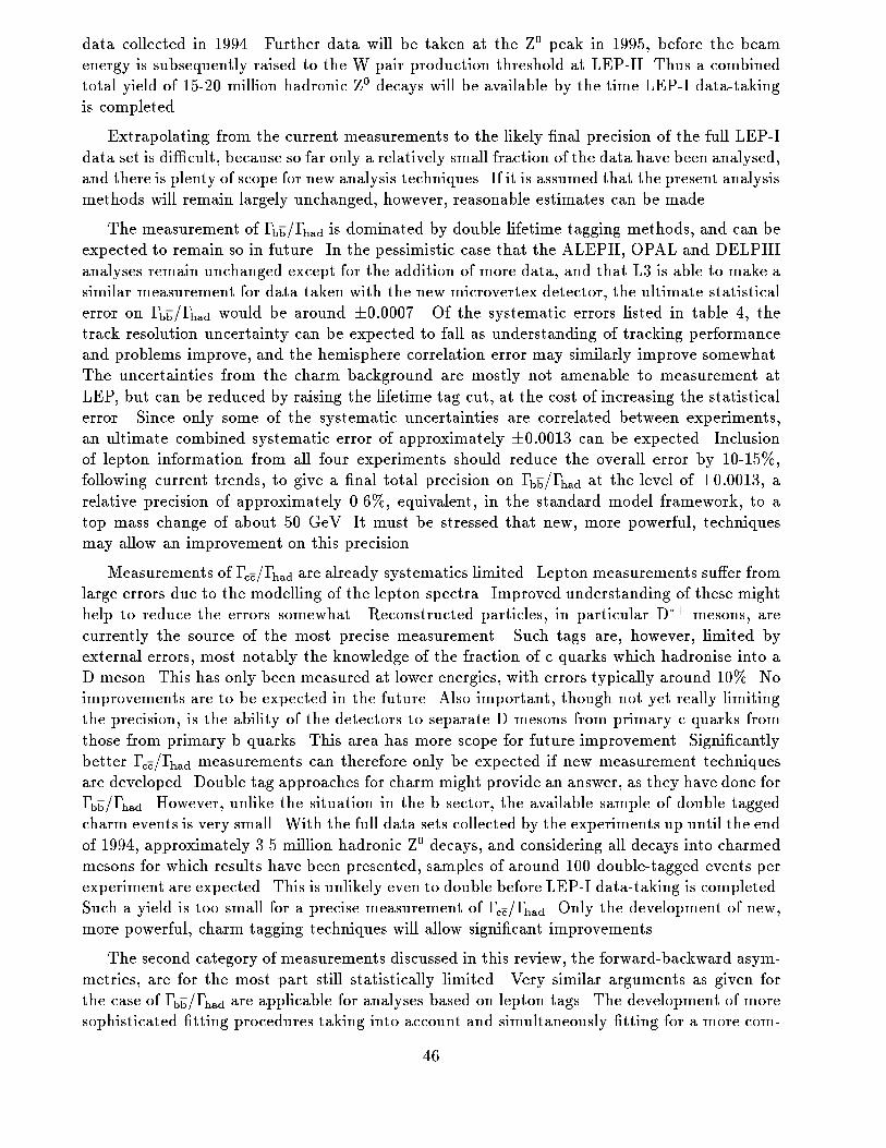
data collected in 1994. Further data will be taken at the Z0 peak in 1995, before the beamenergy is subsequently raised to the W pair production threshold at LEP-II. Thus a combinedtotal yield of 15-20 million hadronic Z0 decays will be available by the time LEP-I data-takingis completed.

Extrapolating from the current measurements to the likely �nal precision of the full LEP-Idata set is di�cult, because so far only a relatively small fraction of the data have been analysed,and there is plenty of scope for new analysis techniques. If it is assumed that the present analysismethods will remain largely unchanged, however, reasonable estimates can be made.

The measurement of �bb=�had is dominated by double lifetime tagging methods, and can beexpected to remain so in future. In the pessimistic case that the ALEPH, OPAL and DELPHIanalyses remain unchanged except for the addition of more data, and that L3 is able to make asimilar measurement for data taken with the new microvertex detector, the ultimate statisticalerror on �bb=�had would be around �0:0007. Of the systematic errors listed in table 4, thetrack resolution uncertainty can be expected to fall as understanding of tracking performanceand problems improve, and the hemisphere correlation error may similarly improve somewhat.The uncertainties from the charm background are mostly not amenable to measurement atLEP, but can be reduced by raising the lifetime tag cut, at the cost of increasing the statisticalerror. Since only some of the systematic uncertainties are correlated between experiments,an ultimate combined systematic error of approximately �0:0013 can be expected. Inclusionof lepton information from all four experiments should reduce the overall error by 10-15%,following current trends, to give a �nal total precision on �bb=�had at the level of �0:0013, arelative precision of approximately 0.6%, equivalent, in the standard model framework, to atop mass change of about 50 GeV. It must be stressed that new, more powerful, techniquesmay allow an improvement on this precision.

Measurements of �cc=�had are already systematics limited. Lepton measurements su�er fromlarge errors due to the modelling of the lepton spectra. Improved understanding of these mighthelp to reduce the errors somewhat. Reconstructed particles, in particular D�+ mesons, arecurrently the source of the most precise measurement. Such tags are, however, limited byexternal errors, most notably the knowledge of the fraction of c quarks which hadronise into aD meson. This has only been measured at lower energies, with errors typically around 10%. Noimprovements are to be expected in the future. Also important, though not yet really limitingthe precision, is the ability of the detectors to separate D mesons from primary c quarks fromthose from primary b quarks. This area has more scope for future improvement. Signi�cantlybetter �cc=�had measurements can therefore only be expected if new measurement techniquesare developed. Double tag approaches for charm might provide an answer, as they have done for�bb=�had. However, unlike the situation in the b sector, the available sample of double taggedcharm events is very small. With the full data sets collected by the experiments up until the endof 1994, approximately 3.5 million hadronic Z0 decays, and considering all decays into charmedmesons for which results have been presented, samples of around 100 double-tagged events perexperiment are expected. This is unlikely even to double before LEP-I data-taking is completed.Such a yield is too small for a precise measurement of �cc=�had. Only the development of new,more powerful, charm tagging techniques will allow signi�cant improvements.

The second category of measurements discussed in this review, the forward-backward asym-metries, are for the most part still statistically limited. Very similar arguments as given forthe case of �bb=�had are applicable for analyses based on lepton tags. The development of moresophisticated �tting procedures taking into account and simultaneously �tting for a more com-

46

plete set of electroweak parameters should allow a further and signi�cant decrease in the �nalerror, both for the b and for the c asymmetry.

Measurements of the charm asymmetry using charm tagged samples will pro�t signi�cantlyfrom the large increase in statistics that will be available by the time LEP-I stops. The precise�nal error is rather di�cult to predict, but it seems feasible to reach errors similar to the onesobtained using the leptonic sample.

There is scope to complement the measurements discussed in this review by making elec-troweak measurements in the light quark sector. Very few analyses have been shown so far.Progress in the development of techniques to separate these avours seems possible, however,and measurements of asymmetries for all three light avours should be feasible.

Further progress in the determination of the electroweak couplings beyond LEP-I will bepossible by combining LEP results with present and future results from SLD. The presenceof polarised beams at SLD provides interesting and complementary possibilities to the LEPmeasurements discussed here.

10 Conclusion

Techniques for measuring electroweak heavy quark parameters have matured remarkably in thelast few years. A wide range of di�erent tagging techniques have been developed. The partialZ0 decay width to bb pairs has been particularly precisely measured using double lifetime tags.Combining the published results from the LEP experiments, a value of

�bb=�had = 0:2207 � 0:0022

is obtained, where the error includes statistical and systematic e�ects. The averaging procedureemployed takes into account LEP measurements of all the heavy quark electroweak quantities,rather than using the standard model predictions. If the rather precise �bb=�had measurementsare interpreted in the framework of the standard model, which predicts �cc=�had = 0:171 rela-tively precisely, an average of

�bb=�had = 0:2189 � 0:0020

is obtained.

Measurement of the cc partial width has also been vigorously pursued. A combined LEPresult of

�cc=�had = 0:153 � 0:011

is obtained by averaging the published measurements using the combined averaging procedure.

Measurements of the forward-backward production asymmetries of b and c quarks in Z0

decays give information about the e�ective electroweak mixing angle, sin2 �e�W . A consistenttreatment of the measurements and their errors has been used to derive average values, forps = 91:26 GeV, of:

AbFB = 0:0902 � 0:0045

AcFB = 0:070 � 0:012

47

from the published measurements. In the context of the standard model, the b quark asymmetryin particular gives a precise measurement of the e�ective electroweak mixing angle, sin2 �e�W :

sin2 �e�W = 0:2328 � 0:0008 :

The future prospects for improvements of these measurements are excellent. The asymmetrymeasurements, in particular, are still statistics limited, and are likely to remain so for the du-ration of LEP-I data-taking. The measurements of �bb=�had will also improve with increasingstatistics, although e�ort is required to keep the systematic errors under control. Measure-ments of �cc=�had are largely systematics limited at present. Further improvement requires thedevelopment of new techniques.

Acknowledgements

The measurements presented here are the work of our colleagues in the four LEP collaborations,too numerous to name. We thank them for producing such elegant and well-documentedanalyses. The sta� of the SL Division at CERN are also to be thanked for their continuingstewardship of the LEP accelerator, the excellent and continually improving performance ofwhich makes these precise measurements possible. The combination of the di�erent resultswould have been a much more arduous task but for the work of the LEP electroweak workinggroup, and its heavy avour sub-group, in standardising systematic errors.

Valuable assistance was provided by C.M.Hawkes, P. M�attig, K. M�onig, M.Morii, D.P. Stick-land, L. Taylor, R. Tenchini and P.S. Wells in the production of this review. In particular wewish to acknowledge P.S. Wells for the provision of the LEP electroweak heavy avour averagingprogram.

We wish to acknowledge the support of our funding bodies: the Bundesministerium f�urForschung und Technologie, Germany; the Royal Society; and the Particle Physics and Astron-omy Research Council, United Kingdom; as well as support sta� at CERN.

48

References

[1] See, for example, D. Schaile, Fortsch.Phys. 42 (1994) 429.

[2] Calculated using the ZFITTER program described in:D. Bardin et al., CERN-TH 6443/92 (May 1992); Phys. Lett. B255 (1991) 290; Nucl. Phys.B351 (1991) 1; Z. Phys. C44 (1989) 493.

[3] The LEP Collaborations, ALEPH, DELPHI, L3 and OPAL, and the LEP ElectroweakWorking Group, CERN-PPE/94-187, and references therein.

[4] T. Sj�ostrand, PYTHIA 5.6 and JETSET 7.3: Physics and Manual, CERN-TH.6488/92;T. Sj�ostrand and M. Bengtsson, Computer Physics Commun. 43 (1987) 367;T. Sj�ostrand, Computer Physics Commun. 39 (1986) 347.

[5] ALEPH Collab., D. Decamp et al., Nucl. Instrum. Methods A294 (1990) 121;DELPHI Collab., P. Aarnio et al., Nucl. Instrum. Methods A303 (1991) 233;L3 Collab., B. Adeva et al., Nucl. Instrum. Methods A289 (1990) 35;OPAL Collab., K. Ahmet et al., Nucl. Instrum. Methods A305 (1991) 275.

[6] JADE Collab., W. Bartel et al., Z. Phys. C33 (1986) 23;JADE Collab., S. Bethke et al., Phys. Lett. B213 (1988) 235.

[7] OPAL Collab., R. Akers et al., Z. Phys. C61 (1994) 209.

[8] MARK III collab., D. Co�man et al., Phys. Lett. B263 (1991) 135.

[9] Particle Data Group, L. Montanet et al., Phys. Rev. D50 (1994) 1173.

[10] ALEPH Collab., D. Buskulic et al., Phys. Lett. B313 (1993) 535.

[11] Mark II Collab., R.G. Jacobsen et al., Phys. Rev. Lett. 67 (1991) 3347.

[12] OPAL Collab., P.D. Acton et al., Z. Phys. C60 (1993) 579.

[13] DELPHI Collab., P. Abreu et al., CERN-PPE/94-131.

[14] DELPHI Collab., P. Abreu et al., CERN-PPE/94-161.

[15] OPAL Collab., R. Akers et al., CERN-PPE/94-106.

[16] ALEPH Collab., D. Buskulic et al., CERN-PPE/94-165, submitted to Phys. Lett.;ALEPH Collab., D. Buskulic et al., Phys. Lett. B298 (1993) 479;L3 Collab., M. Acciarri et al., Phys. Lett. B332 (1994) 201.

[17] L3 Collab., M. Acciarri et al., CERN-PPE/94-089.

[18] OPAL Collab., R. Akers et al., Z. Phys. C60 (1993) 199.

[19] ALEPH Collab., D. Buskulic et al., Z. Phys. C62 (1994) 179;ALEPH Collab., D. Buskulic et al., Nucl. Instrum. Methods A346 (1994) 461.

[20] N. Isgur, D. Scora, B. Grinstein and M. Wise, Phys. Rev. D39 (1989) 799.

49

[21] G. Altarelli et al., Nucl. Phys. B208 (1982) 365.

[22] CLEO Collab., D. Bortoletto et al., Phys. Rev. D45 (1992) 21.

[23] DELCO Collab., W. Bacino et al., Phys. Rev. Lett. 43 (1979) 1073.

[24] MARK III Collab., R.M. Baltrusaitis et al., Phys. Rev. Lett. 54 (1985) 1976.

[25] ALEPH Collab., D. Buskulic et al., Z. Phys. C62 (1994) 1.

[26] ALEPH Collab., D. Buskulic et al., Phys. Lett. B313 (1993) 549.

[27] OPAL Collab., R. Akers et al., CERN-PPE/94-217.

[28] L3 Collab., O. Adriani et al., Phys. Lett. B307 (1993) 237.

[29] For an introduction to neural networks see: D.E. Rumelhart, G.E. Hinton, R.J. William,in Nature 323 (1986) 533;most analyses use the program JETNET to implement the algorithms: L. Lonnblad et al.,Comp. Phys. Commun. 81 (1994) 185.

[30] DELPHI Collab., P. Abreu et al., Phys. Lett. B295 (1992) 383.

[31] DELPHI Collab., P. Abreu et al., Z. Phys. C59 (1993) 533.

[32] OPAL Collab., R. Akers et al., CERN-PPE/94-206.

[33] ALEPH Collab., D. Buskulic et al., Phys. Lett. B335 (1994) 99.

[34] M.H. Seymour, LU TP 94-7, Lund Univ., May 1994.

[35] L. Lyons, D. Gibaut, P. Cli�ord, Nucl. Instrum. Methods A270 (1988) 110.

[36] L3 Collab., O. Adriani et al., Phys. Rept. 236 (1993) 1.

[37] DELPHI Collab., P. Abreu et al., CERN-PPE/95-08.

[38] ALEPH Collab., D. Decamp et al., Phys. Lett. B244 (1990) 551.

[39] DELPHI Collab., P. Abreu et al., Phys. Lett. B252 (1990) 140.

[40] OPAL Collab., P.D. Acton et al., Z. Phys. C60 (1993) 19.

[41] L3 Collab., O. Adriani et al., Phys. Lett. B292 (1992) 454.

[42] DELPHI Collab., P. Abreu et al., CERN-PPE/94-194.

[43] OPAL Collab., P.D. Acton et al., Z. Phys. C60 (1993) 601.

[44] I.Bigi and R.R�uckl, private communication.

[45] B. Lampe, MPI-Ph/93-74;A. Djouadi, B. Lampe, P.M. Zerwas, MPI-Ph/94-81, UdeM-GPP-TH-94-09, DESY 94-201.

[46] SLD Collab., K. Abe et al., SLAC-PUB-6607;SLD Collab., K. Abe et al., SLAC-PUB-6644.

50

[47] DELPHI Collab., P. Abreu et al., Z. Phys. C53 (1992) 555;L3 Collab., O. Adriani et al., Phys. Lett. B301 (1993) 136;OPAL Collab., P.D. Acton et al., Z. Phys. C58 (1993) 405;P. M�attig, CERN-PPE/93-87.

[48] L3 Collab., B. Adeva et al., Phys. Lett. B238 (1990) 122;ALEPH Collab., D. Decamp et al., Phys. Lett. B259 (1991) 377;DELPHI Collab., P. Abreu et al., Phys. Lett. B277 (1992) 371;OPAL Collab., P.D. Acton et al., Phys. Lett. B291 (1992) 436.

[49] OPAL Collab., R. Akers et al., Z. Phys. C60 (1993) 397.

[50] DELPHI Collab., P. Abreu et al., CERN PPE/94-219.

51