arX

iv:1

004.

5002

v1 [

phys

ics.

flu-

dyn]

28

Apr

201

0

Hydrodynamic interactions suppress deformation of suspension drops in Poiseuille

flow

Krzysztof Sadlej, Eligiusz Wajnryb, and Maria L. Ekiel-JezewskaInstitute of Fundamental Technological Research,

Polish Academy of Sciences,

ul. Pawinskiego 5B, 02-106 Warsaw, Poland

(Dated: April 29, 2010)

Evolution of a suspension drop entrained by Poiseuille flow is studied numerically at a lowReynolds number. A suspension drop is modelled by a cloud of many non-touching particles, ini-tially randomly distributed inside a spherical volume of a viscous fluid which is identical to the hostfluid outside the drop. Evolution of particle positions and velocities is evaluated by the accuratemultipole method corrected for lubrication, implemented in the hydromultipole numerical code.Deformation of the drop is shown to be smaller for a larger volume fraction. At high concentrations,hydrodynamic interactions between close particles significantly decrease elongation of the suspensiondrop along the flow in comparison to the corresponding elongation of the pure-fluid drop. Owingto hydrodynamic interactions, the particles inside a dense-suspension drop tend to stay for a longtime together in the central part of the drop; later on, small clusters occasionally separate out fromthe drop, and are stabilized by quasi-periodic orbits of the constituent non-touching particles. Botheffects significantly reduces the drop spreading along the flow. At large volume fractions, suspensiondrops destabilize by fragmentation, and at low volume fractions, by dispersing into single particles.

I. INTRODUCTION

Dynamics of a cloud of many non-touching micro-particles forming a suspension drop entrained by thePoiseuille flow in a microchannel is interesting for variousindustrial, biological and medical applications, such ase.g. transport in microfluidic devices [1] or narrow chan-nels [2], drug or gene delivery through the use of magneticnano-particles [3] or inhalator drug delivery [4, 5]. Thebasic question, from a dynamical point of view, is howto control dispersion of the particles and the cloud defor-mation. This is important from the practical perspective,as in some aspects it is important that the particles ormolecule clusters stay intact for a certain time or traveleddistance, while in others fast dispersion is desired.

It is known from other contexts [6] that hydrodynamicinteractions which arise between non-touching particlesmoving in a viscous fluid under a low Reynolds number,in general tend to keep close particles together in groups.This phenomenon is well studied on theoretical, numeri-cal and experimental grounds [7, 8] for particle movementresulting from the gravitational field. In particular, anensemble of initially randomly distributed particles onthe average moves in the same way as a fluid drop set-tling down in a less dense host fluid. For a very long time,such a suspension drop behaves as a cohesive entity eventhough there is no surface tension to hold the suspendedparticles together.

The clustering effect has been also observed for groupsmade of several particles only. In gravitational field,three particles can stay together for a very long time,what gives an indication to the evolution characteristicsof larger particle clouds [9]. In analogy, periodic motionof two particles under shear flow [10] forms a benchmarkwhich we expect to influence dynamics of large clouds of

particles entrained by an ambient fluid flow. In both con-texts, hydrodynamic interactions keep particles togetherfor a long time. A similar mechanism has been observedin Ref. [11], where stability of particle clusters of an or-dered internal structure immersed in a shear flow wasanalyzed.A cloud of randomly distributed particles in an ambi-

ent fluid flow, has yet not been investigated. This paperis therefore devoted to a study of the evolution of sucha suspension drop entrained by a Poiseuille flow insidea two-wall channel, in the low-Reynolds-number regime.A suspension drop is modeled by a cloud of many non-touching particles, which are initially distributed ran-domly inside a given spherical volume of the fluid, iden-tical to the host fluid outside. In the course of evolution,the particles are free to move relative to each other andthe surrounding channel walls.The goal is to analyze to what extent hydrodynamic in-

teractions between the particles inside a suspension dropinfluence its evolution, and in particular, its elongationand dispersion along the flow. The strength of the hy-drodynamic interactions is tuned-up by the increasingvolume fraction of the suspension.The structure of this paper is the following: section

II contains the general system description followed bysection III introducing briefly the numerical procedureused to calculate the hydrodynamic interactions. SectionIV contains the main results and their discussion. Thepaper is summarized and concluded in section V.

II. SYSTEM

Consider a suspension drop made of N particles im-mersed in a viscous fluid identical to the fluid outside

2

the drop. Each individual particle is a hard sphere of di-ameter d. The stick boundary conditions on the particlesurfaces are assumed. The particles cannot overlap, anddo not interact with each other through electrostatic ormagnetic forces or other direct interactions. The parti-cles are initially randomly distributed in a given sphericalfluid volume of diameter D, with equal N -particle prob-ability everywhere except overlapping. Volume fractionφ of the particles is therefore given as

φ =Nd3

D3. (1)

The fluid is bounded by two infinite planar walls sepa-rated by a distance h, which is much larger than the dropradius. This configuration models a micro-channel of awidth and length which are much larger than its height.Across the length of this channel a pressure gradient isexerted. In the absence of a drop, it would lead to theformation of a steady Poiseuille flow,

v0 = 4vm z(h− z)/h2x. (2)

FIG. 1: Model system at initial moment of time.

As illustrated in Fig. 1, the suspension drop is im-mersed in the ambient flow (2), which modifies the fluidvelocity and pressure fields, v(r) and p(r). A low-Reynolds-number flow is assumed and described by thesteady Stokes equations [12, 13],

η∇2v −∇p = 0, ∇ · v = 0. (3)

Therefore, translational velocities of the particle cen-ters, dri/dt, i = 1, ..., N , are linear functions of the max-imal ambient flow velocity vm,

dridt

= vmCi(X), (4)

where the coefficients Ci(X) are Cartesian vectors de-pending on the configuration of all the particle centers,X = (r1, r2, ...rN ).

III. NUMERICAL PROCEDURE

The Cartesian vectors Ci(X) are determined numeri-cally by the hydromultipole algorithm, which imple-ments the theoretical multipole method of calculating hy-drodynamic interactions between bodies [14–17] withinStokesian dynamics. The defined cut-off parameter L forthe multipole method was chosen L = 2 what means that24 multipole moments where calculated for each of theN particles. Such a choice of the multipole cut-off is suf-ficient to achieve a precision of the calculated velocities,normalized by vm, at least 5× 10−6 when calculating ve-locities of particles in our system. This precision estimatewas found by calculating the velocity of the suspensiondrop at t = 0 for L ranging from 2 to 8 with φ = 40%(dense drops, i.e. particles packed close together).

The particle-wall interactions are incorporated by thesingle-wall superposition of hydrodynamic forces for thetwo-wall system [17]. This approximation is poor for nar-row channels when the initial diameter of the drop iscomparable to the width of the channel but it performswell for wide channels [17]. Here we consider the case ofrelatively wide channels compared to the drop diameterwhen use of the single-wall superposition approximationis fully justified.

The first analysis performed was the estimation of walleffects encountered. We compared the initial mean ve-locities of identical drops (same initial configuration ofparticles) in the same external Poiseuille flow, using nu-merical hydromultipole procedures for an unboundedfluid and fluid between two parallel walls. At the initialmoment of time, the difference between the two calcu-lated drop velocities, normalized by vm, was of the orderof 2×10−6, i.e. smaller that the computational accuracy.Taking into account the above result, we used the nu-merical hydromultipole codes for an unbounded fluid,and benefited from the three-time increase in calculationspeed.

Having calculated the instantaneous velocities of allparticles, the evolution of the drop was determined bytime stepping the set of coupled differential equationsfor each particle position.

The number of independent simulation runs finallyperformed varied with the volume fraction. For φ up to30%, ten independent initial configurations where con-sidered. For volume fractions 40% and 50% twenty sim-ulation runs where performed. This was motivated bylarger fluctuations observed for larger volume fractions.

3

IV. EVOLUTION OF A SUSPENSION DROP

A. Model parameters

The simulated model is described by three parameters,the channel height h, the number of particles in the sus-pension drop N and the volume fraction φ. The numberof particles N in the drop was held constant, equal toN = 80. Our goal was to study how the drop evolutionwould change with the increased volume fraction, whenthe hydrodynamic interactions between the close parti-cles are enhanced. Increasing volume fractions, we alsoincreased the size of the particles, d, according to Eq. (1)with a constant drop diameter D. At the same time, wekept a constant channel height h, so as the ratio D/hwas also held constant. This ensured that the flow gradi-ent over a drop diameter was approximately equal for allvolume fractions. Suspension drops of different volumefraction (i.e different diameter when composed of equalnumber of particles) could then be compared in terms ofthe influence the same flow had on the structure of thedrop. We chose a low value D/h = 0.117, with the cor-responding values of h listed in Table I. This enabled usto make hydrodynamic interactions of the drop with thewalls very weak, and therefore to focus on the hydrody-namic interactions between particles inside the drop.

TABLE I: The channel height h/d used in our simulations fora given volume fraction φ, with N = 80 and D/h = 0.117.

φ h/d

5% 100.0010% 79.3720% 63.0030% 55.0440% 50.0050% 46.42

From now on, we normalize distances by the height h ofthe channel (i.e. the distance between the channel walls).Velocities are normalized by the maximum velocity of theflow, vm, attained in the middle of the channel. Time tin the simulations is measured in h/vm. All simulationswere performed for times approximately up to t = 300.

B. Initial moment of time

The average velocity of a suspension drop

U =1

M

M∑

j=1

1

N

N∑

i=1

Ui(j), (5)

calculated at t = 0, is plotted in Fig. 2 as a function ofvolume fraction. Here N = 80 is the number of particlesin a drop andM = 100 is the number of independent sim-ulations performed for different random configurations of

the particles, and Ui(j) is the velocity of particle i in sim-ulation j, divided by vm. Errors of the average veloc-ity(Eq. 5) are smaller than the size of the plotted points.

FIG. 2: The dimensionless velocity of a suspension drop att = 0 averaged over 100 independent, random initial condi-tions (dots). Errors are smaller than the size of the dots. Thedashed line is the limiting case of a volume of fluid havingthe same size and initial position as the considered suspen-sion drops. The dotted line corresponds to a suspension dropcomposed of non-interacting particles.

In comparison, a spherical volume of pure fluid identi-cal to the analyzed suspension drop moves at the initialmoment of time with a velocity

Uf =1

Ω

∫

Ω

v0(z)dΩ =

(

1− D2

5h2

)

, (6)

where Ω denotes the volume of a sphere of diameter Dcentered at (0, 0, 1/2) and v0(z) = |v0|/vm = 4z(1−z).This mean equals Uf = 0.997262 for D/h = 0.117 and isdenoted by the dashed line in Fig. 2.The dotted curve is the velocity of a suspension drop

composed of non-interacting particles, i.e. of a volume offluid, corrected by the Faxen term, corresponding to thenon-zero diameter d of particles,

δU =d2

24h2∇2v0 = −1

3

d2

h2. (7)

Therefore, according to Table I, the Faxen correction de-pends on volume fraction. For example, δU = 1.3× 10−4

for φ = 0.40 (i.e. h = 50d).It can be noticed in Fig. 2 that a change of the suspen-

sion volume fraction results in an overall small differencein mean velocity of the suspension drop, at most of theorder of 10−3. Nevertheless, the changes in evolutionwith the increase of volume fraction are substantial, aswill be pointed out in the next section.

C. Snap-shots from suspension drop evolution

Although the difference in the mean velocity of the sus-pension drop changes only slightly with the change of

4

36.8 37 37.2 37.4

0.2

0.4

0.6

0.8

1

x

z

35 35.2 35.4 35.6 35.8

0.2

0.4

0.6

0.8

1

x

z

35.8 36 36.2 36.4

0.2

0.4

0.6

0.8

1

x

z

37.8 38 38.2 38.4

0.2

0.4

0.6

0.8

1

x

z

38 38.2 38.4 38.6 38.8

0.2

0.4

0.6

0.8

1

x

z

37.2 37.4 37.6 37.8

0.2

0.4

0.6

0.8

1

x

z

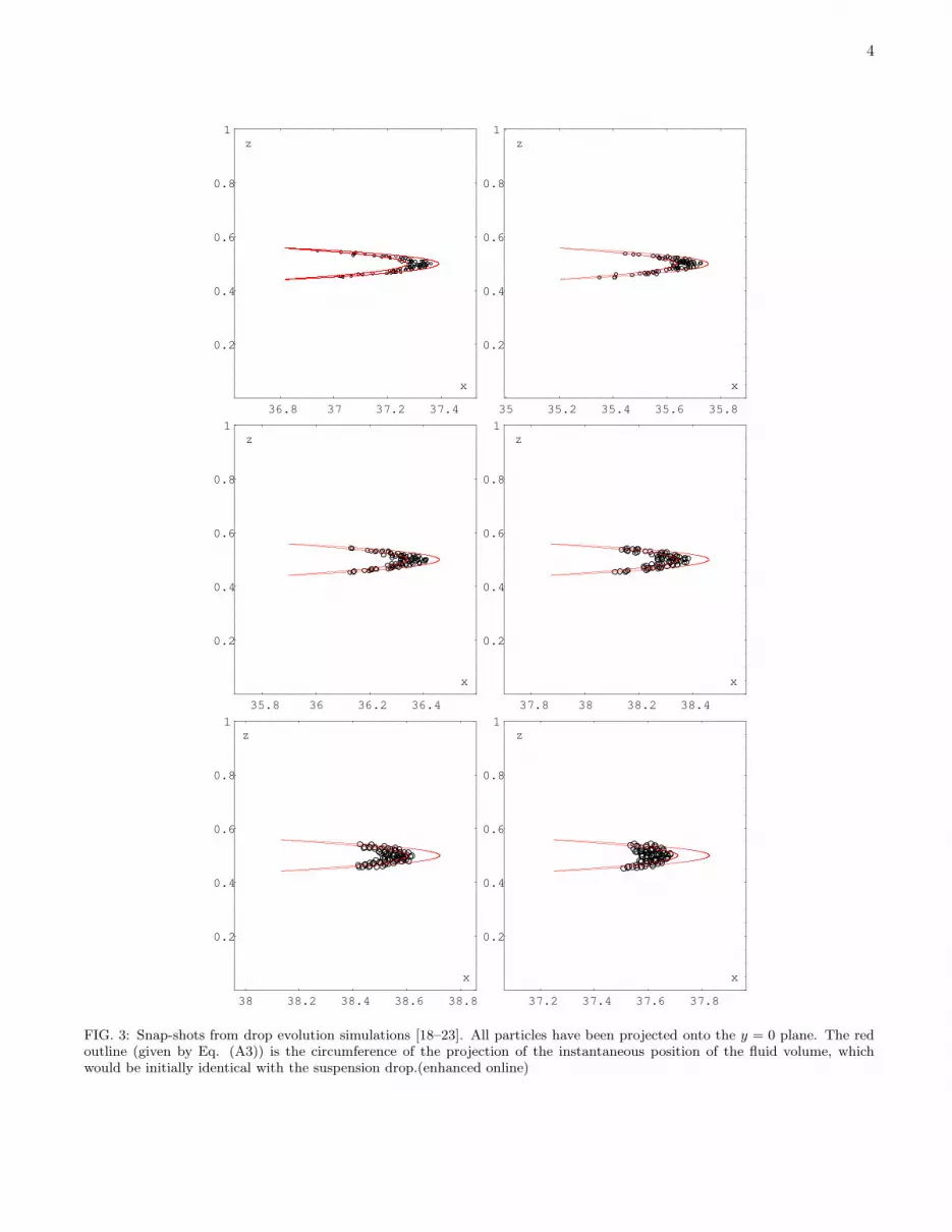
FIG. 3: Snap-shots from drop evolution simulations [18–23]. All particles have been projected onto the y = 0 plane. The redoutline (given by Eq. (A3)) is the circumference of the projection of the instantaneous position of the fluid volume, whichwould be initially identical with the suspension drop.(enhanced online)

5

36.8 37 37.2 37.4

-0.4

-0.2

0

0.2

0.4

x

y

35 35.2 35.4 35.6 35.8

-0.4

-0.2

0

0.2

0.4

x

y

35.8 36 36.2 36.4

-0.4

-0.2

0

0.2

0.4

x

y

37.8 38 38.2 38.4

-0.4

-0.2

0

0.2

0.4

x

y

38 38.2 38.4 38.6 38.8

-0.4

-0.2

0

0.2

0.4

x

y

37.2 37.4 37.6 37.8

-0.4

-0.2

0

0.2

0.4

x

y

FIG. 4: Snap-shots from drop evolution simulations [24–29]. All particles have been projected onto the z = 1/2 plane. The redoutline (given by Eqs. (A2-A4)) is the circumference of the projection of the instantaneous position of the fluid volume, whichwould be initially identical with the suspension drop. (enhanced online)

6

its volume fraction, a quick look at the simulation snap-shots (Fig. 3, see [18–23] and Fig. 4, see [24–29]) showsa clear change in the behavior of all particles. As thevolume fraction increases, particles tend to stay clusteredtogether longer. The stretching of the initial shape of thesuspension drop therefore highly depends of its volumefraction. In order to show this phenomenon clearly it isinstructive to compare the positions of particles with theevolved shape of an initially spherical volume of fluid.The equation describing the circumferential surface ofthis fluid volume is

(x − v0(z)t)2 =

D2

4h2− z2 − y2, (8)

v0(z) = 4z(1− z).

As simulations shown and discussed in this paper arepresented in projections (y = 0 or z = 1/2), the interiorof the drop contained inside the above surface has to beaccordingly projected. Therefore,

1. The boundary of the fluid-drop projection on they = 0 plane is given by Eq. (8) with y = 0.

2. The fluid-drop projection on the z = 1/2 plane is asuperposition of circles shifted with respect to eachother. Its boundary is therefore more sophisticated,see Eqs. (A2)-(A4) derived in Appendix A.

The boundaries of the fluid-drop projections on they = 0 and z = 1/2 planes are plotted in Figs. 3 and4, respectively, and compared with the snapshots of theunderlying movies [click on figure to watch movie], pre-senting the suspension drops at the same time instant.The scale on the x, y and z axes is the same, to keepspherical shape of the particles and the initial volume ofthe drops.For small volume fractions the particles move in a simi-

lar way as the pure fluid. Particles initially concentratedin a spherical drop get spread out evenly and the ini-tial shape of the drop is clearly stretched resembling theevolved shape of the corresponding spherical volume ofpure fluid. No group formation is observed and hydrody-namic interaction between particles seems to be minor.As the volume fraction increases, the shape of the sus-

pension drop at a given time instant is clearly less andless elongated by the flow than the evolved reference vol-ume of pure fluid, as shown in Figs. 3-4. Notice that forthe largest volume fraction φ = 50%, the drop’s shape isstill quite close to a sphere.As the volume fraction increases, the evolution of the

suspension drop changes significantly, and the particleshave a tendency to stay clustered in a single group for alonger time, as illustrated in the movies linked to Figs. 3-4. For larger times, deformation of a dense suspensiondrop increases, and small groups of particles separate outfrom the main cluster. Particle groups which form inboth tails, rotate relative to their center of mass, due tothe gradient of the flow, in a similar way as two particlesin a shear flow [10]. The average number of the particles

in such a group increases with time and is larger for ahigher volume fraction.

D. Quantitative analysis

By viewing the simulation results one can concludethat hydrodynamic interactions hold particles togethermore effectively, when these are packed in larger vol-ume fractions. This qualitative remark can be quantifiedby analyzing the time-dependent dispersion of the parti-cle positions inside a drop, averaged over M simulationscorresponding to different random initial configurations.The dispersion along x-direction is defined by the follow-ing formula,

σx =1

M

M∑

j=1

√

√

√

√

1

N

N∑

i=1

x2i(j) −

(

1

N

N∑

i=1

xi(j)

)2

, (9)

where N = 80 is the number of particles in a dropand M is the number of simulations performed. Thex-coordinates xi(j) of each of the i = 1, . . . , N particlesin each of the j = 1, . . . ,M simulations are functions oftime, and so is the dispersion itself. The same formulaleads to the definition of σy and σz once xi(j) is exchangedfor the appropriate coordinate.Fig. 5 shows the dispersion σx of particle positions in

the drop along the flow (x) direction, evolving in time,for different volume fractions. Color-coding, representingdifferent volume fractions, has been chosen according toTable II. At a given time instant, the dispersion σx issmaller for a larger volume fraction φ, and this effect issignificant.

FIG. 5: Dispersion of particle positions in the drop along theflow (x) direction, evolving in time. Results averaged over alltested initial conditions. Color-coding see Table II; the largervolume fraction, the smaller is σx. The dashed line (φ=0%)corresponds to pure fluid, Eq. (10), and the dotted one to thenon-interacting particles, Eq. (12).

For comparison, the dashed line in Fig. 5 is the analyt-ical result calculated for a spherical volume of pure-fluid

7

TABLE II: Color-coding used to differentiate results for var-ious volume fractions

color φ

black 5%red 10%

yellow 20%green 30%

light blue 40%dark blue 50%

evolving with the flow (φ = 0%). Its dispersion was cal-culated as

σf,x =

√

1

Ω

∫

Ω

(x+ v0(z)t− x)2 dΩ

=1

10

√

32t2D4

7h4+

5D2

h2, (10)

where

x = t

(

1− D2

5h2

)

. (11)

The dispersion σx of a pure-fluid drop is of course largerthan the dispersion of a suspension drop. To investigatethe effect of the excluded volume, the dispersion σx,ni

of a suspension drop made of fictitious non-interactingparticles is also evaluated, defined by Eq. (9) with thereal particle positions xi(j)(t) replaced by xi(j),ni(t), thetime-dependent positions of the fictitious particles, whichwould not interact hydrodynamically, and just translatealong the Poiseuille fluid flow, v0, with the Faxen velocity,v0 + δU , and the Faxen correction δU given by Eq. (7),

xi(j),ni(t) = xi(j),ni(0) + (v0 + δU)t. (12)

The initial configurations of the fictitious particles arethe same as those used in the suspension-drop evolution,xi(j),ni(0) = xi(j)(0). The result is plotted in Fig. 5 witha dotted line. The curves corresponding to φ = 5%, 40%and 50% are practically superimposed. Comparison withthe pure fluid and with the suspension drop indicatesthat elongation of the suspension drop is significantlysuppressed by strong hydrodynamic interactions betweenparticles at larger volume fractions.In Fig. 6 a closeup of Fig. 5 for short times is shown.

Further, the mean standard errors have been plotted(dotted lines) together with the original curves in orderto show that the results obtained distinguish between dif-ferent volume fractions. For volume fractions 40% and50% the errors are smaller than the width of the curve.Systematically, for a larger volume fraction, the disper-

sion σx is smaller, if time is not too small, e.g. t > 5. No-tice that at t = 0 the curves plotted in Fig. 6 do not over-lay each other. On first notice this might seem wrong.But when given further insight, the dispersion at t = 0is shown to change with the volume fraction, as plottedin Fig. 7. This graph shows the dispersion of particle

FIG. 6: Dispersion of particle positions in the drop along theflow (x) direction evolving in time. Results averaged over alltested initial conditions. Top to botton: 5% to 50% respec-tively. Color-coding see Table II. The dotted lines show thestandard mean errors. For 40% and 50% the errors are smallerthan the width of the curve.

0.00001 0.0001 0.001 0.01 0.1Φ

0.024

0.0245

0.025

0.0255

0.026

ΣxHt=0L

Φ=0

FIG. 7: Dispersion of particle positions along the flow (x)direction calculated at t = 0. The dashed line is the limitinganalytical solution. Error-bars are smaller then the size of thepoints.

positions along the flow (x) direction calculated at t = 0for volume fraction ranging from 0.001% to 50%. Theexpected error of σx is equal the standard deviation ofthe dispersion within a single drop, divided by

√M . For

t = 0, the number of initial configurations randomly se-lected is 100000 and thus the error-bars are smaller thenthe size of the points. The non-monotonic dependence ofthe drop dispersion on the volume fraction is a strictlystatistical effect due to excluded volume. In particular,notice that the dispersion for 5% is smaller than for 50%as also visible on Fig. 6. The dashed line is the limitinganalytical solution at t = 0 for a volume of pure fluid (i.e.φ = 0). Of course σy(t = 0) = σz(t = 0) = σx(t = 0).We checked that for a larger number of particles in thesuspension drop (and therefore for a smaller particle di-ameter d), the dispersion σx slightly increases.For larger times, the value of the drop dispersion in the

flow direction decreases more than by a factor of 2, for

8

volume fractions changing form 5% to 50%. This givesa clear indication that hydrodynamic interactions tendto hold close particles together, and therefore suppressdeformation of the drop along the flow.Dispersion of particle positions along the transverse

(y) and (z) direction, respectively, evolving in time, isshown in the two last figures in this section - Fig. 8 andFig. 9. Results have been averaged over all tested initialconditions.

FIG. 8: Dispersion of particle positions in the y direction,evolving in time. Results have been averaged over all testedinitial conditions. The dashed line is the limiting result fora pure-fluid drop. The dotted lines show the standard meanerrors.

FIG. 9: Dispersion of particle positions in the z direction,evolving in time. Results averaged over all tested initial con-ditions. The dashed line is the limiting result for a pure-fluiddrop. The dotted lines show the standard mean errors.

For comparison, we show also the corresponding dis-persion of the pure fluid,

σf,y = σf,z = σf,x(t = 0) = 0.02616. (13)

In the transverse directions, the dispersion of the pure-fluid drop is constant in time.Note that in the direction transverse to the flow the

drop gets contracted as it evolves. This effect is small,

but clearly visible as the volume fraction of the drop in-creases. It is also caused by hydrodynamic interactionsbetween close particles.

E. Group formation

When analyzing the simulation results at longer times,it becomes clear that for larger volume fractions, theparticles which are lost from the main drop have a ten-dency to form small groups in the course of further evo-lution. This effect is readily visible in the movies linkedto Figs. 3-4, and it is a clear indication of hydrodynamicinteractions between close particles.In particular, for simulations with φ ≥ 30% groups of

several particles where observed to stay together until theend of the simulation at t = 300. During this time eachgroup rotated and particles interchanged places. Thisbehavior of close particles resembles periodic trajectoriesof two particles in shear flow [10].We decided to check the group formation quantita-

tively by introducing an algorithm working in the fol-lowing way: First, all particles are divided into two en-sembles, depending if their position z > 1/2 or z ≤ 1/2.Then, within these two ensembles, positions of their cen-ters in the flow direction are compared by ordering. Ifbetween any two consecutive particle centers in such asequence, the distance in the (x) flow direction is largerthan a dimensional parameter g, then these particles aresaid to belong to two distinct groups. This grouping pa-rameter if fully arbitrary. We chose g = 3d. Differentchoices where checked - this discussion can be found inAppendix B.Having in mind the definition of a group, the averaged

time τ of a first destabilization defined as formation ofat least two groups of particles is evaluated and shown inTable III and Fig. 10. Clearly, for a larger volume frac-tion, hydrodynamic interactions between closer particleskeep them together in a single cluster for a longer time.

TABLE III: Averaged time τ of first destabilization definedas formation of at least two groups of particles.

φ τ

5% 14.510% 20.520% 35.230% 44.040% 57.050% 90.0

The error-bars in the figure correspond to the standarddeviation of results calculated for the individual simula-tions. The line is a fit to the data 5% ≤ φ ≤ 40% givenby the formula τ = 9.0 + 120.3φ. The point for φ = 50%is substantially above this fit, while all other results seemto be well in accordance with the linear behavior.The average number of distinct groups which are

9

FIG. 10: Averaged time τ of first destabilization as a func-tion of the drop volume fraction φ. Error-bars are equal thestandard deviation of the average value. The line is a linearfit to the data 5% ≤ φ ≤ 40%.

formed after time t = 50, 100, 150, 200 is listed in Ta-ble IV.

TABLE IV: Average number of distinct groups of particlesafter time t = 50, 100, 150, 200.

φ nt=50 nt=100 nt=150 nt=200

5% 8.3 18.1 24.0 30.010% 5.7 13.3 19.2 22.020% 2.9 9.0 11.3 13.330% 2.0 5.8 8.4 10.140% 1.3 4.2 5.4 6.750% 1.0 2.1 4.4 6.2

FIG. 11: Average number n of groups of particles as a functionof time. Top-down: φ = 5%, 10%, 20%, 30%, 40% and 50%.The errors, calculated as the standard deviation of the mean,are smaller than the distance between the curves.

Fig. 11 shows the average number n of groups as afunction of time, for all studied volume fractions. Moredense drops split into a smaller number of groups. Takinginto account the mean standard deviation as the error of

these results, the dependence on the volume fraction iswell established. Once again the difference between thecase of 50% and 5% is substantial and suppresses 500%.The grouping phenomenon is therefore strictly corre-

lated with the initial high concentration of particles. Forlarge volume fractions, hydrodynamic interactions be-tween particles are strong and tend to cluster them. Thisis why more dense suspension drops destabilize slower.For a high volume fraction, particles stay in one groupfor a very long time, e.g. for times up to τ = 90 if initiallyφ = 50% (refer to Table IV).A higher volume fraction leads to a larger suspension

viscosity. Therefore, the considered cloud of particles canbe interpreted as a drop of a larger viscosity than a hostfluid. In the absence of surface tension, the increase ofthe drop viscosity leads to its slower and smaller deforma-tion. This result gives an additional information to thenumerical study of drop deformations at a finite capillarynumber, presented in Ref. [30].

V. CONCLUSIONS

This paper was devoted to a numerical study of suspen-sion drop evolution in a Poiseuille flow of Stokesian fluidin a parallel-wall channel. The fluid inside the drop wasthe same as outside. The drop was initially centered onthe axes of the channel, away from the walls. We studiedthe effect of the hydrodynamic interactions between sus-pended particles on the process of the drop deformation.Simulations where performed for a wide range of suspen-sion volume fractions, and compared to the evolution ofa spherical volume of pure fluid, of the identical initialsize and position in the Poiseuille flow as the suspensiondrop.The differences in evolution characteristics between the

different volume fractions of suspension drops studied inthis paper, are extensive. For a low volume fraction, theparticles get dispersed evenly occupying an area coveringapproximately the evolved shape of a comparable vol-ume of pure fluid. Dense drops behave differently - fora long time they stay almost non-deformed; later, theirevolution is dominated by formation of small groups ofrotating particles, which are left behind the drop. Theclustering is caused by hydrodynamic interactions. Rel-ative motion of close particles tends to hold them to-gether, pushing the flow out of the cluster and hinderingits destabilization. The closer the particles are, the longerthey stay together in a cluster. For example, at φ = 50%,the stretching of the initially compact drop, measured asthe the dispersion of the particles along the flow, is twotimes smaller than at φ = 5%, and all the particles stayvery close to each other in a compact group more than 6times longer.The results discussed in this paper have a clear impact

on practical application. By changing volume fraction ofsuspension drops produced in microfluidic devices, or in-halators designed for drug delivery, one is able to control

10

the time-dependent dispersion of the particles entrainedby the fluid flow. A large volume fraction will suppressthe drop deformation and lead to clustering, while a smallone to effective and even spreading of the particles.

Acknowledgments

This work was supported in part by by the PolishMinistry of Science and Higher Education grant 45/N-COST/2007/0 and the COST P21 Action “Physics ofdroplets”.

Appendix A: Evolution of an initially spherical

fluid-drop

Volume of a pure-fluid drop remains the same dur-ing its evolution. The time-dependent circumferentialsurface of the fluid-drop has been specified in Eq. (8).Therefore, the boundary of the fluid-drop projection onthe y = 0 plane is given by Eq. (8) with y = 0,

(x− v0(z)t)2 =

D2

4h2− z2, (A1)

where v0(z) = 4z(1−z). An example of such a shape isshown in Fig. 3.The circumference of the fluid-drop projection onto the

plane z = 1/2 consists of the following two curves,

xR(y) = t+

√

D2

4h2− y2, (A2)

i.e. the right boundary of the drop projection, which issimply a half-circle, and

xL(y) = minz∈

[

1

2, 12+√

D2

4h2−y2

]

v0(z)t−

√

D2

4h2−y2−

(

z− 1

2

)2

(A3)

i.e. the left boundary of the drop projection, which con-sists of two parts,

xL(y) =

t−√

D2

4h2 − y2 for y2> D2

4h2 − 164t2 ,

t− 116t +4t

(

y2− D2

4h2

)

for y2≤ D2

4h2 − 164t2 .

(A4)

The curve trailing the area occupied by a projected,evolved shape of the spherical volume of fluid is there-fore in piece a circle given by Eq. (A2) and the firstpart of Eq. (A4), and piecewise a parabola given by thesecond part of Eq. (A4). This curve and its derivativeare continuous. An example of such a curve is shown inFig. 4.

Appendix B: Group detection

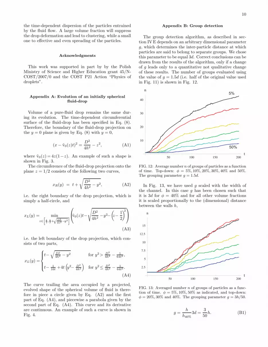
The group detection algorithm, as described in sec-tion IVE depends on an arbitrary dimensional parameterg, which determines the inter-particle distance at whichparticles are said to belong to separate groups. We chosethis parameter to be equal 3d. Correct conclusions can bedrawn from the results of the algorithm, only if a changeof g leads only to a quantitative not qualitative changeof these results. The number of groups evaluated usingthe value of g = 1.5d (i.e. half of the original value usedin Fig. 11) is shown in Fig. 12.

FIG. 12: Average number n of groups of particles as a functionof time. Top-down: φ = 5%, 10%, 20%, 30%, 40% and 50%.The grouping parameter g = 1.5d.

In Fig. 13, we have used g scaled with the width ofthe channel. In this case g has been chosen such thatit is 3d for φ = 40% and for all other volume fractionsit is scaled proportionally to the (dimensional) distancebetween the walls h,

FIG. 13: Averaged number n of groups of particles as a func-tion of time. φ = 5%, 10%, 50% as indicated, and top-down:φ = 20%, 30% and 40%. The grouping parameter g = 3h/50.

g =h

h40%3d =

3

50h. (B1)

11

In both cases, we find that clearly drops of larger vol-ume fraction tend to form fewer clusters. Of course, thenumber of clusters depends on the choice of the param-

eter g. Nevertheless, the general overall picture of theevolution stays qualitatively the same.

[1] K. V. Sharp and R. J. Adrian, Microfluid Nanofluid 1,376 (2005).

[2] M. E. Staben and R. H. Davis, Int. J. of Multiphase Flow31, 529 (2005).

[3] J. Dobson, Drug Dev. Res. 67 55 (2006).[4] D. M. Broday and R. Robinson, Aerosol Science and

Technology 37, 510 (2003).[5] D. A. Edwards at al., Science 276, 1868 (1997).[6] J. M. Nitsche and G. K. Batchelor, J. Fluid Mech. 340,

161 (1997).[7] G. Machu, W. Meile, L.C. Nitsche and U. Schaflinger, J.

Fluid Mech. 447, 299 (2001).[8] M. L. Ekiel-Jezewska, B. Metzger, and E. Guazzelli,

Phys. Fluids 18, 038104 (2006).[9] I. M. Janosi, T. Tel, D. E. Wolf, and J. A. C. Gallas,

Phys. Rev. E 56, 2858 (1997).[10] G. K. Batchelor, J. Fluid Mech. 56, 375 (1972).[11] R. B. Jones, J. Chem. Phys. 115, 5319 (2001).[12] J. Happel and H. Brenner, Low Reynolds Number Hy-

drodynamics. Martinus Nijhoff, Dordrecht, 1986.[13] S. Kim and S. J. Karrila, Microhydrodynamics: Princi-

ples and Selected Applications. Butterworth-Heinemann,London, 1991.

[14] S. Bhattacharya, J. B lawzdziewicz, and E. Wajnryb,Phys. Fluids 18, 053301 (2006).

[15] B. Cichocki, B. U. Felderhof, K. Hinsen, E. Wajnryb, andJ. B lawzdziewicz, J. Chem. Phys. 100, 3780 (1994).

[16] M. L. Ekiel-Jezewska and E. Wajnryb, Precise multipolemethod for calculating hydrodynamic interactions be-tween spherical particles in the Stokes flow. In F. Feuille-bois and A Sellier, editors, Theoretical Methods for Mi-

cro Scale Viscous Flows, pages 127–172. Transworld Re-search Network, 2009.

[17] S. Bhattacharya, J. B lawzdziewicz, and E. Wajnryb,Physica A 356, 294 (2005).

[18] See Supplementary Material Document No. to watch fullsimulation of drop evolution for φ = 5% in MPEG for-

mat.[19] See Supplementary Material Document No. to watch full

simulation of drop evolution for φ = 10% in MPEG for-mat.

[20] See Supplementary Material Document No. to watch fullsimulation of drop evolution for φ = 20% in MPEG for-mat.

[21] See Supplementary Material Document No. to watch fullsimulation of drop evolution for φ = 30% in MPEG for-mat.

[22] See Supplementary Material Document No. to watch fullsimulation of drop evolution for φ = 40% in MPEG for-mat.

[23] See Supplementary Material Document No. to watch fullsimulation of drop evolution for φ = 50% in MPEG for-mat.

[24] See Supplementary Material Document No. to watch fullsimulation of drop evolution for φ = 5% in MPEG for-mat.

[25] See Supplementary Material Document No. to watch fullsimulation of drop evolution for φ = 10% in MPEG for-mat.

[26] See Supplementary Material Document No. to watch fullsimulation of drop evolution for φ = 20% in MPEG for-mat.

[27] See Supplementary Material Document No. to watch fullsimulation of drop evolution for φ = 30% in MPEG for-mat.

[28] See Supplementary Material Document No. to watch fullsimulation of drop evolution for φ = 40% in MPEG for-mat.

[29] See Supplementary Material Document No. to watch fullsimulation of drop evolution for φ = 50% in MPEG for-mat.

[30] A. J. Griggs, A. Z. Zinchenko, and R. H. Davis, Int. J.of Multiphase Flow 33, 182 (2007).