water

Article

Study of Pressure Drops and Heat Transfer of NonequilibrialTwo-Phase Flows

Aleksandr V. Belyaev 1,*, Alexey V. Dedov 1, Ilya I. Krapivin 1, Aleksander N. Varava 1, Peixue Jiang 2 andRuina Xu 2

�����������������

Citation: Belyaev, A.V.; Dedov, A.V.;

Krapivin, I.I.; Varava, A.N.; Jiang, P.;

Xu, R. Study of Pressure Drops and

Heat Transfer of Nonequilibrial

Two-Phase Flows. Water 2021, 13,

2275. https://doi.org/10.3390/

w13162275

Academic Editors:

Maksim Pakhomov and

Pavel Lobanov

Received: 15 July 2021

Accepted: 17 August 2021

Published: 20 August 2021

Publisher’s Note: MDPI stays neutral

with regard to jurisdictional claims in

published maps and institutional affil-

iations.

Copyright: © 2021 by the authors.

Licensee MDPI, Basel, Switzerland.

This article is an open access article

distributed under the terms and

conditions of the Creative Commons

Attribution (CC BY) license (https://

creativecommons.org/licenses/by/

4.0/).

1 Department of General Physics and Nuclear Fusion, The National Research University “MPEI”,Krasnokazarmennaya 14, 111250 Moscow, Russia; dedovav@mpei.ru (A.V.D.); KrapivinII@mpei.ru (I.I.K.);VaravaAN@mpei.ru (A.N.V.)

2 Department of Thermal Engineering, Tsinghua University, Haidian District, Beijing 100084, China;jiangpx@tsinghua.edu.cn (P.J.); ruinaxu@tsinghua.edu.cn (R.X.)

* Correspondence: BeliayevAVL@mpei.ru

Abstract: Currently, there are no universal methods for calculating the heat transfer and pressure dropfor a wide range of two-phase flow parameters in mini-channels due to changes in the void fractionand flow regime. Many experimental studies have been carried out, and narrow-range calculationmethods have been developed. With increasing pressure, it becomes possible to expand the rangeof parameters for applying reliable calculation methods as a result of changes in the flow regime.This paper provides an overview of methods for calculating the pressure drops and heat transferof two-phase flows in small-diameter channels and presents a comparison of calculation methods.For conditions of high reduced pressures pr = p/pcr ≈ 0.4 ÷ 0.6, the results of own experimentalstudies of pressure drops and flow boiling heat transfer of freons in the region of low and high massflow rates (G = 200–2000 kg/m2 s) are presented. A description of the experimental stand is given,and a comparison of own experimental data with those obtained using the most reliable calculatedrelations is carried out.

Keywords: heat transfer; hydrodynamics; high reduced pressure; flow boiling

1. Introduction

An important trend in the development of new energy conservation technologies iscreating more miniature technical objects, an effort that requires extensive backgroundknowledge of hydrodynamics and heat transfer in single-phase convection and flow boilingin mini-channels.

The opportunity to accurately predict the pressure drops and heat transfer and theselection of mini-channel geometry and working conditions are important factors for thedesign of the optimal settings of heat exchangers. In various fields of technology, oneof the effective methods of heat transfer from heating surfaces is the boiling of liquid. Itis necessary to experimentally confirm methods for calculating pressure drops and heattransfer.

1.1. Pressure Drops

The two-phase pressure drop in micro-channels is relatively high compared to conven-tional channels due to their very small size and relatively high mass flow rates, the latterbeing necessary to achieve acceptable heat transfer coefficients. Due to the high-pressuregradient, saturation temperature, and, consequently, thermophysical properties, there is adifference in pressure in mini-channels when the pressure in a certain axial position of thechannel drops below the saturation pressure of the liquid, and the liquid temporarily over-

Water 2021, 13, 2275. https://doi.org/10.3390/w13162275 https://www.mdpi.com/journal/water

Water 2021, 13, 2275 2 of 13

heats in this place. A pressure drop in a two-phase flow is a result of friction, acceleration,gravitation, and channel form change.

∆PTP =

[(dPdZ

)Fr+

(dPdZ

)Ac

+

(dPdZ

)Gr

]Z + ∆PF (1)

Gravitational pressure drop is usually neglected. If the flow is adiabatic, pressuredrop due to flow acceleration is neglected too. Most techniques for calculating pressuredrop relate to either a homogeneous or separated flow model.

1.1.1. Homogeneous Equilibrium Model

For a homogeneous equilibrium model, it is assumed that liquid and gas mix with eachother, and the pressure drop of a two-phase flow can be calculated using the correlationsfor a single-phase flow. For this, the values averaged over the entire cross-section are takenas the calculated thermophysical properties, while there is heat transfer between the phases.(

dPdZ

)Fr

=

(dPdZ

)TP

= ξTP(G)2

2ρTP

1Dh

(2)

where ξTP is obtained by the Filonenko formula [1]:

ξTP =1(

1.82 log10(ReTP)− 1.64)2 (3)

ReTP =GDhµTP

(4)

µTP is calculated according to the method of Cicchitti et al. [2], which is the mostpopular method and researched for a wide range of the Reynolds numbers:

µTP = xµg + (1− x)µl (5)

As it said in Zubov et al. [3], in the limit of high velocities of the mixture at highreduced pressures, there is reason to draw an analogy between the homogeneous modeland the continuum model for gas flow. The traditional homogeneous flow model for shearstress on the wall uses the formula:

τTP =ξTP

8ρβw2

TP (6)

where ρβ = ρ′′β+ (1− β)ρ′:

wTP =Gρ′×[

1 + xρ′ − ρ′′

ρ′′

](7)

And then, pressure drops are calculated as:(dPdZ

)Fr

=4τTPDh

(8)

In two-phase flow, according to research by Venkatesan et al. [4], Cioncolini et al. [5],and Choi and Kim [6], the homogeneous flow model is applicable only to bubbly flow.Homogeneous flow conditions are fulfilled at high flow rates and mass flow rate steamcontent less than 0.1. At large values of the mass vapor quality x > 0.1, the homogeneousmodel, as a rule, is not applied. Under the conditions of subcooled flow, a calculation basedon the homogeneous model demonstrates acceptable accuracy [7].

1.1.2. Separated Flow Model

Liquid and gas in the separated flow model move together, and it is taken as a factthat there is a clear phase boundary through which evaporation occurs. In the last decade,

Water 2021, 13, 2275 3 of 13

a number of studies have been published on pressure drop in micro-channels, basedon the methodology of Lockhart and Martinelli [8], who proposed using the two-phasemultiplier (9) to relate the pressure drop of a two-phase flow to the pressure drop of theliquid phase:

Φl2 =

(dPdZ

)TP

/(dPdZ

)l

(9)

An example of such research is the work of Hwang et al. [9], where the workingfluid was R134a, and the hydraulic diameter varied from 0.244 to 0.792 mm. The studyconcluded that the pressure drop increased with an increase in the Reynolds number andwas similar to the pressure drop for single-phase flow in a channel with a larger equivalentdiameter. In addition, the pressure drop in a two-phase flow increases with a decrease inthe inner diameter. The two-phase multiplier is calculated as:

Φl2 = 1 +

Cχ+

1χ2 (10)

where:C = 227Re0.452

l Co−0.82χ−0.32 (11)

To calculate the two-phase multiplier Φl in conventional channels, for example, theFriedel method is often used [10], in which pipes larger than 4 mm are examined. Thetwo-phase multiplier is calculated as:

Φl = E +

(3.24FH

Fr0.045We0.035

)(12)

where:

E = (1− x)2 + x2 ρlρg

fg

fl(13)

F = x0.78(1− x)0.224 (14)

H =

(1−

µg

µl

)0.7( ρlρg

)0.91(µg

µl

)0.19(15)

Most formulas and methods, including the ones above, are suitable for relativelysmall amounts of fluid and a limited range of flow parameters and geometries. Thus, it isnecessary to check the accuracy of the prediction models and select the best formula forpredicting pressure drops in mini-channels.

1.2. Investigations of Heat Transfer in Mini-Channels

In the literature, there are many methods for determining the heat transfer coefficientwhen boiling a liquid flow in channels.

One of the best-known methods was by J. Chen [11], which was derived in a paperin which the boiling of a saturated water flow in a circular vertical micro-channel wasinvestigated.

Lazarek and Black [12], when calculating the heat transfer coefficient, came to theconclusion that nucleate boiling was the main one that occurred during their tests, sincethe heat transfer coefficient depended on mass flow rate and heat flux density.

The experimental data in a study by Tran et al. [13] showed that when the value ofvapor quality x > 0.2, the heat transfer coefficient does not depend on it. Here, heat transferdepended mainly on the mass velocity and not on the heat flux density. It was found thatthe border between the regions of the dominance of nucleate boiling and evaporation israther abrupt and occurs at significantly smaller changes in saturation temperature thanpredicted.

Kenning-Cooper [14] noted that in the annular flow regime, the heat transfer coefficientis well described by J. Chen [11], but for slug flow, Chen’s method gives deviations. In

Water 2021, 13, 2275 4 of 13

addition, nucleate boiling is sensitive to surface conditions as opposed to evaporativeconditions.

Gungor and Winterton [15] developed a correlation that is versatile in its applicationand generally gives a more accurate fit to the data than the correlations proposed by the au-thors of the studies reviewed. The average deviation between the calculated and measuredheat transfer coefficient was 21.4% for saturated boiling and 25.0% for supercooled boiling.

Shah [16] presented, in graphical form, a general correlation called CHAPT for esti-mating the saturated boiling heat transfer coefficients for subcritical heating of the flow inpipes.

Liu-Winterton [17] presented a comparative analysis of the previously obtained databy J. Chen [11], Gungor and Winterton [15], and Shah [16]. In their correlation, the authorsintroduced the Prandtl constraint as a parameter that affects the coefficient of influence ofthe convective component on the heat transfer coefficient.

Kandlikar [18] conducted a comparative analysis of the earlier studies concentrat-ing on the data obtained by the different researchers. For the correlations, data from24 experimental studies were obtained. For comparison, the correlations of J. Chen [11],Gungor and Winterton [15], and Shah [16] were considered.

Sun and Mishima [19] conducted a comparative analysis of 13 previously obtainedcorrelations, forming a new database. The results showed that J. Chen’s correlation [11]and its modifications were not very well suited for mini-channels and that Lazarek andBlack’s correlation [12] was the most suitable.

Table 1 summarizes the most famous works. Obviously, the data in most of theexperimental works now available in the literature were obtained for low and moderatereduced pressures [20]. In addition, the authors proposed the calculation methods, whichhave an empirical nature and are more suitable for describing experiments close to thosedescribed by the authors. In the field of high reduced pressures, the analysis of the literatureshows a lack of researches.

Table 1. List of works indicating calculation methods.

Author Liquids Formula

Tran et al. R12, R113 αTP = 840(

Bo2Wel only

)0.3(ρg/ρl

)0.4

Lazarek and Black R113 αTP = 30Re0.857l Bo0.714 λl

Dh

Shah R11, R12, R22 αTP = ψαSP

Kenning-Cooper Water, freons αTP =(1 + 1.8χtt

−0.87)αSP

Kandlikar Water, R11, R12, R114, NO2αTPαSP

=

1.136Co−0.9(25Frl)

c + 667.2Bo0.7Fl (1)0.0683Co−0.2(25Frl)

c + 1058Bo0.7Fl (2)(1) : Co< 0.65; (2) : Co >0.65

Sun and Mishima Water, freons αTP =6Re1.05

lo Bo0.54

We0.191lo

(ρlρg

)0.142λlDh

J. Chen Water αTP = SαNB + FαSPGungor and Winterton Water, R22, R113, R114, R11, R12 αTP = SαNB + FαSP

Liu-Winterton Water, R113, R114, R11, R12, R22 αTP =√(SαNB)

2 + (FαCB)2

The size of the channel significantly affects the character of vaporization during flowboiling. In the region of high reduced pressures, based on the analysis performed in [21], itcan be assumed that, in mini-channels, the flow regimes become identical to those seen inconventional channels. In this case, the relationships for the normal channels may be usedto calculate the pressure drop and heat transfer. Based on this assumption, a method forcalculating heat transfer for subcooled flow boiling in mini-channels was tested in [7].

The heat flux density was calculated as follows:

q = qboil + qcon (16)

Water 2021, 13, 2275 5 of 13

It is assumed that convective heat transfer acts in the same way as in a single-phaseturbulent flow:

qcon = αcon(Twall − Tfluid) (17)

where αcon is calculated using the Petukhov formula with employees in the form [22],adjusted for the difference between the wall and liquid temperatures:

Nu =(ξ/8)(Re− 1000)Pr

1 + 12.7(ξ/8)1/2(Pr2/3 − 1)( Prl

Prwall

)0.25(18)

To calculate qboil in conditions of saturated flow boiling in relation (16), it is advisableto use the equation proposed by V.V. Yagov [23]:

qboil = 3.43× 10−4 λ2∆Ts3

νσTs

(1 +

r∆T2RiT2

s

)(1 +√

1 + 800B + 400B)

(19)

where B =r(ρg

µlρl

)3/2

σ(λTs)1/2 and ∆Ts =Twall − Ts (all properties are determined at saturation

temperature Ts). Modified version of Equation (19) for qboil for subcooled flow boilingpresented in the paper [24].

2. Experimental Setup Description

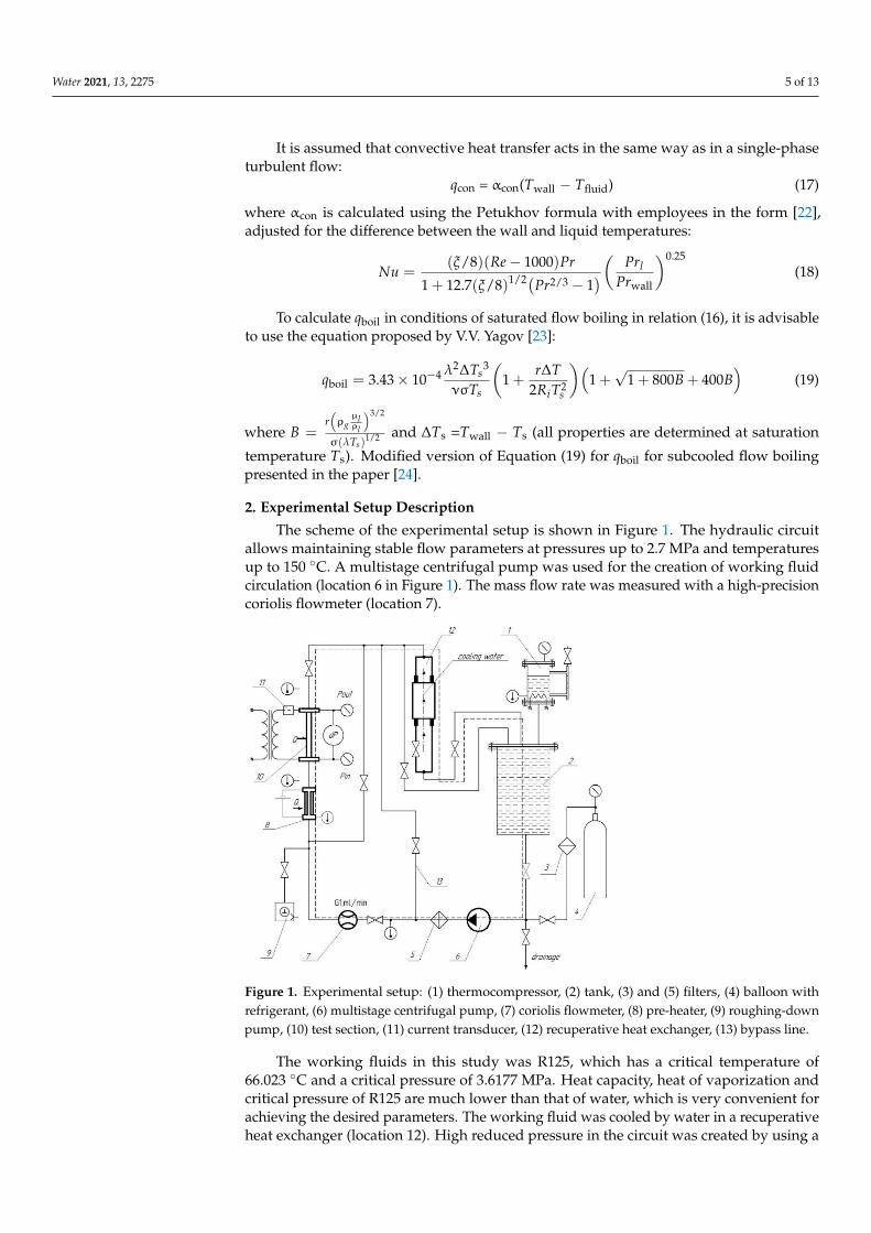
The scheme of the experimental setup is shown in Figure 1. The hydraulic circuitallows maintaining stable flow parameters at pressures up to 2.7 MPa and temperaturesup to 150 ◦C. A multistage centrifugal pump was used for the creation of working fluidcirculation (location 6 in Figure 1). The mass flow rate was measured with a high-precisioncoriolis flowmeter (location 7).

Water 2021, 13, x FOR PEER REVIEW 6 of 14

Figure 1. Experimental setup: (1) thermocompressor, (2) tank, (3) and (5) filters, (4) balloon with refrigerant, (6) multistage centrifugal pump, (7) сoriolis flowmeter, (8) pre-heater, (9) roughing-down pump, (10) test section, (11) current transducer, (12) recuperative heat exchanger, (13) bypass line.

The test section is shown in Figure 2. Vertical stainless-steel tubes with heated lengths of 51 mm each and internal diameters of 1 mm and 1.1 mm were used as mini-channels. The tube was electrically insulated and hydraulically sealed through PTFE (polytetraflu-oroethylene) seals. Electrodes were soldered to the tube with tin.

Figure 2. Design of the test section.

The design of the test section had temperature-compensation. The platform with the inlet collector was mounted on two vertical metal rods on which it could slide. In this way, the inlet collector had a vertical degree of freedom. The platform of the inlet collector was held by a spring along the rods towards the tube to avoid vibration and ensure the stabil-ity of the test tube.

Five Chromel-Copel thermocouples were used to take the measure values of the wall temperatures. On five cross-sections (T1–T5, see Table 2) of the working area of the tube on opposite sides of the tube diameter, the wires (diameter 0.2 mm) were welded using lasers. This mounting method for the thermocouples created low thermal inertia for the sensors and allowed the measurement of the average temperature of the wall along its

Figure 1. Experimental setup: (1) thermocompressor, (2) tank, (3) and (5) filters, (4) balloon withrefrigerant, (6) multistage centrifugal pump, (7) coriolis flowmeter, (8) pre-heater, (9) roughing-downpump, (10) test section, (11) current transducer, (12) recuperative heat exchanger, (13) bypass line.

The working fluids in this study was R125, which has a critical temperature of66.023 ◦C and a critical pressure of 3.6177 MPa. Heat capacity, heat of vaporization andcritical pressure of R125 are much lower than that of water, which is very convenient forachieving the desired parameters. The working fluid was cooled by water in a recuperativeheat exchanger (location 12). High reduced pressure in the circuit was created by using a

Water 2021, 13, 2275 6 of 13

thermocompressor (location 1). A pressure sensor with a measurement accuracy of 0.2%was used for measuring pressure and pressure drops across the inlet and outlet of the testsection. Chromel-Copel cable thermocouples with a cable diameter of 0.7 mm measuredthe inlet and outlet temperatures.

The test section was heated with alternating current. The electrical current strengthwas measured using an LA 55-P current transducer. The measurement error of the electricpower was 1%.

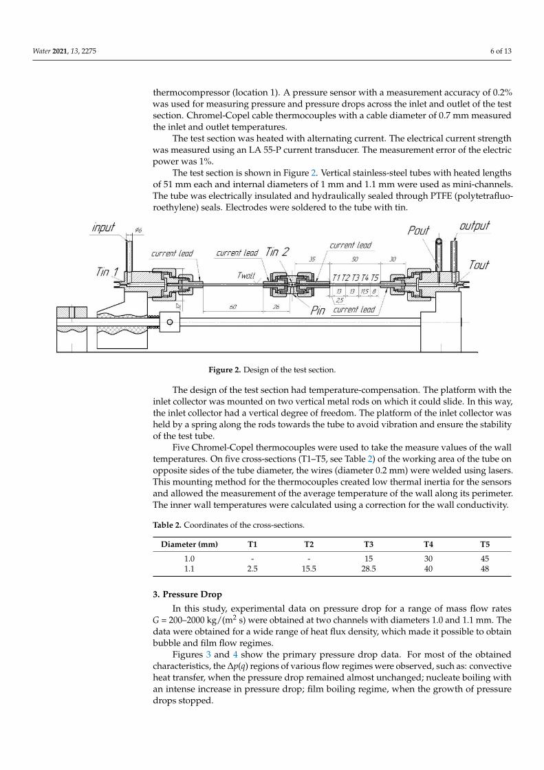
The test section is shown in Figure 2. Vertical stainless-steel tubes with heated lengthsof 51 mm each and internal diameters of 1 mm and 1.1 mm were used as mini-channels.The tube was electrically insulated and hydraulically sealed through PTFE (polytetrafluo-roethylene) seals. Electrodes were soldered to the tube with tin.

Water 2021, 13, x FOR PEER REVIEW 6 of 14

Figure 1. Experimental setup: (1) thermocompressor, (2) tank, (3) and (5) filters, (4) balloon with refrigerant, (6) multistage centrifugal pump, (7) сoriolis flowmeter, (8) pre-heater, (9) roughing-down pump, (10) test section, (11) current transducer, (12) recuperative heat exchanger, (13) bypass line.

The test section is shown in Figure 2. Vertical stainless-steel tubes with heated lengths of 51 mm each and internal diameters of 1 mm and 1.1 mm were used as mini-channels. The tube was electrically insulated and hydraulically sealed through PTFE (polytetraflu-oroethylene) seals. Electrodes were soldered to the tube with tin.

Figure 2. Design of the test section.

The design of the test section had temperature-compensation. The platform with the inlet collector was mounted on two vertical metal rods on which it could slide. In this way, the inlet collector had a vertical degree of freedom. The platform of the inlet collector was held by a spring along the rods towards the tube to avoid vibration and ensure the stabil-ity of the test tube.

Five Chromel-Copel thermocouples were used to take the measure values of the wall temperatures. On five cross-sections (T1–T5, see Table 2) of the working area of the tube on opposite sides of the tube diameter, the wires (diameter 0.2 mm) were welded using lasers. This mounting method for the thermocouples created low thermal inertia for the sensors and allowed the measurement of the average temperature of the wall along its

Figure 2. Design of the test section.

The design of the test section had temperature-compensation. The platform with theinlet collector was mounted on two vertical metal rods on which it could slide. In this way,the inlet collector had a vertical degree of freedom. The platform of the inlet collector washeld by a spring along the rods towards the tube to avoid vibration and ensure the stabilityof the test tube.

Five Chromel-Copel thermocouples were used to take the measure values of the walltemperatures. On five cross-sections (T1–T5, see Table 2) of the working area of the tube onopposite sides of the tube diameter, the wires (diameter 0.2 mm) were welded using lasers.This mounting method for the thermocouples created low thermal inertia for the sensorsand allowed the measurement of the average temperature of the wall along its perimeter.The inner wall temperatures were calculated using a correction for the wall conductivity.

Table 2. Coordinates of the cross-sections.

Diameter (mm) T1 T2 T3 T4 T5

1.0 - - 15 30 451.1 2.5 15.5 28.5 40 48

3. Pressure Drop

In this study, experimental data on pressure drop for a range of mass flow ratesG = 200–2000 kg/(m2 s) were obtained at two channels with diameters 1.0 and 1.1 mm. Thedata were obtained for a wide range of heat flux density, which made it possible to obtainbubble and film flow regimes.

Figures 3 and 4 show the primary pressure drop data. For most of the obtainedcharacteristics, the ∆p(q) regions of various flow regimes were observed, such as: convectiveheat transfer, when the pressure drop remained almost unchanged; nucleate boiling withan intense increase in pressure drop; film boiling regime, when the growth of pressuredrops stopped.

Water 2021, 13, 2275 7 of 13

Water 2021, 13, x FOR PEER REVIEW 7 of 14

perimeter. The inner wall temperatures were calculated using a correction for the wall conductivity.

Table 2. Coordinates of the cross-sections.

Diameter (mm) Т1 Т2 Т3 Т4 Т5 1.0 - - 15 30 45 1.1 2.5 15.5 28.5 40 48

3. Pressure Drop In this study, experimental data on pressure drop for a range of mass flow rates G =

200–2000 kg/(m2s) were obtained at two channels with diameters 1.0 and 1.1 mm. The data were obtained for a wide range of heat flux density, which made it possible to obtain bubble and film flow regimes.

Figures 3 and 4 show the primary pressure drop data. For most of the obtained char-acteristics, the Δp(q) regions of various flow regimes were observed, such as: convective heat transfer, when the pressure drop remained almost unchanged; nucleate boiling with an intense increase in pressure drop; film boiling regime, when the growth of pressure drops stopped.

With an increase in the diameter, the pressure drops decreased for the same values of mass flow rate (see Figure 3), which is quite natural. Analysis of the effect of reduced pressure on the pressure drops at the same values of G = 600 kg/(m2s) (see Figure 4) al-lowed us to draw the following conclusion: the flow regime changed with an increase in the reduced pressure: the region with non-increasing pressure drops due to the heat load increases from 50 to 125 kW/m2.

Figure 3. Pressure drop versus heat flux density at various values of the mass flow rates.

0

2

4

6

8

10

0 50 100 150 200 250

R125d = 1.1; 1.0 mmpr = 0.43

d = 1.1 mm200400600d = 1.0 mm6008001000

Figure 3. Pressure drop versus heat flux density at various values of the mass flow rates.

Water 2021, 13, x FOR PEER REVIEW 8 of 14

Figure 4. Pressure drop versus heat flux density at two values of reduced pressure.

To obtain pressure drops by calculation, the earlier described methods were used. In most of the experiments, the calculation method by [10] had too significant deviation with increasing heat flux, as can be seen in Figure 5, probably due to the quadratic dependence of the two-phase multiplier Ф on the vapor quality х. In addition, this method has been developed for channels with diameters greater than 4 mm. As a result, it was concluded that it was not suitable for generalizing the obtained data on mini-channels, even under conditions of high reduced pressures.

Figure 5. Example of the experimental data with calculated data versus heat flux.

The analysis of the experimental data showed that the reduced pressure mostly af-fected the correspondence of the calculated values to the experimental data. For the inves-tigated range of mass flow rates G = 200–2000 kg/(m2s) and values of vapor quality (up to x ≈ 0.4) for reduced pressure pr = 0.43, the best agreement with the experimental data was observed for the method of [9], which was based on a split flow model. An example of calculations for pressure pr = 0.43 is shown in Figure 6.

0

2

4

6

8

10

0 50 100 150 200 250 300

R125d = 1 mmG = 600 kg/(m2s)

pr = 0.43

pr = 0.57

0.0

0.5

1.0

1.5

2.0

20 30 40 50 60 70

R125d = 1.1 mmG = 200 kg/(m2s)pr = 0.43Ts ≈ 30 ºC

Exp

Cicchitti et al.

Yagov

Hwang and Kim

Friedel

Zubov et al.

Figure 4. Pressure drop versus heat flux density at two values of reduced pressure.

With an increase in the diameter, the pressure drops decreased for the same valuesof mass flow rate (see Figure 3), which is quite natural. Analysis of the effect of reducedpressure on the pressure drops at the same values of G = 600 kg/(m2 s) (see Figure 4)allowed us to draw the following conclusion: the flow regime changed with an increase inthe reduced pressure: the region with non-increasing pressure drops due to the heat loadincreases from 50 to 125 kW/m2.

To obtain pressure drops by calculation, the earlier described methods were used. Inmost of the experiments, the calculation method by [10] had too significant deviation withincreasing heat flux, as can be seen in Figure 5, probably due to the quadratic dependenceof the two-phase multiplier Φl on the vapor quality x. In addition, this method has beendeveloped for channels with diameters greater than 4 mm. As a result, it was concludedthat it was not suitable for generalizing the obtained data on mini-channels, even underconditions of high reduced pressures.

The analysis of the experimental data showed that the reduced pressure mostlyaffected the correspondence of the calculated values to the experimental data. For theinvestigated range of mass flow rates G = 200–2000 kg/(m2 s) and values of vapor quality(up to x ≈ 0.4) for reduced pressure pr = 0.43, the best agreement with the experimentaldata was observed for the method of [9], which was based on a split flow model. Anexample of calculations for pressure pr = 0.43 is shown in Figure 6.

Water 2021, 13, 2275 8 of 13

Water 2021, 13, x FOR PEER REVIEW 8 of 14

Figure 4. Pressure drop versus heat flux density at two values of reduced pressure.

To obtain pressure drops by calculation, the earlier described methods were used. In most of the experiments, the calculation method by [10] had too significant deviation with increasing heat flux, as can be seen in Figure 5, probably due to the quadratic dependence of the two-phase multiplier Ф on the vapor quality х. In addition, this method has been developed for channels with diameters greater than 4 mm. As a result, it was concluded that it was not suitable for generalizing the obtained data on mini-channels, even under conditions of high reduced pressures.

Figure 5. Example of the experimental data with calculated data versus heat flux.

The analysis of the experimental data showed that the reduced pressure mostly af-fected the correspondence of the calculated values to the experimental data. For the inves-tigated range of mass flow rates G = 200–2000 kg/(m2s) and values of vapor quality (up to x ≈ 0.4) for reduced pressure pr = 0.43, the best agreement with the experimental data was observed for the method of [9], which was based on a split flow model. An example of calculations for pressure pr = 0.43 is shown in Figure 6.

0

2

4

6

8

10

0 50 100 150 200 250 300

R125d = 1 mmG = 600 kg/(m2s)

pr = 0.43

pr = 0.57

0.0

0.5

1.0

1.5

2.0

20 30 40 50 60 70

R125d = 1.1 mmG = 200 kg/(m2s)pr = 0.43Ts ≈ 30 ºC

Exp

Cicchitti et al.

Yagov

Hwang and Kim

Friedel

Zubov et al.

Figure 5. Example of the experimental data with calculated data versus heat flux.

Water 2021, 13, x FOR PEER REVIEW 9 of 14

Figure 6. Pressure drop versus heat flux for experimental and calculated data at G = 1250 kg/m2s and pr = 0.43.

For the data obtained at reduced pressure pr = 0.57, the calculation using the homo-geneous models of [2] and [3] was in better agreement with the experiment than the cal-culation using the split flow model. Figure 7 shows an example of a calculation for pr = 0.57 and average mass flow rate G = 750 kg/(m2s).

Figure 7. Pressure drop versus heat flux for experimental and calculated data at G = 750 kg/m2s and pr = 0.56.

The following Table 3 presents the generalization of all experimental pressure drop data summarized by the three considered calculation methods. The data are divided into two groups according to the values of the reduced pressure.

Table 3. Comparison of obtained pressure drop databases with predictions of selected correlation.

pr Deviation 0–10% 0–20% 0–30%

0.43 Cicchitti et al. [2] 14% 23% 37% Zubov et al. [3] 13% 33% 58%

Hwang and Kim [9] 29% 58% 84%

0.57 Cicchitti et al. [2] 13% 42% 71% Zubov et al. [3] 17% 46% 88%

Hwang and Kim [9] 0% 4% 13%

From the analysis of the generalization of the obtained experimental data on pressure drop, it can be concluded that there was a significant effect of reduced pressure on the

2

4

6

8

10

12

70 120 170 220

R125d = 1 mmG = 1250 kg/(m2s)pr = 0.43

Exp

Cicchitti et al.

Yagov

Hwang and Kim

Zubov et al.

0

2

4

6

8

100 120 140 160 180 200 220

R125d = 1 mmG = 750 kg/(m2s)pr = 0.56

Exp

Cicchitti et al.

Yagov

Hwang andKim

Zubov et al.

Figure 6. Pressure drop versus heat flux for experimental and calculated data at G = 1250 kg/m2 sand pr = 0.43.

For the data obtained at reduced pressure pr = 0.57, the calculation using the ho-mogeneous models of [2] and [3] was in better agreement with the experiment than thecalculation using the split flow model. Figure 7 shows an example of a calculation forpr = 0.57 and average mass flow rate G = 750 kg/(m2 s).

Water 2021, 13, x FOR PEER REVIEW 9 of 14

Figure 6. Pressure drop versus heat flux for experimental and calculated data at G = 1250 kg/m2s and pr = 0.43.

For the data obtained at reduced pressure pr = 0.57, the calculation using the homo-geneous models of [2] and [3] was in better agreement with the experiment than the cal-culation using the split flow model. Figure 7 shows an example of a calculation for pr = 0.57 and average mass flow rate G = 750 kg/(m2s).

Figure 7. Pressure drop versus heat flux for experimental and calculated data at G = 750 kg/m2s and pr = 0.56.

The following Table 3 presents the generalization of all experimental pressure drop data summarized by the three considered calculation methods. The data are divided into two groups according to the values of the reduced pressure.

Table 3. Comparison of obtained pressure drop databases with predictions of selected correlation.

pr Deviation 0–10% 0–20% 0–30%

0.43 Cicchitti et al. [2] 14% 23% 37% Zubov et al. [3] 13% 33% 58%

Hwang and Kim [9] 29% 58% 84%

0.57 Cicchitti et al. [2] 13% 42% 71% Zubov et al. [3] 17% 46% 88%

Hwang and Kim [9] 0% 4% 13%

From the analysis of the generalization of the obtained experimental data on pressure drop, it can be concluded that there was a significant effect of reduced pressure on the

2

4

6

8

10

12

70 120 170 220

R125d = 1 mmG = 1250 kg/(m2s)pr = 0.43

Exp

Cicchitti et al.

Yagov

Hwang and Kim

Zubov et al.

0

2

4

6

8

100 120 140 160 180 200 220

R125d = 1 mmG = 750 kg/(m2s)pr = 0.56

Exp

Cicchitti et al.

Yagov

Hwang andKim

Zubov et al.

Figure 7. Pressure drop versus heat flux for experimental and calculated data at G = 750 kg/m2 sand pr = 0.56.

Water 2021, 13, 2275 9 of 13

The following Table 3 presents the generalization of all experimental pressure dropdata summarized by the three considered calculation methods. The data are divided intotwo groups according to the values of the reduced pressure.

Table 3. Comparison of obtained pressure drop databases with predictions of selected correlation.

pr Deviation 0–10% 0–20% 0–30%

0.43Cicchitti et al. [2] 14% 23% 37%Zubov et al. [3] 13% 33% 58%

Hwang and Kim [9] 29% 58% 84%

0.57Cicchitti et al. [2] 13% 42% 71%Zubov et al. [3] 17% 46% 88%

Hwang and Kim [9] 0% 4% 13%

From the analysis of the generalization of the obtained experimental data on pressuredrop, it can be concluded that there was a significant effect of reduced pressure on theagreement of the calculated values obtained using the methods of [2,3,9] with the exper-imental data. As can be seen from Table 3, the homogeneous model was more suited tohigh reduced pressures, and the split flow model showed a good result at lower reducedpressure. This is probably due to a change in the structure of flow boiling with an increasein pressure as a result of a decrease in the diameter of the vapor bubble.

4. Flow Boiling Heat Transfer

Primary data on heat flux based on wall overheating relative to the saturation tem-perature for different mass flow rates are shown in Figure 8. At G ≤ 1750 kg/(m2 s), thecontribution of convective heat transfer to total heat transfer was insignificant, and theboiling curves lay close to each other with a temperature deviation of about 1 ◦C. Withincreasing G, the contribution of convective heat transfer to total heat transfer becamesignificant, which is quite natural, and the boiling curve for G = 2000 kg/(m2 s) was sig-nificantly higher than for other points. Thus, nucleate boiling was obviously the mainmechanism of heat transfer at the given mass flow rates.

Water 2021, 13, x FOR PEER REVIEW 10 of 14

agreement of the calculated values obtained using the methods of [2,3,9] with the experi-mental data. As can be seen from Table 3, the homogeneous model was more suited to high reduced pressures, and the split flow model showed a good result at lower reduced pressure. This is probably due to a change in the structure of flow boiling with an increase in pressure as a result of a decrease in the diameter of the vapor bubble.

4. Flow Boiling Heat Transfer Primary data on heat flux based on wall overheating relative to the saturation tem-

perature for different mass flow rates are shown in Figure 8. At G ≤ 1750 kg/(m2s), the contribution of convective heat transfer to total heat transfer was insignificant, and the boiling curves lay close to each other with a temperature deviation of about 1 °С. With increasing G, the contribution of convective heat transfer to total heat transfer became significant, which is quite natural, and the boiling curve for G = 2000 kg/(m2s) was signif-icantly higher than for other points. Thus, nucleate boiling was obviously the main mech-anism of heat transfer at the given mass flow rates.

Figure 8. Experimental data for heat flux versus wall overheating at various mass flow rates.

The dependence of the heat transfer coefficient on the heat flux density for one mode in comparison with the calculation results given by the Petukhov Formula (18) for con-vective heat transfer is shown in Figure 9. It was possible to obtain a small area of convec-tive heat transfer data points due to the impossibility of making the temperature at the entrance of the test section and, consequently, at subcooling below the room temperature. However, it can be seen from Figure 9 that the calculated values coincided with the ex-perimental data in the region of convective heat transfer, which makes it possible to verify the experimental data.

0

50

100

150

200

250

0 1 2 3 4 5 6

q kW/m2

ΔTs

25050075010001250150017502000

R125d = 1.0 mmpr = 0.43

G, kg/(m2s)

0

5

10

15

20

25

30

35

0 50 100 150 200 250

α, kW/(m2K)

q ,kW/m2

Exp

Petukhovformula

R125d = 1.1 mmpr = 0.43G = 850 kg/(m2s)

Figure 8. Experimental data for heat flux versus wall overheating at various mass flow rates.

The dependence of the heat transfer coefficient on the heat flux density for one mode incomparison with the calculation results given by the Petukhov Formula (18) for convectiveheat transfer is shown in Figure 9. It was possible to obtain a small area of convective heattransfer data points due to the impossibility of making the temperature at the entrance ofthe test section and, consequently, at subcooling below the room temperature. However, itcan be seen from Figure 9 that the calculated values coincided with the experimental datain the region of convective heat transfer, which makes it possible to verify the experimentaldata.

Water 2021, 13, 2275 10 of 13

Water 2021, 13, x FOR PEER REVIEW 10 of 14

agreement of the calculated values obtained using the methods of [2,3,9] with the experi-mental data. As can be seen from Table 3, the homogeneous model was more suited to high reduced pressures, and the split flow model showed a good result at lower reduced pressure. This is probably due to a change in the structure of flow boiling with an increase in pressure as a result of a decrease in the diameter of the vapor bubble.

4. Flow Boiling Heat Transfer Primary data on heat flux based on wall overheating relative to the saturation tem-

perature for different mass flow rates are shown in Figure 8. At G ≤ 1750 kg/(m2s), the contribution of convective heat transfer to total heat transfer was insignificant, and the boiling curves lay close to each other with a temperature deviation of about 1 °С. With increasing G, the contribution of convective heat transfer to total heat transfer became significant, which is quite natural, and the boiling curve for G = 2000 kg/(m2s) was signif-icantly higher than for other points. Thus, nucleate boiling was obviously the main mech-anism of heat transfer at the given mass flow rates.

Figure 8. Experimental data for heat flux versus wall overheating at various mass flow rates.

The dependence of the heat transfer coefficient on the heat flux density for one mode in comparison with the calculation results given by the Petukhov Formula (18) for con-vective heat transfer is shown in Figure 9. It was possible to obtain a small area of convec-tive heat transfer data points due to the impossibility of making the temperature at the entrance of the test section and, consequently, at subcooling below the room temperature. However, it can be seen from Figure 9 that the calculated values coincided with the ex-perimental data in the region of convective heat transfer, which makes it possible to verify the experimental data.

0

50

100

150

200

250

0 1 2 3 4 5 6

q kW/m2

ΔTs

25050075010001250150017502000

R125d = 1.0 mmpr = 0.43

G, kg/(m2s)

0

5

10

15

20

25

30

35

0 50 100 150 200 250

α, kW/(m2K)

q ,kW/m2

Exp

Petukhovformula

R125d = 1.1 mmpr = 0.43G = 850 kg/(m2s)

Figure 9. Heat transfer coefficient versus heat flux.

Comparison of the data obtained from calculations using Formulas (16)–(19) withthe primary experimental data for a low mass flow rate and saturated liquid is shown inFigure 10. A comparison example of the calculation with the experimental data from [7]and [25], corresponding to moderate subcooling and high mass flow rate, is shown inFigure 11.

Water 2021, 13, x FOR PEER REVIEW 11 of 14

Figure 9. Heat transfer coefficient versus heat flux.

Comparison of the data obtained from calculations using Formulas (16)–(19) with the primary experimental data for a low mass flow rate and saturated liquid is shown in Fig-ure 10. A comparison example of the calculation with the experimental data from [7] and [25], corresponding to moderate subcooling and high mass flow rate, is shown in Figure 11.

The graphs show that the calculated values were in good agreement with the exper-imental data. One of the features of the subcooled flow boiling, as can be seen from the primary data obtained, was a higher wall overheating (see Figure 11) compared with the saturated boiling (see Figure 10).

Figure 12 shows the data obtained in the current study for the most requested range of low and moderate mass flow rates G = 200–1000 kg/(m2s). Generalization was per-formed using Formulas (16–19). The calculation results were in good agreement with the experimental data for x > 0, and the mean absolute error is 16%.

Figure 10. Comparison of the calculated data for heat transfer with the experimental data for satu-rated liquid (x local ≈ 0 ÷ −0.4).

Figure 11. Comparison of the experimental data for subcooled liquid ([7,25], x local ≈ −0.15 to −0.05) with the calculated heat transfer data.

0

50

100

150

200

250

0 1 2 3 4 5 6

q kW/m2

ΔTs

Exp

Calc

R125d = 1.0 mmG= 750 kg/(m2s)pr = 0.43

(16) – (19)

0

20

40

60

80

100

120

140

160

2 4 6 8 10

q kW/м2

ΔTs

Exp

Calc

R113d = 0.95 mmG = 1800 kg/(m2s)pr = 0.51x ≈ ‒0.15 ÷ ‒0.05

[24]

Figure 10. Comparison of the calculated data for heat transfer with the experimental data forsaturated liquid (x local ≈ 0 ÷ −0.4).

Water 2021, 13, x FOR PEER REVIEW 11 of 14

Figure 9. Heat transfer coefficient versus heat flux.

Comparison of the data obtained from calculations using Formulas (16)–(19) with the primary experimental data for a low mass flow rate and saturated liquid is shown in Fig-ure 10. A comparison example of the calculation with the experimental data from [7] and [25], corresponding to moderate subcooling and high mass flow rate, is shown in Figure 11.

The graphs show that the calculated values were in good agreement with the exper-imental data. One of the features of the subcooled flow boiling, as can be seen from the primary data obtained, was a higher wall overheating (see Figure 11) compared with the saturated boiling (see Figure 10).

Figure 12 shows the data obtained in the current study for the most requested range of low and moderate mass flow rates G = 200–1000 kg/(m2s). Generalization was per-formed using Formulas (16–19). The calculation results were in good agreement with the experimental data for x > 0, and the mean absolute error is 16%.

Figure 10. Comparison of the calculated data for heat transfer with the experimental data for satu-rated liquid (x local ≈ 0 ÷ −0.4).

Figure 11. Comparison of the experimental data for subcooled liquid ([7,25], x local ≈ −0.15 to −0.05) with the calculated heat transfer data.

0

50

100

150

200

250

0 1 2 3 4 5 6

q kW/m2

ΔTs

Exp

Calc

R125d = 1.0 mmG= 750 kg/(m2s)pr = 0.43

(16) – (19)

0

20

40

60

80

100

120

140

160

2 4 6 8 10

q kW/м2

ΔTs

Exp

Calc

R113d = 0.95 mmG = 1800 kg/(m2s)pr = 0.51x ≈ ‒0.15 ÷ ‒0.05

[24]

Figure 11. Comparison of the experimental data for subcooled liquid ([7,25], x local ≈ −0.15 to −0.05)with the calculated heat transfer data.

Water 2021, 13, 2275 11 of 13

The graphs show that the calculated values were in good agreement with the exper-imental data. One of the features of the subcooled flow boiling, as can be seen from theprimary data obtained, was a higher wall overheating (see Figure 11) compared with thesaturated boiling (see Figure 10).

Figure 12 shows the data obtained in the current study for the most requested rangeof low and moderate mass flow rates G = 200–1000 kg/(m2 s). Generalization was per-formed using Formulas (16–19). The calculation results were in good agreement with theexperimental data for x > 0, and the mean absolute error is 16%.

Water 2021, 13, x FOR PEER REVIEW 12 of 14

Figure 12. Comparison of the experimental data with the calculated data obtained using Formulas (16)–(19).

5. Conclusions This paper has presented an experimental setup along with the results of an investi-

gation of the heat transfer and pressure drop during flow boiling of R125 in two vertical channels with diameters 1.0 and 1.1 mm and lengths 51 mm each under different combi-nations of high reduced pressure, mass flow rate, and heat flux. These parameters were varied within the following ranges: reduced pressure pr ≈ 0.4–0.6, mass flow rate G = 200–2000 kg/(m2s), and heat flux q from boiling onset to crisis.

The most popular methods in the literature for calculating pressure drop and heat transfer during flow boiling in mini-channels have been analyzed. The analysis shows a practical lack of researches with experiments at high reduced pressures.

Generalization of own data on pressure drop and heat transfer has been performed. Based on the literature review, calculation methods of [2,3,9] were chosen for the general-ization of the pressure drop data. From the analysis of the generalization, it was concluded that the homogeneous model was more suited for high reduced pressures, and the split flow model showed a good result at lower reduced pressures. Thus, at a higher reduced pressure, the flow regime was more similar to the homogeneous model, whereas at a lower pressure, the flow structure was more similar to the split flow model. No such effect of the mass flow rate on flow structure was observed.

The methods for calculating pressure drop during flow boiling require further elab-oration. It is necessary to establish the limits of applicability of various types of models for calculating pressure drop, depending on the reduced pressure and the degree of satu-ration of fluid flow.

To generalize the data on heat transfer, the previously approved method [7] was used with the division of the calculation of heat flux into convection and nucleate boiling heat flux. The presented calculation method, which are based on Formulas (16–19), satisfied the obtained experimental results of heat transfer with 16% of mean absolute error. This method can be applied in the most requested range of mass flow rates G = 200–1000 kg/m2s and x > 0.

Author Contributions: Data curation, A.V.B.; formal analysis, A.V.B.; investigation, A.V.B. and R.X.; methodology, A.V.B., A.V.D., A.N.V. and P.J.; writing—original draft preparation, A.V.B. and I.I.K.; conceptualization, A.V.D., P.J. and R.X.; project administration, A.V.D.; validation, A.V.D. and P.J.; writing—review and editing, A.V.D. and R.X.; software, I.I.K.; formal analysis, A.N.V. and P.J.; supervision, A.N.V. All authors have read and agreed to the published version of the manuscript.

Funding: This work was supported by RSF Grant 19-19-00410.

Conflicts of Interest: The authors declare no conflict of interest.

0.00

0.20

0.40

0.60

0.80

1.00

1.20

1.40

0.00 0.10 0.20 0.30 0.40 0.50

q calc/ q exp

x

5007501000850650430220

G, kg/m2s

R125pr = 0.43

d = 1.0 mm

d = 1.1 mm

Figure 12. Comparison of the experimental data with the calculated data obtained usingFormulas (16)–(19).

5. Conclusions

This paper has presented an experimental setup along with the results of an investi-gation of the heat transfer and pressure drop during flow boiling of R125 in two verticalchannels with diameters 1.0 and 1.1 mm and lengths 51 mm each under different com-binations of high reduced pressure, mass flow rate, and heat flux. These parameterswere varied within the following ranges: reduced pressure pr ≈ 0.4–0.6, mass flow rateG = 200–2000 kg/(m2 s), and heat flux q from boiling onset to crisis.

The most popular methods in the literature for calculating pressure drop and heattransfer during flow boiling in mini-channels have been analyzed. The analysis shows apractical lack of researches with experiments at high reduced pressures.

Generalization of own data on pressure drop and heat transfer has been performed.Based on the literature review, calculation methods of [2,3,9] were chosen for the general-ization of the pressure drop data. From the analysis of the generalization, it was concludedthat the homogeneous model was more suited for high reduced pressures, and the splitflow model showed a good result at lower reduced pressures. Thus, at a higher reducedpressure, the flow regime was more similar to the homogeneous model, whereas at a lowerpressure, the flow structure was more similar to the split flow model. No such effect of themass flow rate on flow structure was observed.

The methods for calculating pressure drop during flow boiling require further elabo-ration. It is necessary to establish the limits of applicability of various types of models forcalculating pressure drop, depending on the reduced pressure and the degree of saturationof fluid flow.

To generalize the data on heat transfer, the previously approved method [7] was usedwith the division of the calculation of heat flux into convection and nucleate boiling heatflux. The presented calculation method, which are based on Formulas (16)–(19), satisfiedthe obtained experimental results of heat transfer with 16% of mean absolute error. Thismethod can be applied in the most requested range of mass flow rates G = 200–1000 kg/m2

s and x > 0.

Water 2021, 13, 2275 12 of 13

Author Contributions: Data curation, A.V.B.; formal analysis, A.V.B.; investigation, A.V.B. andR.X.; methodology, A.V.B., A.V.D., A.N.V. and P.J.; writing—original draft preparation, A.V.B. andI.I.K.; conceptualization, A.V.D., P.J. and R.X.; project administration, A.V.D.; validation, A.V.D. andP.J.; writing—review and editing, A.V.D. and R.X.; software, I.I.K.; formal analysis, A.N.V. and P.J.;supervision, A.N.V. All authors have read and agreed to the published version of the manuscript.

Funding: This work was supported by RSF Grant 19-19-00410.

Conflicts of Interest: The authors declare no conflict of interest.

Nomenclature

d diameter, mG mass flow rate, kg/(m2 s)p pressure, PaT temperature, Kx vapor qualitycp specific heat, J/(kg·K)r latent heat of evaporation, J/kgw velocity, m/c2

Greek symbolsα heat transfer coefficient, W/m2·Kσ surface tension, N/mλ thermal conductivity, W/(m·K)ξ hydraulic friction factorρ density, kg/m3

β volume vapor qualityµ viscosity, N·s/m2

χ Martinelli parameterWe Weber number We = G2Dh

ρσ

E; F; H Friedel parametersFr Froude number Fr = w2

gDh

Φ two-phase multiplier

Co confinement number Co =

(σ

g(ρl−ρg)

)0.5D−1

h

Subscriptsl liquidg gasboil boilingcon convectivecalc calculatedexp experimentalsub subcooledcr criticalin inlets saturatedr reducedFr frictionTP two-phasedSP single phaseCB convective boiling

References1. Filonenko, G.I. Gidravlicheskoe soprotivlenie truboprovodov. Teploenergetika 1954, 4, 40.2. Cicchitti, A.; Lombardi, C.; Silvestri, M.; Soldaini, G.; Zavatarelli, R. Two-phase cooling experiments-pressure drop, heat transfer

and burnout measurements. Energ. Nucl. 1960, 7, 407–425.3. Zubov, N.O.; Kaban’Kov, O.N.; Yagov, V.V.; Sukomel, L.A. Prediction of friction pressure drop for low pressure two-phase flows

on the basis of approximate analytical models. Therm. Eng. 2017, 64, 898–911. [CrossRef]

Water 2021, 13, 2275 13 of 13

4. Venkatesan, M.; Das, S.K.; Balakrishnan, A. Effect of diameter on two-phase pressure drop in narrow tubes. Exp. Therm. Fluid Sci.2011, 35, 531–541. [CrossRef]

5. Cioncolini, A.; Thome, J.R.; Lombardi, C. Unified macro-to-microscale method to predict two-phase frictional pressure drops ofannular flows. Int. J. Multiph. Flow 2009, 35, 1138–1148. [CrossRef]

6. Choi, C.; Kim, M. Flow pattern based correlations of two-phase pressure drop in rectangular microchannels. Int. J. Heat Fluid Flow2011, 32, 1199–1207. [CrossRef]

7. Belyaev, A.; Varava, A.; Dedov, A.; Komov, A. An experimental study of flow boiling in minichannels at high reduced pressure.Int. J. Heat Mass Transf. 2017, 110, 360–373. [CrossRef]

8. Lockhart, R.W.; Martinelli, R.C. Proposed correlation of data for isothermal two-phase, twocomponent flow in pipes. Chem. Eng.Prog. 1949, 45, 39–48.

9. Hwang, Y.W.; Kim, M.S. The pressure drop in microtubes and the correlation development. Int. J. Heat Mass Transf. 2006, 49,1804–1812. [CrossRef]

10. Friedel, L. Improved friction pressure drop correlations for horizontal and vertical two-phase pipe flow. In Proceedings of theEuropean Two-Phase Flow Group Meeting, Ispra, Italy, 5–8 June 1979; Paper E2.

11. Chen, J.C. Correlation for Boiling Heat Transfer to Saturated Fluids in Convective Flow. Ind. Eng. Chem. Process. Des. Dev. 1966, 5,322–329. [CrossRef]

12. Lazarek, G.; Black, S. Evaporative heat transfer, pressure drop and critical heat flux in a small vertical tube with R-113. Int. J. HeatMass Transf. 1982, 25, 945–960. [CrossRef]

13. Tran, T.; Wambsganss, M.; France, D. Small circular- and rectangular-channel boiling with two refrigerants. Int. J. Multiph. Flow1996, 22, 485–498. [CrossRef]

14. Kenning, D.B.R.; Cooper, M.G. Saturated flow boiling of water in vertical tubes. Int. J. Heat Mass Transf. 1989, 32, 445–458.[CrossRef]

15. Gungor, K.; Winterton, R. A general correlation for flow boiling in tubes and annuli. Int. J. Heat Mass Transf. 1986, 29, 351–358.[CrossRef]

16. Shah, M.M. Chart correlation for saturated boiling heat transfer: Equations and further study. ASHRAE Trans. 1982, 88, 185–196.17. Liu, Z.; Winterton, R. A general correlation for saturated and subcooled flow boiling in tubes and annuli, based on a nucleate

pool boiling equation. Int. J. Heat Mass Transf. 1991, 34, 2759–2766. [CrossRef]18. Kandlikar, S.G. A General Correlation for Saturated Two-Phase Flow Boiling Heat Transfer Inside Horizontal and Vertical Tubes.

J. Heat Transf. 1990, 112, 219–228. [CrossRef]19. Sun, L.; Mishima, K. An evaluation of prediction methods for saturated flow boiling heat transfer in mini-channels. Int. J. Heat

Mass Transf. 2009, 52, 5323–5329. [CrossRef]20. Kim, S.-M.; Mudawar, I. Review of databases and predictive methods for heat transfer in condensing and boiling mini/micro-

channel flows. Int. J. Heat Mass Transf. 2014, 77, 627–652. [CrossRef]21. Yagov, V.V.; Minko, M.V. Teploobmen v dvukhfaznom potoke pri vysokikh privedennykh davleniyakh. Teploehnergetika 2011, 4,

13–23.22. Gnielinski, V. New equations for heat and mass transfer in turbulent pipe and channel flow. Int. J. Chem. Eng. 1976, 16, 359–368.23. Yagov, V.V. Teploobmen pri razvitom puzyr’kovom kipenii. Teploenergetika 1988, 2, 4–9.24. Dedov, A.V.; Komov, A.T.; Varava, A.N.; Yagov, V.V. Hydrodynamics and heat transfer in swirl flow under conditions of one-side

heating. Part 2: Boiling heat transfer. Crit. Heat Fluxes Int. J. Heat Mass Transf. 2010, 53, 4966–4975.25. Belyaev, A.; Varava, A.; Dedov, A.; Komov, A. Critical heat flux at flow boiling of refrigerants in minichannels at high reduced

pressure. Int. J. Heat Mass Transf. 2018, 122, 732–739. [CrossRef]