Understanding PPA-CompletenessXiaotie Deng1, Jack R. Edmonds2, Zhe Feng3, Zhengyang Liu1,Qi Qi5, and Zeying Xu6

1 Department of Computer Science, Shanghai Jiao Tong University, Shanghai,Chinadengxiaotie@sjtu.edu.cn

2 Waterloo, Canadajack.n2m2m6@gmail.com

3 Zhiyuan College, Shanghai Jiao Tong University, Shanghai, Chinasjtufz@sjtu.edu.cn

4 Department of Computer Science, Shanghai Jiao Tong University, Shanghai,Chinalzy5118@sjtu.edu.cn

5 Department of IELM, Hong Kong University of Science and Technology,Hong Kongkaylaqi@ust.hk

6 Department of Mathematics, Shanghai Jiao Tong University, Shanghai, Chinazane_xu@sjtu.edu.cn

AbstractWe consider the problem of finding a fully colored base triangle on the 2-dimensional Möbiusband under the standard boundary condition, proving it to be PPA-complete. The proof is basedon a construction for the DPZP problem, that of finding a zero point under a discrete versionof continuity condition. It further derives PPA-completeness for versions on the Möbius bandof other related discrete fixed point type problems, and a special version of the Tucker problem,finding an edge such that if the value of one end vertex is x, the other is −x, given a specialanti-symmetry boundary condition.

More generally, this applies to other non-orientable spaces, including the projective plane andthe Klein bottle. However, since those models have a closed boundary, we rely on a version ofthe PPA that states it as to find another fixed point giving a fixed point. This model also makesit presentationally simple for an extension to a high dimensional discrete fixed point problem ona non-orientable (nearly) hyper-grid with a constant side length.

1998 ACM Subject Classification F.1.3 Complexity Measures and Classes

Keywords and phrases Fixed Point Computation, PPA-Completeness

Digital Object Identifier 10.4230/LIPIcs.CCC.2016.23

1 Introduction

In his seminal work on understanding the time complexity of the parity argument, Papadim-itriou introduced the now well known class PPAD [27] that has influenced a generation ofalgorithmic game theorists in their study of economic computations. In the same paper,Papadimitriou also defined a more inclusive complexity class PPA (Polynomial Parity Argu-ment) of search problems whose solution is guaranteed to exist through a proof based onthe fact that “Any undirected graph with an odd-degree vertex must have another one”. Incontrast to PPA, PPAD is based on another straightforward principle: “Any directed graphthat has an unbalanced node must have another”.

© Xiaotie Deng, Jack R. Edmonds, Zhe Feng, Zhengyang Liu, Qi Qi,and Zeying Xu;licensed under Creative Commons License CC-BY

31st Conference on Computational Complexity (CCC 2016).Editor: Ran Raz; Article No. 23; pp. 23:1–23:25

Leibniz International Proceedings in InformaticsSchloss Dagstuhl – Leibniz-Zentrum für Informatik, Dagstuhl Publishing, Germany

23:2 Understanding PPA-Completeness

The class PPA is a superset of PPAD, and the intuitive reason is that directions arehelpful: Finding another node of the appropriate kind is harder to solve when there are nodirections; in fact, oracle separation is known [3]. This difference has also reflected in ourunderstanding in the two classes, especially with regard to their complete problems. Theclass PPAD has now many problems that have been shown complete for PPAD such as inthe incomplete list of 25 of them [22] gathered by Kintali. The class PPA-complete, however,did not fare as well.

On the one hand, there are many interesting existence theorems in Graph Theory,Combinatorics and Number Theory for which the computational problems are in PPA [27]:Smith’s theorem [30] and related existentially polytime (graph) theorems [5], Chevalley’stheorem [10] and Alon’s Combinatorial Nullstellensatz [2], among others. Remarkably, theproblem of factoring an integer has been recently proved to belong to PPA (via randomizedreductions) [21], and the inclusion of this fundamental and critical problem gives the class anew significance.

On the other hand, we know few PPA-complete problems besides the generic one,unfortunately. The only exceptions are certain versions of Sperner’s problem for ratheresoteric non-orientable bodies. About ten years after the introduction of the class, Grigni [17]had the important idea that the right geometric context for PPA are non-orientable bodies,and showed that a version of the Sperner problem in the non-orientable three dimensionalspace is complete in the class. Soon after, Friedl et al. [15] strengthened it to a non-orientableand locally two-dimensional orientable space.

In general, it would be nice to have a growing strong collection of PPA-complete problems(like we have for PPAD), which with luck could eventually include factoring. The progresshas been slow: another ten years passed without any progress in our understanding of theclass PPA-complete for this problem many scientists are interested in.

ContributionsOur main results first end the quest for a complete fixed point characterization of thePPA-complete class. It provides a sharp division on what can be done and what cannotbe done in computing different versions of the fixed point problem on the Möbius band.In particular, it does so by completing the task started by Friedl et al. [15], to reduce thenext dimension demanded by the seminal result of Grigni [17], with the help of a techniquedeveloped by Chen and Deng [7], on the 2D Möbius version of a zero point problem, referredto as DPZP and conceptualised in [20, 8, 7, 11]. Together with the results of Grigni andFriedl, et al., they raise a theoretical connection of computational complexity to topology.The comparison between the 2D versions makes a strong case for this distinction.

Next, as the past works of Chen and Deng [7] as well as Deng, Qi, Saberi and Zhang [11]unify the complexity of the various discrete fixed point concepts in principle the above resultimplies that the same result holds for all the related discrete fixed points on the Möbiusband. However, this may not always hold in general. We develop a new reduction approachto derive those results on the Möbius band. In particular, the 2D Tucker on orientablespace were proven PPAD-hard, originally in the first principle by Pálvölgyi [26] and thenby reduction to another discrete fixed point [11]. Both approaches are complicated whereapplied to the Möbius version. Our new reduction approach makes it easy to be shownin both ways of containing and contained in the PPA class. The same holds for the otherdiscrete fixed point problems.

Third, the simplicity of our 2D version has been handy to make further applications. Onthe higher constant dimension non-orientable space, all the discrete fixed point problemsfollow from the 2D results to become PPA-complete. Those cannot be easily obtained from

X. Deng, J. R. Edmonds, Z. Feng, Z. Liu, Q. Qi, and Z. Xu 23:3

the past works for the Sperner problem alone. An even bigger challenge here is whetherthe PPAD-completeness of the constant side length higher dimensional Sperner’s problemdeveloped by Chen, et al., [9], can be extended to the non-orientable space. Using a new(dicephalic snake) embedding lemma, together with a few demanding technical details, a 2DSperner version is used to reduce to the higher dimension and constant side length Spernerproblem on non-orientable space, and to prove the PPA-hardness of the latter. The proofinvolves quite some technical details but still accessible, which would be extremely difficultdue to the subtlety of the boundary conditions of the non-orientable case if our Sperneron the 2D Möbius band is constructed differently. The same subtlety applies to the otherdiscrete fixed point versions.

Fourth, the concept of the index, with modification of mod 2, is helpful both for theproofs that the above problems are in PPA, It has also be applied to develop algorithmicsolutions for the oracle model of the computational problem. This approach had delivered thematching algorithmic bound for the oracle models for the fixed point problem in the orientablespace [8], closing a previously almost tight gap [19]. The extension to the non-orientablespace is quite natural by simply taking a mod 2 operation upon that for the orientablespace. But it proves very effective. In comparison, past works have taken the path followingparadigm for the fixed point computation. There are some subtleties in using index for thenon-orientable space. We should not interpret the index and other values in the definitionsas in the orientable space: the sense of direction no longer holds in non-orientable space atleast in one dimension. Even though they are named similarly, we still need to treat themdifferently.

Fifth, the techniques for the 3D version may bear some similarity with our 2D version,it is exactly the articulation or, the simplicity if one prefers, in the 2 dimensional resultsthat allows better applications to even better understanding in related problems. As weprove related results for other non-orientable spaces such as the Klein bottle or projectivespace, we would have to refer to less natural 3D (in 5 dimensions) Klein solid bottle or3D projective space, with unbearable complications in the proofs. One such case is in thebeautiful PSPACE proof of the other end of the line for the path following algorithm inthe 2D discrete fixed point proof by Goldberg[16]. In addition, we had 20 years after thedefinition of PPA by Papadimitriou, 15 years after Grigni’s 3D non-orientable space Sperner’sPPA-completeness, and 10 years after the locally 2D Sperner’s PPA-completeness by Friedl,et al. [15]. It is a time for a better understanding.

Relevance of the Möbius BandThe stories of the Möbius band have been a curiosity out of the Mind, such as a brain’stoy of German mathematicians August Ferdinand Möbius (and Johann Benedict Listing),and the fascination art in the parade of ants by a Dutch artist M.C. Escher [13]. In recentyears, it becomes a possibility in scientific discoveries. Scientists made assembled objectcreated by nano technology [18], proposed technical tool to develop negative refractive indexmaterials [14], made experimental observation in electromagnetic metamaterial systems [6].In our work, it plays a role in understanding theoretical complexity of PPA-completeness.Hopefully, one day, they will become truly useful like other creatures of human imagination,if one so demands.

Related LiteraturesThe standard Sperner’s problem, 3D-Sperner, is among the first natural problem provedto be PPAD-complete by Papadimitriou [27]. The problem 2D-Sperner is proved to be

CCC 2016

23:4 Understanding PPA-Completeness

PPAD-complete by Chen and Deng [7]. In [17], Grigni proposed the brilliant idea usingnon-orientable space to model the 3D-Sperner as a PPA-complete problem. The only otherknown PPA-complete problem is the Sperner problem on a sophisticated locally 2D structureby Friedl, Ivanyos, Santha and Verhoeven [15].

Lemke-Howson’s algorithm [24] for Nash equilibrium computation has started a pathfollowing paradigm. However, a worst case exponential lower bound was known for thisalgorithm by Savani and von Stengel [28]. It was shown that the other PPAD-completeproblems demand, under the oracle model, exponential time including the fixed point problemby Hirsch, Papadimitriou and Vavasis [19]. It was further shown to have a tight exponentialtime by Chen and Deng [8], which was extended to include several discrete versions of thefixed point problem by Deng, Qi, Saberi and Zhang [11].

For the PPA class, the path following method was known to take an exponential time forthe Smith problem by Krawczyk [23, 4]. It has been extended to related problems, such asan exponential time bound for finding the second perfect matching on Eulerian graphs byEdmonds and Sanita [12]. An extensive discussion on related problems can be found in [5].Subsequently, Aisenberg et. al. [1] improved our result — proving that general version for2D-Tucker is PPA-complete using an elegant trick.

Organization of PresentationWe prove that the natural Möbius band versions of the problems, Sperner, DPZP and Tuckerto be PPA-complete. A neat reduction allows the problem of finding one fixed point beextended to given-one-find-another types of PPA problems. Along with several importanttechnical details, a dicephalic snake lemma is crucial for the padding and folding to create ahigher dimensional fixed point on a non-orientable grid in order to reduce the problem toone of constant side lengths.

The paper is laid out as follows: In Section 2, we will show some necessary definitions andnotations. In Section 3, we show a key result, the proof of PPA-completeness of the problemmn-DPZP and its applications. In Section 4, we extend our work to prove a high-dimensionalnon-orientable version of fixed point. In Section 5, we applies our main result to othernon-orientable spaces, including the projective plane and the Klein bottle. We prove thePPA-completeness of the problem of finding another fixed point on the projective plane andon the Klein bottle. In Section 6, we discuss the generality of the results obtained here inrelated settings. Finally we discuss potential future works. Because of the space limitation,we put most of our proofs in the Appendix.

2 Preliminaries and Definitions

PPA, (in its complete form, the Polynomial Parity Argument class), is a class of searchproblems based on an exponential size graph consisting of nodes of maximum degree two,with a given node of degree one. The problem asks for an output of another node of degreeone, which is guaranteed to exist by the parity argument. More formally, we define it by acomplete problem, named AEUL as follows:

I Definition 2.1 (Another End of Undirected Lines). Given an input circuit Tn of polynomialsize in n which takes as input u in the configuration space Cn = {0, 1}n, returns asoutput Tn(u) in the form 〈v, w〉, 〈v〉, or 〈〉 where v > w and v, w ∈ Cn \ {u}. 0n is agiven configuration of one tuple, i.e., |Tn(0n)| = 1. The search problem is to find anotherconfiguration v, v 6= 0n such that |Tn(v)| = 1. We should write it as AEUL for short.

X. Deng, J. R. Edmonds, Z. Feng, Z. Liu, Q. Qi, and Z. Xu 23:5

Möbius BandIt is obtained from a rectangle by merging its left and right sides after twisting it 180degrees (counter)-clockwise to form a one-boundary and one-surface band. Therefore, it isnon-orientable. More formally,

I Definition 2.2 (Möbius Band). Let VN,M = {p = (p1, p2) ∈ Z2 : −N ≤ p1 ≤ N,−M ≤p2 ≤M}. A Möbius band is obtained by twisting VN,M 180 degrees clockwise and then joiningevery vertex (N, y) with (−N,−y) to form a loop. We denote it by BN,M . A function f isdefined on the Möbius band BN,M iff ∀y : −M ≤ y ≤M , we have f((N, y)) = f((−N,−y))on VN,M .

I Definition 2.3 (Standard Triangulation). For each i, j ∈ Z : −N ≤ i < N,−M ≤ j < M ,we link (i, j) with (i+ 1, j + 1) on the grids VN,M and BN,M .

We call every unit square in the standard triangulated grid VN,M a base square, everyunit side length triangle of it a base triangle, its every edge a base edge.

IndexWe now define the index [29, 31] but adopt it for the non-orientable space BN,M .

Consider a coloring by {0, 1, 2} of vertices in BN,M , one vertex is assigned by one color.If a base triangle δ has all three colors, we define its index as 1. Otherwise, the index is 0.Alternatively, we define an edge index to be 1 if it is colored by both 1 and 2. The index ofa base triangle is the sum of indices of its three edges, mod 2. It prepares us to define theindex on Möbius band.

I Definition 2.4 (Index of a Non-orientable Triangulated Möbius Grid BN,M ). Given a tri-angulated Möbius grid BN,M , a coloring φ : BN,M → {0, 1, 2} of its vertices. The index ofBN,M is defined as

index(BN,M , φ) :=∑

δ is a base triangle ∈BN,M

index(δ, φ) (mod 2) .

Immediately, one derive the following lemma about indices on the Möbius band.

I Lemma 2.5.

index(BN,M , φ) =∑

e∈∂BN,M

index(e, φ) (mod 2),

where ∂BN,M is the boundary of BN,M , that is, ∂BN,M := {(p1,±M) ∈ Z2 : −N ≤ p1 ≤ N}.

DPZPWe should introduce several concepts to prepare its definition as a numeric version of theoriginal direction preserving zero point.

I Definition 2.6 (Möbius Numeric Feasible Function). A function f : BN,M → {0,±1,±2} isfeasible if it satisfies the Möbius condition, f((N, y)) = f((−N,−y)),∀y ∈ Z,−M ≤ y ≤M .

I Definition 2.7 (Möbius Numeric Direction-preserving Function). A function f : BN,M →{0,±1,±2} is direction-preserving if for any p,q ∈ BN,M where ||p−q||∞ = 1 and f(p) 6= 0,we have f(p) + f(q) 6= 0.

CCC 2016

23:6 Understanding PPA-Completeness

I Definition 2.8 (Zero Point Base Triangle). Given a function f : BN,M → {0,±1,±2}, abase triangle δ of a triangulated Möbius Grid is called a zero point base triangle of f if{f(p) : p ∈ δ} = {0, 1, 2}.

I Definition 2.9 (Admissible Boundary Condition). A function F : BN,M → {0,±1,±2} iscalled admissible if it satisfied the following boundary conditions:

F ((0,M)) = −2; F ((0,−M)) = 2F ((i,M)) = F ((−i,−M)) = −1, for every i ∈ Z: 0 < i ≤ NF ((−i,M)) = F ((i,−M)) = 1, for every i ∈ Z: 0 < i ≤ N

I Definition 2.10 (Numeric Möbius DPZP). Given as input, a triangulated Möbius GridBN,M , and a polynomial-time machine F , which generates a numeric direction-preservingfeasible admissible function f on BN,M : f(p) ∈ {0,±1,±2},∀p ∈ BN,M , we are required tooutput p : f(p) = 0.

As the function F (·, ·) for mn-DPZP has five values, the index defined above does notapply. We should introduce a new definition of index for mn-DPZP.

I Definition 2.11 (Index of a Base Edge and a Base Triangle in mn-DPZP). Given an mn-DPZP grid BN,M , a coloring F : BN,M → {0,±1,±2}, of its vertices. The index of an edgeis 1 if the colors of its two end vertices are {1, 2}, 0 otherwise. The index of a base triangleis the sum of the indices of its three edges (mod 2).

I Definition 2.12 (Index of mn-DPZP). Given a mn-DPZP grid BN,M , a coloring F :BN,M → {0,±1,±2}, of its vertices. The index of BN,M is defined as

index(BN,M , F ) :=∑

δ is a base triangle ∈BN,M

index(δ, F ) (mod 2) .

We have the following lemma on the Möbius grid.

I Lemma 2.13. index(δ, F ) = 1 if and only if F (δ) = {0, 1, 2}. Furthermore, index(BN,M , F ) =∑e∈∂BN,M

index(e, F ) (mod 2), where ∂BN,M is the boundary of BN,M .

Using the index on non-orientable surfaces, it is immediately that:

I Lemma 2.14. The Numeric Möbius DPZP with the admissible boundary always has a zeropoint. Finding a zero point is a PPA problem.

We should next list the results for other related discrete fixed point concepts. We callthe problem of finding a fully colored base triangle on Möbius band BN,M the m-Spernerproblem.

I Definition 2.15 (m-Sperner). Consider a triangulated Möbius grid BN,M and a polynomial-time machine G, which generates a function g on BN,M : g(p) = G(p) ∈ {0, 1, 2},∀p ∈ BN,M .Further, we require that g(·) satisfies the m-Sperner boundary condition, defined as follows.

G((0,M)) = 0; G((0,−M)) = 2G((i,M)) = G((−i,−M)) = 0, for every i ∈ Z: 0 < i ≤ NG((−i,M)) = G((i,−M)) = 1, for every i ∈ Z: 0 < i ≤ N

The required output is a base triangle which contains all three colors.

I Lemma 2.16. On any admissible triangulated Möbius band BN,M for an m-Spernerinstance, the number of Sperner base triangles is odd. Finding one of those is in PPA.

X. Deng, J. R. Edmonds, Z. Feng, Z. Liu, Q. Qi, and Z. Xu 23:7

Proof. As m-Sperner has index 1, the oddness follows. The reduction to an AEUL is similarto the above for the mn-DPZP problem. J

We define the simple Möbius version of Tucker as follows.

I Definition 2.17 (sm-Tucker). Consider a triangulated Möbius grid BN,M and a polynomial-time machineG, which generates a function g onBN,M : g(p) = G(p) ∈ {±1,±2},∀p ∈ BN,M .Further, we require that g(·) satisfies the special antipodal boundary condition, defined asfollows:

g((0,M)) = −2; g((0,−M)) = 2g((i,M)) = g((−i,−M)) = −1, for every i ∈ Z: 0 < i ≤ Ng((−i,M)) = g((i,−M)) = 1, for every i ∈ Z: 0 < i ≤ N

and Möbius boundary condition which is g((N, y)) = g((−N,−y)). The required output is acomplementary edge.

I Lemma 2.18. On sm-Tucker, there is always a complementary edge. Finding one is inPPA.

Proof. Changing the colors {−1,−2} of the vertices in sm-Tucker into 0, we reduce theproblem to m-Sperner. As the boundary of the m-Sperner has index 1, there is always afully colored base triangle δ. The vertex colored 0 in δ was originally either −1 or −2 in thesm-Tucker, we obtain a complementary edge in the sm-Tucker. The claims follow. J

3 PPA-completeness of mn-DPZP and Its Applications

We have already proven that mn-DPZP is in PPA in the last section. We now prove the PPA-hardness of the mn-DPZP. For any input to AEUL(Tn, Cn, 0n), we construct an mn-DPZPinstance in polynomial time so that each zero point in the mn-DPZP instance maps back toan end vertex for some lines in the original instance of AEUL(Tn, Cn, 0n), and vice versa.

Our proof embeds the AEUL(Tn, Cn, 0n) graph on the Möbius band. The reduction ismotivated by the original proof of 2D Sperner being PPAD-complete by Chen and Deng [7].

Given a simple undirected graph G = (V,E), let |V | = N = 2n, we define G∗ = (V ∗, E∗),where V ∗ = V12N2,24N . , and E∗ = {(p,p′) : ‖p− p′‖1 = 1}, i.e., (p,p′) is an edge in G∗ ifand only if their L1 distance is 1. For every p ∈ V ∗, letKp =

{q : qi ∈ {pi, pi+1}

}, i = 1, 2 to

be the vertex set containing all 4 vertices in the base square having p at the left bottom corner,and E1

p = {{p,p+(0, 1)}, {p+(1, 0),p+(1, 1)}}, E2p = {{p,p+(1, 0)}, {p+(0, 1),p+(1, 1)}}

to be its two subsets of edges of Kp. For p,q ∈ V ∗, if pi = qi, i = 1 or 2, let u1,u2, . . . ,um ∈Z2 be all the integer internal points on segment pq which are labeled along pq, where u1 = pand um = q. We say Kp and Kq are connected iff edges set ∪mk=1E

iuk ⊆ E∗, we denote it by

KpKq.On the Möbius band, we also allow that K(12N2−1,y) and K(−12N2,−y−1),−24N ≤

y ≤ 24N − 1 can be connected, that is E2(12N2−1,y) ∪ E

2(−12N2,−y−1) ⊆ E∗. If we have

Ku1Ku2 ,Ku2Ku3 , . . . ,Kum−1Kum , but these points u1,u2, · · · ,um don’t share the same x-coordinate nor y-coordinate, hence the edges introduced need to make turns in its directionsto connect u1 to um. We make a special note that, at a turn on Ku toward the right-upperdirection, the edges {{u, u + (0, 1)}, {u + (0, 1), u + (1, 1)}} will be removed to make thenodes along the paths be of degree no more than two.

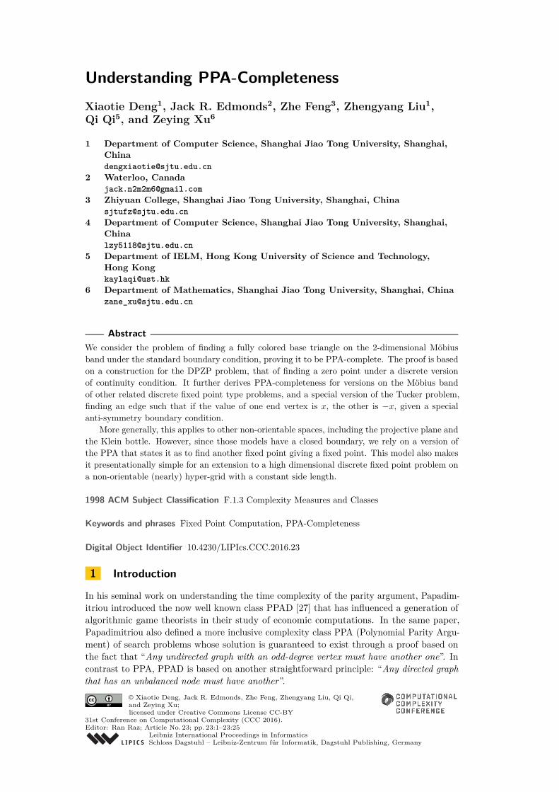
Intuitively, G∗ is a plannar embedding of the graphG for AEUL with vertices {0, 1, . . . , N−1}. The construction is motivated by and has some similar details to that of Chen andDeng [7]. Making it work on the Möbius band requires new ideas.

CCC 2016

23:8 Understanding PPA-Completeness

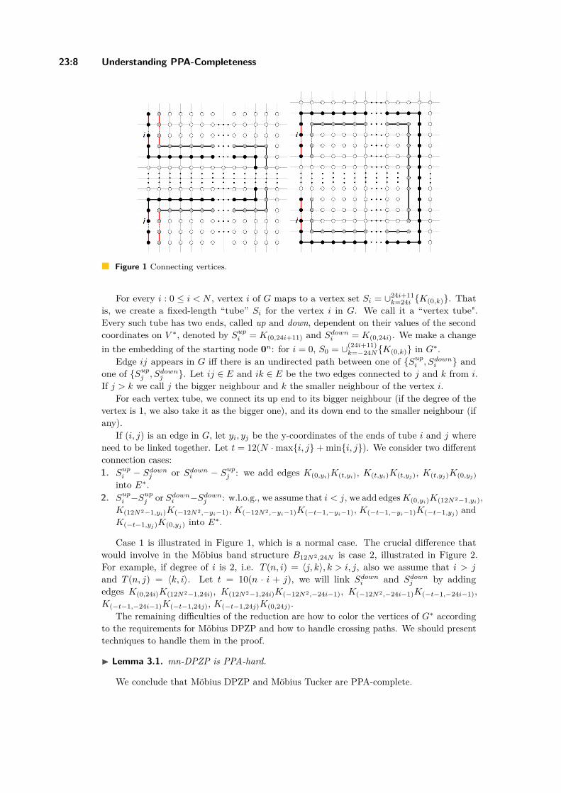
Figure 1 Connecting vertices.

For every i : 0 ≤ i < N , vertex i of G maps to a vertex set Si = ∪24i+11k=24i {K(0,k)}. That

is, we create a fixed-length “tube” Si for the vertex i in G. We call it a “vertex tube".Every such tube has two ends, called up and down, dependent on their values of the secondcoordinates on V ∗, denoted by Supi = K(0,24i+11) and Sdowni = K(0,24i). We make a changein the embedding of the starting node 0n: for i = 0, S0 = ∪(24i+11)

k=−24N{K(0,k)} in G∗.Edge ij appears in G iff there is an undirected path between one of {Supi , Sdowni } and

one of {Supj , Sdownj }. Let ij ∈ E and ik ∈ E be the two edges connected to j and k from i.If j > k we call j the bigger neighbour and k the smaller neighbour of the vertex i.

For each vertex tube, we connect its up end to its bigger neighbour (if the degree of thevertex is 1, we also take it as the bigger one), and its down end to the smaller neighbour (ifany).

If (i, j) is an edge in G, let yi, yj be the y-coordinates of the ends of tube i and j whereneed to be linked together. Let t = 12(N ·max{i, j}+ min{i, j}). We consider two differentconnection cases:1. Supi − Sdownj or Sdowni − Supj : we add edges K(0,yi)K(t,yi), K(t,yi)K(t,yj), K(t,yj)K(0,yj)

into E∗.2. Supi −S

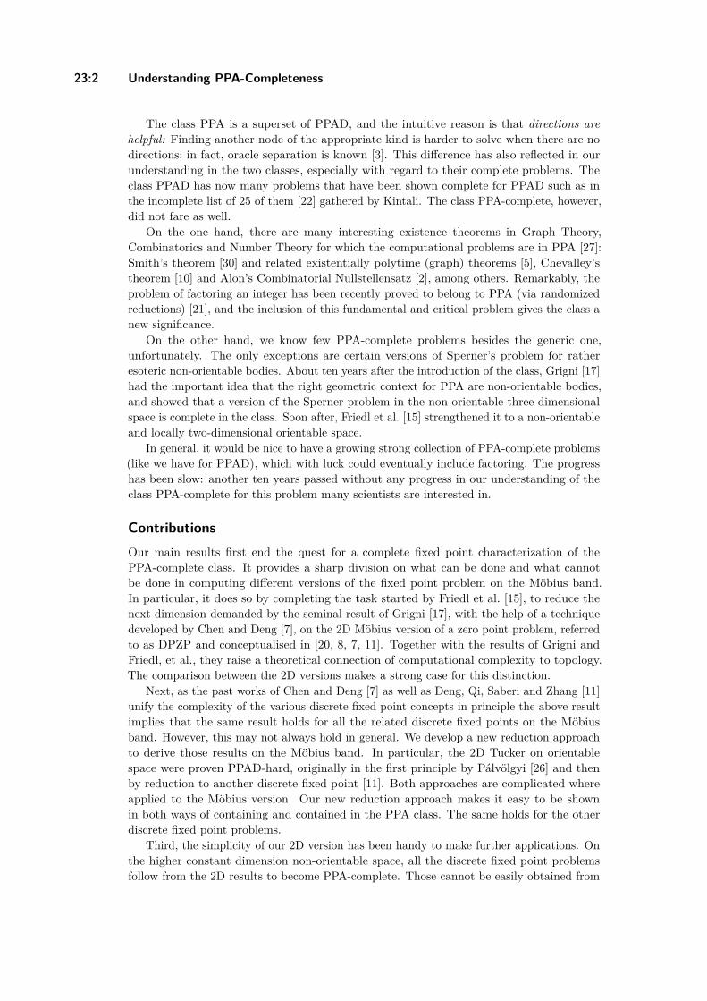
upj or Sdowni −Sdownj : w.l.o.g., we assume that i < j, we add edgesK(0,yi)K(12N2−1,yi),

K(12N2−1,yi)K(−12N2,−yi−1), K(−12N2,−yi−1)K(−t−1,−yi−1), K(−t−1,−yi−1)K(−t−1,yj) andK(−t−1,yj)K(0,yj) into E∗.

Case 1 is illustrated in Figure 1, which is a normal case. The crucial difference thatwould involve in the Möbius band structure B12N2,24N is case 2, illustrated in Figure 2.For example, if degree of i is 2, i.e. T (n, i) = 〈j, k〉, k > i, j, also we assume that i > j

and T (n, j) = 〈k, i〉. Let t = 10(n · i + j), we will link Sdowni and Sdownj by addingedges K(0,24i)K(12N2−1,24i), K(12N2−1,24i)K(−12N2,−24i−1), K(−12N2,−24i−1)K(−t−1,−24i−1),K(−t−1,−24i−1)K(−t−1,24j), K(−t−1,24j)K(0,24j).

The remaining difficulties of the reduction are how to color the vertices of G∗ accordingto the requirements for Möbius DPZP and how to handle crossing paths. We should presenttechniques to handle them in the proof.

I Lemma 3.1. mn-DPZP is PPA-hard.

We conclude that Möbius DPZP and Möbius Tucker are PPA-complete.

X. Deng, J. R. Edmonds, Z. Feng, Z. Liu, Q. Qi, and Z. Xu 23:9

Figure 2 Connecting vertices 2.

I Theorem 3.2. mn-DPZP is PPA-complete.

Proof. By Lemma 2.14, mn-DPZP is in PPA. By Lemma 3.1, mn-DPZP is PPA-hard. Theclaim follows. J

I Theorem 3.3. sm-Tucker is PPA-complete.

Proof. sm-Tucker is in PPA by Lemma 2.18.For PPA-hardness, we use the same construction as the proof of Lemma 3.1, except that

we change vertices colored 0 to color −2. Therefore, at each vertex of color 0 in Lemma 3.1,we have an edge of color +2 and −2; and vice versa. The reduction follows.

Therefore, the theorem holds. J

Finally we show that m-Sperner is PPA-complete.

I Theorem 3.4. m-Sperner is PPA-complete.

Proof. First, m-Sperner is in PPA by Lemma 2.16.To prove it is PPA-hard, we simply replace vertices colored {−1,−2} to color 0 in the

instance constructed in the PPA-hardness proof of mn-DPZP. Finding a fully colored triangleδ in the m-Sperner instance will imply a true zero point in the mn-DPZP instance becausethe direction preserving condition, Definition 2.7, for mn-DPZP will prevent another vertexin the same base triangle of color∈ {−1,−2}.

The claim follows. J

4 High Dimensional Non-orientable Discrete Fixed Point

In the above, some 2D fixed point problems on the Möbius band are proven PPA-complete.The generalized problem in higher dimension space with all constant side lengths is consideredin this section. The proof is motivated by a construction in [9]. To handle the non-orientablespace, the key changes are on the snake lemma. We need a dicephalic snake version.Considerable changes and new ideas are required to make it through. To avoid tediousdetails, we should present a version of the construction and the proof. To observe the pagelimit, we place all the proofs and some lemmas at the appendices.

CCC 2016

23:10 Understanding PPA-Completeness

4.1 Uniform Boundary Discrete Fixed Points on Möbius BandWe introduce a version here for which the boundary of the 2D Möbius band consists verticesall of the same color. Every instance of the problem has index 0. This naturally leads to aversion of the fixed point problem where one fixed point is given and another is sought after.We call such a case the uniform boundary coloring.

More precisely, the coloring function f is of uniform boundary on Möbius band BN,Mif it satisfies that: (1) f((x,±M)) = 0,∀x ∈ Z,−N ≤ x ≤ N . (2) Möbius condition, i.e.f((N, y)) = f((−N,−y)),∀y ∈ Z,−M ≤ y ≤M . Then the Möbius Sperner problem can bedefined as follows.

I Definition 4.1 (Möbius Sperner). The input is a polynomial-time machine F that generatesa uniform boundary 3-coloring function f on BN,M : F (p) = f(p) ∈ {0, 1, 2},∀p ∈ BN,M ,as well as a panchromatic base triangle. The required output is another panchromatic basetriangle on BN,M .

Note that index(BN,M , f) is zero for a color function of uniform boundary on the Möbiusband. According to Lemma 2.5, we have the following lemma:

I Lemma 4.2. For any uniform boundary 3-coloring of the triangulated Möbius band BN,M ,the number of panchromatic base triangles is even. Given one panchromatic base triangle,finding another is a PPA-complete problem.

4.2 High Dimensional Möbius SpernerWe extend the 2-dimensional uniform boundary Möbius Sperner proven PPA-complete inthe above to higher dimension. First we define the well-behaved function.

I Definition 4.3 (Well-behaved Function [9]). A polynomial-time computable integer functionf is well-behaved, if ∃n0 > 0 such that ∀n ≥ n0 3 ≤ f(n) ≤ n/2.

Define Kp ={

q ∈ Zd | qi = pi or pi + 1,∀1 ≤ i ≤ d}.

For a positive integer d and a vector r ∈ Zd+, let

Adr ={

p ∈ Zd | −ri+1 ≤ pi ≤ ri−1,∀1 ≤ i ≤ d}

be the hyper grid with side length r (note that is 2(ri − 1) in the i-th dimension because ofsymmetry with respect to ri = 0). Note that its boundary is, in one dimension, intentionallyleft open,

∂Adr ={

p ∈ Adr | pi = −ri+1 or ri−1,∃2 ≤ i ≤ d}.

I Definition 4.4 (The Valid Boundary Condition). A coloring function C : Adr → {0, 1, . . . , d}is valid on Adr if it satisfies the following Boundary Conditions:1. (Uniform color boundary) For any p ∈ ∂Adr , C(p) = 02. (Reversing face consistency) C((r1−1, x2, x3, . . . , xd)) = C((−r1+1,−x2, x3, . . . , xd)) for

all xi, where i = 2, 3, . . . , d. Note that it is equivalent to merging (r1 − 1, x2, x3, · · · , xd)and (−r1 + 1,−x2, x3, · · · , xd) into one vertex.

The point set {(±(r1−1), x2, . . . , xd) : −ri < xi < ri, i = 2, 3, . . . , d} are called reversing face.Even though they are not on the boundary, we include (2) here to make sure the consistencyof function values on the non-orientable space. Fixing other variables, x3, x4, · · · , xd, wehave a reversing plane for the variables x1 and x2.

X. Deng, J. R. Edmonds, Z. Feng, Z. Liu, Q. Qi, and Z. Xu 23:11

For any well-behaved function f , we define a corresponding Möbius-Sperner fixed pointproblem as follows.

I Definition 4.5 (Möbius Spernerf ). For a well-behaved function f and a parameter n, letm = f(n) and d = dn/f(n)e. An input instance of Möbius Spernerf is a pair (C, 0n) whereC is a valid coloring function with parameter d and r where ri = 2m,∀i : 1 ≤ i ≤ d. Givena point p ∈ Adr where Kp is of degree one, i.e., contains one panchromatic simplex in itstriangulation, the output of this problem is another point q 6= p, such that Kq containsanother panchromatic simplex.

We have the following theorem.

I Theorem 4.6. The problem Möbius Spernerf is PPA-complete for any well-behavedfunction f .

One can show that this problem is in PPA. To prove the hardness, similar to the orientablespace [9], we embed an instance of Möbius Spernerf2 , known in PPA-complete, into onedimensional higher space iteratively till Möbius Spernerf . We should show that the processcan be done in a polynomial number of state transformations. In Subsection B, we showthree crucial lemmas for our reduction. In Subsection C, we employ these three lemmasiteratively to build up our construction. Please see the Appendix for the detail proofs.

5 Discrete Fixed Points on Projective Space and Klein Bottle

The results we have discussed above extend to other non-orientable spaces. The generalidea is to slice out a Möbius band from the more complicated non-orientable space and tocolor it properly, then to patch the rest of the space. Two of the most interesting ones arethe projective space and Klein Bottle. While the Möbius band can be embedded into 3DEuclidean space, neither the projective space nor the Klein bottle can. In this section, wemake a reduction from DPZP to both the Möbius band and the projective plane for thePPA-hardness. As usually, as both cases are two dimensional objects, it is easy to triangulatethem and to develop a path following algorithm.

We have discussed two types of discrete fixed point problems in the above. 1. findingone, and 2. (given one) finding another, dependent on the boundary conditions. As boththe Projective space and the Klein bottle are closed without a boundary, we need to use thesecond version.

Our presentation will focus on the mn-DPZP version of the problems. The same appliesto other types of discrete fixed point concepts discussed above. We omit them here as theresults are similar.

I Theorem 5.1. Given a triangulated projective plane with vertices labelled {0,±1,±2}. Itis PPA-complete to find another zero point.

I Theorem 5.2. Given a triangulated Klein bottle with vertices labelled {0,±1,±2}. It isPPA-complete to find another zero point.

6 Remarks and Discussion

We have discussed two types of discrete fixed point problems on the Möbius band: findingone, and (given one) finding another, dependent on the boundary conditions. We show bothproblems are PPA-complete for several versions of discrete fixed point models, including theSperner’s problem on the two dimensional Möbius band.

CCC 2016

23:12 Understanding PPA-Completeness

Our first step focuses on the 2D version. We start with mn-DPZP, which finds a zeropoint of a discrete version of the continuous functions. Based on this result, we derivePPA-completeness proof of several other related fixed point problems on the Möbius band.We discuss finding another for Möbius Sperner and Index1-Brouwer on Möbius Band. Wediscuss finding one for sm-Tucker and mn-DPZP. They are switchable into the other types.For example, we can change all negative colored vertices to color 0 in mn-DPZP to obtain a“finding one" version for Möbius Sperner. We leave those cases out in this version and onlyexemplify useful structures and techniques choosing the most typical cases.

In this work, the link between non-orientable topological space and undirected pathfollowing computational paradigm, started by Grigni in [17], is further ratified by the simplestructure of 2D Möbius band. It deepens our understanding of the computational complexitydifference between the two classes PPAD and PPA in terms of the underlying topologicalstructures.

The simplicity of our construction allows itself to extend beyond the 2D Möbius bandto more general cases. For example, the PPA completeness of the finding another fixedpoint version extends naturally to the Klein Bottle, the projective space, and to othernon-orientable surfaces [32]. Simplicity has played a role in raising further curiosities fromthe 2D Sperner work [7] in the orientable space, such as in [25, 16].

Further the results extend to higher dimensions, even for the case where each side is of aconstant length. One such high dimension non-orientable space case of finding-another fixedpoint is presented in Section 4. The result extends to different related solution concepts asin the previous related concepts.

Note that the discrete fixed point problems in our discussion has an exponential sizeconfiguration. Otherwise, we can enumerate the space to find a solution by brute force.To compute colors and function values, a polynomial size circuit is given as an input.Alternatively, an oracle model returns those values in a unit oracle time [19]. It is known thatthere is an asymptotic matching bound for finding the Brouwer’s fixed point in Euclideanspace [8], which extends to other discrete fixed point models [11]. The same holds for the non-orientable space we discuss here. The lower bound holds simply because the problem is harderin the non-orientable space. The upper bound follows by the standard divide-and-conqueron the index adopted for the non-orientable space.

We would like to see the natural 2D Möbius Sperner will encourage more constructiveworks to develop a better knowledge of the PPA-complete class. In particular, as hadsuggested by Grigni [17], we would like to see the computational complexity of the Smith’sTheorem, known in the class of PPA, be eventually resolved.

Acknowledgements. This work was partially supported by Tianyuan Special Funds ofthe National Natural Science Foundation of China (No. 11426026), the National ScienceFoundation of China (Grant No. 61173011) and a Project 985 grant of Shanghai Jiao TongUniversity. Qi’s work was supported by the Research Grant Council of Hong Kong (ECSProject No. 26200314 and GRF Project No. 16213115).

We would like to acknowledge our indebtedness to Xi Chen and Christos H. Papadimitrioufor helps, inspirations, suggestions and discussions on PPA problems. The great appreciationis also due to the anonymous reviewers. Their constructive criticism and suggestions havebeen incorporated in the current revision.

X. Deng, J. R. Edmonds, Z. Feng, Z. Liu, Q. Qi, and Z. Xu 23:13

References

1 James Aisenberg, Maria Luisa Bonet, and Sam Buss. 2-D Tucker is PPA complete. ECCCTR15-163, 2015.

2 Noga Alon. Combinatorial nullstellensatz. Combinatorics, Probability and Computing, 8,1999.

3 Paul Beame, Stephen Cook, Jeff Edmonds, Russell Impagliazzo, and Toniann Pitassi. Therelative complexity of NP search problems. Journal of Computer and System Sciences,57(1):3–19, 1998. doi:10.1006/jcss.1998.1575.

4 Kathie Cameron. Thomason’s algorithm for finding a second hamiltonian circuit througha given edge in a cubic graph is exponential on krawczyk’s graphs. Discrete Mathematics,235(1–3):69–77, 2001. Chech and Slovak 3. doi:10.1016/S0012-365X(00)00260-0.

5 Kathie Cameron and Jack Edmonds. Some graphic uses of an even number of odd nodes.Annales de l’institut Fourier, 49(3):815–827, 1999. URL: http://eudml.org/doc/75365.

6 Chih-Wei Chang, Ming Liu, Sunghyun Nam, Shuang Zhang, Yongmin Liu, Guy Bartal, andXiang Zhang. Optical möbius symmetry in metamaterials. Phys. Rev. Lett., 105:235501,Dec 2010. doi:10.1103/PhysRevLett.105.235501.

7 Xi Chen and Xiaotie Deng. On the complexity of 2D discrete fixed point problem. In In Pro-ceedings of the 33rd International Colloquium on Automata, Languages and Programming.Lecture Notes in Computer Science, pages 489–500. Springer-Verlag, 2006.

8 Xi Chen and Xiaotie Deng. Matching algorithmic bounds for finding a brouwer fixed point.JACM, 55(3), 2008.

9 Xi Chen, Xiaotie Deng, and Shang-Hua Teng. Settling the complexity of computingtwo-player nash equilibria. J. ACM, 56(3):14:1–14:57, May 2009. doi:10.1145/1516512.1516516.

10 C. Chevalley. Démonstration d’une hypothèse de m. artin. Abhandlungen aus demMathematischen Seminar der Universität Hamburg, 11(1):73–75, 1935. doi:10.1007/BF02940714.

11 Xiaotie Deng, Qi Qi, Amin Saberi, and Jie Zhang. Discrete fixed points: Models, com-plexities, and applications. Mathematics of Operations Research, 36(4):636–652, 2011.doi:10.1287/moor.1110.0511.

12 Jack Edmonds and Laura Sanità. On finding another room-partitioning of the vertices.Electronic Notes in Discrete Mathematics, 36:1257–1264, 2010. doi:10.1016/j.endm.2010.05.159.

13 M.C. Escher. Möbius strip ii (red ants). http://www.mcescher.com/Gallery/recogn-bmp/LW441.jpg, 1963. [Online; accessed 3-March-2016].

14 Y. N. Fang, Yao Shen, Qing Ai, and C. P. Sun. Negative Refraction Induced by MöbiusTopology. ArXiv e-prints, January 2015. URL: http://arxiv.org/abs/1501.05729.

15 Katalin Friedl, Gábor Ivanyos, Miklos Santha, and Yves F. Verhoeven. Locally 2-dimensional sperner problems complete for the polynomial parity argument classes. sub-mitted. In In Proceedings of the 6th Italian Conference on Algorithms and Complexity.Lecture Notes in Computer Science, pages 380–391. Springer-Verlag, 2006.

16 Paul Goldberg. The complexity of the path-following solutions of two-dimensional spern-er/brouwer functions. arXiv:1506.04882 [cs.CC], 2015.

17 Michelangelo Grigni. A sperner lemma complete for PPA. Information Processing Letters,77(5–6):255–259, 2001. doi:10.1016/S0020-0190(00)00152-6.

18 Dongran Han, Suchetan Pal, Yan Liu, and Hao Yan. Folding and cutting dna intoreconfigurable topological nanostructures. Nat Nano, 5(10):712–717, 10 2010. doi:10.1038/nnano.2010.193.

CCC 2016

23:14 Understanding PPA-Completeness

19 Michael D Hirsch, Christos H Papadimitriou, and Stephen A Vavasis. Exponential lowerbounds for finding brouwer fix points. Journal of Complexity, 5(4):379–416, 1989. doi:10.1016/0885-064X(89)90017-4.

20 Takuya Iimura. A discrete fixed point theorem and its applications. Journal of Mathemat-ical Economics, 39(7):725–742, 2003. doi:10.1016/S0304-4068(03)00007-7.

21 Emil Jerábek. Integer factoring and modular square roots. CoRR, abs/1207.5220, 2012.URL: http://arxiv.org/abs/1207.5220.

22 Shiva Kintali. A compendium of PPAD-complete problems. http://www.cs.princeton.edu/~kintali/ppad.html. [Online; accessed 3-March-2016].

23 Adam Krawczyk. The complexity of finding a second hamiltonian cycle in cubic graphs.Journal of Computer and System Sciences, 58(3):641–647, 1999. doi:10.1006/jcss.1998.1611.

24 O. L. Mangasarian. Equilibrium points of bimatrix games. Journal of the Society forIndustrial and Applied Mathematics, 12(4):778–780, 1964. URL: http://www.jstor.org/stable/2946349.

25 Ruta Mehta. Constant rank bimatrix games are ppad-hard. In Proceedings of the Fourty-Sixth Annual ACM Symposium on Theory of Computing, STOC’14, pages 545–554, NewYork, NY, USA, 2014. ACM.

26 Dömötör Pálvölgyi. 2d-tucker is ppad-complete. In 5th International Workshop, WINE2009, Rome, Italy, December 14-18, 2009. Proceedings, pages 569–574. Springer-Verlag,2009.

27 Christos H. Papadimitriou. On the complexity of the parity argument and other inefficientproofs of existence. Journal of Computer and System Sciences, 48(3):498–532, 1994. doi:10.1016/S0022-0000(05)80063-7.

28 Rahul Savani and Bernhard von Stengel. Hard-to-solve bimatrix games. Econometrica,74(2):397–429, 2006. doi:10.1111/j.1468-0262.2006.00667.x.

29 Herbert E. Scarf. The approximation of fixed points of a continuous mapping. CowlesFoundation Discussion Papers 216R, Cowles Foundation for Research in Economics, YaleUniversity, 1967. URL: http://EconPapers.repec.org/RePEc:cwl:cwldpp:216r.

30 A.G. Thomason. Hamiltonian cycles and uniquely edge colourable graphs. In B. Bollobás,editor, Advances in Graph Theory, volume 3 of Annals of Discrete Mathematics, pages259–268. Elsevier, 1978. doi:10.1016/S0167-5060(08)70511-9.

31 Michael J Todd. The computation of fixed points and applications, volume 124. SpringerScience & Business Media, 2013.

32 Eric W. Weisstein. Klein bottle. http://mathworld.wolfram.com/KleinBottle.html.[Online; accessed 3-March-2016].

A Omitted Figures and Proofs

Proof of Lemma 2.13. First, a base triangle is index 1 if and only if its vertices are colored{x, 1, 2} where x /∈ {1, 2}. As all vertices in a base triangle are of distance 1 in ∞-metric.Therefore, x can be neither −1 nor −2 by the direction preserving property. The only index1 base triangle is {0, 1, 2}.

Next, as any internal base edge appears in the calculation of indices of two base triangles,the summation of the indices of them is either 0 or 2, which equals to 0 (mod 2). The claimfollows. J

Proof of Lemma 2.14. Since we have only one edge with (2, 1) on the boundary of theMöbius band, the index of edges along the boundary is 1. Therefore, by Lemma 2.13, there

X. Deng, J. R. Edmonds, Z. Feng, Z. Liu, Q. Qi, and Z. Xu 23:15

is an odd number of zero point base triangles on the Möbius grid. Therefore, there is alwaysa zero point inside the Möbius grid.

For the construction of the AEUL, we take the boundary edge (2, 1) as the origin vertexof AEUL. Two such edges of mn-DPZP are connected in AEUL if they are in the same basetriangle. Any such edge in mn-DPZP is an leaf node in AEUL if it is the single {1, 2} edgein a base triangle.

Therefore, an end of lines of the AEUL instance is a base triangle of the mn-DPZP.Finding a zero point base triangle is an AEUL problem, and in PPA. J

Proof of Lemma 3.1. Using the main structure presented above, we show how to colorB12N2,24N , so that for any zero point of this mn-DPZP, we can get a corresponding solutionfor the search problem AEUL.

The circuit Tn of AEUL generates an undirected graph G = (Cn, E), where Cn = {0, 1}n.An edge (u, v) appears in E iff u ∈ Tn(v) and v ∈ Tn(u).

So given any G, we construct an instance (f,G∗) for mn-DPZP problem where f is acoloring function for the generated G∗ = B12N2,24N . We should also use T12N2,24N to referto G∗ in case of no ambiguity, with the understanding that (−12N2, y) and (12N2,−y) arethe same vertex.

In constructing the coloring function f for G∗, we make use of the input circuit of Tn, toidentify edges connecting a node to another, and vice versa, and to identify the degree onenode of the AEUL graph.

We define the coloring function as follows:1. Color vertices on the boundary according to the admissible conditions, Definition 2.9.2. Color the long vertex tube: ∀j : −24N ≤ j < 12, set f((0, j)) = 2, f((1, j)) = 1, which is

a long vertex tube for the given degree one vertex 0.3. Coat the long vertex tube (to protect positive colored 1 and 2 inside tube): ∀j : −24N ≤

j < 12, set f((−1, j)) = −1 and f((2, j)) = −2.4. Color the other vertex tubes: ∀i : 0 < i < N , set f((0, 24i + k)) = 2, f((1, 24i + k)) =

1, k = 0, 1, 2, . . . , 11. We need to make some modifications in the colors for the case k = 0later.

5. Coat vertex tubes (to protect positive colored 1 and 2 inside tube): ∀i : 0 < i < N :f((−1, 24i+ k)) = −1, f((2, 24i+ k)) = −2, k = 0, 1, 2, . . . , 11.

6. Make feasible: fill in the the rest of the interior vertices by color −2. Some of thosevertices will be re-colorred in the following steps.

7. Direction preserving on end of lines: For a leaf vertex i : 0 < i < N , we have f(0, 24i) =f(1, 24i) = 0.

8. Build an edge path: Given an edge (i, j) ∈ E, w.l.o.g., assume that i < j, we construct apath between i and j in G∗. Let (i′, j) ∈ E and (i, j′) ∈ E. If j > j′, then the upper endof tube for i is connected to that of j, else the lower end of the tube for i is connected tothat of j. Therefore, there are four possibilities one end of the vertex tube is connectedto another vertex tube.a. i > i′ and j < j′: Lower end of vertex tube for i is connected to the upper end of the

vertex tube for j. See Figure 1.b. i < i′ and j > j′: Upper end of vertex tube for i is connected to the lower end of the

vertex tube for j. See Figure 1.c. i < i′ and j < j′: Lower end of vertex tube for i is connected to the lower end of the

vertex tube for j. See Figure 2.d. i > i′ and j > j′: Upper end of vertex tube for i is connected to the upper end of the

vertex tube for j. Similar to item (c).

CCC 2016

23:16 Understanding PPA-Completeness

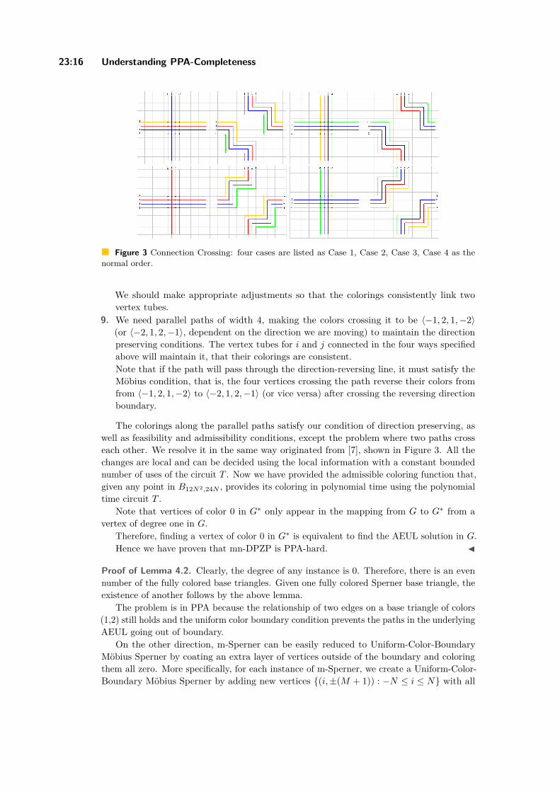
Figure 3 Connection Crossing: four cases are listed as Case 1, Case 2, Case 3, Case 4 as thenormal order.

We should make appropriate adjustments so that the colorings consistently link twovertex tubes.

9. We need parallel paths of width 4, making the colors crossing it to be 〈−1, 2, 1,−2〉(or 〈−2, 1, 2,−1〉, dependent on the direction we are moving) to maintain the directionpreserving conditions. The vertex tubes for i and j connected in the four ways specifiedabove will maintain it, that their colorings are consistent.Note that if the path will pass through the direction-reversing line, it must satisfy theMöbius condition, that is, the four vertices crossing the path reverse their colors fromfrom 〈−1, 2, 1,−2〉 to 〈−2, 1, 2,−1〉 (or vice versa) after crossing the reversing directionboundary.

The colorings along the parallel paths satisfy our condition of direction preserving, aswell as feasibility and admissibility conditions, except the problem where two paths crosseach other. We resolve it in the same way originated from [7], shown in Figure 3. All thechanges are local and can be decided using the local information with a constant boundednumber of uses of the circuit T . Now we have provided the admissible coloring function that,given any point in B12N2,24N , provides its coloring in polynomial time using the polynomialtime circuit T .

Note that vertices of color 0 in G∗ only appear in the mapping from G to G∗ from avertex of degree one in G.

Therefore, finding a vertex of color 0 in G∗ is equivalent to find the AEUL solution in G.Hence we have proven that mn-DPZP is PPA-hard. J

Proof of Lemma 4.2. Clearly, the degree of any instance is 0. Therefore, there is an evennumber of the fully colored base triangles. Given one fully colored Sperner base triangle, theexistence of another follows by the above lemma.

The problem is in PPA because the relationship of two edges on a base triangle of colors(1,2) still holds and the uniform color boundary condition prevents the paths in the underlyingAEUL going out of boundary.

On the other direction, m-Sperner can be easily reduced to Uniform-Color-BoundaryMöbius Sperner by coating an extra layer of vertices outside of the boundary and coloringthem all zero. More specifically, for each instance of m-Sperner, we create a Uniform-Color-Boundary Möbius Sperner by adding new vertices {(i,±(M + 1)) : −N ≤ i ≤ N} with all

X. Deng, J. R. Edmonds, Z. Feng, Z. Liu, Q. Qi, and Z. Xu 23:17

-2 2

-1

1

0

-2

-2

-2

-2

-2

-2

2

2

2

2

2

2-1-1-1-1-1-1

-1-1-1-1-1-1

-1-1-1-1-1-1

-1-1-1-1-1-1

-1-1-1-1-1-1

-1-1-1-1-1-1

-1-1-1-1-1-1

-1-1-1-1-1-1

-1-1-1-1-1-1

-1-1-1-1-1-1

-1-1-1-1-1-1

-1-1-1-1-1-1

-1-1-1-1-1-1

1 1 1 1 1 1

1 1 1 1 1 1

1 1 1 1 1 1

1 1 1 1 1 1

1 1 1 1 1 1

1 1 1 1 1 1

1 1 1 1 1 1

1 1 1 1 1 1

1 1 1 1 1 1

1 1 1 1 1 1

1 1 1 1 1 1

1 1 1 1 1 1

1 1 1 1 1 1

0

-1

-1

-1

1

1

1-2

2

Figure 4 Disk.

2

-2

-11

Figure 5 The Möbius Band.

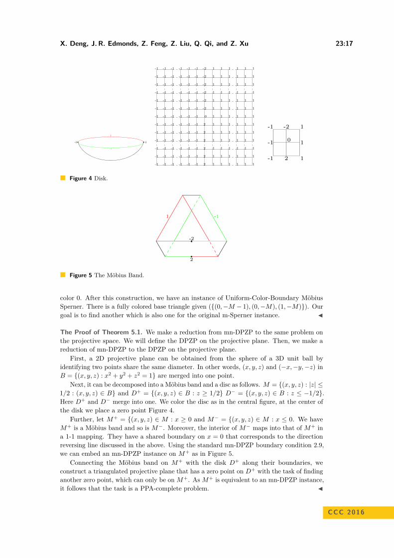
color 0. After this construction, we have an instance of Uniform-Color-Boundary MöbiusSperner. There is a fully colored base triangle given ({(0,−M − 1), (0,−M), (1,−M)}). Ourgoal is to find another which is also one for the original m-Sperner instance. J

The Proof of Theorem 5.1. We make a reduction from mn-DPZP to the same problem onthe projective space. We will define the DPZP on the projective plane. Then, we make areduction of mn-DPZP to the DPZP on the projective plane.

First, a 2D projective plane can be obtained from the sphere of a 3D unit ball byidentifying two points share the same diameter. In other words, (x, y, z) and (−x,−y,−z) inB = {(x, y, z) : x2 + y2 + z2 = 1} are merged into one point.

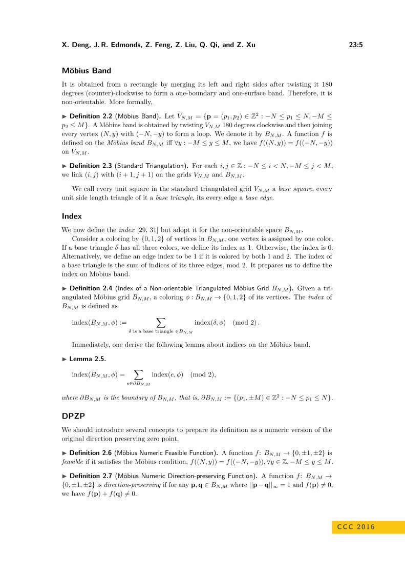
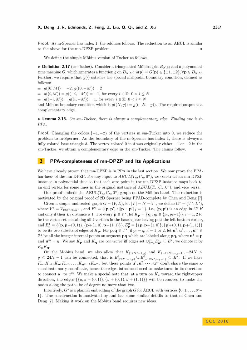
Next, it can be decomposed into a Möbius band and a disc as follows. M = {(x, y, z) : |z| ≤1/2 : (x, y, z) ∈ B} and D+ = {(x, y, z) ∈ B : z ≥ 1/2} D− = {(x, y, z) ∈ B : z ≤ −1/2}.Here D+ and D− merge into one. We color the disc as in the central figure, at the center ofthe disk we place a zero point Figure 4.

Further, let M+ = {(x, y, z) ∈ M : x ≥ 0 and M− = {(x, y, z) ∈ M : x ≤ 0. We haveM+ is a Möbius band and so is M−. Moreover, the interior of M− maps into that of M+ ina 1-1 mapping. They have a shared boundary on x = 0 that corresponds to the directionreversing line discussed in the above. Using the standard mn-DPZP boundary condition 2.9,we can embed an mn-DPZP instance on M+ as in Figure 5.

Connecting the Möbius band on M+ with the disk D+ along their boundaries, weconstruct a triangulated projective plane that has a zero point on D+ with the task of findinganother zero point, which can only be on M+. As M+ is equivalent to an mn-DPZP instance,it follows that the task is a PPA-complete problem. J

CCC 2016

23:18 Understanding PPA-Completeness

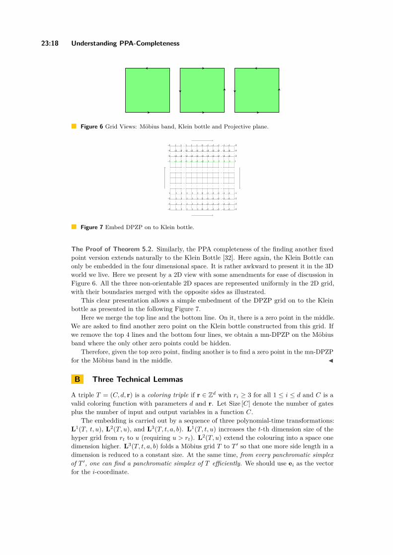
Figure 6 Grid Views: Möbius band, Klein bottle and Projective plane.

-2

-2

-2

2

2

2

-1 -1 -1 -1 -1

1 1 1 1 1 -1 -1 -1 -1 -1

1 1 1 1 1 1

1 1 1 1 1 -1 -1 -1 -1 -1

0

0

1 -1

-1

-2 -2

-2 -2

-2 -2

-2 -2

-2 -2

-2 -2

1

1

1

1

1

1

1

1

1

1

1

1

1

1

1

-1

-1

-1

-1

-1

-1

-1

-1

-1

-1

-1

-1

-1

-1

-1

-2

-2

-2

-2

-2

-2

-2

-2

-2

-2

-2

-2

-2

-2

-2

-2

-2

-2

-2

-2

Figure 7 Embed DPZP on to Klein bottle.

The Proof of Theorem 5.2. Similarly, the PPA completeness of the finding another fixedpoint version extends naturally to the Klein Bottle [32]. Here again, the Klein Bottle canonly be embedded in the four dimensional space. It is rather awkward to present it in the 3Dworld we live. Here we present by a 2D view with some amendments for ease of discussion inFigure 6. All the three non-orientable 2D spaces are represented uniformly in the 2D grid,with their boundaries merged with the opposite sides as illustrated.

This clear presentation allows a simple embedment of the DPZP grid on to the Kleinbottle as presented in the following Figure 7.

Here we merge the top line and the bottom line. On it, there is a zero point in the middle.We are asked to find another zero point on the Klein bottle constructed from this grid. Ifwe remove the top 4 lines and the bottom four lines, we obtain a mn-DPZP on the Möbiusband where the only other zero points could be hidden.

Therefore, given the top zero point, finding another is to find a zero point in the mn-DPZPfor the Möbius band in the middle. J

B Three Technical Lemmas

A triple T = (C, d, r) is a coloring triple if r ∈ Zd with ri ≥ 3 for all 1 ≤ i ≤ d and C is avalid coloring function with parameters d and r. Let Size [C] denote the number of gatesplus the number of input and output variables in a function C.

The embedding is carried out by a sequence of three polynomial-time transformations:L1(T, t, u), L2(T, u), and L3(T, t, a, b). L1(T, t, u) increases the t-th dimension size of thehyper grid from rt to u (requiring u > rt). L2(T, u) extend the colouring into a space onedimension higher. L3(T, t, a, b) folds a Möbius grid T to T ′ so that one more side length in adimension is reduced to a constant size. At the same time, from every panchromatic simplexof T ′, one can find a panchromatic simplex of T efficiently. We should use ei as the vectorfor the i-coordinate.

X. Deng, J. R. Edmonds, Z. Feng, Z. Liu, Q. Qi, and Z. Xu 23:19

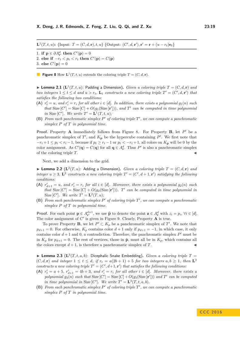
L1(T, t, u): {Input: T = (C, d, r), t, u} {Output: (C ′, d, r′), r′ = r + (u− rt)et}

1. if p ∈ ∂Adr′ then C ′(p) = 02. else if −rt < pt < rt then C ′(p) = C(p)3. else C ′(p) = 0

Figure 8 How L1(T, t, u) extends the coloring triple T = (C, d, r).

I Lemma 2.1 (L1(T, t, u): Padding a Dimension). Given a coloring triple T = (C, d, r) andtwo integers 1 ≤ t ≤ d and u > rt, L1 constructs a new coloring triple T ′ = (C ′, d, r′) thatsatisfies the following two conditions:(A) r′t = u, and r′i = ri for all other i ∈ [d]. In addition, there exists a polynomial g1(n) such

that Size [C ′] = Size [C] +O(g1(Size [r′])), and T ′ can be computed in time polynomialin Size [C ′]. We write T ′ = L1(T, t, u);

(B) From each panchromatic simplex P ′ of coloring triple T ′, we can compute a panchromaticsimplex P of T in polynomial time.

Proof. Property A immediately follows from Figure 8. For Property B, let P ′ be apanchromatic simplex of T ′, and Kp be the hypercube containing P ′. We first note that−rt + 1 ≤ pt < rt− 1, because if pt ≥ rt− 1 or pt < −rt + 1, all colors on Kp will be 0 by thecolor assignment. As C ′(q) = C(q) for all q ∈ Adr . Thus P ′ is also a panchromatic simplexof the coloring triple T . J

Next, we add a dimension to the grid.

I Lemma 2.2 (L2(T, u): Adding a Dimension). Given a coloring triple T = (C, d, r) andinteger u ≥ 3, L2 constructs a new coloring triple T ′ = (C ′, d+ 1, r′) satisfying the followingconditions:(A) r′d+1 = u, and r′i = ri for all i ∈ [d]. Moreover, there exists a polynomial g2(n) such

that Size [C ′] = Size [C] + O(g2(Size [r′])). T ′ can be computed in time polynomial inSize [C ′]. We write T ′ = L2(T, u);

(B) From each panchromatic simplex P ′ of coloring triple T ′, we can compute a panchromaticsimplex P of T in polynomial time.

Proof. For each point p ∈ Ad+1r′ , we use p̂ to denote the point z ∈ Adr with zi = pi, ∀i ∈ [d].

The color assignment of C ′ is given in Figure 9. Clearly, Property A is true.To prove Property B, we let P ′ ⊂ Kp be a panchromatic simplex of T ′. We note that

pd+1 = 0. For otherwise, Kp contains color d+ 1 only if pd+1 = −1, in which case, it onlycontains color d+ 1 and 0, a contradiction. Therefore, the panchromatic simplex P ′ must bein Kp for pd+1 = 0. The rest of vertices, those in p̂, must all be in Kp, which contains allthe colors except d+ 1, is therefore a panchromatic simplex of T . J

I Lemma 2.3 (L3(T, t, a, b): Dicephalic Snake Embedding). Given a coloring triple T =(C, d, r) and integer 1 ≤ t ≤ d, if rt = a(2b + 1) + 5 for two integers a, b ≥ 1, then L3

constructs a new coloring triple T ′ = (C ′, d+1, r′) that satisfies the following conditions:(A) r′t = a + 5, r′d+1 = 4b + 3, and r′i = ri for all other i ∈ [d]. Moreover, there exists a

polynomial g3(n) such that Size [C ′] = Size [C] +O(g3(Size [r′])) and T ′ can be computedin time polynomial in Size [C ′]. We write T ′ = L3(T, t, a, b).

(B) From each panchromatic simplex P ′ of coloring triple T ′, we can compute a panchromaticsimplex P of T in polynomial time.

CCC 2016

23:20 Understanding PPA-Completeness

L2(T, u): {Input: T = (C, d, r), u} {Output: T ′ = (C ′, d + 1, r′), r′d+1 = u, (∀i : 1 ≤ i ≤d)r′i = ri }

1. if p ∈ ∂Ad+1r′ then C ′(p) = 0.

2. else if pd+1 = 1 then C ′(p) = C(p̂) where p̂ ∈ Zd satisfying p̂i = pi for all 1 ≤ i ≤ d.3. else if pd+1 = 0 then C ′(p) = d+ 1.4. else C ′(p) = 0

Figure 9 How L2(T, u) extends the coloring triple T = (C, d, r).

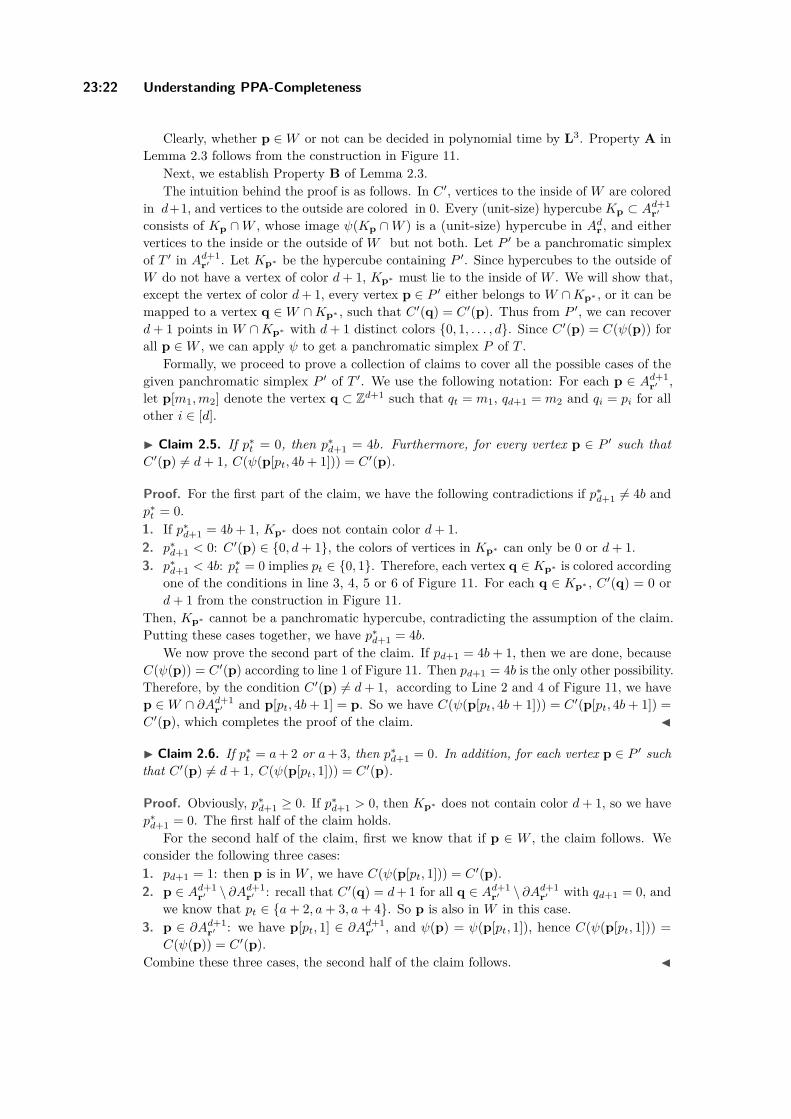
Figure 10 The two dimensional view of set W ⊂ Ad+1r′ .

Proof. Consider the domains Adr ⊂ Zd and Ad+1r′ ⊂ Zd+1 of our coloring triples. The

reduction L3(T, t, a, b) is carried out in three steps. First, we define a d-dimensional setW ⊂ Ad+1

r′ that is large enough to contain Adr . Second, we define a (many to one) mapψ from W to Adr that specifies an implicit embedding of Adr into W . Finally, we build afunction C ′ for Ad+1

r′ and show that from each panchromatic simplex of T ′, a panchromaticsimplex of T can be found in polynomial time.

A two dimensional view of W ⊂ Ad+1r′ is illustrated in Figure 10. We use a (dicephalic)

snake-pattern to realize the longer tth dimension of Adr using the two-dimensional spacedefined by a new shorter tth dimension and the (d+1)th dimension (smaller by a multiplicativefactor less than one) of Ad+1

r′ , such that it is roughly rt = r′t ∗ r′d+1 (in fact, rt = O(r′t ∗ r′d+1)).Formally, W consists of points p ∈ Ad+1

r′ satisfying 1 ≤ pd+1 ≤ 4b+ 1 andif pd+1 = 1, then 2 ≤ pt ≤ a+ 4 or −(a+ 4) ≤ pt ≤ −2;if pd+1 = 4b+ 1, then −(a+ 2) ≤ pt ≤ a+ 2;if pd+1 = 4(b− i)− 1 where 0 ≤ i ≤ b− 1, then 2 ≤ pt ≤ a+ 2 or −(a+ 2) ≤ pt ≤ −2;if pd+1 = 4(b− i)− 3 where 0 ≤ i ≤ b− 2, then 2 ≤ pt ≤ a+ 2 or −(a+ 2) ≤ pt ≤ −2;if pd+1 = 4(b− i)− 2 where 0 ≤ i ≤ b− 1, then pt = 2 or −2;if pd+1 = 4(b− i) where 0 ≤ i ≤ b− 1, then pt = a+ 2 or −(a+ 2).

To build T ′, we embed the coloring triple T into W . The embedding is implicitlygiven by a many-to-one map ψ from W to Adr , which will play a vital role in the coloring

X. Deng, J. R. Edmonds, Z. Feng, Z. Liu, Q. Qi, and Z. Xu 23:21

L3(T, t, a, b):Input: T = (C, d, r), t, a, b, 1 ≤ t ≤ d, rt = a(2b+ 1) + 5, a, b ≥ 1Output: T ′ = (C ′, d+ 1, r′), r′t = a+ 5, r′d+1 = 4b+ 3, (∀i 6= t, 1 ≤ i ≤ d)r′i = ri

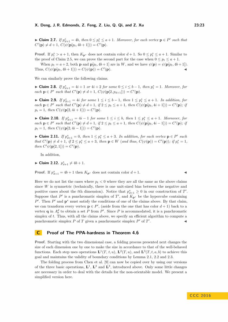
1. if p ∈W then C ′(p) = C(ψ(p))2. else if p ∈ ∂Ad+1

r′ then C ′(p) = 03. else if pd+1 = 0 then C ′(p) = d+ 1.4. else if pd+1 = 4i where 1 ≤ i ≤ b and 0 ≤ |pt| ≤ a+ 1 then C ′(p) = d+ 15. else if pd+1 = 4i+ 1, 4i+ 2 or 4i+ 3 where 0 ≤ i ≤ b− 1 and |pt| ≤ 1 then C ′(p) = d+ 16. else C ′(p) = 0

Figure 11 How L3(T, t, a, b) extends the coloring triple T = (f, d, r).

and the analysis of our reduction. For each p ∈ W , we use p[m] to denote the pointq in Zd with qt = m and qi = pi for all other i ∈ [d]. We denote by the functionsgn(x) = 1 if x > 0,−1 if x < 0, 0 if x = 0. We define ψ(p) according to the following cases:

if pd+1 = 1, then ψ(p) = p[2ab · sgn(pt) + pt]if pd+1 = 4b+ 1, then ψ(p) = p[pt];if pd+1 = 4(b− i)− 1 where 0 ≤ i ≤ b− 1, then ψ(p) = p[((2i+ 2)a+ 4) · sgn(pt)− pt];if pd+1 = 4(b− i)− 3 where 0 ≤ i ≤ b− 2, then ψ(p) = p[(2i+ 2)a · sgn(pt) + pt];if pd+1 = 4(b− i)− 2 where 0 ≤ i ≤ b− 1, then ψ(p) = p[((2i+ 2)a+ 2) · sgn(pt)];if pd+1 = 4(b− i) where 0 ≤ i ≤ b− 1, then ψ(p) = p[((2i+ 1)a+ 2) · sgn(pt)].

We let ψi(p) denote the ith component of ψ(p).

I Proposition 2.4 (Valid Boundary Condition Preserving). The coloring function C ′ describedin Figure 11 is valid on Ad+1

r′ .

Proof. First we show that C ′ satisfies the uniform color boundary condition (1) for allp ∈ ∂Ad+1

r′ . We only need to prove every vertex p ∈W ∩ ∂Ad+1r′ is colored zero, by Step 2 of

Figure 11.∀p ∈ W ∩ ∂Ad+1

r′ , by the definition of ψ(·), we have pi = ±(r′i−1) if and only ifψi(p) = ±(ri−1) for (i : d ≥ i ≥ 2). It follows that C ′(p) = C(ψ(p)) = 0 by the validboundary condition for C. Therefore, C ′ satisfies the valid boundary condition (1).

Next we show that C ′ satisfies the reversing face boundary condition (2).If t > 2, obviously, C ′ satisfies the boundary condition (2), since we have no change in x1nor x2 for any set of other variables.If t = 1, we consider p = (r′1−1, x2, x3, . . . , xd, xd+1) and p′ =(−r′1+1,−x2, x3, . . . , xd, xd+1). If xd+1 6= 1, C ′(p) = C ′(p′) = 0. If xd+1 = 1,then p,p′ ∈ W . Thus C ′(p) = C(ψ(p)), C ′(p′) = C(ψ(p′)). Since C is valid,C(ψ(p)) = C(ψ(p′))) by definition of ψ(·). Therefore, C ′(p) = C ′(p′).If t = 2, we consider p = (r1−1, x′2, x3, . . . , xd, xd+1) and p′ =(−r1+1,−x′2, x3, . . . , xd, xd+1). Because p and p′ are central symmetric onthe reversing plane, they are both in W or both not. If p,p′ ∈ W , thenC ′(p) = C(ψ(p)) = C(ψ(p′)) = C ′(p′)(since C is valid). If p,p′ are not in W ,we have C ′(p) = C ′(p′) = 0 (where p is outsideW or pd+1 < 0) or C ′(p) = C ′(p′) = d+1(where p is inside W ).

Therefore, C ′ is a valid coloring function on Ad+1r′ . J

CCC 2016

23:22 Understanding PPA-Completeness

Clearly, whether p ∈W or not can be decided in polynomial time by L3. Property A inLemma 2.3 follows from the construction in Figure 11.

Next, we establish Property B of Lemma 2.3.The intuition behind the proof is as follows. In C ′, vertices to the inside of W are colored

in d+1, and vertices to the outside are colored in 0. Every (unit-size) hypercube Kp ⊂ Ad+1r′

consists of Kp ∩W , whose image ψ(Kp ∩W ) is a (unit-size) hypercube in Adr , and eithervertices to the inside or the outside of W but not both. Let P ′ be a panchromatic simplexof T ′ in Ad+1

r′ . Let Kp∗ be the hypercube containing P ′. Since hypercubes to the outside ofW do not have a vertex of color d+ 1, Kp∗ must lie to the inside of W . We will show that,except the vertex of color d+ 1, every vertex p ∈ P ′ either belongs to W ∩Kp∗ , or it can bemapped to a vertex q ∈W ∩Kp∗ , such that C ′(q) = C ′(p). Thus from P ′, we can recoverd+ 1 points in W ∩Kp∗ with d+ 1 distinct colors {0, 1, . . . , d}. Since C ′(p) = C(ψ(p)) forall p ∈W , we can apply ψ to get a panchromatic simplex P of T .

Formally, we proceed to prove a collection of claims to cover all the possible cases of thegiven panchromatic simplex P ′ of T ′. We use the following notation: For each p ∈ Ad+1

r′ ,let p[m1,m2] denote the vertex q ⊂ Zd+1 such that qt = m1, qd+1 = m2 and qi = pi for allother i ∈ [d].

I Claim 2.5. If p∗t = 0, then p∗d+1 = 4b. Furthermore, for every vertex p ∈ P ′ such thatC ′(p) 6= d+ 1, C(ψ(p[pt, 4b+ 1])) = C ′(p).

Proof. For the first part of the claim, we have the following contradictions if p∗d+1 6= 4b andp∗t = 0.1. If p∗d+1 = 4b+ 1, Kp∗ does not contain color d+ 1.2. p∗d+1 < 0: C ′(p) ∈ {0, d+ 1}, the colors of vertices in Kp∗ can only be 0 or d+ 1.3. p∗d+1 < 4b: p∗t = 0 implies pt ∈ {0, 1}. Therefore, each vertex q ∈ Kp∗ is colored according

one of the conditions in line 3, 4, 5 or 6 of Figure 11. For each q ∈ Kp∗ , C ′(q) = 0 ord+ 1 from the construction in Figure 11.

Then, Kp∗ cannot be a panchromatic hypercube, contradicting the assumption of the claim.Putting these cases together, we have p∗d+1 = 4b.

We now prove the second part of the claim. If pd+1 = 4b+ 1, then we are done, becauseC(ψ(p)) = C ′(p) according to line 1 of Figure 11. Then pd+1 = 4b is the only other possibility.Therefore, by the condition C ′(p) 6= d+ 1, according to Line 2 and 4 of Figure 11, we havep ∈W ∩ ∂Ad+1

r′ and p[pt, 4b+ 1] = p. So we have C(ψ(p[pt, 4b+ 1])) = C ′(p[pt, 4b+ 1]) =C ′(p), which completes the proof of the claim. J

I Claim 2.6. If p∗t = a+ 2 or a+ 3, then p∗d+1 = 0. In addition, for each vertex p ∈ P ′ suchthat C ′(p) 6= d+ 1, C(ψ(p[pt, 1])) = C ′(p).

Proof. Obviously, p∗d+1 ≥ 0. If p∗d+1 > 0, then Kp∗ does not contain color d+ 1, so we havep∗d+1 = 0. The first half of the claim holds.

For the second half of the claim, first we know that if p ∈ W , the claim follows. Weconsider the following three cases:1. pd+1 = 1: then p is in W , we have C(ψ(p[pt, 1])) = C ′(p).2. p ∈ Ad+1

r′ \ ∂Ad+1r′ : recall that C ′(q) = d+ 1 for all q ∈ Ad+1

r′ \ ∂Ad+1r′ with qd+1 = 0, and

we know that pt ∈ {a+ 2, a+ 3, a+ 4}. So p is also in W in this case.3. p ∈ ∂Ad+1

r′ : we have p[pt, 1] ∈ ∂Ad+1r′ , and ψ(p) = ψ(p[pt, 1]), hence C(ψ(p[pt, 1])) =

C(ψ(p)) = C ′(p).Combine these three cases, the second half of the claim follows. J

X. Deng, J. R. Edmonds, Z. Feng, Z. Liu, Q. Qi, and Z. Xu 23:23

I Claim 2.7. If p∗d+1 = 4b, then 0 ≤ p∗t ≤ a+ 1. Moreover, for each vertex p ∈ P ′ such thatC ′(p) 6= d+ 1, C(ψ(p[pt, 4b+ 1])) = C ′(p).

Proof. If p∗t > a+ 1, then Kp∗ does not contain color d+ 1. So 0 ≤ p∗t ≤ a+ 1. Similar tothe proof of Claim 2.5, we can prove the second part for the case when 0 ≤ pt ≤ a+ 1.

When pt = a+ 2, both p and p[pt, 4b+ 1] are in W , and we have ψ(p) = ψ(p[pt, 4b+ 1]).Thus, C(ψ(p[pt, 4b+ 1])) = C(ψ(p)) = C ′(p). J

We can similarly prove the following claims.

I Claim 2.8. If p∗d+1 = 4i+ 1 or 4i+ 2 for some 0 ≤ i ≤ b− 1, then p∗t = 1. Moreover, foreach p ∈ P ′ such that C ′(p) 6= d+ 1, C(ψ(p[2, pd+1])) = C ′(p).

I Claim 2.9. If p∗d+1 = 4i for some 1 ≤ i ≤ b − 1, then 1 ≤ p∗t ≤ a + 1. In addition, foreach p ∈ P ′ such that C ′(p) 6= d+ 1, if 2 ≤ pt ≤ a+ 1, then C(ψ(p[pt, 4i+ 1])) = C ′(p); ifpt = 1, then C(ψ(p[2, 4i+ 1])) = C ′(p).

I Claim 2.10. If p∗d+1 = 4i − 1 for some 1 ≤ i ≤ b, then 1 ≤ p∗t ≤ a + 1. Moreover, foreach p ∈ P ′ such that C ′(p) 6= d+ 1, if 2 ≤ pt ≤ a+ 1, then C(ψ(p[pt, 4i− 1])) = C ′(p); ifpt = 1, then C(ψ(p[2, 4i− 1])) = C ′(p).

I Claim 2.11. If p∗d+1 = 0, then 1 ≤ p∗t ≤ a+ 3. In addition, for each vertex p ∈ P ′ suchthat C ′(p) 6= d+ 1, if 2 ≤ p∗t ≤ a+ 3, then p ∈W (and thus, C(ψ(p)) = C ′(p)); if p∗t = 1,then C ′ψ(p[2, 1])) = C ′(p).

In addition,

I Claim 2.12. p∗d+1 6= 4b+ 1.

Proof. If p∗d+1 = 4b+ 1 then Kp∗ does not contain color d+ 1. J

Here we do not list the cases where pt < 0 where they are all the same as the above claimssince W is symmetric (technically, there is one unit-sized bias between the negative andpositive cases about the tth dimension). Notice that p∗d+1 ≥ 0 in our construction of T ′.Suppose that P ′ is a panchromatic simplex of T ′, and Kp∗ be the hypercube containingP ′. Then P ′ and p∗ must satisfy the conditions of one of the claims above. By that claim,we can transform every vertex p ∈ P ′, (aside from the one that has color d+ 1) back to avertex q in Adr to obtain a set P from P ′. Since P is accommodated, it is a panchromaticsimplex of t. Thus, with all the claims above, we specify an efficient algorithm to compute apanchromatic simplex P of T given a panchromatic simplex P ′ of T ′. J

C Proof of The PPA-hardness in Theorem 4.6

Proof. Starting with the two dimensional case, a folding process presented next changes thesize of each dimension one by one to make the size in accordance to that of the well-behavedfunctions. Each step uses operations L1(T, t, u), L2(T, u), and L3(T, t, a, b) to achieve thisgoal and maintains the validity of boundary conditions by Lemma 2.1, 2.2 and 2.3.

The folding process from Chen et al. [9] can now be copied over by using our versionsof the three basic operations, L1, L2 and L3, introduced above. Only some little changesare necessary in order to deal with the details for the non-orientable model. We present asimplified version here.

CCC 2016

23:24 Understanding PPA-Completeness

The Construction of T 3m′−14 from T 1

1. for any t from 0 to m′ − 6 do2. let u = (2(m′−t−1)(l−2) − 5)(2l−1 − 1) + 53. T 3t+2 = L1(T 3t+1, 1, u)4. T 3t+3 = L3(T 3t+2, 1, 2(m′−t−1)(l−2), 2l−2 − 1)5. T 3t+4 = L1(T 3t+3, t+ 3, 2l)

Figure 12 The Construction of T 3m′−14 from T 1.

The Construction of Tw′ from T 3m′−14

1. let t = 02. while T 3(m′+t)−14 = (C3(m′+t)−14,m′ + t− 3, r3(m′+t)−14) satisfies r3(m′+t)−14

1 > 2l do3. let k = d(r3(m′+t)−14

1 − 5)/(2l−1 − 1)e+ 54. T 3(m′+t)−13 = L1(T 3(m′+t)−14, 1, (k − 5)(2l−1 − 1) + 5)5. T 3(m′+t)−12 = L3(T 3(m′+t)−13, 1, k, 2l−2 − 1)6. T 3(m′+t)−11 = L1(T 3(m′+t)−12,m′ + t− 2, 2l), set t = t+ 17. let w′ = 3(m′ + t)− 13 and Tw′ = L1(T 3(m′+t)−14, 1, 2l)

Figure 13 The Construction of T w′ from T 3m′−14.

Formally, let (C, 02n) be an input instance of Möbius Spernerf2 , already proven PPA-complete. Recall that f2(n) = bn/2c. Let

l = f(11n) ≥ 3,m′ =⌈

n

l − 2

⌉, and m =

⌈11nl

⌉.

For any well-behaved function f , we reduce Möbius Spernerf2 to Möbius Spernerf byiteratively constructing a sequence of coloring triple T = {T 0, T 1, . . . , Tw} for some w =O(m), where T0 = (C, 2, (2n, 2n)) and Tw = (Cw,m, rw) such that rw ∈ Zm and rwi = 2l forany i, 1 ≤ i ≤ m. At each phase t, we employ one of the three technical lemmas L1,L2 and L3

described in the previous subsection with appropriate parameters to construct T t+1 from T t.First, we invoke L1

(T 0, 1, 2m′(l−2)

)to get T 1 =

(C1, 2,

(2m′(l−2), 2n

)), where the pre-

condition of L1 holds as m′(l−2) ≥ n. Next we call the procedure in Figure 12. During everyloop, the first component of r decreases by a factor of 2l−2 while the dimension of the space in-creases by 1 and the new dimension has a size already satisfied the requirement. So when finish-ing this function, we get a temporary coloring triple T 3m′−14 =

(C3m′−14, d3m′−14, r3m′−14

),

such that

d3m′−14 = m′−3, r3m′−141 = 25(l−2), r3m′−14

2 = 2n and r3m′−14i = 2l, for any i : 3 ≤ i ≤ m′−3.

Next, well invoke the procedure given in Figure 13. Note that the while-loop must terminatein at most 8 iterations because we start with r3m′−14

1 = 25(l−2). The procedure returns acoloring triple Tw′ =

(Cw

′, dw

′, rw′

)that satisfies

w′ ≤ 3m′ + 11, dw′≤ m′ + 5, rw

′

1 = 2l, rw′

2 = 2n, rw′

i = 2l, for any i : 3 ≤ i ≤ dw′.

X. Deng, J. R. Edmonds, Z. Feng, Z. Liu, Q. Qi, and Z. Xu 23:25

Then we repeat the whole process above on the second coordinate and obtain a coloringtriple Tw′′ =

(Cw

′′, dw

′′, rw′′

)such that

w′′ ≤ 6m′ + 21, dw′′≤ 2m′ + 8 and rw

′′

i = 2l, for any i : 1 ≤ i ≤ dw′′.

Now follow our initial definition for m and m′, we have

dw′′≤ 2m′ + 8 ≤ 2

(n

l − 2 + 1)

+ 8 ≤ 2(n

l/3

)+ 10 = 6n

l+ 10 ≤ 11n

l≤ m.

Finally, we repeat applying L2 for m − dw′′ times with parameter u = 2l to obtain thefinal coloring triple Tw = (Cw) ,m, rw where rwi = 2l for any i, 1 ≤ i ≤ m. It follows ourconstruction, w = O(m).

Now we prove that the whole construction is indeed a reduction from Möbius Spernerf2

to Möbius Spernerf . Let T i =(Ci, di, ri

), as sequence

{Size

[ri]}

0≤i≤w is non-decreasingand w = O(m) = O(n), by Property A of Lemma 2.1, 2.2 and 2.3, there exists a polynomialg(n) such that Size [Cw] = Size [C]+O(g(n)). By these Properties A again, we can constructthe whole sequence T and in particularly, Tw =

(Cw,m, r2), in time polynomial in Size [C].

As we know, the pair(Cw, 011n) is an input instance of Möbius Spernerf . Given a panchro-

matic simplex P of(Cw, 011n), using the algorithm in Property B of Lemma 2.1, 2.2 and 2.3,

we can compute a sequence of panchromatic simplex Pw = P, Pw−1, . . . , P 0 iteratively inpolynomial time, where P t is a panchromatic simplex of T t and can be computed from thepanchromatic simplex P t+1 of T t+1. In the end, we obtain P 0, which is a panchromatic setof(C, 02n). J

CCC 2016