TECHNICAL PAPER

On absolute linear instability analysis of plane Poiseuille flowby a semi-analytical treatment

Nemat Dalir • S. Salman Nourazar

Received: 16 November 2013 / Accepted: 25 April 2014

� The Brazilian Society of Mechanical Sciences and Engineering 2014

Abstract The absolute linear hydrodynamic instability of

the plane Poiseuille flow is investigated by solving the Orr–

Sommerfeld equation using the semi-analytical treatment

of the Adomian decomposition method (ADM). In order to

use the ADM, a new zero-order ADM approximation is

defined. The results for the spectrum of eigenvalues are

obtained using various orders of the ADM approximations

and discussed. A comparative study of the results for the

first, second and third eigenvalues with the ones from a

previously published work is also presented. A monotonic

trend of approach of decreasing relative error with the

increase of the orders of ADM approximation is indicated.

The results for the first, second and third eigenvalues show

that they are in good agreement within 1.5 % error with the

ones obtained by a previously published work using the

Chebyshev spectral method. The results also show that

the first eigenvalue is positioned in the unstable zone of the

spectrum, while the second and third eigenvalues are

located in the stable zone.

Keywords Adomian decomposition method � Linear

instability � Plane Poiseuille flow � Orr–Sommerfeld

equation

List of symbols

a Initial condition in Eq. (16) (value of second

derivative of u with respect to z at z = -1)

b Initial condition in Eq. (16) (value of third derivative

of u with respect to z at z = -1)

c1 Lower boundary limit

c2 Higher boundary limit

D Differential operator in Eq. (3)

ei Coefficients of u1(z) in Eq. (21)

fi Coefficients of u2(z) in Eq. (21)

g Zero order approximation

h Source term in Eq. (3)

i Index for imaginary; indicator of imaginary part

L Linear invertible part of differential operator D

L-1 Inverse of operator L

m Index of u in Eq. (17)

N Nonlinear part of differential operator D

r Index for real

R Reynolds number

S Rest linear part of differential operator D

u Dependent variable in Eq. (3)

U Velocity of mean (base) flow

z Transversal coordinate in Eq. (1), independent

variable in Eq. (3)

Greek symbols

a Axial wave-umber

ar Real axial wave-umber

k Frequency

ki Imaginary part of frequency kkr Real part of frequency ku Amplitude of velocity disturbance

K Coefficient in Eq. (14)

Technical Editor: Francisco Ricardo Cunha.

N. Dalir � S. S. Nourazar (&)

Department of Mechanical Engineering, Amirkabir University

of Technology, 158754413 Tehran, Iran

e-mail: icp@aut.ac.ir

N. Dalir

e-mail: dalir@aut.ac.ir

123

J Braz. Soc. Mech. Sci. Eng.

DOI 10.1007/s40430-014-0187-2

1 Introduction

The hydrodynamic instability involves with the response of

a laminar flow to a disturbance of small amplitude. If the

flow returns to its original laminar state the flow is defined

as stable, whereas if the disturbance grows and causes the

laminar flow to change into a different state, the flow is

defined as unstable. Instabilities often result in turbulent

flow, but they may also take the flow into a different

laminar, usually more complicated state. Stability theory

deals with the mathematical analysis of the evolution of

disturbances superposed on a laminar base flow [1]. In

many cases, the disturbances are assumed to be small in

amplitude which results in a linear equation governing the

evolution of disturbances.

From the Navier–Stokes equations, the Orr–Sommerfeld

equation is obtained if a small-amplitude disturbance is

imposed into the base flow between two parallel plates.

Thus the Orr–Sommerfeld equation is the governing

equation for the fluid instability of the plane steady parallel

flows of incompressible viscous fluids. By parallel flow it is

meant that the dependent variables for the base flow are at

most function of only one independent variable, while

steady denotes that the mean flow does not change with

time. The disturbance is described by the Orr–Sommerfeld

equation and the base flow is described by the plane

Poiseuille flow by several studies. The Orr–Sommerfeld

stability equation is as follows [2]:

d4udz4� 2a2 d2u

dz2þ a4u

� iaR ðU � kÞ d2udz2� a2u

� �� d2U

dz2u

� �¼ 0

ð1Þ

The boundary conditions are

u ¼ dudz¼ 0 at z ¼ �1; 1 ð2Þ

where u is the amplitude of the velocity disturbance, z is

the transversal coordinate, a is the axial wave-number, k is

the frequency, R is the Reynolds number and U is the

velocity of mean (base) flow and the two plates are located

at z = ±1. The Orr–Sommerfeld Eq. (1) with its boundary

conditions of Eq. (2) is an eigenvalues problem with

u = u(z) as the eigenfunction. The complex eigenfunction

u is an unknown function of z. When the complex fre-

quency k = kr ? iki, kr = Re(k), ki = Im(k) is determined

as a function of the real wave-number a = ar, an absolute

or temporal instability investigation is performed. The

disturbance is applied in space by the fixed real wave-

number a and is observed as it evolves in time through the

complex frequency k calculated as the eigenvalue. Thus

the eigenvalue problem governing the flow instability is

expressed as k = f (a, R) which yields a k = kr ? iki when

a, R are specified. The temporal growth rate is given by ki.

Thus disturbances can be grouped into three classes

depending on the sign of ki, namely ki [ 0: amplified

disturbances (absolute unstable flow); ki = 0: no change in

time (neutral); ki \ 0: damped disturbances (absolute sta-

ble flow). The base flow velocity profile can be described in

various ways (i.e. plane Poiseuille flow, plane Couette

flow, Blasius flow). However, in this study, plane Poiseu-

ille flow, with the velocity profile U(z) = 1 - z2, is con-

sidered as the base flow to compare the results of the

present work with the previously published work [3].

Numerical methods have previously been used by

several researchers to solve the Orr–Sommerfeld equation

to investigate the absolute linear instability of various

flows. Orszag [3] applied the Chebyshev spectral method

to solve the Orr–Sommerfeld equation. He found that

for a = 1, R = 10,000 the exact eigenvalue for the

most unstable mode of the plane Poiseuille flow is

0.23752649 ? 0.00373967i. He also found the stable

eigenvalues. Shkalikov and Tumanov [4] studied the

spectrum of the Orr–Sommerfeld equation, in particular

for Couette flow. Mamou and Khalid [5] proposed a finite

element solution of the Orr–Sommerfeld equation using

Hermite elements and validated their results for the plane

Pouseille flow. Bera and Dey [6] used the Orr–Sommer-

feld equation to examine the linear instability of boundary

layer flow subject to uniform shear using a spectral col-

location method. Makinde and Mhone [7] investigated the

temporal development of small disturbances in magneto-

hydrodynamic Jeffery–Hamel flows to understand the

stability of hydro-magnetic steady flows in convergent/

divergent channels at very small magnetic Reynolds

number. Meseguer and Mellibovsky [8] studied the effi-

ciency of a spectral Petrov–Galerkin method for the linear

and nonlinear stability analysis of the Hagen-Poiseuille

flow. They formulated the problem in solenoidal primitive

variables for the velocity field and eliminated the pressure

term from the scheme. Broadhurst and Sherwin [9] con-

sidered the numerical implementation of the parabolised

stability equations using a spectral/hp-element discretisa-

tion and presented the numerical stability of the govern-

ing equations. Prusa [10] analyzed the influence of choice

of boundary condition (no-slip and Navier’s slip boundary

conditions) on stability of Hagen-Poiseuille flow. He

concluded that Navier’s slip boundary condition has a

destabilizing effect on the flow. Giannakis et al. [11]

developed and tested spectral Galerkin schemes to solve

the coupled Orr–Sommerfeld and induction equations for

parallel incompressible MHD in free-surface and fixed-

boundary geometries. Elcoot [12] investigated the Kelvin–

Helmholtz instability for parallel flow between two

dielectric fluids in porous media. They introduced a

J Braz. Soc. Mech. Sci. Eng.

123

non-linear perturbation technique which was based on the

Fourier transform and the multiple scales method. Drag-

omirescu and Gheorghiu [13] studied the linear stability

problem of an electro-hydrodynamic convection between

two parallel walls which is an eighth-order eigenvalue

problem supplied with hinged boundary conditions for the

even derivatives up to sixth order. You and Guo [14]

investigated the effects of an electrical double layer

(EDL) together with boundary slip on the micro-channel

flow stability. They used a new electrical current density

balance mode to compute the conduction current when

the effect of EDL is considered. Saravanan and Brindha

[15] employed the energy method to investigate the sta-

bility of a steady convective flow in a heat-generating

fluid arising due to the effects of buoyancy, shear and

pressure gradient. Malik et al. [16] performed linear sta-

bility analysis of a dielectric fluid confined in a cylin-

drical annulus of infinite length under microgravity

conditions. They concluded that a radial temperature

gradient and a high alternating electric field imposed over

the gap induce an effective gravity that can lead to a

thermal convection. Asthana et al. [17] studied the Kevin–

Helmholtz instability in a porous medium using viscous

potential flow theory. They found that medium porosity

has stabilizing effect on the flow. Modica et al. [18]

attempted to bring simulations and experiments into better

agreement for the Rayleigh–Taylor instability by extend-

ing the classic purely hydrodynamic model to include

self-generation of magnetic fields and anisotropic thermal

conduction. Hagan and Priede [19] proposed a technique

for avoiding physically spurious eigen-modes that often

occur in the solution of hydrodynamic stability problems

by the Chebyshev collocation method. They applied their

method on the solution of the Orr–Sommerfeld equation

for plane Poiseuille flow. The fluid instability has also

some applications in computer code verification. For

instance, Gennaro et al. [20] performed the verification

and accuracy comparison of various commercial CFD

codes using hydrodynamic instability.

Recently, semi-analytical methods such as the Adomian

decomposition methods have been developed and applied

to many problems. Wazwaz [21] presented an efficient

algorithm of the Adomian decomposition method for

approximate solutions of higher order boundary value

problems with two-point boundary conditions. Wazwaz

[22] applied the modified Adomian decomposition method

for analytical treatment of nonlinear differential equations

that appear on boundary layers in fluid mechanics. Somali

and Gokmen [23] applied the Adomian decomposition

method to the nonlinear second-order Sturm–Liouville

problems and demonstrated the eigenvalues and the

behavior of eigenfuctions. Hayat et al. [24] investigated the

magneto-hydrodynamic boundary layer flow by employing

the modified Adomian decomposition method and the Pade

approximation. They developed the series solution of the

governing non-linear problem. Lin et al. [25] proposed a

new Adomian decomposition method using an integrating

factor and solved nonlinear models by this method to get

more reliable and efficient results. More literature survey

on the semi-analytical methods and also on the hydrody-

namic instability makes it clear that the semi-analytical

methods have not been used for investigating the hydro-

dynamic instability of various flows.

In the present paper, the semi-analytical treatment of

the Adomian decomposition method (ADM) is used for

solving the Orr–Sommerfeld equation to investigate the

absolute linear instability of the plane Poiseuille flow. The

instability problem is solved by defining a new zero-order

ADM approximation. It is shown that this new definition

proves to be useful. The results for the first, second and

third eigenvalues using various orders of ADM approxi-

mations are obtained and then compared with the Ors-

zag’s [3] numerical solution using the Chebyshev spectral

method. The comparison is shown to give an excellent

agreement within the relative error of 1.5 % at the eighth

order approximation of ADM. Accurate results of the

spectrum of eigenvalues are also obtained using the ADM

which show a monotonic trend of approach towards the

previously obtained numerical results [3].

2 The basic idea of ADM

Consider the general ordinary differential equation (ODE)

with boundary conditions [24]:

DuðzÞ ¼ hðzÞ; uðc1Þ ¼ 0; uðc2Þ ¼ 0; ð3Þ

where D is the differential operator, u is the dependent

variable, z is the independent variable, h is the source term

and c1, c2 are the lower and higher boundary limits,

respectively (c1 \ c2) which are constants. By supposing

that L is the linear invertible part of the D, N is the non-

linear part of D and S is the rest of D which is linear:

Luþ Nuþ Su ¼ h: ð4Þ

Equation (4) is rewritten as

Lu ¼ h� Nu� Su: ð5Þ

Considering L-1 as the inverse of operator L, and then

applying L-1 on both sides of Eq. (5) gives

uðzÞ ¼ gðzÞ þ L�1h� L�1ðNuÞ � L�1ðSuÞ; ð6Þ

where g(z), i.e. the zero-order approximation of solution, is

due to the boundary condition for lower limit in Eq. (3), i.e.

u(c1) = 0. It should be noted that if L is the first-order

differential operator, then L-1 is as follows:

J Braz. Soc. Mech. Sci. Eng.

123

Lu ¼ ou

oz) Lð�Þ ¼ oð�Þ

oz) L�1ð�Þ ¼

Zz

c1

ð�Þdz ð7Þ

In order to solve Eq. (6), the Adomian decomposition method

(ADM) [10] states that the dependent variable u(z) and the

nonlinear terms Nu should be written as infinite series:

uðzÞ ¼X1m¼0

umðzÞ; NuðzÞ ¼X1m¼0

AmðzÞ; ð8Þ

where Am are defined as [11] AmðzÞ ¼1m!

dm

dkm NuPm

i¼0 kiuiðzÞ� �h i

k¼0. Substitution of the infinite

series (8) in Eq. (6) gives

X1m¼0

umðzÞ ¼ gðzÞ þ L�1h� L�1X1m¼0

AmðzÞ !

� L�1 SX1m¼0

umðzÞ !

ð9Þ

Due to the ADM, from Eq. (9), any term of u(z) except

u0(z), is determined by recurrence relations as follows [12]:

u0ðzÞ ¼ gðzÞ;umþ1ðzÞ ¼ L�1h� L�1ðAmðzÞÞ � L�1ðSumÞ; m� 0 ð10Þ

3 Application of the ADM on the Orr–Sommerfeld

equation

In order to use the ADM, the Orr–Sommerfeld equation,

Eq. (1), is rewritten as

d4udz4¼ 2a2 d2u

dz2� a4u

þ iaR ðU � kÞ d2udz2� a2u

� �� d2U

dz2u

� �ð11Þ

The linear differential operator L is defined as the fourth-

order derivative with respect to z as

Lð�Þ ¼ d4ð�Þdz4

ð12Þ

which gives the inverse operator L-1 as

L�1ð�Þ ¼Zz

�1

Zz

�1

Zz

�1

Zz

�1

ð�Þdzdzdzdz; ð13Þ

which is a fourfold integral operator. Application of the

L-1 from Eq. (13) on both sides of Eq. (11) gives the

following outcome:

uðzÞ ¼ gðzÞ þ L�1

� 2a2 d2udz2� a4uþ iaR ðU � kÞ d2u

dz2� a2u

� �� d2U

dz2u

� �� �|fflfflfflfflfflfflfflfflfflfflfflfflfflfflfflfflfflfflfflfflfflfflfflfflfflfflfflfflfflfflfflfflfflfflfflfflfflfflfflfflfflfflfflfflfflfflfflfflfflfflfflfflffl{zfflfflfflfflfflfflfflfflfflfflfflfflfflfflfflfflfflfflfflfflfflfflfflfflfflfflfflfflfflfflfflfflfflfflfflfflfflfflfflfflfflfflfflfflfflfflfflfflfflfflfflfflffl}

K/

ð14Þ

where g(z) represents the zero-order approximation. The

Ku in Eq. (14) can be rewritten as

Ku ¼ 2a2 þ iaRðU � kÞ� � d2u

dz2

� a4 þ ia3RðU � kÞ þ iaRd2U

dz2

� �u ð15Þ

It is obvious that the inverse operator, Eq. (13), and its

derivatives are zero at z = -1; thus g(z) and its first

derivative are zero at z = –1. Nevertheless, by the con-

sideration of (d2u/dz2)|z=-1 = a, (d3u/dz3)|z=-1 = b,

through the ADM [21] and the use of the boundary con-

ditions for lower limit in Eq. (2), i.e. u(z = -1) = (du/

dz)|z=-1 = 0, the function g(z) can be defined as

gðzÞ ¼ 1

6bz3 þ 1

2ðaþ bÞz2 þ aþ 1

2b

� �zþ 1

2aþ 1

6b

� �

ð16Þ

According to the ADM, the solution of Eq. (14) is

expressed as an infinite series for the dependent variable

u(z) as

uðzÞ ¼X1m¼0

umðzÞ ð17Þ

Substituting Ku from Eq. (15) into Eq. (14) and the use of

infinite series of Eq. (17) gives

X1m¼0

umðzÞ ¼ gðzÞ þ L�1

�2a2 þ iaRðU � kÞ� �X1

m¼0

d2um

dz2

� a4 þ ia3RðU � kÞ þ iaRd2U

dz2

� �X1m¼0

umðzÞ

0BBBB@

1CCCCA

ð18Þ

The base flow of the present problem is assumed to be the

plane Poiseuille flow. The plane Poiseuille flow has the

velocity profile U(z) = 1 - z2, where if substituted in

Eq. (18), it gives

X1m¼0

umðzÞ ¼ gðzÞ þ L�1

�2a2 þ iaRðð1� z2Þ � kÞ� �X1

m¼0

d2um

dz2

� a4 þ ia3Rðð1� z2Þ � kÞ � 2iaR� �X1

m¼0

umðzÞ

0BBBB@

1CCCCA

ð19Þ

where g(z) is the zero-order approximation in the ADM

first component, u0(z). The recursive relations of Eq. (19)

due to the ADM are expressed as

J Braz. Soc. Mech. Sci. Eng.

123

u0ðzÞ ¼ gðzÞ;

umþ1ðzÞ ¼ L�1 2a2 þ iaRðð1� z2Þ � kÞ� � d2um

dz2

�

� a4 þ ia3Rðð1� z2Þ � kÞ � 2iaR� �

umðzÞ�;

for m� 0

ð20Þ

The first three components of u(z), using Eq. (20), are

obtained as follows:

u0ðzÞ ¼1

6bz3 þ 1

2ðaþ bÞz2 þ aþ 1

2b

� �zþ 1

2aþ 1

6b

� �;

u1ðzÞ ¼e1z9 þ e2z8 þ e3z7 þ e4z6 þ e5z5 þ e6z4 þ e7z3

þ e8z2 þ e9zþ e10;

u2ðzÞ ¼f1 þ f2zþ f3z2 þ f4z3 þ f5z4 þ f6z5 þ f7z6 þ f8z7

þ f9z8 þ f10z9

þ f11z10 þ f12z11 þ f13z12 þ f14z13 þ f15z14 þ f16z15:

ð21Þ

Here the coefficients ei and fi are functions of the real axial

wave-number a, the Reynolds number R, the complex

frequency k and the initial conditions a and b. Since the

coefficients fi include lengthy terms, it was not possible to

indicate them in here. However, the coefficients ei are

obtained as follows.

e1 ¼�1

18144ia3Rb;

e2 ¼�1

3360ia3Rðaþ bÞ;

e3 ¼�1

2520ia3Rbþ 1

5040a4b� 1

5040ika3Rb� 1

840ia3Ra

þ 1

1260iaRb;

e4 ¼1

1080ia3Rbþ 1

720a4aþ 1

720a4b� 1

720ika3Ra

� 1

720ika3Rb;

e5 ¼�1

60iaRb� 1

60iaRaþ 1

240ia3Rbþ 1

120ikaRb

þ 1

120a4aþ 1

240a4b� 1

240ika3Rbþ 1

120ia3Ra

� 1

120ika3Ra� 1

60a2b;

e6 ¼�1

144ika3Rbþ 1

144ia3Rb� 1

18iaRb� 1

48ika3Ra

þ 1

144a4bþ 1

48ia3Ra� 1

12iaRaþ 1

24ikaRa

� 2

24a2aþ 1

24ikaRb� 2

24a2bþ 1

48a4a;

e7 ¼�1

36ika3Raþ 7

1080ia3Rb� 2

12a2bþ 1

40ia3Ra

� 1

6iaRc1 þ

1

36a4a� 1

144ika3Rb� 1

12iaRb

þ 1

12ikaRbþ 1

6ikaRa� 1

3a2aþ 1

144a4b;

e8 ¼1

48a4a� 1

240ika3Rbþ 1

60ia3Ra� 1

48ika3Ra

� 1

2a2aþ 1

240a4b� 1

6iaRa� 1

15iaRbþ 1

280ia3Rb

þ 1

4ikaRaþ 1

12ikaRb� 2

12a2b;

e9 ¼1

120a4aþ 11

10080ia3Rb� 1

720ika3Rbþ 1

720a4b

þ 1

24ikaRb� 1

120ika3Ra� 1

12a2b� 1

36iaRb

þ 1

168ia3Raþ 1

6ikaRa� 1

12iaRa� 1

3a2a;

e10 ¼�1

5040ika3Rb� 1

720ika3Ra� 1

60iaRa� 1

12a2a

� 1

60a2bþ 1

1120ia3Raþ 1

24ikaRaþ 1

120ikaRb

� 1

210iaRbþ 13

90720ia3Rbþ 1

5040a4bþ 1

720a2a:

ð22Þ

4 Results and discussion

The absolute fluid instability of the plane Poiseuille

flow is taken into account by considering real constant

given values of the axial wave-number (a) and the

Reynolds number (R). To achieve this purpose, we use

exactly the same data as Orszag [3] used, i.e. a = 1,

R = 10,000, to compare the ADM results for the

complex eigenvalue k with the ones obtained numeri-

cally by Orszag [3]. The numerical result of the first

three eigenvalues using Chebysev’s spectral method [3]

is compared with the relevant eigenvalues obtained in

the present work using the semi-analytical Adomian

decomposition method. In order to acquire the eigen-

values, the truncated solution u(z) = u0 ? u1 ? u2

? ��� ? um is considered for the first eighth-order

ADM approximations. Then the boundary conditions at

the higher boundary limit (z = 1), i.e. u(z = 1) = (du/

dz)|z=1=0, are applied on the u. This course of action

gives a system of two homogeneous linear algebraic

equations as functions of k, a and b. Then since the

system is homogeneous, the determinant is equated to

zero, which will give the eigen-condition equation that

can be solved for k. It should be mentioned that these

procedures have been incorporated into a MATHEM-

ATICA package code.

J Braz. Soc. Mech. Sci. Eng.

123

Here the procedure explained above is indicated for the

first-order ADM approximation of u. It is assumed that u is

approximated by u = u0 ? u1. Then the two boundary

conditions u(z = 1) = (du/dz)|z=1=0 are applied on uwhich gives:

52

63bþ 152000

63ikbþ 52000

9ikaþ 34

45a� 32000

7ia

� 1312000

567ib ¼ 0;

32000

3ikaþ 34

45bþ 52000

9ikb� 2

5a� 232000

21ia

� 400000

63ib ¼ 0;

8>>>>>>>>>><>>>>>>>>>>:

ð23Þ

which can be re-ordered as:

34

45� 32000

7iþ 52000

9ik

� �a

þ 52

63� 1312000

567iþ 152000

63ik

� �b ¼ 0;

� 2

5� 232000

21iþ 32000

3ik

� �a

þ 34

45� 400000

63iþ 52000

9ik

� �b ¼ 0;

8>>>>>>>>>>>><>>>>>>>>>>>>:

ð24Þ

Eq. (24) is a system of two homogeneous linear algebraic

equations. Since it is homogeneous, the system has a

solution if the determinant equates zero, i.e.,

34

45� 32000

7iþ 52000

9ik

� �34

45� 400000

63iþ 52000

9ik

� �

� 52

63� 1312000

567iþ 152000

63ik

� �

� � 2

5� 232000

21iþ 32000

3ik

� �¼ 0; ð25Þ

which is the equation of eigen-condition. Here the eigen-

condition is a second-order linear algebraic equation in k.

Solving Eq. (25) gives the two roots as follows:

k1 ¼ 0:39662415þ 0:00005191i;

k2 ¼ 1:14124260þ 0:00016852i;ð26Þ

where only the first root, 0.39662415 ? 0.00005191i, is

acceptable as an eigen-value. If the second-order ADM

approximation for u is taken into account, i.e. the approx-

imation of u is considered to be u = u0 ? u1 ? u2, then

its equation of eigen-condition gives four roots as follows:

k1 ¼ 1:14754394� 0:00010754i;

k2 ¼ 0:32602906þ 0:00012854i;

k3 ¼ 0:72624279þ 0:00002869i;

k4 ¼ 0:86867262þ 0:00065560i;

ð27Þ

in which only the second root, 0.32602906 ? 0.00012854i,

may be accepted as an eigenvalue. When u is approxi-

mated by u = u0 ? u1 ? u2 ? u3 which are the third-

order ADM approximation for u, six roots are found from

the relevant eigen-condition equation as

k1 ¼ 0:98075999� 0:00049907i;

k2 ¼ 1:12207738� 0:00025474i;

k3 ¼ 0:78447423� 0:05150667i;

k4 ¼ 0:27443272þ 0:00008555i;

k5 ¼ 0:78408212þ 0:05234203i;

k6 ¼ 0:64296165þ 0:00020925i;

ð28Þ

Among six roots of (28), only the third and fourth

roots, i.e. 0.27443272 ? 0.00008555i and 0.78447423

- 0.05150667i, are recognized as two eigenvalues. How-

ever, the roots for the case of fourth-order ADM approxi-

mation for u, i.e. u = u0 ? u1 ? u2 ? u3 ? u4,

using the relevant eigen-condition equation, are obtained

as

k1 ¼ 0:75129208� 0:06996643i;

k2 ¼ 0:82495217� 0:04098886i;

k3 ¼ 1:09394231� 0:00042828i;

k4 ¼ 0:23911480þ 0:00006589i;

k5 ¼ 0:75108018þ 0:07112940i;

k6 ¼ 0:58336542þ 0:00033610i;

k7 ¼ 0:82191491þ 0:04293999i;

k8 ¼ 1:04208368þ 0:00041633i;

ð29Þ

where roots 0.23911480 ? 0.00006589i, 0.82495217

- 0.04098886i, 0.75129208 - 0.06996643i are acceptable

as eigenvalues. By considering the fifth-order ADM

approximation of u, i.e. u being approximated by

u = u0 ? u1 ? u2 ? u3 ? u4 ? u5, the relevant eigen-

condition equation roots are obtained as:

k1 ¼ 0:66335869� 0:00094393i;

k2 ¼ 0:80890671� 0:06726736i;

k3 ¼ 0:86278237� 0:04241511i;

k4 ¼ 1:07234816� 0:01887326i;

k5 ¼ 0:23842576þ 0:00005713i;

k6 ¼ 0:53873696þ 0:00040909i;

k7 ¼ 1:07197041þ 0:01863580i;

k8 ¼ 1:16531234þ 0:00081859i

k9 ¼ 0:86302774þ 0:04337901i;

k10 ¼ 0:80901005þ 0:06776103i;

ð30Þ

where only the roots of 0.23842576 ? 0.00005713i,

0.86278237 - 0.04241511i, 0.80890671 - 0.06726736i

can be recognized as eigen-values. For the sixth-order

J Braz. Soc. Mech. Sci. Eng.

123

ADM approximation for u, i.e. with u = u0 ? u1 ? u2

? u3 ? u4 ? u5 ? u6, the 12 roots of eigen-condition

equation are obtained as follows:

k1 ¼ 0:79452091� 0:00062926i;

k2 ¼ 0:86289067� 0:06696342i;

k3 ¼ 1:09246133� 0:01887326i;

k4 ¼ 1:03041658� 0:00116829i;

k5 ¼ 0:91712153� 0:03713498i;

k6 ¼ 0:23797422þ 0:00004978i;

k7 ¼ 0:49279325þ 0:00006843i;

k8 ¼ 0:71741196þ 0:00125416i;

k9 ¼ 1:09186193þ 0:01775982i;

k10 ¼ 0:91329473þ 0:03895159i;

k11 ¼ 1:17501560þ 0:00049561i;

k12 ¼ 0:86925685þ 0:06863910i;

ð31Þ

where only 0.23797422 ? 0.00004978i, 0.91712153

- 0.03713498i, 0.86289067 - 0.06696342i are taken to

be eigenvalues. When u is approximated by u = u0 ?

u1 ? u2 ? u3 ? u4 ? u5 ? u6 ? u7, which are the

seventh-order ADM approximation of u, eigen-condition

roots are found as follows:

k1 ¼ 1:19380782� 0:02699236i;

k2 ¼ 0:84683305� 0:00104921i;

k3 ¼ 0:94078642� 0:03675124i;

k4 ¼ 0:34452091� 0:08662926i;

k5 ¼ 0:90145390� 0:06613121i;

k6 ¼ 1:26125794� 0:00009357i;

k7 ¼ 0:23768787þ 0:00004365i;

k8 ¼ 0:35286961þ 0:08879383i;

k9 ¼ 0:68543296þ 0:00071908i;

k10 ¼ 0:47725644þ 0:00008572i;

k11 ¼ 1:19036170þ 0:02715631i;

k12 ¼ 0:94674964þ 0:03725437i;

k13 ¼ 0:90756419þ 0:06210643i;

k14 ¼ 0:99685653þ 0:00085934i;

ð32Þ

in which the three roots of 0.23768787 ? 0.00004365i,

0.94078642 - 0.03675124i, 0.90145390 - 0.06613121i

can be accepted as eigenvalues. For the eighth-order ADM

approximation of u, i.e. u = u0 ? u1 ? u2 ? u3 ? u4 ?

u5 ? u6 ? u7 ? u8, the roots are obtained as

k1 ¼ 0:38257378� 0:08257890i;

k2 ¼ 0:45537619� 0:00047173i;

k3 ¼ 1:29326743� 0:00210695i;

k4 ¼ 0:95662987� 0:03691370i;

k5 ¼ 0:92684819� 0:06440772i;

k6 ¼ 1:08251583� 0:00006212i;

k7 ¼ 1:22659235� 0:03455131i;

k8 ¼ 0:86365101� 0:00311448i;

k9 ¼ 0:23759293þ 0:00004172i;

k10 ¼ 1:22481017þ 0:03644291i;

k11 ¼ 0:95873618þ 0:03211574i;

k12 ¼ 0:78157662þ 0:00007218i;

k13 ¼ 0:39946965þ 0:08625781i;

k14 ¼ 0:91948472þ 0:06336409i;

k15 ¼ 0:62787846þ 0:00083195i;

k16 ¼ 1:15449129þ 0:00068925i;

ð33Þ

Among the 16 roots of (33), only the three roots

0.23759293 ? 0.00004172i, 0.95662987 - 0.03691370i

and 0.92684819 - 0.06440772i may be considered as

eigenvalues.

It should be pointed out that to find the acceptable

eigenvalues among the roots of the eigen-condition equa-

tions, the following procedure is applied: at first step, all the

72 roots (2 ? 4 ? 6 ? 8 ? 10 ? 12 ? 14 ? 16 = 72)

obtained for various orders of ADM approximations from

1st to 8th order are plotted in a ki - kr diagram (a diagram

with ki as vertical axis and kr as horizontal axis). Since the

ADM is basically a series solution, thus with the addition of

each term of approximation (i.e. increase of the order of

ADM approximation) the new solution must give a trend of

approach toward an exact value of the solution. This sig-

nificant point is used to obtain the eigenvalues among the

roots in the ki - kr diagram such that the roots which would

finally bring an eigenvalue must show a monotonic trend of

approach. Thus, at the second step, the ki - kr diagram is

very carefully checked for any pattern of roots showing a

monotonic trend of approach with the increase of the order

of ADM approximations, and three patterns are found.

Those roots with patterns are considered to be the eigen-

values among all the roots of eigen-conditions.

The first, second and third eigenvalues which are

obtained semi-analytically for the first- to eighth-order

ADM approximations among the roots of relevant eigen-

condition equations are indicated in Table 1. It may be

observed that the first eigenvalue monotonically approaches

from 0.39662415 ? 0.00005191i to 0.23759293 ?

0.00004172i with the increase of the order of ADM

J Braz. Soc. Mech. Sci. Eng.

123

approximation from first to eighth. Thus the first eigenvalue

obtained by the eighth-order ADM approximation, i.e.

0.23759293 ? 0.00004172i, can be considered as the first

eigenvalue achieved using the semi-analytical treatment.

This first eigenvalue is an unstable one because its imaginary

part has positive sign (ki [ 0). This eigenvalue could be

compared with the first eigenvalue given by Orszag [3], i.e.

0.23752649 ? 0.00373967i. The comparison shows a rela-

tive error of only 0.54 %. For the second eigenvalue, a

monotonic trend of approach from 0.78447423

- 0.05150667i to 0.95662987 - 0.03691370i for the third-

to eighth-order ADM approximation is observed. Hence the

value of 0.95662987 - 0.03691370i could be taken as the

second eigenvalue obtained by ADM. It can be seen that

this is a stable eigenvalue (ki \ 0). The second eigenvalue

obtained by Orszag [3] is 0.96463092 - 0.03516728i which

when compared to the ADM result, i.e. 0.95662987

- 0.03691370i, presents an error of 0.98 %. Table 1 also

shows that with the increase of order of ADM approxima-

tions from fourth to eighth the third eigenvalue approaches

from 0.75129208 - 0.06996643i to 0.92684819

- 0.06440772i in a monotonic trend. Therefore,

0.92684819 - 0.06440772i is the third eigenvalue obtained

using the Adomian decomposition method which in com-

parison to the third eigenvalue obtained by Orszag [3], i.e.

0.93631654 - 0.06320150i, gives a relative error of

1.43 %.

Table 2 indicates the relative error for the first eigen-

value obtained by the ADM for various orders of ADM

approximations compared to the first eigenvalue given by

Orszag [3]. The relative errors are calculated based on the

magnitudes of the complex eigenvalues. The results for the

first eigenvalue obtained by the ADM show that with the

increase of the orders of ADM approximations the relative

error reduces with a fast trend. This observation makes it

clear that a fast monotonic trend of approach towards the

numerical results is achieved by the ADM. The least of

relative error for the first eigenvalue is 0.54 %. Table 3

presents the second eigenvalue obtained using various

orders of the ADM approximations and the relative error in

comparison to the second eigenvalue obtained by Orszag

[3], i.e. 0.96463092 - 0.03516728i. It may be observed

that, with the increase of the order of ADM approximations

from third to eighth, the relative error decreases somewhat

monotonically from 18.63 to 0.98 %. Table 4 shows the

third eigenvalue for various orders of ADM approxima-

tions and the relative error in comparison to the third

eigenvalue of Orszag [3]. With the increase of the order of

ADM approximations from forth to eighth, the relative

error diminishes from 24.61 to 1.43 %. Hence the mono-

tonic trend of approach of ADM results toward the

numerical result is also achievable in this case.

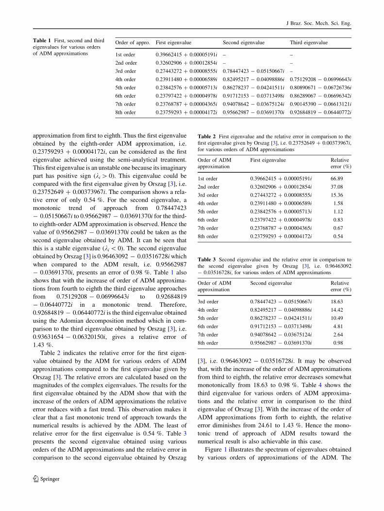
Figure 1 illustrates the spectrum of eigenvalues obtained

by various orders of approximations of the ADM. The

Table 1 First, second and third

eigenvalues for various orders

of ADM approximations

Order of appro. First eigenvalue Second eigenvalue Third eigenvalue

1st order 0.39662415 ? 0.00005191i – –

2nd order 0.32602906 ? 0.00012854i – –

3rd order 0.27443272 ? 0.00008555i 0.78447423 - 0.05150667i –

4th order 0.23911480 ? 0.00006589i 0.82495217 - 0.04098886i 0.75129208 - 0.06996643i

5th order 0.23842576 ? 0.00005713i 0.86278237 - 0.04241511i 0.80890671 - 0.06726736i

6th order 0.23797422 ? 0.00004978i 0.91712153 - 0.03713498i 0.86289067 - 0.06696342i

7th order 0.23768787 ? 0.00004365i 0.94078642 - 0.03675124i 0.90145390 - 0.06613121i

8th order 0.23759293 ? 0.00004172i 0.95662987 - 0.03691370i 0.92684819 - 0.06440772i

Table 2 First eigenvalue and the relative error in comparison to the

first eigenvalue given by Orszag [3], i.e. 0.23752649 ? 0.00373967i,

for various orders of ADM approximations

Order of ADM

approximation

First eigenvalue Relative

error (%)

1st order 0.39662415 ? 0.00005191i 66.89

2nd order 0.32602906 ? 0.00012854i 37.08

3rd order 0.27443272 ? 0.00008555i 15.36

4th order 0.23911480 ? 0.00006589i 1.58

5th order 0.23842576 ? 0.00005713i 1.12

6th order 0.23797422 ? 0.00004978i 0.83

7th order 0.23768787 ? 0.00004365i 0.67

8th order 0.23759293 ? 0.00004172i 0.54

Table 3 Second eigenvalue and the relative error in comparison to

the second eigenvalue given by Orszag [3], i.e. 0.96463092

- 0.03516728i, for various orders of ADM approximations

Order of ADM

approximation

Second eigenvalue Relative

error (%)

3rd order 0.78447423 - 0.05150667i 18.63

4th order 0.82495217 - 0.04098886i 14.42

5th order 0.86278237 - 0.04241511i 10.49

6th order 0.91712153 - 0.03713498i 4.81

7th order 0.94078642 - 0.03675124i 2.64

8th order 0.95662987 - 0.03691370i 0.98

J Braz. Soc. Mech. Sci. Eng.

123

spectrum of eigenvalues is in fact the eigenvalues on the

(kr, ki) plane. It can be seen that the first, second and third

eigenvalues of the ADM semi-analytical treatment

approach the eigenvalues given by Orszag [3]. It is also

observed that as the orders of ADM approximations

increase a monotonic approach towards the Orszag’s [3]

numerically obtained eigenvalues is achieved. It is also

seen that, while the first eigenvalue is in the unstable zone,

ki [ 0, the second and third eigenvalues are in the stable

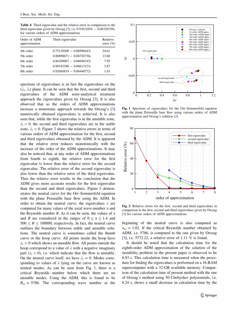
zone, ki \ 0. Figure 2 shows the relative errors in terms of

various orders of ADM approximation for the first, second

and third eigenvalues obtained by the ADM. It is apparent

that the relative error reduces monotonically with the

increase of the order of the ADM approximations. It may

also be noticed that, at any order of ADM approximations

from fourth to eighth, the relative error for the first

eigenvalue is lower than the relative error for the second

eigenvalue. The relative error of the second eigenvalue is

also lower than the relative error of the third eigenvalue.

Thus the relative error results in the conclusion that the

ADM gives more accurate results for the first eigenvalue

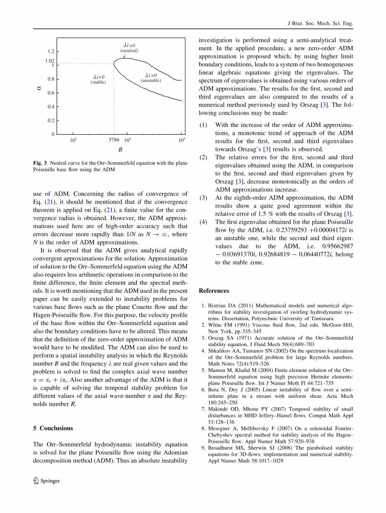
than the second and third eigenvalues. Figure 3 demon-

strates the neutral curve for the Orr–Sommerfeld equation

with the plane Poiseuille base flow using the ADM. In

order to obtain the neutral curve, the eigenvalues k are

computed for many values of the axial wave-number a and

the Reynolds number R. As it can be seen, the values of aand R are considered in the ranges of 0 B a B 1.4 and

500 B R B 100000, respectively. In fact, the neutral curve

outlines the boundary between stable and unstable solu-

tions. The neutral curve is sometimes called the thumb

curve or the hoop curve. All points inside the hoop have

ki [ 0 which shows an unstable flow. All points outside the

hoop correspond to a value of k with a negative imaginary

part (ki \ 0), i.e. which indicate that the flow is unstable.

On the neutral curve itself, we have ki = 0. Modes corre-

sponding to values of k lying on the curve are known as

neutral modes. As can be seen from Fig. 3, there is a

critical Reynolds number below which there are no

unstable modes. Using the ADM, this is found to be

Rcr = 5786. The corresponding wave number at the

beginning of the neutral curve is also computed as

acr = 1.02. If the critical Reynolds number obtained by

ADM, i.e. 5786, is compared to the one given by Orszag

[3], i.e. 5772.22, a relative error of 1.11 % is found.

It should be noted that the calculation time for the

eighth-order ADM approximation of the solution of the

instability problem in the present paper is observed to be

6.93 s. This calculation time is measured when the proce-

dure for finding the eigenvalues is performed on a 16-RAM

supercomputer with a 32-GB available memory. Compar-

ison of the calculation time of present method with the one

of Orszag’s method using 50 Chebyshev polynomials, i.e.

8.24 s, shows a small decrease in calculation time by the

Ψ

Ψ

Ψ

0 0.2 0.4 0.6 0.8 1 1.2-0

-0.05

0

0.05

0.1Orszag' s solution1st order ADM appro.2nd order ADM appro.3rd order ADM appro.4th order ADM appro.5th order ADM appro.6th order ADM appro.7th order ADM appro.8th order ADM appro.

Ψ

first eigenvalue

second eigenvalue

third eigenvalue

λi

λr

Fig. 1 Spectrum of eigenvalues for the Orr–Sommerfeld equation

with the plane Poiseuille base flow using various orders of ADM

approximation and Orszag’s solution [3]

order of approximation

Rel

ativ

e er

ror

(%)

1 2 3 4 5 6 7 80

20

40

60

80

first eigenvaluesecond eigenvaluethird eigenvalue

Fig. 2 Relative errors for the first, second and third eigenvalues in

comparison to the first, second and third eigenvalues given by Orszag

[3] for various orders of ADM approximations

Table 4 Third eigenvalue and the relative error in comparison to the

third eigenvalue given by Orszag [3], i.e. 0.93631654 - 0.06320150i,

for various orders of ADM approximations

Order of ADM

approximation

Third eigenvalue Relative

error (%)

4th order 0.75129208 - 0.06996643i 24.61

5th order 0.80890671 - 0.06726736i 13.68

6th order 0.86289067 - 0.06696342i 7.95

7th order 0.90145390 - 0.06613121i 3.87

8th order 0.92684819 - 0.06440772i 1.43

J Braz. Soc. Mech. Sci. Eng.

123

use of ADM. Concerning the radius of convergence of

Eq. (21), it should be mentioned that if the convergence

theorem is applied on Eq. (21), a finite value for the con-

vergence radius is obtained. However, the ADM approxi-

mations used here are of high-order accuracy such that

errors decrease more rapidly than 1/N as N ? ?, where

N is the order of ADM approximations.

It is observed that the ADM gives analytical rapidly

convergent approximations for the solution. Approximation

of solution to the Orr–Sommerfeld equation using the ADM

also requires less arithmetic operations in comparison to the

finite difference, the finite element and the spectral meth-

ods. It is worth mentioning that the ADM used in the present

paper can be easily extended to instability problems for

various base flows such as the plane Couette flow and the

Hagen-Poiseuille flow. For this purpose, the velocity profile

of the base flow within the Orr–Sommerfeld equation and

also the boundary conditions have to be altered. This means

that the definition of the zero-order approximation of ADM

would have to be modified. The ADM can also be used to

perform a spatial instability analysis in which the Reynolds

number R and the frequency k are real given values and the

problem is solved to find the complex axial wave number

a = ar ? iai. Also another advantage of the ADM is that it

is capable of solving the temporal stability problem for

different values of the axial wave-number a and the Rey-

nolds number R.

5 Conclusions

The Orr–Sommerfeld hydrodynamic instability equation

is solved for the plane Poiseuille flow using the Adomian

decomposition method (ADM). Thus an absolute instability

investigation is performed using a semi-analytical treat-

ment. In the applied procedure, a new zero-order ADM

approximation is proposed which, by using higher limit

boundary conditions, leads to a system of two homogeneous

linear algebraic equations giving the eigenvalues. The

spectrum of eigenvalues is obtained using various orders of

ADM approximations. The results for the first, second and

third eigenvalues are also compared to the results of a

numerical method previously used by Orszag [3]. The fol-

lowing conclusions may be made:

(1) With the increase of the order of ADM approxima-

tions, a monotonic trend of approach of the ADM

results for the first, second and third eigenvalues

towards Orszag’s [3] results is observed.

(2) The relative errors for the first, second and third

eigenvalues obtained using the ADM, in comparison

to the first, second and third eigenvalues given by

Orszag [3], decrease monotonically as the orders of

ADM approximations increase.

(3) At the eighth-order ADM approximation, the ADM

results show a quite good agreement within the

relative error of 1.5 % with the results of Orszag [3].

(4) The first eigenvalue obtained for the plane Poiseuille

flow by the ADM, i.e. 0.23759293 ?0.00004172i is

an unstable one, while the second and third eigen-

values due to the ADM, i.e. 0.95662987

- 0.03691370i, 0.92684819 - 0.06440772i, belong

to the stable zone.

References

1. Bistrian DA (2011) Mathematical models and numerical algo-

rithms for stability investigation of swirling hydrodynamic sys-

tems. Dissertation, Polytechnic University of Timisoara

2. White FM (1991) Viscous fluid flow, 2nd edn. McGraw-Hill,

New York, pp 335–345

3. Orszag SA (1971) Accurate solution of the Orr–Sommerfeld

stability equation. J Fluid Mech 50(4):689–703

4. Shkalikov AA, Tumanov SN (2002) On the spectrum localization

of the Orr–Sommerfeld problem for large Reynolds numbers.

Math Notes 72(4):519–526

5. Mamou M, Khalid M (2004) Finite element solution of the Orr–

Sommerfeld equation using high precision Hermite elements:

plane Poiseuille flow. Int J Numer Meth Fl 44:721–735

6. Bera N, Dey J (2005) Linear instability of flow over a semi-

infinite plate in a stream with uniform shear. Acta Mech

180:245–250

7. Makinde OD, Mhone PY (2007) Temporal stability of small

disturbances in MHD Jeffery–Hamel flows. Comput Math Appl

53:128–136

8. Meseguer A, Mellibovsky F (2007) On a solenoidal Fourier-

Chebyshev spectral method for stability analysis of the Hagen–

Poiseuille flow. Appl Numer Math 57:920–938

9. Broadhurst MS, Sherwin SJ (2008) The parabolised stability

equations for 3D-flows: implementation and numerical stability.

Appl Numer Math 58:1017–1029

R

α

103 104 1050

0.2

0.4

0.6

0.8

1

1.2

>0(unstable)

<0(stable)

=0(neutral)

5786

1.02

λi

λiλi

Fig. 3 Neutral curve for the Orr–Sommerfeld equation with the plane

Poiseuille base flow using the ADM

J Braz. Soc. Mech. Sci. Eng.

123

10. Prusa V (2009) On the influence of boundary condition on sta-

bility of Hagen–Poiseuille flow. Comput Math Appl 57:763–771

11. Giannakis D, Fischer PF, Rosner R (2009) A spectral Galerkin

method for the coupled Orr–Sommerfeld and induction equations

for free-surface MHD. J Comput Phys 228:1188–1233

12. Elcoot AEK (2010) New analytical approximation forms for non-

linear instability of electric porous media. Int J Nonlinear Mech

45:1–11

13. Dragomirescu FI, Gheorghiu CI (2010) Analytical and numerical

solutions to an electro-hydrodynamic stability problem. Appl

Math Comput 216(12):3718–3727

14. You XY, Guo L (2010) Combined effects of EDL and boundary

slip on mean flow and its stability in microchannels. CR Mec

338:181–190

15. Saravanan S, Brindha D (2011) Global nonlinear stability of

convection in a heat generating fluid filled channel with a moving

boundary. Appl Math Lett 24:487–493

16. Malik SV, Yoshikawa HN, Crumeyrolle O, Mutabazi I (2012)

Thermo-electro-hydrodynamic instabilities in a dielectric liquid

under microgravity. Acta Astronaut 81:563–569

17. Asthana R, Awasthi MK, Agrawal GS (2012) Kelvin-Helmholtz

instability of two viscous fluids in porous medium. Int J Appl

Math Mech 8(14):1–13

18. Modica F, Plewa T, Zhiglo A (2013) The Braginskii model of the

Rayleigh-Taylor instability: I. Effects of self-generated magnetic

fields and thermal conduction in two dimensions. High Energy

Density Phys 9:767–780

19. Hagan J, Priede J (2013) Capacitance matrix technique for

avoiding spurious eigenmodes in the solution of hydrodynamic

stability problems by Chebyshev collocation method. J Comput

Phys 238:210–216

20. Gennaro EM, Simoes LGC, Malatesta V, Reis DC, Medeiros

MAF (2013) Verification and accuracy comparison of commer-

cial CFD codes using hydrodynamic instability. J Brazil Soc

Mech Sci Eng. doi:10.1007/s4043001300573

21. Wazwaz AM (2000) Approximate solutions to boundary value

problems of higher order by the modified decomposition method.

Comput Math Appl 40:679–691

22. Wazwaz AM (2006) The modified decomposition method and

Pade approximants for a boundary layer equation in unbounded

domain. Appl Math Comput 177:737–744

23. Somali S, Gokmen G (2007) Adomian decomposition method for

nonlinear Sturm-Liouville problems. Surv Math Appl 2:11–20

24. Hayat T, Hussain Q, Javed T (2009) The modified decomposition

method and Pade approximants for the MHD flow over a non-

linear stretching sheet. Nonlinear Anal Real World Appl

10:966–973

25. Lin Y, Lu TT, Chen CK (2013) Adomian decomposition method

using integrating factor. Commun Theor Phys 60:159–164

J Braz. Soc. Mech. Sci. Eng.

123