Guideline for the Certification of Wind Turbines Edition 2010
Upload
khangminh22Category
view
0download
0

Industrial gasturbines
Performance and operability
A. M. Y. Razak
CRC PressBoca Raton Boston New York Washington, DC
W O O D H E A D P U B L I S H I N G L I M I T E DCambridge England
iii
© 2007 by Taylor & Francis Group, LLC
https
://boil
ersinf
o.com

Published by Woodhead Publishing Limited, Abington Hall, Abington,Cambridge CB21 6AH, Englandwww.woodheadpublishing.com
Published in North America by CRC Press LLC, 6000 Broken Sound Parkway, NW,Boca Raton, FL 33487, USA
First published 2007, Woodhead Publishing Limited and CRC Press LLC© 2007, Woodhead Publishing LimitedCD-ROM © 2007, Gas Path Analysis LtdThe author has asserted his moral rights.
This book contains information obtained from authentic and highly regarded sources.Reprinted material is quoted with permission, and sources are indicated. Reasonableefforts have been made to publish reliable data and information, but the author andthe publishers cannot assume responsibility for the validity of all materials. Neitherthe author nor the publishers, nor anyone else associated with this publication, shallbe liable for any loss, damage or liability directly or indirectly caused or alleged to becaused by this book.
Neither this book nor any part may be reproduced or transmitted in any form or byany means, electronic or mechanical, including photocopying, microfilming andrecording, or by any information storage or retrieval system, without permission inwriting from Woodhead Publishing Limited.
The consent of Woodhead Publishing Limited does not extend to copying forgeneral distribution, for promotion, for creating new works, or for resale. Specificpermission must be obtained in writing from Woodhead Publishing Limited for suchcopying.
Trademark notice: Product or corporate names may be trademarks or registeredtrademarks, and are used only for identification and explanation, without intent toinfringe.
British Library Cataloguing in Publication DataA catalogue record for this book is available from the British Library.
Library of Congress Cataloging in Publication DataA catalog record for this book is available from the Library of Congress.
Woodhead Publishing ISBN 978-1-84569-205-6 (book)Woodhead Publishing ISBN 978-1-84569-340-4 (e-book)CRC Press ISBN 978-1-4200-4455-3CRC Press order number WP4455
The publishers’ policy is to use permanent paper from mills that operate asustainable forestry policy, and which has been manufactured from pulpwhich is processed using acid-free and elementary chlorine-free practices.Furthermore, the publishers ensure that the text paper and cover board usedhave met acceptable environmental accreditation standards.
Typeset by Replika Press Pvt Ltd, IndiaPrinted by TJ International Limited, Padstow, Cornwall, England
iv
© 2007 by Taylor & Francis Group, LLC
https
://boil
ersinf
o.com

Contents
Foreword xiii
Preface xv
Acknowledgements xvii
Note about the CD-ROM accompanying this book xviii
CD-ROM: copyright information and terms of use xix
Abbreviations and notation xxi
1 Introduction 1
1.1 The gas turbine 21.2 Gas turbine layouts 31.3 Closed cycle gas turbine 61.4 Environmental impact 71.5 Engine controls 91.6 Performance deterioration 91.7 Gas turbine simulators 101.8 References 10
Part I Principles of gas turbine performance
2 Thermodynamics of gas turbine cycles 13
2.1 The first law of thermodynamics 132.2 The second law of thermodynamics 132.3 Entropy 142.4 Steady flow energy equation 152.5 Pressure–volume and temperature–entropy diagram 162.6 Ideal simple cycle gas turbine 16
v
© 2007 by Taylor & Francis Group, LLC
https
://boil
ersinf
o.com

2.7 Ideal regenerative gas turbine cycle 212.8 Reversibility and efficiency 252.9 Effect of irreversibility on the performance of the ideal
simple cycle gas turbine 312.10 Effect of pressure losses on gas turbine performance 322.11 Variation of specific heats 322.12 Enthalpy and entropy 372.13 Combustion charts 392.14 Heat exchanger performance 402.15 Performance of an actual (practical) simple cycle gas
turbine 422.16 Performance of an actual (practical) regenerative gas
turbine cycle 452.17 Turbine entry temperature and stator outlet temperature 502.18 Worked examples 512.19 References 59
3 Complex gas turbine cycle 60
3.1 Intercooled gas turbine cycles 603.2 Reheat gas turbine cycle 723.3 Intercooled, reheat and regenerative cycles 853.4 Ericsson cycle 893.5 Combined cycle gas turbines 943.6 Co-generation systems 953.7 Hybrid fuel cell–gas turbine system 963.8 References 97
4 Compressors 98
4.1 Axial compressors 984.2 Compressor blading 994.3 Work done factor 1024.4 Stage load coefficient 1034.5 Stage pressure ratio 1064.6 Overall compressor characteristics 1094.7 Rotating stall 1104.8 Compressor surge 1104.9 Compressor annulus geometry 1134.10 Compressor off-design operation 1154.11 References 118
5 Axial turbines 120
5.1 Turbine blading 120
Contentsvi
© 2007 by Taylor & Francis Group, LLC
https
://boil
ersinf
o.com

5.2 Stage load and flow coefficient 1225.3 Deviation and profile loss 1255.4 Stage pressure ratio 1255.5 Overall turbine characteristics 1275.6 Turbine creep life 1295.7 Turbine blade cooling 1305.8 Turbine metal temperature assessment 1335.9 Effect of cooling technology on thermal efficiency 1345.10 References 136
6 Gas turbine combustion 137
6.1 Combustion of hydrocarbon fuels 1376.2 Gas turbine combustion system 1406.3 Combustor cooling 1466.4 Types of gas turbine combustor 1476.5 Fuel injection and atomisation 1496.6 Combustion stability and heat release rate 1526.7 Combustion pressure loss and efficiency 1546.8 Formation of pollutants 1566.9 NOx suppression using water and steam injection 1576.10 Selective catalytic reduction (SCR) 1586.11 Dry low emission combustion systems (DLE) 1586.12 Variable geometry combustor 1606.13 Staged combustion 1606.14 Rich-burn, quick-quench, lean-burn (RQL) combustor 1626.15 Lean premixed (LPM) combustion 1646.16 Catalytic combustion 1656.17 Impact of engine configuration on DLE combustion
systems 1666.18 Correlations for prediction of NOx, CO and UHC and the
calculation of CO2 emissions 1686.19 References 173
7 Off-design performance prediction 174
7.1 Component matching and component characteristics 1747.2 Off-design performance prediction of a single-shaft gas
turbine 1777.3 Off-design performance prediction of a two-shaft gas
turbine with a free power turbine 1817.4 Matrix method of solution 1857.5 Off-design performance prediction of a three-shaft gas
turbine with a free power turbine 187
Contents vii
© 2007 by Taylor & Francis Group, LLC
https
://boil
ersinf
o.com

7.6 Off-design performance prediction of a two-shaft gasturbine 188
7.7 Off-design performance prediction of a three-shaft gasturbine 190
7.8 Off-design performance prediction of complex gas turbinecycles 191
7.9 Off-design prediction of a two-shaft gas turbine using afree power turbine and employing intercooling,regeneration and reheat 196
7.10 Off-design prediction of a three-shaft gas turbine using apower turbine and employing intercooling, regenerationand reheat 198
7.11 Variable geometry compressors 2007.12 Variable geometry turbines 2017.13 References 201
8 Behaviour of gas turbines during off-designoperation 202
8.1 Steady-state running line 2028.2 Displacement of running line (single- and two-shaft free
power turbine gas turbine) 2088.3 Three-shaft gas turbine operating with a free power
turbine 2178.4 Displacement of running line (three-shaft gas turbine) 2218.5 Running line for a two-shaft gas turbine 2238.6 Running lines of gas turbine complex cycles 2268.7 Running line, non-dimensional parameters and correcting
data to standard conditions 2368.8 Power turbine curves 2378.9 Gas power and gas thermal efficiency 2398.10 Heat rate and specific fuel consumption 2408.11 References 240
9 Gas turbine performance deterioration 241
9.1 Compressor fouling 2429.2 Variable inlet guide vane (VIGV) and variable stator
vane (VSV) problems 2469.3 Hot end damage 2489.4 Tip rubs and seal damage 2509.5 Quantifying performance deterioration and diagnosing
faults 2509.6 References 261
Contentsviii
© 2007 by Taylor & Francis Group, LLC
https
://boil
ersinf
o.com

10 Principles of engine control systems and transientperformance 262
10.1 PID loop 26310.2 Signal selection 26610.3 Acceleration–deceleration lines 26710.4 Control of variable geometry gas turbines 27010.5 Starting and shutdown 27510.6 Transient performance 27710.7 References 288
Part II Simulating the performance of a two-shaft gas turbine
11 Simulating the effects of ambient temperature onengine performance, emissions and turbine lifeusage 293
11.1 Compressor running line 29311.2 Representation of other non-dimensional parameters 29411.3 Effects of ambient temperature on engine performance
(high-power operating case) 29611.4 Effect of reduced power output during a change in
ambient temperature 31311.5 Effect of humidity on gas turbine performance and
emissions 320
12 Simulating the effect of change in ambient pressureon engine performance 323
12.1 Effect of ambient pressure on engine performance(high-power case) 324
12.2 Effect of ambient pressure changes on engineperformance at lower power outputs 329
13 Simulating the effects of engine componentdeterioration on engine performance 337
13.1 Compressor fouling (high operating power) 33713.2 Compressor fouling (low operating power) 34913.3 Turbine damage 35713.4 References 375
14 Power augmentation 376
14.1 Peak rating 377
Contents ix
© 2007 by Taylor & Francis Group, LLC
https
://boil
ersinf
o.com

14.2 Maximum continuous rating 38014.3 Power augmentation at very low ambient temperatures 38314.4 Power augmentation by water injection 38814.5 Turbine inlet cooling 39314.6 Power turbine performance 40214.7 The effect of change in fuel composition on gas
turbine performance and emissions 40414.8 References 408
15 Simulation of engine control system performance 409
15.1 Proportional action 40915.2 Proportional and integral action 41015.3 Signal selection 41415.4 Acceleration and deceleration lines 41715.5 Integral wind-up 42115.6 Engine trips 42515.7 References 428
Part III Simulating the performance of a single-shaft gasturbine
16 Simulating the effects of ambient temperature onengine performance, emissions and turbine lifeusage 431
16.1 Configuration of the single-shaft simulator 43116.2 Effect of ambient temperature on engine performance at
high power 43216.3 Effect of ambient temperature on engine performance at
low power 44416.4 Effect of ambient temperature on engine performance at
high power (single-shaft gas turbine operating with anactive variable inlet guide vane) 454
16.5 Effect of humidity on gas turbine performance andemissions 463
17 Simulating the effect of change in ambient pressureon engine performance 466
17.1 Effect of ambient pressure on engine performance at highpower 467
17.2 Effect of ambient pressure on engine performance at lowpower 472
Contentsx
© 2007 by Taylor & Francis Group, LLC
https
://boil
ersinf
o.com

17.3 Effect of ambient pressure on engine performance at lowpower (single-shaft gas turbine operating with an activevariable inlet guide vane) 479
18 Simulating the effects of engine componentdeterioration on engine performance 489
18.1 Compressor fouling (high-power operation) 48918.2 Compressor fouling (low-power operation) 49718.3 Compressor fouling at low-power operation (single-shaft
gas turbine operating with an active variable inlet guidevane) 504
18.4 Turbine damage (hot end damage) at high-power outputs 50818.5 Hot end damage at low power with active VIGV
operation 515
19 Power augmentation 524
19.1 Peak rating 52519.2 Power augmentation by increasing VIGV angle 52819.3 Power augmentation using water injection 53319.4 Power augmentation at low ambient temperatures 53719.5 Turbine inlet cooling 543
20 Simulation of engine control system performance 545
20.1 VIGV control system simulation 54520.2 VIGV control when the VIGV is active during the normal
operating power range 54920.3 Optimisation of the EGT limit for a single-shaft gas
turbine with ambient temperature 563
21 Simulation exercises 566
Exercises using the single-shaft gas turbine simulator21.1 Effects of ambient temperature and pressure on engine
performance 56621.2 Effects of component performance deterioration 56821.3 Power augmentation 56821.4 Combined cycle and co-generation 57021.5 Engine control systems 57121.6 Gas turbine emissions 571
Exercises using the two-shaft gas turbine simulator21.7 Effects of ambient temperature, pressure and humidity on
engine performance 573
Contents xi
© 2007 by Taylor & Francis Group, LLC
https
://boil
ersinf
o.com

21.8 Effects of component performance deterioration 57521.9 Power augmentation 57621.10 Combined cycle and co-generation 57821.11 Engine control systems 57921.12 Gas turbine emissions 57921.13 Answers to exercises 582
Appendix: Steady flow energy equation and stagnationproperties 589
A1.1 Steady flow energy equation 589A1.2 Stagnation temperatures and pressures 590A1.3 References 591
Contentsxii
© 2007 by Taylor & Francis Group, LLC

Foreword
Improving gas turbine performance involves the bringing together andoptimisation of the disciplines and skills required to achieve an operationallycompetitive gas turbine engine. Certainly, the design and performance ofindividual engine components, such as the compressors, combustors andturbine, could alone present an engineer with a worthwhile career. It is,however, the overall performance of the gas turbine that the customer actuallypurchases. The optimisation process involves many uncertainties and a properunderstanding of these, together with the established facts and the method ofhandling this information, is required to permit manufacturers to develop theirengines successfully and allow operators to operate the machines to their bestadvantage. This is particularly true in the de-regulated market in which manyoperate today and which others will be joining in the near future.
Although there are many very remarkable books on industrial gas turbineperformance and engineering, this book offers something different througha combined approach to the theory of gas turbines, their performance, andthe use of gas turbine simulators. Simulators form an analysis method whichcan be used to bring together the many disciplines involved and whichprovides a way of assessing the impact of uncertainties. The combination ofthe book with the example simulators provides an added dimension to theproduct and this seems to conform to what many educational and trainingexperts in this field have been demanding for some time. The book/simulatorcombination provides a useful reference text for students and practisingengineers in both gas turbine manufacturing and operations.
The book initially covers the theory of gas turbine performance from adesign and off-design point of view, including transient analysis, and givesmuch detail on these two very important aspects of engine performance. Thelatter part of the book revisits the earlier chapters, using the simulators tohighlight in detail the issues facing industrial gas turbines in the real world.The simulators are effectively virtual engines with respect to performance,deterioration, emissions, control, and life usage. There is also a useful lifecycle calculation module. This provides a clear view of the operability of thegas turbine under different conditions.
xiii
© 2007 by Taylor & Francis Group, LLC

Forewordxiv
The book includes numerous simulation exercises. These exercises arenot restrictively academic but include much of the author’s experience, gainedfrom an operator’s viewpoint. Unlike numerical exercises, which give asomewhat narrow understanding of the problem, simulation exercises providea holistic view of performance, which students, manufacturers and operatorswill find invaluable.
Robin Elder, BSc, PhD, C Eng, FIMechEDirector, PCA Engineers Limited
© 2007 by Taylor & Francis Group, LLC

Preface
The use of industrial gas turbines is widespread in many industries that requirepower. The power is used to generate electricity or drive equipment such aspumps and process compressors. Gas turbines are also used extensively innaval propulsion and in this case are often referred to as naval gas turbines. Inany of these applications, the performance of the gas turbines is the end productthat strongly influences the profitability of the business that employs them.Industrial gas turbines often have to operate for prolonged periods at conditionsthat do not correspond to their design conditions. Therefore, understanding theperformance of gas turbines at such operating conditions is particularlyimportant, especially in a deregulated market.
Other factors in addition to the performance of gas turbines affect theiroperability. These factors include emissions, deterioration, life usage andcontrols. For example, legislation may result in emissions being too high andthe means to control them could affect the engine performance and thus revenue.Gas turbine performance deterioration is inevitable. This could be due tocompressor fouling, which can be easily rectified by compressor washing, orto more serious damage to compressors or turbines. Therefore, an understandingof performance deterioration is now paramount. Various engine operating limitsare imposed by manufacturers and correspond to the exhaust gas turbine limit,speed and power. These are necessary to achieve suitable engine life, namelyturbine creep life. It is the responsibility of the engine control system to ensurethat such operating limits are not exceeded. Furthermore, it is also the job ofthe control system to ensure that any engine load changes occur safely.
Improving the understanding of the above issues has provided the impetusto write this book. The book begins with a brief revision of engineeringthermodynamics before considering the design point performance of gasturbines, including both simple and complex cycles. The performance of gasturbine components (compressors, combustors and turbines) is also discussed.Means to improve dry low-emission combustion systems are included. Theprediction and modelling of the off-design performance of gas turbines isdiscussed, including the modelling of complex cycles which employintercooling, reheat and regeneration. The impact and detection of performance
xv
© 2007 by Taylor & Francis Group, LLC

Prefacexvi
deterioration and the importance of such detection and rectification are alsodiscussed. Control system performance, including the prediction of the transientperformance of gas turbines, is considered. Furthermore, the application ofcontrol systems to improve the performance of dry low-emission combustionsystems by the use of variable geometry components is discussed.
The CD accompanying the book contains two gas turbine simulators, whichcorrespond to single-shaft and two-shaft engines. These two engineconfigurations cover the vast majority of industrial gas turbines operating inthe field. Much of the text describing the performance and operability ofindustrial gas turbines can be illustrated and enlivened by the use of these gasturbine simulators. The simulators are used extensively in Parts II and III to:
(1) simulate the effects of ambient temperature, pressure and humidity onperformance, turbine creep life and emissions, including the impact ofinlet and exhaust losses;
(2) simulate the effects of engine deterioration on performance, creep lifeand emissions;
(3) simulate the impact of power augmentation and enhancement usingturbine inlet cooling, peak rating, water injection and optimisation onperformance, creep life and emissions;
(4) simulate control system performance on engine operability includingproportional off-set, integral wind-up and engine trips;
(5) simulate the effect of a change in fuel type (e.g. natural gas or diesel) onperformance and emissions.
There are nearly 50 simulation exercises included using each simulator.Exercises using simulators give a holistic view of engine performance andoperability which numerical exercises fail to achieve. Nevertheless, numericalexercises are essential to augment the understanding of engine performanceand some worked examples are given.
The simulators include other useful features and can show:
(1) impact on life cycle costs, revenue and profitability (including the impactof emissions taxes such as CO2 and NOx on life cycle costs and, thus,profitability);
(2) output from the turbine inlet cooling simulation which can be used toevaluate the suitability of turbine inlet cooling for any gas turbine for aparticular site;
(3) trends for many engine parameters, including key parameters such asEGT and speeds that protect the engine from damage;
(4) compressor characteristics and the operating point during enginetransients;
(5) bar charts;(6) simulated data that can be exported to other computer packages (e.g.
Microsoft Excel spreadsheets).
© 2007 by Taylor & Francis Group, LLC

Acknowledgements
Much of this work would have been impossible without the support, help andsuggestions from friends and colleagues. In particular, I wish to thank Dr JohnGreenbank and John Layton for their expert proofreading, which has improvedthe quality of the text and presentation of the book. Also, my friend and mentorProfessor Robin Elder, who is wholly responsible for first introducing me toserious engineering computing, for his encouragement and support throughoutthe writing and preparation of this book. Also, I thank Woodhead Publishingfor its patience during the preparation of the manuscript, particularly SherilLeich for her thorough checking of the manuscript and suggestions.
I also wish to remember J. R. (Jimmy) Palmer of Cranfield Institute ofTechnology (now Cranfield University) who, in his day, was considered oneof the authorities on gas turbine performance. I am privileged to have knownhim.
xvii
© 2007 by Taylor & Francis Group, LLC

Note about the CD-ROM accompanyingthis book
As stated in the Preface, this CD-ROM includes software simulating theoperation of a single-shaft gas turbine and a two-shaft gas turbine. Thesimulators are built on the engine modelling concepts discussed in the bookand should be used to repeat the simulation discussion in Parts II and III and toperform the exercises in Chapter 21.
• Minimum system requirementsThis CD-ROM is intended for use with Windows-compatible computers. Youwill require an internet connection for registration (see below).
Please note that, as part of the registration process, you will need to make anote of the Disk ID Number. This can be found on the front of the plasticwallet containing the CD-ROM. We suggest you make a note of this numbernow. You need take no further steps in the registration process until you installthe CD-ROM.
• Software requirementsAdobe® Reader®
• Installation instructionsInsert the CD-ROM into the CD-ROM drive. The CD-ROM should auto-run.If the CD-ROM does not auto-run, open Microsoft Internet Explorer® on yourcomputer and open the file index.html. If you continue to experience difficulties,please contact Gas Path Analysis Ltd for help (e-mail: [email protected])
• Registration processOnce you have inserted the CD-ROM and want to install the simulator software,you will need to go through a registration process to ensure uninterrupted useof the software. The registration process is designed to prevent unauthorisedcopying and distribution of the software. The CD-ROM contains an installationguide which will take you through the relevant steps.
xviii
© 2007 by Taylor & Francis Group, LLC

CD-ROM: copyright information andterms of use
The CD-ROM which accompanies this book is © 2007 Gas Path Analysis Ltd.All rights are reserved. Use of the CD-ROM is governed by the terms of thesoftware licence agreement which follows. The licence grants licensees a non-exclusive, non-transferable, single-user licence. The licensed software may beinstalled on only one computer at a time. Installation of the software on two ormore computers requires the purchase of additional licences from Gas PathAnalysis Ltd. Loading the CD-ROM implies you agree to the terms of thesoftware licence agreement. You will be asked to confirm your agreement tothe terms of the licence as part of the installation process for the CD-ROM.
Gas Path Analysis Ltd (GPAL) gas turbine simulator
software licence agreement
This licence is issued by:
Gas Path Analysis LtdEmail: [email protected]: www.gpal.co.uk
Read this agreement carefully as it constitutes the terms of the software licenceagreement.
1. Software product
This agreement is for a single-user licence of the GPAL Gas Turbine SimulatorSoftware CD-ROM (‘the Software’) supplied with your purchase of Industrialgas turbines: performance and operability from Woodhead Publishing Limited.
2. Software licence
Gas Path Analysis Limited (GPAL) ‘the Licensor’ grants to the Licensee anon-exclusive, non-transferable, single-user licence. The registered version ofthe Software may only be installed on one computer at a time and requires a
xix
© 2007 by Taylor & Francis Group, LLC

registration code to function properly. The registration code can be obtainedfrom the Licensor. Installation of the Software on a second or more computersrequires the purchase of additional licences which can be obtained from GasPath Analysis Limited.
3. Liability
The CD-ROM contains information from authentic and highly-regardedsources. Reprinted material is quoted with permission, and sources are indicated.Reasonable efforts have been made to publish reliable data and information,but neither Gas Path Analysis Limited and Woodhead Publishing Limited, noranyone else associated with this CD-ROM, are engaged in renderingprofessional services and shall not be liable for any loss, damage or liabilitydirectly or indirectly caused or alleged to be caused by any material containedin this CD-ROM or the accompanying book.
4. Proprietary rights
The Licensee agrees that the Software is the property of the Licensor. Anyrights under patents, copyrights, trademarks, and trade secrets related to theSoftware are and shall remain vested in the Licensor. The Licensee agrees topreserve any copyright notices contained within the Software. The Licenseeacknowledges that he or she is specifically prohibited from reverse engineeringor disassembling the Software in whole or in part.
Unless otherwise stated in the installation guide and user guides containedin this CD-ROM, neither this CD-ROM nor the accompanying book or anypart may be reproduced or transmitted in any form or by any means, electronicor mechanical, including photocopying, microfilming and recording, or by anyinformation storage or retrieval system, without permission in writing fromGas Path Analysis Limited. The consent of Gas Path Analysis Limited doesnot extend to copying for general distribution, for promotion, for creating newworks, or for resale. Specific permission must be obtained in writing from GasPath Analysis Limited for such copying.
5. General
The laws of England shall govern in all respects as to the validity, interpretation,construction and enforcement of this licence.
6. Copyright
All rights are reserved and all copyrights in the Software belong to Gas PathAnalysis Limited (UK company registration number: 3447319).
CD-ROM: copyright information and terms of usexx
© 2007 by Taylor & Francis Group, LLC

C thermal capacity ratioCO carbon monoxideCO2 carbon dioxidecp specific heat at constant pressurecv specific heat at constant volumeDLE dry low emissionEGT exhaust gas temperatureGG gas generatorH enthalpyHP high pressureICRHR intercooled, reheat and regenerative cycleIP intermediate pressureISO International Standards OrganisationJ JoulesK Kelvinkg kilogramLP low pressureLPM lean premixedm mass flow rateMCFC molten carbonate fuel cellMEA methanol amineMW MegaWatt or molecular weightNGV nozzle guide vaneNOx oxides of nitrogenNTU number of transfer unitsP pressurePID Proportional, Integral and Derivativepr pressure ratioQ heat inputR gas constantRQL Rich-burn, Quick-quench, Lean-burns second
Abbreviations and notation
xxi
© 2007 by Taylor & Francis Group, LLC

S entropySCR selective catalytic reductionSOFC solid oxide fuel cellsSOT stator outlet temperatureT temperatureTET turbine entry temperatureUHC unburnt hydrocarbonsVIGV variable inlet guide vaneVSV variable stator vaneW work outputx number of carbon atomsy number of hydrogen atomsZ compressibility factorγ ratio of specific heatsε effectiveness of heat exchangerη efficiencyφ relative humidityω specific or absolute humidity
Abbreviations and notationxxii
© 2007 by Taylor & Francis Group, LLC

1
The history of the gas turbine goes back to 1791, when John Barber took outa patent for ‘A Method for Rising Inflammable Air for the Purposes ofProducing Motion and Facilitating Metallurgical Operations’. Many endeavourshave been made since then particularly in the early 1900s to build an operationalgas turbine. In 1903, a Norwegian, Aegidius Elling, built the first successfulgas turbine using a rotary/dynamic compressor and turbines, and is creditedwith building the first gas turbine that produced excess power of about 8 kW(11 hp). By 1904 Elling had improved his design, achieving exhaust gastemperatures of 773 K (500 degrees Celsius), up from 673 K (400 degreesCelsius), producing about 33 kW (44 hp). The engine operated at about20 000 rpm. Much of his later work was carried out (from 1924 to 1927) atKongsberg, in Norway.
Elling’s gas turbine was very similar to Frank Whittle’s jet engine, whichwas patented in 1930 in England. Whittle’s design also consisted of a centrifugalcompressor and an axial turbine and the engine was subsequently tested inApril 1937. Meanwhile, in 1936, Hans von Ohain and Max Hahn, in Germany,developed and patented their own design. Unlike Frank Whittle’s design,von Ohain’s engine employed a centrifugal compressor and turbine placedvery close together, back to back. The work by both Whittle and Ohaineffectively started the gas turbine industry.1
Today, gas turbines are used widely in various industries to producemechanical power and are employed to drive various loads such as generators,pumps, process compressors, or a propeller. The gas turbine began as arelatively simple engine and evolved into a complex but reliable and highefficiency prime mover. The performance and satisfactory operation of gasturbines are of paramount importance to the profitability of industries, varyingfrom civil and military aviation to power generation, and also oil and gasexploration and production.
In the quest to perfect the gas turbine, compressor pressure ratios haveincreased from about 4:1 to over 40:1 together with high operating temperatures
1Introduction
© 2007 by Taylor & Francis Group, LLC

Industrial gas turbines2
(about 1800 K), resulting in thermal efficiencies exceeding 40%. Thesefeatures make the gas turbine a formidable competitor to other types ofprime movers. In increasing the performance of the gas turbine, variousengine configurations have evolved and such engine component arrangementsand their applications will be discussed. However, the principles of the gasturbine and the main components that are required for these engines will bediscussed first.
1.1 The gas turbine
For a turbine to produce power, it must have a higher inlet pressure than thatat the exit. A compressor is normally used to provide this increase in pressureinto the turbine. If the compressor discharge flow through the turbine isexpanded, the turbine power output will be less than the power absorbed bythe compressor because of losses in the compressor and turbine. Under theseconditions, the whole engine will cease to rotate.
If energy is added into the compressor discharge air, corresponding to thelosses in the compressor and turbine, then the system will run but will notproduce any net power output. To produce net power from the gas turbine,additional energy needs to be supplied into the compressor discharge air. Theenergy supplied to the compressor discharge air is normally achieved byburning fuel in the compressor discharge air and this is accomplished in acombustion chamber or combustor, which is located or positioned betweenthe compressor and turbine as shown in Fig. 1.1.
Clearly, the power output from a gas turbine depends on the efficiency ofthe compressor, turbine and the combustor. The higher the efficiency ofthese components, the better will be the performance of the gas turbine,resulting in increased power output and thermal efficiency.
The gas turbine has developed over 50 years into a high efficiency primemover, and compressor and turbine efficiencies (polytropic) above 90% canbe achieved today.
Combustor
Fuel input
Compressor Load
Turb
ine
1.1 Schematic layout of a single-shaft gas turbine.
© 2007 by Taylor & Francis Group, LLC

Introduction 3
From the above discussion, a gas turbine must therefore have at least thefollowing components:
(1) compressor(2) combustor(3) turbine.
A gas turbine comprising these components is often referred to as a simplecycle gas turbine. Gas turbines can include other components, such asintercoolers to reduce the compression power absorbed, re-heaters to increasethe turbine power output and heat exchangers to reduce the heat input. Thesetypes of gas turbines are referred to as complex cycles. Although such complexcycles were developed in the early days of the gas turbine, today, simplecycle gas turbines dominate, and this is due to the high levels of performanceachieved by engine components such the compressor, turbine and combustor.However, there is a renewed interest in complex cycle designs as a means ofimproving the performance of the gas turbine further.
1.2 Gas turbine layouts
Various arrangements of the gas turbine components have evolved over theyears. Some are better suited for certain applications such as power generation(constant speed operation of the load, i.e. the generator) and other layoutsare more suited to mechanical drive applications where the gas turbine isused to drive a process compressor or a pump (where the speed of the drivenequipment can vary with load). In this section, we shall discuss these variousarrangements, highlighting their advantages and disadvantages.
1.2.1 Single-shaft gas turbine
A single-shaft gas turbine consists of a compressor, combustor and a turbineas shown in Fig. 1.1. The compressor draws in air and increases its pressure.This compressed air is then introduced into the combustor, where heat isadded by burning fuel. The hot, high-pressure gases are then expanded in aturbine to extract useful power. Part of the turbine power output is absorbedby the compressor, thus providing power for the compression process via theshaft connecting the compressor and turbine. The remaining power outputfrom the turbine is used to drive a load such as a generator.
Single-shaft gas turbines are most suited for fixed speed operation such asbase-load power generation. Single-shaft gas turbines have the advantage ofpreventing over-speed conditions due to the high power required by thecompressor and can act as an effective brake should the loss of electricalload occur.
© 2007 by Taylor & Francis Group, LLC

Industrial gas turbines4
1.2.2 Two-shaft gas turbine with a power turbine
The expansion process in the turbine shown in Fig. 1.1 above may be splitinto two separate turbines. The first is used to drive the compressor and thesecond is used to drive the load. The mechanically independent (free) turbinedriving the load is called the power turbine. The remaining turbine or high-pressure turbine, compressor and the combustor are called the gas generator.Figure 1.2 shows a schematic layout of a two-shaft gas turbine with a powerturbine and is probably the most common engine configuration that is employedfor gas turbines in general.
The function of the gas generator is to produce high pressure and hightemperature gases for the power turbine. Two-shaft gas turbines operatingwith a power turbine are often used to drive loads where there is a significantvariation in the speed with power demand (mechanical drive applicationssuch as gas compression). Examples are pipeline compressors and pumps.The process conditions may be such that the load runs at low speed butabsorbs or demands a large amount of power. In such a situation, the powerturbine can run at the speed of the load and the gas generator can run at itsmaximum speed. If a single shaft gas turbine were employed to provide thepower requirements for such applications, the whole engine would beconstrained to run at the speed of the load thus resulting in poor engineperformance due to the low operating speed condition.
Two-shaft gas turbines are also employed in industrial power generationwith the power turbine designed to operate at a fixed speed determined bythe generator. Unlike a single-shaft engine, the gas generator speed will varywith electrical load. The main advantage is smaller starting power requirements,as the gas generator only needs to be turned during starting, and better off-design performance. The disadvantage is that the shedding of the electricalload can result in over-speeding of the power turbine.
Combustor
Fuel input
Compressor Load
Po
wer
tu
rbin
e
Turb
ine
Gas generator
1.2 Schematic layout of a two-shaft gas turbine with a power turbine.
© 2007 by Taylor & Francis Group, LLC

Introduction 5
1.2.3 Three-shaft gas turbine with a power turbine
The gas generator (GG), as discussed in Section 1.2.2, can be divided furtherto produce a two-shaft or a twin spool gas generator. When this is done, thehigh-pressure GG turbine drives the high-pressure GG compressor, and thelow pressure GG turbine drives the low pressure GG compressor. However,there is no mechanical linkage between the high pressure and low pressureshafts in the gas generator. Figure 1.3 shows a schematic layout of a three-shaft gas turbine with a power turbine. The power turbine is still mechanicallyindependent from the gas generator as described in Section 1.2.2.
Such three-shaft arrangements, as with a two-shaft gas turbine with itsown power turbine, are widely used in mechanical drive applications. Muchhigher-pressure ratios and thermal efficiencies may be achieved with such alayout without having to resort to variable geometry compressors as wouldbe required by two-shaft gas engines when designed to operate at highcompressor pressure ratios.
Three-shaft gas turbines also have the added advantage of lower startingpowers because only the high-pressure compressor and turbine in the gasgenerator need to be turned during starting. Engines that use such aconfiguration are often derived from aircraft gas turbines and are referred toas aero-derivatives.
1.2.4 Two-shaft gas turbine
As seen in the power turbine configurations described in Sections 1.2.2 and1.2.3, the power turbine can over-speed if the electrical load is shed whendriving a generator. The two-shaft gas turbine overcomes this problem andstill requires smaller starting powers than the single shaft gas turbine. Theconfiguration is very similar to that of a three-shaft gas turbine but the powerturbine is now an integral part of the LP turbine and drives both the LP
Combustor
LPcompressor
LoadPo
wer
turb
ine
Gas generator
HPcompressor
HPturbine LP
turbine
1.3 Schematic layout of a three-shaft gas turbine with a powerturbine.
© 2007 by Taylor & Francis Group, LLC

Industrial gas turbines6
compressor and load. Should electrical load shedding occur, the LP compressorwould now act as a brake, thus providing a useful means of over-speedprotection as with a single shaft engine. However, starting power requirementsare low because we only need to turn the HP spool during the starting of thegas turbine. Figure 1.4 shows a schematic layout of a two-shaft gas turbine.
1.3 Closed cycle gas turbine
One of the weaknesses of a gas turbine is its poor performance whenoperating at low powers. This is due to the reduction in the turbine entrytemperature and compressor pressure ratios when operating at low poweroutputs, resulting in poor thermal efficiencies. The effect of turbine entrytemperature and pressure ratio on engine performance is discussed in moredetail in Chapter 2.
Unlike the open cycle gas turbine discussed previously, the closed cyclegas turbine is a self-contained system in which the system pressure is variedto alter the power output from the gas turbine. Thus, it is possible to operatea closed cycle gas turbine at constant turbine entry temperature and compressorpressure ratio, thereby maintaining good thermal efficiency at low powers.Essentially, the mass flow rate through the engine is reduced by reducing theworking pressure due to the opening of the blow-off valve as shown in Fig.1.5, which is a schematic representation of a closed cycle gas turbine. Thisresults in lower power outputs. The heat supplied to the gas turbine is absorbedby the heat exchanger, which is supplied by hot gases from the combustor asshown in Fig. 1.5.
Although the off-design performance of the engine is improved using aclosed cycle gas turbine, the design point thermal efficiency of the closedcycle gas turbine is lower than that of an open cycle gas turbine. The reasonsfor the efficiency drop are the imperfections of the heat exchanger. The heatexchanger cannot transfer all the heat generated by the combustor to the
Combustor
LPcompressor
LoadLPtu
rbin
e
HPcompressor
HPturbine
1.4 Schematic layout of a two-shaft gas turbine.
© 2007 by Taylor & Francis Group, LLC

Introduction 7
closed cycle gas turbine, because some of this heat is lost at the exit of theheat exchanger, resulting in a lower thermal efficiency at design pointconditions.
On the positive side, the working pressure of a closed cycle gas turbinecan be higher than atmospheric pressure, thus reducing the size of the turbomachinery and compensating for the increased bulk of a closed cycle gasturbine. The increase in working pressure also improves the heat transfercharacteristics of the heat exchanger. Furthermore, the working fluid in aclosed cycle gas turbine need not be air, and other gases such as helium canbe used. This has better thermal properties than air, resulting in a smallerengine size and higher heat transfer coefficients, which help improve thedesign point thermal efficiency. Because of the self-containment of the workingfluid of a closed cycle gas turbine, this type has been actively considered fornuclear power generation applications.2
1.4 Environmental impact
All combustion systems including those in gas turbines produce pollutantssuch as oxides of nitrogen (NOx), carbon monoxide (CO) and unburnedhydrocarbons (UHC). NOx formation occurs due to the high combustionpressure and temperatures that prevail, resulting in the oxidation of atmosphericnitrogen. The formation of CO and UHC is generally due to poor combustionefficiencies. NOx has been associated with the formation of acid rain andsmog, and it has also been associated with the depletion of the ozone layer.CO is a poisonous gas whereas UHC is not only toxic but UHCs alsocombine with NOx to produce smog. Combustion systems that use hydrocarbonfuels produce carbon dioxide (CO2) and water vapour (H2O) due to theoxidation of carbon and hydrogen. Although CO2 and H2O are considerednon-toxic, they are greenhouse gases and have been associated with globalwarming.
1.5 Schematic representation of a closed cycle gas turbine.
Compressor Load
Turb
ine
Heat sink
Blow-off
Compressorgas supply
Heat exchanger Combustor
© 2007 by Taylor & Francis Group, LLC

Industrial gas turbines8
The need to reduce emissions is now of paramount importance in protectinghealth and the environment. The last decade has seen a rapid change inregulations for controlling gas turbine emissions. Such regulations have resultedin the development of dry low emission (DLE) combustion systems and,today, many gas turbines operate using such combustors.
Although DLE combustion systems have reduced emissions of NOx, COand UHC appreciably, for a given fuel, the reduction of CO2 and H2O canonly be achieved by improving the thermal efficiency of the gas turbineswithout resorting to carbon capture and storage. To achieve this improvement,combined cycle and co-generation systems, where the exhaust heat from thegas turbine is utilised to improve the overall thermal efficiency of the powerplant, are now in operation. These systems can achieve overall thermalefficiencies of about 60% and 80%, respectively. Other technologies, wherefuel cells are used in conjunction with gas turbines, are capable of producingpower at thermal efficiencies approaching 70%. The use of low carbon contentfuel or carbon-free fuels, such as hydrogen, will also help reduce or eliminateCO2 emissions.
Other systems considered include CO2 capture using solvents such asmethanol amine (MEA) and storage, therefore preventing these gases fromentering the atmosphere. This is often referred to as post-combustion carboncapture and storage and is being actively considered for current gas turbinepower plants. Another method involves the removal and capture of CO2before combustion and is therefore referred to as pre-combustion carboncapture and storage. Here, the fuel, normally natural gas, is converted to COand H2. Steam (H2O) is added in the presence of a catalyst where the steamis reduced to hydrogen (H2) and oxygen (O2). The CO is now oxidised toCO2, which is then captured and stored. The reduction of H2O and oxidationof CO is often referred to as the water gas shift reaction and was discoveredby the Italian physicist, Felice Fontana, in 1780. The hydrogen (from thefuel and steam) is burnt in the gas turbine to produce power. A third methodof carbon capture and storage, known as oxyfuel, involves the burning offuel in oxygen. Thus the only gaseous emission is CO2, which is capturedand stored. The oxygen required for combustion is captured or separatedfrom the air. The above methods of carbon capture and storage are discussedin Andersen et al.3 and in Griffiths et al.4
The use of fuel cells, such as solid oxide fuel cells, in combination withgas turbines, can also be used to capture CO2 by keeping the CO2 streamand the water vapour streams separate. This is achieved by avoiding mixingthe cathode and anode exit streams as the anode stream in principle is amixture of CO2, water vapour and some unused fuel. As stated above, thehigh thermal efficiencies reduce the amount of required CO2 emissions forremoval and storage.
© 2007 by Taylor & Francis Group, LLC

Introduction 9
In oil and gas exploration and production, oil and gas wells deplete overtime and affect production. The storage of CO2 in these depleted wells notonly provides a means of storage but also increases the pressures in thesewells, therefore enhancing production. The additional cost of carbon captureand storage can therefore be offset partly by the increased production of oiland gas.
1.5 Engine controls
The power output from the gas turbine is controlled primarily by the amountof fuel that is burnt in the combustion system. Excess or uncontrolled fueladdition results in overheating of the turbine and over-speeding, which canseriously damage the engine. It is the responsibility of the engine controlsystem to prevent any engine operating limits from being exceeded. However,in the process it should not compromise the performance of the gas turbine.Control systems are quite complex, particularly in controlling DLE gas turbines,where the added requirements of maintaining air–fuel ratios within acceptablelimits to maintain low emissions of NOx, CO and UHC now exist. Theseissues are discussed in some detail later in this book.
1.6 Performance deterioration
One area that has been of increased interest is gas turbine performancemonitoring. This approach has received significant amounts of attention inthe last three decades. All gas turbines deteriorate in performance duringoperation, leading to reduced capacity and thermal efficiency. Loss of capacityresults in lost production, affecting revenue. Loss in thermal efficiency increasesfuel consumption and therefore leads to higher fuel costs. Both these factorsreduce profits. Performance deterioration generally results in increasedemissions of NOx and CO2. If emissions are taxed, then a further increase inoperating costs occurs due to performance deterioration, and is reflected instill higher life cycle costs.
The most common form of performance deterioration is compressor foulingand this manifests itself by the ingestion of dirt and dust from the environment.Compressor fouling results in reduced compressor capacity and efficiency,but regular washing of the engine should remedy this problem. Other causesof performance deterioration include increased clearance between rotor tipsbut the casings enclosing components such as compressors and turbines.Seals are also provided to prevent leakage from the high-pressure sections tothe low-pressure sections. During usage, these clearances increase due to tiprubs, resulting in reduced performance of the gas turbine. Unlike compressorfouling, which can be mitigated by washing, an engine overhaul is requiredto return these increased clearances to their design condition.
© 2007 by Taylor & Francis Group, LLC

Industrial gas turbines10
1.7 Gas turbine simulators
Much of what is said and discussed in this book can be elegantly illustratedby the use of a gas turbine simulator. The concept of component matching(the interaction of gas turbine components), which determines engineperformance, and modelling of engine control systems as discussed in thisbook, has been used to build two industrial gas turbine simulators. Thesecorrespond to a two-shaft gas turbine operating with a free power turbineand a single-shaft gas turbine, respectively. Thus, these simulators now covera majority of applications of industrial gas turbines.
The simulators are used extensively in the course of this book to illustratethe factors that affect engine performance, gas turbine emissions and enginelife.
It is worth pointing out that such simulators are of paramount importancein the management of assets such as gas turbines. For example, these simulatorsmay be used to understand changes in performance, emissions and life usageof the gas turbine due to changes in ambient conditions, deterioration andmethods of power augmentation (e.g. peak rating, water injection and turbineinlet cooling where the inlet air is cooled by the evaporation of water or theuse of chillers). Such information enables the user to obtain a deeper insightinto gas turbine performance and operation, and information obtained bysuch means is sometimes referred to as knowledge management.
1.8 References
1. Fifty years of civil aero gas turbines, 9th Young Engineers Forum Lecture, Singh, R.,ASME TURBO EXPO (1996).
2. Closed-cycle Gas Turbines: Operating Experience and Future Potential, 1st Edition,Frutschi, H. U., ASME Press (2005).
3. Gas turbine combined cycle with CO2 capture using auto thermal reforming of naturalgas, Andersen, T., Bolland, O. and Kvamsdal, H., ASME 2000-GT-126, (2000).
4. Carbon Capture and Storage: An Arrow in the Quiver or a Silver Bullet to CombatClimate Change? A Canadian Primer, Griffiths, M., Cobb, P. and Marr-Laing, T., ThePembina Institute, (November 2005).
© 2007 by Taylor & Francis Group, LLC

Part I
Principles of gas turbine performance
The book has three parts. Part I deals with the theory of gas turbine performanceapplied to industrial gas turbines and discusses the principle of gas turbinecombustion and control. The principles of compressors and turbines are alsoincluded in order to introduce the concept of component characteristics,which is of paramount importance in the prediction of off-design performanceof gas turbines.
In Parts II and III, we revisit Part I to further explain the concepts behindgas turbine performance and operability using gas turbine simulators in aseries of simulations. We first consider the two-shaft gas turbine operatingwith a free power turbine. This is the most common configuration based onthe number of gas turbines operating in the field although, on an installedpower basis, the single-shaft gas turbine is more common. Furthermore, theconcept of (approximate) unique running lines prevalent within a two-shaftgas turbine facilitates easier understanding of gas turbine performance, andtherefore makes it worth considering before the single-shaft gas turbinesimulator.
11
© 2007 by Taylor & Francis Group, LLC

13
It was stated in Chapter 1 that gas turbines produce power by converting heatinto work and that the heat input is achieved by burning fuel in the combustionsystem. Thus the performance analysis of a gas turbine is best achieved byapplying the principles of thermodynamics. Two of the laws of thermodynamicsconcern us regarding gas turbine cycles: the first and the second laws ofthermodynamics. There are many definitions of these laws, particularly thesecond law of thermodynamics. The following definitions will be used.
2.1 The first law of thermodynamics
The first law of thermodynamics states simply that energy cannot be createdor destroyed but can only be converted from one type or form to another. Forexample, if we supply 10 MJ of heat into a thermodynamic system operatingin a cycle to produce work, then only up to 10 MJ of work can be produced.
2.2 The second law of thermodynamics
The second law of thermodynamics is normally associated with a heat engine.A heat engine is a device operating in a cycle, producing work from a heatsource and rejecting heat to a heat sink as shown in Fig. 2.1. It should benoted that when thermodynamic systems such as a heat engine operate in acycle, this results in the initial and final states being identical. One definitionof the second law limits the amount of work that can be produced. In otherwords, if we supply 10 MJ (Q1) of heat to produce work (W), we can onlydevelop less than 10 MJ of work, because the heat rejected to the sink, Q2,cannot be zero. Therefore, the efficiency of a heat engine, which is the ratioof the work output, W, and the heat input, Q1, can never be unity, becausesome heat must always be rejected by the system (i.e. Q2 cannot be zero).The immediate question that arises is ‘what is the maximum efficiency aheat engine can produce’? This is best answered by using the Carnot efficiency.
2Thermodynamics of gas turbine cycles
© 2007 by Taylor & Francis Group, LLC

Industrial gas turbines – principles of performance14
Carnot showed that the maximum thermal efficiency ‘ηth,max’ a heat enginecan develop is given by Equation 2.1.
η th,max2
1 = 1 –
TT
[2.1]
where T1 and T2 are the temperatures of the heat source and heat sink,respectively and the efficiency ηth,max is called the Carnot efficiency. Clearly,the Carnot efficiency will increase as the ratio T2/T1 decreases, as expressedin Equation 2.1. To satisfy the Carnot efficiency condition, all the heat suppliedfrom the heat source must occur at a constant temperature, T1, and all theheat rejected to the heat sink must also occur at a constant temperature, T2.
2.3 Entropy
The availability and accessibility of energy is important in producing workfrom a heat engine. The more accessible the energy is, the lower is itsentropy. Consequently, the less available the energy, the higher is its entropy.Entropy is a thermodynamic property given the symbol S, and the change inentropy during a thermodynamic process is defined as:
∆SQT
= d∫ [2.2]
If it is assumed that the work done, W, by the heat engine is zero, then Q1 =Q2 = Q as would be required by the first law of thermodynamics. Thedecrease in entropy of the heat source is given by ∆Ssource = –Q/T1 and theincrease in entropy of the heat sink is ∆Ssink = Q/T2, as convention states thatthe heat lost from a thermodynamic system is negative and the work done bya thermodynamic system is positive. The net change in the entropy of thesystem ∆Ssystem is:
Heat sink attemperature T2
Heat source attemperature T1
WHeat
engine
Q1
Q2
2.1 Representation of a heat engine.
© 2007 by Taylor & Francis Group, LLC

Thermodynamics of gas turbine cycles 15
∆Ssystem = ∆Ssource + ∆Ssink [2.3]
∆SQT
QT
QT Tsystem
2 1 2 1 = – = 1 – 1
[2.4]
Since T1 must be higher than T2 for heat to flow from the heat source to theheat sink, from Equation 2.4 the change in the entropy of the system will bepositive. Although the entropy of the heat source decreases, the increase inthe entropy of the heat sink is greater than the decrease in the entropy of theheat source. Thus the entropy of a system cannot decrease, but will increasewhenever possible, and this is another statement of the second law ofthermodynamics.
What prevents the heat engine above from achieving 100% thermalefficiency is this increase in entropy or degradation of energy, thus preventingthe heat rejected to the heat sink (Q2) from reaching zero. Therefore, someheat must be rejected from a heat engine (i.e. Q2 cannot be zero). Thiscondition is effectively the statement of the second law of thermodynamics.Further information on entropy and the second law of thermodynamics maybe found in Rogers and Mayhew1 and in Eastop and McConkey.2
2.4 Steady flow energy equation
Unlike a piston engine, where the compression and expansion processes areintermittent, the gas turbine cycle is a continuous flow process. Therefore,the governing equation that satisfies the first law of thermodynamics is thesteady flow energy equation. The steady flow energy equation may be simplydescribed as:
Q – W = ∆H [2.5]
whereQ represents the heat input into a steady flow thermodynamic systemW represents the work done by the thermodynamic system∆H represents the change in the energy of the gas in the system.
∆H has capacity to hold heat (specific heat) and is called the change in thestagnation or total enthalpy in the thermodynamic system. (See the Appendixfor details on the steady flow energy equation and stagnation properties.)
For an ideal gas, the change in enthalpy can be represented by:
∆H = m × cp × ∆T [2.6]
wherem is the mass flow ratecp is the specific heat of the gas at constant pressure
© 2007 by Taylor & Francis Group, LLC

Industrial gas turbines – principles of performance16
∆T is the total temperature change in the thermodynamic system.We can therefore rewrite the steady flow energy Equation 2.5 as:
Q – W = m × cp × ∆T [2.7]
2.5 Pressure–volume and temperature–entropy
diagram
Thermodynamic processes may be represented on a pressure–volume diagramand on a temperature–entropy diagram. Figure 2.2 shows an example of anisothermal expansion process in these respective diagrams, where thetemperature of the gas remains constant during the thermodynamic process.The areas shown in the pressure–volume and temperature–entropy diagramscorrespond to the work and heat transfers, respectively.
The work and heat transfers shown in Fig. 2.2 can be determined by
solving the integrals ∫ p vd and ∫ t Sd , respectively. Note the increase in
entropy during the expansion process on the temperature–entropy diagram.Of the many thermodynamic processes that exist in the gas turbine, we areparticularly interested in reversible and adiabatic processes, which are alsoknown as isentropic processes. In such an ideal process both the heat transferand the entropy changes are zero. Such a process is represented as a verticalstraight line on a temperature–entropy diagram as shown in Fig. 2.4.
2.6 Ideal simple cycle gas turbine
The ideal gas turbine can be considered as a heat engine because it works ina cycle exchanging heat from a heat source and exhausting heat to a heat sink
Pre
ssu
re
Work transfer
Volume
(a)
Entropy
(b)
Tem
per
atu
re
Heat transfer
2
1
2.2 Work and heat transfers on (a) pressure – volume and(b) temperature – entropy diagrams.
© 2007 by Taylor & Francis Group, LLC

Thermodynamics of gas turbine cycles 17
and producing work. The processes involved in the ideal gas turbine cycle,are shown on Fig. 2.3:
1 compression (isentropic)2 heat addition (constant pressure)3 expansion (isentropic)4 heat rejection (constant pressure).
The gas turbine cycle is best represented on a temperature–entropy diagramas shown in Fig. 2.4, which illustrates the thermodynamic processes involved.From the steady flow energy equation, the adiabatic compression work requiredwill be given by:
W12 = cp(T2 – T1) [2.8]
Load
Turb
ine
Compressor
Combustor
Fuel input 4
32
1
2.3 Representation of a simple cycle gas turbine.
2.4 Representation of gas turbine cycle on temperature–entropydiagram.
Net work transfer 4
3
2
1
Constant pressureheat addition
Isentropicexpansion
Constant pressureheat rejection
Isentropiccompression
Entropy
Tem
per
atu
re
1–2 Isentropic compression
2–3 Constant pressure heat addition
3–4 Isentropic expansion
4–1 Constant pressure heat rejection
© 2007 by Taylor & Francis Group, LLC

Industrial gas turbines – principles of performance18
and the compressor discharge temperature, T2, for an isentropic compressionis given by:
T TPP2 1
2
1 =
–1
γγ
[2.9]
whereγ is the ratio of specific heats of the gas (cp/cv) and is known as theisentropic index, and cv is the specific heat at constant volume.Similarly, the adiabatic expansion work and expander exit temperature,
T4, is given by:
W34 = cp(T3 – T4) [2.10]
and
T TPP4 3
4
3 =
–1
γγ
[2.11]
The heat input is given by Equation 2.12. Since the work done in the combustionsystem is zero, the heat input, Q23, is:
Q23 = cp(T3 – T2) [2.12]
The net work done by the cycle per unit mass flow rate (specific work, Wnet)is the difference between the expansion and compression work. Hence Wnet
is given by:
Wnet = cp(T3 – T4) – cp(T2 – T1) [2.13]
The cycle thermal efficiency, ηth, is defined as the ratio of the net work doneand the heat input. Hence the thermal efficiency is given by:
η thnet
23 =
WQ
[2.14]
which can be rewritten as
η th3 4 2 1
3 2 =
( – ) – ( – )( – )
c T T c T Tc T T
p p
p[2.15]
η th3 2 4 1
3 2 =
( – ) – ( – ) –
T T T TT T
[2.16]
η th4 1
3 2 = 1 –
– –
T TT T
[2.17]
Substituting for T2 and T4 using Equations 2.9 and 2.11, respectively, intoEquation 2.17 reduces Equation 2.17 to:
© 2007 by Taylor & Francis Group, LLC

Thermodynamics of gas turbine cycles 19
η th1
2 = 1 –
TT
[2.18]
Hence the ideal gas turbine cycle thermal efficiency is dependent only onthe compressor temperature ratio. Comparing the ideal gas turbine cycleefficiency with the corresponding Carnot efficiency (ηth = 1 – T1/T3), theideal gas turbine efficiency is less than the Carnot efficiency, since T2 is lessthan T3.
We can represent Equation 2.18 in terms of compressor pressure ratiousing Equation 2.9 giving:
η th = 1 – 1c
[2.19]
where
cPP
= 2
1
–1
γγ
The thermal efficiency will therefore increase with the pressure ratio, andmaximum possible thermal efficiency is achieved when T2 tends to T3, asthis corresponds to the Carnot efficiency. The thermal efficiency will be zeroas the pressure ratio tends to 1, which now results in T3 tending to T4. Thetemperature–entropy diagram for these limiting cases is shown in Fig. 2.5.
Tem
per
atu
re
Net work transfer
1
1–2 Isentropic compression
2–3 Constant pressure heat addition
3–4 Isentropic expansion
4–1 Constant pressure heat rejection
2
24
4
23
T2 tends to T3 and Wnet tends to zero
T3 tends to T4 and Wnet tends to zero
Wnet maximum
3 34
Entropy
2.5 Effect of pressure ratio on the temperature–entropy diagram foran ideal gas turbine cycle when T3 is constant.
© 2007 by Taylor & Francis Group, LLC

Industrial gas turbines – principles of performance20
The specific work Wnet given in Equation 2.13 can be rewritten as:
W c T cc
TT
cpnet 13
1 = – 1 – ( )
[2.20]
Thus, for a given gas the specific work of the ideal gas turbine cycle dependson the compressor pressure ratio, P2/P1, the maximum to minimum temperatureratio, T3/T1, and compressor inlet temperature, T1. Increasing the temperatureratio, T3/T1, for a given T1 will increase the specific work, whereas increasingthe pressure ratio will increase the specific work initially, but this will decreaseat high pressure ratios. When the compressor pressure ratio equals unity, thespecific work, Wnet, will be zero. When the compressor pressure ratio isincreased such that c = (P2/P1)
(γ–1)/γ, which is equal to T3/T1 from Equation2.19, the specific work will again reduce to zero. Thus, the maximum specificwork occurs at some pressure ratio between these values, and this optimumpressure ratio will depend on γ, T1 and T3/T1.
Differentiating Equation 2.20 with respect to c enables us to find anexpression for the compressor pressure ratio, which will correspond to thecase when the specific work is a maximum. Thus, it can be shown that:
CTTopt
3
1 = [2.21]
where
C propt opt = ( )–1γγ
and
propt is the optimum pressure ratio.At the optimum pressure ratio, when the specific work is a maximum, the
expander or turbine exit temperature, T4, is equal to the compressor dischargetemperature, T2.
Figure 2.5 shows the temperature–entropy diagram for the limit cases andthe optimum case when the specific work is a maximum.
Advanced gas turbines operate at very high maximum cycle temperaturesup to about 1800 K and achieve very high simple cycle thermal efficienciesin the order of 40%. However, for discussion and illustrative purposes, lowvalues for maximum cycle temperature will be assumed as these yield lowand realistic pressure ratio ranges when explaining the features discussed upto now. The performance of gas turbines using higher values for maximumcycle temperatures will be considered later in this chapter and will illustratehow efficient gas turbines are. For a given gas, it has been shown that thethermal efficiency of an ideal simple cycle gas turbine is dependent only onthe pressure ratio, whereas the specific work is dependent on the pressureratio and the maximum to minimum cycle temperature. This is illustrated in
© 2007 by Taylor & Francis Group, LLC

Thermodynamics of gas turbine cycles 21
Fig. 2.6, which also shows the effect of maximum cycle temperature, T3. Thespecific work curve has been displayed for three values of T3, which correspondto 700 K, 800 K and 900 K. The limiting thermal efficiencies for each valueof T3 are also shown and they correspond to the points where the specificwork is zero. Note also that the optimum compressor pressure ratio increaseswith T3 when the specific work is a maximum, as described by Equation2.21.
It is worth pointing out that the maximum thermal efficiency points shownin Fig. 2.6 correspond to the Carnot thermal efficiency for each T3 value.Although the Carnot efficiency can be achieved by the ideal simple cycle gasturbine, at these compressor pressure ratios, the turbine work done equalsthe compressor work absorbed, hence resulting in zero net specific work.Thus the thermal efficiency cannot continue to be increased simply byincreasing the pressure ratio as implied by Equation 2.19. The maximumthermal efficiency that can be achieved by the ideal simple cycle gas turbineis indeed the Carnot efficiency, therefore complying with the second law ofthermodynamics.
2.7 Ideal regenerative gas turbine cycle
It has been seen from the analysis of an ideal simple cycle gas turbine thatthe maximum specific work occurs when the turbine exit temperature, T4, isequal to the compressor discharge temperature, T2, and the optimum pressureratio is determined by Equation 2.21. At pressure ratios below this optimumvalue the turbine exit temperature, T4, will be higher than the compressor
2.6 Variation of thermal efficiency and specific work with compressorpressure ratio.
Th
erm
al e
ffic
ien
cy (
–)0.8
0.7
0.6
0.5
0.4
0.3
0.2
0.1
00 10 20 30 40 50 60
Pressure ratio
Specific work T3 = 700 K
Specific work T3 = 800 K
Specific work T3 = 900 K
Maximum thermal efficiency when T3 = 800 K
Maximum thermal efficiency when T3 = 700 K
Thermal efficiency
Maximum thermal efficiency when T3 = 900 K T1 = 288 K180
160
140
120
100
80
60
40
20
0
Sp
ecif
ic w
ork
(kJ
/kg
)
© 2007 by Taylor & Francis Group, LLC

Industrial gas turbines – principles of performance22
discharge temperature, T2. Clearly, there is potential to transfer some of theheat rejected by the simple cycle to the compressor discharge air, therebyreducing the heat input. Although the specific work is reducing, the resultantreduction in heat input more than compensates for the loss in specific workand therefore improves the thermal efficiency. This is the concept of theregenerative gas turbine cycle. In effect some of the degraded energy isbeing utilised to produce useful work. A schematic representation of theregenerative gas turbine cycle is shown in Fig. 2.7. The only additionalcomponent is the heat exchanger, needed to transfer heat from the turbineexit to the compressor discharge.
The temperature at the exit of the turbine is cooled ideally from T5 to T2,while the compressor discharge gas is heated from T2 to T5 at point 3 by theheat exchanger. The heat source increases the gas temperature further fromT3 to T4, which is now the maximum cycle temperature and the temperatureat point 6 is reduced by the heat sink from T2 to T1. The temperature–entropydiagram in Fig. 2.8 shows the potential of heat transfer to the compressordischarge gas.
The heat input for the regenerative cycle is therefore given by:
Q34 = cp(T4 – T3) [2.22]
The equation defining the net specific work output is the same and is givenby Equation 2.13:
Wnet = cp(T4 – T5) – cp(T2 – T1) [2.23]
Therefore, the thermal efficiency of the regenerative cycle is given by:
Compressor
1 T1
T2
Heat exchanger
Heat sink
2
6T6 = T2
3T3 = T5
T4
Heat source
4
Turb
ine
5T5
Load
1–2 Isentropic compression2–3 Constant pressure heat addition via heat exchanger3–4 Constant pressure heat addition via external heat source4–5 Isentropic expansion5–6 Constant pressure heat transfer for heating process 2–36–1 Constant pressure heat rejecton
2.7 Schematic representation of a regenerative cycle.
© 2007 by Taylor & Francis Group, LLC

Thermodynamics of gas turbine cycles 23
η th4 3 2 1
4 3=
( – ) – ( – )( – )
c T T c T Tc T T
p p
p[2.24]
which reduces to
η th1
4 = 1 –
TT
c [2.25]
where
cPP
= 2
1
–1
γγ
and T4 is now the maximum cycle temperature.
Unlike the simple cycle, the thermal efficiency of the regenerative cycle isdependent on the cycle temperatures, particularly the ratio of the maximumto minimum temperature ratio, T4/T1. The effect of the pressure ratio on thethermal efficiency is opposite to that for a simple cycle gas turbine. Thethermal efficiency of the regenerative cycle increases as the pressure ratiodecreases and, when the pressure ratio tends to unity, the thermal efficiencytends to that of the Carnot cycle efficiency, 1 – T1/T4. This result is notentirely surprising because, when the pressure ratio tends to unity, all the
Entropy
1
5
1–2 Isentropic compression2–3 Constant pressure heat addition via heat exchanger3–4 Constant pressure heat addition via external heat source4–5 Isentropic expansion5–6 Constant pressure heat transfer for heating process 2–36–1 Constant pressure heat rejecton
Tem
per
atu
re
Potential for heat transfer
Heat
2 6
3
4
2.8 Heat transfer for a regenerative gas turbine cycle.
© 2007 by Taylor & Francis Group, LLC

Industrial gas turbines – principles of performance24
heat is supplied at the maximum temperature and all the heat rejectedoccurs at the minimum temperature. This is the Carnot requirement asdiscussed in Section 2.2. Although the work output tends to zero as thepressure ratio tends to unity and is of little practical importance, it is importantto realise that the maximum thermal efficiency cannot exceed the Carnotefficiency, as required by the second law of thermodynamics.
The variation of thermal efficiency with pressure ratio for a regenerativegas turbine cycle is shown in Fig. 2.9. The thermal efficiency is shown forthree different values of T4. The Figure also shows the simple cycle gasturbine thermal efficiency for comparison. The limiting pressure ratio for theregenerative cycle occurs when the turbine exit temperature T5 equals thecompressor discharge temperature, T2. The variation of the specific work forthe ideal regenerative cycle is no different from that of the ideal simple cycleand will correspond to the curves shown in Fig. 2.6.
Further improvement in performance of the ideal simple cycle is possibleby intercooling the compression process and reheating the working fluid asit passes through the compressor and turbine, respectively. Such modificationswill improve the specific work output but will generally have a detrimentaleffect on the ideal cycle thermal efficiency unless a heat exchanger is added.This approach is discussed in detail in Chapter 3.
2.9 Effect of T4 and pressure ratio on the thermal efficiency of aregenerative cycle. The limiting pressure ratios when T5 = T2 areshown.
Th
erm
al e
ffic
ien
cy (
–)
0.7
0.6
0.5
0.4
0.3
0.2
0.1
0
T5 = T2
1 2 3 4 5 6 7 8 9 10Pressure ratio
Simple cycle
Regenerative cycle(T4 = 700 K)
Regenerative cycle (T4 = 900 K)
Regenerative cycle (T4 = 800 K)
T1 = 288 K
T5 = T2
T5 = T2
© 2007 by Taylor & Francis Group, LLC

Thermodynamics of gas turbine cycles 25
2.8 Reversibility and efficiency
Until now we have discussed the thermodynamic cycles of the gas turbineassuming that there are no thermodynamic losses in any of the components.In practice, however, this is not the case and the individual processes ofcompression, expansion and heat addition will each have losses. It has beenstated that, in any thermodynamic process, the energy is degraded thus makingthe energy unavailable when increasing the entropy. This feature gives riseto the concept of efficiency in a thermodynamic process such as compressionand expansion.
2.8.1 Reversibility
Using the temperature–entropy diagram shown in Figure 2.10, consider anideal compression process where the pressure is increased from P1 to P2
along the process 1 to 2′ and is then followed by an ideal expansion from P2
to P1 along the process 2′ to 1.
2.10 Ideal and actual compression and expansion processes on thetemperature–entropy diagram.
P2
P1
2′
3′3
2
1
Degraded energyduring expansion
Entropy
Increase in entropyduring compression
Increase in entropyduring expansion
Tem
per
atu
re
Degraded energyduring compression
1–2′ Isentropic compression1–2 Actual or inrreversible compression2–3′ Isentropic expansion2–3 Actual or irreversible expansion
© 2007 by Taylor & Francis Group, LLC

Industrial gas turbines – principles of performance26
The compression work per unit flow rate will be:
W c T Tpcomp 2 1 = ( – )′ [2.26]
And the expansion work will be identical and therefore equal to:
W c T Tpexpansion 2 1 = ( – )′ [2.27]
These compression and expansion processes are then said to be reversible. Inpractice, however, the actual compression and expansion processes, includinglosses, will be along the process line 1 to 2 and from 2 to 3, respectively, asis also shown in Fig. 2.10. The Figure also shows the amount of energy thathas been degraded during compression and has to be supplied in addition tothe theoretical amount of work needed to increase the pressure from P1 to P2.This additional work corresponds to cp(T2 – T2′). Similarly, the energyunavailable during the expansion due to energy degradation is given bycp(T3 – T3′). The resultant increases in entropy during the actual compressionand expansion processes are also shown in Fig. 2.10.
The efficiency of the compression process may be defined as the ratio ofthe ideal compression work to the actual compression work. For an expansionprocess, the efficiency is the ratio of the actual expansion work to the idealexpansion work. The efficiency will be less than unity because of the presenceof irreversibilities.
2.8.2 Isentropic efficiency
The definition for efficiency given in Section 2.8.1 is indeed the isentropicefficiency and, referring to Fig. 2.10, the compressor efficiency is thereforegiven by:
ηcp
p
c T Tc T T
T TT T
= ( – )( – )
= – –
2 1
2 1
2 1
2 1
′ ′ [2.28]
For an isentropic process TT
c′2
1 =
where
cPP
= 2
1
–1
γγ
. Therefore
ηcT cT T
= ( – 1) –
1
2 1[2.29]
Similarly, the isentropic efficiency for an expansion process is given by:
ηcp
p
c T Tc T T
T TT T
= ( – )( – )
= – –
2 3
2 3
2 3
2 3′ ′[2.30]
© 2007 by Taylor & Francis Group, LLC

Thermodynamics of gas turbine cycles 27
For an isentropic process,
T3′/T2 = 1/c,
then
η tT T
Tc
= –
1 – 12 3
2 ( ) [2.31]
where ηt is the expander/turbine isentropic efficiency
2.8.3 Polytropic efficiency
The isentropic efficiency considers only the start and end states of thecompression and expansion processes and pays no attention to the actualpaths the compression and expansion processes take. Since the work is nota thermodynamic property and depends on the actual path, the polytropicanalysis endeavours to account for the path taken during the compressionand expansion processes in determining the actual work.
In a polytropic process, the compression or expansion process takes placein small steps (infinitesimally small steps). Calculating the work for thepolytropic process involves the summation of the work for each step. Tocalculate the work for each infinitesimal step, we use the isentropic analysisdiscussed in Section 2.8.2.
For a compression process:
η pTT
= dd
′ [2.32]
wheredT ′ is the ideal temperature rise, dT is the actual temperature rise for eachstepηp is now the polytropic efficiency.
For an isentropic process:
′T
Pγγ–1 = constant [2.33]
where P is the pressure, and
γ = cc
p
v
This equation in differential form is given by
d = – 1
d′ ×TT
PP
γγ [2.34]
Substituting dT ′ from Equation 2.34 into Equation 2.32:
© 2007 by Taylor & Francis Group, LLC

Industrial gas turbines – principles of performance28
η γγp
TT
PP
d = – 1
d× × [2.35]
Integrating Equation 2.35:
η
γγ
p
PP
TT
= ln
ln
2
1
2
1
–1
[2.36]
Given the polytropic efficiency and pressure ratio, the compressor dischargetemperature can be calculated from:
T TPP
p
2 12
1 =
–1
γγη
[2.37]
Similarly, for an expansion process expanding from state 3 to 4 (expanderinlet to expander exit), the polytropic efficiency is given by:
η γγ
p
TT
PP
= ln
ln
4
3
4
3
–1
[2.38]
The expander exit temperature is calculated from:
T TPP
p
4 34
3 =
( –1)
η γγ
[2.39]
We can derive an expression relating the polytropic efficiency to the isentropicefficiency via the pressure ratio.
For a compressor, the isentropic efficiency is
η cT TT T
TTTT
= – –
= – 1
– 1
2 1
2 1
2
1
2
1
′
′
[2.40]
Hence,
η
γγ
γγη
c
PP
PP
p
= – 1
– 1
2
1
2
1
–1
–1
[2.41]
© 2007 by Taylor & Francis Group, LLC

Thermodynamics of gas turbine cycles 29
And for an expander, the isentropic efficiency is
η t
TTTT
= 1 –
1 –
4
3
4
3
′[2.42]
Hence,
η
η γγ
γγ
t
PP
PP
p
= 1 –
1 –
4
3
4
3
( –1)
–1
[2.43]
It can be seen from Equations 2.41 and 2.43 that, for a given polytropicefficiency, the compressor isentropic efficiency decreases, whereas the turbineisentropic efficiency increases with increase in pressure ratio. This is illustratedin Fig. 2.11, where the polytropic efficiency of the compressor and turbineis assumed to be 0.87. During the compression process, as defined by apolytropic path, there is an increase in the inlet temperature to each compressionstage due to irreversibility (degradation) in the previous stage, thus resultingin increased compressor work demand. However, in a turbine this increase intemperature will be recovered partly by the expansion in the next turbinestage and this explains the different trends in the isentropic efficiencies forthe compressor and turbine, as shown in Fig. 2.11. Note that the isentropic
Turbine
Compressor
Isen
tro
pic
eff
icie
ncy
(–)
0.92
0.90
0.88
0.86
0.84
0.82
0.801 2 3 4 5 6 7 8 9 10 11 12 13 14 15 16 17 18 19 20 21
Pressure ratio
2.11 Variation of the isentropic efficiency with pressure ratio for apolytropic efficiency of 0.87.
© 2007 by Taylor & Francis Group, LLC

Industrial gas turbines – principles of performance30
efficiency tends to the polytropic efficiency as the pressure ratio tends tounity.
To analyse the polytropic efficiency further, let us consider an axialcompressor comprising three stages increasing the pressure from P1 to P4, asshown in Fig. 2.12. It will be assumed that the pressure ratio in each state issmall enough, such that the path described by each stage is polytropic.Furthermore, it will also be assumed that the isentropic efficiency of eachstage is equal and would now be the polytropic efficiency ηp due to the smallstage pressure ratio.
The stage temperature rise is given by ∆Ts = ∆Ts p′ /η where ∆Ts ′ is theideal stage temperature rise. The total temperature rise across the compressorwould therefore be ∆T = 1/ηp × Σ∆Ts ′. However, ∆T = ∆T ′/ηc, where ηc is theisentropic efficiency of the compressor. Thus ηp/ηc = Σ∆Ts ′/∆T ′. Since linesof constant pressure diverge on the temperature–entropy diagram, Σ∆Ts ′ willbe greater than ∆T ′. Hence ηp will be greater than ηc for the compressionprocess as discussed in Saravanamuttoo et al.3
If more stages are added to the compressor, then the difference betweenthese two efficiencies will also increase. However, the increase in the numberof stages will also increase the pressure ratio of the compressor. Thus thedecrease in compressor isentropic efficiency with pressure ratio is observedas shown in Fig. 2.11.
2.12 Polytropic process of a multi-stage compressor.
P42
P3
P2
P1
Entropy
Tem
per
atu
re
2′∆T
∆T
∆Ts∆Ts
1–2′ Isentropic compression1–2 Actual or irreversible compression
1
© 2007 by Taylor & Francis Group, LLC

Thermodynamics of gas turbine cycles 31
Similarly, it can be shown that, for a turbine, the isentropic efficiency willincrease with pressure ratio and this is due to the reheating of the gas enteringthe next turbine stage due to the losses in the previous stage.
2.9 Effect of irreversibility on the performance of
the ideal simple cycle gas turbine
It has been shown that, for an ideal simple cycle gas turbine, the thermalefficiency is dependent only on the pressure ratio and the working fluid.When irreversibilities are present, the thermal efficiency is also dependenton the cycle temperatures, namely the ratio of the maximum to minimumtemperature, T3/T1.
Figure 2.13(a) shows a gas turbine cycle on a temperature–entropy diagram,when irreversibilities are present and no heat addition is assumed (1,2,3,4).The turbine work output will be less than the compressor work absorbed,resulting in a negative net work output from the cycle. This implies thatenergy has to be provided to sustain the cycle and the amount of energyneeded corresponds to cp(T4 – T1) to make the cycle self-sustaining.
If enough heat is supplied such that the turbine work is just sufficient todrive the compressor (cp(T3 – T4) = cp(T2 – T1)), the net work output and thethermal efficiency will be zero because a finite amount of heat has to besupplied (Fig. 2.13(b)). Any further increase in heat input (i.e. T3 increasesto T3′), then the thermal efficiency and the specific work output will alsoincrease. Thus, when irreversibilities are present, as we would find in practice,
P1
2,3
Entropy(a)
Tem
per
atu
re
1–2 Actual or irreversible compression2–3 and 2–3’ Constant pressure heat addition3–4 and 3’–4’ Actual or irreversible expansion
Entropy(b)
Tem
per
atu
re
P2
4
1
cp(T4 – T1)
P1
P2
4
1
cp(T3 – T4) = cp(T2 – T1)
4′
2
3
3′
2.13 (a) and (b) Effect of irreversibilities on temperature–entropy.
© 2007 by Taylor & Francis Group, LLC

Industrial gas turbines – principles of performance32
the simple cycle gas turbine performance also depends on T3 and improvesas T3 increases. Similarly, it can be shown that the thermal efficiency of theactual or practical gas turbine increases with decrease in the minimum cycletemperature T1. In fact, the practical gas turbine thermal efficiency isdependent on the pressure ratio and the maximum to minimum cycletemperature ratio, T3/T1.
2.10 Effect of pressure losses on gas turbine
performance
The heat addition and the heat rejection in an ideal gas turbine cycle occurat constant pressure. In a practical gas turbine the heat is supplied by burningfuel in a combustor. The combustor and the heat addition process incurpressure losses and therefore the heat addition is not a constant pressureprocess in a practical gas turbine cycle. Similarly, the heat sink in a practicalgas turbine cycle is the atmosphere, and the ductwork to remove the exhaustgases from the gas turbine will also incur a pressure loss. Furthermore,practical gas turbines normally operate on open cycles and air is drawn incontinuously to provide fresh working fluid for the gas turbine. As a result,there is also a pressure loss in the inlet system.
The combustion pressure loss varies from about 1% of the compressordischarge pressure for an industrial gas turbine to about 5% for an aero-derived gas turbine. Inlet and exhaust losses are much smaller and a typicalpressure loss is about 10 mBar. Pressure losses that occur in the combustion,inlet and exhaust systems reduce the turbine work output and increase thecompressor work absorbed, therefore increasing the sensitivity of the cycleperformance to cycle temperatures, namely T3/T1. Figure 2.14 shows thetemperature–entropy diagram of a practical gas turbine cycle includingcombustor inlet and exhaust system losses.
2.11 Variation of specific heats
In the ideal gas turbine cycle we have assumed that the specific heat, cp, andthe isentropic index, γ, which is the ratio of specific heats (cp/cv), are constantduring the various thermodynamic processes. In practice, however, the specificheats vary during compression, heat addition and expansion. In open cyclegas turbines, air is the working fluid and, at the normal operating pressuresand temperatures that occur in a gas turbine cycle, the specific heat is onlya function of temperature (i.e. air acts as a perfect gas).
Furthermore, the burning of fuel changes the composition of the air toproducts of combustion, hence this change is another factor affecting thespecific heat and the isentropic index. The specific heats for air and productsof combustion may be expressed as a polynomial in temperature or as an
© 2007 by Taylor & Francis Group, LLC

Thermodynamics of gas turbine cycles 33
equation as a function of temperature, as shown by Equation 2.44. The ratiosof specific heats, γ, may then be calculated from Equation 2.45. Furtherdiscussion on thermo-physical properties of air and products of combustionapplicable to gas turbines are discussed in Walsh and Fletcher.4
c a b T c Tp = +
100 +
100
–2( ) [2.44]
whereT is temperature in Ka, b and c are constants for a given gas; their values are given in Table 2.1.They have been taken from Harman.5
cp is the specific heat at constant pressure whose units are J/kg K.Another excellent source for thermophysical properties of air and itscomponents is Rogers and Mayhew.6
γ = – c
c Rp
p[2.45]
where R is the gas constant, which is given by Equation 2.46
RR
MW = 0 [2.46]
whereMW is the molecular weight of the air or products of combustion and R0
is the universal gas constant.The composition of dry air on a gravimetric or mass analysis basis is
shown in Table 2.2. To determine the specific heat, cp, of air for a given
Tem
per
atu
re
Entropy
Inlet and exhaustpressure loss
Combustionpressure loss
2.14 Temperature–entropy diagram for a practical gas turbine cycle.
© 2007 by Taylor & Francis Group, LLC

Industrial gas turbines – principles of performance34
temperature, we calculate the specific heat cp for each component of air fromEquation 2.44 using the corresponding constants a, b and c given above. Thespecific heat, cp, of air for a given temperature is then computed by:
cp air = 0.7553 × cpN2 + 0.2314 × cpO2 + 0.0128 × cpAr
+ 0.0005 × cpCO2 [2.47]
where cpN2, cpO2, cpAr and cpCO2 in Equation 2.47 are the specific heats forN2, O2, Ar and CO2 at the given temperature, respectively, and are calculatedby Equation 2.44 using the data given in Table 2.1.
When the changes in specific heat are considered in the calculation ofcompressor and turbine exit temperatures, the process is implicit or iterative.The iterative process begins with computation of the exit temperatures forthe compression and expansion process by assuming the exit values for cp
and γ for air or products of combustions are equal to the inlet values. Newcp and γ values at exit are computed as described above and the processrepeated. However, at the start of the subsequent iteration, the values for cp
and γ are based on the average temperature change in the compression orexpansion process. After each iterative step, the current values of cp and γ atthe exit of the compressor or turbine are compared with the values of theprevious iteration. The iterative process is repeated until there is sufficientagreement between the current and previous values of cp and γ.
The flow chart described in Fig. 2.15 summarises the above iterativeprocess in calculating the compressor or turbine exit temperatures for agiven inlet pressure, temperature and fuel–air ratio, taking into account thevariation of cp and γ.
Table 2.1 Coefficients for calculating the specific heat of air and products of combustion
Coefficients → a b c Molecularweight
O2 936 13.1 –523 31.999N2 1020 13.4 –179 28.013H2O 1695 57.1 0.0 18.030CO2 1005 20.0 –1959 44.010Ar 521 0.0 0.0 39.948
Table 2.2 Composition of dry air on a gravimetric basis
Component Gravimetric or mass fraction
N2 0.7553O2 0.2314Ar 0.0128CO2 0.0005
© 2007 by Taylor & Francis Group, LLC

Thermodynamics of gas turbine cycles 35
2.11.1 Effect of humidity
The above analysis considers the calculation of gas properties such as cp andγ for dry air. However, air contains water vapour and, at high ambienttemperatures, the effect of humidity can be significant and has to be accounted
Start
Specify pressure, temperature,pressure ratio and fuel–air ratioat inlet of compressor or turbine
Calculate cp and γ at inlet
Calculate temperature at exit usingequation for an isentropic analysis
or for a polytropic analysis
Initially use inlet cp and γ and thereafteruse average values
Calculate cp and γ at the exit
No
Yes
End
Do the current valuesof cp and γ agreewith the previous
values?
2.15 Flowchart describing the process to compute the exittemperature from a turbine or compressor when cp and γ vary.
© 2007 by Taylor & Francis Group, LLC

Industrial gas turbines – principles of performance36
for in the calculation of the gas properties. The humidity of air is presentednormally as the amount of water vapour needed to saturate the air and isreferred to as the relative humidity. It is defined as the ratio of the watervapour pressure to the saturated water pressure and is given in Equation2.48.
φ = 100pps
× [2.48]
where p is vapour pressure of water, ps is the saturated water vapour pressureand φ is the relative humidity as a percentage. The units for p and ps arenormally in millibars.The saturated vapour pressure, ps, can be determined from:
p es
TT = 6.112 17.67
+243.5××
[2.49]
where T is the ambient temperature in Celsius.Thus, given the ambient temperature and relative humidity, the vapour
pressure of water vapour can be determined from Equation 2.48.For gas turbine performance calculations, we need to know the amount of
water vapour on a mass basis. This can now be determined using the definitionof specific humidity, which is the mass of water vapour present in a unitmass of dry air and is given by Equation 2.50.
ω = massmass
w
a[2.50]
Using Dalton’s laws of partial pressures, Equation 2.50 can be representedas:
ω = 0.622 – p
P p[2.51]
where P is the ambient pressure in millibars (mb).Given the relative humidity, ambient pressure and temperature, the mass
of water vapour can be determined using the equations discussed in thissection. This can be incorporated in the specific heat calculations, where thecp humid is now given by:
cp humid = cp air × mf air + cp water × mf water [2.52]
wherecp humid = specific heat at constant pressure for humid air
cp air = specific heat at constant pressure of dry aircp water = specific heat at constant pressure of water vapour
mf air = mass of dry air in 1 kg of humid airmf water = mass of water vapour in 1 kg of humid air.
© 2007 by Taylor & Francis Group, LLC

Thermodynamics of gas turbine cycles 37
Clearly, specific humidity and relative humidity are related. This can beillustrated on the psychrometric chart shown in Fig. 2.16. For a given increasein relative humidity, there is also an increase in specific humidity. However,the increase in specific humidity and therefore the change in the mass ofvapour in the air, are small at low ambient temperature, and are shown as thedry bulb temperature. It is at high ambient temperatures that the effects ofhumidity are noticeable in performance calculations. It should be pointedout that Fig. 2.16 is valid only for a given ambient pressure that correspondsto 1 bar. The impact of humidity on engine performance is discussed inMathioudakis et al.7
2.12 Enthalpy and entropy
Although the use of mean specific heats in performance calculations givesgood accuracy to within 1%, for rigorous calculations, enthalpy and entropyshould be used. The specific enthalpy of a gas may be given by:
H H c T HpR = + d + 0 ∫ [2.53]
whereH R is the residual property and is given by:
H RT ZT
PP
TR
p = – d const 2 ∫ ∂
∂
[2.54]
For a perfect gas, the compressibility factor, Z, is very close to unity and is
Sp
ecif
ic h
um
idit
y (g
of
wat
erva
po
ur
per
kg
of
dry
air
)
Am
bie
nt
pre
ssu
re =
1(B
ar)
100
90
80
70
60
50
40
30
20
10
0–20 –10 0 10 20 30 40 50 60
Dry bulb temperature (°C)
RH = 100%
RH = 80%
RH = 60%
RH = 40%
RH = 20%
RH = Relative humidity
2.16 Typical psychrometric chart at a pressure of 1 Bar.
© 2007 by Taylor & Francis Group, LLC

Industrial gas turbines – principles of performance38
independent of pressures and temperatures that occur in gas turbines. ThusH R can be considered to be zero. Therefore Equation 2.53 reduces to:
H H c Tp = + d0 ∫ [2.55]
The specific heat, cp, is a polynomial in temperature T or a suitable equationsuch as that defined by Equation 2.44. The units for specific enthalpy arekJ/kg. Since the first and second law of thermodynamics do not permit thecalculation of the absolute value enthalpy, we need a reference temperaturewhere the enthalpy is zero (usually 273 K). However, in gas turbine performancecalculations, the reference specific enthalpy is unimportant as our interest isin the change in specific enthalpy in such calculations. A similar argumentholds for entropy, which will be discussed next.
The specific entropy of a gas may be given as:
S S c TT
R PP
SpR = + d – ln + 0
0∫ [2.56]
where S R is the residual property and given by:
S RT ZT
PP
Z PP
TR
p = – d – ( – 1) d const ∫ ∫∂
∂
[2.57]
Again, for a perfect gas, we can neglect the residual term and Equation 2.56reduces to:
S S c TT
R PPp = + d – ln 0
0∫ [2.58]
The reference temperature and pressure, when the entropy is zero, is usually273 K and 1.013 Bar-A, respectively. The units for entropy are kJ/kg K.
The evaluation of the residual terms for enthalpy and entropy requires anequation of state and these issues are discussed in detail in Smith et al.8 Asstated above, the temperature and pressure ranges that occur in gas turbinesare such that these residual terms are very small and can be neglected (i.e. airand products of combustion behave as a perfect gas for this temperature andpressure range).
Given a pressure ratio, inlet temperature T1 and pressure P1, the calculationof discharge temperatures for a compression or expansion process is asfollows. The inlet specific entropy, S1, is evaluated using Equation 2.58.Using the discharge pressure for the compression or expansion process,the temperature discharge temperature T2′ from Equation 2.58 will becalculated such that the specific entropy at the end of the compression orexpansion process is equal to S1 (i.e. isentropic compression or expansion).Using Equation 2.55, the ideal specific enthalpy, H2′, is calculated at thecompressor or turbine discharge. From Equation 2.55 the specific enthalpy
© 2007 by Taylor & Francis Group, LLC

Thermodynamics of gas turbine cycles 39
at the inlet, H1, is also calculated The isentropic efficiency equation usingspecific enthalpies is:
ηisen2 1
2 1 =
– –
for compressionH HH H
′ [2.59]
or
ηisen2 1
2 1 =
– –
for expansionH HH H′
[2.60]
Given an isentropic efficiency, the actual discharge specific enthalpy, H2, iscalculated for a compression or expansion process. Knowing H2 from Equation2.55, the discharge temperature, T2, is calculated. The specific work, whichis the work done per unit mass flow rate of air/gas, for the expansion orcompression process, is simply the difference between these enthalpies (i.e.H2 – H1). A worked example using entropies and enthalpies is given inSection 2.18.3.
2.13 Combustion charts
The process described above may also be used to compute the heat input ina practical gas turbine cycle, taking into account the variation of specificheats or enthalpies during combustion. In practice, however, the heat inputis computed from the combustion chart for a given fuel.
The following describes the computation of the combustion temperaturerise using combustion charts. Combustion charts are normally plotted describingthe combustion temperature rise with fuel–air ratio for a series of combustioninlet temperatures, as shown in Fig. 2.17, which, in this case, is applicable tokerosene. These charts are plotted for the theoretical fuel–air ratio (i.e.
LHV = 43.1 MJ/kg Combustion air inlet temperature 900 K
Combustion air inlet temperature 300 K
Combustion air inlet temperature 700 K
Combustion air inlet temperature 500 K
Theoretical fuel–air ratio
Co
mb
ust
ion
tem
per
atu
re r
ise
(K)
800
750
700
650
600
550
500
450
400
350
3000.0095 0.0115 0.0135 0.0155 0.0175 0.0195 0.0215
2.17 Combustion temperature rise versus fuel–air ratio.
© 2007 by Taylor & Francis Group, LLC

Industrial gas turbines – principles of performance40
combustion efficiency is 100%). For a given theoretical fuel–air ratio andcombustion inlet temperature, the combustion temperature rise can be readilydetermined. If the combustion airflow is known, the theoretical heat input iscalculated by mc × f/a × LHV, where mc is the combustion air mass flow,f/a is the theoretical fuel–air ratio and LHV is the lower heating value of thefuel. For kerosene, the LHV corresponds to about 43 MJ/kg. Similarly, if thecombustion temperature rise and inlet temperature are given, the theoreticalfuel–air ratio can be determined.
The actual fuel–air ratios and hence the actual heat input is determinedusing the equation:
ηbf a T
f a T =
theoretical / for a given actual / for a given
∆∆ [2.61]
where ∆T is the combustion temperature rise and ηb is the combustionefficiency.
2.14 Heat exchanger performance
In Section 2.7 the design point performance of an ideal regenerative gasturbine cycle was discussed. A perfect heat exchanger results in the air exittemperature from the heat exchanger being equal to the turbine exit temperature.In addition, the exit temperature of the gas from the heat exchanger is equalto the compressor discharge temperature. In practice, these limitingtemperatures are never reached due to the imperfections of the heat exchanger.An effectiveness parameter is used to determine the actual temperatures atexit from the heat exchanger and it is defined as:
ε = – –
out in
in in
T TT T
a a
g a[2.62]
where
ε is the heat exchanger effectivenessTaout is the air temperature at exit from the heat exchanger (and willbecome the combustor inlet temperature) (K or Celsius)Tain is the heat exchanger inlet temperature (which is also the compressordischarge temperature) (K or Celsius)Tgin is the heat exchanger gas inlet temperature (which is also the turbineexit temperature) (K or Celsius).
The gas temperature at exit from the heat exchanger is calculated from theenergy balance according to the first law of thermodynamics and is given by:
T Tma c amc gm mg
T Tg gp
pa aout in out in = –
( – )×
× [2.63]
© 2007 by Taylor & Francis Group, LLC

Thermodynamics of gas turbine cycles 41
where
ma is the air flow rate (into the heat exchanger)cpam is the mean specific heat at constant pressure of the air being heatedin the heat exchanger (kJ/kg K)mg is the gas flow rate into the heat exchanger from the turbine exit(kg/s)cpgm is the mean specific heat at constant pressure of the turbine exitgases being cooled in the heat exchanger (kJ/kg K)Tgout is the gas temperature at exit from the heat exchanger (K orCelsius).
Furthermore, Cc am mac gm mg
p
p =
×× is known as the ratio of thermal capacities of
air and combustion gases. This ratio must be always less than, or equal to,unity to satisfy the second law of thermodynamics.
The evaluation of the heat exchanger effectiveness depends on the type ofheat exchanger. The types of heat exchangers that have been employed bygas turbines are counter- and cross-flow recuperators, where the heat exchangetakes place through a separating (conducting) wall, and regenerators. Withregenerators, the hot exhaust gases heats a matrix, after which the cold air ispassed through the matrix to absorb the heat given up by the hot gases. Thus,with regenerators the matrix requires a large thermal capacity whereas withrecuperators, the separating wall requires a small thermal capacity and goodconduction.
The effectiveness of the heat exchanger may be determined from itsperformance curves, which depend on the type of the heat exchanger, asdiscussed above. The performance curves for a heat exchanger are shown inFig. 2.18, where the effectiveness of the heat exchanger is plotted against the
2.18 Performance curves of a typical counter flow heat exchanger.
C = 1.0C = 0.75C = 0.5C = 0.25C = 0.0
Number of transfer units (NTU) = AU/Cmin
6543210
0.8
1
0.6
0.4
0.2
0
Eff
ecti
ven
ess
(–)
© 2007 by Taylor & Francis Group, LLC
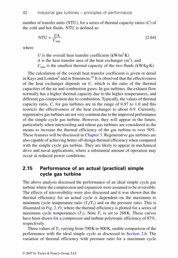
Industrial gas turbines – principles of performance42
number of transfer units (NTU), for a series of thermal capacity ratios (C) ofthe cold and hot fluids. NTU is defined as:
NTU = min
UAC
[2.64]
where
U is the overall heat transfer coefficient (kW/m2 K)A is the heat transfer area of the heat exchanger (m2), andCmin is the smallest thermal capacity of the two fluids (kW/kg K).
The calculation of the overall heat transfer coefficient is given in detailin Kays and London9 and in Simonson.10 It is observed that the effectivenessof the heat exchanger depends on C, which is the ratio of the thermalcapacities of the air and combustion gases. In gas turbines, the exhaust flownormally has a higher thermal capacity due to the higher temperatures, anddifferent gas composition due to combustion. Typically, the values of thermalcapacity ratio, C, for gas turbines are in the range of 0.97 to 1.0 and thisrestricts the effectiveness of the heat exchanger to about 0.9. Currently,regenerative gas turbines are not very common due to the improved performanceof the simple cycle gas turbine. However, they will appear in the future,particularly when intercooling and reheat gas turbines are considered as themeans to increase the thermal efficiency of the gas turbine to over 50%.These features will be discussed in Chapter 3. Regenerative gas turbines arealso capable of achieving better off-design thermal efficiency when comparedwith the simple cycle gas turbine. They are likely to appear in mechanicaldrive and naval applications, where a substantial amount of operation mayoccur at reduced power conditions.
2.15 Performance of an actual (practical) simple
cycle gas turbine
The above analysis discussed the performance of an ideal simple cycle gasturbine where the compression and expansion were assumed to be reversible.The effects of irreversibility were also discussed and it was shown that thethermal efficiency for an actual cycle is dependent on the maximum tominimum cycle temperature ratio (T3/T1) and on the pressure ratio. This isillustrated in Fig. 2.19, where the thermal efficiency is plotted for a series ofmaximum cycle temperatures (T3). Note T1 is set to 288 K. These curveshave been drawn for a compressor and turbine polytropic efficiency of 87%,respectively.
Three values of T3 varying from 700 K to 900 K, enable comparison of theperformance with the ideal simple cycle as discussed in Section 2.6. Thevariation of thermal efficiency with pressure ratio for a maximum cycle
© 2007 by Taylor & Francis Group, LLC

Thermodynamics of gas turbine cycles 43
temperature of 1400 K is also shown and is likely to be found in existing gasturbines. The ideal cycle thermal efficiency is also shown for comparison.Unlike the ideal cycle case, the thermal efficiency initially increases withpressure ratio and then decreases as the pressure ratio is further increased.The thermal efficiency therefore peaks and the peak thermal efficiency, andthe pressure ratio at which it occurs, also increase with T3. For example,when T3 equals 700 K, the peak efficiency occurs at a pressure ratio of about4 and corresponds to about 15%. At a T3 value of 900 K, the peak thermalefficiency occurs at a pressure ratio of about 8 and the peak thermal efficiencyis about 24%.
Although the specific work of an ideal cycle is dependent on the maximumto minimum cycle temperature ratio, the effect of irreversibility is to reducethe specific work, as illustrated in Fig. 2.20. The ideal specific work is alsoshown in dotted lines for comparison. The peak specific work occurs at apressure ratio lower than that where the maximum thermal efficiency occurs.For example, at a T3 value of 700 K, the maximum specific work occurs ata pressure ratio of about 3, whereas the maximum thermal efficiency occursat a pressure ratio of 4 (see Fig. 2.19). The maximum specific work correspondsto about 44 kJ/kg. When T3 equals 900 K, the maximum specific workcorresponds to about 98 kJ/kg and the pressure ratio is about 5. The maximumthermal efficiency, when T3 equals 900K, occurs at a pressure ratio of about8. At a maximum cycle temperature of 1400K, the maximum thermal efficiencyoccurs at a pressure ratio greater than 14, whereas the maximum specificwork occurs at about 12. The thermal efficiency and specific work aresignificantly greater for this case, which corresponds to about 35% and315kJ/kg, respectively.
2.19 Simple gas turbine thermal efficiency varying with pressureratio.
Compressor polytropic efficiency = 0.87Turbine polytropic efficiency = 0.87T1 = 288 KCombustion pressure loss = 0
Ideal thermal efficiencyT3 = 1400 K
T3 = 900 K
T3 = 800 KT3 = 700 K
Th
erm
al e
ffic
ien
cy (
–)0.6
0.5
0.4
0.3
0.2
0.1
0.00 2 4 6 8 10 12 14
Pressure ratio
© 2007 by Taylor & Francis Group, LLC

Industrial gas turbines – principles of performance44
Increasing the maximum cycle temperature and pressure ratio generallyincreases the thermal efficiency and specific work. The increase in thermalefficiency results in reduced fuel consumption and the increase in specificwork reduces the size of the gas turbine. As stated, the values for T3 andpressure ratios are rather low for a practical gas turbine because of lowthermal efficiency, and the gas turbine will be large due to a low specificwork output. Currently, gas turbine designs can utilise a maximum cycletemperature up to about 1800 K and pressure ratios up to about 45. Thisrange is illustrated in Fig. 2.21, where the performance of a practical gasturbine is displayed when operating at current values for pressure ratios andmaximum cycle temperatures.
Maximum cycle temperatures are unlikely to exceed 1800 K because athigher temperatures NOx emissions become prohibitive, as discussed in Chapter6. At higher maximum cycle temperatures, there are claims that the thermalefficiency may actually decrease, as reported by Wilcock et al.11 The changesin gas properties (increase in cp and decrease in γ ) of the actual combustiongases at such high temperatures introduce irreversibilities into the cycle andcould explain this unexpected performance behaviour.
At a pressure ratio of 20 and a maximum cycle temperature of 1400 K, thethermal efficiency and specific work correspond to about 36% and 300 kJ/kg, respectively. These values are more typical for existing gas turbines. Asstated above, gas turbines operating at a maximum cycle temperature of1800K and pressure ratio of 40 have been developed with increased compressorand turbine efficiencies, thus improving the thermal efficiency of the gasturbine further. With such developments, the thermal efficiency of simplecycle gas turbines has increased to about 42%.
Compressor polytropic efficiency = 0.87Turbine polytropic efficiency = 0.87T1 = 288 KCombustion pressure loss = 0
T3 = 1400 K
T3 = 900 K
T3 = 800 K
T3 = 700 K
Sp
ecif
ic w
ork
(kJ
/kg
)350
0 2 4 6 8 10 12 14Pressure ratio
300
250
200
150
100
50
0
2.20 Variation of specific work with pressure ratio.
© 2007 by Taylor & Francis Group, LLC

Thermodynamics of gas turbine cycles 45
2.16 Performance of an actual (practical)
regenerative gas turbine cycle
From the analysis of an ideal regenerative gas turbine cycle in Section 2.7,it was shown that the efficiency increases with decrease in pressure ratio,and the limiting value for the thermal efficiency occurs when the pressureratio tends to unity. The thermal efficiency under this limiting casecorresponds to the Carnot efficiency. However, when the pressure ratio tendsto unity, the specific work tends to zero and this limiting case is only ofacademic interest.
In the forementioned description of the ideal case, it was assumed that theheat exchanger was perfect and therefore had an effectiveness of unity. In apractical cycle, however, the effectiveness is less than unity. When the pressureratio tends to unity, the imperfection in the heat exchanger will require afinite amount of heat to be supplied to maintain the required value of themaximum cycle temperature, T4. Since the work output, W, is zero and afinite amount of heat is supplied (Q ≠ 0), the thermal efficiency, W/Q, willbe zero.
This is illustrated in Fig. 2.22, where the thermal efficiency of a practicalregenerative cycle is plotted against pressure ratio. Three cases of effectivenessare shown varying from 0.7 to 0.9. The practical simple cycle thermal efficiencyis also shown for comparative purposes. The value of the maximum cycletemperature T4 for both the regenerative and simple cycle cases is assumedto be 900 K.
Compressor polytropic efficiency = 0.87Turbine polytropic efficiency = 0.87T1 = 288 KCombustion pressure loss = 3%
Pr = 50
T3 = 1800 KT3 = 1400 KT3 = 1200 K
Th
erm
al e
ffic
ien
cy (
–)0.45
0Specific work (kJ/kg)
0.4
0.35
0.3
0.25
0.2100 200 300 400 500 600
T3 = 1600 K
Pr = 45 Pr = 40
Pr = 35Pr = 30Pr = 25Pr = 20
Pr = 15
Pr = 10
Pr = 5
2.21 Performance of a practical simple gas turbine cycle as a carpetplot for a series of maximum cycle temperatures and pressure ratios.
© 2007 by Taylor & Francis Group, LLC

Industrial gas turbines – principles of performance46
The pressure ratio where the maximum thermal efficiency occurs issignificantly less than that of a simple cycle. Furthermore, the optimumpressure ratio decreases as the heat exchanger effectiveness increases andthis is expected, since the actual regenerative cycle tends towards the idealcycle. Increasing the heat exchanger effectiveness increases the thermalefficiency as more of the waste heat can be recovered.
For a heat exchanger effectiveness of 0.7, the maximum thermal efficiencyoccurs at a pressure ratio of about 3.5 and the corresponding thermal efficiencyis about 28%. When the effectiveness is increased to 0.9, the optimum pressureratio is about 2.5 and the thermal efficiency is increased to about 36%. Themaximum thermal efficiency of the simple cycle is about 23%, requiring apressure ratio of about 8.
Increasing the maximum cycle temperature has a larger beneficial effecton the performance of the regenerative cycle compared with the simplecycle. This result is because the ideal regenerative cycle thermal efficiencyis dependent on the ratio of the maximum to minimum cycle temperature,whereas the ideal simple cycle efficiency is independent of maximum tominimum temperature ratio. This is illustrated in Fig. 2.23, where the variationof thermal efficiency with pressure ratio is shown for a series of maximumcycle temperatures. The heat exchanger effectiveness is kept constant at avalue of 0.8. The maximum cycle temperature is increased from 700K to900 K in steps of 100 K.
The pressure ratio corresponding to the maximum thermal efficiencyincreases with the maximum cycle temperature T4. However, the increase inthis pressure ratio is greater for the simple cycle compared with the regenerativecycle. The above analysis shows that regenerative cycle gas turbines are
2.22 Effect of heat exchanger effectiveness on thermal efficiency.
Compressor polytropic efficiency = 0.87Turbine polytropic efficiency = 0.87T1 = 288 KT4 = 900 KCombustion pressure loss = 0Heat exchanger pressure loss = 0
Th
erm
al e
ffic
ien
cy (
–)0.40
1Pressure ratio
Regenerative cycleeffectiveness = 0.90.35
0.30
0.25
0.20
0.15
0.10
0.05
0.002 3 4 5 6 7 8 9 10 11 12
Regenerative cycleeffectiveness = 0.8
Regenerative cycleeffectiveness = 0.7
Simple cycle
© 2007 by Taylor & Francis Group, LLC

Thermodynamics of gas turbine cycles 47
more efficient than simple cycle gas turbines and their thermal efficiencyincreases significantly with increase in maximum cycle temperature andheat exchanger effectiveness. Furthermore, the pressure ratios required aresmaller than that required by a simple cycle gas turbine to achieve themaximum thermal efficiency.
The specific work output curves for a regenerative cycle will be similar tothose of a simple cycle, as shown in Fig. 2.20. However, the specific workof the regenerative cycle will be less than that of a simple cycle engine,resulting in a bigger gas turbine due to lower pressure ratios employed by theregenerative gas turbine. The addition of the heat exchanger will also add tothe bulk and weight of the engine. Furthermore, the heat exchanger introducesan additional pressure loss in the heat addition and heat rejection processes– as discussed later. These are the main drawbacks to the regenerative cycledesign. However, the lower pressure ratios required may result in a smallercompressor, compensating for part of the increased weight and bulk. Thelow compressor pressure ratios also result in colder cooling air temperaturesthat may be needed for turbine blade cooling and this will reduce the amountof cooling air requirements, as discussed in Chapter 5.
Figure 2.24 shows a carpet plot illustrating the variation of the thermalefficiency with specific work for a series of pressure ratios and maximumcycle temperatures T4. A heat exchanger effectiveness of 0.9 is assumed anda heat exchanger pressure loss of 5% is also assumed for both the hot andcold side, respectively. The values for the maximum cycle temperatures usedare more practical and therefore give an indication of what a practicalregenerative cycle can achieve in terms of performance. In spite of the high
Th
erm
al e
ffic
ien
cy (
–)
1Pressure ratio
0.35
0.30
0.25
0.20
0.15
0.10
0.05
0.002 3 4 5 6 7 8 9 10 11 12
Simple cycle T3 = 700 K
Compressor polytropic efficiency = 0.87Turbine polytropic efficiency = 0.87T1 = 288 KEffectiveness = 0.8Combustor pressure loss = 0Heat exchanger pressure loss = 0
Regenerative cycleT4 = 700 K
Regenerative cycleT4 = 800 K
Regenerative cycleT4 = 900 K
Simple cycle T3 = 900 K
Simple cycle T3 = 800 K
2.23 Effect of maximum cycle temperature on the thermal efficiencyof a regenerative cycle.
© 2007 by Taylor & Francis Group, LLC
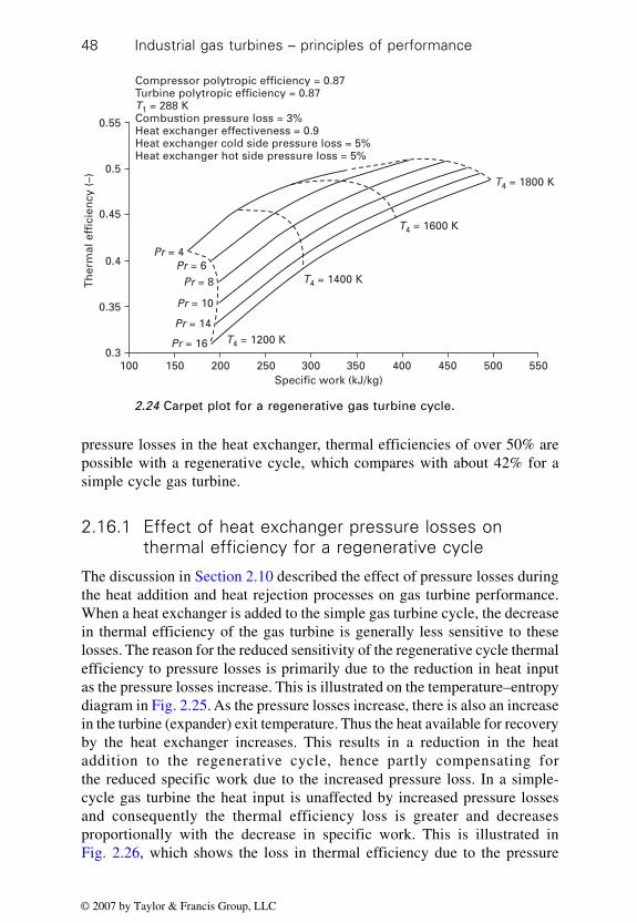
Industrial gas turbines – principles of performance48
pressure losses in the heat exchanger, thermal efficiencies of over 50% arepossible with a regenerative cycle, which compares with about 42% for asimple cycle gas turbine.
2.16.1 Effect of heat exchanger pressure losses onthermal efficiency for a regenerative cycle
The discussion in Section 2.10 described the effect of pressure losses duringthe heat addition and heat rejection processes on gas turbine performance.When a heat exchanger is added to the simple gas turbine cycle, the decreasein thermal efficiency of the gas turbine is generally less sensitive to theselosses. The reason for the reduced sensitivity of the regenerative cycle thermalefficiency to pressure losses is primarily due to the reduction in heat inputas the pressure losses increase. This is illustrated on the temperature–entropydiagram in Fig. 2.25. As the pressure losses increase, there is also an increasein the turbine (expander) exit temperature. Thus the heat available for recoveryby the heat exchanger increases. This results in a reduction in the heataddition to the regenerative cycle, hence partly compensating forthe reduced specific work due to the increased pressure loss. In a simple-cycle gas turbine the heat input is unaffected by increased pressure lossesand consequently the thermal efficiency loss is greater and decreasesproportionally with the decrease in specific work. This is illustrated inFig. 2.26, which shows the loss in thermal efficiency due to the pressure
Compressor polytropic efficiency = 0.87Turbine polytropic efficiency = 0.87T1 = 288 KCombustion pressure loss = 3%Heat exchanger effectiveness = 0.9Heat exchanger cold side pressure loss = 5%Heat exchanger hot side pressure loss = 5%
Pr = 4
T4 = 1200 K
T4 = 1400 K
T4 = 1800 K
Th
erm
al e
ffic
ien
cy (
–)
0.55
100Specific work (kJ/kg)
150
T4 = 1600 K
Pr = 6Pr = 8
Pr = 16
Pr = 10
Pr = 14
0.5
0.45
0.4
0.3
0.35
200 250 300 350 400 450 500 550
2.24 Carpet plot for a regenerative gas turbine cycle.
© 2007 by Taylor & Francis Group, LLC

Thermodynamics of gas turbine cycles 49
losses in the heat exchanger and for a series of heat exchanger effectiveness.It has been assumed that the losses on both the hot and cold side of the heatexchanger are equal.
Heat addition (zero pressure loss)
Reduction in heat addition due to pressure loss
Heat addition (non-zero pressure loss)
Tem
per
atu
re3 3
4
4
2
1
Entropy
Increase in expanderexit temperature dueto pressure losses
1–2 Compression2–3 Heat addition3–4 Expansion4–1 Heat rejection
2.25 Effect of reduction in heat addition for a regenerative cycle dueto pressure losses in the heat addition and rejection processes.
T1 = 288 KT3 = 1800 KCompressor polytropic efficiency = 0.87Turbine polytropic efficiency = 0.87
Effectiveness = 0Effectiveness = 0.2Effectiveness = 0.4
Effectiveness = 0.6
Effectiveness = 0.8
0 2 4 6 8 10 12Heat exchanger pressure loss (%)
9
8
7
6
5
4
3
2
1
0
Loss
in t
her
mal
eff
icie
ncy
(%
)
2.26 Loss in thermal efficiency due to heat exchanger pressure lossand effectiveness.
© 2007 by Taylor & Francis Group, LLC

Industrial gas turbines – principles of performance50
2.17 Turbine entry temperature and stator outlet
temperature
The maximum cycle temperatures discussed previously have varied from1200K to 1800K. It has also been shown that the higher the maximum cycletemperature, the better the performance of the gas turbine cycles. It is theturbine that is subjected to high gas temperatures and the materials used inthe manufacture of the turbine must be capable of withstanding suchtemperatures. This issue is illustrated in Fig. 2.27, which shows the trends inmaterial temperature capability and the significant increase in turbine bladetemperature that has occurred over the years. Further significant increase ingas temperature, known as the turbine entry temperature (TET), is also possibleby employing cooling of the turbine, also shown in Fig. 2.27.
Turbine cooling reduces the blade temperature such that the turbine creeplife remains satisfactory during operation. This technology is discussed furtherin Chapter 5 (Section 5.7). The cooling air is generally divided into threeparts and is used to cool the stator or nozzle guide vane, the rotor and thedisc, as shown in Fig. 2.28. After carrying out the cooling function, thecooling air enters the gas stream at the stator and rotor trailing edge. Themixing of the stator cooling air with the gas stream reduces the rotor inlettemperature and therefore requires a higher TET to obtain the required powerfrom the turbine as all the work in a turbine stage is done by the rotor. Thusthe rotor inlet temperature is an important parameter and many manufacturersrefer to this temperature as the stator outlet temperature (SOT) or the firstrotor temperature. The SOT may be as much as 150 degrees lower than theTET. The rotor cooling air is unavailable for producing power and would be
Uncooled turbineblades
Cooled turbineblades
TET
Ceramics
Bladetemperature
1930 1940 1950 1960 1970 1980 1990 2000 2010 2020Year
Tem
pera
ture
(K)
2000
1900
1800
1700
1600
1500
1400
1300
1200
1100
1000
2.27 Trends in high-temperature material technology for turbines.
© 2007 by Taylor & Francis Group, LLC
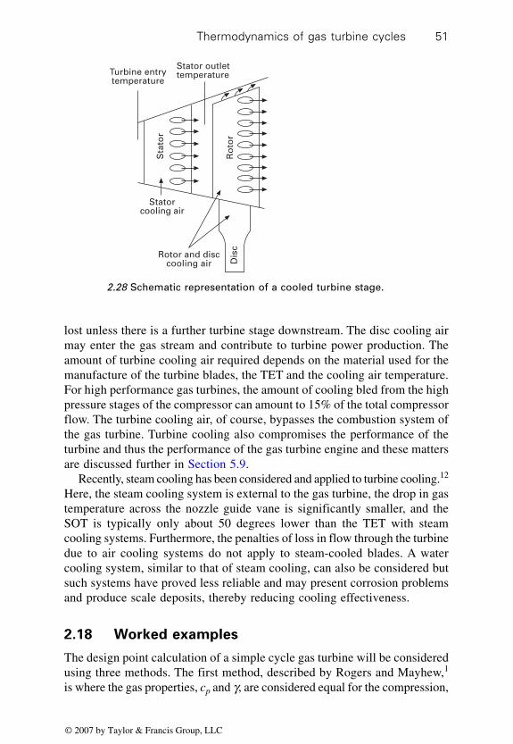
Thermodynamics of gas turbine cycles 51
lost unless there is a further turbine stage downstream. The disc cooling airmay enter the gas stream and contribute to turbine power production. Theamount of turbine cooling air required depends on the material used for themanufacture of the turbine blades, the TET and the cooling air temperature.For high performance gas turbines, the amount of cooling bled from the highpressure stages of the compressor can amount to 15% of the total compressorflow. The turbine cooling air, of course, bypasses the combustion system ofthe gas turbine. Turbine cooling also compromises the performance of theturbine and thus the performance of the gas turbine engine and these mattersare discussed further in Section 5.9.
Recently, steam cooling has been considered and applied to turbine cooling.12
Here, the steam cooling system is external to the gas turbine, the drop in gastemperature across the nozzle guide vane is significantly smaller, and theSOT is typically only about 50 degrees lower than the TET with steamcooling systems. Furthermore, the penalties of loss in flow through the turbinedue to air cooling systems do not apply to steam-cooled blades. A watercooling system, similar to that of steam cooling, can also be considered butsuch systems have proved less reliable and may present corrosion problemsand produce scale deposits, thereby reducing cooling effectiveness.
2.18 Worked examples
The design point calculation of a simple cycle gas turbine will be consideredusing three methods. The first method, described by Rogers and Mayhew,1
is where the gas properties, cp and γ, are considered equal for the compression,
Turbine entrytemperature
Stator outlettemperature
Sta
tor
Ro
tor
Statorcooling air
Rotor and disccooling air D
isc
2.28 Schematic representation of a cooled turbine stage.
© 2007 by Taylor & Francis Group, LLC

Industrial gas turbines – principles of performance52
heat addition and expansion processes. The second method corresponds tothat discussed by Saravanamutto et al.3 where fixed but different values forcp and γ are used. The heat addition is determined from combustion charts asshown in Fig. 2.17. In the third method the enthalpy–entropy approach isused, as discussed in Section 2.12. The heat input is determined by using thecombustion charts shown in Figure 2.17. The effect of increased turbineflow rate due to the addition of fuel in the combustor is ignored as thisincreased flow rate can approximately be assumed to be lost due to leakagesand cooling effects.
Design point data correspond to the following:
• working media is air• compressor inlet temperature, T1 = 288 K• compressor inlet pressure, P1 = 1.013 Bar• compressor pressure ratio, Rpc = 20• compressor isentropic efficiency, ηc = 0.87• combustor pressure loss, ∆P = 5% of compressor delivery pressure• combustion efficiency, ηb = 0.99• turbine entry temperature, T3 = 1400 K• turbine isentropic efficiency, ηt = 0.9• inlet and exhaust losses = 0• fuel is kerosene
2.18.1 First method
For the first method, the values for cp and γ are set as 1.005 and 1.4, respectively,for the compression heat addition and expansion process present in the gasturbine cycle.
From Equation 2.29 the compressor discharge temperature, T2, is calculatedby:
T TT
Rpcc
2 11 = + ( ) – 1
–1
ηγ
γ
T2 = 288 + 2880.87
(20) – 1 = 736.07K1
3.5
The compressor specific work input, Wc
Wc = 1.005 × (736.07 – 288) = 450.31 kJ/kg
and the compressor discharge pressure, P2 equals
P2 = P1 × Rpc = 1.013 × 20 = 20.26 Bar-A
The turbine inlet pressure, P3 is equal to:
© 2007 by Taylor & Francis Group, LLC

Thermodynamics of gas turbine cycles 53
P3 = P2 × (1 – ∆P/100) = 20.26 × (1 – 5/100) = 19.247 Bar-A
Therefore the turbine pressure ratio is given by:
Rpt = 19.247/1.013 = 19
From Equation 2.31 the turbine exit temperature is given by:
T T T tRpt4 3 3 = – 1 – 1
13.5
× ×
η
T4 = 1400 – 1400 0.9 1 – 119
= 683.266K1
3.5× × ( )
and the turbine specific work output, Wt is:
Wt = 1.005 × (1400 – 683.266) = 720.318 kJ/kg
The specific heat input, Qin is given by Equation 2.12:
Qin = 1.005 × (1400 – 736.07)/0.99 = 673.99 kJ/kg
The net turbine specific work, Wnet = Wt – Wc
Wnet = 720.318 – 450.31 =270.01 kJ/kg
The thermal efficiency is the ratio of the net turbine specific work to the heatinput. The thermal efficiency, ηth, is therefore:
η th = 270.01673.99
= 0.401
2.18.2 Second method
The second method also considers fixed values for cp and γ but uses differentvalues for the compression and expansion processes. These values for thecompression process are the same as those used in the first method. Therefore,the compressor discharge temperature and the compressor specific work arethe same as that calculated in Section 2.18.1. Thus:
T2 = 736.07K
Wc = 450.31 kJ/kg
Since the compressor pressure ratio and the combustor pressure loss are thesame as above, the compressor discharge pressure and turbine inlet pressurewould also be the same as that determined in Section 2.18.1. Therefore:
P2 = 20.26 Bar-A
The turbine inlet pressure is equal to:
© 2007 by Taylor & Francis Group, LLC

Industrial gas turbines – principles of performance54
P3 = 19.247 Bar-A
The combustion temperature rise T32 = T3 – T2.
T32 = 1400 – 736.07 = 663.93K
For the combustor inlet temperature of 736.07 K, which is equal to thecompressor discharge temperature, and combustor temperature rise of 663.93K, from Fig. 2.17 the theoretical fuel–air f is 0.0195. The actual fuel–air ratiofa = f/ηb. Thus the actual fuel–air ratio is fa = 0.0197. We have assumed thefuel is kerosene, which has a lower heating value (LHV): Qnet is 43 100 kJ/kg. Therefore, the specific heat input is equal to:
Qin = fa × Qnet = 0.0197 × 43 100 = 849.07 kJ/kg
For the expansion process we shall assume that cp and γ are 1.148 and 1.333,respectively. The turbine exit temperature equals:
T4 = 1400 – 1400 0.9 1 – 119
= 743.84 K0.3331.333
× × ( )
The turbine specific work is:
Wt = 1.148 × (1400 – 743.84) =753.318 kJ/kg
The net specific work is
Wnet = 753.318 – 450.31 = 303.008 kJ/kg
The thermal efficiency for this case is:
η th = 303.008849.07
= 0.35687
2.18.3 Third method
The third method determines the performance of the gas turbine using theenthalpies and entropies at the various salient points in the cycle. It is consideredthe most accurate method for calculating the design point performance of agas turbine. The method is much more detailed and is usually carried outusing a computer program developed for this purpose. However, the processesinvolved will be outlined.
Integrating Equation 2.44, which describes the variation of specific heatwith temperature for air and products of combustion, equations for enthalpyand entropy can be developed. Therefore:
H a T T bT T
cT T
= ( – ) + – 2
– 1 – 10
202
0
[2.65]
© 2007 by Taylor & Francis Group, LLC

Thermodynamics of gas turbine cycles 55
S a TT
b T T cT T
R PP
= ln + ( – ) – 2
1 – 1 – ln 0
0 202
0
[2.66]
where T and P are the temperature and pressure of air or gas, respectively,and T0 and P0 are the reference temperature and pressure when the enthalpyand entropy, respectively, are assumed to be zero, when the temperature andpressure are 273K and 1.013 Bar-A, respectively.
The constants a, b and c are determined as follows:
a a mfi i i = =1
noc
Σ ×
b b mfi i i = =1
noc
Σ ×
c c mfi i i = =1
noc
Σ ×
ai, bi and ci are the constants defined in Table 2.1 for each component andnoc are the number of components in air or products of combustion.
In the example, the compressor inlet pressure and temperature is 1.013 Barand 288 K. From Equations 2.65 and 2.66 we calculate the enthalpy andentropy at the compressor inlet as:
H1 = 14.876 kJ/kg
S1 = 0.053 kJ/kg K.
For a compressor pressure ratio of 20, the compressor discharge pressure,P2 = 20.26 Bar-A. From Equation 2.66 the isentropic compressor dischargetemperature can be determined. This is achieved by using P2 for the pressureterm in Equation 2.66 and varying the temperature until the entropy equals0.053 kJ/kg K. The isentropic compressor discharge temperature, T2′, worksout to:
T2′ = 659.452 K.
Using this value in Equation 2.65, the enthalpy at compressor discharge,H2′ due to isentropic compression is obtained:
H2′ = 402.286 kJ/kg
The isentropic efficiency Equation 2.28 for a compression process can bewritten in terms of enthalpies as:
ηcH HH H
= – –
2 1
2 1
′ where H2 is the actual enthalpy at the discharge of the
compressor which corresponds to:
H2 = 460.175 kJ/kg
© 2007 by Taylor & Francis Group, LLC

Industrial gas turbines – principles of performance56
Using the value for H2 in Equation 2.65, the actual compressor dischargetemperature, T2, can be determined implicitly:
T2 = 713.102 K
The compressor-specific work: Wc = H2 – H1. Therefore:
Wc = 445.3 kJ/kg
The fuel–air ratio may now be computed similarly to that discussed in Method2. The combustor inlet temperature and combustor temperature rise for thiscase are 702.86 K and 697.14 K, respectively. A theoretical fuel–air ratio, f,of 0.0195 is obtained. The actual fuel–air ratio, fa = 0.0195/0.99 = 0.0197.The heat input Qin is:
Qin = 0.0197 × 43100 = 849.388 kJ/kg
The fuel used is kerosene and can be modelled as C12H24. Knowing thefuel–air ratio and the air composition, the composition of the products ofcombustion can be calculated, as described by Goodger.13
C H + O + 0.78090.2095
N + 0.00930.2095
Ar + 0.00030.2095
CO2 2 2x y m
= n1CO2 + n2H2O + n3N2 + n4 Ar + n5O2 [2.67]
The quantities 0.7809, 0.0093, 0.003 and 0.2095 are the volume-fractions ormolar-fractions (mole-fraction) of N2, Ar, CO2 and O2 in air, respectively,and n1, n2, n3, n4 and n5 are the mole-fraction of CO2, H2O, N2, Ar and O2 inthe products of combustion, respectively. The terms x and y are the mole-fractions of carbon and hydrogen in the fuel. For kerosene, x = 12 and y = 24and the term m is the excess air which is determined using the fuel–air ratio(fa) as follows:
fx y
MWa =
12.01 + 1.008
1 + 0.78090.2095
+ 0.00930.2095
+ 0.00030.2095
where MW is the mole-weight of air and the factors 12.01 and 1.008 are theatomic weights of carbon and hydrogen, respectively.
By performing a molar balance using Equation 2.67, the mole-fraction ofthe products of combustion (n1, n2, n3, n4 and n5) can be determined in amanner similar to that discussed in Chapter 6 (Section 6.18.4).
Since the turbine entry temperature, T3, pressure, P3, and the combustiongas composition are now known, Equations 2.65 and 2.66 can be used todetermine the enthalpy, H3 and entropy, S3 at turbine entry. The enthalpy atthe exit due to isentropic expansion must be determined. This is achieved byusing Equation 2.66 and varying the turbine exit temperature, T4, until theentropy equals the value determined at the inlet of the turbine, S3. From
© 2007 by Taylor & Francis Group, LLC

Thermodynamics of gas turbine cycles 57
Equation 2.65 the enthalpy, H4′ at turbine exit due to isentropic expansioncan be determined. The turbine isentropic efficiency in Equation 2.30 can berepresented as:
η tH HH H
= – –
3 4
3 4 ′
where H4 is the actual enthalpy at turbine exit.The values for H3, S3 and H4′ are 1272.995 kJ/kg, 0.958 kJ/kg K and
428.005 kJ/kg, respectively. For a turbine isentropic efficiency of 0.9, theactual enthalpy at exit from the turbine is 512.504 kJ/kg and the entropy atturbine exit is 1.0768 kJ/kg K. Thus the turbine specific work, Wt, is:
Wt = H3 – H4 = 1272.995 – 512.504 = 760.491 kJ/kg
The net specific work (Wnet) from the gas turbine is:
Wnet = Wc – Wt = 760.491 – 445.3 =315.191kJ/kg
The thermal efficiency (ηth) is:
η thnet
in = = 315.191
849.388 = 0.3711
WQ
.
The specific heats at the salient points 1, 2, 3 and 4, as shown in Fig. 2.29,correspond to 1.0011, 1.083, 1.2193 and 1.1198, respectively. Thecorresponding values for the ratios of specific heats, γ = cp/cv, at the salientpoints 1, 2, 3 and 4 are 1.402, 1.3607, 1.3082 and 1.345, respectively. Theincrease in cp due to compression is due to the increase in temperature asdescribed by Equation 2.44. Similarly, there is an increase in cp at salientpoint 3 and a decrease at point 4. However, the increase in cp at point 3 is
2.29 Turbine cycle on the temperature–entropy diagram.
Tem
per
atu
re
2′
2
4′
42
3
Entropy
1–2’ Isentropic compresson1–2 Actual or irreversible compression2–3 and 2’–3 heat addition3–4’ Isentropic expansion3–4 Actual or irreversible expansion4–1 and 4’–1 Heat rejection
© 2007 by Taylor & Francis Group, LLC

Industrial gas turbines – principles of performance58
also due to the increase in water vapour in the products of combustion,which is significant, as can be seen in Table 2.3. Also, note there is anincrease in CO2 content in the products of combustion, a greenhouse gas andthought to be responsible for global warming. Therefore, gas turbines operatingwith fuels such as natural gas or methane, which have a higher hydrogencontent, will result in increased specific work due the high content of watervapour in the products of combustion. With methane as fuel, this increase inpower output may be as high as 2% compared with that when using kerosene.Note that the increases in specific heats have resulted in a decrease in γ.
The above example considered dry air. The effects of humidity can alsobe included in the analysis. For example, given the relative humidity of theair, the specific humidity can be calculated, as discussed in Section 2.11.1,which is the mass of water vapour per unit of dry air. Therefore, the specifichumidity can be added to the composition of air as shown in Table 2.2 andair/gas composition normalised to determine the gravimetric composition ofmoist/humid air and then repeat the above procedure. The additional heatinput required to heat the water vapour from the compressor dischargetemperature, T2, to the turbine entry temperature, T3, needs to be calculated.This can be determined using Equation 2.68:
Hs = 2.232Ts + 2352.623 [2.68]
where Hs is the water/steam enthalpy (kJ/kg) and Ts is the water vapour/steam temperature in Celsius.
2.18.4 Summary of calculations
Table 2.4 summarises the error due to the different methods of calculatingthe design point performance of gas turbines. Error 1 in Table 2.4 is thepercentage error between Method 1 and 3 and Error 2 is the percentage errorbetween Method 2 and 3. Note that the first method gives the greatest error,particularly in the heat input. This is because the method of calculating theheat input pays no attention to the change in gas composition during combustion.The error using Method 2 is quite small and this is because we are calculatingthe heat input using combustion curves and endeavouring to adjust for the
Table 2.3 Composition of products of combustion
Component Gravimetric or mass fraction
N2 0.744O2 0.162Ar 0.009CO2 0.061H2O 0.025
© 2007 by Taylor & Francis Group, LLC

Thermodynamics of gas turbine cycles 59
Table 2.4 Error in methods of calculating the design point performance of gas turbinesrelative to Method 3
Method→ 1 2 3 Error 1 (%) Error 2 (%)
T2 (K) 736.07 736.07 713.102 3.221 3.221Wc (kJ/kg) 450.631 450.631 445.3 1.197 1.197Qin (kJ/kg) 673.99 836.14 849.388 20.65 –1.597T4 (K) 683.266 743.84 750.103 –8.91 –0.835Wt (kJ/kg) 720.318 753.27 760.491 –5.283 –0.95Wnet (kJ/kg) 270.01 303.008 315.191 –14.334 –3.865ηth(–) 0.401 0.35687 0.3711 8.057 –3.835
change in gas composition by using different values for cp and γ duringexpansion. Since these values are closer to the true average values for cp andγ, the errors in the calculation of the design point performance are small. Itmust be pointed out that Method 2 is unsuitable for designing gas turbinesand Method 3 should be adopted. However, Method 2 gives a quick way ofestimating the design point performance of gas turbines.
2.19 References
1. Engineering Thermodynamics, Work and Heat Transfer, 4th Edition. Rogers, G.F.C.and Mayhew, Y.R., Longman (1992).
2. Applied Thermodynamics for Engineers and Technologists, 5th Edition, Eastop,T.D. and McConkey, A., Longman (1993).
3. Gas Turbine Theory, 5th Edition, Saravanamuttoo H.I.H., Rogers, G.F.C. and Cohen,H, Longman (2001).
4. Gas Turbine Performance, 2nd Edition, Walsh, P.P. and Fletcher, P., BlackwellPublishing (2004).
5. Gas Turbine Engineering, Harman, R.T.C., Macmillan Press (1981).6. Thermodynamic and Transport Properties of Fluids, Rogers, G.F.C. and Mayhew,
Y.R., Blackwell (1994).7. Increasing diagnostics effectiveness by inclusion of fuel composition and water
injection effects, Mathioudakis, K., Aretakis, N. and Tsalavoutas, A., ASME TurboExpo 2002, Paper GT-2002-30032, (2002).
8. Introduction to Chemical Engineering Thermodynamics, 5th Edition, Smith, J.M.,Van Ness, H.C. and Abbot, M.M., McGraw-Hill (1996).
9. Compact Heat Exchangers, Kays, W.M and London, A.L., MacGraw-Hill (1964).10. Engineering Heat Transfer, Simonson, J.R., Macmillan Press (1975).11. Gas properties as a limit to gas turbine performance, Wilcock, R.C., Young, J.B. and
Horlock, J.H., ASME Paper GT-2002-30517, (2002).12. H system steams on, Modern Power Systems, February 2004.13. Hydrocarbon Fuels, Goodger, E.M., Macmillan Press (1975).
© 2007 by Taylor & Francis Group, LLC

60
In Chapter 2 the design point performance of the simple cycle gas turbine,which consists of a compressor, combustor and turbine, was considered.Although the inclusion of a heat exchanger (referred to as the regenerativecycle) was also considered, it is the addition of intercooling to reduce thecompressor work, and reheat to augment the turbine work, that are usuallyreferred to as complex cycles. In this chapter the design point performanceof such cycles, including the addition of a heat exchanger, will be considered.
3.1 Intercooled gas turbine cycles
When the performance of the simple and regenerative cycle gas turbine wasconsidered, it was assumed that the compression process was isentropic. Thecompression work required by these cycles may be reduced by dividing thecompression process into two stages. These comprise the LP and the HPstages as shown in Fig. 3.1, and also cooling to reduce the LP compressordischarge air temperature, T2, back to its inlet temperature (i.e. reducing T3
to T1). It was shown in Chapter 2 that the compressor-specific work requirementto achieve a given pressure ratio is given by:
Wcomp = cp(T2 – T1)which, for an isentropic process, can be expressed as
3Complex gas turbine cycle
3.1 Schematic representation of an intercooled gas turbine.
1–2 Low pressure (LP) compression2–3 Intercooling3–4 High pressure (HP) compression4–5 Heat addition5–6 Expansion
Intercooler
Fuel input
Combustor
1
2 3
LP HP
Compressors
5
6
Load
Turb
ine
4
© 2007 by Taylor & Francis Group, LLC

Complex gas turbine cycle 61
W c T Prpcomp 1 = (( ) – 1)–1γγ
Therefore, reducing T1 will reduce the compressor work required to achievea given compressor pressure ratio, Pr. Thus, intercooling results in a reductionin the compressor work requirement of the HP compressor and hence reducesthe overall compression work required to achieve a given overall compressorpressure ratio, P4/P1.
3.1.1 Optimisation of intercooled compressors
The optimisation of an intercooled compressor involves the determination ofthe LP and HP compressor pressure ratios such that the compression powerrequired is a minimum. If the LP compressor pressure ratio is unity or equalto the overall pressure ratio, P4/P1, then no reduction in compressor workabsorbed will occur. The question that arises is ‘what LP compressor pressureratio will result in the minimum compressor work absorbed’. The compressionprocess for intercooled compressors is shown on the temperature–entropydiagram in Fig. 3.2 for an arbitrary value for the LP compressor ratio, Prlp.The HP pressure ratio, Prhp, will then be given by Pro/Prlp, where Pro is theoverall pressure ratio, P4/P1. The compression work, Wcomp, is therefore:
Wcomp = cp(T2 – T1) + cp(T4 – T3)
Since T3 = T1 due to intercooling
Wcomp = cp[(T2 – T1) + cp(T4 – T1)] [3.1]
1–2 Low pressure (isentropic)compression
2–3 Constant pressure heat rejection(intercooling)
3–4 High pressure (isentropic)compression
Entropy
Tem
per
atu
re
4
3 1
2
3.2 Two-stage intercooled compression process on the temperature–entropy diagram.
© 2007 by Taylor & Francis Group, LLC

Industrial gas turbines – principles of performance62
Equation 3.1 can be represented in terms of the LP and overall pressure ratioas:
W c T PrPrPrp lp
o
lpcomp 1 = ( ) + – 2
–1–1
γγ
γγ
[3.2]
Differentiating Equation 3.2 with respect to Prlp and equating to zero gives:
Pr Prlp o = [3.3]
By considering the second derivative of Equation 3.2, it can be shown thatthe condition expressed in Equation 3.3 is a minimum. Therefore, the minimumwork absorbed by an intercooled compression system occurs when the LPand HP compressor pressure ratios are equal.
3.1.2 Thermal efficiency and specific work of an idealintercooled gas turbine
The intercooled gas turbine shown in Fig. 3.1 may be represented on thetemperature–entropy diagram as shown in Fig. 3.3. Since we are consideringthe ideal performance of the cycle, the thermodynamic processes involvedare:
• 1–2 isentropic compression• 2–3 constant pressure heat rejection• 3–4 isentropic compression• 4–5 constant pressure heat addition• 5–6 isentropic expansion.
In fact, it may be considered that an ideal intercooled gas turbine cycleconsists of two ideal simple cycle gas turbines (2–3–4–4′ and 1–4′–5–6), asshown in Fig. 3.3. The increased specific work of the intercooled gas turbineis due to the specific work of the smaller simple cycle gas turbine 2–3–4–4′.The smaller gas turbine cycle requires an additional heat input whichcorresponds to the heat input from 4–4′. However, the pressure ratio of thesmaller simple cycle gas turbine, P4/P3, is less than the pressure ratio of thelarger simple cycle gas turbine 1–4′–5–6. Therefore, the ideal thermal efficiencyof the smaller ideal gas turbine cycle is less than that of the larger gas turbinecycle. In effect, a less efficient gas turbine cycle has been added to a moreefficient cycle. Thus the ideal thermal efficiency of an intercooled gas turbinecycle is less than that of the simple cycle gas turbine whose overall pressureratios are the same as illustrated in Fig. 3.4.
Furthermore, for a given minimum cycle temperature, T1, increasing themaximum cycle temperature, T5, increases the specific work of the larger
© 2007 by Taylor & Francis Group, LLC

Complex gas turbine cycle 63
gas turbine cycle and requires additional heat input to this cycle. Since theideal thermal efficiency of the larger gas turbine is greater than the smallergas turbine, the ideal thermal efficiency of the intercooled gas turbine cyclewill increase with increase in the maximum cycle temperature, as illustratedin Fig. 3.4.
Entropy
Tem
per
atu
re5
6
1
4′
2
3
4
1–2 Isentropic compression
2–3 Constant pressure heat rejection
3–4 Isentropic compression
4–5 Constant pressure heat addition
5–6 Isentropic expansion
3.3 Temperature–entropy diagram of an ideal, intercooled gasturbine.
Ideal simple cycle
T5 = 1200 K
T5 = 1800 K
T1 = 288 K
Idealintercooled
cycle
Compressor pressure ratio (overall)0 10 20 30 40 50 60
Th
erm
al e
ffic
ien
cy (
–)
0.8
0.7
0.6
0.5
0.4
0.3
0.2
0.1
0
3.4 Variation of thermal efficiency with pressure ratio and maximumcycle temperature for an ideal, intercooled gas turbine.
© 2007 by Taylor & Francis Group, LLC

Industrial gas turbines – principles of performance64
Therefore, the ideal thermal efficiency of an intercooled gas turbine cycleincreases with an increase in maximum to minimum cycle temperature ratio,and this differs from the case of the simple gas turbine cycle, where the idealthermal efficiency is independent of this temperature ratio. Of course, thespecific work of the intercooled gas turbine is higher than that of the idealsimple cycle gas turbine, as shown in Fig. 3.5. As was found with the idealsimple cycle gas turbine, the specific work of the ideal intercooled gasturbine is dependent on the maximum to minimum cycle temperature ratio,as shown in Fig. 3.5. It is additionally observed that the maximum specificwork occurs at a higher pressure ratio compared with the simple cycle gasturbine.
3.1.3 Practical intercooled cycle
The ideal intercooled cycle considers only isentropic compression andexpansion processes and ignores any pressure losses during the heat additionand heat rejection processes. In a practical cycle, such assumptions are neverachieved and the effect of irreversibilities discussed in Chapter 2 results ina significant loss in thermal efficiency and specific work. Furthermore, theconclusion that an ideal intercooled cycle always results in a lower thermalefficiency compared with the simple cycle gas turbine may not hold.
This is illustrated by considering the case discussed in Section 2.9 wherethe impact of irreversibilities on the performance of the simple cycle gasturbine was investigated. In particular, the case where the maximum cycletemperature was increased sufficiently so that the turbine expansion work
Compressor pressure ratio (overall)0 10 20 30 40 50 60
Sp
ecif
ic w
ork
(kJ
/kg
)
900
Ideal simplecycle
T5 = 1200 K
T5 = 1800 K
T1 = 288 K
Idealintercooled
cycle
800
700
600
500
400
300
200
100
0
3.5 Variation of specific work with pressure ratio for an ideal,intercooled cycle.
© 2007 by Taylor & Francis Group, LLC

Complex gas turbine cycle 65
was equal to the compressor absorbed work will be considered. Since a finiteamount of heat was supplied, the thermal efficiency was zero. If the compressionprocess is intercooled, the reduction in compressor specific work will nowresult in a finite specific work from the intercooled gas turbine cycle, i.e. theturbine work remains the same, while the compression work decreases.
Although the heat input has now increased to maintain the same maximumcycle temperature, as illustrated in Fig. 3.6, the positive specific work fromthe intercooled gas turbine cycle will result in a positive thermal efficiency.Thus, when irreversibilities are considered, intercooling can increase thethermal efficiency compared with the simple cycle gas turbine. The optimisationof a practical intercooled gas turbine for maximum thermal efficiency maynot result in the LP and HP compressor pressure ratios being equal andgenerally the LP compressor pressure ratio will be much less than the optimumvalue for minimum compression work.
Optimisation of the split in the LP and HP compressor pressure ratios cantherefore achieve a worthwhile increase in the thermal efficiency comparedwith the simple cycle gas turbine. This point is illustrated in Fig. 3.7 wherethe optimised intercooled gas turbine thermal efficiency is plotted againstspecific work for a series of overall pressure ratios, Pr, and maximum cycletemperatures, T5. Thermal efficiencies of the order of 45% are possible withintercooling and one major manufacturer is seriously considering themanufacture of such gas turbines.1 A discussion of the benefits is given inModern Power Systems.2 The optimised LP compressor pressure ratios areshown in Fig. 3.8. It is observed that the optimised LP compressor pressureincreases with overall pressure ratio and decreases with increase in maximum
3.6 Change in the temperature–entropy diagram due to intercooling apractical simple cycle gas turbine.
1–2s–3s–4s = Simple cycle1–2–3–4–5–6 = Intercooled cycle
53s
64s
2s
Simple cycleheat input
Increase in heat input(intercooled cycle)
42
13
Tem
per
atu
re
Entropy
© 2007 by Taylor & Francis Group, LLC

Industrial gas turbines – principles of performance66
cycle temperature. The optimised LP compressor pressure ratio is well belowthe case when the specific work is maximum, which corresponds to thesquare root of the overall compressor pressure ratio.
Optimising the LP compressor pressure ratio to maximise the specificwork results in a lower thermal efficiency as is illustrated in Fig. 3.9. In this
Compressor polytropic efficiency = 0.87Turbine polytropic efficiency = 0.87T1 = 288 KCombustion pressure loss = 3%Intercooler pressure loss = 1%
Pr = 50
T5 = 1800 KT5 = 1400 KT5 = 1200 K
Th
erm
al e
ffic
ien
cy (
–)0.5
Specific work (kJ/kg)100 200 300 400 500 600
T5 = 1600 K
Pr = 45Pr = 40
Pr = 35Pr = 30
Pr = 25Pr = 20
Pr = 15
Pr = 10
Pr = 5
0.45
0.4
0.35
0.3
0.25
0.2700
3.7 Variation of thermal efficiency with specific work for a practicalintercooled gas turbine when optimised for maximum thermalefficiency.
3.8 Optimised low-pressure (LP) compressor pressure ratio toachieve maximum thermal efficiency in a practical intercooled gasturbine.
T5 = 1800 K
Increasing T5Op
tim
um
LP
co
mp
ress
or
pre
ssu
re r
atio
4.5
Overall compressor pressure ratio5
T5 = 1200 K
4
3.5
3
2.5
2
1.510 15 20 25 30 35 40 45 50
© 2007 by Taylor & Francis Group, LLC

Complex gas turbine cycle 67
case the LP pressure ratio is approximately equal to the square root of theoverall compressor pressure ratio. It has been assumed that the LP and HPcompressor polytropic efficiencies are equal. It is when different values ofpolytropic efficiencies for respective compressors are considered that theoptimised pressure ratio for maximum specific work departs from the squareroot relationship. The compressor pressure ratio split will be biased towardsthe higher efficiency compressor.
3.1.4 Ideal intercooled and regenerative gas turbinecycle
The thermal efficiency of the ideal intercooled cycle may be increased by theaddition of a heat exchanger to recover the exhaust heat and transfer it to thecompressor discharge air before combustion. A schematic representation ofsuch a cycle, known as the intercooled regenerative cycle, is shown in Fig.3.10. It is very similar to the regenerative cycle discussed in Section 2.7 butdiffers due to the addition of an intercooled compressor.
In the case of the ideal cycle, the compressor discharge air at station 4 isheated by the exhaust gas such that the temperature of the compressor dischargeair rises to the turbine exhaust temperature, T7, at station 5. The temperatureof the heated air leaving the heat exchanger is then increased to the maximumcycle temperature by burning fuel in the combustor. The work done by theturbine, which drops the turbine exhaust temperature to T7, drives both the
Compressor polytropic efficiency = 0.87Turbine polytropic efficiency = 0.87T1 = 288 KCombustion pressure loss = 3%Intercooler pressure loss = 1%
Pr = 50
T3 = 1800 K
T3 = 1400 KT
3 = 1200 K
Th
erm
al e
ffic
ien
cy (
–)
0.5
Specific work (kJ/kg)100 200 300 400 500 600
T3 = 1600 K
Pr = 45 Pr = 40Pr = 35
Pr = 25Pr = 20
Pr = 15
Pr = 10
Pr = 5
0.45
0.4
0.35
0.3
0.25
0.2700
3.9 Variation of thermal efficiency with specific work for a practicalintercooled gas turbine, where low-pressure (LP) compressorpressure ratio is optimised for maximum specific work.
© 2007 by Taylor & Francis Group, LLC

Industrial gas turbines – principles of performance68
load and the intercooled compressors. The heating of the compressor dischargeair by the exhaust heat from the turbine results in the turbine exhaust temperaturedecreasing to T4 at station 8.
These thermodynamic processes are displayed on the temperature–entropydiagram in Fig. 3.11. The case for the non-intercooled regenerative cycle isalso shown for comparative purposes. In the ideal case the heat input, Q56 =cp(T6 – T5), for the intercooled regenerative cycle (1–2–3–4–5–6–7–8) is nodifferent to that of the non-intercooled regenerative cycle (1–4′–5–6–7–7′).However, the specific work output from the intercooled cycle is greater, asdiscussed in Section 3.1. Thus the thermal efficiency of the intercooledregenerative cycle will be greater. For a given heat input, the thermal efficiencywill be a maximum when the specific work is a maximum and will correspondto the case when the compressor work absorbed is a minimum. It was shownin Section 3.1 that the work absorbed by the intercooled compressors will bea minimum when the pressure ratios of the LP and HP compressors areequal. Thus, in the ideal case, the temperatures T4, T2 and T8 shown in Fig.3.11 will be equal. A relatively simple expression may be derived for theoptimised ideal thermal efficiency, ηth, for an intercooled regenerative cycleas follows:
It was shown for the maximum thermal efficiency case that the compressorwork is a minimum and equals 2cp(T2 – T1). This occurs at equal LP and HP
Intercooler
Fuel input
Combustor6
Turb
ine
Load
7
5
8
4
HPLP
1
2 3
Heat exchanger
1–2 LP compressor isentropic compression2–3 Constant pressure heat rejection (intercooling)3–4 HP compressor isentropic compression4–5 Constant pressure heat addition via heat exchanger5–6 Constant heat addition via external heat source6–7 Isentropic expansion7–8 Constant pressure heat transfer for heating process 4–5
3.10 Schematic representation of an intercooled, regenerative gasturbine cycle.
© 2007 by Taylor & Francis Group, LLC

Complex gas turbine cycle 69
compressor pressure ratios. Therefore, the thermal efficiency of the intercooledregenerative cycle is:
η th5 6 2 1
5 6 =
( – ) – 2 ( – )( – )
c T T c T Tc T T
p p
p[3.4]
η th2 1
5 6 = 1 –
2 ( – )( – )
T TT T
[3.5]
The LP compressor discharge temperature is expressed as
T T Prlp2 1 = ( )–1
×γ
γ
1–2 LP compressor isentropic compression2–3 Constant pressure heat rejection (intercooling)3–4 HP compressor isentropic compression4–5 Constant pressure heat addition via heat exchanger5–6 Constant heat addition via external heat source6–7 Isentropic expansion7–8 Constant pressure heat transfer for heating process 4–58–1 Constant pressure heat rejection
6
7
7′
Heat
5
4′
4
3
2 8
1
Tem
per
atu
re
Potential for heat transfer
Entropy
3.11 Temperature–entropy diagram for the intercooled and non-intercooled, regenerative gas turbine cycles.
© 2007 by Taylor & Francis Group, LLC

Industrial gas turbines – principles of performance70
where
Prlp = P2/P1.
Similarly,
T TPro
6 5 = 1–1
×
γγ
where
Pro = P5/P6
is the overall pressure ratio. If
c Prlp1 = ( )–1γγ
and
c Pro= ( )–1γγ
and substituting T2 and T6 into Equation 3.5,
η th1 1
5
= 1 – 2 ( – 1)
1 – 1T c
Tc( ) [3.6]
Since c c = 12 for minimum compressor work requirement, c c1 = . Therefore,
η th1
5 = 1 –
2 – 1 – 1
TT
cc
c
[3.7]
Factorising (c – 1) gives ( – 1)( + 1)c c . Therefore, the thermal efficiencybecomes
η th1
5 = 1 – 2
( + 1)TT
cc
[3.8]
Equation 3.8 is identical to Equation 2.25, which describes the thermalefficiency for a simple cycle employing regeneration, except for the factor
2( + 1)c
. Since c + 1 > 2 for c > 1, the thermal efficiency of the
intercooled regenerative cycle is greater than that of the simple regenerativecycle. When c = 1, the thermal efficiencies of both regenerative cycles are
© 2007 by Taylor & Francis Group, LLC

Complex gas turbine cycle 71
the same and equal to the Carnot efficiency. By differentiating cc2
( + 1)
with respect to c, it can be shown that the thermal efficiency of an intercooledregenerative cycle decreases with increase in pressure ratio P4/P1 or P6/P7.From Equation 3.8, the thermal efficiency increases as T1/T5 decreases.These conclusions are similar to that of the regenerative cycle discussed inSection 2.7.
Figure 3.12 illustrates the variation of the thermal efficiency with pressureratio for the regenerative cycles. For comparison, the figure also shows thevariation of thermal efficiency with pressure ratio for the simple and intercooledcycles. The point where the curves for the regenerative cycles meet thesimple and intercooled cycles corresponds to the condition that the turbineexit temperature equals the compressor discharge temperature. The pressureratio for this condition is greater for the intercooled cycle.
3.1.5 Practical intercooled regenerative cycle
When irreversibilities in the various thermodynamic processes are considered,there is a decrease in the ideal thermal efficiency of the intercooled regenerativecycle. Nonetheless, very high thermal efficiencies may be achieved usingsuch a cycle. This is illustrated in Figure 3.13, where the variation of thermalefficiency with specific work is shown for a series of maximum cycletemperatures and pressure ratios.
Thermal efficiencies in the order of 55% are possible with such cycles
Th
erm
al e
ffic
ien
cy (
–)
0.8
0.7
0.6
0.5
0.4
0.3
0.2
0.1
00
Compressor pressure ratio (overall)10 20 30 40 50 60
T1 = 288 KT5 = 1200 K
Ideal simplecycle
Idealregenerative simple cycle
Idealregenerative intercooled
cycle
Idealintercooled
cycle
3.12 Variation of thermal efficiency with pressure ratio for ideal,regenerated cycles (intercooled and simple).
© 2007 by Taylor & Francis Group, LLC

Industrial gas turbines – principles of performance72
and represent a step increase in the thermal efficiency when compared withthe practical intercooled cycle. Furthermore, the optimum overall pressureratio is significantly smaller compared with the practical intercooled cycle,resulting in a simpler compression system for the gas turbine. The turbinecooling air temperature will also be lower, thus reducing cooling air flowrequirements. The optimum compressor pressure ratio split is close to thecase of maximum specific work for a given overall compressor pressureratio (i.e. the LP and HP compressor pressure ratios are equal) but at highheat exchanger effectiveness. As the heat exchanger effectiveness decreases,the optimum LP pressure ratio will be lower than that required for maximumspecific work, as illustrated in Fig. 3.14.
3.2 Reheat gas turbine cycle
The turbine work of the ideal simple cycle gas turbine may be augmented byreheating the gases back to the maximum cycle temperature at someintermediate point. This is illustrated in Fig. 3.15, which shows a schematicrepresentation of a reheat gas turbine cycle. The gases leaving the HP turbineare reheated by burning additional fuel in the reheat combustor to increasethe gas temperature to the maximum cycle temperature, T3, at station 5,before it is expanded in the LP turbine. It was shown in Chapter 2 that thespecific work output for a turbine is given by Wturb = cp(T3 – T4), where T3is the turbine entry temperature and T4 is the turbine exit temperature. For anisentropic process, the specific work can be expressed as:
Compressor polytropic efficiency = 0.87Turbine polytropic efficiency = 0.87T1 = 288 KCombustion pressure loss = 3%Intercooler pressure loss = 1%
Pr = 15
T3 = 1800 K
T3 = 1400 K
T3 = 1200 K
Th
erm
al e
ffic
ien
cy (
–)0.6
Specific work (kJ/kg)100 200 300 400 500 600
T3 = 1600 K
Pr = 10Pr = 25
Pr = 30
Pr = 35
Pr = 40
Pr = 45
0.55
0.5
700
Pr = 20
0.45
0.4
0.35
0.3
Heat exchanger (HP) pressure loss = 5%Heat exchanger (LP) pressure loss = 5%Heat exchanger effectiveness = 0.9
Pr = 5
3.13 Variation of thermal efficiency with specific work for a practicalintercooled, regenerative gas turbine cycle
© 2007 by Taylor & Francis Group, LLC

Complex gas turbine cycle 73
W c TPrpturb 3 = 1 – 1
( –1)
( )
γγ
where Pr is the pressure ratio.Thus, for a given turbine pressure ratio, Pr, the turbine specific work,
Wturb, will increase with T3. Hence, reheating the turbine, as shown in Figure3.15, increases the total turbine work output.
Optimum thermalefficiency
(regenerative cycle)
Op
tim
um
LP
co
mp
ress
or
pre
ssu
re r
atio
8.0
Overall compressor pressure ratio5 10 15 20 25 30 35 40 45 50
7.0
6.0
5.0
4.0
3.0
2.0
T3 = 1800 KHeat exchanger effectiveness = 0.9
Optimum specificwork
Increasing heat exchangereffectiveness
3.14 Variation of the optimum low-pressure (LP) compressorpressure ratio to achieve maximum thermal efficiency in a practicalintercooled, regenerative gas turbine cycle.
3.15 Schematic representation of a reheat gas turbine.
1
Compressor
2 3
Fuel input
Combustor
HP
tu
rbin
e
4 5Reheater
Fuel input
LP t
urb
ine
6
Load
1–2 Compression2–3 Heat addition3–4 High pressure (HP) turbine expansion4–5 Reheat (heat addition)5–6 Low pressure (LP) turbine expansion
© 2007 by Taylor & Francis Group, LLC

Industrial gas turbines – principles of performance74
3.2.1 Optimisation of reheated turbines
The analysis carried out for intercooled compressors in Section 3.1.1 mayalso be used to determine the optimum pressure ratio split, which will maximisethe turbine work output. Referring to Fig. 3.16, for two stages of reheat theturbine-specific work output is given by:
Wturb = cp(T3 – T4) + cp(T5 – T6) [3.9]
Since T5 = T3 due to reheating, and substituting the HP and overall pressureratios, Prhp and Pro, respectively, into Equation 3.9, for an isentropic process:
W c TPr
PrPrp
hp
hp
oturb 3 = 2 – 1 –
–1 –1
γγ
γγ
[3.10]
By differentiating Equation 3.10 with respect to Prhp, it can be shown thatthe maximum turbine work occurs when the HP turbine pressure equals theLP turbine pressure. Thus, the HP turbine pressure ratio Prhp, is given by:
Pr Prhp o = [3.11]
where Pro is the overall pressure ratio, which in this case equals the compressorpressure ratio, P2/P1.
3.2.2 Thermal efficiency and specific work of an idealreheat gas turbine
From the discussion in Section 3.2, the specific work of an ideal simplecycle gas turbine may be augmented by the application of reheat. The
Entropy
Tem
per
atu
re
3
4
5
6
3–4 High pressure (HP) turbine(isentropic) expansion
4–5 Reheat (heat addition)
5–6 Low pressure (LP) turbine(isentropic) expansion
3.16 Two-stage reheat expansion process.
© 2007 by Taylor & Francis Group, LLC

Complex gas turbine cycle 75
temperature–entropy diagram for such a cycle is shown in Fig. 3.17. Sincethe ideal cycle is being considered, the thermodynamic processes involvedin an ideal reheat gas turbine cycle are:
• 1–2 isentropic compression• 2–3 constant pressure heat addition• 3–4 isentropic expansion• 4–5 constant pressure heat addition• 5–6 isentropic expansion.
As with the intercooled cycle discussed in Section 3.1.2 above, we canconsider the ideal reheat gas turbine cycle consisting of two ideal simplecycles (1–2–3–4′ and 4′–4–5–6) as shown in Fig. 3.17.
Note that the pressure ratio of the ideal simple cycle representing thereheating part of the cycle (4′–4–5–6) has a low pressure ratio and thereforea lower thermal efficiency compared with the base ideal cycle 1–2–3–4′.Thus, by the argument made in Section 3.1.2 when the ideal intercooledcycle was considered, the thermal efficiency of the reheat cycle will be lessthan that of the ideal simple cycle gas turbine. Furthermore, the thermalefficiency of the reheat cycle will also depend on the maximum to minimumcycle temperature for the same reason discussed in Section 3.1.2. The moreefficient base cycle (1–2–3–4′) produces more of the specific work developedby the reheat cycle as the maximum cycle temperature, T3, is increasedand therefore there is an increase in thermal efficiency. This is illustrated inFigs 3.18 and 3.19, which show the variation of thermal efficiency andspecific work with pressure ratio for the reheat cycle.
1–2 Isentropic compression
2–3 Constant pressure heat addition
3–4 Isentropic expansion
4–5 Constant pressure heat addition
5–6 Isentropic expansion
Entropy
Tem
per
atu
re
2
1
3
4
4′
6
5
3.17 Temperature–entropy diagram for an ideal, reheat gas turbinecycle.
© 2007 by Taylor & Francis Group, LLC

Industrial gas turbines – principles of performance76
3.18 Variation of thermal efficiency with pressure ratio and maximumcycle temperature for an ideal, reheat gas turbine cycle.
3.19 Variation of specific work with pressure ratio and maximumcycle temperature for an ideal reheat gas turbine cycle.
3.2.3 Comparison of performance of the idealintercooled and reheat cycle
To compare the performance of the ideal intercooled and reheat cycle, it isnecessary to consider the performance of the added simple gas turbine cyclesto the base cycle when intercooling and reheat is applied. These cyclescorrespond to (2–3–4–4′) in Fig. 3.11 and to (4′–4–5–6) in Fig. 3.17 for theintercooled and reheat cycles, respectively.
Th
erm
al e
ffic
ien
cy (
–)0.8
Compressor pressure ratio (overall)0 10 20 30 40 50 60
0.7
0.6
0.5
0.4
0.2
0.1
Ideal simple cycle
T3 = 1800 K
T3 = 1200 K
T1 = 288 K
Ideal reheatcycle
0.3
0
Sp
ecif
ic w
ork
(kJ
/kg
)
1200
Compressor pressure ratio (overall)0 10 20 30 40 50 60
T3 = 1800 K
T3 = 1200 K
T1 = 288 K
Ideal simplecycle
1000
800
600
400
200
0
Ideal reheatcycle
© 2007 by Taylor & Francis Group, LLC

Complex gas turbine cycle 77
Since only the optimised case for these added cycles has been considered,the LP compressor and HP turbine pressure ratios as shown (Sections 3.1.1and 3.2.1) are equal for the respective cases. Furthermore, this conditionresults in the exhaust temperatures for these added cycles being equal to thecompressor discharge temperatures (i.e. T2 = T4 in Fig. 3.11 and T6 = T4 inFig. 3.17). This is indeed the condition for maximum specific work for thesegas turbine cycles as discussed in Chapter 2 (Section 2.6).
If the overall compressor pressure ratios for the intercooled and reheatcycles (P4/P1 and P2/P1, respectively) are the same, then the compressorpressure ratios for each of the added cycles will also be the same (i.e. P4/P3
in Fig. 3.11 and P4/P4′ in Fig. 3.17). This also results in the maximum tominimum temperature ratios for the added cycle being the same. Thus thethermal efficiencies of these added cycles are indeed the same due to thesame compressor pressure ratio but they are less than those for the base cycledue to the higher compressor pressure ratio of the base cycle as explainedabove. The specific work of the added cycles are, however, different and thereheat cycle will produce a larger specific work which is due to the higherminimum temperature of this cycle compared with the corresponding casefor the intercooled cycle (i.e. T4′ > T1). Also, see Equation 2.20, whichdescribes the specific work in terms of cycle pressure ratio, temperature ratioand minimum temperature. Thus the reheat cycle will have a higher specificwork but lower thermal efficiency compared with the intercooled cycle asshown in Fig. 3.4 and 3.18, which show the thermal efficiencies of theintercooled and reheat cycles respectively. However, a comparison of Fig.3.5 and 3.19 shows that the reheat cycle has a higher specific work output.
3.2.4 Practical reheat cycle
It was shown in Section 3.1.3 that, when irreversibilities are considered inthe compression, expansion and heat transfer processes, intercooling canincrease the thermal efficiency of a practical simple cycle gas turbine.Referring to Fig. 3.20 a similar argument can be made when the effects ofirreversibilities are considered for a practical reheat gas turbine cycle. Thusthe thermal efficiency of the reheat gas turbine can exceed the thermal efficiencyof a practical simple cycle gas turbine, particularly at lower maximum cycletemperatures.
This can be seen by comparing Fig. 3.21 with Fig. 2.21 in Chapter 2,which shows the variation of thermal efficiency with specific work for aseries of overall pressure ratios and maximum cycle temperatures for practicalreheat and simple cycles respectively. The curves in Fig. 3.21 are optimisedfor maximum thermal efficiency. When the practical reheat cycle is optimisedfor maximum specific work, there is a significant loss in thermal efficiency,as shown in Fig. 3.22.
© 2007 by Taylor & Francis Group, LLC

Industrial gas turbines – principles of performance78
3.20 Change in temperature–entropy diagram due to reheating apractical simple cycle gas turbine.
3.21 Variation of thermal efficiency with specific work whenoptimised for maximum thermal efficiency.
The variation of optimised HP turbine pressure ratio with overall pressureratio to achieve maximum thermal efficiency is illustrated in Fig. 3.23. Thefigure shows the variation of HP turbine pressure ratios for two maximumcycle temperatures. Particularly at low maximum cycle temperatures, theincrease in compressor pressure ratio increases the effects of irreversibility,thus the optimum HP turbine pressure ratio increases with the increase inoverall pressure ratio.
Tem
per
atu
re
Entropy
1
2
3 6
75
4
The simple cycle (1–2–3–4) develops zerowork, but requires a finite amount of heat,thus zero thermal efficiency.
Reheating the cycle (1–2–3–5–6–7) nowproduces positive work. Although theheat input has increased, the positivework done gives a thermal efficiencygreater than zero. Thus, reheat canincrease thermal efficiency of a practicalreheat cycle.
Compressor polytropic efficiency = 0.87Turbine polytropic efficiency = 0.87T1 = 288 KCombustion pressure loss = 3%Reheat pressure loss = 1%
Pr = 50
T3 = 1800 KT3 = 1400 KT3 = 1200 K
Th
erm
al e
ffic
ien
cy (
–)
0.45
Specific work (kJ/kg)150
T3 = 1600 K
Pr = 45Pr = 40
Pr = 30Pr = 25Pr = 20
Pr = 15
Pr = 10
Pr = 5
0.4
0.35
0.3
0.25
0.2200 250 300 350 400 450 500 550 600
Pr = 35
© 2007 by Taylor & Francis Group, LLC

Complex gas turbine cycle 79
3.22 Variation of thermal efficiency with specific work whenoptimised for maximum specific work.
Op
tim
um
HP
tu
rbin
e p
ress
ure
rat
io
3.00
2.50
2.00
1.50
1.00
0.50
0.00
Increasing T3
T3 = 1200 K
T3 = 1800 K
0 10 20 30 40 50 60Overall compressor pressure ratio
3.23 Variation of optimum high-pressure (HP) turbine pressure ratiowith overall pressure ratio to maintain maximum thermal efficiency.
3.2.5 Ideal reheat and regenerative cycle
The thermal efficiency of the ideal reheat gas turbine cycle can be increasedby the addition of a heat exchanger. A schematic representation of such areheat–regenerative cycle is shown in Fig. 3.24. The reheat–regenerative gasturbine recovers some of the exhaust heat from the LP turbine via the heatexchanger. The compressor discharge air is heated ideally from T2 to T7, i.e.
Compressor polytropic efficiency = 0.87Turbine polytropic efficiency = 0.87T1 = 288 KCombustion pressure loss = 3%Reheat pressure loss = 2%
Pr = 50
T3 = 1800 KT3 = 1400 K
T3 = 1200 K
Th
erm
al e
ffic
ien
cy (
–)0.40
Specific work (kJ/kg)200
T3 = 1600 K
Pr = 45
Pr = 40
Pr = 30Pr = 25
Pr = 20
Pr = 15
Pr = 10
Pr = 5
Pr = 350.38
0.36
0.34
0.32
0.30
0.28
0.26
0.24
0.22
0.20300 400 500 600 700 800
© 2007 by Taylor & Francis Group, LLC

Industrial gas turbines – principles of performance80
the temperature at station 3 is equal to the LP turbine exhaust temperature,T7. The air leaving the regenerator at station 3 is heated further, normally byburning fuel in the combustor until it reaches the maximum cycle temperatureat station 4. The gases at station 7 are cooled in the heat exchanger byheating the compressor discharge air. Such preheating of the compressordischarge air decreases the heat input in the combustor and thereby increasesthe thermal efficiency.
The thermodynamic processes for a reheated regenerative cycle may bedisplayed on the temperature–entropy diagram as shown in Fig. 3.25.The potential for heat recovery is also shown. The combustor heat inputdecreases from:
Qs = cp(T4 – T2)
to
Qs = cp(T4 – T3)
where Qs is the combustor heat input and cp is the specific heat at constantpressure.
Although there is a decrease in the combustor heat input, the additionalheat input in the reheat chamber, Qr = cp(T6 – T5) needs to be accounted for.In spite of increased heat input due to reheat, the increased specific workresults in an increase in thermal efficiency compared with the ideal simplecycle. The total heat input (Qnet) is therefore:
Qnet = cp(T4 – T3) + cp(T6 – T5)
For a perfect heat exchanger T3 = T7
3.24 Schematic representation of a reheat–regenerative gas turbine.
1
Compressor
2 3
Fuel input
Combustor
HP
tu
rbin
e
4
5
Fuel input
LP t
urb
ine
6
Load
1–2 Compression2–3 Heat addition via heat exchanger3–4 Heat addition4–5 HP turbine expansion
Regenerator
8
5–6 Reheat (heat addition)6–7 LP turbine expansion7–8 Heat transfer for heating process 2–3
Reheater
7
© 2007 by Taylor & Francis Group, LLC

Complex gas turbine cycle 81
Therefore,
Qnet = cp(T4 – T7) + cp(T6 – T5)
Rearranging gives
Qnet = cp(T4 – T5) + cp(T6 – T7) [3.12]
Equation 3.12 is the same as the total turbine work, irrespective of the HPand LP turbine pressure ratio split. As discussed in Section 3.2.1, the maximumturbine work occurs when the HP and LP turbine pressure ratios are equal.Therefore, when the turbine pressure ratio split is optimised for maximumwork, the total heat input is also a maximum.
By considering the net work and heat transfers, we may derive an expressionrelating the thermal efficiency, ηth, with overall pressure ratio and temperatureas follows:
η thnet
net net net = = –
WQ
WQ
WQ
t c
3.25 The reheat–regenerative cycle on the temperature–entropydiagram.
1–2 Isentropic compression2–3 Constant pressure heat addition via heat exchanger3–4 Constant pressure heat addition via external heat source4–5 Isentropic HP turbine expansion5–6 Reheat (heat addition – external heat source)6–7 Isentropic LP turbine expansion7–8 Constant pressure heat transfer for heating process 2–3
Entropy
Tem
per
atu
re
Potential for heat transfer
Heat
2
1
8
35
7
64
© 2007 by Taylor & Francis Group, LLC

Industrial gas turbines – principles of performance82
where Wnet is the net specific work, Wt is the total turbine work, Wc is thecompressor work and Qnet is the total heat input. As discussed, in an idealregenerative reheat cycle Qnet = Wt
then:
η thnet
= 1 – WQ
c [3.13]
Therefore, from Equation 3.13, the thermal efficiency will be a maximumwhen Wc/Qnet is a minimum. For a given compressor pressure ratio, Wc/Qnet
is a minimum when Qnet is a maximum, which occurs when the HP andLP turbine pressure ratios are equal (i.e. when turbine pressure ratios areoptimised for maximum specific work). Optimised (equal) turbine pressureratios also result in T3 = T5 = T7 (see Fig. 3.25). Thus Qnet becomes:
Qnet = 2cp(T4 – T5)
and the compressor work, Wc is given by:
Wc = cp(T2 – T1)
Hence, from Equation 3.13, the thermal efficiency of the ideal reheated–regenerative cycle is:
η th2 1
4 5= 1 –
( – )2 ( – )
T TT T
[3.14]
where T2 = T1 × c and T Tc
5 4 = 1
and when c Pro = ( )–1γγ and Pr
PPo = 2
1
Therefore, Equation 3.14 becomes:
η th1
4
1
4= 1 –
( – 1)
2 1 – 1 = 1 –
2( – 1)
( – 1)
T c
Tc
TT
c cc
[3.15]
Factorising (c – 1) = ( – 1)( + 1)c c and substituting into Equation 3.15gives:
η th1
4= 1 –
2( + 1)
TT
c c
Multiplying and dividing by c gives:
η th1
4= 1 – + 1
2TT
c cc
[3.16]
© 2007 by Taylor & Francis Group, LLC

Complex gas turbine cycle 83
Since 1 1c
≤ for c ≥ 1, it can be shown that cc
+ 12
1≤ . Therefore, the
thermal efficiency of the reheat–regenerative cycle is greater than the thermalefficiency of the conventional regenerative cycle whose thermal efficiencyis given in Chapter 2 by Equation 2.25. When c = 1, the thermal efficienciesof the conventional and reheat–regenerative cycles give the same thermalefficiency and this equals the Carnot efficiency.
The thermal efficiency of the reheat regenerative cycle can also bedetermined as less than the thermal efficiency of the intercooled regenerativecycle. This can be proved by considering the inequality:
( – 1) 02c ≥ for c ≥ 1 [3.17]
Expanding:
c c – 2 + 1 0≥
Adding 4 c gives:
c c c + 2 + 1 4≥
Factorising gives:
( + 1) 42c c≥ [3.18]
Dividing by 2 ( + 1)c then multiplying by – 1
4
TT
c and adding 1 we get
1 – + 12
1 – 2 + 1
1
4
1
4
TT
c cc
TT
cc
≤ [3.19]
The left-hand side of inequality 3.19 is the thermal efficiency of the reheat–regenerative cycle while the right-hand side is the thermal efficiency of theintercooled regenerative cycle. T4 is the maximum cycle temperature forboth the intercooled and reheat regenerative cycles. Thus, the thermal efficiencyof the ideal intercooled regenerative cycle is greater than the thermal efficiencyof the ideal reheat–regenerative cycle.
The variation of the thermal efficiency of the ideal reheated regenerativecycle with compressor pressure ratio is shown in Fig. 3.26. The figurealso shows the variation of thermal efficiency of the simple cycle,conventional regeneration cycle and the reheat cycle for comparison. Thevariation of specific work with pressure ratio is the same as that shown inFig. 3.19.
© 2007 by Taylor & Francis Group, LLC

Industrial gas turbines – principles of performance84
Th
erm
al e
ffic
ien
cy (
–)0.8
0.7
0.6
0.5
0.4
0.3
0.2
0.1
00
Compressor pressure ratio (overall)10 20 30 40 50 60
T1 = 288 KT5 = 1200 K
Ideal simplecycle
Idealregenerative simple cycle
Idealreheated
regenerativecycle
Idealreheatcycle
3.2.6 Practical reheat–regenerative gas turbine cycle
Allowing for losses, the reheat regenerative cycle is quite capable of achievingrespectable thermal efficiencies as is shown in Fig. 3.27. The optimumcompressor ratios for maximum thermal efficiency are lower than for thesimple cycle and similar to that for the intercooled regenerative cycle.The pressure ratio range where regeneration is possible is smaller than thatfor an intercooled regenerative cycle and this is due to the lower compressordischarge temperature due to intercooling. The turbine exhaust temperatures,on the other hand, are much higher for the reheated regenerative cycle.For example, at a compressor pressure ratio of 10 and maximum cycletemperature of 1800 K, the turbine exhaust temperature is in the order of1450K (1177 Celsius). The corresponding case for the intercooled regenerativecycle is about 1200 K (927 Celsius). Thus ceramic-based materials such assilicon carbide and nitride must be employed for the heat exchanger whenoperating at the higher exhaust gas temperatures. Such materials have beenused in the process industry for many years and can operate at temperaturesin the order of 2000 K. Thus the reheated regenerative cycle should not beruled out because of the higher turbine exhaust temperatures. Thermalefficiencies of about 50% are possible with such cycles but they are lowerthan those of the intercooled cycle. This is primarily due to the lower idealthermal efficiency compared with the intercooled regenerative cycle. On theother hand, bulky intercoolers and cooling systems are unnecessary and theself-contained nature of the gas turbine is preserved with the reheat–regenerativegas turbine cycle.
3.26 Variation of thermal efficiency with pressure ratio.
© 2007 by Taylor & Francis Group, LLC

Complex gas turbine cycle 85
At high heat exchanger effectiveness, the optimum HP turbine pressureratio for maximum thermal efficiency also approaches the case when optimisedfor maximum specific work. This is shown in Fig. 3.28, which shows thevariation of optimum HP turbine pressure ratio with the overall pressure ratio.
3.3 Intercooled, reheat and regenerative cycles
The inclusion of intercoolers and reheaters will no doubt increase the specificwork of the ideal simple cycle gas turbine. A combined intercooled andreheat cycle will give a very similar performance to that discussed in Section3.1.3. But it is the addition of a heat exchanger to such a cycle that willfurther increase the thermal efficiency of the gas turbine. The design pointperformance of gas turbine cycles that incorporate both intercooling, reheatingand the addition of regeneration will now be discussed. A schematicrepresentation of the ICRHR cycle is shown in Fig. 3.29.
3.3.1 Ideal ICRHR cycle
We have shown that the minimum compression specific work due tointercooling occurs when the LP and HP compressor pressure ratios areequal. We have also shown that the maximum turbine specific work due toreheating occurs when the HP and LP turbine pressure ratios are equal andcorresponds to the condition when the heat input is a maximum. Thus, fromthe argument in Section 3.2.5, the maximum ideal cycle thermal efficiency
3.27 Variation of thermal efficiency with specific work for practicalreheated–regenerative cycle.
Compressor polytropic efficiency = 0.87Turbine polytropic efficiency = 0.87T1 = 288 KCombustion pressure loss = 3%Reheat pressure loss = 2%
Pr = 15
T3 = 1800 K
T3 = 1400 K
T3 = 1200 K
Th
erm
al e
ffic
ien
cy (
–)0.55
Specific work (kJ/kg)100 200 300 400 500 600
T3 = 1600 K
Pr = 25Pr = 30
700
Pr = 20
Heat exchanger (HP) pressure loss = 5%Heat exchanger (LP) pressure loss = 5%Heat exchanger effectiveness = 0.9
0.50
0.45
0.40
0.35
0.30
0.25800
Pr = 5 Pr = 10
© 2007 by Taylor & Francis Group, LLC

Industrial gas turbines – principles of performance86
Op
tim
um
HP
tu
rbin
e p
ress
ure
rat
io7.5
7.0
6.5
6.0
5.5
5.0
4.0
3.5
3.0
2.5
2.0
1.5
1.0
4.5
0 10 20 30 40 50 60Overall compressor pressure ratio
Optimum thermalefficiency
(regenerative cycle)
Increasing heatexchanger
effectiveness
Optimum specificwork
3.28 Optimum pressure ratio of the high-pressure (HP) turbine toachieve maximum specific work and thermal efficiency.
3.29 Schematic representation of an intercooled, reheat andregenerative cycle.
of the ICRHR cycle occurs when these optimum conditions apply. Thetemperature–entropy diagram for the ICRHR cycle is shown in Fig. 3.30.The potential for transfer of exhaust heat to the compressor discharge air isalso shown. In fact, it can be argued that the ICRHR cycle consist of two
Combustor
Fuel input
HP
tu
rbin
e
5
1
Fuel input
LP t
urb
ine
9
Load
LPcompressor
4
Intercooler
10Heat exchanger
87ReheaterHP
compressor
1–2 Isentropic LP compression2–3 Intercooling3–4 Isentropic HP compression4–5 Constant pressure heat addition via heat exchanger5–6 Constant pressure heat addition via external heat source6–7 Isentropic HP turbine expansion7–8 Reheat (heat addition – external heat source)8–9 Isentropic LP turbine expansion9–10 Constant pressure heat transfer for heating process 4–5
2 36
© 2007 by Taylor & Francis Group, LLC

Complex gas turbine cycle 87
identical conventional regenerative cycles 1–2–8–9 and 3–4–6–7, as shownin Fig. 2.8 in Chapter 2 and therefore the thermal efficiency of the ICRHRcycle equals that of each cycle. Hence the thermal efficiency of the ICRHRcycle is given by:
η th1
6 = 1 –
TT
c [3.20]
where T6 is the maximum cycle temperature and
cPP
= 4
1
–1
γγ
.
Since c c ≤ for c ≥ 1, the ICRHR cycle has a greater thermal efficiencythan the conventional regenerative cycle and equals the conventionalregenerative cycle when c = 1, which corresponds to the Carnot efficiency.It may also be concluded that the ideal thermal efficiency of the ICRHR isgreater than that of the intercooled regenerative cycle and is therefore betterthan that of the reheated regenerative cycle by considering the inequality:
1–2 Isentropic LP compression2–3 Intercooling3–4 Isentropic HP compression4–5 Constant pressure heat addition via heat exchanger5–6 Constant pressure heat addition via external heat source6–7 Isentropic HP turbine expansion7–8 Reheat (heat addition – external heat source)8–9 Isentropic LP turbine expansion9–10 Constant pressure heat transfer for heating process 4–510–1 Constant pressure heat rejection
6
95
4
3
2 10
1
Tem
per
atu
re
Potential for heat transfer
Entropy
Heat
7
8
3.30 Temperature–entropy diagram for the intercooled, reheat andregenerative (ICRHR) cycle.
© 2007 by Taylor & Francis Group, LLC

Industrial gas turbines – principles of performance88
2 1 + 1≥c
for c ≥ 1
Therefore:
cc
cc
2 + 1
≥ [3.21]
Multiplying inequality 3.21 by –TT
c1
6 and adding 1 gives:
1 – 2 + 1
1 – 1
6
1
6
TT
cc
TT
cc
c≤ [3.22]
1 – 2 + 1
1 – 1
6
1
6
TT
cc
TT
c≤ [3.23]
The left-hand side of the inequality 3.23 is the ideal thermal efficiency ofthe intercooled–regenerative cycle and the right-hand side of theinequality is the thermal efficiency of ICRHR cycle. Thus the ICRHR hasthe highest thermal efficiency of all the gas turbine regenerative cycles discussedso far.
The variation of the ideal thermal efficiencies with overall compressorpressure ratios for the different regenerative cycles for a maximum cycletemperature of 1200K is summarised in Fig. 3.31. Clearly, the Figure showsthat the ICRHR cycle achieves the greatest thermal efficiency for pressureratios greater than unity.
Th
erm
al e
ffic
ien
cy (
–)
0.8
Reheatedregenerative cycle Intercooled
regenerative cycle
Conventionalregenerative cycle
0 5 10 15 20 25 30Compressor pressure ratio (overall)
0.75
0.7
0.65
0.6
0.55
0.5
0.45
0.4
ICRHR cycle T1 = 288 KTmax = 1200 K
3.31 Variation of the ideal thermal efficiency with compressorpressure ratio.
© 2007 by Taylor & Francis Group, LLC

Complex gas turbine cycle 89
3.3.2 Practical ICRHR cycle
When irreversibilities in the thermodynamic processes occur in the ICRHRcycle, there is a decrease in the thermal efficiency and specific work fromthe ideal case. In spite of the high pressure losses in the heating and coolingprocesses, thermal efficiencies approaching 60% are possible with suchcomplexes as shown in Fig. 3.32.
3.4 Ericsson cycle
The intercooling and reheating processes in the compression and expansionin the ICRHR cycle may be increased from one to many stages. In thelimiting case we may increase the number of intercooled and reheat stages toinfinity. When this is done, the compression and expansion processes becomeisothermal. An expression for the specific work for an ideal isothermalcompression and expansion can be derived from the equations:
W p v = d∫ [3.24]
and
pv = c [3.25]
where p is pressure, v is specific volume, and c is constantto give
Compressor polytropic efficiency = 0.87Turbine polytropic efficiency = 0.87T1 = 288 KCombustion pressure loss = 3%Intercooler pressure loss = 1%Reheat pressure loss = 2%
Pr = 15
TET = 1800 K
TET = 1400 K
TET = 1200 K
Th
erm
al e
ffic
ien
cy (
–)
0.58
Specific work (kJ/kg)100 200 300 400 500 600
TET = 1600 K
Pr = 25
Pr = 35
700
Pr = 20
Heat exchanger (HP) pressure loss = 5%Heat exchanger (LP) pressure loss = 5%Heat exchanger effectiveness = 0.9
800
Pr = 5
Pr = 10
Pr = 45Pr = 50
Pr = 40
Pr = 30
0 900 1000
0.56
0.54
0.52
0.50
0.48
0.46
0.44
0.42
0.40
3.32 Variation of thermal efficiency with specific work for practicalintercooled, reheat and regenerative (ICRHR) cycle.
© 2007 by Taylor & Francis Group, LLC

Industrial gas turbines – principles of performance90
W = RT1 ln (Pro) [3.26]
where T1 is the temperature at the start of compression and expansion, Pro isthe pressure ratio of the compression and expansion processes and R is thegas constant of the fluid being compressed or expanded, which is usually air.From the steady flow energy equation:
Q – W = cp(T2 – T1)
For an ideal isothermal process, T2 = T1. Thus:
Q – W = 0
Hence, for an ideal isothermal process, the heat transfer equals the worktransfer as described by Equation 3.26 above.
The ideal Ericsson cycle may be described on a temperature–entropydiagram as shown in Fig. 3.33. The thermodynamic processes involved inthe cycle are:
• 1–2 isothermal compression• 2–3 constant pressure heat addition• 3–4 isothermal expansion• 4–1 constant pressure heat rejection.
The heat rejected (4–1) by the Ericsson cycle may be transferred via a heatexchanger to supply all the constant pressure heat addition (2–3). Thus thenet heat supplied in the Ericsson cycle is the heat transfer during isothermalexpansion (3–4) and equals W = RT3 ln (Pro).
Tem
per
atu
re
Constant pressureheat addition Heat
Constant pressureheat rejection
3 4Isothermalexpansion
2 1Isothermalcompression
Potential forheat transfer
Entropy
3.33 Ericsson cycle on the temperature–entropy diagram.
© 2007 by Taylor & Francis Group, LLC

Complex gas turbine cycle 91
The ideal net work done by the Ericsson cycle is:
Wnet = RT3 ln(Pro) – RT1 ln (Pro)
Thus, the ideal thermal efficiency of the Ericsson cycle is:
η th3 1
3 =
ln ( ) – ln ( )ln ( )
RT Pr RT PrRT Pr
o o
o
This reduces to:
η th1
3 = 1 –
TT
[3.27]
Thus the ideal thermal efficiency of the Ericsson cycle is independent ofpressure ratio and only depends on the maximum and minimum cycletemperatures, T3 and T1, respectively, and is equal to the Carnot efficiency.This is not entirely surprising as all the heat is supplied at the highest cycletemperature and all the heat is rejected at the lowest cycle temperature. Thisis indeed the Carnot requirement for maximum thermal efficiency and hencethe Carnot efficiency is achieved. It should be pointed out that this is incontrast with the ideal simple cycle gas turbine, whose thermal efficiency isdependent only on the pressure ratio and is independent of the maximum tominimum cycle temperature ratio.
Other cycles have been previously encountered that can achieve the Carnotefficiency but these were at some limit condition when the work done by thecycle is zero. The Ericsson cycle, however, produces positive net work andtherefore is of practical importance. It is possible to replace the constantpressure heat addition and heat rejection processes by constant volume heataddition and heat rejection. When this is done, the cycle is known as theStirling cycle and it, too, is capable of achieving the Carnot efficiency. TheEricsson cycle may be implemented using gas turbine engines and the Stirlingcycle finds applications in reciprocating engines.
There are two other gas powered cycles that are capable of attaining theCarnot cycle and they are both modified forms of the Ericsson and Stirlingcycle. The modified Ericsson cycle consists of an isothermal compressionprocess followed by an isentropic compression process. Heat is added atconstant pressure followed by an isothermal expansion. The isothermalexpansion is then followed by a constant pressure heat rejection process,which is then followed by an isentropic expansion, as illustrated in Fig. 3.34.It is necessary that the isothermal compression and expansion processes areof equal pressure ratio and therefore require that the isentropic compressionand expansion pressure ratios are also equal. A heat exchanger is employedto transfer the constant pressure heat rejection process (5–6) to the constantpressure heat addition process (3–4). In the case of the modified Stirling
© 2007 by Taylor & Francis Group, LLC

Industrial gas turbines – principles of performance92
cycle, the constant pressure processes are replaced by constant volumeprocesses.
The following list summarises the thermodynamic processes present inthe modified Ericsson cycle:
• 1–2 isothermal compression• 2–3 isentropic compression• 3–4 constant pressure heat addition• 4–5 isothermal expansion• 5–6 constant pressure heat rejection• 6–1 isentropic expansion.
Since a heat exchanger transfers all the constant pressure heat rejection 5–6to supply all the constant pressure heat addition 3–4, all the heat is suppliedat the maximum cycle temperature T4 and all the heat rejection occurs at theminimum cycle temperature T1. Hence the thermal efficiency of the modifiedEricsson cycle corresponds to the Carnot efficiency
η th1
4 = 1 –
TT
It can be argued that these modified cycles are a general case of the Ericssonand Stirling cycles since only when the isentropic compression and expansionpressure ratios tend to unity do these modified cycles approach the Ericsson
1–2 isothermal compression2–3 isentropic compression3–4 constant pressure heat addition4–5 isothermal expansion5–6 constant pressure heat rejection6–1 isentropic expansion
Entropy
Tem
per
atu
re
3 6
2 1
4 5
3.34 Temperature–entropy diagram for modified Ericsson cycle.
© 2007 by Taylor & Francis Group, LLC

Complex gas turbine cycle 93
and Stirling cycles. When the isothermal compression and expansion pressuresratio tend to unity, the modified Ericsson cycles approach the conventionalregenerative cycle. Such regenerative cycles have been considered as a meansto improve the part-load or off-design thermal efficiency of gas turbines.3
3.4.1 Practical Ericsson cycle
In practice, approximate isothermal compression involves many stages ofintercooling and such compressors have been developed for application inthe process industry. Typically, they consist of three or four stages ofintercooling and are often referred to as isotherm compressors. Isothermalexpanders for gas turbines are rare and, when developed, may consist ofthree or four stages of reheat. Furthermore, the thermodynamic processes ina practical cycle are not reversible. When such imperfections are taken intoaccount, there is a significant departure in the thermal efficiency from theideal case.
Nonetheless, thermal efficiencies exceeding 60% are possible, as illustratedin Fig. 3.35. However, it should be noted that the thermal efficiency is moredependent on the maximum cycle temperature than on pressure ratio,particularly at high cycle pressure ratios and this is due to the ideal Ericssoncycle thermal efficiency being dependent on temperatures rather than onpressure ratios.
3.35 Variation of thermal efficiency with specific work for a practicalEricsson cycle.
Compressor polytropic efficiency = 0.87Turbine polytropic efficiency = 0.87T1 = 288 KCombustion pressure loss = 3%Intercooler pressure loss = 1%Reheat pressure loss = 2%Number of compressor and turbinestages = 4
Pr = 15
T3 = 1400 K
T3 = 1200 K
Th
erm
al e
ffic
ien
cy (
–)
0.58
Specific work (kJ/kg)100 300 500
T3 = 1600 K
Pr = 25
Pr = 35
700
Pr = 20
Heat exchanger (HP) pressure loss = 5%Heat exchanger (LP) pressure loss = 5%Heat exchanger effectiveness = 0.9
Pr = 5
Pr = 10
Pr = 45Pr = 50
Pr = 40
Pr = 30
900 1100
0.56
0.54
0.52
0.50
0.48
0.46
0.44
0.62
0.60T3 = 1800 K
© 2007 by Taylor & Francis Group, LLC

Industrial gas turbines – principles of performance94
3.5 Combined cycle gas turbines
With ideal regenerative gas turbine cycles, the increase in thermal efficiencyis achieved by transferring some of the heat rejected into the compressordischarge air via a heat exchanger, resulting in a reduction in the heat input.The power output remains essentially the same. In combined cycle gas turbines,we utilise the rejected heat to produce more power thus increasing the thermalefficiency of the whole power-producing system. The waste heat or exhaustheat from the gas turbine is passed through a waste heat recovery boiler(WHB) to raise high-pressure steam, which is used by a steam turbine toproduce power. Since the increase in power output occurs without the inputof additional heat, the overall thermal efficiency is increased.
A schematic presentation of a combined cycle gas turbine plant using adual pressure boiler system is shown in Fig. 3.36. A dual pressure systemsincrease the average temperature of the steam, as shown in Fig. 3.37, whichdescribes the temperature–enthalpy diagram of a combined cycle gas turbine.This approach increases the thermal efficiency of the steam cycle, thusconverting more of the exhaust heat from the gas turbine into useful power.However, dual pressure systems reduce the amount of superheat and would
3.36 Schematic representation of a combined cycle gas turbine.
Exhaust gases
LPeconomiser
LPboiler
HPeconomiser
HPboiler
HPsuperheater
LPsuperheater
LP drum
HP drum
HP drum
LP steam
Gas turbine Generator HP steam turbine LPsteamturbine
Condenser
© 2007 by Taylor & Francis Group, LLC

Complex gas turbine cycle 95
reduce the dryness fraction of the steam leaving the steam turbine resultingin erosion problems in the LP stages of the steam turbine. Rogers and Mayhew4
give further details on the performance of steam turbines and boilers.Combined cycle gas turbines using a dual pressure system can achieve
thermal efficiencies exceeding 55%. Triple pressure combined cycle gasturbines using a reheat gas turbine to increase the gas turbine exhaust gastemperature are being actively proposed. It is claimed that such systems arecapable of achieving a thermal efficiency in the order of 60%. The pinchpoints and the terminal temperature difference should be about 20 °C for aboiler of economic size. The gas exit temperature should be above 120 °C toprevent corrosion.
3.6 Co-generation systems
Industries often require both power and heating loads. In these instances, theexhaust heat from the gas turbine may be used to provide the necessaryheating load. Such systems are referred to as co-generation or combined heatand power. The steam generated by the boiler is now used for heating purposesrather than producing power. An overall efficiency of 90% is possible withco-generation systems, but the major problem is low efficiencies when heating
3.37 Temperature–enthalpy diagram for the waste heat recoveryboiler (WHB).
120 °C
Tem
per
atu
re (
°C)
Dual pressure
Pinch pointsGas
Single pressure
Terminal temperature difference
LP b
oile
r
LP e
con
om
iser
HP
bo
iler
LP a
nd
HP
su
per
hea
ter
HP
eco
no
mis
er
Enthalpy (H)
© 2007 by Taylor & Francis Group, LLC

Industrial gas turbines – principles of performance96
demands are low. Such problems may be overcome by employing intercooledregenerative gas turbine cycles to improve the thermal efficiency when heatdemand is low and bypassing the gas turbine heat exchanger when the heatdemand is high.
Cooling load, as required by air conditioning and chilled water systems,may also be served by co-generation systems. Here, the exhaust heat from thegas turbine is used to drive absorption refrigeration systems to produce thenecessary cooling loads. Although such refrigeration systems are less efficientthan vapour compression systems, the lower efficiency is of little consequenceas the heat source for such refrigeration systems would normally be wasted.
3.7 Hybrid fuel cell–gas turbine system
The employment of heat engines such as gas turbines in the production ofelectricity involves the gas turbine producing mechanical power, which isthen converted to electrical energy by a generator. A fuel cell, on the otherhand, directly converts chemical energy such as hydrogen in the presence ofoxygen into electrical energy by an electrochemical reaction. As a result, theefficiency of conversion of chemical energy into electrical energy is notconstrained by the Carnot efficiency. Thus, in theory, all the chemical energycan be converted into electrical energy, so achieving an equivalent thermalefficiency of 100%. In practice, however, about 80% of the energy can beconverted directly into electricity. The electricity produced by fuel cells isdirect current (DC) which is converted to alternating current by the use of aninverter.
Although fuel cells can use oxygen from the air, the lack of abundanthydrogen requires this element to be produced from hydrocarbons such asnatural gas. This process is referred to as ‘reforming’ where steam reactswith the hydrocarbon to produce hydrogen, and carbon monoxide, which isoxidised to carbon dioxide. Thus a significant amount of energy from thefuel is lost and the overall efficiency of the fuel cells decreases to about 40%.Currently, fuel cells manufactured using solid-state material are beingconsidered, which also carry out the reforming process but need to operateat high temperatures, typically at about 1000 degrees Celsius. The energyconversion efficiency of these fuel cells, known as solid oxide fuel cells(SOFC), is only about 50%. Nonetheless, this represents an impressive thermalefficiency. Another type of fuel cell that has been considered for use withhydrocarbon fuels and air is the molten carbonate fuel cell (MCFC).
The exhaust heat from such fuel cells, still at a high temperature, may beused to generate electricity via a heat engine. By combining such fuel cellswith a gas turbine, practical thermal efficiencies approaching 70% can beachieved.5 A schematic representation of a hybrid fuel cell–gas turbinesystem is shown in Fig. 3.38. The high pressure compressor discharge air is
© 2007 by Taylor & Francis Group, LLC

Complex gas turbine cycle 97
heated in the heat exchanger using the turbine exhaust gases. The heatedcompressor discharge air enters the fuel cell, where fuel is added and electricityis produced. The high temperature gases leaving the fuel cell enter the turbine,which produces power to drive the compressor and the electrical generator.An oxidiser is provided to ensure combustion is complete. Such a hybridsystem is referred to as a ‘direct fired turbine’ system.
Hybrid fuel cell–gas turbine systems are currently under development andno doubt they will appear in the future. They may first find application indistributed power generation, where power is generated close to the user’ssite as opposed to centralised power generation, where power is transmittedto users over long distances. Fuel cells may also be used in co-generationsystems, where both power and heat/cooling loads are needed by the user.
It must be pointed out that complex gas turbine cycles may also competefor distributed power generation, but will probably include a fuel cell whenfully developed. Such complex cycles used in conjunction with fuel cellsmay be capable of practical thermal efficiencies in excess of 70%.
3.8 References
1. GE’s LMS100, a game changer, Diesel and Gas Turbine Worldwide, January–February2004.
2. Intercooled LMS100 pushes simple-cycle efficiency to new heights, Modern PowerSystems, December 2003.
3. Unconventional gas turbine cycles for transport application, Razak, A.M.Y. MSc.dissertation, Cranfield Institute of Technology, 1983.
4. Engineering Thermodynamics, Work and Heat Transfer, 4th Edition, Rogers, G.F.C.and Mayhew, Y.R., Longman (1992).
5. Fuel cell/gas turbine hybrid system, Samuelsen, S., National Fuel Cell Research Centre,University of California, Irvine, CA 926997-3550, ASME/International Gas TurbineInstitute Conference, 2004. http:/igti.asme.org/resources/articles/turbo-fuel-cell_report_feb04.pdf
3.38 Schematic representation of a hybrid fuel cell–gas turbinesystem.
Compressor
Heat exchanger
Electricalpower (directconversion)
Fuel cell andreformer
Oxidiser
Load
Turb
ine
Electricalpower
© 2007 by Taylor & Francis Group, LLC

98
It has been stated earlier that a simple cycle gas turbine consists of a compressionprocess, a heat addition process and an expansion process. Various devicesare required to achieve these processes. Dynamic compressors normallycarry out the compression processes in gas turbines and examples of theseare centrifugal and axial compressors. Dynamic compressors are compactand quite efficient compared with other types of compressors such as thepositive displacement compressor. In this book, the primary concern is withaxial compressors, as their use is widespread in gas turbines. The design ofaxial compressors is a specialist area and only the elementary aspects ofaxial compressor design will be discussed. Further details on compressordesign may be found in Saravanamuttoo et al.1, Cumpsty2 and McKenzie.3
Early work on axial compressors may be found in Horlock4 and Dunham.5
4.1 Axial compressors
An axial compressor consists of a series of stages where each stage comprisesa rotor and a stator as shown in Fig. 4.1. The kinetic energy of the workingfluid, which is usually air, is increased by the rotor and then diffused (the airvelocity is reduced) in the stage to increase the static pressure at the outletof the stage. The amount of diffusion in the rotor and stator is controlled by
4Compressors
Annulus
Compressorstage
Compressorstage
First stage Last stage
Ro
tor
Ro
tor
Sta
tor
Sta
tor
4.1 Axial compressor showing the first and last stages.
© 2007 by Taylor & Francis Group, LLC

Compressors 99
the design of the compressor and is often called the reaction of the stage.When all the diffusion takes place in the rotor, the reaction is said to be100%, and when all the diffusion takes place in the stator, the reaction is 0%(also known as impulse stage). High diffusion in the rotor or stator reducesthe efficiency of the compressor and it is normal practice to design for 50%reaction, in which case the diffusion is equal in the stator and the rotor. Thisis the case at blade mid-height. The reaction will vary from the root to the tipand is dependent on the design of the blade. Further details may be found inSaravanamuttoo et al.1
4.2 Compressor blading
The stage pressure ratio and efficiency is primarily dependent on bladeprofile. Figure 4.2 shows the blade profile of a compressor stage. The airenters the rotor and is deflected by the rotor through an angle suitable for thestator, which would prevent it from stalling. The air may diffuse as it passesthrough the rotor and stator depending on the reaction of the stage. Figure4.2 also shows the velocity triangles at blade mid-height, where U is therotor velocity. The air enters the rotor at a relative velocity of V1. Theabsolute velocity is C1 and the angles of V1 and C1 relative to the vertical areβ1 and α1, respectively. The relative and absolute velocities of air leaving therotor are V2 and C2 and their respective angles to the vertical are β2 and α2.The design assumes a constant axial velocity Ca and this can be allowed for
4.2 Blade profile of compressor stage.
Rotor
Stator
Direction of rotation
U
CaC1
V1 β1 α1
C2V2
β2
α2Ca
© 2007 by Taylor & Francis Group, LLC

Industrial gas turbines – principles of performance100
by adjusting the convergence of the annulus due to the increase in density asthe pressure rises in the compressor.
All the work input into the compressor stage can be entered only via therotor due to its rotation. Since there is no change in the axial velocity, all thework absorbed by the compressor stage is due to the change in the tangentialor whirl velocity (Cw1 and Cw2)
where Cw1 = Ca tan(α1)
and Cw2 = Ca tan(α2).
For a unit mass flow rate through the stage, the change in whirl velocity isthe rate of change in momentum. Newton tells us that the rate of change inmomentum is the force acting on the rotor blade. Therefore, the powerabsorbed by the compressor stage is the force multiplied by the velocity,which in this case is the blade velocity, U. Therefore, the work done per unitmass flow rate, W, is given by:
W = U∆Vw = U(Cw2 – Cw1) = UCa(tan(α2) – tan(α1)) [4.1]
and the power absorbed will be:
Power = W × m where m is mass flow rate.
Equation 4.1 will be more useful if we represent the stage work using rotorair angles β1 and β2. When this is done, Equation 4.1 can be written as
W = UCa(tan(β1) – tan(β2)) [4.2]
where β2 – β1 is the deflection of the air by the rotor.Since the two velocity triangles in Fig. 4.2 have the same height Ca and
base U, they can be superimposed to produce the combined velocity triangleand this is shown in Fig. 4.3.
Figure 4.3 also shows the rotor and stator deflection and the change inwhirl or tangential velocity ∆Vw. The diffusion in the rotor and stator resultsin velocity vector V2 being less than the velocity vector V1, and the velocityvector C1 being less than the velocity vector C2. The greater is the rotor andstator deflection, the greater the diffusion in the rotor and stator. Since we
4.3 Combined velocity triangles for rotor and stator.
β1α1
C1 Ca
U
∆Vw
Stator deflectionα2 – α1
Rotor deflectionβ1 – β2
C2
V1
V2
α2β2
© 2007 by Taylor & Francis Group, LLC

Compressors 101
have constructed the velocity triangles such that the rotor and stator deflectionsare equal, therefore the amount of diffusion in the rotor and the stator isequal. Thus the reaction for this compressor stage is 50%.
It is evident from Equation 4.2 that the stage work absorbed will increasewith the deflection, axial velocity and blade velocity. Increasing the stagework input will result in a smaller number of compressor stages to achievea given overall pressure ratio.
4.2.1 Increased rotor deflection
Although increasing the deflection will increase the work input, an increasein deflection will also increase the amount of diffusion because it results ina reduction in velocity vector V2. The change in the velocity triangles due toincreased deflection is shown in Fig. 4.4 by the dotted lines. The diffusionmay be defined as the ratio of V2 and V1. From Fig. 4.4, it is evident that
′V V2 1/ is less than V2/V1 and therefore an increase in diffusion will occur dueto an increase in deflection. The amount of diffusion must be controlled, ashigh diffusion will result in increased losses in the stage resulting in lowerstage efficiency. A design parameter employed to limit the amount of diffusionis the de Haller number, which is simply the ratio of V2/V1. Experience hasshown that, for acceptable losses, the de Haller number must not beless than 0.72. Also note an increase in tangential or ‘whirl’ velocity andtherefore an increase in stage work input will occur with increased deflection.The increase in diffusion in the rotor increases the reaction of the compressorstage.
4.2.2 Increased axial velocity
From Equation 4.2 it is evident that the stage work input will increase withthe axial velocity, Ca. Increasing Ca also reduces the air flow area required
4.4 Change in velocity triangles due to increased deflection.
Stator deflectionα2 – α1
Rotor deflectionβ1 – β2
U
Increase in deflection
Increase in tangentialor ‘whirl’ velocity
CaC1
β1
α1
C2
V1
V2V2′
α2
β2
∆Vw
© 2007 by Taylor & Francis Group, LLC

Industrial gas turbines – principles of performance102
and the frontal area of the compressor will be smaller. Although of littleimportance in industrial gas turbines, this effect is of paramount importancein aero-engines to reduce drag. However, the increase in the axial velocitymust be limited because the Mach number may be too high and will give riseto compressibility effects. The change in the velocity triangles due to theincrease in axial velocity is shown in Fig. 4.5. Note the increase in tangentialor whirl velocity. The increase in axial velocity and whirl velocity results inan increase in stage work input. There is also an increase in the stator deflectionand therefore increased stator diffusion. This has to be controlled if highlosses are to be avoided. The increase in stator diffusion reduces the reactionof the compressor stage.
4.2.3 Increased blade velocity
From Equation 4.2, the effect of increasing the blade velocity U results inincreasing work demand by the compressor stage. The upper limit on increasingU is usually the centrifugal stress on the blade. Increasing the blade velocityis quite desirable because there is generally a reduction in deflection andhence in diffusion, as illustrated by Fig. 4.6. This has the effect of improvingthe stage efficiency. We observe that the stator diffusion has decreased, andtherefore increasing the blade speed increases the reaction of the stage. It isquite possible to increase the blade speed such that the reaction is 50%. Thiswill result in a reduction in both rotor and stator deflection.
4.3 Work done factor
The above discusses the aerodynamics of a single compressor stage at blademid-height. However, the compressor will have many such stages along the
4.5 Effect on increasing Ca on velocity triangles.
Stator deflectionα2 – α1
C1
V1Rotor deflectionβ1 – β2
U
Ca
Increase in Ca
Increase in V1
Increase in ∆Vw
∆Vw
C2
β1
α1α2β2
V2
© 2007 by Taylor & Francis Group, LLC

Compressors 103
annulus of the compressor. The nature of compression is to increase thepressure as the flow progresses along the annulus. This adverse pressuregradient, combined with the flow along an annulus, results in an increase inthe thickness of the boundary layer along the annulus. The effect of theboundary layer growth is to reduce the flow area along the annulus and thisreduces the work input into the stage due to the reduction in the axial velocityin the boundary layer.
The effect of the boundary layer is more profound at the latter stages(high-pressure stages) than at the front or low-pressure stages, due to theboundary layer thickness being the greatest at the high-pressure stages. Thisblockage effectively reduces the mean axial velocity Ca, thus reducing thestage work as illustrated in Fig. 4.7.
The effect of boundary layer build-up can be allowed for by including afactor λ , known as the work done factor, into Equation 4.2, which gives:
W = λUCa(tan(β1) – tan(β2)) [4.3]
λ is less 1.The variation of the work done factor from stage to stage for a typical
compressor is shown in Fig. 4.8.
4.4 Stage load coefficient
Since the compression process is adiabatic, the work input, W, is equal to thechange in stagnation enthalpy, and this is easily derived from the steady flowenergy equation Q – W = ∆H. Since Q = 0:
∆H = λUCa(tan(β1) – tan(β2)) [4.4]
Dividing Equation 4.4 by U2 and assuming an ideal compressor (λ = 1):
4.6 Effect of increasing U on velocity triangles.
C1
β1
V1
∆Vw
Stator deflectionα2 – α1
U
Increase in U
Ca
Rotor deflectionβ1 – β2
C2
α1
V2
β2 α2
© 2007 by Taylor & Francis Group, LLC

Industrial gas turbines – principles of performance104
∆HU
CaU2 1 2 = (tan ( ) – tan ( ))β β [4.5]
∆H/U2 is known as the stage-loading coefficient, ψ, and Ca/U is known asthe flow coefficient, Φ. We can rearrange Equation 4.5 in terms of the airoutlet angle of the previous stator α1 and rotor air outlet angle β2. Theseangles are determined largely by the blade geometry of the rotor and statorand, in the ideal case, may be assumed independent of the air incidenceangles to the rotor, β1 and the stator, α2.
4.7 Growth of boundary layer along the compressor annulus,resulting in a decrease in mean axial velocity.
Number of stages20181614121086420
Wo
rk d
on
e fa
cto
r
1
0.98
0.96
0.94
0.92
0.90
0.88
0.86
0.84
0.82
4.8 Typical variation of λ with the number of compressor stages.
Compressorannulus
Ca mean
Last stageblade height
Boundarylayer
First stageblade height
Velocity profile
© 2007 by Taylor & Francis Group, LLC

Compressors 105
Since
∆Vw = U – Cw1 – Cw2 = U – Ca(tan(α1) – tan(β2))
we can rewrite Equation 4.5 as
∆HU
CaU2 1 2 = 1 – (tan ( ) – tan ( ))α β [4.6]
Since we have assumed α1 and β2 to be constant, (tan(α1) – tan(β2)) is alsoconstant, and Equation 4.6 can be plotted as a straight line, as shown inFigure 4.9.
From Equation 4.6 we see that the stage-loading coefficient tends to 1when the flow coefficient tends to zero. This implies that the blade speed, U,equals the change in tangential or whirl velocity, ∆Vw. The velocity trianglesdescribed previously will be rectangular and the diffusion will be excessive,resulting in very low stage efficiency. For satisfactory operation, the stage-loading coefficient should not exceed about 0.5 (subsonic airfoils) if we areto achieve good stage efficiency.
Figure 4.9 also shows the actual characteristic. The deviation from the idealcharacteristic is due to losses in the compression stage. The losses in a stageresult from the stagnation pressure loss or profile loss across the blade. In anideal stage the blade outlet angle and air exit angle will be the same (i.e. thedeviation, δ, which is the difference between the air exit angle, α2 and the exitblade angle will be zero) as shown in Fig. 4.10. Air is viscous and results inthe growth of a boundary layer along the blade. The growth of the boundary
Flow coefficient (Φ)
Sta
ge
load
ing
co
effi
cien
t (ψ
)
Choked
Stalled
Actual characteristic
Ideal characteristic with constant α1 and β2
4.9 Ideal and actual stage characteristic.
© 2007 by Taylor & Francis Group, LLC

Industrial gas turbines – principles of performance106
layer prevents the air exit angle from reaching the blade exit angle, thus thedeviation δ will not be zero. The growth of the boundary layer depends onthe blade incidence, i. The larger the incidence, the greater is the boundarylayer growth and this results in an increased amount of diffusion and loss, asillustrated by Fig. 4.11, which shows the profile loss varying with incidence.The profile loss manifests itself as a loss in compressor stage efficiency.
As the incidence continues to increase, the blade will eventually stall (i.e.the boundary layer will separate) and this results in a rapid increase in profileloss and deviation as illustrated in Figs 4.11 and 4.12, respectively. At negativeincidence, flow increases through the stage resulting in increased profileloss. At very high flows, the inlet Mach number increases (above the criticalMach number) and the losses increase appreciably due to shock loss and areoften referred to as negative shock stall. In addition, at high Mach numbersthe compressor inlet will choke, restricting the flow in this part of thecharacteristic (see Fig. 4.9). Both negative and positive stall should be avoidedin order to achieve good stage efficiency.
The effect of incidence on deflection is shown in Fig. 4.13. As the incidence,increases, the deflection, and thus the stage pressure ratio, increases. However,when stall starts, the deflection falls as the deviation increases rapidly becausethe flow cannot follow the blade profile. The start of stall also results in arapid increase in profile loss, as shown in Fig. 4.11.
4.5 Stage pressure ratio
The temperature rise in the stage is determined by the stage stagnation enthalpyrise, ∆H. Assuming air as a perfect gas, the stage temperature rise, ∆T =
Rotor Direction of rotation
Blade inlet angle
V1
α1
i
α2
δ
V2 Blade exit angle α2′
4.10 Deviation due to viscous effects.
© 2007 by Taylor & Francis Group, LLC

Compressors 107
Pro
file
loss
co
effi
cien
tRapid increase in lossdue to positive stall(excessive diffusion)
0.08
0.07
0.06
0.05
0.04
0.03
0.02
0.01
0
Incidence (degrees)0–5–10–15–20–25 5 10 15
4.11 Variation of profile loss with blade incidence.
4.12 Variation of deviation with blade incidence.
∆H/cp , where cp is the specific heat of air at constant pressure. The stagepressure ratio Rs can be calculated from the expression:
Rs TTs = 1 +
–1
ηγ
γ∆[ ] [4.7]
whereηs is the stage isentropic efficiencyγ = cp /cv (ratio of specific heats)
and T is the stage stagnation inlet temperature.
Incidence (degrees)151050–5–10–15–20–25
Dev
iati
on
(α 2
–α2
deg
rees
)
Rapid increase in deviationdue to positive stall(excessive diffusion)
34.5
34.0
33.5
33.0
32.5
32.0
31.5
31.0
30.5
30.0
29.5
′
© 2007 by Taylor & Francis Group, LLC

Industrial gas turbines – principles of performance108
4.5.1 Worked example
Stage-loading coefficient = 0.5Blade velocity U = 250 m/sStage inlet temperature T1 = 288 KStage isentropic efficiency ηs = 0.9
cp = 1.005 kJ/kg K
γ =1.4
∆H = 0.5(250)2/1000 = 31.25 kJ/kg
∆T/T1 = 31.25/288 = 0.1085
From Equation 4.7:
Rs = [1 + 0.87 × 0.1085]1.4/(1.4–1) = 1.37125
The stage outlet temperature will be:
T2 = ∆T + T1 = 31.25 + 288 = 319.25K
If the compressor consists of 16 such stages, all having the same stage-loading coefficient and blade velocity at blade mid-height, the temperaturerise per stage will be 31.25 K. However, the stage inlet temperature willincrease progressively as we move along the compressor towards the higher-pressure stages. Therefore, stage pressure ratio will decrease at the high-pressure stages due to the increase in the stage inlet temperature. By ananalysis similar to that discussed in Chapter 2 (Section 2.8.3), we can calculatethe overall pressure ratio for all the 16 stages by repeating the above calculationbut using the stage inlet temperature as the outlet temperature of the previousstage. When this is done, we get an overall pressure ratio for our compressorof about 21.
Def
lect
ion
(α1–
α 2 d
egre
es)
Maximum deflectionnormally correspondsto the beginning ofstalling
Incidence (degrees)0 5 10 15–5–10–15–20–25
40
35
30
25
20
15
10
5
4.13 Effect of incidence on deflection.
© 2007 by Taylor & Francis Group, LLC

Compressors 109
4.6 Overall compressor characteristics
Evaluating the engine performance using the compressor stage characteristicsis rather cumbersome. A more useful means is to generate the overallcompressor characteristic representing the effects of all the stages. This canbe achieved by using the stage characteristics in conjunction with techniquessuch as stage stacking to generate the overall compressor characteristic.6
The overall characteristic is normally represented using non-dimensionalgroups. The groups used are non-dimensional flow, non-dimensional speed,pressure ratio and the isentropic efficiency. The definitions of these groupsare as follows:
• non-dimensional flow W1√T1/P1
• non-dimensional speed N1/√T1
• pressure ratio P2/P1• isentropic efficiency η12.
The station numbers 1 and 2 refer to the inlet and discharge of the compressorrespectively. The non-dimensional flow and speed are in fact Mach numbers,based on the inlet flow rate and rotational speed, respectively. A typicaloverall compressor characteristic is shown in Fig. 4.14.
A feature of a compressor characteristic is that constant speed lines becomevertical and bunch together as the speed increases. This is due to the compressorinlet stages choking. The figure also shows the contours of constant isentropicefficiency and the surge line on the compressor characteristic. Any operation
Non-dimensional flow (W1√T1/P1)
Pre
ssu
re r
atio
(P 2
/P1)
Surge line
Non-dimensional speed N1/√T1
Contours of constantisentropic efficiency (η)
4.14 Typical compressor characteristic.
© 2007 by Taylor & Francis Group, LLC

Industrial gas turbines – principles of performance110
to the left of the surge line is not possible because of an unstable phenomenonknown as surge, which is a violent aerodynamic-induced vibration and mustbe avoided.
4.7 Rotating stall
Another form of instability that gives rise to a loss in compressor efficiencyand can lead into surge is termed rotating stall. As the incidence of the flowentering the blade increases, the flow passing over the blade will separateand stall, resulting in increased losses as shown in Fig. 4.11. Stalling resultsin increased boundary layer growth and reduces the effective flow area,similar to the discussion on blockage and work done factor.
The increase in boundary layer thickness results in the flow spillinginto the adjacent blades, as shown in Fig. 4.15, where the flow into channelB has stalled. This reduces the incidence into channel C and increases theincidence into channel A, forcing channel A to stall. This process continuescausing the stalled channel, or cell as it is commonly known, to rotate in adirection opposite to that of the blade. The efficiency loss during rotatingstall is not sufficient for flow reversal but is often a precursor to surge. Axialcompressors can operate with many of their stages stalled, particularly atlow operating speeds.
4.8 Compressor surge
Compressor surge is a rather complex phenomenon but is associated with thestalling of the compressor blades due to high positive incidence. The followingis a simplified explanation of surge.
The amount of diffusion has to be controlled and an excessive amount ofdiffusion will cause the flow to separate from the blade contours, resultingin stalling. Stalling gives rise to a significant loss in efficiency due to highprofile losses, as shown in Fig. 4.11.
Rotor Direction of rotation
CBA
β1 β1 β1
β1 = Rotor inlet air angle
4.15 Rotating stall.
© 2007 by Taylor & Francis Group, LLC

Compressors 111
Closing the throttle valve shown in Fig. 4.16, which represents a schematicof a compressor test rig, can produce such conditions. For a given temperaturerise across the compressor, the pressure ratio will fall as the efficiency decreases,due to stalling, and this is illustrated in Fig. 4.17, which represents thecompression process on a temperature–entropy diagram. If the efficiencyloss due to stalling is sufficiently large and rapid, the required dischargepressure cannot be delivered by the compressor and the flow will reverse.This flow reversal results in a reduction in pressure in the discharge volumedownstream of the compressor.
When the pressure in the discharge volume has decayed sufficiently, theflow will progress in the normal direction and the discharge pressure willbuild up (normal compression). Since the conditions that gave rise to theflow reversal in the first instance still prevail, the flow can again break down(separate) and reverse.
Throttle valve
DischargeCompressorInlet
4.16 Schematic of a compressor test rig.
Entropy
Tem
per
atu
re
∆T
2 3
1
Suction pressure
Discharge pressure(unstalled or high efficiency)
Discharge pressure (stalledor low efficiency)
1–2 Irreversible compression (high efficiency)2–3 Irreversible compression (low efficiency)
4.17 Effect of efficiency of the compressor discharge pressure on atemperature–entropy diagram.
© 2007 by Taylor & Francis Group, LLC

Industrial gas turbines – principles of performance112
Such a reversal can occur at quite a high frequency, referred to as surge,and can be very destructive to a compressor. This recompression of what iseffectively the compressor discharge air, already at a high temperature, resultsin very high compressor discharge temperatures during surge. Figure 4.18shows the stable and unstable, or surge, part of the characteristic for a givencompressor speed.
Referring to Fig. 4.18, a small reduction in compressor inlet flow whenoperating on the stable part of the compressor characteristic (point A) wouldincrease the compressor pressure ratio to point B and thus increase thedischarge pressure. This increase in discharge pressure would increase theflow through the throttle valve (shown in Figure 4.16). The increase in flowthrough the valve will work its way upstream of the compressor during thetransient and increase the compressor inlet flow, thus forcing the operatingpoint to return to A. Thus, the compressor is stable when operating in theregion where the gradient of the pressure ratio–flow curve is negative.
While operating at point C in Fig. 4.18, a small reduction in flow woulddecrease the compressor pressure ratio and hence discharge pressure (pointD), which will decrease the flow through the valve. The decrease in thevalve flow would make its way upstream of the compressor during thetransient and further reduce the compressor inlet flow, thus forcing the operatingpoint further to the left of the characteristic. Hence, this part of the compressorcharacteristic is unstable and would lead to compressor surge. The fall incompressor pressure ratio with flow in the unstable part of the characteristic,and degree of the instability, depend on the loss in compressor efficiency due
Mass flow
Pre
ssu
re r
atio
Constant speed line
A
B
CD
Stable operationSurge
unstable
4.18 Theoretical characteristic showing regions and surge operation.
© 2007 by Taylor & Francis Group, LLC

Compressors 113
to stalling as discussed, the volumes associated with the compressor, and thedischarge or downstream ducting. The flow reversal due to surge can becyclic, as implied above, or settling or even stable. Greitzer7 showed that asingle parameter can determine the nature of surge. What is often referred toas the Greitzer B parameter is given by:
B Uc
vpAc Lc
= 2 ×
whereU = blade velocityc = velocity of soundvp = downstream volumeAc = compressor mean flow areaLc = compressor length.
When the values for B are in the range of 0.8 to 5, the surge cycles are cyclicand a deep surge cycle occurs at the higher values of B. When values for Bare in the range of 0.45 to 0.6, the surge cycles are settling and give rise tostable (non-oscillatory) conditions at the lower value.
4.9 Compressor annulus geometry
The above discussion describes a single compressor stage and the only referencethat has been made to the annulus geometry is the work done factor, whichprimarily accounts for the boundary layer growth along the compressor annulus.The computation of the stage aerodynamic performance was carried out atthe blade mid-height. Figures 4.19, 4.20 and 4.21 show possible annulusdesigns where the blade mid-height is rising, staying constant or falling.
The effect of increasing deflection, axial velocity and blade velocity canalso be considered on the velocity triangles. It is observed that increase indeflection and axial velocity always increases the change in whirl or tangentialvelocity, resulting in an increase in stage loading coefficient, whereas increasein blade velocity results in a decrease in stage loading coefficient. It has also
Hub
Tip
Blade mid-height
4.19 Rising blade mid-height annulus design.
© 2007 by Taylor & Francis Group, LLC

Industrial gas turbines – principles of performance114
been stated that the stage-loading coefficient should be about 0.5 or less, ifgood stage efficiency is to be achieved.
A rising line design as shown in Fig. 4.19 will increase the blade velocityat blade mid-height as we progress along the compressor annulus. Therefore,the stage loading will decrease, continuously improving the stage efficiency.Alternatively, for a given stage-loading coefficient, a higher stage pressureratio can be obtained as we progress along the annulus with the rising lineannulus design. This reduces the number of stages required to achieve agiven overall pressure ratio. It may be thought that one always designs for arising line for the annulus (Fig. 4.19). However, at the high pressure stages,the blade height will reduce and the boundary layer will increase, coveringmost of the blade height (i.e. the work done factor will decrease), particularlyfor high pressure ratio compressors.
A parameter that is used to ensure that the boundary layer does not affectthe performance of a compressor stage is the hub-to-tip ratio. This ratioshould not be allowed to exceed 0.9. For a given overall pressure ratio, thehub-to-tip ratio of the last stage is influenced by the hub-to-tip ratio of thefirst stage. Due to mechanical stress considerations of the first stage, its hub-to-tip ratio is not allowed to fall below 0.5. For a given compressor stage, theaxial velocity, Va, and discharge density, ρ, which is determined by thedischarge pressure and temperature, are largely fixed by the compressorblading (velocity triangles). For an air mass flow rate, m, the continuityequation m = ρ × Va × A tells us the flow area; A must be fixed and correspondsto the annulus (flow) area as shown by Fig. 4.22.
Hub
Tip
Blade mid-height
4.20 Constant blade mid-height annulus design.
Tip
HubBlade mid-height
4.21 Falling blade mid-height annulus design.
© 2007 by Taylor & Francis Group, LLC

Compressors 115
The flow area is given by:
A hRRRt
t
h = + 1π
[4.8]
whereh is the blade height and equals Rt – Rh
Rh = hub radiusRt = tip radius.For a falling blade mid-height design, the hub radius is fixed (Fig. 4.21
above). For a given flow area, a reduction in the tip radius will result in alarger blade height, h, compared with a rising line design (Equation 4.8).Therefore, using a falling line design for the annulus, as shown in Fig. 4.21above, for the HP stages, will result in less of the blade height being coveredby the boundary layer. Hence, a higher work done factor is achieved. In otherwords, the hub-to-tip ratio will decrease. However, the velocity at blademid-height is falling and a trade-off between lower blade velocity and hub-to-tip ratio should be made in order to optimise the compressor design. Ageneral strategy is to design LP stages using a rising blade mid-height designfollowed by the IP stages using a constant blade mid-height design. Then theHP stage uses a falling blade mid-height design, particularly for very highpressure ratio compressors.
4.10 Compressor off-design operation
As discussed, an axial compressor comprises many stages. The satisfactoryoperation of the compressor at off-design conditions is of paramount importancebecause these conditions are often encountered during start-up and low poweroperation. Compressor stall and surge may be encountered under suchconditions and may make starting the engine or low power operation impossiblewithout some remedial action being taken.
As the compressor speed decreases, the airflow rate falls off more rapidlythan the speed. The effect of this is to choke the HP or back stages of the
Tip
Hub
Flow area
Blade height
4.22 Typical compressor annulus and flow area.
© 2007 by Taylor & Francis Group, LLC

Industrial gas turbines – principles of performance116
compressor due to the increase in the axial velocity needed in these stages tomaintain the flow through the compressor. This forces the LP or front stagesto stall and may eventually lead to surge. Conversely, at high operatingspeeds, the LP or front stages will choke forcing the HP or back compressorstages to stall. The running line on the compressor characteristic, as shownin Fig. 4.23, may intersect the surge line at low compressor speeds, makingstarting or low power operation impossible. This running line is also dependenton the swallowing capacity of the turbines and will be discussed later. Meansto remedy this problem involve incorporating blow-off valves, multi-spooledcompressor and variable geometry stators. A detailed discussion on off-design performance of compressors may be found in Saravanamuttoo, et al.1
Harman,8 and Walsh and Fletcher.9
4.10.1 Blow-off valves
Blow-off valves are positioned at some intermediate stages and may beopened during starting. Blow-off reduces the flow to the HP or back stages,thereby reducing the velocity, hence preventing these stages from choking.Therefore, blow-off prevents the front stages from stalling and preventscompressor surge during start-up or low power operation. Blow-off alsomoves the running line away from the surge line, further improving the surgemargin. However, blow-off is a waste of energy and should normally be usedas little as possible.
4.23 Compressor surge at different operating conditions.
Non-dimensional flow (W1√T1/P1)
Pre
ssu
re r
atio
(P 2
/P1)
Non-dimensionalspeed N1/√T1
Surge line
LP stages surging or stalling
Engine running line
HP stages surging or stalling
© 2007 by Taylor & Francis Group, LLC

Compressors 117
4.10.2 Multi-spool compressors
As the compressor design pressure ratios increase, the difference in densityat the HP stages at design and off-design conditions will increase. Thisincreases the probability of the LP stages stalling and surging during start-upand at low speed operation. The use of blow-off has been discussed as ameans of alleviating such surge conditions.
The compressor may also be divided into two or more spools, where thereis no mechanical linkage between the two compressor spools, although anaerodynamic link exists between them. Such a division of the compressorresults in the HP spool running at a higher speed than the LP spool. Therefore,at low LP compressor speed operation, the HP spool can run at a higherspeed and pass more flow through the HP spool. This prevents the chokeconditions in the HP stages that give rise to the surge problems at start-upand low speed operations. Clearly, blow-off can be eliminated or reducedduring start-up and low speed operation, so improving the performance ofthe gas turbine under these conditions. Schematic representations of gasturbines using such compressor configurations are shown in Figs. 1.3 and1.4 in Chapter 1.
4.10.3 Variable geometry compressors
An alternative to using multi-spooled compressors to improve the off-designperformance of axial compressors operating at high pressure ratios is to useseveral variable stators at the front of the compressor. Closing these variablestators at low compressor speeds reduces the stage loading on these stages.
Figure 4.24 shows the effect of the closure of the stator on the velocitytriangles (dotted lines). We observe how the rotor deflection (β1 – β2) and the
U
Stator deflectionα2–α1
Ca
∆Vw
Rotor deflectionβ1–β2
Reduced deflection dueto closure of stators
Reduced ∆Vw due tostator closures
α1β1
C1C2
V1
V2
α2β2
V2′
4.24 Effect of closure of the stator on the velocity triangles.
© 2007 by Taylor & Francis Group, LLC

Industrial gas turbines – principles of performance118
amount of diffusion (V2′/V1 > V2/V1) decrease and prevent stalling of thefront stages of the compressor. A similar effect is also seen on the statordeflection (α2 – α1). Note the reduction in whirl or tangential velocity ∆Vw,resulting in a lower stage-loading coefficient.
The change in the compressor characteristic due to stator closure isshown in dotted lines in Fig. 4.25. With the stators closed, the running linedoes not intersect the surge line at low compressor speeds and the engine cannow be started. At high compressor speeds, the front stages start to choke,forcing the back stages to stall. It would be possible to open the stators ofthe front stages to allow more flow in an attempt to prevent the back stagesfrom stalling. However, there is a limit to opening the stators and as aresult it is thought that the maximum pressure ratio that can be achieved ina single spool is limited to about 20.10,11
4.11 References
1. Gas Turbine Theory, 5th Edition, Saravanamuttoo, H.I.H., Rogers, C.F.G. and Cohen,H., Longman (2001).
2. Compressor Aerodynamics, Cumpsty, N.A., Longman (1989).3. Axial Flow Fans and Compressors, McKenzie A.B., Ashgate (1997).4. Axial Compressors, Horlock, A.J., Butterworth (1958).5. A.R. Howell: Father of the British axial compressor, Dunham, J., ASME paper 2000-
GT-8, 2000.6. Effects of stage characteristics and matching on axial-flow compressor performance,
Stone, A., Transactions of the ASME, 1958.
4.25 Effect of stator closure on the compressor characteristic.
Non-dimensional flow (W1√T1/P1)
Pre
ssu
re r
atio
(P 2
/P1)
Surge line
LP stages surging
Effect due to closure of stators
© 2007 by Taylor & Francis Group, LLC

Compressors 119
7. Surge, and rotating stall in axial flow compressors, Journal of Engineering andPower, Greitzer, E.M. 98 (April 1976) 190–217.
8. Gas Turbine Engineering, Harman, R.T.C., Macmillan Press (1981).9. Gas Turbine Performance, 2nd Edition, Walsh, P.P. and Fletcher, P., Blackwell
Publishing (2004).10. Design and development of a 12:1 pressure ratio compressor for the Ruston 6 MW
gas turbine, Carchedi, F. and Wood, G.R, ASME Journal of Engineering for Power,1982.
11. Aerodynamic design and testing of an axial-flow compressor with a pressure ratio of23.3 for the LM2500+ gas turbine, Wadia, A.R., Wolf, D.P. and Haaser, F.G., ASMEpaper 99-GT-210.
© 2007 by Taylor & Francis Group, LLC

120
An axial turbine, as with axial compressors, consists of a series of stages,with each stage composed of a stator and a rotor, as shown in Fig. 5.1. Thegases are expanded through the turbine, which extracts work in the process.The amount of expansion in the stator and rotor is controlled by the designof the turbine and is called the reaction of the stage. When all the expansiontakes place in the rotor, the reaction is said to be 100% and when all theexpansion takes place in the stator, the reaction is 0% (impulse stage). Moredetails on axial turbines may be found in Saravanamuttoo, et al.1 Earlynotable work on axial turbines is given in Horlock.2
The pressure decreases through the stages and this condition is referred toas a favourable pressure gradient. As a result, there is no question of turbinessurging, and the amount of work extracted from a turbine stage can beconsiderably larger than that absorbed by a stage of a compressor. Consequently,a single turbine stage can drive many compressor stages as is often observedin practice.
5.1 Turbine blading
As with compressors, the stage pressure ratio and efficiency is dependentmostly on the stator and rotor blade profile. Figure 5.2 shows the blade
5Axial turbines
Sta
tor
Ro
tor
Sta
tor
Ro
tor
Turbinestage
Firststage
Secondstage
5.1 Axial turbine with two stages.
© 2007 by Taylor & Francis Group, LLC

Axial turbines 121
profile for a single turbine stage. The gas enters the stator, also known as thenozzle or nozzle guide vane (NGV), and is deflected through a suitable angleto the rotor to minimise losses (Denton, 1993). The gas may expand as itpasses through the stator and the rotor, and the amount of expansion isdetermined by the reaction of the stage.
Figure 5.2 also shows the velocity triangles at inlet and exit from therotor. The rotor produces all the work done from the turbine stage. Therefore,the power output by a turbine stage is the torque multiplied by the bladevelocity. The torque is produced by a change in the swirl or tangentialvelocity.
The swirl or tangential velocity into the rotor, Cw1, is given by:
Cw1 = Ca tan(α1) [5.1]
and the swirl or tangential velocity at exit from the rotor, Cw2, is given by:
Cw2 = Ca tan(α2) [5.2]
Thus, the change in swirl velocity ∆Vw is given by:
∆Vw = Cw1 – (–Cw2) = Cw1 + Cw2 [5.3]
because Cw2 acts in the opposite direction to Cw1.
The work done per unit mass flow rate, W, is given by:
W = ∆VwU [5.4]
where U is the blade velocity.
Gas flow
Direction ofrotationRotor
Stator or NGV
U
Ca
α2
C2V2
β2
U
C1
α1
V1Ca
β1
5.2 Turbine stage.
© 2007 by Taylor & Francis Group, LLC

Industrial gas turbines – principles of performance122
∆Vw = Ca(tan(α1) + tan(α2)) [5.5]
Therefore:
W = UCa(tan(α1) + tan(α2)) [5.6]
where Ca is the axial velocity.It is more useful to represent Equation 5.6 in terms of rotor angles. Using
the relationship:
U = Ca(tan(α1) – tan(β1)) = Ca(tan(β2) – tan(α2)) [5.7]
W = UCa(tan(β1) + tan(β2)) [5.8]
where β1 + β2 is the rotor deflection.Unlike compressors, with turbines the pressure decreases and, as a result,
the boundary layer growth is much smaller in turbines compared withcompressors. Consequently, the work done factor to account for the boundarylayer growth is unnecessary and therefore the work done factor λ can be setto unity.
The flow area can be increased along the turbine to account for the reducingdensity in such a manner that the axial velocity, Ca, is constant. The inlet andexit velocity triangles can therefore be superimposed on a common base, U,which corresponds to the velocity diagram shown in Fig. 5.3.
5.2 Stage load and flow coefficient
From the steady flow energy equation (Q – W = ∆H), where ∆H is theenthalpy change, for an adiabatic process we can rewrite Equation 5.8 as:
∆H = UCa(tan(β1 + tan(β2)) [5.9]
And dividing by U2:
∆HU
CaU2 1 2 = (tan ( ) + tan ( ))β β [5.10]
∆VW
U
α2β1
Ca Ca
Rotor deflectionβ1 + β2
Stator deflectionα2 + α1
β2
C2
V2C1
V1
α1
5.3 Combined velocity triangles for turbine stage.
© 2007 by Taylor & Francis Group, LLC

Axial turbines 123
∆H/U2 and Ca/U are called the stage loading and flow coefficients, respectively.It is worth noting that the stage loading coefficient is also given by ∆Vw/U.
Smith4 generated a correlation relating turbine efficiency with the stageloading and flow coefficients and this is often referred to as the Smith plot.This is shown in Fig. 5.4. It is a useful source of data when designing aturbine.
Having selected a stage loading and flow coefficient, the designer caneasily estimate the stage efficiency. For instance, with a flow coefficient of0.8 and a stage loading coefficient of 2.5, the stage efficiency can be estimatedto be between 88% and 89%. There is no equivalent diagram for compressorsand the stage-loading coefficient for compressors as stated in Chapter 4should be kept below 0.5 (subsonic compressors). Industrial engines mayuse low stage loading and flow coefficients in order to achieve high stageefficiency. Aero-derived gas turbines may use higher values in order to keepthe weight and frontal area down.
From Equation 5.9 it is observed that the stage work done will increase asthe rotor deflection (β1 + β2), axial velocity, Ca, and blade velocity, U,increase. Increasing one or more of these parameters will result in a smallernumber of stages to achieve a given overall turbine pressure ratio and thuspower output.
5.2.1 Rotor deflection
Increasing the deflection in the rotor will alter the velocity triangles asshown by the dotted lines in Fig. 5.5. There is an increase in the change in
Sta
ge
load
ing
co
effi
cien
t (∆
H/U
2 )
3
2.5
2
1.5
1
0.5
0
Flow coefficient (Ca/U)1.21.110.90.80.70.60.50.40.30.2
Efficiencies
Increasing Ca
Increasing UIncreasing β1 + β2
94 93 92 91 888990
5.4 Variations of stage efficiency with stage loading and flowcoefficient for axial turbines.
© 2007 by Taylor & Francis Group, LLC

Industrial gas turbines – principles of performance124
swirl velocity ∆Vw, which will result in an increase in the stage-loadingcoefficient ∆Vw/U. The flow coefficient remains unaltered since U and Cado not change. The increase in stage-loading coefficient will result in adecrease in stage efficiency, as shown on the Smith plot in Fig. 5.4. Increasingthe rotor deflection increases the velocity of V1 and C1, thus resulting inincreased losses.
5.2.2 Axial velocity
The effect on the velocity triangles of increasing the axial velocity is shownby the dotted lines in Fig. 5.6. Increasing the axial velocity, Ca, increasesboth the stage loading and flow coefficients.
Increases in stage loading and flow coefficients result in a reduction in thestage efficiency as shown in the Smith plot in Fig. 5.4. An increase in allvelocity vectors with the exception of blade velocity is observed. There isalso an increase in the stator deflection. The net effect results in a lowerstage efficiency.
5.2.3 Blade velocity
Increasing blade velocity also increases the stage work done but achievesthis at lower stage loading and flow coefficients. The effect of increasingblade velocity on the velocity triangles is shown by the dotted lines inFig. 5.7.
Referring to Fig. 5.7, we observe a reduction in stage loading, ∆Vw/U,and a low flow coefficient, Ca/U. This results in an increase in stage efficiencyand therefore it is very desirable to maintain high blade velocity. The improvedefficiency due to the increase in blade velocity is also shown in Fig. 5.4(Smith plot).
Stator deflectionα2 + α1
Rotor deflectionβ1 + β2 U
∆Vw
Increase in∆Vw
Ca
α2
β2
C2
V2C1
α1
Ca
β1
Increase inrotor deflection
V1
5.5 Effect of increased rotor deflection on velocity triangles.
© 2007 by Taylor & Francis Group, LLC

Axial turbines 125
5.3 Deviation and profile loss
Unlike a compressor stage the favourable pressure gradient present in aturbine stage means that the gas outlet angle β2 does not change very muchwith incidence and closely follows the blade outlet angle. This is primarilydue to the small boundary layer growth, as stated earlier, enabling a workdone factor of unity to be assumed. The profile loss will increase withincidence and this is due to the high stage velocities (particularly at positiveincidence) caused by increasing friction loss. See Saravanamuttoo et al.1 forfurther details regarding these issues.
5.4 Stage pressure ratio
The temperature change in the stage is determined by the stage stagnationenthalpy change ∆H. Assuming the products of combustion act as a perfectgas, the stage temperature change is given by ∆T = ∆H/cp, where cp is the
5.7 Effect of increased blade velocity on velocity triangles.
Stator deflectionα2 + α1
Rotor deflectionβ1 + β2
Increase in U
U
∆Vw
β2
Ca
α2
C2
V2
V1
Ca
β1
α1
C1
Stator deflectionα2 + α1
α2
Increase in∆Vw
∆Vw
Rotor deflectionβ1 + β2
Increase in Ca
Ca
β2
C2
V2
α1
β1
Ca V1
C1
U
5.6 Effect of increased axial velocity on velocity triangles.
© 2007 by Taylor & Francis Group, LLC

Industrial gas turbines – principles of performance126
specific heat of the gas at constant pressure. The stage pressure ratio, Rs, canbe calculated from the expression:
RsT
T s
= 1
1 – –1∆
η
γγ
[5.11]
whereηs is the stage isentropic efficiencyγ = cp/cv (ratio of specific heats)and T is the stage inlet temperature (total or stagnation).
5.4.1 Worked example
The turbine (Fig. 5.1) consists of two stages whose stage-loading coefficientsare identical and the turbine uses a constant mean diameter design.
First stage
Stage-loading coefficient = 2.5Blade velocity, U = 250 m/sStage inlet temperature, T1 = 1400 KStage isentropic efficiency ηs = 0.9
cp = 1.147 kJ/kg K
γ =1.333
∆H = 2.5(250)2/1000 = 156.25 kJ/kg
∆T = ∆H/cp = 156.25/1.147 =136.22 K
From Equation 5.11:
Rs =1/[1 – 136.22/(1400 × 0.9)]1.333/(1.333–1) = 1.58036
The stage outlet temperature will be:
T2 = T1 – ∆T = 1400 – 136.22 = 1263.78K
Second stage
∆H = 2.5(250)2/1000 = 156.25 kJ/kg
∆T = ∆H/cp = 156.25/1.147 = 136.22 K
Rs = 1/[1 – 136.22/(1263.78 × 0.9)]1.333/(1.333–1) = 1.6657
T2 = T1 – ∆T = 1263.78 – 136.22 = 1127.56 K
© 2007 by Taylor & Francis Group, LLC

Axial turbines 127
The overall pressure ratio will be the product of the two stage pressure ratios.Hence the turbine overall pressure ratio Pro = 1.58036 × 1.6657 = 2.5045.
If the two-stage turbine were to drive the compressor, as discussed inChapter 4 (Section 4.5), there would be a shortage on power. The enthalpyrise per compressor stage is 31.25 kJ/kg. For 16 stages, the total enthalpy perunit mass flow rate would be 500 kJ/kg. The turbine produces only an enthalpydrop of 156.25 × 2 = 312.5 kJ/kg. If the blade velocity, U, is increased from250 m/s to 325 m/s and the same enthalpy rise in the compressor is maintained,then the turbine will produce an enthalpy drop of 528.125 kJ/kg, which is inexcess of that needed by the compressor.
A turbine entry temperature of 1400 K will require cooled turbine bladesand the efficiency will be reduced to about 90%. A constant enthalpy rise hasbeen maintained across the compressor stage and the speed has been increased.This will result in a reduced stage-loading coefficient and will benefit thecompressor by improving the efficiency of the compressor.
It may be concluded that a two-stage turbine could drive the compressordiscussed above, thus illustrating that the higher stage-loading coefficients presentin turbines require fewer turbine stages to drive many stages of compressors.
5.5 Overall turbine characteristics
As with compressors, it is convenient to represent turbine performance interms of non-dimensional parameters such as flows and speeds, which arebased on all the stages in the turbine. This is very useful when we wish tocarry out off-design performance calculations of the gas turbine. Typicalturbine characteristics are shown in Figs 5.8, 5.9 and 5.10, where the inlet
1.2
1
0.8
0.6
0.4
0.2
0
Inle
t n
on
-dim
ensi
on
al f
low
Pressure ratio4.543.532.521.51
N/√T increasing0.4
1.00.6
0.8
Turbine unchoked Turbine choked (NGV)
5.8 Turbine flow characteristic (NGV choked).
© 2007 by Taylor & Francis Group, LLC

Industrial gas turbines – principles of performance128
Pressure ratio4.543.532.521.51
1.1
1
0.9
0.8
0.7
0.6
0.5
0.4
Inle
t n
on
-dim
ensi
on
al f
low
N/√T increasing
Turbine choked (rotor)Turbine unchoked1.00.80.60.4
5.9 Turbine flow characteristic (rotor choked).
non-dimensional flow and turbine isentropic efficiency are plotted againstthe pressure ratio for a series of non-dimensional speeds. The non-dimensionalmass flow and speeds are relative to the design. The non-dimensional massflow increases with pressure ratio and beyond a certain pressure ratio theMach number inside the aerofoil reaches unity and this restricts the amountof non-dimensional flow that can pass through the turbine. Under theseoperating conditions the turbine is said to be choked. The non-dimensionalmass flow remains constant due to choking only if the stator (NGV) ischoked, as shown in Fig. 5.8. If the rotor is choked, there is some variation
Pressure ratio4.543.532.521.51
1.0
0.9
0.8
0.7
0.6
0.5
0.4
Isen
tro
pic
eff
icie
ncy
(–)
N/√T increasing
1.0
0.6
0.8
0.4
5.10 Turbine efficiency characteristic.
© 2007 by Taylor & Francis Group, LLC

Axial turbines 129
of non-dimensional flow with turbine speed but this is usually small, particularlyin the normal operating speed range (90% and above) of the turbine. Theturbine characteristic for a choked rotor is shown in Fig. 5.9.
A typical turbine efficiency characteristic is shown in Fig. 5.10. There issome decrease in the efficiency with pressure ratio at lower speeds but in thenormal operating speed range, at 80% and higher the efficiency is essentiallyconstant.
5.6 Turbine creep life
Metals operating above a certain temperature under tensile stress willelongate with time. This phenomenon is commonly known as creep and ismeasured by the rate of strain per hour for a given stress and temperature.The higher the stress and temperature, the greater is the amount of creepstrain. Creep deformation will eventually result in fracture of the turbineblade material.
As discussed previously, the importance of high turbine entry temperatureon engine performance has been established. As a result, modern gas turbinesoperate at very high temperatures where creep is a serious problem. Specialnickel-based alloys have been developed to resist creep. Currently, industrialgas turbines can operate continuously at blade metal temperatures at about1000K. Nonetheless, creep is a major factor that limits the allowable turbineentry temperature.
One parameter that has found widespread use in assessing creep life is theLarson–Miller (LM) parameter. This parameter combines temperature andcreep life data and is a useful analytical technique for evaluating the effectsof stress on creep life over a range of temperatures. The parameter, LM, isquoted as:
LM = 1.8T(20 + ln(t)) [5.12]
where T is the metal temperature in K and t is the creep life in hours.Figure 5.11 shows a typical Larson–Miller curve relating stress to the LMparameter.
If, for a given stress level, a creep life of say 25 000 hours is required ata blade temperature of 900 K, from Equation 5.12 a Larson–Miller parameteris obtained of 48 805. If the same blade now operates at a slightly lowertemperature of 880 K but at a constant stress level, the creep life will beincreased to 49 575 hours. The creep life has nearly doubled for a 20Kreduction in blade temperature at a constant stress level. A similar effect oncreep life is also found with a change in tensile stress. However, the changein creep life is not as dramatic as is found with a change in blade temperature.Further details of turbine creep life and turbine materials may be found inBoyce.5
© 2007 by Taylor & Francis Group, LLC

Industrial gas turbines – principles of performance130
Larson–Miller parameter500004950049000485004800047500470004650046000
300
250
200
150
100
50
0
Str
ess
(MN
/m2 )
5.11 Example of a Larson–Miller curve.
5.7 Turbine blade cooling
Gas turbine performance is dependent on the gas temperature at entry to theturbine. In the absence of turbine blade cooling, the gas temperature and theturbine blade temperature will be the same. Significant increases in gastemperature can be achieved by cooling the turbine blade so as to maintainthe blade metal temperature at an acceptable value, thus achieving the requiredcreep life. The benefit in increased engine performance due to the higher gastemperature is still substantial, even after accounting for any additional lossesin the turbine due to the effects of employing cooling techniques.
Turbine blade cooling can use either liquid or air as the cooling medium.Liquid cooling systems using water have been tried but have proved to beunreliable; currently, air as a cooling medium is used almost exclusively.However, steam, and mist (wet steam) cooling have been investigated andare currently applied to gas turbines used in combined cycle plants.
Air is normally bled from the compressor discharge and channelled intothe turbine nozzle and rotor internal passages. The bleeding of air for coolingpurposes has an impact on engine performance, and the cooling air is normallyre-introduced into the gas stream after carrying out the cooling function, tominimise the loss due to these bleeds.
The four following techniques are used for turbine (air) cooling, based onconvection, impingement, film and transpiration cooling processes.
© 2007 by Taylor & Francis Group, LLC

Axial turbines 131
5.7.1 Convection cooling
Convection cooling involves the cooling air being directed to flow inside thenozzles and rotor blades, thereby removing heat from the blade material. Theflow is usually radial, making multiple passes through the nozzle or rotorblade. The cooling air normally re-enters the gas stream at the blade tip andtrailing edge. Figure 5.12 shows a schematic of convection cooling.
5.7.2 Impingement cooling
Impingement cooling is similar to convection cooling but with a much higherintensity. The cooling air is forced to impinge on the blade internal surfaces,usually at the leading edge of the blade. The increased level of turbulencethat is generated increases the heat transfer and is used to cool the leadingedge of the blade where the maximum blade temperature usually occurs(stagnation point). The cooling air may also enter the gas stream at thetrailing edge of the blade. An example of impingement cooling of the bladeleading edge is shown in Fig. 5.13.
Cooling air
Blade Gas stream
Leading edge
Struts forcooling air
5.12 Schematic of a convection-cooled blade.
Cooling air
Blade metal
Cooling air hole
5.13 Impingement cooling.
© 2007 by Taylor & Francis Group, LLC

Industrial gas turbines – principles of performance132
5.7.3 Film cooling
Film cooling is achieved by allowing the cooling air to flow over the bladeexterior, thus forming an insulating layer to protect the blade material fromthe hot gases. The cooling air leaves the blade internals through cooling slotson the blade surface as shown in Fig. 5.14.
5.7.4 Transpiration cooling
The method of cooling in transpiration cooling is similar to that of filmcooling, but the cooling air leaves the internals of the blade through a poroussection of the blade wall. The cooling air can cover the whole blade andtherefore is very effective for very high temperature applications. However,it has a negative effect on stage efficiency.
5.7.5 Steam and mist cooling
As stated earlier, steam and mist cooling is a new development in turbinecooling and uses steam as the cooling medium. As explained in Chapter 2,there are advantages in employing steam cooling, particularly in reducingthe temperature drop across the nozzle guide vane. As a result, steam coolingincreases the stator outlet temperature (SOT) relative to an air-cooled turbinewhere the cooling air returns to the gas stream and reduces the gas temperaturedue to mixing. Therefore, air-cooled turbines require increased firingtemperatures (TET) to maintain the required SOT, thus increasing NOx
emissions. However, a large amount of steam is needed and currentdevelopments are looking at the application of mist cooling where watervapour is injected into the steam for blade cooling. The high latent heat ofwater helps reduce the steam cooling requirements. Some issues of steamand mist cooling are discussed in Wang et al.6
Gas stream
Blade metal
Cooling air
Cooling air slot
5.14 Blade surface being cooled by application of film cooling.
© 2007 by Taylor & Francis Group, LLC

Axial turbines 133
The scheme for steam cooling is similar to convection cooling as shownin Fig. 5.12; however, the steam does not enter the gas stream but returns tothe external cooling system. In a combined cycle plant the turbine coolingsteam is provided from the steam cycle, and the heat removed from theturbine blades is returned to the steam cycle, where it is utilised in powerproduction, thus improving the performance of the combined cycle.7
A schematic representation of a gas turbine combined cycle plant employingsteam for turbine cooling is shown in Fig. 5.15. Steam for turbine cooling istaken at the exit of the high pressure (HP) steam turbine and returned to theinlet of the low pressure (LP) steam turbine after cooling the gas turbineblades.
5.8 Turbine metal temperature assessment
The previous section discussed the blade cooling technology that can beemployed to lower the turbine blade metal temperature below that of the gasstream. For air-cooled turbines, the turbine metal temperature can be calculatedby using the cooling effectiveness parameter which is defined by:
Steam for turbine cooling
Condenser
LPsteamturbine
HP steam turbineGenerator
Gas turbine
Exhaust gases
LP drum
HP drum
LP superheater
LP steam
HP steam
HP superheater
LPeconomiser
LPboiler
HPeconomiser
HPboiler
5.15 Gas turbine combined cycle plant employing steam for theturbine cooling system.
© 2007 by Taylor & Francis Group, LLC

Industrial gas turbines – principles of performance134
ε = – –
T TT T
g m
g c[5.13]
whereε is the cooling effectiveness parameterTg is the gas temperatureTm is the turbine blade metal temperatureTc is the cooling air temperature.
The value of ε will vary depending on the cooling technology employed and,this value could be about 0.65 for film cooling, or higher for advancedcooling concepts.
The cooling air for the high-pressure turbine stages will be bled off at thecompressor discharge and the cooling air temperature will be about 630 K.For a turbine entry temperature of 1400K and a cooling effectiveness parameterof 0.65, the turbine metal temperature will then be about 900K. From ouranalysis of turbine life using the Larson–Miller parameter above, theseconditions will give a creep life of about 25 000 hours. The importance of thecooling air temperature on the metal temperature, hence on creep life, mustbe emphasised. A reduction in compressor efficiency will increase thecompressor discharge temperature and therefore the cooling air temperature.If the cooling air temperature is raised by 20 K, due to poor compressorefficiency, the metal temperature will increase to 912.5 K. We have seen thata 20 K increase in metal temperature can reduce the creep life by about half.In this instance the creep life will reduce to about 16 500 hours, representinga significant loss in creep and therefore blade life. Thus, reducing the coolingair temperature by external cooling or employing intercooled cycles as discussedin Chapter 3 will be beneficial in significantly increasing the turbine creeplife.
5.9 Effect of cooling technology on thermal
efficiency
The cooling air requirements for two different cooling technologies areillustrated in Fig. 5.16 for a metal temperature of about 1000 K. The coolingair mass flow requirement for convection cooling is always higher than forfilm cooling. In fact, the cooling air requirement for convection coolingincreases exponentially with increase in turbine entry temperature, and asthe turbine entry temperature increases, the cooling air requirement becomesprohibitively high. This is also illustrated in Fig. 5.17, which shows theimpact of these cooling technologies on the thermal efficiency of the gasturbine. Figure 5.17 shows the thermal efficiency actually decreasing withconvection cooling at turbine temperatures above 1250 K.
© 2007 by Taylor & Francis Group, LLC

Axial turbines 135
Turbine entry temperature (K)1000 1100 1200 1300 1400 1500 1600 1700 1800
Film cooling
Convection cooling
6
5
4
3
2
1
0
Co
olin
g a
ir m
ass
flo
w r
ate
as a
% o
f co
mp
ress
or
flo
w
5.16 Cooling air requirements for two different cooling technologiesfor a given turbine metal temperature.
Turbine entry temperature (K)180017001600150014001300120011001000900800
45
40
35
30
25
20
15
10
Th
erm
al e
ffic
ien
cy (
%) Film cooling
No cooling
Convection cooling
5.17 Impact of different cooling technologies on gas turbine thermalefficiency.
Although convection cooling is not as efficient compared with film cooling,it is more reliable as dirt and dust do not impact upon the cooling performancecompared with film cooling, where the cooling holes are rather small andcan easily become clogged. In practice, both these technologies are used inan attempt to obtain the best compromise.
© 2007 by Taylor & Francis Group, LLC

Industrial gas turbines – principles of performance136
5.10 References
1. Gas Turbine Theory, 5th Edition. Saravanamuttoo, H.I.H., Rogers, C.F.G, and Cohen,H., Longman (2001).
2. Axial Flow Turbines, Horlock, J.H., Butterworth (1966).3. Loss mechanisms in turbomachines, Denton, J., ASME – IGTI Scholar Lecture, 93-
GT-435, 1993.4. Smith, F.A., A simple correlation of turbine efficiency. Journal of Royal Aeronautical
Society, Vol 69, 1965.5. Gas Turbine Engineering Handbook. Boyce, M.P., Gulf Publishing (1992).6. Closed loop steam/mist cooling for advanced turbine systems. Wang, T., Gaddis, J.L.,
Guo, T., Li, X., Department of Mechanical Engineering, Clemson University, Box5400921, Clemson, SC 29634-0921, USA.
7. H system steams on, Modern Power Systems, February 2004.
© 2007 by Taylor & Francis Group, LLC

137
The power output of a gas turbine is controlled by the heat input, which isgenerated by burning fuel in the combustion chamber, using air from thedischarge of the compressor. The use of hydrocarbon fuels is widespread ingas turbines. Liquid fuels such as kerosene, or gaseous fuels such as naturalgas, are examples and the use of natural gas is becoming increasingly commonin industrial gas turbines. The amount of heat input is often referred to as thenet thermal input.
The combustion chamber exit temperature must be controlled to that requiredby the turbine in order that the creep life of the turbine component is notcompromised. This is achieved by dividing the combustion process into twoor three distinct parts. These are: the primary zone where the fuel is burntand the heat from the fuel is released; an intermediate zone where additionalair is introduced to complete the combustion; and the dilution zone wherethe remaining air is introduced to reduce the combustion chamber exittemperature to that required for the turbine.
As with compressors and turbines, combustion is a specialist area andonly the fundamentals of gas turbine combustion are discussed in this chapter.The reader should consult references given at the end of this chapter fordetailed information on aspects of gas turbine combustion.
6.1 Combustion of hydrocarbon fuels
Hydrocarbon fuels at atmospheric conditions do not burn in air spontaneously.In order to burn such fuels, they have to be heated to a high enough temperaturewhere the fuel molecules are broken down into elementary parts called radicals.The energy input to produce these radicals is often called the activationenergy. These radicals are generally unstable at normal atmospheric conditionsand will revert back to their original hydrocarbon state in the absence ofoxygen. However, such radicals have a strong affinity for oxygen and willreadily react to form carbon dioxide and water and release heat in the process.Figure 6.1 summarises the combustion process.
6Gas turbine combustion
© 2007 by Taylor & Francis Group, LLC

Industrial gas turbines – principles of performance138
The oxidation of carbon to carbon monoxide (CO) is fairly rapid but theoxidation of carbon monoxide to carbon dioxide is rather slow. The reactionbetween the hydroxyl radical and carbon monoxide is also fairly rapid and itis thought that the formation of CO2 from burning hydrocarbon fuels is dueto the reaction between CO and OH. In this reducing reaction, the OHradical is reduced to hydrogen H and the released oxygen combines with theCO to produce CO2.
Fuels that have a high carbon–hydrogen ratio, such as heavy fuel oils,may thus require a longer burning time to convert the CO into CO2. Theburning time is an important factor in combustor design. It is referred to asthe residence time and represents the time the fuel spends in the burning orprimary zone. If large residence times are required, as with heavy fuel oils,the volume of the combustion chamber will have to increase.
An example of the chemical equation governing the combustion of methane(CH4) in O2 is given by Equation 6.1:
CH + 2O (CO + OH + CH ) CO + 2H O4 2 Heat release 3 Heat release 2 2 → →[6.1]
Thus one molecule of CH4 will combine with two molecules of O2 to produceone molecule of CO2 and two molecule of H2O.
The carbon and hydrogen content of the fuel determine the amount of fuelneeded for complete combustion in air. For hydrocarbon fuels this can berepresented by the carbon–hydrogen ratio. Any hydrocarbon may be representedas CxHy where x and y are the numbers of carbon and hydrogen atoms in thefuel, respectively.
Heat release
Radical formationActivation energy
Energy level
Fuel + air
Carbon dioxide,nitrogen and water
6.1 Main process in the combustion of hydrocarbon fuels.
© 2007 by Taylor & Francis Group, LLC

Gas turbine combustion 139
The ratio of fuel to air on a mass basis for complete combustion is calledthe stoichiometric fuel–air ratio. Fuel–air mixtures that have excess air arecalled lean mixtures and when excess fuel is present are referred to as richmixtures.
6.1.1 Stoichiometric fuel–air ratio
Air contains 1 molecule (mole) of O2 and 3.76 molecules (moles) nitrogen(N2). We have ignored the amount of carbon dioxide and argon as these arevery small compared with the amount of oxygen and nitrogen in air. It hasbeen stated that a molecule of a hydrocarbon fuel can be represented by itscarbon–hydrogen ratio. The stoichiometric combustion equation can now berepresented as:
CxHy + ms(O2 + 3.76N2)
= xCO2 + (y/2) H2O + 3.76 ms N2 [6.2]
and
CxHy + msO2 = xCO2 + (y/2)H2O [6.2a]
where ms are the moles of air required for complete combustion. For completecombustion, the number of moles of O2 per mole of fuel is ms = x + y/4(Equation 6.2a).
The stoichiometric fuel–air mass ratio (FAR)s is given by:
( ) = 12.01 + 1.008(32 + 3.76 28.013)
FARx y
mss × [6.3]
where 12.01 is the atomic weight of carbon, 1.008 is the atomic weight ofH2, 32 is the mole weight of O2 and 28.013 is the mole weight of N2.
Therefore, the stoichiometric fuel–air mass ratio is:
( ) = 12.01 + 1.008
137.33 + 4
FARx y
xys
[6.4]
If we burn methane (CH4, x = 1 and y = 4) in air, the stoichiometric fuel–airratio is 0.0584. So we require, for complete combustion, 17.12 kg of air toburn 1 kg of methane. If we burn kerosene, which can be represented asC12H24, where x = 12 and y = 24, the stoichiometric fuel–air ratio is 0.068and we require 14.71 kg of air to burn 1 kg of kerosene.
6.1.2 Combustion in excess air
Combustion in excess air will result in the presence of oxygen in the productsof combustion and is the normal case in gas turbines. Equation 6.5 gives themolar balance for this case:
© 2007 by Taylor & Francis Group, LLC

Industrial gas turbines – principles of performance140
CxHy + m(O2 + 3.76N2)
= xCO2 + (y/2)H2O + (m – x – y/4)O2 + 3.76N2 [6.5]
where ‘m’ is now in excess of ‘ms’ and results in unreacted oxygen beingpresent in the combustion gas stream. The fuel–air ratio (FAR) is:
FARx y
m =
12.01 + 1.008137.33
[6.6]
6.1.3 Adiabatic flame temperature
The purpose of burning fuel in a combustion chamber is to increase thetemperature of the gas stream, and the flame temperature is one of the factorsbecause it influences the reaction rate of combustion. Another parameter thatinfluences the reaction rate is the combustion pressure. In the absence of anyexternal heat transfer, the temperature achieved is called the adiabatic flametemperature. In practice, there is always some heat transfer and the temperatureachieved during combustion is always less than the true adiabatic flametemperature.
At flame temperatures above 1800K, products of combustion may dissociateto form radicals and species. These reactions absorb energy (endothermic)and will further suppress the flame temperature. When comparing the flametemperature of different fuels, it is convenient to work with equivalenceratios. The equivalence ratio, φ, is defined as:
φ = ( )
= FARFAR
mmss
[6.7]
For lean mixtures, the equivalence ratio will be less than one and for richmixtures the equivalence ratio will be greater than one. Fuel–air ratioscorresponding to the stoichiometric ratio have an equivalence ratio of one.
Figure 6.2 shows the adiabatic flame temperature for CH4 varying withequivalence ratio. The figure also shows the deviation of the actual adiabaticflame temperature from the theoretical value due to the effects of dissociation.Note the maximum actual adiabatic flame temperature occurs at slightly richmixtures (e.g. φ = 1.05). The adiabatic temperature for higher carbon contentfuels will be higher and the equivalence ratio where the maximum adiabaticflame temperature occurs also increases. Goodger1 gives more details on thecombustion of hydrocarbon fuels.
6.2 Gas turbine combustion system
The chemical kinetics of combustion have been discussed briefly above. Theaspects of achieving combustion in a gas turbine will now be discussed. A
© 2007 by Taylor & Francis Group, LLC

Gas turbine combustion 141
gas turbine combustion system consists of the following regions andcomponents:
(1) diffuser(2) fuel nozzle(3) primary zone(4) intermediate zone(5) dilution zone.
These regions are shown in Fig. 6.3, which is a schematic representation ofa gas turbine combustion system.
6.2 Effect of equivalence ratio on adiabatic flame temperature forCH4.
Theoretical adiabatic flame temperature
Actual adiabatic flame temperature
Equivalence ratio (Φ)0.6 0.7 0.8 0.9 1 1.1 1.2 1.3
Ad
iab
atic
fla
me
tem
per
atu
re (
K)
2500
2400
2300
2200
2100
2000
1900
1800
1700
1600
1500
Diffuser
Fuelnozzle
Primaryair
holes
Secondaryair holes
Dilution airholes
Pri
mar
y zo
ne
No
zzle
gu
ide
van
e
Intermediatezone
Dilutionzone
Swirlers
6.3 Schematic representation of a typical combustion chamber.
© 2007 by Taylor & Francis Group, LLC

Industrial gas turbines – principles of performance142
6.2.1 Diffuser
The function of the diffuser is to reduce the flow velocity sufficiently to helpstart the combustion process. Fuel is burnt in the compressor discharge air,which has a velocity of about 200 m/s. Apart from the significant combustionproblems of burning fuel in such a high velocity air stream, the pressure lossin the combustor will be excessive, resulting in poor gas turbine performance.The velocity of the compressor exit air velocity must be reduced and this isachieved by the use of a diffuser.
A simple diffuser is essentially a straight-walled, divergent duct as shownin Fig. 6.4 where the air velocity is reduced resulting in an increase in staticpressure. The function of the diffuser is to reduce the compressor exit airvelocity to about a fifth of its initial value. For a given area ratio, the lengthof the diffuser has a big impact on the diffuser performance. If a diffuser istoo long, the pressure loss increases due to frictional effects. If too short, thedecelerating flow (adverse pressure gradient) will separate and stall, causinghigher pressure losses. The effect of length on diffuser performance is illustratedin Fig. 6.5 and there is a specific length which corresponds to the minimumloss. The objective of the diffuser is to achieve the diffusion in the shortestpossible length, incurring the lowest pressure loss. One diffuser design thathas found favour particularly in aero-engine application is the vortex-controlleddiffuser (VCD) which is shown in Fig. 6.6.2
A VCD achieves good diffusion in a short length by bleeding controlledamounts of air from the compressor discharge so that a vortex is generatedand the resultant streamlines essentially act as the diffuser surface. About80% of the theoretical static pressure rise is possible, thus reducing thevelocity of the combustion air, but a significant bleed is required, whichamounts to about 4% of the total flow. This bleed can be used for enginecooling purposes and therefore may not present a significant penalty. A VCD
Length
Area 1 Area 2
Area ratio = area 2/area 1
6.4 Schematic representation of a straight walled diffuser.
© 2007 by Taylor & Francis Group, LLC

Gas turbine combustion 143
can reduce the flow velocity to about 25 m/s, considerably better than asimple diffuser.
6.2.2 Primary zone
The velocity of the air leaving the diffuser is about 25 m/s and the flamevelocity of hydrocarbon fuels is in the order of a few m/s (5 to 7 m/s). Anyattempt to burn fuel in the air stream leaving the diffuser will result in the
Diffuser length
Pre
ssu
re lo
ss
Stall loss
Friction loss
Total loss
Minimum diffuser loss
Optimum diffuser loss
6.5 Influence of a diffuser length on pressure loss for a given arearatio.
Inlet Outlet
FenceVortex chamber
VortexCoanda bubble
3–4% bleed
6.6 Vortex controlled diffuser.
© 2007 by Taylor & Francis Group, LLC

Industrial gas turbines – principles of performance144
flame being extinguished. This is because the time available for combustion(chemical reaction) is less than the time needed to heat the fresh mixture toits ignition temperature (formation of radicals and species in the fuel). Thevelocity of the combustion air has to be reduced sufficiently to increase thetime available to achieve stable combustion.
Bluff bodies
Bluff bodies are objects such as a flat plate or a Vee gutter placed in the airstream. The flows past these bluff bodies separate and form vortices justdownstream of the bluff body as shown in Fig. 6.7 for a flat plate. Thevelocity at the eye of each vortex is zero and increases towards the tip of thevortex. This type of vortex is called a forced vortex.
Combustion can be initiated by injecting fuel into the eye of the vortex,where the air velocity will be below the flame velocity, resulting in sufficienttime for the heat released to sustain combustion. The vortices formed by thebluff bodies will eventually break down into turbulence represented by smallervortices. This increase in the level of turbulence will increase the rate of fuelbeing burnt, hence increasing the heat release rate, and will therefore enablesmaller combustion volumes to be used for a given heat release rate.
In gas turbine combustion systems, air is introduced through theprimary and secondary holes. These flows form a forced vortex and canincrease the level of turbulence in the primary zone, resulting in better flamestabilisation and heat release rate. It must be pointed out that the primaryzone is the major heat release zone in a gas turbine combustion system.The vortex pattern generated by the primary and secondary airflow isshown in Fig. 6.8.
Fuel is injected through the nozzle directed towards the eye of the vortex.The fuel mixes with the swirl air shown in Fig. 6.8, which helps break up the
Vortex
Vortex eye
Flat plate
Stream lines
6.7 Flow passing over a bluff body.
© 2007 by Taylor & Francis Group, LLC

Gas turbine combustion 145
fuel into fine droplets. Combustion begins at a region near the eye of thevortex and the fuel resides in the vortex for a sufficient length of time(residence time), until the fuel is oxidised, liberating heat.
6.2.3 Intermediate zone
The equivalence ratio, φ, in the primary zone will be close to unity and thetemperature of the gases and products of combustion leaving the primaryzone is in the order of 2000 K. At these temperatures, the products willcontain radicals and fuel species in the form of unburned hydrocarbons(UHC) and CO, due to dissociation of carbon dioxide and water.
Should the combustion gases pass directly to the dilution zone, they willbe quenched, due to the large amount of air being added in the dilution zone.They will appear as pollutants and give an indication of poor combustioninefficiency. The intermediate zone reduces these species or radicals byintroducing small amounts of air, which lower the temperature and encouragethe formation of carbon dioxide and water vapour.
6.2.4 Dilution zone
The combustion gases leaving the intermediate zone will be at about 1800Kand may still be too hot for the turbine downstream. The dilution zone mustensure that the gas temperature entering the turbine is satisfactory and itachieves this by admitting the remaining air to mix with the products ofcombustion.
The pattern factor is a parameter that is used to determine how well themixing has been performed by the dilution zone and is defined as:
PF = –
– max 2
2 1
T TT T
[6.8]
Casing
Primary air
Secondary air Flame tube
Swirlair
Fuelnozzle
Swirler Vortex
6.8 Section through a typical gas turbine combustor.
© 2007 by Taylor & Francis Group, LLC

Industrial gas turbines – principles of performance146
wherePF is the pattern factorTmax is the maximum or peak temperatureT2 is the average exit temperatureT1 is the combustion inlet temperature and usually corresponds to thecompressor discharge temperature.A satisfactory value for the pattern factor is about 0.2. A typical temperature
distribution at the exit of the combustion chamber is shown in Fig. 6.9.
6.3 Combustor cooling
The high temperatures that prevail within the combustion chamber duringcombustion subject the flame tube to a very high temperature. Although theair that bypasses the combustion process (dilution air) provides some coolingof the flame tube, additional cooling is normally required. Additional flametube cooling is provided by including a number of slots along the flame tubeto generate a film of cooling air over the flame tube material in a mannersimilar to that discussed in turbine film cooling. This film of cooling air actsas a thermal barrier and protects the flame tube, as is shown in Fig. 6.10.
Techniques such as transpiration cooling, as discussed in Section 5.7.4,can be applied to flame tube cooling. Such cooling techniques result in asignificant reduction in cooling air requirements and it is claimed that abouta 50% reduction in flame tube-cooling air occurs with such techniques.
(Tmax – T2)
T2
Temperature
Bla
de
span
(%
)
100
0
6.9 Typical combustor temperature exit profile.
© 2007 by Taylor & Francis Group, LLC

Gas turbine combustion 147
6.4 Types of gas turbine combustor
There are two categories of engines having different requirements regardingcombustor size and weight. These are the aero-derivatives and the industrialgas turbines. As the name implies, the aero-derivatives are derived fromaircraft engines where size and weight are of paramount importance. Industrialgas turbines are less concerned with size and weight issues but may berequired to burn a wide range of fuel types.
6.4.1 Aero-derivative combustors
There are generally three types of combustors used in aero-derivatives, knownas the tubular, tuboannular and the annular types.
Tubular combustor
The tubular combustor, also known as the ‘can’ combustor, consists of aflame tube enclosed within a cylindrical liner positioned concentrically, asshown in Fig. 6.11. The interconnector or crossover tubes are required toensure light-up of all the cans during start-up by the flame spreading via theinterconnector tubes. The cylindrical liner ensures that each flame tube hasits own combustion air supply. These combustors were heavy and incurred ahigh pressure loss, eventually giving rise to the tuboannular combustor.Tubular combustors were used in the very early gas turbines such as theWhittle W2B and the Jumo 004.
Tuboannular combustor
The main difference between the tubular and tuboannular (can-annular)combustor is the common air supply to all the flame tubes. This is achievedby placing the flame tubes within a single cylindrical casing as shown inFig. 6.12.
High-temperature gases
Cooling slots Cooling air
Cooling air
6.10 Example of film cooling applied to a combustor flame tube.
© 2007 by Taylor & Francis Group, LLC

Industrial gas turbines – principles of performance148
Such an arrangement results in a more compact and lighter combustor.However, it is more difficult to achieve a satisfactory distribution of combustionair between the flame tubes when compared with the tubular combustor.Nonetheless, tuboannular combustors have been used extensively.
Annular combustor
In the annular combustor an annular flame tube is placed within the cylindricalliner or casing. The annular combustor has a lower pressure loss and is morecompact, compared with the tuboannular design. Its use is now widespreadin aero-engines and as a result it is also found in aero-derived gas turbines.Figure 6.13 shows a cross-sectional view of an annular combustor.
Interconnectortubes
Flame tubeCylindricalliner
6.11 Cross-section of a tubular combustor.
Flame tube
Interconnectortubes
Cylindrical liner
6.12 Cross-section of a tuboannular combustor.
© 2007 by Taylor & Francis Group, LLC

Gas turbine combustion 149
6.4.2 Industrial combustors
Industrial gas turbines are not normally constrained by size and weight andmay need to burn a wider range of fuels varying from natural gas to treatedcrude oil. As a result, industrial combustors tend to be much larger than aero-derived gas turbine combustors.
The increase in combustor size results in an increase in the residencetime, enabling lower quality fuels to be burnt. Also, the gas velocities arelower and this results in lower pressure losses in the combustor. Their appearanceis similar to a large single tubular combustor as shown in Fig. 6.14.
6.5 Fuel injection and atomisation
For satisfactory combustion of liquid fuel, such as kerosene, sufficient quantitiesof fuel vapour must be produced to sustain the combustion process in gasturbines. The production of fuel vapour in necessary quantities starts withthe atomisation of the fuel, where a large number of fine droplets are produced.However, the droplets are still liquid and have to be evaporated and heatedto the ignition temperature. The droplet temperature increases until it reachesthe fuel boiling point and then remains constant due to the absorption oflatent heat required by the evaporation process. Clearly, the rate of evaporationdepends on many factors such as the droplet size, combustion air pressureand temperature, and the specific heat of the fuel. Poor atomisation can leadto reduced combustion efficiency and the formation of pollutants such as COand UHC.
6.5.1 Pressure swirl atomisers
Liquid fuels, as stated, require atomisation before combustion. Fuel underpressure is forced through an orifice to form a thin conical sheet of fuel. This
Flame tube
Cylindricalliner
6.13 Cross-section of an annular combustor.
© 2007 by Taylor & Francis Group, LLC

Industrial gas turbines – principles of performance150
sheet of fuel will become unstable when the external forces overcome thesurface tension forces maintaining the sheet of fuel and divide the sheet offuel into droplets. The mixing of the swirl air, as discussed, with the conicalsheet of fuel will augment the atomisation process.
Figures 6.15(a) and (b) show a simplex pressure swirl atomiser. The fuelenters the vortex chamber tangentially (Fig. 6.15(b)) and leaves through theorifice producing a conical sheet of fuel as shown in Fig. 6.15(a). The majorproblem with a simplex atomiser is obtaining good atomisation over a widefuel flow range. Typically, a gas turbine will require a fuel turndown of about40:1 to cover its operating power range (i.e. idle power fuel flow requirementswill be about 1/40th of the full power fuel flow requirements).
When the orifice is optimised (made small enough) to give good atomisationat low fuel flow rates, then the required pressures for high fuel flows becomesexcessive. The problem may be resolved by providing a dual-orifice atomiseras shown in Fig. 6.16. The orifice for the pilot fuel is of a smaller size andoperates during low power settings. At higher power settings, the main fuelflow is also active and passes fuel through its own swirl chamber and orifice.
6.5.2 Air blast atomiser
The atomisation process in an air blast atomiser is achieved by allowinghigh-speed air to flow over a surface where the air mingles with the fuel atthe lip or at the end of this surface. Good atomisation is achieved with lowerfuel pressures compared with the pressure swirl atomiser. Very little or nosoot formation occurs, resulting in lower radiant heat, hence smaller flametube cooling air requirements. The heat release rate is higher, resulting in asmaller combustor. Figure 6.17 shows a schematic of an air blast atomiser.
Silo type combustor
Combustionair
Tuboannular typecombustor
Compressor
Combustor
Combustor Turb
ine
6.14 Industrial combustor.
© 2007 by Taylor & Francis Group, LLC

Gas turbine combustion 151
The disadvantages of this type of atomiser are a smaller stability limit andpoor atomisation at lower airflow rates and start-up conditions. These problemsare overcome by combining the air blast atomiser with a pressure swirlatomiser. This design is more complex because the fuel flow for the idle andlow power operating conditions is supplied by the pressure swirl atomiser,whereas at higher power settings, the fuel supply is provided by the air blastatomiser.
6.5.3 Fuel vaporisers
As an alternative to atomisation, liquid fuels can be heated above theirboiling point so that all the liquid is converted into vapour. Such methods ofpreparing fuel for combustion are applicable only to high-grade fuels whichleave no solid residue. The fuel enters the vaporising system, as shown inFig. 6.18, and is heated in the vaporising tube using the heat in the primaryzone. The vaporised fuel now enters the primary zone and mixes with thecombustion air where it is burnt.
Fuel
(a)
Vortexchamber
Conicalsheet of fuel
Tangentialfuel entry
Vortexchamber Tangential
fuel entry
Orifice
(b)
6.15 (a) and (b): Simplex pressure swirl atomiser.
Pilot fuel
Main fuel
6.16 Duplex pressure swirl atomiser.
Fuel
FuelFuel exit surface
Air
Air
Air
6.17 Air blast atomiser.
© 2007 by Taylor & Francis Group, LLC

Industrial gas turbines – principles of performance152
Advantages of using a vaporising system are low fuel pressure requirementsand low soot formation. Disadvantages are the likelihood of thermal damageto the vaporiser tube and poor vaporisation during starting, when the vaporisertube is cold. Also, during rapid acceleration, the fuel schedule has to becontrolled to prevent the increase in fuel flow from overcooling the tube andresulting in poor vaporisation and combustion.
6.5.4 Gaseous fuels and injection
Unlike liquid fuels, gaseous fuels do not require atomisation and vaporisation.The fuel–air mixture needs only to be heated to high enough temperatures toproduce radicals and species to initiate combustion. They therefore presentfew problems, provided that the fuel has a high calorific value such asnatural gas. Lower calorific value fuels result in a considerable increase infuel flow and can represent a significant portion of the combustor mass flow.Fuels with a low calorific value can result in lower burning or heat releaserates requiring longer residence times and hence combustion volumes. Evenwith natural gas, the content of non-combustibles, particularly of CO2, has tobe carefully monitored and controlled as a significant swing in calorificvalue can result due to a modest change in the CO2 content because of itshigh molecular weight. With gaseous fuels, fuel injection is normally achievedby the use of swirlers or nozzles.
6.6 Combustion stability and heat release rate
There is only a narrow range of fuel–air ratios or equivalence ratios whencombustion is possible. Figure 6.19 shows a typical combustion stabilityloop, where the equivalence ratio is plotted against the combustion airflowrate.
Fuel inlet
Fuel inlet
Vaporiser tube
Vaporised fuel
Combustion air
Flame tube
6.18 Fuel vaporising system.
© 2007 by Taylor & Francis Group, LLC

Gas turbine combustion 153
For a given combustion airflow rate, there is a lean and rich equivalenceratio range within which combustion is possible. Increasing the flow ratereduces the range of equivalence ratio when combustion is possible due tothe increase in velocity, reaching a unique flow rate when these two stabilityranges meet and this corresponds to an equivalence ratio of about 1.0(stoichiometric fuel–air ratio).
The effect of combustion pressure on the stability loop is illustrated inFig. 6.20. Decreasing the combustion pressure reduces the size of the stabilityloop and can be associated with a reduced reaction rate as the pressure reduces.
For a given equivalence ratio and airflow rate, the fuel flow can bedetermined by:
mf = ma Φ (FAR)s [6.9]
wheremf = fuel flow ratema = combustion airflow rateΦ = equivalence ratio(FAR)s = stoichiometric fuel–air ratio.
And the heat release rate, HRR, is given by
HRR = mf × Qnet
then,
HRR = ma × Φ × (FAR)s × Qnet [6.10]
where Qnet is the lower heating value (LHV) of the fuel.
Combustion stability curve
Unstable
Rich mixtures
Stable
Lean mixtures
Eq
uiv
alen
ce r
atio
3.0
2.0
1.0
0.00.0 0.25 0.50 0.75 1.00
Combustion airflow rate (kg/s)
6.19 Typical combustion stability curve.
© 2007 by Taylor & Francis Group, LLC

Industrial gas turbines – principles of performance154
Clearly, the heat release rate is proportional to the combustion airflowrate and the airflow rate represented on the x-axis in Fig. 6.20 could bereplaced with the heat release rate when comparing fuel atomisation techniques.The higher the heat release rate, the smaller will be the combustion volumerequired. The method employed to atomise the fuel also has an impact onthe combustion stability curve. Figure 6.21 shows the stability curves for anair blast atomiser and a pressure swirl atomiser, respectively. The atomisationof the fuel using an air blast atomiser is much greater than that achieved bythe pressure swirl atomiser. Consequently, the heat release rate using an airblast atomiser is greater but the stability loop is much narrower comparedwith the pressure swirl atomiser. This is due to a more homogeneous mixturewith air blast atomisers compared with the pressure swirl atomisers, whichproduce a larger variation of fuel–air ratios, thus resulting in a wider stabilityloop. More details on all aspects of turbine combustion may be found inLefebvre.3
6.7 Combustion pressure loss and efficiency
Components of the combustor resist the flow of air, resulting in a pressureloss. The high level of turbulence necessary for combustion also extractsenergy from the air entering the combustor. Both these factors result in a lossin (stagnation) pressure in the combustor. This pressure loss is called thecold loss and is proportional to the combustor inlet dynamic pressure1/2 ρu2. There is another source of pressure loss and that is associated withthe addition of heat. The addition of heat results in a reduction of density,which in turn increases the velocity and this is known as Rayleigh flow. A
Combustion airflow rate
Eq
uiv
alen
ce r
atio
Decreasing combustion pressure
6.20 Effect of combustion pressure on stability.
© 2007 by Taylor & Francis Group, LLC

Gas turbine combustion 155
pressure loss is necessary to increase the velocity (momentum) and is calledthe hot or fundamental loss.
The non-dimensional pressure loss can be expressed as:
∆PP
W R TP
12
1
1 1 1 1
1
2
= PLF/
γ
γ
× [6.11]
where∆P12 is the combustor stagnation pressure dropP1 is the combustor inlet pressureT1 is the combustor inlet temperaturePLF is the combustor pressure loss factorR1 is the gas constantγ is the isentropic index (cp/cv), where cp and cv are the specific heats atconstant pressure and constant volume, respectively.
The pressure loss factor is given by:
PLF = K1 + K2 (T2/T1–1) [6.12]
where K1 and K2 are constants for a given combustor, T2 is the combustorexit temperature and T2/T1 is the ratio of the stagnation temperature riseacross the combustor. The variation of the pressure loss factor with T2/T1 isshown in Fig. 6.22. Combustion pressure loss varies from about 2% for anindustrial combustor to about 6% for an aero-derivative combustor.
The combustion efficiency is defined as the ratio of the actual heat releasedto that of maximum heat released due to the combustion. This translates tothe theoretical fuel–air ratio for a given combustion temperature rise to that
Combustion airflow rate
Eq
uiv
alen
ce r
atio
Air blast atomiser
Pressure swirl atomiser
6.21 Effect of fuel preparation method on combustion stability.
© 2007 by Taylor & Francis Group, LLC

Industrial gas turbines – principles of performance156
of the actual fuel–air ratio for the same temperature rise. The values for thetheoretical fuel–air ratio can be obtained from Fig. 2.17, Chapter 2. Therefore,the combustion efficiency ηb is given by:
ηb = (theoretical (F/A) for a given ∆T)/(actual (F/A)
for a given ∆T) [6.13]
where F/A is the fuel–air ratio and ∆T is the overall combustor temperaturerise required.
6.8 Formation of pollutants
The combustion process described previously occurs because of the formationof radicals and species such as CO and hydrocarbon radicals (H–C). Theintermediate zone of the combustor normally reduces these radicals by additionof more air and by forcing the chemical reaction towards the production ofcarbon dioxide and water.
The combustion efficiency is very high, typically 98.5% to 99.5%, but the0.5% to 1.5% loss in combustion efficiency results in the presence of COand H–C in the exhaust gases, usually referred to as unburned hydrocarbons(UHC). Conditions that promote the formation of UHCs also promote COand both these compounds are toxic. Unlike CO, which is a colourless,odourless gas, UHCs have the characteristic smell usually found in airportenvironments.
Another pollutant formed during combustion is due to the oxidation ofnitrogen found in the combustion air. Nitrogen does not take part in thecombustion; however, the pressures and temperatures that prevail in theprimary zone result in a small amount of nitrogen being oxidised. The impact
35
30
25
20
15
10
5
0
Pre
ssu
re lo
ss f
acto
r
Temperature ratio, T2/T1
4321
6.22 Variation of the pressure loss factor with temperature ratio.
© 2007 by Taylor & Francis Group, LLC

Gas turbine combustion 157
of pressure and temperature is significant in the formation of NOx and itincreases exponentially with these parameters. The oxides that are formed,NO and NO2, of which NO is dominant, are usually referred to as thermalNOx. NOx is toxic and also takes part in the formation of chemical smog, andenhances the depletion of ozone in the stratosphere. Another source of nitrogenfor the formation of NOx is from certain fuels and is often referred to as fuel-bound NOx.
Clearly, the formation of pollutants is dependent on the combustion pressure,temperature and mixing of the fuel and combustion air. The higher thetemperature and pressure, the higher is the reaction rate resulting in lowerCO and UHC, but also in an increase in NOx formation. The combustionpressure and temperature vary with engine load, decreasing when the load isreduced. Therefore, we observe increasing levels of CO and UHC and adecrease in the level of NOx with the reduction in engine load, as illustratedin Fig. 6.23.
6.9 NOx suppression using water and steam
injection
We have stated that the formation of NOx is very sensitive to combustiontemperature. Introducing a heat sink to reduce the combustion temperaturecan dramatically reduce the amount of NOx produced during combustion.Water is a good heat sink because of its high specific heat. Injection of waterinto the primary zone can significantly reduce the amount of NOx. For example,if we inject equal amounts of water and fuel (i.e. water to fuel ratio of 1.0)we can reduce NOx by some 80%.4
Power output
Em
issi
on
s
UHC
CO
NOx
6.23 Variation of emissions with engine load.
© 2007 by Taylor & Francis Group, LLC

Industrial gas turbines – principles of performance158
Although water injection can dramatically reduce NOx it has manydisadvantages. The suppression of the combustion temperature results inincreased production of CO and UHC. The cost of water treatment to improvethe purity of water results in increased operating costs. Also, the potentialexists for corrosion of hot sections and therefore increased maintenancecosts. The heat absorbed by the water also results in increased fuel consumption.Although there is an increase in power output, the net effect is a reduction inthermal efficiency.
In spite of these drawbacks, water injection is used for NOx suppressionbecause, for many years, water injection was the most effective means tosuppress NOx emissions substantially. In fact, about 35% of industrial gasturbines currently employ water injection for NOx suppression. When suchengines use liquid fuels, water injection is probably the most effective meansof NOx control. Operators also use water injection for power augmentation.Although there is a loss in thermal efficiency, the increased power output isworthwhile in terms of increased production and revenue.
Steam injection has a similar impact in reducing NOx but the impact onthermal efficiency is more favourable because the latent heat of evaporationis normally supplied from the turbine exhaust heat. However, NOx suppressionusing water injection is greater.
6.10 Selective catalytic reduction (SCR)
Another means of reducing gas turbine emissions is to employ selectivecatalytic reduction. SCR converts NOx into nitrogen by injecting ammoniainto the exhaust stream in the presence of a catalyst. The CO and UHC arealso removed by using an oxidation catalyst to convert these emissions intoCO2 and water vapour.
The NOx levels may be first reduced by using water or steam injection toreduce the NOx levels to about 30 ppmv, and SCR then reduces them furtherto about 10 ppmv. SCR systems are quite complex and work when theexhaust gas temperature is within a fairly narrow band ranging from 550Kto about 700 K. Therefore, SCR is normally restricted to applications whereexhaust heat recovery is applicable, such as combined heat and power orcombined cycle power plants. However, in simple-cycle power plants whereno heat recovery is accomplished, high temperature catalysts (e.g. Zeolite),which can operate at temperatures up to 870K, are an option.
6.11 Dry low emission combustion systems (DLE)
Methods of reducing emissions using water/steam injection and SCR methodshave been discussed and their drawbacks highlighted. What is desirable is toachieve low emissions by controlling the combustion temperature. The effect
© 2007 by Taylor & Francis Group, LLC

Gas turbine combustion 159
of primary zone fuel–air ratio on NOx is shown Fig. 6.24. The figure alsoshows the regions of fuel–air ratio where conventional (diffusion) combustionoccurs giving high NOx emissions and regions of low fuel–air ratio whereNOx formation is low, which is close to the lean extinction limit. The variationof NOx with primary zone temperature, which is influenced by the primaryzone fuel–air ratio, is illustrated in Fig. 6.25. The figure also shows therequired operating range for low emissions.
6.24 Influence of the fuel–air ratio on emissions.
Required temperaturerange for low
emissions is between1700 K and 1900 K
CO
NOx
Primary zone temperature
NO
x an
d C
O e
mis
sio
ns
6.25 Influence of the primary zone temperature on emissions.
Conventionalcombustion(diffusionflames)
NO
x em
issi
on
s
Low emissions
Lean extinction limit
Lean mixtures Rich
Fuel–air ratio
NO
x em
issi
on
s
© 2007 by Taylor & Francis Group, LLC

Industrial gas turbines – principles of performance160
For a small range of primary zone temperatures, approximately between1700K and 1900 K, the NOx and CO emissions are less than 25 ppmv.The principle behind combustors designed for low emissions is to maintainthe primary zone temperature within these limits. This can be achieved ifthe primary zone fuel–air ratio is kept reasonably constant as the engineload varies.
6.12 Variable geometry combustor
A constant primary zone fuel–air ratio can be achieved as the load is reducedby diverting part of the primary zone air to the dilution zone by means ofsome variable geometry. This action maintains a constant primary zonetemperature and low emissions. Figure 6.26 shows a schematic representationof a variable geometry combustor. The primary zone airflow is controlled bythe variable geometry flow controller as the fuel flow changes, so maintaininga constant primary zone fuel–air ratio and thereby maintaining low emissions.Variable geometry has been used in large industrial gas turbines, but itsreliability has proved to be a problem with smaller gas turbines.
6.13 Staged combustion
The problems presented by the variable geometry combustors have led to thedevelopment of the staged combustor. The variable geometry combustorcontrols the combustion temperature within the limits where low emissionsoccur by controlling or maintaining the fuel–air ratio as the engine loadchanges. This is achieved by switching combustion air from one zone (primaryzone) to another (dilution zone) as the load changes. In staged combustion,the airflow distribution between zones is unaltered but the fuel flow is switchedfrom one zone to another.
Fuel Primary air Dilution air
Dilution zone
Variablegeometryflow control Primary zone
Flame tube
6.26 Schematic representation of a variable geometry combustor.
© 2007 by Taylor & Francis Group, LLC

Gas turbine combustion 161
To obtain the same flexibility as variable geometry combustion systems,staged combustors will require many stages, which is impractical. In practice,however, staged combustors seldom exceed three stages. Two arrangementsof staged combustion are possible and are referred to as parallel and seriesstaging. Figure 6.27 shows a schematic representation of these two stagedcombustion systems.
The first stage is active at low power operation and both stages are activeat high power settings. The main advantage of the parallel staging system isthat the combustion system length is shorter compared with the series stagingsystem. The series staging system often uses a radial inward arrangement toovercome the increased length but the combustion flow path can be tortuous,as shown in Fig. 6.28.
The main disadvantage of the parallel staging system is that the combustionair temperature for all the stages corresponds to the compressor dischargetemperature, resulting in a poor lean extinction limit. Also, at low powersettings, the lower temperature of the second stage may ‘chill’ the combustionin the first stage resulting in increased amounts of CO and UHC. Parallel
First stage fuel
First stageSecondstage
Second stage fuel
(b) Parallel staging
Secondstage
First stage
First stage fuel
(a) Series staging
Second stage fuel
6.27 Schematic representation of (a) series and (b) parallel stagecombustors.
6.28 Radial inward arrangement in a series staging combustionsystem.
To turbineCombustor inlet air
First stage fuel
Second stage fuel
Seco
nd
stage
Firststag
e
© 2007 by Taylor & Francis Group, LLC

Industrial gas turbines – principles of performance162
staging systems often employ combustion air bleeds to control the fuel–airratio, thus preventing the increase in CO and UHC. These bleeds are normallydumped overboard and result in a loss in gas turbine performance.
Series staging has a lower lean extinction limit because the first stage actas a pilot for the second (main) stage and the hot gases from the first stageact as a reliable ignition source for the second stage. Also, the flow of hotgases from the pilot stage into the main stage ensures good combustionefficiency even at very low equivalence ratios. However, as the second stagecombustion temperature starts to fall with engine load, CO will start to riseand bleeds as discussed for parallel staging may be required. By increasingthe first stage temperature (higher equivalence ratio) at low loads, the COmay be reduced without having to use combustion bleeds.
6.13.1 DLE combustors for industrial gas turbines
The above description of staged combustion has found application in aero-derived gas turbines. There are a significant number of industrial designs,which have adapted a different approach and achieve low emission combustioneffectively in a single stage. These engines are of the single shaft type andoften employ a variable inlet guide vane to maintain approximately constantfuel–air ratio, as discussed in Section 6.17. A notable design developed byABB/Alstom is the EV burner,5 which uses two half cones, shifted to formtwo air slots of constant width6 as shown in Fig. 6.29. Gaseous fuels areinjected into the combustion air by means of fuel distribution tubes consistingof two rows of small holes perpendicular to the inlet ports of the swirler. Thefuel and air is completely mixed shortly after injection. The swirl mixture offuel and air then flows into the flame zone. The breakdown of the swirlingflow at the outlet of the burner results in flame stabilisation in free space justdownstream of the burner. During start-up, the EV burner is piloted by fuelsupplied to a central fuel nozzle in the tip of the cone through a lance leadingto a diffusion type flame. Other manufacturers such as General Electric havealso designed DLE for their industrial gas turbines and these are describedby Davis and Washam.7
6.14 Rich-burn, quick-quench, lean-burn (RQL)
combustor
Series staging lends itself well to RQL combustion. The first stage operatesat a high equivalence ratio of about 1.5. The incomplete combustion resultsin a low combustion temperature, thus producing low levels of NOx. However,there will be substantial amounts of CO and UHC. These reactants andproducts of combustion are admitted into the second stage, where largeamounts of air are introduced and mixed rapidly so that the equivalence ratio
© 2007 by Taylor & Francis Group, LLC

Gas turbine com
bustion163
Pulsation probe
Fuelsupply
Pulsationprobe
Pulsation probe Exhaust
Pulsationprobe
Hot air supply
Air inlet
Air inletbackside
Lower mass flow tubes
Combustionand exhaust
Taken from ASME 2003–GT–38393
Upper mass flow tubes
6.29 Operating principle of the ABB/Alstom burner.
© 2007 by Taylor & Francis Group, LLC

Industrial gas turbines – principles of performance164
in any part of the second stage is never above 0.6. Combustion will continuein the second stage, but the low equivalence ratio will prevent high combustiontemperatures in the second zone, hence preventing the formation of NOx butwill burn out the UHC and CO.
If the mixing is not thorough, then regions of high enough equivalenceratio will occur in the second stage, resulting in high temperatures givingrise to high levels of NOx, particularly if the equivalence ratios approachunity. Figure 6.30 illustrates the principle of RQL combustion showing thehigh NOx path due to poor mixing of the reactants and air in the second zoneand the low NOx path resulting from good mixing of air and reactants. Theconcept of RQL combustion has proved difficult to implement in a practicalgas turbine.
6.15 Lean premixed (LPM) combustion
We have stated that good mixing of the fuel and air results in a high heatrelease rate, as was found with air blast atomisers in Section 6.6. The highheat release rate also increases the combustion temperature and will result inhigh NOx emissions. However, when operating at low or lean fuel–air ratios,good mixing will result in homogeneous fuel and air mixtures, thus reducingthe probability of regions in the mixture where the fuel–air ratio would behigh enough to produce high NOx levels. This will result in significantreductions in NOx emissions and is illustrated in Fig. 6.31.
NO
x em
issi
on
s Equivalenceratio = 0.6(low NOx)
Lean extinction limit
Equivalenceratio = 1
(high NOx)
Low NOxpath
High NOxpath
Equivalenceratio = 1.5(low NOx)
Rich extinctionlimit
Equivalence ratio
6.30 Principle of rich-burn, quick-quench combustion.
© 2007 by Taylor & Francis Group, LLC

Gas turbine combustion 165
Fuel and air are thoroughly mixed upstream of the combustion zone,whereas the staged combustion discussed above assumed that the fuel andair mixes during the combustion process and the low overall equivalenceratios are primarily responsible for NOx reduction. LPM combustion is usedextensively in gas-fired engines and the concept can be extended to liquidfuels. However, the fuel must first be completely vaporised before mixingand then burnt in the combustion zone. Such systems are known as lean, pre-mixed, pre-vaporised combustion or LPP combustion. LPP combustion hasa tendency to auto-ignite, which is due to the long time periods needed tovaporise and mix the fuel and air. At the high combustor inlet temperaturesthat occur, high power conditions can result in the mixture igniting beforereaching the combustion zone.
6.16 Catalytic combustion
Catalytic combustion is receiving a great deal of attention because it has theability to reduce pollutants to levels far below that which can be achievedby the systems described previously. Fuel and air are mixed thoroughlybefore entering the catalyst, which promotes chemical reactions and thereforereleases the heat of combustion. Catalytic combustion can take place atequivalence ratios that are well below the lean extinction limit encounteredin conventional combustion systems. At such low temperatures, the NOx
levels are reduced dramatically. Figure 6.32 shows a possible schematicrepresentation of a catalytic combustor. An intermediate zone is provided toconvert any CO and UHC into products such as CO2 and H2O and is followed
6.31 Impact of lean premixed (LPM) combustion on NOx reduction.
NO
x em
issi
on
s
Equivalenceratio = 1
(high NOx)
Non-lean premixedcombustion
Equivalence ratio
Reduction in NOx dueto lean premixed
combustion
Lean premixedcombustion
© 2007 by Taylor & Francis Group, LLC

Industrial gas turbines – principles of performance166
by a dilution zone to prepare the combustor exhaust gases for entry into theturbine section.
At start-up and idle, the compressor delivery temperature may be too lowfor the catalyst to be effective and a separate combustion chamber may beneeded for start-up and during idle operating conditions. Catalytic combustionis still under development. The significant problems to overcome aresatisfactory catalyst life and reliability in the harsh and varied operatingconditions that prevail in a gas turbine combustor.
It must be pointed out that the turbine entry temperatures (TET) haveincreased progressively and gas turbines today operate at firing temperaturesof 1800K. At such high temperatures, the potential for emission reductionusing catalytic combustion is limited, as stable combustion is possible withother forms of the low emission combustion systems discussed earlier. Sincethese combustion systems are quite well developed, catalytic combustion ismost likely to find application in small units where the TET is below theweak extinction limit. However, if the control system for catalytic combustionis significantly simpler than the DLE combustion system (particularly ifoverboard bleeds are dispensed with), then there may be a strong case forwidespread use of the catalytic combustion in gas turbines, provided the costof such combustion systems are competitive. It is also worth pointing outthat the turbine entry temperature is unlikely to exceed 1800 K because, athigher turbine entry temperatures, NOx emissions increase significantly.
6.17 Impact of engine configuration on DLE
combustion systems
It was stated in Section 6.12 that a variable geometry combustor can be usedto maintain the primary zone temperature at a constant level where emissionsare low. Gas turbines have also used variable geometry devices such as
6.32 Schematic representation of a catalyst combustion system.
Fuel FuelCombustor for
idle and start-up
Dilution zone
CatalystFuel airpremixer
© 2007 by Taylor & Francis Group, LLC

Gas turbine combustion 167
variable inlet guide vanes and stators in compressors and variable nozzleguide vanes in turbines for controlling the flow through compressors andturbines. Such devices may also be employed in maintaining the flow throughcombustors so that the combustor fuel–air ratio is constant, thus attaininglow emissions at various engine loads.
6.17.1 Single-shaft gas turbines
The use of single-shaft gas turbines is widespread in power generation,particularly in combined cycle mode where they operate at constant speedsas required by the electrical power generation system. The use of variableinlet guide vanes is common in such engine configurations as they reducestarting power requirements and have the ability to maintain the exhaust gastemperature at low operating power output condition; this can improve gasturbine thermal efficiency under such conditions.
Maintaining constant exhaust gas temperature also results in the combustiontemperature remaining approximately constant, thus having the potential ofmaintaining a constant primary zone temperature at low engine load. Thus,the incorporation of variable inlet guide vanes in the compressor can achieveall the requirements of variable geometry combustion. It is also possible toincrease the combustion temperature at lower load above the design value,helping to maintain CO emissions, which tend to increase due to lowercombustion pressure. As a result, variable inlet guide vanes are now a majorpart of DLE combustion gas turbines as described in Maghon et al.8
6.17.2 Free power turbines
Gas turbines incorporating free power turbines are widespread in applicationssuch as mechanical drives, where the speed of the load varies significantlywith power demand. The (single spool) gas generator, which consists of acompressor, combustor and a turbine, produces high pressure–high temperaturegas necessary for the power turbine to generate the required power demandedby the load.
Although compressor variable geometry inlet guide vanes and stators areused widely in such engine configurations, they are there mainly to provideadequate surge margins for satisfactory operation rather than to control theflow through the engine. Thus, parallel staged DLE combustors or combustionsystems that attempt to achieve the goals of low emissions in a single stagemay use overboard bleeds to maintain the fuel–air ratios at low operatingloads to prevent high emissions of CO and UHC and flame out at theseoperating conditions. This is due to combustor operation at conditions farremoved from its design point. In effect, an overboard bleed is being usedto maintain the combustion temperature and thus emissions, but at the
© 2007 by Taylor & Francis Group, LLC

Industrial gas turbines – principles of performance168
expense of the inevitable loss in engine performance due to the overboardbleeds.
The loss in engine performance due to overboard bleeds is particularlyprofound at low ambient temperatures when the maximum engine poweravailable may be constrained by gas generator speed rather than by exhaustgas temperature. During such an operation at constant gas generator speed,there is an inevitable reduction in fuel–air ratio as the ambient temperaturedecreases, hence increasing the emissions of CO and UHC. The reduction inthe fuel–air ratio at these operating conditions also increases the risk offlame out due to the weak extinction limit being exceeded. Thus it may benecessary to bleed combustion air when maximum power demand is calledfor at such low ambient temperatures. This not only increases the fuelconsumption but also reduces the maximum power available. Hence, theperformance penalty due to combustion overboard bleeds is more severe atlow ambient temperatures.
Variable geometry power turbines were developed and applied widely toregenerative gas turbines for automotive applications in the 1960s. Theywere needed to improve the off-design fuel efficiency. This was achieved byclosing the power turbine nozzle guide vane at low loads, thus maintainingthe maximum cycle temperature at these off-design conditions. Thus, thecombustion temperature is also maintained at low loads, in effect maintainingthe fuel–air ratio without the need of overboard bleeds.
At low ambient temperatures, when constant gas generator speed operationmay occur, the use of variable nozzle guide vanes in the power turbine notonly maintains low gas turbine emissions without the need for overboardbleeds, but also improves the gas turbine thermal efficiency at these ambientconditions. This is due to the higher compressor pressure ratios, which occurwhen the power turbine nozzle guide vanes are closed to maintain the exhaustgas temperature.
Variable geometry power turbines are employed currently by a few gasturbines which incorporate heat exchangers as a means of improving fuelefficiency at off-design conditions. Their application could be extended tocover all DLE gas turbines operating with power turbines, as this wouldresult in better gas turbine performance while maintaining low emissionssuch as CO, UHC and NOx, without increasing CO2 emissions due to theapplication of overboard bleeds.
6.18 Correlations for prediction of NOx, CO and UHC
and the calculation of CO2 emissions
Some of the factors that affect the formation of pollutants such as NOx, COand UHC have been discussed. The chemical reactions governing the formationof these pollutants are quite complex. Three predominant factors are combustion
© 2007 by Taylor & Francis Group, LLC

Gas turbine combustion 169
temperature, pressure and humidity. There are other parameters that alsoaffect the formation of these pollutants, such as fuel–air ratio, fuel and airmixing, combustor geometry and residence times. Various correlations havebeen proposed and validated and serve as a very useful means of predictingemissions from gas turbines. CO2 is also produced during combustion. Althoughit is not normally considered as a toxic pollutant, it is a greenhouse gas andthought to be responsible for global warming. The prediction of CO2 isrelatively straightforward. If the carbon–hydrogen ratio of the fuel is known,the CO2 emissions can be readily calculated.
6.18.1 NOx correlations
Many correlations have been developed and validated by various researchprogrammes and some of these parametric models for predicting NOx willnow be discussed. The first correlation is due to Lefebvre,9 who suggeststhat NOx is given by:
NOx = 9 × 10⁻⁸ P1.25 Vc exp(0.01Tst)Tpz/ma [6.14]
whereVc is the combustion volume (m3)P is the combustion pressure, kPaTst is the stoichiometric temperature, Kma is the combustion airflow, kg/sTpz is the average primary zone temperature, K
NOx is calculated as an emissions index in g/kg of fuel.
The correlation has been developed for conventional spray combustorsonly. It is also claimed to work for lean pre-mixed vaporiser combustorsprovided that the primary zone temperature, Tpz, which will be the maximumtemperature attained during combustion, is substituted for Tst.
Odgers and Kretschmer10 also developed a correlation for predicting NOx,based on aero-engines, and this is given by:
NOx = 28exp – (21670/Tc)P0.66 [1 – exp – (250τ)] [6.15]
whereTc is the combustion temperature, KP is combustion pressure in atmospheresτ is the residence time in seconds.
They recommend that the time constant for air blast atomisers is set to0.8 ms and for pressure swirl atomisers τ is set to 1.0 ms.NOx is calculated as an emissions index in g/kg of fuel.
Rokke et al.11 also proposed a correlation for predicting the NOx from
© 2007 by Taylor & Francis Group, LLC

Industrial gas turbines – principles of performance170
natural gas fired gas turbines and it has been tested on various gas turbineswhose power output varied from 1.5 MW to 35 MW. The correlation is:
NOx = 18.1P1.42ma0.3f 0.72 [6.16]
whereP is the combustion pressure in atmospheresma is the combustion airflow, kg/sf is the fuel–air ratio
NOx is given in ppmv at 15% O2 dry.
Although the combustion temperature term is absent in this correlation, itis represented by the fuel–air ratio term.
The following correlation is due to Rizk and Mongia12 and is given by:
NOx = 0.15 × 10¹⁶(t – te)0.5exp – (71 000/Tst)/P0.05(∆P/P)0.5
[6.17]
wheret is the residence time in seconds and te is the evaporation time in secondsP is the combustion pressure, kPaTst is the stoichiometric temperature, K
NOx is calculated as an emissions index in g/kg of fuel.
This correlation is similar to that proposed by Lefebvre.A correlation proposed and validated by Sullivan13 is given by Equation
6.18:
NOx = Anox × P0.5f 1.4ma–0.22exp(Tc/250) [6.18]
whereAnox is a reference parameter reflecting the combustor geometryP is the combustion pressure, PaTc is the combustion temperature, Kf is the fuel–air ratioma is the combustion airflow, kg/s
NOx is given in ppmv at 15% O2 dry.
Bakken and Skogly14 proposed a similar correlation developed for naturalgas fired gas turbines, as given by Equation 6.19.
NOx = 62P0.5f 1.4exp – (635/Tc) [6.19]
whereP is the combustion pressure, PaTc is the combustion temperature, Cf is the fuel–air ratio
NOx is given in ppmv at 15% O2 dry.
© 2007 by Taylor & Francis Group, LLC

Gas turbine combustion 171
According to Bakken, the parameters should be corrected to standardcondition (15 °C and 1.013 Bar). This implies that NOx is dependent onTc/T1 and P/P1, where T1 and P1 are the compressor inlet temperatureand pressure, respectively, rather than the combustion temperature, Tc andpressure, P.
6.18.2 CO correlations
A correlation proposed by Lefebvre9 for the prediction of CO is given inEquation 6.20:
CO = 86ma × Tpz × exp – (0.00345Tpz)/(Vc – Ve)(∆P/P)0.5P1.5
[6.20]
whereVc is the combustion volume, m3
Ve is the volume occupied by the evaporated fuel, m3
P is the combustion pressure, kPa∆P is the combustion non-dimensional pressure dropma is the combustion airflow, kg/sTpz is the average primary zone temperature, K
CO is calculated as an emissions index in g/kg of fuel.
The following correlation similar to that proposed by Lefebvre is givenby Rizk and Mongia:12
CO = 0.179 × 10⁹ exp(7800/Tpz)/P2(t – 0.4te)(∆P/P)0.5 [6.21]
wheret is the residence time in seconds and te is the evaporation time in secondsP is the combustion pressure, kPaTpz is the primary zone temperature, K
CO is calculated as an emissions index in g/kg of fuel.
6.18.3 UHC correlation
Correlations for predicting UHC have been developed, but they tend to beless reliable than those developed for NOx and CO. However, Rizk andMongia12 offer the following correlation for predicting UHC as an emissionsindex:
UHC = 0.755 × 10¹¹ exp(9756/Tpz)/P2.5(t – 0.35te)0.1 (∆P/P)0.6
[6.22]
wheret is the residence time in seconds and te is the evaporation time in secondsP is the combustion pressure, kPaTpz is the primary zone temperature, K.
© 2007 by Taylor & Francis Group, LLC

Industrial gas turbines – principles of performance172
6.18.4 Calculation of CO2
The equation governing the formation of CO2 during the burning ofhydrocarbon fuels is given by:
CxHy + nO2 = n1CO2 + n2H2O [6.23]
wherex/y is the carbon–hydrogen atomic ratio of the fuel.
The equation states that 1 molecule (mole) of the fuel will react with nmoles of O2 to produce n1 moles of CO2 and n2 moles of H2O. Performinga molar balance:
n1 = x
n2 = 0.5y
n = n1 + 0.5n2 = x + 0.25y
Substituting n, n1 and n2 into Equation 6.23:
CxHy + (x + 0.25y)O2 = xCO2 + 0.5yH2O [6.24]
Therefore, 1 mole of fuel will produce x moles of CO2. But 1 mole of fuelwill weigh x × 12 + y × 1 kg and 1 mole of CO2 will weigh 44 kg. Therefore:
1 kg of fuel = 44x/(12x + y) kg of CO2 [6.25]
or
1 kg of fuel = 44/(12 + y/x) kg of CO2 [6.26]
Values of 44 and 12 in Equations 6.25 and 6.26 represent the molecularweight and atomic weight of CO2 and carbon, respectively. The atomicweight of hydrogen is, of course, unity.
If 1 kg of methane (CH4) whose x/y ratio is 0.25 is burnt, from Equation6.26, 2.75 kg of CO2. If will be obtained 1 kg of kerosene (C12H24) whosex/y is 0.5 is burnt, 3.14 kg of CO2 will be obtained, which represents abouta 14% increase in CO2.
In practice, the CO2 emissions are greater. For example, if a gas turbineproduces 20 MW of power at a thermal efficiency of 35%, the thermal inputrequired is (20/0.35) = 57.14 MW. If methane is burnt, whose LHV is about50 MJ/kg, a fuel flow rate of (57.14/50) 1.143 kg/s will be required and theCO2 emissions will be 3.14 kg/s. If kerosene with a LHV of about 43 MJ/kgis used, the fuel flow required is (57.14/43) = 1.329 kg/s and the CO2 emissionswill be 4.17 kg/s of CO2. This represents about a 16% increase in fuel flowand a 32% increase in CO2. (It is assumed that there is no change in gas turbineperformance due to the change in fuel from methane to kerosene. However,there is a slight loss in performance when burning kerosene.)
© 2007 by Taylor & Francis Group, LLC

Gas turbine combustion 173
6.19 References
1. Hydrocarbon Fuels, Goodger, E.M., Macmillan Press (1975).2. A short diffuser with low pressure loss, Adkins, R.C., Journal of Fluid Engineering
(1975), p. 297–302.3. Gas Turbine Combustion, Lefebvre, A.H., Taylor and Francis (1998).4. Hung W.S.Y., Accurate method of predicting the effect of humidity or injected water
on NOx emissions from industrial gas turbines, ASME Paper 74-WA/GT-6, 1974.5. Sattelmeyer, T., Felchlin, M.P., Haumann, J. and Styner, D., Second generation low
emission combustors for ABB gas turbines – burner development test at atmosphericpressure, Transactions of ASME, 114, 1992.
6. Doebbeling, K., Eroglu, A., Joos, F. and Hellat, J. Novel technologies for natural gascombustion in turbine systems. Eurogas 99, Ruhr University Bochum, Germany,May 25–27, 1999.
7. Davis, L.B. and Washam, R.M., Development of a low NOx combustor, ASME paper89-GT-255, 1989.
8. Maghon, H., Berenbrink, P., Termuehlen, H. and Gartner, G., Progress in NOx andCO emission reduction of gas turbines, ASME paper 90-JPGC/GT-4, 1990.
9. Lefebvre A.H., Fuel effects on gas turbine combustion – liner temperature, patternfactor, and pollutant emissions, Journal of Aircraft, 21, (11), 887–898, 1984.
10. Odgers, J. and Kretschmer, D., The prediction of thermal NOx in gas turbines. ASMEPaper 85-1GT-126, 1985.
11. Rokke, N.A., Husted, J.E. and Berg, S., Pollutant emissions from gas fired turbineengines in offshore practices – measurement and scaling. ASME Paper 93-GT-170,1993.
12. Rizk, N.K and Mongia, H.C., Emissions predictions of different gas turbine combustors,AIAA Paper 94-0118, 1994.
13. Sullivan, D.A., A simple gas turbine combustor NOx correlation including the effectof vitiated air. Journal of Engineering for Power, 1977.
14. Bakkan, L.E. and Skogly, L., ASME Paper 95-GT-399, 1995.
© 2007 by Taylor & Francis Group, LLC

174
Chapters 2 and 3 discussed the evaluation of the design point performance ofa gas turbine. The designer selects a pressure ratio, component efficienciesand a maximum cycle temperature T3 (also known as the turbine entrytemperature or TET) to achieve a required engine performance. The designpoint calculation determines the thermal efficiency and airflow rate for agiven power demand. This information is used in the design of theturbomachinery and combustion system as described in Chapters 4, 5 and 6.The design of the turbomachinery and combustion system is a specialist areaand the designer’s experience is used to achieve the desired performance ofthese engine components.
An engine designed on this principle will usually achieve the designperformance. However, gas turbines have to operate for prolonged periods atconditions outside their design conditions and this state is referred to as theoff-design performance. An off-design condition manifests itself due to achange in engine load and ambient conditions. For example, the ambienttemperature may change significantly from winter to summer and will havea significant impact on the engine performance. Hence, the engine will notonly have to perform satisfactorily at the design conditions, but the off-design performance is also of paramount importance.
This chapter discusses the prediction of the off-design performance of gasturbines. An interesting alternative method for the prediction of the off-design performance of gas turbines is described in Saravanamuttoo et al.1
Also, much information on gas turbine performance can be found in Walshand Fletcher.2
7.1 Component matching and component
characteristics
The off-design performance of a gas turbine is determined by the interactionof the engine components, namely the compressors, combustors and turbines.
7Off-design performance prediction
© 2007 by Taylor & Francis Group, LLC

Off-design performance prediction 175
The interaction of these gas turbine components is often referred to ascomponent matching. Typical characteristics for a compressor and a turbineare shown in Figs 7.1, 7.2 and 7.3. Although a wide operating range isshown, the component interaction or the matching of the gas turbine componentswill restrict the operating range severely. Therefore, the performance of thecomponent must be satisfactory in this restricted region to achieve satisfactoryperformance at off-design conditions.
Pre
ssu
re r
atio
Surge line
Non-dimensional speed
Contours of constantisentropic efficiency (η)
Non-dimensional flow
7.1 Typical axial compressor characteristics.
Turbine unchoked Turbine choked (NGV)
Non-dimensional speedincreasing
Pressure ratio1 1.5 2 2.5 3 3.5 4 4.5
1.2
1
0.8
0.6
0.4
0.2
0
Inle
t n
on
-dim
ensi
on
al f
low
0.4
0.60.8 1.0
7.2 Turbine flow characteristics.
© 2007 by Taylor & Francis Group, LLC

Industrial gas turbines – principles of performance176
These characteristics are normally plotted on a non-dimensional basis soas to allow for the variation of pressure, temperature, speed and flow in amanageable manner. These groups, as discussed in Section 4.6, are thecomponent non-dimensional mass flow, non-dimensional speed, pressureratio and efficiency. Temperature ratios are often omitted because they canbe derived from pressure ratio and efficiency. The representation of componentefficiency in gas turbine practice is often the isentropic efficiency. The correctdefinitions of these non-dimensional groups are:
Non-dimensional flow = /1 1 1 1
21
W R T
D P
γ
Non-dimensional speed = 1
1 1 1
N
R Tγ
Pressure ratio = 2
1
PP
where W1, T1, P1 and D are the inlet mass flow rate, temperature, pressureand reference diameter of the compressor or turbine, respectively, and N1 isthe rotational speed of the compressor or turbine. P2 is the discharge pressureof the compressor or turbine and R1 and γ1 are the gas constant and isentropicindex (cp/cv), where cp and cv are the specific heats at constant pressure andvolume, respectively. (Note the gas constant γ1 and R1 will be different forair and products of combustion.)
In fact, the non-dimensional mass flow and speed are Mach numbers. Theflow rate W1 is given by the continuity equation W1 = ρ1 × U1 × A1, whereA1 is the flow area and U1 and ρ1 are the inlet velocity and inlet density
Non-dimensional speedincreasing
Pressure ratio1 1.5 2 2.5 3 3.5 4 4.5
1Is
entr
op
ic e
ffic
ien
cy (
–)
0.4
0.6
0.8
1.00.9
0.8
0.7
0.6
0.5
0.4
7.3 Typical turbine efficiency characteristics.
© 2007 by Taylor & Francis Group, LLC

Off-design performance prediction 177
respectively. From the equation of state, pressure P1 is given by P1 = ρ1 × R× T1. The Mach number is defined as:
MU
RT = 1
1γ
It can thus be shown that W RT
D PMF
1 12
1
/
γ∝
where MF is the Mach number based on inlet flow.Similarly, the non-dimensional speed:
U
RTND
RTMR
1
1 1
γ γ
∝ ∝
where MR is the Mach number based on rotational speed.For a given compressor, the flow area is constant. It is usual to omit the
geometry term D from the non-dimensional flow and speed parameters inrepresenting compressor and turbine characteristics as these values do notchange for a given compressor or turbine.
7.2 Off-design performance prediction of a single-
shaft gas turbine
Single-shaft gas turbines are used widely in power generation. In this applicationthe gas turbine is maintained at a constant speed, which corresponds to thesynchronous speed of the electrical generator. Due to design considerations,if the gas turbine speed is different from that of the generator synchronousspeed, a gearbox is used to step up/down the gas turbine speed to match therequired generator speed. Nonetheless, the gas turbine speed is constant withvarying generation load. A schematic representation of a single-shaft gasturbine is shown in Fig. 7.4.
7.4 Schematic representation of a single shaft gas turbine (simplecycle).
1
2
Compressor
Combustor 3
Fuel input
Load
1 Compressor inlet2 Compressor exit/Combustor inlet3 Combustor exit/Turbine inlet4 Turbine exit
4
Turb
ine
© 2007 by Taylor & Francis Group, LLC

Industrial gas turbines – principles of performance178
The air enters the compressor at station 1 and exits the compressor atstation 2 after compression. The high-pressure air enters the combustionchamber, where fuel is burnt and the air–gas temperature is increased. Thehigh-pressure, high-temperature gases are expanded through the turbine andexit the gas turbine at station 4. Part of the turbine power, typically about50%, is used to drive the compressor and the remaining turbine power drivesthe load, which is normally a generator.
Referring to Fig. 7.4, the matching process is as follows. The requiredpower output, gas turbine speed, N1, compressor inlet pressure, P1, temperature,T1, and humidity are specified. The temperature and humidity are used todetermine gas constant R and the isentropic index γ, as discussed in Chapter2. We shall ignore inlet and exhaust losses and therefore P4 = P1. For simplicitywe shall also ignore any turbine blade cooling air requirements on engineperformance.
Step 1 – Estimates
Step 1.1 Estimate the compressor inlet flow W1, pressure ratio PP
2
1 and
combustion exit temperature or turbine entry temperature, (T3).
Step 2 – Compressor
Step 2.1 Calculate the compressor inlet non-dimensional flow W R T
P1 1 1 1
1
/γ.
Step 2.2 Using the compressor non-dimensional flow and pressure ratio PP
2
1
determine the compressor non-dimensional speed N
R T1
1 1 1γ and compressor
isentropic efficiency η12 by interpolation using the compressor characteristic(Fig. 7.1).
Step 2.3 Calculate the compressor exit mass flow pressure, temperature andspeed using the following, ignoring bleeds
W2 = W1 [7.1]
P PPP2 1
2
1 = × [7.2]
T T TPP
aa
2 1 12
1 = + / – 1
–1
ηγ
γ
12
[7.3]
© 2007 by Taylor & Francis Group, LLC

Off-design performance prediction 179
N R TNR T1 1 1 1
1
1 1 1 = γ γ× × [7.4]
where γa is the mean isentropic index between T1 and T2. γ1 and R1 are theisentropic index and gas constant at inlet to the compressor.
Step 2.4 Calculate the compressor power absorbed (cpow) using:
cpow = W1 × cpa(T2 – T1) [7.5]
Where cpa is the specific heat at constant pressure between T1 and T2
Step 3 – Combustor
Step 3.1 Using the estimated combustor exit temperature or turbine entry,temperature, T3, calculate the fuel flow, mf, using the temperature rise, T3–T2, combustor inlet temperature T2 and the combustion charts (Fig. 2.17 inChapter 2).
Step 3.2 Calculate the combustor exit pressure, P3 using Equations 7.6 and7.7.
∆PP
W R TP
K KTT
23
2
2 2 2 2
2
2
2 1 23
2 = PLF
/ + + – 1×
γγ [7.6]
where PLF is the power loss factor, K1 and K2 are the cold loss (whichcorresponds to the combustion pressure loss due to friction), and hot loss orfundamental loss (which corresponds to the combustion pressure loss due toheat addition) of the combustor (See Section 6.7 in Chapter 6):
P PPP3 2
23
2 = 1 – ×
∆[7.7]
Step 3.3 Calculate the exit mass flow. In the absence of bleeds:
W3 = W2 + mf [7.8]
Step 4 – Turbine
Step 4.1 Calculate the turbine inlet non-dimensional flow, pressure ratio and
non-dimensional speed W R T
PPP
3 3 3 3
3
3
4
/,
γ and
N
R T3
3 3 3γ, respectively.
Step 4.2 Using the turbine pressure ratio PP
3
4 and the calculated non-
dimensional speed N
R T3
3 3 3γ in step 4.1, determine the turbine inlet non-
© 2007 by Taylor & Francis Group, LLC

Industrial gas turbines – principles of performance180
dimensional flow W R T
Pc
3 3 3 3
2
/γ
and isentropic efficiency η34 by
interpolation using the turbine characteristic (Figs. 7.2 and 7.3).
Step 4.3 Calculate the turbine exit temperature and power output using:
T T TPP
gg
4 3 3 344
3 = – 1 –
–1
×
ηγ
γ[7.9]
tpow = W3 × cpg(T3 – T4) [7.10]
where γg and cpg are the mean isentropic index and specific heat at constantpressure between T3 and T4.
Step 5 – Check 1
Step 5.1 Compare the calculated turbine inlet non-dimensional flows
W R TP
3 3 3 3
3
/γ
in step 4.1 and the turbine inlet non-dimensional flow determined from theturbine characteristic, in step 4.2. If they do not agree, return to step 3,estimate a different T3 and repeat to step 5.1 until the two values for turbineinlet non-dimensional flows agree.
Step 6 – Check 2
Step 6.1 Calculate the net turbine power output, pnet using
pnet = tpow – cpow [7.11]
Step 6.2 Compare the calculated turbine power output with the requiredpower output from the gas turbine. If they do not agree, return to step 2,
estimate a different compressor pressure ratio PP
2
1
and repeat to step 6.2
until the powers agree.
Step 7 – Check 3
Step 7.1 Compare the compressor speed, N1 calculated in step 2 with thespeed required by the load. If they do not agree, estimate a different compressorinlet mass flow, W1, return to step 2 and repeat to step 7.1 until the speedsagree.
© 2007 by Taylor & Francis Group, LLC

Off-design performance prediction 181
7.3 Off-design performance prediction of a two-
shaft gas turbine with a free power turbine
Gas turbines employing free power turbines are widely used where the speedof the load changes significantly. Applications where the load speed changesare pumps, gas compressors and fixed pitch propellers used in marinepropulsion. They are generally designed for smaller power ranges (up toabout 50MW) compared with single shaft gas turbines and are also employedin power generation when no single shaft gas turbine is available in thispower range. A schematic representation of a two-shaft gas turbine using afree power turbine is shown in Fig. 7.5. There is no mechanical couplingbetween the gas generator turbine and the power turbine but there exists astrong fluid or aerodynamic coupling between the gas generator turbine andthe power turbine.
Air enters the compressor at station 1 as shown in Fig. 7.5. The compressordischarge air enters the combustor at station 2 and fuel is burnt to raise theair–gas temperature at station 3. The hot gases are expanded in the gasgenerator turbine to develop enough power to drive the compressor. Thegases leaving the gas generator turbine are then expanded in the powerturbine and leave the power turbine at station 5. The power output from thepower turbine drives a load such as a gas compressor, pump or a propeller.
The matching process for a two-shaft gas turbine is as follows. The requiredpower, compressor inlet temperature, pressure, humidity and the power turbinespeed are specified. Making the same assumptions as in Section 7.2 regardinginlet and exhaust losses and turbine cooling, the matching procedure for atwo-shaft gas turbine operating with a free power turbine involves:
7.5 Schematic representation of a two-shaft gas turbine with a freepower turbine.
12
Compressor
Combustor3
Fuel input
Load
1 Compressor inlet2 Compressor exit/combustor inlet3 Combustor exit/gas generator turbine inlet4 Gas generator turbine exit/power turbine inlet5 Power turbine exit
4 5
Po
wer
tu
rbin
e
Turb
ine
Gas generator
© 2007 by Taylor & Francis Group, LLC

Industrial gas turbines – principles of performance182
Step 1 – Estimates
Step 1.1 Estimate the compressor inlet flow, W1, pressure ratio, PP
2
1 combustion
exit temperature or turbine entry temperature, T3, and the gas generator
pressure ratio, PP
3
4.
Step 2 – Compressor
Step 2.1 Calculate the compressor inlet non-dimensional flow W R T
P1 1 1
1
/γ.
Step 2.2 Using the compressor non-dimensional flow and pressure ratio,
determine the compressor non-dimensional speed N
R T1
1 1 1γ and compressor
isentropic efficiency η12 by interpolation using the compressor characteristic.
Step 2.3 Calculate the compressor discharge mass flow, pressure, temperatureand gas generator speed, N1 using the following:
In the absence of bleeds:
W2 = W1 [7.12]
P PPP2 1
2
1 = × [7.13]
T T TPP
aa
2 1 1 122
1 = + / – 1
–1
ηγ
γ
[7.14]
N R TNR T1 1 1 1
1
1 1 1 = γ γ× × [7.15]
where γa is the mean isentropic index between T1 and T2
Step 2.4 Calculate the compressor power absorbed using:
cpow = W1 × cpa(T2 – T1) [7.16]
where cpa is the mean specific heat at constant pressure between T1 and T2.
Step 3 – Combustor
Step 3.1 Using the estimated combustor exit temperature or turbine entrytemperature, T3 calculate the fuel flow, mf, using the temperature rise, T3–T2,combustor inlet temperature T2 and the combustion charts (Figure 2.17 inChapter 2)
© 2007 by Taylor & Francis Group, LLC

Off-design performance prediction 183
Step 3.2 Calculate the combustor exit pressure, P3 using Equations 7.17 and7.18.
∆PP
W R TP
K KTT
23
2
2 2 2 2
2
2
2 1 23
2 = PLF
/ + + – 1×
γγ
[7.17]
P PPP3 2
23
2 = 1 – ×
∆[7.18]
Step 3.3 Calculate the exit mass flow. In the absence of bleeds:
W3 = W2 + mf [7.19]
Step 4 – Gas generator turbine
Step 4.1 Calculate the turbine inlet non-dimensional flow, pressure ratio and
non-dimensional speed W R T
P3 3 3
3
/γ and
N
R T3
3 3 3γ, respectively, (note N3
= N1).
Step 4.2 Using the estimated turbine pressure ratio PP
3
4 and the calculated
non-dimensional speed N
R T3
3 3 3γ, determine the turbine inlet non-dimensional
flow:
W R TP
c
3 3 3 3
3
/γ
and isentropic efficiency η34 by interpolation using the turbine characteristic.
Step 4.3 Calculate the turbine exit temperature and power output using:
T T TPP
gg
4 3 3 344
3 = – 1 –
–1
×
ηγ
γ[7.20]
tpow = W1 × cpg(T2 – T1) [7.21]
where γg and cpg are the mean isentropic index and specific heat at constantpressure between T3 and T4, respectively.
Step 4.4 Calculate the gas generator turbine exit pressure, P4, using:
P PPP4 3
4
3 = × [7.22]
Set the gas generator turbine exit mass flow, W4 to W3; that is W4 = W3 (nobleeds).
© 2007 by Taylor & Francis Group, LLC

Industrial gas turbines – principles of performance184
Step 5 – Power turbine
Step 5.1 Calculate the power turbine inlet non-dimensional flow, pressure
ratio and non-dimensional speed, W R T
PPP
4 4 4 4
4
4
5
/,
γ and
NptR Tγ 4 4 4
,
respectively. where Npt is the specified power turbine speed.
Step 5.2 Using the power turbine pressure ratio PP
4
5 and the calculated non-
dimensional speed Npt
T4
, determine the power turbine inlet non-dimensional
flow W R T
Pc
4 4 4 4
4
/γ
isentropic efficiency ηpt by interpolation using the
power turbine characteristic.
Step 5.3 Calculate the turbine exit temperature and power output using:
T T TPP
gg
5 4 4 pt5
4 = – 1 –
–1
×
ηγ
γ[7.23]
ptpow = W4 × cpg(T4 – T5) [7.24]
where γg and cpg are the mean isentropic index and specific heat at constantpressure, respectively, between T4 and T5. ptpow is the power turbine poweroutput.
Step 6 – Check 1
Step 6.1 Compare the calculated gas generator turbine inlet non-dimensionalflow
W R TP
3 3 3 3
3
/γ
and the corresponding non-dimensional flow determined from the gas generatorturbine characteristic
W R TP
c
3 3 3 3
3
/γ
in steps 4.1 and 4.2. If they do not agree, return to step 3, estimate a differentT3 and repeat to step 6.1 until the two values for the turbine inlet non-dimensional flows agree.
© 2007 by Taylor & Francis Group, LLC

Off-design performance prediction 185
Step 7 – Check 2
Step 7.1 Compare the compressor absorbed power, cpow, and the gas generatorturbine power output, tpow, (steps 2.4 and 4.3). If they do not agree, estimate
a different gas generator turbine pressure ratio PP
3
4 and repeat from step 4 to
step 7.1 until these powers agree.
Step 8 – Check 3
Step 8.1 Compare the calculated power turbine inlet non-dimensional flow
W R TP
4 4 4 4
4
/γ
and the corresponding non-dimensional flow determined from the powerturbine characteristic
W R TP
c
4 4 4 4
4
/γ
in steps 5.1 and 5.2. If they do not agree, return to step 2 and estimate adifferent compressor pressure ratio and repeat to step 8.1 until the two valuesfor turbine inlet non-dimensional flows agree.
Step 9 – Check 4
Step 9.1 Compare the power turbine power output, gtpow calculated in step5.3 with the required power output from the gas turbine. If they do not agree,return to step 2 and estimate a different compressor inlet mass flow, W1 andrepeat to step 9.1 until these powers agree.
7.4 Matrix method of solution
Clearly, the off-design analysis is tedious and a computer program is usuallydeveloped to determine the off-design performance of a gas turbine. Methodsemployed by computer programs often use matrix manipulations using theestimates and checks described above to solve a set of non-linear equations.In matrix notation, the solution of a set of equations is given by:
J.�x = –F [7.25]
where J is a matrix that represents the rates of change of the variables usedin the calculation of the checks above, such as non-dimensional flows andpower balance with respect to the estimated variables such as compressorpressure ratio and turbine entry temperature, as discussed in Sections 7.2and 7.3.
© 2007 by Taylor & Francis Group, LLC
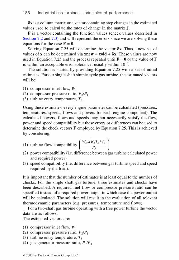
Industrial gas turbines – principles of performance186
�x is a column matrix or a vector containing step changes in the estimatedvalues used to calculate the rates of change in the matrix J.
F is a vector containing the function values (check values described inSection 7.2 and 7.3) and will represent the errors since we are solving theseequations for the case F = 0.
Solving Equation 7.25 will determine the vector �x. Thus a new set ofvalues of x can be determined via xnew = xold + �x. These values are nowused in Equation 7.25 and the process repeated until F = 0 or the value of Fis within an acceptable error tolerance, usually within 10–6.
The solution is started by providing Equation 7.25 with a set of initialestimates. For our single shaft simple cycle gas turbine, the estimated vectorswill be:
(1) compressor inlet flow, W1
(2) compressor pressure ratio, P2/P1
(3) turbine entry temperature, T3.
Using these estimates, every engine parameter can be calculated (pressures,temperatures, speeds, flows and powers for each engine component). Thecalculated powers, flows and speeds may not necessarily satisfy the flow,power and speed compatibility but these errors or differences can be used todetermine the check vectors F employed by Equation 7.25. This is achievedby considering:
(1) turbine flow compatibility W R T
P3 3 3 3
3
/γ
(2) power compatibility (i.e. difference between gas turbine calculated power
and required power)(3) speed compatibility (i.e. difference between gas turbine speed and speed
required by the load).
It is important that the number of estimates is at least equal to the number ofchecks. For the single shaft gas turbine, three estimates and checks havebeen described. A required fuel flow or compressor pressure ratio can bespecified instead of a required power output in which case the power outputwill be calculated. The solution will result in the evaluation of all relevantthermodynamic parameters (e.g. pressures, temperature and flows).
For a two-shaft gas turbine operating with a free power turbine the vectordata are as follows.The estimated vectors are:
(1) compressor inlet flow, W1
(2) compressor pressure ratio, P2/P1
(3) turbine entry temperature, T3(4) gas generator pressure ratio, P3/P4
© 2007 by Taylor & Francis Group, LLC

Off-design performance prediction 187
And the check vectors are:
(1) gas generator flow compatibility W R T
P3 3 3 3
3
/γ
(2) power balance between the compressor and gas generator turbineW1 × cpa × (T2 – T1) and W3 × cpg × (T3 – T4), respectively
(3) power turbine flow compatibility W R T
P5 5 5 5
5
/γ
(4) the difference between the power output from the power turbine and therequired power output.
There are four estimates and checks for a two-shaft gas turbine operatingwith a power turbine. Fuel flow, gas generator speed, compressor non-dimensional speed or compressor pressure ratio can be specified as checkvectors instead of the required power output.
The matrix method effectively applies Newton’s method (also known asthe Newton-Raphson method) to solve a set of non-linear simultaneousequations. Teukolsky et al.3 and Gerald and Wheatly4 give further details.
7.5 Off-design performance prediction of a three-
shaft gas turbine with a free power turbine
At high compressor pressure ratios, gas turbines may employ more than onespool in the gas generator to overcome the compressor instabilities, as discussedin Section 4.10.2. A schematic representation of a three-shaft gas turbineemploying a free power turbine to drive the load is shown in Fig. 7.6. Thereis no mechanical coupling between the LP and the HP spool but there existsa strong fluid or aerodynamic coupling between these spools. The vectordata needed for the prediction of the off-design performance of a three-shaftengine operating with a power turbine are as follows.
Referring to Fig. 7.6 the estimated vectors are:
(1) LP compressor inlet flow, W1
(2) LP compressor pressure ratio, P2/P1
(3) HP compressor pressure ratio, P3/P2
(4) HP turbine entry temperature, T4(5) HP turbine pressure ratio, P4/P5(6) LP turbine pressure ratio, P5/P6.
And the check vectors are:
(1) HP turbine flow compatibility W R T
P4 4 4 4
4
/γ
© 2007 by Taylor & Francis Group, LLC

Industrial gas turbines – principles of performance188
(2) HP turbine power balance (W2 × cpa × (T3 – T2) – W3 × cpg × (T4 – T5))
(3) LP turbine flow compatibility W R T
P5 5 5 5
5
/γ
(4) LP turbine power balance (W1 × cpa × (T2 – T1) – W5 × cpg × (T5 – T6))
(5) power turbine flow compatibility W R T
P6 6 6 6
6
/γ
(6) comparison between the power output from the power turbine and thepower required.
The three-shaft free power turbine gas turbine has six estimated vectorsand check vectors. Note: Instead of the power output check (6), LP speed ornon-dimensional speed, LP compressor pressure ratio, HP spool speed ornon-dimensional speed, HP compressor pressure ratio or fuel flow can beused.
7.6 Off-design performance prediction of a two-
shaft gas turbine
The three-shaft gas turbine operating with a free power turbine can be modifiedinto a two-shaft gas turbine. This is achieved by integrating the LP turbinewith the power turbine. Therefore, the LP turbine now drives the LP compressorand the load. Such an engine configuration is again best suited for power
7.6 Schematic representation of a three-shaft free turbine gasturbine.
12
LPcompressor
Combustor
3
Load
1 LP compressor inlet2 HP compressor inlet3 HP combustor exit/combustor inlet4 Combustor exit/HP turbine inlet5 LP turbine exit6 Power turbine inlet7 Power turbine exit
4
5
Po
wer
tu
rbin
e
Gas generator
6
7
HPcompressor
HPturbine LP
turbine
© 2007 by Taylor & Francis Group, LLC

Off-design performance prediction 189
generation where the load (i.e. electrical generator) operates at a constantspeed. The advantages are similar to that of a single shaft gas turbine discussedpreviously. A schematic representation of a two-shaft gas turbine is shown inFig. 7.7.
The off-design performance prediction of a two-shaft gas turbine requiresonly minor modification to that discussed in Section 7.5, where the off-design performance prediction of a three-shaft gas turbine operating with afree power turbine was considered.The estimated and check vectors are:
(1) LP compressor inlet flow, W1
(2) LP compressor pressure ratio, P2/P1
(3) HP compressor pressure ratio, P3/P2
(4) HP turbine entry temperature, T4
(5) HP turbine pressure ratio, P4/P5.
And the check vectors are:
(1) HP turbine flow compatibility W R T
P4 4 4 4
4
/γ
(2) HP turbine power balance (W2 × cpa × (T3 – T2) – W4 × cpg × (T4 – T5))
(3) LP turbine flow compatibility W R T
P5 5 5 5
5
/γ
(4) speed compatibility between the LP compressor/turbine speed and theload
(5) comparison between the power output from the gas turbine and thepower required.
The two-shaft gas turbine has five estimated vectors and check vectors.Note: Instead of the power output check (5), HP spool speed or non-dimensionalspeed, LP or the HP compressor pressure ratio or fuel flow can be used.
12
LPcompressor
Combustor
3
Load
4
5
LP t
urb
ine
6
HPcompressor
HPturbine
7.7 Schematic representation of a two-shaft gas turbine.
© 2007 by Taylor & Francis Group, LLC

Industrial gas turbines – principles of performance190
7.7 Off-design performance prediction of a three-
shaft gas turbine
A three-shaft gas turbine is essentially a three-shaft gas turbine operatingwith a free power turbine where the power turbine drives a booster compressorand the load. Thus the booster compressor now becomes the LP compressorand the LP compressor and turbine becomes the intermediate (IP) compressorand IP turbine, respectively. This is illustrated in Fig. 7.8, which shows aschematic representation of a three-shaft gas turbine.
The vector data needed for the prediction of the off-design performanceof a three-shaft gas turbine are as follows.
Estimated vectors are:
(1) LP compressor inlet flow, W1
(2) LP compressor pressure ratio, P2/P1
(3) IP compressor pressure ratio, P3/P2
(4) HP compressor pressure ratio, P4/P3
(5) HP turbine entry temperature, T4(6) HP turbine pressure ratio, P4/P5(7) IP turbine pressure ratio, P6/P7.
Check vectors are:
(1) HP turbine flow compatibility W R T
P5 5 5 5
5
/γ
(2) HP turbine power balance (W3 × cpa × (T4 – T3) – W5 × cpg × (T5 – T6))
7.8 Schematic representation of a three-shaft gas turbine.
1 2
IPcompressor
Combustor3 4 5
HPcompressor HP
turbine
Load
LP t
urb
ine
67
8
LP c
om
pre
sso
r
IPturbine
1 LP compressor inlet2 IP compressor inlet3 HP compressor inlet4 HP compressor exit/combustor inlet5 Combustor exit/HP turbine inlet6 IP turbine inlet7 LP turbine inlet8 LP turbine exit
© 2007 by Taylor & Francis Group, LLC

Off-design performance prediction 191
(3) IP Turbine flow compatibility W R T
P6 6 6 6
6
/γ
(4) IP turbine power balance (W2 × cpa × (T3 – T2) – W6 × cpg × (T6 – T7))
(5) LP Turbine flow compatibility W R T
P7 7 7 7
7
/γ
(6) speed compatibility between the LP compressor/turbine speed and theload
(7) comparison between the power output from the gas turbine and thepower required.
The three-shaft gas turbine has seven estimated vectors and check vectors.Note: Instead of the power output check (7), the IP or HP spool speed or theirnon-dimensional speeds or pressure ratios, LP compressor pressure ratio orfuel flow can be used.
7.8 Off-design performance prediction of complex
gas turbine cycles
In Chapter 3 was discussed the design point performance of complex cycleswhich incorporated intercooling to reduce the compressor power requirement,reheat to augment the turbine power output, and regeneration to decrease thethermal input in order to improve the thermal efficiency of the simple cyclegas turbine. Complex cycles may employ engine configurations such asmulti-spooling compressors and turbines, including the use of free powerturbines, as described, when discussing the methods for predicting the off-design performance of a simple cycle. These methods can also be used inpredicting the off-design performance of complex cycles.
7.8.1 Off-design performance prediction of a single-shaftgas turbine employing an intercooler
The performance prediction of compressors, turbines and the combustionsystem has been discussed. The thermodynamic performance of an intercoolercan be determined using the method described in Section 2.14. For anintercooler, the ratio of the thermal capacities of the heated and cooled fluidmay be significantly different, and thus the ratio of thermal capacities forintercoolers could as low as 0.2. Referring to Fig. 2.18 in Chapter 2, theeffectiveness of the intercooler can approach unity, particularly if water isemployed as the cooling medium. This is primarily due to the higher specificheat of water compared with air, and the water flow rate through the intercoolercan be greater than that of the air flow in the cooler. Thus the air temperature
© 2007 by Taylor & Francis Group, LLC

Industrial gas turbines – principles of performance192
leaving the intercooler, T3, can approach the ambient temperature, T1 asshown in Fig. 7.9, which represents a single shaft intercooled gas turbine.
The pressure loss in the intercooler may be modelled using the losscoefficient, K1, and the cooler inlet non-dimensional flow W2√T2/P2, utilisingthe expression for the cooler non-dimensional pressure loss ∆P23/P2 (Equation7.17).
∆PP
KW R T
Pl23
2
2 2 2 2
2
2
2 = /γ
γ
[7.26]
The necessary estimates and checks can be developed as follows. The requiredpower output, gas turbine speed, N1, compressor inlet pressure, P1, humidity,ω , and temperature, T1, are specified. Ignoring bleeds, turbine cooling, inletand exhaust losses and referring to Fig. 7.9, the estimate vectors are:
(1) compressor inlet mass flow, W1(2) LP compressor pressure ratio, P2/P1
(3) HP compressor inlet temperature, T3
(4) HP compressor pressure ratio, P4/P3
(5) turbine entry temperature, T3
The check vectors are:
(1) turbine flow compatibility W R T
P3 3 3 3
3
/γ
(2) speed compatibility (i.e. difference between the LP compressor speedand HP compressor speed)
7.9 Schematic representation of an intercooled single-shaft gasturbine.
1
2 Combustor3 4 5
Load
6
LP
1 LP compressor inlet2 IP compressor exit/intercooler inlet3 Intercooler exit/HP compressor inlet4 HP compressor exit/combustor inlet5 Combustor exit/turbine inlet6 Turbine exit
Intercooler
HP
Compressors
Turb
ine
Fuel input
© 2007 by Taylor & Francis Group, LLC

Off-design performance prediction 193
(3) power compatibility (i.e. difference between gas turbine calculated powerand required power)
(4) speed compatibility (i.e. difference between gas turbine speed and thespeed required by the load)
(5) difference between the estimated cooler exit temperature, T3, and thatcalculated from the cooler effectiveness Equation 7.27:
ε cooler2
2
3 = – TT
TTc
[7.27]
where εcooler is the effectiveness of the cooler and Tc is the coolant inlettemperature normally equal to T1. It is assumed that the thermal capacityof the coolant is greater than that of the air being cooled, which wouldnormally be the case.
Note: Required fuel flow can be specified rather than the required poweroutput for the check vector (3), in which case the power output from the gasturbine will be calculated.
7.8.2 Off-design performance prediction of a single-shaftgas turbine employing intercooling andregeneration
The prediction of the off-design performance of an intercooled–regenerativegas turbine requires an additional estimate that corresponds to the heatexchanger air exit temperature, which now is the combustor inlet temperature.Referring to Fig. 7.10, the additional temperature estimate corresponds toT5. The estimated vectors are:
(1) compressor inlet mass flow, W1(2) LP compressor pressure ratio, P2/P1(3) HP compressor inlet temperature, T3
(4) HP compressor pressure ratio, P4/P3
(5) heat exchanger exit air temperature, T5
(6) turbine entry temperature, T6
Check vectors are:
(1) turbine flow compatibility W R T
P6 6 6 6
6
/γ
(2) speed compatibility (i.e. difference between the LP compressor speedand HP compressor speed)
(3) power compatibility (i.e. difference between gas turbine calculated powerand required power)
© 2007 by Taylor & Francis Group, LLC

Industrial gas turbines – principles of performance194
(4) speed compatibility (i.e. difference between gas turbine speed and speedrequired by the load)
(5) difference between the estimated cooler exit temperature, T3, and thatcalculated from the cooler effectiveness in Equation 7.27
(6) difference between the estimated heat exchanger air exit temperatureand that calculated by the heat exchanger in Equation 2.35 given inChapter 2.
If we ignore intercooling and consider only regeneration, the vector datareferring to Fig. 7.10 as follows:
(1) compressor inlet mass flow, W1
(2) compressor pressure ratio, P4/P1, which is now the overall compressorpressure ratio
(3) heat exchanger exit air temperature, T5(4) turbine entry temperature, T6
Check vectors are:
(1) turbine flow compatibility W R T
P6 6 6 6
6
/γ
(2) power compatibility (i.e. difference between gas turbine calculated powerand required power)
1
2 Combustor3
4 5
Load
6
LP
1 LP compressor inlet2 IP compressor exit/intercooler inlet3 Intercooler exit/HP compressor inlet4 HP compressor exit/heat exchanger inlet (cold side)5 Heat exchanger exit (cold side)/combustor inlet6 Combustor exit/turbine inlet7 Turbine exit/heat exchanger inlet (hot side)8 Heat exchanger exit (hot side)
Intercooler
HP
Heat exchanger
Turb
ine
Fuel input
8
7
7.10 Schematic representation of an intercooled–regenerated gasturbine.
© 2007 by Taylor & Francis Group, LLC

Off-design performance prediction 195
(3) speed compatibility (i.e. difference between gas turbine speed and thespeed required by the load)
(4) difference between the estimated heat exchanger air exit temperatureand that calculated for the heat exchanger in Equation 2.35 given inChapter 2.
7.8.3 Off-design performance prediction of a single-shaftgas turbine employing intercooling, regenerationand reheat
To predict the off-design performance of an intercooled–regenerative–reheatgas turbine an additional estimate is required to that described in Section7.8.2 where the performance of the intercooled regenerative gas turbine wasconsidered. This corresponds to the HP turbine pressure ratio, P6/P7, asshown in Fig. 7.11, which shows a schematic representation of an intercooled–regenerative–reheat gas turbine. It is also necessary to specify the reheat exittemperature, which also corresponds with the LP turbine entry temperature,T8. The estimated vector data are:
(1) compressor inlet mass flow, W1
(2) LP compressor pressure ratio, P2/P1
(3) HP compressor inlet temperature, T3
7.11 Intercooled–regenerative–reheat gas turbine.
1
2 Combustor3
4 5
Load
1 LP compressor inlet2 LP compressor exit/intercooler inlet3 Intercooler exit/HP compressor inlet4 HP compressor exit/heat exchanger inlet (cold side)5 Heat exchanger exit (cold side)/combustor inlet6 Combustor exit/HP turbine inlet7 HP turbine exit/reheater inlet8 Reheater exit/LP turbine inlet9 LP turbine exit/heat exchanger inlet (hot side)
10 Heat exchanger exit (hot side)
6
Intercooler
Heat exchanger
LP t
urb
ine
Fuel input
9
7
HP
tu
rbin
e
8
Fuel input
10LPcompressor
HPcompressor
Reheater
© 2007 by Taylor & Francis Group, LLC

Industrial gas turbines – principles of performance196
(4) HP compressor pressure ratio, P4/P3
(5) heat exchanger exit air temperature, T5(6) turbine entry temperature, T6
(7) HP turbine pressure ratio, P6/P7.
Check vectors are:
(1) HP turbine flow compatibility W R T
P6 6 6 6
6
/γ
(2) LP turbine flow compatibility W R T
P8 8 8 8
8
/γ
(3) speed compatibility (i.e. difference between the LP compressor speedand HP compressor speed)
(4) power compatibility (i.e. difference between gas turbine calculated powerand required power)
(5) speed compatibility (i.e. difference between gas turbine speed and thespeed required by the load)
(6) difference between the estimated cooler exit temperature, T3, and thatcalculated from the cooler effectiveness in Equation 7.27
(7) difference between the estimated heat exchanger air exit temperatureand that calculated by the heat exchanger in Equation 2.35 given inChapter 2.
If intercooling is ignored, then the estimate vectors (3) and (4) and thecheck vectors (3) and (6) can be omitted. Similarly, if regeneration is ignoredand only reheat considered, then estimate vectors (3), (4) and (5) and thecheck vectors (3), (6) and (7) can be omitted.
7.9 Off-design prediction of a two-shaft gas
turbine using a free power turbine and
employing intercooling, regeneration and
reheat
The method applied to predict the off-design performance of a two-shaft gasturbine operating with a free power turbine (Section 7.3) may be modified toinclude intercooling, regeneration and reheating. Three more estimates needto be added, which correspond to the intercooler exit temperature (i.e. HPcompressor inlet temperature), T3, HP compressor pressure ratio, P4/P3, andthe heat exchange exit or combustion inlet temperature, T5, as shown in Fig.7.12. The reheat exit temperature, T8 also needs to be specified. Three morecheck conditions or vectors will now be needed. These correspond to thespeed compatibility of the LP and HP compressor, a check against the intercooler
© 2007 by Taylor & Francis Group, LLC

Off-design performance prediction 197
discharge temperature using Equation 7.27, and a check on the heat exchangerexit temperature, T5, using Equation 2.35 in Chapter 2.Therefore, the estimated vectors are:
(1) LP compressor inlet flow, W1
(2) LP compressor pressure ratio, P2/P1(3) HP compressor inlet temperature, T3(4) combustor inlet temperature, T5
(5) HP compressor pressure ratio, P4/P3
(6) turbine entry temperature, T3
(7) gas generator pressure ratio, P3/P4.
Check vectors are:
(1) gas generator flow compatibility W R T
P6 6 6 6
6
/γ
(2) power balance between the compressor and gas generator turbineW1 × cpa × (T2 – T1) + W2 × cpa × (T4 – T2) andW6 × cpg × (T6 – T7) + W7 × cpg × (T7 – T8) respectively
7.12 Schematic representation of a two-shaft gas turbine includingintercooling, regeneration and reheating operating with a free powerturbine.
1
2 Combustor3
4 5
Load
6
1 LP compressor inlet2 LP compressor exit/intercooler inlet3 Intercooler exit/HP compressor inlet4 HP compressor exit/heat exchanger inlet (cold side)5 Heat exchanger exit (cold side)/combustor inlet6 Combustor exit/gas generator (GG) turbine inlet7 GG turbine exit/reheater inlet8 Reheater exit/power turbine inlet9 Power turbine exit/heat exchanger inlet (hot side)
10 Heat exchanger exit (hot side)
Intercooler
Heat exchanger
Pow
er tu
rbin
e
Fuel input
9
7
GG
tu
rbin
e
8
Fuel input
10LPcompressor
HPcompressor
Reheater
© 2007 by Taylor & Francis Group, LLC

Industrial gas turbines – principles of performance198
(3) power turbine flow compatibility W R T
P8 8 8 8
8
/γ
(4) speed compatibility (i.e. difference between the LP compressor speedand HP compressor speed)
(5) difference between the estimated heat exchanger air exit temperatureand that calculated by the heat exchanger in Equation 2.35 given inChapter 2
(6) difference between the estimated cooler exit temperature, T3 and thatcalculated from the cooler effectiveness in Equation 7.27
(7) the difference between the power output from the power turbine and therequired power output.
7.10 Off-design prediction of a three-shaft gas
turbine using a power turbine and employing
intercooling, regeneration and reheat
For the prediction of the off-design performance of a three-shaft gas turbineoperating with a free power turbine incorporating intercooling, a heat exchangerand reheat, only two more estimates are required in addition to the estimatesneeded for the corresponding simple cycle as described in Section 7.5. Theseestimates correspond to the intercooler discharge temperature, T3, and theheat exchanger or combustion inlet temperature, T5, as shown in Fig. 7.13.The corresponding checks are the intercooler discharge temperature calculatedby Equation 7.27 and the heat exchanger exit temperature using Equation2.35, described in Chapter 2. Again, the reheat or power turbine entrytemperature needs to be specified.
Therefore, the estimate vectors needed to predict the off-design performanceof a complex three-shaft gas turbine using a free power turbine as shown inFigure 7.13 are:
(1) LP compressor inlet flow, W1
(2) LP compressor pressure ratio, P2/P1
(3) HP compressor inlet temperature, T3
(4) HP compressor pressure ratio, P3/P2(5) combustor inlet temperature, T5(6) HP turbine entry temperature, T4
(7) HP turbine pressure ratio, P4/P5
(8) LP turbine pressure ratio, P5/P6.
Check vectors are:
(1) HP turbine flow compatibility, W R T
P4 4 4 4
4
/γ
© 2007 by Taylor & Francis Group, LLC

Off-design performance prediction 199
7.13 Schematic representation of a two-shaft gas turbine includingintercooling, regeneration and reheating operating with a free powerturbine.
(2) HP turbine power balance, (W2 × cpa × (T3 – T2) – W3 × cpg × (T4 – T5))
(3) LP turbine flow compatibility W R T
P5 5 5 5
5
/γ
(4) LP turbine power balance (W1 × cpa × (T2 – T1) – W5 × cpg × (T5 – T6))
(5) power turbine flow compatibility W R T
P6 6 6 6
6
/γ
(6) difference between the estimated heat exchanger air exit temperatureand that calculated by the heat exchanger in Equation 2.35 given inChapter 2
(7) difference between the estimated cooler exit temperature, T3, and thatcalculated from the cooler effectiveness in Equation 7.27
(8) comparison between the power output from the power turbine and thepower required.
Intercooling may be ignored, in which case estimated vector (3) andcheck vector (7) can be omitted. If intercooling and regeneration are ignoredand only reheat considered, then the estimated and check vectors are thesame as shown in Section 7.5.
1
2 Combustor3
4 5
Load
6
1 LP compressor inlet2 LP compressor exit/intercooler inlet3 Intercooler exit/HP compressor inlet4 HP compressor exit/heat exchanger inlet (cold side)5 Heat exchanger exit (cold side)/combustor inlet6 Combustor exit/HP turbine inlet7 LP turbine inlet8 LP turbine exit/reheater inlet9 Reheater exit/power turbine inlet
10 Power turbine exit/heat exchanger inlet (hot side)11 Heat exchanger exit (hot side)
Intercooler
Heat exchanger
Pow
er tu
rbin
e
Fuel input 97
HPturbine
8
Fuel input
11LPcompressor
HPcompressor
Reheater
10LP
turbine
© 2007 by Taylor & Francis Group, LLC

Industrial gas turbines – principles of performance200
Similarly, the off-design performance of two- and three-shaft gas turbinesmay be predicted as discussed in Sections 7.6 and 7.7 using intercooling andreheat, and the reader is left to develop the necessary vector data to predictthe off-design performance of these cycles.
7.11 Variable geometry compressors
The use of variable geometry in compressors has been discussed in Chapter4 (variable inlet guide vanes and stators, VIGVs and VSVs, respectively) toprevent compressor instabilities such as compressor stall and surge. Althoughthe compressor characteristic will indeed change with the position of suchvariable geometry devices (guide vane angle), the control philosophy ofthese devices applied to a two- or three- shaft gas turbine operating with afree power turbine is such that the compressor non-dimensional speed isused in determining the position of the VIGV and VSV. Thus, for a givencompressor non-dimensional speed, there is a unique VIGV and VSV positionor guide vane angle which, in turn, fixes the compressor flow capacity,pressure ratio and efficiency. Provided the compressor characteristic employedin the prediction of the off-design performance of such engine configurationsincludes the effect of the position of these variable geometry devices in thecompressor, then no change in the procedures given previously for predictingthe off-design performance of such engines is necessary.
Single-shaft gas turbines, particularly generating large power outputs (aboveabout 50 MW), also employ variable geometry in the compressor, usuallyVIGVs. The purpose of variable geometry in compressors employed bysingle-shaft gas turbines is to control the air flow through the compressor,such that the turbine exit temperature (also known as the exhaust gastemperature) is maintained at some predetermined value. Controlling theexhaust gas temperature by such means results in a reduction in the compressorflows at low power outputs, thus significantly decreasing the starting powerrequirements of the gas turbine. Variable geometry may also be employed tomaintain the exhaust gas temperature at its design value at low power.Maintaining the exhaust gas temperature at the design value at low powersis particularly beneficial to the thermal efficiency at these powers when aheat exchanger is added or when the gas turbine is part of a combined cycleplant. Furthermore, the fuel–air ratio remains approximately constant at constantexhaust gas temperature operation, which is particularly useful in DLEcombustion systems, as discussed in Chapter 6 on gas turbine combustion.
Unlike the case of a free power turbine discussed above, the compressorcharacteristic needs to be known for each VIGV and VSV setting (angle).Furthermore, an additional estimate and check is necessary when predictingthe off-design performance of a single-shaft gas turbine operating with variablegeometry compressors. This estimate and check corresponds to the guide
© 2007 by Taylor & Francis Group, LLC

Off-design performance prediction 201
vane angle and required exhaust temperature, respectively. Alternatively thecompressor flow capacity of a fixed geometry compressor may be decreasedby an amount depending on the guide vane angle of the VIGV and VSV. Inthis event it is important to adjust the compressor efficiency characteristic ofthe compressor due to the change in the guide vane angle.
7.12 Variable geometry turbines
Turbines may also incorporate variable geometry and this is usually appliedto power turbines where the nozzle guide vanes (NGVs) are turned to alterthe flow capacity and thus the turbine characteristic. Variable geometry hasbeen employed in turbines operating with free power turbines to improve theoff-design thermal efficiency (i.e. low power outputs), particularly when aheat exchanger is added. Variable geometry power turbines also provideimproved acceleration when the NGVs are full opened and can also be usedto provide substantial engine braking when the NGVs are rotated sufficiently,such that the gases leaving the NGV impinge on the turbine rotor in theopposite direction.
The prediction of the off-design performance of gas turbines employingvariable geometry turbines requires an additional estimate and check vector,which correspond to the NGV angle and the required exhaust gas temperature,respectively. The exhaust gas temperature may be measured downstream ofthe gas generator turbine rather than at the power turbine exit. It is alsonecessary to know the change in the turbine characteristic with NGV angle,and the appropriate turbine characteristic must be used as the NGV anglechanges during the iterations described above.
7.13 References
1. Gas Turbine Theory, 5th Edition, Saravanamuttoo, H.I.H., Rogers, C.F.G. and Cohen,H., Longman (2001).
2. Gas Turbine Performance, 2nd Edition, Walsh, P.P. and Fletcher, P., BlackwellPublishing (2004).
3. Numerical Recipes in Fortran 77, 2nd Edition, Press, W.H., Teukolsky, S.A., Vetting,W.T. and Flannery, B.P., Ch. 9, Sections 9.6 and 9.7, Cambridge University Press(1992).
4. Applied Numerical Analysis, 6th Edition, Gerald C.F. and Wheatly, P.O., Addison-Wesley.
© 2007 by Taylor & Francis Group, LLC

202
It was stated in Chapter 7 that the change in ambient conditions and powerdemand from design conditions results in performance of the gas turbinedeviating from its design point. In this chapter the concepts of componentmatching, discussed in the previous chapter, will be used to predict some ofthe behaviour of gas turbines during off-design operation. Some assumptionswill be made as this will simplify the explanation of the behaviour of gasturbines during off-design operation.
8.1 Steady-state running line
Chapter 7 discussed the prediction of the off-design performance of variousgas turbine configurations. Using these techniques, it is possible to determinethe operating point for each non-dimensional speed line on the compressorcharacteristic. Joining these points will result in the steady-state running lineon the compressor characteristic.
8.1.1 Single-shaft gas turbine
As stated, single-shaft gas turbines are used extensively in power generation;the gas turbine speed will be constant and will normally correspond to thegenerator speed. For a given ambient condition, this results in the runningline aligning with a particular non-dimensional speed line. Before the generatorcan be loaded, the gas turbine speed is increased along the generator no-loadline until it reaches the generator synchronous speed. Figure 8.1 shows thisrunning line on the compressor characteristic. The effect of the change inambient temperature, T1, will result in the running line moving to anothernon-dimensional speed, as shown in Fig. 8.1. With lower ambient temperature,the non-dimensional speed, N1/√T1, will increase and conversely, the higherthe ambient temperature, the lower will be the non-dimensional speed.Consequently, the compressor inlet non-dimensional flow increases with
8Behaviour of gas turbines during off-design
operation
© 2007 by Taylor & Francis Group, LLC

Behaviour of gas turbines during off-design operation 203
decreasing ambient temperature and decreases with increase in ambienttemperature.
Although the analysis of the off-design performance of a gas turbine isquite tedious, much useful insight may be obtained by considering a simplifiedanalysis of the flow, work and speed compatibility equations.
Referring to Fig. 8.2 and ignoring the gas properties terms R and γ, aschanges in these values are smaller compared with the changes in massflows, pressures and temperatures, the flow compatibility equation may bewritten as discussed in Saravanamutto et al.1 as:
W TP
W TP
PP
PP
TT
WW
3 3
3
1 1
1
1
2
2
3
3
1
3
1 = × × × × [8.1]
If we assume that the turbine remains choked, particularly at high power,then W3√T3/P3 will remain constant with turbine pressure ratio. If we alsoassume that the compressor speed line is near choke conditions, especially athigh operating speeds, the variation of the compressor inlet non-dimensionalflow W1√T1/P1 with pressure ratio will be small. Furthermore, if the combustionpressure loss and bleeds are also assumed constant, then P2/P3 and W3/W1will also be constant. Hence, an increase in compressor pressure ratio mustbe accompanied by an increase in T3/T1 to satisfy the flow compatibility inEquation 8.1.
Figure 8.3 shows a compressor characteristic, where the compressor non-dimensional temperature rise is plotted against the pressure ratio for a seriesof non-dimensional speeds. It can be seen that the non-dimensional temperature
8.1 Steady-state running line for a single-shaft gas turbine.
Surge line
No load line
Pre
ssu
re r
atio
(P 2
/P1)
Non-dimensional flow (W1√T1/P1)
Contours of constantisentropic efficiency (η)
Load running line
Non-dimensonal speed N1/√T1
Effect of low ambienttemperature on the runningline
Effect of high ambienttemperature on the runningline
© 2007 by Taylor & Francis Group, LLC

Industrial gas turbines – principles of performance204
rise for a given non-dimensional speed is approximately constant, particularlyat low-pressure ratios. This is due to the fall in compressor efficiency as theoperating point moves away from the design point. Therefore, for a givencompressor non-dimensional speed and inlet temperature, the temperaturerise ∆T21 = T2 – T1 will be approximately constant, as discussed inSaravanamuttoo et al.1
The work compatibility equation gives us the net power output, pnet:
pnet = W3 × cpg × (T3 – T4) – W1 × cpa × (T2 – T1) [8.2]
1 Compressor inlet
2 Compressor exit/combustor inlet
3 Combustor exit/turbine inlet
4 Turbine exit
Combustor
Compressor
Fuel input
Load
Turb
ine
4
321
8.2 Schematic representation of a single-shaft gas turbine (simplecycle).
8.3 Compressor characteristic where the non-dimensionaltemperature rise varies with pressure ratio for a series of non-dimensional speeds.
Surge line
P2/P1
∆T21
/T1
N1/√T1
© 2007 by Taylor & Francis Group, LLC

Behaviour of gas turbines during off-design operation 205
The temperature drop across the turbine is:
( – ) = 1 – 3 4 3 t4
3
–1
T T T cpgPP
gg
× × ×
ηγ
γ
where cpa and cpg are the mean specific heats at constant pressure duringcompression and expansion respectively and γg is the mean isentropic expansionindex.
Unlike the compressor, the turbine efficiency does not vary very muchwith pressure ratio and non-dimensional speed. Therefore, as the turbinepressure ratio and turbine entry temperature, T3, increase, there is an increasein turbine power output. Since the compressor power absorbed W1 × cpa ×(T2 – T1) is approximately constant, there is an increase in the gas turbinepower output pnet. Thus, a series of running lines can be produced on thecompressor characteristic, due to the increase in power and ambienttemperature, T1, as illustrated in Fig. 8.4.
In fact, the detailed analysis in determining the off-design performance ofa gas turbine essentially solves these equations using detailed componentcharacteristics. It also allows for the change in the thermodynamic propertiesof air and products of combustion due to temperature changes.
8.4 Series of running lines for various power and ambienttemperature conditions for a single-shaft gas turbine.
Pre
ssu
re r
atio
(P 2
/P1)
Non-dimensional flow (W1√T1/P1)
Increasing ambient
temperature
Non-dimensionalspeed N1/√T1
Increasingpower
© 2007 by Taylor & Francis Group, LLC

Industrial gas turbines – principles of performance206
8.1.2 Two-shaft gas turbine operating with a free powerturbine
To predict the running line for a two-shaft gas turbine, it is necessary toconsider the performance behaviour of turbines operating in series. Figure8.5 shows the characteristics of two turbines operating in series. For example,the HP turbine and the LP turbine would represent the gas generator (GG)turbine and power turbine respectively when applied to a two-shaft gasturbine.
The GG turbine inlet non-dimensional flow increases initially with turbinepressure ratio until the GG turbine chokes, after which the inlet non-dimensionalflow remains constant. However, the GG turbine outlet non-dimensionalflow increases continuously with turbine pressure ratio as shown in Fig. 8.5.The power turbine inlet flow also increases with pressure ratio until it alsochokes. The GG turbine exit flow must be ‘swallowed’ by the power turbine.Thus, the power turbine controls the GG turbine exit non-dimensional flow,and hence controls the GG turbine pressure ratio. The operating points 1, 2and 3 in Fig. 8.5 illustrate this point.
When the power turbine operates unchoked, point (1) in Fig. 8.5, the gasgenerator turbine will be forced to operate at point (1) on its characteristic tosatisfy the flow compatibility between these turbines. When the power turbineoperates under choked conditions, points (2) and (3) on the power turbinecharacteristic, the gas generator turbine will be forced to operate at a fixedpressure ratio as shown by point (2, 3) on the gas generator characteristic.
No
n-d
imen
sio
nal
flo
w
HP or GG turbine outlet flow
HP or GG turbineinlet flow
LP or power turbine inlet flow
HP or GG turbine
Pressure ratio(1) (2,3)
Pressure ratio(1) (2) (3)
LP or power turbine
8.5 Turbines operating in series.
© 2007 by Taylor & Francis Group, LLC

Behaviour of gas turbines during off-design operation 207
Thus, the operating point on the gas generator turbine characteristic isdetermined primarily by the swallowing capacity of the power turbine.
In this analysis, it has been assumed that the gas generator turbine efficiencyremains constant for the three operating cases shown in Fig. 8.5 and this isusually the case. If there is a change in the gas generator turbine efficiencyat these conditions, then the operating points (2) and (3) will not be coincident.However, this is usually small because of the small change in turbine efficiencywith pressure ratio and non-dimensional speed.
Referring to Fig. 8.6 and ignoring the gas properties terms, R and γ, the flowcompatibility equation for turbines operating in series can be written as:
W TP
W TP
PP
TT
WW
4 4
4
3 3
3
3
4
4
3
4
3 = × × × [8.3]
whereW3√T3/P3 is the non-dimensional flow at entry to the gas generator turbineP3/P4 is the gas generator turbine pressure ratioT3/T4 is the gas turbine temperature ratioW3/W4 is the ratio of gas flow at inlet of gas generator turbine to gas flow
at inlet of power turbineW4√T4/P4 is the power turbine inlet non-dimensional flow.During power turbine choked conditions, the gas generator turbine pressure
ratio and thus the non-dimensional temperature drop, ∆T34/T3, will be constantprovided the generator turbine efficiency is also constant.
Combustor
Fuel input
Gas generator
Load
Turb
ine
Po
wer
tu
rbin
e
Compressor
54
32
1
1 Compressor inlet
2 Compressor exit/combustor inlet
3 Combustor exit/gas generator turbine inlet
4 Gas generator turbine exit/power turbine inlet
5 Power turbine exit
8.6 Schematic representation of a two-shaft turbine operating with afree power turbine.
© 2007 by Taylor & Francis Group, LLC

Industrial gas turbines – principles of performance208
Writing the power balance or work compatibility equation for the gasgenerator:
∆ ∆TT
TT
TT
cpgcpa
WW
21
1
34
3
3
1
3
1 = × × × [8.4]
For a given compressor non-dimensional speed, N1/√T1, the compressornon-dimensional temperature rise, ∆T21/T1 will be approximately constant(see Fig. 8.3). If compressor bleeds and the effect of fuel flow on W3 areignored, it can be assumed that W3 equals W1. For constant specific heats,Equation 8.4 indicates that, for a given compressor speed, there will be aunique value for T3/T1. To maintain the flow compatibility between thecompressor and the gas generator turbine and referring to Fig. 8.6 we have:
W TP
W TP
PP
PP
TT
WW
3 3
3
1 1
1
1
2
2
3
3
1
3
1 = × × × × [8.5]
W3√T3/P3 will be fixed by the choking of the gas generator turbine as discussed.For a constant combustor pressure loss, P2/P3 will be constant. Although itis possible to find more than one solution for P2/P1 and W1√T1/P1 fromEquation 8.5, in practice, the shape of the compressor characteristic does notshow a significant change in flow with pressure ratio, particularly at highspeed, where W1√T1/P1 is approximately constant. Thus only a single solutionis possible.
At different compressor non-dimensional speeds, different values for ∆T21/T1 would apply, resulting in different values for T3/T1 (Equation 8.4), hencegiving unique operating points on each compressor speed line. Joining thesepoints gives the (unique) running line on the compressor characteristic for atwo-shaft gas turbine operating with a free power turbine. If gas propertychanges are considered, then the running line will change with ambientconditions but this is usually small, particularly at low ambient temperatures.For rigorous analysis, gas property changes need to be allowed for as discussedin Chapter 7. The compressor characteristic with the running line superimposedon it is shown in Fig. 8.7. This line differs from the case of a single-shaft gasturbine, where a series of running lines occurs, each of constant poweroutput as shown in Fig. 8.4.
8.2 Displacement of running line (single- and two-
shaft free power turbine gas turbine)
At low power and idle operating conditions, the running line may intersectwith the surge line as shown in Fig. 4.23 (Chapter 4). This is primarilydue to the stalling of the front stages as the compressor operates far fromits design condition as discussed in Section 4.10. Therefore, it may notbe possible to accelerate the engine without some remedial action being
© 2007 by Taylor & Francis Group, LLC

Behaviour of gas turbines during off-design operation 209
taken. Section 4.10 also discusses the remedies employed to overcome theproblem. The impact that such remedies have on the running line will nowbe examined.
Blow-off
The impact of blow-off is to reduce the flow through the turbine sectionrelative to the compressor. For simplicity, it will be assumed that the blow-off acts at the discharge of the compressor, although in practice the blow-offwill be positioned at some intermediate point, so that the choking effect ofthe HP stages of the compressor are reduced during low compressor speedoperation.
Referring to Fig. 8.8 and writing the power balance equation for the gasgenerator:
∆ ∆TT
TT
TT
cpgcpa
WW
21
1
34
3
3
1
3
1 = × × × [8.6]
If it is assumed that the compressor continues to operate at a constant non-dimensional speed (by adjusting the fuel flow), the non-dimensionaltemperature rise ∆T21/T1 will be approximately constant. When the blow-offvalve is opened, W3/W1 will decrease. If it is also assumed that the turbinesare choked, then from Section 8.1.2, ∆T34/T3 will also be constant. FromEquation 8.6, any reduction in W3/W1 must be compensated bya corresponding increase in T3/T1, that is T3/T1 is inversely proportional toW3/W1.
8.7 Running line on the compressor characteristic for a two-shaft gasturbine.
Pre
ssu
re r
atio
(P 2
/P1)
Non-dimensional flow (W1√T1/P1)
Non-dimensionalspeed N1/√T1
Surge line
Running line
Contours of constantisentropic efficiency (η)
© 2007 by Taylor & Francis Group, LLC

Industrial gas turbines – principles of performance210
Writing the flow compatibility equation for the gas generator:
W TP
W TP
PP
PP
TT
WW
3 3
3
1 1
1
1
2
2
3
3
1
3
1 = × × × × [8.7]
If we assume W3√T3/P3, W1√T1/P1 and P2/P3 are approximately constant,then any reduction of W3/W1 must increase P1/P2 because the effect of theincrease in T3/T1 will only be increasing by the value of its square root. Thus,during blow-off valve operation, the pressure ratio, P2/P1, for each non-dimensional speed line will decrease to satisfy the flow compatibility Equation8.7. This is illustrated in Fig. 8.9, which shows the effect of blow-off valveoperation on the running line on the compressor characteristic.
Variable stator vanes and inlet guide vanes (compressors)
Variable stators (VSVs)and variable inlet guide vanes (VIGVs) significantlyalter the flow capacity of the compressor along a given speed line. However,they do not have a significant impact on the position of the running line. Thechange in compressor efficiency, on the other hand, does influence the runningline. Closing the stator vanes will reduce the deflection in the correspondingrotors and result in a reduction in stage loading (Section 4.10.3 in Chapter 4).This would normally increase the efficiency of the compressor. The effect ofincreased compressor efficiency on the non-dimensional temperature rise,
1 Compressor inlet
2 Compressor exit/combustor inlet
3 Combustor exit/gas generator turbine inlet
4 Gas generator turbine exit/power turbine inlet
5 Power turbine exit
Combustor
Fuel input
Load
Gas generator
Compressor
Blow-off valve
Po
wer
tu
rbin
e
Turb
ine
54
321
8.8 Schematic representation of a two-shaft gas turbine operatingwith a blow-off valve.
© 2007 by Taylor & Francis Group, LLC

Behaviour of gas turbines during off-design operation 211
resulting in a reduction in non-dimensional temperature rise for a given non-dimensional speed, is shown in Fig. 8.10. Early work2 on variable geometrycompressors using VSV/VIGVs showed an improvement in efficiency atlow compressor speeds, but that a notable loss in efficiency occurs at highcompressor speeds due to the closure of the VSV/VIGVs. Thus, during high-speed operation, closure of the VSV/VIGVs will result in an increase in thecompressor non-dimensional temperature.
If the gas generator of a two-shaft gas turbine employing a free powerturbine is operating at low speeds, and we assume that the change in theefficiency of the compressor due to the closure of the VSV/VIGV is small,then the compressor non-dimensional temperature rise, ∆T21/T1, for a givencompressor non-dimensional speed, N1/√T1, will be unchanged due to theclosure of the VSV/VIGV. Making the usual assumptions for turbines operatingin series, the power balance or work compatibility in Equation 8.4 indicatesthat T3/T1 is constant. For a given compressor inlet non-dimensional flow,and from the flow compatibility, Equation 8.5, the compressor pressure ratiowill be constant. Hence, the gas turbine power output remains constant dueto VIGV/VSV closure. Therefore, these assumptions result in the operatingpoint on the compressor characteristic remaining unaltered due to VSV/VIGV closure. However, the change in the compressor characteristic due tothe closure of the VSV/VIGV will result in an increase in the compressornon-dimensional speed and thus an increase in the gas generator speed. Thisis illustrated in Fig. 8.11, which shows the operating point on the compressorcharacteristic due to VSV/VIGV closure. The figure also shows the changein the compressor characteristic due to VSV/VIGV closure.
8.9 Effect of blow-off valve operation on the running line.
Pre
ssu
re r
atio
(P 2
/P1)
Non-dimensional flow (W1√T1/P1)
Non-dimensional speed N1/√T1
Surge line
Running line (blow-off valve opened)
Running line (blow-offvalve closed)
© 2007 by Taylor & Francis Group, LLC

Industrial gas turbines – principles of performance212
It has been stated that the compressor efficiency may decrease at highercompressor speeds due to the closure of the VIGV. This would indeed increasethe compressor non-dimensional temperature rise which, in turn, would increaseT3/T1 to satisfy the power balance in the gas generator. For a given compressor
Surge line
Compressor pressure ratio (P2/P1)
Reduction in non-dimensional
temperature rise
No
n-d
imen
sio
nal
tem
per
atu
re (
∆T21
/T1)
ConstantN1/√T1
8.10 Effect of improved compressor efficiency on the non-dimensional temperature rise.
N
T1
1
= 105%
N
T1
1
= 100%
N
T1
1
= 90%
Pre
ssu
re r
atio
(P 2
/P1)
Non-dimensional flow (W1√T1/P1)
Running linedue to loss incompressorefficiency
CharacteristicVIGV closed
CharacteristicVIGV opened
Operating point due to lossin compressor efficiency
Normal operating point
Normalrunning line
(normally affected by compressorefficiency change rather than flow
capacity change)
8.11 Effect of variable inlet guide vanes (VIGV) closure on theengine running line and operating point on the compressorcharacteristic.
© 2007 by Taylor & Francis Group, LLC

Behaviour of gas turbines during off-design operation 213
inlet non-dimensional flow, the increase in T3/T1 will then increase thecompressor pressure ratio P2/P1 in order to satisfy the flow compatibility ofthe gas generator. Hence, a loss in compressor efficiency will shift the operatingline towards surge and the effects for VIGV closure and compressor efficiencyloss are illustrated in Fig. 8.11. The figure shows the compressor speed isabout 90% when the VIGV is opened and the speed increases to over 100%due to the closure of the VIGV. (Note: Whilst operating on a constantcompressor speed line, the increase in T3/T1 due to a loss in compressorefficiency can indeed increase the power output of the gas turbine. But thedrawback is the increased turbine creep life usage due to the higher turbineentry temperature.)
Variable stators and inlet guide vanes may also be applied to single-shaftgas turbines. Their application in single-shaft gas turbines is primarily tocontrol the flow through the compressor. This is possible because a single-shaft gas turbine normally operates at a constant speed, thus any closure ofthe VSVs/VIGVs will result in a decrease in compressor flow. The control ofthe compressor flow by such means can result in constant turbine entrytemperature operation at low powers. Considering the flow compatibility,Equation 8.1, for a constant T3/T1, any reduction in compressor flow andhence W1√T1/P1, will result in a decrease in the compressor pressure ratioP2/P1. Thus the decrease in compressor flow and pressure ratio will result ina decrease in power output and thermal efficiency.
As stated in Section 7.11, constant turbine temperature operation is quitedesirable because the combustion temperature can be maintained and thusthe fuel–air ratio at low power, which makes the implementation of DLEcombustion easier, as discussed in Chapter 6. The incorporation of a heatexchanger/regenerator, or if the gas turbine is part of a combined cycle plant,there will be a significant improvement in the off-design thermal efficiency.Furthermore, the reduction in compressor flows at low power, due to guidevane closure, also reduces the starting power requirements. However, theclosure of these stators and VIGVs at high speeds will result in a decrease incompressor efficiency, and hence engine performance. All these effects arediscussed in some detail later in the book where these issues will be illustratedusing the gas turbine simulators.
Variable nozzle guide vanes (turbines)
Choking of the nozzle guide vanes (NGVs) normally controls the flow capacityof a turbine. Choking of the rotor is uncommon. Thus, any change in thenozzle guide vane flow area will affect the flow capacity. Changes in theflow areas of both the NGVs and rotors will affect the efficiency of theturbine and are usually due to the change in deflections across the NGVs androtors. Early work on the development of such turbines was carried out byRanhk.3
© 2007 by Taylor & Francis Group, LLC

Industrial gas turbines – principles of performance214
When turbines operate in series, as in a two-shaft gas turbine operatingwith a power turbine, any change in the turbine flow capacity will redistributethe pressure ratios across each turbine to satisfy the flow compatibility betweenthe turbines. Thus, the gas generator and power turbine pressure ratio will beaffected and the resultant change in the work done or power output by thegas generator turbine will displace the running line of the compressorcharacteristic. The effect of increasing the power turbine area will increasethe gas generator pressure ratio. An increase in power turbine capacity canonly be satisfied by increasing the gas generator (GG) turbine exit non-dimensional flow. This is achieved by increasing the gas generator turbinepressure ratio, as illustrated in Fig. 8.12.
The increase in GG turbine work will result in an increase in the non-dimensional temperature drop across the GG turbine, ∆T34/T3. Consideringthe work compatibility across the gas generator, an increase in ∆T34/T3 willresult in a decrease in T3/T1 if operation is continued on a constant compressornon-dimensional speed line, as seen by the work compatibility Equation 8.4.
Considering the flow compatibility Equation 8.5, it can be seen that thepressure ratio P2/P1 along a constant compressor speed line should decrease.Thus, the running line will be shifted away from the surge line in a mannersimilar to that shown in Figure 8.9.
A decrease in power turbine area will therefore result in the running linebeing shifted towards the surge line. Also, T3/T1 will increase as the powerturbine area is closed, so increasing the power turbine exhaust temperature.Gas turbines that employ variable geometry power turbines may increase thepower turbine area during low power operations to shift the running line in
Pressure ratio Pressure ratio
No
n-d
imen
sio
nal
flo
w
Increase in gas generatorturbine pressure ratio
Effect of increased flow capacity onthe power turbine characteristic
8.12 Effect of increasing the power turbine area on the gas generator(GG) pressure ratio.
© 2007 by Taylor & Francis Group, LLC

Behaviour of gas turbines during off-design operation 215
order to prevent compressor surge during start-up and low power operatingconditions. The advantage of using variable geometry power turbines is theprevention or reduction of wasteful blow-off, thus improving fuel efficiencyat operating conditions where blow-off is needed to prevent compressorsurge. When heat exchangers or waste heat boilers are used to recover gasturbine exhaust heat, the power turbine area may be reduced at low powersto optimise the exhaust heat recovery. They can also be used to providesubstantial engine braking, as discussed in Chapter 7.
Reducing the gas generator turbine capacity will also increase the pressureratio across the gas generator (GG) turbine as illustrated in Fig. 8.13. Areduction in the gas generator turbine flow capacity will necessarily reducethe outlet non-dimensional flow from the turbine. To maintain the same non-dimensional flow into the power turbine, the flow compatibility between thegenerator and power turbine will dictate an increase in the gas generatorturbine pressure ratio.
The increase in gas generator turbine pressure ratio results in an increasein the GG turbine work done, or power output. The work compatibilitybetween the GG turbine and compressor will therefore result in a reductionin T3/T1 as discussed above. From the flow compatibility, this reduction inT3/T1 will be compensated by a decrease in the compressor pressure ratio,P2/P1. However, the reduction in the flow capacity of the GG turbine, W3√T3/P3 will require an increase in compressor pressure ratio to satisfy the flowcompatibility of the gas generator. The reduction in the compressor pressureratio, due to the reduction in T3/T1, will decrease only by the square root ofT3/T1. However, the increase in compressor pressure ratio due to a decrease
No
n-d
imen
sio
nal
flo
w
Pressure ratio Pressure ratio
Increase gas generator turbinepressure ratio
Effect of reduced flow capacity on thegas generator turbine characteristic
8.13 The matching of turbines operating due to a reduction of thegas generator (GG) turbine flow capacity.
© 2007 by Taylor & Francis Group, LLC

Industrial gas turbines – principles of performance216
in GG turbine flow capacity will be inversely proportional to the reductionin GG turbine flow capacity. Generally, the net effect of a reduced GGturbine flow capacity is an increase in compressor pressure ratio. Conversely,an increase in flow capacity of the gas generator turbine will result in anincrease in T3/T1 (i.e. the engine will run hotter), but the compressor pressureratio will decrease.
Variable geometry GG turbines are uncommon because of the hightemperatures that prevail in the GG turbine. However, such effects (changein GG turbine pressure ratios) may be experienced due to deterioration of theturbine resulting in a change in capacity and will be discussed later.
By varying either the power turbine or GG turbine flow capacity, it ispossible to plot the lines of constant T3/T1 on the compressor characteristic,as shown in Fig. 8.14. In practice, however, variable geometry power turbinesare employed, and with such devices it is possible to operate under off-design conditions at constant T3. However, the running line will drift towardssurge on the compressor characteristic. At low power (low compressorspeeds), it may be necessary to increase the power turbine flow capacity toprevent surge.
Variable geometry power turbines show little or no improvement at off-design conditions over simple cycle gas turbines when operating at constantT3 (Bareau4). This is primarily due to the increased heat rejection at off-design conditions, which is very beneficial for a regenerative cycle. It would,however, be beneficial in DLE combustion engines using a two-shaft freepower turbine configuration by maintaining a constant fuel–air ratio withoutincurring significant performance penalties due to overboard bleeds currentlyemployed in such engine configurations.
8.14 Lines for constant T3/T1 on the compressor.
Non-dimensional flow (W1√T1/P1)
Co
mp
ress
or
pre
ssu
re r
atio
Power turbine area increasingto prevent surgeat low compressor speeds
Non-dimensional speed N1/√T1
Running line (fixedgeometry power turbine)
T3/T1 increasing
Surge line
Constant T3 operation
© 2007 by Taylor & Francis Group, LLC

Behaviour of gas turbines during off-design operation 217
Variable geometry power turbines, as stated, are also useful in improvingthe transient response of a two-shaft gas turbine operating with a freepower turbine. Rapid acceleration is made possible by opening the powerturbine to increase the surge margin. However, care is needed to preventoverheating of the gas generator turbine because of increased fuel flow, thushigh turbine entry temperatures, lead to unacceptable loss in turbine bladecreep life.
The off-design behaviour of single shaft gas turbines, due to changes inturbine flow capacity, is similar to that discussed above and can be establishedby considering the flow compatibility equation. For a constant T3/T1, anyincrease in the turbine flow capacity, W3√T3/P3, will result in a decrease inthe compressor pressure ratio P2/P1. Thus, the running line for a given poweroutput will shift away from surge in a manner similar to that shown in Figure8.9. However, with single-shaft engines, constant T3 operation is best achievedby modulating a compressor variable inlet guide vane at off-design conditionsas discussed earlier. The running line in this case will be similar to thatshown in Fig. 8.14.
8.3 Three-shaft gas turbine operating with a free
power turbine
A schematic representation of a three-shaft gas turbine operating with afree power turbine is shown in Fig. 8.15. The HP shaft, also known as theHP spool, which consists of the HP compressor driven by its own (HP)turbine, may be considered to act as the gas generator of a two-shaft gasturbine. The LP turbine will now be the corresponding power turbine. TheLP turbine drives its own (LP) compressor, which acts as the load, andtogether they are referred to as the LP spool. Thus, a unique running line onthe HP compressor characteristic will be determined by the swallowing andchoking capacity of the LP turbine.
The LP turbine pressure ratio is now determined by the matching ofthe LP and power turbine characteristics. As discussed for a two-shaftengine, the power turbine swallowing capacity again determines the LPturbine pressure ratio. These details are shown in Figure 8.16. The matchingof the turbines for a three-shaft gas turbine operating with a free powerturbine will also establish a unique running line on the LP compressorcharacteristic.
Referring to Fig. 8.15, the power balance equation between the LPcompressor and turbine may be written as follows:
∆ ∆TT
TT
cpacpa
TT
WW
21
1
56
5
5
1
5
1 = × × × [8.8]
The choking of the power turbine will restrict the LP pressure ratio, P5/P6 as
© 2007 by Taylor & Francis Group, LLC

Industrial gas turbines – principles of performance218
8.15 Schematic representation of a three-shaft gas turbinehighlighting the HP spool and LP turbine.
8.16 Matching of turbines for a three-shaft gas turbine operating withfree power turbine.
Combustor
Load
LPcompressor
The HP spool and LP turbineeffectively make up a two-shaft gas turbine where theLP turbine is considered toact as the power turbine
Po
wer
tu
rbin
e
5
4321
6
7
HPcompressor
HPturbine LP
turbine
1 LP compressor inlet2 HP compressor inlet3 HP compressor exit/combustor inlet4 Combustor exit/HP turbine inlet5 LP turbine inlet6 Power turbine inlet7 Power turbine exit
No
n-d
imen
sio
nal
flo
w
HP turbine
LP turbine
HP pressure ratio LP pressure ratio Power turbine pressure ratio
Power turbine
HP turbine pressure ratio determinedby the swallowing capacity and
choking of the LP turbine
LP turbine pressure ratio determinedby the swallowing capacity and
choking of the power turbine
© 2007 by Taylor & Francis Group, LLC

Behaviour of gas turbines during off-design operation 219
shown in Figure 8.16. For a given LP turbine efficiency, the non-dimensionaltemperature drop, ∆T56/T5, will therefore be constant. If a constant non-dimensional speed line on the LP compressor characteristic is operatedon, then from the previous assumption and discussions, the LP compressornon-dimensional temperature rise, ∆T21/T1, will also be constant. Ignoringthe changes in specific heats (cpa and cpg) and any bleeds, W5 = W1; itmay be concluded from the power balance Equation 8.8 that T5/T1 is alsoconstant.
Similarly, the matching of the HP and LP turbine (Fig. 8.16) results in aconstant non-dimensional temperature drop (i.e. ∆T45/T4 = Constant) acrossthe HP turbine (assuming constant HP and LP turbine efficiencies). Since T5
is constant, it may be concluded that T4 is also constant. For a given ambienttemperature, T1, a constant ∆T21/T1 will result in a constant T2. Thus T4/T2 isconstant, which is the maximum to minimum temperature ratio for the HPspool in a three-shaft gas turbine. It has been stated that the HP spool behavesas a two-shaft gas turbine operating with a free power turbine, while the LPturbine acts as the power turbine. Thus the HP compressor will have a uniquerunning line and the intersection of this running line with the correspondingT4/T2 line will fix the HP compressor inlet non-dimensional flow, W2√T2/P2,and pressure ratio, P3/P2. Therefore, the LP compressor non-dimensionalspeed, N1/√T1, essentially fixes the operating point on the HP compressorcharacteristic. The flow compatibility between the LP and HP compressormay be written as:
W TP
W TP
PP
TT
WW
2 2
2
1 1
1
1
2
2
1
2
1 = × × × [8.9]
Since the flow along the compressor speed line is approximately vertical,and using the assumptions stated above, W1√T1/P1 and T2/T1 will beapproximately constant. Ignoring bleeds, W2 = W1, for a required W2√T2/P2
(HP compressor inlet non-dimensional flow) will result in a unique LPcompressor pressure ratio, P2/P1. Thus all LP compressor speed lines willhave a unique pressure ratio, and joining these points will generate theunique running line on the LP compressor characteristic. This is illustratedin Fig. 8.17, which also shows the lines of constant temperature ratio, T4/T1,and T4/T2, on the LP and HP compressor, respectively. Unlike the HPcompressor characteristic where the lines of constant temperature ratio, T4/T2, move towards surge as T4/T2 increases, the lines of constant temperatureratio, T4/T1, move away from surge on the LP compressor, as shown inFig. 8.17. At low powers, the running line on the LP compressor characteristicmay intersect the surge line and, in this case, a variable geometry LP compressorin the form of VIGVs may be necessary for satisfactory operation of a three-shaft gas turbine operating with a free power turbine.
© 2007 by Taylor & Francis Group, LLC

Industrial gas turbines – principles of performance220
Since the lines of temperature T4/T1 on the LP compressor characteristicmove away from surge, three-shaft engines using a free power turbine do notnormally encounter surge during acceleration. However, during deceleration,the reduction of LP surge margin could give rise to LP compressor surge.Again, the incorporation of variable inlet guide vanes would prevent surgeby improving the surge margin due to the closure of the VIGV.
8.17 Running lines of the LP and HP characteristics for a three-shaftgas turbine operating with a free power turbine.
LP compressor characteristic
Surge line
Co
mp
ress
or
pre
ssu
re r
atio
(P 2
/P1) T4 /T1 increasing
Running line (LP)
Non-dimensional speed N1/√T1
Non-dimensional flow (W1√T1/P1)
HP compressor characteristic
Surge line
Co
mp
ress
or
pre
ssu
re r
atio
(P 3
/P2)
T4 /T2 increasing
Running line (HP)
Non-dimensional speed N2/√T2
Non-dimensional flow (W2√T2/P2)
© 2007 by Taylor & Francis Group, LLC

Behaviour of gas turbines during off-design operation 221
8.4 Displacement of running line (three-shaft gas
turbine)
A similar analysis as was discussed for a two-shaft engine can be carried outfor a three-shaft gas turbine. However, discussion will be restricted to theeffects of the changes in the power turbine flow capacity. Making theassumption that the turbines remain choked, the HP spool will be shieldedfrom any change in the power turbine flow capacity due to the chokedcondition of the LP turbine. Therefore, the running line on the HP compressorcharacteristic will remain unaffected by any change in the flow capacity ofthe power turbine.
Increasing the power turbine flow capacity will result in an increase in theLP turbine pressure ratio, as illustrated in Fig. 8.18. This increase in LPturbine pressure ratio will increase the LP turbine power output. If we considerthat the LP compressor continues to operate at a constant non-dimensionalspeed, the LP compressor discharge temperature will remain approximatelyconstant. Since the non-dimensional speed lines describing the variation offlow with pressure ratio are steep, there is little variation in mass flow ratethrough the LP compressor with any change in LP compressor pressure.Thus, the power absorbed by the LP compressor will remain essentiallyconstant with the change in power turbine flow capacity.
The turbine entry temperature, T4, must therefore reduce to maintain thepower LP spool balance. Since the HP compressor-running line is not affectedby the change in the power turbine flow capacity due to the LP turbinechoked conditions, and T2 is approximately constant, T4/T2 will decrease.
8.18 Matching of turbines due to an increase in power turbine flowcapacity.
No
n-d
imen
sio
nal
flo
w
No change in HP turbinepressure ratio due to theincrease in power turbineflow capacity due to thechoked conditions of the
LP turbine
HP turbine LP turbine
HP Pressure ratio LP Pressure ratio
Power turbine
Power turbine pressure ratio
Increase in powerturbine flow capacityIncrease LP turbine
pressure ratio
© 2007 by Taylor & Francis Group, LLC

Industrial gas turbines – principles of performance222
This will force the operating point on the HP compressor characteristicrunning line to fall to a lower pressure ratio and inlet non-dimensional flow,as illustrated in Fig. 8.19. The reduction in HP compressor inlet non-dimensionalflow can only be satisfied by a reduction in LP compressor discharge non-
8.19 Effect of increasing power turbine capacity on the operatingpoints of the LP and HP characteristics.
LP compressor characteristic
Operating point due to an increasein power turbine flow capacity
Co
mp
ress
or
pre
ssu
re r
atio
(P 2
/P1)
T4 /T1 increasing
Non-dimensional speed N1/√T1
Non-dimensional flow (W1√T1/P1)
Normal operating point
Running line (LP)
HP compressor characteristic
Operating point due to anincrease in power turbineflow capacity
Com
pres
sor p
ress
ure
ratio
(P3/
P 2)
T4 /T2 increasing
Non-dimensional speed N2/√T2
Non-dimensional flow (W2√T2/P2)
Normal operating point
Running line (HP)
© 2007 by Taylor & Francis Group, LLC

Behaviour of gas turbines during off-design operation 223
dimensional flow. Considering the flow identity between the inlet and dischargeof the LP compressor, as described in Equation 8.9, since T2/T1 (constantnon-dimensional speed), W2/W1 (no bleeds) and W1√T1/P1 are constant (steepnon-dimensional speed lines), any reduction in LP compressor non-dimensionaldischarge flow, W2√T2/P2, must be accompanied by a reduction in P1/P2.This implies that the LP compressor pressure ratio, P2/P1 increases. Thus wesee why the turbine entry temperature decreases and the LP compressorpressure ratio increases when the power turbine capacity is increased. Thiseffect is illustrated on the LP compressor characteristic in Fig. 8.19.
Consequently, a reduction in the power turbine flow capacity will result inan increase in the turbine entry temperature, T4, and causes the operatingpoint to move along the HP compressor running line to a higher non-dimensional flow and pressure ratio. The effect on the LP compressorcharacteristic will be a decrease in pressure ratio along a given non-dimensionalspeed line.
8.5 Running line for a two-shaft gas turbine
The off-design performance prediction of a two-shaft gas turbine was discussedin Chapter 7. It was also stated that the two-shaft gas turbine case is similarto that of a three-shaft gas turbine operating with a free power turbine butwith the LP and power turbine being integrated as one component (Fig. 7.7in Chapter 7). Therefore, the LP turbine now drives both the LP compressorand load. It was also stated that such a configuration is quite suitable fordriving a generator and therefore finds application in electrical powergeneration. Since the LP compressor, LP turbine and the load operate at aconstant speed corresponding to the synchronous speed of the generator, fora given ambient temperature, T1, the running line will be along a constantnon-dimensional speed line on the LP compressor characteristic, as shown inFig. 8.20. The matching of the HP and LP turbines is similar to that shownin Fig. 8.5.
Since the engine operates at a constant LP spool speed, for a givenambient temperature, T1, the flow rate through the compressor and the LPcompressor discharge temperature, T2, remain approximately constant. Hencethe increase in power output from the gas turbine must be accomplished byincreasing the turbine entry temperature, T4, and general overall pressureratio, P3/P1 (i.e. increase in specific work). Since the LP compressor dischargetemperature, T2, which is also the HP compressor inlet temperature, isapproximately constant, an increase in T4 will result in an increase in T4/T2.From Fig. 8.20, the operating point would move along the HP running linefrom a low to a higher HP compressor inlet non-dimensional flow, W2√T2/P2, and pressure ratio, P3/P2. Thus a higher HP compressor inlet non-dimensional flow must result in a decrease in the LP compressor pressure
© 2007 by Taylor & Francis Group, LLC

Industrial gas turbines – principles of performance224
8.20 Operating point on the LP and HP compressor characteristicsdue to low and high power operation.
ratio to satisfy the flow compatibility between the LP and the HP compressor(Equation 8.9). Thus, as the power output from the gas turbine increases, theoperating points on the respective compressor characteristics move from Ato B (Fig. 8.20).
At different ambient temperatures, the operating point will switch to adifferent non-dimensional speed, increasing in speed as the ambient temperature
LP compressor characteristic
Low-power operation
Co
mp
ress
or
pre
ssu
re r
atio
(P 2
/P1) T4 /T1 increasing
Non-dimensional speed N1/√T1
Non-dimensional flow (W1√T1/P1)
High-power operation
A
B
Running line (LP)
HP compressor characteristic
High-power operation
Co
mp
ress
or
pre
ssu
re r
atio
(P3/
P 2)
T4 /T2 increasing
Non-dimensional speed N2/√T2
Non-dimensional flow (W2√T2/P2)
Low-power operation
A
B
Running line (HP)
© 2007 by Taylor & Francis Group, LLC

Behaviour of gas turbines during off-design operation 225
falls. Hence lines of constant gas turbine power output can be produced onthe LP compressor characteristic similar to those shown in Fig. 8.4, whichpresents the case for a single shaft gas turbine – the exception being that thelines of constant power move away from surge with increase in power asshown in Fig. 8.21. Unlike the case for the HP compressor, there is no uniquerunning line on the LP compressor, and the running line is determined by thepower output and ambient conditions.
Since the lines of constant power move away from surge as the poweroutput from the gas turbine increases, it is possible that the zero load line onthe LP compressor characteristic will be in the compressor surge regionand therefore make the gas turbine impossible to start. Implementing blow-off at the LP compressor discharge will enable the starting of the engine.Considering the flow compatibility in Equation 8.9, blow-off will decreaseW2/W1. For a given demand of HP compressor inlet non-dimensional flow(i.e. W2√T2/P2 is constant), any decrease in W2/W1 must be accompanied bya decrease in the LP compressor pressure ratio, P2/P1, thus shifting therunning line away from surge. The blow-off may remain open until adequatepower demand has occurred, thereby shifting the running line sufficientlyaway from surge enabling the blow-off to be closed. Incorporating variablestators and VIGVs will also help shift the LP compressor running line awayfrom surge. By closing these guide vanes during starting and low poweroperation, the turbine entry temperature is increased for a given LP compressornon-dimensional speed. As explained in Section 8.4, the LP compressorrunning line will move away from surge, thus easing the start-up of the gas
8.21 Running lines on the LP compressor characteristic of a two-shaftgas turbine illustrating effects of increases in power and ambienttemperature.
LP compressor characteristic
Pre
ssu
re r
atio
(P 2
/P1)
Non-dimensional speed N1/√T1
Non-dimensional flow (W1√T1/P1)
Increasing power
Increasing ambienttemperature
© 2007 by Taylor & Francis Group, LLC

Industrial gas turbines – principles of performance226
turbine. Furthermore, VIGVs also shift the surge line to the left, thus increasingthe surge margin.
8.6 Running lines of gas turbine complex cycles
The design point and off-design performance of complex cycles incorporatingintercooling, regeneration and reheat have been discussed. The off-designperformance of complex cycles using regeneration is very similar to thatdiscussed above, the main difference being the increased pressure losses inthe heating and exhaust part of the gas turbine cycle. Intercooling and reheataffect the off-design performance of the gas turbine differently from thatdiscussed previously and depend on the engine configuration (i.e. singleshaft, free power turbine, etc.). Discussion, however, will be restricted toonly that which is noteworthy.
8.6.1 Intercooled single-shaft gas turbine
The off-design behaviour of an intercooled single-shaft gas turbine may beunderstood by dividing the process into two parts. The HP compressor andthe turbine can be treated as a simple cycle single-shaft engine and thereforethe off-design behaviour of this part of the gas turbine is similar to thatdiscussed in Section 8.1.1. The HP compressor inlet temperature T3 in Fig.8.22, which shows a schematic representation of an intercooled single shaftgas turbine, will remain constant due to intercooling. Hence, the operatingpoint on the HP compressor characteristic will approach surge along a line of
Combustor
Fuel input
Load
Turb
ine
Compressors
Intercooler
LP HP
6
5432
1
1 LP compressor inlet
2 LP compressor exit/intercooler inlet
3 Intercooler exit/HP compressor inlet
4 HP compressor exit/combustor inlet
5 Combustor exit/turbine inlet
6 Turbine exit
8.22 Schematic representation of a single-shaft gas turbine withintercooler.
© 2007 by Taylor & Francis Group, LLC
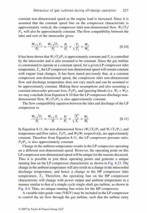
Behaviour of gas turbines during off-design operation 227
constant non-dimensional speed as the engine load is increased. Since it isassumed that the constant speed line on the compressor characteristic isapproximately vertical, the compressor inlet non-dimensional flow, W3√T3/P3, will also be approximately constant. The flow compatibility between theinlet and exit of the intercooler gives:
W TP
W TP
PP
TT
WW
3 3
3
2 2
2
2
3
3
2
3
2 = × × × [8.10]
It has been shown that W3√T3/P3 is approximately constant and T3 is controlledby the intercooler and is also assumed to be constant. Since the gas turbineis constrained to operate at a constant speed, for a given LP compressor inlettemperature, T1, the LP compressor non-dimensional speed will remain constantwith engine load changes. It has been stated previously that, at a constantcompressor non-dimensional speed, the compressor inlet non-dimensionalflow and discharge temperature does not vary much and can be assumed tobe approximately constant. Making these assumptions and also assuming aconstant intercooler pressure loss, P2/P3, and ignoring bleeds (i.e. W3 = W2),we may conclude from Equation 8.10 that the LP compressor discharge non-dimensional flow, W2√T2/P2 is also approximately constant.
The flow compatibility equation between the inlet and discharge of the LPcompressor is:
W TP
W TP
PP
TT
WW
2 2
2
1 1
1
1
2
2
1
2
1 = × × × [8.11]
In Equation 8.11, the non-dimensional flows (W2√T2/P2 and W1√T1/P1), andtemperature and flow ratios, T2/T1, and W2/W1 respectively, are approximatelyconstant. Therefore from Equation 8.11, the LP compressor pressure ratio,P2/P1, is also approximately constant.
Change in the ambient temperature results in the LP compressor operatingon a different non-dimensional speed. However, the operating point on thisLP compressor non-dimensional speed will be unique for the reasons discussed.Thus it is possible to join these operating points and generate a uniquerunning line on the LP compressor characteristic as shown in Fig. 8.23. Thechange in the ambient temperature will also result in a change in the intercooleddischarge temperature, and hence a change in the HP compressor inlettemperature, T3. Therefore, the operating line on the HP compressorcharacteristic will change with power output and ambient temperature in amanner similar to that of a simple cycle single-shaft gas turbine, as shown inFig. 8.4. Thus, no unique running line exists for the HP compressor.
A variable inlet guide vane (VIGV) may be included in the LP compressorto control the air flow through the gas turbine, such that the turbine entry
© 2007 by Taylor & Francis Group, LLC
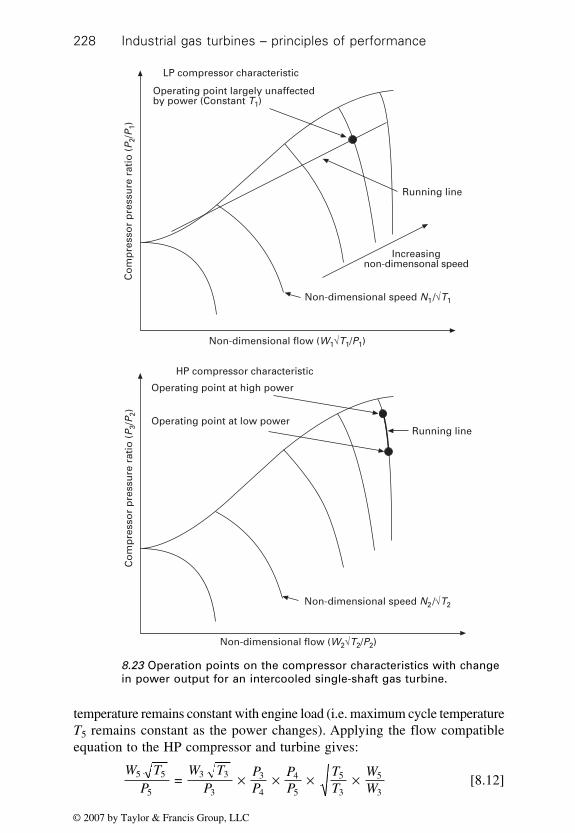
Industrial gas turbines – principles of performance228
temperature remains constant with engine load (i.e. maximum cycle temperatureT5 remains constant as the power changes). Applying the flow compatibleequation to the HP compressor and turbine gives:
W TP
W TP
PP
PP
TT
WW
5 5
5
3 3
3
3
4
4
5
5
3
5
3 = × × × × [8.12]
8.23 Operation points on the compressor characteristics with changein power output for an intercooled single-shaft gas turbine.
LP compressor characteristic
Operating point largely unaffectedby power (Constant T1)
Co
mp
ress
or
pre
ssu
re r
atio
(P 2
/P1)
Non-dimensional speed N1/√T1
Non-dimensional flow (W1√T1/P1)
Increasingnon-dimensonal speed
Running line
HP compressor characteristic
Operating point at high power
Co
mp
ress
or
pre
ssu
re r
atio
(P 3
/P2)
Non-dimensional speed N2/√T2
Non-dimensional flow (W2√T2/P2)
Running lineOperating point at low power
© 2007 by Taylor & Francis Group, LLC

Behaviour of gas turbines during off-design operation 229
Making the usual assumptions, W3√T3/P3 and W5√T5/P5 will be constant(vertical compressor speed lines and choked turbine nozzle, respectively).Assuming constant pressure losses and ignoring bleeds, P4/P5 will be constantand W5 = W3. Operating at the constant maximum cycle temperature, T5,thus for a given minimum cycle temperature, T3 (which would ideally beequal to the ambient temperature, T1–perfect intercooler), the HP compressorpressure ratio must remain essentially constant as the engine load changes inorder to maintain the flow compatibility between the HP compressor andturbine (Equation 8.12). Thus, for a given compressor inlet temperature, allthe pressure ratio change takes place in the LP compressor, as illustrated inFig. 8.24. This is in contrast with the previous case, (no VIGV), where it wasdetermined that all the pressure ratio changes take place in the HP compressorrather than in the LP compressor.
A similar off-design behaviour occurs with an intercooled three-shaft gasturbine operating with a variable geometry free power turbine. When thepower turbine capacity is adjusted such that the turbine entry temperatureremains constant at part load conditions, the operating point on the HPcompressor remains unchanged and all the pressure ratio change occurs in theLP compressor. It is assumed that the intercooling process takes place betweenthe LP and HP compressors. This result is due to the LP turbine remainingchoked and therefore forcing the HP turbine pressure ratio to be fixed. Thusthe HP turbine non-dimensional temperature drop is also fixed. Due to theconstant turbine entry temperature at off-design conditions, the HP turbinetemperature drop will also remain constant. Since the HP compressor inlettemperature is maintained at a constant value due to intercooling the HP spool,the power balance between the HP compressor and turbine will maintain theHP compressor non-dimensional speed at a fixed value. As the turbine entrytemperature and the HP compressor inlet temperature remain constant, dueto the effect of the variable geometry power turbine and intercooling, respectively,the operating point on the HP compressor characteristic will be fixed wherethe HP compressor non-dimensional speed intersects the line of constantmaximum to minimum temperature ratio on the HP compressor characteristic.
It must be pointed out that, when the design point performance is optimisedfor maximum thermal efficiency (i.e. approximately equal LP and HPcompressor pressure ratio for a regenerative cycle), this optimum split incompressor ratios cannot be maintained at off-design conditions. Thusintercooled cycles may not achieve the maximum possible thermal efficiencyat off-design conditions due to intercooling.
8.6.2 Reheat: two- and three-shaft gas turbine operatingwith a free power turbine
It has been discussed that the matching of turbines in series results in the lowpressure turbine restrict the operating range of the high pressure turbine in
© 2007 by Taylor & Francis Group, LLC

Industrial gas turbines – principles of performance230
N
T1
1
= 90%
N
T1
1
= 105%
N
T1
1
= 100%
LP compressor characteristic
CharacteristicVIGV closed
Co
mp
ress
or
pre
ssu
re r
atio
(P
2/P
1)
Running line
Non-dimensional flow (W1√T1/P1)
HP compressor characteristic
Operating point largelyunaffected by power output
Com
pres
sor
pres
sure
rat
io (P
3/P
2)
Non-dimensional speed N2/√T2
Non-dimensional flow (W2√T2/P2)
CharacteristicVIGV opened
8.24 Running lines on the LP and HP compressor characteristics foran intercooled single-shaft gas turbine using a VIGV in the LPcompressor.
order to maintain the flow compatibility between them. For a two-shaft gasturbine operating with a free power turbine, the power turbine characteristiccontrols the operating point on the gas generator (GG) turbine characteristicsuch that the flow demanded by the power turbine is satisfied. When we
© 2007 by Taylor & Francis Group, LLC

Behaviour of gas turbines during off-design operation 231
apply reheat to such an engine, as shown in Fig. 8.25, the reheat is usuallyapplied between the gas generator and power turbine and this affects thematching of the turbines resulting in a redistribution of the turbine pressureratios in order to satisfy the flow compatibility between them. Consideringthe flow identity (Equation 8.13), describing the non-dimensional flow atexit from the GG turbine:
W TP
W TP
PP
TT
WW
4 4
4
3 3
3
3
4
4
3
4
3 = × × × [8.13]
and the flow identity at the exit of the reheat chamber:
W TP
W TP
PP
TT
WW
5 5
5
4 4
4
4
5
5
4
5
4 = × × × [8.14]
The reheater exit non-dimensional flow, W5√T5/P5, must be ‘swallowed’ bythe power turbine. If it is assumed that the power turbine is choked, thenW5√T5/P5 will remain constant as the amount of reheat is varied, which isgiven by Tr (reheat temperature ratio) = T5/T4. Increasing reheat will increaseT5/T4 and thus Tr. If we assume that the reheater pressure loss, P4/P5, isconstant and ignore bleeds, any increase in reheat must be accompanied bya decrease in W4√T4/P4 to satisfy the flow compatibility in the reheater(Equation 8.14). However, W4√T4/P4 is the exit non-dimensional flow fromthe GG turbine. Assuming the GG turbine is choked and ignoring bleeds, the
Load
Po
wer
tu
rbin
e
GG
tu
rbin
e
Reheater
Fuel input
Fuel input
Combustor
Compressor
6
54
321
1 Compressor inlet
2 Compressor exit/combustor inlet
3 Combustor exit/gas generator (GG) turbine inlet
4 GG turbine exit/reheater inlet
5 Reheater exit/power turbine inlet
6 Power turbine exit
8.25 Schematic representation of a two-shaft reheat gas turbineoperating with a free power turbine.
© 2007 by Taylor & Francis Group, LLC

Industrial gas turbines – principles of performance232
reduction in W4√T4/P4 will result in a decrease in GG turbine pressure ratio,P3/P4, as required by Equation 8.13. (Although there is an increase in T4/T3due to the decrease in P3/P4, the effect of the reduction in GG turbine pressure(P3/P4) is dominant). The effect of reheat on the GG turbine pressure ratio isillustrated in Fig. 8.26, which shows the matching of the GG and powerturbine characteristics due to the application of reheat. The operating pointon the GG turbine characteristic decreases in pressure ratio as the amount ofreheat, Tr, is increased (from (1) to (2) in Fig. 8.26). Note the zero reheat linecorresponds to the case when Tr = 1.
Reheat is usually applied when the gas generator is operating at its maximumspeed or at the maximum turbine entry temperature. However, the decreasein the GG turbine pressure will decrease the non-dimensional temperaturedrop across the GG turbine, ∆T34/T3. If we are continuously operating at themaximum compressor speed and a given compressor inlet temperature, T1,the compressor non-dimensional speed, N1/√T1 will be constant during theapplication of reheat. From the discussion above, the compressor non-dimensional temperature rise, ∆T21/T1, will be approximately constant. Fromthe work compatibility equation or power balance Equation 8.4, the decreasein ∆T34/T3 must result in an increase in T3/T1 and for a given T1, will thereforeincrease the turbine entry temperature, T3.
Assuming that the compressor speed lines are approximately vertical,therefore there is little variation in the compressor inlet non-dimensionalflow, W1√T1/P1 with compressor pressure, P2/P1. For a choked gas generatorturbine, W3√T3/P3, is a constant) and from Equation 8.5, which describes the
8.26 Matching of the GG and power turbines due to the applicationof reheat.
(2) (1)Pressure ratio
Pressure ratio
HP or GG turbinecharacteristic
No
n-d
imen
sio
nal
flo
w
Increasing reheat
LP or power turbinecharacteristic
Increased power turbinearea to maintain GG
turbine pressure ratiodue to reheat
Decrease gas generatorturbine pressure ratio
due to reheat
Tr = 1.0(No reheat)
Tr = 1.4Tr = 1.3Tr = 1.2Tr = 1.1
© 2007 by Taylor & Francis Group, LLC

Behaviour of gas turbines during off-design operation 233
flow compatibility of the gas generator, an increase in T3/T1 will result in anincrease in the compressor pressure ratio, P2/P1. Thus reheat increases thecompressor pressure ratio as illustrated in Fig. 8.27, which shows the changein the operating point on the compressor characteristic due to reheat.
Thus reheat increases the turbine entry temperature and will contributefurther in the increase in the power output of the gas turbine. However, theturbine creep life may be compromised severely and the application of reheatwould normally require a variable geometry power turbine. It has been shownthat increasing the power turbine capacity will increase the GG turbine pressureratio as illustrated in Fig. 8.26. Thus by increasing the power turbine capacitysufficiently during reheat, it is possible to maintain the design turbine entrytemperature and compressor pressure ratio. (It is worth pointing out that,when jet engines employ reheat or afterburning to augment the thrust, theyoften incorporate a variable geometry propelling nozzle, which is open duringreheat operation.)
A three-shaft gas turbine operating with a free power turbine will usuallyapply reheat between the LP turbine and the power turbine. The redistributionof pressure ratio across the three turbines during the reheat operation isillustrated in Fig. 8.28. In this case, we observe the decrease in the LPturbine pressure ratio due to the application of reheat results in a decrease inLP turbine work. Hence a higher LP turbine inlet temperature is required tomaintain the power balance of the LP spool when operating at a constant
8.27 Change in the operating point on the compressor characteristicdue to reheat.
Surge line
Co
mp
ress
or
pre
ssu
re r
atio
(P 2
/P1)
T3 /T1 increasing
Non-dimensional speed N1/√T1
Non-dimensional flow (W1√T1/P1)
Operating pointreheat
Running lineno reheat
Operating pointno reheat
© 2007 by Taylor & Francis Group, LLC

Industrial gas turbines – principles of performance234
speed. Since the HP turbine is shielded from the effects of reheat due to thechoking of the LP turbine, the increase in LP turbine entry temperature willresult in an increase in the HP turbine entry temperature, thus increasing thework done by the HP turbine. The increase in HP turbine work is absorbedin the HP compressor by increasing the HP spool speed as illustrated in Fig.8.29. Since we are operating at a constant LP compressor speed, the increasein HP compressor non-dimensional flow due to its increase speed can onlybe satisfied by decreasing the LP compressor pressure, as shown in Fig.8.29. Thus the effect of reheat on the LP compressor is opposite to theprevious case, where reheating was considered for a two-shaft gas turbineoperating with a free power turbine.
Reheating a single-shaft gas turbine may also be considered by splittingthe turbine into two parts. The matching of the flows between the turbineswill be similar to that shown in Fig. 8.26. Although there will be a reductionin the HP turbine pressure ratio, and thus the work produced by the HPturbine, the two turbines are linked mechanically and therefore transfer ofpower from the LP to the HP turbine can occur. Hence, the compressoroperating point and the turbine entry temperature can remain at the designvalue without the use of any variable geometry in the turbine.
In fact, power transfer has been applied to two-shaft gas turbines operatingwith a free power turbine, where controlled amounts of power are transferredfrom the GG turbine to the power turbine by the use of clutches (Turunenand Collman, 1965). Such techniques have been applied to regenerativeautomotive gas turbines to improve the part-load thermal efficiency. For
8.28 Turbine characteristics of a three-shaft gas turbine operatingwith a free power turbine during the application of reheat.
(1A) (2)HP pressure ratio Power turbine pressure ratio
No change in HPturbine pressure ratio
due to reheat
No
n-d
imen
sio
nal
flo
w
Increasing reheat
Decrease LP turbinepressure ratio due
to reheat
Tr = 1.4Tr = 1.3Tr = 1.2Tr = 1.1Tr = 1.0
Zero reheat line
HP turbine LP turbine
(1)LP pressure ratio
Power turbine
© 2007 by Taylor & Francis Group, LLC

Behaviour of gas turbines during off-design operation 235
naval applications, it is possible to consider a separate variable pitch propellerand shaft connected to the GG turbine. Thus it is possible to transfer powerfrom the GG shaft such that the maximum turbine entry temperature ismaintained at part-load operation. The incorporation of a heat exchanger andpower transfer then can result in significant increase in off-design thermalefficiency of the gas turbine.
8.29 Change in the operating points on the LP and HP compressorcharacteristics due to reheating a three-shaft gas turbineincorporating a free power turbine.
LP compressor characteristic
Surge line
Co
mp
ress
or
pre
ssu
re r
atio
(P 2
/P1)
Non-dimensional speed N1/√T1
Non-dimensional flow (W1√T1/P1)
HP compressor characteristic
Co
mp
ress
or
pre
ssu
re r
atio
(P 3
/P2)
Non-dimensional speed N2/√T2
Non-dimensional flow (W2√T2/P2)
Running line (LP)
T4/T1 increasing
Operating pointreheat
Operating pointreheat
Surge line
Running line (HP)
T4/T2 increasing
© 2007 by Taylor & Francis Group, LLC

Industrial gas turbines – principles of performance236
8.7 Running line, non-dimensional parameters and
correcting data to standard conditions
The previous analysis on gas turbines using a free power turbine (withoutreheat) essentially describes a unique running line on the compressor andturbine characteristics. Therefore, for any given parameter, such as thecompressor non-dimensional speed, there is a unique value for other parameterssuch as the compressor pressure ratio, temperature ratio, and non-dimensionalmass flow. If these parameters are now plotted against compressor non-dimensional speed, we should obtain a unique line. The reason why theseunique lines are obtained is because gas turbines behave non-dimensionally.Figure 8.30 shows such an example for the compressor inlet non-dimensionalflow varying with compressor non-dimensional speed. Similar figures canbe drawn for other parameters for each engine component such as compressorsand turbines. Power and fuel flow can also be written in non-dimensionalterms and these terms may be derived from the non-dimensional steady flowenergy equation. The non-dimensional terms for power and fuel flow arePower/(P1√T1) and Fuel flow/(P√T1), respectively.
8.7.1 Correction of data to standard conditions
Gas turbine performance is very sensitive to ambient conditions. Operatorsoften require the engine performance at some standard atmospheric conditions
8.30 Variation of a compressor inlet non-dimensional flow with speeddue to the non-dimensional nature of gas turbines.
Non-dimensional speed (N1/√T1)
No
n-d
imen
sio
nal
flo
w (
W1√
T 1/P
1)
© 2007 by Taylor & Francis Group, LLC

Behaviour of gas turbines during off-design operation 237
so that the performance of different engines may be compared. Standardconditions normally refer to 1 standard atmosphere, usually 1.013 Bar, and288.15 K or 15 degrees Celsius (also referred to as ISO conditions). However,for gas turbines operating in tropical environments, we have to correct theengine performance to an ambient temperature of 30 degrees Celsius. InNordic countries, the average ambient temperature would be 0 degrees Celsiusto give a more meaningful performance of the gas turbine.
The correction of data to these standard conditions is achieved by equatingthe respective non-dimensional parameters at the two different operatingconditions. For example, when correcting power to standard conditions thenon-dimensional power at the actual condition is equated to that of thestandard condition as follows.
Pow = PowCor
Cor Cor1 1 1 1P T P T
thus
PowCor = Pow Cor Cor1 1
1 1P T
P T×
where Pow, T1 and P1 correspond to the actual power and ambient conditionsand PowCor, T1Cor and P1Cor correspond to the standard ambient conditions.Similarly, we can correct fuel flow, airflow, speeds and other engine parameterssuch as pressures and temperatures to standard conditions by equating theirrespective non-dimensional parameters.
In fact, the corrected value for power may be determined directly using
corrected parameters and corresponds to PowCor
δ θ
where δ = cor1
1
PP
and θ = cor1
1
TT
.
Similarly, corrected compressor flow, W1Cor and speed, N1Cor are determinedby:
W1Cor θδ and
N1Cor
θrespectively. More information on non-dimensional groups may be found inWalsh and Fletcher.6
8.8 Power turbine curves
Power turbines are used to drive various loads. In power generation applicationsthe power turbine (and generator) will run at a synchronous (mechanical)speed independent of the power output, whereas in mechanical drive
© 2007 by Taylor & Francis Group, LLC

Industrial gas turbines – principles of performance238
applications, the power turbine runs at different speeds depending on theload, which is determined by the process conditions. However, the performanceof the power turbine is not entirely determined by the mechanical speed butalso by its non-dimensional speed, which is dependent on the power turbineinlet temperature and pressure ratio. Thus, the non-dimensional speed willvary with load even in power generation applications where the mechanicalspeed of the power turbine remains constant. However, operators often requiresuch data in terms of mechanical speed rather than in terms of non-dimensionalspeed because it is easier to relate such data to their process conditions.
This is achieved by plotting the power turbine power output with speedfor a series of gas generator speeds, as illustrated in Fig. 8.31. This shows thevariation of power output with power turbine speed for a range of gas generatorspeeds and is normally drawn for ISO conditions. For a three-shaft engineoperating with a free power turbine, the curves is drawn for a series of LPspool speeds.
For a given gas generator speed, there is a region where the power outputincreases with power turbine speed. This increase is primarily due to anincrease in power turbine efficiency. Often, operators are concerned with themaximum power available from the gas turbine at various ambient temperatures.The above figure can be represented in terms of ambient temperature. Linesof constant gas generator speeds are shown in Fig. 8.31 and can be replacedby lines of constant ambient temperatures while maintaining the mechanicalspeed of the gas generator at 100%. It should be noted that each constanttemperature line also corresponds to a particular compressor non-dimensional
Power turbine speed (RPM)
Po
wer
tu
rbin
e p
ow
er o
utp
ut
100% gas generator speed
Increasinggas generator
speed
8.31 Variation of power turbine power output with power turbinespeed for a series of gas generator speeds.
© 2007 by Taylor & Francis Group, LLC

Behaviour of gas turbines during off-design operation 239
speed, although the mechanical speed of the gas generator remains at 100%,as illustrated in Fig. 8.32.
With aero-derived gas turbines, one manufacturer may build the gasgenerator while another, normally a package provider, will provide thepower turbine. Providing the power turbine swallowing capacity matchesthat specified by the gas generator manufacturer, the performance of the gasgenerator should not be compromised. Having selected a gas generator, theuser may consider various power turbines by comparing their performanceas shown in Figures 8.31 and 8.32. The variations of thermal efficiency withpower turbine speed can also be illustrated and will be similar in shape to thecurves shown in Figures 8.31 and 8.32.
8.9 Gas power and gas thermal efficiency
Means of comparing the performance of power turbines have been discussed.The performance of gas generators may be compared by comparing the gaspowers generated. The gas power is calculated by assuming that the expansionthrough the power turbine is isentropic (i.e. that the power turbine efficiencyis 100%). The thermal efficiency of the gas generator is referred to as the gasthermal efficiency and is calculated from the gas power, thus enablingcomparison of the performance of different gas generators. The comparisonof gas generator performance may be carried out at various ambienttemperatures and pressures, which the user is more likely to encounter during
8.32 Variation of power turbine output with power turbine speed fora series of ambient temperatures.
Power turbine speed (RPM)
Po
wer
tu
rbin
e p
ow
er o
utp
ut
Gas generator speed constant at 100%
Increasing ambienttemperature or
decreasing compressornon-dimensional
speed
© 2007 by Taylor & Francis Group, LLC

Industrial gas turbines – principles of performance240
operation rather than at ISO conditions. These are therefore more useful andare often referred to as site-rated conditions.
8.10 Heat rate and specific fuel consumption
The thermal efficiency of the gas turbine has been defined as the work doneper unit input of heat. However, operators on occasions require the amountof heat per unit of work done and this is referred to as the heat rate of theengine. Thus, the heat rate is simply the reciprocal or the inverse of thethermal efficiency and is usually quoted in kJ of heat per kW hour. Thus theheat rate (HR) is given by:
HR = 3600thη [8.15]
where ηth is the thermal efficiencyAn alternative means to determine the heat input per unit of work done is
to express the heat input in terms of fuel consumption. This is referred to asthe specific fuel consumption or SFC. It is usually quoted as kg of fuel perkW hour and is given by:
SFC = 3600 th netη × Q
[8.16]
where Qnet is the lower heating value (LHV) of the fuel.It is evident from Equations 8.15 and 8.16 that the heat rate and specific
fuel consumption are related via the LHV of the fuel. Thus the heat rate canbe expressed as:
HR = SFC × Qnet [8.17]
8.11 References
1. Gas Turbine Theory, 5th Edition, Saravanamuttoo, H.I.H., Rogers, C.F.G., Cohen,H., Longman (2001).
2. Effect of variable-position inlet guide vane and inter-stage bleed on compressorperformance of a high-pressure-ratio turbo jet engine. Huntly, S.C. and Braithwait,W.N, NACA Research Memorandum, December 1956.
3. The variable geometry power turbine. Ranhk, W.A., Trans. SAE (1969).4. The performance of vehicular gas turbines, Bareau, D.E., Trans. SAE (1970).5. The General Motors Research GT-309 gas turbine, Turunen, W.A. and Collman,
J.S., SAE Trans., 740[iv]. (1965), pp. 337–77.6. Gas Turbine Performance, 2nd Edition, Walsh, P.P. and Fletcher, P., Blackwell
Publishing (2004).
© 2007 by Taylor & Francis Group, LLC

241
Earlier chapters described the matching of engine component characteristics,namely compressors, combustors and turbines in determining gas turbineperformance. In fact, it is the interaction of engine components that determinesengine parameters such as pressures, temperatures, flows, speeds and poweroutputs. Any engine performance deterioration results from a change in thecomponent characteristic of the deteriorated components. The interaction ofthese deteriorated characteristics results in a loss of power output and thermalefficiency. The measurable parameters such as pressures, temperatures, flowsand speeds will also change for a given engine operating condition and theeffect of performance deterioration is summarised in Fig. 9.1. Useful discussionsare found in Ping and Saravanamuttoo1 and Urban.2
The following conditions are typical causes of gas turbine performancedeterioration:
• fouling• variable inlet guide vane and variable stator vane problems
9Gas turbine performance deterioration
The interaction of thesedeteriorated
characteristics results ina change in measurableparameters and a lossin power and thermal
efficiency
Results in change incomponent
characteristics
Componentperformancedeterioration
9.1 Effect of component performance deterioration on engineperformance.
© 2007 by Taylor & Francis Group, LLC

242 Industrial gas turbines – principles of performance
• hot end damage• tip rubs• vibration• seal wear and damage• foreign object damage (FOD) and domestic object damage (DOD)• erosion• corrosion• control system malfunction.
A good general discussion on the causes and consequences of componentperformance deterioration on overall engine performance is given inSaravanamuttoo et al.3
9.1 Compressor fouling
Compressor fouling is probably the most common cause of performancedeterioration. Compressor fouling results from the ingestion of dirt, dust,pollen, sap and general airborne debris. Filtration can only arrest fouling butcannot prevent it. Compressor fouling affects both compressor flow capacityand efficiency, but the effect on flow capacity is usually greater. The effectof fouling on the possible change in the compressor blade profile is shownin Fig. 9.2. The build-up of deposits will reduce the flow area, thus reducingthe flow coefficient, and the change in blade profile will increase the tendencyfor the flow to separate, reducing the efficiency of the compressor.
The change in the compressor flow characteristic due to fouling is shownin Fig. 9.3 where the lines of constant non-dimensional speeds are shifted tothe left, thus reducing the flow capacity of the compressor. Figure 9.4 showsthe impact of fouling on compressor efficiency. Compressor fouling affectsall stages; however, the biggest impact is on the front stages of the compressor.At normal operating speeds (high speeds), the compressor flow is controlledby the front stages of the compressor, thus fouling reduces the compressorflow capacity. However, at low compressor speeds, the choking of the HP
9.2 Build-up of deposits on the compressor blade profile duringcompressor fouling.
Rotor Direction ofrotation
Build-up of depositsdue to fouling Increase in tendency for
the flow to separate at thetrailing edge
© 2007 by Taylor & Francis Group, LLC

Gas turbine performance deterioration 243
stages normally controls the flow through the compressor where fouling isminimal. No change in the compressor flow characteristic will therefore beobserved at these low speeds. Such low speed operation is usually at engineidle conditions and is of little importance. It is the high-speed part of thecompressor characteristic that is important, as it is here that the enginespends most of its operating time and fouling effects are greatest. An excellentdescription of the effects of fouling on the compressor characteristic usingcomputer simulations is given in Saravanamutoo and Lakshmiranasimha.4
In Section 8.2, under the heading ‘Variable stator vanes and inlet guide
Surge line
Fouled compressorClean compressor
Pre
ssu
re r
atio
25
20
15
10
5
00.3 0.4 0.5 0.6 0.7 0.8 0.9 1 1.1
Non-dimensional flow relative to design
9.3 Impact of compressor fouling on the compressor flowcharacteristic.
9.4 Effect of compressor fouling on the compressor efficiencycharacteristic for a given compressor non-dimensional speed.
Fouled compressor
Clean compressor
Isen
tro
pic
eff
icie
ncy
(–)
0.88
10Compressor pressure ratio
0.87
0.86
0.85
0.84
0.83
0.82
0.81
0.80
0.79
0.7811 12 13 14 15 16 17 18 19 20
© 2007 by Taylor & Francis Group, LLC

244 Industrial gas turbines – principles of performance
vanes (compressors)’ the impact of improved compressor efficiency on therunning line was discussed. It was shown that an improvement in the compressorefficiency moves the running line on the compressor characteristic awayfrom surge (two-shaft gas turbine operating with a free-power turbine). Whencompressors foul, there is a loss of compressor efficiency, thus shifting therunning line towards surge and reducing the surge margin, as illustrated inFig. 9.5.
Since the change or reduction in flow capacity is usually greater than theeffect on compressor efficiency, the compressor pressure ratio decreaseswith compressor fouling for a given compressor non-dimensional speed andthis situation is illustrated in Fig. 9.6.
Although measuring the change in compressor pressure ratio withcompressor non-dimensional speed gives an indication of compressor fouling,care is necessary as other performance-related faults can also influence thechange in compressor ratio with non-dimensional speed. For instance, anychange in the turbine areas can also give rise to a displacement in the runningline and thus alter the relationship between the compressor pressure ratioand its non-dimensional speed. This has been illustrated in Section 8.2‘Displacement of running line (two-shaft gas turbine)’.
A better indication of compressor fouling can be obtained by plotting thevariation of compressor non-dimensional speed with compressor inlet non-dimensional flow. The variation of the compressor non-dimensional speed
Fouledcompressor
Clean compressorPre
ssu
re r
atio
(P 2
/P1)
Non-dimensional flow (W1√T1/P1)
Running line (fouled)
Operating point (fouled compressor)
Running line (clean)
Operating point(clean compressor)
Surge lines
9.5 Effect of compressor fouling on the running line and operatingpoint for a given compressor non-dimensional speed.
© 2007 by Taylor & Francis Group, LLC

Gas turbine performance deterioration 245
with inlet non-dimensional flow remains unaffected by other performance-related faults and is due to the steep flow line for a given non-dimensionalspeed. However, a measurement of the compressor flow is required and theaccurate measurement of the compressor inlet flow on engines operating outin the field has yet to be achieved. The use of inlet depression measurementsas an indication of compressor flow has been used by Diakunchak5 to detectcompressor fouling. Figure 9.7 shows the variation of non-dimensional flowwith non-dimensional speed due to compressor fouling.
Performance deterioration due to compressor fouling is often recoverableafter a compressor wash. The factors that determine when it is economical towash the compressor are many. They include power demand, fuel cost, down-time for wash (and may include emissions taxes, e.g. CO2). It is necessary todetermine accurately the cost of compressor fouling, i.e. loss in power andincreased heat rate, which can then determine the increase in operating cost(fuel cost) and lost revenue. A general strategy is to increase the wash frequencywhen power demand is high and decrease it at low power demands because,at low power demands, no loss in production should occur because theengine is not on a power limit under low power conditions. However, therewill be an increase in fuel cost, but in applications where fuel cost is low oreven zero, such as in oil and gas exploration and production, washes may bedelayed significantly. Should emissions taxes be imposed, particularly onCO2 emissions, the fuel cost in these industries will no longer be insignificantand optimising compressor washes will be of paramount importance. Onlinewashing seems to be an effective method in combating fouling, but there are
Compressor non-dimensional speed
Co
mp
ress
or
pre
ssu
re r
atio
Fouled compressor
Clean compressor
9.6 Effect of compressor fouling on compressor pressure ratio.
© 2007 by Taylor & Francis Group, LLC

246 Industrial gas turbines – principles of performance
many cases where online washing has done severe damage to compressorblades. However, current manufacturers of online wash systems claim theyhave resolved these issues. Details on the benefits of wash procedures arediscussed in Meher-Homji6 and methods to optimise compressor washingare discussed in Section 9.5.5.
9.2 Variable inlet guide vane (VIGV) and variable
stator vane (VSV) problems
Multi-shaft free turbine gas turbines operating at high-pressure ratios oftenuse variable inlet guide vanes and variable stators to ensure satisfactory andsafe operation of the compressor, particularly at low speeds. The positions ofthe VIGV and VSV are normally functions of the compressor non-dimensionalspeed and Figure 9.8 shows the variation of the VIGV/VSV angle with non-dimensional speed. A region where operation is not possible is also shown,as compressor surge is very likely in this region. Any deviation of the operatingpoint from the operating line (during steady-state operation) would imply afault with the VIGV/VSV system.
In Section 4.10.3 under variable geometry compressors, the effect ofVIGV and VSV on the compressor characteristic has been discussed. Closureof the VIGV will result in the non-dimensional flow decreasing and improvingthe surge margin. Thus, excessive closure of the VIGV/VSV will result in
Compressor non-dimensional speed
Co
mp
ress
or
inle
t n
on
-dim
ensi
on
al f
low
Fouled compressor
Clean compressor
Fouling increasing
9.7 Variation of compressor inlet non-dimensional flow withcompressor speed due to fouling.
© 2007 by Taylor & Francis Group, LLC

Gas turbine performance deterioration 247
the compressor behaving as if it is fouled. This is illustrated in Fig. 9.9,showing the effect of VIGV/VSV closure on the compressor characteristic.Thus, the variation of compressor non-dimensional flow with its non-dimensional speed will be similar to that shown in Fig. 9.7. However,compressor washing would have no effect on the displacement of this runningline. The effect of excessive VIGV closure on compressor flow capacity has
9.8 Variation of VIGV/VSV angle with compressor inlet non-dimensional speed.
9.9 Effect of VIGV/VSV movement on the compressor characteristic.
Non-dimensional speed
Gu
ide
van
e an
gle
(d
egre
es)
Operating line
Variation of VIGV/VSV angle with compressor-non dimensional speed
Do not operate here
300 310 320 330 340 350 360 370 380 390
40
35
30
25
20
15
10
5
0
–5
–10
Pre
ssu
re r
atio
(P 2
/P1)
Non-dimensional flow (W1√T1/P1)
Movement of compressorsurge line due toVIGV/VSV action
Non-dimensionalspeed N1/√T1
Characteristic dueto normalVIGV/VSV position
Increase in flow dueto an insufficientclosure of theVIGV/VSV
Reduction in flow dueto an excessive closureof the VIGV/VSV
© 2007 by Taylor & Francis Group, LLC

248 Industrial gas turbines – principles of performance
been investigated and described in Razak and Dosanjh.7 If the VIGV/VSV isopened excessively, then the running line will move above the baseline inFig. 9.7, where the baseline is shown as a bold line (clean compressors).Excessive opening of the VIGV/VSV is rather more serious, as the surge linemay drift towards the running line and thereby increase the likelihood ofcompressor surge. The influence of VIGV/VSV on the compressor characteristicis also discussed in Muir et al.8
9.3 Hot end damage
Hot end damage is normally associated with turbines. Turbines operate atvery high gas temperatures, often above the melting point of the turbineblade material. Extensive turbine cooling is therefore employed (as discussedin Section 5.7) to achieve satisfactory turbine creep life. The highesttemperatures that occur are at the stagnation points which correspond to theleading and trailing edges of the turbine blade. The trailing edge of theturbine blade has little material and cooling is often difficult; thus, over aperiod of time, damage can occur to this part of the turbine blade. The flowcapacity of the turbine is normally controlled by the nozzle guide vane(NGV) and is determined by the flow area defined by the trailing edge of theblade. Any change in the turbine blade profile involving the trailing edge ofthe blade will also have an impact on the turbine characteristic and thus onthe performance of the engine.
Hot end damage will normally increase the turbine non-dimensional flowcapacity and any change in the incidence of the gas on the turbine rotor willalso affect its efficiency. Figure 9.10 shows a schematic representation of thenozzle guide vane, indicating trailing edge damage. The increase in turbineflow capacity does not reduce turbine performance necessarily. Under certaincircumstances, for example, when the gas generator speed limits the poweroutput of the gas turbine, an increase in power output is possible; however,an adverse impact on turbine life would occur. A reduction in turbine efficiencywill always have a negative impact on the gas turbine performance and
Stator or NGV
Trailing edge damageto a NGV
9.10 Change in the NGV profile due to hot end damage.
© 2007 by Taylor & Francis Group, LLC

Gas turbine performance deterioration 249
engine life. Figures 9.11 and 9.12 show the changes in the turbine flow andefficiency characteristics due to hot end damage, respectively.
The effect of hot end damage on the gas generator turbine of a two-shaftgas turbine (using a free power turbine) would be to move the running lineaway from surge, as discussed in Section 8.2, ‘Displacement of running line(single- and two-shaft free power turbine gas turbine’. Thus, the variation ofcompressor pressure ratio with compressor non-dimensional speed would besimilar to that observed during compressor fouling. Gas turbines that burnfuel containing high ash content may suffer from a reduction in the turbineflow capacity due to deposit of ash on the turbine components, and thevariation of compressor pressure ratio with compressor non-dimensional
No
n-d
imen
sio
nal
flo
w r
elat
ive
to d
esig
n 1.2
1.0
0.8
0.6
0.4
0.2
01 1.5 2 2.5 3 3.5 4 4.5
Deteriorated characteristic
Design characteristic
Pressure ratio
9.11 Effect of hot end damage on the turbine flow characteristic.
Isen
tro
pic
eff
icie
ncy
(–)
0.90
1 1.5 2 2.5 3 3.5 4 4.5
Deteriorated characteristicDesign characteristic
Pressure ratio
0.88
0.86
0.84
0.82
0.80
0.78
0.76
0.74
0.72
0.70
9.12 Effect of hot end damage on the turbine efficiency characteristic.
© 2007 by Taylor & Francis Group, LLC

250 Industrial gas turbines – principles of performance
speed will be the opposite to that due to hot end damage of the turbine.Regular cleaning of the turbine would be required to maintain the performanceof the gas turbine. Means to detect turbine fouling can be developed wherethe variation of the turbine non-dimensional flow with its pressure ratio isplotted, as shown in Fig. 9.11.
9.4 Tip rubs and seal damage
The clearances between the rotor and the casing in turbomachinery shouldbe kept to a minimum in order to minimise overtip leakages. In axialcompressors, the stage pressure ratios are small compared with axial turbines.Thus, turbine rotors are usually provided with tip seals, in the form of ashroud to prevent such overtip leakages. Compressors normally do not havesuch shrouds; however, the clearances are kept to a minimum.
During normal operation, rubs occur during start-up and also, possibly,due to high vibration. Operation over a period of time will also increasethese clearances due to wear. In axial compressors, an increase in tip clearanceof the front stages would result in a change in both compressor flow capacityand efficiency, as it is the front stages of the compressor that control theflow. Increases in clearance of the HP stages of an axial compressor normallyaffect the compressor efficiency rather than the flow capacity. Thus, thechange in capacity characteristic of the compressor due to front stages rubbingis similar to that of compressor fouling. However, unlike compressor fouling,this performance loss is not recoverable after an engine wash.
The effect of damage to the turbine shroud normally affects the efficiencyof the turbine rather than the flow and this is mainly due to the flow capacityof the turbine being set by the choking of the nozzle guide vanes. Other sealsare also provided in compressors and turbines to prevent or reduce internalleakages. One type of seal is called a labyrinth seal, which consists of knife-edges on a static or rotating component of the turbine or compressor assembly,as illustrated in Fig. 9.13. Other types of seals are honeycomb seals and ringseals. Damage to these seals normally affects the compressor/turbine efficiencyrather than the flow capacity.
9.5 Quantifying performance deterioration and
diagnosing faults
The above discusses performance deterioration in a qualitative manner andmeans to detect performance deterioration. However, we require methods toquantify performance deterioration. Such information is required on acomponent level basis. Additionally, since performance deterioration adverselyaffects gas turbine power output and heat rate/thermal efficiency, the impactof any performance deterioration on these performance parameters is also
© 2007 by Taylor & Francis Group, LLC

Gas turbine performance deterioration 251
required. It was stated at the beginning of this chapter that performancedeterioration results from the change in component characteristics, namelycompressors and turbines, as shown in Figs 9.3, 9.4 for compressors andFigs 9.11 and 9.12 for turbines. It was also stated that measurable parameterssuch as pressures, temperatures, flows and speeds are determined by theinteraction of engine components and when performance deteriorationoccurs the change in these component characteristics results in the changein the measurable parameters, as summarised in Fig. 9.1. A performance-related fault can therefore be defined as a change in the componentcharacteristic.
9.5.1 Fault indices
Fault indices are means of determining the deteriorated componentcharacteristics. They represent the percentage change of the undeterioratedcharacteristic. Two fault indices can be defined for any component and theycorrespond to the fouling and efficiency fault index. For example, the fouledcompressor flow characteristic, as shown in Fig. 9.3 is determined by reducingthe compressor non-dimensional flow for any given non-dimensional speedline by 3%, and the deteriorated compressor efficiency characteristic shownin Fig. 9.4 is obtained by reducing the compressor isentropic efficiency forany given speed line by 1%. Thus, for a fouled compressor, the compressorfouling fault index and the compressor efficiency fault index is –3% and –1%, respectively, for this case.
Similarly, fault indices can be used to determine deteriorated turbinecharacteristics and these fault indices correspond to the turbine fouling faultindex and turbine efficiency fault index. The deteriorated turbine characteristicsshown in Figs 9.11 and 9.12 are obtained by applying a turbine fouling faultindex of 3% and a turbine efficiency fault index of –1%, respectively.
Stator Labyrinth seals
Low pressure
Rotor
High pressure
Gas flow direction
9.13 Schematic representation of a labyrinth seal arrangement.
© 2007 by Taylor & Francis Group, LLC

252 Industrial gas turbines – principles of performance
9.5.2 Quantifying performance deterioration
Fault indices are quite powerful in quantifying performance deterioration asthey provide a means of determining the deteriorated component characteristic.As a result, they also detect and quantify performance deterioration on acomponent by component basis. Thus, one of the objectives in performancemonitoring and diagnostics is achieved by the use of fault indices. Sincefault indices give us the deteriorated component characteristic, the enginemodel with deteriorated component characteristics can now be used to evaluatethe loss in power output and increase in heat rate due to performancedeterioration and therefore achieve the second objective of performancemonitoring and diagnostics.
To determine fault indices, we need to be armed with an engine modelrepresenting the undeteriorated gas turbine that we wish to monitor. Themodel can be a steady-state model, built using the methods discussed inChapter 7. In this event the measured data should also correspond to steady-state conditions. This can be achieved by filtering the measured data as doneby Teukolsky et al.9 and by Dole.10 The engine model is run at the currentoperating conditions of the gas turbine and the measured data is comparedwith corresponding data determined by the model (expected or predictedmeasured values). If they do not match, fault indices are used to alter thecomponent characteristics until they match. At the end of this iterative orimplicit process, all the component fault indices are determined. This processfor a single-shaft gas turbine is summarised in Fig. 9.14. The measurementsrequired for a single-shaft gas turbine are as follows:
(1) compressor inlet temperature(2) compressor inlet pressure(3) compressor exit temperature(4) compressor exit pressure(5) turbine exit temperature (exhaust gas temperature, EGT)(6) turbine exit pressure(7) fuel flow(8) gas turbine speed(9) gas turbine power output
(10) variable inlet guide vane/variable stator vane position if applicable.
Single shaft gas turbines are often used in power generation and the gasturbine power output can be determined from the generator output. The totalnumber of fault indices is four and they correspond to the compressor foulingand efficiency fault indices and to the turbine fouling and efficiency fault indices.
A similar approach can be used to determine the fault indices for otherengine configurations discussed earlier. For a two-shaft gas turbine operatingwith a free power turbine the required measurements are:
© 2007 by Taylor & Francis Group, LLC

Gas turbine performance deterioration 253
9.14 Procedure to determine fault indices by comparing the enginemeasured parameters with those obtained from the model.
Start
Initialise all faultindices to zero
Run the engine model at the operatingconditions (i.e. run the model at themeasured compressor inlet pressure
and temperature, turbine exitpressure, power output and
VIGV position)
NoAdjust the turbineefficiency fault index
Does themeasured
EGT match thevalue fromthe model?
Yes
NoAdjust the turbinefouling fault index
Does thecompressorexit pressure
match themodelvalue?
Yes
No
Yes
No
Adjust the compressorefficiency fault index
Adjust the compressorfouling fault index
Does thecompressor
exit temperaturematch the
modelvalue?
Doesthe fuel flow
match themodelvalue?
Yes
End
© 2007 by Taylor & Francis Group, LLC

254 Industrial gas turbines – principles of performance
(1) gas generator compressor inlet temperature(2) gas generator compressor inlet pressure(3) gas generator compressor exit temperature(4) gas generator compressor exit pressure(5) gas generator turbine exit temperature (EGT)(6) gas generator turbine exit pressure(7) power turbine exit temperature(8) power turbine exit pressure(9) fuel flow
(10) gas generator speed(11) power turbine speed.
Note the absence of the power measurement for the case of the two-shaftgas turbine described above. Six fault indices can now be determined for atwo-shaft gas turbine operating with a free power turbine. They correspondto the gas generator compressor fouling and efficiency fault index; gas generatorturbine fouling and efficiency fault index; and the power turbine fouling andefficiency fault index.
The measurement of specific humidity should also be included, particularlyat high ambient temperatures where the change in specific humidity withrelative humidity is significant. As discussed in Chapter 2 (Section 2.11.1),a change in specific humidity will have a noticeable affect on the thermo-dynamic properties of air and products of combustion, hence influencing theengine performance, as shown in Fig. 11.30. Further details can be found inMathioudakis and Tsalavoutas.11
Fault indices can also be determined using methods such as Newton–Raphson, in a manner similar to that discussed in Section 7.4 in Chapter 7.For a single-shaft gas turbine the estimated vectors are:
(1) compressor fouling fault index(2) compressor efficiency fault index(3) turbine fouling fault index(4) turbine efficiency fault index
The corresponding check vectors are:
(1) difference between the measured EGT and the model(2) difference between the measured compressor exit pressure and the model(3) difference between the measured compressor exit temperature and the
model(4) difference between the measured fuel flow and the model.
For a two-shaft gas turbine operating with a free power turbine, the estimatedvectors are:
(1) gas generator compressor fouling index(2) gas generator compressor efficiency index
© 2007 by Taylor & Francis Group, LLC

Gas turbine performance deterioration 255
(3) gas generator turbine fouling index(4) gas generator turbine efficiency index(5) power turbine fouling index(6) power turbine efficiency index.
The corresponding checks are:
(1) difference between the measured power turbine exit temperature and themodel
(2) difference between the measured gas generator exit pressure and themodel
(3) difference between the measured EGT and the model(4) difference between the measured compressor exit pressure and the model(5) difference between the measured compressor exit temperature and the
model(6) difference between the measured fuel flow and the model.
Similar methods are discussed by Esher12 and earlier by Stamatis,Mathioudakis and Papailiou.13 The simulators enclosed with this book areeffectively virtual gas turbines and they enable the simulation of faulty enginesusing fault indices. Faults can be planted and therefore measurements generateddue to performance-related faults using these simulators. Thus they can beused to develop performance-monitoring systems based on the discussionabove.
9.5.3 Diagnostics
Fault indices, which represent the change in component (compressor andturbine) characteristics usually due to faults, indicate a faulty engine component.In diagnostics the cause of the fault needs to be determined. A number ofcauses have been stated that can result in gas turbine performance deteriorationin the introduction of this chapter. Diagnostics attempts to detect one ormore of these causes that is responsible for the deterioration of engineperformance.
Trends in fault indices are an effective means of diagnosing performance-related problems as they show changes with component characteristics intime and satisfy the third requirement of gas turbine performance monitoringsystems (diagnostics). For example, compressor fouling will display a trendsimilar to that shown in Fig. 9.15. If the low pressure (LP) stages of thecompressor have also rubbed, resulting in increased clearance between therotor tip and the casing, the trends in compressor fault indices would besimilar to those shown in Fig. 9.16. Since the LP stage of an axial compressorcontrols the flow capacity at normal operating speeds, any increase tip casingclearance will affect the flow capacity and efficiency adversely, as discussedin Section 9.4. The trends in compressor fouling indices will leave an offset
© 2007 by Taylor & Francis Group, LLC

256 Industrial gas turbines – principles of performance
after every wash, as shown in Fig. 9.16. Expected trends in turbine faults dueto hot end damage and labyrinth seal damage are shown in Figs 9.17 and9.18. Unlike hot end damage, labyrinth seal damage does not affect theturbine flow capacity.
In the above discussion and analysis it has been assumed that themeasurements taken from the engine are correct. However, instrumentation/
9.15 Expected trend in a compressor fault indices due to fouling only.
9.16 Expected trend in a compressor fault indices due to fouling andLP stage rubs.
Fou
ling
fau
lt in
dex
(%
)6
4
2
0
–2
–4
–6
Clean compressor Clean compressor Compressorefficiency fault index
Eff
icie
ncy
fau
lt in
dex
(%
)
6
4
2
0
–2
–4
–6
Compressor foulingfault index
Operating hours
0 200 400 600 800 1000 1200
Fou
ling
fau
lt in
dex
(%
)
6
4
2
0
–2
–4
–6
Clean compressor
0 200
Compressorefficiency fault index
Eff
icie
ncy
fau
lt in
dex
(%
)
6
4
2
0
–2
–4
–6
Compressor foulingfault index
800 1000 1200
Clean compressor
Operating hours
400 600
Offset in fault indicesdue to LP stage rub
© 2007 by Taylor & Francis Group, LLC

Gas turbine performance deterioration 257
measurement errors could result in incorrect diagnostics. An effective meansto detect instrumentation errors is to build in instrumentation redundancy.For example, three sensors can be used to measure, say, the compressor exitpressure and compare these readings. Any significant deviation betweenthese reading will highlight instrumentation errors.
9.17 Expected trends in the turbine fault indices when hot enddamage is present.
9.18 Expected trend in the turbine fault index due to tip rubs or iflabyrinth seal damage is present.
Turb
ine
fou
ling
fau
lt in
dex
(%
)5
0
Turbine efficiencyfault index
0 200
Turb
ine
effi
cien
cy f
ault
ind
ex (
%)
5
800 1000 1200400 600
Turbine foulingfault index
Operating hours
4
3
2
1
–1
–2
–3
–4
–5
4
3
2
1
0
–1
–2
–3
–4
–5
Turb
ine
fou
ling
fau
lt in
dex
(%
)
5
0
Turbine efficiency fault index
0 200
Turb
ine
effi
cien
cy f
ault
ind
ex (
%)
5
800 1000 1200400 600
Turbine fouling fault indexshows no change
Operating hours
4
3
2
1
–1
–2
–3
–4
–5
4
3
2
1
0
–1
–2
–3
–4
–5
© 2007 by Taylor & Francis Group, LLC

258 Industrial gas turbines – principles of performance
Fault indices can also be used to detect measurement errors. Wheninstrumentation faults are present, the values for the fault indices give rise tounreasonable values, especially where some inter-stage measurement isincorrect. For example, in a single-shaft gas turbine, if the compressor exitpressure is reading lower than expected, the non-dimensional flow into theturbine will increase while the entropy change during the expansion in theturbine will decrease. Also, the entropy change during compression willsimultaneously increase. These changes, relative to the design values forflow and efficiencies, will result in an increase in the turbine fouling andefficiency fault index, while the compressor efficiency fault index decreases.Such patterns can be used to initiate an instrumentation calibration as discussedby Razak and Carlyle.14
9.5.4 Application of fault indices to root cause analysis(RCA)
Root cause analysis is a relatively new methodology for determining theactual cause of failures and then taking appropriate steps to prevent theoccurrence of the failure. When performing root cause analysis, it is necessaryto look beyond the reasons for the immediate reason for the failure. Therecan be many other reasons for the failure, including organisational structuresand methods. To determine the root causes of failures, a significant amountof data has to be logged and analysed. The data logged will include operatingconditions, events and any barriers or protection systems that have beenexceeded.
It has been stated that fault indices indicate change in componentcharacteristics due to faults, while examining the trends of fault indicesgives diagnostics. Such data and information are invaluable in performingRCA, as the onset of damage and faults in gas turbines can be detected andaction taken before engine failure occurs. For example, compressor foulingor seal wear shown in Figs 9.15 and 9.18 are expected during engine operationand would not normally result in engine failure. But blade rubs and hot enddamage, as shown in Figs 9.16 and 9.17 are more serious. By examiningsuch trends, action can be taken to prevent potential engine failures, thereforeimproving availability and profitability.
9.5.5 Compressor wash optimisation
Although we have stated that compressor fouling does not normally result inengine failure, the build-up of dirt and deposits during engine operationreduces the capacity and efficiency of the compressor as discussed. Thus aregular clean, normally by washing the compressor, is required to maintainproduction and profitability. If compressor washing is too frequent, the increase
© 2007 by Taylor & Francis Group, LLC

Gas turbine performance deterioration 259
downtime for washing and cost will affect production adversely due to theunavailability of the engine. Infrequent washing will also reduce productionand therefore profit due to the decrease in engine performance due to fouling.Thus there is a need to optimise the compressor wash frequency such that theloss in profit or revenue due to fouling and washing is minimised.
The downtime for engine washing will affect revenue directly. The cost ofthe wash needs to be added to this lost revenue to determine the total costdue to compressor washing. The lost revenue per annum due to enginewashing will be equal to the lost revenue per engine wash, times the numberof washes per annum, and will increase with wash frequency, as shown inFig. 9.19. As stated above, compressor fouling will also reduce the revenuedue to performance deterioration. This can be determined by using thecompressor fault index profile (Fig. 9.15) due to fouling in conjunction withthe engine model. The engine model is used to determine the loss in maximumpower available and the loss in thermal efficiency at various times duringfouling. The maximum power available from the engine is determined byrunning the model at some limiting condition such as the exhaust gastemperature (EGT) or speed limit imposed by the manufacturer. Issues onengine control limits are discussed in the next chapter, where engine controlsystems and the transient performance of gas turbines will be discussed. Thefouling index profile, similar to that shown in Fig. 9.15, has to be determinedby monitoring the compressor performance deterioration due to fouling. Thelost revenue due to one fouling cycle can be used to extrapolate the lostrevenue per annum due to fouling. Infrequent washing will result in increased
Wash frequency
Lost
rev
enu
e p
er a
nn
um
Total lost revenue
Required wash frequency
Lost revenue due to downtime
Lost revenue dueto fouling
9.19 Optimised wash frequency when operating at high power.
© 2007 by Taylor & Francis Group, LLC

260 Industrial gas turbines – principles of performance
lost revenue due to fouling, as shown in Fig. 9.19. The summation of thesetwo sources of lost revenue will give the total lost revenue curve. The optimisedwash frequency occurs when the total lost revenue is a minimum, as shownin Figs 9.19 and 9.20 for a high and low power case, respectively. Factorsthat influence wash frequency include the following:
• price of product (e.g. electricity unit price)• production• fuel cost• emissions CO2 taxes if applicable• downtime and cost of wash (including the cost of disposal of wash material
such as detergents).
Increase in unit price, fuel cost and emissions taxes will tend to increasethe wash frequency, while increase in downtime and costs associated withthe compressor wash activity will tend to reduce the wash frequency. Thepower demand will also influence the wash frequency. A higher power demand,where the engine has to operate near or at the engine operating limit such asthe EGT, will tend to increase the wash frequency.
The method described above can be adapted to cover online wash systems.This is achieved by generating the compressor fouling profile due to onlinewashing. It should be noted that online washing is not as effective as offlinewashes and the fouling fault index profile will look similar to that shown inFig. 9.16, where there would be a small offset in the fault indices after eachonline wash. This offset would get progressively larger after each wash, dueto residual fouling. However, there is no downtime penalty for washing and
9.20 Optimised wash frequency when operating at low power.
Wash frequency
Lost
rev
enu
e p
er a
nn
um
Total lost revenue
Required wash frequency
Lost revenue due to downtime
Lost revenue dueto fouling
© 2007 by Taylor & Francis Group, LLC

Gas turbine performance deterioration 261
the engine availability is high. Thus, online wash frequencies would tend tobe high. When the engine performance loss due to residual fouling is greaterthan the performance improvement due to an offline wash, then this will bean indication as to when an offline wash will be beneficial as discussed byRazak and Carlyle.14 The benefits of online washing have yet to be clearlydemonstrated and, as stated above, there have been reports of impact damageand erosion to compressor blades resulting from online washes. These effectswould therefore have an effect on online wash frequency.
9.6 References
1. Ping, Z. and Saravanamuttoo, H.I.H., Simulation of an advanced twin-spool industrialgas turbine, ASME paper 91-GT-34 (1991).
2. Urban, L.A., Gas path analysis applied to turbine engine conditioning monitoring,AIAA/SAE paper 72-1082 (1972).
3. Gas Turbine Theory, 5th Edition. Saravanamuttoo, H.I.H., Rogers C.F.G. and Cohen,H., Longman (2001).
4. Saravanamutoo, H.I.H. and Lakshmiranasimha, A.N., A preliminary assessment ofcompressor fouling, ASME paper 91-GT-153 (1991).
5. Diakunchak, I.S., Performance deterioration in industrial gas turbines, ASME paper91-GT-288 (1991).
6. Meher-Homji, C.B., Gas turbine axial compressor fouling: a unified treatment of itseffects, detection and control, International Journal of Turbo and Jet Engines, 9,1992, 311–34.
7. Razak, A.M.Y. and Dosanjh, M.S., Application of an advanced performance monitoringsystem to detect an implanted fault on a twin spool aero derived gas turbine, ASMEpaper GT-2002-30022 (2002).
8. Muir, D.E., Saravanamuttoo, H.I.H. and Marshall, D.J., Health monitoring of variablegeometry gas turbines for the Canadian Navy, Transactions of ASME pp. 244–250,April 1989.
9. Numerical Recipes in Fortran 77, Second Edition, Press, W.H., Teukolsky, S.A.,Vetting, W.T. and Flannery, B.P., Cambridge University Press (1992).
10. Dole, D.L., Interpretation of weighted least squares gas path analysis results, ASMEPaper GT-2002-30025 (2002).
11. Mathioudakis, K. and Tsalavoutas, A., ‘Uncertainty reduction in gas turbine performancediagnostics by accounting for humidity effects’, ASME 2001-GT-0010, ASME TURBOEXPO 2001, New Orleans, Louisiana, June 2001.
12. Esher, P., Gas turbine data validation using gas path analysis, ASME Paper GT-2002-30024 (2002).
13. Stamatis, A., Mathioudakis, K. and Papailiou, K.D., ‘Adaptive simulation of gasturbine performance’, ASME Journal of Engineering for Gas Turbine and Power,Vol. 112, No. 2, pp 168–175, 1990.
14. Razak, A.M.Y. and Carlyle, J.S., Methods, strategies and technologies to reducetotal equipment ownership cost, Aramco Conference Proceedings, pp. 69–84, October1997.
© 2007 by Taylor & Francis Group, LLC

262
The power output from a gas turbine is determined by fuel flow (thermalinput), and the control system must ensure that the desired power output isachieved. However, the control system must also protect the engine fromexceeding any design limits. These limits include component speeds,temperatures and operating regions which can result in compressor surge.The control strategy normally involves a set point and the control systemdrives the engine towards the set point. In the case of power generation, theset point will be the required power output from the generator. In mechanicaldrive applications such as a process compressor, the set point could be thedischarge or suction pressure, compressor speed or inlet flow of thecompressor. If the necessary power output or set point is not achieved, thecontrol system will alter the fuel flow to the engine until the set point orrequired power is attained.
There are two groups of control systems, which are referred to as the openand closed loop control systems. In an open loop control system, the input(fuel flow) to the control system is independent of the output (generatoroutput) and the input usually acts for a period of time after which the outputis expected to have reached the required set point. In such a control system,the output seldom reaches the set point and the control system usually leavesan offset between the output and the set point.
In a closed loop control system, the offset left by the open loop controlsystem is used as the input to the closed loop controller to generate the output.By such means, it is possible to eliminate the offset and the control systemoutput will then correspond to the set point. In a closed loop control system theoffset is converted to an error which is calculated as the percentage deviationfrom the set point and used as the input to the controller. For example, if thepower output from the load, such as an electrical generator, is 10MW and theset point is 15MW, the error will be (15 – 10)/15 × 100 = 33.33%, which is usedto control the fuel valves that alter the power output from the gas turbine,eventually reducing the error to zero (i.e. steady state). When the error is
10Principles of engine control systems and
transient performance
© 2007 by Taylor & Francis Group, LLC

Engine control systems and transient performance 263
determined as a difference between the generator output and the set point asdescribed above, the control system is said to operate as a negative feedbackloop. A simple closed loop control system is shown in Fig. 10.1.
10.1 PID loop
A closed loop control system normally achieves the output using a proportional(P), integral (I) and derivative (D) action or a PID loop. Such a system is alsoknown as a three-term controller.
10.1.1 Proportional (P) only controller
The proportional action results by producing an output which is proportionalto the error plus a bias, and the output from a proportional only controller isgiven by Equation 10.1:
OP = Kc × err + C [10.1]
where Kc is the proportional gain, err is the error between the process output(power output in this case) and the set point (which is the required poweroutput from the gas turbine). C is the proportional bias.
The drawback of a proportional only controller is that it will leave asteady-state error known as the proportional offset, as illustrated in Fig.10.2. The proportional offset can be eliminated by adjusting the fuel flowmanually until the proportional offset (steady error) is zero.
10.1.2 Proportional and integral (PI) controller
The manual reset described above can be automated by including the integralcomponent or action of the PID controller. The output from the integralcontroller is given by Equation 10.2.
10.1 Simple gas turbine closed loop control system.
Control system Error Set point
Fuel input
Combustor
Compressor
Turb
ine
Po
wer
tu
rbin
e
Generator
© 2007 by Taylor & Francis Group, LLC

Industrial gas turbines – principles of performance264
OP = err dKcTi
t∫ ⋅ [10.2]
where Ti is the integral time or reset time.The integral action occurs as a result of the error being integrated
continuously or summed up. Thus, the proportional offset is eliminated whenboth proportional and integral control are employed and there is no need forresetting the proportional offset manually. This and is often referred to asautomatic reset. The addition of integral action can also result in drawbacksand this is referred to as integral wind-up. Wind-up can occur when theconditions are such that the output from the process (in this case the gasturbine power output) is unaffected by the controller action. For example, itoccurs when the fuel valve remains full open due to insufficient valve sizebefore the power demand from the gas turbine is reached. In this event, thecontrol system responds by increasing the integral output in an attempt toincrease the fuel valve position, thus increasing the fuel flow to the engine.Since the fuel valve is fully opened, no further change in fuel flow is possibleand power output from the engine remains unchanged. As long as this conditionremains, the integral output will continue to increase, but with no change inthe power output of the engine.
If the power demand is now reduced sufficiently (change in set point) sothat the fuel valve will not be fully opened, the control system will stillrespond by keeping the valve fully opened because of the winding-up of theintegral output. The valve will remain fully opened until the integral outputhas completely unwound itself before responding to the change in the setpoint. This rather unexpected response from the control system is referred to
Po
wer
(M
W)
25
20
15
10
5
00 20 40 60 80 100 120 140 160
Time (seconds)
Controller output
Change inset point
Proportional offset due to zero integral gain (IG)
10.2 Proportional offset due to proportional action only.
© 2007 by Taylor & Francis Group, LLC

Engine control systems and transient performance 265
as integral wind-up. The period of time the control system remains in thissituation depends on the amount of wind-up. The means to rectify this problemare quite simple. The integral output is reset, normally to 100%, should thefuel valve reach a limiting condition such as a fully opened position. Figure10.3 illustrates integral wind-up due to an insufficient fuel valve size.
10.1.3 Proportional, integral and derivative (PID) controller
The derivative output enhances the controller output during a transient response.It is normally used when the response of the system is very slow (e.g.furnaces), but is often omitted in gas turbine control systems. It should benoted that derivative control produces no action when a steady-state erroroccurs due to the proportional offset or integral wind-up, as the rate ofchange of the error under these conditions will be zero. The PID loop controllermay be written as:
OP = err + err d + d (err)
d× ⋅ ×∫Kc Kc
Tit Kc Td
t[10.3]
where Td is the derivative time constant.Some control manufacturers prefer to use the concept of proportional
band, which is defined as the change in the input to cause a change in the
output from zero to 100%. Thus, the proportional gain Kc is given by Kc 100PB
where PB is the proportional band. The terms Kc/Ti and Kc × Td in Equation10.3 can also be expressed as IG and DG, which correspond to the integralgain and derivative gain, respectively. Substituting PB, IG and DG intoEquation 10.3:
10.3 Effect of integral wind-up due to an insufficient fuel valve size.
Po
wer
(M
W)
25
20
15
10
5
00 50
Time (seconds)
Set pointchange from10 to 20 MW
Set pointchange from20 to 10 MW
Power output remains at 15 MWdue to the integral wind-up
preventing the fuel valve from closing
Control system satisfies thepower demand of 10 MW asthe integral output unwinds.
Controller output limited to 15 MWdue to insufficient fuel flowresulting in integral wind-up
Note the fuel valveclosure as the powerdemand is achieved
100
90
80
70
60
50
Fuel
val
ve p
osi
tio
n (
% o
pen
ed)
100 150 200 250 300 350
© 2007 by Taylor & Francis Group, LLC

Industrial gas turbines – principles of performance266
OP = err 100PB
+ IG err d + DGd (err)
d∫ ⋅ tt
[10.4]
where OP is the controller output, PB is the proportional band, %, IG is theintegral gain, and DG is the derivative gain.
Further details on control systems may be found in Shaw1 and Sivanandam.2
10.2 Signal selection
It has been stated that the control system must achieve the necessary output,but it must also protect the gas turbine from exceeding any engine designlimits. An engine has various limiting conditions, which prevent any damageto the engine. The following are the most common for a two-shaft gas turbineoperating with a free power turbine.
(1) The exhaust gas temperature limit (EGT) is used to prevent the turbinesfrom overheating and resulting in premature turbine blade failure.
(2) The gas turbine speed limit prevents the rotating parts from becomingover-stressed, resulting in failure.
(3) High performance engines operate at high compressor pressure ratios,and an upper limit on the aerodynamic or non-dimensional speed maybe imposed so as to prevent stalling and surging of the compressor athigh speeds.
(4) A power turbine speed limit is used to prevent the rotating parts of thepower turbine from becoming over-stressed.
The control system shown in Fig. 10.1 has no means of preventing theseengine limits from being exceeded. A continuous increase in power demandcan be satisfied by a continuous increase in fuel flow. This could, of course,result in the engine over-speeding and overheating. Signal selection can beused to protect the engine by preventing such engine limits from beingexceeded. With signal selection, further errors are calculated using the engineoperating limits as the set point and comparing them with the current values.Figure 10.4 shows an engine control system with signal selection. The fourengine limits discussed above are shown (aerodynamic speed limit, gasgenerator speed limit, EGT limit and the power turbine speed limit). Thelowest error is used as the input to the control system and is often referredto as low signal select. Similarly, when the control system uses the highesterror for control purposes, the signal selection is referred to as high signalselect. High signal selection is used to prevent the gas generator and thepower turbine speeds from reaching critical speeds, which occur at between50% and 70% of the design speed, where high vibrations can occur resultingin engine damage.
© 2007 by Taylor & Francis Group, LLC

Engine control systems and transient performance 267
10.3 Acceleration–deceleration lines
It has been stated that a change in the power output from the gas turbine isachieved by varying the fuel flow. During transients, such as accelerationand deceleration, the operating points will shift or leave the steady-staterunning line, as shown in Fig. 10.5. If the change in fuel flow is very rapid,surge problems may be encountered during acceleration; and engine flameoutduring deceleration due to the fuel–air ratio being too weak. Flameoutconditions may also be encountered during acceleration resulting from thefuel–air ratios becoming too rich and this situation may result in high turbinetemperatures, thus compromising the turbine creep life.
It is therefore necessary to restrict the fuel flow rate during such transients,thereby preventing conditions that would lead to trips due to flameout andengine damage due to overheating and compressor surge. This is achievedby imposing limit lines on the compressor characteristic, thus preventingoperating points from crossing these lines and hence avoiding conditionsthat would lead to the flameout and surge conditions discussed above. Figure10.6 shows these lines on the compressor characteristic as acceleration anddeceleration limit lines. The expected transient running lines during accelerationand deceleration are also shown in the Figure. Note that the transient runninglines remain within these limit lines and therefore trips due to flameoutconditions and compressor problems do not occur.
The implementation of such limit lines is impractical within engine control
Output InputControlsystem Low signal select
Set point
Generator
Error
Power turbinespeed signal
Npterror
Power turbinespeed limit
Po
wer
tu
rbin
e
Turb
ine
Fuel input
Combustor
Compressor
Aerodynamicspeed signal
Aerodynamicspeed limit
N1/√T1error
Gasgenerator
speed limit
N1error
EGT limitEGTerror
EGT signal
Gas generatorspeed signal
10.4 Simple engine control system with low signal select.
© 2007 by Taylor & Francis Group, LLC

Industrial gas turbines – principles of performance268
systems, especially if some of the necessary measured parameters areunavailable, such as compressor inlet airflow rate, W1. Furthermore, thecomputation of the error is quite complex, especially on older hydro-mechanicalengine control systems. However, the non-dimensional behaviour of gas
10.5 Transient running line on the compressor characteristic duringacceleration and deceleration.
10.6 Transient performance on the compressor characteristic whenacceleration and deceleration limit lines are present.
Non-dimensional flow (W1√T1/P1)
Co
mp
ress
or
pre
ssu
re r
atio
(P 2
/P1)
Non-dimensional speed N1/√T1
Deceleration
Steady staterunning line
T3/T1 increasing
Acceleration
Surge line
Non-dimensional flow (W1√T1/P1)
Co
mp
ress
or
pre
ssu
re r
atio
(P 2
/P1)
Deceleration
Acceleration
Surge line
Steady-staterunning line
Decelerationlimit line
Accelerationlimit line
© 2007 by Taylor & Francis Group, LLC

Engine control systems and transient performance 269
turbines enables such limit lines to be implemented on the basis of thecompressor pressure ratio and compressor non-dimensional speed, as shownin Fig. 10.7. If the transient running lines are contained within such accelerationand deceleration limit lines, as shown in Fig. 10.7, this will ensure satisfactorytransient performance from the gas turbine. Therefore, the acceleration limitline, often referred to as the accel line, is provided to prevent compressorsurge, excessive high turbine entry temperatures and flameout due to toorich a fuel–air mixture during engine acceleration. Similarly, the decelerationlimit line, often referred to as the decel line, is provided to prevent flameoutconditions due to too lean a fuel–air ratio. In practice, manufacturers mayuse the compressor discharge pressure or fuel flow, with varying gas generatorspeed to implement the accel and decel limit lines.
The implementation of signal selection to protect the engine during steady-state operation and therefore prevent the engine from overheating and over-speeding has been discussed. The implementation of the acceleration anddeceleration limit lines also uses signal selection. The error required by thecontrol system for signal selection is calculated using the accel and decellines as set points. This error is compared with the errors calculated using thegas generator speed, EGT, aerodynamic speed and power turbine speed limitsas set points, as shown in Fig. 10.4. Thus, a low signal selection will ensurethat the operating point will remain below the acceleration limit line and ahigh signal selection will ensure that the operating point will remain abovethe deceleration limit line during engine transients.
10.7 Transient running line of compressor pressure ratio and non-dimensional speed.
Compressor non-dimensional speed (N1/√T1)
Co
mp
ress
or
pre
ssu
re r
atio
(P 2
/P1)
Deceleration
Acceleration
Steady-staterunning line
Decelerationlimit line
Accelerationlimit line
© 2007 by Taylor & Francis Group, LLC

Industrial gas turbines – principles of performance270
The calculation of the error is as follows. Referring to Fig. 10.8, the errorbased on the acceleration line (erra) is defined as:
erra = Pra – ProPra
100× [10.5]
and the error based on the deceleration line (errd) is defined as:
errd = Pro – PrdPrd
100× [10.6]
where Pra is the compressor pressure ratio limit during acceleration for agiven compressor non-dimensional speed, Prd is the compressor pressureratio limit during deceleration for a given non-dimensional speed and Pro isthe operating compressor pressure ratio.
Alternatively, non-dimensional fuel flow may be used instead of compressorpressure ratio in setting the accel–decel line. The optimisation of these accel–decel lines will require the application of mathematical models to simulatethe dynamic or transient behaviour of gas turbines.
10.4 Control of variable geometry gas turbines
It has been stated that the gas turbine may include variable geometry in thecompressor for satisfactory compressor operation at off-design conditionsand variable geometry turbines for improved off-design performance of the
10.8 Typical acceleration–deceleration lines during an enginetransient.
Pre
ssu
re r
atio
Prd
Pro
Pra
Operating pointduring acceleration(transient)
Accel line
Decel line
Steady-state operating line
Compressor non-dimensional speed
© 2007 by Taylor & Francis Group, LLC

Engine control systems and transient performance 271
engine. The engine control system described above has to include the controlof these variable geometry devices and this is discussed below.
10.4.1 Control of variable geometry compressor in freepower turbine engines
Gas turbines employing free power turbines and operating with high compressorpressure ratios require variable geometry compressors in the form of variableinlet guide vanes (VIGVs) and stators (VSVs) to achieve satisfactorycompressor surge margins as was discussed in Chapter 4. The operation ofthese devices results in the turning or rotating of the variable guide vanes viaan actuator ring connected to a piston or ramp. Air or hydraulic pressure isapplied to the ramp resulting in turning of the VIGVs and VSVs. The amountof turning of these devices is normally determined by the compressor non-dimensional speed, and these variable guide vanes open as the compressornon-dimensional speed increases. This process is shown in Fig. 10.9.
Early gas turbines, many of which are still in operation today, use an openloop system to actuate the variable guide vane. In other words, the amountof pressure applied to actuate the variable guide vanes is predeterminedeffectively by the value of the compressor non-dimensional speed. Althoughthey generally operate satisfactorily, the control system performance issusceptible to wear and dirt in the guide vane and actuator system. As aresult, such control systems seldom achieve the required guide vane angle(set point). Current gas turbines employ a closed loop system thus cancellingout any errors.
10.9 Variation of the required variable guide vane angle (set point)with compressor non-dimensional speed.
Non-dimensional speed
Gu
ide
van
e o
pen
ing Operating line
Required guide vane angle(set point)
Compressor operatingnon-dimensional speed
© 2007 by Taylor & Francis Group, LLC

Industrial gas turbines – principles of performance272
10.4.2 Control of variable geometry compressor in singleshaft gas turbine
In Chapters 7 and 8 the off-design performance of gas turbines employingVIGVs and VSVs in order to maintain constant exhaust gas temperature(EGT) at off-design conditions was discussed. This was achieved by closingthe variable stators at low power conditions, thereby reducing the mass flowrate through the engine, in turn requiring a higher turbine entry temperatureto maintain the power required at these conditions. The control of the variablestators is achieved by employing a closed loop control system, as open loopsystems may leave an offset resulting in too large a closure of the stators andmay give rise to higher turbine entry temperatures than permitted, whichwould seriously compromise the turbine creep life.
One strategy for controlling the variable stator position is to employ twoPID loops. The first PID loop controls the fuel flow using the power demandas a set point. The second loop controls the variable stator vane position tomaintain the exhaust temperature (EGT) at the required value, which will bethe set point for the second PID loop. This is described schematically in Fig.10.10.
Such a strategy for VIGV control is suitable when the EGT set point forVIGV control is below the maximum EGT limit. It is normally employedprimarily to reduce gas turbine starting power requirements for single-shaftgas turbines. Since the EGT set point for operating the VIGV is below themaximum EGT limit, the VIGV will be fully opened for most of the useful
Output InputControlsystem 1
Low signalselect
Set point
Error
Powererror
Turb
ine
Fuel input
Combustor
Controlsystem 2
EGTerror
EGT signal
Maximumpower limit
Compressor
EGTerror
EGTset point
EGTlimit
Generator
VIGVactuator
10.10 Control system strategy for VIGV control applied to a single-shaft gas turbine (EGT = exhaust gas temperature).
© 2007 by Taylor & Francis Group, LLC

Engine control systems and transient performance 273
power output range of the gas turbine. Another strategy for controlling theVIGV is to maintain the EGT at the maximum or limiting value for reducedpower outputs. If the above control strategy is attempted, an increase inpower demand from the gas turbine will result in the EGT limit being reachedbefore the VIGV is fully open. Thus the maximum power output from thegas turbine cannot be achieved. An open loop response may be incorporatedinto the control system of the VIGV to rectify this problem. The open loopresponse may be such that the VIGV is opened fully for a fixed time periodwhen an increase in power demand is required. Provided this time period issufficiently large, the desired power output from the gas turbine can beachieved. After the elapse of this time period, the control switches to closeloop control so that the VIGV closes to maintain the EGT on its limit.
Inclusion of the open loop response resolves the difficulty of maintainingthe power demand from the gas turbine at constant EGT operation, whensuch a control system is used in DLE engines, in the period when the VIGVis fully opened (open loop) the fuel–air ratio may exceed the lower extinctionlimit. This results in flameout and tripping of the engine. A better controlstrategy, in this instance, is to modulate the VIGV to maintain the powerdemand and to modulate the fuel valve to maintain the EGT on the requiredlimit. By employing such a control strategy, the open loop response describedabove can be eliminated. A schematic representation of such a control strategyis shown in Fig. 10.11. Both these control strategies are discussed furtherwhen the use of the engine simulator to illustrate the control system behaviouris considered.
During starting and operating at low power outputs, the VIGV is fullyclosed (due to the EGT being below the limiting value). The control systemstrategy during this period of operation must be changed such that the poweroutput is controlled by modulating the fuel flow. It is only when the EGTlimit is reached that the switch is made to the control strategy described inFig. 10.11.
A maximum power limit may be imposed on the engine. In this event, alow signal selection must be included in the control system, which operatesthe VIGV as shown in Fig. 10.11. Should the gas turbine power outputexceed the maximum power limit, as could happen at low ambient temperature,the effect of low signal selection is to close the VIGV so as to maintain thegas turbine power output and the EGT on their maximum limits.
10.4.3 Control of variable geometry power turbine (two-shaft gas turbine)
It has been stated that a two-shaft gas turbine operating with a free powerturbine can maintain the exhaust gas temperature (EGT) at off-design conditionsby using a variable geometry power turbine. This is achieved by closing the
© 2007 by Taylor & Francis Group, LLC

Industrial gas turbines – principles of performance274
nozzle guide vanes (NGVs) of the power turbine at low power conditions. Ifthe choice is made to modulate the NGV to maintain the EGT, then it maynot be possible to increase the power output of the gas turbine as the engineis already on the EGT limit. However, an open loop control response may beincluded to overcome the problem, similar to that discussed in Section 10.4.2.With such a control system the NGVs are opened fully for a fixed period oftime, thus reducing the EGT. This will enable the engine power output toreach the increased power demand before the control system switches to theclosed loop mode where the NGV is closed sufficiently to maintain the EGTon its limiting value.
Such a control strategy can maintain the EGT on the limiting value at off-design conditions; however, during transient operation, the EGT may bereduced and the use of such a control strategy in DLE combustion enginesmay lead to the fuel–air ratio exceeding the lower extinction limit, causingtripping of the engine. An alternative control strategy may be proposed,which is similar to that also discussed in Section 10.4.2, where the NGV ismodulated to alter the power output from the gas turbine and the fuel flowis modulated to maintain the EGT on the limiting value. Such a controlstrategy will eliminate the need of an open loop response as discussed
Output InputControlsystem 1
Set point
Error
Turb
ine
Fuel input
Combustor
Controlsystem 2
EGTerror
EGT signal
Compressor
Powererror
EGTlimit
Generator
VIGV actuator
Low signalselect
Maximumpower limit
Input
10.11 Control system strategy for maintaining the exhaust gastemperature (EGT) on the limiting value without the use of an openloop response.
© 2007 by Taylor & Francis Group, LLC

Engine control systems and transient performance 275
previously. Figure 10.12 shows a schematic representation of such a controlsystem applied to a two-shaft gas turbine operating with a free power turbine.
10.5 Starting and shutdown
Starting a gas turbine is probably one of the most difficult aspects of engineoperation. The process begins with the turning or cranking of the engineusing an external power source such as an electric starter motor. Other typesof starters include air turbines and hydraulic motors.3,4 The speed of thecompressor must be high enough (about 20% of design speed) to build upsufficient mass flow and pressure in the combustion system so that ignitioncan be initiated. The igniters are initiated and the fuel is admitted into thecombustion system. When ignition occurs, the increased turbine power willaccelerate the engine. However, the starter motor will still be engaged, as thecompressor speed is too low and the compressor efficiency is therefore poor.Thus, disengaging the starter motor too soon will result in the engine coastingdown. Another problem during starting is ‘hanging’ and this is due to insufficientfuel flow or starter motor power. The failure of all the burners to light-upduring starting will result in reduced heat input and this can result in ahanged start. Hanging therefore results in a very slow or even no accelerationof the engine during starting. This aspect is discussed further in Harman3 andWalsh and Fletcher.4
Output InputControlsystem 2
Fuel input
Combustor
Compressor
Low signalselect
Set point
Generator
Error
Power turbinespeed signal
Npterror
Power turbine
speed limitP
ow
er t
urb
ine
Turb
ine
Aer
od
ynam
icsp
eed
sig
nal
Aer
od
ynam
icsp
eed
lim
it
N1/√T1error
Gas
gen
erat
or
spee
d li
mit
N1error
EGT signal
EGTerror
EGT limit
Gas generatorspeed signal
NGVactuator
Controlsystem 1
Input
10.12 Control system strategy for maintaining the exhaust gastemperature (EGT) on the limiting value without the use of an openloop response (two-shaft free power turbine gas turbine).
© 2007 by Taylor & Francis Group, LLC

Industrial gas turbines – principles of performance276
Starting power demand must be minimised and this is achieved in multi-spooled engines by rotation of only one of the spools, usually the HP spool.Blow-off valves are opened to ensure satisfactory surge margin during starting.The power demand for starting large single-shaft gas turbines can be verylarge. The compressors of these engines are usually fitted with VIGVs toreduce the mass flow rate, thus decreasing the starting power demands ofsuch gas turbines. These guide vanes are then fully opened during normaloperation using a control strategy described in Section 10.4.2.
Although the above gives an overview of the starting process of a gasturbine, there are other sequences or phases that have to be passed beforeignition can be initiated. One such sequence is purging where the crankingof the engine is carried without any combustion to clear the combustionsystem and the engine from fuel–air mixtures that can ignite in an uncontrolledmanner and result in an explosion. This is particularly so for natural gas-fired engines where fuel gas can leak into the engine and present an explosivehazard. With liquid-fuelled engines using diesel or kerosene, purging is normallycarried out after a trip, where fuel can be still flowing into the combustionsystem during coasting down after a flameout situation. The liquid fuelcontacts the hot engine components and vaporises to forming an explosivemixture when mixed with the air stream.
After successful starting, the engine operates at idle conditions for a period,referred to as thermal soaking, when the engine components can achieve anew operating temperature. Thermal soaking is important in reducing thethermal stressing and minimising life usage. The idle speed is also importantand must be above any critical speed to prevent resonance resulting in highengine vibration. A typical idle speed range for gas turbines is between 40%and 70% of the design speed and should be low enough to minimise idlepower output of the engine. Figure 10.13 shows the speed–time displayduring the starting process for a single-shaft gas turbine. The figure alsoshows the major phases of the starting sequence. The starting torque requiredand turbine entry temperature (TET) during starting are shown in Fig. 10.14.Note the higher TET requirements at low speeds, which are due to lowcompressor and turbine efficiencies during low speeds.
It may be thought that shutting down a gas turbine is much simpler andmore easily achieved by shutting off the fuel flow to the engine. However,such rapid shutdowns, which occur during engine trips, can cause rapidshrinkage of engine components resulting in temporary or even permanentseizure of the engine. The normal process of shutdown is to bring theengine to idle, where it remains for a suitable cooling down period, beforethe fuel flow is shut off to shutdown the engine. The cooling down perioddepends on the engine size, a large engine requiring a long idle period beforeshutdown.
© 2007 by Taylor & Francis Group, LLC
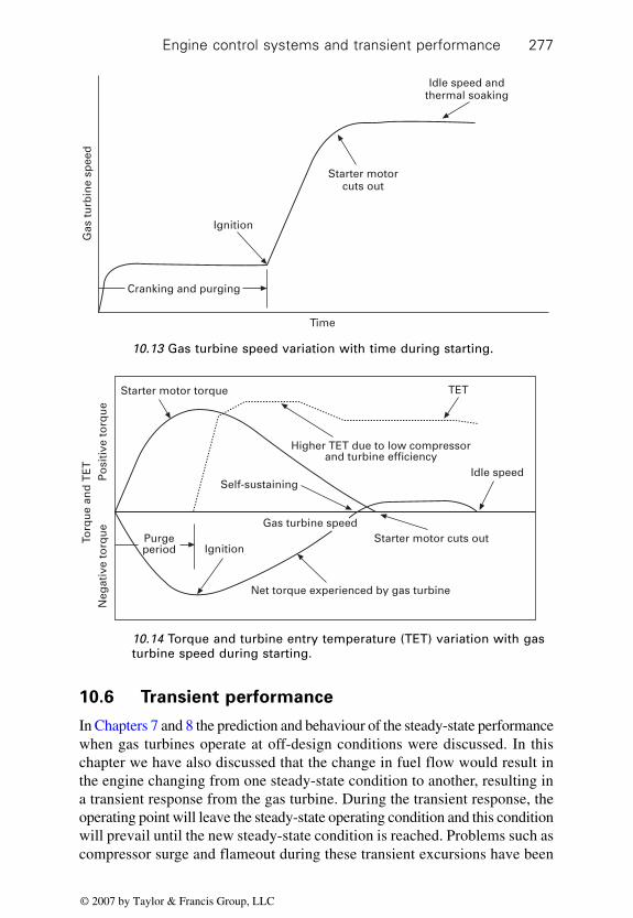
Engine control systems and transient performance 277
10.6 Transient performance
In Chapters 7 and 8 the prediction and behaviour of the steady-state performancewhen gas turbines operate at off-design conditions were discussed. In thischapter we have also discussed that the change in fuel flow would result inthe engine changing from one steady-state condition to another, resulting ina transient response from the gas turbine. During the transient response, theoperating point will leave the steady-state operating condition and this conditionwill prevail until the new steady-state condition is reached. Problems such ascompressor surge and flameout during these transient excursions have been
Gas
tu
rbin
e sp
eed
Time
Cranking and purging
Ignition
Starter motorcuts out
Idle speed andthermal soaking
10.13 Gas turbine speed variation with time during starting.
Torq
ue
and
TE
TP
osi
tive
to
rqu
eN
egat
ive
torq
ue
Starter motor torque
Self-sustaining
Gas turbine speed
Higher TET due to low compressorand turbine efficiency
TET
Idle speed
Starter motor cuts out
Net torque experienced by gas turbine
IgnitionPurgeperiod
10.14 Torque and turbine entry temperature (TET) variation with gasturbine speed during starting.
© 2007 by Taylor & Francis Group, LLC

Industrial gas turbines – principles of performance278
highlighted and means to protect the engine during the transient period ofoperation were discussed. In this section, means of predicting the transientperformance of the gas turbine will be discussed.
In predicting the steady-state performance of gas turbines only flowcompatibility has been considered, which is effectively the steady-state lawof continuity or conservation of mass and the power or energy balancebetween and within engine components such as compressors, turbines andcombustors. Again, only the steady-state aspect of the law of conservation ofenergy has been considered. To simulate the transient performance of the gasturbine it is necessary to consider the dynamic terms present in these lawsand also to consider the laws of conservation of momentum. If an engineelement in general is considered at any instance in time as shown in Fig.10.15, it would experience a fluid flow rate, W1 and W2, temperatures, Ts1
and Ts2, and pressures, Ps1 and Ps2, entering the element and leaving theelement. Also, there would be external forces, Fnet, on the element. Similarly,there would be net energy, Enet, either entering or leaving the element, asshown in Fig. 10.15. There would also be mass trapped within the element,M. It should be noted that the temperatures and pressures are static valuesrather than stagnation or total values. The element may represent a compressor,turbine, combustor or duct work such as a transition piece connecting thecompressor, turbine and combustor.
10.6.1 Continuity
From the law of conservation of mass (continuity), the change in mass, M,trapped within the element is determined by the difference in amount ofmass (of fluid) entering and leaving the element. Therefore, the rate ofchange in the mass trapped within the element is determined by the differencein the fluid flow rate at the inlet and exit of the element, W1 and W2, respectively.This can be represented mathematically by Equation 10.7:
1Enet
M
Fnet
2
∆x
W1P1Ts1
W2
P2
Ts2
10.15 Generalised non-dimensional flow element.
© 2007 by Taylor & Francis Group, LLC

Engine control systems and transient performance 279
dd
= – 1 2Mt
W W [10.7]
The density of the fluid within the element in differential form is given by:
d = dρ MV
[10.8]
where ρ is the static density at some midpoint within the element and V is thevolume of the element.
Substituting Equation 10.8 into Equation 10.7:
Vt
W Wdd
= – 1 2ρ
[10.9]
The equation of state for gases is given by Ps = ρ × R × Ts. For a giventemperature and gas this equation in differential form is given by:dPs = RTs × dρ [10.10]
Note: It has been assumed that the gas or fluid is perfect and this is usuallythe case for air and products of combustion at pressures and temperaturespresent in gas turbines. Since the methods developed here are applicable toall gases, the compressibility factor, Z, discussed in Chapter 2, should beincluded when appropriate.
Substituting Equation 10.10 into Equation 10.9 and rearranging:
dd
= ( – )1 2Pst
RTsV
W W [10.11]
Thus the rate of change of pressure at some midpoint within the element isgiven by Equation 10.11.
10.6.2 Momentum
In Section 10.6.1, the charging and discharging of the element due to flowsentering and exiting the element were effectively considered and an equationwas developed describing the rate of change of pressure within the element.It is also possible to consider the fluid within the element in motion. This canbe achieved by forces acting on the element and these forces will correspondto the pressures surrounding the element and external forces, Fnet actingdirectly on the element. Examples of such external forces could be frictionin fluids flowing in pipes and ducts or the forces applied by the compressorrotor blade to the fluid. To develop equations to describe the effect of suchforces on the movement of the element, the laws of conservation of momentumare used in the form of Newton’s Second Law of Motion, which states thatthe rate of change of momentum is equal to the net force acting on an objector, in this case, the fluid element.
© 2007 by Taylor & Francis Group, LLC

Industrial gas turbines – principles of performance280
Restricting the discussion to a one-dimensional analysis and applyingNewton’s Second Law to the fluid trapped within the element:
M ut
Am Ps Ps F = dd
( – + )1 2 net [10.12]
where u is the velocity of the element, Am is the mean flow area and Fnet isthe external pressure-force acting on the element. du/dt is the rate of changein velocity = acceleration or deceleration of the fluid trapped within theelement.
Differentiating the continuity equation W = ρ × u × Am with respect totime, t, for a given density and area:
dd
= 1
dd
Wt Am
utρ × [10.13]
Substituting Equation 10.13 into Equation 10.12 for the acceleration, du/dt:
MAm
Wt
Am Ps Ps Fρdd
= ( – + )1 2 net [10.14]
Since density ρ = M/V and volume V can be expressed as Am∆x where ∆x isthe element length, Equation 10.14 can be rearranged as:
dd
= = ( – + )1 2 netWt
Amx
Ps Ps F∆ [10.15]
Thus an expression has been derived to describe the rate of change of flowrate at some mean position within the element due to external forces.
10.6.3 Energy
Using a similar argument to that above for continuity, the dynamics of theenergy equation can be considered. The rate of change of the internal energy,U, of the element can be given by:
dd
= – + 1 1 1 2 2 2 netUt
W c T W c T Ep p [10.16]
where Enet is the net external energy entering or leaving the element and T1
and T2 are the total or stagnation temperatures at inlet and exit of the element.The internal energy for the element is given by:
U = McvT [10.17]
where cv is the specific heat at constant volume and T is the mean temperatureof the element.
The rate of change of internal energy can be represented by:
dd
= d
+ dd
Ut
UM
dMt
UT
Tt
∂∂
∂∂
[10.18]
© 2007 by Taylor & Francis Group, LLC

Engine control systems and transient performance 281
From Equation 10.17, ∂∂
UM
c Tv = and ∂∂UT
Mcv = . Substituting these partial
derivatives into Equation 10.18:
dd
= dd
+ dd
Ut
c T Mt
Mc Ttv v [10.19]
Using Equation 10.19 in Equation 10.16:
c T Mt
Mc Tt
W c T W c T Ev v p pdd
+ dd
= – + 1 1 1 2 2 2 net
This can be rearranged to determine the rate of change of mean temperaturein the element as follows:
Mc Tt
W c T W c T E c T Mtv p p v
dd
= – + – dd1 1 1 2 2 2 net [10.20]
Since M = ρV and from Equation 10.7 dd
= – 1 2Mt
W W , Equation 10.20
becomes:
dd
= – + – ( – )1 1 1 2 2 2 net 1 2T
t
W c T W c T E c T W W
Vcp p v
vρ [10.21]
10.6.4 Linearly distributed and lumped model
The rates of change of pressures, flows and temperatures discussed aboveoccur at some midpoint within the element. However, these rates of changeare required either at the inlet or exit of the element. Two models can be usedto determine these rates of change at the required element boundary and theycorrespond to the linearly distributed and lumped models.
The linearly distributed model assumes that these rates of change arelinear across the element. Applying the linear distributed model to Equations10.11, 10.15 and 10.21:
dd
+ d
d = 2 ( – )1 2
1 2P st
P st
RTsV
W W [10.22]
dd
+ dd
= 2 ( – + )1 21 2 net
Wt
Wt
Amx
Ps Ps F∆ [10.23]
dd
+ dd
= – + – ( – )
0.51 2 1 1 1 2 2 2 net 1 2Tt
Tt
W c T W c T E c T W W
Vcp p v
vρ[10.24]
When applying the lumped parameter model, it is assumed that these meanvalues for the rates of change remain constant across the element. Therefore,Equations, 10.22, 10.23 and 10.24 become:
© 2007 by Taylor & Francis Group, LLC

Industrial gas turbines – principles of performance282
dd
= ( – )2 21 2
P st
RT sV
W W [10.25]
dd
= ( – + )11 2 net
Wt
Amx
P P F∆ [10.26]
dd
= – + – ( – )
2 1 1 1 2 2 2 net 2 1 2
2
Tt
W c T W c T E c T W W
Vcp p v
vρ[10.27]
10.6.5 Choice of model
Much of the early work on dynamic simulation of gas turbines was carriedout by Corbett and Elder5 and also by Elder and MacDougal.6 They reportthat the simulated results for the lumped and linearly distributed modelswere in good agreement, but that the linear model required a significantincrease in computational effort (some 2–3 times more computing time).Thus lumped models are often employed in the prediction of the transientperformance of gas turbines. It should be pointed out that such models areequally applicable in the simulation of gas compression system present inthe process industry.7
The equations described use static values for pressures and temperatures.However, total or stagnation values for these parameters are preferable inanalysing engine performance in general. If element boundaries are chosenwhere the Mach number is low (Mx < 0.3), the differences between the staticand total values will be small and the values computed using the equationsdescribed above could be treated as total or stagnation values. Examples ofsuch boundaries are upstream and downstream of compressor stages ratherthan choosing boundaries between the rotor and stator of a compressor stageor close to the rotor inlet where the velocities are very high.
The assumption in the lumped parameter model imposes frequencylimitations because second- or higher-order equations are being solved. Suchsystems of equations employed in predicting transient performance of gasturbines and gas compression systems are capable of simulating longitudinalwaves. For air, the element length, ∆x, in Equation 10.26 should be less thanabout 34 metres (∆x << 34 m) as determined by Corbett and Elder.5 This isusually the case with gas turbine components.
It should be noted that these models are capable of simulating compressorsurge cycles. Elder and Macdougal6 developed a frequency parameter modelto account for surge and pre-surge oscillations during the transient responseof the compressor element. They related a frequency parameter to the phasechange across the compressor element in terms of an expected error whencomparing the lumped parameter model with the true solutions. Using an
© 2007 by Taylor & Francis Group, LLC

Engine control systems and transient performance 283
expected frequency of interest, fx, and Mach number, Mx, of 0.3 or less, asuitable element length for the compressor could be determined using:
2πfx∆x < a(1 – Mx) [10.28]
where a is the velocity of soundAlthough the above analysis improves the simulation, the elements do not
communicate in a realistic manner if the adjacent element volumes aresignificantly different. In order for elements to interact in a realistic manner,a criterion of approximately equal volumes is used, in conjunction with thefrequency parameter model.
Other researchers in the field of transient analysis of gas turbines includeGreitzer8 and Fawke and Saravamuttoo.9 Although Greitzer used a similarapproach to the one described by Elder and discussed above, Fawke andSaravamuttoo restricted their models to continuity only. Pre- and post-surgeoscillations are unavailable using the continuity-only model.
10.6.6 Element definition
The starting values for pressures, flows, temperatures and speeds for transientanalysis would be determined by a steady-state model of the gas turbine asdiscussed in Chapter 7. However, the force and energy terms Fnet and Enetneed to be defined in Equations 10.26 and 10.27, respectively. These aredetermined by applying the quasi-steady-state assumption, where theinstantaneous values are used with the steady-state component characteristicto determine these terms, as discussed below.
Compressor
In the dynamic simulation of gas turbines, it is usual to employ compressorstage characteristics rather than overall characteristics as discussed in Chapter7, where the prediction of the off-design performance of the gas turbine wasconsidered. These stage characteristics are normally stacked together10 toproduce the overall characteristic used in the prediction of the steady-stateperformance of the gas turbine. A typical compressor stage characteristic isshown in Fig. 10.16. At any instance the flows, pressures, temperatures andspeeds at the inlet to the compressor stage will be known. Given the compressorgeometry (flow area), using the equation of state and the continuity equation,the axial velocity, Va, and blade velocity, U, at the reference point can becalculated (e.g. blade mid-height). Thus the flow coefficient, Va/U, can bedetermined. Using the stage characteristic and by interpolation, the stageloading coefficient, ∆h/U2, and the isentropic efficiency can be determined.∆h is the specific enthalpy rise.
© 2007 by Taylor & Francis Group, LLC

Industrial gas turbines – principles of performance284
The stage pressure ratio, P2/P1 can now be calculated from
∆h c T prp c = – 1 /1
–1γγ η
,
which will yield the compressor stage pressure ratio. cp is the specific heatat constant pressure, γ is the isentropic index, T1 is the stage inlet temperatureand ηc is the stage isentropic efficiency. Note that pressures and temperaturesare now assumed to be stagnation or total values.
The Fnet term is defined as the pressure change (rise) across the compressorstage and is therefore given by:
Fnet = P2 – P1
in terms of the stage pressure ratio:
Fnet = P1(pr – 1) [10.29]
Since the compression process is assumed to be adiabatic, the Enet term isequal to the rise in enthalpy, ∆h × W1, where W1 is the inlet compressor flowrate.
Sta
ge
load
ing
co
effi
cien
t∆h U
2S
tag
e is
entr
op
ic e
ffic
ien
cy
Flow coefficient VaU
10.16 Typical axial compressor stage characteristic.
© 2007 by Taylor & Francis Group, LLC

Engine control systems and transient performance 285
Transition ducts and combustors
The forcing term, Fnet, for transition ducts and combustors can be determinedby Equation 7.6 in Chapter 7. This equation gives the non-dimensional pressureloss across the combustor. For transition ducts, the temperature rise is zero.Therefore, the Fnet term is simply the pressure loss across the transition ductor combustor.
The energy term, Enet, is zero for transition ducts because a thermodynamicprocess in such components is considered as adiabatic with no work transfer.However, for combustors the Enet term is calculated by the instantaneousflow, mf, times the lower heating value of the fuel, LHV. The work transferfor combustors is zero. Thus for combustors:
Enet = mf × LHV [10.30]
Gas turbines often employ bleeds to prevent surge at starting conditions orwhen operating at low powers. This was discussed in Chapter 4. The dynamicmodelling of such an element requires a modification to the continuity Equation10.25. Referring to Fig. 10.17, which represents a blow-off valve element,Equation 10.25 becomes:
dd
= ( – – )2 21 2 3
Pt
RTV
W W W [10.31]
where W3 is the bleed or blow-off flow rate. Similarly, for combining flows,the term –W3 becomes +W3.
Turbines
As was found with compressors, the turbine characteristics can also be usedto determine the necessary force and energy terms required to determine the
W1P1T1
Enet
Element
Fnet
W2
P2
T2
21
W3
10.17 Dividing flow or blow-off element.
© 2007 by Taylor & Francis Group, LLC

Industrial gas turbines – principles of performance286
transient performance of turbines. Typical turbine characteristics are shownin Figs 5.8 and 5.10 in Chapter 5. Knowing the current values for inlet flow,pressure, temperature and turbine speed, these characteristics can be used todetermine the pressure ratio and isentropic efficiency. The pressure ratio canthen be translated to the Fnet term using Equation 10.29. However, this isonly applicable to the unchoked part of the turbine characteristic. Whenturbines operate in the choked part of the characteristic, the momentumEquation 10.26 is not applicable, and only the continuity and energy equationsneed to be considered (Equations 10.25 and 10.27, respectively).
Since the thermodynamic process in turbines is assumed to be adiabatic,the energy term, Enet can be determined from the turbine pressure ratio andisentropic efficiency as:
E W cPrp tnet 1 = 1 – 1
–1
ηγ
γ( )
[10.32]
10.6.7 Boundary conditions
Equations 10.25, 10.26 and 10.27 calculated the mass flow rate at the inletof an element and pressure and temperature at the exit of an element. Therefore,a means of defining the inlet pressure and temperature into the first elementin a simulation system and the mass flow rate at the exit from the lastelement of the system from boundary conditions is needed. In industrial gasturbines, the inlet pressure at the entry to the system, which is usually thefiltration system, is the ambient pressure and therefore can be used as theinlet boundary condition. This is shown in Fig. 10.18, which is an elementalrepresentation of a single shaft gas turbine. The inlet temperature at the entryto the system will also correspond to the ambient temperature.
The last element of an industrial gas turbine would normally be the exhaustsystem as shown in Fig. 10.18. This element incurs a small pressure loss,typically in the order of about 100 mm water gauge and can be used todetermine the flow at the exit from the last dynamic element – the turbine asshown in Fig. 10.18. Since the pressure and temperature at the exit from theturbine element (which is the inlet to the exhaust system) are known, calculationof the mass flow rate at the exit from the turbine element is possible usingthe equation describing the pressure loss in the exhaust system. The pressure
Ambientpressure
Ambientpressure 5
Exhaustsystem
4Turbine
3Combustor
2Compressor
1Inlet system
10.18 Elemental representation of a single-shaft gas turbine.
© 2007 by Taylor & Francis Group, LLC

Engine control systems and transient performance 287
loss equation for the exhaust system is similar to Equation 7.6 in Chapter 7,but the temperature rise is zero. Since the pressure at the exit of the exhaustsystem is the ambient pressure, the pressure loss in the exhaust system isreadily known. From Equation 7.6, the mass flow rate can be calculated.
10.6.8 Compressor–turbine speed calculation
During transients, the compressor–turbine and the driven load may vary inspeed depending on the power absorbed by the compressor and load, and thepower developed by the turbine. Also, the gas turbine configuration andcontrol system performance will influence the changes in speed of thesecomponents. The power absorbed by the compressor and the power developedby the turbine are readily calculated as discussed previously. For a givencompressor and turbine speed, the torque at the compressor and turbine arereadily calculated using the relationship:
power = torque × angular velocity
Therefore, at any instance the torque at the compressor and turbine can becalculated. Furthermore, for a given power output and load speed, the torqueat the load is also known. For a single-shaft gas turbine rotor, as shown inFig. 10.19, the net torque, Tnet, is given by
Tnet = Tturb – (Tcomp + Tload),
where Tturb, Tcomp and Tload are the torque at the turbine, compressor andload, respectively.
Applying Newton’s second law of motion:
α ω = dd
= net
tT
I[10.33]
where α and I are the angular acceleration or deceleration of the rotor systemand polar moment of inertia of the rotor, respectively.
Given an initial angular velocity, the current angular velocity can becalculated from the angular acceleration calculated from Equation 10.33.The analysis can be extended to other engine configurations discussed inChapter 1.
10.19 Rotor system for a single-shaft gas turbine.
Load
Turb
ine
Compressor
© 2007 by Taylor & Francis Group, LLC

Industrial gas turbines – principles of performance288
10.6.9 Numerical solutions of differential equations
Equations 10.25, 10.26, 10.27 and 10.33 are referred to as first-order ordinarydifferential equations. These are non-linear differential equations and thereforeno analytical solutions exist. In these situations the only means of finding asolution is numerically. Many such methods have been developed, fromsimple Euler to more advanced methods such as Rung–Kutta–Felberg andGears methods.
Rung–Kutta–Felberg and Euler are referred to as the single-step methodsbecause the current solutions and rates of change only are required to determinethe solution at the next (time) step. Gears, on the other hand, requires previoussolutions and rates of change and is known as a multi-step or predictor–corrector method. This method is generally more efficient compared withRung–Kutta–Felberg, as fewer coefficients are needed to determine the nextsolution. However, single-step methods such as Rung–Kutta–Felberg areinitially invoked to generate the necessary past solutions and rates of changebefore switching to multi-step methods. In this case, multi-step methods canbe employed directly because steady-state conditions are always in place atthe start. In this situation the previous solutions can be conveniently set tothe current values and the previous rates of change set to zero.
Numerical methods have drawbacks where the solutions become unstable.For example, Euler would require very small time steps to achieve stablesolutions and is rarely used. Rung–Kutta–Felberg and Gears can achievestable solutions using larger steps and are therefore more efficient. Gearsmethod is particularly suited because it is capable of overcoming a particulartype of numerical instability referred to as stiff equations. Such instabilitiesoccur when the general solution contains an exponential term such as Cebx
where b > 0 with initial conditions C = 0, but the rounding off errors in thenumerical computation produces a solution in which C <> 0. Further detailson numerical methods for solving differential equations can be found inPress11 and in Gerald and Wheatly.12
10.7 References
1. PID Control Algorithm. How it Works, how to Tune it and how to Use it, 2nd Edition,John A. Shaw, December 1 2003. E-book, http://www.jashaw.com/.
2. Control Systems Engineering, S.N. Sivanandam, Vikas Publishing, (2001).3. Gas Turbine Engineering, Harman, R.T.C., Macmillan Press Ltd, (1981).4. Gas Turbine Performance, 2nd Edition, Walsh, P.P. and Fletcher, P., Blackwell
Publishing, (2004).5. Stability of an axial compressor with steady inlet conditions, Corbett, A.G. and
Elder, R.L, J. Mech. Eng. Sci., 16 (6), 1975.6. Simulation of centrifugal compressor transient performance for process plant
application, Elder, R.L., MacDougal, I., ASME Paper, 1983.
© 2007 by Taylor & Francis Group, LLC

Engine control systems and transient performance 289
7. Simulation of the transient performance of a compressor in a natural gas pumpingstation, Elder, R.L., Gill, M.E. and Razak, A.M.Y., Third European Congress onFluid Machinery, The Hague, Netherlands, 18th–20th May, 1987.
8. Surge and rotating stall in axial compressors. Part II – Experimental results andcomparison with theory, Greitzer, E.M., J. Eng for Power, April 1978.
9. Digital computer methods for prediction of gas turbine dynamic response, Fawke,A.J. and Saravamuttoo, H.I.H., Transactions of the Society of Automotive Engineers,1971.
10. Effects of stage characteristics and matching on axial-flow compressor performance,Stone, A., Transactions of the ASME, 1958.
11. Numerical Recipes in Fortran 77, 2nd Edition, The Art of Scientific Computing,Press, W.H., Teukolsky, S.A., Vetting, W.T. and Flannery, B.P., Cambridge UniversityPress (1992).
12. Applied Numerical Analysis, 6th Edition, Gerald, C.F., Wheatly, P.O., Addison-Wesley, (1997).
© 2007 by Taylor & Francis Group, LLC

Much of what has already been discussed is rather complex, particularlyengine off-design performance prediction. The use of a gas turbine simulatorcan illustrate eloquently these rather complex concepts. The gas turbinesimulators will now be used to re-visit many of the preceding chapters,particularly off-design performance prediction, performance deterioration,gas turbine emissions, turbine creep life usage and the engine control system.
The gas turbine simulator is based on the quasi-steady-state model, usingtime constants to simulate the transient effects. Although such simulators arestrictly only valid under steady-state conditions, much useful insight intoengine operation can be achieved during transients using such simulators.They are excellent as training simulators. The concept of component matching,as discussed in Chapter 7, has been extensively used in building the simulator,thus making it capable of illustrating much of what has been discussed inChapters 8, 9 and 10 in detail, including turbine creep life usage and engineemissions as discussed in Chapters 5 and 6.
Two engine simulators are used and they correspond to a single-shaft anda two-shaft gas turbine operating with a free power turbine. The single-shaftgas turbine simulator is also capable of simulating the performance of asingle-shaft gas turbine when variable inlet guide vanes are incorporated.The single-shaft gas turbine is the most common engine configuration usedin power generation and the use of the two-shaft gas turbine configurationoperating with a free power turbine is widespread in mechanical driveapplications. Although their use is widespread in mechanical drive, there arealso a significant number of gas turbines using a two-shaft configurationemployed in power generation. Thus, these two simulators cover the vastmajority of gas turbines operating in the field. Simulation exercises providedin Chapter 21 are included to help readers to improve their understanding ofgas turbine performance and operation.
Part II
Simulating the performance of a two-shaftgas turbine
291
© 2007 by Taylor & Francis Group, LLC

293
The engine simulator discussed here is based on a two-shaft gas turbineoperating with a free power turbine. The engine corresponds to an advancedaero-derived industrial gas turbine having an ISO rating of about 20 MW.The simulator assumes that the driven load is an electrical generator.
11.1 Compressor running line
The reasons why an approximately unique running line occurs in a multi-shaft engine were discussed in Section 8.1.2. This can be demonstrated byproducing the engine running line on the compressor characteristic using thesimulator. This is achieved by running the simulator at different power andambient conditions, increasing any engine limits such as exhaust gastemperature (EGT) and gas generator speed to produce the complete runningline. Figure 11.1 shows the compressor characteristic with the running line
11Simulating the effects of ambient
temperature on engine performance,emissions and turbine life usage
11.1 Running line on the compressor characteristic.
Co
mp
ress
or
pre
ssu
re r
atio
(P 2
/P1)
25
20
15
10
5
0
Compressor surge line
Compressor speed lines
0 100 200 300 400 500 600
Speed = 73%Speed = 80% Running line
Speed = 86%Speed = 89%
Speed = 92%Speed = 95%
Speed = 97%Speed = 100%
Speed = 107%
Speed = 1
1 1 1
N
R Tγ
Compressor inlet non-dimensional flow
W R T
P1 1 1 1
1
/γ
© 2007 by Taylor & Francis Group, LLC

Industrial gas turbines – two-shaft294
superimposed on it. The means of producing these characteristics and theoperating points on the characteristics are found in the user guide on the CD,accompanying this book.
The reader is encouraged to run the simulations discussed below in orderto become more familiar with these concepts. Instructions on how to use thesimulator are also given in the user guide.
The pressure ratio of the compressor at design conditions is about 17.5. Itwas seen in Section 4.10.3 under variable geometry compressors that, atsuch high-pressure ratios, many stages of variable stator vanes are necessaryto prevent compressor surge, particularly during low speed operation. Infact, this compressor has six variable stator vanes and one variable inletguide vane to ensure satisfactory operation of the gas turbine. The variationof these guide vane positions with compressor (quasi) non-dimensional speedis shown in Fig. 11.2.
11.2 Representation of other non-dimensional
parameters
Gas turbines behave in a non-dimensional manner and that is the reason why theunique running line is observed on the compressor characteristic when theyoperate with a free power turbine. Thus, the variation of non-dimensionalparameters such as mass flow and pressure and temperature ratios can becompared with, say, compressor non-dimensional speed. Also any other non-dimensional parameter may be used instead of compressor non-dimensionalspeed.
Figure 11.3 shows the variation of the compressor non-dimensional flowwith speed. Two kinks are observed in the display. One corresponds to the
120
100
80
60
40
20
0
VIG
V/V
SV
an
gle
(p
erce
nta
ge
op
ened
)
Kink
Compressor non-dimensional speed (N1/√T1)560550540530520510500490480
11.2 Variation of the variable stator vanes with compressor (quasi)non-dimensional speed. (It is usual to use quasi non-dimensionalspeed for this characteristic as the changes in R and γ are small.)
© 2007 by Taylor & Francis Group, LLC

Simulating the effects of ambient temperature on performance 295
kink found in the VSV/VIGV movement shown in Fig. 11.2, which is due tothe rapid opening of the VSV/VIGV as the compressor approaches its normaloperating speed range. The other kink is due to the choking of the compressorinlet at high compressor non-dimensional speeds. This can also be observedin Fig. 11.1, where the increase in flow with speed is smaller at the high-speed part of the compressor characteristic when compared with the lowspeed part. Thus, as the compressor inlet chokes, the compressor non-dimensional speeds will collapse into a single line and no increase in non-dimensional flow is possible with any increase in compressor speed. Indeed,such a phenomenon has been observed with turbines, where the non-dimensional flow remains constant after the turbine chokes (see Fig. 5.8 inChapter 5).
The variation of compressor pressure ratio and non-dimensional temperaturerise with compressor non-dimensional speed is shown in Fig. 11.4. Thekinks are observed again as described above when discussing the non-dimensional flow variation with speed. Because of the choking in thecompressor inlet, the compressor pressure ratio flattens and imposes a maximumcompressor pressure ratio of about 18. Thus, compressor inlet chokingdetermines the maximum pressure ratio that a compressor can achieve.
Figures 11.5 and 11.6 show the variation of various turbine parameterswith compressor non-dimensional speed, and Fig. 11.7 shows the variationof non-dimensional fuel flow and power with compressor non-dimensionalspeed. A similar picture emerges where the effects of the VSV/VIGV kinkand the choking of the compressor inlet are observed. These non-dimensionalparameters may be converted to corrected or standard conditions by usingthe equations described in Section 8.7.1 in Chapter 8.
11.3 Variation of compressor non-dimensional flow withnon-dimensional speed.
550
500
450
400
350
300
Kink due tocompressorinlet choking
Kink due toVSV movement
750 770 790 810 830 850 870 890 910 930 950
Co
mp
ress
or
inle
t n
on
-dim
ensi
on
al
flo
w W
RT
P1
11
1
1
/γ
Compressor non-dimensional speed
N
R T1
1 1 1γ
© 2007 by Taylor & Francis Group, LLC

Industrial gas turbines – two-shaft296
11.3 Effects of ambient temperature on engine
performance (high-power operating case)
The engine model can be used to simulate the change in ambient temperatureand its impact on engine performance. It has been stated that the simulatoris based on a quasi-steady-state model, thus it is possible to subject themodel to significant changes in ambient conditions. In practice, however,rapid changes in ambient conditions are not common and could lead tocompressor surge.
11.4 Variation of compressor pressure ratio and non-dimensionaltemperature rise with compressor non-dimensional speed.
20
18
16
14
12
8
Kink due tocompressorinlet choking
Kink due toVSV movement
750 770 790 810 830 850 870 890 910 930 950
10
Pressure ratio
Temperature rise
P 2/P
13.9
3.7
3.5
3.3
3.1
2.9
2.7
γγ
– 1
– 1
2 1
T T
Compressor non-dimensional speed
N
R T1
1 1 1γ
11.5 Variation of gas generation pressure ratio and non-dimensionaltemperature rise with compressor non-dimensional speed.
18
17
16
15
13
Kink due tocompressorinlet choking
Kink due toVSV movement
750 770 790 810 830 850 870 890 910
14
Pressure ratio
Temperature rise
P 3/P
1
930 950
10.5
10.0
9.5
9.0
8.5
8.0
7.0
12
11
10
9
8
7.5
γγ
– 1
– 1
3 1
T T
Compressor non-dimensional speed
N
R T1
1 1 1γ
© 2007 by Taylor & Francis Group, LLC

Simulating the effects of ambient temperature on performance 297
In this simulation, the ambient temperature will be changed from +30degrees Celsius to –30 degrees Celsius, linearly. The power demand fromthe simulator will be set to 25 MW throughout the simulation. The change inambient temperature will take place over 60 minutes. The ambient pressureis set to 1.013 Bar during the change in ambient temperature. Also, theeffects of the gas property terms R, cp and γ will be ignored, as the changesin these parameters are small compared with the changes in temperaturesand pressures.
During the simulation it will be observed that the power output from thegas turbine is limited by the exhaust gas temperature (EGT) at high ambient
11.6 Variation of power turbine pressure ratio and non-dimensionaltemperature rise with compressor non-dimensional speed.
4.5
Kink due tocompressorinlet choking
Kink due toVSV movement
750 770 790 810 830 850 870 890 910
Pressure ratio
Temperature riseP 4/P
1
930 950
7.5
7.0
6.5
6.0
5.5
5.0
4.0
4.5
4.0
3.5
3.0
2.5
2.0
Compressor non-dimensional speed
N
R T1
1 1 1γ
γγ
– 1
(E
GT
) – 1
4
1
TT
11.7 Variation of non-dimensional fuel flow and power with non-dimensional compressor speed.
Compressor non-dimensional speed
N
R T1
1 1 1γ
Po
w
11
11
1γ
γ×
×P
RT
0.015
Kink due tocompressorinlet choking
Kink due toVSV movement
750 770 790 810 830 850 870 890 910
Power
Fuel flow
930 950
1.6
1.4
1.2
1
0.8
0.6
0.4
0.014
0.013
0.012
0.011
0.010
0.009
0.008
0.007
0.006
mf
R
cpP
T
1
11
11
×
×γ
© 2007 by Taylor & Francis Group, LLC

Industrial gas turbines – two-shaft298
temperatures (from 30 degrees C to about 12 degrees C) to prevent theturbine from overheating. As the ambient temperature decreases and operationis continued at the EGT limit, then the ratio of EGT to the ambient temperature,T4(EGT)/T1, will increase. From Fig. 11.6, an increase in T4(EGT)/T1 musttherefore result in an increase in the compressor non-dimensional speed, N1/√T1. However, the gas generator speed, N1, initially decreases with decreasein ambient temperature, T1 before increasing at lower ambient temperaturewhile power output is limited by the exhaust gas temperature. This conditionis shown in Fig. 11.8. The initial decrease in gas generator speed is dueprimarily to the opening of VIGV/VSV as the compressor non-dimensionalspeed increases. At lower ambient temperatures, the increase in gas generatorspeed is due to the choking of the compressor inlet.
When the power output from the engine is limited by the gas generatorspeed (i.e. when N1 is constant), as would occur at lower ambient temperatures,from about 12 degrees C to –12 degrees C, the drop in ambient temperature,T1, will result in an increase in the N1/√T1. Thus as the ambient temperaturedecreases, the operating point on these characteristics (Figs 11.3 to 11.7)moves from left to right and becomes constrained to operate at the maximumpermissible compressor non-dimensional speed, which occurs at ambienttemperatures below –12 degrees C. At such low ambient temperatures, thepower output is limited by the compressor non-dimensional speed, N1/√T1.
11.3.1 Trends in speed
The impact of the reduction in ambient temperature on gas generator speedis illustrated in Fig. 11.8. The change in gas generator speed with the reduction
Gas
gen
erat
or
spee
d (
RP
M)
9600
9500
9400
9300
9200
9100
9000
VIGV/VSVopening
results in adecrease in
gas generatorspeed
N1/√T1
Compressor inletchoking results in anincrease in gasgenerator speed Gas generator
speed
EGT limitedGas generator speed
limited N1/√T1 limited
590
580
570
560
550
540
530 Qu
asi-
no
n-d
imen
sio
nal
sp
eed
(N
1/√T
1)
0Time (seconds)
500 1000 1500 2000 2500 3000 3500 4000
11.8 Variation of gas generator speed due to the reduction inambient temperature.
© 2007 by Taylor & Francis Group, LLC
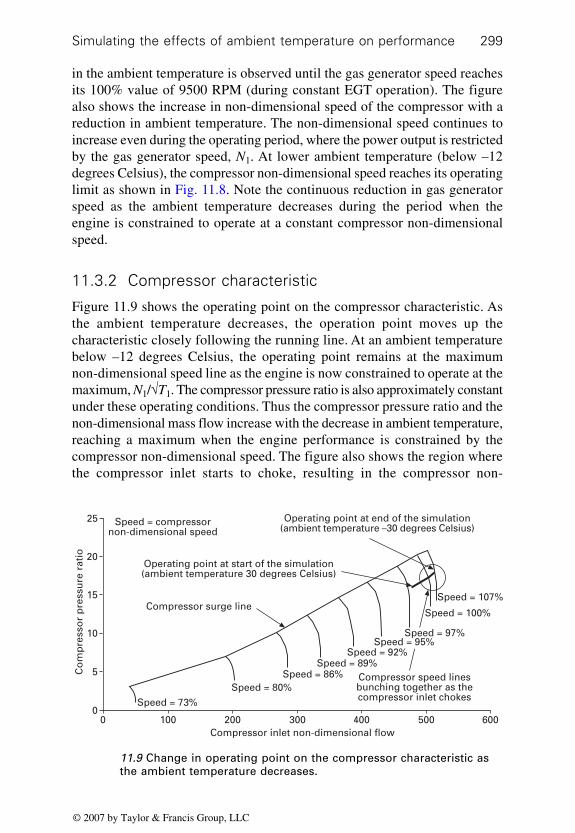
Simulating the effects of ambient temperature on performance 299
in the ambient temperature is observed until the gas generator speed reachesits 100% value of 9500 RPM (during constant EGT operation). The figurealso shows the increase in non-dimensional speed of the compressor with areduction in ambient temperature. The non-dimensional speed continues toincrease even during the operating period, where the power output is restrictedby the gas generator speed, N1. At lower ambient temperature (below –12degrees Celsius), the compressor non-dimensional speed reaches its operatinglimit as shown in Fig. 11.8. Note the continuous reduction in gas generatorspeed as the ambient temperature decreases during the period when theengine is constrained to operate at a constant compressor non-dimensionalspeed.
11.3.2 Compressor characteristic
Figure 11.9 shows the operating point on the compressor characteristic. Asthe ambient temperature decreases, the operation point moves up thecharacteristic closely following the running line. At an ambient temperaturebelow –12 degrees Celsius, the operating point remains at the maximumnon-dimensional speed line as the engine is now constrained to operate at themaximum, N1/√T1. The compressor pressure ratio is also approximately constantunder these operating conditions. Thus the compressor pressure ratio and thenon-dimensional mass flow increase with the decrease in ambient temperature,reaching a maximum when the engine performance is constrained by thecompressor non-dimensional speed. The figure also shows the region wherethe compressor inlet starts to choke, resulting in the compressor non-
Co
mp
ress
or
pre
ssu
re r
atio
25
20
15
10
5
0
Operating point at start of the simulation(ambient temperature 30 degrees Celsius)
Operating point at end of the simulation(ambient temperature –30 degrees Celsius)
0 100 200 300 400 500 600
Speed = 73%
Speed = 80%Compressor speed linesbunching together as thecompressor inlet chokes
Speed = 86%Speed = 89%
Speed = 92%
Speed = 100%
Speed = 107%
Compressor inlet non-dimensional flow
Speed = 95%Speed = 97%
Compressor surge line
Speed = compressornon-dimensional speed
11.9 Change in operating point on the compressor characteristic asthe ambient temperature decreases.
© 2007 by Taylor & Francis Group, LLC

Industrial gas turbines – two-shaft300
dimensional speed lines bunching together, thus restricting the increase inpressure ratio and mass flow in this region.
11.3.3 Trends in pressure ratio
The trends in the pressure ratios for the engine components are shown in Fig.11.10 during the ambient temperature change. The Figure also shows theratio of T3/T1, which is the ratio of the maximum cycle temperature (TET),to the compressor inlet temperature, T1. Note that, as the compressor pressureratio increases, the ratio of T3/T1 also increases. Also observe that the gasgenerator turbine pressure ratio remains essentially constant, although thepower turbine pressures ratio increases as the ambient temperature decreases.This is due to the choked conditions of the power turbine restricting the gasgenerator turbine pressure ratio from changing. This was discussed in Section8.1.2 where the matching of turbines operating in series was considered andit was established that the power turbine swallowing capacity controls thegas generator turbine pressure ratio. The Figure also shows the pressureratios remaining constant when the engine is constrained to operate at aconstant compressor non-dimensional speed.
11.3.4 Trends in flow
The trends in the compressor airflow rate, fuel flow rate, air–fuel ratio andthe position of the fuel valve during the ambient temperature transient areshown in Fig. 11.11. (The simulator displays the trends of air–fuel ratiorather than the fuel–air ratio and this has been done for better clarity on the
Co
mp
ress
or
pre
ssu
re r
atio
18.5
0Time (seconds)
18
17.5
17
16.5
16
15.5500 1000 1500 2000 2500 3000 3500 4000
EGT limitedGas generator speed
limited N1/√T1 limited
5.5
Max
imu
m t
o m
inim
um
cyc
le t
emp
erat
ure
rati
o,
GG
an
d p
ow
er t
urb
ine
pre
ssu
re r
atio
GG (gas generator) pressure ratio
Power turbine pressure ratio
Compressor pressure ratio
Maximum to minimum cycle temperature ratio
5
4.5
4
3.5
3
11.10 Trends in pressure ratio of the engine components duringambient temperature transient.
© 2007 by Taylor & Francis Group, LLC

Simulating the effects of ambient temperature on performance 301
display.) It has been established that the compressor non-dimensional speedincreases as the ambient temperature falls for the ambient temperature transientcase we are considering. From Fig. 11.3, it was observed that the compressornon-dimensional flow increases continuously with non-dimensional speed.Thus, the compressor airflow rate increases continuously with the reductionin ambient temperature because in general, as W1√T1/P1 increases and as T1falls, W1 must increase to compensate the reduction in √T1. The rate ofincrease of airflow rate is the greatest when the engine performance is controlledby the exhaust gas temperature. During this period of operation, the compressoris farthest away from compressor inlet choking, as the lines of constant non-dimensional speed on the compressor characteristic are more spaced out,particularly at high ambient temperatures.
At low ambient temperatures, when the compressor operates under near-choked conditions, a flatter line describes the increase in compressor non-dimensional flow with its non-dimensional speed (Fig. 11.3). Thus, the rateof increase of compressor airflow rate decreases when the gas generatorspeed or the compressor non-dimensional speed controls the engineperformance, which occurs at low ambient temperatures.
It is observed that the fuel flow rate increases during the period when theengine performance is controlled by the exhaust gas temperature, and decreaseswhen the engine performance is controlled by the gas generator speed or thecompressor non-dimensional speed. As the ambient temperature decreases,the power output and the thermal efficiency increase, particularly in theperiod when the power output from the gas turbine power output is controlledby EGT. This is due to the increase in compressor pressure ratio, maximumto minimum cycle temperature ratio and mass flow rate as discussed above.
75
70
65
60
55
50
45
40
Co
mp
ress
or
inle
t ai
rflo
w (
kg/s
), f
uel
valv
e p
osi
tio
n (
%),
air
–fu
el r
atio
0Time (seconds)
500 1000 1500 2000 2500 3000 3500 4000
EGT limitedGas generator speed
limited N1/√T1 limited
1.22
Fuel
flo
w (
kg/s
)
Fuel valve postion
Fuel flow
Air–fuel ratio
Compressor inlet airflow
1.2
1.18
1.16
1.14
1.12
1.1
1.08
11.11 Variation of compressor airflow rate, fuel flow rate, air–fuelratio and fuel valve position during ambient temperature transient.
© 2007 by Taylor & Francis Group, LLC

Industrial gas turbines – two-shaft302
However, the increase in power output is greater than the increase in thermalefficiency and is discussed in the next section. Hence, the fuel flow increasesduring the period when the EGT limits the gas turbine power output, asshown in Fig. 11.11.
At lower ambient temperature operation (+12 to –12 degrees Celsius), thepower output of the gas turbine is controlled by the gas generator speed. Thepower output from the gas turbine during this period of operation remainsessentially constant (see Fig. 11.12). However, the thermal efficiency of thegas turbine continues to increase due to the increase in pressure ratio and themaximum to minimum temperature ratio, T3/T1. Thus the increase in thermalefficiency and approximately constant power output from the gas turbineresults in a decrease in the thermal input and hence fuel flow (Fig. 11.11).
At ambient temperatures below –12 degrees Celsius, the gas turbine poweroutput is controlled by the compressor non-dimensional speed and thereforethe engine operates at a constant compressor non-dimensional speed. FromFig. 11.7, which shows the variation of non-dimensional fuel flow and power,a constant compressor non-dimensional speed implies a constant gas turbinenon-dimensional fuel flow, Mf/P1√T1, and power output, Pow/P1√T1.Thus, a decrease in the ambient temperature, T1, will result in a decrease inthe fuel flow, Mf, in order to maintain the constant non-dimensional fuelflow. Hence, a decrease is observed in the fuel flow with the decrease inambient temperature when the gas turbine is operating at a constant compressornon-dimensional speed.
It is observed that the air–fuel ratio decreases initially during the periodwhen the engine performance is controlled by the exhaust gas temperature,
27
Po
wer
(M
W)
0Time (seconds)
500 1000 1500 2000 2500 3000 3500 4000
EGT limitedGas generator speed
limited N1/√T1 limited
43T
her
mal
eff
icie
nci
es (
%)
Gas turbine poweroutput
Thermalefficiency
Generator power
Gas thermalefficiency
25
23
21
19
17
15
Gas power
Power required
42
41
40
39
38
37
36
35
11.12 Trends in power and thermal efficiency during ambienttemperature transient.
© 2007 by Taylor & Francis Group, LLC

Simulating the effects of ambient temperature on performance 303
and then increases during the period when the engine performance is controlledby the gas generator speed and the compressor non-dimensional speed. Inthe period when the engine performance is controlled by the exhaust gastemperature, there is an increase in both compressor airflow and fuel flow(the increase in airflow must also increase the combustion airflow). The rateof increase in fuel flow is greater than the increase in combustion airflowthus resulting in a decrease in the air–fuel ratio and is due to an increase inthe combustion temperature rise, as shown in Fig. 11.15. In the period whenthe engine performance is controlled by the gas generator speed and thecompressor non-dimensional speed, the fuel flow rate decreases while theairflow rate increases. Thus, the air–fuel ratio increases during this period ofoperation.
11.3.5 Trends in power and thermal efficiency
Figure 11.12 shows the trends in power and thermal efficiency as the ambienttemperature decreases from +30 degrees Celsius to –30 degrees Celsius. Inthe period when the engine performance is controlled by the exhaust gastemperature, the power output of the gas turbine and the thermal efficiencyincrease. The increase in power output results because of the increase inmaximum to minimum cycle temperature ratio, T3/T1 (Fig. 11.10) and theincrease in compressor airflow as discussed in Section 11.3.4. The increasein compressor pressure ratio will contribute only to an increase in poweroutput provided design compressor pressure ratio is below the maximumcycle specific work, as discussed in Chapter 2. The power output of the gasturbine can be represented as the product of the airflow and the specificwork as discussed in Chapter 2. The specific work is given by Equation2.20. The increase in cycle temperature ratio always increases the specificwork, whereas a change of the pressure ratio will increase only the specificwork, provided that the compressor pressure ratio is below that which givesthe maximum specific work. It should be noted that the specific work isproportional to the ambient temperature, T1; thus, for a given pressure ratioand temperature ratio, T3/T1, the specific work will actually decrease as T1decreases. In the engine simulator, the maximum compressor pressure ratiois slightly above the case where the specific work is a maximum. Thus, theincrease in specific work is due primarily to the increased maximum cycletemperature ratio, resulting in increased power output as the ambienttemperature decreases, at ambient temperatures above 15 degrees Celsius.The increase in compressor pressure ratio and cycle temperature ratio, T3/T1,however, increases the thermal efficiency as discussed in Chapter 2 and asshown in Fig. 11.12. The increase in air flow (discussed above) also increasesthe power output of the gas turbine but has no direct effect on the thermalefficiency. The decrease in ambient temperature generally results in a larger
© 2007 by Taylor & Francis Group, LLC

Industrial gas turbines – two-shaft304
increase in power output compared with the thermal efficiency of the gasturbine (during constant EGT operation).
Figure 11.12 also shows the trends in the gas power, which is effectivelythe power output of the gas generator and is calculated assuming that theisentropic efficiency of the power turbine is 100%. The gas thermal efficiencyis also shown in Fig. 11.12 and is the thermal efficiency of the gas generator,which is calculated using the gas power output rather than the shaft power.Consequently, the gas power output and gas thermal efficiency will be higherthan the gas turbine (shaft) power output and thermal efficiency of the gasturbine. The use of gas power and gas thermal efficiency is primarily tocompare the performance of different gas generators and is included hereonly for completeness.
As the ambient temperature decreases below 12 degrees Celsius, the gasturbine performance becomes constrained by the gas generator speed. In theperiod of operation at constant gas generator speed, the power output increasesvery slightly. During this period of operation, the rate of increase of themaximum cycle temperature ratio, T3/T1, decreases due to near chokedconditions at the compressor inlet. However, this temperature ratio and thecompressor airflow have indeed increased, due to the increase in the compressornon-dimensional speed. The increase in these parameters will result in anincrease in power output. But the impact of the lower ambient temperaturereduces the specific work during the period of constant gas generator speedoperation and this is shown in Fig. 11.13. Thus the net effect is only a modestor small increase in power output, as shown in Fig. 11.14, which representsthe power and thermal efficiency trends shown in Fig. 11.12 on an ambient
11.13 Variation of specific work and compressor airflow with ambienttemperature.
Compressor airflow
Ambient temperature (°C)0
EGT limitedGas generator speed limitedN1/√T1 limited
75
Co
mp
ress
or
inle
t ai
rflo
w (
kg/s
)
–40 –30 –20 –10 10 20 30 40
73
71
69
67
65
63
61
59
57
55
Specific work
325
320
315
305
300
295
290
285
280
Sp
ecif
ic w
ork
(kJ
/kg
)
310
© 2007 by Taylor & Francis Group, LLC

Simulating the effects of ambient temperature on performance 305
temperature basis. When gas turbines are designed to operate at lowercompressor pressure ratios, the compressor inlet choking is less severe. Thiswill result in a larger increase in power output during constant gas generatorspeed operation, due to the larger increase in maximum to minimum temperatureratios and airflow rate as the ambient temperature decreases, particularly ifthe design compressor pressure ratio is below the maximum cycle specificwork condition. In this case the resultant increase in pressure ratio will alsocontribute to an increase in gas turbine power output.
Figure 11.12 shows that, at lower ambient temperatures below –12 degreesCelsius, the gas turbine performance is constrained by the compressor non-dimensional speed, N1/√T1. The operating point on the compressor characteristicwill now correspond to the –30 degrees Celsius case, as shown in Fig. 11.9.The compressor will continue to operate at this point, restricting the increasein compressor ratio and thus the maximum to minimum cycle temperatureratio, as shown in Figure 11.10. Therefore, as the ambient temperature decreasesbelow –15 Celsius, the decrease in specific work will be more acute, asshown in Fig. 11.13. Although there is an increase in airflow during thisperiod of operation, the net effect is a reduction in gas turbine power output,as shown in Fig. 11.14.
Another explanation as to why the power output falls as the ambienttemperature decreases when the engine is constrained to operate at a constantcompressor non-dimensional speed may be found in Fig. 11.7. This Figureshows the variation of non-dimensional power, Pow/P1√T1, with compressornon-dimensional speed, N1/√T1. Since the engine is constrained to operate ata constant non-dimensional speed, the non-dimensional power must also be
11.14 Variation of power output and thermal efficiency with ambienttemperature.
Thermalefficiency
Ambient temperature (°C)0
EGT limitedGas generator speed limitedN1/√T1 limited
38.00
Th
erm
al e
ffic
ien
cy (
%)
–40 –30 –20 –10 10 20 30 40
Power
22.00P
ow
er (
MW
)
37.50
37.00
36.50
36.00
35.50
35.00
34.00
21.50
21.00
20.50
20.00
19.50
19.00
18.50
18.00
© 2007 by Taylor & Francis Group, LLC

Industrial gas turbines – two-shaft306
constant. Thus, as T1 decreases, the power must also decrease to maintain aconstant non-dimensional power.
Figure 11.12 also shows the required power from the generator, which isset to 25 MW. It is observed that the generator power output never reachesthis required power output. In practice, there will be a frequency shift as thegenerator slows down and this will result in a trip of the generation system.Thus it is very important for operators to know the capacity of their generationsystem. The simulators used here should prove an invaluable tool in predictinggenerating capacity, especially when engine deterioration is taken into accountand this will be discussed later.
11.3.6 Trends in temperature
The temperature changes in the engine during the transient in the ambienttemperature, T1, are shown in Fig. 11.15. In the period of engine operationwhere the exhaust gas temperature is constant, it is observed that the turbineentry temperature is also essentially constant, thus preventing the gas generatorturbine from overheating. Note that the power turbine exit temperature, T5,decreases during the ambient temperature transient and this is due to theincrease in the power turbine pressure ratio as shown in Fig. 11.10. Thecompressor discharge temperature also decreases slightly, although thecompressor pressure ratio increases during this period (see Fig. 11.10). Althoughthe compressor temperature ratio, T2/T1, increases, the decrease in T1 duringthe ambient temperature transient is sufficient to decrease T2. The Figurealso includes the combustion primary zone temperature whose trend is very
Specifichumidity
Time (seconds)
EGT limited N1/√T1 limited
18
Sp
ecif
ic h
um
idit
y (g
of
wat
er v
apo
ur
per
kg
of
dry
air
)
2500
EGT limit
2000
1500
Tem
per
atu
re (
K)
1000
500
0
Gas generator turbinemetal temperature
Gas generator speed limited
T5T2
Temperature drop in combustorprimary zone to ensuresatisfactory turbine life
Primary zonetemperature
T3
T4
T1
16
14
12
10
8
4
2
0
6
0 500 1000 1500 2000 2500 3000 3500 4000
11.15 Trends in temperature and humidity during ambienttemperature transient.
© 2007 by Taylor & Francis Group, LLC

Simulating the effects of ambient temperature on performance 307
similar to that of the turbine entry temperature. The primary zone temperatureis much too high for the turbine and the combustion dilution zone reducesthe temperature of the products of combustion entering the turbine sufficientlyto ensure satisfactory turbine creep life.
11.3.7 Trends in pressure
Figure 11.16 shows the trends in pressure at the inlet and exit of each enginecomponent. The compressor discharge pressure and the turbine entry pressure,P2 and P3, respectively, increase during the periods of operation when theengine performance is controlled by the exhaust gas temperature and gasgenerator speed. During these periods of operation, there is an increase incompressor pressure ratio as discussed previously and shown in Fig. 11.10;thus there is an increase in these pressures as the ambient temperature falls.The Figure also shows that the gas generator turbine exit pressure or thepower turbine inlet pressure, P4 increases during the change in ambienttemperature. Note from Fig. 11.10 that the gas generator pressure ratio remainsessentially constant due to the choking conditions that prevail in the powerturbine. Thus, as the gas generator turbine entry pressure increases, therewill be an increase in P4. At low ambient temperature when the engineperformance is controlled by the compressor non-dimensional speed, thecompressor pressure ratio remain constant. Thus the compressor dischargepressure, turbine entry pressure and the power inlet pressure also remainconstant. Since the ambient pressure and the inlet and exhaust losses remainconstant during the ambient temperature transient, the compressor inlet pressure,
Time (seconds)
EGT limited N1/√T1 limited
20
Pre
ssu
re (
Bar
-A)
Gas generator speed limited
16
14
12
10
8
4
2
0
6
0 500 1000 1500 2000 2500 3000 3500 4000
18 P2
P4
P1 and P5
P3
11.16 Trends in engine pressure during ambient temperaturetransient.
© 2007 by Taylor & Francis Group, LLC

Industrial gas turbines – two-shaft308
P1, and the power turbine exit pressures, P5, also remain constant. Due to thesmall inlet and exhaust losses, the trends in P1 and P5 are almost superimposedand are shown in Fig. 11.16.
11.3.8 Trends in turbine creep life
Turbine creep life analysis was discussed in Chapter 5 (Section 5.6), statingthe importance of turbine blade temperature and stress on the plasticdeformation of the turbine material when operating at elevated temperatures,even though the stresses in the blade material are below its yield point. Thetime for a given amount of plastic deformation defines the creep life of theturbine blade material. At the high temperatures that prevail in the gas generatorturbine, the turbine creep life is about 20 000 hours operating at the designpoint and under ISO conditions. Significant turbine cooling is employed tomaintain the blade temperature at about 1100 K. The corresponding turbinecreep life for the power turbine is about 75000 hours. The gas temperaturesare much lower for the power turbine, which operates at about 1050 K. Thiscompares with the gas entering the gas generator turbine, which may be atabout 1400 K. Thus the simulator assumes that no turbine cooling is necessaryfor the power turbine blades.
Figure 11.17 shows the trends in the creep life usage for the gas generatorand power turbines. The gas generator creep life usage remains essentiallyconstant at ambient temperatures where the engine performance is controlledby the exhaust gas temperature. As the ambient temperature falls below 25
Time (seconds)
EGT limited N1/√T1 limited
300 000
Cre
ep li
fe a
s ti
me
to n
ext
ove
rhau
l (h
ou
rs)
Gas generator speed limited
0 500 1000 1500 2000 2500 3000 3500 4000
Powerturbine
Gas generatorturbine
250 000
200 000
150 000
100 000
50 000
0
11.17 Trends in gas generator and power turbine creep life duringambient temperature transient.
© 2007 by Taylor & Francis Group, LLC

Simulating the effects of ambient temperature on performance 309
degrees Celsius, the gas generator speed increases as seen in Fig. 11.8 duringconstant exhaust gas temperature operation. This increase in speed will indeedincrease the (centrifugal) stresses in the turbine rotor blade. Furthermore, thegas generator turbine temperature drop will be constant due to the constantturbine pressure ratio resulting from the choked conditions that prevail in thepower turbine and results in near-constant turbine entry temperature. Theincrease in mass flow rate through the engine (see Fig. 11.11) implies thatthe gas generator turbine power output is increasing and it is necessary tosatisfy the increased power demand from the compressor as the ambienttemperature decreases. Thus, the torque on the turbine rotor blades may alsoincrease. The effect of the increased speed and torque will increase the stresson the rotor blades, thus having an adverse effect on the gas generatorturbine creep life usage and reducing the time between overhauls duringconstant exhaust gas temperature operation. However, the cooling airtemperature, T2, decreases as the ambient temperature decreases, hence reducingthe turbine blade temperature (see Fig. 11.15) as the ambient temperaturefalls during constant exhaust gas temperature operation. The net effect ofthese changes is that the change in gas generator creep life usage is minimalduring constant exhaust gas temperature operation.
The impact on power turbine creep life usage is somewhat different. Inthe simulator the power turbine drives an electrical generator, which operatesat constant (synchronous) speed. Thus the centrifugal stress remains constant.The power output from the gas turbine and thus the power generated increasesas the ambient temperature falls during the period of constant exhaust gastemperature operation, as seen in Figs 11.12 and 11.14. This increase inpower output at lower ambient temperatures increases the torque and stresson the rotor blades of the power turbine. It has been assumed that the powerturbine is not cooled and therefore the power turbine blade temperaturewould be the same as the gas temperature (EGT), which is constant duringthis period of operation. Thus an increase in power turbine creep life usageis observed during the operating period when the exhaust gas temperature isconstant.
When operating at lower ambient temperatures where the engineperformance is governed by either the gas generator speed or compressornon-dimensional speed, the creep life usage of both turbines decreasessignificantly. The turbine entry temperature and exhaust gas temperaturedecrease during the period of operation when the gas generator speed isconstant or when the compressor non-dimensional speed in constant (Fig.11.15). Also note that the gas generator speed falls with decreasing ambienttemperature when operating at constant compressor non-dimensional speed(Fig. 11.8). Irrespective of the changes in stress levels (due to restrictions inspeed), the lower operating temperatures result in this significant decrease inturbine creep life usage. Figure 11.18 shows the creep life usage represented
© 2007 by Taylor & Francis Group, LLC

Industrial gas turbines – two-shaft310
as time to next overhaul of the turbines plotted on an ambient temperaturebasis. At ambient temperatures below –12 degrees Celsius, hardly any creeplife usage occurs.
Manufacturers often restrict the gas generator speeds at low ambienttemperatures to achieve good creep life at high ambient operating conditions.The manufacturers assume a certain number of hours of engine operation atlow and high ambient temperatures in determining turbine creep life andoften refer to these operating cycles as rating curves. Rating curves find theirorigins in aero-engines, where the exhaust gas temperature limit may beraised on hot days to achieve adequate thrust for take-off. On cold days, theexhaust gas temperature limit would be reduced to compensate for the lostcreep life when operating on hot days. The improved engine performance atlow ambient temperatures would be adequate to ensure satisfactory engineperformance for take-off. By restricting the power output at low ambienttemperatures, such rating curves are normally universal and applicable toengines operating in any part of the world. Hence the manufacturer wouldguarantee the turbine creep life, no matter where in the world the engineoperates.
11.3.9 Trends in emission
Gas turbine emissions such as NOx and CO are dependent on the combustionpressure and temperature for a given fuel. In addition, NOx is dependent onthe specific humidity of the combustion air. The higher the specific humidity,the lower are the NOx emissions due to the humidity suppressing the ‘peak’combustion temperature. The higher the combustion pressure and temperature,the higher will be the NOx emissions.
11.18 Turbine life changing with ambient temperature.
Cre
ep li
fe a
s ti
me
to n
ext
ove
rhau
l (h
ou
rs)
300 000
Powerturbine
Gas generatorturbine
250 000
200 000
150 000
50 000
EGT limitedGas generator speed limited
100 000
Ambient temperature (°C)0–40 –30 –20 –10 10 20 30 40
N1/√T1 limited0
© 2007 by Taylor & Francis Group, LLC

Simulating the effects of ambient temperature on performance 311
However, these conditions prompt the oxidation of CO to CO2, thus reducingCO. Different operating conditions can give rise to significant changes incombustion pressures, temperatures and specific humidity, thus producingchanges in such emissions. The simulator uses emission parametric modelsto predict the NOx and CO emissions, which are discussed in Chapter 6(Section 6.18). The NOx emissions are predicted using the Bakken correlationand CO emissions are predicted using Rizk and Mongia’s correlation.
Figure 11.19 shows the changes in NOx and CO during the ambienttemperature transient. As the ambient temperature decreases and the engineperformance is limited by the exhaust gas temperature, NOx increases whilea small reduction in CO occurs. Figure 11.16 shows that the compressordischarge pressure increases during this period of engine operation, and thusan increase in the combustion pressure will occur. The mean primary zonetemperature also increases and the specific humidity decreases (Fig. 11.15).These three factors result in an increase in NOx and a reduction in CO. COlevels are much lower than NOx and any significant increase in CO wouldimply a loss in combustion efficiency.
At lower ambient temperatures the engine performance is constrained bythe gas generator speed, and there is an increase in NOx and CO. During thisperiod of engine operation, we note that the combustion pressure increasesbut at a lower rate of increase (Fig. 11.16). However, the combustiontemperature (primary zone temperature) decreases but the specific humiditycontinues to decrease (Fig. 11.15). The effect of the decrease in combustiontemperature and specific humidity gives a relatively flat NOx curve duringconstant gas generator speed operation, as seen in Fig. 11.19. The decrease
Time (seconds)
EGT limited N1/√T1 limited
300
NO
x an
d C
O (
pp
mv
@15
%O
2 d
ry),
CO
2 m
ass
bas
is (
ton
nes
/day
)
0 500 1000 1500 2000 2500 3000 3500 4000
CO
Gas generator speed limited
CO2 emissionsNOx
CO2 mass basis250
200
150
100
50
0
0.575
0.570
0.565
0.560
0.555
0.550
0.545
0.540
0.535
0.530
CO
2 em
issi
on
s in
dex
(kg
/kW
h)
11.19 Trends in engine emissions and CO2 during ambienttemperature transient.
© 2007 by Taylor & Francis Group, LLC

Industrial gas turbines – two-shaft312
in combustion temperature increases the CO emissions during constant gasgenerator speed operation.
At ambient temperatures when the engine performance is controlledby the compressor non-dimensional speed, the compressor dischargepressure is essentially constant. However, the combustion temperaturecontinues to fall, thus decreasing NOx but also increasing CO. This is betterillustrated in Fig. 11.20, where the emissions are shown to vary with ambienttemperature.
Figure 11.19 also shows the trend in the production of CO2 with thechange in ambient temperature. The production of CO2 is proportional tothe fuel consumption and thus shows a very similar trend to the fuel flowillustrated in Fig. 11.11. CO2, as stated previously, is not considered as atoxic pollutant but is a greenhouse gas, and is thought to contribute toglobal warming. Thus endeavours are made to reduce emissions of CO2.Reductions in CO2 can be achieved only by improving energy efficiency orburning fuels of low carbon content. Figure 11.19 also represents CO2
emissions on an index basis, which is defined as the mass of CO2 emissionsper kW h of power produced. The increase in thermal efficiency at lowerambient temperatures reduces the fuel flow per unit of power generated.Thus, the CO2 emission index decreases with decrease in ambient temperature.Reduction in emissions of NOx, CO and UHCs have been achieved by thedevelopment of combustion technologies such as DLE combustors, wherethe emissions of NOx and CO are below 25 ppm.
11.20 Variation of NOx and CO with ambient temperature.
EGT limitedN1/√T1 limited
Ambient temperature (°C)0–40 –30 –20 –10 10 20 30 40
Gas generator speed limited
180
190
170
160
150
140
130
120
CO
NO
x (p
pm
v @
15%
O2
dry
)
NOx
14
13
12
11
10
9
8
CO
(p
pm
v @
15%
O2
dry
)
© 2007 by Taylor & Francis Group, LLC

Simulating the effects of ambient temperature on performance 313
11.4 Effect of reduced power output during a
change in ambient temperature
Preceding sections discussed the impact of ambient temperature on engineperformance when the engine was operating on limits such as the exhaustgas temperature, gas generator speed and compressor non-dimensional speed.The case is now considered where the engine is operating at a low enoughpower output, such that no engine limit is reached during the same ambienttemperature transient. To achieve this, the simulator is operated at an electricalpower demand of 17.5 MW. As the ambient temperature decreases whenoperating at a constant power output (17.5 MW), the non-dimensional power(Power/P1√T1) will increase. Figure 11.7 shows that the non-dimensionalpower increases with the increase in compressor non-dimensional speed.Thus an increase in non-dimensional power implies an increase in compressornon-dimensional speed. This increase in non-dimensional speed will thereforeresult in an increase in compressor pressure ratio and temperature ratio, andother non-dimensional parameters, as shown in Figs 11.3 to 11.7.
11.4.1 Compressor characteristic
The operating point on the compressor characteristic during the ambienttemperature transient is shown in Fig. 11.21. Due to the increase in compressornon-dimensional flow and pressure ratio, the operating point moves up thecharacteristic closely following the engine running line. Note that the movementof the operating point on the compressor characteristics is not as great as inthe previous case when the engine was forced to operate on control systemlimits, as shown in Fig. 11.9.
Co
mp
ress
or
pre
ssu
re r
atio
25
20
15
10
5
0
Operating point at start of the simulation(ambient temperature 30 degrees celsius)
Operating point at end of the simulation(ambient temperature –30 degrees Celsius)
0 100 200 300 400 500 600
Speed = 73%Speed = 80%
Speed = 86%Speed = 89%
Speed = 92%
Speed = 100%Speed = 107%
Compressor inlet non-dimensional flow
Speed = 95%Speed = 97%
Compressor surge line
Speed = compressornon-dimensional speed
11.21 Operating points on the compressor characteristic duringambient temperature transient and low-power operation.
© 2007 by Taylor & Francis Group, LLC

Industrial gas turbines – two-shaft314
11.4.2 Trends in speed
The trends of the gas generator and compressor non-dimensional speed areshown in Fig. 11.22. Observe that the compressor non-dimensional speedincreases, as explained in Section 11.4. The gas generator speed, however,decreases with the decrease in ambient temperature. Note that the increase incompressor non-dimensional speed is not as great as was observed when theengine power output was constrained by a control system limit. Thus, theincrease in compressor non-dimensional speed is smaller for a given fall inambient temperature. The interaction of the component characteristics(compressor and turbines) and the shape of the compressor characteristic(including VIGV position) result in a continuous fall in the gas generatorspeed with decreasing ambient temperature. N1/√T1 increases as T1 falls, butrequires a drop in N1 to maintain the required N1/√T1 as dictated by componentmatching between the compressor and turbines (speed compatibility). Thusthis trend differs from the previous case where the gas generator speed wasobserved to increase as the ambient temperature decreased during constantEGT operation, as shown in Fig. 11.8.
11.4.3 Trends in pressure ratio
Figure 11.23 shows the trends in the pressure ratios of the engine components(compressor and turbines). The compressor pressure ratio is observed toincrease due to the increase in compressor non-dimensional speed. The trendin the pressure ratio of the gas generator turbine is essentially constant and
Gas generator speed
Compressor non-dimensionalspeed
Time (seconds)
Gas
gen
erat
or
spee
d (
RP
M)
0 500 1000 1500 2000 2500 3000 3500 4000
9400
9300
9200
9100
9000
8900
8800
8700
8600
8500
8400
8300
852
850
848
846
844
842
840
838
Co
mp
ress
or
no
n-d
imen
sio
nal
sp
eed
N1
γ 1R
1T1
11.22 Trends in speed during ambient temperature transient and low-power operation.
© 2007 by Taylor & Francis Group, LLC

Simulating the effects of ambient temperature on performance 315
is due to the choked conditions that prevail in the power turbine. Hence anincrease in the power turbine pressure ratio is observed. The figure showsthat the ratio of the maximum to minimum cycle temperature, T3/T1 alsoincreases as the ambient temperature decreases.
11.4.4 Trends in power and thermal efficiency
As no engine limits are exceeded, the engine is capable of delivering therequired power demand by the generator (17.5 MW) during the ambienttemperature transient. The gas power also remains essentially constant, althougha very slight decrease in gas power is observed, as seen in Fig. 11.24. Notein Fig. 11.26 that the exhaust gas temperature decreases with ambienttemperature and this will be discussed later. Since the power turbine speedis constant, the power turbine non-dimensional speed Npt/√T4, where Npt isthe power turbine speed and T4 is the exhaust gas temperature), actuallyincreases as the ambient temperature decreases. The increase in non-dimensional speed would improve the power turbine efficiency, hence requiringslightly lower gas power for a given shaft power demand.
The thermal efficiency and the gas thermal efficiency increase as theambient temperature decreases. It was seen in Fig. 11.23 that the compressorpressure ratio and maximum to minimum cycle temperature increase as theambient temperature decreases. It was seen in Chapter 2 that increases inthese parameters would increase the thermal efficiency of the gas turbine.
Maximum to minimum cycle temperature ratio
Compressor pressure ratio
Gas generator pressure ratio
Power turbine pressure ratio
Time (seconds)
16.8C
om
pre
sso
r p
ress
ure
rat
io
0 500 1000 1500 2000 2500 3000 3500 4000
5
Max
imum
to m
inim
um c
ycle
tem
pera
ture
rat
io, g
asg
ener
ato
r ra
tio
an
d p
ow
er t
urb
ine
pre
ssu
re r
atio
16.6
16.4
16.2
16
15.8
15.6
4.8
4.6
4.4
4.2
4
3.8
3.6
3.4
3.2
3
11.23 Trends in pressure ratio during ambient temperature transientand low-power operation.
© 2007 by Taylor & Francis Group, LLC

Industrial gas turbines – two-shaft316
11.4.5 Trends in flow
The increase in compressor non-dimensional flow will require an increase incompressor inlet mass flow as the ambient temperature decreases. Theimprovement in thermal efficiency at lower ambient temperature will resultin a lower fuel flow for a constant power output. These effects are seen inFig. 11.25, which shows the trends in compressor mass flow and fuel flow.The fuel valve position is also shown and follows the fuel flow closely. Thetrend in air–fuel ratio will increase and is due to the increase in air flow andthe reduction in fuel flow.
11.4.6 Trends in temperature
The trends in the temperatures at inlet and exit of each engine component areshown in Fig. 11.26. All the temperatures are observed decreasing with thefall in ambient temperature. The fall in the exhaust gas temperature occursbecause the engine performance improves. Similarly, the turbine entrytemperature, T3, also decreases with a fall in ambient temperature, althoughT3/T1 increases with the reduction in ambient temperature, as shown in Fig.11.23.
11.4.7 Trends in pressure
The trends in the pressure during the ambient temperature transient are shownin Fig. 11.27. The compressor discharge pressure and the combustion pressure
Gas power
Thermal efficiency
Time (seconds)
20.5P
ow
er (
MW
)
0 500 1000 1500 2000 2500 3000 3500 4000
Th
erm
al e
ffic
ien
cy (
%)
42
Generator power
Gas turbine power output
Gas thermalefficiency
20
19.5
19
18.5
18
17.5
17
41
40
39
38
37
36
35
34
11.24 Trends in power and thermal efficiency during ambienttemperature transient and low-power operation.
© 2007 by Taylor & Francis Group, LLC

Simulating the effects of ambient temperature on performance 317
increase as the ambient temperature decreases, due to the increase in compressorpressure ratio, as observed in Fig. 11.23. The power turbine inlet pressure,P4, also increases during the transient and this is a result of the increase incompressor pressure ratio and constant gas generator pressure ratio, due tochoking conditions that prevail in the power turbine.
Time (seconds)
2500
Tem
per
atu
re (
K)
0 500 1000 1500 2000 2500 3000 3500 4000
2000
1500
1000
500
0
Gas generator turbinemetal temperature
Exhaust gastemperature limit
Primary zonetemperature
T3
T4
T2
T1
11.26 Trends in temperature due to ambient temperature transientduring low-power operation.
75C
om
pre
sso
r in
let
airf
low
(kg
/s),
fu
el v
alve
po
siti
on
(%
), a
ir–f
uel
rat
io
0
Fuel valve position
Compressorinlet airflow70
65
60
55
50
Time (seconds)500 1000 1500 2000 2500 3000 3500 4000
Air–fuel ratio
Fuel
flo
w (
kg/s
)
1.07
Fuel flow
1.06
1.05
1.04
1.03
1.02
1.01
1
11.25 Trends in flow during ambient temperature transient andlow-power operation.
© 2007 by Taylor & Francis Group, LLC
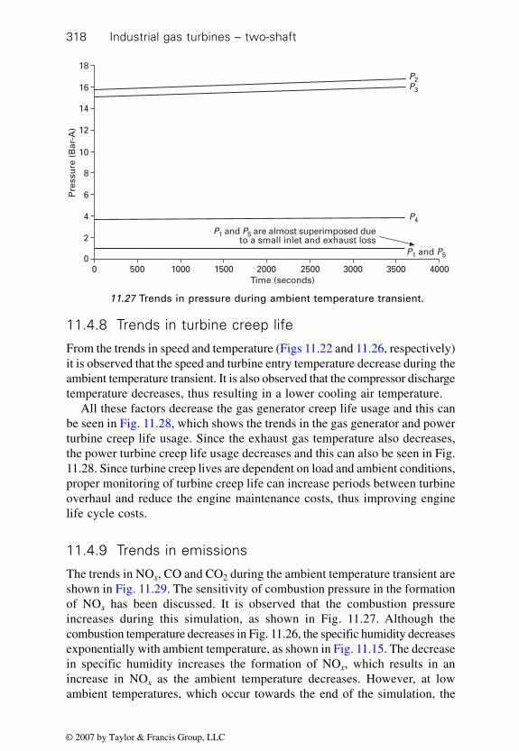
Industrial gas turbines – two-shaft318
11.4.8 Trends in turbine creep life
From the trends in speed and temperature (Figs 11.22 and 11.26, respectively)it is observed that the speed and turbine entry temperature decrease during theambient temperature transient. It is also observed that the compressor dischargetemperature decreases, thus resulting in a lower cooling air temperature.
All these factors decrease the gas generator creep life usage and this canbe seen in Fig. 11.28, which shows the trends in the gas generator and powerturbine creep life usage. Since the exhaust gas temperature also decreases,the power turbine creep life usage decreases and this can also be seen in Fig.11.28. Since turbine creep lives are dependent on load and ambient conditions,proper monitoring of turbine creep life can increase periods between turbineoverhaul and reduce the engine maintenance costs, thus improving enginelife cycle costs.
11.4.9 Trends in emissions
The trends in NOx, CO and CO2 during the ambient temperature transient areshown in Fig. 11.29. The sensitivity of combustion pressure in the formationof NOx has been discussed. It is observed that the combustion pressureincreases during this simulation, as shown in Fig. 11.27. Although thecombustion temperature decreases in Fig. 11.26, the specific humidity decreasesexponentially with ambient temperature, as shown in Fig. 11.15. The decreasein specific humidity increases the formation of NOx, which results in anincrease in NOx as the ambient temperature decreases. However, at lowambient temperatures, which occur towards the end of the simulation, the
Time (seconds)
18P
ress
ure
(B
ar-A
)
0 500 1000 1500 2000 2500 3000 3500 4000
P1 and P5 are almost superimposed dueto a small inlet and exhaust loss
P2P3
P4
P1 and P5
16
14
12
10
8
6
4
2
0
11.27 Trends in pressure during ambient temperature transient.
© 2007 by Taylor & Francis Group, LLC

Simulating the effects of ambient temperature on performance 319
specific humidity is small and the decrease in combustion temperaturedominates, resulting in a decrease in NOx emissions. This can be seen in Fig.11.29, which shows the trend in emissions when the engine is operating atlow power. The figure also shows that CO increases during this transient. Ithas been discussed that CO formation is more sensitive to combustiontemperature than combustion pressure, thus the decrease in combustion
300
NO
x an
d C
O (
pp
mv
@15
%O
z d
ry),
CO
2 m
ass
bas
is (
ton
nes
/day
)
Time (seconds)0 500 1000 1500 2000 2500 3000 3500 4000
CO
CO2 emissionsindex
NOx
CO2 mass basis250
200
150
100
50
0
CO
2 em
issi
on
s in
dex
(kg
/kW
h)
0.58
0.57
0.56
0.55
0.54
0.53
11.29 Trends in emissions due to ambient temperature transient andlow-power operating conditions.
300 000Ti
me
to n
ext
ove
rhau
l (h
ou
rs)
Time (seconds)0 500 1000 1500 2000 2500 3000 3500 4000
Gas generatorturbinePower
turbine
350 000
200 000
150 000
100 000
50 000
0
11.28 Increase in turbine creep life during ambient temperaturetransient and low-power operation.
© 2007 by Taylor & Francis Group, LLC

Industrial gas turbines – two-shaft320
temperature results in an increase in CO as the ambient temperature decreases.The figure also shows the trends in CO2. A reduction in CO2 is observed andis due to the reduction in fuel flow, because of the better thermal efficiency,as the ambient temperature decreases.
11.5 Effect of humidity on gas turbine performance
and emissions
It was stated in Chapter 2 that it is the specific humidity which affects theperformance of gas turbines. Also the effects of humidity on emissions havebeen discussed, particularly NOx. Increasing the specific humidity increasesthe gas constant, R, and specific heat at constant pressure, cp, while the ratioof specific heats, γ, decreases. These trends are shown in Fig. 11.30, whichshows the variation of these gas properties with specific humidity. Alsoobserve that the variation in γ is small compared with cp and R.
For a given ambient temperature and pressure, an increase in relativehumidity will increase the specific humidity, as can be seen from Fig. 2.16in Chapter 2. During maximum power demand and operating at high ambienttemperatures, the power output of the gas turbine is limited by the exhaustgas temperature (EGT). For a given ambient temperature, the ratio of exhaustgas temperature to compressor inlet temperature, T4(EGT)/T1, is fixed (notethe change in γ is small as discussed above). From Fig. 11.6, the compressornon-dimensional speed, N1/√(γR1T1) is also fixed, which in turn would fixthe non-dimensional power output (see Fig. 11.7). Referring to Fig. 11.7, anyincrease in the gas constant, R, results in an increase in the gas turbine poweroutput in order to maintain the non-dimensional power output of the gas
1.08
Gas
pro
per
ty r
elat
ive
to d
ry a
ir
Specific humidity (g water vapour/kg dry air)0.00
Specific heat (cp)
10.00 20.00 30.00 50.0040.00 60.00 70.00 80.00 90.00 100.00
Ratio of specific heats (γ)
Gas constant (R)
1.07
1.06
1.05
1.04
1.03
1.02
1.01
1
0.99
0.98
11.30 Variation of cp, R and γ relative to dry air with specific humidity.
© 2007 by Taylor & Francis Group, LLC

Simulating the effects of ambient temperature on performance 321
turbine. This is illustrated in Fig. 11.31, which shows the gas turbine poweroutput with ambient temperature for a series of values for relative humidity.However, the increase in specific humidity reduces the thermal efficiency,due to the additional fuel required to heat the water vapour to the requiredturbine entry temperature. The variation of gas turbine thermal efficiencywith ambient temperature for a series of values of relative humidity, is shownin Fig. 11.32. At high ambient temperatures (30 degrees Celsius), the increasein gas turbine power output due to the increase in relative humidity (from0% to 100%) can be about 1.5% and this increase in power increases withambient temperature. Thus, at high ambient temperature, an increase in humiditywill result in a worthwhile increase in power output. Operating at constantcompressor non-dimensional speed, N1/√(γRT), an increase in the gas constant,R, due to the increase in specific humidity, will require an increase in the gas
11.31 Impact of relative humidity on gas turbine power output.
11.32 Impact of relative humidity on gas turbine thermal efficiency.
Ambient temperature (°C)0–40 –30 –20 –10 10 20 30 40
RH = Relative humidity
Compressornon-dimensional
speed limited Gas generator speed limited
RH = 0%
EGT limited RH = 60
RH = 100%
22
Po
wer
ou
tpu
t (M
W)
22.5
21.5
21
20.5
20
19.5
19
18.5
Ambient temperature (°C)0–40 –30 –20 –10 10 20 30 40
Th
erm
al e
ffic
ien
cy (
%)
38.0
Compressornon-dimensional
speed limited
RH = 0%
EGT limitedRH = 60
RH = 100%
37.5
37.0
36.5
36.0
35.5
35.0
34.5
Gas generator speed limited
RH = Relative humidity
© 2007 by Taylor & Francis Group, LLC

Industrial gas turbines – two-shaft322
generator speed, N1. Therefore, the gas generator speed limit is reached at ahigher ambient temperature as the relative humidity increases, as observedin Fig. 11.31. Furthermore, from Fig. 11.3, it is evident that the compressorinlet mass flow rate, W1, would decrease with increased humidity.
At low ambient temperatures, the gas turbine power output is limited bythe gas generator speed or N1/√T1. Thus, an increase in the gas constant, R,results in a decrease in compressor non-dimensional speed, N1/√(γRT). This,in turn, would reduce the turbine entry temperature, T3, as seen in Fig. 11.5.Therefore, the specific work decreases due to the decrease in T3. Althoughthe increase in R and therefore cp to increase the specific work, the decreasesin T3 and W1 result in a decrease in gas turbine power output. The decreasein power output is small due to the low ambient temperatures, when the gasturbine power output is limited by the gas generator speed or N1/√T1. At suchlow ambient temperatures, the change in specific humidity with the relativehumidity is small as can be seen in Fig. 2.16. Thus the changes in gasproperties such as R and cp are also small. Hence, there is a very small lossin power output with increase in relative humidity at low ambient temperatureswhen the gas generator speed or N1/√T1 limit the power output of the gasturbine.
The impact of humidity on NOx emissions is more profound. High specifichumidity results in increased presence of water vapour in the combustor,thus suppressing the ‘peak’ combustion temperature. This decrease intemperature results in a significant decrease in NOx with the increase inhumidity, as illustrated in Fig. 11.33.
11.33 Impact of relative humidity on NOx emissions
Ambient temperature (°C)0–40 –30 –20 –10 10 20 30 40
NO
x (p
pm
v @
15%
O2
dry
)Compressor
non-dimensionalspeed limited
RH = 0%
EGT limited
RH = 60%
RH = 100%
RH = Relative humidity
Gas generator speedlimited
200
220
180
160
140
120
100
© 2007 by Taylor & Francis Group, LLC

323
The impact of the change in ambient temperature on engine performancewas considered in Chapter 11, where the negative impact of high ambienttemperatures on performance was observed. Another factor that affects engineperformance is the ambient pressure, where low ambient pressure reducesmaximum power output from the engine. The two-shaft gas turbine simulatorwill now be used to investigate the effects of the change in ambient pressureon engine performance. The ambient pressure may change quite significantlyat a given elevation. At sea level it may vary from 1.04 Bar to 0.96 Bar fora high pressure day and a low pressure day, respectively. This representsabout an 8% change in ambient pressure corresponding to those days. Gasturbines that operate at high elevations, where the ambient pressure is lowerthan at sea level will show a reduced power output. For example, at anelevation of 1000 metres, the ambient pressure would be about 0.9 Bar on anISA (International Standard Atmosphere) day. However, the ambienttemperature at this altitude will be lower, thus partly compensating for thereduced power output.
To cover this ambient pressure range, the ambient pressure will be variedfrom 1.03 Bar to 0.9 Bar in 1 hour (3600 seconds). Also considered will betwo operating cases, which correspond to high power and low power operatingconditions. The high power operating condition will be represented by settingthe power demand from the generator such that the engine will always be onan operating limit. This is simulated by setting the generator power demandto 25 MW. The low power case will be simulated by setting the powerdemand from the generator such that an engine operating limit is neverreached (low power case power demand is set to 17.5 MW). To investigatethe impact of ambient pressure changes on engine performance, the ambienttemperature will be assumed to remain constant at 15 degrees Celsius. Thiswill result in the engine power output being limited by the exhaust gastemperature (EGT) limit rather than by the speed limits from the gas turbine.The inlet and exhaust losses will be set to 100 mm water gauge during these
12Simulating the effect of change in ambient
pressure on engine performance
© 2007 by Taylor & Francis Group, LLC

Industrial gas turbines – two-shaft324
simulations. Again we shall ignore the gas properties terms (γ and R) presentin the non-dimensional parameters for flows and speeds, and we shall makereference to them when relevant.
12.1 Effect of ambient pressure on engine
performance (high-power case)
During high power operation, the exhaust gas temperature limits the engineperformance. Since the ambient temperature remains constant and the engineoperates on the EGT limit, the ratio of T4 (EGT)/T1 also remains constant asthe ambient pressure decreases from 1.03 Bar to 0.9 Bar. Figure 11.6 showsthe running line describing the variation of T4 (EGT)/T1 with the compressornon-dimensional speed, (N1/√T1). A constant T4 (EGT)/T1, implies that thecompressor non-dimensional speed will also remain constant. Thus, the non-dimensional speed of the compressor remains constant throughout thesimulation. A constant compressor non-dimensional speed will mean thatother engine non-dimensional parameters will remain constant throughoutthe simulation (see Figs 11.3 to 11.7). Hence the pressure ratios, temperatureratios, non-dimensional flows and non-dimensional power will all remainconstant during the simulation.
12.1.1 Trends in compressor characteristic and flow
Since the pressure ratio and compressor non-dimensional flow remain constant,the operating point does not move on the compressor characteristic duringthe ambient pressure transient, as shown in Fig. 12.1.
Co
mp
ress
or
pre
ssu
re r
atio
25
20
15
10
5
00 100 200 300 400 500 600
Speed = 73%Speed = 80%
Speed = 86%Speed = 89%
Speed = 92%
Speed = 100%
Speed = 107%
Compressor inlet non-dimensional flow
Speed = 95%Speed = 97%
Compressor surge line
Speed = compressor non-dimensional speed
12.1 Operating point on the compressor characteristic duringambient pressure transient.
© 2007 by Taylor & Francis Group, LLC

Simulating the effect of change in ambient pressure 325
Since the compressor inlet non-dimensional flow W1√T1/P1 is constantduring this transient, the compressor inlet flow W1 decreases proportionallywith P1 due to the fall in the ambient pressure. This can be seen in Fig. 12.2,which shows the trends in flow and fuel valve position during the ambientpressure transient. The temperature rise across the combustion system andthe combustion inlet temperature, T2, also remain constant during this ambientpressure transient. Figure 2.17 in Chapter 2, which shows the variation of theair–fuel ratio as a function of the combustor inlet temperature and temperaturerise, indicates that the air–fuel ratio is also constant. Since the compressorairflow is decreasing, the amount of combustion air also reduces. As the air–fuel ratio is constant, a decrease in combustion airflow will result in a decreasein fuel flow as can be seen in Figure 12.2. The figure also shows the trendin the fuel valve position and this trend is similar to the trend in fuel flow.
12.1.2 Trends in power and thermal efficiency
As the compressor non-dimensional speed is constant during the ambientpressure transient, the non-dimensional power also remains constant. Thusany reduction in P1 requires a corresponding reduction in power output tomaintain the constant non-dimensional power and results in a lower poweroutput (shaft and gas power) due to the decrease of ambient pressure, asshown in Fig. 12.3. Hence, the negative impact of low ambient pressure onmaximum engine power output is illustrated, a problem often encounteredby gas turbines operating at high elevations.
70
Co
mp
ress
or
inle
t ai
rflo
w (
kg/s
), f
uel
val
vep
osi
tio
n (
%),
air
–fu
el r
atio
0
Fuel valve position
Air–fuel ratio
Time (hours)
500 1000 1500 2000 2500 3000 3500 4000
Air flow
Fuel
flo
w (
kg/s
)1.24
Fuel flow
65
60
55
50
45
40
1.22
1.20
1.18
1.16
1.14
1.12
1.10
1.08
1.06
1.04
12.2 Trends in flow during ambient pressure transient.
© 2007 by Taylor & Francis Group, LLC

Industrial gas turbines – two-shaft326
The thermal efficiencies are affected by the compressor pressure ratio,P2/P1, and temperature ratio, T3/T1. These parameters remain constant due tothe constant compressor non-dimensional speed, thus the thermal efficienciesdo not change very much for the current operating conditions. The slightdecrease in thermal efficiency is largely attributed to the increase in specifichumidity due to the decrease in ambient pressure.
12.1.3 Trends in pressure
The compressor and turbine pressure ratios are constant during the decreasein the ambient pressure, and any fall in ambient pressure will result in adecrease in compressor discharge pressure. The decrease in the compressordischarge pressure will be directly proportional to the ambient pressure.Similarly, the gas generator and power turbine inlet and exit pressures alsofall proportionally with the ambient pressure, as shown in Fig. 12.4.
12.1.4 Trends in creep life
The trends in creep life usage of the gas generator and power turbines duringthe ambient pressure transient are shown in Fig. 12.5. Observe that the creeplife usage of the gas generator and power turbine decreases as the ambientpressure decreases. Note from Fig. 12.3 that the power output also decreaseswith the decrease in ambient pressure. Therefore, the torque acting on thepower turbine blades must decrease, as the power turbine speed is constant.
27P
ow
er (
MW
)
0
Gas power
Generator power
Time (hours)500 1000 1500 2000 2500 3000 3500 4000
Gas turbine power output
Th
erm
al e
ffic
ien
cies
(%
)
42
Thermal efficiency
Power required
Gas thermalefficiency
41
40
39
38
37
36
35
25
23
21
19
17
15
12.3 Trends in power output and thermal efficiency during ambientpressure transient.
© 2007 by Taylor & Francis Group, LLC

Simulating the effect of change in ambient pressure 327
This reduction in torque will result in a lower total stress level on the blades,although the centrifugal stress is constant. Since the exhaust gas temperatureremains constant, the lower stress levels result in a decrease in creep lifeusage of the power turbine.
A similar situation exists for the gas generator turbine. Because of theconstant compressor non-dimensional speed, the gas generator speed and theturbine entry temperature will also remain constant. Furthermore, the
0Time (seconds)
500 1000 1500 2000 2500 3000 3500 4000
20P
ress
ure
(B
ar-A
)
P1 and P5 are almost superimposeddue to a small inlet and exhaust loss
P2P3
P4
P1 and P5
16
14
12
10
8
6
4
2
0
18
100 000
Tim
e to
nex
t o
verh
aul (
ho
urs
)
Time (seconds)0 500 1000 1500 2000 2500 3000 3500 4000
Gas generatorturbine
Powerturbine
90 000
80 000
70 000
30 000
20 000
60 000
50 000
40 000
10 000
0
12.4 Trends in pressure during ambient pressure transient.
12.5 Trends in creep lives of gas generator and power turbine bladesduring ambient pressure transient.
© 2007 by Taylor & Francis Group, LLC

Industrial gas turbines – two-shaft328
compressor discharge temperature and hence the cooling air temperaturewill also remain constant. Since the airflow through the compressor decreaseswith the ambient pressure, the power absorbed by the compressor will alsoreduce. All the power required by the compressor is provided by the gasgenerator turbine, so the power produced by the gas generator turbine willalso reduce. Although the gas generator turbine speed and temperature areconstant during the ambient pressure transient, the reduced compressor powerdemand results in less torque in the gas generator turbine blades. The lowerstresses in the gas generator turbine blades due to the lower torque requirementsresult in a decrease in the gas generator turbine creep life usage and can beseen in Fig. 12.5.
12.1.5 Trends in emissions
Figure 12.6 shows the trends in NOx, CO and CO2 emissions. Observe thatthe compressor discharge pressure decreases with ambient pressure, leadingto a decrease in combustion pressure. The combustion temperature remainsconstant due to the constant compressor non-dimensional speed. Thus, thedecrease in combustion pressure results in a decrease in NOx emission andan increase in CO emissions. Also, the increase in specific humidity due tothe decrease in ambient pressure will contribute to the reduction in NOx.
Since the fuel flow decreases with ambient pressure, the CO2 emissionson a mass basis also decrease with reduced ambient pressure and follow thefuel flow trend. The thermal efficiency decreases slightly as discussed above,
300
NO
x an
d C
O (
pp
mv
@15
%O
z d
ry),
CO
z m
ass
bas
is (
ton
nes
/day
)
Time (seconds)0 500 1000 1500 2000 2500 3000 3500 4000
CO
CO2 emissionsindex
NOx
CO2 mass basis
250
200
150
100
50
0
CO
2 em
issi
on
s in
dex
(kg
/kW
h)
0.580
0.575
0.570
0.565
0.560
0.555
0.550
0.545
0.540
0.535
0.530
12.6 Trends in gas turbine emissions during ambient pressuretransient.
© 2007 by Taylor & Francis Group, LLC

Simulating the effect of change in ambient pressure 329
so the CO2 emission index also increases slightly. The trends in these emissionparameters are shown in Fig. 12.6.
12.2 Effect of ambient pressure changes on engine
performance at lower power outputs
Section 12.1 considered the impact of ambient pressure changes on engineperformance when the engine performance is constrained by an engine operatinglimit, as would be encountered at high-power output levels. Consider nowthe impact of change in the ambient pressure when the engine is operating atlower power such that no engine operating limits are encountered. The sameambient pressure transient used previously will be repeated (i.e. reducing theambient pressure from 1.03 to 0.9 Bar in 1 hour), with the ambient temperatureset to 15 degrees Celsius, and inlet and exhaust losses set to 100 mm watergauge. The generator power demand is set to 17.5 MW throughout thesimulation to represent the low power case.
Since the power output of the gas turbine will be constant throughout thesimulation as no engine limits are reached, the non-dimensional power, Power/(P1√T1), will increase as the ambient pressure P1 decreases. Referring to Fig.11.7, which shows the variation of non-dimensional power with compressornon-dimensional speed, any increase in non-dimensional power must beaccompanied by an increase in compressor non-dimensional speed. Thus theincrease in non-dimensional speed will result in increases in other non-dimensional parameters such as pressure ratios, temperature ratios and non-dimensional flows.
12.2.1 Compressor characteristic
The operating point on the compressor characteristic for the low power caseis shown in Fig. 12.7. The operation point is observed moving up the runningline from a lower compressor non-dimensional flow and pressure ratio to ahigher compressor non-dimensional flow and pressure ratio. This is due tothe increase in compressor non-dimensional speed as the ambient pressuredecreases.
12.2.2 Trends in speed
The ambient pressure transient results in an increase in compressor non-dimensional speed, N1/√T1 and therefore an increase in gas generator speeddue to a constant ambient temperature, T1. This is shown in Fig. 12.8, whichillustrates the changes in the gas generator and compressor non-dimensionalspeed during the ambient pressure transient.
It is also observed that the rate of increase in gas generator speed increases
© 2007 by Taylor & Francis Group, LLC

Industrial gas turbines – two-shaft330
as the ambient pressure falls. This is due to higher compressor non-dimensionalspeeds forcing the compressor to operate closer to compressor inlet chokeconditions. Note that the speeds do not reach or exceed any limiting valuesduring this transient.
12.2.3 Trends in pressure ratios
The trends in pressure ratios for the compressor, gas generator turbine andpower turbine are shown in Fig. 12.9. The increase in compressor non-
Co
mp
ress
or
pre
ssu
re r
atio
25
20
15
10
5
00 100 200 300 400 500
Speed = 73%
Speed = 80%Speed = 86%
Speed = 89%Speed = 92%
Compressor inlet non-dimensional flow
Speed = 95%
Compressor surge line
600
Speed = 100%
Speed = 107%
Speed = 97%
Speed = compressor non-dimensional speed
Start of ambient pressure transientambient pressure = 1.03 Bar
End of ambient pressure transientambient pressure = 0.9 Bar
Gas generator speed
Compressornon-dimensional speed
Time (seconds)
Gas
gen
erat
or
spee
d (
RP
M)
0 500 1000 1500 2000 2500 3000 3500 4000
9240 858
856
854
852
850
846
844
842
Co
mp
ress
or
no
n-d
imen
sio
nal
sp
eed
N1
γR1T
1
9220
9200
9180
9160
9140
9120
9100
9080
9060
9040
848
840
838
12.7 Operating point on the compressor characteristic duringambient pressure transient.
12.8 Compressor speed changes during ambient pressure transient.
© 2007 by Taylor & Francis Group, LLC

Simulating the effect of change in ambient pressure 331
dimensional speed results in an increase in compressor pressure ratio, as canbe observed in Fig. 11.4. The gas generator turbine pressure ratio remainsessentially constant, due to the choking conditions that prevail in the powerturbine. Thus an increase in compressor pressure ratio results in an increasein the power turbine pressure ratio.
The figure also shows the trend in the maximum to minimum cycletemperature ratio, T3/T1. An increase in T3/T1 is necessary because of theincrease in compressor non-dimensional speed, as illustrated in Fig. 11.5.
12.2.4 Trends in power and thermal efficiency
Since no engine operating limits are exceeded during the ambient pressuretransient, the power required by the generator will always be provided by thegas turbine. Thus the generator power output trend remains on the powerdemand set point. Hence, the gas turbine power output and the gas poweralso remain essentially constant during this ambient pressure transient, ascan be seen in Fig. 12.10, which shows the trends in powers and thermalefficiencies during the ambient pressure transient. The slight increase in gaspower is due primarily to a small decrease in the power turbine isentropicefficiency. As the ambient pressure decreases, the exhaust gas temperatureincreases to maintain the generator power demand. The power turbine non-dimensional speed now decreases (note that the power turbine speed isconstant), resulting in a small decrease in power turbine efficiency. Thus a
Maximum to minimum cycle temperature ratio
Compressor pressure ratio
Power turbine pressure ratio
Time (seconds)
17.2C
om
pre
sso
r p
ress
ure
rat
io
0 500 1000 1500 2000 2500 3000 3500 4000
5.0
Max
imum
to m
inim
um c
ycle
tem
pera
ture
rat
io.
GG
an
d p
ow
er t
urb
ine
pre
ssu
re r
atio
4.817.0
16.8
16.6
16.4
16.2
16.0
15.8
15.6
4.6
4.4
4.2
4.0
3.8
3.6
3.4
3.2
3.0
GG (gas generator)pressure ratio
12.9 Trends in pressure ratios for compressor, gas generator turbineand power turbine.
© 2007 by Taylor & Francis Group, LLC

Industrial gas turbines – two-shaft332
corresponding increase in gas power output occurs to maintain the powerdemand from the generator as observed in Fig. 12.10.
The gas turbine thermal efficiency and the gas thermal efficiency, whichrepresents the efficiency of the gas generator, increase as the ambient pressuredecreases. As was seen in Fig. 12.9, the compressor pressure ratio and themaximum to minimum cycle temperature ratio, T3/T1 increase as the ambientpressure decreases. The thermal efficiencies essentially are functions of theseratios and independent of ambient pressure as discussed in Chapter 2. Thusthe increases in the compressor pressure ratio and temperature ratio, T3/T1,result in increases in the gas turbine thermal efficiency and the gas generatorthermal efficiency. Therefore, when the power demand is below the maximumcapacity of the engine, a low ambient pressure is desirable because it resultsin an increase in thermal efficiency. It is worth pointing out that this isindeed the principle of a closed cycle gas turbine where we reduce the cycleworking pressure to reduce the load, thus maintaining a constant thermalefficiency at lower loads. Such closed cycle gas turbines have been built andoperated as a means of overcoming the poor thermal efficiencies of gasturbines at low loads.
12.2.5 Trends in flow
Figure 12.11 shows the trends in compressor inlet flow, fuel flow and theair–fuel ratio during the ambient pressure transient. The figure also showsthe position of the fuel valve during this transient. It has been observed that
Gas power
Gas turbine thermal efficiency
20.5P
ow
er (
MW
)
0 500 1000 1500 2000 2500 3000 3500 4000
Th
erm
al e
ffic
ien
cy (
%)
Generator power
Gas turbine power output
Gas generatorthermal efficiency
20.0
19.5
19.0
18.5
18.0
17.5
17.0
41
40
39
38
37
36
35
34
Time (seconds)
12.10 Trends in the power and thermal efficiency during ambientpressure transient.
© 2007 by Taylor & Francis Group, LLC

Simulating the effect of change in ambient pressure 333
70C
om
pre
sso
r in
let
airf
low
(kg
/s),
fu
el v
alve
po
siti
on
(%
), a
ir–f
uel
rat
io
0
Fuel valve position
Compressor inletairflow
Time (seconds)500 1000 1500 2000 2500 3000 3500 4000
Air–fuel ratio Fuel
flo
w (
kg/s
)
1.055
Fuel flow
65
60
55
50
45
40
1.050
1.045
1.040
1.035
1.030
1.025
12.11 Trends in flow during ambient pressure transient.
the compressor pressure ratio and the temperature ratio, T3/T1, increase duringthe ambient pressure transient. The specific work will increase and this isdue to the increase in T3/T1. As the power output remain constant (see Fig.12.10), the increase in specific work will result in a decrease in compressorinlet air flow as shown in Fig. 12.11.
It is worth noting that the decrease in compressor flow, compared with theprevious case, where the engine was operating on an exhaust gas temperaturelimit (Fig. 12.2), is smaller. This is due to the resultant increase in thecompressor non-dimensional flow and speed for this case, whereas in theprevious case the compressor non-dimensional flow remained constant asthe ambient pressure decreased.
The trends in the fuel flow and fuel valve position also show a decline.This is due primarily to the increased thermal efficiency. Since the poweroutput remains constant, any increase in the thermal efficiency must result ina decrease in fuel flow, as shown in Fig. 12.11. The air–fuel ratio decreasesbecause of the increase in T3/T1, as shown in Fig. 12.9. This results in anincrease in the turbine entry temperature, T3, as the ambient temperature, T1
is constant during this transient. Although there is an increase in the compressordischarge temperature, thus also an increase in combustion inlet temperature,due to the increase in compressor pressure ratio (see Fig. 12.9), the increasein T3 is greater, as shown in Fig. 12.12. Hence, the combustion temperaturerises as the ambient pressure decreases. The net effect of the increase incombustion temperature rise is a decrease in the air–fuel ratio, as observedin Fig. 12.11.
© 2007 by Taylor & Francis Group, LLC

Industrial gas turbines – two-shaft334
12.2.6 Trends in temperature
Figure 12.12 shows the trends in temperature during the ambient pressuretransient. The increase in compressor non-dimensional speed results in anincrease in the temperature ratios, T2/T1, T3/T1, and T4 (EGT)/T1). Since theambient temperature, T1, remains constant during this transient, an increasein all the other temperatures is observed during this ambient pressuretransient. Note that the exhaust gas temperature, T4, remains below its limitingvalue during this transient.
12.2.7 Trends in pressure
Although the compressor pressure ratio increases during the decrease inambient pressure, the fall in ambient pressure is greater than the increase incompressor pressure ratio. Thus the net result is a fall in compressor dischargepressure during the ambient pressure transient, as shown in Fig. 12.13, whichillustrates the pressure trends during the ambient pressure transient. The gasgenerator turbine inlet pressure trend closely follows the compressor dischargepressure and shows a reduction in the gas generator turbine inlet pressure.Since the gas generator turbine pressure ratio remains essentially constantdue to the choked conditions that prevail in the power turbine, a decrease inthe compressor discharge pressure results in a decrease in the powerturbine inlet pressure. The power turbine exit pressure, which is very similarto the compressor inlet pressure, decreases in line with the transient beingsimulated.
Time (seconds)
2500Te
mp
erat
ure
(K
)
0 500 1000 1500 2000 2500 3000 3500 4000
2000
1500
1000
500
0
Gas generator turbinemetal temperature
Exhaust gas temperature limit
Primary zonetemperature
T3
T4T2
T1
12.12 Trends in temperature during ambient pressure transient.
© 2007 by Taylor & Francis Group, LLC

Simulating the effect of change in ambient pressure 335
12.2.8 Trends in turbine creep life
The trends in the gas generator and power turbine creep life usage changeduring the ambient pressure transient are shown in Fig. 12.14. It has beenobserved that the gas generator speed, turbine entry temperature and hencethe exhaust gas temperature increase during the decrease in ambient pressure.This also results in an increase in the gas generator turbine metal temperature.
Time (seconds)
18P
ress
ure
(B
ar-A
)
0 500 1000 1500 2000 2500 3000 3500 4000
P1 and P5 are almost superimposeddue to a small inlet and exhaust loss
P2P3
P4
P1 and P5
16
14
12
10
8
6
4
2
0
12.13 Trends in pressure during ambient pressure transient.
300 000
Tim
e to
nex
t o
verh
aul (
ho
urs
)
Time (seconds)0 500 1000 1500 2000 2500 3000 3500 4000
Gas generatorturbine
Powerturbine
250 000
200 000
150 000
100 000
50 000
0
12.14 Trends in gas generator and power turbine creep life duringambient pressure transient.
© 2007 by Taylor & Francis Group, LLC

Industrial gas turbines – two-shaft336
Thus, the creep life usage of the gas generator turbine and power turbineincrease as the ambient pressure falls, resulting in a reduction in the timebetween overhauls. At the start of the ambient pressure transient, the powerturbine operating life is in excess of 300 000 hours; thus it is outside the scaleof the trend shown in Fig. 12.14 and is set by the speeds and temperature thatprevail at the start of this simulation.
12.2.9 Trends in gas turbine emissions
During the ambient pressure transient, the compressor discharge pressurehas been observed to decrease, although the compressor pressure ratio increases.It was also observed that the primary zone temperature increases. In this casethe influence of the increase in primary zone temperature is greater than theresultant decrease in combustion pressure, thus increasing the NOx, as shownin Fig. 12.15, where the trends in emissions during this transient are illustrated.The emission of CO remains essentially constant and is due to the increasein primary zone temperature compensating for the decrease in combustionpressure during the production of CO.
The production of CO2 decreases and follows the fuel flow trend, thusshowing a decrease in CO2 production during this ambient pressure transientdue to the improved thermal efficiency. Hence, at low engine power outputs,low ambient pressures are very beneficial in reducing CO2 emissions; CO2
is considered a greenhouse gas and is thought to be responsible for globalwarming.
12.15 Trends in gas turbine emissions during ambient pressuretransient.
300
NO
x an
d C
O (
pp
mv
@15
%O
2 d
ry),
CO
2 m
ass
bas
is (
ton
nes
/day
)
Time (seconds)0 500 1000 1500 2000 2500 3000 3500 4000
CO
CO2 emissionsindex
NOx
CO2 mass basis
250
200
150
100
50
0
CO
2 em
issi
on
s in
dex
(kg
/kW
h)
0.568
0.564
0.562
0.558
0.554
0.552
0.566
0.560
0.556
© 2007 by Taylor & Francis Group, LLC

337
In Chapter 9 the impact of component deterioration on engine performanceand the undesirable effect on power output and thermal efficiency werediscussed. The factors that affect engine performance deterioration were alsodiscussed. In this chapter the engine simulator will be used to simulate manyof these faults to investigate the impact they have on engine performanceand the change in running line characteristics. Some simple methods todetect engine performance deterioration will also be discussed, particularlycompressor fouling, which is the most common cause of performancedeterioration. Two operating cases will be considered and they correspond toa high power output and a low power output condition, respectively.
13.1 Compressor fouling (high operating power)
As stated above, compressor fouling is the most common form of engineperformance deterioration and it affects all open cycle gas turbines. Thelevel of fouling depends on many factors. The main factors are the level ofdirt and particles in the atmosphere, quality of air filtration and, to a certainextent, the power output of the gas turbine, particularly in multiple shaft gasturbines such as that represented by this simulator. As explained above,compressor fouling occurs because of the deposit of dirt and dust particleson the compressor blades, thus altering the shape of the compressorcharacteristic. An example of the change in compressor characteristic isshown and discussed in Chapter 9, Section 9.1.
Compressor fouling is simulated using this simulator by reducing thecompressor non-dimensional flow linearly with time for any given non-dimensional compressor speed. (It should be noted that compressor foulingis not linear. Experience has shown that the rate of fouling decreases withtime as deposits of dirt and dust collect on the compressor blades, changingthe profile of the blade.) Thus the compressor non-dimensional speed lineshifts to the left due to the reduction in capacity as shown in Fig. 9.3. Fouling
13Simulating the effects of engine component
deterioration on engine performance
© 2007 by Taylor & Francis Group, LLC

Industrial gas turbines – two-shaft338
also reduces the efficiency of the compressor and this is simulated bydecreasing the compressor efficiency linearly and simultaneously with non-dimensional flow. The reduction in compressor non-dimensional flow andcompressor efficiency for a moderately fouled compressor is about 3% and1% respectively.
Fault indices are used to represent engine component performancedeterioration. Fault indices simply represent the changes in the componentcharacteristics. There are two fault indices per engine component and theseare referred to as the fouling fault index and the efficiency fault index. Thefouling fault index represents the change in the non-dimensional flow capacityof the engine component and the efficiency fault index represents the changein the efficiency of the engine component. The simulation of compressorfouling is achieved by displaying the gas turbine degradation page and typingin –3% for the compressor fouling fault index and –1% for the compressorefficiency fault index. A suitable ramp time is selected, which represents thetime for compressor fouling to take effect. Compressor fouling takes weeksor months but the process will be accelerated and a ramp time of 1 hour(3600 seconds) used.
As the current interest is in the impact of compressor fouling at highpowers, such that the engine is on an engine-operating limit, the power fromthe generator is set to 25 MW. The ambient pressure, temperature and relativehumidity will be set to 1.013 Bar, 15 degrees Celsius and 60%, respectively,and the inlet and exhaust losses will both be set to 100 mm of water gauge.The simulation is carried out for 4000 seconds.
13.1.1 Trends in fault indices
The trends in fault indices are shown in Fig. 13.1, which displays the changesin the compressor fouling and efficiency fault indices, respectively. Thecompressor fouling fault index varies linearly from 0% to –3% in 3600seconds and this is, of course, the input made to the model. Similarly, thecompressor efficiency fault index varies linearly from 0% to –1% in 3600seconds.
These changes in compressor fault indices affect the compressorcharacteristic by reducing the non-dimensional flow and compressor efficiency,thus simulating compressor fouling. No other fault is present and this isindicated by the fault indices for the turbine components remaining at zerothroughout the simulation.
13.1.2 Compressor characteristic
The movement of the operating point on the compressor characteristic isshown in Fig. 13.2. The operating point moves down the characteristic as the
© 2007 by Taylor & Francis Group, LLC

Simulating the effects of engine component deterioration 339
compressor speed lines shift to the left during fouling (the characteristicdisplayed is for a clean compressor). Thus a reduction in compressor non-dimensional flow and pressure ratio is observed during fouling.
The non-dimensional speed of the compressor remains essentially constantduring fouling when the engine is operating on a control limit – EGT limited(high power operation). Thus compressor fouling at these operating conditionswill result in a decrease in compressor discharge pressure and compressorinlet mass flow.
0Fa
ult
ind
ices
(%
)Time (seconds)
0 500 1000 1500 2000 2500 3000 3500 4000
Compressor fouling fault index
Compressor efficiency fault index
–0.5
–1
–1.5
–2
–2.5
–3
–3.5
13.1 Trends in compressor and turbine fault indices duringcompressor fouling.
Co
mp
ress
or
pre
ssu
re r
atio
25
20
15
10
5
00 100 200 300 400 500
Speed = 73%
Speed = 80%Speed = 86%
Speed = 89%Speed = 92%
Compressor inlet non-dimensional flow
Speed = 95%
Compressor surge line
600
Speed = 100%
Speed = 107%
Speed = 97%
Fouled compressor
Start of compressorfouling
13.2 Operating point on the compressor characteristic duringcompressor fouling when the engine is operating at a control limit.
© 2007 by Taylor & Francis Group, LLC

Industrial gas turbines – two-shaft340
13.1.3 Trends in pressure ratio
The trends in pressure ratio during compressor fouling are shown in Fig.13.3. As discussed previously, a decrease in compressor pressure ratio isobserved. The choked conditions that prevail in the power turbine preventthe gas generator turbine pressure ratio from changing, as seen in Section8.1.2. The constant gas generator turbine pressure ratio now results in adecrease in the power turbine pressure ratio. However, the decrease in powerturbine pressure ratio is smaller than the decrease in the compressor pressureratio.
The figure also shows the trend in the maximum to minimum cycletemperature, T3/T1, which remains constant during fouling. This is becausethe engine is operating on an exhaust gas temperature limit. Since the ambienttemperature is constant during this simulation, T3/T1 is therefore essentiallyconstant.
13.1.4 Trends in pressure
Figure 13.4 shows the trends in pressure during compressor fouling. Thedecrease in compressor pressure ratio during fouling results in a decrease inthe compressor discharge pressure. The decrease in compressor dischargepressure also results in a decrease in the power turbine inlet pressure becausethe gas generator turbine operates at a constant pressure ratio. The gas generatorturbine inlet pressure decreases with the compressor discharge pressure, asthe combustion system pressure loss does not change very much.
Maximum to minimum cycle temperature ratio
Compressorpressure ratio
GG (gas generator) pressure ratio
Power turbine pressure ratio
Time (seconds)
17.40
Co
mp
ress
or
pre
ssu
re r
atio
0 500 1000 1500 2000 2500 3000 3500 4000
Max
imu
m t
o m
inim
um
cyc
le t
emp
erat
ure
rati
o, G
G a
nd
po
wer
tu
rbin
e p
ress
ure
rat
io5.50
17.35
17.30
17.25
17.20
17.15
17.10
17.05
17.00
16.95
16.90
16.85
5.30
5.10
4.90
4.70
4.50
4.30
4.10
3.90
3.70
3.50
13.3 Trends in compressor and turbine pressure ratios duringcompressor fouling when the engine is operating at a control limit.
© 2007 by Taylor & Francis Group, LLC

Simulating the effects of engine component deterioration 341
13.1.5 Trends in power and thermal efficiency
The most important aspects of engine performance are power output andthermal efficiency. The impact of compressor fouling has an adverse effecton these performance parameters and, in Fig. 13.5 the power output from the
Time (seconds)
18
Pre
ssu
re (
Bar
-A)
0 500 1000 1500 2000 2500 3000 3500 4000
P1 and P5 are almost superimposed dueto a small inlet and exhaust loss
P2P3
P4
P1 and P5
16
14
12
10
8
6
4
2
0
20
13.4 Trends in pressure during compressor fouling when engine isoperating at a control limit.
Gas power
Power required
Time (seconds)
27
Po
wer
(M
W)
0 500 1000 1500 2000 2500 3000 3500 4000
Th
erm
al e
ffic
ien
cies
(%
)
42
Generator power
Gas turbine power output
Gas thermalefficiency
41
40
39
38
37
36
35
Thermal efficiency
25
23
21
19
17
15
13.5 Trends in power and thermal efficiency during fouling whenengine is operating at an engine limit.
© 2007 by Taylor & Francis Group, LLC

Industrial gas turbines – two-shaft342
gas turbine is observed decreasing from about 21 MW to about 20 MW.Although this only represents a 1 MW drop in power output, it correspondsto about a 5% loss in power output and thus a loss of 5% in revenue. It is alsoobserved that the thermal efficiency decreases from 36% to about 35.5%,which represents about 1.5% increase in fuel flow and therefore a 1.5%increase in fuel cost. Although these numbers appear small, they represent asignificant loss in revenue and increase in operating costs. Thus the detectionand management of compressor fouling is of paramount importance inmaintaining the profitability of industries that use gas turbines as a source ofpower. The figure also shows the trends in gas power and gas thermal efficiencyand these follow a similar trend to the gas turbine power output and gasturbine thermal efficiency.
13.1.6 Trends in flow
The trends in flow during compressor fouling are shown in Fig. 13.6. Thecompressor inlet mass flow is observed to decrease and this is due to thedecrease in the compressor non-dimensional flow during fouling.
Since the compressor inlet pressure and temperature remain constant inthis simulation, any decrease in the compressor non-dimensional flow W1√T1/P1 results in a proportional decrease in compressor inlet mass flow, W1.Since the power loss due to compressor fouling is greater than the efficiencyloss, the fuel flow decreases. The air–fuel ratio remains constant because thecombustion system temperature rises and the compressor exit temperatureremain essentially constant during fouling, as shown in Fig. 13.7.
70
Co
mp
ress
or
inle
t ai
rflo
w (
kg/s
), f
uel
val
vep
osi
tio
n (
%),
air
–fu
el r
atio
0
Fuel valve position
Compressor inletairflow
Time (seconds)500 1000 1500 2000 2500 3000 3500 4000
Air–fuel ratio
Fuel
flo
w (
kg/s
)1.205
Fuel flow
65
60
55
50
45
40
1.200
1.195
1.190
1.185
1.180
1.175
1.170
1.165
13.6 Trends in flow during compressor fouling when engine isoperating at a control limit.
© 2007 by Taylor & Francis Group, LLC

Simulating the effects of engine component deterioration 343
13.1.7 Trends in temperature
The trends in the temperature at the inlet and exit of each engine componentare shown in Fig. 13.7. The temperature trends remain essentially constantduring compressor fouling for this case. Although the compressor pressureratio decreases, the loss in compressor efficiency results in a near constantcompressor exit temperature.
The choked conditions that prevail in the power turbine prevent the gasgenerator turbine pressure ratio from changing. Thus the temperature ratioacross the gas generator turbine is approximately constant as discussed inSection 8.1.2. Since the engine operates at a constant exhaust gas temperature,T4, the turbine entry temperature, T3 and the combustion temperature remainessentially constant.
As the exhaust gas temperature remains constant and there is only a smalldecrease in the power turbine pressure ratio that occurs during this transient,as shown in Fig. 13.3, the increase in the power turbine exit temperature issmall.
13.1.8 Trends in speed
Figure 13.8 shows the trends in the gas generator and compressor non-dimensional speeds during compressor fouling. These speeds are observedto remain essentially constant during compressor fouling. This is because theengine performance is controlled by the exhaust gas temperature limit andtherefore there is no significant margin to increase or alter the speed duringfouling.
Time (seconds)
2500Te
mp
erat
ure
(K
)
0 500 1000 1500 2000 2500 3000 3500 4000
2000
1500
1000
500
0
Gas generator turbinemetal temperature
EGT limit
Primary zonetemperature
T3
T4
T5
T1
T2
13.7 Trends in temperature during compressor fouling.
© 2007 by Taylor & Francis Group, LLC

Industrial gas turbines – two-shaft344
13.1.9 Trends in turbine creep life
The trends in the gas generator and power turbine creep life usage duringcompressor fouling are shown in Fig. 13.9. A slight decrease is observed inboth the gas generator and power turbine creep life usage during compressorfouling. It was observed that the compressor mass flow decreases during
Gas generator speed
Compressornon-dimensional speed
Time (seconds)
Gas
gen
erat
or
spee
d (
RP
M)
0 500 1000 1500 2000 2500 3000 3500 4000
9470 879
Co
mp
ress
or
no
n-d
imen
sio
nal
sp
eed
N1
γR1T
1
9460
9450
9440
9430
9420
9410
9400
878.5
878
877.5
877
876.5
876
875.5
875
874.5
874
873.5
13.8 Trends in speed during compressor fouling when engine isoperating at a control limit.
100 000
Tim
e to
nex
t o
verh
aul (
ho
urs
)
Time (seconds)0 500 1000 1500 2000 2500 3000 3500 4000
Gas generatorturbine
Powerturbine
90 000
70 000
60 000
40 000
30 000
0
80 000
50 000
20 000
10 000
13.9 Trends in turbine creep life during compressor fouling whenengine is operating at a control limit.
© 2007 by Taylor & Francis Group, LLC

Simulating the effects of engine component deterioration 345
compressor fouling and the compressor temperature rise is essentially constant.Thus the power absorbed by the compressor decreases during fouling. Sincethe compressor power is provided by the gas generator turbine, the gasgenerator turbine power also decreases during fouling. Thus the torque producedby the gas generator turbine blades will decrease. It was also observed thatthe gas generator speed and turbine temperatures remain essentially constantduring fouling. The constant gas generator speed will result in a constantcentrifugal stress, but the reduction in the torque acting on the turbine bladewill result in a lower bending stress. The net effect reduces the stresses in thegas generator turbine blades and therefore decreases the gas generator turbinecreep life usage.
The power turbine speed remains constant at 3000 RPM during thesimulation. The decrease in power output from the gas turbine due to compressorfouling will therefore reduce the stress in the power turbine blades (lowertorque). As the exhaust gas temperature remains constant during this simulation,the creep life usage of the power turbine also decreases due to the lowerstresses that prevail in the power turbine blades. However, for a given exhaustgas temperature, compressor fouling results in reduced power output fromthe gas turbine and therefore, in real terms, there is an increase in creep lifeusage due to fouling. The reader can illustrate this by running the simulatorat reduced power outputs typical of fouling, but when no compressor foulingis present.
13.1.10 Trends in gas turbine emissions
It has been observed that the compressor discharge pressure, and hence thecombustion pressure, decreases during compressor fouling. However, theprimary zone temperature remains constant during the simulation of fouling.Thus a decrease in NOx is observed during compressor fouling, due to thelower combustion pressure. The emission of CO, on the other hand, remainsessentially constant, as the formation of CO is more sensitive to primaryzone temperature than combustion pressure. These trends can be seen in Fig.13.10. The figure also shows the decrease in CO2, which is proportional tothe fuel flow. Since the fuel flow during fouling decreases, we also observea decrease in CO2. However, the increase in the CO2 index (also shown inFig. 13.10) implies an increase in CO2 emissions in real terms.
It has been stated that the NOx emissions decrease during fouling, and thiseffect seems to indicate that fouling has a beneficial effect on gas turbineemissions. However, this is somewhat misleading as the power output fromthe gas turbine has also decreased. The correct picture only appears when thesimulator is run at the reduced power output caused by fouling and when noperformance deterioration is present. It is only then that the emissions due toa fouled compressor are indeed observed to be higher than those from aclean engine and the user is left to simulate this case.
© 2007 by Taylor & Francis Group, LLC

Industrial gas turbines – two-shaft346
13.1.11 Effect of ambient temperature and compressorfouling on engine performance
The previous discussions on compressor fouling considered the case whenthe ambient temperature was 15 degrees Celsius. The effect of a change inambient temperature during compressor fouling is now considered bysummarising the effect on gas turbine power output.
Figure 13.11 shows the variation of power output with ambient temperaturefor both a clean and fouled compressor, respectively. The loss in gas turbinepower at different ambient temperatures has also been shown. Simulatingthe compressor fouling discussed above at different ambient temperaturesproduced this figure. Note that the loss of power is most significant at lowerambient temperatures when the power output from the gas turbine is limitedby speed rather than by the exhaust gas temperature. Furthermore, at highambient temperatures, the compressor flow tends to be controlled by the HPstages of the compressor as the operating point moves down the compressorcharacteristic similar to that shown in Fig. 11.9 (lower compressor non-dimensional speed). However, fouling affects the LP stages of the compressorcompared with the HP stages. Thus, the impact of fouling will be moreimportant at low ambient temperatures. A very interesting discussion of theeffects of compressor fouling at different compressor non-dimensional speedsis given in Saravanamutoo and Lakshmiranasimha.1
300N
Ox
and
CO
(p
pm
v @
15%
O2
dry
),C
O2
mas
s b
asis
(to
nn
es/d
ay)
Time (seconds)0 500 1000 1500 2000 2500 3000 3500 4000
CO
CO2 emissionsindex
NOx
CO2 mass basis250
200
150
100
50
0
CO
2 em
issi
on
s in
dex
(kg
/kW
h)
0.559
0.558
0.557
0.556
0.555
0.554
0.553
0.552
0.551
0.550
0.549
13.10 Trends in gas turbine emissions due to compressor foulingwhen engine is operating at a control limit.
© 2007 by Taylor & Francis Group, LLC

Simulating the effects of engine component deterioration 347
13.1.12 Displacement of running lines due to compressorfouling
The variation of non-dimensional parameters was discussed in Chapter 11,Section 11.1 and it was stated that the running lines are essentially an invariantof operating conditions (Figs 11.3 to 11.7). When engine performancedeterioration takes place due to compressor fouling, these running lineschange and the changes may be used to detect performance-related faultssuch as compressor fouling. Compressor fouling as stated earlier reduces thecompressor non-dimensional flow and efficiency for a given non-dimensionalspeed.
These deteriorated compressor characteristics have been used to simulatethe effect of compressor fouling on engine performance. The effect foulinghas on these running lines can also be represented. Figure 13.12 shows therunning line on the compressor characteristic for both a clean and a fouledcompressor. The running line for the case when the compressor is fouledshows only a slight displacement towards surge, and is primarily due to thereduction of the compressor efficiency. The efficiency reduction is only 1%(compressor efficiency fault index), thus resulting in a small shift in therunning line. Figure 13.12 also shows the operating points for the clean andfouled cases for the high-power operation cases just discussed.
The displacement of the running line on the compressor characteristic isonly small, and, at lower power, the operating points for the two cases willbe almost coincident; as will be demonstrated later. A better strategy is to
13.11 Variation of gas turbine power output with ambienttemperature for a clean and fouled compressor, respectively.
Time (seconds)0–40 –30 –20 –10 10 20 30 40
21 000
Power loss
EGT limited
–2
Po
wer
loss
du
e to
co
mp
ress
or
fou
ling
(%
)
–2.5
–3
–3.5
–4
–4.5
–5
–5.5
–6
N1/√T1 limited
Fouled compressor
Po
wer
(M
W)
22 000
21 000
20 000
20 000
19 500
19 000
18 500
18 000
17 500
Gas generator speed limited
Cleancompressor
© 2007 by Taylor & Francis Group, LLC

Industrial gas turbines – two-shaft348
represent these running lines on a compressor non-dimensional flow versusnon-dimensional speed basis, as shown in Fig. 13.13. The displacement ofthe running line due to compressor fouling is shown clearly. The shift in therunning line is dependent only on the compressor fouling fault index, whichrepresents the level of compressor fouling.
13.12 Running lines on the compressor characteristic for a clean andfouled compressor operating at high power.
13.13 Variation of compressor non-dimensional flow with non-dimensional speed.
Co
mp
ress
or
pre
ssu
re r
atio
(P2/
P 1)
25
20
15
10
5
00 100 200 300 400 500
Speed = 73%Speed = 80%
Speed = 86%Speed = 89%
Speed = 92%Speed = 95%
Compressor surge line
600
Speed = 100%Speed = 107%
Speed = 97%
Compressor speed lines
Operating point(clean compressor)Speed =
N1
γ1R1T1 Running line (fouledcompressor)
Operating point(fouled
compressor)
Running line(clean compressor)
Compressor inlet non-dimensional flow
W R T
P1 1 1 1
1
/γ
WR
T
P1
11
1
1
/γ
Co
mp
ress
or
inle
t n
on
-dim
ensi
on
al f
low
550
500
450
400
350
300750 770 790 810 830 850 870 890 910 930 950
Compressor non-dimensional speed
Fouled compressor
Clean compressor
Operating points for cleanand fouled compressor
N
R T1
1 1 1γ
© 2007 by Taylor & Francis Group, LLC

Simulating the effects of engine component deterioration 349
The reduction in compressor non-dimensional flow for a given compressornon-dimensional speed during compressor fouling not only shifts the runningline on the compressor characteristic but the compressor pressure ratio willalso decrease as the compressor fouls, as shown in Fig. 13.3. This effect isbest illustrated by displaying the variation of the compressor pressure ratiowith its non-dimensional speed, as shown in Fig. 13.14, where the displacementin the running line is clearly shown. Unlike the variation of the compressornon-dimensional flow with its non-dimensional speed, which is only influencedby compressor fouling, the variation of compressor pressure ratio will alsobe influenced by other engine faults, as will be seen later when damage toturbines is considered.
Similarly, the running lines based on other non-dimensional parametersmay be produced. The user can generate these running lines with the respectiveoperating points for a clean and fouled compressor.
13.2 Compressor fouling (low operating power)
The effect of compressor fouling when the gas turbine is operating at highenough powers such that the engine is always on an operating limit hasbeen discussed. The effect of fouling on engine performance will now beconsidered when the power demand from the generator is sufficiently lowenough (17.5 MW) to prevent the engine from reaching an operating limitduring compressor fouling. The simulation of the compressor fouling is the
13.14 Variation of compressor pressure ratio with compressor non-dimensional speed.
Co
mp
ress
or
pre
ssu
re r
atio
(P 2
/P2)
20
750 770 790 810 830 850 870 890 910 930 950
Compressor non-dimensional speed
Fouled compressor
Clean compressor
Operating points for cleanand fouled compressor
18
16
14
12
10
8
N
R T1
1 1 1γ
© 2007 by Taylor & Francis Group, LLC

Industrial gas turbines – two-shaft350
same as that discussed for the case previously where the effect of compressorfouling at high operating power was discussed.
13.2.1 Compressor characteristic
The movement of the operating point on the compressor characteristic duringfouling when operating at low power is shown in Fig. 13.15. The movementof the operating point in this case is significantly less when compared withthe case of high operating power (see Fig. 13.2). This is due to the enginebeing able to increase the gas generator speed and exhaust gas temperatureto maintain the generator power demand.
13.2.2 Trends in speed
Since the engine is not on an operating limit during low power operation,compressor fouling will result in an increased gas generator speed in orderto maintain the power demand, which is met by increasing the fuel flow.Since the compressor inlet temperature does not change, the increase in gasgenerator speed results in an increase in the compressor non-dimensionalspeed. This is illustrated in Fig. 13.16, which shows the trends in the gasgenerator and compressor non-dimensional speeds during fouling whenoperating at low power.
13.2.3 Trends in temperature
The trends in temperature during compressor fouling when operating at lowpower are shown in Fig. 13.17. Note that the exhaust gas temperature, turbine
13.15 Movement of operating point on compressor characteristicduring compressor fouling when operating at low power.
Co
mp
ress
or
pre
ssu
re r
atio
25
20
15
10
5Speed = 80%
Speed = 86%Speed = 89%
Speed = 92%Speed = 95%
Compressor surge line Speed = 100%Speed = 107%
Speed = 97%
Start of compressorfouling
Fouled compressor
00 100 200 300 400 500
Speed = 73%
600Compressor inlet non-dimensional flow
Speed = compressor non-dimensional speed
© 2007 by Taylor & Francis Group, LLC

Simulating the effects of engine component deterioration 351
entry temperature and the primary zone temperature are all increasing duringfouling. This is due to the loss in engine performance, thus requiringhigher operating temperatures to maintain the generator power demand.However, the compressor exit temperature remains essentially constant duringcompressor fouling and any slight increase is due to the loss in compressorefficiency.
13.16 Trends in speed during compressor fouling when operating atlow power.
Time (seconds)
2500
Tem
per
atu
re (
K)
0 500 1000 1500 2000 2500 3000 3500 4000
2000
1500
1000
500
0
Gas generator turbinemetal temperature
EGT limit
Primary zonetemperature
T3
T4
T5
T1
T2
13.17 Trends in temperature during compressor fouling whenoperating at low power.
Gas
gen
erat
or
spee
d (
RP
M) Compressor
non-dimensional speed
Gas generator speed
9120
9115
9110
9105
9100
9095
9090
9085
9080
9075
90700 500 1000 1500 2000 2500 3000 3500 4000
Time (seconds)
847.0
846.5
846.0
845.5
845.0
844.5
844.0
843.5
842.5
843.0
Co
mp
ress
or
no
n-d
imen
sio
nal
sp
eed
N RT
1
11
1γ
© 2007 by Taylor & Francis Group, LLC

Industrial gas turbines – two-shaft352
13.2.4 Trends in power and efficiency
The trends in power and thermal efficiency are shown in Fig. 13.18. Thegenerator power output remains on the set point (17.5 MW), thus the gasturbine power output and the gas power also remain constant during fouling.The gas turbine thermal efficiency and the gas thermal efficiency decreaseduring compressor fouling and this is due to the loss in engine performance.Thus, compressor fouling at low power has no effect on revenue, as thepower demand can be met, since no engine limits are reached. However, theloss in thermal efficiency will result in increased fuel costs.
In industries where fuel costs are minimal, such as in oil and gas explorationand production, compressor fouling is of little consequence if engines operateat relatively low powers. Thus, compressor washes can be infrequent. However,if dirt and debris are allowed to accumulate on the compressor blades,particularly on the high pressure stages where such debris can become bakedon due to the higher temperatures in these compressor stages, subsequentwashing of the compressor may not return the compressor back to its bestperformance.2 This will result in reduced revenue when maximum powerdemand is required. Thus frequent washing is important but has to be balancedwith the loss of production due to downtime during washing.
13.2.5 Trends in flow
Figure 13.19 shows the trends in flow during compressor fouling. Observethat the compressor inlet flow decreases slightly since the movement of the
Gas power
Time (seconds)
21.0
Po
wer
(M
W)
0 500 1000 1500 2000 2500 3000 3500 4000
Th
erm
al e
ffic
ien
cies
(%
)
Generator power
Gas turbine power output
Gas thermalefficiency
41
40
39
38
37
36
Gas turbinethermal efficiency
35
20.5
20.0
19.5
19.0
18.5
18.0
17.5
13.18 Trends in power and thermal efficiency during compressorfouling when operating at low power.
© 2007 by Taylor & Francis Group, LLC

Simulating the effects of engine component deterioration 353
compressor operating point is small compared with the case when the effectof fouling on engine performance at high operating powers is considered.There is an increase in fuel flow and fuel valve position during foulingand this is due to the lower thermal efficiency as discussed before. Sincethere is an increase in fuel flow and a decrease in compressor inlet flow, thereduction in combustion airflow causes the air–fuel ratio to decrease duringfouling.
13.2.6 Trends in pressure ratio and pressure
The trends in the pressure ratio during compressor fouling are shown in Fig.13.20. Due to little movement in the operating point on the compressorcharacteristic during fouling when operating at low power, only a smallchange in the compressor pressure ratio occurs during fouling at these poweroutput conditions. There is a slight increase in the maximum to minimumcycle temperature ratio, T3/T1, and this is due to the increase in turbine entrytemperature during compressor fouling. As there is only a small change inthese pressure ratios, the changes in pressure trends during compressor foulingare also small and are shown in Fig. 13.21.
13.2.7 Trends in turbine creep life
It has been observed that the gas generator speed and the turbine entrytemperature increase with compressor fouling when operating at low power
64
Co
mp
ress
or
inle
t ai
rflo
w (
kg/s
), f
uel
val
vep
osi
tio
n (
%),
air
–fu
el r
atio
0
Fuel valve positionCompressor inletairflow
Time (seconds)500 1000 1500 2000 2500 3000 3500 4000
Air–fuel ratio
Fuel
flo
w (
kg/s
)1.080
Fuel flow
62
60
58
56
54
52
1.078
1.076
1.074
1.072
1.070
13.19 Trends in compressor inlet air and fuel flow during compressorfouling when operating at low power.
© 2007 by Taylor & Francis Group, LLC

Industrial gas turbines – two-shaft354
outputs. The increase in gas generator speed results in an increase in thecentrifugal stress of the rotor blades, and the increase in turbine entrytemperature results in the increase in the turbine blade temperature. Thesetwo factors have an adverse effect on the gas generator turbine creep lifesuch that the gas generator turbine creep life usage is observed to increasesignificantly as the compressor fouls. This is shown in Fig. 13.22 and isclearly different from the high power operating case (see Fig. 13.9).
Maximum to minimum cycle temperature ratio
Compressorpressure ratio
Gas generator (GG) turbine pressure ratio
Power turbine pressure ratio
Time (seconds)
16.18C
om
pre
sso
r p
ress
ure
rat
io
0 500 1000 1500 2000 2500 3000 3500 4000
Max
imu
m t
o m
inim
um
cyc
le t
emp
erat
ure
rati
o G
G a
nd
po
wer
tu
rbin
e p
ress
ure
rat
io
4.9
16.17
16.16
16.15
16.14
16.13
16.12
16.11
16.10
4.7
4.5
4.3
4.1
3.9
3.7
3.5
13.20 Trends in pressure ratio during compressor fouling at low power.
Time (seconds)
18
Pre
ssu
re (
Bar
-A)
0 500 1000 1500 2000 2500 3000 3500 4000
P1 and P5 are almost superimposed, dueto a small inlet and exhaust loss
P2P3
P4
P1 and P5
16
14
12
10
8
6
4
2
0
13.21 Trends in pressure during compressor fouling at low power.
© 2007 by Taylor & Francis Group, LLC

Simulating the effects of engine component deterioration 355
The power turbine operates at a constant speed as dictated by the generatorwith the load being constant, thus the stress in the power turbine blades willalso remain constant. However, the increase in the exhaust gas temperaturedue to compressor fouling results in an increase in the power turbine bladetemperature leading to an increase in power turbine creep life usage. Notethat the gas generator turbine time to overhaul decreases from about 75 000hours at the start of compressor fouling to about 35 000 hours at the end ofcompressor fouling. The power turbine time to overhaul is in excess of 300000hours at the start of compressor fouling and decreases to about 240 000 hoursat the end of compressor fouling. The creep life for both turbines at the endof compressor fouling is still in excess of the hours when engine overhaulstake place (about 20 000 hours). Thus decreases in turbine creep life are oflittle consequence unless the actual turbine creep life is monitored. As thecreep life is in excess of 20,000 hours at low gas turbine power outputs,proper monitoring of turbine creep life usage can result in a significantincrease in time between overhauls resulting in reduced maintenance costs.
13.2.8 Trends in emissions
The increase in primary zone temperature during compressor fouling, asshown in Fig. 13.17, results in an increase in NOx during fouling, althoughthere is a slight decrease in compressor discharge pressure and therefore incombustion pressure. The effect of the changes in these parameters on CO issmall. The increase in fuel flow due to the reduction in gas turbine thermalefficiency results in an increase in CO2 emission and this is seen in Fig.
300 000Ti
me
to n
ext
ove
rhau
l (h
ou
rs)
Time (seconds)0 500 1000 1500 2000 2500 3000 3500 4000
Gas generatorturbine
Powerturbine
250 000
200 000
150 000
100 000
50 000
0
13.22 Trends in creep life during compressor fouling.
© 2007 by Taylor & Francis Group, LLC

Industrial gas turbines – two-shaft356
13.23, which shows the trends in gas turbine emissions during compressorfouling at low power.
It has been stated that in industries where the fuel cost is relatively low,the impact of compressor fouling on revenue is small when operating at lowpower. However, if emissions become important, the operators may be taxedon the amount of emissions produced by their gas turbines. Then, compressorfouling at low power output becomes important as increased emissions wouldhave an adverse effect on profitability.
13.2.9 Displacement of running lines due to compressorfouling (low power)
The displacement of the running line is no different from that shown in Fig.13.13, as the amount of compressor fouling for the high and low power casesare the same. All that changes are the operating points, as shown in Fig.13.24, which illustrates the change in compressor non-dimensional flowwith its non-dimensional speed due to compressor fouling.
Figure 13.25 shows the displacement of the compressor pressure ratiowith its non-dimensional speed. It is again observed that the displacement ofthe running line is the same as that shown for the high power case (Fig.13.14), since the compressor fouling simulation is no different. The twooperating points are shown for the clean and fouled cases, respectively,when the engine is operating at low power. The high power operating pointsare also shown for comparison.
300N
Ox
and
CO
(p
pm
v @
15%
O2
dry
),C
O2
mas
s b
asis
(to
nn
es/d
ay)
Time (seconds)0 500 1000 1500 2000 2500 3000 3500 4000
CO
CO2 emissionindex
NOx
CO2 mass basis
250
200
150
100
50
0
CO
2 em
issi
on
ind
ex (
kg/k
W h
)
0.5660
0.5655
0.5650
0.5645
0.5640
0.5635
0.5630
0.5625
0.5620
0.5615
0.5610
13.23 Trends in gas turbine emissions during compressor fouling atlow power.
© 2007 by Taylor & Francis Group, LLC

Simulating the effects of engine component deterioration 357
13.3 Turbine damage
Turbines are exposed to very high temperatures, particularly the gas generatorturbine, and these turbines often employ cooling to achieve satisfactory
13.24 Displacement of compressor non-dimensional flow running lineand operating points due to compressor fouling for high power andlow power cases.
13.25 Displacement of compressor pressure ratio running line andoperating points for low and high power cases.
Co
mp
ress
or
inle
t n
on
-dim
ensi
on
al f
low
550
500
450
400
350
300750 770 790 810 830 850 870 890 910 930 950
Compressor non-dimensional speed
Fouled compressorClean compressor
Operating points for cleanand fouled compressor
(high power case)
Operating points for cleanand fouled compressor (low
power case)
WR
T
P1
11
1
1
/γ
N
R T1
1 1 1γ
Co
mp
ress
or
pre
ssu
re r
atio
(P 2
/P2)
20
750 770 790 810 830 850 870 910 930 950
Compressor non-dimensional speed
Fouled compressorClean compressor
18
16
14
12
10
8
Operating points for cleanand fouled compressor
(high power case)
Operating points for cleanand fouled compressor
(low power case)
990
N
R T1
1 1 1γ
© 2007 by Taylor & Francis Group, LLC
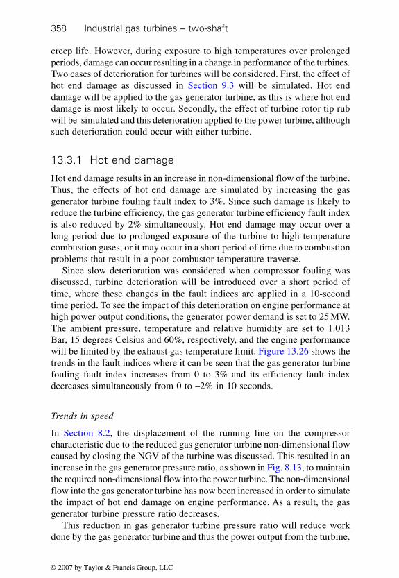
Industrial gas turbines – two-shaft358
creep life. However, during exposure to high temperatures over prolongedperiods, damage can occur resulting in a change in performance of the turbines.Two cases of deterioration for turbines will be considered. First, the effect ofhot end damage as discussed in Section 9.3 will be simulated. Hot enddamage will be applied to the gas generator turbine, as this is where hot enddamage is most likely to occur. Secondly, the effect of turbine rotor tip rubwill be simulated and this deterioration applied to the power turbine, althoughsuch deterioration could occur with either turbine.
13.3.1 Hot end damage
Hot end damage results in an increase in non-dimensional flow of the turbine.Thus, the effects of hot end damage are simulated by increasing the gasgenerator turbine fouling fault index to 3%. Since such damage is likely toreduce the turbine efficiency, the gas generator turbine efficiency fault indexis also reduced by 2% simultaneously. Hot end damage may occur over along period due to prolonged exposure of the turbine to high temperaturecombustion gases, or it may occur in a short period of time due to combustionproblems that result in a poor combustor temperature traverse.
Since slow deterioration was considered when compressor fouling wasdiscussed, turbine deterioration will be introduced over a short period oftime, where these changes in the fault indices are applied in a 10-secondtime period. To see the impact of this deterioration on engine performance athigh power output conditions, the generator power demand is set to 25 MW.The ambient pressure, temperature and relative humidity are set to 1.013Bar, 15 degrees Celsius and 60%, respectively, and the engine performancewill be limited by the exhaust gas temperature limit. Figure 13.26 shows thetrends in the fault indices where it can be seen that the gas generator turbinefouling fault index increases from 0 to 3% and its efficiency fault indexdecreases simultaneously from 0 to –2% in 10 seconds.
Trends in speed
In Section 8.2, the displacement of the running line on the compressorcharacteristic due to the reduced gas generator turbine non-dimensional flowcaused by closing the NGV of the turbine was discussed. This resulted in anincrease in the gas generator pressure ratio, as shown in Fig. 8.13, to maintainthe required non-dimensional flow into the power turbine. The non-dimensionalflow into the gas generator turbine has now been increased in order to simulatethe impact of hot end damage on engine performance. As a result, the gasgenerator turbine pressure ratio decreases.
This reduction in gas generator turbine pressure ratio will reduce workdone by the gas generator turbine and thus the power output from the turbine.
© 2007 by Taylor & Francis Group, LLC

Simulating the effects of engine component deterioration 359
Since the power output from the gas generator turbine drives the compressor,the gas generator will slow down, as seen in Fig. 13.27, where the speedtrends are shown. The compressor non-dimensional speed will also decreasedue to the reduction in the gas generator speed.
Trends in pressure ratio and pressure
The reduction in gas generator speed due to hot end damage will reduce thecompressor pressure ratio as the operating point on the compressor characteristicmoves down. The effect of increased non-dimensional flow through the gasgenerator turbine due to hot end damage will also move the compressorrunning line away from surge, thus further reducing the compressor pressureratio. This can be seen in Fig. 13.28, which shows the trends in pressureratios due to the effect of hot end damage to the gas generator turbine. Thetrends also show a reduction in maximum to minimum cycle temperatureratio, T3/T1.
It is also observed that the gas generator turbine pressure ratio decreasesdue to increasing non-dimensional flow through the gas generator turbine, asdiscussed previously. The compressor pressure ratio decreases from about17.3 to 15.8, whereas the gas generator turbine pressure ratio decreases fromabout 4.1 to about 3.9. Since the fall in compressor pressure ratio is greaterthan the fall in gas generator turbine pressure ratio, a decrease in the powerturbine pressure ratio is observed.
Gas generator turbine fouling fault index
Gas generator turbine efficiency fault index
Time (seconds)
Fau
lt in
dic
es (
%)
4
0
3
2
1
0
–1
–2
–3
10 20 30 40 50 60 70
13.26 Trends in gas generator turbine fault indices due to hot enddamage in the power turbine.
© 2007 by Taylor & Francis Group, LLC

Industrial gas turbines – two-shaft360
The decrease in the pressure ratios now results in decreases in the compressordischarge pressure, combustion pressure and power turbine inlet pressure, asshown in Fig. 13.29.
13.27 Trends in speed due to hot end damage of the gas generatorturbine.
18
Co
mp
ress
or
pre
ssu
re r
atio
16
14
12
10
8
6
4
2
0
20
0 10 20 30 40 50 60 70Time (seconds)
4.92
Max
imu
m t
o m
inim
um
cyc
le t
emp
erat
ure
rat
io,
GG
an
d p
ow
er t
urb
ine
pre
ssu
re r
atio
Power turbine pressure ratio
GG (gas generator) pressure ratio
Maximum to minimum cycle temperature ratio
Compressor pressure ratio
4.91
4.90
4.89
4.88
4.87
4.86
4.85
4.84
4.83
13.28 Trends in pressure ratios due to hot end damage in the gasgenerator turbine.
Gas
gen
erat
or
spee
d (
RP
M)
Compressornon-dimensional speed
Gas generator speed
9450
0 10 20 30 40 50 60 70Time (seconds)
880
Co
mp
ress
or
no
n-d
imen
sio
nal
sp
eed
9400
9350
9300
9250
9200
9150
9100
9050
9000
875
870
865
860
855
850
845
840
835
N RT
1
11
1γ
© 2007 by Taylor & Francis Group, LLC

Simulating the effects of engine component deterioration 361
Trends in temperature
The trends in temperature due to hot end damage in the gas generator turbineare shown in Fig. 13.30. The reduction in compressor pressure ratio resultsin a decrease in the compressor discharge temperature. Since the exhaust gastemperature limits the engine performance (constant EGT), the decrease inthe gas generator turbine pressure ratio, as explained, will decrease the turbine
18
Pre
ssu
res
(Bar
-A)
16
14
12
10
8
6
4
2
0
20
0 10 20 30 40 50 60 70Time (seconds)
P1 and P5 are almost superimposed,due to a small inlet and exhaust loss
P2P3
P4
P1 and P5
13.29 Trends in pressure due to gas generator turbine hot enddamage.
2500
Tem
per
atu
re (
K)
2000
1500
1000
500
0
Gas generator turbinemetal temperature
Exhaust gas temperaturelimit
Primary zonetemperature
T3
T4
T5
T1
T2
0 10 20 30 40 50 60 70Time (seconds)
13.30 Trends in temperature due to hot end damage in the gasgenerator turbine.
© 2007 by Taylor & Francis Group, LLC

Industrial gas turbines – two-shaft362
entry temperature, the primary zone temperature and T3/T1, as seen in Fig.13.28. However, the decrease in the power turbine pressure ratio will increasethe power turbine exit temperature, T5, as seen in Fig. 13.30.
Trends in power and thermal efficiency
The decrease in the gas generator turbine efficiency and the maximum tominimum cycle temperature ratio, T3/T1, reduces the specific work.Furthermore, the compressor inlet airflow will also decrease as can be seenin Fig. 13.32, resulting in a decrease in the gas power and the gas turbinepower output. The decreases in compressor pressure ratio, gas generatorturbine efficiency and the cycle temperature ratio, T3/T1, result in a decreasein the thermal efficiency. Thus the decrease in powers and thermal efficienciesare observed as shown in Fig. 13.31, where the trends in power and thermalefficiency due to hot end damage in the gas generator turbine are illustrated.The generator power output decreases from about 20.5MW to 18.1 MW,representing nearly a 12% loss in generation power and thus revenue. Thegas turbine thermal efficiency decreases from about 36% to 34.6%, thisrepresenting nearly 4% increase in fuel cost in real terms.
Trends in flow
Figure 13.32 shows the trends in compressor inlet airflow, fuel flow and theair–fuel ratio due to hot end damage in the gas generator turbine. The figure
13.31 Trends in power and thermal efficiency due to gas generatorturbine hot end damage.
Gas power
Power required30
Po
wer
(M
W)
42
Generator power
Gas turbine power output Gas thermal efficiency
41
40
39
38
37
36
35
thermal efficiency
0 10 20 30 40 50 60 70Time (seconds)
25
20
15
10
5
0 34
Gas turbine
Th
erm
al e
ffic
ien
cies
(%
)
© 2007 by Taylor & Francis Group, LLC

Simulating the effects of engine component deterioration 363
also shows the trend in the fuel valve position. The decrease in compressorspeed, as observed in Fig. 13.27, forces the operating point down along therunning line on the compressor characteristic and thus we observe a decreasein compressor inlet mass flow. Although the gas turbine thermal efficiencydecreases, the loss in power output is greater than the loss in gas turbinethermal efficiency and therefore a reduction in fuel flow is observed. (If thesimulator is run at low power level such that the engine is not on an operatinglimit, an increase in fuel flow would then be observed for the same turbinedeterioration.)
The decrease in the compressor inlet airflow and thus the combustionairflow is similar to the decrease in fuel flow. Furthermore, the combustiontemperature rise remains essentially unchanged before and after hot enddamage (Fig. 13.30). Thus, only a slight change in the air–fuel ratio isobserved due to hot end damage in the gas generator turbine.
Trends in turbine creep life
The trends in turbine creep life due to hot end damage are shown in Fig.13.33. It is interesting to note that the gas generator turbine creep life usageactually decreases due to this deterioration. The time to overhaul for the gasgenerator turbine increases from about 22 000 hours to 45 000 hours. In theabove figures it has been observed that the gas generator speed and turbineentry temperature decrease due to hot end damage, resulting in lower stressand blade temperature during hot end damage. These factors therefore decrease
0 10 20 30 40 50 60 70Time (seconds)
70C
om
pre
sso
r in
let
airf
low
(kg
/s),
fu
el v
alve
po
siti
on
(%
), a
ir–f
uel
rat
io
Fuel valve position
Compressor inletairflow
Air–fuel ratio
Fuel
flo
w (
kg/s
)
1.21
Fuel flow
65
60
55
50
45
1.20
1.19
1.18
1.17
1.16
1.15
1.14
1.13
1.12
13.32 Trends in flow due to gas generator hot end damage.
© 2007 by Taylor & Francis Group, LLC

Industrial gas turbines – two-shaft364
the gas generator turbine life usage due to this deterioration. However, thisdecrease in turbine creep life usage is very misleading. To obtain the completepicture the simulator needs to be run at the maximum power available whenhot end damage is present and with no performance deterioration (i.e. at agenerator power of 18.8 MW). The gas generator turbine time to overhaulwould then be observed increasing to about 55 500 hours. Thus, hot enddamage actually results in a loss in gas generator turbine creep life.
Figure 13.33 also shows the trend in the power turbine creep life. Observethat the power turbine creep life usage increases during the period when hotend damage to the gas generator turbines first occurs. The power turbinecreep life usage is observed to decrease apparently above that before hot enddamage was applied to the gas generator turbine. This is due to the transientas the control system responds by closing the fuel valve, hence reducing thefuel flow, in an attempt to keep the exhaust gas temperature within thecontrol limits. This action results in a slight over-shoot of the exhaust gastemperature, as seen in Fig. 13.30, and results in the increased power turbinecreep life usage during the transient. If the hot end damage was applied tothe gas generator turbine over a longer time period, greater than 500 seconds,a continuous decrease in the power turbine creep life usage would be observed.This decrease in power turbine creep life usage occurs mainly due to thereduction in power output from the power turbine resulting in lower stress inthe power turbine blades.
Again, this increase in power turbine life is misleading. The simulatorneeds to be run at the limiting power due to hot end damage, but when no
0 10 20 30 50 60 70Time (seconds)
100 000Ti
me
to n
ext
ove
rhau
l (h
ou
rs)
Gas generatorturbine
Power turbine
90 000
70 000
60 000
40 000
30 000
80 000
50 000
20 000
10 000
400
13.33 Trends in gas generator and power turbine creep life due togas generator turbine hot end damage.
© 2007 by Taylor & Francis Group, LLC

Simulating the effects of engine component deterioration 365
turbine deterioration is present, to determine the actual effect of hot enddamage on the power turbine creep life usage. Then a decrease in creep lifeusage would be seen, thus indicating the negative impact on power turbinecreep life due to hot end damage. The user is left to demonstrate this differencein creep life.
Trends in gas turbine emissions
The trend in gas turbine emissions due to hot end damage to the gas generatorturbine is shown in Fig. 13.34. Observe that NOx and CO2 decrease, while aslight increase in CO occurs. It has been observed that the compressor dischargepressure, hence combustion pressure and primary zone temperature, decreasedue to this degradation, thereby resulting in a decrease in NOx and an increasein CO. The decrease in CO2 is primarily due to the decrease in fuel flowresulting from hot end damage to the gas generator turbine. However, theincrease in CO2 emission index implies an increase in CO2 emission in realterms.
The maximum power available from the engine, due to the gas generatorturbine hot end damage, is about 18.8 MW. If the engine was run at thispower, but when no engine degradation is present, then a further decrease inNOx would be observed. Thus, in real terms, hot end damage does result inan increase in these emissions, particularly of NOx and CO2.
300
NO
x an
d C
O (
pp
mv
@15
%O
2 d
ry),
CO
2 m
ass
bas
is (
ton
nes
/day
)
CO
CO2 emissionindex
NOx
CO2 mass basis
250
200
150
100
50
0
CO
2 em
issi
on
ind
ex (
kg/k
W h
)0.574
0 10 20 30 50 60 70Time (seconds)
40
0.572
0.570
0.568
0.566
0.564
0.562
0.560
0.558
0.556
0.554
0.552
13.34 Trends in gas turbine emissions when hot end damage ispresent in the gas generator turbine.
© 2007 by Taylor & Francis Group, LLC

Industrial gas turbines – two-shaft366
Displacement of running line due to hot end damage in the gas generatorturbine
It was discussed in Section 8.2 that decreasing the swallowing capacity(non-dimensional flow) of the gas generator turbine would shift the runningline on the compressor characteristic towards surge. Conversely, an increasein the capacity of the gas generator turbine would shift the running line awayfrom surge. However, the effect of reducing the gas generator turbine efficiencywould shift the running line towards surge. This can be demonstrated byrunning the simulator where only the effect of reducing the gas generatorturbine efficiency fault index by 2% is considered.
The effect of increasing the capacity of the turbine dominates because theshift in the running line due to the fall in gas generator turbine efficiency issmall. Thus, the net effect on the running line of the compressor characteristicis a slight shift away from surge.
This is seen in Fig. 13.35, which shows the running line on the compressorcharacteristic when hot end damage is present in the gas generator turbine.The running line when no performance deterioration is present is alsoshown in the figure. The figure also shows the operating points for boththese cases.
The variation of the compressor non-dimensional flow with its non-dimensional speed is shown in Fig. 13.36. The figure shows the curves whenno engine faults are present and also the case when hot end damage ispresent. No shift is observed in this running line when hot end damage is
13.35 Running line and operating points in the compressorcharacteristic with and without hot end damage in the gas generatorturbine.
Co
mp
ress
or
pre
ssu
re r
atio
(P 2
/P1)
25
20
15
10
5
Speed = 80%Speed = 86%
Speed = 89%
Speed = 95%
Compressor surge line Speed = 100%Speed = 107%
Speed = 97%
Compressor speed lines
Operating pointwhen no faults are
presentSpeed =
N1
γ1R1T1
Running line due tohot end damage
Operating pointdue to hot end
damage
00 100 200 300 400 500
Speed = 73%
600
Running linewhen no faults are present
Compressor inlet non-dimensional flow
Speed = 92%
W R T
P1 1 1 1
1
/γ
© 2007 by Taylor & Francis Group, LLC

Simulating the effects of engine component deterioration 367
present, unlike the case when compressor fouling was considered (Fig. 13.24).The operating points on this figure have also been shown for the cases withand without hot end damage. The effect of hot end damage results in areduction in compressor speed and compressor inlet flow for a given compressorinlet temperature and pressure. Since compressor fouling influences only thedisplacement of this running line, it is a good indication of compressorfouling.
The variation of the compressor pressure ratio with its non-dimensionalspeed when hot end damage is present is shown in Fig. 13.37. The case whenno damage is present is also shown in the Figure. Unlike the previous casewhen the effect on compressor non-dimensional mass flow varying with itsnon-dimensional speed due to hot end damage was considered, here therunning line is shifted down when hot end damage is present. It has also beenobserved that the variation of compressor pressure ratio with its non-dimensional speed is influenced by compressor fouling, as shown in Fig.13.25. Thus the variation of the compressor pressure ratio with its non-dimensional speed is not a good indication of compressor fouling as thisrunning line is influenced by other fault conditions.
The above fault condition may be simulated for a low power conditionwhere no engine operating limits are reached. The user is left to carry outthis simulation where the power demand from the generator may be set to18.5 MW to represent the low power case.
13.36 Variation of compressor non-dimensional flow with non-dimensional speed when hot end damage is present in the gasgenerator turbine.
WR
T
P1
11
1
1
/γ
Co
mp
ress
or
inle
t n
on
-dim
ensi
on
al f
low
550
500
450
400
350
300750 770 790 810 830 850 870 890 910 930 950
Compressor non-dimensional speed
Operating point dueto hot end damage
Running line with andwithout hot end damage
is coincident Operating point when noengine faults present
N
R T1
1 1 1γ
© 2007 by Taylor & Francis Group, LLC

Industrial gas turbines – two-shaft368
13.3.2 Turbine damage due to rotor tip rub
In Section 9.4, the importance of maintaining the clearances between theturbine rotor tip and the casing was discussed. Turbine blade rubs may resultfrom high vibration, thus increasing the clearance between the turbine rotorand casing. The impact of such damage largely affects the turbine efficiency,rather than the non-dimensional flow capacity. Thus, this fault condition issimulated by decreasing the turbine efficiency fault index and thereby reducingthe turbine efficiency.
Such faults may happen in either the gas generator or power turbine. Theeffect of turbine rotor tip rubs on the power turbine will be simulated on thisoccasion. Furthermore, a low power case will be considered where the enginedoes not reach an operating limit such as the exhaust gas temperature limit.This may be achieved by setting the power demand from the generator to18 MW. The reader is left to consider the high power case when engine-operating limits are reached. The power turbine rotor tip damage is simulatedby reducing the power turbine efficiency fault index by 2% over a 10-secondperiod.
Figure 13.38 shows the trend in this fault index. The power turbine efficiencyfault index is observed changing from 0% to –2% in 10 seconds, as this is thefault being simulated.
13.37 Variation of compressor pressure ratio with compressor non-dimensional speed when hot end damage is present in the gasgenerator turbine.
Co
mp
ress
or
pre
ssu
re r
atio
(P 2
/P2)
20
750 770 790 810 830 850 870 890 910 930 950
Running line due to hotend damage
Undamaged compressor
Operating point when noengine faults are present
18
16
14
12
10
8
Operating point dueto hot end damage
Compressor non-dimensional speed
N
R T1
1 1 1γ
© 2007 by Taylor & Francis Group, LLC

Simulating the effects of engine component deterioration 369
Compressor characteristic
Figure 13.39 shows the operating point on the compressor characteristic.The operating point is observed moving up the characteristic, thus increasingthe compressor pressure ratio, non-dimensional flow and non-dimensionalspeed. Since the engine is not operating on an engine limit, the fuel flow willincrease to meet the power demanded by the generator, thus producing thesechanges on the compressor characteristic.
0.00P
ow
er t
urb
ine
effi
cien
cy f
ault
ind
ex (
%)
0 10 20 30 40 50 70
Time (seconds)
60
–0.50
–1.00
–1.50
–2.00
–2.50
13.38 Trend in fault indices due to power turbine tip rub.
13.39 Operating point on the compressor characteristic due to powerturbine damage.
Co
mp
ress
or
pre
ssu
re r
atio
25
20
15
10
5Speed = 80%
Speed = 86%Speed = 89%
Speed = 92%Speed = 95%
Compressor surge line Speed = 100%Speed = 107%
Speed = 97%
End of powerturbine damage
Speed = compressor non-dimensional speed
Start of powerturbine damage
00 100 200 300 400 500
Speed = 73%
600
Compressor inlet non-dimensional flow
W R T
P1 1 1 1
1
/γ
© 2007 by Taylor & Francis Group, LLC

Industrial gas turbines – two-shaft370
Trends in pressure ratio and pressure
The trends in the compressor and turbine pressure ratios are shown in Fig.13.40. Increases in the compressor and the power turbine pressure ratiosare observed. The gas generator turbine pressure ratio remains constant becauseof the choke conditions that prevail in the power turbine. Thus any increasein the compressor pressure ratio results in an increase in the power turbinepressure ratio.
Since the operating point on the compressor characteristic moves up dueto this fault condition, the maximum cycle temperature ratio, T3/T1 will alsoincrease as shown in Fig. 13.40. Figure 13.41 shows the trends in pressurefor the compressor and turbines.
Trends in temperature
The trends in temperature due to power turbine damage are shown in Fig.13.42. An increase in exhaust gas temperature, turbine entry temperature andthe primary zone temperature are observed. This is due to the loss in thepower turbine efficiency, thus requiring a higher firing temperature to maintainthe generator power demand. The increase in power turbine exit temperatureresults from the increase in exhaust gas temperature and the loss in powerturbine efficiency, although the power turbine pressure ratio has increasedslightly, as shown in Fig. 13.40.
Co
mp
ress
or
pre
ssu
re r
atio
16.36 4.90
Max
imu
m t
o m
inim
um
cyc
le t
emp
erat
ure
rati
o, G
G a
nd
po
wer
tu
rbin
e p
ress
ure
rat
io
Power turbine pressure ratio
GG (gas generator)pressure ratio
Maximum to minimumcycle temperature ratio
Compressor pressure ratio
0 10 20 30 40 50 70Time (seconds)
60
4.70
4.50
4.30
4.10
3.90
3.70
3.50
16.34
16.32
16.30
16.28
16.26
16.24
16.22
16.20
16.18
16.16
13.40 Trends in compressor and turbine pressure ratios due to powerturbine damage.
© 2007 by Taylor & Francis Group, LLC

Simulating the effects of engine component deterioration 371
Trends in flow
The trends in compressor inlet airflow, fuel flow and air–fuel ratio are shownin Fig. 13.43. The figure also shows the trend in the fuel valve position,which is very similar to the fuel flow trend. The increase in airflow resultsbecause of the increase in compressor non-dimensional flow due to theoperating point moving up the running line on the compressor characteristic,as shown in Fig. 13.39.
18P
ress
ure
(B
ar-A
)
16
14
12
10
8
6
4
2
00 10 20 30 40 50 60 70
Time (seconds)
P1 and P5 are almost superimposed,due to a small inlet and exhaust loss
P2P3
P4
P1 and P5
13.41 Trends in pressure due to power turbine damage.
2200
Tem
per
atu
re (
K)
Gas generator turbinemetal temperature
Primary zonetemperature
T3
T4
T5
T1
T2
0 10 20 30 40 50 60 70Time (seconds)
2000
1800
1600
1400
1200
1000
800
600
400
200
13.42 Trends in temperature due to power turbine damage.
© 2007 by Taylor & Francis Group, LLC

Industrial gas turbines – two-shaft372
The combustor temperature rise, T3 – T2, has been observed to increasedue to the power turbine damage, as shown in Fig. 13.42, and results fromthe higher firing temperature, T3, needed to maintain the power demand, dueto power turbine damage. Thus, the increase in combustion temperatureresults in a decrease in air–fuel ratio.
The loss in gas turbine thermal efficiency due to power turbine damageresults in an increase in fuel flow to maintain the required power output. Thefuel valve position increases in order to allow an increase in fuel flow to thegas turbine, enabling the power output demand to be maintained.
Trends in speed
The trends in the gas generator and compressor non-dimensional speeds areshown in Fig. 13.44. As the operating point moves up the compressorcharacteristic due to the power turbine damage, the compressor non-dimensionalspeed must increase, as seen in Fig. 13.39. Since the compressor inlettemperature remains constant, there must be an increase in the gas generatorspeed to satisfy the required compressor non-dimensional speed, N1/√T1.
Trends in power and efficiency
The trends in power and thermal efficiency are shown in Fig. 13.45. It isobserved that the gas turbine power output and the generator power demandremain constant due to the power turbine damage. Since the engine is not
13.43 Trends in flow due to power turbine damage.
64C
om
pre
sso
r in
let
airf
low
(kg
/s),
fu
el v
alve
po
siti
on
(%
), a
ir–f
uel
rat
io
Compressor inlet airflow
0 10 20 30 40 50 60 70Time (seconds)
62
60
58
56
54
52
Fuel valve position
Fuel flow
Air–fuel ratio
1.090
1.088
1.086
1.084
1.082
1.080
1.078
1.076
1.074
1.072
1.070
Fuel
flo
w (
kg/s
)
© 2007 by Taylor & Francis Group, LLC

Simulating the effects of engine component deterioration 373
operating on an engine limit, the fuel flow can increase to satisfy the generatorpower demand, thereby resulting in increases in pressures, temperatures,flows and speeds, as seen in previous figures.
Notice that the gas power has indeed increased due to the power turbinedamage. Since the power turbine fault resulted only in a loss in powerturbine efficiency, the gas generator performance is unaffected by thisdegradation. The loss in power turbine efficiency thus results in an increase
13.44 Trends in speeds due to power turbine damage.
21.50
Po
wer
(M
W)
0 10 20 30 40 50 60 70Time (seconds)
Gas thermal efficiency
41
Th
erm
al e
ffic
ien
cy (
%)
21.00
20.50
20.00
19.50
19.00
18.50
18.00
17.50
Gas turbine power outputThermal efficiency
Generator power
Gas power
40
39
38
37
36
35
34
13.45 Trends in power and thermal efficiency due to power turbinedamage.
9092G
as g
ener
ato
r sp
eed
(R
PM
)Compressor
non-dimensionalspeed
0 10 20 30 40 50 60 70Time (seconds)
Gas generator speed
844.60
9090
9088
9086
9084
9082
9080
9078
9076
9074
844.40
844.20
844.00
843.80
843.60
843.40
843.20
843.00
842.80 Co
mp
ress
or
no
n-d
imen
sio
nal
sp
eed
N RT
1
11
1γ
© 2007 by Taylor & Francis Group, LLC

Industrial gas turbines – two-shaft374
in gas power to maintain the same gas turbine power output, hence theincrease in the gas power output (as seen in Fig. 13.45 where the generatorpower output remains on the set point). This increase in gas power outputimproves the gas thermal efficiency due to the increase in compressor ratioand maximum to minimum cycle temperature ratio. The increase in gaspower demands an increase in fuel flow; however the gas turbine poweroutput remains the same. Hence the gas turbine thermal efficiency decreasesdue to the power turbine damage.
Trends in turbine creep life usage
The trends in creep life usage for the gas generator turbine and power turbinedue to power turbine damage are shown in Fig. 13.46. An increase in creeplife usage is observed for both these turbines. Power turbine damage resultsin an increase in gas generator speed and turbine entry temperature. Theincrease in stress due to the increase in speed, and the higher turbine bladetemperature due to the increase in turbine entry temperature, result in anincrease in the gas generator turbine creep life usage. The increase in theexhaust gas temperature also results in an increase in the power turbine bladetemperature, thus increasing the power turbine creep life usage.
Trends in gas turbine emissions
The trends in gas turbine emissions due to power turbine damage are shownin Fig. 13.47. The increase in combustion pressure and temperature due to
0 10 20 30 50 60 70Time (seconds)
450 000
Tim
e to
nex
t o
verh
aul (
ho
urs
)
Gas generatorturbine
Power turbine
40
400 000
350 000
300 000
250 000
200 000
150 000
100 000
50 000
0
13.46 Trend in gas generator and power turbine creep life usage dueto power turbine damage.
© 2007 by Taylor & Francis Group, LLC

Simulating the effects of engine component deterioration 375
power turbine damage results in an increase in NOx, while the effect on COis small. The increase in fuel flow and loss in thermal efficiency, due topower turbine damage, results in an increase in CO2 emissions on a mass andindex basis.
Displacement of the running line
Since the power turbine efficiency loss due to rotor blade tip rubs does notaffect the performance of the gas generator, there is no shift in the runninglines. The reader is left to plot the running lines and compare them with thecase when no faults are present to demonstrate that there is no displacementin the running line. However, if the power turbine suffered from hot enddamage, thus changing the non-dimensional flow of the power turbine, therewould be a displacement in the running line. Again, the reader is left to runthis simulation to demonstrate the effect of power turbine hot end damage onthe running lines. Setting the power turbine fouling fault index and efficiencyfault index to 3% and –2%, respectively can simulate hot end damage of thepower turbine over a suitable ramp rate.
13.4 References
1. Saravanamutoo, H.I.H. and Lakshmiranasimha, A.N., A preliminary assessment ofcompressor fouling, ASME paper 91-GT-153, 1991.
2. Gas Turbine Theory, 5th Edition, Saravanamuttoo, H.I.H., Rogers, C.F.G. and Cohen,H., Longman (2001).
13.47 Trends in gas turbine emissions due to power turbine damage.
300N
Ox
and
CO
(p
pm
v @
15%
O2
dry
),C
O2
mas
s b
asis
(to
nn
es/d
ay)
CO
CO2 emissionsindex
NOx
CO2 mass basis
250
200
150
100
50
0
CO
2 em
issi
on
s in
dex
(kg
/kW
h)
0.572
0 10 20 30 50 60 70Time (seconds)
40
0.568
0.570
0.566
0.564
0.562
0.560
© 2007 by Taylor & Francis Group, LLC

376
The power output of the gas turbine is limited, as has been seen, by theexhaust gas temperature, gas generator speed and the compressor non-dimensional speed. The exhaust gas temperature limit prevents the turbinefrom overheating thus preventing the excess usage of turbine creep life. Thegas generator speed limit prevents the over-stressing of the rotating memberssuch as compressor/turbine blades and discs. Any increase in stress levelsdue to speed excursions will also contribute to a reduction in turbine creeplife. The compressor non-dimensional speed limit prevents the compressorfrom stalling and surging at high compressor speeds due to choke conditionsat the inlet of the compressor.
It has been observed that, at different ambient temperatures, the performanceof the gas turbine is limited by different limiting parameters. At high ambienttemperatures above 15 degrees Celsius, it is the exhaust gas temperature thatlimits the engine performance. At ambient temperatures between +15 and–15 degrees Celsius, the engine performance is controlled by the gas generatorspeed and at ambient temperatures below –15 degrees Celsius, the engineperformance is controlled by the compressor non-dimensional speed. Thevalues for these parameters are as follows and are referred to as the continuousrating or base rating:
• exhaust gas temperature limit 1058 K• gas generator speed limit 9500 RPM• compressor non-dimensional speed limit 587.
At high ambient temperatures, when the engine performance is restricted bythe exhaust gas temperature limit, the performance of the gas turbine may beimproved by increasing the limit by about 20 degrees Celsius. However,there will be a significant reduction in turbine creep life due to the higheroperating blade temperatures and stress. Augmenting the power by increasingthe exhaust gas temperature limit is often referred to as peak rating.
The gas generator speed limit is normally the base-rated condition, whichcorresponds to its 100% value of 9500 RPM. However, manufacturers often
14Power augmentation
© 2007 by Taylor & Francis Group, LLC

Power augmentation 377
offer a maximum continuous rating value, which usually corresponds to105% gas generator speed. Thus at ambient temperatures when the engineperformance is restricted by the gas generator speed, the gas generator speedlimit can be increased to the maximum continuous rating value, therebyimproving the performance of the engine. Operating at the maximum continuousrating will have an impact on the turbine creep life, due to the increasedstress and turbine blade temperatures resulting from higher gas temperaturesrequired to achieve the increased gas generator speed. Thus the manufacturerwill require major engine overhauls on a more frequent basis, which resultin increasing maintenance costs.
At very low ambient temperatures, when the engine performance is limitedby the compressor non-dimensional speed, it may not be possible to improvethe engine performance by increasing the compressor non-dimensionalspeed limit because compressor surge could be encountered, which shouldbe avoided.
However, when operating is at low ambient temperatures for significantperiods, it may be possible to increase the engine performance by reducingthe power turbine non-dimensional flow capacity. The net effect of reducingthe power turbine non-dimensional flow capacity is to increase the compressorpressure ratio and the maximum to minimum cycle temperature ratio, T3/T1,when the engine performance in limited by the compressor non-dimensionalspeed. Thus a significant increase in both thermal efficiency and poweroutput results and this will be discussed later in this chapter. However, theincrease in T3/T1 will increase T3, resulting in a higher turbine blade temperature,which reduces the turbine creep life, and hence increases maintenance cost.
The engine simulator will now be used to augment the power output fromthe gas turbine using each of these methods and the effect on performance,emissions and loss in creep life will be determined.
14.1 Peak rating
The simulator is run by setting the generator power demand at 25 MW, thusensuring the engine is always on an engine limit. The exhaust gas temperaturelimit is increased by 20 degrees Celsius to 1078 K (peak rating value) andthen the ambient temperature changed from 30 degrees to –30 degrees Celsiusin steps of 10 degrees. The increase in the exhaust gas temperature limit willresult in an increase in T4(EGT)/T1. From Fig. 11.6, which shows the variationof T4(EGT)/T1 with the compressor non-dimensional speed (N1/√T1), anincrease in compressor non-dimensional speed will result. Thus an increasein compressor pressure ratio, turbine entry temperature and power outputwill also occur. For a given ambient temperature, T1, the increase in N1/√T1
will also result in an increase in the gas generator speed, N1, due to peakrating.
© 2007 by Taylor & Francis Group, LLC
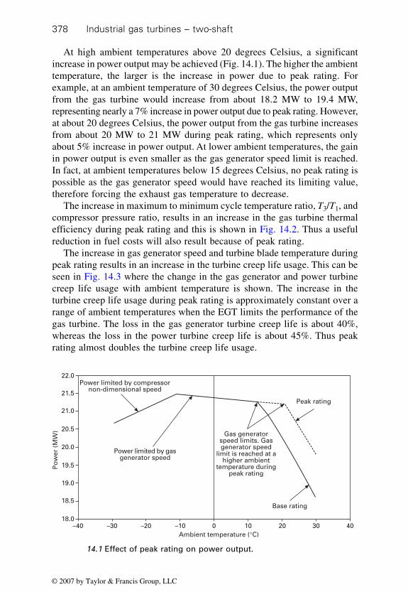
Industrial gas turbines – two-shaft378
At high ambient temperatures above 20 degrees Celsius, a significantincrease in power output may be achieved (Fig. 14.1). The higher the ambienttemperature, the larger is the increase in power due to peak rating. Forexample, at an ambient temperature of 30 degrees Celsius, the power outputfrom the gas turbine would increase from about 18.2 MW to 19.4 MW,representing nearly a 7% increase in power output due to peak rating. However,at about 20 degrees Celsius, the power output from the gas turbine increasesfrom about 20 MW to 21 MW during peak rating, which represents onlyabout 5% increase in power output. At lower ambient temperatures, the gainin power output is even smaller as the gas generator speed limit is reached.In fact, at ambient temperatures below 15 degrees Celsius, no peak rating ispossible as the gas generator speed would have reached its limiting value,therefore forcing the exhaust gas temperature to decrease.
The increase in maximum to minimum cycle temperature ratio, T3/T1, andcompressor pressure ratio, results in an increase in the gas turbine thermalefficiency during peak rating and this is shown in Fig. 14.2. Thus a usefulreduction in fuel costs will also result because of peak rating.
The increase in gas generator speed and turbine blade temperature duringpeak rating results in an increase in the turbine creep life usage. This can beseen in Fig. 14.3 where the change in the gas generator and power turbinecreep life usage with ambient temperature is shown. The increase in theturbine creep life usage during peak rating is approximately constant over arange of ambient temperatures when the EGT limits the performance of thegas turbine. The loss in the gas generator turbine creep life is about 40%,whereas the loss in the power turbine creep life is about 45%. Thus peakrating almost doubles the turbine creep life usage.
14.1 Effect of peak rating on power output.
Power limited by gasgenerator speed
Ambient temperature (°C)0–40 –30 –20 –10 10 20 30 40
21.5
Po
wer
(M
W)
22.0Power limited by compressor
non-dimensional speed
21.0
20.5
20.0
19.5
19.0
18.5
18.0
Gas generatorspeed limits. Gasgenerator speed
limit is reached at ahigher ambient
temperature duringpeak rating
Base rating
Peak rating
© 2007 by Taylor & Francis Group, LLC

Power augmentation 379
The impact of peak rating on gas turbine emissions is shown in Fig. 14.4.Since the compressor pressure ratio, the combustion pressure and thecombustion temperature have increased during peak rating, the NOx emissionswill increase. However, an increase in these parameters will result in areduction of CO. CO2 emissions will also increase due to the increasedpower output during peak rating because of increased fuel flow.
14.2 Effect of peak rating on thermal efficiency.
Ambient temperature (°C)0–40 –30 –20 –10 10 20 30 40
38.0
Gas generatorspeed limits. Gasgenerator speed
limit is reached at ahigher ambient
temperature duringpeak rating
Base rating
Increase in thermalefficiency due to
peak rating
Th
erm
al e
ffic
ien
cy (
%)
37.5
37.0
36.5
36.0
35.5
35.0
34.5
14.3 Effect of peak rating on turbine creep.
Temperature (°C)0–20 –10 10 20 30 40
140 000
Tim
e to
nex
t o
verh
aul (
ho
urs
)
Gas generatorturbine life (base
rating)
Power turbine life(base rating)
120 000
100 000
80 000
60 000
40 000
20 000
0
Decrease in gasgenerator turbine creeplife due to peak rating
Decrease in powerturbine creep lifedue to peak rating
© 2007 by Taylor & Francis Group, LLC

Industrial gas turbines – two-shaft380
Although a significant increase in creep life usage occurs during peakrating, on occasions, increased revenue due to the increased power generationcapacity will justify the increased maintenance costs.
Thus the business case for peak rating should be evaluated carefully,taking into consideration the increased capacity, better thermal efficiencyand increased maintenance costs, particularly at high ambient temperatures,where the increase in power output is the greatest for a given loss in turbinecreep life.
14.2 Maximum continuous rating
It has been stated that the base rating of the engine restricts the gas generatorspeed to 100%. However, manufacturers may allow a maximum continuousrating of 105% gas generator speed, provided the impact on turbine creeplife is not too excessive. This may be the case at low ambient temperatureswhere the engine power output is limited by the gas generator speed, resultingin reduction in turbine creep life usage due to the reduction in turbinetemperatures (Section 11.3). Increasing the gas generator speed limit to themaximum continuous rating value will result in an increase in the compressornon-dimensional speed for a given ambient temperature. This will result inan increase in compressor pressure ratio, turbine entry temperature andcompressor inlet mass flow rate, and therefore an increase in thermal efficiencyand power output from the gas turbine will occur.
The increased power output during maximum continuous rating is shownin Fig. 14.5. The maximum increase in power occurs at an ambient temperature
14.4 Change in gas turbine emissions during peak rating.
Ambient temperature (°C)0–40 –30 –20 –10 10 20 30 40
Decrease in CO dueto peak rating
14
CO
(p
pm
v @
15%
O2
dry
)
13
12
11
10
9
8
7
6
Increase in NOxdue to peak rating
NOx
CO
190
180
170
160
150
140
130
120
NO
x (p
pm
v @
15%
O2
dry
)
© 2007 by Taylor & Francis Group, LLC

Power augmentation 381
of about 5 degrees Celsius. The power output from the gas turbine increasesfrom about 21.3 MW to about 22 MW, representing about a 3% increase inpower output. Thus, a useful increase in power output can be achievedduring maximum continuous rating. Figure 14.6 shows the change in thermalefficiency during maximum continuous rating. There is also a useful increasein thermal efficiency during maximum continuous rating due to the higher
14.5 Effect of maximum continuous rating on power output.
14.6 Effect of maximum continuous rating on gas turbine thermalefficiency.
Ambient temperature (°C)0–40 –30 –20 –10 10 20 30 40
Increase in thermal efficiency dueto maximum continuous rating
Th
erm
al e
ffic
ien
cy (
%)
37.5
37.0
36.5
36.0
35.5
35.0
Increase in non-dimensionalspeed operating range due tomaximum continuous rating
Ambient temperature (°C)0–40 –30 –20 –10 10 20 30 40
Increase in EGT operatingrange due to maximum
continuous rating
Increase in power outputdue to maximumcontinuous rating
Base rating
22.0
22.0
21.5
21.0
20.5
20.0
19.5
19.0
18.5
18.0
Po
wer
(M
W)
© 2007 by Taylor & Francis Group, LLC

Industrial gas turbines – two-shaft382
compressor pressure ratio and turbine entry temperature. The increase in thegas generator speed limit results in an increase in ambient temperaturerange where the engine power output is limited by the exhaust gas temperature.Operating at maximum continuous rating also results in an increase in theambient temperature range where the engine power output is limited by thecompressor non-dimensional speed. In fact, there is no operation at constantgas generator speed on this engine when operating at maximum continuousrating.
The impact of maximum continuous rating on turbine creep life is shownin Fig. 14.7. An increase in turbine life usage is observed to occur duringmaximum continuous rating operation. However, this increase is not as dramaticas with the case of peak rating. Nonetheless, the manufacturer may requirean increase in engine maintenance frequency to allow for the reduction inturbine creep life. It would be possible to maintain the same maintenancefrequency but to accept a reduced exhaust gas temperature limit at higherambient temperatures, resulting in a loss in power output at these ambienttemperatures. Although, at first sight, it may appear unacceptable to theoperator to reduce the exhaust gas temperature limit at higher ambienttemperatures, in temperate countries where maximum power demand is oftenat low ambient temperatures, such a compromise may result in more revenueand thus more profit.
Figure 14.8 shows the change in gas turbine emissions when operatingat the maximum continuous rating. The increase in compressor pressureratio and combustion temperature results in an increase in NOx and a decreasein CO.
14.7 Effect of maximum continuous rating on turbine creep life.
500 000
Tim
e to
nex
t o
verh
aul (
ho
urs
)
Gas generatorturbine life
(base rating)
Power turbine life(base rating)
Decrease in power turbinecreep life due to maximum
continuous rating
Decrease in power turbinecreep life due to maximum
continuous rating
Ambient temperature (°C)0–40 –30 –20 –10 10 20 30 40
600 000
400 000
200 000
0
100 000
300 000
© 2007 by Taylor & Francis Group, LLC

Power augmentation 383
14.3 Power augmentation at very low ambient
temperatures
At ambient temperatures below –15 degrees Celsius it has been observedthat the gas turbine power output is limited by the compressor non-dimensionalspeed, and the maximum non-dimensional speed of the compressor cannotbe increased due to the likelihood of compressor surge. It has also beenobserved that, as the ambient temperature falls, the gas generator speedincreases and eventually becomes the factor that limits the engine performance.To increase the power output at such low temperatures, a method of increasingthe turbine entry temperature is required whilst the compressor non-dimensionalspeed is not increased.
From the discussion of the component matching process for turbinesoperating in series in Section 8.2 (Fig. 8.12), the effect of reducing the powerturbine area, and thus its non-dimensional flow capacity, will decrease thegas generator turbine pressure ratio. If operation is continued at a constantcompressor non-dimensional speed, the power balance between the compressorand gas generator turbine will result in an increase in turbine entry temperature.Furthermore, the flow compatibility between the compressor and the gasgenerator turbine will also result in an increase in compressor pressure ratio.Thus, by reducing the power turbine area, at ambient temperatures where thepower output from the gas turbine is limited by the compressor non-dimensionalspeed, an increase in thermal efficiency and power output will occur due tothe higher compressor pressure ratio and turbine entry temperature.
14.8 Change in gas turbine emissions due to operation at maximumcontinuous rating.
Ambient temperature (°C)0–40 –30 –20 –10 10 20 30 40
14
NOx
CO
Decrease in CO due tomaximum continuous rating
Increase in NOx due tomaximum continuous
rating 13
12
11
10
9
8
7
6
CO
(p
pm
v @
15%
O2
dry
)
200
180
170
160
140
130
120
150
NO
x (p
pm
v @
15%
O2
dry
)
190
© 2007 by Taylor & Francis Group, LLC
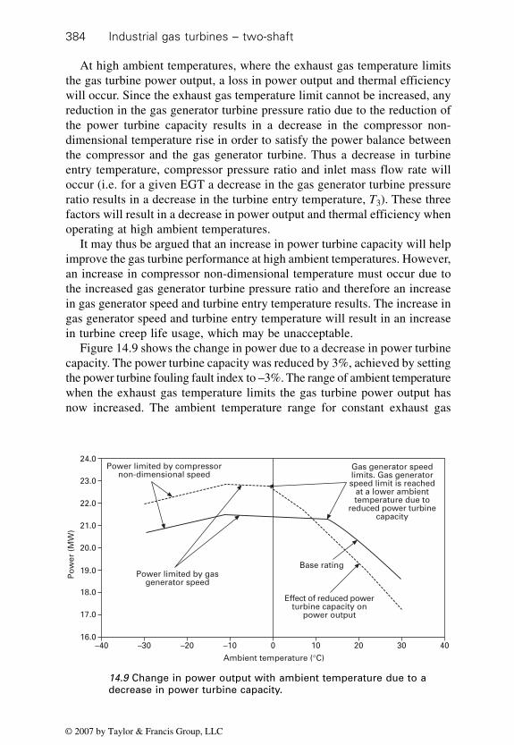
Industrial gas turbines – two-shaft384
At high ambient temperatures, where the exhaust gas temperature limitsthe gas turbine power output, a loss in power output and thermal efficiencywill occur. Since the exhaust gas temperature limit cannot be increased, anyreduction in the gas generator turbine pressure ratio due to the reduction ofthe power turbine capacity results in a decrease in the compressor non-dimensional temperature rise in order to satisfy the power balance betweenthe compressor and the gas generator turbine. Thus a decrease in turbineentry temperature, compressor pressure ratio and inlet mass flow rate willoccur (i.e. for a given EGT a decrease in the gas generator turbine pressureratio results in a decrease in the turbine entry temperature, T3). These threefactors will result in a decrease in power output and thermal efficiency whenoperating at high ambient temperatures.
It may thus be argued that an increase in power turbine capacity will helpimprove the gas turbine performance at high ambient temperatures. However,an increase in compressor non-dimensional temperature must occur due tothe increased gas generator turbine pressure ratio and therefore an increasein gas generator speed and turbine entry temperature results. The increase ingas generator speed and turbine entry temperature will result in an increasein turbine creep life usage, which may be unacceptable.
Figure 14.9 shows the change in power due to a decrease in power turbinecapacity. The power turbine capacity was reduced by 3%, achieved by settingthe power turbine fouling fault index to –3%. The range of ambient temperaturewhen the exhaust gas temperature limits the gas turbine power output hasnow increased. The ambient temperature range for constant exhaust gas
14.9 Change in power output with ambient temperature due to adecrease in power turbine capacity.
Ambient temperature (°C)
0–40 –30 –20 –10 10 20 30 40
Gas generator speedlimits. Gas generatorspeed limit is reached
at a lower ambienttemperature due to
reduced power turbinecapacity
Base rating
Effect of reduced powerturbine capacity on
power output
Power limited by compressornon-dimensional speed
Power limited by gasgenerator speed
24.0
Po
wer
(M
W)
23.0
22.0
20.0
21.0
19.0
18.0
17.0
16.0
© 2007 by Taylor & Francis Group, LLC

Power augmentation 385
temperature operation for the base rated case is from 30 to about 15 degreesCelsius, below which the power output is limited by the gas generator speed.Where there is a reduction in the power turbine capacity, the ambienttemperature range for constant exhaust gas temperature operation now increasesto 30 to about 0 degrees Celsius.
It is observed that the power output due to the decrease in power turbinecapacity exceeds the base-rating case when the ambient temperature decreasesto below 10 degrees Celsius. This is due to the higher exhaust gas temperatureand therefore higher turbine entry temperature. At an ambient temperature of–5 degrees Celsius, the power output increases from about 21.4 MW toabout 22.7 MW, which is a 6% increase. At lower ambient temperatures, theincrease in power output is even greater. However, at ambient temperaturesabove 15 degrees Celsius, a loss in power output results due to the decreasein turbine entry temperature as explained above. Thus a significant increasein power output is possible by optimising the power turbine capacity at lowambient temperatures, when the engine performance is limited by the gasgenerator speed. This results in increased revenue and profit.
The increases in compressor pressure ratio and turbine entry temperatureat low ambient temperatures result in an increase in the gas turbine thermalefficiency. Thus a reduction in fuel costs in real terms will occur, leading tolower operating costs. At high ambient temperatures, of course, a decrease inthermal efficiency would be incurred, due to the reasons discussed above andthus fuel costs would increase. Figure 14.10 shows the effect of reduced powerturbine capacity on thermal efficiency for a range of ambient temperatures.
14.10 Variation of gas turbine thermal efficiency due to reduction inpower turbine capacity.
Ambient temperature (°C)
0–40 –30 –20 –10 10 20 30 40
Gas generator speedlimits. Gas generatorspeed limit is reached
at a lower ambienttemperature due to
reduced power turbinecapacity
Base rating
Effect of reduced powerturbine capacity onthermal efficiency
38.0
Th
erm
al e
ffic
ien
cy (
%)
37.5
37.0
36.5
36.0
35.5
35.0
34.5
34.0
© 2007 by Taylor & Francis Group, LLC

Industrial gas turbines – two-shaft386
The impact of reduced power turbine capacity on turbine creep life isshown in Fig. 14.11. At ambient temperatures above 12 degrees Celsius, thegas generator turbine creep life usage is actually smaller compared with thebase-rating case. This is due to the reduction in the gas generator speed andturbine entry temperature when the exhaust gas temperature limits the enginepower output. There is also a slight reduction in the power turbine creep lifeusage above an ambient temperature of about 12 degrees Celsius. This is dueto the lower stress in the turbine blades resulting from less torque due to thereduction in gas turbine power output.
At ambient temperatures below 12 degrees Celsius, the gas turbine creeplife usage increases and this increase is due to the increase in turbine entrytemperature that arises from the reduced power turbine capacity. At ambienttemperatures below 12 degrees Celsius, the power turbine life also decreasesand this is due to the higher exhaust gas temperature compared with thebase-rating case. This is shown in Fig. 14.11, which illustrates the effect ofreduced power turbine capacity on turbine creep life.
Although a significant increase in turbine creep life usage occurs at lowambient temperatures, the creep life is still above 20000 hours, when normallyengine overhauls are necessary. However, manufacturers may want an increasedfrequency of engine overhaul but the improvement in creep life usage at highambient temperature should be considered before agreeing to any such increasein engine maintenance. Clearly, a worthwhile increase in power output atlow ambient temperatures is possible without any significant change inmaintenance cost. Furthermore, the increase in the thermal efficiency will
14.11 Change in turbine creep life due to reduction in power turbinecapacity.
Powerturbine life
Ambient temperature (°C)0–20 –10 10 20 30 40
Baserating
Effect of reducedpower
Gas generatorturbine life
200 000
Tim
e to
nex
t o
verh
aul (
ho
urs
)
250 000
150 000
0
100 000
50 000
© 2007 by Taylor & Francis Group, LLC

Power augmentation 387
reduce fuel costs resulting in lower operating costs. However, the drawbackis lower power output and thermal efficiency at high ambient temperatures.If demand for power is important during winter months, then such optimisationof the power turbine capacity will result in higher profits during these months.The increase in fuel costs during the summer months would have to becarefully evaluated before deciding whether such optimisation results inreduced life cycle costs.
A similar improvement in engine performance at low ambient temperaturesmay be obtained by increasing the gas generator turbine swallowing capacity.The reader is left to run the simulator to demonstrate the impact of increasingthe gas generator turbine capacity on engine performance at low ambienttemperatures.
Figure 14.12 shows the effect of reduced power turbine capacity on engineemissions. At high ambient temperatures, the decrease in turbine entrytemperature, compressor pressure ratio, and thus combustion pressure, resultsin a decrease in NOx and an increase in CO. At low ambient temperatures theincrease in combustion pressure and temperature, results in the increase ofNOx and decrease in CO.
Figure 14.13 shows the shift of the running line on the compressorcharacteristic. It is observed that the running line has indeed shifted towardssurge, thereby reducing the surge margin. However, this shift in the runningline is small. The VIGV/VSV schedule may be changed if necessary so thatthe variable stators do not open as much. This could increase the surgemargin, but reduce the flow capacity of the compressor, and the resultantloss in compressor capacity should be taken into account. Alternatively, the
14.12 Effect of reduced power turbine capacity on engine emissions.
Ambient temperature (°C)0–40 –30 –20 –10 10 20 30 40
14
NOx
CO
Baserating
13
12
11
10
9
8
7
CO
(p
pm
v @
15%
O2
dry
)
Effect of reduced powerturbine capacity
220
200
180
160
140
120
100
NO
x (p
pm
v @
15%
O2
dry
)
© 2007 by Taylor & Francis Group, LLC

Industrial gas turbines – two-shaft388
acceleration line may be reduced, thus reducing the transient response of theengine and this condition will be discussed in the next chapter.
14.4 Power augmentation by water injection
Gas turbine power output may be augmented by water injection. Water maybe injected into the inlet of the compressor or directly into the primary zoneof the combustion system. When water is injected into the inlet of thecompressor, the reduction of the compressor inlet temperature due to theevaporation of the water is primarily responsible for the increase in poweroutput. The amount of water that can be evaporated depends on the humidityof the air. The lower the humidity, the larger is the amount of water that canbe evaporated, resulting in a greater decrease in the compressor inlettemperature. Such means of power augmentation is, in fact, referred to asturbine inlet cooling and is only applicable where the relative humidity ofthe air is low and the ambient temperature is high. Turbine inlet cooling willbe discussed in the next section.
Direct injection of water into the primary zone augments the power outputby increasing the flow through the turbines. The ambient temperature andhumidity have no influence on how much water can be injected, but injectionis limited by the increase in emission of CO and UHC. In this section theimpact of direct injection of water into the combustion system on engineperformance is considered.
The increase in gas turbine power output due to water injection into thecombustion system is shown in Fig. 14.14. The water–fuel ratio is maintained
14.13 Shift in the running line on compressor characteristic due toreduction in power turbine capacity.
Co
mp
ress
or
pre
ssu
re r
atio
(P 2
/P1)
25
20
15
10
5Speed = 80%
Speed = 86%Speed = 89%
Speed = 92%Speed = 95%
Compressor surge lineSpeed = 100%
Speed = 107%
Speed = 97%
Shift in running linedue to reduced power
turbine capacity
Compressor speed lines
00 100 200 300 400 500
Speed = 73%
600
Running line
Compressor inlet non-dimensional flow
W R T
P1 1 1 1
1
/γ
Speed =
N
R T1
1 1 1γ
© 2007 by Taylor & Francis Group, LLC

Power augmentation 389
at unity during the change in the ambient temperature range. At high ambienttemperatures, a significant increase in power output is achieved by waterinjection. The gas turbine power output increases by about 6% and 7% abovethe base rating for ambient temperatures of 20 and 30 degrees Celsius,respectively. As the ambient temperature falls below 20 degrees Celsius, thepower output starts to flatten out and is due to the gas generator speedreaching its operating limit (continuous rating limit), which now occurs at anhigher ambient temperature compared with the base-rated base.
At zero degrees Celsius, the power increase due to water injection is onlyabout 1%. At such low ambient temperatures, the gas generator speed limitsthe power output of the gas turbine. Direct water injection into the combustorwould increase the mass flow rate through the gas generator turbine, thusincreasing the power output of the gas generator turbine and this wouldincrease the gas generator speed as observed at high ambient temperatureswhen the exhaust gas temperature limits the power output of the gas turbine.At low ambient temperatures, when the gas generator speed or compressornon-dimensional speed limits the performance of the gas turbine, a decreasein turbine entry temperature, T3, is necessary to maintain the power balancebetween the compressor and gas generator turbine. The reduction in turbineentry temperature reduces the specific work, while water injection increasesthe gas generator turbine power output. The net effect is a small increase inpower output at low ambient temperatures due to water injection when speedslimit the power output of the gas turbine.
The effect of water injection on the gas turbine thermal efficiency isshown in Fig. 14.15. Water injection results in a reduction in thermal efficiency.
14.14 Increase in gas turbine power output due to water injection.
Power limited by gasgenerator speed
Ambient temperature (°C)0–40 –30 –20 –10 10 20 30 40
Power limited by compressornon-dimensional speed
Gas generatorspeed limits. Gasgenerator speed
limit is reached at ahigher ambient
temperature due towater injection
Base rating
Peak rating21.5
Po
wer
(M
W)
22.0
21.0
20.5
20.0
19.5
19.0
18.5
18.0
© 2007 by Taylor & Francis Group, LLC

Industrial gas turbines – two-shaft390
Additional fuel input is necessary to evaporate the water and heat the steamto the required turbine entry temperature. However, the latent heat ofevaporation of water required to evaporate the water cannot be used by theengine because the power turbine exhaust temperature is well above theboiling point of water (i.e. it is not possible to condense the steam andretrieve the latent heat).
Thus the latent heat supplied is wasted in the exhaust system, resulting ina decrease in the gas turbine efficiency. At ambient temperatures below 20degrees Celsius, a greater loss in thermal efficiency occurs because theturbine entry temperature decreases due to constant speed operation. Theloss in thermal efficiency at an ambient temperature of 30 degrees Celsius isabout 4%, whereas the loss in thermal efficiency at 0 degrees Celsius isabout 6%. Thus, water injection at low ambient temperatures, where thepower output from the gas turbine is limited by the gas generator speed orcompressor non-dimensional speed, may be uneconomical because of theincrease in fuel cost, unless the fuel is relatively inexpensive. However,water injection can suppress NOx emissions significantly and would be usedfor reducing emissions at such low ambient temperatures. This is discussedlater in this section.
Figure 14.16 shows the variation of turbine creep life usage with ambienttemperature, as affected by water injection. A loss in gas generator turbinecreep life occurs at ambient temperatures above 20 degrees Celsius. Theincrease in gas generator speed at these ambient temperatures is responsiblefor the increase in creep life usage. At ambient temperatures below 20 degrees
14.15 Decrease in gas turbine thermal efficiency due to waterinjection.
Ambient temperature (°C)0–40 –30 –20 –10 10 20 30 40
38.0
Gas generator speed limits. Gasgenerator speed limit is reached
at a higher ambienttemperature during peak rating
Base rating
Th
erm
al e
ffic
ien
cy (
%)
37.5
37.0
36.5
36.0
35.5
35.0
33.5
33.0
34.5
34.0
Decrease in gas turbinethermal efficiency due
to water injection
© 2007 by Taylor & Francis Group, LLC

Power augmentation 391
Celsius, the gas generator creep life usage reduces and this is primarily dueto the decrease in the turbine entry temperature.
The power turbine creep life also decreases for ambient temperaturesabove 20 degrees Celsius and this is because of the increase in power outputfrom the power turbine, resulting in increased stresses due to the increase intorque in the blades. At ambient temperature below 20 degrees Celsius, thereduction in power turbine creep life usage is due to the decrease in theexhaust gas temperature, when the gas turbine power output is limited by thegas generator speed.
Since water injection gives rise only to a small increase in power outputat low ambient temperatures, it is unlikely that water injection would beemployed at these temperatures when the increase in fuel cost, due to themarked reduction in thermal efficiency, is significant. Thus it may not bepossible to exploit the decreased creep life usage at low ambient temperatureto compensate for the loss in creep life at high ambient temperatures, wherethe power output from the gas turbine is limited by the exhaust gas temperature.Therefore, an increase in engine overhaul frequency will lead to increasedmaintenance costs. Water injection also results in damage to the combustionsystem due to the significant chilling of the flame, resulting in increasedthermal stress cycles and corrosion, hence adding further maintenance costs.It must be noted that demineralised water must be used and this adds to theoperating cost.
The greatest effect of water injection directly into the primary zone of thecombustion system is a significant suppression of NOx emissions as discussedin Section 6.9. The impact of water injection on NOx and CO emissions is
14.16 Effect of water injection on turbine creep life.
Tim
e to
nex
t o
verh
aul (
ho
urs
)
Gas generatorturbine life
Effect of water
Powerturbine life
Base rating
5–10 –5 0 10 15 20 25
Ambient temperature (°C)
30 35
125 000
25 000
0
50 000
75 000
100 000
© 2007 by Taylor & Francis Group, LLC

Industrial gas turbines – two-shaft392
shown in Fig. 14.17. About 80% reduction in NOx has occurred. However,the CO emissions have increased by a factor of 3.5. Also note that theincrease in CO is the greatest at lower ambient temperatures. Thus the degreeof NOx suppression by water injection may be limited at low ambienttemperatures if the CO emissions exceed any alarm levels. The emissions ofCO2 will also increase as a result of water injection and this effect is shownin Fig. 14.18. This is because of the loss in thermal efficiency and increasedpower output, which require increased fuel consumption.
14.17 Effect of water injection on gas turbine emissions.
Ambient temperature (°C)0–40 –30 –20 –10 10 20 30 40
50
NOxCO
Effect ofwater
injection
CO
(p
pm
v @
15%
O2
dry
)
Baserating
45
40
35
30
25
20
15
10
5
0
200
180
160
140
120
100
80
60
40
20
NO
x (p
pm
v @
15%
O2
dry
)
14.18 Impact of water injection on CO2 production.
Ambient temperature (°C)0–40 –30 –20 –10 10 20 30 40
Increased CO2 emissionsdue to water injection
300
310
290
280
270
260
250
CO
2 em
issi
on
s (t
on
nes
/day
)
© 2007 by Taylor & Francis Group, LLC

Power augmentation 393
If water injection is used for NOx suppression, then the decrease in turbinecreep life usage at low ambient temperatures should be considered whendetermining mean time between turbine overhauls. This should result in auseful reduction in maintenance costs of the turbine.
14.5 Turbine inlet cooling
The adverse effect that high ambient temperature has on power output andthermal efficiency has been observed. Means to improve gas turbine poweroutput at high ambient temperatures using methods such as peak rating andwater injection have also been discussed. However, they invariably havesome disadvantages such as increased creep life usage and lower thermalefficiencies with direct water injection. As stated in Section 14.4, the turbineinlet can be cooled, thereby reducing the compressor inlet temperature toaugment the power output at high ambient temperatures. This is referred toas turbine inlet cooling or TIC. There are two main technologies available toreduce the compressor inlet temperature and they are known as evaporative(wetted media and inlet fogging) and chilling.1
Wetted media cooling and fogging operate on the same principles, wherethe evaporation of water absorbs latent heat of evaporation, thus cooling theturbine inlet air. With wetted media, the media is saturated with water, isexposed to the compressor inlet air, and the resultant evaporation reduces thecompressor inlet temperature thus increasing the gas turbine power output.Alternatively, the water can be introduced into the inlet as a very fine spray.The evaporation of the fine water droplets similarly cools the compressorinlet air and is known as fogging. The design issues regarding fogging systemsare discussed by Meher-Homji and Mee.2
Wetted media can operate on raw water; however, the mineral and saltcontent has to be controlled in order to prevent damage to the wetted media.Over time, the concentration of these minerals and salts will increase in thewetted media, resulting in blockage and damage to the wetted media. Thisreduces the effectiveness of the cooling media. With media cooling usingraw water, a sufficient amount of water recirculation is necessary to preventthe concentration of minerals and salts in the evaporative media. Unlikewetted media evaporative cooling, which can operate with raw water, foggingsystems require demineralised water. It should be noted that demineralisedwater is quite aggressive and will attack certain metals, and the inlet systemsshould use materials such as stainless steel or coatings that are resistant toattack from demineralised water.
The amount of water that can be evaporated depends on the relativehumidity of the air. The lower the humidity, the more water can be evaporatedand this results in a greater degree of turbine inlet temperature cooling.Another factor that limits the amount of cooling is the effectiveness of the
© 2007 by Taylor & Francis Group, LLC

Industrial gas turbines – two-shaft394
cooling system. The more efficient the cooling, the closer the dry bulbtemperature (which is effectively the ambient temperature) approaches theweb bulb temperature. For evaporative cooling systems using wetted media,the effectiveness can vary from 0.85 to 0.95, which is a measure of thedifference between the final dry bulb and wet bulb temperature. There is anadditional inlet loss due to the presence of the wetted media. This is consideredsmall and can vary between 5 mm water gauge and 10 mm water gauge,depending on the effectiveness of the cooling media.
For a fogging system, the effectiveness can approach unity. In this casethe dry bulb temperature approaches the wet bulb temperature and thecompressor inlet air will be saturated. In fact, evaporative cooling occurs ata constant wet bulb temperature. Therefore, if the ambient wet bulb temperatureis close to the dry bulb temperature (i.e. high relative humidity), only a littleturbine inlet cooling is possible. There is no noticeable increase in inlet losswith fogging systems.
Another evaporative cooling technique is wet compression or overspray.Here, additional water is added as a fine spray directly into the inlet of thecompressor. This water evaporates in the compressor due to the hightemperatures that occur during adiabatic compression, thus cooling the airwithin the compressor. This is similar to isothermal compression, but to alesser degree, and it reduces the compression power demand, thereforeincreasing the power output of the gas turbine. Hence this method of poweraugmentation is also referred to as fog intercooling. Since water is addeddirectly into the compressor as a spray, there is an increased risk of compressordamage due to erosion, which can result in severe engine damage. It isargued that such damage is more than justified, considering the increasedproduction. However, such compressor blade damage could easily result insurge, which can destroy the engine. In the event of such damage and reducedavailability, any benefit from a wet compressor could easily be lost. As witha fogging system, demineralised water should be used for wet compressionand should be applied in conjunction with evaporative cooling such as fogging.
Unlike evaporative cooling which is adiabatic, with inlet chilling heat isremoved from the inlet air using some form of refrigeration. Thus inletchillers are not limited by the wet bulb temperature, and the compressor inletair can be cooled down to any desired temperature provided the coolingcapacity is available. However, when the inlet temperature decreases below10 degrees Celsius, there is an increased risk of ice formation in the inlet,which can break away and enter the engine, thereby damaging the engine.Thus turbine inlet cooling, whether evaporative or chilling is limited tocompressor inlet temperatures of about 10 degrees Celsius. Refrigerationsystems for chillers can be either vapour compression or vapour absorptionsystems. The power demand from vapour compression systems is significantand is referred to as parasitic loss. In spite of such losses, there is still a
© 2007 by Taylor & Francis Group, LLC

Power augmentation 395
useful gain in engine performance and so these have been employed toaugment the power output at high ambient temperatures. Absorptionrefrigeration systems require a heat source, which can be provided fromwaste heat. Thus their parasitic losses are very small; however their performanceis much poorer than vapour compression systems. If waste heat is readilyavailable, the poor performance of vapour absorption refrigeration systemsis of little consequence.3 Vapour compression systems can be part of a thermalstorage system (TES) where low cost (off-peak electricity) is used to drivethe chillers to produce ice or chilled water. During peak demand, the TES isused to provide the necessary turbine inlet cooling using ice or chilled water.Other sources for chilling include LNG evaporation systems where the turbineinlet air is used as a heat source for the evaporation of LNG.
14.5.1 Wet bulb temperature, dry bulb temperature andcooling effectiveness
Wet bulb temperature is the lowest temperature to which air can be cooled bythe evaporation of water into the air at a constant pressure. It is thereforemeasured by wrapping a wet wick around the bulb of a thermometer and themeasured temperature corresponds to the wet bulb temperature. The drybulb temperature is the ambient temperature. The difference between thesetwo temperatures is a measure of the humidity of the air. The higher thedifference in these temperatures, the lower is the humidity. Given the wetbulb temperature, dry bulb temperature and ambient pressure, the humidityof the air can be calculated as follows:.
p = pw – 0.00066P(Ta – Tw)(1 + 0.00115Tw) [14.1]
where p is the vapour pressure of water vapour, pw is the saturated vapourpressure of water vapour at the wet bulb temperature, P the ambient pressure,Ta is the ambient or dry bulb temperature, and Tw is the wet bulb temperature.
The saturated vapour pressure of water vapour at the wet bulb temperature,pw is given by:
pwTw
T = 6.112 e17.67
+ 243.5××
[14.2]
Also the saturated vapour pressure of water vapour at the dry bulb temperatureis:
psTa
T = 6.112 e17.67
+ 243.5××
[14.3]
Using Equations 14.1 and 14.3, the relative humidity, φ, is calculated by:
φ = 100pps
× [14.4]
© 2007 by Taylor & Francis Group, LLC

Industrial gas turbines – two-shaft396
The specific humidity, ω, can also be determined and is given by:
ω = 0.622 – p
P p[14.5]
The dew point can also be determined from:
Td
p
p =
243.5 ln 6.112
17.67 – ln 6.112
×
[14.6]
The pressures in Equations 14.1 to 14.6 are in millibars (mb) and thetemperatures are in degrees Celsius.
Figure 14.19 shows a schematic representation of an evaporative coolingsystem. The ambient (warm, dry) airflow enters the wetted media/foggingchamber, where water is added and evaporated. The resultant cooled, moistair leaving the wetted media/fogging chamber enters the engine inlet. Asstated above, the cooling effectiveness is a measure of how close the temperatureof the moist, cooled, Tcool, air approaches the wet bulb temperature, Tw. Thecooling effectiveness, ε, is defined as:
Water flow (in)
Tcool Moistcool air
Wetted mediaor
foggingchamber
Tdry Warmdry air
Water flow (out)
14.19 Schematic representation of a (wetted media) evaporativecooling system.
© 2007 by Taylor & Francis Group, LLC

Power augmentation 397
ε = – –
coolTa TTa Tw [14.7]
Wetted media and chillers may be positioned either upstream or downstreamof the gas turbine inlet filter/plenum. If they are positioned upstream of theinlet system, the filters have to be made of synthetic material. If paper filterswere to be employed, the cool high humidity air would cause these filters toswell and become damaged.
14.5.2 Power augmentation using turbine inlet cooling
The amount of turbine inlet cooling using the three types of technologies, fora range of ambient temperatures, is shown in Fig. 14.20. The most significantcooling is achieved using chillers followed by fogging and wetted mediacooling. This Figure has been produced assuming a constant relative humidityof 60%, and cooling effectiveness for fogging and wetted media are assumedto be 1.0 and 0.85, respectively. The amount of cooling is observed to increasewith ambient temperature. With wetted media and fogging, the potential tocool the compressor inlet decreases with ambient temperature, due to thedivergence of the lines of constant relative humidity on the psychrometricchart, as shown in Fig. 14.21. With chillers, this decrease is more acute, asseen in Fig. 14.20. Turbine inlet cooling using chillers is not restricted by thehumidity of the air and therefore more cooling is possible at high ambienttemperatures compared with evaporative cooling, provided the cooling capacity
Relative humidity = 60%
Chiller
Fogging
Wetted media
Ambient temperature (°C)0 5 10 15 20 25 30 35
Turb
ine
inle
t co
olin
g (
°C)
25
20
15
10
5
0
14.20 Amount of turbine inlet cooling with ambient temperatureusing different cooling technologies.
© 2007 by Taylor & Francis Group, LLC

Industrial gas turbines – two-shaft398
is available. The maximum cooling capacity of 4.5 MW has been assumed,which is sufficient to maintain the compressor inlet temperature at 10 degreesCelsius for the ambient temperature range considered in Fig. 14.20. It hasbeen stated that the relative humidity does not limit the amount of turbineinlet cooling using chillers, but high relative humidity will result in a significantamount of water condensation occurring. Since the latent heat of evaporationis given up by the condensing water, much of the cooling load is used up inproducing the condensation rather than in cooling the inlet air. Thus theparasitic load increases at high humidity, requiring larger chiller capacity toachieve a given level of turbine inlet cooling. The reader should reproducethis figure for various levels of relative humidity using the gas turbine simulatorto illustrate the impact of humidity on turbine inlet cooling.
The resultant decrease in compressor inlet temperature increases the poweroutput of the gas turbine and thus the generator power output. This is shownin Fig. 14.22 for each of the above-mentioned cooling technologies. It can beseen that chillers produce the largest gain in power output, followed byfogging and wetted media. The figure also shows the effect of the coolingtechnology employed by chillers. With vapour compression chillers, theimpact of power demand by the chiller on generator output is significant andappears as a parasitic loss. Nevertheless, there is still a significant increasein power output at the generator terminals. With vapour absorption chillers,this parasitic loss is small and is ignored by the simulator as the simulatorrepresents an open cycle gas turbine, and the heating required by the absorptionrefrigeration system can be provided from the gas turbine exhaust heat.
The decrease in compressor inlet temperature due to turbine inlet coolingalso increases the thermal efficiency of the gas turbine, which the user should
14.21 Variation of humidity with ambient temperature.
Ambientpressure1.013 Bar
Simplified psychometric chart
Wet bulbtemperature 10 °C
Wet bulbtemperature 20 °C
RH = Relative humidity
RH = 100%
RH = 80%
RH = 60%
RH = 40%
RH = 20%
–20 –10 0 10 20 30 40 50 60Ambient or dry bulb temperature (°C)
Sp
ecif
ic h
um
idit
y (g
of
wat
erva
po
ur
per
kg
of
dry
air
)90
100
80
70
60
50
40
30
20
10
0
© 2007 by Taylor & Francis Group, LLC

Power augmentation 399
produce as an exercise. The increase in compressor airflow and thereforeincreased exhaust flow rate due to turbine inlet cooling also increases the heatrejection from the gas turbine and is beneficial to combined cycle power plants.
Turbine inlet cooling using wetted media and fogging requires water forevaporation and water requirements are shown in Fig. 14.23. The simulatoris a useful calculator to determine the water requirements for a given levelof turbine inlet cooling. The information can be scaled to suit any gas turbineengine. Details are given in the simulation user guide. With chillers,
Gen
erat
or
po
wer
ou
tpu
t (M
W)
21.5 Chiller (vapourabsorption)
5Ambient temperature (°C)
21.0
20.5
20.0
19.5
19.0
18.5
18.010 15 25 30 3520
Base rating
Relative humidity = 60%
Parasiticloss
Chiller (vapourcompression)
Fogging
Wetted media
14.22 Generator power output with ambient temperatures usingvarious turbine inlet cooling technologies.
Relative humidity = 60%
Water produced bycondensation due to chilling
Water requirementfor fogging
Water requirement for wetted media
5 10 15 20 25 30 35Ambient temperature (°C)
0.6
0.5
0.4
0.3
0.2
0.1
0
Wat
er f
low
rat
e (k
g/s
)
14.23 Water requirements for turbine inlet cooling systems.
© 2007 by Taylor & Francis Group, LLC

Industrial gas turbines – two-shaft400
condensation can occur when the relative humidity reaches 100% due tocooling and condensation produced is also shown in Fig. 14.23. At highambient temperatures, the condensation can be about three times that requiredby evaporative cooling systems. For example, at an ambient temperature of30 degrees Celsius, the condensation flow rates can be as much as 50 tonnesper day. Thus, means to remove this water must be provided when chillersare employed. The cooling loads and power demand for chillers using vapourcompression systems are shown in Fig. 14.24. Note that the cooling loadsand power demand increase exponentially when condensation occurs. Thisis primarily due to the absorption of the latent heat of evaporation for waterby the chillers. For example, when turbine inlet cooling of about 8 degreesCelsius is required, the cooling loads and power demand are about 0.5MWand 0.1 MW, respectively (assuming a coefficient of performance ofrefrigeration of 5.0). If the turbine inlet cooling required is doubled (16degrees Celsius), the cooling load and power demand from the chiller increaseto nearly 2.75MW and 0.55 MW, respectively. This is due to the formationof condensation at the higher levels of turbine inlet cooling.
The application of turbine inlet cooling using evaporative cooling resultsin an increase in relative and specific humidity, as illustrated in Fig. 14.25.It should be noted that the wet bulb temperature remains constant. Theambient temperature and relative humidity are held constant at 30 degreesCelsius and 60%, respectively. The increase in specific humidity suppressesthe increase in NOx emissions, which are due to the increase in combustiontemperature and pressure as the compressor inlet temperature decreases.
With chillers, the relative humidity increases and the wet bulb temperaturedecreases, while the specific humidity remains constant, provided no
Relative humidity = 60%
Nocondensation Condensation
Refrigerationload
Mechanical power demand forvapour compression system
Po
wer
dem
and
(M
W)
5
0Turbine inlet cooling (°C)
5 10 15 20 25
4
4
3
3
2
2
1
1
0
14.24 Cooling loads and power demand for vapour compressionrefrigeration system due to turbine inlet cooling.
© 2007 by Taylor & Francis Group, LLC

Power augmentation 401
condensation occurs. When relative humidity reaches 100%, any furthercooling produces condensation and this decreases the specific humidity, asshown in Fig. 14.25. Thus, the decrease in specific humidity and the increasein combustion temperature and pressure result in an increase in NOx emissions.These effects can be simulated and the reader should use the simulator toillustrate these issues. As with wetted media cooling and fogging, it shouldbe noted that the simulator is a useful calculator to determine the coolingload requirements for a given level of turbine inlet cooling. The informationcan be scaled to suit any gas turbine with either single- and multi-shaftengines.
The choice of cooling technology is not defined very clearly and it dependson the site ambient conditions. Lower humidity tends to favour evaporativecooling technologies such as wetted media and fogging systems, as theamount of turbine inlet air cooling will be significant. Conversely, a highhumidity environment will tend to favour chillers; however, parasitic losseswill be high. Also, low humidity and very high ambient temperature (above35 degrees Celsius), as found in desert conditions, will tend to favour chillers.Under these ambient conditions, more inlet air cooling is possible with chillerscompared with evaporative cooling and the parasitic loss will be low. Turbineinlet cooling is also applicable in temperate climates, where summertimetemperatures and humidity will justify turbine inlet cooling.4 Ideally, theincrease in engine performance due to turbine inlet cooling needs to beanalysed on a day-by-day basis over a long enough period, typically a year,for each type of cooling technology. Another important factor is the capitalcost of the turbine inlet cooling system. The capital cost of chillers can be
Spe
cific
hum
idity
(g w
ater
vap
our
per
kg
dry
air
)
40
Chiller
RH = Relative humidityTWB = Wet bulb temperature
RH = 60%
RH = 40%
RH = 20%
5Dry bulb temperature at compressor inlet (°C)
RH = 100%
RH = 80%
35
30
25
20
15
10
5
010 15 20 25 30 35 40
Fogging
TWB = 20 °C
TWB 10 °C
Wetted media
TWB = 30 °C
14.25 Running line on psychrometric chart for various turbine inletcooling technologies.
© 2007 by Taylor & Francis Group, LLC

Industrial gas turbines – two-shaft402
orders of magnitude greater (as much as ten or more) than that of evaporativecooling systems. Further information on the selection of turbine inlet coolingsystems can be found in Ameri et al.5
14.6 Power turbine performance
The performance of the power turbine is of paramount importance, as thiscomponent is responsible for converting the energy at the exit from the gasgenerator into shaft power. The power developed from the power turbine isdependent on the pressure ratio across the power turbine, which is determinedby the gas generator performance and the power turbine efficiency. For agiven power turbine pressure ratio, the efficiency is dependent on the non-dimensional speed of the turbine, as shown in Fig. 7.3. The power turbinespeed (mechanical speed) is determined by the driven load, and therefore thedriven load has a direct impact on the power turbine non-dimensional speed.In our simulator, it has been assumed that the power turbine drives an electricalgenerator, which requires the power turbine speed to remain constant withthe change in load to maintain the required frequency. However, in othercases such as mechanical drive applications (process compressors and pumps),the speed of the process compressor may be low during dense phase operationdue to high suction pressures in the process compressor. The process compressorspeed and therefore the power turbine speed may be as low as 70% of therated (100%) speed. Hence it is important to determine the power output ofthe gas turbine at different power turbine speeds.
Figure 14.26 shows the variation of the power developed by the powerturbine with power turbine speed at ISO conditions and zero inlet and exhaustlosses. The power output has been drawn for different gas generator speedsand of particular interest is the 100% gas generator (GG) speed, as thissituation normally corresponds to the maximum gas power generated by thegas generator. At a power turbine of 70% speed, which corresponds to apower turbine 2100 RPM, the power output decreases by about 11%, henceillustrating the importance of the power turbine performance. At high powerturbine speeds, there is little variation of power turbine efficiency with thepower turbine non-dimensional speed, thus resulting in a relatively flat powercurve when operating at these speeds. It will therefore be necessary for ourloads to operate at relatively high speeds or a very flat power turbine curvewill be required if a significant loss in power is not to be incurred at lowpower turbine speeds (similar in shape to the curve describing the 85% GGspeed in Fig. 14.26). The figure also shows the effect of the gas generatorspeed on power output. There is a loss in power output at lower gas generatorspeeds due to the reduction in air mass flow and turbine entry temperatureand generally in pressure ratio (i.e. reduced gas power).
© 2007 by Taylor & Francis Group, LLC

Power augmentation 403
The variation of the gas turbine thermal efficiency with power output fordifferent power turbine speeds is shown in Fig. 14.27. The decrease in thermalefficiency with power for a given power turbine speed is due to the reductionin the gas generator speed, resulting in lower compressor pressure ratio andturbine entry temperature. However, for a given power output, the thermalefficiency improves with the increase in power turbine speed and this is due
Gas
tu
rbin
e p
ow
er o
utp
ut
(MW
)25 Ambient temperature 15 °C
Ambient pressure 1.013 BarInlet and exhaust losses 0
1000Power turbine speed (RPM)
GG speed100%
1500 2000 2500 3000 3500
20
15
10
5
0
GG speed95%
GG speed90%
GG speed85%
14.26 Variation of power output with turbine speeds at different gasgenerator speeds.
25
Power turbine speed 1500 RPM
Power turbine speed 2000 RPM
Power turbine speed 2500 RPM
Power turbine speed 3000 RPM
20151050Gas turbine power output (MW)
38
36
34
32
30
28
26
24
22
20
Th
erm
al e
ffic
ien
cy (
%)
14.27 Variation of gas turbine efficiency with power output fordifferent power turbine speeds.
© 2007 by Taylor & Francis Group, LLC

Industrial gas turbines – two-shaft404
to the improvement in the power turbine efficiency. At high power turbinespeeds (around 3000 RPM), there is only a small variation in the thermalefficiency with the power turbine speed and this is due to minimal variationin power turbine efficiency at these speeds. Thus the loss in performance inthe power turbine at low speeds is responsible for the low thermal efficiencyat these power turbine speeds.
Furthermore, gas turbines are most efficient at high load conditions and,if a significant turndown in power is required, it is best to employ twosmaller engines, where each engine operates near its design condition at anygiven load condition. This is the principle of Combination Of Gas turbine OrGas turbine (COGOG)/Combination Of Gas turbine And Gas turbine (COGAG)where one engine is used at low powers and either or both engines operateat higher power requirements.
The principle of COGOG and COGAG is often used in naval applicationswhere the cruise speed of the ship is about half the boost speed. Due to thepropeller law, which states that the power required is proportional to thecube of the speed, the cruise power requirement is only about 12.5% of theboost power requirements. At such low powers, the thermal efficiency of thegas turbine will be very poor. The thermal efficiency at cruise conditions isimproved by employing a smaller gas turbine to operate at cruise conditionsand switching to a larger gas turbine for boost conditions. The power outputof the cruise gas turbine is about 30% of the total propulsive power requirement.It is worth noting that naval ships spend a significant time (about 95%) atcruise conditions.
For naval applications, the use of a variable pitch propeller would enablethe power turbine speed to be varied independently of the power requirements.By employing a variable pitch propeller, it would be possible to operate atthe maximum thermal efficiency for a given gas generator speed resulting ina useful improvement in thermal efficiency, particularly at low power operation,typical of cruise conditions. This is illustrated in Fig. 14.28, where the gasturbine thermal efficiency is displayed as a function of power turbine speedfor different gas generator speeds. The figure shows the load lines for a fixedpitch propeller and also for an electrical generator. The optimum line indicateswhat could be achieved by using a variable pitch propeller for naval propulsion.At low power, a 4% improvement in thermal efficiency may be possibleusing a variable pitch propeller and this corresponds to a significant reductionin fuel cost.
14.7 The effect of change in fuel composition on
gas turbine performance and emissions
All of the simulations discussed above were carried out using natural gas,whose lower heating value (LHV) is about 48 MJ/kg. Gas turbines can
© 2007 by Taylor & Francis Group, LLC

Power augmentation 405
operate on a range of fuels, which include liquid fuels such as diesel, kerosene,naphtha, crude oil and residual fuels. This simulator can operate on eithernatural gas, methane or diesel fuel. The impact of the change in fuel fromnatural gas to diesel on gas turbine performance will now be considered.
Table 14.1 shows the tabulated output of the exhaust gas composition asmole percentages when the gas turbine is operating with natural gas. Table14.2 shows the tabulated output for the case when the gas turbine is operatingwith diesel fuel. Note that the exhaust gas composition has changed in thatthe amount of CO2 has increased and the amount of H2O has decreased when
14.28 Load lines for a propeller and electrical generator,superimposed on the power turbine performance curves.
Table 14.1 Exhaust gas composition when operating with natural gas
Exhaust gas composition as mole %
CO2 H2O N2 O2 Ar3.120 7.032 74.994 13.961 0.893
Table 14.2 Exhaust gas composition when operating with diesel fuel
Exhaust gas composition as mole %
CO2 H2O N2 O2 Ar4.128 5.091 75.738 14.141 0.902
38
36
34
32
30
28
26
24
22
20
Gas
tu
rbin
e th
erm
al e
ffic
ien
cy (
%)
1000Power turbine speed (RPM)
1500 2000 2500 3000 3500
Propeller
Optimised(Variable pitch propeller)
Power generation
GG speed 105%
GG speed 100%
GG speed 90%
GG speed 85%
© 2007 by Taylor & Francis Group, LLC

Industrial gas turbines – two-shaft406
diesel fuel is employed. The decrease in H2O results in a decrease in thespecific heat of the products of combustion, cp. However, the impact of theisentropic index, γ = cp /cv, is small when changing from natural gas to diesel.The isentropic index, γ, relates to cp by the expression 1/γ = 1 – R/cp, whereR = Ro/MW is the gas constant of the products of combustion, and Ro andMW are the universal gas constant and molecular weight, respectively. Anincrease in R when operating with natural gas is due to its lower molecularweight compared with diesel fuel, but this is compensated by the increase incp. Hence only a small change in γ occurs when switching from natural gasto diesel. However, the increase in cp results in an increase in the powerdeveloped by the turbine and hence an improvement in gas turbine performanceoccurs when natural gas is used. The improvement in performance dependson the fuel gas composition. An increase in power output and thermal efficiencyof about 1 to 2 per cent is possible when operating with natural gas comparedwith diesel.
In this simulator, about 1 per cent increase in engine performance wasobtained when the switch was made from diesel oil to natural gas and thereader is left to demonstrate this effect of the change in fuel on engineperformance.
The effect of switching from natural gas to diesel fuel has a significantimpact on engine emissions, as shown in Fig. 14.29. It is observed that NOx
has increased from 175 ppmv to nearly 300 ppmv, representing about 70%increase in NOx. A significant increase in CO is also observed when changing
400
CO2 mass basis
NOx
CO2 emissions index
CO
CO
2 em
issi
on
s in
dex
(kg
/kW
h)
0.80
0.75
0.70
0.65
0.60
0.55
0.50
350
300
250
200
150
100
50
0
NO
x an
d C
O (
pp
mv
@15
% O
2 d
ry),
CO
2m
ass
bas
is (
ton
nes
/day
)
0 10 20 30 40 50 60 70Time (seconds)
14.29 Trends in gas turbine emissions when switching from naturalgas fuel to diesel fuel.
© 2007 by Taylor & Francis Group, LLC

Power augmentation 407
from natural gas to diesel fuel, when the CO increases from 8 ppmv to18 ppmv, thus more than doubling the emission of CO.
When operating with diesel fuel, the atomisation process results in localisedair–fuel mixtures nearer to stoichiometric compared with the case of naturalgas fuel, although the overall air–fuel ratio would be much higher. Thus thehigher flame temperatures that prevail in the vicinity of the burning liquidfuel droplets result in higher NOx emissions when burning liquid fuels suchas diesel. Furthermore, the adiabatic flame temperature achieved when usingdiesel fuel is greater than that with natural gas due to the reduced presenceof H2O and this also contributes to higher NOx when burning diesel fuel. InSection 6.5, the importance of good atomisation and mixing in arresting theformation of CO was discussed. With gaseous fuels, good mixing is easilyachieved compared with liquid fuels and therefore the formation of CO isreduced when burning natural gas.
The increase in CO2 is largely due to the higher carbon–hydrogen ratioand low LHV of diesel fuel compared with natural gas fuel. Figure 14.29shows the trends in gas turbine emissions when the change is made fromnatural gas fuel to diesel fuel, where an increase in gas turbine emissionsoccurs. Figure 14.30 shows the trends in the fuel flow and valve positionwhen the switch is made to diesel fuel operation. The figure also shows thetrends in the air–fuel ratio and compressor inlet airflow.
The increase in fuel flow and fuel valve position is primarily due to thelower LHV of diesel fuel, thus resulting in a decrease in the air–fuel ratio.
14.30 Trends in the change of fuel flow and air–fuel ratio due todiesel fuel operation.
80.0
Fuel valve position
1.36
Co
mp
ress
or
inle
t ai
rflo
w (
kg/s
), f
uel
valv
e p
osi
tio
n (
%),
air
–fu
el r
atio
0 10 20 30 40 50 60 70Time (seconds)
75.0
70.0
65.0
60.0
55.0
50.0
45.0
40.0
Compressor inlet airflow
Fuel flow
Air–fuel ratio
1.34
1.32
1.30
1.28
1.26
1.24
1.22
1.20
1.18
Fuel
flo
w (
kg/s
)
© 2007 by Taylor & Francis Group, LLC

Industrial gas turbines – two-shaft408
14.8 References
1. Gas turbine inlet air cooling and the effect on a Westinghouse 501D5 CT, Kohlenberger,C., ASME Paper 95-GT-284, 1995.
2. Inlet fogging of gas turbine engines Part A: Theory, psychometrics and fog generation,Meher-Homji C.B. and Mee III T.I.L., ASME Paper 2000-GT-307, 2000.
3. Analysis of a combined gas turbine and absorption–refrigeration cycle, Nagib,M.M., Journal of Engineering for Power, January 1971.
4. Inlet fogging of gas turbine engines: climate analysis of gas turbine evaporativecooling potentials of international locations, Chaker, M. and Meher-Homji, C.B.,ASME Paper GT-2002-30559, 2002.
5. Gas turbine power augmentation using fog inlet air-cooling system, Ameri, A., Nabati,H. and Keshtgar, A. Proceedings of ESDA04, 7th Biennial Conference on EngineeringSystems Design and Analysis, July 19–22, 2004, Manchester, United Kingdom,ESDA2004-58101, 2004.
© 2007 by Taylor & Francis Group, LLC

409
In Chapter 10, the principles of gas turbine control were discussed where itwas stated that the change in engine power is accomplished by altering theenergy input to the gas turbine. This is achieved by varying the fuel flow intothe combustion system until the desired power output is reached. It has alsobeen stated that this change in power output from the gas turbine should beaccomplished without any detrimental effect to the gas turbine. The principleof a simple PID control system was introduced, together with the concept oflow signal select. Such a simple control system has been implemented in thisgas turbine simulator and much of what was discussed in Chapter 10 will besimulated to illustrate the principles of gas turbine control systems. The two-shaft gas turbine simulator will now be used to illustrate some of the featuresof control systems applied to gas turbine control. A PID control systemcontains the P – proportional, I – integral and D – derivative terms and isoften referred to as a three-term control system.
15.1 Proportional action
Pure proportional action results in the proportional band acting on the errorthat is determined by the difference of the power output from the electricalgenerator and the set point, which represents the power required by thegenerator. Pure proportional action leaves an offset as illustrated by Fig.15.1, which shows the trends in power due to a step change in the requiredpower output of the generator from 1 MW to 19 MW. Pure proportionalaction is achieved in the simulator by switching off the integral output in theengine control setting option.
The trends in power as shown in Fig. 15.1 have been generated for threevalues of proportional band and correspond to 100%, 75% and 50%. As theproportional band decreases, which corresponds to an increase in proportionalgain, there is an increase in output from the process, which in this case is theelectrical generator power output. However, the set point of 19 MW is never
15Simulation of engine control system
performance
© 2007 by Taylor & Francis Group, LLC

Industrial gas turbines – two-shaft410
reached by the generator output and pure proportional action normally leavesa difference between the generator output and the set point. This differenceis referred to as the proportional offset, which reduces as the proportionalband decreases. The manual reset discussed in Chapter 10 may be applied toremove the proportional offset (not available in the simulator).
15.2 Proportional and integral action
Integral action is essentially a summation or integration process on the residualerror left by the proportional action (proportional offset). This action (automaticreset as discussed in Chapter 10) results in reducing the error to zero andtherefore achieving the required generator output as specified by the setpoint. Hence both proportional and integral actions are required in controlsystems if the specified set point and therefore the desired power output isto be achieved. The value of the integral gain is very important, as a smallgain will result in prohibitively long time periods before the set point isreached. Too large an integral gain will result in excessive oscillatory response,again resulting in too long a time period before the required set point isreached. Such oscillatory response will also have a detrimental effect onturbine creep life due to overshoots in speeds and temperatures above thesteady-state values and can cause unexpected trips in order to protect theengine.
The trend in power due to the integral action for a set point change from1 MW to 19 MW is shown in Fig. 15.2. Initially, only proportional action is
Gen
erat
or
po
wer
ou
tpu
t (M
W)
20
18
16
14
12
10
8
6
4
2
00 50 100 150 200 250 300 350
Time (seconds)
PB = Proportional band
Increase in setpoint from 1 to19 MW
Proportionaloffset due toPB of 100%
Proportionaloffset due to PBof 75% Proportional
offset due to PBof 50%
Generator setpoint
Generatorpower output
15.1 Trends in generator power output due to proportional actiononly. (PB = proportional band).
Proportional offset is thedifference between thegenerator set point andgenerator power output
© 2007 by Taylor & Francis Group, LLC

Simulation of engine control system performance 411
applied, resulting in the proportional offset as shown in Fig. 15.2. Theproportional band is set at 100%. After about 100 seconds, the integral actionis switched on and the power output from the gas turbine is observedapproaching the set point of 19 MW. The integral gain is set to 0.1 and a longtime period results (about 100 seconds) before the required set point isreached and this delay is due to the small value of the integral gain.
Increasing the integral gain to 2 results in a very rapid increase in poweroutput, as observed in Fig. 15.3. The oscillatory response is clearly seen andthe control system reaches the set point of 19 MW in about 15 seconds, thusrepresenting a significant improvement in transient response of the enginecompared with the previous case, which represented a small integral gain of0.1. (It is necessary to inactivate the engine trips during this type of simulationexercise – see the user guide on the CD for instructions to inactive enginetrips.)
Reducing the integral gain to about 0.4 still maintains a rapid response inpower output but virtually eliminates the overshoots, as shown in Fig. 15.4.Such optimisation is necessary in tuning control systems and the optimisationprocess is a specialist area, which is outside the scope of this book but isdiscussed in Shaw1 and in Sivanandam.2
It has been stated above that an oscillatory response due to poor controlsystem performance has a detrimental effect on turbine creep life. This isillustrated in Fig. 15.5, which shows the trend in turbine creep life usagewhen the integral gain is set to 2. The creep life usage is observed for bothgas generator and power turbines where the creep lives undershoot the steady-
Gen
erat
or
po
wer
ou
tpu
t (M
W)
20
18
16
14
12
10
8
6
4
2
00 50 100 150 200 250 300 350
Time (seconds)
Increasein setpointfrom 1 to19 MW
Start of integralaction
Proportional offsetdue to PB of 100%
The effect of integral actionreduces the error to zero
15.2 Trends in generator power output due to proportional andintegral action. (PB = proportional band).
© 2007 by Taylor & Francis Group, LLC

Industrial gas turbines – two-shaft412
state values by significant amounts. The gas generator turbine creep lifeundershoots the steady-state creep life by about 30 000 hours and the powerturbine creep life undershoots the steady-state value by about 150 000 hours.The decrease in creep life occurs due to the fuel flow overcompensatingbecause of the poor performance of the control system. This results in
Gen
erat
or
po
wer
ou
tpu
t (M
W)
25
0 50 100 150 200 250 300 350Time (seconds)
Increasein setpointfrom 1 to19 MW
Start of integralaction
Rapid transient response dueto high integral gain
Proportional offsetdue to PB of 100%
20
15
10
05
0
15.3 Trends in generator power due to high integral gain.(PB = proportional band).
15.4 Trends in generator power output due to optimised controlsystem.
Gen
erat
or
po
wer
ou
tpu
t (M
W)
20
18
16
14
12
10
8
6
4
2
00 50 100
Increasein setpointfrom 1 to19 MW
Proportional offsetdue to PB of 100%
150 200 250 300 350Time (seconds)
Start of integralaction
Improved transient responsedue to optimised integral gain
© 2007 by Taylor & Francis Group, LLC

Simulation of engine control system performance 413
overshoots in the gas generator speed and turbine entry temperature, asshown in Figs 15.6 and 15.7, respectively. The increase in speed and turbineentry temperature during the overshoot is always greater than the decreasesin speed and turbine entry temperature during the corresponding undershootas the control system endeavours to attain steady state conditions. Furthermore,the non-linear nature of the Larson–Miller curve (see Fig. 5.11), which describesthe average creep life of the turbine blades, results in a greater decrease in
Gas
gen
erat
or
spee
d (
RP
M)
10 000
150
Overshoot in speed, whichcould result in trips Gas generator speed limit (100%)
155 160 165 170 175
9500
9000
8500
8000
7500
Time (seconds)
15.6 Trends in speed due to high integral gain.
15.5 Trends in turbine creep life due to integral gain.
Tim
e to
nex
t o
verh
aul (
ho
urs
)350 000
150
Power turbine
Gas generatorturbine
Increase in creep life usage due toovershoot speed and temperature
due to high integral gain
155 160 165 170 175
300 000
250 000
200 000
150 000
100 000
50 000
0
Time (seconds)
© 2007 by Taylor & Francis Group, LLC

Industrial gas turbines – two-shaft414
the Larson–Miller parameter during the overshoot than the increase in thisparameter during the undershoot in speed and temperature. Thus both theseeffects result in a decrease in creep life.
Although the significant loss in creep life occurs for only a very shortperiod of time, the decrease in creep life of the turbines will accumulate ifsuch oscillatory response is allowed to continue, leading to a reduced enginelife and increased engine overhauls and therefore increasing maintenancecosts.
The trend for speeds and temperatures for the optimised case, where theintegral gain was set to 0.4, is shown in Figs 15.8 and 15.9, respectively.Virtually no oscillatory response is observed. Consequently, a satisfactorytrend in turbine creep life is obtained, as shown in Fig. 15.10.
15.3 Signal selection
In Section 10.2 the use of signal selection to prevent any operating limitssuch as exhaust gas temperature and gas generator speeds being exceededwas described. This action protects the engine from damage and achievessuitable turbine creep life. In fact, signal selection was used when the effectof ambient temperature on engine performance was considered in Section11.3, where the power output of the gas turbine becoming limited by eitherthe exhaust gas temperature, gas generator speed or compressor non-dimensional speed limits was demonstrated. Hence these figures are reproducedhere for a discussion of signal selection.
Referring to Fig. 15.11, at high ambient temperatures, the exhaust gas
Tem
per
atu
re (
K)
1500
150
Turbine entry temperature
Exhaust gas temperaturelimit
155 160 165 170 175Time (seconds)
1400
1300
1200
1100
1000
900
800
700
600
Exhaust gas temperature
Gas generator turbinemetal temperature
15.7 Trends in temperature due to high integral gain.
© 2007 by Taylor & Francis Group, LLC

Simulation of engine control system performance 415
temperature limits the power output, as the gas generator speed and compressornon-dimensional speed are below their limiting condition. This is observedin Fig. 15.12, which shows the trends in speeds during the ambient temperaturetransient (+ 30 to –30 degrees over one hour).
As the ambient temperature decreases, the gas generator speed and thecompressor non-dimensional speed increase until the ambient temperaturereduces to about 12 degrees Celsius, at which point the gas generator speedlimit is reached. At ambient temperatures below 12 degrees Celsius, the
Gas
gen
erat
or
spee
d (
RP
M)
10 000
150
Start of integral action
155 160 165 170 175
9500
9000
8500
8000
7500
Time (seconds)
15.8 Trends in speed when the control system is optimised.
Tem
per
atu
re (
K)
1500
150
Turbine entry temperature
Exhaust gas temperaturelimit
155 160 165 170 175Time (seconds)
1400
1300
1200
1100
1000
900
800
700
600
Exhaust gas temperature
Gas generator turbinemetal temperature
15.9 Trends in temperature when the control system is optimised.
© 2007 by Taylor & Francis Group, LLC

Industrial gas turbines – two-shaft416
signal selection switches from exhaust gas temperature control to gas generatorspeed control, when the gas generator speed will remain constant at its 100%speed, or a continuous rating value until the ambient temperature reduces toabout –11 degrees Celsius (Fig. 15.12).
Note that the exhaust gas temperature decreases (Fig. 15.11) during constantgas generator speed operation and the compressor non-dimensional speedcontinues to increase. At ambient temperatures below –11 degrees Celsius,
Tim
e to
nex
t o
verh
aul (
ho
urs
)350 000
150
Gas generatorturbine
155 160 165 170 175Time (seconds)
Power turbine
300 000
250 000
200 000
150 000
100 000
50 000
0
15.10 Trends in turbine creep life when the control system isoptimised.
Tem
per
atu
re (
K)
1080
0
N1/√T1 limited
Exhaust gas temperaturelimit
Time (seconds)
Exhaust gas temperature
Gas generator speed limited
1060
1040
1020
1000
980
960
940
920
900500 1000 1500 2000 2500 3000 3500 4000
Exhaust gastemperature limited
15.11 Trends in temperature during ambient temperature transient.
© 2007 by Taylor & Francis Group, LLC

Simulation of engine control system performance 417
the compressor non-dimensional speed limit is reached and the signal selectionnow switches to compressor non-dimensional speed control. At an ambienttemperature below –11 degrees Celsius, both the exhaust gas temperatureand gas generator speed are observed to continue to decrease. Thus, this ishow signal selection protects the engine from over-speeding or overheating.
15.4 Acceleration and deceleration lines
Signal selection discussed above considered only limits on the exhaust gastemperature and speed. Although these would be the limiting values duringsteady-state and slow transient conditions, a means is needed of preventingconditions that would occur during fast transients, such as rapid accelerationand deceleration, resulting in flameout or compressor surge. It is the variationof the air–fuel ratio that is important, as flameout occurs when the air–fuelratio is outside the combustion stability limits. The computation of the air–fuel ratio is not practical, as the combustion airflow value is needed and isoften unavailable.
Figure 15.13 shows the variation of fuel flow with gas generator speed fora series of ambient temperatures, T1 varying from –30 degrees Celsius to 30degrees Celsius. The figure also shows the acceleration and decelerationlimits. Figure 15.14 shows the variation of air–fuel ratio with ambienttemperature, T1, and gas generator speed. Note that the variation of the air–fuel ratio with ambient temperature is small for a limited range of gas generatorspeed (from about 8000 RPM to 10 000 RPM). Referring to Fig. 15.13, at
Gas
gen
erat
or
spee
d (
RP
M)
9550
0
N1/√T1 limited
Time (seconds)
Gas generator speed limited
500 1000 1500 2000 2500 3000 3500 4000
Gas generatorspeed
N1/√T1
9500
9450
9400
9350
9300
9250
9200
9150
9100 Co
mp
ress
or
qu
asi-n
on
-dim
ensi
on
al s
pee
d (N
1/√T
1)590
580
570
560
550
540
530
Exhaust gastemperature
limited
15.12 Trends in speed during ambient temperature transient.
© 2007 by Taylor & Francis Group, LLC

Industrial gas turbines – two-shaft418
low ambient temperatures, the margin for acceleration will decrease and themargin for deceleration will increase. Thus the transient response duringacceleration will be poor and the increased deceleration margin could resultin flameout during deceleration. Conversely, at high ambient temperatures
T1 = –30 °CT1 = –20 °CT1 = –10 °CT1 = 0 °CT1 = 10 °CT1 = 20 °CT1 = 30 °C
Fuel
flo
w (
kg/s
)1.6
Gas generator speed (RPM)6000
Deceleration limit
Acceleration limit
1.4
1.2
1.0
0.6
0.8
0.4
0.2
0.06500 7000 7500 8000 8500 9000 9500 10 000 10 500
15.13 Variation of fuel flow with gas generator speed for a series ofambient temperatures.
15.14 Variation of air–fuel ratio with gas generator speed for a seriesof ambient temperatures.
T1 = –30 °CT1 = –20 °CT1 = –10 °CT1 = 0 °CT1 = 10 °CT1 = 20 °CT1 = 30 °C
Air
–fu
el r
atio
Gas generator speed (RPM)6000
100
6500 7000 7500 8000 8500 9000 9500 10 000 10 500
90
80
70
50
40
60
© 2007 by Taylor & Francis Group, LLC

Simulation of engine control system performance 419
the acceleration margin will increase, whereas the deceleration margin willdecrease. Thus at high ambient temperatures, the increased acceleration margincould result in flameout due to low air–fuel ratios. Low air–fuel ratios canalso result in high turbine temperatures and compressor surge. The reduceddeceleration margin at high ambient temperatures will result in poor transientresponse of the gas turbine during deceleration. These problems may beovercome by implementing the acceleration–deceleration (‘accel–decel’)schedules, also known as the fuel schedule curves, using non-dimensionalparameters as discussed in Section 10.3. Because of the non-dimensionalbehaviour of gas turbines resulting in unique running lines, as shown inFigures 11.3 to 11.7 in Section 11.2, the accel–decel schedules are applicablefor all ambient temperatures and pressure. The non-dimensional parametersconsidered in Section 10.3 were the compressor pressure ratio and non-dimensional speed. However, the variation of these non-dimensional parametersexhibit a kink and this is due to the VIGV/VSV movement as discussed inSection 11.2 and shown in Fig. 15.15, which also displays the accel anddecel lines.
The implementation of the accel and decel lines would be simpler if thekink is eliminated and this can be achieved by using the non-dimensionalparameters for fuel flow and compressor pressure ratio, as shown in Fig.15.16. The figure also shows the accel and decel lines. Thus, in the simulatorthe variation of non-dimensional fuel flow is used with compressor pressureratio to implement the accel–decel lines. In practice, manufacturers mayomit the temperature term present in the non-dimensional fuel flow as it isa weaker function compared with the pressure term.3
Co
mp
ress
or
pre
ssu
re r
atio
(P 2
/P1)
Non-dimensional speed (N1/√T1)350
25
20
15
10
5
0400 450 500 550 600 650
Kink
Acceleration limit
Deceleration limit
15.15 Acceleration and deceleration line on the compressor pressureratio versus speed characteristic.
© 2007 by Taylor & Francis Group, LLC

Industrial gas turbines – two-shaft420
The transient operating points due to a step increase in power demandfrom 1 MW to 19 MW on the acceleration–deceleration curve are shown inFig. 15.17. The figure also shows the transient operating points due to a stepdecrease in power demand from 19 MW to 1MW. All the transient operatingpoints during both acceleration and deceleration are observed to remain
No
n-d
imen
sio
nal
fu
el f
low
(m
f/ (
P 1/√
T 1))
Compressor pressure ratio (P2/P1)0
0.035
Acceleration limit
Deceleration limit
5 10 15 20 25
0.030
0.025
0.020
0.015
0.010
0.005
0.000
15.16 Acceleration and deceleration line on the non-dimensional fuelflow versus compressor pressure ratio characteristic.
No
n-d
imen
sio
nal
fu
el f
low
(m
f/ (
P 1√P
1))
Compressor pressure ratio (P2/P1)0
0.040
Transient pointsduring acceleration
Deceleration limit
Acceleration limit
Transient pointsduring deceleration
2 4 6 8 10 12 14 16 18
0.035
0.030
0.025
0.020
0.015
0.010
0.005
0.000
15.17 Transient operating points on acceleration–deceleration lines.
© 2007 by Taylor & Francis Group, LLC

Simulation of engine control system performance 421
within the acceleration–deceleration limit lines, thus ensuring satisfactorytransient operation of the engine. Fig. 15.18 shows the transient operatingpoints on the compressor characteristic during acceleration and deceleration.Note that all the transient operating points do not cross the compressor surgeline during acceleration, thus preventing compressor surge during acceleration.
In the absence of acceleration and deceleration lines, the operating pointsduring engine transient may cross these limiting lines, resulting in compressorsurge or flameout conditions. This is illustrated in Fig. 15.19, which showsthe operating points for the same transient described above on the acceleration–deceleration curve when the acceleration and deceleration lines are inactive.It is observed that the operating points cross the acceleration and decelerationlines during the transient, particularly during deceleration, and could resultin flameout due to the air–fuel ratio exceeding the weak flammability limit.The operating points crossing the acceleration line would result in compressorsurge, as shown in Fig. 15.20, which displays the operating points on thecompressor characteristic during these transients.
15.5 Integral wind-up
The size of the fuel valve is of paramount importance in ensuring satisfactoryfuel flow to the engine and thus achieving the required power output subjectto engine operating limits such as exhaust gas temperature and speed limitsas discussed previously, particularly during transient operation. Inadequatefuel valve capacity will result in unexpected behaviour of the control system
15.18 Transient operating points on compressor characteristic due toa step change in power demand.
Co
mp
ress
or
pre
ssu
re r
atio
(P2/
P 1)
25
20
15
10
5
00 100 200 300 400 500
Speed = 73%Speed = 80%
Speed = 86%
Speed = 92%Speed = 95%
Compressor surge line
600
Speed = 100%Speed = 107%
Speed = 97%Transient points
during acceleration
Compressor inlet non-dimensional flow
Speed =N1
γ1R1T1
Steady state running
Transient points duringdeceleration
Speed = 89%
Compressor speed lines
W R T
P1 1 1 1
1
/γ
© 2007 by Taylor & Francis Group, LLC

Industrial gas turbines – two-shaft422
and one such behaviour is due to the continuous increase in the integraloutput, often referred to as integral wind-up, due to the fuel valve becomingfully opened, as discussed in Section 10.1.2. It should also be noted that, ifthe fuel pressure is low due to a fault in the fuel system, the fuel valve couldbecome fully opened. Integral wind-up will now be illustrated using the gas
No
n-d
imen
sio
nal
fu
el f
low
(m
f/ (
P 1√T
1))
Compressor pressure ratio (P2/P1)0
0.040
Transient pointsduring acceleration
Deceleration limit
Acceleration limit
Transient pointsduring deceleration
2 4 6 8 10 12 14 16 18
0.035
0.030
0.025
0.020
0.015
0.010
0.005
0.000
15.19 Operating points during step changes in power demand whenacceleration–deceleration lines are inactive.
15.20 Operating points due to step changes in power on thecompressor characteristic when acceleration–deceleration lines areinactive.
Co
mp
ress
or
pre
ssu
re r
atio
(P 2
/P1)
25
20
15
10
5
00 100 200 300
Speed = 73%Speed = 80%
Compressor surge line
Compressor speed lines
400 500 600
Speed = 86%Speed = 89%
Speed = 100%Speed = 107%
Speed = 97%
Speed =N1
γ1R1T1
Transient points duringacceleration
Compressor inlet non-dimensional flow
Steady state running
Transient pointsduring deceleration
Speed = 95%Speed = 92%
W R T
P1 1 1 1
1
/γ
© 2007 by Taylor & Francis Group, LLC

Simulation of engine control system performance 423
turbine simulator. (It is necessary to ensure that the integral reset wind-up isswitched off for this simulation exercise – see the user guide on the CD forinstructions on switching off the reset wind-up.)
The valve flow coefficient (CG) is reduced to half its design value from1100 to 550. If the power demand from the electric generator is increasedfrom 1MW to 20 MW, the fuel valve will open fully (100%). However, thepower output will not meet the generator power demand due to insufficientfuel flow. The power output from the generator would be about 14.8 MW,which is well short of the required power demand of 20 MW. The importantpoint to note is that no engine operating limits such as the exhaust gastemperature or speed limit have been reached. Under these conditions theintegral output would be observed to continue to increase and exceed 100%output as the control system attempts to open the fuel valve to meet thegenerator power demand. Since the fuel valve is fully opened, no furtherincrease in fuel flow can occur and thus no increase in power output from thegas turbine is possible. As long as these conditions prevail, the integraloutput continues to increase or wind up and should be observed in the maindisplay screen of the gas turbine simulator.
If we reduce the generator set point from 20 MW to, say, 12 MW, whichis below the current power output from the generator, it is observed that thegenerator power output will remain at 14.8MW. This unexpected result occursbecause the integral output is above 100% but will then be observed to startwinding down and this can be seen on the main screen of the simulator. Thepower output from the generator will remain at 14.8 MW until the integraloutput has completely wound down (below 100%), after which the poweroutput from the electrical generator will decrease and eventually match theset point value of 12 MW.
The above is summarised in Figs 15.21 and 15.22, which show the trendsin power and fuel flow/valve position, respectively. Figure 15.21 shows thegenerator power output remaining at 14.8 MW until the integral output haswound down, although the generator set point has decreased from 20 MW to12 MW after about 100 seconds. Figure 15.22 shows the trend in the fuelvalve position, which remains at 100% until the integral output has wounddown. The fuel valve then closes so that the power output from the generatormatches the required power as stipulated by the generator set point.
To prevent the integral output from winding up, so resulting in thisunexpected response from the engine control system, the output from thePID controller is reset to 100% if the output from the control system exceeds100% and the fuel valve is concurrently fully open. This is achieved with thesimulator by clicking the reset wind-up option to ‘Reset Wind-up On’ withthe engine control setting display (see user guide). The above simulation isrun again and the generator power output set point reduced to 12 MW asabove. However, on this occasion the power output from the generator responds
© 2007 by Taylor & Francis Group, LLC

Industrial gas turbines – two-shaft424
almost immediately and achieves the required power output of 12 MW. Figure15.23 displays the trends in power when reset wind-up is active and thepower output from the gas generator is observed responding to the change inset point to 12 MW. The trend in flows and fuel valve position are shown inFig. 15.24. Again, the fuel valve is observed responding to the change inpower demand from the generator almost immediately when the reset wind-up option is active.
Po
wer
ou
tpu
t (M
W)
25
20
15
10
5
00 50
Integral wind-downcomplete and
generator outputmatches the setpoint of 12 MW
100 150 200 250 300 350Time (seconds)
Integralwind-down
Integralwind-up
Generator poweroutput 14.8 MW
Decrease in generatorset point to 12 MW
Increase in generator setpoint from 1 MW to 20 MW
15.21 Trends in power due to integral wind-up.
Fuel
val
ve p
osi
tio
n (
%)
op
ened
120
0 50
Integral wind-downcomplete and
generator outputmatches the setpoint of 12 MW
100 150 200 250 300 350Time (seconds)
Integralwind-down
Integralwind-up
100
80
60
40
20
0
Fuel
flo
w (
kg/s
)
1
0.9
0.8
0.7
0.6
0.5
0.4
0.3
0.2
0.1
0
Fuel valveposition
Fuel flow
15.22 Trend of the fuel valve position due to integral wind-up.
© 2007 by Taylor & Francis Group, LLC

Simulation of engine control system performance 425
15.6 Engine trips
In Section 15.2, the likelihood of trips due to poor control system performancewas discussed, where excursions in exhaust gas temperature and speeds canoccur, thereby exceeding their trip levels. A well-tuned control system wouldprevent such excursions and hence engine trips. However, in certain situations
Po
wer
ou
tpu
t (M
W)
25
20
15
10
5
00 50
Due to reset of the wind-up the generatorpower output matches the required power
demand (12 MW)
100 150 200 250 300 350Time (seconds)
Generator poweroutput 14.8 MW due toinsufficient flow flow
Decrease in generatorset point to 12 MW
Increase in generator setpoint from 1 MW to 20 MW
15.23 Trends in power when reset wind-up is active.
Fuel
val
ve p
osi
tio
n (
%)
op
ened
120
0 50
Fuel valve responding due to resetwind-up being active and ensuring
that the power output required is met
100 150 200 250 300 350Time (seconds)
Fuel valve open 100% due toinsufficient capacity when the
power demand is 20 MW
100
80
60
40
20
0
Fuel
flo
w (
kg/s
)
1
0.9
0.8
0.7
0.6
0.5
0.4
0.3
0.2
0.1
0
Fuel flow
15.24 Trend in the fuel valve position due to the reset wind-up beingactive.
© 2007 by Taylor & Francis Group, LLC

Industrial gas turbines – two-shaft426
the control system may not be able to respond adequately and will result intrips. Although trip levels are important to protect the engine from damage,their frequent occurrence is indicative of faults either in the control systemor in the operating procedure, resulting in increased unscheduled downtimeand reduced availability. Some engine faults, such as compressor VIGV/VSV schedule problems, may also result in trips. These problems affectrevenue and profits and thereby increase life cycle costs.
One such trip is illustrated, where water injection to augment the poweroutput of the gas turbine is considered. The injection of water results in adecrease in thermal efficiency and thus, for a given power output, requiresan increase in fuel flow. If water injection is ceased then care must be takennot to reduce the water injection rate rapidly as the fuel flow rate may notdecrease sufficiently, thus injecting too much fuel resulting in a very highgas temperature (due to the absence of water). Such increases in gas temperaturemay result in engine trips.
The simulator is run at an ambient temperature of 30 degrees Celsiuswhere water injection for power augmentation is most beneficial and thegenerator power demand (power set point) is set to 25 MW. After 10 secondsof operation, water is injected over a period of 10 seconds (ramp time) toachieve a water–fuel ratio of 1.5. Figure 15.25 shows the trends in power andthe generator power is observed to be increasing when water injection ispresent. After about 50 seconds water injection is ceased by reducing theramp time to just 1 second, so reducing the water injection very rapidly. Theengine is observed to trip very shortly after 50 seconds.
Po
wer
ou
tpu
t (M
W)
25
20
15
10
5
00 20 40 60
Time (seconds)
Increase in power outputdue to water injection
Start of waterinjection
End of waterinjection
Trip due to high EGT
80 100 120
15.25 Trend in power when the engine trips due to high exhaust gastemperature (EGT).
© 2007 by Taylor & Francis Group, LLC

Simulation of engine control system performance 427
This is illustrated more clearly in Fig. 15.26, which show the correspondingtrends in exhaust gas temperature (EGT). The exhaust gas temperature isobserved to rise and it reaches its trip level, resulting in the engine trip.Figure 15.27 shows the trends in speed and it is noted that an increase in gasgenerator speed occurs but that this increase in speed is insufficient to initiatea trip. (Note: In the simulator, a trip is simulated by reducing the poweroutput of the gas turbine to its idle power output, which is set to 1 MW.)However, the solution in preventing this trip condition is quite simple. The
Exh
aust
gas
tem
per
atu
re, E
GT
(K
)
1150
0 20 40 60Time (seconds)
Start of waterinjection
End of waterinjection
80 100 120
Exhaust gastemperature limit
Exhaust gastemperature trip limit Exhaust gas temperature
exceeds trip limit
1100
1050
1000
950
900
850
800
15.26 Trends in exhaust gas temperature during engine trip.
Gas
gen
erat
or
spee
d (
RP
M)
11 000
0 20 40 60Time (seconds)
Gas generator speed increases dueto high exhaust gas temperature
80 100 120
10 500
10 000
9500
9000
8500
8000
7500
7000
GG speed trip limit
100% GG speed limit
15.27 Trends in speed during engine trip.
© 2007 by Taylor & Francis Group, LLC

Industrial gas turbines – two-shaft428
ramp time is increased sufficiently when water injection cessation is desired,thus preventing the exhaust gas temperature from rising rapidly. To use ashort ramp time, it would be necessary to reduce the power demand beforeshutting off the water injection. The case is illustrated where the ramp timeis increased when shutting off the water injection. The ramp time is increasedfrom 1 second to 10 seconds in this case.
Figure 15.28 shows the trend in exhaust gas temperature when the ramptime is increased to 10 seconds, and it can be seen that the exhaust gastemperature rises, but not sufficiently to cause a trip condition. Thus, increasingthe ramp time representing the time period for switching off the water reducesthe increase in exhaust gas temperature. In the simulation, the user shouldalso note the change in primary zone temperature due to water injection. Itis left to the user to vary the ramp time to investigate its influence on thechange in exhaust gas temperature due to shutting off the water injection.
15.7 References
1. PID Control Algorithm. How it Works, How to Tune it and How to Use it, 2ndEdition, Shaw, J. A., December 1, 2003. E-book, http://www.jashaw.com/.
2. Control Systems Engineering, Sivanandam, S. N., Vikas Publishing (2001).3. Gas Turbine Performance, 2nd edition, Walsh, P. and Fletcher, P., Blackwell Publishing
(2004).
15.28 Trends in temperature with and without water injection.
Exh
aust
gas
tem
per
atu
re, E
GT
(K
)1120
0 20 40 60Time (seconds)
Start of waterinjection
End of waterinjection
80 100 120
Exhaust gastemperature limit
Exhaust gastemperature trip limit
1110
1100
1090
1080
1070
1060
1050
1040
1030
© 2007 by Taylor & Francis Group, LLC

In Part II the two-shaft gas turbine simulator was used to illustrate theperformance, turbine life usage and engine emissions of a two-shaft gasturbine operating with a free power turbine. The simulator was also used toillustrate the behaviour and performance of the engine control system appliedto such an engine.
In Part III the single-shaft gas turbine simulator will be used to illustratethese effects and repeat many of the simulations carried out in Part II. Thesingle-shaft gas turbine simulator can be operated in two modes and bothmodes of operation will be considered in this part of the book. The first ofthese modes refers to the variable inlet guide vane (VIGV) remaining fullyopened during the normal power output range, while in the second mode ofoperation the VIGV is modulated to maintain the exhaust gas temperature(EGT) on its limiting value as the power output from the gas turbine isreduced. Control of the VIGV is usually achieved using a PID loop asdiscussed in Chapter 10, Section 10.4.2 and will also be discussed later inChapter 20.
Unlike the case of the two-shaft gas turbine operating with a free powerturbine, there are no unique running lines for a single-shaft gas turbine. Theonly exception is the variation of the compressor inlet non-dimensional flowwith its speed, particularly if the compressor flow speed lines are vertical onthe compressor characteristic. This was discussed in Chapter 8.
Part III
Simulating the performance of a single-shaftgas turbine
429
© 2007 by Taylor & Francis Group, LLC

431
The single-shaft gas turbine simulator is based on an industrial gas turbinehaving an ISO rating of about 40 MW and a maximum power limit of45 MW at low ambient temperatures. As already stated, single-shaft gasturbines are widely used in power generation and therefore the driven loadis assumed to be an electrical generator that operates at the synchronousspeed determined by the frequency. Thus the gas turbine also operates at aconstant speed as the load and ambient conditions change.
The reader is encouraged to run the simulations discussed below to becomemore familiar with concepts of engine performance, turbine life usage, gasturbine emissions and the behaviour of the engine control system. The singlegas turbine simulator user guide gives details on how to use the simulator.
16.1 Configuration of the single-shaft simulator
The configuration of the single-shaft gas turbine simulator is similar to thatshown in Fig. 2.3 except that the compressor is fitted with VIGV. One of thepurposes of the VIGV is to reduce gas turbine starting power requirements(mode 1 as discussed previously, where the fuel flow is varied to maintainthe generator output and the VIGV is modulated to maintain the exhaust gastemperature). This is achieved by closing the inlet guide vane during startingand low power operation. The closure of the inlet guide vane results in areduction in airflow rate through the compressor, thus reducing the startingpower demands. The normal operating power range of the gas turbine isbetween 60% and 100% when the VIGV is fully open. Control of the VIGVis achieved by maintaining the exhaust gas temperature (EGT) on a set pointby modulating the inlet guide vane. Thus, when the EGT is below the setpoint temperature, the guide vane will be fully closed in an attempt to maintainthe EGT on the set point, hence reducing starting power requirements. Whenthe EGT is above the set point temperature, the inlet guide vane will thereforebe fully opened, which corresponds to the normal operating power range.
16Simulating the effects of ambient
temperature on engine performance,emissions and turbine life usage
© 2007 by Taylor & Francis Group, LLC

Industrial gas turbines – single-shaft432
Thus, the set point temperature for modulating the inlet guide vane needsto be below the maximum exhaust gas temperature limit (EGT limit). Thevalues for the EGT limit and the (exhaust gas) set point temperature forVIGV modulation used by the simulator correspond to 825 K and 650Krespectively.
When regenerative cycles are employed in single-shaft gas turbines, theuse of the VIGV is useful in maintaining constant maximum EGT duringpart-load operation. This results in a much improved thermal efficiency atpart-load operation due to near constant maximum to minimum cycletemperature ratio, T3/T1, at these operating conditions. Similarly, the use ofVIGV improves the part-load performance of combined cycle plants. MaximumEGT operation can be achieved at part-load by setting the temperature setpoint for variable inlet guide vane operation to the maximum EGT limit (i.e.the EGT for VIGV operation is increased from 650 K to 825 K) – mode 2 asdiscussed previously. Up to about 65% reduction in power output can beachieved at the maximum EGT by the use of VIGV.
With such VIGV operation, the air–fuel ratio remains approximatelyconstant, resulting in approximately constant combustion temperature withthe change in power output. In Section 6.11 it was seen that, if the combustiontemperature is kept within certain limits (1700 K to 1900 K), the emissionsof NOx and CO are small and this approach is the basis of dry low emission(DLE) combustion systems. Thus the application of VIGV (mode 2 operation)in single-shaft gas turbines can achieve DLE combustion without having toresort to multi-staged combustion. In fact, such a combustion system willhave similar characteristics to the variable geometry combustion systemdiscussed in Section 6.12.
16.2 Effect of ambient temperature on engine
performance at high power
The simulator can be used to investigate the effect of change in ambienttemperature on engine performance. It has been stated in Part II that thesimulators are based on a quasi-steady-state model, thus it is possible tosubject the model to significant changes in ambient conditions. In practice,however, rapid changes in ambient conditions are not common and couldlead to compressor surge.
In the simulation, the ambient temperature will be changed from +35degrees Celsius to –30 degrees Celsius linearly over a period of 3600 seconds.The power demand from the simulator will be set above the ISO rating to60 MW throughout the simulation. This action simulates the effects of thechanges in ambient temperature on engine performance when the enginecontinuously operates on an engine operating limit such as the EGT or
© 2007 by Taylor & Francis Group, LLC

Simulating the effects of ambient temperature on performance 433
power limit. It should be noted that such high power demands from thegenerator would result in trips due to the frequency shift. However, in asimulator this can be considered as it is a convenient means of maintainingthe engine on a limiting condition, such as the EGT or maximum power, asthe ambient temperature changes. The ambient pressure is held constant at1.013 Bar during the change in ambient temperature and the inlet and exhaustpressure losses are set to 100 mm water gauge. The relative humidity is alsoheld constant at 60%. For simplicity, the gas property terms, R and γ, will beomitted from any non-dimensional terms such as flow and speed but referencewill be made to them when relevant.
16.2.1 Trends in power, pressure and temperature ratiosand compressor characteristics
The gas turbine speed and thus the compressor speed, N1, remain constant asthe electrical generator speed (synchronous speed) remains constant with thechange in load. The reduction of ambient temperature will therefore result inan increase in the compressor non-dimensional speed, N1/√T1. This is seen inFig. 16.1, which depicts the operating point on the compressor characteristicduring this ambient temperature transient.
The increase in compressor non-dimensional speed will increase thecompressor inlet non-dimensional flow, W1√T1/P1. If at first it is assumed
16.1 Operating point on compressor characteristic duringtemperature transient.
Compressor inlet non-dimensional flow
Operating point at the startof simulation (ambient
temperature 35 °C)
Exhaust gastemperature
limited
Powerlimited
Operating point at the end ofsimulation (ambienttemperature –30 °C)
Speed 89%
Speed 92%
Speed 96%
Speed 100%Speed 103% Speed 109%
700 800 900 1000 1100 1200 1300
16
14
12
10
8
6
4
2
0
Co
mp
ress
or
pre
ssu
re r
atio
Speed
N
R T1
1 1 1γ
W R T
P1 1 1 1
1
/γ
© 2007 by Taylor & Francis Group, LLC

Industrial gas turbines – single-shaft434
that the maximum to minimum temperature, T3/T1, remains constant (byadjusting the power output as the ambient temperature decreases), thecompressor pressure ratio, P2/P1, must increase to satisfy the flow compatibility(Equation 8.1 assuming a choked turbine, i.e. W3√T3/P3 is constant). Thehigher compressor pressure ratio will also result in a higher turbine pressureratio. Also, at high ambient temperatures, the engine power output will belimited by the EGT limit. Thus, an increase in turbine pressure ratio mustnecessarily increase the turbine entry temperature, T3. The decrease in ambienttemperature will therefore result in an increase in the temperature ratio,T3/T1, which in turn further increases the compressor pressure ratio in orderto satisfy the flow compatibility (Equation 8.1). This results in a steep operatingline on the compressor characteristic, as shown in Fig. 16.1. The highercompressor pressure ratio and temperature ratio, T3/T1, will improve thethermal efficiency, as seen in Fig. 16.2.
The higher T3/T1 will also increase the specific work, but at these operatingpressure ratios the increase in T3/T1 will have a greater influence on specificwork than will pressure ratio (see Chapter 2, Section 2.15). The highercompressor inlet non-dimensional flow with the reduction in ambient temperature,T1, will result in an increase in the compressor inlet air flow rate. Both theincreased specific work and airflow rate increase the power output from thegas turbine as the ambient temperature decreases, as shown in Fig. 16.2.
The steep running line on the compressor characteristic may intersect thecompressor surge line, which must be avoided for reasons discussed in Section4.8. Adequate margin between the surge line and the operating point must be
Po
wer
ou
tpu
t (M
W)
65
60
55
50
45
40
35
30
25
20
Maximum power limit
Thermal efficiency
Power required
Gas turbine power output
Generator power output
Power limitedExhaust gas temperature limited
0 500 1000 1500 2000 2500 3000 3500 4000Time (seconds)
35.0T
her
mal
eff
icie
ncy
(%
)
34.5
34.0
33.5
33.0
32.5
32.0
31.5
31.0
30.5
30.0
29.5
16.2 Changes in gas turbine power output and thermal efficiencyduring temperature transient.
© 2007 by Taylor & Francis Group, LLC

Simulating the effects of ambient temperature on performance 435
maintained to allow for transient conditions. This is achieved by limiting themaximum power output from the gas turbine at low ambient temperatures to45 MW. Limiting the power output at low ambient temperatures will decreasethe turbine entry temperature, T3. This is necessary to reduce the specificwork in order to maintain the power output from the gas turbine at themaximum power limit of 45 MW. As a result, the rate of increase in thecompressor pressure ratio decreases as can be seen in Figs 16.1 and 16.3.The reduction in T3 will reduce the turbine creep life usage at these ambienttemperatures. Thus manufacturers may impose the maximum power limit toensure satisfactory turbine creep life at low ambient temperatures in a mannersimilar to that discussed in Section 11.3.8 (rating curves).
The rate of increase in thermal efficiency also decreases when operatingat constant power output (Fig. 16.2), as the ambient temperature lowers. Thisis primarily due to the effect on compressor pressure ratio and the (slight)decrease in T3/T1 (Fig. 16.3). There is also a reduction in compressor efficiencyunder these conditions as the compressor operates in a region on the compressorcharacteristic where the compressor efficiency is lower.
The trends in compressor and turbine powers are shown in Fig. 16.4. Theincrease in the turbine power output is due to the increase in turbine entrytemperature, pressure ratio and mass flow rate through the turbine. Theincrease in compressor power absorbed is due primarily to the increase inmass flow rate through the compressor and pressure ratio. The figure alsoshows the trends in the isentropic efficiencies of the compressor and turbine.
16.3 Trends in pressure and temperature ratios during temperaturetransient.
Pre
ssu
re r
atio
13.0
Compressorpressure ratio
Power limitedExhaust gas temperature limited
0 500 1000 1500 2000 2500 3000 3500 4000Time (seconds)
5.2Te
mp
erat
ure
rat
io
Turbine pressure ratio
Maximum to minimum cycletemperature ratio12.5
12.0
11.5
11.0
10.5
10.0
9.5
9.0
8.5
8.0
5.1
5.0
4.9
4.8
4.7
4.6
4.5
4.4
4.3
© 2007 by Taylor & Francis Group, LLC

Industrial gas turbines – single-shaft436
The compressor efficiency initially increases slightly before decreasing asthe compressor operates in a lower efficiency part of its characteristic at lowambient temperatures. The turbine efficiency decreases slightly beforeincreasing slightly, due to the change in the turbine non-dimensional speed.During constant EGT operation the turbine entry temperature increases (Fig.16.8), resulting in a decrease in the turbine non-dimensional speed, thusgiving a slight reduction in turbine efficiency. During constant power operation,the turbine entry temperature decreases, hence increasing the turbine non-dimensional speed resulting in a slight gain in the turbine efficiency.
The changes in power and thermal efficiency trends can be displayed onan ambient temperature basis and these are shown in Figs 16.5 and 16.6,respectively. Figure 16.6 also shows the change in specific work where theincrease in specific work is noted during constant EGT operation and adecrease in specific work during constant power operation.
16.2.2 Trends in pressure and temperatures
During constant EGT operation it has been shown that the compressor pressureratio and thus the turbine pressure ratio increase. This results in an increasedcompressor discharge pressure, P2, and turbine entry pressure, P3, during thetransient as shown in Fig. 16.7. However, when operating at constant poweroutput a decrease in rate of pressure rise is observed, which is due to adecrease in the rate of compressor pressure ratio increase (Fig. 16.3). Since
16.4 Trends in compressor and turbine power efficiency duringambient temperature transient.
Po
wer
(M
W)
100
Compressorpower absorbed
Power limited
0 500 1000 1500 2000 2500 3000 3500 4000Time (seconds)
88.0E
ffic
ien
cies
(%
)
Turbineefficiency
Exhaust gas temperature limited
Compressorefficiency
Turbine power output
90
80
70
60
50
40
87.5
87.0
86.5
86.0
85.5
85.0
84.5
84.0
83.5
© 2007 by Taylor & Francis Group, LLC

Simulating the effects of ambient temperature on performance 437
the ambient pressure does not change during this transient, the compressorinlet and turbine exit pressures do not change during this transient.
The trends in temperature are shown in Fig. 16.8. The turbine entrytemperature, T3, rises as mentioned earlier and this also results in an increasein primary zone temperature during the period when the engine power outputis limited by the EGT. These temperatures decrease as the engine becomes
16.5 Variation of gas turbine output on an ambient temperaturebasis.
16.6 Variation of thermal efficiency and specific work on an ambienttemperature basis.
Power limited
–40
Exhaust gastemperature limited
–30 –20 –10 0 10 20 30 40Ambient temperature (°C)
Po
wer
(M
W)
48
44
46
42
40
38
36
34
32
30
Thermal efficiency
Power limitedExhaust gas
temperature limited
35.0
Th
erm
al e
ffic
ien
cy (
%)
34.5
34.0
33.5
33.0
32.5
32.0
31.5
31.0
30.5
30.0
29.5–40 –30 –20 –10 0 10 20 30 40
Specific work
Ambient temperature (°C)
Sp
ecif
ic w
ork
(kJ
/kg
)
320
310
300
290
280
270
260
250
© 2007 by Taylor & Francis Group, LLC

Industrial gas turbines – single-shaft438
power limited. The trend in the EGT, T4, remains constant until the enginebecomes power limited, after which the EGT decreases. The increase incompressor non-dimensional speed increases the compressor non-dimensionaltemperature rise, ∆T21/T1, as shown in Fig. 8.3 in Chapter 8. However, thedecrease in ambient temperature, T1, results in a reduction in the compressordischarge temperature, T2.
The figure also shows the turbine blade metal temperature, and an increasein the turbine blade metal temperature occurs during the period when theengine is EGT limited. This is due primarily to the increase in turbine entry
14
12
10
8
6
4
2
0
Power limited
0 500 1000 1500 2000 2500 3000 3500 4000Time (seconds)
Exhaust gas temperature limited
Pre
ssu
res
(Bar
-A)
P2
P1 and P4
P3
16.7 Trends in pressure during ambient temperature transient.
2500
Power limited
0 500 1000 1500 2000 2500 3000 3500 4000Time (seconds)
Exhaust gas temperature limited
Tem
per
atu
re (
K)
Exhaust gas temperature limited
Turbine metal temperature
Temperature drop incombustor to ensuresatisfactory turbine creep life
Primary zone temperature
2000
1500
1000
500
0
T3 (TET)
T4
T2
T1
16.8 Trends in temperature during ambient temperature transient
© 2007 by Taylor & Francis Group, LLC

Simulating the effects of ambient temperature on performance 439
temperature, T3, although the cooling air temperature, T2, is decreasing. Thereduction in cooling air temperature during this transient reduces the rate ofincrease in the turbine blade metal temperature. When the engine power islimited, the turbine blade temperature decreases and this is due to the decreasein turbine entry and cooling air temperatures.
16.2.3 Trends in flow
The trends in air flow, fuel flow, fuel valve position and the air–fuel ratio areshown in Fig. 16.9. The air flow increases continuously due to the increasein compressor inlet non-dimensional flow, W1√T1/P1, and the decrease inambient temperature, T1. The fuel flow increases during the period when thepower output is controlled by the EGT. During this period, the power outputfrom the gas turbine and its thermal efficiency increase.
However, the increase in power output is greater than the increase inthermal efficiency, thus the fuel flow increases to satisfy the increased poweroutput. During the period when the gas turbine is power limited, the fuelflow decreases. This is because the thermal efficiency increases while thepower output remains constant. The fuel valve position follows a similartrend to the fuel flow. The air–fuel ratio decreases during the period ofconstant EGT operation due to the combustor temperature rise, T3 – T1,during this period of operation (Fig. 16.8). Conversely, the air–fuel ratioincreases during the period when the engine is power limited because of adecrease in combustor temperature.
180
Power limited
0 500 1000 1500 2000 2500 3000 3500 4000Time (seconds)
Exhaust gas temperature limitedCo
mp
ress
or
inle
t ai
rflo
w (
kg/s
), f
uel
val
vep
osi
tio
n (
%),
air
–fu
el r
atio
Air–fuel ratio
Fuel flow
Fuel valveposition
Airflow160
140
120
100
80
60
40
20
0
2.9
2.8
2.7
2.6
2.5
2.4
2.3
2.2
2.1
2.0
Fuel
flo
w (
kg/s
)
16.9 Trends in flow, fuel valve position and air-fuel ratio duringambient temperature transient.
© 2007 by Taylor & Francis Group, LLC

Industrial gas turbines – single-shaft440
16.2.4 Trends in turbine creep life
The trend in turbine creep life usage, which is shown as the time to nextoverhaul, decreases during the period when the engine power output is limitedby the EGT (Fig. 16.10). The increase in turbine blade temperature has beenobserved (Fig. 16.8) and an increase in turbine power output (Fig. 16.4).
The increased power developed by the turbine increases the stress in theblades due to the increased torque (note turbine speed is constant). Thus,together with the increase in blade temperature, the creep life usage increases.During the period when the engine power output is constant, the turbineblade metal temperature decreases. Although the turbine power output increasesduring constant power operation, it increases at a lower rate (Fig. 16.4). Thereduction in turbine blade metal temperature has a greater effect on reducingcreep life usage than the increased torque, which produces increased stressin the turbine blade material. The net effect is a decrease in turbine creep lifeusage (Fig. 16.10). Figure 16.11 shows the creep life usage on an ambienttemperature basis during this transient.
The turbine creep life usage has been seen to be lower at high ambienttemperatures and this is due to the lower turbine pressure ratios resulting inlower turbine entry temperatures while operating at the EGT limit. It istherefore possible to increase the turbine creep life usage under these conditionsby increasing the EGT limit as the ambient temperature increases and this isoften the case with single-shaft gas turbines. This will improve the engineperformance due to the increase in compressor pressure ratio and maximum
300 000
Power limited
0 500 1000 1500 2000 2500 3000 3500 4000Time (seconds)
Exhaust gas temperature limited
Tim
e to
nex
t o
verh
aul (
ho
urs
) 250 000
200 000
150 000
100 000
50 000
0
16.10 Trends in turbine creep life usage during ambient temperaturetransient.
© 2007 by Taylor & Francis Group, LLC

Simulating the effects of ambient temperature on performance 441
to minimum cycle temperature, T3/T1, at high ambient temperatures and isdiscussed further in Chapter 20.
16.2.5 Trends in gas turbine emissions
The trends in gas turbine emissions during the ambient temperature transientare shown in Fig. 16.12. NOx is observed to be increasing while operating on
180Power limited
0 500 1000 1500 2000 2500 3000 3500 4000Time (seconds)
Exhaust gas temperature limited
NO
x an
d C
O e
mis
sio
ns
(pp
mv
@15
% O
2 d
ry)
CO
160
140
120
100
80
60
40
20
0
680
CO
2 em
issi
on
s in
dex
(EI)
(kg
/MW
h) a
nd
mas
sb
asis
(to
nn
es/d
ay)
CO2 mass basis
CO2 El
NOx660
640
620
600
580
560
540
520
500
16.12 Trends in gas turbine emissions during temperature transient.
16.11 Creep life usage as time to next overhaul on an ambienttemperature basis.
300 000
Power limited
–20Ambient temperature (°C)
Exhaust gas temperature limited
Tim
e to
nex
t o
verh
aul (
ho
urs
)
250 000
200 000
150 000
50 000
0
100 000
–10 0 10 20 30 40
© 2007 by Taylor & Francis Group, LLC

Industrial gas turbines – single-shaft442
the EGT limit. Note also that the compressor pressure ratio, as well as thecombustion pressure, increases during this period of operation. It is alsoobserved that the primary zone temperature increases during this period ofengine operation. Also, the specific humidity of the ambient air decreases asthe ambient temperature decreases, as seen in Fig. 11.15. The change inthese parameters with ambient temperature results in an increase in NOx asdiscussed in Section 6.8. However, an increase in these parameters alsoresults in a decrease in CO (Section 6.8). Thus it is observed that NOx
increases while CO decreases when operating on the EGT limit.When the engine is constrained to operate on the power limit, it is observed
that the combustion temperature falls. Although the compressor dischargepressure and the combustion pressure continue to increase, they do so at adecreased rate. The fall in combustion temperature is greater and a decreasein NOx is observed, although the fall is not as great as the rise in NOx duringconstant EGT operation because of the continuous rise in the combustionpressure. These factors also give rise to an increase in CO when the engineis constrained to operate at constant power.
The trend in CO2 emissions is also shown in Fig. 16.12. The mass flowrate of CO2 is observed to increase during constant EGT operation and thisis due to the increase in fuel flow during this period of operation. Duringconstant power operation the fuel flow falls, thus a decrease in CO2 flow rateis observed. The figure also shows the CO2 emissions as an emissions index,kg/MW h, and represents the emission of CO2 on a mass basis per unit ofpower produced. Note that the emissions index falls continuously during thistransient. This index is similar to the specific fuel consumption and, for agiven fuel, it is proportional to the specific fuel consumption. Since thespecific fuel consumption is inversely proportional to the thermal efficiency,the continuous increase in thermal efficiency results in a continuous decreasein the CO2 emissions index. Thus less CO2 is generated at constant power ifthe ambient temperature falls. Figure 16.13 shows the NOx and CO emissionson an ambient temperature basis while Fig. 16.14 shows the CO2 emissionsindex on an ambient temperature basis. It must be noted that the NOx and COemissions are predicted using Bakken’s and Rick and Mongia’s correlationat discussed in Sections 6.18.1 and 6.18.2, respectively.
16.2.6 Speed and VIGV position trends
The gas turbine speed remains constant and the speed is determined by thegenerator, depending on the required frequency. As the ambient temperaturefalls during this transient, the compressor non-dimensional speed, N1/√T1,increases. This is observed in Fig. 16.15, which shows the trends incompressor non-dimensional speed and the trend in the VIGV position duringthis transient.
© 2007 by Taylor & Francis Group, LLC

Simulating the effects of ambient temperature on performance 443
The figure also shows the trend in the turbine non-dimensional speed,N1/√T3). It is observed that the turbine entry temperature, T3 increases duringthe period when the EGT limits the power output and then decreases duringthe period when the power output from the gas turbine is limited (Fig. 16.8).Thus it is observed that the turbine non-dimensional speed decreases duringthe period when the engine power output is limited during constant EGT
16.14 CO2 emissions index on an ambient temperature basis.
670
Power limited Exhaust gas temperature limited
–40 –30 –20 –10 0 10 20 30 40Ambient temperature (°C)
660
650
640
630
620
610
600
590
580
570
CO
2 em
issi
on
s in
dex
(kg
/MW
h)
16.13 NOx and CO emissions on an ambient temperature basis.
Power limited
CO
CO
em
issi
on
s (p
pm
v @
15%
O2
dry
)
NOx
–40 –30 –20 –10 0 10 20 30 40Ambient temperature (°C)
14
13
12
11
10
9
8
7
6
Exhaust gas temperature limited
180N
Ox
emis
sio
ns
(pp
mv
@15
% O
2 d
ry) 170
160
150
140
130
120
110
100
80
90
© 2007 by Taylor & Francis Group, LLC

Industrial gas turbines – single-shaft444
operation. However, when the power output limit operates, the turbine non-dimensional speed increases.
Since the EGT always remains above the temperature set point for VIGVmodulation, the VIGV stays fully opened during this transient.
16.3 Effect of ambient temperature on engine
performance at low power
The effect of varying the ambient temperature has been considered whenthe gas turbine is always on an engine limit, which would be encountered athigh power operating conditions. The same ambient temperature transient isnow considered but at lower power such that the engine never reaches anengine-limiting condition. This is achieved by setting the power demandfrom the generator to 30 MW. Again, the pressure is maintained at 1.013 Bar,the inlet and exhaust losses at 100 mm water gauge and relative humidity at60%.
16.3.1 Trends in temperature and pressure ratio
Since no engine limit is reached or exceeded during this ambient temperaturetransient, the power output remains constant. The increased mass flow rateat lower ambient temperatures leads to a reduction in specific work due tomaintaining the required (constant) power output from the generator. Thus areduction in the maximum to minimum cycle temperature, T3/T1, occurs in
310
Power limited
0 500 1000 1500 2000 2500 3000 3500 4000Time (seconds)
Co
mp
ress
or
no
n-d
imen
sio
nal
sp
eed
140
Turb
ine
no
n-d
imen
sio
nal
sp
eed
an
d V
IGV
po
siti
on
(%
op
ened
)
305
300
295
290
285
280
275
270
265
Compressor non-dimensional speed
Turbine non-dimensional speed135
130
125
120
115
110
105
100
95
90
Exhaust gas temperature limited
VIGV position
16.15 Trends in non-dimensional speeds and VIGV position.
© 2007 by Taylor & Francis Group, LLC

Simulating the effects of ambient temperature on performance 445
order to reduce the specific work, (in the period of constant VIGV operation)as seen in Figure 16.16. The reduction in T1 and T3/T1 will result in a decreasein turbine entry temperature, T3. Since the turbine pressure ratio increases(to satisfy the flow compatibility between the compressor and turbine), thedecrease in T3 results in a decrease in EGT. This is shown in Fig. 16.17,which displays the trends in temperature during this ambient temperaturetransient.
11.4
0 500 1000 1500 2000 2500 3000 3500 4000Time (seconds)
VIGV full opened
Pre
ssu
re r
atio
4.6
Tem
per
atu
re r
atio
VIGV closing tomaintain exhaustgas temperature
Maximum tominimum cycle
temperature ratio
Turbine pressure ratio
Compressor pressure ratio
11.2
11.0
10.8
10.6
10.4
10.2
10.0
9.8
9.6
9.4
9.2
4.6
4.5
4.5
4.4
4.4
4.3
4.3
4.2
2000
0 500 1000 1500 2000 2500 3000 3500 4000Time (seconds)
VIGV full opened
Tem
per
atu
re (
K)
T4
T2
T1
Primary zone temperature
T3 (TET)
VIGV closing tomaintain EGT
Exhaust gas temperatureset point for VIGV control
Exhaust gas temperature limit
Turbine metaltemperature
1800
1600
1400
1200
1000
800
600
400
200
0
16.16 Trends in compressor and turbine pressure ratios. Also shownis the trend in T3/T1.
16.17 Trends in gas turbine temperature during ambient temperaturetransient.
© 2007 by Taylor & Francis Group, LLC

Industrial gas turbines – single-shaft446
During this transient, the decrease in EGT is significantly large such thatit decreases below the EGT limit of 650 K, which is the set point for VIGVcontrol. The VIGV control system responds by closing the VIGV so that theEGT remains at its set point of 650 K as shown in Fig. 16.17. Thus, duringthe period when the VIGV is closing, the EGT remains constant. The closureof the VIGV, for a given compressor non-dimensional speed, N1/√T1), willreduce the compressor inlet non-dimensional flow, (W1√T1/P1). For a givenT3/T1, the reduction in W1√T1/P1 requires a decrease in compressor pressureratio, P2/P1, to satisfy the flow compatibility Equation 8.1 (Chapter 8). Althoughthe ambient temperature and thus the compressor inlet temperature isdecreasing, and therefore resulting in an increase in the compressor non-dimensional speed, the closure of the VIGV is sufficient to reduce thecompressor inlet non-dimensional flow, resulting in a decrease in compressorpressure ratio to satisfy the flow compatibility equation. The reduction incompressor pressure ratio also results in a reduction in turbine pressure ratio.Since the EGT remains constant during the period of VIGV operation, thisresults in a decrease in the turbine entry temperature, T3. Thus the trend in T3
shows a small decrease, as shown in Fig. 16.17.Although the compressor non-dimensional temperature rise, ∆T21/T1,
increases due to the increase in the compressor non-dimensional speed, N1/√T1, and compressor pressure ratio, P2/P1, a decrease in T1 results in thereduction in the compressor discharge temperature, T2. The decrease in thetemperatures T3 and T2 results in a decrease in turbine blade metal temperature,even during the period of VIGV operation (Fig. 16.17).
16.3.2 Trends in pressure
During the period when the VIGV is fully opened, the increase in compressorratio results in an increase in compressor discharge pressure and turbine inletpressure. This can be seen in Fig. 16.18, which shows the trends in pressuresduring this transient. It is also observed that the compressor discharge pressureand turbine inlet pressure decrease during the period of VIGV closure. Thisis due to the decrease in compressor pressure ratio when the VIGV closes.The figure also shows the trends in the compressor inlet and turbine exitpressures. Since it has been assumed that the inlet and exhaust losses aresmall, the trends for these two pressures are almost superimposed.
16.3.3 Compressor characteristic
It has been explained that, to satisfy flow compatibility, the compressor inletnon-dimensional flow and compressor pressure ratio increase when the ambienttemperature decreases during operation at a constant gas turbine power output(high power output case in Section 16.2.1). This is illustrated in Fig. 16.19,
© 2007 by Taylor & Francis Group, LLC

Simulating the effects of ambient temperature on performance 447
which shows the operating point on the compressor characteristic during theperiod when the VIGV remains fully opened. The VIGV remains fully openuntil the ambient temperature has decreased to about –10 degrees Celsius.As the ambient temperature falls below this temperature, the VIGV starts toclose because otherwise the EGT would fall below the EGT set point for
16.19 Operating point on compressor characteristic for period whenthe VIGV remains open during ambient transient.
Non-dimensional flow (W1√T1/P1)
Pre
ssu
re r
atio
16.0
12.0
8.0
4.0
0.00.5 0.6 0.7 0.8 0.9 1.0 1.1 1.2
89%Operating point at the
start of simulation.Ambient temperature
35°C
92%
96%
103%100%
Speed=109%
Operating point when the ambienttemperature is about –10°C
12
10
8
6
4
2
VIGV closing tomaintain exhaustgas temperature
0 500 1000 1500 2000 2500 3000 3500 4000Time (seconds)
VIGV full openedPre
ssu
res
(Bar
-A)
P3
P1 and P4
0
P2
16.18 Trends in pressure during ambient temperature transient.
© 2007 by Taylor & Francis Group, LLC

Industrial gas turbines – single-shaft448
VIGV control. The closure of the VIGV endeavours to maintain a constantEGT at its corresponding set point as shown in Fig. 16.17. Figure 16.20shows the change in the compressor characteristic due to the closure of theVIGV and the operating point on the compressor characteristic at the end ofthis ambient temperature transient. The figure shows the change in compressorspeed lines as patches due to the closure of the VIGV. The shift in thecompressor surge line due to the closure of the VIGV is also shown. Theshift in the surge line is only approximate.
The effect of the VIGV closure on the compressor characteristic is illustratedschematically in Fig. 16.21. The closure of the VIGV shifts the lines ofconstant non-dimensional speed and the surge line to the left. This results ina reduction in the compressor inlet non-dimensional flow for each compressornon-dimensional speed. The running line is also superimposed on thecompressor characteristic. Note that the running line tends to match thecompressor characteristic at lower efficiency contours when the VIGV isclosed. It must be pointed out that the shift of the surge line due to theclosure of the VIGV is generally less distinct at the high speed part of thecompressor characteristic. This is because the surge conditions are producedby the stalling of the HP stages rather than by the LP stages at high compressorspeeds. At low compressor speeds, it is the stalling of the LP stages thatcause surge, and therefore the closure of the VIGV under low speed conditions
16.20 Operating point on compressor characteristic for period whenVIGV closes to maintain constant EGT.
Non-dimensional flow (W1√T1/P1)
Pre
ssu
re r
atio
16.0
12.0
8.0
4.0
0.00.5 0.6 0.7 0.8 0.9 1.0 1.1 1.2
Change in compressorcharacteristic due to
VIGV closure
Shift in surge line due toVIGV closure
Operating point at theend of simulation
© 2007 by Taylor & Francis Group, LLC

Simulating the effects of ambient temperature on performance 449
delays stall and results in a greater shift of the surge line to the left-hand sideof the compressor characteristic, hence improving the surge margin. Thiswas discussed in Section 4.10.3.
16.3.4 Trends in speed and VIGV position
The constant speed of the gas turbine and the reduction in ambient temperatureresults in a continuous increase in the compressor non-dimensional speed asobserved in Fig. 16.22, which shows the trends in non-dimensional speedsand VIGV position during this transient. The turbine entry temperature, T3 isalso observed to decrease during the period when the VIGV is fully opened,as discussed in Section 16.3.1. Since the gas turbine speed is constant, theturbine non-dimensional speed increases. However, the turbine entrytemperature remains essentially constant to maintain a constant EGT duringthe period when the VIGV closes. Thus the turbine non-dimensional speedremains approximately constant during this period of engine operation.
The figure also shows the trend of the VIGV position. It is observed thatVIGV starts to close as the EGT attempts to fall below the temperature setpoint (650 K) when VIGV control is active. The VIGV is about 43% openedat the end of the ambient temperature transient.
16.3.5 Trends in flow
During the period when the VIGV remains fully open, it is observed that thecompressor inlet non-dimensional flow, W1√T1/P1, increases. Since the ambient
Pre
ssu
re r
atio
(P 2
/P1)
Non-dimensional flow (W1√T1/P1)
Running line
Efficiencycontours
VIGV openedVIGV closed
Increase in compressorefficiency
16.21 Shift in the compressor characteristic due to closure of VIGV.
© 2007 by Taylor & Francis Group, LLC

Industrial gas turbines – single-shaft450
temperature, T1, decreases during this transient, the mass flow rate throughthe compressor increases. It is also observed that, during the period when theVIGV is fully opened, the compressor pressure ratio increases while themaximum to minimum cycle temperature, T3/T1, decreases as shown in Fig.16.16. The net effect is a small increase in thermal efficiency which is dueto the increase in compressor pressure ratio. Since the gas turbine poweroutput remains constant, the increased thermal efficiency results in the fuelflow and the fuel valve position decreasing during this transient. The increasein airflow and the decrease in fuel flow result in an increase in the air–fuelratio as shown in Fig. 16.23, which displays the trends in flow and fuel valveposition for this transient.
In the period when the VIGV closes, the compressor inlet mass flow ratedecreases, although the compressor non-dimensional speed continues toincrease (Fig. 16.22). There is a decrease in compressor pressure ratio whilethe maximum to minimum temperature ratio, T3/T1, increases. Furthermore,the operating point on the compressor characteristic is in a region where thecompressor efficiency is lower (Figure 16.21). The net effect of these changesis that the thermal efficiency remains essentially constant. Since the poweroutput from the gas turbine remains constant during this transient, the fuelflow and fuel valve position also remain constant as seen in Fig. 16.23. Notethat compressor airflow and thus combustion airflow decrease slightly whilethe fuel flow remains constant. Thus the air–fuel ratio decreases slightlyduring this transient.
310
VIGV position
0 500 1000 1500 2000 2500 3000 3500 4000Time (seconds)
VIGV full opened
Co
mp
ress
or
no
n-d
imen
sio
nal
sp
eed
160
Turb
ine
no
n-d
imen
sio
nal
sp
eed
an
d V
IGV
po
siti
on
(%
op
ened
)
305
300
295
290
285
280
275
270
265
Compressor non-dimensional
speed
Turbine non-dimensional speed
VIGV closing tomaintain exhaustgas temperature
140
120
100
80
60
40
16.22 Trends in non-dimensional speeds and VIGV positions duringambient temperature transient.
© 2007 by Taylor & Francis Group, LLC

Simulating the effects of ambient temperature on performance 451
16.3.6 Trends in power and efficiency
The gas turbine and generator power remain constant because no engineoperating limits are exceeded during this transient. The gas turbine thermalefficiency increases during the period when the VIGV is fully opened andremains essentially constant during the period when the VIGV closes. Thisis explained in Section 16.3.5 and these trends are shown in Fig. 16.24.
180
0 500 1000 1500 2000 2500 3000 3500 4000Time (seconds)
VIGV full openedC
om
pre
sso
r in
let
airf
low
(kg
/s),
fu
el v
alve
po
siti
on
(%
), a
ir–f
uel
rat
io
2.14
Fuel
flo
w (
kg/s
)
Fuel valveposition
Air–fuel ratio
Fuel flow
Airflow
VIGV closing tomaintain exhaustgas temperature
2.12
2.1
2.08
2.06
2.04
2.02
2
160
140
120
100
80
60
40
16.23 Trends in flow and fuel valve position due to ambienttemperature transient.
31.6
0 500 1000 1500 2000 2500 3000 3500 4000Time (seconds)
VIGV full opened
Po
wer
ou
tpu
t (M
W)
and
th
erm
al e
ffic
ien
cy (
%)
Gas turbine poweroutput
Thermal efficiency
Generator power output
31.4
31.2
31.0
30.8
30.6
30.4
30.2
30.0
29.8
29.6
VIGV closing tomaintain exhaustgas temperature
16.24 Trends in gas turbine power output and thermal efficiencyduring ambient temperature transient.
© 2007 by Taylor & Francis Group, LLC

Industrial gas turbines – single-shaft452
The trends in compressor and turbine isentropic efficiencies are shown inFig. 16.25. There is a slight increase in turbine isentropic efficiency duringthe period when the VIGV remains fully open, and this effect is associatedwith the increased turbine non-dimensional speed as shown in Fig. 16.22.During the period when the VIGV closes, the turbine efficiency remainsapproximately constant and this is due largely to the approximately constantturbine non-dimensional speed during this period of operation.
The trend in the compressor isentropic efficiency shows an increase in thecompressor efficiency followed by a decrease during the period when theVIGV is fully opened. As the ambient temperature decreases, the compressoroperating point moves through regions on the compressor characteristic wherethe efficiency is high and then through regions (at low ambient temperatures)where the compressor efficiency is low. This is shown schematically in Fig.16.21 for the case when the VIGV is fully opened.
During the period of engine operation when the VIGV closes, the compressorefficiency decreases more rapidly and this is due to the compressor operatingon the part of the compressor characteristic that is further away from surgeas explained in Section 16.3.3. Thus the isentropic efficiency of the compressoris lower in this region and this is also shown in Fig. 16.21 for the case whenthe VIGV is closed.
The increase in compressor power absorbed (Fig. 16.25), during the periodwhen the VIGV remains fully opened, is due to the increase in mass flowrate through the compressor as shown in Fig. 16.23. Conversely, the decreasein compressor power absorbed during the period when the VIGV closes isdue to the decrease in mass flow rate through the compressor as can be seenin Fig. 16.23.
16.25 Trends in compressor and turbine efficiency and power.
Po
wer
(M
W)
Compressorpower absorbed
0 500 1000 1500 2000 2500 3000 3500 4000Time (seconds)
89
Eff
icie
ncy
(%
)
Turbineefficiency
VIGV full opened
Compressorefficiency
Turbine power output
85
VIGV closing tomaintain exhaustgas temperature
80
75
70
65
60
55
50
45
40
88
87
86
85
84
83
82
81
© 2007 by Taylor & Francis Group, LLC

Simulating the effects of ambient temperature on performance 453
Since the power output from the gas turbine remains constant during thistransient, the change in compressor power absorbed results in a change inturbine power output to maintain the power compatibility. Thus, the turbinepower output increases during the period when the VIGV is fully opened anddecreases when the VIGV closes, as is shown in Fig. 16.25.
16.3.7 Trends in turbine creep life
The turbine blade metal temperature decreases during the transient (Fig.16.17) and this reduction is due to the decrease in the turbine entry temperature,T3, and compressor discharge temperature, T2, which is also the cooling airtemperature. Although the turbine power output increases and therefore thestress in the turbine increases due to the extra torque, the reduction in turbineblade metal temperature dominates, thus decreasing the turbine creep lifeusage. This is shown in Fig. 16.26 as an increase in the time to next engineoverhaul, which increases to over 500 000 hours, which means that the usageof turbine creep life is minimal during this transient.
16.3.8 Trends in gas turbine emissions
The trends in gas turbine emissions during this transient are shown in Figure16.27. Although there is an increase in compressor discharge pressure andhence the combustion pressure increases (Fig. 16.18) during the period whenthe VIGV is fully opened, there is also a reduction in combustion temperature(Fig. 16.17). However, the specific humidity decreases exponentially with
16.26 Trend in turbine creep life usage during ambient temperaturetransient.
500000
450000
400000
350000
300000
250000
200000
150000
100000
50000
0
Tim
e to
nex
t o
verh
aul (
ho
urs
)
Time (seconds)500450400350300250200150100500
© 2007 by Taylor & Francis Group, LLC

Industrial gas turbines – single-shaft454
ambient temperature. The net effect is an initial increase in NOx emissionsdue to the decrease in specific humidity followed by a decrease in NOx
emissions due to the decrease in combustion temperature. The decrease incombustion temperature results in an increase in CO emissions during theperiod of operation when the VIGV is fully opened. During the period whenthe VIGV closes, there is an increase in combustion temperature while thecombustion pressure decreases. The ambient temperature when the VIGVcloses is also low (about –10 degrees Celsius) and therefore the specifichumidity is low. This results in a small increase in NOx emissions, while theCO emissions remain essentially constant.
There is a decrease in CO2 emissions during the period when the VIGVremains fully opened due to the increase in the gas turbine thermal efficiency.Since the thermal efficiency is essentially constant during the period whenthe VIGV closes, the CO2 emissions also remain approximately constantduring this period of engine operation.
16.4 Effect of ambient temperature on engine
performance at high power (single-shaft gas
turbine operating with an active variable inlet
guide vane)
The simulator used to describe the performance of the single-shaft gas turbinein Sections 16.2 and 16.3 assumed that the VIGV remained opened during
100
VIGV full opened
0 500 1000 1500 2000 2500 3000 3500 4000Time (seconds)
VIGV closing tomaintain exhaustgas temperature
NO
x am
d C
O e
mis
sio
ns
(pp
mv
@15
% O
2 d
ry)
CO
700
CO
2 em
issi
ons
inde
x (E
I) (k
g/M
W h
) and
mas
sb
asis
(to
nn
es/d
ay)
CO2 mass basis
CO2 El
NOx
90
80
70
60
50
40
30
20
10
0
650
600
550
500
450
400
16.27 Trends in gas turbine emissions during ambient temperaturetransient.
© 2007 by Taylor & Francis Group, LLC

Simulating the effects of ambient temperature on performance 455
the normal operating power range (60% to 100%) of the gas turbine. It wasstated in Section 16.1 that it is possible to operate the gas turbine when theVIGV is active during the normal operating power range. This is achievedby setting the EGT limit (set point) for VIGV control to that of the maximumEGT limit for the engine. In this case the EGT will remain at the limitingvalue at low power outputs from the gas turbine provided the VIGV is notfully closed. Such operation of the gas turbine results in approximatelyconstant air to fuel ratio and is a suitable means of implementing dry lowemissions (DLE) combustion systems.
While operating at low powers (say 70%) the EGT will be maintained atthe maximum/limiting value and the VIGV will be partly closed. Any attemptto increase the power output (greater than 70%) will now require the EGT toexceed its limiting value. The control system will prevent this in order toprotect the turbine from overheating. This is achieved by the control systemusing low signal selection where the lowest error is used to change the fuelflow as discussed in Section 10.2. Thus, it will not be possible to increase thepower output of the gas turbine unless some remedial action is taken. Onemethod of overcoming this problem is to employ an open loop control system,when the power demand is increased as discussed in Section 10.4.2. Theopen loop response has been implemented in the simulator, resulting in theopening of the VIGV fully for a fixed period. During this period the EGTwill decrease, thus providing the necessary EGT margin or error (i.e. thedifference between the EGT limit and EGT) in the engine control system toincrease the fuel flow and thus the power output from the gas turbine. Inpractice, the EGT limit for VIGV control would also be set to be slightlylower, by say 2 degrees, than the maximum EGT limit. This will preventunnecessary VIGV operation as the ambient temperature changes duringmaximum power operation.
The ambient temperature transient has been repeated as described in Section16.2, where the ambient pressure, inlet and exhaust losses and relativehumidity were held constant at 1.013 Bar, 100 mm water gauge and 60%relative humidity. The trends in the parameters discussed are the same duringthe period when the engine power output is limited by the EGT (i.e. highambient temperature operation when the VIGV is fully opened). It is onlywhen the engine performance is power limited that the differences inperformance are seen when compared with the case discussed in Section16.2 above.
16.4.1 Trends in temperature
As stated above, the trends in temperature during the period when the EGTlimits the power output from the gas turbine are the same as those shown inFig. 16.8. When the engine is limited by power output, and the VIGV closes
© 2007 by Taylor & Francis Group, LLC

Industrial gas turbines – single-shaft456
to maintain the EGT, the trends in temperature now differ from those shownin Fig. 16.8. Accordingly, it is observed that the EGT remains constantthroughout the transient, as shown in Fig. 16.28.
The closure of the VIGV also results in an increase in the combustiontemperature, whereas the combustion temperature falls when the VIGV isfully opened, as is shown in Fig. 16.8. Similarly, the turbine entry temperature,T3, remains essentially constant during the period when the VIGVcloses. The compressor discharge temperature decreases for the reasongiven in Section 16.2.2. Due to a higher turbine entry temperature, T3, asthe VIGV closes, there is a smaller decrease in the turbine blade metaltemperature compared with the case when the VIGV remains opened(Fig. 16.8).
16.4.2 Trends in speed and VIGV position
The effect of the closure of the VIGV during the period when the gas turbineperformance is power limited can be seen in Fig. 16.29. The VIGV closesfrom 100% to about 15% at the end of the ambient transient. The figure alsoshows the change in the compressor and turbine non-dimensional speedduring this transient. The increase in compressor non-dimensional speed issimilar to that discussed in Section 16.2.6. The turbine non-dimensionalspeed remains essentially constant because the turbine entry temperatureremains virtually constant during this transient.
Time (seconds)10005000 1500 2000 2500 3000 3500 4000
2500
2000
1500
1000
500
0
Tem
per
atu
re (
K)
Primary zone temperature
Turbine metaltemperature
Exhaust gas temperature limited Power limited
T3 (TET)
T4
T2
T1
16.28 Trends in temperature during the ambient temperaturetransient when VIGV is operational at normal operating powerrange.
© 2007 by Taylor & Francis Group, LLC

Simulating the effects of ambient temperature on performance 457
16.4.3 Trends in temperature ratio and pressure ratio
When the VIGV closes, the trends in temperature and pressure ratios differfrom the case described in Section 16.2.1. It is observed that the compressorand thus the turbine pressure ratio decrease during the period when theengine is power limited, resulting from the closure of the VIGV, as shown inFig. 16.30. It is also observed that the maximum to minimum cycle temperatureratio increases due to the turbine temperature, T3, remaining constant whilethe ambient temperature and thus the compressor inlet temperature decreases.
The decrease in pressure ratio is necessary to satisfy the flow compatibilitybetween the compressor and turbine as discussed in Section 16.3.1, where asimilar response was observed from the engine when the VIGV closes at lowambient temperatures and low power outputs to maintain the EGT on its setpoint for VIGV control.
16.4.4 Trends in power, efficiency and compressorcharacteristic
The trend in power output from the gas turbine is the same as discussed inSection 16.2.1. The trend in the thermal efficiency of the gas turbine is,however, different during the period when the engine reaches the powerlimit. This can be seen in Figure 16.31, where the thermal efficiency remainsessentially constant during this period. It is observed in Figure 16.30 that thecompressor pressure ratio decreases while the maximum to minimum cycle
350C
om
pre
sso
r an
d t
urb
ine
no
n-d
imen
sio
nal
sp
eed
Exhaust gas temperature limited Power limited
0 500 1000 1500 2000 3000 3500 4000Time (seconds)
2000
VIGV position
Turbine non-dimensional speed
Compressornon-dimensional speed
300
250
200
150
100
120
VIG
V p
osi
tio
n (
% o
pen
ed)
100
80
60
40
20
0
16.29 Trends in non-dimensional speed and VIGV position duringambient temperature transient.
© 2007 by Taylor & Francis Group, LLC

Industrial gas turbines – single-shaft458
temperature, T3/T1, increases when the power output limits the engineperformance. There is also a decrease in the compressor isentropic efficiencyas the VIGV closes and this is explained in Section 16.3.3. The net effect ofthese factors results in virtually no change in thermal efficiency during thisperiod of engine operation.
12.0P
ress
ure
rat
io
Exhaust gas temperature limited Power limited
0 500 1000 1500 2000 3000 3500 4000Time (seconds)
2500
Turbine pressureratio
Compressorpressure ratio
6.0
Tem
per
atu
re r
atio
Maximum to minimumcycle temperature ratio
5.8
5.6
5.4
5.2
5.0
4.8
4.6
4.4
4.2
4.0
11.5
11.0
10.5
10.0
9.5
9.0
16.30 Trends in pressure and temperature ratios during ambienttemperature transient.
16.31 Trends in power output and thermal efficiency.
Time (seconds)10005000 1500 2000 2500 3000 3500 4000
50
45
40
35
30
25Po
wer
ou
tpu
t (M
W)
and
th
erm
al e
ffic
ien
cy (
%)
Exhaust gas temperature limited Power limited
Maximum generator power limit
Gas turbine power
Generator power output
Thermal efficiency
© 2007 by Taylor & Francis Group, LLC

Simulating the effects of ambient temperature on performance 459
Figure 16.32 shows the trends in the compressor and turbine powers andisentropic efficiencies. Again, it is the period when the engine power limit isreached that is of interest. The compressor power is observed decreasing asthe VIGV closes and this is largely due to a reduction in mass flow ratethrough the compressor. A reduction in turbine power output also results, inorder to maintain the power output from the gas turbine at its limiting valueof 45 MW. The compressor efficiency is observed to reduce and this isassociated with the closing of the VIGV as explained in Section 16.3.3. Thetrend in turbine isentropic efficiency is similar to the case described inSection 16.2.1, where the turbine efficiency remains essentially constant.This is due to approximately constant turbine non-dimensional speed (Fig.16.29).
The performance of the gas turbine when the engine power output islimited by the EGT is not different to that discussed in Section 16.2.1. Thusthe movement of the operating point on the compressor characteristic isthe same as that shown in Fig. 16.1 when the VIGV remains fully opened.It is only when the gas turbine becomes power limited that the differencein compressor performance is seen, which is due to the closure of theVIGV in order to maintain the exhaust gas temperature on its set point.This results in the change of the compressor characteristic as shown inFig. 16.33. It is similar to that discussed in Section 16.3.3, when the EGTdecreased below the EGT set point for VIGV movement, which was then setat 650 K.
16.32 Trends in compressor and turbine power and isentropicefficiency during transient when VIGV operates during normaloperating power range.
Time (seconds)10005000 1500 2000 2500 3000 3500 4000
80
81
82
83
84
85
86
87
88E
ffic
ien
cy (
%)
100
90
80
70
60
50
40
Po
wer
s (M
W)
Power limitedExhaust gas temperature limited
Turbine efficiency
Compressorefficiency
Turbine poweroutput
Compressor powerabsorbed
© 2007 by Taylor & Francis Group, LLC

Industrial gas turbines – single-shaft460
16.4.5 Trends in flow
During the period when the power limit of the gas turbine is reached, thecompressor flow decreases due to the closure of the VIGV (Fig. 16.34). Thefuel flow and the fuel valve position remain essentially constant due to thethermal efficiency remaining approximately constant as shown in Fig. 16.31.The small decrease in compressor air flow and approximately constant fuelflow results in a slight decrease in the air–fuel ratio.
16.4.6 Trends in pressure
The trends in pressure during this transient are shown in Figure 16.35. Duringthe period after the gas turbine power limit is reached, the compressor dischargeand turbine inlet pressures decrease. This is due to the decrease in thecompressor pressure ratio, as shown in Fig. 16.30, in order to satisfy the flowcompatibility between the compressor and turbine.
16.4.7 Trends in turbine creep life
The trend in turbine creep life usage is similar to the case when the VIGVremains fully open, as discussed in Section 16.2.4. However, the turbinecreep life usage is greater during the period of constant power output, as
16.33 Change in compressor characteristic due to VIGV closing.
Non-dimensional flow (W1√T1/P1)
Pre
ssu
re r
atio
16.0
12.0
8.0
4.0
0.00.5 0.6 0.7 0.8 0.9 1.0 1.1 1.2
Change in compressorcharacteristic due to
VIGV closure
Shift in surge linedue to VIGV closure
Operating point at theend of simulation
© 2007 by Taylor & Francis Group, LLC

Simulating the effects of ambient temperature on performance 461
shown in Fig. 16.36. This is due primarily to the higher turbine entry temperatureduring this period of engine operation, resulting in higher turbine blademetal temperatures, as shown in Fig. 16.28.
Time (seconds)40003500300025002000150010005000
170
150
130
110
90
70
50
30
Co
mp
ress
or
inle
t ai
rflo
w (
kg/s
), f
uel
val
vep
osi
tio
n (
%),
air
–fu
el r
atio
2.9
2.8
2.7
2.6
2.5
2.4
2.3
2.2
2.1
2.0
Fuel
flo
w (
kg/s
)
Power limitedExhaust gas temperature limited
Airflow
Fuel flow
Air–fuel ratio
Fuel valve position
16.34 Trends in flow during temperature transient when VIGV closesat low ambient temperatures.
Time (seconds)10005000 1500 2000 2500 3000 3500 4000
14
12
10
8
6
4
2
0
Pre
ssu
res
(Bar
-A)
Power limitedExhaust gas temperature limited
P1 and P4
P2
P3
16.35 Trends in pressure during temperature transient where VIGVcloses at low ambient temperatures.
© 2007 by Taylor & Francis Group, LLC

Industrial gas turbines – single-shaft462
16.4.8 Trends in gas turbine emissions
Although the combustion pressure decreases during the period when the gasturbine power limits the performance of the engine, the combustion temperatureincreases during this period of operation (Fig. 16.28). The increase incombustion temperature is sufficient to result in an increase in NOx. COemissions, however, remain approximately constant, whereas an increase inCO was previously observed during the period of constant power operation(Fig. 16.12). This is due to the higher primary zone temperature comparedwith the previous case (Fig. 16.8). The emissions of CO2 on a mass flowbasis and as an emission index remain essentially constant during the periodwhen the gas turbine is power limited. This is because the thermal efficiencydoes not vary much during this period, as shown in Figure 16.31. Thesetrends in emissions are shown in Fig. 16.37.
This simulation may be repeated at lower powers when no engineoperating limit is reached. The results will be similar to that discussed whenthe engine is operating on a power limit. However, at lower powers, theVIGV will close further, in order to maintain the EGT on the control setpoint, and may become fully closed, depending on the power demandfrom the generator and the change in the ambient temperature during thetransient. The reader is left to carry out these simulations and confirm thesimilarity.
16.36 Trends in turbine creep life usage during temperature transientwhere VIGV closes at low ambient temperatures.
Time (seconds)10005000 1500 2000 2500 3000 3500 4000
Power limitedExhaust gas temperature limitedTim
e to
nex
t o
verh
aul (
ho
urs
)200000
180000
160000
140000
120000
100000
80000
60000
40000
20000
0
© 2007 by Taylor & Francis Group, LLC

Simulating the effects of ambient temperature on performance 463
16.5 Effect of humidity on gas turbine performance
and emissions
In Chapter 2, it was stated that it is the specific humidity that affects theperformance of gas turbines. Also the effects of humidity on emissions havebeen discussed, particularly on NOx. Increasing the specific humidity increasesthe gas constant, R, and specific heat at constant pressure, cp, while the ratioof specific heats, γ, decreases. These trends are shown in Fig. 11.30, whichshows the variation of these gas properties with specific humidity. The variationin γ is also observed to be small compared with cp and R. These issueswere discussed and illustrated for a two-shaft gas turbine operating with afree power turbine in Chapter 11, Section 11.5. The impact of humidityon the performance and emissions of a single-shaft gas turbine are nowconsidered.
At any given ambient temperature and pressure, an increase in relativehumidity increases the specific humidity. This results in an increase in thegas constant, R, and specific heat at constant pressure, cp, for air, whiledecreasing its isentropic index, γ. As stated in Section 11.5, the increase inR and cp is greater than γ. For Equation 2.19 in Chapter 2, which describesthe specific work of an ideal gas turbine cycle, it is seen that the specificwork is directly proportional to the specific heat at constant pressure, cp. Fora given compressor ratio and maximum to minimum cycle temperature ratio,T3/T1, any increase in humidity will increase the specific work of the gasturbine cycle. This is due to the corresponding increase in cp. However, the
200N
Ox
and
CO
em
issi
on
s (p
pm
v @
15%
O2
dry
)
0 500 1000 1500 2000 3000 3500 4000Time (seconds)
2500
680
CO
2 em
issi
ons
inde
x, (E
I) (k
g/M
W h
) and
mas
sb
asis
(to
nn
es/d
ay)
180
160
140
120
100
80
60
40
20
0
660
640
620
600
580
560
540
520
500
CO
NOx CO2 EI
CO2 mass basis
Power limitedExhaust gas temperature limited
16.37 Trends in gas turbine emissions during temperature transientwhere VIGV closes at low ambient temperatures.
© 2007 by Taylor & Francis Group, LLC

Industrial gas turbines – single-shaft464
compressor non-dimensional speed, N1/√(γ1R1T1) decreases due to the increasethe increase in R (note the compressor speed is constant for the single-shaftgas turbine. Also, only the effect of humidity is being considered and thus aconstant ambient pressure P1 and temperature T1 are assumed).
The increase in humidity will therefore result in the compressor operatingat a lower speed on the compressor characteristic. The decrease in compressornon-dimensional speed will also decrease the compressor non-dimensional
flow W R T
P1 1 1 1
1
/γ.The decrease in compressor non-dimensional flow and
the increase in the gas constant, R1, due to the increase in humidity, willresult in a decrease in the airflow rate through the compressor. As discussedearlier in the chapter, the decrease in the compressor non-dimensional flowwill also decrease the maximum to minimum temperature cycle temperatureratio, T3/T1. Although the increase in cp due to the increase in humidityincreases the specific work, the decrease in T3/T1 will decrease the specificwork. The decrease in airflow rate through the compressor will also reducethe power output from the gas turbine. The net effect of these changes is asmall decrease in power output due to the increase in humidity. This isillustrated in Fig. 16.38, which shows the variation of gas turbine poweroutput with ambient temperature for relative humidity zero and 100%. Theeffect of humidity on the thermal efficiency of a single shaft gas turbine isillustrated in Figure 16.39. The decreases in the parameters that decrease thepower output also contribute to a lower thermal efficiency. The decrease incompressor pressure due to the decrease in compressor non-dimensionalspeed, and the heat addition due to the increased water content of the air, alsocontribute to a lower thermal efficiency.
16.38 Effect of relative humidity on gas turbine power output.
Power limited
–40
Exhaust gas temperature limited
–30 –20 –10 0 10 20 30 40
RH = Relative humidity
RH = 0%
RH = 100%
Ambient temperature (°C)
Po
wer
ou
tpu
t (M
W)
48
44
46
42
40
38
36
34
32
30
© 2007 by Taylor & Francis Group, LLC

Simulating the effects of ambient temperature on performance 465
At high ambient temperatures, when the EGT limits the power output ofthe gas turbine, the effect of humidity on gas turbine power output differsfrom the two-shaft gas turbine operating with a free power turbine, whichshows a worthwhile increase in power output from the gas turbine withhumidity, particularly at high ambient temperatures. However, the impact ofthermal efficiency is similar.
The impact of humidity on NOx emissions is more profound. High specifichumidity results in increased presence of water vapour in the combustor,thus suppressing the ‘peak’ combustion temperature. This decrease intemperature results in a significant decrease in NOx with the increase inhumidity, as illustrated in Fig. 16.40.
16.40 Effect of relative humidity on gas turbine emissions.
Power limited
–40
Exhaust gastemperature limited
–30 –20 –10 0 10 20 30 40
RH = 100%
RH = 100%
Ambient temperature (°C)
RH = 60%
CO
NOx
RH = Relative humidity
CO
(p
pm
v @
15%
O2
dry
)
13
12
11
10
9
8
7
RH = 0
RH = 0
RH = 60%
NO
x (p
pm
v @
15%
O2
dry
)
180
140
160
120
100
80
60
16.39 Effect of relative humidity on gas turbine thermal efficiency.
Th
erm
al e
ffic
ien
cy (
%)
Power limited
–40
Exhaust gas temperature limited
35.0
–30 –20 –10 0 10 20 30 40
RH = 0%
RH = 100%
Ambient temperature (°C)
RH = 60%
RH = Relative humidity34.5
34.0
33.5
33.0
32.5
32.0
31.5
31.0
30.5
30.0
© 2007 by Taylor & Francis Group, LLC

466
The impact of the change in ambient temperature on engine performancewas considered in Chapter 16, where the negative impact of high ambienttemperatures on performance was observed. Another factor that affects engineperformance is the ambient pressure. The single-shaft gas turbine simulatorwill now be used to investigate the effects of the change in ambient pressureon engine performance. The ambient pressure may change quite significantlyat a given elevation. At sea level it may vary from 1.04 Bar to 0.96 Bar fora high pressure and a low pressure day, respectively. This represents aboutan 8% change in ambient pressure corresponding to these days. Gas turbinesthat operate at high elevations, where the ambient pressure is lower than atsea level, will show a reduced power output. For example, at an elevation of1000 metres, the ambient pressure would be about 0.9 Bar on an ISA(International Standard Atmosphere) day. However, the ambient temperatureat this altitude will be lower in general, thus partly compensating for thereduced power output.
To cover this ambient pressure range, the ambient pressure will be variedfrom 1.03 Bar to 0.9 Bar in 1 hour (3600 seconds). Two operating cases willalso be considered, which correspond to a high-power and low-power operatingcondition. The high-power operating condition will be represented by settingthe power demand from the generator such that the engine will always be onan operating limit. Conversely, the low-power case will be simulated bysetting the power demand from the generator such that an engine operatinglimit is never reached. Since the impact of ambient pressure changes onengine performance is to be investigated, it will be assumed that the ambienttemperature remains constant at 15 degrees Celsius. This results in the enginepower output being limited by the exhaust gas temperature (EGT) limitrather than by the power limit from the gas turbine. The inlet and exhaustlosses will be ignored during these simulations.
Again, the gas property terms from the various non-dimensional parameterswill be omitted for simplicity but reference will be made to them when relevant.
17Simulating the effect of change in ambient
pressure on engine performance
© 2007 by Taylor & Francis Group, LLC

Simulating the effect of change in ambient pressure 467
17.1 Effect of ambient pressure on engine
performance at high power
In this section the change in gas turbine performance due to the ambientpressure transient will be considered when the engine is operating at highpower. A constant ambient temperature of 15 degrees Celsius has been selectedand therefore the power output from the gas turbine is always limited by theexhaust gas temperature during this transient.
17.1.1 Compressor characteristic
Since the gas turbine speed and the compressor inlet temperature remainconstant (constant ambient temperature), the compressor non-dimensionalspeed, N1/√T1, will also remain constant. If it is assumed that the turbineentry temperature, T3, is constant, then the maximum to minimum cycletemperature, T3/T1, will remain constant. For a given compressor non-dimensional speed, the compressor inlet non-dimensional flow, W1√T1/P1,will not vary very much with compressor pressure ratio, due to nearly verticalspeed lines. Furthermore, the choked conditions that prevail in the turbinewill maintain a constant turbine inlet non-dimensional flow, W3√T3/P3. Tosatisfy the flow compatibility Equation 8.1, the compressor pressure ratiowill also be nearly constant. A constant compressor ratio also implies anapproximately constant turbine pressure ratio and a constant compressor exittemperature, T2. If operation is at a constant turbine entry temperature, theexhaust gas temperature (EGT) will also be constant.
Since the engine performance is limited by the EGT (high-power case),from the above analysis, any decrease in the ambient pressure and thuscompressor inlet pressure, P1, will not have any effect on the operating pointon the compressor characteristic, provided an EGT limit is maintained as theambient pressure changes. This can be seen in Fig. 17.1, which shows theoperating point on the compressor characteristic during this transient. Sincethe compressor pressure ratio and the maximum to minimum cycle temperatureratio is fixed, from Equation 2.20, the specific work output from the gasturbine cycle will also remain constant.
17.1.2 Trends in power and efficiency
As the compressor inlet non-dimensional flow, W1√T1/P1, remains constantduring this transient, the compressor air flow rate decreases proportionallywith the ambient pressure. Since the specific work does not change withambient pressure, a decrease in air flow rate results in a decrease in poweroutput from the gas turbine and thus from the generator. This can be seen in
© 2007 by Taylor & Francis Group, LLC

Industrial gas turbines – single-shaft468
Fig. 17.2, which shows the trends in power output from the gas turbine andthe generator. As the thermal efficiency is dependent largely on the compressorpressure ratio and the maximum to minimum cycle temperature ratio, and asthese parameters remain constant during this transient, the thermal efficiency
17.1 Operating point on compressor characteristic during ambientpressure transient.
0 500 1000 1500 2000 2500 3000 3500 4000Time (seconds)
Generator power output
Gas turbine power output
Thermal efficiency
Power required
Po
wer
ou
tpu
t (M
W)
65
60
55
50
45
40
35
30
Th
erm
al e
ffic
ien
cy (
%)
35.0
34.5
34.0
33.5
33.0
32.5
32.0
31.5
31.0
30.5
30.0
17.2 Trends in power output and thermal efficiency during ambientpressure transient.
Compressor inlet non-dimensional flow
Speed 89%
Speed 92%
Speed 96%
Speed 100%
Speed 103%Speed 109%
700 800 900 1000 1100 1200 1300
16
14
12
10
8
6
4
2
0
Co
mp
ress
or
pre
ssu
re r
atio
Speed
N
R T1
1 1 1γ
W R T
P1 1 1 1
1
/γ
© 2007 by Taylor & Francis Group, LLC

Simulating the effect of change in ambient pressure 469
of the gas turbine also remains nearly constant during this transient. This canbe seen in Fig. 17.2, which also shows the trend in the thermal efficiency ofthe gas turbine during this transient. The slight decrease in thermal efficiencyis due primarily to the slight increase in specific humidity as the ambientpressure decreases.
Since the compressor pressure ratio and consequently the turbine pressureratio remain constant, the power associated with these components alsodecreases due to the reduction in mass flow rate through these components.This can be seen in Fig. 17.3, which shows the trends in the powers associatedwith the compressor and turbine. As the operating points on the compressorand turbine characteristics do not change very much, their efficiencies alsoremain constant during this transient as shown in Fig. 17.3.
17.1.3 Trends in pressure
The constant pressure ratios that prevail in the compressor and turbine resultin a decrease in the compressor discharge pressure and in the turbine inletpressure. The decrease in these pressures is proportional to the decrease inthe ambient pressure during this transient, as shown in Fig. 17.4. The figurealso shows the trends in compressor inlet pressure and the turbine exit pressure.The decrease in these pressures is due to the introduction of the ambientpressure transient.
0 500 1000 1500 2000 2500 3000 3500 4000Time (seconds)
Turbine efficiency
Po
wer
s (M
W)
100E
ffic
ien
cies
(%
)87
Turbine poweroutput
Compressorefficiency
Compressor powerabsorbed
86.8
86.6
86.4
86.2
86
85.8
85.6
85.4
85.2
90
80
70
60
50
40
17.3 Trends in power and isentropic efficiency associated withcompressor and turbine during ambient pressure transient.
© 2007 by Taylor & Francis Group, LLC

Industrial gas turbines – single-shaft470
17.1.4 Trends in creep life
Figure 17.5 shows the trend in turbine creep life usage during this transient.It has been stated that the ambient temperature does not change during thistransient and therefore the turbine entry temperature, T3, and the turbinecooling air temperature, T2, remain constant. Thus the turbine blade metal
0 500 1000 1500 2000 2500 3000 3500 4000Time (seconds)
Pre
ssu
res
P 2 a
nd
P3
(Bar
-A)
11.5
Pre
ssu
res
P 1 a
nd
P4
(Bar
-A)
1.06
11.0
10.5
10.0
9.5
9.0
P2
P3
P4
P1
1.04
1.02
1.00
0.98
0.96
0.94
0.92
0.90
0.88
17.4 Trends in pressure during the ambient pressure transient.
Time (seconds)10005000 1500 2000 2500 3000 3500 4000
Tim
e to
nex
t o
verh
aul (
ho
urs
)
87000
86000
85000
84000
83000
82000
81000
80000
79000
17.5 Trend in turbine creep life usage during ambient pressuretransient.
© 2007 by Taylor & Francis Group, LLC

Simulating the effect of change in ambient pressure 471
temperature also remains constant during this transient. Since the gas turbinespeed is constant, the radial stress will not vary. However, we see that theturbine power output decreases due to the reduction in the mass flow ratethrough the turbine. This results in a decrease in stress in the turbine bladematerial due to the reduced torque. The consequent reduction in the stressand the constant blade metal temperature result in a slight decrease in theturbine creep life usage as illustrated in Fig. 17.5, which shows the trend inthe turbine creep life usage as time to next overhaul.
17.1.5 Trends in flow
The reduction in the mass flow rate due to the decrease in the ambientpressure is shown in Fig. 17.6. The figure also shows the trend in the fuelflow rate during this transient. Since the power output from the gas turbinedecreases and the thermal efficiency remains approximately constant, thefuel flow decreases. Consequently, the fuel valve position also decreases dueto the reduction in fuel flow. Since the temperature rise across the combustorremains constant, the air–fuel ratio also remains constant, as shown inFig. 17.6.
17.1.6 Trends in emissions
The constant combustion temperatures and the decrease in the compressordischarge pressure referred to above, and thus the combustion pressure,
0 500 1000 1500 2000 2500 3000 3500 4000Time (seconds)
Co
mp
ress
or
inle
t ai
rflo
w (
kg/s
), f
uel
val
vep
osi
tio
n (
%),
air
–fu
el r
atio
160Fu
el f
low
(kg
/s)
2.65
Air–fuel ratio
Fuel valveposition Fuel flow
Airflow
140
120
100
80
60
40
20
0
2.6
2.55
2.5
2.45
2.4
2.35
2.3
2.25
17.6 Trends in flow and air-to-fuel ratio during ambient pressuretransient.
© 2007 by Taylor & Francis Group, LLC

Industrial gas turbines – single-shaft472
result in a decrease in NOx but an increase in CO during this transient, asshown in Fig. 17.7. The decrease in fuel flow causes a decrease in the massflow rate of CO2, which is proportional to the decrease in fuel flow as shownin Fig. 17.7. The CO2 emissions index remains constant because the thermalefficiency remains constant. Thus there is no change in CO2 emission perunit of power produced.
17.2 Effect of ambient pressure on engine
performance at low power
Simulating the effect of the change in ambient pressure at low operatingpower is based on the same assumptions as were stated as in Section 17.1.However, the power demand from the generator is reduced to 34 MW, ensuringthat no engine operating limits will be encountered during the ambient pressuretransient.
It has been seen that the decrease in ambient pressure results in a decreasein power output from the gas turbine when the engine is subjected to anengine operating limit as discussed in Section 17.1. When the engine isoperating at a reduced power output, the specific work increases to compensatefor the decrease in mass flow rate due to the decrease in ambient pressure,such that the power output remains constant. This is possible because theengine is not constrained by an operating limit such as the exhaust gas
0 500 1000 1500 2000 2500 3000 3500 4000Time (seconds)
NO
x an
d C
O e
mis
sio
ns
(pp
mv
@15
% O
2 d
ry)
160
CO
2 em
issi
on
s in
dex
(E
I) (
kg/M
W h
) an
dm
ass
bas
is (
ton
nes
/day
)
640
CO2 EI140
120
100
80
60
40
20
0
NOx
CO2 mass basis
CO
620
600
580
560
540
520
17.7 Trends in gas turbine emissions due to ambient pressuretransient.
© 2007 by Taylor & Francis Group, LLC

Simulating the effect of change in ambient pressure 473
temperature (EGT). The increase in specific work results in an increase inthe maximum to minimum temperature ratio, T3/T1. The increase in T3/T1also increases the compressor pressure ratio to satisfy the flow compatibilitybetween the compressor and the turbine. The increase in these parametersthen raises the thermal efficiency of the gas turbine.
17.2.1 Compressor characteristic
The necessity to increase the specific work to maintain the power demandfrom the generator results in an increase in the maximum to minimum cycletemperature ratio and thus compressor pressure ratio. As the gas turbinespeed and the compressor inlet temperature remain constant, the operatingpoint on the compressor characteristic is forced to operate at a constantcompressor non-dimensional speed, N1/√T1. Thus the increase in compressorpressure ratio is achieved by the operating point moving up the constant non-dimensional speed line on the compressor characteristic, as shown in Fig. 17.8.
17.2.2 Trends in pressure ratio and temperature ratio
The increase in compressor pressure ratio is shown as a trend in Fig. 17.9.The figure also shows the trend in the maximum to minimum cycle temperatureratio, T3/T1. It has been stated that the increase in specific work results in an
17.8 Operating point on compressor characteristic during ambientpressure transient.
Compressor inlet non-dimensional flow
Speed 89%
Speed 92%
Speed 96%
Speed 100%Speed 103% Speed 109%
700 800 900 1000 1100 1200 1300
16
14
12
10
8
6
4
2
0
Co
mp
ress
or
pre
ssu
re r
atio Start of simulation ambient
pressure 1.03 Bar
End of simulation ambientpressure 0.9 Bar
Speed
N
R T1
1 1 1γ
W R T
P1 1 1 1
1
/γ
© 2007 by Taylor & Francis Group, LLC

Industrial gas turbines – single-shaft474
increase in turbine entry temperature, T3. Since the ambient temperature,thus the compressor inlet temperature, T1, is constant, T3/T1 willincrease. Since the turbine is choked and the speed line on the compressorcharacteristic is steep, the compressor and turbine inlet non-dimensionalflows remain essentially constant. If a constant combustion pressure loss isassumed, then, from Equation 8.1, any increase in T3/T1 must result in anincrease in the compressor pressure ratio, P2/P1. Thus an increase in P2/P1 isseen as the ambient pressure falls (see Fig. 17.9). The figure also shows thetrend in turbine pressure ratio, which is similar to that of the compressorpressure ratio.
17.2.3 Trends in power and efficiency
The increases in the compressor pressure and temperature ratios result in anincrease in the thermal efficiency, as seen in Fig. 17.10. Thus, low ambientpressures are beneficial when the power demand from the gas turbine doesnot subject it to an engine operating limit. A similar conclusion was drawnwhen the ambient pressure transient was considered using the two-shaft gasturbine simulator (Section 12.2). The principle of the closed cycle gas turbinewas also discussed, where the system pressure is varied to reduce the poweroutput of the gas turbine while maintaining the thermal efficiency. Closedcycle gas turbines are equally applicable to single-shaft gas turbines andwere first implemented using such an engine configuration.
Figure 17.10 also shows the trends in the gas turbine and generator power
0 500 1000 1500 2000 2500 3000 3500 4000Time (seconds)
Pre
ssu
re r
atio
11.0
Tem
per
atu
re r
atio
4.80
10.9
10.8
10.7
10.6
10.5
10.4
10.3
10.2
Turbine pressure ratio
Maximum to minimumcycle temperature ratio
Compressor pressure ratio 4.75
4.70
4.65
4.60
4.55
4.50
4.45
17.9 Trends in pressure and temperature ratios during ambientpressure transient.
© 2007 by Taylor & Francis Group, LLC

Simulating the effect of change in ambient pressure 475
outputs. These remain constant because the engine is not subjected to anoperating constraint. Since the compressor is constrained to operate at aconstant compressor non-dimensional speed, the compressor non-dimensionaltemperature rise, ∆T21/T1 also remains approximately constant, as discussedin Section 8.1.1. Therefore, for a given compressor inlet temperature, T1, thecompressor temperature rise, ∆T21 will be approximately constant. Thus thedecrease in the compressor mass flow rate results in a decrease in the compressorpower absorbed. This can be seen in Fig. 17.11, which shows the trend in thecompressor power absorbed during the ambient pressure transient. As thepower output from the gas turbine remains constant, the power developed bythe turbine section/component also falls, to maintain the power demand fromthe generator as shown in Fig. 17.11.
The trends in compressor and turbine isentropic efficiency are also shownin Fig. 17.11. The small movement of the operating point on the compressorcharacteristic results in little or no change in the compressor efficiency. Theturbine efficiency also shows a similar trend, and the small fall in turbineefficiency is associated with the small decrease in the turbine non-dimensionalspeed due to the increase in T3 as the ambient pressure falls.
17.2.4 Trends in flow
The trends in flows, air–fuel ratio and the fuel valve position during thistransient are shown in Fig. 17.12. The decrease in air flow rate is due to thedecrease in ambient pressure and near constant compressor non-dimensional
17.10 Trends in power output and thermal efficiency during ambientpressure transient.
0 500 1000 1500 2000 2500 3000 3500 4000Time (seconds)
Po
wer
ou
tpu
t (M
W)
34.8
Th
erm
al e
ffic
ien
cy (
%)
32.1
Gas turbine power output
Generator power output
Thermal efficiency
34.7
34.6
34.5
34.4
34.3
34.2
34.1
34.0
33.9
32.0
31.9
31.8
31.7
31.6
31.5
31.4
31.3
© 2007 by Taylor & Francis Group, LLC

Industrial gas turbines – single-shaft476
flow, W1√T1/P1 due to the steepness of the speed line. The change in massflow during this transient is similar to that of the high-power case and is dueto the same compressor inlet conditions and a similar change in the compressornon-dimensional flow during the transient.
Since the thermal efficiency improves and the power output from the gasturbine is constant, a decrease in fuel flow is observed as the ambient pressure
17.11 Trends in compressor and turbine power and efficiencychanges during ambient pressure transient.
0 500 1000 1500 2000 2500 3000 3500 4000Time (seconds)
Co
mp
ress
or
inle
t ai
rflo
w (
kg/s
), f
uel
val
vep
osi
tio
n (
%),
air
–fu
el r
atio
160
Fuel
flo
w (
kg/s
)
2.30
Air–fuel ratio
Fuel valveposition
Fuel flow
Airflow140
120
100
80
60
40
2.29
2.28
2.27
2.26
2.25
2.24
17.12 Trends in flow, air–fuel ratio and fuel valve position duringambient pressure transient.
0 500 1000 1500 2000 2500 3000 3500 4000Time (seconds)
Po
wer
s (M
W)
85
Eff
icie
nci
es (
%)
87.5
Compressorefficiency
Compressorpower absorbed
Turbineefficiency
Turbine poweroutput
80
75
70
65
60
55
50
45
40
87.0
86.5
86.0
85.5
85.0
© 2007 by Taylor & Francis Group, LLC

Simulating the effect of change in ambient pressure 477
falls. A similar downward trend in the fuel valve position is also observed.The air–fuel ratio decreases due to the increase in the temperature rise acrossthe combustor, T3 – T2, as shown in Fig. 17.13.
17.2.5 Trends in temperature
Since the compressor inlet temperature, T1 remains constant during thistransient, the increase in the maximum to minimum cycle temperature ratioresults in an increase in the turbine entry temperature, T3. Due to the constantcompressor inlet temperature and constant compressor non-dimensional speed,the compressor non-dimensional temperature rise, ∆T21/T1, is approximatelyconstant, as discussed in Section 8.1.1. Thus the compressor dischargetemperature, T2 remains essentially constant. The increase in T3 results in anincrease in the primary zone temperature as shown in Fig. 17.13, whichdisplays the trends of these temperatures. For a given turbine entry temperature,the increase in turbine pressure ratio will decrease the exhaust gas temperature.However, the increase in the turbine entry temperature is sufficiently large toresult in an increase in exhaust gas temperature, T4. Also, the increase in theturbine entry temperature results in an increase in the turbine blade metaltemperature.
17.2.6 Trends in pressure
Although there is an increase in the compressor ratio, the decrease in theambient pressure during this transient results in a decrease in the compressor
17.13 Trends in temperature during ambient pressure transient.
Time (seconds)1000 15005000 2000 2500 3000 3500 4000
2500
2000
1500
1000
500
0
Tem
per
atu
re (
K)
Primary zone temperature
Exhaust gas temperature limit
Turbine metaltemperature
T3 (TET)
T4
T2
T1
© 2007 by Taylor & Francis Group, LLC

Industrial gas turbines – single-shaft478
discharge and turbine inlet pressure, as seen in Fig. 17.14. The decrease inthe compressor inlet and turbine exhaust pressures is due to the transient(decreasing ambient pressure) which is being simulated.
17.2.7 Trends in creep life
It is observed that the turbine blade metal temperature increases during thistransient, and this is shown in Fig. 17.13. It is also observed that the turbinepower developed decreases (Fig. 17.11), hence the torque is reduced, whichlowers the stresses in the turbine blade material. However, the effect of theincrease in turbine metal temperature prevails and this results in an increasein turbine creep life usage, as is shown in Fig. 17.15.
At the beginning of this transient, the temperatures and stress in the turbineblades result in a creep life exceeding 500 000 hours. Although the thermalefficiency of the gas turbine is improved under these conditions, the penaltypaid is an increased creep life usage where the time to next overhaul isreduced from over 500 000 hours to just over 100000 hours. Since the creeplife usage is still over 75000 hours, when overhauls are due for this engine,the increase in creep life usage is of little consequence unless creep lifemonitoring is implemented, in which event it is necessary to track suchchanges in creep life usage carefully. With such monitoring, the time betweenoverhauls may be increased to over 75 000 hours, thus resulting in a usefulreduction in maintenance costs.
0 500 1000 1500 2000 2500 3000 3500 4000Time (seconds)
Pre
ssu
res
P 2 a
nd
P3
(Bar
-A)
11.0
Pre
ssu
res
P 1 a
nd
P4
(Bar
-A)
1.06
P2
P3
P4
P1
1.04
1.02
1.00
0.98
0.96
0.94
0.92
0.90
0.88
10.8
10.6
10.4
10.2
10.0
9.8
9.6
9.4
9.2
9.0
17.14 Trends in pressure during ambient pressure transient.
© 2007 by Taylor & Francis Group, LLC

Simulating the effect of change in ambient pressure 479
17.2.8 Trends in gas turbine emissions
It is observed in Figure 17.13 that the primary zone temperature has increasedand will increase the NOx emissions while decreasing CO emissions. But thecombustion pressure decreases (Figure 17.14) and this change has the oppositeeffect on these emissions. However, it is also observed that the compressorpressure ratio increases and tends to suppress the full effect of the decreasein ambient pressure on the combustion pressure. Hence, the net effect is anincrease in NOx, while decreasing CO, as shown in Fig. 17.16.
The increase in thermal efficiency has resulted in a decrease in fuel flow.The increase in thermal efficiency and reduced fuel flow therefore reducesboth the CO2 mass flow rate and the emissions index as shown in Fig. 17.16,thus reducing greenhouse gas emissions.
17.3 Effect of ambient pressure on engine
performance at low power (single-shaft gas
turbine operating with an active variable inlet
guide vane)
The effect of varying ambient pressure on engine performance has beensimulated for a single-shaft gas turbine. The VIGV control system was set,in that case, such that the VIGV remained fully opened for most of the usefuloperating power range. The effect of varying the ambient pressure on theengine performance is now considered when the VIGV operates in the usefulpower range. This is achieved by setting the EGT set point to that of the EGTlimit, as discussed in Section 16.4. The low power operating case will now
17.15 Turbine creep life usage during ambient pressure transient.
Time (seconds)10005000 1500 2000 2500 3000 3500 4000
600000
500000
400000
300000
200000
100000
0
Tim
e to
nex
t o
verh
aul (
ho
urs
)
© 2007 by Taylor & Francis Group, LLC

Industrial gas turbines – single-shaft480
be considered as the high-power case will not differ from that discussed inSection 17.1. If the ambient temperature is low enough, such that the engineperformance is limited by the power limit, then varying the ambient pressurewill result in a different engine performance from that discussed in Section17.1 when operating at high power. However, the performance will be similarto the case being considered here, as the power output from the gas turbineremains constant during the ambient pressure transient.
The power demand from the generator is set to 34 MW and the ambientpressure is decreased from 1.03 Bar to 0.9 Bar in 3600 seconds. The ambienttemperature and relative humidity are maintained at 15 degrees Celsius and60%, respectively. The inlet and exhaust losses are each set to 100 mm watergauge.
17.3.1 Compressor characteristics and trends in pressureand temperature ratios
As the ambient pressure decreases and the VIGV remains fully opened, itis observed that the air flow rate through the engine decreases (Section17.2.4). This results in an increase in specific work to compensate for theloss in air flow rate in order to maintain the power output from the gasturbine. The increase in specific work is achieved by increasing the turbineentry temperature, T3, thus increasing the maximum to minimum cycletemperature ratio, T3/T1. The increase in turbine entry temperature also increases
0 500 1000 1500 2000 2500 3000 3500 4000Time (seconds)
NO
x an
d C
O e
mis
sio
ns
(pp
mv
@15
% O
2 d
ry)
CO
2 em
issi
on
s in
dex
(E
I) (
kg/M
W h
) an
dm
ass
bas
is (
ton
nes
/day
)
CO2 EI140
120
100
80
60
40
20
0
NOx
CO2 mass basis
CO
660
640
620
580
560
540
600
520
500
17.16 Trends in gas turbine emissions during ambient pressuretransient.
© 2007 by Taylor & Francis Group, LLC

Simulating the effect of change in ambient pressure 481
the EGT and, in this case, the VIGV control system responds by opening theVIGV to maintain the EGT at its set point, thus altering the compressorcharacteristic. The change in the compressor characteristic due to the openingof the VIGV is shown in Fig. 17.17. The resultant increase in the compressornon-dimensional flow increases the compressor pressure ratio to satisfy theflow compatibility, as indicated by the operating points on the compressorcharacteristic. The effect of the change in the turbine entry temperature andthus the increase in the maximum to minimum cycle temperature ratio,T3/T1, which is smaller in this case, is shown in Fig. 17.18 as a trend. Thefigure also shows the trend in compressor and turbine pressure ratio.
17.3.2 Trends in power and efficiency
The opening of the VIGV increases the compressor non-dimensional flow,as shown in Fig. 17.17. The decrease in ambient pressure and thus thecompressor inlet pressure are sufficient to decrease the mass flow rate throughthe compressor. Although there is a small increase in the compressor dischargetemperature, the decrease in air flow rate results in a reduction in the compressorabsorbed power, as shown in Fig. 17.19. However, the decrease in thecompressor power absorbed is smaller than in the case when the VIGVremained opened, as shown in Fig. 17.11. This is due to the decrease inmass flow rate through the compressor being greater in the previous case
17.17 Change in compressor characteristic due to opening of VIGV.
Non-dimensional flow (W1√T1/P1)
Pre
ssu
re r
atio
16.0
12.0
8.0
4.0
0.00.5 0.6 0.7 0.8 0.9 1.0 1.1 1.2
Shift in surge line due toopening of the VIGV
Start of simulation.Ambient pressure 1.03 Bar
End of simulation.Ambient pressure 0.9 Bar
Change in compressorcharacteristic due toopening of the VIGV
© 2007 by Taylor & Francis Group, LLC

Industrial gas turbines – single-shaft482
(see Figs 17.12 and 17.24). To maintain the constant power demand from thegenerator, the turbine power also decreases with the ambient pressure. Thesmaller decrease in mass flow rate results in a smaller increase in T3/T1 tomaintain the required power out from the gas turbine (i.e. the specific workincrease in this case is smaller compared with the previous case discussed inSection 17.2). The compressor efficiency increases and this is due to the
80
0 500 1000 1500 2000 2500 3000 3500 4000Time (seconds)
Po
wer
(M
W)
87.5
Eff
icie
ncy
(%
)
Compressorefficiency
Turbine poweroutput
Turbineefficiency
Compressorpower absorbed
75
70
65
60
55
50
45
40
87.0
86.5
86.0
85.5
85.0
84.5
84.0
83.5
83.0
17.19 Trends in compressor and turbine power and efficiency.
11.0
0 500 1000 1500 2000 2500 3000 3500 4000Time (seconds)
Pre
ssu
re r
atio
4.81
Tem
per
atu
re r
atio
Turbine pressureratio
Compressorpressure ratio
Maximum to minimumcycle temperature ratio
10.8
10.6
10.4
10.2
10.0
9.8
9.6
9.4
4.80
4.79
4.78
4.77
4.76
4.75
4.74
4.73
4.72
17.18 Trends in pressure and temperature ratios for compressor andturbine during ambient pressure transient.
© 2007 by Taylor & Francis Group, LLC

Simulating the effect of change in ambient pressure 483
opening of the VIGV. The turbine efficiency remains essentially constantdue to the small change in turbine entry temperature.
The increase in the compressor pressure ratio and maximum to minimumcycle temperature ratio increases the thermal efficiency of the gas turbine.This is shown in Fig. 17.20. The power output from the generator remains onthe required set point of 34 MW as no engine operating limit is reachedduring this transient. The benefit on thermal efficiency is also seen at lowambient pressures when the engine is not subjected to an engine operatinglimit. The increase in thermal efficiency, as the ambient pressure falls, willresult in lower fuel consumption, and thus operating costs.
17.3.3 Trends in temperature and pressure
The trends in temperature due to the decrease in ambient pressure during thistransient are shown in Fig. 17.21. It is observed that the EGT remains constantthroughout the transient and this is due to the opening of the VIGV as theambient pressure decreases to maintain the EGT in the set point. The increasein specific work results in the increase in the turbine entry temperature, T3.The increase in T3 is smaller compared with the previous case, and this isdue primarily to a small decrease in compressor flow rate during the transientcaused by the increase in compressor non-dimensional flow, resulting fromthe opening of the VIGV. The increase in compressor pressure ratio alsoresults in a small increase in the compressor discharge temperatures. Theincrease in the turbine entry temperature and compressor discharge temperature,
34.8
0 500 1000 1500 2000 2500 3000 3500 4000Time (seconds)
Po
wer
ou
tpu
t (M
W)
32.2T
her
mal
eff
icie
ncy
(%
)
Generator power output
Gas turbine power output
Thermal efficiency
34.7
34.6
34.5
34.4
34.3
34.2
34.1
34.0
33.9
32.0
31.8
31.6
31.4
31.2
31.0
30.8
30.6
17.20 Trends in gas turbine efficiency and power output duringambient pressure transient.
© 2007 by Taylor & Francis Group, LLC

Industrial gas turbines – single-shaft484
which is also the cooling air temperature, increase the primary zone andturbine metal temperatures.
It has been observed that the compressor pressure ratio increases duringthe transient, as shown in Fig. 17.18. But whether the compressor dischargepressure, and hence the turbine inlet pressure, decrease during the transientdepends on the compressor characteristic changes due to the opening of theVIGV and to the decrease in ambient pressure. Since the change in themaximum to minimum temperature ratio, T3/T1, is small in this case, theincrease in compressor non-dimensional flow due to the opening of theVIGV results in the increase in compressor pressure ratio, as shown in Fig.17.18. This is necessary to satisfy the flow compatibility between thecompressor and turbine (Equation 8.1). It is also observed that the increasein the compressor pressure ratio is greater compared with the previous case(Fig. 17.9), where the increase in compressor ratio resulted largely from theincrease in T3/T1 (i.e. the compressor inlet non-dimensional flow isapproximately constant in the previous case). However the pressure ratio inthe previous case is affected only by the factor √T3/T1, thus the increase inpressure ratio in this case is greater. The decrease in the ambient pressure issufficient to decrease the compressor discharge pressure and turbine inletpressure in spite of the increase in compressor pressure ratio, but the decreasein these pressures is smaller compared with the previous case (Section 7.2),as shown in Fig. 17.22 and 17.14, respectively.
2500
0 500 1000 1500 2000 2500 3000 3500 4000Time (seconds)
Tem
per
atu
re (
K)
T3 (TET)
Turbine metal temperature
Primary zone temperature
T4
T2
T1
2000
1500
1000
500
0
17.21 Trends in temperature during ambient pressure transient.
© 2007 by Taylor & Francis Group, LLC

Simulating the effect of change in ambient pressure 485
17.3.4 Trends in VIGV position and speed
The opening of the VIGV due to the decrease in the ambient pressure isshown in Fig. 17.23. The VIGV opens from about 60% to about 95% as theambient pressure decreases. The compressor non-dimensional speed remainsconstant during this transient because the ambient temperature and gas turbine
10.2
0 500 1000 1500 2000 2500 3000 3500 4000Time (seconds)
Pre
ssu
res
P 2 a
nd
P3
(Bar
-A)
1.06
10.1
10.0
9.9
9.8
9.7
9.6
9.5
P2
P3
P1P4
Pre
ssu
res
P 1 a
nd
P4
(Bar
-A)
1.04
1.02
1.00
0.98
0.96
0.94
0.92
0.90
0.88
17.22 Trend in pressure during ambient pressure transient.
305
0 500 1000 1500 2000 2500 3000 3500 4000Time (seconds)
Co
mp
ress
or
and
tu
rbin
e n
on
-dim
ensi
on
al s
pee
d 100
VIG
V p
osi
tio
n (
% o
pen
ed)
Turbine non-dimensional speed
Compressor non-dimensional speed
VIGV position
285
265
245
225
205
185
165
145
125
95
90
85
80
75
70
65
60
55
50
17.23 Trends in VIGV position and compressor and turbine speedduring ambient pressure transient.
© 2007 by Taylor & Francis Group, LLC

Industrial gas turbines – single-shaft486
speed also remain constant. Similarly, the turbine non-dimensional speedalso remains essentially constant and any variation is due to the small variationin the turbine entry temperature, as shown in Fig. 17.21.
17.3.5 Trends in flow
Although the compressor non-dimensional flow increases during the transient,the decrease in compressor inlet pressure results in a decrease in compressorflow as the ambient pressure reduces. This is shown in Fig. 17.24, whichgives the trends in flow, fuel valve position and air–fuel ratio during theambient pressure transient. It has been seen that the thermal efficiency increasesand this is due to the increase in the compressor pressure ratio and themaximum to minimum cycle temperature ratio.
Since the gas turbine power output remains constant, the fuel flow decreasesduring the transient. The fuel valve also closes due to the decrease in fuelflow. The small increases in the compressor discharge temperature and turbineentry temperature result in the air–fuel ratio remaining essentially constant.Thus the suitability of the use of a VIGV compressor in DLE engines is againobserved where the air–fuel ratio can be maintained during a change in load.
17.3.6 Trends in creep life
It has been seen that the turbine entry temperature and the compressor dischargetemperature (which is also the turbine cooling air temperature) increase only
140
0 500 1000 1500 2000 2500 3000 3500 4000Time (seconds)
Co
mp
ress
or
inle
t ai
rflo
w (
kg/s
), f
uel
valv
e p
osi
tio
n (
%)
air–
fuel
rat
io
2.35Fu
el f
low
(kg
/s)
Air–fuel ratio
Airflow
Fuel valve position
Fuel flow
130
120
110
100
90
80
70
60
50
40
2.34
2.33
2.32
2.31
2.30
2.29
2.28
2.27
2.26
2.25
2.24
17.24 Trends in flow and air–fuel ratios during ambient pressuretransient.
© 2007 by Taylor & Francis Group, LLC

Simulating the effect of change in ambient pressure 487
slightly. Therefore, there is only a slight increase in the turbine blade metaltemperature. However, the turbine creep life usage is very sensitive to theturbine blade metal temperature and this increase results in higher turbinecreep life usage, as shown in Fig. 17.25.
Although the creep life usage in the present case is greater compared withthe previous case when the VIGV remained fully opened (Fig. 17.15), the
17.25 Turbine creep life usage during ambient temperature transient.
17.26 Trends in gas turbine emissions during ambient pressuretransient.
Time (seconds)10005000 1500 2000 2500 3000 3500 4000
140
120
100
80
60
40
20
0
NO
x an
d C
O e
mis
sio
ns
(pp
mv
at 1
5% O
2 d
ry)
660
640
620
600
580
560
540
520
500
CO
2 em
issi
on
s in
dex
(E
I) (
kg/M
W h
) an
d m
ass
bas
is (
ton
nes
/day
)
CO
CO2 mass basis
CO2 EI
NOx
Time (seconds)10005000 1500 2000 2500 3000 3500 4000
160000
Tim
e to
nex
t o
verh
aul (
ho
urs
)
140000
120000
100000
80000
60000
40000
20000
0
© 2007 by Taylor & Francis Group, LLC

Industrial gas turbines – single-shaft488
change in the creep life usage with ambient pressure is greater in the previouscase and this is due to the larger increase in the turbine entry temperatureduring the transient. This can be seen by comparing Figs 17.15 and 17.25.
17.3.7 Trends in gas turbine emissions
The combustion pressure and temperature changes are quite small during inthis case. Thus the changes in NOx and CO emissions are also small asshown in Fig. 17.26. The increase in gas turbine thermal efficiency leads toa decrease in the fuel flow as the gas turbine power output remains constantduring the decrease in ambient pressure. The decrease in fuel flow thereforereduces the CO2 emissions on a mass basis and the increase in the turbinethermal efficiency also results in the decrease in CO2 emissions index asshown in Fig. 17.26.
© 2007 by Taylor & Francis Group, LLC

489
The effects of component performance deterioration on engine performancewere discussed in Chapter 9 and these deteriorations applied to the two-shaftgas turbine. These deteriorations are now applied to investigate the impact ofcomponent performance deterioration on a single shaft gas turbine. The engineperformance is deteriorated or degraded by applying fault indices as discussedwhen the two-shaft gas turbine was considered. However, there are only fourfault indices, due to the absence of the power turbine in the single-shaft gasturbine. These indices correspond to the compressor fouling and efficiencyfault indices and the turbine fouling and efficiency fault indices, respectively.
18.1 Compressor fouling (high-power operation)
As stated, compressor fouling is the most common form of performancedeterioration and compressor fouling is simulated by reducing the flow capacityand efficiency of the compressor through the use of fault indices. Again,moderate compressor fouling is considered and this is simulated by settingthe compressor fouling fault index and the compressor efficiency fault indexto –3% and –1%, respectively, to change over 1 hour (3600 seconds) linearly.It is also assumed that the ambient pressure, temperature and relative humidityremain constant during compressor fouling at 1.013 Bar, 15 degrees Celsiusand 60%, respectively. The inlet and exhaust losses are assumed to be at100 mm of water gauge. As the impact of compressor fouling at high poweris to be investigated, the generator power demand is set at 60 MW. At theassumed ambient conditions, the engine will always remain on the EGTlimit during the simulation.
18.1.1 Trends in fault indices
The trend in fault indices is shown in Fig. 18.1 and the changes in thecompressor fouling and efficiency fault indices due to compressor fouling
18Simulating the effects of engine
component deterioration onengine performance
© 2007 by Taylor & Francis Group, LLC

Industrial gas turbines – single-shaft490
are observed. These changes in compressor fault indices affect the compressorcharacteristic by reducing the non-dimensional flow and compressor efficiency,thus simulating compressor fouling. No other fault is present and this isindicated by the fault indices for the turbine component remaining at zerothroughout the simulation.
18.1.2 Compressor characteristic and pressure andtemperature ratios
Since the ambient temperature, and hence the compressor inlet temperature,remain constant and the compressor speed does not change (determined bythe frequency of the electrical generator), the compressor non-dimensionalspeed, N1/√T1, remains constant. Due to the shift in the compressor non-dimensional speed line during fouling, the operating point on the compressorcharacteristic shifts to the left. This is shown in Fig. 18.2, where the movementof the operating point is shown on the compressor characteristic duringcompressor fouling. Thus compressor fouling will result in a decrease incompressor non-dimensional flow. The reduction in compressor non-dimensional flow will also result in a decrease in compressor pressure ratio,as shown in Fig. 18.3. This is due to the effects of re-matching between thecompressor and turbine due to compressor fouling.
In a single-shaft gas turbine, the turbine pressure ratio is influenced directlyby the compressor pressure ratio, so a decrease is also observed in the turbinepressure ratio (Fig. 18.3). Since the operation is on an EGT limit and the
18.1 Trends in fault indices during compressor fouling.
Fau
lt in
dic
es (
%)
0.00 500 1000 1500 2000 2500 3000 3500 4000
Time (seconds)
Compressor efficiencyfault index
Compressor foulingfault index
–0.5
–1.0
–1.5
–2.0
–2.5
–3.0
–3.5
© 2007 by Taylor & Francis Group, LLC

Simulating the effects of engine component deterioration 491
ambient temperature remains constant, the decrease in turbine pressure ratioalso results in a decrease in the turbine entry temperature and thus the reductionin the maximum to minimum cycle temperature ratio, T3/T1.
Speed 89%
Speed 92%
Speed 96%
Speed 100%Speed 103% Speed 109%
700 800 900 1000 1100 1200 1300
16
14
12
10
8
6
4
2
0
Co
mp
ress
or
pre
ssu
re r
atio
End of compressorfouling
Start of compressorfouling
Speed 1
1 1 1
N
R Tγ
Compressor inlet non-dimensional flow
W R T
P1 1 1 1
1
/γ
18.2 Operating point on compressor characteristic during compressorfouling.
0
Pre
ssu
re r
atio
Compressorpressure ratio
500 1000 1500 2000 2500 3000 3500 4000Time (seconds)
Turbine pressureratio
Maximum tominimum cycle
temperature ratio
11.1
10.0
10.9
10.8
10.7
10.6
10.5
10.4
10.3
Tem
per
atu
re r
atio
4.820
4.815
4.810
4.805
4.800
4.795
4.790
4.785
18.3 Trends in pressure and temperature ratios during compressorfouling.
© 2007 by Taylor & Francis Group, LLC

Industrial gas turbines – single-shaft492
18.1.3 Trends in pressure and temperature
The decrease in the compressor discharge pressure and turbine inlet pressureis due to the decrease in the compressor pressure ratio. As the ambientpressure and the inlet and exhaust losses remain constant during compressorfouling, the compressor inlet and turbine exit pressures do not change muchduring compressor fouling. The trends in these pressures are shown in Fig. 18.4.
Although the compressor pressure ratio decreases, the loss in compressorefficiency during fouling, and the constant compressor non-dimensional speed,result in an approximately constant compressor discharge temperature, asshown in Fig. 18.5. The decrease in the turbine pressure ratio results in adecrease in the turbine entry temperature since the EGT remains constant onits operating limit. The reduction in the turbine entry temperature and thenear-constant compressor discharge temperature also result in a small decreasein the turbine metal temperature, and this can be seen in Fig. 18.5. Thedecrease in the turbine entry temperature during compressor fouling alsoreduces the combustor primary zone temperature.
18.1.4 Trends in flow
The trends in flow during compressor fouling are shown in Fig. 18.6. Thedecrease in the compressor air flow rate is primarily due to the decrease inthe compressor non-dimensional flow. The decrease in the turbine entrytemperature and constant compressor discharge temperature, and thus
0
Pre
ssu
res
P 2 a
nd
P3
(Bar
-A)
500 1000 1500 2000 2500 3000 3500 4000Time (seconds)
11.10
Pre
ssu
re P
1 an
d P
4 (B
ar-A
)
1.025
P1
P3
P2
P4
11.05
11.00
10.95
10.90
10.85
10.80
10.75
10.70
10.65
10.60
10.55
1.020
1.015
1.010
1.005
1.000
18.4 Trends in pressure during compressor fouling.
© 2007 by Taylor & Francis Group, LLC

Simulating the effects of engine component deterioration 493
combustor inlet temperature, result in an increase in the air–fuel ratio. Thedecrease in the combustion air flow due to the decrease in the compressor airflow rate, and the increase in air–fuel ratio, result in a decrease in the fuelflow during compressor fouling. The fuel valve position also decreases tosatisfy the reduction in fuel flow.
0
Air
an
d g
as t
emp
erat
ure
s (K
)
500 1000 1500 2000 2500 3000 3500 4000Time (seconds)
2500
Turb
ine
met
al t
emp
erat
ure
(K
)
1043
T3(TET)
T4
T2
T1
Turbine metaltemperature
Primary zone temperature
2000
1500
1000
500
0
1042
1041
1040
1039
1038
1037
18.5 Trends in temperature during compressor fouling.
0
Co
mp
ress
or
inle
t ai
rflo
w (
kg/s
), f
uel
valv
e p
osi
tio
n (
%),
air
–fu
el r
atio
500 1000 1500 2000 2500 3000 3500 4000Time (seconds)
160
Fuel
flo
w (
kg/s
)
2.58
Fuel valveposition
Air–fuel ratio
Fuel flow
Airflow
140
120
100
80
60
40
2.57
2.56
2.55
2.54
2.53
2.52
2.51
2.5
2.49
2.48
18.6 Trends in flow during compressor fouling.
© 2007 by Taylor & Francis Group, LLC

Industrial gas turbines – single-shaft494
18.1.5 Trends in power and efficiency
Since the compressor temperature rise remains essentially constant, the specificwork absorbed by the compressor also remains constant. However, the reductionin the compressor mass flow rate through the compressor due to foulingresults in a decrease in the power absorbed by the compressor and this isshown in Fig. 18.7, as is the decrease in the compressor efficiency. Theturbine power output also decreases due to the decreases in the turbinepressure ratio, mass flow rate through the turbine and the turbine entrytemperature. The small decrease in the turbine entry temperature does notaffect the turbine efficiency and this is also shown in Fig. 18.7. The decreasein the above parameters also results in a decrease in the gas turbine thermalefficiency, gas turbine power output and hence a reduction in the poweroutput from the generator (Fig. 18.8).
Unlike the case of the two-shaft gas turbine where the gas generator speedmay increase, thereby increasing the air flow rate to partly compensate forthe loss in power output due to compressor fouling, the fixed gas turbinespeed of a single-shaft gas turbine generally has a more adverse effect onengine performance when compressor fouling occurs.
18.1.6 Trends in turbine creep life
The decrease in the turbine metal temperature as seen in Fig. 18.5 and thereduced power developed by the turbine result in a decrease in creep life
0
Po
wer
(M
W)
500 1000 1500 2000 2500 3000 3500 4000Time (seconds)
90E
ffic
ien
cy (
%)
87.0
Compressor powerabsorbed
85
80
75
70
65
60
55
50
45
40
Compressorefficiency
Turbine poweroutput
Turbineefficiency
86.5
86.0
85.5
85.0
84.5
84.0
18.7 Trends in compressor and turbine power and efficiencies due tocompressor fouling.
© 2007 by Taylor & Francis Group, LLC

Simulating the effects of engine component deterioration 495
usage. This can be seen in Fig. 18.9, where the trend in the creep life usage,as the time to next overhaul, is shown when compressor fouling occurs.However, this decrease in creep life usage is somewhat misleading and thetrue picture emerges only when the simulator is run at the reduced gasturbine power available due to fouling (at about 37.3 MW), but when no
0
Po
wer
ou
tpu
t (M
W)
500 1000 1500 2000 2500 3000 3500 4000Time (seconds)
40.5
Th
erm
al e
ffic
ien
cy (
%)
32.3
Generator poweroutput
Gas turbine power output
40.0
39.5
39.0
38.5
38.0
37.5
37.0
Thermal efficiency
32.2
32.1
32.0
31.9
31.8
31.7
31.6
18.8 Trends in gas turbine thermal efficiency, power and generatoroutput due to compressor fouling.
18.9 Trends in creep life usage due to compressor fouling.
Time (seconds)10005000 1500 2000 2500 3000 3500 4000
Tim
e to
nex
t o
verh
aul (
ho
urs
)
98000
96000
94000
92000
90000
88000
86000
84000
82000
80000
78000
© 2007 by Taylor & Francis Group, LLC

Industrial gas turbines – single-shaft496
fouling is present. It is only then that the creep life usage is observed todecrease further, thus illustrating the actual impact of compressor fouling onturbine creep life usage. The reader is left to run the necessary simulation todetermine the actual increase in the turbine creep life usage due to compressorfouling.
18.1.7 Trends in gas turbine emissions
The decrease in the combustion pressures and temperatures due to compressorfouling results in a decrease in NOx and an increase in CO, as shown in Fig.18.10. Again, it is when the simulator is run at the reduced power availabledue to fouling, but when no fouling is present, that we observe an actualincrease in NOx due to compressor fouling. The decrease in fuel flow resultsin the decrease in CO2 on a mass flow basis. However, the decrease in thethermal efficiency results in an increase in the CO2 emissions index asshown in Fig. 18.10. Thus, in real terms, fouling increases NOx and CO2
emissions. The reader should run the simulator at the power available due tocompressor fouling but when fouling is absent and determine the true impactof compressor fouling on NOx, CO and CO2 emissions.
18.1.8 Displacement of running line due to compressorfouling
It has been stated that no unique running line exists for a single-shaft gasturbine. However, due to the steepness of the non-dimensional speed lines
18.10 Trends in gas turbine emissions due to compressor fouling.
0
NO
x an
d C
O e
mis
sio
ns
(pp
mv
@15
% O
2 d
ry)
500 1000 1500 2000 2500 3000 3500 4000Time (seconds)
CO
2 em
issi
on
s in
dex
(E
I) (
kg/M
W h
)an
d m
ass
bas
is (
ton
nes
/day
)
640
CO2 mass basis
CO
CO2 EI
NOx
160.0
140.0
120.0
100.0
80.0
60.0
40.0
20.0
0.0
630
620
610
600
590
580
570
© 2007 by Taylor & Francis Group, LLC

Simulating the effects of engine component deterioration 497
on the compressor characteristic, the change in the compressor non-dimensionalflow with its pressure ratio is usually small and can be used to detect compressorfouling for a fixed geometry compressor. This was discussed in Section 9.1,where the change in compressor non-dimensional flow with its non-dimensionalspeed due to compressor fouling was considered. Figure 18.11 shows thevariation of the compressor non-dimensional flow with its speed. The figurealso shows the change in this running line, which is shifted downwards dueto compressor fouling. The compressor operating points for the clean andfouled cases are also shown on this figure. Such a plot is useful in detectingcompressor fouling and is similar to that discussed previously where theeffects of compressor fouling on a two-shaft gas turbine were considered.
18.2 Compressor fouling (low-power operation)
In Section 18.1 the effects of compressor fouling on the performance of asingle-shaft gas turbine were considered when operating at high power sothat the engine is always on an operating limit such as the EGT. The effectsof compressor fouling are now considered when the gas turbine power demandis sufficiently low such that the engine never reaches an operating limit. Thisis achieved by setting the generator power demand to 35 MW and subjectingthe engine to compressor fouling with ambient operating conditions as describedin Section 18.1. As the compressor is being subjected to the same level ofcompressor fouling as when operating at high power levels, the trends in the
Co
mp
ress
or
pre
ssu
re r
atio
WR
T
P1
11
1
1
/γ
265
Fouled compressor
1250
1200
1150
1100
1050
1000
950270 275 280 285 290 295 300 305 310
Operatingpoints forclean and
fouledcompressor
Clean compressor
Compressor non-dimensional speed
N
R T1
1 1 1γ
18.11 Effect of fouling on variation of compressor non-dimensionalflow with speed.
© 2007 by Taylor & Francis Group, LLC

Industrial gas turbines – single-shaft498
fault indices for this case are the same as those described in Section 18.1.1and shown in Fig. 18.1.
18.2.1 Compressor characteristic, pressure andtemperature ratios
As gas turbine speed and compressor inlet temperature do not change, thecompressor non-dimensional speed remains constant during this simulation.Thus the movement of the operating point on the compressor characteristicdue to fouling is similar to that shown in Fig. 18.2. The main differencewhen operating at lower power is that the compressor pressure ratio is lower.However, the decrease in the compressor ratio due to fouling is smallerbecause operation is at a constant (lower) power output and the turbine entrytemperature increases to maintain the power output of the gas turbine. Thiscan be seen in Fig. 18.12. It is also observed that this differs from thecorresponding case for the two-shaft gas turbine where the gas generatorspeed increases, thus partly compensating for the effects of compressorfouling by maintaining the compressor operating point on the compressorcharacteristic.
The decreases in the compressor and turbine pressure ratios are shown inFig. 18.13. To maintain the power output of the gas turbine, the specificwork must therefore increase as the mass flow rate decreases. This is achieved
Speed 89%
Speed 92%
Speed 96%
Speed 100%Speed 109%
700 800 900 1000 1100 1200 1300
16
14
12
10
8
6
4
2
0
Co
mp
ress
or
pre
ssu
re r
atio
End of compressorfouling
Start of compressorfouling
Speed 103%
Speed
N
R T1
1 1 1γ
Compressor inlet non-dimensional flow
W R T
P1 1 1 1
1
/γ
18.12 Operating point on compressor characteristic due to foulingand operating at low power.
© 2007 by Taylor & Francis Group, LLC

Simulating the effects of engine component deterioration 499
by increasing the maximum to minimum cycle temperature ratio, T3/T1, andan increase in T3/T1 is observed, as shown in Fig. 18.13.
18.2.2 Trends in pressure and temperature
It has been seen that the compressor and turbine pressure ratios decrease andtherefore there is a decrease in the compressor discharge pressure and turbineinlet pressure during compressor fouling, as shown in Fig. 18.14. Comparedwith the case for the two-shaft gas turbine, these pressures remain essentiallyconstant due to the increase in the gas generator speed during compressorfouling. The compressor inlet and turbine exit pressures do not change andthis is due to maintaining constant ambient pressure during this simulation.
To maintain the power output of the gas turbine, the turbine entry temperatureand thus the EGT increases. The compressor discharge temperature remainsconstant and this is due to the constant compressor non-dimensional speedand the decrease in compressor pressure ratio and efficiency caused by fouling.Since the compressor discharge temperature and thus the cooling air temperatureremain constant, the increase in turbine entry temperature results in theincrease in turbine blade metal temperature. The increase in the turbine entrytemperature also results in an increase in the combustion primary zonetemperature. The trends in these temperatures can be seen in Fig. 18.15.Comparing the trends in these temperatures with the case when operating atthe EGT limit (Fig. 18.5), it is observed that the trends in temperature for thiscase are the opposite, with the exception of that for the compressor dischargetemperature.
0
Pre
ssu
re r
atio
500 1000 1500 2000 2500 3000 3500 4000Time (seconds)
Tem
per
atu
re r
atio
4.66
Maximum to minimumcycle temperature ratio
10.8
10.7
10.6
10.5
10.4
10.3
10.2
10.1
4.65
4.64
4.63
4.62
4.61
4.60
4.59
4.58
4.57
4.56
Turbine pressure ratio
Compressor pressure ratio
18.13 Trends in pressure and temperature ratio.
© 2007 by Taylor & Francis Group, LLC

Industrial gas turbines – single-shaft500
18.2.3 Trends in flow
The decrease in the compressor non-dimensional flow and the constantcompressor inlet pressure and temperature result in a decrease in the compressorairflow, as shown in Fig. 18.16. Since operation is at a constant compressor
0
Pre
ssu
res
P 2 a
nd
P3
(Bar
-A)
500 1000 1500 2000 2500 3000 3500 4000Time (seconds)
10.80
Pre
ssu
res
P 1 a
nd
P4
(Bar
-A)
1.025
P1
P3
P2
P4
10.75
10.70
10.65
10.60
10.55
10.50
10.45
10.40
1.020
1.015
1.010
1.005
1.000
18.14 Trends in pressure due to compressor fouling when operatingat low power.
0
Air
an
d g
as t
emp
erat
ure
(K
)
500 1000 1500 2000 2500 3000 3500 4000Time (seconds)
2500
Turb
ine
met
al t
emp
erat
ure
(K
)
1016
EGT limit
Turbine metaltemperature
Primary zone temperature
2000
1500
1000
500
0
1014
1012
1010
1008
1006
1004
1002
1000
998
T3
T4
T2
T1
18.15 Trends in temperature due to fouling and operating at lowpower.
© 2007 by Taylor & Francis Group, LLC

Simulating the effects of engine component deterioration 501
non-dimensional speed, the decrease in the compressor airflow is very similarto that when operating at the EGT limiting condition (Fig. 18.6). Since thepower output from the gas turbine remains constant in this case and the gasturbine thermal efficiency decreases due to fouling, the fuel flow increases.As a result, the fuel valve position also follows a similar trend to that shownin Figure 18.6. The increase in the temperature rise across the combustor andthe approximately constant combustion inlet temperature, T2, result in adecrease in the air–fuel ratio. Again, these trends differ from the maximumpower case discussed in Section 18.1.4.
18.2.4 Trends in power and efficiency
The decrease in the compressor airflow rate results in a decrease in thecompressor power absorbed. Similarly, the reduction in the turbine flow alsoresults in a decrease in turbine power. The compressor efficiency decrease isdue primarily to the effects of compressor fouling. Any reduction in theturbine efficiency is due to the decrease in the turbine non-dimensionalspeed resulting from the increase in the turbine entry temperatures, as observedin Fig. 18.15. The trends in compressor and turbine powers with theirefficiencies are shown in Fig. 18.17.
The trends in the gas turbine thermal efficiency and power output areshown in Fig. 18.18. The figure also shows the trend in the generator poweroutput, which remains constant on the generator set point. The decrease inthe thermal efficiency is due to the decrease in the compressor efficiency andpressure ratio.
0
Co
mp
ress
or
inle
t ai
rflo
w (
kg/s
), f
uel
val
vep
osi
tio
n (
%),
air
–fu
el r
atio
500 1000 1500 2000 2500 3000 3500 4000Time (seconds)
160
Fuel
flo
w (
kg/s
)
2.365Airflow
Fuel flow
Fuel valveposition
Air–fuel ratio
140
120
100
80
60
40
2.360
2.355
2.350
2.345
2.340
18.16 Trends in flow due to compressor fouling and operating at lowpower.
© 2007 by Taylor & Francis Group, LLC

Industrial gas turbines – single-shaft502
18.2.5 Trends in turbine creep life
It has been shown that the turbine metal temperature increases during thissimulation of compressor fouling, mainly because of the increase in theturbine entry temperature (Fig. 18.15). Although there is a reduction in the
18.18 Trends in gas turbine power and thermal efficiency due tocompressor fouling when operating at low power.
18.17 Trends in compressor and turbine power and efficiency due tocompressor fouling at low power.
Time (seconds)10005000 1500 2000 2500 3000 3500 4000
85
80
75
70
65
60
55
50
45
40
Po
wer
(M
W)
Eff
icie
ncy
(%
)
87.5
87.0
86.5
86.0
85.5
85.0
84.5
84.0
Turbine efficiency
Turbine power output
Compressor efficiency
Compressor powerabsorbed
Time (seconds)10005000 1500 2000 2500 3000 3500 4000
35.8
35.7
35.6
35.5
35.4
35.3
35.2
35.1
35.0
34.9
Po
wer
ou
tpu
t (M
W)
Th
erm
al e
ffic
ien
cy (
%)
31.65
31.60
31.55
31.50
31.45
31.40
31.35
Thermal efficiency
Generator power output
Gas turbine power output
© 2007 by Taylor & Francis Group, LLC

Simulating the effects of engine component deterioration 503
turbine power resulting in a reduction in stress in the turbine blade material,the increase in temperature dominates and increases the creep life usage asshown in Fig. 18.19.
18.2.6 Trends in gas turbine emissions
The combustion primary zone temperature increases while the combustionpressure decreases, as discussed in Section 18.2.2. Although the decrease incombustion pressure would reduce NOx the increase in combustion temperatureis sufficient to result in an increase in the NOx emissions. These changes incombustion pressures and temperatures have little effect on CO emissions,which remain essentially constant.
The decrease in the gas turbine thermal efficiency results in an increase inthe CO2 emissions index. The increase in the fuel flow to maintain the powerrequired also results in an increase in CO2 emissions on a mass basis. Thetrends in these emissions are shown in Fig. 18.20.
18.2.7 Displacement of running line due to compressorfouling
Since the level of compressor fouling in this case is the same as that appliedto the high-power operating case, the shift in the running line is very similar.As operation is at the same compressor non-dimensional speed and the steepnessof the compressor speed lines are the same, therefore, the operating points
18.19 Trends in turbine creep life usage due to compressor foulingwhen operating at low power.
Time (seconds)10005000 1500 2000 2500 3000 3500 4000
Tim
e to
nex
t o
verh
aul (
ho
urs
)
350000
300000
250000
200000
150000
100000
50000
0
© 2007 by Taylor & Francis Group, LLC

Industrial gas turbines – single-shaft504
due to fouling for the high- and low-power cases are similar, as shown inFig. 18.21. It is only when the ambient temperature changes that the operatingpoint moves along the respective lines, depending on whether the compressoris fouled or not.
18.3 Compressor fouling at low-power operation
(single-shaft gas turbine operating with an
active variable inlet guide vane)
In Section 18.2 the effects of compressor fouling when operating at lowpowers were considered such that no engine operating limit was reached duringthe simulation. Furthermore, these cases assumed that the VIGV remainedopen during compressor fouling. The effects of compressor fouling on engineperformance are now considered when the VIGV is active during the normalpower range of the gas turbine. Means to achieve active VIGV operationduring the normal power range have been discussed in Chapter 16 and in thischapter, and are described in the simulator user guide on the CD.
Compressor fouling is introduced via fault indices as discussed earlier inthis chapter and the fouling and ambient conditions are the same as thatdiscussed previously. The power demand is set to 35 MW for the low powercase. The case of maximum power can be considered, but this would be thesame as that discussed in Section 18.1 as the VIGV would remains opensince the engine power output is limited by the EGT.
At low ambient temperatures, the performance of the gas turbine will bedifferent, as the engine is power limited rather than EGT limited. The response
18.20 Trends in gas turbine emissions due to compressor foulingwhen operating at low power.
Time (seconds)
10005000 1500 2000 2500 3000 3500 4000
120
100
80
60
40
20
0
NO
x an
d C
O e
mis
sio
ns
(pp
mv
@ 1
5% O
2 d
ry)
CO
NOx
CO2 EI
CO2 mass basis
CO
2 em
issi
ons
inde
x (E
I) (k
g/M
W h
) and
mas
s ba
sis
(to
nn
es/d
ay)
660
640
620
600
580
560
540
520
© 2007 by Taylor & Francis Group, LLC

Simulating the effects of engine component deterioration 505
of the engine will then be similar to that discussed here, since power outputof the generator is held constant during this simulation. The reader is left tosimulate the effect of compressor fouling when the engine power is limited,as will happen at low ambient temperatures. The generator power demandfor this maximum power case should be set to 60 MW.
Since the level of fouling over the time period of 1 hour is the same as thatdiscussed in Section 18.1, the trends in the fault indices will be the same asshown in Fig. 18.1. When operating at low power, compressor fouling willincrease the EGT if the VIGV remains open as was found in Section 18.2.2.In this case, the VIGV control system will open, the VIGV to maintain theEGT at its set point. The opening of the VIGV increases the compressor non-dimensional flow, thus compensating for the reduced flow capacity of thecompressor due to fouling. Hence, the operating point on the compressorcharacteristic remains essentially unchanged as shown in Fig. 18.22.Furthermore, the opening of the VIGV improves the compressor efficiencydue to the operating point matching on the compressor characteristic wherethe efficiency is higher. The compensates for the loss in compressor efficiencydue to fouling and is discussed in Section 16.3.3.
As a result, there is very little change in the trends in powers, efficiencies(see Fig. 18.23), pressures, temperature, etc. with the exception of the VIGVtrend. This shows an increase during compressor fouling, as shown in Fig.18.24, where the VIGV position increases from 72% to about 86%.
It should not be thought that compressor washing and cleaning can bedeferred because of the very small loss in engine performance resulting from
18.21 Operating points for the fouled compressor when operating atlow and high power.
265
Fouled compressor
1250
1200
1150
1100
1050
1000
950270 275 280 285 290 295 300 305 310
Clean compressor
Circle represents the fouled casewhen operating at low power
Operatingpoints forclean and
fouledcompressor
Compressor non-dimensional speed
N
R T1
1 1 1γ
Co
mp
ress
or
pre
ssu
re r
atio
WR
T
P1
11
1
1
/γ
© 2007 by Taylor & Francis Group, LLC

Industrial gas turbines – single-shaft506
the opening of the VIGV due to compressor fouling. It is only when themaximum power demand from the gas turbine is required that the loss inpower output and thermal efficiency is observed. Thus it is always necessaryto clean the compressor on a regular basis if lost production and increasedfuel costs are to be avoided at high-power conditions. Certainly, some delayin the washing of the compressor may occur when operating at low power;however, such wash optimisation should take into careful consideration theincreased life cycle costs when maximum power output from the gas turbineis required.
18.3.1 Displacement of the running line duringcompressor fouling
Also discussed in Section 18.2.7 was the effect of compressor fouling on therunning line as shown in Fig. 18.21. The compressor characteristic wasfixed, due to the VIGV being fully opened, thus an approximate uniquerunning line (describing the variation of compressor non-dimensional flowwith compressor non-dimensional speed, as shown in Figures 18.11 and18.21) is observed and the shift of this running line is affected only bycompressor fouling. When the VIGV is active in the normal operating power
Non-dimensional flow (W1√T1/P1)
Pre
ssu
re r
atio
16.0
12.0
8.0
4.0
0.00.5 0.6 0.7 0.8 0.9 1.0 1.1 1.2
Compressor characteristic
Shift in compressor surgeline due to VIGV opening
Change in compressorcharacteristic due to
VIGV opening
Compressor operating point
18.22 Operating point due to compressor fouling, at low power andwith VIGV operation.
© 2007 by Taylor & Francis Group, LLC

Simulating the effects of engine component deterioration 507
range, the characteristic is continuously changing, thus the running line fora clean compressor will also change. Hence, compressor fouling cannot bedetected due to the shift of the running line as shown in Fig. 18.21, and thereis no simple means of detecting compressor fouling for a single shaft gasturbine when the VIGV is active. In this instance, gas turbine models are
0
Po
wer
ou
tpu
t (M
W)
500 1000 1500 2000 2500 3000 3500 4000Time (seconds)
35.8
Th
erm
al e
ffic
ien
cy (
%)
32.0
Generator poweroutput
Gas turbine power output
Thermal efficiency
35.7
35.6
35.5
35.4
35.3
35.2
35.1
35.0
34.9
31.8
31.6
31.4
31.2
31.0
30.8
30.6
30.4
30.2
30.0
18.23 Trends in power and thermal efficiency. Note the very slightdrop in thermal efficiency due to compressor fouling at low powerand with VIGV operation.
0
Co
mp
ress
or
and
tu
rbin
e n
on
-dim
ensi
on
al s
pee
d
500 1000 1500 2000 2500 3000 3500 4000Time (seconds)
300
VIG
V p
osi
tio
n (
% o
pen
ed)
88
Compressor non-dimensional speed
VIGV position
Turbine non-dimensional speed
280
260
240
220
200
180
160
140
120
100
86
84
82
80
78
76
74
72
70
18.24 Trend in VIGV position due to compressor fouling at low powerand with VIGV operation.
© 2007 by Taylor & Francis Group, LLC

Industrial gas turbines – single-shaft508
needed such as that used in building this simulator in conjunction with gaspath analysis techniques to detect compressor fouling.
It should be pointed out that the compressor of the two-shaft gas turbinealso uses VIGV and VSV to achieve satisfactory performance of the engineand the concept of unique running lines was applied to detect compressorfouling. In this case, the movement of the VIGV and VSV is determined bythe compressor non-dimensional speed rather than by the EGT. Thus, for agiven compressor non-dimensional speed, there is a unique VIGV/VSV positionand this results in a unique compressor characteristic for a given compressornon-dimensional speed. Therefore, the displacement of the unique runninglines can be used to detect compressor fouling for a two-shaft gas turbineand this has been discussed in Section 13.1.12.
18.4 Turbine damage (hot end damage) at high-
power outputs
As discussed previously, turbines are exposed to high temperatures and theturbine blades are often cooled to achieve satisfactory life. Over a period oftime, turbine damage may occur where the bowing and erosion of the nozzleguide vanes (NGV) increases the non-dimensional flow capacity of the turbine(hot end damage). The change in incident and deflection of the gas throughthe turbine stages, due to damage of the turbine blades, will also affect theturbine efficiency. Turbine blade rubs also result in reduced engine performanceand such damage normally affects the turbine efficiency rather than the flowcapacity of the turbine. The effect of hot end damage on engine performancewill be considered and the reader left to simulate the effects of turbine bladerubs on engine performance. The simulation of hot end damage is achievedby increasing the turbine fouling fault index by 3%, while decreasing theturbine efficiency fault index by 2%. On this occasion hot end damage whichoccurs over a 1-hour period will be simulated.
The effect of hot end damage will be considered when the engine isoperating at two power output conditions. The first is at a power level suchthat the engine is always on an operating limit such as EGT. The second caseis at reduced power, when no engine operating limit is reached during hotend damage; but the case of the VIGV being active at reduced operatingpower will be considered so that the EGT is maintained on the set point,which corresponds to the maximum EGT limit. The ambient pressure andtemperature is set at 1.013 Bar and 15 degrees Celsius, respectively. Inletand exhaust losses of 100 mm water gauge are also assumed. The high-power case is simulated by setting the power demand from the generator to60 MW. At an ambient temperature of 15 degrees Celsius, the engine isconstrained to operate on the EGT limit.
© 2007 by Taylor & Francis Group, LLC

Simulating the effects of engine component deterioration 509
18.4.1 Trends in fault indices
Hot end damage has been implemented by increasing the turbine capacityand decreasing its efficiency via fault indices. This is shown as a trend inFig. 18.25, where it is observed that the turbine fouling fault index increasesfrom 0% to 3%, while the efficiency fault index decreases from 0% to – 2%over a period of 1 hour.
18.4.2 Compressor characteristic and trends in pressureand temperature ratios
The increase in the turbine fouling fault index results in increased turbinenon-dimensional flow capacity. If it is assumed that the maximum to minimumcycle, temperature ratio T3/T1, remains constant, then from the flowcompatibility equation (Equation 8.1) the compressor pressure ratio, P2/P1,decreases. This is because the compressor non-dimensional flow remainsessentially constant due to the steepness of the compressor non-dimensionalspeed lines.
Since the engine is on an EGT limit, any decrease in the compressorpressure ratio, and therefore in the turbine pressure ratio, causes the turbineentry temperature to decrease, which requires a further reduction in thecompressor pressure ratio to maintain the flow compatibility between thecompressor and the turbine. This is shown in Fig. 18.26.
The decrease in the compressor pressure ratio due to hot end damage isalso shown on the compressor characteristic, where a change in the operating
Fau
lt in
dic
es (
%)
–4
–3
–2
–1
0
1
2
3
4
Time (seconds)150010005000 2000 2500 3000 3500 4000
Turbine efficiency fault index
Turbine fouling fault index
18.25 Trends in turbine fault indices due to hot end damage.
© 2007 by Taylor & Francis Group, LLC

Industrial gas turbines – single-shaft510
point on the compressor characteristics is shown in Fig. 18.27. The operatingpoint is constrained to operate on a fixed compressor non-dimensional speedas the ambient temperature (which is also the compressor inlet temperature),and the compressor speed remain constant. As stated this results in littlechange in the compressor non-dimensional mass flow and is due to thesteepness of the compressor non-dimensional speed line.
18.4.3 Trends in power and efficiency
The decrease in T3/T1 and the compressor pressure ratio result in the reductionsin the gas turbine thermal efficiency and power output. At the operatingcompressor pressure ratios, the loss in power output is largely due to thereduction in T3/T1 rather than the decrease in the compressor pressure ratio.However, the decrease in the gas turbine thermal efficiency is affected byboth these parameters. Furthermore, the decrease in the turbine efficiencyalso affects both the power output and thermal efficiency quite adversely, asshown in Fig. 18.28 (where the trends in gas turbine power and thermalefficiency is shown to be due to hot end damage).
The loss in turbine power due to hot end damage is evident and is shownin Fig. 18.29 (which shows the trends in compressor and turbine powers andefficiencies). The change in compressor power absorbed is much smaller,compared to the change in the turbine power and is primarily due to thesignificant loss in the turbine efficiency.
0
Pre
ssu
re r
atio
500 1000 1500 2000 2500 3000 3500 4000Time (seconds)
11.1
Tem
per
atu
re r
atio
4.82
Maximum to minimum
cycle temperature ratio
Compressor pressure ratio
Turbine pressure ratio
4.81
4.80
4.79
4.78
4.77
4.76
4.75
4.74
4.73
4.72
11.0
10.9
10.8
10.7
10.6
10.5
10.4
10.3
10.2
18.26 Trends in compressor, turbine and maximum-to-minimum cycletemperature are shown due to hot end damage.
© 2007 by Taylor & Francis Group, LLC

Simulating the effects of engine component deterioration 511
18.4.4 Trends in pressure and temperature
As the ambient pressure and thus the compressor inlet pressure remain constant,the decrease in compressor pressure ratio and the turbine pressure ratioresult in decreases in the compressor discharge pressure and turbine inlet
Speed 89%
Speed 92%
Speed 96%
Speed 109%
700 800 900 1000 1100 1200 1300
16
14
12
10
8
6
4
2
0
Co
mp
ress
or
pre
ssu
re r
atio
End of hot end damage
Start of hot enddamage
Speed 103%Speed 100%
Compressor inlet non-dimensional flow
W R T
P1 1 1 1
1
/γ
Speed
N
R T1
1 1 1γ
18.27 Change in the operating point on the compressor characteristicdue to hot end damage.
0
Po
wer
ou
tpu
t (M
W)
500 1000 1500 2000 2500 3000 3500 4000Time (seconds)
40.5
Th
erm
al e
ffic
ien
cy (
%)
32.4
Generator poweroutput
Gas turbine power output
Thermal efficiency
40.0
39.5
39.0
38.5
38.0
37.5
37.0
36.5
36.0
32.2
32.0
31.8
31.6
31.4
31.2
31.0
30.8
30.6
30.4
30.2
18.28 Trends in gas turbine and generator power outputs, andthermal efficiency due to the effect of hot end damage.
© 2007 by Taylor & Francis Group, LLC

Industrial gas turbines – single-shaft512
pressure. This can be seen in Fig. 18.30 which shows the trends in pressuredue to hot end damage.
The decrease in T3/T1 shown in Fig. 18.26 results in a decrease in theturbine entry temperature, T3, since the compressor inlet temperature remainsconstant during this simulation. The EGT remains on the limit as it preventsthe engine from overheating the turbine during high-power operation. Sincethe compressor is operating at a constant non-dimensional speed, the non-dimensional temperature rise across the compressor does not change muchand hence no significant change is seen in the compressor discharge temperaturedue to hot end damage. The decrease in the turbine entry temperature alsoresults in decreases in the combustor primary zone temperature and in theturbine metal temperature. The trends in these temperatures due to hot enddamage are shown in Fig. 18.31.
18.4.5 Trends in flow
Since the compressor non-dimensional speed remains constant during thissimulation, the compressor non-dimensional flow also essentially remainsconstant. As the compressor inlet temperature and pressure remain constant,there is little change in the compressor airflow rate due to hot end damage,as shown in Fig. 18.32. As a result, the combustion air flow also remainsessentially constant. The loss in power output due to hot end damage isgreater than the loss in the gas turbine thermal efficiency and therefore a
18.29 Trends in compressor and turbine power and efficiency due tothe effect of hot end damage.
0
Po
wer
(M
W)
500 1000 1500 2000 2500 3000 3500 4000Time (seconds)
90
Eff
icie
ncy
(%
)
87.0
Compressorefficiency
Turbine efficiency
Compressor power absorbed
Turbine poweroutput
85
80
75
70
65
60
55
50
45
40
86.8
86.6
86.4
86.2
86.0
85.8
85.6
85.4
85.2
85.0
© 2007 by Taylor & Francis Group, LLC

Simulating the effects of engine component deterioration 513
decrease in the fuel flow is observed. The air–fuel ratio now increases andthis is due to the decrease in fuel flow, while the combustion air flowremains essentially constant. The fuel valve position follows the fuel flowtrend and therefore shows a decrease in the fuel valve position during thissimulation.
0 500 1000 1500 2000 2500 3000 3500 4000Time (seconds)
Air
an
d g
as t
emp
erat
ure
(K
)
2500
Turb
ine
met
al t
emp
erat
ure
(K
)
1044
Turbine metaltemperature
Primary zone temperature
2000
1500
1000
500
0
1042
1040
1032
1032
1028
1026
1038
1036
1030
1024
T3
T4
T2
T1
18.30 Trends in pressure due to hot end damage.
0 500 1000 1500 2000 2500 3000 3500 4000Time (seconds)
Pre
ssu
re P
2 an
d P
3 (B
ar-A
)11.1
Pre
ssu
re P
1 an
d P
4 (B
ar-A
)
1.025
P1
P3
P2
P4
11.0
10.9
10.8
10.7
10.6
10.5
1.020
1.015
1.010
1.005
1.000
18.31 Trends in temperature due to hot end damage.
© 2007 by Taylor & Francis Group, LLC

Industrial gas turbines – single-shaft514
18.4.6 Trends in turbine creep life
During the simulation of hot end damage when operating at high power, adecrease in the turbine blade metal temperature is observed, as shown in Fig.18.31. It is also observed that the turbine power decreases (Fig. 18.29),which results in a decrease in the turbine blade torque, hence reducing stressin the turbine blade material. These two factors reduce the turbine creep lifeusage as shown in Fig. 18.33. It must again be pointed out that the poweroutput has also reduced. Thus it is only when the simulator is run at thisreduced maximum power and when no performance deterioration is presentthat an increase in creep life usage is seen in real terms due to hot enddamage. This is left as a simulation exercise for the reader to demonstrate theactual creep life usage due to hot end damage.
18.4.7 Trends in gas turbine emissions
The decrease in combustion pressure (Fig. 18.30) and temperature (Fig.18.31) result in a decrease in NOx emissions, while CO emissions increase.To determine the true picture of the impact of hot end damage on theseemissions, it is necessary to run the simulator at the reduced power availabledue to this performance deterioration, but when no hot end damage is present.It is then that an increase in NOx emissions will be observed in real terms.
The reduction in fuel flow results in the decrease in CO2 emission on amass basis but, due to the decrease in the gas turbine thermal efficiency, an
18.32 Trends in flow, air-to-fuel ratio and fuel valve position due tothe effect of hot end damage.
Time (seconds)10005000 1500 2000 2500 3000 3500 4000
Fuel
flo
w (
kg/s
)
2.58
2.57
2.56
2.55
2.54
2.53
2.52
2.51
160
140
120
100
80
60
40
Co
mp
ress
or
inle
t ai
rflo
w (
kg/s
), f
uel
val
vep
osi
tio
n (
%),
air
–fu
el r
atio
Airflow
Fuel flow
Fuel valve position
Air–fuel ratio
© 2007 by Taylor & Francis Group, LLC

Simulating the effects of engine component deterioration 515
increase in the CO2 emissions index is observed, as can be seen in Fig.18.34. This shows the trends in gas turbine emissions due to hot end damagewhen operating at high power. Thus, in real terms, there is an increase inCO2 emissions due to hot end damage.
18.5 Hot end damage at low power with active
VIGV operation
The effect of hot end damage on the engine performance has been discussedwhen operating at high power and the reader left to simulate the case whenoperating at low power, when the VIGV remains fully opened. The impact ofhot end damage at low operating power (e.g. 35 MW) with the VIGV fullyopened is an increase in the EGT so that the power demand can be maintained.This results in an increase in turbine entry temperature, and thus an increasein T3/T1, but a decrease in compressor pressure ratio.
The impact of hot end damage is now investigated when the VIGV isactive to maintain the EGT on its set point (maximum EGT limit) during thenormal operating power range. The method of implementation of hot enddamage using the simulator and the ambient conditions are the same as thosediscussed in Section 18.4. Thus the trends in the fault indices are the sameas those shown in Fig. 18.25. However, the power demand from the generatoris reduced to 35 MW, as the case is being simulated when the power demandis below the maximum available from the gas turbine.
18.33 Turbine creep life usage due to hot end damage and operatingat high power.
Time (seconds)10005000 1500 2000 2500 3000 3500 4000
Tim
e to
nex
t o
verh
aul (
ho
urs
)160000
140000
120000
100000
80000
60000
40000
20000
0
© 2007 by Taylor & Francis Group, LLC

Industrial gas turbines – single-shaft516
18.5.1 Compressor characteristic and trends in pressureand temperature ratio
The increase in the EGT due to hot end damage results in the opening of theVIGV, such that the EGT remains on the EGT limit, which is also the setpoint for the VIGV control system, during this simulation. The opening ofthe VIGV results in an increase in the compressor non-dimensional flowcapacity. The effect of hot end damage also results in an increase in theturbine non-dimensional flow capacity. The increase in the turbine non-dimensional flow is almost compensated by the increase in the compressornon-dimensional flow due to the opening of the VIGV. As a result, only asmall change (increase) in the compressor pressure ratio is needed to satisfythe flow compatibility between the compressor and turbine. This can be seenin Fig. 18.35, which shows the operating points on the compressor characteristicduring the simulation of hot end damage. Furthermore, the change in themaximum to minimum cycle temperature ratio, T3/T1, is also small, althougha slight decrease is observed in the trend of T3/T1, as shown in Fig. 18.36.This is due to the increase in mass flow rate through the engine, resultingfrom the increase in compressor non-dimensional flow (due to the openingof the VIGV), thus compensating for the loss in specific work due to hot enddamage. Figure 18.36 also shows the changes in compressor and turbinepressure ratios and, as stated, there are only small increases in these pressureratios.
18.34 Trends in gas turbine emissions due to hot end damage whenoperating at high power.
Time (seconds)10005000 1500 2000 2500 3000 3500 4000
660
650
640
630
620
610
600
590
580
570
CO
2 em
issi
on
s in
dex
(E
I) (
kg/M
W h
) an
d m
ass
bas
is (
ton
nes
/day
)
160
140
120
100
80
60
40
20
0
NO
x an
d C
O e
mis
sio
ns
(pp
mv
@15
% O
2 d
ry)
CO
NOx
CO2 EI
CO2 mass basis
© 2007 by Taylor & Francis Group, LLC

Simulating the effects of engine component deterioration 517
18.35 Operating point on the compressor characteristic due to hotend damage at low power with VIGV operation.
Non-dimensional flow (W1√T1/P1)
Pre
ssu
re r
atio
16.0
12.0
8.0
4.0
0.00.5 0.6 0.7 0.8 0.9 1.0 1.1 1.2
Shift in compressor surge line dueto the opening of the VIGV
Start of hot end damage
Change in compressorcharacteristic due toopening of the VIGV
End of hot end damage
Time (seconds)10005000 1500 2000 2500 3000 3500 4000
Pre
ssu
re r
atio
10.5
10.4
10.3
10.2
10.1
10.0
9.9
Tem
per
atu
re r
atio
4.760
4.755
4.750
4.745
4.740
4.735
4.730
4.725
4.720
4.715
4.710
Turbine pressure ratio
Compressor pressure ratio
Maximum to minimumcycle temperature ratio
18.36 Trends in pressure and temperature ratios due to hot enddamage when operating at low power with active VIGV operation.
© 2007 by Taylor & Francis Group, LLC

Industrial gas turbines – single-shaft518
18.5.2 Trends in power and efficiency
The increase in the compressor flow results in an increase in the compressorpower absorbed. The turbine power output also increases to satisfy the workcompatibility between the compressor and the turbine when operating at afixed power demand from the generator. The compressor efficiency increasesdue to the opening of the VIGV, where the operating point on the compressorcharacteristic corresponds to a higher efficiency, as explained in Section16.3.3. The decrease in the turbine efficiency is due to hot end damage (seeFig. 18.37).
Figure 18.38 shows the trends in the gas turbine and generator poweroutputs and thermal efficiency. The gas turbine and generator power outputsremain constant during this simulation as no engine operating limits areexceeded during hot end damage due to the low power demand from the gasturbine. The generator power output remains on the power set point of 35MW. Although there is an increase in the compressor efficiency and pressureratio, the loss in the turbine efficiency due to hot end damage results in adecrease in the thermal efficiency.
18.5.3 Trends in pressure and temperature
Since the compressor and turbine pressure ratios increase slightly, the trendsin compressor discharge and turbine inlet pressure do not vary much, as seen
18.37 Trends in compressor and turbine power and efficiency due tothe effect of hot end damage when operating at low power withVIGV operation.
Time (seconds)10005000 1500 2000 2500 3000 3500 4000
85
80
75
70
65
60
55
50
45
40
Po
wer
(M
W)
Eff
icie
ncy
(%
)87.5
87.0
86.5
86.0
85.5
85.0
84.5
84.0
83.5Compressor power absorbed
Compressor efficiency
Turbine efficiency
Turbine power output
© 2007 by Taylor & Francis Group, LLC

Simulating the effects of engine component deterioration 519
in Fig. 18.39. The small decrease in the maximum to minimum cycletemperature ratio, T3/T1, results in a small decrease in the turbine entrytemperature, T3, since the compressor inlet temperature, T1, remains constantduring this simulation. A small increase in the compressor pressure ratio andefficiency results in the compressor discharge temperature, T2, remainingalmost constant. The small decreases in turbine entry temperature andcompressor discharge temperature results in a slight decrease in the turbineblade metal temperature. There is also a small reduction in the combustorprimary zone temperature. These are shown as trends in Fig. 18.40.
18.5.4 Trends in flow
Since the compressor inlet temperature and pressure remain constant, theincrease in the compressor non-dimensional flow due to the opening of theVIGV results in an increase in the compressor mass flow rate. This can beseen in Fig. 18.41, which shows the trends in flows due to hot end damagewhen operating at low powers.
The decrease in the gas turbine thermal efficiency results in an increase infuel flow to maintain the power demand from the generator. To satisfy theincrease in fuel flow the fuel valve also opens as shown in Fig. 18.41. Fromthe trends in temperatures it has been seen that a slight decrease in theturbine entry temperature occurs while the compressor discharge temperatureremains essentially constant. The air–fuel ratio therefore increases slightlyas shown in Fig. 18.41.
18.38 Trends in gas turbine and generator power outputs andthermal efficiency due to hot end damage when operating at lowpower with VIGV operation.
Time (seconds)10005000 1500 2000 2500 3000 3500 4000
Po
wer
ou
tpu
t (M
W)
35.8
35.7
35.6
35.5
35.4
35.3
35.2
35.1
35.0
34.9
Th
erm
al e
ffic
ien
cy (
%)
31.4
31.2
31.0
30.8
30.6
30.4
30.2
30.0
Thermal efficiency
Generator power output
Gas turbine power output
© 2007 by Taylor & Francis Group, LLC

Industrial gas turbines – single-shaft520
18.5.5 Trends in VIGV position and speed
The increase in the VIGV position to maintain the EGT on its set pointduring hot end damage is shown as a trend in Fig. 18.42. The VIGV opensfrom about 72% to 92% in order to maintain the EGT on its set point. The
Time (seconds)10005000 1500 2000 2500 3000 3500 4000
1.025
Pre
ssu
re P
1 an
d P
4 (B
ar-A
)
1.020
1.015
1.010
1.005
1.000
P4
P2
P3
P1
10.45
10.40
10.35
10.30
10.25
10.20
10.15
10.10
Pre
ssu
re P
2 an
d P
3 (B
ar-A
)
18.39 Trends in pressure due to hot end damage when operating atlow power with VIGV operation.
Time (seconds)10005000 1500 2000 2500 3000 3500 4000
2500
2000
1500
1000
500
0
Tem
per
atu
re (
K)
1031
1030
1029
1028
1027
1026
1025
1024
1023
1022
Turb
ine
met
al t
emp
erat
ure
(K
)
Primary zone temperature
Turbine metal temperature
T1
T2
T4
T3(TET)
18.40 Trends in temperature due to hot end damage and operating atlow power with VIGV operation.
© 2007 by Taylor & Francis Group, LLC

Simulating the effects of engine component deterioration 521
trend in the compressor non-dimensional speed shows no variation becausethe compressor speed and the inlet temperature remain constant. Since theturbine entry temperature is essentially constant and the gas turbine speed isconstant, the turbine non-dimensional speed also essentially remains constantas shown in Fig. 18.42.
18.5.6 Trends in turbine creep life
Figure 18.43 shows the trend in the creep life usage due to hot end damagewhen operating at low power, and the VIGV operating to maintain the EGTon its limit. In Fig. 18.43 the noticeable decreasing turbine creep life usageis observed in real terms, which is primarily due to the decrease in theturbine metal temperature, although there is an increase in the stress in theturbine material due to the increased power output from the turbine, as seenin Fig. 18.37. This is indeed different to other cases that have been considered,where deterioration in gas turbine performance resulted in an increase increep life usage in real terms and would generally result in increased lifecycle costs due to the higher maintenance cost of the engine. It should benoted that, for a given turbine pressure ratio, the turbine entry temperaturewould decrease as the turbine efficiency decreases, while operating at afixed EGT limit.
18.41 Trends in flow, fuel valve position and air–fuel ratio due to theeffect of hot end damage when operating at low power with VIGVoperation.
1000Time (seconds)
5000 1500 2000 2500 3000 3500 4000
160
140
120
100
80
60
40Co
mp
ress
or
inle
t air
flow
(kg
/s),
fuel
val
ve p
osi
tion
(%),
air–
fuel
rat
io2.46
2.45
2.44
2.43
2.42
2.41
2.40
2.39
2.38
2.37
Fuel
flo
w (
kg/s
)
Airflow
Fuel flow
Fuel valve position
Air–fuel ratio
© 2007 by Taylor & Francis Group, LLC

Industrial gas turbines – single-shaft522
18.5.7 Trends in gas turbine emissions
The small changes in combustion pressure and temperature due to hot enddamage for this case result in very small changes in NOx and CO emissions,
0 500 1000 1500 2000 2500 3000 3500 4000Time (seconds)
Co
mp
ress
or
and
turb
ine
no
n-d
imen
sio
nal
sp
eed 300
VIG
V p
osi
tio
n (
% o
pen
ed)
95
Compressor non-dimensional speed
280
260
240
220
200
180
160
140
120
100
VIGV position
Turbine non-dimensional speed
90
85
80
75
70
18.42 Trends in the VIGV and compressor and turbine non-dimensional speeds due to the effect of hot end damage.
18.43 Trend in turbine creep life usage due to the effect of hot enddamage when operating at low power with active VIGV operation.
Time (seconds)10005000 1500 2000 2500 3000 3500 4000
180000
160000
140000
120000
100000
80000
60000
40000
20000
0
Tim
e to
nex
t o
verh
aul (
ho
urs
)
© 2007 by Taylor & Francis Group, LLC

Simulating the effects of engine component deterioration 523
18.44 Trends in gas turbine emissions due to hot end damage whenoperating at low power with active VIGV operation.
as shown in Fig. 18.44. The decrease in the gas turbine thermal efficiency,however, results in an increase in the CO2 emissions, on a mass and emissionindex basis.
Time (seconds)10005000 1500 2000 2500 3000 3500 4000
140
120
100
80
60
40
20
0
NO
x an
d C
O e
mis
sio
ns
(pp
mv
@15
% O
2 d
ry)
CO
2 em
issi
ons
inde
x (E
I) (k
g/M
W h
) and
mas
s ba
sis
(to
nn
es/d
ay)
680
660
640
620
600
580
560
540
520
500
CO
CO2 mass basis
CO2 EI
NOx
© 2007 by Taylor & Francis Group, LLC

524
For a single-shaft gas turbine, the power output is limited by the EGT at highambient temperatures and by the power limit at low ambient temperatures.This is necessary to achieve satisfactory turbine blade creep life by preventingthe turbine over-heating and also to prevent operational problems such ascompressor surge at low ambient temperatures. Unlike the two-shaft gasturbine discussed earlier, the single-shaft gas turbine usually operates at aconstant speed so the radial or centrifugal stress will remain constant, althoughthe bending stress will change due to the change in the power produced bythe turbine. Thus, the performance-limiting parameters for a single-shaft gasturbine are generally EGT and power limit, unlike a two-shaft gas turbineoperating with a free power turbine, where the speeds of the gas generatorand the power turbine also limit the power output from the engine. Thelimiting values for the EGT and power of the single-shaft gas turbine(simulator), referred to as the base rating case, are as follows:
1. EGT limit 825K2. Power limit 45 MW.
The power output from the gas turbine at high ambient temperatures can beincreased by raising the EGT limit by about 20 degrees. However, this willhave an adverse impact on turbine blade creep life usage and the frequencyof engine overhauls may increase, thus increasing the maintenance costs.Such augmentation of the power by increasing the EGT limit is often referredto as peak rating and is very similar to the case discussed for the two-shaftgas turbine.
At low ambient temperatures, the power output of the gas turbine islimited to reduce creep life usage, which can then be utilised at high ambienttemperatures by increasing the EGT limit. In aero-gas turbines, this is referredto as flat rating, where the takeoff thrust can be increased on hot days, whilethe engine throttles are adjusted to provide only the required thrust on colddays (rating curves as discussed above in Chapter 11, Section 11.3.8). Limiting
19Power augmentation
© 2007 by Taylor & Francis Group, LLC

Power augmentation 525
the power output at low ambient temperature also helps maintain adequatesurge margin as discussed in Chapter 16. The power output from the gasturbine can be increased at low ambient temperatures by increasing theturbine non-dimensional flow capacity. This has the effect of maintaining anadequate compressor surge margin by reducing the compressor pressureratio. It also lowers the turbine entry temperature for a given EGT thusminimising the effect on increased creep life usage at these increased poweroutput conditions at low ambient temperatures. However, the performanceof the gas turbine is reduced at high ambient temperatures when the EGTlimits the power output. Thus, such modifications to the turbine sectionshould only be considered if a substantial amount of operation occurs atlower limiting conditions. But such modifications will result in reducedturbine blade creep life usage at high ambient temperatures when the EGTlimits the power output of the gas turbine and this is discussed later.
As with the case of the two-shaft gas turbine, the power output from asingle-shaft gas turbine may be increased by water and steam injected directlyinto the combustor because of the increased flow rate through the turbinerelative to the compressor. Alternatively, water may also be injected into theinlet system and the resultant evaporation produces a cooling effect(evaporative), thus increasing the power output from the gas turbine due tothe reduction in compressor inlet temperature. Such power augmentation isoften referred to as turbine inlet cooling (TIC). The impact of both directwater injection and turbine inlet cooling on power augmentation will beconsidered in this section.
Another means of augmenting the power output of a single-shaft gasturbine is to increase the air flow through the engine. This can be achievedby opening the VIGV and a useful increase in power output is possible byusing such a technique.
The single-shaft gas turbine simulator will now be used to augment thepower output from the gas turbine using each of these methods and theirimpact on performance, turbine blade life creep usage and emissions will bedetermined.
19.1 Peak rating
The simulator is run by setting the generator power demand at 60 MW(maximum capacity of the generator), thus ensuring that the engine is alwayson an operating limit such as the EGT. Peak rating is simulated by increasingthe EGT limit by 20 degrees to 845 K. To consider the impact of peak ratingat different ambient temperatures, the ambient temperature is changed from35 degrees Celsius to –30 degrees Celsius in steps of 10 degrees. The increasein the EGT limit will result in an increase in the maximum to minimum cycletemperature ratio, T3/T1. To satisfy the flow compatibility between the
© 2007 by Taylor & Francis Group, LLC

Industrial gas turbines – single-shaft526
compressor and turbine, there is also an increase in the compressor pressureratio. The increases in these two performance parameters increase the poweroutput and the thermal efficiency of the gas turbine, as shown in Fig. 19.1and 19.2, respectively.
At high ambient temperature (30 degrees Celsius), the increase in poweroutput is over 5%. Comparing the increase in power output with the case of
19.1 Increase in power outlet from gas turbine due to effect of peakrating.
Po
wer
(M
W)
Power limited.Gas turbine
power limit isreached at a
higher ambienttemperaturedue to peak
rating
–40
48
44
46
42
40
38
36
34
32
30–30 –20 –10 0 10 20 30 40
Increased power dueto peak rating
Ambient temperature (°C)
Ambient temperature (°C)0–40 –30 –20 –10 10 20 30 40
Th
erm
al e
ffic
ien
cy (
%)
35.0
Power limited. Gasturbine power limit isreached at a higher
ambient temperaturedue to peak rating
34.5
34.0
33.5
33.0
32.5
32.0
31.5
31.0
30.5
30.0
29.5
Increased powerdue to peak rating
19.2 Increase in thermal efficiency from gas turbine due to effect ofpeak rating.
© 2007 by Taylor & Francis Group, LLC

Power augmentation 527
the two-shaft gas turbine, peak rating the two-shaft gas turbine is observedto give about a 7% increase in power output. In the case of the single-shaftgas turbine, for a given compressor inlet temperature, the compressor non-dimensional speed remains constant. Thus, the compressor mass flow rateand therefore the mass flow rate through the gas turbine remain constant,due to peak rating at a given ambient temperature. In the case of the two-shaft gas turbine, the gas generator speed increases with the increase in EGT,as the gas generator speed does not limit the power output from the gasturbine at high ambient temperatures. This results in an increase in thecompressor non-dimensional speed and thus an increase in mass flow ratethrough the engine, hence the greater increase in power output from the two-shaft gas turbine due to peak rating. In general, and for the same increase inthe EGT limit, peak rating a two-shaft gas turbine results in a greater increasein the percentage power output for this reason.
The increase in the thermal efficiency of the single-shaft gas turbine dueto peak rating is shown in Fig. 19.2. At high ambient temperature, there isabout a 1% increase in thermal efficiency and this is due to the increase inthe compressor pressure ratio and T3/T1. A slightly higher increase in thermalefficiency is observed with the peak-rated two-shaft gas turbine. For a givenincrease in T3/T1, the increase in the gas generator speed results in a highercompressor pressure ratio due to the increase in the compressor non-dimensionalspeed. The higher compressor pressure ratio results in a better thermal efficiencydue to peak rating of the two-shaft gas turbine operating with a free powerturbine.
The higher EGT will result in an increase in the turbine entry temperatureand thus an increase in the turbine blade metal temperature. The increase inturbine power will also increase the stress in the turbine blade material. Boththese factors increase the turbine creep life usage, as shown in Fig. 19.3. Theincrease in creep life usage due to peak rating almost halves the time betweenturbine overhauls. Although there is a very useful increase in power outputand thermal efficiency, peak rating is usually used sparingly to prevent highmaintenance costs. It is normally used at high ambient temperatures, wherethe largest increase in power output occurs.
The higher turbine entry temperature and compressor pressure ratios resultin an increase in the combustion pressure and temperature. These two factorsincrease the formation of NOx while decreasing CO emissions, as shown inFig. 19.4. The increase in the power output of the gas turbine is greater thanthe increase in the thermal efficiency, and therefore there will be increasedCO2 emissions on a mass basis. The better thermal efficiency decreases theCO2 emissions index, thus peak rating decreases CO2 emissions in real terms(i.e. peaking produces less CO2 emissions per unit of power generated), ascan be seen in Fig. 19.5.
© 2007 by Taylor & Francis Group, LLC

Industrial gas turbines – single-shaft528
19.2 Power augmentation by increasing VIGV angle
Some manufacturers of single-shaft gas turbines offer a modification, wherethe VIGV angle may be increased by a small amount. Such modifications tothe VIGV angle will increase the compressor flow rate and thus the poweroutput from the gas turbine. However, this increase in power output is possible
19.3 Increase in turbine creep life usage due to effect of peak rating.
200 000
Loss in turbine creep lifedue to peak rating
–20–40 –30 –10 20 30 40
250 000
0
50 000
0 10
Ambient temperature (°C)
Tim
e to
nex
t o
verh
aul (
ho
urs
)
150 000
100 000
19.4 Change in NOx and CO emissions due to effect of peak rating.
Ambient temperature (°C)0–40 –30 –20 –10 10 20 30 40
190
170
150
130
110
14
CO
em
issi
on
(p
pm
v @
15%
O2
dry
)13
12
11
10
9
8
7
6
NOx
CO
70
NO
x em
issi
on
(p
pm
v @
15%
O2
dry
)
90
© 2007 by Taylor & Francis Group, LLC
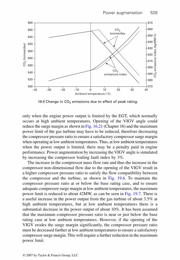
Power augmentation 529
only when the engine power output is limited by the EGT, which normallyoccurs at high ambient temperatures. Opening of the VIGV angle couldreduce the surge margin as shown in Fig. 16.21 (Chapter 16) and the maximumpower limit of the gas turbine may have to be reduced, therefore decreasingthe compressor pressure ratio to ensure a satisfactory compressor surge marginwhen operating at low ambient temperatures. Thus, at low ambient temperatureswhen the power output is limited, there may be a penalty paid in engineperformance. Power augmentation by increasing the VIGV angle is simulatedby increasing the compressor fouling fault index by 3%.
The increase in the compressor mass flow rate and thus the increase in thecompressor non-dimensional flow due to the opening of the VIGV result ina higher compressor pressure ratio to satisfy the flow compatibility betweenthe compressor and the turbine, as shown in Fig. 19.6. To maintain thecompressor pressure ratio at or below the base rating case, and to ensureadequate compressor surge margin at low ambient temperatures, the maximumpower limit is reduced to about 42MW, as can be seen in Fig. 19.7. There isa useful increase in the power output from the gas turbine of about 3.5% athigh ambient temperatures, but at low ambient temperatures there is asubstantial decrease in the power output of about 10%. It has been assumedthat the maximum compressor pressure ratio is near or just below the baserating case at low ambient temperatures. However, if the opening of theVIGV erodes the surge margin significantly, the compressor pressure ratiomust be decreased further at low ambient temperatures to ensure a satisfactorycompressor surge margin. This will require a further reduction in the maximumpower limit.
19.5 Change in CO2 emissions due to effect of peak rating.
Ambient temperature (°C)0–40 –30 –20 –10 10 20 30 40
680C
O2
(to
nn
es/d
ay)
670
CO
2 em
issi
on
s in
dex
(kg
/MW
h)
CO2tonnes/day
CO2emissions index
660
640
620
600
580
560
540
520
500
660
650
640
630
620
610
600
590
580
570
© 2007 by Taylor & Francis Group, LLC

Industrial gas turbines – single-shaft530
The increase in the compressor pressure ratio at high ambient temperaturesalso results in an improvement in the gas turbine thermal efficiency due tothe increase in the VIGV position. But, at low ambient temperatures, whenthe engine is operating at the maximum power limit, the turbine entrytemperature decreases due to the reduced gas turbine maximum power limit.Thus there is a reduction in the maximum cycle temperature, T3/T1, relative
19.6 Change in compressor ratio due to effect of increasing the VIGVangle.
Time (seconds)0–40 –30 –20 –10 10 20 30 40
Base rating
Compressor pressure ratiowhen the gas turbine is
power limted for therespective cases
IncreasedVIGV angle
12.5
Co
mp
ress
or
pre
ssu
re r
atio
13.0
12.0
11.5
11.0
10.5
10.0
9.5
9.0
19.7 Change in gas turbine power output due to effect of increasingthe VIGV angle.
Gas turbine powerlimit at a higher
ambienttemperature due
to increasedopening of the
VIGV
–40 –30 –20 –10 0 10 20 30 40
Change in power due toincreased VIGV opening
Ambient temperature (°C)
Baserating
Po
wer
(M
W)
48
44
46
42
40
38
36
34
32
30
© 2007 by Taylor & Francis Group, LLC

Power augmentation 531
to the base case, which results in a noticeable decrease in the thermal efficiencyof the gas turbine at lower ambient temperatures, as shown in Fig. 19.8.
At high ambient temperatures, when the engine power output is EGTlimited, the increase in power output from the gas turbine is due largely tothe increase in the air flow rate through the engine, due to the increase in theVIGV angle. Thus, there is only a slight increase in the temperature entrytemperature, and hence in the turbine blade metal temperature. However, theincrease in turbine power results in an increase of the torque in the turbineblade material and this raises stresses in the turbine blade material. Theincreased turbine metal temperature and stress result in a small increase inthe turbine creep life usage at higher ambient temperatures as shown inFig. 19.9. At low ambient temperatures, the decrease in the gas turbinepower output and reduced turbine entry temperature result in a substantialdecrease in the turbine creep life usage. Thus there will be no need to increasethe mean time between overhauls due to the increase in turbine creep lifeusage at high ambient temperature. In fact, it could be argued that the EGTlimit should be increased to compensate for the significant decrease in creeplife usage at low ambient temperatures. Such an increase in the EGT limitwill augment the gas turbine power output and thermal efficiency further athigh ambient temperatures, resulting in increased production and reducedfuel costs.
The increase in the VIGV angle results in an increase in compressorpressure ratio at high ambient temperature when the gas turbine power outputis limited by the EGT. This results in an increase in the combustion pressure.The increase in the combustion pressure increases the NOx emissions, while
19.8 Change in gas turbine thermal efficiency due to effect ofincreasing the VIGV angle.
Gas turbine power limit at ahigher ambient temperaturedue to increased opening of
the VIGV
–40 –30 –20 –10 0 10 20 30 40
Change in power due toincreased VIGV opening
Ambient temperature (°C)
Baserating
35.0
Th
erm
al e
ffic
ien
cy (
%)
34.5
34.0
32.5
32.0
31.5
31.0
30.5
30.0
29.5
33.5
33.0
© 2007 by Taylor & Francis Group, LLC

Industrial gas turbines – single-shaft532
decreasing the CO emissions, as shown in Fig. 19.10. At low ambienttemperatures, the decrease in the combustion temperature, due to the reducedmaximum power limit, results in a decrease in NOx emissions. However,there is a significant increase in CO emissions, as seen in Fig. 19.10.
Although there are increases in gas turbine power output and thermalefficiency at high ambient temperature, due to the increase in the VIGV
19.9 Change in turbine creep life usage due to effect of increasingthe VIGV angle.
200 000 Change in creep life usage dueto increased VIGV opening
0–40 –10 10 20 30 40
250 000
0
50 000
Ambient temperature (°C)
150 000
100 000
Tim
e to
nex
t o
verh
aul (
ho
urs
)
Base rating
19.10 Change in NOx and CO emissions due to effect of increasingthe VIGV angle.
Ambient temperature (°C)0–40 –30 –20 –10 10 20 30 40
190 14
NOx
CO
13
12
11
10
9
8
6
CO
em
issi
on
s (p
pm
v @
15%
O2
dry
)
170
150
130
110
70
90
NO
x em
issi
on
s (p
pm
v @
15%
O2
dry
)
7
IncreasedVIGVangle
© 2007 by Taylor & Francis Group, LLC

Power augmentation 533
angle, the increase in power output is greater than the increase in the thermalefficiency. This results in an increase in CO2 on a mass flow basis. However,the increase in the thermal efficiency decreases the CO2 emissions index, ascan be seen in Fig. 19.11. Thus a decrease in CO2 emissions is achieved inreal terms due to the opening of the VIGV angle. At low ambient temperatures,the decrease in the maximum power limit of the gas turbine is greater thanthe decrease in the thermal efficiency. This results in a decrease in CO2
emissions on a mass basis, but the decrease in the thermal efficiency resultsin an increase in the CO2 emissions index, as shown in Fig. 19.11.
19.3 Power augmentation using water injection
The power output of a single-shaft gas turbine may also be augmented by theuse of water injection. The water may be injected either at the inlet of thecompressor or directly into the primary zone of the combustion system. Asdiscussed earlier, power augmentation by injecting water into the compressorinlet occurs due to the suppression of the compressor inlet temperature, andthe amount of compressor inlet temperature suppression depends on thehumidity of the air at the inlet of the compressor (wetted media and inletfogging).
The case of direct water injection into the combustion system will beconsidered where the increase in power output is a result of the increasedmass flow rate through the turbine, relative to that through the compressor.The limit on the increase in power is normally governed by the increase in
19.11 Change in CO2 emissions due to effect of increasing the VIGVangle.
Time (seconds)0–40 –30 –20 –10 10 20 30 40
680
CO2 tonnes/day
CO
2 em
issi
on
s in
dex
(kg
/MW
h)
CO2 emissionsindex
CO
2 (t
on
nes
/day
)
660
640
620
580
520
500
600
560
540
670
660
650
640
630
620
610
600
590
580
570
© 2007 by Taylor & Francis Group, LLC

Industrial gas turbines – single-shaft534
CO and UHC emissions due to the chilling of the flame in the primary zone.There is also an adverse effect on the turbine blade creep life usage, whichmust be taken into consideration.
Figure 19.12 shows the increase in gas turbine power output due to waterinjection where the water–fuel ratio is unity. At an ambient temperature of30 degrees Celsius, there is about a 5% increase in gas turbine power output.This compares with about a 7% increase in power output for the two-shaftgas turbine. Unlike the case of the two-shaft gas turbine, the single-shaft gasturbine speed is constant and therefore the compressor flow essentially remainsconstant. In the case of the two-shaft gas turbine, there is an increase in thegas generator speed due to the increase in the power output from the gasgenerator turbine. This results in an increase in the compressor flow rate,contributing to the increased power output from the engine due to waterinjection. In the single-shaft gas turbine, the increase in power output due towater injection is due primarily to the increase in turbine power. With thedecrease in ambient temperature, the gas turbine becomes power limitedand, with water injection, the power limit is reached at a higher ambienttemperature, as seen in Fig. 19.12.
As with the two-shaft gas turbine, there is a significant loss in gas turbinethermal efficiency due to water injection, as shown in Fig. 19.13. Additionalfuel is needed to evaporate the water in the combustion chamber (latent heat)and heat the steam to the turbine entry temperature.
Injecting the water directly into the combustor results in an increase incompressor pressure ratio (Fig. 19.17) and in the turbine power output. The
19.12 Increase in power output from the gas turbine due to effect ofwater injection.
–40 –30 –20 –10 0 10 20 30 40
Water injection
Ambient temperature (°C)
Base rating
Gas turbine becomespower limited at higherambient temperature
48
42
40
38
36
34
32
30
Po
wer
(M
W)
46
44
© 2007 by Taylor & Francis Group, LLC

Power augmentation 535
increased power output from the turbine also results in an increased stressdue to the increased torque. There is also a small increase in the turbine entrytemperature and therefore in the turbine blade temperature. These two factorshave an adverse effect on turbine creep life usage at high ambient temperatureswhere the gas turbine power output is limited by the EGT. This can be seenin Fig. 19.14. At low ambient temperatures, however, the gas turbine ispower limited and the increased flow rate through the turbine will result in
19.13 Change in gas turbine thermal efficiency due to water injection.
–40 –30 –20 –10 0 10 20 30 40
Base rating
Ambient temperature (°C)
Water injectionGas turbine becomespower limited at higherambient temperature
34
35
33
32
30
29
28
31
Th
erm
al e
ffic
ien
cy (
%)
19.14 Change in turbine creep life usage due to water injection.
200 000
Base rating
0–20 –10 20 30 40
250 000
0
50 000
10Ambient temperature (°C)
150 000
100 000
Tim
e to
nex
t o
verh
aul (
ho
urs
)
Water injection
© 2007 by Taylor & Francis Group, LLC

Industrial gas turbines – single-shaft536
a decrease in the turbine entry temperature relative to the base rating case.Thus the turbine creep life usage will decrease as can be seen in Fig. 19.14.Unfortunately, since the power is limiting at this ambient condition, waterinjection is not used unless NOx suppression is required. Thus the decreasein creep life usage at low ambient temperature does not occur and waterinjection may result in an increase in turbine overhauls with increasingmaintenance costs. It must also be noted that damage to the combustionsystem may arise due to water injection, as discussed in Chapter 6.
In spite of these drawbacks, water injection is an effective means of NOx
control and is quite widely used. Direct injection of water into the primaryzone results in the suppression of the primary zone temperature where NOx
normally forms. Thus a significant decrease in NOx emissions occurs due tothe decrease in the primary zone temperature. However, the reduction inprimary zone temperature also results in a substantial increase in the formationof CO and is a limiting factor on the amount of water injection. This can beseen in Fig. 19.15. The decrease in gas turbine thermal efficiency inevitablywill increase the CO2 emissions on a mass and emissions index basis, asshown in Fig. 19.16. Direct water injection into the combustor also increasesthe compressor pressure ratio, as shown in Fig. 19.17 and therefore theoperating point moves towards the compressor surge line. This movement isonly small and should not present any problems with respect to the transientperformance of the gas turbine and may only be an issue at low ambienttemperatures when the gas turbine is power limited.
19.15 Change in NOx and CO emissions due to water injection.
Ambient temperature (°C)0–40 –30 –20 –10 10 20 30 40
45
NOx
CO
CO
em
issi
on
s (p
pm
v @
15%
O2
dry
)
180
140
160
120
100
80
60
40
20
0
NO
x em
issi
on
s (p
pm
v @
15%
O2
dry
) 40
35
30
25
20
15
10
5
0
Base rating = solid lineWater injection = dotted line
© 2007 by Taylor & Francis Group, LLC

Power augmentation 537
19.4 Power augmentation at low ambient
temperatures
The power output of the gas turbine has been observed to become powerlimited at ambient temperatures below 2 degrees Celsius, and the EGT fallsbelow the limiting value at lower ambient temperatures. Means to augmentpower at higher ambient temperature such as peak rating do not increase the
19.16 Increase in CO2 due to water injection.
Ambient temperature (°C)0–40 –30 –20 –10 10 20 30 40
700
700
CO
2 em
issi
on
s in
dex
(kg
/MW
h)
CO2 emissions index
680
660
640
620
600
580
560
CO
2 (t
on
nes
/day
)750
650
600
550
500
CO2 tonnes/day
19.17 Increase in compressor pressure ratio due to water injection.
Ambient temperature (°C)0–40 –30 –20 –10 10 20 30 40
Base rating
Water injectionGas turbine becomes power limited
at higher ambient temperature12.5
Co
mp
ress
or
pre
ssu
re r
atio
13.0
11.5
12.0
11.0
10.5
10.0
9.5
9.0
© 2007 by Taylor & Francis Group, LLC

Industrial gas turbines – single-shaft538
power output of the gas turbine in the low ambient conditions. In fact, inSection 19.2 it was shown that the augmentation of power at high ambienttemperature by increasing the VIGV angle may result in a decrease in poweroutput from the gas turbine at lower ambient temperatures.
Increasing the gas turbine maximum power limit will indeed increase thepower output from the gas turbine at low ambient temperatures. This willincrease the turbine entry temperature and thus increase the turbine creeplife usage requiring increased frequency of engine overhauls resulting inhigher maintenance costs. The resultant increase in the compressor pressureratio due to component matching then decreases the surge margin and increasesthe risk of compressor surge during transients, but this rise is usually verysmall. There will also be an increase in the power developed by the turbineand thus an increase in the power transmitted through the shaft to the load,seals and bearings. Thus, any power augmentation at low ambient temperaturemay need these components to be strengthened to ensure that no mechanicalfailure occurs due to the increased level of power that is transmitted. Themodifications needed to achieve satisfactory aero-thermodynamic performanceof the gas turbine due to power augmentation at low ambient temperatureswill now be discussed.
It has been stated that increasing the maximum power limit will increasethe EGT resulting in increased turbine creep life usage. If a substantialamount of engine operating occurs at low ambient temperatures, the gasturbine power limit can be increased but the EGT limit decreased. In thiscase the reduced creep life usage at high ambient temperature, when theengine power output is limited by the EGT, compensates for the increaseturbine creep life usage at low ambient temperatures (flat rating in reverse).However, the power output of the gas turbine will be reduced at high ambienttemperatures, but this will be of little consequence if the power demand fromthe generator is low under these operating conditions. Figure 19.18 showsthe power output from the gas turbine when the EGT limit is reduced by 20degrees, while the maximum power limit is raised to 47.5 MW. Thus thepower output from the gas turbine has effectively been increased by about6% without increasing the maintenance cost.
The increase in the turbine entry temperature and compressor pressureratio due to the higher power limit of the gas turbine will also increase thethermal efficiency, thus reducing fuel costs and hence improving profit. Theeffects of increasing the power output at low ambient temperatures on thermalefficiency and compressor pressure ratio are shown in Figs 19.19 and 19.20,respectively.
The reduced power at high ambient temperature is about 5% (at an ambienttemperature of 15 degrees Celsius) compared to the gain in power outputfrom the gas turbine at low ambient temperature (6%). Reducing the EGTlimit further, by 10 degrees, will almost halve the usage of turbine blade
© 2007 by Taylor & Francis Group, LLC

Power augmentation 539
creep life at high ambient temperatures. Hence it could be argued that theEGT limit should be raised at high ambient temperature, whilst decreasingthe maximum power limit to reduce the turbine blade creep life usage at lowambient temperatures. This would be more suitable if the power demandfrom the gas turbine is critical at high ambient temperatures (e.g. high air
19.18 Variation of gas turbine power output due to increased powerlimit and reduced EGT limit.
Ambient temperature (°C)
Base ratingPowerlimited
Augmented powerat low ambient
temperature
100 20 30 40–10–20–30–40
32
30
34
36
38
40
42
44
46
48
50P
ow
er (
MW
)
19.19 Variation of gas turbine thermal efficiency due to increasedpower limit and reduced EGT limit.
Time (seconds)0–40 –30 –20 –10 10 20 30 40
Base rating
Power limited
Effect of augmentedpower at low ambient
temperatures onthermal efficiency
35
36
34
33
32
31
30
29
Th
erm
al e
ffic
ien
cy (
%)
© 2007 by Taylor & Francis Group, LLC

Industrial gas turbines – single-shaft540
conditioning loads in the summer). This is effectively peak rating the engine,but the reduced maximum power limit would prevent increased overhaulfrequencies, thus preventing increased maintenance costs due to engineoperation at peak rating conditions (normal flat rating).
Due to the increase in gas turbine power limit, it is observed that thecompressor pressure ratio has increased. If the increase in the compressorpressure ratio is considered to be too high, the turbine capacity may beincreased. This will decrease the compressor pressure ratio and also reducethe creep life usage due to the decrease in turbine entry temperature. However,the decrease in the compressor pressure ratio and turbine entry temperaturewill reduce the thermal efficiency.
The impact of the increased gas turbine power limit on turbine creep lifeusage is shown in Fig. 19.21. The increase in the turbine entry temperatureat low ambient temperatures, due to the increase in the power limit, showsan increased usage of turbine blade creep life usage when the power outputof the gas turbine limits its performance. At high ambient temperatures, thedecrease in the turbine blade creep life usage is due to the reduction in theEGT limit.
The increases in compressor pressure ratio and combustion temperaturedue to the higher maximum power limit at low ambient temperatures, resultin an increase in the emissions of NOx, while decreasing the emissions ofCO. At high ambient temperatures, when the engine power output is limitedby the EGT, the decreases in the compressor pressure ratio and combustiontemperature due to the reduction in EGT limit results in a decrease in NOx
emissions whilst increasing the CO emissions, as shown in Fig. 19.22.
19.20 Variation of compressor pressure ratio due to increased powerlimit and reduced EGT limit.
Time (seconds)0–40 –30 –20 –10 10 20 30 40
Base rating
Power limited
Effect of augmentedpower at low
ambienttemperatures on
compressorpressure ratio
12.5
13.0
12.0
11.5
11.0
10.5
10.0
9.5
Co
mp
ress
or
pre
ssu
re r
atio
© 2007 by Taylor & Francis Group, LLC

Power augmentation 541
The changes in the compressor ratio and turbine entry temperature resultin an increase in the thermal efficiency at low ambient temperatures. At highambient temperatures, the thermal efficiency decreases due to the decreasein the compressor ratio and turbine entry temperature, as the EGT limit isdecreased. Thus it is observed that the CO2 emissions index decreases at lowambient temperatures and increases at high ambient temperatures, as shown
19.21 Variation of turbine creep life usage due to increased powerlimit and reduced EGT limit.
200 000
0–30 –20 10 20 30 40
250 000
0
50 000
Time seconds
Base rating
–10
Power limited
Effect of augmentedpower at low
ambienttemperatures on
creep life
150 000
100 000
Tim
e to
nex
t o
verh
aul (
ho
urs
)
19.22 Variation of NOx and CO emissions due to increased powerlimit and reduced EGT limit.
Time (seconds)0–40 –30 –20 –10 10 20 30 40
16
CO
em
issi
on
s (p
pm
v @
15%
O2
dry
)
NOx
180
CO
Base rating = solid lineAugmented power = dotted line
140
160
120
100
60
80
NO
x em
issi
on
s (p
pm
v @
15%
O2
dry
) 15
14
13
12
11
10
9
8
7
6
© 2007 by Taylor & Francis Group, LLC

Industrial gas turbines – single-shaft542
in Fig. 19.23. However, the CO2 emissions on a mass basis are lower at highambient temperatures, compared with the case at low ambient temperatures.This is due to the change in the gas turbine power output being greater thanthe change in the thermal efficiency.
When the VIGV is active in the normal operating power range, at lowambient temperatures, the increase in the gas turbine power limit will resultin the opening of VIGV to maintain the EGT limit. However, the opening ofthe VIGV increases the compressor flow rate and thus the compressorpressure ratio in order to maintain the flow compatibility between thecompressor and turbine. This will also increase the turbine entry temperatureslightly and hence the turbine blade creep life usage. If the EGT limit is nowdecreased, this will result in a further opening of the VIGV, thus increasingthe air flow rate through the engine further. This increase in the air flow ratecompensates for the reduction in power output due to the lower EGT limit.The opening of the VIGV will improve the compressor efficiency, thereforereducing the turbine entry temperature further. Thus, the turbine blade creeplife usage could remain unchanged due to the increase in the maximumpower limit of the gas turbine when operating at low ambient temperatureswith active VIGV in the normal operating power range. The decrease in EGTlimit will, of course, decrease the power output at high ambient temperatures.Since there is no compromise in the turbine blade creep life usage whenaugmenting the gas turbine power output at low ambient temperatures, theEGT limit can be increased to its design (base) value at high ambienttemperatures, thus incurring no penalty in turbine blade creep life usage due
19.23 Variation of CO2 emissions due to increased power limit andreduced EGT limit.
Time (seconds)0–40 –30 –20 –10 10 20 30 40
680
CO
2 em
issi
on
s in
dex
(kg
/MW
h)
CO2 emissions index
CO2 tonnes/day 660
640
620
600
580
560
Base rating = solid lineAugmented power = dotted line
CO
2 (t
on
nes
/day
)
700
600
550
500
450
400
650
© 2007 by Taylor & Francis Group, LLC

Power augmentation 543
to power augmentation at low ambient temperatures. When the gas turbine isused in a combined cycle, the decrease in the EGT limit will have a detrimentaleffect on the performance of the steam plant and needs to be consideredwhen augmenting the power output of the gas turbine by such means at lowambient temperatures.
An alternative is to increase the turbine capacity so that the compressorpressure ratio will decrease, thus resulting in a decrease in turbine entrytemperature, in order to maintain turbine blade creep life. A significant increasein the turbine capacity may be necessary to achieve a sufficient decrease inthe turbine entry temperature, but this could seriously penalise the gas turbineperformance at high ambient temperatures, which may be unacceptable interms of power output and thermal efficiency.
When the VIGV is active in the normal power range and used in conjunctionwith dry low emission (DLE) combustion systems, the decrease in the EGTlimit, or increased turbine capacity to augment the power output from thegas turbine at low ambient temperatures, will result in a decrease in combustiontemperature. Thus, there is a limit to how much the combustion temperaturemay decrease because there would be an increase in CO and UHC, whichmust be avoided. As an extreme case, the decrease in the combustiontemperature could result in the weak extinction limit being exceeded, thusleading to engine trips.
The reader is left to use the simulator to illustrate the augmentation of thepower output at low ambient temperatures using both these methods andproducing the figures similar to those shown in Figs 19.18 to 19.23.
19.5 Turbine inlet cooling
In Section 19.3, power augmentation using direct water injection was discussed.An alternative means of water injection to augment the power output of gasturbines is to use it in turbine inlet cooling. In Chapter 14 Section 14.5,turbine inlet cooling applied to a two-shaft gas turbine operating with a freepower turbine was discussed. Here, water can be evaporated in the inlet ofthe engine and the absorption of latent heat required for the evaporationprocess results in a decrease in the compressor inlet temperature. This resultsin an increase in power output and improved thermal efficiency of the gasturbine. Another means of turbine inlet cooling is the use of chillers (mechanicaland absorption types), as also discussed in Section 14.5. These technologiesare applicable equally to a single-shaft gas turbine and the benefits aresimilar to those discussed in Section 14.5; the figures produced in Section14.5 can be determined for a single-shaft gas turbine. The reader is invitedto reproduce these figures for the single-shaft gas turbine simulator.
The notable difference is that a single-shaft gas turbine normally operatesat a constant speed, particularly in power generation, whereas in a two-shaft
© 2007 by Taylor & Francis Group, LLC

Industrial gas turbines – single-shaft544
gas turbine the gas generator speed increases. At low compressor inlettemperatures (at about 13 degrees Celsius) the two-shaft gas turbine poweroutput can become limited by the gas generator speed. Any further coolingwill only result in a small increase in power output due to constant gasgenerator speed operation. Therefore, the cooler size has to be optimised formaximum gain in power output due to turbine inlet cooling.
In a single-shaft gas turbine, the maximum power limit is reached at alower ambient temperature (at about 2 degrees Celsius). Thus a greater benefitfrom turbine inlet cooling would be achieved with the single-shaft gas turbineby cooling the turbine inlet air down to 10 degrees Celsius. Cooling thecompressor inlet air to lower temperatures increases the risk of the formationof ice, particularly at high humidity, which occurs due to turbine inlet cooling.Such ice formation can break away and enter the compressor, which maydamage the engine. Therefore, in practice, it is unlikely that we would considerturbine inlet cooling much lower than 10 degrees Celsius.
© 2007 by Taylor & Francis Group, LLC

545
In Chapter 10 the principles of engine control and its function in preventingthe engine from exceeding maximum limiting values, thereby protecting theengine from damage, were discussed. The principles of engine controls usingthe two-shaft gas turbine simulator were illustrated. Much of what was discussedusing the two-shaft gas turbine simulator can be demonstrated with the single-shaft gas turbine simulator and similar conclusions drawn with respect to theperformance of the fuel control system. However, it is the control of theVIGV in a single-shaft gas turbine that differs primarily from the two-shaftgas turbine. The problems associated with the control of the VIGV willtherefore be demonstrated and the means to overcome these difficulties usingthe single-shaft gas turbine simulator, as discussed in Chapter 10, will bedescribed.
20.1 VIGV control system simulation
One of the advantages of using a VIGV is that it reduces the starting powerrequirement due to the decreased mass flow rate through the compressorwhen the VIGV is closed. The VIGV is full opened during the normal operatingrange so that the mass flow rate through the engine is increased, so helpingto achieve the designed power output of the gas turbine. This is accomplishedby controlling the VIGV system independently of the fuel control system,where the VIGV modulates to maintain a certain value for the exhaust gastemperature (EGT). The limit or set point for the EGT may be at a valuebelow the maximum/limiting value for the EGT needed to protect the engine.When the EGT is above the set point for VIGV control, the VIGV will befully opened, enabling the engine to achieve its designed power output.When the EGT is below this set point, the VIGV will be fully closed, hencereducing starting power requirements.
The operation of the VIGV control system is illustrated by subjecting thesingle-shaft gas turbine simulator to a step change in power demand from the
20Simulation of engine control system
performance
© 2007 by Taylor & Francis Group, LLC

Industrial gas turbines – single-shaft546
generator by increasing the power demand from 1 MW to 60 MW. The EGTset point for the VIGV control is 650 K and the maximum EGT limit is 825K. The increase in power demand from the generator results in an increasein the EGT, which corresponds to T4, as shown in Fig. 20.1, where it exceedsthe VIGV set point after 23 seconds. Since the EGT exceeds the set point forVIGV control, the VIGV starts to open just after 23 seconds (Fig. 20.2) inorder to maintain the EGT at 650 K (set point). The VIGV continues to openas the EGT increases to achieve the power demand by the generator and isfully opened after about 28 seconds. The continuous increase in EGT can beseen in Fig. 20.1, but the rate of increase decreases during the period whenthe VIGV is opening. In fact, the EGT falls slightly during the period whenthe VIGV is opening, before increasing to the maximum limiting value of825 K. Figure 20.2 also shows the trend in the turbine non-dimensionalspeed, where a decrease in the turbine non-dimensional speed, N/√T3, isobserved, due to the increase in the turbine entry temperature, T3, since theturbine speed, N, remains constant. The compressor non-dimensional speed,N/√T1, remains constant since the ambient temperature, and hence T1, do notchange during this simulation.
The opening of the VIGV results in a change in the compressor characteristic,where the capacity of the compressor increases. This is shown in Fig. 20.3where the operating points for when the VIGV is fully closed, fully openedand the period when the VIGV is opening are marked clearly on the compressorcharacteristic. Note that the compressor non-dimensional flow and henceflow capacity increase as the VIGV opens.
The increase in flow capacity results in an increase in the compressorflow rate, shown as a trend in Fig. 20.4. The increase in the compressor flow
20.1 Trends in temperature due to a step change in power demand.Time (seconds)
100 20 30 40 50 60 70
1600
1400
1200
1000
800
600
400
Tem
per
atu
re (
K)
Turbine entrytemperature T3
Exhaust gastemperature T4
Compressor dischargetemperature T2
Exhaust gastemperature limit
Exhaust gas temperatureset point for VIGV control
© 2007 by Taylor & Francis Group, LLC

Simulation of engine control system performance 547
20.2 Trends in VIGV position and non-dimensional speed for a stepchange in power demand.
20.3 Change in compressor characteristic due to opening of VIGVresulting from increased power demand.
Time (seconds)10 20 30 40 50 60 700
120
100
80
60
40
20
0
VIG
V p
osi
tio
n (
%)
op
ened
Turb
ine
no
n-d
imen
sio
nal
sp
eed
180
170
160
150
140
130
120
VIGV position
Turbine non-dimensional speed
Non-dimensional flow (W1√T1/P1)0.5 0.6 0.7 0.8 0.9 1.0 1.1 1.2
16.0
12.0
8.0
4.0
0.0
Pre
ssu
re r
atio
VIGV fully closed
VIGV fully opened
VIGV opening
Shift in surge linedue to VIGV opening
Change in the compressorcharacteristic due to the
opening of the VIGV
© 2007 by Taylor & Francis Group, LLC

Industrial gas turbines – single-shaft548
also results in an increase in the compressor power absorbed. This powerincreases substantially from about 28 MW to about 45 MW, as shown in Fig.20.5 due to the opening of VIGV. The turbine produces the power requiredby the compressor during normal operation; however, during starting of thegas turbine, the turbine power output is very small and a significant amount
20.4 Increase in air flow through the compressor due to opening ofthe VIGV.
20.5 Increase in compressor power absorbed due to opening of theVIGV.
3.0
2.5
2.0
1.5
1.0
0.5
0.0
Fuel
flo
w (
kg/s
)
Time (seconds)100 20 30 40 50 60 70
Air–fuel ratio
Fuel valve position
Airflow
Fuel flowC
om
pre
sso
r in
let
airf
low
(kg
/s),
fu
el v
alve
po
siti
on
(%
), a
ir–f
uel
rat
io
250
200
150
100
50
0
Time (seconds)10 200 30 40 50 60 70
Po
wer
(M
W)
100
90
80
70
60
50
40
30
20
10
0
89
Eff
icie
nci
es (
%)
88
87
86
85
84
83
82
81Compressor efficiency
Increase in compressor powerabsorbed due to the openingof the VIGV
Compressorpower absorbed
Turbine efficiency
Turbine power output
© 2007 by Taylor & Francis Group, LLC

Simulation of engine control system performance 549
of starting power must be provided by an external source as discussed inChapter 10. Thus, closing the VIGV during starting will result in a significantdecrease in the starting power requirements. The increase in the gas turbineand generator power output is shown in Fig. 20.6. The figure also shows thetrends in the gas turbine thermal efficiency and the set point for the poweroutput. In this instance, the power is limited to about 40 MW by the EGTlimit. In practice, this would trip the engine due to the shift in the generatorfrequency resulting from insufficient power available from the gas turbine.However, such trips are ignored so that the power capacity of the engine canbe investigated in more detail.
20.2 VIGV control when the VIGV is active during
the normal operating power range
In Section 20.1 the control of the VIGV was discussed when it is fully openduring the normal operating power range. The performance of a single-shaftgas turbine has also been discussed when the VIGV is modulating at thenormal power range of the gas turbine and maintaining the EGT on itsmaximum limit (i.e. the EGT set point for VIGV control corresponds to themaximum EGT limit). At first sight, it would appear that increasing the EGTlimit for VIGV control to the limiting value required to protect the engine(i.e. increasing the EGT for VIGV control from 650K to 825 K) wouldachieve the desired result. However, this presents some difficulties, as theengine may respond unexpectedly, as discussed in Chapter 10.
20.6 Change in power demand from generator and variation of gasturbine thermal efficiency due to increased power demand.
Time (seconds)100 20 30 40 50 60 70
Increase in powerdemand from
1 MW to 60 MW
70
60
50
40
30
20
10
0
Po
wer
ou
tpu
t (M
W)
Th
erm
al e
ffic
ien
cy (
%)
35
30
25
20
15
10
5
0
Generator power output
Gas turbine power output
Thermal efficiency
Set point for generatorpower demand
© 2007 by Taylor & Francis Group, LLC

Industrial gas turbines – single-shaft550
If the simulation carried out in Section 20.1 is repeated but with the EGTset point for VIGV control increased to the maximum value of 825 K, thepower output from the gas turbine is significantly reduced while the engineis operating on the maximum EGT limit. The maximum power output of thegas turbine should be about 40 MW, but the power output in this instance isrestricted to 28 MW and is well short of the required power from the gasturbine as shown in Fig. 20.7. As the power demand from the gas turbine isincreased, the EGT increases. However, the EGT is below the VIGV operatingset point and the VIGV remains closed. When the EGT exceeds the EGTlimit for VIGV operation, the VIGV starts to open. Since the EGT set pointfor VIGV operation is the maximum permitted value, the low signal selectionprevents the VIGV from opening fully, as it endeavours to protect the turbinefrom over-heating by preventing the EGT from exceeding the maximumvalue. Thus, the airflow through the compressor is severely restricted andhence the power output from the gas turbine also becomes severely limited.The restriction of flow through the compressor also results in a reduction inthe maximum to minimum cycle temperature ratio, T3/T1. This is necessaryto satisfy the flow compatibility between the compressor and turbine, thusreducing the specific work of the gas turbine. The reduction in specific workalso contributes significantly to the loss in gas turbine power output due toinsufficient opening of the VIGV.
This increase in EGT, T4, can be seen in Fig. 20.8 and is due to theincrease in power demand from the gas turbine. Note that the EGT reachesthe limiting value while the VIGV has opened only marginally, as shown in
20.7 Severe reduction in power due to insufficient opening of theVIGV.
Time (seconds)10
Po
wer
ou
tpu
t (M
W)
50
45
40
35
30
25
20
15
10
5
0200 30 40 50 60 70
Exhaust gas temperaturepower limit
Generator power output dueto an increase in set point
from 1 MW to 60MW
Shortfall in power outputdue to the VIGV unable
to open fully
© 2007 by Taylor & Francis Group, LLC

Simulation of engine control system performance 551
Fig. 20.9. The change in the compressor characteristic is small due to thissmall opening of the VIGV (Fig. 20.10), resulting in little or no change inair-flow through the compressor, as shown in Fig. 20.11. It may be possibleto reduce the response of the gas turbine by reducing the gain of the fuelcontrol system or by increasing the gain of the VIGV control system, but thisimproves the situation only marginally and would result in an oscillatoryresponse of the gas turbine and increase the likelihood of trips.
20.8 Increase in EGT due to increased power demand.
20.9 Insufficient opening of the VIGV due to the maximum EGT limitbeing reached.
Time (seconds)
1400
1300
1200
1100
1000
900
800
700
600
500
400
Tem
per
atu
re (
K)
100 20 30 40 50 60 70
Compressor dischargetemperature T2
Exhaust gastemperature T4
Exhaust gas temperaturelimit
Turbine entrytemperature T3
Time (seconds)100 20 30 40 50 60 70
6
5
4
3
2
1
0
VIG
V p
osi
tio
n (
%)
op
ened
180
170
160
150
140
130
120
Turb
ine
no
n-d
imen
sio
nal
sp
eed
Turbine non-dimensional speed
VIGV position
© 2007 by Taylor & Francis Group, LLC

Industrial gas turbines – single-shaft552
20.11 Little or no change in compressor flow resulting in the gasturbine power output becoming severely restricted.
20.10 The small change in the compressor characteristic due toinsufficient VIGV opening.
Non-dimensional flow (W1√T1/P1)
0.60.5 0.7 0.8 0.9 1.0 1.1 1.2
16.0
12.0
8.0
4.0
0.0
Pre
ssu
re r
atio
Operating points oncompressor characteristicdue to insufficient opening
of VIGV
Time (seconds)10 20 30 40 50 60 700
250
200
150
100
50
0
Co
mp
ress
or
inle
t ai
rflo
w (
kg/s
), f
uel
val
vep
osi
tio
n (
%),
air
–fu
el r
atio
Fuel
flo
w (
kg/s
)2.5
2
1.5
1
0.5
0
Fuel flow
Airflow
Air–fuel ratio
Fuel valve position
© 2007 by Taylor & Francis Group, LLC

Simulation of engine control system performance 553
20.2.1 Open and closed loop control system
It is clear that insufficient opening of the VIGV is the main cause of severeloss in the gas turbine power output, although the engine is on the EGT limit.The VIGV opening must be increased so that the mass flow rate through thecompressor and thus the engine can increase. However, this would result inthe engine behaving as discussed in Section 20.1, where the control systemperformance was considered when the VIGV is fully opened during thenormal operating power range, when no problems in the VIGV action wereexperienced. This feature is exploited when the VIGV is opened, to say full,for a short period of time, thus decreasing the EGT. This allows the enginepower to increase to the required set point or maximum engine operatingpower. When the VIGV action is implemented in this manner, it is referredto as an open loop control system, as there is no feedback mechanism tocorrect any errors after this period. Any error left by the open loop systemcan be rectified by switching to the closed loop control system.
The open and closed loop control systems are illustrated by repeating theearlier simulation but by activating the open loop response when the setpoint for the power output from the generator is increased. The VIGV isopened fully and linearly over a period of 2 seconds, which is its opening orstroke time. The VIGV is left fully opened for a period 15 seconds. On thisoccasion, the power demand is increased from 1 to 35 MW, as this willillustrate the opened and closed loop action more clearly. Increasing thepower demand from the gas turbine results in the VIGV initially openingfully under open loop response, as shown in Fig. 20.12. During this period,
20.12 VIGV opening during open and closed loop response fromVIGV control system.
Time (seconds)100 20 30 40 50 60 70
180
170
160
150
140
130
120
Turb
ine
no
n-d
imen
sio
nal
sp
eed
VIG
V p
osi
tio
n (
% o
pen
ed)
120
100
80
60
40
20
0
Open loopresponse
Closed loop response
VIGV position
Trim
Turbine non-dimensional speed
© 2007 by Taylor & Francis Group, LLC

Industrial gas turbines – single-shaft554
the EGT increases, as shown in Fig. 20.13, but it does not reach the limitvalue as observed in the previous case. Thus the power demand from the gasturbine may be achieved as the VIGV remains fully opened for a sufficientlylong period of time so that the EGT remains below its limiting value. Hencethe fuel flow control system sees a sufficient error, thus allowing the powerdemand to be met. This is shown in Fig. 20.14.
20.13 Change in temperature due to open and closed loop responseof the VIGV control system.
Time (seconds)100 20 30 40 50 60 70
36
Po
wer
ou
tpu
t (M
W)
35
34
33
32
31
30
Trim
Generator power output
Increase in power demandfrom 1 MW to 35 MW
20.14 Increase in gas turbine power output due to the open andclosed loop response of VIGV control system.
Time (seconds)100 20 30 40 50 60 70
1600
1400
1200
1000
800
600
400
Tem
per
atu
re (
K)
Closed loop responseOpen loop response
Exhaust gastemperature limit
Turbine entrytemperature T3
Exhaust gastemperature T4 (EGT)
Compressor dischargetemperature T2
© 2007 by Taylor & Francis Group, LLC

Simulation of engine control system performance 555
After 15 seconds of open loop response from the VIGV control system,the closed loop response takes over and results in the VIGV closing (Fig.20.12) to maintain the EGT on the set point for the VIGV control system,which now corresponds to the maximum EGT limit. This results in theVIGV closing from 100% (open loop output) to about 70% (closed loopoutput) and the increase in the EGT during the closed loop response isshown in Fig. 20.13. Although this control strategy improves the response ofthe engine to power demand, as shown in Fig. 20.14, the open loop responsemay still leave an offset in the power output, resulting in the power outputfrom the gas turbine being slightly lower than the power demand (Fig. 20.14).These small differences in outputs may be ironed out or trimmed by settingthe EGT limit for VIGV operation to be slightly lower than the maximumEGT limit, thus enabling the required power demand to be met. The effect oftrimming the VIGV movement on the gas turbine power output is shown inFigs 20.12 and 20.14, where the VIGV opens due to the slight decrease in theEGT set point and the power output reaches the generator power demand setpoint. The EGT limit for VIGV control is reduced by 2 degrees, from the 825K to 823 K (for trimming). Such small temperature differences will havelittle impact on engine performance, but will provide a simple and effectivemeans for overcoming control problems associated with variable guide vanesystems under these conditions.
The effect of the VIGV opening on the compressor characteristic is shownin Figs 20.15 and 20.16. During the open loop response, the VIGV controlsystem opens the VIGV fully and remains opened fully for a fixed period oftime (15 seconds). The compressor characteristic changes from the fullyclosed position to the fully opened position of the VIGV and the change inthe compressor characteristic (Fig. 20.15) is similar to that shown in Fig.20.3 previously. However, the operating point on the characteristic differsfrom that shown in Fig. 20.3. The VIGV starts to open as soon as the setpoint in power demand from the gas turbine increases, whereas, in the casedescribed in Fig. 20.3, the VIGV starts to open only when the EGT exceedsthe set point (650 K) for VIGV control. Thus, there is a period of engineoperation when the VIGV remains closed at low gas turbine power outputs,which is absent in the present case.
During the closed loop response, the VIGV sufficiently closes so that theEGT returns to the set point specified for VIGV control. This results in adecrease in compressor capacity by shifting the compressor speed lines tothe left, as shown in Fig. 20.16. The operating points on the compressorcharacteristic are also shown during open and closed loop response of theVIGV control system. It is also observed that the compressor pressure ratiodecreases during the closed loop response, as shown in Fig. 20.16.
This is due to the decrease in compressor flow capacity, resulting in adecrease in compressor pressure ratio to satisfy the flow compatibility between
© 2007 by Taylor & Francis Group, LLC

Industrial gas turbines – single-shaft556
20.15 Change in compressor characteristic due to the open loopresponse of VIGV control system.
20.16 Change in compressor characteristic due to the closed loopresponse of VIGV control system.
Non-dimensional flow (W1√T1/P1)0.60.5 0.7 0.8 0.9 1.0 1.1 1.2
16.0
12.0
8.0
4.0
0.0
Pre
ssu
re r
atio
VIGV closing due toclosed loop response
Change in compressorcharacteristic due to
the VIGV closing
Shift in surge linedue to VIGV closing
Non-dimensional flow (W1√T1/P1)
0.5 0.6 0.7 0.8 0.9 1.0 1.1 1.2
16.0
12.0
8.0
4.0
0.0
Pre
ssu
re r
atio
VIGV fully closed
VIGV fully opened
VIGV opening due toopen loop response
Shift in surge linedue to VIGV opening
Change in compressorcharacteristic due to the
opening of the VIGV
© 2007 by Taylor & Francis Group, LLC

Simulation of engine control system performance 557
the compressor and turbine. However, the maximum to minimum cycletemperature, T3/T1, is higher when the EGT set point for VIGV control isincreased. The net effect on the gas turbine thermal efficiency is minimal,although a slight decrease in thermal efficiency occurs when operating witha higher EGT limit for VIGV control. It is only when a heat exchanger isincorporated or in combined cycle applications that a significant improvementin the thermal efficiency will occur at part loads due to the increased exhaustheat being available for recovery via the heat exchangers.
20.2.2 VIGV systems for dry low emission (DLE)combustor gas turbines
Apart from reducing starting power requirements of large gas turbines, VIGVsystems are used widely in dry low emission combustion (DLE) engines. Itwas stated in Chapter 6 that gas turbine emissions such as NOx and CO canbe reduced significantly if the combustion temperature is kept within strictlimits, which means the air–fuel ratio should remain approximately constantwith the change in load. The application of VIGV to maintain a constantEGT with the decrease in engine power output does indeed maintain theturbine entry temperature and combustion temperature approximately constant.This is exploited in the manufacture of single-shaft gas turbines employingDLE combustion systems.
The suitability of the use of VIGV for DLE combustion gas turbines willnow be demonstrated using the simulator. The power demand from the gasturbine is increased in steps of approximately 2.5 MW, so that the normalpower range of the gas turbine is covered as shown in Fig. 20.17. Theincrease in the power demand results in the VIGV responding as describedin Section 20.2.1 and as shown in Fig. 20.18. The open and closed loopresponses of the VIGV control system is clearly shown for each step increasein the power demand from the generator. The corresponding trends in gasturbine temperatures are shown in Fig. 20.19. The simulator assumes aconventional (diffusion) combustion system, where the combustion temperaturewill be high and result in high NOx emissions. In a DLE combustion system,these temperatures will be about 300 to 500 degrees lower, hence producingsignificantly lower NOx emissions.
The EGT is observed to remain on its set point during the period of closedloop response from the VIGV control system. The turbine entry and combustiontemperature also remain approximately constant. However, during the periodof open loop response, the opening of the VIGV results in a decrease in theEGT below its set point, and the largest decrease occurs at low gas turbinepower output. There is therefore a significant decrease in turbine entry andcombustion temperatures. This will result in the air–fuel ratio increasingduring the period of open loop response, whilst the air–fuel ratio remains
© 2007 by Taylor & Francis Group, LLC

Industrial gas turbines – single-shaft558
essentially constant during the period of closed loop response, as shown inFig. 20.20. Such increases in air–fuel ratios can exceed the weak extinctionlimit for the DLE combustion system, resulting in the flaming out of combustionsystems, particularly at low gas turbine power levels. The change in turbinecreep life usage due to the open and closed loop response is shown inFig. 20.21.
20.17 Change in gas turbine power output for a series of setincreases in power demand from the generator.
20.18 Open and closed loop response of the VIGV control system toa series of step increases in power demand from the gas turbine.
Time (seconds)100500 150 200 250 300 350
140
139
138
137
136
135
134
133
132
131
130
Turb
ine
no
n-d
imen
sio
nal
sp
eed
120
100
80
60
40
20
0
VIG
V p
osi
tio
n (
% o
pen
ed)
Closed loop response
Non-dimensional speed
VIGV
Open loop response
Time (seconds)100500 150 200 250 300 350
40
38
36
34
32
30
28
26
Po
wer
ou
tpu
t (M
W)
Generator power output
Increase in generator setpoint from 27.5 MW to
30 MW
Increase in generatorset point from
37.5 MW to 60 MW
Increase in generatorset point from 35 MW
to 37.5 MW
Increase in generatorset point from 32.5 MW
to 35 MW
Increase in generatorset point from 30 MW
to 32.5 MW
© 2007 by Taylor & Francis Group, LLC

Simulation of engine control system performance 559
An alternative engine control strategy is to modulate the VIGV in responseto a change in power demand and modulate the fuel flow to maintain theEGT on its set point. Such a control strategy is described in Figure 10.11(Chapter 10) and would eliminate the need for an open loop response ortrimming from the control system. However, when the power demand falls
Time (seconds)100500 150 200 250 300 350
2500
2000
1500
1000
500
0
Tem
per
atu
re (
K)
Closed loop response
Combustion primary zone
Turbine entrytemperature
Open loop response
Exhaust gas temperature limit
Compressor dischargetemperature
Exhaust gastemperature T4
20.19 Gas turbine temperature changes due to a series of stepincreases in gas turbine power output.
20.20 Change in air–fuel ratio and flow due to a series of stepincreases in power demand from the gas turbine.
Time (seconds)100500 150 200 250 300 350
Co
mp
ress
or
inle
t ai
rflo
w (
kg/s
), a
ir–f
uel
rat
io
160
140
120
100
80
60
40
20
0
Fuel
flo
w (
kg/s
)
2.8
2.6
2.4
2.2
2.0
1.8
1.6
1.4
1.2
1.0Closed loop response
Air–fuel ratio
Open loop response
Fuel flow
Airflow
© 2007 by Taylor & Francis Group, LLC

Industrial gas turbines – single-shaft560
sufficiently the VIGV will remain closed, and the control strategy must shiftto modulate the fuel flow to the change in power demand from the gasturbine at these power conditions. During this period of engine operation theair–fuel ratio cannot be maintained and the combustion system switches toa diffusion flame similar to that found in conventional combustion systems.Since this occurs at low power, typically below 65% of the design poweroutput, the high NOx emissions during this period of operation are normallyof little consequence because the amount of operation at such low power isusually small. Generally, the control of DLE combustion gas turbines ismuch more complex. At the time of writing, these combustion systems arestill being developed to overcome combustion instabilities, which occurquite frequently in production engines. The corresponding figures for thealternative control strategy are shown in Figs 20.22, 20.23, 20.24, 20.25 and20.26, respectively. It can be seen that the absence of the open loop responsegives a steady air–fuel ratio, as shown in Fig. 20.25.
20.2.3 Increasing the EGT limit to reduce CO at off-design conditions
The decrease in power results in a decrease in the compressor pressure ratioand thus a decrease in the turbine pressure ratio. If operation is at aconstant EGT at lower power as discussed above, the turbine entry temperatureand the combustion temperature decrease as the compressor pressure ratiodecreases. The decreases in combustion temperature and pressure will increase
20.21 Increase in turbine creep life usage due to constant EGToperation at low power.
Time (seconds)100500 150 200 250 300 350
Closed loop response
Open loop response
350000
300000
250000
200000
150000
100000
50000
Tim
e to
nex
t o
verh
aul (
ho
urs
)
© 2007 by Taylor & Francis Group, LLC

Simulation of engine control system performance 561
the CO and UHC emissions, particularly using DLE combustion. This problemis more acute in staged combustion employed in multi-shaft gas turbinesoperating with a free power turbine and using overboard bleeds, whichadversely affect the gas turbine thermal efficiency. It was suggested earlier
20.22 Change in gas turbine power output for a series of stepincreases in power demand from the generator using alternativecontrol strategy.
20.23 Response of the VIGV control system to a series of stepincreases in power demand from the gas turbine using alternativecontrol strategy.
Time (seconds)100500 150 200 250 300 350
Po
wer
ou
tpu
t (M
W)
40
38
36
34
32
30
28
26
Generator power output
Increase in generatorset point from
37.5 MW to 60 MW
Increase in generatorset point from
35 MW to 37.5 MW
Increase in generatorset point from27.5 MW to 30 MW
Increase in generatorset point from
32.5 MW to 35 MW
Increase in generatorset point from
30 MW to 32.5 MW
Time (seconds)100500 150 200 250 300 350
120
100
80
60
40
20
0
VIG
V p
osi
tio
n (
% o
pen
ed)
Turb
ine
no
n-d
imen
sio
nal
sp
eed
140.0
139.0
138.0
137.0
136.0
135.0
134.0
133.0
132.0
131.0
130.0
VIGV
Non-dimensional speed
© 2007 by Taylor & Francis Group, LLC

Industrial gas turbines – single-shaft562
that the use of a variable geometry power turbine and higher EGT limit(Chapter 10) would indeed help maintain high combustion temperatures atlower power outputs and thus help eliminate such overboard bleeds andmaintain low CO and UHC emissions.
20.25 Change in air-to-fuel ratio due to a series of step increases inpower demand from the gas turbine using alternative controlstrategy.
20.24 Gas turbine temperatures due to a series of step increases ingas turbine power output using alternative control strategy.
Time (seconds)100500 150 200 250 300 350
2400
2200
2000
1800
1600
1400
1200
1000
800
600
400
Tem
per
atu
re (
K)
Compressor dischargetemperature T2
Exhaust gastemperature T4
Turbine entrytemperature T3
Combustion/primary zone
Time (seconds)100 150500 200 250 300 350
Fuel
flo
w (
kg/s
)
3.0
2.8
2.6
2.4
2.2
2.0
1.8
1.6
1.4
1.2
1.0
Co
mp
ress
or
inle
t ai
rflo
w (
kg/s
), a
ir–f
uel
rat
io
160
140
120
100
80
60
40
20
0
Airflow
Fuel flow
Air–fuel ratio
© 2007 by Taylor & Francis Group, LLC

Simulation of engine control system performance 563
A similar strategy may be implemented for single-shaft gas turbines, wherethe EGT limit is increased at low power conditions to maintain high combustiontemperatures, thus minimising CO and UHC emissions at these operatingconditions. Increasing the EGT limit at reduced power outputs must takeinto account the increase in creep life usage due to the higher turbine metaltemperature. From Fig. 20.26, it is observed that the turbine creep life usagedecreases and this is because of the reduced turbine entry temperature andcooling air temperature due to the lower compressor pressure ratios at lowerpower. Thus the potential to increase the EGT limit at these powers exists,such that the turbine creep life usage remains constant with reducing power,hence minimising CO and UHC emissions at these operating conditions.
20.3 Optimisation of the EGT limit for a single-shaft
gas turbine with ambient temperature
It has been assumed that the EGT limit remains constant with variation ofthe ambient temperature for both the single- and the two-shaft gas turbinesimulators. This is a reasonable assumption for a two-shaft gas turbine,where the EGT is measured at the exit of the gas generator turbine ratherthan at the exit of the power turbine. Since the gas generator pressure ratioremains essentially constant due to the choked conditions in the power turbine,this forces the gas generator turbine to operate at an approximately fixedpressure ratio. Thus, the turbine entry temperature remains essentially constantas does the turbine creep life usage when the engine power output is limitedby the EGT. With a single-shaft gas turbine, the EGT is usually measured at
20.26 Increase in turbine creep life usage due to constant EGToperation at low power using alternative control strategy.
Time (seconds)100500 150 200 250 300 350
Tim
e to
nex
t o
verh
aul (
ho
urs
)400000
350000
300000
250000
200000
150000
100000
50000
0
© 2007 by Taylor & Francis Group, LLC

Industrial gas turbines – single-shaft564
the exit of the turbine rather than at some intermediate point between theinlet and exit of the turbine. The increase in ambient temperature results ina decrease in the compressor pressure ratio and thus in the turbine pressureratio. For a fixed EGT limit, this results in a decrease in the turbine entrytemperature and hence a decrease in turbine creep life usage and therefore anincrease in the time to next overhaul, as shown in Fig. 20.27.
20.28 Change in gas turbine power output for a fixed and variableEGT limit with ambient temperature.
20.27 Effect of EGT limit on turbine creep life usage with ambienttemperature.
Time (seconds)105–5–10 0 15 20 25 30 35 40
Exh
aust
gas
tem
per
atu
re (
EG
T)
limit
(K
)
Turbine creep life usage
Exhaust gas temperature
Tim
e to
nex
t o
verh
aul (
ho
urs
)840
850
830
820
810
800
790
780
300000
250000
200000
150000
100000
50000
0
Fixed EGTlimitVariable EGT limit
with ambienttemperature
Time (seconds)4035302520151050–5–10
Fixed exhaust gastemperature limit
Variable exhaust gastemperature limit withambient temperature
Po
wer
ou
tpu
t (M
W)
48
46
44
42
40
38
36
34
32
30
© 2007 by Taylor & Francis Group, LLC

Simulation of engine control system performance 565
It is therefore possible to increase the EGT limit at higher ambienttemperatures such that the turbine creep life usage remains approximatelyconstant with the change in ambient temperature. The resultant increase inthe EGT limit at high ambient temperatures will increase the power outputof the gas turbine at these ambient temperatures, as shown in Fig. 20.28. Atan ambient temperature of 30 degrees Celsius, the gas turbine power outputincreases by about 3%, compared with the case when the EGT limit remainsconstant with ambient temperature changes. There is also a useful increasein the thermal efficiency of the gas turbine due to the higher EGT limit.
© 2007 by Taylor & Francis Group, LLC

566
Exercises using the single-shaft gas turbine simulator
The following exercises (1–46) use the single-shaft gas turbine simulator onthe CD accompanying this book. The default values given in the simulatorand the generator power demand set to 60 MW should be used unless otherinput values are specifically stated.
21.1 Effects of ambient temperature and pressure
on engine performance
1. Determine the maximum generator power, gas turbine shaft power andthermal efficiency for the engine when operating at ISO conditions.What is the creep life usage of the turbine? ISO conditions refer to anambient temperature of 15 degrees Celsius, pressure of 1.013 Bar,relative humidity of 60% and zero inlet and exhaust losses. What limitsthe power output from the gas turbine?
Determine the emissions from the gas turbine and hence calculatethe amount of NOx, CO and CO2 in tonnes/day.
2. The engine operating at site has the following conditions.
• ambient temperature 15 degrees Celsius• ambient pressure 1.013 Bar• inlet and exhaust loss of 100 mm water gauge
Determine the parameters in Exercise 1 above and calculate the percentagechanges in the parameters when operating at site rated conditions.Explain the changes in the turbine life usage.
3. Determine the percentage changes in the parameters in Exercise 1 when
(1) the ambient temperature is 30 degrees Celsius(2) the ambient temperature is zero degrees Celsius(3) the ambient temperature is –15 degrees Celsius
21Simulation exercises
© 2007 by Taylor & Francis Group, LLC

Simulation exercises 567
What limits the power output from the gas turbine when operating atthese ambient temperatures? Repeat this exercise using the controlsystem Option 2. Comment on the operation of the variable inlet guidevane (VIGV) at these ambient conditions.
4. When operating at site rated conditions as stipulated in Exercise 2,determine the parameters in Exercise 1 when the ambient pressure is0.975 Bar and calculate the percentage change from the values determinedin Exercise 1.
5. When the required power output from the generator is 37 MW and theambient pressure and temperature, are 0.975 Bar and 15 degrees Celsius,respectively, determine the thermal efficiency of the gas turbine. If theambient pressure increases to 1.03 Bar, explain why the thermal efficiencydecreases and explain the changes in the turbine creep life usage andemissions.
6. Produce a graph describing the maximum gas turbine power outputwith ambient temperature, indicating which engine parameter restrictsthe capacity of the gas turbine at different ambient temperatures. Also,determine the ambient temperature when the engine power output islimited by exhaust gas temperature and maximum power limit. Thevariation in ambient temperature should be from 30 to –30 degreesCelsius in steps of 10 degrees.
7. Determine the maximum power output of the gas turbine when therelative humidity is 0.05% and 100%. The ambient temperature is 35degrees Celsius. Repeat the simulation when the ambient temperatureis –5 degrees Celsius and comment on the differences.
8. Increased filter loss and low ambient pressure reduces the compressorinlet pressure. When the engine is developing 37 MW of electricalpower explain the difference in thermal efficiency when the compressorinlet pressure decreases due to a high filter loss and low ambient pressure.
9. Use the gas turbine to demonstrate the benefits of a closed cycle gasturbine.
10. If this engine operates as a closed cycle gas turbine using air as theworking fluid with a system pressure of 5 Bar, estimate the maximumpower output from the gas turbine. What is the thermal efficiency ofthe closed cycle gas turbine? Assume a compressor inlet temperatureof 15 degrees Celsius.
11. A factory is being planned and it has been decided that the plant willgenerate its own electrical power of 32 MW, with the prospect of sellingany surplus power to the grid. Two possible sites are suitable. Theaverage ambient temperature and pressure of the first site is 30 degreesCelsius and 1.013 Bar, respectively. The second site is at a higherelevation and the average ambient temperature and pressure is 15 degreesCelsius and 0.975 Bar, respectively. Use the simulator to determine the
© 2007 by Taylor & Francis Group, LLC

Industrial gas turbines568
more suitable site based on engine performance. Assume an inlet andexhaust loss of 100 mm water gauge respectively.
21.2 Effects of component performance deterioration
12. Determine the loss in engine performance (loss in power output andthermal efficiency) due to moderate compressor fouling. Compressorfouling is simulated by reducing the compressor fouling and efficiencyfault index to –3% and –1%, respectively. The engine is operating atsite-rated conditions as described in Exercise 2.
Also, determine the actual change in turbine creep life usage andemissions due to fouling.
13. Show the variation of the inlet non-dimensional flow with compressornon-dimensional speed due to compressor fouling. Assume the samecompressor fault indices as used in the previous simulation (Exercise 12).
14. The gas turbine has been operating for 80,000 hours and is due for itsmajor overhaul. The compressor and turbine efficiencies have eachreduced by 1%. There is also some residual compressor fouling reducingthe compressor capacity by 1.5%. Determine the loss in performance.
15. Simulate the effect of hot end damage on the turbine where the flowcapacity of the turbine is increased by 3% and the efficiency of theturbine is reduced by 1%. Determine the loss in power output andthermal efficiency of the gas turbine. Explain why the turbine creeplife usage decreased and determine the actual increase in turbine creeplife usage due to this fault.
16. A piece of the transition duct has been dislodged and adhered to theturbine nozzle guide vane, resulting in a reduction in the flow capacityof the turbine by 4%. This damage also results in a loss in the turbineefficiency by 1%. Determine the loss in performance of the gas turbinewhen the ambient temperature is 30 and –15 degrees Celsius. Whatlimits the power output from the gas turbine at each of these ambienttemperatures?
21.3 Power augmentation
17. The engine is operating at site-rating conditions and the ambient pressureis 1.013 Bar. Determine the increase in maximum power output fromthe gas turbine at ambient temperature of 30, 0 and –15 degrees Celsiuswhen the exhaust gas temperature limit is increased by 20 degreesCelsius. What is the impact on thermal efficiency, turbine creep lifeusage and emissions?
18. The engine is operating at site-rated conditions at an ambient pressureand temperature of 1.013 Bar and 30 degrees Celsius respectively. It is
© 2007 by Taylor & Francis Group, LLC

Simulation exercises 569
necessary to increase the maximum power output of the gas turbine by5%. Two methods of increasing the power output are considered:
(1) increase the exhaust gas temperature limit(2) water injection.
Determine the increase in exhaust gas temperature limit and the water–fuel ratio required in each case to achieve the increased power outputfrom the gas turbine. Comment on the advantages and disadvantagesof each method.
19. The engine is operating at site rated conditions when the ambient pressureand temperature is 1.013 Bar and 30 degrees Celsius respectively. Agenerator power output of 37 MW is required. It is decided to use waterinjection to achieve the necessary power demand. Estimate the water–fuel ratio required and comment on the increase in turbine creep lifeusage.
20. It is thought that the loss in the turbine creep life determined in Exercise19 is unacceptable. If we maintain the same water–fuel ratio, determinethe generator output and exhaust gas temperature limit so that there isno change in turbine creep life usage.
21. The turbine is approaching its major overhaul. However, due to theunavailability of a replacement turbine it is decided to postpone theturbine overhaul. A generator power output of about 39.2 MW must bemet. The manufacturer suggests that the turbine creep life usage shouldbe halved. The user suggests water injection as a means to reduce theturbine creep life usage. Explain how this can be achieved and determinethe water–fuel ratio necessary to halve the turbine creep life usage.What is the drawback using this method? The ambient pressure andtemperature is 1.013 Bar and 15 degrees Celsius, respectively. Inletand exhaust losses are 100 mm water gauge, respectively.
22. Determine the maximum generator power output when the ambienttemperature is 35 degrees Celsius. Apply turbine inlet cooling using:
• wetted media• fogging• chillers
and determine the turbine inlet cooling (TIC), the percentage increasein power outputs (generator and gas turbine) and the increase in thermalefficiency using each of these cooling technologies. Comment on thechange in gas turbine emissions. The coefficient of performance ofchillers is 5. Also investigate the effect of vapour absorption chillers ongenerator output.
If the effectiveness of the wetted media is increased to 0.95, what isthe turbine inlet cooling, increased power output and thermal efficiencyfor this case? Comment on the profit using each of the turbine inlet
© 2007 by Taylor & Francis Group, LLC

Industrial gas turbines570
cooling technologies. What is the impact of emissions taxes on profitdue to turbine inlet cooling?
23. Repeat Exercise 22 when the relative humidity is 20% and 90% anddetermine what parameter limits the power output of the gas turbinefor each of these relative humidity cases.
24. It is thought that including a wetted media evaporative cooling stagebefore the chiller can improve increase turbine inlet cooling. Use thesimulator to determine if this statement is true.
25. At low power, controlling the VIGV using Option 2 will partly closethe VIGV. This results in a decrease in compressor efficiency. If turbineinlet cooling using chillers is applied, then the VIGV will close evenfurther resulting in a greater loss in compressor efficiency. Determineif the decrease in compressor inlet temperature due to turbine inletcooling is sufficient to improve the thermal efficiency in spite of thedecrease in compressor efficiency, or if there is potential to optimisethe turbine inlet cooling such that the thermal efficiency can bemaximised.
21.4 Combined cycle and co-generation
26. The gas turbine simulator is a part of a combined cycle power plant. Ifthe stack temperature is limited to 120 degrees Celsius and the steamplant thermal efficiency is 32%, estimate the maximum combined cyclethermal efficiency and power output. The ambient temperature andpressure are 15 degrees Celsius and 1.013 Bar at site conditions.Assume the mean specific heat at constant pressure for exhaust gasesis 1.074 kJ/kgK.
27. Repeat Exercise 26 when the gas turbine compressor is moderatelyfouled. Determine the percentage change in the gas turbine and combinedcycle power outputs and thermal efficiencies. Comment on these changes.
28. Repeat Exercises 26 and 27 when the generator power output is set at32 MW. Compare the results with those obtained from Exercises 26, 27and comment on the differences.
29. Repeat Exercise 28 using the engine control system Option 2.30. The gas turbine is a part of a co-generation system where the exhaust
heat is used to produce hot water to satisfy a process heat load. Determinethe maximum generator power, maximum heat load, heat-to-powerloading and the overall efficiency of the co-generation system.
If the compressor is moderately fouled, determine these parametersfor this case and comment on the differences.
Assume the mean specific heat at constant pressure for exhaustgases is 1.074 kJ/kgK and the stack temperature is limited to 120degrees Celsius. The ambient temperature and pressure are 15 degrees
© 2007 by Taylor & Francis Group, LLC

Simulation exercises 571
Celsius and 1.013 Bar. Assume the inlet and exhaust losses are 100 mmwater gauge respectively.
31. Repeat Exercise 30 using engine control system Option 2 when thegenerator output is set to 32 MW.
32. A co-generation system uses a gas turbine similar to that described bythe simulator. An electrical power output and heat load of 32MW and135 MW are required. Determine the performance of the co-generationsystem and state if supplementary firing is required. Use the assumptionsstated in Exercise 30. If the compressor is moderately fouled, what isthe performance of the co-generation system compared with that of acleaned compressor?
21.5 Engine control systems
33. Set the proportional band and the integral gain for the fuel controlsystem to 1000% and 2 respectively. Load the generator output from1 MW to 39.2 MW. Explain the response of the gas turbine.
34. Run the simulator for a generator output set point of 39 MW. A fuelcontrol system fault occurs where the integral output becomes zero(see user guide on how to set the integral output to zero). Explain theresultant loss in power output. What would be the consequence of thisfault to the electrical system? Determine the gas turbine power outputwhen the proportional band is 75% and 200%.
35. Repeat Exercise 34 but simulate the control system fault for the VIGVcontrol system. Explain the resultant trip of the gas turbine. Repeat thissimulation using control system Option 2 and explain the response ofthe gas turbine.
36. Start the simulator and select (VIGV) control system Option 2. Set thepower demand from the generator to 60 MW. After the engine reachesthe EGT limit, switch off the integral wind up from the control settingsfor the VIGV system. After a lapse of 100 seconds, reduce the generatorpower demand to 30 MW. Explain the response of the gas turbine.
37. Repeat Exercise 36 but switch off the integral windup before loadingthe generator. Now set the generator power required to 35 MW. Explainwhy the required power output from the generator cannot be achieved.Describe the response of the gas turbine when the integral wind up isswitched on.
21.6 Gas turbine emissions
38. A power plant consists of two gas turbines as described by the simulator.The total electrical power requirement is 39 MW. Determine theperformance of the plant when operating one engine at 39 MW and
© 2007 by Taylor & Francis Group, LLC

Industrial gas turbines572
operating both engines at equal load of 19.5 MW. Comment on theeffect on CO2, NOx and CO emissions for each case.
39. When operating at ISO conditions it is necessary to reduce the NOx
emissions to 25 ppmv. Direct water injection is used to suppress NOx
emissions. The power demand from the generator is set to 39.2 MW.Determine the water–fuel ratio and water flow rate. If the relativehumidity is 20%, what is the water–fuel ratio and water flow rate tomaintain the NOx emissions at 25 ppmv? Comment on the difference.
40. Repeat Exercise 39 when the ambient temperature is 35 degrees Celsius.The generator power demand is 32.93 MW. Comment on the differencein water flow rate.
41. Produce a graph describing the NOx emissions with ambient temperatureand relative humidity. The range for ambient temperature is from +30to –30 degrees Celsius in steps of 10 degrees and the range for relativehumidity is from 10% to 100% in steps of 20%. The power demandfrom the generator is set to 60 MW. What will be the effect on NOx
emissions for this ambient temperature and relative humidity rangewhen the power demand from the generator is set to 34 MW?
42. The gas turbine operates at three different ambient temperaturescorresponding to 30, 15 and 0 degrees Celsius. The power demandfrom the generator is set to 32 MW. Determine the emissions of CO2,NOx and CO and comment on the changes in each of these emissionsat the different ambient temperatures. The ambient pressure is 1.013Bar with inlet and exhaust losses of 100 mm water gauge respectively.
43. Investigate the impact of the change in ambient pressure on engineemissions when operating at ambient pressures of 1.03, 1 and 0.97 Bar.Ignore inlet losses and assume an ambient temperature of 15 degreesCelsius. What is the effect of the change in inlet loss from 0 to 200 mmwater gauge when operating at an ambient pressure of 1 Bar?
44. Determine the change in emissions when the gas turbine is operatingon natural gas and diesel. The ambient temperature and pressure are 15degrees Celsius and 1.013 Bar respectively. The inlet and exhaust lossesare 100 mm of water gauge.
45. Simulate the effect of moderate compressor fouling on engine emissionswhen operating at a high power and limited by the exhaust gastemperature. Repeat the simulation at a power output of 37MW. Commenton the changes in emissions. The ambient temperature is 15 degreesCelsius; pressure is 1.013 Bar. Assume an inlet and exhaust loss of100 mm water gauge.
46. When the engine is operating at an ambient temperature of 30 degreesCelsius whilst the generator is producing 32 MW of electrical poweroutput, it is necessary to reduce the NOx by 40%. Determine the amountof water injection required to achieve the reduction in NOx. Comment
© 2007 by Taylor & Francis Group, LLC

Simulation exercises 573
on the changes in CO2 and CO. What is the impact on turbine creep lifeusage? The ambient pressure is 1.013 Bar and the inlet and exhaustlosses are 100 mm water gauge.
If a standby engine is available, what is the impact on emissionswhen operating both engines at 50% power output? Comment on whetheroperating two engines is better than operating one engine at 32 MW.
Exercises using the two-shaft gas turbine simulator
The following simulation exercises use the two-shaft gas turbine simulatorprovided on the CD accompanying this book. The default values given in thesimulator and the generator power demand set to 25 MW should be usedunless other input values are specifically stated.
21.7 Effects of ambient temperature, pressure and
humidity on engine performance
47. Determine the maximum generator power, gas turbine shaft power, gaspower output, thermal efficiency and the gas thermal efficiency for theengine when operating at ISO conditions. Hence, calculate the isentropicefficiency of the power turbine. What is the creep life usage of the gasgenerator and power turbine? ISO conditions refer to an ambienttemperature of 15 degrees Celsius, ambient pressure of 1.013 Bar,relative humidity of 60% and zero inlet and exhaust losses. What limitsthe power output from the gas turbine?
Determine the emissions (as an emissions index) from the gas turbineand hence calculate the amount of NOx, CO and CO2 in tonnes/year.
48. The engine operating at site has the following conditions:
• ambient temperature 15 degrees Celsius• ambient pressure 1.013 Bar• inlet and exhaust loss of 100 mm water gauge• relative humidity of 60%.
Determine the parameters in Exercise 47 and calculate the percentchanges in the parameters when operating at site rated conditions.Explain the changes in power turbine life usage.
49. Determine the percent changes in the parameters in Exercise 47 when
(1) the ambient temperature is 30 degrees Celsius(2) the ambient temperature is zero degrees Celsius(3) the ambient temperature is –15 degrees Celsius.
© 2007 by Taylor & Francis Group, LLC

Industrial gas turbines574
What limits the power output from the gas turbine when operating atthese ambient temperatures?
50. When operating at site-rated conditions as stipulated in Exercise 48,determine the parameters in Exercise 47 when the ambient pressure is0.975 Bar and calculate the percentage change from the values determinedin Exercise 47.
51. When the required power output from the generator is 19 MW, theambient pressure is 0.975 Bar and the temperature is 15 degrees Celsius.Determine the thermal efficiency of the gas turbine. If the ambientpressure increases to 1.03 Bar, explain why the thermal efficiencydecreases. Also, explain changes in the turbine creep life usage andemissions.
52. Produce a graph describing the maximum gas turbine power outputwith ambient temperature, indicating what engine parameter restrictsthe capacity of the gas turbine at different ambient temperatures. Also,determine the ambient temperature when the engine power output islimited by exhaust gas temperature and gas generator speed limits. Thevariation in ambient temperature should be from 30 to –30 degreesCelsius in steps of 10 degrees.
53. Determine the maximum power output of the gas turbine when therelative humidity is 0.05% and 100%. The ambient temperature is 35degrees Celsius. Repeat the simulation when the ambient temperatureis zero degrees Celsius and comment on the differences.
54. Increased filter loss and low ambient pressure reduce the compressorinlet pressure. When the engine is developing 16 MW of electricalpower, explain the difference in thermal efficiency when the compressorinlet pressure decreases due to a high filter loss and low ambient pressure.
55. Use the gas turbine to demonstrate the benefits of a closed cycle gasturbine.
56. If the engine operates as a closed-cycle gas turbine using air as theworking fluid with a system pressure of 5 Bar, estimate the maximumpower output from the gas turbine and the thermal efficiency. Assumea compressor inlet temperature of 15 degrees Celsius.
57. A factory is being planned and it has been decided that the plant shallgenerate its own electrical power of 16 MW with the prospect of sellingany surplus power to the grid. Two possible sites are suitable. Theaverage ambient temperature of the first site is 30 degrees Celsius andthe pressure is 1.013 Bar. The second site is at a higher elevation andthe average ambient temperature and pressure are 15 degrees Celsiusand 0.975 Bar, respectively. Use the simulator to determine the mostsuitable site, based on engine performance. Assume an inlet and exhaustloss of 100 mm water gauge respectively.
58. The manufacturer of the engine claims the power output at ISO conditions
© 2007 by Taylor & Francis Group, LLC

Simulation exercises 575
is 21.5 MW at an exhaust gas temperature limit (EGT) of 1,058K. Anengine test is to be conducted to establish whether this power outputfrom the gas turbine can be achieved. On the day of the test the ambienttemperature and pressure are 15 degrees Celsius and 1.0 Bar respectively.The inlet and exhaust losses are 100 mm of water gauge. Use the simulatorto conduct the engine test and demonstrate what the power capability ofthe engine is at ISO conditions (to an accuracy of about 2%).
Repeat the test when the ambient temperature is zero degrees Celsius.
21.8 Effects of component performance
deterioration
59. Determine the loss in engine performance (loss in power output andthermal efficiency) due to moderate compressor fouling. Compressorfouling is simulated by reducing the compressor fouling and efficiencyfault index to –3% and –1% respectively. The engine is operating atsite rated conditions as described in Exercise 48.
Also, determine the actual change in turbine creep life usage andemissions due to fouling.
60. Show the variation of the inlet non-dimensional flow with compressornon-dimensional speed due to compressor fouling. Assume the samecompressor fault indices as used as in the previous simulation.
61. The gas turbine has been operating for 22 ,000 hours and is due for itsmajor overhaul. The compressor and turbine efficiencies have eachreduced by 1%. There is also some residual compressor fouling reducingthe compressor capacity by 1.5%. Determine the loss in performance.
62. Simulate the effect of hot-end damage on the power turbine where theflow capacity of the power turbine is reduced by 3% and the efficiencyof the power turbine is reduced by 1%. Determine the loss in poweroutput and thermal efficiency of the gas turbine. Explain why the turbine(gas generator and power turbine) creep-life usage decreased anddetermine the actual changes in turbine creep-life usage due to thisfault.
63. A piece of the transition duct has been dislodged and is adhering to thepower turbine nozzle guide vane, resulting in a reduction in the flowcapacity of the power turbine by 4%. This damage has also resulted ina loss in the power turbine efficiency of 1%. Determine the loss inperformance of the gas turbine when the ambient temperature is 30 and–15 degrees Celsius. What limits the power output from the gas turbineat these ambient temperatures? Explain why there is an increase inpower output due to this degradation at low ambient temperatures.Comment on the turbine creep life usage.
64. Repeat Exercises 62 and 63 by applying these degradations to the gas
© 2007 by Taylor & Francis Group, LLC

Industrial gas turbines576
generator turbine and compare the differences in performance of theengine.
65. An engine similar to that of the simulator is operating in the tropicswhere the ambient temperature is 30 degrees Celsius and the ambientpressure is 1.013 Bar. The engine persistently suffers from power turbinefailure due to poor creep-life characteristics. It is suggested that theexhaust gas temperature should be reduced such that there is effectivelya 75% increase in creep life of the power turbine. What changes ormodification could be made to the power turbine so that no loss inpower output would result when operating at the lower exhaust gastemperature limit?
What is the consequence on engine performance due to thismodification if this engine operates in temperate countries where theambient temperature is zero degrees Celsius?
21.9 Power augmentation
66. The engine is operating at site rate conditions and the ambient pressureis 1.013 Bar. Determine the increase in maximum power output fromthe gas turbine when the ambient temperature is 30, 0 and –15 degreesCelsius when:
(1) the exhaust gas temperature limit is increased by 20 degrees Celsius(2) the gas generator speed limit is increased by 5%.
Discuss the impact on thermal efficiency, turbine creep life usage andemissions in each case.
67. The engine is operating at site rated conditions at an ambient pressureand temperature of 1.013 Bar and 30 degrees Celsius. It is necessary toincrease the maximum power output of the gas turbine by 5%. Twomethods of increasing the power output are considered:
(1) increase the exhaust gas temperature limit(2) water injection.
Determine the increase in exhaust gas temperature limit and the water–fuel ratio required to achieve the increased power output from the gasturbine for each case. Comment on the advantages and disadvantagesof each method.
68. The engine is operating at site-rated conditions of 1.013 Bar and 30degrees Celsius. A generator power output of 20.5 MW is required. Itis decided to use water injection to achieve the necessary power demand.Estimate the water–fuel ratio required and comment on the increase ingas generator and power turbine creep life usage.
69. It is thought that the loss in the gas generator turbine creep life determined
© 2007 by Taylor & Francis Group, LLC

Simulation exercises 577
in Exercise 68 is unacceptable. If we maintain the same water–fuelratio, determine the generator output and exhaust gas temperature limitso that there is no change in gas generator creep life usage. Commenton the change in power turbine creep life usage.
70. The power turbine is approaching its major overhaul. However, due tothe unavailability of a replacement engine, it is decided to postpone theoverhaul. A generator power output of about 20.59 MW demand mustbe met. The manufacturer suggests that the power turbine creep-lifeusage should be halved. The user suggests water injection as a meansto reduce the power turbine creep-life usage. Explain how this can beachieved and determine the water–fuel ratio necessary to halve thepower turbine creep life usage. Comment on the change in gas generatorcreep-life usage. What is the drawback of using this method? Theambient pressure and temperature are 1.013 Bar and 15 degrees Celsius.Inlet and exhaust losses are 100 mm water gauge, respectively.
71. Determine the maximum generator power output, turbine inlet cooling,percentage increase in generator power output and thermal efficiencywhen applying turbine inlet cooling (the ambient temperature is35 degrees Celsius) using:
• wetted media• fogging• chillers (coefficient of performance (COP) = 5).
Comment on the change in gas turbine emissions.If the effectiveness of the wetted media is increased to 0.95, what is
the turbine inlet cooling, increased power output and thermal efficiencyfor this case? The increase in the effectiveness of the wetted media alsoresults in an increased inlet loss of 50 mm water gauge.
Comment on the profit using each of the turbine inlet coolingtechnologies. What is the impact of emissions taxes when using wettedmedia, fogging and chillers?
72. Determine the percentage increase in generator power output usingwetted media, fogging and chillers (COP = 5) when the relative humidityis 20% and 90%. What parameter limits the power output of the gasturbine for each of these relative humidity cases? Ambient temperatureis 35 degrees Celsius.
73. When using chillers for turbine inlet cooling, optimise the power turbinecapacity for maximum power output based on EGT limit rather thanGG speed limit. Comment on the turbine creep-life usage due tooptimising the capacity of the power turbine. The ambient temperatureis 35 degrees Celsius and the relative humidity is 20%.
74. If direct water injection into the combustor and turbine inlet coolingusing chillers (COP = 5) are simultaneously employed to augment the
© 2007 by Taylor & Francis Group, LLC

Industrial gas turbines578
power output of the gas turbine, determine the generator power outputwhen employing a water–fuel ratio of unity. What limits the maximumpower output? Optimise the power turbine capacity for maximum poweroutput based on EGT. The ambient temperature and relative humidityare 35 degrees Celsius and 60%, respectively.
What will be the optimised power turbine capacity if the relativehumidity is 20%? Comment on the cooling load capacity for each caseof relative humidity.
75. It is thought that including wetted media evaporative cooling before thechiller can increase turbine inlet cooling. Use the simulator to determineif this statement is true. The ambient temperature is 35 degrees Celsius.
21.10 Combined cycle and co-generation
76. The gas turbine simulator is a part of a combined-cycle power plant. Ifthe stack temperature is limited to 120 degrees Celsius and the steamplant thermal efficiency is 32%, estimate the maximum combined-cycle thermal efficiency and power output. The ambient temperatureand pressure are 15 degrees Celsius and 1.013 Bar at site conditions.Assume the mean specific heat at constant pressure for the exhaustgases is 1.074 kJ/kgK.
77. Repeat Exercise 76 when the gas turbine compressor is moderatelyfouled. Determine the percentage change in the gas turbine and combinedcycle power outputs and thermal efficiencies. Comment on these changes.
78. Repeat Exercises 76 and 77 when the generator power output is set at19 MW. Compare the results with those obtained from Exercises 76and 77, and comment on the differences.
79. The gas turbine is a part of a co-generation system where the exhaustheat is used to produce hot water to satisfy a process heat load. Determinethe maximum generator power, maximum heat load, heat-to-powerloading and the overall efficiency of the co-generation system.
If the compressor is moderately fouled, determine these parametersfor this case and comment on the differences.
Assume the mean specific heat at constant pressure for exhaustgases is 1.074 kJ/kgK and the stack temperature is limited to 120degrees Celsius. The ambient temperature and pressure are 15 degreesCelsius and 1.013 Bar. Assume the inlet and exhaust losses are 100 mmwater gauge respectively.
80. A co-generation system uses a gas turbine similar to that described bythe simulator. An electrical power output and heat load of 19 MW and35 MW are required. Determine the performance of the co-generationsystem and state if supplementary firing is required. Use the assumptionsstated in Exercise 79.
© 2007 by Taylor & Francis Group, LLC

Simulation exercises 579
If the compressor is moderately fouled, what is the performance ofthe co-generation system compared with that of a cleaned compressor?
21.11 Engine control systems
81. Set the proportional band and the integral gain to 400% and 1.2respectively. Load the generator output from 1 MW to 20 MW. Explainthe response of the gas turbine.
82. Run the simulator for a generator output set to 20 MW. A controlsystem fault occurs where the integral output becomes zero (see thesimulator user guide for instructions on how to set the integral outputto zero). Explain the resultant loss in power output. What will be theconsequence of this fault to the electrical system? What will the loss inpower output be if the proportional band is 75% instead of 100%?
83. Start the simulator and introduce a variable stator vane (VSV) fault wherethe VSV has closed. This fault is simulated by setting the compressorfouling fault index to –10. Now load the gas turbine by setting thepower demand from the generator to 20 MW. Explain why the generatorpower demand cannot be met and what limits the power output. Ambientpressure and temperature are 1.013 Bar and 15 degrees Celsius.
84. Due to combustion hot spots, the gas generator turbine nozzle guidevanes have eroded and this has effectively increased the capacity of theturbine by 10%. The damage to the gas generator turbine has alsoresulted in a turbine efficiency reduction of –8%. Simulate these faultsand explain why the power demand cannot be met when no alarmshave been raised by the control system. The power demand from thegenerator was set to 19 MW before the fault occurred.
De-activate the ‘Accel–Decel’ lines and comment on the change inpower output from the gas turbine. What limits the power output of thegas turbine in this case?
85. Repeat Exercise 83 but implement the turbine fault over a two secondperiod. Explain why the engine trips.
86. The gas turbine undergoes a hot-end change on site. The replacementgas generator turbine has a smaller capacity than the original turbine.The reduction in the turbine capacity is 7.5%. During the acceptancetest, the engine is loaded to generate a power output of 20 MW. Explainwhy the engine trips. Determine approximately the maximum generatorpower output above which the engine will trip.
21.12 Gas turbine emissions
87. A simple-cycle power plant consists of two gas turbines. The totalpower requirement is 20 MW. Determine the emissions of NOx, CO
© 2007 by Taylor & Francis Group, LLC

Industrial gas turbines580
and CO2 when both engines are operating at equal load and whenrunning one engine. Comment on the performance of the gas turbinefor each case.
88. When operating at ISO conditions it is necessary to reduce theNOx emissions to 25 ppmv. Direct water injection is used to suppressNOx emissions. The power demand from the generator is set to20.5 MW. Determine the water–fuel ratio and water flow rate. If therelative humidity is 20%, what is the water–fuel ratio and water flowrate to maintain the NOx emissions at 25 ppmv? Comment on thedifference.
89. The gas turbine has to operate at three different ambient temperaturescorresponding to 30, 15 and 0 degrees Celsius respectively. The powerdemand from the generator is set to 18 MW. Determine the emissionsof CO2, NOx and CO and comment on the change in each of theseemissions at the different ambient temperatures. The ambient pressureis 1.013 Bar with inlet and exhaust losses of 100 mm water gaugerespectively.
90. Produce a graph describing the NOx emissions with ambient temperatureand relative humidity. The range for ambient temperature is from 30 to–30 degrees Celsius in steps of 10 degrees and the range for relativehumidity is from 10% to 100% in steps of 10%. The power demandfrom the generator is set to 25 MW. What will be the effect on NOxemissions for this ambient temperature and relative humidity rangewhen the power demand from the generator is set to 18 MW?
91. Investigate the impact in the change in ambient pressure on engineemissions when operating at ambient pressures of 1.03, 1 and 0.97 Bar.Ignore inlet losses and assume an ambient temperature of 15 degreesCelsius. What is the effect of the change in inlet loss from 0 to 200 mmwater gauge when operating at an ambient pressure of 1 Bar? Set thepower demand from the generator to 25 MW.
92. Determine the change in emissions when the gas turbine is operatingon natural gas and diesel respectively. The ambient temperature andpressure are 20 degrees Celsius and 1.013 Bar respectively. The inletand exhaust losses are 100 mm of water gauge. The power demandfrom the generator is 25 MW. Comment on the change in gas generatorspeed.
93. Simulate the effect of moderate compressor fouling on engine emissionswhilst operating at high power (generator power demand 25 MW)when limited by the exhaust gas temperature and when the generatorpower demand is 17 MW (low power demand). Comment on the changesin emissions. The ambient temperature and pressure are 15 degreesCelsius and 1.013 Bar. Assume an inlet and exhaust loss of 100 mmwater gauge.
© 2007 by Taylor & Francis Group, LLC

Simulation exercises 581
94. When the engine is operating at an ambient temperature of 30 degreesCelsius whilst the generator is producing 17 MW of electrical poweroutput, it is necessary to reduce the NOx by 40%. Determine the amountof water injection necessary to achieve the reduction in NOx. Commenton the changes in CO2 and CO. The ambient pressure is 1.013 Bar andthe inlet and exhaust losses are 100 mm water gauge.
If a standby engine is available, discuss the impact on emissionswhen operating both engines at 50% power output. Comment whetheroperating two engines is better that operating one engine at 17 MW.
© 2007 by Taylor & Francis Group, LLC

Industrial gas turbines582
21.13 Answers to exercises
Single-shaft gas turbine simulator
A21.1 Effects of ambient temperature and pressure
on engine performance
1. 40.408 MW, 41.232 MW, 32.673%, 72,955 hours. Exhaust gastemperature limits power output.NOx, 2.718, CO, 0.104 and CO2, 604.501 tonnes/day respectively.
2. 39.210 MW, 40.010 MW, 32.219%, 80,701 hours.NOx, 2.626, CO, 0.106 and CO2, 594.853 tonnes/day.–2.965%, –2.964%, –1.39%, 10.618, –3.385%, –1.923%, –1.596%.
3. At 30 degrees Celsius: 14.507%, –14.506%, –5.43%, –1.802%,–30.836%, 10.083%, 8.130%. Exhaust gas temperature limits power.
At zero degrees Celsius: 8.969%, 8.971%, 2.271%, 35.933%, 27.535%,–6.196%, 8.282%. Exhaust gas temperature limited.
At –15 degrees Celsius: 11.364%, 11.365%, 4.012%, >311.212%,23.741%, 3.064%, 8.806%. Power limited.
Control system option 2: At 30 degrees Celsius: –14.507%, –14.506%,–5.43%, –1.802%, –30.836%, 10.083%, –8.130%. Exhaust gastemperature limits power.
At zero degrees Celsius: 8.969%, 8.971%, 2.271%, 35.933%, 27.535%,–6.196%, 8.282%. Exhaust gas temperature limited.
At –15 degrees Celsius: 11.364%, 11.365%, 3.045%, 156.364%,36.67%, –3.230%, 9.829%. Power limited.
4. 37.693 MW, 38.463 MW, 32.198%, 82,488 hours.NOx, 2.475963, CO, 0.110736, CO2, 572.22144 tonnes/day. –6.719%,–6.716%, –1.454%, 13.067%, –5.715%, 4.468%, –3.804%.
5. 32.1%.7. At a relative humidity of 0.05%, 33.868 MW.
At a relative humidity of 100%, 33.446 MW.10. 97.405 MW and 32.212%.
A21.2 Effects of performance deterioration
12. Power loss –4.876%. Thermal efficiency loss –1.555%. Increase increep life usage, 34.977%.
NOx, CO and CO2 emissions change by 5.789%, –4.486%, 0.738%respectively.
14. Power loss –6.358%. Thermal efficiency loss –3.541%.15. Power loss –4.179%. Thermal efficiency loss –3.101%. Turbine creep
life increases by 15.356%.
© 2007 by Taylor & Francis Group, LLC

Simulation exercises 583
16. At 30 degrees Celsius: power and thermal efficiency losses are –2.740%,–1.537%. Exhaust gas temperature limits the power output.
At –15 degrees Celsius: power loss is zero and thermal efficiencyloss –1.442%. Engine is power limited.
A21.3 Power augmentation
17. At 30 degrees Celsius: increase in power output is 5.007%. At zerodegrees Celsius: increase in power output is 2.197%. At –15 degreesCelsius ambient temperature: there is a gain in power output and thermalefficiency due to the increase in exhaust gas temperature limit.
18. Exhaust gas temperature increases by 33.866 degrees Celsius. Water–fuel ratio is 0.9555.
19. 1.311.20. 36.512 MW, 833.776K.21. 1.492.22. Maximum generator output 32.93 MW. Wetted media: Increase in
generator output 5.366%. Increase in gas turbine power output 5.366%.Increase in thermal efficiency 1.654%. TIC 5.727 degrees Celsius.Fogging: Increase in generator output 6.301%. Increase in gas turbinepower output 6.3%. Increase in thermal efficiency 1.924%. TIC 6.738degrees Celsius. Chillers: Increase in generator output 11.585%. Increasein gas turbine power output 17.163%. Increase in thermal efficiency5.416%. TIC 18.053 degrees Celsius. Wetted media effectiveness 0.95case. Increase in generator output 5.998%. Increase in gas turbine poweroutput 5.997%. Increase in thermal efficiency 1.838%, TIC 6.401 degreesCelsius.
23. Humidity 20% case. Maximum generator power 33.102. Wetted media:Increase in generator output 12.262%. Increase in gas turbine poweroutput 12.259%. Increase in thermal efficiency 3.474%, TIC 15.547degrees Celsius. Fogging: Increase in generator output 14.516%. Gasturbine power output 14.515%. Increase in thermal efficiency 4.063%,TIC 15.937 degrees Celsius. Chillers: Increase in generator output21.138%. Increase in gas turbine power output 23.388%. Increase inthermal efficiency 6.702%. TIC 25 degrees Celsius. Wetted mediaeffective 0.95 case. Increase in generator output 13.764%. Increase ingas turbine power output 13.763%. Increase in thermal efficiency 3.870%,TIC 15.141 degrees Celsius.
Humidity 90%. Maximum power output 32.812 MW. Wetted media:Increase in generator output 1.201%. Increase in gas turbine poweroutput 1.204%. Increase in thermal efficiency 0.367%. TIC 1.294 degreesCelsius. Fogging: Increase in generator output 1.417%. Increase in gasturbine power output 1.419%. Increase in thermal efficiency 0.437%,
© 2007 by Taylor & Francis Group, LLC

Industrial gas turbines584
TIC 1.522 degrees Celsius. Chillers: Increase in generator output 3.517%.Increase in gas turbine thermal efficiency 9.116%. Increase in thermalefficiency 3.223%. TIC 9.304 degrees Celsius. Wetted media effective0.95 case. Increase in generator output 1.347%. Increase in gas turbinepower output 1.347%. Increase in thermal efficiency 0.414%, TIC 1.446degrees Celsius.
A21.4 Combined cycle and co-generation
26. 49.246%, 61.143 MW.27. Loss in gas turbine power output 4.876%. Loss in gas turbine thermal
efficiency 1.588%. Combined cycle power loss, –4.109%. Combinedcycle thermal efficiency loss –0.795%.
28. Repeating Exercise 26 with the generator power demand set at 32 MW,the thermal efficiency and power output is 47.833% and 50.182 MWrespectively.
Repeating Exercise 27, loss in gas turbine power output is 0. Loss ingas turbine thermal efficiency is –0.755%. Combined cycle power outputgains by 0.706%. Combined cycle thermal efficiency decreases by0.075%.
29. Using VIGV control system option 2: Repeating Exercise 26 when thegenerator power demand is 32 MW, the combined cycle thermal efficiencyis 47.891% and the power output is 51.423 MW.
Repeating Exercise 27, the loss in gas turbine power outputis 0. Loss in gas turbine thermal efficiency is –0.802%. Poweroutput of the combined cycle system increases by 0.404%. Thermalefficiency of the combined cycle system decreases by 0.402%.
30. 39.21 MW, 66.041 MW, 1.684, 84.772%. Fouled case, 37.298 MW,64.286 MW, 1.724, 84.647%.
31. 32 MW, 58.652 MW, 1.833, 84.427%. Fouled case, 32MW, 58.875MW,1.84, 84.408%.
32. Overall efficiency 90.205% without fouling and 90.345% whencompressor is fouled. Supplementary firing is necessary. It has beenassumed that no losses occur during supplementary firing.
A21.5 Engine control systems
34. 4.710 MW and 13.956 MW.35. When the proportional band is 75% the power output is 31.481 MW
and when the proportional band is 200% the power output is 29.293MW. With VIGV control option 2, the power output is 30.950 MWwhen the proportional band is 75%. When the proportional band increasesto 200% the power output is 29.267 MW.
© 2007 by Taylor & Francis Group, LLC

Simulation exercises 585
A21.6 Gas turbine emissions
38. One engine operating: Thermal efficiency 32.192%, NOx 134.078 ppmvat 15% O2 dry, CO 9.131 ppmv at 15% O2 dry, 592.168 tonnes/day.
Two engines operating: Thermal efficiency 27.508%, NOx 49.418ppmv at 15% O2 dry, CO 50.784 ppmv at 15% O2 dry, 346.495 tonnes/day.
39. ISO: Water–fuel ratio 1.00583. Water flow rate 2.718 kg/s.At 20% relative humidity: Water–fuel ratio 1.0517. Water flow rate2.844 kg/s.
40. At 60% relative humidity: Water–fuel ratio 0.7708. Water flow rate1.834 kg/s. At 20% relative humidity: Water–fuel ratio 0.930699. Waterflow rate 2.220 kg/s.
42. At 30 degrees Celsius: 513.527 tonnes/day, 89.871 ppmv at 15% O2
dry, 12.999 ppmv at 15% O2 dry. At 15 degrees Celsius: 502.622tonnes/day, 96.558 ppmv at 15% O2 dry, 15.25 ppmv at 15% O2 dry.At 0 degrees Celsius: 494.634 tonnes/day, 93.834 ppmv at 15% O2 dry,18.208 ppmv at 15% O2 dry.
44. Natural gas: NOx 135.316 ppmv at 15% O2 dry, 9.005 ppmv 15% O2dry, CO2 594.853 tonnes/day. Diesel: NOx 233.856 ppmv at 15% O2
dry, CO 19.734 ppmv at 15% O2 dry, CO2 779.500 tonnes/day.46. Water–fuel ratio 0.33068.
Two-shaft gas turbine simulator
In this section we quote emissions of NOx and CO as an index.
A21.7 Effects of ambient temperature, pressure and
humidity on engine performance
47. Generator output 21.011MW. Gas turbine shaft power output 21.439MW.Gas power 24.271 MW. Thermal efficiency 36.664%. Gas thermalefficiency 41.506%. Power turbine isentropic efficiency 88.335%. Gasturbine and power turbine creep life usage are 23,453 and 85,740 hoursrespectively. Exhaust gas temperature limits power output. NOx, COand CO2 emissions 15.341 g/kg fuel, 0.435 g/kg fuel and 0.544 kg/kWh respectively. NOx, CO and CO2 emissions on a mass basis are586.491, 16.644 and 102,239 tonnes/year respectively.
48. Generator output 20.59 MW. Gas turbine shaft power output 21.01MW.Gas power 23.756 MW. Thermal efficiency 36.278%. Gas thermalefficiency 41.02%. Power turbine isentropic efficiency 88.44%. Gasturbine and power turbine creep life usage are 23,554 and86,516 hours respectively. Exhaust gas temperature limits power output.
© 2007 by Taylor & Francis Group, LLC

Industrial gas turbines586
NOx, CO and CO2 emissions 15.266 g/kg fuel, 0.444 g/kg fuel and0.550 kg/kWh respectively. NOx, CO and CO2 emissions on a massbasis are 578.029, 16.802 and 101,256 tonnes/year respectively.
Percentage changes: –2.004, –2.001, –2.119, –1.053, –1.169, 0.118,0.432, 0.904, –0.486, 1.963, and 1.064.
49. At 30 degrees Celsius: –13.281, –13.278, –13.711, –4.464, –4.940, 0.5,–7.562, 5.929, –24.856, 21.53 and 4.673. EGT limited.
At zero degrees Celsius: –0.362, –0.359, –0.533, 0.189, 0.015, 0.173,158.59, 175.66, 5.156, 8.345 and –0.188. GG speed limits power.
At –15 degrees Celsius: –0.62, –0.616, –0.99, 1.253, 0.876, 0.374,883.971, >250, 2.231, 23.277 and –1.237. Quasi non-dimensional speed(N1/√T1) limits power.
50. 19.804MW, 20.208MW, 22.848%, 36.258%, 40.996%, 88.443%, 23,956hours. 87,955 hours, 14.974 g/kg fuel, 0.479 g/kg fuel and 0.55 kg/kWh. Percentages: –5.745, –5.743, –5.860, –1.108, –1.230, 0.122, 2.145,2.583, –2.393, 10.147 and 1.121.
51. 36.091%.53. At 35 degrees Celsius: Relative humidity 0.05%, gas turbine power
17.42 MW. Relative humidity 100%, gas turbine power 17.834 MW.At zero degrees Celsius: Relative humidity 0.05%, gas turbine power
21.366 MW. Relative humidity 100%, 21.36 MW.56. 105.05 MW, 36.278%.
A21.8 Effects of performance deterioration
59. Power output and thermal efficiency decrease by 3.979%, 1.442%. GGand PT creep life usage increase by 33.787% and 38.829% respectively.NOx, CO and CO2 emissions change by 4.148%, –4.766% and 1.011%respectively.
61. Power output and thermal efficiency loss 6.311% and 2.916%respectively.
62. Power output and thermal efficiency loss 4.531% and 1.158%respectively. GG and PT creep life usage increase by 13.666% and42.542% respectively.
63. At 30 degrees Celsius: Power and thermal efficiency loss 10.94% and3.409%. EGT limits the power output. At –15 degrees Celsius: Powerand thermal efficiency increase by 7.605% and 0.738%. N1/√T1 limitsthe power output.
64. Repeating Exercise 62 by applying the damage to the GG turbine:power output and thermal efficiency decrease by 0.895% and 0.336%.GG turbine creep life usage increases by 10.754% while the powerturbine creep life usage decreases by 0.391%. The actual increase in creeplife for the GG and power turbine is 20.275% and 12.23 respectively.
© 2007 by Taylor & Francis Group, LLC

Simulation exercises 587
Repeating Exercise 63 and applying the damage to the GG turbine:At 30 degrees Celsius: Power and thermal efficiency loss 0.32% and0.151%. EGT limits the power output.
At –15 degrees Celsius: Power and thermal efficiency decrease by0.572% and 0.14%. N1/√T1 limits the power output.
A21.9 Power augmentation
66. At 30 degrees Celsius: Increase in power due to an increase in EGTlimit by 20 degrees Celsius is 6.54%. There is no increase in poweroutput due to a 5% increase in GG speed limit. At zero degrees Celsius:There is no increase in power output due to a 20 degree increase in theEGT limit, but there is a 2.694% increase in power output due to a 5%increase in GG speed limit.
At –15 degrees Celsius: There is no increase in power output due toan increase in EGT limit or GG speed due to the engine being controlledon N1/√T1.
67. 1. EGT increases to 1073.174K. 2. Water–fuel ratio is 0.75418.68. 1.7332.69. Generator output 19.9195 MW, EGT limit 1048.877K.70. Water–fuel ratio 1.062255.71. Wetted media: 18.434 MW, TIC = 5.727°C, 6.58%, 1.634%. Fogging:
18.62 MW, TIC = 6.738°C, 7.654%, 1.871%. Chillers: 19.578 MW,TIC = 18.823°C. 13.194%, 5.02% (gross), 0.311% (net - allowing forparasitic losses). Wetted media effectiveness = 0.95: 18.415 MW, TIC= 6.408°C, 6.467%, 1.485%.
72. Relative humidity 20%: Wetted media 14.813% EGT limiting poweroutput. Fogging: 17.135% EGT limiting power output. Chillers: 19.672%gas generator speed limiting power output. Relative humidity 90%:Wetted media 1.646%, EGT limiting power output. Fogging: 1.941%EGT limiting power output. Chillers: 4.444% EGT limiting poweroutput.
73. Power turbine capacity should be reduced by 0.67392%.74. Net generator power output 20.079 MW. Gas generator speed limits
the power output. Power turbine capacity should be reduced by0.92145%. At 20% relative humidity, the power turbine capacity shouldbe reduced by 2.0616%.
A21.10 Combined cycle and co-generation
76. 51.842%, 30.03 MW.77. Simple/open cycle power and thermal efficiency loss: 3.979%, 1.44%.
Combined cycle power and thermal efficiency loss: 3.257%, 0.694%.
© 2007 by Taylor & Francis Group, LLC

Industrial gas turbines588
78. Repeating Exercise 76: 27.784 MW, 51.429%. Repeating Exercise 77:Simple/open cycle power loss and thermal efficiency: 0%, 0.797%.Change in combined cycle power output and thermal efficiency: 0.5704%,–0.231%.
79. 20.59 MW, 28.196 MW, 1.369, 84.214%. Compressor fouled case:19.77 MW, 27.752MW, 1.404, 84.205%.
80. Overall efficiency 86%. Supplementary firing is required. Compressorfouled case: Overall efficiency 86.09%. Supplementary firing is required.
A21.11 Engine control systems
82. Power loss is –64.622%.85. Repeat Exercise 84 but implement the turbine fault over a two second
period. Explain why the engine trips.86. Approximately 11MW.
A21.12 Gas turbine emissions
87. With two engines operating at 10MW each: NOx, CO and CO2 emissionsas indices are 7.275 g/kg fuel, 2.083 g/kg fuel and 0.646 kg/kWhrespectively. One engine operating at 20 MW: NOx, CO and CO2
emissions as indices are 14.677 g/kg fuel, 0.478 g/kg fuel and 0.552kg/kWh respectively.
88. At ISO: Water–fuel ratio 1.1283, water flow rate 1.433 kg/s. At 20%relative humidity: Water–fuel ratio 1.17165, water flow rate 1.489 kg/s.
89. At 30 degrees Celsius: NOx, CO and CO2 emissions are 11.379 g/kgfuel, 0.543 g/kg fuel and 0.571 kg/kWh respectively. At 15 degreesCelsius: NOx, CO and CO2 emissions are 13.005 g/kg fuel, 0.607 g/kgfuel and 0.562 kg/kWh respectively. At zero degrees Celsius: NOx, COand CO2 emissions are 13.244 g/kg fuel, 0.692 g/kg fuel and 0.553 kg/kWh respectively.
92. When operating with natural gas: NOx, CO and CO2 emissions are14.159 g/kg fuel, 0.467 g/kg fuel, 0.555 kg/kWh respectively. Whenoperating with diesel: NOx, CO and CO2 emissions are 21.821 g/kgfuel, 0.941 g/kg fuel and 0.732 kg/kWh respectively.
94. Required water–fuel ratio 0.33242.
© 2007 by Taylor & Francis Group, LLC

589
A1.1 Steady flow energy equation
A steady flow system is schematically represented in Fig. A1, where a fluidflows through the system at a steady rate while transferring work and heatwith the surroundings.The steady flow energy equation is given by:
Q W h h v v g z z – = ( – ) + 12
( – ) + ( – )1 2 12
22
1 2 [A1]
whereQ is the specific heat transfer, kJ/kg
AppendixSteady flow energy equation and
stagnation properties
A1 Schematic representation of a steady flow system exchangingwork and heat with the surroundings.
z2
z1
v1
v2
2
1
Q
System boundary
Heat transferWWork transfer
© 2007 by Taylor & Francis Group, LLC

Industrial gas turbines590
W is the specific work transfer, kJ/kg(h1 – h2) is the (specific) static enthalpy change, kJ/kg1
2 12
22 ( – )v v is the kinetic energy change, kJ/kg
v1 and v2 are the fluid velocities at inlet and exit of the system as shownin Fig. A1,g(z1 – z2) is the potential energy change, where g is the gravitationalconstant (kJ/kg)
Stations 1 and 2 refer to the inlet and exit of the thermodynamic system. Theterm ‘specific’ refers to work and heat transfer, and to thermodynamic propertiessuch as enthalpy for a unit of mass of the fluid.
The change in elevation, z1 – z2, is often small enough to be neglected,thus the steady flow energy equation reduces to:
Q W h h v v – = ( – ) + 12
( – )1 2 12
22 [A2]
For a perfect gas, h = cp × Ts, where cp is the specific heat at constantpressure, Ts is the static temperature and h is the static specific enthalpy ofthe gas. Thus, for a perfect gas, the steady flow energy equation becomes:
Q W c s s v vp – = ( – ) + 12
( – )1 2 12
22Τ Τ [A3]
A1.2 Stagnation temperatures and pressures
In calculating the work and heat transfer in thermodynamic systems, thetotal work and heat transfer are often required. Therefore, the changes inkinetic energy which occur in thermodynamic processes such as compression,expansion and heat transfer need to be accounted for. The changes in kineticenergy can be accounted for by using the concept of stagnation or totalvalues of the thermodynamic properties such as enthalpy.
The stagnation thermodynamic property of a fluid is the property of thefluid which is brought to rest, reversibly and adiabatically, without any worktransfer. Therefore, the steady flow energy equation becomes:
H h v – + 12
(0 – ) = 02
Therefore,
H h v = + 12
2
where H is the specific stagnation or total enthalpy, h is the specific staticenthalpy and v is the velocity.
When the fluid is a perfect gas, H = cp × T and h = cp × Ts, where T andTs are the stagnation (or total) temperature and static temperature, respectively.Thus,
© 2007 by Taylor & Francis Group, LLC

Steady flow energy equation and stagnation properties 591
T Ts v cp = + 12
/2 [A4]
1/2v2/cp is referred to as the dynamic temperature. Thus, the total temperature
is equal to the sum of the static temperature and the dynamic temperature.The steady flow Equation [A3] becomes:
Q – W = cp(T1 – T2) [A5]
The total (specific) work done (i.e. work done per unit flow of fluid) duringa compression process with no heat transfer (adiabatically) is given by:
W = – cp(T2 – T1)
And for a heating process (i.e. no work transfer) the specific heat transfer:
Q = cp(T2 – T1)
Thus, for a flow in a duct without heat and work transfer, the total temperature,T, remains constant.
By employing total or stagnation temperatures, there is no need to calculatethe kinetic energy terms in the steady flow energy equation. Furthermore, itis easier to measure the total temperature of the flow rather than the statictemperature.
The increase in temperature of a gas stream when it is brought to rest alsoresults in an increase in pressure which is called the stagnation or totalpressure. This increase in pressure or stagnation pressure can be calculatedif it is assumed that the gas is brought to rest adiabatically and reversibly (i.e.isentropically). The total to static pressure ratio is given by:
PPs
TTs
=
–1
γγ
[A6]
where P is the total or stagnation pressurePs is the static pressureand γ is the isentropic index, cp /cv.
Unlike the total temperature, which is constant for a stream flowing withoutheat and work transfer, the total pressure will only remain constant in theabsence of friction. Further details on stagnation properties may be found inRogers et al.1
A1.3 References
1. Gas Turbine Theory, 5th Edition. Rogers, C.F.G., Cohen, H. and Saravanamuttoo,H.I.H., Longman (2001).
© 2007 by Taylor & Francis Group, LLC
Copyright © 2022 FDOKUMEN