Absolute magnitudes and slope parameters for 250,000 asteroidsobserved by Pan-STARRS PS1 - preliminary results

Vereš, P., Jedicke, R., Fitzsimmons, A., Denneau, L., Granvik, M., Bolin, B., Chastel, S., Wainscoat, R. J.,Burgett, W. S., Chambers, K. C., Flewelling, H., Kaiser, N., Magnier, E. A., Morgan, J. S., Price, P. A., Tonry, J.L., & Waters, C. (2015). Absolute magnitudes and slope parameters for 250,000 asteroids observed by Pan-STARRS PS1 - preliminary results. Icarus, 261, 34-47. https://doi.org/10.1016/j.icarus.2015.08.007

Published in:Icarus

Document Version:Peer reviewed version

Queen's University Belfast - Research Portal:Link to publication record in Queen's University Belfast Research Portal

Publisher rights© 2015, Elsevier. Licensed under the Creative Commons Attribution-NonCommercial-NoDerivatives 4.0 Internationalhttp://creativecommons.org/licenses/by-nc-nd/4.0/ which permits distribution and reproduction for non-commercial purposes, provided theauthor and source are cited.

General rightsCopyright for the publications made accessible via the Queen's University Belfast Research Portal is retained by the author(s) and / or othercopyright owners and it is a condition of accessing these publications that users recognise and abide by the legal requirements associatedwith these rights.

Take down policyThe Research Portal is Queen's institutional repository that provides access to Queen's research output. Every effort has been made toensure that content in the Research Portal does not infringe any person's rights, or applicable UK laws. If you discover content in theResearch Portal that you believe breaches copyright or violates any law, please contact openaccess@qub.ac.uk.

Download date:12. Jan. 2022

Accepted Manuscript

Absolute magnitudes and slope parameters for 250,000 asteroids observed by

Pan-STARRS PS1- preliminary results

Peter Vereš, Robert Jedicke, Alan Fitzsimmons, Larry Denneau, Mikael

Granvik, Bryce Bolin, Serge Chastel, Richard J. Wainscoat, William S. Burgett,

Kenneth C. Chambers, Heather Flewelling, Nick Kaiser, Eugen A. Magnier, Jeff

S. Morgan, Paul A. Price, John L. Tonry, Christopher Waters

PII: S0019-1035(15)00351-6

DOI: http://dx.doi.org/10.1016/j.icarus.2015.08.007

Reference: YICAR 11678

To appear in: Icarus

Received Date: 2 June 2015

Please cite this article as: Vereš, P., Jedicke, R., Fitzsimmons, A., Denneau, L., Granvik, M., Bolin, B., Chastel, S.,

Wainscoat, R.J., Burgett, W.S., Chambers, K.C., Flewelling, H., Kaiser, N., Magnier, E.A., Morgan, J.S., Price,

P.A., Tonry, J.L., Waters, C., Absolute magnitudes and slope parameters for 250,000 asteroids observed by Pan-

STARRS PS1- preliminary results, Icarus (2015), doi: http://dx.doi.org/10.1016/j.icarus.2015.08.007

This is a PDF file of an unedited manuscript that has been accepted for publication. As a service to our customers

we are providing this early version of the manuscript. The manuscript will undergo copyediting, typesetting, and

review of the resulting proof before it is published in its final form. Please note that during the production process

errors may be discovered which could affect the content, and all legal disclaimers that apply to the journal pertain.

Absolute magnitudes and slope parameters

for 250,000 asteroids observed by Pan-STARRS PS1

- preliminary results.

Peter Veres1,2, Robert Jedicke1, Alan Fitzsimmons3, Larry Denneau1,

Mikael Granvik4,5, Bryce Bolin1,6, Serge Chastel1, Richard J. Wainscoat1,

William S. Burgett7, Kenneth C. Chambers1, Heather Flewelling1, Nick Kaiser1,

Eugen A. Magnier1, Jeff S. Morgan1, Paul A. Price1, John L. Tonry1, Christopher Waters1

veres@fmph.uniba.sk

Received ; accepted

1Institute for Astronomy, University of Hawaii at Manoa, 2680 Woodlawn Drive,

Honolulu, HI 96822, USA

2Faculty of Mathematics, Physics and Informatics, Comenius University in Bratislava,

Mlynska Dolina F1, 84248 Bratislava, Slovakia

3Queen’s University Belfast, Belfast BT7 1NN, Northern Ireland, UK

4Department of Physics, P.O. Box 64, 00014 University of Helsinki, Finland

5Finnish Geospatial Research Institute, P.O. Box 15, 02430 Masala, Finland

6UNS-CNRS-Observatoire de la Cote d‘Azur, BP 4229, 06304 Nice Cedex 4, France

7GMTO Corp., 251 S. Lake Ave., Suite 300, Pasadena, CA 91101, USA

– 2 –

ABSTRACT

We present the results of a Monte Carlo technique to calculate the absolute

magnitudes (H) and slope parameters (G) of ∼ 240, 000 asteroids observed by the

Pan-STARRS1 telescope during the first 15 months of its 3-year all-sky survey

mission. The system’s exquisite photometry with photometric errors . 0.04 mag,

and well-defined filter and photometric system, allowed us to derive accurate

H and G even with a limited number of observations and restricted range in

phase angles. Our Monte Carlo method simulates each asteroid’s rotation period,

amplitude and color to derive the most-likely H and G, but its major advantage

is in estimating realistic statistical+systematic uncertainties and errors on each

parameter. The method was tested by comparison with the well-established and

accurate results for about 500 asteroids provided by Pravec et al. (2012) and then

applied to determining H and G for the Pan-STARRS1 asteroids using both the

Muinonen et al. (2010) and Bowell et al. (1989) phase functions. Our results

confirm the bias in MPC photometry discovered by (Juric et al. 2002).

Subject headings: Solar system, Near-Earth objects, Asteroids, Data Reduction

Techniques

– 3 –

1. Introduction

Asteroid diameters are critical to understanding their dynamical and morphological

evolution, potential as spacecraft targets, impact threat, and much more, yet most asteroid

diameters are uncertain by > 50% because of the difficulties involved in calculating diameter

from apparent brightness. The problem is that an asteroid’s apparent brightness is a

complicated function of the observing geometry, their irregular shapes, rotation phase,

albedo, lack of atmosphere, and their rough, regolith-covered surfaces. Most of these data

are unknown for most asteroids. The issue has been further confused because catalogued

apparent magnitudes for individual asteroids may have been reported by numerous observers

and observatories over many years (even decades) in a variety of photometric systems with

varying concern for ensuring accuracy and precision. This work describes our process for

calculating asteroid absolute magnitudes (from which diameter is calculated) and their

statistical and systematic uncertainties for hundreds of thousands of asteroids using sparse

but accurate and precise data from a single observatory, the Pan-STARRS1 facility on

Maui, HI, USA. Our technique is suited to estimating absolute magnitudes when the phase

curve coverage is even more sparse than those obtained by the Palomar Transient Factory

(Law et al. 2009).

An asteroid’s absolute magnitude, H, is the apparent Johnson V band magnitude, m,

it would have if observed from the Sun at a distance of 1 au (i.e. observed at zero phase

angle and 1 au distance). Accurate measurements of H as a function of time, together with

infrared, polarimetric and radiometric observations, can provide crucial information about

an asteroid’s size and shape, geometric albedo, surface properties and spin characteristics.

In 1985 the International Astronomical Union (IAU) adopted the two-parameter phase

function developed by Bowell et al. (1989, hereafter B89), ΦB(α; HB, GB), describing the

– 4 –

behavior of the apparent magnitude:

m(r, ∆; HB, GB) = 5 log(r∆) + ΦB(α; HB, GB) (1)

where ∆ represents the topocentric distance, r the heliocentric distance, and α(r, ∆) is

the phase angle, the angle between the Earth and Sun as observed from the asteroid. We

denote absolute magnitude in the B89 system as HB with a corresponding slope parameter,

GB, that depends in a non-analytical manner on (at least) an asteroid’s albedo and spectral

type (B89; Lagerkvist and Magnusson 1990). The slope parameter determines how strongly

the apparent brightness of an asteroid depends on the phase angle and accounts for the

properties of scattered light on the asteroid’s surfaces. GB has an average value of ∼ 0.15

(B89) for the most numerous S and C-class main belt asteroid taxonomies. An accurate

determination of both HB and GB requires a wide and dense time coverage of the object’s

apparent magnitude. Therefore, it is not surprising that only a few tens of slope parameters

were measured before the advent of dedicated CCD asteroid surveys.

The B89 phase function was very successful, but observations in the past twenty years

have shown it can not reproduce the opposition brightening of E-type asteroids, the linear

phase curve of the F-type asteroids, and fails to accurately predict the apparent brightness

of asteroids at small phase angles. To address these issues Muinonen et al. (2010, hereafter

M10) introduced an alternative phase function, ϕM , with two slope parameters, G1 and G2

that uses cubic splines to more accurately describe the behavior of the apparent magnitude.

An alternative M10 formulation with a single slope parameter, G12 that is denoted in

our work as GM , can be used when the data are not sufficient to derive the values of the

two-parameter formulation i.e. m = 5 log(r∆) + ΦM(α; HM , GM). Their phase function was

constructed such that HM ∼ HB and the average asteroid would have a slope parameter

of GM ∼ 0.5. This form of the phase function can provide better apparent magnitude

predictions but derivation of HM and GM still requires extensive light curve coverage and

– 5 –

well-calibrated observational data (Oszkiewicz et al. 2012). The IAU adopted the M10

(H,G1, G2) system as the new photometric system for asteroids in 2012.

In the remainder of this work we use H and G to represent ‘generic’ absolute

magnitudes and slope parameters respectively, and use the subscripts B and M on each

parameter when referring to the values calculated using the B89 and M10 phase functions

respectively. We implemented both functions to facilitate comparison with 1) past work

that used the B89 parameterization and 2) future work that will use the now-standard M10

implementation. When we use GM we specifically mean the M10 G12 parameter.

The accuracy of most reported absolute magnitudes is poor due to the lack of good

photometry and limited phase curve coverage. Juric et al. (e.g. 2002) first reported a

systematic error of about 0.4 mag in the MPC’s absolute magnitudes which the MPC (and

others) now attempt to address with observatory-dependent corrections to the reported

apparent magnitudes.

The determination of G has traditionally been even more of a challenge — they are

so difficult to measure that they have only been calculated for ≪ 0.1% of asteroids and,

even then, the uncertainty is usually large (Pravec et al. 2012). An accurate measurement

requires dense coverage of the phase curve and observations at different viewing aspects

on the asteroid i.e. sub-solar positions. The vast majority of asteroids have no measured

slope parameter so the average values of GB = 0.15 or GM = 0.5 are used. This assumption

translates into a systematic error in an individual asteroid’s H and G, and large uncertainty

on the distribution of the parameters in the population. The problem is particularly acute

for objects that have been observed only at large phase angles e.g. resonant objects like

3753 Cruithne (de la Fuente Marcos and de la Fuente Marcos 2013; Wiegert et al. 1997),

and objects that orbit the Sun entirely within Earth’s orbit (Zavodny et al. 2008) for which

absolute magnitudes might be in error by up to about 1 mag.

– 6 –

In summary, the problems with our current knowledge of asteroid absolute magnitudes

and slope parameters are due to:

1. Reporting observations to the Minor Planet Center (MPC) in non-standard filters

and/or without accurate calibration.

2. Not performing the color transformation from the filter used for an observation to the

Johnson V band for an asteroid’s (usually unknown) color.

3. The lack of information about the photometric uncertainty on each observation

reported to the MPC so that it must be statistically ‘back-calculated’ for each

observatory (or observer) from historical observations.

4. The MPC database storing photometric values with only 0.1 mag precision.

5. Assuming that GB = 0.15 for all asteroids that do not have a reported value for the

slope parameter.

6. Sparse observations (in time). The lack of information about their rotation amplitudes

induces an error and uncertainty in H.

7. Selection effects (Jedicke et al. 2002) that bias the discovery of asteroids towards their

rotation amplitude maxima which induce a systematic error in their derived H.

8. Most of the effort in deriving H and G focuses on their statistical uncertainties when

the systematic uncertainties dominate.

In this work we address each of these issues and derive the (HB, GB) and (HM , GM)

parameters for known asteroids in the inner solar system out to, and including, Jupiter’s

Trojan asteroids. All the data were acquired by a single wide-field survey, Pan-STARRS1

(Kaiser et al. 2010), in standard filters with measured transformations to an accepted

– 7 –

photometric system yielding photometric uncertainties that are typically about an order of

magnitude smaller than earlier surveys. We use a Monte Carlo technique to measure the

systematic errors introduced by filter transformations for unknown spectral types, unknown

G, and the unknown asteroid spin and amplitude.

2. Pan-STARRS1 asteroids.

The Panoramic Survey Telescope and Rapid Response System’s prototype telescope

(Pan-STARRS1; Kaiser et al. 2010) was operated by the PS1 Science Consortium during

the time period in which the data used in this study was acquired. The telescope has

a 1.4 gigapixel camera (Tonry and Onaka 2009) and 1.8 m f/4 Ritchey-Chretien optical

assembly and has been surveying the sky since the second half of 2011. Although the

scientific scope of the survey is wide — including the solar system, exoplanets, brown

dwarfs, stellar astronomy, galaxies, cosmology, etc. — most of the data products are suitable

for asteroid science. About 5% of the survey time was dedicated to the ‘Solar System’ (SS)

survey (more accurately a survey for near-Earth objects, NEO) through the end of 2012,

was increased to about 11% from then till 2014 March 31, and the system is now 100%

dedicated to NEO surveying.

Pan-STARRS1 surveys in six broadband filters, four of which were designed to

be similar to the Sloan Digital Sky Survey photometric system (SDSS; Fukugita et al.

1996). Most of the observing time was devoted to the 3π survey of the sky north of −30◦

declination for which each field was observed up to 20×/year in each of 5 filters — gP1, rP1,

iP1, zP1 and yP1. In the 3π survey the same field is observed 2 or 4 times on a single night

in 30-40 s exposures obtained within about an hour. The dedicated solar system survey

used only the wide-band wP1 filter that is roughly equivalent to gP1 + rP1 + iP1 with 45 s

exposures and a cadence of ∼ 20 min to image the same field 4×/night. The SS survey

– 8 –

typically included fields within about 30◦ of opposition or at small solar elongations ranging

from 60◦ to 90◦ of the Sun.

Image processing was performed automatically and almost in real time by the Image

Processing Pipeline (IPP; Magnier 2006). Transient objects were identified after ‘difference

imaging’ (Lupton 2007) in which two consecutive images were convolved and subtracted

to identify moving, or stationary but variable, targets. The photometric calibration until

May 2012 was based on combined fluxes of bright stars from Tycho, USNO-B and 2MASS

catalogs. Since that time the entire northern sky has been imaged by Pan-STARRS1

in all 5 filters allowing the development and use of the Pan-STARRS1 star catalog with

‘ubercalibrated’ magnitudes and zero points providing photometric uncertainties of ∼ 1%

(Schlafly et al. 2012; Magnier et al. 2013).

Moving transient detections are identified and linked into tracklets by the Moving

Object Processing System (MOPS; Denneau et al. 2013) and tracklets are associated with

known asteroids by known server (Milani et al. 2008). As of May 2015 the Pan-STARRS1

MOPS team has submitted ∼ 16, 700, 000 positions and magnitudes of 575,000 known

asteroids to the MPC representing 85% of all numbered asteroids. During the same time

period the system discovered ∼41,000 asteroids, among them about 850 NEOs and 46

comets, and reported about 2,500,000 detections of unknown asteroids to the MPC. About

∼ 42% of the detections were in the wP1 filter acquired during the solar system survey while

only about 9% were in the yP1 and zP1 bands.

To ensure a consistent data set of high quality photometry (Fig. 1) we restricted the

detections used in this study to known asteroids in the inner solar system (out to and

including Jupiter’s Trojans) with multi-opposition orbits acquired during a sub-set of the

3π and solar system surveys between February 2011 and May 2012 (see Table 1) The

detections were selected from the IPP’s calibrated chip-stage PSF-fit photometry (Schlafly

– 9 –

et al. 2012) and were required to be unsaturated, with S/N>5, and not blended with stars

or image artifacts. The Pan-STARRS1 IPP never implemented the capability of fitting

trailed asteroid detections, so we restricted our data sample to asteroids that trailed by

less than 5 pixels during the exposure, equivalent to the typical PSF-width of ∼ 1′′. This

limited the maximum rate of motion of the asteroids to about 0.75 deg/day, excluding most

NEOs and even fast-moving asteroids like Hungarias and Phocaeas on the inner edge of

the main belt. Our strict criteria resulted in a set of more than one million detections of

approximately 240,000 asteroids

Table 1: Percentage of Pan-STARRS1 asteroid detections in each filter in the time period

from February 2011 to May 2012 (values do not add to 100% due to rounding).

Band gP1 rP1 iP1 yP1 zP1 wP1

Fraction (%) 18 20 17 2.2 6.2 36

– 10 –

12 14 16 18 20 22 24 260.0

0.5

1.0

1.5

0.00 0.05 0.10

0.2

0.4

0.6

0.8

1.0

0 10 20 30 40 50 100

101

102

103

104

105

0 5 10 15 20100

101

102

103

104

Num

ber (

x105 )

All reported PS1 asteroids This work

Magnitude

Num

ber (

x105 )

Photometric uncertainty (mag)

Num

ber

Phase angle range per object (deg)

Num

ber

Number of detections per object

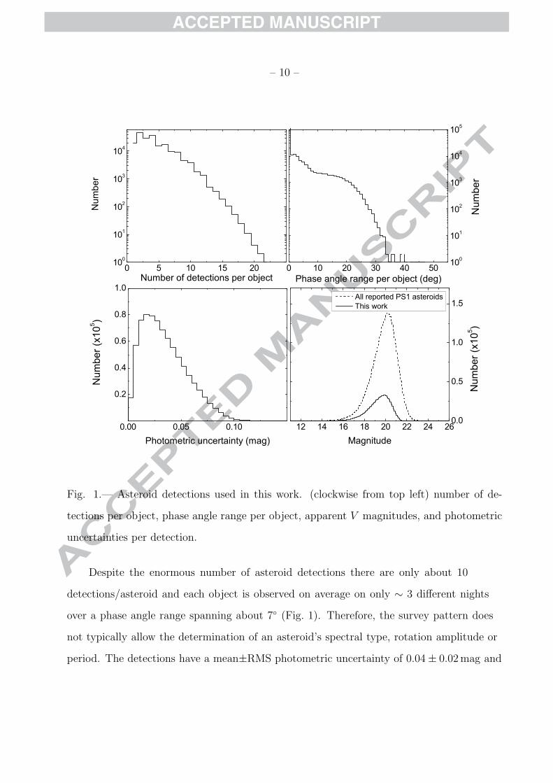
Fig. 1.— Asteroid detections used in this work. (clockwise from top left) number of de-

tections per object, phase angle range per object, apparent V magnitudes, and photometric

uncertainties per detection.

Despite the enormous number of asteroid detections there are only about 10

detections/asteroid and each object is observed on average on only ∼ 3 different nights

over a phase angle range spanning about 7◦ (Fig. 1). Therefore, the survey pattern does

not typically allow the determination of an asteroid’s spectral type, rotation amplitude or

period. The detections have a mean±RMS photometric uncertainty of 0.04 ± 0.02 mag and

– 11 –

average±RMS visual magnitude of 19.8 ± 1.2 mag. The photometric uncertainty mode is

∼ 0.02 mag corresponding to S/N∼ 50 detections. This surprisingly high value is due to

our selection criteria: the multi-opposition objects were identified in earlier surveys with

smaller telescopes so they are typically brighter when observed with Pan-STARRS1. Note

that only ∼ 1% of the detections in our data sub-set have a photometric uncertainty greater

than the 0.1 mag precision provided by the MPC.

3. Method

This work introduces a Monte Carlo technique to determine H (and G when possible)

and its statistical+systematic uncertainty based on the generation of synthetic asteroids

(clones) that are each consistent with the known asteroid. The power of the MC technique

lies in its ability to estimate the true statistical and systematic uncertainty in the absolute

magnitude due to the unknown parameters in the analysis. The clones explore the phase

space of light curve rotation amplitudes, periods, colors and slope parameter in an attempt

to replicate the observed apparent magnitudes. Each clone’s observations are evaluated

individually in the fitting process to derive H and G in the same manner as the actual

observations so that the distribution of values for each object’s clones provide a measure of

the systematic errors in the values. Mathematically, our model is justified by its similarity

to a sparse Bayesian marginalization over taxonomic classification, light curve amplitude

and period.

3.1. Step 1: Initial fit for H and G

The first step is essentially identical to the typical technique for calculating H and

G: we fit the apparent V -band magnitude to the B89 and M10 phase functions using

– 12 –

the IDL procedure mpfit2dfun1 that employs the Levenberg-Marquardt least-squares

fitting technique (Levenberg 1944; Marquardt 1963) to minimize the variance between the

detections’ apparent magnitudes and the values predicted by the models. We converted

the Pan-STARRS1 apparent magnitudes to V -band using taxonomy-dependent filter

transformations if the asteroid’s taxonomy was specified by Hasselmann et al. (2012) and,

if not, the mean S+C class color (see Table 2).

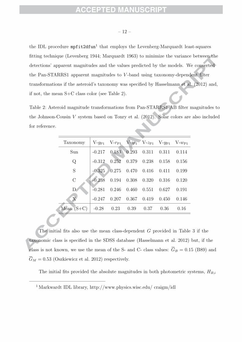
Table 2: Asteroid magnitude transformations from Pan-STARRS1 AB filter magnitudes to

the Johnson-Cousin V system based on Tonry et al. (2012). Solar colors are also included

for reference.

Taxonomy V-gP1 V-rP1 V-iP1 V-zP1 V-yP1 V-wP1

Sun -0.217 0.183 0.293 0.311 0.311 0.114

Q -0.312 0.252 0.379 0.238 0.158 0.156

S -0.325 0.275 0.470 0.416 0.411 0.199

C -0.238 0.194 0.308 0.320 0.316 0.120

D -0.281 0.246 0.460 0.551 0.627 0.191

X -0.247 0.207 0.367 0.419 0.450 0.146

Mean (S+C) -0.28 0.23 0.39 0.37 0.36 0.16

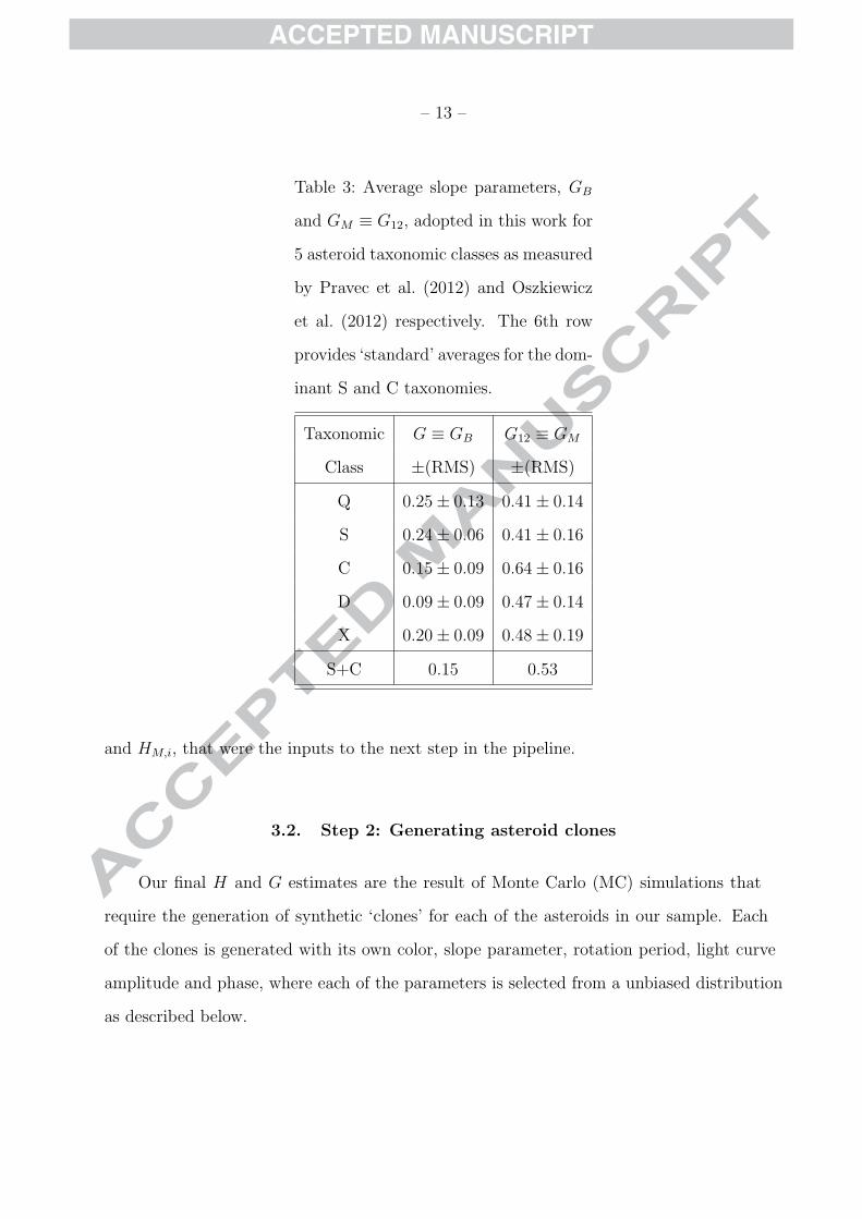
The initial fits also use the mean class-dependent G provided in Table 3 if the

taxonomic class is specified in the SDSS database (Hasselmann et al. 2012) but, if the

class is not known, we use the mean of the S- and C- class values: GB = 0.15 (B89) and

GM = 0.53 (Oszkiewicz et al. 2012) respectively.

The initial fits provided the absolute magnitudes in both photometric systems, HB,i

1 Markwardt IDL library, http://www.physics.wisc.edu/ craigm/idl

– 13 –

Table 3: Average slope parameters, GB

and GM ≡ G12, adopted in this work for

5 asteroid taxonomic classes as measured

by Pravec et al. (2012) and Oszkiewicz

et al. (2012) respectively. The 6th row

provides ‘standard’ averages for the dom-

inant S and C taxonomies.

Taxonomic G ≡ GB G12 ≡ GM

Class ±(RMS) ±(RMS)

Q 0.25 ± 0.13 0.41 ± 0.14

S 0.24 ± 0.06 0.41 ± 0.16

C 0.15 ± 0.09 0.64 ± 0.16

D 0.09 ± 0.09 0.47 ± 0.14

X 0.20 ± 0.09 0.48 ± 0.19

S+C 0.15 0.53

and HM,i, that were the inputs to the next step in the pipeline.

3.2. Step 2: Generating asteroid clones

Our final H and G estimates are the result of Monte Carlo (MC) simulations that

require the generation of synthetic ‘clones’ for each of the asteroids in our sample. Each

of the clones is generated with its own color, slope parameter, rotation period, light curve

amplitude and phase, where each of the parameters is selected from a unbiased distribution

as described below.

– 14 –

3.2.1. Clone colors

Our pipeline can assign each clone the color of its parent asteroid (if known) or, when

the parent’s color is not known, a random color based on an appropriate mix of taxonomies

as a function of semi-major axis. About 16% of the asteroids in our sample have taxonomies

defined by Hasselmann et al. (2012) (SDSS).

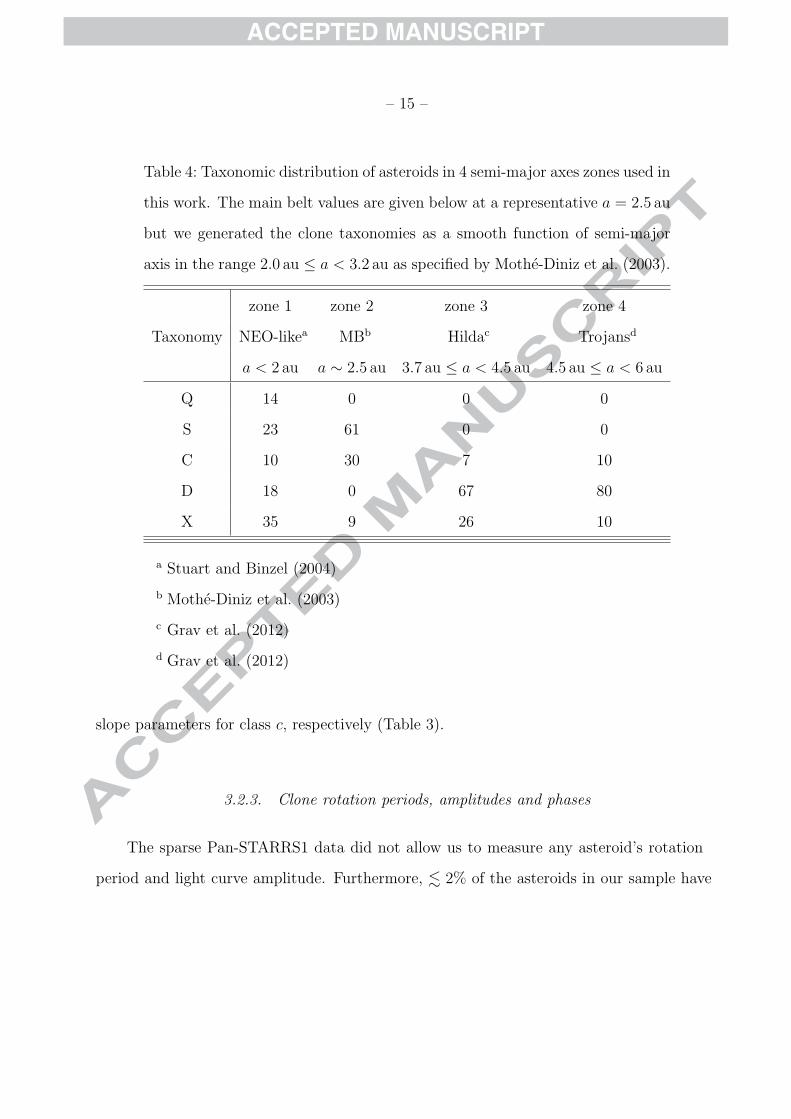
We implemented this technique by dividing the inner solar system into 4 zones (see

table 4): NEO-like (a < 2 au), main belt (2 au ≤ a < 3.7 au), Hildas (3.7 au ≤ a < 4.5 au)

and Trojans (4.5 au ≤ a < 6.0 au). The semi-major limits defining the zone edges were set

at or near a minimum in the number distribution as a function of semi-major axis and by

the availability of published taxonomic distributions. The exact values make little difference

to this work. We used the published, debiased taxonomic distributions in Table 4 in the 4

zones with the qualification that for the main belt (Mothe-Diniz et al. 2003) we aggregated

many related taxonomic types into 3 broad spectral classes: S-class=(A, AQ, AV, O, OV,

S, SA, SO, SQ, SV, V, L, LA, LQ, LS), X-class=(X, XD, XL, XS), and Q-class=(Q, QO,

QV). We required that the fraction, f(c, z), of asteroids with spectral class c in zone z

satisfies∑

c f(c, z) = 1. In the main belt, zone 2, we were able to generate the taxonomies

as a finer function of a as provided by (Mothe-Diniz et al. 2003) with a similar requirement

that∑

c f(c, a) = 1 at each semi-major axis.

3.2.2. Clone slope parameters

We assigned slope parameters to the clones as a function of their assigned taxonomic

class (c). i.e. the kth clone was assigned a slope parameter Gk(c) = ran[G(c), σG(c)] where

ran[x, y] is a random number generated from a normal distribution with mean x and

standard deviation y, and G(c) and σG(T ) are the mean and RMS of the distribution of

– 15 –

Table 4: Taxonomic distribution of asteroids in 4 semi-major axes zones used in

this work. The main belt values are given below at a representative a = 2.5 au

but we generated the clone taxonomies as a smooth function of semi-major

axis in the range 2.0 au ≤ a < 3.2 au as specified by Mothe-Diniz et al. (2003).

zone 1 zone 2 zone 3 zone 4

Taxonomy NEO-likea MBb Hildac Trojansd

a < 2 au a ∼ 2.5 au 3.7 au ≤ a < 4.5 au 4.5 au ≤ a < 6 au

Q 14 0 0 0

S 23 61 0 0

C 10 30 7 10

D 18 0 67 80

X 35 9 26 10

a Stuart and Binzel (2004)

b Mothe-Diniz et al. (2003)

c Grav et al. (2012)

d Grav et al. (2012)

slope parameters for class c, respectively (Table 3).

3.2.3. Clone rotation periods, amplitudes and phases

The sparse Pan-STARRS1 data did not allow us to measure any asteroid’s rotation

period and light curve amplitude. Furthermore, . 2% of the asteroids in our sample have

– 16 –

measured light curves reported in the asteroid light curve database (LCDB2; Warner et al.

2009; Waszczak et al. 2015) The lack of this information introduces systematic uncertainty

and error into the absolute magnitude and slope parameter determination. We quantified

these effects using our Monte Carlo technique with synthetic sinusoidal light curves for each

clone.

Asteroid brightness variations on the hours-to-days timescales are usually caused by

their non-spherical shape and rotation (the exceptions are for the unusual cases where the

phase angle changes rapidly for close approaching NEOs, for multiple-systems in which

brightness changes can occur if the objects transit or eclipse each other, and for objects

with significant color variations). We assumed that the observing geometry (i.e. phase

angle) effect on the asteroids’ light curves are negligible in the Pan-STARRS1 data because

of the limited range in phase angle coverage in our sample (Fig. 1). For the purpose of

generating the clones’ light curves we assumed that all objects generate simple sinusoidal

light curves with peak-to-peak amplitude A, period P , and rotation phase θ. The offset

from the unmodulated light curve at time t is then ∆m(t) = A sin(2πt/P + θ)/2.

Light curve amplitudes tend to be larger for smaller asteroids (see Fig. 2, Warner et al.

2009), probably because the smaller objects tend to be more irregularly shaped. Overall,

the set of measured amplitudes and periods will be larger and shorter respectively than the

true distribution because of observational selection effects, larger amplitudes and shorter

periods are easier to detect and measure.

To reduce the impact of the light curve amplitude and period selection effects we

employed the debiased distributions derived by Masiero et al. (2009) that are representative

2 The asteroid lightcurve database is publicly available at

http://www.minorplanet.info/lightcurvedatabase.html

– 17 –

30 25 20 15 10 50.0

0.5

1.0

1.50.01 0.1 1 10 100 1000

30 25 20 15 10 5 00.01

0.1

1

10

100

10000.01 0.1 1 10 100 1000

1000

100

10

1

0.1

Diameter (km)

Am

plitu

de (m

ag)

Absolute magnitude

Spi

n ra

te (r

ev/d

ay)

Absolute magnitude

Diameter (km)

Rot

atio

n pe

riod

(hou

r)

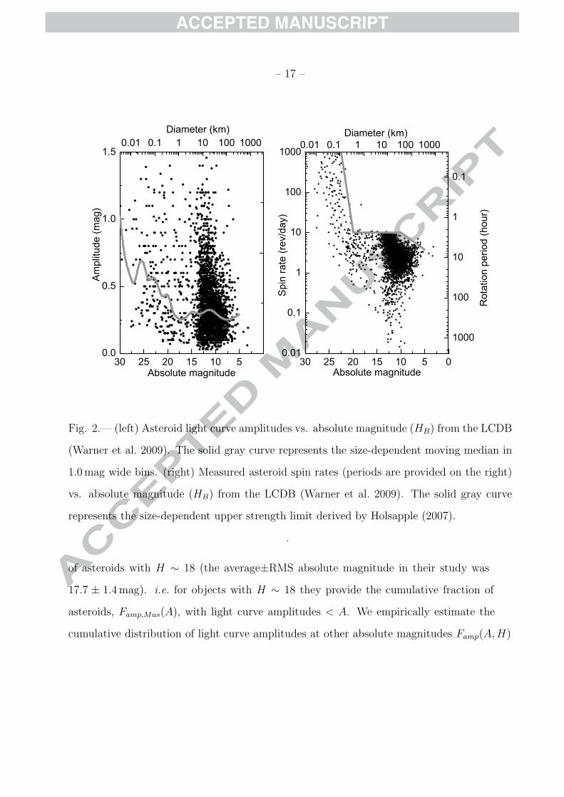
Fig. 2.— (left) Asteroid light curve amplitudes vs. absolute magnitude (HB) from the LCDB

(Warner et al. 2009). The solid gray curve represents the size-dependent moving median in

1.0 mag wide bins. (right) Measured asteroid spin rates (periods are provided on the right)

vs. absolute magnitude (HB) from the LCDB (Warner et al. 2009). The solid gray curve

represents the size-dependent upper strength limit derived by Holsapple (2007).

.

of asteroids with H ∼ 18 (the average±RMS absolute magnitude in their study was

17.7 ± 1.4 mag). i.e. for objects with H ∼ 18 they provide the cumulative fraction of

asteroids, Famp,Mas(A), with light curve amplitudes < A. We empirically estimate the

cumulative distribution of light curve amplitudes at other absolute magnitudes Famp(A,H)

– 18 –

by ‘normalizing’ to the median at H = 18 from the median at other values:

Famp(A,H) = Famp,Mas

[A × Amed(18)

Amed(H)

](2)

where Amed(H) is an empirical function (Fig. 2) representing the median amplitude of

asteroids in the LCDB (Warner et al. 2009). Thus, given a clone’s initial (§3.1) absolute

magnitude, Hi, we generated a random light curve amplitude for the clone according to the

cumulative fractional distribution given by eq. 2.

We followed a similar procedure in assigning each clone a rotation rate R or,

equivalently, a rotation period P ≡ 1/R. Masiero et al. (2009) also provide the data from

which we derive the cumulative fraction of asteroids, Frot,Mas(R), with rotation rates < R.

Once again, their results are representative of asteroids with H ∼ 18, about 2 mag fainter

than the mean value in our data sample, so we developed an empirical technique to extend

their cumulative fractional rotation rate distribution to other absolute magnitudes.

Asteroids with diameters & 100 m (H . 23) have an empirically observed upper limit

to their rotation rate of about 12 rev/day (Fig. 2) and about 99% of the distribution of

debiased spin rates are < 12 rev/day (Masiero et al. 2009). Asteroids larger than a few

tens of kilometers (H . 12) have an even more restricted upper limit to their rotation

rates. We empirically defined an Rmax(H) as illustrated in fig. 2 and ‘compress’ or ‘expand’

the Masiero et al. (2009) distribution as necessary to create the cumulative fractional

distribution at any H:

Frot(R, H) = Frot,Mas

[R × Rmax(18)

Rmax(H)

]. (3)

Once again, given a clone’s initial (§3.1) absolute magnitude, Hi, we generated a random

rotation rate for the clone according to the cumulative fractional distribution given by eq. 3.

Finally, the rotational phase θk for the kth clone was generated from a random uniform

distribution in the range [0◦, 360◦).

– 19 –

Our light curves were simple sinusoids even though we understand that real asteroid

light curves can be much more complicated. The technique could easily be extended to

incorporate actual light curve properties or a more realistic distribution but i) only a tiny

fraction of known asteroids have measured light curves ii) we will show below that our

results are not particularly sensitive to the actual light curve parameter distribution and iii)

if the actual light curve is known then there is no need for any of the methods developed

here. i.e. this method only applies to the 98% of asteroids that do not have measured

light curves. Since this is a preliminary work we have not made any effort to remove those

asteroids that have published light curves.

3.3. Step 3: Refining H and G (First Monte Carlo simulation).

The first Monte Carlo (MC) simulation yields our MC estimate for H and G from the

sparse Pan-STARRS1 phase curve coverage data. As described in detail above, we created

500 clones of each object where the kth clone was assigned a taxonomic class (color) ck,

light curve amplitude Ak, and period Pk. We then fit for each clone’s absolute magnitude,

slope parameter and light curve phase, (H ′k, G

′k, θ

′k), by minimizing the χ2 with respect to

the actual observations:

χ2k,obs =

n∑j=1

[mk(tj; H

′k, G

′k, θ

′k) − m(tj)

δm(tj)

]2

(4)

where n is the number of observations (detections) of the object, m(tj) is the actual

object’s observed apparent magnitude, δm(tj) is the reported uncertainty on the actual

Pan-STARRS1 apparent magnitude for that observation in the original filter, and mk is

the clone’s predicted apparent magnitude at the actual time of observation, tj, in the

Pan-STARRS1 filter in which the observation was made, with the clone’s appropriate color

– 20 –

transformation (∆mk(tj); Table 2):

mk(tj) = 5 log[r(tj)∆(tj)] + Φ[α(tj); H′k, G

′k] + Ak sin[2πtj/Pk + θ′k]/2 + ∆mk(tj), (5)

and Φ is the B89 or M10 phase function.

The ‘best’ clone is the one (k∗) that produces the minimum χ2 and we adopt that

clone’s H ′k∗ and G′

k∗ values as our MC estimate for the object’s absolute magnitude and

slope parameter. The process was run separately for both the B89 and M10 phase functions

to provide our MC estimates for (HB, GB) and (HM , GM) respectively. To avoid unphysical

values the fitting process required that −0.25 ≤ GB ≤ 0.8 and −0.5 ≤ GM ≤ 1.5.

We found that 500 clones provides a good balance between the computation time and

our ability to estimate the uncertainty on the absolute magnitudes and slope parameters.

It is likely that when there are only a small number of detections that the number of

clones could be decreased but we did not pursue this simplification. When the number of

detections becomes very large then our technique becomes unnecessary as either traditional

(Pravec et al. 2012) or sparse light curve fitting (Muinonen et al. 2010; Law et al. 2009)

becomes more effective.

3.4. Step 4: Estimating uncertainties and error on H and G

(second Monte Carlo fit).

At the risk of being pedantic, error is the difference between the value of a measurement

and the true value of the measurand, and uncertainty is an estimate of the error applicable

to a measurement. We estimated the uncertainties and errors on H ′k∗ and G′

k∗ by fitting for

the absolute magnitude and slope parameter with purely synthetic light curves generated

from the clone with the best fit. i.e. we re-applied the same method as described in Step 3

(§3.3) except that we fit the clones to the best synthetic object rather than the real object

– 21 –

(we continue to use the sub-script k to refer to clones but the clones used here are distinct

from the clones used in the last step):

χ2k,syn =

n∑i=1

[mk(tj; H

′k, G

′k, θ

′k) − mk∗(tj)

δmk∗(tj)

]2

. (6)

where δmk∗(tj) = δm(tj), i.e. the uncertainty on the synthetic observation at time tj was

set to the uncertainty on the actual observation at time tj.

If we let X generically represent either H or G then the combined statistical+systematic

uncertainty (later denoted as uncertainty) on X is the standard deviation of the clones’ X

distribution:

δX =

√1

n

∑k

(X ′k − X ′)

2(7)

where X ′ is the average value of X for all the synthetic objects’ clones. Similarly, the

combined statistical+systematic error (later denoted as error) on X is the average error on

the values for the synthetic clones:

∆X =1

n

∑k

(X ′k − X ′

k∗) (8)

3.5. Verification

We verified our method with two independent sets of synthetic data generated from

real Pan-STARRS1 data: 1) 10,000 randomly selected known Pan-STARRS1 objects, most

of them with sparse phase curve coverage and 2) the 1,000 known Pan-STARRS1 objects

with the best phase coverage. To have better control over assessing our method’s validity

we generated photometric magnitudes and uncertainties with synthetic absolute magnitudes

(HB and HM) and slope parameters (GB and GM) at each real time of observation with the

known object’s orbit. We then employed our pipeline to calculate each synthetic object’s H

and G to measure the statistical and systematic errors induced by our technique. Moreover,

– 22 –

we tested two different scenarios for assigning light curve amplitudes and periods to the

clones: 1) the debiased distributions from Masiero et al. (2009), 2) and the observed

distributions from the LCDB (Warner et al. 2009).

The result is that for both synthetic populations (sparse and dense phase curve

coverage) and for both light curve amplitude-period relations (debiased and observed) the

difference between the generated synthetic values and the values returned by our method

was normally distributed with zero mean. i.e. our technique correctly derives the H and

G. Use of the debiased or observed amplitude and period distributions does not affect the

derived H and G at the level of photometric accuracy and uncertainty of the Pan-STARRS1

data with its associated phase curve coverage i.e. does not cause any systematic errors.

4. Results & Discussion

4.1. Absolute magnitudes comparison with Pravec et al. (2012)

We think Pravec et al. (2012)’s detailed light curve study of ∼ 500 asteroids sets

the standard in measuring asteroid photometric properties. They provided only HB (it

was before the adoption of the new IAU standard) but that value should be identical

to HM . Our results agree with Pravec et al. (2012) for the 347 objects that appear in

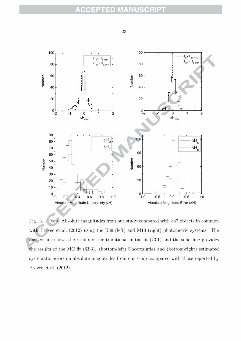
both data sets (fig. 3). The mean differences of HB − HB,Pra = −0.06 ± 0.02 mag and

HM − HB,Pra = 0.02 ± 0.02 mag are consistent with zero to within 3σ and 1σ respectively,

with better agreement for the new IAU standard photometric system of M10. The RMS of

each distribution is 0.36 mag and 0.29 mag respectively, due to the quadratic combination

of the errors in both Pravec et al. (2012)’s and this work.

The distribution of HB − HB,Pra is quasi-normally distributed (fig. 3) with an RMS

of 0.31 mag including a tail extending to HB − HB,Pra < −1. Interestingly, the difference

– 23 –

-2 -1 0 1 20

20

40

60

80

100

Num

ber

HPRA

HB - HB, PRA

HB,I - HB, PRA

-2 -1 0 1 20

20

40

60

80

100

HM - HB, PRA

HM,I - HB, PRA

HPRA

Num

ber

0.0 0.2 0.4 0.6 0.8 1.00

10

20

30

40

50

60

70

80

90

Num

ber

Absolute Magnitude Uncertainty ( H)

HM

HB

-1.0 -0.5 0.0 0.5 1.00

30

60

90

120

N

umbe

r

Absolute Magnitude Error ( H)

HM

HB

Fig. 3.— (top) Absolute magnitudes from our study compared with 347 objects in common

with Pravec et al. (2012) using the B89 (left) and M10 (right) photometric systems. The

dashed line shows the results of the traditional initial fit (§3.1) and the solid line provides

the results of the MC fit (§3.3). (bottom-left) Uncertainties and (bottom-right) estimated

systematic errors on absolute magnitudes from our study compared with those reported by

Pravec et al. (2012).

– 24 –

between our initial fits with assumed slope parameter (§3.1) and Pravec et al. (2012),

HB,i − HB,Pra, is roughly normally distributed with a mean error of −0.06 ± 0.02 mag

and RMS of 0.26 mag. Thus, the simple, traditional, fitting procedure with assumed G to

our high-precision but sparse data produces comparable absolute magnitudes to the MC

technique.

Our absolute magnitudes calculated with the M10 phase function (HM) are better

behaved (fig. 3) in the sense that the distribution is more normally distributed. The

initial fit to the sparse data in the M10 system provided absolute magnitudes with mean

systematic errors of 0.00 ± 0.02 mag and σ ∼ 0.26 mag compared to the MC technique

with a mean error of 0.02 ± 0.02 mag and σ ∼ 0.28 mag. The good behavior of both the

MC and initial fits with M10 that results in a normal error distribution leads us to the

conclusion that it is superior for the determination of absolute magnitudes even for sparse

data samples.

We also used the Pravec et al. (2012) values to test our technique (§3.4) for establishing

the uncertainty and error on our measured absolute magnitudes. Their technique allows

excellent control of all the statistical and systematic uncertainties in the H calculation

because they observed targets for more than a decade in a systematically controlled program

and had 2 to 3 orders of magnitude more data per object. Thus, they report H uncertainties

about 3× less than our uncertainties and we can compare our measured uncertainties (δH)

to the RMS spread of H − HPra, and our measured error estimates to its average (fig. 3).

As stated earlier, the real power of the MC technique is its ability to estimate the

statistical and systematic uncertainties on the derived H and G values. Our estimated

absolute magnitude uncertainties (δHB; fig. 3; §3.4) for the asteroids that overlap the

Pravec et al. (2012) data sample have the expected poissonian distribution with a mean

of δHB= 0.36 ± 0.01 mag using the B89 phase function (fig. 3), comparable to the RMS

– 25 –

of 0.37 ± 0.02 mag for the distribution of the error in our measurement, HB − HB,Pra,

as expected. Similarly, our mean estimated systematic error of ∆HB = 0.03 ± 0.02 mag

agrees with the actual systematic offset in the HB − HB,Pra distribution. We can compare

our estimated uncertainties and systematic errors in the same manner for the M10

phase curve. Our estimated mean uncertainty, δHM = 0.26 ± 0.01 mag, is consistent

with RMS(HM − HB,Pra) = 0.28 ± 0.02 mag and our estimated systematic error of

∆HM = 0.00 ± 0.02 mag, is consistent with (HM − HB,Pra) = 0.02 ± 0.02 mag.

The good agreement between our results and those of Pravec et al. (2012) illustrates the

utility of our MC technique at measuring an asteroid’s absolute magnitude and estimating

the associated statistical+systematic uncertainty and any systematic bias, even for sparse

data sets with limited phase angle coverage. Furthermore, the nice behavior of our results

with the M10 phase curve and the good agreement between our HM and HB,Pra provides

evidence that HM ∼ HB when care is taken to ensure that the photometric data is of

excellent quality.

4.2. Absolute magnitudes

Having established the utility of our technique on a well-controlled data set in the

previous section we now employ it on all the asteroids in our selected Pan-STARRS1 data

sample. We were able to calculate the absolute magnitudes with combined statistical

and systematic uncertainties for more than 240,000 asteroids spanning the range from

6.4 < H < 26.5 (fig. 4). Our results include objects ranging from NEOs in the inner

solar system to Jupiter’s Trojan asteroids. Our sample represents ∼ 38% of all known

asteroids in that range as of February 2014, with the highest completion of ∼ 75% from

10.5 < H < 11.0.

– 26 –

5 10 15 20 251

10

100

1000

10000

100000

Num

ber

Absolute magnitude

HM

HB

0.0 0.5 1.0 1.5 2.01

10

100

1000

10000

Num

ber

Absolute Magnitude Uncertainty ( H)

HM

HB

-2 -1 0 1 21

10

100

1000

10000

Num

ber

Absolute Magnitude Error ( H)

HM

HB

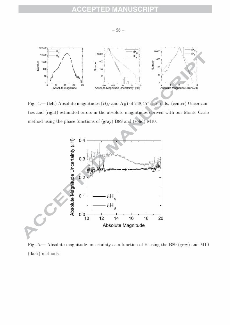
Fig. 4.— (left) Absolute magnitudes (HM and HB) of 248,457 asteroids. (center) Uncertain-

ties and (right) estimated errors in the absolute magnitudes derived with our Monte Carlo

method using the phase functions of (gray) B89 and (solid) M10.

10 12 14 16 18 200.0

0.1

0.2

0.3

0.4

HM

HB

Abso

lute

Mag

nitu

de U

ncer

tain

ty (

H)

Absolute Magnitude

Fig. 5.— Absolute magnitude uncertainty as a function of H using the B89 (grey) and M10

(dark) methods.

– 27 –

The mean uncertainties of δHB = 0.30 ± 0.01 mag and δHM = 0.25 ± 0.01 mag (Fig

4) show that the new IAU photometric scheme of M10 is better than B89 for the sparse

Pan-STARRS1 data and phase coverage but this conclusion mis-represents the full utility

of the M10 technique. For one, the M10 system uncertainty is almost uniform with

δHM ∼ 0.24 mag for the entire range 10 < H < 20 (fig. 5). Second, even though the two

techniques yield approximately the same uncertainties for the faintest objects for which the

uncertainty is dominated by the measurement statistics (fig. 5), the B89 method’s statistical

uncertainty is ∼ 0.35% larger for bright objects (10 < H < 14).

The mean of our estimated statistical+systematic error using the M10 method,

|∆HM | = 0.02 ± 0.01 mag, is comparable to the B89 method, |∆HB| = 0.01 ± 0.01 mag

(fig. 4). The error in the absolute magnitude for each asteroid is less than the estimated

uncertainty in ∼ 62% of all the asteroids in our HB sample and ∼ 73% in our HM sample.

The RMS of the |∆HB| and |∆HM | errors respectively of ∼ 0.35 mag and ∼ 0.25 mag

confirms that the new IAU photometric system is an improvement over the earlier one and,

furthermore, the shape of the error distribution is more reasonable for ∆HM than ∆HB

(note the peak of ∆HB is shifted by 0.05 mag from zero but the ∆HM peak is near zero

(fig. 4).

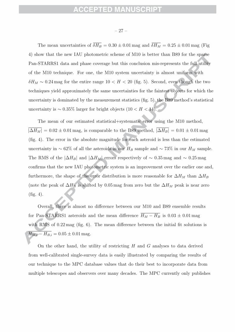
Overall, there is almost no difference between our M10 and B89 ensemble results

for Pan-STARRS1 asteroids and the mean difference HM − HB is 0.03 ± 0.01 mag

with RMS of 0.22 mag (fig. 6). The mean difference between the initial fit solutions is

HM,i − HB,i = 0.05 ± 0.01 mag.

On the other hand, the utility of restricting H and G analyses to data derived

from well-calibrated single-survey data is easily illustrated by comparing the results of

our technique to the MPC database values that do their best to incorporate data from

multiple telescopes and observers over many decades. The MPC currently only publishes

– 28 –

-1.0 -0.5 0.0 0.5 1.01

10

100

1000

10000

100000

Num

ber

Absolute Magnitude Difference

HM-HB

HM,I-HB,I

-1.0 -0.5 0.0 0.5 1.01

10

100

1000

10000

100000

Num

ber

Absolute Magnitude Difference

HM-HM,i

HB-HB,I

Fig. 6.— (left) Difference between the M10 and B89 absolute magnitudes for the MC and

initial fit solutions. (right) Difference between MC and initial fit solutions for the absolute

magnitude using the M10 and B89 methods.

absolute magnitudes using the B89 phase function and there is a mean difference of

HM − HB,MPC = 0.26 ± 0.01 mag and HB − HB,MPC = 0.22 ± 0.01 mag between our

technique and the MPC values. The consistency between the mean differences is at least

reassuring and the RMS spread in values is due to 1) the systematics introduced by the

MPC’s procedure that incorporates apparent magnitudes from many different observatories

in many different passbands and 2) the systematics introduced by our sparse light curve

coverage. Given that we established in §4.1 that our technique works well in comparison

to the ‘standard’ Pravec et al. (2012) values, our conclusion is that the error is due to

the MPC’s incorporation of photometry from different sites and filters over a long period

of time. The error reported here is less than the ∼ 0.4 mag value reported by Juric et al.

(2002), but since the time of that study the MPC database has been further populated

by photometry from Pan-STARRS1 and other large surveys with better photometric

calibrations than previous surveys. Hence, it is unsurprising that the HB,MPC values

– 29 –

-2 -1 0 1 20

10000

20000

30000

40000

50000

Num

ber

HMPC

HM - HB, MPC

HB - HB, MPC

-2 -1 0 1 20

10000

20000

30000

40000

50000

Num

ber

HOSK

HM - HM, OSK

HB - HB, OSK

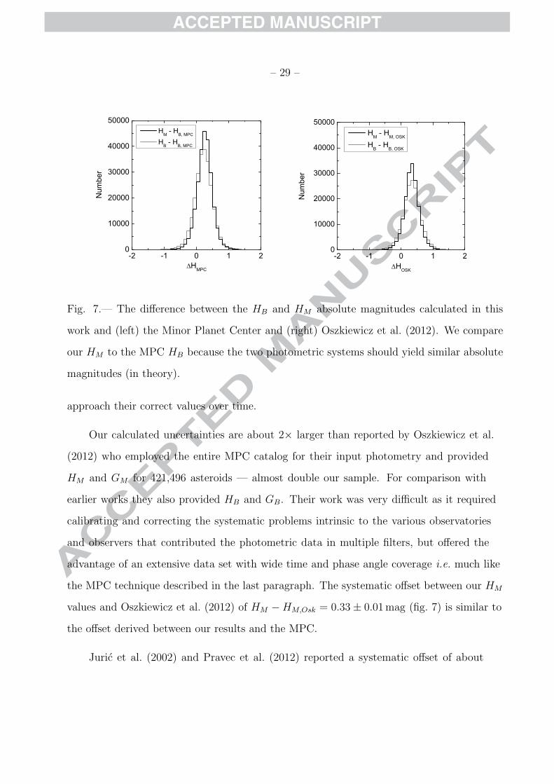
Fig. 7.— The difference between the HB and HM absolute magnitudes calculated in this

work and (left) the Minor Planet Center and (right) Oszkiewicz et al. (2012). We compare

our HM to the MPC HB because the two photometric systems should yield similar absolute

magnitudes (in theory).

approach their correct values over time.

Our calculated uncertainties are about 2× larger than reported by Oszkiewicz et al.

(2012) who employed the entire MPC catalog for their input photometry and provided

HM and GM for 421,496 asteroids — almost double our sample. For comparison with

earlier works they also provided HB and GB. Their work was very difficult as it required

calibrating and correcting the systematic problems intrinsic to the various observatories

and observers that contributed the photometric data in multiple filters, but offered the

advantage of an extensive data set with wide time and phase angle coverage i.e. much like

the MPC technique described in the last paragraph. The systematic offset between our HM

values and Oszkiewicz et al. (2012) of HM − HM,Osk = 0.33 ± 0.01 mag (fig. 7) is similar to

the offset derived between our results and the MPC.

Juric et al. (2002) and Pravec et al. (2012) reported a systematic offset of about

– 30 –

0.38 mag to 0.5 mag between their calculated absolute magnitudes and the values reported

by the MPC while Parker et al. (2008) found an ∼ 0.33 mag offset between their HB and

the ASTORB3 database. Those values are in rough agreement with Waszczak et al. (2015)

who reported HB and GB from over 54,000 asteroids observed in g and R-band with the

Palomar Transient Factory (PTF). They measured a mean value of RPTF = VMPC + 0.00

which implies a systematic offset of ∼ 0.4 mag in the MPC absolute magnitudes because

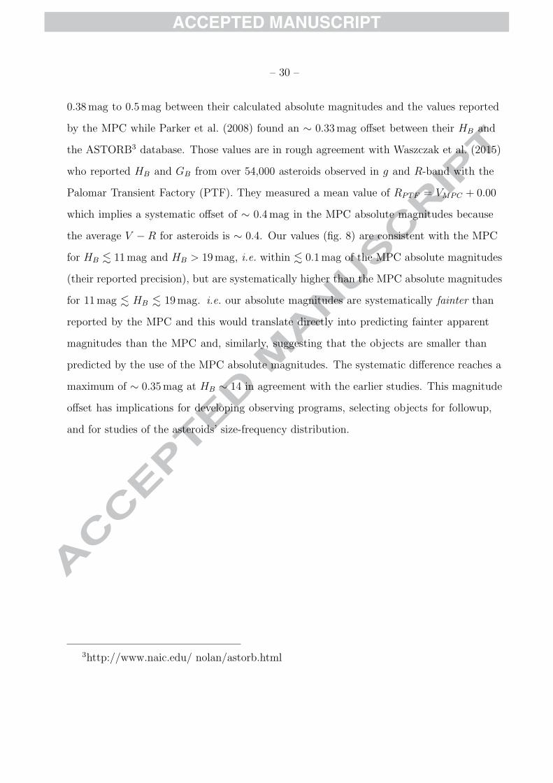
the average V − R for asteroids is ∼ 0.4. Our values (fig. 8) are consistent with the MPC

for HB . 11 mag and HB > 19 mag, i.e. within . 0.1 mag of the MPC absolute magnitudes

(their reported precision), but are systematically higher than the MPC absolute magnitudes

for 11 mag . HB . 19 mag. i.e. our absolute magnitudes are systematically fainter than

reported by the MPC and this would translate directly into predicting fainter apparent

magnitudes than the MPC and, similarly, suggesting that the objects are smaller than

predicted by the use of the MPC absolute magnitudes. The systematic difference reaches a

maximum of ∼ 0.35 mag at HB ∼ 14 in agreement with the earlier studies. This magnitude

offset has implications for developing observing programs, selecting objects for followup,

and for studies of the asteroids’ size-frequency distribution.

3http://www.naic.edu/ nolan/astorb.html

– 31 –

10 12 14 16 18 20-1.0

-0.5

0.0

0.5

1.0

HB-H

MP

C

HMPC

Fig. 8.— The difference between the absolute magnitude HMPC reported by the MPC using

the B89 phase function and this work’s HB value as a function of absolute magnitude. The

thick solid black line represents the average in each 0.1 mag wide bin and the standard error

on the mean is shown with error bars. The error bars are about the width of the line for

13 . HMPC . 18.

– 32 –

4.3. Slope Parameters

The vast majority of Pan-STARRS1 asteroids offer only sparse phase angle coverage

(Fig. 1) for the determination of the slope parameter but our MC technique should provide

a realistic estimate of the statistical uncertainty and systematic error when the phase angle

coverage is not too large and the detections are not in multiple apparitions.

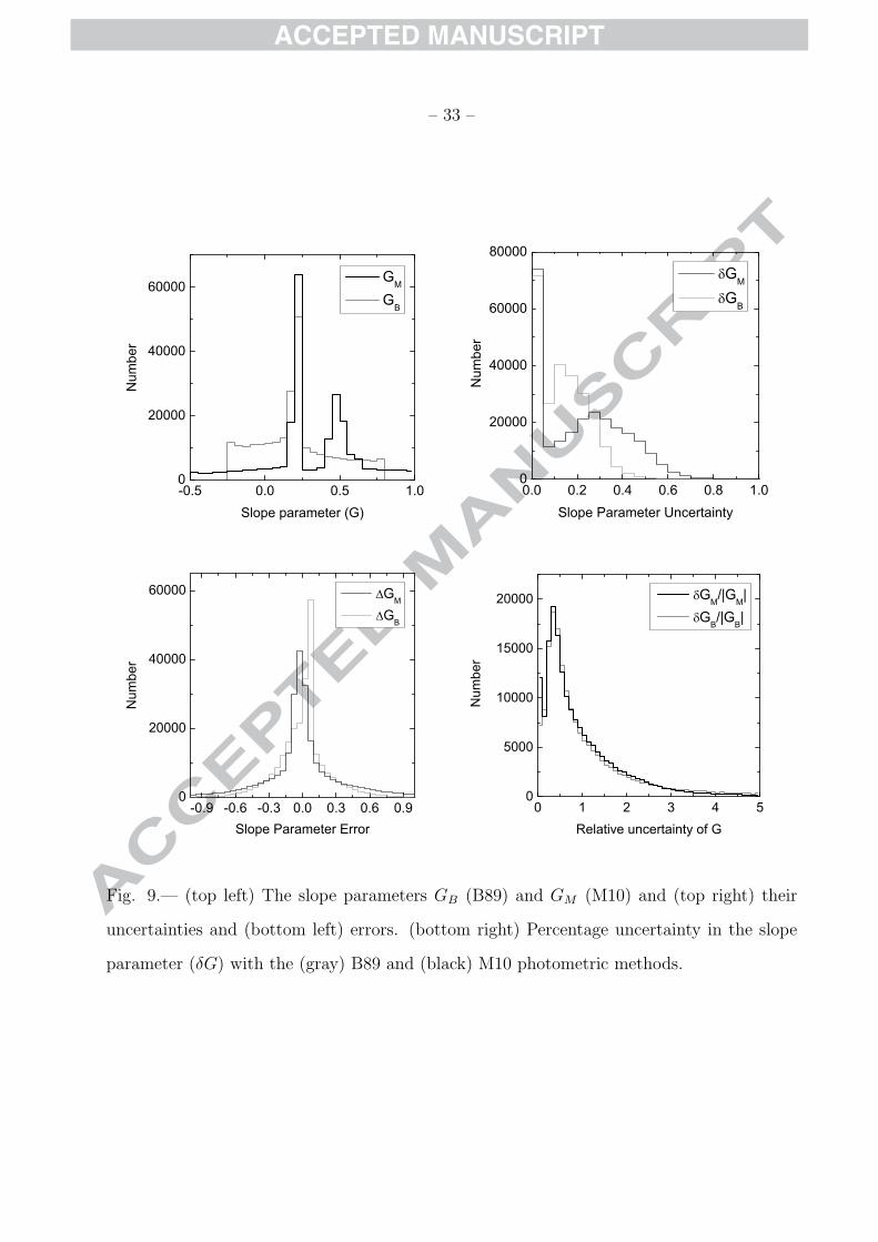
The GB distribution (fig. 9) is very wide with a peak near 0.15, the default

slope parameter for objects of unknown spectral class (most of the asteroids in our

sample). The distribution is artificially constrained between the lower and upper limits

(−0.25 < GB < 0.8). On the other hand, the GM distribution has a broad peak centered

on GM ∼ 0.5 superimposed on a roughly flat distribution of slope parameters between our

artificial limits (−0.5 < GM < 1.5). The large peak near GM = 0.2 that contains ∼ 30%

of all GM values is due to a discontinuity in the M10 phase function, it is not an error in

our implementation. In comparison, ∼ 8% of the Oszkiewicz et al. (2012) GM values were

also ∼ 0.2. Our technique is particularly sensitive to the function discontinuity and has a

propensity to drive the fitted GM value to 0.2 when the number of data points is small. We

suggest that future attempts to use the M10 phase function flag and address this situation,

perhaps by forcing GM = 0.5 in those cases.

The slope parameter uncertainty (δG) distributions have peaks at zero corresponding

to the ∼ 24% of cases in both methods where the MC technique did not converge and

we fixed the slopes. Those GB that were actually fit have a normal-like distribution with

mean GB = 0.18 ± 0.01 and RMS of 0.05 (Fig. 9). Similarly, the GM uncertainty has a

normal-like distribution with mean at 0.29 ± 0.01 and RMS of 0.17. The δGM distribution

is wider and shifted towards larger values than the δGB distribution because the GM values

are fundamentally larger than the corresponding GB values. The percentage uncertainties

(δG/|G|, fig. 9) in both slope parameters are very similar, suggesting that the two phase

– 33 –

-0.5 0.0 0.5 1.00

20000

40000

60000

Num

ber

Slope parameter (G)

GM

GB

0.0 0.2 0.4 0.6 0.8 1.00

20000

40000

60000

80000

Num

ber

Slope Parameter Uncertainty

GM

GB

-0.9 -0.6 -0.3 0.0 0.3 0.6 0.90

20000

40000

60000

Num

ber

Slope Parameter Error

GM

GB

0 1 2 3 4 50

5000

10000

15000

20000

Num

ber

Relative uncertainty of G

GM/|GM| GB/|GB|

Fig. 9.— (top left) The slope parameters GB (B89) and GM (M10) and (top right) their

uncertainties and (bottom left) errors. (bottom right) Percentage uncertainty in the slope

parameter (δG) with the (gray) B89 and (black) M10 photometric methods.

– 34 –

functions are equally effective for calculating the slope parameters, at least in the regime

applicable to this data sample. The mean relative slope parameter uncertainties are ∼ 34%

and ∼ 0.36% for GB and GM respectively, the large values being due mostly to the limited

phase curve coverage.

0 10 20 30 40 500.00

0.05

0.10

0.15

0.20

0.25

0.30

0.35

0.40

GM

GB

Slo

pe P

aram

eter

Unc

erta

inty

(G

)

(deg)

0 10 20 30 40 50

-0.9

-0.6

-0.3

0.0

0.3

0.6

0.9

Slo

pe P

aram

eter

Err

or (

G)

(deg)

GM

GB

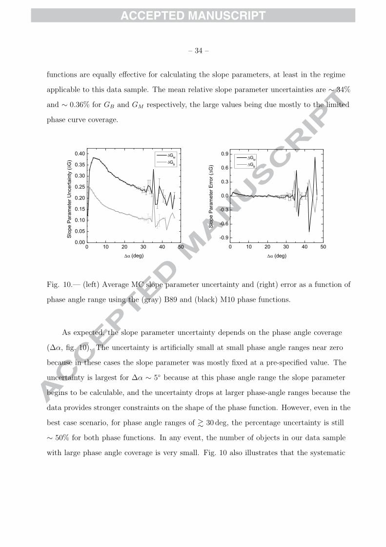
Fig. 10.— (left) Average MC slope parameter uncertainty and (right) error as a function of

phase angle range using the (gray) B89 and (black) M10 phase functions.

As expected, the slope parameter uncertainty depends on the phase angle coverage

(∆α, fig. 10). The uncertainty is artificially small at small phase angle ranges near zero

because in these cases the slope parameter was mostly fixed at a pre-specified value. The

uncertainty is largest for ∆α ∼ 5◦ because at this phase angle range the slope parameter

begins to be calculable, and the uncertainty drops at larger phase-angle ranges because the

data provides stronger constraints on the shape of the phase function. However, even in the

best case scenario, for phase angle ranges of & 30 deg, the percentage uncertainty is still

∼ 50% for both phase functions. In any event, the number of objects in our data sample

with large phase angle coverage is very small. Fig. 10 also illustrates that the systematic

– 35 –

errors introduced by our MC technique are not dependent on phase angle coverage.

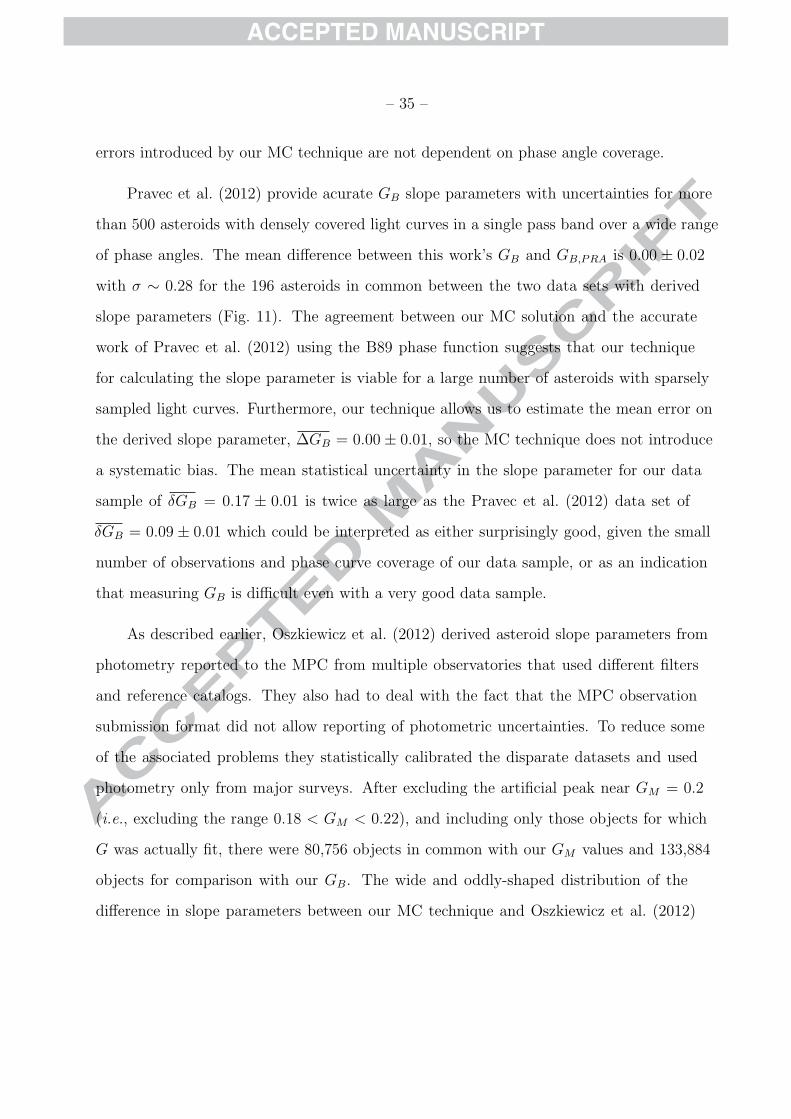
Pravec et al. (2012) provide acurate GB slope parameters with uncertainties for more

than 500 asteroids with densely covered light curves in a single pass band over a wide range

of phase angles. The mean difference between this work’s GB and GB,PRA is 0.00 ± 0.02

with σ ∼ 0.28 for the 196 asteroids in common between the two data sets with derived

slope parameters (Fig. 11). The agreement between our MC solution and the accurate

work of Pravec et al. (2012) using the B89 phase function suggests that our technique

for calculating the slope parameter is viable for a large number of asteroids with sparsely

sampled light curves. Furthermore, our technique allows us to estimate the mean error on

the derived slope parameter, ∆GB = 0.00 ± 0.01, so the MC technique does not introduce

a systematic bias. The mean statistical uncertainty in the slope parameter for our data

sample of δGB = 0.17 ± 0.01 is twice as large as the Pravec et al. (2012) data set of

δGB = 0.09 ± 0.01 which could be interpreted as either surprisingly good, given the small

number of observations and phase curve coverage of our data sample, or as an indication

that measuring GB is difficult even with a very good data sample.

As described earlier, Oszkiewicz et al. (2012) derived asteroid slope parameters from

photometry reported to the MPC from multiple observatories that used different filters

and reference catalogs. They also had to deal with the fact that the MPC observation

submission format did not allow reporting of photometric uncertainties. To reduce some

of the associated problems they statistically calibrated the disparate datasets and used

photometry only from major surveys. After excluding the artificial peak near GM = 0.2

(i.e., excluding the range 0.18 < GM < 0.22), and including only those objects for which

G was actually fit, there were 80,756 objects in common with our GM values and 133,884

objects for comparison with our GB. The wide and oddly-shaped distribution of the

difference in slope parameters between our MC technique and Oszkiewicz et al. (2012)

– 36 –

-1.0 -0.5 0.0 0.5 1.00

25

50

75

100

Num

ber

Slope Parameter Difference (GB-GB,PRA)0.0 0.1 0.2 0.3 0.4 0.50

30

60

90

120

150

180

Num

ber

Slope Parameter Uncertainty

GB

GB,PRA

Fig. 11.— (left) The difference between our MC GB values (B89) and 196 objects in common

with Pravec et al. (2012). (right) Slope parameter uncertainty distributions for the same

196 objects for (solid) our MC values and (dashed) Pravec et al. (2012).

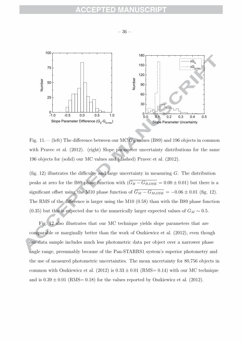
(fig. 12) illustrates the difficulty and large uncertainty in measuring G. The distribution

peaks at zero for the B89 phase function with (GB − GB,OSK = 0.00 ± 0.01) but there is a

significant offset using the M10 phase function of GM − GM,OSK = −0.06 ± 0.01 (fig. 12).

The RMS of the difference is larger using the M10 (0.58) than with the B89 phase function

(0.35) but this is expected due to the numerically larger expected values of GM ∼ 0.5.

Fig. 12 also illustrates that our MC technique yields slope parameters that are

comparable or marginally better than the work of Oszkiewicz et al. (2012), even though

our data sample includes much less photometric data per object over a narrower phase

angle range, presumably because of the Pan-STARRS1 system’s superior photometry and

the use of measured photometric uncertainties. The mean uncertainty for 80,756 objects in

common with Oszkiewicz et al. (2012) is 0.33 ± 0.01 (RMS= 0.14) with our MC technique

and is 0.39 ± 0.01 (RMS= 0.18) for the values reported by Oszkiewicz et al. (2012).

– 37 –

-2 -1 0 1 20

2000

4000

6000

8000

10000 GB-GB, OSK

N

umbe

r

Slope Parameter Difference0.0 0.2 0.4 0.6 0.8 1.00

10000

20000

30000

40000

Num

ber

Slope Parameter Uncertainty

GB

GB,OSK

-2 -1 0 1 20

1000

2000

3000

4000

5000

GM-GM,OSK

Num

ber

Slope Parameter Difference0.0 0.2 0.4 0.6 0.8 1.00

2000

4000

6000

8000

10000

12000

14000

GM

GM,OSK

Num

ber

Slope Parameter Uncertainty

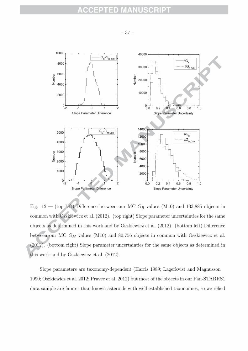
Fig. 12.— (top left) Difference between our MC GB values (M10) and 133,885 objects in

common with Oszkiewicz et al. (2012). (top right) Slope parameter uncertainties for the same

objects as determined in this work and by Oszkiewicz et al. (2012). (bottom left) Difference

between our MC GM values (M10) and 80,756 objects in common with Oszkiewicz et al.

(2012). (bottom right) Slope parameter uncertainties for the same objects as determined in

this work and by Oszkiewicz et al. (2012).

Slope parameters are taxonomy-dependent (Harris 1989; Lagerkvist and Magnusson

1990; Oszkiewicz et al. 2012; Pravec et al. 2012) but most of the objects in our Pan-STARRS1

data sample are fainter than known asteroids with well established taxonomies, so we relied

– 38 –

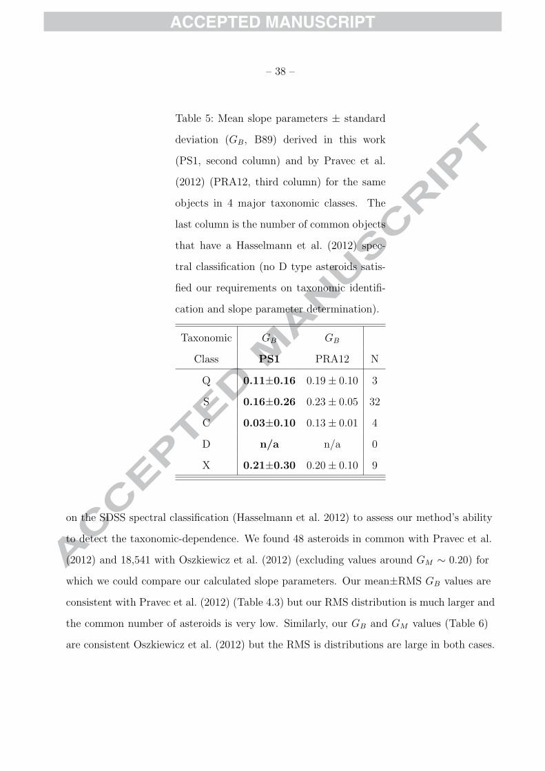
Table 5: Mean slope parameters ± standard

deviation (GB, B89) derived in this work

(PS1, second column) and by Pravec et al.

(2012) (PRA12, third column) for the same

objects in 4 major taxonomic classes. The

last column is the number of common objects

that have a Hasselmann et al. (2012) spec-

tral classification (no D type asteroids satis-

fied our requirements on taxonomic identifi-

cation and slope parameter determination).

Taxonomic GB GB

Class PS1 PRA12 N

Q 0.11±0.16 0.19 ± 0.10 3

S 0.16±0.26 0.23 ± 0.05 32

C 0.03±0.10 0.13 ± 0.01 4

D n/a n/a 0

X 0.21±0.30 0.20 ± 0.10 9

on the SDSS spectral classification (Hasselmann et al. 2012) to assess our method’s ability

to detect the taxonomic-dependence. We found 48 asteroids in common with Pravec et al.

(2012) and 18,541 with Oszkiewicz et al. (2012) (excluding values around GM ∼ 0.20) for

which we could compare our calculated slope parameters. Our mean±RMS GB values are

consistent with Pravec et al. (2012) (Table 4.3) but our RMS distribution is much larger and

the common number of asteroids is very low. Similarly, our GB and GM values (Table 6)

are consistent Oszkiewicz et al. (2012) but the RMS is distributions are large in both cases.

– 39 –

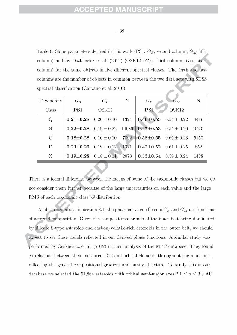
Table 6: Slope parameters derived in this work (PS1: GB, second column; GM fifth

column) and by Oszkiewicz et al. (2012) (OSK12: GB, third column; GM , sixth

column) for the same objects in five different spectral classes. The forth and last

columns are the number of objects in common between the two data sets with SDSS

spectral classification (Carvano et al. 2010).

Taxonomic GB GB N GM GM N

Class PS1 OSK12 PS1 OSK12

Q 0.21±0.28 0.20 ± 0.10 1324 0.46±0.53 0.54 ± 0.22 886

S 0.22±0.28 0.19 ± 0.22 14686 0.47±0.53 0.55 ± 0.20 10231

C 0.18±0.28 0.16 ± 0.10 7892 0.58±0.55 0.66 ± 0.23 5150

D 0.23±0.29 0.19 ± 0.12 1321 0.42±0.52 0.61 ± 0.25 852

X 0.19±0.28 0.18 ± 0.11 2073 0.53±0.54 0.59 ± 0.24 1428

There is a formal difference between the means of some of the taxonomic classes but we do

not consider them further because of the large uncertainties on each value and the large

RMS of each taxonomic class’ G distribution.

As discussed above in section 3.1, the phase curve coefficients GB and GM are functions

of asteroid composition. Given the compositional trends of the inner belt being dominated

by silicate S-type asteroids and carbon/volatile-rich asteroids in the outer belt, we should

expect to see these trends reflected in our derived phase functions. A similar study was

performed by Oszkiewicz et al. (2012) in their analysis of the MPC database. They found

correlations between their measured G12 and orbital elements throughout the main belt,

reflecting the general compositional gradient and family structure. To study this in our

database we selected the 51,864 asteroids with orbital semi-major axes 2.1 ≤ a ≤ 3.3 AU

– 40 –

where the range of phase angles observed was ∆α ≥ 5◦ and there were N ≥ 6 observations.

We then calculated the running median values GB and GM as a function of orbital a over a

range ∆a = 0.05 AU.

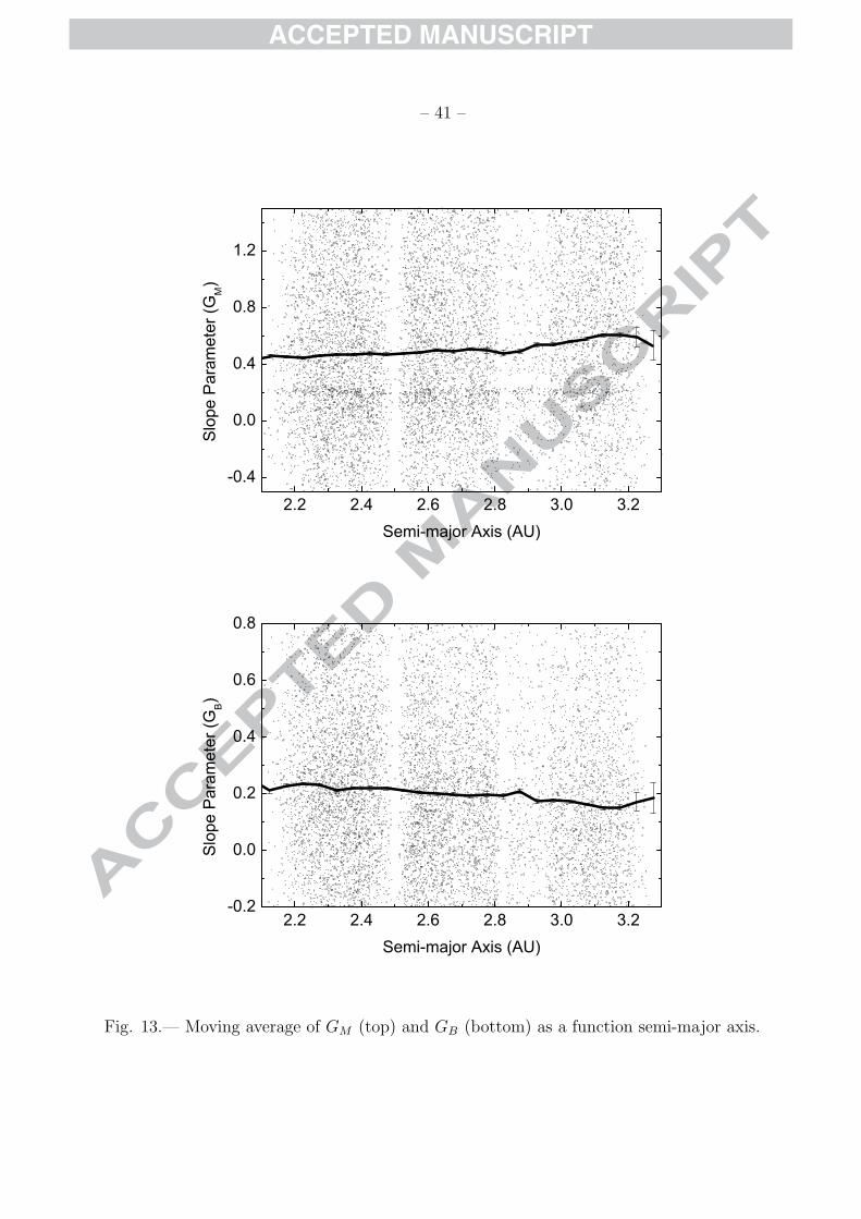
Figure 13 clearly shows clear a negative trend in GB and a positive trend in GM with

orbital a. As GB is larger for S-type than C-type asteroids, while GM becomes smaller,

this agrees with the established compositional gradient in the main-belt. For modelling

purposes, these trends may be approximated by the relationships GB = −0.103a+0.446 and

GM = 0.237a − 0.175 within the main belt. The largest deviations from these relationships

occur at the 3:1 Kirkwood gap at 2.50 AU, and at the 7:3 gap at 2.95 AU. This latter

position marks where the S-type asteroids of the dominant Koronis family of gives way to

the T/X/K/D-type asteroids of the Eos family (Mothe-Diniz et al. 2005). We note that the

overall observed scatter in individual values is dominated by ∆G, although it will also be

partly due to the large amount of compositional mixing present in the main belt (DeMeo

and Carry 2013).

– 41 –

2.2 2.4 2.6 2.8 3.0 3.2

-0.4

0.0

0.4

0.8

1.2

S

lope

Par

amet

er (G

M)

Semi-major Axis (AU)

2.2 2.4 2.6 2.8 3.0 3.2-0.2

0.0

0.2

0.4

0.6

0.8

Slo

pe P

aram

eter

(GB)

Semi-major Axis (AU)

Fig. 13.— Moving average of GM (top) and GB (bottom) as a function semi-major axis.

– 42 –

5. Availability

The Pan-STARRS1 absolute magnitudes and slope parameters with associated

uncertainties as described herein are available on-line (Appendix A). The eventual goal is

that the catalog will be updated with all the data from the entire 3 year Pan-STARRS1

mission and then updated regularly with new data from the ongoing extended mission that

is purely focused on the solar system. This effort will provide almost complete coverage of

all known asteroids with extensive phase angle coverage and good number of detections per

object.

6. Conclusions

Our work introduces a Monte Carlo method for calculating absolute magnitudes (H)

and slope parameters (G) and their statistical uncertainties and systematic errors that

is applicable to single apparition asteroid observations and designed to handle limited

photometric data over a restricted phase angle range. The technique’s utility was confirmed

by comparing our H and G values to the well-established results of Pravec et al. (2012)

for a limited number of objects. We then applied it to derive H and G with statistical

uncertainties and systematic errors for ∼ 240, 000 numbered asteroids observed in the first

15 months of Pan-STARRS1’s 3-year nominal mission. The single-survey data, consistent

image processing, and well-defined photometric calibration, eliminates many of the problems

encountered in past attempts to measure absolute magnitudes and slope parameters from a

combination of different surveys.

We find that the Muinonen et al. (2010) phase function provides better results than

the Bowell et al. (1989) phase function in terms of reducing the statistical uncertainty

and systematic error on the absolute magnitude — both crucial to accurately predicting

– 43 –

ephemeris apparent magnitudes and calculating asteroid albedos from H and measured

asteroid diameters. There is a systematic H-dependent offset between the Minor Planet

Center’s reported absolute magnitude and H derived in this work with a maximum offset

of about 0.25 mag at H ∼ 14.

The measured slope parameters are generally in agreement with the results of Pravec

et al. (2012) and Oszkiewicz et al. (2012) but the statistical uncertainty and systematic

error on any individual asteroid’s G is large due to poor temporal and phase-space coverage.

7. Acknowledgements

The Pan-STARRS1 Surveys have been made possible through contributions of

the Institute for Astronomy, the University of Hawaii, the Pan-STARRSProject Office,

the Max-Planck Society and its participating institutes, the Max Planck Institute for

Astronomy, Heidelberg and the Max Planck Institute for Extraterrestrial Physics, Garching,

The Johns Hopkins University, Durham University, the University of Edinburgh, Queen’s

University Belfast, the Harvard-Smithsonian Center for Astrophysics, and the Las Cumbres

Observatory Global Telescope Network, Incorporated, the National Central University

of Taiwan, and the National Aeronautics and Space Administration under Grant No.

NNX08AR22G and No. NNX12AR65G issued through the Planetary Science Division of

the NASA Science Mission Directorate. We would like to thank two anonymous reviewers

for their constructive feedback.

– 44 –

A. Pan-STARRS1 asteroid database

Version 1.0 of the Pan-STARRS1 asteroid database is available at http://www.ifa.hawaii.edu/NEO/.

It provides derived H and G values for 248,457 asteroids with a total of 1,242,282 detections

spanning the time interval from February 2011 to May 2012 as described in this work. The

18 column data file is comma-delimited and each line represents a single asteroid. The

columns are described in table 7.

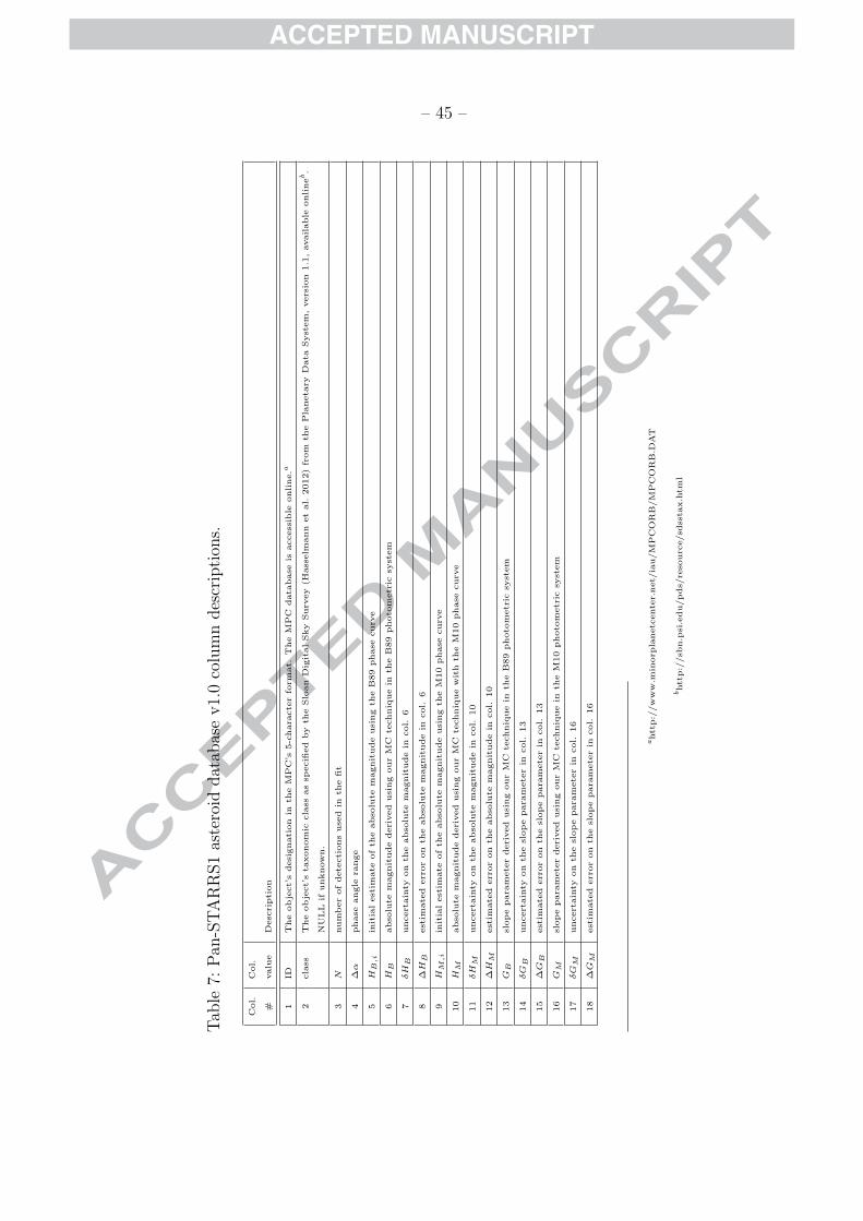
– 45 –

Tab

le7:

Pan

-STA

RR

S1

aste

roid

dat

abas

ev1.

0co

lum

ndes

crip

tion

s.

Col.

Col.

#valu

eD

esc

ripti

on

1ID

The

obje

ct’

sdesi

gnati

on

inth

eM

PC

’s5-c

hara

cte

rfo

rmat.

The

MPC

data

base

isaccess

ible

online.a

2cla

ssT

he

obje

ct’

sta

xonom

iccla

ssas

specifi

ed

by

the

Slo

an

Dig

italSky

Surv

ey

(Hass

elm

ann

et

al.

2012)

from

the

Pla

neta

ryD

ata

Syst

em

,vers

ion

1.1

,available

onlineb.

NU

LL

ifunknow

n.

3N

num

ber

ofdete

cti

ons

use

din

the

fit

4∆

αphase

angle

range

5H

B,i

init

ialest

imate

ofth

eabso

lute

magnit

ude

usi

ng

the

B89

phase

curv

e

6H

Babso

lute

magnit

ude

deri

ved

usi

ng

our

MC

techniq

ue

inth

eB

89

photo

metr

icsy

stem

7δH

Buncert

ain

tyon

the

abso

lute

magnit

ude

incol.

6

8∆

HB

est

imate

derr

or

on

the

abso

lute

magnit

ude

incol.

6

9H

M,i

init

ialest

imate

ofth

eabso

lute

magnit

ude

usi

ng

the

M10

phase

curv

e

10

HM

abso

lute

magnit

ude

deri

ved

usi

ng

our

MC

techniq

ue

wit

hth

eM

10

phase

curv

e

11

δH

Muncert

ain

tyon

the

abso

lute

magnit

ude

incol.

10

12

∆H

Mest

imate

derr

or

on

the

abso

lute

magnit

ude

incol.

10

13

GB

slope

para

mete

rderi

ved

usi

ng

our

MC

techniq

ue

inth

eB

89

photo

metr

icsy

stem

14

δG

Buncert

ain

tyon

the

slope

para

mete

rin

col.

13

15

∆G

Best

imate

derr

or

on

the

slope

para

mete

rin

col.

13

16

GM

slope

para

mete

rderi

ved

usi

ng

our

MC

techniq

ue

inth

eM

10

photo

metr

icsy

stem

17

δG

Muncert

ain

tyon

the

slope

para

mete

rin

col.

16

18

∆G

Mest

imate

derr

or

on

the

slope

para

mete

rin

col.

16

ahtt

p:/

/w

ww

.min

orp

lanetc

ente

r.net/

iau/M

PC

OR

B/M

PC

OR

B.D

AT

bhtt

p:/

/sb

n.p

si.e

du/pds/

reso

urc

e/sd

ssta

x.h

tml

– 46 –

REFERENCES

Bowell, E., Happke, B., Domingue, D., Lumme, K., Peltoniemi, J., Harris, A., 1989. In:

Gehrels, T., Matthews, M. T., Binzel, R. P. (Eds.), Asteroids III. University of

Arizona Press, Chapter Application of photometric models to asteroids, pp. 524–555.

Carvano, J. M., Hasselmann, P. H., Lazzaro, D., Mothe-Diniz, T., 2010. SDSS-based

taxonomic classification and orbital distribution of main belt asteroids. A&A 510,

A43.

de la Fuente Marcos, C., de la Fuente Marcos, R., 2013. A resonant family of dynamically

cold small bodies in the near-Earth asteroid belt. MNRAS 434, L1–L5.

DeMeo, F. E., Carry, B., 2013. The taxonomic distribution of asteroids from multi-filter

all-sky photometric surveys. 226 (1), 723–741.

Denneau, L., Jedicke, R., Grav, T., Granvik, M., Kubica, J., Milani, A., Veres, P.,

Wainscoat, R., Chang, D., Pierfederici, F., Kaiser, N., Chambers, K. C., Heasley,

J. N., Magnier, E. A., Price, P. A., Myers, J., Kleyna, J., Hsieh, H., Farnocchia, D.,

Waters, C., Sweeney, W. H., Green, D., Bolin, B., Burgett, W. S., Morgan, J. S.,

Tonry, J. L., Hodapp, K. W., Chastel, S., Chesley, S., Fitzsimmons, A., Holman,

M., Spahr, T., Tholen, D., Williams, G. V., Abe, S., Armstrong, J. D., Bressi, T. H.,

Holmes, R., Lister, T., McMillan, R. S., Micheli, M., Ryan, E. V., Ryan, W. H.,

Scotti, J. V., 2013. The Pan-STARRS Moving Object Processing System. PASP 125,

357–395.

Fukugita, M., Ichikawa, T., Gunn, J. E., Doi, M., Shimasaku, K., Schneider, D. P., 1996.

The Sloan Digital Sky Survey Photometric System. AJ 111, 1748.

Grav, T., Mainzer, A. K., Bauer, J., Masiero, J., Spahr, T., McMillan, R. S., Walker,

R., Cutri, R., Wright, E., Eisenhardt, P. R., Blauvelt, E., DeBaun, E., Elsbury,

– 47 –

D., Gautier, T., Gomillion, S., Hand, E., Wilkins, A., 2012. WISE/NEOWISE

Observations of the Hilda Population: Preliminary Results. ApJ 744, 197.

Grav, T., Mainzer, A. K., Bauer, J. M., Masiero, J. R., Nugent, C. R., 2012.

WISE/NEOWISE Observations of the Jovian Trojan Population: Taxonomy.

ApJ 759, 49.

Harris, A. W., 1989. The H-G Asteroid Magnitude System: Mean Slope Parameters. In:

Lunar and Planetary Institute Science Conference Abstracts, Volume 20 of Lunar

and Planetary Inst. Technical Report, pp. 375.

Hasselmann, P., Carvano, J. M., Lazzaro, D., 2012. Sdss-based asteroid taxonomy v1.1.

ear-a-i0035-5-sdsstax-v1.1.

Holsapple, K. A., 2007. Spin limits of Solar System bodies: From the small fast-rotators to

2003 EL61. Icarus 187, 500–509.

Jedicke, R., Larsen, J., Spahr, T., 2002. Observational Selection Effects in Asteroid Surveys.

Asteroids III, 71–87.

Juric, M., Ivezic, Z., Lupton, R. H., Quinn, T., Tabachnik, S., Fan, X., Gunn, J. E.,

Hennessy, G. S., Knapp, G. R., Munn, J. A., Pier, J. R., Rockosi, C. M., Schneider,

D. P., Brinkmann, J., Csabai, I., Fukugita, M., 2002. Comparison of Positions

and Magnitudes of Asteroids Observed in the Sloan Digital Sky Survey with Those

Predicted for Known Asteroids. AJ 124, 1776–1787.

Kaiser, N., Burgett, W., Chambers, K., Denneau, L., Heasley, J., Jedicke, R., Magnier,

E., Morgan, J., Onaka, P., Tonry, J., 2010. The pan-starrs wide-field optical/nir

imaging survey. In: Stepp L.M., G. R., H.J., H. (Eds.), Ground-based and Airborne

Telescopes III, Volume 7732 of Proceedings of the SPIE, pp. 77330E–77330E–14.

– 48 –

Lagerkvist, C.-I., Magnusson, P., 1990. Analysis of asteroid lightcurves. II - Phase curves

in a generalized HG-system. A&AS 86, 119–165.

Law, N. M., Kulkarni, S. R., Dekany, R. G., Ofek, E. O., Quimby, R. M., Nugent, P. E.,

Surace, J., Grillmair, C. C., Bloom, J. S., Kasliwal, M. M., Bildsten, L., Brown, T.,

Cenko, S. B., Ciardi, D., Croner, E., Djorgovski, S. G., van Eyken, J., Filippenko,

A. V., Fox, D. B., Gal-Yam, A., Hale, D., Hamam, N., Helou, G., Henning, J.,

Howell, D. A., Jacobsen, J., Laher, R., Mattingly, S., McKenna, D., Pickles, A.,

Poznanski, D., Rahmer, G., Rau, A., Rosing, W., Shara, M., Smith, R., Starr, D.,

Sullivan, M., Velur, V., Walters, R., Zolkower, J., 2009. The Palomar Transient

Factory: System Overview, Performance, and First Results. PASP 121, 1395–1408.

Levenberg, K., 1944. A method for the solution of certain problems in least squares.

Quarterly of Applied Mathematics 2, 164–168.

Lupton, R., 2007. The characterization, subtraction, and addition of astronomical images.

In: G.J., B., E.D., F. (Eds.), Statistical Challenges in Modern Astronomy IV,

Volume 371 of ASP Conference Series, pp. 160–172.

Magnier, E., 2006. The Pan-STARRS PS1 Image Processing Pipeline. In: The Advanced

Maui Optical and Space Surveillance Technologies Conference.

Magnier, E. A., Schlafly, E., Finkbeiner, D., Juric, M., Tonry, J. L., Burgett, W. S.,

Chambers, K. C., Flewelling, H. A., Kaiser, N., Kudritzki, R.-P., Morgan, J. S.,

Price, P. A., Sweeney, W. E., Stubbs, C. W., 2013. The Pan-STARRS 1 Photometric

Reference Ladder, Release 12.01. ApJS 205, 20.

Marquardt, D., 1963. An algorithm for least-squares estimation of nonlinear parameters.

SIAM Journal on Applied Mathematics 11, 431–441.

– 49 –

Masiero, J., Jedicke, R., Durech, J., Gwyn, S., Denneau, L., Larsen, J., 2009. The Thousand

Asteroid Light Curve Survey. Icarus 204, 145–171.

Milani, A., Gronchi, G. F., Farnocchia, D., Knezevic, Z., Jedicke, R., Denneau, L.,

Pierfederici, F., 2008. Topocentric orbit determination: Algorithms for the next

generation surveys. Icarus 195, 474–492.

Mothe-Diniz, T., Carvano, J. M. A., Lazzaro, D., 2003. Distribution of taxonomic classes

in the main belt of asteroids. Icarus 162, 10–21.

Mothe-Diniz, T., Roig, F., Carvano, J. M., 2005. Reanalysis of asteroid families structure

through visible spectroscopy. Icarus 174 (1), 54–80.

Muinonen, K., Belskaya, I., Cellino, A., Delbo, M., Levasseur-Regourd, A.-C., Penttila,

A., Tedesco, E., 2010. A three-parameter magnitude phase function for asteroids.

Icarus 209, 542–555.

Oszkiewicz, D. A., Bowell, E., Wasserman, L. H., Muinonen, K., Penttila, A., Pieniluoma,

T., Trilling, D. E., Thomas, C. A., 2012. Asteroid taxonomic signatures from

photometric phase curves. Icarus 219, 283–296.

Parker, A., Ivezic, Z., Juric, M., Lupton, R., Sekora, M. D., Kowalski, A., 2008. The size

distributions of asteroid families in the SDSS Moving Object Catalog 4. Icarus 198,

138–155.

Pravec, P., Harris, A. W., Kusnirak, P., Galad, A., Hornoch, K., 2012. Absolute magnitudes

of asteroids and a revision of asteroid albedo estimates from WISE thermal

observations. Icarus 221, 365–387.

Schlafly, E. F., Finkbeiner, D. P., Juric, M., Magnier, E. A., Burgett, W. S., Chambers,

K. C., Grav, T., Hodapp, K. W., Kaiser, N., Kudritzki, R.-P., Martin, N. F.,

– 50 –

Morgan, J. S., Price, P. A., Rix, H.-W., Stubbs, C. W., Tonry, J. L., Wainscoat,

R. J., 2012. Photometric Calibration of the First 1.5 Years of the Pan-STARRS1

Survey. ApJ 756, 158.

Stuart, J. S., Binzel, R. P., 2004. Bias-corrected population, size distribution, and impact

hazard for the near-Earth objects. Icarus 170, 295–311.

Tonry, J., Onaka, P., 2009. The Pan-STARRS Gigapixel Camera. In: Advanced Maui

Optical and Space Surveillance Technologies Conference.

Tonry, J. L., Stubbs, C. W., Lykke, K. R., Doherty, P., Shivvers, I. S., Burgett, W. S.,

Chambers, K. C., Hodapp, K. W., Kaiser, N., Kudritzki, R.-P., Magnier, E. A.,

Morgan, J. S., Price, P. A., Wainscoat, R. J., 2012. The Pan-STARRS1 Photometric

System. ApJ 750, 99.

Warner, B. D., Harris, A. W., Pravec, P., 2009. The asteroid lightcurve database. Icarus 202,

134–146.

Waszczak, A., Chang, C.-K., Ofek, E. O., Laher, R., Masci, F., Levitan, D., Surace, J.,

Cheng, Y.-C., Ip, W.-H., Kinoshita, D., Helou, G., Prince, T. A., Kulkarni, S., 2015.

Asteroid lightcurves from the Palomar Transient Factory survey: Rotation periods

and phase functions from sparse photometry. ArXiv e-prints.

Wiegert, P. A., Innanen, K. A., Mikkola, S., 1997. An asteroidal companion to the Earth.

Nature 387, 685–686.

Zavodny, M., Jedicke, R., Beshore, E. C., Bernardi, F., Larson, S., 2008. The orbit and size

distribution of small Solar System objects orbiting the Sun interior to the Earth’s

orbit. Icarus 198, 284–293.

This manuscript was prepared with the AAS LATEX macros v5.2.

We calculated absolute magnitudes and slope parameters of 240,000 asteroids We provided uncertainties and errors on derived values Photometry from the Pan-STARRS1 survey was used in our work We employed both Bowell's (1989) and Muinonen's (2010) phase functions We found discrepancy between our absolute magnitudes and those derived by MPC

Highlights