Runoff regime estimation at high-elevation sites: a parsimonious water balance approach

HESSD8, 957–990, 2011

High-elevation waterbalance

E. Bartolini et al.

Title Page

Abstract Introduction

Conclusions References

Tables Figures

J I

J I

Back Close

Full Screen / Esc

Printer-friendly Version

Interactive Discussion

Discussion

Paper

|D

iscussionP

aper|

Discussion

Paper

|D

iscussionP

aper|

Hydrol. Earth Syst. Sci. Discuss., 8, 957–990, 2011www.hydrol-earth-syst-sci-discuss.net/8/957/2011/doi:10.5194/hessd-8-957-2011© Author(s) 2011. CC Attribution 3.0 License.

Hydrology andEarth System

SciencesDiscussions

This discussion paper is/has been under review for the journal Hydrology and EarthSystem Sciences (HESS). Please refer to the corresponding final paper in HESSif available.

Runoff regime estimation athigh-elevation sites: a parsimoniouswater balance approachE. Bartolini, P. Allamano, F. Laio, and P. Claps

Dipartimento di Idraulica, Trasporti e Infrastrutture Civili, Politecnico di Torino, Torino, Italy

Received: 4 January 2011 – Accepted: 5 January 2011 – Published: 24 January 2011

Correspondence to: E. Bartolini ([email protected])

Published by Copernicus Publications on behalf of the European Geosciences Union.

957

http://www.hydrol-earth-syst-sci-discuss.net

http://www.hydrol-earth-syst-sci-discuss.net/8/957/2011/hessd-8-957-2011-print.pdf

http://www.hydrol-earth-syst-sci-discuss.net/8/957/2011/hessd-8-957-2011-discussion.html

http://creativecommons.org/licenses/by/3.0/

HESSD8, 957–990, 2011


E. Bartolini et al.

Title Page



Tables Figures

J I

J I

Back Close

Full Screen / Esc



Discussion

Paper

|D

iscussionP

aper|

Discussion

Paper

|D

iscussionP

aper|

Abstract

We develop a water balance model, parsimonious both in terms of parameterizationand of required input data, to characterize runoff regime of high-elevation basins. Themodel uses a temperature threshold to partition precipitation into rainfall and snow-fall, and to estimate evapotranspiration volumes. The role of snow in the transposition5

of precipitation to runoff at the monthly time scale is investigated through a specificsnowmelt module that estimates melted quantities by a non-linear function of tempera-ture. A probabilistic representation of temperature is also introduced, in order to mimicits sub-monthly variability. To account for the commonly reported rainfall underestima-tion at high elevations, a two-step precipitation adjustment procedure is implemented10

to guarantee the closure of the water balance.The model is applied to a group of catchments in the North-Western Italian Alps, and

its performances are assessed by comparing measured and simulated runoff regimesboth in terms of total bias and anomalies. The obtained results are good, especiallyconsidering that the model has only two parameters to be estimated. More in de-15

tail, when the parameter calibration is separately performed for each basin, the modelproves to be able to reproduce the runoff seasonality. At the regional scale (i.e., withuniform parameters for the whole region), the performances are slightly declining, butthe model is still able to discern among different mechanisms of runoff formation thatdepend on the role of the snow storage. Thanks to its parsimony, the model is suit-20

able for application in ungauged basins and for large scale investigations of the role ofclimatic variables on water availability and runoff timing in mountainous regions.

1 Introduction

Runoff regime, intended as the sequence of mean monthly runoff values, is a usefulindicator of the seasonality of runoff, to be used for the development of water manage-25

ment strategies. The interaction between river ecosystems and human activities, in

958





HESSD8, 957–990, 2011


E. Bartolini et al.

Title Page



Tables Figures

J I

J I

Back Close

Full Screen / Esc



Discussion

Paper

|D

iscussionP

aper|

Discussion

Paper

|D

iscussionP

aper|

fact, crucially depends on the timing of runoff peaks and on the periods of low flow, dueto the fact that several water uses require water volumes during a specific period of theyear (e.g., irrigation, artificial snow for ski resort). A reliable estimation of runoff regimeis particulary important in mountainous regions, as these areas supply fresh water notonly in their close neighborhoods but also in the lowland downstream, where most of5

the economic and agricultural activities take place. Moreover, the increasing populationof the piedmont areas and the vulnerability to climate change shown by mountain re-gions (e.g., Beniston et al., 1997; Allamano et al., 2009b) raise further important issuesfor water resources planning and management (e.g., Zierl and Bugman, 2005; Hortonet al., 2006; Adam et al., 2009).10

Runoff depends on the volume of water supplied to a catchment in terms of rainor snow, as well as on the effects of the other processes involved in the water cycle(i.e., interception, infiltration, evapotranspiration, lakes and aquifers depletion). Thetransformation of precipitation into streamflow at the basin outlet has been extensivelyinvestigated over the last century and various water balance models have been pro-15

posed in the literature (e.g., Alley, 1985; Gleick, 1986; Xu et al., 1996; Limbrunner et al.,2006). In particular, models operating at the monthly scale have been extensively usedin hydrological applications as recently reviewed by Xu and Sing (1998). In fact, thanksto their ease of use and flexibility, these models are suitable for applications at differentspatial scales (Gleick, 1986), and they have been extensively used for climate change20

impact assessment studies in various catchments all over the world (e.g., Xu et al.,1996; Jasper et al., 2004; Wang et al., 2009).

For high-elevation basins, however, runoff regime estimation remains a challengingproblem, due to the need to account for the dynamics of snow accumulation and melt.For these areas, specific and more complex water balance models, generally operating25

at finer time scales (e.g., daily), have been developed, in order to properly describe thesnow processes and their effects on the timing and volumes of runoff (e.g., Zappa et al.,2003; Eder et al., 2005; Schaefli et al., 2005). These models attain a good reproduc-tion of daily runoff processes, at the cost of requiring input data with a high temporal

959





HESSD8, 957–990, 2011


E. Bartolini et al.

Title Page



Tables Figures

J I

J I

Back Close

Full Screen / Esc



Discussion

Paper

|D

iscussionP

aper|

Discussion

Paper

|D

iscussionP

aper|

resolution (i.e., daily temperature and precipitation). However, it is well known that thedensity of the monitoring networks tends to decrease with elevation, while measure-ments errors tend to increase, leading to a precipitation underestimation that in turnaffects the quality of the reconstructed runoff (e.g., Milly and Dunne, 2002; Xia andGuoqiang, 2007; Valery et al., 2010). The adoption of complex model structures in the5

presence of scarce data rises important issues, mainly related to the detrimental effecton the results of having many nuisance parameters and few data to estimate them. Infact, while complex models can be useful to investigate the hydrologic processes occur-ring in specific, well monitored, basins, their validation or extension is generally difficultin regional-scale studies involving several catchments (e.g., Beven, 1989; Limbrunner10

et al., 2006; Sivakumar, 2008).The modelling framework adopted in this study operates at the monthly time scale

and investigates the effects of snow accumulation and melt in the transposition of therainfall regime into the corresponding runoff regime. The model partially resembles theone proposed by Woods (2009), but our analysis is focused on measured (not analyt-15

ical) mean precipitation and temperature seasonal curves. Dealing with observations,the model has to take into account the well known problem of precipitation undercatchin mountain rain gauges. For this reason, a precipitation correction is considered, ob-tained as the solution of an inverse problem that uses the difference in the observedand simulated runoff as the variable to be minimized.20

The model is parsimonious in terms of number of parameters to estimate and pro-vides a simple and controllable framework, suitable to control annual and monthly wa-ter budgets over large areas. Parsimony in the hydrological modelling, as proposedby Woods (2003), Mouelhi et al. (2006), Allamano et al. (2009a) among others, allowsone to investigate the dominant hydrologic processes in complex orography and data-25

scarce regions. This makes water balance models a suitable tool for applications inscarcely monitored regions and ungauged basins, based on a proper framework forparameter regionalization (Vandewiele and Elias, 1995).

960





HESSD8, 957–990, 2011


E. Bartolini et al.

Title Page



Tables Figures

J I

J I

Back Close

Full Screen / Esc



Discussion

Paper

|D

iscussionP

aper|

Discussion

Paper

|D

iscussionP

aper|

2 Model description

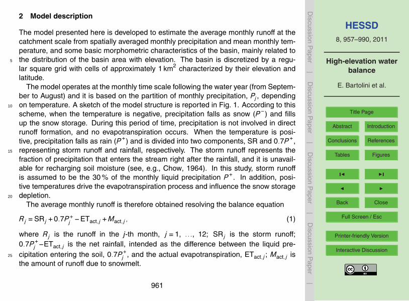
The model presented here is developed to estimate the average monthly runoff at thecatchment scale from spatially averaged monthly precipitation and mean monthly tem-perature, and some basic morphometric characteristics of the basin, mainly related tothe distribution of the basin area with elevation. The basin is discretized by a regu-5

lar square grid with cells of approximately 1 km2 characterized by their elevation andlatitude.

The model operates at the monthly time scale following the water year (from Septem-ber to August) and it is based on the partition of monthly precipitation, Pj , dependingon temperature. A sketch of the model structure is reported in Fig. 1. According to this10

scheme, when the temperature is negative, precipitation falls as snow (P −) and fillsup the snow storage. During this period of time, precipitation is not involved in directrunoff formation, and no evapotranspiration occurs. When the temperature is posi-tive, precipitation falls as rain (P +) and is divided into two components, SR and 0.7P +,representing storm runoff and rainfall, respectively. The storm runoff represents the15

fraction of precipitation that enters the stream right after the rainfall, and it is unavail-able for recharging soil moisture (see, e.g., Chow, 1964). In this study, storm runoffis assumed to be the 30 % of the monthly liquid precipitation P +. In addition, posi-tive temperatures drive the evapotranspiration process and influence the snow storagedepletion.20

The average monthly runoff is therefore obtained resolving the balance equation

Rj =SRj +0.7P +j −ETact,j +Mact,j , (1)

where Rj is the runoff in the j-th month, j =1, ..., 12; SRj is the storm runoff;0.7P +

j −ETact,j is the net rainfall, intended as the difference between the liquid pre-cipitation entering the soil, 0.7P +

j , and the actual evapotranspiration, ETact,j ; Mact,j is25

the amount of runoff due to snowmelt.

961





HESSD8, 957–990, 2011


E. Bartolini et al.

Title Page



Tables Figures

J I

J I

Back Close

Full Screen / Esc



Discussion

Paper

|D

iscussionP

aper|

Discussion

Paper

|D

iscussionP

aper|

A constant temperature threshold is assumed to separate snow from rainfall. Thisrepresents a rough approximation, but it allows one to apply the water balance modelto a vast range of situations and has been extensively used in the literature (see, e.g.,Collins, 1998; Limbrunner et al., 2006; Woods, 2009).

Equation (1) is applied to each cell separately, and runoff is then combined to form5

the discharge at the basin outlet. No lateral flow between cells is considered. Giventhat we consider mean basin precipitation, P is uniformly distributed among cells.

The water balance is devised to be applied at a monthly time scale. While this tempo-ral resolution is suitable to characterize runoff seasonality, the assumption of a constanttemperature within the month is inappropriate to describe the processes of snow ac-10

cumulation and melting, which are strongly influenced by the crossing of the freezingtemperature, also occurring as a consequence of the daily temperature oscillations.For this reason, even in a monthly water balance framework, a description of the sub-monthly temperature variations is desirable (Kling et al., 2006). To provide a simple,yet realistic, representation of the sub-monthly temperature oscillations, a probabilis-15

tic description of the within-month temperature variability is introduced. For reason ofanalytical tractability, the average daily temperature T is assumed to follow a logisticdistribution (e.g., Johnson et al., 1995, chapter 23), whose probability density function(pdf) reads

p(T ;µj ,sj )=e−(T−µj )/sj

sj (1+e−(T−µj )/sj )2=

14sj

sech2(T −µj

2sj

), (2)20

where µj is the mean monthly temperature and sj is a scale parameter, directly relatedto the standard deviation of the daily temperature within the month, σj , through thefollowing relation:

sj =

√3π

σj . (3)

The standard deviation of the average daily temperatures, σj , is assumed to be con-25

stant across different months, so that σj =σ (and sj = s), with j =1, ..., 12; σ it will962





HESSD8, 957–990, 2011


E. Bartolini et al.

Title Page



Tables Figures

J I

J I

Back Close

Full Screen / Esc



Discussion

Paper

|D

iscussionP

aper|

Discussion

Paper

|D

iscussionP

aper|

be a model parameter to be calibrated. Based on this description of the within-monthvariability of temperature, it is possible to identify the fractions of month characterizedby negative and positive temperatures. Processes occurring within each month arethen considered to operate in parallel, according to temperature conditions. The firstclass of processes lasts for NTj , that is the fraction of months characterized by negative5

temperatures and it is computed as the probability to have T <0 ◦C:

NTj = P (T <0;µj ,s)=1

1+e−(T−µj )/s=

12+

12· tanh

(T −µj

2s

). (4)

During this time, precipitation falls as snow and no evapotranspiration or directrunoff occur. The second class of processes, relative to positive temperature, lastsfor P Tj =1−NTj , receives liquid precipitation P +

j = Pj ·P Tj , and is characterized by10

snowmelt, storm runoff and evapotranspiration. Each cell of the basin is potentiallysubjected to both classes of processes, according to the local distribution of tempera-ture.

2.1 Modelling snow accumulation and melt

In the model, the volume of snowpack is quantified in terms of millimeters of snow water15

equivalent (SWE) stored in each cell of the basin. The snowpack dynamics follow theequation:

SWEj =SWEj−1−Mact,j +NTj ·Pj , (5)

so that the volume of the current month j, SWEj , is a function of the snowpack of theprevious month j−1, SWEj−1, the losses due to snowmelt, Mact,j , and of the amount of20

new snowfall, P − =NTj ·Pj , obtained as the precipitation Pj fallen during the fraction ofmonth with negative temperatures NTj . No effects of rain-on-snow are considered.

The snowpack melting is estimated by evaluating the monthly potential snowmeltMpot,j and by comparing it with the snowpack available for melting. The potential

963





HESSD8, 957–990, 2011


E. Bartolini et al.

Title Page



Tables Figures

J I

J I

Back Close

Full Screen / Esc



Discussion

Paper

|D

iscussionP

aper|

Discussion

Paper

|D

iscussionP

aper|

snowmelt reflects the available energy and it is modelled as a parabolic function oftemperature,

Mpot,j =c · (T+j )2 ·P Tj , (6)

where c is a coefficient expressing the melting rate, that is, beside σ, the other param-eter of the model. (T+

j )2, used as a proxy for melting energy, is the squared average5

temperature (conditional above zero) and reads

(Tj )+2 =

∫∞0 T 2p(T |µj ,s)dT∫∞

0 p(T |µj ,s)dT=

−2s2Li2

(−e

µjs

)1− 1

1+eµjs

, (7)

where Li2(·) is the dilogarithm function (Abramowitz and Stegun, 1964, chapter 27,Spence’s integral for n=2).

The actual monthly snowmelt, Mact,j , is equal to its corresponding potential value10

when the amount of the stored SWE is sufficient to sustain snowmelt; otherwise itequals SWEj :

Mpot,j if SWEj ≥Mpot,j , (8a)Mact,j =

{SWEj if SWEj <Mpot,j . (8b)15

This modelling framework represents a variant of the classical degree-day approach(e.g., Hock, 2003), which is based on a relation similar to Eq. (6) but with a linear de-pendence of potential snowmelt on temperature. However, the adoption of a quadraticdependence allows one to roughly differentiate the snowmelt rate of the cold seasonfrom that of the warm season. In fact, one can interpret the parabolic function of Eq. (6)20

as a standard degree-day approach with melting rate coefficients that vary along theyear, resulting in a slower snowmelt when temperature is slightly positive (i.e., duringthe cold season), and a faster snowmelt for increasing values of T+

j . In the discussion

964





HESSD8, 957–990, 2011


E. Bartolini et al.

Title Page



Tables Figures

J I

J I

Back Close

Full Screen / Esc



Discussion

Paper

|D

iscussionP

aper|

Discussion

Paper

|D

iscussionP

aper|

section it will be shown that this assumption allows one to obtain a better representa-tion of the runoff regime with the same number of parameters of the standard lineardegree-day method.

2.2 Modelling evapotranspiration

Evapotranspiration is assumed to be dependent only on temperature; evaporation from5

snowmelt and sublimation are neglected.Monthly potential evapotranspiration, ETpot,j , expressed in millimeters, is computed

according to the Thornthwaite equation (1948):

ETpot,j =Nj

12·16

(10 ·

T+j

I

)a

, (9)

where T+j is the average temperature (conditional above zero) obtained as10

Tj =

∫∞0 Tp(T |µj ,s)dT∫∞0 p(T |µj ,s)dT

=s · ln(1+e

µjs )

1− 1

1+eµjs

. (10)

In Eq. (9), the fraction Nj/12 is a monthly correction factor, dependent on latitude,which is required to adjust actual daylight (Bras, 1990) and a is a coefficient dependenton I, the annual heat index, obtained by combination of the positive mean monthlytemperature values µj15

I =max[ k∑j=1

(µj

5

1.514);5], (11)

being k the number of months characterized by positive mean monthly temperatures.As a consequence of the variability of k on elevation, I assumes low values for high-elevation cells, where monthly temperatures are above zero only for short periods in

965





HESSD8, 957–990, 2011


E. Bartolini et al.

Title Page



Tables Figures

J I

J I

Back Close

Full Screen / Esc



Discussion

Paper

|D

iscussionP

aper|

Discussion

Paper

|D

iscussionP

aper|

a year (i.e., 1–2 months). This leads to an overestimation of monthly potential evapo-transpiration, due to the fact that Thornthwaite’s method was not specifically developedfor snow-dominated regions. Nevertheless, its parsimony, that allows one to estimatepotential evapotranspiration based only on monthly temperature, makes it suitable forour purposes. In order to correct the effect of low temperatures on I, heat indices are5

supposed to take only values greater than 5 ◦C (Eq. 11). Following this assumption, themodel proves to be able to predict realistic values of evapotranspiration also at high-elevation sites, as detectable from a comparison with some reference values obtainedwith the Penman modified approach reported by Henning and Henning (1981).

Monthly actual evapotranspiration, ETact,j , is obtained by comparing its potential10

value, ETpot,j , with the water effectively available for evapotranspiration (i.e., monthlyrainfall):

ETpot,j , if 0.7P +j ≥ETpot,j , (12a)

ETact,j ={

P +j , if 0.7P +

j <ETpot,j . (12b)15

3 Case study

The study domain is located in the North-Western Italian Alps and embraces a wideheterogeneous region, including catchments which strongly differ for mean elevation,altitude range and climatic characteristics. This variety of conditions involves a differ-entiation in the regime shapes, both in term of precipitation and runoff. In fact, moving20

from the higher to the lower elevations, the shape of the runoff regime changes fromone with a single peak, principally driven by snowmelt, to a curve with a second relativemaximum during autumn, which is more typical of middle-elevation catchments.

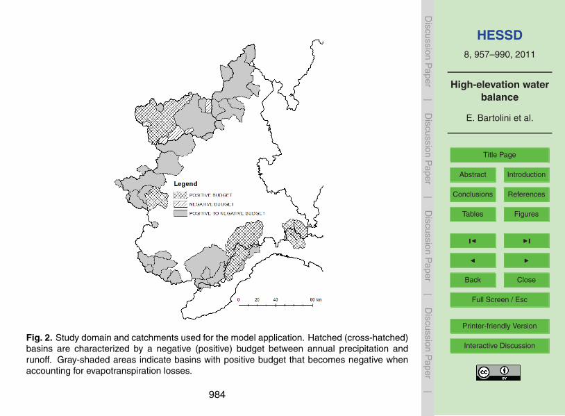
In the study domain, 40 catchments are selected (Fig. 2), with areas ranging from 40to 3310 km2 and with altitudinal range between 117 and 4727 m a.s.l. (for more informa-25

tion, see the Supplement). The basins are preliminarily checked to identify possible an-thropogenic disturbances in runoff seasonality. In particular, we examine the presence

966





HESSD8, 957–990, 2011


E. Bartolini et al.

Title Page



Tables Figures

J I

J I

Back Close

Full Screen / Esc



Discussion

Paper

|D

iscussionP

aper|

Discussion

Paper

|D

iscussionP

aper|

of dams and flow regulation infrastructures, that may affect the regime shape by miti-gating the discharge variability. To this aim we introduce a reservoir index, RI= Vw/Vl,defined as the ratio between the total water volume that flows at the basin outlet ina year, Vw, and the sum of the total retention volumes of the artificial lakes locatedwithin the basin Vl. A threshold value of RI equal to 0.25 is chosen to characterize the5

transition from an undisturbed to a disturbed regime. Only for river Toce at Cadarese(RI=0.29) the condition on the RI index is not satisfied. Consequently, the final set ofcatchments used in the model application is composed by 39 elements. The secondbasin in terms of larger RI value is river Orco at Ponte Canavese, with RI=0.14.

To run the model, precipitation and temperature mean monthly values are used as10

meteorological forcing variables. In particular, the variability of temperature with ele-vation and geographic position is explicitly considered using maps of mean monthlytemperatures obtained at 1 km2 grid resolution by Claps et al. (2008). In that study, theauthors spatialized average monthly temperatures by means of a multi-regression ap-proach based on elevation, latitude, distance from the sea, orientation and topographic15

concavity. However, it is worth noting that, if gridded temperature data were not avail-able in the region of interest, elevation data could be used as a proxy of temperaturethrough the use of suitable values of the lapse rate (see e.g., Allamano et al., 2009a).The necessary geographic parameters, namely latitude, longitude and elevation, areobtained at a 1 km resolution using the digital elevation model GTOPO30, developed by20

the United States Geological Survey (USGS, 2006). Observed runoff regimes, com-puted as monthly runoff averages, and multi-year monthly time series serve for theevaluation of the model performances.

3.1 Correction of precipitation

Basin mean monthly precipitation data are used in the model to define the total amount25

of water available and are uniformly divided in order to assign a precipitation input toeach cell. However, basin precipitation is largely uncertain because it is the resultof the spatialization of point-precipitation measurements, that are in turn affected by

967





HESSD8, 957–990, 2011


E. Bartolini et al.

Title Page



Tables Figures

J I

J I

Back Close

Full Screen / Esc



Discussion

Paper

|D

iscussionP

aper|

Discussion

Paper

|D

iscussionP

aper|

undercatch for wind effects, evaporation, wetting, splashing, blowing and drifting snow(e.g., Sevruk, 1983). These problems are exacerbated in mountainous areas, wherethe measurement network density is often inadequate to detect the small scale fea-tures of precipitation induced by the complex orography (Milly and Dunne, 2002). Asa consequence, an imbalance between measured annual precipitation and runoff, the5

first being sometimes smaller than the latter, can be observed in some cases (Valeryet al., 2010). In fact, a preliminary analysis on the data of our study domain reveals thatmeasured annual precipitation is smaller than total runoff in 5 catchments (the hatchedones in Fig. 2). Considering also a preliminary estimate of mean annual evapotranspi-ration, the precipitation underestimation becomes even more critical, with 33 out of 3910

basins that would turn out to have a negative water balance (i.e., annual runoff largerthan the sum of measured precipitation and evapotranspiration, gray-shaded basinsin Fig. 2). This is a crucial clue that precipitation is underestimated, and should besuitably corrected to improve the model performances.

Given these premises, a two-step procedure is implemented in the model for the15

correction of the monthly precipitation bias. Firstly, the model is run by assigning fixedvalues to the model parameters. In particular, the standard deviation of daily temper-ature σ is assumed to be 3 ◦C and the melting rate is set to c=0.7 mm/◦C2 day. Thelatter corresponds, for T+

j =5 ◦C, to a melt factor of 3.5 mm/◦C day, analogous to thevalues proposed by the US Army Corps of Engineers (1998, Chapt. 6). The model bias20

in runoff estimation,

b=Rtot,obs−Rtot,sim, (13)

is calculated as the difference between the annual simulated, Rtot,sim, and observedrunoff, Rtot,obs. Adjusted monthly precipitation, Padj,j , is thus obtained as a function ofthe model bias according to the expression25

Padj,j = Pj +b12

. (14)

968





HESSD8, 957–990, 2011


E. Bartolini et al.

Title Page



Tables Figures

J I

J I

Back Close

Full Screen / Esc



Discussion

Paper

|D

iscussionP

aper|

Discussion

Paper

|D

iscussionP

aper|

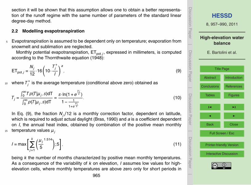
The bias in Eq. (13) has been observed not to significantly vary with the subsequentadjustment of the model parameters. This is probably due to the fact that both parame-ters (c and σ) principally affect the timing of the phenomena involved in runoff formation(i.e., the snowmelt peak and the beginning of the snow season) rather than the annualwater volumes. As a consequences, b remains almost unchanged with variations of c5

and σ, which allows us to keep it constant in the calibration run.Since we are interested in applying the model also in ungauged basins, where no

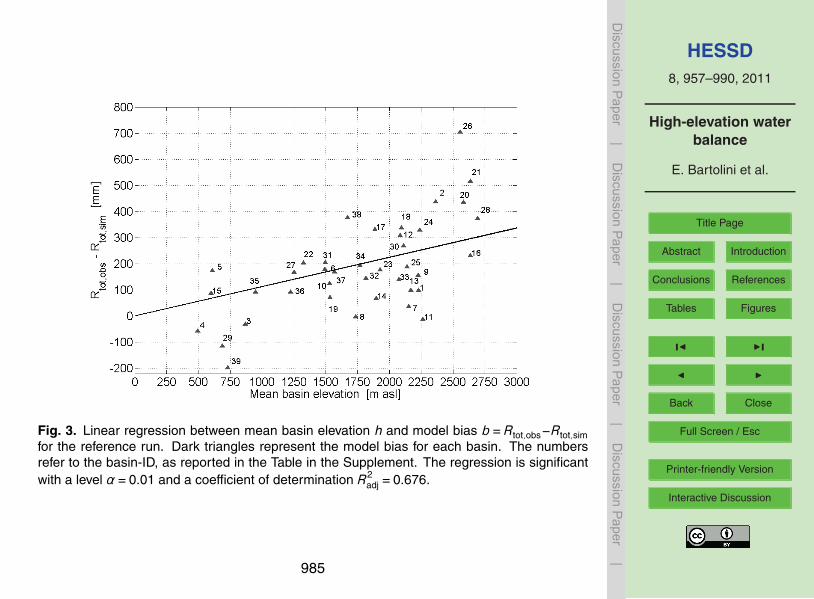
runoff data are available, the dependence of b on geomorphic parameters should bestudied. The analysis of the model bias demonstrates that b increases with the meanbasin elevation (see Fig. 3), consistently with the common notion that the undercatch10

increases when precipitation falls in a solid form. Precipitation correction in Eq. (14)can thus be generalized by substituting the model bias b with b∗, obtained by a lin-ear regression of model bias on mean basin elevation h (Fig. 3). The regression isconstrained to the origin, so that no negative correction is applied to measured precip-itation. For the Western Italian Alps we obtain15

b∗ =0.112 ·h, (15)

where b∗ is in mm and h in m a.s.l.

3.2 Parameter calibration

The parsimony in the model structure is reflected by the fact that the model has onlytwo parameters to be calibrated, namely the temperature standard deviation, σ, and20

the snowmelt rate, c. In the calibration run, these parameters are allowed to vary ina wide range, in order to assess model sensitivity. More specifically, σ takes values inthe range 1–10 ◦C and c in the interval 0.02–1 mm/◦C2 day.

Two different approaches for parameter calibration are followed, one consideringa basin-specific and the other a regional point of view. In both cases, the mean absolute25

error

969





HESSD8, 957–990, 2011


E. Bartolini et al.

Title Page



Tables Figures

J I

J I

Back Close

Full Screen / Esc



Discussion

Paper

|D

iscussionP

aper|

Discussion

Paper

|D

iscussionP

aper|

MAE(c,σ)=1

12·

12∑j=1

|Robs,j −Rsim,j | (16)

is minimized, being Robs,j and Rsim,j the observed and simulated values of monthlyaverage runoff, respectively. In particular, the basin-specific calibration minimizes theMAE for each basin, providing locally optimal parameter values.

The regional calibration procedure, instead, considers the whole set of catchments5

and seeks the combination of parameters that minimizes the global error, obtained bycombining the MAE of each basin. This condition is considered with the aim of ex-tending the application of the method to ungauged basins, once the suitability of takingspatially uniform parameters is assessed. In details, the regional calibration processrequires the following steps: (i) n=500 combinations of parameters are considered:10

σ is varied between 1 and 10 ◦C in steps of 1 ◦C and c from 0.02 to 1 mm/◦C2 day insteps of 0.02 mm/◦C2 day; (ii) the MAEm,i is calculated for each basin m and for eachparameter combination i ; (iii) for each basin m, a rank rm,i is assigned to the parametercombination ci ,σi where MAE(ci ,σi ) is the r-th smaller value in the set of n possiblevalues; (iv) the average rank ri is calculated as ri =1/39

∑39m=1rm,i for each parameter15

combination; (v) the parameter combination producing the smaller r value is selectedas the regional set of calibrated parameters.

The use of a ranked error indicator instead of the simple regional average MAEallows one to assign the same weight to all the basins considered. In fact, being theMAE a dimensional error statistic, it can be affected by the size of the basins and the20

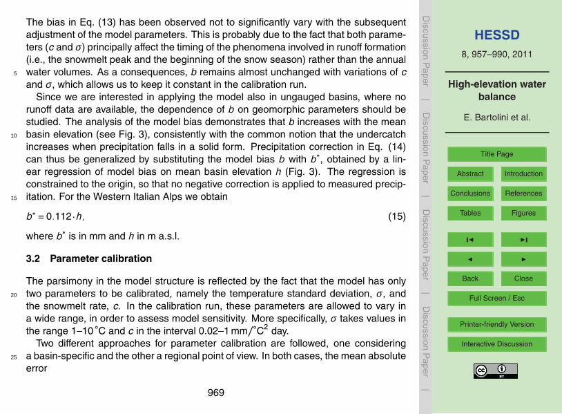
entity of total annual runoff, leading to bias in the model calibration.To avoid progressive snow accumulation over time, a condition on the parameter

space is imposed. This condition requires the snow storage to empty at the end of thewater year, so that the total annual inflow equals the outflow. However, over mountain-ous areas it is fair to assume that, at high elevations, snow can persist even during25

summer. It is therefore assumed that snow can persist also during the warm season,but only in the portion of basin higher than 3000 m a.s.l. The parameter combinations

970





HESSD8, 957–990, 2011


E. Bartolini et al.

Title Page



Tables Figures

J I

J I

Back Close

Full Screen / Esc



Discussion

Paper

|D

iscussionP

aper|

Discussion

Paper

|D

iscussionP

aper|

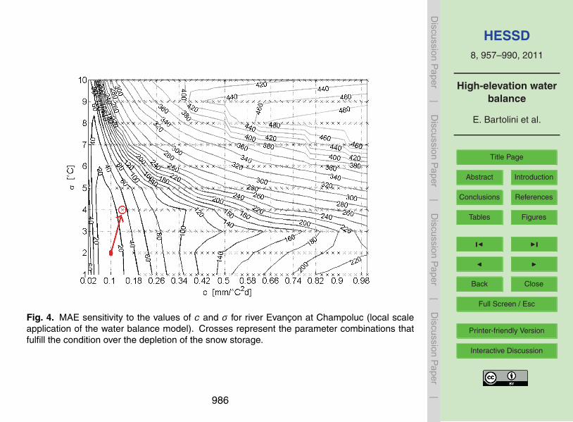
that do not allow the model to match this requirement are eliminated. An examplecan be seen in Fig. 4, that shows the MAE variability in the parameter space for riverEvancon at Champoluc, as resulted from the basin-specific application of the water bal-ance. Contour lines represent the MAE variability considering all the possible (n=500)parameter combinations, while crosses identify the parameter combinations that fulfill5

the condition on the snow storage depletion. It can be seen that the parameters cor-respondent to the global MAE minimum (i.e., c=0.1 mm/◦C2 day and σ =2 ◦C) do notallow to completely melt the snow accumulated during the cold season. Therefore, itis necessary to select the parameter set within the boundary of the surface defined bythe crosses (the red circle in Fig. 4) in order to fulfil the snow depletion condition.10

4 Results

4.1 Application at the local scale

The water balance model is first applied and tested at the local scale (i.e., basin-specificapplication). This means that the local precipitation correction (i.e. dependent on thelocally determined model bias) and the basin-specific calibration of the parameters are15

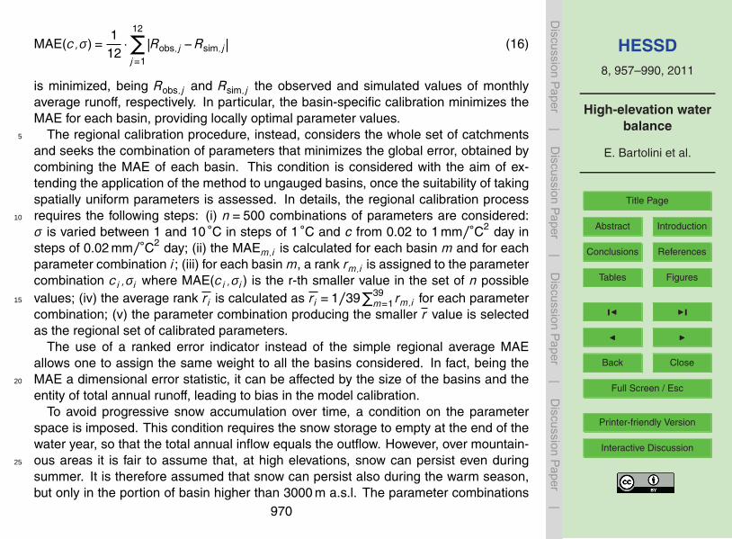
used.The goodness of the reconstructed runoff regime is quantified by a quality index

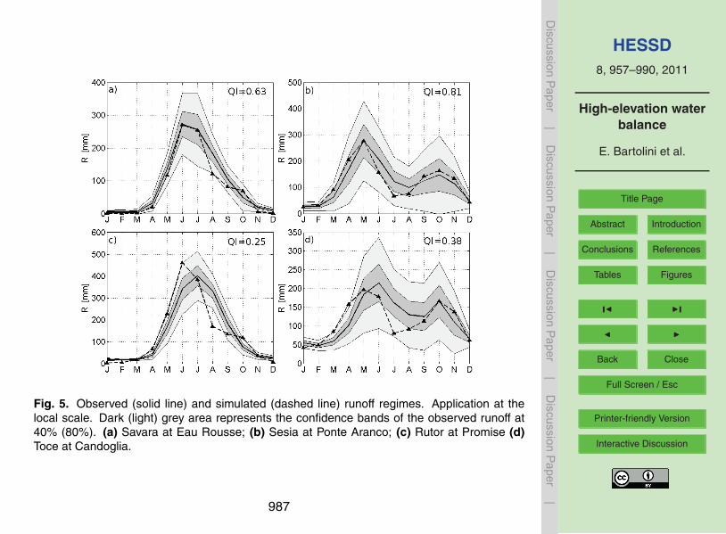
QI (see Appendix A for more details). This indicator varies between 0, which standsfor a poor agreement between observed and simulated runoff, and 1, which indicatesa perfect reconstruction of the observed values.20

Figure 5 shows good (poor) quality results in the upper (lower) panels, respectivelyfor high-elevation snow-dominated catchments (Fig. 5a: Savara at Eau Rousse and5c: Rutor at Promise) and for middle-elevation basins (Fig. 5b: Sesia at Ponte Arancoand 5d: Toce at Candoglia). Dark (light) gray-shaded areas show the 40% (80%)confidence bands, calculated under the hypothesis of normality, as Rj,obs ±0.53σR,j25

971





HESSD8, 957–990, 2011


E. Bartolini et al.

Title Page



Tables Figures

J I

J I

Back Close

Full Screen / Esc



Discussion

Paper

|D

iscussionP

aper|

Discussion

Paper

|D

iscussionP

aper|

(Rj,obs ±1.28σR,j ), where σR,j is the standard deviation of the observed runoff in monthj, calculated from the original multi-year time series.

Overall, the simulated runoff regimes reproduce quite well the observed ones, alsoconsidering the difficulty in dealing with very different regime shapes. However, it ispossible to detect systematic errors, in that most of the basins are characterized by5

a runoff overestimation in October and by an underestimation in August or July. Withrespect to the overestimation, it is important to notice that in October mean measuredprecipitation is higher than measured runoff. Being the evapotranspiration fluxes onlyof secondary importance during the fall season, it follows that, in the real system, thiswater surplus probably feeds the soil storage, that is not simulated in our water balance10

model. Also the summer runoff underestimation can possibly be a consequence of theabsence of a soil module in the model framework. In fact, the high summer temper-atures cause high evapotranspiration that limits the amount of precipitation that con-tributes to runoff. The water stored in the soil could partially feed this process, reducingthe precipitation contribution to evapotranspiration. In this respect, the hypotheses of15

taking into account a fraction of rainfall as storm runoff constitutes a simple method toattenuate this error. In fact, the introduction of a specific module to account for the soileffect would improve realism but at the cost of increasing the model complexity (i.e.,number of parameters) and the uncertainties in the model results.

4.2 Application at the regional scale20

When no measured runoff data are available, the water balance can be applied at theregional scale using the generalized precipitation correction defined by Eq. (15) andthe regional parameter calibration procedure.

The parameters achieving the best average rank are σ =3 ◦C and c=0.22 mm/◦C2

day. It is interesting to notice that, in this case, the melting rate results to be smaller25

than 0.7 mm/◦C2 day, which is the reference value (see Sect. 3.1) used in the firststep of model application. This discrepancy may be related to the time scale of theapplication, which is monthly rather than daily as in standard degree-day approaches.

972





HESSD8, 957–990, 2011


E. Bartolini et al.

Title Page



Tables Figures

J I

J I

Back Close

Full Screen / Esc



Discussion

Paper

|D

iscussionP

aper|

Discussion

Paper

|D

iscussionP

aper|

In any case, the range of variability of melt factors reported in the literature is extremelywide (US Army Corps of Engineers, 1998).

Figure 6 presents the observed and simulated runoff regimes in the same basinsshown in Fig. 5. The highest QI is associated to river Sesia at Ponte Aranco (Fig. 6b).On the contrary, Fig. 6d shows the runoff regimes for river Toce at Candoglia, a middle-5

elevation catchment in which the performances of the model are particularly poor. Theaverage runoff seasonality of Savara at Eau Rousse, that is an high-elevation catch-ment, is presented in Fig. 6a. It shows a good agreement between observed andsimulated curves during the first part of the year (from January to June) and an im-portant runoff underestimation during the summer (July and August). The same error,10

even more significant, is evident in Fig. 6c for the case of river Rutor at Promise. Inthis last case, the simulated regime presents a further incongruence in that the peakanticipates of 1 month the timing of the observed runoff peak. It is interesting to noticethat river Toce at Candoglia and river Rutor at Promise correspond, in Fig. 3, to thepoints 38 and 26. Since these points, representing the model bias, are located far from15

the regression line used in the precipitation correction, one may conclude that the poorperformances of the model are also contributed by underestimation of the precipitationcorrection.

Overall, it appears that the water balance model, when applied at the regional scale,is still able to reproduce the regime shapes recognizing the different mechanisms of20

runoff formation. However, the regional application, requiring reduced data, leads, asexpected, to generally poorer model performances.

Figure 7 shows the quality indices QI related to the basin-specific (light gray) and theregional (dark gray) scale application of the model. This representation is suitable toidentify the basins where the model is able to better simulate the mean water balance25

and can be used as a tool to concisely present the results for a wide number of basins.However, due to its dependence on the error quantiles (see Appendix A for more de-tails), the QI can not be used to compare different model applications (i.e., local vs.regional application).

973





HESSD8, 957–990, 2011


E. Bartolini et al.

Title Page



Tables Figures

J I

J I

Back Close

Full Screen / Esc



Discussion

Paper

|D

iscussionP

aper|

Discussion

Paper

|D

iscussionP

aper|

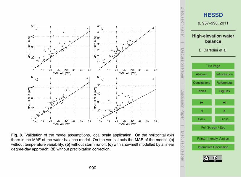
5 Discussion

To attain a parsimonious, yet realistic, representation of runoff regime in high-elevationbasins, various assumptions have been undertaken in the development of the proposedwater balance model: (i) a probabilistic representation of the sub-monthly temperaturevariability; (ii) the presence of a rainfall fraction SR, unavailable for evapotranspiration,5

that directly contributes to runoff; (iii) a quadratic dependency of snowmelt on temper-ature; and (iv) the adjustment of average annual basin precipitation dependent on themean annual observed runoff Rtot,obs or, if not available, on mean basin elevation. Inthe following, the motivations behind these hypotheses are discussed, along with someconsiderations on their consequences.10

Temperature is, beside precipitation, the main triggering variable of runoff formationin mountainous basins. For this reason, to properly describe the dynamics of snowaccumulation and melting, the temperature sub-monthly variability has been modelledthrough a logistic distribution (Eq. 2). To test this hypothesis, an alternative modelstructure, TEST1, that considers a constant monthly temperature, is developed. Fig-15

ure 8 a compares the MAE of the model proposed in this study (on the horizontal axis)to that obtained with the TEST1 model structure (on the vertical axis). Both modelsare applied at the local scale, and each point represents a basin of the study region.Since the majority of points is located above the 1:1 line, one can conclude that tak-ing into account the sub-monthly variability of temperature significantly improves the20

performances of the model. This was expected, since the TEST1 model has less pa-rameters than the standard model, but the improvement in the performances is largeenough to justify, in our opinion, the addition of a further model parameter. When thepartition of the months into periods of positive and negative temperature is allowed, twomain consequences can be observed depending on the catchment altitude: (i) at high25

elevations, during the cold season, the snow storage assumes smaller proportions, be-cause part of the monthly precipitation is allowed to contribute to runoff at the expenseof the snow storage; (ii) at middle elevations the parameter σ allows one to simulate

974





HESSD8, 957–990, 2011


E. Bartolini et al.

Title Page



Tables Figures

J I

J I

Back Close

Full Screen / Esc



Discussion

Paper

|D

iscussionP

aper|

Discussion

Paper

|D

iscussionP

aper|

the coexistence of snow accumulation, melt and evapotranspiration even when wintermonthly temperatures are slightly positive.

Another assumption of the water balance model consists, as previously mentioned,in considering a fraction of monthly rainfall, namely the storm runoff SR, that is notavailable for evapotranspiration. This water amount is used to roughly separate vol-5

umes related to heavy storms and infiltration into the soil, respectively. Using a di-agnostic plot similar to the one shown before, the storm runoff assumption is testedagainst the hypothesis of SR=0 (model TEST2 in Fig. 8b, vertical axis). TEST2 dif-fers from the original water balance in that all the monthly liquid rainfall firstly feeds theevapotranspiration, while only the remaining part contributes to runoff formation. The10

MAE associated to the model TEST2 is larger than the MAE associated to the modelwe propose in 37 basins out of 39, indicating that considering a fraction of storm runoffis a reasonable assumption. Moreover, in this case, the comparison is fair, becausethe two model structures have the same number of parameters. On a more physicalbasis, the positive effect of SR is important during the warm season, when net pre-15

cipitation (i.e., the difference between rainfall P + and evapotranspiration ETact) is verylow or equal to zero, and, without the contribute of SR, the simulated runoff would becomposed only by snowmelt, if any.

In Fig. 8c a comparison between the use of the parabolic law for snowmelt (Eq. 6)and the standard (i.e., linear) degree-day approach (TEST3) is reported. Again, al-20

most all the points are above the 1:1 line, demonstrating the ability of the proposedframework to better simulate snowmelt dynamics. This result can be explained by con-sidering that a common drawback of the degree-day method is related to the use ofa constant (i.e., not depending on the season) melt factor (see, e.g., chapter 6 in Singhand Singh, 2001). In contrast, the parabolic law allows one to simulate higher (lower)25

snowmelt rates in correspondence with largely (slightly) positive temperatures, with theadvantage of requiring only one parameter.

The last model assumption to discuss is related to the way we quantify the meanbasin precipitation undercatch, whose characterization is fundamental in high-elevation

975





HESSD8, 957–990, 2011


E. Bartolini et al.

Title Page



Tables Figures

J I

J I

Back Close

Full Screen / Esc



Discussion

Paper

|D

iscussionP

aper|

Discussion

Paper

|D

iscussionP

aper|

basins (Valery et al., 2010). In the case of basin-specific application, it is assumed thatthe correction depends only on the observed runoff and, consequently, on the modelbias. The effects of this assumption are shown in Fig. 8d, which reports the meanabsolute error of the model with (without) precipitation correction on the horizontal(vertical) axis. It can be noticed that the MAE, in this latter case, is significantly lower5

for almost all the basins.

6 Conclusions

A simple and parsimonious water balance model, particularly conceived for high-elevation regions, has been developed, primarily to reconstruct the shape of the runoffregime and the timing of its peaks. The model proves to be able to discern between dif-10

ferent mechanisms of runoff formation in the study domain, which is a transition regioncharacterized by headwater basins governed by snow dynamics and middle-elevationcatchments characterized by temperate regimes. The adoption of such a simple modelframework is motivated by the aim of identification of the main governing mechanismsaffecting the water balance at the monthly time-scale in high-elevation basins. More-15

over, the parsimony approach is essential in view of the extension of the proposedmethod to ungauged catchments.

The good results are encouraging. However, in the study region some problemsremain concerning the model results in some specific periods of the year. In partic-ular, most of the basins show runoff overestimation in October and underestimation20

during July or August. These systematic errors seem to be due principally to the highlysimplified model structure.

Concerning the possibility of applying and calibrating the model also in ungaugedcontexts, the regional parameter calibration procedure and the generalized precip-itation adjustment allows one to pass from the local scale to the regional scale,25

with the opportunity to investigate, with a simple and parsimonious approach, theinterplay among the different variables in the water balance. However, when the

976





HESSD8, 957–990, 2011


E. Bartolini et al.

Title Page



Tables Figures

J I

J I

Back Close

Full Screen / Esc



Discussion

Paper

|D

iscussionP

aper|

Discussion

Paper

|D

iscussionP

aper|

regional balance is applied, the summer underestimation becomes more critical forhigh-elevation basins, indicating that the generalized precipitation correction needs tobe ameliorated in terms of water volumes and seasonality. With respect to other re-gionalization procedures, the use of a water balance model to reconstruct runoff sea-sonality allows one to obtain not only runoff regimes but also the average volumes5

of actual evapotranspiration, SWE and snowmelt, generally not available at the basinscale, but fundamental to understand and reproduce the rainfall-runoff mechanismswhen snow dynamics are involved. Moreover, due to the driving role that temperaturehas in triggering snow accumulation, melt and evapotranspiration, the model is suitablefor preliminary investigation on the possible effects that global warming may have on10

the physical processes of the hydrologic cycle.

Appendix A

Measure of model quality

In order to evaluate the performances of the model, a quality index QI is introduced.15

The index is computed as a function of four quality indicators,

QI= f (σR,j ,MAE,b,tpeak), (A1)

that are the monthly measured runoff standard deviation σR,j , the mean absolute er-ror MAE, the model bias b, and the month tpeak in which the runoff peak occurs. Thechoice of a combination of measures is motivated by the fact that the assessment of the20

similarity between two curves, namely the simulated and observed mean runoff, hasto take into account several factors: the volume imbalance (i.e., bias), the differencesbetween the shape of the curves (i.e., the amplitude of the oscillations), representedby the MAE, and the model capability in predicting the timing of the runoff peak. More-over, since the evaluation of the model considers only mean seasonality curves, it is25

important to considers also the year to year runoff variability, represented by σR,j . It977





HESSD8, 957–990, 2011


E. Bartolini et al.

Title Page



Tables Figures

J I

J I

Back Close

Full Screen / Esc



Discussion

Paper

|D

iscussionP

aper|

Discussion

Paper

|D

iscussionP

aper|

is fair to assume that, if the simulated runoff falls inside the observed variability range,the model is able to adequately simulate the runoff formation mechanism.

The calculation of the QI requires to score these quality indicators. The monthlyrunoff standard deviation σR,j is used to calculate the 80% confidence bands under thehypothesis of normality as Robs,j ±1.28σR,j . These values are used as a threshold to5

count the number of months where simulated runoff falls outside the bands. The scores1, 0.75, 0.5, 0.25 and 0 are then assigned, to each basins, respectively for 1, 2, 3, and 5or more months characterized by mean monthly values outside the confidence bands.MAE and bias are divided into 5 equiprobable classes, whose limits are their respective0.2, 0.4, 0.6 and 0.8 quantiles. A score varying from 1 to 0 (i.e., 1, 0.75, 0.5, 0.25, 0) is10

assigned to each class. The timing of the peak is evaluated assigning a score 1 in caseof perfect timing and 0.5 in case of delay or anticipation. For middle-elevation basins,where runoff regime is sometimes characterized by two maxima corresponding to thespring snowmelt and fall peaks, only the global maximum is considered. The QI is thenobtained as the mean of the scores assigned to each factor.15

For example, the simulated runoff regime of river Sesia at Ponte Aranco, obtainedwith the application of the water balance at the local scale (Fig. 5), has the followingcharacteristics: (i) the runoff never falls outside the confidence bands (score 1); (ii) theMAE is equal to 21.73 mm and corresponds to the third equiprobable class, whoselimits are the 0.4 and the 0.6 quantiles (score 0.5); (iii) model bias b=14.66 mm falls in20

the fourth class, defined by the 0.2 and the 0.4 quantiles (score 0.75); (iv) the months ofthe simulated and the observed peak are concordant (score 1). Averaging the scoresassigned, one obtains QI=0.88, that is the value of the quality index assigned to thisbasin with respect to the local model application.

The quality index QI can be used to judge the quality of the reconstructed runoff25

regime by comparison with the other QI indices obtained using the same model struc-ture. This means that, given the model results, the QI can be used to discern basinswhere the simulated runoff well represents the measured one from basins where thewater balance performances are poor. On the contrary, due to the mechanism of score

978





HESSD8, 957–990, 2011


E. Bartolini et al.

Title Page



Tables Figures

J I

J I

Back Close

Full Screen / Esc



Discussion

Paper

|D

iscussionP

aper|

Discussion

Paper

|D

iscussionP

aper|

assignment based on quantiles, this QI cannot be used to compare the results of twodifferent modelling frameworks (i.e., local versus regional scale).

Supplementary material related to this article is available online at:http://www.hydrol-earth-syst-sci-discuss.net/8/957/2011/hessd-8-957-2011-supplement.pdf.5

Acknowledgements. The work was funded by the Italian Ministry of Education (CUBISTProject, grant 2007HBTS85).

References

Abramowitz, M. and Stegun, I. A.: Handbook of Mathematical Functions with Formulas, Graphs,and Mathematical Tables, Tenth Dover printing edition, Dover, New York, 1964. 96410

Adam, J. C., Hamlet, A. F., and Lettenmaier, D. P.: Implications of global climate changefor snowmelt hydrology in the twenty-first century, Hydrol. Process., 23, 962–972,doi:10.1002/hyp.7201, 2009. 959

Allamano, P., Claps, P., and Laio, F.: An analytical model of the effects of catch-ment elevation on the flood frequency distribution, Water Resour. Res., 45, W01402,15

doi:10.1029/2007WR006658, 2009a. 960, 967Allamano, P., Claps, P., and Laio, F.: Global warming increases flood risk in mountainous areas,

Geophys. Res. Lett., 36, L24404, doi:10.1029/2009GL041395, 2009b. 959Alley, W. M.: Water balance models in one-month ahead streamflow forecasting, Water Resour.

Res., 21, 597–606, 1985. 95920

Beniston, M., Diaz, H. F., and Bradley, R. S.: Climatic change at high elevation sites: anoverview, Climatic Change, 36, 233–251, 1997. 959

Beven, K.: Changing ideas in hydrology – the case of physically based models, J. Hydrol., 105,157–172, 1989. 960

Bras, R. L.: Hydrology, an Introduction to Hydrologic Science, Addison-Wesley, New York,25

1990. 965Chow, V. T.: Handbook of Applied Hydrology, McGraw-Hill, New York, USA, 1964. 961

979





http://www.hydrol-earth-syst-sci-discuss.net/8/957/2011/hessd-8-957-2011-supplement.pdf



HESSD8, 957–990, 2011


E. Bartolini et al.

Title Page



Tables Figures

J I

J I

Back Close

Full Screen / Esc



Discussion

Paper

|D

iscussionP

aper|

Discussion

Paper

|D

iscussionP

aper|

Claps, P., Giordano, P., and Laguardia, G.: Spatial distribution of the average air temperaturesin Italy: quantitative analysis, J. Hydrol. Eng., 13, 242–249, 2008. 967

Collins, D. N.: Rainfall-induced high-magnitude runoff events in highly-glacierized Alpinebasins, Hydrology, Water Resources and Ecology in Headwaters, Proceedings of the Head-Water’98 Conference, Merano, Italy, April 1998, IAHS Publication no. 248, 1998. 9625

Eder, G., Fuchs, M., Nachtnebel, H. P., and Loibl, W.: Semi-distributed modelling of the monthlywater balance in an alpine catchment, Hydrol. Process., 19, 2339–2360, 2005. 959

Gleick, P. H.: Methods for evaluating the regional hydrologic impacts of global climatic changes,J. Hydrol., 88, 99–116, 1986. 959

Henning, I. and Henning, D.: Potential evapotranspiration in mountain geoecosystems of differ-10

ent altitudes and latitudes, Mt. Res. Dev., 1, 267–274, 1981. 966Hock, R.: Temperature index melt modelling in mountain areas, J. Hydrol., 282, 104–115, 2003.

964Horton, P., Schaefli, B., Mezghani, A., Hingray, B., and Musy, A.: Assessment of climate-change

impacts on alpine discharge regimes with climate model uncertainty, Hydrol. Process., 20,15

2091–2109, 2006. 959Jasper, K., Calanca, P., Gyalistras, D., and Fuhrer, J.: Differential impacts of climate change on

the hydrology of two alpine river basins, Clim. Res., 26, 113–129, 2004. 959Johnson, N. L., Kotz, S., and Balakrishnan, N.: Continuous Univariate Distribution, vol. 2,

2nd edition, Wiley series in Probability and Statistics, Wiley & Sons, NY, USA, 1995. 96220

Kling, H., Furst, J., and Nachtnebel, H. P.: Seasonal, spatially distributed modelling of snowaccumulation and melting for computing runoff in a long-term, large-basin water balancemodel, Hydrol. Process., 20, 2141–2156, 2006. 962

Limbrunner, J. F., Vogel, R. M., and Chapra, S. C.: A parsimonious watershed model, in: Wa-tershed Models, edited by: Singh, V. P. and Frevert, D. K., CRC Press, Boca Raton, Florida,25

2006. 959, 960, 962Milly, P. C. D. and Dunne, K. A.: Macroscale water fluxes, 1. Quantifying errors in the estimation

of basin mean precipitation, Water Resour. Res., 38, 1205, doi:10.1029/2001WR000759,2002. 960, 968

Mouelhi, S., Michel, C., Perrin, C., and Andreassian, V.: Stepwise development of a two-30

parameter monthly water balance model, J. Hydrol., 318, 200–214, 2006. 960

980





HESSD8, 957–990, 2011


E. Bartolini et al.

Title Page



Tables Figures

J I

J I

Back Close

Full Screen / Esc



Discussion

Paper

|D

iscussionP

aper|

Discussion

Paper

|D

iscussionP

aper|

Schaefli, B., Hingray, B., Niggli, M., and Musy, A.: A conceptual glacio-hydrological model forhigh mountainous catchments, Hydrol. Earth Syst. Sci., 9, 95-109, doi:10.5194/hess-9-95-2005, 2005. 959

Sevruk, B.: Correction of measured precipitation in the Alps using the water equivalent of newsnow, Nord. Hydrol., 14, 49–58, 1983. 9685

Singh, P. S. and Singh, V. P.: Snow and Glacier Hydrology, Water Science and TechnologyLibrary, Kluwer Academic Publishers, Dordrecht, The Netherlands, 2001. 975

Sivakumar, B.: Dominant processes concept, model simplification and classification frameworkin catchment hydrology, Stoch. Environ. Res. Risk Assess., 22, 737–748, 2008. 960

Thornthwaite, W. C.: An approach toward a rational classification of climate, Geogr. Rev., 38,10

55–94, 1948. 965US Army Corps of Engineers: Runoff from snowmelt, 20314-1000 Manual, Department of the

Army, Washington, DC, 1998. 968, 973US Geological Survey (USGS): GTOPO30 Documentation, available at: http://edc.usgs.gov/

products/elevation/gtopo30/README.html, last access: 13 February, 2006. 96715

Valery, A., Andreassian, V., and Perrin, C.: Regionalization of precipitation and air temperatureover high-altitude catchments – learning from outliers, Hydrolog. Sci. J., 55, 928–940, 2010.960, 968, 976

Vandewiele, G. L. and Elias, A.: Monthly water balance of ungauged catchments obtained bygeographical regionalization, J. Hydrol., 170, 277–291, 1995. 96020

Wang, G., Xia, J., and Chen, J.: Quantification of effects of climate variations and humanactivities on runoff by a monthly water balance model: a casa study for the Chaobai RiverBasin in Northern China, Water Resour. Res., 26, 295–309, 2009. 959

Woods, R.: The relative role of climate, soil, vegetation and topography in determinig seasonaland long-term catchments dynamics, Adv. Water Resour., 26, 295–309, 2003. 96025

Woods, R.: Analytical model of seasonal climate impacts on snow hydrology: continuous snow-packs, Adv. Water Resour., 32, 1465–1481, 2008. 960, 962

Xia, Y. and Guoqiang, X.: Impacts of systematic precipitation bias on simulations of water andenergy balance in Northwest America, Adv. Atmos. Sci., 24, 739–449, 2007. 960

Xu, C., Seibert, J., and Halldin, S.: Regional water balance modelling in the nopex area: devel-30

opment and application of monthly water balance models, J. Hydrol., 180, 211–236, 1996.959

981





http://edc.usgs.gov/products/elevation/gtopo30/README.html



HESSD8, 957–990, 2011


E. Bartolini et al.

Title Page



Tables Figures

J I

J I

Back Close

Full Screen / Esc



Discussion

Paper

|D

iscussionP

aper|

Discussion

Paper

|D

iscussionP

aper|

Xu, C. Y. and Sing, V. P.: A review of monthly water balance models for water resources inves-tigations, Water Resour. Manag., 12, 31–50, 1998. 959

Zappa, M., Pos, F., and Strasser, U.: Seasonal water balance of an alpine catchment as eval-uated by different methods for spatially distributed snowmelt modelling, Nord. Hydrol., 34,179–202, 2003. 9595

Zierl, B. and Bugman, H.: Global change impacts on hydrological processes in alpine catch-ments, Water Resour. Res., 41, W02028, doi:10.1029/2004WR003447, 2005. 959

982





HESSD8, 957–990, 2011


E. Bartolini et al.

Title Page



Tables Figures

J I

J I

Back Close

Full Screen / Esc



Discussion

Paper

|D

iscussionP

aper|

Discussion

Paper

|D

iscussionP

aper|

Fig. 1. Qualitative representation of the structure of the water balance model. P is the inputto the system, divided into liquid (P +) and solid (P −) precipitation. SWE is the snow waterequivalent contained in the snow storage; T + represents positive temperatures; Mact is thesnowmelt and ETact the actual evapotranspiration.

983





HESSD8, 957–990, 2011


E. Bartolini et al.

Title Page



Tables Figures

J I

J I

Back Close

Full Screen / Esc



Discussion

Paper

|D

iscussionP

aper|

Discussion

Paper

|D

iscussionP

aper|

Fig. 2. Study domain and catchments used for the model application. Hatched (cross-hatched)basins are characterized by a negative (positive) budget between annual precipitation andrunoff. Gray-shaded areas indicate basins with positive budget that becomes negative whenaccounting for evapotranspiration losses.

984





HESSD8, 957–990, 2011


E. Bartolini et al.

Title Page



Tables Figures

J I

J I

Back Close

Full Screen / Esc



Discussion

Paper

|D

iscussionP

aper|

Discussion

Paper

|D

iscussionP

aper|

Fig. 3. Linear regression between mean basin elevation h and model bias b=Rtot,obs−Rtot,simfor the reference run. Dark triangles represent the model bias for each basin. The numbersrefer to the basin-ID, as reported in the Table in the Supplement. The regression is significantwith a level α=0.01 and a coefficient of determination R2

adj =0.676.

985





HESSD8, 957–990, 2011


E. Bartolini et al.

Title Page



Tables Figures

J I

J I

Back Close

Full Screen / Esc



Discussion

Paper

|D

iscussionP

aper|

Discussion

Paper

|D

iscussionP

aper|

Fig. 4. MAE sensitivity to the values of c and σ for river Evancon at Champoluc (local scaleapplication of the water balance model). Crosses represent the parameter combinations thatfulfill the condition over the depletion of the snow storage.

986





HESSD8, 957–990, 2011


E. Bartolini et al.

Title Page



Tables Figures

J I

J I

Back Close

Full Screen / Esc



Discussion

Paper

|D

iscussionP

aper|

Discussion

Paper

|D

iscussionP

aper|

Fig. 5. Observed (solid line) and simulated (dashed line) runoff regimes. Application at thelocal scale. Dark (light) grey area represents the confidence bands of the observed runoff at40% (80%). (a) Savara at Eau Rousse; (b) Sesia at Ponte Aranco; (c) Rutor at Promise (d)Toce at Candoglia.

987





HESSD8, 957–990, 2011


E. Bartolini et al.

Title Page



Tables Figures

J I

J I

Back Close

Full Screen / Esc



Discussion

Paper

|D

iscussionP

aper|

Discussion

Paper

|D

iscussionP

aper|

Fig. 6. Observed (solid line) and simulated (dashed line) runoff regimes. Application at theregional scale. Dark (light) grey area represents the confidence bands of the observed runoffat 40% (80%). (a) Savara at Eau Rousse; (b) Sesia at Ponte Aranco; (c) Rutor at Promise (d)Toce at Candoglia.

988





HESSD8, 957–990, 2011


E. Bartolini et al.

Title Page



Tables Figures

J I

J I

Back Close

Full Screen / Esc



Discussion

Paper

|D

iscussionP

aper|

Discussion

Paper

|D

iscussionP

aper|

Fig. 7. Comparison between the Quality Index QI obtained with the model application at thecatchment scale (light gray) and at the regional scale (dark gray). The basin numbers refer tothe table in the Supplement.

989





HESSD8, 957–990, 2011


E. Bartolini et al.

Title Page



Tables Figures

J I

J I

Back Close

Full Screen / Esc



Discussion

Paper

|D

iscussionP

aper|

Discussion

Paper

|D

iscussionP

aper|

Fig. 8. Validation of the model assumptions, local scale application. On the horizontal axisthere is the MAE of the water balance model. On the vertical axis the MAE of the model: (a)without temperature variability; (b) without storm runoff; (c) with snowmelt modelled by a lineardegree-day approach; (d) without precipitation correction.

990





Runoff regime estimation at high-elevation sites: a parsimonious water balance approach

Documents

Transcript of Runoff regime estimation at high-elevation sites: a parsimonious water balance approach