Coastal Water Quality Impact of Stormwater Runoff from an ...

Comment Letters Received from Academia

� Dr. Jenny Jay

� Dr. Richard Horner

� UCLA La Kretz Center

Coastal Water Quality Impact ofStormwater Runoff from an UrbanWatershed in Southern CaliforniaJ O N G H O A H N , † S T A N L E Y B . G R A N T , * , †

C R I S T I A N E Q . S U R B E C K , †

P A U L M . D I G I A C O M O , ‡

N I K O L A Y P . N E Z L I N , § A N DS U N N Y J I A N G |

Department of Chemical Engineering and Materials Science,Henry Samueli School of Engineering, University ofCalifornia, Irvine, California 92697, Jet PropulsionLaboratory, California Institute of Technology, Pasadena,California 91109, Southern California Coastal Water ResearchProject, Westminster, California 92683, and Department ofEnvironmental Health, Science, and Policy, School of SocialEcology, University of California, Irvine, California 92697

Field studies were conducted to assess the coastal waterquality impact of stormwater runoff from the Santa AnaRiver, which drains a large urban watershed located insouthern California. Stormwater runoff from the river leadsto very poor surf zone water quality, with fecal indicatorbacteria concentrations exceeding California ocean bathingwater standards by up to 500%. However, cross-shorecurrents (e.g., rip cells) dilute contaminated surf zone waterwith cleaner water from offshore, such that surf zonecontamination is generally confined to <5 km around theriver outlet. Offshore of the surf zone, stormwater runoffejected from the mouth of the river spreads out over a verylarge area, in some cases exceeding 100 km2 on thebasis of satellite observations. Fecal indicator bacteriaconcentrations in these large stormwater plumes generallydo not exceed California ocean bathing water standards,even in cases where offshore samples test positive for humanpathogenic viruses (human adenoviruses and enteroviruses)and fecal indicator viruses (F+ coliphage). Multiplelines of evidence indicate that bacteria and viruses in theoffshore stormwater plumes are either associated withrelatively small particles (<53 µm) or not particle-associated.Collectively, these results demonstrate that stormwaterrunoff from the Santa Ana River negatively impacts coastalwater quality, both in the surf zone and offshore. However,the extent of this impact, and its human health significance,is influenced by numerous factors, including prevailing oceancurrents, within-plume processing of particles andpathogens, and the timing, magnitude, and nature ofrunoff discharged from river outlets over the course of astorm.

IntroductionOceans adjacent to large urban areas, or “urban oceans”, arethe final repositories of pollutants from a myriad of pointand nonpoint sources of human waste (1). Pollutants aretransported to the urban ocean by surface water runoff(1-4), discharge of treated sewage through submarine outfalls(5), wet and dry deposition of airborne pollutants (6), andsubmarine discharge of contaminated groundwater (7). Untilrecently, effluent from sewage treatment plants was oftenthe primary source of urban coastal pollution, includingnutrients, pathogens, pesticides, and heavy metals (8).However, pollutant loading from many sewage treatmentplants has declined over the past several decades because ofimprovements in civil infrastructure (e.g., separation of thestorm and sanitary sewer systems to prevent combined seweroverflows), pollutant source control, and disposal/treatmenttechnology (9). As a result, surface water runoff, in manycases, has supplanted sewage treatment plants as the primarysource of pollutant loading to the urban ocean (3, 10).

The focus of this study is the coastal water quality impactof surface water runoff during storms, or “stormwater runoff”,from an urban watershed in southern California. The studywas motivated by several considerations. First, beneficial usedesignations for the coastal ocean in southern Californiaapply year-round and, consequently, watershed managersare legally required to develop stormwater management plansfor reducing wet-weather impairments of the coastal ocean(11). The impact of stormwater runoff on coastal water qualityis of particular concern in arid regions such as southernCalifornia because, on an annual basis, a large percentage(>99.9% according to Reeves et al. (2) and >95% accordingto Schiff et al. (10)) of the surface water runoff and associatedpollution flows into the ocean during a few storms in thewinter. Second, while recreational use of the coastal oceanin southern California is lighter in the winter, compared tothe summer, winter ocean recreation is still very common,particularly among surfers who surf the large waves that oftenaccompany storm events (R. Wilson, personal communica-tion). Third, to the extent that particles in stormwater runoffare associated with pathogens and other contaminants, theirdischarge to the ocean during storms may serve as a sourceof near-shore pollution that persists long after the stormseason is over (10, 12). Finally, in many urban watershedsin southern California and elsewhere, the flow of stormwaterrunoff is highly regulated by civil infrastructure (e.g., dams)designed to minimize flood potential and maximize waterreclamation. As will be demonstrated later in this paper, theregulated nature of stormwater runoff implies that the oceandischarge of stormwater runoff from urban watersheds canoccur days after the cessation of rain, when the potential forhuman exposure to pathogens by marine recreational contactis significant.

This paper describes how stormwater runoff from severalmajor rivers in southern California, with particular focus onthe Santa Ana River in Orange County, impacts coastal waterquality, as measured by turbidity, particle size spectra, totalorganic carbon, fecal indicator bacteria, fecal indicatorviruses, and human pathogenic viruses. The present studyis unique in the combination of data resources utilized,including data and information from routine surf zone waterquality and wave field monitoring programs, an automatedin-situ ocean observing sensor, shipboard sampling cruises,and satellite sensors. Further, this is the first wet weatherstudy to examine the linkage between water quality in thesurf zone, where routine monitoring samples are collected

* Corresponding author phone: (949)824-7320; fax: (949)824-2541;e-mail: [email protected].

† Henry Samueli School of Engineering, University of California.‡ California Institute of Technology.§ Southern California Coastal Water Research Project.| School of Social Ecology, University of California.

Environ. Sci. Technol. 2005, 39, 5940-5953

5940 9 ENVIRONMENTAL SCIENCE & TECHNOLOGY / VOL. 39, NO. 16, 2005 10.1021/es0501464 CCC: $30.25 © 2005 American Chemical SocietyPublished on Web 07/15/2005

and most human exposure occurs, and water quality offshoreof the surf zone. The work described in this study was carriedout in parallel with a watershed-focused study that examinedthe spatial variability of fecal indicators, and the relationshipbetween suspended particle size and fecal indicators, in stormrunoff from the Santa Ana River watershed (13). Backgroundinformation is available elsewhere on coastal water qualityimpairment at our Orange County field site (2, 14-18) andthe transport and mixing dynamics of sediment plumes asthey flow into the coastal ocean from river outlets in southernCalifornia (4, 19, 20).

Materials and MethodsRainfall and River Discharge. Weather information and NextGeneration Radar (NEXRAD) images for planning the fieldstudies and interpreting rainfall patterns were obtained on-line from the National Weather Service (http://www.

nwsla.noaa.gov/). Precipitation and stream discharge datawere obtained at two sites, one located where the Santa AnaRiver crosses 5th Street in the City of Santa Ana and anotherlocated where the San Gabriel River crosses Spring Street inthe City of Long Beach (black squares in inset, Figure 1).These data were obtained, respectively, from the U.S. ArmyCorps of Engineers and the Los Angeles County Departmentof Public Works. Both of these gauge sites are located relativelyclose (within 11 km) to the rivers’ respective ocean outlets,and hence streamflow measured at these sites will likely makeits way to the ocean.

Surf Zone Measurements: NEOCO Data. Time series ofwater temperature, conductivity, chlorophyll, and waterdepth were obtained from an instrument package deployedat the end of the Newport Pier, where the local water depthis between 6.5 and 9 m (blue star in Figure 1). This instrumentpackage is part of a recently deployed network of coastal

FIGURE 1. Map showing location of field site and sampling sites in the surf zone and offshore. Also shown are the locations of the NEOCOsensor on the end of the Newport Pier and the rain and stream gauges located on the Santa Ana River and the San Gabriel River.Abbreviations are Los Angeles River (LAR), San Gabriel River (SGR), Santa Ana River (SAR), Orange County Sanitary District (OCSD), andUniversity of California, Irvine (UCI).

VOL. 39, NO. 16, 2005 / ENVIRONMENTAL SCIENCE & TECHNOLOGY 9 5941

sensors in southern California called the Network forEnvironmental Observations of the Coastal Ocean (NEOCO).The NEOCO sensor package contains an SBE-16plus CTD(Sea-Bird Electronics, Inc., Bellevue, WA) and a SeapointChlorophyll Fluorometer (Seapoint Sensors, Inc.). Theseinstruments are mounted on a pier piling at a depth ofapproximately 1 m (below mean lower low water) and areprogrammed to acquire data at a sampling frequency of 0.25min-1.

Surf Zone Measurements: Fecal Indicator Bacteria andBreaking Waves. The concentration of fecal indicator bacteriain the surf zone was measured at 17 stations (black circlesalong shoreline in Figure 1) by personnel at the OrangeCounty Sanitation District (OCSD). The stations are desig-nated by OCSD according to their distance (in thousands offeet) north or south of the Santa Ana River outlet (e.g., station15N is located approximately 15 000 ft, approximately 5 km,north of the Santa Ana River outlet). Water samples werecollected 5 days per week (not on Friday and Sunday) from5:30 to 10:00 local time at ankle depth on an incoming wave,placed on ice in the dark, and returned to the OCSD (FountainValley, CA) where they were analyzed within 6 h of collectionfor total coliform (TC), fecal coliform (FC), and enterococcibacteria (ENT) using standard methods 9221B and 9221Eand EPA method 1600, respectively. Results are reported inunits of colony forming units per 100 mL of sample (CFU/100 mL). Wave conditions, including both the direction andheight of breaking waves, were recorded by lifeguards at theNewport Beach pier (near surf zone station 15S, Figure 1)twice per day, once at 7:00 and again at 14:00 local time.

Offshore Measurements: Satellite Ocean Color Imagery.The satellite images used in this study were collected byNASA’s Moderate-Resolution Imaging Spectroradiometer(MODIS) instruments. These instruments operate onboardtwo near-polar sun-synchronous satellite platforms orbitingat 705 km altitude: Terra (since February 24, 2000) and Aqua(since June 24, 2002). Terra passes across the equator fromnorth to south at !10:30 local time, while Aqua passes theequator south to north at !13:30 local time. As such, all theimages were acquired within 2 h before or after local noonor between 18:00 and 22:00 UTC. The MODIS sensors collectdata in 36 spectral bands, from 400 to 14 000 nm. We utilizedbands 1 (250-m spatial resolution, 620-670 nm), 3, and 4(500-m resolution, 459-479 and 545-565 nm, respectively)to produce “true color” (i.e., RGB) images, with band 1 usedfor the red channel, band 4 for the green channel, and band3 for the blue channel. Using a MATLAB program, the 500-mgreen (band 4) and blue (band 3) monochrome channelswere “sharpened” to 250-m resolution using fine details fromthe higher resolution red channel (band 1). Then, the contrastof each of these monochrome channels was increased toemphasize maximum details in the coastal ocean region ofinterest. Finally, all three monochrome channels (i.e., red,green, and blue) were combined to form a single true colorimage. In all, 16 satellite images from February 23 to March5 were acquired and processed for this study; four of themwere selected as most illustrative, on the basis of their qualityand observed features. The timing of these satellite acquisi-tions relative to the storms and sampling periods is indicatedat the top of Figure 2.

Offshore Measurements: Sampling Cruises. The offshoremonitoring grid (red triangles in Figure 1) was sampled duringthree separate cruises on February 23, February 28, and March1, 2004, coinciding with a sequence of storm events in lateFebruary 2004. Table 1 provides a summary of activitiesperformed during each cruise. A short description of theoffshore sampling and analysis protocols is presented here;details can be found in the Supporting Information for thispaper. All offshore water samples were analyzed for salinityand fecal indicator bacteria, specifically, total coliform (TC),

Escherichia coli (EC, a subset of FC), and enterococci bacteria(ENT), using the defined substrate tests known commerciallyas Colilert-18 and Enterolert (IDEXX, Westbrook, ME)implemented in a 97-well quantitray format; results arereported in units of most probable number of bacteria per100 mL of sample (MPN/100 mL). A subset of the offshorewater samples was analyzed for total organic carbon (TOC)by U.S. EPA Method 415.1, fecal indicator viruses (F+

coliphage) by a two-step enrichment method (U.S. EPAMethod 1601), and human pathogenic viruses (humanadenovirus and human enterovirus) by real-time quantitativepolymerase chain reaction (Q-PCR), nested PCR, and reverse-transcriptase (RT)-PCR using published protocols (21-25).Details on the PCR protocols used here can be found in theSupporting Information for this paper.

Coincident with the collection of the offshore watersamples, temperature, particle size spectra, and light trans-missivity were measured using an LISST-100 (laser in situscattering and transmissometry) analyzer (Sequoia Scientific,Inc., Bellevue, WA). The LISST-100 estimates the particlevolume per unit fluid volume (!V) resident in 32 logarithmi-cally spaced particle diameter bins ranging in size from dp

) 2.5 to 500 µm. At least 10 replicates of the particle sizespectra were collected at each offshore station. Followingthe recommendation of Mikkelsen (26), !V was taken as themedian of all replicate measurements. The LISST-100 dataare presented in this paper in one of three ways: (1) particlesize spectra represented by plots of !V/!log dp against logdp, (2) the number of particles per unit fluid volume or totalnumber concentration (TNC), and (3) the number-averagedparticle size, dh. The last two parameters were computed fromthe particle size spectra as follows (26, 27):

Results and DiscussionRainfall and River Discharge. Over the period of study(February 18 through March 3, 2004), four rain events wererecorded by the rain gauge on the Santa Ana River in the Cityof Santa Ana (black curve, top panel, top axis, Figure 2). Thefirst event accumulated 16.0 mm of rain in the afternoon ofFebruary 21 (RE1 in Figure 2), the second event accumulated23.4 mm of rain in the afternoon of February 22 (RE2), thethird event accumulated 51.3 mm of rain in the evening ofFebruary 25 (RE3), and the fourth event accumulated 6.8 mmof rain in the evening of March 1 (RE4). The rain gauge locatedon the San Gabriel River in the City of Long Beach did notrecord RE2 but recorded a fifth rain event on February 18(red curve, top panel, top axis, Figure 2). The difference inrainfall recorded at the Santa Ana River and the San GabrielRiver sites is a consequence of the spatial variability of rainfallnear the coast (see Figures S1 and S2, Supporting Information,for NEXRAD maps acquired during RE1 and RE2). Records ofstream discharge (in units of m3/s) at the Santa Ana Riverand the San Gabriel River sites are also quite different (blackand red curves, top panel, bottom axis, Figure 2). While rainfalland stream discharge are coupled at the San Gabriel Riversite (i.e., stream discharge increases shortly after locallyrecorded rain events, compare set of red curves in top panel,Figure 2), rainfall and stream discharge are frequentlyuncoupled at the Santa Ana River site. For example, the SantaAna River discharge events DE3 and DE4 do not obviouslycorrelate with records of local rainfall. Instead, these twodischarge events can be traced to stormwater runoff gener-ated from inland regions of the Santa Ana River watershed

TNC )∑i)1

32 6!Vi

!dp,i3

(1a)

dh ) "36!∑i)1

32 !Vi

TNC(1b)

5942 9 ENVIRONMENTAL SCIENCE & TECHNOLOGY / VOL. 39, NO. 16, 2005

that was released from inland dams after the cessation ofrain (13). For comparison, we have also included in the plothourly volume discharge records (unit of m3/s, blue curve,

top panel, Figure 2) of treated sewage discharged from theOrange County Sanitation District (OCSD) sewage outfall(courtesy of OCSD).

FIGURE 2. Time series measurements of rainfall, stream discharge at the Santa Ana River and San Gabriel River, and discharge of treatedsewage from the OCSD outfall (top panel); water level, salinity, temperature, and chlorophyll measured at the NEOCO sensor (second andthird panels); the direction and height of breaking waves at the Newport Beach Pier (fourth panel); and the concentration of fecal indicatorbacteria in the surf zone (color contour plots, fifth through seventh panels). Shown at the top of the figure is the timing of the satelliteimages (blue lettering) and the offshore sampling cruises (black squares).


Surf Zone Measurements: NEOCO Data. Water level,salinity, temperature, and chlorophyll measurements at theNEOCO sensor, located on the end of the Newport Pier atthe offshore edge of the surf zone, are presented in Figure2 (second and third panels). The largest rain event (RE3) andthe largest discharge of stormwater runoff from the SantaAna River (DE4) occurred during a neap tide when the dailytide range was small (see quarter moon and water levelmeasurements in the second panel, Figure 2). The otherrainfall and stream discharge events occurred during periodsof time when the daily tide range was larger, either duringthe transition from spring to neap tide (RE1, RE2, DE1, DE2,DE3) or during the transition from neap to spring tide (RE4,DE5).

Salinity recorded at the NEOCO sensor is characterizedby a series of low salinity events, relative to ambient oceanwater salinity of 32.5-33.0 ppt (salinity events SE1-SE6, Figure2). These low salinity events may be caused, at least in part,by stormwater discharged from the Santa Ana River (e.g., SE6

appears to be related to DE4). However, correlating dischargeand the low salinity events is complicated by the fact thatonce river water is discharged to the ocean, its offshoretransport is controlled by a complex set of near-shore currents(28). These near-shore currents, and their impact on thespatial distribution of stormwater runoff plumes, are exploredin the next several sections. Temperature and chlorophyllrecords at the NEOCO sensor appear to be relativelyunaffected by rainfall or discharge from the Santa Ana River.Surf zone temperature exhibits a diurnal pattern consistentwith solar heating (i.e., temperatures are higher during theday and lower at night). Chlorophyll measurements indicatea bloom event occurred early in the study period (bloomevent 1, BE1), but this bloom event mostly dissipated priorto the rain and discharge events that occurred later. Whilethe chlorophyll fluorometer was being maintained duringthis period, we cannot rule out the possibility that thedownward trend in the chlorophyll signal is related toinstrument fouling.

Surf Zone Measurements: Wave Data and Along-ShoreCurrents. Wave conditions, including the direction andheight of breaking waves, were recorded twice per day bylifeguards stationed at the Newport Pier (surf zone station15S, Figure 1). These wave data, which are plotted in thefourth panel of Figure 2, can be divided into five events,depending on whether waves approach the beach from thewest (WE1, WE3, and WE5) or from the south to southwest(WE2 and WE4). Because this particular stretch of shorelinestrikes northwest-southeast (see Figure 1), waves approach-ing the beach from the west are likely to yield a down-coastsurf zone current (i.e., directed to the southeast). Likewise,waves approaching the beach from the south are likely toyield an up-coast surf zone current (i.e., directed to thenorthwest) (28, 29).

This expectation is consistent with the salinity signalmeasured at the NEOCO sensor, which is located ap-proximately 5 km down-coast of the Santa Ana River oceanoutlet. The onset of low salinity event SE6 at the NEOCOsensor coincides very closely in time with the change in waveconditions from WE2 to WE3 and a likely change in thedirection of the surf zone current from up-coast to down-coast (Figure 2). Discharge from the Santa Ana River wasparticularly high during this period (discharge event DE4

overlaps wave events WE2 and WE3). Hence, the onset of SE6

was probably triggered by a change in the direction of wave-driven surf zone currents from up-coast during WE2 to down-coast during WE3 and a consequent down-coast transport ofstormwater runoff entrained in the surf zone from the SantaAna River during DE4.

Employing the same logic, low salinity events SE3-SE5,which occurred during a period when waves were out of theTA

BLE

1.Su

mm

ary

ofAn

alys

esPe

rform

eddu

ring

the

Sam

plin

gCr

uise

s

num

bero

foffs

hore

site

ssa

mpl

ed

sam

plin

gpa

ram

eter

sm

etho

dsFe

brua

ry23

,200

4Fe

brua

ry28

,200

4M

arch

1,20

04

cond

uctiv

itya

Ther

mo

Ori

on16

2Aor

CTD

(SB

E-32

)20

2121

tem

pera

ture

bth

erm

ocou

ple

w/L

ISS

T-10

0or

CTD

(SB

E-32

)20

2121

tota

lcol

iform

, Esc

heri

chia

coli,

ente

roco

ccus

cC

olile

rtan

dEn

tero

lert

(IDEX

X)

20(+

2se

tsof

frac

tiona

ted

sam

ples

)21

(+6

sets

offr

actio

nate

dsa

mpl

es)

21

tota

lorg

anic

carb

ond

EPA

415.

117

(+2

sets

offr

actio

nate

dsa

mpl

es)

hum

anad

enov

irus

es&

ente

rovi

ruse

s5ne

sted

PCR

RT-

PCR

26

feca

lind

icat

orvi

ruse

s(F

+co

lipha

ge)e

two-

step

enri

chm

ent

26

part

icle

size

spec

tra

LIS

ST-

100

(ligh

tdiff

ract

ion)

2016

21tr

ansm

issi

vity

LIS

ST-

100

2016

21a

Mea

sure

dus

ing

aTh

erm

oO

rion

162A

cond

uctiv

itym

eter

onFe

brua

ry23

and

aC

TDin

stru

men

t(S

BE-

32)o

nFe

brua

ry28

and

Mar

ch1.

bM

easu

red

usin

ga

ther

moc

oupl

ebu

ndle

dw

ithan

LIS

ST-

100

onFe

brua

ry23

and

aC

TDin

stru

men

t(S

BE-

32)

onFe

brua

ry28

and

Mar

ch1.

cS

ampl

esco

llect

edby

UC

Iand

anal

yzed

byO

CS

Don

Febr

uary

23an

dco

llect

edan

dan

alyz

edby

OC

SD

onFe

brua

ry28

and

Mar

ch1.

Frac

tiona

ted

sam

ples

colle

cted

and

anal

yzed

byU

CIo

nFe

brua

ry23

and

28.d

Col

lect

edby

UC

Iand

anal

yzed

byD

elM

arA

naly

tical

(Irvi

ne,C

A).

eC

arri

edou

ton

the

frac

tiona

ted

sam

ples

and

mea

sure

dus

ing

are

al-t

ime

PCR

for

ente

rovi

rus

and

ane

sted

PCR

for

aden

ovir

us.


south to southwest, may have originated from stormwaterdischarged by river outlets or embayment located down-coast of the NEOCO sensor (e.g., the Newport Bay outlet).Low salinity events SE1 and SE2, which occurred during aperiod when waves were out of the west, may have originatedfrom stormwater discharged by outlets located up-coast ofthe NEOCO sensor, although no significant discharge fromthe Santa Ana River was recorded during this period of time.

Some of these low salinity events may have originatedfrom the cross-shore transport of lower salinity water fromoffshore, perhaps from surface runoff plumes or submarinewastewater fields associated with local sewage outfalls (16),or from the submarine discharge of low salinity groundwater(7). While the power-plant cooling water intake and outfallappear to affect local circulation patterns offshore ofHuntington Beach (30), the power-plant effluent consists ofpure ocean water and therefore is very unlikely to be a sourceof the low salinity events documented in Figure 2. It istheoretically possible that the OCSD sewage outfall is a sourceof SE1 and SE2, although there is nothing unusual about thesewage discharge rates observed during these two periodsof time (compare SE1 and SE2 with the blue curve, top panel,Figure 2).

Surf Zone Measurements: Fecal Indicator Bacteria. Theconcentrations of the three fecal indicator bacteria groups(TC, FC, and ENT) in the surf zone are presented as a set ofcolor contour plots in Figure 2 (bottom three panels). Fecalindicator bacteria concentrations were log-transformed tovisualize the temporal and spatial variability associated withthese measurements. For comparison, the California single-sample standards for the three fecal indicator bacteria (104

for TC, 102.602 for FC, and 102.017 for ENT, all CFU or MPN/100mL) are indicated by a set of arrows on the scale bar in thefigure. The concentration of fecal indicator bacteria wasfrequently elevated around the ocean outlet of the Santa AnaRiver (near surf zone station 0), particularly during and afterrain events when stormwater was discharging from the river.For example, during stormwater discharge events (DE3 andDE4), water quality around the Santa Ana River outlet wasvery poor (see water quality events TC2, FC2, and ENT2 inFigure 2). During this period of time, fecal indicator bacteriaconcentrations around the Santa Ana River outlet frequentlyexceeded one or more state standards, in some cases by asmuch as 300-500% (depending on the fecal indicator group).

The spatial distribution of fecal indicator bacteria in thesurf zone around the Santa Ana River outlet appears to becontrolled by local wave conditions, in a manner consistentwith the earlier discussion of wave-driven surf zone currents.When waves approach the beach from the west and down-coast currents are likely to prevail, the concentration of fecalindicator bacteria in the surf zone is higher on the down-coast side of the ocean outlet (compare WE1 with TC1, FC1,ENT1 and WE3 with TC3, FC3, ENT3). Likewise, when wavesapproach the beach from the south and up-coast currentsare likely to prevail, the concentration of fecal indicatorbacteria in the surf zone is higher on the up-coast side of theocean outlet (compare WE2 with TC2, FC2, ENT2). Theexception is a short period of time when relatively small waves(wave height<0.5 m) approach the beach from the southwestand the concentration of fecal indicator bacteria is higher onthe down-coast side of the river (compare WE4 with TC4, FC4,ENT4). This exception can be rationalized by noting that wavesout of the southwest break with their crests parallel to thebeach, and hence the direction of long-shore transport inthe surf zone is likely to be unpredictable under theseconditions. The apparent time delay between change in wavedirection (e.g., from WE1 to WE2) and change in the spatialdistribution of fecal indicator bacteria around the Santa AnaRiver outlet (e.g., from TC1 to TC2) is, at least in part, asampling artifact. Wave height and direction were recorded

twice per day while fecal indicator bacteria concentrationsin the surf zone were sampled at most once per day (the graydots in the color contour plots indicate the timing of surfsamples at each station).

Stormwater runoff discharged from the Santa Ana Riverappears to severely impact water quality in the surf zoneover a fairly limited stretch of the beach (<5 km either sideof the river between surf zone stations 15N and 15S). Thisspatial confinement of stormwater plumes in the surf zone,which is particularly evident for FC and ENT, could be theresult of physical transport processes (e.g., dilution by ripcell mediated exchange of water between the surf zone andoffshore) or nonconservative processes (e.g., the removal offecal indicator bacteria from the surf zone by die-off orsedimentation) (28, 29). An analysis of historical fecalindicator bacteria measurements at Huntington Beachconcluded that the length of surf zone impacted by pointsources of fecal indicator bacteria, such as the Santa AnaRiver, is influenced more by rip cell dilution and less bynonconservative processes such as die-off (31). The decaylength scale reported here of 5 km is very close to the lengthscale predicted by rip cell dilution alone (2-4 km, assuminga rip cell spacing of 0.5 km) (31). Hence, die-off probablyplays a secondary role, compared to dilution, in limiting thedistance over which water quality is impaired in the surfzone by stormwater runoff from the Santa Ana River.

Fecal indicator bacteria events also occur in the surf zoneat the northern (events TC6, TC7, ENT6, ENT7) and southern(events TC5, FC5, and ENT5) edges of our study area. Possiblesources of these fecal indicator bacteria events includestormwater discharged from the Huntington Harbor andNewport Bay Harbor located at the extreme northern (5 kmup-coast of station 39N) and southern (stations 27S and 29S)ends of the study site and, possibly, from river outlets locatedoutside of the study area (e.g., the Los Angeles River and SanGabriel River, see inset in Figure 1). Boehm and co-workers(32, 33) suggested that the OCSD sewage outfall might be asource of fecal indicator bacteria in the surf zone atHuntington Beach, particularly during dry weather summerperiods. However, compared to the Santa Ana River, thesewage outfall probably had a negligible impact on surf zonewater quality at Huntington Beach and Newport Beach duringthe storm events sampled in this study. This conclusion isbased on the following evidence. First, during our studyperiod, sewage effluent discharged by OCSD was chlorinatedand the fecal indicator bacteria concentrations in the finaleffluent (mean of 6000, 400, and 100 MPN/100 mL for TC,EC, and ENT, n ) 17, C. McGee, personal communication)were significantly below the concentration of fecal indicatorbacteria measured in stormwater runoff from the Santa AnaRiver (mean 17000, 5000, and 8000 MPN/100 mL for TC, EC,and ENT, n ) 30, Surbeck et al. (13)). Second, the peakdischarge rate from the OCSD outfall (ca. 13 m3/s) is muchsmaller than the peak discharge rate of stormwater runofffrom the Santa Ana River (ca. 300 m3/s) (compare blue andblack curves, second panel, Figure 2). Third, the sewageeffluent is discharged 6 km offshore of the surf zone througha 1-km-long diffuser located at the end of OCSD’s submarineoutfall at a water depth of approximately 60 m (hatched regionof the outfall pipe in Figure 1). By contrast, stormwater runofffrom the Santa Ana River is discharged into the ocean directlyat the surf line.

Offshore Measurements: Satellite Ocean Color Imagery.The spatio-temporal distributions of offshore stormwaterrunoff plumes sampled during this study are revealed byMODIS true color satellite imagery of a 100-km stretch of thecoastline centered around our field site (Figure 3). Themonitoring grid sampled during the offshore cruises isdepicted on the satellite images by yellow dots. The timingof the satellite passes, relative to rain events, discharge events,


wave events, surf zone water quality events, and offshoresampling cruises, is indicated at the top of Figure 2.

Generally speaking, in this collection of true color imagerythe stormwater runoff plumes appear to be characterized bya band of turbid water turquoise to brown in appearancethat is observed along the entire imaged region, althoughboth cross-shelf and along-shore gradients in the colorsignature are evident. Following the rain events on February21-22 (total of 39.4 mm, see RE1 and RE2 in Figure 2), aMODIS Aqua imagery from February 23 demonstrates thecross-shelf extent of the runoff plume to be variable, rangingfrom under 1 km in some places to more than 10 km offshoreof the Los Angeles River and San Gabriel River (Figure 3A).At our study site, which is centrally located within this broadregion, a distinct and apparently heavily particulate-ladenrunoff plume was observed in the vicinity of the Santa AnaRiver outlet and nearby station 2201 (see Figure 1 fornumerical designation of offshore sampling sites). The SantaAna River plume extended offshore past station 2203, withan apparent turn down-coast (i.e., southeast), continuingpast stations 2104 and 2024. During this time, breaking waveswere out of the south and the transport direction of fecalindicator bacteria in the surf zone was directed up-coast,opposite the apparent transport direction of stormwaterplumes offshore of the surf zone (compare timing of satelliteimage 1 with WE2 and fecal indicator bacteria events TC2,FC2, and ENT2, Figure 2). It also appears that a portion of theLos Angeles River and the San Gabriel River stormwaterplumes may have advected south and comingled with theSanta Ana River stormwater plume. Further south, offshoreparticulate loadings off the Newport Bay outlet (station 2001)do not appear to be as large as those off the Santa Ana Riveroutlet.

A MODIS image on February 27 revealed two distinctplumes of considerable size and offshore extent (Figure 3B).

This satellite acquisition preceded by 1 day the samplingcruise on February 28 (described in the next section), followedthe large precipitation event on February 25-26 (total of51.3 mm, see RE3 in Figure 2), and followed the large dischargeevent from the Santa Ana River (DE4, in Figure 2). The plumeto the northwest in this image appears to be associated withthe Los Angeles River or the San Gabriel River outlets, withan approximate areal extent of 450 km2. The plume to thesoutheast appears to be distinct from the former plume andlikely originated from the Santa Ana River outlet, with anapproximate areal extent of 100 km2 (the presumptive LosAngeles River, San Gabriel River, and Santa Ana River plumesare delineated by red lines in Figure 3B). The February 27Santa Ana River stormwater plume is considerably larger insize than the one observed on February 23 (compare Figure3A and 3B), consistent with the very large volume of waterdischarged from the Santa Ana River just prior to this satelliteacquisition (approximately 4 # 107 m3, see DE4 in Figure 2).Further, the Los Angeles River, San Gabriel River, and SantaAna River runoff plumes on February 27 differed from thoseon February 23 in that they penetrated farther offshore (30km compared to 10 km) and thus potentially transported moresediments into the deep waters of the San Pedro Channel.

The jetlike appearance of the presumptive Los AngelesRiver, San Gabriel River, and Santa Ana River stormwaterrunoff plumes in Figure 3B has been observed elsewhere inthe Southern California Bight, for example, off the Santa ClaraRiver discharge (4, 29), and is potentially the result of inertia-driven flow. At the time of this second satellite acquisition,breaking waves out of the west, and along-shore transportin the surf zone and offshore of the surf zone, appear to bedirected down-coast (compare timing of satellite image 2with WE3 and fecal indicator events TC3, FC3, and ENT3).

Subsequent MODIS true color imagery on February 28(Figure 3C) and February 29 (Figure 3D) indicates that both

FIGURE 3. MODIS Terra and Aqua true color satellite imagery of stormwater runoff plumes along the San Pedro Channel, California, withnominal spatial resolution of 250 m. Yellow dots indicate location of field sampling stations offshore of Huntington and Newport Beach;black arrows denote the Los Angeles River (LAR) outlet, San Gabriel River (SGR) outlet, Santa Ana River/Talbert Marsh (SAR/TM) outlet,and Newport Bay outlet. (A) MODIS-Aqua, February 23, 2004, at 21:00 UTC (13:00 local time), (B) MODIS-Aqua, February 27, 2004, at 20:35UTC (12:35 local time), (C) MODIS-Aqua, February 28, 2004, at 21:20 UTC (13:20 local time), (D) MODIS-Terra, February 29, 2004, at 18:50UTC (10:50 local time).


the Los Angeles River/San Gabriel River and the Santa AnaRiver runoff plumes had significantly decreased in size,consistent with reduced flow out of the respective rivers(compare stream discharge curves with timing of satelliteimages 2 and 3, Figure 2). However, particulate matterappeared to remain high in the general vicinity of the SantaAna River outlet. Whereas this zone of elevated particulatematter extended south to at least station 2021 on February27-28, by February 29 it had receded somewhat and wasfairly localized around station 2201. Unfortunately, no satelliteimagery was available the following day (March 1) tocomplement the third sampling cruise, given persistentregional cloud cover that day.

Offshore Measurements: In-Situ Turbidity and Number-Averaged Particle Size. In-situ turbidity measurementscollected during the three offshore cruises are presented asa series of color contour plots in Figure 4. During the February23 cruise, a region of high turbidity, as evidenced by lowtransmissivity and high TNC, is evident offshore of, and tothe south of, the Santa Ana River outlet (left-hand columnof panels, Figure 4). The number-averaged particle size isdepressed in this same region, as well as in the region offshoreof the Newport Bay outlet. During subsequent cruises, theocean became progressively less turbid closer to shore(although not necessarily offshore), as evidenced by increas-ing transmissivity and decreasing TNC, and the number-averaged particle size progressively increased (second andthird columns, Figure 4). These results suggest that, offshoreof the surf zone, particle size was steadily increasing and

particle concentrations were steadily decreasing followingthe rain and stream discharge events that ended on, or before,the evening of February 27. The above turbidity patterns aregenerally consistent with the plume signatures and gradientsobserved in the true color satellite imagery (Figure 3),although some differences exist which could result from theoffset timing (up to several hours) between the acquisitionof the satellite images and the field measurements. As atechnical aside, the number-averaged particle size (dh, see eq1b) and the median particle size (d50) follow similar trends(i.e., they both rise and fall together), although the magnitudeof d50 was approximately 16-fold larger (Figure S3, SupportingInformation). For the results presented here, dh was chosenbecause it emphasizes changes in the small end of particlesize spectra.

Offshore Measurements: Fecal Indicator Bacteria. Waterquality test results from the three offshore cruises arepresented as a set of color contour plots in Figure 5. Duringthe February 23 cruise, the concentration of fecal indicatorbacteria exceeded the California single-sample standards forTC, ENT, and EC in several samples collected just offshore,and to the south, of the Santa Ana River and Newport Bayoutlets (left-hand column of panels in Figure 5). Nevertheless,the highest concentrations measured offshore of the surfzone are generally lower, in many cases by several orders ofmagnitude, compared to the highest concentrations mea-sured in the surf zone (compare concentration scales for EC,FC, and ENT in Figures 2 and 5). The difference in offshoreand surf zone fecal indicator bacteria concentrations is even

FIGURE 4. Particle measurements collected during the three sampling cruises. The bottom row of panels indicates the sampling track.TNC is an abbreviation for total particle number concentration. TNC and number-averaged particle size were calculated from measuredparticle size spectra using eq 1a, b.


more pronounced during the later cruise dates. For example,none of the samples collected during the February 28 andMarch 1 cruises exceeded state standards for fecal indicatorbacteria, yet several of the samples collected from the surfzone during the same time period exceeded single-samplestandards for one or more fecal indicator bacteria groups(compare concentrations measured during the second cruisedate with TC3, FC3, and ENT3 and concentrations measuredduring the third cruise date with TC4, FC4, and ENT4, Figures2 and 5).

Offshore Measurements: F+ Coliphage and HumanViruses. Offshore samples tested positive for F+ coliphage (n) 8, see Table 1), with the exception of a single samplecollected on the February 28 cruise from offshore of theNewport Pier (blue, green, and red plus symbols, bottompanels, Figure 5). Human adenoviruses and enteroviruseswere detected by real time Q-PCR, nested PCR, and RT-PCRin a sample collected from station 2201 located directlyoffshore of the Santa Ana River outlet during the February28 cruise (red plus, middle bottom panel, Figure 5). Theconcentration of human adenoviruses in this sample isestimated to be 9.5 # 103 genomes per liter of water, whichis approximately equivalent to 10 plaque forming units perliter of water, according to a laboratory study comparingQ-PCR results with plaque assay (35). Human enteroviruseswere also detected in a sample collected directly offshore ofthe Santa Ana River outlet (station 2201) on the February 23cruise (green plus, bottom left panel, Figure 5). Whilerelatively few samples were tested for human viruses

(n ) 8), these results demonstrate that human viruses arepresent in surface water offshore of the Santa Ana River outletfollowing storm events, even when the fecal indicator bacteriaconcentrations are below state standards (e.g., station 2201during the February 28 cruise, Figure 5). These results areconsistent with previous observations that human pathogenicviruses and fecal indicator viruses persist longer than fecalindicator bacteria in ocean water (36). Direct PCR measure-ment of pathogenic viruses in highly turbid water is chal-lenging because of PCR inhibition (35).

Offshore Measurements: Relationship between FecalIndicator Bacteria, Turbidity, and Number-Averaged Par-ticle Size. Turbidity has been suggested as a possible proxyfor water quality (37, 38). However, on the basis of our offshoredata, turbidity per se appears to be an inconsistent proxy forthe concentration of fecal indicator bacteria. For example,during the February 23 cruise, there is good coherencebetween turbidity and TC, EC, and ENT concentrations offthe Santa Ana River outlet and Newport Pier (comparetransmissivity and TNC with fecal indicator bacteria results,left-hand column of panels, Figures 4 and 5). However,turbidity is low off of the Newport Bay outlet where thebacteria concentrations are particularly high. In addition,there are no consistently robust relationships betweenshipboard measurements of fecal indicator bacteria andshipboard measurements of TOC, temperature, or salinity(see Figure S4, Supporting Information). The number-averaged particle size, on the other hand, comes close tomatching the along-shore spatial pattern of fecal indicator

FIGURE 5. Fecal indicator bacteria concentrations measured during the three sampling cruises. The bottom row of panels indicates thesampling track (blue arrows) and the detection of F+ coliphage and human viruses. SAR/TM is an abbreviation for the outlet of the SantaAna River and Talbert Marsh.


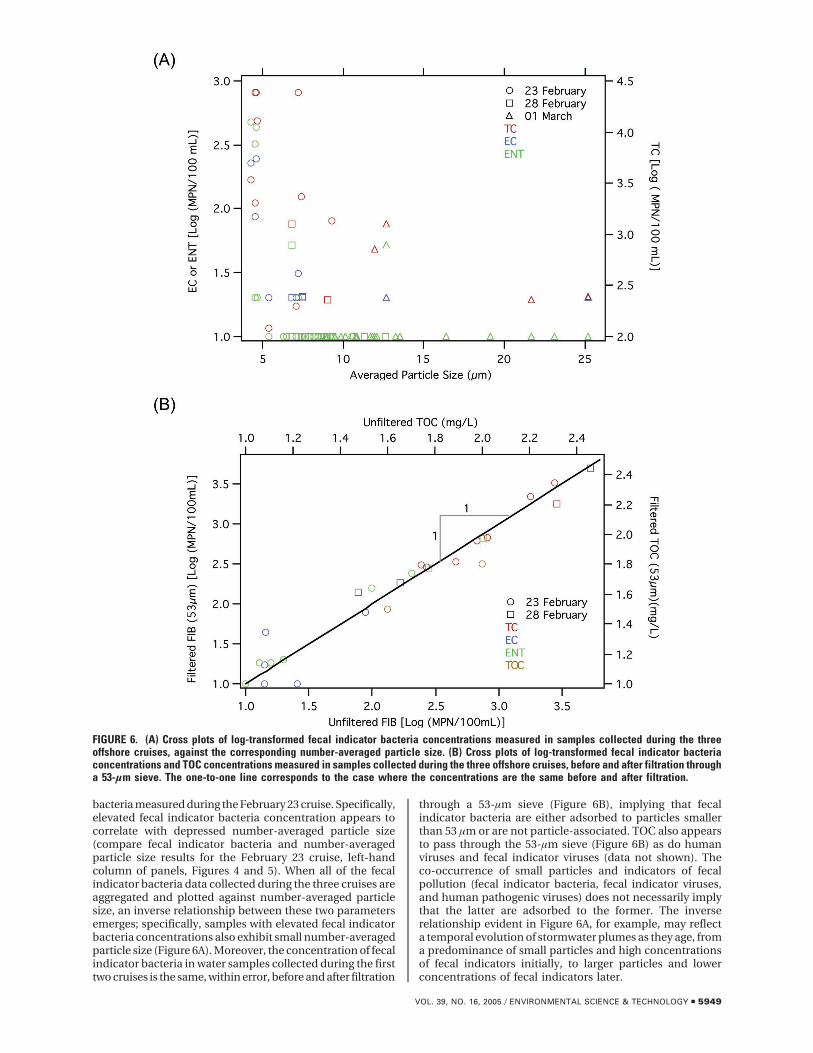
bacteria measured during the February 23 cruise. Specifically,elevated fecal indicator bacteria concentration appears tocorrelate with depressed number-averaged particle size(compare fecal indicator bacteria and number-averagedparticle size results for the February 23 cruise, left-handcolumn of panels, Figures 4 and 5). When all of the fecalindicator bacteria data collected during the three cruises areaggregated and plotted against number-averaged particlesize, an inverse relationship between these two parametersemerges; specifically, samples with elevated fecal indicatorbacteria concentrations also exhibit small number-averagedparticle size (Figure 6A). Moreover, the concentration of fecalindicator bacteria in water samples collected during the firsttwo cruises is the same, within error, before and after filtration

through a 53-µm sieve (Figure 6B), implying that fecalindicator bacteria are either adsorbed to particles smallerthan 53 µm or are not particle-associated. TOC also appearsto pass through the 53-µm sieve (Figure 6B) as do humanviruses and fecal indicator viruses (data not shown). Theco-occurrence of small particles and indicators of fecalpollution (fecal indicator bacteria, fecal indicator viruses,and human pathogenic viruses) does not necessarily implythat the latter are adsorbed to the former. The inverserelationship evident in Figure 6A, for example, may reflecta temporal evolution of stormwater plumes as they age, froma predominance of small particles and high concentrationsof fecal indicators initially, to larger particles and lowerconcentrations of fecal indicators later.

FIGURE 6. (A) Cross plots of log-transformed fecal indicator bacteria concentrations measured in samples collected during the threeoffshore cruises, against the corresponding number-averaged particle size. (B) Cross plots of log-transformed fecal indicator bacteriaconcentrations and TOC concentrations measured in samples collected during the three offshore cruises, before and after filtration througha 53-µm sieve. The one-to-one line corresponds to the case where the concentrations are the same before and after filtration.


Offshore Measurements: Particle Size Spectra. Particlesize spectra acquired during the three cruises are presentedin Figure 7. Each plot displays the normalized particle volume(vertical axis) detected in 32 logarithmically spaced particlediameter bins ranging in size from 2.5 to 500 µm (horizontalaxis). The particle size spectrum measured at a particularoffshore location and time appear to be related to the specificstormwater plume the particles are associated with and,possibly, the elapsed time stormwater has spent in the ocean.Stormwater flowing out of the Santa Ana River during theFebruary 23 cruise, for example, is characterized by twomodes at the small end of the size spectrum, one in the <5µm bin and another in the 10-50 µm bins (set of red curves,Figure 7). These modes are present in stormwater runoffsampled at several locations in the Santa Ana River watershed(13), in samples collected at the ocean outlet of the SantaAna River (panel labeled “SAR Outlet” at top of Figure 7), andin samples collected just offshore (red curve at station 2201,Figure 7) and down-coast (red curve at station 2101, Figure7) of the Santa Ana River outlet. Particles discharged fromthe Santa Ana River appear to dilute and merge into abackground turbidity characterized by a single broad modein the 50-300 µm size range (evident in the red curves atmost stations, Figure 7).

Referring to Figure 3A and the earlier discussion of thissatellite image, the 50-300 µm mode observed on February23 may be characteristic of a large runoff plume originatingfrom one or more up-coast sources of stormwater runoff,

most likely the Los Angeles River or the San Gabriel River.Several factors can lead to artifacts in the particle size spectraestimated from the light-scattering instrument deployed inthis study (39). However, in our case this caveat is mitigatedsomewhat by the observation that particle volume fractionscalculated from the particle size spectra are strongly cor-related (Spearman’s rank correlation Sp ) 0.90, p ) 0.02)with independent measurements of total suspended solids(data not shown).

During the second and third cruises, the particle sizespectra progressively coarsen with the result that, by March1, virtually all of the particle volume is associated with thelargest size bin (>500 µm, green curves in Figure 7). Theobserved temporal evolution in particle size spectra, fromhigh turbidity and multiple modes at the lower end of theparticle size spectrum to low turbidity and a single mode atthe large end of the particle size spectrum, may reflectdecreasing particle supply (i.e., reduced stormwater dischargefrom major river outlets) coupled with within-plume co-agulation of particles into larger size classes and, ultimately,removal of the largest particles by gravitational sedimenta-tion. Coagulation time scales estimated from these particlesize spectra measurements are short (minutes to hours orlonger) compared to time scales associated with the genera-tion and offshore transport of stormwater plumes (hours todays), and hence coagulation cannot be ruled out as animportant mechanism at our field site (see SupportingInformation for details on the time scale calculations).

FIGURE 7. Particle size spectra measured during the three offshore cruises; numbers at the top of each panel denote the station numberwhere the particle size spectra were measured (see Figure 1). The vertical axis in each plot represents the particle volume resident inlogarithmically spaced particle diameter bins; the horizontal axis represents the diameter of the particles (in µm). These plots are arrangedso that the stations progress from onshore to offshore (top to bottom) and up-coast to down-coast (left to right). The single plot labeled“SAR Outlet” corresponds to a particle size spectrum measured in stormwater runoff flowing out of the Santa Ana River outlet, just upstreamof where it flows over the beach and into the ocean.


Whether coagulation, in fact, plays a role in the fate andtransport of particles and particle-associated contaminantsin stormwater plumes will likely depend on the coagulationefficiency (i.e., the fraction of particle-particle collisions thatresult in sticking events) and shear rates present at a givenlocation and time (40, 41). Alternatively, the observedtemporal coarsening of particles in the offshore may reflectchanges in the particle size spectra of the stormwater runoffbefore it enters the ocean, from a predominance of smallerparticles during the peak of the hydrograph, to a predomi-nance of coarser particles during the falling limb of thehydrograph. Further studies are needed to determine whetherobserved coarsening of the offshore particle size spectra iscaused by within-plume coagulation or by temporal evolutionof the particle size spectra in stormwater runoff before itenters the ocean.

Data Synthesis. Results presented in this paper arerepresented schematically in Figure 8, including potentialoffshore transport mechanisms (panel A) and the resultingdistribution of particles, bacteria, and viruses (panel B). Asstormwater is discharged from the river outlet and flows overthe beach, a fraction is entrained in the surf zone and the

rest is ejected offshore in a momentum jet. Measurementsof fecal indicator bacteria in the surf zone suggest that, onceentrained, contaminants are transported parallel to shoreby wave-driven currents, in a direction (i.e., up- or down-coast) controlled by the approaching wave field. When wavesstrike the beach so that a component of wave momentumis directed up-coast (the scenario pictured in Figure 8), fecalindicator bacteria in the surf zone are carried up-coast of theriver outlet. Conversely, when waves strike the beach so thata component of wave momentum is directed down-coast,fecal indicator bacteria in the surf zone are carried down-coast of the river outlet. The buildup of water in the surf zonefrom breaking waves drives a cross-shore circulation cell,which can transport material between the surf zone andoffshore of the surf zone. At our field site, this cross-shorecirculation appears to limit the length of beach severelypolluted with fecal indicator bacteria to <5 km around theriver outlet, by diluting contaminated surf zone water withcleaner water from offshore. While the transport processesdescribed here are based on measurements of fecal indicatorbacteria in the surf zone, it is likely that other contaminantsin stormwater runoff, in particular, human viruses and toxic

FIGURE 8. (A) Transport mechanisms that can affect the offshore distribution of contaminants discharged from river outlets. (B) Schematicrepresentation of the spatial distribution of particles (black circles of varying size), fecal indicator bacteria (red symbols), and F+ coliphageand human pathogenic viruses (green symbols). Abbreviations are SAR (Santa Ana River), SGR (San Gabriel River), and LAR (Los AngelesRiver).


contaminants associated with suspended particles (13, 42),will behave similarly.

Further offshore, stormwater runoff plumes are commonand readily detected through a variety of geophysicalparameters (e.g., salinity, transmissivity, surface color). Aclear linkage between these parameters and fecal indicatorbacteria could not be established here. However, fecalindicator bacteria did appear to be associated with thesmallest particle sizes, on the basis of both fractionationstudies (Figure 6B) and the inverse relationship observedbetween fecal indicator bacteria concentrations and number-averaged particle size (Figure 6A). Particle size spectra in theoffshore plumes coarsen with time post-release, and fecalindicator bacteria concentrations steadily drop (see theschematic representation of particle size in the variousoffshore plumes, Figure 8B). These results have severalimplications. First, they suggest that high concentrations offecal indicator bacteria in the surf zone at our field site areprobably not brought into the study area by coastal currentsfrom distal sources (e.g., the Los Angeles river or the SanGabriel river). Second, cross-shore transport of water betweenthe surf zone and offshore of the surf zone, for example, byrip cell currents, is likely to improve surf zone water qualityby diluting dirty river effluent entrained in the surf zone withrelatively clean ocean water from offshore.

While the concentrations of fecal indicator bacteria inthe offshore plumes are generally below surf zone waterquality standards, particularly during the latter two cruises,fecal indicator viruses (F+ coliphage) were detected in nearlyall offshore samples tested, and human adenoviruses andenteroviruses were detected in several offshore samples,including two collected offshore of the Santa Ana River outlet(station 2201 on February 23 and 28, see Figure 5). It is likelythat the virus results presented here represent a conservativeestimate of viral prevalence, because a limited numbers ofsamples were tested (n) 8). In addition, the presence of PCRinhibitors in stormwater reduces the efficiency of PCRdetection of human pathogenic viruses, as mentioned earlier.At present, there are no water quality standards for fecalindicator viruses and human pathogenic viruses, largelybecause epidemiological data are not available to link adversehuman health outcomes (e.g., gastrointestinal disease) torecreational ocean exposure to these organisms. However,the offshore detection of human pathogenic viruses begsseveral questions: First, do these viruses constitute a humanhealth risk, either by contaminating the surf zone directly(see arrow with question mark, indicting the possible transferof contaminants from offshore into the surf zone, Figure 8B)or by sequestering in offshore sediments? Second, given thefact that the Santa Ana River has separate storm and sanitarysewer systems, what is the source of human fecal pathogensin the wet weather water runoff? Many studies have shownthat human fecal pathogens are associated with storm runofffrom urban areas located throughout the United States(25, 43-45), so the association between stormwater runoffand human fecal pathogens observed here is certainly notunique. Possible sources of human pathogens in stormwaterrunoff from urban areas include leaking sewer pipes, illicitsewage connections to the stormwater sewer system, home-less populations, and so forth.

Taken together, the results presented in this paperdemonstrate that stormwater runoff from the Santa Ana Riveris a significant source of near-shore pollution, includingturbidity, fecal indicator bacteria, fecal indicator viruses, andhuman pathogenic viruses. However, relationships betweenvariables (e.g., between turbidity and fecal indicator bacteriaand between fecal indicator bacteria and human viruses)vary from site to site (at the same time) and from time totime (at the same site) suggesting that the sources, fate, andtransport processes are contaminant specific. The apparent

exception is the inverse relationship observed between fecalindicator bacteria and number-averaged particle size, al-though further studies are needed to determine if this resultis generalizable to other storm seasons and coastal sites and,if so, to determine the underlying mechanism at work. Therelationship between water quality parameters (e.g., fecalindicator bacteria), turbidity, and other field proxies, suchas number-averaged particle size, salinity, and coloreddissolved organic matter, are the focus of ongoing and futureregional studies, including as part of a coastal waterquality observing program within the Bight ’03 Project(http://www.sccwrp.org/regional/03bight/bight03_fact_sheet.html), as well as other investigations being carried outas part of the Southern California Coastal Ocean ObservingSystem (SCCOOS).

AcknowledgmentsThis study was funded by a joint grant from the NationalWater Research Institute (03-WQ-001) and the U.S. GeologicalSurvey National Institutes for Water Research (UCOP-33808),together with matching funds from the counties of Orange,Riverside, and San Bernardino in southern California. MODISdata were acquired as part of the NASA’s Earth ScienceEnterprise and were processed by the MODIS AdaptiveProcessing System (MODAPS) and the Goddard DistributedActive Archive Center (DAAC) and are archived and distrib-uted by the Goddard DAAC. The JPL effort was supported bythe National Aeronautics and Space Administration througha contract with the Jet Propulsion Laboratory, CaliforniaInstitute of Technology. NEOCO measurements were sup-ported by the University of California Marine Council’sCoastal Environmental Quality Initiative. Partial support forhuman virus and fecal indicator virus study was provided byWater Environmental Research Foundation award 01-HHE-2a. We also acknowledge the contribution of Weiping Chuat UCI for technical assistance with human viruses analysis.The authors acknowledge the input and feedback fromnumerous colleagues, most notably Chris Crompton, GeorgeL. Roberson, Charles D. McGee, Rick Wilson, Brett F. Sanders,Patricia Holden, Ronald Linsky, and Steve Weisberg. Samplecollection and processing was carried out with the help ofYoungsul Jeong and Ryan Reeves. The authors also thankthe Assistant Manager of the City of Newport Beach, DavidKiff, the Chief of the Newport Beach Fire Department,Timothy Riley, John Moore, and Brian O’Rourke for arrangingthe February 23 cruise, and the officials at the Orange CountySanitation District for assisting in the collection and analysisof offshore and surf zone water samples. Some of the dataand ship time for this study were donated by the Bight’03program. The authors also acknowledge the excellent feed-back provided on the manuscript by three anonymousreviewers.

Supporting Information AvailableSampling and analysis protocols, calculation of the ortho-kinetic coagulation time scales, and additional figures. Thismaterial is available free of charge via the Internet at http://pubs.acs.org.

Literature Cited(1) Culliton, T. J. Population; distribution, density and growth; A

state of the coast report; NOAA’s state of the coast report; NationalOceanic and Atmospheric Administration: Silver Spring, MD,1998.

(2) Reeves, R. L.; Grant, S. B.; Mrse, R. D.; Copil Oancea, C. M.;Sanders, B. F.; Boehm, A. B. Scaling and management of fecalindicator bacteria in runoff from a coastal urban watershed insouthern California. Environ. Sci. Technol. 2004, 38, 2637-2648.

(3) Bay, S.; Jones, B. H.; Schiff, K.; Washburn L. Water quality impactsof stormwater discharges to Santa Monica Bay. Mar. Environ.Res. 2003, 56, 205-223.


(4) Warrick, J. A.; Mertes, L. A. K.; Washburn, L.; Siegel, D. A. Dispersalforcing of southern California river plumes, based on field andremote sensing observations. Geo-Mar. Lett. 2004, 24, 46-52.

(5) Koh, R. C. Y.; Brooks, N. H. Fluid mechanics of wastewaterdisposal in the ocean. Annu. Rev. Fluid Mech. 1975, 7, 187-211.

(6) Lu, R.; Turco, R. P.; Stolzenbach, K.; Fiedlander, S. K.; Xiong, C.Dry deposition of airborne trace metals on the Los AngelesBasin and adjacent coastal waters. J. Geophys. Res.-Atmos. 2003,108, AAC 11, 1-24.

(7) Boehm, A. B.; Shellenbarger, G. G.; Paytan, A. Groundwaterdischarge: potential association with fecal indicator bacteriain the surf zone. Environ. Sci. Technol. 2004, 38, 3558-3566.

(8) Schiff, K. C. Development of a model publicly owned treatmentwork (POTW) monitoring program; Southern California CoastalWater Research Project: Westminster, CA, 1999.

(9) Warrick, J. A.; Rubin, D. M.; Orzech K. M. The effects ofurbanization and flood control on suspended sediment dis-charge of a southern California river, evidence of a dilutioneffect. Water Resour. Res. 2004, submitted.

(10) Schiff, K. C.; Allen, M. J.; Zeng, E. Y.; Bay, S. M. SouthernCalifornia. Mar. Pollut. Bull. 2000, 41, 76-93.

(11) King, J. A.; Leubs, R. A.; Hardy, W. T.; Smith, A. B.; Withers, J.B.; Reynolds, A.; Henriques, M.; Johnson, T.; Thibeault, G. J.Water quality control plan; Santa Ana River Basin (8); CaliforniaRegional Water Quality Control Board, Santa Ana Region, 1995.

(12) DiGiacomo, P. M.; Washburn L.; Holt, B.; Jones, B. H. Coastalpollution hazards in southern California observed by SARimagery: stormwater plumes, wastewater plumes, and naturalhydrocarbon seeps. Mar. Pollut. Bull. 2004, 49, 1013-1024.

(13) Surbeck, C. Q.; Grant, S. B.; Ahn, J. H.; Jiang, S. Transport ofsuspended particles and fecal pollution in storm water runofffrom an urban watershed in southern California. Environ. Sci.Technol. 2005, submitted.

(14) Grant, S. B.; Sanders, B. F.; Boehm, A. B.; Redman, J. A.; Kim,J. H.; Mrse, R. D.; Chu, A. K.; Gouldin, M.; McGee, C. D.; Gardiner,N. A.; Jones, B. H.; Svejkovsky, J.; Leipzig, G. V.; Brown, A.Generation of Enterococci Bacteria in a coastal saltwater marshand its impact on surf zone water quality. Environ. Sci. Technol.2001, 35, 2407-2416.

(15) Boehm, A. B.; Grant, S. B.; Kim, J. H.; Mowbray, S. L.; Mcgee,C. D.; Clark, C. D.; Foley, D. M.; Wellman, D. E. Decadal andshorter period variability of surf zone water quality at HuntingtonBeach, California. Environ. Sci. Technol. 2002, 36, 3885-3892.

(16) Boehm, A. B.; Sanders, B. F.; Winant, C. D. Cross-shelf transportat Huntington Beach: Implications for the fate of sewagedischarged through an offshore ocean outfall. Environ. Sci.Technol. 2002, 36, 1899-1906.

(17) Grant, S. B.; Sanders, B. F.; Boehm, A. B.; Arega F.; Ensari, S.;Mrse, R. D.; Kang H. Y.; Reeves R. L.; Kim, J. H.; Redman, J. A.Coastal runoff impact study phase II: Sources and dynamics offecal indicators in the lower Santa Ana River Watershed; A draftreport prepared for the National Water Research Institute,County of Orange, and the Santa Ana Regional Water QualityControl Board, 2002.

(18) Turbow, D.; Lin, T. H.; Jiang, S. Impacts of beach closures onperceptions of swimming-related health risk in Orange County,California. Mar. Pollut. Bull. 2004, 48, 132-136.

(19) Jones, B. H.; Noble, M. A.; Dickey, T. D. Hydrographic and particledistributions over the Palos Verdes Continental Shelf: spatial,seasonal and daily variability. Cont. Shelf Res. 2002, 22, 945-965.

(20) Washburn, L.; McClure, K. A.; Jones, B. H.; Bay, S. M. Spatialscales and evolution of stormwater plumes in Santa MonicaBay. Mar. Environ. Res. 2003, 56, 103-125.

(21) DeLeon, R.; Shieh, Y. S. C.; Baric, R. S.; Sobey, M. D. Detectionof enteroviruses and hepatitis A virus in environmental samplesby gene probes and polymerase chain reaction. Water QualityConference; American Water Works Association: Denver, CO,1990, 833-853.

(22) Tsai, Y. L.; Sobsey, M. D.; Sangermano, L. R.; Palmer, C. J. Simplemethod of concentrating enteroviruses and hepatitis A virusfrom sewage and ocean water for rapid detection by reversetranscriptase-polymerase chain reaction. Appl. Environ.Microbiol. 1993, 59, 3488-3491.

(23) Jiang, S. C.; Chu, W. PCR detection of pathogenic viruses insouthern California urban river. J. Appl. Microbiol. 2004, 97,17-28.

(24) Pina, S.; Puig, M.; Lucena, F.; Jofre, J.; Girones, R. Viral pollutionin the environment and in shellfish: Human adenovirus

detection by PCR as an index of human viruses. Appl. Environ.Microbiol. 1998, 64, 3376-3382.

(25) He, J.; Jiang, S. Quantification of enterococci and humanadenoviruses in environmental samples by real-time PCR. Appl.Environ. Microbiol. 2004, in press.

(26) Mikkelsen, O. A. Variation in the projected surface of suspendedparticles: Implications for remote sensing assessment of TSM.Rem. Sens. Environ. 2002, 79, 23-29.

(27) Serra, T.; Colmer, J.; Cristina, X. P.; Vila, X.; Arellano, J. B.;Casamitjana, X. J. Evaluation of laser in-situ instrument formeasuring concentration of phytoplankton, purple sulfurbacteria, and suspended inorganic sediments in lakes. Environ.Eng. 2001, 11, 1023-1030.

(28) Kim, J. H.; Grant, S. B.; McGee, C. D.; Sanders, B. F.; Largier, J.L. Locating sources of surf zone pollution: A mass budgetanalysis of fecal indicator bacteria at Huntington Beach,California. Environ. Sci. Technol. 2004, 38, 2626-2636.

(29) Inman, D. L.; Brush, B. M. Coastal challenge. Science 1973, 181,20-32.

(30) AES Huntington Beach generating station surf zone water qualitystudy final draft; A consultant report prepared for CaliforniaEnergy Commission; KOMEX H2O Science Incorporated: West-minster, CA, 1998.

(31) Boehm, A. B. Model of microbial transport and inactivation inthe surf zone and application to field measurements of totalcoliform in northern Orange County, California. Environ. Sci.Technol. 2003, 37, 5511-5517.

(32) Boehm, A. B.; Sanders, B. F.; Winant, C. D. Cross-shelf transportat Huntington Beach. Implications for the fate of sewagedischarged through an offshore ocean outfall. Environ. Sci.Technol. 2002, 36, 1899-1906.

(33) Boehm, A. B.; Lluch-Cota D. B.; David, K. A.; Winant, C. D.;Monismith S. G. Covariation of coastal water temperature andmicrobial pollution at interannual to tidal periods. Geophys.Res. Lett. 2004, 31, L06309.

(34) Mertes, L. A. K.; Warrick, J. A. Measuring flood output from 110coastal watersheds in California with field measurements andSeaWiFS. Geology 2001, 29, 659-662.

(35) Jiang, S. C.; Deszfulian, H.; Chu, W. Real-time quantitative PCRfor enteric adenovirus serotype 40 in environmental waters.Can. J. Microbiol. 2004, submitted.

(36) Shuval, H. I. Developments in Water Quality Research; Ann Arbor-Humphrey Science: Ann Arbor, MI, 1970.

(37) Boucier, D. R.; Sharma, R. P. Heavy metals and their relationshipto solids in urban runoff. Int. J. Environ. Anal. Chem. 1980, 7,273-283.

(38) Gippel, C. J. Potential of turbidity monitoring for measuring thetransport of suspended-solids in streams. Hydrol. Processes 1995,9, 83-97.

(39) Mikkelsen O. A. In-situ particle size spectra and density of particleaggregates in a dredging plume. Mar. Geol. 2000, 170, 443-459.

(40) Grant, S. B.; Poor, C.; Relle, S. Scaling theory and solutions forthe steady-state coagulation and settling of fractal aggregatesin aquatic systems. Colloids Surf. 1996, 107, 155-174.

(41) Grant, S. B.; Kim, J. H.; Poor, C. Kinetic theories for thecoagulation and sedimentation of particles. J. Colloid InterfacesSci. 2001, 238, 238-250.

(42) Glenn, D. W.; Sansalone, J. J. Accretion and partitioning of heavymetals associated with snow exposed to urban traffic and winterstorm maintenance activities. II. J. Environ. Eng. ASCE 2002, 2,167-185.

(43) Lipp, E. K.; Kurz, R.; Vincent, R.; Rodriguez-Palacios, C.; Farrah,S. R.; Rose, J. R.; The effects of seasonal variability and weatheron microbial fecal pollution and enteric pathogens in asubtropical estuary. Estuaries 2001, 24, 266-276.

(44) Noble, R. T.; Fuhrman, J. A.; Enteroviruses detected by reversetranscriptase polymerase chain reaction from the coastal watersof Santa Monica Bay, California: low correlation to bacterialindicator levels. Hydrobiologia 2001, 460, 175-184.

(45) Jiang, S. C.; Chu., W.; PCR detection of pathogenic viruses insouthern California urban rivers. J. Appl. Microbiol. 2004, 97,17-28.

Received for review January 22, 2005. Revised manuscriptreceived May 19, 2005. Accepted May 20, 2005.

ES0501464


Available at www.sciencedirect.com

journal homepage: www.elsevier.com/locate/watres

Confirmation of putative stormwater impact on waterquality at a Florida beach by microbial source trackingmethods and structure of indicator organism populations

M.J. Brownella, V.J. Harwooda,!, R.C. Kurzb, S.M. McQuaiga, J. Lukasikc, T.M. Scottc

aDepartment of Biology, University of South Florida, SCA 110, Tampa, FL 33620, USAbPBS & J, 2803 Fruitville Road, Sarasota, FL 34237, USAcBiological Consulting Services of N. Florida, Inc., 4641 NW 6th St., Gainesville, FL 32609, USA

a r t i c l e i n f o

Article history:

Received 16 January 2007

Received in revised form

30 March 2007

Accepted 6 April 2007

Available online 1 June 2007

Keywords:

Indicator organisms

Water quality

BOX-PCR

Stormwater

Microbial source tracking

a b s t r a c t

The effect of a stormwater conveyance system on indicator bacteria levels at a Florida

beach was assessed using microbial source tracking methods, and by investigating

indicator bacteria population structure in water and sediments. During a rain event,

regulatory standards for both fecal coliforms and Enterococcus spp. were exceeded,

contrasting with significantly lower levels under dry conditions. Indicator bacteria levels

were high in sediments under all conditions. The involvement of human sewage in the

contamination was investigated using polymerase chain reaction (PCR) assays for the esp

gene of Enterococcus faecium and for the conserved T antigen of human polyomaviruses, all

of which were negative. BOX-PCR subtyping of Escherichia coli and Enterococcus showed

higher population diversity during the rain event; and higher population similarity during

dry conditions, suggesting that without fresh inputs, only a subset of the population

survives the selective pressure of the secondary habitat. These data indicate that high

indicator bacteria levels were attributable to a stormwater system that acted as a reservoir

and conduit, flushing high levels of indicator bacteria to the beach during a rain event. Such

environmental reservoirs of indicator bacteria further complicate the already questionable

relationship between indicator organisms and human pathogens, and call for a better

understanding of the ecology, fate and persistence of indicator bacteria.

& 2007 Elsevier Ltd. All rights reserved.

1. Introduction

Stormwater runoff can cause an influx of indicator bacteria toreceiving waters. Previous studies in southern California havedemonstrated increased indicator bacteria levels in coastalwaters influenced by stormwater runoff (Noble et al., 2003;Reeves et al., 2004; Ahn et al., 2005). Reeves et al. (2004)observed that during dry conditions, total coliforms, Escher-ichia coli and Enterococcus spp. were highly concentrated inrunoff from forebays (underground storage tanks), which wastransported to coastal water during storm events.

Underground storage of stormwater runoff may wellprovide favorable conditions for bacterial persistence, assediments in the stormwater conveyance systems may actas a reservoir. Both E. coli and Enterococcus spp. can persist in a

culturable state in sediments for weeks or months (Byappa-nahalli, 1998; Desmarais et al., 2002; Anderson et al., 2005;Jeng et al., 2005). Studies of indicator bacterial survival haveshown lower decay rates in sediment compared to water(Sherer et al., 1992; Howell et al., 1996; Anderson et al., 2005),indicating that sediments provide protection from harm-ful stressors (e.g., high temperatures and sunlight). Both

ARTICLE IN PRESS

0043-1354/$ - see front matter & 2007 Elsevier Ltd. All rights reserved.doi:10.1016/j.watres.2007.04.001

!Corresponding author. Tel.: +1813 9741524; fax: +1813 974 3263.E-mail address: [email protected] (V.J. Harwood).

WAT E R R E S E A R C H 41 ( 2007 ) 3747 – 3757

http://dx.doi.org/10.1016/j.watres.2007.04.001

mailto:[email protected]

sediments and underground storage systems provide protec-tion from these abiotic influences, and in addition supplyinorganic and organic nutrients, promoting survival and

possible regrowth.Areas with widely different land-use practices, including

agricultural, commercial, rural or residential, can contri-bute stormwater to environmental waters. The possibi-lity also exists of cross-connections from sewer pipes, orleakage from sewer or septic systems delivering humansewage to the stormwater conveyance system. Bothhuman health risk and strategies for remediation of mi-crobial pollution from stormwater are influenced by thehost source of microorganisms, but measurement ofindicator bacteria alone does not provide information on this

important parameter. Microbial source tracking (MST) is agroup of methods whose goal is to define the source(s) ofindicator bacteria. Such methods may be library-dependent;relying on a reference database of patterns, or fingerprints, oforganisms from fecal material of known source (Wiggins,1996; Hagedorn et al., 1999; Parveen et al., 1999; Dombeket al., 2000; Harwood et al., 2000; Moore et al., 2005).Library-independent methods do not require a database ofpatterns for comparison, but instead have a specifictarget which, when present, indicates fecal contaminationfrom a particular source. The target could be a gene

(Martellini et al., 2005), virus (Hsu et al., 1995; McQuaiget al., 2006) or a bacterium (Bernhard et al., 2003; Scott et al.,2005) associated with a specific host, and is frequentlydetected by a molecular method such as the polymerasechain reaction (PCR) (USEPA, 2005).Two library-independent MST methods for detection of

human-associated markers were used in this study todetermine whether human sewage was impacting thestormwater system: the enterococcal surface protein (esp)gene of Enterococcus faecium, and the conserved T antigenof human polyomavirus strains JC and BK. The Ent. faecium

strain(s) containing the esp gene is present throughout theUS and other countries (Willems et al., 2001; Rice et al.,2003). At least two published studies detected the espmarker in 100% of sewage influent samples tested in theUS (Scott et al., 2005; Soule et al., 2006). Furthermore, 100%of sewage samples tested in New Zealand (n ! 4) werealso positive (Harwood, unpublished data); and all thesewage samples representing greater than half of the statesin the US have also tested positive (T. Scott, unpublisheddata). Human polyomaviruses are estimated to infect up to80% of the human population, and are shed in urine and feces

(Knowles et al., 2003; Behzad-Behbahani et al., 2004). InFlorida, 36 sewage influent samples from three wastewatertreatment facilities and 14 samples from different septictanks were all positive for human polyomaviruses (McQuaiget al., 2006). Detection of esp and human polyomavirusmarkers were significantly correlated in Florida surfacewaters that were suspected of contamination from sewage(McQuaig et al., 2006). These markers were therefore con-sidered good candidates for detection of human sewagecontamination in this study, and were further confirmedduring the study.This study investigated the source of indicator bacteria

contaminating waters at a Florida beach by combining

library-independent MST methods (human-associated mar-kers) and a MST tool previously used as a library-dependentmethod (BOX-PCR of indicator bacteria strains) to investigate

the population structure of these bacteria under varyinghydrological conditions. The goals of the study were three-fold: (1) to determine whether the stormwater conveyancesystem contributed high indicator bacteria numbers to Gulf ofMexico waters; (2) determine whether human sewage wascontributing to the indicator bacteria contamination and (3)determine whether survival in the stormwater conveyancesystem might contribute to elevated indicator bacteria levels.Characteristics of the E. coli and Enterococcus populations,including population diversity and population similarity, wereused to explore the hypothesis that the microbial contamina-

tion at Siesta Key Beach originated from the stormwatersystem.

2. Materials and methods

2.1. Study site and sampling strategy

Siesta Key Beach is located on a barrier island on the west

coast of Florida in Sarasota County. A stormwater conveyancesystem runs parallel to the beach underneath a pavedthoroughfare (Fig. 1). The stormwater system receives runofffrom an urban, residential area of approximately 0.24km2 (60acres). The stormwater remains in the underground system,which runs southward to an underground concrete vault onthe west side of the road, approximately 300m from thebeach. Water may be retained in the vault for many days untila rain event causes overflow, which is pumped into anadjacent retention pond. Surface runoff from the road andoverflow from the pond enter a ditch, which flows "300m

before it empties onto the beach. During heavy rain, the ditchoutfall reaches the Gulf waters.

Two sampling events were conducted during this study; onewithin 48h of heavy rainfall and one after a dry period (6 daysof no precipitation). Water and sediment samples were takenat various points, i.e., access was obtained via a manhole tosample the stormpipe that feeds the vault, the vault wassampled through a metal-covered access portal, and the ditchand its beach outfall were sampled from the surface. The landaround the ditch and the ditch itself was heavily vegetated,and therefore shaded, with Brazilian pepper trees and

mangroves. More surface sampling sites were added (reten-tion pond and Gulf of Mexico) for the second sampling (dryperiod) in order to obtain a more complete picture of thepossible sources and sinks of microorganisms in the drainagesystem.

For genetic diversity studies, Enterococcus spp. were alsoisolated from sewage and a pristine water site. Untreatedsewage sampleswere obtained from lift stations in the Floridacounties of Duval andWakulla. Water samples from a pristinesite were collected at Deer Prairie Slough in the Myakka River,Myakka River State Park (Sarasota County; N Latitude

27110.5430 and W Longitude 82112.7050). This site was chosendue to the absence of known human impact and urbanstormwater runoff.

ARTICLE IN PRESS

WAT E R R E S E A R C H 41 ( 2007 ) 3747 – 37573748

2.2. Isolation and enumeration of indicator bacteria

Water and sediment samples were collected in sterilecontainers (in duplicate), immediately placed on ice andprocessed within 4h of collection at the USF (Tampa, FL)laboratory. Water samples and supernatant from sonicatedsediments were filtered through sterile nitrocellulose mem-branes (0.45mm pore size, 47mm diameter) using standardmethods for fecal coliforms (APHA, 1998) and enterococci

(USEPA, 2000). Twenty grams (wet weight) of sediment wereadded to 200ml of sterile buffered water (0.0425gL#1 KH2PO4

and 0.4055g L#1 MgCl2) and sonicated as modified fromAnderson et al. (2005). The power was increased to 16W for30 s based on experiments that determined the highestrecovery of indicator bacteria from contaminated sediments(data not shown).

Fecal coliforms were enumerated on mFC agar (Difco) andincubated for 24h at 44.5 1C in a water bath (APHA, 1998). Bluecolonies were counted as fecal coliforms and then inoculatedinto microtiter plates containing EC broth amended with

4-methylumbelliferyl-b-D-glucuronide (MUG) (50mgml#1) inorder to determine the percentage of the colonies that wereE. coli. After incubation for 24h at 37 1C, the microtiter plateswere exposed to ultraviolet (UV) light. Fluorescence indicatedstrains that had b-glucuronidase activity (MUG+), a character-istic of E. coli. For further confirmation, 25% of the MUG+isolates were profiled biochemically using API 20E strips(BioMerieux), and 100% were identified as E. coli. MUG+ fecalcoliforms were therefore designated E. coli and fingerprintedby BOX-PCR for the similarity/diversity study.

Enterococci were enumerated by Method 1600 (USEPA,

2000), in which filters were incubated on mEI agar (basemedium from Difco; indoxyl b-D-glucoside from SigmaAldrich) at 41 1C for 24h. All resultant colonies with a bluehalo were inoculated into Enterococcosel Broth (Becton

Dickinson) to confirm esculin hydrolyzation. Concentrationsfor all indicators were log10-transformed and recorded as CFU100ml#1 (water samples) or 100 gwetweight#1 (sedimentsamples).

2.3. Human-associated genetic markers

The method used for detection of an enterococcal surfaceprotein (esp) gene of Ent. faecium was carried out as previouslydescribed (Scott et al., 2005). Briefly, 300ml of each water

sample was filtered using 0.45mm pore-size membranefilters. Sediment samples were diluted 1:6 with steriledistilled water, vortexed for 2min and allowed to stand for2min (Byappanahalli et al., 2003). The supernatant wasfiltered through sterile nitrocellulose membranes (0.45mmpore size, 47mm diameter). Filters were incubated on mEIagar at 41 1C for 48h in awater bath. Filters were suspended intryptic soy broth (Difco), vortexed and incubated for 3h at41 1C. Two milliliters of culture were used for DNA extraction,which was performed using a QIAamp DNA extraction kit(Qiagen, Inc.) according to manufacturer’s instructions.

The forward primer (Scott et al., 2005), which is specific forthe Ent. faecium esp gene (50-TAT GAA AGC AAC AGC ACA AGTT-30), and a conserved reverse primer (50-ACG TCG AAA GTTCGA TTT CC-30) (Hammerum and Jensen, 2002) were bothpreviously published. PCR reactions were performed in a 50mlreaction mixture containing 1$PCR buffer, 1.5mM MgCl2,200mM of each of the four deoxyribonucleotides, 0.3 mM ofeach primer, 2.5U of HotStarTaq DNA polymerase (Qiagen,Inc.) and 5 ml of template DNA. Amplification consisted of aninitial denaturation at 95 1C for 15min (to activate Taqpolymerase), followed by 35 cycles of 94 1C for 1min, 58 1Cfor 1min and 72 1C for 1min. The amplicon (680bps) wasstained with GelStar nucleic acid stain (BioWhittaker) on a1.5% agarose gel and viewed under UV light. The reliable

ARTICLE IN PRESS

Fig. 1 – Sampling locations within the stormwater system draining to Siesta Key Beach.

WATER RESEARCH 41 (2007) 3747– 3757 3749

presence of the esp marker in human sewage was determinedin sewage samples collected throughout the State of Florida,including the study area (Sarasota County).

The method to detect human polyomaviruses (HPyVs) inwater samples was carried out as previously described(McQuaig et al., 2006). Briefly, each water sample (600ml) wasadjusted to 9.5 pH using 1M NaOH, and then prefiltered using a47mm filter (Millipore Cat. No. RW0304700). The filtrate wasadjusted to 3.5 pH using 2.0N HCl, and then filtered through a0.45mmpore size, 47mm diameter nitrocellulose filter. The filterwas placed into a 30ml polypropylene tube with 2ml of beefextract (pH 9.3) and vortexed for 30s to elute viruses from filter.DNAwas extracted from the resulting eluate using the QIAampBlood Midi Kit (Qiagen, Inc., Valencia, CA). Previously published

primers specific for the homologous T-antigen of both JC virusand BK virus were used to amplify HPyVs DNA (Fwd: 50-AGTCTT TAG GGT CTT CTA CC-30 and Rev: 50-GGT GCC AAC CTATGG AAC AG-30) (Askamit, 1993). PCR reactions were preparedusing 45ml of Platinums Blue PCR SuperMix (Invitrogen, Inc.,Carlsbad, CA), 200nM of each primer, and 4ml of DNA template.The final reaction volume was adjusted to 50ml using reagent-grade water (Whiley et al., 2004). The PCR reaction conditionswere as follows: initial denaturation at 94 1C for 2min, followedby 45 cycles of: 94 1C for 20s, 55 1C for 20s and 72 1C for 20s, thena final elongation at 72 1C for 2min. The nested PCR was run

under the same reaction conditions as above, with 1ml of thefirst reaction used as the template. PCR productswere separatedby agarose gel electrophoresis (1.5%). DNA was viewed usingGelStar nucleic acid stain under UV light. Bands appearing at172bp were recorded as a positive PCR result. Throughout thecourse of the study, 17 sewage influent samples were tested forthe presence of HPyVs, and all were positive.Controls used for all PCR assays included method blanks

(sterile buffer carried through the entire filtration/extraction/PCR procedure) and matrix spikes (water samples spiked withsewage to insure PCR performance, including lack of inhibition).

2.4. BOX-PCR of E. coli and Enterococcus spp.

E. coli strains were grown overnight in microcentrifuge tubescontaining 750ml of BHI broth (Becton Dickinson). Aftercentrifugation at 14,000RPM for 1min, pellets were washedwith sterile buffered water 2 times and resuspended in 500 mlof deionized sterile water. The cell suspension was boiled for5min to lyse the cells and then centrifuged again at

14,000RPM for 1min. Two ml of supernatant was used astemplate for each PCR reaction. BOX-PCR patterns (finger-prints) were generated using the previously published BOX-A1R primer (Koeuth et al., 1995), which has the followingsequence: 50-CTA CGG CAA GGC GAC GCT GAC G-30. Reagentsand volumes for each 25ml reaction were: 2.5ml 10X Buffer B(Fisher Scientific); 3.0 ml 25mM MgCl2; 1.0 ml 10mM dNTPs(Fisher Scientific); 2.5ml 2% bovine serum albumin (Sigma);1.3ml 10mM BOXA1R primer (IDT, Coralville, IA); 1.0 ml Taqpolymerase (5000uml#1) (Fisher Scientific); and 11.7ml PCR-grade water. Amplification contained three steps: (1) initial

denaturation at 95 1C for 5min; (2) 35 cycles of 94 1C for 1min,60 1C for 1min and 72 1C for 1min; and (3) final extension at72 1C for 10min. The preceding protocol was provided by

correspondence with Dr. Cindy Nakatsu (2004), Purdue Uni-versity, West Lafayette, IN.

Enterococci were grown overnight in microcentrifuge tubes

containing 1.5ml of BHI broth (Becton Dickinson). DNA wasextracted using the DNeasy Tissue Kit (Qiagen, Valencia, CA)and the manufacturer’s protocol for Gram-positive bacteria.BOX-PCR fingerprints for enterococci were generated using theBOXA2R primer (Koeuth et al., 1995), which has the followingsequence: 50-ACG TGG TTT GAA GAG ATT TTC G-30. PCRreagents and conditions used were from previously publishedprotocols with modifications (Versalovic et al., 1991; Malathumet al., 1998). Each 25ml PCR reaction contained: 5ml of 5$Gitschier Buffer (Kogan et al., 1987); 2.5ml of 10% dimethylsulfoxide; 0.4ml bovine serum albumin(10mgml#1); 2.0ml 10mM

dNTPs; 1.0ml Taq polymerase (5000uml#1); 11.6ml PCR-gradewater; 1.5ml 10mM BOXA2R primer; and 1.0ml of DNA template,containing between 30 and 100ngml#1. Amplification containedthree steps: (1) initial denaturation at 95 1C for 7min; (2) 35cycles of 90 1C for 30s, 40 1C for 1min and 65 1C for 8min; and (3)final extension at 65 1C for 16min.

Fragments were separated by electrophoresis through a1.5% agarose gel for 4h at 90V (E. coli fingerprints), or 6h at60V (Enterococcus spp. fingerprints). Gels were stained withethidium bromide (1% solution). Gels were digitally docu-mented under UV light using a FOTO/Analyst Archiver

(Fotodyne, Hartland, WI).

2.5. Statistical analysis

Fingerprint patterns of E. coli and Enterococcus spp. subtypesgenerated by BOX-PCR were analyzed with BioNumerics 4.0software (Applied Maths, Belgium). Samples from whichfewer than 10 isolates were recovered were not included inthe analysis. Dendrograms were created using a densiometriccurve-based algorithm (Pearson correlation coefficient, opti-

mization 1%) and UPGMA to cluster patterns by similarity.Repeated runs of the control strains, ATCC 9637 for E. coli andATCC 19433 (E. faecalis) for Enterococcus spp., were 86% and93% similar, respectively. Therefore, as a first approximation,patterns showingXthe similarity value established by thecontrol strains were considered identical. The relationship ofpatterns considered similar was also visually confirmed.

The relationships among indicator bacteria populationsisolated from the various sites were based on comparison ofBOX-PCR genotypes. The relationships were visualized bydendrograms constructed using a population similarity coeffi-

cient (Sp), previously published by Kuhn et al. (1991). Thealgorithm (Sp ! (

Pqxi/Nx+

Pqyi/Ny)/2) is based on the proportion

of identical BOX-PCR patterns between two populations, x and y.For example, if two populations x and y have 10 isolates eachand isolate (i ! 1) in population x is repeated 2 times inpopulation x and 3 times in population y, then the qx1 wouldbe 2/10 divided by 3/10. The qxi is calculated for every isolate inpopulation x, and then the

Pqxi is divided by the number (N) of

isolates in population x. The same process is applied to everyisolate in population y. Therefore, if two populations have noidentical subtypes Sp ! 0, and as the number of identical

subtypes increases between two populations, the Sp increasesto a maximum of 1.0 (Kuhn et al., 1991). The populationsimilarity coefficient was used to compare E. coli and Enterococcus

ARTICLE IN PRESS

WAT E R R E S E A R C H 41 ( 2007 ) 3747 – 37573750

populations at Siesta Key after a rain event and during dryconditions, and to further compare Enterococcus populations atSiesta Key to Enterococcus populations in sewage and in a

sampled site on Myakka River.The population characteristics (assessed by BOX-PCR) were

also assessed by accumulation curves and the Shannon–Wei-ner diversity index, which were calculated using EcoSim 7software (Acquired Intelligence Inc. & Kesey-Bear, Jericho,VT). An accumulation curve measures the diversity of asampled population (in this case, the number of unique BOX-PCR types) by plotting new subtypes as a function of samplingeffort. As the curve approaches an asymptote (slope ! 0), theprobability of obtaining new subtypes with additional sam-pling diminishes. The Shannon–Weiner index of diversity,

(H0) ! #Spi ln(pi), considers the frequency of the varioussubtypes in a population as well as the total number ofsubtypes; pi being the number of isolates with pattern idivided by total number of isolates. H0 was calculated withapproximately the same number of isolates (19 or 20) per sitepopulation for Siesta Key, as this was the largest sample sizethat was common to all treatments. Data sets containingmore isolates were randomly subsampled for inclusion in thediversity values. Both the accumulation curve and theShannon–Weiner index were used to compare the relativediversities of E. coli and Enterococcus populations after a rain

event and during dry conditions at Siesta Key, and to furthercompare Enterococcus populations at Siesta Key to Enterococcuspopulations in sewage and in a sampled site on Myakka River.Paired t tests, nonparametric tests (Mann-Whitney), andANOVA were used to determine significant difference in thecomparisons. GraphPad Prism version 4.02 (GraphPad Soft-ware, San Diego, CA) was used for the statistical analyses.

3. Results and discussion

3.1. Indicator organism concentrations and human-associated markers

The indicator bacterial concentrations and the absence/presence of the human-associated markers are summarized

in Table 1A for samples collected after a rain event, and inTable 1B for samples collected during dry conditions. Highlevels of indicator bacteria in the stormwater drainage

system, and stormwater flow during the rain event demon-strated the ability of the stormwater system to contaminatebeach waters, and also raised the possibility of a sewageinfluence. Tests for human polyomaviruses and the enter-ococcal surface protein gene (esp) for Ent. faecium, which havepreviously been used to determine the presence of humansewage in environmental waters (Scott et al., 2005; McDonaldet al., 2006; McQuaig et al., 2006) were carried out at allsites. All tests for human-associated markers were negative(Table 1A and B). These human-associated markers are veryreliably present in human sewage in Florida and in all other

geographic areas in which the markers have been tested,which suggests that human sewage input was not involved inthe contamination. Furthermore, the wastewater collectionsystem was examined for connections or leaks into thestormwater system by the Siesta Key Utility Authority severalmonths prior to this study, and no connections were found.While the negative results for human-associated suggest

the absence of sewage contamination in the stormwatersystem, other factors can influence these results. In parti-cular, little is known about the inactivation rates of most ofthe bacteria and viruses used in MST studies (Stoeckel and

Harwood, 2007). The survival of Ent. faecium C68, whichcarries the esp gene, was assessed in the laboratory and wasfound to be 9 days in simulated freshwater and 10 days insimulated seawater (Scott et al., 2005). HPyVs in sewage couldbe detected by PCR in laboratory mesocosms for over 3months (Bofill-Mas et al., 2001). These data should beinterpreted in light of the knowledge that many factorsinfluence the inactivation rates of microorganisms in aquaticenvironments that cannot be adequately simulated in thelaboratory (Anderson et al., 2005); environmental stressessuch as radiation, temperature variations, salinity and pre-

dators are among the factors that influence persistenceoutside the host. As MST methods continue to mature andthe organisms are better characterized, this will be animportant point to address. Chemical methods for MST, suchas fluorometry, can provide additional or corroborating

ARTICLE IN PRESS

Table 1A – Sites sampled at Siesta Key Beach after a rain event (A) and during dry conditions (B)

Stormpipewater

Vaultwater

Ditchwater

Ditchsediment

Standingwater onbeach

Beachsediment

Fecal coliform concentration 2.12 3.55a 3.72a 3.24 3.29a 3.64Enterococci concentration 4.01a 4.23a 4.72a 4.37 3.86a 3.63esp gene of Ent. Faecium — — — — — —

Human polyomaviruses — — — N/A — N/ABOX-PCR E. coli ’ ’ ’ ’ ’ ’

BOX-PCR Enterococcus spp. ’ ’ ’ ’ ’ ’

Concentrations for all indicators were log10-transformed and recorded as CFU100ml#1 (water samples) or 100 gwetweight#1 (sedimentsamples). Human-associated markers are recorded as present/absent (+/–), and BOX-PCR analyses were conducted (’), or not conducted (&).a Concentrations exceeded state regulatory standards. The Florida Department of Health, which monitors the beaches of Florida, considers awater sample of 100ml containing X104 Enterococcus spp. and/orX400 fecal coliforms an indicator of poor water quality (http://esetappsdoh.doh.state.fl.us/irm00beachwater/terms.htm). N/A, sediments were not tested for human polyomaviruses.

WATER RESEARCH 41 (2007) 3747– 3757 3751

http://esetappsdoh.doh.state.fl.us/irm00beachwater/terms.htm


evidence of human sewage (or the lack thereof) in stormwatersystems and other environmental waters (McDonald et al.,2006). Because MST markers targeting only human sewage

were used here, the results do not point toward a specificsource of contamination (only away from one). This limita-tion of library-independent methods can be addressed by theuse of multiple markers; however, reliable markers are nowavailable for only a handful of target species, e.g., human,ruminant, horse and pig (Bernhard and Field, 2000; Dick et al.,2005; Scott et al., 2005; Layton et al., 2006; McQuaig et al.,2006).

All water samples collected after the rain event had fecalcoliforms and Enterococcus concentrations above the regula-tory level for recreational waters, with the exception of

fecal coliforms in the stormpipe water (Table 1A). Enterococcusspp. concentrations were significantly higher than fecalcoliforms (P ! 0.041, paired t test). The mean concentrations(log10-transformed) were 3.1770.72 and 4.2070.37 for fecalcoliforms and Enterococcus spp., respectively. Indicator bacter-ial levels were also high in sediments collected during therain event, at 4103CFU100g#1, although there are noregulatory standards for indicator bacteria concentrations insediment.

During dry conditions (Table 1B), Enterococcus spp. concen-trations also exceeded regulatory levels in the stormwater

conveyance system (stormpipe and vault), which providedprotection from such stressors as sunlight and high tempera-tures. Only the standing water on beach, where water poolsand does not reach the Gulf, was in violation for fecalcoliform concentrations (as well as Enterococcus spp.). Thebeach area may have been impacted by another source ofindicator bacteria such as seagulls, which were observedflocking to the standing water on the beach. Indicator bacteriaconcentrations remained high in sediment samples duringdry conditions; e.g., levels in stormpipe sediment werehighest at 4103.5 CFU100g#1 for both fecal coliforms and

Enterococcus spp. Enterococcus spp. concentrations in sedi-ments during dry conditions were significantly higher thanfecal coliform concentrations (paired t test, P ! 0.020). Themean concentrations (log10-transformed) were 1.7071.38 and3.2171.11 for fecal coliforms and Enterococcus spp., respec-tively. The fact that indicator bacteria concentrations re-mained high in sediments during dry conditions when theoverlaying water column (retention pond, ditch and Gulf) hadconcentrations below regulatory standards supports previousreports in the literature (Craig et al., 2002; Anderson et al.,2005; Ferguson et al., 2005), and indicates that the sediments

act as a reservoir for these organisms.Indicator bacteria concentrations in water samples at sites

sampled in rainy and dry conditions (i.e., stormpipe water,vault water, ditch water and beach water) were compared bycalculating the mean of log10-transformed concentrations atall sites. In general, indicator bacteria concentrations weresignificantly higher during the rain event than duringdry conditions. The mean fecal coliform concentration dur-ing the rain event was 3.17CFU100ml#1, while it was1.57CFU100ml#1 under dry conditions. Correspondingmeansfor Enterococcus spp. were 4.20 and 2.55CFU100ml#1. Thedifference in mean concentrations for rainy versus dry

conditions was statistically significant for Enterococcus spp.

ARTICLE IN PRESS

Table

1B

Storm

pipe

water

Storm

pipe

sedim

ent

Vau

ltwater

Pond

water

Pond

sedim

ent

Ditch

water

Ditch

sedim

ent

Standingwater

on

bea

chBea

chse

dim

ent

Gulf

water

Gulf

sedim

ent

Feca

lco

liform

conce

ntration

0.70

3.85

1.37

0.40

1.30

1.36

1.60

2.86

a1.74

1.62

0.0

Entero

cocc

ico

nce

ntration

3.05

a4.44

2.31

a0.81

2.97

1.71

4.29

3.16

a2.36

0.98

2.0

espge

neofEn

t.Fa

ecium

——

——

——

——

——

—

Human

polyomav

iruse

s—

N/A

——

N/A

—N/A

–#N/A

—N/A

BOX-PCRE.

coli

&’

’&

&’

&’

&’

&

BOX-PCR

Enterococcussp

p.

’’

’&

&’

&’

&’

&

&Fe

wer

than

10isolatesreco

vered.

aConce

ntrationsex

ceed

edstateregu

latory

stan

dards.

TheFloridaDep

artm

entofHea

lth,whichmonitors

thebea

ches

ofFlorida,

considersawater

sample

of10

0mlco

ntainingX10

4En

terococcus

spp.an

d/orX40

0feca

lco

liform

san

indicatorofpoorwater

quality(http://ese

tappsd

oh.doh.state.fl.us/irm00

bea

chwater/terms.htm

).N/A

,se

dim

ents

werenottested

forhuman

polyomav

iruse

s.

WAT E R R E S E A R C H 41 ( 2007 ) 3747 – 37573752


(P ! 0.028) and nearly significant for fecal coliforms (P ! 0.057)at the a ! 0.05 level.

3.2. Population diversity

BOX-PCR patterns of E. coli and Enterococcus spp. isolatedduring the rain event were compared to those isolated duringthe dry sampling in order to determine whether the popula-tion structure was influenced by these conditions. The twomethods used to estimate indicator bacteria populationdiversity were: (1) the Shannon–Weiner index, which has

been previously used to measure microbial populationdiversity in habitats such as rhizospheres, artesian springsediments and microbial mats (McCaig et al., 1999; Nubelet al., 1999; Elshahed et al., 2003); and (2) the accumulationcurve, used to estimate diversity in animal populations(Bohannan and Hughes, 2003) and bacterial populations(Anderson et al., 2006).

Accumulation curves for vault water samples (Fig. 2) illustratea tendency toward greater diversity during rainy conditions forboth E. coli and Enterococcus populations. The Shannon–Weinerindex of diversity corroborated these data, showing significantly

greater diversity in E. coli and Enterococcus populations in therain event versus dry conditions (Table 2). The increasedpopulation diversity during the rain event suggests that higherdiversity is due to recent inputs into the stormwater system,undoubtedly from multiple sources.

The diversity of Enterococcus populations during the rainevent and during dry conditions was compared to thediversity of Enterococcus populations sampled from sewageand from water samples collected from the Myakka River,considered to be a relatively unimpacted site with no directhuman or agricultural input, or urban runoff (Fig. 3). Averaged

accumulation curves were constructed for Enterococcus popu-lations for the rain event (n ! 4 sites), dry conditions (n ! 4sites), sewage samples (n ! 6) and samples collected atMyakka River (n ! 3). Similar diversity levels were observedin Siesta Key Enterococcus populations during the rain event

and Enterococcus populations in sewage samples. In contrast,significantly lower diversity was found in Enterococcus popula-tions during dry conditions and at Myakka River (unimpactedsite) (Fig. 3). Previous studies have shown that Enterococcuspopulations in domestic sewage display higher diversity thanthose sampled from river water (Vilanova et al., 2002), andanimal feces (Manero et al., 2002; Kuhn et al., 2003). TheShannon–Weiner index for these four groups reveals asignificant difference in the diversity levels of Siesta Key rain

event and sewage populations versus Siesta Key dry condi-tions and Myakka River populations (Table 3). These resultssuggest that stormwater can influence the diversity ofindicator bacteria populations in waters it impacts toapproach that of sewage input. Interestingly, the Enterococcuspopulation from sewage shares very few subtypeswith that ofSiesta Key or Myakka River (see Section 3.3).

3.3. Population similarity

The population similarity of indicator bacteria (E. coli orEnterococcus spp.) was compared by site for the rain event and

ARTICLE IN PRESS

0

2

4

6

8

10

12

14

16

1 3 5 7 9 13 15 17 19

Sampling effort

Su

bty

pes

11

Fig. 2 – Accumulation curves of BOX-PCR fingerprintpatterns of indicator bacteria from vault water samples.E. coli sampled after a rain event (m) and during dry condi-tions (n); Enterococcus spp. sampled after a rain event (’)and during dry conditions (&).

Table 2 – Comparison of the population diversity(Shannon-Weiner index, H0) of E. coli and Enterococcusspp. during the rain event versus dry conditions

Indicatororganism

Mean H0 P value

E. colia Rain event ! 2.3970.22 P ! 0.047Dry conditions ! 1.1270.34

Enterococcusspp.b

Rain event ! 2.6570.13 P ! 0.008

Dry conditions ! 1.8870.28

a Site populations averaged for E. coli: beach water, ditch water andvault water.b Site populations averaged for Enterococcus spp.: beach water,ditch water, stormpipe water and vault water.

0

2

4

6

8

10

12

14

16

18

1 3 5 7 9 11 13 15 17 19

Sampling effort

Su

bty

pes

Fig. 3 – Accumulation curves based on averaged richnessestimates for Enterococcus spp. sampled at Siesta Key sitesafter a rain event (’), at Siesta Key sites during dryconditions (&), from wastewater influent (x) and fromMyakka River water (n).

WATER RESEARCH 41 (2007) 3747– 3757 3753

dry conditions. A similarity coefficient was used to expressthe proportion of identical BOX-PCR subtypes sampled fromthe various sites (Kuhn et al., 1991). This strategy has been

used to compare phenotypic subtypes of coliforms inenvironmental water samples (Kuhn et al., 1991), andphenotypic subtypes of fecal coliforms and enterococci insewage (Manero et al., 2002; Vilanova et al., 2002, 2004), and inthe feces of livestock, seabirds and dogs (Kuhn et al., 2003;Wallis and Taylor, 2003).Higher similarity between sites was observed for E. coli

populations sampled during dry conditions compared to therain event (Fig. 4). Higher similarity also existed between sitesfor Enterococcus populations during dry conditions (Fig. 5), butthe difference was less pronounced than for the E. coli

populations. Increased population similarity for E. coli andEnterococcus spp. during dry conditions suggests that a greaterportion of the population is composed of ‘‘survivor’’ isolates(Anderson et al., 2005) that have survived under the selectivepressure of this secondary habitat. Interestingly, the in-creased population similarity for both E. coli and Enterococcus

spp. under dry conditions was not observed in Gulf waters. Apossible explanation is that under dry conditions, thestanding water on the beach did not reach the Gulf,

demonstrating the physical and microbiological disconnectbetween the stormwater drainage system and the Gulf, whichcontrasts with the direct stormwater flow observed during therain event.

BOX-PCR patterns of enterococci from all stormwater sitesused for the above analysis were pooled for a comparison ofpopulation similarity between rainy conditions and dryconditions, as well as sewage populations (positive controlfor human contamination) and Myakka River populations(control for unimpacted water) (Fig. 6). The two Enterococcuspopulations with the highest similarity were Myakka River

and Siesta Key (dry), and the population with the leastsimilarity to all other groups was sewage. Thus, the popula-tions in the environments with relatively low levels of recentinputs of indicator bacteria (Myakka River and Siesta Key Dry)contain more identical Enterococcus genotypes, suggestingthat survival in this secondary habitat is a form of selectivepressure.

Even though human sewage input was not detected atSiesta Key Beach, one cannot rule out risk to humanhealth from contact with the water. The health risksassociated with exposure to recreational waters impacted

by stormwater runoff have not been as well studied asthe risks associated with sewage-impacted waters. Onestudy found that respiratory and gastrointestinal symp-toms increased as the distance decreased between swimmersand a stormwater outlet in Santa Monica Bay, CA (Haile et al.,1999). During an El Nino year, surfers in Orange County, CAreported twice as many symptoms as surfers in Santa CruzCounty, considered to be less impacted by urban runoff(Dwight et al., 2004). These studies suggest that adverse heathoutcomes are associated with stormwater impact of recrea-tional waters.

ARTICLE IN PRESS

beach sediment

stormpipe water

ditch water

vault water

beach water

ditch sediment

ditch water

vault water

beach water

stormpipe sediment

gulf water

10

20

30

40

50

60

70

80

90

100

10

0 20

30

40

50

60

70

80

90

100

Fig. 4 – Similarity of E. coli populations by site at Siesta Key during the rain event (A), and during dry conditions (B), based onBOX-PCR fingerprint patterns.

Table 3 – Comparison of the population diversity(Shannon–Weiner index, H0) of Enterococcus spp. insewage, Myakka River water and Siesta Key water duringrain event and dry conditions

Site Mean H0

Sewage 2.6970.09 (a)Myakka 1.9670.22 (b)Siesta key (dry) 1.8870.28 (b)Siesta key (rain) 2.6570.13 (a)

Values that share the same letter within columns are notsignificantly different. ANOVA (P ! 0.0001, a ! 0.05).

WAT E R R E S E A R C H 41 ( 2007 ) 3747 – 37573754

The population dynamics of indicator bacteria in the stormdrainage system at Siesta Key Beach are evidently affected bythe hydrological changes caused by rain events. A change inbacterial concentrations and diversity, as well as similarity, ofthe populations extending from the stormpipe to the Gulf wasobserved. The transport of urban runoff collecting for days inthe stormpipe and vault, and the persistence of survivorisolates in the sediments, suggests a reservoir for indicatorbacteria that can be flushed through the system to the Gulf

during a rain event, causing high levels of indicator bacteria.The design of the stormwater conveyance system, in whichsediments collect during low-flow conditions, ultimatelycontributes to contamination of receiving waters underhigh-flow conditions, when collected material is flushedthrough the system. These observations suggest that betterhandling and treatment of stormwater is needed, particularlywhen it impacts areas that receive heavy human use. Suchenvironmental reservoirs of indicator bacteria further com-plicate the already questionable relationship between indi-cator organisms and human pathogens (Byappanahalli, 1998;

Anderson et al., 2005), and call for a better understanding of

the ecology, fate and persistence of indicator bacteria inwater.

4. Conclusions

Although indicator bacteria levels during the rain event were

above state standards for recreational waters, no evidence ofhuman fecal contamination was found by library-indepen-dent MST methods. The persistent high bacterial concentra-tions in stormwater sediment samples during dry conditionssuggest that sediments are a reservoir of these organisms.During high flow (rainy) conditions indicator bacteria diver-sity was high and population similarity was low, suggestingfresh inputs of bacteria from many sources. These observa-tions contrasted with results from dry conditions, whereindicator bacteria diversity was lower and population simi-larity was higher, suggesting that a group of ‘‘survivor’’ strains

may form a significant portion of the population when freshinputs of indicator bacteria are minimal. The combination ofecological and hydrological approaches with MST methods

ARTICLE IN PRESS

ditch water

stormpipe water

beach water

ditch sediment

beach sediment

vault water

beach water

ditch water

stormpipe sediment

stormpipe water

vault water

gulf water

10

20

30

40

50

60

70

80

90

100

10

0 20

30

40

50

60

70

80

90

100

Fig. 5 – Similarity of Enterococcus populations by site at Siesta Key during the rain event (A), and during dry conditions (B),based on BOX-PCR fingerprint patterns.

Myakka River

Siesta Key dry

Siesta Key rain

sewage

10

20

30

40

50

60

70

80

90

100

Fig. 6 – Similarity of Enterococcus populations sampled at Siesta Key during the rain event and dry conditions, compared topopulations from sewage and from Myakka River, based on BOX-PCR fingerprint patterns.

WATER RESEARCH 41 (2007) 3747– 3757 3755

allowed assessment of the source of E. coli and Enterococcuspopulations, where the library-independent methods alonewould not have been sufficient.

Acknowledgments

This work was supported by Sarasota County. We thank Dr.Stephaney Leskinen and Mariya Dontchev for sample collec-

tion and analysis.

R E F E R E N C E S

Ahn, J.H., Grant, S.B., et al., 2005. Coastal water quality impact ofstormwater runoff from an urban watershed in southernCalifornia. Environ. Sci. Technol. 39 (16), 5940–5953.

Anderson, K.L., Whitlock, J.E., et al., 2005. Persistence anddifferential survival of fecal indicator bacteria in subtropicalwaters and sediments. Appl. Environ. Microbiol. 71 (6),3041–3048.

Anderson, M.A., Whitlock, J.E., et al., 2006. Diversity and distribu-tion of Escherichia coli genotypes and antibiotic resistancephenotypes in feces of humans, cattle, and horses. Appl.Environ. Microbiol. 72 (11), 6914–6922.

APHA, 1998. Standards for the Examination of Water and Waste-water. American Public Health Association, Washington, DC.

Askamit, A.J., 1993. PCR detection of JC virus. In:Persing, T.F.S.D.H., Tenover, F.C., White, T.J., (Eds.), DiagnosticMolecular Microbiology Principles and Applications. MayoFoundation, Rochester.

Behzad-Behbahani, A., Klapper, P.E., et al., 2004. Detection of BKvirus and JC virus DNA in urine samples from immunocom-promised (HIV-infected) and immunocompetent (HIV-non-infected) patients using polymerase chain reaction andmicroplate hybridisation. J. Clin. Virol. 29 (4), 224–229.

Bernhard, A.E., Field, K.G., 2000. Identification of nonpointsources of fecal pollution in coastal waters by using host-specific 16S ribosomal DNA genetic markers from fecal anae-robes. Appl. Environ. Microbiol. 66 (4), 1587–1594.

Bernhard, A.E., Goyard, T., et al., 2003. Application of a rapidmethod for identifying fecal pollution sources in a multi-useestuary. Water Res. 37 (4), 909–913.

Bofill-Mas, S., Formiga-Cruz, M., et al., 2001. Potential transmis-sion of human polyomaviruses through the gastrointestinaltract after exposure to virions or viral DNA. J. Virol. 75 (21),10290–10299.

Bohannan, B.J., Hughes, J., 2003. New approaches to analyzingmicrobial biodiversity data. Curr. Opin. Microbiol. 6 (3),282–287.

Byappanahalli, M.N.a.R.S.F., 1998. Evidence that tropical soilenvironment can support the growth of Eschericia Coli.Water Sci. Technol. 38 (12), 171–174.

Byappanahalli, M., Fowler, M., et al., 2003. Ubiquity and persis-tence of Escherichia coli in a Midwestern coastal stream. Appl.Environ. Microbiol. 69 (8), 4549–4555.

Craig, D.L., Fallowfield, H.J., et al., 2002. Enumeration of faecalcoliforms from recreational coastal sites: evaluation of tech-niques for the separation of bacteria from sediments. J. Appl.Microbiol. 93 (4), 557–565.

Desmarais, T.R., Solo-Gabriele, H.M., et al., 2002. Influence of soilon fecal indicator organisms in a tidally influenced subtropicalenvironment. Appl. Environ. Microbiol. 68 (3), 1165–1172.

Dick, L.K., Bernhard, A.E., et al., 2005. Host distributions ofuncultivated fecal Bacteroidales bacteria reveal genetic mar-kers for fecal source identification. Appl. Environ. Microbiol. 71(6), 3184–3191.

Dombek, P.E., Johnson, L.K., et al., 2000. Use of repetitive DNAsequences and the PCR To differentiate Escherichia coli isolatesfrom human and animal sources. Appl. Environ. Microbiol. 66(6), 2572–2577.

Dwight, R.H., Baker, D.B., et al., 2004. Health effects associatedwith recreational coastal water use: urban versus ruralCalifornia. Am. J. Public Health 94 (4), 565–567.

Elshahed, M.S., Senko, J.M., et al., 2003. Bacterial diversity andsulfur cycling in a mesophilic sulfide-rich spring. Appl.Environ. Microbiol. 69 (9), 5609–5621.

Ferguson, D.M., Moore, D.F., et al., 2005. Enumeration andspeciation of enterococci found in marine and intertidalsediments and coastal water in southern California. J. Appl.Microbiol. 99 (3), 598–608.

Hagedorn, C., Robinson, S.L., et al., 1999. Determining sources offecal pollution in a rural Virginia watershed with antibioticresistance patterns in fecal streptococci. Appl. Environ.Microbiol. 65 (12), 5522–5531.

Haile, R.W., Witte, J.S., et al., 1999. The health effects of swimmingin ocean water contaminated by storm drain runoff. Epide-miology 10 (4), 355–363.

Hammerum, A.M., Jensen, L.B., 2002. Prevalence of esp, encodingthe enterococcal surface protein, in Enterococcus faecalis andEnterococcus faecium isolates from hospital patients, poultry,and pigs in Denmark. J. Clin. Microbiol. 40 (11), 4396.

Harwood, V.J., Whitlock, J., et al., 2000. Classification of antibioticresistance patterns of indicator bacteria by discriminant analysis:use in predicting the source of fecal contamination in subtropicalwaters. Appl. Environ. Microbiol. 66 (9), 3698–3704.

Howell, J.M., Coyne, M.S., Cornelius, P.L., 1996. Effect of sedimentparticle size and temperature on fecal bacteria mortality ratesand the fecal coliform/fecal streptococci ratio. J. Environ. Qual.25, 1216–1220.

Hsu, F.C., Shieh, Y.S., et al., 1995. Genotyping male-specific RNAcoliphages by hybridization with oligonucleotide probes. Appl.Environ. Microbiol. 61 (11), 3960–3966.

Jeng, H.C., England, A.J., et al., 2005. Indicator organismsassociated with stormwater suspended particles and estuar-ine sediment. J. Environ. Sci. Health A Tox. Hazard. Subst.Environ. Eng. 40 (4), 779–791.

Knowles, W.A., Pipkin, P., et al., 2003. Population-based study ofantibody to the human polyomaviruses BKV and JCV and thesimian polyomavirus SV40. J. Med. Virol. 71 (1), 115–123.

Koeuth, T., Versalovic, J., et al., 1995. Differential subsequenceconservation of interspersed repetitive Streptococcus pneumo-niae BOX elements in diverse bacteria. Genome Res. 5 (4), 408–418.

Kogan, S.C., Doherty, M., et al., 1987. An improved method forprenatal diagnosis of genetic diseases by analysis of amplifiedDNA sequences. Application to hemophilia A. N. Engl. J. Med.317 (16), 985–990.

Kuhn, I., Allestam, G., et al., 1991. Biochemical fingerprinting ofwater coliform bacteria, a new method for measuringphenotypic diversity and for comparing different bacterialpopulations. Appl. Environ. Microbiol. 57 (11), 3171–3177.

Kuhn, I., Iverson, A., et al., 2003. Comparison of enterococcalpopulations in animals, humans, and the environment—aEuropean study. Int. J. Food Microbiol. 88 (2–3), 133–145.

Layton, A., McKay, L., et al., 2006. Development of Bacteroides 16SrRNA gene TaqMan-based real-time PCR assays for estimationof total, human, and bovine fecal pollution in water. Appl.Environ. Microbiol. 72 (6), 4214–4224.

Malathum, K., Singh, K.V., et al., 1998. Repetitive sequence-basedPCR versus pulsed-field gel electrophoresis for typing ofEnterococcus faecalis at the subspecies level. J. Clin. Microbiol.36 (1), 211–215.

Manero, A., Vilanova, X., et al., 2002. Characterization of sewagewaters by biochemical fingerprinting of Enterococci. WaterRes. 36 (11), 2831–2835.

ARTICLE IN PRESS

WAT E R R E S E A R C H 41 ( 2007 ) 3747 – 37573756

Martellini, A., Payment, P., et al., 2005. Use of eukaryoticmitochondrial DNA to differentiate human, bovine, porcineand ovine sources in fecally contaminated surface water.Water Res. 39 (4), 541–548.

McCaig, A.E., Glover, L.A., et al., 1999. Molecular analysis ofbacterial community structure and diversity in unimprovedand improved upland grass pastures. Appl. Environ. Microbiol.65 (4), 1721–1730.

McDonald, J.L., Hartel, P.G., et al., 2006. Identifying sources of fecalcontamination inexpensively with targeted sampling andbacterial source tracking. J. Environ. Qual. 35 (3), 889–897.

McQuaig, S.M., Scott, T.M., et al., 2006. Detection of human-derived fecal pollution in environmental waters by use of aPCR-based human polyomavirus assay. Appl. Environ. Micro-biol. 72 (12), 7567–7574.

Moore, D.F., Harwood, V.J., et al., 2005. Evaluation of antibioticresistance analysis and ribotyping for identification of faecalpollution sources in an urban watershed. J. Appl. Microbiol. 99(3), 618–628.

Noble, R.T., Weisberg, S.B., et al., 2003. Storm effects on regionalbeach water quality along the southern California shoreline.J. Water Health 1 (1), 23–31.

Nubel, U., Garcia-Pichel, F., et al., 1999. Quantifying microbialdiversity: morphotypes, 16S rRNA genes, and carotenoids ofoxygenic phototrophs in microbial mats. Appl. Environ.Microbiol 65 (2), 422–430.

Parveen, S., Portier, K.M., et al., 1999. Discriminant analysis ofribotype profiles of Escherichia coli for differentiating humanand nonhuman sources of fecal pollution. Appl. Environ.Microbiol. 65 (7), 3142–3147.

Reeves, R.L., Grant, S.B., et al., 2004. Scaling and management offecal indicator bacteria in runoff from a coastal urbanwatershed in southern California. Environ. Sci. Technol. 38 (9),2637–2648.

Rice, L.B., Carias, L., et al., 2003. A potential virulence gene,hylEfm, predominates in Enterococcus faecium of clinical origin.J. Infect. Dis. 187 (3), 508–512.

Scott, T.M., Jenkins, T.M., et al., 2005. Potential use of a hostassociated molecular marker in Enterococcus faecium as anindex of human fecal pollution. Environ. Sci. Technol. 39 (1),283–287.

Sherer, B.M., Miner, J.R., Moore, J.A., Buckhouse, J.C., 1992.Indicator bacterial survival in stream sediments. J. Environ.Qual. 21, 101–115.

Soule, M., Kuhn, E., et al., 2006. Using DNAmicroarrays to identifylibrary-independent markers for bacterial source tracking.Appl. Environ. Microbiol. 72 (3), 1843–1851.

Stoeckel, D.M., Harwood, V.J., 2007. Performance, Design, andAnalysis in Microbial Source Tracking Studies. Appl. Environ.Microbiol. 73 (8), 2405–2415.

USEPA, 2000. Improved Enumeration Methods for the Recrea-tional Water Quality Indicators: Enterococci and Escheria coli.US Environmental Protection Agency, Washington, DC.

USEPA, 2005. Microbial Source Tracking Guide Document. USEnvironmental Protection Agency, Washington, DC.

Versalovic, J., Koeuth, T., et al., 1991. Distribution of repetitiveDNA sequences in eubacteria and application to fingerprintingof bacterial genomes. Nucleic Acids Res. 19 (24), 6823–6831.

Vilanova, X., Manero, A., et al., 2002. The effect of a sewagetreatment plant effluent on the faecal coliforms and enter-ococci populations of the reception river waters. J. Appl.Microbiol. 92 (2), 210–214.

Vilanova, X., Manero, A., et al., 2004. The composition andpersistence of faecal coliforms and enterococcal populationsin sewage treatment plants. J. Appl. Microbiol. 96 (2), 279–288.

Wallis, J.L., Taylor, H.D., 2003. Phenotypic population character-istics of the enterococci in wastewater and animal faeces:implications for the new European directive on the quality ofbathing waters. Water Sci. Technol. 47 (3), 27–32.

Whiley, D.M., Arden, K.E., et al., 2004. Simultaneous detection anddifferentiation of human polyomaviruses JC and BK by a rapidand sensitive PCR-ELAHA assay and a survey of the JCVsubtypes within an Australian population. J. Med. Virol. 72 (3),467–472.

Wiggins, B.A., 1996. Discriminant analysis of antibiotic resistancepatterns in fecal streptococci, a method to differentiatehuman and animal sources of fecal pollution in naturalwaters. Appl. Environ. Microbiol. 62 (11), 3997–4002.

Willems, R.J., Homan, W., et al., 2001. Variant esp gene as amarkerof a distinct genetic lineage of vancomycin-resistant Enter-ococcus faecium spreading in hospitals. Lancet 357 (9259),853–855.

ARTICLE IN PRESS

WATER RESEARCH 41 (2007) 3747– 3757 3757

AMERICAN JOUKNAL OF EPIDEMIOLOGY Vol. 115, No. 4Copyright © 1982 by The Johns Hopkins University School of Hygiene and Public Health Printed in U£AAll rights reserved

SWIMMING-ASSOCIATED GASTROENTERITIS AND WATER QUALITY1

V. J. CABELLI,1 A. P DUFOUR,3 L. J. McCABE,3 AND M. A LEVIN4

Cabelll, V. J. (Dept. of Microbiology, U. of Rhode Island, Kingston, Rl 02881),A. P. Dufour, L. J. McCabe and M. A. Levin. Swimming-associated gastroen-teritis and water quality. Am J Epidemiol 1982;115:606-16.

A direct, linear relationship between swimming-associated gastrointestinalillness and the quality of the bathing water was obtained from a multi-year,multiple-location prospective epidemlologlc-microblologic research programconducted in New York City, 1973-1975, Lake Pontchartraln, Louisiana, 1977-1978, and Boston, Massachusetts, 1978. Several mlcrobial Indicators wereused In attempting to define the quality of the water; and, of those examined,enterococci showed the best correlation to total and "highly credible" gastro-intestinal symptoms. The frequency of gastrointestinal symptoms also hada high degree of association with distance from known sources of municipalwastewater. A striking feature of the relationship was the very low entero-coccus and Eacherlchla coll densities In the water (10/100 ml) associatedwith appreciable attack rates (about 10/1000 persons) for "highly credible"gastrointestinal symptoms. Moreover, the ratio of the swimmer to nonswimmersymptom rates indlpated that swimming In even marginally polluted marinebathing water is a significant route of transmission for the observed gastro-enteritis.

gastroenteritis; swimming; water microbiology

In an earlier report (1), the authors dards (2). The swimming-associated ill-presented evidence from a prospective ness observed was an acute, relativelyepidemiologic-microbiologic study that benign gastroenteritis which had a shortthere are measurable health effects as- incubation period and duration. The ac-sociated with swimming in sewage- companying symptoms, as pointed out inpolluted waters. In some cases, these ef- another report (3), suggested that thefects were observed even in waters that etiologic agent might be the humanwere in compliance with existing recrea- rotaviruses or Norwalk-like viruses. Thetional water quality guidelines and stan- water-related nature of one of these

agents, the Norwalk-like virus, recentlyhas been confirmed in a shellfish-asso-

Received for publication October 16,1980, and in ciated outbreak of gastroenteritis infinal form October 7, 1981 . , , . . nnnn i A \ J •

1 From the US Environmental Protection Agency, Australia of some 2000 cases (4) and mHealth Effects Research Laboratory, Marine Field several outbreaks associated with drink-Station, West Kingston, RI. xns* water (5)

•Present address, Department of Microbiology, Z,, . . .'. ., .. „ ,University of Rhode Island, Kingston, Rl 02881. T h e objective of the overall research(Reprint requests to Dr. Cabelli.) program was to determine if there are

3 Prea^ address, Health Effects Research Labo- i i i n e S ses associated with swimming inratory, US Environmental Protection Agency, Cin- .. . . . . . ~\cinnati, OH. sewage-polluted water and, if so, whether

* Present address, Office of Research and Devel- their rates can be quantitatively relatedopment, US Environmental Protection Agency, to g o m e m e a s u r e o f the quality of the ba-Washongton, DC , . . mi. • - u u i-i-

The authors thank the many individuals who con- thing water, lrus question has been thetributed to the conduct of the individual studies. subject of controversy since the 1950s

606

at University of California, Los A

ngeles on July 23, 2012http://aje.oxfordjournals.org/

Dow

nloaded from

http://aje.oxfordjournals.org/

SWIMMING-ASSOCIATED GASTROENTERITIS 607

when Stevenson (6) and Moore (7) ob-tained seemingly contradictory results.Therefore, studies similar to those re-ported for New York City beaches (8, 9)were conducted at two other locations inthe United States: Lake Pontchartrain,Louisiana and Boston, Massachusetts.The results obtained at these two siteswere essentially the same as those foundin the New York City study.

This report describes the quantitativerelationship of the swimming-associatedgastroenteritis to the mean enterococcusdensity of the water as obtained from allthe epidemiologic-microbiologic studiesconducted in the United States.

MATERIALS AND METHODS

Study sites. Studies were conducted atthree general locations: New York City(beaches on Coney Island and the Rocka-ways) in 1973-1975; Lake Pontchartrain,Louisiana (Levee Beach and Fontain-bleau Beach) in 1977 and 1978; and Bos-ton, Massachusetts (Revere Beach andNahant Beach) in 1978. The beaches werechosen because they were near large met-ropolitan areas and, hence, used by largenumbers of individuals who swam onweekends but not during midweek days.This was an essential requirement of theexperimental design for reasons to begiven.

The sources of pollution reaching thebeaches in the New York City study werereasonably well defined as those emerg-ing from the mouth of the Hudson River.They were less defined in the Bostonstudy, and least defined in the LakePontchartrain study. Moreover, in orderto determine which, if any, symptoms orgroups of symptons were both swimming-associated and pollution-related (a majorobjective of the first two years of theNew York City study), a relatively un-polluted beach at the Rockaways waspaired with a barely acceptable beachon Coney Island. The latter was adjacentto a beach area classified by local au-

thorities as unsafe for swimming. Thepaired beaches were also chosen so thatthey would have demographically similarpopulations. The results obtained withreference to this objective of the NewYork City study have been published (1).

Study design. A prospective cohort de-sign was used in all the studies. The es-sential features of the design, which havebeen described previously (1, 9, 10), areas follows:

1. Discrete trials were conducted onlyon Saturdays and Sundays. Potential par-ticipants were recruited at the beach, pref-erably as family groups. Trials were lim-ited to weekend days to maximize the sizeof the beachgoing population, especiallythe portion that comes to the beach onlyon weekends. By excluding from the studythose individuals who swam in the fivemidweek days before and after theweekend in question or at other locationson either weekend day, exposure to ba-thing water was limited to that at thespecific beach during a single day, or twodays at the most. This decreased the con-founding effect of beach-to-beach andday-to-day variability in pollution levelson the illness-pollution relationshipssought. In addition, it allowed the anal-yses of the data by trials (study days) orby groups of trials when the pollutionlevels as indicated by the mean indicatordensities in the water were similar.

2. Demographic information was ob-tained at the initial beach interview andduring the subsequent telephone follow-up survey. The information included age,sex, ethnicity and socioeconomic status,as determined from a persons-to-roomsratio.

3. Information on bathing activity wasobtained at the initial beach interview.Swimming was stringently defined ascomplete exposure of the head to thewater. This characteristic was deter-mined by direct inquiry and by observa-tion, i.e., whether or not the hair of thesubject was wet. Individuals who did not



Dow

nloaded from


608 CABELLI, DUFOUR, McCABE AND LEVIN

immerse their heads in the water wereconsidered nonswimmers. The validity ofthe respondents' information on bathingactivity was evaluated at the New YorkCity beaches in 1972 by comparing theirresponses to information collected byteams of observers. Good agreement wasobtained with regard to immersion of thehead in the water, but not the duration ofimmersion or even the time spent in thewater with the head not necessarily im-mersed. Recruitment of the participantsat the beach as family groups and theirdesignation as swimmers and nonswim-mers provided a nonswimming but beach-going control (cohort) population which,in general, came from the same familygroups as the swimmers.

4. One or two days after the initial con-tact, participating families were sent areminder letter asking them to note anyillnesses that might occur in the week fol-lowing the beach activity. In the first year(1973) (pretest) of the New York Citystudy, a telephone number was providedso that follow-up medical or laboratoryexaminations could be obtained by indi-viduals with subsequent illnesses. Veryfew individuals called the number, andthis approach toward confirming the re-ported symptomatology was abandoned.A substitute for the approach is describedbelow.

5. Eight to 10 days after the initialbeach interview, the participants werecontacted by telephone and informationon symptomatology and demographiccharacteristics was obtained. Participantswere questioned about gastrointestinal,respiratory, "other" and disabling symp-tomatology. The categorized symptomsare shown in table 1. Follow-up inquiriesfor information on a variety of symptomswere consistent with another require-ment of the experimental design, that noprejudgment would be made as to whichare the "important" illnesses, diseases orsymptoms. In fact, only gastrointestinalsymptoms (vomiting, diarrhea, nausea or

TABLE 1Symptoms for which queries were made in studies

of the relationship between illnesses and swimmingin sewage-polluted waters in New York City,1973-1975, Lake Pontchartrain, Louisiana,1977-1978 and Boston, Massachusetts, 1978

GastrointestinalVomitingDiarrheaStomachacheNausea

RespiratorySore throatBad coughChest coldRunny or stuffy noseEarache or runny earsSneering, wheezing, tightness in chest

"Other"Fever (over 37 78 C)Headache (more than a few hours)BackacheSkin rash, itchy skin, welts

DisablingHome because of symptomsIn bed because of symptomsMedical help because of symptoms

stomachache) were consistently bothswimming-associated and pollution-related (1, 9). Therefore, only gastrointes-tinal symptomatology was examined rela-tive to the indicator densities in the ba-thing water. Disability was estimated byasking whether the respondents re-mained home, remained in bed or soughtmedical advice. Hospitalization was notreported by any of the subjects, and theobservation period was too short to iden-tify illness with long incubation periods.

6. As an alternative to follow-up medi-cal and laboratory examinations, the cred-ibility of the information obtained ongastrointestinal symptomatology wasconfirmed by comparing the rates andtrends for total gastrointestinal symp-toms to those in a subset designated"highly credible." Highly credible gas-trointestinal symptoms included all casesof vomiting, instances of diarrhea thatwere accompanied by a fever or that weredisabling, or cases of nausea or stomach-ache that were accompanied by a fever.Henceforth, highly credible gastrointes-



Dow

nloaded from



tinal symptoms and gastroenteritis will beused synonomously.

Water quality monitoring. Water sam-ples were collected periodically on trialdays during the time of maximum swim-ming activity at the beaches. This wasgenerally between the hours of 11 a.m.and 5 p.m. Usually, three to four sampleswere collected at two or three sites fromeach beach at chest depth approximatelyfour inches below the surface of the water.Upon collection, the samples were icedand delivered to the laboratory, wherethey were assayed within eight hours ofcollection. Potential water quality indi-cators that were examined are shown intable 2. Total coliform and fecal coliformdensities were obtained using the mostprobable number or membrane filtermethods, as described (11). The densities oftotal colifonns and the component generaof that group (Escherichia, Klebsiella,Citrobacter-Enterobacter) were alsomeasured using the membrane filter pro-cedure for coliforms (mC) of Dufour andCabelli (12). After 1974, Escherichia colidensities were determined by the mem-brane filter method for thermotolerantE. coli (mTEC) (13). Enterococci (14),Pseudomonas aeruginosa (15), Aeromonashydrophila (16), Clostridium perfringens(17) and Vibrio parahemolyticus (18) wereassayed using membrane filter methods.

Analysis. The relationship of swim-ming-associated (swimmer minus non-swimmer) gastrointestinal symptom ratesto the mean indicator densities in thewater was examined by regression analy-sis. Because the participants were re-cruited at the beach on weekends andindividuals who were swimming in themidweeks before and after the one inquestion were eliminated from the study,the symptom rates for a given weekendday (trial) and the associated mean indi-cator density could have been analyzed asa point on the regression line. In fact, thiswas not possible with most of the trialsbecause the number of nonswimming par-

TABLE 2

Potential water quality indicators used at theNew York City, Lake Pontchartrain, Louisianaand Boston, Massachusetts beaches, 1973-1978

IndicatorsNew

PontcCrain

EnterococciEschenchia coliKlebsiella spEnterobacter spCitrobacter sp.Total cohformsClostruUum perfnngensPseudomonas aeruginosaFecal cohformsAeromonas hydrophilaVibrio parahemolyticus

* + shows that measurements were made for this indi-cator at the specified location

ticipants was too small. This problem wascircumvented by grouping the trials.Single-day trials were arrayed accordingto increasing indicator densities. Groupswere selected by utilizing "naturalbreaks" in the array; in this way, thosetrial days with similar indicator densitiesformed a group of data from which a geo-metric mean density and the associatedrates for gastrointestinal and highly cred-ible gastrointestinal symptoms could becalculated. This arbitrary grouping oftrials was done for each of the indicatororganisms.

The attack rates for gastrointestinaland highly credible gastrointestinalsymptoms were regressed against themean indicator density. The log-linearregression equation

7 = a + 61ogX (1)was used in which X was the mean indi-cator density and Y the gastrointestinalsymptom rate.

RESULTS

Studies were conducted over severalyears at three locations in the UnitedStates. The locations, beaches, studyyears, follow-up percentages and numberof usable responses are shown in table 3.



Dow

nloaded from


610 CABELLJ, DUFOUR, McCABE AND LEVIN

TABLE 3

Location of beaches and the number of usable responses by beach and study year, 1973 -1978

Location

New York City*

Lake Pontchartrain, LAt

Boston, MAt

Beaches

Coney IslandRockawaysLeveeFontainbleauRevereNahant

%

1

82.386.677.2

81.281.2

Follow-up duringstudy year

2 3

78 3 78.382 977 9—§

No. of usableresponses during study year

1

641681

3432

18242229

2 33146 649149232768

551

* Coney Island, 1973-1975, Rockaways, 1973-1974.t Levee, 1977-1978, Fontainbleau, 1978.t Revere, 1978; Nahant, 1978.8 Included with Levee Beach.

The degree of association of the meanindicator densities to swimming-asso-ciated gastrointestinal symptoms in thethree years of the New York City studywas used to reduce the number of in-dicators examined in subsequent studies.The correlation coefficients for the variousindicators obtained from these regressionanalyses are shown in table 4. It can beseen that enterococci was the best indi-cator of those examined. Equally impor-tant, fecal coliform densities, the basisfor most federal and state guidelines andstandards (2), correlated very poorly withswimming-associated gastrointestinalsymptoms.

The rates for total and highly crediblegastrointestinal symptoms among swim-mers and nonswimmers and the residuals(swimmer minus nonswimmer rates) forthe grouped trials are given in table 5.Also included are the correspondingmeans and ranges of the enterococcus den-sities and the number of trials (days) ineach group. Similar data for E. coli aregiven in table 6 by way of contrast. In anumber of instances, the swimmer andnonswimmer rates were significantly dif-ferent from each other. This was morefrequent for residual rates associatedwith high enterococcus densities and withtotal gastrointestinal symptoms.

The regression lines obtained from thedata given in tables 5 and 6 are shown infigure 1 along with their correlation co-efficients (r). In addition to having higherr values, the enterococcus regression linesdiffer from those for E. coli in two otherways. The E. coli lines have shallowerslopes and intercept the X axis at muchlower densities. However, in the regres-sion lines for both indicators, rather lowdensities are associated with appreciableattack rates. Attack rates for highly cred-ible gastrointestinal symptoms of about

TABLE 4

Correlation coefficients for total gastrointestinal (GI)symptoms and the "highly credible" gastrointestinal(HCGI) portion against the mean indicator densitiesfor studies at New York City beaches, 1973-1975

Indicator

EnterococciEschenchia coliKUbsiellaEnterobacter-CUrobacterTotal coliformsClostndium perfringens*Pseudomonas aeruginosaFecal coliformsAeromonas hydrophilaVibrio parahemolyticus*

Correlationcoefficients (r)HCGI

0.960.580.610.640.650.010.590 510.600.42

GI

0.810.510.470 540.46

-0.360.350.360.270.05

No.f

ofpoints

99

111311

8111211

7

* No data for 1973.



Dow

nloaded from


TAB

LK

5

Sum

mar

y of

the

mea

n en

tero

cocc

us d

ensi

ty—

gast

roin

test

inal

(G

I) s

ympt

om r

ate

rela

tions

hips

am

ong

swim

mer

s, n

onsw

imm

ers

and

resi

dual

sob

tain

ed f

rom

clu

ster

ed t

rial

s m

stu

dies

on

swim

min

g-as

soci

ated

gas

troi

ntes

tinal

illn

ess,

19

73-1

978

Stud

y Be

ach

New

Yor

k Ci

ty

Rock

away

sCo

ney

Isla

nd

Lake

Pon

t-ch

artr

ain,

LA

Le

vee

Leve

eFo

ntai

nblea

uLe

vee

Bosto

n, M

A

Reve

reN

ahan

tRe

vere

Yea

r

1973

t

1974

1975

1977

1978

1978

Enter

ococ

cus

dens

ity/1

00 m

lM

ean

21.8

91.2 3.6

70 13.5

31 5 57 20.3

154 44 224

495 11

.114

.414

2 4.3

7.3

12 0

Rang

e

1.2-

596-

186

2-5

7 10-1

730

-33

2-11

14-3

886

-298

9 7-

8819

0-24

934

4-71

13-

303-

3367

-303

2-6

6-9

12

Tria

ls(d

ays)

cluste

red

8 8 3 3 2 2 14 10 4 8 4 2 8 6 4 3 2 1

No o

fsw

imm

ers

484

474

1391 96

162

583

122

3218

96 679

874

720

895

1230 24

880

169

711

30 222

No o

fno

n-sw

imm

ers

197

167

711

1009 41

944

093

567

819

1

451

456

464

415

303

322

629

1099 37

6

Swim

mer

s

81 72 27 38 42 43 63 69 60 86 108

108 76 81 112 83 71 108

Sym

ptom

rat

es in

case

s/100

0To

tal G

INo

n-sw

imm

ers

46 24 23 34 17 23 55 37 31 61 50 54 34 63 60 66 67 74

Resid

uals

35 48* 4 4 25'

20 8 22*

29 36*

68"

64"

41**

18 62"

17 4 34*

Hig

hly

cred

ible

GI

Swim

mer

s

30.4

46.4 76 10 6

16.0

18 1

18 8

14 8

34 5

32 0

31.9

35 8

36 6

44.3

42 4

23.0

33.0

410

Non-

swim

mer

s15

.218

.0 4.2

69 2.4

19 3 7.4

11.1 8.8

8.6

14.5

23 1

15 6

11.0

28.0

13.0

Resid

uals

16.2

28.4 34 3.6

13.6

18.1*

-OS 7.4

34£«

20.9*

231*

213"

221*

21.2

26.9*

12.0 50 28.0*

*p <

0 05

, "p

<0.0

1.t

Stud

y po

pula

tion

too

smal

l to

cluste

r tn

als

by si

mila

r in

dica

tor

dens

ities

at University of California, Los Angeles on July 23, 2012http://aje.oxfordjournals.org/Downloaded from


O5 I—"

bO

TAB

LE 6

Sum

mar

y of

the

mea

n E

. co

h de

nsity

—ga

stro

inte

stin

al (

GI)

sym

ptom

rat

e re

latio

nshi

ps a

mon

g sw

imm

ers,

non

swim

mer

s an

d re

sidu

als

obta

ined

fro

m c

lust

ered

tri

als

in s

tudi

es o

n sw

imm

ing-

asso

ciat

ed g

astr

oint

estin

al i

llnes

s,

1973

-197

8

Stud

y Be

ach

New

Yor

k Ci

ty

Rock

away

sCo

ney

Isla

nd

Lake

Pon

t-ch

artra

in, L

A

Leve

e

Font

ainb

leau

Leve

e

Bosto

n, M

A

Yea

r

1973

t

1974

1976

1977

1978

1978

tt. C

Otl

dens

itv/1

00 m

lM

ean

24 8

174 22 13 3

30 6

46 8

142

278

514 44 161

497

3091 9.

032

.693

7 55 70 17 5

29 5

Rang

e

3-34

50-7

081-

49-

1926

-36

22-8

911

6-16

920

8-35

644

1-65

9

33-5

411

2-22

143

5-55

610

30-4

270

1-23

17-8

753

-177

4-7

5-9

13-2

228

-31

Tria

ls(d

ays)

clus

tere

d

8 8 6 4 2 10 6 8 4 2 3 4 5 8 5 4 2 2 2 2

No o

fsw

imm

ers

484

474

2514

1304 60

019

45 776

1049 93

7

372

910

574

419

248

1123 91

8

541

477

589

442

No o

fno

n-sw

imm

ers

Swim

mer

s

197

167

1641

1045 42

510

99 194

330

271

222

306

307

204

303

382

365

874

410

225

495

81 72 25 38 66 55 76 55 68 132

120 85 88 81 78 103 72 86 70 93

Tota

lSy

mpt

om r

ates

in

case

s/100

0GI

No

n-

Resid

uals

swim

mer

s46 24 34 29 33 61 41 24 55 46 66 45 83 63 44 36 63 68 67 71

35 48*

-99 32* 4 35 31*

13 87**

65" *

40* 5 18 34*

67** 9 18 3 22

Hig

hly

cred

ible

Swim

mer

s

30

44

64

80

14 1

23

313

42

45

21.0

24 5

32 3

62 7

32 8

31

04

43

38 3

39 2

39 0

23 0

27.0

32 0

Non

-ff

wim

mer

B

15.2

18.0 3.7

5.7 24

17 8

10 3 30 74

90

22 8

13 0 49

23.1

20 9 85

29

010

027

.014

0

GI

Resid

uals

15.2

28.4 43 8 4*

20.9

-4 4

14.2

180*

171

23.3

29.9*

19.8

261

21

217

.430

7

100

13 0 0.0

18.0

o

• p

< 0

06,

**p

< 0

.01

t St

udy

popu

latio

n to

o sm

all t

o cl

uste

r tri

als

by si

mila

r in

dica

tor

dens

ities

O

at University of California, Los Angeles on July 23, 2012http://aje.oxfordjournals.org/Downloaded from



O

to *-*or

OC UJO Q.

oUJ O

HCGIAA

© A|— 9 A

O A

STUDYNEW YORK CITYNEW YORK CITYNEW YORK CITYLAKE PONTCHARTRAINLAKE PONTCHARTRAINBOSTON HARBOR

YEAR197319741975197719781978

= .25

I01 10' 10- I 0 4

MEAN ENTEROCOCCUSDENSITY PER 100 ml

MEAN E. coliDENSITY PErTlOOml

FIGURE 1 Regression of swimming-associated (swimmer minus nonswimmer) rates for gastrointestinal(GD symptoms on the mean enterococcus and 2?. coh densities in the water Coordinate points are from tables6 and 6. Correlation coefficients (r) are as given HCGI, highly credible gastrointestinal.

10/1000 (1 per cent) are associated withenterococcus densities of about 10/100 ml.

The enterococcus regression lines, theirformulae, the r and p values and 95 percent confidence limits for the lines areshown in figure 2. These relationshipspredict the illness rates from the meanenterococcus densities.

The relative importance of swimmingin sewage-polluted water as a route oftransmission for enteric illness was de-termined by examining the ratio ofswimmer to nonswimmer gastroenteritisrates against the mean enterococcus den-sity. It was assumed that all the cases ac-quired by all the routes other than swim-ming in sewage-polluted waters were in-cluded in the nonswimmer rates. Theregression lines obtained for the trialsclustered by indicator densities are shownin figure 3. It can be seen that the rates

for both total and highly credible gastro-intestinal symptoms were equal at a meanenterococcus density of about 17100 ml. Ata level of 10/100 ml, the rates for total andhighly credible gastrointestinal symp-toms were 1.5 times for swimmers andtwice those for nonswimmers, respec-tively. The higher ratios for highly credi-ble than for total gastrointestinal symp-toms are of interest because of their im-plications concerning the reliability of therespondents' information to the illnessqueries.

DISCUSSIONThe results clearly show that the risk of

gastroenteritis associated with swimmingin marine waters impacted with munici-pal wastewaters is related to the qualityof the water as indexed by the mean en-terococcus density in the water. More-



Dow

nloaded from


614 CABELLI, DUFOUR, McCABE AND LEVIN

OT70

8£UJ

OUJ

oocoS3

£60SIo8soCO

—

REGRESSION UNE(Y ON X)

9 5 % C L AROUND UNE

-

TOTAL GI SYMPTOMS

~Zy ^ """ ' ' / ^ ' ^ " "

^V\ ytd nil i i

/ '/y\y' '

y y

"HIGHLY CREDIBLEGI SYMPTOMS

1

40 -

^ 3 0to

20 -

10 -

10° iO! iO2 I 0 3

MEAN ENTERCXiOCCUS DENSITY / 100 mlFIGURE 2. Regression of swimming-associated gastrointestinal (GD symptom rates on the mean en-

terococcus densities in the water Data are from all US studies. The 95 per cent confidence limits (CL) for thelines are as shown. The slopes, intercepts, r andp values for GI symptoms are, respectively, 24 2, -5 .1 , 0.82and <0 001. For highly credible GI symptoms, they are, respectively, 12 2, 0.2, 0 75 and <0.001.

over, the risk is detectable at extremelylow levels of pollution. According to thecriteria suggested by Hill (19), there isa strong suggestion of causality. First,the association is a good one; in sometrials, the swimming-associated gas-troenteritis rate was three to four timesgreater than the nonswimming rate.Second, there was a consistency in theassociation in that it was observed atmultiple locations over multiple years.Third, the association between entericdisease and fecal contamination is a rea-sonable one by its very nature. Fourth,the association is a coherent one sincethere is a precedent for such a relation-ship by other waterbome routes of trans-mission, i.e., in shellfish (20) and potablewater (21).

It was also understandable that, of theindicators examined, enterococcus den-

sities in the water correlated best withthe rates for the swimming-associatedgastroenteritis. The two salient indicatorcharacteristics required for the specificassociation obtained are a consistent fecalsource and "good" survival during sewagetreatment and transport in the aquaticenvironment. Of the indicators examined,enterococci and E. coli best satisfy thefirst requirement (22, 23); and, of the two,enterococci have the best survival charac-teristics (24), although their densities inraw or treated sewage are 1-2 orders ofmagnitude less than those of E. coli (25).These two differences are consistent withthose observed in the slopes andX axis in-tercepts of the regression lines for the twoindicators. That is, the slopes of the re-gression lines should become shallowerand the lines should cross the X axis atlower indicator densities as the survival



Dow

nloaded from


COCO 5 cUJ o 5

I - »-2 1> 4

UJ .

CO COZ UJ o

i s 2^ ocr ^ IUJ t '

Scr ,oo

SWIMMING-ASSOCIATED GASTROENTERITIS

A 6,5 AO TOTAL G1A HIGHLY CREDIBLE 61

615

I I I I I II I I I I I Illl 1 I I I I I I !

MEANI01 I 0 2 I 0 3

ENTEROCOCCUS DENSITY/KX)mlFIGURE 3 The relative nsk of swimming in sewage-polluted waters as shown by the regression of the

ratio of swimmer to nonswimmer (background) rates for gastrointestinal (GD symptoms on the mean en-terococcus density in the water. Data are from table 5

characteristics of the indicator becomepoorer relative to those of the etiologicagent(s).

There are two implications from thefinding of rather high gastroenteritis rates(1 per cent) associated with the ingestionof one to five enterococci (the accidentalingestion of 10-15 ml of water (26) whoseenterococcus density was about 10/100ml). The first is that even enterococcimay not survive as well as the etiologicagent for the gastroenteritis. The secondis that the agent must be present in thebathing waters and, hence, municipalwastewaters in very large numbers, behighly infectious, survive very well inthe marine environment or, most prob-ably, a combination of all three.

The analysis of the ratios of the swim-mer to nonswimmer gastroenteritis rateswould suggest that, for individuals of"swimming age," swimming in sewage-polluted waters is not an insignificantroute of transmission for the disease.Moreover, the risk of gastroenteritis is

present even at relatively low pollutionlevels, as seen from the indicator den-sities. The higher ratio of the swimmerto nonswimmer rates observed withhighly credible as opposed to total gas-trointestinal symptoms suggests thatnausea, stomachache and even diarrheaare disproportionately reported by non-swimmers. This, in turn, suggests thatthe swimming-associated rates for totalgastrointestinal symptoms are under-estimated.

Finally, the finding of swimming-related rates of gastroenteritis associatedwith very low indicator densities, i.e., theingestion of one to five enterococci, hassome interesting implications with regardto the existence of sporadic cases of thisillness by the other potential water-associated routes of transmission, e.g.,shellfish, drinking water and even aero-sols generated from municipal sewageand its receiving waters. These possibil-ities should be pursued by prospectiveepidemiologic investigations.



Dow

nloaded from


616 CABELLI. DUFOUR, McCABE AND LEVIN

REFERENCES

1 Cabelli VJ, Dufour AP, Levin MA, et al Re-lationship of microbial indicators to health ef-fects at marine bathing beaches. Am J PublicHealth 1979;69:690-6.

2. US Environmental Protection Agency Qualitycriteria for water. Washington, DC: USEPA1976:42-50.

3. Cabelli VJ. Evaluation of recreational waterquality In James S, Evison L, eds. Biologicalindicators of water quality. London: Wiley,1979:14-1 to 14-22

4 Murphy AM, Grohmann GS, Christopher PJ, etal. An Australia-wide outbreak of gastroen-teritis from oysters caused by Norwalk virus.Med J Auat 1979;2:329-33.

5. Haley CE, Gunn RA, Hughes JM, et al Out-breaks of waterborne disease in the UnitedStates, 1978 J Infect Dis 1980;141794-7

6. Stevenson AH. Studies of bathing water qualityand health. J Am Public Health Assoc1953;43:529-38.

7. Moore B. Sewage contamination of coastal ba-thing waters in England and Wales' a bac-teriological and epidemiological study. J Hyg1959;57:435-72.

8. Anderson AC, Ktsanes VK, Diem JE, et al.Bacterial indicators and health effects amongswimmers. Abstracts of the Annual Meeting ofthe American Society for Microbiology,1979:222.

9. Cabelli VJ. Health effects criteria for marinerecreational waters. Cincinnati, OH: HERL,United States Environmental ProtectionAgency, 1980 (EPA-600/1-80-031).

10 Cabelli VJ, Levin MA, Dufour AP, et al. Thedevelopment of criteria for recreation waters.In: Gameson H, ed. International symposium ondischarge of sewage from sea outfalls. London:Pergamon, 1975.63-73

11. American Public Health Association. Standardmethods for the examination of water andwastewater, 14th ed. Washington, DC: Ameri-can Public Health Association, 1976.

12. Dufour AP, Cabelli VJ. Membrane filter proce-dure for enumerating the component genera ofthe coliform group in seawater. Appl Microbiol1975^9 826-33.

13. Dufour AP, Strickland ER, Cabelli VJ. Mem-brane filter method for enumerating Ea-cherichia coh. Appl Environ Microbiol 1981;41:1152-8

14. Levin MA, Fischer JR, Cabelli VJ. Membranefilter technique for enumeration of enterococciin marine waters. Appl Microbiol 1975;30 66-71.

15. Levin MA, Cabelli VJ. Membrane filter tech-nique for enumeration of P&eudomonas aeru-ginosa. Appl Microbiol 1972;24:864-70.

16. Rippey, SR, Cabelli VJ. Membrane filter proce-dure for enumeration of Aeromonas hydrophilaAppl Environ Microbiol 1979;38108-13.

17. Bisson JW, Cabelli VJ. Membrane filter enu-meration method for Clostridium perfnngens.Appl Environ Microbiol 1979;37:55-66.

18. Watkins WD, Thomas CD, Cabelli VJ Mem-brane filter procedure for enumeration of Vibrioparahaemolyticu8. Appl Environ Microbiol1976;32 679-84.

19. Hill AB The environment and disease, associa-tion or causation? Proc R Soc Med 1965;58:295-300.

20 Verber JL. Shellfish borne disease outbreaks.Internal report Davisville, RI: Northeast Tech-nical Service Unit, USFDA, 1972.

21 McCabe LJ. Epidemiological consideration inthe application of indicator bacteria in NorthAmerica. In: Hoadley AW, Dutka BJ, eds.Bacterial indicators/health hazards associatedwith water Philadelphia. American Society forTesting & Materials, 1976.15-22.

22 Dufour AP. E coh: the fecal coliform. In: Hoad-ley AW, Dutka BJ, eds. Bacterial indicators/health hazards associated with water. Philadel-phia: American Society for Testing & Materials,1976:48-58.

23. Cabelli VJ. Indicators of recreational waterquality. In Hoadley AW, Dutka BJ, eds Bacte-rial indicators/health hazards associated withwater Philadelphia: American Society for Test-ing & Materials, 1976:222-38

24. Hanes NB, Fragala R. Effect of seawater con-centration on survival of indicator bacteria. JWater Pollut Control Fed 1967;39 97-104.

25. Miescier JJ, Cabelli VJ. Enterococci and othermicrobial indicators in municipal sewageeffluents J Water Pollut Control Fed 1982 (inpress).

26. Streeter HW. Bacterial quality objectives for theOhio River. A guide for the evaluation of sani-tary condition of waters used for potablesupplies and recreational uses. Cincinnati, Ohio,Ohio River Valley Sanitation Commission, 1951.



Dow

nloaded from


Using rapid indicators for Enterococcus to assess the riskof illness after exposure to urban runoff contaminatedmarine water

John M. Colford Jr.a,*, Kenneth C. Schiff b, John F. Griffith b, Vince Yau a,1,Benjamin F. Arnold a, Catherine C. Wright a, Joshua S. Gruber a, Timothy J. Wade c,Susan Burns d, Jacqueline Hayes d, Charles McGee e, Mark Gold f, Yiping Cao b,Rachel T. Noble g, Richard Haugland h, Stephen B. Weisberg b

aUniversity of California Berkeley, School of Public Health, 101 Haviland, MC# 7358, Berkeley, CA 94720-7358, USAb Southern California Coastal Water Research Project, 3535 Harbor Blvd., Suite 110, Costa Mesa, CA 92626, USAcUnited States Environmental Protection Agency, National Environmental Health Effects Research Laboratory, Chapel Hill, NC 27711, USAdUniversity of California Berkeley, Survey Research Center, 2538 Channing Way #C, Berkeley, CA 94720-5101, USAeOrange County Sanitation District, 10844 Ellis Avenue, Fountain Valley, CA 92708, USAfHeal the Bay, 1444 9th Street, Santa Monica, CA 90401, USAgUniversity of North Carolina at Chapel Hill, Institute of Marine Sciences, 3431 Arendell Street, Morehead City, NC 28557, USAhUnited States Environmental Protection Agency, National Exposure Research Laboratory, 26 W. Martin Luther King Dr.,Cincinnati, OH 45268, USA


Article history:

Received 23 July 2011


24 January 2012

Accepted 25 January 2012

Available online 2 February 2012

Keywords:

Gastrointestinal illness

Recreational water quality

Diarrhea

Indicator organisms

qPCR

a b s t r a c t

Background: Traditional fecal indicator bacteria (FIB) measurement is too slow (>18 h) for

timely swimmer warnings.

Objectives: Assess relationship of rapid indicator methods (qPCR) to illness at a marine-

beach impacted by urban runoff.

Methods: We measured baseline and two-week health in 9525 individuals visiting Doheny

Beach 2007e08. Illness rates were compared (swimmers vs. non-swimmers). FIB measured

by traditional (Enterococcus spp. by EPA Method 1600 or Enterolert!, fecal coliforms, total

coliforms) and three rapid qPCR assays for Enterococcus spp. (Taqman, Scorpion-1, Scor-

pion-2) were compared to health. Primary bacterial source was a creek flowing untreated

into ocean; the creek did not reach the ocean when a sand berm formed. This provided

a natural experiment for examining FIB-health relationships under varying conditions.

Results: We observed significant increases in diarrhea (OR 1.90, 95% CI 1.29e2.80 for swal-

lowing water) and other outcomes in swimmers compared to non-swimmers. Exposure

(body immersion, head immersion, swallowed water) was associated with increasing risk

of gastrointestinal illness (GI). Daily GI incidence patterns were different: swimmers (2-day

peak) and non-swimmers (no peak). With berm-open, we observed associations between GI

and traditional and rapid methods for Enterococcus; fewer associations occurred when berm

status was not considered.

Abbreviations: FIB, fecal indicator bacteria; qPCR, quantitative polymerase chain reaction; GI, gastrointestinal illness; HCGI, highlycredible gastrointestinal illness; UTI, urinary tract infection; HCRESP, highly credible respiratory illness; CI, confidence interval; OR, oddsratio; CFU, colony forming unit; WQS, water quality standard; LOD, level of detection; MGD, million gallons per day.* Corresponding author. Tel.: !1 510 642 9370; fax: !1 510 666 2551.E-mail address: [email protected] (J.M. Colford).

1 Present address. Kaiser Permanente Division of Research, 2000 Broadway, Oakland, CA 94612, USA.

Available online at www.sciencedirect.com

journal homepage: www.elsevier .com/locate /watres

wat e r r e s e a r c h 4 6 ( 2 0 1 2 ) 2 1 7 6e2 1 8 6

0043-1354/$ e see front matter ª 2012 Elsevier Ltd. All rights reserved.doi:10.1016/j.watres.2012.01.033


www.sciencedirect.com/science/journal/00431354

http://www.elsevier.com/locate/watres




Conclusions: We found increased risk of GI at this urban runoff beach. When FIB source

flowed freely (berm-open), several traditional and rapid indicators were related to illness.

When FIB source was weak (berm-closed) fewer illness associations were seen. These

different relationships under different conditions at a single beach demonstrate the diffi-

culties using these indicators to predict health risk.

ª 2012 Elsevier Ltd. All rights reserved.

1. Introduction

Current methods for monitoring beach water quality involvethe enumeration of fecal indicator bacteria (FIB) using culture-based methods, such as membrane filtration or definedsubstrate kits. These methods are widely accepted because ofrelative ease of use, low cost, and demonstrated relationshipto health risk (Wade et al., 2003; Zmirou et al., 2003). However,the time required for FIB enumeration ranges from 18 to 24 h,with confirmation steps adding 1! days. Each beach is unique,but FIB concentrations can change substantially on timescales of less than a day (Boehm et al., 2002). Thus, contami-nated beaches remain open during the enumeration periodand the contamination event may have passed by the timewarnings are posted (Leecaster and Weisberg, 2001).

Technological advances provide opportunities to measurebacterial water quality more rapidly (Bushon et al., 2009;Haugland et al., 2005; Noble et al., 2010; Noble and Weisberg,2005). Whereas current EPA-approved methods rely on bacte-rial growth and metabolic activity, these new rapid molecularmethods directly quantify intracellular molecules, such asATP, DNA, or RNA. Eliminating the enrichment and incubationsteps associated with culture-based methods reduces assaytime to as little as two hours and provides the opportunity forpublic health warnings to be issued on the same day thatsamples are collected (Griffith and Weisberg, 2011). The bestdeveloped of these methods is quantitative polymerase chainreaction (qPCR), such as the Enterococcus spp. (herein referredto as Enterococcus) assay developed by Haugland et al. (2005).

Quantitative PCRhas been found to correlatewith traditionalculture-basedmethods (Griffithetal., 2009;Hauglandetal., 2005;Lavender and Kinzelman, 2009; Noble et al., 2010), even thoughthe measurement endpoint is different. Given the inherentdifferences between the two classes of methods, epidemiologystudies are needed to establish health-risk relationships beforeestablishing qPCR-based standards. Several studies havedeveloped this relationship for waters affected by wastewatereffluent (Wade et al., 2006, 2008, 2010), but few have assessed itfor beaches affected by urban runoff (Sinigalliano et al., 2010).Here we report results from an epidemiologic study comparinghealth-risk relationships between qPCR-based (three differentassays) and culture-based quantification of Enterococcus ata marine recreational beach affected by urban runoff.


2.1. Study site

The studywas conducted at Doheny State Beach in Dana Point,California, USA. Based on the frequency and magnitude of FIB

water quality standards exceedances, Doheny Beach is chron-ically listed as one of the most polluted beaches in California(www.healthebay.org). Several potential sources of beach FIBexist including an adjacent small craft harbor and a 21 MGDsecondary treated wastewater outfall 2.1 km offshore, butmodeling and currentmeasurement studies suggest that thesesources are too distant to have a consistent effect on waterquality at this beach (Jones, 2009). The largest and most directFIB source to Doheny State Beach is San Juan Creek, whichdrains the adjacent 347 km2 watershed. However, southernCalifornia has a Mediterranean climate and San Juan Creekdoes not flow to the ocean year-round because a sand bermforms and effectively dams the creek when creek flow is low.When the berm is open, the untreated creek-flow dischargesdirectly to the surf zone and dramatically increases FIBconcentration; when closed, water quality generally improves.There was nomeasurable rain during this 12-week study, as istypical in the summer, and the bermwas open for threeweeks.

2.2. Study design

The study was designed as a prospective cohort, similar toprior studies (Coford et al., 2007; Wade et al., 2006, 2008, 2010).Participants were recruited each sampling day with currenthealth and degree of water exposure recorded. Ten to 14 dayslater interviewers contacted participants by phone andrecorded illness occurring after their visit. We used regressionmodels to evaluate the association of illness between swim-mers and non-swimmers and between FIB and illness.

2.3. Water quality data collection and analysis

Surfacewater sampleswere collected in sterilizedcontainersat0.5 m depth on incoming waves. We collected samples threetimes (8 AM, 12 Noon, 3 PM) at each of five beach sites, three ofwhichwerewithin 400m of the creekmouth (sites A, B, and D),one that was in the creek (site C), and one that was a referencesite located about 3000m to the south (site E; see SupplementalMaterial, Figure 1). Samples were analyzed for traditionalculture-based FIB (Enterococcus, fecal coliforms, total coliforms)and three qPCR assays for Enterococcus. Total and fecal coliformbacteria were enumerated by membrane filtration on m-Endoand m-FC media, respectively (APHA, 2009). Culture methodsfor Enterococcus included EPA Method 1600 (USEPA, 2006) andEnterolertTM (IDEXX, Westbrook ME; APHA, 2009) a definedsubstrate technology. All culture methods were processedimmediately, while filters for the three qPCR methods werefrozen for later processing. Two of the qPCR methods, herereferred to as TaqMan and Scorpion-1 targeted the same broadspecies range of the genus Enterococcus, but differed in theirprobe chemistries and the manner in which final quantitative

wat e r r e s e a r c h 4 6 ( 2 0 1 2 ) 2 1 7 6e2 1 8 6 2177

http://www.healthebay.org



resultswere calculated (Hauglandetal., 2005;Nobleet al., 2010).The thirdmethod, here referred to as Scorpion-2, was identicalto Scorpion-1 except that the primer-probe complex wasslightly modified for more specific amplification of Enterococcusfaecium and Enterococcus faecalis, two of the more commonEnterococcus spp. commonly found in human fecal contamina-tion (Layton et al., 2010). TaqmanqPCR resultswere reported ascalibrator cell equivalents per 100mlbasedon thedelta-deltaCtmethoddescribed inHaugland et al. (2005), whereas Scorpion-1andScorpion-2 resultswere reported incell equivalents (CE)per100 ml using the deltaCt method outlined in Pfaffl (2001) andused by Noble et al. (2010).

2.4. Beach recruitment and follow-up interviews

The Committee for Protection of Human Subjects at theUniversity of California, Berkeley approved all protocols.Eligibility criteria included: 1) no previous participation in thestudy; 2) at least onehouseholdmemberat thebeach"18yearsold; 3) home address in United States, Canada, or Mexico; and4) verbal consent. Interviewers recorded the closest water-sampling site to the recruit. Participants were given an incen-tive (beach ball) and a questionnaire to complete prior todeparture. The questionnaire assessed possible confoundingexposures at the beach and exposures/illnesses experiencedthe previous three days. Participants failing to complete thebeach survey on-site were contacted within 3 days by tele-phone. Ten to 14 days following their visit, participants weretelephoned for a 10e15min interview. This interview collecteddemographic information, swimming and exposures since thebeach day, pre-existing health problems (e.g., chronic diar-rhea), and acute health conditions since the beach visit. Theheadof household answeredquestions on behalf of the family.

2.5. Health outcomes

Health outcomes included gastrointestinal, respiratory,dermatologic symptoms, and non-specific symptoms. Gastro-intestinal outcomes included nausea, vomiting, diarrhea, andstomachache or abdominal cramping. Diarrhea was defined as"3 loose or watery stools in 24 h (Baqui et al., 1991). Highlycredible gastrointestinal illness (HCGI) was defined as: i) diar-rhea; or ii) vomiting; or iii) nausea and stomach cramps; or iv)nausea and missed daily activities due to gastrointestinalillness, or (v) stomach cramps andmissed daily activities due togastrointestinal illness (identical to “GI illness” defined inWadeet al., 2010). Respiratory outcomes included cough and sorethroat symptoms. Highly credible respiratory illness wasdefinedasany 2of the following symptoms: cough, runnynose,sore throat, fever or cold.Dermatologic outcomes included skinrashes and infected cuts. Non-specific symptoms includedfever, ear infection, allergies, watery eyes, eye infection, andurinary tract infection. Respondents who reported a symptomat baseline (within 72 h before the beach visit) were excludedfrom analysis for that outcome, but not other outcomes.

2.6. Definition of swimming

We used four graded definitions of “swimmer” based on anindividual’s reportedminimum exposure: i) any water contact;

ii) body immersion; iii) head immersion; and iv) swallowedwater. We defined body immersion as water contact above thewaist, head immersion as head below the water line, andswallowed water as ingestion of any ocean water.

2.7. Statistical methods and data analysis

For swim exposure analyses, we modeled the probability ofillness, p, with a logistic regression:

ln #p=$1% p&' ( a! b1A! b2S! gX (1)

where A is an indicator variable for any water contact, S isa dichotomous indicator variable for exposure greater than orequal to some level of water contact (body immersion, headimmersion, swallowed water), and X is a vector of potentiallyconfounding covariates (see below). We estimated the relativerisk of illness due to swim exposure using the odds ratio (OR),estimated as OR ( exp (b1 ! b2). Thus the comparison groupfor these analyses was non-swimmers: individuals who hadno contact with ocean water during their day at the beach.

In our analyses of the relationships between FIB concen-trations and health outcomes, our goal was first to identifya set of conditions under which the traditional indicatorsappeared to have the expected relationships to healthoutcomes, especially gastrointestinal symptoms, as reportedin prior studies (Wade et al., 2006, 2008, 2010). The conditionswe examined included berm status (open, closed, and all dayscombined), level of participant exposure to water (bodyimmersion, head immersion, swallowed water), specifichealth symptoms (detailed in 2.5 above) and indicator aver-aging method. Based on these exploratory analyses, we choseto use a site-specific daily average (one of nine averagingmethods that we considered). We estimated site-specific dailyaverages by calculating the geometric mean of the indicatorconcentration levels over the 8:00 AM, 12 Noon, and 3 PMsamples for each of the five sampling sites. Each swimmerwas assigned the average indicator value for the sampling sitenearest to where the individual reported swimming.

FIB concentrations were log10 transformed for the analysisbecause they were right-skewed. When indicator values werebelow the level of detection (LOD) for a given assay resultswere set equal to 10 per 100 ml. We also explored otherimputation methods by substituting the LOD, the LOD/2, andLOD/SQRT(2). We restricted the population for each analysisto swimmers with a defined level of water contact. Theprobability of illness, p, was modeled for all berm dayscombined using logistic regression:

ln #p=$1% p&' ( a! bI ( gX (2)

where I is a continuous measure of the site-specific dailyaverage for the indicator of interest and X is a vector ofpotentially confounding covariates. All ORs were estimated asOR ( exp $b& and, thus estimate the increase in risk for a oneunit change on the log10 scale of the indicator concentrationamong swimmers with a defined water exposure level.

The probability of illness, p, on berm-open and berm-closed days was modeled using logistic regression witha berm-indicator interaction term:

ln #p=1% p' ( a! bI! gX!dB!4$I ) B& (3)

wat e r r e s e a r c h 4 6 ( 2 0 1 2 ) 2 1 7 6e2 1 8 62178



where I and X are equivalent to equation (2), B is a dichoto-mous indicator of berm status (open( 1, closed( 0) and I * B isan interaction term between indicator concentration andberm status. ORs for berm-closed days were estimated fromequation (3) as OR ( exp (b) and for berm-open days asOR ( exp (b! 4), and estimate the increase in risk for a oneunit change on the log10 scale of the indicator concentrationamong swimmers with a defined water exposure level. Thecoefficient (4) and associated p-value were used to testwhether the interaction term differed from 0, and thuswhether the association between an indicator concentrationand health differed by berm status. Both models (2) and (3)assume that the association between indicators and illnessis linear on the log-odds scale.

Models were adjusted for covariates, X, that were associ-ated with the outcome or judged to be potential confounders:study year, age, sex, race, swimming on multiple days, aller-gies, contact with animals, contact with other sick people,frequency of beach visits, digging in the sand, and consump-tion of raw or undercooked eggs ormeat. All covariates, exceptage and frequency of beach visits, were categorized as 1 or 0.Race was dichotomized as white or nonwhite. Consistent withprior recreational water analyses (Coford et al., 2007; Wadeet al., 2006, 2008, 2010), we selected a subset of these cova-riates for each model using a change in estimate algorithm,which retains covariates that change the estimated OR by atleast 5% when removed from a multivariable specification(Rothman and Greenland, 1998 ). We estimated the 95%confidence intervals (CIs) for the ORs using robust standarderrors (Freedman, 2010) that allow for correlated observationswithin household, but assume that households are indepen-dent. The decision to examine the health-indicator relation-ships stratified by berm status (berm-open, berm-closed, andall days combined) was planned prior to the initiation of thestudy. The “berm-open” analyses provide estimates ofindicator-health relationships under poor water qualityconditions; the “combined” analyses provide estimates of theindicator-health relationships averaged over the mix of bermconditions as would be typical for use of FIB at this beach.

3. Results

3.1. Water quality

A total of 481 water samples were collected and analyzed.Overall, Enterococcus concentrations by EPA 1600 ranged from<2 to 41,000 colony forming units (CFU)/100 mL. Overall, 17%of the samples exceeded the single sample marine waterquality standard (WQS) of 104 CFU/100 ml for Enterococcus asdetermined by EPA Method 1600. At least 10% of the samplesexceeded the standard at each of the three sampling siteslocated near the creek (see sites A, B, and D in SupplementalMaterial, Figure 1). Water quality at Doheny Beach differedsignificantly when the sand berm restraining San Juan Creekwas closed compared to when open and the creek floweduntreated into beach waters (see Supplemental Material,Figure 2). Examining the site directly in front of the creek,median Enterococcus concentrations as measured by EPA1600were 316 CFU/100 mL on berm-open days compared to

10 CFU/100 mL on berm-closed days. Similarly, 5% of samplesfrom the same site exceeded single sample WQS on berm-closed days compared to 71% on berm-open days (data notshown).

3.2. Population characteristics

We approached 6686 eligible households. Of these, 4499households (67%) agreed to participate and completed thebeach interview, and 3587 households completed the two-week follow-up interview. Of 9525 individuals completingthe study, 62% were swimmers (Table 1). Among individualscompleting the study, 21% failed to complete beach interviewson-site (while at the beach) and were contacted by phonewithin 3 days of their visit, consistent with Coford et al. (2007).No differences were found in reported swim exposures bybeach interview format (on-site vs. phone) or in the basicdemographics of the two groups (data not shown). Wecollected limited data on those who enrolled but could not belocated for follow-up; we did not observe notable differences(“lost to follow-up” in Tables 1 and 2).

3.3. Health outcomes for swimmers compared to non-swimmers

Among the 3585 non-swimmers at Doheny Beach, 3.49% hadan episode of diarrhea in the 10e14 days following their visit(Table 3); this is comparable to the estimated 3.26% endemic12-day prevalence of diarrhea in the United States (Scallanet al., 2005). The incidence of diarrhea following the beachvisit was significantly higher for body immersion (4.58%), headimmersion (4.59%) and those who swallowed water (6.13%)than among those with no contact. The adjusted odds ratio(aOR) for diarrhea among swimmers compared to non-swimmers increased with increasing water exposure: bodyimmersion (aOR ( 1.38, 95% CI 1.03e1.86); head immersion(aOR 1.46, 95% CI 1.07e1.99); and swallowed water (aOR 1.90,95% CI 1.29e2.80). Similar patterns were observed for HCGI.We also collected information on non-gastrointestinaloutcomes (see Supplemental Material, Tables 1e4 and 6e9).Generally these symptomswere less frequently observed thandiarrhea and HCGI.

3.4. Associations of indicators with diarrhea and HCGI

The strongest associations between levels of FIB and diarrheaamong swimmers were seen among those with highest levelof water exposure (“swallowed water“) on berm-open days(Table 4). For example, log10 increases in Enterococcus CFUmeasured by EPAMethod 1600 were associated with an aOR of2.50 (95% CI 1.52e4.11), fecal coliforms had an aOR of 2.30 (95%CI 1.48e-3.59) and TaqMan qPCR had an aOR of 2.34 (95% CI1.13e4.84) when swimmers swallowed water on berm-opendays. Berm-open ORs were consistently higher than berm-closed and berm-combined ORs. For each indicator, wereport P-values for a test of interaction between indicatorconcentration and berm status (comparing open and closedestimates from the interactionmodel). The tests of interactionsuggest that indicator-health associations differ byberm status, in particular among swimmers that swallowed

wat e r r e s e a r c h 4 6 ( 2 0 1 2 ) 2 1 7 6e2 1 8 6 2179



water. Similar patterns (stronger, significant effects on berm-open days, among those who swallowed water) were seen forthe association of traditional and rapid measurements of FIBwith gastrointestinal illness (Table 5). Alternate LOD imputa-tionmethodswere explored for indicator analyses, but did notalter conclusions (see Supplemental Material, Tables 10e12for LOD/2; other results not shown.)

3.5. Lagged analysis (EPA 1600)

In current beachmonitoring practice, the 24 h incubation timeneeded for culture-based methods means that water qualityresults are not available until the day following collection. Wetherefore repeated our epidemiological analyses laggingculture-based exposure by one day to account for laboratoryprocessing time (i.e. measuring the association between FIBon a given day and illness among swimmers the followingday). In these analyses (Supplemental Material, Table 13) wefound no significant associations between prior-day FIB andillness. For example, with berm-open the aOR for diarrheawas1.30 (95% CI, 0.66e2.52) among swimmers with headimmersion.

3.6. Dichotomized analysis (EPA 1600)

In current practice, single samples measuring EPA 1600 aretypically reported as values above or below 104 CFU/100 ml.As a further check on the internal consistency of our findings,we dichotomized site-specific daily average values for log10EPA 1600 at 2.017, corresponding to a concentration of104 CFU/ml. We then took this dichotomized variable andmeasured the association with diarrhea and HCGI. We foundstrong associations between exposure and illness whenspecifying Enterococcus in this manner (see SupplementalMaterial, Tables 14 and 15). For example, among the smallsubsample of those who swallowed water (N ( 181) on berm-open days, the aOR for diarrhea was 8.66 (95% CI 1.89e39.81)for those exposed to EPA 1600 levels above 104 CFU/100 mlcompared to those exposed to levels below 104 CFU/100 ml.

Table 2 e Doheny beach demographics, household level.

Variable Lost tofollow-up (%)

Completedfollow-up (%)

Number of household residents1 14.9 9.52 17.7 19.83 24.6 22.34 26.1 27.95 11.9 13.46 3.3 5.27 1.3 1.08 0.4 0.8

Household income<$10,000e$25,000 e 5.50$25,001e$50,000 e 10.90$50,001e$75,000 e 14.50$75,001e$100,000 e 15.80$100,001e$150,000 e 22.70>$150,000 e 19.10Missing e 11.50

CitizenshipUS 99.5 99.6Canada 0.2 0.03Mexico 0.3 0.4

Table 1 e Doheny beach demographics by swimmer exposure status, individual level.

Variable Lost tofollow-up

Completedfollow-up

Non-swimmers Bodyimmersion

Headimmersion

Swallowedwater

Individuals 2194 9525 3585 4335 3290 1219Households 912 3587 913 2159 1784 769Age (years)0e5 12.7% 12.5% 9.7% 13.3% 10.3% 16.5%5.1e10 13.6 14.2 2.9 24.1 25.2 29.110.1e20 15.6 15.2 7.5 23.3 26.1 26.220.1e30 13.9 9.1 10.2 7.9 7.7 7.530.1e40 18.0 18.4 24.2 12.6 11.9 9.440.1e50 16.8 18.2 26.1 12.1 12.0 7.2>50 9.4 12.0 19.0 6.3 6.5 3.8Missing 0.4 0.4 0.4 0.3 0.3 0.4

SexMale 45.9% 47.4% 38.0% 58.3% 62.1% 59.8%Female 54.1 52.2 61.8 41.3 37.4 39.7Missing 0.4 0.3 0.3 0.4 0.5 0.5

Race/EthnicityWhite 58.0% 66.8% 68.8% 66.8% 67.4% 66.9%White, Hispanic 0.0 4.4 4.4 4.3 4.4 5.7Non-White, Hispanic 0.0 10.8 10.5 10.3 9.9 8.9Black 2.4 1.3 1.3 1.2 1.1 1.0Asian 7.3 4.9 5.4 4.3 3.6 3.7Indian 0.0 0.5 0.6 0.5 0.4 0.3Multiple 0.0 7.1 5.3 8.9 9.8 10.2Other 8.8 2.0 1.9 1.9 1.7 1.9Missing 23.5 2.0 1.9 1.8 1.6 1.4

wat e r r e s e a r c h 4 6 ( 2 0 1 2 ) 2 1 7 6e2 1 8 62180



3.7. Indicator-illness associations among non-swimmers: “negative controls”

Our a priori assumption was that there should be onlyrandom associations between FIB concentrations and

gastrointestinal illness among the non-swimmers. Becauseour study was observational rather than randomized andinvolved a multiplicity of analyses (i.e. multiple hypothesistesting), we carried out an additional step to investigate therobustness of the associations we observed. We used non-

Table 3 e Associations between gastrointestinal illness and swimming for various levels of water exposure and differentberm conditions.

Health outcome No contact(N ( 3585)

Body immersion(N ( 4335)

Head immersion(N ( 3290)

Swallowed water(N ( 1219)

% Ill % Ill Adjusted ORa

[95% CI]% Ill Adjusted ORa

[95% CI]% Ill Adjusted ORa

[95% CI]

Berm-combinedDiarrhea 3.49 4.58 1.38 [1.03e1.86] 4.59 1.46 [1.07e1.99] 6.13 1.90 [1.29e2.80]HCGI 5.37 6.82 1.16 [0.90e1.50] 6.92 1.25 [0.96e1.63] 8.07 1.32 [0.96e1.79]

Berm-openDiarrhea 3.65 4.13 1.27 [0.64,2.51] 4.71 1.61 [0.82,3.16] 6.28 1.92 [0.77,4.78]HCGI 6.41 6.80 1.00 [0.59,1.67] 7.50 1.21 [0.72,2.01] 8.97 1.31 [0.67,2.56]

HCGI, highly credible gastrointestinal illness.a Odds Ratio calculated using non-swimmers as the reference group.

Table 4 eAssociations between diarrhea and exposure to specific indicators for various levels of water exposure and bermconditions.

Indicatorsa Berm-combinedAdjusted OR (95%)b

Berm-closedAdjusted OR (95%)c

Berm-openAdjusted OR (95%)c

Test of interactionP-valued

Body immersionTraditionalEPA 1600 1.33 [1.07,1.64] 1.20 [0.94,1.53] 1.70 [1.17,2.46] 0.12Enterolert 1.25 [1.03,1.50] 1.20 [0.99,1.46] 1.46 [0.94,2.26] 0.42Fecal coliform 1.14 [0.93,1.40] 1.02 [0.82,1.28] 1.52 [1.05,2.19] 0.07Total coliform 1.11 [0.93,1.31] 1.08 [0.9,1.29] 1.40 [0.81,2.41] 0.38RapidTaqman qPCR (delta delta) 1.03 [0.78,1.35] 0.92 [0.69,1.22] 1.50 [0.92,2.44] 0.09Scorpion-1 qPCR 1.05 [0.82,1.33] 0.99 [0.74,1.33] 1.20 [0.76,1.91] 0.34Scorpion-2 qPCR 1.03 [0.82,1.30] 1.01 [0.79,1.29] 1.15 [0.71,1.88] 0.64

Head immersionTraditionalEPA 1600 1.33 [1.03,1.73] 1.12 [0.83,1.51] 1.87 [1.28,2.72] 0.04Enterolert 1.29 [1.02,1.62] 1.20 [0.95,1.51] 1.54 [0.97,2.45] 0.35Fecal coliform 1.18 [0.92,1.52] 1.04 [0.79,1.38] 1.61 [1.12,2.31] 0.06Total coliform 1.12 [0.91,1.37] 1.03 [0.84,1.28] 1.49 [0.85,2.59] 0.23RapidTaqman qPCR (delta delta) 1.05 [0.76,1.45] 0.87 [0.62,1.22] 1.66 [1.02,2.68] 0.03Scorpion-1 qPCR 1.12 [0.84,1.49] 1.07 [0.75,1.53] 1.24 [0.74,2.06] 0.65Scorpion-2 qPCR 1.04 [0.79,1.36] 0.93 [0.67,1.27] 1.30 [0.82,2.04] 0.23

Swallowed waterTraditionalEPA 1600 1.74 [1.25,2.43] 1.42 [0.93,2.18] 2.50 [1.52,4.11] 0.09Enterolert 1.38 [0.99,1.93] 1.07 [0.77,1.49] 2.17 [1.35,3.49] 0.02Fecal coliform 1.29 [0.89,1.87] 0.96 [0.65,1.43] 2.30 [1.48,3.59] 0.00Total coliform 1.29 [0.93,1.80] 1.13 [0.82,1.56] 2.15 [0.91,5.13] 0.17RapidTaqman qPCR (delta delta) 1.28 [0.82,2.01] 0.90 [0.56,1.44] 2.34 [1.13,4.84] 0.03Scorpion-1 qPCR 1.34 [0.89,2.03] 1.16 [0.72,1.87] 2.02 [0.73,5.60] 0.34Scorpion-2 qPCR 1.49 [1.14,1.95] 1.25 [0.90,1.73] 2.30 [1.46,3.61] 0.03

a Indicator exposure assigned based on site-specific daily average.b Odds Ratio for diarrhea associated with a 1 unit increase in the log10 indicator concentration using non-interaction model.c Odds Ratio for diarrhea associated with a 1 unit increase in the log10 indicator concentration using interaction model.d P-value associated with interaction term comparing open to closed berm conditions.

wat e r r e s e a r c h 4 6 ( 2 0 1 2 ) 2 1 7 6e2 1 8 6 2181



swimmers as “negative controls” (Lipsitch et al., 2010): weexplored the association between average FIB concentrationsat the beach for a given day and gastrointestinal illnessamong non-swimmers who visited the same day (who didnot contact water, and were unlikely to be exposed towaterborne pathogens). In comparison with the indicator-illness associations seen among swimmers (Tables 4 and 5)there appear to be no patterns in the associations betweenFIB concentrations and gastrointestinal outcomes amongnon-swimmers (see Supplemental Material, Table 16). Thissuggests that health associations with FIB concentrations(both traditional and rapid) observed among swimmers areunlikely to be an artifact of unmeasured confounding, or ourestimation approach.

3.8. Daily incidence of diarrhea

Swimmers reported a markedly different pattern of diarrheaincidence than non-swimmers following their beach visit(see Supplemental Material, Figure 3). Among swimmers,

diarrhea rates were strongly elevated two days post-exposure relative to non-swimmers. Furthermore, theseincreases among swimmers were consistent with a dos-eeresponse relationship; the greatest elevation seen amongswimmers who swallowed water, followed by swimmerswith head immersion, and finally swimmers with bodyimmersion.

3.9. Morning vs. afternoon sampling

As described in Methods (Section 2.7), we assigned indicatorvalues to swimmers using the site-specific daily average of allmorning and afternoon sample-values for the site nearest tothe swimmer’s area of immersion. To evaluate the impact ofthe timing of water sampling on indicator-health relation-ships, we analyzed the morning and afternoon samplesseparately (see Supplemental Material, Tables 17e20). Acrossall point estimates for the indicators, there appeared to bea stronger relationship to health when analyzing the morningrather than the afternoon samples.

Table 5 e Associations between HCGI and exposure to specific indicators for various levels of water exposure and bermconditions.

Indicatorsa Berm-combinedAdjusted OR (95%)b

Berm-closedAdjusted OR (95%)c

Berm-openAdjusted OR (95%)c

Test of interactionP-valued

Body immersionTraditionalEPA 1600 1.16 [0.97,1.39] 1.08 [0.88,1.32] 1.36 [0.98,1.89] 0.24Enterolert 1.10 [0.94,1.30] 1.09 [0.92,1.29] 1.15 [0.79,1.66] 0.79Fecal coliform 1.11 [0.95,1.31] 1.03 [0.87,1.23] 1.36 [1.00,1.84] 0.13Total coliform 1.10 [0.96,1.27] 1.09 [0.94,1.27] 1.19 [0.83,1.72] 0.66RapidTaqman qPCR (delta delta) 0.97 [0.79,1.20] 0.90 [0.71,1.13] 1.23 [0.80,1.91] 0.21Scorpion-1 qPCR 1.02 [0.84,1.24] 1.00 [0.79,1.28] 1.06 [0.75,1.50] 0.80Scorpion-2 qPCR 0.96 [0.79,1.16] 0.95 [0.77,1.17] 0.98 [0.66,1.45] 0.91

Head immersionTraditionalEPA 1600 1.16 [0.94,1.45] 1.01 [0.79,1.29] 1.54 [1.10,2.16] 0.04Enterolert 1.13 [0.93,1.36] 1.07 [0.87,1.30] 1.26 [0.85,1.86] 0.45Fecal coliform 1.15 [0.94,1.39] 1.03 [0.83,1.29] 1.49 [1.09,2.03] 0.06Total coliform 1.16 [0.99,1.36] 1.09 [0.91,1.31] 1.38 [0.95,2.01] 0.27RapidTaqman qPCR (delta delta) 0.94 [0.74,1.21] 0.83 [0.63,1.09] 1.26 [0.78,2.03] 0.14Scorpion-1 qPCR 1.11 [0.89,1.39] 1.02 [0.77,1.36] 1.25 [0.85,1.82] 0.41Scorpion-2 qPCR 1.00 [0.80,1.23] 0.93 [0.73,1.18] 1.12 [0.75,1.67] 0.42

Swallowed waterTraditionalEPA 1600 1.52 [1.12,2.06] 1.29 [0.88,1.88] 1.94 [1.23,3.05] 0.18Enterolert 1.20 [0.88,1.63] 0.93 [0.69,1.26] 1.75 [1.16,2.64] 0.02Fecal coliform 1.15 [0.84,1.59] 0.89 [0.63,1.27] 1.95 [1.29,2.97] 0.00Total coliform 1.32 [1.01,1.72] 1.16 [0.88,1.53] 2.01 [1.06,3.83] 0.12RapidTaqman qPCR (delta delta) 1.21 [0.83,1.75] 0.95 [0.65,1.39] 1.95 [1.05,3.59] 0.05Scorpion-1 qPCR 1.28 [0.92,1.77] 1.17 [0.79,1.71] 1.55 [0.80,3.00] 0.46Scorpion-2 qPCR 1.35 [1.03,1.75] 1.19 [0.88,1.61] 1.70 [1.10,2.63] 0.18

HCGI, highly credible gastrointestinal illness.a Indicator exposure assigned based on site-specific daily average.b Odds Ratio for HCGI associated with a 1 unit increase in the log10 indicator concentration using non-interaction model.c Odds Ratio for HGCI associated with a 1 unit increase in the log10 indicator concentration using interaction model.d p-value associated with interaction term comparing open to closed berm conditions.

wat e r r e s e a r c h 4 6 ( 2 0 1 2 ) 2 1 7 6e2 1 8 62182



3.10. Associations of indicators with other (non-gastrointestinal) symptoms

Although the principal goal of our study was to measureassociations between FIB concentrations and gastrointestinalillnesses, we also measured associations between FIBconcentrations and non-gastrointestinal health outcomes,including respiratory, eye, ear, and skin complaints. Becausethese outcomes were less frequently reported, we show onlythe data for swimmers who placed their heads under water(see Supplemental Material, Tables 21e27). Unlike associa-tions seen for the indicators with diarrhea and highly crediblegastrointestinal illness, there were no clear patterns ofindicator-illness associations.

4. Discussion

4.1. Summary

We found that swimmers at Doheny Beach in the summers of2007 and 2008 experienced diarrhea at a significantlyincreased rate compared to non-swimmers. Additionally,although it was not a primary focus of our study, we foundincreased rates of eye infections and earaches among swim-mers. We found strong associations between several FIBquantification approaches and diarrhea, with evidence thatthese associations differed by berm status. Additionally, thedata suggest an increasing doseeresponse relationship; thestrongest associations were seen for those who reportedswallowing water, especially on berm-open days. The asso-ciations of the FIB concentrations, using rapid molecularassays, with gastrointestinal health outcomes were similar tothose of the traditional culture-based assays when examinedunder the same berm conditions. The pattern of time todiarrhea onset among swimmers (strong peak at 2 days)appears to be different from that seen among non-swimmers.Using non-swimmers as “negative controls” we saw no rela-tionship between FIB and diarrhea among individuals with nowater contact, further strengthening the suggestion that theassociations observed between traditional and rapid indica-tors and illness among swimmers were not spurious findingsrelated to our observational design.

4.2. Berm status: open, closed and all days combined

Our observation of a large difference in the associationsbetween measures of Enterococcus and illness when the bermwas open compared to berm-closed days, and all dayscombined could indicate a different FIB source between thedifferent conditions. Boehmet al. (2004) suggested that FIB cantransport through sand, but the transport of contaminatedmaterial to the beach is more rapid when the berm is open,reducing time for degradation and inactivation of FIB andpathogens alike. Additionally when the berm is closed, sandcan filter out pathogens and Enterococcus, and appears to beimpacting the association between Enterococcus densities andadverse health effects often seen among swimmers proximateto direct, flowing sources. More research is needed on thedifferential fate and transport impacts of pathogens and FIB

through sand, and the potential cause of the breakdown of FIBdensity-illness relationships.

4.3. Lagged analyses

The associations we observed were similar between theculture-based and qPCR methods, but this is based on anal-yses assessing health relationships with samples collected onthe same day that swimmerswere in thewater.We found thatthe indicator-health associations for the culture-basedmethods were no longer significant (nor was there a patternof increasing odds ratios with increasing swimmer exposure)when the results were lagged by one day, typical of currentbeach monitoring practice. Thus, while these methods theo-retically provide comparable levels of health protection, qPCRcould provide a substantial advantage in practical applicationif rapid results were used to make decisions about health-riskmanagement on the same day.

4.4. Morning vs. afternoon results

The processing lag for qPCR is less than for culture-basedmethods, but there is still about six hours from morningsample collection to when warnings are issued in the after-noon. Our results suggest that the effect of this 6-hr lag wouldbe minimal, though, as we found that the odds ratios forsamples collected in the morning were more likely to bestatistically significant than those for samples collected in theafternoon (see Supplemental Material, Tables 17e20). This isin apparent contrast with rapid changes in bacterial concen-trations that have been observed at some beaches (Boehmet al., 2002). A likely explanation is that the morningsamples better represent the average swimmer’s exposurecompared to afternoon samples. This may be due to solarinactivation, which alters the relationship between FIB andthe pathogens with which they co-occur (Davies-Colley et al.,1994; Noble et al., 2004; Sinton et al., 2007). This is consistentwith our observation of consistently lower Enterococcusconcentrations in the afternoon samples compared tomorning samples (data not shown).

4.5. Differences in rapid indicators

We evaluated three qPCR assays that utilize primer-probe setsspecific for Enterococcus and found little difference in theirassociations with illness. Two (TaqMan and Scorpion-1) usedprimer-probe sets targeting a gene sequence similar to that ofLudwig and Schleifer (2000) and are intended to quantify thebroad range of Enterococcus species enumerated by EPA 1600(Moore et al., 2008). The similarity in odds ratios between thesetwo methods is consistent with several studies finding theyyield similar Enterococcus concentrations (Griffith et al., 2009;Noble et al., 2010). The third primer-probe set (Scorpion-2)was amodified design intended tomore specifically amplify E.facaelis and E. faecium, species thought to be important inhuman fecal contamination. The lack of difference in healthrelationships for this third method may result from the fecalsources at the site already having high concentrations of thesespecies. Alternatively, it may result from the Scorpion-2primer-probe design not being exclusionary and still

wat e r r e s e a r c h 4 6 ( 2 0 1 2 ) 2 1 7 6e2 1 8 6 2183



amplifying a wide array of species, as suggested by theconcentration correlations with the other two methodsobserved over a range of sample types (Noble et al., 2010).

4.6. Previous studies

Most bathing water epidemiology studies investigating munic-ipal wastewater effluent-impacted waters, and studies exam-ining the health risks from exposure to land-based runoff areequivocal. Schoen and Ashbolt (2010) used quantitative micro-bial risk assessment to show that non-point source runoff-affected beaches present considerably less health risk thanthose affected by wastewater, which is consistent with severalstudies that found no relationship between GI illness andincreasing levels of Enterococci at beaches without knownsources of sewage (Calderon et al., 1991; Coford et al., 2007;Fleisher et al., 2010). In contrast, McBride et al. (1998) foundhealth risk from human and animal fecal material were notsubstantially different. Similarly, Haile et al. (1999) foundincreased health risk for several health outcomes (includingfever, chills, cough, ear discharge and respiratory diseasealthough not for HCGI-1 and HCGI-2) from swimming in prox-imity to urban runoff sources; these runoff source were knownto contain human sources of fecal contamination based on thepresence of human enteric viruses. Despite the separation ofsanitary from storm-water runoff pipes and conduits insouthern California, our study also provides an equivocalanswer. When the berm was open, we observed associationsbetween Enterococcus andhealth outcomes thatwere consistentwith those seen in studies conducted near wastewater effluent(Wade et al., 2010). In contrast, these associations were weakwhen the berm status was not taken into account. The UnitedStates Environmental Protection Agency has committed toa new water quality standard by October 2012. Boehm et al.(2009) noted that some have suggested the potential establish-ment of different standards for beaches without direct impactfromhuman fecal sources. Findings fromour studysuggest thatwhile this option may be possible, the contamination sourceand delivery must be well understood, as FIB-illness relation-ships can vary between conditions even within a beach.

4.7. Limitations

There are potential limitations when evaluating our results.Although multiple attempts were made to contact all partici-pants, 22% of participants could not be reached. We have nodata to suggest that this introduced a systematic bias into ourfindingsas thebaselineenrollment characteristicsof thosewhocompleted the study and those who did not are similar. Thefinal number of participants completing the study (9525) wasless than the 12,230wehad initially hoped to enroll. Enrollmentwas impacted byweather conditions that reduced beach usageduring the months of our study and conceivably could havelimited our ability to detect indicator-health associations forless frequently observed outcomes. We assigned exposure toeach participant based on the FIB concentrations collected atthe site closest to where that participant swam. Although thismay not represent each individual’s actual exposure, theinternal consistency of the results (increased illness whenwaterqualitywaspoorduringopen-bermconditions,markedly

different daily incidence pattern for swimmers and non-swimmers, increasing illness with increasing exposure) doesnot suggest a systematic bias.Although indicator exposurewasnot randomly assigned in our study, neither participants norinvestigators had knowledge of water quality results duringwater exposure. Finally, our results must be interpreted withthe understanding that we estimated and report numerous(indicator and health outcome) associations.

5. Conclusions

Our data suggest an increased risk of swimming-associatedgastrointestinal illness at this urban runoff contaminatedbeach. When the source of FIB consistently exceeded waterquality standards (berm-open), traditional and rapid methodsfor Enterococcuswere both strongly related to illness.When thesource of FIB was diffuse (berm status not adjusted for), fewersignificant associations were measured. These differences inrelationships between FIB and illness, even at a single beach,demonstrate that it can be difficult to consistently predict FIB-health associations at urban runoff impacted beaches usingcurrently available indicators.

Role of funder

Partial funding was provided by the National Institute ofHealth (R01-ES013515), the California State Water ResourcesControl Board, the US Environmental Protection Agency, andthe City of Dana Point.

The funders played no role in the collection, analysis orinterpretation of the data, nor in the writing of this report andthe decision to submit the paper for publication. The viewsexpressed in this article are those of the authors and do notnecessarily reflect the views or policies of the U.S. Environ-mental Protection Agency.

Acknowledgements

The authors are grateful to the following individuals for theirassistance with this study: Donna Ferguson, Melissa Madison,Darcy Ebentier, Ann Harley, David Pryor and Ali Boehm. Aspecial note of thanks to Jed Fuhrman, John Witte, HildyMeyers, and David Kay for technical review.

Appendix. Supplementary material

Supplementary material associated with this article can befound, in the online version, at doi:10.1016/j.watres.2012.01.033.

r e f e r e n c e s

APHA, 2009. Standard Methods for the Examination of Water andWastewater. American Public Health Association,Washington, DC.

wat e r r e s e a r c h 4 6 ( 2 0 1 2 ) 2 1 7 6e2 1 8 62184




Baqui, A.H., Black, R.E., Yunus, M., Hoque, A.R.A.,Chowdhury, H.R., Sack, R.B., 1991. Methodological issues indiarrhoeal diseases epidemiology: definition of diarrhoealepisodes. International Journal of Epidemiology 20 (4),1057e1063.

Boehm, A., Grant, S., Kim, J., Mowbray, S., McGee, C., Clark, C.,et al., 2002. Decadal and shorter period variability of surf zonewater quality at Huntington Beach, California. EnvironmentalScience & Technology 36 (18), 3885e3892.

Boehm, A.B., Ashbolt, N.J., Colford Jr., J.M., Dunbar, L.E.,Fleming, L.E., Gold, M.A., et al., 2009. A sea change ahead forrecreational water quality criteria. Journal of Water andHealth 7 (1), 9e20.

Boehm, A.B., Shellenbarger, G.G., Paytan, A., 2004. Groundwaterdischarge: potential association with fecal indicator bacteriain the surf zone. Environmental Science & Technology 38 (13),3558e3566.

Bushon, R., Brady, A., Likirdopulos, C., Cireddu, J., 2009. Rapiddetection of Escherichia coli and Enterococci in recreationalwater using an immunomagnetic separation/adenosinetriphosphate technique. Journal of Applied Microbiology 106(2), 432e441.

Calderon, R.L., Mood, E.W., Dufour, A.P., 1991. Health effects ofswimmers and nonpoint sources of contaminated water.International Journal of Environmental Health Research 1 (1),21e31.

Coford, J.M., Wade, T.J., Schiff, K.C., Wright, C.C., Griffith, J.F.,Sandhu, S.K., et al., 2007. Water quality indicators and the riskof illness at beaches with nonpoint sources of fecalcontamination. Epidemiology 18 (1), 27.

Davies-Colley, R.J., Bell, R.G., Donnison, A.M., 1994. Sunlightinactivation of Enterococci and fecal coliforms in sewageeffluent diluted in seawater. Applied and EnvironmentalMicrobiology 60 (6), 2049.

Fleisher, J.M., Fleming, L.E., Solo-Gabriele, H.M., Kish, J.K.,Sinigalliano, C.D., Plano, L., et al., 2010. The BEACHES Study:health effects and exposures from non-point source microbialcontaminants in subtropical recreational marine waters.International Journal of Epidemiology 39 (5), 1291.

Freedman, D.A., 2010. Statistical Models and Causal Inference.Cambridge University Press.

Griffith, J.F., Cao, Y., McGee, C.D., Weisberg, S.B., 2009. Evaluationof rapid methods and novel indicators for assessingmicrobiological beach water quality. Water Research 43 (19),4900e4907.

Griffith, J.F., Weisberg, S.B., 2011. Challenges in implementingnew technology for beach water quality monitoring: lessonsfrom a California demonstration project. Marine TechnologySociety Journal 45 (2), 65e73.

Haile, R.W., Witte, J.S., Gold, M., Cressey, R., McGee, C.,Millikan, R.C., et al., 1999. The health effects of swimming inocean water contaminated by storm drain runoff.Epidemiology 10 (4), 355.

Haugland, R.A., Siefring, S.C., Wymer, L.J., Brenner, K.P.,Dufour, A.P., 2005. Comparison of Enterococcusmeasurements in freshwater at two recreational beaches byquantitative polymerase chain reaction and membrane filterculture analysis. Water Research 39 (4), 559e568.

Jones, B., 2009. Report to SOCWA on Results of Glider Deploymentfrom JulyeSeptember 2008 to Map and Monitor the EffluentPlume from the San Juan Creek Ocean Outfall. Submitted bythe University of Southern California to the South OrangeCounty Wastewater Authority.

Lavender, J.S., Kinzelman, J.L., 2009. A cross comparison of QPCRto agar-based or defined substrate test methods for thedetermination of Escherichia coli and Enterococci inmunicipal water quality monitoring programs. WaterResearch 43 (19), 4967e4979.

Layton, B.A., Walters, S.P., Lam, L.H., A.B. B., 2010. Enterococcusspecies distribution among human and animal hosts usingmultiplex PCR. 109, 539-547.

Leecaster, M.K., Weisberg, S.B., 2001. Effect of sampling frequencyon shoreline microbiology assessments. Marine PollutionBulletin 42 (11), 1150e1154.

Lipsitch, M., Tchetgen, E.T., Cohen, T., 2010. Negative controls:a tool for detecting confounding and bias in observationalstudies. Epidemiology 21, 383e388.

Ludwig, W., Schleifer, K.H., 2000. How quantitative is quantitativePCR with respect to cell counts? Systematic and AppliedMicrobiology 23 (4), 556.

McBride, G., Salmond, C., Bandaranayake, D., Turner, S., Lewis, G.,Till, D., 1998. Health effects of marine bathing in New Zealand.International Journal of Environmental Health Research 8 (3),173e189.

Moore, D., Guzman, J., McGee, C., 2008. Species distribution andantimicrobial resistance of Enterococci isolated from surfaceand ocean water. Journal of Applied Microbiology 105 (4),1017e1025.

Noble, R., Lee, I., Schiff, K., 2004. Inactivation of indicatormicroorganisms from various sources of faecal contaminationin seawater and freshwater. Journal of Applied Microbiology96 (3), 464e472.

Noble, R.T., Blackwood, A.D., Griffith, J.F., McGee, C.D.,Weisberg, S.B., 2010. Comparison of rapid QPCR-based andconventional culture-based methods for enumeration ofEnterococcus sp. and Escherichia coli in recreationalwaters. Applied and Environmental Microbiology 76,7437e7443.

Noble, R.T., Weisberg, S.B., 2005. A review of technologies forrapid detection of bacteria in recreational waters. Journal ofWater and Health 3 (4), 381e392.

Pfaffl, M.W., 2001. A newmathematical model for relativequantification in real-timeRT-PCR.Nucleic Acids Research 29 (9),e45.

Rothman, K., Greenland, S.,, 1998. Modern Epidemiology, seconded. Lippincott-Raven Publishers, Philadelphia.

Scallan, E., Majowicz, S.E., Hall, G., Banerjee, A.,Bowman, C.L., Daly, L., et al., 2005. Prevalence of diarrhoeain the community in Australia, Canada, Ireland, and theUnited States. International Journal of Epidemiology 34,454e460.

Schoen, M.E., Ashbolt, N.J., 2010. Assessing pathogen risk toswimmers at non-sewage impacted recreational beaches.Environmental Science & Technology 44 (7), 2286e2291.

Sinigalliano, C.D., Fleisher, J.M., Gidley, M.L., Solo-Gabriele, H.M.,Shibata, T., Plano, L.R.W., et al., 2010. Traditional andmolecular analyses for fecal indicator bacteria in non-pointsource subtropical recreational marine waters. WaterResearch 44 (13), 3763e3772.

Sinton, L., Hall, C., Braithwaite, R., 2007. Sunlight inactivation ofCampylobacter jejuni and Salmonella enterica, comparedwith Escherichia coli, in seawater and river water. Journal ofWater and Health 5 (3), 357e365.

USEPA, 2006. Method 1600: Enterococci in Water by MembraneFiltration Using membrane-Enterococcus Indoxyl-beta-D-Glucoside Agar (mEI). USEPA Office of Water.

Wade, T.J., Calderon, R.L., Brenner, K.P., Sams, E., Beach, M.,Haugland, R., et al., 2008. High sensitivity of children toswimming-associated gastrointestinal illness: results usinga rapid assay of recreational water quality. Epidemiology 19(3), 375.

Wade, T.J., Calderon, R.L., Sams, E., Beach, M., Brenner, K.P.,Williams, A.H., et al., 2006. Rapidly measured indicators ofrecreational water quality are predictive of swimming-associated gastrointestinal illness. Environmental HealthPerspectives 114 (1), 24.

wat e r r e s e a r c h 4 6 ( 2 0 1 2 ) 2 1 7 6e2 1 8 6 2185



Wade, T.J., Pai, N., Eisenberg, J.N.S., Colford Jr., J.M., 2003. Do USEnvironmental Protection Agency water quality guidelines forrecreational waters prevent gastrointestinal illness? Asystematic review and meta-analysis. Environmental HealthPerspectives 111 (8), 1102.

Wade, T.J., Sams, E., Brenner, K.P., Haugland, R., Chern, E.,Beach, M., et al., 2010. Rapidly measured indicators ofrecreational water quality and swimming-associated illness at

marine beaches: a prospective cohort study. EnvironmentalHealth 9 (1), 66.

Zmirou, D., Pena, L., Ledrans, M., Letertre, A., 2003. Risksassociated with the microbiological quality of bodies of freshand marine water used for recreational purposes: summaryestimates based on published epidemiological studies.Archives of Environmental Health: An International Journal 58(11), 703e711.

wat e r r e s e a r c h 4 6 ( 2 0 1 2 ) 2 1 7 6e2 1 8 62186



This article was downloaded by: [University of California, Los Angeles (UCLA)]On: 23 July 2012, At: 09:40Publisher: Taylor & FrancisInforma Ltd Registered in England and Wales Registered Number: 1072954 Registeredoffice: Mortimer House, 37-41 Mortimer Street, London W1T 3JH, UK

International Journal of EnvironmentalHealth ResearchPublication details, including instructions for authors andsubscription information:http://www.tandfonline.com/loi/cije20

Outbreaks associated with recreationalwater in the United StatesGunther F Craun a , Rebecca L Calderon b & Michael F Craun aa Staunton, Virginia, USAb US Environmental Protection Agency, National Health andEnvironmental Effects Research Laboratory Research TrianglePark, North Carolina, USA

Version of record first published: 22 Jan 2007

To cite this article: Gunther F Craun , Rebecca L Calderon & Michael F Craun (2005): Outbreaksassociated with recreational water in the United States, International Journal of EnvironmentalHealth Research, 15:4, 243-262

To link to this article: http://dx.doi.org/10.1080/09603120500155716

PLEASE SCROLL DOWN FOR ARTICLE

Full terms and conditions of use: http://www.tandfonline.com/page/terms-and-conditions

This article may be used for research, teaching, and private study purposes. Anysubstantial or systematic reproduction, redistribution, reselling, loan, sub-licensing,systematic supply, or distribution in any form to anyone is expressly forbidden.

The publisher does not give any warranty express or implied or make any representationthat the contents will be complete or accurate or up to date. The accuracy of anyinstructions, formulae, and drug doses should be independently verified with primarysources. The publisher shall not be liable for any loss, actions, claims, proceedings,demand, or costs or damages whatsoever or howsoever caused arising directly orindirectly in connection with or arising out of the use of this material.

http://www.tandfonline.com/loi/cije20

http://dx.doi.org/10.1080/09603120500155716

http://www.tandfonline.com/page/terms-and-conditions

http://www.tandfonline.com/page/terms-and-conditions

Outbreaks associated with recreational water in the UnitedStates

GUNTHER F. CRAUN1, REBECCA L. CALDERON2, &

MICHAEL F. CRAUN1

1Gunther F. Craun & Associates, Staunton, Virginia, USA, 2US Environmental Protection Agency,

National Health and Environmental Effects Research Laboratory Research Triangle Park, North

Carolina, USA

AbstractIn this article, we review the causes of outbreaks associated with recreational water during 1971 – 2000.A bacterial or protozoan etiology was identified in three-quarters of the outbreaks; 23% of the outbreakswere of undetermined etiology. The most frequently identified agents were Cryptosporidium (15%),Pseudomonas (14%), Shigella (13%), Naegleria (11%), Giardia (6%), and toxigenic E. coli (6%).Outbreaks attributed to Shigella, E. coli O157:H7, and Naegleria were primarily associated withswimming in fresh waters such as lakes, ponds, and rivers. In contrast, outbreaks caused byCryptosporidium and Giardia were primarily associated with treated water in swimming and wadingpools. Important sources of contamination for both treated and untreated recreational waters were thebathers themselves. Contamination from sewage discharges and wild or domestic animals were alsoimportant sources for untreated waters. Contributing factors in swimming-pool outbreaks wereinadequate attention to maintenance, operation, disinfection, and filtration. Although not all waterborneoutbreaks are recognized nor reported, the national surveillance of these outbreaks has helped identifyimportant sources of contamination of recreational waters and the etiologic agents. This information canaffect prevention recommendations and research priorities that may lead to improved water qualityguidelines.

Keywords: Waterborne disease, waterborne pathogens, swimming and bathing, water quality

Introduction

In 1971, the U.S. Environmental Protection Agency (EPA), the Centers for Disease Controland Prevention (CDC), and the Council of State and Territorial Epidemiologists initiated asurveillance system for reporting the occurrence and causes of waterborne outbreaks in theUnited States (Craun et al. 1990). State and local health agencies have primary responsibilityfor detecting and investigating waterborne outbreaks which are then voluntarily reported tothe CDC and EPA. The surveillance system provides information about outbreaks associatedwith drinking water systems and other types of water. Recently, national statistics werereported for outbreaks associated with recreational water during 2001 – 2002 (Yoder et al.

Correspondence: Gunther F. Craun & Associates, 101 West Frederick Street, Suite 205, Staunton, VA 24401, USA.

Tel/Fax: 540 886 1939. E-mail: [email protected]

International Journal of Environmental Health ResearchAugust 2005; 15(4): 243 – 262

ISSN 0960-3123 print/ISSN 1369-1619 online ª 2005 Taylor & Francis Group Ltd

DOI: 10.1080/09603120500155716

Dow

nloa

ded

by [U

nive

rsity

of C

alifo

rnia

, Los

Ang

eles

(UCL

A)]

at 0

9:40

23

July

201

2

2004). To supplement these recent statistics, we reviewed the historical information forwaterborne outbreaks reported during 1971 – 2000. Recreational waters encompass swim-ming and wading pools, thermal and other natural springs, fresh and marine waters, waterparks, interactive fountains, and other venues where water contact may take place. Fresh andmarine waters are classified as untreated water; treated waters refer to the remainingrecreational venues. Occasionally, an outbreak may be reported in a private swimming orwading pool that is a drain and fill type with no additional disinfection or filtration.

Yoder et al. (2004) included statistics for outbreaks associated with the use of whirlpools orhot tubs. In our review, we include these outbreaks only when persons also had a swimmingpool exposure that was associated with illness. Also not included in this review are outbreakson cruise ships operating from U.S. ports and wound infections associated with waterrecreation.

Methods

Information about the outbreaks reviewed here were obtained from the CDC-EPA databaseand surveillance summaries that have been published biennially or annually since 1973 (CDC1973, 1974, 1976a, 1976b, 1977, 1979, 1980, 1981, 1982a, 1982b, 1983, 1984, 1985, St.Louis 1988; Levine and Craun 1990; Herwaldt et al. 1991; Moore et al. 1993; Kramer et al.1996; Levy et al. 1998; Barwick et al. 2000; Lee et al. 2002). In 1978, the CDC began tospecifically request information about recreational water outbreaks from state health agencies.Before then, recreational water outbreaks were sporadically reported, and in the early years,the database included several outbreaks reported in the literature.

Waterborne outbreak surveillance

Information available from the surveillance system pertains to outbreaks voluntarily reported.The outbreaks are classified according to the strength of the epidemiologic evidenceimplicating water as the vehicle of transmission. At least two persons must experience asimilar illness after the ingestion of or contact with water, and epidemiologic evidence mustimplicate water as the probable source of the illness. Exceptions are single cases of laboratory-confirmed, primary amebic meningoencephalitis (PAM) and chemical poisoning if water-quality data indicate contamination by the chemical.

Since resources available for outbreak investigations differ from locality to locality and notall outbreaks are rigorously investigated (Craun et al. 2001; Yoder et al. 2004), the reportedoutbreaks do not always contain complete information about the number of ill or exposedpersons, duration of illness, etiologic agent, or suspected sources of contamination.Outbreaks without water quality data or with incomplete information about sources ofcontamination are included in the surveillance data if the epidemiologic evidence implicateswater (Lee et al. 2002; Yoder et al. 2004).

The surveillance system does not include endemic illnesses that may be associated withrecreational water. In addition, not all outbreaks are recognized, investigated, or reported,and not all outbreaks are sufficiently investigated to estimate the total number of persons whomay have been affected. The likelihood that individual cases of illness will be detected andinvestigated is dependent on many factors including: (a) public awareness of waterborneillnesses, (b) local requirements for reporting cases of particular diseases, (c) the surveillanceand investigative activities of state and local public health and environmental agencies, and (d)availability of and extent of laboratory facilities. Outbreaks associated with recreational waterare difficult to recognize and investigate because they usually result from persons who

244 G. F. Craun et al.

Dow

nloa

ded

by [U

nive

rsity

of C

alifo

rnia

, Los

Ang

eles

(UCL

A)]

at 0

9:40

23

July

201

2

congregate in one venue and then disperse among the community or to other localities. Illpersons may consult different health-care providers, and different health districts may havejurisdiction for surveillance and investigation. Reliable estimates of the number ofunrecognized and unreported waterborne outbreaks or illnesses are not available (Yoder etal. 2004).

Results

Outbreak statistics

During 1971 – 2000, the surveillance system contained information about 259 outbreaks andan estimated 21,740 cases of illness, 36 emergency room visits, 206 hospitalizations, and 28deaths (Table I). Most (58%) illnesses were associated with protozoan outbreaks, and most(67%) hospitalizations and emergency room visits were associated with bacterial outbreaks.Most frequently, exposure to contaminated recreational waters resulted in acute gastro-enteritis and dermatitis (Table II). Gastroenteritis was reported in 61% of the outbreaks and85% of the illnesses. Dermatitis was reported in 20% of the outbreaks and 8% of the illnesses.PAM was reported in 28 single-case outbreaks. Occasionally, outbreaks of typhoid fever,infectious hepatitis, leptospirosis, and other illnesses were reported.

Outbreaks were primarily associated with recreational activities in lakes or ponds and swimpools (Table III). Other venues included wading pools, water slides, wave pools, interactivewater fountains, rivers, canals, springs, and creeks. In one outbreak, 61 persons whovolunteered for a dunking booth at a local fair became ill after accidentally swallowing water(Moore et al. 1993).

Reporting trends. Almost two-thirds of the outbreaks were reported during 1991 – 2000(Figure 1). The recent increase in the number of outbreaks may be due, in part, to increasedrecreational activities and increased exposure to contaminated water; however, improvedsurveillance and outbreak detection, investigation, and reporting by public health agencies arealso important. There has been a greater public awareness of waterborne pathogens such asGiardia, Cryptosporidium, and E. coli O157:H7 and more prompt reporting of these illnesses tohealth agencies in recent years. Reporting was inconsistent during the first half of the 30-yearsurveillance period when fewer than five outbreaks were reported in each of 11 years. In threeof these years, no outbreaks were reported. The increase in the number of outbreaks wasprimarily due to outbreaks associated with gastroenteritis symptoms (Figure 2). An increased

Table I. Etiology, recreational water outbreaks, USA, 1971—2000.

Outbreaks Cases of Illness

Etiology (n) % (n) %

Protozoa 97 37.5 12 701 58.4

Bacteria 97 37.5 4 548 20.9Unidentified agents 40 15.4 2 966 13.6

Viruses 18 6.9 1 433 6.6

Chemicals 5 1.9 40 0.2

Bacteria and protozoa 1 0.4 38 0.2Algae 1 0.4 14 0.1

Totals 259 100.0 21 740 100.0

Outbreaks associated with recreational water 245

Dow

nloa

ded

by [U

nive

rsity

of C

alifo

rnia

, Los

Ang

eles

(UCL

A)]

at 0

9:40

23

July

201

2

number of outbreaks were reported for both treated and untreated recreational water (Figure3). In 2000, 20 outbreaks were associated with swimming, wading, and wave pools, waterslides, and interactive fountains, whereas only eight and nine outbreaks were associated with

Table II. Disease or Symptoms, Recreational Water Outbreaks, USA, 1971—2000.

Outbreaks Cases of illness

Disease or symptoms (n) % (n) %

Gastroenteritis 157 60.6 18 584 85.5

Non-chemical dermatitisa 49 18.9 1 761 8.1Primary amebic

meningoencephalitis

28 10.8 28 0.1

Leptospirosis 7 2.7 426 2.0

Conjunctivitisb, pharyngitis,or aseptic meningitis

(adenovirus or enterovirus)

6 2.3 746 3.4

Otitis externa 3 1.2 118 0.5

Chemical dermatitis 3 1.2 34 0.1Hepatitis 2 0.8 26 0.1

Typhoid fever 2 0.8 11 0.1

Chemical bronchial irritation 1 0.4 3 5 0.1

Chemical keratitis 1 0.4 3 5 0.1

a includes one outbreak (35 cases) of dermatitis with otitis externa. b includes one outbreak (5 cases) of dermatitis withconjunctival irritation.

Table III. Water source, recreational water outbreaks, USA, 1971—2000.

Outbreaks Cases of illness

Recreational water (n) % (n) %

Lake or pond 116 44.8 7 559 34.8

Swimming pool only 72 27.8 11 692 53.8

Swimming pool and other

watersa17 6.6 431 2.0

River, stream, creek, or canal 12 4.6 80 0.4

Wading pool 10 3.9 195 0.9

Water slide, wave pool, orinteractive water fountain

7 2.7 1 247 5.7

Spring 7 2.7 137 0.6

Ditch or puddle 6 2.3 22 0.1

Swimming pool and wadingpool

5 1.9 268 1.2

Lake, pond, or river and other

watersb3 1.2 3 5 0.1

Ocean 2 0.8 44 0.2Dunking booth 1 0.4 61 0.3

Unknown 1 0.4 1 5 0.1

Totals 259 100.0 21 740 100.0

a Swimming pool and whirlpool (7 outbreaks), swimming pool and hot tub (9 outbreaks), and swimming pool and

sauna (1 outbreak). b Pond and swimming pool (1 outbreak), lake and swimming pool (1 outbreak), and river andwastewater holding pond (1 outbreak).


Dow

nloa

ded

by [U

nive

rsity

of C

alifo

rnia

, Los

Ang

eles

(UCL

A)]

at 0

9:40

23

July

201

2

Figure 1.

Figure 2.


Dow

nloa

ded

by [U

nive

rsity

of C

alifo

rnia

, Los

Ang

eles

(UCL

A)]

at 0

9:40

23

July

201

2

these venues in 1999 and 1998, respectively. Before 1998, there were only two years whenmore than five outbreaks were reported in treated recreation water. The number of outbreaksreported during 1991 – 2000 in untreated water venues was significantly greater than thenumber reported during the previous ten-year period; however, the annual number variedgreatly from as few as two outbreaks in 1997 to as many as thirteen in 1995.

Outbreak etiologies. A bacterial or protozoan etiology was identified in most outbreaks (75%)and cases of illness (79%) during 1971 – 2000 (Table I). A viral etiology was identified in only7% of both outbreaks and illnesses. Exposures to high levels of pool chemicals (chlorine,bromine, sodium hydroxide) caused 2% of the outbreaks and less than 1% of the illnesses. Aninfectious etiologic agent was suspected but not identified in the remaining outbreaks andillnesses. All but two outbreaks of undetermined etiology resulted in acute gastroenteritis; inthese two outbreaks, investigators suspected Pseudomonas aeruginosa as the cause of otitisexterna and folliculitis.

Almost half (47%) of the protozoan outbreaks were associated with swimming or wadingpools and water fountains; 35% of the outbreaks were associated with lakes or ponds.Outbreaks of bacterial etiology were also associated with swimming or wading pools andfountains (45%) and lakes and ponds (46%). In an outbreak that occurred at an interactivewater fountain, both a bacterial and protozoan etiology (Shigella and Cryptosporidium) wasidentified. Of the 18 reported viral outbreaks, 56% were associated with lakes or ponds.

Two dermatitis outbreaks were associated with marine water. One outbreak was attributedto Microcoleus lyngbyaceus algae at an ocean beach in Hawaii (Moore et al. 1993). The second

Figure 3.


Dow

nloa

ded

by [U

nive

rsity

of C

alifo

rnia

, Los

Ang

eles

(UCL

A)]

at 0

9:40

23

July

201

2

outbreak occurred at an ocean beach in Delaware where local snails were found to containcercariae of Austrobilharzia variglandis, an avian schistosome that can cause cercarialdermatitis (CDC 1982).

In recent years, reports of outbreaks of undetermined etiology have decreased, andoutbreaks of protozoan etiologies have increased. Only 11% of the outbreaks reported during1991 – 2000 were of undetermined etiology; during 1986 – 90, 34% of the reported outbreakswere of unknown etiology. During 1991 – 2000, 50% of the reported outbreaks were caused byprotozoa, but only 16% of the outbreaks reported during 1986 – 90 were caused by protozoa.

Seasonal distribution. The date of occurrence was available for 252 (97%) outbreaks reportedduring 1971 – 2000. More than 70% of the outbreaks occurred during June, July, and Augustwhen increased numbers of persons participate in water recreation. Persons have access toindoor pools, especially at resorts and motels during cold weather months, and some areas ofthe United States are warm enough for year-round water recreation. Some 17% of outbreaksoccurred during the months of September through February. Almost all (90%) of theoutbreaks of gastroenteritis occurred during the summer months. However, almost all (92%)of the outbreaks of dermatitis occurred during the months of September through February.

Severity of illness. The number of illnesses associated with outbreaks varied during the 30-yearperiod. In 1981 only 14 illnesses were reported; 5,623 illnesses were reported in 1995. Thelargest outbreaks occurred most recently when an average of 137 and 83 illnesses per outbreakwere reported during 1991 – 95 and 1996 – 2000, respectively (Figure 4).

Although information was not always reported about the severity of illness, at least 75outbreaks (29%) resulted in one or more hospital admissions. Hospitalizations were caused byvarious etiologic agents. The most frequent admissions were for persons diagnosed withshigellosis (32%), cryptosporidiosis (24%), E. coli O157:H7 gastroenteritis (18%), and

Figure 4.


Dow

nloa

ded

by [U

nive

rsity

of C

alifo

rnia

, Los

Ang

eles

(UCL

A)]

at 0

9:40

23

July

201

2

leptospirosis (14%). In an additional four outbreaks, persons visited a hospital emergencyroom, primarily for medical treatment of shigellosis. Shigellosis is characterized by diarrheaaccompanied by fever, nausea and sometimes vomiting, cramps, and tenesmus. In typicalcases, the stools contain blood and mucus.

PAM, an infection of the central nervous system caused by free-living ameba Naegleriafowleri, usually occurs within 5 – 8 days after swimming and diving in warm fresh orbrackish water. The majority of cases have been reported from states with more temperateclimates like Florida and Texas, but cases have also been associated with lakes and pondsin Arkansas, North Carolina, New York, and Oklahoma and a thermal spring inCalifornia. The portal of entry is probably the nasal mucosa overlying the cribriform plateduring underwater swimming and diving (Visvesvara and Stehr-Green 1990; CDC 1991).Infection is almost always fatal. Twenty-seven persons, mostly children and young adults3 – 19 years old, died after becoming infected during the 30-year surveillance period. Asingle non-fatal case was reported; a nine-year-old child survived after being infected whilebathing in a thermal spring.

A single death was associated with E. coli O157:H7, a pathogen that can elaborate potentcytotoxins and cause hemolytic-uremic syndrome. Diarrhea can be mild or very severe withstools that are virtually all blood.

Sources of contamination and deficiencies. In about half of the outbreaks reported during 1971 –2000, information was available about sources of contamination and contributing factors suchas a high density of bathers. Multiple sources of contamination and deficiencies includinginadequate disinfection were reported in several outbreaks.

Inadequate attention to maintenance, operation, or treatment (e.g., disinfection orfiltration) was frequently reported in treated-water outbreaks. Important sources ofcontamination for both treated and untreated waters included fecal accidents, ill bathers,and diaper-age children (Table IV). In several outbreaks, adults were reported rinsingdiapers in the water. High bather density, heavy bather use, and bather crowding wereoften cited as the possible source of contamination or as a contributing factor.Overcrowding was a subjective conclusion based on investigators’ comments. For example,investigators may have noted that the outbreak occurred during a time when the facilityhad a very large number of bathers due to a holiday, special event, or high temperatures

Table IV. Source of contamination and deficiencies, recreational water outbreaks, USA, 1971 – 2000.

Percentage of outbreaks with listed contamination or deficiency a

Treated water Untreated water

Source of contamination or deficiency (%) (%)

Feces in water or ill bathers 36 31Poor maintenance or operation; inadequate or

malfunctioning filter or disinfection

52 –

Bather overloading or crowding 13 34

Diaper aged children 18 25Seepage or overflow of sewage 2 21

Animals 2 18

Flooding, heavy rainfall – 3

a Some outbreaks have multiple deficiencies; thus, totals are 4100%. One swimming pool outbreak is included

where no treatment was provided.


Dow

nloa

ded

by [U

nive

rsity

of C

alifo

rnia

, Los

Ang

eles

(UCL

A)]

at 0

9:40

23

July

201

2

(e.g., the hottest day of the season). Overcrowding was also noted without additionalcomments. Sources of contamination for untreated waters included sewage discharges,wildlife, and domestic animals.

Fecal accidents were identified or suspected in 39 outbreaks. In 15 (38%) of theseoutbreaks, Cryptosporidium was the etiologic agent. E. coli O15:H7 and Shigella each causedseven (18%) outbreaks where fecal accidents were reported. Norovirus and Giardia eachcaused three (8%) and two (5%) outbreaks, respectively. The remaining outbreaks (13%)were of undetermined etiology.

Cryptosporidium or Shigella caused most of the 25 outbreaks where diaper-age children weresuspected sources of contamination. Shigella was identified as the etiologic agent in seven(28%) of these outbreaks, Cryptosporidium was identified in 6 (24%), and both agents wereidentified in one (4%) outbreak.

In the 28 outbreaks where large numbers of bathers were reported or overcrowding wasnoted, Shigella was the most frequently (32%) identified agent; no agent was identified ineleven (39%) outbreaks.

Water quality. Water samples collected during the investigation were found to be coliform-positive in 40 (85%) outbreaks where fecal accidents, diapered children, ill bathers, or bathercrowding was reported and in 8 (73%) outbreaks where a sewage discharge was identified.Quantitative information about bacterial water quality was available for relatively few (38)outbreaks (Table V). Less than 500 organisms per 100 ml were detected in 59% of thoseoutbreaks where water samples were analyzed for fecal coliforms, E. coli, or fecalstreptococcus.

In 1986, EPA recommended microbiological water quality guidelines for fresh and marinerecreational waters (EPA 1986; Dufour et al. 1984; Cabelli et al. 1983). The guideline forfresh waters is a monthly geometric mean (based on five equally spaced samples) of 4 33/100 ml for enterococci or 4 126/100 ml for Escherichia coli. For marine waters, the monthlygeometric mean water quality indicator concentration should be 4 35/100 ml enterococci.State and local governments establish and enforce regulations for recreational water and mayuse different guidelines, including a single sample maximum value, to determine when toclose beaches or post warning signs to alert potential bathers of poor water quality. The waterquality of a recreational lake or pond was reported as meeting local bathing water qualitystandards in 12 (93%) of 13 outbreaks where this information was provided. In these 13outbreaks, investigation reports provided no information about the limits that were applied. If

Table V. Number of outbreaks with water quality data obtained during outbreak investigations, 1971—2000.

Number of outbreaks and average number of coliforms/100 ml:

4126/100 ml 127 to 499/100 ml 5500/100 ml

Recreational water Fecal Coliform or E. coli Fecal Coliform or E. coli Fecal Coliform or E. coli

Lakes, ponds 16a 7 b 12c

Rivers, streams, creek, or canal 2

Springs 1

All 16 7a 15

a Includes 2 outbreaks where samples were analyzed only for total coliforms (30 TC/100 ml and 30 TC/100 ml).b Includes one outbreak where sample was analyzed for fecal streptococcus (380 FS/100ml) and one outbreak wheresample was analyzed for total coliforms (208.5 TC/100ml). c Includes one outbreak where sample was analyzed for

only for total coliforms (1400 TC/100ml).


Dow

nloa

ded

by [U

nive

rsity

of C

alifo

rnia

, Los

Ang

eles

(UCL

A)]

at 0

9:40

23

July

201

2

the water samples that were collected during the outbreak investigations are assumed to be ameasure of compliance with EPA guidelines, then 16 (42%) outbreaks occurred inrecreational waters that met the EPA guidelines for fresh water (Table V). This includeswater samples where only total coliforms were measured; (i.e., it was assumed that thecoliforms were fecal coliforms). In an outbreak of E. coli O157:H7 in Wisconsin in 1999 (Leeet al. 2002), total and fecal coliforms were detected in water samples collected before andduring the outbreak, but the levels detected did not exceed EPA guidelines for recreation infresh waters.

Outbreaks associated with treated tecreational water

During 1971 – 2000, almost all (94%) treated-water outbreaks were associated withswimming and wading pools. Pool locations included community centers, parks andcampgrounds, water theme parks, motels and hotels, country clubs, day-care centers, schools,and hospitals. Cryptosporidium, Pseudomonas, and Giardia were the three most frequentlyidentified etiologies of outbreaks in treated recreational water (Figure 5). Cryptosporidiumcaused 32% of treated-water outbreaks and 80% of the cases of illness. Pseudomonas caused31% of the outbreaks but only 10% of the illnesses. Giardia caused 9% of the outbreaks and4% of the illnesses. An agent was not identified in 9% of the outbreaks and 4% of the cases ofillness. Cryptosporidium was an important cause of outbreaks associated with swimming poolswith and without wading pools, water slides, wave pools, and interactive water fountains.

Figure 5.


Dow

nloa

ded

by [U

nive

rsity

of C

alifo

rnia

, Los

Ang

eles

(UCL

A)]

at 0

9:40

23

July

201

2

Pseudomonas primarily caused outbreaks among users of swimming pools with and withouthot tubs or whirlpool baths. Giardia was an important cause of outbreaks among childrenusing wading pools.

A cryptosporidiosis outbreak in 1998 involved three community swimming pools inWisconsin (Barwick et al. 2000). A child, later diagnosed with Cryptosporidium, had a fecalaccident in each of the three pools on three successive days. Poor water quality and lowchlorine levels were noted in two cryptosporidiosis outbreaks at an apartment complex andresort in Florida in 2000 (Lee et al. 2002). Fecal material was visible in the apartment pool.At the resort, there were complaints of ‘‘cloudy’’ water, and numerous diaper-aged childrenswam in the pool. In a third Florida outbreak in 2000, an infected child reportedly swamwhile ill (Lee et al. 2002). In a cryptosporidiosis outbreak that affected 700 members of alarge private swim club in Ohio in 2000, oocysts were found in the water and inadequateoperation, low chlorine residuals, high bather loads, and fecal accidents were reported (Leeet al. 2002). Another large outbreak of cryptosporidiosis was reported in Nebraska in 2000;225 cases were associated with a cluster of four pools – outdoor adult and baby pools andindoor adult and baby pools (CDC 2002). Before the outbreak, several fecal accidents hadoccurred, and there was a two-day period when the baby pool was not chlorinated. In 1995,an outbreak at a water park in Georgia caused an estimated 5,449 cases of cryptosporidiosisafter a probable fecal accident in the children’s pool; several stool specimens were positivefor both Cryptosporidium and Giardia (Levy et al. 1998). In 1996, an estimated 3,000persons acquired cryptosporidiosis after being exposed to untreated water at a swimmingpool and water from a jet-ski spray while watching a water show at a water park inCalifornia (Levy et al. 1998). As in the Georgia outbreak, some stool specimens were alsofound to be positive for Giardia.

Waterborne outbreaks of dermatitis (rash or folliculitis) caused by Ps. aeruginosa serotypes0 – 11 have been reported since 1975 (McCausland and Cox 1975; Washburn et al. 1976). Therash has been described as intensely pruritic, progressing from a maculopapular tovesiculopustular eruption within hours to several days after exposure (CDC 1980). Extendedand painful rashes associated with Pseudomonas outbreaks are unusual but have been reported(Lee et al. 2002). Most of these outbreaks have been associated with whirlpool baths and hottubs, but swimming pool outbreaks have also been reported. Pseudomonads are well adaptedto survival in whirlpools, hot tubs, and indoor pools because of the warm water temperatures.These waters are especially prone to contamination during periods of high use when it is diffi-cult to maintain adequate disinfection levels. Ps. aeruginosa was identified as the etiologic agentin 36 outbreaks, 35 of which occurred in treated waters. In 16 outbreaks, ill persons reportedusing both a swimming pool and whirlpool, hot tub, or sauna. Also of interest are reports ofconjunctivitis, otitis externa, and other symptoms reported in Pseudomonas outbreaks. Inrecent outbreaks in Alaska and Maine, persons reported nausea, headache, fever, fatigue andsore throat in addition to dermatitis (Lee et al. 2002). In another outbreak inMaine in 2000, 11persons who were staying at a hotel during a sports tournament reported a rash accompaniedby symptoms including ear infection, cough, headache and joint pain (Lee et al. 2002).

Other agents that caused outbreaks in treated water included Shigella (4%), chemicals(4%), and E. coli O157:H7 (3%). Three Shigella outbreaks occurred among children usingwading pools or an interactive fountain and the fourth among water park visitors using a waterslide. Three swimming pool-associated E. coli outbreaks were reported. One outbreak wasassociated with swimming in a poorly maintained and chlorinated indoor pool, and anotheroccurred at a wading pool frequented by diaper-aged children. The third E. coli outbreakoccurred at a water park where seven case-patients developed hemolytic uremic syndromeand one person died.


Dow

nloa

ded

by [U

nive

rsity

of C

alifo

rnia

, Los

Ang

eles

(UCL

A)]

at 0

9:40

23

July

201

2

Outbreaks of chemical dermatitis were associated with incorrect dosing of chemicals toadjust the pH of swimming pool water, the addition of chemicals to remove excesschloramines, and high levels of disinfectants. Excess chlorine caused bronchial irritation inone outbreak and rash and conjunctivitis in another. Three cases of chemical keratitis resultedfrom exposure to bromine in a Vermont hotel swimming pool in February 2000 (Lee et al.2002). Bromine levels were found to be greater than 5 mg/l.

Several outbreaks were associated with interactive fountains. In 1997, 369 persons becameill with cryptosporidiosis after playing in a sprinkler fountain at a Minnesota zoo (Barwick etal. 2000). The fountain was a popular place for diaper-age children to soak themselves duringthe heat of the summer. Water was sprayed through the air, drained through grates, collected,passed through a sand filter, chlorinated, and recirculated; however, it was not designed as aninteractive fountain. In Massachusetts, nine persons became ill from Shigella sonnei in 1997after play in a wading pool that included a sprinkler fountain. Recirculated water wasdisinfected with chlorine but not filtered, and many diaper-aged children were observedsitting in the wading pool (Barwick et al. 2000). An outbreak that occurred in August 1999among 38 persons who visited a Florida beach park was attributed to both S. sonnei and C.parvum (Lee et al. 2002). The fountain’s recirculation, filtration and disinfection systemswere not approved by the health department and were inadequate or not completelyoperational at the time of its use.

In 1995, an outbreak of Salmonella serotype Java was reported in Idaho among personsusing a scuba dive pool that had been filled with fish (Levy et al. 1998). In 1999, an outbreakof Campylobacter jejuni was associated with a private pool in Florida that had ducks swimmingin the pool but did not have continuous chlorine disinfection (Lee et al. 2002).

Two swimming-pool outbreaks of conjunctivitis and pharyngitis in 1980 and 1982 werecaused by adenoviruses; the source of contamination was not identified in either outbreak(CDC 1982a, 1983). In 1987, two outbreaks of enterovirus-like illness and aseptic meningitiswere reported in an inadequately chlorinated wading pool and a private pool that had beenfilled with water from a nearby creek (Levine and Craun 1990). In 1989, 20 persons inLouisiana contracted hepatitis after swimming in a campground pool; diaper-aged childrenwere the likely source of contamination (Herwaldt et al. 1991). One norovirus outbreak inJanuary 2000 was associated with swimming in a Wisconsin motel pool during a party wherediapered infants were allowed in the water (Lee et al. 2002). Persons became ill within48 hours after attending the event, and stool specimens tested positive for norovirus. Anoutbreak of suspected viral etiology occurred among 23 persons who attended three separatepool parties at a California apartment complex in June 1999 (Lee et al. 2002). Swimmersreported that the pool was overcrowded and toddlers were swimming in the pool.

Outbreaks associated with untreated recreational water

An etiologic agent was not identified in 21% of the outbreaks and 30% of the cases of illnessassociated with bathing activities in untreated water venues during 1971 – 2000 (Figure 6).Most of these outbreaks were associated with lakes and ponds (Table V). Shigella was themost frequently identified etiology of outbreaks (21%) and illnesses (29%) in untreated-wateroutbreaks. Other important agents included N. fowleri (17%), E. coli O157:H7 (9%),Schistosoma causing swimmer’s itch (9%), norovirus (6%), Leptospira (5%), and Giardia (4%).Cryptosporidium caused only 3% of the outbreaks, all among swimmers in lakes or ponds.Causes of outbreaks among bathers in springs were due primarily to norovirus or N. fowleri.

Sixteen of the 28 single-case outbreaks of PAM were associated with swimming in lakes orponds. Five PAM cases were associated with swimming in rivers and canals, and three cases


Dow

nloa

ded

by [U

nive

rsity

of C

alifo

rnia

, Los

Ang

eles

(UCL

A)]

at 0

9:40

23

July

201

2

were associated with bathing in a thermal spring. PAM cases also occurred after facialimmersion in a puddle and playing in mud holes and swimming in a waste water holdingpond. In one outbreak, the infected person had fallen from a jet ski into the water.

In an E. coli O157:H7 outbreak of 36 laboratory-confirmed cases among visitors to aWashington state park in 1999, seven persons were hospitalized; E. coli O157:H7 wasisolated from samples of lake water and sediment (Lee et al. 2002). E. coli O157:H7 alsowas implicated in a September 1999 outbreak among two young children who had beenplaying in ditch water in Florida (Lee et al. 2002); both clinical specimens and watersamples were positive for E. coli O157:H7. A toddler with severe diarrhea reportedly swamin a Connecticut lake during a one-week period before an outbreak of E. coli O121:H19 in2000 (Lee et al. 2002); lake water sampled after the outbreak was positive for total and fecalcoliforms.

In a New Jersey park, at least 300 cases of shigellosis occurred in a 1994 outbreak amongbathers in the swimming area of a reservoir where numerous fecal accidents had occurred andpeople were seen rinsing diapers (Kramer et al. 1996). During 1995 – 1996, swimming in alake in Colorado contaminated with human feces caused 120 persons to become ill in twoseparate outbreaks; in a Pennsylvania outbreak where most cases occurred among childrenwho were playing in the sand close to the water, soiled diapers were found near the implicatedlake (Levy et al. 1998). S. sonnei was the cause of two outbreaks at freshwater lakes inMinnesota in 2000; in one outbreak, a large number of children were swimming, and a fecalaccident was the likely source of contamination (Lee et al. 2002).

Figure 6.


Dow

nloa

ded

by [U

nive

rsity

of C

alifo

rnia

, Los

Ang

eles

(UCL

A)]

at 0

9:40

23

July

201

2

In August 2000, a cryptosporidiosis outbreak of 220 persons occurred at a Minnesotaswimming beach where persons washed babies in the lake while changing diapers (Lee et al.2002). Three persons in Indiana became ill with cryptosporidiosis in 1996 after heavy rainswashed cattle feces into a lake (Levy et al. 1998). In Massachusetts, 18 persons wereconfirmed with G. intestinalis in a 1999 outbreak after swimming in a local pond that had highcoliform levels (Lee et al. 2002). Two outbreaks of typhoid fever in 1971 and 1972 affected 11children who swam and played in drainage pools and ditches contaminated with sewage(CDC 1973; Klein 1972).

An outbreak of conjunctivitis and pharyngitis attributed to enterovirus was reported amongswimmers at a Wisconsin lake in 1983; the source of the contamination was not identified(CDC 1984). Adenovirus serotype 3 was isolated from clinical and water samples in a 1991outbreak of 595 persons who reported conjunctivitis, pharyngitis, and fever after swimming ina pond in North Carolina (Moore et al. 1993). In Missouri in 1971, six persons contractedhepatitis A after swimming in a sewage-contaminated river (anon. 1971). In three norovirusoutbreaks that occurred among bathers at lakes, fecal contamination from the bathers orsewage was identified as the source of contamination. In the four remaining norovirusoutbreaks, a source of contamination was not identified. In one of two norovirus outbreaks inthermal springs, poor personal hygiene was the likely source of contamination.

The largest outbreak of leptospirosis ever reported in the United States occurred in Illinoisduring 1998 among competitors in a triathlon; 375 persons became ill after swimming in alake; 28 were hospitalized (Barwick et al. 2000; CDC 1998). In 1991, an outbreak ofleptospirosis was associated with swimming in a rural pond in Illinois; Leptospira interroganswas found in urine specimens from cases and in pond water (Moore et al. 1993). Swimmingin waters contaminated by animal urine was the likely explanation for an outbreak ofleptospirosis among 21 persons who participated in an adventure race in Guam in July 2000(Lee et al. 2002). These persons reported various outdoor exposures including swimming in ariver and a reservoir. Leptospira was confirmed via serology, and the epidemiologicinvestigation demonstrated that swimming in the reservoir, submerging one’s head in thereservoir and swallowing water while swimming were significant risk factors for illness.

Discussion

The discussion includes a comparison of the recently reported 2001 – 2002 outbreak statistics(Yoder et al. 2004) and the 1971 – 2000 statistics. During 2001 – 2002 Yoder et al. reportedoutbreaks that included: 30 gastroenteritis outbreaks associated with recreation in lakes,pools, a river, a pool/hot spring, and a puddle; eight dermatitis outbreaks reported amongpersons who swam in a lake or used both a pool and spa; seven single-case outbreaks of PAMassociated with lakes; one single-case outbreak of PAM associated with a river; two outbreaksof acute respiratory illness associated with exposure to an accidential release of chlorine gas atan indoor and outdoor pool; and two outbreaks of acute respiratory illness associated withexposure to an accumulation of chloramines at indoor pools. The seasonal distribution ofthese outbreaks was similar to that reported for outbreaks during 1971 – 2000.

Outbreaks associated with recreational water continued to increase during 2001 – 2000when, an average of 25 outbreaks per year were reported. During 1991 – 1995 and 1996 –2000, respectively, an annual average of 14 and 18 outbreaks were reported. This increasecould reflect improved surveillance and reporting at the local and state level, a true increase inthe number of outbreaks, or more likely, a combination of these factors. Although increasedreporting of outbreaks occurred in both treated and untreated recreational water, a greaterincrease occurred in treated-water outbreaks where, on average, 14.5 outbreaks per year were


Dow

nloa

ded

by [U

nive

rsity

of C

alifo

rnia

, Los

Ang

eles

(UCL

A)]

at 0

9:40

23

July

201

2

reported during 2001 – 2002 compared to 5 and 9 outbreaks per year during 1991 – 1995 and1996 – 2000, respectively. A relative modest increase occurred for outbreaks in untreatedwater where outbreaks increased from 8 to 9.5 per year during 1996 – 2000 to 2001 – 2002.

In recent years, cases of illness associated with these outbreaks have exceeded thosereported in drinking water outbreaks. During 1995 – 2000, 13,131 illnesses were reported inrecreational water outbreaks compared with 9,094 illnesses in drinking water outbreaks.During 2001 – 2002, this difference was even greater, as the number of illnesses reported inrecreational water outbreaks was more than two-fold greater than illnesses in drinking wateroutbreaks.

Dose-response studies have shown that relatively few organisms of Cryptosporidium,Giardia, Shigella and E. coli O157:H7 are required to cause infection (Rendtorff 1954;DuPont et al. 1995, 1989; Moyer 1999; Benenson 1995). Thus, the unintentional ingestionof a single mouthful of contaminated water while swimming and bathing can cause illness,even in non-outbreak settings (Seyfried et al. 1986; Calderon et al. 1991). Swimming isessentially communal bathing, and pathogens can be introduced by the rinsing of soiledbodies and other bather activities. Most recreational outbreaks reported both during 1971 –2000 and 2001 – 2002 occurred while swimming in lakes and swimming pools that werecontaminated by fecal accidents and children in diapers and where bather overcrowding wassuspected. However, in outbreaks during 2001 – 2002, bather overcrowding and diaperedchildren were reported more frequently in treated water venues and less frequently inuntreated water venues. High temperatures, special events, and holidays can result in batherovercrowding, and weather conditions (e.g., wind, rain, drought) can affect the water qualityin pools and lakes. Outbreaks were also caused by contamination of untreated water bysewage discharges, watershed runoff from agricultural and residential areas, algal blooms, andvarious animal and avian species. Wild and domestic animals, as well as infected humans, canbe sources of pathogens that can cause gastroenteritis, dermatitis, or other illnesses.

During both 1971 – 2000 and 2001 – 2002, relatively few (14 – 15%) outbreaks were ofundetermined etiology. Outbreaks of undetermined etiology primarily occurred in untreatedwaters. Protozoan and bacterial agents caused almost three-fourths of the outbreaks reportedduring 1971 – 2000 and slightly more than half of the outbreaks reported during 2001 – 2002.During 2001 – 2002, norovirus was identified in 10% of the outbreaks compared to only 4%during 1971 – 2000. This may largely be due to improved laboratory capabilities andincreased analyses. Outbreaks associated with chemical exposures were also more importantduring 2001 – 2002 (8%) than during 1971 – 2000 (2%). Outbreaks in 2001 and 2002emphasize the importance of adequate operation, maintenance, and training; illnessesassociated with exposure to chlorine gas or chloramines were characterized by respiratorysymptoms, nausea, skin rash, and eye and throat irritation (Yoder et al. 2004). Chloramineexposures occurred at indoor pools, and chlorine gas exposures occurred at an indoor and anoutdoor pool.

Outbreaks attributed to bacteria, such as Shigella and E. coli O157:H7, were associatedprimarily with swimming in fresh water (i.e., lakes, ponds, reservoirs). In contrast, most of theoutbreaks caused by Cryptosporidium and Giardia were reported in chlorinated, filtered poolwaters. Although Cryptosporidium and Pseudomonas were the principal causes of outbreaks intreated recreational water both in 2001 – 2002 (56%) and 1971 – 2000 (63%), other etiologiesdiffered. During 2001 – 2002 compared to 1971 – 2000, there were increased percentages oftreated-water outbreaks caused by norovirus (10 vs. 5 1%) and Shigella (7 vs. 4%). NoGiardia outbreaks were reported in treated water during 2001 – 2002, whereas 9% of thetreated-water outbreaks during 1971 – 2000 were caused by Giardia. In untreated recreationalwaters, N. fowleri, Cryptosporidium, norovirus, and toxigenic E. coli increased in importance.


Dow

nloa

ded

by [U

nive

rsity

of C

alifo

rnia

, Los

Ang

eles

(UCL

A)]

at 0

9:40

23

July

201

2

During 2001 – 2002 compared to 1971 – 2000, there were increased percentages of untreated-water outbreaks caused by N. fowleri (38 vs. 17%), Cryptosporidium (10 vs. 3%), norovirus (14vs. 6%), and toxigenic E. coli (14 vs. 9%). No Shigella outbreaks were associated with treatedrecreational water during 2001—2002, whereas 21% of the treated-water outbreaks during1971 – 2000 were caused by Shigella.

Cryptosporidium and Giardia are relatively resistant to disinfection by chlorine, and somepool filtration systems might not be effective in removing oocysts. Poor maintenance oroperation and inadequate water treatment were identified as deficiencies that contributed to52% of all outbreaks reported in treated water venues during 1971 – 2000. Similar statisticswere reported during 2001—2002. Even pools with filters and disinfection practices capableof removing or killing these parasites may require hours or even a day to completelyrecirculate and disinfect the pool water once it becomes contaminated (e.g., by a fecalaccident). Swimmers remain at risk until the contaminated water is recirculated through aneffective water treatment process, and the water can become recontaminated if personscontinue to swim. The risk for transmission of waterborne pathogens can also increasebecause of problems in the design of pools that result in areas with poor water circulation,mixing of water from different pools during filtration, and the depletion of residualdisinfection levels (Carpenter et al. 1999; CDC 1976).

Although most bacterial outbreaks were associated with untreated water, outbreaks ofbacterial etiology also occurred in treated water where residual disinfectant levels would beexpected to prevent these outbreaks. Low chlorine levels found during an outbreak at a largewater park emphasize the importance of frequent monitoring and maintaining adequatechlorination levels in large shallow pools, especially those used by young children. Since fecalcontaminants and other organic material can rapidly consume the available chlorine, lowchlorine residuals indicate possible water quality deterioration.

Although gastroenteritis is the most frequently reported illness in recreational wateroutbreaks, other illness have been reported and efforts to prevent these illnesses should not beforgotten. Outbreaks of Pseudomonas dermatitis are preventable if water is maintained at a pHof 7.2 – 7.8 with free, residual chlorine levels in the range of 2.0 – 5.0 mg/L (CDC 1981). Aperson’s susceptibility and immersion time, along with the number of bathers per unit area,also influence the risk for infection (Highsmith and McNamara 1988). Close attention tobather overcrowding, as well as frequent disinfectant level monitoring and attention tomaintaining adequate treatment, can help prevent these outbreaks.

Spring water was implicated in seven outbreaks during 1971 – 2000, five of which wereassociated with thermal springs. Springs and geothermal pools pose an increased risk toswimmers because their high levels of minerals and elevated temperatures may contribute tomicrobial growth and contamination. Improved education of patrons and staff about goodhygiene practices is important, and in some instances, supplementary treatment or othermeasures may be needed to reduce risks.

Leptospira spp. can be found frequently in wild animal urine, and leptospirosis can beacquired through abrasions, inhalation of aerosols, or ingestion of water while swimming(Nelson et al. 1973; Lee et al. 2002). Swimmers should be educated about the potential risksof swimming in ponds and lakes that are not secured from entry by wild animals and that maybe subject to contamination by wild or domestic animals.

The extent of the problem of cercarial dermatitis due to freshwater exposure is unknown,but it is likely that it occurs more frequently than what has been reported. Cercariae occurnaturally in ecosystems that bring snails and birds closely together, and a number of thefreshwater lakes in the United States have the potential to cause dermatitis among swimmers(Verbrugge et al. 2004). Persons should pay careful attention to where they swim, avoid


Dow

nloa

ded

by [U

nive

rsity

of C

alifo

rnia

, Los

Ang

eles

(UCL

A)]

at 0

9:40

23

July

201

2

shallow swimming areas known to be appropriate snail habitats in lakes associated withcercarial dermatitis, and report any incidents to their local health department to preventfurther illnesses.

Inadequate pool operation and maintenance were often reported as contributing factors totreated-water outbreaks. Analysis of over 22,000 pool inspection records revealed that themajority of pool inspections had at least one pool code violation for water quality,recirculation system, or pool management and 8.3% of inspections resulted in immediatepool closure (CDC 2003). In partnership with a consortium of local and national poolassociations, the CDC developed health communication materials for staff who work attreated water venues. This includes a caution to the public about health risks associated withswimming and wading pools, ways to reduce these risks, and a recreational water outbreakinvestigation tool kit for public health professionals (www.cdc.gov/healthyswimming).CDC has also developed and published technical information concerning laboratorydiagnostics and a recreational water outbreak investigation toolkit that can be used by publichealth professionals.

Training of water park and pool managers, operators, and staff should include informationabout the transmission of waterborne illnesses and the critical role of treatment (i.e.,disinfection, pH control, and filtration), operation/maintenance, and monitoring inpreventing these illnesses. Health education activities should stress the potential forcontamination by overcrowding, fecal accidents, and diaper-aged children. Good hygienepractices are required. Adequate toilet and diaper-changing facilities should be provided, andshowers required before bathing. Although difficult to enforce, an important measure ispreventing persons, especially young children from entering recreational waters if they areexperiencing or convalescing from a diarrheal illness. The development of effective policiesregarding fecal accidents and limiting the number of bathers in recreational water facilities arealso needed, but additional research is needed, especially for water quality indicators andmonitoring to assess bather contamination (CDC 2001). Contamination of pools andfreshwater venues may require lengthy periods of closure or other ways to limit use beforeswimming can resume.

Because of the severe consequences associated with PAM, it is important to educate thepublic about the risks of PAM when swimming in certain locations. Since the amoebasassociated with PAM are believed to enter through the nasal passage, limiting the amount ofwater forced into the nasal passages during jumping or diving by holding the nose or wearingnose plugs can reduce the risk of infection.

The effectiveness of health communication messages should be also assessed. For example,although cercarial dermatitis was a known problem at several of the lakes implicated inoutbreaks during 1999 – 2000, signs posted by the health department regarding this problemwere ignored by swimmers. Also, one gastroenteritis outbreak involved persons who swam ina lake that was clearly marked with signs indicating that the lake was unsafe for swimming.Additional microbial indicators and monitoring for fecal contamination may also be neededfor freshwater recreational areas potentially contaminated by sewage. When one or moresamples were collected during the outbreak investigations, it was surprising to find thatcurrent fecal indicators were present in relatively low numbers, and although the data arelimited to only 13 outbreaks, investigators reported that the water quality had not exceededstate or local bathing water limits. In addition, limited water quality data are available for 26%of the outbreaks in fresh water. If it is assumed that water samples collected during theoutbreak investigation reflect compliance samples, almost half of these outbreaks would haveoccurred in freshwaters that did not exceed EPA guidelines. It should be recognized thatinvestigations were conducted after illnesses were reported, and the water quality of samples


Dow

nloa

ded

by [U

nive

rsity

of C

alifo

rnia

, Los

Ang

eles

(UCL

A)]

at 0

9:40

23

July

201

2

collected then might reflect improved water quality. However, these findings suggest the needfor additional research on appropriate health indicators and monitoring frequency.

Current efforts by EPA under the Beaches Environmental Assessment, Closure, andHealth (BEACH) program are aimed at reducing the risk for infection attributed to fresh andmarine recreational water by strengthening water quality standards and monitoring frequency.Other activities include evaluating faster laboratory test methods, assessing sources ofcontamination, and increasing health- and methods-related research. To improve publicaccess to information regarding both the quality of the water at their beaches and health risksassociated with swimming in polluted water, EPA’s Beach Watch (www.epa.gov/water-science/beaches) provides online information regarding water quality, local protectionprograms, and other beach-related programs. Ongoing epidemiologic studies by EPA willprovide information about the effectiveness of new, rapid (results in less than 2 hours) waterquality indicator methods (www.epa.gov/nerlcwww/neearnerl.htm) and will be used todevelop new EPA recreational water quality guidelines.

Conclusions

Although reporting is incomplete and the accuracy of case counts vary, surveillance activitieshave helped identify the types of recreational water, deficiencies and sources of contamina-tion, and etiologic agents that are important causes of outbreaks in the United States. Thisinformation and recent increases in the number of reported outbreaks suggest the need todevelop improved prevention and control to provide safe recreational waters. The preventionof illness from contaminated recreational waters requires a comprehensive approach thatincludes the control and remediation of environmental contamination, improved training ofbeach/pool managers and maintenance staff, and enhanced health education activities. To beeffective, prevention and control programs depend on the close collaboration of local, state,and federal public health and regulatory agencies. It is also important that ways be developedto share surveillance, monitoring, and research information.

An important limitation of the outbreak surveillance data is the lack of information aboutsporadic waterborne illness. The outbreak statistics do not reflect the true incidence ofwaterborne outbreaks or illness, and additional regulations and control strategies may benecessary to prevent endemic waterborne illness. Recently initiated epidemiologic studies ofendemic disease risks should help provide information in this regard.

Increased outbreak surveillance activities should also be considered to improve outbreakrecognition and investigation, especially in localities where exposures may differ from thereported outbreaks in terms of recreational activities, water temperatures, contaminationsources, or other local conditions. The evaluation and reporting of recreational-associatedwaterborne outbreak statistics from other countries is also encouraged.

Acknowledgments

We wish to acknowledge the efforts of the epidemiologists, microbiologists, engineers,sanitarians, and other health officials who have investigated and reported the outbreaks andour colleagues at the CDC with whom we have collaborated during the past thirty years,especially Deborah Levy, Michael Beach, Barbara Herwaldt, Sherline Lee, and JonathanYoder. Without their cooperation, this summary would not be possible.


Dow

nloa

ded

by [U

nive

rsity

of C

alifo

rnia

, Los

Ang

eles

(UCL

A)]

at 0

9:40

23

July

201

2

References

Anonymous. 1971. Infectious hepatitis outbreak, St. Louis, Missouri. Unpublished report. p 7.

Barwick RS, Levy D, Craun GF, Beach MJ, Calderon RL. 2000. Surveillance for waterborne-disease outbreaks –

United States, 1997 – 1998, Morb Mort Weekly Report 49 (No. SS-4), 1 – 35.Benenson AS, Ed. 1995. Control of Communicable Diseases Manual, American Public Health Association,

Washington, DC. p 142.

Cabelli VJ. 1983. Health Effects Criteria for Marine Recreational Waters, Research Triangle Park, NC: USEnvironmental Protection Agency (EPA publication 600/1-80-031).

Calderon RL, Mood EW, Dufour AP. 1991. Health effects of swimmers and nonpoint sources of contaminated

water, Inter J Env Health Research 1:21.

Carpenter C, Fayer R, Trout J, Beach MJ. 1999. Chlorine disinfection of recreational water for Cryptosporidiumparvum. Emerg Infect Dis 5:579 – 84.

CDC. 1973. Typhoid fever-Alabama. Morb Mort Weekly Report 22(19):167.

CDC. 1973. Foodborne Outbreaks, Annual Summary 1972. Atlanta, GA: U.S. Dept. of Health and Human Services

(Publication 76-8185, November).CDC. 1974. Foodborne and Waterborne Disease Outbreaks, Annual Summary 1973. Atlanta, GA: U.S. Dept. of

Health and Human Services (Publication 75-8185, August).

CDC. 1976. Swimming Pools: Safety and Disease Control Through Proper Design and Operation. Atlanta, GA: U.S.Dept. of Health and Human Services (Publication 88-8319).

CDC. 1976a. Foodborne and Waterborne Disease Outbreaks, Annual Summary 1974. Atlanta, GA: U.S. Dept. of

Health and Human Services (Publication 76-8185, January).

CDC. 1976b. Foodborne and Waterborne Disease Outbreaks, Annual Summary 1975. Atlanta, GA: U.S. Dept. ofHealth and Human Services (Publication 76-8185, August).

CDC. 1977. Foodborne and Waterborne Disease Outbreaks, Annual Summary 1976. Atlanta, GA: U.S. Dept. of

Health and Human Services (Publication 78-8185, October).

CDC. 1979. Foodborne and Waterborne Disease Outbreaks, Annual Summary 1977. Atlanta, GA: U.S. Dept. ofHealth and Human Services (Publication 79-81385, August).

CDC. 1980. Water-related Disease Outbreaks, Annual Summary 1978. Atlanta, GA: U.S. Dept. of Health and

Human Services (HHS Publication 80-8385, May).CDC. 1981. Water-related Disease Outbreaks, Annual Summary 1979. Atlanta, GA: U.S. Dept. of Health and

Human Services (HHS Publication 81-8385, September).

CDC. 1982a. Water-related Disease Outbreaks, Annual Summary 1980. Atlanta, GA: U.S. Dept. of Health and

Human Services (HHS Publication 82-8385, February).CDC. 1982b. Water-related Disease Outbreaks, Annual Summary 1981. Atlanta, GA: U.S. Dept. of Health and



Human Services (HHS Publication 83-8385, August).CDC. 1984. Water-related Disease Outbreaks, Annual Summary 1983. Atlanta, GA: U.S. Dept. of Health and



Human Services (HHS Publication 99-2510, November).CDC. 1991. Primary amebic meningoencephalitis –North Carolina. Morb. Mort. Weekly Report 41:437 – 440.

CDC. 1981. Suggested Health and Safety Guidelines for Public Spas and Hot Tubs. Atlanta, GA: U.S. Dept. of

Health and Human Services (Publication 99-960).CDC. 1998. Outbreak of acute febrile illness among athletes participating in triathlons –Wisconsin and Illinois. Morb

Mort Weekly Report 47:585 – 8.

CDC. 2001. Notice to readers: responding to fecal accidents in disinfected swimming venues. Morb Mort Weekly

Report 50:416 – 417.CDC. 2003. Surveillance Data from Swimming Pool Inspections — Selected States and Counties, United States,

May – September 2002. Morb Mort Weekly Report 52:513 – 6.

Craun GF, Ed. 1990. Methods for the Investigation and Prevention of Waterborne Disease Outbreaks. Cincinnati,

OH: US Environmental Protection Agency EPA publication no. 600/1-90/005a).Craun GF, Frost FJ, Calderon RL, Hilborn ED, Fox KM, Reasoner DJ, Poole CL, Rexing DJ, Hubbs SA, Dufour

AP. 2001. Improving waterborne disease outbreak investigations. Int J Env Health Research 11:229 – 243.

Dufour AP. 1984. Health Effects Criteria for Fresh Recreational Waters. Research Triangle Park, NC: USEnvironmental Protection Agency (EPA publication no. 600/1-84-004).

DuPont H, Levine M, Hornick R, Formal S. 1989. Inoculum size in shigellosis and implications for expected mode of

transmission. J Infec Dis 159:1126– 8.


Dow

nloa

ded

by [U

nive

rsity

of C

alifo

rnia

, Los

Ang

eles

(UCL

A)]

at 0

9:40

23

July

201

2

DuPont HL, Chappel CL, Sterling CR, et al. 1995. The infectivity of Cryptosporidium parvum in healthy volunteers.New England J Med 332:855.

Herwaldt BL, Craun GF, Stokes SL, Juranek DD. 1991. Waterborne-disease outbreaks, 1989 – 1990. Morb Mort

Weekly Report 40 (No. SS-3), 1 – 21.

Highsmith AK, McNamara AM. 1988. Microbiology of recreational and therapeutic whirlpools. Tox Assess 3:599 –611.

Klein CA. 1972. Typhoid fever in a trailer camp. EIS Conference April 10 – 14, 1972, Atlanta, GA: U.S. Dept. of

Health and Human Services, p 26.

Kramer MH, Herwaldt BL, Craun GF, Calderon RL, Juranek DD. 1996. Surveillance for waterborne-diseaseoutbreaks –United States, 1993 – 1994. Morb Mort Weekly Report 45 (No. SS-1), 1 – 33.

Lee SH, Levy DA, Craun GF, Beach MJ, Calderon RL. 2002. Surveillance for waterborne-disease outbreaks –

United States, 1999 – 2000. Morb Mort Weekly Report 51(SS-8), 1 – 48.Levy DA, Bens MS, Craun GF, Calderon RL, Herwaldt BL. 1998. Surveillance for waterborne-disease outbreaks –

United States, 1995 – 1996, Morb Mort Weekly Report 47 (No. SS-5), 1 – 33.

Levine WC, Craun GF. 1990. Waterborne disease outbreaks, 1986 – 1988, MorbMort Weekly Report 39 (No. SS-1),

1 – 13.McCausland WJ, Cox PJ. 1975. Pseudomonas infection traced to motel whirlpool. J Environ Health 37:455 – 459.

Moore AC, Herwaldt BL, Craun GF, Calderon RL, Highsmith AK, Juranek DD. 1993. Surveillance for waterborne

disease outbreaks –United States, 1991 – 1992, Morb Mort Weekly Report 42 (No.SS-5), 1 – 22.

Moyer NP. 1999. Shigella. In: Waterborne Pathogens, American Water Works Association, AWWA M48, DenverCO. pp 115 – 117.

Nelson KE, Ager EA, Galton MM, Gillespie RW, Sulzer, CR. 1973. An outbreak of leptospirosis in Washington

State. Amer J Epidemiol 98:336 – 47.

Rendtorff RC. 1954. The experimental transmission of human intestinal protozoan parasites. II. Giardia lamblia cystsgiven in capsules. Amer J Hygiene 59:209 – 220.

Seyfried PL, Tobin RS, Brown NE, Ness PF. 1985. A prospective study of swimming-related illness. I. Swimming-

associated health risk, Amer J Public Health 75:1068.St Louis ME. 1988. Water-related disease outbreaks, 1985 – 1996, Morb Mort Weekly Report 37 (No. SS-2), 15 – 24.

US Environmental Protection Agency, Office of Water. 1986. Ambient water quality criteria for bacteria – 1986.

Cincinnati, OH: National Service Center for Environmental Publications (EPA publication no. 440584002).

Verbrugge LM, Rainey JJ, Reimink RL, Blankespoor HD. 2004. Swimmer’s itch: Incidence and risk factors. Amer JPublic. Health 94(5):738 – 41.

Visvesvara GS, Stehr-Gree JK. 1990. Epidemiology of free-living ameba infections. J Protozool 37(suppl):25S – 33S.

Washburn J, Jacobson JA, Marston E, Thorsen B. 1976. Pseudomonas aeruginosa rash associated with a whirlpool.

JAMA 235:2205 – 7.


Dow

nloa

ded

by [U

nive

rsity

of C

alifo

rnia

, Los

Ang

eles

(UCL

A)]

at 0

9:40

23

July

201

2

Current focus

Cryptosporidiosis: epidemiology and impactRebecca A. Dillingham a, Aldo A. Lima b, Richard L. Guerrant a,*

a Division of Geographic and International Medicine, University of Virginia School of Medicine, Health Sciences Center, P.O. Box 801379,Charlottesville, VA 22908-1379, USA

b Clinical Research Unit, Federal University of Ceará, Fortaleza, Brazil

Abstract

Cryptosporidium was first recognized in humans in 1976 and came to prominence in the 1980s and 1990s as a cause of severe diarrhealillness in patients with AIDS. Its hardy, chlorine-resistant oocysts, tiny size, low infectious dose, fully infectious development when shedand zoonotic potential make it a threat in drinking and recreational water, contaminated food, day care centers, hospitals, and in personswith exposure to animals or unsanitary conditions, with potentially huge, long-term impact in malnourished children, as reviewed herein.© 2002 Éditions scientifiques et médicales Elsevier SAS. All rights reserved.

Keywords: Cryptosporidium; Protozoa; Diarrhea; Malnutrition; Parasite

1. History

Cryptosporidiosis, first recognized in the stomachs ofautopsied mice by Tyzzer in 1907 [1] and first reported inhumans in an immunocompetent child and in an immuno-suppressed adult with diarrhea in 1976 [2,3], had only beenanecdotally described in eight human patients (six withdocumented immunocompromise, including a child withcongenital hypogammaglobulinemia and another with IgAdeficiency) until AIDS patients with sometimes devastating,cholera-like diarrhea (and an outbreak among veterinarystudents with impressive calf diarrhea exposure) brought itto prominence [4–6]. Since then, cryptosporidiosis hasbecome recognized as a highly chlorine-resistant pathogenfor immunocompetent as well as immunocompromisedhumans. Most notorious is the huge waterborne outbreakaffecting over 400,000 residents of South Milwaukee in1993 [7]. In addition, cryptosporidiosis is increasinglyappreciated as a cause of intestinal malabsorptive functionnot only in patients with AIDS [8,9], but also in malnour-ished children living in impoverished, developing areas[10–15].As discussed in detail elsewhere, although over 20

different “species” of Cryptosporidium have been “named”in the literature, biologic, ribosomal RNA and genetic

studies suggest that three larger, “gastric” (or cloacal)species (C. muris, C. serpentis, and C. baileyi, in rodents,reptiles and chickens, respectively) are distinct from thesmaller, intestinal C. parvum (both the human genotype 1and the bovine (and human genotype 2)) and its close“relatives” C. felis, C. meleagridis (seen in turkeys),C. wrairi (seen in guinea pigs) and possibly C. saurophilum(seen in skinks), and C. nasorum (seen in fish). To date,most human infections are with C. parvum (type 1 and sometype 2). In addition, C. meleagridis, C. felis, and a doggenotype of C. parvum have been associated with humaninfections and/or diarrhea in adults with AIDS as well as inchildren in developing areas [16–20].

2. Cryptosporidiosis in immunocompromisedand normal hosts

Cryptosporidiosis has now been reported from over 40countries in six continents in both immunocompetent aswell as immunocompromised patients around the world[21]. In a review of over 130,000 presumably immunocom-petent patients with diarrhea in 43 studies in developingareas (Asia, Africa and Latin America) and in 35 studies inindustrialized countries (in Europe, North America andAustralia), Adal et al. [22] noted that 6.1% and 2.1% indeveloping and developed areas with diarrhea (vs. 1.5% and0.15% in controls without diarrhea) had Cryptosporidiuminfections (see Table 1). Among HIV-positive patients with

* Corresponding author. Tel.: +1-434-924-5242; fax: +1-434-977-5323.E-mail address: [email protected] (R.L. Guerrant).

Microbes and Infection 4 (2002) 1059–1066www.elsevier.com/locate/micinf

© 2002 Éditions scientifiques et médicales Elsevier SAS. All rights reserved.PII: S 1 2 8 6 - 4 5 7 9 ( 0 2 ) 0 1 6 3 0 - 1

diarrhea, the percentages with Cryptosporidium infectionsrose to 24% and 14% (vs. 5% and 0 in HIV-infected controlswithout diarrhea) in over 1500 patients in nine studies indeveloping and in 13 studies in developed areas, respec-tively (Table 1) [22].Serosurveys suggest that about 20% of individuals in the

US experience cryptosporidial infections by young adult-hood (numbers reach 58% in Oklahoma adolescents [23]and are higher, of course, for Peace Corps volunteers afterworking in developing areas [24]), while about 65% ofchildren living in rural China become seropositive by8–10 years of age and over 90% of children living in anurban shantytown in Northeast Brazil are seropositive bythe end of their first year of life [10,25]. The consequencesof these numerous infections (many of which may haveimportant effects on absorption, nutrition and development,especially those in early childhood, with or without causingovert “diarrhea”) are discussed in detail in Section 6.

3. Life cycle, biology and epidemiology

As shown in Table 2, critical to the epidemiology andspread of Cryptosporidium are five remarkable, distinguish-ing characteristics: (1) its impressively hardy oocysts thatare highly resistant to chlorine and to acid; (2) its relativelysmall size; (3) its apparent low infectious dose; (4) its fullysporulated and infectious nature immediately upon shedding(unlike, for example, its “cousin”, Cyclospora); and (5) itszoonotic potential (at least for strains other than C. parvum,genotype 1).

3.1. Chlorine, iodine (and relative acid) resistance

A distinguishing characteristic of Cryptosporidium is itsremarkable resistance to chlorine as used in drinking watertreatment, swimming pools and even, for short periods, fullstrength household laundry bleach. A study of effects offecal material on the chlorine concentration–time (Ct)calculation required to kill infectious Cryptosporidium oo-cysts for mice [26] confirms the previously published Ctvalues of 7200–9600 [27], i.e. >2 d (2880 min) at “normal”pool chlorine concentrations of 2 ppm. However, whenfecal material was added, the Ct was increased overthreefold; in fact, all oocysts remained infectious even afterexposure of fecally contaminated material to 10 ppm chlo-rine for 48 h [26]. Consequently, Cryptosporidium is readilytransmitted in fully chlorinated drinking water, as well as inpublic swimming pools [28]. Its relative acid resistancemeans that even though it does not multiply in foods,Cryptosporidium can also be transmitted in relatively acidicfoods such as apple cider [29].

3.2. Relatively small size

As its 4–6-µm size is about one-third the size of amebicor Giardia cysts for which traditional filtration methods areeffective, Cryptosporidium oocysts have proven to be ahuge menace to the water treatment industry, requiringincreasingly strict criteria for turbidity standards. The smallsize of cryptosporidial oocysts means that they are moredifficult to filter (relative to oocysts of larger Giardia orCyclospora parasites, for example), thus making Cryptosporidium a particular challenge to effective water treatmentmethods. For example, the 1993 Milwaukee outbreak in-volved water with acceptable turbidity at that time(<0.5 NTU, nephilometry turbidity units), a standard thathas subsequently been tightened. However, even the new,more stringent criteria may not be perfectly safe, as sug-gested by the outbreak of cryptosporidiosis in Clark Co.,Nevada, despite full chlorination and “state-of-the-art” wa-ter treatment [30].

3.3. Low infectious dose

The infectious dose, initially reported to be a median of132 oocysts for a single, type 2 (bovine) strain given tohuman volunteers [31], now appears to range from 9 to 1042for three different bovine strains fed to humans [9,32], and

Table 1Frequency of Cryptosporidium positivity in patients with diarrhea andcontrols with and without HIV in developing and developed countries a

Cases (%) Controls (%)

Developing countriesHIV– 6.1% (1486/24,269) 1.5% (61/4146)HIV+ 24% (120/503) 5% (5/101)Developed countriesHIV– 2.1% (2232/107,329) 0.15% (3/1941)HIV+ 13.8% (148/1074) 0% (0/35).

a From a review of 52 studies in developing countries and 48 studiesin developed countries [22].

Table 2Special characteristics of Cryptosporidium that are relevant to its epidemiology and transmission

Characteristic Epidemiologic significance

1 Hardy, chlorine (and acid)-resistant oocysts Readily spread in fully chlorinated water or swimming pools and acidic foods (e.g. cider)2 Relatively small size Difficult to filter; menace to water industry3 Low infectious dose Easily acquired with high infection rates (e.g. Milwaukee water, DCC, hospitals, households)4 Fully infectious when shed Person-to-person spread (e.g. households, hospitals, day care centers)5 Zoonotic potential Animal contact (e.g. vet students; cattle, zoo related outbreaks).

1060 R.A. Dillingham et al. / Microbes and Infection 4 (2002) 1059–1066

even less is known about the infectious dose of the humanstrain that causes most outbreaks. Extrapolations from theMilwaukee outbreak suggest that the infectious dose may beas low as 1–10 oocysts for some individuals [10,33].

3.4. Fully infectious oocysts upon shedding

In addition to their remarkable chlorine resistance, smallsize and low infectious dose, the full development ofCryptosporidium oocysts by the time they are excreted to apromptly infectious stage means that it can be readily spreadby direct person-to-person contact, and thus determines akey aspect of the epidemiology of Cryptosporidium infec-tions. This is quite different, for example, for its sporozoanrelative, Cyclospora, which, though also readily infectiouswith low oocyst doses, and also spread in foods (likeraspberries) and water, is not initially infectious when shed,and thus does not appear to exhibit the same problem ofsecondary household spread or spread in institutions, at leastto the extent that Cryptosporidium can. Consequently, takenwith its low infectious dose described above, like otherenteric pathogens with low infectious doses, Cryptospo-ridium can be readily spread by direct person-to-personcontact in households [10], hospitals and extended careinstitutions [34,35], and day care centers [36,37]. Further-more, especially difficult for control is the extended periodof shedding often long after the overt symptomatic illness[36]. This may also lead to relapse or secondary spread,although the latter usually tapers off after an outbreak[38,39].

3.5. Zoonotic potential

While apparently not the case for genotype 1 C. parvum,genotype 2 C. parvum and other genotypes and Cryptospo-ridium species increasingly appear to have less stringenthost species specificities. An impressive range of 152different mammalian species have been reported to beinfected with C. parvum or with a C. parvum-like organism[40]. This is again quite different from Cyclospora, which,despite a careful search in endemic Haiti, has not beenfound in animals [41]. As noted above, in addition to manyhuman infections related to cattle exposure (as in veterinarystudents, farm and zoo exposures, and even cider fromindirect cattle exposure), several reports now describeassociations of C. felis, C. meleagridis and a dog genotypeof C. parvum with human infections in adults with AIDSand in children in developing areas. One report describes theshedding of apparent C. muris oocysts by two asymptomaticIndonesian children [42]. Recently, the specificity of geno-type 1 for humans has also been challenged by the report ofits infecting a dugong [43].Genetic studies of 39 outbreak isolates of Cryptospo-

ridium (from nine different outbreaks in the US and Canada)suggest that most outbreaks in the US (six of eight) are withthe human (genotype 1) parasite [44–46], which, when fed

to calves or mice fails to infect, suggesting at least relativehuman host specificity [44]. In contrast, most sporadic casesof cryptosporidiosis reported in the UK are often with thebovine genotype [45], suggesting possible zoonotic sources.In an extensive study of over 1700 human fecal samples incases in the UK, fully 61.5% were with genotype 2 (bovine)C. parvum, often with animal contact, while genotype 1 isseen (often with genotype 2 in mixed infections) in drinkingwater, swimming pool and travel-related cases [47]. Fur-thermore, epidemiologic studies in three of the four geno-type 2 outbreaks in North America (one in Maine [29], onein British Columbia [48], one in Pennsylvania [44]) sug-gested zoonotic sources, and the fourth outbreak could wellhave been zoonotic, because it was associated with asprinkler at a zoo [49].Finally, new (as well as recognized) genotypes being

found in wildlife suggest that sylvatic transmission ofC. parvum genotype 2 and possibly novel genotypes iscommon in deer, chipmunks, mice, muskrats and occasionalraccoons and skunks, and must be considered when strainsare found in water sources or in association with outbreaks[50].

4. Means of transmission

As introduced above (and as shown in Fig. 1), the tiny,hardy, chlorine-resistant oocycsts of Cryptosporidium canbe transmitted in several different ways.

4.1. Drinking water

Probably most common is waterborne transmission,whether in fully chlorinated drinking water (that has beencontaminated usually via contaminated surface water) or bysewage effluent, since sewage treatment often does not killthe parasite [27,40,51,52]. Fayer et al. have reviewed some50 waterborne outbreaks reported from throughout the US,UK, Canada and New Zealand, and the documentation ofwidespread fecal contamination with oocysts in wastewater,activated sludge, ground and surface water, and treateddrinking water [40]. Although questions remain aboutviability, species and sources of oocysts found in tap water,numerous outbreaks (including the huge Milwaukee out-break) amply document the importance of waterbornetransmission of C. parvum infections in humans.

4.2. Recreational water

In addition, 31 outbreaks [40] affecting over 10,000people have associated cryptosporidiosis with exposure torecreational water, often despite its full chlorination, andoften related to frequent fecal accidents by diapered infants,toddlers, or incontinent individuals.

R.A. Dillingham et al. / Microbes and Infection 4 (2002) 1059–1066 1061

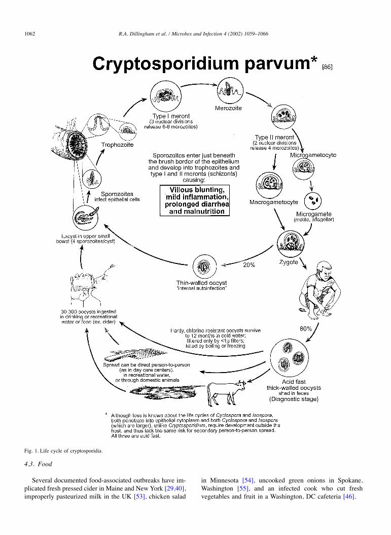
4.3. Food

Several documented food-associated outbreaks have im-plicated fresh pressed cider in Maine and NewYork [29,40],improperly pasteurized milk in the UK [53], chicken salad

in Minnesota [54], uncooked green onions in Spokane,Washington [55], and an infected cook who cut freshvegetables and fruit in a Washington, DC cafeteria [46].

Fig. 1. Life cycle of cryptosporidia.


4.4. Person-to-person

Person-to-person transmission occurred in households in5.4% (of household contacts who developed symptomaticdisease in the Milwaukee outbreak) to 19% (of familymembers of infected children in Fortaleza, Brazil develop-ing disease or seroconversion) [38]. The nosocomial andday care center outbreaks noted above [34–36] are alsolikely related to direct person-to-person spread in institu-tional settings where sanitation is difficult. Association withanal sexual exposure also likely reflects person-to-persondirect spread as well [56].

4.5. Animals-to-people

In addition to the links of bovine (genotype 2) cryptospo-ridiosis to cattle exposure on farms and through unpasteur-ized milk and apple cider, the outbreak of cryptosporidiosisamong veterinary students in the early 1980s illustrates thepotential for direct animal-to-person transmission of C. par-vum [6]. The cases of human infection with cat, dog, andturkey genotypes mentioned above also implicate transmis-sion from animals [10].

4.6. Other potential environmental sources

Environmental sources include well-documented com-mon presence of Cryptosporidium oocysts in cattle, manureand farm watershed runoff [57,58]. Other potential environ-mental sources of cryptosporidial infections include Canadageese, Peking ducks, oysters, mussels and cockles[17,40,59,60], although care must be taken to distinguishsimilar acid fast Haplosporidium [61].

4.7. Flies, cockroaches and other potential vectors

Cockroaches, houseflies, dung beetles and microscopicrotifers in water have all been suggested as potential vectorsof spread for C. parvum [40,62,63,64]. Finally, despitefrequent pulmonary symptoms in immunocompromised pa-tients with cryptosporidiosis and apparent respiratory acqui-sition of avian species among birds, airborne transmission tohumans is not well documented.

5. Seasonality and other risk factors

Cryptosporidial infections are typically seen predomi-nantly during the warm or wet season in tropical developingareas, when increased rainfall presumably results in greaterspread of contaminated surface water used for drinking [10],an effect that is not seen with other enteric protozoa likemicrosporidia, for example [65]. Bern et al. [66] also foundthat Cryptosporidium infections were most common in therainy season in Guatemala (while Cyclospora peaked in thewarmer months, and tended to affect older children, and was

more associated with diarrhea). Others, however, do not seea distinct association with the rainy season and see Cy-clospora in cooler months (in Haiti) [67].Another risk factor appears to be weaning, especially at

a young age, suggesting that breast feeding provides someprotection, whether by protective factors like immunoglo-bulin or simply by a safer source of primary sustenance invulnerable young infants [68–71].Other major risk factors include consumption of poten-

tially contaminated water, lower household income andolder age [72]. In addition, among homosexual and bisexualHIV-infected men, seropositivity was related to spa andsauna exposure and to anal sexual exposure, albeit not toCD-4 lymphocyte counts (while symptoms are highly cor-related with low CD-4 counts) [73].

6. Impact and consequences

Without question, cryptosporidiosis constitutes a leadingcause of persistent diarrhea in tropical, developing areas,both among children, in whom it often signals a period ofincreased diarrhea burden or nutrition shortfalls [14,15,74]as well as in patients with AIDS, in whom it can bedevastating and often fatal [30,65,75].In addition, however, the impact and consequences of

cryptosporidiosis may well be far greater than generallyappreciated, because of the lasting impairments in growthand development that may follow, especially with earlychildhood infections in impoverished areas, and possiblywith malabsorption of key drugs such as antiretroviral orantituberculous drugs (Brantley, Silva, Lima, Guerrant,unpublished observations). Checkley et al. [11] reportedimpaired weight gain in the month following symptomaticor even asymptomatic cryptosporidial infections in childrenin Peru, where malnutrition did not appear to be a significantrisk factor for infection. In a follow-up study of 185children, those with cryptosporidial infection experiencedseveral months of weight and height faltering, an effect thatin young children (i.e. <6 months) or stunted children per-sisted (with about 1 cm growth shortfall) at 1 year afterinfection [12]; i.e. young and stunted children did notexperience “catch-up” growth after their cryptosporidialinfections.Furthermore, we are now learning that the 4–8 dehydrat-

ing, malnourishing diarrheal illnesses that often occur eachyear in the critically formative first 2 years of life may haveprofound, lasting consequences for impaired fitness, growth,cognitive development and school performance severalyears later. Our initial studies in Northeast Brazil showreduced fitness 4–6 years later associated with early child-hood diarrhea, and specifically with cryptosporidial infec-tions in the first 2 years of life, independent of respiratoryillnesses, anthropometry, anemia and intestinal helminths[76]. The fitness deficits that associate with the averagediarrhea burdens in the first 2 years of life in these studies


are comparable to that associated with a 17% decrement inwork productivity in Zimbabwe sugar cane workers [76,77].Furthermore, these early childhood diarrheal illnesses

and intestinal helminthic infections in the first 2 years of lifeindependently and additively associate with substantiallong-term linear growth shortfalls that continue beyond6 years of age (totaling an average of 8.2 cm (3 and 1/4 in.)growth shortfall at 7 years of age) [78]. We also findsignificant associations of early childhood diarrhea withlong-term cognitive deficits (by standard “Test of NonverbalIntelligence” or TONI) even when controlling for maternaleducation, breast-feeding duration and early helminthicinfections [76,79]. Furthermore, WISC (Wechsler Intelli-gence Scale for Children; The Psychological Corp, SanAntonio, TX) coding and digit span scores were lower inchildren with persistent diarrheal illnesses in their first2 years of life, even when controlling for helminths andmaternal education [79]. Finally, these effects are seen in a“best case” scenario in which we have documented substan-tial improvements in disease rates and in nutritional statusover the several years in which we have conducted close,long-term surveillance of this population [78], effects thatwe have subsequently not found in other nearby shantytowncommunities that had not been under such intensive surveil-lance (Lima, Guerrant et al., unpublished observations).These correlations of early childhood diarrhea with

fitness, growth and cognitive deficits are also extending toschool performance, with significant associations of diar-rhea in the first 2 years of life with delayed age at startingschool (late starters are also twofold more likely to haveexperienced cryptosporidial infections) and age for grade(the latter independent of height for age Z scores at 2 yearsof age) ([80]; R.L. Guerrant et al, trends Parasitol. 18 (2002)191–193).Consistent with these lasting effects of early childhood

illnesses (or infections, without overt illness, withCryptosporidium) are studies of the importance of earlychildhood years in human brain development [79,81–83].The major brain growth and synapse formation occursduring the first 2 years of life in humans. If impaired at thiscritical formative stage, these synapses may never form ormay be substantially delayed, thus potentially explainingwhy these early childhood infections may have such alasting impact.

7. Prevention of spread

Special attention to care in the treatment of drinkingwater can prevent most cases of cryptosporidiosis. This isespecially important for immunocompromised individualsin whom it can be devastating and life threatening. Probablythe surest way to inactivate viable cryptosporidial oocysts iswith heat (to 72 °C for 1 min or simply bring water to a boil)[84]. Water filters that limit to <1 µm and reverse osmosisfilters are usually effective, but may fail [85]. As notedabove, chlorine and iodine treatment is usually ineffective,

and even the more rigorous water treatment standards(to <0.5 NTU) may not be fully protective [30].

Acknowledgements

Much of the work in this article and Drs. Lima andGuerrant are supported by NIH ICIDR Grant No. 5-UO1-AI26512. We also thank Ms. Ruth Aldridge and Yatta Jacobfor their help in preparing the manuscript.

References

[1] E.E. Tyzzer, A sporozoan found in the peptic glands of the commonmouse, Proc. Soc. Exp. Biol. Med. 5 (1907) 12–13.

[2] F.A. Nime, J.D. Burek, D.L. Page, et al., Acute enterocolitis in ahuman being infected with the protozoan Cryptosporidium, Gastro-enterology 70 (1976) 592–598.

[3] J.L. Meisel, D.R. Perea, C. Meligro, et al., Overwhelming waterydiarrhea associated with Cryptosporidium in an immunocompro-mised patient, Gastroenterology 70 (1976) 1156–1160.

[4] Centers for Disease Control and Prevention (CDC), MMWR Morb.Mortal. Wkly. Rep. 31 (1982) 580.

[5] T.R. Navin, D.D. Juranek, Cryptosporidiosis: clinical, epidemio-logic, and parasitologic review, Rev. Infect. Dis. 6 (1984) 313–327.

[6] W.L. Current, N.C. Reese, J.V. Ernst, W.S. Bailey, W.B. Heyman,W.M.Weinstein, Human cryptosporidiosis in immunocompetent andimmunodeficient persons. Studies of an outbreak and experimentaltransmission, N. Engl. J. Med. 308 (1983) 1252–1257.

[7] W.R. MacKenzie, N.J. Hoxie, M.E. Proctor, M.S. Gradus,K.A. Blair, D.E. Peterson, J.J. Kazmierczak, D.G. Addiss, K.R. Fox,J.B. Rose, J.P. Davis, A massive outbreak in Milwaukee ofCryptosporidium infection transmitted through the public watersupply, N. Engl. J. Med. 331 (1994) 161–167.

[8] R.W. Goodgame, K. Kimball, C.N. Ou, A.C. White Jr, R.M. Genta,C.H. Lifschitz, C.L. Chappell, Intestinal function and injury inacquired immunodeficiency syndrome-related cryptosporidiosis,Gastroenterology 108 (1995) 1075–1082.

[9] A.A.M. Lima, T.J. Silva, A.M.R. Gifoni, L.J. Barrett, I.T. McAuliffe,Y. Bao, J.W. Fox, D.P. Fedorko, R.L. Guerrant, Mucosal injury anddisruption of intestinal barrier function in HIV-infected individualswith and without diarrhea and cryptosporidiosis in Northeast Brazil,Am. J. Gastroenterol. 92 (1997) 1861–1866.

[10] R.D. Newman, S.X. Zu, T. Wuhib, A.A.M. Lima, R.L. Guerrant,C.L. Sears, Household epidemiology of Cryptosporidium parvuminfection, Ann. Intern. Med. 120 (1994) 500–505.

[11] W. Checkley, R.H. Gilman, L.D. Epstein, M. Suarez, J.F. Diaz,L. Cabrera, R.E. Black, C.R. Sterling, Asymptomatic and symptom-atic cryptosporidiosis: their acute effect on weight gain in Peruvianchildren, Am. J. Epidemiol. 145 (1997) 156–163.

[12] W. Checkley, L.D. Epstein, R.H. Gilman, R.E. Black, L. Cabrera,C.R. Sterling, Effects of Cryptosporidium parvum infection inPeruvian children: growth faltering and subsequent catch-up growth,Am. J. Epidemiol. 148 (1998) 497–506.

[13] D.G. Agnew, A.A.M. Lima, R.D. Newman, T. Wuhib, R.D. Moore,R.L. Guerrant, C.L. Sears, Cryptosporidiosis in Northeastern Bra-zilian children: Association with increased diarrheal morbidity,J. Infect. Dis. 177 (1998) 754–760.

[14] R.D. Newman, C.L. Sears, S.R. Moore, J.P. Nataro, T. Wuhib,D.A. Agnew, R.L. Guerrant, A.A.M. Lima, Longitudinal study ofCryptosporidium infection in children in northeastern Brazil, J. In-fect. Dis. 180 (1999) 167–175.


[15] A.M. Lima, S.R. Moore, M.S. Barboza, A.M. Soares, M.A. Schle-upner, R.D. Newman, C.L. Sears, J.P. Nataro, D.P. Fedorko, T. Wu-hib, J.B. Schorling, R.L. Guerrant, Persistent diarrhea signals acritical period of increased diarrhea burdens and nutritional short-falls: a prospective cohort study among children in northeasternBrazil, J. Infect. Dis. 181 (2000) 1643–1651.

[16] L. Xiao, U.M. Morgan, R. Fayer, R.C. Thompson, A.A. Lal,Cryptosporidium systematics and implications for public health,Parasitol. Today 16 (2000) 287–292.

[17] L. Xiao, C. Bern, J. Limor, I. Sulaiman, J. Roberts, W. Checkley,L. Cabrera, R.H. Gilman, A.A. Lal, Identification of 5 types ofCryptosporidium parasites in children in Lima, Peru, J. Infect. Dis.183 (2001) 492–497.

[18] N.J. Pieniazek, F.J. Bornay-Llinares, S.B. Slemenda, A.J. da Silva,I.N. Moura, M.J. Arrowood, O. Ditrich, D.G. Addiss, Newcryptosporidium genotypes in HIV-infected persons, Emerg. Infect.Dis. 5 (1999) 444–449.

[19] U. Morgan, R. Weber, L. Xiao, I. Sulaiman, R.C. Thompson,W. Ndiritu, A. Lal, A. Moore, P. Deplazes, Molecular characteriza-tion of Cryptosporidium isolates obtained from human immunode-ficiency virus-infected individuals living in Switzerland, Kenya, andthe United States, J. Clin. Microbiol. 38 (2000) 1180–1183.

[20] S. Pedraza-Diaz, C. Amar, J. McLauchlin, The identification andcharacterisation of an unusual genotype of Cryptosporidium fromhuman faeces as Cryptosporidium meleagridis, FEMS Microbiol.Lett. 189 (2000) 189–194.

[21] M. Kosek, C. Alcantara, A.A. Lima, R.L. Guerrant, Cryptosporidi-osis: an update, Lancet Infect. Dis. 1 (2001) 262–269.

[22] K.A. Adal, C.R. Sterling, R.L. Guerrant, Cryptosporidium andrelated species, in: M.J. Blaser, P.D. Smith, J.I. Ravdin, H.B. Green-berg, R.L. Guerrant (Eds.), Infections of the Gastrointestinal Tract,Raven Press, New York, 1995, pp. 1107–1128.

[23] T.L. Kuhls, D.A. Mosier, D.L. Crawford, J. Griffis, Seroprevalenceof cryptosporidial antibodies during infancy, childhood, and adoles-cence, Clin. Infect. Dis. 18 (1994) 731–735.

[24] B.L. Ungar, M. Mulligan, T.B. Nutman, Serologic evidence ofCryptosporidium infection in US volunteers before and during PeaceCorps service in Africa, Arch. Intern. Med. 149 (1989) 894–897.

[25] S.X. Zu, J.F. Li, L.J. Barrett, R. Fayer, S.Y. Zhu, J.F. McAuliffe,J.K. Roche, R.L. Guerrant, Seroepidemiologic study of Cryptospo-ridium infection in children from rural communities of Anhui,China, Am. J. Tropical Med. Hyg. 51 (1994) 1–10.

[26] C. Carpenter, R. Fayer, J. Trout, M.J. Beach, Chlorine disinfection ofrecreational water for Cryptosporidium parvum, Emerg. Infect. Dis.5 (1999) 579–584.

[27] D.G. Korich, J.R. Mead, M.S. Madore, N.A. Sinclair, C.R. Sterling,Effects of ozone, chlorine dioxide, chlorine, and monochloramine onCryptosporidium parvum oocyst viability, Appl. Environ. Microbiol.56 (1990) 1423–1428.

[28] J.M. McAnulty, D.W. Fleming, A.H. Gonzalez, A community-wideoutbreak of cryptosporidiosis associated with swimming at a wavepool, J. Am. Med. Assoc. 272 (1994) 1597–1600.

[29] P.S. Millard, K.F. Gensheimer, D.G. Addiss, D.M. Sosin, G.A. Beck-ett, A. Houck-Jankoski, A. Hudson, An outbreak of cryptosporidiosisfrom fresh-pressed apple cider, J. Am. Med. Assoc. 272 (1994)1592–1596 (published erratum appears in JAMA 273 (10) (1995)776).

[30] S.T. Goldstein, D.D. Juranek, O. Ravenholt, A.W. Hightower,D.G. Martin, J.L. Mesnik, S.D. Griffiths, A.J. Bryant, R.R. Reich,B.L. Herwaldt, Cryptosporidiosis: an outbreak associated withdrinking water despite state-of-the-art water treatment, Ann. Intern.Med. 124 (1996) 459.

[31] H.L. DuPont, C.L. Chappell, C.R. Sterling, P.C. Okhuysen,J.B. Rose, W. Jakubowski, The infectivity of Cryptosporidiumparvum in healthy volunteers, N. Engl. J. Med. 332 (1995) 855–859.

[32] P.C. Okhuysen, C.L. Chappell, J.H. Crabb, C.R. Sterling, H.L. Du-Pont, Virulence of three distinct Cryptosporidium parvum isolatesfor healthy adults, J. Infect. Dis. 180 (1999) 1275–1281.

[33] J.N. Eisenberg, E.Y. Seto, J.M. Colford Jr, A. Olivieri, R.C. Spear,An analysis of the Milwaukee cryptosporidiosis outbreak based on adynamic model of the infection process, Epidemiology 9 (1998)255–263.

[34] K.L. Koch, D.J. Phillips, R.C. Aber, W.L. Current, Cryptosporidiosisin hospital personnel, Ann. Intern. Med. 102 (1985) 593–596.

[35] M.A. Neill, S.K. Rice, N.V. Ahmad, T.P. Flanigan, Cryptosporidi-osis: an unrecognized cause of diarrhea in elderly hospitalizedpatients, Clin. Infect. Dis. 22 (1996) 168–170.

[36] R.L. Cordell, D.G. Addiss, Cryptosporidiosis in child care settings:a review of the literature and recommendations for prevention andcontrol, Pediatr. Infect. Dis. J. 13 (1994) 310–317 (review; 62 refs).

[37] H. Heijbel, K. Slaine, B. Seigel, P. Wall, S.J. McNabb, W. Gibbons,G.R. Istre, Outbreak of diarrhea in a day care center with spread tohousehold members: the role of Cryptosporidium, Pediatr. Infect.Dis. J. 6 (1987) 532–535.

[38] W.R. MacKenzie, W.L. Schell, K.A. Blair, D.G. Addiss, D.E. Peter-son, N.J. Hoxie, J.J. Kazmierczak, J.P. Davis, Massive outbreak ofwaterborne cryptosporidium infection in Milwaukee, Wisconsin:recurrence of illness and risk of secondary transmission, Clin. Infect.Dis. 21 (1995) 57–62.

[39] P. Osewe, D.G. Addiss, K.A. Blair, A. Hightower, M.L. Kamb,J.P. Davis, Cryptosporidiosis in Wisconsin: a case-control study ofpost-outbreak transmission, Epidemiol. Infect. 117 (1996) 297–304.

[40] R. Fayer, U. Morgan, S.J. Upton, Epidemiology of Cryptosporidium:transmission, detection and identification, Int. J. Parasitol. 30 (2000)1305–1322.

[41] M.L. Eberhard, E.K. Nace, A.R. Freeman, Survey for Cyclosporacayetanensis in domestic animals in an endemic area in Haiti,J. Parasitol. 85 (1999) 562–563.

[42] T. Katsumata, D. Hosea, I.G. Ranuh, S. Uga, T. Yanagi, S. Kohno,Short report: possible Cryptosporidium muris infection in humans,Am. J. Tropical Med. Hyg. 62 (2000) 70–72.

[43] U.M. Morgan, L. Xiao, B.D. Hill, P. O’Donoghue, J. Limor, A. Lal,R.C. Thompson, Detection of the Cryptosporidium parvum “human”genotype in a dugong (Dugong dugon), J. Parasitol. 86 (2000)1352–1354.

[44] M.M. Peng, L. Xiao, A.R. Freeman, M.J. Arrowood, A.A. Escalante,A.C. Weltman, C.S. Ong, W.R. Mac Kenzie, A.A. Lal, C.B. Beard,Genetic polymorphism among Cryptosporidium parvum isolates:evidence of two distinct human transmission cycles, Emerg. Infect.Dis. 3 (1997) 567–573.

[45] I.M. Sulaiman, L. Xiao, C. Yang, L. Escalante, A. Moore,C.B. Beard, M.J. Arrowood, A.A. Lal, Differentiating human fromanimal isolates of Cryptosporidium parvum, Emerg. Infect. Dis. 4(1998) 681–685.

[46] E.S. Quiroz, C. Bern, J.R. MacArthur, L. Xiao, M. Fletcher,M.J. Arrowood, D.K. Shay, M.E. Levy, R.I. Glass, A. Lal, Anoutbreak of cryptosporidiosis linked to a foodhandler, J. Infect. Dis.181 (2000) 695–700.

[47] J. McLauchlin, C. Amar, S. Pedraza-Diaz, G.L. Nichols, Molecularepidemiological analysis of Cryptosporidium spp. in the UnitedKingdom: results of genotyping Cryptosporidium spp. in 1,705 fecalsamples from humans and 105 fecal samples from livestock animals,J. Clin. Microbiol. 38 (2000) 3984–3990.

[48] C.S. Ong, D.L. Eisler, S.H. Goh, J. Tomblin, F.M. Awad-El-Kariem,C.B. Beard, L. Xiao, I. Sulaiman, A. Lal, M. Fyfe, A. King,W.R. Bowie, J.L. Isaac-Renton, Molecular epidemiology ofcryptosporidiosis outbreaks and transmission in British Columbia,Canada, Am. J. Tropical Med. Hyg. 61 (1999) 63–69.

[49] Outbreak of cryptosporidiosis associated with a water sprinklerfountain–Minnesota, MMWR Morb. Mortal. Wkly. Rep. 47 (1998)(1997) 856–860.


[50] J.F. Perz, S.M. Le Blancq, Cryptosporidium parvum infectioninvolving novel genotypes in wildlife from lower New York state,Appl. Environ. Microbiol. 67 (2001) 1154–1162.

[51] M.S. Madore, J.B. Rose, C.P. Gerba, M.J. Arrowood, C.R. Sterling,Occurrence of Cryptosporidium oocysts in sewage effluents andselected surface waters, J. Parasitol. 73 (1987) 702–705.

[52] M.W. LeChevallier, W.D. Norton, R.G. Lee, Giardia and Cryptospo-ridium spp. in filtered drinking water supplies, Appl. Environ.Microbiol. 57 (1991) 2617–2621.

[53] R. Gelletlie, J. Stuart, N. Soltanpoor, R. Armstrong, G. Nichols,Cryptosporidiosis associated with school milk, Lancet 350 (1997)1005–1006.

[54] Foodborne outbreak of diarrheal illness associated with Cryptospo-ridium parvum – Minnesota, MMWR Morb. Mortal. Wkly. Rep. 45(1996) (1995) 783–784.

[55] Foodborne outbreak of cryptosporidiosis – Spokane, Washington,1997, MMWR Morb. Mortal. Wkly. Rep. 47 (1998) 565–567.

[56] J.K. Griffiths, Human cryptosporidiosis: epidemiology, transmis-sion, clinical disease, treatment and diagnosis, in: J.R. Baker,R. Muller, D. Rollinson, S. Tzipori (Eds.), Opportunistic Protozoa inHumans, Advances in Parasitology, Academic Press, New York,1999, pp. 38–85.

[57] T.K. Graczyk, B.M. Evans, C.J. Shiff, H.J. Karreman, J.A. Patz,Environmental and geographical factors contributing to watershedcontamination with Cryptosporidium parvum oocysts, Environ. Res.82 (2000) 263–271.

[58] G. Widmer, M. Carraway, S. Tzipori, Water-borne Cryptosporidium:a prospective from the USA, Parasitol. Today 12 (1996) 286–290.

[59] R. Fayer, E.J. Lewis, J.M. Trout, T.K. Graczyk, M.C. Jenkins,J. Higgins, L. Xiao, A.A. Lal, Cryptosporidium parvum in oystersfrom commercial harvesting sites in the Chesapeake Bay, Emerg.Infect. Dis. 5 (1999) 706–710.

[60] M. Gomez-Bautista, L.M. Ortega-Mora, E. Tabares, V. Lopez-Rodas, E. Costas, Detection of infectious Cryptosporidium parvumoocysts in mussels (Mytilus galloprovincialis) and cockles (Ceras-toderma edule), Appl. Environ. Microbiol. 66 (2000) 1866–1870.

[61] T.K. Graczyk, C.A. Farley, R. Fayer, E.J. Lewis, J.M. Trout,Detection of Cryptosporidium oocysts and Giardia cysts in thetissues of eastern oysters (Crassostrea virginica) carrying principaloyster infectious diseases, J. Parasitol. 84 (1998) 1039–1042.

[62] R. Zerpa, L. Huicho, Childhood cryptosporidial diarrhea associatedwith identification of Cryptosporidium sp. in the cockroachPeriplaneta americana, Pediatr. Infect. Dis. J. 13 (1994) 546–548.

[63] T.K. Graczyk, M.R. Cranfield, R. Fayer, H. Bixler, House flies(Musca domestica) as transport hosts of Cryptosporidium parvum,Am. J. Tropical Med. Hyg. 61 (1999) 500–504.

[64] J. McLauchlin, S. Pedraza-Diaz, C. Amar-Hoetzeneder,G.L. Nichols, Genetic characterization of Cryptosporidium strainsfrom 218 patients with diarrhea diagnosed as having sporadiccryptosporidiosis, J. Clin. Microbiol. 37 (1999) 3153–3158.

[65] T. Wuhib, T.M. Silva, R.D. Newman, L.S. Garcia, M.L. Pereira,C.S. Chaves, S.P. Wahlquist, R.T. Bryan, R.L. Guerrant, A.Q. Sousa,T.R.B.S. Queiroz, C.L. Sears, Cryptosporidial and microsporidialinfections in human immunodeficiency virus-infected patients innortheastern Brazil, J. Infect. Dis. 170 (1994) 494–497.

[66] C. Bern, B. Hernandez, M.B. Lopez, M.J. Arrowood, A.M. DeMerida, R.E. Klein, The contrasting epidemiology of Cyclosporaand Cryptosporidium among outpatients in Guatemala, Am. J. Tropi-cal Med. Hyg. 63 (2000) 231–235.

[67] M.L. Eberhard, E.K. Nace, A.R. Freeman, R.G. Streit, A.J. DeSilva,P.J. Lammie, Cyclospora cayetanensis infections in Haiti: a commonoccurrence in the absence of watery diarrhea, Am. J. Tropical Med.Hyg. 60 (1999) 584–586.

[68] N. Hojlyng, K. Molbak, S. Jepsen, Cryptosporidium spp., a frequentcause of diarrhea in Liberian children, J. Clin. Microbiol. 23 (1986)1109–1113.

[69] J.W. Pape, E. Levine, M.E. Beaulieu, F. Marshall, R. Verdier,W.D. Johnson Jr, Cryptosporidiosis in Haitian children, Am.J. Tropical Med. Hyg. 36 (1987) 333–337.

[70] K. Molbak, P. Aaby, N. Hojlyng, A.P. da Silva, Risk factors forCryptosporidium diarrhea in early childhood: a case-control studyfrom Guinea-Bissau, West Africa, Am. J. Epidemiol. 139 (1994)734–740.

[71] K. Molbak, M. Andersen, P. Aaby, N. Hojlyng, M. Jakobsen,M. Sodemann, A.P. da Silva, Cryptosporidium infection in infancyas a cause of malnutrition: a community study from Guinea-Bissau,west Africa, Am. J. Clin. Nutrition 65 (1997) 149–152.

[72] C.T. Leach, F.C. Koo, T.L. Kuhls, S.G. Hilsenbeck, H.B. Jenson,Prevalence of Cryptosporidium parvum infection in children alongthe Texas–Mexico border and associated risk factors, Am. J. Tropi-cal Med. Hyg. 62 (2000) 656–661.

[73] C. Caputo, A. Forbes, F. Frost, M.I. Sinclair, T.R. Kunde, J.F. Hoy,C.K. Fairley, Determinants of antibodies to Cryptosporidium infec-tion among gay and bisexual men with HIV infection, Epidemiol.Infect. 122 (1999) 291–297.

[74] D.G. Agnew, A.A.M. Lima, R.D. Newman, T. Wuhib, R.D. Moore,R.L. Guerrant, C.L. Sears, Cryptosporidiosis in northeastern Brazil-ian children: association with increased diarrhea morbidity, J. Infect.Dis. 177 (1998) 754–760.

[75] N.B. Vakil, S.M. Schwartz, B.P. Buggy, C.F. Brummitt, M. Kherel-lah, D.M. Letzer, I.H. Gilson, P.G. Jones, Biliary cryptosporidiosisin HIV-infected people after the waterborne outbreak of cryptospo-ridiosis in Milwaukee, N. Engl. J. Med. 334 (1996) 19–23.

[76] D.I. Guerrant, S.R. Moore, A.A.M. Lima, P. Patrick, J.B. Schorling,R.L. Guerrant, Association of early childhood diarrhea andcryptosporidiosis with impaired physical fitness and cognitive func-tion four–seven years later in a poor urban community in NortheastBrazil, Am. J. Tropical Med. Hyg. 61 (1999) 707–713.

[77] J. Ndamba, N. Makaza, M. Munjoma, E. Gomo, K.C. Kaondera, Thephysical fitness and work performance of agricultural workersinfected with Schistosoma mansoni in Zimbabwe, Ann. TropicalMed. Parasitol. 87 (1993) 553–561.

[78] S.R. Moore, A.A. Lima, J.B. Schorling, M.S. Barboza Jr.,A.M. Soares, R.L. Guerrant, Changes over time in the epidemiologyof diarrhea and malnutrition among children in an urban Brazilianshantytown, 1989 to 1996, Int. J. Infect. Dis. 4 (2000) 179–186.

[79] M.D. Niehaus, S.R. Moore, P.D. Patrick, L.L. Derr, B. Lorntz,A.A.M. Lima, R.L. Guerrant, Early childhood diarrhea is associatedwith diminished cognitive function years later in children in aNortheast Brazilian shantytown, Am. J. Tropical Med. Hyg. (2002)4–7 (in press).

[80] B. Lorntz, A. Lima, R. Silva, P. Chen, M. Kosek, S. Moore,R. Guerrant, Diarrhea in first two years of life (ECD) is associatedwith increased age for grade (AFG) and age at starting school(AASS) 5–9 years later, 49th Annual Meeting of American Societyof Tropical Medicine and Hygiene in Atlanta, 2000.

[81] J. Dobbing, J. Sands, Cell size and cell number in tissue growth anddevelopment. An old hypothesis reconsidered, Archives FrancaisesDe Pediatrie 42 (1985) 199–203.

[82] J. Dobbing, Infant nutrition and later achievement, Am. J. Clin.Nutrition 41 (1985) 477–484 (review; 29 refs).

[83] J. Dobbing, Boyd Orr memorial lecture. Early nutrition and laterachievement, Proc. Nutrition Soc. 49 (1990) 103–118 (review; 57refs).

[84] B.C. Anderson, Moist heat inactivation of Cryptosporidium sp, Am.J. Public Health 75 (1985) 1433–1434.

[85] D.G. Addiss, R.S. Pond, M. Remshak, D.D. Juranek, S. Stokes,J.P. Davis, Reduction of risk of watery diarrhea with point-of-usewater filters during a massive outbreak of waterborne Cryptospo-ridium infection in Milwaukee, Wisconsin, 1993, Am. J. TropicalMed. Hyg. 54 (1996) 549–553.


Environmental Science & Technology is published by the American Chemical Society.1155 Sixteenth Street N.W., Washington, DC 20036

Policy AnalysisRegional Public Health Cost Estimates of Contaminated Coastal

Waters: A Case Study of Gastroenteritis at Southern California BeachesSuzan Given, Linwood H. Pendleton, and Alexandria B. Boehm

Environ. Sci. Technol., 2006, 40 (16), 4851-4858• DOI: 10.1021/es060679s • Publication Date (Web): 15 July 2006Downloaded from http://pubs.acs.org on March 18, 2009

More About This Article

Additional resources and features associated with this article are available within the HTML version:

• Supporting Information• Links to the 2 articles that cite this article, as of the time of this article download• Access to high resolution figures• Links to articles and content related to this article• Copyright permission to reproduce figures and/or text from this article

http://pubs.acs.org/doi/full/10.1021/es060679s

Regional Public Health CostEstimates of Contaminated CoastalWaters: A Case Study ofGastroenteritis at SouthernCalifornia BeachesS U Z A N G I V E N , †

L I N W O O D H . P E N D L E T O N , * , † A N DA L E X A N D R I A B . B O E H M ‡

Department of Environmental Health Sciences,Environmental Science and Engineering Program,46-071A Center for Health Sciences, University of California,Los Angeles, California 90095-1772, and Environmental WaterStudies, Department of Civil and Environmental Engineering,Stanford University, Stanford, California 94305-4020

We present estimates of annual public health impacts,both illnesses and cost of illness, attributable to excessgastrointestinal illnesses caused by swimming in contaminatedcoastal waters at beaches in southern California. Beach-specific enterococci densities are used as inputs totwo epidemiological dose-response models to predictthe risk of gastrointestinal illness at 28 beaches spanning160 km of coastline in Los Angeles and Orange Counties.We use attendance data along with the health cost ofgastrointestinal illness to estimate the number of illnessesamong swimmers and their likely economic impact. Weestimate that between 627,800 and 1,479,200 excessgastrointestinal illnesses occur at beaches in Los Angelesand Orange Counties each year. Using a conservativehealth cost of gastroenteritis, this corresponds to an annualeconomic loss of $21 or $51 million depending upon theunderlying epidemiological model used (in year 2000 dollars).Results demonstrate that improving coastal water qualitycould result in a reduction of gastrointestinal illnesses locallyand a concurrent savings in expenditures on relatedhealth care costs.

IntroductionEach year between 150 million and nearly 400 million visitsare made to California (CA) beaches generating billions ofdollars in expenditures, by tourists and local swimmers, andnonmarket values enjoyed mostly by local area residents (1,2). Nonmarket benefits represent the value society places onresources, such as beaches, beyond what people have to payto enjoy these resources (see Pendleton and Kildow (1) fora review of the nonmarket value of CA beaches). In an effortto protect the health of beach swimmers, the CA StateLegislature passed Assembly Bill 411 (AB411) in 1997 withformal guidance and regulations for beach water qualitywhich are formally codified as a state statute (3). AB411requires monitoring of bathing waters for fecal indicator

bacteria (FIB, including total coliform (TC), fecal coliform(FC), and enterococcci (ENT)) on at least a weekly basis duringthe dry season (1 April through 31 October) if the beach isvisited by over 50,000 people annually or is located adjacentto a flowing storm drain. Beaches can be posted with healthwarnings if single-sample or geometric mean standards forTC, FC, and ENT exceed prescribed levels (see SupportingInformation (SI) for standards).

Based on AB411 water quality criteria and their profes-sional judgment, CA county health officials posted or closedbeaches 3,985 days during 2004 (4). Sixty percent (2,408beach-days) of these occurred at Los Angeles and OrangeCounty (LAOC) beaches (4), and nearly all (93%) of the LAOCadvisories and closures were caused by unknown sources ofFIB. The number of beach closures and advisories in CA(and the country as a whole) rises each year as countiesmonitor more beaches (4). Needless to say, public awarenessof coastal contamination issues is growing, and in some casesstrongly influencing the development of programs to improvecoastal water quality. For example, public pressure on theOrange County Sanitation District (OCSD) prevented themfrom reapplying for a waiver from the USEPA to releasepartially treated sewage to the coastal ocean. Instead, OCSDplans to implement a costly upgrade to their sewage treatmentplant. New stormwater permits issued by CA Regional WaterBoards require counties and municipalities to implementprevention and control programs to meet coastal waterquality criteria. The cost of such mitigation measures isdifficult to determine, yet cost has been used as an argumentin court challenges to the permits (4). In 2004 elections, votersin the city of Los Angeles approved a measure to spend $500million on stormwater mitigation (5).

To understand the potential public health benefits ofcleaning up coastal waters, we need a better idea of themagnitude of health costs associated with illnesses that aredue to coastal water contamination. Several previous studiesaddress the potential economic impacts of swimming-relatedillnesses. Rabinovici et al. (6) and Hou et al. (7) focused onthe economic and policy implications of varying beachclosure and advisory policies at Lake Michigan and Hun-tington Beach, CA, respectively. Dwight et al. (8) estimatedthe per case medical costs associated with illnesses at twobeaches in southern California and used this to makeestimates of public health costs at two Orange Countybeaches. Our study is novel in that it provides the first regionalestimates of the public health costs of coastal water qualityimpairment.

While many different illnesses are associated with swim-ming in contaminated marine waters, we focus our analysison gastrointestinal illness (GI) because this is the mostfrequent adverse health outcome associated with exposureto FIB in coastal waters (9, 10). We estimate daily excess GIbased on attendance data, beach-specific water qualitymonitoring data, and two separate epidemiological modelsdeveloped by Kay et al. (11) and Cabelli et al. (12) that modelGI based on exposure to fecal streptococci and ENT,respectively. Finally, we provide estimates of the potentialannual economic impact of GI associated with swimming atstudy beaches.

We conduct our analysis using data from 28 LAOC beachesduring the year 2000. Together, these beaches span 160 kmof coastline (Figure 1, Table S1). We limit our analysis tothese beaches and the year 2000 in particular because wewere able to obtain relatively complete daily and weeklyattendance and water quality data for these beaches during

* Corresponding author e-mail: [email protected]; phone: (310)825-8569; fax: (310) 206-3358.

† University of California, Los Angeles.‡ Stanford University.

Environ. Sci. Technol. 2006, 40, 4851-4858

10.1021/es060679s CCC: $33.50 © 2006 American Chemical Society VOL. 40, NO. 16, 2006 / ENVIRONMENTAL SCIENCE & TECHNOLOGY 9 4851Published on Web 07/15/2006

this year. The 28 beaches represent a large, but incomplete,subset of the total beach shoreline in LAOC. Large stretchesof relatively inaccessible beaches (e.g., portions of LagunaBeach, much of Malibu, and Broad Beach) were omitted fromthe analysis as were several large public beaches (e.g., SealBeach and Long Beach) because of paucity of attendanceand/or water quality data. The 1999-2000 and 2000-2001winter rainy seasons were typical for southern CA (13), so2000 was not particularly unique with respect to rainfall. Acomparison of inter-annual water quality at a subset ofbeaches suggests that pollution levels in 2000 were moderate(data not shown). Thus, the estimates we provide can beviewed as typical for the region.

MethodsNumber of Swimmers. Morton and Pendleton (2) compileddaily attendance data from lifeguards’ records and beachmanagement agencies. When data were missing, attendancewas estimated using corresponding monthly median weekdayor weekend values from previous years. (Table S1 shows thenumber of days in 2000 when data are availablesfor mostbeaches, this number approaches 366.) Because these dataare based on actual counts, we do not need to factor in effectsdue to the issuance of advisories at a particular beach. Onlya fraction of beach visitors enter the water. This fractionvaries by month in southern CA from 9.56 to 43.62% (TableS2) (14). We applied the appropriate fraction to the attendancedata to determine the number of individual swimmersexposed to coastal waters. Although research suggests thepresence of FIB in sand in the study area (15, 16), we do notconsider the potential health risk that may arise from sandexposure because it has not been evaluated.

Water Quality Data. ENT data were obtained from thelocal monitoring agencies and are publicly available. Localmonitoring agencies sample coastal waters at ankle depth inthe early morning in sterile containers. Samples are returnedto the lab and analyzed for ENT using USEPA methods. WhenENT values are reported as being below or above the detection

limit of the ENT assay, we assume that ENT densities wereequal to the detection limit.

During 2000, monitoring rarely occurred on a daily basis;ENT densities were measured 14-100% of the 366 days in2000, depending on monitoring site (Table S1). For example,Zuma beach was monitored once per week during the studyperiod, while Cabrillo beach was monitored daily. To estimateENT densities on unsampled days, we used a Monte Carlotechnique. Normalized cumulative frequency distributionsof observed ENT densities at each monitoring site wereconstructed for the 1999-2000 wet season (Nov 1, 1999through Mar 31, 2000), 2000 dry season (April 1, 2000 throughOct 31, 2000), and the 2000-2001 wet season (Nov 1, 2000through Mar 31, 2001). ENT densities on unsampled daysduring 2000 were estimated by randomly sampling from theappropriate seasonal distribution. Because day-to-day ENTconcentrations at marine beaches are weakly correlated andvariable (17), we chose not to follow the estimation methodof Turbow et al. (18) who assumed a linear relationshipbetween day-to-day ENT densities at two CA beaches.Comparisons between the Monte Carlo method and a methodthat simply used the monthly arithmetic average ENT densityindicated the two provided similar results (data not shown).

The beaches in our study area (Figure 1) are of variablesizes; each beach may include 1-7 monitoring sites (TableS1). If more than one monitoring site exists within theboundaries of a beach, the arithmetic mean of ENT at thesites was used as a single estimate for ENT concentrationswithin the beach (19). There is considerable evidence thatENT densities at a beach vary rapidly over as little as 10minutes (17, 20). Therefore, even though we used up to 7measurements or estimates to determine ENT at a beach ona given day, there is still uncertainty associated with ourestimate because sampling is conducted at a single time eachday.

Dose-Response. Of all the illnesses considered in theliterature, GI is most commonly associated with exposure topolluted water (10-12, 21-26). To estimate the risk of GI

FIGURE 1. The 28 beaches considered in this study. HSB ) Huntington State Beach, HCB) Huntington City Beach, SCC ) San ClementeCity Beach, and SCS ) San Clemente State Beach.


from swimming in contaminated marine waters in southernCA, we utilized two dose-response models (11, 12) (Table1) developed in epidemiology studies conducted elsewhere(in marine waters of the East U.S. coast and United Kingdom)(18, 27). A local dose-response model for GI would bepreferable, but does not exist. Haile et al. (28) conducted anepidemiology study at Los Angeles beaches and found thatskin rash, eye and ear infections, significant respiratorydisease, and GI were associated with swimming in waterswith elevated FIB or near storm drains; however, they didnot report dose-response models for illness and bacterialdensities.

The two dose-response models (hereafter referred to asmodels C (12) and K (11)) are fundamentally different in thatmodel C was derived from a prospective cohort study whilemodel K was developed using a randomized trial study. ModelC has been scrutinized in the literature (20, 26, 29-31). Amongthe criticisms are lack of ENT measurement precision andinappropriate pooling of data from marine and brackishwaters. World Health Organization (WHO) experts (10)suggest that epidemiology studies that apply a randomizedtrial design, such as model K, offer a more precise dose-response relationship because they allow for better controlover confounding variables and exposure (26). Thus, the WHOhas embraced model K over cohort studies such as modelC for assessing risk. We report GI estimates obtained fromboth models C and K in our study because they have bothbeen applied in the literature (8, 18), and form the basis forwater quality criteria worldwide.

Models C and K were developed in waters suspected tobe polluted with wastewater. The source of pollution at our

study site during the dry season is largely unknown (4),although human viruses have been identified in LAOC coastalcreeks and rivers (32-36) and an ENT source tracking studyat one beach suggests sewage is a source (37). During the wetseason, stormwater is a major source of FIB to coastal watersand Ahn et al. (38) detected human viruses in LAOCstormwater. Because we cannot confirm that all the ENT atour study site was from wastewater, there may be errorsassociated with the application of models C and K. In addition,there is evidence that dose-response relationships may besite specific (30). The results presented in our study shouldbe interpreted in light of these limitations.

We converted incidence and odds, the dependent vari-ables reported for model C and K, respectively, into risk ofGI (P) (Table 1). P represents total risk of GI to the swimmer,and includes risk due to water exposure plus the backgroundGI rate (P0). Excess risk was calculated by subtracting thebackground risk from risk (P - P0). While ENT is theindependent variable for model C, model K requires fecalstreptococci (FS), the larger bacterial group of which ENTare a subset, as the independent variable. We assumed thatFS and ENT represent the same bacteria, following guidancefrom the WHO (9).

Models C and K provide different functional relationshipsbetween ENT and excess GI risk (Figure 2). Model C predictsrelatively low, constant risks across moderate to high ENTdensities relative to model K. At ENT less than 32 CFU/100mL, model K predicts no excess risk; model C, however, doespredict nonzero risks even at these low levels of contamina-tion. The data range upon which each model was built variesconsiderably. Model C is based on measurements ranging

TABLE 1. Dose-Response Models for Predicting GIa

name original model model converted to excess risk

model C (12) 1000(P - Po) ) 24.2 log10(ENT) - 5.1 (P - P0) ) (24.2 log10(ENT) - 5.1)/1000model K (11) X ) Ln(P/(1 - P)) ) 0.201 (FS - 32)1/2 - 2.36 (P - P0) ) (eX/(1 + eX)) - P0

a ENT ) enterococci, FS ) fecal streptococci. Both ENT and FS are in units of CFU or MPN per 100 mL water. P is the risk of GI for swimmers,P0 is the background risk of GI.

FIGURE 2. Dose-response relationships for the two epidemiological models. Excess risk of GI is shown as a function of ENT density.The inset more clearly shows the differences between the relationship for the randomized trial study (model K (11)) and the cohort study(model C (12)).


from 1.2-711 CFU/100 mL and model K is based onmeasurements from 0-35 to 158 CFU/100 mL. We extrapo-lated models C and K when ENT densities were outside theepidemiology study data ranges. Given the lack of epide-miological data on illlness outside the ranges, extrapolationof the models represents a reasonable method of estimatingexcess GI.

Excess Illness Due To Swimming. The excess incidenceof GI on day i at beach j (GIi,j) is given by the followingexpression:

Pi,j -Po is the excess risk of GI on day i at beach j as estimatedfrom models C or K (Table 1), Ai,j is the number of beachvisitors, and fi is the fraction of swimmers on day i (14). Weassume P0 is 0.06sthe background risk for stomach pain asreported by Haile et al. (28) for beaches within Santa MonicaBay, CA. Daily values were summed across the year or seasonto estimate the number of excess GI per beach. Seasonalcomparisons are useful in this region because of distinctdifferences between attendance and water quality betweenseasons. The wet season is defined as November throughMarch and the dry season is defined as April through October.Note that the dry season corresponds to the season whenstate law mandates beach monitoring (3).

Public Health Costs of Coastal Water Pollution. GI canresult in loss of time at work, a visit to the doctor, expenditureson medicine, and even significant nonmarket impacts thatrepresent the “willingness-to-pay” of swimmers to avoidgetting sick (sometimes referred to as psychic costs). Becausethere is a lack of information on the costs of waterborne GI,Rabinovici et al. (6) used the cost of a case of food-borne GI,$280 (year 2000 dollars) per illness from Mauskopf and French(39), as a proxy for the cost of water-borne GI for swimmersin the Great Lakes. The $280 per illness represents thewillingness-to-pay to avoid GI and includes both market andnonmarket costs (6). Dwight et al. (8) conducted a cost ofillness study for water-borne GI for two beaches in southernCalifornia (Huntington State Beach and Newport Beach) anddetermined the cost as $36.58 per illness in 2004 dollars basedon lost work and medical costs. Discounting for inflation,this amount is equivalent to $33.35 in the year 2000 dollars.This value does not include lost recreational values or thewillingness-to-pay to avoid getting sick from swimming. Weuse the more conservative estimate of Dwight et al. (8) tocalculate the health costs of excess GI at LAOC beaches.However, we also provide more inclusive estimates of thecost of illness using Mauskopf and French’s $280 willingness-to-pay value (39). Unless otherwise stated, all costs arereported in year 2000 dollars.

ResultsAttendance and Swimmers. Beach attendance was higherduring the dry season (from May through October) than inthe wet season (November through April) (Figure 3). Weestimate that the annual visitation to Los Angeles and OrangeCounty (LAOC) beaches for the year 2000 approached 80million visits.

Water Quality. Water quality (measured in terms of ENTconcentration) varies widely across the beaches in the study.(Figure S1 shows the log-mean of ENT observations at eachbeach during the dry and wet seasons.) In general ENTdensities are higher during the wet season compared to thedry. Water quality problems at a beach may exist chronicallyover the course of the year or may be confined to particularlywet days when precipitation washes bacteria into stormdrains and into the sea. The most serious, acute water qualityimpairments can result in the issuance of a beach advisoryor beach closure. According to CA state law, water quality

exceeds safe levels for swimming if a single beach watersample has a concentration of ENT greater than 104 CFU/100 mL. Figure 4 illustrates the percentage of the days forwhich daily estimated ENT concentrations were in excess ofthe state single sample standard. Exceedances during thewet months generally outnumber exceedances during thedry months. The exceptions are Corral, Bolsa Chica, andCrystal Cove, which are all relatively clean beaches, even inthe wet season. Doheny, Malibu, Marina Del Rey, Cabrillo,and Las Tunas had the worst water quality with over 33% ofthe daily estimates in 2000 greater than 104 CFU/100 mL,while Newport, Hermosa, Abalone Cove, Manhattan, Tor-rance, and Bolsa Chica had the best water quality with lessthan 5% of daily estimates under the standard.

Estimates of Excess GI and Associated Public HealthCosts due to Swimming. Figure 5 illustrates estimated annualexcess GI at beaches based on models C and K; results aregiven for dry and wet months. Models C and K both indicatethat Santa Monica, the beach with the highest attendance(Figure 3), has the highest excess GI of all beaches duringwet and dry seasons. Both models predict that the threebeaches with the lowest excess GI were San Clemente State,Nicholas Canyon, and Las Tunas, a direct result of thesebeaches being among the smallest and least visited in ourstudy area (Figure 3).

GIi,j ) Ai,jfi(Pi,j - Po) (1)

FIGURE 3. Beach attendance during wet and dry seasons 2000.


There are marked seasonal differences between excessGI predictions. Although water quality is typically worseduring the wet season compared to the dry (Figures 4 andS1), more excess GI are predicted for the dry season for mostbeaches. This result is driven by seasonal variation inattendance (Figure 3). The exceptions are model K predictionsfor Zuma that indicate 0 and 6647 excess GI during the dryand wet seasons, respectively. Zuma had no ENT densitiesgreater than 32 CFU/100 mL during the dry season, hencethe prediction of 0 excess GI.

Numerical predictions of excess GI for the entire yearfrom model C and model K vary markedly between beaches.At 24 beaches, model K predicts between 18% and 700%greater excess GI than model C. The greatest difference inthe estimated GI is at Doheny beach where models C andK predict 18,000 and 153,000 excess GI, respectively. At 4beaches (Zuma, Hermosa, Torrance, and Newport), modelK predicts between 1 and 90% lower incidence of GI thanmodel C. These beaches are generally clean with ENTdensities below the model K threshold of 32 CFU/100 mL forexcess risk.

The public health burden of coastal contaminationdepends on both attendance and water quality. Figure 6

illustrates how excess GI, based on predictions from modelsC and K, varies as a function of water quality (percent ofdaily ENT estimates in exceedance of standard) and at-tendance. Red, yellow, and green symbols indicate beacheswith increasing numbers of GI. If reduction of public healthburden is a goal of local health care agencies, then beacheswith a red symbol are candidates for immediate action. Nearlyall beaches are categorized as high priority during the dryseason based on model K (panels A and B). Model C indicatesthat dry weather mitigation measures at Venice, Zuma, SantaMonica, and Newport, some of the most visited beaches,would significantly reduce the public health burden (panelC), more so than wet weather mitigation measures (panelD).

Another way of prioritizing beach remediation is toexamine the risk of GI relative to the USEPA guideline of 19illnesses per 1000 swimmers (Figure S2). Model K indicatesthat at 19 and 15 of the 28 LAOC beaches during the wet anddry seasons, respectively, risk is greater than twice the EPAacceptable risk. Model C, on the other hand, indicates thatonly two beaches (Marina del Rey and Doheny) during the

FIGURE 4. Percentage of days on which daily ENT estimates weregreater than the CA Department of Health single-sample ENTstandard of 104 CFU/100 mL.

FIGURE 5. Excess GI by beach and season for models C and K.


dry season, and six (Marina del Rey, Doheny, Santa Monica,Las Tunas, Will Rogers, and Malibu) in the wet season fallinto this “high” risk category.

Public Health Costs of Coastal Water Pollution. Table2 summarizes the number of excess GI and associated publichealth costs during wet and dry periods by county and season.Based on the conservative cost of illness given by Dwight etal. (8), the estimated health costs of GI based on models Cand K is over $21 million and $50 million, respectively. If wefollow Rabinovici et al.(6) and use $280 per GI, the estimatedpublic health impacts are $176 million based on model Cand $414 million based on model K. For both LA and OCbeaches, county-wide costs obtained using model K yieldhigher results than those obtained from model C, a direct

result of the difference in GI estimates (Figures 5 and 6).Health costs are greater in the dry season compared to thewet suggesting that money may be well spent on dry-weatherdiversions.

DiscussionA significant public health burden, in terms of both numbersof GI and the costs of GI, is likely to result from beach waterquality contamination in southern CA. The corollary to thisfinding is that water quality improvements in the regionwould result in public health benefits. Specifically, we makethree key findings: (1) removing fecal contamination fromcoastal water in LAOC beaches could result in the preventionof between 627,800 and 1,479,200 GI and a public health costof between $21 and $51 million (depending upon theepidemiological model used) each year in the region usingthe most conservative cost estimates and as much as $176million or $414 million if we use the larger estimate of healthcosts (6, 39); (2) even beaches within the same region differsignificantly in the degree to which swimming poses a publichealth impact; and (3) public health risks differ betweenseasons. Findings (2) and (3) are not surprising given spatio-temporal variation in water quality (17, 40) and attendancewithin the study site.

A previous study by Turbow et al. (18) estimated 36,778excess HCGI (highly credible GI) per year from swimming atNewport and Huntington State beaches (8). Our estimatesfor the same stretch of shoreline are higher (68,011 and 87,513 excess GI based on models C and K, respectively). Notonly did we use a different measure of illness (GI vs. HCGI)we also used a Monte Carlo scheme to estimate ENT onunsampled days whereas Turbow et al. (18) used linearinterpolation, and we used higher, empirically determined

FIGURE 6. Excess GI at each beach as a function of % ENT in exceedance of the single sample standard and attendance. Results forthe dry (panels A and C) and wet (panels B and D) seasons are shown for Models K (panels A and B) and C (panels C and D). Beachesare labeled; SCC is San Clemente City Beach, SCS is San Clemente State, HSB is Huntington State Beach, and HCB is Huntington CityBeach. In panels A and C, numbers on symbols correspond to beaches, as indicated in the upper right corner of panel C. The color scalein panel A applies to all panels.

TABLE 2. Countywide Public Health Impacts and Costs for Wetand Dry Months (2000)

GI cases health costscounty/region season model C model K model C model K

LosAngeles

dry 394,000 804,000 $13,100,000 $28,800,000wet 33,800 189,000 $1,130,000 $6,310,000total 427,800 993,000 $14,230,000 $35,110,000

Orangedry 185,000 420,000 $6,180,000 $14,000,000wet 15,000 66,200 $500,000 $2,210,000total 200,000 486,200 $6,680,000 $16,210,000

regiontotal

dry 579,000 1,224,000 $19,280,000 $40,800,000wet 48,800 255,200 $1,630,000 $8,520,000total 627,800 1,479,200 $20,910,000 $51,320,000


(14) measures of the percent of beach goers that swim. Dwightet al. (8) used Turbow et al.’s (18) estimate to determine thatthe health costs of excess GI at the same beaches were $1.2million. Our health cost estimates are higher ($2.3 and $2.9million for models C and K, respectively), due to the higherincidence of ilness predicted by our models.

Beaches with chronic water quality problems are obviouscandidates for immediate contamination mitigation. Manybeaches in LAOC, however, are relatively clean and meetwater quality standards on most days. Clean beaches withmoderate to low levels of attendance do not represent asignificant public health burden (Figure 6). Nevertheless,public health impacts are still substantial at heavily visitedbeaches (for instance those with over 6,000,000 visitors peryear) even when water quality is good (e.g., Manhattan Beach)(Figure 6). Generally speaking, it will be more difficult toreduce contaminant levels at cleaner beaches. At beacheswith high attendance and generally good water quality (likeNewport Beach and Zuma), policy managers should continuedry weather source reduction efforts (e.g., education cam-paigns and watershed management), but should also rec-ognize that the cost of eliminating all beach contaminationmay outweigh the marginal public health benefits of doingso.

Our estimates of the potential health benefits that mightresult from removing bacterial contamination from coastalwater in LAOC beaches have limitations. First, we focus ona lower bound estimate of the health cost of GI that does notconsider the amount a beach goer is willing to pay to avoidgetting sick (estimates using higher, but less scientificallyconservative estimates also are provided). Second, while wefocus on the public health impacts from GI. Exposure tomicrobial pollution at beaches also increases the chance ofsuffering from various symptoms and illnesses (28, 41). Forinstance, Haile et al. (28) and Fleisher et al. (41) documentassociations between water quality and respiratory illnesses,acute febrile illness, fever, diarrhea with blood, nausea, andvomiting, and earaches. Third, if the public believes swim-ming is associated with an increased risk of illness, they maybe discouraged from going to the beach, resulting in a lossof beach-related expenditures to local businesses andrecreational benefits to swimmers in addition to the loss inhealth benefits described here. Fourth, we consider GIoccurring at a subset of LAOC beaches for which water qualityand attendance data were available (Figure 1). Fifth, implicitin our analysis is the assumption that models C and K canbe applied to LAOC beaches. Despite these limitations, theresults reported here represent the best estimates possiblein light of imperfect information. Future studies that establishdose-response relationships for the LAOC region or confirmincidence of swimming GI medically would improve esti-mates of public health burden and costs.

AcknowledgmentsThis project was supported by a grant from the ToxicsSubstances Research and Teaching Program of the Universityof California. We acknowledge the assistance of Stan Asato,Clay Clifton, Masahiro Dojiri, Eric Edwards, Monica Mazur,David Pryor, and Kathy Walker in obtaining and interpretingthe water quality data from monitoring agencies around thesouthern California Bight. The insightful comments andsuggestions from five anonymous reviewers improved themanuscript substantially.

Note Added after ASAP PublicationThe Model C discussion in the Methods section publishedASAP July 15, 2006 has been revised. The corrected versionwas published July 26, 2006.

Supporting Information AvailableTables S1 and S2, Figures S1 and S2, and the California statewater quality standards. This material is available free ofcharge via the Internet at http://pubs.acs.org.

Literature Cited(1) Pendleton, L.; Kildow, J. The Non-Market Value of California

Beaches. Shore and Beach 2006, 74 (2), 34-37.(2) Morton, J.; Pendleton, L. A Database of Beach Closures and

Historical Water Quality; State Water Resources Control Board:Sacramento, CA, 2001.

(3) California State Department of Health Services. Statutes of 1997.Health and Safety Code §115880. Assembly Bill 411, Chapter765.

(4) Natural Resources Defense Council. Testing the Waters 2005:A Guide to Water Quality at Vacation Beaches; NRDC: NewYork, 2005. http://www.nrdc.org/water/oceans/ttw/ titinx.asp.

(5) Los Angeles County, CA, Voter Proposition O (Nov., 2004). http://www.lastormwater.org/index1.htm.

(6) Rabinovici, S.; Bernknopf, R. L.; Wein, A. M.; Coursey, D. L.;Whitman, R. L. Economic and health risk tradeoffs of swimclosures at a Lake Michigan Beach. Environ. Sci. Technol. 2004,38, 2742-2750.

(7) Hou, D.; Rabinovici, S. J. M.; Boehm, A. B. Enterococcipredictions from partial least squares regression models inconjunction with a single-sample standard improve the efficacyof beach management advisories. Environ. Sci. Technol. 2006,40, 1737-1743.

(8) Dwight, R. H.; Fernandez, L. M.; Baker, D. B.; Semenza, J. C.;Olson, B. H. Estimating the economic burden from illnessesassociated with recreational coastal water pollutionsA casestudy in Orange County, California. J. Environ. Manage. 2005,76, 95-103.

(9) World Health Organization. Guidelines for Safe RecreationalWater Environments; WHO: Geneva, 2003; Ch. 4. http://www.who.int/water_sanitation_health/bathing/srwg1.pdf.

(10) Pruss, A. Review of epidemiological studies on health effectsfrom exposure to recreational water. Int. J. Epidemiol. 1998, 27,1-9.

(11) Kay, D.; Fleisher, J. M.; Salmon, R. L., Jones, F.; Wyer, M.; Godfree,A.; Zelenauch-Jacquotte, Z.; Shore, R. Predicting likelihood ofgastroenteritis from sea bathing: results from randomizedexposure. Lancet 1994, 344, 904-909.

(12) Cabelli, V. J.; Dufour, A. P.; McCabe, L. J.; Levin, M. A. Swimming-associated gastroenteritis and water quality. Am. J. Epidemiol.1982, 115, 606-616.

(13) NOAA. Region 6 Climate Data; National Oceanic and Atmo-spheric Administration: Washington, DC. http://www.ncdc.noaa.gov/oa/land.html#dandp.

(14) Hannemann, M.; Pendleton, L.; Mohn, C.; Hilger, J.; Kurisawa,K.; Layton, D.; Vasquez, F. Using Revealed Preference Models toEstimate the Affect of Coastal Water Quality on Beach Choice inSouthern California; National Oceanic and Atmospheric Ad-ministration, Minerals Management Service; The California StateWater Resources Control Board, California Department of Fishand Game: Sacramento, CA, 2004.

(15) Lee, C. M.; Lin, T.; Lin, C.-C.; Kohbodi, G. A.; Bhatt, A.; Lee, R.;Jay, J. A. Persistence of fecal indicator bacteria in Santa MonicaBay beach sediments. Water Res. 2006, 40 (14), 2593-2602.

(16) Ferguson, D. M.; Moore, D. F.; Getrich, M. A.; Zhowandai, M.H. Enumeration and speciation of enterococci found in marineand intertidal sediments and coastal water in southern Cali-fornia. J. Appl. Microbiol. 2005, 99, 598-608.

(17) Boehm, A. B.; Grant, S. B.; Kim, J. H.; Mowbray, S. L.; McGee,C. D.; Clark, C. D.; Foley, D. M.; Wellman, D. E. Decadal andshorter period variability of surf zone water quality at HuntingtonBeach, California. Environ. Sci. Technol. 2002, 36, 3885-3892.

(18) Turbow, D.; Osgood, N.; Jiang, S. C. Evaluation of recreationalhealth risk in coastal waters based on Enterococcus densitiesand bathing patterns. Environ. Health Perspect. 2003, 111, 598-603.

(19) Haas, C. N. How to average microbial densities to characterizerisk. Water Res. 1996, 30, 1036-1038.

(20) Fleisher, J. M. The effects of measurement error on previouslyreported mathematical relationships between indicator organ-ism density and swimming associated illness: a quantitativeestimate of the resulting bias. Int. J. Epidemiol. 1990, 19, 1100-1106.

(21) Wade, T. J.; Pai, N.; Eisenberg, J. S.; Colford, J. M. Do U. S.Environmental Protection Agency water quality guidelines for


recreational waters prevent gastrointestinal illness? A systematicreview and meta-analysis. Environ. Health Perspect. 2003, 111,1102-1109.

(22) Alexander, L. M.; Heaven, A.; Tennant, A.; Morris, R. Symp-tomatology of children in contact with seawater contaminatedwith sewage. J. Epidemiol. Commun. Health 1992,46, 340-344.

(23) Cheung, W. S.; Chang, K. K.; Hung, R. S.; Kleevens, J. L. Healtheffects of beach waer pollution in Hong Kong. Epidemiol. Infect.1990, 105, 139-162.

(24) McBride, G. B.; Salmond, C. E.; Bandaranayake, D. R.; Turner,S. J.; Lewis, G. D.; Till, D. G. Health effects of marine bathingin New Zealand. Int. J. Environ. Health Res. 1998, 8, 173-189.

(25) Prieto, M. D.; Lopez, B.; Juanes, J. A.; Revilla, J. A.; Llorca, J.;Delgado-Rodrıgueza, M. Recreation in coastal waters: healthrisks associated with bathing in sea water. J. Epidemiol.Commun. Health 2001, 55, 442-447.

(26) Havelaar, A.; Blumenthal, U. J.; Strauss, M.; Kay, D.; Bartram,J. Guidelines: the current position. In Water Quality: Guidelines,Standards and Health; Fewtrell, L., Bartram, J., Eds.; IWAPublishing: London, UK, 2001.

(27) Soller, J.; Olivieri, A. W.; Crook, J.; Tchobanoglous, G.; Parkin,R.; Spear, R. C.; Eisenberg, J. S. Risk-based approach to evaluatethe public health benefit of additional wastewater treatment.Environ. Sci. Technol. 2003, 37, 1882-1891.

(28) Haile, R. W.; Witte, J. S.; Gold, M.; Cressey, R.; McGee, C.; Millikan,R. C.; Glasser, A.; Harawa, N.; Ervin, C.; Harmon, P.; Harper, J.;Dermand, J.; Alamillo, J.; Barrett, K.; Nides, M.; Wang, G. Y. Thehealth effects of swimming in ocean water contaminated bystorm drain runoff. Epidemiology 1999, 10, 355-363.

(29) Fleisher, J. M. Conducting recreational water quality surveys.Some problems and suggested remedies. Mar. Pollut. Bull. 1990,21, 562-567.

(30) Fleisher, J. M. A reanalysis of data supporting the US Federalbacteriological water quality criteria governing marine recre-ational waters. J. Water Pollut. Control Fed. 1991, 63, 259-264.

(31) Fleisher, J. M.; Jones, F.; Kay, D.; Morano, R. Setting recreationalwater quality criteria. In Recreational Water Quality Manage-ment: Freshwater; Kay, D., Hanbury, R., Eds.; Ellis Horwood:Chichester, UK, 1993.

(32) Choi, S.; Jiang, S. C. Real-time PCR quantification of humanadenoviruses in urban rivers indicates genome prevalence but

low infectivity. Appl. Environ. Microbiol. 2005, 71, 7426-7433.

(33) Jiang, S. C.; Chu, W. PCR detection of pathogenic viruses insouthern California urban rivers. J. Appl. Microbiol. 2004, 97,17-28.

(34) Noble, R. T.; Griffith, J. F.; Blackwood, A. D.; Fuhrman, J. A.;Gregory, J. B.; Hernandez, X.; Liang, X. L.; Bera, A. A.; Schiff, K.Multitiered approach using quantitative PCR to track sourcesof fecal pollution affecting Santa Monica Bay, California. Appl.Environ. Microbiol. 2006, 72, 1604-1612.

(35) Fuhrman, J. A.; Liang, X. L.; Noble, R. T. Rapid detection ofenteroviruses in small volumes of natural waters by real-timequantitative reverse transcriptase PCR. Appl. Environ. Microbiol.2005, 71, 4523-4530.

(36) Noble, R. T.; Fuhrman, J. A. Enteroviruses detected by reversetranscriptase polymerase chain reaction from the coastal watersof Santa Monica Bay, California: low correlation to bacterialindicator levels. Hydrobiologia 2001, 460, 175-184.

(37) Choi, S.; Chu, W. P.; Brown, J.; Becker, S. J.; Harwood: V. J.;Jiang, S. C. Application of enterococci antibiotic resistancepatterns for contamination source identification at HuntingtonBeach, California. Mar. Pollut. Bull. 2003, 46, 748-755.

(38) Ahn, J. H.; Grant, S. B.; Surbeck, C. Q.; Digiacomo, P. M.; Nezlin,N. P.; Jiang, S. Coastal water quality impact of stormwater runofffrom an urban watershed in southern California. Environ. Sci.Technol. 2005, 39, 5940-5953.

(39) Mauskopf, J. A.; French, M. T. Estimating the value of avoidingmorbidity and mortality from foodborne illnesses. Risk Anal.1991, 11, 619-632.

(40) Schiff, K. C.; Morton, J.; Weisberg, S. B. Retrospective evaluationof shoreline water quality along Santa Monica Bay beaches.Mar. Environ. Res. 2003, 56, 245-253.

(41) Fleisher, J. M.; Kay, D.; Wyer, M. D.; Godfree, A. F. Estimates ofthe severity of illnesses associated with bathing in marinerecreational waters contaminated with sewage. Int. J. Epidemiol.1998, 27, 722-726.

Received for review March 21, 2006. Revised manuscriptreceived June 6, 2006. Accepted June 7, 2006.

ES060679S


The Health Effects of Swimming in Ocean Water Contaminated by Storm DrainRunoff

Robert W. Haile; John S. Witte; Mark Gold; Ron Cressey; Charles McGee; Robert C. Millikan;Alice Glasser; Nina Harawa; Carolyn Ervin; Patricia Harmon; Janice Harper; John Dermand;James Alamillo; Kevin Barrett; Mitchell Nides; Guang-yu Wang

Epidemiology, Vol. 10, No. 4. (Jul., 1999), pp. 355-363.

Stable URL:http://links.jstor.org/sici?sici=1044-3983%28199907%2910%3A4%3C355%3ATHEOSI%3E2.0.CO%3B2-B

Epidemiology is currently published by Lippincott Williams & Wilkins.

Your use of the JSTOR archive indicates your acceptance of JSTOR's Terms and Conditions of Use, available athttp://www.jstor.org/about/terms.html. JSTOR's Terms and Conditions of Use provides, in part, that unless you have obtainedprior permission, you may not download an entire issue of a journal or multiple copies of articles, and you may use content inthe JSTOR archive only for your personal, non-commercial use.

Please contact the publisher regarding any further use of this work. Publisher contact information may be obtained athttp://www.jstor.org/journals/lww.html.

Each copy of any part of a JSTOR transmission must contain the same copyright notice that appears on the screen or printedpage of such transmission.

The JSTOR Archive is a trusted digital repository providing for long-term preservation and access to leading academicjournals and scholarly literature from around the world. The Archive is supported by libraries, scholarly societies, publishers,and foundations. It is an initiative of JSTOR, a not-for-profit organization with a mission to help the scholarly community takeadvantage of advances in technology. For more information regarding JSTOR, please contact [email protected].

http://www.jstor.orgMon Jul 23 20:27:09 2007

http://links.jstor.org/sici?sici=1044-3983%28199907%2910%3A4%3C355%3ATHEOSI%3E2.0.CO%3B2-B

http://www.jstor.org/about/terms.html

http://www.jstor.org/journals/lww.html

The Health Effects of Swimming in Ocean Water Contaminated by Storm Drain Runoff

Robert W. Haile, John S. Wittej2 Mark Gold13 Ron Cressey ,4 Charles McGee ,5

Robert C . Millikan,6 Alice Glasser , Nina Harawa, Carolyn Erwin, Patricia Harmon, Janice Harper, John Dermand, James Ahil lo ,3 Kevin Barrett, l Mitchell Nides ,9

and Guang- yu Wanglo

Waters adjacent to the County of Los Angeles (CA) receive untreated runoff from a series of storm drains year round. Many other coastal areas face a similar situation. To our knowledge, there has not been a large-scale epidemiologic study of persons who swim in marine waters subject to such runoff. We report here results of a cohort study conducted to investigate this issue. Measures of exposure included distance from the storm drain, selected bacterial indicators (total and fecal coliforms, enterococci, and Escherichia coli), and a direct measure of enteric viruses. We found higher risks of a broad range of

symptoms, including both upper respiratory and gastrointestinal, for subjects swimming (a) closer to storm drains, (b) in water with high levels of single bacterial indicators and a low ratio of total to fecal coliforms, and (c) in water where enteric viruses were detected. The strength and consistency of the associations we observed across various measures of exposure imply that there may be an increased risk of adverse health outcomes associated with swimming in ocean water that is contaminated with untreated urban runoff. (Epidemiology 1999;10:355-363)

Keywords: environmental epidemiology, gastrointestinal illness, ocean, recreational exposures, sewage, storm drains, waterborne illnesses, waterborne pathogens.

Runoff from a system of storm drains enters the Santa Monica Bay adjacent to Los Angeles County (CA). Even in the dry months of summer 10-25 million gallons of runoff (or non-storm water discharge) per day enter the bay from the storm drain system. Storm drain

From 'University of Southern California, Department of Preventive Medicine, Los Angeles, California; 2Case Western Reserve University, Department of Epidemiology and Biostatistics, Cleveland, Ohio; 'Heal the Bay, Santa Monica, California; 'City of Los Angeles, Depamnent of Public Works, Bureau of San- itation, Environmental Monitoring Division, Los Angeles, California; 5County Sanitation Districts of Orange County, California; Wniversity of North Caro- lina, Department of Epidemiology, Chapel Hill, North Carolina; 'University of California Los Angeles, Department of Prevention & Control, Los Angeles, California; BUnivenity of California Los Angles, Department of Epidemiology, Los Angeles, California; 9University of California Los Angeles, Department of Pulmonary and Critical Care Medicine, Los Angeles, California; 1°Santa Monica Bay Restoration Project, Monterey Park, California.

Address reprint requests to: Robert W. Haile, USClNorris Comprehensive Cancer Center, Department of Preventive Medicine, 1441 Eastlake Avenue, Room 4455, P.O. Box 33800, Los Angeles, CA 90033.0800.

This work was supported by the Santa Monica Bay Restoration Project, City of Los Angeles, California State Water Resources Control Board, Beach Cities Health District, City of Santa Monica, Los Angeles County Department of Public Works, Heal the Bay, Los Angeles Regional Water Quality Control Board, Chevron USA, Las Virgenes Municipal Water District, U. S. Environ- mental Protection Agency, and Milken Families Foundation.

Submitted March 4, 1998; final version accepted January 22, 1999

Editors' note: See related editorial on page 351 of this Issue.

O 1999 by Epidemiology Resources Inc.

water is not subject to treatment and is discharged directly into the ocean. Total and fecal coliforms, as well as enterococci, are sometimes elevated in the surf zone adjacent to storm drain outlets; pathogenic human enteric viruses have also been isolated from storm drain effluents, even when levels of all commonly used indicators, including F2 male-specific bacteriophage, were low.'

Approximately 50-60 million persons visit Santa Monica Bay beaches annually. Concern about possible adverse health effects due to swimming in the bay has been raised by numerous interested parties2 Previous reports indicate that swimming in polluted water (for example, due to sewage) increases risks of numerous adverse health outcomes (Pruss3 provides a recent review of this literature). To our knowledge, however, there has never been a large epidemiologic study of persons who swim in marine waters contaminated by heavy urban runoff.

These circumstances provided the motivation to study the possible health effects of swimming in the bay. We present here the main results from a large cohort study of people that addressed the issue of adverse health effects of swimming in ocean water subject to untreated urban runoff.

Methods DESIGNAND SUBJECTS The exposures of interest were distance swimming from storm drains, levels of bacterial indicators (total coli-

356 HAILE ET AL

forms, fecal coliforms, enterococcus, Escherichia coli) for pathogens that potentially produce acute illness, and human enteric viruses. We studied three beaches located in Santa Monica Bay (CA) that exhibited a wide range of pathogen indicator counts and a high density of swimmers (Santa Monica, Will Rogers, and Surfrider).

Persons who immersed their heads in the ocean water were potential subjects for this study. There was no restriction based on age, sex, or race. We excluded anyone who swam at the study beaches or in heavily polluted areas (that is, Mothers' Beach in Marina del Rev or near the Santa Monica Pier) within 7 days before thd study date, or between the date of the beadh interview and the telephone follow-up interview. We ex-cluded subjects who swam on multiple days, as one of our primary questions was whether risk of health outcomes was associated with levels of indicator organisms on the -specific day a subject entered the water. We targeted persons bathing within 100 yards upcoast or downcoast of the storm drain and persons bathing greater than 400 yards beyond a storm drain.

For this study, 22,085 subjects were interviewed on the beach from June 25 to September 14, 1995, to ascertain eligibility and willingness to participate. We found that 17,253 of these subjects were eligible and able to participate (that is, had a telephone and were able to speak English or Spanish). Of these, 15,492 (90% of the eligible subjects) agreed to participate. They were interviewed about their age, residence, and swimming, particularly immersion of the head into ocean water. The interviewer noted distance from the storm drain (within the categories 0, 1-50, 51-100, or 400 yards), gender, and race of the subject. (Distances from each drain were marked with inconspicuous objects such as beach towels and umbrellas.)

Nine to 14 days after the beach interview, subjects were interviewed bv te le~hone to ascertain the occur- r ence (~) of: fever, chills, eye discharge, earache, ear discharge, skin rash, infected cuts, nausea, vomiting, diarrhea, diarrhea with blood, stomach pain, coughing, coughing with phlegm, nasal congestion, and sore throat. For this study we defined a priori three groupings of svmvtoms indicative of gastrointestinal illness or re- , -

Epidemiology July 1999, Volume 10 Number 4

they did not confirm immersing their faces in ocean water, leaving 11,686 subjects. One subject had a missing value for age, which we imputed (as the median value among all subjects) for inclusion in the adjusted analyses (discussed below). For the bacteriological analyses, we excluded an additional 1,227 subjects who had missing values, leaving 10,459 subjects. In the virus analyses we included only the 3,554 subjects who swam within 50 yards of the drain on days when viruses were measured (as the samples were collected only at the storm drain).

Samples were collected on days that subjects were interviewed on the beaches. Each day, ankle depth samples were collected from each location (0 yards, 100 yards upcoast and downcoast of the drain, and one sample at 400 yards). One duplicate sample per site was collected daily. Samples were collected in sterile 1 liter polypropylene bottles and transferred on ice to the microbiology laboratory. All samples were analyzed for total coliforms, fecal coliforms, enterococcus, and E. coli. Densities of total and fecal coliforms and enterococci were deter-mined using the appropriate membrane filtration techniques in Ref 5. E. coli densities were determined by membrane filtration using Hach Method 10029 for m- ColiBlue24 Broth.

For looking at enteric viruses, we collected samples from the three storm drain sites on Fridays, Saturdays, and Sundays, using Method 9510 C g of Ref 5. Ambient pH, temperature, conductivity, and total dissolved solids were measured. Samples as large as 100 gallons chosen to minimize the impacts of seawater dilution were filtered through electropositive filters at ambient pH. Adsorp- tion filters were eluted in the field with 1 liter of sterile 3% beef extract adjusted to pH 9.0 with sodium hydroxide. Field eluates were reconcentrated in the laboratorv

spiratory disease. In particular, following Cabelli et ~ 1 , ~using an organic reflocculation p r~cedure .~All final subjects were classified as having highly credible gastrointestinal illness 1 (HCGI 1) if they experienced at least one of the following: (1) vomiting, (2) diarrhea and fever, or (3) stomach vain and fever. We also classified subjects as having higLly credible gastrointestinal illness 2 (HCGI 2) if they had vomiting and fever. Finally, we classified subjects as having significant respiratory disease (SRD) if they had one of the following: (1) fever and nasal congestion, (2) fever and sore throat, or (3) coughing with phlegm.

We were able to contact and interview 13,278 subjects (86%follow-up). Of those interviewed, 1,485 were found to be ineligible because thev swam (and immersed their heads) at studv beach dr in hiavilv volluted waters between the day of the beach interview &and the telephone follow-up. We excluded 107 subjects because

concentrates were detoxified before ana l~s i s .~ All samples were analyzed for infectious human en-

teric viruses in Buffalo green monkey kidney cells (BGMK) by the plaque assay technique. Ten percent of the final concentrate was tested in this manner to determine whether there were a quantifiable number of viruses present. The remaining concentrate volume was divided in half and analyzed using the liquid overlay technique known as the cytopathic effect (CPE) assay.8 The CPE assay generally detects a greater number of viruses than the plaque assay, but it is not quantitative. Flasks that did not exhibit CPE were considered to be negative for detectable infectious virus. We further examined any flask exhibiting CPE by the plaque-forming unit method to confirm the presence of infectious viruses.


Our analysis addressed two main questions. First, are there different risks of specific outcomes among subjects swimming 0, 1-50, 51-100, and 400 or more yards from a storm drain? If pathogens in the storm drain result in increased acute illnesses, one would expect higher risks among swimmers closer to the drain. Second, are risks of specific outcomes associated with levels of specific bacterial indicators or enteric viruses?

To address the second question, we estimated risks arising from exposure to levels within categories defined a pliori by existing standards or expert consensus. Spe- cifically, for total coliforms we defined categories using 1,000 and 10,000 colony-forming units (cfu) per 100 ml as cutpoints, which are based on the California Code of Regulations (S.7958 in Title 17).9 For fecal coliforms we created categories using cutpoints of 200 and 400 cfu per 100 ml, which reflect criteria set by the State Water Resources Control Board.lo For enterococcus we used cutpoints of 35 and 104 cfu per 100 ml of water, which were established by the U.S. Environmental Protection Agency." Finally, categories for E. coli were selected in meetings with staff from the Santa Monica Bay Resto- ration Project (SMBRP), Heal the Bay, and the Los Angeles County Department of Health Services. These meetings resulted in initially selecting categories based on cutpoints of 35 and 70 cfu per 100 ml, and then subsequently adding categories using cutpoints of 160 and 320 cfu per 100 ml; the latter were added because it is believed that E. coli comprises about 80% of the fecal coliforms. Using these knowledge-based categories, however, assumes a homogeneous risk between cutpoints. This might not be a reasonable assumption because the adequacy of these cutpoints is unclear, and because a large percentage of the subjects were in a single (that is, the lowest) category. Therefore, we further explored the bacteriological relations using categories defined by deciles.

In addition to considering total and fecal coliforms separately, we investigated the potential effect of the ratio of total to fecal coliforms. Motivation for this arose from our expectation that the risk of adverse health outcomes might be higher when the ratio is smaller, indicating a relatively greater proportion of fecal contamination. We used categories of this ratio defined by a cutpoint of 5 (where 5 corresponds to there being 5 times as much total as fecal coliform in the water). The human enteric virus exposure was reported as a dichotomous (that is, virus detected us not detected) measure.

We first calculated simple descriptive statistics giving the number of subjects with each adverse health outcome who swam (1) at the prespecified distances from the drain or (2) in water with the prespecified levels of pathogens. From these counts we estimated the crude risk associated with each exposure. We then used logistic regression to estimate the adjusted relative risks of each outcome. For each exposure/outcome combination, we fit a separate model. All models adjusted for the potential confounding of: age (three categories: 0-12 years,

STORM DRAIN RUNOFF AND ILL HEALTH 357

13-25 years, >25 years); sex; beach; race (four categories: white, black, Latinola, and Asian/multiethnic/other); California us out-of-state resident; and concern about potential health hazards at the beach (four categories: not at all, somewhat, a little, and very).

Results Table 1 presents results for each of the adverse health outcomes by distance swimming from the storm drain. Across all distances, risks ranged from about 0.001 (that is, 1 per 1,000) for diarrhea with blood to about 0.1 for runny nose. The risk of numerous outcomes was higher for people who swam at the drain (0 yards away), in comparison with those who swam 1-50, 51-100, or >400 yards from the drain. In particular, we observed increases in risk for fever, chills, ear discharge, coughing with phlegm, HCGI 2, and SRD. In addition, the risks for eye discharge, earache, sore throat, infected cut, and HCGI 1 were also slightly elevated. A handful of outcomes exhibited small increased risks among swimmers at 1-50 yards (skin rash) or at 51-100 yards (cough, cough with phlegm, runny nose, and sore throat). Ad- justed estimates of relative risk (RR) comparing swimmers at 0, 1-50, or 51-100 yards from the drain with swimmers at least 400 yards away from the drain showed similar relations as the aforementioned patterns of risks (Table 1). Among the positive associations for swimmers at the drain, RRs ranged in magnitude from about 1.2 (eye discharge, sore throat, HCGI 1) to 2.3 (earache), with varying degrees of precision; most of these RRs ranged from 1.4 to 1.6.

In Table 2 we see that the risk of skin rash increased for the highest prespecified category of total coliforms (that is, >10,000 cfu). Furthermore, the adjusted RR comparing swimmers exposed at this level us those exposed to levels 51,000 cfu was 2.6. Whereas the RR for diarrhea with blood also suggested a positive association, this result was based on a single adverse health event (as evinced by the wide 95% CIS). When looking at deciles, in relation to the lowest exposure level (that is, the lowest lo%), we observed increased risks of skin rash at all other levels (Figure 1). The adjusted RRs ranged from 1.6 to 6.2, with five of the nine RRs in the 2-3 range. In addition, there were increased risks of HCGI 2 for all deciles except one (the eighth); the corresponding adjusted RRs ranged from 1.4 to 4.7, with varying levels of precision (Figure 1 ) .

When looking at fecal coliforms, we again observed among those in the highest category (that is, >400 cfu) an increased risk for skin rash (Table 3). There were also slight increased risks for infected cut, runny nose, and diarrhea with blood in the highest category, as well as for nausea, vomiting, coughing, sore throat, and HCGI 2 in the middle category (200-400 cfu). The adjusted RRs also indicated positive associations for these outcomes (Table 3 ) . When we used deciles to categorize subjects, however, in comparison with the lowest decile, we only observed marginal increased risks for infection and skin rash (not shown). In our investigation of the ratio of

358 HAILE ET AL Epidemiology July 1999, Volume 10 Number 4

TABLE 1. Adverse Health Outcomes by Distance Swimming from Drain: Number Ill, Acute Risks, Adjusted Relative Risk (RR) Estimates and 95% Confidence Intervals (CI)

Distance from Drain (in Yards)

>400 (N = 3030)* 51-100 (N = 3311) 1-50 (N = 4518) 0 (N = 827)

Outcome No. Ill Risk No. Ill Risk RR (95% CI) t No. Ill Risk RR (95% CI) t No. I11 Risk RR (95% CI)t

Fever 138 0.046 158 0.048 1.06 (0.84-1.34) 208 0.046 1.07 (0.85-1.33) 59 0.071 1.61 (1.16-2.24) .. .. - - -

Chills 72 0.024 85 0.026 1.07 (0.7 7-1.4jj 108 0.024 1.05 (0.77-i.42j 31 0.037 1.60 (1.03-2.5oj Eye discharge 61 0.020 59 0.018 0.88 (0.61-1.27) 73 0.016 0.77 (0.55-1.09) 19 0.023 1.15 (0.67-1.98) Earache 116 0.038 116 0.035 0.89 (0.68-1.16) 136 0.030 0.81 (0.63-1.04) 38 0.046 1.34 (0.91-1.98) Ear discharee 21 0.007 19 0.006 0.78 (0.42-1.46j 25 0.006 0.80 (0.45-1.44) 13 0.016 2.09 (1.014.33) --.. -~...--.-Skin rash Infected cut Nausea

~ i a r r h e a 204 0.067 163 0.049 0.70 (0 .5w.86j 202 0.045 0.69 io.56-0.84j 53 0.064 1.04 (0.75-i.44j Diarrhea with blood 7 0.002 2 0.001 0.26 (0.05-1.26) 3 0.001 0.27 (0.07-1.06) 2 0.002 0.87 (0.154.57) Stomach pain 206 0.068 194 0.059 0.85 (0.70-1.05) 271 0.060 0.93 (0.77-1.12) 61 0.074 1.11 (0.82-1.51) Cough 209 0.069 263 0.079 1.18 (0.97-1.42) 296 0.066 0.98 (0.82-1.18) 55 0.067 1.01 (0.73-1.38) Cough and phlegm 90 0.030 114 0.034 1.16 (0.88-1.54) 143 0.032 1.09 (0.83-1.43) 39 0.047 1.65 (1.1 1-2.46) Runny nose 273 0.090 351 0.106 1.18 (1.00-1.40) 371 0.082 0.95 (0.80-1.12) 74 0.089 1.10 (0.84-1.46) Sore throat 190 0.063 244 0.074 1.17 (0.96-1.43) 304 0.067 1.12 (0.93-1.35) 59 0.071 1.25 (0.92-1.71) HCGI 1 102 0.034 96 0.029 0.88 (0.661.17) 121 0.027 0.84 (0.64-1.10) 35 0.042 1.21 (0.81-1.82) HCGI 2 26 0.009 28 0.008 1.04 (0.61-1.79) 32 0.007 0.90 (0.53-1.53) 15 0.018 1.64 (0.84-3.21) Significant respiratory 139 0.046 177 0.053 1.18 (0.94-1.49) 205 0.045 1.03 (0.82-1.23) 63 0.076 1.78 (1.29-2.45)

disease

The total number of swimmers in each category is given in (N).HCGI1, highly credible gastrolntestlnal illness wlth vomiting, dlarrhea and fever or stomach paln and fever. HCGT2, highly credible gastrointestinal illness with vomiting and fever only. Significant respiratory disease, fever and nasal congestion, fever and sore throat or coughing with phlegm. * Referent category (RR = 1.0). t Adjusted for age, sex, beach, race, Califomla us outeof-state resident, and concem about potential health hazards at the beach.

total to fecal coliforms, we observed a consistent pattern 1,000 or 5,000 cfu, we then restricted our analysis to of higher risks for diarrhea and HCGI 2 as the ratio subjects swimming in water above these levels. In the category became lower (not shown, but available in Ref first case, increased risks with decreasing cutpoints were 12). Because any effect of this lower ratio should be observed for nausea, diarrhea, and HCGI 2.12When we stronger when there was a higher degree of contamina- restricted our investigation to subjects in water in which tion, indicated by total coliform counts in excess of the total coliforms exceeded 5,000 cfu, we observed

TABLE 2. Adverse Health Outcomes by Total Coliform Levels: Number Ill, Acute Risks, Adjusted Relative Risk (RR) Estimates and 95% Confidence Intervals (CI)

Total Coliforms (cfu/lOOml)

51,000 (N = 7,574)* >1,00&10,000 (N = 1,988) >10,000 (N = 757)

Outcome No. I11 Risk No. I11 Risk RRt No. I11 Risk RRt

Fever 368 0.049 88 0.044 0.92 (0.72-1.17) 42 0.055 1.23 (0.87-1.73) Chills 193 0.025 51 0.026 1.03 (0.75-1.42) 9 0.012 0.51 (0.261.01) Eye discharge Earache Ear discharge Skin rash Infected cut Nausea Vomiting Diarrhea Diarrhea with blood Stomach pain Cough Cough and phlegm Runny nose Sore throat HCGI 1 242 0.032 54 0.027 0.84 (0.62-1.14) 17 0.022 0.74 (0.44-1.23) HCGI 2 72 0.010 16 0.008 0.89 (0.51-1.55) 5 0.007 0.83 (0.32-2.12) Significant respiratory disease 396 0.052 84 0.042 0.80 (0.62-1.02) 42 0.055 1.1 1 (0.79-1.55)

The total number of swimmers in each category IS given In parentheses (N).* Referent category (RR = 1.0). t Adjusted for age, sex, beach, race, Callfom~a us out-of-state resident, and concern about potentla1 health hazards at the beach

Epidemiology July 1999, Volume 10 Number 4 STORM DRAIN RUNOFF AND ILL HEALTH 359

- 0 5 0 1 2 5 4 5 6 7 8 9 1 0

D e c i l e s Sore Throat FIGURE 1. Log odds of adverse health outcomes by deciles of exposure for selected bacterial exposures. -, Total coliform and skin rash; - - - ., total coliform and HCGI 2; - ., Enterococci and infected cut; ---,E coli and eye discharge; ..-,E coli and skin rash; .- ,E coli and infected cut. HCGI 2 = highly credible gastrointestinal illness with vomiting and fever only.

increased risks with eye discharge, ear discharge, skin rash, nausea, diarrhea, stomach pain, nasal congestion, HCGI 1, and HCGI 2.12There was a consistent pattern FIGURE 2. Selected attributable numbers/10,000 ex- of stronger risk ratios as the cutpoint became lower posed subjects for total to fecal coliforms. +, All days; ., (when the analyses were restricted to times when total >1000; A, > 5000. HCGI 1 = highly credible gastrointes- coliforms exceeded 1,000 or 5,000 cfu), with the stron- tinal illness with vomiting, diarrhea and fever or stomach gest effects generally observed with the cutpoint of 2, as pain and fever. illustrated in Figure 2 for diarrhea, vomiting, sore throat, and HCGI1. served an increased risk of skin rash among those in the

Table 4 gives results for the relation among entero- highest category (that is, >I04 cfu). In addition, com- cocci and the adverse health outcomes. Again, we ob- paring the highest to other categories of exposure, there

TABLE 3. Adverse Health Outcomes by Fecal Coliform Levels: Number Ill, Acute Risks, Adjusted Relative Risk (RR) Estimates and 95% Confidence Intervals (CI)

Fecal Coliforms (cfu/lOOml)

5200 (N = 8,005)* >200-400 (N= 768) >400 (N= 1,636)

Outcome No. I11 Risk No. I11 Risk RRt No. I11 Risk RRt

Fever 381 0.048 39 0.051 1.04 (0.74-1.46) 80 0.049 1.02 (0.80-1.32) Chills 197 0.025 24 0.031 1.14 (0.74-1.76) 34 0.021 0.78 (0.54-1.14) Eye discharge Earache Ear discharge Skin rash Infected cut Nausea Vomiting Diarrhea Diarrhea with blood Stomach vain 495 0.062 51 0.066 1.04 (0.77-1.41)' 103 0.063 0.98 i0.78-1.23j Cough Cough and phlegm Runny nose Sore throat HCGI 1 HCGI 2 65 0.008 1 1 0.014 1.63 (0.85-3.12j 17 0.010 1.13 (0.65-i.95j Significant respiratory disease 399 0.050 42 0.055 1.08 (0.77-1.50) 85 0.052 1.04 (0.81-1.33)

The total number of swimmers in each catego7 is given in parentheses (N) .* Referent category (RR = 1.0). t Adlusted for age, sex, beach, race, California us out,of-state resident, and concern about potential health hazards at the beach.


TABLE 4. Adverse Health Outcomes by Enterococci Levels: Number Ill, Acute Risks, Adjusted Relative Risk (RR) Estimates and 95% Confidence Intervals (CI)

Enterococci (cfu/lOOml)

5 3 5 (N= 7,689)* >35-104 (N = 1,863) >lo4 (N= 857)

Outcome No. 111 Risk No. I11 Risk RRt No. I11 Risk R R t

Fever 371 0.048 84 0.045 0.91 (0.71-1.16) 45 0.053 1.00 (0.72-1.40) Chills 198 0.026 33 0.018 0.67 (0.4W.97) 24 0.028 0.94 (0.60-1.48) Eye discharge 149 0.019 25 0.013 0.69 (0.45-1.07) 16 0.019 1.01 (0.5g1.75) Earache 270 0.035 57 0.031 0.82 (0.61-1.11) 3 1 0.036 0.88 (0.59-1.31) Ear discharge 52 0.007 12 0.006 0.85 (0.45-1.62) 4 0.005 0.53 (0.19-1.51) Skin rash 74 0.010 13 0.007 0.71 (0.39-1.30) 13 0.015 1.72 (0.89-3.31) Infected cut 46 0.006 12 0.006 0.95 (0.49-1.82) 6 0.007 0.90 (0.37-2.18) Nausea 271 0.035 72 0.039 1.07 (0.82-1.41) 4 1 0.048 1.19 (0.84-1.70) Vomiting 130 0.017 34 0.018 1.13 (0.77-1.67) 18 0.021 1.20 (0.71-2.04) Diarrhea 398 0.052 101 0.054 0.99 (0.78-1.25) 57 0.067 1.01 (0.75-1.36) Diarrhea with blood 8 0.001 0 - - 3 0.004 2.90 i0.66-12.68) Stomach pain 464 0.060 126 0.068 1.09 (0.89-1.35) 59 0.069 0.97 (0.72-1.30) Cough 554 0.072 121 0.065 0.91 (0.73-1.12) 63 0.074 1.00 (0.75-1.34) Cough and phlegm 266 0.035 59 0.032 0.91 (0.68-1.22) 3 1 0.036 1.03 (0.69-1.54) Runny nose 704 0.092 165 0.089 0.96 (0.80-1.15) 85 0.099 1.01 (0.79-1.30) Sore throat 533 0.069 118 0.063 0.89 (0.72-1.10) 5 2 0.061 0.80 (0.59-1.09) HCGI 1 230 0.030 51 0.027 0.92 (0.67-1.26) 36 0.042 1.31 (0.89-1.92) HCGI 2 67 0.009 14 0.008 0.82 (0.461.48) 12 0.014 1.30 (0.67-2.51) S~gnificant 397 0.052 84 0.045 0.86 (0.67-1.1 1) 45 0.053 0.98 (0.70-1.37)

respiratory disease

The total number of swimmers m each category 1s given in parentheses (N).* Referent category (RR = 1.0). t Adjusted for age, sex, beach, race, California us out-of-state resident, and concern about potential health hazards at the beach

were increased risks of nausea, vomiting, diarrhea with adjusting for each bacterial indicator (one-at-a-time) blood, HCGI 1, and HCGI 2. Our adjusted RRs sug- also left these results essentially unchanged.12 As ex-gested similar positive associations, except for diarrhea; pected, there was an association between presence of although the risk increased from 0.05 to 0.07, the ad- virus and fecal coliforms within 50 yards of the drain. justed RR comparing the highest to lowest category was The mean density of fecal coliforms when no virus was 1.0 (Table 4). When comparing the lowest to higher detected was 234.8 cfu (SD 542.5 cfu); whereas it was deciles, we observed increased risks in most categories 2,233.8 (SD 2,634.1) when viruses were detected (N = for infected cut and skin rash (Figure 1). Other adverse 386). The median values were 47.8 and 452.6 cfu, re- health outcomes-infected cut, nausea, diarrhea, diar- spectively. rhea with blood, HCGI 1, and HCGI 2-exhibited increased risks only in particular quantiles. In comparison with the lowest decile, the risk of each of these Discussion outcomes was higher in the 10th decile. For example, W e observed differences in risk for a number of out- the risk for HCGI 2 was 0.007 in the first decile, but comes when we compared subjects swimming at 0 yards 0.015 in the 10th. us 400+ yards. Most of the relative risks suggested an

Table 5 presents results for E. coli. We once again approximately 50% increase in risk. Furthermore, as found an increased risk of skin rash in the highest evinced by both the risks and RRs, there is an apparent prespecified category (that is, >320 cfu). Furthermore, threshold of increased risk occurring primarily at the we observed slight increased risks in this highest cate- drain: no dose response is evinced with increasing close- gory for eye discharge, earache, stomach pain, coughing ness to the drain, but there is a jump in risk for many with phlegm, runny nose, and HCGI 1 (Table 5). In our adverse health outcomes among those swimming at the decile-based analysis, however, we only observed mate- drain. W e also found that distance is a reasonably good rially increased risks for eye discharge, skin rash, and surrogate for bacterial indicators, with higher levels ob- infection (Figure 1). served closer to the drain.12

Numerous adverse health outcomes exhibited higher For bacterial indicators, we observed a relation among risks among subjects swimming on days when samples numerous higher exposures and adverse health out-were positive for viruses (Table 6). In particular, the risk comes. These increases were mostly restricted to the of fever, eye discharge, vomiting, sore throat, HCGI 1, highest knowledge-based categories (no effect was ob- and HCGI 2, and to a lesser extent, chills, diarrhea, served below any existing standards). When looking at diarrhea with blood, cough, coughing with phlegm, and quantiles, we found higher risks of skin rash and infec- SRD were higher on days when viruses were detected. tion at fairly low levels. In contrast with what one might Our adjusted RR estimates showed similar relations, expect, however, there was no clear dose-response pat- most ranging from 1.3 to 1.9 (Table 6). Additionally, tern across increasing levels of bacteriological exposures.

TABLE 5. Adverse Health Outcomes by E. coli Levels: Number Ill, Acute Risks, Adjusted Relative Risk (RR) Estimates and 95% Confidence Intervals (CI)

E. coli (cfu/lOOml)

535 (N = 6,104)*

-- 135-75 (N = 1,620) >75-160 (N= 1,145) >I66320 (N = 518) >320 (N = 991)

Outcome No. Ill Risk No. I11 Risk RRI No. Ill Risk RRt No. Ill Risk RRt No. Ill Risk RRt

Fever 274 0.045 89 0.055 1.22 61 0.053 1.20 29 0.056 1.22 45 0.045 0.98

Chills 145 0.024 41 0.025 (0.95-1.56)

1.OO 28 0.024 (0.90-1.60)

1.OO 18 0.035 (0.81-1.84)

1.38 22 0.022 (0.70-1.37)

0.79

Eye discharge

Earache

116

214

0.019

0.035

30

45

0.019

0.028

(0.70-1.44) 0.99

(0.65-1.49) 0.75

14

33

0.012

0.029

(0.66-1.52) 0.65

(0.37-1.15) 0.78

6

18

0.012

0.035

(0.82-2.33) 0.61

(0.26-1.43) 0.91

23

47

0.023

0.047

(0.49-1.26) 1.36

(0.84-2.19) 1.25

Ear discharge

Skin rash

42

57

0.007

0.009

8

15

0.005

0.009

(0.54-1.04)0.60

(0.28-1.28) 1.01

5

7

0.004

0.006

(0.53-1.14)0.57

(0.22-1.46) 0.66

6

6

0.012

0.012

(0.55-1.50)1.28

(0.52-3.15) 1.21

6

15

0.0066

0.015

(0.89-1.77)0.67

(0.27-1.62)2.04

Infected cut 42 0.007 7 0.004 (0.56-1.80)

0.53 3 0.003 (0.30-1.46)

0.33 3 0.006 (0.49-2.98)

0.66 9 0.009 (1.11-3.76)

1.02

Nausea 216 0.035 74 0.046 (0.24-1.20)

1.22 34 0.030 (0.10-1.06)

0.80 18 0.035 (0.20-2.19)

0.88 42 0.042 (0.48-2.19)

1.03

Vomiting

Diarrhea

107

310

0.018

0.051

31

101

0.019

0.062

(0.93-1.61) 1.09

(0.72-1.64) 1.14

16

63

0.014

0.055

(0.55-1.16) 0.82

(0.48-1.40) 1.OO

8

25

0.015

0.048

(0.53-1.46) 0.87

(0.41-1.85) 0.80

20

56

0.020

0.057

(0.73-1.47) 1.05

(0.63-1.74) 0.91

Diarrhea with blood 5 0.001 3 0.002 (0.90-1.44)

2.06 1 0.001 (0.75-1.33)

1.03 2 0.004 (0.52-1.23)

3.98 0 -(0.67-1.23)

Stomach pain 353 0.058 124 0.077 (0.48-8.89)

1.28 (1.03-1.59)

70 0.061 (0.12-9.01)

1.02 (0.78-1.33)

31 0.060 (0.68-23.21 )

0.95 (0.64-1.40)

70 0.071 1.06 (0.80-1.40)

Cough

Cough and phlegm

444

226

0.073

0.037

96

41

0.059

0.025

0.81 (0.64-1.02)

0.66 (0.474.92)

86

34

0.075

0.030

1.04 (0.82-1.33)

0.78 (0.54-1.12)

29

11

0.056

0.021

0.77 (0.5 1-1.14)

0.53 (0.28-1.00)

82

43

0.083

0.043

1.14 (0.88-1.48)

1.12 (0.79-1.59)

Runny nose

Sore throat

566

417

0.093

0.068

136

99

0.084

0.061

0.87 (0.71-1.06)

0.86

105

82

0.092

0.072

0.96 (0.77-1.20)

1.02

38

29

0.073

0.056

0.76 (0.53-1.08)

0.78

108

75

0.109

0.076

1.12 (0.89-1.41)

1.04

HCGI 1 183 0.030 51 0.031 (0.68-1.08)

1.03 30 0.026 (0.80-1.31)

0.88 17 0.033 (0.52-1.17)

1.06 36 0.036 (0.80-1.37)

1.12 (0.75-1.42) (0.59-1.30) (0.63-1.80) (0.76-1.64)

HCGI 2 48 0.008 21 0.013 1.55 8 0.007 0.85 6 0.012 1.25 10 0.010 1.04

Significant respiratory disease

3 19 0.052 71 0.044 (0.92-2.64)

0.82 (0.62-107)

58 0.051 (0.40-1.81)

0.96 (0.72-1.28)

21 0.041 (0.51-3.03)

0.74 (0.47-1.18)

56 0.057 (0.5 1-2.13)

1.03 (0.76-1.40)

-- -

The total number of swimmers in each category is given m parentheses (N).* Referent category (RR= 1.0). t Adjusted for age, sex, beach, race, California ws out-of-state resrdent, and concern about potential health hazards at the beach.


TABLE 6. Number Ill, Risks, and Adjusted Relative Risk (RR) Estimates of Adverse Health Outcomes by Virus

Viruses

No (N = 3,168)* Yes (N = 386)

Outcome No. I11 Risk No. 111 Risk RR (95% CI)t

Fever Chills Eye discharge Earache Ear discharge Skin rash Infected cut Nausea Vomiting Diarrhea Diarrhea with blood Stomach ~ a i n Cough Cough and phlegm Runnv nose Sore throat HCGI 1 HCGI 2 Significant respiratory disease

The total number of swlmrners In each category 1s glven In parentheses (N)* Referent category (RR = 1 0 ) t Adjusted for age, sex, beach, race, Cal~fomla us out-of-state restdent, and concern about potentla1 health hazards at the beach

When looking at the ratio of total to fecal coliforms using the entire dataset, no consistent pattern emerged.12 This is not entirely surprising inasmuch as an analysis of all data points treats all ratios of similar numerical value equally. Thus, for example, even though a ratio of 5 when the total coliforms are very low may not increase risk, the same ratio may be associated with increased risks when the density of total coliforms is above 1,000 or 5,000 cfu. When the analysis was restricted to swimmers exposed to total coliform densities above 1,000 or 5,000 cfu, a consistent pattern emerged, with higher risks associated with low ratios.'*

This is the first large-scale epidemiologic study that included measurements of viruses. A number of adverse health effects were reported more often on days when the samples were positive, suggesting assays for viruses may be informative for predicting risk. Norwalk-like viruses are a plausible cause of gas t r~enter i t i s .~~ '~ Entero-viruses, the most common viruses in sewage effluent, can cause respiratory symptoms. Not only are viruses responsible for many of the symptoms associated with swimming in ocean water but also they die off at slower rates in sea water than do bacteria, and they can cause infection at a much lower dose.14

Our design substantially reduced the potential for confounding by restricting the study entirely to swimmers and making comparisons between groups of swimmers (for example, defined by distance from the drain) to estimate relative risks. Previous studies looking at the effects of exposure to polluted recreational water (for example, due to sewage outflows) have been criticized for comparing risks in swimmers with risks in non-~ w i m m e r s . ~ J ~ J ~In these earlier studies, background risks among subjects who swim PIS those choosing not to swim may differ because there are many other (potentially

noncontrollable) exposures/pathways that can produce the symptoms under investigation. By restricting the present study to swimmers, we have reduced potential differences between the background risks of exposed us unexposed subjects (for example, swimmers choosing to swim at the drain us those swimming at the same beach but farther away from the drain). Furthermore, we were able to adjust our relative risk estimates for a number of additional factors (listed above) that could confound the observed relations. Of course, this does not exclude the possibility that residual confounding in these factors, or other unknown factors, might have confounded the observed relations.

Nevertheless, any actual (that is, causal) effects may be higher than we observed in this study because both distance and pathogenic indicators are proxy measures of the true pathogenic agents. Also, recall that we excluded subjects who frequently entered the water at these beaches. If there is a dose-response relation such that higher cumulative exposures are associated with in-creased risk, then one may infer that persons who frequently enter the water and immerse their heads (for example, surfers) may have a higher risk of adverse health outcomes than the relatively infrequent swimmers included in this study.

In summary, we observed positive associations between adverse health effects and (1) distance from the drain, (2) bacterial indicators, and ( 3 ) presence of enteric viruses. Taken together, these results imply that there may be an increased risk of a broad range of adverse health effects associated with swimming in ocean water subject to urban runoff. Moreover, attributable numbers-that is, estimates of the number of new cases of an adverse health outcome that is attributable to the exposure of interest-reached well into the 100s per


10,000exposed subjects for many of the positive associations observed here.12 This finding implies that these risks mieht not be trivial when we consider the millions

L7

of persons who visit these beaches each year. Further- more, the factors apparently contributing to the increased risk of adverse health outcomes observed here are not unique to Santa Monica Bay (similar levels of bacterial indicators are observed at manv other beaches). Consequently, the prospect that untreated storm drain runoff poses a health risk to swimmers is probably relevant to many beaches subject to such runoff, including areas on the East, West, and Gulf coasts of North Amer- ica, as well as numerous beaches on other continents.

Acknowledgments We thank the reviewers for their helpful comments.

References 1. Gold M, Bartlett M, Dorsey J , McGee C. Storm drains as a source of surf

zone bacterial indicators and human enteric viruses to Santa Monica Bay. Document prepared for the Santa Monica Bay Restoration Project, August 1991.

2. Santa Monica Bay Restoration Project 1995 - State of the Bay. 3. Pmss A. Review of epidemiological studies on health effects from exposure

STORM DRAIN RUNOFF AND ILL HEALTH 363

to recreational water. lnt J Epidemiol 1998;27:1-9. 4. Cabelli V, Dufour AP, McCabe, LJ,Levin MA. Swimming-associated gas-

troenteritis and water quality. Am J Epidemiol 1982;115:606-616. 5. APHA. Standard Methods for the Analysis of Wastewater. 16th ed. Sections

909,909a, and 913-A. Sections 9222B, 9222D, and 923CC, 1985. 6. Katzenelson E, Fattal B, Hotrovesky T.Organic flocculation: an efficient

second step concentration method for the detection of viruses in tap water. Appl Environ Microbiol 1976;32:638-639.

7. Glass JS, van Sluis RJ, Yanko WA. Practical method for detecting poliovirus in anaerobic digester sludge. Appl Environ Microbiol 1978;35:983-985.

8. Lennette EH, Schmidt NJ. Diagnostic procedures for viral and rickettsia1 infections. New York: APHA Publishers, 1969.

9. State Water Resources Control Board. Water Quality Control Plan for Ocean Waters of California (California Ocean Plan). State Board Resolu- tion No. 90-27. 1990;23.

10. State Water Resources Control Board. Functional Equivalent Document: Amendment of the Water Quality Control Plan for Ocean Waters of California (California Ocean Plan). State Board Resolution No. 90-27. 1990;179.

11. Cabelli V. Health effects criteria for marine recreational waters. EPA 600: 1-80-31, Washington DC: U.S. Environmental Protection Agency, 1983.

12. Haile RW, Witte JS, Gold M, Cressey R, McGee C, Millikan RC, Glasser A, Harawa N, Ervin C, Harmon P, Harper], Demand J, Alamillo J, Barren K, Nides M, Wang G-y. An epidemiologic study of possible adverse health effects of swimming in Santa Monica Bay. Final (technical) report, 1996.

13. Kay D, Fleisher JM, Salmon RL,Jones F, Wyer MD, Godfree AF, Zelenauch- Jacquotte 2, Shore R. Predicting likelihood of gastroenteritis from sea bathing: results from randomized exposure. Lancet 1994;344:905-909.

14. Walker, A. Swimming: the hazards of taking a dip. BMJ 1992;304:242-245. 15. Saliba L, Helmer R. WHO Stats Q 1990;43:177-187. 16. Fleisher JM, Jones F, Kay D, Stanwell-Smith R, Wyer M, Morano R. Water

and non-water-related risk factors for gastroenteritis among bathers exposed to sewage-contaminated marine waters. Int J Epidemiol 1993;22:698-708.

905

Predicting likelihood of gastroenteritis from sea bathing: resultsfrom randomised exposure

SummaryThe health effects of bathing in coastal waters is an area ofscientific controversy. We conducted the first ever

randomised "trial" of an environmental exposure to

measure the health effects of this activity. The trial wasspread over four summers in four UK resorts and 1216adults took part. Detailed interviews were used to collectdata on potential confounding factors and intensive waterquality monitoring was used to provide more preciseindices of exposure. 548 people were randomised to

bathing, and the exposure included total immersion of thehead. Crude rates of gastroenteritis were significantlyhigher in the exposed group (14·8 per 100) than the

unexposed group (9·7 per 100; p=0·01).Linear trend and multiple logistic regression techniques

were used to establish relations between gastroenteritisand microbiological water quality. Of a range of

microbiological indicators assayed only faecal streptococciconcentration, measured at chest depth, showed a

significant dose-response relation with gastroenteritis.Adverse health effects were identified when faecal

streptococci concentrations exceeded 32 per 100 mL. Thisrelation was independent of non-water-related predictors ofgastroenteritis.We do not suggest that faecal streptococci caused the

excess of gastrointestinal symptoms in sea bathers butthese microorganisms do seem to be a better indicator ofwater quality than the traditional coliform counts. Bathingwater standards should be revised with these findings inmind.

IntroductionThere is a widespread belief that sea bathing may lead toillness’ but evidence for such an association has provedelusive. No consistent relation between any singlemicrobiological indicator of water quality and disease hasemerged2,3 from the many studies that have beenundertaken.4-15 Despite this, microbiological standardsand recommendations have been drawn up for bathingwaters in Europe and North America.16-21

Previous studies have suffered from three

methodological flaws: (1) those who bathed and thosewho did not selected themselves and may have differed inrespect to factors other than the quality of the bathingwater to which they were exposed, (2) the microbiologicalquality of water was not assigned to each bather at thetime and place of bathing, and (3) non-water-related riskfactors were not measured or adequately controlled for.To overcome these problems, and following a suggestionof the World Health Organization (WHO),22 we haveconducted a randomised controlled exposure study.Groups of healthy adults were allocated at random tobathe or not to bathe at UK resorts that met the

mandatory EC standards. The levels of indicator

organisms to which each bather was exposed were

precisely determined. Four such studies were done, andpreliminary results, based on the first two, have been

published.23,24 In this paper we present the dose-responserelation between gastroenteritis and exposure to sea waterof varying microbial quality based on the results of the fullfour year programme.

Methods

EpidemiologicalFour sites around the UK coast that had met EC mandatorybacteriological criteria for bathing waters18 in the previoussummer were selected by an independent committee. Adultvolunteers (>18 years) were recruited in population centres closeto the study sites in the 3 weeks before the study. Backgroundrates in previous studies gave our study the power to detect anincrease in illness rate of 5% above background at alpha=0·01and beta=0·02. The acceptable water quality and minimum ageof volunteers were both requirements defined in ethical clearancefor the studies granted by the Royal College of PhysiciansCommittee for Research on Healthy Volunteers. The studiestook place at four separate locations on four successive bathingseasons between 1989-1992 (beaches A-D)

Volunteers attended for an extensive structured personalenrolment interview and medical examination not more than 2

days before the exposure day. The interview recorded age, sex,occupation, household size, general health, illness in previous 3weeks, water contact activities, and other possible confoundingfactors associated with gastroenteritis. Those deemed unfit at the

Centre for Research into Environment and Health,Leeds Environment Centre, University of Leeds LS2 9JT, UK(Prof D Kay PhD, F Jones MSc, M D Wyer PhD); Department of Preven-tive Medicine, State University of New York, Health Sciences Cen-ter at Brooklyn, Brooklyn, NY, USA (J M Fleisher PhD); PHLSCommunicable Disease Surveillance Centre (Welsh Unit), Cardiff (RL Salmon MFPHM); Acer Environmental, Runcorn(A F Godfree BSc); and Institute of Environmental Medicine,New York University Medical Centre, New York(A Zelenauch-Jacquotte MD, R Shore PhD)

Correspondence to: Prof D Kay

906

Sex

History of migraine headachesHistory of stress or anxietyFrequency of diarrhoea (often/sometimes/ rarely/ never)Current use of prescription drugsIllnesses in 4 weeks before study day lasting more than 24 hUse of prescription drugs in 4 weeks before study dayConsumption of following foods in period from 3 days before to 7 days after trial dayMayonnaisePurchased sandwichesChicken

EggsHamburgersHot dogsRaw milkCold meat piesSeafood

Illness in household within 3 weeks after trial dayAlcohol consumption within 7 day period after trialFrequency of usual alchol consumptionTaking of laxatives within 4 weeks of trial dayTaking of other stomach remedies within 4 weeks of trial dayAdditional bathing within 3 day before and 3 weeks after trial day**Included to control for possible confounding due to multiple exposures amongbathers and exposure among non-bathers before or after trial day.Table 1: Non-exposure-related risk factors for gastroenteritis

medical examination (eg, serious heart conditions, life-

threatening illness, fear of water; n=16) and those who failed toattend on the trial day (n=183) were excluded from furtheranalysis. 23 volunteers who failed to comply with theirrandomisation status were also excluded because no water

quality data were available for "non-bathers" who bathed and theresearch team could not confirm that "bathers" who claimed tohave stayed on the beach had not entered the water unobserved.The remaining 1306 volunteers (table 2) were randomised into

bathing and non-bathing groups using a computerised table ofrandom numbers on the exposure day. Some recruitment wasalso undertaken on the trial day itself. Participants recruited onthe trial day were given the initial trial day interviews, examinedby a physician, and randomised to bather or non-bather.Volunteers were unaware of their group status until they reportedto the beach. The bathing group (exposed) entered a defined androped-off 20 m area of water for at least 10 min, completelyimmersing their heads at least three times. Their location andduration of exposure was closely monitored. The non-bathing(unexposed) group remained in a designated area on the adjacentbeach. Before they left the beach, participants were interviewedabout their current health and dietary habits for the days beforethe trial day.

Further extensive interviews inquiring about health, diet, watercontact activity, and other possible non-water-related risk factorsfor gastroenteritis in the intervening period were done 1 weekafter the trial day. Volunteers were also given medicalexaminations. Interviewers were blind to exposure status. 3weeks subsequent to the trial date participants each received afinal questionnaire by post on which to record any further

symptoms of illness and exposure to bathing water. These delayperiods were chosen to accommodate the incubation periods ofillness often attributed to bathing exposures such as viral

gastroenteritis and cryptosporidiosis. The study was not designedto pick up longer incubation illness such as hepatitis A.

B=bather, NB=non-bather. *Excluded from further analysis due to missing indicatororganism exposure data or incomplete follow-up. tlncludes 104 participants whoreported gastroenteritis symptoms on exposure day.Table 2: Study population

p (trend) for all classes <0.01, p (trend) exposed classes only <0.01.

Table 3: Gastroenteritis among non-bathers and bathersexposed to less than 34, 35-69, and greater than 70 faecalstreptococci (per 100 mL) derived from samples taken atchest depth

BacteriologicalThe bathing area was sampled every half-hour over the exposureperiod every 20 m and at surf, mid (1 m depth, 30 cm below thesurface) and chest (1-3-1-4 m depth, 30 cm below the surface)depths. The chest depth was the location at which immersionexposure took place. Samples were analysed for total and faecalcoliforms, faecal streptococci, and Pseudomonas aeruginosa.25Total staphylococci26,27 were counted at three of the study sites.All samples were analysed by standard methods and the resultswere first known to the researchers at 24-48 h post exposure.

AnalyticalThe success of randomisation was assessed by comparing thedistribution of non-water-related risk factors for gastroenteritisamong bathers and non-bathers (table 1). This was done byunivariate X2 analysis. If randomisation was successful, the cruderates of illness for bathers and non-bathers would be adjusted forany of those extraneous risk factors. If randomisation was notsuccessful for any non-water-related risk factor, the effect of thisfailure was assessed, for any association between illness at

increasing indicator organism exposure, by multiple logisticregression.The indicator organism concentrations to which individual

bathers were exposed were assigned from results obtained fromsamples at three depths taken at the location of, and during, theexposure to sea water. Where this was not possible the closestsample results of the time of the individual exiting the water wereassigned as the measure of exposure. All volunteers (andinterviewers) were "blind" to the water quality attributed to eachbather.

Statistical analyses examined dose-response relationshipsbetween exposure (as measured by microbiological water quality)and gastroenteritis, whilst controlling for the effects of

confounding factors. Confounding factors included non-

exposure-related variables likely to affect the incidence ofgastroenteritis. Gastroenteritis was defined as any case of

vomiting or diarrhoea plus any case of either indigestion ornausea accompanied by fever reported at either post-exposureinterview. Participants were excluded from the analysis wherethey failed to attend for follow-up interviews or where precisedetails of the indicator organism density to which the batherswere exposed could not be determined.Trends in gastroenteritis rate with indicator organism exposure

measured at the three depths were examined by the Mantel-Haenszel X2 test for linear trend .21 Exposure classes for total andfaecal coliforms were defined, on the basis of existing standards,as 0-2400 and greater than 2400 total coliforms per 100 mL(dL) and 0-200 and greater than 200 faecal coliforms/dL and0-34, 35-69, and greater than 70 faecal streptococci/dL. Rates ofgastroenteritis amongst the unexposed were thus compared withrates amongst those exposed to water quality judged to complywith or to exceed current standards for total coliforms, faecalcoliform, and faecal streptococci.

Since no quantitative standards exist for Pseudomonasaeruginosa and total staphylococci, median values were used todefine exposure, the classes being 0 and greater than 0P aeruginosaldL and 0-172 and greater than 172 totalstaphylococci/dL. Trend analyses were repeated excluding theunexposed group. A trend was considered significant if the

907

Mantel Haenszel XI for linear trend yielded a p value less than0-05 with and without the inclusion of the unexposed group.This ensured that the trend statistic was not unduly influencedby an excessive difference between the gastroenteritis rate in theunexposed group and that in the lowest exposure class."’2Trends were also assessed by study site and the differences instratum-specific gastroenteritis rates between sites examined tojustify combining the data.Any significant trends were further analysed by quartiles and

20-unit intervals to define exposure categories. Multiple logisticregression analysis was then used to examine the details of

significant dose relationships between indicator organismconcentration and gastroenteritis whilst controlling for significantnon-exposure-related risk, or confounding, factors found byunivariate xZ analyses between the exposed and reference groups.Two independent analyses were conducted with the BMDP" (byJMF) and MULTLR34 (by RLS) statistical packages. Thisprovided an independent validation of the results of the BDMPmodels which are reported herein and were constructed withbackwards selection procedures to control for confoundingfactors.

ResultsTable 2 shows numbers of volunteers who came to thebeach on the four trial days, the exclusions due to missingindicator organism data or incomplete follow-up, the finalcohorts, and the percentages with complete follow-upinformation. The median ages of the volunteers beforeexclusions were bathers 31-8 years and non-bathers 32-4years. After exclusions the medians were 31-7 years and32-1, respectively. The sex balance was 47-4%males/52-6% females before exclusions and 45-6%/54-4%afterwards.Each trial covered a 3 h period. Significant spatial and

temporal variability was observed in indicator organismconcentrations at each site throughout the 3 h period ofsea water sampling during which bathers were exposed.Crude rates of gastroenteritis were significantly higher

in the exposed group (14-8%) than in the unexposedgroup (9-7%) (p=001). A check on non-water-relatedrisk factors showed randomisation to have been successfulin that no confounding was observed between non-water-related factors and the excess risk for bathers at increasinglevels of indicator organism exposure.34-3% of gastroenteritis cases developed within 7 days

of the study day, the remaining 65-7% had onset dates upto 21 days. No difference in onset of symptoms wasobserved between the exposed and unexposed groups. Ofthe five indicator organisms analysed, only increases infaecal streptococci concentrations derived from samplestaken at chest depth were associated with a trend towardsincreased rates of gastroenteritis when the unexposed(non-bather) group was included or excluded in the trendanalysis (table 3). The exposure categories were thendefined by the quartile points of the faecal streptococcidistribution. This was done to remove any possible

p (trend) for all classes <0.001, p (trend) exposed classes only <0.002.

Table 4: Gastroenteritis among non-bathers and bathersexposed in quartile categories of faecal streptococci(per 100 mL) derived from samples taken at chest depth

p (trend) for all classes <0.001, p (trend) exposed classes only <0.001.*Rates significant relative to unexposed (non-bather) group (p<0.05).Table 5: Gastroenteritis among unexposed individuals vsbathers exposed to 20 unit categories of faecal streptococci(per 100 mL) derived from samples taken at chest depth

subjectivity in the selection of cut-points and to look forrelations between faecal streptococci exposure andgastroenteritis at indicator organism density below 35/dL.Table 4 shows gastroenteritis rates for exposure categoriesdefined by quartiles of faecal streptococci exposure at

chest depth and provides data on bathers exposed to

concentrations below 35/dL. A significant trend wasobserved with or without inclusion of the non-bathergroup (table 4).

Better to delineate the faecal streptococci exposure atwhich bathers reported gastroenteritis significantly morethan non-bathers, the data were split into 20 unit intervalsof faecal streptococci exposure (table 5). The increasedrisk to the bathers did not start until exposure to 40 ormore faecal streptococci/dL.Trends in gastroenteritis rate with increasing faecal

streptococci exposure were not significantly differentbetween sites, indicating that the pooling of data from allfour studies was justified. Furthermore, all volunteers atall sites were healthy adults who underwent medicalexamination and screening before exposure.

Logistic regression analysis (BMDP model) revealed noconfounding of the relation between exposure to faecalstreptococci and illness by the risk factors shown (table6). Nor was there any significant interaction betweenfaecal streptococci exposure and any of these non-water-related risk factors. Results with the MULTR model weresimilar. The lack of interaction between faecalstreptococci exposure and the non-water-related riskfactors shows that the non-water factors are independentpredictors of illness.The analyses presented thus far suggest that the risk of

gastroenteritis does not increase until bathers are exposedto about 40 faecal streptococci/dL. To define thethreshold more precisely, we did logistic regressionmodelling comparing ill with non-ill bathers as the

*p (trend)=0.009. tcomposite variable of non-water-related risk factors (a), (b), (c),(g), and (h) (see figure legend). *Modelled continuously m intervals of 10 years.§Symptoms in family members preceding symptom m individual bathers. Referencegroup males.

Table 6: Logistic regression analysis of gastroenteritisamongst bathers only

908

Figure: Probability of gastroenteritis amongst bathers exposedto increasing faecal streptococci densities from samples takenat chest depthModel is adjusted for following significant non-exposure related riskfactors identified between bathers reporting gastroenteritis and thosenot reporting gastroenteritis post exposure:(a) Predisposition to diarrhoea (diarrhoea at least once per month vsless than twice per year) (site A). (b) Diarrhoea lasting over 24 h within3 weeks before exposure (all sites). (c) Usual fatigue lasting over 23 hwithin 3 weeks before exposure (site B). (d) Gastroenteritis in familymembers preceding illness experienced by individual bathers (all sites)(e) Gender (all sites). (f) Age (10 unit categories) (all sites).(g) Hamburgers or take-out food consumed within 3 days before and 7days post exposure (site B). (h) Purchased sandwiches consumedwithin 3 days before and 7 days post exposure (site A).From equaton (see Results) a value of 32 per 100 mL on x axis forfaecal streptococcal density is the approximate density at whichpredicted probability of gastroenteritis equals observed proportion ofnon-bathers reporting gastroenteritis (ie, y, the excess, is zero).

outcome variable with faecal streptococci density as a

continuous variable. Since all previous models hadindicated no excess risk among bathers exposed to 20-39faecal streptococci/dL, the median faecal streptococcidensity to which bathers were exposed within thisexposure grouping was chosen as the cut-point on whichto conduct separate logistic regression analysis-ie,separate logistic models were computed for bathersexposed to less than 32 and more than 32 faecalstreptococci/dL. Because the faecal streptococci densitywas a continuous variable here, a square-roottransformation was necessary to ensure linearity.The model for bathers exposed to less than 32 faecal

streptococci/dL was not significant (likelihood ratio

=0-67, p=041) but for bathers exposed to more than32 faecal streptococci/dL there was a significant result(6-33, p=002), as follows:

Logn odds (of gastroententis)=O’20102B{FS-32)-2-3561

This model was then used to calculate the probability ofgastroenteritis symptoms with increased faecalstreptococci exposure (figure 1). The model predicts aprobability of illness of 0-0866 at 32 faecal

streptococci/dL and 0-1039 at 33/dL. When comparedwith the observed rate of gastroenteritis symptoms amongnon-bathers (0-0975) the model does provide strongevidence that 33 faecal streptococci/100 mL is thethreshold of increased risk.

DiscussionThis is the first time that the methods of a randomisedcontrolled clinical trial have been applied to an

environmental exposure. The relation between faecalstreptococci concentration measured at chest depth andgastroenteritis is robust. No other microbiologicalindicator at any sampling depth displayed a significanttrend relating concentration to gastroenteritis rate. Thebiological basis of this observation is unknown and thereis no suggestion that faecal streptococci was theaetiological agent involved. However, it would be logicalto presume that whatever causes gastroenteritis co-

partitions in sea water with faecal streptococci. ANorwalk-like virus is one possibility. The case definitionof gastroenteritis used gave relative prominence to

upper gastrointestinal symptoms which frequentlypredominate in outbreaks of viral gastroenteritis.35 Theseviruses cannot be isolated from surface waters withcurrent techniques.36The use of organisms similar to faecal streptococci as

indicators of risk of gastroenteritis has been proposedbefore.6,20 Nevertheless the increase in rates of illness inthose studies with increasing indicator concentration islower than in our study. US Environmental ProtectionAgency (EPA) studies report lower rates of gastroenteritis,both in bathing and non-bathing groups, than we found.5,6We cannot explain this discrepancy thoughmethodological criticisms have been levelled at EPA typestudies.13,30 The healthy volunteers in our study may dfferfrom the weekend family groups who participated in theEPA studies. Prospective cohort studies in the UK"confirm the generally higher rates of gastroenteritisobserved in UK investigations than in EPA studies .5

Our findings are not applicable to younger bathers orspecial interest groups such as surfers, sailboarders, anddivers; nor can they be extrapolated to freshwaterrecreation sites. They do show that existing ECstandards" have very little public health significance tocoastal bathing waters in temperate north-west Europe.Indeed coliforms seem to have little value as indicators ofthe risks of gastroenteritis from sewage pollution ofcoastal waters. Faecal streptococci concentrations are abetter microbiological indicator of whether sea water is fitfor bathing in and should replace coliform concentrationsas the basis for official standards. Some movement in thisdirection is evident in proposed amendments to EC

bathing water standards.21 Information on faecalstreptococci concentrations, resort-by-resort and day-by-day, may have an important role in helping people decidewhether to bathe or not

This UK research was funded by the Department of the Environment, theDepartment of Health, the National Rivers Authority and the WelshOffice. We thank Dr E B Pike and colleagues (Water Research Centre),Mr H Jones (Department of Environment), Dr A Dawson (Department ofHealth), Mr D Lowthion (National Rivers Authority), Dr H Prosser(Welsh Office), Dr R Stanwell-Smith and colleagues (CommunicableDiseases Surveillance Centre, Colindale) for their guidance and advice;the environmental health officers, scientists, medical teams, districtcouncil officers, National Rivers Authority officers and volunteers at eachof our study locations. We are indebted to the local authorities of Swansea,Wirral, Portsmouth and Southend where our studies took place.

References1 Walker A. Swimming-the hazards of taking a dip. BMJ 1992; 304:

242-45.

2 Jones J, Kay D, Stanwell-Smith R, Wyer MD. An appraisal of thepotential health impacts of sewage disposal to UK coastal waters. J InstWater Environ Management 1990; 4: 295-303.

909

3 Kay D, Wyer MD. Recent epidemiological studies. In: Kay D, ed.Recreational water quality management, vol I: coastal waters.Chichester: Ellis Horwood, 1992: 129-56.

4 Stevenson AH. Studies of bathing water quality and health. Am J PublicHealth 1953; 43: 529-38.

5 Cabelli VJ, Dufour AP, McCabe LJ, Levin MA. Swimming associatedgastroenteritis and water quality. Am J Epidemiol 1982; 115: 606-16.

6 Cabelli VJ, Dufour AP, McCabe LJ, Levin MA. A marine recreationalwater quality criterion consistent with indicator concepts and riskanalysis. J Water Pollut Control Fed 1983; 55: 1306-14.

7 El Sharkawi F, Hassan MNER. The relation between the state ofpollution in Alexandria swimming beaches and the occurrence oftyphoid among bathers. Bull High Inst Publ Health Alexandria 1982; 12:337-51.

8 Foulon G, Martin J, Quoi NN, Martin-Bouyer G. Etude de lamorbidité humaine en relation avec la pollution bacteriologique deseaux de baignade en mer: étude preliminaire. Sciences 1983; 2: 127-43.

9 Seyfned PL, Tobin R, Brown NE, Ness PF. A prospective study ofswimming related illness I: swimming associated health risk. Am JPublic Health 1985; 75: 1068-70.

10 Seyfried PL, Tobin R, Brown NE, Ness PF. A prospective study ofswimming related illness. II. Morbidity and the microbiological qualityof water. Am J Public Health 1985; 75: 1071-75.

11 Fattal B, Peleg-Olevsky T, Agurshy T, Shuval HI. The associationbetween sea-water pollution as measured by bacterial indicators andmorbidity of bathers at Mediterranean beaches in Israel. Chemosphere1986; 16: 565-70.

12 Cheung WHS, Kleevens JWL, Chang K, Jung RPS. Health effects ofbeach water pollution in Hong Kong. Proc Inst Water EnvironManagement 1988; Brighton, 378-83.

13 Lightfoot NE. A prospective study of swimming related illness at sixfreshwater beaches in southern Ontario. PhD thesis, University ofToronto, 1989.

14 Balarajan R, Soni Raleigh V, Yuen P, Wheeler D, Machin D,Cartwright R. Health risks associated with bathing in sea water. BMJ1991; 303: 1444-45.

15 Alexander LM, Heaven A, Tennant A, Morris R. Symptomatology ofchildren in contact with seawater contaminated with sewage.J Epidemiol Community Health 1992; 46: 340-43.

16 Anon. Sewage contamination of bathing beaches in England andWales. (Med Res Coun Memo no 37). London: Medical ResearchCouncil, 1959.

17 Anon. Water quality criteria: report from National Technical AdvisoryCommittee. Washington, DC: Federal Water Pollution ControlAdministration/Department of the Interior, 1968.

18 Anon. EEC Council directive of 8 December 1975 concerning thequality of bathing water (76/160/EEC). Offic J Eur Commun 1976;L/31: 1-7.

19 US Environmental Protection Agency. Quality criteria for water.

Washington, DC: Office of Water Regulations and Standards Division,1976.

20 US Environmental Protection Agency. Ambient water quality criteriafor bacteria (EPA440/5-84-002). Washington, DC: Office of WaterRegulations and Standards Division, 1986.

21 Commission of the European Communities. Proposal for a Councildirective concerning the quality of bathing waters: COM(94)94/0006(SYN) (ISBN 92-77-65137-7).

22 Anon. Health criteria for the quality of recreational waters with specialreference to coastal waters and beaches. Copenhagen: WHO, 1972.

23 Jones F, Kay D, Stanwell-Smith R, Wyer MD. Results of the first pilotscale controlled cohort epidemiological investigation into the possiblehealth effects of bathing in sea water at Langland Bay. J Inst WaterEnviron Management 1991; 5: 91-97.

24 Fleisher JM, Jones F, Kay D, Stanwell-Smith R, Wyer MD, Morano R.Water and non-water related risk factors for gastroenteritis amongbathers exposed to sewage contaminated marine waters. Int J Epidemiol1993; 22: 698-708.

25 Anon. The bacteriological examination of drinking water supplies (RepPublic Health Med Subj no 71). London: HM Stationery Office, 1983.

26 Alico RK, Dragonjac MF. Evaluation of media for recovery ofStaphylococcus aureus from swimming pools. Appl Environ Microbiol1986; 51: 699-702.

27 Stengren SR, Starzyk MJ. Modified medium for recovery ofStaphylococcus aureus from water. Microbios 1984; 41: 191-203.

28 SAS Institute. Users guide: statistics, version 5 edition. Cary: SASInstitute, 1985.

29 Anon. Beach and harbor sampling program. New York: New York CityDepartment of Health, 1980.

30 Fleisher JM. A re-analysis of data supporting the US Federalbacteriological water quality criteria governing marine recreationalwaters. J Water Pollut Control Fed 1991; 63: 259-64.

31 Breslow NE, Day NE. Statistical methods in cancer research: vol I,analysis of case control studies. Lyon: International Agency forResearch on Cancer, 1980.

32 Maclure M, Greenland S. Tests for trend and dose responsemisinterpretations and alternatives. Am J Epidemiol 1992; 135: 92-104.

33 Dixon WJ. BMDP statistical software manual: vol 2. Berkeley:University of California Press, 1988.

34 Nelson Campos-Filho BS, Franco EL. MULTLR: a microcomputerprogram for multiple logistic regression by unconditional andconditional maximum likelihood methods. São Paulo: Ludwig Institutefor Cancer Research, 1988.

35 Kaplan JE, Feldman R, Campbell DS, Lookabaugh C, Gary GW. Thefrequency of a Norwalk like pattern of illness in outbreaks of acutegastroenteritis. Am J Public Health 1982; 72: 1329-32.

36 Lambden PR, Caul EO, Ashley CR, Clarke IN. Sequence and genomeorganization of a human small round structured (Norwalk-like) virus.Science 1993; 259: 516-18.

REVIEW ARTICLE

Critical processes a!ecting Cryptosporidium oocyst survivalin the environment

B. J. KING and P. T. MONIS*

The Co-operative Research Centre for Water Quality and Treatment, Australian Water Quality Centre,SA Water Corporation, Salisbury, South Australia 5108, Australia

(Received 16 May 2006; revised 21 August 2006; accepted 21 August 2006; first published online 13 November 2006)

SUMMARY

Cryptosporidium are parasitic protozoans that cause gastrointestinal disease and represent a significant risk to publichealth. Cryptosporidium oocysts are prevalent in surface waters as a result of human, livestock and native animal faecal

contamination. The resistance of oocysts to the concentrations of chlorine and monochloramine used to disinfect potablewater increases the risk of waterborne transmission via drinking water. In addition to being resistant to commonly useddisinfectants, it is thought that oocysts can persist in the environment and be readily mobilized by precipitation events.

This paper will review the critical processes involved in the inactivation or removal of oocysts in the terrestrial and aquaticenvironments and consider how these processes will respond in the context of climate change.

Key words: Cryptosporidium, survival, environment, inactivation, processes, review, climate change.

INTRODUCTION

Protozoan parasites of the genus Cryptosporidiumare ubiquitous and a significant enteropathogen of awide range of vertebrates, including mammals,birds, reptiles, and fish (O’Donoghue, 1995; Sturdeeet al. 1999; Fayer et al. 2000a; Sreter and Varga,2000; Alvarez-Pellitero and Sitja-Bobadilla, 2002;Xiao et al. 2004). They are the cause of the gastro-intestinal disease cryptosporidiosis, which primarilyinvolves watery diarrhoea in mammals and birdsand gastritis in reptiles and fish (O’Donoghue,1995). While the disease is normally self-limiting,persistent infections have been associated withsevere, chronic disease, particularly in snakes orimmuno-compromised mammals (Current et al.1983). Recent research has identified drugs (e.g.nitrazoxanide) for the treatment of cryptospor-idiosis, making this less of a concern in immuno-compromised human patients (Smith and Corcoran,2004; Rossignol et al. 2006).

The infectious form is the oocyst, and a singleoocyst is su"cient to produce infection and diseasein an animal model (Pereira et al. 2002). In humans,the median infectious dose for some isolates ofC. parvum has been reported to be as low as 12oocysts or as high as 2066 oocysts (Messner et al.2001). Transmission can occur via the faecal/oral

route or by ingestion of contaminated food or water,the latter of which serves as an excellent vehicle for itstransmission (Juranek, 1997). Following ingestionby the host of an infectious oocyst, exposure tostomach acid, bile salts and host metabolic tem-perature promotes destabilization of the oocyst wall,resulting in release of the sporozoites that can theninfect the epithelial cells lining the luminal surfacesof the digestive and respiratory tract of the host(O’Donoghue, 1995; Chen et al. 2004). The life-cycle is complex, comprising asexual and sexualstages, with the sexual cycle resulting in the pro-duction of millions of thick walled, environmentallyrobust oocysts (Fayer et al. 2000a; Atwill et al.2003), which are excreted with the faeces of the hostand subjected to the rigors of the environment untilrendered non-infectious or ingested by a susceptiblehost (Fayer et al. 1998a).

Cryptosporidium sparked enormous public healthinterest after the large human waterborne outbreakin Milwaukee in 1993 (MacKenzie et al. 1995). Inthe past decade, Cryptosporidium has been identifiedas the cause of numerous outbreaks of waterbornedisease a!ecting hundreds of thousands of in-dividuals (SoloGabriele and Neumeister, 1996;Smith and Rose, 1998; Causer et al. 2006). However,because diagnosis of cryptosporidiosis is frequentlynot considered by many clinicians outside of thecontext of immunodeficient patients and many lab-oratories do not routinely test stool specimens forCryptosporidium unless specifically requested, there

* Corresponding author. Tel:+61 8 8259 0223. Fax:+618 8259 0228. E-mail : [email protected]

309

Parasitology (2007), 134, 309–323. f 2006 Cambridge University Press

doi:10.1017/S0031182006001491 Printed in the United Kingdom

is speculation that many cases of gastroenteritiscaused by this parasite go undiagnosed and there-fore unreported (Tillett et al. 1998; Hunter et al.2001).

Cross-infection studies lead to the proposal thatCryptosporidium are zoonotic, with transmission re-ported between animals and humans (Meisel et al.1976; Anderson et al. 1982; Reese et al. 1982).More recent genetic studies have demonstratedconsiderable genetic diversity among isolates ofthe same species suggesting that some species are infact species complexes and that some of these spe-cies, such as C. hominis, may be host specific (Monisand Thompson, 2003). However, Cryptosporidiumparvum is truly zoonotic and small percentages ofhuman infections may also be caused by speciesother than C. parvum or Cryptosporidium hominis(Caccio, 2005). The widespread distribution ofCryptosporidium amongst vertebrates highlights thepotential for transmission between host species(Sturdee et al. 1999; Hunter and Thompson, 2005).

Oocysts in the terrestrial environment are oftenassociated with faeces from domestic and wildanimals (Power et al. 2003) and can be readily mo-bilized by precipitation events (Davies et al. 2004).Consequently, oocysts of various species ofCryptosporidium are frequently detected in riversand lakes and have also been detected in ground-water and treated drinking water (Smith and Rose,1990; LeChevallier et al. 1995). In addition to beingextremely resistant to chemical disinfection, oocystscan survive for several months in the aquatic en-vironment (Robertson et al. 1992; Johnson et al.1997). Therefore, Cryptosporidium represents notonly a threat to public health but also a challenge tosuppliers of drinking water.

The aim of this paper is to review the critical pro-cesses involved in the inactivation or removal ofoocysts from both the terrestrial and aquaticenvironments, identify those processes that warrantfurther attention and consider how these processeswill be impacted by climate change.A comprehensiveunderstanding of these environmental matrices mayhelp in mitigating the threat that Cryptosporidiumoocysts pose by providing a valuable framework forrisk assessment of Cryptosporidium oocysts in boththe terrestrial and aquatic environments.

DETERMINATION OF CRYPTOSPORIDIUM

OOCYST INACTIVATION

Studies investigating oocyst inactivation via bioticand abiotic mechanisms have used a varietyof methods including animal infectivity or surrogatein vitro assays to determine oocyst viability. Beforediscussing critical processes a!ecting oocyst vi-ability, it is prudent that the di!erent methodologiesused for determination of oocyst viability and thevalidity of these methods be considered.

A number of studies have examined oocyst sur-vival using techniques such as in vitro excystation orvital dye staining (Robertson et al. 1992; Chauretet al. 1998), but such methods are only indictors ofviability and are known to overestimate infectivity(Black et al. 1996; Bukhari et al. 2000). It thereforewill be noted in this review where only these meth-ods have been used for the determination of oocystinactivation rates for particular biotic/abioticstresses. Animal bioassays are considered the ‘goldstandard’ for the assessment of Cryptosporidiumoocyst infectivity, and the neonatal mouse model hasbeen used extensively in the assessment of oocystinactivation for Cryptosporidium parvum (Bukhariet al. 2000; Rochelle et al. 2002). However, thismodel is limited in its application for the assessmentof C. hominis as this species cannot infect mice.While C. hominis (‘human genotype’) can be cul-tured in gnotobiotic pigs (Widmer et al. 1999), andthis model has been used to assess drug e"cacy(Theodos et al. 1998), it has not been used for thestudy of environmental oocyst inactivation.

Significant progress in the measurement of oocystinfectivity was catalysed by the development of cellculture (CC) assays for both C. hominis oocysts(Hijjawi et al. 2001) and C. parvum oocysts (Currentand Haynes, 1984; Upton et al. 1994; Di Giovanniet al. 1999; Hijjawi et al. 2001; Rochelle et al. 2002).Evaluation of the cell culture assays using the humanileocecal adenocarcinoma (HCT-8) cells have shownthem to be equivalent to the gold standard neonatalmouse infectivity assay (Shin et al. 2001; Rochelleet al. 2002; Slifko et al. 2002). A range of methods,including reverse transcriptase PCR (Rochelle et al.1997), immunofluorescence microscopy (Slifko et al.1997), colorimetric in situ hybridization (Rochelleet al. 2002) and real-time PCR (Keegan et al. 2003)have been applied for the analysis of CC infection.The combination of high throughput rapid molecu-lar methods with CC, used to measure oocyst inac-tivation by temperature and solar inactivation(King et al. 2005, and manuscript in preparation),promises to improve our ability to rapidly quantifyenvironmental oocyst inactivation through bioticand abiotic mechanisms. However, it is reasonable toconsider that di!erences in reported inactivationrates for oocysts challenged by a particular stressmay result from actual di!erences in the sensitivitiesof di!erent methodologies employed by particularinvestigators to quantify oocyst inactivation. Duringthis review we will endeavour to identify dissimilarmethodologies used by investigators where sig-nificant di!erences in inactivation rates are reportedfor the same environmental stress.

TEMPERATURE

The ability of Cryptosporidium oocysts to initiateinfection has been linked to finite carbohydrate

B. J. King and P. T. Monis 310

energy reserves in the form of amylopectin, whichare consumed in direct response to ambient en-vironmental temperatures (Fayer et al. 1998b). Kinget al. (2005), using ATP and CC-PCR assays, dem-onstrated that temperature inactivation at highertemperatures (up to 37 xC) is a function of increasedmetabolic activity. Temperature, therefore, is oneof the most critical processes governing the fate ofoocysts in the environment. While Cryptosporidiumoocysts appear to be resilient to a wide range oftemperatures (Chauret et al. 1998; Fayer et al.1998b; Widmer et al. 1999; Freire-Santos et al.1999, 2000a; Jenkins et al. 2000) increased holdingtemperatures correspond to decreased oocyst infec-tivity (Fayer et al. 1998b). At temperatures below15 xC oocysts can maintain high levels of infectivityfor periods of at least 24 weeks (Fayer et al. 1998b)with one report suggesting oocysts may remaininfectious for periods longer than a year (Jenkinset al. 2002) (using 4k6-diaminidino-2-phenylindole(DAPI) and propidium iodide (PI) vital dyes). Incontrast, at slightly increased environmental tem-peratures of 20 xC and 25 xC, inactivation is morerapid, leading to complete inactivation after 12weeks and 8 weeks, respectively (King et al. 2005)(using CC-PCR). While Fayer et al. (1998b) (usingneonatal BALB/c mice) described a longer survivaltime at these holding temperatures (24 weeks and 12weeks for 20 xC and 25 xC respectively), they toodescribed rapid inactivation rates as determined byreductions in mouse infectivity at these tempera-tures. At higher temperatures, King et al. (2005)described complete oocyst inactivation at 30 xC and37 xC within 500 h and 72 h respectively. Therefore,Cryptosporidium oocysts, which have a finite energysupply, are highly susceptible to higher (>15 xC)environmental temperatures which they may en-counter in the environment.

Oocysts are extremely susceptible to temperaturesabove 37 xC. Fayer (1994), using neonatal BALB/cmice, reported oocysts held at 64.2 xC for 5 mincompletely lost their ability to infect mice whileMoriarty et al. (2005) reported that oocysts wererendered non-infective against monolayers of HCT-8 cells following treatments of 60 xC for 45 s and75 xC for 20 s. Work in our laboratory (unpublishedobservations, using CC-PCR) has identified greaterthan 2 logs of inactivation at temperatures as low as45 xC for holding times of only 20 min. These resultssuggest that oocysts are particularly susceptible toheat-shock. Oocysts may encounter such extremetemperatures, especially within manure, with bovinefaecal material exhibiting temperature peaks over40 xC and up to 70 xC if exposed to ambient tem-peratures of mid-20 to 30 xC under direct exposureto solar radiation (Li et al. 2005). Li et al. (2005)examined oocyst viability using a thermocycler toemulate the diurnal cycles found in bovine faecesand under such conditions they reported a complete

loss of infectivity in the first diurnal cycle (usingneonatal BALB/c mice). They determined that onceclimatic conditions generate internal faecal tem-peratures of greater than 40 xC, rapid inactivationoccurs at rates of greater than 3 logs per day forC. parvum oocysts deposited in the faeces of beef anddairy cattle. Therefore, any substantial delays intime between the deposition of faeces containingCryptosporidium and hydrological events such asrainfall, particularly under arid climatic conditions,will have the consequence that the initial load ofinfective oocysts may be significantly reduced bythermal inactivation.

The e!ects of low freezing temperatures also posea serious challenge to oocyst survival. Fayer andNerad (1996) reported that oocysts frozen atx10 xCfor up to 168 h and then thawed out at roomtemperature were able to retain viability and infec-tivity to neonatal BALB/c mice. However, oocystsfrozen at x20 xC for greater than 24 h and thenthawed at room temperature did not infect mice.A similar study (using DAPI/PI vital dyes) byRobertson et al. (1992) found that after 21 h atx22 xC, 67% of oocysts were no longer viable. Katoet al. (2002) found that 99% of oocysts that werefrozen at x10 xC in soils became inactivated within50 days (using DAPI/PI vital dyes). Robertson andGjerde (2004), using a vital dye assay, reported thatoocysts did not persist in a Norwegian terrestrialenvironment over winter. They postulated thatshear forces generated during the freeze-thaw cyclesdisintegrated the parasites. However, Fayer andNerad (1996) predicted that for surface soil tem-peratures just below freezing and insulated by acover of snow, oocysts may survive for weeks ormonths. The survival (measured using DAPI/PIvital dyes) of sentinel and control oocysts in field soilfor 39 days (Jenkins et al. 1999b) adds weight to thisprediction.

The predicted global temperature increases inthe near future may have dramatic consequencesfor oocyst longevity in the environment, with smallincreases in temperatures above 15 xC increasinginactivation. However, warmer temperatures mayalso increase survival of oocysts in areas prone to soilsubsurface freezing or lake ice covers, resulting insubstantial numbers remaining infective after thewinter period, where previously they may have beeninactivated.

AMMONIA

Ammonia occurs naturally in the environment as aproduct of urea hydrolysis and of microbiologicaldegradation of proteins and other nitrogen con-taining compounds (ammonification) (Jenkins et al.1998). Other important sources of ammonia can in-clude fertilizers, human and animal wastes, and by-products from industrial manufacturing processes

Cryptosporidium oocyst survival in the environment 311

(www.telwf.org/watertesting/ammonia.htm). Am-monia exists in 2 forms simultaneously, with theequilibrium between these forms governed largelyby pH and temperature. These forms are NH3 (un-ionized ammonia) and NH4

+ (ionized ammonia orammonium) and it is the NH3 form that is particu-larly harmful to aquatic organisms (Arauzo andValladolid, 2003). The formation of NH3 is favouredat higher pHs but is also a!ected by increasedtemperature, so while the concentration of totalammonia may remain constant in a water body,the proportion of un-ionized ammonia fluctuateswith temperature and pH. Significant formationof NH3 can occur within a single day as water tem-peratures fluctuate (www.ec.gc.ca/substances/ese/eng/psap/final/ammonia.cfm).

Fayer et al. (1996) reported that oocysts sus-pended in water exposed to one atmosphere of pureammonia at room temperature (21 xC to 23 xC) for24 h were no longer infectious when fed to neonatalBALB/c mice, identifying ammonia as a useful dis-infectant for oocysts. Jenkins et al. (1998) identifiedsignificant decreases in oocyst viability using DAPI/PI dye permeability and in vitro excystation assays.Based on their kinetic analysis, they predicted ex-posure to 0.06 M ammonia would inactivate 99.999%of freshly purified oocysts in 8.2 days at a tempera-ture of 24 xC. The rate of inactivation for oocystsexposed to the same concentration at 4 xC was sig-nificantly less, with a hypothetical 55.1 days to reach99.999% inactivation (Jenkins et al. 1999a). Theyconcluded that environmentally relevant concen-trations of free ammonia may significantly increasethe inactivation of oocysts in ammonia-containingenvironments.

Significant concentrations of ammonia can bepresent in decomposing manure, especially manurestorages (Muck and Steenhuis, 1982; Muck andRichards, 1983; Patni and Jui, 1991). Concen-trations in cattle slurries have been measured at aninitial concentration of 0.05 M, rising to 0.2 M after 3weeks (Whitehead and Raistrick, 1993). Accordingto ammonia induced oocyst inactivation data pro-duced by Jenkins et al. (1998), exposures to suchhigh concentrations would have significant e!ects onoocyst viability even at cool temperatures givenlonger exposure times (Ruxton, 1995). Therefore,storage of animal waste products may be regarded asan e!ective strategy to reduce oocyst numbers inlivestock wastes before being spread onto the land(Hutchison et al. 2005).

While ammonia levels in manure storages may behigh enough to substantially a!ect oocyst viability,Brookes et al. (2004) concluded that the impact offree ammonia on oocyst viability would be negligiblein drinking water reservoirs. They calculated thatlevels of ammonium in the hypolimnion of lakes(often the highest concentration) are typically lessthan 1 mg/l, values considerably less than the lowest

concentration tested by Jenkins et al. (1998), 0.007 M

being equivalent to 1780 mg/l at a pH of 8 in anaquatic environment. Even for lakes undergoingeutrophication, ammonia levels according to thesedata would be too low to significantly a!ect oocystviability. However, anthropogenic induced increasesin ammonia levels in aquatic systems may have in-direct e!ects on the survival of oocysts in aquaticsystems through the disruption of benthic fauna andflora responsible for oocyst removal (see section onpredation). Such fauna and flora may be significantlymore susceptible to the lower ammonia levels thatoocysts resist. Additionally, small increases in globaltemperature due to climatic change and the con-comitant increase in water temperatures may raiseammonia levels in some water bodies. Such changesin the aquatic environment could possibly see anincrease in the presence of oocysts due to slight in-creases in ammonia, to which some predatory or-ganisms may be more susceptible.

Oocysts may reside in the soil for a considerabledegree of time before mobilization by a precipitationevent. Soils typically contain ammonia levels rangingbetween 1 and 5 ppm, which are not high enoughto a!ect oocyst viability. However, freshly fertilizedsoils may contain levels as high as 3000 ppm (http://www.npi.gov.au/database/substance-info/profiles/8.html#env-whate!ect), which is high enough tohave an e!ect. It may be prudent to revisit the e!ectof ammonia on oocyst viability, but measuringinactivation using cell culture models instead of vitaldye and in vitro excystation methods, which aretoo conservative for estimating reductions in oocystinfectivity. Any dramatic increases recorded inoocyst sensitivity to ammonia levels would haveconsequences for the predicted survival of oocysts,especially in manures, soils and possibly heavilypolluted waters.

DESICCATION

While the robust nature of Cryptosporidium oocystsis well recognized and they are known to be resistantto many forms of environmental stress, desiccationis apparently an exception. Robertson et al. (1992)reported desiccation to be lethal with only 3% ofoocysts viable as judged by DAPI/PI vital dye stain-ing after being air-dried for 2 h at room temperature.Deng and Cliver, (1999), using PI vital dye staining,reported similar rates of survival with only 5% ofoocysts remaining viable after 4 h of air drying atroom temperature. This is in contrast to anothercoccidian, Eimeria, which has been reported tomaintain viability under conditions of severe desic-cation (Thomas et al. 1995).

Once oocysts are excreted into the terrestrial en-vironment and released from faeces by precipitationor other physical processes, their survival above thesoil milieu is greatly limited due to the process of


desiccation. It is envisaged that this may vary greatlydepending on the climatic setting, with increasedrates of inactivation expected in more arid environ-ments. However, once within the soil environmentoocysts appear to be protected from desiccation asindicated by a majority of studies identifying soilmoisture and soil water potential to have littlee!ect on oocyst viability (see section on the physicalterrestrial environment). Therefore, while thoseoocysts above the soil matrix may be extremelyvulnerable to desiccation, those within it may beprotected.

Since only vital dye assays have been used tomeasure oocyst inactivation from desiccation, itwould be prudent to conduct further studies usingthe neonatal mouse or cell culture assays for moreaccurate measurements of inactivation. In addition,due to the limited number of studies undertaken itwould be warranted to further investigate the pro-cess of desiccation by challenging oocysts to a varietyof environmental conditions, with particular atten-tion to synergistic interactions with temperature. Inthe light that climate change is predicted to increasethe frequency and duration of droughts, it is possiblethat the process of desiccation may predominate insuch areas as one of the critical processes inactivatingoocysts.

THE PHYSICAL TERRESTRIAL ENVIRONMENT

(SOIL MATRIX AND VEGETATION)

Once oocysts are shed in faeces, they may be releasedfrom the faecal matrix by the action of rainfall(Davies et al. 2004). After dispersal from the faecalmatrix, inactivation may be dependent on thephysical, chemical and biological properties of thesoil environment (Ferguson et al. 2003). Jenkinset al. (2002) used DAPI/PI dye permeability andDavies et al. (2005) used fluorescent in situ hy-bridization (FISH) to estimate oocyst viability andfound significant di!erences in oocyst survival indi!erent soil types, identifying soil texture as im-portant for survival. However, neither gave detailedexplanations of how this parameter was able toinfluence oocyst viability, with the exception ofJenkins et al. (2002),who indicated that while un-likely, lower soil pH may contribute somewhat tothis inactivation. Soil moisture in the ranges testedwere not shown to be influential to oocyst survival(Jenkins et al. 2002; Kato et al. 2004; Davies et al.2005), with the exception of a study by Nasser et al.(2003) that suggested oocysts in a loam soil canbecome susceptible to dehydration. Increased waterpotential (measured using osmotic potential as asurrogate for total water potential in soils, whichcan avoid problems such as heterogeneity in soilmoisture distribution) has been identified as leadingto oocyst population degradation (measured usingPI vital dye and microscopy) (Walker et al. 2001).

Therefore, it is possible that environmental soilmoisture content may a!ect oocyst survival, but thisrequires further research e!ort for this to be con-clusively determined. From the limited studies,biotic status appears to have little e!ect on oocystinactivation within the soil environment (Davieset al. 2005). However, temperature (see abovesection) was identified (Jenkins et al. 2002; Davieset al. 2005) as the critical factor a!ecting oocystsurvival within the soil profile, indicating thatoocysts within the soil profile at 4 xC may remaininfectious for very long periods (even years) regard-less of soil texture.

Pathogen fate within the soil environment is notonly a function of survival within the soil but alsoretention by soil particles (Zyman and Sorber,1988). Soils have been shown to act as an e!ectivepathogen filter, with a number of studies indicatingthat the majority of bacteria and/or viruses are re-moved in a relatively short distance (Cilimburg et al.2000). Soil pore size may significantly a!ect themovement of protozoa through soil and protozoancysts and oocysts are likely to be dependent onmacropores for their transport and may be expectedto show an even greater response to a lack of mac-ropores in disturbed soils from precipitation events(Mawdsley et al. 1995; Davies et al. 2004). However,a study of the movement of Cryptosporidium parvumthrough 3 contrasting soil types identified distri-bution within the cores as similar in all 3 soil types,with the majority of oocysts in the top 2 cm of soil,and oocyst numbers decreasing with increasingdepth (Mawdsley et al. 1996). Depending on soilsaturation and soil type, this suggests the possibilityfor remobilization of those oocysts close to the soilsurface with further precipitation events. Soils thatconsist predominantly of clay-sized particles cancake with wetting and drying, or freezing and thaw-ing, and may pool water, establish water tables, andencourage runo! (Fuller and Warrick, 1985).However, Zyman and Sorber (1988) found that insoils with high clay content, adsorption plays animportant role in virus removal. So it is possible thatfor less than saturating conditions, soils with higherclay contents may retain oocysts more readily undersuch conditions. Soil pH may also a!ect propertieslike adsorption (Mawdsley et al. 1996). However,Davies et al. (2005) identified little adsorption ofoocysts in intact soils plots without vegetation.

Vegetation surfaces have been identified as verye!ective in reducing Cryptosporidium in surfaceruno! into drinking and irrigation water supplies(Tate et al. 2004; Trask et al. 2004). Grasslandbu!ers of only 1.1 to 2.1 m in width have beenshown to generate between 3 and 8 log retention ofCryptosporidium oocysts (Atwill et al. 2006), and incombination with soil type, vegetated bu!ered stripsconstructed on soils of lower bulk densities havebeen identified as most e!ective in retaining oocysts


(Atwill et al. 2002). Davies et al. (2004), usingintact soil blocks, showed that runo! load wassignificantly a!ected by vegetation status, the slopeof the soil, and event characteristics in terms ofrainfall intensity and duration. Based on their ob-servations, a significant risk existed for the disper-sion of oocysts from recent animal faecal depositsand their transport into nearby surface waters onsloping land of 10x or more with little or no veg-etation after a short burst of rainfall of significantintensity.

On the soil surface, high temperature, desiccationand ultraviolet radiation (see relevant individualsections) can be lethal to pathogens. Therefore,oocysts within the soil column are to a large extentprotected from inactivation depending on soil tem-perature and to a lesser extent soil texture. Oocystswithin the soil column are tied away from host in-gestion until a precipitation event can mobilizethem. Climate change models predict more intenseprecipitation events in the future for a number ofgeographical locations (Easterling et al. 2000).Such scenarios may increase saturation of soil pro-files, mobilize infectious oocysts within the soilcolumn more often, and in combination with urba-nization and deforestation of the landscape, maysignificantly increase the risk that Cryptosporidiumoocysts pose. Further attention to particular water-sheds at risk of oocyst contamination may thereforebe warranted, so as to better predict source waterquality.

SOLAR INACTIVATION

It is well established that solar radiation is a genotoxicagent with short-wavelength UV radiation, UV-B(280 nm to 320 nm) and UV-A (320 nm–400 nm),the most biologically damaging and mutagenic com-ponent of the electromagnetic spectrum (Caldwell,1971; Ravanat et al. 2001). Although short-wavelength UV radiation can disturb most macro-molecules, including proteins, lipids and nucleicacids, studies in animal systems suggest that damageto the structure and function of DNA is the primarymechanism responsible for cell injury and loss ofviability by UV radiation (Friedberg et al. 1995;Malloy et al. 1997). UV exposure has been identifiedas being detrimental to a wide range of organismsincluding bacteria (Slieman and Nicholson, 2000;Whitman et al. 2004), fungi (Hughes et al. 2003),plants (Deckmyn and Impens, 1999; Ries et al. 2000;Hollosy, 2002) and animals (Misra et al. 2005). Aswell as impacting organisms on the terrestrial en-vironment, surface irradiances are high enough tocause injurious e!ects in aquatic organisms even incoastal waters characterized by strong attenuation ofUV radiation (Piazena and Hader, 1994). Therefore,oocysts in both terrestrial and aquatic environmentsare targets for solar inactivation.

While the e"cacy of UV-C on Cryptosporidiumparvum oocyst infectivity has been well documentedduring the last 10 years (for a review see Rochelleet al. (2005)), the e!ects of solar radiation onCryptosporidium are little known. The e!ect of solarinactivation of Cryptosporidium has been limitedto one study carried out in marine waters whichidentified a 90% reduction in viability (measuredusing excystation) after a 3-day exposure period(Johnson et al. 1997). Recent work has investigatedthe inactivation of C. parvum oocysts incubated intap water and a range of environmental waters ex-posed to solar radiation over consecutive winter andsummer periods (CC-PCR) (King et al., manuscriptin preparation). These experiments, conducted ondays with varying levels of solar insolation, identifiedrapid inactivation of Cryptosporidium oocysts in tapwater, with up to 90% inactivation occurring withinthe first hour on the highest UV index days.

Results from these tap water inactivation exper-iments indicate that C. parvum oocysts are particu-larly susceptible to inactivation via solar insolation,indicating the potential for solar insolation to play asignificant role in inactivating oocysts in the terres-trial environment. Cryptosporidium oocysts presenton the soil surface may be exposed to the micro-bicidal e!ects of solar radiation and become quicklyinactivated. While it is assumed that the majorityof oocysts will be protected in the bulk of the soilmatrix, including those in the top few centimetres ofthe bulk soil (Mawdsley et al. 1996; McGechan,2002), precipitation events may re-mobilize oocystsand deposit them on top of the soil matrix, exposingpreviously protected oocysts to inactivation via solarradiation. This cycle may be repeated multiple timesdepending on the frequency of precipitation andpresence of vegetation bu!er zones which reduceoocyst runo!, therefore e!ecting significant re-ductions in the infectivity of the total oocyst loadof the terrestrial environment.

Outdoor tank experiments have also identifiedrapid oocyst inactivation in environmental waters ofvarying water quality with up to 2 log inactivationrecorded on a winter’s day and up to 3 log inacti-vation recorded on a summer’s day for C. parvum(King et al., manuscript in preparation). DissolvedOrganic Carbon (DOC) content of the environmen-tal waters was identified as significantly a!ectingoocyst induced solar inactivation, with increasedDOC levels rapidly reducing oocyst inactivation. Itis well known that in freshwater environments, thepenetration of UV is dependent on the concentrationand type of DOC as it is highly absorptive in theultraviolet spectrum and determines the extinctionco-e"cient of UV light in a particular water body(Morris et al. 1995; Jerome and Bukata, 1998;Hutchison et al. 2005). Therefore, waters high inDOC can provide a natural shield to harmful solarradiation (Jerome andBukata, 1998).However, while


solar inactivation of Cryptosporidium oocysts may benegligible in waters of high DOC content at depth, itmay still play an important contributing factor tooocyst inactivation when oocysts mobilized by pre-cipitation events are carried into such water bodiesby warm water inflows. Inflows are controlled bytheir density relative to that of the lake, such thatwarm inflows will flow over the surface of the lake asa buoyant surface flow and cold, dense inflows willsink beneath the lake water where they will flowalong the lake bed towards the deepest point(Brookes et al. 2004). With >90% oocyst inacti-vation occurring in just a few hours in the top 5 cmof environmental waters high in DOC (King et al.,manuscript in preparation), oocysts present in warmwater inflows into water bodies with strong UV lightattenuation may still be strongly inactivated by UVlight as they would be in the top few cm of the watercolumn. Oocysts in water bodies with low DOClevels may, on the other hand, be quite vulnerable tosolar inactivation at significant depths because UVcan penetrate to a depth of 46 m in fresh waterbodies (Brookes et al. 2004). However, those oocystscarried into water bodies by cold water inflowsmay escape the damaging e!ects of solar radiation ifwater bodies are high in DOC content.

Long-pass filter experiments have identifiedUV-Bas the most germicidal wavelength (King et al.2006). However, a pronounced but lesser e!ect onoocyst infectivity from UV-A (<380 nm) was alsoidentified by the end of each experimental period.This is consistent with other findings that UV-Alight also exhibits cytotoxic and mutagenic e!ects,however, to a smaller extent than UV-B (Ravanatet al. 2001). While UV-A may be less cytotoxic, itmay have greater ecological significance, especiallywhere oocysts are found in water bodies where lowerwavelengths are more rapidly attenuated in the watercolumn.

While it has been recently demonstrated that solarUV can substantially a!ect Cryptosporidium oocystinfectivity in environmental waters of varying waterquality, suggesting that it may be a major factordriving oocyst inactivation in both terrestrial andaquatic environments, there is an enormous lack ofdata on solar inactivation rates in di!erent environ-ments. Previously, models for determining oocystfate have incorporated solar radiation inactivationrates of other surrogate organisms (Brookes et al.2004).However, data produced byKing et al. (manu-script in preparation) suggests a greater degree ofsusceptibility to solar radiation than previouslythought, warranting further e!ort to study the im-pact that solar radiation has on oocyst survival. Forsome environments, this may be the critical processdetermining oocyst inactivation.

Drastic stratospheric ozone depletion over theAntarctic and Artic, as well as moderate decreasesin total ozone column over high and mid-latitude

waters, have been reported (Hader et al. 1998).Changes in the spectral composition exceeding thoseexperienced during the evolution of exposed organ-isms may pose significant stress for diverse aquaticecosystems (IASC, 1995). Any anthropogenic in-creases in UV-B radiation from atmospheric ozonedestruction may not just a!ect exposed oocysts inthe terrestrial environment or upper water columnof low DOC water bodies, but may a!ect oocystsdeeper in the water column in higher DOC waterbodies due increased solar UV photolytic degra-dation of dissolved organic carbon (Naganuma et al.1996), resulting in a significant e!ect on oocyst sur-vival in environments susceptible to such changes.

BIOTIC ANTAGONISM

It has been proposed that natural biological antag-onism has a pronounced influence in determining theenvironmental stability of Cryptosporidium oocysts(Chauret et al. 1998). Yet to date, little work hasbeen published on the predation of Cryptosporidiumoocysts in either the terrestrial (Huamanchay et al.2004) or aquatic environments (Fayer et al. 2000b;Stott et al. 2001, 2003), while no work has identifiedbacterial antagonism of oocysts. Rotifers, ciliates,amoebae, gastrotrichs and platyhelminths have pre-viously been reported as capable of ingesting oocysts(Fayer et al. 2000b; Harvey, 2004; Huamanchay et al.2004; Stott et al. 2001, 2003). However, there isminimal information on the e!ect that predationhas on either the removal of oocysts from the en-vironment, or on oocyst infectivity.

Fayer et al. (2000b) noted that rotifers excretedoocysts in boluses. King et al. (2005) also identifiedoocyst clumping in a number of raw water exper-iments, which was absent in the sterilized watercontrols, and concluded this to be a result of pre-dation. It is therefore possible that oocyst predationand then excretion of oocysts in boluses or clumpsmay hasten the settling of oocysts in water bodies,removing them more quickly to the sediment(Brookes et al. 2004) (see Hydrological Parameterssection). Brookes et al. (2004) noted that the feedingexperiments reported in the literature exposedpredatory organisms to prey densities greater than104 oocysts/ml. This density is far greater than theoocyst density in the environment, which in a waterreservoir can typically be 0 to 100 oocysts per 100litres, leading to their suggestion that this representsan extremely low prey density for grazing (Brookeset al. 2004). However, of those organisms shown toingest oocysts, many are phagotrophic size-selectivefilter feeders, therefore their prey range may includea plethora of particles in the same size range asCryptosporidium oocysts. Prey and predatory den-sities may therefore be high enough to e!ectivelyingest large numbers of oocysts finding their way intothe aquatic environment. The e!ects of predation in


the natural terrestrial environment are unknown,with the limited oocyst microcosm studies in thesoil environment not yet identifying any e!ect ofmicrobial activity on oocyst survival (Davies et al.2005).

Caenorhabditis elegans has been shown to ingestoocysts and excrete both intact oocysts and emptyoocysts (Huamanchay et al. 2004). King et al. (2005)observed variation in oocyst FITC staining whichthey concluded could be a result of partial digestionof the oocyst wall due to predation of oocysts in rawwater samples. Harvey (2004) found that DAPI- andFITC-stained oocysts were being degraded throughthe gut of a number of predatory organisms infeeding experiments. While empty oocysts can besafely assumed to be no longer infectious, it is notknown if intact excreted oocysts are still infectious,or if these oocysts are as environmentally robust asthey were before ingestion. It is also not knownwhether ingestion of oocysts by any of these organ-isms may act to protect oocysts from other bioticor abiotic stresses, potentially enhancing oocystsurvival in the environment before ingestion by asusceptible host.

A number of RNA viruses have been identified asinfecting protozoan parasites including Leishmania(Patterson, 1993), Giardia (Wang and Wang, 1986;Tai et al. 1996), Trichomonas, Eimeria and Babesia(Wang and Wang, 1991). Viral-like double-strandedRNAs and virus-like particles have also recentlybeen identified in Cryptosporidium sporozoites(Khramtsov and Upton, 1998, 2000). However, it isunknown whether the presence of the virus a!ectssporozoite infectivity, survival, or fitness. It istherefore interesting to speculate that oocysts con-taining infected sporozoites may be more susceptibleto environmental degradation through synergistic in-teractions with other stresses. For example, increasedmetabolic temperatures may result in increased viralreplication within the sporozoite, increasing meta-bolic demand, therefore reducing the longevity of theoocyst in the environment.

Invertebrates, such as dung beetles which feed ondung, can rapidly degrade manure pats and reducethe activity of other organisms within the pat such asflies, fungi and nematodes (Fincher, 1975; Beesley,1982; Biggane and Gormally, 1994). Such activitymay also reduce the survival of Cryptosporidiumoocysts in faeces either directly by feeding activityand ingestion and inactivation of oocysts (Mathisonand Ditrich, 1999) or through the breakdown of thedung pat and exposure to abiotic stresses such assolar radiation and desiccation. Considering theenormous oocyst load in animal faeces, the activityof dung beetles may significantly impact on the sur-vival of oocysts in the terrestrial environment, andthe study of this warrants further e!ort. However,invertebrates have also been implicated in thespread and dissemination ofCryptosporidium oocysts

(Graczyk et al. 2000, 2005; Follet-Dumoulin et al.2001; Szostakowska et al. 2004). The feeding mech-anisms, breeding habits and indiscriminate travelbetween filth and food make some groups of insects,such as non-biting flies and cockroaches, e"cientvectors of protozoan parasites of concern to humanhealth (Graczyk et al. 2005).

Many potential predators of Cryptosporidiumoocysts may be found in animal faeces, the soil oraquatic environments. Invertebrate organisms maypose both negative and positive stresses on oocystsurvival. Further experiments designed to measureoocyst removal or attenuation from the environmentdue to such biotic processes are needed if we areable to e!ectively model the fate of Cryptosporidiumoocysts in the environment. Until we know whichorganisms are responsible for removal, attenuation,dissemination or reduction in general fitness ofoocysts, it is not possible to predict the e!ect thatclimate change may have on these organisms andtherefore the fate of oocysts in the environment.

HYDROLOGICAL PARAMETERS

Once oocysts escape the terrestrial environment andenter the aquatic ecosystem, water can serve as anexcellent vehicle for their transmission and sub-sequent contact with and ingestion by hosts.However, there are a number of important processescontrolling the transport and distribution of patho-gens within water bodies. These include dispersion,dilution, horizontal and vertical transport. The set-tling of pathogen particles and their partition intothe sediment (hydrodynamic processes) is discussedin detail by Brookes et al. (2004).

Horizontal transport is predominantly driven byinflows and basin-scale circulation patterns includ-ing wind-driven currents and internal waves. Theriverine inflow is considered to be a major source ofpathogens to water bodies. Inflows are controlled bytheir density relative to that of the lake, such thatwarm inflows flow over the surface of the lake andcold dense inflows sink beneath the lake water. Asalready discussed, this can impact enormously onthe solar radiation exposure oocysts receive. Theinflow will entrain water from the lake, increasing itsvolume and diluting the concentration of oocysts.The speed at which an inflow travels through thelake, its entrainment of lake water and resultingdilution of its characteristics and its insertion depthare all of critical importance in determining the hy-drodynamic distribution of oocysts (Brookes et al.2004).

The vertical distribution of pathogens can bea!ected by the settling rate of the pathogen, which inturn is a!ected by its size and density (Reynolds,1984). Aggregation of pathogens to particulatematerial or integration into an organic matrix willinfluence settling. Medema et al. (1998) identified


individual oocysts with a settling velocity in water of0.03 m/day, and when attached to particles frombiological e#uent the rate increased to 2.5 m/day.Hawkins et al. (2000) estimated sedimentation ratesof oocysts of 5–10 m/day. Therefore, while the set-tling of individual oocysts is extremely slow, whenattached to other particles this can increase theirsettling velocity by 2 orders of magnitude (Brookeset al. 2004). Therefore, the size of particles withwhich Cryptosporidium associates is a major factorinfluencing its transport in a water body. However, astudy by Dai and Boll (2003) determined thatoocysts do not attach to natural soil particles andwould travel freely in water. This is supported bythe negative surface charge of oocysts at neutral pH,suggesting that they would not readily adsorb toparticles (Ongerth and Pecoraro, 1996). However,this conflicts with the high settling velocities re-corded by Hawkins et al. (2000) and Medema et al.(1998), suggesting that in some situations oocystsmust associate with larger particles. Brookes et al.(2004) suggested that the aggregation of oocysts toparticles in water will be primarily controlled byturbulence, therefore if aggregation is to occur it ismuch more likely in inflowing rivers than withinlakes and reservoirs due to the higher rates of tur-bulence in riverine systems. Vertical transport mayalso be a!ected by internal waves, which may gen-erate significant vertical movements in the order oftens of metres, resulting in the vertical advectionof pathogens and particles (Deen and Antenucci,2000; Brookes et al. 2004).

While sedimentation of oocysts may remove themfrom host ingestion, it may only be temporarily.Since oocysts can remain viable for lengthy periodsof time within the sediment, especially if coldand dark, any re-suspension and subsequent re-distribution will be important in estimating the risksuch oocysts still pose. Turbulence generated byunderflow events and internal waves can result insediment re-suspension of particulate material(Michallet and Ivey, 1999). If the turbulent zoneof benthic boundary layers coincides with the zone ofsubstantial sediment accretion, then large amountsof suspended oocysts may occur in this region.Climate change predictions forecast more intenseprecipitation events, this may in turn result in in-creased disturbance of sediments and re-suspensionof infectious oocysts; however it may also result inincreased settling of oocysts due to increased turbu-lence combined with increased organic matter inwaters in which oocysts may become enmeshed.

SALINITY AND ACCUMULATION IN FILTER

FEEDING SHELLFISH

Large quantities of oocysts find their way to theocean from precipitation events or through the dis-charge of treated and untreated waste products,

resulting in contamination of marine waters. Anysurvival of oocysts for significant periods at en-vironmental temperatures provides potential forexposure to humans and marine animals. Significantreductions in oocyst viability have been identified inseawater trials using DAPI/PI vital dyes (Robertsonet al. 1992), with concentrations of 20 ppt andhigher demonstrated to have a significant e!ect onCryptosporidium infectivity (Fayer et al. 1998a)(neonatal BALB/c mice). Salinity, time and salinity-time interactions have been described as importantfactors a!ecting infection intensity (Freire-Santoset al. 1999) (neonatal CD-1 mice). Fayer et al.(1998a) also identified a strong synergistic interac-tion of salinity and temperature, with oocysts held at20 xC infectious at salinities of 0 and 10 ppt for 12weeks, 20 ppt for 4 weeks, and 30 ppt for 2 weeks.While these findings demonstrate that salinity canhave a pronounced e!ect on oocyst viability, theyalso suggest that oocysts could survive in marinewaters long enough to be removed by filter feeders orinfect marine animals. This is supported by theidentification of Cryptosporidium species in marinemammal species (Fayer et al. 2004; Appelbee et al.2005; Hughes-Hanks et al. 2005) fish (Sitja-Bobadilla et al. 2005) and the detection and recoveryof infectious oocysts in filter feeding shellfishworldwide (Fayer et al. 1998a, 2002; Freire-Santoset al. 2001, 2000b; Gomez-Couso et al. 2003, 2004;Giangaspero et al. 2005; MacRae et al. 2005).Because shellfish are able to filter large volumes ofwater and concentrate oocysts, this poses a threat notonly to human health but to marine wildlife that mayfeed on these shellfish as well. With increased globaltemperatures predicted and subsequent estimates oflarge rises in sea levels due to melting of the Articand Antarctic ice sheets (Overpeck et al. 2006), anylarge decreases in salinity or ocean freshening(Wadhams and Munk, 2004) may result in increasedsurvival of oocysts. Any lengthening of the period ofexposure for marine wildlife to oocysts may havedetrimental consequences for marine ecosystemsdue to increased parasitism.

CONCLUSIONS

While Cryptosporidium oocysts are considered tobe environmentally robust, they are sensitive to anumber of abiotic and biotic processes that they mayencounter in either the terrestrial or aquatic en-vironment. While a number of these processes(e.g. temperature) have been well quantified by re-searchers, other processes a!ecting oocyst viability(e.g. solar radiation/biotic antagonism) need muchmore attention. Importantly, it is largely unknownwhat synergetic processes occur between these dif-ferent stresses and how they a!ect oocyst survivaland/or viability in the environment. When furtherstudies are undertaken, attention must be paid to


the methodology used to measure oocyst inacti-vation. Using either the neonatal mouse assay or cellculture assays for measuring oocyst viability (insteadof vital dye or excystation) after being challengedby these stresses will help provide accurate datafor estimating Cryptosporidium risks in di!erentenvironments.

While much progress has been made in the disin-fection of oocysts in treated water supplies usingartificial UV-C (Clancy et al. 2004; Johnson et al.2005; Hijnen et al. 2006), it is important to realizethat the vast amount of potable water used for con-sumption by the world’s populus will not be disin-fected using such processes and Cryptosporidiumoocysts will continue to pose a threat to many com-munities, as well as impacting wildlife and domesticanimals. Climate change and climate warming havebeen predicted to increase pathogen developmentand survival rates, disease transmission and hostsusceptibility. However, while the severity and fre-quency of diseases are predicted to increase for manyhost-parasite systems, a subset of pathogens mightdecline, releasing hosts from disease (Harvell et al.2002). Our analysis of the critical processes involvedin the inactivation and removal of oocysts from theenvironment leads us to predict that while someregions of the world will experience increasing in-cidences of cryptosporidiosis, other areas will see adecline in the disease. Further attention to thosecritical processes a!ecting oocyst survival in par-ticular environments will help us to determine whichareas may become more susceptible to outbreaks ofcryptosporidiosis. Finally it has not escaped ourattention that the processes discussed in this reviewand how they may respond to climate change willalso have important implications for other coccidianswith an infectious oocyst stage. Any substantialchanges in the levels of host parasitism by coccidianparasites will have important ramifications for theecology of those particular systems.

We thank the South AustralianWater Corporation and theCooperative Research Centre for Water Quality andTreatment for funding support.

REFERENCES

Alvarez-Pellitero, P. and Sitja-Bobadilla, A. (2002).Cryptosporidium molnari n. sp. (Apicomplexa:Cryptosporidiidae) infecting two marine fish species,Sparus aurata L. and Dicentrarchus labrax L.International Journal for Parasitology 32, 1007–1021.

Anderson, B. C., Donndelinger, T., Wilkins, R. M.and Smith, J. (1982). Cryptosporidiosis in a VeterinaryStudent. Journal of the American Veterinary MedicalAssociation 180, 408–409.

Appelbee, A. J., Thompson, R. C. and Olson, M. E.(2005). Giardia and Cryptosporidium in mammalian

wildlife – current status and future needs. Trends inParasitology 21, 370–376.

Arauzo, M. and Valladolid, M. (2003). Short-termharmful e!ects of unionised ammonia on naturalpopulations ofMoina micrura and Brachionus rubens in adeep waste treatment pond. Water Research 37,2547–2554.

Atwill, E. R., Hoar, B., Das Gracas Cabral Pereira,M., Tate, K. W., Rulofson, F. and Nader, G. (2003).Improved quantitative estimates of low environmentalloading and sporadic periparturient shedding ofCryptosporidium parvum in adult beef cattle. Appliedand Environmental Microbiology 69, 4604–4610.

Atwill, E. R., Hou, L., Karle, B. M., Harter, T.,Tate, K. W. and Dahlgren, R. A. (2002). Transport

of Cryptosporidium parvum oocysts through vegetatedbu!er strips and estimated filtration e"ciency.Applied and Environmental Microbiology 68, 5517–5527.

Atwill, E. R., Tate, K. W., Pereira, M. D., Bartolome,J. and Nader, G. (2006). E"cacy of natural grasslandbu!ers for removal of Cryptosporidium parvum inrangeland runo!. Journal of Food Protection 69,177–184.

Beesley, W. N. (1982). The ecological basis of parasitecontrol : ticks and flies. Veterinary Parasitology 11,99–106.

Biggane, R. P. J. and Gormally, M. J. (1994). The e!ectof dung beetle activity on the discharge of Pilobolus(Fungi, Mucorales) sporangia in cattle, sheep and horse

feces. Entomophaga 39, 95–98.Black, E. K., Finch, G. R., Taghi-Kilani, R. and

Belosevic, M. (1996). Comparison of assays for

Cryptosporidium parvum oocysts viability after chemicaldisinfection. FEMS Microbiology Letters 135, 187–189.

Brookes, J. D., Antenucci, J., Hipsey, M., Burch,M. D., Ashbolt, N. J. and Ferguson, C. (2004). Fateand transport of pathogens in lakes and reservoirs.Environment International 30, 741–759.

Bukhari, Z., Marshall, M. M., Korich, D. G.,Fricker, C. R., Smith, H. V., Rosen, J. andClancy, J. L. (2000). Comparison of Cryptosporidiumparvum viability and infectivity assays following ozone

treatment of oocysts. Applied and EnvironmentalMicrobiology 66, 2972–2980.

Caccio, S. M. (2005). Molecular epidemiology of human

cryptosporidiosis. Parassitologia 47, 185–192.Caldwell, M. M. (1971). Solar UV irradiation and the

growth and development of higher plants. In

Photophysiology, Vol. 6 (ed. Giese, A. C.), pp. 131–177.Academic Press, NewYork.

Causer, L. M., Handzel, T., Welch, P., Carr, M.,Culp, D., Lucht, R., Mudahar, K., Robinson, D.,Neavear, E., Fenton, S., Rose, C., Craig, L.,Arrowood, M., Wahlquist, S., Xiao, L., Lee, Y. M.,Mirel, L., Levy, D., Beach, M. J., Poquette, G.and Dworkin, M. S. (2006). An outbreak ofCryptosporidium hominis infection at anIllinois recreational waterpark. Epidemiology andInfection 134, 147–156.

Chauret, C., Nolan, K., Chen, P., Springthorpe, S. andSattar, S. (1998). Aging of Cryptosporidium parvumoocysts in river water and their susceptibility todisinfection by chlorine and monochloramine.Canadian Journal of Microbiology 44, 1154–1160.

Chen, X. M., O’hara, S. P., Huang, B. Q., Nelson, J. B.,Lin, J. J., Zhu, G., Ward, H. D. and Larusso, N. F.


(2004). Apical organelle discharge by Cryptosporidiumparvum is temperature, cytoskeleton, and intracellularcalcium dependent and required for host cellinvasion. Infection and Immunity 72, 6806–6816.

Cilimburg, A., Monz, C. and Kehoe, S. (2000).PROFILE: Wildland recreation and human waste: areview of problems, practices, and concerns.

Environmental Management 25, 587–598.Clancy, J. L., Marshall, M. M., Hargy, T. M. andKorich, D. G. (2004). Susceptibility of five strains of

Cryptosporidium parvum oocysts to UV light. Journal ofthe American Water Works Association 96, 84–93.

Current, W. L. and Haynes, T. B. (1984). Complete

development of Cryptosporidium in cell culture.Science 224, 603–605.

Current, W. L., Reese, N. C., Ernst, J. V., Bailey,W. S., Heyman, M. B. and Weinstein, W. M. (1983).Human cryptosporidiosis in immunocompetent andimmunodeficient persons. Studies of an outbreakand experimental transmission. The New EnglandJournal of Medicine 308, 1252–1257.

Dai, X. and Boll, J. (2003). Evaluation of attachment ofCryptosporidium parvum and Giardia lamblia to soil

particles. Journal of Environmental Quality 32, 296–304.Davies, C. M., Altavilla, N., Krogh, M., Ferguson,C. M., Deere, D. A. and Ashbolt, N. J. (2005).Environmental inactivation of Cryptosporidium oocysts

in catchment soils. Journal of Applied Microbiology 98,308–317.

Davies, C. M., Ferguson, C. M., Kaucner, C., Krogh,M., Altavilla, N., Deere, D. A. and Ashbolt, N. J.(2004). Dispersion and transport of Cryptosporidiumoocysts from fecal pats under simulated rainfall events.

Applied and Environmental Microbiology 70, 1151–1159.Deckmyn, G. and Impens, I. (1999). Seasonal responsesof six Poaceae to di!erential levels of solar UV-B

radiation. Environmental and Experimental Botany 41,177–184.

Deen, A. and Antenucci, J. P. (2000). The SydneyWater contamination incident of 1998-monitoring and

modelling. In Hydro 2000, 3rd International Hydrologyand Water Resources Symposium, Vol. 1, pp. 103–109.IEAUST, Australia : Institiution of Engineers

Australia, Perth, Australia.Deng, M. Q. and Cliver, D. O. (1999). Cryptosporidiumparvum studies with dairy products. InternationalJournal of Food Microbiology 46, 113–121.

Di Giovanni, G. D., Hashemi, F. H., Shaw, N. J.,Abrams, F. A., Lechevallier, M. W. andAbbaszadegan, M. (1999). Detection of infectious

Cryptosporidium parvum oocysts in surface and filterbackwash water samples by immunomagneticseparation and integrated cell culture-PCR. Applied andEnvironmental Microbiology 65, 3427–3432.

Easterling, D. R., Meehl, G. A., Parmesan, C.,Changnon, S. A., Karl, T. R. and Mearns, L. O.(2000). Climate extremes: observations, modeling,and impacts. Science 289, 2068–2074.

Fayer, R. (1994). E!ect of high temperature on infectivity

of Cryptosporidium parvum oocysts in water. Appliedand Environmental Microbiology 60, 2732–2735.

Fayer, R., Dubey, J. P. and Lindsay, D. S. (2004).Zoonotic protozoa: from land to sea. Trends inParasitology 20, 531–536.

Fayer, R., Graczyk, T. K., Cranfield, M. R. and Trout,J. M. (1996). Gaseous disinfection of Cryptosporidiumparvum oocysts. Applied and EnvironmentalMicrobiology 62, 3908–3909.

Fayer, R., Graczyk, T. K., Lewis, E. J., Trout, J. M.and Farley, C. A. (1998a). Survival of infectiousCryptosporidium parvum oocysts in seawater and eastern

oysters (Crassostrea virginica) in the Chesapeake Bay.Applied and Environmental Microbiology 64, 1070–1074.

Fayer, R., Morgan, U. and Upton, S. J (2000a).Epidemiology of Cryptosporidium : transmission,detection and identification. International Journal forParasitology 30, 1305–1322.

Fayer, R. and Nerad, T. (1996). E!ects of lowtemperatures on viability of Cryptosporidium parvumoocysts. Applied and Environmental Microbiology 62,1431–1433.

Fayer, R., Trout, J. M. and Jenkins, M. C. (1998b).Infectivity of Cryptosporidium parvum oocysts stored inwater at environmental temperatures. Journal ofParasitology 84, 1165–1169.

Fayer, R., Trout, J. M., Lewis, E. J., Xiao, L., Lal, A.,Jenkins, M. C. and Graczyk, T. K. (2002). Temporal

variability of Cryptosporidium in the Chesapeake Bay.Parasitology Research 88, 998–1003.

Fayer, R., Trout, J. M., Walsh, E. and Cole, R. (2000b).Rotifers ingest oocysts of Cryptosporidium parvum.

Journal of Eukaryotic Microbiology 47, 161–163.Ferguson, C., Husman, A. M. D., Altavilla, N., Deere,D. and Ashbolt, N. (2003). Fate and transport of

surface water pathogens in watersheds. Critical Reviewsin Environmental Science and Technology 33, 299–361.

Fincher, G. T. (1975). E!ects of dung beetle activity on

the number of nematode parasites acquired by grazingcattle. Journal of Parasitology 61, 759–762.

Follet-Dumoulin, A., Guyot, K., Duchatelle, S.,Bourel, B., Guilbert, F., Dei-Cas, E., Gosset, D. andCailliez, J. C. (2001). Involvement of insects in thedissemination of Cryptosporidium in the environment.Journal of Eukaryotic Microbiology (Suppl.) 36S.

Freire-Santos, F., Oteiza-Lopez, A. M., Castro-Hermida, J. A., Garcia-Martin, O. and Ares-Mazas, M. E. (2001). Viability and infectivity of

oocysts recovered from clams, Ruditapes philippinarum,experimentally contaminated with Cryptosporidiumparvum. Parasitology Research 87, 428–430.

Freire-Santos, F., Oteiza-Lopez, A. M., Vergara-Castiblanco, C. A. and Ares-Mazas, E. (2000a).Study of the combined influence of environmentalfactors on viability of Cryptosporidium parvum oocysts

in water evaluated by fluorogenic vital dyes andexcystation techniques. Veterinary Parasitology 89,253–259.

Freire-Santos, F., Oteiza-Lopez, A. M., Vergara-Castiblanco, C. A., Ares-Mazas, E., Alvarez-Suarez, E. and Garcia-Martin, O. (2000b). Detection

of Cryptosporidium oocysts in bivalve molluscs destinedfor human consumption. Journal of Parasitology 86,853–854.

Freire-Santos, F., Oteiza-Lopez, A. M., Vergara-Castiblanco, C. A. and Ares-Mazas, M. E. (1999).E!ect of salinity, temperature and storage time onmouse experimental infection by Cryptosporidiumparvum. Veterinary Parasitology 87, 1–7.


Friedberg, E., Walker, G. and Siede, W. (1995). DNAand Mutagenesis. ASM Press, Washington, DC.

Fuller, W. H. and Warrick, A. (1985). Soils in WasteTreatment and Utilization. Vol. I (ed. Press, C.),

pp. 268. Boca Raton, FL.Giangaspero, A., Molini, U., Iorio, R., Traversa, D.,

Paoletti, B. andGiansante, C. (2005).Cryptosporidiumparvum oocysts in seawater clams (Chameleagallina)in Italy. Preventative Veterinary Medicine 69, 203–212.

Gomez-Couso, H., Freire-Santos, F., Amar, C. F.,Grant, K. A., Williamson, K., Ares-Mazas, M. E.and McLauchlin, J. (2004). Detection ofCryptosporidium and Giardia in molluscan shellfish by

multiplexed nested-PCR. International Journal of FoodMicrobiology 91, 279–288.

Gomez-Couso, H., Freire-Santos, F., Martinez-Urtaza, J., Garcia-Martin, O. and Ares-Mazas,M. E. (2003). Contamination of bivalve molluscs byCryptosporidium oocysts: the need for new qualitycontrol standards. International Journal of FoodMicrobiology 87, 97–105.

Graczyk, T. K., Fayer, R., Knight, R., Mhangami-Ruwende, B., Trout, J. M., Da Silva, A. J. andPieniazek, N. J. (2000). Mechanical transport andtransmission of Cryptosporidium parvum oocysts by wildfilth flies. American Journal of Tropical Medicine andHygiene 63, 178–183.

Graczyk, T. K., Knight, R. and Tamang, L.(2005). Mechanical transmission of human protozoanparasites by insects. Clinical Microbiological Reviews 18,128–132.

Hader, D. P., Kumar, H. D., Smith, R. C. andWorrest, R. C. (1998). E!ects on aquatic ecosystems.

Journal of Photochemistry and Photobiology B-Biology46, 53–68.

Harvell, C. D., Mitchell, C. E., Ward, J. R., Altizer,S., Dobson, A. P., Ostfeld, R. S. and Samuel,M. D. (2002). Ecology – climate warming and diseaserisks for terrestrial and marine biota. Science 296,2158–2162.

Harvey, K. (2004). Investigation into the predation ofCryptosporidium in the environment. Thesis, HealthSciences, University of South Australia, Adelaide.

Hawkins, P. R., Swanson, P., Warnecke, M.,Shanker, S. R. and Nicholson, C. (2000).Understanding the fate of Cryptosporidium and Giardiain storage reservoirs : a legacy of Sydney’s watercontamination incident. Journal of Water SupplyResearch and Technology-Aqua 49, 289–306.

Hijjawi, N. S., Meloni, B. P., Morgan, U. M. andThompson, R. C. (2001). Complete development andlong-term maintenance of Cryptosporidium parvumhuman and cattle genotypes in cell culture. InternationalJournal for Parasitology 31, 1048–1055.

Hijnen, W. A. M., Beerendonk, E. F. and Medema,G. J. (2006). Inactivation credit of UV radiation for

viruses, bacteria and protozoan (oo)cysts in water: areview. Water Research 40, 3–22.

Hollosy, F. (2002). E!ects of ultraviolet radiation on plant

cells. Micron 33, 179–197.Huamanchay, O., Genzlinger, L., Iglesias, M. and

Ortega, Y. R. (2004). Ingestion of Cryptosporidiumoocysts by Caenorhabditis elegans. Journal ofParasitology 90, 1176–1178.

Hughes-Hanks, J. M., Rickard, L. G., Panuska, C.,Saucier, J. R., O’hara, T. M., Dehn, L. and Rolland,R. M. (2005). Prevalence of Cryptosporidium spp. andGiardia spp. in five marine mammal species. Journal ofParasitology 91, 1225–1228.

Hughes, K. A., Lawley, B. and Newsham, K. K.(2003). Solar UV-B radiation inhibits the growth of

Antarctic terrestrial fungi. Applied and EnvironmentalMicrobiology 69, 1488–1491.

Hunter, P., Syed, Q. and Naumova, E. N. (2001).Possible undetected outbreaks of cryptosporidiosis inareas of the north west of England supplied by anunfiltered surface water source. Communicable Diseaseand Public Health 4, 136–138.

Hunter, P. R. and Thompson, R. C. (2005). Thezoonotic transmission of Giardia and Cryptosporidium.International Journal for Parasitology 35, 1181–1190.

Hutchison, M. L., Walters, L. D., Moore, T., Thomas,D. J. and Avery, S. M. (2005). Fate of pathogenspresent in livestock wastes spread onto fescue plots.

Applied and Environmental Microbiology 71, 691–696.IASC (1995). E!ects of increased ultraviolet radiation in

the Artic. IASC Report No. 2, IASC Secretariat,Journal of Plant Physiology 148, 42–48.

Jenkins, M. B., Bowman, D. D., Fogarty, E. A. andGhiorse, W. C. (2002). Cryptosporidium parvum oocystinactivation in three soil types at various temperatures

and water potentials. Soil Biology and Biochemistry 34,1101–1109.

Jenkins, M. B., Bowman, D. D. and Ghiorse, W. C.(1998). Inactivation of Cryptosporidium parvum oocystsby ammonia. Applied and Environmental Microbiology64, 784–788.

Jenkins, M. B., Bowman, D. D. and Ghiorse, W. C.(1999a). Inactivation of Cryptosporidium parvumoocysts by ammonia (vol 64, pg 784, 1998). Applied andEnvironmental Microbiology 65, 1362.

Jenkins, M. B., Walker, M. J., Bowman, D. D.,Anthony, L. C. and Ghiorse, W. C. (1999b).Use of a sentinel system for field measurements of

Cryptosporidium parvum oocyst inactivation in soiland animal waste. Applied and EnvironmentalMicrobiology 65, 1998–2005.

Jenkins, M. C., Trout, J., Abrahamsen, M. S., Lancto,C. A., Higgins, J. and Fayer, R. (2000). Estimatingviability of Cryptosporidium parvum oocysts using

reverse transcriptase-polymerase chain reaction(RT-PCR) directed at mRNA encodingamyloglucosidase. Journal of Microbiological Methods43, 97–106.

Jerome, J. H. and Bukata, R. P. (1998). Tracking thepropagation of solar ultraviolet radiation: dispersal ofultraviolet photons in inland waters. Journal of GreatLakes Research 24, 666–680.

Johnson, A. M., Linden, K., Ciociola, K. M., De Leon,R., Widmer, G. and Rochelle, P. A. (2005). UV

inactivation of Cryptosporidium hominis as measured incell culture. Applied and Environmental Microbiology 71,2800–2802.

Johnson, D. C., Enriquez, C. E., Pepper, I. L., Davis,T. L., Gerba, C. P. and Rose, J. B. (1997). Survival ofGiardia, Cryptosporidium, poliovirus and Salmonella inmarine waters. Water Science and Technology 35,261–268.


Juranek, D. D. (1997). Cryptosporidium and water: apublic health handbook – 1997. Clinical LaboratoryScience 10, 272.

Kato, S., Jenkins, M., Fogarty, E. and Bowman, D.(2004). Cryptosporidium parvum oocyst inactivation infield soil and its relation to soil characteristics : analysesusing the geographic information systems. Science of theTotal Environment 321, 47–58.

Kato, S., Jenkins, M. B., Fogarty, E. A. and Bowman,D. D. (2002). E!ects of freeze-thaw events on the

viability of Cryptosporidium parvum oocysts in soil.Journal of Parasitology 88, 718–722.

Keegan, A. R., Fanok, S., Monis, P. T. and Saint, C. P.(2003). Cell culture-Taqman PCR assay for evaluationof Cryptosporidium parvum disinfection. Applied andEnvironmental Microbiology 69, 2505–2511.

Khramtsov, N. V. and Upton, S. J. (1998). High-

temperature inducible cell-free transcription andreplication of double-stranded RNAs within theparasitic protozoan Cryptosporidium parvum. Virology245, 331–337.

Khramtsov, N. V. and Upton, S. J. (2000). Associationof RNA polymerase complexes of the parasitic

protozoan Cryptosporidium parvum with virus-likeparticles : heterogeneous system. Journal of Virology 74,5788–5795.

King, B. J., Keegan, A. R., Monis, P. T. and Saint,C. P. (2005). Environmental temperature controlsCryptosporidium oocyst metabolic rate and associatedretention of infectivity. Applied and EnvironmentalMicrobiology 71, 3848–3857.

LeChevallier, M. W., Norton, W. D., Siegel, J. E. andAbbaszadegan, M. (1995). Evaluation of the

immunofluorescence procedure for detection of Giardiacysts and Cryptosporidium oocysts in water. Applied andEnvironmental Microbiology 61, 690–697.

Li, X., Atwill, E. R., Dunbar, L. A., Jones, T., Hook, J.and Tate, K. W. (2005). Seasonal temperaturefluctuations induces rapid inactivation ofCryptosporidium parvum. Environmental Science andTechnology 39, 4484–4489.

Mackenzie, W. R., Schell, W. L., Blair, K. A., Addiss,D. G., Peterson, D. E., Hoxie, N. J., Kazmierczak,J. J. and Davis, J. P. (1995). Massive outbreak ofwaterborne Cryptosporidium infection in Milwaukee,Wisconsin: recurrence of illness and risk of secondary

transmission. Clinical Infectious Diseases 21, 57–62.MacRae,M., Hamilton, C., Strachan, N. J., Wright, S.and Ogden, I. D. (2005). The detection ofCryptosporidium parvum and Escherichia coli O157 in

UK bivalve shellfish. Journal of Microbiological Methods60, 395–401.

Malloy, K. D., Holman, M. A., Mitchell, D. andDetrich, H. W., 3rd (1997). Solar UVB-induced DNAdamage and photoenzymatic DNA repair in antarcticzooplankton. Proceedings of the National Academy ofSciences, USA 94, 1258–1263.

Mathison, B. A. and Ditrich, O. (1999). The fate ofCryptosporidium parvum oocysts ingested by dung

beetles and their possible role in the dissemination ofcryptosporidiosis. Journal of Parasitology 85, 678–681.

Mawdsley, J. L., Bardgett, R. D., Merry, R. J., Pain,B. F. and Theodorou, M. K. (1995). Pathogens inlivestock waste, their potential for movement through

soil and environmental pollution. Applied Soil Ecology2, 1–15.

Mawdsley, J. L., Brooks, A. E. andMerry, R. J. (1996).Movement of the protozoan pathogen Cryptosporidiumparvum through three contrasting soil types. Biology andFertility of Soils 21, 30–36.

McGechan, M. B. (2002). Transport of particulate and

colloid-sorbed contaminants through soil, part 2:trapping processes and soil pore geometry. BiosystemsEngineering 83, 387–395.

Medema, G. J., Schets, F. M., Teunis, P. F. andHavelaar, A. H. (1998). Sedimentation of free andattached Cryptosporidium oocysts and Giardia cysts in

water. Applied and Environmental Microbiology 64,4460–4466.

Meisel, J. L., Perera, D. R., Meligro, C. and Rubin,C. E. (1976). Overwhelming watery diarrhea associated

with a Cryptosporidium in an immunosuppressedpatient. Gastroenterology 70, 1156–1160.

Messner, M. J., Chappell, C. L. and Okhuysen, P. C.(2001). Risk assessment for Cryptosporidium : ahierarchical Bayesian analysis of human dose responsedata. Water Research 35, 3934–3940.

Michallet, H. and Ivey, G. N. (1999). Experiments onmixing due to internal solitary waves breaking onuniform slopes. Journal of GeophysicalResearch – Oceans 104, 13467–13477.

Misra, R. B., Lal, K., Farooq, M. and Hans, R. K.(2005). E!ect of solar UV radiation on earthworm(Metaphire posthuma). Ecotoxicology and EnvironmentalSafety 62, 391–396.

Monis, P. T. and Thompson, R. C. (2003).Cryptosporidium and Giardia-zoonoses: fact orfiction? Infection, Genetics and Evolution 3, 233–244.

Moriarty, E. M., Du!y, G., Mcevoy, J. M., Caccio, S.,Sheridan, J. J., Mcdowell, D. and Blair, I. S. (2005).The e!ect of thermal treatments on the viability andinfectivity of Cryptosporidium parvum on beef surfaces.Journal of Applied Microbiology 98, 618–623.

Morris, D. P., Zagarese, H., Williamson, C. E.,Balseiro, E. G., Hargreaves, B. R., Modenutti, B.,Moeller, R. and Queimalinos, C. (1995). Theattentuation of solar UV radiation in lakes and the

role of dissolved organic carbon. Limnology andOceanography 40, 1381–1391.

Muck, R. E. and Richards, B. K. (1983). Losses of

manurial nitrogen in free-stall barns. AgriculturalWastes 7, 65–79.

Muck, R. E. and Steenhuis, T. S. (1982). Nitrogen lossesfrom manure storages. Agricultural Wastes 4, 41–54.

Naganuma, T., Konishi, S., Inoue, T., Nakane, T.and Sukizaki, S. (1996). Photodegradation orphotoalteration? Microbial assay of the e!ect of UV-B

on dissolved organic matter. Marine Ecology ProgressSeries 135, 309–310.

Nasser, A. M., Teuto, E., Tenenbaum, L. andNetzan,Y. (2003). Die-o! of Cryptosporidium spp. in tap water,in seawater and in soil : comparision between infectivityand viability. In IWA Health Related WaterMicrobiology Symposium, London. IWA, Cape Town,Africa.

O’Donoghue, P. J. (1995). Cryptosporidium andcryptosporidiosis in man and animals. InternationalJournal for Parasitology 25, 139–195.


Ongerth, J. E. and Pecoraro, J. P. (1996).Electrophoretic mobility of Cryptosporidium oocystsand Giardia cysts. Journal of EnvironmentalEngineering-Asce 122, 228–231.

Overpeck, J. T., Otto-Bliesner, B. L., Miller, G. H.,Muhs, D. R., Alley, R. B. and Kiehl, J. T. (2006).Paleoclimatic evidence for future ice-sheet instability

and rapid sea-level rise. Science 311, 1747–1750.Patni, N. K. and Jui, P. Y. (1991). Nitrogen

concentration variability in dairy-cattle slurry

stored in farm tanks. Transactions of the Asae 34,609–615.

Patterson, J. L. (1993). The current status of LeishmaniaRNA virus I. Parasitology Today 9, 135–136.

Pereira, S. J., Ramirez, N. E., Xiao, L. and Ward,L. A. (2002). Pathogenesis of human and bovineCryptosporidium parvum in gnotobiotic pigs. Journal ofInfectious Diseases 186, 715–718.

Piazena, H. and Hader, D. P. (1994). Penetration ofsolar UV irradiation in coastal lagoons of the southern

Baltic Sea and its e!ect on phytoplankton communities.Photochemistry and Photobiology 60, 463–469.

Power, M. L., Shanker, S. R., Sangster, N. C. andVeal, D. A. (2003). Evaluation of a combinedimmunomagnetic separation/flow cytometry techniquefor epidemiological investigations of Cryptosporidium indomestic and Australian native animals. VeterinaryParasitology 112, 21–31.

Ravanat, J. L., Douki, T. and Cadet, J. (2001). Directand indirect e!ects of UV radiation on DNA and its

components. Journal of Photochemistry and PhotobiologyB-Biology 63, 88–102.

Reese, N. C., Current, W. L., Ernst, J. V. and Bailey,W. S. (1982). Cryptosporidiosis of man and calf : a casereport and results of experimental infections in mice andrats. American Journal of Tropical Medicine and Hygiene31, 226–229.

Reynolds, C. S. (1984). The Ecology of FreshwaterPhytoplankton. Cambridge University Press,Cambridge, UK.

Ries, G., Heller, W., Puchta, H., Sandermann, H.,Seidlitz, H. K. and Hohn, B. (2000). Elevated UV-Bradiation reduces genome stability in plants. Nature406, 98–101.

Robertson, L. J., Campbell, A. T. and Smith, H. V.(1992). Survival of Cryptosporidium parvum oocysts

under various environmental pressures. Applied andEnvironmental Microbiology 58, 3494–3500.

Robertson, L. J. and Gjerde, B. K. (2004). E!ects ofthe Norwegian winter environment on Giardiacysts and Cryptosporidium oocysts. Microbial Ecology47, 359–365.

Rochelle, P. A., Ferguson, D. M., Handojo, T. J., DeLeon, R., Stewart, M. H. andWolfe, R. L. (1997). Anassay combining cell culture with reverse transcriptasePCR to detect and determine the infectivity of

waterborne Cryptosporidium parvum. Applied andEnvironmental Microbiology 63, 2029–2037.

Rochelle, P. A., Marshall, M. M., Mead, J. R.,Johnson, A. M., Korich, D. G., Rosen, J. S. and DeLeon, R. (2002). Comparison of in vitro cell culture anda mouse assay for measuring infectivity ofCryptosporidium parvum. Applied and EnvironmentalMicrobiology 68, 3809–3817.

Rochelle, P. A., Upton, S. J., Montelone, B. A. andWoods, K. (2005). The response of Cryptosporidiumparvum to UV light. Trends in Parasitology 21, 81–87.

Rossignol, J. F., Kabil, S. M., El-Gohary, Y. andYounis, A. M. (2006). E!ect of nitazoxanide in diarrheaand enteritis caused byCryptosporidium species. ClinicalGastroenterology and Hepatology 4, 320–324.

Ruxton, G. D. (1995). Mathematical-modeling ofammonia volatilization from slurry stores and its e!ecton Cryptosporidium oocyst viability. Journal ofAgricultural Science 124, 55–60.

Shin, G. A., Linden, K. G., Arrowood, M. J. andSobsey, M. D. (2001). Low-pressure UV inactivation

and DNA repair potential of Cryptosporidium parvumoocysts. Applied and Environmental Microbiology 67,3029–3032.

Sitja-Bobadilla, A., Padros, F., Aguilera, C. andAlvarez-Pellitero, P. (2005). Epidemiology ofCryptosporidium molnari in Spanish gilthead seabream (Sparus aurata L.) and European sea bass

(Dicentrarchus labrax L.) cultures: from hatchery tomarket size.Applied and Environmental Microbiology 71,131–139.

Slieman, T. A. and Nicholson, W. L. (2000). Artificialand solar UV radiation induces strand breaks andcyclobutane pyrimidine dimers in Bacillus subtilis sporeDNA. Applied and Environmental Microbiology 66,199–205.

Slifko, T. R., Friedman, D., Rose, J. B. andJakubowski, W. (1997). An in vitro method for

detecting infectious Cryptosporidium oocysts with cellculture. Applied and Environmental Microbiology 63,3669–3675.

Slifko, T. R., Hu!man, D. E., Dussert, B., Owens,J. H., Jakubowski, W., Haas, C. N. and Rose, J. B.(2002). Comparison of tissue culture and animal models

for assessment of Cryptospridium parvum infection.Experimental Parasitology 101, 97–106.

Smith, H. V. and Corcoran, G. D. (2004). New drugsand treatment for cryptosporidiosis. Current Opinionin Infectious Diseases 17, 557–564.

Smith, H. V. and Rose, J. B. (1990). Waterbornecryptosporidiosis. Parasitology Today 6, 8–12.

Smith, H. V. and Rose, J. B. (1998). Waterbornecryptosporidiosis : current status. Parasitology Today14, 14–22.

SoloGabriele, H. and Neumeister, S. (1996). USoutbreaks of cryptosporidiosis. Journal American WaterWorks Association 88, 76–86.

Sreter, T. and Varga, I. (2000). Cryptosporidiosis in

birds – a review. Veterinary Parasitology 87, 261–279.Stott, R., May, E., Matsushita, E. and Warren, A.

(2001). Protozoan predation as a mechanism for the

removal of Cryptosporidium oocysts from wastewaters inconstructed wetlands. Water Science and Technology 44,191–198.

Stott, R., May, E., Ramirez, E. and Warren, A. (2003).Predation of Cryptosporidium oocysts by protozoa androtifers: implications for water quality and public

health. Water Science and Technology 47, 77–83.Sturdee, A. P., Chalmers, R. M. and Bull, S. A. (1999).

Detection of Cryptosporidium oocysts in wild mammalsof mainland Britain. Veterinary Parasitology 80,273–280.


Szostakowska, B., Kruminis-Lozowska, W.,Racewicz, M., Knight, R., Tamang, L., Myjak, P.and Graczyk, T. K. (2004). Cryptosporidium parvumand Giardia lamblia recovered from flies on a cattle farm

and in a landfill. Applied and EnvironmentalMicrobiology 70, 3742–3744.

Tai, J. H., Chang, S. C., Chou, C. F. and Ong, S. J.(1996). Separation and characterization of two relatedgiardiaviruses in the parasitic protozoan Giardialamblia. Virology 216, 124–132.

Tate, K. W., Pereira, M. D. and Atwill, E. R. (2004).E"cacy of vegetated bu!er strips for retainingCryptosporidium parvum. Journal of EnvironmentalQuality 33, 2243–2251.

Theodos, C. M., Gri"ths, J. K., D’onfro, J., Fairfield,A. and Tzipori, S. (1998). E"cacy of nitazoxanideagainst Cryptosporidium parvum in cell culture and in

animal models. Antimicrobial Agents and Chemotherapy42, 1959–1965.

Thomas, D. M., Stanton, N. L. and Seville, R. S.(1995). A stable Eimerian assemblage in Wyomingground squirrels (Spermophilus elegans elegans) –maintaining viability over winter. Journal of theHelminthological Society of Washington 62, 1–5.

Tillett, H. E., De Louvois, J. and Wall, P. G. (1998).Surveillance of outbreaks of waterborne infectiousdisease: categorizing levels of evidence. Epidemiologyand Infection 120, 37–42.

Trask, J. R., Kalita, P. K., Kuhlenschmidt, M. S.,Smith, R. D. and Funk, T. L. (2004). Overland and

near-surface transport of Cryptosporidium parvum fromvegetated and nonvegetated surfaces. Journal ofEnvironmental Quality 33, 984–993.

Upton, S. J., Tilley, M., Nesterenko, M. V. andBrillhart, D. B. (1994). A simple and reliable methodof producing in vitro Infections of Cryptosporidiumparvum (Apicomplexa). FEMS Microbiology Letters118, 45–49.

Wadhams, P. and Munk, W. (2004). Ocean freshening,sea level rising, sea ice melting. Geophysical ResearchLetters 31, Article no. L11311, June 12.

Walker, M., Leddy, K. and Hager, E. (2001).E!ects of combined water potential andtemperature stresses on Cryptosporidium parvumoocysts. Applied and Environmental Microbiology 67,5526–5529.

Wang, A. L. and Wang, C. C. (1986). Discovery ofa specific double-stranded RNA virus in Giardialamblia. Molecular and Biochemical Parasitology 21,269–276.

Wang, A. L. andWang, C. C. (1991). Viruses of parasitic

protozoa. Parasitology Today 7, 76–80.Whitehead, D. C. and Raistrick, N. (1993). Thevolatilization of ammonia from cattle urine applied tosoils as influenced by soil properties. Plant and Soil 148,43–51.

Whitman, R. L., Nevers, M. B., Korinek, G. C. andByappanahalli, M. N. (2004). Solar and temporal

e!ects on Escherichia coli concentration at a LakeMichigan swimming beach. Applied and EnvironmentalMicrobiology 70, 4276–4285.

Widmer, G., Orbacz, E. A. and Tzipori, S. (1999).beta-tubulin mRNA as a marker of Cryptosporidiumparvum oocyst viability. Applied and EnvironmentalMicrobiology 65, 1584–1588.

Xiao, L., Ryan, U. M., Graczyk, T. K., Limor, J., Li,L., Kombert, M., Junge, R., Sulaiman, I. M., Zhou,L., Arrowood, M. J., Koudela, B., Modry, D. andLal, A. A. (2004). Genetic diversity of Cryptosporidiumspp. in captive reptiles. Applied and EnvironmentalMicrobiology 70, 891–899.

Zyman, J. and Sorber, C. A. (1988). Influence ofsimulated rainfall on the transport and survival ofselected indicator organisms in sludge-amended soils.

Journal of the Water Pollution Control Federation 60,2105–2110.


LEPTOSPIROSIS AFTER RECREATIONAL EXPOSURE TO WATER IN THEYAEYAMA ISLANDS, JAPAN

MASASHI NARITA,* SHIGEKI FUJITANI, DAVID A. HAAKE, AND DAVID L. PATERSONUniversity of Pittsburgh, Internal Medicine Department, Pittsburgh, Pennsylvania; University of Pittsburgh Medical Center,Presbyterian Shadyside, Pittsburgh, Pennsylvania; University of Pittsburgh, Critical Care Medicine Department, Pittsburgh,

Pennsylvania; VA Greater Los Angeles Healthcare System, Infectious Diseases Section, Los Angeles, California; The David GeffenSchool of Medicine at UCLA, Los Angeles, California; University of Pittsburgh, Division of Infectious Diseases,

Pittsburgh, Pennsylvania

Abstract. Leptospirosis is a global zoonotic disease with a variety of clinical manifestations. We report an outbreakof leptospirosis in the Yaeyama Islands, Japan, in the summer of 1999 associated with heavy rainfall. Fourteen peoplewere diagnosed with leptospirosis and required hospitalization. All cases were found to have exposure to contaminatedsoil or water. A history of recreational activities involving water sports was more frequent (71%) than occupational riskfactors related to agriculture or construction (29%). Fever was the primary symptom in all cases, followed by chills(93%), headache (86%), myalgias (57%) and conjunctival suffusion (57%). All cases were successfully treated withantimicrobial therapy except one patient who improved spontaneously. Jarisch-Herxheimer reactions were seen in sixcases (43%). The increasing incidence of leptospirosis related to recreational sports is an important public healthproblem in resort areas. A high-index of suspicion, early treatment, and prevention are crucial in this latently endemicarea.

INTRODUCTION

The Yaeyama Islands consist of two major islands, Ishigakiand Iriomote, and a number of smaller islets located in themost southern part of Japan. Due to its location at a latitudeof 24 degrees, the climate of the Yaeyama Islands is subtropi-cal. As in other subtropical resort locations, such as Hawaiiand Florida, marine sports are major tourist attractions in thisarea.

Leptospirosis has a worldwide distribution. The incidenceis higher in the tropics than in temperate regions.1 In bothdeveloping and developed countries, leptospirosis is an im-portant public health problem related to poor housing condi-tions. The disease is seasonal, with peak incidence occurringin summer or fall in temperate regions.2 Extensive floodingand seasonal rainfall are significant risk factors for exposureto water contaminated with leptospires. A report from Brazildescribed a relationship between rainfall and human lep-tospirosis.3 Leptospirosis was formerly considered to be pri-marily an occupational disease associated with agriculture,mining, livestock farming, and military maneuvers.1,4

Although leptospirosis related to occupational exposurehas decreased, reports of recreational exposure involving wa-ter-sports including swimming, canoeing, or rafting have beenincreasing conspicuously.5–8 Travelers returning from loca-tions where leptospirosis is endemic are at risk. The incuba-tion period of the disease is usually 5–14 days but may last upto 1 month.9 Therefore, the relationship between symptomsand the water exposure may not always be apparent. In thisreport, we describe 14 cases of leptospirosis requiring hospi-talization in a 2-month period, with the majority acquiring thedisease after recreational exposure to water.


The medical records of all patients with a laboratory diag-nosis of leptospirosis during summer 1999 at the Yaeyama

Hospital, Okinawa, Japan, were retrospectively reviewed. Insome cases, patients were also interviewed during hospital-ization.

In this institution, all patients suspected to have leptospiro-sis on the basis of history and symptoms were studied by twomethods: culture isolation and serological diagnosis. Blood,urine, and cerebrospinal fluid were inoculated into Korthofmedia (Denka Seiken Co. Ltd., Tokyo, Japan), followed bysubculturing 300 !L into 5 mL of Stuart media. Repeatedweekly subculturing was continued at least 4 weeks until posi-tive growth was visualized by dark-field microscopy. Other-wise, the results were regarded as negative. Serotyping ofisolates was performed by cross-agglutination absorption.

As for serological diagnosis, microcapsule agglutinationtest and microagglutination tests were performed on pairedacute and convalescent sera.

A positive laboratory diagnosis of leptospirosis requiredone of the following two criteria: 1) culture isolation or 2)serological diagnosis by greater than 4-fold elevation inpaired sera, or a titer of greater than 1/80 in a single serum.Laboratory studies were performed by the microbiology sec-tion at the Okinawa Prefectural Institute of Health and En-vironment.

The following clinical information was collected; exposurehistory of contaminated water or soil, injury on extremities,resident or nonresident, occupation, clinical symptoms, andclinical data from all hospitalized 14 cases.

Descriptive weather data including the amount of rainfallduring summer 1999 in the Yaeyama Islands were retrievedfrom the Ishigakijima Local Meteorological Observatory. Thetiming of the onset of symptoms of leptospirosis and heavyrainfall were compared.

RESULTS

Fourteen cases met criteria for a laboratory diagnosis ofleptospirosis. 11 cases occurred in the Iriomote Island and 3cases in the Ishigaki Island. Most patients were males (86%).The average age was 35 years. All patients reported exposureto contaminated water or soil, and 4 cases (29%) had an open

* Address correspondence to Masashi Narita, University of Pitts-burgh Presbyterian Shadyside Internal Medicine Residency Program,5230 Centre Avenue, Pittsburgh, PA 15232. E-mail: [email protected]

Am. J. Trop. Med. Hyg., 73(4), 2005, pp. 652–656Copyright © 2005 by The American Society of Tropical Medicine and Hygiene

652

wound on hands or feet. Nine patients (64%) were nonresi-dents of the Yaeyama Islands. Ten of 14 (71%) patients re-ported recreational exposures, including kayaking or canoe-ing.

In terms of clinical findings, fever (100%), chills (93%), andheadache (86%) were the most common symptoms. Myalgia,arthralgia, and conjunctival suffusion were seen more thanhalf of cases. Jarisch-Herxheimer reactions (JHR) character-ized by rigors followed by hypotension were seen in 6 cases(43%) after ampicillin administration. Urinary protein wasseen in 50%.

Leptospires were isolated in 9 cases (2 cases from the Ishi-gaki Island, 7 cases from the Iriomote Island). Serovar iden-tity was determined either by serotyping of isolates or byserology and the majority of cases were due to serovars heb-domadis or grippotyphosa (Table 1).

Detailed clinical information is provided in Table 2. Theincubation period was defined as the period from the day ofexposure to contaminated water or soil to the day of onset ofsymptoms. Incubation periods were determined in only 4cases, ranging from 6 to 14 days (Table 2). The other caseswere exposed to water or soil on a regular basis, making itdifficult to estimate the incubation period. There were nocases of icteric leptospirosis (Weil disease). One case had atypical biphasic clinical course accompanied by aseptic men-ingitis. All cases recovered without long-term complications.

Cases were clustered from July to September in 1999, afterunusually heavy rainfall (Figure 1). During summer 1999,peaks of rainfall alternated with dry weather. According tothe the Ishigakijima Local Meteorological Observatory, onlySeptember 1999 showed a significant increase in precipitationof 150–200% greater than average. Most of this excess pre-cipitation occurred over a relatively short period of a fewdays.

DISCUSSION

The epidemiology of human leptospirosis reflects the eco-logic relationship between humans and chronically infectedmammalian reservoir hosts.10 Three epidemiologic patternsof leptospirosis were originally defined by Faine.11 The firstpattern is a “farming type” that occurs in temperate regions,due to direct contact with animals through exposure to a lim-ited number of serovars that infect cattle and pigs.12 Thesecond pattern is an “urban type” that comprises rodent-borne infection in the urban environment.13,14 The third pat-tern is a ”tropical type” that occurs in humid, wet areas, fromexposure to a larger number of serovars infecting a diversityof reservoir animals including rodents and farm animals. The

outbreak in the Yaeyama Islands corresponds typically to this“tropical type.” Eleven out of our 14 cases were from theIriomote Island.

Transmission frequently occurs via skin abrasion or ex-posed mucous membranes. Haake and others reported intheir case report of leptospirosis that leech bites, skin abra-sions, and maceration might have served as risk factors forinfection.6 All cases in the outbreak presented here demon-strated water-soil exposure, and 4 cases (29%) were con-firmed with some injury on extremities. Many of our caseswere tour guides or water-sports instructors with frequentexposure to white water. Three cases reported swimming in ariver and were presumed to be exposed through immersion incontaminated water. In our study, skin maceration, conjunc-tivae, and skin injury were possible portals of entry. In mice,immunity to leptospirosis is exclusively humoral.15 Immunityis strongly restricted to the homologous serovar or closelyrelated serovars.16–18

Nine cases (64%) of leptospirosis occurred in nonresidentsof the Yaeyama Islands. This finding may suggest that non-residents are more susceptible to leptospirosis in theYaeyama Islands, due to a lack of immunity. A report fromthe Okinawa Prefectural Institute of Health and Environmentshowed that 29% of the population in Iriomote Island hadpositive antibodies for serovars hebdomadis and 13% for se-rovars grippotyphosa.19 Leptospirosis can be prevented byserovar-specific vaccination or prophylactic antibiotictherapy. Of note, from 1977, serovar-specific vaccination asprotection against serovars pyrogenes, autumnalis, and heb-domadis had succeeded in the Izena Island, Okinawa, Ja-pan.20 As Bharti and others mentioned, several problems con-front the development of vaccines to prevent human lep-tospirosis.1 Further study of the role of immunization forprevention of leptospirosis in water-sports instructers in en-demic areas is warranted.

Human infections of leptospirosis may be acquired throughtwo types of exposures: occupational and recreational.2 In theprevious report from this area, the main occupational expo-sures were secondary to agriculture or construction.21 By con-trast, the current report from the Yaeyama Islands found thatrecreational exposure predominated. Recent case reports andreview articles describe recreational exposure including eco-tourism as epidemiologic risk factors.2,5–10,22,23 Young malepatients were predominantly affected in this outbreak, a pre-dilection that seems to be related to recreational exposure.The leading demographic characteristics of this outbreakwere tour guides or instructors of water-sports, such as kay-aking or canoeing. They were exposed to contaminated tur-bulent river water daily while paddling. Their activity as the

TABLE 1Identified serovars of leptospirosis

Serovar(s)

Ishigaki Iriomote

TotalSerologically

diagnosedIsolated

microbiologicallySerologically

diagnosedIsolated

microbiologically

Hebdomadis 0 0 3 4 7Grippotyphosa 0 2 1 2 5Kremastos 1 0 0 0 1Pyrogenes 0 0 0 1 1Total 1 2 4 7 14

LEPTOSPIROSIS AFTER RECREATIONAL EXPOSURE 653

cause of infection related to river water in the Yaeyama Is-lands represents an overlap between occupation and recre-ation.

The clinical spectrum of leptospirosis is broad, rangingfrom asymptomatic illness to the classic syndrome of Weildisease. The great majority of infections caused by leptospiro-sis are subclinical, thus, patients probably will not seek medi-cal attention.2 In Japan, including the Yaeyama Islands, lep-tospirosis only became a reportable disease in 2003 through arevision of the infectious diseases reporting regulations. Wehave only described hospitalized cases; it is likely that largernumbers of people were affected who did not require hospi-talization.

The biodiversity of leptospirosis in the environment is af-fected by geography, climate, biotic interactions, and anthro-pogenic activities.1 Leptospiral diversity is limited in islandssuch as Barbados, where only four pathogenic serovars infec-tious to people have been identified.24,25 On the other side, intropical regions with a rich diversity of animal reservoir spe-

cies such as in the Amazon basin or rural areas in SoutheastAsia, leptospires are also highly diverse. A report described11 serovars in Okinawa Prefecture includes the Yaeyama Is-land.26 The result showed 9 cases of serovars kremastos, 5cases of canicola, 3 cases each of hebdomadis, pyrogenes,rachmati, 2 cases each of autumnalis and javanica, one caseeach of australis, castellonis, icterohemorrhagiae, andpomona. The result on Table 1 shows four serovars. It isinteresting to observe that serovars grippotyphosa was foundon two separate islands, Ishigaki and Iriomote. Multiple se-rovars are also found in the mainland of Japan because theclimate and reservoir animals are diverse.

For prevention, travelers and tour instructors should knowhow to minimize exposure to contaminated soil and water.Protective clothing is recommended to prevent skin injury.6

Walking with bare feet should be avoided. Swimming in freshwater should be abandoned in endemic areas.

Chemoprophylaxis with doxycycline is likely to be usefulfor adventure travelers who visit endemic areas.1,27 In a studyof U.S. army soldiers in Panama, doxycycline, 200 mg weekly,was found to reduce the attack rate of symptomatic lep-tospirosis.27 A study suggested that the use of postexposurechemoprophylaxis may be useful for rural residents of an areaof high endemicity with flood-associated outbreaks of lep-tospirosis.28 In the Yaeyama area, chemoprophylaxis shouldbe considered, especially for high-risk subjects to prevent se-rious complications. Administrative interventions includingpublic information and education also play an important role.

Human exposure to leptospires is not limited by occupationbut results more often from widespread environmental con-tamination, particularly during rainy seasons. Large out-breaks of leptospirosis are most likely to occur followingfloods, hurricanes or other disasters. Outbreaks of leptospiro-sis associated with water sports have demonstrated the abilityof pathogenic leptospira species to survive in water for ex-tended periods.9 Survival of pathogenic leptospires in the en-vironment is dependent of several factors, including pH, tem-perature, and the presence of inhibitory compounds. In soilsaturated with rainwater, leptospires have been found to sur-vive for at least 3 weeks.29 Outbreaks of leptospirosis fol-lowed extensive flooding.30–32 Cases of leptospirsis in Puerto

FIGURE 1. Relationship between rainfall and leptospirosis. Casesof leptospirosis were clustered from July to September 1999, severaldays (latent period) after unusually heavy rainfall. According to theIshigakijima Local Meteorological Observatory, most of this excessprecipitation occurred over a relatively short period of a few days.

TABLE 2Detailed clinical information of 14 cases of leptospirosis

Summary of leptospirosis (all cases)

Case OccupationWater/soilexposure

Native vs.nonresident Serovar(s) Clinical course JHR

IP(days)

61 yr M Agriculture Rice farming Nonresident Pyrogenes Thrombocytopenia, renal failure + NA22 yr M Agriculture Rice farming Nonresident Hebdomadis Improved without antibiotics ! NA26 yr M Tour guide River Nonresident Hebdomadis Thrombocytopenia + NA49 yr M Tour guide River Nonresident Hebdomadis Conjunctival hemorrhage, calf muscle pain + NA13 yr M Junion high student Swimming Native Grippotyphosa Vomiting, diarrhea, concerned HUS ! 628 yr M Tour guide River Nonresident Grippotyphosa Headache without meningismus + NA54 yr M Tour guide River Native Hebdomadis Arthralgia, myalgia ! NA22 yr M Agriculture Swimming Nonresident Hebdomadis General joint pain ! NA22 yr M Tour guide River Nonresident Hebdomadis Doxycycline, switched to ampicillin ! NA48 yr M Tour guide River Nonresident Hebdomadis Headache and lower back pain ! NA31 yr M Doctor Canoeing Nonresident Grippotyphosa Biphasic clinical course with aseptic meningitis ! 1030 yr M Laborer River Native Kremastos Severe JHR + NA25 yr F Office worker Swimming Native Grippotyphosa Well clinical course ! 1460 yr F Agriculture Rice farming Native Grippotyphosa General fatigue, joint pain + 7

HUS, hemolytic uremic syndrome; JHR, Jarisch-Herixheimer reaction; IP, incubational period; NA, not assessed.

NARITA AND OTHERS654

Rico increased in 1966 after a hurricane,33 and a report ofurban epidemic in Brazil described peaks of leptospirosis af-ter excessive rainfall.3 Other authors found an associationbetween leptospirosis and seasonal rainfall.3,33–36 As Figure 1shows, most of the cases of leptospirosis in this outbreak oc-curred after heavy rainfall. The role of rainfall in outbreak ofleptospirosis is thought to occur as follows: Leptospires areshed by reservoir hosts and accumulate in moist soil duringdrier periods. The spirochete requires a warm, moist climateof 25°C and water and soil pH level of 7.0–8.0 for optimalsurvival outside the host.37 When precipitation from a heavyrainstorm exceeds the capacity of the soil to absorb the mois-ture, leptospires are gathered from contaminated soil intorivers. The meteorological conditions during the outbreak de-scribed in this report meets with these environmental condi-tions. The caveat is that this relationship between rainfall andoutbreaks of leptospirosis might represent the exceptionrather than the rule. Further investigation is warranted forpublic health of residents and visitors to the Yaeyama Islands.

CONCLUSION

Increasing cases of leptospirosis due to recreational sportsaffects public health in a resort area. Our study suggested therelationship of large volume of rain precipitation and the out-break of leptospirosis. Understanding the relationship be-tween the epidemiology and rainfall in a subtropical area iscrucial to prevention of leptospirosis outbreaks. Further ob-servational study is warranted to confirm these conclusions.

Received March 3, 2005. Accepted for publication April 2, 2005.

Acknowledgments: The authors thank Drs. Kyoko Maesato,Masamoto Nakamura, Kasen Kobashigawa, Daisuke Asou, HitoshiTamaki, Kousei Yoshimine, Seishou Niimura, Masaki Imamura, Osa-mu Ikehara, and Nozomi Kidokoro for providing us clinical informa-tion and Masaji Nakamura for providing microbiological data. TheAmerican Committee on Clinical Tropical Medicine and Travellers’Health (ACCTMTH) assisted with publication expenses.

Authors’ addresses: Masashi Narita, University of Pittsburgh Presby-terian Shadyside Internal Medicine Residency Program, 5230 CentreAvenue, Pittsburgh, PA 15232, Telephone: 412-623-2465, Fax: 412-623-3592, E-mail: [email protected]. Shigeki Fujitani, University ofPittsburgh Critical Care Medicine, 3550 Terrace Street, 655 ScaifeHall, Pittsburgh, PA 15261, Telephone: 412-647-6249, Fax: 412-647-8060, E-mail: [email protected]. David A. Haake, Associ-ate Professor of Medicine in Residence, The David Geffen School ofMedicine at UCLA, Infectious Diseases Section, 111F, VA GreaterLos Angeles Healthcare System, 11301 Wilshire Blvd., Los Angeles,CA 90073, Telephone: 310-268-3814, Fax: 310-268-4928, E-mail:[email protected]. David L. Paterson, Associate Professor, InfectiousDisease Department, University of Pittsburgh, Falk Medical Build-ing, Suite 3-A, 3601 Fifth Avenue, Pittsburgh, PA 15213, Telephone:412-648-6401, Fax: 412-648-6399, E-mail: [email protected].

Reprint requests: Masashi Narita, University of Pittsburgh Presbyte-rian Shadyside Internal Medicine Residency Program, 5230 CentreAvenue, Pittsburgh, PA 15232, Telephone: 412-623-2465, Fax: 412-623-3592, E-mail: [email protected].

REFERENCES

1. Bharti AR, Nally JE, Ricaldi JN, Matthias MA, Diaz MM, LovettMA, Levett PN, Gilman RH, Willig MR, Gotuzzo E, VinetzJM, 2003. Leptospirosis: a zoonotic disease of global impor-tance. Lancet Infect Dis 3: 757–771.

2. Levett PN, 2001. Leptospirosis. Clin Microbiol Rev 14: 296–326.3. Ko AI, Galvao Reis M, Ribeiro Dourado CM, Johnson WD Jr,

Riley LW, 1999. Urban epidemic of severe leptospirosis in

Brazil. Salvador Leptospirosis Study Group. Lancet 354: 820–825.

4. Corwin A, Ryan A, Bloys W, Thomas R, Deniega B, Watts D,1990. A waterborne outbreak of leptospirosis among UnitedStates military personnel in Okinawa, Japan. Int J Epidemiol19: 743–748.

5. From the Centers for Disease Control and Prevention, 1997. Out-break of leptospirosis among white-water rafters–Costa Rica,1996. JAMA 278: 808–809.

6. Haake DA, Dundoo M, Cader R, Kubak BM, Hartskeerl RA,Sejvar JJ, Ashford DA, 2002. Leptospirosis, water sports, andchemoprophylaxis. Clin Infect Dis 34: e40–e43.

7. Morgan J, Bornstein SL, Karpati AM, Bruce M, Bolin CA, Aus-tin CC, Woods CW, Lingappa J, Langkop C, Davis B, GrahamDR, Proctor M, Ashford DA, Bajani M, Bragg SL, Shutt K,Perkins BA, Tappero JW, 2002. Outbreak of leptospirosisamong triathlon participants and community residents inSpringfield, Illinois, 1998. Clin Infect Dis 34: 1593–1599.

8. Sejvar J, Bancroft E, Winthrop K, Bettinger J, Bajani M, Bragg S,Shutt K, Kaiser R, Marano N, Popovic T, Tappero J, AshfordD, Mascola L, Vugia D, Perkins B, Rosenstein N, 2003. Lep-tospirosis in “Eco-Challenge” athletes, Malaysian Borneo,2000. Emerg Infect Dis 9: 702–707.

9. Tappero JW, Ashford DA, Perkins BA, 2000. Leptospira species(leptospirosis). Principles and Practice of Infectious Diseases.5th edition. Philadelphia: Churchill Livingstone.

10. Vinetz JM, 2001. Leptospirosis. Curr Opin Infect Dis 14: 527–538.11. Faine S, 1994. Leptospira and Leptospirosis. Boca Raton, FL:

CRC Press.12. Campagnolo ER, Warwick MC, Marx HL Jr, Cowart RP, Don-

nell HD Jr, Bajani MD, Bragg SL, Esteban JE, Alt DP, Tap-pero JW, Bolin CA, Ashford DA, 2000. Analysis of the 1998outbreak of leptospirosis in Missouri in humans exposed toinfected swine. J Am Vet Med Assoc 216: 676–682.

13. Binder WD, Mermel LA, 1998. Leptospirosis in an urban setting:case report and review of an emerging infectious disease. JEmerg Med 16: 851–856.

14. Vinetz JM, Glass GE, Flexner CE, Mueller P, Kaslow DC, 1996.Sporadic urban leptospirosis. Ann Intern Med 125: 794–798.

15. Adler B, Faine S, 1977. Host immunological mechanisms in theresistance of mice to leptospiral infections. Infect Immun 17:67–72.

16. Kalambaheti T, Bulach DM, Rajakumar K, Adler B, 1999. Ge-netic organization of the lipopolysaccharide O-antigen biosyn-thetic locus of Leptospira borgpetersenii serovar Hardjobovis.Microb Pathog 27: 105–117.

17. Midwinter A, Vinh T, Faine S, Adler B, 1994. Characterization ofan antigenic oligosaccharide from Leptospira interrogans se-rovar pomona and its role in immunity. Infect Immun 62: 5477–5482.

18. Vinh T, Faine S, Handley CJ, Adler B, 1994. Immunochemicalstudies of opsonic epitopes of the lipopolysaccharide of Lep-tospira interrogans serovar hardjo. FEMS Immunol Med Mi-crobiol 8: 99–107.

19. Nakamura M, 2001. A survey on leptospira antibody in sevenmunicipalities of Okinawa Prefecture people. Annual Reportof Okinawa Prefectural Institute of Health and Environment 35:43–46.

20. Fujie Y, 1978. Fight against Leptospirosis. Japan Med J 2817:29–31.

21. Shirakawa M, Yamaguchi T, Fukamachi S, Sugata S, 1979. On theleptospirosis occurred in a worker under construction of WorldOcean Exposition in Okinawa Prefecture [author’s transla-tion]. Sangyo Igaku 21: 366–369.

22. Meites E, Jay MT, Deresinski S, Shieh WJ, Zaki SR, Tompkins L,Smith DS, 2004. Reemerging leptospirosis, California. EmergInfect Dis 10: 406–412.

23. Teichmann D, Gobels K, Simon J, Grobusch MP, Suttorp N,2001. A severe case of leptospirosis acquired during an ironman contest. Eur J Clin Microbiol Infect Dis 20: 137–138.

24. Levett PN, Walton D, Waterman LD, Whittington CU, MathisonGE, Everard CO, 1998. Surveillance of leptospiral carriage byferal rats in Barbados. West Indian Med J 47: 15–17.

25. Matthias MA, Levett PN, 2002. Leptospiral carriage by mice and

LEPTOSPIROSIS AFTER RECREATIONAL EXPOSURE 655

mongooses on the island of Barbados. West Indian Med J 51:10–13.

26. Ohno A, 1997. The serovars of Leptospirosis in Okinawa Prefec-ture. Annual Report of Okinawa Prefectural Institute of Healthand Environment 31: 49–55.

27. Takafuji ET, Kirkpatrick JW, Miller RN, Karwacki JJ, KelleyPW, Gray MR, McNeill KM, Timboe HL, Kane RE, SanchezJL, 1984. An efficacy trial of doxycycline chemoprophylaxisagainst leptospirosis. N Engl J Med 310: 497–500.

28. Gonsalez CR, Casseb J, Monteiro FG, Paula-Neto JB, FernandezRB, Silva MV, Camargo ED, Mairinque JM, Tavares LC, 1998.Use of doxycycline for leptospirosis after high-risk exposure inSao Paulo, Brazil. Rev Inst Med Trop Sao Paulo 40: 59–61.

29. Smith DJ, Self HR, 1955. Observations on the survival of Lep-tospira australis A in soil and water. J Hyg (Lond) 53: 436–444.

30. Epstein PR, Calix Pena O, Blanco Racedo J, 1995. Climate anddisease in Colombia. Lancet 346: 1243–1244.

31. Gubler DJ, Reiter P, Ebi KL, Yap W, Nasci R, Patz JA, 2001.Climate variability and change in the United States: potentialimpacts on vector- and rodent-borne diseases. Environ HealthPerspect 109 (Suppl 2): 223–233.

32. Patz JA, McGeehin MA, Bernard SM, Ebi KL, Epstein PR,Grambsch A, Gubler DJ, Reither P, Romieu I, Rose JB, SametJM, Trtanj J, 2000. The potential health impacts of climate

variability and change for the United States: executive sum-mary of the report of the health sector of the U.S. NationalAssessment. Environ Health Perspect 108: 367–376.

33. Sanders EJ, Rigau-Perez JG, Smits HL, Deseda CC, VorndamVA, Aye T, Spiegel RA, Weyant RS, Bragg SL, 1999. Increaseof leptospirosis in dengue-negative patients after a hurricane inPuerto Rico in 1996. Am J Trop Med Hyg 61: 399–404.

34. Bunnell JE, Hice CL, Watts DM, Montrueil V, Tesh RB, VinetzJM, 2000. Detection of pathogenic Leptospira spp. infectionsamong mammals captured in the Peruvian Amazon basin re-gion. Am J Trop Med Hyg 63: 255–258.

35. Russell KL, Montiel Gonzalez MA, Watts DM, Lagos-FigueroaRC, Chauca G, Ore M, Gonzalez JE, Moron C, Tesh RB,Vinetz JM, 2003. An outbreak of leptospirosis among Peruvianmilitary recruits. Am J Trop Med Hyg 69: 53–57.

36. Trevejo RT, Rigau-Perez JG, Ashford DA, McClure EM, Jar-quin-Gonzalez C, Amador JJ, de los Reyes JO, Gonzalez A,Zaki SR, Shieh WJ, McLean RG, Nasci RS, Weyant RS, BolinCA, Bragg SL, Perkins BA, Spiegel RA, 1998. Epidemic lep-tospirosis associated with pulmonary hemorrhage-Nicaragua,1995. J Infect Dis 178: 1457–1463.

37. Smith GCE, Turner HL, 1961. The effect of pH on the survival ofleptospirosis in water. Bull World Health Org 24: 35–43.

NARITA AND OTHERS656

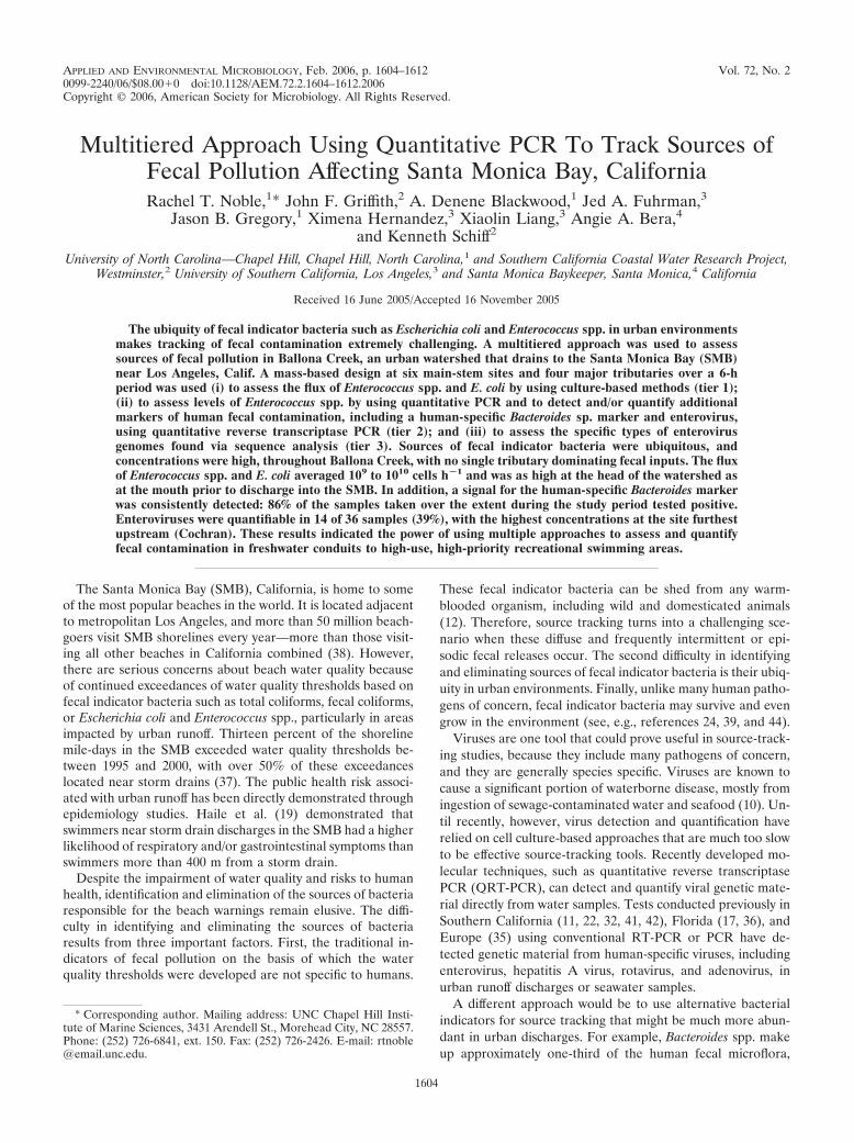
APPLIED AND ENVIRONMENTAL MICROBIOLOGY, Feb. 2006, p. 1604–1612 Vol. 72, No. 20099-2240/06/$08.00!0 doi:10.1128/AEM.72.2.1604–1612.2006Copyright © 2006, American Society for Microbiology. All Rights Reserved.

Multitiered Approach Using Quantitative PCR To Track Sources ofFecal Pollution Affecting Santa Monica Bay, CaliforniaRachel T. Noble,1* John F. Griffith,2 A. Denene Blackwood,1 Jed A. Fuhrman,3

Jason B. Gregory,1 Ximena Hernandez,3 Xiaolin Liang,3 Angie A. Bera,4and Kenneth Schiff2

University of North Carolina—Chapel Hill, Chapel Hill, North Carolina,1 and Southern California Coastal Water Research Project,Westminster,2 University of Southern California, Los Angeles,3 and Santa Monica Baykeeper, Santa Monica,4 California

Received 16 June 2005/Accepted 16 November 2005

The ubiquity of fecal indicator bacteria such as Escherichia coli and Enterococcus spp. in urban environmentsmakes tracking of fecal contamination extremely challenging. A multitiered approach was used to assesssources of fecal pollution in Ballona Creek, an urban watershed that drains to the Santa Monica Bay (SMB)near Los Angeles, Calif. A mass-based design at six main-stem sites and four major tributaries over a 6-hperiod was used (i) to assess the flux of Enterococcus spp. and E. coli by using culture-based methods (tier 1);(ii) to assess levels of Enterococcus spp. by using quantitative PCR and to detect and/or quantify additionalmarkers of human fecal contamination, including a human-specific Bacteroides sp. marker and enterovirus,using quantitative reverse transcriptase PCR (tier 2); and (iii) to assess the specific types of enterovirusgenomes found via sequence analysis (tier 3). Sources of fecal indicator bacteria were ubiquitous, andconcentrations were high, throughout Ballona Creek, with no single tributary dominating fecal inputs. The fluxof Enterococcus spp. and E. coli averaged 109 to 1010 cells h!1 and was as high at the head of the watershed asat the mouth prior to discharge into the SMB. In addition, a signal for the human-specific Bacteroides markerwas consistently detected: 86% of the samples taken over the extent during the study period tested positive.Enteroviruses were quantifiable in 14 of 36 samples (39%), with the highest concentrations at the site furthestupstream (Cochran). These results indicated the power of using multiple approaches to assess and quantifyfecal contamination in freshwater conduits to high-use, high-priority recreational swimming areas.

The Santa Monica Bay (SMB), California, is home to someof the most popular beaches in the world. It is located adjacentto metropolitan Los Angeles, and more than 50 million beach-goers visit SMB shorelines every year—more than those visit-ing all other beaches in California combined (38). However,there are serious concerns about beach water quality becauseof continued exceedances of water quality thresholds based onfecal indicator bacteria such as total coliforms, fecal coliforms,or Escherichia coli and Enterococcus spp., particularly in areasimpacted by urban runoff. Thirteen percent of the shorelinemile-days in the SMB exceeded water quality thresholds be-tween 1995 and 2000, with over 50% of these exceedanceslocated near storm drains (37). The public health risk associ-ated with urban runoff has been directly demonstrated throughepidemiology studies. Haile et al. (19) demonstrated thatswimmers near storm drain discharges in the SMB had a higherlikelihood of respiratory and/or gastrointestinal symptoms thanswimmers more than 400 m from a storm drain.

Despite the impairment of water quality and risks to humanhealth, identification and elimination of the sources of bacteriaresponsible for the beach warnings remain elusive. The diffi-culty in identifying and eliminating the sources of bacteriaresults from three important factors. First, the traditional in-dicators of fecal pollution on the basis of which the waterquality thresholds were developed are not specific to humans.

These fecal indicator bacteria can be shed from any warm-blooded organism, including wild and domesticated animals(12). Therefore, source tracking turns into a challenging sce-nario when these diffuse and frequently intermittent or epi-sodic fecal releases occur. The second difficulty in identifyingand eliminating sources of fecal indicator bacteria is their ubiq-uity in urban environments. Finally, unlike many human patho-gens of concern, fecal indicator bacteria may survive and evengrow in the environment (see, e.g., references 24, 39, and 44).

Viruses are one tool that could prove useful in source-track-ing studies, because they include many pathogens of concern,and they are generally species specific. Viruses are known tocause a significant portion of waterborne disease, mostly fromingestion of sewage-contaminated water and seafood (10). Un-til recently, however, virus detection and quantification haverelied on cell culture-based approaches that are much too slowto be effective source-tracking tools. Recently developed mo-lecular techniques, such as quantitative reverse transcriptasePCR (QRT-PCR), can detect and quantify viral genetic mate-rial directly from water samples. Tests conducted previously inSouthern California (11, 22, 32, 41, 42), Florida (17, 36), andEurope (35) using conventional RT-PCR or PCR have de-tected genetic material from human-specific viruses, includingenterovirus, hepatitis A virus, rotavirus, and adenovirus, inurban runoff discharges or seawater samples.

A different approach would be to use alternative bacterialindicators for source tracking that might be much more abun-dant in urban discharges. For example, Bacteroides spp. makeup approximately one-third of the human fecal microflora,

* Corresponding author. Mailing address: UNC Chapel Hill Insti-tute of Marine Sciences, 3431 Arendell St., Morehead City, NC 28557.Phone: (252) 726-6841, ext. 150. Fax: (252) 726-2426. E-mail: [email protected].

1604

considerably outnumbering fecal coliforms, E. coli, and Entero-coccus spp. Bacteroides spp. are obligate anaerobes, so there islittle concern over persistence or regrowth in the environment.More importantly, human-specific Bacteroides markers havebeen developed, increasing the value of this potential indicator(2, 3, 7).

Both viruses and alternative bacterial indicators such as Bac-teroides spp. have been shown to be potentially useful source-tracking tools. Griffith et al. (18) and Noble et al. (33) con-cluded that genetics-based methods, such as PCR, consistentlyprovided the best information in efforts to conduct sourcetracking on mixed-source samples. To date, however, no singlemethod has all of the traits necessary to be the consummatesource-tracking tool. Therefore, a multitiered, multiindicatorapproach has been recommended by some investigators (4,40). By using multiple tools, investigators can utilize thestrengths of each to ascertain inputs and track fates that willultimately lead to successful management solutions.

The objective of this study was to identify the contributionsand quantify the loading of fecal contamination affecting theSMB by using a multitiered approach. The first tier includedtraditional measurements of fecal indicator bacteria. The sec-ond tier included molecular assays developed and conductedfor Enterococcus spp., a human-specific Bacteroides marker,and enterovirus. These methods rely on conventional PCR,quantitative PCR (QPCR), or QRT-PCR, which have not pre-viously been applied in conjunction with one another forsource-tracking studies in urban watersheds. The third tierinvolved sequencing of the enterovirus from the field sampleswith the greatest concentrations so as to determine the likelytype of enterovirus amplified in the assay. The multitiered

approach was applied using a mass-based design to quantifyinputs and flux through an urban watershed to the beach.


Study site. This study quantified inputs of flow, bacterial concentrations, andvirus genomic equivalents and then tracked them through an urban watershedover time. This mass-based design was applied in the watershed of BallonaCreek, the largest tributary to the SMB. Ballona Creek is over 85% developedand currently has the largest inputs of fecal indicator bacteria to the SMB (Fig.1).

Sample collection and filtration. Samples were collected at six main-stem sitesand four major tributaries to Ballona Creek. The six main-stem sites extendedfrom Cochran Ave. (where the system daylights from the underground stormdrainage system) to Inglewood Ave. (located at the head of tide just prior todischarge into the SMB) (Table 1). The four tributaries represented the four

FIG. 1. Map of the Ballona Creek watershed in Los Angeles, Calif. Tributary and main-stem sampling sites for the water quality study areindicated. (Inset) Santa Monica Bay, in Southern California.

TABLE 1. Sampling sites along the main stem and majortributaries of Ballona Creek

Site Description GPS coordinates(NAD 83 datum)a

Cochran Ave. Main stem/tributary

34°02.662"N, 118°21.237"W

Fairfax drain Tributary 34°02.298"N, 118°22.136"WAdams Ave. Main stem 34°02.009"N, 118°22.494"WAdams drain Tributary 34°02.009"N, 118°22.494"WRodeo/Higuera Main stem 34°01.305"N, 118°22.693"WBenedict Box Channel Tributary 34°00.925"N, 118°23.432"WOverland Ave. Main stem 33°00.429"N, 118°23.771"WSawtelle Ave. Main stem 33°59.816"N, 118°24.164"WSepulveda channel Tributary 33°59.512"N, 118°24.693"WInglewood Ave. Main stem 33°59.394"N, 118°24.696"W

a GPS, global positioning system; NAD 83 datum, North American datum of1983.

VOL. 72, 2006 TRACKING FECAL POLLUTION 1605

largest hydrodynamic inputs to the system and were located in reaches betweeneach of the main-stem sampling sites. Flow was calculated as the product of theflow rate and the wetted cross-sectional area (43). Doppler area-velocity sensors(Teledyne ISCO, Los Angeles, CA) were used to measure flow rate. Pressuretransducers that measure stage, along with verified as-built cross sections, wereused to estimate the wetted cross-sectional area. One-minute instantaneous flowwas logged electronically during the entire 6-h sampling period. Both the area-velocity sensors and the pressure transducers were calibrated prior to sampling.

One-hour composite water samples were collected immediately downstreamof flow measurement devices at each site (Table 1, GPS coordinates) between8:00 and 14:00 on 26 August 2004. The 6-h sampling period corresponds to theapproximate hydrodynamic travel time from Cochran Ave. to Inglewood Ave.(1). The hourly 4-liter composite samples at each site were created after com-bining 10 individual 400-ml grab samples collected every 6 min into a singlecontainer. In total, 60 composite samples were collected at Ballona Creek as aresult of sampling 6 h at 10 different sites.

After collection, samples were placed on ice and transported immediately tothe University of Southern California for processing. For each composite sample,100 ml of water was devoted to indicator bacteria analysis, and 200 to 600 ml ofthe sample volume was vacuum filtered through replicate 47-mm-diameter, 0.4-#m-pore-size polycarbonate filters (Poretics, Inc., Livermore, CA) using a filterfunnel and receiver (Millipore, Inc., Bedford, MA) for Enterococcus sp. analysesby QPCR or Bacteroides sp. analysis by conventional PCR, as suggested byHaugland et al. (20). In addition, replicate filtrations were also conducted using47-mm-diameter, 0.45-#m-pore-size type HA (Millipore, Inc., Bedford, MA)mixed cellulose ester filters for enterovirus analysis as suggested by Fuhrman etal. (11). For each filter, the volume filtered was the maximum filterable withinca. 10 min of the start of filtration. The total volume filtered was dependent onthe location and turbidity of each individual sample, and the filter volumes werecarefully recorded to the nearest 1 ml. All filters were placed in microcentrifugetubes and stored at $80°C for further analysis.

Analysis of indicator bacteria. Concentrations of E. coli and Enterococcus spp.were measured by defined substrate technology using kits supplied by IDEXXLaboratories, Inc. (Westbrook, ME) according to the manufacturer’s instruc-tions. Briefly, 10-fold and 100-fold dilutions of the water samples were made withdeionized water containing the appropriate media and sodium thiosulfate, mixedto dissolve, dispensed into trays (Quanti-Tray/2000), and heat sealed. E. coli wasmeasured using the Colilert-18 reagents, while Enterococcus spp. were measuredusing Enterolert reagents. Samples were incubated overnight according to themanufacturer’s instructions and inspected for positive wells. Conversion of pos-itive wells from these tests to a most probable number was done following Hurleyand Roscoe (21).

Extraction of DNA. The polycarbonate filters were processed for DNA extrac-tion using the UltraClean fecal DNA isolation kit (MoBio Laboratories, Inc.,Carlsbad, CA) according to the manufacturer’s alternative protocol for maxi-mum yield. Eluted DNA extracts were stored at $20°C until use.

The concentration of the extracted DNA was measured using the Quant-iTPicogreen double-stranded DNA reagent (Invitrogen, Carlsbad, CA) accordingto the manufacturer’s instructions. Standard curves were generated in duplicateusing Lambda DNA standards between 2.5 ng/ml and 600 ng/ml and a negativecontrol (0 ng/ml). Fluorometric measurements were made using a Bio-RadVersaFluor fluorometer.

Bacterial analyses using QPCR. The total Enterococcus sp. primers and probeare described by Ludwig and Schleifer (28) and were constructed using the 23SrRNA gene regions around the target site of a well-established Enterococcusgroup-specific primer (ENC854R). Primer ECST748F targets Enterococcus spp.,lactococci, and several clostridia. The target site of probe GPL813TQ is presentin the 23S rRNA genes from a variety of representatives of gram-positive bac-teria with low G!C DNA contents (28).

The master mix contained 1% Taq buffer, 4 mM MgCl2, 3 mM deoxynucleo-side triphosphates (dNTPs), 2.5 U Ex Taq R polymerase (R PCR kit for quan-titative PCR; TaKaRa Mirus Bio, Madison, WI), 1 #M ENC854R, 1 #MECST748F, 0.1 #M GPL813 TQ Cy3 Probe (synthesized by MWG Biotech, HighPoint, NC), and nuclease-free water, yielding a final volume of 20 #l, to which 5#l of sample (either DNA extract from an environmental sample, ranging from1 to 76 ng genomic DNA, or 5 #l of lysed cell suspension or genomic equivalents)was added for a final volume of 25 #l. The samples were run under the followingoptimized assay conditions for PCR: 1 cycle consisting of an initial hold at 95°Cfor 2 min and 45 cycles of denaturation at 94°C for 15 s and annealing/extensionat 60°C for 30 s (the optics were turned on during the annealing step). TheCepheid Smart Cycler II was set with the following specific parameters for thisassay. The Dye Set was set for FCTC25. The cycle threshold analysis mode wasset for growth curve (linear) analyses, with a manual threshold typically set at 5

to 15 fluorescence units. The background subtract level was set at a minimum of12 and a maximum of 40. The BoxCar averaging feature was set at zero. Theassay was previously optimized for Taq, Mg2!, and dNTP concentrations as wellas all cycling parameters (data not shown). For quality control, Enterococcusfaecalis ATCC 29212 and Enterococcus faecium ATCC 35667 combined wereused as our calibration strains for the total-Enterococcus primer and probe set.Control bacterial preparations were prepared by boiling bacteria for 5 min,centrifuging for 2 min at 12,000 % g at 4°C, and storing immediately on ice. E.faecalis and E. faecium cells were enumerated using SYBR Green I epifluores-cence microscopy (30). Serial dilutions of the standards were made in diethylpyrocarbonate-treated sterile water, and four-point standard curves were run induplicate in concert with the unknown samples on the Smart Cycler II instru-ment. Total-Enterococcus primers were tested with all 19 validly described spe-cies of the genus Enterococcus and demonstrated amplification of rRNA genes ofall strains, with varying efficiencies (28).

Analysis of Bacteroides spp. using conventional PCR. Amplification of thehuman-specific Bacteroides/Prevotella marker generally followed the procedureof Bernhard and Field (2), with PCR primers that amplify partial 16S rRNA fromthe human feces-specific group (BAC708R and HS183F). A range of extractedDNA quantities (representing 1 to 70 ng per assay, with most samples in therange of 5 to 20 ng) was tested to avoid problems with inhibition of the PCR.DNA was amplified with the Bacteroides-Provotella-specific primers described byBernhard and Field (2). The PCR mixture was 1% Taq polymerase buffer, 1#meach primer, 200 #m dNTPs, 1.25 U Taq polymerase, 640 ng #l$1 BSA, and 1.5mM MgCl2. The PCR conditions were specifically optimized for this study anddiffered from those in the original publication: 2 min at 95°C, then 25 cycles of95°C for 30 s, 60°C for 30 s, and 72°C for 30 s, followed by a 5-min extension at72°C. Then 1 #l of each PCR product was reamplified using the conditions givenabove for another 25 cycles. PCR was performed on a 3000MX thermal cycler(Stratagene). PCR products were visualized in a 2% agarose gel stained with 1%SYBR Gold (Molecular Probes, Eugene, OR) and compared to a 100-bp DNAladder (Promega). Positive results yielded 525-bp amplicons. The positive con-trol was a human fecal sample extracted with a QIAamp DNA stool kit (QIA-GEN, Valencia, CA). Negative controls contained water instead of sample. Allsamples were initially run with 5 #l of extracted material. After the initialanalyses, all negative samples (14 of 60) were spiked with 0.1 ng of positive-control DNA and reanalyzed to determine possible inhibition. Three of the 14negative samples (two from Benedict Box Channel and one from Adams) weredetermined to be inhibited. Inhibited samples were reanalyzed using 2 #l ofsample, but all three remained negative.

Enterovirus analyses. Samples, along with negative controls, were extractedusing a modified RNeasy plant minikit (QIAGEN Plant and Fungi RNA isola-tion protocol). The RLT homogenization buffer supplied was supplemented withpolyvinyl pyrrolidone 40 (PVP-40) at a final concentration of 2%. Prior to theextraction, fresh &-mercaptoethanol (Sigma Chemical Co.) was added to theextraction buffer in the exact concentration recommended by the manufacturer.Filters (type HA) were manually homogenized with a pipette tip, and 700 #l ofthe RLT/filter slurry was applied to a QiaShredder column (QIAGEN) and spunat maximum speed, !8,000 % g, for 2 min to aid in viral lysis as well as to separatefilter particles from the filtrate (11). The filtrate was then carefully removedwithout disturbing the pelleted material and was placed into a new 1.5-ml tube.The volume of solution in each tube was estimated by pipetting, and 0.4 volumeof 5 M potassium acetate (pH 6.5) was added. Tubes were mixed by inversion andincubated on ice for 15 min. The mixture was then spun (12,000 % g) at 4°C for15 to 30 min and the supernatant transferred to a new 1.5-ml microcentrifugetube. Subsequently, the Plant and Fungi RNA isolation protocol was followedstarting at step 5. RNA was eluted with 50 #l of the supplied RNase-free water.A one-step TaqMan QRT-PCR was performed on the extracted RNA, with finalreaction volumes of 25 #l, using a QIAGEN One-Step RT-PCR kit. Five mi-croliters of extracted RNA was added to 20 #l of master mix containing 1% RTbuffer, 6 mM MgCl2, 500 nM dNTPs, 700 nM EV1 reverse primer (5'-TGTCACCATA AGCAGCCA-3'), 700 nM EV1 forward primer (5'-CCCTGAATGCGGCTAAT-3'), 30 #g bovine serum albumin, 20 U of recombinant RNasin (Pro-mega Corp.), 1.5% PVP-25 (29) (Sigma Chemical Co.), 100 genomic equivalentunits of a competitive internal positive control (CIPC) developed in-house (16)by following the general approach of Kleiboeker (25), plus 300 nM CIPC probe5'-Cy5-TGTGCTGCAAGGCGATTAAGTTGGGT–BHQ-2–3', and 300 nMEV-BHQ probe 5'–6-carboxyfluorescein–ACGGACACCCAAAGTAGTCGGTTC–BHQ-1–3', and 1 #l of enzyme mix (containing both reverse transcriptaseand DNA polymerase). The probe and primers were synthesized by MWGBiotech, Inc. The Cepheid Smart Cycler II was programmed as follows: a 1-hreverse transcription step at 50°C followed by a 15-min hold at 95°C for DNA

1606 NOBLE ET AL. APPL. ENVIRON. MICROBIOL.

polymerase activation, then 45 cycles of 94°C for 15 s (denaturation) and 60°C for1 min (annealing and extension, with optics on).

QRT-PCR results were available 3 h after the start of analysis, making thetotal RNA extraction, QRT-PCR preparation, and analysis time less than 5 h.After the first analyses, those samples that appeared to have inhibition of theQRT-PCR (as indicated by the CIPC) had RNA sample volumes reduced in halfand were rerun. No inhibition was observed at this lower RNA concentration.Standard curves were generated using a synthetic enterovirus transcript that wasquantified using fluorometric analysis, and sample genome concentrations wereinterpolated from the standard curve using the manufacturer’s curve-fitting soft-ware. Quantitative results are reported per liter sample volume.

Sequencing of enterovirus QRT-PCR positives. QRT-PCR-positive samplesfrom the enterovirus analyses were sequenced to assess the specificity and fidelityof our enterovirus QRT-PCR and to elucidate the identities of the enterovirusgenomes being amplified by the assay. Following the initial enteroviral analysis ofthe Ballona Creek samples, RNA samples identified as positive for enterovirusgenomes were again amplified using the QRT-PCR protocol. However, afternumerous repetitions of freezing and thawing of the extracted RNAs for variousanalyses, only Cochran Ave. samples from 9:00, 10:00, and 11:00 containedamplifiable enterovirus genetic material (11). The 144-bp enterovirus QRT-PCRproduct was distinguished from the 126-bp internal positive control productusing a 10% polyacrylamide–1% Tris-borate-EDTA gel. The gel was stained withethidium bromide and visualized with a 254-nm UV light. The larger 144-bpenterovirus QRT-PCR products were excised, homogenized in 50 #l of 1%QIAGEN One-Step RT-PCR buffer using a microcentrifuge pestle, and incu-bated overnight at 37°C with shaking. The enterovirus products were purified(Wizard SV gel and PCR Clean Up System; Promega), cloned into the 3.9-kilobase pCR 2.1 TOPOVector (TOPO TA cloning kit; Invitrogen, Carlsbad,CA), transformed into TOP10 chemically competent E. coli, and plated onLuria-Bertani agar plates containing 100 #g/ml of ampicillin. Bacterial cloneswere screened using QPCR, and positive colonies from each of the three siteswere selected and grown individually in 3 ml of 2% medium overnight at 37°C.Plasmid DNA was isolated (PerfectPrep plasmid minikit; Eppendorf, Westbury,CT), and the DNA concentration was calculated using yeast extract-tryptoneRibogreen (Molecular Probes). Plasmid DNA was sequenced bidirectionally byMWG Biotech, and the chromatograms were inspected using Sequencher, ver-sion 4.2 (Gene Codes Corp., Ann Arbor, MI). The sequences were aligned tosequences in the NCBI GenBank using BLAST and are available by searchingnucleotide accession numbers DQ196482 through DQ196487.

Calculations and statistical analyses. Data analysis comprised four steps.First, the hydrologic budget was evaluated to determine if the majority of theflow was sampled. This evaluation was conducted by comparing the volumetricinputs from each of the tributaries to the volumetric discharges along the mainstem of Ballona Creek. The second step was to examine temporal and spatialtrends in the flux of fecal indicator bacteria. The flux of indicator bacterial cellsper hour was calculated by multiplying the concentration of the indicator bac-teria (per deciliter [100 ml]) by the flow rate (in deciliters per hour). The meanhourly flux (temporal analysis) was calculated by averaging the flux of indicatorbacteria at all main-stem locations for each hourly interval (n ( 6). The meanflux at each site (spatial analysis) was calculated by averaging the flux at eachmain-stem or tributary site for all hourly samples (n ( 6). Statistical analysis ofthe differences in bacterial flux between hourly time periods or, alternatively,between main-stem sites was conducted using analysis of variance (46). The thirddata analysis step was to examine spatial and temporal patterns in the frequencyof Bacteroides detection. The Bacteroides method used in this study was a pres-ence/absence end point. This examination was conducted by tabulating the lo-cations and time periods of Bacteroides detection to detect patterns movingdownstream, adjacent to tributaries, or over time. The fourth data analysis stepwas to examine the spatial and temporal extent of enterovirus concentrations.Unlike that of Bacteroides, the presence of enterovirus was quantified, so themagnitude of enterovirus concentrations was tabulated among the different lo-cations across the different time periods. As in the Bacteroides data analysis,patterns moving downstream, adjacent to tributaries, or over time were exam-ined.

RESULTS

The total volume discharged from Ballona Creek during the6-h sampling period was 13,390 m3 (Fig. 2). Of this volume,97% was attributed to monitored inputs from Cochran, Fair-fax, Adams, Benedict, and Sepulveda tributaries. The largest

volume was contributed at Cochran Ave., where the creekemerges into daylight from beneath downtown Los Angeles.Flow remained relatively stable over the study period at allsites, with little variation or pattern in discharge. For example,the coefficient of variation for flow at the most-downstreamsite, Inglewood Ave., was less than 8%, approaching the reso-lution of our flow-monitoring devices.

There was no observed spatial trend in the flux of fecalindicator bacteria in Ballona Creek during this study (Fig. 3).The average flux of E. coli ranged from 1.1 % 1010 to 5.3 % 1010

cells h$1 at the six main-stem sites. The average flux of En-terococcus spp. ranged from 6.6 % 108 to 1.4 % 109 cells h$1 atthe six main-stem sites. In both cases, there was no discernibleincrease in bacterial flux as one moved downstream; no twomain-stem sites were significantly different from one another inthe flux of either E. coli or Enterococcus spp. (P ) 0.05 byanalysis of variance).

A temporal trend in the flux of fecal indicator bacteria inBallona Creek was observed during this study (Fig. 4). Theaverage flux of Enterococcus spp. was highest at 9:00 (2.9 %1010 cells h$1) and decreased monotonically throughout thestudy period. The lowest flux was measured at 14:00 (3.0 % 109

cells h$1). Similar patterns were observed for E. coli (data notshown). In contrast to the results obtained by the culture-basedmethods, the QPCR results for Enterococcus spp. did not de-crease over time. The flux of Enterococcus spp. ranged from 2.7% 1010 to 4.7 % 1010 cells h$1, and the 9:00 and 14:00 sampleswere nearly equivalent (Fig. 4).

The relative patterns of Enterococcus contributions from thetributaries were similar at all time periods (Fig. 5). Benedicttributary always had the greatest flux of fecal indicator bacte-ria, followed by Sepulveda, Fairfax, and Adams tributaries. A

FIG. 2. Schematic diagram depicting additive flow in the mainchannel of Ballona Creek and the percentage contributed by eachtributary sampled.


similar pattern was also observed for E. coli. The flux of En-terococcus spp. from Benedict tributary ranged from 4.1 % 109

to 1.4 % 1010 cells h$1 throughout the sampling period whilethe flux of Enterococcus spp. from Adams tributary rangedfrom 3.7 % 105 to 4.4 % 106 cells h$1. On average, Benedicttributary contributed 81% of the Enterococcus spp. loadingfrom all four tributaries.

The hourly flux of Enterococcus spp. (determined by culture-based methods) from each of the four main tributaries approx-imated the load being passed down Ballona Creek (Fig. 5).Regardless of the hour, the flux from each of the tributarieswas within a factor of 101 compared to its nearest downstreamsite on the main stem of Ballona Creek. The only exceptionwas the Adams tributary, for which the flux was as much as 4

FIG. 3. Mean flux of E. coli and Enterococcus cells (expressed as cells per hour) at main-channel sampling sites of Ballona Creek (26 August2004).

FIG. 4. Mean hourly flux of Enterococcus spp. (expressed as cells per hour) along the main channel of Ballona Creek, measured by using eitheran IDEXX chromogenic substrate (Enterolert) or QPCR methods on 26 August 2004.


orders of magnitude less than that for the nearest downstreamsite. The main stem showed virtually no response to any ofthese tributary inputs, including that of Adams. The flux ofEnterococcus spp. remained virtually unchanged from up-stream to downstream of each of the tributary inputs (Fig. 3and 5).

The human-specific Bacteroides marker was positively de-tected throughout the main stem of Ballona Creek; its pres-ence in 31 of the 36 main-stem samples tested (86%) wasconfirmed (Table 2). A positive signal was observed at all sitesduring the early morning hours, but during periods of height-ened UV radiation (midday and late afternoon), a decrease inthe number of positive results for the human-specific Bacte-roides marker was observed. For example, only three of six sam-ples at 14:00 were positive for the human-specific Bacteroidesmarker and exceeded the water quality threshold for E. coli.

Enteroviruses were detected and quantified in 14 of the 36main-stem samples tested (39%) (Table 2). Moreover, spatialand temporal patterns in enterovirus concentrations were alsoevident in the Ballona Creek system. Main-channel locations inthe upper reaches of the study area were more likely to bepositive for enteroviruses than downstream sites. The mostconsistently positive site was Cochran Ave., where 89% of thesamples contained measurable levels of enterovirus. In addi-tion, some of the highest concentrations of enterovirus weremeasured at Cochran during four of the six time periods (con-centrations ranging from 1,336 to 3,255 enterovirus genomesper liter). A general pattern in enterovirus detection was ob-served during the course of the day. Enterovirus was detectedduring the early morning and at midday at upstream sites butwas detected most frequently late in the day at the downstreamsites. The 12:00 sampling interval had the most frequent de-

FIG. 5. Loading of Enterococcus spp. (expressed as cells per hour) in the main channel and tributaries of Ballona Creek at 9:00 (a), 10:00 (b),11:00 (c), 12:00 (d), 13:00 (e), and 14:00 (f) on 26 August 2004.


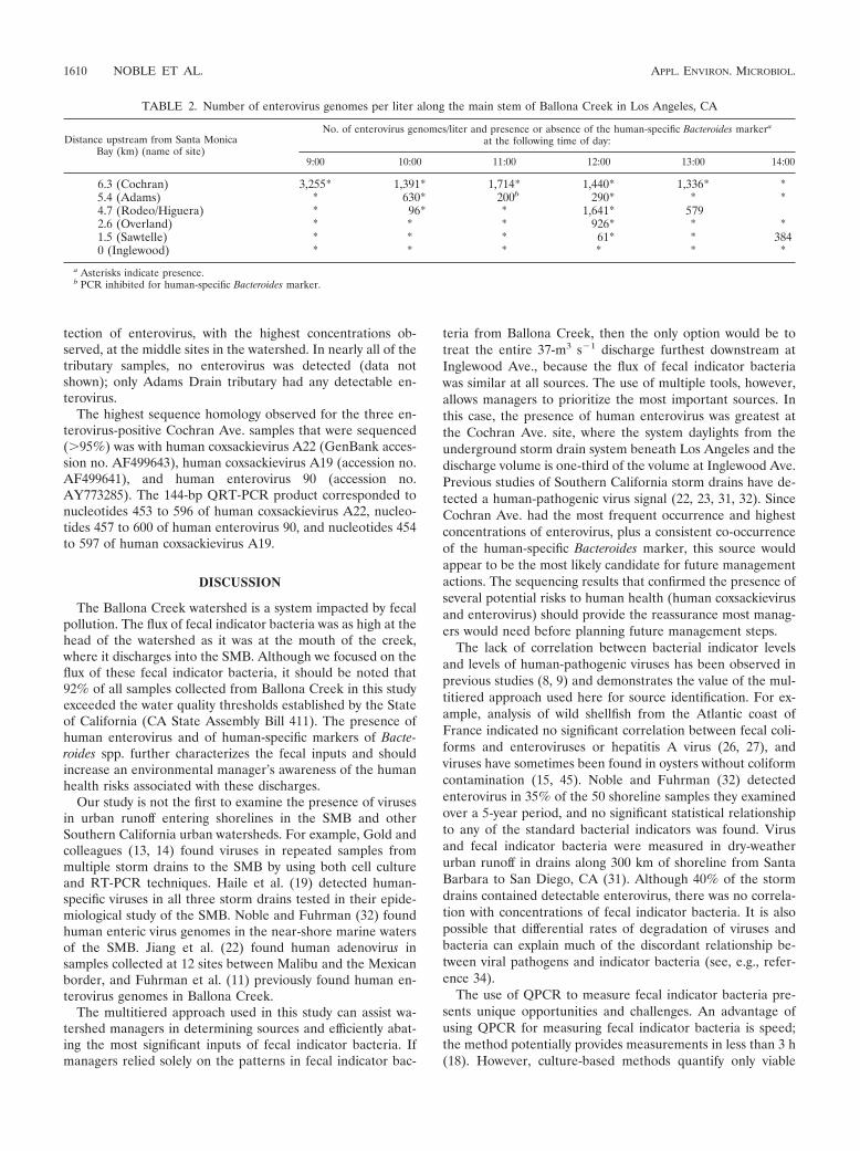
tection of enterovirus, with the highest concentrations ob-served, at the middle sites in the watershed. In nearly all of thetributary samples, no enterovirus was detected (data notshown); only Adams Drain tributary had any detectable en-terovirus.

The highest sequence homology observed for the three en-terovirus-positive Cochran Ave. samples that were sequenced()95%) was with human coxsackievirus A22 (GenBank acces-sion no. AF499643), human coxsackievirus A19 (accession no.AF499641), and human enterovirus 90 (accession no.AY773285). The 144-bp QRT-PCR product corresponded tonucleotides 453 to 596 of human coxsackievirus A22, nucleo-tides 457 to 600 of human enterovirus 90, and nucleotides 454to 597 of human coxsackievirus A19.

DISCUSSION

The Ballona Creek watershed is a system impacted by fecalpollution. The flux of fecal indicator bacteria was as high at thehead of the watershed as it was at the mouth of the creek,where it discharges into the SMB. Although we focused on theflux of these fecal indicator bacteria, it should be noted that92% of all samples collected from Ballona Creek in this studyexceeded the water quality thresholds established by the Stateof California (CA State Assembly Bill 411). The presence ofhuman enterovirus and of human-specific markers of Bacte-roides spp. further characterizes the fecal inputs and shouldincrease an environmental manager’s awareness of the humanhealth risks associated with these discharges.

Our study is not the first to examine the presence of virusesin urban runoff entering shorelines in the SMB and otherSouthern California urban watersheds. For example, Gold andcolleagues (13, 14) found viruses in repeated samples frommultiple storm drains to the SMB by using both cell cultureand RT-PCR techniques. Haile et al. (19) detected human-specific viruses in all three storm drains tested in their epide-miological study of the SMB. Noble and Fuhrman (32) foundhuman enteric virus genomes in the near-shore marine watersof the SMB. Jiang et al. (22) found human adenovirus insamples collected at 12 sites between Malibu and the Mexicanborder, and Fuhrman et al. (11) previously found human en-terovirus genomes in Ballona Creek.

The multitiered approach used in this study can assist wa-tershed managers in determining sources and efficiently abat-ing the most significant inputs of fecal indicator bacteria. Ifmanagers relied solely on the patterns in fecal indicator bac-

teria from Ballona Creek, then the only option would be totreat the entire 37-m3 s$1 discharge furthest downstream atInglewood Ave., because the flux of fecal indicator bacteriawas similar at all sources. The use of multiple tools, however,allows managers to prioritize the most important sources. Inthis case, the presence of human enterovirus was greatest atthe Cochran Ave. site, where the system daylights from theunderground storm drain system beneath Los Angeles and thedischarge volume is one-third of the volume at Inglewood Ave.Previous studies of Southern California storm drains have de-tected a human-pathogenic virus signal (22, 23, 31, 32). SinceCochran Ave. had the most frequent occurrence and highestconcentrations of enterovirus, plus a consistent co-occurrenceof the human-specific Bacteroides marker, this source wouldappear to be the most likely candidate for future managementactions. The sequencing results that confirmed the presence ofseveral potential risks to human health (human coxsackievirusand enterovirus) should provide the reassurance most manag-ers would need before planning future management steps.

The lack of correlation between bacterial indicator levelsand levels of human-pathogenic viruses has been observed inprevious studies (8, 9) and demonstrates the value of the mul-titiered approach used here for source identification. For ex-ample, analysis of wild shellfish from the Atlantic coast ofFrance indicated no significant correlation between fecal coli-forms and enteroviruses or hepatitis A virus (26, 27), andviruses have sometimes been found in oysters without coliformcontamination (15, 45). Noble and Fuhrman (32) detectedenterovirus in 35% of the 50 shoreline samples they examinedover a 5-year period, and no significant statistical relationshipto any of the standard bacterial indicators was found. Virusand fecal indicator bacteria were measured in dry-weatherurban runoff in drains along 300 km of shoreline from SantaBarbara to San Diego, CA (31). Although 40% of the stormdrains contained detectable enterovirus, there was no correla-tion with concentrations of fecal indicator bacteria. It is alsopossible that differential rates of degradation of viruses andbacteria can explain much of the discordant relationship be-tween viral pathogens and indicator bacteria (see, e.g., refer-ence 34).

The use of QPCR to measure fecal indicator bacteria pre-sents unique opportunities and challenges. An advantage ofusing QPCR for measuring fecal indicator bacteria is speed;the method potentially provides measurements in less than 3 h(18). However, culture-based methods quantify only viable

TABLE 2. Number of enterovirus genomes per liter along the main stem of Ballona Creek in Los Angeles, CA

Distance upstream from Santa MonicaBay (km) (name of site)

No. of enterovirus genomes/liter and presence or absence of the human-specific Bacteroides markera

at the following time of day:

9:00 10:00 11:00 12:00 13:00 14:00

6.3 (Cochran) 3,255* 1,391* 1,714* 1,440* 1,336* *5.4 (Adams) * 630* 200b 290* * *4.7 (Rodeo/Higuera) * 96* * 1,641* 5792.6 (Overland) * * * 926* * *1.5 (Sawtelle) * * * 61* * 3840 (Inglewood) * * * * * *

a Asterisks indicate presence.b PCR inhibited for human-specific Bacteroides marker.


bacteria, while QPCR measures the DNA from both cultivableand noncultivable microbes. This was most apparent in thetemporal trends from Ballona Creek. Levels of Enterococcusspp. determined using culture-based methods generally de-creased as the day progressed, most likely as a result of pho-toinactivation of cells by sunlight (5, 6, 34). Ballona Creek is a40-m-wide concrete-lined channel, concentrating solar energyinto the shallow creek in the channel invert. The QPCR results,however, remained steady, indicating that the bacterial DNAwas still intact and detectable, even though the Enterococcusspp. were not viable.

Overall, the use of multiple approaches provided convincingevidence of the extent and types of microbial contamination inthis urban watershed. We believe such studies should provideinvaluable information for researchers and managers trying tobalance regulatory burdens and public safety.

ACKNOWLEDGMENTS

Funding for this project has been provided in full through agreement02-039-254-0 with the State Water Resources Control Board(SWRCB) pursuant to the Costa-Machado Water Act of 2000 (Prop-osition 13) and any amendments thereto for the implementation ofCalifornia’s Nonpoint Source Pollution Control Program. Additionalsupport was provided by a USC Sea Grant.

The contents of this document do not necessarily reflect the viewsand policies of the SWRCB, nor does mention of trade names orcommercial products constitute endorsement or recommendation foruse.

We thank Orange County Public Health Laboratories (DouglasMoore) for their high-titer poliovirus stock and Ian Hewson, JoshuaSteele, Mike Schwalbach, and Sheila O’Brien for assistance with sam-ple collection and processing. We also thank the volunteers of SantaMonica Baykeeper for assistance with sample collection and environ-mental parameter data collection.

REFERENCES

1. Ackerman, D., K. Schiff, and S. B. Weisberg. 2003. Evaluating HSPF in anarid urban watershed, p. 78–85. In S. B. Weisberg (ed.), Southern CaliforniaCoastal Water Research Project Annual Report 2000–2002. Southern Cali-fornia Coastal Water Research Project, Westminster, Calif.

2. Bernhard, A. E., and K. G. Field. 2000. A PCR assay to discriminate humanand ruminant feces on the basis of host differences in Bacteroides-Prevotellagenes encoding 16S rRNA. Appl. Environ. Microbiol. 66:4571–4574.

3. Bernhard, A. E., and K. G. Field. 2000. Identification of nonpoint sources offecal pollution in coastal waters by using host-specific 16S ribosomal DNAgenetic markers from fecal anaerobes. Appl. Environ. Microbiol. 66:1587–1594.

4. Boehm, A. B., J. A. Fuhrman, R. D. Morse, and S. B. Grant. 2003. Tieredapproach for identification of a human fecal pollution source at a recre-ational beach: case study at Avalon Bay, Catalina Island, California. Environ.Sci. Technol. 37:673–680.

5. Davies, C. M., and L. M. Evison. 1991. Sunlight and the survival of entericbacteria in natural waters. J. Appl. Microbiol. 70:265–274.

6. Davies-Colley, R., R. Bell, and A. Donnison. 1994. Sunlight inactivation ofenterococci and fecal coliforms in sewage effluent diluted in seawater. Appl.Environ. Microbiol. 60:2049–2058.

7. Dick, L., and K. G. Field. 2004. Rapid estimation of numbers of fecalBacteroidetes by use of a quantitative PCR assay for 16S rRNA genes. Appl.Environ. Microbiol. 70:5695–5697.

8. Dufour, A. P. 1984. Bacterial indicators of recreational water quality. Can. J.Public Health 75:49–56.

9. Elliott, E. L., and R. R. Colwell. 1985. Indicator organisms for estuarine andmarine waters. FEMS Microbiol. Rev. 32:61–79.

10. Fogarty, J., L. Thornton, C. Hayes, M. Laffoy, D. O’Flanagan, J. Devlin, andR. Corcoran. 1995. Illness in a community associated with an episode ofwater contamination with sewage. Epidemiol. Infect. 114:289–295.

11. Fuhrman, J. A., X. Liang, and R. T. Noble. 2005. Rapid detection of entero-viruses from small volumes of natural waters by real-time RT-PCR. Appl.Environ. Microbiol. 71:4523–4530.

12. Geldreich, E. E. 1978. Bacterial populations and indicator concepts in feces,sewage, stormwater and solid wastes, p. 51–97. In G. Berg (ed.), Indicatorsof viruses in water and food. Ann Arbor Science Publishers, Ann Arbor,Mich.

13. Gold, M., M. Bartlett, J. H. Dorsey, and C. D. McGee. 1990. An assessmentof inputs of fecal indicator organisms and human enteric viruses from twoSanta Monica storm drains. Santa Monica Bay Restoration Project Com-mission, Monterey Park, Calif.

14. Gold, M., M. Bartlett, C. D. McGee, and G. Deets. 1992. Pathogens andindicators in storm drains within the Santa Monica Bay Watershed. SantaMonica Bay Restoration Project Commission, Monterey Park, Calif.

15. Goyal, S. M., W. N. Adams, M. L. O’Malley, and D. W. Lear. 1984. Humanpathogenic viruses at sewage sludge disposal sites in the Middle Atlanticregion. Appl. Environ. Microbiol. 48:757–763.

16. Gregory, J. B., R. W. Litaker, and R. T. Noble. A rapid one step quantitativereverse transcriptase PCR assay with competitive internal positive controlfor environmental enteroviral detection. Submitted for publication.

17. Griffin, D. W., C. J. Gibson III, E. K. Lipp, K. Riley, J. H. Paul III, and J. B.Rose. 1999. Detection of viral pathogens by reverse transcriptase PCR and ofmicrobial indicators by standard methods in the canals of the Florida Keys.Appl. Environ. Microbiol. 65:4118–4125.

18. Griffith, J. F., S. B. Weisberg, and C. D. McGee. 2003. Evaluation of micro-bial source tracking methods using mixed fecal sources in aqueous testsamples. J. Water Health 1:141–151.

19. Haile, R. W., J. S. Witte, M. Gold, R. Cressey, C. McGee, R. C. Millikan, A.Glasser, N. Harawa, C. Ervin, P. Harmon, J. Harper, J. Dermand, J. Ala-millo, K. Barrett, M. Nides, and G.-Y. Wang. 1999. The health effects ofswimming in ocean water contaminated by storm drain runoff. Epidemiology10:355–363.

20. Haugland, R. A., S. C. Siefring, L. J. Wymer, K. P. Brenner, and A. P.Dufour. Comparison of Enterococcus measurements in freshwater at tworecreational beaches by quantitative polymerase chain reaction and mem-brane filter culture analysis. Water Res. 39:559–568.

21. Hurley, M. A., and M. E. Roscoe. 1983. Automated statistical analysis ofmicrobial enumeration by dilution series. J. Appl. Bacteriol. 55:159–164.

22. Jiang, S., R. T. Noble, and W. Chu. 2001. Human adenoviruses and coliph-ages in urban runoff-impacted coastal waters of Southern California. Appl.Environ. Microbiol. 67:179–184.

23. Jiang, S. C., and W. Chu. 2004. PCR detection of pathogenic viruses insouthern California urban rivers. J. Appl. Microbiol. 97:17–28.

24. Kinzelman, J., K. Pond, K. Longmaid, and R. Bagley. 2004. The effect of twomechanical beach grooming strategies on Escherichia coli density in beachsand at a southwestern Lake Michigan beach. Aquat. Ecosyst, Health Man-agement 7:425–432.

25. Kleiboeker, S. B. 2003. Applications of competitor RNA in diagnostic re-verse transcription-PCR. J. Clin. Microbiol. 41:2055–2061.

26. LeGuyader, F., V. Apaire-Marchais, J. Brillet, and S. Billaudel. 1993. Use ofgenomic probes to detect hepatitis A virus and enterovirus RNAs in wildshellfish and relationship of viral contamination to bacterial contamination.Appl. Environ. Microbiol. 59:3963–3968.

27. Leguyader, F., E. Dubois, D. Menard, and M. Pommepuy. 1994. Detection ofhepatitis A virus, rotavirus, and enterovirus in naturally contaminated shell-fish and sediment by reverse transcription-seminested PCR. Appl. Environ.Microbiol. 60:3665–3671.

28. Ludwig, W., and K. H. Schleifer. 2000. How quantitative is quantitative PCRwith respect to cell counts? Syst. Appl. Microbiol. 23:556–562.

29. Monpoeho, S., A. Maul, B. Mignotte-Cadiergues, L. Schwartzbrod, S. Bil-laudel, and V. Ferre. 2001. Best viral elution method available for quantifi-cation of enteroviruses in sludge by both cell culture and reverse transcrip-tion-PCR. Appl. Environ. Microbiol. 67:2484–2488.

30. Noble, R. T., and J. A. Fuhrman. 1998. Use of SYBR Green I for rapidepifluorescence counts of marine viruses and bacteria. Aquat. Microb. Ecol.14:113–118.

31. Noble, R. T., and J. A. Fuhrman. 2001. Enterovirus detection by reversetranscriptase polymerase chain reaction from the coastal waters of southernCalifornia, p. 226–233. In S. B. Weisberg (ed.), Southern California CoastalWater Research Project Annual Report 1999-2000. Southern CaliforniaCoastal Water Research Project, Westminster, Calif.

32. Noble, R. T., and J. A. Fuhrman. 2001. Enteroviruses detected by reversetranscriptase polymerase chain reaction from the coastal waters of SantaMonica Bay, California: low correlation to bacterial indicator levels. Hydro-biologia 460:175–184.

33. Noble, R. T., S. M. Allen, A. D. Blackwood, W.-P. Chu, S. C. Jiang, G. L.Lovelace, M. D. Sobsey, J. R. Stewart, and D. A. Wait. 2003. Use of viralpathogens and indicators to differentiate between human and non-humanfecal contamination in a microbial source tracking comparison study. J.Water Health 1:195–207.

34. Noble, R. T., I. M. Lee, and K. Schiff. 2004. Inactivation of indicator bacteriafrom various sources of fecal contamination in seawater and freshwater.J. Appl. Microbiol. 96:464–472.

35. Pina, S., M. Puig, F. Lucena, J. Jofre, and R. Girones. 1998. Viral pollutionin the environment and in shellfish: human adenovirus detection by PCR asan index of human viruses. Appl. Environ. Microbiol. 64:3376–3382.

36. Rose, J. B., X. T. Zhou, D. W. Griffin, and J. H. Paul. 1997. Comparison ofPCR and plaque assay for detection and enumeration of coliphage in pol-luted marine waters. Appl. Environ. Microbiol. 63:4564–4566.


37. Schiff, K., J. Morton, and S. Weisberg. 2003. Retrospective evaluation ofshoreline water quality along Santa Monica Bay beaches. Marine Environ.Res. 56:245–253.

38. SMBRC. 2005. State of Santa Monica Bay: 2004 progress and challenges.Santa Monica Bay Restoration Commission, Los Angeles, Calif.

39. Solo-Gabriele, H. M., M. A. Wolfert, T. R. Desmarais, and C. J. Palmer.2000. Sources of Escherichia coli in a coastal subtropical environment. Appl.Environ. Microbiol. 66:230–237.

40. Stewart, J. R., R. D. Ellender, J. A. Gooch, S. Jiang, S. P. Myoda, and S. B.Weisberg. 2003. Recommendations for microbial source tracking: lessonsfrom a methods evaluation study. J. Water Health 1:225–231.

41. Tsai, Y., M. D. Sobsey, L. R. Sangermano, and C. J. Palmer. 1993. Simplemethod of concentrating enteroviruses and hepatitis A virus from sewage

and ocean water for rapid detection by reverse transcriptase-polymerasechain reaction. Appl. Environ. Microbiol. 59:3488–3491.

42. Tsai, Y. L., B. Tran, L. R. Sangermano, and C. J. Palmer. 1994. Detection ofpoliovirus, hepatitis A virus, and rotavirus from sewage and ocean water bytriplex reverse transcriptase PCR. Appl. Environ. Microbiol. 60:2400–2407.

43. Viessman, W., G. Lewis, and J. Knapp. 1989. Introduction to hydrology, 3rded. Harper & Row, Publishers, Inc., New York, N.Y.

44. Weiskel, P. K., B. L. Howes, and G. R. Heufelder. 1996. Coliform contami-nation of a coastal embayment: sources and transport pathways. Environ.Sci. Technol. 30:1872–1881.

45. Yamashita, T., K. Sakae, Y. Ishihara, and S. Isomura. 1992. A 2-year surveyof the prevalence of enteric viral infections in children compared with con-tamination in locally harvested oysters. Epidemiol. Infect. 108:155–163.

46. Zar, J. 1984. Biostatistics. Prentice-Hall, Pub., Englewood Cliffs, N.J.


Characterizing fecal contamination in stormwater runoff incoastal North Carolina, USA

J.K. Parker a, D. McIntyre b, R.T. Noble c,*aDepartment of Entomology and Plant Pathology, Auburn University, 217 Rouse Life Sciences Building, Auburn, AL 36849, USAb Institute for the Environment, University of North Carolina at Chapel Hill, 100 Miller Hall, CB #1105, Chapel Hill, NC 27599, USAc Institute of Marine Sciences, University of North Carolina at Chapel Hill, 3431 Arendell St., Morehead City, NC 28557, USA


Article history:

Received 14 September 2009


12 May 2010

Accepted 12 May 2010

Available online 4 June 2010

Keywords:

Bacteroides

Beaches

Fecal indicator

North Carolina

Stormwater

Water quality

a b s t r a c t

Microbial contaminants in stormwater runoff have the potential to negatively impact

public health. Stormwater runoff to coastal waters is increasing in amount and rate of

discharge due to loss of vegetated landscape and increasing coastal development.

However, the extent and nature of microbial contamination of stormwater runoff in North

Carolina (NC) has not been previously characterized. The aim of this study was to measure

a range of fecal indicator bacteria (FIB) and molecular markers at three coastal sites. E. coli

and Enterococcus sp. were measured in addition to molecular markers including Bacteroides

Human-Specific Marker (HS) and fecal Bacteroides spp. Levels of FIB in stormwater far

exceeded recreational water quality guidelines, frequently by several orders of magnitude.

High concentrations of fecal Bacteroides spp. and the presence of HS indicated the presence

of human fecal contamination in the stormwater runoff, but only during specific storms.

Examinations of levels of fecal contamination in stormwater over multiple seasons and

a range of storm conditions will allow managers to consider appropriate design of effective

mitigation strategies necessary to maintain and restore coastal water quality.

ª 2010 Elsevier Ltd. All rights reserved.

1. Introduction

Stormwater runoff, one of the most common forms of non-point source (NPS) pollution, has been identified as a potentialthreat to human and ecosystem health due to the high levelsof chemical and biological contaminants it contains that havebeen directly linked to disease outbreaks (Curriero et al., 2001;Gaffield et al., 2003), toxic effects in aquatic life (Bay et al.,2003; Heaney et al., 1999), and dramatic negative impacts onwater quality (Ahn et al., 2005; Makepeace et al., 1995). Asprecipitation washes over land, it picks up and transportsa variety of chemicals, pesticides,metals, petroleumproducts,sediment, and human and animal fecal wastes. Knowledge ofthe composition of the resultant runoff, as well as its delivery

pathways and distribution in the environment, is crucial inmanaging the overall risk associated with stormwater runoff.

Discharge of stormwater runoff onto recreational beachesin the US is particularly problematic in terms of public health,as it is the largest known cause of beach closures and advi-sories in the US (Dorfman, 2006). Many of these advisories(75% in 2005) are in response to elevated fecal indicatorbacteria (FIB) levels that exceed USEPA recommended beachwater quality standards (Dorfman, 2006; USEPA, 1986).Furthermore, US recreational waters serve as a known routeof exposure to human pathogens, with 95 documentedrecreational water-associated outbreaks occurring from 1996to 2000 (Arnone and Walling, 2007). Evidence from epidemio-logical studies of recreational water-associated health effects

* Corresponding author. Tel.: !1 252 726 6841; fax: !1 252 726 2426.E-mail address: [email protected] (R.T. Noble).

Avai lab le at www.sc iencedi rect .com

journa l homepage : www.e lsev ier . com/ loca te /wat res

wat e r r e s e a r c h 4 4 ( 2 0 1 0 ) 4 1 8 6e4 1 9 4

0043-1354/$ e see front matter ª 2010 Elsevier Ltd. All rights reserved.doi:10.1016/j.watres.2010.05.018


http://www.elsevier.com/locate/watres




suggests a causal dose-related relationship between gastro-intestinal symptoms and FIB counts and strong relationshipsbetween urban runoff and illness (Pruss, 1998). Therefore,mitigating stormwater runoff to decrease loading rates of FIBand viral, bacterial, and protozoan pathogens to recreationalbeaches is a direct way to improve beach water quality andprotect public health.

In some locations, such as the coast of California, themicrobial contaminants in stormwater and their associatedhealth risks have been studied (Dwight et al., 2004; Haile et al.,1999). However, in coastal NC, the microbial contaminants instormwater and their impacts on recreational beaches havenot yet been assessed. North Carolina ranks sixth of the fiftyUS states in tourism (by person-trip volume, NC Departmentof Commerce, 2008), with more than 6.5 million coastal tour-ists annually (Dorfman, 2006). Stormwater runoff in coastalNC is also receiving greater attention from the public ascoastal development, number of septic tanks, and percentageof impervious surface area increase along with tourism andvisitation of beaches. In Carteret County, located in coastalNC, 68% of housing units utilize septic tank systems forwastewater disposal, according to 1990 census data, which isconsiderably higher than the statewide average of 50% (NCNational Estuarine Research Reserve, 2004). A study onsoutheastern NC coastal watersheds showed the percentageof watershed impervious surface is the most importantanthropogenic factor associated with FIB concentrations inestuarine creeks (Mallin et al., 2000). Furthermore, the shell-fish-harvesting industry is a prominent economic and culturalresource in NC which is impacted by poor microbiologicalwater quality. These factors provide numerous opportunitiesfor stormwater runoff to affect the coast of NC, increasing theneed for research to identify and quantify the microbialcontaminants therein.

To date, most published studies of microbial contaminantsin stormwater runoff are limited by reliance on quantificationof single types of FIB only and by low numbers of storms

characterized. In this study of NC stormwater runoff,a sampling scheme was implemented to assess microbialcontaminant concentrations in both baseflowand stormwaterrunoff samples by measuring several types of FIB and alter-nate molecular markers of human fecal contamination overthe course of many storm events. Concentrations of FIB,including total coliforms, E. coli, and Enterococcus spp., and theBacteroides Human-Specific Marker (HS) and fecal Bacteroidesspp., were examined in an attempt to quantify levels of fecalcontamination and determine the likelihood for the presenceof human fecal contamination in stormwater runoff.


2.1. Sample site selection

The study was conducted at three sites in coastal CarteretCounty, NC: two impacted by stormwater outfalls (pipesemptying to the beach, also called storm drains) and oneimpacted by a culvert/ditch system that funnels runoff to anestuarine marina. The two stormwater outfall sites are BogueInlet Pier (BIP), located in Emerald Isle, NC, and Triple S Pier(TSP), located in Atlantic Beach, NC (Fig. 1). Both are located atfishing piers frequented by fishermen and collect water fromparking lots and residential areas which is discharged at thedune lines of popular recreational beaches. Stormwateroutfall sites were selected based on historical data demon-strating poor microbial water quality of recreational beachwaters after rainfall (R. T. Noble, unpublished data), anecdotalreports of failing health of surfers at recreational beachesreceiving stormwater runoff (J. D. Siekmann, personalcommunication), and a need to initiate an examination ofstormwater runoff in NC due to findings in other locations(Jeong et al., 2005; Noble et al., 2003). The estuarine site, TownCreek Marina (TCM), is located on Turner Street in Beaufort,NC (Fig. 1), where the majority of runoff from the nearby

Fig. 1 e Map of sample sites.

wat e r r e s e a r c h 4 4 ( 2 0 1 0 ) 4 1 8 6e4 1 9 4 4187



watershed flows into a popular marina in close proximity tohigh priority shellfish-harvesting waters and sound-sideswimming areas. TCM was selected based on results froma pilot study which demonstrated high levels of FIB at the siteafter rainfall (Parker, 2004).

2.2. Water sample collection

The sampling scheme was designed to collect stormwaterrunoff from a range of storm events. Storm sampling wasinitiated at any point after a sustained period of moderate toheavy rainfall produced precipitation of at leastw0.5 cm untilw1 h after the storm ended. This ensured that flowwas visiblefrom the stormwater outfalls. Rainfall was monitored in real-time using online data from weather stations in close prox-imity to each sampling site to make this determination.Weather stations used for each sampling site were: BIP e

Oceanside of Emerald Isle Crystal Shores Station (ID# KNCE-MERA1) from Weather Underground; TSP e Atlantic BeachWater Plant Station (ID# COOP 310356) from the NationalClimatic Data Center; TCM e Beaufort Michael J Smith FieldStation (ID# WBAN 93765) from the National Climatic DataCenter. Grab samples were collected using a triple acid-rinsedbucket (5% HCl) which was rinsed twice with water from thesample site before filling 4 L sample bottles prepared in thesame way. At BIP, samples were taken directly from the pipeor, under conditions of very heavy rainfall, at the interface offlow from the pipe and the pool of accumulated water (storm,n " 21, baseflow n " 4). At TSP, the pipe rises w1 m fromground level, and samples were taken as water flowed out atthis height (storm n " 14, baseflow n " 4). At TCM, sampleswere takene0.3m below the surface of thewater (storm, n" 14,baseflow, n " 7). Baseflow samples from TSP and BIP werecollected after a period of at least five days without rain, andwere taken from the wavewash area of the Atlantic Ocean, aspipe discharge was absent. Samples were stored on ice andanalyzed in the laboratory within 2 h of collection.

2.3. Time series sampling

During several rainfall events, time series experiments wereconducted where multiple samples were collected overdurations of 2e3 h. Two of the time series studies were startedimmediately prior to the peak rainfall rate for the given storm(BIP 24 Oct 2005 and TSP 21 Nov 2005), while one was initiatedduring the peak rainfall rate (BIP 7 Oct 2005). Samples for thefirst BIP time series (BIP 7 Oct 2005) were collected over 2.1 h,beginning after 14 h (5.26 cm) of rainfall, ca. 1.5 h after thepeak rainfall rate for the storm. Samples for the second BIPtime series (BIP 24 Oct 2005) were collected over 1.3 h, begin-ning after 5 h (1.30 cm) rainfall, ca. 2.5 h before the peakrainfall rate for the storm. Samples for the TSP time series(TSP 21 Nov 2005) were collected over 2.7 h, beginning after 5 h(0.53 cm) rainfall, ca. 4.5 h before the peak rainfall rate for thestorm.

2.4. Fecal indicator bacteria measurements

Concentrations of FIB used as monitoring standards for bothfreshwater (TC and EC) and marine waters (ENT) were

enumerated, since the stormwater samples were essentiallyfreshwater, yet were contaminating marine recreationalwaters. Colilert-18! was used for enumeration of total coli-forms and E. coli and Enterolert"was used for Enterococcus spp.(IDEXX Laboratories, Westbrook, ME). Since concentrations ofFIB were typically high, duplicate samples were diluted to10 ml, 1 ml, or 0.1 ml per 100 ml with deionized water. Thereagents were added to each sample, dissolved by shaking 10times, poured into a Quanti!-Tray/2000 tray, and incubatedovernight at 35 #C for Colilert-18! and 41 #C for Enterolert" asrequired by manufacturer’s instructions. Trays were countedaccording to manufacturer’s instructions and most probablenumber (MPN) per 100ml of sample was determined using themanufacturer’s MPN tables. For each set of duplicate MPNvalues (per dilution), average MPN values were calculatedusing the dilution set that yielded usable counts, with pref-erence to the least diluted sample set if more than one set wasusable.

2.5. Molecular analyses of stormwater samples

For molecular analyses, duplicate 100 ml samples werevacuum filtered through 0.4 mm polycarbonate (PC) filters (GEOsmonics, Minnetonka, MN). The filters were placed intosterile, DNase/RNase-freemicrocentrifuge tubes and stored at$80 #C. DNA extractions were performed on the filters usingthe UltraClean" Soil DNA Isolation Kit (Mo Bio Laboratories,Inc., Solana Beach, CA) following the protocol for maximumyield, with extracts stored at $20 #C.

Quantitative PCR (QPCR) was performed on extracted DNAusing the fecal Bacteroides spp. primer-probe set (Converseet al., 2009). The DNA template in each reaction ranged from1 to 50 ng, determined fluorometrically with PicoGreen (Invi-trogen Carlsbad, CA) using a Turner TBS-380 Fluorometer.QPCR was conducted on a SmartCycler! II (Cepheid, Sunny-vale, CA) using TaKaRa Ex Taq version 2.1 (Mirus Bio, Madison,WI), with each 25 ml reaction containing the following:300 mmol l$1 dNTPs, 4 mmol l$1 MgCl2, 0.05 U Taq polymerase,1% Taq buffer, and 5 ml DNA template. Reaction conditionswere as follows: 95 #C for 2 min, followed by 45 cycles of 95 #Cfor 15 s and 60 #C for 45 s. Quantification was conducted usingBacteroides thetaiotaomicron cells (Converse et al., 2009)enumerated via epifluorescence microscopy (Noble andFuhrman, 1998). Quantified cells were used to establish a 4-log standard curve, with reactions run in duplicate. QPCRamplification efficiencies of >90% and R2 values of >0.95 weredocumented for all standard curves.

Conventional PCR was performed on the DNA extractsusing the human-specific Bacteroides/Prevotella marker,referred to in this manuscript as “HS” (Bernhard and Field,2000) using primers targeting a segment of the 16S rRNAgene from the human feces-specific group (HS183F andBAC708R). PCRmastermixwas composed of 1.25 U HotMasterpolymerase (Eppendorf, Westbury, NY), 1% Taq Polymeraseself-adjusting magnesium buffer (Eppendorf, Westbury, NY),1 mmol l$1 each primer, 200 mmol l$1 dNTPs, and 640 ng ml$1

bovine serum albumin. PCR was performed on a Geniusthermal cycler (Techne, Burlington, NJ) using the followingcycling parameters: 2 min at 94 #C, then 30 cycles of 94 #C for30 s, 58 #C for 30 s, and 68 #C for 30 s, followed by 5min at 68 #C.

wat e r r e s e a r c h 4 4 ( 2 0 1 0 ) 4 1 8 6e4 1 9 44188



PCR products were visualized in a 1.2% agarose gel stainedwith 1 mg ml$1 ethidium bromide and compared to a 100-bpDNA ladder (Promega, Madison, WI).

2.6. Statistical analyses

Normality tests on non-transformed data indicate that the FIBdata are not normally distributed. Therefore, FIB measure-ments were log10 transformed prior to all statistical analyses.Normality tests were conducted for the datasets to select theappropriate statistical analyses. Independent sample t-testsexamined significant differences (alpha (a) " 0.05, two-tailed)between FIB concentrations for storm and baseflow samplesand for seasonal comparisons. Levene’s test for equality ofvariances was used to determine whether equal varianceswere or were not assumed (a " 0.05, two-tailed). Seasonaldifferences for FIB concentrations were determined using theone-way ANOVA with the post-hoc comparison Bonferroni(e.g. Salkind, 2004). A significant relationship was determinedwith respect to an alpha (a) of 0.05 (two-tailed). The percent ofsamples positive for the molecular markers was calculated bydividing the number of samples with positive detection oftarget by the total number of samples and multiplying by 100.

Ongoing research is being conductedon fecalBacteroides spp.QPCR data to establish relationships among fecal contamina-tion types. Preliminary work (Coulliette and Noble, 2008)suggests an “action threshold” of 5000 cells per 100 ml (asdetermined by QPCR), i.e. water samples exhibiting concentra-tions of fecal Bacteroides spp. above this concentration shouldbefurther examined for the potential presence of human fecalcontamination using other “toolbox” approaches such as thosepresented previously (Noble et al., 2006). Furthermore, ratios ofEnterococcus spp. and E. coli and the fecal Bacteroides spp. QPCRnumbers have been suggested to be predictive of source(Converse et al., 2009). Someratios fromthiswork arepresentedhere to examine these ideas. The HS marker, developed byBernhard andField (2000), has beenutilized for a rangeof sourcetracking studies, including Noble et al. (2006). Recently, Ahmedet al. (2009) conducted an evaluation study on Bacteroides-based PCR markers and found the HS marker, reported for usehere,wasable todiscriminatebetweenhumanandanimal feces99% of the time.

3. Results

3.1. Fecal indicator bacteria measurements

Coastal areas of eastern NC are subject to extensive microbialcontamination due to stormwater runoff. Concentrations ofFIB in runoff samples collected during storm events reachedas high as 2.39% 106, 1.20 % 105, and 1.00 % 105 MPN per 100mlfor total coliforms, E. coli and Enterococcus spp., respectively.Even the mean concentrations of FIB across storms were atleast one order of magnitude above existing single-samplestandards for recreational waters (Table 1). All three sitesappeared to be impacted by stormwater runoff contributinghigh concentrations of FIB to receiving waters, thoughconcentrations of FIB varied widely from sample to sampleand season to season. Precipitation amounts prior to collec-tion of storm samples ranged from 0.2 to 11.4 cm, witha median value of 1.3 cm. There was no correlation of rainfallto FIB concentrations, but the sample size was relativelysmall.

Baseflow FIB concentrations ranged from 79e2.18 % 104,10e8.31% 102, and 10e4.78% 102 for total coliforms, E. coli, andEnterococcus spp., respectively. Concentrations of FIB in base-flow samples were significantly lower than concentrations instormwater samples (Table 1, p < 0.001). However, comparedto historical data examined from the NCDENR RecreationalWater Quality Section, some baseflow concentrations of FIBwere higher than expected.

Concentrations of FIB exceeded the single-sample marinerecreational water quality standard of 104 MPN per 100 mlEnterococcus spp. in almost all stormwater samples (Table 1),often by an order of magnitude. Stormwater samples from theoutfall sites were more consistent in the degree of contami-nation and showed the most marked differences betweenstormflowand baseflow (Table 1). TCMhad FIB concentrationsthat were more variable from sample to sample (Table 1). Thetotal coliform:E. coli ratio was analyzed for each sample at allsites. When total coliform concentrations exceed 1000 CFU orMPN per 100 ml and the total coliforms:E. coli ratio is less than5, stormwater runoff may be predictive of gastrointestinalillness and the presence of “fresh” human sewage is indicated(Haile et al., 1999). In all stormwater samples, this ratio

Table 1eAverage, standard deviation, andmedian values for total coliforms, E. coli, and Enterococcus spp. concentrations inMPN per 100 ml for all stormwater samples and baseflow samples collected from Bogue Inlet Pier (BIP), Triple S Pier (TSP)and Town Creek Marina (TCM).

Total coliforms E. coli Enterococcus

Average Standarddeviation

Median Average Standarddeviation

Median Average Standarddeviation

Median

Stormwater samplesBIP 1.80E5 5.20E5 2.93E4 7.21E3 2.60E4 5.70E2 7.92E3 2.15E4 3.12E3TSP 1.65E5 1.41E5 1.65E5 4.92E3 1.14E4 1.64E3 4.36E3 5.89E3 2.23E3TCM 2.91E5 6.26E5 1.10E5 5.17E3 7.32E3 1.15E3 1.15E4 2.01E4 2.44E3

Baseflow samplesBIP 7.82E2 7.09E2 6.41E2 5.70E1 2.2E1 5.8E1 1.5E1 1.4E1 1.0E1TSP 4.88E2 4.78E2 4.23E2 7.50E1 7.5E1 6.2E1 8.0 1.0 8.0TCM 8.46E3 6.66E3 6.52E3 3.95E2 2.46E2 3.66E2 1.29E2 1.62E2 7.5E1

wat e r r e s e a r c h 4 4 ( 2 0 1 0 ) 4 1 8 6e4 1 9 4 4189



exceeded 5.0. Linear regressions and correlations of log-transformed Enterococcus versus E. coli were also examined.Stormwater runoff from TSP and TCM demonstrated strong,significant correlations between Enterococcus and E. coli(r2 " 0.85 and 0.92, respectively, Table 3). The presence of HSand the high concentrations of fecal Bacteroides spp. indicatea strong likelihood for the presence of human fecal contami-nation at BIP and TCM. The overall relationship between thepresence of HS and fecal Bacteroides spp. was significant(r2 " 0.50, p " 0.001, n " 39), yet weak.

3.2. Bogue Inlet Pier, Town of Emerald Isle, NC

Overall mean FIB storm sample concentrations at BIP werehigh and were similar for E. coli (7212 MPN per 100 ml) andEnterococcus spp. (7915 MPN per 100 ml, n " 21, Table 1).Concentrations of total coliforms, E. coli, and Enterococcus spp.in stormwater sampleswere statistically higher than baseflowconcentrations (Fig. 2a, p < 0.001). None of the baseflowsamples exceeded the single-sample recreational waterquality standard for Enterococcus spp. E. coli concentrationstended to be higher in the spring and summer, while Entero-coccus spp. concentrations were highest from spring to fall(Fig. 3a). The relationship between Enterococcus spp. and E. coliin BIP storm samples was weak and insignificant (r2 " 0.15).The HS marker was found in 1 of 15 samples (7%), indicatingan ephemeral human fecal contamination signal duringa single intense storm event (Table 2). This sample also con-tained BT (1148 cells/100 ml), but it did not exceed 5000 cellsper 100 ml. Fecal Bacteroides spp. were detected in 82% ofsamples, but the concentrations were generally low, with only2 of 17 storm samples having concentrations greater than5000 cells per 100 ml (Table 2).

3.3. Triple S Pier, Town of Atlantic Beach, NC

Overall mean FIB concentrations at TSP were similar for E. coli(4920 MPN per 100 ml) and Enterococcus spp. (4358 MPN per100 ml, n " 14, Table 1). Storm total coliforms, E. coli, andEnterococcus spp. concentrations were statistically higher thanbaseflow concentrations ( p < 0.05, Fig. 2b). Baseflow samplesnever exceeded the single-sample limit for recreationalguidelines. Seasonal trends showed that E. coli concentrationswere highest in the summer and fall, while Enterococcus spp.concentrations were highest in the fall (Fig. 3b). Storm sampleEnterococcus spp. and E. coli concentrations had a significant,positive, and strong correlation (r2 " 0.85), a departure fromthe weak relationship observed at BIP. The Bacteroides HSMarker was found in 0 of 13 samples, and fecal Bacteroides spp.were detected in 64% of samples, generally at very lowconcentrations. The quantity of fecal Bacteroides spp. cells inone sample was greater than 30,000 per 100 ml, however HSwas not detected in this sample. These results indicate a lowlikelihood of human fecal contamination in TSP stormsamples for the periods studied.

3.4. Town Creek Marina, Town of Beaufort, NC

Overallmean FIB concentrations at TCMweremuch higher forEnterococcus spp. (11,486MPN per 100ml) than E. coli (5174MPN

per 100 ml, n " 14, Table 1). Although mean stormwaterconcentrations were generally higher for total coliforms, E.coli, and Enterococcus spp. than in baseflow samples (Table 1,Fig. 2c), only Enterococcus spp. concentrations were signifi-cantly different ( p < 0.05). Seasonal trends showed that E. coli

Fig. 2 e Log-transformed fecal indicator bacteriaconcentrations reported in MPN per 100 ml for samplescollected from a) Bogue Inlet Pier, b) Triple S Pier, andc) Town Creek Marina. On 6 May 2005 a sewage spillcontributed 12,000 gallons of sewage to Town CreekMarina. Error bars are ± one standard deviation.

wat e r r e s e a r c h 4 4 ( 2 0 1 0 ) 4 1 8 6e4 1 9 44190



and Enterococcus spp. were highest in the summer (Fig. 3c). Thecorrelation between Enterococcus spp. and E. coli concentra-tions in storm samples was strong, (r2 " 0.91). Bacteroides HSmarker was found in 4 of 13 samples (31%, Table 2). FecalBacteroides spp. were detected and quantified in 11 of 11

samples, and 8 of the 11 samples exceeded concentrations of5000 cells per 100 ml (Table 2). All of the TCM samples thatwere positive for HS also had BT concentrations greater than5000 cells per 100 ml (Table 2.) These findings suggest thathuman fecal contamination was present during the periodstudied.

3.5. Time series

Time series experiments were conducted to see if FIB andmolecular marker concentrations would change over shorttime scales. Observed FIB concentrations indicated themagnitude of the storm response during the time seriesevents was similar to that typically seen for other stormevents of similar-size. Concentrations of FIB were high andvaried little over time, with variability generally not exceedingan order of magnitude (data not shown). There were no clearpatterns of either increasing or decreasing concentrationsaccording to the progression of the storm.

Concentrations of FIB were notably similar in both BIP timeseries (Fig. 4a and b), and the total storm rainfall amountswere similar, although storm hydrographs are not available.Ocean samples taken during the TSP time series exceededrecreational guidelines for Enterococcus spp. concentrations(Fig. 4c), though the magnitude of exceedance was much lessthan for the samples taken directly from the stormwateroutfall.

Fig. 3 e Log-transformed fecal indicator bacteriaconcentrations reported as seasonal averages in MPN per100 ml for samples collected from a) Bogue Inlet Pier, b)Triple S Pier, and c) Town Creek Marina. Total rainfall (cm)is on the secondary y-axis. Error bars are ± one standarddeviation.

Table 2 e Percent of samples testing positive by PCR forBacteroides HS Marker (HS) and Bacteroidesthetaiotaomicron (BT) from samples collected at BogueInlet Pier (BIP), Triple S Pier (TSP) and Town Creek Marina(TCM).

SampleSite

Percentpositive

(# samplestested)

Percent HSpositive with>5000 BT

cells/100 ml

Percentpositive

(# samplestested)

Percentsamples

with >5000cells/100 ml

HS HS BT BT

BIP 6.7 (15) 0 82 (17) 12TSP 0.0 (13) 0 64 (11) 9TCM 44 (9) 100 100 (11) 73

Table 3 e Linear regression of log-transformed E. coli andEnterococcus spp. concentrations for all three samplingsites, for all samples (baseflow and storm) and for stormsamples only.

Regression R2 interceptp-value

x p-Value

n

All samples y " 0.9678x ! 0.1511 0.5887 0.610 1.42E-13 64All storm y " 0.722x ! 1.1101 0.546 4.46E-4 1.34E-9 49BIP storm y " 0.3094x ! 2.4573 0.1502 8.92E-5 0.0826 21BIP all y " 0.7037x ! 1.0976 0.3307 0.0714 0.00264 25TSP storm y " 0.8968x ! 0.4302 0.8524 0.228 2.49E-6 14TSP all y " 1.0718x $ 0.2517 0.8105 0.509 3.58E-7 18TCM storm y " 1.0951x $ 0.1325 0.916 0.669 8.22E-8 14TCM all y " 1.2331x $ 0.7921 0.8092 0.066 2.91E-8 21

wat e r r e s e a r c h 4 4 ( 2 0 1 0 ) 4 1 8 6e4 1 9 4 4191



4. Discussion

Stormwater runoff is a public health concern in coastal NC.Recreating on beaches with stormwater outfalls during andafter storm periods could pose a significant public health risk.

Concentrations of all three types of FIB in stormwater samplesfar exceeded recreational water quality standards, frequentlyby one or two orders of magnitude. This was true regardless ofthe amount of precipitation occurring prior to stormsampling. Overall, 88% of stormwater samples exceeded thesingle-sample threshold for designated recreational waters of104 MPN per 100 ml for Enterococcus sp. (USEPA, 1986). All siteswere impacted by both E. coli and Enterococcus spp. The higherlevels of E. coli and Enterococcus spp. in summer and fall cor-responded to warmer temperatures, greater amounts ofrainfall, and increased human use of the watersheds drainingto the sample sites. Positive confirmation of human fecalcontamination in a subset of the stormwater samples tested isparticularly problematic because of greater potential for thepresence of human pathogens, increasing the risk of a water-borne disease outbreak.

Based on historical and baseflow data collected during thisstudy, it appears to be safe to recreate at beaches close tostormwater outfalls during non-storm periods. FIB concen-trations generally do not exceed water quality guidelines indry weather, probably due to lack of runoff. Similar differ-ences between stormwater and baseflow FIB concentrationshave been found in other studies (Brownell et al., 2007;Krometis et al., 2007; Noble et al., 2003). NC runoff is domi-nated by rain events, and stormwater runoff flow is greatlyreduced or absent during dry weather. In this study, flow fromthe stormwater outfalls at BIP and TSP was only observedduring and directly after storm events. This differs fromstormwater outlets in areas like California, which candischarge millions of gallons of urban runoff even in dryweather (Haile et al., 1999; Stein and Ackerman, 2007). Thepossible exception to this is TCM, where baseflow samplesexceeded guidelines on occasion. TCM collects non-pointsource runoff from inland areas. Flow is always present at thesample site and may collect dry weather runoff, possiblycontributing human contamination in the form of septicsystem leachate, bird and dog feces, and agricultural runoff tothe area.

From a management standpoint, there is more interest inmitigating stormwater contamination at BIP and TSP, whichare located on recreational beaches where humans are morelikely to come into direct contact with stormwater. Storm-water outfalls at these sites discharge directly onto the beach,creating large standing pools of contaminated water thatchildren are often observed playing in, as well as streams ofwater which flow downhill into the ocean. Total loadingamounts are of great concern for these sites, as large volumesof water flow from the pipe continuously during and imme-diately after a storm. Although flow measuring equipmentwas not in place during this study, similar ongoing studies inDare County, NC are equipped for flow measurements, andestimated total flows have ranged from 3.8 % 106 to 1.2 % 107 Lfor 2e5 cm storms of roughly 12 h duration in watersheds ofsimilar-size to those studied here (n " 10, Converse, 2009). Inaddition, the loading of FIB during these storms has consis-tently ranged from 1011 to 1012 FIB per storm (Converse, 2009).For very large storms of long duration at BIP and TSP, thestanding water and visible plume can last for days (J.K. Parkerand R.T. Noble, unpublished data). Results indicate that thetwo stormwater outfall sites have a low likelihood of being

Fig. 4 e Samples collected during time series sampling.Error bars are ± one standard deviation. Samples shownwere collected at: a) Bogue Inlet Pier on 7 October 2005;b) Bogue Inlet Pier on 24 October 2005; c) Triple S Pier on 21November 2005.

wat e r r e s e a r c h 4 4 ( 2 0 1 0 ) 4 1 8 6e4 1 9 44192



heavily impacted by human fecal contamination, possiblyindicating a lower public health risk. However, the risk ofswimming in contaminated stormwater runoff has beendemonstrated (Haile et al., 1999), and, as a major componentof NPS runoff, it is of great concern for recreational waterquality. Based on the magnitude of contamination observedduring this study, even if human fecal contamination is notprominent, one could speculate that other types of contami-nation (e.g. bird or dog) could contain zoonotic pathogenswhich pose a health risk to those using the waters for recre-ation. Regardless of the associated public health risk, forcompliance with USEPA recommended standards stormwaterrequires mitigation to reduce concentrations of FIB contrib-uted to receiving waters.

While not discharging directly to the beach, stormwatercontamination at TCM is of concern because it is proximal tohigh priority (Type SA) shellfish-harvesting waters that arevaluable to the NC economy and society (North CarolinaDivision of Shellfish Sanitation, Map 29, Area E5 and E6).Though used for swimming less often than the beach sites,TCM is located in a marina frequented by recreational boatersand the site of sailing camps for children. Based on the rela-tively strong relationship between Enterococcus spp. and E. coliat TCM and the number of samples concurrently containingHS and high concentrations of fecal Bacteroides spp., it can bespeculated that this site was contaminated by human fecalmaterial, at least during the course of this study. While thesenoted markers on their own might cause one to only suggestthe possible presence of human fecal contamination, theirsimultaneous presence lends strength to the likelihood thathuman fecal contamination is present. The main source ofhuman fecal contamination is probably stormwater runoff,but it is also possible that illicit dumping of boat vessel wastewithin the marina or leakage from septic tanks in the devel-opments surrounding the marina contribute to the humanfecal contamination signal during storms (during poorweather many boaters who live aboard are forced to keep theboat within the marina). Further investigations are necessaryto determine the source of contamination at this site and todetermine whether the contamination is chronic or episodic.However, this example shows that measuring both ENT andEC, and then analyzing the correlation between the twodatasets,might be an informative and fairly simple addition tocurrent FIB testing schemes used by recreational water qualitymonitoring agencies. This practice is currently conducted inthe State of California, where they use the total coliform tofecal coliform (or EC) ratio as one means of posting or closinga beach (Noble et al., 2003).

The time series analysis of stormwater outfall FIBconcentrations was intended to provide insight as to how FIBconcentrations vary over short time scales during a stormevent. In this study, sampling was conducted for a shortduration (2e3 h). The concentrations of FIB remained high andvaried only slightly over the sampling time. Another shorttime scale study of stormwater FIB found similar results(Dorner et al., 2007). Results are consistent with a study ofurban surface runoff drainage outfalls which concluded thereis usually enough pollution available for wash-off to occurthroughout the duration of normal storm events (Deletic,1998). Also, observed concentrations of FIB from the two

different BIP time series presented here, conducted during twodifferent storms, showed extremely similar FIBconcentrations.

It is notable that ocean samples collected during the TSPtime series storm event exceeded recreational water qualityguidelines. None of the baseflow samples at TSP exceededguidelines, so this is evidence that the ephemeral streamcreated by the stormwater runoff directly impacts the oceanwaters nearby. Dorner et al. (2007) found that trends instormwater FIB concentrations are more easily observed overlonger time spans. Also, it has been demonstrated in Florida,though it differs from NC in having distinct wet/dry seasons,that FIB concentrations increase with proximity to theshoreline, especially during the time subsequent to high tidewhen wash-off from contaminated beach areas occurs(Shibata et al., 2004). It would be important to repeat this set oftime series experiments for the entire duration of a storm,with concomitant measurements of flow, to thoroughlyexamine the process of first flush. Future studies to determinethe duration of stormwater impact and to assess the area ofinfluence of stormwater plumes are necessary to betterunderstand the potential for adverse public health outcomes.

5. Conclusions

This study has shown that stormwater in NC contains highlevels of FIB and includes human fecal contamination attimes. These findings demonstrate the need for further char-acterization of possible health risks. Storm events contributefecal matter to receiving waters, likely from a range of sour-ces. These sources need to be identified to help with riskassessment and mitigation efforts. This study also demon-strates the successful use ofmolecularmarkers to confirm thepresence of human fecal contamination.

Total FIB loading to receiving waters also needs to bedetermined for storm events. This would require instrumen-tation at the stormwater outfalls to accurately measure flowrates and volumes so that totalmicrobial contaminant loadingcan be estimated. Loading rates and fate and transport mayalso be affected by variability of partitioning of FIB and path-ogens during the course of a storm, and this effect should bemore thoroughly examined (Krometis et al., 2007). Epidemio-logical research should be conducted along the NC coast toascertain actual human health risks from contact withstormwater runoff. It has been shown that rapid molecularmethods (notably QPCR for Enterococcus spp.) can be used topredict swimming-associated health effects (Wade et al.,2006), so further application of molecular methods inconjunction with collection of epidemiological data in NC isrecommended.

Acknowledgements

Funding for this project was provided by the UNC Office of thePresident. The authors thank the students and technicians ofthe Noble laboratory that contributed to sample collection andanalyses and Megan Parker for help with figures.

wat e r r e s e a r c h 4 4 ( 2 0 1 0 ) 4 1 8 6e4 1 9 4 4193



r e f e r e n c e s

Ahmed, W., Goonetilleke, A., Powell, D., Gardner, T., 2009.Evaluation of multiple sewage-associated Bacteroides PCRmarkers for sewage pollution tracking. Water Research 43 (19),4872e4877.

Ahn, J.H., Grant, S.B., Surbeck, C.Q., DiGiacomo, P.M., Nezlin, N.P.,Jiang, S., 2005. Coastal water quality impact of stormwaterrunoff from an urban watershed in southern California.Environmental Science and Technology 39 (16), 5940e5953.

Arnone, R.D., Walling, J.P., 2007. Waterborne pathogens in urbanwatersheds. Journal of Water and Health 5 (1), 149e162.

Bay, S., Jones, B.H., Schiff, K., Washburn, L., 2003. Water qualityimpacts of stormwater discharges to Santa Monica Bay.Marine Environmental Research 56 (1e2), 205e223.

Bernhard, A.E., Field, K.G., 2000. A PCR assay to discriminatehuman and ruminant feces on the basis of host differences inBacteroides-Prevotella genes encoding 16S rRNA. Applied andEnvironmental Microbiology 66 (10), 4571e4574.

Brownell, M.J., Harwood, V.J., Kurz, R.C., McQuaig, S.M., Lukasik, J.,Scott, T.M., 2007. Confirmation of Putative Stormwater Impacton Water Quality at a Florida Beach by Microbial SourceTracking Methods and Structure of Indicator OrganismPopulations.

Converse, R.R., Griffith, J.F., Noble, R.T., 2009. Rapid QPCR-basedassays for fecal Bacteroides and Enterococcus speciation as toolsfor assessing fecal contamination in recreational waters.Journal of Water Research 43 (19), 4828e4837.

Converse, R.R., 2009. Bridging the Gap Between Molecular andTraditional Assessments of Recreational Water Quality. Ph. D.Dissertation. UNC Press, UNC Chapel Hill, Chapel Hill, NC.

Coulliette, A.D., Noble, R.T., 2008. Impacts of rainfall on the waterquality of the Newport River Estuary (Eastern North Carolina,USA). Journal of Water and Health 6 (4), 473e482.

Curriero, F.C., Patz, J.A., Rose, J.B., Lele, S., 2001. The associationbetween extreme precipitation and waterborne diseaseoutbreaks in the United States, 1948e1994. American Journalof Public Health 91 (8), 1194e1199.

Deletic, A., 1998. The first flush load of urban surface runoff.Water Research 32 (8), 2462e2470.

Dorfman, M., 2006. Testing the Waters: a Guide to Water Qualityat Vacation Beaches. National Resource Defense Council.

Dorner, S.M., Anderson, W.B., Gaulin, T., Candon, H.L.,Slawson, R.M., Payment, P., Huck, P.M., 2007. Pathogen andindicator variability in a heavily impacted watershed. Journalof Water and Health 5 (2), 241e257.

Dwight, R.H., Baker, D.B., Semenza, J.C., Olson, B.H., 2004. Healtheffects associated with recreational coastal water use: urbanversus rural California. American Journal of Public Health 94(4), 565e567.

Gaffield, S.J., Goo, R.L., Richards, L.A., Jackson, R.J., 2003. Publichealth effects of inadequately managed stormwater runoff.American Journal of Public Health 93 (9), 1527e1533.

Haile, R.W., Witte, J.S., Gold, M., Cressey, R., McGee, C.,Millikan, R.C., Glasser, A., Harawa, N., Ervin, C., Harmon, P.,Harper, J., Dermand, J., Alamillo, J., Barrett, K., Nides, M.,Wang, G., 1999. The health effects of swimming in oceanwater contaminated by storm drain runoff. Epidemiology(Cambridge, Mass.) 10 (4), 355e363.

Heaney, J.P., Pitt, R., Field, R., 1999. Innovative urban wet-weatherflow management systems. EPA/600/R-99/029.

Jeong, Y., Grant, S.B., Ritter, S., Pednekar, A., Candelaria, L.,Winant, C., 2005. Identifying pollutant sources in tidally mixedsystems: case study of fecal indicator bacteria frommarinas inNewport Bay, southern California. Environmental Science andTechnology 39 (23), 9083e9093.

Krometis, L.A., Characklis, G.W., Simmons III, O.D., Dilts, M.J.,Likirdopulos, C.A., Sobsey, M.D., 2007. Intra-storm variabilityin microbial partitioning and microbial loading rates. WaterResearch 41 (2), 506e516.

Makepeace, D.K., Smith, D.W., Stanley, S.J., 1995. Urbanstormwater quality e summary of contaminant data. CriticalReviews in Environmental Science and Technology 25 (2),93e139.

Mallin, M.A., Williams, K.E., Esham, E.C., Lowe, R.P., 2000. Effectof human development on bacteriological water quality incoastal watersheds. Ecological Applications 10 (4),1047e1056.

NC Department of Commerce, 2008. Fast facts: 2008 economicimpact of tourism. www.nccommerce.com.

NC National Estuarine Research Reserve, 2004. Septic systems incoastal North Carolina: basics for a healthy environment.www.nccoastalreserve.net.

Noble, R.T., Fuhrman, J.A., 1998. Use of SYBR Green I for rapidepifluorescence counts of marine viruses and bacteria.Aquatic Microbial Ecology 14, 113e118.

Noble, R.T., Griffith, J.F., Blackwood, A.D., Fuhrman, J.A.,Gregory, J.B., Hernandez, X., Liang, X., Bera, A.A., Schiff, K.,2006. Multitiered approach using quantitative PCR to tracksources of fecal pollution affecting Santa Monica Bay,California. Applied Environmental Microbiology 72 (2),1604e1612.

Noble, R.T., Weisberg, S.B., Leecaster, M.K., McGee, C.D., Dorsey, J.H., Vainik, P., Orozco-Borbon, V., 2003. Storm effects onregional beach water quality along the southern Californiashoreline. Journal of Water and Health 1 (1), 23e31.

Parker, J., 2004. Preliminary Assessments of Fecal Contaminationvia Microbial Indicator Species. UNC-CH Institute of MarineSciences, Town Creek Marina, Beaufort, North Carolina.

Pruss, A., 1998. Review of epidemiological studies on healtheffects from exposure to recreational water. InternationalJournal of Epidemiology 27 (1), 1e9.

Salkind, N.J., 2004. Statistics for People Who (Think They) HateStatistics. Sage Publications, Thousand Oaks, CA, ISBN076192776X.

Shibata, T., Solo-Gabriele, H.M., Fleming, L.E., Elmir, S., 2004.Monitoring marine recreational water quality using multiplemicrobial indicators in an urban tropical environment. WaterResearch 38 (13), 3119e3131.

Stein, E.D., Ackerman, D., 2007. Dry weather water qualityloadings in arid, urban watersheds of the Los Angeles Basin,California, USA. Journal of the American Water ResourcesAssociation 43 (2), 398e413.

USEPA, 1986. Ambient Water Quality Criteria for Bacteria e 1986.(EPA440/5-84-002), pp. 18.

Wade, T.J., Calderon, R.L., Sams, E., Beach, M., Brenner, K.P.,Williams, A.H., Dufour, A.P., 2006. Rapidly measuredindicators of recreational water quality are predictive ofswimming-associated gastrointestinal illness. EnvironmentalHealth Perspectives 114 (1), 24e28.

wat e r r e s e a r c h 4 4 ( 2 0 1 0 ) 4 1 8 6e4 1 9 44194

http://www.nccommerce.com

http://www.nccoastalreserve.net



RICHARD R. HORNER, PH.D.

1752 NW MARKET STREET, # 551 TELEPHONE: (206) 782-7400

SEATTLE, WASHINGTON 98107 E-MAIL: [email protected]

July 23, 2012

Mr. Sam Unger, Executive Officer, and Members of the Board

California Regional Water Quality Control Board, Los Angeles Region

320 West 4th Street, Suite 200

Los Angeles, CA 90013

Dear Mr. Unger and Members of the Board:

At the request of the Natural Resources Defense Council, I wish to submit the following

comments regarding tentative Order No. R4-2012-XXXX; NPDES Permit No. CAS004001;

Waste Discharge Requirements for Municipal Separate Storm Sewer System (MS4) Discharges.

In formulating my comments I applied the experience of my 35 years of work in the stormwater

management field and 11 additional years of engineering practice. During this period I have

performed research, taught, and offered consulting services on all aspects of the subject,

including investigating the sources of pollutants and other causes of aquatic ecological damage,

impacts on organisms in waters receiving urban stormwater drainage, and the full range of

methods of avoiding or reducing these impacts. Attachment A to this letter presents a more

complete description of my background and experience. My full curriculum vitae are available

upon request.

Synopsis of Comments

In this letter I express and provide documentation for my opinions that:

The permit’s key management criterion at paragraph 6.c.i(2)(b), page 70, properly requires

retaining on-site (i.e., not discharging to a surface receiving water) runoff from a designated

rainfall event. That standard that has been demonstrated to be feasible in California.

I base my opinion of the criterion’s feasibility on three analyses that I have performed in recent

years, for Ventura County, the San Francisco Bay Area, and four climate regions nationally

(including north San Diego County). Average annual precipitation for California sites covered in

these studies varies from slightly under 10 to approximately 20 inches, essentially bracketing the

range for the developed portion of Los Angeles County. Soil conditions examined in these

investigations also represent the range of Los Angeles County soil types.

I concluded from these analyses using the low-impact development (LID) practice of infiltrating

bioretention alone would meet the permit’s criterion in residential land use cases throughout the

developed portion of Los Angeles County on all but the most restrictive soils. In fact, this



July 23, 2012

Page 2

management strategy could save all pre-development groundwater recharge and avoid any

increase in pollutant mass loadings to receiving waters.

With more intense urban land uses, like large retail commercial and infill redevelopment cases, I

have shown that the criterion would be achieved in most of the County, possibly excluding higher

rainfall, foothill areas. There, adding a special roof runoff management LID practice (e.g., water

harvesting for some beneficial use) would achieve the standard for these more developed land

uses.

On the most restrictive soils present in the County, roof runoff harvesting in the most impervious

developments or broad landscape dispersal in less intensive land uses would capture, on average,

an estimated 37 to 66 percent of the total runoff produced. The pollutant loading reduction could

be further increased by treating non-retained runoff with a vegetative practice. Relative to the

retention volume required by the Los Angeles County’s permit, more than 50 percent of the

requirement can be met with any land use considered on this restrictive soil by using only roof

runoff management strategies.

In my quantitative analyses of surface runoff reduction through bioretention, I took no credit for

evaporation or transpiration loss to the atmosphere, attributing the decrease only to infiltration.

However, I performed an evaporation assessment showing Los Angeles has a much greater

excess of evaporation over precipitation in the highest rainfall months than elsewhere in the

nation where runoff retention standards are in force or under consideration. Thus, I believe

atmospheric loss would add substantially to the surface runoff reduction via infiltration. This

finding gives me further confidence in the feasibility of the permit’s retention criterion.

This letter presents data showing that installing an underdrain in a bioretention unit cuts the

hydrologic advantage by roughly one-third to one-half; adding a liner diminishes that advantage

by around two-thirds. Therefore, these design features should only be incorporated for a good

reason. Without such a reason, bioretention cells and other soil- and vegetation-based LID

practices should be built without an underdrain or liner for maximum infiltration opportunity and

minimum surface discharge. I therefore disagree with the categorical provision in Appendix H of

the permit stating, “Biofiltration BMPs are designed and constructed with an underdrain.”

The letter also presents data showing LID options are generally less costly than traditional

drainage system designs (e.g., using curb and gutter collectors and pipe conveyances). These

financial advantages add to the feasibility of achieving the permit’s criterion.

I agree with the permit’s questioning the technical feasibility of infiltration where seasonal high

groundwater table is within 5 ft of the surface but disagree with extending the concern to a

separation of as much as 10 ft. In my experience 5 ft is adequate to ensure no groundwater

intrusion. If the concern is with groundwater quality in rapidly infiltrating soils, a geotextile

material can be placed in the bed to limit the infiltration rate to a safe value, e.g., 2 inches/hour.

I present my rationale for these opinions after a general discussion of municipal separate storm

sewer systems and their problems.


July 23, 2012

Page 3

The Nature of Stormwater Runoff and Other Urban Runoff Conveyed by Municipal

Separate Storm Sewer Systems

When precipitation falls to earth, it can evaporate, infiltrate into soil, or generate surface runoff.

Runoff typically first forms in a thin, broadly distributed sheet (“sheet flow”) as rain drops strike

the ground and coalesce. In a natural landscape, if they even form at all, sheet flows are often

quickly attenuated as water travels slowly over the soil and through vegetation, infiltrating and

percolating downward to groundwater or being drawn into plant tissues. In such a landscape

sheet flows that persist may eventually concentrate into a more confined stream in a natural draw

and flow, seasonally or permanently, to a receiving water, such as a creek, river, lake, estuary, or

ocean.

This hydrologic picture changes when development occurs. Vegetation is removed and

impervious surfaces (e.g., roofs, pavement) overlay some or even most of the soil, not admitting

water for infiltration. Construction activity typically results in the removal of topsoils, and their

associated water storage capacity, and compaction of the remaining soils, tending to reduce the

perviousness of even revegetated areas. With this hardening, sheet flows are more rapid, greatly

cutting the time for evaporation to occur. This reduced infiltration and evaporation results in a

higher proportion of surface runoff than seen in a natural landscape. Sheet flows are typically

collected close to their point of formation into a structural conveyance (e.g., pipe, channel)

engineered to carry them to the receiving water as quickly as possible, to prevent accumulations

that would interfere with the human activities on the landscape. A typical example is the “curb-

and-gutter” system employed on urban roadways. The road is designed to pass sheet flows to a

curb at the side, which guides them via periodically placed inlets to a subsurface pipe.

Not only is urban runoff proportionately greater than runoff from natural lands, but it also carries

substances, present not at all or in smaller quantities in non-urban flows, that are detrimental to

aquatic life and human consumers; i.e., pollutants. These contaminants are varied and numerous

and occur in the categories of bacteria, some disease-causing; metals, oils, and organic

chemicals, many toxic to living organisms; nutrients, which can cause excessive algal and

aquatic plant growths deleterious to ecosystems and human uses of water; and sediments, which

have a number of direct negative effects in receiving waters and also transport pollutants in the

other categories. These pollutants are deposited by humans in their outdoor activities of driving,

fertilizing plants, raising animals, killing pests, doing construction, manufacturing products, and

many others. Water contacting these deposits entrains the solids and dissolves the soluble

contaminants and conveys them along to receiving waters.

An important point about urban stormwater runoff arises from the dual burden of more flow and

more pollutants that it imposes on the environment as compared to natural land runoff. The

higher flow quantities, even if they would be uncontaminated, erode stream channels, increasing

sediment pollutants and destroying aquatic habitats, and of course also contribute to downstream

flooding. Pollutants occur at elevated concentrations (mass per unit volume) in urban

stormwater, which can cause acute negative effects (e.g., toxic reactions). The combination of

greater volumes and higher concentrations in this runoff impose the burden on the receiving


July 23, 2012

Page 4

water of increased cumulative mass loadings, loading being the multiplication product of volume

times concentration. Even if acute effects do not occur, longer term chronic ones can as a result

of cumulative mass of contaminants. Many pollutants tend to accumulate in the bottom muds

and sands of water bodies. The solids deposited there and the dissolved pollutants reacting with

and attaching to the bed materials harm organisms that dwell or feed there. They can also be

resuspended or redissolved into the water column and impact the pelagic life.

A municipal separate storm sewer system is a network of pipes, channels, and the entrance points

to them, operated by one or more municipalities, that collect and convey surface runoff from at

or near the point of formation to a receiving water. The word “separate” denotes that these

systems are designed for flows generated directly and immediately by precipitation, to be

conveyed separately from waste streams produced after water is used and processed by humans,

for example, as household water or supply for an industrial process. While separation of these

flows is the intention, sanitary sewage can leak or overflow into storm sewers. Although not a

factor in Los Angeles County, combined sanitary and storm sewers exist in many places in the

nation. In these cases stormwater receives treatment at the municipal sewage treatment plant,

until the stormwater volume exceeds its capacity, after which the combined flow bypasses the

plant and discharges to a receiving water without treatment. In a separate storm sewer the flow

always discharges to the receiving water with no treatment. In functioning as they do, MS4s

convert what was originally dispersed flow to a “point source” of water pollution.

Flow can enter municipal drainage systems during dry weather too. The leading example is

excess irrigation runoff, but vehicle and pavement washing and other sources also contribute.

Not only do these flows entrain and dissolve pollutants in the same way as stormwater, but they

also add contaminants directly associated with the operation, like oil residue on vehicles and

detergents in cleaning products. Dry-weather runoff diversions that have been put in place

successfully, though they handle only a limited quantity of runoff short of the amounts generally

accompanying rainfall.

In recent years the classic MS4 as described above has begun to change to some degree.

Recognizing the benefits of vegetation and soil in a natural landscape, scientists and engineers

are attempting to replace the highly structural elements with features offering vegetation and soil

contact, with the attendant opportunities to infiltrate and evaporate precipitation instead of

allowing it to become surface runoff. These practices are usually termed “low impact

development” (LID) techniques. They are many and diverse and can be decentralized through

the landscape to manage runoff before it concentrates much or at all, when it is easier to manage.

There are even opportunities to apply these methods in an already built, dense urban area,

especially when it redevelops to a different form.


July 23, 2012

Page 5

Feasibility of the Permit’s Quantitative Management Criterion

The Criterion and Los Angeles County’s Physiographic Setting

The permit’s fundamental quantitative management criterion1 properly requires retaining on-site

(i.e., not discharging to a surface receiving water) runoff from a designated rainfall event, a

standard that has been demonstrated to be feasible in California. Over the last five years I have

analyzed the feasibility and benefits of this criterion in three locations in the state.

Climatological and soil conditions in these locations bracket such circumstances found in Los

Angeles County and thus constitute a feasibility demonstration valid in the County.

Average annual precipitation for the Los Angeles area is highly variable and terrain-dependent,

ranging from approximately twelve inches at the ocean to about twice that in the foothills. At the

Civic Center in downtown Los Angeles the average annual rainfall is 14.77 inches.2 Regarding

soils, Los Angeles County’s Hydrology Manual3 observes that valley soils are alluvial and grade

from coarse sand and gravel near San Gabriel Mountain canyon mouths to silty clay and clay in

the lower valleys and coastal plain. Residual soils in other mountainous and hilly areas are

shallow and generally less pervious than those of the San Gabriel Mountains. Water infiltration

potential thus ranges widely in the County, from high in the alluvium to restricted in the clays.

Scope of Previous Analyses

Ventura County

My first analysis concerned Ventura County, reported in Attachment B. The analysis was

performed to evaluate proposed permit terms to limit effective impervious area (EIA) of certain

types of new development and redevelopment projects to 5 percent of total development project

area. EIA is defined as hardened surface hydrologically connected via sheet flow or a discrete

hardened conveyance to a drainage system or receiving water body. The study modified this

requirement to 3 percent, as a way to test both the feasibility of meeting the higher, 5 percent

standard in the draft permit and a more environmentally protective 3 percent EIA.

The study’s objective was to compare the water quantity and quality management benefits of

LID methods in comparison to conventional stormwater management best management practices

(BMPs) and to no stormwater management at all. In this investigation and all of the subsequent

ones, including my analysis for this letter, I define LID practices as those that retain runoff and

thus avoid discharge on the surface. Accordingly, vegetative methods that still produce a surface

1 Retain on-site the Stormwater Quality Design Volume (SWQDv) defined as the runoff from: (a) The 0.75-inch,

24-hour rain event, or (b) The 85th percentile, 24-hour rain event, as determined from the Los Angeles County 85th

percentile precipitation isohyetal map, whichever is greater, with exceptions as provided in Parts VI.D.6.c.ii and

VI.D.6.c.v. 2 http://www.wrh.noaa.gov/lox/climate/climate_intro.php

3 Los Angeles County Department of Public Works. 2006. Hydrology Manual. Water Resources Division,

Alhambra, CA.

http://www.wrh.noaa.gov/lox/climate/climate_intro.php


July 23, 2012

Page 6

effluent (e.g., by including an underdrain collecting percolating water and ultimately discharging

it on the surface) are not included in my definition. The letter revisits this subject later under the

heading Bioretention with Underdrains.

Average annual precipitation in the City of Ventura is 14.71 inches, rising to as much as 21.32

inches elsewhere.1 Calculations in this analysis used a 0.75-inch quantity as the best estimate of

the 85th

percentile, 24-hour rainfall, the design event. The most prominent soils in developed

and developing areas of Ventura County are loams, sandy loams, loamy sands, and silty clay

loams.2 The analysis involved six land use case studies, three residential developments, a

restaurant, a relatively small office park, and a large retail commercial development.

The study evaluated the hydrologic and water quality benefits of draining all runoff produced by

storms up to the design event to pervious area, to reduce the quantity discharging from the site

and improve the quality of any remnant runoff. This pervious land could be in the form of

bioretention (also known as a rain garden), a vegetated cell providing runoff storage, or via land

dispersion on a parcel over which water travels as a sheet flow (often called a filter strip). While

these LID practices offer the opportunity for runoff both to infiltrate the soil and evaporate or

transpire to the atmosphere, the quantitative analysis conservatively assessed only infiltration as

a runoff-reduction mechanism (please see the section later in this letter titled Evaporation

Considerations for a discussion of the substantial role that this mechanism probably plays).

The investigation also examined how special efforts at roof water management harvesting could

contribute to storm water management for case study sites where infiltration capacity, available

space, or both appeared to be limited. Roof runoff can be subtracted from the surface runoff by

harvesting and storing it for uses such as irrigation and toilet flushing or distributed over and/or

in the soil in a dispersion trench (e.g., French drain). Water storage capacity in such a trench

effectuates infiltration, even at a slow rate, and also increases the opportunity for evaporation.

The study assumed the former mode for the large retail commercial development and the latter

for less intense land uses needing special roof runoff management. The Ventura County analysis

further included an assessment of the benefits of conventional stormwater management methods,

used alone without any LID practices or applied just to effective impervious area.

San Francisco Bay Area

I followed up with analyses of a four-county region of the San Francisco Bay Area, the initial

report for which is in Attachment C. I obtained rainfall records from a number of sites in the

region, finding that the mean annual range is from 13.73 to 24.30 inches, with quantities close to

1 Ventura County Watershed Protection District (http://www.vcwatershed.org/fws/specialmedia.htm). The City of

Ventura is considered to be representative of most of the developed and developing areas in Ventura County.

However, there is some variation around the county, with the maximum precipitation registered at Ojai (annual

average 21.32 inches). Ojai is about 15 miles inland and lies at elevation 745 ft at the foot of the Topatopa

Mountains, the orographic effect of which influences its meteorology. Ojai’s higher rainfall was taken into account

in the calculations, and the report notes the few instances where it affected the conclusions. 2 Cabrillo Port Liquefied Natural Gas Deepwater Port Draft EIS/EIR (Oct. 2004)

(http://www.cabrilloport.ene.com/files/eiseir/4.05%20%20-Agriculture%20and%20Soils.pdf).

http://www.vcwatershed.org/fws/specialmedia.htm

http://www.cabrilloport.ene.com/files/eiseir/4.05%20%20-Agriculture%20and%20Soils.pdf


July 23, 2012

Page 7

either 14 or 20 inches predominating. The report details how I estimated 85 percentile, 24-hour

event quantities of 0.77 and 0.82 inch for the 14 and 20-inch Bay Area rainfall zones,

respectively. Loam soils are common formations in the portion of the Bay Area covered by this

report, those areas with Hydrologic Soil Groups (HSGs) A, B, and C.1 However, a minority but

still substantial fraction of the Bay Area has group D soils (39.3, 68.0, 18.3, and 50.1 percent of

the mapped areas of Alameda, Contra Costa, San Mateo, and Santa Clara Counties, respectively).

Whereas A and B soils generally effectively infiltrate water, and C soils can be amended with

organic compost according standard techniques to do so, D soils are usually not amenable to

infiltration. Accordingly, I prepared a supplementary analysis covering those soils in the 14-inch

rainfall region, included here as Attachment D.

The initial analysis covered six urban land use types (four residential, a restaurant, and an office

park). The supplementary analysis added to those case studies a large retail commercial

development and an infill redevelopment. These studies evaluated the hydrologic and water

quality benefits of soil- and vegetation-based and roof runoff management LID techniques, as

well as conventional stormwater best management practices (BMPs) in a fashion similar to the

Ventura County analysis.

National Study, Including North San Diego County

Finally, I extended the analysis nationally, in this case assessing the feasibility of four potential

regulatory standards in addition to the 85 percentile, 24-hour event. Attachment E presents the

resulting report. This study assessed five urban land use types (three residential, one retail

commercial, and one infill redevelopment), each placed in four climate regions in the continental

United States on two regionally common soil types. One of the regions was the Southwest,

represented by San Marcos in north San Diego County. Its average annual precipitation, 9.68

inches, is based on the NOAA Hourly Precipitation Data Rainfall Event Statistics2 for the nearest

station with a long-term record, San Diego International Airport. The 85th

percentile, 24-hour

rainfall quantity was taken as 0.76 inch, determined as described in the report. Soils were

characterized by a web soil survey for an 8267.5-acre area of interest centered in San Marcos.

The leading HSG is D (58 percent of the area), followed by group C (26 percent) and group B

(14 percent). Soil textures include sandy loam (19 percent), coarse sandy loam (17 percent), silt

loam (15 percent), very fine sandy loam (14 percent), loamy fine sand (12 percent), loam (7

percent), and clay (5 percent). The leading drainage classification is well drained (51 percent of

the area), followed by moderately well drained (34 percent). It was accordingly decided to

perform the analysis based on characteristics consistent with both D and C soils for this climate

region.

These analyses concerned only LID-type practices. Infiltrating bioretention was applied as an

initial strategy in the analysis of each case. When the initial strategy could not fully retain post-

1 http://gis.ca.gov/catalog/BrowseCatalog.epl?id=108, http://websoilsurvey.nrcs.usda.gov/applWebSoiISurvey.aspx

2 National Climatic Data Center, Hourly Precipitation Data Rainfall Event Statistics (http://cdo.ncdc.noaa.gov/cgi-

bin/HPD/HPDStats.pl).

http://gis.ca.gov/catalog/BrowseCatalog.epl?id=108

http://websoilsurvey.nrcs.usda.gov/applWebSoiISurvey.aspx

http://cdo.ncdc.noaa.gov/cgi-bin/HPD/HPDStats.pl

http://cdo.ncdc.noaa.gov/cgi-bin/HPD/HPDStats.pl


July 23, 2012

Page 8

development runoff, additional methods were applied, involving roof runoff harvesting in the

most impervious development cases and roof water dispersion in those with substantial pervious

area.

Basis of Estimates of Runoff Reduction Through LID in Previous Analyses

All of the previous analyses assumed that runoff discharged from the site on the surface would

be reduced only by infiltration while draining into or over a vegetated LID practice on HSG A,

B, or C (organically amended as necessary) soils, taking no credit for evapotranspiration. In the

Ventura County and San Francisco Bay Area analyses, the chief basis for infiltration estimation

was an assessment of infiltration capacity and benefits performed earlier for Los Angeles’ San

Fernando Valley by Chralowicz et al. (2001).1 This study posited providing 0.1-0.5 acre for

infiltration basins to serve each 5 acres of contributing drainage area. At 2-3 ft deep, it was

estimated that such basins could infiltrate 0.90-1.87 acre-ft/year of runoff in San Fernando

Valley conditions. Soils there are generally various loam textures with infiltration rates in the

approximate range of 0.5-2.0 inches/hour. Similar soils predominate in Ventura County and are

an important component of the Bay Area soil matrix, excepting the HSG D soil areas where zero

infiltration was assumed. Information from the Chralowicz et al. study was used to estimate how

much of each case study site’s annual runoff would be infiltratable, and if the pervious portion

would provide sufficient area for infiltration.

In the national study, bioretention cell surface areas were calculated using an equation in the City

of Santa Barbara’s Storm Water BMP Guidance Manual2, runoff volume based on the design

standard, a design infiltration rate based on saturated hydraulic conductivity, and other

characteristics. HSG C soils, such as found in north San Diego County, either have

conductivities in excess of 0.5 inch/hour, the rate often regarded in the stormwater management

field as the minimum for the use of infiltration practices (e.g., Geosyntec Consultants 2008)2 or,

in my experience, can be and have been successfully organically amended to produce such a rate

and infiltrate accumulated water within 72 hours, and usually less time. Bioretention sizing was

accordingly based on a 0.5-inch/hour infiltration rate for such soils. The D soils also found in

north San Diego County were regarded as not amendable to reach 0.5 inch/hour conductivity to

host facilities designed specifically for infiltration.

The national study also incorporated a groundwater mounding analysis intended to avoid water

table rise that would compromise the infiltration facility or any other infrastructure. The analysis

was based on limiting the yearly rate of infiltration, as volume of runoff per unit infiltrating

surface area, to hold water table rise to no more than 1 ft/year. As another conservative feature

of the analysis, the yearly rate was capped at a maximum value based on the results of

Chralowicz et al. (2001) from the San Fernando Valley.

1 Chralowicz, D., T. Goff, M. Mascali, and E. Taylor. 2001. Infiltration of Urban Stormwater Runoff to Recharge

Groundwater Used for Drinking Water: A Study of the San Fernando Valley, California. Master of

Environmental Science and Management Report, University of California at Santa Barbara, Santa Barbara, CA. 2 Geosyntec Consultants. 2008. Post‐Construction BMP Technical Guidance Manual. City of Santa Barbara, CA.


July 23, 2012

Page 9

Comparison of Previous Study Locations to Los Angeles County

Overall, among the three previous sets of analyses, average annual precipitation for California

sites varies from slightly under 10 to approximately 20 inches, essentially bracketing the range

for the developed portion of Los Angeles County (roughly 12 inches to about twice that

quantity). The 85th

percentile, 24-hour rainfall amounts are very similar for these sites, as well as

for Los Angeles County. All four Hydrologic Soil Groups and the range of soil types present in

the County were represented in these analyses. Results of an infiltration study based on soil

conditions in Los Angeles’ San Fernando Valley were important components of all previous

analyses. Therefore, it is my strong opinion that their results apply in Los Angeles County and

can be used to assess the feasibility of the permit’s quantitative management criterion.

Summary of Results of Previous Analyses

Organization of the Summary

Previous studies conducted for areas with approximately 14 inches average annual precipitation

on infiltrating soils (HSG A and B, as well as C with compost soil amendment) have the broadest

relevance to Los Angeles County; i.e., the analyses for Ventura County and one Bay Area

rainfall region, which are summarized first. Analysis of the 20-inch Bay Area rainfall region,

along with observations for Ojai in Ventura County, provides insights applicable to the wetter

portions of developed Los Angeles County. The C soil assessment in north San Diego County

shows the relatively high retention potential present in a relatively low rainfall area. Results for

these higher and lower rainfall cases are summarized next. More restrictive soils are represented

by the HSG D soil analyses performed for the Bay Area and north San Diego County, the final

topic in the summary.

Ventura County and San Francisco Bay Results for Predominant Los Angeles County Rainfall

and Infiltratable Soils

These analyses demonstrated that, on infiltrating soils, all land use cases except the large retail

development have sufficient pervious area to infiltrate all runoff produced in the average year,

even that from the allowable EIA. This retention would save all pre-development groundwater

recharge, whereas as much as 65 percent of that recharge would be lost with no stormwater

BMPs or with conventional techniques having hardened beds (e.g., box filters). Full retention, of

course, would also capture and prevent the discharge of all pollutants.

The large commercial development would have pervious area sufficient to infiltrate about 26

percent of the annual runoff, falling well short of performance with the less intense land uses.

Nevertheless, it still would have the capacity to limit EIA to 3 percent and thus exceed the draft

permit term under consideration at the time of the report. Harvesting its roof runoff would raise

infiltration to 45 percent of the total remaining production. The combination of infiltration to

recharge groundwater and harvesting for some beneficial use would reduce the loss of water

supply available as a potential resource from 86 percent of the incident rainfall with no BMPs or


July 23, 2012

Page 10

with hard-bottom conventional ones to just 37 percent. With this LID management scheme plus

conventional treatment of EIA runoff, I estimated that annual pollutant mass loadings to

receiving waters would fall by at least 89 percent for total suspended solids (TSS) and the metals

copper and zinc and by 83 percent for total phosphorus, compared to a case with no BMPs.

Conventional BMPs would provide far less reduction in pollutant loadings; for example, as little

as zero reduction of copper with the poorest treatment and no more than 55 percent phosphorus

decrease with the best treatment for that pollutant.

Effects of Higher and Lower Rainfall

Repeating the analyses for the Bay Area 20-inch annual rainfall region yielded no change in the

conclusions regarding infiltration capability, recharge, and pollutant loadings. That analysis did

not consider a large retail commercial case, but that land use was represented in the Ventura

County study. Assuming Ojai average annual rainfall of 21.32 inches would slightly reduce the

infiltration estimate from 26 near the coast to 18 percent of average annual production with

infiltrative BMPs only, and from 45 to 32 percent when roof harvesting is added. With the

higher rainfall, the multi-family residential development could no longer infiltrate all runoff but

could retain it all if the deficit were made up by special management of roof runoff (e.g., by

harvesting or broad land dispersion).

With the lower rainfall in the San Diego area, not only the residential cases but also the large

retail commercial and redevelopment scenarios would achieve full runoff retention with

bioretention on the C soil. Full retention would save all pre-development groundwater recharge

and attenuate all pollutant loading.

The national study did not include a climate region having average annual precipitation in the

area of 20 ± 5 inches to serve in assessing the wetter portions of developed Los Angeles County.

The closest case was from the South Central U.S., represented by Round Rock, TX, an Austin

suburb. Average annual precipitation there is 32.67 inches, and the 85th

percentile, 24-hour

event quantity is 1.19 inch, both substantially higher than anywhere in developed areas of Los

Angeles County. The analysis determined that, on HSG C soil with compost amendment as

needed, use of bioretention alone would meet the 85th

percentile, 24-hour standard in the

residential land use cases. Adding roof water management in the large retail commercial and

infill redevelopment cases would achieve that standard. Hence, I strongly believe that the Los

Angeles permit’s quantitative management criterion can be met with a wide range of land uses,

anywhere A, B, and C soils occur, in any Los Angeles County climate regime. The criterion can

probably be achieved with bioretention alone in most of the County, and roof water management

can meet it with the more intensely developed land uses in foothill areas with higher rainfall.

Results with Low Infiltration Capabilities

The Bay Area analysis for HSG D soils in the 14-inch/year rainfall region assumed roof runoff

harvesting for the multi-family residential, office park, restaurant, large retail commercial and

redevelopment cases; harvesting supplemented by dispersion of roof runoff for three single-

family residential scenarios of different scales; and treatment of remaining runoff by


July 23, 2012

Page 11

conventional extended-detention basins (EDBs). This management strategy was estimated to

decrease the average annual runoff by 40 to 79 percent, compared to no BMPs, depending on the

land use case. I estimated that the average annual mass loadings of TSS, metals, and phosphorus

would drop by 61 to 92 percent, depending on land use and pollutant. Conventional EDB

treatment alone would reduce runoff quantity by only 8 to 23 percent and pollutant loadings by

44 to 78 percent.

With the San Diego area D soil, a similar management plan would reduce average annual runoff

quantity by 37 to 66 percent from the amount with no BMPs, depending on land use. The

pollutant loading reduction would be at least equal, and could be increased to an estimated 67 to

85 percent by treating non-retained runoff with a vegetative BMP. Relative to the retention

volume required by an 85th

percentile, 24-hour event standard, more than 50 percent of the

requirement can be met with any land use considered on this D soil by using only rooftop

dispersion or harvest and reuse of rooftop water (100 percent for the redevelopment case).

Evaporation Considerations

As I pointed out above, I estimated surface runoff reduction in bioretention cells and filter strips

only as a function of infiltration and assumed no loss as vapor to the atmosphere through

evaporation from free water surfaces or transpiration from plants. If evapotranspiration (ET) is

substantial, though, it would reinforce my conclusion that the permit’s criterion of retaining

runoff produced by events up to and including the 85th

percentile, 24-hour storm can be met, and

in fact exceeded, on all developed land uses in most of Los Angeles County. To examine the

extent of the additional insurance that ET would provide, I prepared a report (Attachment F)

comparing recorded evaporation and rainfall records in California with other locations in the

nation that have adopted or considered stormwater runoff retention standards.

I based the analysis primarily on the excess of evaporation over precipitation in the three and six

months of highest rainfall in the respective locations. I learned that Los Angeles and other

Southern California locations exhibit a substantial excess of evaporation over precipitation in the

six highest months of precipitation, almost twice the excess in the next highest location (Atlanta).

Among the cities assessed elsewhere in the nation, only Philadelphia has any excess in the three

highest rainfall months; and the southern California cities’ excess is about two to four times as

large as Philadelphia’s in these months. Therefore, even though southern California’s wet

season coincides with its period of lowest evaporation, its generally warm, sunny winters give it

an advantage over other locations in the nation that have adopted runoff retentive LID measures.

To gauge how this demonstrated evaporation potential would affect surface runoff I considered

green roof research performed at Pennsylvania State University, located in central PA, a location

for which I have evaporation data. The researchers found over 50 percent of annual stormwater

volume to be retained and not discharged, even with as little as 20 mm (under 1 inch) of storage

capacity, and peak discharge rate attenuation to no more than the pre-development level for the

2-, 25-, and 100-year frequency events. Central PA has a deficit of evaporation relative to

precipitation in both the three and six months of highest precipitation. With the far more

favorable position of Los Angeles in this regard, it can be expected that runoff retention afforded


July 23, 2012

Page 12

by green roofs would be well over 50 percent. This advantage would also accrue to other LID

BMP types, such as bioretention, and gives me further confidence in the feasibility of the

permit’s retention criterion.

Bioretention with Underdrains

Bioretention facilities have been built and studied with and without impermeable liners and/or

underdrains, either entirely eliminating (if lined) or reducing (if unlined but underdrained)

infiltration. Obviously, this design feature would be expected to have a major influence on

performance. Table 1 below presents a comparison in surface runoff volume reduction with and

without underdrains. Installing an underdrain but leaving the facility unlined appears to cut the

hydrologic advantage by roughly one-third to one-half, while adding a liner diminishes that

advantage by around two-thirds. Therefore, these design features should only be incorporated

for a good reason (e.g., high groundwater table; very restricted infiltration rate that cannot be

sufficiently increased by soil amendment; buried contaminants in the soil below, which could be

mobilized by concentrated infiltration). Without such a reason, bioretention cells and other soil-

and vegetation-based LID practices should be built without these features for maximum

infiltration opportunity and minimum surface discharge. I therefore disagree with the provision

in Appendix H of the permit stating, “Biofiltration BMPs are designed and constructed with an

underdrain.”

While unlined, free-draining systems are preferable, lined and underdrained units still can

provide a benefit where some good reason exists for incorporating one or both of these features.

The 20-29 percent of the inflow lost from the lined facility reported in the table could only have

departed via evapotranspiration, pointing out again the substantial role that loss to the

atmosphere can play in surface runoff reduction.

Davis et al. (2009) summarized water quality performance registered by several bioretention

studies in the eastern United States from New Hampshire to North Carolina. As shown in Table

2, the results were highly variable, most likely as a consequence of the several design variables

listed earlier, differing behavior among geo-climatological regions, or both. The results overall

do not provide good indices of effectiveness and signify that relative certainty is quite poor.

They do, though, indicate the strong potential of bioretention to eliminate the discharge of almost

all pollutant mass in the best applications and to meet or at least approach achievement of water

quality standards at the point of release.


July 23, 2012

Page 13

Table 1. Surface Runoff Volume Reduction Achieved by Bioretention Systems With and

Without Underdrains (adapted from NRC [2009] and references cited)1

Design

Location

Volume

Reduction (%)

Reference

Unlined, no underdrain Connecticut 99 Dietz and Clausen (2006)

Unlined, no underdrain Pennsylvania 86 Ermilio and Traver (2006)

Unlined, no underdrain Florida 98 Rushton (2002)

Unlined, no underdrain Australia 73 Lloyd et al. (2002)

Unlined, with underdrain Ontario 40 Van Seters et al. (2002)

Unlined, with underdrain North Carolina 40-60 Smith and Hunt (2007)

Unlined, with underdrain North Carolina 52-56 Hunt et al. (2008)

Unlined, with underdrain Maryland 52-65 Davis (2008)

Lined, with underdrain North Carolina 20-29 Sharkey (2006)

Table 2. Summary of Water Quality Performance of Eastern United States Bioretention Cells

(after Davis et al. 20092, excluding laboratory and pilot tests)

Pollutant

Effluent Concentration Range

Mass Loading Reduction Range

(%) Total suspended solids 13-20 mg/L 54-99 Total nitrogen 0.80-4.38 mg/L 32-97 Total phosphorus 58-560 µg/L negative 240-79 Total zinc 17-48 µg/L 54-99

1 Davis, A.P. 2008. Field Performance of Bioretention: Hydrology Impacts. Journal of Hydrologic Engineering

13(2):90-95.

Dietz, M., and J. Clausen. 2006. Saturation to Improve Pollutant Retention in a Rain Garden. Environmental

Science and Technology 40(4):1335-1340.

Ermilio, J., and R. Traver. 2006. Hydrologic and Pollutant Removal Performance of a Bio-infiltration BMP.

EWRI 2006, National Symposium.

Hunt, W.F., J.T. Smith, S.J. Jadlocki, J.M. Hathaway, and P.R. Eubanks. 2008. Pollutant Removal and Peak Flow

Mitigation by a Bioretention Cell in Urban Charlotte, NC. Journal of Environmental Engineering 134(5):403-

408.

Lloyd, S., T. Wong and C. Chesterfield. 2002. Water Sensitive Urban Design: A Stormwater Management

Perspective. Cooperative Research Centre for Catchment, Monash University, Victoria, Australia.

National Research Council (NRC). 2009. Urban Stormwater Management in the United States. The National

Academies Press, Washington, DC.

Rushton, B. 2002. Low Impact Parking Lot Design Infiltrates Stormwater. Florida Department of Environmental

Protection, Tallahassee, FL.

Sharkey, L.J. 2006. The Performance of Bioretention Areas in North Carolina: A Study of Water Quality, Water

Quantity, and Soil Media. Thesis, North Carolina State University, Raleigh, NC.

Smith, R.A., and W.F. Hunt. 2007. Pollutant Removal in Bioretention Cells with Grass Cover. Proceedings of

the World Environmental and Water Resources Congress.

Van Seters, T., D. Smith and G. MacMillan. 2006. Performance Evaluation of Permeable Pavement and a Bioretentions Swale. Proceedings 8th International Conference on Concrete Block Paving, San Fransisco, CA.

2 Davis, A.P., W.F. Hunt, R.G. Traver, and M. Clar. 2009. Bioretention Technology: An Overview of Current

Practice and Future Needs. Journal of Environmental Engineering 135(3):109-117.


July 23, 2012

Page 14

Low-Impact Development Stormwater Management Costs

The U.S. Environmental Protection Agency (USEPA, 2007)1 assembled a series of LID case

studies, including costs. In general, the investigation concluded that:

... applying LID techniques can reduce project costs and improve environmental

performance. In most cases, LID practices were shown to be both fiscally and

environmentally beneficial to communities. In a few cases, LID project costs were

higher than those for conventional stormwater management practices. However, in the

vast majority of cases, significant savings were realized due to reduced costs for site

grading and preparation, stormwater infrastructure, site paving, and landscaping. Total

capital cost savings ranged from 15 to 80 percent when LID methods were used, with a

few exceptions in which LID project costs were higher than conventional stormwater

management costs.

Among examples covered by the USEPA report, the 2nd

Avenue NW SEA Streets bioretention

project in Seattle, WA saved $217,255 of the expected $868,803 cost (25 percent) of upgrading

the street’s previous “informal” drainage system to a conventional street curb-and-gutter

configuration. Two parking lot rain garden retrofits in Bellingham, WA saved 76 and 80 percent

of the costs of the conventional stormwater management alternative of underground vaults. A

design study for a Pierce County, WA subdivision using an integrated range of LID techniques

estimated 20 percent savings compared to managing stormwater conventionally. On the other

hand, in a design study for another subdivision in the same county maximizing LID

opportunities, including home roof water collection, capital costs were estimated as about twice

as high as for a conventional system. These costs were expected to be offset somewhat by

operating savings over time. The residential roof downspout disconnection program conducted

by Portland, OR has cost the city $8.5 million thus far in materials and incentive payments but is

expected to save $250 million in construction costs for piping to store an extra 1 billion gallons

per year to prevent combined sewer overflows.

The City of Seattle2 reported costs in comparison to traditional methods for two types of

bioretention systems built in the City’s Natural Drainage System program: (1) SEA Streets, a

series of bioretention cells on relatively flat streets, and (2) Cascades, stepped bioretention cells

divided by weirs placed on streets sloping at approximately 4-6 percent. All costs were for a

residential area with 35 percent impervious land cover. The SEA Street cost per block (330 ft)

on a local, low-traffic street was $325,000, compared to $425,000 for the same street built with a

traditional curb and gutter and piped drainage system. In a 15-block network the per-block cost

fell to $280,000. The Cascade system for a higher-traffic collector street was $285,000 per

block, considerably below the $520,400 cost of a traditional system on a collector.

1 U.S. Environmental Protection Agency (USEPA). 2007b. Reducing Stormwater Costs through Low Impact

Development (LID) Strategies and Practices. USEPA, Nonpoint Source Control Branch, Washington, DC. 2 http://www.seattle.gov/util/groups/public/@spu/@usm/documents/webcontent/spu02_019986.pdf

http://www.seattle.gov/util/groups/public/@spu/@usm/documents/webcontent/spu02_019986.pdf


July 23, 2012

Page 15

Groundwater Separation

I agree with the permit provision at c.ii.(2)(b) on page 70 to question technical feasibility where

seasonal high groundwater table is within 5 ft of the surface but not, everything else being equal,

when it is more than 5 ft below the bed of the infiltration facility. In my experience such a

separation is adequate to ensure no groundwater intrusion. If the concern is with groundwater

quality in rapidly infiltrating soils, a geotextile material can be placed in the bed to limit the

infiltration rate to a safe value, e.g., 2 inches/hour.

I would be pleased to discuss my comment with you and invite you contact me if you wish to do

so.

Sincerely,

Richard R. Horner, Ph.D.

A-1

ATTACHMENT A

RICHARD R. HORNER, PH.D.

BACKGROUND AND EXPERIENCE

I have 35 years of experience in the urban stormwater management field and 11 additional years

of engineering practice. During this period I have performed research, taught, and offered

consulting services on all aspects of the subject, including investigating the sources of pollutants

and other causes of aquatic ecological damage, impacts on organisms in waters receiving urban

stormwater drainage, and the full range of methods of avoiding or reducing these impacts.

I received a Ph.D. in Civil and Environmental Engineering from the University of Washington in

1978, following two Mechanical Engineering degrees from the University of Pennsylvania.

Although my degrees are all in engineering, I have had substantial course work and practical

experience in aquatic biology and chemistry. For 12 years beginning in 1981, I was a full-time

research professor in the University of Washington’s Department of Civil and Environmental

Engineering. From 1993 until 2011, I served half time in that position and had adjunct

appointments in two additional departments (Landscape Architecture and the College of the

Environment’s Center for Urban Horticulture). I spent the remainder of my time in private

consulting through a sole proprietorship. My appointment became emeritus in late 2011, but I

continue university research and teaching at a reduced level while maintaining my consulting

practice.

I have conducted numerous research investigations and consulting projects involving all aspects

of stormwater management. Serving as a principal or co-principal investigator on more than 40

research studies, my work has produced three books, approximately 30 papers in the peer-

reviewed literature, and over 20 reviewed papers in conference proceedings. I have also

authored or co-authored more than 80 scientific or technical reports. In addition to graduate and

undergraduate teaching, I have taught many continuing education short courses to professionals

in practice. My consulting clients include federal, state, and local government agencies; citizens’

environmental groups; and private firms that work for these entities, primarily on the West Coast

of the United States and Canada but in some instances elsewhere in the nation.

Over an 18-year period I spent a major share of my time as the principal investigator on two

extended research projects concerning the ecological responses of freshwater resources to urban

conditions and the urbanization process. I led an interdisciplinary team for 11 years in studying

the effects of human activities on freshwater wetlands of the Puget Sound lowlands. This work

led to a comprehensive set of management guidelines to reduce negative effects and a published

book detailing the study and its results. The second effort, extending 10 years, involved an

analogous investigation of human effects on Puget Sound’s salmon spawning and rearing

streams. These two research programs had broad sponsorship, including the U.S. Environmental

Protection Agency, the Washington Department of Ecology, and a number of local governments.

A-2

I have helped to develop stormwater management programs in Washington State, California, and

British Columbia and studied such programs around the nation. I was one of four principal

participants in a U.S. Environmental Protection Agency-sponsored assessment of 32 state,

regional, and local programs spread among 14 states in arid, semi-arid, and humid areas of the

West and Southwest, as well as the Midwest, Northeast, and Southeast. This evaluation led to

the 1997 publication of “Institutional Aspects of Urban Runoff Management: A Guide for

Program Development and Implementation” (subtitled “A Comprehensive Review of the

Institutional Framework of Successful Urban Runoff Management Programs”).

My background includes 18 years of work in California, where I have been a federal court-

appointed overseer of stormwater program development and implementation at the city and

county level and for two Caltrans districts. I was directly involved in the process of developing

the 13 volumes of Los Angeles County’s Stormwater Program Implementation Manual, working

under the terms of a settlement agreement in federal court as the plaintiffs’ technical

representative. My role was to provide quality-control review of multiple drafts of each volume

and contribute to bringing the program and all of its elements to an adequate level. I have also

evaluated the stormwater programs in San Diego, Orange, Riverside, San Bernardino, Ventura,

Santa Barbara, San Luis Obispo, and Monterey Counties, as well as a regional program for the

San Francisco Bay Area. My clients in these cases include Natural Resources Defense Council,

Santa Monica Baykeeper, Orange County Coastkeeper, Ventura Coastkeeper, Santa Barbara

Channelkeeper, Russian Riverkeeper, and San Diego Coastkeeper. At the recommendation of

the latter organization, I have been a consultant on stormwater issues to the City of San Diego,

the San Diego Unified Port District, and the San Diego County Regional Airport Authority.

For the last six years I have been a member of Salmon-Safe’s assessment team. Salmon-Safe is

an organization based in Portland, Oregon that certifies academic and professional campuses and

other developed lands for maintaining practices supportive of salmon protection and recovery.

We have assessed numerous parcels in Oregon and Washington and extended certification to

those whose practices met our criteria or conditions imposed to achieve certification.

I was a member of the National Academy of Sciences-National Research Council (NAS-NRC)

committee on Reducing Stormwater Discharge Contributions to Water Pollution. NAS-NRC

committees bring together experts to address broad national issues and give unbiased advice to

the federal government. The present panel was the first ever to be appointed on the subject of

stormwater. Its broad goals were to understand better the links between stormwater discharges

and impacts on water resources, to assess the state of the science of stormwater management, and

to apply the findings to make policy recommendations to the U.S. Environmental Protection

Agency relative to municipal, industrial, and construction stormwater permitting. The committee

issued its final report in October 2008.

1

ATTACHMENT B

INVESTIGATION OF THE FEASIBILITY AND BENEFITS OF LOW-IMPACT SITE DESIGN PRACTICES (“LID”)

FOR VENTURA COUNTY

Richard R. Horner† ABSTRACT The Clean Water Act NPDES permit that regulates municipal separate storm sewer systems (MS4s) in Ventura County, California will be reissued in 2007. The draft permit includes provisions for requiring the use of low impact development practices (LID) for certain kinds of development and redevelopment projects. Using six representative development project case studies, the author investigated the practicability and relative benefits of the permit’s LID requirements. The results showed that (1) LID site design and source control techniques are more effective than conventional best management practices (BMPs) in reducing runoff rates; (2) Effective Impervious Area (EIA) can practicably be capped at three percent, a standard more protective than that proposed in the draft permit; and (3) in five out of six case studies, LID methods would reduce site runoff volume and pollutant loading to zero in typical rainfall scenarios. INTRODUCTION The Assessment in Relation to Municipal Permit Conditions This purpose of this study is to investigate the relative water quality and water reuse benefits of three levels of storm water treatment best management practices (BMPs): (1) basic “treat-and-release” BMPs (e.g., drain inlet filters, CDS units), (2) commonly used BMPs that expose runoff to soils and vegetation (extended-detention basins and biofiltration swales and filter strips), and (3) low-impact development (LID) practices. The factors considered in the investigation are runoff volume, pollutant loading, and the availability of water for infiltration or other reuse. In order to assess the differential impact of storm water reduction approaches on these factors, this study examines six case studies typical of development covered by the Ventura County Municipal Separate Storm Sewer System Permit. Low-impact development methods reduce storm runoff and its contaminants by decreasing their generation at sources, infiltrating into the soil or evaporating storm flows before they can enter surface receiving waters, and treating flow remaining on the surface through contact with vegetation and soil, or a combination of these strategies. Soil-based LID practices often use soil enhancements such as compost, and thus improve upon the performance of more traditional basins and biofilters. For the study’s purposes, verification of the practicability and utility of LID practices was based on a modified version of the Planning and Land Development Program (Part 4, section E) in the Draft Ventura County Municipal Separate Storm Sewer

† Richard R. Horner, Ph.D., Research Associate Professor, University of Washington

Departments of Civil and Environmental Engineering and Landscape Architecture; Adjunct Associate Professor, University of Washington Center for Urban Horticulture

2

System Permit (“Draft Permit”). The Draft Permit requires that Effective Impervious Area (EIA) of certain types of new development and redevelopment projects be limited to five percent of total development project area. EIA is defined as hardened surface hydrologically connected via sheet flow or a discrete hardened conveyance to a drainage system or receiving water body. (Draft Permit p. 50) The study modified this requirement to three percent, as a way to test both the feasibility of meeting the higher, five percent standard in the draft permit and because the lower, three percent EIA is essential to protect the Ventura County aquatic environment (see Attachment A). The Draft Permit further requires minimizing the overall percentage of impervious surfaces in new development and redevelopment projects to support storm water infiltration. The Draft Permit also directs an integrated approach to minimizing and mitigating storm water pollution, using a suite of strategies including source control, LID, and treatment control BMPs. (Draft Permit p. 50) It is noted in this section of the document that impervious surfaces can be rendered "ineffective" if runoff is dispersed through properly designed vegetated swales. In testing the practicability of the draft permit’s requirements and a three percent EIA standard, this study broadened this approach to encompass not only vegetated swales (channels for conveyance at some depth and velocity) but also vegetated filter strips (surfaces for conveyance in thin sheet flow) and bioretention areas (shallow basins with a range of vegetation types in which runoff infiltrates through soil either to groundwater or a subdrain for eventual surface discharge). The Draft Permit’s stipulation of “properly designed” facilities was interpreted to entail, among other requirements, either determination that existing site soils can support runoff reduction through infiltration or that soils will be amended using accepted LID techniques to attain this objective. Finally, the study further broadened implementation options to include water harvesting (collection and storage for use in, for example, irrigation or gray water systems), roof downspout infiltration trenches, and porous pavements. The Draft permit was interpreted to require management of EIA, other impervious area (what might be termed Not-Connected Impervious Area, NCIA), and pervious areas as follows:

Runoff from EIA is subject to treatment control and the Draft Permit’s Hydromodification Mitigation Control requirements before discharge.

NCIA must be drained onto a properly designed vegetated surface or its runoff managed by one of the other options discussed in the preceding paragraph. To the extent NCIA runoff is not eliminated prior to discharge from the site in one of these ways, it is subject to treatment control and the Draft Permit’s Hydromodification Mitigation Control requirements before discharge.

Runoff from pervious areas is subject to treatment control and the Draft Permit’s Hydromodification Mitigation Control requirements before discharge. This provision applies to pervious areas that both do and do not receive drainage from NCIA.

Where treatment control BMPs are required to manage runoff from the site, the Draft Permit’s Volumetric or Hydrodynamic (Flow Based) Treatment Control design bases were assumed to apply. The former basis applies to storage-type BMPs, like ponds, and requires capturing and treating either the runoff volume from the 85th percentile 24-hour rainfall event for the location, the volume of annual runoff to achieve 80 percent or more volume treatment, or the volume of runoff produced from a 0.75 inch storm event. The calculations in this analysis used the 0.75-inch quantity. The Hydrodynamic basis applies to flow-through BMPs, like swales, and requires treating the runoff flow rate produced from a rain event equal to at least 0.2 inches per hour intensity (or one of two other approximately equivalent options).

3

Scope of the Assessment With respect to each of the six development case studies, three assessments were undertaken: a baseline scenario incorporating no storm water management controls; a second scenario employing conventional BMPs; and a third development scenario employing LID storm water management strategies. To establish a baseline for each case study, annual storm water runoff volumes were estimated, as well as concentrations and mass loadings of four pollutants: (1) total suspended solids (TSS), (2) total recoverable copper (TCu), (3) total recoverable zinc (TZn), and (4) total phosphorus (TP). These baseline estimates were based on the anticipated land use and cover with no storm water management efforts. Two sets of calculations were then conducted using the parameters defined for the six case studies. The first group of calculations estimated the extent to which basic BMPs reduce runoff volumes and pollutant concentrations and loadings, and what impact, if any, such BMPs have on recharge rates or water retention on-site. The second group of calculations estimated the extent to which commonly used soil-based BMPs and LID site design strategies ameliorate runoff volumes and pollutant concentrations and loadings, and the effect such techniques have on recharge rates. When evaluating LID strategies, it was presumed that EIA would be limited to three percent and runoff from EIA, NCIA, and pervious areas would be managed as indicated above. The assessment of basins, biofiltration, and low-impact design practices analyzed the expected infiltration capacity of the case study sites. It also considered related LID techniques and practices, such as source reduction strategies, that could work in concert with infiltration to serve the goals of: (1) preventing increase in annual runoff volume from the pre- to the post-developed state, (2) preventing increase in annual pollutant mass loadings between the two development states, and (3) avoiding exceedances of California Toxics Rule (CTR) acute saltwater criteria for copper and zinc. The results of this analysis show that:

Developments implementing no post-construction BMPs result in storm water runoff volume and pollutant loading that are substantially increased, and recharge rates that are substantially decreased, compared to pre-development conditions.

Developments implementing basic post-construction treatment BMPs achieve reduced pollutant loading compared to developments with no BMPs, but storm water runoff volume and recharge rates are similar to developments with no BMPs.

Developments implementing traditional basins and biofilters, and even more so low-impact post-construction BMPs, achieve significant reduction of pollutant loading and runoff volume as well as greatly enhanced recharge rates compared to both developments with no BMPs and developments with basic treatment BMPs.

Typical development categories, ranging from single family residential to large commercial, can feasibly implement low-impact post-construction BMPs designed in compliance with the draft permit’s requirements, as modified to include a lower, three percent EIA requirement.

4

This report covers the methods employed in the investigation, data sources, and references for both. It then presents the results, discusses their consequences, draws conclusions, and makes recommendations relative to the feasibility of utilizing low-impact development practices in Ventura County developments. CASE STUDIES Six case studies were selected to represent a range of urban development types considered to be representative of coastal Southern California, including Ventura County. These case studies involved: a multi-family residential complex (MFR), a relatively small-scale (23 homes) single-family residential development (Sm-SFR), a restaurant (REST), an office building (OFF), a relatively large (1000 homes) single-family residential development (Lg-SFR) and a sizeable commercial retail installation (COMM).

1

Parking spaces were estimated to be 176 sq ft in area, which corresponds to 8 ft width by 22 ft length dimensions. Code requirements vary by jurisdiction, with the tendency now to drop below the traditional 200 sq ft average. About 180 sq ft is common, but various standards for full- and compact-car spaces, and for the mix of the two, can raise or lower the average.

2 The

176 sq ft size is considered to be a reasonable value for conventional practice. Roadways and walkways assume a wide variety of patterns. Exclusive of the two SFR cases, simple, square parking lots with roadways around the four sides and square buildings with walkways also around the four sides were assumed. Roadways and walkways were taken to be 20 ft and 6 ft wide, respectively. Single-family residences were assumed each to have a driveway 20 ft wide and 30 ft long. It was further assumed that each would have a sidewalk along the front of the lot, which was calculated to be 5749 sq ft in area. Assuming a square lot, the front dimension would be 76 ft. A 40-ft walkway was included within the property. Sidewalks and walkways were taken to be 4 ft wide. Exclusive of the COMM case, the total area for all of these impervious features was subtracted from the total site area to estimate the pervious area, which was assumed to have conventional landscaping cover (grass, small herbaceous decorative plants, bushes, and a few trees). For the COMM scenario, the hypothetical total impervious cover was enlarged by 10 percent to represent the landscaping, on the belief that a typical retail commercial establishment would typically be mostly impervious. Table 1 (page 5) summarizes the characteristics of the six case studies. The table also provides the recorded or estimated areas in each land use and cover type.

1 Building permit records from the City of San Marcos in San Diego County provided data on total site

areas for the first four case studies, including numbers of buildings, building footprint areas (including porch and garage for Sm-SFR), and numbers of parking spaces associated with the development projects. While the building permit records made no reference to features such as roadways, walkways, and landscaping normally associated with development projects, these features were taken into account in the case studies using assumptions described herein. Larger developments were not represented in the sampling of building permits from the San Marcos database. To take larger development projects into account in the subsequent analysis, the two larger scale case studies were hypothesized. The Lg-SFR scenario scaled up all land use estimates from the Sm-SFR case in the ratio of 1000:23. The hypothetical COMM scenario consisted of a building with a 2-acre footprint and 500 parking spaces. As with the smaller-scale cases, these hypothetical developments were assumed to have roadways, walkways, and landscaping, as described herein. 2 J. Gibbons, Parking Lots, NONPOINT EDUCATION FOR MUNICIPAL OFFICERS, Technical Paper No. 5 (1999)

(http://nemo.uconn.edu/tools/publications/tech_papers/tech_paper_5.pdf).

http://nemo.uconn.edu/tools/publications/tech_papers/tech_paper_5.pdf

5

Table 1. Case Study Characteristics and Land Use and Land Cover Areas

MFRa Sm-SFR

a REST

a OFF

a Lg-SFR

a COMM

a

No. buildings 11 23 1 1 1000 1

Total area (ft2) 476,982 132,227 33,669 92,612 5,749,000 226,529

Roof area (ft2) 184,338 34,949 3,220 7,500 1,519,522 87,120

No. parking spaces 438 - 33 37 - 500

Parking area (ft2) 77,088 - 5808 6512 - 88,000

Access road area (ft2) 22,212 - 6097 6456 - 23,732

Walkway area (ft2) 33,960 10,656 1362 2078 463,289 7,084

Driveway area (ft2) - 13,800 - - 600,000 -

Landscape area (ft2) 159,384 72,822 17,182 70,066 3,166,190 20,594

a MFR—multi-family residential; Sm-SFR—small-scale single-family residential;

REST—restaurant; OFF—office building; Lg-SFR—large-scale single-family residential; COMM—retail commercial

METHODS OF ANALYSIS Annual Storm Water Runoff Volumes Annual surface runoff volumes produced were estimated for both pre- and post-development conditions for each case study site. Runoff volume was computed as the product of annual precipitation, contributing drainage area, and a runoff coefficient (ratio of runoff produced to rainfall received). For impervious areas the following equation was used:

C = (0.009) I + 0.05 where I is the impervious percentage. This equation was derived by Schueler (1987) from Nationwide Urban Runoff Program data (U.S. Environmental Protection Agency 1983). With I = 100 percent for fully impervious surfaces, C is 0.95. The basis for pervious area runoff coefficients was the Natural Resource Conservation Service’s (NRCS) Urban Hydrology for Small Watersheds (NRCS 1986, as revised from the original 1975 edition). This model estimates storm event runoff as a function of precipitation and a variable representing land cover and soil, termed the curve number (CN). Larger events are forecast to produce a greater amount of runoff in relation to amount of rainfall because they more fully saturate the soil. Therefore, use of the model to estimate annual runoff requires selecting some event or group of events to represent the year. A 0.75-inch rainfall event was used in the analysis here for the relative comparison between pre- and post-development and applied to deriving a runoff coefficient for annual estimates, recognizing that smaller storms would produce less and larger storms more runoff. To select CN for the pre-development case, an analysis performed in the area of the Cedar Fire in San Diego County was used in which CN was determined before and after the 2003 fire.

3 In

the San Diego analysis, CN = 83 was estimated for the pre-existing land cover, which was generally chaparral, a vegetative cover also typical of Ventura County. As indicated below, soils are also similar in Ventura and San Diego Counties, making the parameter selection reasonable for use in both locations. For post-development landscaping, CN = 86 was selected based on tabulated data in NRCS (1986) and professional judgment. Pre- and post-development runoff quantities were computed with these CN values and the 0.75-inch rainfall, and then divided by the rainfall to obtain runoff coefficients. The results were 0.07

3 American Forests, San Diego Urban Ecosystem Analysis After the Cedar Fire (Feb. 3, 2006)

(http://www.ufei.org/files/pubs/SanDiegoUrbanEcosystemAnalysis-PostCedarFire.pdf).

http://www.ufei.org/files/pubs/SanDiegoUrbanEcosystemAnalysis-PostCedarFire.pdf

6

and 0.12, respectively. Finally, total annual runoff volumes were estimated based on an average annual precipitation in the City of Ventura of 14.71 inches.

4

Storm Water Runoff Pollutant Discharges Annual pollutant mass discharges were estimated as the product of annual runoff volumes produced by the various land use and cover types and pollutant concentrations typical of those areas. Again, the 0.75-inch precipitation event was used as a basis for volumes. Storm water pollutant data have typically been measured and reported for general land use types (e.g., single-family residential, commercial). However, an investigation of low-impact development practices of the type this study sought to conduct demands data on specific land coverages. The literature offers few data on this basis. Those available and used herein were assembled by a consultant to the City of Seattle for a project in which the author participated. They appear in Attachment B (Herrera Environmental Consultants, Inc. undated). Pollutant concentrations expected to occur typically in the mixed runoff from the several land use and cover types making up a development were estimated by mass balance; i.e., the concentrations from the different areas of the sites were combined in proportion to their contribution to the total runoff. The Effect of Conventional Treatment BMPs on Runoff Volume, Pollutant Discharges, and Recharge Rates The first question in analyzing how BMPs reduce runoff volumes and pollutant discharges was, What BMPs are being employed in Ventura County developments under the permit now in force? This permit is open-ended and provides regulated entities with a large number of choices and few fixed requirements. These options presumably include manufactured BMPs, such as drain inlet inserts (DIIs) and continuous deflective separation (CDS) units. Developments may also select such non-proprietary devices as extended-detention basins (EDBs) and biofiltration swales and filter strips. EDBs hold water for two to three days for solids settlement before releasing whatever does not infiltrate or evaporate. Biofiltration treats runoff through various processes mediated by vegetation and soil. In a swale, runoff flows at some depth in a channel, whereas a filter strip is a broad surface over which water sheet flows. Each of these BMP types was applied to each case study, although it is not clear that these BMPs, in actuality, have been implemented consistently within Ventura County to date. The principal basis for the analysis of BMP performance was the California Department of Transportation’s (CalTrans, 2004) BMP Retrofit Pilot Program, performed in San Diego and Los Angeles Counties. One important result of the program was that BMPs with a natural surface infiltrate and evaporate (probably, mostly infiltrate) a substantial amount of runoff, even if conditions do not appear to be favorable for an infiltration basin. On average, the EDBs, swales, and filter strips lost 40, 50 and 30 percent, respectively, of the entering flow before the discharge point. DIIs and CDS units do not contact runoff with a natural surface, and therefore do not reduce runoff volume. The CalTrans program further determined that BMP effluent concentrations were usually a function of the influent concentrations, and equations were developed for the functional

4 Ventura County Watershed Protection District (http://www.vcwatershed.org/fws/specialmedia.htm). The

City of Ventura is considered to be representative of most of the developed and developing areas in Ventura County. However, there is some variation around the county, with the maximum precipitation registered at Ojai (annual average 21.32 inches). Ojai is about 15 miles inland and lies at elevation 745 ft at the foot of the Topatopa Mountains, the orographic effect of which influences its meteorology. Ojai’s higher rainfall was taken into account in the calculations, and the report notes the few instances where it affected the conclusions.

http://www.vcwatershed.org/fws/specialmedia.htm

7

relationships in these cases. BMPs generally reduced influent concentrations proportionately more when they were high. In relatively few situations influent concentrations were constant at an “irreducible minimum” level regardless of inflow concentrations. In analyzing the effects of BMPs on the case study runoff, the first step was to reduce the runoff volumes estimated with no BMPs by the fractions observed to be lost in the pilot study. The next task was estimating the effluent concentrations from the relationships in the CalTrans report. The final step was calculating discharge pollutant loadings as the product of the reduced volumes and predicted effluent concentrations. As before, typical pollutant concentrations in the mixed runoff were established by mass balance. Estimating Infiltration Capacity of the Case Study Sites Infiltrating sufficient runoff to maintain pre-development hydrologic characteristics and prevent pollutant transport is the most effective way to protect surface receiving waters. Successfully applying infiltration requires soils and hydrogeological conditions that will pass water sufficiently rapidly to avoid overly-lengthy ponding, while not allowing percolating water to reach ground-water before the soil column captures pollutants. The study assumed that infiltration would occur in surface facilities and not in below-ground trenches. The use of trenches is certainly possible, and was judged to be an approved BMP by CalTrans after the pilot study. However, the intent of this investigation was to determine the ability of pervious areas to manage the site runoff. This was accomplished by determining the infiltration capability of the pervious areas in their original condition for each development case study, and further assessing the pervious areas’ infiltration capabilities if soils were modified according to low impact development practices. The chief basis for this aspect of the work was an assessment of infiltration capacity and benefits for Los Angeles’ San Fernando Valley (Chralowicz et al. 2001). The Chralowicz study posited providing 0.1-0.5 acre for infiltration basins to serve each 5 acres of contributing drainage area. At 2-3 ft deep, it was estimated that such basins could infiltrate 0.90-1.87 acre-ft/year of runoff in San Fernando Valley conditions. Soils there are generally various loam textures with infiltration rates of approximately 0.5-2.0 inches/hour. The most prominent soils in Ventura County, at least relatively near the coast, are loams, sandy loams, loamy sands, and silty clay loams, thus making the conclusions of the San Fernando Valley study applicable for these purposes.

5 This information was used to estimate how much of each case study site’s

annual runoff would be infiltratable, and if the pervious portion would provide sufficient area for infiltration. For instance, if sufficient area were available, the infiltration configuration would not have to be in basin form but could be shallower and larger in surface area. This study’s analyses assumed the use of bioretention areas rather than traditional infiltration basins. Volume and Pollutant Source Reduction Strategies As mentioned above, the essence of low-impact development is reducing runoff problems before they can develop, at their sources, or exploiting the infiltration and treatment abilities of soils and vegetation. If a site’s existing infiltration and treatment capabilities are inadequate to preserve pre-development hydrology and prevent runoff from causing or contributing to violations of water quality standards, then LID-based source reduction strategies can be implemented, infiltration and treatment capabilities can be upgraded, or both.

5 Cabrillo Port Liquefied Natural Gas Deepwater Port Draft EIS/EIR (Oct. 2004)

(http://www.cabrilloport.ene.com/files/eiseir/4.05%20%20-Agriculture%20and%20Soils.pdf).

http://www.cabrilloport.ene.com/files/eiseir/4.05%20%20-Agriculture%20and%20Soils.pdf

8

Source reduction can be accomplished through various LID techniques. Soil can be upgraded to store runoff until it can infiltrate, evaporate, or transpire from plants through compost addition. Soil amendment, as this practice is known, is a standard LID technique. Upgraded soils are used in bioretention cells that hold runoff and effect its transfer to the subsurface zone. This standard LID tool can be used where sufficient space is available. This study analyzed whether the six development case study sites would have sufficient space to effectively reduce runoff using bioretention cells, assuming the soils and vegetation could be amended and enhanced where necessary. Conventional pavements can be converted to porous asphalt or concrete or replaced with concrete or plastic unit pavers or grid systems. For such approaches to be most effective, the soils must be capable of infiltrating the runoff passing through, and may require renovation. Source reduction can be enhanced by the LID practice of water harvesting, in which water from impervious surfaces is captured and stored for reuse in irrigation or gray water systems. For example, runoff from roofs and parking lots can be harvested, with the former being somewhat easier because of the possibility of avoiding pumping to use the water and fewer pollutants. Harvesting is a standard technique for Leadership in Energy and Environmental Design (LEED) buildings.

6 Many successful systems of this type are in operation, such as the Natural

Resources Defense Council offices (Santa Monica, CA), the King County Administration Building (Seattle, WA), and two buildings on the Portland State University campus (Portland, OR). This investigation examined how water harvesting could contribute to storm water management for case study sites where infiltration capacity, available space, or both appeared to be limited. RESULTS OF THE ANALYSIS 1. “Base Case” Analysis: Development without Storm Water Controls

Comparison of Pre- and Post-Development Runoff Volumes Table 2 (page 9) presents a comparison between the estimated runoff volumes generated by the respective case study sites in the pre- and post-development conditions, assuming implementation of no storm water controls on the developed sites. On sites dominated by impervious land cover, most of the infiltration that would recharge groundwater in the undeveloped state is expected to be lost to surface runoff after development. This greatly increased surface flow would raise peak flow rates and volumes in receiving water courses, raise flooding risk, and transport pollutants. Only the office building, the plan for which retained substantial pervious area, would lose less than half of the site’s pre-development recharge.

6 New Buildings Institute, Inc., Advanced Buildings (2005)

(http://www.poweryourdesign.com/LEEDGuide.pdf).

http://www.poweryourdesign.com/LEEDGuide.pdf

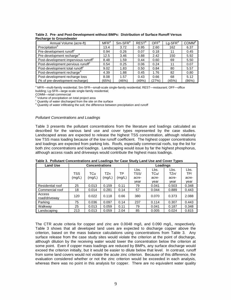
9

Table 2. Pre- and Post-Development without BMPs: Distribution of Surface Runoff Versus Recharge to Groundwater

Annual Volume (acre-ft) MFRa Sm-SFR

a REST

a OFF

a Lg-SFR

a COMM

a

Precipitationb 13.4 3.72 0.95 2.60 162 6.37

Pre-development runoffc 0.94 0.26 0.07 0.18 11 0.45

Pre-development recharged 12.5 3.46 0.88 2.42 150 5.92

Post-development impervious runoffc 8.48 1.59 0.44 0.60 69 5.50

Post-development pervious runoffc 0.54 0.25 0.06 0.24 11 0.07

Post-development total runoffc 9.02 1.83 0.50 0.84 80 5.57

Post-development recharged 4.39 1.88 0.45 1.76 82 0.80

Post-development recharge loss (% of pre-development recharge)

8.08 (65%)

1.57 (46%)

0.43 (49%)

0.66 (27%)

68 (45%)

5.12 (86%)

a MFR—multi-family residential; Sm-SFR—small-scale single-family residential; REST—restaurant; OFF—office

building; Lg-SFR—large-scale single-family residential; COMM—retail commercial b Volume of precipitation on total project area

c Quantity of water discharged from the site on the surface

d Quantity of water infiltrating the soil; the difference between precipitation and runoff

Pollutant Concentrations and Loadings Table 3 presents the pollutant concentrations from the literature and loadings calculated as described for the various land use and cover types represented by the case studies. Landscaped areas are expected to release the highest TSS concentration, although relatively low TSS mass loading because of the low runoff coefficient. The highest copper concentrations and loadings are expected from parking lots. Roofs, especially commercial roofs, top the list for both zinc concentrations and loadings. Landscaping would issue by far the highest phosphorus, although access roads and driveways would contribute the highest mass loadings. Table 3. Pollutant Concentrations and Loadings for Case Study Land Use and Cover Types

Land Use Concentrations Loadings

TSS

(mg/L) TCu

(mg/L) TZn

(mg/L) TP

(mg/L)

Lbs. TSS/ acre-year

Lbs. TCu/ acre-year

Lbs. TZn/ acre-year

Lbs. TP/

acre-year

Residential roof 25 0.013 0.159 0.11 79 0.041 0.503 0.348

Commercial roof 18 0.014 0.281 0.14 57 0.044 0.889 0.443

Access road/driveway

120 0.022 0.118 0.66 380 0.070 0.373 2.088

Parking 75 0.036 0.097 0.14 237 0.114 0.307 0.443

Walkway 25 0.013 0.059 0.11 79 0.041 0.187 0.348

Landscaping 213 0.013 0.059 2.04 85 0.005 0.024 0.815

The CTR acute criteria for copper and zinc are 0.0048 mg/L and 0.090 mg/L, respectively. Table 3 shows that all developed land uses are expected to discharge copper above the criterion, based on the mass balance calculations using concentrations from Table 3. Any surface release from the case study sites would violate the criterion at the point of discharge, although dilution by the receiving water would lower the concentration below the criterion at some point. Even if copper mass loadings are reduced by BMPs, any surface discharge would exceed the criterion initially, but it would be easier to dilute below that level. In contrast, runoff from some land covers would not violate the acute zinc criterion. Because of this difference, the evaluation considered whether or not the zinc criterion would be exceeded in each analysis, whereas there was no point in this analysis for copper. There are no equivalent water quality

10

criteria for TSS and TP; hence, their concentrations were not further analyzed in the different scenarios. Table 4 shows the overall loadings, as well as zinc concentrations, expected to be delivered from the case study developments should they not be fitted with any BMPs. As Table 4 shows, all cases are forecast to exceed the 0.090 mg/L acute zinc criterion, and the retail commercial development does so by a wide margin. Because of its size, the large residential development dominates the mass loading emissions. Table 4. Case Study Pollutant Concentration and Loading Estimates without BMPs

MFRa Sm-SFR

a REST

a OFF

a Lg-SFR

a COMM

a

TZn (mg/L) 0.127 0.123 0.128 0.133 0.123 0.175

Lbs. TSS/year 1321 345 125 242 15016 853

Lbs. TCu/year 0.46 0.074 0.032 0.045 3.21 0.37

Lbs. TZn/year 3.09 0.607 0.174 0.301 26.4 2.64

Lbs. TP/year 6.58 2.39 0.72 1.78 104 3.36

a MFR—multi-family residential; Sm-SFR—small-scale single-family residential; REST—restaurant;

OFF—office building; Lg-SFR—large-scale single-family residential; COMM—retail commercial

2. “Conventional BMP” Analysis: Effect of Basic Treatment BMPs Effect of Basic Treatment BMPs on Post-Development Runoff Volumes The current permit allows regulated parties to select from a range of BMPs in order to treat or infiltrate a given quantity of annual rainfall. The range includes drain inlet inserts, CDS units, and other manufactured BMPs, detention vaults, and sand filters, all of which isolate runoff from the soil; as well as basins and biofiltration BMPs built in soil and generally having vegetation. Treatment BMPs that do not permit any runoff contact with soils discharge as much storm water runoff as equivalent sites with no BMPs, and hence yield zero savings in recharge. As mentioned above, the CalTrans (2004) study found that BMPs with a natural surface can reduce runoff by substantial margins (30-50 percent for extended-detention basins and biofiltration). With such a wide range of BMPs in use, runoff reduction ranging from 0 to 50 percent, and a lack of clearly ascertainable requirements, it is not possible to make a single estimate of how much recharge savings are afforded by maximal implementation of the current permit. We made the following assumptions regarding implementation of BMPs. Assuming natural-surface BMPs perform at the average of the three types tested by CalTrans (2004), i.e., 40 percent runoff reduction, the estimate can be bounded as shown in Table 5 (page 11). The table demonstrates that allowing free choice of BMPs without regard to their ability to direct water into the ground forfeits substantial groundwater recharge benefits when hardened-surface BMPs are selected. Use of soil-based conventional BMPs could cut recharge losses from half or even more of the full potential to about one-quarter to one-third or less, except with the highly impervious commercial development. This analysis shows the wisdom of draining impervious to pervious surfaces, even if those surfaces are not prepared in any special way. But as subsequent analyses showed, soil amendment can gain considerably greater benefits.

11

Table 5. Pre- and Post-Development with Conventional BMPs: Distribution of Surface Runoff Versus Recharge to Groundwater

Annual Volume (acre-ft)

MFRa

Sm-SFR

a

RESTa OFF

a Lg-SFR

a COMM

a

Precipitationb 13.4 3.72 0.95 2.60 162 6.37

Pre-development runoff

c

0.94 0.26 0.07 0.18 11 0.45

Pre-development recharge

12.5 3.46 0.88 2.42 150 5.92

Post-development impervious runoff

c, d

5.09-8.48

0.95-1.59

0.26-0.44

0.36-0.60

41-69

3.30-5.50

Post-development pervious runoff

c, d

0.32-0.54 0.15-0.25 0.04-0.06 0.14-0.24 6.6-11 0.04-0.07

Post-development total runoff

c, d

5.41-9.02 1.10-1.83 0.30-0.50 0.50-0.84 48-80 3.34-5.57

Post-development recharge

d, e

4.39-7.99 1.88-2.62 0.45-0.65 1.76-2.10 82-114 0.80-3.03

Post-development recharge loss (% of pre-development recharge)

d, e

4.51-8.08 (36-65%)

0.84-1.57 (24-46%)

0.23-0.43 (26-49%)

0.32-0.66 (13-27%)

36-68 (24-45%)

2.89-5.12 (49-86%)


building; Lg-SFR—large-scale single-family residential; COMM—retail commercial. Ranges represent 40 percent runoff volume reduction, with full site coverage by BMPs having a natural surface, to no reduction, with BMPs isolating runoff from soil. b Volume of precipitation on total project area

c Quantity of water discharged from the site on the surface

d Ranging from the quantity with hardened bed BMPs to the quantity with soil-based BMPs

e Quantity of water infiltrating the soil; the difference between precipitation and runoff

Effect of Basic Treatment BMPs on Pollutant Discharges Table 6 (page 12) presents estimates of zinc effluent concentrations and mass loadings of the various pollutants discharged from four types of conventional treatment BMPs. The manufactured CDS BMPs in this table, which do not expose runoff to soil or vegetation, are not expected to drop any of the concentrations sufficiently to meet the acute zinc criterion at the discharge point. The loading reduction results show the CDS units always performing below 50 percent reduction for all pollutants analyzed, and most often in the vicinity of 20 percent, with zero copper reduction. When treated with swales or filter strips, effluents from each development case study site are expected to fall below the CTR acute zinc criterion. All but the large commercial site would meet the criterion with EDB treatment. These natural-surface BMPs, if fully implemented and well maintained, are predicted to prevent the majority of the pollutant masses generated on most of the development sites from reaching a receiving water. Only total phosphorus reduction falls below 50 percent for two case studies. Otherwise, mass loading reductions range from about 60 to above 80 percent for the EDB, swale, and filter strip. This data indicates that draining impervious to pervious surfaces, even if those surfaces are not prepared in any special way, pays water quality as well as hydrologic dividends.

12

Table 6. Pollutant Concentration and Loading Reduction Estimates with Conventional BMPs

MFRa Sm-SFR

a REST

a OFF

a Lg-SFR

a COMM

a

Effluent Concentrations:

CDS TZn (mg/L)a 0.095 0.095 0.098 0.102 0.095 0.131

EDB TZn (mg/L)a 0.085 0.086 0.084 0.084 0.086 0.098

Swale TZn (mg/L) 0.055 0.054 0.055 0.056 0.054 0.068

Filter strip TZn (mg/L) 0.039 0.039 0.039 0.041 0.039 0.048

Loading Reductions:

CDS TSS loading reduction 15.7% 19.9% 22.0% 24.0% 19.9% 16.9%

CDS TCu loading reduction 0.0% 0.0% 0.0% 0.0% 0.0% 0.0%

CDS TZn loading reduction 22.7% 22.4% 22.9% 23.1% 22.4% 25.1%

CDS TP loading reduction 30.6% 41.5% 40.7% 45.9% 41.5% 20.3%

EDB TSS loading reduction 68.1% 73.7% 79.0% 81.1% 73.7% 71.7%

EDB TCu loading reduction 61.9% 55.7% 66.2% 63.0% 55.7% 66.8%

EDB TZn loading reduction 59.7% 59.6% 60.4% 61.9% 59.6% 66.6%

EDB TP loading reduction 61.9% 69.7% 69.1% 72.9% 69.7% 54.5%

Swale TSS loading reduction 68.8% 71.1% 73.1% 73.9% 71.1% 69.4%

Swale TCu loading reduction 72.5% 68.5% 78.2% 73.3% 68.5% 75.8%

Swale TZn loading reduction 78.4% 78.1% 84.3% 78.8% 78.1% 80.7%

Swale TP loading reduction 66.3% 70.7% 67.2% 76.2% 70.7% 55.0%

Filter strip TSS loading reduction 69.9% 75.4% 80.6% 82.6% 75.4% 72.3%

Filter strip TCu loading reduction 74.4% 69.1% 78.2% 75.4% 69.1% 78.7%

Filter strip TZn loading reduction 78.3% 77.9% 78.4% 78.7% 77.9% 80.9%

Filter strip TP loading reduction 48.4% 53.1% 63.7% 59.8% 53.1% 34.6%


OFF—office building; Lg-SFR—large-scale single-family residential; COMM—retail commercial; CDS— continuous deflective separation unit; EDB—extended-detention basin

3. LID Analysis: Development According to Modified Draft Permit Provisions (a) Hydrologic Analysis The LID analysis was first performed according to the Draft Permit provisions under the Planning and Land Development Program (Part 4, section E). In this analysis, however, EIA was limited to three instead of five percent, under the reasoning presented in Attachment A. All runoff from NCIA was assumed to drain to vegetated surfaces, as provided in the Draft Permit. One goal of this exercise was to identify methods that reduce runoff production in the first place. It was hypothesized that implementation of source reduction techniques could allow all of the case study sites to infiltrate substantial proportions of the developed site runoff, advancing the hydromodification mitigation objective of the Draft Permit. When runoff is dispersed into the soil instead of being rapidly collected and conveyed away, it recharges groundwater, supplementing a resource that maintains dry season stream flow and wetlands. An increased water balance can be tapped by humans for potable, irrigation, and process water supply. Additionally, runoff volume reduction would commensurately decrease pollutant mass loadings. Accordingly, the analysis considered the practicability of more than one scenario by which the draft permit’s terms could be met, as modified to reflect three percent EIA. In one option, all roof runoff is harvested and stored for some beneficial use. A second option disperses runoff into the soil via roof downspout infiltration trenches. The former option is probably best suited to cases like the large commercial and office buildings, while distribution in the soil would fit best with residences and relatively small commercial developments. The analysis was repeated with the assumptions of harvesting OFF and COMM roof runoff for some beneficial use and dispersing roof runoff from the remaining four cases in roof downspout infiltration systems.

13

Expected Infiltration Capacities of the Case Study Sites The first inquiry on this subject sought to determine how much of the total annual runoff each property is expected to infiltrate. This assessment tested the feasibility of draining all but three percent of impervious area to pervious land on the sites. Based on the findings of Chralowicz et al. (2001), it was assumed that an infiltration zone of 0.1-0.5 acres in area and 2-3 ft deep would serve a drainage catchment area in the size range 0-5 acres and infiltrate 0.9-1.9 acre-ft/year. The conclusions of Chralowicz et al. (2001) were extrapolated to conservatively assume that 0.5 acre would be required to serve each additional five acres of catchment, and would infiltrate an incremental 1.4 acre-ft/year (the midpoint of the 0.9-1.9 acre-ft/year range). According to these assumptions, the following schedule of estimates applies:

Pervious Area Available for Infiltration Catchment Served acres Infiltration Capacity 0.5 acres 0-5 acres 1.4 acre-ft/year 1.0 acres 5-10 acres 2.8 acre-ft/year 1.5 acres 10-15 acres 4.2 acre-ft/year

(Etc.) ... ...

As a formula, infiltration capacity ≈ 2.8 x available pervious area. To apply the formula conservatively, the available area was reduced to the next lower 0.5-acre increment before multiplying by 2.8. As shown in Table 7, five of the six sites have adequate or greater capacity to infiltrate the full annual runoff volume from NCIA and pervious areas where EIA is limited to three percent of the total site area (four at the higher Ojai rainfall). Indeed, five of the six development types have sufficient pervious area to infiltrate all runoff, including runoff from EIA areas. With the most representative rainfall, only the large commercial development, with little available pervious area, falls short of the needed capacity to infiltrate all rainfall, but it still has the capacity to meet the terms of the draft permit, as modified for this analysis. These results are based on infiltrating in the native soils with no soil amendment. For any development project at which infiltration-oriented BMPs are considered, it is important that infiltration potential be carefully assessed using site-specific soils and hydrogeologic data. In the event such an investigation reveals a marginal condition (e.g., hydraulic conductivity, spacing to groundwater) for infiltration basins, soils could be enhanced to produce bioretention zones to assist infiltration. Notably, the four case studies with far greater than necessary infiltration capacity would offer substantial flexibility in designing infiltration, allowing ponding at less than 2-3 ft depth. Table 7. Infiltration and Runoff Volume With 3 Percent EIA and All NCIA Draining to Pervious Areas

MFRa Sm-SFR

a REST

a OFF

a Lg-SFR

a COMM

a

EIA runoff (acre-ft/year) 0.38 0.11 0.03 0.07 4.6 0.18

NCIA + pervious area runoff (acre-ft/year)

8.63 1.73 0.47 0.76 75.0 5.39

Total runoff (acre-ft/year) 9.01 1.84 0.50 0.83 79.6 5.57

Pervious area available for infiltration (acres)

3.66 1.67 0.39 1.61 72.7 0.47

Estimated infiltration capacity (acre-ft/year)

b

9.8 4.2 1.4 4.2 203 1.4

Infiltration capacity c > 100%

d > 100% > 100% > 100% > 100% ~26%

d


OFF—office building; Lg-SFR—large-scale single-family residential; COMM—retail commercial; b Based on Chralowicz et al. (2001) according to the schedule described above

c Compare runoff production from NCIA + pervious area (row 3) with estimated infiltration capacity (row 6)

d At Ojai rainfall levels, capacity would be ~78 percent at the MFR site and ~18 percent at the COMM site.

14

As Table 7 shows, five of the six case study sites have the capacity to infiltrate all runoff produced onsite by draining impervious surfaces to pervious areas. Even runoff from the area assumed to be EIA could be infiltrated in most cases based on the amount of pervious area available in typical development projects. By showing that it is possible under normal site conditions and using native soils to retain all runoff in typical developments, these results demonstrate that a three percent EIA requirement, which would not demand that all runoff be retained, is feasible and practicable. Additional Source Reduction Capabilities of the Case Study Sites: Water Harvesting Example Infiltration is one of a wide variety of LID-based source reduction techniques. Where site conditions such as soil quality or available area limit a site’s infiltration capacity, other source LID measures can enhance a site’s runoff retention capability. For example, soil amendment, which improves infiltration, is a standard LID technique. Water harvesting is another. Such practices can also be used where infiltration capacity is adequate, but the developer desires greater flexibility for land use on-site. Table 8 shows the added implementation flexibility created by subtracting roof runoff by harvesting it or efficiently directing it into the soil through downspout dispersion systems, further demonstrating the feasibility of meeting the draft permit’s proposed requirements, as modified to include a three percent EIA standard. Table 8. Infiltration and Runoff Volume Reduction Analysis Including Roof Runoff Harvesting or Disposal in Infiltration Trenches (Assuming 3 Percent EIA and All NCIA Draining to Pervious Areas)

MFRa Sm-SFR

a REST

a OFF

a Lg-SFR

a COMM

a

EIA runoff (acre-ft/year) 0.38 0.11 0.03 0.07 4.6 0.18

Roof runoff (acre-ft/year) 4.92 0.93 0.09 0.20 41 2.33

Other NCIA + pervious area runoff (acre-ft/year)

3.71 0.79 0.39 0.56 35 3.06

Total runoff (acre-ft/year) 9.01 1.84 0.50 0.83 79.6 5.57

Pervious area available for infiltration (acres)

3.66 1.67 0.39 1.61 72.7 0.47

Estimated infiltration capacity (acre-ft/year)

b

9.8 4.2 1.4 4.2 203 1.4

Infiltration capacity c > 100% > 100% > 100% > 100% > 100% ~45%

d


OFF—office building; Lg-SFR—large-scale single-family residential; COMM—retail commercial; b Based on Chralowicz et al. (2001) according to the schedule described above

c Comparison of runoff production from NCIA + pervious area (row 3) with estimated infiltration capacity (row 6)

d If the higher rainfall at Ojai is assumed, capacity would be ~32 percent of the amount needed for the COMM case.

Effect of Full LID Approach on Recharge Table 9 (page 15) shows the recharge benefits of preventing roofs from generating runoff and infiltrating as much as possible of the runoff from the remainder of the case study sites. The data show that LID methods offer significant benefits relative to the baseline (no storm water controls) in all cases. These benefits are particularly impressive in developments with relatively high site imperviousness, such as in the MFR and COMM cases. In the latter case the full LID approach (excluding the common and effective practice of soil amendment) would cut loss of the potential water resource represented by recharge and harvesting from 86 to 37 percent.

15

Table 9. Comparison of Water Captured Annually (in acre-ft) from Development Sites for Beneficial Use With a Full LID Approach Compared to Development With No BMPs

MFRa Sm-SFR

a REST

a OFF

a Lg-SFR

a COMM

a

Pre-development rechargeb

(acre-ft) 12.5 3.46 0.88 2.42 150 5.92

No BMPs:

post-development recharge b

(acre-ft) 4.39 1.88 0.45 1.76 82 0.80

post-development runoff (acre-ft) 8.08 1.57 0.43 0.66 68 5.12

post-development % recharge lost 65% 46% 49% 27% 45% 86%

Full LID approach:

post-development runoff capture (acre-ft)c 12.5 3.46 0.88 2.42 150 3.73

post-development runoff (acre-ft) 0 0 0 0 0 2.19

post-development % recharge lost 0% 0% 0% 0% 0% 37%


building; Lg-SFR—large-scale single-family residential; COMM—retail commercial b Quantity of water infiltrating the soil; the difference between precipitation and runoff

c Water either entirely infiltrated in BMPs and recharged to groundwater or partially harvested from roofs and partially

infiltrated in BMPs. For the first five case studies, EIA was not distinguished from the remainder of the development, because these sites have the potential to capture all runoff. (b) Water Quality Analysis As outlined above, it was assumed that EIA discharges, as well as runoff from all pervious surfaces, are subject to treatment control. For purposes of the analysis, treatment control was assumed to be provided by conventional sand filtration. This choice is appropriate for study purposes for two reasons. First, sand filters can be installed below grade, and land above can be put to other uses. Under the Draft Permit’s approach, pervious area should be reserved for receiving NCIA drainage, and using sand filters would not draw land away from that service or other site uses. A second reason for the choice is that sand filter performance data equivalent to the data used in analyzing other conventional BMPs are available from the CalTrans (2004) work. Sand filters may or may not expose water to soil, depending on whether or not they have a hard bed. This analysis assumed a hard bed, meaning that no infiltration would occur and thus there would be no additional recharge in sand filters. Performance would be even better than shown in the analytical results if sand filters were built in earth. Pollutant Discharge Reduction Through LID Techniques The preceding analyses demonstrated that each of the six case studies could feasibly comply with the draft permit’s requirements, as modified to include a more protective three percent EIA standard. Moreover, for five of the six case studies, all storm water discharges could be eliminated at least under most meteorological conditions by dispersing runoff from impervious surfaces to pervious areas. Therefore, pollutant additions to receiving waters would also be eliminated. This demonstrates not only that a lower EIA (three percent) is a feasible and practicable approach to maintaining the natural hydrology of land being developed, as discussed above, but that a lower EIA is a feasible and practicable way to eliminate the discharge of pollutants that could cause or contribute to violations of water quality standards. While the high proportion of impervious area present on the large commercial site relative to pervious area would not allow eliminating all discharge, harvesting roof water and draining NCIA to properly-prepared pervious area would substantially decrease the volume discharged. Deployment of treatment control BMPs (e.g. sand filter treatment) could cut contaminant discharges from pollutants in the remaining volume of runoff to low levels.

16

Table 10 presents the pollutant reductions from the untreated case achievable through the complete LID approach described above in comparison to conventional treatments (from Table 6). Assuming EIA still discharges through sand filters, pollutant loadings from the untreated condition are expected to decrease by more than 96 percent for all but the COMM case. In that challenging case loadings would still fall by at least 89 percent for TSS and the metals and by 83 percent for total phosphorus, assuming City of Ventura rainfall levels, and slightly less assuming the higher Ojai rainfall levels. Thus, the Draft Permit’s basic premise of disconnecting most impervious area, supplemented by specially managing roof water, is shown by both water quality and hydrologic results to be feasible and to afford broad and significant environmental benefits. Table 10. Pollutant Loading Reduction Estimates With a Full LID Approach Relative to Conventional BMPs

MFRa Sm-SFR

a REST

a OFF

a Lg-SFR

a COMM

a

Conventional TSS loading reduction

b

15.7-69.9%

19.9-75.4%

22.0-80.6%

24.0-82.6%

19.9-75.4%

16.9-72.3%

Conventional TCu loading reduction

b

0.0-74.4%

0.0-69.1%

0.0-78.2%

0.0-75.4%

0.0-69.1% 0.0-78.7%

Conventional TZn loading reduction

b

22.7-78.4%

22.4-78.1%

22.9-84.3%

23.1-78.8%

22.4-78.1%

25.1-80.9%

Conventional TP loading reduction

b

30.6-66.3%

41.5-70.7%

40.7-69.1%

45.9-76.2%

41.5-70.7%

20.3-55.0%

LID TSS loading reductionc 99.4% 99.3% 99.5% 99.4% 99.3% 89.0%

d

LID TCu loading reductionc 98.1% 96.7% 98.0% 96.2% 96.7% 90.6%

d

LID TZn loading reductionc 99.1% 98.8% 98.9% 98.3% 98.8% 94.8%

d

LID TP loading reductionc 98.1% 98.6% 98.8% 98.7% 98.6% 83.1%

d


building; Lg-SFR—large-scale single-family residential; COMM—retail commercial; CDS— continuous deflective separation unit; EDB—extended-detention basin; NCIA—not connected impervious area; EIA—effective (connected) impervious area b Range from Table 6 represented by treatment by CDS unit, EDB, biofiltration swale, or biofiltration strip

c Based on directing roof runoff to downspout infiltration trenches (MFR, Sm-SFR, REST, and Lg-SFR) or harvesting it

(OFF and COMM), draining other NCIA to pervious areas, and treating EIA with sand filters d If the higher rainfall at Ojai is assumed, reduction estimates for TSS, TCu, TZn, and TP would be 84.0, 86.3, 92.5, and

75.5 percent, respectively.

SUMMARY AND CONCLUSIONS This paper demonstrated that common Ventura County area residential and commercial development types subject to the Municipal NPDES Permit are likely, without storm water management, to reduce groundwater recharge from the predevelopment state by approximately half in most cases to a much higher fraction with a large ratio of impervious to pervious area. With no treatment, runoff from these developments is expected to exceed CTR acute copper and zinc criteria at the point of discharge and to deliver large pollutant mass loadings to receiving waters. Conventional soil-based BMP solutions that promote and are component parts of low-impact development approaches, by contrast, regain about 30-50 percent of the recharge lost in development without storm water management, although commercially-manufactured filtration and hydrodynamic BMPs for storm water management give no benefits in this area. It is expected the soil-based BMPs generally would release effluent that meets the acute zinc criterion at the point of discharge, although it would still exceed the copper limit. Excepting phosphorus, it was found that these BMPs would capture and prevent the movement to receiving waters of the majority of the pollutant loadings considered in the analysis.

17

It was found that a three percent Effective Impervious Area standard can be met in typical developments, and that by draining all site runoff to pervious areas, runoff can be eliminated entirely in most development types. This result was reached assuming the use of native soils. Soil enhancement (typically, with compost) can further advance infiltration. Draining impervious surfaces onto the loam soils typical of Ventura County, in connection with limiting directly connected impervious area to three percent of the site total area, should eliminate storm runoff from some development types and greatly reduce it from more highly impervious types. Adding roof runoff elimination to the LID approach (by harvesting or directing it to downspout infiltration trenches) should eliminate runoff from all but mostly impervious developments. Even in the development scenario involving the highest relative proportion of impervious surface, losses of rainfall capture for beneficial uses could be reduced from more than 85 to less than 40 percent, and pollutant mass loadings would fall by 83-95 percent from the untreated scenario when draining to pervious areas was supplemented with water harvesting. These results demonstrate the basic soundness of the Draft Permit’s concept to limit directly connected impervious area and drain the remainder over pervious surfaces.

REFERENCES California Department of Transportation. 2004. BMP Retrofit Pilot Program Final Report.

California Department of Transportation, Sacramento, CA. Chralowicz, D., T. Goff, M. Mascali, and E. Taylor. 2001. Infiltration of Urban Stormwater

Runoff to Recharge Groundwater Used for Drinking Water: A Study of the San Fernando Valley, California. Master of Environmental Science and Management Report, University of California at Santa Barbara, Santa Barbara, CA.

Herrera Environmental Consultants, Inc. Undated. Pollutant Concentrations for Urban Source

Areas, unpublished data table. Natural Resource Conservation Service. 1986. Urban Hydrology for Small Watersheds,

Technical Release-55. U.S. Department of Agriculture, Washington, D.C. Schueler, T.R. 1987. Controlling Urban Runoff: A Practical Manual for Planning and Designing

Urban BMPs. Metropolitan Washington Council of Governments, Washington, D.C. U.S. Environmental Protection Agency. 1983. Results of the Nationwide Urban Runoff

Program: Volume 1 - Final Report, Report No. 832R83112. Office of Water, Washington, D.C.

18

This page intentionally left blank.

A-1

ATTACHMENT A

JUSTIFICATION OF PROPOSED EFFECTIVE IMPERVIOUS AREA LIMITATION

Summary

The literature shows that adverse impacts to the physical habitat and biological integrity of receiving waters occur as a result of the conversion of natural areas to impervious cover. These effects are observed at the lowest levels of impervious cover in associated catchments (two to three percent) and are pronounced by the point that impervious cover reaches five percent. To protect biological productivity, physical habitat, and other beneficial uses, effective impervious area should be capped at no more than three percent.

I. Impacts to physical habitat of California receiving waters observed at three

percent impervious cover Stein et al.

7 note that while studies from parts of the country with climates more humid than

California’s indicate that physical degradation of stream channels can initially be detected when watershed impervious cover approaches 10%, biological effects, which may be more difficult to detect, may occur at lower levels (CWP 2003).

8 Recent studies from both northern and southern

California indicate that intermittent and ephemeral streams in California are more susceptible to the effects of hydromodification than streams from other regions of the US, with stream degradation being recognized when the associated catchment’s impervious cover is as little as 3-5% (Coleman et al. 2005).

9 Furthermore, supplemental landscape irrigation in semi-arid

regions, like California, can substantially increase the frequency of erosive flows (AQUA TERRA Consultants 2004).

10

Coleman, et al.

3 report that the ephemeral/intermittent streams in southern California

(northwestern Los Angeles County through southern Ventura County to central Orange County) appear to be more sensitive to changes in percent impervious cover than streams in other areas. Stream channel response can be represented using an enlargement curve, which relates the percent of impervious cover to a change in cross-sectional area. The data for southern California streams forms a relationship very similar in shape to the enlargement curves developed for other North American streams. However, the curve for southern California streams is above the general curve for streams in other climates. This suggests that a specific enlargement ratio is produced at a lower value of impervious surface area in southern California than in other parts of North America. Specifically, the estimated threshold of response is approximately 2-3% impervious cover, as compared to 7-10% for other portions of the U.S. It is important to note that this conclusion applies specifically to streams with a catchment drainage area less than 5 square miles.

7 Stein, E.D., S. Zaleski, (2005) Managing Runoff to Protect Natural Streams: The Latest Developments on

Investigation and Management of Hydromodification in California. (Proceedings of a Special Technical Workshop Co-sponsored by California Stormwater Quality Association (CASQA), Stormwater Monitoring Coalition (SMC), University of Southern California Sea Grant (USC Sea Grant), Technical Report #475). 8 Center for Watershed Protection (CWP), (2003) Impacts of Impervious Cover on Aquatic Systems. Ellicott City, MD.

9 Coleman, D., C. MacRae, and E.D. Stein, (2005) Effect of Increases in Peak Flows and Imperviousness on the Morphology of Southern California Streams. Southern California Coastal Water Research Project Technical Report #450, Westminster, CA. 10 AQUA TERRA Consultants, (2004) Urbanization and Channel Stability Assessment in the Arroyo Simi Watershed of Ventura County CA. FINAL REPORT. Prepared for Ventura County Watershed Protection Division, Ventura CA.

A-2

This study concludes that disconnecting impervious areas from the drainage network and adjacent impervious areas is a key approach to protecting channel stability. Utilizing this strategy can make it practical to keep the effective impervious cover (i.e. the amount hydrologically connected to the stream) equal to or less than the identified threshold of 2-3%.

II. Impacts to biological integrity of receiving waters observed with any conversion from natural to impervious surface

Two separate studies conducted by Horner et al.

11,12 in the Puget Sound region (Washington

State), Montgomery County, Maryland, and Austin, Texas built a database totaling more than 650 reaches on low-order streams in watersheds ranging from no urbanization and relatively little human influence (the reference state, representing “best attainable” conditions) to highly urban (>60 percent total impervious area, “TIA”). Biological health was assessed according to the benthic index of biotic integrity (B-IBI) and, in Puget Sound, the ratio of young-of-the-year coho salmon (Oncorhynchus kisutch), a relatively stress-intolerant fish, to cutthroat trout (Oncorhynchus clarki), a more stress-tolerant species. The following discussion summarizes the results and conclusions of these two studies. There is no single cause for the decline of water resource conditions in urbanizing watersheds. Instead, it is the cumulative effects of multiple stressors that are responsible for degraded aquatic habitat and water quality. Imperviousness, while not a perfect yardstick, appears to be a useful predictor of ecological condition. However, a range of stream conditions can be associated with any given level of imperviousness. In general, only streams that retain a significant proportion of their natural vegetative land-cover and have very low levels of watershed imperviousness appear to retain their natural ecological integrity. It is this change in watershed land-cover that is largely responsible for the shift in hydrologic regime from a sub-surface flow dominated system to one dominated by surface runoff. While the decline in ecological integrity is relatively continuous and is consistent for all parameters, the impact on physical conditions appears to be more pronounced earlier in the urbanization process than chemical degradation. It is generally acknowledged, based on field research and hydrologic modeling, that it is the shift in hydrologic conditions that is the driving force behind physical changes in urban stream-wetland ecosystems. Multiple scales of impact operate within urbanizing watersheds: landscape-level impacts, including the loss of natural forest cover and the increase in impervious surface area throughout the watershed; riparian corridor-specific impacts such as encroachment, fragmentation, and loss of native vegetation; and local impacts such as water diversions, exotic vegetation, stream channelization, streambank hardening, culvert installation, and pollution from the widespread use of pesticides and herbicides. All of these stressors contribute to the overall cumulative impact. The researchers found that there is no clear threshold of urbanization below which there exists a “no-effect” condition. Instead, there appears to be a relatively continuous decline in almost all measures of water quality or ecological integrity. Losses of integrity occur from the lowest levels of TIA and are already pronounced by the point that TIA reaches 5 percent.

11

Horner, R. R., C. W. May, (2002) The Limitations of Mitigation-Based Stormwater Management in the Pacific Northwest and the Potential of a Conservation Strategy based on Low-Impact Development Principles. (Proceedings of the American Society of Engineers Stormwater Conference, Portland, OR). 12 Horner, R.R., E. H. Livingston, C. W. May, J. Maxted, (2006) BMPs, Impervious Cover, and Biological Integrity of Small Streams. (Proceedings of the Eighth Biennial Stormwater Research and Watershed Management Conference, Tampa, FL).

A-3

Similarly, the Alliance for the Chesapeake Bay13

reports that small-watershed studies by the Maryland Department of Natural Resources Biological Stream Survey have shown that some sensitive species are affected by even low amounts of impervious cover. In one study, no brook trout were observed in any stream whose watershed had more than 2 percent impervious cover, and brook trout were rare in any watershed with more than 0.5 percent impervious cover. III. Ventura County’s watersheds include biologically-significant water bodies The literature discussed above is relevant to the watersheds of Ventura County, which contain rivers and streams that currently or historically support a variety of beneficial uses that may be impaired by water quality degradation and stream hydromodification as a result of storm water runoff from impervious land cover. Unlike some Southern California watersheds, Ventura County still has many natural stream systems with a high degree of natural functionality. For instance, the Ventura River watershed in northwestern Ventura County “supports a large number of sensitive aquatic species,”

14 including steelhead trout, a federally-listed endangered

species. Although “local populations of steelhead and rainbow trout have nearly been eliminated along the Ventura River” itself, the California Department of Fish and Game has “recognized the potential for the restoration of the estuary and enhancement of steelhead populations in the Ventura River.”

15 Steelhead may also be present in tributaries such as San Antonio Creek.

16

Thriving rainbow trout populations exist in tributaries of the Ventura River including Matilija Creek and Coyote Creek.

17 The Ventura River either does or is projected to support the

following beneficial uses: warm freshwater habitat; cold freshwater habitat; wildlife habitat; rare, threatened, or endangered species; migration of aquatic organisms; and spawning and reproduction.

18 Furthermore, the Ventura River Estuary also supports commercial fishing,

shellfish harvesting, and wetland habitat.19

The Ventura River receives municipal storm drain discharges from Ojai, San Buenaventura, and unincorporated areas of Ventura County.

20

The Santa Clara River watershed in northern Ventura County “is the largest river system in southern California that remains in a relatively natural state.”

21 Sespe Creek is one of the Santa

Clara’s largest tributaries, and “supports significant steelhead spawning and rearing habitat.”22

Other creeks in the Santa Clara River watershed that support steelhead are Piru Creek and Santa Paula Creek. Sespe Creek and the Santa Clara River also provide spawning habitat for the Pacific lamprey. Rainbow trout populations exist in tributaries of the Santa Clara River including Sespe Creek.

23 The creeks and the Santa Clara river do or are projected to support

the following beneficial uses: warm freshwater habitat; cold freshwater habitat; wildlife habitat; preservation of biological habitats rare, threatened, or endangered species; migration of aquatic organisms; and spawning and reproduction.

24 Los Padres National Forest covers much of the

Santa Clara River watershed, but increasing development in floodplain areas has been

13 Karl Blankenship, BAY JOURNAL,”It’s a hard road ahead for meeting new sprawl goal: States will try to control growth of impervious” (July/August 2004), at http://www.bayjournal.com/article.cfm?article=66. 14

Los Angeles Region Water Quality Control Plan (1994) p. 1-18 (“Basin Plan”). 15

Basin Plan, p. 1-16; Ventura County Environmental & Energy Resources Division, “Endangered Steelhead Trout in Ventura County: Past, Present, and Future,” available at http://www.wasteless.org/Eye_articles/steelhead.htm. 16

Ventura County Environmental & Energy Resources Division, “Steelhead Spawning in Ventura County,” (2005), available at http://www.wasteless.org/Eye_articles/steehead2005.html. 17

Ventura County Environmental & Energy Resources Division, “Endangered Steelhead Trout in Ventura County: Past, Present, and Future,” available at http://www.wasteless.org/Eye_articles/steelhead.htm. 18

Basin Plan, Table 2-1. 19


Ventura County Watershed Protection District, Report of Waste Discharge (January 2005) at p. 3. 21

Basin Plan, p. 1-16. 22


Ventura County Environmental & Energy Resources Division, “Endangered Steelhead Trout in Ventura County: Past, Present, and Future,” available at http://www.wasteless.org/Eye_articles/steelhead.htm. 24

Basin Plan, Table 2-1.

http://www.bayjournal.com/article.cfm?article=66

http://www.wasteless.org/Eye_articles/steelhead.htm

http://www.wasteless.org/Eye_articles/steehead2005.html



A-4

identified as a threat to the river system’s water quality.25

Furthermore, the Santa Clara estuary supports the additional beneficial uses of shellfish harvesting and wetlands habitat.

26 The Santa

Clara River receives municipal storm drain discharges from Fillmore, Oxnard, San Buenaventura, Santa Paula, and unincorporated areas of Ventura County.

27

The Calleguas Creek watershed “empties into Mugu Lagoon, one of southern California’s few remaining large wetlands.”

28 It supports or is projected to support the following beneficial uses:

estuarine habitat; marine habitat; wildlife habitat; preservation of biological habitats; rare, threatened, or endangered species; migration of aquatic organisms; spawning and reproduction; shellfish harvesting; and wetlands habitat.

29 Historically, Calleguas Creek drained

largely agricultural areas. But this watershed has been under increasing pressure from sedimentation due to increased surface flow from municipal discharges and urban wastewaters, among other sources.

30 Increasing residential developments on steep slopes has been

identified as a substantial contributing factor to the problem of accelerated erosion in the watershed (and sedimentation in the Lagoon). Calleguas Creek receives municipal storm drain discharges from Camarillo, Moorpark, Simi Valley, Thousand Oaks, and unincorporated areas of Ventura County.

31

Ventura County’s coastal streams also support a variety of beneficial uses:

32

Little Sycamore Canyon Creek in southern Ventura County (warm freshwater habitat; wildlife habitat; rare, threatened or endangered species; and spawning and reproduction);

Lake Casitas tributaries (warm freshwater habitat; cold freshwater habitat; wildlife habitat; rare, threatened or endangered species; spawning and reproduction; and wetland habitat);

Javon Canyon and Padre Juan Canyon (warm freshwater habitat; cold freshwater habitat; wildlife habitat; and spawning and reproduction); and

Los Sauces Creek in northern Ventura County (warm freshwater habitat; cold freshwater habitat; wildlife habitat; migration of aquatic species; and spawning and reproduction).

IV. Conclusion In order to protect the biological habitat, physical integrity, and other beneficial uses of the water bodies in Ventura County, effective impervious area should be capped at no more than three percent.

25

Basin Plan, pp. 1-16, 1-18. 26





Basin Plan, pp. 1-16, 1-18. 31


Basin Plan, Table 2-1.

B-1

ATTACHMENT B

POLLUTANT CONCENTRATIONS FOR URBAN SOURCE AREAS (HERRERA ENVIRONMENTAL CONSULTANTS, INC. UNDATED)

Source Area Study Location Sample Size (n) TSS (mg/L) TCu (ug/L) TPb (ug/L) TZn (ug/L) TP (mg/L) Notes

Roofs

Residential Steuer, et al. 1997 MI 12 36 7 25 201 0.06 2

Residential Bannerman, et al. 1993 WI ~48 27 15 21 149 0.15 3

Residential Waschbusch, et al. 2000 WI 25 15 n.a. n.a. n.a. 0.07 3

Residential FAR 2003 NY 19 20 21 312 0.11 4

Residential Gromaire, et al. 2001 France 29 37 493 3422 n.a. 5

Representative Residential Roof Values 25 13 22 159 0.11

Commercial Steuer, et al. 1997 MI 12 24 20 48 215 0.09 2

Commercial Bannerman, et al. 1993 WI ~16 15 9 9 330 0.20 3

Commercial Waschbusch, et al. 2000 WI 25 18 n.a. n.a. n.a. 0.13 3

Representative Commercial Roof Values 18 14 26 281 0.14

Parking Areas

Res. Driveways Steuer, et al. 1997 MI 12 157 34 52 148 0.35 2

Res. Driveways Bannerman, et al. 1993 WI ~32 173 17 17 107 1.16 3

Res. Driveways Waschbusch, et al. 2000 WI 25 34 n.a. n.a. n.a. 0.18 3

Driveway FAR 2003 NY 173 17 107 0.56 4

Representative Residential Driveway Values 120 22 27 118 0.66

Comm./ Inst. Park. Areas Pitt, et al. 1995 AL 16 110 116 46 110 n.a. 1

Comm. Park. Areas Steuer, et al. 1997 MI 12 110 22 40 178 0.2 2

Com. Park. Lot Bannerman, et al. 1993 WI 5 58 15 22 178 0.19 3

Parking Lot Waschbusch, et al. 2000 WI 25 51 n.a. n.a. n.a. 0.1 3

Parking Lot Tiefenthaler, et al. 2001 CA 5 36 28 45 293 n.a. 6

Loading Docks Pitt, et al. 1995 AL 3 40 22 55 55 n.a. 1

Highway Rest Areas CalTrans 2003 CA 53 63 16 8 142 0.47 7

Park and Ride Facilities CalTrans 2003 CA 179 69 17 10 154 0.33 7

Comm./ Res. Parking FAR 2003 NY 27 51 28 139 0.15 4

Representative Parking Area/Lot Values 75 36 26 97 0.14

B-2

Landscaping/Lawns

Landscaped Areas Pitt, et al. 1995 AL 6 33 81 24 230 n.a. 1

Landscaping FAR 2003 NY 37 94 29 263 n.a. 4

Representative Landscaping Values 33 81 24 230 n.a.

Lawns - Residential Steuer, et al. 1997 MI 12 262 n.a. n.a. n.a. 2.33 2

Lawns - Residential Bannerman, et al. 1993 WI ~30 397 13 n.a. 59 2.67 3

Lawns Waschbusch, et al. 2000 WI 25 59 n.a. n.a. n.a. 0.79 3

Lawns Waschbusch, et al. 2000 WI 25 122 n.a. n.a. n.a. 1.61 3

Lawns - Fertilized USGS 2002 WI 58 n.a. n.a. n.a. n.a. 2.57 3

Lawns - Non-P Fertilized USGS 2002 WI 38 n.a. n.a. n.a. n.a. 1.89 3

Lawns - Unfertilized USGS 2002 WI 19 n.a. n.a. n.a. n.a. 1.73 3

Lawns FAR 2003 NY 3 602 17 17 50 2.1 4

Representative Lawn Values 213 13 n.a. 59 2.04

Notes:

Representative values are weighted means of collected data. Italicized values were omitted from these calculations.

1 - Grab samples from residential, commercial/institutional, and industrial rooftops. Values represent mean of

DETECTED concentrations

2 - Flow-weighted composite samples, geometric mean concentrations

3 - Geometric mean concentrations

4 - Citation appears to be erroneous - original source of data is unknown. Not used to calculate representative value

5 - Median concentrations. Not used to calculate representative values due to site location and variation from other values.

6 - Mean concentrations from simulated rainfall study

7 - Mean concentrations. Not used to calculate representative values due to transportation nature of land use.

INITIAL INVESTIGATION OF THEFEASIBILITY AND BENEFITS

OF LOW-IMPACT SITE DESIGN PRACTICES ("LID")FOR THE SAN FRANCISCO BAY AREA

Richard R. Hornert

ABSTRACT

The Clean Water Act NPDES permit that regulates municipal separate storm sewer systems(MS4s) in the San Francisco Bay Area, California will be reissued in 2007. The draft permitincludes general provisions related to low impact development practices (LID) for certain kindsof development and redevelopment projects. Using six representative development projectcase studies, based on California building records, the author investigated the practicability andrelative benefits of LID options for the majority of the region having soils potentially suitable forinfiltration either in their natural state or after amendment using well recognized LID techniques.The results showed that (1) LID site design and source control techniques are more effectivethan conventional best management practices (BMPs) in reducing runoff rates; and (2) in eachof the case studies, LID methods would reduce site runoff volume and pollutant loading to zeroin typical rainfall scenarios.

t Richard R. Horner, Ph.D., Research Associate Professor, University of WashingtonDepartments of Civil and Environmental Engineering and Landscape Architecture;Adjunct Associate Professor, University of Washington Center for Urban Horticulture

INTRODUCTION

The Assessment in Relation to Municipal Permit Conditions

This purpose of this study is to investigate the relative water quality and water reuse benefits ofthree levels of storm water treatment best management practices (BMPs): (1) basic "treat-andrelease" BMPs (e.g., drain inlet filters, CDS units), (2) commonly used BMPs that expose runoffto soils and vegetation (extended-detention basins and biofiltration swales and filter strips), and(3) low impact development (LID) practices. The factors considered in the investigation arerunoff volume, pollutant loading, and the availability of water for infiltration or other reuse. Inorder to assess the differential impact of storm water reduction approaches on these factors,this study examines six case studies typical of development covered by the proposed MunicipalRegional Urban Runoff Phase I NPDES Stormwater Permit (MRP).

This report covers locations in the Bay Area most amenable to soil infiltration of stormwaterrunoff, those areas having soils in Natural Resources Conservation Service (NRCS) HydrologicSoil Groups A, B, or C as classified by the Natural Resources Conservation Service(http://websoilsurvey.nrcs.usda.gov/applWebSoilSurvey.aspx). Depending on site-specificconditions, A and B soils would generally effectively infiltrate water without modification,whereas C soils could require organic amendments according to now standard LID methods.This report does not cover locations with group 0 soils, which are generally not amenable toinfiltration, again depending on the specific conditions on-site. A subsequent report willexamine options in these locations, which include other LID techniques (e.g., roof runoffharvesting for irrigation or gray water supply) and state-of-the-art conventional stormwater

1

management practices. A minority but still substantial fraction of the Bay Area has group Dsoils (39.3, 68.0, 18.3, and 50.1 percent of the mapped areas of Alameda, Contra Costa, SanMateo, and Santa Clara Counties, respectively). Regarding any mapped soil type, it isimportant to keep in mind that soils vary considerably within small distances. Characteristics atspecific locations can deviate greatly from those of the major mapped unit, making infiltrationpotential either more or less than may be expected from the mapping.

Low impact development methods reduce storm runoff and its contaminants by decreasing theirgeneration at sources, infiltrating into the soil or evaporating storm flows before they can entersurface receiving waters, and treating flow remaining on the surface through contact withvegetation and soil, or a combination of these strategies. Soil-based LID practices often usesoil enhancements such as compost, and thus improve upon the performance of moretraditional basins and biofilters. The study encompassed vegetated swales (channels forconveyance at some depth and velocity), vegetated filter strips (surfaces for conveyance in thinsheet flow), and bioretention areas (shallow basins with a range of vegetation types in whichrunoff infiltrates through soil either to groundwater or a subdrain for eventual surface discharge).Application of these practices in a low impact site design mode requires either determinationthat existing site soils can support runoff reduction through infiltration or that soils will beamended using accepted LID techniques to attain this objective. Finally, the study furtherbroadened implementation options to include water harvesting (collection and storage for usein, for example, irrigation or gray water systems), roof downspout infiltration trenches, andporous pavements.

The investigation also considered whether typical development patterns and local conditions inthe Bay Area would enable LID implementation as required by a new standard proposed for the2007 Ventura County Municipal Storm Water Permit. This standard requires management ofeffective impervious area (EIA), limiting it to 5%, as well as other impervious area (what mightbe termed Not-Connected Impervious Area, NCIA), and pervious areas.

Where treatment control BMPs are required to manage runoff from a site, Volume or FlowHydraulic Design Bases commonly used in California were assumed to apply. The former basisapplies to storage-type BMPs, like ponds, and requires capturing and treating either the runoffvolume from the 85th percentile, 24-hour rainfall event for the location or the volume of annualrunoff to achieve 80 percent or more volume treatment. The calculations in this analysis usedthe 85th percentile 24-hour rainfall event basis. The Flow basis applies to flow-through BMPs,like swales, and requires treating the runoff flow rate produced from a rain event equal to atleast 0.2 inches per hour intensity (or one of two other approximately equivalent options).

Scope of the Assessment

With respect to each of the six development case studies, three assessments were undertaken:a baseline scenario incorporating no stormwater management controls; a second scenarioemploying conventional BMPs; and a third development scenario employing LID stormwatermanagement strategies.

To establish a baseline for each case study, annual stormwater runoff volumes were estimated,as well as concentrations and mass loadings of four pollutants: (1) total suspended solids(TSS), (2) total recoverable copper (TCu), (3) total recoverable zinc (TZn), and (4) totalphosphorus (TP). These baseline estimates were based on the anticipated land use and coverwith no stormwater management efforts.

Two sets of calculations were then conducted using the parameters defined for the six casestudies. The first group of calculations estimated the extent to which basic BMPs reduce runoffvolumes and pollutant concentrations and loadings, and what impact, if any, such BMPs haveon recharge rates or water retention on-site.

2

The second group of calculations estimated the extent to which commonly used soil-basedBMPs and LID site design strategies ameliorate runoff volumes and pollutant concentrationsand loadings, and the effect such techniques have on recharge rates. When evaluating LIDstrategies in the context of the EIA concept employed in the draft Ventura County MS4 permit, itwas presumed that EIA would be limited to three percent. It was also assumed that pervioussurfaces on a site receiving runoff from other areas on the site would be sized and prepared tomanage (through infiltration or storage) the volume directed there in addition to precipitationfalling directly on those areas. The assessment of basins, biofiltration, and low impact designpractices analyzed the expected infiltration capacity of the case study sites. It also consideredrelated LID techniques and practices, such as source reduction strategies, that could work inconcert with infiltration to serve the goals of: (1) preventing increase in annual runoff volumefrom the pre- to the post-developed state, (2) preventing increase in annual pollutant massloadings between the two development states, and (3) avoiding exceedances of the WaterQuality Control Plan for the San Francisco Bay Basin (Basin Plan) criteria for copper and zinc.

The results of this analysis show that:

• A full-range of typical development categories common in the Bay Area, from singlefamily residential to restaurants, housing developments, and commercial uses likeoffice buildings, can feasibly implement standard LID techniques to achieve nostormwater discharge during rain events equal to, and in some cases greater than,design storm conditions. This conclusion is based on an analysis that used actualbuilding records in California and annual rainfall records in two rainfall zones in the BayArea to show that site conditions support this level of performance. In addition, siteconditions typical at a wide range of development projects are more than sufficient toattain compliance with a three percent EIA limit, as is being contemplated in other MS4re-issuance proceedings in California presently.

• Developments implementing no post-construction BMPs result in storm water runoffvolume and pollutant loading that are substantially increased, and recharge rates thatare substantially decreased, compared to pre-development conditions.

• Developments implementing basic post-construction treatment BMPs achieve reducedpollutant loading compared to developments with no BMPs, but stormwater runoffvolume and recharge rates are similar to developments with no BMPs.

• Developments implementing traditional basins and biofilters, and even more so lowimpact post-construction BMPs, achieve significant reduction of pollutant loading andrunoff volume as well as greatly enhanced recharge rates compared to bothdevelopments with no BMPs and developments with basic treatment BMPs.

This report covers the methods employed in the investigation, data sources, and references forboth. It then presents the results, discusses their consequences, draws conclusions, andmakes recommendations relative to the feasibility of utilizing low-impact development practicesin Bay Area developments.

3

CASE STUDIES

Six case studies were selected to represent a range of urban development types considered tobe representative of the Bay Area. These case studies involved: a multi-family residentialcomplex (MFR), a relatively small-scale (23 homes) single-family residential development (SmSFR), a restaurant (REST), an office building (OFF), a relatively large (1000 homes) singlefamily residential development (Lg-SFR), and a single home (SINGLE).1

Parking spaces were estimated to be 176 sq ft in area, which corresponds to 8 ft width by 22 ftlength dimensions. Code requirements vary by jurisdiction, with the tendency now to dropbelow the traditional 200 sq ft average. About 180 sq ft is common, but various standards forfull- and compact-car spaces, and for the mix of the two, can raise or lower the average.2 The176 sq ft size is considered to be a reasonable value for conventional practice.

Roadways and walkways assume a wide variety of patterns. Exclusive of the two SFR cases,simple, square parking lots with roadways around the four sides and square buildings withwalkways also around the four sides were assumed. Roadways and walkways were taken tobe 20 ft and 6 ft wide, respectively.

Single-family residences were assumed each to have a driveway 20 ft wide and 30 ft long. Itwas further assumed that each would have a sidewalk along the front of the lot, which wascalculated to be 5749 sq ft in area. Assuming a square lot, the front dimension would be 76 ft.A 40-ft walkway was included within the property. Sidewalks and walkways were taken to be 4ft wide. For each case study the total area for all of these impervious features was subtractedfrom the total site area to estimate the pervious area, which was assumed to have conventionallandscaping cover (grass, small herbaceous decorative plants, bushes, and a few trees).

1 Building permit records from the City of San Marcos in San Diego County provided data on total siteareas for the first four case studies, including numbers of buildings, building footprint areas (includingporch and garage for Sm-SFR), and numbers of parking spaces associated with the development projects.While the building permit records made no reference to features such as roadways, walkways, andlandscaping normally associated with development projects, these features were taken into account in thecase studies using assumptions described herein. Larger developments and redevelopment were notrepresented in the sampling of building permits from the San Marcos database. To take these types ofprojects into account in the subsequent analysis, the Lg-SFR scenario scaled up all land use estimatesfrom the Sm-SFR case in the ratio of 1000:23. The single home case (SINGLE) was derived from BayArea records obtained at http://www,ppic.org/content/otherI706EHEP web only appendix.pdf, whichshowed 8000 ff as a rough average for a single home lot in the region. As with the other cases, thesehypothetical developments were assumed to have roadways, walkways, and landscaping, as describedherein.

2 J. Gibbons, Parking Lots, NONPOINT EDUCATION FOR MUNICIPAl OFFICERS, Technical Paper No.5 (1999)(http://nemo.uconn.edu/tools/publications/tech papers/tech paper 5.pdf).

4

Table 1 summarizes the characteristics of the six case studies. The table also provides therecorded or estimated areas in each land use and cover type.

Ad La d Cd L d UChCTable 1. ase Study aracteristics an an se an n over reas

MFRa Sm-SFRa RESra OFFa LQ-SFRa SINGLEa

No. buildin s 11 23 1 1 1000 1Total area ft") 476,982 132,227 33,669 92,612 5,749,000 8,000Roof area +") 184,338 34,949 3,220 7,500 1,519,522 2114No. parkingspaces 438 - 33 37 - -Parking area(ff) 77,088 - 5808 6512 - -Access roadarea (ff) 22,212 - 6097 6456 - -Walkway area(ff) 33,960 10,656 1362 2078 463,289 518Driveway area(ff) - 13,800 - - 600,000 835Landscapearea (ff) 159,384 72,822 17,182 70,066 3,166,190 4533

a MFR-multi-family residential; Sm-SFR-small-scale single-family residential; REST-restaurant; OFF-officebuilding; Lg-SFR-Iarge-scale single-family residential; SINGLE-single-family home

METHODS OF ANALYSIS

Annual Stormwater Runoff Volumes

Annual surface runoff volumes produced were estimated for both pre- and post-developmentconditions for each case study site. Runoff volume was computed as the product of annualprecipitation, contributing drainage area, and a runoff coefficient (ratio of runoff produced torainfall received). For impervious areas the following equation was used:

C = (0.009) 1+ 0.05

where I is the impervious percentage. This equation was derived by Schueler (1987) fromNationwide Urban Runoff Program data (U.S. Environmental Protection Agency 1983). With 1=100 percent for fUlly impervious surfaces, C is 0.95.

The basis for pervious area runoff coefficients was the Natural Resource ConservationService's (NRCS) Urban Hydrology for Small Watersheds (NRCS 1986, as revised from theoriginal 1975 edition). This model estimates storm event runoff as a function of precipitationand a variable representing land cover and soil, termed the curve number (CN). Larger eventsare forecast to produce a greater amount of runoff in relation to amount of rainfall because theymore fully saturate the soil. Therefore, use of the model to estimate annual runoff requiresselecting some event or group of events to represent the year. The 85th percentile, 24-hourrainfall event was used in the analysis here for the relative comparison between pre- and postdevelopment and applied to deriving a runoff coefficient for annual estimates, recognizing thatsmaller storms would produce less and larger storms more runoff.

A memorandum titled Rainfall Data Analysis and Guidance for Sizing Treatment BMPs(http://www.cccleanwater.org/construction/Publications/CCCWPBasinSizingMemoFINAL 4-2005.pdD prepared for the Contra Costa Clean Water Program demonstrated a linear relationshipbetween unit basin storage volume for 80 percent capture (which is related to the 85th

5

percentile event) and mean annual precipitation. Rainfall for Bay Area 85th percentile, 24-hourevents could thus be determined from locations where events have been established in directproportion to mean annual rainfall.

In order to obtain appropriate regional estimates of annual precipitation, rainfall records wereobtained from a number of sites in the four counties, plus the city of Vallejo, covered by thepermit.3 The mean annual range is from 13.73 to 24.30 inches, with quantities close to either14 or 20 inches predominating. The study was performed for both of these rainfall totals.These figures were used in conjunction with 85th percentile, 24-hour event amounts of 0.75 forLos Angeles and 0.92 for Santa Rosa (http://ci.santarosa.ca.us/pworks/other/SW/SRSWManuaIFinaIDraft.pdf), respectively, and mean annual totalsof 12 and 31 inches for the respective cities to estimate 85 percentile, 24-hour event quantitiesof 0.77 and 0.82 inch for the 14 and 20-inch Bay Area rainfall zones, respectively.

Pre- and post-development runoff quantities were computed with selected CN values and the0.77- and 0.82-inch rainfalls. The CN choices based on tabulated data in NRCS (1986) andprofessional judgment were 83 before development and 86 after land modification. Estimaterunoff amounts were then divided by the rainfall totals to obtain runoff coefficients. The resultswere about the same for the two rainfall zones at 0.07 and 0.12 before and after development,respectively. Finally, total annual runoff volumes were estimated based on the two averageannual precipitation figures.

Stormwater Runoff Pollutant Discharges

Annual pollutant mass discharges were estimated as the product of annual runoff volumesproduced by the various land use and cover types and pollutant concentrations typical of thoseareas. Again, the 0.75-inch precipitation event was used as a basis for volumes. Stormwaterpollutant data have typically been measured and reported for general land use types (e.g.,single-family residential, commercial). However, an investigation of low impact developmentpractices of the type this study sought to conduct demands data on specific land coverages.The literature offers few data on this basis. Those available and used herein were assembledby a consultant to the City of Seattle for a project in which the author participated. They appearin Attachment A (Herrera Environmental Consultants, Inc. undated).

Pollutant concentrations expected to occur typically in the mixed runoff from the several landuse and cover types making up a development were estimated by mass balance; i.e., theconcentrations from the different areas of the sites were combined in proportion to theircontribution to the total runoff.

The Effect of Conventional Treatment BMPs on Runoff Volume, Pollutant Discharges, andRecharge Rates

The first question in analyzing how BMPs reduce runoff volumes and pollutant discharges was,What BMPs are being employed in Bay Area developments under the permit now in force?These county permits provide regulated entities with a large number of choices and few fixedrequirements regarding the selection of stormwater BMPs. (See Contra Costa County NPDESMunicipal Stormwater Permit, Order No. 99-058; see also Santa Clara County NPDESMunicipal Stormwater Permit, Order No. 01-024, at C.3.a.). Clean Water Program Availableoptions presumably include manufactured BMPs, such as drain inlet inserts (Dlls) andcontinuous deflective separation (CDS) units. Developments may also select such non-

3 http://www.census.gov/stab/ccdb/cit7140a.txt,http://www.acwd.org/dms docs176dOb026b60d97830492079a48b1eb88.pdf,http://www.ei.berkely.ca.us/aboutberkeley/weather.html, http://www.usbr.gov/dataweb/dams/ea10168.htm,http://www.redwoodcitv.org/aboutfweather.html.

6

proprietary devices as extended-detention basins (EDBs) and biofiltration swales and filterstrips. EDBs hold water for two to three days for solids settlement before releasing whateverdoes not infiltrate or evaporate. Biofiltration treats runoff through various processes mediatedby vegetation and soil. In a swale, runoff flows at some depth in a channel, whereas a filter stripis a broad surface over which water sheet flows. Each of these BMP types was applied to eachcase study, although it is not clear that these BMPs, in actuality, have been implementedconsistently within the Bay Area to date.

The principal basis for the analysis of BMP performance was the California Department ofTransportation's (CalTrans, 2004) BMP Retrofit Pilot Program, performed in San Diego and LosAngeles Counties. One important result of the program was that BMPs with a natural surfaceinfiltrate and evaporate (probably, mostly infiltrate) a substantial amount of runoff, even ifconditions do not appear to be favorable for an infiltration basin. On average, the EDBs,swales, and filter strips lost 40, 50 and 30 percent, respectively, of the entering flow before thedischarge point. Dlls and CDS units do not contact runoff with a natural surface, and thereforedo not reduce runoff volume.

The CalTrans program further determined that BMP effluent concentrations were usually afunction of the influent concentrations, and equations were developed for the functionalrelationships in these cases. BMPs generally reduced influent concentrations proportionatelymore when they were high. In relatively few situations influent concentrations were constant atan "irreducible minimum" level regardless of inflow concentrations.

In analyzing the effects of BMPs on the case study runoff, the first step was to reduce the runoffvolumes estimated with no BMPs by the fractions observed to be lost in the pilot study. Thenext task was estimating the effluent concentrations from the relationships in the CalTransreport. The final step was calculating discharge pollutant loadings as the product of the reducedvolumes and predicted effluent concentrations. As before, typical pollutant concentrations in themixed runoff were established by mass balance.

Estimating Infiltration Capacity of the Case Study Sites

Infiltrating sufficient runoff to maintain pre-development hydrologic characteristics and preventpollutant transport is the most effective way to protect surface receiving waters. Successfullyapplying infiltration requires soils and hydrogeological conditions that will pass water sufficientlyrapidly to avoid overly-lengthy ponding, while not allowing percolating water to reach groundwater before the soil column captures pollutants.

The study assumed that infiltration would occur in surface facilities and not in below-groundtrenches. The use of trenches is certainly possible, and was judged to be an approved BMP byCalTrans after the pilot study. However, the intent of this investigation was to determine theability of pervious areas to manage the site runoff. This was accomplished by determining theinfiltration capability of the pervious areas in their original condition for each development casestudy, and further assessing the pervious areas' infiltration capabilities if soils were modifiedaccording to low impact development practices.

The chief basis for this aspect of the work was an assessment of infiltration capacity andbenefits for Los Angeles' San Fernando Valley (Chralowicz et al. 2001). The Chralowicz studyposited providing 0.1-0.5 acre for infiltration basins to serve each 5 acres of contributingdrainage area. At 2-3 ft deep, it was estimated that such basins could infiltrate 0.90-1.87 acreft/year of runoff in San Fernando Valley conditions. Soils there are generally various loamtextures with infiltration rates of approximately 0.5-2.0 inches/hour. Loams are also commonformations in the portion of the Bay Area covered by this report, those areas with Hydrologic

7

Soil Groups A, B, and C,4 thus making the conclusions of the San Fernando Valley studyapplicable for these purposes. This information was used to estimate how much of each casestudy site's annual runoff would be infiltratable, and if the pervious portion would providesufficient area for infiltration. For instance, if sufficient area were available, the infiltrationconfiguration would not have to be in basin form but could be shallower and larger in surfacearea. This study's analyses assumed the use of bioretention areas rather than traditionalinfiltration basins.

Volume and Pollutant Source Reduction Strategies

As mentioned above, the essence of low impact development is reducing runoff problemsbefore they can develop, at their sources, or exploiting the infiltration and treatment abilities ofsoils and vegetation. If a site's existing infiltration and treatment capabilities are inadequate topreserve pre-development hydrology and prevent runoff from causing or contributing toviolations of water quality standards, then LID-based source reduction strategies can beimplemented, infiltration and treatment capabilities can be upgraded, or both.

Source reduction can be accomplished through various LID techniques. Soil can be upgradedto store runoff until it can infiltrate, evaporate, or transpire from plants through compost addition.Soil amendment, as this practice is known, is a standard LID technique.

Upgraded soils are used in bioretention cells that hold runoff and effect its transfer to thesubsurface zone. This standard LID tool can be used where sufficient space is available. Thisstudy analyzed whether the six development case study sites would have sufficient space toeffectively reduce runoff using bioretention cells, assuming the soils and vegetation could beamended and enhanced where necessary.

Conventional pavements can be converted to porous asphalt or concrete or replaced withconcrete or plastic unit pavers or grid systems. For such approaches to be most effective, thesoils must be capable of infiltrating the runoff passing through, and may require renovation.

Source reduction can be enhanced by the LID practice of water harvesting, in which water fromimpervious surfaces is captured and stored for reuse in irrigation or gray water systems. Forexample, runoff from roofs and parking lots can be harvested, with the former being somewhateasier because of the possibility of avoiding pumping to use the water and fewer pollutants.Harvestin~ is a standard technique for Leadership in Energy and Environmental Design (LEED)buildings. Many successful systems of this type are in operation, such as the NaturalResources Defense Council office (Santa Monica, CA), the King County Administration BUilding(Seattle, WA), and two buildings on the Portland State University campus (Portland, OR). Thisinvestigation examined how water harvesting could contribute to stormwater management forcase study sites where infiltration capacity, available space, or both appeared to be limited.

4 http://gis.ca.gov/catalog/BrowseCatalog.epl?id=108,http://websoilsurvey.nrcs.usda.gov/applWebSoiISurvey.aspx

5 New Buildings Institute, Inc., Advanced Buildings (2005)(http://www.powervourdesign.com/LEEDGuide.pdD.

8

RESULTS OF THE ANALYSIS

1. "Base Case" Analysis: Development without Stormwater Controls

Comparison of Pre- and Post-Development Runoff Volumes

Table 2 presents a comparison between the estimated runoff volumes generated by therespective case study sites in the pre- and post-development conditions, assumingimplementation of no stormwater controls on the developed sites. On sites dominated byimpervious land cover, most of the infiltration that would recharge groundwater in theundeveloped state is expected to be lost to surface runoff after development. This greatlyincreased surface flow would raise peak flow rates and volumes in receiving water courses,raise flooding risk, and transport pollutants. Only the office building, the plan for which retainedsubstantial pervious area, would lose less than 40 percent of the site's pre-developmentrecharge.

Table 2. Pre- and Post-Development without BMPs: Distribution of Surface Runoff VersusRecharge to Groundwater annual volume in acre-ft)

Distribution MFRa Sm-SFRaRES~ OFFa Lo-SFRa SINGLEa

141nchesNear Rainfall:PrecipitationO 12.8 3.54 0.90 2.47 154 0.21Pre-development runoff 0.89 0.25 0.07 0.17 10 0.02Pre-developmentrechamed 11.9 3.29 0.83 2.30 144 0.19Post-developmentimpervious runoff 8.07 1.51 0.42 0.57 66 0.09Post-developmentpervious runoff 0.51 0.24 0.06 0.23 10 0.01Post-development totalrunoff 8.58 1.75 0.48 0.80 76 0.10Post-developmentrecharoed 4.22 1.79 0.42 1.67 78 0.11Post-developmentrecharge loss 7.68 1.50 0.41 0.65 66 0.08(% of pre-development) (65%) (46%) (49%) (27%) (45%) (41%)20 InchesNear Rainfall:PrecipitationO 18.2 5.06 1.29 3.54 220 0.30Pre-development runoff 1.28 0.35 0.10 0.24 15 0.03Pre-developmentrecharged 16.9 4.71 1.19 3.30 205 0.27Post-developmentimpervious runoff 11.5 2.16 0.60 0.82 94 0.13Post-developmentpervious runoff 0.73 0.34 0.08 0.33 15 0.01Post-development totalrunoff 12.2 2.50 0.68 1.15 109 0.14Post-developmentrecharged 6.0 2.56 0.61 2.39 111 0.16Post-developmentrecharge loss 10.9 2.15 0.58 0.91 94 0.11(% of pre-development) (65%) (46%) (49%) (27%) (45%) (41%)

a MFR-multi-family residential; Sm-SFR-small-scale single-family residential; REST-restaurant; OFF-officebuilding; Lg-SFR-Iarge-scale single-family residential; SINGLE-single family homeb Volume of precipitation on total project areaC Quantity of water discharged from the site on the surfaced Quantity of water infiltrating the soil; the difference between precipitation and runoff

9

Pollutant Concentrations and Loadings

Table 3 presents the pollutant concentrations from the literature and loadings calculated asdescribed for the various land use and cover types represented by the case studies.Landscaped areas are expected to release the highest TSS concentration, although relativelylow TSS mass loading because of the low runoff coefficient. The highest copper concentrationsand loadings are expected from parking lots. Roofs, especially commercial roofs, top the list forboth zinc concentrations and loadings. Landscaping would issue by far the highest phosphorus,although access roads and driveways would contribute the highest mass loadings. Withexpected concentrations being equal in the two rainfall zones, mass loadings in the 20inches/year zone would be higher than those in the 14 inches/year zone in the same proportionas the ratio of rainfall quantities.

TdCSt d L dUf Cd L d"Ca e o utant oncentratlons an oa mgs or ase u IV an se an over I ypesLand Use Concentrations Loadinas

Lbs. Lbs. Lbs. Lbs.TSS TCu TZn TP TSS/ TCu/ TZn/ TP/

(mg/L) (mg/L) (mg/L) (mg/L) acre- acre- acre- acre-year year year year

141nchesNearRainfall:Residential roof 25 0.013 0.159 0.11 75 0.039 0.477 0.330Commercial roof 18 0.014 0.281 0.14 54 0.042 0.844 0.420Accessroad/driveway 120 0.022 0.118 0.66 360 0.066 0.354 1.981Parkina 75 0.036 0.097 0.14 225 0.108 0.291 0.420Walkwav 25 0.013 0.059 0.11 75 0.039 0.177 0.330Landscapina 213 0.013 0.059 2.04 81 0.005 0.022 0.77420 InchesNearRainfall:Residential roof 25 0.013 0.159 0.11 107 0.056 0.683 0.472Commercial roof 18 0.014 0.281 0.14 77 0.060 1.207 0.601Accessroad/driveway 120 0.022 0.118 0.66 515 0.094 0.507 2.834Parking 75 0.036 0.097 0.14 322 0.155 0.417 0.601Walkway 25 0.013 0.059 0.11 107 0.056 0.253 0.472Landscapina 213 0.013 0.059 2.04 135 0.008 0.037 1.291

T bl 3 P II

The Basin Plan freshwater acute criteria for copper and zinc are 0.013 mg/L and 0.120 mg/L,respectively (http://www.swrcb.ca.gov/rwgcb2/basinplan/web/BP CH3.html). All developedland uses are expected to discharge copper at or above the criterion, based on the massbalance calculations using concentrations from Table 3. Any surface release from the casestudy sites would just meet or violate the criterion at the point of discharge, although dilution bythe receiving water would lower the concentration below the criterion at some point. Even ifcopper mass loadings are reduced by BMPs, any surface discharge would equal or exceed thecriterion initially, but it would be easier to dilute below that level. In contrast, runoff from landcovers other than roofs would not violate the acute zinc criterion. Because of this difference,the evaluation considered whether or not the zinc criterion would be exceeded in each analysis,whereas there was no point in this analysis for copper. There are no equivalent water qualitycriteria for TSS and TP; hence, their concentrations were not further analyzed in the differentscenarios.

10

Table 4 shows the overall loadings, as well as zinc concentrations, expected to be deliveredfrom the case study developments should they not be fitted with any BMPs. As Table 4 shows,all cases are forecast to exceed the 0.120 mg/L acute zinc criterion. Because of its size, thelarge residential development dominates the mass loading emissions.

h 8ML dcP IIscbTa Ie 4. ase tudy 0 utant oncentrat on and oa ing Estimates wit out PsMFRa Sm-SFRa RESr OFFa Lq-SFRa SINGLe

141ncheslYear Rainfall:TZn (mq/L) 0.127 0.123 0.128 0.133 0.123 0.121Lbs. TSS/vear 1254 328 119 230 14249 20Lbs. TCu/year 0:44 0.070 0.030 0.043 3.04 0.004Lbs. TZn/year 2.94 0.576 0.165 0.286 25.04 0.034Lbs. TP/year 6.24 2.27 0.68 1.69 98.55 0:1420lncheslYear Rainfall:TZn (mg/L) 0.127 0.123 0.128 0.133 0.123 0.121Lbs. TSS/vear 1864 501 180 360 21781 30Lbs. TCu/year 0.63 0.102 0.043 0.063 4.44 0.006Lbs. TZn/vear 4.22 0.833 0.238 0.417 36.2 0.050Lbs. TP/year 9.60 3.55 1.05 2.71 154 0.22

a MFR-multi-family residential; Sm-SFR-small-scale single-family residential; REST-restaurant;OFF-<lffice building; Lg-SFR-Iarge-scale single-family residential; SINGLE-single-family home

2. "Conventional BMP" Analysis: Effect ofBasic Treatment BMPs

Effect of Basic Treatment BMPs on Post-Development Runoff Volumes

The current set of regional permits allows regulated parties to select from a range of BMPs inorder to treat or infiltrate a given quantity of annual rainfall. The administrative draft of theproposed MRP is also non-specific regarding the role of LID in satisfying permit conditions. Therange of BMPs includes drain inlet inserts, CDS units, and other manufactured BMPs, detentionvaults, and sand filters, all of which isolate runoff from the soil; as well as basins and biofiltrationBMPs built in soil and generally having vegetation. Treatment BMPs that do not permit anyrunoff contact with soils discharge as much stormwater runoff as equivalent sites with no BMPs,and hence yield zero savings in recharge. As mentioned above, the CalTrans (2004) studyfound that BMPs with a natural surface can reduce runoff by substantial margins (30-50 percentfor extended-detention basins and biofiltration).

With such a wide range of BMPs in use, runoff reduction ranging from 0 to 50 percent, and alack of clearly ascertainable requirements, it is not possible to make a single estimate of howmuch recharge savings are afforded by maximal implementation of the current permits or theMunicipal Regional Permit (MRP), if issued as now proposed. We made the followingassumptions regarding implementation of BMPs. Assuming natural-surface BMPs perform atthe average of the three types tested by CalTrans (2004), i.e., 40 percent runoff reduction, theestimate can be bounded as shown in Table 5. The table demonstrates that allowing freechoice of BMPs without regard to their ability to direct water into the ground forfeits substantialgroundwater recharge benefits when hardened-surface BMPs are selected. Use of soil-basedconventional BMPs could cut recharge losses from half or more of the full potential to aboutone-quarter to one-third or less, except with the highly impervious commercial development.This analysis shows the wisdom of draining impervious to pervious surfaces, even if thosesurfaces are not prepared in any special way. But as SUbsequent analyses showed, soilamendment can gain considerably greater benefits.

11

Table 5. Pre~ and Post-Development with Conventional BMPs: Distribution of Surface RunoffVersus Recharge to Groundwater annual volume in acre-ft)

Distribution MFRa Sm-SFRa RESTa OFFa LQ-SFRa SINGLEa

141nchesNearRainfall:Precipitation° 12.8 3.54 0.90 2.47 154 0.21Pre-developmentrunoff 0.89 0.25 0.07 0.17 10 0.02Pre-developmentrecharged 11.9 3.29 0.83 2.30 144 0.19Post-developmentimpervious runoff 4.84-8.07 0.90-1.51 0.25-0.42 0.34-0.57 39-66 0.05-0.09Post-developmentpervious runoff 0.30-0.51 0.14-0.24 0.04-0.06 0.13-0.23 6.3-10 0.006-0.01Post-developmenttotal runoff 5.15-8.58 1.05-1.75 0.29-0.48 0.48-0.80 46-76 0.06-0.10Post-developmentrecharQed, e 4.22-7.60 1.79-2.49 0.42-0.62 1.67-2.00 78-108 0.11-0.15Post-developmentrecharge loss(% of pre- 4.29-7.68 0.80-1.50 0.80-0.41 0.30-0.65 34-66 0.05-0.08development) e (36-65%) (24-46%) (26-49%) (13-27%) (24-45%) (24-41%)20 InchesNearRainfall:Precipitation° 18.2 5.06 1.29 3.54 220 0.30Pre-developmentrunoff 1.28 0.35 0.10 0.24 15 0.03Pre-developmentrecharaed 16.9 4.71 1.19 3.30 205 0.27Post-developmentimpervious runoff 6.92-11.5 1.29-2.16 0.35-0.60 0.49-0.82 56-94 0.08-0.13Post-developmentpervious runoff 0.44-0.73 0.20-0.34 0.05-0.08 0.19-0.33 9.0-15 0.006-0.01Post-developmenttotal runoff 7.36-12.2 1.50-2.50 0.41-0.68 0.68-1.15 65-109 0.08-0.14Post-developmentrecharQed, e 6.0-10.8 2.56-3.56 0.61-0.88 2.39-2.86 111-155 0.16-0.22Post-developmentrecharge loss(% of pre- 6.1-10.9 1.14-2.15 0.31-0.58 0.44-0.91 49-94 0.07-0.11development) e (36-65%) (24-46%) (26-49%) (13-27%) (24-45%) (24-41%)

a MFR-multi-family residential; Sm-SFR-small-scale single-family residential; REST-restaurant; OFF-officebuilding; Lg-SFR-Iarge-scale single-family residential; SINGLE-single-family home. Ranges represent 40 percentrunoff volume reduction, with full site coverage by BMPs having a natural surface, to no reduction, with BMPs isolatingrunoff from soil.b Volume of precipitation on total project areaC Quantity of water discharged from the site on the surfaced Quantity of water infiltrating the soil; the difference between precipitation and runoff e Ranging from the quantity withhardened bed BMPs to the quantity with soil-based BMPs

12

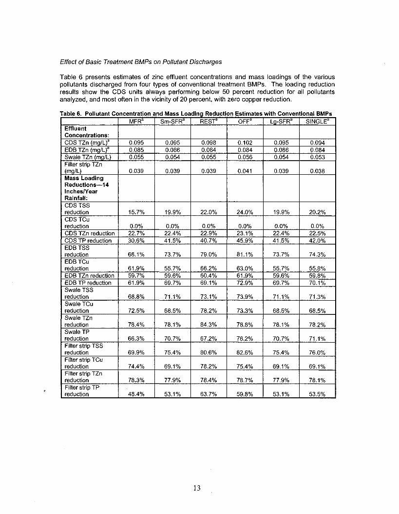
Effect of Basic Treatment BMPs on Pollutant Discharges

Table 6 presents estimates of zinc effluent concentrations and mass loadings of the variouspollutants discharged from four types of conventional treatment BMPs. The loading reductionresults show the CDS units always performing below 50 percent reduction for all pollutantsanalyzed, and most often in the vicinity of 20 percent, with zero copper reduction.

IBCER dCTable 6. Pollutant oncentration and Mass Loading e uction stimates with onventiona MPsMFRa Sm-SFRa RES-r OFFa LQ-SFRa SINGLEa

EffluentConcentrations:CDS TZn (mQ/L)a 0.095 0.095 0.098 0.102 0.095 0.094EDB TZn (mg/Ua 0.085 0.086 0.084 0.084 0.086 0.084Swale TZn (mQ/L) 0.055 0.054 0.055 0.056 0.054 0.053Filter strip TZn(mQ/U 0.039 0.039 0.039 0.041 0.039 0.038Mass LoadingReductions-14IncheslYearRainfall:CDSTSSreduction 15.7% 19.9% 22.0% 24.0% 19.9% 20.2%CDS TCureduction 0.0% 0.0% 0.0% 0.0% 0.0% 0.0%CDS TZn reduction 22.7% 22.4% 22.9% 23.1% 22.4% 22.5%CDS TP reduction 30.6% 41.5% 40.7% 45.9% 41.5% 42.0%EDB TSSreduction 68.1% 73.7% 79.0% 81.1% 73.7% 74.3%EDB TCureduction 61.9% 55.7% 66.2% 63.0% 55.7% 55.8%EDB TZn reduction 59.7% 59.6% 60.4% 61.9% 59.6% 59.8%EDB TP reduction 61.9% 69.7% 69.1% 72.9% 69.7% 70.1%Swale TSSreduction 68.8% 71.1% 73.1% 73.9% 71.1% 71.3%SwaleTCureduction 72.5% 68.5% 78.2% 73.3% 68.5% 68.5%SwaleTZnreduction 78.4% 78.1% 84.3% 78.8% 78.1% 78.2%SwaleTPreduction 66.3% 70.7% 67.2% 76.2% 70.7% 71.1%Filter strip TSSreduction 69.9% 75.4% 80.6% 82.6% 75.4% 76.0%Filter strip TCureduction 74.4% 69.1% 78.2% 75.4% 69.1% 69.1%Filter strip TZnreduction 78.3% 77.9% 78.4% 78.7% 77.9% 78.1%Filter strip TPreduction 48.4% 53.1% 63.7% 59.8% 53.1% 53.5%

13

Table 6 continuedMFRS Sm-SFRs RESr' OFFs Lg-SFRa SINGLEa

Mass LoadingReductions-20InchesNearRainfall:CDS TSSreduction 18.8% 25.0% 26.3% 30.5% 25.0% 25.4%CDSTCureduction 0.7% 1.9% 1.1% 3.0% 1.9% 2.0%CDS TZn reduction 23.1% 23.3% 23.6% 24.7% 23.3% 23.4%CDS TP reduction 35.4% 46.6% 44.8% 51.8% 46.6% 47.1%EDB TSSreduction 68.8% 74.6% 79.6% 81.6% 74.6% 75.1%EDB TCureduction 61.8% 55.6% 66.0% 62.7% 55.6% 55.7%EDB TZn reduction 59.6% 59.3% 60.2% 61.5% 59.3% 59.6%EDB TP reduction 63.0% 70.4% 69.7% 73.4% 70.4% 70.7%Swale TSSreduction 69.1% 71.4% 73.6% 74.1% 71.4% 71.6%SwaleTCureduction 72.5% 68.4% 77.9% 73.1% 68.4% 68.5%Swale TZnreduction 78.3% 78.0% 84.1% 78.6% 78.0% 78.1%SwaleTPreduction 67.6% 71.9% 68.2% 77.1% 71.9% 72.3%Filter strip TSSreduction 70.6% 76.3% 81.2% 83.1% 76.3% 76.8%Filter strip TCureduction 74.4% 69.0% 78.0% 75.1% 69.0% 69.1%Filter strip TZnreduction 78.2% 77.8% 78.3% 78.5% 77.8% 77.9%Filter strip TPreduction 49.9% 54.6% 66.3% 61.0% 54.6% 55.0%

a MFR-multi-family residential; Sm-SFR-small-scale single-family residential; REST-restaurant;OFF-office building; Lg-SFR-Iarge-scale single-family residential; SINGLE-single family home;CDS- continuous deflective separation unit; EDB-extended-detention basin

When treated with extended-detention basins, swales, or filter strips, effluents from eachdevelopment case study site are expected to fall below the Basin Plan acute zinc criterion.These natural-surface BMPs, if fully implemented and well maintained, are predicted to preventthe pollutant masses generated on the six case study development sites from reaching areceiving water in both rainfall zones, which do not differ appreciably. Only total phosphorusreduction falls below 50 percent for three case studies. Otherwise, mass loading reductionsrange from about 60 to above 80 percent for the EDB, swale, and filter strip. These dataindicate that draining impervious to pervious surfaces, even if those surfaces are not preparedin any special way, pays water quality as well as hydrologic dividends.

3. LID Analysis

(a) Hydrologic Analysis

The LID analysis repeats the analysis above, focusing here on the performance of LIDtechniques in reducing or eliminating runoff from the six development case studies. In additionto assessing the total runoff that would be expected, the analysis also considered whether LIDtechniques would be sufficient to attain compliance wit[l a performance standard being

14

considered by the Los Angeles Regional Water Quality Control Board for Ventura County,California. This standard limits EIA (Effective Impervious Area) to five percent (but our analysisfurther assumed EIA would be ultimately reduced to three percent). All runoff from NCIA (NotConnected Impervious Area) was assumed to drain to vegetated surfaces.

One goal of this exercise was to identify methods that reduce runoff production in the first place.It was hypothesized that implementation of source reduction techniques could allow all of thecase study sites to infiltrate substantial proportions, or all, of the developed site runoff,advancing the hydromodification mitigation objective of the Draft Permit. When runoff isdispersed into the soil instead of being rapidly collected and conveyed away, it rechargesgroundwater, supplementing a resource that maintains dry season stream flow and wetlands.An increased water balance can be tapped by humans for potable, irrigation, and process watersupply. Additionally, runoff volume reduction would commensurately decrease pollutant massloadings.

Accordingly, the analysis considered the practicability of more than one scenario. In one option,all roof runoff is harvested and stored for some beneficial use. A second option disperses runoffinto the soil via roof downspout infiltration trenches. The former option is probably best suited tocases like large commercial and office buildings, while distribution in the soil would fit best withresidences and relatively small commercial developments. The analysis was repeated with theassumptions of harvesting OFF roof runoff for some beneficial use and dispersing roof runofffrom the remaining four cases in roof downspout infiltration systems.

Expected Infiltration Capacities of the Case Study Sites

The first inquiry on this subject sought to determine how much of the total annual runoff eachproperty is expected to infiltrate, since infiltration is a basic (although not exclusive) LIDtechnique. Based on the findings of Chralowicz et al. (2001), it was assumed that an infiltrationzone of 0.1-0.5 acres in area and 2-3 ft deep would serve a drainage catchment area in the sizerange 0-5 acres and infiltrate 0.9~1.9 acre-fVyear. The conclusions of Chralowicz et al. (2001)were extrapolated to conservatively assume that 0.5 acre would be required to serve eachadditional five acres of catchment, and would infiltrate an incremental 1.4 acre-fVyear (themidpoint of the 0.9-1.9 acre-fVyear range). According to these assumptions, the followingschedule of estimates applies:

Infiltration Capacity1.4 acre-fUyear2.8 acre-fUyear4.2 acre-fUyear

Catchment Served acres0-5 acres

5-10 acres10-15 acres

Pervious Area Available for Infiltration0.5 acres1.0 acres1.5 acres

(Etc.)As a formula, infiltration capacity = 2.8 x available pervious area. To apply the formulaconservatively, the available area was reduced to the next lower 0.5-acre increment beforemultiplying by 2.8.

As shown in Table 7, in both rainfall zones all six of the sites have adequate or greater capacityto infiltrate the full annual runoff volume expected from NCIA and pervious areas where EIA islimited to three percent of the total site area. Indeed, five of the six development types havesufficient pervious area to infiltrate all runoff, including runoff from EIA areas. These results arebased on infiltrating in the native soils with no soil amendment. For any development project atwhich infiltration-oriented BMPs are considered, it is important that infiltration potential becarefully assessed using site-specific soils and hydrogeologic data. In the event such aninvestigation reveals a marginal condition (e.g., hydraulic conductivity, spacing to groundwater)for infiltration basins, soils could be enhanced to produce bioretention zones to assist infiltration.Notably, the five case studies with far greater than necessary infiltration capacity would offersubstantial fleXibility in designing infiltration, allowing ponding at less than 2-3 ft depth.

15

Table 7. Infiltration and Runoff Volume (With 3 Percent EIA and All NCIA Draining to PerviousAreas)

MFRa Sm-SFRa RESr' OFFa Lg-SFRa SINGLEa

141nchesNearRainfall:EIA runoff (acre-

0.36 0.10 0.03 0.07 4.4 0.01fUyear)NCIA + perviousarea runoff (acre- 8.20 1.64 0.45 0.73 71.3 0.08fUyear)Total runoff 8.56 1.74 0.48 0.80 75.7 0.09(acre-fUyear)Pervious areaavailable for 3.66 1.67 0.39 1.61 72.7 0.10infiltration (acres)Estimatedinfiltration 9.8 4.2 1.4 4.2 203 0.28capaci~ (acre-fUyearrInfiltration >100% >100% >100% >100% >100% >100%Dotentialc

20lnchesNearRainfall:EIA runoff (acre- 0.52 0.14 0.04 0.10 6.2 0.01fUyear)NCIA + perviousarea runoff (acre- 11.7 2.34 0.64 1.04 101.7 0.14fUyear)Total runoff

12.2 2.48 0.68 1.14 108.0 0.15(acre-fUyear)Pervious areaavailable for 3.66 1.67 0.39 1.61 72.7 0.10infiltration (acres)Estimatedinfiltration 9.8 4.2 1.4 4.2 203 0.28capaci~ (acre-fUvear)'Infiltration

84% >100% >100% >100% >100% >100%potentialc

a MFR-multi-family residential; Sm-SFR~mall-scale single-family residential; REST-restaurant;OFF-office building; Lg-SFR-Iarge-scale single-family residential; SINGLE-single family home;b Based on Chralowicz et al. (2001) according to the schedule described aboveC Compare runoff production from NCIA + pervious area (row 3) with estimated infiltration capacity (row 6)

As Table 7 shows, each of the six case study sites have the capacity to infiltrate all orSUbstantially all of the runoff produced onsite annually by draining impervious surfaces topervious areas on native soils or, in some soil regimes, soils amended with organic matter. Ifthese sites were designed as envisioned in this analysis, no runoff discharge is expected instorms as large as, and probably larger than, the design storm event-using infiltration only.Discharge would be anticipated only with exceptionally intense, large, or prolonged rainfall thatsaturates the ground at a faster rate than water can infiltrate or evaporate. Even runoff from thearea assumed to be EIA could be infiltrated in most cases based on the amount of perviousarea available in typical development projects. Therefore, this analysis shows that the EIAperformance standard being considered for Ventura County, California, or one more stringent,can be met readily in development projects occurring on A, B, and C soils in the San FranciscoBay Area.

16

Additional Source Reduction Capabilities of the Case Study Sites: Water Harvesting Example

As noted, infiltration is one of a wide variety of LID-based source reduction techniques. Wheresite conditions such as soil quality or available area limit a site's infiltration capacity, othersource LID measures can enhance a site's runoff retention capability. For example, soilamendment, which improves infiltration, is a standard LID technique. Water harvesting isanother. Such practices can also be used where infiltration capacity is adequate, but thedeveloper desires greater flexibility for land use on-site. Table 8 shows the added LIDimplementation flexibility created by subtracting roof runoff by harvesting it or efficiently directingit into the soil through downspout dispersion systems, further demonstrating the feasibility androbust performance of LID options for reducing or eliminating runoff in most expectedconditions. Specifically, all development types studied could readily infiltrate and/or retain allexpected annual precipitation.

Table 8. Infiltration and Runoff Volume Reduction Analysis Including Roof Runoff Harvesting orDisposal in Infiltration Trenches (Assuming 3 Percent EIA and All NCIA Draining to Pervious Areas\

MFRa Sm-SFRa RESr OFFa Lg-SFRa SINGLEa

14IncheslYearRainfall:EIA runoff

0.36 0.10 0.03 0.07 4.4 0.01(acre-ftlyear)Roof runoff 4.68 0.89 0.08 0.19 38.5 0.05(acre-ftlyear)Other NCIA +pervious area 3.52 0.75 0.37 0.54 32.7 0.04runoff (acre-ftlvear)Total runoff

8.56 1.74 0.48 0.80 75.6 0.10(acre-ftlyear)Pervious areaavailable for 3.66 1.67 0.39 1.61 72.7 0.10infiltration(acres)Estimatedinfiltration 9.8 4.2 1.4 4.2 203 0.28capaci~ (acre-ftlyear)[Infiltration >100% >100% >100% >100% >100% >100%capacitl20IncheslYearRainfall:EIA runoff 0.52 0.14 0.04 0.10 6.2 0.01(acre-ftlyear)Roof runoff 6.67 1.27 0.12 0.28 55.1 0.08(acre-ftlyear)Other NCIA +pervious area 5.03 1.07 0.52 0.76 46.7 0.06runoff (acre-ftlyear)Total runoff 12.2 2.48 0.68 1.14 108.0 0.15(acre-ftlyear)Pervious areaavailable for 3.66 1.67 0.39 1.61 72.7 0.10infiItration(acres)

17

Table 8 continuedMFRa Sm-SFRa

RES~ OFFa LQ-SFRa SINGLEa

Estimatedinfiltration 9.8 4.2 1.4 4.2 203 0.28capaci~ (acre-ftIyeadInfiltration >100% >100% >100% >100% >100% >100%capacit/

a MFR-multi-family residential; Sm-SFR-small-scale single-family residential; REST-restaurant;OFF-office building; Lg-SFR-Iarge-scale single-family residential; SINGLE-single family home;b Based on Chralowicz et al. (2001) according to the schedule described aboveC Comparison of runoff production from NCIA + pervious area (row 3) with estimated infiltration capacity (row 6)

Effect of Full LID Approach on Recharge

Table 9 shows the recharge benefits of preventing roofs from generating runoff and infiltratingas much as possible of the runoff from the remainder of the case study sites. The data showthat LID methods offer significant benefits relative to the baseline (no stormwater controls) in allcases. These benefits are particularly impressive in developments with relatively high siteimperviousness, such as in the MFR case.

sewl a u ,pproac ompare 0 eve opmen I 0 S

MFRa Sm-SFRaRES~ OFFa Lg-SFRa SINGLEa

141nchesNearRainfall:Pre-developmentrechargeb

(acre-ft) 11.9 3.29 0.83 2.30 144 0.19

NoBMPs-Post-developmentrechargeb

(acre-ft) 4.22 1.79 0.42 1.67 78 0.11Post-developmentrecharge lost(acre-ft) 7.68 1.50 0.41 0.65 66 0.08Post-development %recharae lost 65% 46% 49% 27% 45% 41%Full LIDalJlJroac~

Post-developmentrunoff capture(acre-fOe 11.9 3.29 0.83 2.30 144 0.19Post-developmentrecharge lost(acre-tO 0 0 0 0 0 0Post-development %recharQe lost 0% 0% 0% 0% 0% 0%

Table 9. Comparison of Water Captured Annually (in acre-ttl from Development Sites for BeneficialU 'th F II LID A h C d t D I t W·th N BMP

18

Table 9 continued

MFRa Sm-SFRaRES~ OFFa Lg-SFRa SINGLEa

20 IncheslYearRainfall:Pre-developmentrechargeb

(acre-tt) 16.9 4.71 1.19 3.30 205 0.27

NoBMPs-Post-developmentrechargeb

(acre-ft) 6.0 2.56 0.61 2.39 111 0.16Post-developmentrecharge lost(acre-ft) 10.9 2.15 0.58 0.91 94 0.11Post-development %recharoe lost 65% 46% 49% 27% 45% 41%Full LIDalJlJroach-Post-developmentrunoff capture(acre-fOe 16.9 4.71 1.19 3.30 205 0.27Post-developmentrecharge lost(acre-ft) 0 0 0 0 0 0Post-development %recharoe lost 0% 0% 0% 0% 0% 0%

a MFR-multi-family residential; Sm-SFR-small-scale single-family residential; REST-restaurant; OFF--officebuilding; Lg-SFR-Iarge-scale single-family residential; SINGLE-Single family homeb Quantity of water infiltrating the soil; the difference between precipitation and runoffC Water either entirely infiltrated in BMPs and recharged to groundwater or partially harvested from roofs and partiallyinfiltrated in BMPs. EIA was not distinguished from the remainder of the development, because these sites have thepotential to capture all runoff.

(b) Water Quality Analysis

It was assumed that any site discharges would be subject to treatment control. For purposes ofthe analysis, treatment control was assumed to be provided by conventional sand filtration.This choice is appropriate for study purposes for two reasons. First, sand filters can be installedbelow grade, and land above can be put to other uses. Pervious area should be reserved forreceiving NCIA drainage, and using sand filters would not draw land away from that service orother site uses. A second reason for the choice is that sand filter performance data equivalentto the data used in analyzing other conventional BMPs are available from the CalTrans (2004)work. Sand filters mayor may not expose water to soil, depending on whether or not they havea hard bed. This analysis assumed a hard bed, meaning that no infiltration would occur andthus there would be no additional recharge in sand filters. Performance would be even betterthan shown in the analytical results if sand filters were built in earth.

19

Pollutant Discharge Reduction Through LID Techniques

The preceding analyses demonstrated that in each of the six case studies, all stormwaterdischarges could be eliminated at least under most meteorological conditions by dispersingrunoff from impervious surfaces to pervious areas. Therefore, pollutant additions to receivingwaters would also be eliminated.

SUMMARY AND CONCLUSIONS

This paper demonstrated that common Bay Area residential and commercial development typessubject to the Municipal NPDES Permit are likely, without stormwater management, to reducegroundwater recharge from the pre-development state by approximately half in most cases to amuch higher fraction with a large ratio of impervious to pervious area. With no treatment, runofffrom these developments is expected to exceed Basin Plan acute copper and zinc criteria at thepoint of discharge and to deliver large pollutant mass loadings to receiving waters.

Conventional soil-based BMP solutions that promote and are component parts of low impactdevelopment approaches, by contrast, regain about 30-50 percent of the recharge lost indevelopment without stormwater management in Bay Area locations having NRCS HydrologicSoil Groups A, B, and C. It is expected the soil-based BMPs generally would release effluentthat meets the acute zinc criterion at the point of discharge, although it would still exceed or justbarely meet the copper limit. Excepting phosphorus, it was found that these BMPs wouldcapture and prevent the movement to receiving waters of the majority of the pollutant loadingsconsidered in the analysis.

It was found that by draining all site runoff to pervious areas with A, B, or C soil types, runoffcan be eliminated entirely in most development categories. It follows that a three percentEffective Impervious Area standard can be met in typical developments, as well. This resultwas reached assuming the use of native soils or well recognized soil enhancement techniques(typically, with compost). Draining impervious surfaces onto these soils, in connection withlimiting directly connected impervious area to three percent of the site total area, shouldeliminate storm runoff from some development types and greatly reduce it from more highlyimpervious types. Adding roof runoff elimination to the LID approach (by harvesting or directingit to downspout infiltration trenches) provides an additional tool, increasing flexibility andconfidence that no discharge in most meteorological conditions is a feasible performanceexpectation. Even in the development scenarios involving the highest relative proportion ofimpervious surface, losses of rainfall capture for beneficial uses could be reduced from theuntreated scenario when draining to pervious areas was supplemented with water harvesting.These results demonstrate the basic soundness of the concept of using LID techniques toreduce stormwater pollution in the Bay Area, and further show that limiting directly connectedimpervious area and draining the remainder over pervious surfaces, as contemplated by someRegional Water Boards in California, is also feasible.

20

REFERENCES

California Department of Transportation. 2004. BMP Retrofit Pilot Program Final Report.California Department of Transportation, Sacramento, CA.

Chralowicz, D., T. Goff, M. Mascali, and E. Taylor. 2001. Infiltration of Urban StormwaterRunoff to Recharge Groundwater Used for Drinking Water: A Study of the San FernandoValley, California. Master of Environmental Science and Management Report, University ofCalifornia at Santa Barbara, Santa Barbara, California.

Herrera Environmental Consultants, Inc. Undated. Pollutant Concentrations for Urban SourceAreas, unpublished data table.

Natural Resource Conservation Service. 1986. Urban Hydrology for Small Watersheds,Technical Release-55. U.S. Department of Agriculture, Washington, D.C.

Schueler, T.R. 1987. Controlling Urban Runoff: A Practical Manual for Planning and DesigningUrban BMPs. Metropolitan Washington Council of Governments, Washington, D.C.

U.S. Environmental Protection Agency. 1983. Results of the Nationwide Urban RunoffProgram: Volume 1 - Final Report, Report No. 832R83112. Office of Water, Washington,D.C.

21

This page intentionally left blank

A-I

ATIACHMENTA

POLLUTANT CONCENTRATIONS FOR URBAN SOURCE AREAS (HERRERA ENVIRONMENTAL CONSULTANTS, INC. UNDATED)

Residential Steuer, et al. 1997 MI 12 36 7 25 201 0.06 2Residential Bannerman, et al. 1993 WI -48 27 15 21 149 0.15 3Residential Waschbusch, et al. 2000 WI 25 15 n.a. n.a. n.a. 0.07 3Residential FAR 2003 NY 19 20 21 312 0.11 4Residential Gromaire, et al. 2001 France 29 37 493 3422 n.a. 5Representative Residential Roof Values 25 13 22 159Commercial Steuer, et al. 1997 MI 12 24 20 48 215 0.09 2Commercial Bannerman, et al. 1993 WI -16 15 9 9 330 0.20 3Commercial Waschbusch, et al. 2000 WI 25 18 n.a. n.a. n.a. 0.13 3

Res. Driveways Steuer, et al. 1997 MI 12 157 34 52 148 0.35 2Res. Driveways Bannerman, et al. 1993 WI -32 173 17 17 107 1.16 3Res. Driveways Waschbusch, et al. 2000 WI 25 34 n.a. n.a. n.a. 0.18 3Driveway FAR 2003 NY 173 17 107 0.56 4Representative Residential Driveway Values 120 22 27 118 0.66

Comm.llnst. Park. Areas Pitt, et al. 1995 AL 16 110 116 46 110 n.a. 1Comm. Park. Areas Steuer, et al. 1997 MI 12 110 22 40 178 0.2 2Com. Park. Lot Bannerman, et al. 1993 WI 5 58 15 22 178 0.19 3Parking Lot Waschbusch, et al. 2000 WI 25 51 n.a. n.a. n.a. 0.1 3Parking Lot Tiefenthaler, et al. 2001 CA 5 36 28 45 293 n.a. 6Loading Docks Pitt, et al. 1995 AL 3 40 22 55 55 n.a. 1Highway Rest Areas CalTrans 2003 CA 53 63 16 8 142 0.47 7

Park and Ride Facilities CalTrans 2003 CA 179 69 17 10 154 0.33 7

Comm.l Res. Parking FAR 2003 NY 27 51 28 139 0.15 4Representative Parking Area/Lot Values 75 36 26 97 0.14

A-I

Landscaped Areas Pitt, et al. 1995 AL 6Landscaping FAR 2003 NYRepresentative Landscaping ValuesLawns - Residential Steuer, et al. 1997 MI 12Lawns - Residential Bannerman, et al. 1993 WI -30Lawns Waschbusch, et al. 2000 WI 25Lawns Waschbusch, et al. 2000 WI 25Lawns - Fertilized USGS 2002 WI 58

Lawns - Non-P Fertilized USGS 2002 WI 38Lawns - Unfertilized USGS 2002 WI 19Lawns FAR 2003 NY 3ReDresentative Lawn Values

33 81 24 230 n.a. 137 94 29 263 n.a. 433 81 24 230 n.a.

262 n.a. n.a. n.a. 2.33 2397 13 n.a. 59 2.67 359 n.a. n.a. n.a. 0.79 3122 n.a. n.a. n.a. 1.61 3n.a. n.a. n.a. n.a. 2.57 3

n.a. n.a. n.a. n.a. 1.89 3n.a. n.a. n.a. n.a. 1.73 3602 17 17 50 2.1 4213 13 n.a. 59 2.04

Notes:Representative values are weighted means of collected data. Italicized values were omitted from these calculations.1 - Grab samples from residential, commercial/institutional, and industrial rooftops. Values represent mean of

DETECTED concentrations2 - Flow-weighted composite samples, geometric mean concentrations3 - Geometric mean concentrations4 - Citation appears to be erroneous - original source of data is unknown. Not used to calculate representative value5 - Median concentrations. Not used to calculate representative values due to site location and variation from other values.6 - Mean concentrations from simulated rainfall study7 - Mean concentrations. Not used to calculate representative values due to transportation nature of land use.

A-2

SUPPLEMENTARY INVESTIGATION OF THE FEASIBILITY AND BENEFITS

OF LOW-IMPACT SITE DESIGN PRACTICES (“LID”) FOR THE SAN FRANCISCO BAY AREA

Richard R. Horner† ABSTRACT The Clean Water Act NPDES permit that regulates municipal separate storm sewer systems (MS4s) in the San Francisco Bay Area, California will be reissued in 2007. The draft permit includes general provisions related to low impact development practices (LID) for certain kinds of development and redevelopment projects. Using eight representative development project case studies, based on California building records, the author investigated the practicability and relative benefits of LID options for the portion of the region having soils potentially limiting to infiltration. The principal LID option applicable in this situation is roof runoff harvesting, supplement by dispersion of the roof water in single-home sites. Other site runoff would be treated by conventional stormwater best management practices (BMPs), as specified in the permit. The results showed that effectively managing roof runoff and treating the remainder with conventional BMPS can: (1) reduce annual runoff volumes by almost half to more than 3/4, depending on land use characteristics, with much of the water saved available for a beneficial use; and (2) decrease mass loadings of pollutants to receiving waters by 63 to over 90 percent, depending on pollutant and land use.

† Richard R. Horner, Ph.D., Research Associate Professor, University of Washington Departments of Civil and Environmental Engineering and Landscape Architecture; Adjunct Associate Professor, University of Washington Center for Urban Horticulture

INTRODUCTION Background A report titled Initial Investigation of the Feasibility and Benefits of Low-Impact Development Practices (“LID”) for the San Francisco Bay Area used six representative development project case studies, based on California building records, to investigate the practicability and relative benefits of LID options for the majority of the region having soils potentially suitable for infiltration either in their natural state or after amendment using well recognized LID techniques. The results demonstrated that: (1) LID site design and source control techniques are more effective than conventional best management practices (BMPs) in reducing runoff rates; and (2) in each of the case studies, LID methods would reduce site runoff volume and pollutant loading to zero in typical rainfall scenarios. For a broad regional assessment of relatively large scale use of soil-based, infiltrative LID practices, the initial report covered areas having soils in Natural Resources Conservation Service (NRCS) Hydrologic Soil Groups A, B, or C as classified by the Natural Resources Conservation Service (http://websoilsurvey.nrcs.usda.gov/app/WebSoilSurvey.aspx). Depending on site-specific conditions, A and B soils would generally effectively infiltrate water without modification, whereas C soils could require organic amendments according to now standard LID methods. This supplementary report covers locations with group D soils, which are generally not amenable to infiltration, again depending on the specific conditions on-site. A minority but still substantial fraction of the Bay Area has group D soils (39.3, 68.0, 18.3, and 50.1 percent of the mapped areas of Alameda, Contra Costa, San Mateo, and Santa Clara Counties, respectively). Regarding any mapped soil type, it is important to keep in mind that soils vary considerably within small distances. Characteristics at specific locations can deviate greatly from

1

http://websoilsurvey.nrcs.usda.gov/app/WebSoilSurvey.aspx

those of the major mapped unit, making infiltration potential either more or less than may be expected from the mapping. The soil survey data are regarded as appropriate for use in broad-scale assessments such as underlie this and the initial report, but once site-specific implementation begins, it is important to verify site conditions. General Assessment Methods The assessment for group D soils reported herein emphasizes the use of LID practices appropriate in areas with relatively restrictive soils to the greatest possible extent, supplemented by conventional stormwater management practices implemented at fully practicable, high levels of effectiveness. The assessment was performed in a manner analogous to the analysis for the other soil groups and as described in the initial report. To recap briefly, with respect to each of several development case studies, three assessments were undertaken: a baseline scenario incorporating no stormwater management controls; a second scenario employing conventional BMPs; and a third development scenario employing LID stormwater management strategies. In each assessment, annual stormwater runoff volumes were estimated, as well as concentrations and mass loadings (the products of concentrations times flow volumes) of four pollutants: (1) total suspended solids (TSS), (2) total recoverable copper (TCu), (3) total recoverable zinc (TZn), and (4) total phosphorus (TP). The results of the second and third assessments were expressed in terms of the extent to which the management practices would reduce pollutant concentrations and loadings and runoff volumes, converting stormwater discharge a potential beneficial use (direct consumption or, in the case of group A, B, C soil areas, groundwater recharge). Six case studies were selected to represent a range of urban development types considered to be representative of the Bay Area. These case studies involved: a multi-family residential complex (MFR), a relatively small-scale (23 homes) single-family residential development (Sm-SFR), a restaurant (REST), an office building (OFF), a relatively large (1000 homes) single-family residential development (Lg-SFR), and a single home (SINGLE). The land cover types for these various land uses were derived from building permit and other public records from the Bay Area or elsewhere in California. Adaptation of Methods for Areas with Group D Soils A key LID technique in a setting with soils relatively restrictive to infiltration is water harvesting, which can be applied at larger scales in commercial and light industrial developments and at smaller residential scales using cisterns or rain barrels. Harvesting has been successful in reducing runoff discharged to the storm drain system and conserving water in applications at all scales. For example, in downtown Seattle the King County Government Center collects enough roof runoff to supply over 60 percent of the toilet flushing and plant irrigation water requirements, saving approximately 1.4 million gallons of potable water per year (http://www.psat.wa.gov/Publications/LID_studies/rooftop_rainwater.htm, http://dnr.metrokc.gov/dnrp/ksc_tour/features/features.htm). A much smaller public building in Seattle, the Carkeek Environmental Learning Center, drains roof runoff into a 3500-gallon cistern to supply toilets (http://www.harvesth2o.com/seattle.shtml). Collecting drainage from individual dwellings for household use is a standard technique around the world, particularly in areas deficient in rainfall and without affordable alternative sources. An additional general category of LID practices for poorly infiltrating locations, applicable especially at single homes and other relatively small-scale developments, is runoff dispersion for storage in vegetation and soil until evapotranspiration and some infiltration occurs. Section C.3.c of the California Regional Water Quality Control Board San Francisco Bay Region "Administrative Draft" NPDES Municipal Regional Stormwater Permit (“the Permit”) requires all single-family home projects that create and/or replace 5,000 square feet or more of impervious surface to implement one or more stormwater lot-scale BMPs from a selection of: (1) diverting roof runoff to vegetated areas; (2) directing paved surface runoff flow to vegetated areas; and/or (3) installing driveways, patios, and walkways with pervious material such as pervious concrete or pavers. Another way of distributing and dissipating roof runoff used successfully in varied soils in the state of Washington is the downspout dispersion system, consisting of a splash block or gravel-filled trench serving to spread roof runoff over a vegetated area (Washington Department of Ecology 2005 [Volume III, Section 3.1.2]).

2

http://www.psat.wa.gov/Publications/LID_studies/rooftop_rainwater.htm

http://dnr.metrokc.gov/dnrp/ksc_tour/features/features.htm

http://www.harvesth2o.com/seattle.shtml

The basis of the group D soils assessment was harvesting roof runoff to the maximum possible degree, supplemented in smaller-scale developments by runoff dispersion methods. The report asserts that, through these LID BMPs, it is practicable to prevent the entrance of any roof runoff into the municipal storm drain system in any soils setting in the Bay Area. In group D soils, infiltration likely cannot be relied upon to reduce runoff from other portions of developments, such as walkways, driveways, parking lots, access roads, and landscaping. Some water loss would undoubtedly occur, especially through evapotranspiration and at least some infiltration of runoff generated on or directed to landscaping. The analysis presented in this report does not take account of these losses and hence is somewhat conservative in estimating benefits. As required by the Permit, any runoff not attenuated by harvest, evapotranspiration, or infiltration would be subject to quantity and quality controls. The analysis assumes that extended-detention basins (EDBs) with water residence times up to 72 hours would provide this control. EDBs are one of several general-purpose, conventional stormwater BMPs available for this service, others being wet ponds, constructed wetlands, sand or other media filters, and biofiltration swales and filter strips. The California Department of Transportation (Caltrans, 2004) tested the performance of all of these practices in its BMP Retrofit Pilot Program, conducted in San Diego and Los Angeles Counties. The initial report investigating LID for A, B, and C soils presented estimates of benefits for EDBs, swales, and filter strips, along with continuous deflective separation (CDS) units, a practice that effectively captures only large particulate pollutants. For brevity, this follow-up report focuses on just EDBs as the supplement to LID. In performance, EDBs tend to fall between swales and filter strips for total suspended solids, slightly lower than the other two BMP types for metals, and either between the two or comparable to swales for total phosphorus. These practices were applied to the same six case studies used in the initial analysis and described in Table 1 of the first report. Two additional case studies were defined for the assessment reported here: a sizeable commercial retail installation (COMM) and an urban redevelopment (REDEV). The hypothetical COMM scenario consists of a building with a 2-acre footprint and 500 parking spaces. Parking spaces were estimated to be 176 sq ft in area, which corresponds to 8 ft width by 22 ft length dimensions. A simple, square parking lot with roadways around the four sides and a square building with walkways also around the four sides were assumed. Roadways and walkways were taken to be 20 ft and 6 ft wide, respectively. The REDEV case was taken from an actual project in Berkeley involving a remodel of an existing structure, built originally as a corner grocery store with apartments above and a large side yard, and the addition of a new building on the same site to create a nine-unit, mixed-use, urban infill project. Table 1 summarizes the characteristics of these two case studies. The table also provides the recorded or estimated areas in each land use and cover type. Table 1. Characteristics and Land Use and Land Cover Areas of Added Case Studies

COMMa REDEVa No. buildings 1 1 Total area (ft2) 226,529 5,451 Roof area (ft2) 87,120 3,435

No. parking spaces 500

2 uncovered

Parking area (ft2) 88,000

316 uncovered

Access road area (ft2) 23,732 -

Walkway area (ft2) 7,084 350 Driveway area (ft2) - 650 Landscape area (ft2) 20,594 700

a COMM—retail commercial; REDEV—commercial/residential infill The assessment for group D soils employed the same methods as the earlier analysis to estimate annual stormwater runoff volumes and pollutant discharges. Please refer to the initial report for details on those

3

4

methods. The Natural Resource Conservation Service (NRCS, 1986) methodology cited in that report was applied to estimate that infiltration in group D soils would be roughly 60 percent of the amount through landscaping or the bed of a conventional BMP in C soils, which were the basis for establishing runoff coefficients in the first analysis. While that initial analysis was performed for both 14- and 20-inch average annual runoff zones, typical of different Bay Area locations, this supplementary work covered only the former condition. This simplification was made in the interest of brevity in this report, given that the first analysis showed almost no difference in conclusions between the two situations. RESULTS OF THE ANALYSIS Table 2 provides a comprehensive summary of the results. Rows shaded in gray compare runoff and pollutant discharges with and without treatment by CDS units, which can capture relatively large solids but have no mechanisms for dissolved substances and the finer particles. Having no soil contact and very limited residence time for evaporation, this BMP cannot reduce runoff volume at all. It can achieve some substantial reductions in TSS and TP for land uses relatively high in landscaped area but little removal of metals, especially copper. The blue-shaded rows show the performance of conventional EDBs. In the group D soils considered in this analysis, they were estimated to reduce annual runoff volumes by 13-23 percent, the higher values for land uses with relatively small impervious footprints (OFF and REST). These BMPs can capture the majority of the long-term mass loading of most pollutants from most land uses in these soils, falling below 50 percent in reducing metals in stormwater flowing from residential developments. Rows shaded in green present the results of applying LID BMPs appropriate for group D soils, roof runoff harvesting supplemented by dispersion in single-home land uses, plus treating the remaining runoff with EDBs. Comparing annual runoff volumes with and without LID, it can be seen that removing roof runoff from the storm drain system affords very significant benefits in reducing surface discharge and putting much of that water to productive use. Compared to directing all site runoff to EDBs, LID is expected to reduce volume by almost 10 times in the REDEV case, by about five times for the various residential land uses, 3.6 times for the large commercial development, and around twice for the OFF and REST cases. This management strategy can recover over 3/4 of the stormwater that would otherwise go down the drain in the intense redevelopment case, approximately 2/3 for the multi- and single-family residential cases, over half in the COMM development, and almost half in the office and restaurant cases with relatively small roof footprints. Reduction of volume translates to decreases in pollutant loadings also. The combination of LID and EDB treatment is estimated to raise copper and zinc reductions to about 70 to over 90 percent in all except the developments with relatively low roof proportions (60-65 percent in these cases). TSS predictions come in at a quite consistent 75-82 percent across land uses. Total phosphorus estimates are a similarly consistent 63-71 percent, a bit higher in the highly impervious REDEV case. Effectively managing roof runoff gives a way out of the dilemma posed by group D soils in the Bay Area. The analysis has demonstrated that harvesting this runoff stream, supplemented by ground dispersion techniques with sufficient space, shows strong promise to reduce the majority of flow inputs to municipal storm drain systems while conserving water. Moreover, this strategy can also stem the majority of solids, copper, zinc, and phosphorus transport to receiving waters.

Table 2. Runoff Volume and Pollutant Loading Reductions with Conventional and Low-Impact Development (LID) Best Management Practices (BMPs) for Eight Land Use Case Studies in Hydrologic Group D Soils COMMa OFFa RESTa REDEVa MFRa Lg-SFRa Sm-SFRa SINGLE Total annual runoff with no BMPs (ac-ft) 5.29 0.80 0.47 0.12 8.57 75.66 1.74 0.10 Total annual runoff with CDS unitsb (reduction)

5.29 (0.0%)

0.80 (0.0%)

0.47 (0.0%)

0.12 (0.0%)

8.57 (0.0%)

75.66 (0.0%)

1.74 (0.0%)

0.10 (0.0%)

Total annual runoff with EDBsb (reduction)

4.43 (16.3%)

0.63 (21.3%)

0.36 (23.2%)

0.11 (8.1%)

7.48 (12.7%)

65.27 (13.7%)

1.50 (13.7%)

0.09 (13.3%)

Total annual runoff with LIDb (reduction) 2.22 (58.0%)

0.44 (45.0%)

0.28 (40.4%)

0.03 (78.9%)

2.80 (67.3%)

26.72 (64.8%)

0.61 (64.8%)

0.04 (65.7%)

CDS TSS reductionb, c 19.4% 44.8% 33.9% 22.1% 27.1% 37.1% 37.1% 37.7% CDS TCu reductionb, c 0.4% 11.0% 4.2% 0.9% 2.7% 7.3% 7.3% 7.6% CDS TZn reductionb, c 25.3% 29.1% 25.5% 25.5% 24.1% 25.6% 25.6% 25.9% CDS TP reductionb, c 25.9% 63.7% 54.3% 35.7% 46.7% 57.6% 57.6% 58.2% EDB TSS reductionb, c 64.7% 78.1% 74.9% 66.5% 62.8% 70.3% 70.3% 70.9% EDB TCu reductionb, c 57.9% 51.6% 56.4% 53.2% 51.4% 43.5% 43.5% 43.6% EDB TZn reductionb, c 57.6% 49.6% 48.9% 58.1% 48.5% 47.7% 47.7% 48.0% EDB TP reductionb, c 44.4% 67.6% 63.3% 52.8% 56.3% 64.4% 64.4% 64.7% LID + EDB TSS reductionb, c, d 74.6% 80.3% 77.0% 81.5% 79.4% 81.3% 81.3% 81.8% LID + EDB TCu reductionb, c, d 71.9% 60.3% 62.2% 82.3% 73.8% 68.9% 68.9% 69.5% LID + EDB TZn reductionb, c, d 79.7% 65.1% 60.9% 92.3% 78.9% 76.4% 76.4% 77.0% LID + EDB TP reductionb, c, d 63.1% 69.8% 66.0% 75.2% 69.4% 70.8% 70.8% 71.1%

a COMM—retail commercial; OFF—office building; REST—restaurant; REDEV—commercial/residential redevelopment; MFR—multi-family residential; Lg-SFR—large-scale single-family residential; Sm-SFR—small-scale single-family residential; SINGLE—single family home b CDS— continuous deflective separation; EDBs—extended-detention basins; reduction—comparison with no BMPs c TSS—total suspended solids; TCu—total recoverable copper; TZn—total recoverable zinc; TP—total phosphorus d LID + EDB—roof runoff harvesting for COMM, OFF, REST, REDEV, AND MFR; harvesting supplemented by dispersion of roof runoff for Lg-SFR, Sm-SFR, and SINGLE; treatment of remaining runoff by EDBs

5

REFERENCES California Department of Transportation. 2004. BMP Retrofit Pilot Program Final Report. California

Department of Transportation, Sacramento, CA. Natural Resource Conservation Service. 1986. Urban Hydrology for Small Watersheds, Technical

Release-55. U.S. Department of Agriculture, Washington, D.C. Washington Department of Ecology. 2005. Stormwater Management Manual for Western Washington.

Washington Department of Ecology, Olympia, WA. http://www.ecy.wa.gov/programs/wq/stormwater/index.html.

6

http://www.ecy.wa.gov/programs/wq/stormwater/index.html

1 of 3

UNIVERSITY OF CALIFORNIA, LOS ANGELES

UCLA LA KRETZ CENTER FOR CALIFORNIA CONSERVATION SCIENCE

INSTITUTE OF THE ENVIRONMENT AND SUSTAINABILITY

LA KRETZ HALL, SUITE 300

619 CHARLES E. YOUNG DR. EAST

BOX 951496

LOS ANGELES, CA 90095-1496

PHONE: 310-825-5008

FAX: 310-825-9663

http://www.environment.ucla.edu/lakretz/ July 23, 2010

Mr. Ivar Ridgeway

Los Angeles Regional Water Quality Control Board

320 W. 4th Street, Suite 200

Los Angeles, CA 90013

Submitted electronically to [email protected]

RE: Comments on Greater Los Angeles County MS4 Permit Draft Tentative Oder No. R4-

2012-XXXX, NPDES No. CAS004001, Dated June 6, 2012

Dear Mr. Ridgeway:

This letter provides comments on the hydromodification provisions in the subject draft tentative

order.

My experience includes ten years of research and practice in the field of urban hydromodification

impacts and management, and co-authorship of the report released earlier this year entitled:

Hydromodification Assessment and Management in California1, prepared for the State Water

Resources Control Board.

Section VI.D.6.c.v.(1)(c)(ii) Interim Hydromodification Control Criteria for project disturbing 50

acres or more within natural drainage systems, provides three alternative options that are each

presumed to meet pre-development hydrology:

1. The site infiltrates on-site at least the runoff from a 2-year, 24-hour storm event

2. The runoff flow rate, volume, velocity, and duration for the post-development condition

does not exceed the pre-development condition for the 2-year, 24-hour rainfall events

3. The Erosion Potential (Ep) in the receiving water channel will approximate 1, as

determined by a Hydromodification Analysis Study and the equation presented in

Attachment J.

The proposed criteria are inconsistent with current scientific understanding. These three options

represent very different levels of control and will not provide equivalent protection of downstream

resources for the following reasons:

SANTA BARBARA • SANTA CRUZ

BERKELEY • DAVIS • IRVINE • LOS ANGELES • MERCED • RIVERSIDE • SAN DIEGO • SAN FRANCISCO

UCLA

2 of 3

A. Options 1 and 2 are event-based criteria, whereas current scientific understanding of

hydromodification impacts is that a range of moderately frequent, “geomorphically

significant” flows transport the majority of the sediment over the long term2,3,4

and are the

most influential in determining channel form. Rather than focusing on a single event,

hydromodification control requirements should therefore address this critical range of flows.

This scientific understanding has been reflected in other hydromodification regulations in the

State of California by establishing flow-control criteria that require pre-project flow rates,

volumes and durations to be matched across a range of flows (e.g., 0.5Q2 through Q10).

B. I am unaware of any studies that have evaluated the use of the 2-yr, 24-hr storm event (as

either an infiltration volume or as a basis for matching flow rates, volumes and durations) to

determine its equivalence to an Erosion Potential metric or to a flow control criteria using a

range of geomorphically significant flows. Options 1 and 2 do not appear to have any basis in

the scientific literature.

C. The use of a flow-control criterion assumes this range of flows to be appropriate for all

receiving waters, and had been provided in other permits as an easy-to-implement option for

smaller development projects. However, field research and modeling show that characteristics

of the receiving stream channel (such as cross-section, slope, and sediment size) will influence

the in-stream impacts of a changed runoff regime. This is why larger developments have been

required to use an Erosion Potential metric, as it accounts for in-stream characteristics, as well

as the full range of flows, to establish design criteria to minimize excess erosion and channel

instability.

The Ventura County MS4 Permit (finalized by the Los Angeles Regional Board in January 2010)

contains requirements for a Hydromodification Analysis Study (HAS) for projects disturbing 50

acres or greater. The HAS must demonstrate that post development conditions approximate pre-

project erosive effects in receiving waters through the incorporation of an Erosion Potential or

equivalent metric. I recommend that the Board modify the draft tentative order for Los Angeles

County to be consistent with the Ventura County Permit hydromodification control criteria for

projects of 50 acres or greater.

I also suggest that Attachment J be modified to indicate that the Work equation shown is just one

of several equations that could be used to calculate an Erosion Potential. Other options include

sediment transport function such as the Brownlie equation or the Meyer-Peter and Muller

equation5. Allowing additional options supported by the scientific literature will permit the use of

equations most appropriate for the characteristics of the receiving channel.

I am available to discuss these comments in more detail with Regional Board staff if desired.

Sincerely,

Felicia Federico, D.Env.

Executive Director, UCLA La Kretz Center

1Stein, E.D., Federico, F., Booth, D.B., Bledsoe, B.P., Bowles, C., Rubin, Z., Kondolf, G.M.,

Sengupta, A., 2012. Hydromodification Assessment and Management in California. Southern

California Coastal Water Research Project Technical Report 667, April 2012.

3 of 3

2King County. 1990. Soos Creek Basin Plan and Final Environmental Impact Statement: Seattle,

Department of Public Works, Surface Water Management Division. Seattle, WA. 3Bledsoe, B.P. 2002. Stream erosion potential and stormwater management strategies. Journal of

Water Resources Planning and Management 128: 451-455. 4Roesner, L. and B. Bledsoe. 2003. Physical Effects of Wet Weather Flows on Aquatic Habitats:

Present Knowledge and Research Needs. Water Environment Research Foundation Report 00-

WSM-4Rep. 5US Department of Agriculture, Natural Resources Conservation Service, 2007. Part 654 Stream

Restoration Design, National Engineering Handbook, August 2007.

Coastal Water Quality Impact of Stormwater Runoff from an ...

Documents

Transcript of Coastal Water Quality Impact of Stormwater Runoff from an ...