"DETERMINATION OF RAINFALL/RUNOFF MODEL PARAMETERS"

A. G. GOYEN

Submitted in fulfilment of the requirements for the Master of Engineering Degree at the New South Wales Insti­tute of Technology.

December 1981

I hereby not comprise

CERTIFICATION STATEMENT

submitted for a Degree or other other Institute of Technology

this thesis does I have previously

from any

Allan G Goyen B E. MIE. Aust.

ABSTRACT

"DETERMINATION OF RAINFALL/RUNOFF MODEL PARAMETERS"

KEY WORDS: Rainfall/Runoff Models. Joint Parameters-Field Measurements.

Stochastic-Deterministic, Probability, Antecedence,

ABSTRACT: Runoff estimates both peaks and volumes are called for in design analysis for the sizing of a wide range of engineering structures. In many instances runoff records are very short or not available and it is necessary to use synthetic rainfall data and apply a rainfall/runoff model to estimate appropriate design hydrographs. This thesis addresses the particular portion of the rainfall/runoff process conversion dealing with the devel­opment of excess hyetographs prior to catchment routing and the estimation of the parameters affecting such develop­ment. Details are given on field based parameter estimating procedures as well as further model development to better reflect measurable input parameters. A joint probability model linking moisture deficiency criteria prior to an event, rainfall data and measured catchment parameters is developed and applied on Canberra data.

REFERENCE: GOYEN, A.G. (1981). Determination of Rainfall/Runoff Model Parameters. Thesis M.Eng., N.S.W. Institute of Technology, December (unpublished).

i i i

ACKNOWLEDGEMENTS

The assistance of the National Capital Development Commission in providing funds for field measurements and computer use is greatly acknowledged as this thesis would not have been possible without such financial assistance. The Department of Housing & Construction is also acknowl­edged for providing basic rainfall and runoff data, for the Giralang, Gungahlin and Mawson study catchments, used ex­tensively in this thesis.

i V

TABLE OF CONTENTS

ABSTRACT ACKNOWLEDGEMENTS LIST OF FIGURES LIST OF TABLES LIST OF PHOTOGRAPHS LIST OF SYMBOLS

Chapter

1 INTRODUCTION

2 BACKGROUND AND SCOPE OF THESIS

3

2.1 Description of RSWM

FIELD DATA COLLECTION AND ANALYSIS

3.1 Introduction 3.2 Study Catchments

3.2.1 3.2.2 3.2.3

Giralang and Gungahlin Mawson Black Mountain Reserve

Page iv

V viii

X xi

xii

1

3

4

10

10 15

15 17 17

3.3 Scope of Data Collection Program 18 3.4 Description of Sampling Stations 19 3.5 Sampling Methods 27

3.5.1 Soil Moisture Profiles 3.5.2 Infiltration Parameters

3.6 Results from Gauging Program

3.6.1 Long Term Soil Moisture

27 34

37

Fluctuations 37

3.6.2 Sorptivity and Hydraulic Conductivity 44

3.7 Discussion on Results 45

V

4 THEORETICAL RAINFALL/RUNOFF MODEL DEVELOPMENT

4.1 Discussion on Current Techniques 47 4.2 Development of a Combined Stochastic­

Deterministic Rainfall/Runoff Model 50

4.2.1 General 50 4.2.2 Continuous Water Balance Model

Development 56

4.2.2.1 4.2.2.2 4.2.2.3

Urban Land Domains ARBM Model Results Development of an Antecedent Moisture Index

73 75

86

4.2.3 Review of Existing Stochastic-Deterministic Models 89

4.2.4 Development of SDRRM Model 92 4.2.5 Results from SDRRM 102

4.3 Parameter Assessment for Ungaged and Gauged Urban Catchments 105

4.4 Runoff Generation from Different Land Domains 106

4.5 Comparative Analysis Employing the SDRRM and Existing Runoff Estimating Procedures 107

4.5.1 4.5.2 4.5.3

4.5.4

4.5.5

4.5.6

4.5.7

Introduction Catchment Data Rational Formula Method of Analysis Regional Flood Frequency Technique Runoff Routing Approach Employing a Design Storm with Initial and Continuing Losses Runoff Routing Approach Employing a Stochastically Derived Rainfall Excess Lumped Catchment Runoff Routing Approach Employing a Stochastically Derived Rainfall Excess­Separate Pervious­Impervious Consideration

vi

108 108

109

111

111

111

112

5

6

APPENDICES

APPENDIX A

4.5.8 Direct Application of the SDRRM 112

4.5.9 Frequency Analysis of Gauged Data 112

4.5.10 Discussion on the Methods and their Results 113

4.6 Application of Proposed Parameter Estimating and Modelling Techniques

4.6.1 Major Drainage Analysis and Design

4.6.2 Minor Drainage Design

SUMMARY AND CONCLUSIONS

5.1 Introduction 5.2 Combined Stochastic­

Deterministic Urban Drainage Model

5.3 Summary 5.4 Conclusions

REFERENCES

Engineering Logs Stations Nos 1-8

Vi i

114

114

115

119

119

120 120 122

123

Figure

2-1

2-2

3-1

3-2 3-3 3-4

3-5

3-6

3-7

3-8 4-1

4-2

4-3

4-4 4-5 4-6 4-7

4-8

4-9

4-10

4-11

4-12 4-13

4-14

4-15

LIST OF FIGURES

Diagrammatic Sketch of RSWM Typical Watershed Breakup for Analysis by RSWM Location of Canberra Study Catchments Giralang Urban Catchment Mawson Urban Catchment Giralang and Gungahlin Paired Catchments Troxler Surface Moisture/ Density Meter Scatter Diagram Comparing Nuclear and Conventional Soil Moisture Readings Shallow Soil Moisture Readings during the 1979/1980 Period Profile Summaries Annual Max 30, 60, and 120 Minute Rainfall Bursts and Simulated Runoff 1933-75 Seasonal Distribution of Annual Max 30, 60 and 120 Min. Rainfall Bursts Canberra Intensity-Frequency Duration, Pan Evaporation and Daily Rainfall Distribution Diagrammatic Sketch of the ARBM Sensitivity of ARBM Model Parameters Gungahlin Scatter Diagrams Long Term {US) Soil Moisture Simulation Antecedent Rainfall-Pre Burst Moisture Scatter Diagram for Simulated Max. Ann. Pervious Runoff Events.

Probability Curves for Index Type I Probability Curves for Index Type II Diagrammatic Representation of The SDRRM Model SDRRM Model Output Flow Diagram of SDRRM Routing Operations Simulated Excess Rainfall and Runoff Peaks for Different Land Domains Simulated Excess Rainfall and Runoff Peaks for Giralang

V i i i

Page

6

7

11 12 13

14

29

32

39 40

53

54

55 57 61 77

78

84

87

88

93 99

101

103

104

4-16

4-17

4-18 4-19

Sensitivity of Runoff Peaks to Land Domains. Giralang Catchment Comparative Simulations for Mawson Simulated Total Storm Losses Simulated Rational Method, Canberra Runoff Coefficients

i X

107

110 116

118

Table

3-1

4-1

4-2

4-3

4-4

4-5

4-6

4-7

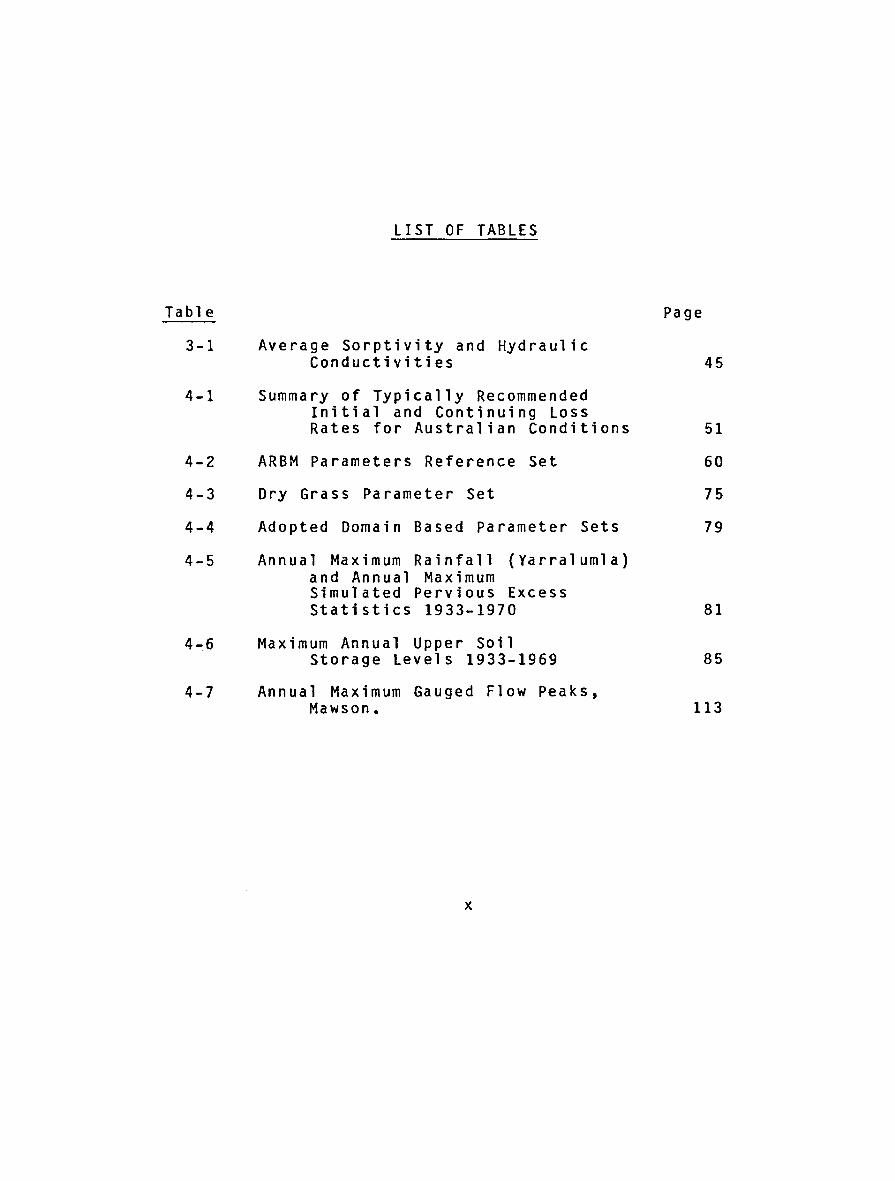
LIST OF TABLES

Average Sorptivity and Hydraulic Conductivities

Summary of Typically Recommended Initial and Continuing Loss Rates for Australian Conditions

ARBM Parameters Reference Set

Dry Grass Parameter Set

Adopted Domain Based Parameter Sets

Annual Maximum Rainfall { Yarral uml a) and Annual Maximum Simulated Pervious Excess Statistics 1933-1970

Maximum Annual Upper Soil Storage Levels 1933-1969

Annual Maximum Gauged Flow Peaks, Mawson.

X

Page

45

51

60

75

79

81

85

113

Photo

3-1

3-2

3-3

3-4

3-5

3-6

3-7

3-8

3-9

3-10

3-11

3-12

3-13

3-14

LIST OF PHOTOGRAPHS

Gi ral ang Station No. 1 - General View

Giralang Station No. 1 - Strata Details

Giralang Station No. 2- General View

Giralang Station No. 2- Strata Details

Giralang Station No. 3- General View

Giralang Station No. 3 - Strata Details

Giralang Station No. 5 - General View

Page

Giralang Station No. 5 - Showing Initial Nuclear Gauging

Giralang Station No. 6 - General View

Giralang Station No. 6 - General View

Blackmountain Station No. 8 - General View.

Black Mountain Station No. 8 - Detailed Surface View

Installation of Thermocouples Station No. 1

Completed Installation of Thermocouples Station No. 1

xi

20

20

21

22

23

23

24

24

25

25

26

27

33

33

A A A Ac AO,Al API5 B B bjik

CAP IMP CWI c os DSC D D(wet) D(dry) ER ECOR f FIMP GN GS H

i ISC IAR

IDS IS I

I KG K Ko L LSC LH

LDF LS 1 Mk mk

LIST OF SYMBOLS

Subcatchment area in km 2• Transition Probabiliti~s MatriJ. Infiltration parameter (cm/min ) 2 Cross-Sectional area of core (cm ). Redistribution Parameters. Five day antecedent prec. index. Subarea coefficient. Infiltration parameter (cm/min 3/ 2). Conditional probability of QoJ. given Ri. and M • Imper~ious store capacity.(mm). Catchment Wetness Index. Rational Method Runoff Coefficient. Pervious Depression storage.(mm). Depression store capacity.(mm). Diameter of soil §Ore.(mm). 3 Wet density.(g/mm 3 ) and (gjcm 3). Dry density.(g/mm ) and (g/cm ). Proportion of transpiration from US. Ratio of Pot. Evap. to A class pan. Dimension of vector Qo. Proportion of catchment that is impervious. Variable rate groundwater recession factor. Groundwater storage.(mm). Hydraulic head - dist. from base of core to pondage surface.(cm). Cumulative infiltration.(cm). Interception store capacity.(mm). Proportion of rainfall intercepted by vegetation. Impervious depression storage.(mm). Interception storage.(mm). Rainfall intensity in mm/hr for a return period fy and duration Ta. Infiltration rate.(mm/hr). Constant rate groundwater recession factor. Subarea storage delay time in hours. Saturated hydraulic conductivity.(cm/min). Length of soil core.{cm). Lower soil store capacity.(mm). Maxrate of water uptake from roots from lower soil store.(mm/day), Lower soil drainage factor. Lower soil storage.(mm). Dimension of vector R. Particular value of parameter. Probability of Mk.

xii

m Parameter value. P(Q) Peak flow prob. of exceedence. p(Q,Ti,Rj,Ik) Conditional probability of

Q being exceeded given that Ti ,rJ. and Ik occur.

qo. Qo~ qoJ Q{fy) R

r . rl R. sl s so SMD t T Ta ( l+U}

us

UH

use Vt V

Ww Ws Wt W ( Vo 1 ) W(Wt) X) y) •

Probability of Ti occuring. Probability of v. occuring. Probability of IJ occuring. Instantaneous rate of runoff in m3ts. Volume of water discharged in time t.(cm 3 ). Vector representing probability distribution of output. Probability of Qo .• Particular value ~f output. Output variable. Peak runoff for return period fy years.(m 3ts). Vector representing probability distribution of input. probability of R .• input variable. 1

Particular value of input. Main channel slope 1)2 %. Sorptivity (cm/min ). Sorptivity at zero moisture level. Soil moisture deficiency. Time (min). Time of concentration. Rainfall intensity averaging time. Urbanisation factor - equals fraction urbanised. Initial moisture content in upper soil store (mm). Maxrate of water uptake from roots from upper soil store. Upper soil store capacity.(mm). 3 Total volume of soil sample.(mm ). Basin storage constant for an assumed linear reservoir. Weight of water in soil sample (g). Weight of dry soil in soil sample (g). Total weight of soil sample (g). Moisture content by volume. (%). Moisture content by weight. (%). values related to time in infiltration equ.

Xi i i

CHAPTER 1

INTRODUCTION

This thesis covers the particular area of the rainfall/runoff modelling process dealing with urban and rural runoff estimates used for engineering design purposes.

Rainfall/runoff models have been used extensively in Australia for the estimating of flow peaks and volumes to size hydraulic structures such as bridges, culverts, chan­nels and piped stormwater systems. Methods employed have included simple empirical equations (such as the Rational Formula) , Unit Hydrograph procedures, regression analysis based on regional data and more recently runoff routing techniques based on conceptual catchment storages. The thesis has looked at the latter method and in particular the estimation of design or frequency based runoff magnitu­des.

Based on extensive development and use of runoff routing models in a design environment over recent years, it had become apparent that the main inputs needed to cor­rectly develop runoff estimates were the combination of parameters affecting the development of excess rainfall and in turn its appropriate routing through the catchment. Ini­tial catchment wetness or antecedent wetness in urban design procedures had received little documented attention and the combined effects of design rainfall bursts and catchment wetness even less. The definition of appropriate design pre event catchment wetness for urban catchments in­corporating different land types and covers as well as artificial watering, has formulated one of the main terms of reference for this thesis.

Although there were a large number of factors and par­ameters that could affect the runoff response from a given rainfall event, the current work was mainly centred around those affecting the volume of surface runoff and its ini­tial distribution before catchment routing.

In recent years synthetic design storms based on dimensionless temporal patterns for a particular region have been used extensively for the estimation of design hy­drographs using rainfall/runoff models. To improve the understanding and implications of this approach this thesis sought to test their general application.

1

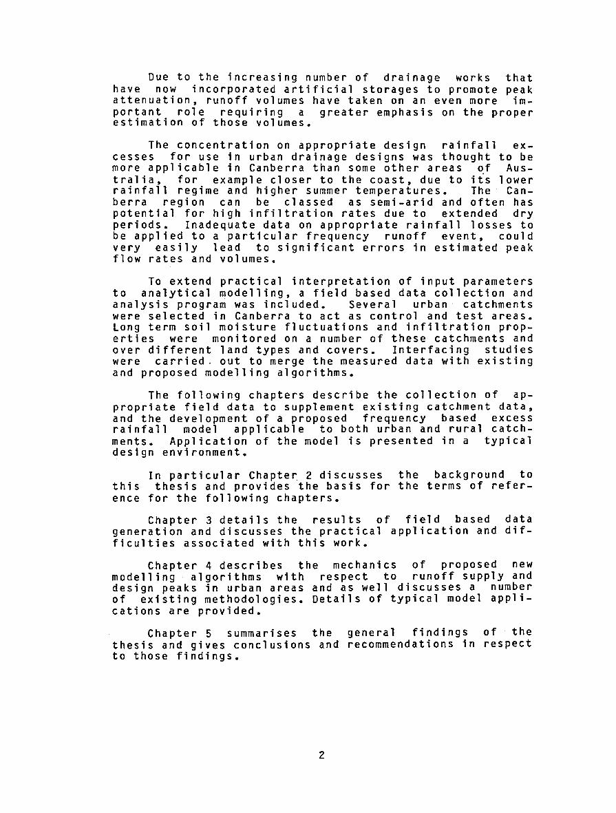
Due to the increasing number of drainage works that have now incorporated artificial storages to promote p~ak attenuation, runoff volumes have taken on an even more lm­portant role requiring a greater emphasis on the proper estimation of those volumes.

The concentration on appropriate design rainfall ex­cesses for use in urban drainage designs was thought to be more applicable in Canberra than some other areas of Aus­tralia, for example closer to the coast, due to iis lower rainfall regime and higher summer temperatures. The Can­berra region can be classed as semi-arid and often has potential for high infiltration rates due to extended dry periods. Inadequate data on appropriate rainfall losses to be applied to a particular frequency runoff event, could very easily lead to significant errors in estimated peak flow rates and volumes.

To extend practical interpretation of input parameters to analytical modelling, a field based data collection and analysis program was included. Several urban catchments were selected in Canberra to act as control and test areas. Long term soil moisture fluctuations and infiltration prop­erties were monitored on a number of these catchments and over different land types and covers. Interfacing studies were carried. out to merge the measured data with existing and proposed modelling algorithms.

The following chapters describe the collection of ap­propriate field data to supplement existing catchment data, and the development of a proposed frequency based excess rainfall model applicable to both urban and rural catch­ments. Application of the model is presented in a typical design environment.

In particular Chapter 2 discusses the background to this thesis and provides the basis for the terms of refer­ence for the following chapters.

Chapter 3 details the results of field based data generation and discusses the practical application and dif­ficulties associated with this work.

Chapter 4 describes the mechanics of proposed new modelling algorithms with respect to runoff supply and design peaks in urban areas and as well discusses a number of existing methodologies. Details of typical model appli­cations are provided.

Chapter 5 summarises the general findings of the thesis and gives conclusions and recommendations in respect to those findings.

2

CHAPTER 2

BACKGROUND AND SCOPE OF THESIS

Over the last eight years the author with others ( Goyen & Aitken(1976), Henkel & Goyen{1980}) has been re­sponsible for the development and use , in practise , of a number of computer based urban stormwater drainage models. These have been applied in varied hydrologic and hydraulic projects throughout Australia and Papua New Guinea.

The evolutionary process involved in model development has necessitated constant inclusion of new algorithms to meet increased complexities in both analysis and design re­quirements.

One such rainfall/runoff model eo-developed by the author entitled the Regional Stormwater Drainage Model {RSWM) has been used extensively, since its inception in 1974, in both the analysis and design of both urban and rural drainage systems. The RSWM has .gained widespread use by a number of private consultants and government organisa­tions in Eastern Australia on both minor and major drainage and flood mitigation projects and has now been developed into an efficient and versatile watershed model appropriate for both design and analysis of urbanised and rural drain­age systems.

Through continued use of the RSWM several application shortcomings had come to the author•s attention that could not be solved without indepth research and development. A major item related to the specifications of appropriate loss rates for design analyses , particularly when synthe­tic storms were to be applied. The RSWM in its present form, as with other rainfall/runoff models, requires rain­fall losses to be input as raw data. These are entered as either initial and continuing loss rates or decay type loss functions based on input antecedent conditions. Because little data have been available on appropriate losses to be applied in varied design situations, this section of any runoff analysis, under certain circumstances, has . placed the accuracy of some runoff estimates in serious jeopardy.

The scope of this thesis was therefore aimed at devel­oping methods whereby appropriate losses could be estimated for particular design runoff events and the incorporation of these methods into models similar to the RSWM.

A brief synopsis of the RSWM as used prior to this thesis has been included below to further clarify the starting position of this thesis.

3

2.1 Description of RSWM. To design complex stormwater drainage systems, especially those which include flood storage, it is desirable to carry out the calculation by means of a rainfall/runoff model programmed for solution on a digital computer. This approach eliminates much of the repetitive calculations and allows the detailed investigation of many alternatives. The RSWM rainfall/runoff model described in this thesis was originally developed in 1974 to analyse catchments in a pro~osed new urban growth area near Darwin covering some 85 km and was intended for use in the design and analysis of the trunk stormwater drainage systems. Since that time however the model has undergone extensive development and is now suitable for the analysis and design of urban and rural drainage systems with catchments varying upwards from 25 ha.

Details of the model have been presented by Goyen and Aitken (1976). Figure 2-1 shows a diagrammatic representa­tion of the RSWM which consists of four modules:

(i) A library module which controls the overall operation of the program including most of the data input and the sequencing of calls to the other three modules. Given sufficient computer storage space, any conceivable arrangement of catchment areas, channels and stormwater re­tarding basins can be modelled.

(ii) A catchment hydrograph module which estimates the runoff hydrograph from a catchment, using Laurenson•s non-linear runoff routing model (Laurenson, 1964). The module operates on a rainfall excess hyetograph which is derived from either an actual rainfall or a synthetic design storm hyetograph and losses calculated using initial and continuing tinits or Philip•s (Philip, 1957) infiltr­ation equation. The catchment storage delay parameter for Laurenson•s equation may be calculated from the catchment area, catchment slope and degree of urbanisation using a regression equation derived by Aitken (1975).

(iii) A channel routing module which routes estimated runoff hydrographs along the channels using the Muskingum­Cunge procedure (Price, 1973) or, alternatively, simple lagging of the peak flow by translating the hydrograph in time. Lateral inflow to the channel is included in the procedure.

(iv) A reservoir routing module which routes an inflow hydrograph through a retarding basin or ornamental storage using a level pool routing procedure. The stage/discharge relationship may be calculated within the program by hydraulic equations for a circular pipe outlet and a high level spillway. The stage/storage relationship may be approximated by an exponential equation. Alternati­vely, either or both ·of these relationships may be input as a set of known points on a curve.

4

The hydrograph module of the RSWM utilises the follow­ing equations to estimate the storage delay time in the non-linear model:

K = BQ-0.285

B = o. 2ssA0.520( 1 .0+U)-1.972s-0.499

K = sub-area storage delay time in hours

(2-1)

(2-2)

Q = instantaneous rate of runoff in cubic metres per second at the headwater

B = the sub-area coefficient

A = subcatchment area in square kilometres

S = main channel slope in percent

(1.0+U} = an urbanisation factor.

The urbanisation factor "U" varies from zero for a rural catchment to unity for a fully· urban catchment.

The output from the RSWM includes, for each subcatch-ment:

(i) A summary of subcatchment and rainfall data.

(ii} A summary of flow peaks, storage volumes and water levels.

(iii) The complete details of the outflow hydrographs and water levels in a retarding basin.

(iv} A graphical plot of all computed hydrographs.

Of the several modules making up the RSWM the most significant one likely to effect the outcome of a watershed analysis is the one controlling hydrograph generation.

As described above the hydrograph generation module of the RSWM uses Laurenson•s runoff routing algorithms (Lau­renson, 1964} with additional regression coefficients to allow for catchment urbanisation developed by Aitken (1975).

5

Q Q

t

FIGURE 2-1. Diagrammatic Sketch of RSWM

Whether the RSWM is being used to analyse an historic event by simulation or to produce a design hydrograph using a synthetic storm, it first calls for the separation of excess rainfall from the total storm input. When analysing an historic event this can often be achieved by abstracting volume data from gauged rainfall and runoff charts. In a design mode, however, it is necessary to estimate appro­priate loss rafus for the·type of storm under consideration and the particular catchment under study.

Unfortunately this often designated "simple" first step in the hydrograph generation process is far from simple. Depending on antecedent conditions and spatially averaged infiltration parameters , as well as the frequency of the storm, a poor estimate can very often influence the final peak and volume of the resulting hydrograph far more than any other subsequent step.

The continued development of this module particularly relating to catchment data for the development of rainfall excess is described in subsequent chapters of this thesis.

The Regional Stormwater Model (RSWM) is structured si­milarly to the Stanford Watershed Model described by Crawford and Lindsay (1966) and Larson (1965) in as much as it includes both land and channel phases. Figure 2-2 indi­cates a typical watershed breakup for analysis by the RSWM.

6

LEGEND

--- CATCHMENT BOUNDARY

---- SUB-CATCHMENT BOONOARY

------- WATERCOURSE

~ LINK NUMBERS

~-·- ISOCHRON£

FIGURE 2-2. Typical Watershed Breakup for Analysis by RSWM

In principle the total study area is divi.ded into subcatchments so that outlet nodes are located at points where flow estimates are required. Each subcatchment is then considered and analysed in isolation with outlet hy­drographs transposed between nodes via appropriate main channel routing.

Subcatchment analysist being the nucleus of the model, is approached as a two phase system. Firstly a land phase is included whereby rainfall excess or runoff supply is es­timated then secondly a channel phase is applied for routing of rainfall excess through ten conceptual storages made up from isochronal areas to achieve a total runoff hydrograph at the outlet of the subcatchment.

The subcatchment channel phase therefore includes both overland flow and minor channel and pipe contributions. The total watershed analysis, considering the interconnec­tion of the individual subcatchmentst requires a second or major channel phase based on defined channel hydraulics.

It was proposed in this thesis to concentrate on the land phase of the RSWM in an urban environment principally

7

at the subcatchment level.

It is well documented {Wittenburg, H.(1975)) that urban stormwater systems and rural runoff respond very dif­ferently to a similar storm event. In most modern day urban drainage systems there would appea~ to be broadly two separate runoff segments, ie. from the impervious areas and pervious areas respectively. These become fused together to provide the total runoff hydrograph at particular points in the system.

To take the analysis one step further however, it was also proposed to divide the land and minor channel phases into their pervious and impervious component parts, analyse separate hydrographs then superimpose these prior to any major channel phase to test the appropriateness of such ac­tions.

The latter work was included to test the applicability or otherwise of using lumped models, usually associated with rural catchments, in an urban environment. Also it was necessary to ascertain the representative influences of both the impervious and pervious components of urban flows throughout the frequency range and urban land types.

The current edition of "Australian Rainfall and Runoff Flood Analysis and Design" (ARR, 1977), Chapter 8 contains a discussion on 'Initial and Continuing Losses•. In this, some discussion is provided on the selection of design values, however, apart from stating the various factors in­fluencing them, it gives only general values for typical design situations. Initial losses are described as 'extre­mely variable, having a range from around zero to more than 50 mm'.

In urban stormwater drainage designs the normal range of storm events usually considered do not exceed two hours in duration.In Canberra, a total of 50 mm of rainfall cor­responds to a once in 500+ year for a 15 minute storm or a once in 200+ year for a 30 minute storm or a once in 100 year for a 1 hour storm. As can be appreciated all of the stated storm bursts as well as variations in between fall beyond the normal range used in urban design analyses. With the vast extremes suggested for initial losses, with­out even considering continuing losses, it is not surprising that the generation of significant pervious runoff under a number of circumstances could be questioned. Conversely, a range of other meteorological and catchment circumstances could cause significant pervious runoff.

Added to the above discussion there was a very real problem of assigning appropriate losses to design storm bursts rather than tota~ storms.. Design storm bursts {design storms) are derived on a statistical basis from a long period of pluviograph record representative of a study area. Significant bursts of varying durations are accumul­ated from the record and mean dimensionless temporal

8

patterns deduced. Such bursts can consist of the total storm or be imbedded within the event.

Assigning loss rates to design storms took on the added problem of assigning appropriate pre-storm burst wet­ness or average catchment antecedent wetness immediately prior to the start of the design burst. Chapter 3 in ARR 1977 gives typical temporal patterns of rainfall bursts for various locations in Australia based on long term continu­ous rainfall data. The use of such data has gained widespread acceptance in drainage design work and as such the question of appropriate losses needed urgent resolu­tion.

Some Australian work has been carried out on this aspect notably by Laurenson & Pilgrim (1963), Pilgrim (1966), Cordery & Webb (1974) and Cordery (1970). Cordery studied 42 years and 32 years of rainfall records at Sydney and Griffith, N.S.W. respectively. He showed that antece­dent wetness was an important factor in assigning initial losses to design storms particularly in areas where the mean annual rainfall was significantly less than 1200 mm.

Cordery developed a procedure to estimate a median an­tecedent precipitation index (API) prior to a design storm burst by relating the difference in catchment wetness oc­curring between the 9 a.m. estimate via normal API calculations using 24 hour rainfall data and the start of the design burst.

The API was then related to potential initial loss by an expression based on observed rainfall and runoff data for 14 rural catchments in eastern New South Wales.

The current thesis has carried on in a similar vein to Cordery•s work making use of 45 years of continuous pluvio­graph record at Canberra in conjunction with a variable time water balance model to develop statistical antecedent relationships for several types of urban land domains.

To cover the significant factors that affect loss rate estimates on urban catchments the current thesis proposed to examine existing analytical estimating techniques with the view to adopting or developing suitable methods for use in urban design procedures. It was also proposed to review, adopt and devise suitable field data collection techniques to collect additional data for this thesis as well as provide data collecting guidelines for similar stu­dies in other regions and land domains.

It was anticipated that relatively simple and rapid field data collection methods may be developed for adoption into regular stormwater drainage design exercises.

The following Chapter details the results of field based data generation and discusses the practical applica­tion and difficulties associated with this work.

9

CHAPTER 3

FIELD DATA COLLECTION AND ANALYSIS

3.1 Introduction

The original scope of the data collection and analysis program was not constrained by any predetermined ideas but ultimately because of funding and time constraints was lim­ited to a number of specific experiments aimed at providing fundamental input data for loss rate determination on the catchments studied.

The major elements of the program in summary form in­cluded work;

(i) to measure long term variations in soil moisture occurring specifically in the top 300 mm profile in different Canberra urban land domains;

(ii) to define infiltration parameters for the land domains being studied;

(iii) to determine the make up of typical urban wat­ersheds and the interaction of the various domains including the relative significance of impervious and per­vious areas as the major subgroups of a catchment.

Canberra has several well gauged urban and rural catchments. Instrumentation includes pluviographs, stage recorders to monitor runoff, ancillary daily rainfall rec­orders and on one urban catchment water quality recorders.

The present gauging network was funded by the National Capital Development Commission and is maintained and oper­ated by the Department of Housing & Construction and as such-provides -high quality data collected by skilled and dedicated hydrographers.

The catchments addressed in this thesis are at Gira­lang and Gungahlin in the town of Belconnen in the northwest sector of Canberra, at Mawson in the Woden Valley immediately south of Canberra City and the northern slopes of Black Mountain immediately adjacent to Canberra city.

The locations of these catchments are shown on Figure 3-1.

10

YARRALUMLA ---+-~::;.-r RAINFALL STATION

FIGURE 3-1. Location of Canberra Study Catchments.

Both the Giralang and Mawson catchments are for all practical purposes fully built up and represent typical Canberra type urban catchments. They have fully sealed roads with kerb and gutter, are fully sewered and have roof drainage directly connected to the piped drainage system. Planning and development in both areas occurred in close sympathy with the natural drainage. lines and both a pipe drainage system to take flows up to about the once in 5 year level, together with an overland flow path over public land to protect private property from rarer flooding was provided.

Figures 3-2 and 3-3 indicate the two urban catchments. A description of the type of drainage systems (both minor and major) used and the general drainage policies adopted in Canberra have been given by Higgins & Mills (1975) and Henkel & Goyen {1980).

11

FIGURE 3- 2• Giralang Urban Catchment.

12

PEARCE

LEGEND

4 GAUGING STATION

• PLUVIOGRAPH

e DAILY READ RAINGAUGE

--·--·- CATCHMENTBOUNDARY

--- CATCHMENT AREA DIVERTED

------ STORMWATER DRAIN

NOTE:

CONTOURS ARE TO AHD

100 0 100 200 300

METRES

FIGURE 3-3. Mawson Urban Catchment.

13

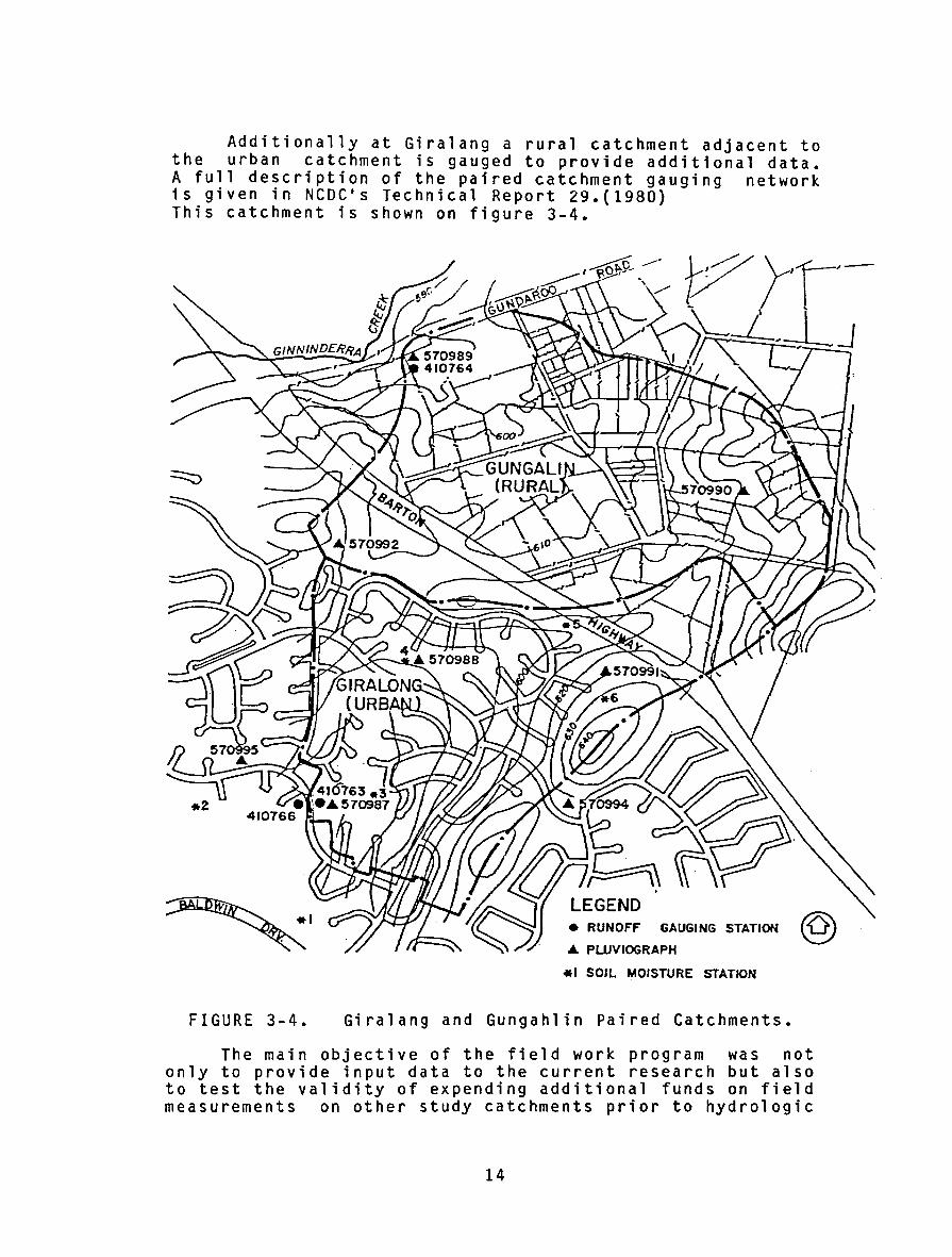
Additionally at Giralang a rural catchment adjacent to the urban catchment is gauged to provide additional data. A full description of the paired catchment gauging network is given in NCDC's Technical Report 29.(1980) This catchment is shown on figure 3-4.

e RUNOFF GAUGING STATION @ .A. PWVIOGRAPH

*I SOIL MOISTURE STATION

FIGURE 3-4. Giralang and Gungahlin Paired Catchments.

The main objective of the field work program was not only to provide input data to the current research but also to test the validity of expending additional funds on field measurements on other study catchments prior to hydrologic

14

analyses or designs.

Specifically~ the Giralang urban catchment was used as the base catchment where most field measurements were car­ried out. The Mawson catchment was used as a comparative test cachment on which to test the transferrability of data from the Giralang catchment to other typical urban catch­ments in the region.

Limited field data was also collected from the Black Mountain Reserve area to gather information on native for­ested areas which are fairly common on the surrounds of urban watersheds within the region.

The following briefly summarises the hydrologic data made available during the course of the thesis:

• Pluviograph data from the Yarralumla Forestry Research Station is shown on Figure 3-1 for the complete. years 1933 through 1961 and 1966 through 1970 •

• Pluviograph data at the outlet of the Giralang urban study catchment for years 1976 through 1979 •

• Pluviograph data at the outlet of the Gungahlin rural study catchment for years 1976 through 1979 •

• Pluviograph data at the city gauge adjacent to the Black Mountain soil moisture stations 7 and 8 for the years 1979 through 1980.

• Pluviograph data at the creek catchment for 1980. (Data not fully this Thesis.)

outlet of the Mawson the years 1972 through processed at the time of

• Continuous runoff data at the Gungahlin rural catchment outlet for the complete years 1976 through 1979 •

• Continuous runoff data at the outlet of the Mawson urban catchment for the complete years 1972 through 1980. (All data had not been processed at the time of this Thesis.)

3.2 Study Catchments

3.2.1 Giralang and Gungahlin. The Giralang urban catchment indicated on Figures 3-2 and 3-4 formed the main study catchment used in this thesis. It has a total area of 94 hectares including 24 hectares of impervious surfaces and 32 hectares of predominantly indigenous soil unirrigated

15

grassland. The residue 38 hectares consists of urban resi­dential pervious areas made up of lawns and gardens with, predominantly, imported topsails.

Indigenous areas have native grass cover similar to the sister Gungahlin rural catchment with some imported species, predominantly chewings fescue and ryes sown in the areas adjacent to residential lots.

Grasses common on residential lots are chewings fescue, couch, kentucky blue and various species of clover. Root depths are usually limited to less than 50 mm.

Native soil types consist basically of red podzolic on the upper slopes and yellow podzolics on the lower slopes of the catchment.

The 'A' horizon native topsails or root zone consists mainly of sandy clay to clayey-sand of low plasticity which varies in thickness from virtually zero on some of the upper slopes where the weathered rock is exposed, to 400 mm at the bottom of the catchment close to ephemeral water courses.

Imported topsails vary considerably in nature, from light sandy-clays to puggy organic clays depending on the area of procurement •. Included in the appendix are engi­neering logs taken at six locations in the catchment as indicated on Figure 3-4. A detailed description of the Gi­ralang gauging network is given in Technical Paper No. 29 published by the National Capital Development Commission, 1980.

Instrumentation, as described in the above document, consists of a runoff recording station at the outlet of the catchment consisting of a sloping crest crump weir to meas­ure flows in the pipe system and an additional cut throat flume incorporated in a walkway underpass to measure excess overland flows up to at least the once in 100 year flow. Also included are five rainfall stations either in or just outside the catchment area consisting of various types of pluviographs capable of monitoring variations in storm pat­terns across the catchmenti - Additionally~·two-rainfall stations are located within the adjacent rural Gungahlin catchment no more than 600 metres north of the Giralang catchment border. The location of all gauges are shown on Figure 3-4.

Urbanisation of the Giralang catchment was commenced in 1974 and was completed by late 1976. Tree planting was progressively implemented from early 1976 and was virtually complete by late 1977.

Rainfall and runoff data was made available for the years 1976, 1977, 1978 and 1979 on both the Gungahlin rural and Giralang urban catchments for use in this thesis.

16

The sister Gungahlin rural catchment as shown on Figure 3-4 has a total area of 112 hectares and is part of the CSIRO's experimental farm. As such its paddocks are better maintained than on the average grazing property in the region, hence the catchment probably relates to the dry grass areas in the adjacent urban area more than typical rural areas.

The Gungahlhn rural catchment was used principally to help isolate pervious and impervious runoff in the adjoin­ing urban catchment and to help calibrate the water balance model parameters through rainfall/runoff simulation de­scribed in Chapter 4.

3.2.2 Mawson. The Mawson urban catchment indicated on Figure 3-3 formed the proving catchment in this thesis. It has an area of 445 hectares including 115 hectares of im­pervious surfaces, 320 hectares of dry grass and residential lawn area and 10 hectares of irrigated non­residential area.

The catchment's average slope is 2.5% and the general soils and grass covers appear to be reasonably similar to tie Giralang catchment with the geology of the area from the Upper Silurian period made up of the Deakin volcanics.

Instrumentation on this catchment started in 1971, and entails a runoff recording station at the outlet of the catchment consisting of a stage level recorder situated in a lined open channel, a rainfall recording station also at the outlet and several daily rainfall gauges situated within the catchment.

Urbanisation of the Mawson catchment commenced in the early 1960s and was predominantly completed by 1970. Some isolated infill areas have been developed on a progressive basis up to the present, however these would account for less than 5% of the total catchment area.

3.2.3 Black Mountain Reserve. Black Mountain is situated immediately adjacent and to the west of Canberra city, see Figure 3-1, and contains approximately 500 hectares of na­tural forest, predominantly eucalypts. The total area has been retained as a nature reserve and is typical of a number of the higher areas covering the upper portions of catchments with highly urbanised areas on the lower slopes.

The geology of the mountain is mainly from the middle to the Upper Ordovician and is classified as the Pittmen formation Action shale member.

This generally consists of shale, mudstone, sandstone, siltstone, radislarian cherts and some areas of black sili­ceous graptolitic slate.

17

Topsoils over the mountain are virtually non existent with mainly decomposed and broken rock combined with silty, sandy gravels mixed in the root zone for some 100 to 300 mm over more solid rock.

A thin layer of litter covers most of the surface, mainly twigs and leaves in various stages of decomposition and generally the top layers appear to be highly permeable.

3.3 Scope of Data Collection Program

From the apparent lack of published information on the general use of field based data as input to urban stormwa­ter drainage models as well as procedural techniques it appeared that there was considerable scope to develop both measurement techniques and integration methods whereby ad­ditional field data would be used to improve runoff estimates.

Data was required in the form of spatial and temporal variations in soil moisture both short and long term; wet­ting front movement parameters including infiltration rates and upper soil storage capacities; depression storage; in­terception parameters by urban trees, shrubs, gardens and grasses; the significance of different land domains, their maintenance and connection with the overall drainage system (in particular the relationship between impervious and per­vious areas) and the retardence factors affecting flow routing in typical urban catchments within the different domains.

The above lists a wide range of items requiring data acquisition, it is by no means complete, however it would represent the main parameters that could potentially affect the magnitude of runoff peaks and volumes occurring from a given rainfall event within an urban or rural area.

Due to the limited resources available, data collec­tion in this thesis mainly concentrated on changes in soil moisture and infiltration parameters affecting pervious runoff. Additionally the effects of catchment structure and the relative importance of various land domains occur­ring was considered.

A number of primary data measurement stations were selected including six (6) at Giralang and two (2} on Black Mountain to provide permanently located data collection sites representative of different urban and non-urban land types.

The selection of individual sites took into consider­ation the soil type and its depth and structure, type of cover (dry grass, irrigated grass, gardens, residential lawns, etc), its elevation in catchment, site slope, prox­imity to watercourses and drainage pipes, depressions, humps and trees.

18

Six of the eight (8) primary stations are located as shown on Figure 3-4. At each of the stations full engi­neering 1nvestig~t1ons were carried out including logging and dens1ty prof1l1ng. The other two (2) station locations are shown on Figure 3-1.

Additionally, by adopting a random selection technique (dividing the total Giralang watershed into 1000 half al­lotment p~rcels), secondary temporary stations were selected to describe moisture changes within residential allotments • Twenty (20) individual allotment measure­ments, based on random number generation selection, were taken in any one recording session to represent an average catchment wide wetness.

Additionally, using the same random selection techni­ques, limited representative infiltration and soil storage data was obtained for a number of the land domains within the catchment. These were carried out employing insitu in­filtrometer rings to derive soil conductivity and sorptivity values using methods described by Talsma (1969). Samples were also collected to obtain soil/water storage capacities.

Soil moisture/density readings were made using several methods including neutron scatter and gamma ray absorption techniques, conventional sampling techniques combined with oven drying methods and the installation and monitoring of thermocouples using a psychrometer.

Measurements were taken regularly proximately 10 months between July roughly at monthly intervals, with taken on an event basis.

over a period of ap-1979 and April 1980, additional readings

Two additional runoff gauging stations were installed in the form of maximum stage boards to monitor peak pervi­ous runoff from discrete land domains. These were located immediately upstream of Antares Crescent and at the under­pass under Chuculba Crescent in Giralang. The additional stations were used to measure the significance of pervious runoff from these areas in small to moderate events.

3.4 Description of Sampling Stations

Station No 1. This station is situated just outside the Giralang study catchment adjacent to Ginninderra Creek as shown on Figure 3-4. Station 1 was chosen to reflect changes in soil moisture in a typical dry grass area with a good grass cover close to an emphemeral stream to monitor possible interflow affects in the lower portion of the catchment. See photos 3-1 and 3-2.

19

Photo 3-1. Giralang-Station No 1. General View.

Photo 3-2. Giralang-Station No 1. Strata Details.

Station No 2. Indicated on Figure 3-4, is situated on the edge of a formalised playing fie.ld immediately to the west of the Giralang catchment in an area encompassed by an automatic irrigation system. The site contains mainly na­tural soils which are considerably denser and more clayey

20

than the imported topsails immediately adjacent and cover­ing the fields themselves. See photos 3-3 and 3-4.

Photo 3-3. Giralang. Station No 2. General View.

21

Photo 3-4. Giralang. Station No 2. Strata Details.

This station was chosen to test the effects of irrigation on an otherwise dry grass area.

Random sampling on the adjacent playing fields was also carried out over the course of the monitoring peri~d to compare moisture changes.

Stations Nos 3 and 4. Both stations are situated in dry grass areas in the middle portions of the catchment as shown on Figure 3-4 with Station 3 being somewhat lower than Station 4. See photos 3-5 and 3-6.

22

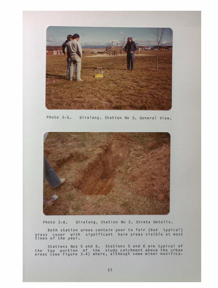
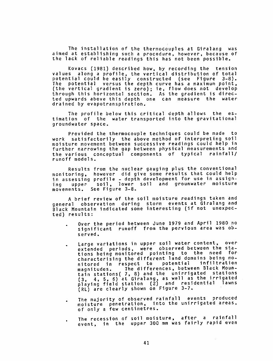
Photo 3-5. Giralang. Station No 3. General View.

Photo 3-6. Giralang. Station No 3. Strata Details.

Both station areas contain poor to fair {but typical) grass cover with significant bare areas visible at most times of the year.

Stations Nos 5 and 6. Stations 5 and 6 are typical of the top portion of the study catchment above the urban areas (see Figure 3-4) where, although some minor modifica-

23

tion to the land surface has occurred, it has been predominantly left in its rural form. Cover consists mainly of native grasses which in wetter weather can grow to a height in excess of 400 mm. Infrequent mowing is car­ried out on this portion of the catchment to minimise grass fires and vermen. See photos 3-7 , 3-8 , 3-9 and 3-10

Photo 3-7

Photo 3-8

Giralang Station No 5. General View.

Giralang Station No 5. Showing Initial Nuclear Gauging.

24

Photo 3-9 Giralang Station No 6. General View.

Photo 3-10 Giralang Station No 6. General View.

Station 5 is approximately on the floor of the main valley of the catchment. Considerable depths of topsoil exceeding 300 mm were common around the site.

25

Station 6, which is close to the top of the northeast boundary of the catchment~ contains only a thin layer of topsoil with rock outcrops occurring either at or just below the surface in a number of locations adjacent to the site.

Stations Nos 7 and 8. Stations 7 and 8 are located on the north face of Black Mountain about midway up the slope from Barry Drive and situated approximately 500 metres apart. Both represent similar, typical areas on the moun­tain and are included together to check for consistency in their response characteristics. Apart from a thin layer of decomposed as well as fresh litter the areas generally have poor topsails. Because of the decomposed nature of the shallow rock however and the significant amounts of tree roots the area would appear to be quite permeable and con­tain significant storage capacity. The sites were chosen so as not to be adversely affected by tree canopy, yet not too exposed to reflect a non-typical area. See photos 3-11 and 3-12.

Photo 3-11 Black Mountain. Station No 8. General View.

26

Photo 3-12 Black Mountain. Station No 8 Detailed Surface View.

Random Sampling Stations. To expand the monitoring network to include residential lawn readings and as men­tioned in the section on Station No 2, additional irrigated grass readings, it was necessary to use a random selection technique to provide representative area sampling to take into account spatial variability.

To this end the total number of residential allotments were sequentially numbered to provide nearly 1,000 half al­lotments for testing.

Using a random number generator, up to 20 areas were selected for any one monitoring session. At each selected area a sample was taken from or a reading made at a point as close as possible to the centre of the area described.

The playing field was similarly divided into areas from which a number of sampling points were randomly selec­ted.

The samples from the random stations for any one land domain were accumulated and the mean value was derived by dividing by the total number of samples or readings taken.

3.5 Sampling Methods

3.5.1 Soil Moisture Profiles. The measurement of soil moisture profiles was carried out by two methods, namely by taking cores and weighing before and after oven drying and

27

by making direct measurements using nuclear scatter meth­ods.

As the depth of influence, corresponding to shorter duration storms adopted in urban drainage design, is usually limited to significantly less than 300 mm it was decided to limit moisture profile measurements to this level. This decision was also based on the measurement techniques proposed and described below. It was realised that monitoring of a deeper profile could assist in overall water balance analysis as described in Section 3.6.1.

Additionally, special interest was taken to accurately define the profile over the top 100 mm as in most cases this depth would be expected to control storm infiltration response.

The pervious land domains for which soil moisture measurements were undertaken consisted of residential lawns, ·reconstituted dry grass areas, natural dry grass areas, irrigated grass areas and natural forest.

A brief description of the measurement techniques adopted is given below to familiarise the reader with the equipment used.

i Conventional Oven Drying - Soil Moisture Measurements. Using a spoon tube soi samp er with a 15.0 mm internal diameter, soil cores were extracted and divided into the following sectional lengths: surface to 25 mm, 25 to 50 mm, 50 to 100 mm and where appropriate 100 to 200 mm.

The sectioned core samples were directly placed into separately labelled containers with screw top lids. When a sufficient number of samples had been collected to provide a representative sample set, the containers were weighed. Conventional oven drying and reweighing of the samples in the containers was then carried out and the following information calculated:

Units

Moisture Content Wwt Wet Density Dwet Dry Density Odry Equiv. Water Level

= Ww/Ws x 100 % = Wt/Vt g/mm~ = Ws/Vt g/mm = (Wwx4000)/(LxD 2xN) mm

where: All weights in grams (g) All volumes in millimetres cubed (mm 3)

(3-1) (3-2) (3-3) (3-4)

(ii) Nuclear Soil Moisture and Density Measurements. Soil moisture profiles were obtained using nuclear techniques with a Troxler Model 3411B Surface Moisture/Density Meter. Initially nuclear measurements were, where possible, sup-

28

plemented by conventional moisture measurements via oven drying o! .collected samples. Additionally, sand replace­ment dens1t1es were taken to help verify gamma ray wet density readings.

The instrument in operation is shown in Photograph 3-7 and diagrammatically in Figure 3-5.

PHOTON PATHS

BACK SCATTER

PHOTON PATHS

DIRECT TRANSMISSION

Figure 3-5 Troxler Surface Moisture/Density Meter

As indicated above the instrument can be used in both backscatter or direct transmission mode. In the latter mode, density readings only were possible.

The instrument source to measure vely.

contains both a gamma and neutron density and moisture content respecti-

The position of the sources is shown above with the gamma source at the lower extremity of the probe and the neutron sources at the base of the main body of the instru­ment.

(a) Neutron Approach. Soil moisture content could, unfortunately, only be measured in the backscatter mode as the instrument is only calibrated to the source/detector geometry in that position. In the direct transmission mode (with the probe lowered to a set depth) moisture readings although displayed referred to repeated backscatter scans only.

Soil moisture content is deduced by counting the number of thermal or slow neutrons detected after fast neu­trons collide with hydrogen atoms in the material. This number is then compared with a reference number in the instrument's memory deduced from a calibration block sup­plied with the instrument which has a known moisture

29

content and density.

The moisture content displayed is expressed as a per­centage representing the average water content over the depth of influence. Unfortunately this depth is variable and dependent on the moisture content itself. The follow­ing relationship is cited in the manual for the instrument operating in the backscatter mode:

* Depth of influence (cm) = 28-27 Dwet

*source Troxler operating manual.

where: Dwet = Moisture content (g/cm 3)

(3-5)

Depth refers to depth over which reading averaged

When trying to relate changes in the near surface moisture profile, specifically between 0 and 300 mm, this situation was far from satisfactory as variations in the profile were undetectable. It would appear at this stage that for the purposes of this thesis a better profile de­finition measuring technique employing the instrument was needed if it was to be used to gather meaningful data.

The backscatter reading however could be useful as a rapid index measurement. Unfortunately this possibility has not been developed in this thesis mai~ly through lack of time. It may have been possible, through regression analysis, to link this index with the overall moisture/runoff response based on the sensitivity of re­sults obtained in the analysis section of this thesis described in Chapter 4. It would appear that there is con­siderable scope to develop this form of rapid surface measuring technique because of its inherent repeatability characteristics over conventional extraction techniques.

(b~ Gamma Ray Approach. An alternative method was develo­pe using the same instrument to obtain soil m~isture content over incremental depths up to 300 mm adopting the direct transmission mode to indirectly deduce soil moisture via density measurements. On the assumption that dry den­sity was relatively constant within the increment it was only necessary to either measure soil moisture once by con­ventional means to obtain by deduction a dry density profile for the site or take readings over extended dry periods to obtain dry density when moisture content was near zero. Subsequent moisture-readings were then taken by measuring wet density and relating this to the station dry density profile. Within the measuring period there were significant dry periods where soil moisture was very low. hence in the majority of cases it was possible to deduce from these dry density profiles.

Alternatively, conventional samples were extracted using a soil core ~ampler with an external diameter equal

30

to the solid drill supplied with the Troxler. The collec­ted core was divided· into 50 mm increments between 0 and 300 mm and conventional oven dryed moisture content obtain­ed. The tube sampler had the added advantage of minimising density effects within the area surrounding the probe hole. The same hole was subsequently used to take the nuclear meter's gamma source probe.

From the readings taken the following results were de­duced:

Wet Density - direct reading Dry Density - direct reading Moisture Content - Wvol = (Dwet-Ddry) x 100

Ddry

As can be seen from the above list, moisture content measurements are given units, whereas oven dry values are expressed of dry weight.

Units

g/cm~ g/cm

%

{3-6} (3-7) {3-8)

nuclear based in volumetric as a percent

The different modes of expressing moisture content adopted by the two methods presented some difficulties when comparisons were required however, provided wet density was obtainable the following expression allowed one to be con­verted to the other:

Wvol = (Wwt% x Dwet)/{Wwt% + 100) {3-9)

A number of comparison runs , using the nuclear techniques described above were carried out to test the applicability of the method, against conventional oven dryed moisture measurements, as a suitable rapid non des­tructive method for determining moisture data. The results from a series of comparative readings using conventional and nuclear methods are shown on Figure 3-6.

31

12r-------------------------------------------------~

I I 0

~ 10 0

a1 9 > 0 ..J 8 ex: z 0 1- 7 .z w ~6 0 u e s E -w 4 0:: :::> 1-(1) 3 0 :E _.J 2 0 (/)

X X

X X

X

X

r= 0.93

0~------~--~--~--~--~--~~--~------~--~--~ 0 2 3 4 5 6 7 8 9 10 11 12

SOIL MOISTURE (m m) NUCLEAR MEASUREMENT

FIGURE 3-6 Scatter Diagram Comparing Nuclear and Conventional Soil Moisture Readin-gs

(iii Moisture Measurements. As an ad 1t1ona met od to measure ong term f uctuations in moisture content over shallow soil profiles, thermocou­ples were installed at defined incremental depths at each of the six permanent stations at Giralang. These were to be monitored using a portable psychrometer.

It was intended that this technique would also monitor any hysteresis effects in long term-~ettin~-a~d drying cycles of the soils as well as soil moisture changes deeper than 300 mm.

It was also intended to assess and comment on the gen­eral suitability of this type of apparatus.

Two thermocouples were placed at each of Stations 1, 3, 4, 5 and 6 at depths of 150 and 300 mm and five at Station 2 at depths ranging down to 500 mm.

32

Typical installation of these units is shown on Photo­graphs 3-13 and 3-14 at Station No. 1.

Photo 3-13 Installation of Thermocouples - Station No 1

Photo 3-14 Completed Installation of Thermocouples Station No 1

Core samples were taken from as close as possible to the thermocouples and taken to the laboratory to obtain reference soil moisture/soil suction (pF) relationships for

33

both wetting and drying cycles. pF readings from the psy­chrometer field measurements were then to be related to la~oratory reference graphs to obtain representative soil mo1sture values.

3.5.2 Infiltration Parameters.

~a{ Sorptivity. In this thesis the main theoretical in­i tration algorithms adopted in Chapter 4 were based on

the work carried out by Philip (1957) when he showed that cumulative absorption or desorption into or out of a hori­zontal column of soil of uniform properties and initial moisture content was proportional to' the square root of time. Philip also showed that for shorter times of (t),_ vertical. one - dime~sional infil~rat~on IQ~ld be described by a rap1dly converg1ng power ser1es 1n t I • The coeffi­cient of the leading term of the series (bracketed below) was termed sorptivity. Talsma {1969) proposed methods of measuring sorptivity in the field on undisturbed soil, for subsequent use in analytical applications.

i = (S)t 11 2 + At + Bt 3/ 2 ••••• (3-10)

where: i = cumulative infiltration (cm) t = time (min) S = sorptivity (cm/min11 2) A, B, are parameters of the second and third terms (cm/min 1 , cm/min 31 2).

Philip (1957) and again Talsma (1969) pointed out that sorptivity depended on initial moisture content and on the depth of water over the soil. Talsma varied these paramet­ers in a series of field based experiments to test their effect on sorptivity values. Measurements of sorptivity were made by Talsma on large samples enclosed with 300 mm diameter, 150 mm high, infiltrometer rings pushed 100 mm into the soil.

Water was rapidly ponded in the rings to a depth of about 30 mm and the subsequent drop in water level was noted at regular time increments of 10 to 15 seconds after ponding.

Sorptivities were calculated from the linear portions of initial inflow against the square root of time. Samples of soil for initial and final moisture content were taken close to and inside the rings.

Based on the work by Talsma (1969) the method relied on the reasonable assumptions (a) that during the short time of measurement (1-2 minutes) water flow would remain vertical within the ring infiltrometer, and (b) that the first term of the infiltration equation (Philip, 1957) ac­counted for nearly all of the flow.

34

The first condition was found, within the accuracies of experimental technique, to be easily verified, however the second depended on the magnitude of A relative to s. Talsma found that plots of i against t 1 12 remained essen­tially linear at least to 1 minute and showed that for the wide range of different textured and structured soils stu­died the drop in head during the measuring process was not significant. He concluded that the accuracy of the ring infiltrometer method of measuring S insitu was quite ac­ceptable even in soils with high saturated hydraulic conductivity relative to sorptivity. He also con~luded that neither the diameter nor shape of the ring affected the results.

In the work carried out on the Giralang catchment per­spex rings were used where possible in preference to steel ones to provide a visual check on the wall/soil interface as well as allowing direct head drop measurements through the wall.

Sorptivities were measured at a number of random sites over the Giralang catchment to add data to the work of Talsma in the Canberra region.

(b) Hydraulic Conductivity. Hydraulic conductivity, a meas­urement of the ability of a section of soil profile to conduct water, is reflected in the second tiY~ in the in-filtration equation by Philip (1957) i = St + At •••

Talsma (1969) showed that for a wide range of soils, A could be expressed as follows:

A = Ko/ 2. 8 (3-11)

where Ko equaled the saturated hydraulic conductivity.

Ko therefore is the ability of a soil profile to transmit water when the soil is fully saturated. Ko is therefore only a special case of general hydraulic conduc-tivity.

To apply Philip's infiltration equation it was therefore necessary to obtain measurements of Ko as well as sorptivity for each of the land domains.

Subsequent to reviewing the above equations 3-10 and 3-11, a modified equation eliminating the need for equation 3-11 was cited in a paper by Chong and Green (1979).

In this publication work was described by Talsma and Parlange (1972) and Parlange {1971,1975,1977) where the following equations were developed:

X = Y - 1 + exp(-X) (3-12)

where X and Y were related to time, t, and accumulative in­filtration, i, by the series expansion of equation 3-10 and

35

the substitution of equation 3-13 and 3-14 in31

the result, with rearrangement and truncation after the t 2 term. where: X = 2 X Ko 2 x t/S 2 (3-13) and: V = 2 X Ko X I/S 2 (3-14)

The new equation termed the "Talsma-Parlange Equation" was therefore shown as follows:

i = St 1f 2 + ( 1/3 X Ko) + ( 1/9 X Ko 2/S X t 3/ 2 ) ( 3-15)

in which i was the cumulative infiltration, S the sorptivity at a specified antecedent soil moisture content, and Ko the hydraulic conductivity at water saturation.

Equation 3-15 was subsequently adopted in place of equations 3-10 and 3-11.

The method·of measurement adopted for Ko followed a similar procedure to measuring sorptivity, only on this occasion the undisturbed core sample held by the infiltrom­eter ring was removed from the surrounding soil and placed on a wire grid raised above ground level. A 100 cm length of core was adopted for all Ko and S measurements.

In this way zero moisture potential at the base of the core was assured. Water was then ponded on top of the soil until a steady outflow was observed. This flow was then measured at constant head and the saturated hydraulic con­ductivity calculated as follows:

Ko = Qw X l/(H X Ac X t) (3-16)

where: Ko = Saturated hydraulic conductivity {cm/minj Qw = volume of water discharged in time t (cm ) t = time (min) l = length of soil core {cm) H = hydraulic head

= dist. from base of core to ponda~e surface {cm) Ac = cross-sectional area of core (cm )

{c) Storage Capacity. The same. samples .u~ed for the determination of saturated hydraul1c conduct1v1ty were used to measure water storage capacity in the depth of sample.

To achieve this the sample was first weighed then oven dryed and reweighed to deduce moisture content.

In both the hydraulic conductivity and storage capa­city sampling procedure two rings were used, one to obtain the sample and an additional ring containing an imported sample to reinstate the sampling area.

36

.Upper Soil Storage Capacity (USC), defined below, was an 1mportant parameter in the infiltration process using the Australian Representative Basins Model (ARBM) described in. Chapter 4 to relate sorptivities of varying initial mo1sture contents. The following relationship was given by Black and Aitken (1977):

S = SO x (1 - US(init)/USC) (3-17}

where:

S = sorptivity SO = sorptivity at zero moisture cdntent US(init) = initial moist. content in upper soil store (mmmm) use = maximum moist. content of upper soil store ( )

3.6 Results from Gauging Program

3.6.1 Long Term Soil Moisture Fluctuations. Soil moisture monitoring via both nuclear and conventional means on an event basis was carried out at the stations shown on Figure 3-4 on the Giralang catchment as well as Black Mountain.

Figure 3-7 shows in graphical form a summary of the results from this work.

It would appear was a particularly type of rapid repeat of analysis.

that the Troxler neutron-gamma probe suitable device for carrying out the

measurements necessary for this type

The measurement tolerances of the Troxler were speci­fied by the manufacturers at + 2 to 4 percent of absolute values.

In carrying out repetitive measurements at the same location with the probe left in position between measure­ments, both moisture and wet density readings remainded fairly constant with a typical standard deviation from the mean, expressed as a coefficient of variation of .20.

' As for the absolute accuracy of soil moisture read-ings, Figure 3-6 shows the scatter of conventional oven dryed samples compared with the values deduced frofm the Troxler probe. As can be seen from the figure the correl­ation is fair with a correlation coefficient r = 0.93. There appeared to be a general tendency for the Troxler to predict values on the high side of those decuded using con­ventional oven drying methods.

Based on an upper soil moisture saturation level of 12.5 mm, being roughly the top 25 mm of the soil profile, up to a 2 mm error in soil moisture at the start of a storm event would not unduly effect the resulting runoff peak using the procedures described in Chapter 4. Based on com­puter runs this difference would account for less than a 5% change in peak.

37

As a 2 mm error in reading would account for a 16% to­lerance in field estimation it is contended that the Troxler would be most valuable in providing long term data for model calibration. From Figure 3-7 it is shown that the differences in soil moisture between stations of simi­lar description presents a far more challenging problem to contend with.

Serious problems were encountered with the thermocou­ple-psychometer techniques and as a consequence no reliable readings were forthcoming during the period of this thesis.

The main problems tended to be with the thermocouples themselves including their fragility and problems involved in obtaining a satisfactory contact between the soil and the porous thermocouple. Unfortunately the resources available for this thesis precluded detailed study into im­proving the thermocouple technique. Considerable scope does however exist for continued work in this field as the use of these instruments in conjunction with soil moisture readings was seen to offer definite advantages in estimat­ing the distribution of soil moisture going to evapotranspiration and groundwater respectively.

Vachaud et al (1973) and Kovacs (1979 and 1981), pro­posed to simultaneously measure, over the .soil profile, both .soil tension and soil moisture (see Figure 3-8).

38

Jo - -- ·- l - -_14r------r------t-----~------+------i-------4-------~----~------~-----+----~ j 12 r------+-------+-------+------+------4~----~~~~-4--~---+------4-----~+-----~ 0: 10 1----t----+-----+-----1-----+-----ll+-t-++--1-T-111 ~ ~ 81-------+-------~--------t-------~------4-~~~~

~ 6 1------+------~--------t------J--.--.. -IJ+J D.

?::; 4 ~ 2 1-.-....---l--h--r:~-J--I...---.--1-

0

24

22

20

EIS E ~

:JIG

~14 z < 12 0::

>-:10 ~ 8 et 0

,. ..

t

I. i I. • ]ij

-;:::-

t --

I. !--;-- J ,n - L 11. J I I

,, I l 11 I

6

4

2

0 JUNE JULY AUG SEPT ClCT NOV DEC

DAILY RAINFALL_:CITY GAUGE

' I

I .l • I.J

JAN fEB MAR APR

--14 E

.§. 12 .__~Sfl~ Jg_L_§g b!BAT 101'!.__: EVEL __

I-...._ AVARAGED DRY GRAsS READINGS

!=10 D.

~ e w 6 0::

~ 4 ~ 0 2 ~

0

.... 14 i 12 ::I:JQ

~ 8 0

w 6 0::

~ 4 Cl)

0 2 ~

0

-~

•I •I • ~.I

·~ .. - •2 . ............

•f-* . .~ •S 6

•1 .. .IUNE JULY AUG

1979

/ SEASONAL DROP 4

r{. I / 1-~v •2

s '-4._

. ·:. •4

Sf.PT OCT NOV DEC

GIRALANG- MOISTURE LEVELS

• I STATION ADJACENT TOCREEK

• 2 IRRIGATED PLAYING FIELD

• 3 14 1 !516 1 DRY GRASS

• 71 8 NATURAL FOREST

(BASED ON GIRALANG· RA NFALL)

•4

·~

RL llCRL

-«4

4

JAN fEB MAR APR 1980

X OVEN DRYED SAMPLES

• NUCLEAR SAMPLES BASED ON DENSITY

RL RES. LAWN RANDOM SAMPLE

2. STATION No.

_ ESTIMATED SATURATION lEV~ VALUES RELATE TO EQUIVALENT MOISTURE

I' JUNE .JULY

DEPTH (mm) IN TOP 2S mm OF SOIL.

CITY

• ;_7 •8 8 •8

•8 •8 •a

AUG SEPT OCT NOV DEC .I AN f£8 MAR

197S

BLACK MOUNTAIN -MOISTURE LEVElS

FIGURE 3-7 Shallow Soil Moisture Readings During the 1979,80 Period

39

1980

RAINFALL •8

APR

I

vr-----------------------~

E ,,,

.§ w u ~·oo a: :::> ., ~·oo 0 er ....

~2J.> a. LU 0

• AY'I IIIJIIIIoOf liltCI81' UIWI ... D'I(Jt to,..,. INC.IItiWI;~~&T

n~,.ua l•"fii[O AI lltiTIO 01 •tf OUrti'I'T DVIIII 01111 Df:HSIT'J Till!( I 100 VIA MUC\.14111 .. (AIUIIIEIIIINT.

STATION No. 8

Eoo E -

tOO

STATION No. "'

~0:-------~.~------~~------~~~------~N~------J MOISTURE COiflENT YOL. 'M.

~0~------~------~------~,r-------~------~ .. OIST\JR£ toHTEifl VOL.%

TOTAL POTENTIAL HEAD IN cm. VOLUMETRIC WATER CONTENT -600 -400 -zoo 0 040 0.45

().3

0.2

0.1

0 _!8

·01

i •0.2

TIME DAYS

9 10 I 12 13 14 15 16 17 18

APRIL I

CALCULATIOH OF" EVAPOTRANSPIRATION BY COMBINING THE MEASURED VALUES OF TENSION AND WATER CONTENT. (SOURCE, VACHAUO ET AL 1973)

FIGURE 3-8 Profile Summaries

40

The installation of the thermocouples at Giralang was aimed at establishing such a procedure, however, because of the lack of reliable readings this has not been possible.

Kovacs (1981) described how, by recording the tension values along a profile, the vertical distribution of total potential could be easily constructed (see Figure 3-8}. The potential versus the depth curve has a maximum point, (the vertical gradient is zero); ie, flow does not develop through this horizontal section. As the gradient is direc­ted upwards above this depth one can measure the water drained by evapotranspiration.

The profile below this critical depth allows the es­timation of the water transported into the gravitational groundwater space.

Provided the thermocouple techniques could be made to work satisfactorily the above method of interpreting soil moisture movement between successive readings could help in further narrowing the gap between physical·measurements and the various conceptual components of typical rainfall/ runoff models.

Results monitoring, in assessing

from the nuclear gauging plus the conventional however did give some results that could help profile - depth development for use in assign-soil, lower soil and grounwater moisture

See Figure 3-8. ing upper movements.

A brief review of the soil moisture readings taken and g.eneral observation during storm events at Giralang and Black Mountain indicated some interesting (if not unexpec­ted) results:

•

•

•

Over the period between June 1979 and April 1980 no significant runoff from the pervious area was ob-served.

Large variations in upper soil water content, over extended periods, were observed between the sta­tions being monitored pointing to the need for characterising the different land domains being mo­nitored in respect to potential infiltration magnitudes. The differences, between Black Moun­tain stations( 7, 8) and the unirrigated stations (3, 4, 5, 6) at Giralang, as well as the irrigated playing field station (2) and residential lawns (RL) are clearly shown on Figure 3-7.

The majority of observed rainfall events produced moisture penetration, into the unirrigated areas, of only a few centimetres.

The recession of soil moisture, after a rainfall event, in the upper 300 mm was fairly rapid ·even

41

•

•

during the winter period.

This fact can be seen in Figure 3-7 (Station 4) taking for example the 35 mm rainfall event in late September 1979. An apparent seasonal moisture equilibrium was reached in only 20 days after that event, even with intervening lesser rainfalls in that period. In that period the rapid increase in evapotranspiration typical of the commencement of Spring/Summer had an overriding effect on the upper soil store.

There was a very rapid decrease in dry grass soil moisture over the top 30 cm after November 1979 in line with the higher temperatures and stronger winds.

Figure 3-7, showing the results from the ten months monitoring program, indicates the typical varia­tions in soil moisture at a point in time at the different locations measured. The measurements are representative of approximately the top 25 mm of the soil profile and as such are very sensitive to the amount of grass cover and drainage available.

Throughout this thesis the upper soil store has been considered as the thin band of the soil pro­file forming the root zone. For the type of grass found in Canberra this is limited to approximately the first 25 to 50 mm. The typical clay soils found in Canberra have soil saturation capacities of approximately 50% by volume. Based on the aim of this thesis to be able to estimate flood peaks resulting from short storm durations, it was ·deci­ded at this stage to fix the upper soil storage at 12.5 mm. In this manner a relatively fixed 25 mm band was adopted as the physical upper soil pro­file. This was further based on the observed shallow penetration of short burst storm water as stated above.

As can be seen the dry grass readings (Station Nos 3, 4, 5 and 6), particularly in the Winter months, vary significantly.

The irrigated playing field (Station No. 2) was predominantly wetter than the dry grass stations although on two occasions at least one of the dry grass stations was wetter. Station No. 1 adjacent to the Giralang Creek was consistently wetter than all the other dry grass stations.

The random residential lawn samples were consis­tently above the representative dry grass Station No. 4 although the difference was not as great as would have been expected based on observation of individual lawns.

42

•

•

Station Nos 7 and 8 representing the forest area on Black Mountain consistently showed very low soil moisture readings.

T~e differences in moisture levels between, in par­tlcular, the dry grass stations appeared to be at least partly due to the difference in grass cover at the various locations. This did not however ac­~ount for all the differences and these require a lot more work to further quantify the differences.

T~e results from the short measurement program car­rled out confirmed the need for assessing factors such as land type, cover and surface maintenance on the production of runoff from pervious portions of urban catchments. Chapter 4 studies the absolute effects· of various domain changes and consequental differences in soil moisture, by modelling the ef­fects of the changes on the flood peak and volume results.

The difference in soil moisture profiles at any one time, between individual land units was most marked between Black Mountain readings and irrigated gras­sed areas as would be expected. The difference between residential lawn areas and dry grass areas was significant, however this was not as much as expected when the random selection of residential sites was considered. Individual variations in re­sidential lawn areas caused by lawn watering was greatly offset by the overall averaged affect caused by the significant number of poorly watered sites within the catchment as a whole.

Because of the lack of apparent runoff from pervi­ous areas in Canberra, it is considered that the measurements described in this chapter are particu­larly relevant in obtaining additional rainfall/runoff response data over and above total catchment outlet rainfall/runoff data. Gauged catchment outlet flow data provide the accumulated flows from both pervious and impervious areas. In most cases in semi-arid areas, such as Canberra, this only includes impervious runoff. Any model parameter calibration using only total catchment rainfall/runoff data could be in serious error when analyses are extrapolated to more significant events where pervious runoff may be significant. The problems of non-homogeneity of urban runoff, because of pervious and impervious areas , is dealt with in Chapter 4. It would appear that the major­ity of present catchment outlet gauged data in urban areas gives little, if any, information on the mechanisms and responses from pervious areas. The paired catchment at Giralang and Gungahlin res­pectively representing similar urban and rural catchments seeked to partially overcome this prob-

43

lem by allowing correlation between the adjoining pervious areas.

3.6.2 Sorptivity and Hydraulic Conductivity. Table 3-1 lists averaged sorptivity and saturated hydraulic conduc­tivity values for the typical land domains studied. The values relate approximately to the top lOO mm of soil pro­file. Because of lack of time and resources it was not possible to carry out extensive measurements on all the do­mains. Some measurements, however, were taken on residential lawns and dry grass areas. Other data was ab­stracted from Talsma•s results. This was deemed appropriate as those measurements were representative of the region under study.

44

Table 3-1 Average Sorptivity and Hydraulic Conductivities

Land Domain Hydraulic Moist Cont{by wt)

Conductivity Initial Final Ko (cm/min) %/100 %/100

Sorptivity

(cm/min 112)

** *** Residential Lawns, 0.140{.40)[10] 0.22 0.37 1.4{.50)[10] Giralang Urban Dry Grass Area Medium Grass Cover, 0.200{.30)[12] 0.15 0.40 .45(.40)[12] Giralang Pialligo Sand*

Dry 0.424(.13) 0.04 0.40 3.08(.12) Moist 0.11 0.40 2.16(.9)

Wet 0.20 0.40 1.04(.28)

Ginnindera Silty Clay Loam* 0.184(.29) 0.11 0.46 0.90(.28)

Ginnindera Clay Loam* 0.120{.55) 0.04 0.38 0.45(.18)

* **

***

Values taken from Table 1, Talsma (1969). Figures in brackets are standard deviations from the means expressed as coefficients of variation. Number of samples shown in square brackets.

3.7 Discussion on Results

Substantial differences were found in the results ob­tained from the relatively simple data collection program over the Giralang study catchment as well as limited work in the forested area on Black Mountain.

The differences in long term fluctuations in soil moisture occurring in the upper soil profile for the dif­ferent land domains indicated in a quantitative way one of the most significant factors affecting the production of runoff, that was point variations in moisture content at any point in time.

The combined effects of variations in prevailing mois­ture content shown in Figure 3-7 and the variations in infiltration parameters indicated in Table 3-1 indicate the probable reasons for the experienced differences in runoff produced from different pervious urban land domains.

45

The effects of residential lawn planting~ watering and topsoil development can significantly increase sorptivity and possibly hydraulic conductivity values to a smaller degree over and above average dry grass areas {See Table 3-1). The results for sorptivity measured on the residential lawns compared with the dry grass areas indicated a sta­tistical difference at the 0.01% level. Saturated hydraulic conductivity values between the two domains were not found to be statistically different at the 0.10% of level. Additionally, persistent soil moisture can be higher than for dry grass areas. Similarly irrigated areas have high persistent moisture profiles combined with high sorptivity and hydraulic conductivity. The actual magni­tude of potential infiltration is dependent on the total effects of the three parameters measured (Moisture Content, Sorptivity, Hydraulic Conductivity). The sensitivity of the individual parameters is treated in Chapter 4.

The gauging program described in this Chapter must be described as a feasibility program rather than a rigidly controlled field data collection program.

Over the limited time that the program was carried out it was only possible to carry out preliminary assessments on the various measurement techniques described to indicate if, individually, they showed promise to be included in future analysis and design situations.

The general results from the program were most encour­aging and provided valuable model calibration aids for the methods described in Chapter 4. There is, however, consi­derable work still to be carried out in the further development of the methods described as well as additional techniques still to be found.

The following Chapter considers how the data collected as part of this Chapter can be best utilized in rainfall/runoff modelling techniques. Existing models are discussed and new modelling techniques developed.

46

CHAPTER 4

THEORETICAL RAINFALL/RUNOFF MODEL DEVELOPMENT

4.1 Discussion on Current Techniques

The general objective of this chapter was to establish improved analytical methods for deterministic rainfall/ runoff modelling in a design environment.

To date methods employed to estimate design runoff events have largely been dependent on empirical parameters for which physical correlation has often been difficult. Probably the best known and widely used analytical design tool for estimating runoff peaks in Australia has been the Rational Formula. This method first attributed to Mulvaney in 1850 is a very simplistic model requiring the estimation of only two parameters. These are a runoff coefficient "C" and a time of concentration.

The "C" value has been very difficult to define with any degree of certainty. Unfortunately embedded in the parameter "C" are all the factors determining the ratio­between rainfall and runoff rates. These include catchment wetness, infiltration parameters, the effects of non­uniform rainfall and catchment routing characteristics to name a few.

Over a number of years the Rational Method, as a de­terministic model, has come under heavy criticism by many researchers and users, most notably French et al (1974), Watkins (1962), Aitken (1975) and Schaake et al (1967), for its poor general performance.

Despite the present uncertainties in parameter estima­tes the Rational Method still attracts widespread use and is by far the predominant method used by Australian prac­tising engineers to estimate both urban and rural flow peaks for the sizing of drainage structures. Its general acceptance is further encouraged by the fact that the method is currently recommended in the Institution of Engi­neers publication •Australian Rainfall and Runoff- Flood Analysis and Design• (ARR 1977) 2for the sizing of structu­res with catchments up to 25 km •

The main difference however between the Rational Method recommended (ARR 1977) over the deterministic form discussed above is that it is expressed in its statistical form. Design runoff peaks of a defined frequency are cal­culated from the same frequency rainfall inten~ity appropriate to a storm duration equal to the catchment time of concentration. Intensities are usually selected from

47

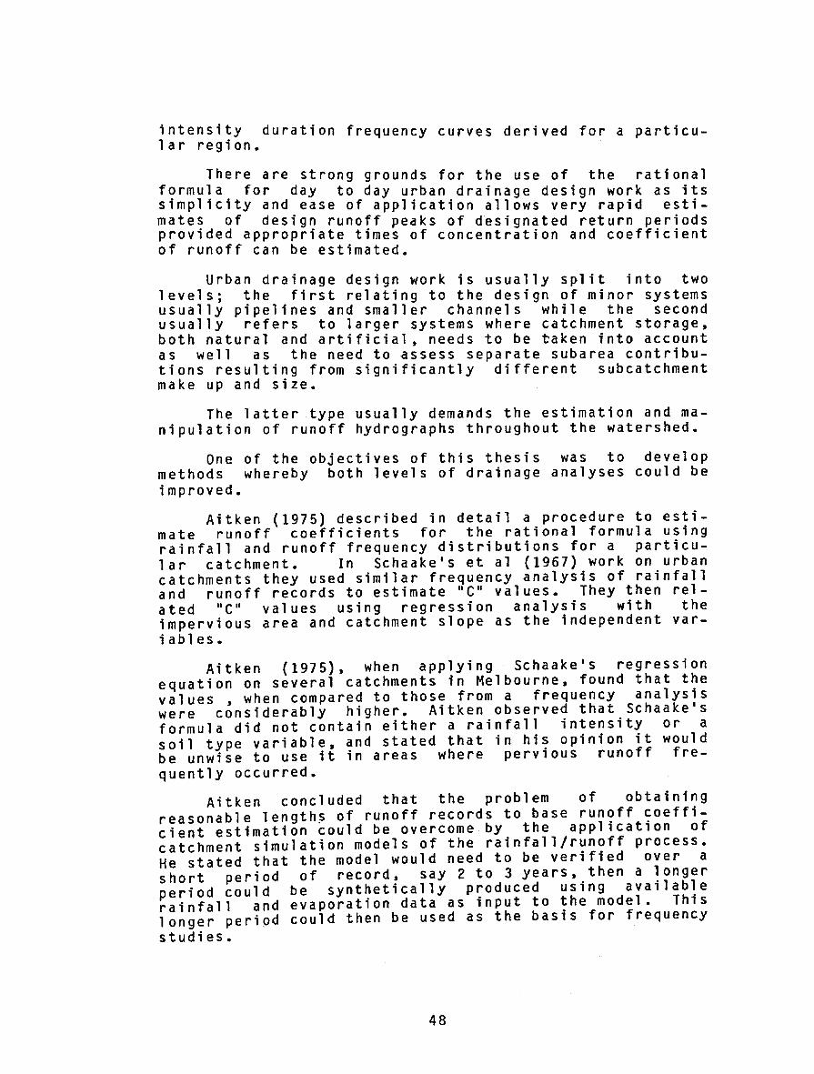
intensity duration frequency curves derived for a particu­lar region.

There are strong grounds for the use of the rational f~rmu~a. for day to day urban drainage design work as its s1mpl1c1ty and ease of application allows very rapid esti­mate~ of desigry runoff peaks of designated return periods prov1ded appropr1ate t1mes of concentration and coefficient of runoff can be estimated.

Urban drainage design work is usually split into two levels; the first relating to the design of minor systems usually pipelines and smaller channels while the second usually refers to larger systems where catchment storage, both natural and artificial, needs to be taken into account as well as the need to assess separate subarea contribu­tions resulting from significantly different subcatchment make up and size.

The latter type usually demands the estimation and ma­nipulation of runoff hydrographs throughout the watershed.

One of the objectives of this thesis was to develop methods whereby both levels of drainage analyses could be improved.

Aitken (1975) described in detail a procedure to esti­mate runoff coefficients for the rational formula using rainfall and runoff frequency distributions for a particu­lar catchment. In Schaake•s et al {1967) work on urban catchments they used similar frequency analysis of rainfall and runoff records to estimate "C" values. They then rel­ated "C" values using regression analysis with the impervious area and catchment slope as the independent var-iables.

Aitken {1975), when applying Schaake•s regression equation on several catchments in Melbourne, found that the values , when compared to those from a frequency analysis were considerably higher. Aitken observed that Schaake•s formula did not contain either a rainfall intensity or a soil type variable, and stated that in his opinion it would be unwise to use it in areas where pervious runoff fre-quently occurred.

Aitken concluded that the problem of obtaining reasonable length~ of runoff records to base run~ff ~oeffi­cient estimation could be overcome by the appl1cat1on of catchment simulation models of the rainfall/runoff process. He stated that the model would need to be verified over a short period of record, say 2 to 3 years, then a longer period could be synthetically produced using available rainfall and evaporation data as input to the model. This longer period could then be used as the basis for frequency studies.

48

. The p~ocedures described above have been taken up in th1s thes1s to deduce rational formula runoff coefficients for use in the more minor flow peak analysis based on the development of frequency curves described later in this chapter.

In recent years a number of more complex deterministic design orientated rainfall/runoff models have been develo­ped in an attempt to better quantify the imbedded factors included in the rational formula runoff coefficient.

Two models widely applied in Australia are 'RORB' de­veloped by Laurenson & Mein (1978) and the 'RSWM' -'Regional Stormwater Drainage Model • -developed by Goyen & Aitken (1976) briefly described in Chapter 2. Both models employ catchment routing techniques, channel routing and allow for variations in rainfall loss rates, catchment sto­rage parameters and storm patterns over the catchment to allow complete watershed analysis.

A non linear catchment storage runoff routing model (LRRM} developed by Laureson (1964} has been adopted in both the RSWM and RORB. The LRRM was developed for use on rural catchments and as such was modified by Aitken (1975) to include its application on urban and urbanising catch­ments. In Aitken•s work the storage delay coefficient operating within different catchments was related to catch­ment characteristics including area, main channel, slope and urbanisation content using regression analysis.

Since the inception of the RSWM in late 1974 signifi­cant work has been carried out and is continuing to further refine appropriate storage delay coefficients appropriate for the LRRM based on measurable or estimated catchment parameters. Although this development phase of the total catchment modelling process is far from exhausted it has been the aim of this current thesis to concentrate predomi­nantly on the estimation of excess rainfall and with particular reference to design events rather than catchment routing.

The estimation of excess rainfall is made difficult because of the fact that in most day to day design ex­ercises using deterministic models a design storm approach is employed rather than historical events. Appropriate design losses in this instance have to be compatible on a statistical basis with that of the design rainfall. This necessarily has to take into account the factors affecting the chance of certain rainfall events occurring with vary­ing loss rates to produce catchment runoff. One of the main factors affecting this is the uncertainty of catchment wetness prior to a design event due to the short as well as longer term time-dependent fluctuations in catchment wet-ness.

It was at the relationships between catchment wetness, design rainfalls and the deterministic processes involved

49

in loss rate estimation that the model development de­scribed in Chapter 4.2 was directed.

4.2 Development of a Combined Stochastic-Deterministic Rainfall/Runoff Model

4.2.1 General. In the development of suitable analytical tools capable of responding to the parameters affecting the conyersion of rainfall to runoff it was first necessary to def1ne the scope of the processes occurring and the param­eters likely to be significant.

The current work was aimed at desi~n procedures for both rural and urban catchments and consequently analytical tools would need to respond to the various land domains and their corresponding parameters existing in an urban as well as rural environment. Such domains would necessarily in­clude residential lawns 5 dry grass areas 5 irrigated grassed areas, natural forested fringe areas and impervious areas as well as adjacent rural catchments.

The following is a brief description of the methods used at present to estimate excess rainfall with determin­istic rainfall/runoff models, based on the RSWM as a typical model.

The RSWM accepts either an estimated initial plus continuing loss rate or infiltration parameters and an es­timated prestorm catchment wetness in conjunction with Philip•s Infiltration Equations Philip (1957). The losses to infiltration are then subtracted from the total design storm to deduce an excess rainfall hyetograph.

In the majority of day to d~y cases the initial loss­continuing loss estimates have been used in preference to the more complex infiltration equations as the calculation or estimation of an appropriate prestorm catchment wetness or moisture deficiency has not been possible or practical.

Initial and continuing loss rates generally applied with design storms up to date have been taken from the lit­erature where appropriate design values dependent on various catchment parameters or soil types have been recom­mended. As indicated in Chapter 2 however the values stated have often been misleading or vague and therefore could lead to significant errors when improperly interpre-ted.

Table 4-1 summarises some of the typical values quoted and applied to Australian urban and rural stormwater an-alyses.

50

TABLE 4-1

Summary of Typically Recommended Initial and Continuing Loss Rates for

Australian Conditions

Type of Catchment Surface

Impervious areas

Roofs of houses, factories and commercial buildings, road surfaces etc.

Pervious areas

(i) Sandy, open structured soils

(ii) Loam soils

(iii) Clays, dense Structured soils

(iv) Clays subject to high shrinkage and in a cracked state at the start of rain

(v) ARR (1977)

Initial Loss (mm)

1.5

5.0-20*

5.0-20*

5.0-20*

25-35*

0-50

Continuing Loss (mm/hr)

0.0

10-2.5*

3.0-10*

0.5-3.0*

4.0-6.0*

* Values taken from an unpublished report by Aitken {1974) based on various textbook values.

As stated above the problem of loss estimation is com­plicated by the fact that the design storm approach in urban drainage design infers the use of rainfall bursts rather than complete storm events. Consequently design storm loss rates need to reflect the possibilities of pre­burst catchment wetting. Depending on historical sequences of storms and the statistical interpretation of catchment parameters, the design storm loss rates could vary greatly from those associated with complete storm analyses. As mentioned in Chapter 2, Cordery (1970) carried out work on two New South Wales catchments in Sydney and Griffith res-

51

pectively to test the effects of the problems described.

The values given in Table 4-1 and in the majority of the literature would unfortunately appear to be directed towards complete storms and therefore could be quite in­applicable for urban design modelling based on design storm bursts.

Based on the historical rainfall record in the Can­berra region, it would appear that the average values quoted may well be low taking into account the semi-arid nature of the region and the long term timing of events.

Figures 4-1 to 4-3 reinforce this opinion by the pre­dominance of short duration historical events occurring in the high evaporation summer periods and then in the latter part of the day after potentially high catchment drying. To take this hypothesis a step further it was necessary for a detailed assessment of the time sequence of all rainfall events be made to ascertain, in real time, fluctuations in runoff producing catchment parameters. To achieve this aim a long term continuous water bala~ce model was employed to simulate the catchment response over the period of rainfall record available. The development and application of the water balance model selected is described below.

In particular the analysis was intended to include the definition of moisture deficiencies, over extended periods, on different urban land types and the role of these in pro­ducing runoff of varying magnitudes.

52

• • 30

... 10 ... .. ... .. .. "' 10

40 S!l 150 70 7!1

30 MINUTE CURioTION

!101---- ~U!!.l_OO...!.!Lf.!!t.!1....._ ----· -.----- -- -----­

t---- ONCE ~~~0----- _ --__ --- --- __ ---

1-----loNNUioL UAXIMUU RloiHFALL BIJRST 40

f--- 'lliU_I 'i .. .l!LI!\ ... fl!.t$1._ 1--·--·-- --- ------ --- __ -1--

::! .. ... 2 0 z lljo c ONCE

11: 11 11 11 I

10 11 11

• l I 11 11 •

I

li- -~ I I

~f.-L .!!!...,_ ~ I L I I

- I 1-- ~ 1!- r. f-f-~ I I I I I I .. I I I I 11

• I I I I 11 I • I I I I I • I I I I I I 11

I I I I a I I I I I

I I I

1 I I I I .: I I I I I • • I I• I

I I I I 11 • I I I

I I I I I I I

0 ••n " 40 so O!l eo I& 70 75

150 MINUTE OURATION

1-

NOTE • JIAINf'ALt. DATA TAI<EN fROW YAIIIIAL~A

70

10

SO

FOREST II[S£ARCH STATlOIII.

t----O.!:!.il....!..N ..!£Q..!J!.f'l...i9..,_ -- __ 1--- --- --- --- ---- ·---

1---~[IN !10 YR~ ----- -------------

ANNUAL UloXIMUiol SII.ULATED ,... f'[RVIOUS RUNNOFF BURST

I BASED ON DRY GRASSI

40 f.-- __2!:!C.t..U!..l2., Y~ +-- -----,.---1---· -1-- --- --- ---

• I

... liO ... .. ~ 1--~ ..Q!!ll IN I 'rl' '!!~\r- ~~·-+ ...--+--+ 1-4-1-.1-11---· -1--- -~-: 10

I•

0 • • . • •

40 411 110 !IS 10 70

120 MINUT[ DURATION

53

75

e

7 Cl)

w 6 0 z w 5 0: 0: ::l 4 --, g I I o 3 L __ , u. 0 0 2 z

--., I I

ANNUAL MAX. RAINFALL BURST 1933-1970

ANNUAL MAX. PERVIOUS RUNOFF 1933-1970

j3o MIN. DURATION I

~-----

r--1 I I I

O+-~~r7~~~~~~~-.--4-~--~~ J F M A M J J A S 0 N 0

8

7 Cl)

w 6 0 z ~ 0 0: ::l 4 0 0 0 3 u. 0 0 2 z

I I I I I I L_J

WONTHS

!so MIN. DURATION I

--, r-----. 1 I I L_J L_

I I ----.J

N 0 0 0+-~-=-r--.--1---r---.--,---r--~--~~~

J F M A M J J A s

Cl) 6 w 0 z 0 LLJ 0: g; 4 --, o I 0 3 I 0

~ 2 0 Z I

MONTHS

1120 MIN. DURATION)

------------. I I

O+-J~-=F--r-M-.-A~r-M-+-J~-J~~A-+-5~---0r-N~-D~

NONTHS

FIGURE 4-2 Seasonal Distribution of Annual Maximum 30, 60 and 120 Minute Rainfall Bursts

54

too

...

...

RAINFALL (TOTAL tnm) 18,30,60,120 MIN. BURSTS

100

E ~ -1 -1 C(

"-z ~ a:

- -;..,.- - -~~~~ --~ -- .... -~ ......>"' ...........-I I I / ::::::::-::: [.....:--:" ~ :,_......

-; I c:.-:--~ . . I

10 . . • • "-..__ 30 J.CIH.OURATION POINTS . PLOTTED FROM TABLE 4-5 •NO

MAX. ANNUAL FREQ. ANALYSIS

2 !I 10 20 &> 100 1000 10000 FiETURN PERIOD (TRS)

f ; . i &' . a I

•"" av• ••• ect ••• •&C 4•• ,., w•• .. ,. ••• ••• .AV[IIACi[ MONTH~T [VAPOAATIOH

.AT CAIIBEIIRA AIRPORT

TIME OF OCCURENCE STORMS ) I YR FREO.

FIGURE 4-3 Canberra Intensity-Frequency Duration, Pan Evaporation and Daily Rainfall Distribution

55

4.2.2 Continuous Water Balance Model Development.

After careful consideration of the models available for continuous rainfall/runoff simulation, the Australian Representative Basins Model (ARBM) originally developed by Chapman (1968,1970) and further modified by Black & Aitken (1977) was chosen for the following reasons:

(1) The model structure.provided for detailed sensi-tivity analysis of a large number of catchment parameters.

(2) The model allowed infinitely variable time steps thus allowing direct input from existing Australian Water Resources Council standard format digitised pluviograph and runoff records.

(3) The combination of both pervious and impervious areas were allowed for.

(4) In its simplist form the model provided an eco-nomical tool capable of analysing very long records within a limited budget.

(5) As the model is currently being examined and used in a research environment by several organisations throughout Australia, further research into the operation of the ARBM and required modifications could only help to strengthen the basis for the model •s use in Australian con-ditions.

Other similar models such as the Hydrocomp Simulation Model (Stanford Model) developed in the USA were considered but rejected on the basis of their unnecessary complexity and~ consequent cost to run. The basis for this assessment was further detailed by Black & Aitken (1977). Figure 4-4 gives a diagrammatic representation of the ARBM as de­scribed by Black & Aitken (1977).

The basic structure of the ARBM, described by Black & Aitken, was retained in this thesis. Some changes were made to data input, output provisions, allowances for the acceptance of variable time step computations and the way time steps were interpreted and modelling algorithms ap-plied.

56

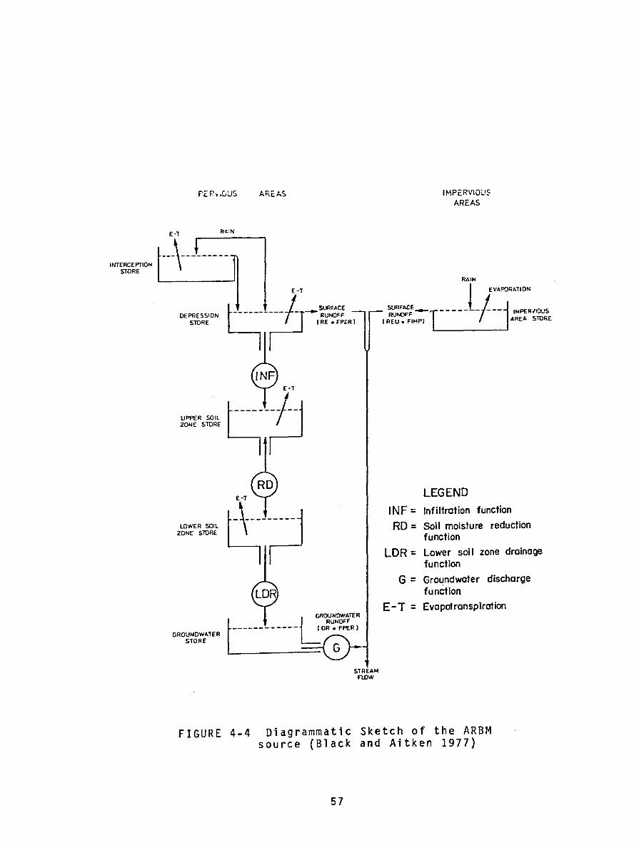
INTERCEPTION STORE

ARct.S

E-l Rt.:N

---\---------

DEPRESSION STORE lE -l SURFACE

I RE • FPER) --~--- -r ....,. E-l

UPPER SOIL r-------~~---- 1 20" "0" ~ ~

E-T

"'"" ""' t -\--------1 zo~~" ~ ~

GROUNOWA.TER STORE

STREAM Fl.OW

IMPERVIOi..'S AREAS

RAIN

t EVA"'Rt.liON

SURFACE

R\)NQFF --T----- -1- n j '""""""' I REU., FtMPI AREA STORE

LEGEND INF = Infiltration function

RD = Soil moisture reduction function

LDR = Lower soil zone drainage function

G = Gro~ndwater discharge function

E-T = Evopotranspiration

FIGURE 4-4 Diagrammatic Sketch of the ARBM source (Black and Aitken 1977)

57

In the form described by Black .& Aitken the model operated in predetermined time increments depending on pre­vailing weather conditions.

If the day was dry and the depression storage empty the~ the ti~e interval used was one day. If there was rai~ dur1ng t~e ~ay, or the depression storage was not empty at the· beg1nn1ng of a~y day, then an hourly time step was used. If there was rain during any given hour then a shor­ter time step was used during that hour. Six minutes was usually recommended for smaller urban catchments.

Unfortunately the use of the model in the above format required the search, backtrack and interpretation of inter­mediate data from the pluviograph record resulting in high running costs.

The model was modified to receive data directly from the digitised pluviograph record. Intermediate time step data was interpreted, only as required, to maintain stable model operation.

As a first step, catchment parameters needed to exe­cute the ARBM were taken directly from data suggested by Black & Aitken (1977) appropriate for the Giralang urban catchment described in Chapter 3. The initial parameter set in fact closely resembled the data set for Yarralumla Creek catchment described by Black & Aitken.

Table 4-2 lists this initial set of p~rameters design­ated the reference set. The variables were adopted as the •standard textbook set• from which all variations were com­pared in the subsequent proving and sensitivity analysis.

The term •standard textbook set• was used to indicate the typical model parameters one might obtain from readily available reference material (eg, Black & Aitken (1977), Chapman (1970), Eagleson {1970), Talsma (1969)) without, apart from rudimentary catchment examination necessary to assess literature data, going to detailed rainfall/runoff simulation runs or the inclusion of field measured values.

Model Calibration

The major objective of this thesis was clearly to es­tablish if additional simple field measurements could be included in the course of hydrologic studies to allow more relevant input to the mathematical models now used to pred­ict runoff events, and in particular, urban events of short duration.

Over the last decade much has been published (Mein & Brown (1978), Johnstone & Pilgrim (1973), Fleming & Black (1974)) in regard to the complex calibration processes available for continuous water balance models such as the

58

ARBM.

As stated in the work by Johnstone & Pilgrim (1973) "A true optimum set of values was not found in over two years of full-time work". This was based on the study of a single study catchment with well documented rainfall runoff and soil moisture data. The above declaration indicated the inappropriateness of such complex machine optimisation processes for day to day design exercises for all but the largest projects.

As this thesis was aimed at everyd~y trunk drainage systems of small to medium scale it was decided to test the appropriateness of the much simpler process put forward by the Australian Water Resources Council's Technical Report No. 26 (Black & Aitken, 1977).

This document proposed that a set of parameters based on a number of published works be selected • Additionally where data could be measured it be so included in place of the more generalised published data.

To test the accuracy of such a procedure, in lieu of the more tedious optimisation methods, the results (ie, runoff peaks) would need to be compared with gauged data. This point is taken up in Chapter 4 using Mawson data.

59

Parameter

CAP IMP ISC DSC use LSC UH

LH

ER

FIMP

GN

KG

so A AO A1 LDF

ECOR

IAR

TABLE 4-2

ARBM PARAMETERS REFERENCE SET

Description

Impervious store capacity Interception store capacity Depression store capacity Upper soil store capacity Lower soil store capacity (Maxrate of water uptake from roots (for upper and lower soil stores Proportion of transpiration from US Proportion of catchment that is impervious Variable rate groundwater recession factor Constant rate groundwater recession factor Sorptivity Function of soil conductivity (Redistribution (Parameters Lower soil drainage factor Ratio of Potential Evaporation to A class pan Proportion of rainfall intercepted by vegetation

Value

.5 1.0 5.0

12.5 200.0

10.0

10.0

.7

.25

1.0

.94

7.0 • 5

57.0 .063 .05

.7

.7

Unit

mm mm mm mm mm

mm/day

mm/day

mm/min 112

mm/min

output variables defining the status of the various storage components of the ARBM at the end of any time in­crement were as follows:

( 1) lDS Impervious depression storage (mm)

( 2) IS Interception storage (mm)

( 3) os Pervious depression storage (mm)

( 4) us Upper soil storage (mm)

( 5) LS Lower soil storage (mm)

( 6) GS Groundwater storage (mm).

60

A.sensitivity analysis was carried out on the 1977 set ?f .ra~n~all data to test model output responses to changes 1n 1nd1v1dual and combinations of the more sensitive input parameters defined in Table 4-2.

Figure 4-5 summarises the sensitivity of the maximum value of US for 1977 to changes in individual parameters from the reference set.

12.5 SATURATION

11 .-----.----·-----f:: ---:::::-

12 LREFERENCE SET. TABLE 3-2 .-----·

!:!! 9 ---~ ~~~~~~~~~====~==-------------------~ 8 --........

;t ----~ a: 7 ~

U) 0------::::1 6

~ BASED ON 1977 DATA, GIRALANG

3

2

LINE NOTATION o '--r--r----.--r--r---r-,.----.-.....--..,----------.....J -- use Cmml o 5 10 15 20 25 30 35 40 45 50

------~~--~~----------------------------------- LSC(mm) 290 480

---····A 6 20

-+-AI .005 .08 .99

-o- LDF .005 .05 r-------~----------------------------------------~

--- ECOR .01 .7 1.0

FIGURE 4-5 Sensitivity of ARBM Model Parameters

As indicated on Figure 4-5, the sensitivity of the maximum annual upper soil storage content (US) to moderate changes in the more sensitive input parameters was signifi­cant. As this output variable was potentially one of the most important in the prediction of infiltration, it showed that the most accurate definition of the more sensitive parameters was essential if accurate simulation was to be achieved.

61

Similarly it was found that changes to model paramet­ers ~ignificantly affected upper soil moisture responses both 1n short term fluctuations and base magnitudes over extended periods.

The parameters directly affecting runoff volumes of short term storm events were sorptivity (S), hydraulic con­ductivity parameter (A) and the redistribution parameters (AO,A1). Sorptivity however is directly. related to the prestorm burst soil moisture and most significantly the upper soil storage content {US).

As the percentage of moisture residing in the upper store at any time related not only to infiltration into it but also redistribution between it and the lower storage, the parameters affecting this later soil movement, includ­ing redistribution parameters and the defined upper and lower soil moisture capacities, were equally important.

The following provides a brief synopsis of a number of important aspects of ARBM operations borne out during ini­tial use and testing.

•

In Canberra, based on rainfall and evaporation data between 1933 and 1942, the total amount of pervious runoff simulated using the reference set was insig­nificant. As a percentage of the total rainfall this amounted to only .002% with flows occurring in only two of the 10 years simulated.

Based on recorded rainfall/runoff data accrued at the outlet of the Giralang urban catchment for the years 1976, 1977 and 1978 it was impossible to sep­arate the contributions of pervious, impervious and artificial baseflow from the total gauged flow. It was found that during the three years examined that the total annual baseflows were of the same order as the total impervious flow and that it was not possible to assess the pervious flow at all.

In consequence to the above findings it was shown that significant changes to the majority of input parameters relating to pervious areas, ie, SO, Ko, USC, LSC, AO, AI, LDF, and ECOR had little or no effect on predicted runoff amounts. Total catch­ment runoff monitoring on urban catchments with pervious areas would therfore not- appear to be ap­propriate for the calibrating of the above parameters unless the separate contribution from the pervious and impervious components could be re-solved.

The most sensitive input parameters and variables affecting the production of pervious runoff from a given rainfall event were SO, Ko, us, use and LSC with us being the most critical after the field es­tablishment of SO and Ko and model calibration runs

62

to fit use and LSC.

Particularly during dry spells , the accuracy of t~e potential evaporation input was insensitive w1t~ respect to model output ; as the maximum water uptake parameter from plant roots nearly always controlled the transpiration rate.

• During marginaJ runoff events the infiltration rou­tine, employing Philip's equation, could give false results due to the trigger mechanism in setting new sorptivity values at the beginning of a storm burst based on the criteria of the depression storage being empty.

• During initial model runs using data directly from the record it was found that runoff from pervious areas was predicted from long duration time steps with low rainfall. This wJS primarily caused by rainfall exceeding the upper soil store within the time step before it could be dissipated to the lower stores.

The ARBM model is a one dimensional model working in discrete time steps. It volumes in terms of depth in all designated end of each time period.

water balance describes water stores at the

As shown on Figure 4-4 the main soil stores are repre­sented by the upper zone, lower zone and groundwater sections. These must necessarily define the status of the complete soil moisture profile at any point in time.

As can be well appreciated this i~ very simplistic and in some cases can cause significant soil moisture profile distribution errors.

To model profile development it was necessary to take account of all redistribution movements between the upper and lower soil stores as well as infiltration and evapo­transpiration movements into and out of the soil strata. The mechanisms for this in the ARBM , as reported , are fairly limited , particularly in respect to probable hys­tersis effects throughout the wetting and drying cycles of the profile.

The ARBM model provid~d for runoff o~ly when the upper store was full and overtopping occurred.This, in some cases, led to false runoff simulation when the additional constraint of rainfall rate exceeding infiltration rate was not met. Even when the ground surface was completely sa­turated, water still infiltrated at a rate equal to the saturated hydraulic conductivity level provided no barrier below the upper soil zone existed to cause backwater ef-fects.

63

The model as described unfortunately did not account for this occurrence. It was necessary therefore to alter the modelling algorithms in this area to allow additional infiltration, provided redistribution to the lower store was sufficient to offset the increase to the upper store due to the rainfall infiltration in the incremental time period. This philosophy was further expanded to provide for the changing status of the upper store (US) during the time step caused by inflows and outflows due to transpir­ation, evaporation and redistribution between the depression storage and the ground storage. It was assumed that flow rates would act as a linear function over the time increment. In this fashion the model was in pseudo fashion changed from an incremental model to a continuous one.

The rate of moisture movement through the upper and lower soil stores was modelled for a number of historic runoff producing events by varying the lower soil storage capacity and redistribution parameters with a fixed upper storage capacity until gauged and simulated runoff volumes agreed. To isolate pervious and impervious runoff, gauged data was used from the rural Gungahlin catchment immediate­ly adjacent to the Giralang urban catchment. The calibrated parameter set for the Gunghalin catchment was then used to compare with the reference set and to ~rovide a base for additional sensitivity analysis.

The complexities of soil moisture profiles, particu­larly over a catchment with wide variations in soil characteristics, made it necessary to test the limitations of a lumped model such as the ARBM in providing acceptable runoff simulation. This facet of the thesis is taken up later in this chapter.

Using 33 years of pluviograph record between 1933 and 1970 from the Yarralumla Forest Research Station, Canberra, and the ARBM modified as described, long term soil profile movements and runoff simulation were carried out to examine fluctuation patterns and possible trends.

Following is a condensed listing of the ARBM as adop­ted -in analysis work for this thesis together with the input data for the single year 1977 on the Giralang urban catchment and a part of the output and the summarised annual statistical data.

64

••

.. ••

..

.. ••

••

••

.. "

••

.. ,.

••

.. ••

••

...

...

...

... •••

...

... us

...

...

...

...

...

... ,,.

~RBH PROGRAM LIS T!NG ••on~~·~~~ a •• •1' •••u~. ,.,.,,..,., ,.,, ••nu;.;ui,llr•••·••"'",

:!:r~:;•:,.;:::::;.: :;•:::~!:•.:;::!~•t•tJ•t (II.UJII!t JOO«Ir ,.ocaal :~:t :::•uC,Io.C,l.II,&.Df,aG,II,JWF,U,LI,t.H,&.IC Ul

•t.III"• .. I"W a.,.-zc tOI.J,I:DfiiUB18),1Tli('JI­DUtllll01 ltUIC41111 ,.t•C'C1'CU Dllf'"ISJOI IUIII'ftoJ't,t•IOft.21,JJDif4,f),C'I (1,2) DJ •• •••,. 11ar •••. 1111 au, '"'' u .. J,Ifuf'lor••••• DIJifUII"'tf f1Tiot:f40) ,PIU toO, ,PfiUf1,1'(4 .. 1) DllrUIOI 11( hfl! ,CrMIU-00) 0 Pt'JUIO),DU•t.U) OIMI IS I !'HI IDUflf4J,IIUIITU) ,J•DIIfU,U-Dir(4JoiiC'II(•IJ ,aiC'IP(.),

tiPaf:CJ.fl) ,IJoiiCCrc 4) ,CUP0114J 1 JI•?JU ,tl, ICCIIIOI,tJ ,liS 1'1• 1:!:.·~!:~i!D!~; lfiiC Ul,t) ,DUUUI ,U ,IDU Ull ,tt.JID.IC .... 11

c c c c c c c c c c c c c c c c c c c •

··~· .. ._,, ..... , DIJI Jlfi/)IIIIU/ Dlfl I.JU/)NJII/ DITI IIU/IIIP(I/

on·a ••••n••••1 Dlt.l .IPIII)M&PIII DJT.I IIIU/IM•atl IIUT.I IJU•IIMJUII Dnl IJU&.I JMJU"I Dll'.l .IUCIIIUoUC/ OAT .I 11:•.1 t•st•l DU'l OCT.Il•OC:t'.l IUT.I l11091lUUo0fl IAT.I HC'I1oMOI:C:I DIU" .IYlaiiJihlll/ DUI Allll.l)lhlllll

ClofC:MIII:trt (11U.It'nltt1'"JCI KPII~IIJOtl 11'0.1" ~J. • .IC'I'Pt 11 taat UJfi"C'IP'IJOtl ltO .. GI tVIC:I1'1 U filii) lti'PU ann. 10111: l'rOUCI C.,_ICII'f Ill .(UI &.a"• IOU. 10111: I'I"OIIICI (APlCitf Ill -111.11 IIAI 1:UPOfiiU•IPI .. T1~ FIIOI- U.ll U 1•11./t&f) IIAI IWAI'OTIIIII.IPIIIIUOII •• _.. &.11 Ill filii/OUt ··~TIOtl or I'IIPOT'IIUIPJUI:JCMI ,.0. IUI a.nMPIJYtrf OF OIIJ JOJL 11 Ull U f.IIII/IIJI IIJJ (OlYI•UOIIIC Jllri"TJI'IT'INI IAH Ill UIIIIUII) MU. •oUf\1111 lt:DJI'fUIUTJo- co•JtU"tl

IIIP~I't'IOUII HI'IIUI-1011 IT'OiiCI Jl 111111 t.Otlf'll a-nu, 10111. o•n .. c.r ••n• GIIOUIIDIIUI. OI"PLHJOII COWSTU"! PIIOPOitftO. NI IAU Ut'CICE"ID If WIGI1'1'I'ICHI II&TIO Of' IUPOIITIH FIO. PU '1'0 Elf. PO'I. l"fiPOt• Pll~~fiDII tw ClfC'•• 111!'1 tJil't 11 fiiPHUDUI aYoaacc CIPICiff or IIIPEit"JOVa Alii. J:1 C•IJ QUJU•DUtiEI: IDUf .. G CDitlf .. 9 III: ... DC IO .. I4t•J •JO.aa pO ••••• ..~ ... , .IJJOitll IC:C'f•1 .IC"£11UII•I .IC"IIP•O &CII•O .ICIIIJ••• ac••• ACl•O lraocu.tJol)'tll'l..l' •P1fl(lol!§4JO)'tJTI.C

tsoo roa•uTt ut .•oa.u uoa roa•aTC4oa:n

IIEADC10.,IO§f1 JtJPIIIP.IIC •• ac.e•C.LIC.,UIIololo&:"ll ••tTI:C I .. 1Tl0Jt'JPIIIP ,IICoiNColfiC oiAC.,Wit ... oU

t'fl• ro.t•.aTUI olr10.U IIEAOol I Ool SOt JJOtoPI .. oll .DI.UI .u ... u.U WilT£( lolllt)IO&oPJ .. oJI.,NoUioU.OoC. &IOI&•IN •••••ts IDSI•D& IUSI•U& u ....... JGai•GS lCIII•t;l II:.I.D' 11.1 '1o11 JIIO,&.JOo.lloloDI" .JGoiCOitolll lrll'fCfl.ll1tJI00 .1.,1DoAJ oloDI' ,.C.KOI!.UI

noa ron••uctrtv.IJ. · ... .~ ... IIUPUioUtt)l

... ... ••• ... .. .. •• 10 I .. •• ... . ., •• ... 1<110 1'111. C'IPI .. Cl

Utt f"O.•UUIOJ IIE.10(10 0 JSOI]11Wio•ll•

1111 FOfiiiAU2HOJ IIEADC 11 • ~Oil) IOPI .. Ja.I.ICIIPiol QP4 oiOPioJOI'' ol OPJ 01.CAY ohllo .,LO ••.••••. ,.C1'

t-HI Fntiii.T(tiJ.r•.o.JPS,.O.JtJ IIIIJTCU .. IOIUI .... 0 JI1&CIACI•JJ rr cc•• .ca.a. a eo 70 ••"

ltt J rot•&'fC IM .• JII"CLUOI:I •.,Piolo• .. ,.. •,&lo 11 Lad ltAtci:JIIC•J .. 1111"£ lloltlU..,.IoOW

ltlt f"Oa'IIA'tll. o• UKD UIU'LC* ....... ftD n •,ri.J) loiii•UtfiKIC••J '

u•t lPCIOPJ.I£0.1) CO t'O 1161 HID( lt.to•t) flllhU olllFCollo,.loiOfU

tOOl POIIill.lf( U JU 1MI ,,.uon.a:o.tJ eo t"O ••••

at:ancu. ,.,., ceDUit.u.,.a.JDP11 ,.,. ,..... ... ,.,.," .. , •••• trctoPt .. IO.IJ eo tG '"' I!AOIIOol 'Ill J fli .. PIIl .~c IJ ,.HriJ ,aanraa, INitlloi•J,•I •••• •~'~~•'" u.Jt,lrJo.J,It ,a1,11,111

CO TO 1110 IDIZ IF. AD( I u.JSO'?t fllo Pill olfJ) ,HrJ),IIfftUJ,IIDIUJolal•fJJ o.ld,ll ssn rn.••Ttn,u, lfii.I.~I,&J.,Jt,aa,r1.1) tltt cn••••uc C' IOUTUC tO t•ff•l:nG:l'fl He PJ1,.1 to t.Otlo'l'l ......... UIJ•UII

C: .16TOI-JC:IIo 1\'0illl •uaaYa 01 NIJIICO !MiaUJOII •.... IFCIOf'l.EO.IJ CO "fa Jlll

IU~ DCJ lGU Ul•l,.JOPJ Oh I D.JdJ•IN.CIIII UUIIf(IUJ•t.t ••t•l .,..,

11lt Cn.ITIIIUI' JP(o.J .. G1'.'f"III1111U CO 1'0 1111 CO TQ IUU.!OU,JOSUoLil

1151 CALL UTIPtt",P,IOOI.II.IIolo.II.9NoPaiJ CALL JliiiTIIP(t.P,IOOI,. ... tf"&.ltiPiol"ll'••ll'l CO TO Jell

lOll CIL-Io IMTIPCt,IPt:l.ltlt,IJ,alol•l&t.tU,HII C.lio-1. UUPi.f ,tPI:I ... OOI,DoJ,ri',J,.Ht.,TaF,...,-J eo to JOtt

IOU CA"L I11TitCf,IW1"0oiiOI,IIolfl,l,.ll'to'fU •• tl) CAL .. IIIT•tct ,IWTOo I .. O,D..I ,n.I,Wt.tOP ••11 1

11•1 CO .. I'UUE nc•rt.u.••t~ 10 ro nu lf'CIIFT.IEQ.IJ CO fO 1111 Jfl(f(IP"fl•l'(lf1•1Uolol.tl.» ofO YO UIJ D.J•'I'I"TUI OhDJ ... IDU.fiAI) ea TO nu

Uti Jrc'ft•t'f) .L'f.ll.l •o 'rCI IUI p.Ja1'tllr'f)•l Dt•b.J•IOUUIIoll eo •o JUt

UU DTeDJ•I OJ•Pl .. DUIICUU u•• co•rJ•u~: "ffiU.&'f•PI•I• IPCf0P4eltOoloiiiO.t.ai.IRO.Il 1'111111'aP,Ut1'/ll.t Jrcr•uan .. u.aauutrU&)) eo t'O 10!4 &IUIIt(IAI)•f•IJIIII JWDUCUU••I1 uo•ruua•••" ::~~!, eiiE.S I II•P c•ni•CI&C'triCJIIJI(P(.If)•PCIII.,._IlllffCIII'f)

•·•c•n·t JU IICUCia&t•'lll eac•rcuu•"•r II"II:CICI.I&J•PII •••rcrtl&lJ•P•r CLIX'•I•ft .. f)•I&C.Iflll) IC'•C'&.DCIIIIt.l CU.POI(IAli•C~I • IC•Jt.t

Go"" hlt 1IU -=::!~:~: ,UhU.IUII'tCUIJ ,UOIIUAU.IIOJPIUI),II.IACitCIAU.,

t•ICIF(IJ1) ,loPICCIUUI.IPIC:C'PflllloC'1.&PCNtUU

c "'' :~:::~• ;:. ·~::·:r::: 'i!::;!i!:!:i!~, •.. u•••··••"··• ••••··• .. • c ., ... 11 .. , ..

DO 1•11 JN•I•l CO TO C'f011.10U."UI.lOit,n41tltflltiH

!tll A'fi•E•CLOC:l.l •JU"ltltO GO 1'0 JOtJ

7111 Jl't•l•CLQCIII • I•:U•tl 1.0 'tO 1001'

...

... •••

•••

•••

•••

... ., .. ...

...

...

,101

I 1 ... • i lJIS

I ... ... •••

... •••

1, .. I

... •••

.... i tu• I !

I

...

...

... ~u•

...

-, •• ., &TJ•~·c~•• ~ 24• .... Ch to nu . ·

c c

'Oit lT'J•I:.CLCK'•I • IJitf ea 'fa nn

1110 .lt'JMI:• t:LOC"Ia • lt 50 Tl) 1143 '

1141 Af"lllll: • CLOt'll • lt 1142 Cl.t.L JftiP('t'.P,Je00.&1'J•I:.Ja.t.WJ't,'t'NtPIII

JI(,.U.Lt.e.eOOil) GO tO lOU U•'IUID&.J.IIJ a llf•l IC:CI(IOK.UIJ•Ilfll•ll IPCI0,.4.IO.IJ IC"CICIDI.J.UJ•AtCatll*o UU/U.t CO '10 JO)I

1tt4:t JUTifiHoJIU • llf ace• c ro• .uaJ•x-...•• 1rc IOIJ4.IIoll &ccac JDt:oiAI J•..le"CI(IPoi.IIJIIt.l

10U CGII'IIMUC: "101"l CG•'IIMUI" 10)1. cn•TUUC ., .. ....... .,..

aoc••:• &.re••·• JOI•IIPII Jldlll N .. DI&

••••u•• UsiL.I • C&.ZG-S. c•••G•I A•r•a • a.•atle(I.•V.IVSC)

cc•••·• He••·• ,,., .... CLEHI•t.l , ..... Jna•l.o l'falf IIIIIUL11'101f M JIITEif'ICE HDC'CU JPCTOI'l.r:G.O) CO 1'0 lOOS lff.&.U.IJ.U CO to IHI w•rTUloiOOI)

• ... f"OI•ITCI• .451 0 •0111 1 lftMIU. a•D &1CIII IIIIWA&.I. ..... A.IJ•I) w•JTUI •• 001)

1-111 ,.,....,, .... •uDC& ., .. ••• 1•c •• aare tnr;up 111tn 1 lP' 1 •" 1111 I &.OWIU I CIIIDW I a .. r 1•1' IDI&f 'IIN J'"Of'F •111 J•otr I FLOIItTI• 1111 ,•••••• ••• ''' •••••• •••• ••••••• ••••••• I ••••• ••••••• ••••••• .. ,.,,,. •••• ••• ••••• ••••• . ......................... , .... ~·· ......... .., .... fti•II•N•UI•U." r•n•1.1 cs:•••·• ••••1.0 .., nu •••••·• l"CC"YCI•al•IIDIIUIIW)•I JFCIJC".IIf•••le&.T .. I .. tOOII J l.c:'C"'fUUtd-Uit••J JfCIIKC1't•u).&.1'.11 ltJCCI(JJia)al

UJ4 nsu••••• Jr(JOI'l.£0~1) CO 'fQ 1001 U"fl.a&,IE.U C& 1'0 1101 ••JYtt a,IG01).J.J.J .. AJ .l&lo.DUII.I ...... ..,. Jl. N. "N.&.a.ca

IHI DO 110 .N.,.•••·••• Jf'(.J.I.J.EO.II CO 1"G 1110 •P•P(J.J.I)-Pl.J.JJ-1) 1'T•t"ft.u.J'I•'14JJ.J-1JI'IO .. Prr:•Prc.u.u-Ht.s.a.J-IJ so TO not

liM ... •P(.J..IJJ H•T(J.,J.t)l•l. .Ei.•Pf(.J..Iol)

11e1 CO.IUUC Tt•H •11,. ou•••H Tr•OVI&IJt.l tu••rc ·~ HC•PI:J caul•t.l JlfiO .... II.U ppapp.tae

n•·•• lf'CIIIIYI(,JJJ}.Iht.I"IIIY.na.UTU.J.J.,JJ.CO.I.JCFIJ IlD 70 aUt JFCJ•T&f.JJJJ,EI.LIUL,.Da.UTltJ.J.IJ.,&O.AUC) GO 1'0 ISII JFIIaT&4.1.JJJ .. to.HI') IG 'fO tUI JP(I..a" .. IQ.I) CO 1'0 tsSS IFC't"T".C>?.I.U .P..PP+IIP••ft CO 1'0 IU1

1111 ............ ,... 10 'ftl IUJ

UU JPCIK'I.•I.I) CO ftl 1111 ,,..,...,. •• , •• n,a.e

1151 COifTJ•u• P!IP•PP ... PIP l!P•PP IZT•n ...... ........ ,., .. , ... u•• ., ••

uu aJ••J•J ...... ,, .. ...... n•H,III PF..J•K.J/aJ DUitlaTI •tE••U-'•1 Pliii•PII.P/•J PEC•Pr.J l'faTFI•I IJ.-t'IIJII IOII.•fJK~III ..... .., . IH.S•U JFCtH•Ua)•&h.I.)IJI.I&Iollt .............. ~.. eo&•Ctl ~·u• M 1'0 6511

IU lti•UC ..... .. eaa•n•Da•.,•IOII

6111 JPI P'I"J.ID.Il I() 1'0 6110 JriPU.Cfelllll) CQ 1D INa DII•QJ.I.••LI en 'to .,,,

tltt r~t•ru .. Ja 011•1 U(P.L't.·C£.GNI M 10 ... a IDI•ON•PII ea Yo ut•

1101 PEt•Hf•OO .. 00£•1 • :r-.•OUI•fl .•,.IPI•'fP•UMIUICl) FL•ot.l•ti .. •IIPC•tr•LVLIC:I) .. ,.,,.n .c£ .ru• eo to •u• e••·•••ll't CO TO tSot

lltU Ot••£11ti'U 1•14 OUa•OU&•O ..

ncPtt.s.r.r&.a eo to 11n •c•r J •• ,...,,ra, GO t"D •lit

11111 Ll•fl.•t=u••n • .... oa..&•OL&•LC

CO M 6tOS ........... 8111l•LE

• ••• IOt•'fl•lttiiC t•lll•lllt(lJ•Iol:t ur•aT.n.2•~•, IOt•JO .. I ID1'• (Qd•l.t•OU•&2) •C I •IUC• .. "fl )I( 1.•11) IPCYr.LI:.t~l) 10 't'O Ut.t &1'011•1 taC'•III • CDIC•DIJ • tiiC<-UII •8111••ot ~rctr~cT .. to.u " tG uu lfCIP.L't.,O.IOIU CO TO •14e l:f'CI"rO.f.L"f.aPJ CO 'tD Ult

•••• •••••PI•'I'r "'*'••JsT••• l)aU&.AIIGa W (.UC"II•I•t H1't'IIIC ..... ....... . ... lf'CPJII.CT.JIC•II·) ea ID IIU Ja•ta..,.t•

''"··· -··· eo TO aoto ••" P1'•••·1K•II

c c c

.ODIIUID •llti.LIP8 IOUITIOII

.... IC

•••

...

...

...

... nt

...

...

... •••

...

... •••

...

... Ut

Ul

...

... •••

...

...

...

...

... no

...

...

...

...

...

... ••• ...

10tt ::~::::•u•1 f1t•f£ I•IQ•ItfiJ lt .. , UU'tl•lllt41111JUJ .Ill

arc,..,. .et .PhD&, ••r•PhDI Jrc•oT.&.l.t.•J lOT••·•

'''''-"''····· •...... AI•C IIIC•UIJ 1lft1'101-. 1Pflllr'.LI .. all Gft tO 2Ut Jlf•AE

,,,. cur•r••r•ur ...•.... , III•O.I•Pt•lllf' arco-a.u.e. t oo ro n•• ll•?l•tl IFCDI.Ll'.DICI 50 fD 2211 .hDI•D&C III•DIC CO tO J1tl ,, .. ,,..,_ l•a4'M'fl.•h'UAC1 ,,.. •r••·

c ~ IUULitiOII Of' C&fCitiiiUI .. 11111

2Jtl lftf'U.u.t.J ea to :auo IFC"J.c:"f.ll) CO tD- Jilt ........ u "10 , ...

1141 PUaPU•JI ...... lrfHt'.CE.OI) CO ID Ute ........ ,1:1' eo t£1 nu

IJII PU•Pr:l•lll ...... ru•ut•ct ··•••«•tr•u•Jult'J 1 IL•LJ.Ict .•&I'•C•t'riLIIIIII.K) I

~''""·"·"• ~to u .. Ut:•t'••rtt CO 1'0 JIU

IUO •E•EIIIfU 1471 lti:CIUI'CIUC

Ul•tJS•UI "''n.u.na eo YO :1121 LF..•U .-c•l•flo GC 'tO UJI

tl1'1 &.lt•f J.•C.JIPI.~ IUt .. IC•UC•Iol

...•LI•L'I: CO ID :UU

, ... &.r.••· •r.:•La

c • c II•UL&tiOt Of' IOIIo MUTUII IROJafttaV1'101' ao.c1.1 • rUM~ raoa •••r• ta &.ovll aau. ao.r ID.I.I.I • '"'* PIOII &.a.r-1 fO ltfoP&I aGU1 ICNII• e

c JS71 •o•TJ•AO• fl.•l& J•I'IPUUUJ

arc•o.sY.u.•• to•20.t · · aD• tUS•li•Loi•U) •C I • •liP( •IOU If 1.•-11 J

•nc••oc••• nc•o .. L.c.•.•J eo "o n•• Jr(lltO.a.tt.UI) GO R 2111 Ll•ld•lll

u•••· g) Y'O ,.,. Ul8 Jr(aiDaU:.U) CO fti 1711

UI•Ua•L• .... .•. GO TO 11:11

lfll I.I•La•tD •••ua-ao

1'UI IPlbi.I.I".WK) GO WO 1111 IA•LI•CUI-II&C) •••uac

c C lt•ULITIOII tW POU•O•l~U IICWUCI ... •IJIIOf'P c 171. IFIDI.U •• J 50 '1'0 17ft

ra••· ••ao•fa•U .. IIJKJ

1711 &.D••L.te ( J. •ltiP( •JreLDr•U•t(LIJ'LaC))) arra.a·&.oa.c;r.LICJ ~•Loa•&.ae &.I•LS-LH I:LOa•C'&.OI'•;&.H U•CA•&.H

c c c

, ..... t:COfl•toa1'C'tP•t.•c•n:c .. r"-l)lt'ffJ•a.H:ft1'r) JPIG&.C:!.I) C••"'c••IICGa arcct.n.uJ .... c••c•-c:• I:Gtl-tctl.ctl

I•D RIJI '-001' fW IIQOCI.

IPC JOPI-.£1.11 A '1'0 t11l .... cl• ••• , .. , .,.,., •. n.••• 10 t'O 1011 IIII(LJ•MII&.) • etlolt CO ,.0 7H1 , ••••..••• -=·· .,., ••• ct.u•J ea ,.. "" &.• ... 1 CO 70 1•11

10U COitlaUE •1ll I'Ya•II•H•UI•LI•-GI

C J .. IUWIOUI laD KIYION· tlf•IWI'

11"1••·• .ar:u••·• .,,,, ..... re .. aa GO I'D ua ClPl•IDt CAP•JDI•Pf-:ftiiP utc•-.cr.carr•PJ eo ID 111 JI'I•CaP•PEI 1FUDI.I.t.l.t) IU•I.I ,., .... &Jrz••·• II:U•I.I GO 10 an ua uucu-capiiPJ.L-t. KrJ u to na ar:u• (tAP•CIPS.IIf I•P&:I ID.I•(IPftiP .... , .. , .. ,., ~ TO .Ill

na 1ru••·• , ...... JDI•CAP•PI"I JrCJDI,.LTaf•l• IDI•t .. t

1111 ..... , •• , .... , .. , J11 ta•tllfUI , .... , ...... ..

JF(IOPJ.II.U ID ft laf-f tUJICM laD ltOtll IPPaOIIIlfl &)la• lf11'U: III.AICI Dlt.l ... , ITOI• All• DAta f,CAICIII DO 1141' IIIP•J.IIW1 DO ,.., ••o••·• IPIJJ!J.,ai..JUTJ(UO.I&F:U 10 1'0 IliA tflltll(llAD,IIAF,ti•J:I I'OttJ.fltiDoiJIP • U•DI I'Dai(UD,&IF,JJ•Iill I'OIIIUAO,all ,.UaLI I'OIII(aiO,.IoF 1 11•0,. ITntiiUIDollftii•O•

10416 COIIITIIUI n•• cn•T••ur

C' •ti'IJ• lUll' aa•• .OUA UUCI DO ,041 JII•J,JGIJ JFCUCC,IIAU.ct.J•OJPIIUU tO 70 UU Jrt.JJJ.II&:.t•CCTCJAJ)J &0 H 'tltl J•ct-UUl Jdii('C1'(Uihl UUIIlhiUCI&lltl I•U1CIAU IIID&CII,JAIJ ... .J.I tTOJtllltUiol J•ll .l'fOJtiCI•UI.II•DI .. ,. ............ ,., , .... . tflli:UI.Jito•J•L.t ITOIIIIUollllloll•"l I!OIIIIUol&l,. )•IIIIU DIU Cl, IIIJ•IStiCJ.IJI IDtf c• .IUJ•JOOICJ.IJ) UCUIIt•taL ITOIIIIII DI1'A arc•.ro .. n eo 'tO 1041 aru.•I.U GO 10 1010 lP (UCUt UI.J .Lt.I.IIOOU CO tO 1111 ICCI(I,UI)•If&;fCIU.UI ' JFCIOP •• U. t) aCCIC I, UU•IP.rCICUI)IJI,t lfiiii-(I,UII•I•C•all UJ tTOIIIItl,llloii .. C '"'l•tlotAIJ/Cli.YU .. Oo) ITOUf.,IU~t t•ICUtU r•ti,UIIIUJUUUt.» aUIIIto(IU)•OUf&

• •• ... ... ... ... . .. j !us ; . .. ... ... ; ... I ,.,. .,.

.... Ill

IH

... '"

.... I .... ...

•••

••• ... : ... 1 .

l..

.,.

...

Gli" fu-lot"1 ,.41 ltC'Ctii(,,UIJ •1.1

., •• (7,1111•6.1 11'oaan.Ja&.u•o .. o lfOPifii .. Jat,•J•I .. I "'0714'1 .

10tl ICCJt•,.JU.J•lC(Ifii"'I,JAlJ•"" ITJ•t•,raU•I'UIIIII•t 1 111) • oett:a•6t., IDU•LI,I&JeDUal

n4J tD•tUUI: C I:O .. ICUOII Y0 Llaf 1111!• .... u 8KA" er •

71t4 tO•tiiiUI: IPUOP6.1G.IJ Ctl tO 1012 JPCDVIIII.G1.1t .. I.UO.ff,.Lt,J.I) IIVIII(J..J.It•ara.o.

usz conuur IPE.(J,JJ )•efllt(.JJJ•I ).al' IW'tDCJ.JJJ•I•I'O(.J,J.J•I )d:hf lf'(IOPI.ti.IJ GO 'tO •oo1 1rcua.•r.11 eo TO uo1 •••trr:a.••oJJ.JJJ,11•Tif..IJ.Jl.tDDtr.J.J.JJ,~a.tP.ta.sa,N.aa.~oa.ca.

•••r ,a•r ,oo.cGa.•r.•r•. atuiiiiJ.JJJ •••2 ro••a1'c •• • rt.J•·••·•, .. re ••• ,.,.,,,., .J ·'" .t.ra.a.n.a .. raa.t,P&t.t,

., • .. J .r7 .2. ,., • t. •••. rt. 1. '' .1.rt. 2. r1: o.JI c ••ontouL a1o.• au••••Y

1111 Htton.ao.oJ eo to tttl src•cc7.C1.JOPJJ eo ro to•• I"(LU ... I.IJ GO 10 JN I.J.II•WIICIIIC(1) a.Jr••ttfacc'J II'CJ,.,.LI.IIJ.IA) CO 'fO 1099 rrcJ..IJ.cr .a.Jn GO to ••n J".I.JJ.".:Il U TO lotl trt.ll-f•·C1 .. 1J GO fO t•U IC&•\fti•ICIIU••••-CJ..I.1)9DU•I•IIH "'1'0 •••• ~

htJ JPIJa,...Gf .. l) CO 'tO IIU aca•v••'e ... u•• c sau•• >~.JJ) •11 uarN.J•Il JIJ .. equ.a• sou •••• u••••c•r • •r .. cat•U...PIIPJ•••· lf!:ShJCIJ • IIUUoCat'•FJ•PUt. CO '1'0 50 ..

c ••JTt 11'o•• • .,. ... , •••• IH"'C'1'••cn•• •"'•''"·•••u lf.J.to.•Jr h6J ro.•af'«'• .Jat,•arDaa auuuy- •ooc•.11.• n ltCOC•.JtiJ

WIJ'I'I 11 .St37J ICIIP•JC&P•ICit •IJ'flf ••• 011JPo1Uil) .. NIU•J, ltaaUII.ACII ,JCIP.ACIJf JC'J•u••• .ICIP•I ICSJ•I

IIU IP'C.J..J.I.ct.l) CO,., lttf art.:tata.u.u " fO 1011 &CIU••JC'I INI•IliU.C.J.I..I J IDUIAIJ6•1 • COYO UJt

hll IFC.JITA.G'r.U CO TO Sill .aca .. •.aCaft • uau•r...u.tl • ••••t......,..IJ)IJ.e_..,.1,.auN.

• ••• :~r::g::~~:rc:,:;~::=:~:P•••,••• ... ,. JFIJI.Lf:.CU COn MU ....... ,. C'tdt Jti•II•-.JU ar.a•tMaUT&f.I,I.JI IJ.aet•lHI'C.I.J.JJ

tell lri04.LI.CU CO ft HI. IDI••N C'J•DI . ........... ~ ID~If'IM'•WII'1'1f.,.,.,.) JDIDI•JDDI'IJ.a.JJ t••• IJ'.:u..a.&.e.cn so 111 1011

·····u.a C'J•US aua•u••.t.J.I au.t•T••••TttJ.UJ I8SD .. IOOT(.I.J.J)

Hit IFILI.LE.,C'U CO 'IG lOll ln .. a••&.a c••'-" JLs•u•......., I.L.S•TM•J.aHt.J.J.J) JLSOJ•I~U.WoiJ

1111 C'OIJ1'UUI: ... JFtUTZI.JJ.Jl.U.JWO'I'."OI'.JifTII.J.J.J).IO.DI'CI .1•2 J.f'CI•T&I.J.J.J).I:8.1.JA •• ;N.IIITII.I.IJJ.CO.PEI) .1•1 J:Pcla1'11.J ..... J.1:1.111'U.CM:.JIITII.Ir.I.JI • .CO.AP., .1•1 J~'cta.a.c.rru,oln ea 'fG. uu CICI,JI• 11 •••Oct •• n• .JJ~ au•tu •• n • ••nr.~..t.~:t JQA(I ~"I• ID~Jt.J.J.II

NI• arc.oa..a.a.ru:a.o~u a '1'0 NH CICJ.J) aN •••on.JI• .w.1 IJJ11f(l .. l1• .. 1'l(.JJ.IJ Jao•f J,J)•II'IOIC.J.J.I)

1111 a.-caa.u .. rau •• nJ so 1'0 1111 CJC) • .J)•aa aa.ou •• n • J.J.J UUtU.oll• U'tiC.u.J) ISDAU,..IIJ• IDa'll.loJ.,I)

la1"J JPcU .. LC,.r.Ut •• UI .CO 90 IIJJ (1(4 • .JJ•Io• Jtlf014.•U•.J.I.J na•YUoJI• JaU(.J..IJ'I saoau • .11• IDDIC.w..Jl

un co.Ta•uR IFCUPU.eteHU.LI.:UI) 110 1'0 :UIA

IN co.n•• UCJQIIJ.r•-•• ce '1'0 , ... JPCL&a.•.r ... l 1 GO H ,.tl

e ounuT au.•u• ••JTirt ••• ,.,. seas,,. •• ,.,, ... J•a.•oayPVt • .,...,., • •u&.&. au••n ••ncu.a•J1J ·

1111 ,..,. • .,. ..... • 'tO" au• ftn' ...,.. et · u-.cro n.lf •••""'· tu •••• 1. •r• ....... Tn .,, .... :r.••••·•••··••··•••·••••s•.u.•ru·•••••· I41,.,L•"'•••1• ,t.lr•PL•••••J•) &7Jha.c:t..ac• IJli•PCIIa•t IP(IO,..f.C4.1J pru••IUI:II. lfiJ fiEf lo SIJI) Pill ,PIIUa:l• ICIIHI,ACI 1 ACPt Jlt•

Nil roa•.l'rtllil ... r1.1alllll WIITt:fl,tOJt) '

1111 ro••nc•• .u•.••UtHII 8TOI.ae& DC'HI au•u•r•n III:JtiCl•llleJ

1111• roa•I1'Cll .lu.•JIIT I!OIICAII HI ITOI:IClP ""ra t'I'OI:IC&f ILOIII• ITOIIIf!l .. •l •IIIU'Efl.o:!IOll! IIPoiDU,IUP,U&I

1111 rHM.&TCUI .•oc•T•U•) •,rtt.J.•J,PII.I.II,Fie.I.II.Pif.tl WllTif lolt.lJ·)JIIIUJI.INIUa.tUIIUtloiLI•U•

IOJJ rDaJIAIIIIf r• JIIDI&• .&1. Jl.lll,l6,10.1oll 1 111. t•• •tliEC lolllJ Jl UIDio tNDfoiiUOT.oi.&.IDY

IISJ roa•atl t• .•ott•.taa. U.l41.lto141olloiCI.J:U III•J,ECJ.IOU JIIS•'••IOI•Ttt. 1Uh1'No ...... IN

lilt fO.III•TUIII .••o.'fl•.ta,&J.UI.U,IS&.ai,III.JJ/1) DO ,.,,, a•t.a arc•.c•.u eo ro •••• • ••aflCloiUI) CO 'TO 1011

• • ., •••nn.t•au tt•l FCMINITI IN ,.101o 1 11161 IUIIII&:I ITNIA~I N•t'N I.,II.Ait•lt •••• raa•uc•N ·•••··•u wun• aroa•'• Hn• av .. an•n ut.a •••uu.tuu

aaaf'.:u ·••s•ucrc•.cl.•••·•l waJ1'1U .ttJ2JUI.JIIOC•,at.a•Jo41 111117111 ,SOJUCUOlCI'.a!.l•l .41 llfii1'CC loiOU)(IUII(II•&I,a•l,f)

t•lt CO.tiiUil JPCIDP:t.CI.I) &0 to Jt:ll l&lltof•l DO lOll J•ltloll II•Tf'I•MIIOf' ... (1.)

llt.J co..,·J•uc GrfltiCII•tlll"'ft fUtU•tvl. 00 ,104 I•J.LIN CI ... IIJ•Citlllll•fl • PII•U •ne ,,.,, .. , • ., .. ro,••••·

tl .. ('OIIITJIIUI •uuu.net)

"" ro.a•att• .a .. uu auaaall •11cntaa: •••• u.ua aon l"ttOI&CC ILUtLS•II •unu.J•o•J uu roa•.af'CIIII .••u""''* ucu•ut 1'01'U. ••• .... •• •tRY. uea.

I PtiOI Dl" UCECOUCC '• J •••c•• . lflltl:t 1. 1h11C'INotl•( l J .ar•ll( llo"ll( I) '"' FG~~•.atu• .• •·••• • •.r •• .a,a•'·''·'·•••.rt.a.aea.r&.tt

M 1111 I•J,Ua

, .. •••

... ,..

, .. 111

, .. ,..

, ..

,..

1U

...

...

...

...

... , .. ,.

::~:~:~·:•uttta,J .. C.IItMfJJ,CJII~C- !•~lllf t .--­~::; ~::;~:~:~~ • .... ,• • •, Pl,l, lti,P) ,J, UI,F7. 2, III,PI.,U

•IIITUI.7Dt•J lOIO PDIIItUCN'J

Jell tUr, ~=~!:~!t::~::~::u~!!!~~::!;ID81 fiiiiiiS.,DUIIIA,~' ,,I:ColloDI,.I.,IdoGet,

C OU"TPUT Of' OUUT ITITU'ftCa I

JDSI ~c;~:!·~=i~:a~; to 1111 ! u ,,.. ::.~:,!~~::;:~::~::~:~;!:: I 70U ~OII•&IUIIN :HJ,•a .. U.IL 11.&1111\l••.r•.t,• IIU IUIIT .,.lfllfiCI l

tGO TO ~~!:• l&l AUIIr&lft. • JIIPIII IUIIIWP • 111• PA&Cf • •,rt.JJ J1

;:;: ::!!~~~;!:!'!:~~!:!;:!:' •• ., • .,. .. , •. ,.• •n euan IUTJifla I •~•;0 •;.,::• nnaova lr.11orr • ••• raAct • •,rs.u •

JTOJ ••If£( I ,7011JI'OUif.J1 ~PI liP JllJ PniiiiA'I'(IItll rUI,•UIIU&L IIAIIIIUit•,rt.l,• •U lUll. ata'fJifiCI ,,.•;~!;,;:,•u nJcnu •••orr - a•• run • •.rt.u

.. ,l'l'lf:I,JOUJ 1os• ro.•atii;M .•Dat~ C&.nel •••• ace-u• tC'C'ua •

tiiU&..Aif!D DAtlo•11• ,.• 01 U•t: UDCI tiiiJ lata 2PI Ul 1.1 Hat llll'l:af•ltll .•11111 {ttii'IJ 1" ~::: ,.t. •••J n•J r••l u•J a•orr ••orr•J "TO C'7tSI,10IJ,!Otl,fllt,11ti,.1Hl)J

Till J.•DAJ ........ CT•('LIP'ftaf.J) c.o to ,.,,

10IJ AIIOAI J'l'••t tyar'LrPOifJJ t;.O '1'0 , .. ,

1111 ..... , n•·• C'f•C&.rPOJf,J) Cl'l "tO n•J

11SI a•••a JT .. I2 CY•CL-rPOJ(.Jl•ll,l JFit'J ,et .14.1) n•C1'•1t .. l Gn YCI l"ltl , ........ . ....... C'1'•tLCPDa(,l) •1 lf'U'f,Lf.l.,ll CT•lt.l...cY ea n ltl-2

''" ••••u J'l'••lO C'I'•C'LKPI\I(J)-1 .. 1 IP'(C't~LT.I.Il Cfdt.l.ct'

1161 JIUt•JUTJflooU+I •• et19Ulol16U a,.lf.C'f,ll&at.ICC1UJ,.,U,U7CMIJ(I,.J,IoJ.L•I,t)

,,,, r••a'~'n• • aJ,JJ,ri .. J.rt,ta,r•. 2. •••.2rt.a,rt.t.,ra.al 1:01-1 COIITJIIK

L•J!IIJ) tP•••••ccrrJ) IPUDft4 .. !0,1 J 8P••ntr'C'f'(.J,II.I IC'CI CJ,,,.JJ•lC'CI(Io,.IJ ... II-1 ITI•CL,.Jl•Atl I(L,JJ·a•c•rr.JJ aTOll I Lo,J ,I 1 • 11'0111C L ,J, S) e UTJ• ILooJI-11'1•fL•J ,,1) )ltOVILfJl .. l,) lfO .. I &.,J ,t J•lfH.IU. 1 .1, & JtUIU U. ,,U-11'J•f••J,oll )lt:ltUIL.Jle.l,.l .. , ... &I£UW•I .awt•••o IDO le•t. J•loL r••D•t•DIIIoJ1 WlltE r I • 7115 JOA fl fi,.J) .ol DTit l.oll ,la•D ,&tr••l.tl) •• e-ttU ,.IJ.

1U1'DIISCJ ,.J,..) ,1•1.1) 111• f'Oilii&TCIM ,a I ,JJ,II,II4P"f.loFI,I,•e•.,trt.J,PI41or1•tt7PI,.II

a•.:••••~••a?o•arr • .J. I) a•EU••I"IU••IYOit&CI,JI.IJ AlfTfl••aWTa .. rla•~lfOIJC I ,.t ,IJ•Ct .•tl••) ••tDIItl,oi,IJ

18U COM1'JIIUE .. 1uc •• ,,,,, ......... ,ua.anH nn rot~•nc•• ·•••.JM .. 2J '"' eo.Tlllll ....... , ......

nrua.Lt.tl so to Uti 1•SJ COIIfUUI toot co•u•ul

""" ltOI' CIO

11

..

.. ••

••

••

••

--,ir.i'O'ijffir"tiiU,.c&r .or .•r ,w ,ora,•aG .•aT ,aaca1' ,,, .,,, ot•.ru,ce ••~ •rJ.orc•"J Jf'(IIJ.C,•I•II CO TG 101 DO Ut2 l•Ut,ar trcaru t-Mrtun.t,l

2 GPJ.O·I'( I)

••c•t••·• PUt•••et GO 'rO Ul

J Jf'tJ.'IG.II CO ID Ul IWJ•OF ( f J•f llf C I )•11'1 I UP'( I J•a:FC 1•1 J J•f&f' 11 )•OI'U•I)) ltCif•JI'CIJ•MP P•IC'l•O,.CJ)-GFI 50 'I'D 1 ..

••• '"'"'·'"·• .. •• eo to aaa .,. ...... uo:r•o.t rau·•••·• CO Y'O lOt

JU or'I•O'CU•CII'UI•IP)IN'CU._,UJ ••~•T•aru, ... ,. •••c••orru .. ora

ctt to'" U:11 COdUUI

.OI'I•Of"CI•II loiC'lT•I,I Pta.c•••·•

CO TO 110 Ill DO IJH J•Ut,•f'

sre~"n-•rJt,•.nal I eti•OP(I)

IACliT•t.t PUCI•t.t Ctl TO 110

1 .,. .. ore • , .. ,..,. .. arc u ucarn-t J•II'U n•uwn J-ern-• n aac-T•IIP•IfUJ PUC'&•OI'(IJ•II"I GC TO Ut

nu co.u•uc: IDrJ:•.OI'Ct•l) aacll1'•t.t ru.u.••·• ••T•l•l "TO Uti

IH 111'•1 1111 lEntil ...

....

:I

INPUT OBTA I

197't WlftM. ..... awtlll. CAL.J ... TI-0111 ... "t ::• ~::, t:. ,!:·• l~i!" 'too :~ :::) CATCJIME"N"r .FARAI'I'!Er&e .S:.Fr •·• .. :·'" ...... .... .... •·•• •·• •·• ~. oF ~w1r«: JflA1NFALL .rArJEIIAP. mrA vvc.t o • a, la • :!! ·• .• .. - 6cJTI•vr o/71DN1:. 1 ~'~" .L!i!J4el Sn~ _ -S£V.V_ -PAnt= c:dV<J'D?t::~.+rA ·

' -.:ao. ... ·.·.·.·. -=~=--.,.,......,.,,....~-"'.--.~ •• -. i :; :;:::: ::::~::::; ::::::: ::: :: ::;; .. u .. •U u,111 o~•• •• tt,.Jtt ,.uu.•u •••·••• ••• u ... 11 :-: t;::: ::!:::~: :~:::: · ~:: -;-::: :--tt---n:::: 1:::::::~1 ::::::: ::: -n--::::-

: ::::: ;:;:::;:: .:::::: ~!: .; :::: ----! - : ~ :: ;::::: :::~~::::: ::::::: ::: :: ::::

: . ::;~; :::;::;:: ::t:~: ~== ·: ::~! --·--~ .. !·· ;: :::::: ::::!::;:: ::::::: ::: :: :::: :-.:- ;:::: =~~:~::~: ::;:::1 :::-:--:u• :-u---;;:t:: ·r:::l:::a-;:;:111·:::-~t-::u--------........ --------. :: ::::; ::::::::: ::::::: ::: : . :::: --; ... ! . ~: :;:::: :::::::;;; ::::::: ::: :: ::::

11 t,o21 llltlf.IU tU,tll 1.18 J: 1nl •. l. 1'1.1U a••n ... tlt I·U .. aOI •.t.l tl ,eo I u t.ue •••n.•ta tii.J.tl ••• 1 • .en ... • 1A Jt.en JtlttJ • .an •u.c•a ••• u ·•••

:- ;:---- it:n; ::::~:~::- ::::1:;- ;::-1--::;~ :-u---l!:t~: n::::::n-tu:n:-;::-it~:u--------------11 u.ut , ... , .• .., •••.n• •.u 1 ,on .. • " u.au ... dl.IU an.ns ••• 11 .••• u u.n• tnJt,l11 ....... ••• 1 .on ----·~ •- U ··- n.••• u•ru.ut au.au .... 11 ..... ;: :::~;: ::::::;:: ::::::: ::: : ::;: --, ~:. :: :::::: :::;~::;;: ::::::: ::: ;; : . :::: .

u :::;n :::;:::~:-- :::!:::- ::: -~::; :-:1--- :::;~; · n::::::u- :a::::-~~~-U--!;:1!------------ ·------1 :: :::~:: ::::::::; ::::::: ::: : - !::: -- -- --- ~: :: :::;:: ::::::::;~ :;::::: ::: :: -:::: ;: ·:::~!: ::~:::::~ ::::::: ::: ; ::!: -------~ ~=· ::·-·· . :::~!: :~:;:t::: :!::::: ::: 'I :::1- --·~ ·--·---- -·

:::: -·· :::::: ::!~~:::: --:::::::- :::--:--:::; , :~:---:~::;:-;;::;::;:;-:a::::-:::-;~:;-•-------------------~ H. ~= :::::: ::;:::::: ::::::: ::: : ::~: ... ~ j \oot:- ;: -·-· . :::::: :::::::::; ::::::: ::: : :::: ": :~ :::::: ::::~:m ::~:::: ::: : :::: -- , i ... :- :: -- :::m ::::::::~: ::::::: :;: : :::: :-:: ···-· ::::;: ::::::::: __ ::::::; .::: ·- :--!::: · :-;:---n::u u:::::u; -:a::::· :::--1-:::r-·-------...... -----------c.. ll u.en n•n.•u ••• .. u• ••• t .on ! • " 91.Jla uuta.n• •u.ou ••• 1 ttl : :~ :::m ::::::::: ::::::: ::: : :::: -- ___ l ... :-::- -:::::; :::::::m ::::~:: ::: : ;:::

"-· :: ---·- :::::: :::;;::;:: ·--·::::::; :::-::----;:::. . :-{:1--:::;:H-::::;;~:::--:::;;::-:::~::;--------------------: :: :::m :::m:m ::::::: ::: :: · :::: ·------ --:-:::- ::::::: :::::::m ::::::: ::: : - :::: ·

!

-------------·• ll u.••J Ulttt.o~a an.ilae ••• u .;eu=9.--·---- ~w•- , .. · ....... tat••a.••• .. u.Jtl ••• 1 ·•••

: :: n:m ::::~~:::: ::::::; ::: :: . :::: - --- - ~: ::: ::::::: m::::::: ::::m ::: : - :::: :-:: :::::: :::::~:~~: ... ::::::: ::: ::~-;:::. . :-:::---:::;::; .g:::t:!l-::t:::-:::-~:::--------------------' = u iUH mm~m m~m m g ~m--~~~~~~~-m m~m mm~m m~m m -i -~m -------~-~--.. _ :- :; :::;:: ::::::::;: -- :::~:::. :::-::--;:;: ... :-:::--::::::: :;::;::::: --::~!:~: ::: -t-!::1---------~ : :: :::::: ::m::m ::::::: ::: :: :m -: m ::::m :m::: m ::::::: m : · :m

11 s:a.••• u~~n.n• •••·c•• ••• 11 •• ,. .. :111 tu.tel unn.an on.•s• ••• 1 ·••• •• n.ao:a uun.os2 •u.uo .... 11 · .on .,. - Ut IU.ell aunt.~'• au.eet .ara I ·•••

... 11 tt.UJ uuu.na u•.••• ••• 11 .nt • ut an.an uu.11,111 •"·'•' .a•• 1 ••••

.... 11 ••·"" uuu.,tto -- , ...... - ... n·-;on .,,,.--,aa.o~• ,,.., ... ,. - '''·"• ara·-t-.to-1 t~ •t ll,UI teUfl.t,.lll ttt.ttll Ul 11 ,Ut ., 111 Ut,UI IUII'tt.UI tii,.IOt AP• I .111

.. tO IJ.U' toU .... UJ UI,IOI Ul: 11 ,Ut ' •. IU 111.111 111114.111 tit., lOt IPI I ••01 '' u.•n ••"'!·"! !'~!!~~ .... !! ,•!! • pa us.llt !~~~u.1n ....... u• ! ~••!

114 121oJI"t 1211 12'···· '" .,,_.,,

• tn uu.otl ,-121 IJO,IU 1 Ut .... ,.. • Ut 1.U,4U ~ 111 IJt.ut • IU 111,a1• ' tU III~IJS , · tu - •••.sn • Ut uo.ut • IU ltO.Itl • an 141.111 . ... ... .... , : ~-u: ::~::~; . .... . ..... . • tu , ..... .,, • 14) 1-41,1'1 • 144 JU,1'01 ... , ...... , .-Ju ,.., •• ,. 11 •• , ••••••• . ... .. .... , . ... ······· .. ... .. .... , 11 .,, ttt.471 1 ~ IU Ut.UI

, tiJ '"·'" a IU 1!2.471 • tsl IU.I11 • u• JIJ.nt .. U1' ut.4ll .-ua ·-· tsl.nl • Ut Jllotll • Ill tU,t71 • Ill u2.n1 • 16:1 ..... .,.

. .. .... 111.611 • -,u-- •••·"' . ... ··'·"'' .... , .... ..,. ... ., ..... ..,. • ... ti7 .. 4'U ~ ... . ..... .,. .. -. .,. __ ...... ..,. • 171 ., ••• ,. • PI JU.471 el ,,, • .,. •• .,..

• J'74 ,,.,.,. • 111 tll.l71 .. -,,, -- tn.:na

171 ., • .,. ... 111 J'JJ,]ll • Ut tU.t71 .. Ill 174.171

:. ::;- .. :~;::~: IIJ an.tu

.. ... 171.171 " US JU.271 ... . ... ,.

Ill ..... ,. Ill 1Uo171

·~ J''-~- _ tu,.u , ... .. ... ,. (. ' ••• 117,]71

• lt:l ..... ,. . ... . .... ,. • lf4 ., ••• ,. '~.1'1.__ ...... ,. . ... . .... ,. • :111 lfl.411 • ••• ttt.271 • ,,., ttt.nt • Ill Jf~.UI

•J~l-- ····1'11 11 203 ••••• ., • JOt •••.n• • 304 :ao1.n1 • JOI 102,.171 11 a•• 114,3'71 : -J:: ·- ~::::~:

"'~"- !!! - ~~!!!'~

!

I_"

n~:!::~~~ :;t::~ ::: : :::; .. "• 201.3'' t nua.eu •u •• u ape 1 ,ou • 311 :ao'J ,111

: ::~:!:!!1 :;::!;: ::: I ··· ". :::; : ::~ :::::~: t Utta.ut •21.211 .... 1 ,,., • ,.. uo .. nt IJJUl.llt •u.tot JPt I ••'J ... • 11• ttl,l'll lllllt.114 •• ,,.01 art 11 .tll a 216 211 0 411 111Jitlt,UIII 6U.ot• ,,... ll ..,Oil 1t 117 212,.1'71

:::::::;;: ::;:::: :~: H·---· :::J : ::: ;::::~: nnt•·''' '"·••• .,,.1 u ,tea 1

•- tto 214.011 ltJtU.S14 au,oat IIPI 11 .111 ·•'- • Ill 1U.411

:::!:::::: . ::~:::: ::: :: :::: ---. : ::: :::::~: U'llt,ttl .-: 111,141 ••• tl 00 "'"• 124 JU.Ut

:::::::::: :~:::!! :::-~::::. :-I~:-- :~:::;: tstJU.UI US,UI ltl J1 ,ttl ----- ._a 127 221 .. 471

:::!~!:::~ ::::::: ::: ;: :::: ·-~ =~ ::: ·- =~~::!: :::!:::::: ::::::: :::- ;:--:::: ' . £ =~: =~:::!: :::::::::: ::::::: ::: ;; :::: -----1 ... =·.~:.!-- .:,:,:.:.:!,! 16117J.UI •u.ao• •PI :11 .101 ~ • :::::!:::: ::::::: ::: ~: :::: --- .._: =~: ~n::;: t102tl~-o1J - llt,UI •u 2T ·--,IIJ - • U1 221.t'JI 2t01JS.1U 'Ut.~t~IO •at 27 ,HI .-, .. -- 221.611 Ult2&.Ht 11t.lll .. , If ~tOI ~ to,.." 2Jt :IU.IU 1UUJ,I42 n•.••• •u Jt .. ••• _____J • Ht :uo.211 1JISI6,1Jf Ul.ttt a•r If .ttl - ..... :· ;:; :::::~: ::::::;:~: -~;;:::: :!; ~;----!::~• I • • .,•:,• -- •,•,,•.·,•,',' 21ttu.au tu.us ut 11 :ott

~~~~~~:!:~ ~:::!:! ~~ a: . :::: -- "": ::: =~;::~: ~::~:::::: ~:::::: ~: ;: ·::: . ::: :::::~: 24U7t.ttl-- UI,IOI ;»vi 21--:oo§ . 241 24t,OU 21JJ21

0UI ll't.tet oiUL 1 ,tU U 111 Jtt,l11

::~u;:::: :::::!: ~=t :: ~::: :-~;~-- ;:~!:~: ::~::::::: :::::~! ~~~ :: . :::! . '"':. ::: - ~ :::::;: ::~:;::::: --- :::::::. ~:-:::-:::. '""':- ::: . . . :::::~: Jt11lJ.14t ...... ,. ~IIIo ,, •••• I •-f",-- 211,:111 lt1111,t-tt oot,.1U .1411. a• • 011 • 21 )st.J'JI ,,,.,,,.2.. • ••. ,., .JUl. ... :... • '-. ~~· u ••• ,. unu."• ....... "'"" 11 ·••• • u-t u:a.•1• J0411lt;ttt. ~- IIS;lll ;,ur;-1-r--;'ll ,

0 111 JJJ,I11

11114t .. ttt IU,.ttt a•G a . .ttl . "" 0

JIJ J-11.671

:::;~::::: :;;:;;; ::: ·: -- :::r :-t:t-.-·-~~;::;: ;::::::~:: . :!!:::: :: .: - :::: ~:-:::- ~::::~: n•u2.6U- •n;ue·- aoc-sr---;a.o •. '" Jst.:an JJlvU.tll IU.4H auc 11 !HI .....,: ~:: ::~·:~: ~:::::::!: ::::::: -:: ::. ·::: .-,1·-- )62!211

::::::·::: ::!·;:: :: :: !::: -: :;~ ;::::~: JUUI:I04 141:115 IK 11 :101 : :~: ;:;·:~: u•u•.••i __ '''·•'! !Y~_Jt.___.tt - • J1S :au':a11 uno a .. ••• ou.nJ auc: ao •''' • -,,, --- 21:1 ·nl IJC111&,'Jft tt~.IIJ .JUC 11 ,ttl • J'JJ 211.1'11

:~: ;:::::: :::::;: :: :: .~:::: f -:- =~= -- :~:::~: JJitlt,nt au.uo auc at ·••• ··• .~ ae•- 111 '"'

1:::::::::- ::::~n -:~J--:::. ! ~ :~:;--:::::;: ::!~:::::: ::::::: ::: :: - . :::: .f -:. ::: -- - ;:t:;: ••nn.••• u1.••• AW4 :n _ •••1 a tts ns.na su•••. tt4 •••·•- auc If ·••• _ • Ul au.na Jt ... Jt,'ftt_ ltJ,t•t_JVC 2l PI a: 211 11l.t11 uun.t•t tu .. ••• awG 2t ,tot • -,,, -- Ju.:an

::::;::::: ::;::~: :: :: ··~· :::: -: ::: - ::::::: J44t,..99t 16J •• tt IYC Jl .. -•••1 • 2ft JOt.n• UUt'f."t .. J.t6l IUC 11 0 10& e. l'fl Jot IJI

;:::::::::- ::::UJ-t:J-1: :::. -:-;~:-- ::~:n: !~·21~:!!~ ·- !~~:~!! ~~ .!~. --- !!~! --~- :- ~:: :::::~:

• ]tf J01.3'JI

.QC:S r !LT S ~·! -:-· !!'•'"

J~lllt,ttt tlt,•ll Ult ! .aoa

:::;:!:::: :~::::: ::: : :::: :::~~!:::: :;;:::: ::: ; ,- :::: UfJYtl.•tt Ul.IJJ llf 1 ,HI u•n•.••• uJ.a21 •" 1 ,ooa J:s.t•lt.tt4 111.111 II:P 1 .101 J•tltt,tft ttt .. ttl J(P 11 ,101

:::~:::::: ::::;:: :~: u ~ ~- !::: Jt-tttt.ttt tlt,tiJ II:P 11 -oOII ht9tt,'ttt tto.gtt ICP 11 ,111

!:!·~··:.. ::::~!! :~: ;• .... ••• :.::.:: •• ,,2" su 1: ·::: ___________ _ IUIJt.tt• •••.,lt iU• I --!U·i 1.,.,....... • •• _,., lit 11 .••. Uti ft ... 4 ttt,211 IC:P Jt • .oo& J6SUt.tU tto.lJJ HP 11 ,otl JISHt.tttl tti,Jt•l liP U ,111

;::::::::: -- ::::::: · :: U-!::t------------,.-~2,..... Ut,tll II.P 11 ,111 Jttsto. ut tu. Ut ,,. a-1 ... :a ,,,.,.,.ut 'ft2.tlf a~:• :n ,ooJ

:::~:::~;: ;:~:::; ::: 21 ··02----..,...----'-.. .,, •• Uo --- tU. 20, ICP ;: -- :::~-lt•J•a • ll$ 9tl. JJI II:P 21 , ,et] JIUH .:aft IUetSJ ac• 21 0 NJ ,,.,,, •• ,, •••·''' au Jl ,otJ Jtttu.•'• t•J·••• ac• 11 .ooJ

;::::~::;: -- ::;:::: :: ::-~:::------------Jt0t)J .. 216 · t4J.•tt II:P 21 eiiJ J'tllU,.JU ttJ,tH liP 2t ,.ell •••••a·''' t•J.att ono 21 ,.eoJ )to21J.,J21 tU,6N SIP Jl .otJ JtiiiJ,.UJ ttl-oiN 51'P lt -oiOJ JtOJSJ.•tt ttJ,tll a.c:• H .toJ

;::!~!:::: ::!!::: :: n --!~:~ ------------1""'·1)· ....... ,,,. :a• .... 2 ).1-t .. t,Ut 9U.IOt lE.. Jl r .H2 J-tn•t,llt ttJ,•te llP Jt ,.Ht ,.,.,..... ....... l-It ,. ·"' •

;:u~::::: --· ::::::: ::: n--:::1----...:..-------,.,..,._.,, tU.Jtl OCf a .tet

••'"'·••• •••.a•• oct • ·•" ::!~!!:!:: ::!:~:: :: : :::: . :::~:!::~;- ::;:::: -~ -:---:::~.------------..... .,. JSl •• , •• ,. DC! ' •••• 4011U.UJ t6l.ttl oct • ,tot toJ1JJ.t6S t11 .. tl• OCT J •''' 4e:an4.fll t1t,t•e OCT J •'"

::;:~~:::~ -,::J :~;f :: -H----!::::-----------...., 4U'ttle 111 1141,211 1101 11 •••• 4UDU.SIS. IUII.Ht lOt 11 .HI

::::::::;: n:::::~ :: n :::: ::~::t~:: - :::t~~: ::: ::--!:::------------4thlt.u:a ut:a.••• 10t n .... UU:at,ott IUJ,.I .. ao' U •'" t!-J•Jt.•2t Ul2.tt• •ut IJ .... unn.ttl ttiJ.-s'fo •o• 11 ~"'

:~:::;:::~ -· ::::;::: ::: ::----!:::------~---~~ .,.,,, ••• , 1211.111 IOOf J) •••• 4lt7tY,.ttJ uu.too •o• 11 ;111 41ttn,ttJ uu.tte •o' 11 .••• tlOIU.tt) 1211.100 IHJ' aJ ;eH :~:::~:::~- :;:::::: ~: =~--::::;•------------nonl,ttJ uu.tet ao-. lJ ... . 11otn,ttJ uu.eM .n J-4 ... . 11Gtt7 •••• 11...... ltOt 24 •••• 47ott1.ttJ uu.uo 1101' :14 ;ooe =~:;;;:::: - :~:;~::: :; ;: --:::::------------lltJJl,.9tJ nn.sot ao• 2t ·••• tllt4t,HJ 1211.201 101 16 .atl IUllt,HI: US•.oH HC" J1 1 MI ~lSIH•!!• ~~~~~~~! ~C !! :~!

, •. ·=-·~· -· ... _ .. _._ - ..... -- ;-. ---·

J_

l

I'

~ """'" ... :-.~:::.~ ~:~ ~::~.~-== ·::~-=- -.:.... ... .. ·- -·-- ------ !·:.~ I faltiTfOII J•C'IE .. UI l'n?IL .... tu• J1o "'- -· 4 -........ ,Sol ~--- UJI n ·--2 flU, J•C~- !1011 f# Ut~EP!!Cl t --,, ·~1 "'. I... . .,..... ...... -------- ---- I '4,i:t~tt6j :-.: ••• --- •::::::---::::~::----:~·,: -------1----·--------- ' • u~eo• •n.!• ......... •s·:, ~ - - ; '"" ! 1; ... : .:::: "!·" 1n1!i .!~!·~ • ,1-,.111 -:- J.tol. ____ ,,.;• ____ ut~,n ---- 11 , 11 • ·~~ •• , • • ... , .. ·.: ••••. u ..... I A ....... 1~1---;;l:r---~- - I • i: ••• .-l:so• ---tn',----r•n,tt ___ ••,1• ##-N,-vvrrc..- . .,GI~Nt#-1,! ~~~~ • l.too ,.;,; .:::·;: :•·;• > - ' "'I,• :[1;!!:: :·!!: tn.n . uu!u tl!i,t'-------f--~~-----:-=:--:::..:...---:...-::::-::=---~1 · .,.. .. ~ •• : ... ----;:::: ----;::·::--- Nl· I 'lo ._,,.,.; tH= ..O£.&uvEO.-. ~~,·· . ,,.... .., .• , .. . -- cJ' f (. '! !•61,-;-1·"·---·-ln:u----,:,:::----:·:: .

'J.: '.!::: •.::: ';:I; ::l:l: J;:' LCVI:l.-5 eH: l?fO,STcJ~- 1: I '-"H····~· ...... ____ .... 224.21 1·t. , •• 'J • .... • ...... -, ,.----,, .. ----~·.,-------l~--~-~~-~ I • ._...... ...... ,·.. • .. ·.. .·.. \ JI.J t.IPP'~~ -_- ~:.·..-. ·- -_- • J

(.. Ill ..... , ......... .: •• ----,.,,.. ,... ~"-C: - • . :~:: • :; .. ;:• "·" ,,.·.. 1:.. I .... · !~~~~ • . ot •.n ru:la s li--------f-------:-------------1 ~:--H;;::: H;;::--.:::::----::::::----~,':::------=~'------------ -----~-~-~ : . . . . . - . ": ---~-------------------------- ------ ~ .c: DHIIO,Ooo,•oo, 0 o,oo ,u ,n 0 to,OI•O,OO~O,oo o.oo ,:

o:r--.~rnT•,~:;~.;~:~::r-!!i%,!1i:,cr!a.u:1"'71e• ~- ---------- ;: • .;,, Ct..OC«. pnt Jc:tu• Jccu• • • aJ•UL.&tte ean ,- - 1.• • ol Tht J•Oil tut li • ! u ••

Cr~~!!!_ ___ J .. I!J _j!lf!L_I~•J. • t•~tl ciiii, ,::, 4~:1 ::~ :::,, l • • •1 !'.u••o-u.•••''' , ..... -a:er-J~•••~'n-,---l.fT.c.~~=--------l~-----------·- •J 1

,. -~~~.:.l_H:.••_LJII ···~· .,.. •••• ...... .;:: • • I ""'•1 ~· •I U.ttl;ttt i,itil,tli.tt-t.tn~.h-ii------------~f---------'--·---- •-,. • MU•I'I "' 11 J·"' I 10 I to I IOU J 4i " •\J'

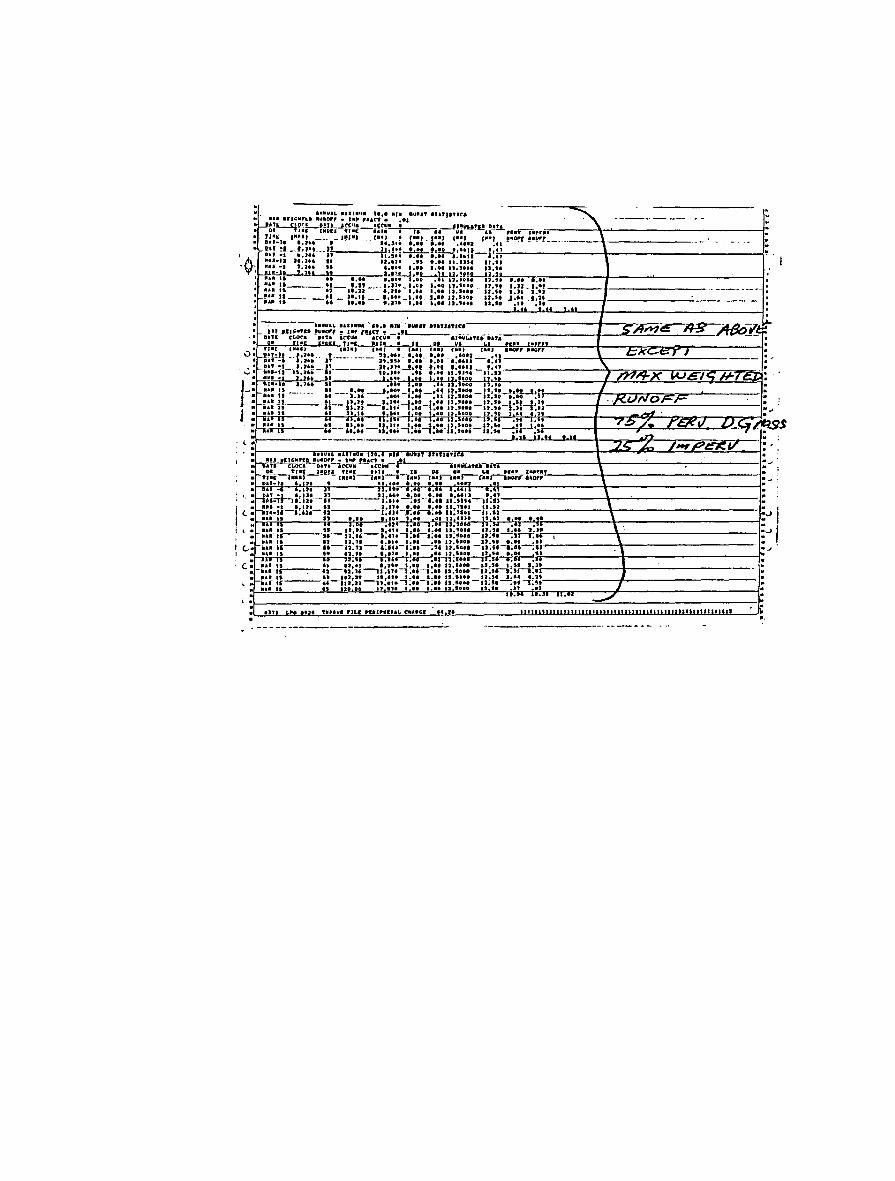
•••uaL au , .. .,. ••·• •r• eu•a" *"'"'aut'a """\ '" 1111 •I' ICIIft'LD fiUIIOI, • I liP PlaCI • . ,ea .

:~1'--'t~a-r~:~n::-u~~~~ : Ja u-'~j!.IY!I!L:.!!l. IU¥""ii-~rir----\-~--------------f ., ,.,.~ .... ., --· -11!1!1 .. ( .. J ~ .... , , ....... , .(1!'"1 !~0!"[ !•9f'.r __________ -\\ ________ _

:~;;-;: .... ::;::.~ .• ; ;:;:~; :::: ;;;;_,;::;;_!;:~ : 1 b.U •I "·"' )1 Jt,Stl t,•t l,lt l.t•IJ a.ic .. i----------+---------------~ A •u-n 11.:1u •• u .• ,.. .u •·•• u.nu u.u ·v·;~;-i: ;·;:: :: ;:;~:__t;~~;:;;::_:;:u

• ••• ,, •• •·•• •·••• 1 , 00 ·'' ,,,,.... u .. 't,.!-i"o.:Oooii""""io-..•"•~-----,1-----'---------'----1 : ::: ::---- :J-.::u ---· :::::-1::: :::: ::::::: · ::::: ::n-::::-------~-----------·----- ----­

~:: ~: ----::- ~::!: -- :::;: -J:::- t::: g::::: n::: .J:~: t:t: ------1--------------'...n

::, =~ ::~~: ~, ;;:::: :::: :::: ::::!; :::~-------------\-\-~-------------1= f-i~s;;rr,t~lu·--,,-----,~, .. -;ts--•~•• u~nu-·u;sJ \ (_ K~=·il-1::::- ;: f:H:~:::H!:: :::~:::-:: ::: -----------\------~-------1;, I

··: n :: ~::: •;:;i+.:~!:=~~:;'-!"~."il'r'~.~··r--------'\-,-,-------------1 l • ••• tt 11 u.n t,•u 1.10 •·•• u.so.. 11.:: •·•• 2.,,.•-;------~-------------I·.· . ..J ! • •·•·•_.----.,·- n~u--, ... ,.--.; .. -a; .. n;soeo-u;u--;n-,;et: \ (..: ::: ~~----::-n:;:-:::::-:;::-;;: g::::: -:t::-::::-;;;:~-------\------------- ... : ·:: :: :: ;~~;:+.:l--!::-H;;::H::•:;:•~·M•~::l"":--:.c;•:-•-------4-------------r.. c. • :,, tt ., nt•J o.u• •·•• •·•• n~U·•• :;:;; ;:;i 1.11 1 .. • ..... tr---:--u-n.u ·-u;n•• ~111:•• t2.to .. -u;s,.-,:n,;!!f---------lll-------------- • ~u 11 n tn.n aa,u• •·•• •·•• 12.••••_n!;•--.!!•:-:~~':-------~h-------------: ;. ~ ::~ :: :~-:::;::;:·:!: -~:::-:::: ::·:::: ::·,: :~, :.: J .. :~-----------------------------------'"-·· __ ·_··· __ ·· __ .... __ ._.~~~~~----------------~~~= C.!•:!"!l'U.!·".t'..t! •··••l!••u .. !!!!••~·!!•..!•:I•!:!...""!!"'!!!''t!"!!'•!! .. !!•w ... ~•!!•!!•'-. .1 '''!..'·.!!."' _______ JJ. ••u•l!uwu.t=uu!llJ ui!LUUllllllillll!llJI!L•Ulw"w'J:"W "W"W ".t"'U"IllJ • 'lll' u•lllJ "l!'---': . . -------------·-----~

The following briefly summarises the main components of the ARBM output:

•

•

At the end of each time increment, the duration of the inc~ement, ~he incremental rainfall and pan :vaporat1on are g1ven together with the water depth 1n each of the stores including interception, de­pre~s~on, upper, lower and groundwater. Add1t1onally, runoff depths are given for the groundwater and the pervious and impervious surface components. Where gauged peak flow data are avail­able, they are input and subsequently shown as output to allow volume checks between simulated and gauged data.

At the end of the detailed output described above, which is optional, a summary output is provided de­tailing a number of run statistics abstracted from the full run results. These include; an Accumul­ated Gauged and Simulated Runoff table in cubic metres to compare overall simulation; a Maximum Storage Depth summary - Winter and Summer; a table detailing the percentage time of moisture levels in the upper store being at certain levels; and a series of Maximum Event Burst statistics for up to four defined durations. The details of these last tables are given in the sample output shown earlier in the Chapter. In brief, fo~ each event duration, data is summarised up to one month before each event with accumulated rainfall and resident mois­ture store values being given 30 days, 5 days, 1 day, 12 hours, 1 hour and 30 minutes prior to the start of the abstracted maximum event under consi­deration. Three scans are carried out for each selected duration to find, in the total period, the maximum pervious, impervious and weighted runoff depths.

4.2.2.1 Urban Land Domains. For a model to predict total urban runoff behaviour it needs to be capable of discerning between different land types. These have been classified here as urban land domains.

In Canberra these can be broadly split into the fol­lowing groups:

(1} Residential lawns (incorporating areas of imported topsoil with sown grasses irregularly watered from domestic sources).

(2) Dry grass areas {generally associated with public open spaces adjacent to residential allotments. usually natural topsails and native grasses with little or no·artificial watering).

73

. (3) Irrigated playing fields (incorporating areas of 1mported sandy topsails with sown grasses irrigated on a regular basis from domestic sources).

(4~ Na~ive and planted forest areas (urban fringe areas 1nclud1ng parks and undeveloped areas such as Black Mountain nature reserve).

Soil moisture measurements weve taken during 1979 and 1980 on the Canberra urban catchments described in Chapter 3. The effects of lawn watering on residential allotments on a catchment wide basis was found to be marginal. Combi­ned, types (1) and (2) generally make ~p to 75% of the pervious area in any particular urban catchment and as such greater emphasis has been placed on these rather than types (3) and (4) in this thesis. Domains (3) and (4) have however been considered as in some areas they can be signi­ficant and it was necessary to assess, in particular, the effects of heavy watering of playing fields on runoff pro­duction.

The ARBM was subsequently used to simulate excess rainfall using Canberra pluviograph data recorded between 1933 and 1970 for domain types (1), (2), (3) and (4). The output from this analysis was used to assess the long term trigger mechanisms for runoff generation from these do-mains.

As indicated, the reference parameter set was taken from values suggested by Black & Aitken and closely resem­bled their published set for the Yarralumla Creek Urban Catchment in South Canberra. As described above using this set little, if any, pervious runoff was predicted.

Gauged rainfall/runoff data was obtained for the Gun­gahlin rural catchment for the years 1977, 1978 and 1979.

From that record it was very apparent that significant runoff was generated in each of the three years, none of which was abnormal.

Based on these records it was evident that there would be contributing runoff from similar pervious areas in the adjoining Giralang urban catchment.

From examination of the soil characteristics and grass cover within the Gungahlin catchment it was concluded that they closely resembled the typical dry grass and poor resi­dential lawn areas within the Giralang urban catchment.

Based on this premise it was possible using the three years of record available on Gungahlin to calibrate the ARBM for that catchment. The resulting parameter set which has been designated 'Dry Grass' is shown in Table 4-3.

As can be seen, it differs significantly from the ref­erence set (Table 4-2) and reflects the greatly reduced

74

infiltration potential required to match simulated and gauged runoff data. The reference set in fact predicted no runoff at all over the same three years.

Parameter

CAP IMP ISC DSC use LSC UH

LH

ER

FIMP

GN

KG

so A AO A1 LDF

ECOR

IAR

TABLE 4-3

DRY GRASS PARAMETER SET

Description

Impervious store capacity Interception store capacity Depression store capacity Upper soil store capacity Lower soil store capacity (Maxrate of water uptake from roots (for upper and lower soil stores Proportion of transpiration from US Proportion of catchment that is impervious Variable rate groundwater recession factor Constant rate groundwater recession factor Sorptivity Function of soil conductivity (Redistribution (parameters Lower soil drainage factor Ratio of Potential Evaporation to A class pan Proportion of rainfall intercepted by vegetation

V a 1 ue

.5 1.0 1.0

12.5 12.5 10.0

10.0

.7

.25

1.0

.94

4.5 .15

17.28 1.0 .os .7 .7

Unit

mm mm mm mm mm

mm/day

mm/day

mm/min 112 mm/min

4.2.2.2 ARBM Model Results. Figure 4-6 shows scatter diag­rams for respective simulated and recorded flows on a monthly, yearly and significant storm basis for the Gungah­lin catchment using the 'Dry Grass• parameter set based on data for 1977,78,79.

An objective function based on the~square of the dif­ference between the estimated and observed runoff, similar to that adopted by Black & Aitken (1977), was used to cali­brate the remaining sensitive parameters LSC, A1, LDF, DSC, ISC after the direct adoption of average measured values

75

for SO, A or Ko, to achieve a minimum value.

Calibration was carried out in an ordered fashion f~r~tly ob~ai~ing the best fit for monthly totals then in­dlvldual s1gn1ficant storm events and then, finally checking a~nual totals.

As can be seen from the diagrams shown on Figure 4-6, the sc~tter was sti~l sig~ificant after considerable parameter ad~ustment. It 1s bel1eved that finer matching would re­qulre structural changes to the program and/or variable parameters in place of the present constant values to better reflect seasonal effects.

The adopted parameter set for dry grass was used to simulate moisture changes during the period July 1979 through December 1979 as shown on Figure 4-7. Because of the scatter between individual dry grass station moisture levels above and below the simulated values, it was not possible to quantify if the fit was as close as could be expected. It was decided to leave the parameter set as it was and to test the overall tolerance of the estimate by testing its effect on model output in respect to changes in runoff volumes and runoff peaks. This is described later in Chapter 4.

Additionally during the observed period 1979 through 1981, there was considerable apparent interflow from the relatively small Gungahlin catchment occurring some hours after the cessation of rainfalls that could not be adequa­tely modelled using the ARBM.

Another problem would appear to be in the accuracy of the gauged runoff itself particularly at low flows. The gauging weir and instrumentation was not ~pecifically de­signed to measure small flows below .01 m js but rather to measure significant storm runoff. It was the accumulation of the low flows that made up the majority of the runoff and consequently calibration based on monthly or annual ac­cumulated flows was not necessarily the most appropriate and convincing method.

Based on appropriate parameter changes rela~ed to measurable catchment characteristics such as So and Ko, parameter sets were developed to represent residential lawns, irrigated playing fields and natural forested areas (Black Mountain).

As it was not possible to obtain individual gauged runoff data from these individual areas, use was made of the soil moisture gauging program described in Chapter 3 to help calibration in particular the natural forested area.

Residential lawns and irrigated playing field parame­ter sets were derived in a relative sense by varying SO and Ko parameters in line with measured values.

76

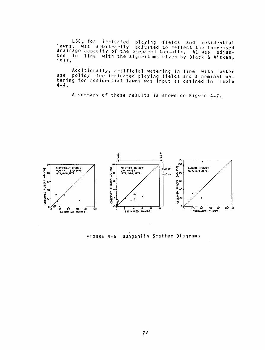
:50

~40 "'e ~30 z ~ a:20 0 ... ffi10

"' "' 0

0 0

LSC, for irrigated playing fields and residential lawns, was arbitrarily adjusted to reflect the increased drainage capacity of the prepared topsails. Al was adjus-ted in line with the algorithms given by Black & Aitken, 1977.

Additionally, artificial watering in line with water use policy for irrigated playing fields and a nominal wa­tering for residential lawns was input as defined in Table 4-4.

A summary of these results is shown on Figure 4-7.

A A 0 "! ~ N ...

110

10 100

SIGNIFICAI'IT STORMS 8 MONTHt.Y RUNOR' 31.4> 0 ANNUAL RUNOFF RUNOFF , 12 EVENTS DRY GRASS 2 1977. 1978 • 1979. 1977,1978,1979. -;a 1977,1978,1979. 20.1>

.:eo RE .!. Its :tso 0 0 z z ~ ~

a<4 "'40 0 0 ... ... > > ~2 :520

"' • "' "' 0 0

0 10 20 30 40 :50 4 6 8 10 0 20 40 60 so 100 110

ESTIMATED RUNOFF ESTIMATED RUI40FF ESTIMATED RUNCFF

FIGURE 4-6 Gungahlin Scatter Diagrams

77

lt .------..--------- --..- -··-- --- •

,_ loll

E 12 ~ Q. 10

~ sr-----1------+------~----~-----L~_.--J~ • :z :6t----r----t----+----4---.--l ~ 4r---~r-----1------~~~~~~~~HI

~21r.r-::-1t:-tr~,.-,l--1.---,d-U-JI.~

0 OCT NOV OEC

24

22

2.0

j•s 3•& ~14 :z ;;( 12 11::;

~•o :::!8 ..: 0

6

4

2

0

I

I. L I. ~ .. Jj .I E UN ~ULY

PAN - EVAPORATION

'· I I I

11 l LJ. I I T • OCT OEC

_DAILY RAINFALL-CITY GAUGE

·--- ---.--- ~ I

'

I L

-14 E -~Sit~ ~'!...J~ ~RATION J ~EL_ 1-

__,AVERAGED DRY GRASS READINGS .!. 12

~l) A. ..... 8 0

..... 6 a: ~ 4 ..... ., 0 2 2

0

...... H ~ 12 -j:IO

fi 8 0 .... 6 a:: i: .. 11)

6 2 ~

0

-•• •I • i.•

·~ V

"' ... -~ •2 . .. -t"l.

* - .. ~ ...(._ ..... •t ~I ~

<IUNE .AlLY AUS

1979

SI MU US IN

4

• •• \ """"'

t1 -\]\ \ \ •Z

1\ ' I _\ ... f\ '~! J \

\ , __

\ ·:. .. ... ..) ·-~--.

RI"T OCT NOV 0£C

GIRALANG- MOISTURE LEVELS

·I STATION ADJACENT TO CREEK

·2 IRRIGATED PLAYING FIELD

• 3 141516 DRY GRASS • 718 NATURAL FOREST

ATED MOfSl: URE LEV~~

~FALL ARIIW AN( DRY 6RA IIIC.II:.n <:IIC.I 0 GIRALANG F

•• ·-ltL wRL

«4

I 4 ....

-~AN n:a ~AAR AN

t980

X OVEN Dft'l'£0 SAMI"L.ES

• NUCLEAR SAMI"L.ES aAS£0 DIC MJISITT

-. MS. LAWN RANDOM SAWf'1..£

2. STATION Ne •

f-_fi!"~ED SATURA~~q_ VALUES ltELa.TE TO £0UIV4LEMT lfOISTVI'£ 0£1"TH (••) ~ TOI" 25- Of' SOIL.

SIMULATED MOISTURE DEPTH r USING ARIIM AND HAT. FOREST PARAMETER SET.CITY RAINFALL

•• •fL r--f--t• •• • I 7

. ••

.r-.J N - .. ·-··----r-J ·--'\. .!.• ~UN[ .IULY AUI S[I"T OCT NOV O£C f"[8 MAR

.. 80 11n

BLACK MOUNTAIN- MOISTURE LEVELS

FIGURE 4-7 Long Term (US) Soil Moisture Simulation

78

I

Table 4-4 shows the parameter sets developed for the fou: land domains studied plus the reference set for com­parlson. It may be noted that the reference set in fact most closely resembles the final set assigned to natural forest rather than the averaged dry grass/residential lawns that are present in the Yarralumla Creek catchment.

TABLE 4-4 Adopted Domain Based Parameter Sets

Parameter Ref Dry Res id* Irr1g.** Playing Natural

Set Grass Lawns Field Forest

CAP IMP 0.5 0.5 0.5 0.5 0.5 ISC 1.0 1.0 1.0 1.0 1.0 DSC 5.0 1.0 1.0 1.0 1.0 use 12.5 12.5 12.5 12.5 12.5 LSC 200.0 12.5 25.0 25.0 100.0 UH 10.0 10.0 10.0 10.0 10.0 LH 10.0 10.0 10.0 10.0 10.0 ER 0.7 0.7 0.7 0.7 0.7

FIMP GN 1.0 1.0 1.0 1.0 1.0 KG 0.94 0.94 0.94 0.94 0.94 so 7.0 4.5 10.0 10.0 10.0

A 0.5 0.15 0.3 0.42 0.15 AO 57.0 17.28 17.28 17.28 17.28 AI 0.063 1.0 0.5 0.5 0.125 LDF 0.05 0.05 0.05 0.05 0.05

ECOR 0.7 0.70 0.7 0.7 0.70 IAR 0.7 0.7 0.7 0.7 0.7

* Additionally, .05 mm/hr domestic lawn watering was ap­plied over the summer months.

** Similarly, .23 applied over the winter period.

mm/hr domestic irrigation water was summer months plus .115 mm/hr over the

As it was the aim of the long term continuous model­ling exercise to find a pattern to express, in particular, pre-storm burst antecedence, several sets of statistics were derived and included in the output. As model runs were carried out on an annual basis, purely for data size and computer storage reasons, the summarised statistical data was also expressed in annual terms where appropriate.

Table 4-5 summarises for •Dry Grass• abstracted output data relating to 30, 60 and 120 min burst events between 1933 and 1970 excluding 1962-1965 inclusive, when data was unavailable due to instrument malfunction. The ARBM model

79

was run in annual data segments with each end of year store status transferred as input to the following year. As stated above the parameter set chosen was the dry grass one shown in Table 4-4 and the rainfall was taken from 'the Yar­ralumla Station. Table 4-5 therefore represents a semi-contin~ous simulated run over 33 years using Yarra­lumla rainfall and evaporation transposed over the pertinent section of the Giralang catchment.

80

TABLE 4-5 Annual Maximum Rainfall (Yarralumla) and Annual Maximum Simulated Pervious* ·

Excess Statistics

30 MIN BURST 60 MIN BURST 120 MIN BURST YEAR Date Date * Date Date * Date Date

Rain Excess Rain Excess Rain Excess

1933 Nov 18 Sep 1 Nov 18 Sep 1 Nov 18 Sep 1 9.74 2.83 18.05 4.69 19.92 7.09

1934 Jan 29 Oct 25 Oct 25 Oct 25 Mar 17 Oct 25 17.62 10.23 22.78 19.10 26.37 20.13

1935 Nov 13 Dec 3 Nov 13 Dec 3 Jan 12 Apr 14 17.16 6.80 17.65 6.90 20.36 9.57

1936 Dec 2 ·Aug 3 Jan 4 Aug 3 Aug 3 Aug 3 6.90 1.21 8.23 2.43 10.57 4.86

1937 Dec 27 Oct 16 Oct 16 Oct 16 Oct 16 Oct 16 10.37 8.43 13.08 10.03 16.95 10.21

1938 Feb 22 Feb 22 Feb 22 Feb 22 Feb 22 Feb 22 16.83 8.49 25.08 9.20 29.93 9.20

1939 Jan 20 Jan 20 Jan 20 Jan 20 Jan 20 Jan 20 19.46 14.42 22.84 15.51 25.11 15.51

1940 Apr 12 Apr 12 Apr 12 Apr 12 Apr 7 Apr 12 17.26 15.71 23.18 19.97 31.32 24.06

1941 Jan 16 Jan 3 Jan 1 Jan 3 Jan 16 Jan 3 7.56 3.32 10.26 5.49 15.84 7.98

1942 Mar 9 Mar 9 Mar 9 Jun 19 Mar 9 Jun 19 18.13 3.31 27.00 4.44 30.22 5.33

1943 Dec 18 Dec 18 Dec 18 Dec 18 Dec 18 Apr 13 18.72 6.94 18.86 7.63 20.90 9.15

1944 Jan 1 Jul 4 Jan 1 Jul 4 Nov 24 Jul 4 15.71 3.53 15.69 3.53 18.76 3.53

1945 Feb 19 Apr 9 Feb 19 Apr 9 Feb 19 Apr 9 21.95 7.75 27.47 13.07 32.38 20.88

1946 Apr 22 Nov 19 Apr 22 Jan 18 Apr 22 Jan 18 8.65 4.82 12.18 5.45 17.45 7.97

1947 Dec 15 Dec 15 Dec 15 Dec 15 Oec 15 Dec 15 24.59 22.97 38.92 35.37 41.35 35.37

1948 Jan 27 May 3 Jan 27 May 3 Feb 15 May 3 21.66 10.42 27.00 18.42 31.28 22.59

1949 Nov 21 Nov 21 Nov 21 Nov 21 Nov 21 Nov 21 7.54 5.81 13.82 10.05 20.03 10.82

1950 Mar 22 Mar 22 Nov 9 Mar 22 Nov 9 Nov 9 13.33 10.38 17.15 12.29 30.08 23.04

1951 Feb 23 Feb 23 Oct 3 Aug 3 Oct 3 Aug 3 11.74 3.97 13.91 4.28 18.56 6.26

1952 Dec 28 Mar 20 Oec 28 Mar 20 Mar 21 Mar 21 13.53 7.58 16.84 10.46 21.04 13.28

1953 Apr 13 May 4 Apr 13 May 5 May 5 May 5 9.47 3.13 12.12 5.69 15.64 8.66

81

*

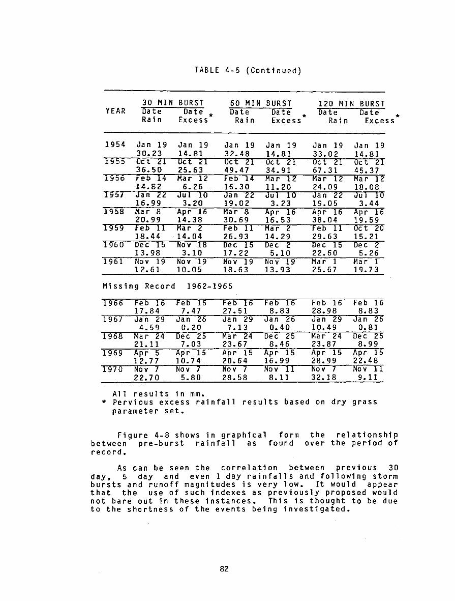
TABLE 4-5 (Continued)

YEAR

1954

1955

l c:;-__ o

1957

1958

1959

1960

1961

30 MIN BURST Date Date * Rain Excess

Jan 19 30.23 Oct 21 36.50 Feb 14 14.82 Jan 22 16.99 Mar 8 20.99 Feb 11 18.44 Dec 15 13.98 Nov 19 12.61

Jan 19 14.81 Oc t 21 25.63 Kar 12

6.26 Jul 10

3.20 Apr 16 14.38 Mar 2

. 14.04 Nov 18 3.10

Nov 19 10.05

60 MIN BURST Date Date *

Rain Excess

Jan 19 32.48 Oct 21 49.47 Feb 14 16.30 Jan 22 19.02 Mar 8 30.69 Feb 11 26.93 Dec 15 17.22 Nov 19 18.63

Ja n 19 14.81 Oc t 21 34.91 Mar 12 11.20 Ju 1 10

3.23 Apr 16 16.53 Mar 2 14.29 Dec 2 5.10

Nov 19 13.93

Missing Record 1962-1965

1966

l967

1968

1969

1970

Feb 16 17.84 Jan 29 4.59

Mar 24 21.11 Apr 5 12.77 Nov 7 2 2. 7 0

Feb 16 7.47

Jan 26 0.20

Dec 25 7.03

Apr 15 10.7 4 Nov 7 5.80

All results in mm.

Feb 16 27.51 Jan 29 7.13

Mar 24 23.67 Apr 15 20.64 Nov 7 28.58

Feb 16 8.83

Jan 26 0.40

Dec 25 8.46

Apr 15 16.99 Nov 11 8.11

120 MIN BURST Date Date *

Rain Excess

Jan 19 33.0 2 Oc t 21 67.31 Mar 12 24.09 Jan 22 19.05 Apr 16 38.04 Feb 11 29.63 Dec 15 22.60 Mar 1 25.67

Feb 16 28.98 Jan 29 10.49 Mar 24 23.87 Apr 15 28.99 Nov 7 32.18

Ja n 19 14.81 Oc t 21 45.37 Mar 12 18.08 Ju 1 10 3.44

Apr 16 19.59 Oc t 20 15.21 Dec 2 5.26

Mar 1 19.7 3

Feb 16 8.83

Jan 26 0.81

Dec 25 8.99

Apr 15 22.48 Nov 11 9.11

* Pervious excess rainfall results based on dry grass parameter set.

Figure 4-8 shows in graphical form the relationship between pre-burst rainfall as found over the period of record.

As can be seen the correlation between previous 30 day, 5 day and even 1 day rainfalls and following storm bursts and runoff magnitudes is very low. It would appear that the use of such indexes as previously proposed would not bare out in these instances. This is thought to be due to the shortness of the events being investigated.

82

Table 4-6 shows predicted annual upper soil storage values for the dry grass parameter set, as well as the ref­erence one.

Annual maximum upper storage moisture levels (US) were extracted for both the summer and winter periods to test seasonal sensitivity. Table 4-6 shows a general ten­dency for lower summer values than winter although the differences are not great. This was generally in agreement with observed data. Rainfall intensity parameters followed the opposite trend with higher summer than winter values. See Pierrehumbert (1974).

As can be also seen from Table 4-6 upper store satur­ation using the reference set was the exception rather than the rule. This was due mainly to the infiltration capacity attributed by the reference parameter set. Table 4-3 lists the parameter set derived from three years of simulation on the Gungahlin rural catchment. Based on this latter param­eter set catchment saturation levels were observed in the simulated run on much more frequent occasions, certainly more frequent than annually.

83

90

eo

e 70 .§ ... C/) a: :::> m ... 60 z w .> w 0 ... !>0 a: 0 a: A. _, _,

40 < ..... z < a: w > 30 i= < _, :::> ~ :::> u 20 0 <

10

0

r:• AU lli RAIN

: SIGN IF JCANTLY D >90(mml + • UPPER STORAGE • • ;;:; SATURATED

~ •

•

EFFECTS OF ANTECEDENT RAINFALL ON ANNUAL MAX. 30 MIN. PREBURST 0

MOISTURE LEVELS (BASED ON SIMULATED DRY GRASS AREA 1933-1971) +

D

• • 30 DAY ANTECEDENT FALL 0

+ 5 DAY ANTECEDENT FALL + D I DAY ANTECEDENT FALL

D

• +

Ill + + 0

0

+ 0

0

0

2 3 4 5 6 7 e 9 10

UPPER STORAGE MOISTURE LEVEL (mm) AT START OF BURST

FIGURE 4-8 Antecedent Rainfall - Pre Burst Moisture Scatter Diagram for Simulated

Max. Annual Pervious Runoff Events.

84

0

+

D

11

.... . ~~ -.

0 0

D

lo

t •to 0

0 t ~

~ + i3+ ~~ fo~c

ro J

0 I col

12 125

TABLE 4-6

Maximum Annual Upper Soil Storage Levels 1933-1969

REF SET DRY GRASS FORESTED AREA

Year Summer Winter Summer Winter Summer Winter

1933 4.35 7.30 12.49999 12.49999 5.05 10.02 1944 5.83 10.52 12.49999 12.49999 9.96 12.49999 1935 6.47 7.40 12.49999 12.49999 7.87 10.29 1936 5.38 7.20 12.49999 12.49999 7.85 9.75 1937 3.08 6.22 12.49999 12.49999 7.76 8.06 1938 4.88 5.05 12.49999 12.49999 6.15 6.31 1939 5. 9 3 6.91 12.49999 12.49999 9.04 7.47 1940 10.11 6.66 12.49999 12.49999 12.49999 7.64 1941 7.08 3 .. 00 12.49991 12.11 12.48 3.66 1942 2.61 7.56 12.49999 12.49999 5.19 9.71 1943 5.39 6.08 12.49999 12.49999 1944 3.36 3.85 12.49999 12.49999 1945 7.54 4.61 12.49999 12.49999 1946 4.67 6.28 12.49999 12.49999 1947 10.11 6.87 12.49999. 12.49999 N N 1948 11.22 12.37 12.49999 12.49999 0 0 1949 4.33 6.67 12.49999 12.49999 T T 1950 12.49999* 12.49999 12.49999 12.49999 1951 3.29 5.97 12.49999 12.49999 R R 1952 8.53 9.30 12.49999 12.49999 u u 1953 2.77 8.66 12.49999 12.49999 N N 1954 4.63 4.57 12.49999 12.49999 1955 4. 7 5 8.16 12.49999 12.49999 1956 8.59 12.42 12.49999 12.49999 1957 3. 7 5 4.12 12.49999 12.49999 1958 8.35 8.11 12.49999 12.49999 1959 8.20 12.11 12.49999 12.49999 1960 6.22 6.52 12.49999 12.49999 1961 9.22 11.22 12.49999 12.49999

1966 5.92 5.87 12.49999 12.49999 1967 3.26 4.30 12.49999 12.49999 1968 6.08 9.76 12.49999 12.49999 1969 9.04 9.81 12.49999 12.49999

* 12.49999 = Effective Saturation

85

The ARBM modelling algorithms in fact do not allow the upper soil store to become fully saturated. The model op­erating in discrete time steps and the moisture storage being calculated at the end of the increment means that the last operation is an infiltration and redistribution move­ment from the upper store to the lower store thus preventing full saturation.

Rather than simply simulating excess runoff over an extended rainfall period and then carrying out a frequency analysis on the output, it was the objective of this thesis to gain from long term simulation an index or indexes suit­able for a particular pervious catchment type that could be transposed between similar catchments. Although it was hoped that gauged catchments could be used to help cali­brate modelling parameter sets it was also hoped that the normal non-transportability constraints of mixed pervious­impervious urban catchments frequency analyses could be overcome by isolating the separate major pervious and im­pervious inputs for use on other similar catchments with different area proportions. This would also allow subse­quent analyses or designs to be made on an event basis rather than the more tedious and expensive continuous mo­delling basis.

It was plainly obvious that the traditional antecedent index based on previous rainfall over a defined period and a catchment parameter was unsatisfactory for urban runoff design analyses. Therefore it was proposed to define an antecedent moisture index based on the sequence of histori­cal events to use in a design context.

4.2.2.3 Development of an Antecedent Moisture Index. An improved index would necessarily need to relate to the catchment parameters affecting the soil moisture profile both on a short as well as long term basis and would sec­ondly need to describe in a statistical sense a relationship with the long term historical rainfall/runoff sequence.

Two antecedent Moisture indexes were proposed at this stage. The first was based on annual maximum upper soil store values. An annual series frequency analysis was car­ried out on this data to define appropriate frequency curves. Figure 4-9 shows the results of this analysis for the reference set plus the dry grass and forested parameter sets.

86

E E -t-z lLJ t-z 0 (.)

0:: lLJ t-<t ;: _J

0 (/)

0:: lLJ D.. D.. :::>

20

tg 8 7 6

5

4

3

2

I 99.9

sLJon 11 Jsml DRY GRAS ,.J FOR~T-"\ ~

~ ~ - A

\ ....- ,. ..,... /.

....- .......: .. 2

.... ~ ..

V ~ < . ;:...-"" '\._ / REFERENCE SET

/. v. .

y·

99.8 99 98 95 90 80 70 GO 50 40 30 20 10 5 % PROB. OF EXCEEDANCE

FIGURE 4-9 Probability Curves for Index Type I

87

2

100.0

DRY GRA~ s (J) 11:33-1942 -E ® 1943-1952

E - ~ 1953-1966

® 1933-1970 SATURATION LEVEL 12.5 mm ....

~ 10.0

0 /V' u ;y

V-;,1

h t?' ~ '2' /, '/ !'Cl

a:: w .... < ~

1®-@-~ ~ 'T'

'-J

J 0 Cl)

1.0 a:: w

117 R: ::1

0.1 99.99 99.999.8 99 98 95 90 eo 10 ro 50 40 30 20 10 :s 2 1 0.5020.1 0.01

100.0

! .... ~ 10.0 .... z 0 u a:: w .... ~ J g a:: 1.0 w c. c. ::1

0.1

Y. PROB. OF EXPOSURE TIME

(a)

OMPARISON OF SOIL MOl STURE CURVES FOR DIFFERENT LAND DOMAINS

J

cp SATURATION U VEL 12.5 mm

L.-- !"""

./ ./' k"":

./ V /

i®-17" ~ V -<..... ®

/ / ~ ~ Vj ~ CD OR GRASS

2)~ ._RESIDENTI L LAWN

I ./ ® NATURAL EUCALYPT. FOREST / ./ ./

~ IRRIGATED PLAYING F"EILD-

BASED ON RECORDS 1933-1942.

93.99 99999.8 99 98 95 90 eo 10 605040 30 20 10 5 2 r 05020.1 001

•;. PROB.OF EXPOSURE TIME

(b)

FIGURE 4-10 Probability Curves for Index Type 11

88

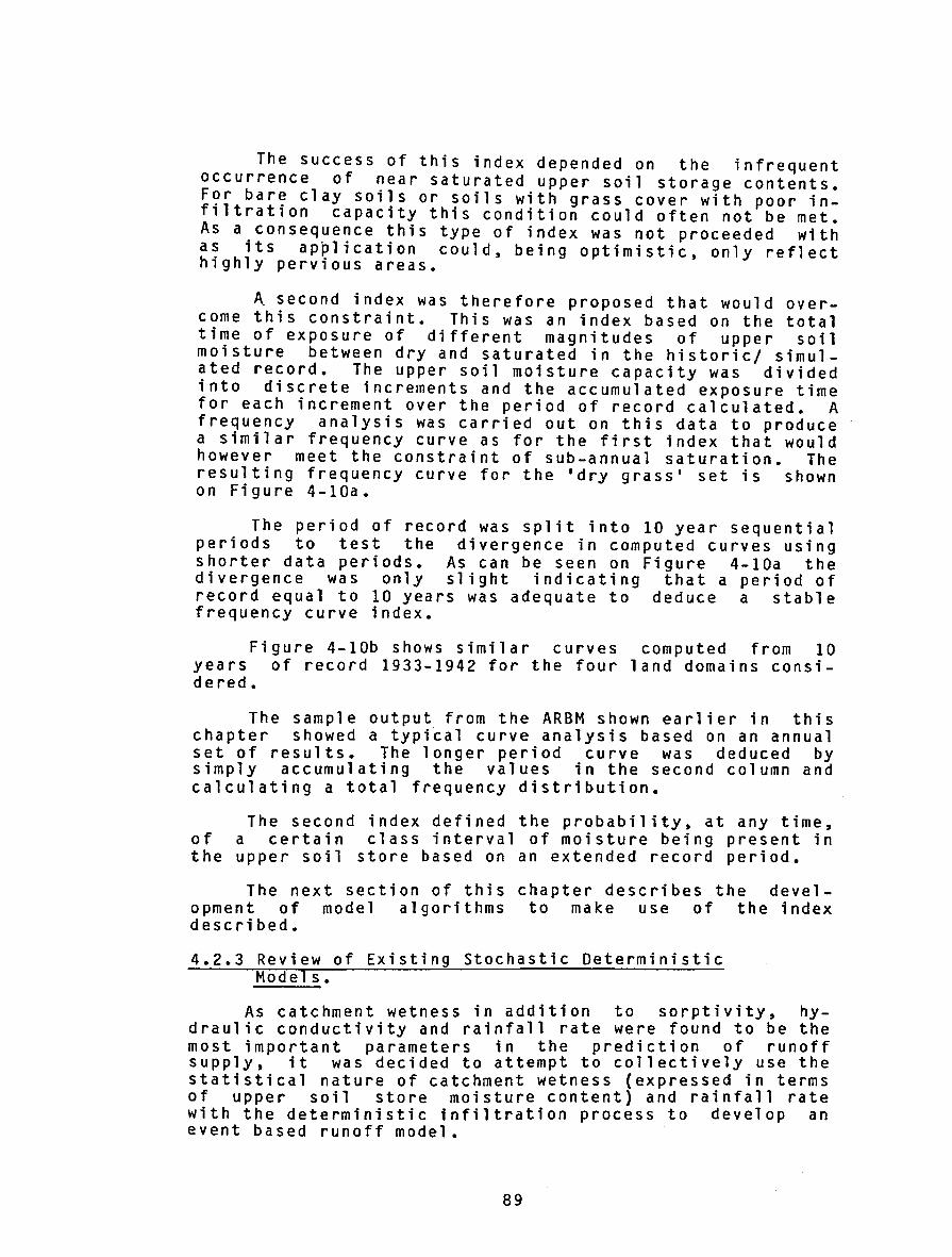
The success of this index depended on the infrequent occurrence of near saturated upper soil storage contents. F?r bare clay soils or soils with grass cover with poor in­flltration capacity this condition could often not be met. As a consequence this type of index was not proceeded with as its application could, being optimistic, only reflect highly pervious areas.

A second index was therefore proposed that would over­come this constraint. This was an index based on the total time of exposure of different magnitudes of upper soil moisture between dry and saturated in the historic/ simul­ated record. The upper soil moisture capacity was divided into discrete increments and the accumulated exposure time for each increment over the period of record calculated. A frequency analysis was carried out on this data to produce a similar frequency curve as for the first index that would however meet the constraint of sub-annual saturation. The resulting frequency curve for the 'dry grass' set is shown on Figure 4-10a.

The period of record was split into 10 year sequential periods to test the divergence in computed curves using shorter data periods. As can be seen on Figure 4-10a the divergence was only slight indicating that a period of record equal to 10 years was adequate to deduce a stable frequency curve index.

Figure 4-IOb shows similar curves computed from 10 years of record 1933-1942 for the four land domains consi­dered.

The sample output from the ARBM shown earlier in this chapter showed a typical curve analysis based on an annual set of results. The longer period curve was deduced by simply accumulating the values in the second column and calculating a total frequency distribution.

The second index defined the probability, at any time, of a certain class interval of moisture being present in the upper soil store based on an extended record period.

The next section of this chapter describes the devel­opment of model algorithms to make use of the index described.

4.2.3 Review of Existing Stochastic Deterministic Models.

As catchment wetness in addition to sorptivity, hy­draulic conductivity and rainfall rate were found to be the most important parameters in the prediction of runoff supply, it was decided to attempt to collectively use the statistical nature of catchment wetness (expressed in terms of upper soil store moisture content) and rainfall rate with the deterministic infiltration process to develop an event based runoff model.

89

In this manner it was proposed to present a method whereby .after an initial ~ong term water balance analysis was carr1ed out for the reg1on, frequency based estimates would be possible, taking into account the combined effects of antecedent moisture and rainfall for design or analysis.

The basic principle behind this phase of the work was to incorporate joint probability theory to link rainfall and catchment wetness.

It was proposed to apply, if possible, a simplified joint probability technique combined with a deterministic element describing infiltration based on similar methods to those described by Laurenson (1974) for water resources systems and confluence studies.

The effects of catchment wetness on the estimation of excess rainfall for design events have been discussed by others, including Cordery (1970) described earlier, Larson (1965) and Beran (1973). Beran (1973) investigated the un­certainty of preserving the nominal rainfall return period in the design flood. He considered the sensitivity of flood magnitude to variations in return period, storm dur­ation, temporal pattern, infiltration loss rate, base flow and unit hydrograph shape. The sensitivity analysis al­lowed for an estimate to be made of any quantity of the distribution of flood magnitude based on sampling across all significant rainfall events resulting in runoff and an­tecedent conditions.

A Catchment Wetness Index (CWI) was computed by Beran using the procedure described by the British Meteorological Office and a five day antecedent precipitation index (API5) using a daily decay constant of 0.5. The formula was:

CWI = 125 - SMD + API5 {4-1)

where SMD = soil moisture deficiency

Beran in a previous study (Beran & Sutcliffe, 1972) observed that wet day rainfall and SMD were statistically independent. He also noted that small changes in the CWI had a marked effect on the resulting flood.

Beran also used joint probability theory to carry out the analytical phase of his study.

Most of the work carried out by Beran as well as Cor­dery related to rural catchments and did not include the additional complications of urban systems.

Russel et al {1979) presented a similar joint proba­bility approach to the estimation of design flows for an urb~n drainage study in Surrey, Canada. They presented the following equation to estimate flow peaks:

90

P( Q ) = 2:; , j , k P ( Q , T i , V j , I k ) p ( T i ) p ( V j ) p ( I k ) ( 4- 2)

w h e r e P ( Q , T i , v1 , I le ) = c o n d i t i on a 1 p r o b a b i 1 i t y o f Q be i n g exceeded g1ven tnat T., v. and Ik occur; and p(T.), p(V.), P ( I 1c ) = pro b a b i 1 i t i e s b f T~ , R . a n d I k o cc u r r i n g • 1 The p to­babTlities were assumed lo b~ independent of one another. T =time of concentration, I = infiltration rate (mm/hr) and V = basin storage constant for an assumed linear reser­voir.

In general, Russel et al used a simple rainfall/runoff model (Clarke, 1943) to analyse sixty major storms in the fifteen years of rainfall record. These storms were run through the model using a standard basin time/area curve for each of 120 different combinations of the parameters T, I and V. The resulting peak flows per unit area for each combination were then plotted on Gumbel probability paper (one plotted line for each combination). From there proba­bilities of exceedance of fifty (50) specified flows were measured. The exceedance probabilities were stored in matrix form with fifty (50) rows - one for each of the specified peak flows and 120 columns - one for each combin­ation ofT, I and V.

Fro m the· stored data , pro b ab i 1 i t i e s of exceed an c e of the stored flows in any particular drainage basin could be computed if probability distributions of the parameters T, I and V were provided using the above equation.

The method was arranged to accept either probable high and low estimates, or single values of each parameter. It appeared therefore that it was necessary for the designer to supply estimates of T, I, and V, all of which in the form described are somewhat difficult to estimate and even more difficult to physically measure.

The methods proposed by Russel et al showed the neces­sity to consider the statistical components of the major parameters in the rainfall/runoff process where accurate design estimates were to be made. The method as described, although referring to an urban catchment, considered a wat­ershed as a lumped unit rather than the accumulation of individual land domains proposed in this thesis.

91

4.2.4 Development of SDRRM Model

This chapter draws on a number of the aspects from the preceding author's work to combine the stochastic compo­nents of soil moisture and rainfall intensities (based on local measured and simulated data) with the deterministic infiltration component currently used in the Regional Stormwater Drainage Mod~l, RSWM, to obtain excess rainfall and flood frequency distributions. The methods were to in­corporate the different land domains described earlier and be capable of assessing imbedded storm bursts. The model was called a Stochastic/Deterministic Rainfall/Runoff Model (SDRRM).

The model development generally followed the techni­ques described by Laurenson (1974) involving the use of joint probabilities and the formulation of appropriate transformation matrices to link the probabilities of oc­currence of the various input parameters together.

The approach recognised the roles of both the stochastic and deterministic components in the analysis. The deterministic component in this thesis consisted of Philip's infiltration algorithms and the combined moisture storages defined in the ARBM.

In summary the modelling system proposed, shown diag­rammatically on Figure 4-11, had as input (Rainfall "R") and output (Excess Rainfall or Peak Runoff "Qo"). The input was transformed to the output by a transformation function representing the deterministic components of the system. In this case the transformation depended also upon the value of an additional input defined here as a "parame­ter" (Antecedent Moisture "M"). Input, output and the parameter were the stochastic elements of the system and had probability distributions.

92

~------------------------INPUT------------------------l

0

DIMENSIONLESS DESIGN STORM TEMPORAL PATTERN

DETERMINISTIC 95 RAINFALL LOSS -

...,: ROUTING PROCESS

~ \ \ \ \o \o ...J

0 (/)

EXCESS OR P~K RAINFALL RUNOFF

\\ 4o

20 0

UPPER SOIL WETNESS INDEX

...,: FREQUENCY ~ DISTRIBUTION.

...J

0 (/)

RAINFALL FREO. E DISTRIBUTION E "X" MINIMUM 3 DURATION. :t z ex a: ....: 0 1-

'-------'--- 0-f----....J.....-....J.....-~~

0 100 99.99 0.01 99.99 0.0 "X" MIN. DURATION RAINFALL INTENSITY. 0/ 0 PROS. OF EXCEED. % PROa OF EXCEED.

(

y CONDITIONAL

PROBABILITY

TRANSITION

MATRIX

X

I CONDITIONAL

RAINFALL

PROBABILITY

ARRAY

OUTPUT~-------------------------l

~r----------------.

~ EXCESS ":J RAINFALL i_ FREQUENCY w: DISTRIBUTION z <i a: (I) (I) w u X w

30-39.9 mm 99.99 O.QI DIMENSIONLESS EXCESS RAIN % PROS OF EXCEED.

TEMPORAL PATTERN

10 ~ .....

E

:X: <I

lt' lt 0 z :::> a:

99.99 0.01 % PROS. OF EXCEED.

FIGURE 4-11 Digrammatic Representation of the SDRRM Model

93

Using Laurenson's definition, the system here was a concentrative determinate process with one independent par­ameter.

The probability distribution Rand M was determined by frequency analysis based on recorded and/or simulated data described earlier where M equalled the anticedent moisture Index.

The deterministic transformation was derived from a matrix of rainfall vs excess rainfall and peak runoff for a range of antecedent conditions from dry to saturated based on the ARBM infiltration algorithms and the RSWM.

Based on the above matrix, conditional probabilities of the parameter M for a range of (excess rainfall or peak runoff) total rainfall amounts could be deduced.

The objects of the model as proposed were to determine the probability distribution of flood peaks and/or runoff volume (qo1 ) from a known probability distribution of rain­fall of duration D and a known probability distribution of soil moisture representing catchment antecedent moisture (mk) and a known deterministic transformation to relate ra1nfall to excess rainfall or peak runoff.

Model output (Qo) was achieved by the matrix multi­plication of an input probability distribution R = (ri) with a matrix of transition probabilities A= [aji] defined by the estimation of conditional probabilities Tor a range of excess rainfalls or runoff peaks and a range of antece­dent conditions, ie:

QO = A X R

or (qoj)m = [aji]m x (ri)f

(4-3)

(4-4)

where m and f are the dimensions of the vectors representing the probability distributions of output and input respectively.

The matrix A reflects the deterministic component of the system. Based on the work carried out by Beran and Sutcliffe, (1972) it was assumed that antecedent moisture content (M) and the following rainfall distributions were independent events.

As defined, the output Q equaled the multiplication of the input with a matrix of transition probabilities A, the latter being defined as follows:

(4-5)

Any particular value of the antecedent moisture param­eter m gave a one to one transformation of r t? q. The conditional distribution of q given r = R; cons1sted of unity and a set of zeroes, ie, a concentrat1ve process.

94

There was a conditional distribution of qo not only for each possible value of r but also for each possible value ?f.m. Each possible value of m, say Mk had a certain probab1l1ty mk. Therefore the probabilities a .. became:

J 1

aji = ~kbjik x mk (4-6)

where biik is the conditional probability of an given inpUt Ri and a parameter value Mk, ie:

output Qo. J

bjik = Pr (qo = Qoj/r = Ri, m = Mk}

Figures 4-12(a}, (b), (c), (d), (e) and the typical process.

(f)

(4-7)

describe

Figures 4-3 and 4-10 show typical exceedance probabil­ity distributions for rainfall (R) and an antecedent moisture index (M}. The rainfall distributions are in re­spect to the Canberra region and of 18,30,60 and 120 minute durations respectively.

A typical output from the SDRRM is given below for a 30 minute duration event on an urban catchment with 75% dry grass and 25% impervious content in Canberra, together with a program listing and input data stream.

Figure 4-12{a) shows matrices indicating the relation­ship between rainfall and excess rainfall.

Figure 4-12(b) represents the transition matrix A with individual elements calculated using equation 4-6 and Figure 4-10 by equating r and q to give Mk. mk was then deduced from Figure 4-10 with m = Mk.

Conditional probabilities were then deduced from the above exceedance probabilities to form the aji elements of the transition matrix.

Figure 4-12{c) shows the transition matrix A together with the rainfall conditional probabilities corresponding to the values of R. shown. The matrix multiplication of A x R provided the r~quired output Qo, the excess rainfall or peak runoff conditional probability array.

Figure 4-12(d) shows the output of Figure 4-12(c) con­verted to exceedance probabilities.

95

' '

. .

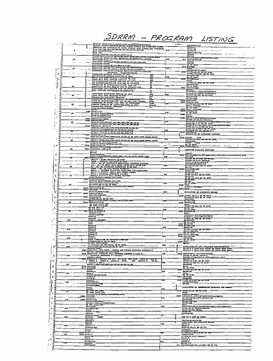
.1..151!/IJG

.. !!.- ti:ID( lt,IUitCAPJJtP,UC,DIC',UK,L.aC._,,;ooi;,~IA;:•:;•ia--------1-------;~t;~:u: •• I) ~ TO u,,;T,'nn<....,nlwt'IO .... ...--------------IIII'flri;'MnJCIPJ•r.T'ICfll~fii,La,ii aTOnensc•YITi'lGir-NJ'fiDA•OIJMI• fnt f'OI'•nu• ,•r••·•• nnr.ct.u.n eo to nu,.--------------------'= !!:~::::~~:::::::;::::::~:i!:::L:~,~G:'''* •1n :::::;!::~;~::;~;:a;~::·

: ~. ------------=~:.,~ . .----------------------;------1J~~-:;:::~:.,Itr-----------------.--• Llle•t.l . ....,. 11-•tJS•UI

: . -~--··• ~:~:::. ::!r~::::;~p-nr»" (I.Pa•t.l 152. u.(l .. •l:lt!'OH~·-----'-------------111 -,. ••• ~!!._ _____________________ , .... -----» .. ,. ~~!f:r..

"----!!!.---r--:::::!:PaUliOI W litiiiiU PIIXU ., Jt .. :~r.a-nlr-------------------• •rn•••t.ao.u eo 1'0 ••n

• '• I""JIL,~ JG nn 1"~- f- .;;::: .. no• rW •on. -.ouNar-atDU'fllllf'fto• 'f'; - ltl .. ·-· :n::::::;!.:.i:ft, .. n f(l 4111 t ao.Gt.l a fL41 hOW UPPU tU Lbhi SOIL lUll

1 1 tMI FOU.t.TCi. :::1,•1.1U 1 II'Ottll a•O IICUI IIUJ'IIol.. aVfll•ut•J) i ~--·0.&.1:!! !!:'!I!..!!U. a.a•1a 90 IIIPIC.& 141&. 10.••

I. .. : •••• r!!!!::;:•::::::~:·:o!!•::n:,u•• Nlltcn. •,rs.a '!!!._~---.--!!!! ;~::;:;:~::;;~:::;:!:!'~' ... !:!!'-------------c. :l--all------~~;~::"::,:~r;!!~~;~:•n•rr<'"Urlll1n...,•n"rrr,r-,r;>urlTD'ICO'""..,rTn1'-,TI'I,...,,....,..,..,--f------~·,_cva·a.••u·nJ•.c • .-c•Pl·•oJ Jn •·••u

QYn• r~~;•:~uu ~."",,•0i1101>fi•'<l.•0 . 01 CD ...... (·: a • .,,.;a·;' i.o••• a cnow 1 aJ•r ur auu•' aDuT ... :._ ____________ _

: --- a21 '.;~::::~~:;~:;::~ .. N.-.. ••• oa.ua.u.ca "' --------E:~;r!.a_._.,_-_ .. _•_•_•_'_'" ______________ _ C: --a---·--::!r:::::~: CO TO llU

!.-----------------------------~-----~! -----·---~=!;~~--------~---------------------c: ---n• ..... ·-----~::;::::!!·~ .. !:·~ ... !.•!!•~·---------------------··- -------,n• ~=-~.::~!.. _____________________ _ ( ! ::~:=~~ UhU.S~··~·~ ................ ,.., ...... -------------~ 1

un ;!!:;f ... =~• ea Will~ ~ • OT•;:Ouuae. -- -~- ... N•NC-·---~~---'-----------------,1 : --· ~!! -· "'---•n•t.un•-'JD e

I. a · U.OWfii•Out - e·- aUIL&IlOII- a,.-·CIDIRI"DWiftf""""'PCI'IKIAU"atlfOI' c.· .. -------·----n•··--· ,., r J .. . llt•ll fi•O• • • - TV

i L: n• DCI toe.: ~aia.nl I•&OICJ•UI,/ .. ('".---~--------------~ : •••• ~~~:~:~: r_ ..... _•_••_•_•m_"" __ •_•_.,_•_•·-'-"-'----------:----ar.• --- ~---~,!a ~;:~!~~!;;;~~CI!':~;:~:;;.!::u!!'~'"!!2'~.,~---------

l (: ---~~.-------;.;; ::;::::::, ..... ~~:· 11 .,l."T U•Ciiti.H'!_ _________________ __, __

, ( : -::!:~~ li~!:-::-'""_·_·~-·-u_·_ .. _._,_··-·--------.,--------'··''"'------- :~:.:=-..~~f(fl'ei •• CIIUG•GI••tCII•I J•trt•IHTt"trJ a Pr•fi.JJ.,U ;w - JrtCJ..CiT;IJ-CI•C•/CII .. COII

, ( a • ·-- Ill '•JIOU111 • lf"tGt.CT.~IJ U~

1 : Pli•O ' • c::~;:: ..... ~-------:------------( • DUU•n 121 -----c--- ·--~-• "Yf'•avunt. c I•D ~au• !:....,!!:!•~or!!...:•~·~"'!!"'---------------1 ( : '" ·~~==:~ •ccoa .,. Hl•t;:~ ........ cs

1 r:•u•o.' ,. .. ;:;.,aurnv-rn:,,,,w,.,.-a,arvo.,,w,..., -------------""---'--· ------;,..:; ... ~--------------------;!"'"'----- ..... ;. •I . -'111 Pl•l- IPCrJIIPoHol. CO 10 111

--------i-I'UP•rP•PIP tlPI•JDI ;::::r f:AP•IDatH•PU;PI'T'..,-,.,.."mr--------------• u• jj;i :i~..... ' i; •• c:;!:i~aPUii cu·:l'r"-u_• _____________ _

' ' ----!=---,,.1,1 -------- :::!!=itT,o_._..,_,.,. __ ._'·--~--------------; • ------------i'n"•U IIPI•O;I·-

1 ( : • Pl~:::.JI•l ,J.. IIU•O.D

• =~:::~~~~~~~~~~~~~~~~-=·~=;_:!:_!_~''_'_'"_' ____________________________ _j,~~----~-'-''_'_''_}_~_·_·<_•_~_'"_'_'_·•_•_·'_"_'_&e __ " __ '_'' ________________ _

( ''----- -----C'ALL LlUU.Oc':.:•=U.::IC!.' ..... =.!.I-----------------1 t;11S4 C'Or;;-J:UE ~•aJ ,- ~ 'I'D·-,•n·-- -----:a;,• •urr~u·n -------,~':!'::"~•:::;roorro'R1rmrr------------------l,..r---_;•;,.~,.;.:~~uoa-.c• ••• •uua .

Jll C'A.I.L ua•CIIIoi.&.I,LL.JJ ••tflCI,SIJ]J ( :

-----------;na.L uuu,•.L&.I.&.WJ ~ •• ,.;;;(tt•u,.a,,o~•J,Ut,J•a, 1u

r •• ------.,,----..,, c!,1;!01 ••••·•a•• •• -• .w-raJutrJ.--;ts.ri.JJ

• Ar"lllfJP,'I1•GU,;tltDrtP;l, rr---------_;-------r.!!..-----:::1~~!2 1•2,16

C Pf'.UOUI • JIPlUIOUI W1HOI 61'01:R t• 1(1,'1) DO I-DU J•t,t!l

( .

: --·-eti _____ _,I,.';IIID~!:, 1 • 11 •·u••• .. • '' 11"1

' ~• •••• ' 6>JI ••ancJ,SeJeJ'ti.,1'1ErCII

101e r!!!!~: a:·!~!:~~~:.T.:;;~ &to;. CA •• Of' •.n.t,• •• UITIU e :::: ::;::~c 1

--' -~----=O:IIlPIIIII'IIIOII"-ITOIACI--fPI;J'f9"D-ncmrJII'ftD...,..rT• ~~(laaaaor..;tiTI"IOU...,N,...-,1110'2111,----------------waJ'fiEtl.leUJitiC' • .IO ••tt'ltl.liiU

r----.. -.----.......... ;,;;;_,::!! .... .i.:·· ··ra:ru~~ a.o•£1' aollo ATDIII•j~~)IUC/IIIot'. n1

... .c ....... .; .. .; .... Jiu •••••••• ='--------~~~••nct;;eottJUC;a;ruP ns•-UKII

l J: --~-~- - ..... ~~~;:H!::::r~:;~~::~r.~~~~~a:-ri:Wi:~ar:!!:~:~ .,. ::;!:::,··"'·------------------• ·un ~=~':*:,•;,unuL • ,na, IVTIL lhiliU tlii*J :;::;::uuct

I. 't' ~ ·-- --· ----- 1111· rnualtllf '•urPrt aoxu•,nlj"'1'1'1'RTunnhuu••J

, !~rurr;nlcnunu.t•t,nt at t :r.---R" 1014 m;::g:,j;,_!-'f!~!!IC!!Ii,;•!:":..!!U~C!,;F7!,•l,t,,_:•:!,•:J'Il!l __________ __::-i'!:U!!Ic__ ____ -:oo:~:::-~:·~l:;.;';"'"-------------------

; : •••• ~D!I:::~~:.r!::r•·n nuHtann •• u.n.•J oo'" '"•...-------------~ ( •••nn .au•uut., u.ncr .n ... •s.•u :~~::!!';:I~:~~~:J:;•co n ,.,. 1 : 461 tttl ~;::~:• ' I•·•• ,nu· • .:, ll••t•l I 0 ', ----·-.~~ untu.••n• -,nn., .. ,-----------~--------

1 »••• ~euaauc . c, ---- c nuJ~•;•c;trorto,-n•

1411 :::~--=----------------------

1 C: ., " ••oe ;;;ITI•,tG.It 10 '10 1111 . • T•NPTf.lhY

: ----·-· UU ~:!!~~:i:u:!. •IICIII •nCif'f D IIIIJO.&.UI UaPOIIU. •An111a•1 -~ ·---,-.-.-~ :~::::::PfC.JJWDDJ"lolr i 1c:

471 .,., ·;;~~~~~= ., ......... , ... , ............... ; .......... , .... , .. ---~!!! ::!:!;!:aa--------------------

•1.jc.·.·--- ______ tnt '..,"""•'•'••"·"••I!,',~:·•IH!!!!!••~oo~••l!!•'!!":t"!!'~' .. ~'...!"!!'!!••!!•:!:u~•:.!•C-'•!!•!..!r~•!!•~n~·~""!.!'!.:•!:l.---~ un•6e .. Tccu=:i,o•nnNJ:n!:l',;'.::••~•'-------------- I -R·---- 1fiJ'Uift.J61t)Qt;JK'2;tl-lfO'Y;"WU',

-~ DO •••• ,j•t,••;llT"'IiilfTr::JT""--------:--------~••• uu1 ;;:~;!!!!a;;~::~~:!;:;cio •.n.a.• au• ac~n •• ., ; t( Ill •••· UOI :~!~~:!F~.i.Gf. • ••u• Sill COIIII.:;•"";r-----------....:..---------1 J : !11!"1 uiJIIICith f44'W CVilh• _, c.: -::;:;!!''"' .. ..-,:::: ~:!!!&,_ ___________________ _

l • __ .__!!!_ :

1 :::; _! ••• 1otf a eo

.. .., ........ Cl t~t~;im'Jrr..~!:t:wrs-n-r~-.... a--• -~l"r•itli UC•IC •• II:.U -GD tO Ul

t' .. :----... ::::~IJ• I I, DO"UU J•r;.r-·=·='-----------------1 JU8 I :::~:Hj!!!!!Ht!c.!.•------------------

1. • •• :---- ::-:::14:~!11 eo ta 100

.., IP'fUI"(I.,,I),ItO.U aa f'O t•U • .'!~

i • ttl arcA!!U;~::.~.:~:cJ:Ia~o~i:;~•'·:.!"':!:"!.!'~'!!":.!'!.I~CCI!!.....!R~<!!f!J"L....----------'fl•-·---- ::•;:r:!:•&lrUl•..-UCIFIII•&rCI•I))•t..Wili...,.CI•IU .-------·--- I&•Whl~ --- tll on•WCI) .. " ... , ... .... .,.~ g~~~!:·---------------------

l : .::: ::::~:~:J•uttr~••~;u·i•J t eo a;!'irii,.r.;n-u---...;.:----------.:...-----~ 4.. ._.. •vu ••• , r .. o .. ,·.· •• '~.· •• ·!,,",.. -~-, •• eo~u., ..•• r; .. .-------------------­

----,---,--.. IPUPIII•MPU 6 UU Q: :;:.--.. --------------'---------i .. ::·;:r::: c; ... ::!:m.m:::...... .. . -----.u: ~:;1:n!iir.r:rrlll••r--11•'n'"'~nr11lltlnrTrr:•-:r•l'•·'liti>Th['llrt•"'•tn .. ll't'u['l•r-: ...... linr:rr.,_,,.,,T,-----

.. --.. -------usa CD.WI..Ul:- Ol'lr•Ortl•ll. '· ... --·-···- -----:::;::~~:··,.. .- :::···-="---------------------JrC•I.LE.II 18J•••~I~~~~~nTnT~r------------------if~------~~~--~-------------------------------~

rtrJliiiJITt"Tn""... I I a .

:·------·--------~·~li::I~C~!!~'~~---------------------------------~~~~;:;:::~~======~====,;r--------------------------o I~

1 ---.--'"•lltD&rti•C-L•••rt••.a.a.J,.L~W~I<t""" _ _:====:.._ ___ _:===--- IIJ t~e;r.'"Jir--··- --. !~:!"!:~=~~n,..-.nanli' ' ~ac=u-Rl:;mr--------------~---

. co••oto uuauu,outn,,,n,.Ptl~ ·- · ·· ------- 110 -tt ,., •••

~~:~::.:~·;c~!:::::;:~o~~~::;•~., .• ut,lon.••u•.u•c,. .. !!~------•• ·:.:!;: .. ~·a •• .-u. ·· ------------_---=--''">r:•,•,T•,• •. t'•<','ct'R1',',"t'•~··~·~·~·:·~··~·~··~·~·":"~'~=============~;----E!!...E"~u.u.tQ.2) rat .. t;-ra., ------~- ---. u 6J•J FDII)erfi,.Jt•to•• 0'1•11<.......... ;J. •

Jl :;!:~~~~=~~!DUI •t _ . --·n ::,~;.:;~j;::~;,llaJ-------------. ::.::• .l•l,ll-· ·---·- ~~ :•:!:u;.I~IGin··--------------·

,---------il2il U•PD(I•II . DO 101 J•I,IDUt "* IJAJ'D

::a.~~~-~:;::.~::.;/JUIIUIC.IJ9JI&.I•tt.e ------~::::::::: ::::.:;!:J;nn----------

-r---·---,---nlml;~~:::~~:;~-;·~-~--~~~======================================~;;;;;;;;~~:~:~!:~:ijl~~~·~=i~:~·-~-~~~~··~-~~~~~~~~~;~;;;;;;;;;;;;;;;;;;;; __ ;_;_;_;_;_;_;; __ ;; __ ~ :11 lil IUilflt SI l1d • ett COII'IJ•ur

! -;·- - ::!:::i!~;2:~~ I ··-·-- hACAt•fJflll'/ill.

u •rio,' m-------------'""'"-------------------------..:.:":.------::~::;~i:t:~-!3•·_,_•:.:·':::"~"''------------------------- ------- - ::•:o tel -------------------------------- ------~;;:;!~.tn~ccnrno.-----------------J• $.111 :!:~!~:a:-:•ll/U.-,:-----------------------...------.... ricafr.'0m1i>01~---------------------------------~--------i1'ro1i'on------------------------------------------------_,11;{::~;:,m•'r-----------------------­'- ----112 ~;~:.n~t:e~n---------------------------- ~~---..:'!."c:• :!:"'"':::"'------------------------· !! . _ _ . ·~!·JI~•uet,UI(U,I•U) ... I,t12JICICI•I.ttt)

eo 0 . .. • •• .. .. ... ... .. ... .. ... ... ... .. ... ... .. ... ... ... ... ... ... ... ... ... ... ... ... ....

I

"·" JOOo 101

JNPvr OAr A ___ .:;.:......;....;.__;. __ ...;:;~;..;...:....;,_. ________ -·' M •1111 8TORif lftY MAal

1 GA-TCJ/M~r f.A~"""'er£11l. scr ... • n

·" JJ.OOo .. •• •• ••• .. .. ... .... ... .. ·-· ... ... ..... ...... ~··· ;as.o 21·· ... ... ••• J ... ... ••• s .... as.J ..... . .. .... Uo4

.IJo Uol ..

... ... "·" • 02,

•• • • • . .. .. ... ... . .•. . . Uol 12.4 Uoll n.J l2o2So l2o2 12.1 n:.M . .. , .... . ... .... .... . ...

. ··~· . ... . .. . .. . .. .. . .. ... ..

U.l U'oiiO ... ... ... . .. ''" UoD .. ... ••• . .. . .. .. .. .~. . ... -•• " .. .. .. • . ... .. .. . .•.

no, ... .. • • ... . .. .. . . .. .... 12 •• u .• .... ... 70 • .... aoo • . ...

l2ol aao •

nc6.~rE~ e/a/q ~- · P:v_.,(;,.,l/

· ·..lf~~$1v,.e.

•.

'•,

~J/~£71/r CHAilM!TQ2./';TIC> AA!.£4 SLDPt:!" PllMNISAno,J li! ~ u nl'll) o.d_

JSo~M- Altd-S

_'1~11-. N FltU-/ Af D/5TU/t.t: . m rJtU>c- D/._.,ENt;' orJ.S

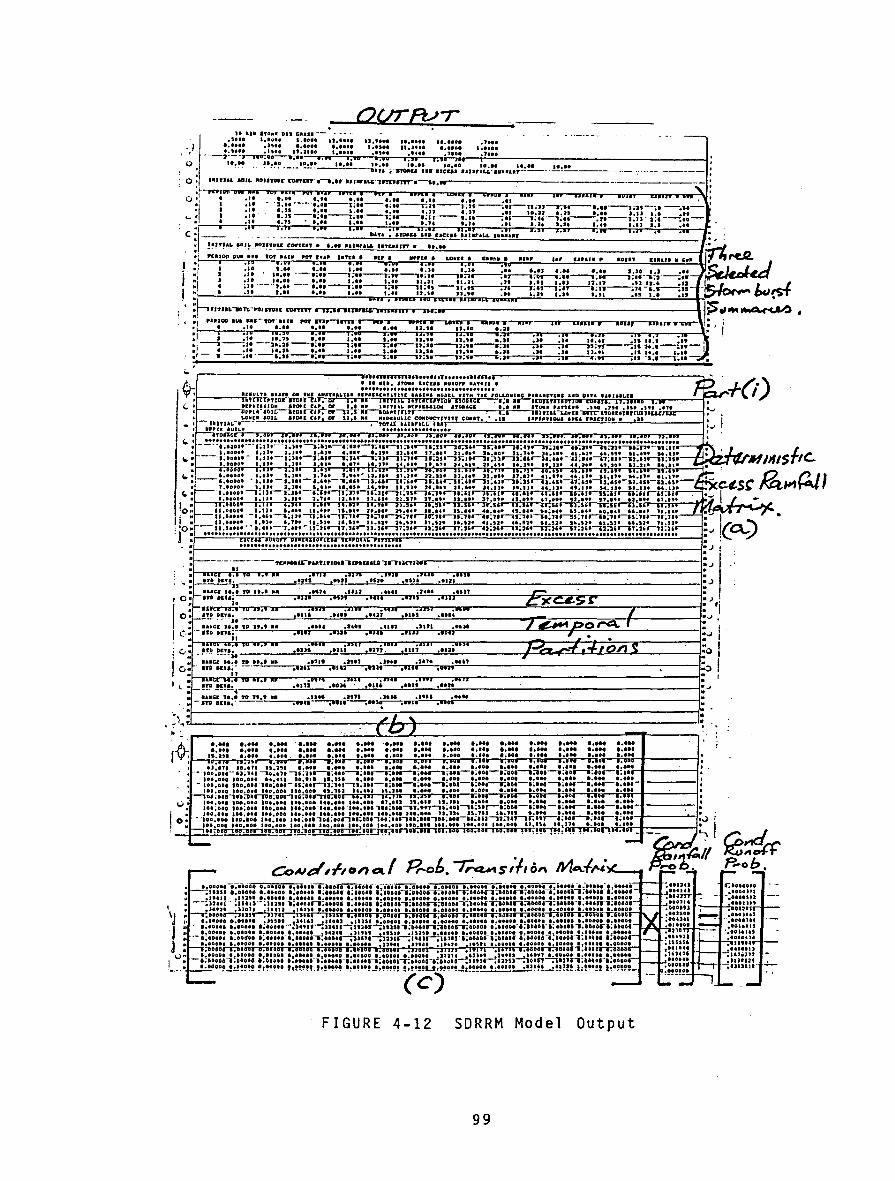
OUTfVr . ·I

,. •u no ... on cuu-- -44,.

,SOOI I,Oota 1,1011 U,ltlt 11,1101 Jl,tt•t II.IDOI ,.1ott

•·•••• .2~•• •·•••• •·•••• '·'''' u.~•u •·•••• '·•••• ----

' ' o.tooo .uoo u.uoo l,toot ·•••• ·•••• ltot ,1oc.o --,---PJ:--rn;w.---.;wi l,e; J,uo 1,00 ••2• J,si JD•r--iF;:..--------------------1'

If!~~ !I_.~~ ~-·-'!!!~--·~:;:·~-no:.:.·: .•. ll~:;:• • .&l•r!~L!:UIIIIIa~!:!!_ _ _!!:::.••o_ ____ --- ··- -- -----: 0

Q • IIUUL •GU, IIDII1'1U" nftEirY .--.-;•.-.:JTIIrll&'li'T'I:WnTr•-.,t, -·---------·, :

CJ :! -,n!w .tt t,ot t,ft 1,11 .... r 1,11 t,tt 1,11 .:1 .. , ..- • t

·1' • ::: ~::;: =:;::--!;::--:;::~n--::~;---::r~::~r-r:;:--::::-;::;-;:: --:::- t """: ~ .u '·" . •·••-..w.--,;,,.-J,sr-s;u---,,,-.,;.,--,.;,~-;,,--J;n z;,--.•• -J

• • -~· ... , •••• •••• •••• '·'· 1,1'4 ••• ...... ,,,, •••• • ••• J,J ••• .

C :1 1 • • ••• '' DA1'1 : •TOt&& a:io- EICUI !~!llt'AU. ,.,;;~at' •• ••• •• •• - •••

:1. !~!T!~~ ~0!~~~~!~.;- (OII'TI:af e leH a&J•ra&.&. U1'USirr a 11.11 ~ ' :, PUJ~ ltVI N-la tot lt&U PGf IUP UtU I 8U I lltPPU t LOWC:I I G••n• 8 iUP J•P UIIJ• p aoU't lt•u• • Cd • I !I "~ J

JJ. :/ a :!: ::.. •=•• ,:,, .:.. ,:,, ::;: :.. •·•• •·•• •·•• 3.1o a.J ·!~ j~~.l. _I_

• 1 • 1' • ••·•• ·-e;e.--,;••~..-,,;Jt~t;-J..---:a~oo~;wt---,;tr-,;to--,.;-,--... _ ; ......,.. "I ~tt _____ !•·••--•~•• •!•• -a.oo u.a. u .. u ·'' 1.11 1.11 at.n .t:a 11.1 .n _ 1 ~- - JwiS"I .. ·•• '·'' •••• ---. •• .----.-a,--,s;t-r--tt;n-;J,~;•,.--,;-.r--a;n--;l.a a. • ..----;ts-, _..,. '-

J .. : ·•• a.•• •·•• •·•• -a.•• 12.•• ,,_,. ·•• '·'' a.at :a.u .t!l '·' ·•' ~'""' .. "h . - .. .... ~ : •ITIR""""JRJTt.-.vtJTVII CDrTnT' ..,...-., IIJifAIII iliiliili I lil;ti i-"fiiiM~ ~ . :1 ''':OCI '"'.~:·~·tot,~!!' ·"",~,-,~;~'"'~ ••• a:anu-r-.n.,--marrT"Ar- :

:1 1 :., :::n ;:,, a:u ,:,, u:u ii:,. ::,. :n :u u: .. .- :11 u:s =•• D =~ ~ --.11 --21; 2S -,;lr-t ;er-T;-.r---JJ;It--,J;ID--1";21-----;-Jr-:-J,.-,S;9,----;JI 26;1 --•• ...-·

:t- ~ ---!:: .--l:;;:---:;::---4;::---P.:~:;:~;::--:;:~:---;~~:;:;-;:: !:::-::::~ .

. .---------~------------------------------------~--~:~ :~wn~~~ftr~~~----~mnr---~~--~~r---~~--~~r-------------------------------------------~ 0 '~~~~.-----------C~~--~~--~~~--~~--~~~------------------------~------------------~:J

~~~r.r~----------~~~~~~~----------------~· :~Y>~~~~~~~~----~~r---~wr--~~r---~Tr--~RTr---------~~~~==~~=-------~----------~=Jf~

----------~~--~~~--~~--~~~--~~--------------~~~~~~~~~-iL------------1:~ . ~~~~~~~r.n~~~i~~--------~~~~~~~~~~~----------~=~

:~.no~~~~~r---~mnr-~nn--~mnr-~mn--~~---------,~~---i~~~-=.w--------~· ------~~--~~~~--~~~~--------~~~~~~~~L-----__,:0

~~wn~~~nw~~------------------------------------~------1:~

FIGURE 4-12 SDRRM Model Output

99

ncr••- IUJorr-rwuvni!"'Y"-n•n------·-··--··----·- -- -·------ -------- ---------ti •• •"~" ••c ••oe ,--. 1 .

I ~~ :t-----;!r.::m:: •:m:: ~>< C n n -ta-,c(Z.. ltolfOit .tJUJ ';{?--. I<: ---u.••••• ,enn----nh,., A~ -0-=,.._=--/-;..-----------------.:_ ........ ...... ~~ ~-+-~ r L-.....

1-___ -_--i:,.::::::: :~!::: ........ ~ . ------------------1

;DOUOI .1011 21.oooot S.SIJJI r-,- 01> :::::::: ::;::::·----.L--=--,-=-=~1' ,::--------------....:.----------l

'- : . 1::::::: ===~~::: ( 01 ./

~~t-------=----r.;_.n; .•• :··===~~~~=====~:~~=====================~-1:

! : .

. J J r

····· ····· ····· ..... ····· ····· ..... . .... • ••••• ••••• ..... ••••• ••••• ••••• ..... ••••• '..::J ~-i~ir~'r.·i''n'~;·~··n·~·-i··~·~·~·~·r.·;··~·r-;·~··n·~·-i··~·~··r-;'r.·~··n•r-;·~·'n'i'-r.iir~r.Tnr-i~;--T~r--r.~r-~ni-f----~·· ·

+-----1:. nr~~~~inrn~~~r.nr,Tr.Tn~~r.r,i~T-;r.~-~~-;r.nr--r.inr-~~-;r.nT--r.inr.----~:

~~----,·~

rm~~~~~~~rnrn~~rnnffiM~~~~~~~,,~J:~~ ·-=~==::~===;=4?:~~==~;:~~~==~~&-:r:'1~AO~ ~~-- . P~&b .

• otOOt 1.10101 t.oooot 1.100.00 0 0 00001 loOIODt loiiOK '·"011 1.110 0 o.tOOIO loiHIO O.HOIO ;oooot· .--;;ooeo.t· t;ttton-:.anae:·t;eeoe.-l~tour-.-;eoo•...-.;ala:l.-.;uoaiT.AII~t61f"T.Htlt · , 01001 •·••••• •·••••• t .. otett •·••••• •·••••• '·''"' •·••••• a. to••• •·••••• •·••••• •·•••••

~ : it''-1,t".~ •• !'!.~,P"'i. !HT'l,!--"-.~<1. rrr:::::r:::::::·:: ::::: '!: :::::-:::::::-:::::::-:::::::-:::::::-::::::::::::::-:::::::-::::::: .. ;oeoamtao~''...-:T1Jn-aHQ""1';1161mnJT"''";';n~nrrr.nnrr.nnmn•t t.oooot 1.11011 i.ttan

•·••••• •·•••" •·••••• .tun. .2ot2t ,ttttt •·••••• •·••••• •·••••• '·"''' '·"••• '•"''' '·'''" •·•••" •·••••• a;11oea '·''"' e,;tuot •••••u·-an .. -atln-;etua-.;••• .. ,; .. ,., "J;o .. oo 'l;ttoll 'l;toooo--.;uoH-.;ouea·taoou~ •·••••• •·••••• •·••••• •·••••• •·••••• .s••u ·•••n .lout •·••••• •·••"• •·••••• •·••·no •·••••• •·••••• t.ootoa t;ooott tolllll e;otoot-.;eoeH-.;ItOI."'T.JIOir-';llli~S6J&ttlf6tJ"'';.IODotT;IUOI-I:II-IIf ... ;;;lltln;•oDII 1;1o•a t.toooe a.ootoo •·••••• o.otoot t.aoooo •·••••• •·••••• .J-JIII ,IIJOl .t4'J24 •·••••• •·••••• a .. oooot t.ooooo o.ooooo ;·ton-rt;ll~nn-1";111011 i.lidil 1.11116 6,.60&11 6,11111 W.IOIOI ,ISili .HI fl I.DiiDOi l .. llfili 1.0 •

-:;:::::-: ;::::: ::::::: :::::::. ::::::: -:~:::::·~;:::::- :~::::: ::::::: -:~:::::-.. ~:~:::-:!::::H;:::::-:;::::: :~::::: ·:'~~~~~~. ~:'~~·• !t!~~!~ ~~~-'!~~! f,~!'!...!!!!!,!..!!!!•!! !~~!!'!U:!~!~ ~!!'''' !t!!!!!..!~!!'!!'!...!%!!~!!...h!!!!!. .... h!!!!~

(c.) -------------------

r------~••r-~awn.want~tno~tDMo~•~•c~•~•~•~••n•~-------------~~------------~:

i ,. .. J,I I'»•Drr •ua ,.ae ~ / •....... ······· - .. -· ~ ..... -- , ,. -- - -J ; ........ :"'" -:x:C~& a. .... c.: oc. u:uo.. .uu1 • ~ I 1-------ia.;•••••-----,.~,,., ~ a'·~ I ••.••••• ····1·-----Jt:::..lJ:_.LJ0~0~~--=--'~~'7-~---

~----:::::::: :;~::: u:eoo!; a::::;;.....:.. ___ .!&;""'~~r'"...::.JoV~e.""':....--------. :1------ ::::::: .;:!:::: _____________________ _

a t.tltOt J;"7S00f a 'l.toeoo tl,tiUI ······ • ·---• .,.orr D-l:ft1'Rrwwl-a:D1twa~n-1--------------_;_---,.-,-,-:---

j :~::~: :::: ::: :::r:;:~:~~:~:,:r-_;_-------~;~;~:;~:~~:g~=~~~::~:--------',r..i •• r-----.. IIAIIIC& 1.6 H 1,1 •cAt D~Pt• • ll,tt ltO Dlt. • t~tl 'J N · •••cc ·'"''PO ·u.t •ru PrrT•-ii-.:.;_----iJ·t~'fD""Dn:.-r-.--------i

.UCiC 11.1 fO U.t a&U OIPTN • 11:4-1 UD on: e e:n !

• IAMC! U~l !'0- U.;l ··ul hPtl ::::r:;:-:!.: : .::~ ;J : -;;::: ::~; !': !::! :::: :::~: : •a.•• liP on. • I.IC

I ~.: :::~:..::;.:.:-.::;: ::::.::~::-: ·:;;:.-~::.::;;: !:!; ' : ------ ----·--- --- --------------------,,.---------;,

FIGURE 4-12 {Continued)

100

The model currently assesses in the first instance excess rainfall in the terms of a frequency distribution together with averaged excess rainfall hyetographs for in­cremental ranges, then on a second pass computes runoff peaks at the catchment outlet based on a separate pervious/impervious catchment routing using the Laurenson runoff routing module from the RSWM as shown on Figure 4-13 for each of the locations in the matrix.

t

/

ROUTED IMPERVIOUS RUNOFF

f PERVIOUS EXCESS RAINFAll

/

TOTAL '---RUNOFF

HYDROGRAAi

ROUTED PERVIOUS RUNOFF

FIGURE 4-13 Flow Diagram of SDRRM Routing Operations

101

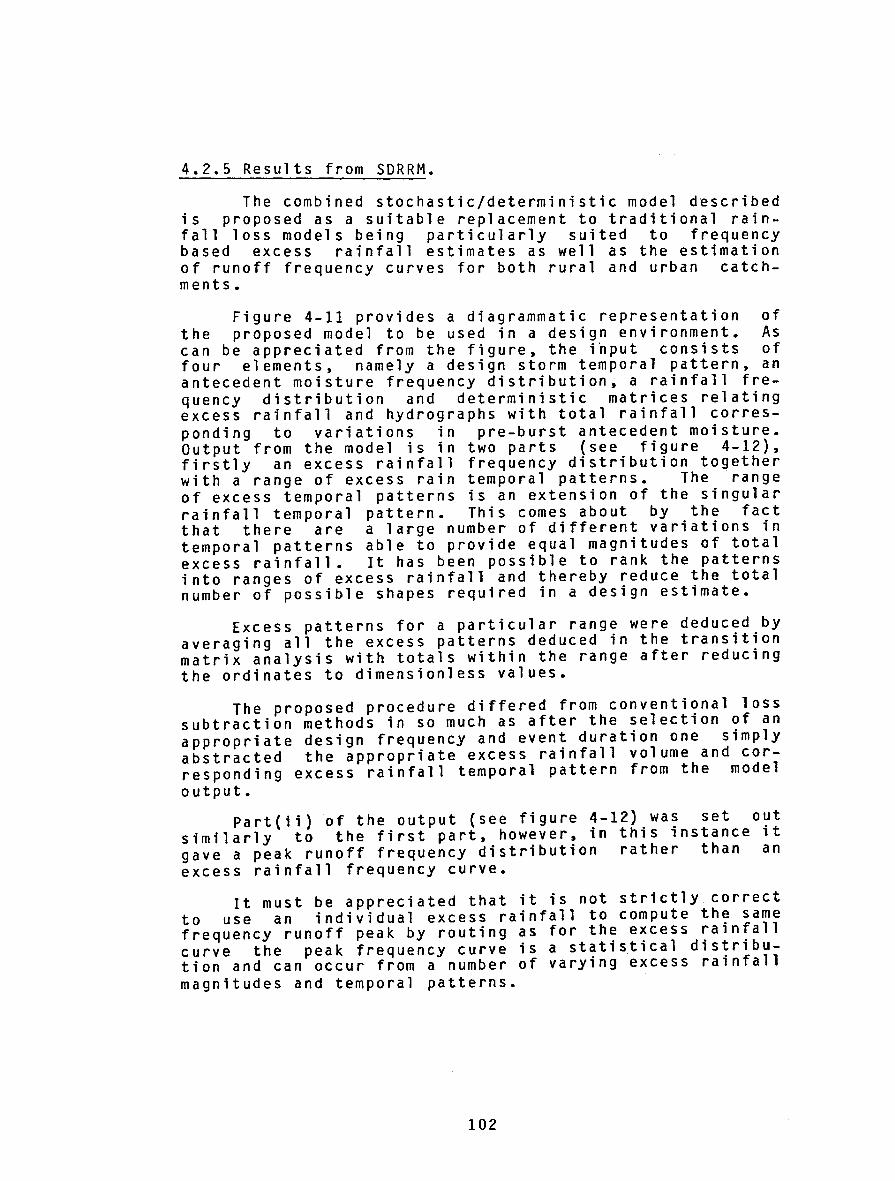
4.2.5 Results from SDRRM.

The combined stochastic/deterministic model described is proposed as a suitable replacement to traditional rain­fall loss models being particularly suited to frequency based excess rainfall estimates as well as the estimation of runoff frequency curves for both rural and urban catch­ments.

Figure 4-11 provides a diagrammatic representation of the proposed model to be used in a design environment. As can be appreciated from the figure, the iriput consists of four elements, namely a design storm temporal pattern, an antecedent moisture frequency distribution, a rainfall fre­quency distribution and deterministic matrices relating excess rainfall and hydrographs with total rainfall corres­ponding to variations in pre-burst antecedent moisture. Output from the model is in two parts (see figure 4-12}, firstly an excess rainfall frequency distribution together with a range of excess rain temporal patterns. The range of excess temporal patterns is an extension of the singular rainfall temporal pattern. This comes about by the fact that there are a large number of different variations in temporal patterns able to provide equal magnitudes of total excess rainfall. It has been possible to rank the patterns into ranges of excess rainfall and thereby reduce the total number of possible shapes required in a design estimate.

Excess patterns for a particular range were deduced by averaging all the excess patterns deduced in the transition matrix analysis with totals within the range after reducing the ordinates to dimensionless values.

The proposed procedure differed from conventional loss subtraction methods in so much as after the selection of an appropriate design frequency and event duration one simply abstracted the appropriate excess rainfall volume and cor­responding excess rainfall temporal pattern from the model output.

Part(ii) of the output (see figure 4-12) was set out similarly to the first part, however, in this instance it gave a peak runoff frequency distribution rather than an excess rainfall frequency curve.

It must be appreciated that it is not strictly correct to use an individual excess rainfall to compute the same frequency runoff peak by routing as for the excess rainfall curve the peak frequency curve is a statistical distribu­tion and can occur from a number of varying excess rainfall magnitudes and temporal patterns.

102

E E

...1

...1

~ z <( a: (/) (/) w u X w

., ..... .., E

~ <( w Q..

... ... 0 z :::1 a:

100

COMPARISON OFL3()-M1d duRATION EVENTS FOR DIFFERENT LAND DOMAINs--- -

1~1~~-..,.,..,.,. ://.

V / V // EXCESS RAI \JFALL V / / v V

/

TOTAL R~lNFALL /"' V /

~ V // r _,

/ /

10

-- V

~ /

V f--L 1- :- -- V ~ - - - V -1-- 1-- / l.® 1/ ~ -- -

..... -J -..!.,; /

-~ _l -r' / r / 1(4)_ I I

/ If

CD DRY GRASS

® RESIDENTIAL LAWN

® NATURAL EUCALYPT FOREST-

@ IRRIGATION PLAYING FIELD

I I I I I I I 11 99.99 99.9 99 98 95 90 80 70 60 !:0 40 ?0 20 10 5 2 I 0.5 02 0.1 005 001

% PROB. OF EXCEEDANCE

RETURN PERIOD YRS.

2 5 10 20 50100

IOO~==~=;~~;;~~~~~;L~~~;;~J;~~~=r-~~ t---t- COMPARISON OF 30 MIN. DURATION EVENTSt-t-+-t-t--i

10

._--+---+--f~--=·o~ p IFFER_~NT Ll A@~_MAN.S -=r--t-+--f

RUNOFF PEAKS

AREA I 100 Ha SLOPE I 1.5%

/

PROPER / / / CURVE // V / / /

'- 4) L / / l/ /_,/ CURVE DUE TO M~ TRIX 1/ / / /V V p '--__ TRUNCATION OVER TOP:*'V'=-t--7''--h!:-b~-+..i-1-.:::--f

,7 ~+--11--cFOUR ELEMENTS. ./ CD:V/ --& 1f-f@ / (SEE FIG. 4-12) V /

0.10 / Ql)5 O.JI

99 98 95 90 eo ro eo 50 40 :30 20 to 5 2 1 0.5 02 0.1 oo5 o 01

% PROB. OF EXCEEDANCE

FIGURE 4-14 Simulated Excess Rainfall and Runoff Peaks for Different land Domains

103

.... E E

...J

...J

rt ~

100

ii 10

~ w u X w

.... .. ..... ... E .... ~ er w Q.

1&. 1&. 0 z ;::) a:

I 99

100

10

I

.99

...-::::

GJRALANG URBAN CATCHMENT I I I I I I I

I I I I I I I I " 1...-:: t:;/

EXCESS RAINFALL. ~ V' v /

At.l. ~ ~ v v v I~/

I6C MIN. 1\ ~ ~ 0 v '1 IBMIN

~ 120 MIN. n J ~~ lk ~ ~ MIN. ... L.-111 ..e .. / 19 / .,..,. ,_;f V V 3 .::;;;;;' )_4 / /

/ EXCESS RAINFALL BASED cr:P V ON FREOl.ENCY ANAlYSIS

OF SIMULATED DATA IN :,oo TABLE 4.~

t.l20 MIN X 60 MIN o 30 MIN

--SDRRM 0

0

99.9 99 98 95 90 80 70 605040 30 20 10 5 2 I 0.5 0.2 0.1 0.05 C: .01

% PROS. OF EXCEEDANCE

RETURN PERIOD YRS.

2 5 10 20 50100

GIRALANG URBAN CATCHMENT I I I I I I I I

I I I I I ~ I I I I I I

RUNOFF PEAKS

AVERAGE SLOPE I J.~ •.4 ~~ IMPERVIOUS AREA I 2~% b

&?' / /

18 M N. ~ ./ / 1/

t>s "" ./ I"' / 30 M IN\ J.-~ ~ ~ V / ~ 6c M£N.

p ~ ~ ...... v V L-- f-- -~ .....

L---- L---~ ~ ~ t.-K 120 1-- MIN. 1---~

99.99 99.9 99 98 95 90 80 70 60 50 40 30 20 10 ~ 2 I 0.~ 0.20.1 O.OS O.DI

FIGURE 4-15 Simulated Excess Rainfall and Runoff Peaks for Giralang

104

Figure 4-14 shows the results of the SDRRM model for a typical catchment of 100 hectares and average slope of 1.5% for the four different land domains studied.

The advantages of the SDRRM model, for the determin­ation of excess rainfall, over more conventional initial loss and continuing loss methods was that the indeterminacy of appropriate loss rate was removed from the procedure. Resulting excess rainfall magnitudes and distributions should therefore reflect suitable design events for a re­quired frequency.

Figure 4-15 shows the results for the Giralang urban catchment for events ranging in duration from 18 through 120 minutes. The results were based on the 75% pervious areas being represented by the dry grass parameter set.

Figure 4-15 also shows the results of a frequency analysis based on annual maximum excess rainfalls shown on Table 4-5 to derive excess frequency curves for 30, 60 and 120 minute burst durations.

This was carried out to help test the validity of the alternative SDRRM joint probability model over traditional frequency analysis methods. The resulting annual maximum frequency results tended to be slightly higher than the SDRRM results however with the short period of record some deviation was not unexpected.

The computer output on figure 4-12 shows the computa­tional components of the method including the transition matrices.

The resulting runoff values accruing from the shaded portion of the transition matrix(c) are however subject to errors due to the truncation of matrix elements. The insert on figure 4-14 indicates the type of problem encountered at the high end of the probability scale. To overcome this po­tential problem however, it is only necessary to select the range of probabilities required with this in mind so as the non- truncated elements are in the area of interest.

4.3 Parameter Assessment for Ungauged and Gauged Urban Catchments.

The main elements necessary to successfully use the SDRRM model are listed as follows:

(a) Catchment Parameters. The complete list of pervious catchment response parameters is shown in Table 4-4. The actual values used depend on the predominant land domain being studied. Iri contrast to the long term water balance requirements the number of significant parameters for the SDRRM is limited to the parameters affecting catchment res­ponse during short term events. These include So, Ko, DSC, use and LSC.

105

On ungauged catchments, values for Sorptivity (So) and hy~rauli~ conductivity (Ko) must be selected from appro­prlate l1terature such as that published by Talsma (1969) and also listed in Chapter 3, Table 3-1.

On_gauged catchments it may be possible to calibrate appropr1ate So and Ko values by event simulation studies based on measured and estimated runoff volumes and measured rainfall. . Additionally, direct assessments of sorptivity a~d hydraul1c conductivity may be made using infiltrometer r1ngs. Chapter 3 addressed the applicability of measuring t~ese parameters, as well as a number of others, in the f1eld.

(b) Rainfall-Intensity-Frequency-Duration Data. This information is usually readily available in most major cities in Australia and appropriately set out in ARR (1977). Similarly, dimensionless temporal patterns for most regions throughout Australia for all normal storm burst durations are published in ARR (1977).

(c) Soil Moisture Antecedence Frequency Data. The deriv­ation of this data has been described in Chapter 4.2. This in brief was based on long term model simulation using the Australian Representative Basins Model (ARBM) and paramet­ers related to particular urban land dom4ins.

On gauged catchments, catchment simulation to optimise parameters can be carried out. This can be supplemented by actual measurement of individual parameters where possible (see Chapter 3).Additionally, it is necessary to have a reasonable period of pluviograph record on which to base the long term water balance analysis. In this thesis ap­proximately 33 years of record was used. A record length of 10 years is thought to be the minimum appropriate for such an anlysis.

On ungauged catchments, model parameters need to be estimated from published literature.

4.4 Runoff Generation from Different Land Domains

In Chapter 4.2, soil moisture frequency distributions for a range of urban land domains were given. These rel­ated to pervious areas such as residential lawns, dry grass areas, natural forested areas and irrigated playing fields.

Figure 4-14 showed clearly the differences in both excess rainfall magnitudes and runoff peaks for the differ­ent land domains used.

Comparing the Figures 4-10 and 4-14 it was evident that, although the antecedent moisture index curves for dry grass was below that of residential lawns, the resulting excess rainfall and peak runoff curves are reversed with dry grass producing the higher magnitude of runoff. This was due to the higher infiltration characteristics of resi­dential lawns more than compensating for the higher initial

106

moisture index.

Figure 4-10 also showed the antecedent moisture curves for natural forest and dry grass crossing at about the 65% probability of exceedance level. It is not clear why this was so, however as shown on Figure 4-14 even at the higher probable levels the magnitudes at corresponding points for natural forest were significantly less than in dry grass a rea.

Based on the results shown on Figure 4-14 it was dent that the particular land domain curves significant effects on the resulting runoff results.

evi­have

Figure 4-16 shows resulting peak curves based on different parameter sets ers for the Giralang urban catchment. from irrigated playing fields to natural

runoff frequency and input paramet­The curves range forest.

Additionally a dry grass - uniform temporal pattern combination was selected to test the significance of the temporal pattern chosen.

.. ...... "'e

:X:: ~ UJ 0..

"-"-0 z ~ ex:

lOO

GIRALANG URBAN CATCHMENT I I I I I I I I

I I I I I I I I I I I

RUNOFF PEAKS

ll"j''

CATCHMENT ·AREA '100 Ha

't ~ AVERAGE SLOPE ' 1.5% A' IMPERVIOUS AREA '25% ~ -:::; ~ ... [;:; IMPERVIOUS Ui '2.0 10

\ / IY/ r\.

/ /.. ~ ~ ~ /! ~ / 3

v -~ / -:::;;,. V / VQ) DRG. GRASS PERV. -l--v J) ~ f.- v V ® RES. LAWN PERv. :.- .....

c.-:::: 1--r-r ~ t- 1--~ @ NAT. FOREST PERV. ....::::::;. ...... ....... v @ IRR. PLAYING FIELD PEFN

I® @ DRY GRASS PERV. UNIFORM TEMP ~TTERN ® IMPERV. SAME ASQ),2xsTOOAGE

Js99 99.9 99 se 95 90 eo 70 so 5040 30 20 10 5 2 1 o.s 0.2 0.1 005 o.ot

% P.ROB. OF EXCEEOANCE

FIGURE 4-16 Sensitivity of Runoff Peaks to Land Domains, Giralang Catchment

4.5 Comparative Analysis Employing the SDRRM and Existing Runoff Estimating Procedures

107

4.5.1 Introduction

This phase of the thesis reviewed some of the cur­rently applied urban flow frequency analysis techniques for catchme~t runoff peak and volume estimations and compared them. w1th the methods proposed in this thesis based on the urban Mawson catchment, in the south of Canberra, described in Chapter 3.

The methods reviewed were the rational formula as prescribed in ARR (1977), a locally developed regional fre­quency method developed in the A.C.T. by Fitzgerald (1975), a frequency analysis of the limited available data for the Mawson catchment, the version of the RSWM described in Chapter 1, the RSWM with proposed stochastic rainfall excess input and finally the SDRRM model direct.

Stochastic and infiltration data necessary for the proposed procedures recommended in this thesis were tran­sposed from the Giralang catchment. No field measurements were carried out on the Mawson catchment. In this way it was proposed to test the transfer of the data from Giralang to other similar constituted catchments within the region and hence the general portability of the proposed model.

4.5.2 Catchment Data

(a) Catchment Features. The Mawson catchment is a fully urbanised catchment as described in Chapter 3 and shown on Figure 3-3. A thin strip of rural land has been left along the southern border of the catchment and this is isolated from the remainder of the catchment by cutoff drains. Catchment slopes range from 1% near its outlet to 15% in the upper reaches.

The existing stormwater collection system consists of underground stormwater pipes which, together with overland flow paths in grass floodways across public land and roadways, provide flood protection to all private property up to and including a once in 100 year storm event.

Entrances to pipes are generally by way of side entry pits plus sag type entry pits at low points in the roadways and depressions.

Pipes sizes range from 150 mm diameter pipes, which collect roof runoff, to multiple 1800 mm diameter pipes at the catchment outlet.

(b) Land Type Breakup. Using the 1:2500 Orthophoto plans plus limited field based assessment, the following list was prepared showing the breakup of the various land types within the catchment:

( 1) Impervious area 115 ha

108

( 2) Residential lawn 150 ha

( 3) Dry grass a rea 170 ha

( 4) Irrigated area 10 ha

TOTAL 445 ha

4.5.3 Rational Formula Method of Analysis

The Rational Formula, following the procedures de­scribed in Chapter 12, ARR (1977), was used to evaluate the capacity of the existing pipe system and to determine the flow paths of any overflows resulting from rarer storms.

The estimated flow peaks were determined throughout the catchment for the 1, 2, 5, 10, 20 and 100 year return frequency based on the system existing as at 1979 employing subareas of 5 hectares or less. The adopted tc time for the catchment was 30 minutes.

A frequency curve based on the results of this analy­sis is shown on Figure 4-17, Curve 1.

109

.. ~ E

!!I: ~ I.U 100 a..

..... ..... 0 z :::> 0:

t---+----+--+---1 MAWSON URBAN CATCHMENT -+-+-1f--+-+-+--f

1---+-----+---+--+--+--41--11 I T -1 I I I I I I

I I I I I I I I

RUNOFF PEAKs-+-+~~44~ I I I I I

CD RATIONAL FORMULA @REGIONAL METHOD CATCHMEN~ .. 1AREA • 445 Ha

t-----1 -+-+--+-AVERAGE j..6ifOPE • 2.0 %_ @ RSWM. INIT. LOSS 5mm, 2mm/hr IMPERVI.CQS"llAREA • 25.8%

CONT. LUMPED CAT. 4\f\Dlt @) R.SW.M.- S.D.R.R.M. EXCESS ~~~DPii'Ai~~~6~

LUMP CAT. ("3) 1,.('€ t~~ }----1 @ RS.WM.- SQRRM. EXCESS S£P. :x.

IMPERV. a PERV. CAT. · . · · r l'\. ~

1---~@ SDRRM.- DRY GRASS PERV. nt'· :Tff; ~'-1< i ~ .,_;.-;> . "'6Jo 14

1--+(1) SQRRM.- RES. LAWN PERV. t--+.,2,..+--+..,~P'l~~.i',;;· ~~~'ltl~f.r~'!lt.:~~-f----1-++~ 1---+@ LOG PEARSON TYPE m DIST. f-f\G~~J:-:i«"'-f'j..~rfli:J~~~iFTTTTlr-J

BASED ON 10 YRS RECORD. +-~!.1'1-~..,..>+·· :p.;;··~l~;;:;iJ~!(A::JS'ia!i~~-g.:Ar\.-:;r-~++++-1---l [L'P ~, .. ~ '=- ~>.;..

.• -~ 7~5J 7

.... ~~~~~-- ...:~@

'Y. PROB. OF EXCEEDANCE

FIGURE 4-17 Comparative Simulations for Mawson

110

4.5.4 Regional Flood Frequency Technique

.A runoff peak frequency curve for Mawson was .prepared by F1tzgerald (1980), using his Key Station Regional Method (Fitzgerald~ 1975) based on extrapolated frequency analyses of o~er 30 selected gauged catchments, mainly rural, repre­sentlng each of the three regional districts defining the A.C.T.

Figure 4-17, Curve 2, shows the frequency curve deri-ved.

4.5.5 Runoff Routing Approach Employing a Design Storm With Initial and Continuing Losses

In this analysis the Mawson catchment was considered in a similar fashion to Fitzgerald•s method, as a lumped watershed.

The total catchment area into 10 isochronal areas. scribed in Chapter 2 with an estimated at 0.80.

of 415 hectares was split The RSWM was employed as de­urbanisation parameter •u•

Initial and continuing loss rates were set at 8 mm/hr and 5 mm/hr respectively. These were based on generally accepted values widely adopted in the past over the region by both government authorities and private organisations.

Appropriate duration design storms were derived for the region adopting the dimensionless temporal patterns·and intensity-frequency-duration curves published in ARR (1977), for a range of storm frequencies between a once in one year and once in 100 year event.

Using the described data the RSWM was applied giving the results summarised as a frequency curve on Figure 4-17, Curve 3.

4.5.6 Runoff Routing Approach Employing a Stochastically Derived Rainfall Excess Lumped Catchment

Using the proposed SDRRM model described earlier in Chapter 4 and the catchment breakdown indicat~d for Mawson, weighted lumped excess hyetographs were est1mated for a range of runoff event frequencies with a duration of 30 mi­nutes.

The excess hyetographs were directly input into the RSWM to produce runoff hydrographs. The resulting fre­quency curve of runoff peaks is shown on Figure 4-17, Curve 4.

111

The analysis was based on a lumped runoff volume de­~uced from the proportions of impervious and pervious areas 1n the catchment and averaged infiltration and storage delay effects. The objectives of this approach w~re aimed at establishing the likely error of shortcutting the full SDRRM model by negating the high computer time necessary for the second step of computing the 15 x 15 runoff peak matrix. It did not allow for the separae development of pervious and impervious hydrograpo components.

4.5.7 Runoff Routing Approach Employing a Stochastically Derived Rainfall Excess-Separate Pervious-Impervious Considerations

This procedure followed the previous one except the SDRRM model was only used to provide the pervious runoff component. The impervious contribution was derived by ap­propriate routing via the RSWM of an excess hyetograph made up of the design storm minus an initial depression storage loss of 2 mm.

The results of this method are also shown on Figure 4-17, Curve 5.

4.5.8 Direct Application of the SDRRM

In this case the full SDRRM was applied to the Mawson catchment to obtain directly a flood frequency curve. Two curves 6 and 7 are shown on Figure 4-17 to describe the re­sults based on pervious areas of dry grass and residential lawns respectively. The true value would lie somewhere in between. The rainfall frequency duration data was based on a log-normal distribution of the rainfall data at the Mawson gauge.

4.5.9 Frequency Analysis of Gauged Data

As a final comparison an attempt to validate the SDRRM model and derived moisture data a frequency analysis was carried out on the 11 years of gauged data available for Mawson

Two frequency distributions were selected for this analysis these being the Log-Normal and the Log-Pearson Type 111. Table 4-7 shows the annual max. flow peaks for station GS410753 Mawson for the years 1971 through 1981.

112

TABLE 4-7 Annual Max. Gauged flow Peaks Mawson.

YEAR DATE

1971 26 Jan 1972 13 Feb 1973 4 Nov 1974 21 Mar 1975 11 Feb 1976 16 Oct 1977 14 Jan 1978 20 Mar 1979 24 Nov 1980 4 Jan 1981 6 Jan

Max Corresp. Hrly Rain(mm)

Mawson Stn

100. 25.6 14.9 42.1 9.9 8.5

28.8 32.4 9.3

16.0 23.0

Annual ~ax. Peak (m /s)

110 24.6 18.9 31.3 14.7 9.75

44.8 57.8 12.3 14.5 43.0

* Estimated peak prior to Gauging Station being esta­blished.

As the period of record was relatively short {11 yrs) it was necessary to look carefully at the individual pe~ks for possible outliers. The 1971 estimated peak of 110 m /s resulted from an exceptional event with the time of con­centration precipitation being of at least a once in 1000 yr frequency.(Fitzgerald, (1980)).

The period on which the SDRRM model results were based was 1932 - 1970 inclusive. In this period no rainfall event of similar duration exceeded a once in 100 yr frequency.

It was thought prudent therefore to exclude, at this stage, the 1971 annual max. peak from the analysis.

The mean, std. deviation and coefficient of skewness of the logarithms of the Ann. Max. Peaks shown in table 4-7 a2e 1.3617, .2655 and .1714 respectively. Based on the Chi X test, the Log-Pearson distribution was a more suitable distribution and therefore it was adopted for comparison purposes.

This resulted in a median runoff peak of 22.65 m3ts. The full plot of the Log-Pearson Type III distribution is plotted as curve 8 on figure 4-17.

4.5.10 Discussion on the Methods and Their Results

The resulting runoff peak frequency curves for Mawson based on the seven· methods of computation described are shown on Figure 4-17 •

113

The variations at any selected frequency are, to say the least, significant with an "order of" difference being apparent between the two extreme curves.

One of the main outcomes was the large disparity between the lumped catchment and separate segment versions of the proposed SDRRM-RSWM model. The results clearly showed the inappropriateness of using total catchment area, weighted rainfall excess and weighted catchment routing ef­fects when considering flow peaks up to say a 10 year return period. The total area of the catchment was in par­ticular a very poor modelling parameter.

A far more appropriate parameter would be an effective contributing area. In events less than say a once in 10 year occurrence this would more closely relate to an effec­tive impervious area.

Curve 5 on figure 4-17 was arrived at by routing the excess pervious hyetograph derived by the SDRRM Model and adding this to an impervious hydrograph separately derived from an appropriately routed excess impervious hyetograph. The result is very close to curve 6 which ts based on the full SDRRM analysis. This fact is most encouraging as the amount of computer time required to produce curve 5 is very much less than curve 6, as catchment routing is not requir­ed for each element in the deterministic matrix.

Although the entirely correct proposed to allow systems.

logic, as detailed earlier, is not further work on this line of analysis is

use of the model on smaller computing

It can be seen on Figure 4-17 that the difference between the gauged data {curve 8) and the SDRRM model re­sults {curve 6) is still significant. The SDRRM however is the only method that remains within the 95% confidence band over the complete range shown.

Without a greater possible to make any ness of either of the frequent range.

length of gauged record it is not definitive judgement on the correct­curves particularly in the less

Obviously further testing and refining is necessary and this will be carried out as and when further gauged data becomes available.

4.6 APPLICATION OF PROPOSED PARAMETER ESTIMATING AND MODELLING TECHNIQUES

4.6.1 Major Drainage Analysis and Design

For major drainage analyses and significant design or­ientated runoff estimates it is recommended that the full SDRRM model be applied.

114

. In this way it is possible to assess the full implica-t1ons of catchment makeup and the interactions of the various individual components. It is also possible to assess the probability of exceedance of not only runoff peaks but also runoff volumes.

Figure 4-18 shows total storm losses based on the re­sults using the SDRRM. They were derived by subtracting excess rainfalls from total rainfalls of similar probabil­ity of exceedance levels.

These may be used to quickly indicate the probable losses to be expected from different land domains within the catchment.

Details are given earlier for the detailed application of the SDRRM. This includes a program listing with sample input and output.

4.6.2 Minor Drainage Design

The preceding discussion relates almost solely to the analysis of regional drainage systems requiring the need for full hydrograph generation and/or catchment storage as­sessment.

In most minor drainage analyses the need for this indepth assessment is not required, rather a simple runoff peak value corresponding to a design frequency is all that is required.

This reasoning has assured that such simple methods as the rational formula will remain with the engineering pro­fession for many years to come.

This phase of the thesis has been aimed at making use of the detailed output results from the developed model de­scribed to assess more accurate runoff coefficients for use with the rational formula.

The following describes the proposed methods for achieving this aim.

115

I

30.MIN. EVENT

---- ----LA

22

2

20

19

18

17

16

---·- YN/

~ ~ .. --··- ---- ---- --------

1---·-· --·----- --- r-...1 E' 1s .5 14

~ 13 0 ..J 12

11

10

9

8

7

6

f----

1.ot

I

22

2

20

19

18

17

16

--15 E 14 .§. (f) 13

912

11

10

9

8

7

6

51.01

·- -·-......, --.·-..,_....., ~---- - - ..

DRY' GRAsS- ·-- -- --1-----\ ..

' \ [:2" ~ --·-URBAN WEIG HrE01 ~

' f-. / ' ' 1/ r--V

IRRIGATED PLAYING FIELDS~

" ' V ' --·--

t.--~

' r\ I --- - ?y -2

RETURN PERIOD 5 10 20 50 lOO 1000

DRY GRASS 75% IMPERVIOUS 25%

---... 120 Min., / ~ /' ~ f\ V

" I/ ""-.. --- r......

"' 60Min. ~ / " ....J.-'

' 30Min h / r--.... ~ y r--V

' 18 Min.-h r-- \ / -

2 RETURN PERIOD

5 10 20 50 100

FIGURE 4-18 Simulated Total Storm Losses

116

1000

Using the approach broadly described in Chapter 2 and the model results generated by SDRRM, rational formula runoff coefficients on a statistical basis have been deri­ved for typical urban catchments in Canberra.

The rational formula expressed in its statistical form was defined as follows:

Q(fy) = 1/3.60 x CIA(Ta,fy}

where:

Q(fy) = peak runoff rate per unit area for a frequency fy

fy = frequency

Ta = rainfall intensity averaging time

I = rainfall intensity in mm/hr for a return period fy and duration Ta

C = Runoff Coefficient

A = catchment area in km 2 •

(4-8)

Aitken (1975) presented Eq. 4-8 in the following manner:

INPUT= 1/3.60 x I(T,A)

where:

T = time of concentration

and

INPUT = rainfall input to catchment (m 3;s)

hence

C = Q(fy)/INPUT

where:

Q(fy} = peak runoff f~r frequency fy years in m /s.

(4-9)

(4-10)

Based on the Giralang and Mawson catchments in Can­berra, described in Chapters 3 and 4, both typical urban watersheds of 94 and 415 hectares respectively and both with a time of concentration of approximately 30 minutes the results of the SDRRM were applied to equation 4-10 to derive rational formula runoff coefficients representative of the total catchment.

117

Figure 4-19 shows the results of this analysis in graphical form.

Using the same analysis technique runoff coefficients were derived based on a typical 100 hectare catchment with an average slope of 1.5% and T of 30 minutes for the four pervious land domains studied in this thesis. The results from this work are also shown graphically on Figure 4-19.

Within the Canberra region it is recommended that these curves be used in preference to the general curves described in ARR (1977) as they are based on local data and should therefore better reflect the complex inputs that affect their development.

1.0 r-----r----"T-r---r-.,---r-------r----.-----,--,---.,--,

0.9~---+------~+---~~--4-------r------r---r--+-~~

0.8~---+------~+---~~--4-------r------+---r--+-~~

0~~--+--~--~-4-+--~----~------r-~r--r--~

% PROB. OF EXCEEDANCE

FIGURE 4-19 Simulated Rational Method, Canberra Runoff Coefficients

118

CHAPTER 5

SUMMARY AND CONCLUSIONS

5.1 Introduction.

The magnitude and frequency of occurrence of hydrolo­gic events is of necessity important to all those whose responsibility it is to design and maintain urban hydraulic structures.

Over recent years the advancement in hydrologic niques has allowed the designer to capitalise on the information that has been collected during a greater of this century.

tech­basic part

In the field of urban stormwater drainage design with its inherent diversities of character the present techni­ques have, however, fallen short of the data available or able to be measured.

Based on studies carried out by the author over recent years, it had become evident that a large amount of basic information on such things as soil characteristics, catch­ment breakup and qualitative antecedent moisture indexes etc, have not been included in design analyses except in very vague qualitative ways.

The hydrologic techniques to date, including such methods as the rational formula and even more advanced runoff routing procedures, have, in their present form, failed to cater for this additional input data.

This thesis was based on the premise that there was a need to increase the capability of present modelling tech­niques and to make use of as much basic data as possible to increase the accuracy of design decisions.

The estimation of flow peaks and volumes in a design context is complicated by the combined stochastic-deterministic nature of the problem.

The two major stochastic elements of the process are rainfall and catchment wetness. The deterministic phase involves the transfer of rainfall to runoff.

In urban drainage analysis to date the effects of catchment wetness on flow estimates has only received nomi­nal attention. Methods have been proposed to include this parameter in current runoff routing techniques.

119

5.2 Combined Stochastic-Deterministic Urban Drainage Model.

Various land domains have been isolated that broadly describe typical urban catchments in Canberra. These include dry grass areas, residential lawns, irrigated areas, native forest and impervious areas.

Based on long term water balance simulation using Can­berra pluviograph records and appropriate catchment parameters, various upper soil moisture indexes were estim­ated. From these, exceedance probability distributions were derived for each of the above domains to represent pre-burst antecedent moisture indexes.

Excess rainfall and peak runoff exceedance probabili­ties were then able to be derived by combining the stochastic nature of both rainfall and catchment wetness with a deterministic infiltration process (in this case using methods described by Philip (1957) employing methods similar to those. proposed by Laurenson {1974) and described in detail in Chapter 4.

5.3 Summary.

The following points summarise the main results of the research carried out during the course of this thesis. Whe.re deemed necessary recommendations are given for future research where the present work has highlighted inadequa­cies.

(a) In the calibration of within an urban environment it is pervious component parameters with only.

rainfall/runoff models not possible to optimise catchment outlet gauging

It is essential to separate the pervious and impervi­ous contributions by way of subcatchment monitoring or at least using a paired catchment technique as described in Chapter 3.

This is mainly due to the predominant influence of im­pervious areas, within an urban area, in the development of runoff peaks and volumes. Up to 95% of total annual flow in an average year was made up of the impervious component.

Additionally base flows caused by artificial watering can also make up a significant part of the total annual flow and are usually of the same order or larger than the total pervious flow.

As it is difficult to separate flow contributions not only between impervious and pervious components the addi­tional complexity of artificial watering due to lawn watering and the like make the task of pervious model cal­ibration all that much harder.

120

In brief necessarily parameters.

the measurement of total runoff is not a good indicator in the assessment of pervious

{b) In the short response urban environment there was a need to modify the Australian representative basin model from_a purely incremental water balance model to a pseudo cont1nuous model to reflect soil water movements within a particular increment of time.

{c) To simulate peak flows from an urban catchment it was found necessary to model separately the pervious and impervious components of the system 'due to the non­homogenous nature of the two contributing systems.

{d) It was found that different pervious land domains responded very differently to a similar storm event. Between dry grass and natural forested areas there was a threefold difference in runoff volumes produced at the 100 year frequency level and a fivefold difference in runoff peak.

(e) The effects of lawn watering on runoff production from urban residential lawns was not found to be signifi­cant as the increase in potential antecedent moisture was more than offset by the increased infiltration capacity caused by better root development and upper strata struc­ture.

(f) An assessment was made of the implications of possible errors in parameter estimates as well as the sen­sitivity of point to areal conversion of individual parameters. Figure 4-16 summarises the magnitude of compu­ted peak flow variations based on a range of parameter sets.

It was shown that although the parameter changes were significant the variation in peak flows over the normal frequency range, between the highest and lowest parameter set, was limited to less than 40%.

It was therefore contended that for design estimating purposes, detailed definition of variations in catchment parameters across similar pervious areas was not required or justified.

{g) Based on results of the proposed model, runoff volume frequency distributions app~are~ to_be highly cor­related with runoff peak frequency d1str1but1ons.

This did not however mean that a deterministic routing of say a once in 50 year excess runoff volume would di­rectly give a once in 50 year runoff peak as both were statistical values based on the contributions of a number of combinations of events resulting in similar output mag-nitudes.

121

. (h) Over the normal frequency range it was shown (see f1gure 4-18) that total storm losses on a statistical sense were fairly constant although of different magnitupes for each of the land domains studied.

5.4 Conclusions.

In conclusion the methodology put forward in this thesis sought to define, in greater detail, the relative importance of the various factors in an urban or rural catchment, in the production of runoff volumes and peaks.

There is considerable scope for improving the proposed model based on continued reseach into the structure of the water balance model selected and the catchment routing res­ponse of the separate land domain inputs, however the present model is believed to be, even at this stage of de­velopment, a responsive one able to reflect in far greater detail than other existing procedures, the contributions of the various components of a catchment. A great deal of further testing and development is still required, however this is believed to be justified in line with the continued research necessary to obtain better runoff frequency esti­mates for engineering design purposes.

One further avenue of development would appear to be in the definition of seasonal soil moisture probability curves ie, Summer and Winter • These combined with similar seasonally defined rainfall probability curves may give further insight into the rainfall/runoff frequency rela­tionship.

There is also scope to improve catchment monitoring techniques to provide more accurate data input to the model. It was the aim of this thesis to assess some of the problems and practical implications and possibilities for future research.

It is contended that there is considerable merit in the further development of techniques to carry out and apply soil moisture monitoring in an urban environment using both nuclear and psychrometer-thermocouple methods.

Further work is recommended to extend the analysis de­scribed to other areas in Australia to test variations in parameter response in those locations.

122

REFERENCES

AITKEN, A.P. {1974). Interim Design R~port Vol. 2. AWRC Research Project 71/22. {Unpublished.)

AITKEN, A.P. {1975). Hydrologic Investigation and Design of Urban Stormwater Drainage Systems. AWRC Tech. Paper No. 10.

BERAN, M.A. {1973). Estimation of Design Floods and the Problem of Equating the Probability of Rainfall and Runoff. UNESCO, WMO, lASH, Sym. on the Design of Water Resources Projects with Inadequate Data, Madrid, Spain.

BERAN, M.A. and SUTCLIFFE, J.V. (1972). An Index of Flood-Producing Rainfall based on Rainfall and Soil Moisture Deficit. Journal of Hydrology, Vol. 17, pp. 229-236.

BLACK, D.C. and AITKEN, A.P. (1977). Simulation of the Urban Runoff Process. Water Res. Council Tech. Paper No. 26. Research Project 75/82.

CHAPMAN, T.G. (1968). Catchment Parameters for a Deterministic Rainfall-Runoff Model. Land Evaluation (ed. G.A. Stewart), Macmillan, Melbourne, pp. 312-323.

CHAPMAN, T.G. (1970). Optimisation of a Rainfall-Runoff Model for an Arid Zone Catchment. lASH-UNESCO Symp. Wellington, N.A. Publ. 96, 126-144.

CHONG, S.K. and GREEN, R.E. {1979). Application of Field-Measured Sorptivity for Simplified Infiltration Prediction. Proceedings of the Hydrologic Transport Modelling Symp., De~ember, Louisiana, USA, ASAE. Publ. 4-80.

123

CLARKE, C.O. (1943). Storage and the Unit Hydrograph. Trans, ASCE, Vol. 69, No.9, Nov.

CORDERY, I. Design Flood Trans., I.E. October, pp.

(1970). Antecedent Wetness Estimation. Civ. Eng. Aust., Vol. CE12, No. 2, 181-184.

CORDERY, I. and WEBB, S.N. (1974). Flood Estimation in Eastern New South Wales. A Design Method. Civ. Eng. Trans., I.E. Aust., Paper No. 3265, February.

CRAWFORD, N.H. and LINDSAY, R.K. (1966). Digital Simulation in Hydrology: Stanford Watershed Model IV. Stanford Univ., Dep. Civ. Eng., Tech. Rep. No. 39.

EAGLESON, P.S. (1970). Dynamic Hydrology. McGraw-Hill.

FITZGERALD, B.J. (1975). A Key Station Approach to Rural and Urban Flood Frequencies in the A.C.T. I.E. Aust., Hydr. Symp., Armidale, pp. 173-177, May.

FITZGERALD, B.J. (1980). A Review of

for

the Woden Valley Flood of 26 January 1971. Seminar Assoc. of Consult. Eng. Aust., Sydney, July.

FLEMING, G. & BLACK, R.E. (1974). Simulation of Flow Records for an Australian Catchment using the Stanford Watershed Model IV. Civil Engineering Transactions.

FRENCH, R., PILGRIM, D.H., and LAURENSON, E.M. (1974). Experimental Examination of the Rational Method for Small Rural Catchments. Civ. Eng. Trans. Paper No. 3174, March.

GOYEN, A.G. and AITKEN, A.P. (1976). A Regional Stormwater Drainage Model. I.E. Aust., Hydr. Symp., Sydney, pp. 40-44, June.

HENKEL, G. and GOYEN, A.G. (1980). Retarding Basins Best Upgrade Stormwater Protection in Old Areas. Int. Symp. on Urban Storm Runoff, Univ. Kentucky, Lexington, July.

HIGGINS, W.L. and MILLS, J.E. (1975). Trunk Stormwater Design in the A.C.T. I.E. Aust., Hydr. Symp., Armidale, pp. 178-182, May.

124

INSTITUTION OF ENGINEERS, AUSTRALIA (1977). Australian Rainfall and Runoff- Flood Analysis and Design.

JOHNSTON, P.R. Optimising the Runoff Model. pp. 173-180.

and PILGRIM, D.H. (1973). Parameter Values of a Rainfall­Hydrology Symposium I.E. Aust.,

KOVACS, G. (1979). Analysis of the Components of Evapotranspiration. Proceedings of the Canberra Symp., IAHS-AISH, Publ. No. 128.

KOVACS, G. and ASSOCIATES (1981). Subterranean Hydrology. Water Resources Publ., Littleton, Colorado 80161, USA.

LARSON, C.L. (1965). A Two Phase Approach to the Prediction of Peak Rates and Frequencies of Runoff for Small Ungauged Watersheds. Stanford Univ., Dept Civ. Eng., Tech. Rpt No. 53, June.

LAURENSON, E.M. and PILGRIM, D.H. {1963). Loss Rates for Australian Catchments and their Significance. The Journ. of I.E. Aust., January-February.

LAURENSON, E.M. (1964). A Catchment Storage Model for Runoff Routing. Journ. of Hydr., Vol. 2, pp 141-163.

LAURENSON, E.M. {1974). Modelling of Stochastic-Deterministic Hydrologic Systems. Water Resources Research, Vol. 10, No. 5, October.

LAURENSON, E.M. and MEIN, R.G. (1978). General Runoff Routing Computer Program. RORB Version 2- User Manual. Monash Univ., Dept Civ. Eng., {in conjunction with ACADS).

MEIN, R.G. & BROWN, B.M. {1978}. Sensitivity of Optimized Parameters in Watershed Models. Water Resources Reseach. Vol. 14, No. 2, pp 299-303.

MULVANEY, T.J. {1851). On the use of Self Registering Rain and Flood Gauges in Making Observations for the Relation of Rainfall and of Flood Discharges in a Given Catchment. Trans., Inst. Civ. Eng. Ire., Vol. 4, pp. 18-31.

NATIONAL CAPITAL DEVELOPMENT COMMISSION {1980). Monitoring Stormwater Flow and Water Quality in Paired Rural and Urban Catchments in the A.C.T. Tech.

125

Paper No. 29, August.

PARLANGE, J.-Y. (1971). Theory of Water Movement in Soils, Part 2. Soil Sci. 111, pp. 170-174.

PARLANGE, J.-Y. (1975). Green and Ampt Equation. pp. 466-467.

PARLANGE, J.-Y. (1977). Infiltration Equations. Am. J. 41, pp. 654-655.

A Note on the Soil Sci. 119,

A Note on the Soil Sci. Sco.

PHILIP, J.R. (1957). The Theory of Infiltration: 4. Sorptivity and Algebraic Infiltration Equations. Soil Sci. 84, pp. 257-264.

PIERREHUMBERT, C.L. (1974). Point Rainfall Intensity-Frequency-Duration Data. Bulletin No 49, Bureau of Meteorology.

PILGRIM, D.H. (1966}. Storm Loss Rates for Regions with Limited Data. Proc. of the Amer. Soc. of Civ. Eng., Hydr. Div., March.

PRICE, R.K. (1973). Flood Routing for British Rivers. Hydr. Res. Stn, Wallingford, (INT 111).

RUSSEL, S.O., KENNING, B.F. & SUNNEL, G.T. (1979). Estimating Design Flows for Urban Drainage, Jour n a 1 of the Hy d r • D i v • AS C E , Vo 1 1 0 5 , H Y 1 , J an •

SCHAAKE, J.C., GEYER, J.C. and KNAPP, J.W. (1967). Experimental Examination of the Rational Method. Proc. of the Amer. Soc. of Civ. Eng. Jour. of Hyd. Div., HY6, November, pp. 353-370.

TALSMA, T. (1969). In Situ Measurement of Sorptivity. Aust. Jour. Soil Res., Vol. 7, pp. 29-276.

TALSMA, T. and PARLANGE, J.-Y. (1972). One Dimensional Vertical Infiltration. Aust. Jour. Soil Res., Vol. 10, pp. 143-150.

VACHAUD, G., TEHEL, J., ROVER, J.M. and BOLCATO, R. (1973). Automatic Control of In Situ Water Transport in the unsaturated Zone. Application to Determine Water Balance (in French) IAEA Symp. on Isotopes and Radiation Techniques in Studies of Soil Physics, Vienna.

126

WATKINS, L.H. {1962). The Design of Urban Sewer Systems; Research Into the Relation Between Rate of Rainfall and Rate of Flow In Sewers. Gt Britain, Dep. Se. and Ind. Res., Road Res. Lab., Road Res. Tech. Paper No. 55.

WITTENBERG, H. {1975). A model to predict the effects of urbanisation on watershed response. Int. Symp. on Urban Hydrology and Sediment Control, Ky. Univ. Lex. Bull. 109, pp 161-168.

127

APPENDIX A

ENGINEERING LOGS

pit no: ~!PI

log- sheet / of J engineering excavation

office and job no: (£u.,_herra.. (2031

pit commenced: (L .- 7-7 !::J

project: ASse.55Mt..ni ,r ~ra'i?c:Je pit location: -5-la.:fion I

• • pit completed: /L- 7-73 (i,rola~ ~£-supervised by: GC

J log checked by: C . '- .T

equipment type and model:

excavation dimensions:

'B £ "' E

notes samples, tests, etc. ...i depth

er metres

m long,

c C> 0 E -;;-.,o c.> c.>.O :c :fE a. ~> ... ... .... C> u

m wide

material

R.L. surface:

datum:

>> ..,c c.>OJ :.2 c·u;

soil type: plasticity or particle characteristics, -... CI>C

.!!~ ·~~ colour, secondary and minor components. oc E8 c~

OlD u'-

m

-cE~ structure and c- ... '"~e additional observations .~:..,

a. kPo 0 000 0 ooo _(\jot).,.

~ Ill u! ~--= ~:~p .. ~1fj_ «;:!.Pt;/_;_-t. IV-11--1 ~~. 11 I

. --,; 1 _

0_,

16. . ___ to~_. __ ---.-- __ ... -··- _

'11 -y/~ --/ ll V'D ---- _--.:;j/- - ---~ -.~ ---

-

-~ :Il-l - ---

----

I~,; :!? ·o.7.S --= h- . -----~~~~-. =-=--~--/J_AJ~j::_L~~-:. '!J.-

~~~ -.·--- ---- : _wqq .; - ·-z --(f;! ;/;f:t:::.- -I...;...W.++-+-.J---1--~·o.:.::u~~dl.,;;··-+---1"---...... ~- ~;/iJ;;-__;:: Dfk~-i ---o-S- -~ w~1l,,ra.vd ___ ~- JW-..,..

j! I •H

'' i ------

li·-!11 -=-~--~ ~~~---= =~ -~--- ----- --------- ----1

----------- ------·- --------------·----;. ... ----·------ ·-~- :.... .. ---- -------------- ---··--- ----

li ,_,~. ------ •·····. _.:..... .. .,.- _:._.

1 -----~ -·-·. ·-·- -·.

liq-, ---- -~-:~.~~ ~-~-

I ---- --

lli -c -~== l ' 1

1

1 • ! - ·-

- ----

i . - -·--1

-----­··- ·-~

.. --· -.. -

------

----.

-------------- -----------.---------- -·--------

--------------------- ---

~-_.:...-. -- - -· -------

I

-!I ! 1-, '' 1 i ; I

IH i I I

I! ! l

I i I I 1 i

• I l·i,l i li l

I I

1111

,

I! I l! ,.

; z: I I:

kev ~ ~ samples and tests

undisturbed sample 50 mm diameter

classification symbols "iiiii'J'So•l descnpt•on

method -N natural exposure E existing excavation BH backhoe bucket B bulldozer blade R ripper

T timbering

penetration

~o r!!sistance angmg to efusal

~fb Oot, 73 w"~ lwol on date shown water inflow

i w;>tPr nutflovv

U50

0 N

N• Ne

disturbed samp_Je standard penetration test:figure • result SPT +sample cone penetrometer

based on unified classification system moisture 0 -dry M -moist W -wet

·----­-------- ----

- -· ___ _;_

-----·-------­. ·-- --

---- -

- ------

- ---

-

-

consistency/relatove density

VS -very soft S -soft F -firm St -stiff VSt -very stiff H -hard Fb -friabie VL -very loose L -loose MO -moderately dense 0 -dense VD ,-very dense

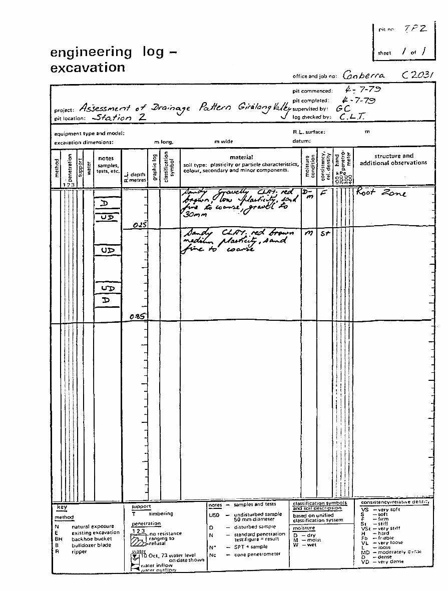
engineering excavation

log-

project: A.sSess,.u,;'t D -r .2ra~n~e pit location: -5-la...f,on 2..

equipment type and model:

excavation dimensions:

c "0 .Q

m long,

c C'l 0

sheet

office and job no: Gt:) be rra..

m wide

pit commenced:

pit completed:

(;,rtila'::J fa./& supervised by:

J log checked by:

R.L. surface:

datum:

material

(t.. :- 7-7::!} /t--7-73

GC C.L.T.

m

I ot I

(2031

0 ; r. .... c; c; !i :::>

... ., ; ~

notes samples,

tests, etc. _j depth

.£ -~0

.!:! U.D

.r: :;:E a. ·v; >

soil type: plasticity or particle characteristics, colour, secondary and minor components.

.,c .. o :=~·;:;

.!!~ oc E8

>>­u.~ c .. CJC

·~~ c..:

structure and additional observations

E c "' Q

1 23

~

! I ! :

I I I I i I ! i l ! i l I

i ~ : j I I

i ~ ~

I

I I i i i i !

I i I I

i i ! ! I I i ! I

I I

I

key

method

..

N natural exposure E existing excavation BH backhoe bucket B bulldozer blade A ripper

0:: metres ~ :g 0

C'l u

---

-

------

().?$_

-------------

---

--

~ T timbering

penetration

123 . no resrstance rangrng to refusal

~watfb Oct, 73 water level

on date shown v,ater inflow vi!!er outiiO'''

--notes - samples and tests -U50 - undisturbed sample

50 mm diameter

D - disturbed sample

N - standard penetration test:figure =result

N" - SPT-+ sample

Ne - cone penetrometer

O"' u'-

Ill I :

I

' :· ':i: •• i l '!' 1 I.! j ~ I :I

, ! I classification symbols iii'iCIS'orl oescr•ptron

based on unified classification system

moisture

0 -dry M -moist W -wet

--

-

-

-

-

---

-

--

--

consrstency.relatove oens;-::,

VS - very soft S -soft F -firm St -stiff VSt -very strtf H - h<Jrd Fb -friable VL -very loose L -lOOS!: MD - moderatelv :::~r.:..: 0 -dense VD -very dense

. . eng1neer1ng log-excavation

project: As..sessMe.nf D r 2ra'nVe pit location: -5-la.:fion 3

equipment type and model:

excavation dimensions:

c notes ... ~ samples,

m long,

c: 0> .Q 2 ~0 -~ u.D soil type:

rit no. -;P3

I of I I

office and job no: G.11 be, ra.. (203/

m wide

pit commenced:

pit completed:

a,ra"la':J fa./& supervised by:

J log checked by:

R.L. surface:

datum:

>> material ..,c: ... 0 g.~

plasticity or particle characteristics, :;:>·- C>C:

;. :- 7-7~ .{L.- 7-7.3

GC C .L.T

m

~e~ structure and c:--"'"'"' additional observations LgE -g

£ Cl

-~ I~ o; I e-c :::> "' .r:::

;: tests, etc. ...i depth

a. .; ;g

~E _;;

.,,_ colour, secondary and minor components. oc: ~-=

c. Eo kPo E

Cl "' a. 123

l j:

I. ~ l I i ! I it

11 I,

i I

11 ! I :I ! i ! f

! I 11 I, 11

__ Ll key

method

N natural exposure E existing excavation BH backhoe bucket B bulldo:zer blade R ripper

~ :£"' 0:: metres C1 u

----

-(>~$"-

---

o.&::. -

--------

-

-

---

---

--

T timbering

penetration

1 2 3 no r~sistance rangtng to refusal

~V'.<l'fb Oct, 73 water level

on date shown water inflow

1 wat~>r outilo''l

notes - samples and tests -U50 - undisturbed sample

50 mm diameter

D

N

N" Ne

- disturbed sample

- standard penetration test:figure =result

- SPT ~ sample

- cone penetrometer

u oa> u'" oOOO

0 000 (\jr<)~

11 ! l KoPf Z>~~

illi 11 r Frv:sh .5J,Mc

~ ~ ';I

11 11

i ! i

j !

-

-

-

-

-

-

-

classification symbols ! ana-5otl oe~croptJon J based on unified classification system

consrstencyirelat•~e censoty

VS -very soft

moisture

D -dry M -moist W -wet

I I i I

S -soft F -firm St -stiff VSt -very stttf H -hard Fb -friable VL -very IOO>c L -loose 1\10 - moderat.:l ~ .J~-...: D -dense VD -very drn>i:

. . eng1neer1ng log-excavation

project: AS:Se.s.s"'e..':'i D -r 2ra,n~e pit location: -5-la_ftor? 4-

equipment type and model:

excavation dimensions:

notes samples.

m long.

., c .E .Q

;:;c; .!:! u.o soil type:

~,1 p.•A ril no. .,._

sheet / of }

olficeandjobno: {];Aherra. (203/

pit commenced:

pit completed:

Q,'hi/a':J fJ/_,., supervised by:

J log checked by;

m wide

material

R.l. surface:

datum:

>> ..,c u-~.Q c:·u;

plzsticity or particle characteristics, z.-=. "' c

;. : 7-7-~ /L -7-73

GC C.L.T.

m

-uEt structure and c--"'"'"' additional observations .r.~E

-g £ "' E

tests. etc. _j depth

.r. ~E a. V> -~ "0 -~~ colour, secondary and miner components. oc c. Eo c..: kPo

.'':,: ! !

li!

~ :

i I i i ! i i,! !

I I I

i l I I

! I 1 i I ill

(J::P

:t>

'-')2

.::31

key

method

N natural exposure E existing excavation BH backhoe bucket B bulldozer blade R ripper

I :

e lii"' ci metres ., u

----

-Q-32-

---

--

0-~

·--

-----

----

-

------

-...:

- ~ -

~ T timbering

penetration

~no r~sistance rangmg to refusal

@'fb 0", 73 w .... ·~" on date shown

water inflow "al!'f outfln,•

notes - samples and tests

U50 - undisturbed sample

D -N -N• -Ne -

50 mm diameter disturbea sample standard penetration test:figure" result SPT-+ sample cone peneuome1er

u O"' 0 000 u .. 0 000

Nr'l<t

~I!!! !fAc-1-, I i I

I ; I i · · - ·

! ill .. - . ., . - ... ,

s-r 1 I I I i l

11! l I 11 I a: ' I; I . :

I; if

1 ~ i

: I i

classification sy:-nbols andsotl ae~cr:pllon based on unified classification system

mo1sture D -dry M - moi~t W - Vltet

---

--

-

--

-

--

--

cons•stencyaelatt·.e aer.s.:-,

VS -very soft S -soft F -firm St -stiff VSt -very suff H -hard Fb - f11able VL -very loo;.e L -loo~e r-.10 -moderate!) .::.;~.~ D -deme Vu - "'NV o .. ;;s.-

. . engtneertng log excavation

project: Asses.s,.-,erd D r .2ra,nc::;e pit location: -5-la .. :fion 5

equipment type and model:

excavation dimensions:

c "0 0 notes 0 ~ ...

"' samples,

m long.

C'l c:

.E. .!? ;;O

-~ u.!:l soil type:

I r' "'

sheet

7?5

/ of }

office and joo no: Gn be rra. c 203/

m wide

pit commenced·

pit completed:

c;,rt.ila':J J!Jty supervised by:

J log checked by:

R.L. surface:

datum:

>> material .,c: u-... 0 c·Vi plasticity or particle characteristics, E:-= <.>c:

.(! :- 7-7:;) /t. -7-73

GC C .. L.T

m

~g£ structure and c :J t,)

2~E additional observations li £ ; ;;; ~ !:E -~~ .;~ "' "' ;:: tests, etc. a. colour, secondary and minor components. oc 0.

::;, -!depth ~~ "' kPo E8 c...: E c "' "' c.

123

VJ:>

:I> O;:p

l<ey

method -N natural exposure E existing excavation BH backhoe bucket B bulldozer blade R ripper

!

!

.., a: metres c, u

---

0·2.---

o.~

-----

-

---

-

--

-------

-

- -·- ..

~ notes

T timbering U50 penetration

1 2 3 . D ~no f~SISiilfiCe N rang•ng to

refusal N"

Ne on date shown

- samples and tests

- undisturbed sample

--

--

50 mm d•ameter

dasturbt!d ~<;m,:: le

standard penetration tesl:fagure =result

SPT .. sample

cone penetr orneter

oo oOOC u'-0 000 (\1...,.,.

!ll!~r~ I! ll 'I! f liil-·-- -----1. ':

--. ~ i I i

I

.. I ! I :

'i ! I i I; . I i I i:

! ! l I: I i

i ! i ! 1 ~ ~ i ! :! l

·1 i i I j I

; ~

i i l

' ;

: ;

' L : :

' i :

1 !

_L:.

I classificat;on symbols and SOli Oe><..fiPitOO

b11sed on uniiied I classification sys\em

' mo•:;tJre

D -dry M - moast W -wet

-

---...;

--

-

-

-

-

-

- ·-cc-nsistency/relatl\1€ ,:; ;;n~.: r

VS -very soft S -soft F -form ~t -Stiff VSl -very sutf H -hard Fe - fri;,t;l;, VL -very loo·~ L - IC.OO$t: :.:c, -· mod&-r~tt: '• .:::-:: • ~ D -d.:nse VD · tJe.y C.:c•·:.or:

~------------~~~~~~~----~~---------.--.----~------------__.----------·----~

~·ro o". 73 ..... '"''

I water inflo," ··~tPr outflo,•J

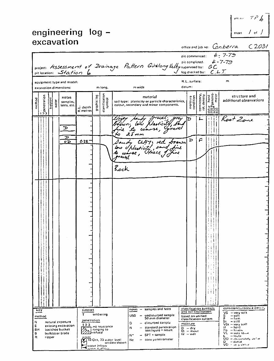
log . .

eng1neer1ng excavation

project: As.se.ss,.u .. ni o-/ .2Jra'nVe pit location: -5-la...fion b equipment type and model:

excavation dimensions:

"0 0

c: notes samples,

m long.

c: C> 0 .£ ·~o .!:! u.O soil type:

lP j,

sheet / of }

office and job no: Gn berra. (2031

pit commenced:

pit compli!ted:

C,rila':j fa./£, supervised by:

J log cnecked by:

m wide

material

R.L. surface:

datum:

>> oC: .,_ c·u;

plasticity or particle characteristics, .., c: -..,

;. -; 7-7~ /L. -7-73

GC C.L.T

m

~et stn:cture and c--... ~"' additional observations .c~E £ "

-~ 1~ E c; I '9 "' c: ::> il: tests, etc.

-! depth .s::: ·- E c. V>

-~~ colour, secondary c;nd minor components. -~ "0 n oc: .., E8 c:..: kPa E .., "'

Q

123

I I

i! I I i!

I i I I:; :! I : !

l ' j I! ~ i I i : I i i ! i I

ill I

: i

~ l

1

1

ll 11

I!

:I>

':l)

u:p

"' V VI s, r:: a: metres u

---

o:z~-..:

------

--

-

----

--"

-

-----

-'

--1

'll' Jji - ---1 ·----'

key

method -N natural exposure E existing excavation BH backhoe bucket 8 bulldozer blade R ripper

i

I

~ T tombering

penetratoon

123 ~no re:>ostance

rangong to refusal

.1.~ ~ 1 Oct, 73 • .,at"' le11el on date shown

watt:r inllow &'i'lt•"f 0-..ltfiO'."'J

notes -U50

D N

N"

Ne

- samples and tests

- undisturbed sample

--

--

50 mm diameter

disturbed ~ampi.;

standard penetration test:logure = res1.1lt

SPT.,. sample

conE: I.H:netrometer

QCo> u ... oOCC 0 occ (\J~~

! , I! . ::: ~ I I l i l . I I

i I

!I i I ll ! I :'

i ! :I I ! t l . :

!

I

! ; : ~

! classif1cat1on syrr.bols

1

1iiiel"Sou oe~crtptlon

based on unified classification system

moist .... re

D -dry M - rnoi>t W -wet

-•

l --

-

·-conso~tenc·,oeo:HivE ce~.;-7,

VS - very soft S -soft F -form St - S!iff I VSt - vt-ry ~uti

I H - h2rd

I Fb - t;i"L'h· VL - vt:<V 10~--" l - l:>vSt

j r-..~D - .• ,c_.·...:c:rat~l) .;:-.~

D - d<'n>e J VD - wE·. '1 .;..!~I&.~

. . eng1neer1ng log excavation

project: Asses.s~Y~enf o-r .2ra'nc::Je pit location: -5-la..fion ,7

equipment type and model:

excavation dimensions:

c notes

m long,

c "" .2 E.

TP7

sheet I et J

office and job no: ea, berra.. (2031

m wide

pit commenced:

pit completed:

a,rila':J fa./& supervised by:

J log checked by:

R.L. surface:

datum:

>-> material .,c u-... 0 C~iii

{/.- 7-7:;, /L -7-7.9

GC C.L.T.

m

"C~~ c-- structure and

"0 0

= .g ~ samples,

c;o u u.o :c ~E

::::>·- .. .., <.> soil type: plasticity or particle characteristics, -.~ G>C ..cf.E

-~ "C -c: -~ "C

additional observations l <.> E "' c

"' Q.

tests, etc.

1:?3

'Key

method

N natural exposure E existing excavation BH backhoe bucket B bulldozer blade A ripper I

-!depth 0. .., > :: ~"" a: metres C> u

--

0·15-·. --

-----------

----

-

-

----

--

support

T timbering

penetration

1 2 3 ~no r~s•stance

rangong to refusal

colour. secondary and minor components.

notes - samples and tests

U50 - undisturbed sample

D -N -N" -Ne -

50 mm diameter

disturt.ed sanple

standard penetration test:figure "'result

SPT -t sample

cone penettometer on date shown

oc Q

eo c~ kPo u 0"' oooc u ... cOOO

_(\J.....,t;t

' ' i

' : i

! '

i I ' l : .

' ' ! I

: : i : : '

: : :

.. : j classification symbols

"a"i'i'sool de;,croptoon

based on unified classification system

moist..Jre

D --dry M -moist W -wet

I

--t

-.

J

l

J

j ··-·-

consostency/relato • .: ce:-:s.:, VS -very soft S -soft F -firm St - st;ff V5t - v~ry stott H -h3rd FL - fll .. !.lh: Vl - v<:r"( lv~,..,

l -IO(JS" r.1c. - nivJ·:, ~t~•., .... _ Jc

D - dtm>e VD - vt''\' f.!,·

L---------------~~~~~----~----------------~---------------------------

~'"/, 0". 73 """ ''"" I water inflow

... :'\lt""r 0d1~!o.·,

. . eng1neer1ng log-excavation

project: Assess,.,eni c -r pit location: ...5-la.:fion S equipment type and model:

excavation di!Oiensions:

c "tl .2

m long,

l ~''" -~ r-,_; I ,_- 6

/ c; J

office and job no: cat') be rra.. c 20311

pit commenced:

pit completed:

C,i-ti/a'::J fa.Jl, supen.•isPd by:

J log dlecked by:

m wide

material

R.L. surface:

datum:

"' c ,;.,. ... -c ·~

/L :- 7-7:'1 /L -7-73

GC C.L.T.

m

"C e t ~tructure 2'1d

l l 0

.r; ; ~ "' ::>

... := '"" ~

notes samples, tests, etc. •

...J depth

soil type: plasticity or particle characteristics, colour, secondary and minor components.

~:¥ .~~ cc E8

c~o I ~ [ E additional observations

kPo

"' c -~~ V. c~ E c

"' "' u 123

I !

-·

method

N natural exposure E existing excavation BH backhoe bucket B bulldozer blade R ri11per

0:: metres

--

O·F.i- - . -

---

0·.35-----·---------------------

--

~ T timbering

penetration

1 2 3 no rcs•stance rang•ng 10 refusal

~1"·'Cb Oct. 73 water le\tel

on date shown wat.,r inllow "''f-H•llr (),JtiiO\',•

notes

U50

D

N

N• Ne

- samples and tests

- undisturbed sample 50 mm diameter

- disturbed sample

- stanclard penetration test:ftgure "'result

- SPT .. sample

- con .. penetrometer

c "' .., ... oOOO o2~$

il ! l I ! : ~ :ill I . I

I: I' I; ! i ~ I i

' !

;

' I

;

:

: l

' I

:

i • . ~

~~~n symbols 1 and SOli ue•CJtpuon 1

based on unified I cla~ificattOn system 1

f--· _____,

I I~~Oo~l~:: ! - rno.~t I - -.'"oiet 1

I I

74;FZ~ _I - - - - - -~ - '

j ----...;

...,

J ~'15~!::;;~~~;;· ... ~ Cf~!.:., S -soft F - f11n·. I St - s:ofl VSt - ver V ~to:1 H •· h;;rd fo - fr·-.~~ t:

VL - V<:IV ,.;_,_

L - .;.,~~'" ~-~C. r:· ..... !:.:i -<: , ~ ,. 0 ~!'C't1t.t: \TJ ,,.,; :1.· ·: