Ayodele Ebenezer Ajayi Surface runoff and infiltration ... - ZEF
151
Ecology and Development Series No. 18, 2004 Editor-in-Chief: Paul L.G.Vlek Editors: Manfred Denich Christopher Martius Nick van de Giesen Ayodele Ebenezer Ajayi Surface runoff and infiltration processes in the Volta Basin, West Africa: Observation and modeling Cuvillier Verlag Göttingen
-
Upload
khangminh22 -
Category
Documents
-
view
0 -
download
0
Transcript of Ayodele Ebenezer Ajayi Surface runoff and infiltration ... - ZEF

Ecology and Development Series No. 18, 2004
Editor-in-Chief: Paul L.G.Vlek
Editors:
Manfred Denich Christopher Martius Nick van de Giesen
Ayodele Ebenezer Ajayi
Surface runoff and infiltration processes in the Volta Basin, West Africa:
Observation and modeling
Cuvillier Verlag Göttingen

Dedication
To Bishop (Dr.) David Oyeniyi Oyedepo
for showing me the path to greatness
and
to Mr. Mayowa Oyedeji (ACA)
for encouraging me against the odds

ABSTRACT This study presents the results from field observations and subsequent development and solution of a process-based, two-dimensional numerical model capturing surface runoff processes in the Volta Basin, West Africa. The developed model summarizes the interactions between temporally varying rainfall intensity and interactive infiltration processes in soils with spatially varied soil physical and hydraulic characteristics. Varied catchment geometry, microtopographic (vegetated and soil surface) forms, slope length and angle were also examined. The model also incorporates the rainfall interception by mixed vegetation.
The interactive infiltration process is modeled with the Philip two-term equation (PTT), while ponding time is approximated with the time compression algorithm. Interception by vegetation is estimated with the modified Gash model, while the friction effect of vegetation on surface overland flow is quantified. The developed surface flow equations were solved with a second-order Leapfrog explicit finite difference scheme, with centered time and space derivatives. This scheme was modified to accommodate the peculiar nature of surface runoff on a complex microtopographical plane. The model reliably reproduces the results from experimental field data on the basis of parameterized effective soil hydraulic parameters and passed severe numerical tests for hydrodynamic equations.
The analyses of results from both field observations and numerical simulations shows that the dominant runoff generation mechanism in the study area is the infiltration excess (Hortonian) process. A consistent trend of exponential reduction runoff coefficient and runoff discharge per unit area with increasing slope length was observed. The results also showed that both temporal and spatial variability induced factors determine runoff response to rainfall events. Spatial variability in infiltration opportunities, which varies with slope length, and the distribution pattern of saturated conductivity, leading to differences in temporal dynamics of transmission losses potential during runoff routing downslope; moderated by surface roughness and vegetation (Microtopography), which determines surface depression shapes and networks, results in the consistent differences in runoff response. Temporal patterns of rainfall intensity, particularly the distribution in terms of number of pulses, the duration of pulses, total event time, length of time for recession, also affect runoff response. Initial moisture status of the soil may also significantly increase runoff volume. However, a classical demarcation of the prevalent factor at any instant could be defined.Variability in temporal factors dominates the response to high intensity events, while spatial variability in the distribution pattern of soil-related factors i.e., hydraulic properties dominate the response to low intensity events. The prevalence of temporal factors in the basin is traceable to the high intensity tropical storms, which often do not allow the spatial factors to become fully manifest.
The developed model will be useful in studying surface runoff, water erosion, and nutrient dynamics under complex microtopographic conditions, spatially varying soil hydraulic characteristics and temporally dynamic rainfall intensity occurring in many tropical catchments. It also provides practical tool for facilitating decision processes in soil management techniques aimed at managing surface runoff and soil erosion.

Oberflächenabfluss und Infiltrationsprozess im Volta-Becken: Beobachtungen und Modellierung KURZFASSUNG Diese Studie präsentiert die Ergebnisse aus Felduntersuchungen sowie die Entwicklung und Lösung eines prozessbasierten, zweidimensionalen numerischen Modells, das den Prozess des Oberflächenabflusses im Voltabecken, Westafrika, darstellt. Das Modell erfasst die Wechselwirkung zwischen zeitlich variierender Niederschlagsintensität und Versickerungsprozessen in Böden mit räumlich variierenden physikalischen und hydraulischen Eigenschaften. Eine unterschiedliche Oberflächengestalt des Wassereinzugsgebiets, verschiedene mikrotopographische Formen (mit und ohne Vegetationsbedeckung), Hanglängen und –neigungen wurden ebenfalls untersucht. Das Modell berücksichtigt auch die Interzeption des Niederschlags durch die Vegetation.
Der interaktive Infiltrationsprozess ist mit der ‚Philip two-term‘ Gleichung (PTT) gekoppelt, während die Wasserakkumulation (ponding) mit dem Algorithmus der Zeitkompression (Zeitverdichtung) ermittelt wird. Die Interzeption durch den Niederschlag wird mit dem modifizierten Gash Modell bestimmt, der Reibungseffekt der Vegetation durch einen entwickelten Vegetationsfaktor. Die Gleichung wurde mit dem bekannten Schema 2. Ordnung, Leapfrog Explizit-Finite-Unterschiede (FDM) mit zentrierten zeitlichen und räumlichen Differentialquotienten gelöst. Dieses Schema wurde modifiziert, um die besondere Natur des Oberflächenabflusses auf einer komplexen mikrotopographischen Ebene zu erfassen. Das Modell reproduziert zuverlässig die Ergebnisse der Feldversuche auf der Basis von parametisierten wirksamen bodenhydraulischen Parametern und bestand die strengen numerischen Tests für die hydrodynamischen Gleichungen.
Die Analysen sowohl der Felddaten als auch der numerischen Simulationen weisen den Prozess des Infiltrationsüberschusses als den am stärksten bestimmenden Mechanismus bei der Erzeugung von Oberflächenabfluss im Voltabecken nach. Ein durchgängiger Trend hinsichtlich der exponentiellen Reduktion des Abflusskoeffizienten und der Menge des Oberflächenabflusses wurde mit zunehmender Hanglänge beobachtet. Die Ergebnisse zeigen weiterhin, dass die sowohl durch zeitliche als auch räumliche Variabilität bedingten Faktoren die Reaktion des Abflusses auf das Niederschlagsereignis bestimmen. Eine klassische Abgrenzung des zum jeweiligen Zeitpunkt vorherrschenden Faktors konnte jedoch definiert werden. Zeitliche Muster der Niederschlagsintensität, insbesondere die Verteilung hinsichtlich Anzahl und Dauer der Impulse, Gesamtlänge des Ereignisses, Rezession und durchschnittliche Intensitätswerte kombiniert mit der zeitlichen Variation der Wasserbewegung hangabwärts bestimmen weitgehend die Reaktion auf Niederschlagsereignisse von hoher Intensität. Die räumliche Variabilität der bodenabhängigen Faktoren, z. B. hydraulische Eigenschaften und Hanglänge, beeinflusst Ereignisse von geringer Niederschlagsintensität. Das Vorherrschen der zeitlichen Faktoren im Voltabecken kann auf die Niederschlagsereignisse von hoher Intensität, gleichbedeutend mit tropischen Stürmen, zurückgeführt werden, die oft die Manifestierung der räumlichen Faktoren verhindern. Ein weiterer Bodenfaktor, der die Reaktion beeinflusste, ist der anfängliche Bodenfeuchtigkeitsstatus. Dieser Einfluss wird jedoch ebenfalls begrenzt, da er schnell

durch die hohe Niederschlagsintensität überlagert wird. Bei Ereignissen von geringer Niederschlagsintensität könnte eine hohe anfängliche Bodenfeuchte die Abflussmenge signifikant erhöhen.
Das entwickelte Modell wird hilfreich sein bei Untersuchungen über Oberflächenabfluss, Erosion durch Wasser sowie Nährstoffdynamik unter komplexen mikrotopographischen Bedingungen, mit räumlich variierenden bodenhydraulischen Eigenschaften und bei zeitlich dynamischer Niederschlagsintensität, wie sie in vielen tropischen Wassereinzugsgebieten vorkommen. Es stellt auch ein nützliches Instrument für die Unterstützung von Entscheidungsprozessen im Zusammenhang mit Bodenbewirtschaftungstechniken zur Kontrolle von Oberflächenabfluss und Bodenerosion zur Verfügung.

TABLE OF CONTENTS
1 GENERAL INTRODUCTION ................................................................................ 1
1.1 Surface runoff, infiltration process and rainfall partitioning in the tropics .......... 1 1.2 Research goals and objectives .............................................................................. 3 1.3 Justification of the study....................................................................................... 4
2 STATE OF KNOWLEDGE ..................................................................................... 5
2.1 Runoff generation phenomena .............................................................................. 5 2.2 Field studies .......................................................................................................... 6 2.3 Study by models ................................................................................................... 8 2.4 Geomorphometric analysis and digital terrain modeling.................................... 13 2.5 Infiltration process .............................................................................................. 13 2.6 Scale issues in runoff and infiltration processes ................................................. 16
3 MATERIALS AND METHODS ........................................................................... 20
3.1 Study area description: location, geography and topography. ............................ 20 3.2 Site instrumentation............................................................................................ 23 3.3 Design of runoff plots, construction materials and process................................ 24 3.4 Hydraulic conductivity and infiltration measurement ........................................ 26
4 MODEL DEVELOPMENT.................................................................................... 28
4.1 Background ......................................................................................................... 28 4.2 Model outline ...................................................................................................... 28 4.3 Bed and friction slopes ....................................................................................... 30 4.4 Net lateral inflow................................................................................................ 34
4.4.1 Rainfall and vegetation............................................................................... 35 4.4.2 Infiltration................................................................................................... 36
4.5 Numerical methods for solution of surface runoff equation............................... 38 4.6 Selection of method ............................................................................................ 39 4.7 Leapfrog scheme................................................................................................. 44 4.8 Adaptation of Leapfrog scheme .......................................................................... 46 4.9 Computational process........................................................................................ 48 4.10 Initial and boundary conditions .......................................................................... 53 4.11 Computational time optimization....................................................................... 55 4.12 Time filtering ...................................................................................................... 55 4.13 End of simulation................................................................................................ 57 4.14 Numerical test for the developed solution.......................................................... 58
5 FIELD RESULTS AND DISCUSSION ................................................................ 61
5.1 Rainfall and runoff distribution.......................................................................... 61 5.2 Unit runoff discharge .......................................................................................... 69 5.2 Runoff coefficient ............................................................................................... 73 5.3 Hydraulic characteristics of runoff plots ............................................................ 81 5.4 Soil moisture dynamics....................................................................................... 90 5.5 Scale dependence of runoff response ................................................................. 93

6 MODEL RESULTS AND DISCUSSION.............................................................. 99
6.1 Model implementation........................................................................................ 99 6.2 Model evaluation and testing............................................................................ 100 6.3 Simulation experiments .................................................................................... 108 6.4 Scale effect........................................................................................................ 109 6.5 Spatial variability of soil hydraulic properties and surface runoff process ...... 114 6.6 Effect of microtopography on surface runoff process ...................................... 120
7 CONCLUSIONS AND RECOMMENDATIONS ............................................... 129
8 REFERENCES ..................................................................................................... 133

LIST OF SYMBOLS AND ABBREVIATIONS
Symbol Description Dimension Applied unit U flow velocity in the x-direction L T-1 cms-1 V flow velocity in the y-direction, m/s L T-1 cms-1 Sox ground slope in the x-direction L L-1 ° Soy ground slope in the y-direction L L-1 ° Sfx friction slope in the x-direction L L-1 Sfy friction slope in the y-direction L L-1 qx uh-x-momentum L2 T-1 cm2s-1 qy vh y-momentum L2 T-1 cm2s-1 H height/depth of flow (m) L cm i, j Timesteps; i = first and j = last time steps T S qxb value of qx at boundaries; L2 T-1 cm2s-1 qyb value of qy at boundaries; L2 T-1 cm2s-1 hb value of h at boundaries L cm
xq filtered variable (qx) L2 T-1 cm2s-1
yq filtered variable (qy) L2 T-1 cm2s-1
h filtered variable (h) L cm Fxx flux of x-momentum in x-direction; - - Fxy flux of x-momentum in y-direction; - - Gxy flux of y-momentum in x -direction - Gyy flux of y-momentum in y-direction - - Qx flux of height in x-direction L cm Qy flux of height in y-direction L cm Fxxb Fxx at boundaries - - Fxyb Fxy at boundaries - - Gxyb Gxy at boundaries - Gyyb Gyy at boundaries - - h0 initial constant height L cm hm microtopography height L cm npy no of point on y axis - - npx no of point on x axis - - CFL Courant–Friedrichs–Lewy parameter - - gn-1 Flow generic variable L2 T-1 cm2s-1 α time filtering coefficient - - ∆t time step length T sec ∆s grid length (dx=dy=∆s) L cm kdiff artificial diffusion coefficient - - G Gravitational acceleration L2 T-1 m2 s-1
Frsu flux for the friction slope in the x-direction L Frsv flux for the friction slope in y-direction L
( )eS ψ effective saturation /reduced water content L-3 L-3 m-3 m3
θr residual volumetric water contents L-3 L-3 m-3 m3
θs saturated volumetric water contents L-3 L-3 m-3 m3
Vobs observed runoff volume L3 Liter

Symbol Description Dimension Applied unit Vsim simulated runoff volume L3 Liters Ce coefficient of efficiency % %
iQ observed runoff discharge at time i L3 T-1 Liter s-1 _
Q mean runoff rate of the particular rainfall-runoff event
L3 T-1 Liter s-1
runoff discharge predicted by the model at time I
L3 T-1 Liter s-1
N number of time step in the computation - - G gravitational acceleration, 9.81 L T-2 ms-2 F Darcy–Weisbach friction factor - - Re Reynolds-number - - Ko resistance parameter, which relates to the
ground surface characteristics. - -
ν kinematic viscosity of water = 10 – 6 M L-1 T-1 ms-1
N Manning’s roughness coefficient - - k Dimensionless extinction coefficient - -
( )riR t interception-reduced rainfall intensity L T-1 mm hr-1
I(t) instantaneous infiltration rate [m/s] L T-1 mm s-1
S Sorptivity [m/s½] L T-1/2 mm s-1/2
C effective hydraulic conductivity [m/s] L T-1 mm hr-1
FEM Finite Element Method - - FDM Finite Difference Method - - FVM Finite Volume Method - - A1 B1, A2 & B2 Long Plots (LP) L m A3 & B3 Medium plot (MP) L m A4 & B4 Short Plot (SP) L m RQ Runoff Coefficient L-3 L-3 % UD Runoff Discharge per unit area L-3 m-2 Lit m-2
iQ∧
General Introduction
1
1 GENERAL INTRODUCTION
1.1 Surface runoff, infiltration process and rainfall partitioning in the tropics
Surface runoff (flux at a point in space), often used interchangeably with the term
overland flow (a spatially distributed phenomenon), resulting from the rainfall-runoff
transformation process plays a significant part in the hydrological cycle (process) in
West Africa as in many other tropical regions. It is recognized as an essential
component of most erosion and catchment water balance models (van Dijk, 2002) and is
a critical factor controlling rill erosion and gully development (Hudson, 1995).
Overland flow significantly influences the amount of water available in the
rivers, streams and ponds, and determines the size and shape of flood peaks (Troch et
al., 1994), and, when properly managed, could be converted into valuable water
resources for agricultural production in floodplain farming. This could be very useful in
most sub-Saharan African countries, facing a consistent trend of declining or fluctuating
annual rainfall totals, which is affecting food production under rainfed agriculture (Joel
et al., 2002; Le Barbé and Lebel, 1997; Rockström and Valentin, 1997; FAO, 1995;).
Surface runoff in the form of long-term water availability and extreme flows
are also very important in designing hydraulic structures in civil engineering works
(Lidén and Harlin, 2000). It determines the magnitude of sediment transport in water
erosion process (Kiepe, 1995; Lane et al., 1997), and resolves the transport and fate of
nutrients and agro-chemicals, which reside on the soil surface (Jolánkai and Rast, 1999).
Consequently, adequate understanding and knowledge of its dynamics constitute one of
the most important and challenging problems in hydrology and are quintessential in
understanding several other catchment processes.
Substantial progress has been made in understanding the surface runoff
process and its impact on the global water cycle in some parts of the world. However,
very little has been done in sub-Saharan Africa countries (van de Giesen et al., 2000),
particularly in West Africa, where only few examples exist of detailed hydrological
studies that use sub-daily information on small experimental catchments (<10 km2)
(Chevallier and Planch, 1993).
There is a general consensus among researchers that the Hortonian or
‘infiltration excess’ runoff mechanism, dominates the generation of runoff in tropical

General Introduction
2
catchments, while the Dunne’s or ‘saturation excess’ mechanism applies to the flood
plains and valley bottoms (Esteves and Lapetite, 2003; Masiyandima et al., 2003; Joel et
al., 2002; Peugeot et al., 1997; Dunne, 1978). By definition, Hortonian overland flow
occurs at a point on the ground surface when the rate of rainfall exceeds the infiltration
capacity of the soil and there is a sufficient gradient to facilitate the flow. This process
is well defined and understandable at a point scale, but the model representation of the
process is mostly done at a far higher resolution, i.e., the catchment or regional scale
when done deterministically (Fiedler, 1997).
Understanding and modeling of surface runoff processes, requires the selection
of appropriate spatial and temporal discretization, to reduce scale discrepancies,
between observation and application. It is also essential in formulating appropriate
hydrological models that can most effectively simulate water balances for large areas
with the use of available computer resources. Such models are useful tools in flood
forecasting and in improving the atmospheric circulation models (Schmidt et al., 2000).
However, most large-scale models cannot incorporate detailed and physically based
descriptions of the processes because of unknown boundary conditions, but with
appropriate scale definition, this problem can be solved.
Surface runoff process, as can be seen from the two widely accepted concepts,
is strongly influenced by the infiltration and percolation characteristics of the soil in a
catchment, implying, that surface infiltration or overland flow processes cannot be
adequately understood if the infiltration behavior of the soil in the catchment is not
properly studied. Infiltration properties among other biophysical factors determine the
amount of rainfall that flows on the surface as overland flow. In continental United
States, it is generally held that 70% of the annual precipitation infiltrates and the
remaining contributes to the stream flow through surface runoff (Chow, 1964).
Infiltration process in soil has received more attention in hydrological studies than any
other component, and this has led to the development of several conceptual and
empirical models to describe the process. Commonly used conceptual infiltration
models include models based on the Richards equation, Green-Ampt model, Philip two-
term model, Parlange model, etc., while the empirical models include the Kostyakov
model, Horton model, Holtan model, Overton model, Soil Conservation Service (SCS)
model, Hydrologic Engineering Center (HEC) model among many others (Singh, 1988).

General Introduction
3
These models have been frequently compared and divergent results on effective models
have been reported, depending on experiment locations among other factors. Quite
clearly, the classical point scale infiltration theory (e.g., Green-Ampt Smith-Parlange,
and the Philip Two Term model (PTT) is often used in physically based hydrologic
models (Fiedler and Ramirez, 2000).
1.2 Research goals and objectives
Within the context of the GLOWA Volta Project, (http://www.glowa-volta.de), which
was set up to develop a decision support system (DSS), for sustainable water
management in the Volta Basin, providing a comprehensive monitoring and simulation
framework that will assist decision makers; to evaluate the impact of manageable
(irrigation, primary water use, land-use change, power generation, trans-boundary water
allocation) and less manageable (climate change, rainfall variability, population
pressure) factors on the social, economic, and biological productivity of water
resources; the overall goal of this research work is to provide the details about surface
runoff formation, transmission and dynamics for the decision support system.
Therefore the objectives are:
1. To establish by the means of field studies, the dominant runoff
formation mechanism in the basin;
2. Study the effect of the catchment heterogeneous structure (vegetation,
geometric attributes and spatial variation of hydraulic properties) on
surface runoff processes;
3. Determine possible influence of observation scale on the processes;
4. Develop a process based model capable of representing the observed
surface runoff processes; and consequently
5. Evaluate the influence of temporal factors (varying rainfall intensity,
surface runoff routing) on scale effect.
A combination of scaled-plots experiments, detail catchment monitoring and
process-based numerical investigations is considered necessary to understand these
interactions. It is hypothesized that runoff process responds variably to spatial and
temporal variation in catchment hydraulic properties and rainfall properties. The

General Introduction
4
influence of these parameters varies at each different scale of observation. This will help
in identifying critical field parameters for upscaling.
1.3 Justification of the study
From a historical perspective, surface runoff and overland flow is often recognized as
one of the key components of the hydrological process. However, it has hardly been
studied and quantified over the Volta Basin. Consequently, a knowledge gap still exists
concerning the hydrologic behavior of the catchment in spite of the importance of the
basin to the hydrology of the West African sub-region. There is also a general desire for
efficient regional model of the hydrological processes around the world, which is
expected to incorporate runoff process. However, surface runoff is non-linear, making
upscaling a difficult task. It is therefore necessary to investigate the runoff process at
various scales to achieve this goal. This is challenging but achievable.
This thesis is divided into six chapters. Chapter 2 reviews the state-of-the-
knowledge in rainfall partitioning and surface runoff process modeling. Chapter 3
describes the study area in terms of geography. It also explains the construction of the
runoff plot and presents the methods for all measurements during the field study.
Chapter 4 presents a review of different method of representing surface runoff process.
It also present the development of the numerical model used in this study and the model
validation methods. Results of the field observation presented in chapter 5, while
chapter 6 discuss the result from the model simulation experiments, outlining the effect
of various components. A summary of major findings and recommendation are
thereafter presented.

State of Knowledge
5
2 STATE OF KNOWLEDGE
The surface runoff process is among the most extensively studied in the hydrological
system, leading to great progress in the understanding of the processes governing the
transformation of rainfall to runoff. Comparatively, there are more documented studies
of the process in the temperate climates relative to the tropical zones (van de Giesen et
al. 2000; Chevallier and Planchon 1993). Runoff volume, timing, and duration affect
water supply, flood propagation and many other hydrological processes in catchments.
Surface runoff studies have been approached using different methods that could be
broadly classified under three categories:
• Field studies of the hydrologic processes using runoff plots, watershed
monitoring under natural rainfall and simulated rainfall conditions;
• Physically based mathematical modeling of surface runoff processes using either
field observations, synthetic / hypothetical or simulated data sets or a
combination of the different sets of data; and
• Geomorphometric analysis and digital terrain modeling approaches using
geometric drainage units and simplified flow equations.
A recent trend in the study of this process is the investigation of the response
at various spatial and temporal scales with emphasis on understanding the dynamics of
the numerous factors influencing the process at the different scales. This is often
captured under the heading:
• Scale issue in infiltration and runoff studies.
The review of literature in this study was conducted to highlight the state-of-
the-art within the scope of the research objectives under the various headings. A review
of the issues of scale is integrated to match the goal of understanding the scale
dependency of the rainfall-runoff response.
2.1 Runoff generation phenomena
As observed by Brown (1995), the earliest process studies in watershed hydrology were
motivated by a need to understand, model and predict runoff generation phenomena.
This has led to the identification of two major runoff mechanisms amongst several other
proposed mechanisms, based largely on field observations in the eastern United States.

State of Knowledge
6
Horton (1933) proposed an infiltration capacity-based model (infiltration excess) of
runoff generation, which is often referred to as the Horton overland flow. Other
processes of runoff generation were later presented, but another widely accepted
concept was proposed by Dunne (1970). He outlined the importance of a rising water
table in initiating and sustaining surface runoff generation. Thus, Dunne (1978)
proposed the soil saturation-based (saturation excess) runoff process otherwise referred
to as the Dunne overland flow. A third but less popular runoff generation process is that
proposed by Hursh (1936), which enumerates the importance of subsurface flow in the
runoff generation process. The various runoff generation schemes and their enabling
environmental conditions are illustrated in Figure 2.1.
Figure 2.1 Summary of major runoff generation models
2.2 Field studies
The two major runoff mechanisms have been investigated in a number of field
experiments. Most of the studies are however linked to the understanding of soil
detachment and erosion processes. Some others focus on nutrient dynamics in
agricultural field soils and some on more general topics like soil management

State of Knowledge
7
techniques (Littleboy et al., 1996). Developments in field investigations of the
Hortonian overland flow between the 1930's and late 1970's have been summarized by
Dunne (1978).
Runoff studies are carried out with either model - or statistical-design based
runoff plots measurements or with catchment observation, and sometimes with the
combination of both. One major interest in the study of the runoff processes at field
level has been that of determining discharge or yield (volume of water available at the
plot or catchment outlet) over a specified period of time in relation to the total rainfall.
This fundamental problem in hydrology largely depends on total surface runoff and has
been expressed in several temporal scales using the relationship derived from studies on
catchments, runoff plot experiments, or river gauging studies combined with different
simple empirical formulae or complex models (Ponce and Shetty, 1995; Lal, 1997).
Results from most of the studies have shown a good relationship between discharge and
plot or catchment area subject to the translocation factors. The effect of some
translocation factors which include slope degree, length and orientation on the runoff
process and discharge has also been a major area of interest in several field studies.
Sharman et al. (1983) and Lal (1997) concluded that, an increasing slope length induces
a corresponding increase in runoff volume from plots. This is contrary to the conclusion
that runoff volume decreases with increasing slope length made by Poessen et al.
(1984). Mah et al. (1992) however opined that, slope length had no significant effect on
runoff volume in their plot experiments. These contradictions could possibly emanates
from differences in the study areas. Fitzjohn et al. (1998) also investigated the effect of
soil moisture content and its spatial variation on runoff yield. They concluded that,
runoff yield from the plot increases with increasing soil moisture.
Of particular interest in the present study is the effect of changes in land use
pattern on surface runoff, the importance of micro-scale topography (microtopography)
sometimes associated with the effect of tillage practice and soil properties in controlling
the magnitude and distribution of surface runoff, and the effects of scales of observation
on the rainfall-runoff transformation process. The potential disturbance of the
hydrologic cycle by changing land use is well documented and is now a major topic of
interest in several hydrological forums. Changing land use results in changes in canopy
cover, degradation of the vegetative cover, and increased soil disturbance. These were

State of Knowledge
8
found to increase surface runoff and soil erosion (Návar and Synnott, 2000). In a study
in Argentina, Braud et al. (2001) concluded that it is difficult to relate runoff volume to
simple catchment descriptors such as average slope or average vegetation cover. In a
simulation of the result using the ANSWER model, it was shown that vegetation
significantly affects runoff volumes in small-scale plots when the geology is
homogeneous. From the result of field trials under simulated rainfall, Fiedler et al.
(2002) analyzed the effect of grazing on overland flow in a semi - arid grassland, and
observed that grazing affects the point scale hydraulic conductivity of vegetated soil,
resulting in increased runoff discharge. Under the GLOWA - Volta Project, the effect of
short-term change in vegetation and land use due to bush burning and cropping patterns
and long-term changes due to changing agricultural practices affecting the surface
runoff processes would be investigated.
The latest subject of interest in runoff studies is the understanding of the effect
of scale observation (both temporal and spatial) on the rainfall-runoff dynamics (Yair
and Lavee 1985; Lal 1997; van de Giesen et al., 2000; Joel et al., 2002; Esteves and
Lapetite, 2003). Most attempts at understanding this have been made with a
combination of both field trials and model simulation results, and this has shown to be
very important for the future of runoff studies particularly with the increasing need to
develop or improve the efficiency of regional hydrological models. Such improvement
will enhance the understanding of water resources dynamics. Effect of scale will be
reviewed in detail at a later section of this thesis.
2.3 Study by models
As noted by van Loon (2001), before the computer era (till the early 1970's), the
distributed nature of overland flow was a serious impediment, since (mobile) equipment
was not available to observe and store the relatively large amount of information. From
the 1970's onwards, the relative appreciation of model studies has marginalized the
attention for field observations. Investigation of the rainfall-runoff transformation
process by modeling technique has been shown to be an excellent tool in the
understanding the process at a cost that is very minimal, compared to that for field
measurements.

State of Knowledge
9
Physically based mathematical models have been applied using both
simplified flow equations and more general governing equations. Simplified models are
developed from the kinematic wave approximation or the diffusion wave approximation
of the unsteady open channel flow equation, otherwise called the full hydrodynamic or
shallow water equations (Ponce et al., 1978; Parlange et al., 1981). The diffusion wave
model assumes that the inertia terms in the equation of motion are negligible as
compared with pressure, friction, and gravity terms, while the kinematic wave
approximation assumes that the inertia and pressure terms are negligible compared to
the friction and gravity terms; thus the discharge is taken as a single value function of
depth. Both approximate models have been solved analytically and numerically using
different surface resistance formulas in several studies (Julien and Moglen, 1990; Dunne
et al., 1991; Ogden and Julien, 1993; Woolhiser et al., 1996). Although approximate,
both the kinematic and diffusion models have given fairly good descriptions of the
physical phenomenon in a variety of cases. They are however limited in their abilities to
accommodate spatial variation of hillslope attributes, and do not allow the accurate
simulation of spatially variable hydraulics (Zhang and Cundy, 1989).
Due to its simplicity and good performance in spite of the identified limitation,
the kinematic wave approximation has been used extensively in several modeling
studies of the rainfall-runoff process (Singh, 1996). Smith and Hebbert (1983)
developed a model based on kinematic wave approximations for both surface and
subsurface flows. This model was limited in its ability to handle spatial variability of
soil properties, especially along a hillslope gradient. Beven (1982) analyzed subsurface
storm flow based on the kinematic wave theory. He remarked that the validity of the
model is limited by several limiting assumptions, which include simplified soil
hydraulic properties, uniform initial moisture conditions, and constant rainfall used in
the study. Julien and Moglen (1990) used the kinematic wave approximation combined
with the Manning’s resistance formula to study the influence of spatial variability in
slope, surface roughness, surface width and excess rainfall on surface runoff
characteristics. They reported that the solution of the model using the finite element will
permit quantitative evaluations of the effect of spatial variability in terms of physically
based dimensionless parameters such as dimensionless discharge and duration.
Following the success of Julien and Moglen (1990), van de Giesen et al. (2000) studied

State of Knowledge
10
the scale effects on the Hortonian flow in a tropical catchment using analysis based on
the kinematic wave approximation. Other studies based on this approximation include
the study by de Lima and Singh (2002) that investigated the influence of moving
rainstorm patterns on overland flow.
Kinematic wave modeling of overland flow is implemented in a one-
dimensional form, thereby limiting the accuracy of its prediction compared with actual
field observations. To characterize actual field observations of variable slopes in the
kinematic wave models, Kibler and Woolhiser (1970) proposed the kinematic cascade
method, where the real surface is approximated using a series of plane surfaces each
with different gradients. This attempt was later extended in the work of Borah et al.
(1980) using kinematic shock-fitting techniques and it significantly improve the
accuracy of the kinematic wave model prediction of overland flow. However, such
cascading techniques still do not represent the actual field observation and become
complicated as the cascade levels increases, thus introducing shock and discontinuity
problems in the numerical solution. In reducing this complication, the two-dimensional
modeling technique was pursued by Constantinides and Stephenson (1981). This
approach improved the accuracy of predictions from the kinematic wave approximation,
but equally complicates the numerical solution process. Other common limitations of
the kinematic wave model include the neglect of backwater effect. Backwater effects
often characterize large areal catchment with low slopes, causing widespread ponding
and slow regional flow dynamics (Wasantha-Lal, 1998; Zhang and Cundy, 1989). The
kinematic wave approximation also fails for highly sub-critical flows on flat slopes and
when the downstream boundary condition is an important factor (Morris and Woolhiser,
1980).
Diffusion wave models are applicable over a wider range of flow conditions
and, therefore may be used for highly sub-critical flows. Hromadka et al. (1987)
developed a two-dimensional diffusion wave model assuming constant effective rainfall
intensity. Govinradinju et al. (1988) derived an approximate analytical solution to
overland flow under a specified net lateral inflow using the diffusion wave
approximation. They also provide the complete numerical solutions for the diffusion
wave equation. Todini and Venutelli (1991) also developed a two-dimensional diffusion

State of Knowledge
11
wave model in which the governing equations were solved with both finite difference
and finite element methods.
Although computationally very intensive, clearer understanding of the surface
runoff processes is obtained from the solution of the full hydrodynamic equation. A
one-dimensional form of the equation was developed by Ligget and Woolhiser (1967),
to study overland flow on a plane surface. The study showed the suitability of the
hydrodynamic model in simulating overland flow. Other studies based on the one-
dimensional form include the studies by Strelkoff (1969) and Akan and Yen (1981).
A pioneering study with the two-dimensional form of the hydrodynamic model
is that of Chow and Ben-Zvi (1973), wherein a simple geometry made up of two sloping
faces was modeled using a modified Lax-Wendroff finite difference scheme. The
scheme allows the inclusion of artificial viscosity terms. Their simulated outflow
hydrograph compares well with laboratory measurements. Katopodes and Strelkoff
(1979) developed a solution based on the method of characteristics for the two-
dimensional form of the hydrodynamic equation. This was used to analyze the two-
dimensional dam-break flood wave. The study showed the applicability of the method
of characteristics in the solution of the hydrodynamic equation. However, the solution
did not account for infiltration, soil surface roughness and variability in slope, since
these factors are not tractable in the method of characteristics. The two-dimensional
hydrodynamic equation was solved with a Lax-Wendroff scheme to model flood flow
resulting from a dam break (Iwasa and Inoue, 1982).
Kawahara and Yokoyama (1980) developed and solved the two-dimensional
solution of the hydrodynamic equation using the finite element scheme. This solution,
however, failed to represent spatial variability in infiltration and soil surface roughness.
A semi-implicit finite scheme that utilizes a space-staggered grid system was employed
to solve the shallow water equation in oceans by Casulli (1998). The solution did not
account for rainfall and infiltration, but considers the wind stress term effect on moving
water. It was tested on a rectangular basin and simulates periodic tidal forcing that
represents the boundary conditions.
Higher-order methods are reported to improve the prediction of rapidly
varying flow (Wasantha-Lal, 1998). The studies by Garcia and Kahawita (1986) and
Zhang and Cundy (1989) were part of the pioneering efforts in the application of higher-

State of Knowledge
12
order methods for the solution of hydrodynamic models. Both studies applied the
MacCormack method, which is a simple variation of the Lax-Wendroff scheme, for
solving the full hydrodynamic model. In the study by Zhang and Cundy (1989), runoff
response to a time constant rainfall and infiltration was modeled. This study considered
spatially variable hillslope features including surface roughness, infiltration and
microtopography. Since only time constant rainfall was used, and the scale of
microtopography measurements were coarse, there was not much variation in the output
hydrographs from different surfaces. It was also reported that the simulation process
becomes unstable at intervals after 500 seconds. Another higher-order method shown to
have performed well in solving the hydrodynamic equation is the Leapfrog finite
difference scheme. This method was applied in developing a simulation tool for basin
irrigation schemes (Playan, 1992) and to investigate the effect of soil surface
undulations and variable inflow discharge on the performance of an irrigation event on a
level basin with spatially varying infiltration characteristics (Playan et al., 1994). Detail
discussion on the application of higher order method is given in the section on model
development (4.1) since it was applied in this study.
Conclusively, the problem of determining a solution for fluid flow by
modeling is usually divided into two stages. The first of these is concerned with a
description of the flow of the fluid in such general terms that this description will hold
at each and every point in the domain of the solution at all times. Such a description is
said to be generic to the class of flows concerned. The result is either a so - called ‘point
description’ (i.e. the partial differential equation), or an ‘interval description’ (i.e. the
integral equation). The second stage of the problem is concerned with transforming this
‘point’ or ‘interval’ descriptor into a representation that is distributed over the entire
domain of the solution at all times, such as is, for example, realized by the process of
integrating a partial differential equation. The difficulties experienced in integrating
over complicated domains has led to the widespread and now almost universal use of
numerical methods in which point and integral descriptions are extended to finite spatial
descriptions that are maintained over finite time intervals, thus providing solution
procedures of finite cardinality (Dibike, 2002). Solving this paradigm has led the
development of different methods of defining effective grid points to determine
dependent variables. The way in which the computation proceeds from values of

State of Knowledge
13
dependent variables at grid points at one time level to their values at the next time level
depends on the computational scheme considered (Abbott and Basco, 1989).
2.4 Geomorphometric analysis and digital terrain modeling
The various processes in surface runoff formation and movement have also been studied
with the geomorphometric properties of the catchment including local slope angle,
convergencies and drain density (Schmidt et al., 2000). A classic example is the
TOPMODEL (Beven et al., 1988; Wood et al., 1990), which is a topographically based
hydrological model that aims to reproduce the hydrological behavior of the catchment in
a semi - distributed way (Campling et al., 2002) and has produced good results in
several climate zones. The GUH (geomorphic unit hydrograph) model (Rodriguez-
Iturbe and Valdes, 1979) is also based on this method. This model is admired for the
scale independence in its methods of solution and it is considered useful in studying
microtopography effects. The advent of more precise and high-resolution digital
elevation data over the last two decades and the availability of powerful geographical
information system (GIS) packages have enhanced the use of this method. Specifically,
the application of these techniques has shown that the hillslope - scale observation of
runoff production mechanisms is influenced by soil properties, while the basin - scale
observation is influenced by basin morphometry. Basin morphometry can be expressed
by representative attributes for catchment height distribution (relief indices), length and
form of the basin (form indices), and parameters describing the drainage network
(Schmidt and Dikau, 1999).
2.5 Infiltration process
Infiltration is a key component that significantly influences the rainfall-runoff process.
It must be well understood and represented before a reasonable prediction of overland
flow in catchments can be made. Infiltration during a runoff-generating rainfall event is
regulated by the hydraulic properties of the various soil layers the antecedent soil
moisture conditions. Such hydraulic properties include unsaturated conductivity,
saturated conductivity and soil water retention (holding) capacity. These hydraulic
properties depend on the granular composition (texture) of the soil and on the spatial
arrangement of the particles and voids in the soil (structure). In rainfall-runoff

State of Knowledge
14
processes, soil texture is a static property while the soil structure is dynamic.
Consequently soil structure may vary in space as well as in time, depending on soil type
and soil management (Dunne et al., 1991; Mallants et al., 1996; Stolte et al., 1996)
Spatial and temporal heterogeneity of infiltration and other hydraulic
properties have received considerable attention in several hydrological studies. These
observed variabilities have been attributed to several factors, prompting investigations
into several processes considered to influence the infiltration behavior of soil in spatial
and temporal dimensions. In studies relating spatial variability of infiltration properties
to changes in soil structure as a result of tillage activities, Sharma et al. (1983) and
Cassel and Nelson (1985) found significant differences in bulk density, cone index and
soil water characteristics due to tillage, with the greatest spatial variation in the 0-14 cm
layer. This changes influence the saturated conductivity and therefore infiltration.
However a linear relationship with tillage treatment could not be established. In another
study focused on the influence of repeated tillage treatments in the same locality on
infiltration and hydraulic conductivity in a relatively homogeneous soil profile; Matula
(2003) observed that conventional ploughing techniques (widely practiced in the Volta
basin also) did not result in any significant change in hydraulic conductivity values after
three years. However, reduced till treatment and no-till treatment results in significant
decrease in the infiltration rate after three years. Hydraulic conductivity value decreased
approximately three times for reduced till and six times for no-till treatment. It was
concluded that such decrease associated with the treatment on soil could lead to
negative results in surface soil hydrology and agriculture. This result from the increase
in surface runoff, decrease in water storage and yield, increase in the compaction of soil
surface layer and increased soil erosion. In another study on tillage and crop effects on
ponded and tension infiltration rates in a ‘Kenyon’ loam, it was observed that the effect
of tillage and crop rotation on infiltration patterns is not consistent. This observation
was attributed to possible intra-season dynamics of the soil surface seal. The study also
showed that temporal changes in infiltration were greater than tillage or rotation
differences. It was, therefore, concluded that, evaluating the effect of management
practice on soil hydraulic properties require several well-documented measurements
(Logsdon et al., 1993).

State of Knowledge
15
In several catchments of the Volta basin, there is general trend of change of
vegetation types (e.g., from woodland to cashew plantation or grassland). It was thus of
interest to review the effect of land use change on soil hydraulic properties. In a study
characterizing and comparing hydraulic properties of fine-textured soils on native
grassland, a recently tilled cropland, and a re-established grassland, Schwartz et al.
(2003) observed that long-term structural development on native grasslands was
principally confined to effective pore radii greater than 300 µm, suggesting that land-
use practices had a greater effect on water movement than on the soil series. This
indicates that the modifying effects of tillage, reconsolidation, and pore structure
evolution on hydraulic properties are important processes governing water movement in
fine-textured soils. Mapa et al. (1986) showed that four soil-water properties i.e.,
sorptivity with positive head, sorptivity with negative head, soil hydraulic conductivity
and the soil-water retention characteristic undergo significant temporal changes due to
wetting and subsequent drying during tillage, with the first wetting and drying cycle
being responsible for most of the temporal variability. The study by Diamond and
Shanley (1998) with the aim of deriving soil properties from infiltration measurements
in the summer and winter period in Ireland showed that infiltration tests are a poor
discriminate of soil properties, particularly in the winter period. This is because
infiltration rates are influenced more by the hydrologic regime than by soil properties.
The method is however quite useful in classifying soil during the summer period and as
such would perform well on tropical condition.
Soil surface characteristics (SSCs) have also been reported to influence the
infiltration properties at the surface of the soil and could explain spatial variation in the
infiltration properties observed under natural rainfall in uniform soil. In a study by
Malet et al. (2003), the distribution of hydraulic conductivity curves near saturation for
each SSCs type was developed and was helpful in distributing local hydraulic
conductivity values on hillslopes. The study showed that it is possible to link SSCs in a
catchment to hydrodynamic properties and will assist in identification and delineation of
hydrological and geomorphological response units, based on the SSCs distribution of
the catchment.
Both Hortonian and Dunne’s runoff generation processes are strongly
influenced and regulated by the infiltration property and saturated conductivity of the

State of Knowledge
16
soil layers. There is a consensus, though not unanimous on the spato - temporal changes
in the magnitude of infiltration within a season and also in a during a rainfall event. This
transient behavior of infiltration should be quantified and integrated in developed
models, to represent field condition reasonably. This has led to the concept of
interactive infiltration. Interactive infiltration assumes a small-scale dynamic interaction
between the overland flow and infiltration process caused by spatially variable soil,
ground surface characteristics, depth of overland flow and rainfall intensity (Fiedler and
Ramirez, 2000). In this study, the concept was applied in the modeling technique by
defining sorptivity value, which varies depending on the initial moisture conditions, and
soil state before the runoff events.
2.6 Scale issues in runoff and infiltration processes
Modeling surface runoff and infiltration process over large area is always challenging
particularly when such models are for predictive purposes. This is often the case
because measurement of infiltration, hydraulic conductivity, rainfall, surface feature,
etc., which serve as input for many rainfall - runoff models, are made at point or at the
most on plot scale, whereas the developed models are required for application at basin
or catchment scale. Consequently, great discrepancies exist in the results as most of the
models do not explicitly account for spatial variability of soil hydraulic properties and
the temporal dynamics associated with the processes. For example, the computational
elements of kinematic wave overland models of large areas do not explicitly account for
spatially variable infiltration characteristics or small-scale ground surface unevenness
(microtopography). Effective or apparent parameters are assumed such that the model
can fit observed data, but these parameters may not be valid at other input levels or
application scales.
There have been several research efforts to understand these discrepancies,
commonly referred to as scale dependency or scale effect. Early numerical
investigations include the works of Julien and Moglen (1990), using kinematic wave
approximation of the hydrodynamic equation. The study concludes that variability in
runoff discharge depends primarily on the ratio of rainfall duration tr to the time to
equilibrium te defined as

State of Knowledge
17
β
βα
1
1
=
−iwL
te (2.1)
where w and L are width and the length of plot; β and α are the kinematic wave
parameters; and i is the infiltration excess.
This study further defined a length scale factor that incorporates spatially
averaged values of surface parameter, rainfall intensity and duration factors, to delineate
similarity conditions for spatially varied runoff. In a follow-up study, Ogden and Julien
(1993) partitioned the zone of effectiveness of both spatial and temporal variability
factors in rainfall-runoff response systems as a function of the rainfall duration and the
time to equilibrium. A similar study by Dunne et al. (1991) showed that apparent and
effective infiltration rates depend on hillslope length, and consequently the steady state
discharge will increase linearly with distance downslope thus initiating scale
dependency. An analytical study on the effect of temporal variation of rainfall intensity
on overland flow by Hjelmfelt (1981) showed that the peak discharge from an overland
flow could be influenced by the rainfall intensity pattern. Recent contributions to the
numerical investigation include those of Fiedler et al. (2002), who investigated the
effect of grazing activities on scale response, concluding that grazing alters the
microtopographic formation of the field. Fieldler and Ramirez (2000), Esteves et al.
(2000), and van Loon and Keesman (2000) in their studies solved the full hydrodynamic
equations using different methods, and showed that rainfall-runoff response depends on
the combination of various factors, which include microtopography, spatial
characteristic of hydraulic properties, etc. Wainright and Parson (2002), in their
numerical investigation of scale dependency, showed that temporal characteristics of
rainfall intensity might be an alternative explanation to the commonly assumed spatial
variability of soil properties in explaining scale dependency. In a study focused on
analysis of scale dependency of a lumped hydrological model, Koren et al. (1999)
showed that the Hortonian overland flow process is more scale dependent than the
Dunnes' flow and that all the models tested produced less surface and total runoff with
increasing scale size.
In other studies, De Roo and Riezebos (1992) suggested the combination of
stochastic methods with distributed hydrological models in evaluating the consequences
of the large spatial variability of infiltration on scale dependency in rainfall-runoff

State of Knowledge
18
transformation. Jetten et al. (1999) concluded from their evaluation of runoff and
erosion models that the spatial variability of infiltration-related variables is difficult to
handle, due to differences in scale between observations (on small soil samples) and
application (on entire watersheds). Scale dependency is also attributed to variability in
soil conditions. Auzet et al. (1995) opined that the use of qualitative typologies of soil
condition and rough empirical models of its evolution will constitute a considerable
improvement over approaches ignoring the variability of soil surface state in space and
time in scale dependency studies.
There have also been some efforts to investigate scale dependency in the
rainfall-runoff process by field trials under natural rainfall or simulated rainfall. Esteves
and Lapetite (2003) observed a decrease in the runoff coefficient with increasing plot
area in their field experiment at four different scales under natural rainfall conditions in
Niger. Joel et al. (2002) equally observed in their experiments under natural rainfall that
large plots with an area of 50 m2 only produced 40% of runoff quantities from 0.25 m2
plots per unit area discharge, when compared even in periods of continuous rainfall.
Van de Giesen et al. (2000) also observed a clear reduction in runoff coefficients with
increasing slope length. Their result showed that between 30 to 50% of rainfall, is lost
as runoff on a square meter plot as compared to 4% on a 130 Ha watershed. Lal (1997),
Yair and Kossovsky (2002), and Wilcox et al. (1997) all concurred with the observation
of a reduced runoff coefficient with increasing size of plots, at varying factors.
Summarily, scale dependency in the rainfall-runoff response system in all
types of investigations has been attributed to several spatial and temporal factors.
Spatial variability of several factors such as soil hydraulic conductivity, surface
depression, initial soil water content, slope length, crack development, crust and seal
formation, and rainfall has been given as source of scale dependency of rainfall-runoff
response from catchments (Joel et al., 2003; Arnaud et al., 2002; Gomez et al., 2002;
Julien and Moglen, 1990). Schmidt et al. (2000) showed that effective geomorphometric
parameters such as landform structure, topology, local slope angle, convergence, and
drain density influence scale dependency. They also noted that in small sub-region
catchments, particularly those having low slope angles, the low flow lengths,
concavities and spatial distribution of the soil types, are all important in scale
dependency of the rainfall-runoff response system. Some authors, including de Lima

State of Knowledge
19
and Singh (2002), Wainright and Parson (2002), Ogden and Julien (1993), Dunne et al.
(1991) and Julien and Moglen (1990), have cited temporal dynamics with special focus
on rainfall dynamics. Lapatite and Esteves (2003) and van de Giesen et al. (2000)
suppose that temporal dynamics in infiltration excess play a significant role in scale
dependency.
Using a combination of field trial results and numerical simulation, this study
will answer the following questions:
1. What are the principal factors that influence runoff formation in the
Volta basin?
2. What is the relationship between runoff and catchment hydraulic
properties at different scales?
3. Which are the effective parameters that influence scale response at
each scale of simulation?
4. What role is played by the surface properties and the temporal
dynamics of the rainfall in runoff response at the different scales?
Materials and Methods
20
3 MATERIALS AND METHODS
3.1 Study area description: location, geography and topography.
In investigating and understanding the hydrologic behavior of the Volta Basin, three
pilot sites were selected for intensive observation of several hydro-ecological processes
in the Ghana side of the catchment. The selected areas are Ejura in the middle belt,
Tamale and Navorongo in the northern part. Among the three sites selected, Ejura has
the highest annual rainfall average, and is characterized by undulating landforms that
facilitate runoff process. Extensive flat terrains characterize Tamale and Navorongo
sites. Plots and catchment investigation of the runoff process was consequently studied
at a catchment in the Ejura study area. The research catchment is located about 14 Km
north of Ejura and is locally named Kotokosu (latitude 07° 20' N and longitude 01° 16'
W). The catchment is in the forest–savannah transition zone of Ghana and the study
area has been christened the “food basket of Ghana”. That implies very intense
cultivation and other human activities that have significantly influenced changes in
vegetation patterns and degradation of soil quality. Owing to centuries of human
activities and high rural population density, virtually all natural vegetation in the study
area has been destroyed and replaced by secondary re-growth vegetation, cashew and
cocoa farms, and farms with field crops such as maize, cowpea, guinea corn, cassava
and yams.
The climate is wet semi-equatorial with a long wet season lasting from April
to mid-November. This alternates with a relatively short dry spell that lasts from mid-
November to March. The major rainfall season begins in April and ends in July, and the
minor season begins in September and ends mid-November, displaying large inter-and
intra-season heterogeneity with regard to total rainfall as well as the occurrence of dry
spells. Long-term mean annual rainfall is 1445 mm (Osei-Bonsu and Asibuo, 1998).
The storms are mostly determined by the mesoscale convective system (MCS), which is
a unique, well-organized convective cloud cluster that is well known for its production
of extreme weather conditions and abundant rainfall. A MCS usually originates as a
localized region of convection and subsequently spreads out like a ripple on a pond.
However, unlike water waves, the convective wave rarely spreads in a symmetric
fashion, and convection may be entirely absent from certain sectors. Therefore, an

Materials and Methods
21
expanding arc of convection is more often observed on satellite images than a full
circle. This arc is usually referred to as a squall line (SL) (Raymond, 1976; Friesen,
2002; Abiodun, 2003). A front with high intensities and a tail of longer duration and
lower intensities characterize the typical hyetograph generated by a squall line. Rainfall
distribution in the study area is spatially variable with the intensity ranging between
2 mmhr-1 to 240 mmhr-1 and a median intensity of about 70 mmhr -1. Rainfall duration
is generally short with an average of about 30 to 50 minutes, but some events are longer
especially the monsoonal rains also common in the study area. Average annual
temperature in the study area is about 28°C with no marked seasonal or monthly
departure from the annual average. The area lies in the Voltaian sandstone basin and is
characterized by gently dipping or flat-bedded sandstones, shales, and mudstones,
which are easily eroded. This has resulted in an almost flat and extensive plain, which is
between 60 and 300 meters above sea level (Dickson and Benneh, 1995). The drainage
network is composed of well-formed channels that developed from rills and concentrate
the runoff water away from the shallow soil profile. Schist and granite are the major
rock materials found in the catchment. The nature of soils in this landscape is largely
associated with the parent material. The dominant soil types in the area are Luvisol,
Phinthosols, Acrisol and Leptosols. The catchment consists of a large area of rock
outcrops and soil depth is shallow. There are about four shallow ponds formed in the
valley area that trap runoff water, and 3 other seasonal streams, which discharge into the
one main stream used to monitor catchment discharge. Detail soil characterization for
the study site is presented by Agyare (2004).
During the dry season preceding the 2002 rainfall season, a detailed
topographical survey was conducted. Elevations data at several points were
kinematically collected using ASHTEC Differential Global Positioning System
(DGPS). The obtained data was used to generate a digital elevation model (DEM) of the
study site. The study site can be classified as a medium to low land with elevation
varying between 165 meter and 260 meter above the sea level (figure 3.1).

Materials and Methods
22
27000 27500 28000 28500 29000 29500
812000
812500
813000
813500
814000
814500
175
180
185
190
195
200
205
210
215
220
225
230
235
240
245
250
255
260
0 500 1000 1500 2000
meters
meters
Legend
+ Runoff Plots Site A
X Runoff Plots Site B
Figure 3. 1 Digital elevation map of the study site indicating the location of runoff plots.
The area of the study site as estimated from the survey data is about 8.75 Km2.
The digital elevation model was constructed from about 5000 GPS measurements over

Materials and Methods
23
the entire catchments, which was interpolated by Kriging. The first step involved
modeling the spatial structure of the elevation data using the semi-variogram. The semi-
variogram is a function of distance (lag) separating data points. With a set on n
observation, there are ( 1)
2n n−
unique data pairs. The empirical variogram is computed
as half the average of the squared difference of all data pairs (Chilés et al., 1999). The
experimentally derived variogram was used to fit a linear model of the form:
( ) 45 0.32h hϕ = + (3.1)
where ϕ is the semi variogram and h is the distance in meters.
Kringing was used for interpolation, because it has been shown to be the best
linear unbiased estimator (BLUE).
3.2 Site instrumentation
The study area as mentioned is one of the test sites selected for intensive observation
and monitoring of agro-eco-hydrological variables within the scope of the overall
project objectives. Instruments at the site include an automatic weather station, which
records all weather variables (rainfall, minimum and maximum temperature, net
radiation, relative air humidity, barometric pressure, wind speed and direction, and soil
heat flux). These parameters are logged every 10minutes by a Campbell CR10
datalogger. The site is also equipped with a set scintilometer to capture the heat flux in
the catchment transects. Networks of plastic access-tube were installed at strategically
selected 16 locations to a depth of 100cm. Soil moisture at depths of 10cm, 20cm,
30cm, 40cm, 60cm, and 100cm were monitored with a Delta-T TDR profile moisture
probe type PR1/6 during the study period. Profile soil moisture monitoring is also
supplemented by another network of 15 aluminum tubes installed to a depth each of
120cm, which were monitored concurrently at depths 10cm, 20cm, 30cm, 40cm, 60cm,
100cm and 120cm with a neutron probe. Surface soil moisture in the first 10cm layer
was monitored using the Delta-T TDR moisture probe regularly throughout the period
of observation. At two locations, each close to one aluminum access tube, one plastic
access tube and the runoff plots, soil moisture tension were monitored at the depths
30cm, 60cm, and 100cm from June to November of the 2002 rainfall season with 6 sets
of tensiometers. Within the study period, vegetation development was monitored in a
Materials and Methods
24
series of biomass estimation experiments at various locations in the catchment and
within the plots with Sunscan probe.
3.3 Design of runoff plots, construction materials and process
To capture the surface runoff process at a local scale, two sets of runoff plots were cited
within the catchment to allow discharge measurement. They were composed of natural
soil demarcated with aluminum sheets on three sides, which were driven 20cm into the
soil and protruded 30cm. With this border, upstream flow from both surface and
subsurface flowing into the runoff plots was effectively cut off. The downstream section
of each plot was fitted with an aluminum gutter that discharged into a trough. Each
trough housed a tipping bucket runoff meter designed basically for this field study. A
mercury switch was attached to the base of each tipping bucket and connected to a
HOBO state logger, which logged the date and time (to the nearest second) of each tip
of the bucket as either open or closed state. The site selection for the plots was based on
a reconnaissance survey of the catchment in the later part of the 2001 rainfall season.
The two sets of plots were located close to the valley bottom on transects of discharge
into the main stream which flows through the catchment, and oriented along the slope
direction. Plate 3.1 shows the runoff plots layout.
Each set of plots consisted of a twin plot measuring 2 m x 18 m (long plot,
LP), one 2 m x 6 m plot (medium plot, MP) and one 2°m x 2°m square plot (short plot,
SP). The plots were placed close enough to each other to avoid the influence of soil
spatial variability on rainfall-runoff response monitoring. This implies that the soil in all
the plots at each site was uniform and the soil physical characteristics of all the plots on
both sites were similar. Table 3.1 shows the summary of the physical characteristics of
the soil at each site. The sites were named A and B. The location of the plots within the
catchment is shown in figure 3.1. All the plots were constructed at the end of the rainy
season in 2001, so that all the plots would have sufficient time to stabilize, and return to
natural conditions before the onset of the rainfall season in 2002, used for observation.

Materials and Methods
25
A: Long and Short runoff plot at site when freshly constructed
B: Short runoff plot at site A when freshly constructed
C: The twin runoff plots at site B
Plate 1: Runoff plots in picture

Materials and Methods
26
Table 3.1: Physical properties of soil in site A and B Plots Bulk Density CEC % Sand %Silt % Clay Soil Class* Site A 1.475 4.21 56.76 40.52 3.28 Silt loam Site B 1.366 2.17 67.96 25.52 6.52 Sandy clay loam
*Based on van Genuchten parameter classification
The records of total discharge from each runoff plot during runoff events were
manually measured at the end of each event with calibrated buckets combined with
measuring cylinders. The HOBO event loggers ensured the automated measurement of
total number of tips and frequency (time of tip to nearest seconds) during the runoff
events. From the record of the cumulative tips, the total volumes were also obtained,
and compare very well with the manually measured runoff volume. Between the plots
on each site, a tipping bucket-rain gauge was placed to monitor the rainfall intensity at
the plot level. Each gauge was connected to a HOBO event logger that registered date,
cumulative tip number, and time of tip to the nearest second. The standard amount of
rainfall per tip was between 0.1 and 0.2 mm, but the buckets were calibrated for the
actual amount of discharge per tip that was estimated to be 0.17ml. Three other tipping -
bucket rain gauges also fitted with HOBO event loggers were also distributed along
defined transect within the catchment. This facilitated the comparison of rainfall
intensity distribution on the catchment. The HOBO event and state loggers are normally
read out with the Boxcar software provided with the loggers.
3.4 Hydraulic conductivity and infiltration measurement
In characterizing the hydraulic properties within each runoff plot, cumulative infiltration
curves were obtained from the several-scaled points within the plots. The Decagon’s
0.5cm suction minidisk infiltrometers were used for the infiltration experiment. The
0.5cm suction represents the suction at which raindrop infiltrate into the soil under
natural field conditions. For each measurement, the initial and final moisture content at
the point and its immediate environs were taken with the handheld TDR. These values
were later related to the initial moisture content value.
This study also aim to examine the spatial variability of infiltration and
hydraulic conductivity over the catchment in relation to the spatial distribution of the
soil type and landscape position; consequently infiltration curves were obtained at
selected grid points used to characterize the soil physio-chemical properties, using the

Materials and Methods
27
mini-disc infiltrometers. Measurements were taken at about 200 points within the
catchment and the Philip two-term equation was used to obtain the cumulative
infiltration curve. Using the polynomial fitting techniques of the cumulative infiltration
curve, the van Genuchten parameters were obtained, which were then substituted in
appropriate equations to compute the hydraulic conductivity values at all the measured
points. These values were then analyzed for trend and distribution using statistical and
geo-statistical methods. A summary of routine measurements of the parameters
monitored during the field experiment, their frequency, spatial and temporal resolutions
are given in Table 3.2
Table 3.2: Outline of measured parameters and equipment used during the field experiment.
Parameter No of points Instrument used Temporal resolution Rainfall total 3 Totaling rain
gauge Each rainfall event
Rainfall intensity 6 Rainfall tipping buckets
Intensity to the nearest seconds
Runoff intensity 8 Runoff tipping buckets
Each event
Plot discharge 8 Measuring cylinder
Each event
Catchment discharge 1 Barrow Divers 2002 rainfall season Infiltration & hydraulic conductivity
Several within Runoff plots and catchment Area
Mini disk infiltrometers
2002 rainfall season
Surface soil moisture Several point ML2 Dec. 2001 to Dec. 2002
Profile soil moisture 16 PR1 profile probe Dec. 2001 to Dec. 2002
Soil tension 2 TL2 Tensiometer June 2002 to Nov. 2002
Leaf area index Within Plot and 8 other experimental location.
Sunscan probe
2002 rainfall season

Model Development
28
4 MODEL DEVELOPMENT
4.1 Background
The various mechanisms involved in most hydrological processes could be investigated
and clearly understood, if adequate relationships that characterize the physics of the
process is derived and applied. Consequently, most studies often rely on such numerical
or statistical model(s) to elucidate on field trial results. In the study of surface runoff or
overland flow processes and in many other environmental problems involving unsteady
flow in waterways, mathematical models based on the shallow water wave equation
have become and an accepted efficient tool for representation (Chow and Ben - Zvi,
1973; Zhang and Cundy, 1989; Fiedler, 1997; Singh and Bhallamudi, 1998; Zoppou and
Roberts, 2003). This equation is either used in its complete form as the full
hydrodynamic equation or in its approximate form as a kinematic or diffusion wave
model as earlier discussed (section 2.2). Since this study aimed at improving the
understanding of surface runoff processes at varying scale (spatial and temporal) of
observations, the full hydrodynamic model was selected for application after a review of
the different model. A detailed description of the development of the model and the
solution for this study is given in the following sections.
4.2 Model outline
The two-dimensional unsteady flow equations commonly referred to as the Saint
Venant equation is widely used to describe overland flow and surface runoff process. In
deriving the Saint Venant equation, the four original Navier - Stokes hydrodynamic
equations are vertically averaged over the flow depth using the following kinematic
boundary conditions:
At the free surface h = ( , , )surh x y t
( , , )sur sur sursur sur sur
h h hdhu v w R x y t
dt t x y∂ ∂ ∂
= + + = −∂ ∂ ∂
(4.1)
At the bed surface h = ( , , )bedh x y t
( , , )bed bed bedbed bed bed
h h hdhu v w I x y t
dt t x y∂ ∂ ∂
= + + = +∂ ∂ ∂
(4.2)

Model Development
29
where surh and bedh are the free surface and bed surface elevations above the datum
respectively; ,sur suru v and surw are the velocity components in the x, y, and z directions
respectively at the free surface; ,bed bedu v and bedw are the velocity components in the x,
y, and z direction at the bed surface; ( , , )R x y t is the spatially and temporally variable
rainfall rate; and ( , , )I x y t is the spatially and temporally variable infiltration rate. The
following assumptions are also used (1) velocity is constant across the various depths;
(2) for a shallow water flow of long waves, the vertical velocity and acceleration of the
fluid particles are small compared to the acceleration due to gravity; (3) pressure
distribution is hydrostatic, and, (4) horizontal shear stresses components are small
compared to the vertical shear stress components (Zhang and Cundy, 1989; Fiedler and
Ramirez, 2000). The derived equations (by neglecting all small terms) comprise of the
equation of continuity and two equations of motion, one for each of the planar
coordinate directions x and y. These equations in Cartesian coordinates may be stated as
(Zhang and Cundy, 1989; Esteves et al., 2000).
( )( ) , ,h h h
u v R t I x y tt x y
∂ ∂ ∂+ + = −
∂ ∂ ∂ (4.3)
0=
−+
∂∂
+∂∂
+∂∂
+∂∂
oxfx SSxh
gyu
vxu
utu (4.4)
0=
−+
∂∂
+∂∂
+∂∂
+∂∂
oyfy SSyh
gyv
vxv
utv
(4.5)
where
h= depth; u= local depth-averaged velocity in the x - direction; v = local depth
- averaged velocity in the y - direction; g = gravitational acceleration; Sox = bed slope in
the x - direction; Soy = bed slope in the y-direction; Sfx = friction slope in the x -
direction; Sfy = friction slope in the y-direction; R(t) = rainfall intensity assumed to be
uniform in space but varied in time; and I (x,y,t) = rate of infiltration which could be
spatially varied and time dependent.
The equation could be re - written in terms of the dependent variables, depth, h
and unit discharges (qx=u h), (qx=v h) in the x and y planar directions, by multiplying
the two equations of motion (4.4, and 4.5) by the depth of flow (h) for surface runoff
problems resulting in:

Model Development
30
( , , ) 0,yxl
qqhq x y t
t x y
∂∂∂+ + − =
∂ ∂ ∂ (4.6)
2 2
( ) 02
x yx xfx ox
q qq q ghgh S S
t x h y h ∂ ∂ ∂
+ + + + − = ∂ ∂ ∂ (4.7)
2 2
( ) 02
y y x yfy oy
q q q qghgh S S
t y h x h
∂ ∂ ∂+ + + + − = ∂ ∂ ∂
(4.8)
( , , )lq x y t represents the net lateral inflow i.e., the rate at which water is
vertically added to or removed from the control volume [ ( )( ) , ,R t I x y t− ], and it could
be spatially and temporally varied. Equation (4.6) results from conservation of mass
over a control volume, and its first term connote the variation of depth over time in an
unsteady flow condition. The various differential terms in the momentum equations
represent different quantities related to conservation of momentum. Comparing the
equation in this form to the classical St. Venant equation, the local acceleration,
convective acceleration and pressure force terms in both x and y directions could be
extracted as follows:
tq x
∂∂
, t
q y
∂
∂ Local acceleration in x- and y - directions
∂∂
∂∂
h
yhq
xyxx ,
2
,
∂∂
∂∂
h
xh
q
yyxy ,
2
Convective acceleration in x - y directions,
∂∂
2
2ghx
;
∂∂
2
2ghy
Pressure force in x - y directions
Some of the terms of the surface runoff equations must be derived or
approximated from other equations and relationships. These relationships are based
either on field measurements, empirical models or published data. The following
sections describe in detail, the method of estimation or derivation of the parameters used
for the surface runoff equation in the study.
4.3 Bed and friction slopes
The bed slope, which connotes the ground surface topography and variation of local
slope gradient in the x - y planar directions, S0x and S0y, were estimated from the relative

Model Development
31
ground surface elevation in the z-plane. Data for the computation can were obtained
from the digital elevation model (DEM) data. Mathematically, the bed slope is
computed from the expressions:
0mt
xh
Sx
∂= −
∂ (4.9)
0mt
yh
Sy
∂= −
∂ (4.10)
where mth is the bed elevation from an arbitrary datum (m). In the numerical
code developed for the solution, point elevations at regular grids were defined, which
enable the computation of local bed slope at each grid cell.
The friction slopes depict the slope of the energy grade line and can be
calculated from a number of equations. It constitutes the resistance to overland flow by
soil and vegetation and is an important factor included in the model. The friction factor
varies depending on the type of flow under consideration as it is related to the shear
stress at the bed. It is moderated by several factors including soil texture, soil surface
roughness (microtopography), vegetation type, distribution and density among other
factors. For any prevailing flow condition, there is interplay of significance between the
viscous stress and the Reynolds’ stress. For example, in laminar flow condition, viscous
stress dominates, and consequently, the Reynolds’ stress effect can be ignored and vice-
versa.
The simplest form of the Darcy – Weisbach equation is the one derived for a
steady and uniform flow and is given as:
2
8fxu
S fgh
= (4.11)
2
8fyv
S fgh
= (4.12)
where f is the Darcy – Weisbach factor and u and v are the velocity in the two
direction. This is a very simple form of representation, which however rarely occurs in
field observation, since surface runoff can hardly be uniform because of the various
disturbances in the process. This approach was used by Esteves et al. (2000) to represent
the friction slope factor in their solution developed for the surface runoff equation.

Model Development
32
Another form of the Darcy–Weisbach equation for two-dimensional laminar
flow (i.e., viscous stress dominates and Reynold stress can be ignored) situation is given
as:
3
2/122 )(
8 h
qqq
gf
S yxxfx
+= (4.13)
3
2/122 )(
8 h
qqq
gf
S yxyfy
+= (4.14)
where qx and qy are the fluxes of the velocities in both x and y directions; h is the flow
depth; g is gravitational acceleration and f is the flow resistance factor. In the laminar
flow regime, in which viscous stresses are much larger than Reynolds stresses, f is
computed as a function of the Reynolds-number, Re, captured in the relationship
e
o
RK
f = (4.15)
The parameter Ko is a resistance parameter, which relates to the ground surface
characteristics. It has been estimated for some surface characteristics and other biotic
factors including vegetation type and density, root volume. Table 4.1 shows the
estimated range of Ko for different surfaces from the study by Woolhiser, (1975).
Table: 4.1 Estimated values of Ko for different surfaces Surface type Ko (range) Bare sand Sparse vegetation Short grass
30-120 1000-4000 3000-10000
The Reynolds number for two-dimensional flow is computed from the
equation:
ν
)( 22yx
e
qqR
+= (4.16)
where ν = 10 – 6 m/s is the kinematic viscosity of water. When the expression for Ko and
Re are substituted in equations 4.13 and 4.14, the relationship for the friction slope
factor in laminar flow conditions takes the form:
3
0
8ghqK
S xfx
ν= (4.17)

Model Development
33
3
0
8gh
qKS y
fy
ν= (4.18)
Fiedler and Ramirez (2000) applied equations 4.17 and 4.18 in their study, by
assuming laminar flow dominate surface runoff processes.
The friction slope factor for turbulent flow (i.e. where Reynolds’ stress
dominate and viscous stress can be ignored) is mainly calculated from the Manning
equation using the relationship:
( )1 22 2 2
4 / 3
x yfx
n q qS
h
+= (4.19)
( )1 22 2 2
4/3
x yfy
n q qS
h
+= (4.20)
where n is the Manning’s roughness coefficient. This form was applied in surface
irrigation modeling by Playan et al. (1994).
Another form of the Darcy – Weisbach equation, which accounts for the effect
of rainfall resistance on the frictional resistance, is given by the relationship (Singh and
Bhallamudi, 1998):
2
38x
fx dq
S fgh
= (4.21)
2
38y
fy d
qS f
gh= (4.22)
where fd is the frictional resistance, whose evaluation depends on the instantaneous state
of flow. It is calculated for laminar flow from the relationship:
ld
e
Cf
R= (4.23)
where Cl factor is proportional to rainfall intensity.
In this study, all the above-described methods of computing the friction slope
were evaluated and the numerical code for the solution is developed in a way that any of
the described methods can be activated. To account for the interaction of both temporal
nature of rainfall (which was not considered by Fieldler and Ramirez (2000) since time
constant rainfall was used) and soil surface feature (which was not considered by Singh
and Bhallamudi (1998) since one dimensional form of the equation was solved and this
neglect surface feature), the equation by Zhang and Cundy (1989) was revisited.

Model Development
34
According to Zhang and Cundy (1989), the friction slope factor is the
difference between the shear stresses at the free surface and at the bed i.e.
( )sur bedfx fx fxS S S= − and ( )
sur bedfy fy fyS S S= − (4.24)
where 2 2 1/2
3
( )
8bed
x x yfx
q q qfS
g h
+= ;
2 2 1/2
3
( )
8bed
y x yfy
q q qfS
g h
+= ; accounts for the
friction factor at the bed and is often used alone by ignoring the friction factor at the
surface. The friction slope at the surface in the x and y directions, which takes into
account, the effect of rainfall is stated given as:
sur
xfx
qS R
h= − and
sur
yfy
qS R
h= − . Combining the surface and bed shear stress,
and substituting for f, the friction factor, the friction slope in both directions becomes: 2 2 1/2
3 2
( )
8x x y x
fx
q q q qfS R
g h gh
+= + (4.25)
2 2 1/2
3 2
( )
8x x y y
fx
q q q qfS R
g h gh
+= + (4.26)
The inclusion of rainfall effect is necessary in view of the shallow nature of
overland flow and the peculiar high intensity associated with tropical rain. As raindrops
fall into flowing water, they generate splashing craters on the water surface, and
turbulence in the flow. These can cause energy loss and increase flow resistance (Zhang
and Cundy, 1989). Laminar flow relationship was used for simplicity and any
turbulence that might develop is accounted for in the instantaneous rainfall factor (R).
4.4 Net lateral inflow
Net lateral inflow is literarily the difference between rainfall and infiltration, thus the
value of lateral inflow at any point in time and space varies depending on several
factors, including the time since the beginning of the rainfall, the intensity of the rainfall
event and its distribution, initial moisture condition and hydraulic characteristics of the
soil. Soil hydraulic behavior depends on the type of soil and the landscape position. A
negative net inflow will imply that the rainfall intensity is lower than the infiltration
capacity of the soil; consequently, all the rainwater infiltrates into the soil. To compute

Model Development
35
net lateral inflow, the effect of vegetation on rainfall and the interactive process of
infiltration were considered as discussed below.
4.4.1 Rainfall and vegetation
Rainfall intensity values used as an input in this study are directly computed from
records obtained from the tipping-bucket rainfall gauges installed at the experimental
site. These data are prepared in the frequency format, i.e., cumulative number of tips
and the corresponding time in seconds since the onset of the particular rainfall event.
Average Leaf Area index (LAI) defined as the cumulative one-sided area of
(healthy) leaves per unit area (Watson, 1947) per plot was monitored during the
experiment. The analysis of these record was used to account for rainfall interception by
introducing a reduction factor on the volume of rainfall per tip of the tipping bucket
rainfall gauge as a function of the canopy cover fraction c. Van Dijk and Bruijnzeel
(2001a, b) gave a detailed review of the various analytical model of rainfall interception
for use with vegetation of variable density. A modified equation relating canopy cover
fraction and Leaf Area Index (LAI) was proposed in that study and is expressed as:
1 kLc e−= − (4.27)
where k is a dimensionless extinction coefficient. The value of k depends on leaf
distribution and inclination angle and usually ranges between 0.6 and 0.8 in forests
(Ross, 1975). For a number of agricultural crops, van Heemst (1988) reported values
between 0.2 and 0.8, with values of 0.5 to 0.7 being the most common. The canopy
cover fraction was later used to estimate interception loses from a mixed cropping
system, very similar to the cropping practice in the Volta Basin. This was achieved by
relating the canopy cover fraction to the relative evaporation rate and a range of 5% to
14% of the gross rainfall was found to be lost to vegetation interception. However, the
estimation does not include stemflow. Stemflow may however have no significant effect
on the range, since stem losses are mostly estimated from through fall and not from
gross rainfall.
Calculated rainfall intensity from the tipping bucket is therefore reduced by
the canopy cover fraction to obtain the “effective” rainfall intensity. The characteristic
graph of the average LAI representing the major vegetation covers in the catchment
against the week(s) since the beginning of the rainfall season was used to select an

Model Development
36
appropriate factor for use in the simulation. This enhance large scale application of the
model over the basin, since vegetation development in the basin has a predictable trend
moderated by the widely practiced bush burning during the dry season, which destroys
most of the undergrowth that dominates the basin vegetal cover. The interception-
reduced rainfall intensity ( )riR t could then be defined as:
( ) ( )riR t R t c= × (4.28)
4.4.2 Infiltration
The representations of temporal and spatial dynamics of the infiltration process during
an event need to match observation in field studies. Infiltration components can be
incorporated by the use of empirical model including the Green-Ampt equation, Philip
two-term equations, Smith-Parlange, etc. Another approach is the Richards equation for
unsaturated flow in the sub-surface, in one or two dimensions. Both methods have been
applied in different studies (Wainright and Parson, 2002; Fiedler and Ramirez, 2000;
Esteves et al., 2000; Singh and Bhallamudi, 1997).
The study by Fiedler and Ramirez (2000) and Esteves et al. (2000) outline the
importance of incorporating an infiltration model, if the simulation results are to be used
for explaining practical field observation. The use of a spatially and temporally dynamic
infiltration model creates a scenario of interactive infiltration. Based on the outlined
significance, the infiltration and movement of water through the soil as described by the
Philip-Two-Term (PTT) infiltration equation (Philip, 1957) was adopted for the
developed model. This is given as:
( )1
2I t St C−
= + (4.29)
where I(t) is the instantaneous infiltration rate [m/s] as a function of time, t [s]; S is
sorptivity [m/s½], and C is the effective hydraulic conductivity [m/s]. The physical
properties of the soil influences the van Genuchten parameters used for the estimation
of effective hydraulic conductivity from field data. The choice of the PTT is influenced
by several factors including: adequate representation of the infiltration process in most
tropical soils, the ease and simplicity of estimation of its model parameters from short-
time field measurements. In this study, infiltration curves were obtained for most of the
nodes within the plots and the catchment from field measurements with the Decagon

Model Development
37
0.5cm mini-disc infiltrometers (Zhang, 1997). Spatial interpolation technique
(Kringing) was used to estimate values at grid point that were not measured using the
interpolation procedure in ‘Surfer’ software (Golden software, Inc. 2000). With the
interpolation, the PTT hydraulic parameters at all the computational grid points were
obtained.
Infiltration values according to the PTT are time dependent; its computation
begins with the onset of rain and interactively changes with rainfall duration. This
interactive behavior of the infiltration rate and rainfall intensity results in the three
possible scenarios of rainfall-runoff response. In the first few seconds or minutes since
the onset of a rainfall event, all the rain water tends to infiltrate depending on rainfall
intensity and hydraulic conductivity of the soil. At this time, actual infiltration is
equivalent to the amount of rainfall. When the infiltration capacity of the soil is attained
or when the rainfall intensity becomes greater than the infiltration rate, point runoff
begins to forms. In computing the time interval for this to occur, the Time Compression
Approximation (TCA) approach is used (Revees and Miller 1975). The TCA method
assumes that the infiltration capacity is a function of the cumulative infiltration, since
the onset of a typical rainfall event. TCA eliminates variations in rainfall by
theoretically condensing time. All other re-distributional processes of infiltrating water
are ignored. This assumption has been shown to be properly suited for West African
storm patterns (van de Giesen et al., 2000). The TCA has been shown to be very reliable
in its estimations (Parlange et al., 2000; Gómez et al., 2001). From this phase and
subsequently, most rainfall are converted to surface runoff. Infiltration values in a field
can vary spatially depending on the value of the hydraulic conductivity defined at the
grids. The lateral inflow equation for the developed solution can be given as:
[ ]12( , , ) ( ) ( , )l riq x y t R t St C x y
− = − +
(4.30)
The developed flow equations for used in this study after all the substitution
could be summarily given as: 12 ( , ) ( ) 0,yx
ri
qqhSt C x y R t
t x y
−∂∂∂+ + + + − =
∂ ∂ ∂ (4.31)

Model Development
38
2 20
2 02 8
x yx x x x mtq qq q K q q hgh
R ght x h y h h h x
υ ∂ ∂∂ ∂+ + + + + − = ∂ ∂ ∂ ∂
(4.32)
2 20
2 02 8
y y x y y y mtq q q q K q q hgh
R ght y h x h h h y
υ ∂ ∂∂ ∂+ + + + + − = ∂ ∂ ∂ ∂
(4.33)
4.5 Numerical methods for solution of surface runoff equation
Numerical schemes are still the most valid method of solving the surface runoff
equation, since no analytical solution exists for this system of partial differential
equations (Dibike, 2002). The schemes are, however, much easier to apply in deep-
water flows such as occur in lakes and estuaries, where the shock and discontinuities
often encountered in shallow water equations are not present. The observed shock and
discontinuities are difficult to accommodate in numerical schemes. Shocks capable of
truncating the numerical process can result from any of the following processes and
they represent a major challenge in the process:
(1) At the onset of rainfall, i.e., before ponding occurs in the runoff process,
the depth of overland flow is zero, since all raindrops infiltrate into the soil. This
implies that the flow depth (h) will be equal to zero (dry bed). This condition cannot be
accommodated by any known numerical scheme, for solving the hydrodynamic
equation, because depth is a denominator in several terms.
(2) In field condition, surfaces are ponded differentially and ponding is not
instantaneous and often not uniform. It varies spatially depending on the spatially varied
initial moisture condition, hydraulic properties and rainfall properties. These conditions
lead to discontinuity in the flow regime and consequently introduce large gradients in
the dependent variables, and thus, affecting the stability of the numerical solution.
(3) At the onset of ponding, and even for several flow situations observed in
the surface runoff process, the depth of overland flow is very shallow (sometimes in the
millimeter and at the most in the centimeters range). This is because overland flows
develop and move towards the discharge outlet, thus the build-up is gradual, except
during very intense storms, which often result in flood problems. This shallow depth
demands a small magnitude of computational oscillation, which will lead to truncation
of the solution as negatives depth is computed (negative depth is impossible in field
conditions). The computational instability and collapse is due to the oscillatory nature of

Model Development
39
the hydrodynamic equation (Zoppou and Roberts, 2003). Even in flood situations, depth
change is unstable and such sudden changes will lead to instability of the solution.
(4) The effect of ground surface roughness and microtopographical forms that
characterize most runoff plots, cultivated fields, tilled surfaces, rill channel and other
overland flow surfaces. This surface roughness and the corresponding local slope
gradients significantly regulate overland flow depth and vertical amplitude, particularly
in regions of rapidly varying surfaces. This triggers oscillation in the numerical
solution; consequently the solution becomes unstable.
In view of the above problems associated with the solution of the
hydrodynamic equation, most numerical schemes commonly used in the solution of the
shallow water equation or its overland flow form (surface runoff equation) may not
adequately handle the problem at hand. It was then expedient to critically assess most of
these schemes and modify the selected scheme to achieve the goal of this study.
4.6 Selection of method
The first step in obtaining the solution of the hydrodynamic equation is the re-
presentation of the partial differential equation in a Cartesian matrix form as:
0H U V
Et x y
∂ ∂ ∂+ + + =
∂ ∂ ∂ (4.34)
where H, U, V and E are the cartesian components of the flux vectors. The vectors H, U,
V and E are then presented in the matrix formulation of the unit discharge xq , yq and
flow depth h as
x
y
hH q
q
=
, 2 2
2
x
x
x y
q
q ghU
hq q
h
= +
, 2 2
2
y
y
x y
q
q ghV
hq q
h
= +
, 02
02
( ) ( )
8
8
ri
x x mt
y y mt
R t I t
K q q hE R gh
h h xK q q h
R ghh h y
υ
υ
− ∂ = + − ∂ ∂ + − ∂
(4.35)

Model Development
40
Four major methods are applied to obtain the solution to the matrices that result from
this transformation. These are (1) method of characteristics; (2) finite element method
(FEM); (3) finite difference method (FDM); and (4) finite volume method (FVM).
The method of characteristics (MOC) is an analysis-based method, which
involves the transformation of the partial differential equations (PDE) to ordinary
differential equations (ODE) along the characteristics. These transformed ODE are then
solved numerically using explicit or implicit schemes. The application of this method is
limited to general overland flow cases, since spatial variability, slope, surface
roughness, and infiltration pattern cannot be adequately characterized. MOC can be
used to define the appropriate boundary conditions for use in numerical methods and to
account for the stability conditions. Katapode and Strelkoff (1979) used the method of
characteristics to solve the two-dimensional flow resulting from a dam break.
Most practical applications of the hydrodynamic equation especially (from the
two-dimension) do not have analytical solutions, therefore, analysis-based methods, like
the MOCs, cannot be applied. Consequently, the governing equations, which are in
continuous forms, are transformed into discrete forms, which then result in series of
algebraic equations that can be solved with the computer. The solution of these discrete
algebraic equations represents an approximation of the continuous problem, and several
methods have been developed to find the most appropriate discrete representation of the
actual continuous equation. Such numerical techniques are the basis of other methods
described in the following paragraphs.
The Finite Element Method (FEM) involves the discretization of the system
into a series of sub-domains (triangular or quadrilaterals), called finite elements,
connected at a discrete number of nodal points. Thereafter, each of the dependent
variables (e.g., h, v and u) is approximated in terms of the unknown values and the
known shape function at the nodal points. Subsequently, an appropriate measure of error
from the set of simultaneous equations at each nodal point is minimized and the
resulting set of equations is solved for the unknowns at the nodal points. The Galerkin
form of the FEM has been used in some studies on the runoff process. Taylor et al.
(1974) used this form to solve the two-dimensional shallow water equations for
modeling watershed runoff. He reported the occurrence of shocks at points where there
are sudden changes in the bed slope. This could be attributed to the method of solution
Model Development
41
in which the entire flow domain was represented and solved as a set of matrix equations.
Al-Mashidani and Taylor (1974) also used this form of FEM to solve the one-
dimensional form of the shallow water wave equation for surface runoff. Kawahara and
Yokoyama (1980) used a regular triangular grid discretization of the FEM method to
solve the two-dimensional model of overland flow. Akanbi and Katapodes (1988) used
a Petro-Galerkin form of FEM to model two-dimensional overland flow on a deforming
moving-grid system. The coordinates of these moving grids were transformed in
simulating the flooding of an impervious square plain from one of its corners. This
method produced a very good output when compared to the field data from the border
irrigation system used for the validation. Improvements were made on the FEM method
to accommodate sudden changes in bed slope resulting from changes in surface slope
and soil surface roughness, so that the problem of shock in the solution is removed
(Vieux et al., 1990).
Julien and Moglen (1990) used the FEM method to solve a one-dimensional
hydrodynamic equation for investigating overland flow generated under spatially varied
surface slope, width roughness, and excess rainfall intensity. Ogden and Julien (1993)
also applied the method to study surface runoff sensitivity to spatial and temporal
variability of rainfall. Both studies attest to the usefulness of the method in numerical
investigations. Other possibilities with the FEM methods include the integration with
digital elevation models of catchments to delineate watersheds and consequently route
the surface runoff paths (Goodrich et al., 1991). The FEM method is often credited with
flexibility and a wide range application, and its consistency in the numeric solutions. A
common limitation of the method is that every improvement in the predictive ability
implies a corresponding increase in number of nodal points to be handled, which
consequently increases number of points for solution. This always results in increased
time for efficient computations, particularly when the variable surface properties and
time-varying rainfall intended in this study are used.
The most frequently used method of solution of the hydrodynamic equation is
the finite difference method (FDM). There are three basic steps in the application of this
method to differential equations (Singh, 1996). In the first step, the continuous solution
domain is discretized and replaced by a grid point called the finite-difference mesh.
Secondly, the continuous derivatives of the differential equation are replaced by finite

Model Development
42
differences on the grid points, thus the solution equations, their variables and
coefficients are established at all grid points (nodes). In the final step, for each node, all
the equations are solved using the values of the dependent variable given by the initial
and boundary conditions. This set of solutions is used as initial and boundary conditions
when the solution at the next time step is desired.
Finite difference methods can be solved implicitly or explicitly, depending on
the number of points at which the solutions are obtained in a time step. In implicit
schemes, the sets of difference equations for a complete row of points are solved
simultaneously in a time step, while in the explicit scheme, the difference equations are
solved point by point from one time level to the next. Both schemes have been applied
in numerical solutions of the hydrodynamic equations and have been shown to have
comparative advantages and limitations. Implicit schemes are best applied when the
computer resource is large and a time accurate solution is not so important in the
process under study. The number of points for iterations in each time step necessitates
an increase in time step (lag), for stability purposes. Such increase in time step could
cloud some important processes, particularly in problems that require high time
resolution to appreciate like the one under study in which high-resolution rainfall
intensity data is used. Implicit schemes are unconditionally stable and the accuracy
depends on the grid ratio of distance (∆x) to time lag (∆t). On the other hand, explicit
schemes could accommodate smaller time step, such that the processes could be
understood at very fine time resolutions. These schemes are always preferred when time
accuracy is desired. Explicit schemes (particularly from the second-order schemes) are
generally noted for efficiency in handling shocks and discontinuity. Such discontinuities
originate from sudden changes in depth of flow, which characterize most tropical runoff
processes especially where spatial variability of soil physical and hydrological
properties can be observed even in centimeter ranges, and high rainfall intensity leads to
a abrupt increase in the depth of overland flow.
The finite volume method (FVM) involves the discretization of the continuous
equation into number of finite volumes. In each of these finite volumes, the integral
equations are applied to obtain the exact conservation within each cell. It is particularly
useful in hydrodynamic models, since most of the equation is solved based on the
principle of conservation of momentum. By the discretization of the integral form of the
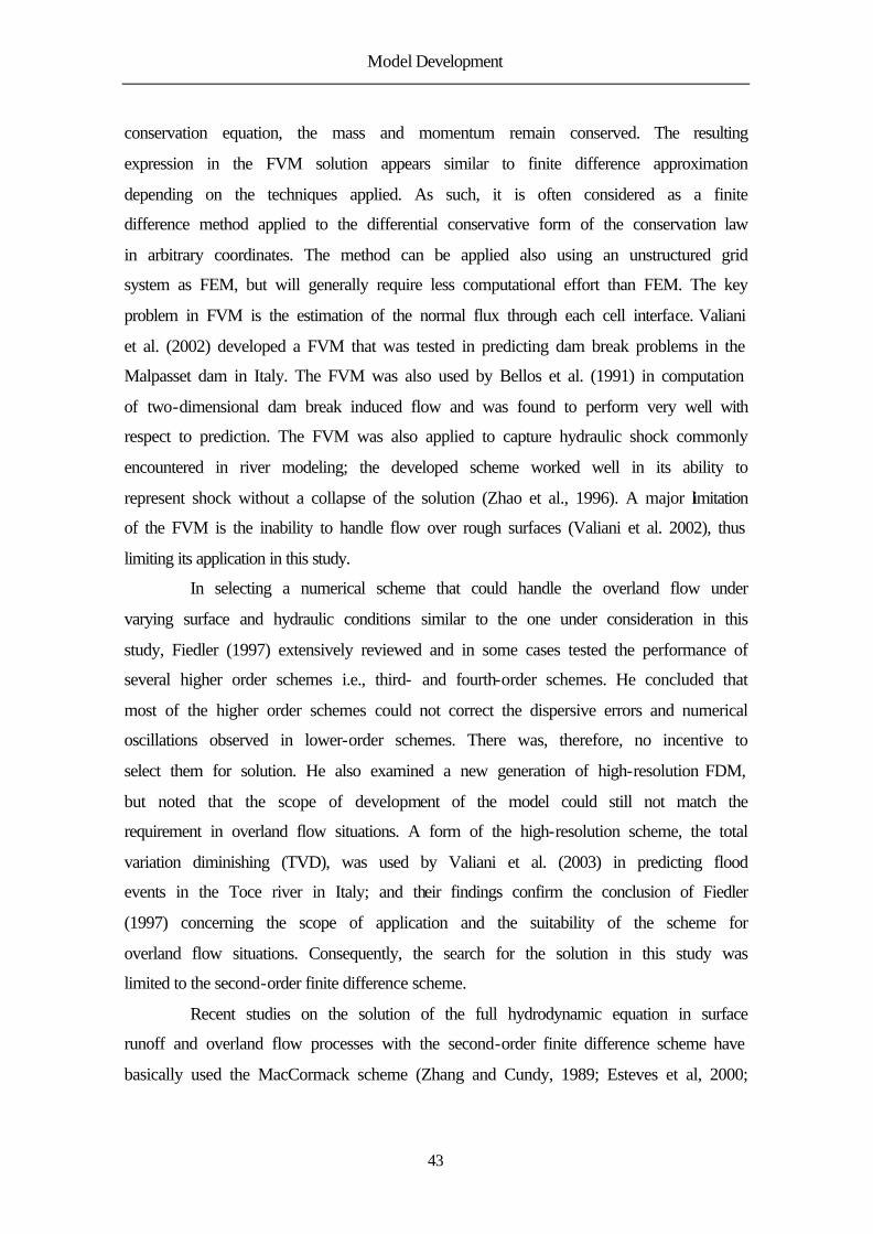
Model Development
43
conservation equation, the mass and momentum remain conserved. The resulting
expression in the FVM solution appears similar to finite difference approximation
depending on the techniques applied. As such, it is often considered as a finite
difference method applied to the differential conservative form of the conservation law
in arbitrary coordinates. The method can be applied also using an unstructured grid
system as FEM, but will generally require less computational effort than FEM. The key
problem in FVM is the estimation of the normal flux through each cell interface. Valiani
et al. (2002) developed a FVM that was tested in predicting dam break problems in the
Malpasset dam in Italy. The FVM was also used by Bellos et al. (1991) in computation
of two-dimensional dam break induced flow and was found to perform very well with
respect to prediction. The FVM was also applied to capture hydraulic shock commonly
encountered in river modeling; the developed scheme worked well in its ability to
represent shock without a collapse of the solution (Zhao et al., 1996). A major limitation
of the FVM is the inability to handle flow over rough surfaces (Valiani et al. 2002), thus
limiting its application in this study.
In selecting a numerical scheme that could handle the overland flow under
varying surface and hydraulic conditions similar to the one under consideration in this
study, Fiedler (1997) extensively reviewed and in some cases tested the performance of
several higher order schemes i.e., third- and fourth-order schemes. He concluded that
most of the higher order schemes could not correct the dispersive errors and numerical
oscillations observed in lower-order schemes. There was, therefore, no incentive to
select them for solution. He also examined a new generation of high-resolution FDM,
but noted that the scope of development of the model could still not match the
requirement in overland flow situations. A form of the high-resolution scheme, the total
variation diminishing (TVD), was used by Valiani et al. (2003) in predicting flood
events in the Toce river in Italy; and their findings confirm the conclusion of Fiedler
(1997) concerning the scope of application and the suitability of the scheme for
overland flow situations. Consequently, the search for the solution in this study was
limited to the second-order finite difference scheme.
Recent studies on the solution of the full hydrodynamic equation in surface
runoff and overland flow processes with the second-order finite difference scheme have
basically used the MacCormack scheme (Zhang and Cundy, 1989; Esteves et al, 2000;

Model Development
44
Fiedler and Ramirez, 2000), because of its simplicity and robustness. It is also second-
order accurate in space and time. It was observed during the review of the various
studies that the original form of the MacCormack scheme could not handle flow on
rough terrain. It requires some modification to accommodate this physical reality. A
variant is the application of the Leapfrog scheme by Playan et al. (1994, 1999). They
applied the Leapfrog scheme to the simulation of overland flow in basin irrigation
schemes on both simple and complex terrains. This scheme was shown to be
numerically stable in solution, but was criticized for being inflexible with respect to
stability at odd grid points and the requirements of artificial viscosity terms due limited
dissipative properties. To correct the problem of stability at odd grid points, a Leapfrog
scheme with centered time and space derivatives was used for this study; the scheme is
described below. A major incentive for the use of the scheme is its ability to accurately
handle very complex terrain and the ease of extension of the simulation area under study
without loss of prediction accuracy. The computational process ensures the efficiency of
computer resources, since the solutions are in staggered form.
4.7 Leapfrog scheme
The Leapfrog scheme is a second-order method for solving differential equations. It is a
three-time-level scheme that is second-order accurate in both space and time as depicted
graphically in Figure 4.1b. It present an attractive alternative for solution of numerical
problem in several fields of study, including meteorology, engineering physics,
astronautics, environment and economics etc, where systematic observations are
normally made.
The Leapfrog scheme has been successfully applied for computational
purposes in hydrology and its efficiency has been evaluated in comparison with other
schemes (Foreman, 1984; Akanbi, 1986; Playan, 1994). A major advantage of the
scheme is the staggered approach to the solution of equations (figure 4.2). Staggering of
the numerical solution, ensures that the numerical fluxes are not calculated the grid cell
interfaces, where jump and discontinuities occur, but rather at the gridcell centers
(figure 4.1a), where the variable varies smoothly (Erbes, 1994). When applied to the
surface runoff equation, the estimation of flow depth and discharges are staggered in
time by a half-time step, enhancing the stability of the scheme. A detailed description of

Model Development
45
the Leapfrog scheme as applied to shallow water equations in a basin irrigation scheme
is found in Playan (1992). However, there is no documented record of the application of
the scheme to surface runoff or overland flow modeling despite the itemized
advantages.
Figure 4.1a: Gridcell structure for staggered and non-staggered method using piecewise linear reconstructions.
Adapted from Erbes, 1994
i-1 i-1/2
i
i+1/2
i+1 i+3/2
i+2
Staggered cell Non-staggered cell
Interface fluxes

Model Development
46
Figure 4.1b: Schematization of a staggered grid (leapfrog method).
4.8 Adaptation of Leapfrog scheme
The general form of solution in the Leapfrog scheme is centered in time, but not in
space. Haltiner and William (1980) have, however, shown that centered differencing in
space is more accurate than forward or backward differencing, and it is used for the
derivative in equations 4.28 – 4.30. Using the leapfrog centered time and space-
differencing scheme; the derived surface runoff equation in finite form could be stated
as:
1, 1, , 1 , 1
,
1 1, , 0
2 2 2i j i j i j i j
i j
n n n nn nx x y yi j i j n
l
q q q qh hq
t x y+ − + −
+ − − −−+ + − =
∆ ∆ ∆ (4.36)
, , 1, 1,
1 , 1 , , 1 , 1
, , ,
,
1 1
0
1, 1,0 0
0
12 2
1( )
4 2 2
i j i j i j i j
i j i j i j i j
i j i j i j
i j
n n n nx x x x
n n n nn nx x y yi j i j n n
f
q q q q
t h x
q q q qh hg gh S S
x h x y
+ −
+ − + −
+ −
+ −
− −+
∆ ∆
− −−+ + = −
∆ ∆ ∆
(4.37)

Model Development
47
, , , 1 , 1
1, 1 , , 1 , 1
, , ,
,
1 1
0
, 1 , 10 0
0
12 2
1( )
4 2 2
i j i j i j i j
i j i j i j i j
i j i j i j
i j
n n n ny y y y
n n n nn nx x y yi j i j n n
f
q q q q
t h y
q q q qh hg gh S S
y h x y
+ −
+ − + −
+ −
+ −
− −+
∆ ∆
− −−+ + = −
∆ ∆ ∆
(4.38)
where i and j are the spatial indices and n is the time indices. The scheme is neutral and
is conditionally stable for problems involving non-linear advection terms, but may be
unstable for dissipative terms, because a short wave component of the solution emerges.
In this case, the profiles of the solution become uncontrollable (Cunge et al., 1980),
implying that two solutions will exist for the problem, whereas the differential equation
that is supposed to be approximated has one solution only. The false solution is simply
an artifact of the numerical scheme and has no bearing with reality.
Various methods have been proposed to handle this undesired condition. An
artificial viscous dissipation term may be introduced in the relationships. This damped
the numerical noise by ensuring smooth results in space (i.e. consecutive grid point),
while still maintaining the stability of the scheme. Another way of solving this problem
is to carry out grid refinement, in which the grid spacing and combination are carefully
selected. This often leads to increase in computational effort.
In this study, the second order turbulent viscosity used to account for turbulent
momentum transfer (Reynolds Stresses) in shallow water equation was applied (Erbes,
1994; Fieldler and Ramirez, 2000). This method involves the introduction of two terms
in second partial derivatives, which are added to the three equations developed for
surface runoff (4.31 – 4.33), thus we have:
22
2 2yx
diff
hhk
x y
∂∂+ ∂ ∂
=1, , 1,2 2
i j i j i jdiffk h h hx + −
∂ − + ∂
+, 1 , , 12
2i j i j i jdiffk h h h
y + −
∂ − + ∂ (4.39)
22
2 2yx
diff
qqk
x y
∂∂+ ∂ ∂
=1, , 1,
2 2i j i j i j
diff x x xk q q qx + −
∂ − + ∂
+, 1 , , 12
2i j i j i j
diff x x xk q q qy + −
∂ − + ∂ (4.40)
and

Model Development
48
22
2 2yx
diff
qqk
x y
∂∂+ ∂ ∂
=1, , 1,
2 2i j i j i j
diff y y yk q q qx + −
∂ − + ∂
+, 1 , , 12
2i j i j i j
diff y y yk q q qy + −
∂ − + ∂ (4.41)
for the three equations respectively. h = height difference along x-axis over a
staggered grid; , 1 , 1i j i j
h h+ −
− = height difference along y-axis over a staggered grid;
1, 1,i j i jx xq q
+ −− = difference in xq along x-axis over a staggered grid;
, 1 , 1i j i jx xq q
+ −− =
difference in xq along y-axis in a single staggered grid; 1, 1,i j i j
y yq q+ −
− = difference in
yq along x - axis over a staggered grid; , 1 , 1i j i j
y yq q+ −
− = difference in yq along y-axis
over a staggered grid; , ,
; ;i j i j
x yq q and ,i j
h are the middle grids values of qx, qy, and h,
while kdiff is the coefficient of diffusion. The value of this coefficient depends on the
type of problem being handled and must be adjusted until the stability of the solution is
achieved. Values of the diffusion factor tried with this model range between 0.5 and 5,
but the kdiff c = 1 is used in all computation processes in the numerical tests reported in
this thesis, since it effectively smears these discontinuities. The introduction of this
coefficient did not in any way affect the accuracy of the scheme.
4.9 Computational process
Numerical computational process in the Leapfrog scheme follows a staggered
implementation process, in which computation proceeds in half-time intervals (Figure
4.3). At the start of the computation process, the fluxes of the discharge momentum, and
that of the height at the nodes (i.e. i = 1, npx and j = 1,npy) in the x and y direction are
estimated from the equations (4.31 - 4.33). The fluxes for the friction slope in the two
directions are also calculated from equation (4.25 - 4.27).
At the whole-time steps, the continuity equation is solved to evaluate flow
depth at necessary nodes. The equation is discretized as:
02 2 2
t t tyx
l
qqh hq
t x y
+∆ ∂∂−+ + + =
∆ ∆ ∆ (4.42)

Model Development
49
where the spatial partial derivatives of the fluxes and the net lateral inflow are evaluated
at the time t+∆t/2 and the discretized equation allows for the solution of ht+∆t explicitly
as:
2 2yt t t x
l
qqh h q t
x y+∆ ∂ ∂
= − + + ∆ ∆ ∆ (4.43)
The centered-in-time formulation is implemented in the numerical scheme as:
, 1 , 1 , , 1 , 1
1 1,
i j i j i j i j i j
n n n n n ni j
t th h Qx Qx Qy Qy
x y+ − + −
+ − ∆ ∆ = − − − − ∆ ∆
1, , 1,
1 1 12
22
i j i j i j
n n ndiff
tk h h h
x + −
− − −∆ + − + ∆
, 1 , , 1
1 1 1 1,2
22 ( )
i j i j i j
n n n ndiff rate i j
tk h h h h
y + −
− − − −∆ + − + + ∆ (4.44)
where hrate is:
, ,( ) ( )
i j i jrate rih R t I t= − (4.45)
Infiltration rate is averaged over the discretized time, and the maximum hrate is
used.
To obtain the transient value for the flux qx and qy in both x - and y - directions
at the nodal points i = 2 to npx-1, on the x - axis, and j = 2, to npy - 1 on the y - axis.
The finite differencing process, i.e., centered – in - time step, is discretized in the
scheme as:
, , 1 , 1 , , 1 , 1
1 1 i j i j i j i j i j i j
n n n n n nx x xx xx xy xy
t tq q F F F F
x y+ − + −
+ − ∆ ∆ = − − − − ∆ ∆
, ,1, 1,( ) ( ) 2 ( )
i j i j
n n n nmt i j mt i j rsu
tgh h h t F
x + −∆ − − − ∆ ∆
1, , 1,
1 1 12
22
i j i j i j
n n ndiff x x x
tk q q q
x + −
− − −∆ + − + ∆
, 1 , , 1
1 1 12
22
i j i j i j
n n ndiff x x x
tk q q q
y + −
− − −∆ + − + ∆
(4.46)

Model Development
50
, , 1 , 1 , , 1 , 1
1 1 i j i j i j i j i j i j
n n n n n ny y xy xy yy yy
t tq q G G G G
x y+ − + −
+ − ∆ ∆ = − − − − ∆ ∆
, , 1 , 1 ,( ) ( ) 2 ( )i j
n n n nmt i j mt i j rsv i j
tgh h h t F
y + −∆ − − − ∆ ∆
1, , 1,
1 1 12
22
i j i j i j
n n ndiff y y x
tk q q q
x + −
− − −∆ + − + ∆
, 1 , , 1
1 1 12
22
i j i j i j
n n ndiff y y y
tk q q q
y + −
− − −∆ + − + ∆
(4.47)
where
1i ix x x+∆ = − ; 1j jy y y+∆ = −

Model Development
51
Define Experiment Parameters: 1. NPX, NPY; 2. Type of simulations; 3. Ksat @ grids; 4. Sorptivity; 5. Surface type; 6. X∆ , Y∆ , t∆ ; 7. Kdiff ; 8. Slope angle 9. Final computation step 10. Time to write data 11. Open or close boundary definition 12. Initial and final velocity 13. Friction factor
Import experiment parameters Write in a file (.par)
Open parameters file
No Stop
Stop No
Yes
Yes
Compute instantaneous Rainfall Intensity; Infiltration rate
Open Output data file
Define terrain Type i.e., Rough or Flat or Inclined
Compute Lateral inflow rate (based on terrain type)
Define initial flow depth, velocity, lateral inflow rate and reference initial conditions
Write data into info file giving summary of setup choices
Write initial values at boundary into data files; Initialize Time Counters (Kcount)
npxi=npx npyi=npy
Is Ksat grid Consistent
Define boundary relaxation coefficients; conservative variable in the interior
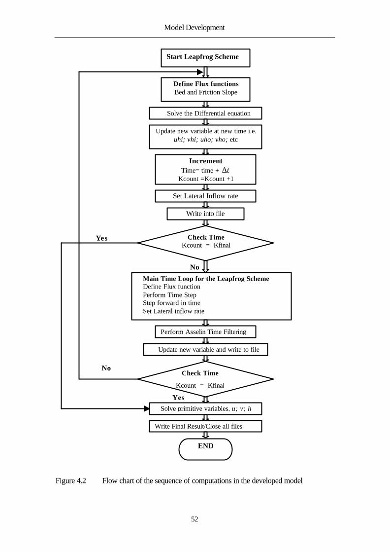
Model Development
52
Figure 4.2 Flow chart of the sequence of computations in the developed model
Start Leapfrog Scheme
Define Flux functions Bed and Friction Slope
Solve the Differential equation
Yes
No
Update new variable at new time i.e. uhi; vhi; uho; vho; etc
Check Time Kcount = Kfinal
Set Lateral Inflow rate
Main Time Loop for the Leapfrog Scheme Define Flux function Perform Time Step Step forward in time Set Lateral inflow rate
Perform Asselin Time Filtering
Write into file
Update new variable and write to file
Solve primitive variables, u; v; h
Increment Time= time + t∆
Kcount =Kcount +1
Check Time
Kcount = Kfinal
Write Final Result/Close all files
END
No
Yes

Model Development
53
Figure 4.3 A grid with three dependent variables that are computed at alternate grid points.
It should be noted in each stage of the leapfrog scheme, both space and time
differencing are implemented. The computation of the same variables at each node is
separated by an entire time step.
4.10 Initial and boundary conditions
The numerical computational procedure in the developed model required the
specification of appropriate initial and boundary conditions. For the purpose of stability
in the solution, a practical situation of zero initial flow depth, which holds before the
onset of a rainfall event till ponding, could not be applied. This necessitates the
definition of an initial overland flow depth, which should be small and insignificant in
the computational procedure. This technique has been applied in several numerical
studies on the overland flow process (Chow and Ben-Zvi, 1967; Zhang and Cundy,
1989; Tayfur et al., 1993; Esteves et al., 2000 and Fiedler and Ramirez, 2000). In this
study, a consistent value of initial depths was used so that the effect on the output will
be uniform and could be corrected.
The model is a limited area model (LAM), implying that it can only describe
or predict variables over the applied domain, not outside the domain. However, it also
requires the variables from this outside domain (i.e., boundaries) to predict those in the
qx, qy h qx, qy qx, qy h h
t0 t1/2 t1 t3/2 t2 t5/2

Model Development
54
applied domain. A boundary relaxation coefficient and a boundary relaxation zone is
defined appropriately. The boundary relaxation zone provide space to handle efficiently,
the error that might have occurred due to reconstruction of the oscillatory behavior by
the finite process. Consequently, in the experimental plot simulations, the closed
boundaries on the three sides of the plots are set such that there is no flow through them.
The fluxes of qx and qy perpendicular to these boundaries ( xbq y bq ) are set to zero.
Depths at close boundaries ( bh ) are defined using inward differences in both the
continuity and momentum equations. For example, when the south boundary is opened,
the following condition is applied from i=1, to i=npx
,1 ,2
,1 ,2
,1 ,2
i i
i i
i i
xb x x
yb y y
b
q q q
q q q
h h h
= =
= =
= =
(4.47)
and when it is fixed or closed:
,1
,1
,1 ,1
0
0i
i
i i
xb x
yb y
b init
q q
q q
h h h
= =
= =
= =
(4.48)
The values of all the fluxes at the boundary relaxation zones, in each time step
is corrected with the boundary relaxation coefficient from the expression:
( ) ( ) ( ), ,
1 1
, , ,(1 )
i j i j
n n nx x xbi j i j i j
q q qγ γ+ +
= − + (4.49)
( ) ( ) ( ), ,
1 1
, , ,(1 )
i j i j
n n n
y y ybi j i j i jq q qγ γ
+ += − + (4.50)
, ,
1 1 1, , ,(1 ) ( )
i j i j
n n ni j i j b i jh h hγ γ+ + += − + (4.51)
where ,i jγ is the boundary relaxation coefficient. ,0 1i jγ≤ ≤ , and it is given by
( )21 tanh 1
4kk
ndampγ
≡ − −
− ; 1k ≥ (4.52)
where ndamp is the width of the relaxation zone, k is the current gridpoint,
and k-1 is the number of grid points to the nearest boundary from the current grid point.

Model Development
55
4.11 Computational time optimization
The maximum allowable time step and horizontal resolution of the Leapfrog scheme as
in all other finite difference schemes are constrained by the Courant-Friedrichs-Lewy
(CFL) condition. The CFL condition provides a framework for the stability of the
numerical scheme, and basically implies that the flow must not progress farther than the
grid size during a time step. The CFL condition used for one-dimension flow is
generally expressed as:
c tCN
x∆
=∆
(4.53)
where c is the celerity (the phase speed) or an advection velocity of a small flow
disturbance (cm/s), ∆t is the time increment (s), and x∆ is the grid spacing in the x-
direction and 0 1CN≤ ≤ .
For the two-dimension solution applied in this study, the maximum admissible
time step is defined according to Bellos et al. (1988) as:
min ,x y
t CNu c v c∆ ∆ ∆ = + +
(4.54)
where ∆x and ∆y are the grid spacing in both directions, u and v are the initial velocity
at a point in time, in both directions, and CNmin indicates the minimum of the two
possible values the CN number. However, the source terms introduces further
restrictions on the admissible time step for simulation. This extent of restriction is
dependent on the rainfall intensity, inclination angle, microtopography, and the defined
artificial diffusion coefficient. Consequently rigorous stability analysis for the
developed equation is difficult. Fiedler, (1997) also reports the same limitation in the
application of MacCormack scheme, implying that the difficulty is not peculiar to the
Leapfrog scheme.
4.12 Time filtering
To reduce the amplitude of the computational mode, ensure smooth results in time (i.e.,
consecutive time steps) and avoid a decoupling of the solutions at odd and even time
steps (time splitting of the solution), an Asselin time-filter is applied at each time step
(Asselin 1972) to the computed values. The variables (qx, qy,) being time stepped is
operated on as follows

Model Development
56
( ) ( ) ( ) ( ) ( )1 1
, , ,, ,2
n nn n nx x x x xi j i j i ji j i j
q q q q qα− + = + − +
(4.54)
( ) ( ) ( ) ( ) ( )1 1
, , ,, ,2
n nn n n
y y y y yi j i j i ji j i jq q q q qα
− + = + − + (4.55)
and
( ) ( ) ( ) ( ) ( )1 1
, , ,, ,2
n nn n n
i j i j i ji j i jh h h h hα
− + = + − + (4.56)
where α is the time filtering coefficient. xq , yq and h are the filtered variables, which
is the model output.
At the first time step and after each time that an Asselin time filter has been
applied, a forward in time step is performed as:
, , 1, 1, , 1 , 1
1 2 2i j i j i j i j i j i j
n n n n n nx x xx xx xy xy
t tq q F F F F
x y+ − + −
+ ∆ ∆ = − − − − ∆ ∆
, 1 , 1, ,2 i j i j i j i j
n n n nmt mt rsu
tgh h h tF
x + −
∆ − − − ∆ ∆
1, , 1,2 2
i j i j i j
n n ndiff x x x
tk q q q
x + −
∆ + − + ∆
, 1 , , 122
i j i j i j
n n ndiff x x x
tk q q q
y + −
∆ + − + ∆
(4.57)
, , 1 , 1 , , 1 , 1
1 2 2i j i j i j i j i j i j
n n n n n ny y xy xy yy yy
t tq q G G G G
x y+ − + −
+ ∆ ∆ = − − − − ∆ ∆
, , 1 , 1 ,2 i j i j i j i j
n n n nmt mt rsv
tgh h h tF
y + −
∆ − − − ∆ ∆
1, , 1,2 2i j i j i j
n n ndiff y y x
tk q q q
x + −
∆ + − + ∆
, 1 , , 12
2i j i j i j
n n ndiff y y y
tk q q q
y + −
∆ + − + ∆
(4.58)

Model Development
57
, 1, 1 , , 1 , 1
1,
2 2i j i j i j i j i j
n n n n n ni j
t th h Qx Qx Qy Qy
x y+ − + −
+ ∆ ∆ = − − − − ∆ ∆
1, , 1,2 2
i j i j i j
n n ndiff
tk h h h
x + −
∆ + − + ∆
, 1 , , 1 ,2
22 ( )
i j i j i j
n n n ndiff rate i j
tk h h h h
y + −
∆ + − + + ∆ (4.59)
The second-order finite-difference approximation for the numerical process for
space and time derivatives is represented as in the following the expressions:
1 1
1 1 12 1
2
2i i i
n n nnx x xq q qg
x x x+ −
− − −− + +∂≈
∂ ∆ ∆ (4.60)
1 1
1 1 12 1
2
2j j j
n n nny y yq q qg
y y y+ −
− − −− + +∂≈
∂ ∆ ∆ (4.61)
1 1 12 11 1
2
n n nnj j jh h hg
y x y
− − −−+ −+ +∂
≈∂ ∆ ∆
(4.62)
where gn-1 is a generic variable describing the flow at each and every point in the
domain of the solution at all times. Figure 4.2 shows the flow chart of the computational
process in the developed solution applied in this study. Detailed descriptions of other
differentiation processes are provided in the numerical code. The solution of the
differential equations at the various boundaries is discussed in the section on boundary
and initial condition.
4.13 End of simulation
The end of the simulation processes in this model is determined by the defined
maximum time steps allowed and the computational time interval ∆t. During simulation
run with actual rainfall data, the maximum time step is determined by dividing the
duration in seconds of the rainfall event by the time interval. During simulation with
constant rainfall intensity, the end of the simulation is determined by the time defined in
the initializing file.

Model Development
58
4.14 Numerical test for the developed solution
No analytical solution exists for the full hydrodynamic equation. However, there are
some analytical solutions for the approximate form of the equation, which could be used
to verify the validity of the developed model. In testing the possibility of a mass balance
problem in the solution, the model output was compared with analytical solution of the
steady state kinematic wave solution for a plane of length 30.48m, with constant lateral
inflow rate of 25.4 mm h-1 developed by Woolhiser et al, 1996, which was also applied
by Fieldler et al. (2000) in validating the developed MacCormack scheme. The bed
slope for the test was 0.05 and the Darcy-Weisbach friction factor is 0.265. Table 4.2
present the result and a mass balance problem would have resulted in marked
discrepancies in computed discharge and flow depth.
Table 4.2 Comparison of output with the steady state kinematic wave test Analytical solution
(Woolhiser et al., 1976)
MacCormack Solution (Fieldler and Ramirez, 2000)
Leapfrog Solution (Ajayi 2004)
Depth (cm) 0.1462 0.1471 0.1470 Discharge (cm2s-1) 2.1505 2.1418 2.1420
Another example, which is generally accepted as a benchmark test problem for
the hydrodynamic equation, is the dam-break problem (Fennema and Chaudhry, 1990;
Jha et al, 1995; Fiedler and Ramirez, 2000; Zoppou and Roberts, 2003). The problem is
based on a scenario in which a shock wave develops at the moment of failure of a dam
wall measuring 1000 m with upstream water depth of the dam remaining constant at
10 m. The downstream water depth is 5m. This problem has a known analytical solution
given by Stoker (1957) and Wu et al. (1999). In simulating the dam break problem in
this model, the channel bed is assumed to be horizontal and frictionless. The time
interval for computation t∆ is =0.2s and the horizontal and vertical distance, x∆ and
y∆ were kept at 25cm. The result compared very well with both the analytical solution
and the solution of Fiedler and Ramirez (2000) produced with the MacCormack scheme
(Figure 4.4). The dam break problem is a measure of the ability of any developed
solution to adequately simulate the surface water component of the hydrodynamic

Model Development
59
model and capture non-physical rarefaction or and expansion shock. The performance
of the developed solution is quite interesting and shows the ability to handle such shock.
The study by Alcurdo and Garcia-Navarro (1994), which was also confirmed
by study by Zoppou and Roberts (2003), noted that at a downstream water depth of 5 m,
sub-critical flow still exists, which could easily cloud the problems in numerical
schemes, by providing a buffer for shocks. They therefore suggested the use of a
downstream water depth of 0.1 m, which they argue is a severe test case (transition
between subcritical and supercritical flows). This has been successfully used to
highlight problems with a number of numerical schemes that passed the first test.
Zoppou and Robert (2003) applied this version of the dam break test in analyzing the
performance of twenty explicit numerical schemes that solve the shallow water
equation. In trying out the second test, the parameters used for the first test were
adopted, but the downstream water depth level was reduced to 0.1 m. The developed
solution successfully captured even the shock initiated by such level of supercritical
flow, a condition in which a number of second-and higher-order schemes including
MacCormack failed to handle. This clearly shows that the developed solution is a good
shock-fitting numerical scheme, which is efficient, accurate and robust and would be
suitable for solving the full hydrodynamic equations when discontinuities are
encountered in the problem.
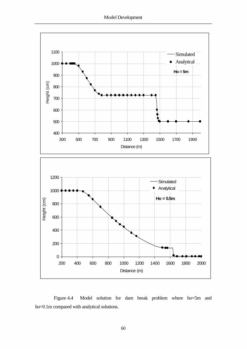
Model Development
60
Figure 4.4 Model solution for dam break problem where ho=5m and
ho=0.1m compared with analytical solutions.
Ho = 0.5m
0
200
400
600
800
1000
1200
200 400 600 800 1000 1200 1400 1600 1800 2000
Distance (m)
Hei
ght (
cm)
Simulated Analytical
Ho = 5m
400
500
600
700
800
900
1000
1100
300 500 700 900 1100 1300 1500 1700 1900
Distance (m)
Hei
ght (
cm)
SimulatedAnalytical
Field Results and Discussion
61
5 FIELD RESULTS AND DISCUSSION
5.1 Rainfall and runoff distribution
Figure 5.1 presents the distribution of rainfall within the catchment in the 2002 season.
A total of 96 rainstorm events were observed, out of which 17 were trace events,
therefore, the total number of effective events were 79. The average rainfall depth for
the season was 17.5mm, and the total rainfall for the season was 1684mm. Mean rainfall
intensity for the season ranged between 49.2mmh-1 – 90mmh-1 and the maximum
intensity range between 115 mmh-1 and 180 mmh-1. Higher intensity (up to 240 mmh-1)
was observed in some events. There were no significant differences in the total seasonal
rainfall recorded with the different rain gauges, but a measure of spatial variation in
rainfall depth were observed in most high intensity storms.
Day of Year (DOY)
0 50 100 150 200 250 300 350
Rai
nfal
l dep
th (m
m)
0
20
40
60
80
100
120
Depth
Figure 5.1 Rainfall distributions in Kotokosu catchment in 2002 season
A linear relationship, with a coefficient of determination of 0.60, (r2 = 0.60)
defines the relationship between the number of rainfall events per month and the
monthly rainfall total (Figure 5.2a,b). The period is characterized by high inter-seasonal
rainfall variability (c.v. = 0.87), synonymous with most tropical areas. Figure 5.2b
compares the cumulated monthly rainfall and number of events per month. With fewer

Field Results and Discussion
62
numbers of events, in comparison to October, the cumulative depth of rainfall in August
was higher, indicating that the rainfall in the month of August has longer duration.
The runoff producing events for the season were selected for further analysis.
The maximum and mean rainfall intensities of the separate events were related to the
rainfall depth, to appraise any possible effect of intensity on rainfall depth. Exponential
equations produce the best fit for the variables (figure 5.3). Both curves have low
coefficient of determination, but the maximum rainfall intensity is better correlated to
rainfall depth (r2=0.43), compared to the mean rainfall intensity (r2=0.18) for the season.
This suggests that, the maximum rainfall intensity will be expected to play a more
significant role in the hydrological processes over the catchment. Van Dijk (2002)
obtained a similar result (r2=0.30) while determining the relationships between depth-
averaged rainfall intensity (R) values derived from both original (R -orig.) and
resampled (R-resampl.) tipping bucket data and the respective storm rainfall depth (P)
values in West Java, Indonesia. The simple exponential relationship formed the basis for
an analytical expression used to derive the model parameters, for characterizing the
(R)USLE and GUEST models used in his study.
During the study period, there were in all about 40 runoff events at both sites.
Thirty-three events were selected, based on the criteria that, at least two plots per sites
(A & B) generate measurable runoff volume. Twenty-three joint events were further
selected in which all the eight runoff plots, simultaneously produced measurable runoff.
Some events could not be monitored at site A due to flash flooding, which submerged
the plots and the measuring equipment in June. Also, substantial contributions from
subsurface flow were noted in some events in the season, i.e., mostly prolonged events
with low intensity.

Field Results and Discussion
63
No of Events
0 5 10 15 20
Mon
thly
rai
nfal
l tot
al (
mm
)
0
100
200
300
400No. of Event vs Mothly Total y = 9.0331 + 16.5045x
r2 = 0.60
Figure 5.2a: Frequency of rainfall event against total depth on a monthly basis
Figure 5.2b Monthly total rainfall depth and number of events
0.0
50.0
100.0
150.0
200.0
250.0
300.0
350.0
February May August NovemberMonth
Dep
th (
mm
)
0
2
46
8
10
12
1416
18
20
No
of E
vent
s
Total depth
No of Event

Field Results and Discussion
64
Rainfall Depth (mm)
0 20 40 60 80 100 120
Rai
nfal
l Int
ensi
ty (m
mhr
-1)
0
50
100
150
200
250Mean Rain IntMax. Rain IntMax Int. = 44.636Rainvdepth0.3225
r2 = 0.43Min int. = 20.3997 Rain Depth0.2726
r2 = 0.18
Figure 5.3 The relationship between mean and maximum rainfall intensity and rainfall depth
Fig 5.4 Comparison of number of rainfall and runoff events per month for the season
A breakdown of total number of runoff events compared with the number of
rainfall events on a monthly basis is shown in Figure 5.4. The graph shows that there
0
5
10
15
20
Februa
ryMarc
hApri
lMay Jun
eJuly
August
Septem
berOctob
er
November
December
Month
No
of E
vent
s
No of Rainfall EventsNo of Runoff Events
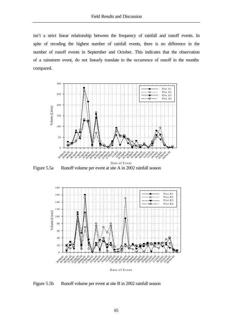
Field Results and Discussion
65
isn’t a strict linear relationship between the frequency of rainfall and runoff events. In
spite of recoding the highest number of rainfall events, there is no difference in the
number of runoff events in September and October. This indicates that the observation
of a rainstorm event, do not linearly translate to the occurrence of runoff in the months
compared.
Date o f Event
20-M
ar-02
29-Mar-
02
06-Apr-
02
08-Apr-
02
13-Apr-
02
15-Apr-
02
23-Apr-
02
05-May-
02
09-M
ay-02
16-M
ay-02
19-M
ay-02
22-May-
02
27-M
ay-02
12-Ju
l-02
23-Jul-
02
01-Aug-
02
29-A
ug-02
02-Sep
-02
03-Se
p-02
06-Se
p-02
06-Oct-0
2
12-Oct-0
2
17-O
ct-02
24-Oct-0
2
25-Oct-0
2
03-Nov-
02
04-N
ov-02
Vol
ume
(Litr
es)
0
50
100
150
200
250
300
Plot A1 Plot A2 Plot A3 Plot A4
Figure 5.5a Runoff volume per event at site A in 2002 rainfall season
D a t e o f E v e n t
29-Mar-0
2
06-A
pr-02
08-A
pr-02
15-Apr-
02
23-A
pr-02
05-M
ay-02
09-May-
02
22-M
ay-02
27-May-
02
03-Ju
n-02
14-Ju
n-02
16-Ju
n-02
19-Ju
n-02
12-Ju
l-02
23-Ju
l-02
01-A
ug-02
05-Aug-
02
29-A
ug-02
02-Se
p-02
03-Sep
-02
06-Se
p-02
07-Se
p-02
09-Se
p-02
18-Se
p-02
06-Oct-0
2
12-O
ct-02
17-Oct-0
2
18-Oct-0
2
24-O
ct-02
25-Oct-0
2
04-N
ov-02
Vol
ume
(Litr
es)
0
20
40
60
80
100
120
140
160
180
P l o t B 1 P l o t B 2 P l o t B 3 P l o t B 4
Figure 5.5b Runoff volume per event at site B in 2002 rainfall season

Field Results and Discussion
66
Figures 5.5a and 5.5b present the volume of runoff per event in each of the
four plots, in the two sites (site A and site B) used for observation. The total depth of
rainfall during the period of occurrence of the runoff events amounted to 747.6 mm in
site A and 995.6 in site B. These figures reveal some differences in the hydrological
behavior of the two sites used for investigation. The following salient points, which can
be interpreted form the graphs deserves mention.
Consistently, the runoff volumes recorded in most events from site (A) are
higher than those from site (B). The causative factor(s) of this observation will be
discussed at a later section in this thesis.
Except on one occasion in site B, the runoff volume generally decreased as the
season progresses, and only picked up towards the end of the season. The declining
trend of runoff volume could among other factors be associated with the change in the
vegetation canopy on all the plots, which apparently reduce the impact of rainfall. The
difference in the type of vegetation that developed from the two sites is also reflected in
the amount of runoff observed. Whereas narrow leave grasses developed at site (A),
wide leaf shrubs developed on the plots at site B.
Vegetation development reduces substantially the flow velocity of surface
runoff and simultaneously increases the friction resistance to the overland flow, and the
time required for initiation of a runoff process. With increasing period since the
beginning of the season, the canopy covers fraction and the vegetation density on all the
plots increases, thereby increasing the effect of vegetative microtopography (mostly for
low intensity events), and frictional resistance to overland flow. The combination of
these processes significantly reduces the discharge volume.
The period during which, the decreasing trend of runoff volume changed,
coincided with the period the whole vegetation on all the plots were carefully removed
to plant maize. The observation show that vegetation cover significantly impact surface
runoff and infiltration process in the catchment.

Field Results and Discussion
67
vol A1
0 50 100 150 200 250 300
vol A
2
0
50
100
150
200
250
300
vol A1 vs vol A2 vol (A2) = 7.3194 + .84 vol (A1)r2 = 0.89
Figure 5.6a Comparison of runoff volume from the twin long plots at site A
In both sites, the highest runoff volumes were recorded early in the season i.e.
April and May. These could be explained by the impact of vegetal cover already
described above. In evaluating the possible effect of random noise in the runoff
responses, the volumes of runoff from the twin long plots A1 vs. A2, and B1 vs. B2 at
each sites were compared. To appreciate inter-site variability in response and random
noise from the two sites, the runoff volume from one selected long plots from each site
i.e. A1 vs. B2 and the short plots i.e. A4 and B4 were compared.
The high coefficient of determination of the linear equations between the
runoff volume, and the narrow dispersion of the data from the twin-runoff plots at site A
(r2 = 0.89) and site B (r2 = 0.75) indicate reasonable similarity in the response from the
runoff plots at each site and that the measurement did not present large random noise.
The small difference in the response, not captured by the linear equations could result
from the natural differences in plot characteristics and the characteristic non-linearity in
Hortonian runoff process.
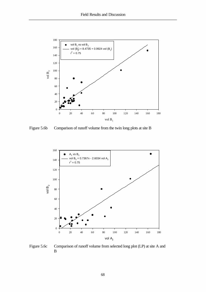
Field Results and Discussion
68
vol B1
0 20 40 60 80 100 120 140 160 180
vol B
2
0
20
40
60
80
100
120
140
160
180
vol B1 vs vol B2 vol (B2) = 8.4735 + 0.9924 vol (B1)
r2 = 0.75
Figure 5.6b Comparison of runoff volume from the twin long plots at site B
vol A2
0 20 40 60 80 100 120 140 160 180
vol B
2
0
20
40
60
80
100
120
140
160A2 vs B2 vol B2 = 0.7367x - 2.6034 vol A2
r2 = 0.75
Figure 5.6c Comparison of runoff volume from selected long plot (LP) at site A and B
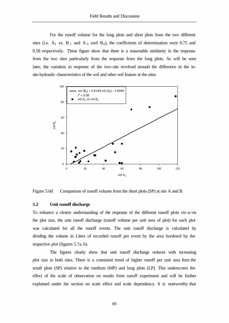
Field Results and Discussion
69
For the runoff volume for the long plots and short plots from the two different
sites (i.e. A1 vs. B 2 and A 4 and B 4), the coefficients of determination were 0.75 and
0.58 respectively. These figure show that there is a reasonable similarity in the response
from the two sites particularly from the response from the long plots. As will be seen
later, the variation in response of the two-site revolved around the difference in the in-
situ hydraulic characteristics of the soil and other soil feature at the sites.
vol A4
0 20 40 60 80 100 120
vol B
4
0
20
40
60
80
100vol (B4) = 0.6149 vol (A4) - 2.6049r2 = 0.58vol A4 vs vol B4
Figure 5.6d Comparison of runoff volume from the short plots (SP) at site A and B
5.2 Unit runoff discharge
To enhance a clearer understanding of the response of the different runoff plots vis-a-vis
the plot size, the unit runoff discharge (runoff volume per unit area of plot) for each plot
was calculated for all the runoff events. The unit runoff discharge is calculated by
dividing the volume in Liters of recorded runoff per event by the area bordered by the
respective plot (figures 5.7a, b).
The figures clearly show that unit runoff discharge reduces with increasing
plot size in both sites. There is a consistent trend of higher runoff per unit area from the
small plots (SP) relative to the medium (MP) and long plots (LP). This underscores the
effect of the scale of observation on results from runoff experiment and will be further
explained under the section on scale effect and scale dependency. It is noteworthy that
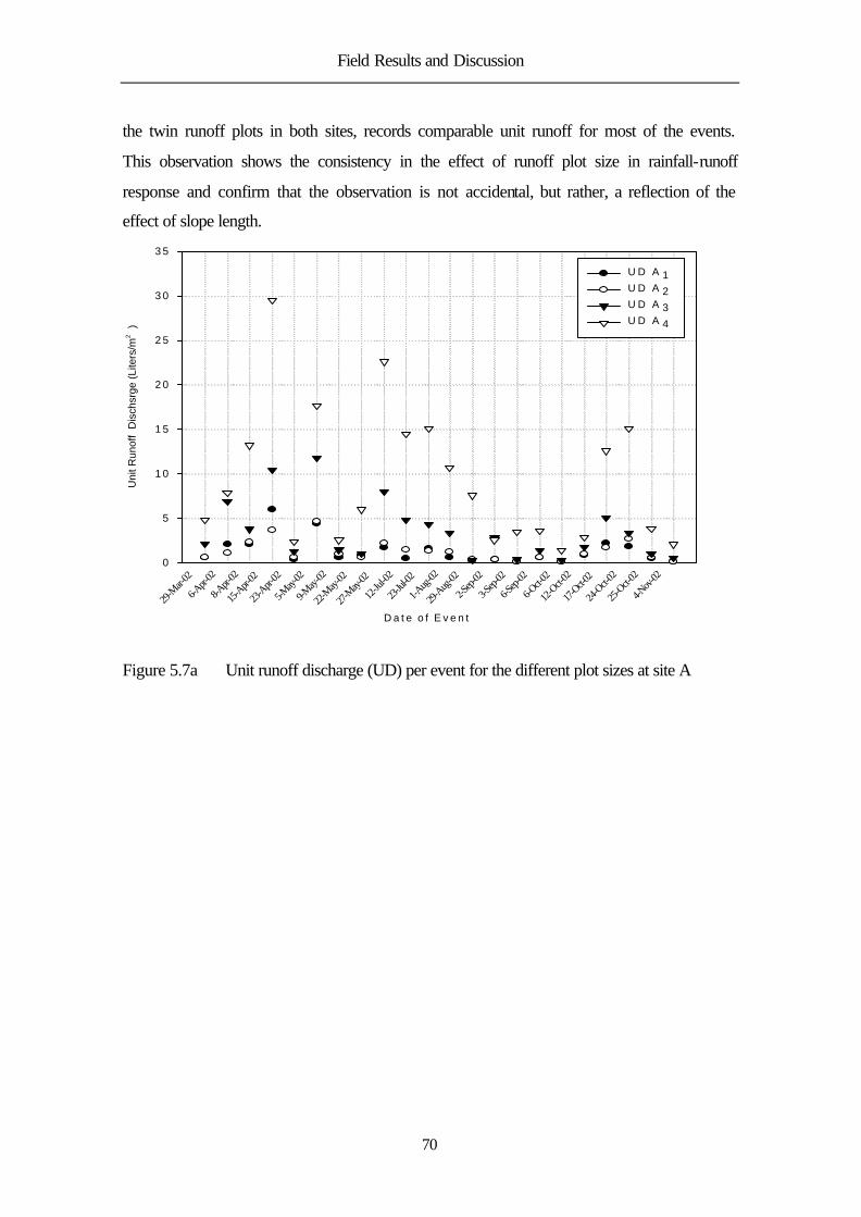
Field Results and Discussion
70
the twin runoff plots in both sites, records comparable unit runoff for most of the events.
This observation shows the consistency in the effect of runoff plot size in rainfall-runoff
response and confirm that the observation is not accidental, but rather, a reflection of the
effect of slope length.
D a t e o f E v e n t
29-M
ar-02
6-Apr-
02
8-Apr-
02
15-A
pr-02
23-A
pr-02
5-May-
02
9-May-
02
22-M
ay-02
27-May-
02
12-Ju
l-02
23-Jul
-02
1-Aug
-02
29-A
ug-02
2-Sep-
02
3-Sep-
02
6-Sep-
02
6-Oct-0
2
12-O
ct-02
17-Oct-0
2
24-O
ct-02
25-O
ct-02
4-Nov-
02
Uni
t Run
off
Dis
chsr
ge (
Lite
rs/m
2 )
0
5
1 0
1 5
2 0
2 5
3 0
3 5
U D A 1
U D A 2
U D A 3
U D A 4
Figure 5.7a Unit runoff discharge (UD) per event for the different plot sizes at site A

Field Results and Discussion
71
D a t e o f E v e n t
29-M
ar-02
6-Apr-
02
8-Apr-
02
15-Apr-
02
23-Apr-
02
5-May-
02
9-May-
02
22-May-
02
27-M
ay-02
12-Jul
-02
23-Jul
-02
1-Aug-
02
29-Aug-
02
2-Sep-
02
3-Sep-
02
6-Sep-
02
6-Oct-0
2
12-O
ct-02
17-O
ct-02
24-O
ct-02
25-Oct-0
2
4-Nov
-02
Uni
t Run
off D
isch
arge
(Lite
rs/m
2 )
0
5
10
15
20
25
U D B 1 U D B 2
U D A 3
U D B 4
Figure 5.7b Unit runoff discharge (UD) per event for the different plot sizes at site B
UD A1
0 2 4 6 8 10
UD
A2
; UD
A3; U
D A
4
0
10
20
30
40
50
UD A 1 vs UD A2 UD A 1 vs UD A3
UD A 1 vs UD A4
Linear UD A1 vs. UD A2
Linear UD A1 vs UD A3
Linear UD A1 vs UD A4
Figure 5.8a Relationship between the unit runoff discharge amongst plots in site A
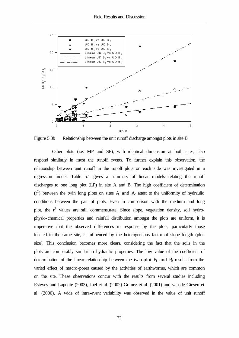
Field Results and Discussion
72
U D B 1
0 1 2 3 4 5
UD
B2; U
B3; U
B4
0
5
1 0
1 5
2 0
2 5
U D B 1 v s U D B 2
U D B 1 v s U D B 3 U D B 1 v s U D B 4 L i n e a r U D B 1 v s U D B 2
L i n e a r U D B 1 v s U D B 3
L i n e a r U D B 1 v s U D B 4
Figure 5.8b Relationship between the unit runoff discharge amongst plots in site B
Other plots (i.e. MP and SP), with identical dimension at both sites, also
respond similarly in most the runoff events. To further explain this observation, the
relationship between unit runoff in the runoff plots on each side was investigated in a
regression model. Table 5.1 gives a summary of linear models relating the runoff
discharges to one long plot (LP) in site A and B. The high coefficient of determination
(r2) between the twin long plots on sites A1 and A2 attest to the uniformity of hydraulic
conditions between the pair of plots. Even in comparison with the medium and long
plot, the r2 values are still commensurate. Since slope, vegetation density, soil hydro-
physio-chemical properties and rainfall distribution amongst the plots are uniform, it is
imperative that the observed differences in response by the plots; particularly those
located in the same site, is influenced by the heterogeneous factor of slope length (plot
size). This conclusion becomes more clears, considering the fact that the soils in the
plots are comparably similar in hydraulic properties. The low value of the coefficient of
determination of the linear relationship between the twin-plot B1 and B2 results from the
varied effect of macro-pores caused by the activities of earthworms, which are common
on the site. These observations concur with the results from several studies including
Esteves and Lapetite (2003), Joel et al. (2002) Gómez et al. (2001) and van de Giesen et
al. (2000). A wide of intra-event variability was observed in the value of unit runoff

Field Results and Discussion
73
discharge in the season. Differences are more pronounced for short duration high
intensity events and low intensity events. For rainstorm with long duration, and high
depth, the unit runoff discharge differs only slightly.
Higher unit runoff discharge in small plots is more often associated with the
spatial variability of the hydrological properties. This is equally observed in this study,
but as will be better discussed in the section on scale effect, spatial variability of soil
properties could not wholly explain the observation. Rainfall duration and directions are
equally uniform; consequently, the temporal dynamics associated with different
opportunities for overland flow reduction or increse in transit, which vary depending on
slope lengths, would be necessary to make the explicit, the difference in unit discharge.
In the analysis of time before onset of runoff and duration of runoff, the time lag
between the onset and cessation of runoff event in different plot size are very close.
Table 5.1 Relationship between unit runoff on all plots at site A and B Variables Equations r2 UDA1 vs. UDA2 y = 0.2000 + 0.8425 x 0.90 UDA1 vs. UDA3 y = 1.0920 + 1.6082 x 0.77 UDA1 vs. UDA4 y = 3.3419 + 4.1456 x 0.78 UDB1 vs. UDB2 y = 0.2312 + 0.9973 x 0.75 UDB1 vs. UDB3 y = 0.5550 + 1.8628 x 0.69 UDB1 vs. UDB4 y = 4.2143 + 4.7704 x 0.43
5.3 Runoff coefficient
Runoff coefficient in percentages or as ratios is a widely accepted statistic in explaining
rainfall-runoff response (van de Giesen et al., 2000; Esteves and Lapetite, 2003;
Wainwright and Parsons, 2003). In this study, the runoff coefficient for all the runoff
events were computed to further elucidate on the response of each of the scaled-plot to
the rainfall events. Rainfall depth for the individual events was converted to volume of
rainfall (per event) over the area enclosed by each runoff plot. The obtained rainfall
volume per plot is then divided by the volume of runoff collected from the
corresponding plots for the event. This value gives an idea of the proportion of rainfall
that is converted to runoff during an event for each runoff plot. Figures 5.9 a and b show
the temporal pattern of the runoff coefficient in the rainfall season under study. It is very
clear from the figures that the runoff coefficient is strongly influenced by the scale of

Field Results and Discussion
74
observation and the rainfall depth (amount). The small runoff plots A4 and B4 has higher
coefficient for all the events, in comparison to the long and medium runoff plots.
D a t e o f e v e n t20-
Mar-02
29-Mar-0
2
06-Apr-
02
08-Apr-
02
13-A
pr-02
15-A
pr-02
23-Apr-
02
05-May-
02
09-May-
02
16-May-
02
19-May-
02
22-M
ay-02
27-May-
02
12-Jul
-02
23-Jul
-02
01-Aug-
02
29-Aug-
02
02-Sep
-02
03-Sep
-02
06-Sep
-02
06-O
ct-02
12-O
ct-02
17-Oct-0
2
24-Oct-0
2
25-O
ct-02
03-Nov-
02
04-Nov-
02
Run
off c
oefi
cien
t
0.0
0.2
0.4
0.6
0.8
1.0
R Q A 1
R Q A 2
R Q A 3
R Q A 4
Figure 5.9a Runoff coefficient per event in site A
During rainfall events with high rainfall depth, the small plots records close to
unity in runoff coefficient (Figures 5.10a and b). This implies a large proportion of the
rainfall is converted to runoff. This can be simply explained by two possible
developments during such events. In the first instance, high rainfall depth may result
from very high intensity event that last a short time. Such events often lead to clogging
and surface sealing, which reduces infiltration significantly and increase runoff. In a
short plot, the effect of surface sealing is more pronounced due to a short slope length.
Short slope lengths translate to reduced time for infiltration downslope and faster
opportunity to reach the gutter. This results in the very high runoff volume for the short
plot and consequently, a high runoff coefficient. Secondly, high rainfall intensity and
the associated surface sealing in a short plot stimulate ponding of the plot in a short
time. Subsequent raindrop after ponding directly contributes to runoff. The volume of
runoff discharged at moments after rain had stopped also enhances the high value of
runoff coefficient.

Field Results and Discussion
75
High depth rainfall events could also arise from low intensity events with
prolonged duration. Low intensity prevents surface sealing and will therefore increase
infiltration rate, and may allow pseudo-saturation in short time interval. Such soil
saturation state is very easily attained in a short plot in comparison to a long plot, due to
the differences in area be covered. From the moment of saturation, any additional
rainfall directly contributes to runoff and such scenarios result in a condition in which
the proportion of runoff volume may be increased in the short plot.
D a t e o f E v e n t29
-Mar-
02
06-A
pr-02
08-A
pr-02
15-A
pr-02
23-A
pr-02
05-M
ay-02
09-M
ay-02
22-M
ay-02
27-M
ay-02
03-Ju
n-02
14-Jun
-02
16-Ju
n-02
19-Ju
n-02
12-Ju
l-02
23-Ju
l-02
01-A
ug-02
05-A
ug-02
29-A
ug-02
02-Se
p-02
03-Se
p-02
06-Se
p-02
07-Se
p-02
09-Se
p-02
18-Se
p-02
06-O
ct-02
12-O
ct-02
17-O
ct-02
18-O
ct-02
24-O
ct-02
25-O
ct-02
04-N
ov-02
Run
off c
oeff
icie
nt
0 .0
0 .2
0 .4
0 .6
0 .8
1 .0
R Q B 1
R Q B 2
R Q B 3
R Q B 4
Figure 5.9b Runoff coefficient per event in site B
For some low depth rainfall event, the difference in runoff coefficient between
the long and short is minimal. Such observation probably occurs with events coming
after a period of dry spell, which would have increase, the infiltration potential of the
soil. In such events, the soil is not saturated, and the low intensity nature of the rain
prevents surface sealing of the soil. Surface sealing would have increased the runoff
volume differentially. It is also evident that the set of twin plots (A1-A2, B1-B2) exhibits
marked similarity in response to the rainfall event.

Field Results and Discussion
76
Date of Event
20-Mar-
02
29-M
ar-02
06-Apr-0
2
08-Apr-0
2
13-Apr-
02
15-Apr-0
2
23-Apr-0
2
05-May-
02
09-May-
02
16-May-
02
19-May-
02
22-May-
02
27-May-
02
12-Ju
l-02
23-Ju
l-02
01-Aug
-02
29-Aug-
02
02-Sep-
02
03-Sep
-02
06-Sep-
02
06-Oct-0
2
12-O
ct-02
17-Oct-0
2
24-Oct-0
2
25-O
ct-02
03-Nov-
02
04-Nov-
02
Run
off C
oeffi
cien
t (%
)
0
20
40
60
80
100
Rai
nfal
l dep
th (
mm
)
0
10
20
30
40
50
60
70
80
RQ A1
RQ A4
Rain Depth
Figure 5.10a: Trend of runoff coefficient and rainfall depth from LP and SP plots at site
A
Event Date
29-Mar-0
2
06-Apr-0
2
08-Apr-0
2
15-Apr-0
2
23-Apr-0
2
05-May-
02
09-May-
02
22-May-
02
27-May-
02
03-Jun
-02
14-Jun
-02
16-Jun
-02
19-Jun
-02
12-Jul-
02
23-Jul-
02
01-Aug-
02
05-Aug-
02
29-Aug-
02
02-Sep
-02
03-Sep
-02
06-Sep
-02
07-Sep
-02
09-Sep
-02
18-Sep
-02
06-Oct-0
2
12-Oct-0
2
17-Oct-0
2
18-Oct-0
2
24-Oct-0
2
25-Oct-0
2
04-Nov-
02
Run
off C
oeffi
cien
t (%
)
0
20
40
60
80
100
Rai
nfal
l Dep
th (m
m)
0
20
40
60
80
100
120
RQ B1 RQ B4
Rain depth
Figure 5.10b: Trend of runoff coefficient and rainfall depth from LP and SP plots at site
B
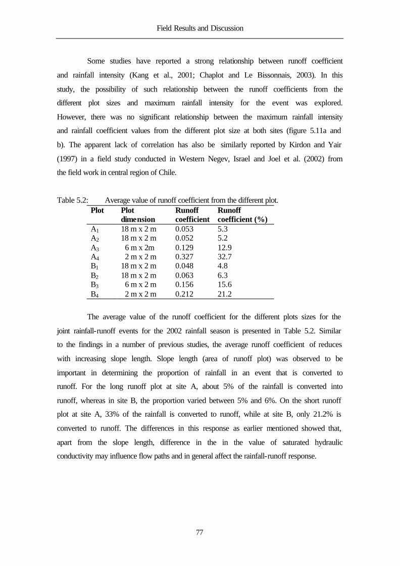
Field Results and Discussion
77
Some studies have reported a strong relationship between runoff coefficient
and rainfall intensity (Kang et al., 2001; Chaplot and Le Bissonnais, 2003). In this
study, the possibility of such relationship between the runoff coefficients from the
different plot sizes and maximum rainfall intensity for the event was explored.
However, there was no significant relationship between the maximum rainfall intensity
and rainfall coefficient values from the different plot size at both sites (figure 5.11a and
b). The apparent lack of correlation has also be similarly reported by Kirdon and Yair
(1997) in a field study conducted in Western Negev, Israel and Joel et al. (2002) from
the field work in central region of Chile.
Table 5.2: Average value of runoff coefficient from the different plot. Plot Plot
dimension Runoff coefficient
Runoff coefficient (%)
A1 18 m x 2 m 0.053 5.3 A2 18 m x 2 m 0.052 5.2 A3 6 m x 2m 0.129 12.9 A4 2 m x 2 m 0.327 32.7 B1 18 m x 2 m 0.048 4.8 B2 18 m x 2 m 0.063 6.3 B3 6 m x 2 m 0.156 15.6 B4 2 m x 2 m 0.212 21.2
The average value of the runoff coefficient for the different plots sizes for the
joint rainfall-runoff events for the 2002 rainfall season is presented in Table 5.2. Similar
to the findings in a number of previous studies, the average runoff coefficient of reduces
with increasing slope length. Slope length (area of runoff plot) was observed to be
important in determining the proportion of rainfall in an event that is converted to
runoff. For the long runoff plot at site A, about 5% of the rainfall is converted into
runoff, whereas in site B, the proportion varied between 5% and 6%. On the short runoff
plot at site A, 33% of the rainfall is converted to runoff, while at site B, only 21.2% is
converted to runoff. The differences in this response as earlier mentioned showed that,
apart from the slope length, difference in the in the value of saturated hydraulic
conductivity may influence flow paths and in general affect the rainfall-runoff response.
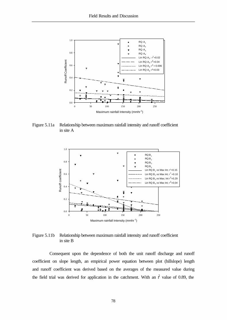
Field Results and Discussion
78
Maximum rainfall Intensity (mmhr-1)
0 50 100 150 200 250
Run
off C
oeffi
cien
t
0.0
0.2
0.4
0.6
0.8
1.0RQ A1
RQ A2 RQ A3
RQ A4
Lin RQ A1; r2=0.02
Lin RQ A2; r2=0.04
Lin RQ A3; r2 = 0.006
Lin RQ A4; r2=0.03
Figure 5.11a Relationship between maximum rainfall intensity and runoff coefficient in site A
Maximum rainfall Intensity (mmhr -1)
0 50 100 150 200 250
Run
off c
oeffi
cien
t
0.0
0.2
0.4
0.6
0.8
1.0
RQ B1 RQ B2
RQ B3
RQ B4
Lin RQ B1 vs Max Int; r 2=0.15
Lin RQ B2 vs Max Int; r2 =0.10
Lin RQ B3 vs Max; Int r2=0.29
Lin RQ B4 vs Max Int; r2=0.04
Figure 5.11b Relationship between maximum rainfall intensity and runoff coefficient in site B
Consequent upon the dependence of both the unit runoff discharge and runoff
coefficient on slope length, an empirical power equation between plot (hillslope) length
and runoff coefficient was derived based on the averages of the measured value during
the field trial was derived for application in the catchment. With an r2 value of 0.89, the

Field Results and Discussion
79
model explains the strong relationship existing between quantity of runoff discharge in
response to rainfall event and the length of travel of the overland flow. Wainwright and
Parsons (2003) in a model study of surface runoff processes similarly obtained power
equations, relating runoff coefficient and slope length, although the effect of slope
length will change with the slope angle and the microtopographic form. The digital
elevation model of the study site show that the average slope angle in all part of the
catchment ranges between 4° and 7°, thus the derived equation could be which was
based on 5° slope could be applied in most part of the catchment.
Slope Length (m)
0 5 10 15 20
Run
off C
oeffi
cien
t (%
)
0
5
10
15
20
25
30
35
Slope Length vs RQ (%) RC (%) = 43.7119 SL-0.6808
r2 = 0.89
Figure 5.12 Relationship between runoff coefficient and plot length
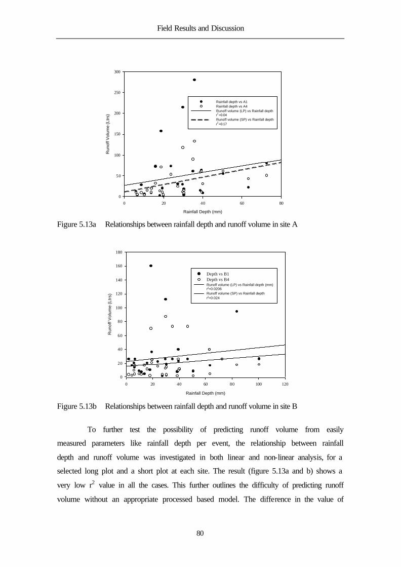
Field Results and Discussion
80
Rainfall Depth (mm)
0 20 40 60 80
Run
off V
olum
e (L
trs)
0
50
100
150
200
250
300
Rainfall depth vs A1 Rainfall depth vs A4 Runoff volume (LP) vs Rainfall depth r2=0.04Runoff volume (SP) vs Rainfall depthr2=0.17
Figure 5.13a Relationships between rainfall depth and runoff volume in site A
Rainfall Depth (mm)
0 20 40 60 80 100 120
Run
off V
olum
e (L
trs)
0
20
40
60
80
100
120
140
160
180
Depth vs B1 Depth vs B4 Runoff volume (LP) vs Rainfall depth (mm) r2=0.0206Runoff volume (SP) vs Rainfall depthr2=0.024
Figure 5.13b Relationships between rainfall depth and runoff volume in site B
To further test the possibility of predicting runoff volume from easily
measured parameters like rainfall depth per event, the relationship between rainfall
depth and runoff volume was investigated in both linear and non-linear analysis, for a
selected long plot and a short plot at each site. The result (figure 5.13a and b) shows a
very low r2 value in all the cases. This further outlines the difficulty of predicting runoff
volume without an appropriate processed based model. The difference in the value of
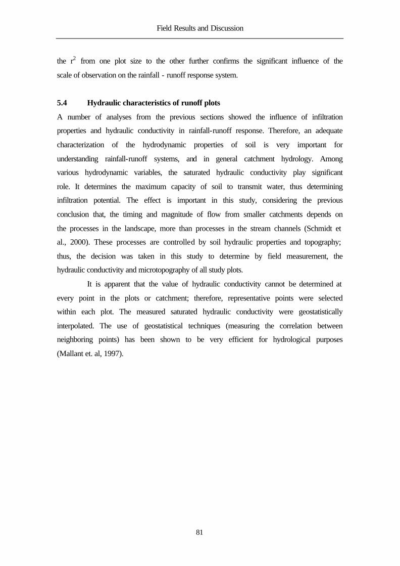
Field Results and Discussion
81
the r2 from one plot size to the other further confirms the significant influence of the
scale of observation on the rainfall - runoff response system.
5.4 Hydraulic characteristics of runoff plots
A number of analyses from the previous sections showed the influence of infiltration
properties and hydraulic conductivity in rainfall-runoff response. Therefore, an adequate
characterization of the hydrodynamic properties of soil is very important for
understanding rainfall-runoff systems, and in general catchment hydrology. Among
various hydrodynamic variables, the saturated hydraulic conductivity play significant
role. It determines the maximum capacity of soil to transmit water, thus determining
infiltration potential. The effect is important in this study, considering the previous
conclusion that, the timing and magnitude of flow from smaller catchments depends on
the processes in the landscape, more than processes in the stream channels (Schmidt et
al., 2000). These processes are controlled by soil hydraulic properties and topography;
thus, the decision was taken in this study to determine by field measurement, the
hydraulic conductivity and microtopography of all study plots.
It is apparent that the value of hydraulic conductivity cannot be determined at
every point in the plots or catchment; therefore, representative points were selected
within each plot. The measured saturated hydraulic conductivity were geostatistically
interpolated. The use of geostatistical techniques (measuring the correlation between
neighboring points) has been shown to be very efficient for hydrological purposes
(Mallant et. al, 1997).

Field Results and Discussion
82
10
12
14
16
18
20
22
24
26
28
30
32
34
36
mm/hr
0 50 100 150 200
centimeters
Figure 5.14a Spatial distribution of saturated hydraulic conductivity (Ksat) in plot A4
30
40
50
60
70
80
90
100
110
120
130
140
150
160
170
mm/hr
0 50 100 150 200
centimeters
Figure 5.15b Spatial distribution of saturated hydraulic conductivity (Ksat) in plot B4

Field Results and Discussion
83
24
6
810
12
14
1618
20
22
2426
28
3032
34
3638
mm/hr
0 500 1000 1500 2000
centimeters
Figure 5.15c Spatial distribution of saturated hydraulic conductivity (Ksat) in LPA
30
40
50
60
70
80
90
100
110
120
130
140
150
160
170
180
mm/hr
0 500 1000 1500 2000
centimeters
Figure 5.15d Spatial distributions of saturated hydraulic conductivity (Ksat) in Plot B1
Figures 5.14a-d present the saturated hydraulic conductivity maps for one long
plot each, and for the short plots, at both sites. The hydraulic conductivity values are
overlaid on the plot’s DEM. These figures show the uniformity and consistency in the
ranges of value of saturated hydraulic conductivity in plots at the same site, while

Field Results and Discussion
84
revealing the wide variation in the values between the two sites. The intra-site variations
is most likely influenced by the difference in the class of soil at the two sites, and the
effect of macropores prevalent in site B. Site A is made up of silt loam while site B is a
sandy clay loam. The difference in the proportions of sand and clay in the two soil types
influence the movement of water. Site A consists of lower proportion of both sand and
clay compared to site B.
Examination of the four figures shows the extent of spatial variability over
very short distance in the distribution of hydraulic conductivity. This is consistent with
the description of the hydrologic behavior of tropical soil, thus placing an extra demand
in the selection of a representative model, when there is a need to characterize
infiltration behavior. There is also a pattern of the prevalence of lower saturated
conductivity values at the slope bottom close to the gutter. Upon the examination of the
distribution of saturated hydraulic conductivity over the whole catchment, it was
observed that hydraulic properties vary largely with the landscape position. An
understanding of this interrelationship between soil hydraulic conductivity and
landscape features is a key to understanding soil hydrologic environment (Mohanty and
Mousli, 2000; Sobieraj at al., 2004). The high values of hydraulic conductivity at site B
attest to the significant influence of macropores resulting from the activities of
earthworms in the site. Earthworms create macropores in form of permanent burrows
deep into the soil, which constitute a major conduit for drainage, particularly under low
intensity rainfall. The increased infiltration capability due to the macropores reduces the
magnitude of overland flow. Moreover, earthworms fragment the organic matter,
thereby increasing soil porosity and aggregation. This significantly increases the water-
holding capacity of soils, thereby reducing runoff volume. Therefore, it can be inferred
that the discrepancies in hydraulic conductivity values to a large extent account for the
consistent difference in runoff volume from the two sites despite substantial spatial
uniformity in the rainfall distribution within the catchment.
Table 5.3 presents the statistical properties of the saturated hydraulic
conductivity within the plots used in the field study. The values also outline the
consistency of Ksat at the two selected sites and the clear difference between one site and
the other.

Field Results and Discussion
85
Table 5.3: Summary statistics of measured and interpolated unsaturated hydraulic conductivity per runoff plot
Plot Name
Maximum (mmhr-1)
Minimum (mmhr-1)
Average (mmhr-1)
Standard deviation
Coefficient of variation
A1 39.1 2.7 23.7 10.1 0.42 A2 33.7 2.6 17.7 6.6 0.37 A3 49.5 5.8 23.8 8.4 0.35 A4 37.8 11.5 21.7 7.5 0.35 B1 188.4 30.0 95.8 30.1 0.31 B2 204.9 25.9 68.4 31.5 0.46 B3 160.9 42.8 87.3 20.2 0.23 B4 187.2 29.6 75.2 29.3 0.39
In spite of the obvious spatial variation in the saturated hydraulic conductivity
within the catchment, there is a need to derive effective (pseudo average) hydraulic
properties for the varied (vertical and horizontal) soil hydraulic parameters. The
effective parameters will be used in the developed numeric model for simulating the
hydrologic response of the catchment. This is necessary because the simulated response
is quite sensitive to soil hydraulic parameters (Jhorar et al. 2004), and hydraulic
parameters are site specific.
In translating the measured saturated hydraulic conductivity from the different
sites into effective hydraulic conductivity (Keff); representative of all the plots at a
particular site, the van Genuchten (1980) model was used to parameterize the soil-water
and tension characteristics data obtained from the field measurement. Soil moisture and
tension properties in the 1000mm profile were monitored at locations cited within the
set of runoff plots at each site used for the field campaign. Soil tension was monitored
with sets of tensiometers installed at three depths, while a TDR profile probe measure
the corresponding soil water at those depth (detailed description already given in
Chapter three). The van Genuchten model is presented as:
11
( ) ( ) 1( )
1 ( )e
n ns r
rS
θ ψ θψ
θ θ αψ−
−= =
− + −
(5.1)
where Se is the effective water saturation, also called the reduced water content
(0 = Se = 1), and θr and θs are the residual and saturated volumetric water contents
respectively. The effective saturation describes the rate of flow of water through a

Field Results and Discussion
86
porous medium that contains more than one fluid, such as water and air in the
unsaturated zone, and which should be specified in terms of both the fluid type and
content and the existing pressure. The representative soil water parameters were
obtained by iteration of the field data with RETC optimization software (van Genuchten
et al., 1991) for the two sites are presented in Table 5.4. In applying the van Genuchten
model in this study, the residual and saturated water content selected by examination of
the 1 - year data, of soil moisture (0-1000mm) collected as part of the study, and the ‘n’
parameter were obtained from the neural network fitting of soil physical properties at
both sites using DISC (USDA) software.
Table 5.4 Summary data of soil water characteristics and hydraulic function for site A & B.
Site Soil type θs m3 m- θr m3 m-3 α /mm-1 n Se Ks eff mmh-1 A Silt loam 0.51 0.10 0.0633 1.8322 0.53 15.8 B Sandy
clay loam 0.57 0.07 0.0610 1.5716 0.68 53.6
Figure 5.16 and Figure 5.17 present the fitted hydraulic characteristics curves
for sites A and B. The coefficient of determination (r2) for the regression of observed
against fitted values for site A is 0 .71, while for site B it is 0.43.
0.0
0.1
0.2
0.3
0.4
0.5
0.6
0 125 250 375 500 625 750 875 1000
Pressure Head (hPa)
A: Moisture Content vs. Pressure Head

Field Results and Discussion
87
0
5
10
15
20
25
0 125 250 375 500 625 750 875 1000
Pressure Head (hPa)
B: Pressure Head vs. Hydraulic Conductivity
0.0
0.2
0.4
0.6
0.8
1.0
0 125 250 375 500 625 750 875 1000
Pressure Head (hPa)
C: Pressure Head vs. Effective Moisture Content
Figure 5.16: Fitted hydraulic characteristics curves for site A based on simultaneously measured soil moisture and tension at 3 depths (30cm, 60cm and 100cm) during the study period.

Field Results and Discussion
88
0.15
0.20
0.25
0.30
0.35
0.40
0.45
0.50
0 125 250 375 500 625 750 875 1000
Pressure Head (hPa)
A: Moisture Content vs. Pressure Head
0
20
40
60
80
100
0 125 250 375 500 625 750 875 1000
Pressure Head (hPa)
B: Pressure Head vs. Hydraulic Conductivity

Field Results and Discussion
89
0.3
0.4
0.5
0.6
0.7
0.8
0.9
1.0
0 125 250 375 500 625 750 875 1000
Pressure Head (hPa)
C: Pressure Head vs. Effective Moisture Content
Figure 5.17: Fitted hydraulic characteristics curves for site B based on simultaneously measured soil moisture and tension at 3 depths (30cm, 60cm and 100cm) during the study period.
To describe the hydraulic conductivity function of each site, the effective
saturation value was then substituted into the Mualem - van Genuchten (1980)
relationship defined as
20.5 1/( ) ( ) 1 (1 )m ms r s e eK K K K S Sθ θ = = − − (5.2)
where Ks and Kr are the saturated and relative conductivity function, respectively. The
parameter m=1-1/n is obtained from the retention characteristic, and determines the
shape of the conductivity function. Zhu and Mohanty (2003) observed that the Gardner
and van Genuchten functions resulted in the most effective parameters amongst the
models they compared. To calculate effective hydraulic conductivity ( )K θ , at least one
measured value is needed as a matching point for Ks (Kasteel et al., 2000). The
arithmetic average of the saturated hydraulic conductivity from measurements on the
plot at the different site was used. This resulted in values of 15.8 mmhr - 1 for site A and
53.6 mmhr - 1 for site B, thus the hydraulic conductivity ratio between site A and site B
is 3.4. This literarily implies that, there should be a scale factor of 3.4 in the difference

Field Results and Discussion
90
of the runoff response to rainfall events from the two sites, if spatial variability of
hydraulic properties alone, could explain the observed differences. However, from the
result of field observation did not show such scale of difference, and this further
necessitates a better understanding of the effect of other factors on hydrological
response.
5.5 Soil moisture dynamics
Soil moisture is another state variable for a range of hydrological processes and act over
a variety of spatial and temporal scales (Hupet and Vanclooster, 2002). It is key among
the factors that influence the partitioning of rainfall into infiltration and runoff. As has
been shown in the previous sections, it is critical in the determination of effective
parameters that describe the hydrological behavior of various catchments. The measured
values of soil moisture, in the first 1000mm depth of soil; where the process of
partitioning of rainfall into surface runoff, infiltration and deep percolation takes place
is used for this analysis. Figure 5.16a and b presents the fluctuations in soil moisture at
the various depths, compared with the rainfall depth in the major rainfall season of year
2002.

Field Results and Discussion
91
Date (Soi l Moisture)01
-Feb-0
2
04-Feb
-02
07-Feb
-02
10-Feb
-02
13-Feb
-02
16-Fe
b-02
19-Feb
-02
22-Fe
b-02
28-Feb
-02
03-M
ar-02
06-M
ar-02
09-M
ar-02
12-Mar-0
2
16-M
ar-02
19-Mar-0
2
22-M
ar-02
25-Mar-
02
29-M
ar-02
04-A
pr-02
08-Apr-0
2
11-A
pr-02
14-Apr-0
2
17-A
pr-02
22-Apr-
02
25-A
pr-02
28-A
pr-02
04-M
ay-02
09-May-
02
13-M
ay-02
18-May-
02
21-M
ay-02
24-May-
02
27-May-
02
30-May-
02
02-Ju
n-02
05-Jun
-02
09-Jun
-02
12-Jun
-02
16-Jun
-02
19-Jun
-02
23-Jun
-02
29-Jun
-02
04-Ju
l-02
Moi
stut
e co
nten
t (m
3m
-3)
0.0
0.1
0.2
0.3
0.4
0.5
0.6
0.7
Date (raifal l)
22-Fe
b-02
04-M
ar-02
15-M
ar-02
17-M
ar-02
18-M
ar-02
20-M
ar-02
21-M
ar-02
22-M
ar-02
28-M
ar-02
29-Mar-0
2
02-Apr-
02
06-Apr-
02
07-Apr-
02
08-Apr-
02
13-Apr-
02
15-A
pr-02
16-A
pr-02
23-A
pr-02
27-A
pr-02
30-A
pr-02
03-M
ay-02
05-M
ay-02
06-M
ay-02
07-May-
02
09-May-
02
10-May-
02
11-May-
02
14-May-
02
16-May-
02
19-May-
02
22-May-
02
27-May-
02
03-Ju
n-02
09-Ju
n-02
12-Ju
n-02
13-Ju
n-02
14-Jun
-02
16-Jun
-02
19-Jun
-02
22-Jun
-02
23-Jun
-02
24-Jun
-02
27-Jun
-02
03-Jul
-02
06-Ju
l-02
Rai
nfal
l Dep
th (
mm
)
0
1 0
2 0
3 0
4 0
5 0
6 0
7 0
Sur face 1 0 0 m m 2 0 0 m m 3 0 0 m m 4 0 0 m m 6 0 0 m m 1 0 0 0 m m Rain depth
Figure 5.17a Profile soil moisture and rainfall dynamics for site A
The linear variation of moisture at the soil surface and at 100mm depth with
the rainfall depth trend is clearly displayed at both sites. However, the deeper portion of
the soil, i.e., depth 600mm to 1000mm, did not respond linearly to rainfall events until a
sufficient build up of soil moisture around the beginning of June. The consistent
fluctuation of moisture content from the surface to the 300mm layer is an indication of
the impact of the soil evaporation process on soil water flux in the catchment. Despite
the presence of macropores in site B, which have been seen to influence hydrologic
behavior in the site, the response of the 600mm to 1000mm layer of soil to input from
rainfall event is slower than the response in site A. Also the amount of water held in the
top layers of site B is lower relative to the corresponding layers in site A. The moisture
regime in the deeper layer are however very close. These observations clearly show that
the macropores from earthworms activities in the site are concentrated in the top
horizon. It also suggests the secondary effect of macropores enhancing evaporation
losses from soil. Results from saturated hydraulic conductivity mapping of the different

Field Results and Discussion
92
sites also show that water movement in the topsoil layer in site B, is enhanced by the
effect of macropores.
Date (so i l mois ture)
01-Feb
-02
04-Feb
-02
07-Feb
-02
10-Feb
-02
13-Feb
-02
16-Feb
-02
19-Feb
-02
22-Feb
-02
28-Feb
-02
03-Mar-
02
06-Mar-
02
09-Mar-0
2
12-Mar-
02
16-Mar-0
2
19-Mar-
02
22-Mar-0
2
25-Mar-
02
29-Mar-
02
04-Apr-
02
08-Apr-
02
11-Apr-
02
14-Apr-
02
17-Apr-
02
22-Apr-
02
25-Apr-
02
28-Apr-
02
04-May-
02
09-May-
02
13-May-
02
18-May-
02
21-May-
02
24-May-
02
27-May-
02
30-May-
02
02-Jun
-02
05-Jun
-02
09-Jun
-02
12-Jun
-02
16-Jun
-02
19-Jun
-02
23-Jun
-02
29-Jun
-02
04-Jul
-02
Soil
Moi
stur
e (m
3 m-3
)
0 .0
0 .1
0 .2
0 .3
0 .4
0 .5
0 .6
Date ( ra infal l )
22-Feb
-02
04-Mar-
02
15-Mar-
02
17-Mar-
02
18-Mar-
02
20-Mar-
02
21-Mar-
02
22-Mar-
02
28-Mar-
02
29-Mar-
02
02-Apr-
02
06-Apr-
02
07-Apr-
02
08-Apr-
02
13-Apr-
02
15-Apr-
02
16-Apr-
02
23-Apr-
02
27-Apr-
02
30-Apr-
02
03-May-
02
05-May-
02
06-May-
02
07-May-
02
09-May-
02
10-May-
02
11-May-
02
14-May-
02
16-May-
02
19-May-
02
22-May-
02
27-May-
02
03-Jun
-02
09-Jun
-02
12-Jun
-02
13-Jun
-02
14-Jun
-02
16-Jun
-02
19-Jun
-02
22-Jun
-02
23-Jun
-02
24-Jun
-02
27-Jun
-02
03-Jul
-02
06-Jul
-02
Rai
nfal
l Dep
th (
mm
)
0
10
20
30
40
50
60
70Sur face 1 0 0 m m 2 0 0 m m 3 0 0 m m 4 0 0 m m 6 0 0 m m 1 0 0 0 m m Rain depth
Figure 5.17b Profile soil moisture and rainfall dynamics for site B
Attempts to relate the surface moisture contents to surface runoff volume and
the possibility of runoff events did not produce any significant results on both sites. This
implies the dominance of the Hortonian rainfall process in the catchment. The initiation
of such surface runoff depends more on the rainfall intensity, rather than soil infiltration
capability. Fitzjohn et al. (1998) and Campbell (1989) also report similar observations
and then concluded that the effect of initial surface moisture content is more important
in the saturation excess overland flow where connectivity between source areas and the
development of continuous hydrological pathway is critical in determining catchment
runoff and erosion. It was, however, observed that the initial surface moisture content at
both sites influences the delay period before the observation of runoff at the gutter.
The effect of macropores could also be clearly seen in the reduced volume of
runoff discharge at site B. It is clear that due to the increase in infiltration capacity, the

Field Results and Discussion
93
quantity of overland flow percolating in transit increases, thereby reducing the volume
of runoff that reaches the gutter. This impact is more pronounced in low and medium
intensity rainfall events and in rainfall events with frequent pulses and prolonged
recession phase. Léonard and Perrier (2001), in a model and field evaluation of the
effect of macropores resulting from earthworm activities in Niger also made similar
observations showing that small heterogeneities like macropores can have a high impact
on the runoff process. This conclusion also lends credence to the argument of
substantial if not domineering effect of temporal dynamics in overland flow routing, in
explaining the scale effect in rainfall–runoff response.
5.6 Scale dependence of runoff response
Results from various analyses of the collected field data have revealed the dependence
of various factors in the rainfall-runoff response system on the scale of observation. The
enclosed area by a runoff plot or a catchment influences runoff coefficient, unit runoff
discharge, ponding time, and in a way, the total volume of runoff recorded. Since all
eight runoff plots used for the field observation in this study have the equal width,
variation in response can be compared with the slope length in each plot. It is often
termed scale dependency of scale effects. Scale dependence of runoff response has been
varyingly attributed to spatial properties of soil, temporal dynamics of rainfall and
temporal dynamics in runoff routing. Possible causes of scale effect in the rainfall
runoff transformation process based on the analysis and interpretation of the observed
data in this study are discussed in this section.
Scale dependency in rainfall-runoff processes is evaluated by comparing the
ratios of runoff coefficient to the length ratio. Another method of evaluating scale effect
is to compare the unit runoff discharge, with the ratio of the area the plots. The unit
runoff discharge gives an estimate of the maximum yield of the runoff plot per unit area
for an event.
In this study, the runoff coefficients (RQA1, RQA2, RQB1, RQB2) for all the
individual events for the long plots (A1, A2, B1, and B2) and the runoff coefficients
(RQA3 and RQB3) for the medium plots (A3 and B3) is divided by the runoff
coefficients (RQA4 and RQB4) of the small plot (A4 and B4) for the corresponding
event. The obtained values are compared with the corresponding length ratio. The

Field Results and Discussion
94
length ratio (LR) is defined as of the length of the short runoff plot (2m) divided by the
length of the long runoff plot (18m) or the length of the medium runoff plot (6m). Thus
A4/A1 = A4/A2 = B4/B1 = B4/B2 = 0.11, while A4/A3 = B4/B3 = 0.33. If RQA1/RQA4 or
RQA2/RQA4 or RQB1/RQB4 or RQB2/RQB4 equals 0.11, or if RQA3/RQA4 or
RQB3/RQB4 = 0.33; the different plot lengths generate the same absolute value of
runoff. If any of these ratios is higher than the corresponding length ratio, the longer
plots generate less runoff compared to the short plot for the event. Furthermore, if
RQA1/RQA4 or RQA2/RQA4 or RQB1/RQB4 or RQB2/RQB4 or RQA3/RQA4 or
RQB3/RQB4 equals one, there is no scale effect as both the long runoff plots and the
short plots runoff the same proportion for the event. Literarily, the ‘LR’ is the minimum
value that would be expected for any event (van de Giesen et al., 2000; Esteves and
Lapetite 2003).
The results from both sites used in the study are presented in Figures 5.18a-d.
Figure 5.18a and c show the graph of the ratio of the runoff coefficient for the twin-long
plots at site, while the two-medium runoff plots are compared in b and d. The ratios of
the coefficients are compared with the corresponding rainfall depth for the event in
order to see the possible relationship in scale dependency and rainfall magnitude. The
results show wide variability in all the four figures.
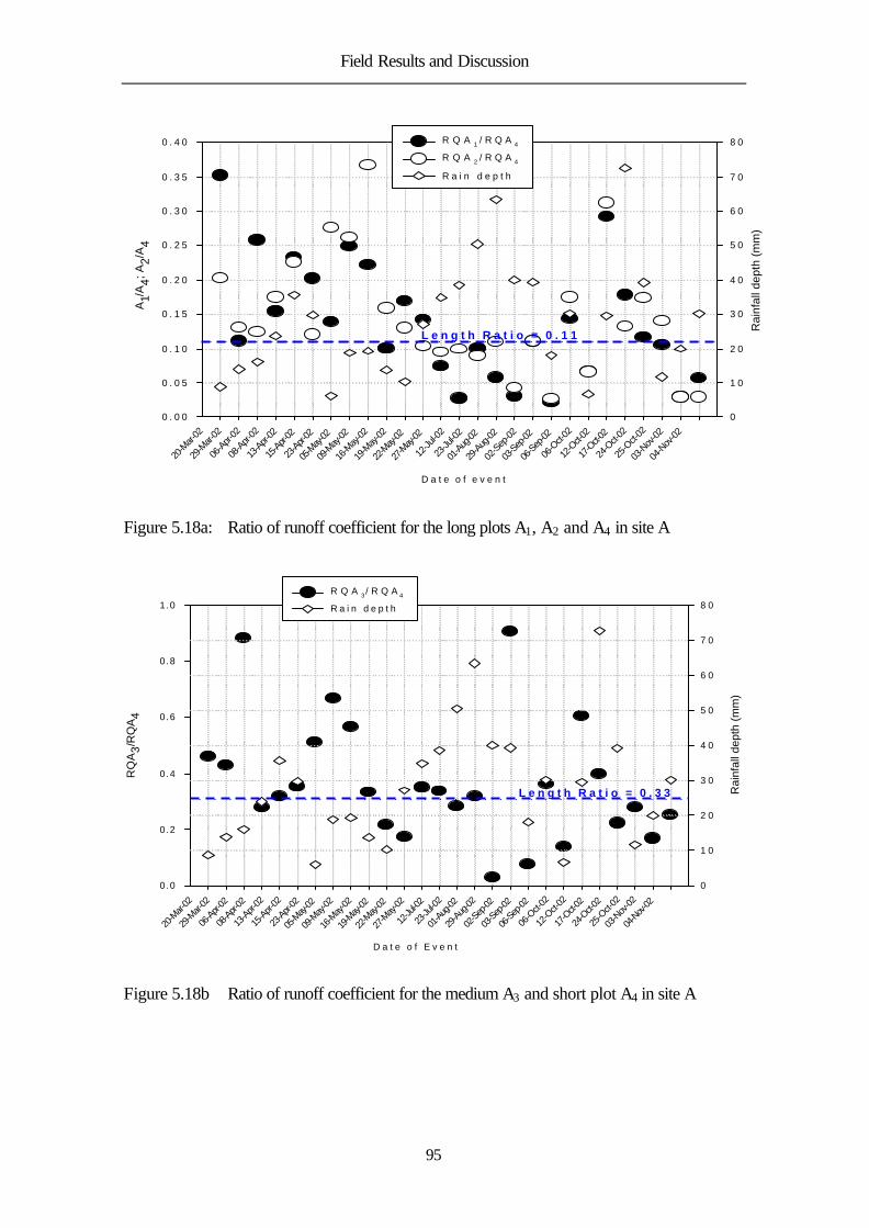
Field Results and Discussion
95
D a t e o f e v e n t
20-M
ar-02
29-M
ar-02
06-A
pr-02
08-A
pr-02
13-A
pr-02
15-Apr-
02
23-Apr-
02
05-M
ay-02
09-M
ay-02
16-M
ay-02
19-M
ay-02
22-M
ay-02
27-M
ay-02
12-Ju
l-02
23-Ju
l-02
01-Aug
-02
29-A
ug-02
02-S
ep-02
03-Sep
-02
06-Sep
-02
06-O
ct-02
12-O
ct-02
17-O
ct-02
24-O
ct-02
25-O
ct-02
03-N
ov-02
04-N
ov-02
A1/A
4; A2/A
4
0 . 0 0
0 . 0 5
0 . 1 0
0 . 1 5
0 . 2 0
0 . 2 5
0 . 3 0
0 . 3 5
0 . 4 0
Rai
nfal
l dep
th (
mm
)
0
1 0
2 0
3 0
4 0
5 0
6 0
7 0
8 0R Q A 1 / R Q A 4
R Q A 2 / R Q A 4
R a i n d e p t h
L e n g t h R a t i o = 0 . 1 1
Figure 5.18a: Ratio of runoff coefficient for the long plots A1, A2 and A4 in site A
D a t e o f E v e n t
20-M
ar-02
29-M
ar-02
06-A
pr-02
08-A
pr-02
13-A
pr-02
15-A
pr-02
23-A
pr-02
05-M
ay-02
09-M
ay-02
16-M
ay-02
19-M
ay-02
22-M
ay-02
27-M
ay-02
12-Ju
l-02
23-Ju
l-02
01-Au
g-02
29-A
ug-02
02-Se
p-02
03-Se
p-02
06-Se
p-02
06-O
ct-02
12-O
ct-02
17-O
ct-02
24-O
ct-02
25-O
ct-02
03-N
ov-02
04-N
ov-02
RQ
A3/
RQ
A4
0.0
0.2
0.4
0.6
0.8
1.0
Rai
nfal
l dep
th (
mm
)
0
1 0
2 0
3 0
4 0
5 0
6 0
7 0
8 0R Q A 3 / R Q A 4
R a i n d e p t h
L e n g t h R a t i o = 0 . 3 3
Figure 5.18b Ratio of runoff coefficient for the medium A3 and short plot A4 in site A

Field Results and Discussion
96
D a t e o f e v e n t
29-M
ar-02
06-A
pr-02
08-A
pr-02
15-A
pr-02
05-M
ay-02
09-M
ay-02
22-M
ay-02
27-M
ay-02
14-Ju
n-02
19-Ju
n-02
12-Ju
l-02
23-Ju
l-02
01-Au
g-02
05-Au
g-02
29-Au
g-02
02-Se
p-02
06-S
ep-02
09-S
ep-02
18-Se
p-02
06-O
ct-02
12-O
ct-02
17-O
ct-02
24-O
ct-02
25-O
ct-02
04-N
ov-02
RQ
B1/
RQ
B 4; R
QB
2/R
QB 4
0.0
0.2
0.4
0.6
0.8
1.0
Rai
nfal
l dep
th (m
m)
0
2 0
4 0
6 0
8 0
1 0 0
1 2 0R Q B 1/ R Q B 4
R Q B 2/ R Q B 4
R a i n d e p t h
L e n g t h R a t i o = 0 . 1 1
Figure 5.18c Ratio of runoff coefficient for the long plots B1, B2 and B4 in site B
D a t e o f E v e n t
29-M
ar-02
06-A
pr-02
08-A
pr-02
15-A
pr-02
05-M
ay-02
09-M
ay-02
22-M
ay-02
27-M
ay-02
14-Ju
n-02
19-Ju
n-02
12-Ju
l-02
23-Ju
l-02
01-A
ug-02
05-A
ug-02
29-A
ug-02
02-S
ep-02
06-S
ep-02
09-S
ep-02
18-S
ep-02
06-O
ct-02
12-O
ct-02
17-O
ct-02
24-O
ct-02
25-O
ct-02
04-N
ov-02
RQ
B3/
RQ
B 4
0 . 0
0 . 2
0 . 4
0 . 6
0 . 8
1 . 0
Rai
nfal
l dep
th (m
m)
0
20
40
60
80
1 0 0
1 2 0R Q B 3 / R Q B 4
R a i n d e p t h
L e n g t h R a t i o = 0 . 3 3
Figure 5.18d Ratio of runoff coefficient for the medium B3 and short plot B4 in site B
For all the runoff events in the season, there was no case in which, the
proportion of runoff generated in the any of the two different plots sizes is equal;
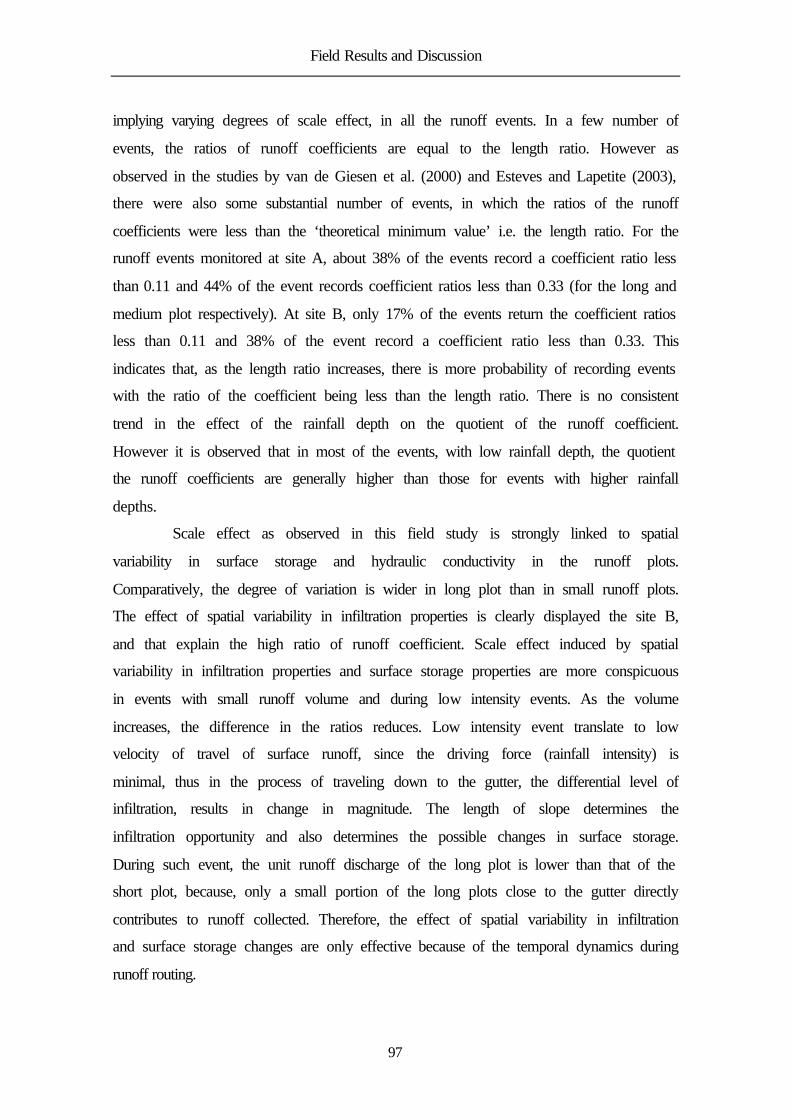
Field Results and Discussion
97
implying varying degrees of scale effect, in all the runoff events. In a few number of
events, the ratios of runoff coefficients are equal to the length ratio. However as
observed in the studies by van de Giesen et al. (2000) and Esteves and Lapetite (2003),
there were also some substantial number of events, in which the ratios of the runoff
coefficients were less than the ‘theoretical minimum value’ i.e. the length ratio. For the
runoff events monitored at site A, about 38% of the events record a coefficient ratio less
than 0.11 and 44% of the event records coefficient ratios less than 0.33 (for the long and
medium plot respectively). At site B, only 17% of the events return the coefficient ratios
less than 0.11 and 38% of the event record a coefficient ratio less than 0.33. This
indicates that, as the length ratio increases, there is more probability of recording events
with the ratio of the coefficient being less than the length ratio. There is no consistent
trend in the effect of the rainfall depth on the quotient of the runoff coefficient.
However it is observed that in most of the events, with low rainfall depth, the quotient
the runoff coefficients are generally higher than those for events with higher rainfall
depths.
Scale effect as observed in this field study is strongly linked to spatial
variability in surface storage and hydraulic conductivity in the runoff plots.
Comparatively, the degree of variation is wider in long plot than in small runoff plots.
The effect of spatial variability in infiltration properties is clearly displayed the site B,
and that explain the high ratio of runoff coefficient. Scale effect induced by spatial
variability in infiltration properties and surface storage properties are more conspicuous
in events with small runoff volume and during low intensity events. As the volume
increases, the difference in the ratios reduces. Low intensity event translate to low
velocity of travel of surface runoff, since the driving force (rainfall intensity) is
minimal, thus in the process of traveling down to the gutter, the differential level of
infiltration, results in change in magnitude. The length of slope determines the
infiltration opportunity and also determines the possible changes in surface storage.
During such event, the unit runoff discharge of the long plot is lower than that of the
short plot, because, only a small portion of the long plots close to the gutter directly
contributes to runoff collected. Therefore, the effect of spatial variability in infiltration
and surface storage changes are only effective because of the temporal dynamics during
runoff routing.

Field Results and Discussion
98
Conclusively, the rainfall runoff transformation processes in the Volta basin as
in several other tropical catchments exhibit a very weak linearity. This has resulted in a
situation, in which results from field observation are inconclusive but rather formulate
the basis of further research need, for adequate representation of the process physics.
This will facilitate adequate diagnosis of the processes, unlike the lumped effect that
always results from field measurements and provide the basin for upscaling of results.
In answering some of those questions, a solution was obtained for the full
hydrodynamic equation, which has been widely shown to represent the surface runoff
process effectively (Fiedler and Ramirez, 2000; Esteves et al., 2000, Zhang and Cundy,
1997). The next chapter presents the validity of the solution in the case of surface runoff
process in the Volta basin and investigates the effect of the various components of the
rainfall-runoff response system with a view to identifying the optimal parameters that
influence scale dependency in the system.

Model Results and Discussion
99
6 MODEL RESULTS AND DISCUSSION
6.1 Model implementation
The model is written as a FORTRAN program. The program requires two types of input
parameters. The general input parameters (table 6.1) include the rainfall data file in
cumulative format, the sorptivity value depending on soil moisture at the surface and in
the first 300mm depth, the saturated hydraulic conductivity data file (allowing the
definition of values on all the grid points), the terrain data file (allowing the definition
of values on all the grid points) the total event time in seconds, the discretized time
interval (including time to summarize the output and write into output files), the initial
flow depth, the initial flow velocity in x and y-directions, the diffusion factor, number
of points for observation, the coordinates of the observation points (in x and y) and the
open / close boundary specifier. The possibility of defining the elevation at all the grids
allows for the use of the model on complex terrains. Since it is possible to define the
saturated hydraulic conductivity at all the grids, it is easy to study a field with spatially
varied hydraulic properties.
The runoff plot or hillslope segment parameters include the plot length and
width, slope, the vegetated (canopy) fraction, the type of surface (i.e., rough, flat, or
inclined), and the friction factor (depending on average rainfall intensity, surface
characteristics and vegetation type and age). By specifying the grid spacing (equal for x
and y), and the number of grid points in the x and y directions, a user is able to change
the runoff plot (hillslope) length and width.
The model output for each runoff plot (hillslope) segments includes the
velocity of flow in the x and y-direction, the depth of flow, the infiltration rate, the net
inflow rate. All these values are averaged over the user-defined time step; therefore a
small time step will ensure the observation of very minute detail. The output variables
are used to generate graphical outputs of discharge in cm 2 sec - 1, depth of overland flow
in cm, interactive infiltration during the event in mmhr-1 and, the rainfall intensity in
mmhr - 1. Other graphical outputs of the model are, the hillslope (runoff plot) terrain, the
flow vector and its values in contour, the flow vector over the terrain, the velocity
vector and the speed contour and the flow vector along a single column (grid interval)
and across the selected observation points. The graphical outputs are produced with

Model Results and Discussion
100
MATLAB software (Mathworks, 2000) using the plotter programs, written for the study
purpose.
Initial infiltration into soil during a rainfall event is regulated by the prevailing
moisture conditions among other factors. In reality, the antecedent moisture conditions
in a hillslope represent a sequence of rainfall, drainage, and redistribution conditions,
and therefore it is extremely difficult to generalize. However, moisture content is known
to fluctuate more at the surface and in the first 300mm profile. Consequently, the
sorptivity value is defined based on the measured soil moisture content at the surface
and in the 300mm profile. In simulation cases with uniform hydraulic conductivity, a
value between the range of the effective hydraulic conductivity for the two sites,
determined from the van Genuchten-Mualem model (see 5.4) is used. The use of a
constant hydraulic conductivity eliminates spatial variability in hydraulic properties.
Such scenarios facilitate the comparison of the effect of temporal factors.
In accounting for vegetation interception, the rainfall volume per tip from the
tipping bucket rain gauge is reduced by the canopy cover fraction, which depends on the
vegetation density. Vegetation density is obtained from the average leaf area index
(LAI) measurements of representative vegetation in the catchment. It is well correlated
to the period since the onset of the rainy season, since the active vegetation pattern in
the catchment and other parts of the Volta basin has a well-defined cycle. The cycle is
regulated by the widely practiced bush burning in the dry season (December through
February) and the characteristic-cropping pattern. The reduction factor is selected based
on the modified Gash model for multiple cropping (van Dijk et al., 2000).
6.2 Model evaluation and testing
The model’s performance was evaluated in two ways. In the first method, we compared
the model output with observed measurement for a selected event. Two performance
criteria were defined as used in the study by Esteves et al. (2000) for the evaluation. The
accuracy or otherwise of the runoff volume is quantified, using the relative error (Re)
calculated from the relationship:
100%sim observede
observed
V VR
V−
= × (6.1)

Model Results and Discussion
101
A low value of the percent relative error indicates that the simulated and
observed volume is close. A negative value of Re indicates that the runoff volume
predicted by the model is lower than the observed and vice-versa. Also the ability to
reproduce the observed runoff hydrograph is evaluated using the coefficient of
efficiency (Ce) defined by Nash and Sutcliffe (1970) as:
2
1_
2
1
( )1
( )
n
i ii
e n
ii
Q QC
Q Q
∧
=
=
−= −
−
∑
∑ (6.2)
where iQ is the observed runoff discharge at time i; _
Q is the mean runoff rate
of the particular rainfall-runoff event; iQ∧
is the runoff discharge predicted by the model
at time i; and n is the number of time step in the computation. Ce =1, indicates a perfect
agreement between the model predicted hydrograph and the observed hydrograph for
the event under consideration. It must however be mentioned that this is rarely possible
in view of certain assumptions often used in model simulation runs which often do not
adequately represent field conditions. The more the value of Ce slides away from 1, the
lesser the goodness of fit, and a negative value implies that the observed mean is a
better estimate than the simulated value (Esteves et al, 2000).
One high intensity event was selected for this validation. Simulations
experiment using the rainfall intensity data for the event was conducted on a long (18m
x 2m) and a short (2m x 2m) runoff plot. The bed slope and the friction slope are
calculated from the microtopography data, while the Darcy–Weisbach formula was used
to estimate the friction slope. A time interval 0.005s was used for the simulation. A
uniform vertical (downslope) and horizontal (cross-slope) grid spacing of 10cm was
used. The 10cm grid spacing is selected to conform with the measured terrain data
resolution for the runoff plots. Consequently, the small runoff plot is discretized into
400 girds, and the long plot to 3600 grids. The surface terrain configuration of the
runoff plots for the simulation is based on the field measurement of the surface
microtopography described earlier. The measured data were transformed with some
limited smoothing into digital terrain models for the corresponding plots, using the
contouring features of the Surfer package (Golden software, Inc. 2000). This limited
smoothening was necessary to eliminate spikes capable of inducing instability in the
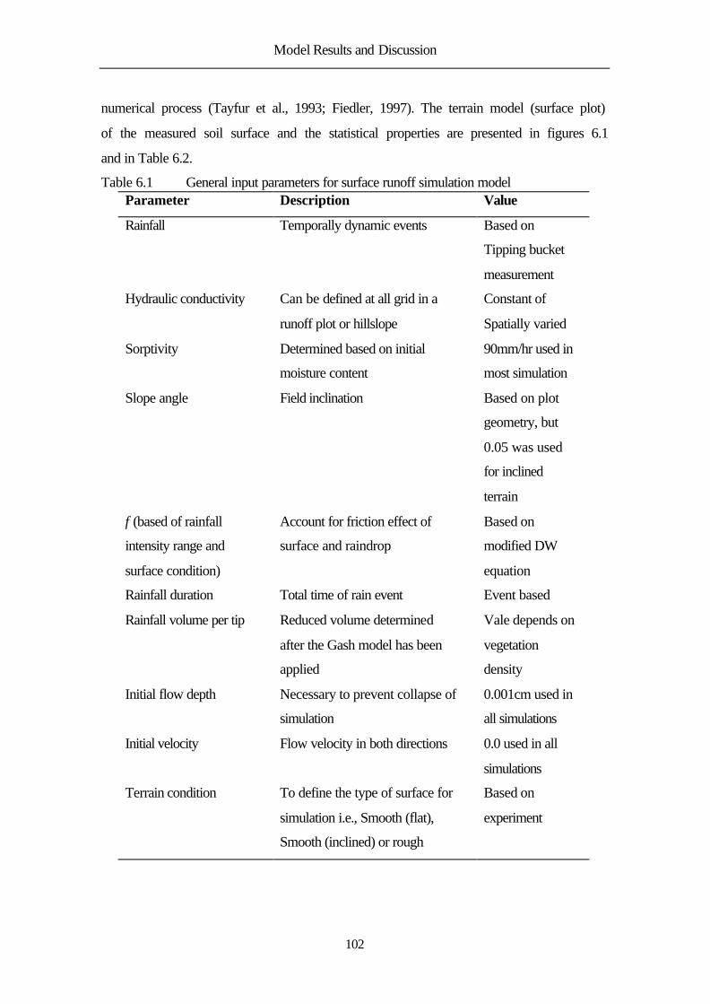
Model Results and Discussion
102
numerical process (Tayfur et al., 1993; Fiedler, 1997). The terrain model (surface plot)
of the measured soil surface and the statistical properties are presented in figures 6.1
and in Table 6.2.
Table 6.1 General input parameters for surface runoff simulation model Parameter Description Value
Rainfall Temporally dynamic events Based on
Tipping bucket
measurement
Hydraulic conductivity Can be defined at all grid in a
runoff plot or hillslope
Constant of
Spatially varied
Sorptivity Determined based on initial
moisture content
90mm/hr used in
most simulation
Slope angle Field inclination Based on plot
geometry, but
0.05 was used
for inclined
terrain
f (based of rainfall
intensity range and
surface condition)
Account for friction effect of
surface and raindrop
Based on
modified DW
equation
Rainfall duration Total time of rain event Event based
Rainfall volume per tip Reduced volume determined
after the Gash model has been
applied
Vale depends on
vegetation
density
Initial flow depth Necessary to prevent collapse of
simulation
0.001cm used in
all simulations
Initial velocity Flow velocity in both directions 0.0 used in all
simulations
Terrain condition To define the type of surface for
simulation i.e., Smooth (flat),
Smooth (inclined) or rough
Based on
experiment
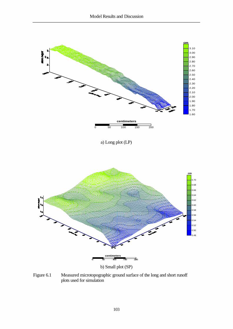
Model Results and Discussion
103
1.60
1.70
1.80
1.90
2.00
2.10
2.20
2.30
2.40
2.50
2.60
2.70
2.80
2.90
3.00
3.10
0 50 100 150 200
centimeters
cm
a) Long plot (LP)
0.48
0.50
0.52
0.54
0.56
0.58
0.60
0.62
0.64
0.66
0.68
0.70
centimeters
cm
b) Small plot (SP)
Figure 6.1 Measured microtopographic ground surface of the long and short runoff plots used for simulation

Model Results and Discussion
104
Table 6.2 Statistical properties of the plot microtopography Zmin Zmax Zmean Zmed ZSTD Zcv Zskew ZXslope ZYslope
LP 1.549 3.244 2.593 2.720 0.442 0.171 -0.394 1.0° 5.1°
SP 0.466 0.736 0.615 0.613 0.053 0.085 -0.088 2.8° 5.4°
Note ZX = slope in x-direction; ZY = slope in y-direction.
Figure 6.2a and b present the rainfall hyetograph, the simulated and the
observed runoff on two plot sizes, for the event used for validation. The agreement in
trend with data points indicates that the developed equation in chapter 4 can describe the
surface runoff process observation very well. Comparison of the hydrographs suggests
that the magnitude of simulated discharge is slightly lower during the pulse period in the
event, and also in the falling limb during the second cycle of the rainfall event. This
was, however, evened out by the slight overestimation in the rising limb and at the peak
periods. Detail inspection of the time before the onset of runoff in both plots sizes also
showed that the simulated time before the onset of runoff is consistently less than the
observed. This consistence difference possibly emanate from the use of an average
effective saturated hydraulic conductivity value in the simulation. The average effective
saturated hydraulic conductivity is obviously less than the actual saturated hydraulic
conductivity from the field measurement. The assumed value of sorptivity may also
influence the delay time in the simulation. A detailed analysis of the performance based
on the defined criteria relative error ( Re) and coefficient of efficiency ( Ce), show that
the model performance is satisfactory and efficient. With an absolute value of less than
12% for the two plot sizes; the model predictions could be described as a very good
representation of the observed process. The summary of simulated and measured values
of maximum runoff intensity, total runoff duration, and relative error and efficiency for
the different plot sizes, are presented in Table 6.3. This is representative of the model
performance for complex (high intensity over short period) rainfall events commonly
associated with tropical rainstorms. It also provides the platform upon which the
understanding of the various complex process associated with the rainfall-runoff
transformation process in the tropics can be evaluated based of the developed model and
its solution.

Model Results and Discussion
105
Figure 6.2a Comparison of observed and simulated discharge on the short plot (SP)
Figure 6.2b Comparison of observed and simulated discharge on the long plot (LP)
The second way that the model was evaluated was to compare in a scatter plot,
the simulated and observed runoff intensity at some selected equivalent times (a time
Time (sec)
0 500 1000 1500 2000
Dis
char
ge (L
iters
/hr)
0
20
40
60
80
100
120
Rai
nfal
l Int
ensi
ty (
mm
hr-1
)
0
20
40
60
80
100
120
140
160
180Simulated ObservedRain Int.
Time (sec)
0 500 1000 1500 2000
Dis
char
ge (L
iters
/hr)
0
20
40
60
80
100
120
140
Rai
nfal
l Int
ensi
ty (
mm
hr-1
)
0
20
40
60
80
100
120
140
160
180
Simulated ObservedRain Int.

Model Results and Discussion
106
simultaneously or very closely recorded in both the simulated and observed hydrograph)
in the event hydrographs. For the hydrograph of the short plot (2m x 2m), Eighteen
equivalent times were randomly selected, while for the hydrograph of the long plot
(18m x 2m), Thirty-two points were randomly selected. Figure 6.3a and b present the
resulting scatter plot, which was fitted with the linear equation appropriately displayed.
For the short runoff plot, the coefficient of determination is 0.85, while for the long
runoff plot; the coefficient of determination is 0.89. The value of r2 in both hydrographs
also reflect the match in both simulated and observed hydrograph and show good
agreement of the observed and simulated hydrographs for an individual event. This
agreement indicates that reasonable inferences could be drawn from the model outputs.
Simulated Runoff Intensity (Lh -1)
20 40 60 80 100 120
Obs
erve
d R
unof
f Int
ensi
ty (
Lh-1)
20
40
60
80
100
120
Obs = 0.99Sim - 3.066 r2=0.85
Figure 6.3a Relationship between observed and simulated runoff intensity at 18 randomly selected equivalent times for the short plot (SP)

Model Results and Discussion
107
Simulated Runoff Intensity (Lh-1)
0 20 40 60 80 100 120
Obs
erve
d R
unof
f Int
ensi
ty (L
h-1)
0
20
40
60
80
100
120
Obs = 1.061Sim - 1.073r2=0.89
Figure 6.3b Relationship between observed and simulated runoff intensity at 32
randomly selected equivalent times for the long plot (LP)
Table 6.3 Summary results of validation event for the two plot sizes Qsim
max Qsim
mean Qobs
max Qobs
mean N Re Ce
SP 110 56 104 59 14 -11.5 0.89
LP 119 54 104 57 28 4.76 0.88
Summarily, the model outputs mimic the relationships observed in the field
study adequately. The complex shape of the observed hydrographs is well represented
by the model, and the different timings (time before the onset of runoff; recession time
at the end of rainfall event; the runoff duration) are fairly described. The rising limbs,
recession limbs and the pulse (transient) moments of the observed runoff hydrographs
have been well replicated by the model. The model equally captures the effects of pulse
moment of rainfall on runoff response. The dynamics of rainfall intensity during an
event are well reflected in the observed and simulated runoff hydrograph. Therefore it is
suffice to use the model result for further investigations of the rainfall-runoff process in
the Volta basin and other tropical climate with similar catchment properties.

Model Results and Discussion
108
6.3 Simulation experiments
Following the satisfactory performance of the model in reproducing close to the field
observations, several numerical experiments were performed in line with the overall
project objectives of evaluating the effect of various hydrological state variables on the
runoff response to selected rainfall events. The different scenarios simulated were
selected to reflect possible field conditions, but some scenarios are only hypothetical,
but are necessary for detail understanding of certain critical parameters in the rainfall-
runoff process. It should, however, be noted that in such hypothetical cases, the model
parameters are selected based on observed values.
It is also important to emphasize here that the purpose of applying a physically
based numerical model in this simulations study is to gain insights into the interactions
between heterogeneities in catchment structure and hydrologic processes, rather than to
make precise predictions of runoff discharge from the plots. The distributed-parameter
approach permits several structural attributes to be varied in a controlled fashion,
including the distribution of soil hydraulic properties, surface feature and slope
geometry.
Generally, the discharge rate and magnitude of surface runoff intensity are
most sensitive to rainfall rate; therefore two contrasting rainfall intensity events were
used in the model simulation. The events were chosen to represent two of the possible
rainfall event scenarios, i.e., high intensity (henceforth referred to as event A), and low
to medium intensity (henceforth referred to as event B) based on the observation from
the record of rainfall intensity in the basin for the 2002 season. The average slope angle
for all the runoff plots from the measured topographic data was 5°, therefore inclined
terrains used in the simulations trials were oriented to that same angle, to establish a
basis for comparison.
Most simulations on rough terrain configurations are performed with the
medium runoff plot (figure 6.4). The statistical properties of the medium plot
microtopography are presented in the table 6.4. Some other simulations are
implemented on the small runoff plot sizes and long runoff earlier described (figure 6.1
and table 6.3), since the responses from all the plots sizes are analogous. A common
point close to the gutter was used to monitor point interactive infiltration, flow depth
and the discharge in most of the simulation, and exceptions are clearly stated. There is

Model Results and Discussion
109
also a possibility to view the predicted flux of all of these parameters at any selected
time, along and across the observation point column and row. In all the simulation
experiments, a uniform depth of 1mm was used as will be noted in the output contribute
to flow depth and discharge even at the moment when there is no flow. The following
sections discuss the results from the various simulation experiments and provide some
basis for better understanding and appreciation of the field experiment results,
enhancing a detail discussion and conclusions from this study.
0.10
0.15
0.20
0.25
0.30
0.35
0.40
0.45
0.50
0.55
0.60
0 50 100 150 200
centimeters
cm
Figure 6.4 Measured microtopographic ground surface of the medium runoff plot
used for simulation
Table 6.4 Statistical properties of the the medium runoff plot microtopography Zmin Zmax Zmean Zmed ZSTD Zcv Zskew ZXslope ZYslope
MP 0.066 0.699 0.408 0.442 0.141 0.345 -0.479 3.8° 4.8°
6.4 Scale effect
The analysis of runoff coefficient and the unit runoff discharges from the field data
showed consistent trend of decreasing coefficient and unit runoff discharge with

Model Results and Discussion
110
increasing plot sizes or better still, with increasing slope length (since all the plots have
uniform width). Consequently, simulation experiments with the different plot sizes
(slope length) were implemented to investigate a possible repeat of the trend and
possibly isolate the causative factor(s). Alongside with the three slope lengths used for
in the field observation, i.e., 2m, 6m and 18m, a simulation run using a slope length of
200m was implemented, for event A to appraise the trend with increasing length of
slope. Both the high intensity and low-medium intensity events were used for the
evaluation.
Figure 6.4a and b present the cumulative discharge per unit plot length, for the
four plot sizes (slope length), under the two rainfall events. The figures clearly reveal
the effect of slope length and rainfall pattern on the runoff discharge. Cumulative
discharge increases with plot size, but the discharge per unit length decreases
exponentially. The shape of the cumulative discharge curves is influenced by the pattern
of the rainfall. For example in event A, the number of flattened portions (constant or no
discharge) is dependent on the number of pulses recorded in the event (no of peaks). At
such pulse moments, the slope length actively partitions infiltration, run-on and runoff
depending of the microtopography.
The responses under event B accentuate the effect of the magnitude of rainfall
on runoff processes. For most part of event B, there was no discharge due to the low
value of rainfall intensity. During low intensity events, the discharge volume and rate is
reduced by the increased redistribution and infiltration opportunity for overland flow.
The velocity of flow depends among other factors on the kinetic energy, which linearly
varies with the rainfall intensity. Since the intensity is low, most of the rainfall will
infiltrate, and a large proportion of overland flow also percolates because of the low
travel velocity. During low intensity rainfall event, there are always unconnected
patches of runoff, and only patches connected to the channel contribute to discharge.
However, during high intensity event, there is an increase in opportunities for the
patches to be connected, hence the path length of runoff increases, and consequently the
volume of runoff is increased.

Model Results and Discussion
111
Time (sec)
0 500 1000 1500 2000
Dis
char
ge (
cm2 /s
ec)/
m
0
100
200
300
400
500
Rai
nfal
l Int
ensi
ty (
mm
hr-1
)
0
50
100
150
200
200m 18m 6m 2m Rain Int.
Figure 6.4a Cumulative discharge per slope length for event A (high intensity)
Time (sec)
0 200 400 600 800 1000 1200 1400 1600
Dis
char
ge (
cm2 /s
ec)/m
0
2
4
6
8
1 0
1 2
1 4
Rai
nfal
l Int
ensi
ty (
mm
hr-1
)
0
20
40
60
8018m 6m 2m Rain Int.
Figure 6.4b Cumulative discharge per slope length for event B (low intensity)
Despite the low volume of discharge, the effect of slope length is evident with
the low intensity event similar to the observation with high intensity rainfall. Inspection
of the figures show that the slope of the cumulative discharges are steeper during low
intensity event, and is drastically reduced as the slope length increases. This observation

Model Results and Discussion
112
is explained by the redistribution of runoff on long slope length during low intensity
event. The redistribution affects the discharge rate during low intensity events and also
at the pulse moment in an event, particularly on plots with rough surface
(microtopography). On short slopes, most of the runoff paths have a better chance to
link up with the gutter, due to their proximity, and will therefore contribute to the
outflow, which increase the discharge per unit length.
Table 6.4 presents the runoff coefficient under the different plot lengths for the
two events. The high intensity event consistently have higher runoff coefficient than the
low intensity event on all the plot sizes. Figure 6.5 shows the plot and fitting of the
runoff coefficient with power equations. It is interesting that for both events; the runoff
coefficient decreases with slope length exponentially, similar to the observation in the
field experiment. The simulation results corroborate the results from the field
observation in agreement with other previous studies (Kirkby et al., 2002; Yair and
Kossovsky, 2002; Joel et al., 2000; van de Giesen et al., 2000). The graph also showed
that the combination of the two different intensity ranges significantly reduces the
coefficient of determination of the power equation, implying that rainfall factor could
explain the difference in magnitude of scale effect reported in several studies. This is
apparent since all hydraulic variables were kept uniform; as such effect of spatial
variability of soil hydraulic properties is eliminated. It also reveals very clearly, that the
difference in response by different plot sizes is closely related to the temporal pattern of
rainfall intensity and slope length. Runoff coefficient is proportional to the rainfall
magnitude. Close examination of the within storm (event) dynamics of the runoff
coefficient shows marked fluctuation. The runoff coefficient dynamically changes with
rainfall intensity and rainfall duration. However, the fraction of the difference from
smaller to longer plot length is more obvious than at lower rainfall intensity. Several
factors as have been observed could have in one way contributed to this observation, but
a very dominant factor is the loss in momentum of the runoff, during travel time from
upslope to the outlet. This is clear, since setting the saturated conductivity at all grid
points to the same value in all the simulation eliminates all spatial variability in
hydraulic properties.

Model Results and Discussion
113
Table 6.5 Runoff Coefficient for the two-events with different slope lengths Slope Length Event A Event B
200m 0.069 0.017
18m 0.095 0.023
6m 0.271 0.084
2m 0.412 0.193
SL-Slope Length (m)
0 50 100 150 200 250
Run
off C
oeffi
cien
t (%
)
0
10
20
30
40
50High Intensity (event A) Low intensity (event B)59.16SL-0.502; r2 = 0.9534.02SL-0.813; r2 = 0.99Combined Events45.55SL-0.578; r2= 0.69
Figure 6.5 Relationship between runoff coefficients and slope length
To elucidate on momentum change during travel, a second series of
simulations using the flat plane terrain and the inclined surface were implemented. The
use of a flat surface ensure that the effect of slope will be completely eliminated, while
the use of inclined terrain is to determine the response on the slope used for runoff
studies, but with a plane surface. This eliminates any influence of surface
microtopography. Figure 6.6 presents the result on a smooth-plane terrain. The figure
show that the length of slope affect runoff coefficient, even on flat terrain. Scale effect
is more conspicuous on such terrain, since the velocity of flow is significantly reduced.
It also shows that the response is affected by the rainfall intensity pattern. The results

Model Results and Discussion
114
for the inclined surface also concur with the observation on both rough and flat-plane
terrain.
Time (sec)
0 500 1000 1500 2000
Run
off Q
uotie
nt
0.000
0.005
0.010
0.015
0.020
0.025
0.030
RQ 2m RQ 18m
Figure 6.6 Variation in runoff coefficient on a flat plane for two-slope length
6.5 Spatial variability of soil hydraulic properties and surface runoff process
Spatial variability of soil hydraulic properties has been cited in a number of studies as
the basis of the observed differences in runoff response using analytical or model-based
evaluation. But as noted by Woolhiser et al. (1996), the different process of
simplification of the routing model has limited the application of the results. Another
limitation of most of the model used for such analysis is the failure to couple infiltration
process. Since the developed model in this study can better take care of most, if not all,
of observed limitations in previous studies, it is imperative to investigate the effect of
spatial variability of infiltration and other hydraulic properties on runoff discharge.
Three possible scenarios were simulated on the medium size plot, using both high and
low intensity events data. In the first experiment ( case A ), a linear increase in saturated
hydraulic conductivity downslope was simulated. In this scenario, the K sat value is
increased by 3% at every grid point along the flow direction (downslope), such that, at
the end of the plot, where discharge is monitored, the final value of K sat is 171.6mm/hr.
Thus, the average hydraulic conductivity is 81.5mm/hr while the standard deviation is

Model Results and Discussion
115
41mm/hr. An inverse of this linear variation was used for the second experiment ( case
B ), such that, the Ksat reduces downslope from a maximum of 171.6mm/hr at the plot
upslope.
For the third scenario ( case C ), the measured saturated conductivity data for
the medium plot at site B i.e., (B3) is used to represent random variation in Ksat value
within a plot. The contour map of the different distributions of Ksat is presented in
Figure 6.7. The contour map shows that the upper and the lower limits of the
hypothetical linear variations in the study could be observed within the plot. The three
cases were used to study the dynamic effect of infiltration opportunity, as limited by a
shrinking or expanding area from which infiltration can occur.
0 50 100 150 2000
50
100
150
200
250
300
350
400
450
500
550
600
30
40
50
60
70
80
90
100
110
120
130
140
150
160
170
0 50 100 150 2000
50
100
150
200
250
300
350
400
450
500
550
600
30
40
50
60
70
80
90
100
110
120
130
140
150
160
170
0 50 100 150 2000
50
100
150
200
250
300
350
400
450
500
550
600
404550556065707580859095100105110115120125130135140145150
case A case B case C
Figure 6.7 Contour map of saturated conductivity (Ksat ) for the different distribution used in the simulation experiment.

Model Results and Discussion
116
Figure 6.8a. Comparison of simulated outflow hydrograph showing the effect variations in the distribution of Ksat for event A
Figure 6.8b. Comparison of simulated outflow hydrograph showing the effect variations in the distribution of Ksat for event B
0.3
0.5
0.7
0.9
1.1
1.3
1.5
1.7
0 200 400 600 800 1000 1200 1400 1600
Time (sec)
Dis
char
ge (c
m2 /sec
)
0
10
20
30
40
50
60
70
80
Rainfall Int. (m
m/hr)
Decreasing
Increasing
Uniform 81.5
Rain Int.
0
5
10
15
20
25
30
35
40
0 200 400 600 800 1000 1200 1400 1600 1800 2000 2200
Time (sec)
Dis
char
ge (
cm2 /
sec)
0
20
40
60
80
100
120
140
160
180
200R
ainfall Int.(mm
/hr)Decreasing
Increasing
Uniform 81.5
Rain Int.
Measured B3

Model Results and Discussion
117
Figures 6.8a and b indicate that the magnitude and spatial pattern of Ksat within
a plot or on a hillslope could significantly affect the observed discharge in a runoff
event. Increasing saturated conductivity downslope allow more of the overland flow
traveling towards the gutter to be lost due to increasing infiltration opportunity. This
results in a significant reduction in discharge and peak rates. The high value of saturated
hydraulic conductivity also induces a substantial reduction in flow depth and this is
clearly displayed in the asymmetric pattern of the flow depths at about 500 sec into the
event. When the conductivity decreases in the downslope direction, flow depth,
discharge, and peak rate increases. Overland flow apparently emanating from the
downslope regions with low saturated conductivity values, and, which only has a short
distance from the gutter to overcome results in the sharp increase in discharge, in this
scenario. With the low intensity events (figure 6.8b), the downslope increase, the
random variation and uniform conductivity of 81.5mmhr-1 produce no surface runoff.
This apparently results from the high infiltration rate compared with the rainfall
intensity in the two cases. Case B produces small quantity of surface runoff and this
explains why the effect of scales in runoff response is often more pronounced with low
rainfall intensity events. In those cases, the differences in runoff appear to be
attributable to increased opportunity for infiltration with increasing slope length. In all
the three different cases, and in both high and low intensity events, the flow pattern is
considerably influenced by the microtopography (Figure 6.9). The magnitude of the
difference between the hydrograph for the downslope-decreasing trend also shows that
most of the runoff that arrives at the gutter emanates from regions not too far from the
point of discharge. There is a marked similarity in the outflow hydrographs of random
variation (measured values) and an average of the Ksat in the varied scenarios. This
indicates that, appropriately selected average Ksat value could be used for investigation
without too much loss of accuracy. At 1750 sec, which corresponds to the tailing part of
the rain for event A, flow pattern and all other parameters are uniform in the three cases.
This also explains why the difference in scale effect is reduced in rainfall event with
extended recession phase or with prolonged pulse moments.
The differences in the outflow hydrograph in the various cases considered
provide an avenue to evaluate the importance of spatial variability of soil hydraulic

Model Results and Discussion
118
properties in the Hortonian runoff process. The trend of spatial variation of infiltration
properties influences the discharge from runoff plots or hillslope.
00.5
11.5
2
0
2
4
60.1
0.2
0.3
0.4
0.5
x-distance(m)
Flow depth at 500sec
y-distance(m)
z-he
ght(c
m)
Downslope increase in Ksat
0.5
1
1.5
2
2.5
3
3.5
0.2 0.4 0.6 0.8 1 1.2 1.4 1.6 1.8 2
0.5
1
1.5
2
2.5
3
3.5
4
4.5
5
5.5
6
x-distace(m)
y-di
stac
e(m
)
0.5
1
1.5
2
2.5
3
3.5Flow vector and values (contour) at 500sec
0.1
0.15
0.2
0.25
0.3
0.35
0.4
0.45
0.5
0.55
0.6
0.2 0.4 0.6 0.8 1 1.2 1.4 1.6 1.8 2
0.5
1
1.5
2
2.5
3
3.5
4
4.5
5
5.5
6
x-distance(m)
y-di
stan
ce(m
)
0.1
0.15
0.2
0.25
0.3
0.35
0.4
0.45
0.5
0.55
0.6 Flow vector and Terrain (contour) at 500sec
0.2 0.4 0.6 0.8 1 1.2 1.4 1.6 1.8 2
0.5
1
1.5
2
2.5
3
3.5
4
4.5
5
5.5
6
x-distace(m)
y-di
stac
e(m
)
Velocity (vector) and speed (contour) at 500sec
0.01
0.01
0.01
0.01
0.01
0.01
0.02
0.02
0.02
0.02
0.02
0.02
0.02
0.03
0.030.03
0.03
0.03
0.030.03 0.03
0.03
0.03
0.03
0.040.04 0.04
0.04
0.04
0.040.04
0.04
0.04
0.05 0.05
0.05
0.05
0.050.05
0.050.05
0.05
0.060.06
0.06
0.060.06
0.060.06
0.07
0.070.07
0.070.08
0.08
0.08
0.09
Downslope increase
00.5
11.5
2
0
2
4
60
0.2
0.4
0.6
0.8
x-distace(m)
Flow depth at 500sec
y-distace(m)
z-he
ght(c
m)
Downslope Decrease in Ksat 0
1
2
3
4
5
6
7
8
0.2 0.4 0.6 0.8 1 1.2 1.4 1.6 1.8 2
0.5
1
1.5
2
2.5
3
3.5
4
4.5
5
5.5
6
x-distace(m)
y-di
stac
e(m
)
0
1
2
3
4
5
6
7
8Flow vector and values (contour) at 500sec
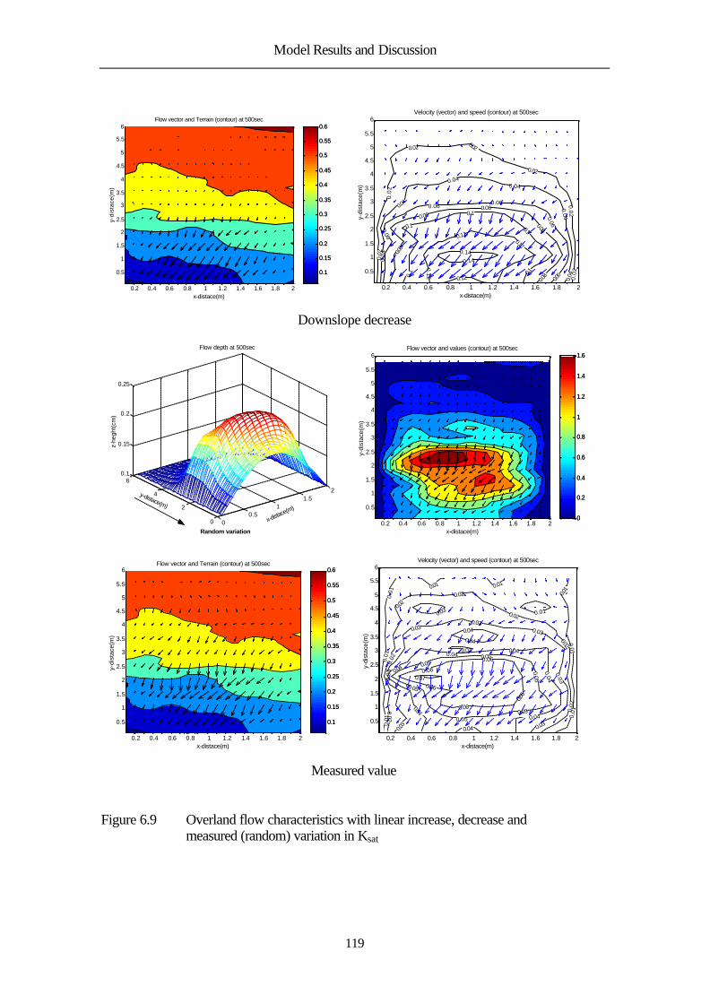
Model Results and Discussion
119
0.1
0.15
0.2
0.25
0.3
0.35
0.4
0.45
0.5
0.55
0.6
0.2 0.4 0.6 0.8 1 1.2 1.4 1.6 1.8 2
0.5
1
1.5
2
2.5
3
3.5
4
4.5
5
5.5
6
x-distace(m)
y-di
stac
e(m
)
0.1
0.15
0.2
0.25
0.3
0.35
0.4
0.45
0.5
0.55
0.6 Flow vector and Terrain (contour) at 500sec
0.2 0.4 0.6 0.8 1 1.2 1.4 1.6 1.8 2
0.5
1
1.5
2
2.5
3
3.5
4
4.5
5
5.5
6
x-distace(m)
y-di
stac
e(m
)
Velocity (vector) and speed (contour) at 500sec
0.02
0.0
2
0.020.02
0.02
0.02
0.02
0.04
0.04
0.040.04
0.04
0.04
0.06
0.06 0.06
0.06
0.06
0.08
0.080.08
0.08
0.080.
1
0.1
0.1
0.1
0.1
0.12
0.120.12
0.12
0.14
0.14
Downslope decrease
00.5
11.5
2
0
2
4
60.1
0.15
0.2
0.25
x-distace(m)
Flow depth at 500sec
y-distace(m)
z-he
ght(c
m)
Random variation
0
0.2
0.4
0.6
0.8
1
1.2
1.4
1.6
0.2 0.4 0.6 0.8 1 1.2 1.4 1.6 1.8 2
0.5
1
1.5
2
2.5
3
3.5
4
4.5
5
5.5
6
x-distace(m)
y-di
stac
e(m
)
0
0.2
0.4
0.6
0.8
1
1.2
1.4
1.6Flow vector and values (contour) at 500sec
0.1
0.15
0.2
0.25
0.3
0.35
0.4
0.45
0.5
0.55
0.6
0.2 0.4 0.6 0.8 1 1.2 1.4 1.6 1.8 2
0.5
1
1.5
2
2.5
3
3.5
4
4.5
5
5.5
6
x-distace(m)
y-di
stac
e(m
)
0.1
0.15
0.2
0.25
0.3
0.35
0.4
0.45
0.5
0.55
0.6 Flow vector and Terrain (contour) at 500sec
0.2 0.4 0.6 0.8 1 1.2 1.4 1.6 1.8 2
0.5
1
1.5
2
2.5
3
3.5
4
4.5
5
5.5
6
x-distace(m)
y-di
stac
e(m
)
Velocity (vector) and speed (contour) at 500sec
0.01
0.01
0.01
0.01 0.01
0.01
0.01
0.01
0.01
0.02
0.02
0.02
0.02
0.02
0.02
0.02
0.03
0.03
0.030.03
0.03
0.03
0.03
0.03
0.03
0.04
0.04
0.040.04
0.04
0.04
0.04
0.04
0.04
0.050.05
0.05
0.050.05
0.05
0.06
0.06
0.06
0.06
0.06
0.07
Measured value
Figure 6.9 Overland flow characteristics with linear increase, decrease and measured (random) variation in Ksat

Model Results and Discussion
120
However the effect can only be explained in the context of the temporal
related changes that occur during the time required for the overland flow to move from
the point of initiations, to the point of collection. The required time depends on the
rainfall intensity, which determines the available kinetic energy, the microtopographic
forms which moderate depression storage and slope of the field. All the three factors
affect the velocity of flow. This observation explains why Wainwright and Parson
(2002) advocated for the use of variable intensity rainfall data in appropriate resolution
(preferably tipping bucket) in better understanding of scale effect. The study has gone
further to enhance the understanding of rainfall runoff dynamics in the face spatially
variable infiltration opportunities, which Woolhiser et al., (1996), admitted was not
possible in their study because of the inability of their model to accommodate
heterogeneity in rainfall intensity as well as incomplete knowledge of field conditions.
6.6 Effect of microtopography on surface runoff process
The significant effect of microtopography in the Hortonian runoff is briefly depicted in
the previous section on spatial variability. In attaining a better understanding of the
effect on surface runoff initiation, flow and discharge, a series of simulation
experiments were implemented. The two selected characteristic rainfall patterns was
simulated over (i) flat (plane) surface (as used in basin irrigation scheme); (ii) plane
surface inclined at 5° (similar to field slope); and (iii) rough terrain based on the digital
elevation model from measurement in the runoff plot. A uniform saturated conductivity
of 30mmhr-1 was used on all the grids, and the sorptivity of 90mmhr-1. Flow depth and
discharges were monitored at the same point in all the experiments in a small plot (2m x
2m). All input parameters are kept uniform, such that the surface and rainfall pattern are
the only variables. The rainfall events duration were discretized in a way to monitor the
detail the responses at short time intervals. For example, event A lasting 2160 seconds is
monitored every 11sec, while event B lasting about 1600 seconds is monitored every
7 seconds.
Figures 6.10a and b compare the cumulative discharge for both events on the
different surfaces, and figure 6.11a and b compare the depth of flow on the three
different surfaces for the two events. The cumulative discharges curves show that
microtopography reduces discharge in both events. This consistent observation in both

Model Results and Discussion
121
high and low intensity events result from interaction of several factors. In the first
instance, the shape and form of microtopography determine the available surface
depression storage. These depression storages delay the process of connections between
the various runoff-forming patches during an event, resulting in an increase, in the time
required for the flow path to link up to the gutter, thereby increasing the time before
discharge is recorded in the rough-surfaced plot, relative to the inclined plane surface.
The delay accounts for the slow rise of the hydrograph of the plane inclined surface.
Moments after the surface depression have been ponded or inundated, signifying the
connections of most of the different flow paths to the gutter, surface roughness
continues to reduce the velocity of flow, when compared to the smooth-surfaced
inclined terrain and flat terrain (figure 6.11). Although both inclined and rough surfaces
have the same range of flow velocities ( 0.05cms-1 to 0.25cms-1 ), the proportion of the
runoff plot under the higher velocity range is higher on the inclined plane surface
compared to the rough terrain.
Figure 6.10a Comparison of cumulative discharge of the 3 different surfaces for event
A
0.0
200.0
400.0
600.0
800.0
1000.0
1200.0
0 500 1000 1500 2000
Time (sec)
Dis
char
ge (
cm2 /
sec)
0
20
40
60
80
100
120
140
160
180
200
Rai
nfal
l Int
ensi
ty (
mm
/hr)
Flat (smooth)
Rough
Inclined
Rain Int.

Model Results and Discussion
122
Figure 6.10b Simulated hydrograph of the 3 different surfaces for event A
0.0
5.0
10.0
15.0
20.0
25.0
30.0
35.0
0 200 400 600 800 1000 1200 1400 1600
Time (sec)
Dis
char
ge (
cm2 /s
ec)
0
10
20
30
40
50
60
70
80
Rai
nfal
l Int
ensi
ty (
mm
/hr)
Flat (smooth)
Rough
Inclined
Rain Int.
Figure 6.10c Comparison of cumulative discharge from the different surfaces for event
B
0.0
5.0
10.0
15.0
20.0
25.0
0 500 1000 1500 2000
Time (sec)
Dis
char
ge (c
m2 /sec
)
0
20
40
60
80
100
120
140
160
180
200
Rai
nfal
l Int
ensi
ty (m
m/h
r)
Flat (smooth)
Rough
Inclined
Rain Int.
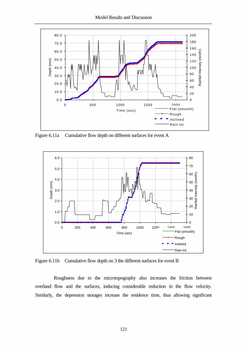
Model Results and Discussion
123
Figure 6.11a Cumulative flow depth on different surfaces for event A
0.0
1.0
2.0
3.0
4.0
5.0
6.0
0 200 400 600 800 1000 1200 1400 1600
Time (sec)
Dep
th (
mm
)
0
10
20
30
40
50
60
70
80
Rai
nfal
l Int
ensi
ty (
mm
/hr)
Flat (smooth)
Rough
Inclined
Rain Int.
Figure 6.11b Cumulative flow depth on 3 the different surfaces for event B
Roughness due to the microtopography also increases the friction between
overland flow and the surfaces, inducing considerable reduction in the flow velocity.
Similarly, the depression storages increase the residence time, thus allowing significant
0.0
10.0
20.0
30.0
40.0
50.0
60.0
70.0
80.0
0 500 1000 1500 2000
Time (sec)
Dep
th (
mm
)
0
20
40
60
80
100
120
140
160
180
200
Rai
nfal
l Int
ensi
ty (
mm
/hr)
F la t (smooth)
Rough
Incl inedRain Int .

Model Results and Discussion
124
poststorm infiltration, which reduces surface runoff volume. This was similarly
observed by Dunne and Dietrich (1980) with vegetated microtopography.
Figure 6.12a and b indicate that microtopography reduces the cumulative flow
depth. Both flat-smooth terrain and inclined-smooth terrain is seen to maintain equal
flow depths throughout the two events, inspite of the very clear difference in slope angle
and discharge rate (Figure 6.12). The magnitude of the difference is reduced in the low
intensity event, apparently due to the substantial reduction in runoff volume. The
influence of surface roughness on flow velocity, flow depth and discharge volume is
observed to increase with increasing slope length and increase duration of the event.
0.2 0.4 0.6 0.8 1 1.2 1.4 1.6 1.8 2
0.2
0.4
0.6
0.8
1
1.2
1.4
1.6
1.8
2
x-distance(m)
y-di
stan
ce(m
)
Velocity (vector) and speed (contour)
0.05
0.05
0.050.05 0.05
0.05
0.050.1
0.1
0.1
0.10.1
0.1
0.1
0.15
0.15
0.15
0.15
0.15
0.15
0.150.
2
0.2
0.2
0.2
0.2
0.2
0.25
0.25
0.25
0.5
0.55
0.6
0.65
0.7
0.2 0.4 0.6 0.8 1 1.2 1.4 1.6 1.8 2
0.2
0.4
0.6
0.8
1
1.2
1.4
1.6
1.8
2
x-distace(m)
y-di
stac
e(m
)
0.5
0.55
0.6
0.65
0.7 Flow vector and Terrain contour at 500sec
0
2
4
6
8
10
12
14
16
0.2 0.4 0.6 0.8 1 1.2 1.4 1.6 1.8 2
0.2
0.4
0.6
0.8
1
1.2
1.4
1.6
1.8
2
x-distance(m)
y-di
stan
ce(m
)
0
2
4
6
8
10
12
14
16Flow vector and values (contour)
00.5
11.5
2
0
0.5
1
1.5
245
50
55
60
65
70
75
x-distance(m)
Terrain
y-distance(m)
z-he
ght(c
m)
(a). Rough Terrain

Model Results and Discussion
125
0.2 0.4 0.6 0.8 1 1.2 1.4 1.6 1.8 2
0.2
0.4
0.6
0.8
1
1.2
1.4
1.6
1.8
2
x-distance(m)
y-di
stan
ce(m
)
Velocity (vector) and speed (contour) at 500sec
0.05 0.05 0.05
0.05
0.05
0.050.050.05
0.1 0.10.1
0.1
0.1
0.10.10.1
0.15 0.15
0.15
0.15
0.15
0.150.15
0.2
0.2
0.2
0.2
0.20.2
0.25
0.25
0.25
0.25
0.25
0
0.02
0.04
0.06
0.08
0.1
0.12
0.14
0.16
0.2 0.4 0.6 0.8 1 1.2 1.4 1.6 1.8 2
0.2
0.4
0.6
0.8
1
1.2
1.4
1.6
1.8
2
x-distance(m)
y-di
stac
e(m
)
0
0.02
0.04
0.06
0.08
0.1
0.12
0.14
0.16Flow vector and Terrain (contour) at 500sec
0
0.2
0.4
0.6
0.8
1
1.2
1.4
1.6
1.8
0.2 0.4 0.6 0.8 1 1.2 1.4 1.6 1.8 2
0.2
0.4
0.6
0.8
1
1.2
1.4
1.6
1.8
2
x-distance(m)
y-di
stan
ce(m
)
0
0.2
0.4
0.6
0.8
1
1.2
1.4
1.6
1.8Flow vector and values (contour) at 500sec
00.5
11.5
2
0
0.5
1
1.5
20
5
10
15
20
x-distance(m)
Inclined Terrain
y-distance(m)
z-he
ght(c
m)
(b) Inclined Terrain
Figure 6.11 Flow vector, speed and depth on different terrain at 500sec for event A
0.5
0.55
0.6
0.65
0.7
0.2 0.4 0.6 0.8 1 1.2 1.4 1.6 1.8 2
0.2
0.4
0.6
0.8
1
1.2
1.4
1.6
1.8
2
x-distace(m)
y-di
stac
e(m
)
0.5
0.55
0.6
0.65
0.7 Flow vector and Terrain contour at 500sec
0.5
1
1.5
2
2.5
3
3.5
0.2 0.4 0.6 0.8 1 1.2 1.4 1.6 1.8 2
0.2
0.4
0.6
0.8
1
1.2
1.4
1.6
1.8
2
x-distace(m)
y-di
stac
e(m
)
0.5
1
1.5
2
2.5
3
3.5Flow vector and values (contour) at 500sec
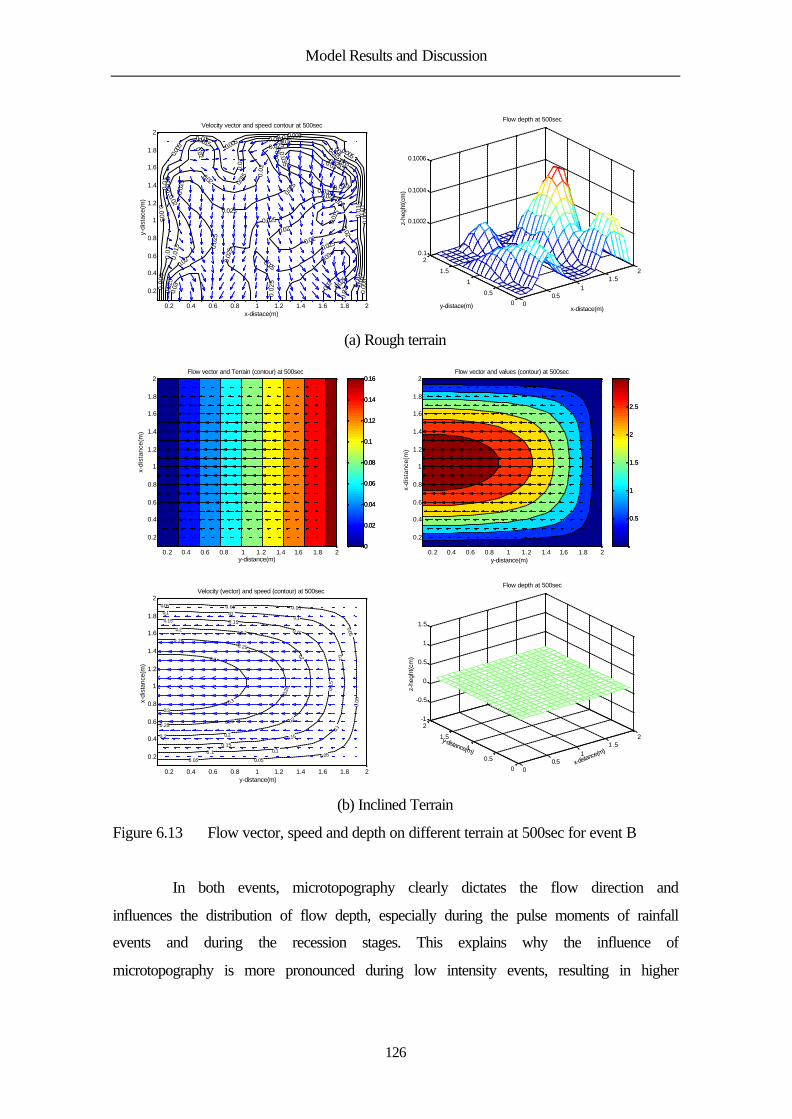
Model Results and Discussion
126
0.2 0.4 0.6 0.8 1 1.2 1.4 1.6 1.8 2
0.2
0.4
0.6
0.8
1
1.2
1.4
1.6
1.8
2
x-distace(m)
y-di
stac
e(m
)
Velocity vector and speed contour at 500sec
0.00
5
0.005
0.005 0.00
50.005
0.005
0.00
50.
005
0.01
0.01
0.01
0.01
0.01
0.01
0.01
0.01
0.01
50.
015
0.015
0.015
0.0150.015
0.01
50.
015
0.01
5
0.02
0.02
0.02
0.02
0.02
0.02
0.02
0.02
0.02
0.02
0.02
0.02
0.02
5
0.02
5
0.02
5
0.025
0.025
0.025
0.025
0.025
0.0250.
025
0.02
50.025
0.025
0.025
0.03
0.03
0.03
0.03
0.03
0.03
0.035
0.035
0
0.51
1.52
0
0.5
1
1.5
20.1
0.1002
0.1004
0.1006
x-distace(m)
Flow depth at 500sec
y-distace(m)
z-he
ght(c
m)
(a) Rough terrain
0
0.02
0.04
0.06
0.08
0.1
0.12
0.14
0.16
0.2 0.4 0.6 0.8 1 1.2 1.4 1.6 1.8 2
0.2
0.4
0.6
0.8
1
1.2
1.4
1.6
1.8
2
x-di
stan
ce(m
)
y-distace(m)0
0.02
0.04
0.06
0.08
0.1
0.12
0.14
0.16Flow vector and Terrain (contour) at 500sec
y-distance(m)
0.5
1
1.5
2
2.5
0.2 0.4 0.6 0.8 1 1.2 1.4 1.6 1.8 2
0.2
0.4
0.6
0.8
1
1.2
1.4
1.6
1.8
2
x-di
stan
ce(m
)
y-distance(m)
0.5
1
1.5
2
2.5
Flow vector and values (contour) at 500sec
0.2 0.4 0.6 0.8 1 1.2 1.4 1.6 1.8 2
0.2
0.4
0.6
0.8
1
1.2
1.4
1.6
1.8
2
x-di
stan
ce(m
)
y-distance(m)
Velocity (vector) and speed (contour) at 500sec
0.05 0.05 0.05
0.05
0.05
0.050.050.05
0.1 0.10.1
0.1
0.1
0.10.1
0.15 0.15
0.15
0.15
0.15
0.15
0.2 0.2
0.2
0.2
0.20.2
0.250.25
0.25
0.250.25
0.3
0.3
0.3
y-distance(m) 0
0.51
1.52
0
0.5
1
1.5
2-1
-0.5
0
0.5
1
1.5
y-distance(m)
x-distance(m)
z-he
ght(c
m)
Flow depth at 500sec
(b) Inclined Terrain
Figure 6.13 Flow vector, speed and depth on different terrain at 500sec for event B
In both events, microtopography clearly dictates the flow direction and
influences the distribution of flow depth, especially during the pulse moments of rainfall
events and during the recession stages. This explains why the influence of
microtopography is more pronounced during low intensity events, resulting in higher

Model Results and Discussion
127
infiltration capability. Figure 6.13a depicting the flow conditions at 500seconds into
event B show that the spatial distribution of flow depth and the flow pattern and
direction are distinctly influenced by the microtopography as was similarly observed by
Esteves et al. (2000). This contrast the observation by Zhang and Cundy (1989) who
concluded that microtopography did not significantly alter flow direction. It could
however, be understood that the effect of microtopography in their simulation
experiments were clouded by the relatively large grid spacing of 1.0m in the simulation.
Changes in surface microtopography are widely influenced by land use at
small scale and catchment morphology at large scale. Small-scale microtopography
results from field cultivation and vegetation changes and has been shown in the model
simulation to be significant in influencing runoff process. Observations like the one
depicted in figure 6.14b are similarly recorded in the tailing period of event A. This
trend of fluctuation between high and low intensity over short time form part of the
distinguishing features characterizing tropical rainstorm patterns and will be very
helpful in the study of the environment related impact of surface runoff processes in the
tropics. It is evident as postulated by Zhang and Cundy, (1989) that, a spatially varying
flow field cannot be obtained by assuming a uniform roughness surface.
It is apparent that rainfall events with prolonged recessions, or more frequent
pulse moments (multiple peak), will behave very differently when compared to a single
peak event with the same depth, in terms of runoff response even when they have equal
duration. It is therefore expedient to agree with the conclusion of Wainwright and
Parson, (2002) that a better understanding of the temporal variability of rainfall intensity
is important in both understanding field measurements and developing robust models of
overland flow. A single peak event will reduce the scale of the difference in discharge
among the three surface conditions.
The low values of discharge on a flat plane surface accentuate the importance
of slope angle in the transformation of ponded water into surface runoff and also lend
credence to the choice of diffusion process in the model operation. The uniformity in
flow depth over the smooth-plane terrain and smooth-inclined plane has been shown
earlier. The low discharge shows that the water only ponded and did not flow, but is
redistributed over the whole plot in manner similar to the application of irrigation water;
with the maximum velocity recorded in the center of the plot. This clearly shows the

Model Results and Discussion
128
ability of the model to monitor the advance and trajectory of applied water in irrigation
schemes similar to the work of Playan et al. (1994). This observation provides a tool
that can aid decision process in soil management techniques aimed at managing surface
runoff and soil erosion
Simulation on different plane surface with different slope angle showed that
the volume of runoff increases proportionately with increase in slope angle, but the
proportionality is not observed when a rough terrain inclined at similarly different
angles was used. This suggests that scale effect in runoff process also depend on the
microtopography.
Conclusions and Recommendations
129
7 CONCLUSIONS AND RECOMMENDATIONS
This study was designed to answer some basic questions about runoff generation and
transmission processes in the Volta river basin, west Africa, such as what proportion of
rain is lost to surface runoff, what is the influence of scale, what are the factors that
determine scale effect and under what conditions it occurs, a concise summary of the
major findings of this research in the light of the research objective and questions are
outlined here:
The dominant runoff generating mechanism in the catchment in the study area
and presumably in the Volta Basin is the infiltration-excess process. This does not
foreclose the pseudo-saturation excess runoff process in the valley area close to the
rivers and in the parts of the basin with very shallow soil depth. The prevalence of high
intensity storm in the catchment combined with poor infiltration properties of the soil
initiate surface runoff flow process.
The diverse nature of response to the same rain event at the two sites within
the same catchment further reflects the importance of heterogeneous soil and hydraulic
properties as they affect storm runoff responses. A study of the profile soil moisture
indicates very high variability in soil moisture content in the first 300mm layer of soil.
The occurrences of rainfall influence the moisture status, at the surface and in the
100mm depth. Possibly due to the high sand content, the temporal analysis of soil
moisture shows that, the stored moisture are quickly depleted. This explains runoff yield
is often not correlated with rainfall amount, or peak rainfall intensities, particularly for
the low intensity events. The moisture gradient always increases sorptivity and increase
time required for ponding. Results from both field and model simulation also show that
vegetation and vegetation changes can significantly influences total runoff observed,
due to the varying interception losses and the reduction of flow velocity.
In both field observations and simulation experiments, an exponential trend of
reduction in runoff coefficient and unit runoff discharge with increasing slope length
was observed, suggesting the import of observation scales in the surface runoff process.
The observed scale effect is mainly caused by spatial variability in infiltration
opportunities. The study also showed that the infiltration opportunities vary with slope
length and the pattern of the distribution of hydraulic conductivity. The difference in

Conclusions and Recommendations
130
infiltration opportunities result in differences in transmission losses potential, during
surface runoff routing downslope. It can also be concluded that the vegetated and
surface microtopography, which become more varied with increase in slope length
determined surface depression storage shape and network, consequently influencing
runoff initiation and flow rate. However, the effect of the two factor of spatial
variability is influenced by the time required to move from point of runoff initiation to
the trough, which also depend on the rainfall intensity and field slope. Thus, the
temporal pattern of rainfall can influence runoff response. Temporal patterns of rainfall
intensity; particularly the distribution in terms of numbers of peaks in the event, the
duration of the pulses, the length of time for recession, and magnitude of rainfall
intensity coupled with temporal variation in travel largely determine the response to
high intensity events while, soil related effect in terms of spatial variability in hydraulic
properties mainly influences low intensity event. The dominance of temporally induced
factors in the basin could be related to the high intensity events synonymous with
tropical storm, which often do not allow the spatial factors to manifest. The other factor
of soil that could significantly influence runoff response is the initial moisture status of
the soil. However, the high intensity rainfall predominant in the Volta basin limits its
influence. In low intensity events, high initial moisture content increases runoff volume.
Analysis of the hydrograph from simulation experiment with different
microtopography shape indicates that, runoff volume can be widely varied from runoff
plot of the same size. This apparently results form the different shape and density of
depression storage created by the microtopography shape, thereby showing that soil
surface microtopography will significantly influences the rainfall-runoff process. In
comparison with smooth terrain of similar inclination, microtopography reduces runoff
discharge. The low values of discharge on a flat plane terrain accentuate the importance
of slope angle in the transformation of ponded water into surface runoff. Another
significant effect of soil surface microtopography is that it influences flow direction of
surface runoff throughout the event even when the surface ought to have been
submerged by increased flow depth. The period of effective influence of
microtopography under less intensive events is more pronounced compared to high
intensity events. This indicates that microtopography plays very determining role in

Conclusions and Recommendations
131
directing flow, creating rill and micro-channel path, and determining flow velocity
under low intensity rainfall.
Results from the model showed that it is possible to predict hydrologic
response, if the model structure is designed to accommodate variability in Ksat or
precipitation as observed in the field. If, however, the model fails to recognize this
variability, we can expect that agreement with observation will be poor. This study as
has also demonstrated that with the inclusion of condition similar to the one obtainable
on the field and the selection of appropriate model, it is possible to capture rain-runoff
transformation in tropical environments. The developed model will be useful in
studying the dynamics of surface runoff, water erosion, and nutrients dynamics under
complex microtopographic condition and spatially varying soil hydraulic characteristic
and temporally dynamic rainfall intensity obtainable in many tropical catchments. It
also provides practical tool for facilitating decision processes in soil management
techniques aimed at managing surface runoff and soil erosion and provide the basis for
upscaling to monitor the basin runoff process.
RECOMMENDATIONS
In the light of the results from both field observations and modeling techniques used in
this study, the following recommendations in terms field experimentation and possible
applications and further extension of the modeling are proposed:
Sustained long term studies on surface runoff process in the basin. The result
from the single season studies will be better validated if it is compared with results from
the same plot over 3-5 seasons. Repeating the field trials ensures that more data will
also be available for comparism with the model simulations.
In carrying out such studies, it will be very good to further improve on the
developed the tipping bucket runoff meter, to handle lower volume of runoff per tip.
Such development will increase the sensitivity of the tipping bucket and will facilitate
better comparism.
The results had indicated that, frictional resistance differs according to plant
structure, which depends on the age and type of vegetation. It would be a good idea, if
further research is carried out on the estimation of frictional resistance by the different
configurations of surface and vegetation microtopography in surface runoff processes.

Conclusions and Recommendations
132
Such estimation will enhance the large scale application of the model, as the derived
factors could be used explicitly to account for microtopography in large scale i.e. basin-
wide applications-
It will also be a good idea to explore the possibility of integration of the
developed model with mesoscale model like MM5 for large scale application and
climate impact studies;
Finally, it will be a good idea to apply the developed model in the area of
Solute Transport studies e.g. erosion, pesticides movement etc. with necessary
subroutine and models incorporated.

References
133
8 REFERENCES
Abbott M.B. and Basco D.R. 1989. Computational fluid dynamics, Longman, London. Abbott M.B. and Minns A. 1998. Computational Hydraulics 1st ed., Pitman,
London/Longman, London, and Wiley, New York/2nd edition, Ashgate, Aldershot, UK, and Brookfield, USA.
Abiodun B.J. 2003. Numerical modeling of mesoscale convective systems over West Africa. Ph.D. dissertation, Department of Meteorology, Federal University of Technology Akure, Nigeria. 120 pp
Abrahams A.D., Parsons A.J., and Wainwright J. 2003 Disposition of rainwater under creosote bush. Hydrological Processes 17 (13) pp. 2555-2566.
Agyare W.A. 2004. Soil characterization and modeling of spatial distribution of saturated conductivity at two sites in the Volta Basin of Ghana. Ecology and Development series No. 17
Akan A.O. and Yen B. C. 1981. Diffusion-wave flood routing in channel networks. J. Hydr. Div., ASCE, 107 (6): 719-731.
Akanbi A.A. and Katapodes 1988. Model for flood propagation on initially dry land. J. Hydr. Engrg. ASCE 114 (7) pp. 689-706
Angermann T., Wallender W.W., Wilson B.W., Werner I., Hinton D.E., Oliver M.N., Zalom F.G., Henderson J.D., Oliveira G.H., Deanovic L.A., Osterli P., Kruegerb W. 2002 Runoff from orchard floors-micro-plot field experiments and modeling. J. Hydrology 265: 178–194
Arnaud P., Bouvier C., Cisneros L. and Dominguez R. 2002. Influence of rainfall spatial variability on flood prediction. J. Hydrology 260 (1-4): 216-230
Asselin R. 1972. Frequency filter for time integrations. Mth. Wea. Rev., 100:487-490. Auzet A.V., Boiffin J. and Ludwig B. 1995. Concentrated flow erosion in cultivated
catchments: Influence of soil surface state. Earth Surface Processes and Landforms 20 (8): 759-767
Bellos C., Soulis J. and Sakkas J. 1991. Computation of two-dimensional dam break induced flow. Adv. in Water Resour. 14(1): 31-41.
Bergkamp G. 1998. A hierarchical view if the interaction of runoff and infiltration with vegetation and microtopography in semiarid shrublands. Catena 33:201-220.
Beven K.J., Wood E.F. and Murugesu S. 1988. On hydrological heterogeneity-catchment morphology and catchment response. J. Hydrol. 100: 353-375.
Borah D.K., Prassas S.N. and Alonso C.V. 1980. Kinematic wave routing incorporating shock fitting. Water Resour. Res., 16: 529–541
Braud I., Vich A.I.J., Zuluaga J., Fornero L. and Pedrani A. 2001. Vegetation influence on runoff and sediment yield in the Andes region: observation and modeling. J. Hydrology 254 (1-4): 124-144
Brown D.L. 1995. An analysis of transient flow in upland watersheds: interactions between structure and process. Ph.D. Dissertation, University of California at Berkeley.
Campbell I.A. 1989. Badlands and badland gullies. In: Thomas SG (eds), Arid zone geomorphology. Belhaven Press, London. pp. 159-183.
Campling P., Gobin A., Beven K. and Feyen J. 2002. Rainfall-runoff modelling of a humid tropical catchment: the TOPMODEL approach. Hydro. Processes 16 (2): 231-253.

References
134
Carsel R.F. and Parrish R.S. 1988. Developing joint probability distributions of soil water retention characteristics. Water Resour. Res. 24: 755-769.
Chaplot V.A.M. and Le Bissonnais Y. 2003. Runoff features for interrill erosion at different rainfall intensities, slope lengths, and gradients in an agricultural loessial hillslope. SSSA J. 67 (3): 844-851
Chevallier P. and Planchon O. 1993. Hydrological process in a small humid savannah basin (Ivory Coast). J. Hydro.151: 173-191.
Chilés J.P. Delfiner P. and Delfiner P. 1999. Geostatistics: Modelling spatial uncertainty. Wiley Joohn and sons. 720pp.
Chow V.T. 1964. Runoff: Section 14 in handbook of applied hydrology. Edited by Chow V.T. McGraw-Hill, New York.
Chow V.T. and Ben-Zvi A. 1973. Hydrodynamic modeling of two-dimensional watershed flow J. Hydr. Div., ASCE 99(11): 2023-2040.
Cunge J.A, Holly F.M. Jr. and Verwey A. 1980. Practical aspects of computational rivers hydraulics. Pitman Publishers, Boston Mass.
Darboux F., Davy P., Gascuel-Odoux C. and Huang C. 2002. Evolution of soil surface roughness and flow path connectivity in overland flow experiments. Catena 46 (2-3): 125-139.
Darboux F., Gascuel-Odoux C. and Davy P. 2002. Effect of surface water storage by soil roughness on overland flow generation. Earth surface processes and landforms 27 (3): 223-233.
de Lima J.L.M.P. and Singh V.P. 2002. The influence of the pattern of moving rainstorms on overland flow Adv. in Water Resou. 25 (7): 817-828.
de Lima J.L.M.P. Singh V.P. and de Lima M.I.P. 2003. The influence of storm movement on water erosion: storm direction and velocity effects Catene 52 (1): 39-56
Diamond J. and Shanley T. 1998. Infiltration rate assessment of some major soils. End of Project Report, Armis 4102, Teagasc, Dublin.
Dibike Y.B. 2002. Developing generic hydrodynamic models using artificial neural networks. J. Hydraulic Res. 40:2
Dickson K.B. and Benneh G. 1995. A New Geography of Ghana. London: Longman Dikau R. and Schmidt J. 1999. Extracting geomorphometric attributes and objects from
digital elevation models-semantics, methods, future needs. In GIS for Earth Surface Systems- Analysis and modeling of the Natural environments, Dikau R Saurer H (eds). Schweizbart’sche Verlagsbuchhandlung: Berlin, Stuttgart; 153-173
Dunne T. 1978. Field studies of hillslope flow processes. In: Hillslope hydrology, Kirkby, M.J., ed., John Wiley & Sons, New York, NY, pp. 227-293.
Dunne T. and Black R.D. 1970a. An experimental investigation of runoff production in permeable soils. Water Resources Res. 6, pp. 478-490.
Dunne T. and Black R.D. 1970b Partial area contributions to storm runoff in a small New England watershed, Water Resour. Res. 6: 1296-1311.
Dunne T. and Dietrich W.E. 1980a. Experimental investigation of Horton overland flow on tropical hillslopes: 1. Soil conditions, infiltration, and frequency of runoff, Z. Geornorph. N.F., Suppl.-Bd. 35: 40-59.
Dunne T., Zhang W. and Aubry B.F. 1991. Effects of rainfall, vegetation and microtopography on infiltration and runoff. Water Resour. Res. 27, 2271–2285
References
135
Erbes G. 1994. A study of finr scale atmospheric dynamics and numerical advection methods. PhD thesis, dept. of meteorology, Stockholm University. (
Esteves M Faucher X Galle S and Vauclin M 2000 Overland flow and infiltration modelling for small plots during unsteady rain: numerical results versus observed values. J. Hydrology, 228: 265–282
Esteves M. and Lapetite J.M. 2003. A multi-scale approach of runoff generation in a Sahelian gully catchment: a case study in Niger Catena 50 (2-4): 255-271
FAO 1995 World agriculture: Towards 2010, An FAO study. N. Alexandratos (Editors) FAO, Rome. pp 210.
Fennema R.J. and Chaudhry M.H. 1986. Explicit numerical schemes for unsteady free-surface flows with shocks. Water Resour. Res. 22: 1923–1930.
Fiedler F.R. 1997. Hydrodynamic simulation of overland flow with spatially variable infiltration and microtopography. Ph.D. thesis, Colorado State University.
Fiedler F.R. and Ramirez J.A. 2000. A numerical method for simulating discontinuous shallow flow over an infiltrating surface. Inter. J. Numerical Methods in Fluids 32 (2): 219-240
Fiedler F.R., Gary P.E., Ramirez J.A. and Ahuja L.R. 2002. Hydrologic response of grasslands: effect of grazing, interactive infiltration and scale.
Fitzjohn C., Ternan J.L. and William A.G. 1998. Soil moisture variability in a semi-arid gully catchment: implication for runoff and erosion control. Catena 32: 55-70
Foreman M.G.G. 1984. A two-dimensional dispersion analysis of selected methods for solving the linearised shallow water equation. J. Computational Physics 56:287-323.
Friesen J. 2002. Spatio-temporal rainfall patterns in Northern Ghana. Diplom Thesis, Geographische Institute der Rheinischen Friedrich-Wilhelms, Universität Bonn
Garcia R. and Kahawita R.A. 1986. Numerical solution of the St. Venant Equations with the MacCormack finite difference scheme. Inter. J. Numerical Methods in Fluids. 6: 507-527.
Gaur M.L. and Mathur B.S. 2003. Modeling event-based temporal variability of flow resistance coefficient. J. Hydrologic Engng 8 (5): 266-277
Golden Software, Inc 2000. Surfer(R) Version 7. Golden Software, Inc. 809 14th Street Golden, CO 80401-1866 USA. http://www.goldensoftware.com
Gomez J.A., Orgaz F., Villalobos F.J. and Fereres E. 2002. Analysis of the effects of soil management on runoff generation in olive orchards using a physically based model. Soil use and management 18 (3):191-198.
Govindaraju R.S., Jones S.E. and Kavvas M.L. 1988. On the diffusion wave model for overland flow 1- Solution for the steep slopes. Water Resor. Res. 24(5): 734-744.
Haltiner G.J. and Williams R.T. 1980. Numerical prediction and dynamic meteorology. John Wiley and Sons
Horton R.E. 1933. The role of infiltration in the hydrologic cycle. Trans. Am. Geophys. Union, 14: 446-460.
Hromadka T.V. II., McCuen R.H. and Yen C.C. 1987. Comparison of overland flow hydrograph models. J. Hydraulic Engng (ASCE) 113(11): 1422-1440.
Hudson N. 1995. Soil conservation. 3rd Edition B.T. Batsford, London 391pp

References
136
Hupet F. and Vanclooster M. 2002. Intraseasonal dynamics of soil moisture variability within a small agricultural maize cropped field. J. Hydrology 261 (1-4): 86-101
Hursh C.R. 1936. Storm-water and absorption. In: Discussion on list of terms with definitions; Report of the Committee on Absorption and Transpiration, Trans. Am. Geophys. Union, 17: 301-302.
Iwasa Y. and Inoue K. 1982. Mathematical simulation of channel and overland flows in view of flood disaster engineering. Natural Disaster Science 41(1): 1-30.
Jetten V., de Roo A. and Favis-Mortlock D. 1999. Evaluation of field-scale and catchment-scale soil erosion models. Catena 37 (3-4): 521-541
Jha A.K., Akiyama J. and Ura M. 1995. First and second-order flux difference schemes for dam break problem. J. Hydraul. Engng., 121: 877–884.
Jhorar R.K., van Dam J.C., Bastiaanssen W.G.M. and Feddes R.A. 2004. Calibration of effective soil hydraulic parameters of heterogeneous soil profiles J. Hydro. 285 (1-4): 233-247.
Joel A., Messing I., Seguel O. and Casanova M. 2002. Measurement of surface runoff from plots of two different sizes. Hydrological Processes 16:1467-1478.
Jolánkai G. and Rast W. 1999. The hydrologic cycle and factors affecting the generation, transport and transformation of nonpoint source pollutants. In: Assessment and control of nonpoint source pollution of aquatic ecosystems: a practical approach. UNESCO and The Parthenon Publishing Group, USA.
Julien P.Y. and Moglen G.E. 1990. Similarity and length scale for spatially varied overland flow. Water Reso. Res. 26: 1819–1832.
Kang S.Z., Zhang L., Song X.Y. Zhang S.H., Liu X.Z., Liang Y.L. and Zheng S.Q. 2001. Runoff and sediment loss responses to rainfall and land use in two agricultural catchments on the Loess Plateau of China Hydrological processes 15 (6): 977-988
Kasteel R., Vogel H.J. and Roth K. 2000. From local hydraulic properties to effective transport in soil. European J. Soil Science 51 (1): 81-91.
Katapodes N.D. and Strelkoff T. 1979. Two-dimensional shallow water-wave model. J. Eng. Mech. Div. Am. Soc. Civ. Eng., 105 (EM2): pp 317-334.
Katopodes N.D. and Strelkoff T. 1978. Computing two-dimensional dam-break flood waves. J. Hydra. Division, ASCE, 104(9): 1269-1288.
Kawahara M. and Yokoyama T. 1980. Finite element method for direct runoff flow. J. hydra. Div. ASCE, 106(4): 519-533.
Kirkby M. 2002. Modeling the interaction between soil surface properties and water erosion. Catena 46 (2-3): 89-102.
Kirkby M., Bracken L., and Reaney S. 2002. The influence of land use, soils and topography on the delivery of hillslope runoff to channels in SE Spain. Earth surf. Process. Landforms 27, 1459–1473.
Lal R. 1997. Soil degradative effects of slope length and tillage methods on alfisols in Western Nigeria, I, Runoff, erosion and crop response. Land Degradation Dev., 8(3): 201–219.
Lane L., Hernandez M. and Nichols M. 1997. Processes controlling sediment yield from watersheds as functions of spatial scale. Environmental Modeling and Software, 12, 355–369.
Le Barbé L. and Lebel T. 1997. Rainfall climatology of the HAPEX-Sahel region during the years 1950-1990. J. Hydro.188-189: 43-73.

References
137
Léonard J. and Perrier E. 2001. A model for simulating the influence of a spatial distribution of large circular macropores on surface runoff. Water Resou. Res. 37 (12): 3217-3225.
Lidén R. and Harlin J. 2000. Analysis of conceptual rainfall modelling performance in different climates. J. Hydro. 238:231-247.
Liggett J.A. and Woolhiser D.A. 1967. Finite-difference solutions of the shallow water equations, Proc. ASCE J. Mech. Div., 93:39–71.
Littleboy M., Cogle A,L., Smith G.D., Rao K.P.C. and Yule D.F. 1996. Soil management and production of Alfisols in the semi-arid tropics .4. Simulation of decline in productivity caused by soil erosion. Australian J. Soil Res. 34 (1): 127-138.
Logsdon S.D. Jordahl J. and Karlen D.L. 1993. Tillage and crop effects on ponded and tension infiltration rates. Soil & Tillage Res. 28 (2): 179-189.
Mah M.G.C., Douglas L.A. and Rigrose-voase A.J. 1992. Effect of crust development and surface slope on erosion by rainfall. Soil Science 154:37-43.
Malet J.P., Auzet A.V., Maquaire O., Ambroise B., Descroix L., Esteves M., Vandervaere J.P. and Truchet E. 2003. Soil surface characteristics influence on infiltration in black marls: Application to the Super-Sauze earthflow (southern Alps, France) Earth Surface Processes and Landforms 28 (5): 547-564
Mallants D., Mohanty B.P., Jacques D. and Feyen J. 1996. Spatial variability of hydraulic properties in a multi-layered soil profile. Soil Sci. 161(3): 167-181.
Masiyandima M.C., van de Giesen N., Diatta S., Windmeijer P.N. and Steenhuis T.S. 2003. The hydrology of inland valleys in the sub-humid zone of West Africa: rainfall-runoff processes in the M'be experimental watershed. Hydrological Processes 17 (6): 1213-1225.
Mathwork Inc (2000). MATLAB The language of Technical computing. Version 6.0.0.88 Release 12.
Matula S. 2003. The influence of tillage treatments on water infiltration into soil profile Plant Soil and Environment 49 (7): 298-306.
Mohanty B.P. and Mousli Z. 2000. Saturated hydraulic conductivity and soil water retention properties across a soil-slope transition. Water Resou. Res. 36 (11): 3311-3324
Nash J.E. and Sutcliffe J.V. 1970. River flow forecasting through conceptual models, 1, a discussion of principles. J. Hydrol. 10 (1): 282–290.
Návar J. and Synnott J.T. 2000. Surface runoff, soil erosion, and land use in Northeastern Mexico Terra Volumen 18 (3).
Ogden L. F. and Julien Y. P. 1993. Runoff sensitivity to temporal and spatial rainfall variability at runoff plane and small basin scales. Water Resou. Res., 29 (8): 2589-2597.
Osei-Bonsu P. Asibuo J.Y. 1998. Using polythene bags to control the growth of Mucuna vines http://www.idrc.ca/books/focus/852/14-sec11.html cited April10, 2003.
Parlange J.Y., Hogarth W., Ross P., Parlange M.B., Sivapalan M., Sander G.C.and Liu M.C. 2000. A note on the error analysis of time compression approximations Water Resource Res. 36 (8): 2401-2406.
Parlange J.Y., Rose C.W. and Sander G. 1981. Kinematic flow approximation of runoff on a plane: an exact analytical solution. J. Hydro. 52:171.

References
138
Peugeot C., Esteves M., Rajot J.L., Vandervaere J.P. and Galle, S. 1997. Runoff generation processes: results and analysis of field data collected at the central supersite of the Hapex-Sahel experiment. J. Hydrol. 188– 189 (1–4): 179–202.
Philip J.R. 1957. The theory of infiltration: 4. Sorptivity and algebraic infiltration equations. Soil Science, 84: 257-264.
Playan E. 1992. Two-dimensional hydrodynamic simulation of basin irrigation: analysis of shape effects on irrigation performance. Ph.D. Dissertation, Utah State University.
Pláyan E. and Martinez-cob A. 1999. Simulation of basin irrigation scheduling as a function of discharge and leveling. Invest. agr. prod. prot. veg. 14 (3).
Pláyan E. Walker W.R. and Merkley G.P. 1994. Two-dimensional simulation of basin irrigation .1.Ttheory J. Irri. and Drain. Engng. ASCE 120 (5): 837-856.
Pláyan E. Walker W.R. and Merkley G.P. 1994. Two-dimensional simulation of basin irrigation .2. Applications J. Irri. and Drain. Engng. ASCE. ASCE 120 (5)
Poesen J. 1984. The influence of slope angle on infiltration rate and Hortonian overland flow volume. Zeitschriftifür Geomorphologie 49: 117-131
Ponce M.V. and Shetty A.V. 1995. A conceptual model of catchment water balance:1 formulation and calibration. J. Hydro. 173:27-40
Ponce M.V., Li R. and Simons F. 1978. Applicability of kinematic and diffusion models. J. Hydraulic division, Proc. ASCE, Vol. 104, No. HY3.
Raymond D. J. 1976. Wave-CISK and convective mesosystems. J. Atmos. Sci. 33: 2392-2398
Reeves M. and Miller E.E. 1975. Estimating infiltration for erratic rainfall. Water Resources Res., 11: 102-110
Rockström J. and Valentin C. 1997. Hillslope dynamics of on-farm generation of surface water flows: the case of rainfed cultivation of pearl millet on sandy soil in the Sahel. Agriculture and Water Management 33:183-210.
Rodriguez-Iturbe I. and Váldes J. 1979. The geomorphologic structure of the hydrologic response- Water Resour. Res., 15(6): 1409-1420
Ross J.K. 1975. Radiative transfer in plant communities. In: J.L. Monteith (ed.), Vegetation and the atmosphere, Vol. 1. Academic Press, London. pp. 13-15.
Schmidt J., Hennrich K. and Dikau R. 2000. Scales and similarities in runoff processes with respect to geomorphometry. Hydrological Process 14:1963-1979.
Schwartz R.C., Evett S.R. and Unger P.W. 2003. Soil hydraulic properties of cropland compared with reestablished and native grassland Geoderma 116 (1-2): 47-60.
Sharman K. Singh H. and Pareek O. 1983. Rain water infiltration into a bare loamy sand. Hydrological Science J. 28:417-424
Singh V. and Bhallamudi S.M. 1998. Conjunctive surface-subsurface modeling of overland flow. Advance in Water Resou. 21: 567-579.
Singh V.P. 1989. Hydrologic system: watershed modeling Volume II. Prentice Hall, Englewood Cliff, New Jersey.
Singh V.P. 1996. Kinematic wave modeling in water resources: surface–water hydrology. John Wiley and Sons Ltd.
Smith R.E. and Hebbert R.H.B. 1983. Mathematical simulation of interdependent surface and subsurface hydrologic processes. Water Resour. Res., 19: 987-1001.
Sobieraja J.A., Elsenbeerb, H. Cameron G. (2004) Scale dependency in spatial patterns of saturated hydraulic conductivity Catena 55 pp. 49–77.

References
139
Stoker J.J. 1957. Water waves, the mathematical theory with applications. Interscience, London.
Stolte J., Ritsema C.J. Veerman G.J. and Hamminga W. 1996. Establishing temporally and spatially variable soil hydraulic data for use in a runoff simulation in a loess region of the Netherlands. Hydr. Processes 10: 1027-1034.
Strelkoff T. 1969. One-dimensional equations of open-channel flow. J. Hydraul. Div. ASCE, 95: 861–876
Tayfur G. and Singh V.P. 2004. Numerical model for sediment transport over nonplanar, nonhomogeneous surfaces. J. hydrologic Engng 9 (1): 35-41
Tayfur G., Kavvas M.L., Govindaraju R.S. and Storm D.E. 1993. Applicability of St-Venant equations for 2-dimensional overland flows over rough infiltrating surfaces J. Hydraulic Engng-ASCE 119 (1): 51-63
Taylor C., Al-Mashidani G. and Davis J.M. 1974. A finite element approach to watershed runoff. J. Hydrology 21: 231-246
Todini E. and Venutelli M. 1991. Overland flow: a two-dimensional modeling approach. In : Recenet Advances in the modeling of Hydrologic system. Kluwer Academic publishers, The Netherlands pp. 153-166
Troch P.A., Smith J.A., Wood E.F. and de Troch F.P. 1994. Hydrologic controls of large floods in a small basin: central Appalachian case study. J. Hydrology 156 (1-4) pp. 285-309
Valiani A., Caleffi V. and Zanni A. 2002. Case study: Malpasset dam-break simulation using a two-dimensional finite volume method J. Hydraulic Engng-ASCE 128 (5): 460-472.
Valiani A., Caleffi V. and Zanni A. 2003. Finite volume method for simulating extreme flood events in natural channels. J. Hydraulic Res. 41 (2): 167-177.
van de Giesen N.C., Stomph T.J. and de Ridder N. 2000. Scale effects of Hortonian overland flow and rainfall-runoff dynamics in a West African catena landscape. Hydrological Processes 14 (1): 165-175.
van Dijk A.I.J.M. and Bruijnzeel L.A. 2001. Modeling rainfall interception by vegetation of variable density using an adapted analytical model. 1. Model description. J. Hydrology 247: 230-238.
van Dijk A.I.J.M. and Bruijnzeel L.A. 2001. Modeling rainfall interception by vegetation of variable density using an adapted analytical model. 2: Model validation for a tropical upland mixed cropping system. J. Hydrology 247: 239-262.
van Genuchten M. Th. 1980. A closed form equation for predicting hydraulic conductivity in unsaturated soils. Soil Sci. Soc. Am. J., 44: 892-898.
van Heemst H.D.J. 1988. Plant data values required for simple crop growth simulation models, review and bibliography. Simulation report CABO-TT 17, Wageningen.
van Loon E.E. 2001. Overland flow: interfacing models with measurements. Ph.D. thesis Wageningen University, The Netherlands. 185 pp
van Loon E.E. Keesman K.J. 2000. Identifying scale-dependent models: The case of overland flow at the hillslope scale Water Resou. Res. 36 (1): 243-254.
Wainwright J. and Parsons A.J. 2002. The effect of temporal variations in rainfall on scale dependency in runoff coefficients. Water Resou. Res. 38 (12): 1271 10.1029/2000WR000188
References
140
Wasantha-Lal A.M. 1998. Performance comparison of overland flow algorithm. ASCE J. Hydraulic Engineering, 124(4): 342-349.
Watson D.J. 1947. Comparative physiological studies on the growth of field crops. Annals of Botany 11: 41-76
Wilcox B.P., Newman B. D., Brandes D., Davenport D. W. and Reid K. 1997. Runoff from a semiarid ponderosa pine hillslope in New Mexico. Water Resour. Res., 33: 2301– 2314.
Wood E.F., Sivapalan M. and Beven K. 1990. Similarity and scale in catchment storm response. Rev. of Geophys., 28: 1-18.
Woolhiser D.A. and Liggett J.A. 1967. Unsteady, one-dimensional flow over a plane-the rising hydrograph. Water Resour. Res., 3(3) : 753-771.
Woolhiser D.A., Smith R.E. and Giraldez J.V. 1996. Effect of spatial variability of saturated hydraulic conductivity on Hortonian overland flow. Water Resou. Res. 32(3): 671-678.
Wu C., Huang G. and Zhang Y. 1999. Theoretical solution of dam-break shock wave. J. Hydraulic Engineering, ASCE125(11): 1210-1215.
Yair A. and Kossovsky A. 2002. Climate and surface properties: hydrological response of small and and semi-arid watersheds Geomorphology 42 (1-2): 43-57.
Yair A. and Lavee H. 1976. Runoff generative process and runoff yield from arid talus antled slopes. Earth Surf. Process Landf. 1: 235–247.
Yair A. Lavee H. 1985. Runoff generation in arid and semi-arid zones. In: Anderson M.G., Burt T.P. (eds.), Hydrological Forecasting. Wiley, Chichester, pp. 183– 220.
Zhang R. 1997. Determination of soil sorptivity and hydraulic conductivity from the disk infiltrometer. SSSA J. 61: 1024-1030.
Zhang W. and Cundy T.W. 1989. Modeling of two-dimensional overland flow. Water Resou. Res. 25(9 ): 2019-2036.
Zhao D.H., Shen H.W., Tabios G.Q. and Lai J.S. 1996. Approximate Riemann solvers in FVM for 2D hydraulic shock wave modeling. J. Hydrologic Engng. 122(12): 692-702.
Zhu J. and Mohanty B.P. 2003. Effective hydraulic parameters for steady state vertical flow in heterogeneous soils. Water Resources Res., 39(8):1029
Zoppou C. and Roberts S. 2003. Explicit schemes for dam-break simulations. J. Hydraulic Engng.-ASCE 129 (1):11-34

ACKNOWLEDGEMENTS
I thank the Almighty God, the giver of all wisdom and grace for the successful completion
of this study. I would like to thank Prof. Helmut Eggers for his supervision and advice; his
suggestions and constructive criticism greatly improved the quality of this work. I would
also like to express my gratitude to Prof. Paul Vlek for his encouragement and
immeasurable support. I sincerely appreciate the excellent guidance from my coach and
tutor Dr. Nick van de Giesen, who inspire this work and provided all the necessary
encouragement till the goal was accomplished. I appreciate the German government, who
through the Deutscher Akademischer Austauschdienst (DAAD) provided me with
scholarship for the PhD studies, and the GLOWA-Volta project that provided the funds for
the research work. I thank the GLOWA project team in Ghana, Drs Marc Andreini and
Matthias Fosu for all the support during the field campaign. I must not fail to mention the
field staff in Ejura, Mr. Emmanuel Amoah, Kojo Moamah, Jacob Agabu. I am grateful to
Mr. Kofi Campion, Dr. Jide Josiah, and Pastor & Dr. (Ms) Mark for their support in
Ghana.
I appreciate the kind support of Dr. Günther Manske, Hannah Peters and the
administrative staff of ZEFC, Sabine Aengenendt-Baer, Andrea Berg, Inga Haller, and
Hagedorn Menasah. I thank Ms. Margaret Jend for editing and reviewing the
manuscript, and for translating the short German version. Thanks to Mr. Volker Merx
for providing the library support.
Special thanks to the management of the Federal University of Technology,
Akure (FUTAkure), for approving my study leave for this study. I appreciate the moral
support of all the academic staff of the Department of Agricultural Engineering,
FUTAkure; Profs. Cornellius Ademosun, Agboola Ogunlowo, Ayorinde Olufayo; Drs
Leo Agbetoye, Michael Alatise, Wale Olukunle, Manuwa, Engrs. Noah Ajayi, Johnson
Fasinminrin, and Richard Falayi. I sincerely appreciate the contributions by the
technical crew of the department, with particular mention of Mr. Adesina, who
appreciably assisted me in the design of the runoff meter used for the study, and Mr.
Jimoh who welded the runoff meters.
I sincerely appreciate the contribution of my modeling tutor and friend Dr.
Babatunde Joseph and my covenant friend and inspiration, Dr. Philip Oguntunde. My
thanks are extended to my friends and colleagues in the doctoral program Drs Ademola

Braimoh, Nii Codjoe, Yaw Osei-Asare, Isaac Osei Akoto, Wilson Agyare just to
mention a few. I am grateful to all the members and pastorate of the Redeemed
Christian Church of God, Bonn, who provided me with spiritual encouragement. I am
also grateful for the moral support from, Ms. Veronica Oguntunde, Ms. Olannike Nist,
Mr. and Ms. Akinbogun, Mr. and Ms. Okosun, Mr. and Ms. Adamolekun, Hon.
Adeniran Ibitoye, Mr. and Ms. Komolafe, Mr. and Ms. Akinjisola Ige, Arc and Ms. Sola
Aluko, Dr. and Ms. Aidi, Senator and Ms. Farukanmi, Mr. and Ms. Adejala, Mr. and
Ms. Liad Tella, Mr. Yinka Tella, Mr. Steve Adedipe, Engr. and Ms. Gbenga Oyeleke
Mr. Zoe Agu and Mr. and Ms. Razaq Ishola.
Thanks to my brother Mr. Gbemiga Arolasafe, who encouraged me, many
years ago, to prepare well for this day and his wife Roseline, who came to my defense
in Bonn. I would like to thank Mr. and Ms. Akintayo Oyedeji for their encouragement. I
thank all the members of Gideon’s International in Akure and Bonn, for being so
supportive. I am also very grateful to the members and pastorate of the Living Faith
Church, Akure. My sincere gratitude to my host family in Germany, Dr. and Ms. Heyde
and to my benefactor Ms. Ayobami Oshinlu and Dr (Ms.) Schäffer, their support was
immeasurable. I also appreciate the spiritual support by Bishop and Pastor (Ms.) Mike
Afolabi, Bishop Thomas Aremu, Pastor (Dr.) and Ms. Oyetade, Pastor Olu Adetomiwa,
Pastor and Ms. Ogbonyomi and Pastor and Ms. Olutoki.
Last, but by no means least, I would like to thank my wife, Ibidunmomi
Oluwaseun, for being very supportive at all moments and enduring the sudden departure
for Bonn, only days after our wedding, my daughter, Jemima Oluwafunto Gbemisola,
for the indescribable encouragement, and my parents for being there for me at all times,
and my in-laws for being so wonderful to me.