Filling gaps and daily disaccumulation of precipitation data for rainfall-runoff model Filling gaps...

BALWOIS 2010 - Ohrid, Republic of Macedonia - 25, 29 May 2010

a

Villazón, M. F. and Willems, P., 2010. Filling gaps and daily disaccumulation of precipitation data for rainfall-runoff model. Eds. Morell, M., Popovska, C., Morell, O., Stojov, V. Procceding at: 4th International Scientific Conference on Water Observation and Information Systems for Decision Support. CD-ROM pp.1-9. Publisher: BALWOIS 2010. 25-29 May Ohrid, Republic of Macedonia.


1

Filling gaps and Daily Disaccumulation of Precipitation Data for Rainfall-runoff model Mauricio F.Villazón a,b, Patrick Willems a

a Katholieke Universiteit Leuven, Hydraulics Section, Kasteelpark Arenberg 40, BE-3001 Leuven - Belgium. [email protected]

b Universidad Mayor de San Simón, Laboratorio de Hidráulica,. Km. 4.2 Avenida Petrolera, Cochabamba – Bolivia

Abstract Precipitation data is one of the most important inputs in rainfall-runoff models. Long records often contain gaps and need to be filled. For the present paper linear regression and multiple linear regression techniques are applied for the estimation of monthly precipitation. For the multiple linear regression technique the tool called HEC4 developed by the U.S. Corps of Engineers is used. The disaccumulation from monthly to daily time scales was done assuming that each station has the same distribution of daily precipitation intensities as the recording station with the highest correlation.

The study area considered for this study is part of the Pirai River basin located in Santa Cruz-Bolivia, which is a tributary of the Amazon River. The available data consisted of 33 daily rainfall stations where 8 have more than 25 years of recorded data. These data have been collected by the regional meteorological and hydrological services SENAMHI (Servicio Nacional de Meteorología e Hidrología – Bolivia) and SEARPI (Servicio de Encauzamiento de Aguas y Regularización del río Piraí – Bolivia). The spatial distribution and the range of altitudes of the stations are quite high (334 m.a.s.l. to 1875 m.a.s.l.). The rain gauge density for the study area is 81.97 km2 per station.

The gap filling techniques were evaluated based on 32 months extracted from the recorded data. The evaluation was done for 6 days, 3 days and 1 day of disaccumulation period. The multiple linear regression technique applied for the monthly rainfall estimation gives us an important reduction (36%) in the Standard Deviation and Root Mean Squared Error over the linear regression. It is observed that the accuracy of the disaccumulated results decrease when the period of accumulation is smaller. At the daily time scale, the multiple linear and linear regression methods have similar performance.

Keywords: Pirai River, linear regression, multiple linear regression, disaccumulation, error reduction

Introduction Precipitation data is the most important input in hydrological models. In many river basins, records collected in long periods of time contain gaps. This could be due to different circumstances, for instance: absence of observers, problems with the measuring device, loss of records, or maybe the lack of funds to continue the measurements. Rainfall runoff modeling of a river basin is a quite important element in the hydrologic analysis to support water resources planning, flood forecasting and pollution control. The rainfall-runoff modeling process is complex since it is influenced by a number of implicit and explicit factors such as precipitation distribution in time and space, evapotranspiration, human activities (e.g. pumping and irrigation), watershed topography and soil types (Shamsudin and Hashim, 2002). The error in these factors can be a potentially large source of uncertainty. Developing countries, as in the present case study (Santa Cruz – Bolivia, Fig. 1), have to deal with lack of data. Therefore, before applying any hydrological model, data analysis should be executed first, to have complete rather than partial rainfall records. There are two main procedures to fill rainfall gaps. The fist one is stochastic modeling of rainfall sequences (Woolhister, 1992; Zucchini et al., 1992). Such procedures, which can be applied irrespective of gaps in the records, are used to generate artificial rainfall sequences. However, this procedure is not applicable when the rainfall records are to be used as input to rainfall-runoff models and when the use involves calibration of these models. In that case, indeed an historical sequence of rainfall depths is required (Makhuvha et al., 1997). The second main procedure is the interpolation based one. Interpolation can be done based on: normal ratio (Paulhus and Kohler, 1952), regression (Makhuvha et al., 1997) or a combination of these methods (Romero et al., 1998). Jeffrey, (2001); Seo, (1996), and others applied advanced interpolation techniques, but these are computationally heavy methods and often appear with very small increase in accuracy (Teegavarapua and Chandramoulia, 2005).


2

The present research focuses on the use of linear regression and multiple linear regression techniques for the estimation of monthly precipitation in the gaps of 33 stations for the period from 1976 to 1999. The disaccumulation was done assuming that each station had the same daily distribution as the recording station with the highest correlation.

Figure 1. Location of Santa Cruz de la Sierra in Bolivia and South America

Materials and methods

Study area The study area considered for this paper is part of the Pirai River basin, which is a tributary of the Amazon River. Even though the Piraí River Basin is a large basin, this study only focuses on the upstream subbasin until the La Belgica (57NP) station passing through Santa Cruz de la Sierra (Fig. 2). In this region the landscape is still wavy with moderate slopes in some places. The vegetation is scarce and little, giving as a result wind and from moderate to high hydraulic erosion. The agriculture is strongly developed. The elevation ranges between 300 to 2700 m.a.s.l. The precipitation data is available in 34 stations, of which 22 are located inside the area and 12 in the surroundings (Fig. 2). One station was dismissed from the study because only a short series was available (less than 10 years and out of date). Fig. 2 presents the distribution of the 33 stations selected.

Data availability Table 1 shows that rainfall stations are irregularly distributed along the basin. Most of the rainfall stations (72%) are located in the more populated areas, usually in the lower part of the basin. Nevertheless 28% are situated at elevations higher than 1160 m.a.s.l. For mountain areas the recommended density per station is 1 in 250 km2 (WMO, 1994). In the present study case this recommendation is fulfilled. The only problem is that there is no rain gauge at elevations higher than 2660 m.a.s.l.. This area, however, only represents 2% of the entire basin. From the 33 rain stations 8 have more than 25 years of recorded data; these stations have been called long-term stations. Details of the 8 long-term stations can be found in Table 2. Table 3 presents the length of precipitation records for the period 1978-1999. From the 33 daily stations 5 have complete records and 9 have less than 5% gaps. 4 additional stations have between 5 and 10% data gaps. Methodologies applied Simple rainfall patching techniques for the monthly estimations are tested: linear and multiple linear regression models. The disaccumulation was done using matrix correlation: the daily distribution of the recording station with the highest correlation was used to disaccumulate the monthly rainfall already estimated.


3

ÿ

ÿ

ÿ

ÿ

ÿ

ÿ

ÿ

ÿ

ÿ

ÿ

#Y

ÿ

ÿ

ÿ

ÿ

ÿ

ÿ

ÿÿ

#Y

ÿ

ÿ

ÿ

ÿ

#Y #Yÿ

ÿ

#Y

#Y

#Y#Y

ÿ

01NP

02NP03NP

04NP

05NP

06NP

07NP

08NP

09NP

10NP

11NP

12NP

13NP

14NP

15NP

16NP

17NP

19NP21NP

25NP

31NP

50NP

51NP

53NP

54NP 56NP

57NP

58NP

71NP

74NP

76NP

77NP

78NP

400000

400000

420000

420000

440000

440000

460000

460000

480000

480000

7960000

7960000

79800007980000

8000000

8000000

8020000

8020000

8040000

8040000

8060000

8060000

N

EW

S

Elevation (m.a.s.l.)300 - 400400 - 500500 - 700700 - 900900 - 12001200 - 15001500 - 18001800 - 21002100 - 24002400 - 2800

#Y Long-term rainfall st.

ÿ Short-term rainfall st.

Pirai River

Figure 2. Rainfall stations in the Piraí River Basin, Bolivia

Table 1 Distribution of rain gauges with elevation

Area Elevation band Absolute Percentage Accumulated

Number of rain gauges

Rain gauges density

(m.a.s.l) (km2) of basin percentage (km2) 2660 2060 55.11 2.04 2.04 0 0 2060 1760 245.41 9.07 11.11 2 122.70 1760 1460 458.58 16.95 28.06 4 114.65 1460 1160 540.21 19.97 48.03 3 180.07 1160 860 335.27 12.39 60.43 5 67.05 860 560 642.86 23.77 84.19 6 107.14 560 330 427.59 15.81 100.00 13 32.89

SUM 2705.02 100.00 33 81.97


4

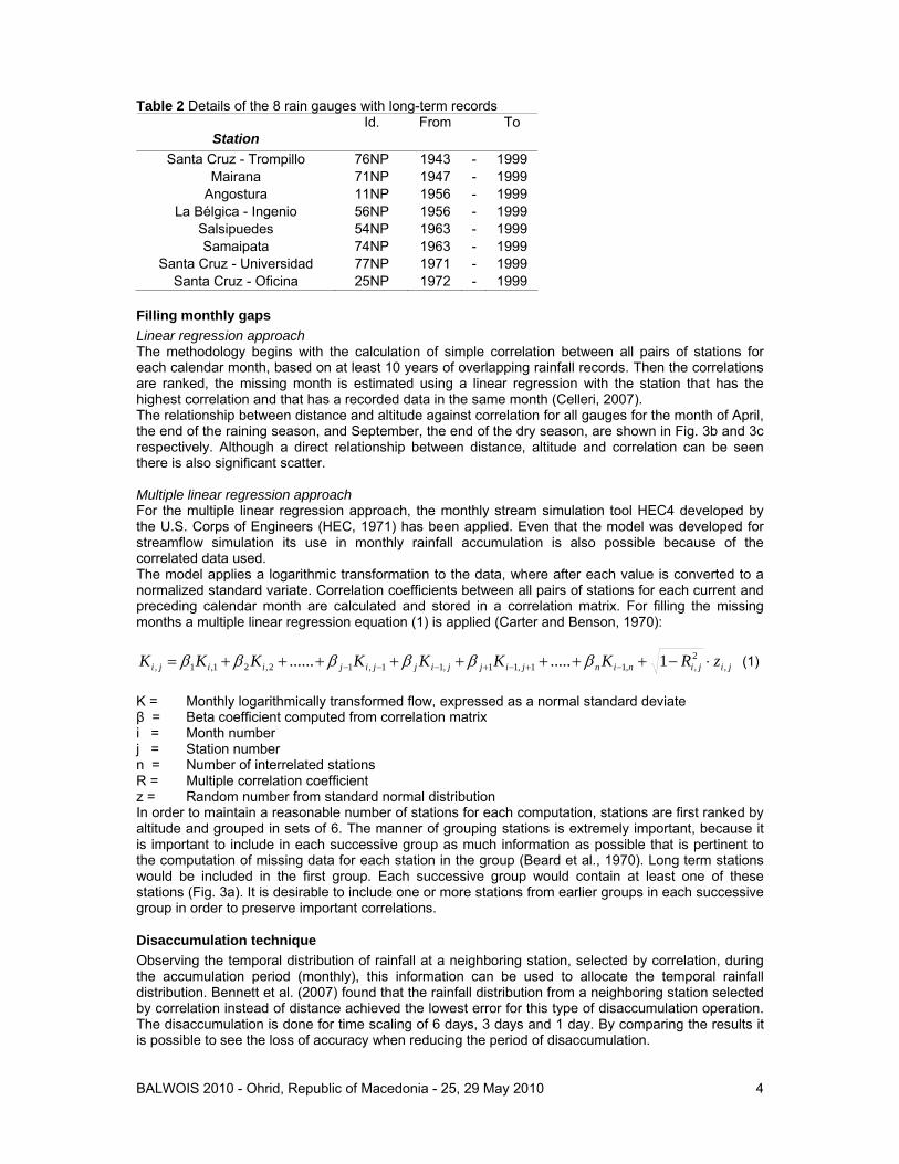
Table 2 Details of the 8 rain gauges with long-term records Id. From To

Station Santa Cruz - Trompillo 76NP 1943 - 1999

Mairana 71NP 1947 - 1999 Angostura 11NP 1956 - 1999

La Bélgica - Ingenio 56NP 1956 - 1999 Salsipuedes 54NP 1963 - 1999 Samaipata 74NP 1963 - 1999

Santa Cruz - Universidad 77NP 1971 - 1999 Santa Cruz - Oficina 25NP 1972 - 1999

Filling monthly gaps Linear regression approach The methodology begins with the calculation of simple correlation between all pairs of stations for each calendar month, based on at least 10 years of overlapping rainfall records. Then the correlations are ranked, the missing month is estimated using a linear regression with the station that has the highest correlation and that has a recorded data in the same month (Celleri, 2007). The relationship between distance and altitude against correlation for all gauges for the month of April, the end of the raining season, and September, the end of the dry season, are shown in Fig. 3b and 3c respectively. Although a direct relationship between distance, altitude and correlation can be seen there is also significant scatter. Multiple linear regression approach For the multiple linear regression approach, the monthly stream simulation tool HEC4 developed by the U.S. Corps of Engineers (HEC, 1971) has been applied. Even that the model was developed for streamflow simulation its use in monthly rainfall accumulation is also possible because of the correlated data used. The model applies a logarithmic transformation to the data, where after each value is converted to a normalized standard variate. Correlation coefficients between all pairs of stations for each current and preceding calendar month are calculated and stored in a correlation matrix. For filling the missing months a multiple linear regression equation (1) is applied (Carter and Benson, 1970):

jijininjijjijjijiiji zRKKKKKKK ,2,,11,11,11,12,21,1, 1........... ⋅−++++++++= −+−+−−− ββββββ (1)

K = Monthly logarithmically transformed flow, expressed as a normal standard deviate β = Beta coefficient computed from correlation matrix i = Month number j = Station number n = Number of interrelated stations R = Multiple correlation coefficient z = Random number from standard normal distribution In order to maintain a reasonable number of stations for each computation, stations are first ranked by altitude and grouped in sets of 6. The manner of grouping stations is extremely important, because it is important to include in each successive group as much information as possible that is pertinent to the computation of missing data for each station in the group (Beard et al., 1970). Long term stations would be included in the first group. Each successive group would contain at least one of these stations (Fig. 3a). It is desirable to include one or more stations from earlier groups in each successive group in order to preserve important correlations.

Disaccumulation technique Observing the temporal distribution of rainfall at a neighboring station, selected by correlation, during the accumulation period (monthly), this information can be used to allocate the temporal rainfall distribution. Bennett et al. (2007) found that the rainfall distribution from a neighboring station selected by correlation instead of distance achieved the lowest error for this type of disaccumulation operation. The disaccumulation is done for time scaling of 6 days, 3 days and 1 day. By comparing the results it is possible to see the loss of accuracy when reducing the period of disaccumulation.


5

Table 2 Precipitation records for the period 1976 - 1999 in the Piraí River Basin, Bolivia


6

-0.4

-0.2

0

0.2

0.4

0.6

0.8

1

0 40000 80000 120000 160000

Distance between rain gauges (m)

Cor

rela

tion

coef

ficie

nt (-

)

0 500 1000 1500 2000Elevation difference between rain gauges (m)

DistanceElevation

11

(b)

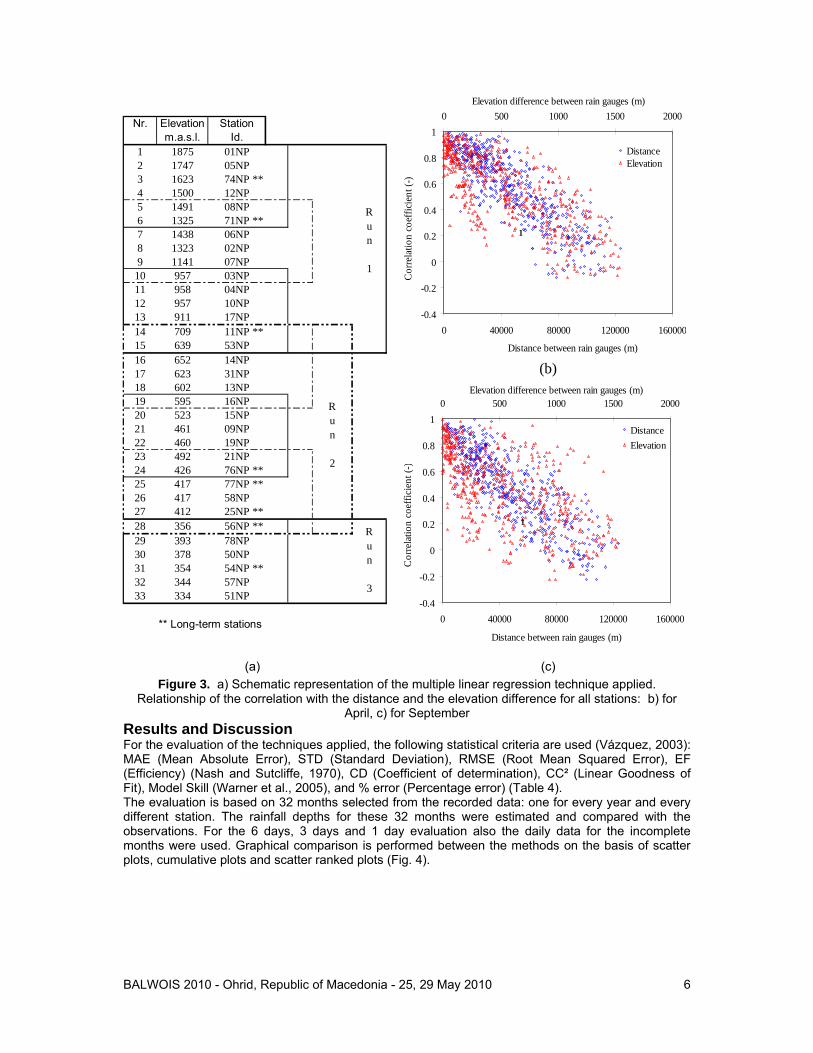
Nr. Elevation Stationm.a.s.l. Id.

1 1875 01NP2 1747 05NP3 1623 74NP **4 1500 12NP5 1491 08NP6 1325 71NP **7 1438 06NP8 1323 02NP9 1141 07NP

10 957 03NP11 958 04NP12 957 10NP13 911 17NP14 709 11NP **15 639 53NP16 652 14NP17 623 31NP18 602 13NP19 595 16NP20 523 15NP21 461 09NP22 460 19NP23 492 21NP24 426 76NP **25 417 77NP **26 417 58NP27 412 25NP **28 356 56NP **29 393 78NP30 378 50NP31 354 54NP **32 344 57NP33 334 51NP

** Long-term stations

Run 1

Run 3

Run 2

-0.4

-0.2

0

0.2

0.4

0.6

0.8

1

0 40000 80000 120000 160000

Distance between rain gauges (m)

Cor

rela

tion

coef

ficie

nt (-

)0 500 1000 1500 2000

Elevation difference between rain gauges (m)

DistanceElevation

11

(a) (c)

Figure 3. a) Schematic representation of the multiple linear regression technique applied. Relationship of the correlation with the distance and the elevation difference for all stations: b) for

April, c) for September Results and Discussion For the evaluation of the techniques applied, the following statistical criteria are used (Vázquez, 2003): MAE (Mean Absolute Error), STD (Standard Deviation), RMSE (Root Mean Squared Error), EF (Efficiency) (Nash and Sutcliffe, 1970), CD (Coefficient of determination), CC² (Linear Goodness of Fit), Model Skill (Warner et al., 2005), and % error (Percentage error) (Table 4). The evaluation is based on 32 months selected from the recorded data: one for every year and every different station. The rainfall depths for these 32 months were estimated and compared with the observations. For the 6 days, 3 days and 1 day evaluation also the daily data for the incomplete months were used. Graphical comparison is performed between the methods on the basis of scatter plots, cumulative plots and scatter ranked plots (Fig. 4).


7

0

500

1000

1500

2000

2500

3000

3500

4000

0 8 16 24 32Number of months

Cum

. rai

nfal

l [m

m]

observedLinear modelMultiple linear model

0

50

100

150

200

250

300

350

0 50 100 150 200 250 300 350Observed monthly accumulated rainfall [mm]

Gen

erat

ed m

onth

ly ra

infa

ll [m

m]

Linear modelMultiple linear model

(a) (b)

0

1000

2000

3000

4000

5000

0 50 100 150 200Number of periods of 6 days

Cum

. rai

nfal

l [m

m]


0

50

100

150

200

250

0 50 100 150 200 250Observed 6 days accumulated rainfall [mm]

Gen

erat

ed 6

day

s rai

nfal

l [m

m]


(c) (d)

0.01

0.1

1

10

100

1000

60% 70% 80% 90% 100%

% of time a given rainfall is not exceeded

Dai

ly ra

infa

ll [m

m]


0

20

4060

80

100

120

140160

180

200

0 50 100 150 200Observed 3 days accumulated rainfall [mm]

Gen

erat

ed 3

day

s rai

nfal

l [m

m]


(e) (f) Figure 4. results: a) cumulative rainfall for generated and observed data (based on 32 months,

validation period), b) scatter plot of generated versus observed monthly data, c) cumulative rainfall for generated and observed data (6 days accumulation, validation period), d) scatter plot of generated

versus observed 6 days accumulation data, e) rainfall distribution curve for daily generated and observed data and f) scatter plot of generated versus observed 3 days accumulation


8

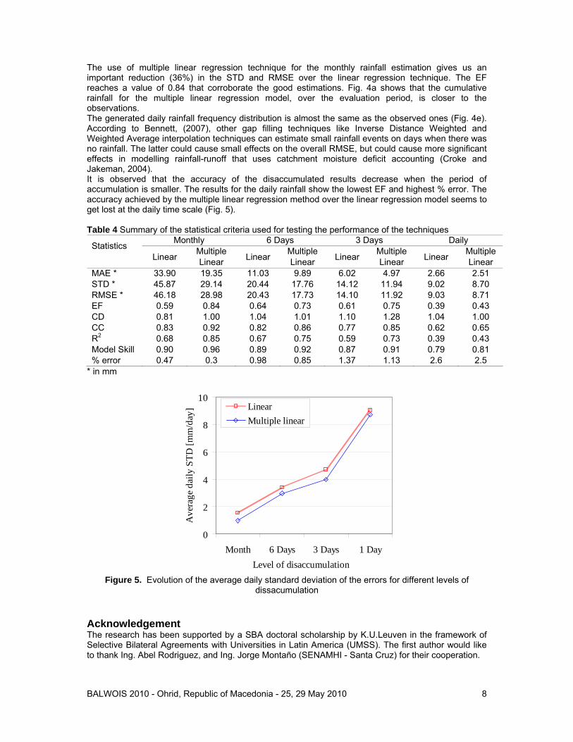
The use of multiple linear regression technique for the monthly rainfall estimation gives us an important reduction (36%) in the STD and RMSE over the linear regression technique. The EF reaches a value of 0.84 that corroborate the good estimations. Fig. 4a shows that the cumulative rainfall for the multiple linear regression model, over the evaluation period, is closer to the observations. The generated daily rainfall frequency distribution is almost the same as the observed ones (Fig. 4e). According to Bennett, (2007), other gap filling techniques like Inverse Distance Weighted and Weighted Average interpolation techniques can estimate small rainfall events on days when there was no rainfall. The latter could cause small effects on the overall RMSE, but could cause more significant effects in modelling rainfall-runoff that uses catchment moisture deficit accounting (Croke and Jakeman, 2004). It is observed that the accuracy of the disaccumulated results decrease when the period of accumulation is smaller. The results for the daily rainfall show the lowest EF and highest % error. The accuracy achieved by the multiple linear regression method over the linear regression model seems to get lost at the daily time scale (Fig. 5). Table 4 Summary of the statistical criteria used for testing the performance of the techniques

Monthly 6 Days 3 Days Daily Statistics Multiple Multiple Multiple Multiple Linear Linear Linear Linear Linear Linear Linear Linear MAE * 33.90 19.35 11.03 9.89 6.02 4.97 2.66 2.51 STD * 45.87 29.14 20.44 17.76 14.12 11.94 9.02 8.70 RMSE * 46.18 28.98 20.43 17.73 14.10 11.92 9.03 8.71 EF 0.59 0.84 0.64 0.73 0.61 0.75 0.39 0.43 CD 0.81 1.00 1.04 1.01 1.10 1.28 1.04 1.00 CC 0.83 0.92 0.82 0.86 0.77 0.85 0.62 0.65 R2 0.68 0.85 0.67 0.75 0.59 0.73 0.39 0.43 Model Skill 0.90 0.96 0.89 0.92 0.87 0.91 0.79 0.81 % error 0.47 0.3 0.98 0.85 1.37 1.13 2.6 2.5

* in mm

0

2

4

6

8

10

Month 6 Days 3 Days 1 DayLevel of disaccumulation

Ave

rage

dai

ly S

TD [m

m/d

ay] Linear

Multiple linear

Figure 5. Evolution of the average daily standard deviation of the errors for different levels of

dissacumulation Acknowledgement The research has been supported by a SBA doctoral scholarship by K.U.Leuven in the framework of Selective Bilateral Agreements with Universities in Latin America (UMSS). The first author would like to thank Ing. Abel Rodriguez, and Ing. Jorge Montaño (SENAMHI - Santa Cruz) for their cooperation.


9

References Shamsudin, S., Hashim, N., 2002: Rainfall Runoff Simulation Using Mike11 NAM. Journal of Civil Engineering Vol. 15 No. 2.

Bennett, N.D., Newham, L.T.H., Croke, B.F.W., Jakeman, A.J. 2007: Patching and Disaccumulation of Rainfall Data for Hydrological Modelling, Oxley, L., Kulasiri, D, eds, MODSIM 2007 International Congress on Modelling and Simulation, Modelling and Simulation Society of Australia and New Zealand, December 2007, 2520-2526.

Beard L. R., Fredrich A. J., Hawkins E. F., 1970: Estimating monthly streamflows within a region. Presented at ASCE National Meeting on Water Resources Engineering, held at Memphis, Tennesee. January 26-30.

Carter, R. W., and Benson, M. A., 1970: Concepts for the design of a streamflow data program: U.S. Geol. Survey open-file report.

Celleri, R. 2007: Rainfall variability and rainfall-runoff dynamics in the Paute River Basin – Southern Ecuadorian Andes. Ph.D thesis, Katholieke Universiteit Leuven, Faculty of Engineering. Leuven, Belgium.

Croke, B. F.W., and Jakeman, A.J., 2004: A catchment moisture deficit module for the IHACRES rainfall-runoff model, Environmental Modelling and Software, 19, 1-5.

Hydrologic Engineering Center, 1971. User´s Manual HEC4, Monthly Streamflow Simulation.

Nash J.E., Sutcliffe J.V. 1970: River flow forecasting through conceptual model. J. Hydrol., 10, 282-290.

Paulhus, J.L.H. and Kohler, M.A. 1952: Interpolation of missing precipitation records, Mon. Wea. Re6., 80, 129–133.

Romero R, Guijarro J.A., Ramis C., Alonso S. 1998: A 30 – years (Romero et al., 1998) daily rainfall data base for the Spanish Mediterranean regions: first exploratory

Makhuvha T., Pegram G., Sparks R., Zucchini W. 1997a: Patching rainfall data using regression methods I. Best subset selection, EM and pseudo-EM methods: theory. Journal of Hydrology 198: pp 289-307

Seo, D. 1996: Nonlinear estimation of spatial distribution of rainfall - an indicator cokriging approach, Stochastic Hydrology and Hydraulics, 10, 127-150.

Teegavarapua R. and Chandramoulia, V. 2005: Improved weighting methods, deterministic and stochastic data-driven models for estimation of missing precipitation records, Journal of Hydrology, 312: 191-206.

Vázquez R. 2003:, Assessment of the performance of physically based distributed codes simulating medium size hydrological systems. PhD dissertation, Katholieke Universiteit Leuven, Faculty of Engineering, Leuven, Belgium, 335 pp.

Warner, J. C., Geyer, W. R. and Lerczak, J. A., 2005: Numerical modelling of an estuary: A comprehensive skill assessment. Journal of Geophysical Research 110, C05001, doi: 10.1029/2004JC002691.

WMO. 1994: Guide to hydrological practices: Data acquisition and processing, analysis, forecasting and other applications. WMO Publication No. 168. World Meteorological Organization: Geneva, Switzerland.

Woolhister, D.A. 1992: Modeling daily precipitation – progress and problems. In A.T. Walden, P. Guttorp (eds.). Statistics in the Environmental and Earth Sciences, Edward Arnold, London. pp. 71-89.

Zucchini, W., P. Adamson and L. McNeill, 1992: Applications of stochastic daily rainfall model, S.Afr. J. Sci. 88: pp 103-109.

Filling gaps and daily disaccumulation of precipitation data for rainfall-runoff model Filling gaps...

Documents

Transcript of Filling gaps and daily disaccumulation of precipitation data for rainfall-runoff model Filling gaps...