Closing gaps in edges and surfaces

~ E Snyder*, R Groshong?, M Hsiaof K L_ Boone” and T tiudacko*

A new method is presented which robu~~tiy deals with errors in edge detector ~~~tpl~t. Based on the ci~ncept of a chamfer map, the meth~~d closes gaps while preserving edge structure and maintains surface connectedness correctly. The technique has been implemented in two rind three dimensions and is compared with published morphological techniques.

Keywords: edge detection, gaps, mor~hologicaI tech- riiq~e.~

INTRODUCTION

In this paper, we are concerned with the problem of closing gaps in edges. In two dimensions, an edge is a curve, and in three dimensions, a surface. Any edge operator, given the presence of noise and other sensor errors, is certain to fail occasionally, resulting in both extraneous edges (false hits) and gaps in edges (false misses). If an edge has holes in it, then connected component labelling (region growing) routines will fail, labelling interior and exterior points the same. Thus, we find it necessary to develop techniques which correct such edge detection errors. Such techniques are generally considered in the class of morphological operators, and we will address them in that context. In addressing the problem of closing gaps in edges, in an earlier work’. we developed a technique called ‘chamfer map edge closing’ after terminology defined by Barrow’, and have implemented this technique in both two and three dimensions. To evaluate the performance of this new technique, we address the problem of gap closing. In two dimensions, we compare binary morphology (mask erosion technique?, and iterative parallel thinning4) with chamfer maps. In three

Department ot Radiolop). Bowman Gray School of Medicinc. Winston-Salem. NC. USA Duke University School of Medicine, Durham, NC. USA Corporate Research and Development Center. General Electric

(.‘omprrny. Schenectady. NY. USA “Department of Electrical and Computer Engineering, North Carol- ina State University. Raleigh. NC. USA

P<tper receit,ed: 13 Decrnther IWO; revised paper received: 24 Sc~prenrher 1991

dimensions, we compare a 3D parallel thinning technique-’ and experiments with 3D m[~rphological techniques with 3D chamfer maps. In every case, we find that chamfer-based techniques produce superior performance. In particular, chamfer-based techniques preserve the shape of sharp corners better than any of the other techniques. As are many of the other techniques, chamfer map algorithms are implement- able on parallel machines, although that aspect of the problem is not explicity addressed in this paper.

Problem definition

We are given a ‘picture’, either two-dimensional f(x, y) or three-dimensional, f(x, y, t), where the parameters, x, y, and z are discrete-valued. We are also given an operator V, which operates on f to produce a new image:

8 = v (f) where we have suppressed the parameters for nota- tional simplicity. V represents our conceptual notion of a gradient operator, and produces some type of ‘edge image’ g. For example, V might literally take the magnitude of the gradient off, and threshold the result.

The details of V need not concern us here. Suffice it to say that many and elaborate methods of edge detection have been developed. In any case, due to noise, blur, or other error, the edge/surface resulting from the applications of any V to a real image will occasionally produce ‘gaps’ - areas in which the response from V is not sufficiently strong to make a positive determination (see Pratth,gi7 for an excellent discussion of edge detector errors.) Such gaps may be closed by various types of morphological operators. In this paper, we introduce one such operator, denoted chamfer-based closing (CBC), and show that its per- formance is superior to other techniques. In particular, CBC not only closes gaps, but simultaneously preserves the shape of edges/surfaces better than comparable techniques.

In the 1989 Computers in cardiology conference, Bister ef a!.’ presented a technique which appears similar in philosophy to ours. Exact comparisons are difficult to make, since their description7 is so brief

0262-8856/92/008523-09 @ 1992 Butterworth-Heinemann Ltd

~0110 no 8 October 1992 523

(only two paragraphs); however, we will provide relevant comparisons later in this paper, as details are discussed.

be computed by:

CT = mink ,crmlsk (C$%!j+i + Ck,i) L

(2)

Synopsis at iteration m, using masks such as:

In the next section we define the chamfer map, the data structure underlying the CBC algorithm, and show how to generate that structure from an image. Then, we present the CBC algorithm, and discuss its implemental tion. We then discuss two- and three-dimensional CBC algorithms concurrently, since the only difference is in the definition of a local neighbourhood.

We illustrate the process of applying CBC to a two- dimensional image with sharp points and other features whose size is of the order of the size of the gaps which must be bridged. The intermediate steps in the process are illustrated, Other published techniques are applied to the same data, and are shown to distort the shape of small features. Finally, similar results are demonstrated for 3D images.

or:

4 3 4

~

3 0 3

4 3 4

EDGE CLOSING WITH CHAMFER MAPS

Chamfer Map

In this section we describe a pre-processing stage required for the operation of our algorithm. In a manner similar to Barrow’, we define an array C(x, y) parameterized identically to ~(x, Y). C(x, y) will contain the ‘KS-distance’ from the point (x, y) to the nearest edge. By KS-distance, we mean that one may place a square convolution kernel of size (2k - 1) (261) centred at (x, y} without covering any edge pixels. The KS-distance may also be referred to as ‘S-neighbour’ distanceX or ‘chessboard’ distance”-‘“.

We refer to the distance transform resulting from application of such masks using equation (2) as ‘chamfer maps’ in our earlier work’ and in this paper, but in other literatures.“‘. ” ,the term ‘chamfer’ is restricted to the use of the second of the masks above. Either definition will suffice for the edge closing method described in the next section.

To construct a complete DT, equation (2) is iterated until no more changes occur between iterations. This is the approach followed by Bister’. For the application of this paper, however, we assume some a priori knowledge of maximum gap size. This allows us to define a value K,,,,, reflecting this knowledge as shown below, and use the following algorithm (for 2D):

Similarly, we may extend this pre-processing step and apply it in three-dimensional space. Array C(x, Y, z) is parameterized identically to g(_x, Y, z) and contains the KS-distance from point (x, Y, z) to the closest edge. The kernel is now a cube with edge length 2k - 1 centred at (x, y, z}.

The chamfer map may be used to assist in the measurement of the properties of regions. At every point, one knows that maximum size convolution kernel which may be applied without crossing an edge’j. In this paper, however, we will utilize the chamfer map in a different way.

The ~-neighbours of a point (x, Y), can be defined in either two or three dimensions as:

0)

1.

2. 3. 4.

F _.

PROCEDURE CreateChamferMap()

BEGIN

FOR all (x, y) DO C(x, y) = Km,,,

FOR all (x, y) DO IF&r, y) = EDGE THEN FOR k = I+ K,,,,,

FOR all hi, yki) E %(I, y) A gh;. yk;) f EDGE) DO

IF C(x,;, yk,) > k THEN C hi, yk,) = k

END CreateChamfer~ap()

KS distance ((xkA, ykA), (x, y)) = k

Here m=8k, k- 1 in two-space and m= (2k+l)“-- (Zk- l)“, ka 1, in three-space.

Step 1 initializes the chamfer map to the maximum desired value K,,,,, . Steps 2 through 5 compute the minimum KS-distance at each point within the square kernel of edge length 2k - 1. Figure 1 illustrates a chamfer map near a gap in an edge. Normally, we use values K,,,<4, since this allows gaps of six pixels to be bridged.

Computing the chamfer map

Borgefors l4 observes that the chamfer map is a type of distance transform (DT), and provides an excellent discussion of such transforms. Our chamfer map may

Generation of the three-dimensional chamfer map proceeds in an analogous manner.

We note that the computational complexity of chamfer map generation is proportional to the numbr of edge points in the image and to the size of K,,,. Larger value of K,,,, increase the size of the kernel & substantially in three dimensions. We further note that the algorithm is local, regular, and uses litle conditional

524 image and vision computing

Figure I. Chamfer map near a gap in

. . . . . . . .

logic. It can therefore be easily implemented on a parallel architecture.

SEGMENTATION USING THE CHAMFER MAP

In this section, we show how the chamfer map may be used to close gaps in edges. By doing so, it provides an important component in the segmentation process. Pixels whose KS-distance from an edge is less than Kin,, are labelled as ‘QUESTIONABLE’. All pixels having a KS-distance equal to K,,, are assigned a region number, i.e. we segment the remaining pixels into disjoint regions. The segmentation may consist of only simple connected component analysis, or may be more sophisticated, perhaps resulting in new edges. For example, the V operator may only determine step edges (maxima in the first derivative), whereas the segmentation may also detect roof edges (maxima in the second derivative, or curvature) or more so

P histi-

cated cooperative processes may be employed’-. The details need not concern us, but somehow we produce a label image, L: L(x, y) = SEGMENT (C(x, y)).

L(x, y) = j is interpreted as ‘the pixef at (x, y} belongs to region j.’ Pixels close to an edge are specially labelled:

{ C(x, y) < K,,, ,,., } --+ { L(x, _Y) = QUESTIONABLE}

For our examples, we used a raster-scan connected component algorithm’~.” consisting of face- connections in 2D, and face-, edge- and vertex- connections in 3D. Bister et al.’ identify local maxima in the DT, and each maximum results in a potential region. They note, however, “Since the distance transform is sensitive to noise producing irregularities in the borders of the region, one cavity [region] can contain many local maxima very close to one another. In order to eliminate these spurious maxima, a . . . filter merges with maxima for which the sum of the heights is much larger than the geometrical distance between them”. We conjecture that the performance of this filter is equivalent to our choice of K,,,. Both techniques identify an area within a region which robustly characterizes that region.

When one compares the difficulty of identifying local maxima, particularly in 3D data, and them making merge decisions on pairs of maxima, the relative simplicity and speed of hardware-imlementable connected-component algorithm would suggest some speed advantages in our approach.

It is convenient if the original edge image provides sufficient padding around the perimeter of the image. By sufficient we mean that any component of the edge image must be at least K,,,, pixels from the boundary

~01 IO no 8 october 1992

of the image. This is required so that the segmentation will correctly identify and label the image background.

Relabelling questionable points The last step in the algorithm relabels the QUES-

TIONABLE points, using the chamfer map C(X, y) and the label image L(x, y) to create a new label image L’(.u, 17). Working inward from those points where C(x, 4’) = K,,,,, (the set of points K,;,, from an edge point), each point is relabelled by assigning it the label of the most appropriate neighbour. This ‘erosion’ is per- formed iteratively. At each iteration, i, only the QUESTIONABLE pixels in the label image L(x, y) that correspond to pixels such that C(x, y) = KlllilX - i are relabelled in each pass.

QUESTIONABLE pixels are relabelled only when there is strong evidence (defined in the next section) indicating to which region the pixel should be assigned. If the reassignment is uncertain, then the pixel is left QUESTIONABLE, and the decision is postponed until the next pass. When all of the QUESTIONABLE pixels in L(x, v) corresponding to the k-valued pixels of the chamfer map have been reassigned to valid image regions, or when no further change takes place in an iteration, k is decremented and the next set of QUESTIONABLEs is considered for relabelling. The relabetling is complete when all of the edge pixels (k = 0) have been assigned to valid image regions. When single-pixel resolution between regions is required. more sophisticated region normalization techniques may be used”.

We note this relaxation method appears quite different from that of Bister ef al.‘, who state “the valley between two local maxima becomes the border of the two adjacent segments.” Although Figure I suggests that such valleys are narrow and easily found, experiments with more realistic images demonstrate the common occurrence of rather large ‘level’ areas in the DT. Such level areas make it difficult to locate valleys with precision to a single pixel. Bister et ai.’ solve this problem with a post-processing filter. Our iterative relaxation of chamber pixels obviates the needs for any such filter.

Identifying points to relabel The intent of this algorithm is to close gaps in edges.

The key to achieving this lies in the strategy used to select the most appropriate region to which to reassign the currently considered pixel L(x, y). To accomplish this in two dimensions, we examine the pixel’s eight surrounding neighbours. In three dimensions, we examine the voxel’s 26 neighbours. We refer to this as finding the pixel’s or voxel’s ‘best neighbour’.

The surrounding pixels may come from one of three possible classes:

I.

2. 3.

A label corresponding to an object or a region of an object in the label image L(x, y) A label corresponding to the image background. The QUESTIONABLE label.

Our first

hope is to relabel the current pixel to one of the two classes. We do this by enumerating the

neighbouring pixels and selecting the “best’ class. Usually, the maximum result of the enumeration will be

525

a valid region within the image, and we can confidently relabel our pixel to the region of the best neighbour. Sometimes, however, we must leave the pixel labelled QUESTIONABLE, and postpone the relabelling deci- sion because either the best neighbour is explicitly found to be QUESTIONABLE (none of its neighbours belong to valid image regions), or constraints we have placed on the relabelling make it undesirable to reassign the pixel to the apparent best neighbour.

An example of such constraints which may be placed on the relabelling algorithm is the selection of the background* region as the best neighbour. In our implementation, neighbours belonging to the back- ground region are considered in a more restricted fashion than those belonging to regions within objects in the image. For the background value to be selected as the best neighbour, we require that the background pixel be face-connected to the pixel under considera- tion. If this condition is not satisfied, background labels are not enumerated in the best-neighbour tally. If this is not done, for very thin sharp vertices (e.g. the fork tines of Figures 5a and 5b), we produce the undesirable result of occasionally finding isolated background pixels inside a closed boundary, (see Rosenfeld’” for more discussion on this connectivity paradox).

When k = 0, the QUESTTONABLE pixels we seek to relabel must be either true edges or false positive noise pixels. If the image is known to contain no noise, then these pixels must all be edge pixels. An edge in an image, by definition, delineates an interface between an object region and one or more other regions within that image, The other region(s) may be either another object region or the background region. We assert a strong bias against relabelling an edge pixel as back- ground, and will reassign such a pixel to an image region over the background region regardtess of the outcome of the enumeration. Only in the case that the edge pixel is completely surrounded by background, do we choose background as the best neighbour.

Relabelling algorithm The following pseudo-code illustrates the steps des- cribed above for a three-dimensional image:

0.

I. 7 _.

3.

4.

5 . .

6. 7. 8.

9.

PROCEDURE ChamferRelabcl()

FOR all (x, y, Z) DO

BEGIN

IF C(X, y. z) = K,,,,, THEN L’(x, y, 2) = L(X, y, 2)

ELSE IF C(x, y, z) = 0 THEN

L’(s, y, 7) = EDGE ELSE L’(s, y, z) = QUESTIONABLE END IF

END FOR all FOR k = K,,,,,, - 1 -+ 0

WHILE lab& are changing DO

FOR all (x, y, Z) DO

IF L(x, y, z) = (QUESTIONABLE OR EDGE) AND C(X, y, z) > k THEN

L’(x. y. z) = BEST_26_NEIGHBOUR (XV Y* 2)

*Use of this constraint is practical, of course, only in those applications in which the background may be easily identified.

526

IO.

Il.

12.

13.

ELSE

L’(X, y, Z) = L(x, y, z) END IF

END FOR all

L temp = L’ L’=L

L = Ltemp

END WHILE

END FOR k END ChamferRelabel();

Step 1 initializes the relabelled image so that voxels greater than K,,, away from edges retain their original label (Step 2). Voxels on edges (KS-distance = 0) are labelled edge (Step 3). All voxels within the KS- distance of K,,, are designated as QUESTIONABLE (Step 4). Steps 7-10 blend all QUESTIONABLE VOX& at the distance of the current K or greater from an edge into the most appropriate neighbouring region. As mentioned earlier, EDGE voxels are also re- labelled, but require a more restricted strategy in the BEST_26_NEIGHBOUR algorithm. Steps 11-13 simply define the input for the next iteration to be the output of the last iteration. Step 6 is necessary to handle the case where the edge structure is such that not all voxels with distance K are assigned to a labelled region of a single pass. Some voxels will meet the criteria in Step 8, yet remain labelled QUESTION- ABLE. The BEST_26__NEIGHBOUR algorithm is defined below:

5. IF Max-Card (Card) = BACKGROUND AND L(x, y, z) = EDGE THEN

0. FUNCTION BEST_26_NEIGHBOUR(x, y, z)

BEGIN

I. FOR all (q. yi. z,) E X, (x, y, z) DO

2. if L(x,. yi, z,) # EDGE THEN IF L(x;. L’;, z,) #BACKGROUND THEN

3. increment Card(Lx,, y,, z;))

ELSE IF FaceConnected (L(x, y, z), L(x,, yi , i;)) THEN

4. increment Card(BACKGROUND) END IF

END IF

END FOR all

RETURN(Next_Max_Card(Card))

6. ELSE RETURN(Next_~ard(Card)~

END BEST_26_N~IGHBOUR();

In this algorithm, ‘Card’ is simply an array which keeps a count (cardinality) of the number of times a particular label is adjacent to the voxel of interest.

X, (x, y, z) is the set of the 26 neighbours of the point L(x, y, z). Note that the test in Step 5 may include more sophisticated conditions to distinguish between EDGE and BACKGROUND voxels. This a priori knowledge of our original edge locations can be used to guide region segmentation, or in the presence of noise, noise suppression.

Closely spaced regions

With the next three figures, we illustrate both the

image and vision ~ornput~ng

Figure 2. Two regions with large gaps in their boun- daries

operation of CBC, and one of its principal strengths: the ability to deal with very closely spaced regions.

Figures 2-4 illustrate the output of an edge detec- tion process which has identified the edges of two adjacent regions. It is important to note that the typical gaps in the edge are larger than the spacing between the regions.

TWO-DIMENSIONAL IMAGES

The chamfer map relabelling process produces a sequence of images which will relate to the following figures in this order: the original image, the chamfer map itself, the ‘thickened edge image’ (all voxels in chamfer map such that C(X, y) < K,,,, are initially relabelled as quetionable, and we refer to the union of

Figure 3. Chamfer map and result of connected- component labelling of Figure 2

~0110 no 8 October 1992

L”““““““”

Figure 4. Segmentation resulting from applying CBC. Note that the regions are correctly partitioned, with a precision accurate to the individual pixel

EDGE and initial QUESTIONABLE pixels by this term), labelled image produced from thickened edge image, relabelled image based on chamfer map and labelled image.

We tested the two-dimensional chamfer map’s per- formance in closing gaps in edges by processing a binary image containing several cutlery objects (knives, spoons. and forks). The varied edge shapes in this image demonstrate the way the algorithm uses the chamfer map to intelligently make decisions on which voxels should be assigned to each region. Figures 5-7 show the results obtained for this input:

a b Figure 5. (a) Original cutlery image, containing gaps in edges; (6) chamfer map of original cut1er.y image

527

a b Figure 6. (a) Thickened edge image; (b) label image based on dilated edges

i Figure 7. Relabelled / cutlery image

COMPARISON WITH PUBLISHED 2D METHODS

To evaluate the performance of chamfer-map thinning in two-space, we compared it with two other types of binary thinning techniques: iterative erosion, and iterative thinning. As input to these algorithms we used the bit-mapped ‘cutlery’ image shown in Figure 5a after it was dilated by a 5 x 5 kernel to close ail gaps. (We note that this is the same dilation used previously). The results of these comparisons are described in the following sections.

A conventional morphological skeleton is formed by decomposing an image into a number of skeleton subsets. The subsets contain information about size, orientation, and connectivity. A minimal skeleton has the property of being able to exactly reconstruct the original image, but does not necessarify preserve path or surface connectivity2”. While this technique can be used for many applications such as image coding and has been widely studied, morphological skeletonization is not directly comparable to 2D or 3D thinning, in which connectivity is preserved. Since, in this apphca- tion of edge/surface gap closing, we insist on preserva-

Al A2 A3 A4

Bl B2

Figure 8. 3 ~3 masks

B3 B4

tion of connectivity, we consider below only techniques which possess this property.

Morphological 2D thinning3

The morphological technique we used for comparison was first described by Arcelli et al.“, and uses a sequence of masks. The origina image is eroded by each of eight 3 x 3 masks in sequence, and the resulting image is used as input to the next iteration until all possible pixels have been eroded. In each mask shown in Figure S’.“, the positions marked in black denote edge pixels, white denotes background and grey are ‘don’t cares’. A mask is said to ‘match’ an image at coordinates (k, /) if, when the centre of the mask is registered to pixel (k, I), then all image pixels covered by the mask are edge or background as denoted by the corresponding mask pixel. If a mask matches an image at a particular edge point, then the edge at that point in the image may be reset to background. The masks are applied in the following order: Al, Bl, A2, B2, A3, B3, A4, B4. The result of thinning Figure 6a using this algorithm is shown in Figure 10. Note how this technique distorts the shape vertices like the fork tines.

Iterative 2D thinning4

In this section, we compare chamfer-map thinning with Zhang and Suen’s” algorithm for thinning binary images. Zhang and Suen’s algorithm iteratively passes over the image, deciding if contour points can be deleted. A contour point is an edge pixel with at least one S-neighbour that is a background pixel. Each iteration contains two passes, and bases the decision to remove a contour pixel on the number of edge neighbours of a pixel, the number of O-l transitions in an sequence around the pixel, and on two sets of background neighbour configurations. The result of iteratively thinning the dilated ‘cutlery’ image (Figure 6a) is shown in Figure 10. Note the similarity with the technique of Arcelli ei al.‘.

THREE-DIMENSIONAL IMAGES

In the following figure representative slices from 3D images are shown. Figures Ila-e show the results obtained by CBC for a box with broken interior partitions. The order of the images is the same as

528 image and vision computing

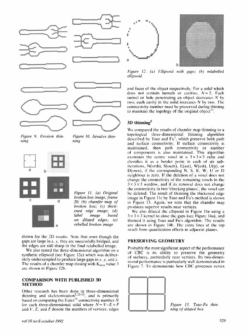
Figure 9. Erosion thin- ning

a b

q c d

Figure 12. (a) Ellipsoid with gaps; (b) relabelled ellipsoid

t

Figure 10. Iterative thin- ning

Figure Il. (a) Original broken box image, frame 20; (6) chamfer map of broken box; (c) thick- ened edge image; (d) label image based on dilated edges; (e) rebelled broken image

shown for the 2D results. Note that even though the gaps are large in x, y, they are successfully bridged, and the edges are still sharp in the final relabelled image.

We also tested the three-dimensional algorithm on a synthetic ellipsoid (see Figure 12a) which was deliber- ately undersampled to produce large gaps in x, y, and z. The results of a chamfer map closing with K,,, value 3 are shown in Figure 12b.

COMPARISON WITH PUBLISHED 3D METHOD

Other research has been done in three-dimensional thinning and skeletonization’.**-*“, and is primarily based on computing the Euler2” connectivity number N for each three-dimensional solid where N = V-E + F and V, E, and F denote the numbers of vertices, edges

and faces of the object respectively. For a solid which does not contain tunnels or cavities, N = 2. Each tunnel or hole penetrating an object decreases N by two; each cavity in the solid increases N by two. The connectivity number must be preserved during thinnng to maintain the topology of the original object”.

3D thinning’

We compared the results of chamfer map thinning to a topological three-dimensional thinning algorithm described by Tsao and FL?, which preserve both path and surface connectivity. If surface connectivity is maintained, then path connectivity or number of components is also maintained. This algorithm examines the centre voxel in a 3 x 3 x 3 cube and classifies it as a border point in each of six sub- iterations, N(orth), S(outh), E(ast), W(est), U(p), or D(own). if the corresponding N, S, E, W, U or D neighbour is zero. If the deletion of a voxel does not change the connectivity of the remaining voxels in the 3 x 3 x 3 window, and if its removal does not change the connectivity in two ‘checking planes’, the voxel can be deleted. The result of thinning the thickened edge image in Figure 1 lc by Tsao and Fu’s method is shown in Figure 13. Again, we note that the chamfer map produces superior results near vertices.

We also dilated the ellipsoid in Figure lle using a 3 x 3 x 3 kernel to close the gaps (see Figure 14a), and thinned it using Tsao and Fu’s algorithm. The results are shown in Figure 14b. The extra lines at the top result from quantization effects in adjacent planes.

PRESERVING GEOMETRY

Probably the most significant aspect of the performance of CBC is its ability to preserve the geometry of surfaces, particularly near vertices. Its two-dimen- sional performance is particularly well demonstrated in Figure 7. To demonstrate how CBC processes vertex

Figure 13. Tsao-Fu thin- ning of dilated box

~0110 no 8 October 1992 529

REFERENCES

Figure 14. (a) Dilated ellipsoid; (b) Tsao-Fu thinned ellipsoid

Figure 15. Cross-section through the apex of a cone which has been processed by chamfer closing (left) and by Tsao-Fu thinning (right)

geometry in three dimensions, we synthesized a cone and extracted the surface with a 3D edge detector.

Gaps in the surface were then closed with CBC. The same cone surface was dilated using conventional dilation to close gaps, and then thinned using the Tsao- Fu algorithm. The results are shown in Figure 15. Since the process of dilation replaces the edge information, the Tsao-Fu thinning algorithm has no memory of the original surface when it thins the dilated image. Of course, neither technique processes the geometry perfectly, but since CBC retains, via the chamfer map, a ‘memory’ of the original, undilated, geometry, CBC is better able to restore that geometry after closing. To perform the operations illustrated in Figure 15, the Tsao-Fu thinning algorithm required 337 seconds of CPU time on a Decstation 2100, not including the dilation process, which was performed as a pre- processing step. Chamfer closing required 54 seconds for the entire operation.

CONCLUSION

CBC is a new approach to a specific problem: closing noise-induced gaps in edges. We have demonstrated in both two and three dimensions that CBC preserves the geometry near sharp vertices. One of the emphases in this work has been the development of an algor- ithm which, insofar as possible, preserves that geometry with single-pixel precision. This feature is most clearly demonstrated in Figures 2-4, and is accom- plished by combining dilation, connected-component- labelling, and successive relaxation/erosion methods.

The relative simplicity of the CBC algorithm provides fast operation on a uniprocessor, and makes the algorithm well-suited to implementation on an array processor.

530

1

2

3

4

5

6

7

8

9

10

11

12

13

14

1.5

16

17

18

19

20

Groshong, B R and Snyder, W E Using Chamfer to Segment Images, Technical Report CCSP-WP- 86/11, Centre for Communications and Signal Processing, North Carolina State University, Raleigh, NC (December 1986) Barrow, H G ‘Parametric correspondence and chamfer matching’, Proc. 5th Znt. Joint Conf. on Artif. fntetl. (August 1977) pp 659-663 Arcelii, C, Codella, L and Levialdi S ‘Parallel thinning of binary pictures’, Electron. Lett., Vol 11 (1975) pp 148-149 Zhang, T Y and Suen, C Y ‘A fast parallel algorithm for thinning digital patterns,’ Commun. ACM, Vol 27 No 3 (March 1984) pp 236-239 Tsao, Y F and Fu, K S ‘A parallel thinning algorithm for 3-D pictures’, Co~nput. Vision, Graph. & image Process., Vol 17 (1981) pp 315- 331 Pratt, W K Digitial Image Processing, Wiley, NY (1978) Bister, M, Taeymans, Y and Cornelis, J ‘Auto- mated segmentation of cardiac MR images,’ Comput. in Cardiology, IEEE Press, Washington, DC (1989) pp 215-218 Borgefors, G ‘Distance transformations in arbit- rary dimension’, Comput. Vision, Graph. & Image Process., Vol 27 (1984) pp 321-345 Rosenfeld, A Picture Processing by Computer, Academic Press, NY (1969) Rosenfeld, A and Kak, A Digital Picture Proces- sing, Volume 2, Academic Press, NY (1982) Rosenfeld, A ‘Distance functions on digital images’, Patt. Recogn., Vol 1 (1968) pp 33-61 Rosenfeld, A and Pfaltz, J ‘Sequential operations in digital picture processing’, Commun. ACM, Vol 13 (1968) pp 471-494 Snyder, W E and Bilbro, G Segmentation of three dimensional range images, CCSP-TR-84/7, North Carolina State University (November 1984) Borgefors, G ‘Distance transformations in digital images,’ Comput. Vision, Graph. Image Process., Vol 34 (1986) pp 344-371 Hiriyannaiah, H, Bilbro, G and Snyder, W ‘Res- toration of locally homogeneous images using mean field annealing’, J. Optical Sot, Am. A, Vol 6 No 12 (December 1989) pp 1901-1912 Snyder, W E and Cowart, A ‘An iterative approach to region growing using associative memories’, IEEE Trans. PAMr, Vol 5 No 6 (November 1985) pp 638-651 Snyder, W E and Savage, C ‘Content-addressable read-write memories for image analysis’, IEEE Trans. Comput., Vol 31 No 10 (October 1982) pp 963-968 Foley, J D, van Dam, A, Feiner, S K and Hughes, J F Comput. Graphics: Principles and Pra~ti&e, Addison-Wesley, Reading, MA (1990) pp 91-99 Rosenfeld, A ‘Connectivity in digital pictures’, Commun. ACM, Vol 17 No 1 (January 1970) pp 1466160 Maragos, P A and Schafer, R W ‘Morphological skeleton representation and coding of binary images,’ IEEE Trans. Acoust., Speech & Signal

image and vision computing

Process., Vol 34 No 5 (1986) pp 1128-1243 21 Preston, K Jr and Duff, M J B ,~~~e~~ ~eZZafar

Automata Theory and Application.~, Plenum Press, NY (1984)

22 Hafford, K J and Preston, K Jr ‘Three- dimensional skeletonization of elongated solids’, Comput. Vision, Graph. & Image Process., Vol27 (1984) pp 78-91

23 Lobregt, S, Verbeek, P W and Groen, F C A ‘Three-dimensional skeletonization: principle and algorithm’. IEEE Tram PAMZ, Vol 2 No 1

(January 1980) pp 75-77 24 Toriwaki, J and Yonekura, T ‘Topological pro-

perties and topology-preserving transformation of a three-dimensional binary picture’, Proc. 6th Znt. Patt. Recogn. Conf., Munich, Germany (1982) pp 414-419

25 Hilbert, D and Cohn-Vossen, S Geometry and the Imagination, Chelsea, New York (1952)

26 Srihari, J K U and Yau, M M ‘Understanding the bin of parts’, IEEE Conf, Decision Control. (December 1979) pp 44-49

WA 10 no 8 October 1992 531