Field Test of the Variable Source Area Interpretationof the Curve Number Rainfall-Runoff Equation

Helen E. Dahlke1; Zachary M. Easton2; M. Todd Walter3; and Tammo S. Steenhuis4

Abstract: The Soil Conservation Service Curve Number (SCS-CN) method is a widely used empirical rainfall-runoff equation. Although thephysical basis of the method has been debated, several researchers have suggested that it can be used to predict the watershed fraction that issaturated and generating runoff by saturation excess from variable source areas (VSAs). In this paper, we compare saturated runoff-contributing areas predicted with the VSA interpretation of the SCS-CN method with field-measured VSAs in a 0.5 ha hillslope in centralNew York State. We installed a trench below a VSA and simultaneously recorded water flux from different soil layers at the trench face andwater table dynamics upslope of the trench. This setup allowed us to monitor runoff initiation and saturation-excess overland flow in responseto rainfall and different water table depths in the hillslope during 16 storm events. We found that the SCS-CN method accurately predicted theobserved VSA and showed best agreement if the VSA was defined as the area where the water table was within 10 cm of the soil surface.These results not only demonstrate that the VSA interpretation of the SCS-CN method accurately predicts VSA extents in small watershedsbut also that the transient water table does not necessarily need to intersect the land surface to cause a storm runoff response. DOI: 10.1061/(ASCE)IR.1943-4774.0000380. © 2012 American Society of Civil Engineers.

CE Database subject headings: Runoff; Slopes; Runoff; Field tests; Rainfall.

Author keywords: Runoff; Variable source areas; Trenched hillslope studies; Curve number.

Introduction

The Soil Conservation Service Curve Number (SCS-CN) (USDA-SCS 1972) method is an empirical rainfall-runoff relationshipthat is widely used to predict storm runoff in ungauged basins.While more sophisticated methods are available, its simplicity anddependence on readily available catchment properties has contrib-uted to its continued popularity, particularly among practicingwater resource engineers (Ponce and Hawkins 1996; Garen andMoore 2005). The rainfall-runoff principle of the SCS-CN methodis such that no runoff occurs until a threshold in rainfall is met,above which the fraction of rainfall contributing to runoff increaseswith rainfall. The SCS-CN method in its original form (Rallison1980) is independent of the underlying runoff-generation mecha-nism, i.e., infiltration excess, saturation excess, or something else.

Runoff generation based on the infiltration excess, or the“Hortonian flow,” concept occurs when rainfall intensity exceedsthe rate at which water can infiltrate the soil (e.g., Horton 1933,1940). In contrast, saturation excess occurs when rain (or snow-melt) encounters soils that are nearly or fully saturated, often dueto a water table perched above a zone of low permeability, therebyprecluding infiltration (e.g., Dunne and Black 1970; Hewlett andNutter 1970). The location of areas generating runoff by saturationexcess, typically called variable source areas (VSAs), depends onthe topographic position in the landscape and the local soil trans-missivity. As the adjective “variable” suggests, VSAs develop andexpand spatially with rainfall and contract between storms (Dunneand Black 1970; Hewlett and Nutter 1970). One important aspect ofthe VSA concept, also known as the partial-area concept, is that themajority of the runoff is generated from small portions of the land-scape (e.g., Dunne and Black 1970); thus, VSAs are importantareas to target for controlling non-point-source pollutant transport(e.g., Walter et al. 2000; Gburek et al. 2002; Easton et al. 2007a;Walter et al. 2007; Dahlke et al. 2012).

In agreement with this partial-area hydrology concept, Steenhuiset al. (1995) demonstrated that the SCS-CN relationship, in its mostelementary form, can be derived from the assumption that onlysaturated areas contribute to direct runoff. Although this VSA inter-pretation of the SCS-CN method has been incorporated into severalcontinuouswatershedmodels, which have been successfully appliedto a variety of catchments (Schneiderman et al. 2007; Easton et al.2008b; Dahlke et al. 2009), the fundamental concept still remains tobe tested against field-measured VSAs to corroborate its physicalaccuracy.

Review of the SCS-CN Method Applied to VSATheory

The SCS (now Natural Resources Conservation Service, NRCS)runoff Curve Number (CN) method (SCS-CN) (USDA-SCS 1972)

1Dept. of Physical Geography and Quaternary Geology, StockholmUniv., Svante Arrhenius väg 8, 10691 Stockholm, Sweden; Dept. of Bio-logical and Environmental Engineering, Cornell Univ., 62 Riley-Robb Hall,Ithaca, NY 14853 (corresponding author). E-mail: helen.dahlke@natgeo.su.se

2Dept. of Biological and Environmental Engineering, Cornell Univ.,62 Riley-Robb Hall, Ithaca, NY 14853; Assistant Professor, Dept. of Bio-logical Systems Engineering, Virginia Tech, 103 Research Drive, Painter,VA 23420. E-mail: zme2@cornell.edu

3Associate Professor, Dept. of Biological and Environmental Engineer-ing, Cornell Univ., 222 Riley-Robb Hall, Ithaca, NY 14853. E-mail:mtw5@cornell.edu

4Professor, Dept. of Biological and Environmental Engineering, CornellUniv., 206 Riley-Robb Hall, Ithaca, NY 14853. E-mail: tss1@cornell.edu

Note. This manuscript was submitted on October 25, 2010; approved onMay 10, 2011; published online on February 15, 2012. Discussion periodopen until August 1, 2012; separate discussions must be submitted forindividual papers. This paper is part of the Journal of Irrigation and Drai-nage Engineering, Vol. 138, No. 3, March 1, 2012. ©ASCE, ISSN 0733-9437/2012/3-235–244/$25.00.

JOURNAL OF IRRIGATION AND DRAINAGE ENGINEERING © ASCE / MARCH 2012 / 235

Downloaded 18 Apr 2012 to 128.84.201.45. Redistribution subject to ASCE license or copyright. Visit http://www.ascelibrary.org

is commonly used to estimate the storm runoff response of a catch-ment [Eq. (1)]:

Q ¼ ðP� IaÞ2Pþ S� Ia

ð1Þ

where Q (mm) is the total watershed runoff depth for a storm,P (mm) is the depth of rainfall, S (mm) is the potential maximumstorage for water available in a watershed, and Ia (mm) is the initialabstraction or the amount of water required to initiate runoff. Tradi-tionally, Ia is generally taken as 0:2S (USDA-SCS 1972).

In its original form, the SCS-CN equation constitutes an empir-ical rainfall-runoff relationship that, according to its originator,Victor Mockus (Rallison 1980), is independent of the underlyingrunoff generation mechanism (i.e., infiltration excess or saturationexcess). Although many current water quality models use theSCS-CN equation in a way that implicitly assumes infiltration ex-cess is the dominant runoff mechanism (Walter and Shaw 2005),Steenhuis et al. (1995) showed that Eq. (1) can be applied to predictsaturation-excess runoff that results from rainfall onto saturatedsoils. The underlying principle of this VSA interpretation of theSCS-CN equation is that the area or fraction of the watershed thatcontributes runoff (Af ) can be estimated from the ratio of runoffdepth (ΔQ) to precipitation depth (ΔP):

Af ¼ ΔQ=ΔP ð2Þ

Here,ΔQ (mm) is the incremental runoff depth or volume of excessrainfall generated during the storm event divided by the watershedarea, and ΔP (mm) is the incremental depth of runoff producingrainfall that occurred during the same time period. Introducingthe effective precipitation, Pe (mm), which is equal to the totalstorm precipitation (P) after the initial abstraction (Ia) is subtracted,Eq. (1) can be rewritten as

Q ¼ P2e

Pe þ Sð3Þ

The fractional area that is contributing saturation-excess runoff(Af ), according to Eq. (2), is equal to the derivative of Q with re-spect to Pe. Thus, by differentiating Eq. (3) with respect to Pe, the

saturated or runoff-generating fraction of the watershed-generatingrunoff is

Af ¼ 1� S2

ðPe þ SÞ2 ð4Þ

In agreement with the mathematical limits of this equation,Pe ¼ 0 when the contributing watershed area Af equals zero andPe goes to infinity as Af approaches 1.

The amount of saturation-excess runoff generated during stormevents is, to a great extent, controlled by the available soil waterstorage (S) in the watershed and depends largely on the moisturestatus of the watershed prior to storm events. The value of S canvary between some maximum, Smax (mm), when the watershed isdry (e.g., during the summer), and a minimum, Smin (mm), whenthe watershed is wet (e.g., late winter and spring) (Saxton et al.1974; Saxton et al. 1986; Schneiderman et al. 2007). However, de-spite these seasonal and daily variations of S, engineers often as-sume that S is a storm-invariant parameter that represents thepotential maximum storage or total amount of water that can bestored in the watershed (e.g., Steenhuis et al. 1995). Operationally,S is determined either using table-derived CN values for averagesoil and land use conditions (USDA-SCS 1972; Chow et al.1988) or it by fitting it to direct measurements of effective precipi-tation and runoff volume (e.g., Shaw and Walter 2009).

Materials and Methods

A total of 16 storm events, monitored for a trenched, 0.5-hahillslope from October 2009 through May 2010 (excluding thewinter period) (Table 1), were used to test the CN-VSA approachof Steenhuis et al. (1995). The saturation-excess runoff generatedin this hillslope site in response to these events was considered indetail using a network of direct measurements and analyticaltechniques.

Site Description

This study was conducted on a 0.5 ha, N-NE facing hillslope in acrest position near Ithaca, NY (76°14′48.44′′ W, 42°24′56.86′′ N).

Table 1. Rainfall and Runoff Information for the 16 Storm Events

Event Qobs (mm)Qbase

(mm=h) Ptot (mm) Ia (mm)Pi-1 hr

(mm=h) API7 (mm) API14 (mm) API30 (mm)Rainfall

duration (h)Water tabledeptha (cm)

April 6, 2010 0.2 0.0313 2.8 0.0 2.0 25 49 104 2 42

April 8, 2010 0.1 0.0114 4.8 3.1 1.8 3 46 105 7 46

April 17, 2010 0.1 0.0025 16.5 11.2 3.0 1 9 89 15 71

April 26, 2010 0.6 0.0036 37.3 18.8 3.8 15 38 82 19 78

October 9, 2009 0.1 0.0034 6.8 2.0 0.8 29 109 147 29 45

October 12, 2009 0.0 0.0027 4.8 2.8 1.5 17 57 148 14 59

October 16, 2009 0.0 0.0031 6.4 0.8 1.8 13 43 155 7 62

October 24, 2009 0.5 0.0008 26.1 5.8 3.6 3 21 144 21 68

October 28, 2009 6.7 0.0020 45.5 2.2 9.8 26 35 109 12 47

October 31, 2009 0.2 0.0105 2.5 0.4 0.7 46 73 122 3 21

November 5, 2009 0.2 0.0059 4.7 2.2 1.8 3 75 107 5 47

November 19, 2009 0.8 0.0004 26.4 9.7 9.4 0 0 80 5 67

November 27, 2009 0.5 0.0029 14.7 0.3 3.8 27 28 82 17 48

November 28, 2009 0.1 0.0083 2.5 0.3 0.8 17 43 51 7 36

November 30, 2009 0.5 0.0160 8.1 0.3 1.8 19 46 53 13 33

December 2, 2009 0.9 0.0115 9.9 0.0 2.3 26 54 60 14 32aAverage depth to the water table in the hillslope prior to each storm event.

236 / JOURNAL OF IRRIGATION AND DRAINAGE ENGINEERING © ASCE / MARCH 2012

Downloaded 18 Apr 2012 to 128.84.201.45. Redistribution subject to ASCE license or copyright. Visit http://www.ascelibrary.org

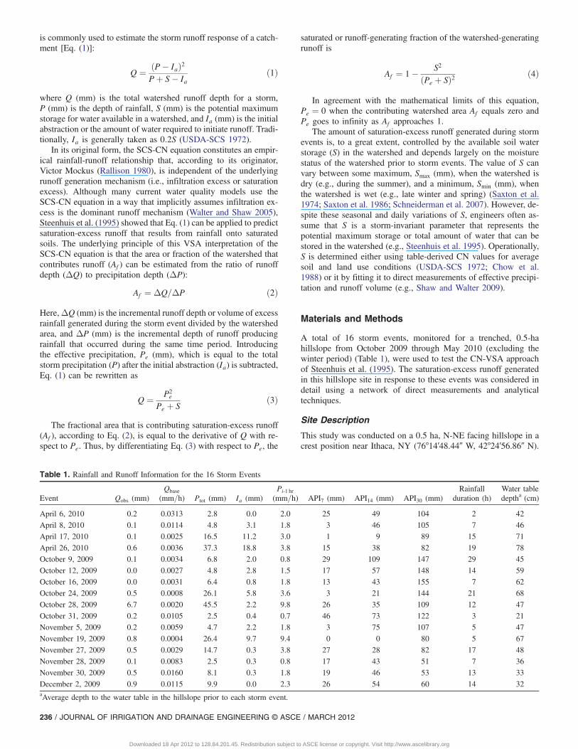
The hillslope is short (< 125 m), moderately steep (average 7°),and located in an elevation ranging from 482 to 499 m (Fig. 1).Annual precipitation averages 930 mm, with an annual mean tem-perature of 7.8°C (climate station Cornell Game Farm). The veg-etation in the study site is mixed grassland that is cut biannually(July, September) for hay production. Hardwood deciduous forestwith American beech, oaks, and sugar maples bound the study sitetoward the western, steeper shoulder.

The subsurface material on site consists of glacial till on middleDevonian shales and siltstones (Miller 1993). The depth to theshale bedrock is locally variable due to moraine deposits and rangesbetween 1.5 m on the hilltops and several meters (> 25 m) inthe main valley around Harford (Miller 1993). The dominant soiltype at the site is a Mardin channery silt loam, which is classifiedas coarse-loamy, mixed, active, mesic typic Fragiudepts (parentmaterial is glacial till) (Soil Survey Geographic Database,NRCS-USDA 2008).

Hydrometric Measurements and TrenchInstrumentation

A 13-m-long by 2-m-wide trench was excavated in a persistentVSA located at the bottom of this ~100-m-long hillslope (Fig. 1).The trench location was based on observed topographic conver-gence and associated VSA formation. The trench face was con-structed orthogonal to flowlines as derived from surfacetopography. The length of the trench was selected to span acrossthe maximum extent of the VSA. The trench was dug to a depth ofapproximately 1.5 m to intersect the top of the fragipan horizon.Both the water flux draining through the trench and water levelmeasurements within the soils in the drainage area of the trenchface were monitored.

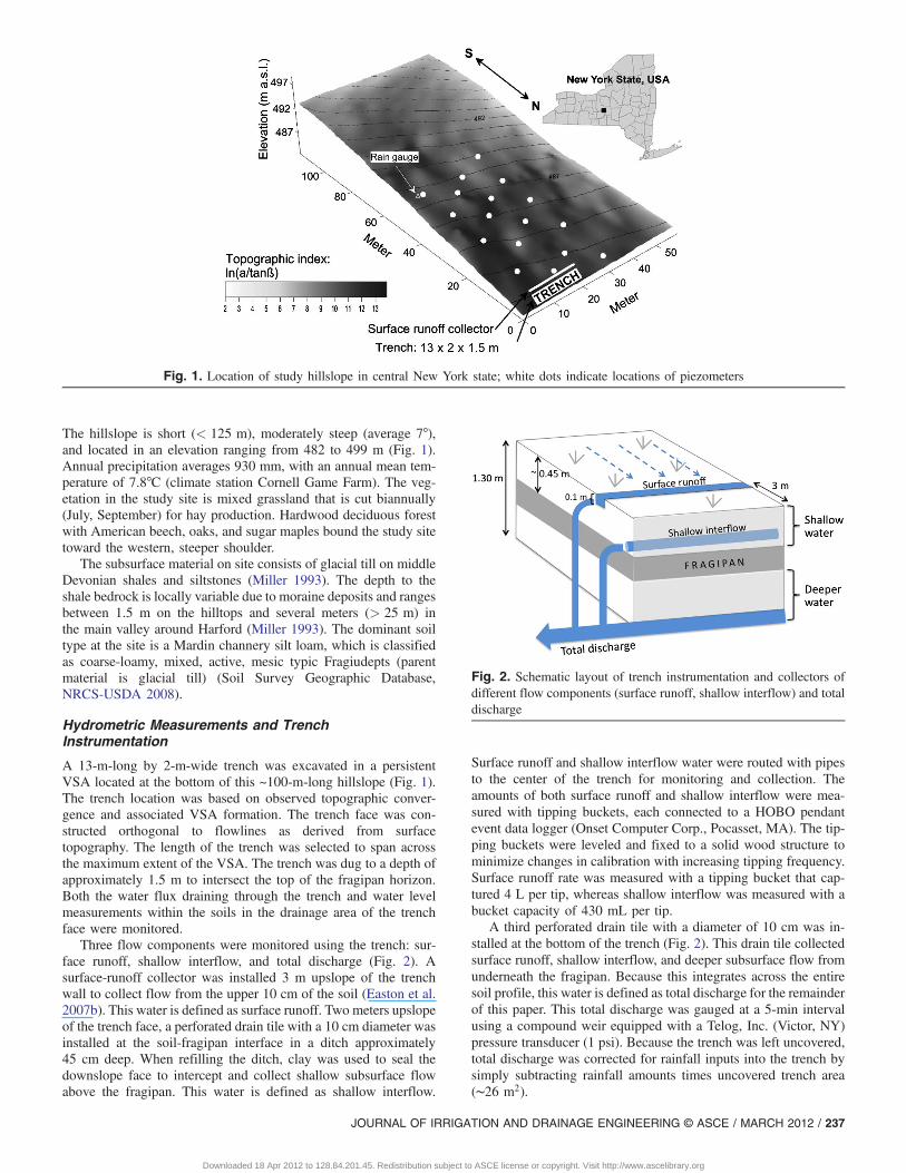
Three flow components were monitored using the trench: sur-face runoff, shallow interflow, and total discharge (Fig. 2). Asurface-runoff collector was installed 3 m upslope of the trenchwall to collect flow from the upper 10 cm of the soil (Easton et al.2007b). This water is defined as surface runoff. Two meters upslopeof the trench face, a perforated drain tile with a 10 cm diameter wasinstalled at the soil-fragipan interface in a ditch approximately45 cm deep. When refilling the ditch, clay was used to seal thedownslope face to intercept and collect shallow subsurface flowabove the fragipan. This water is defined as shallow interflow.

Surface runoff and shallow interflow water were routed with pipesto the center of the trench for monitoring and collection. Theamounts of both surface runoff and shallow interflow were mea-sured with tipping buckets, each connected to a HOBO pendantevent data logger (Onset Computer Corp., Pocasset, MA). The tip-ping buckets were leveled and fixed to a solid wood structure tominimize changes in calibration with increasing tipping frequency.Surface runoff rate was measured with a tipping bucket that cap-tured 4 L per tip, whereas shallow interflow was measured with abucket capacity of 430 mL per tip.

A third perforated drain tile with a diameter of 10 cm was in-stalled at the bottom of the trench (Fig. 2). This drain tile collectedsurface runoff, shallow interflow, and deeper subsurface flow fromunderneath the fragipan. Because this integrates across the entiresoil profile, this water is defined as total discharge for the remainderof this paper. This total discharge was gauged at a 5-min intervalusing a compound weir equipped with a Telog, Inc. (Victor, NY)pressure transducer (1 psi). Because the trench was left uncovered,total discharge was corrected for rainfall inputs into the trench bysimply subtracting rainfall amounts times uncovered trench area(∼26 m2).

Fig. 1. Location of study hillslope in central New York state; white dots indicate locations of piezometers

Fig. 2. Schematic layout of trench instrumentation and collectors ofdifferent flow components (surface runoff, shallow interflow) and totaldischarge

JOURNAL OF IRRIGATION AND DRAINAGE ENGINEERING © ASCE / MARCH 2012 / 237

Downloaded 18 Apr 2012 to 128.84.201.45. Redistribution subject to ASCE license or copyright. Visit http://www.ascelibrary.org

Hillslope InstrumentationA network of 17 water level loggers was installed in the lower halfof the contributing area of the trench (Fig. 1). Water levels weremeasured at 5-min intervals using 50-cm-long and 100-cm-longcapacitance probes (TruTrack, Inc., New Zealand). The loggerswere installed in four transects with a distance of 8 m acrossthe slope and 14 m upslope between the loggers. This logger net-work covered 60% of the total hillslope area. All capacitanceprobes were completely embedded in the soil inside 5-cm PVCtubes, resulting in installation depths of 0.83 m for the WT-HR500 probes (wells P1–P17, except well P3) and 1.30 m forone WT-HR1000 probe (well P3). The PVC tubing was screenedover the lower 25 cm.

A tipping bucket rain gauge (Spectrum Technologies Inc.,Plainfield, IL, USA) was installed on site that recorded rainfallamounts over 5-min intervals. Meteorological data (temperature,precipitation, wind, solar radiation) were concurrently availablefrom a climate reference network station in Harford, NY, approx-imately 2.3 km north of the site.

Estimation of SCS-CN Relevant Parameters fromField-Measured Data

In this study, the trench instrumentation allowed direct estimationof saturation-excess overland flow through installation of collectorsthat recorded water flux from different soil horizons. We assumethat the surface runoff, collected from the upper 10 cm of the soil,represents the amount of saturation-excess overland flow (Qobs)generated during storm events. Observed flow volumes (L=hr) wereconverted to depth values (mm=hr) using an estimated contributingarea of 2;575 m2, which was derived from the surface topographyof the hillslope. To satisfy consideration of the initial abstractionIa (the minimum amount of rainfall necessary to exceed fieldcapacity) in the determination of the effective precipitation (Pe),we obtained Ia as the sum of the precipitation before surface runoffcommenced. The site-specific storage parameter, S, was back-calculated from Eq. (3) for each storm event and then used inEq. (4) to predict Af based on observed Q and Pe.

The average fractional saturated area observed in the hillslope(Af -obs) during storm events was determined using hourly averagesof observed water table depths. During storm events, Af -obs can varybetween zero (minimum extent) and some maximum extent, whichis equal to the total hillslope contributing area. To reflect both theinfluence of antecedent moisture conditions and total storm precipi-tation on VSA expansion, we determined Af -obs as the averagesaturated area extent present in the hillslope for the duration of sur-face runoff generation. To obtain Af -obs, we first interpolated ob-served water table depths using ordinary kriging (Ripley 1981;Goovaerts 1999) and then estimated Af -obs as the ratio of the areawith water tables above a specified threshold to the total contrib-uting area (2;575 m2). Lyon et al. (2006a, b) found that the gen-eration of saturation-excess overland flow rapidly increased whenthe median water table was within the top 10 cm of the soil. How-ever, in this paper we look at a range of possible thresholds (5, 10,15 to 20 cm) and how the observed changes in Af associated witheach water table threshold compare to Af predicted with Eq. (4).

Results

Rainfall-Runoff Response and Saturation Dynamics

The 16 storm events observed with the trenched hillslope showedrainfall depths and peak 1-h rainfall intensities ranging from 2.5 to46 mm and 0.7 to 9:8 mm=h, respectively (Table 1). Ten of the 16

storm events had less than 10 mm of total rainfall. Rainfall eventslasted from 2 to 27 h and generally had low intensities, common torainfall in the northeastern United States (Buda et al. 2009). Atno time during the study was the infiltration capacity of the soilexceeded by the rainfall intensity. This was supported by estimatesof the infiltration rate of the soil surface layer with a sprinkleinfiltrometer (Ogden et al. 1997), which ranged from 148 to334 mm=h across the hillslope, and are far greater than any ofthe rainfall intensities.

Base flow, estimated as the minimum total discharge observedwithin the 24 h prior to a storm event, ranged from 0.00004 to0:03 mm=h and reflected similarly the wide range of antecedentmoisture conditions prior to storm events (Troch et al. 1993).Surface runoff depths or saturation-excess overland flow generatedduring the 16 storm events ranged from 0.005 (October 12, 2009)to 6.7 mm (October 28, 2009).

Moisture conditions in the hillslope, as indicated by the hillslopeaverage depth to the water table (average of 17 water level loggers),ranged from dry antecedent to saturated conditions during the studyperiod (Fig. 3). The driest antecedent conditions, with an averagewater table depth of 78 cm, occurred prior to the storm event onApril 26, 2010 after 9 days without rainfall. The lowest averagewater table depth monitored during the entire study period wasreached during the largest storm event; on October 28, 2009 thesite received 46 mm of rainfall within 12 h, causing the averagewater table to rise from a depth of 47 cm prior to the storm to7 cm 2 h after peak flow, with several areas of the hillslope com-pletely saturating (e.g., water table at or near the soil surface).

Influence of Water Table Threshold on Observed Af

Table 2 summarizes values of the observed saturated fraction in thehillslope for each storm event for different average water table depththresholds of 5 cm (Af -5), 10 cm (Af -10), 15 cm (Af -15), and 20 cm(Af -20). The average observed saturated fraction of the hillslope ob-served during any of the 16 storm events exhibited the smallest Af -value range for the 5-cm threshold (Af -5 ¼ 0 to 6%) and largestvalue range for the 20-cm threshold (Af -20 ¼ 6 to 38%). The differ-ent thresholds influence Af -obs estimates mainly during large stormevents or under dry antecedent conditions. If a threshold of 5 cm wasused to estimate the saturated fraction, observed Af -5 values werezero for most events, except during events with greater rainfallamounts (Pe > 15 mm) when the water table rise was rapid or whenthe average water table depth was less than 40 cm below the soilsurface prior to storm events (Tables 1 and 2). The maximum satu-rated fraction of the hillslope observed during the largest storm eventon October 28, 2009, was 11%, 38%, 49%, and 51% for the 5-, 10-,15-, and 20-cm thresholds, respectively.

Comparison of Observed versus Predicted Af

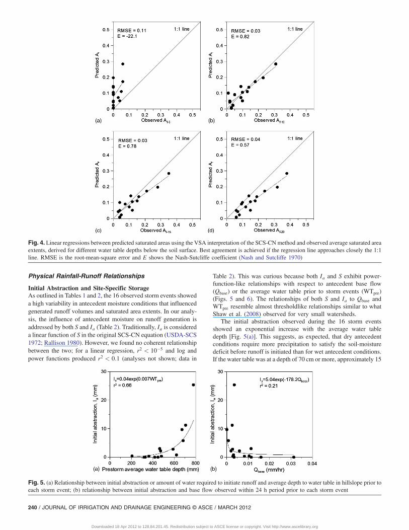
Using the observed Pe and Qobs to back-calculate S from Eq. (3),predicted Af [Eq. (4)] ranged from 1 to 28% for the 16 storm events(Table 2). To estimate the accuracy of predicted Af and the effect ofthe average water table depth on the determination of the saturatedhillslope fraction, we linearly regressed predicted versus observedAf values, derived for the four different thresholds (Fig. 4). A linearfit that most closely approaches the 1∶1 line indicates the bestagreement between predicted and observed Af ; in this case,Af -10 produced the best agreement (Fig. 4) Additionally, theroot-mean-square error (RMSE) and Nash-Sutcliffe criterion (E)(Nash and Sutcliffe 1970) between predicted and observed Af in-dicated that the 10 cm water table threshold showed the closest fit;RMSE ¼ 0:11, 0.03, 0.03, and 0.04 and E ¼ �22:1, 0.82, 0.78,and 0.57 for the 5-, 10-, 15-, and 20-cm thresholds, respectively(Table 2).

238 / JOURNAL OF IRRIGATION AND DRAINAGE ENGINEERING © ASCE / MARCH 2012

Downloaded 18 Apr 2012 to 128.84.201.45. Redistribution subject to ASCE license or copyright. Visit http://www.ascelibrary.org

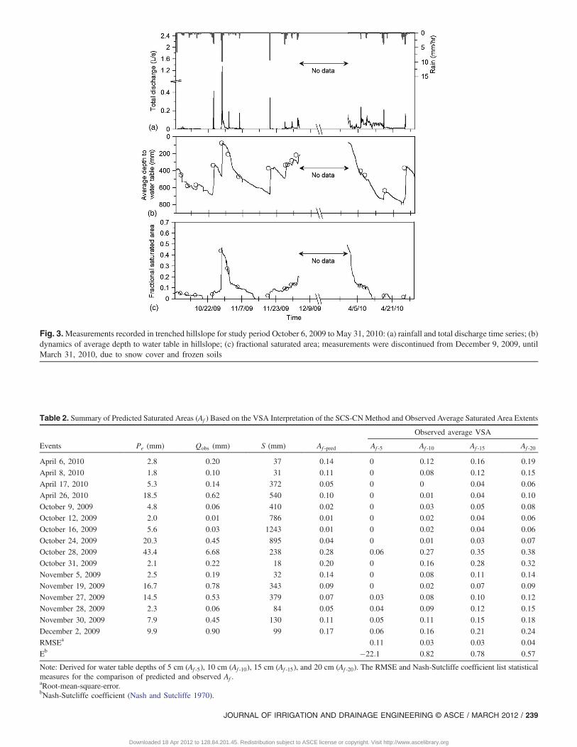
Fig. 3.Measurements recorded in trenched hillslope for study period October 6, 2009 to May 31, 2010: (a) rainfall and total discharge time series; (b)dynamics of average depth to water table in hillslope; (c) fractional saturated area; measurements were discontinued from December 9, 2009, untilMarch 31, 2010, due to snow cover and frozen soils

Table 2. Summary of Predicted Saturated Areas (Af ) Based on the VSA Interpretation of the SCS-CNMethod and Observed Average Saturated Area Extents

Events Pe (mm) Qobs (mm) S (mm) Af -pred

Observed average VSA

Af -5 Af -10 Af -15 Af -20

April 6, 2010 2.8 0.20 37 0.14 0 0.12 0.16 0.19

April 8, 2010 1.8 0.10 31 0.11 0 0.08 0.12 0.15

April 17, 2010 5.3 0.14 372 0.05 0 0 0.04 0.06

April 26, 2010 18.5 0.62 540 0.10 0 0.01 0.04 0.10

October 9, 2009 4.8 0.06 410 0.02 0 0.03 0.05 0.08

October 12, 2009 2.0 0.01 786 0.01 0 0.02 0.04 0.06

October 16, 2009 5.6 0.03 1243 0.01 0 0.02 0.04 0.06

October 24, 2009 20.3 0.45 895 0.04 0 0.01 0.03 0.07

October 28, 2009 43.4 6.68 238 0.28 0.06 0.27 0.35 0.38

October 31, 2009 2.1 0.22 18 0.20 0 0.16 0.28 0.32

November 5, 2009 2.5 0.19 32 0.14 0 0.08 0.11 0.14

November 19, 2009 16.7 0.78 343 0.09 0 0.02 0.07 0.09

November 27, 2009 14.5 0.53 379 0.07 0.03 0.08 0.10 0.12

November 28, 2009 2.3 0.06 84 0.05 0.04 0.09 0.12 0.15

November 30, 2009 7.9 0.45 130 0.11 0.05 0.11 0.15 0.18

December 2, 2009 9.9 0.90 99 0.17 0.06 0.16 0.21 0.24

RMSEa 0.11 0.03 0.03 0.04

Eb �22:1 0.82 0.78 0.57

Note: Derived for water table depths of 5 cm (Af -5), 10 cm (Af -10), 15 cm (Af -15), and 20 cm (Af -20). The RMSE and Nash-Sutcliffe coefficient list statisticalmeasures for the comparison of predicted and observed Af .aRoot-mean-square-error.bNash-Sutcliffe coefficient (Nash and Sutcliffe 1970).

JOURNAL OF IRRIGATION AND DRAINAGE ENGINEERING © ASCE / MARCH 2012 / 239

Downloaded 18 Apr 2012 to 128.84.201.45. Redistribution subject to ASCE license or copyright. Visit http://www.ascelibrary.org

Physical Rainfall-Runoff Relationships

Initial Abstraction and Site-Specific StorageAs outlined in Tables 1 and 2, the 16 observed storm events showeda high variability in antecedent moisture conditions that influencedgenerated runoff volumes and saturated area extents. In our analy-sis, the influence of antecedent moisture on runoff generation isaddressed by both S and Ia (Table 2). Traditionally, Ia is considereda linear function of S in the original SCS-CN equation (USDA-SCS1972; Rallison 1980). However, we found no coherent relationshipbetween the two; for a linear regression, r2 < 10�5 and log andpower functions produced r2 < 0:1 (analyses not shown; data in

Table 2). This was curious because both Ia and S exhibit power-function-like relationships with respect to antecedent base flow(Qbase) or the average water table prior to storm events (WTpre)(Figs. 5 and 6). The relationships of both S and Ia to Qbase andWTpre resemble almost thresholdlike relationships similar to whatShaw et al. (2008) observed for very small watersheds.

The initial abstraction observed during the 16 storm eventsshowed an exponential increase with the average water tabledepth [Fig. 5(a)]. This suggests, as expected, that dry antecedentconditions require more precipitation to satisfy the soil-moisturedeficit before runoff is initiated than for wet antecedent conditions.If the water table was at a depth of 70 cm or more, approximately 15

Fig. 4. Linear regressions between predicted saturated areas using the VSA interpretation of the SCS-CNmethod and observed average saturated areaextents, derived for different water table depths below the soil surface. Best agreement is achieved if the regression line approaches closely the 1∶1line. RMSE is the root-mean-square error and E shows the Nash-Sutcliffe coefficient (Nash and Sutcliffe 1970)

Fig. 5. (a) Relationship between initial abstraction or amount of water required to initiate runoff and average depth to water table in hillslope prior toeach storm event; (b) relationship between initial abstraction and base flow observed within 24 h period prior to each storm event

240 / JOURNAL OF IRRIGATION AND DRAINAGE ENGINEERING © ASCE / MARCH 2012

Downloaded 18 Apr 2012 to 128.84.201.45. Redistribution subject to ASCE license or copyright. Visit http://www.ascelibrary.org

to 25 mm of rainfall were needed to initiate surface runoff. Underwet antecedent conditions, an average water table depth of less than35 cm below the soil surface, less than 5 mm of rainfall wereneeded to initiate surface runoff [Table 1, Fig. 5(a)]. The relation-ship between the back-calculated site-specific storage, S, and theaverage water table depth prior to storm events showed a responsethat was similar to the initial abstraction power law relationship[Fig. 6(a)]. The relationship is less pronounced and the back-calculated S are more scattered during dry antecedent conditionsthan was observed for the relationship between Ia and WTpre.Nevertheless, if the water table was at a depth of 40 cm or less,S was very small, indicating that less rainfall was retained beforerunoff was initiated. Both Ia and S showed power-function-likerelationship with the base flow observed 24 h prior to stormevents [Figs. 5(b) and 6(b)]. Both increased exponentially underdry antecedent conditions when the hillslope received less than36 mm of rainfall within 14 days prior to the storm event, asindicated by a base flow rate of 0:004 mm=h (10 L=h) or less[Figs. 5(b) and 6(b)].

In this study, we were able to account for the variability of both Iaand S with respect to antecedent conditions because we wereable to directly measure all parameters except S, which we back-calculated from Eq. (1). Operationally, it would be convenient toeliminate one of these variables. Contrary to the common assumptionthat Ia ¼ 0:2S (or sometimes 0:05S), we did not find a relationshipbetween S and Ia. Thus, we explored the possibility of using an aver-age S value such that only Ia varied with antecedent conditions; thisis somewhat akin to the approach of Steenhuis et al. (1995) and Lyonet al. (2004), who used the Thornthwaite-Mather soil water budget toestimate Ia. We fitted an average S of 15.5 cm (CN ¼ 62) from Q-Pand Af -Pe pairs using the method outlined by Steenhuis et al. (1995).Based on the fitted average S and observed Q and P, we then back-calculated Ia using Eq. (1). The field-observed Ia and predicted Iarelative to Qbase (Fig. 7) are similar to the relationship in Fig. 5(b),which included the effect of variability of antecedent moisture con-ditions on S. For some events with wet antecedent conditions therewere negative values of the back-calculated Ia, reflecting that thesoils in some parts of the trenched hillslope were already saturatedprior to the storm event, resulting in a soil water surplus and higherrunoff volumes than predicted with the SCS-CN equation due to hill-slope drainage. In this interpretation of the SCS-CN equation, S is astatic watershed-specific parameter. However, to use the SCS-CNmethod in continuous watershed models or to predict runoff fromspecific events, more work is needed to incorporate soil-moistureaccounting schemes (e.g., Michel et al. 2005) or proxies for soil

moisture such as the power-function-like relationship between Sand Qbase or Ia and WTpre (e.g., Shaw and Walter 2009) into theSCS-CN method.

Predicted Runoff VolumesAs stated in Eq. (2), the VSA hydrology concept is based on theassumption that the amount of runoff generated during a stormevent is a function of the rainfall amount and the saturated fractionof the watershed that is contributing runoff during a storm event.Thus, besides the statistical comparison of observed and predictedAf , we tested whether the product of effective rainfall multiplied bythe average saturated hillslope area (Af -obs × Pe) derived for eachof the water table thresholds would match the observed runoffdepths (Qobs) (Fig. 8). The slope of the predicted versus observedQ is closest to unity for the 10 cm water table threshold (Fig. 8).The RMSEs between observed discharge (Qobs) and the productof effective precipitation and the average fractional saturated area(Af -obs × Pe) were 1.10, 1.27, 2.18, and 2.58 mm respectively forthe 5, 10, 15, and 20 cm thresholds (Table 3). Nash-Sutcliffe effi-ciencies were 0.51, 0.34, �0:94, and �1:71 respectively for the 5,10, 15, and 20 cm water table thresholds (Table 3). Statisticalmeasures might be mostly driven by the large storm event in

Fig. 6. (a) Relationship between back-calculated, site-specific storage parameter, S, and average depth to water table in hillslope prior to each stormevent; (b) relationship between S and base flow observed within 24-h period prior to each storm event

Fig. 7. Comparison of observed initial abstraction and calculated initialabstraction if watershed storage is S ¼ 15:5 cm. The estimated initialabstraction shows negative values for events with wet antecedent con-ditions when discharge was greater than rainfall inputs; for these eventsthe observed Ia was set to zero

JOURNAL OF IRRIGATION AND DRAINAGE ENGINEERING © ASCE / MARCH 2012 / 241

Downloaded 18 Apr 2012 to 128.84.201.45. Redistribution subject to ASCE license or copyright. Visit http://www.ascelibrary.org

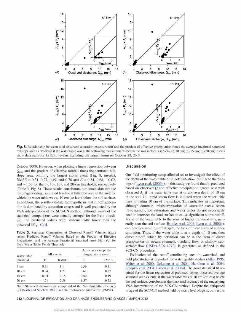
October 2009. However, when plotting a linear regression betweenQobs and the product of effective rainfall times the saturated hill-slope area, omitting the largest storm event (Fig. 8, inserts),RMSE ¼ 0:31, 0.27, 0.49, and 0.78 and E ¼ 0:54, 0.68, �0:02,and �1:57 for the 5-, 10-, 15-, and 20-cm thresholds, respectively(Table 3, Fig. 8). These results corroborate our conclusion that therunoff-generating, saturated fractional hillslope area is the area forwhich the water table was at 10 cm (or less) below the soil surface.In addition, the results validate the hypothesis that runoff genera-tion is dominated by saturation excess and is well predicted by theVSA interpretation of the SCS-CN method; although many of thestatistical comparisons were actually stronger for the 5-cm thresh-old, the predicted values were systematically lower than theobserved [Fig. 8(a)].

Discussion

Our field monitoring setup allowed us to investigate the effect ofthe depth of the water table on runoff initiation. Similar to the find-ings of Lyon et al. (2006b), in this study we found that Af predictedbased on observed Q and effective precipitation agreed best withobserved Af if the water table was at or above a depth of 10 cmin the soil, i.e., rapid storm flow is initiated when the water tablerises to within 10 cm of the surface. This indicates an important,although common, misinterpretation of saturation-excess stormflow, namely, soil saturation and water tables do not necessarilyneed to intersect the land surface to cause significant storm runoff.A rise of the water table to the zone of higher transmissivity, gen-erally near the soil surface (Brooks et al. 2004; Lyon et al. 2006b),can produce rapid runoff despite the lack of clear signs of surfacesaturation. Thus, if the water table is at a depth of 10 cm, thendirect runoff, which by definition can be in the form of directprecipitation on stream channels, overland flow, or shallow sub-surface flow (USDA-SCS 1972), is generated as defined in theSCS-CN procedure.

Estimation of the runoff-contributing area in watershed andfield plot studies is important for water quality studies (Allan 1995;Walter et al. 2000; DeLaune et al. 2004; Hamilton et al. 2004;Sharpley et al. 2004; Easton et al. 2008a). The good statistical fit ob-tained for the linear regression of predicted versus observed averagesaturated area extents, if the water table was at 10 cm (or less) belowthe soil surface, corroborates the theorized accuracy of the underlyingVSA interpretation of the SCS-CN method. Despite the antiquatedimage of the SCS-CN method held by many hydrologists, our results

Fig. 8. Relationship between total observed saturation-excess runoff and the product of effective precipitation times the average fractional saturatedhillslope area as observed if the water table was at the following measurements below the soil surface: (a) 5 cm; (b)10 cm; (c) 15 cm; (d) 20 cm; insertsshow data pairs for 15 storm events excluding the largest storm on October 28, 2009

Table 3. Statistical Comparison of Observed Runoff Volumes (Qobs)versus Predicted Runoff Volumes Based on the Product of EffectivePrecipitation and the Average Fractional Saturated Area (Af × Pe) forEach Water Table Depth Threshold

Water tablethreshold

All eventsAll events except thelargest storm event

E RMSE E RMSE

5 cm 0.51 1.1 0.59 0.31

10 cm 0.34 1.27 0.68 0.27

15 cm �0:94 2.18 �0:02 0.49

20 cm �1:71 2.58 �1:57 0.78

Note: Statistical measures are comprised of the Nash-Sutcliffe efficiency(E) (Nash and Sutcliffe 1970) and the root-mean-square-error (RMSE).

242 / JOURNAL OF IRRIGATION AND DRAINAGE ENGINEERING © ASCE / MARCH 2012

Downloaded 18 Apr 2012 to 128.84.201.45. Redistribution subject to ASCE license or copyright. Visit http://www.ascelibrary.org

indicate that in the correct settings and with the correct assumptions,the prediction of VSAs using the CN method is surprisingly robust inwatersheds (Lyon et al. 2004; Schneiderman et al. 2007; Easton et al.2008a, b) and even small plots (this study) dominated by saturation-excess overland flow. Complete field estimates of VSA extents insmall or large watersheds are difficult to obtain and require eithertime-consuming and cost-intensive field mapping or remote sensingimagery and reliable interpretation. However, a few studies have indi-rectly shown that watershed models using the VSA hydrology con-cept perform better in the northeastern United States than models thatassume infiltration excess as the underlying runoff-generation process(e.g., Lyon et al. 2004; Schneiderman et al. 2007; Easton et al.2008a, b).

The amount of saturation-excess runoff generated during stormevents is, to a great extent, controlled by the available soil waterstorage, which changes daily and seasonally with antecedent mois-ture conditions. However, the traditional SCS-CN method (USDA-SCS 1972) adjusts S based on antecedent rainfall, which has beenshown to be a poor index for antecedent conditions with respect to S(Shaw and Walter 2009). To incorporate the variable S for eachstorm event into an analysis requires a better method for determin-ing antecedent moisture conditions. Several methods have beenproposed to improve estimates of S based on various measures orindicators of antecedent conditions. These include deriving S fromsoil-moisture data (Saxton et al. 1982), the effective available soilwater storage proposed by Schneiderman et al. (2007), and the stor-age versus base flow relationship proposed by Troch et al. (1993)and applied to the SCS-CN method by Shaw and Walter et al.(2009). The latter may be more readily applicable because there arerelatively few places where soil moisture is continuously monitoredand remotely sensed soil moisture is not well developed, whereasthere are many stream gauges throughout much of the world. Inaddition, the availability of continuous watershed-wide water tablemeasurements could be a limiting factor in establishing regionalstorage versus water table depth relationships.

One unique aspect of this study was that the initial abstractionwas directly measured as the sum of the precipitation before surfacerunoff commenced. In both the standard SCS-CN procedure andthe VSA interpretation of the SCS-CNmethod, the initial abstractionis assumed to be a function of S, generally taken as 0:2S(USDA-SCS 1972). However, soil water contents can vary betweenthe wilting point at minimum and field capacity at maximum, mak-ing the initial abstraction dependent on the actual soil water content.Studies by Jiang (2001) and Shaw and Walter (2009) have shownthat much smaller Ia of 0:05S and 0:03S, respectively, resulted inbetter estimates of runoff than the traditional 0:2S. Shaw and Walter(2009) also suggested that when considering only storm events withrainfall amounts greater than 10 mm, neglecting the initial abstrac-tion in watersheds on the order of 100 km2 seems to result in suitableestimates of discharge. However, in smaller watersheds, particularlywith a limited amount of riparian or wetland areas, the initial abstrac-tion serves an important role in runoff production.

In this study, Ia was estimated independently of S, whichresulted in a storm-variant S [back-calculated using Eq. (3)] thatreflects changes in antecedent moisture conditions. However, ifusing a site-specific, constant S, which can be fitted by plottingobserved effective precipitation versus runoff depths for severalstorm events (Steenhuis et al. 1995), variation of Ia with total rain-fall and runoff can be estimated for each storm event (Fig. 7). Boththe estimated and observed Ia show similar values depending onantecedent moisture conditions. Although S represents the potentialaverage storage or the total amount of water that can be stored in thewatershed, differences in the soil moisture prior to storm events(i.e., negative Ia values for storms with wet antecedent conditions)

have a large impact on the amount of runoff generated for a givenrainfall amount (Fig. 7). As shown in this study, the initial abstrac-tion is highly variable in response to differences in antecedentmoisture but shows good relations to indirect indicators such as theaverage water table depth and base flow rate prior to storm events[Figs. 5(a) and 5(b)]. Since direct estimation of S through fieldmeasurements is very complex, estimation of the initial abstractionusing indirect indicators such as base flow or water table depthmight provide an approach that is easier to apply. However, moreresearch is needed to develop more variable, continuous solutionsfor determining S or Ia that reflect antecedent wetness conditions.

Conclusion

We compared variable source runoff areas predicted with the VSAinterpretation of the SCS-CN method (Steenhuis et al. 1995) andfield-observed spatial extents of VSAs in a 0.5-ha trenched hill-slope in central New York state. The trench instrumentation in con-junction with continuous measurements of upslope water tabledynamics in the hillslope allowed quantification of lateral flowfrom different soil layers. Initiation and total volume ofsaturation-excess overland flow in response to rainfall could be di-rectly monitored for different water table depths in the upslope con-tributing area of the trench for 16 storm events between October2009 and May 2010. Using field-measured precipitation anddischarge amounts, the comparison showed that the VSA interpre-tation of the SCS-CN method accurately predicted the runoff-contributing area observed during the 16 storm events. We furtherdemonstrated that predicted and observed saturated areas showedthe best agreement if the water table was within 10 cm of the soilsurface during storm events. These results not only provide evi-dence that the VSA interpretation of the SCS-CN method accu-rately predicts VSA extents in small watersheds or plots butalso that the method has a physical basis and is not simply acurve-fitting routine of observed rainfall and runoff depths. In ad-dition, the results clarify that if the water table is at a depth of 10 cmbelow the soil surface, direct runoff in the form of shallow subsur-face flow is initiated. Thus, not all storm flow is generated as over-land flow due to intersection of the water table with the landsurface, or perhaps the term overland is misleading.

Acknowledgments

We would like to acknowledge the USDA CSREES for projectfunding (Grant # 00-51130-9777) of this research. We also wouldlike to thank the two anonymous reviewers for their valuablecomments.

References

Allan, J. D. (1995). Stream ecology: Structure and function of runningwaters, Chapman and Hall, London.

Brooks, E. S., Boll, J., and McDaniel, P. A. (2004). “A hillslope-scaleexperiment to measure lateral saturated hydraulic conductivity.” WaterResour. Res., 40(4), 10.1029/2003WR002858.

Buda, A. R., Kleinman, P. J. A., Srinivasan, M. S., Bryant, R. B., andFeyereisen, G. W. (2009). “Factors influencing surface runoff genera-tion from two agricultural hillslopes in central Pennsylvania.” Hydrol.Process., 23(9), 1295–1312.

Chow, V. T., Maidment, D. R., and Mays, L. W. (1988). Applied hydrology.McGraw-Hill, New York, 572.

Dahlke, H. E., Easton, Z. M., Fuka, D. R., Lyon, S. W., and Steenhuis, T. S.(2009). “Modeling variable source area dynamics in a CEAP water-shed.” Ecohydrology, 2(3), 337–349.

JOURNAL OF IRRIGATION AND DRAINAGE ENGINEERING © ASCE / MARCH 2012 / 243

Downloaded 18 Apr 2012 to 128.84.201.45. Redistribution subject to ASCE license or copyright. Visit http://www.ascelibrary.org

Dahlke, H. E., Easton, Z. M., Lyon, S. W., Destouni, G., Walter, T., andSteenhuis, T. S. (2012). “Dissecting the variable source area concept—Subsurface flow pathways and water mixing processes in a hillslope.” J.Hydrol. (Amsterdam), 420–421, 125–141.

DeLaune, P. B., Moore, P. A., Carman, D. K., Sharpley, A. N., Haggard,B. E., and Daniel, T. C. (2004). “Evaluation of the phosphorus sourcecomponent in the phosphorus index for pastures.” J. Environ. Qual.,33(6), 2192–2200.

Dunne, T., and Black, R. D. (1970). “Partial area contributions to stormrunoff in a small New England watershed.” Water Resour. Res., 6(5),1296–1311.

Easton, Z. M., Gerard-Marchant, P., Walter, M. T., Petrovic, A. M., andSteenhuis, T. S. (2007a). “Identifying dissolved phosphorus sourceareas and predicting transport from an urban watershed using distrib-uted hydrologic modeling.” Water Resour. Res., 43(11), W11414,10.1029/2006WR005697.

Easton, Z. M., Gerard-Marchant, P., Walter, M. T., Petrovic, A. M., andSteenhuis, T. S. (2007b). “Hydrologic assessment of a suburban vari-able source watershed in the northeast United States.” Water Resour.Res., 43(3), W03413, 10.1029/2006WR005076.

Easton, Z. M., Fuka, D. R., Walter, M. T., Cowan, D. M., Schneiderman,E. M., and Steenhuis, T. S. (2008b). “Re-conceptualizing the soil andwater assessment tool (SWAT) model to predict runoff from variablesource areas.” J. Hydrol., 348(3–4), 279–291.

Easton, Z. M., Walter, M. T., and Steenhuis, T. S. (2008a). “Combinedmonitoring and modeling indicate the most effective agricultural bestmanagement practices.” J. Environ. Qual., 37(5), 1798–1809.

Garen, D. C., and Moore, D. S. (2005). “Curve number hydrology in waterquality modeling: Uses, abuses, and future directions.” J. Am. WaterResour. Assoc., 41(2), 377–388.

Gburek, W. J., Drungil, C. C., Srinivasan, M. S., Needelman, B. A., andWoodward, D. E. (2002). “Variable-source area controls on phosphorustransport: Bridging the gap between research and design.” J. Soil WaterConserv., 57(6), 534–543.

Goovaerts, P. (1999). “Geostatistics in soil science: state-of-the-art andperspectives.” Geoderma, 89(1–2), 1–45.

Hamilton, P. A., Miller, T. L., and Myers, D. N. (2004). Water quality inthe nation’s streams and aquifers: Overview of selected findings, U.S.Geological Survey, Washington, DC, 1265, 1–19.

Hewlett, J. D., and Hibbert, A. R. (1967). “Factors affecting the responseof small watersheds to precipitation in humid regions.” Forest hydrol-ogy, W. E. Sopper and H. W. Lull HW, eds., Pergamon Press, Oxford,UK.

Hewlett, J. D., and Nutter, W. L. (1970). “The varying source area ofstreamflow from upland basins.” Proc., Symp. on InterdisciplinaryAspects of Watershed Management, ASCE, Reston, VA, 65–83.

Horton, R. E. (1933). The role of infiltration in the hydrologic cycle, Eos(Transactions of the American Geophysical Union), 14, 44–460.

Horton, R. E. (1940). “An approach toward a physical interpretation ofinfiltration capacity.” Proc. Soil Sci. Soc. Am., 4, 399–417.

Jiang, R. (2001). “Investigation of runoff curve number initial abstractionratio.” M.S. thesis, Univ. of Ariz., Tucson.

Lyon, S. W., Gérard-Marchant, P., Walter, M. T., and Steenhuis, T. S.(2004). “Using a topographic index to distribute variable source arearunoff predicted with the SCS-Curve Number equation.” Hydrol.Process., 18(15), 2757–2771.

Lyon, S. W., Lembo, A. J., Walter, M. T., and Steenhuis, T. S. (2006a).“Defining probability of saturation with indicator kriging on hardand soft data.” Adv. Water Resour., 29(2), 181–193.

Lyon, S. W., Seibert, J., Lembo, A. J., Walter, M. T., and Steenhuis, T. S.(2006b). “Geostatistical investigation into the temporal evolution ofspatial structure in a shallow water table.” Hydrol. Earth Syst. Sci.,10(1), 113–125.

Michel, C., Andreassian, V., and Perrin, C. (2005). “Soil ConservationService curve number method: How to mend a wrong soil moistureaccounting procedure?” Water Resour. Res., 41(2), W02011,10.1029/2004WR003191.

Miller, T. S. (1993). “Glacial geology and the origin and distribution ofaquifers at the valley heads moraine in the Virgil Creek and Dryden

Lake-Harford Valleys, Tompkins and Cortland Counties.”U.S. GeologicalSurvey Water-Resources Investigations Rep., 90-4168, New York.

Nash, J. E., and Sutcliffe, J. V. (1970). “River flow forecasting throughconceptual models, Part 1—A discussion of principles.” J. Hydrol.,10(3), 282–290.

Natural Resources Conservation Service, U.S. Dept. of Agriculture(NRCS-USDA). (2008). “Soil Survey Geographic (SSURGO)Database for [Tompkins County, Cayuga County, New York State].”⟨http://soildatamart.nrcs.usda.gov⟩ (Jun. 20, 2008).

Ogden, C. B., van Es, H. M., and Schindelbeck, R. R. (1997). “Miniaturerain simulator for measurement of infiltration and runoff.” Soil Sci. Soc.Am. J., 61(4), 1041–1043.

Ponce, V. M., and Hawkins, R. H. (1996). “Runoff curve number: Has itreached maturity?” J. Hydrol. Eng., 1(1), 11–19.

Rallison, R. E. (1980). “Origin and evolution of the SCS runoff equation.”Symposium on Watershed Management, American Society of CivilEngineers, NY, NY, 912–924.

Ripley, B. D. (1981). Spatial statistics, Wiley, NY.Saxton, K. E. (1982). “SPAW model predicts crop stress.” Agricultural

research / U.S. Dept. of Agriculture, 30(12), 16–26.Saxton, K. E., Johnson, H. P., and Shaw, R. H. (1974). “Modeling evapo-

transpiration and soil moisture.” Trans. Am. Soc. of Agri. Eng., 17(4),673–677.

Saxton, K. E., Rawls, W. J., Romberger, J. S., and Papendick, R. I. (1986).“Estimating generalized soil water characteristics from texture.” SoilSci. Soc. Am. J. 50(4), 1031–1036.

Schneiderman, E. M., et al. (2007). “Incorporating variable source areahydrologyinto thecurvenumberbasedgeneralizedwatershedloadingfunc-tion model.” Hydrol. Process., 21(25), 3420–3430, 10.1002/hyp.6556.

Sharpley, A. N., Kleinman, P., and Weld, J. (2004). “Assessment of bestmanagement practices to minimize the runoff of manure-borne phos-phorus in the United States.” N. Z. J. Agric. Res., 47(4), 461–477.

Shaw, S. B., and Walter, M. T. (2009). “Improving runoff risk estimates:Formulating runoff as a bivariate process using the SCS curvenumber method.” Water Resour. Res., 45(3), W03404, 10.1029/2008WR006900.

Shaw, S. B., Walter, M. T., and Marjerison, R. D. (2008). “Groupinglike catchments: A novel means to compare 40+ watersheds inthe Northeastern U. S.” American Geophysical Union Fall Meeting,Eos (Transactions of the American Geophysical Union), AGU,San Francisco, 89(53), Fall Meet. Suppl. Abstract H33D-1038.

Steenhuis, T. S., Winchell, M., Rossing, J., Zollweg, J. A., andWalter, M. F.(1995). “SCS Runoff equation revisited for variable-source runoffareas.” J. Irrig Drain. Eng., 121(3), 234–238.

Troch, P. A., De Troch, F. P., and Brutsaert, W. (1993). “Effectivewater table depth to describe initial conditions prior to storm rainfallin humid regions.” Water Resour. Res., 29(2), 427–434, 10.1029/92WR02087.

U.S. Dept. of Agriculture-Soil Conservation Service (USDA-SCS). (1972).“Hydrology.” Section 4, Chapter 10, Part 630. National engineeringhandbook, Water Resources Publications, Highlands Ranch, CO,“Hydrology.” Section 4, Chapter 10.630.

Walter, M. T., and Shaw, S. B. (2005). “Discussion of Curve number hy-drology in water quality modeling: uses, abuses, and future directionsby Garen and Moore.” J. Am. Water Resour. Assoc., 41(6), 1491–1492.

Walter, M. T., Walter, M. F., Brooks, E. S., Steenhuis, T. S., Boll, J.,and Weiler, K. R. (2000). “Hydrologically sensitive areas: Variablesource area hydrology implications for water quality risk assessment.”J. Soil Water Conserv., 55(3), 277–284.

Walter, M. T., Dosskey, M., Khanna, M., Miller, J., Tomer, M., andWiens, J. (2007). “The science of targeting within landscapes andwatersheds to improve conservation effectiveness.” Managing agricul-tural landscapes for environmental quality, strengthening the sciencebase, M. Schnepf and C. Cox, eds., Soil and Water ConservationSociety, Ankeny, IA, 63–91.

Walter, M. T., et al. (2009). “A new paradigm for sizing riparian buffers toreduce risks of polluted storm water: A practical synthesis.” J. Irrig.Drain. Eng., 135(2), 200–209.

244 / JOURNAL OF IRRIGATION AND DRAINAGE ENGINEERING © ASCE / MARCH 2012

Downloaded 18 Apr 2012 to 128.84.201.45. Redistribution subject to ASCE license or copyright. Visit http://www.ascelibrary.org