Daily Rainfall-Runoff Prediction and Simulation Using ANN, ANFIS and Conceptual Hydrological...

International Journal of Engineering & Technology Sciences (IJETS) 1 (1): 32-50, 2013ISSN xxxx-xxxx© Academic Research Online Publisher

32 | P a g e

Research Article

Daily Rainfall-Runoff Prediction and Simulation Using ANN, ANFIS andConceptual Hydrological MIKE11/NAM Models

Elham Kakaei Lafdani a, Alireza Moghaddam Nia b,*, Ahmad Pahlavanravi c, AzadehAhmadi d, Milad Jajarmizadeh e

a Department of Range and Watershed Management, University of Zabol, Zabol, Iranb Associate Professor of Mountain and Arid Regions Reclamation Department, Faculty of Natural Resources,University of Tehran, Karaj, Iranc Assistant Professor of Range and Watershed Management Department, University of Zabol, Zabol, Irand Assistant Professor of Civil Engineering Department, Isfahan University of Technology, Isfahan, Irane Department of Hydraulic and Hydrology, Universiti Teknologi Malaysia, Johor, Malaysia

* Corresponding author. Tel.: +982632223044 ; fax: +982632249313E-mail address: [email protected]

ARTICLE INFO

Article historyRevised:09April,2013Accepted:23April,2013

A b s t r a c tRainfall-Runoff modelling is considered as one of the major hydrologicprocesses with a key role in predicting flood forecasting and water resources.Furthermore, in order to prevent damages caused by the flood and control andinhibit as well as management and flood alarm, rainfall prediction is inevitable.In the present study, for a 10-year period (1999-2009), the rainfall has beenpredicted using historical rainfall data in Eskandari basin located in Iran usingAdaptive Neural Fuzzy Inference System (ANFIS) and Artificial NeuralNetwork (ANN). In addition, the best input combination was identified usingGamma Test (GT) for the rainfall prediction. Then, runoff discharge producedby the predicted rainfall and the observed rainfall were simulated by aconceptual hydrological model called MIKE11/NAM model and the resultswere compared together. The results indicated that ANFIS model might bebetter than ANN model for predicting rainfall. In this study, the efficiencycoefficient of NAM model in runoff simulations was 0.7 based on observedrainfall and based on predicted rainfall was 0.58 in Eskandari basin. Moreover,the results indicated that NAM model simulated the base flow more accuratethan simulating the peak flow in this basin.

© Academic Research Online Publisher. All rights reserved.

Keywords:Rainfall-RunoffANFISANNMIKE11/NAM ModelGamma Test

1. Introduction

There are plenty of techniques and methods in planning and managing the water resources, which are

directly or indirectly associated with prediction of the discharge flow and rainfall or spatial

examination of hydrologic cycle [1]. Because of its non-linear and multi-dimensional nature, rainfall-

runoff convert modeling is extremely complicated [2]. As an influencing key parameter, rainfall

prediction has a remarkable role in this modeling. Various models are applied for modeling such a

mailto:[email protected]

Kakaei Lafdani et al. / International Journal of Engineering & Technology Sciences (IJETS) 1 (1): 32-50,2013

33 | P a g e

process. These models are divided into experimental model or conceptual black box model, or gray

box model and distributional physically-based models or white box model. Experimental models

(black box model) do not clearly consider the physical laws of the processes and only do connect the

input to the output through the conversion function [3]. The second groups are conceptual models,

which based on confined studies of the existed processes in basin hydrology system, compared with

the distributional physically-based models; its development has not been based on all the total

physical processes but is based on understanding the system behavior model designer. The third group

is the distributional physically-based models; these models attempt to provide all the processes within

the desired hydrological system through the application of physical definitions. The hydrological

Model of NAM1 is an integrated and conceptual model of rainfall-runoff which is able to simulate

surface flow, subsurface and base flow; this model has been developed by Danish Hydraulic Institute

(DHI) in 1972. The NAM model is modeling the different components of rainfall-runoff process

through continuous calculation of amount of water available in four different reservoirs together. Each

reservoir is the representative and includes various physical elements of the basin. This model can

also be utilized for simulating a certain event and well as for simulating a continuous time series [4].

NAM model has been applied as a conceptual model of rainfall-runoff in different parts of the world

[5, 6]. The following are some examples of researches done on this model. Shamsdin and Hashim

(2002) applied NAM model for predicting the runoff rate in Liang River located in northern part of

Malaysia. In this study, the runoff discharge was simulated for a 12-year period (1988-200). They

found that the predicted amounts by the NAM model were in accordance with the historical data

appropriately and in general the results were satisfactory [7]. Lekkas et al. (2004) calibrated the NAM

model to create a flood alarm system in Cam River in east of England and also compared it with other

models. Their results indicated the relative appropriate performance of NAM model [8].

Lipiwattanakarn et al. (2004a) compared the performance of ANN and MILE11-NAM models. The

results showed that ANN model was more efficient in simulating the discharge peak while

MIKE11/NAM was more capable in simulating the basic flow or discharge [2]. Lipiwattanakarn et al.

(2004b) in another research used Back Propagation Neural Network (BPNN) simulation model and

conceptual hydrologic MIKE11/NAM model for modeling runoff-rainfall process in eight sub-basins

of Ping River Basin in northern Thailand. The results illustrated that the both BPNN and

MIKE11/NAM were able to simulate runoff-rainfall process reasonably [9]. Liu and Sun (2010)

suggested a novel sensitive analysis scheme for MIKE11/NAM rainfall-runoff model which indicated

the sensitivity analysis problem in a general multi-objective framework [10].

Theoretically, physical and conceptual models must be extremely accurate and detailed. Because their

basis is based on complicated physical processes that influences on rainfall-runoff conversion. On the

1 Nedbore-Afstromings-Model (Rainfall-Runoff in Danish)


34 | P a g e

other hand, the complexity of the natural systems and the number of processes that are continuously

involved in rainfall and runoff make the modeling difficult based on theoretical concepts. Hence,

artificial intelligence techniques such as Adaptive Neural Fuzzy Inference System (ANFIS), Artificial

Neural Network (ANN) and etc. in last decade have been frequently used due to their flexibility in

modelling the non-linear processes such as rainfall-runoff model. Moreover, one of the major phases

in modelling using artificial intelligence techniques is identifying the inputs into the network [11].

Various techniques are applied to so do including genetic algorithm, Gamma Test (GT) and etc. GT

was first used by Stefansson et al. (1997) [12] and later it was discussed and utilized by many experts

and scientists [13, 14]. So many studies have been conducted using ANFIS and ANN models [15, 16,

17] and GT [18] so far all around the world. Aqil et al. (2007) performed a comparison between

ANFIS and ANN in modeling continuous daily and hourly behavior of runoff in both daily and hourly

time scales. The results showed that ANFIS had a higher efficiency than the two other techniques for

predicting the runoff based on rainfall [19]. Aldrian and Djamil (2008) used adaptive multivariate

ANFIS system using relative humidity, temperature, pressure and rainfall data with a 15-minute

interval for predicting daily rainfall prediction. The results showed that ANFIS model showed a

higher capability in rainfall prediction using relative humidity values [20]. Dastorani et al. (2010)

used ANN and ANFIS models to predict rainfall in arid areas (Yazd Province) in Iran. Final results

indicated that ANN and ANFIS were efficient tools for rainfall prediction in that area [21]. Geetha

and Selvaraj (2011) introduced a new technique using artificial neural network techniques to improve

the results of rainfall prediction. The results illustrated the appropriateness of the model in predicting

average monthly rainfall [22]. Ahmadi et al. (2009) reviewed the capability of GT technique and

entropy theory to determine effective variables on solar radiation in Brue Basin in England. The

results showed that the number of required variables for modeling had a significant reduction using

GT [23]. Noori et al. (2011) investigated the role of input parameters pre-processing using Principal

Component Analysis (PCA) techniques, GT and Forward Selection (FS) method to test the

performance of the support vector machine (SVM) model for the discharge flow prediction [24].

In this study, which has been done on Eskandari Basin in Iran, first the rainfall was predicted using

ANN and ANFIS techniques. In addition, the best combination of input variables has been identified

to predict rainfall using new technique of GT. Thereafter, the runoff obtained from the predicted

rainfall was simulated through the hydrological model of MIKE11/NAM.

2. Experimental procedures

2.1. Gamma Test (GT)

GT is one of the non-linear modelling tools whereby an appropriate combination from input

parameters can be investigated for modelling the output data as well as establishing a smooth model.


35 | P a g e

GT estimates the minimum mean square errors which is obtainable in continuous non-linear models

with unseen data [25]. Suppose there is a set of data as the following:

),()),,...,(( 1 yXyxx m (1)

where mxxX ,...,1 is the input vector in the output vector’s areas of y and mRC . If the relationship

is established between the set members:

(2)rxxfy m,...,1

in which r is a random variable. GT is an estimate for the output variance of a non-smooth model.

According to kiN , , Gamma Test includes a list of )1( pkk the kth neighbour for each

vector )1( MiX i . Delta function calculates the mean squared distance of the kth neighbour.

(3)2

1,

1)(M

iikiNM XX

Mk

where |.| indicates the Euclidean distance and its corresponding Gamma function:

(4)2

1, )(

21)(

M

iikiNM yy

Mk

where kiNy , is the value of y corresponding to the kth neighbour of iX in the equation 14. In order to

calculate , the linear regression is fitted from p spot to values of )(kM & )(kM .

(5)A

The intercept of this line 0 indicates the value and )(kM is equal to the errors variance.

Provided that n is the number of the input variables, the combination of 12n would be among them.

Reviewing all these combinations takes a lot of time. GT can identify the most effective variable in

modeling and the best combination of the input variables. In addition, M test can also identify the

length of training period of the prediction model to establish a smooth model.

2.2. Adaptive Neural Fuzzy Inference System (ANFIS)

ANFIS was first proposed in 1993. ANFIS is a multilayer feed-forward network which uses neural

network training algorithms and fuzzy logic to create an input-output correlation for fuzzy decision

rules that perform well on any given task. ANFIS is the ability of combining the concepts of linguistic


36 | P a g e

terms of fuzzy systems along with the numerical strength of neural networks. Generally, the ANFIS

structure is composed of five layers.

Layer 1(input conjunctions): Every i node in this layer is a node with following function:

(6))(1 xQiAi

Where x is the input node and iA is an expression statement (small, large and etc.) which contributes

in this node function. On the other hand, 1iQ is the iA membership function and this is the degree

where sufficiency of x is determined for iA . Usually, )(xiA is determined as bell-shaped with

maximum and minimum zero using the following equation:

(7)ii b

i

i

A

acx

x2

1

1)(

Where iii cba ,, is the parametric set. Similar to the values of these parameters, its bell-shaped

functions vary accordingly; hence, various membership functions of the linguistic indicators are

illustrated in iA .

Layer 2: Every node (conjunction) in this layer is a circle node marked with II which multiples the

input signals and removes the obtained multiplication. Every output node shows the weight rule. For

example:

(8)2,1),()( iyxwii BAi

Layer 3: Every node in this layer is a circle node marled with N. ith node is calculated relative to the

fire power of ith rule from the sum of all weight of the rules. According to this equation, the output of

this layer is called normalized weighted rules.

(9)2,1,21

iww

ww i

i

Layer 4: Every i node in this layer is a square with following equation:

(10))(4iiiiiii ryqxpwfwQ

Where iw is the output of the third layer and iii rqp ,, are the parameters set.

Layer 5: The single node in this layer is a circle node marked with which calculates the total output

as the sum of all input signals and so forth.

(11)i i

iii

iiii

w

fwfwputoveralloutQ 5


37 | P a g e

2.3. Artificial Neural Network (ANN)

Artificial neural networks were first introduced by McCullogh and Pitts (1943) [26]. They were

inspired to offer this method from neural brain structure. Most of the neural networks possess three or

more layers. One layer which is for the input layer in which data are entered into the network, another

layer as the output layer in which the network response is provided using the input layer, and one or

more layers which are as intermediate layer as an interface between the inputs and outputs. The ability

of the neural network is in data processing which is accomplished though trained data and the input

data and the correlation between them are weighted in order to estimate the output appropriately.

There are several important differences between the neural network model and experimental models.

First, neural networks have the ability to copy the non-linear functions so that it is able to approximate

any continuous function with sufficient accuracy, while most of experimental function does not such a

property. Second, neural networks apply the minimum basic or initial assumption on which the

process that would be obtained from. Due to these specifications and features, neural networks are

less vulnerable to adverse modeling (compared with other parametric non-linear techniques). In this

study, BFGS algorithm (BFGSNN) and, conjugate gradient algorithm (CGNN) and Two Layer Back

Propagation (TLBPNN) models have been used for the rainfall prediction.

2.4. Conceptual Hydrological MIKE11/NAM model

The hydrological NAM model is an integrated and conceptual model of runoff-rainfall. NAM model

simulates the rainfall-runoff process using the linkage rule between the four reservoirs which are

connected together and each is the representative of different physical specifications (Figure 1).These

four reservoirs are: snow storage, surface storage, groundwater storage, root zone storage. The

required basic data for NAM model are: model parameters, initial conditions, meteorological data and

data for hydrometric calibration and validation of the model. Basic meteorological data include

precipitation, potential evapotranspiration, wherein snowmelt also is modeled, temperature and

radiation data should also be added. In addition, NAM model has the ability of simulating the changes

made by human in hydrologic cycle (e.g. irrigation and wells pumping), meanwhile time series of

irrigation and using rate of groundwater aquifers will be required. Model parameters include: the

maximum of water amount in the reservoir surface area ( maxU ), the maximum amount of water in the

root zone storage ( maxL ), overland flow runoff coefficient (CQOF), the time constant for intermediate

flow (CKIF), the time constant for the flow routing of interflow and overland (CK12), root zone

threshold value for the time constant for base flow (TOF) and time constant for routing base flow

(CKBF) [4].


38 | P a g e

Fig. 1. Structure of NAM model [4].

2.5. Model Evaluation

In order to review the performance of ANN and ANFIS models, Root Mean Square Error (RMSE),

Correlation coefficient ( 2R ), Mean Absolute Error (MAE) and EI (Efficiency Index) statistical

criteria were used. Moreover, for investigating the performance of NAM model, in addition to the

above mentioned statistical criteria, the statistical measure of volume balance error ( wbE ) and rainfall

prediction error ( RE ) were also used. These coefficients are calculated according to the following

equations:

(12)n

iii OP

nRMSE

1

2)(1

(13)n

iii

n

iii

OOPP

OOPPR

1

22

12

)()(

))((

(14)n

OPMAE

n

iii

1


39 | P a g e

(15)n

ii

n

i

n

iiii

OO

POOOEI

1

2

1 1

22

)(

)()(

(16)obs

simobswb V

VVE

In these equations, iO and iP are observed and simulated values, respectively, O and P are mean

values for observed and simulated values and n is the number of samples. Furthermore, obsV and

simV are the observed runoff volume and simulated runoff volume respectively.

2.6. Study Area

Eskandari basin with an area of 1836.95 2km is located in the north part of Zayandehrood dam basin

and its most important river is Pelasjan River (Figure 2). It plays a major role in the draining of

Eskandari Station and almost all the tributaries join this river before reaching the dam's lake. The

basin of is located in northwest of the Zayandehrood dam, between the longitudes of 250 to 1450

and the latitudes of 2132 to 6432 . The majority of the surfaces of this basin consists of flat lands

with a climate ranging from very humid in the upstream parts of the basin to semi-humid in the exit

part; however, the dominant climate is semi-humid in that area. The average annual rainfall is about

420 mm which falls mostly in winter and early spring. This basin's runoff is measured in the

Eskandari Hydrometric Station basin. In this study, the used stations in Eskandari basin are five

stations, three of which are rain gauge stations (Eskandari, Fereydan and Bouin), one is Singerd

climatology station and one is hydrometric station (Eskandari). The specifications of the aforesaid

stations are illustrated in Table 1.

Table.1: List of the used stations in Eskandari basin.Station Name Type of Station Latitude Longitude Elevation (m)

Eskandari Hydrometric station 50° 25´ 52´´ 32° 49´ 20´´ 2130Eskandari Rain gauge station 50° 26´ 07´´ 32° 49´ 07´´ 2172

Damaneh Fereydan Rain gauge station 50° 26´ 32° 47´ 2388Bouin Rain gauge station 50° 29´ 55´´ 33° 00´ 53´´ 2449

Singerd Climatology station 50° 09´ 34´´ 32° 04´ 34´´ 2100


40 | P a g e

Fig. 2. Location of Eskandari basin in Iran.

3. Results and discussion

3.1. Rainfall prediction using ANFIS and ANN based on Gamma Test

In this study, statistical period of 2006-1999 for the training (calibration) and the period 2009-2006

for testing (verification) were selected. In order to predict rainfall the three day, five day, and seven

day moving averages of rainfall were used (from one up to seven time lags). Different corresponding

input and output status are shown in Table 2.

Table.2: Different input scenarios for rainfall predictionModel Input Model Output

tR 1tR

1, tt RR 2tR

21 ,, ttt RRR 3tR

321 ,,, tttt RRRR 4tR

4321 ,,,, ttttt RRRRR 5tR

54321 ,,,,, tttttt RRRRRR 6tR

654321 ,,,,,, ttttttt RRRRRRR 7tR

The best input combination for rainfall prediction was identified by the Gamma test. Selecting an

appropriate combination from input parameters is of the most important stages of designing every

mathematical and intelligent modeling. If n is assumed to be the affecting parameter on occurrence of

a phenomenon, 12n is the significant combination from the input parameters. According to the

principals of the GT, the combination with the minimum gamma value and the minimum RMSE


41 | P a g e

would be the best combination for modeling. The results obtained from Gamma test are shown in

Table 3. According to the Gamma Test, using seven-day moving average rainfall with six time lags

with combination of (100011) is selected as the best input combination. Small amounts of gamma

show that the data with the provided combination has the possibility to achieve a better result in

modeling. Low standard error is also a reason for this proof. Low amount of v rate shows that

complexity of modeling is lower regarding the input combination and better responses would be

expected.

Table.3: Results of GT for determining the best combination out of the input variables for the rainfallprediction.

Model Input.Type ofmovingaverage

SE RatioV Best inputcombination

tR3 days 0.0010003 0.00066777 0.47862 15 days 0.0003498 0.00016778 0.24948 17 days 0.00021669 0.00008889 0.19666 1

1, tt RR3 days 0.00054526 0.0002706 0.26083 115 days 0.00026363 0.00008508 0.18798 117 days 0.00021673 0.00008887 0.19666 01

21 ,, ttt RRR3 days 0.00035258 0.00025651 0.16862 1115 days 0.00047351 0.00033765 0.033757 1117 days 0.00025926 0.00008042 0.2352 001

321 ,,, tttt RRRR3 days 0.00017723 0.00021333 0.084738 11115 days 0.00017739 0.00033507 0.12644 01117 days 0.00014104 0.00003628 0.12793 1111

4321 ,,,, ttttt RRRRR3 days 0.00021639 0.00020827 0.10344 011115 days 0.00020264 0.00084969 0.0008469 111017 days 0.00013256 0.00009884 0.12021 10111

54321 ,,,,, tttttt RRRRRR3 days 0.0008441 0.00016511 0.04034 1100015 days 0.00073347 0.00049664 0.05225 0100017 days 0.00010731 0.00003378 0.09729 100011

654321 ,,,,,, ttttttt RRRRRRR3 days 0.00033273 0.00062243 0.15898 00011115 days 0.0007346 0.00049651 0.05232 00100017 days 0.00045185 0.00043942 0.040958 0101000

Given the results of Gamma test, using a seven-day moving average rainfall with combination of

54 ,, tt RRR is the best combination from the input variables. Following determination of the best

combination from the input variables, the rainfall has been predicted using ANN and ANFIS models.

BFGSNN, TLBPNN and CGDNN models have been used to predict by ANN model. In addition, in

order to prediction by the use of ANFIS model, the performance of ANFIS model was investigated

using different membership functions (including Gaussian, Gaussian combination, bell-shaped, two-

sigmoidally, trapezoidal and triangular). The results showed that Gaussian membership function had a

better performance than the other functions. The results obtained from the rainfall prediction using

ANFIS, BFGSNN, TLBPNN and CGNN models are shown in Table 4.


42 | P a g e

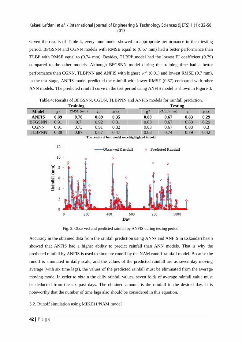
Given the results of Table 4, every four model showed an appropriate performance in their testing

period. BFGSNN and CGNN models with RMSE equal to (0.67 mm) had a better performance than

TLBP with RMSE equal to (0.74 mm). Besides, TLBPP model had the lowest EI coefficient (0.79)

compared to the other models. Although BFGSNN model during the training time had a better

performance than CGNN, TLBPNN and ANFIS with highest 2R (0.91) and lowest RMSE (0.7 mm),

in the test stage, ANFIS model predicted the rainfall with lower RMSE (0.67) compared with other

ANN models. The predicted rainfall curve in the test period using ANFIS model is shown in Figure 3.

Table.4: Results of BFGSNN, CGDN, TLBPNN and ANFIS models for rainfall prediction.Training Testing

Model 2R )(mmRMSE EI MAE 2R )(mmRMSE EI MAEANFIS 0.89 0.78 0.89 0.35 0.88 0.67 0.83 0.29

BFGSNN 0.91 0.7 0.92 0.31 0.83 0.67 0.83 0.29CGNN 0.91 0.73 0.91 0.32 0.83 0.67 0.83 0.3

TLBPNN 0.88 0.87 0.87 0.47 0.83 0.74 0.79 0.42The results of best model were highlighted in bold

Fig. 3. Observed and predicted rainfall by ANFIS during testing period.

Accuracy in the obtained data from the rainfall prediction using ANNs and ANFIS in Eskandari basin

showed that ANFIS had a higher ability to predict rainfall than ANN models. That is why the

predicted rainfall by ANFIS is used to simulate runoff by the NAM runoff-rainfall model. Because the

runoff is simulated in daily scale, and the values of the predicted rainfall are as seven-day moving

average (with six time lags), the values of the predicted rainfall must be eliminated from the average

moving mode. In order to obtain the daily rainfall values, seven folds of average rainfall value must

be deducted from the six past days. The obtained amount is the rainfall in the desired day. It is

noteworthy that the number of time lags also should be considered in this equation.

3.2. Runoff simulation using MIKE11/NAM model


43 | P a g e

The conceptual model of NAM demands for evaporation, temperature and daily rainfall data as the

input data into the model and also requires daily output discharge from the basin (for comparing the

observed flow and simulated flow). The used stations in Eskandari basin are five stations three of

which are rain gauge stations (Eskandari, Fereydan and Bouin), one is Singerd climatology station

and one is hydrometric station (Eskandari). The homogeneity of the rain gauge stations was assessed

using double mass curve test. Furthermore, the impact factor of each rain gauge station in the runoff

for calculating the basin weighted average rainfall obtained through Thiessen Polygon Technique.

After determining the weighted values of the stations, calibration and evaluation of them were

accomplished. Seven-year (1999-2006) was considered for calibration period and three-year (2006-

2009) was considered for verification period. In the verification period of the model, runoff values

were simulated once based on the observed rainfall (we call it NAM) and once based on the predicted

rainfall using ANFIS model (we call it ANFIS-NAM). Statistical analysis of the obtained results from

calibration of NAM model in Eskandari basin is shown in Table 5. As seen in Table 5, the wbE range

in simulation by the model during the calibration varied between 12.58% to 33.97%.

Table.5: Results of NAM model for the calibration period.Period )/( 3 smVobs )/( 3 smVsim % wbE MAE )/( 3 smRMSE EI 2R

1999-2000 299.5 261.798 12.58 0.52 0.69 0.51 0.592000-2001 228.93 153.517 32.94 0.83 1 0.22 0. 362001-2002 684.88 798.2068 -16.54 1.03 1.46 0.73 0.742002-2003 784.365 1032.522 -31.63 1.5 2.18 0.47 0.612003-2004 859.736 1151.803 -33.97 1.67 1.93 0.51 0.642004-2005 1441.542 1728.065 -19.87 2 2.83 0.66 0.692005-2006 3161.365 2661.1253 15.82 4.23 5.83 0.75 0.83

Calibration Period 7460.318 7787.0371 -4.37 1.68 2.78 0.77 0.78

In addition, Tables 6 and 7 illustrate the results of verification period of the NAM model based on

observed and predicted rainfall. In verification period, based on observed rainfall, wbE varied from

0.9% to 25.41%. This error is varied from 6.4 to 37.39% based on the predicted rainfall. In Figure 4,

the cumulative discharge values of the observed and predicted runoff have been compared to each

other during verification period. Comparing the results based on 2R in calibration and verification

periods demonstrated that NAM model had a relative better performance in calibration period than in

verification period. Comparison based on EI also showed this superiority at the evaluation period.

The difference between the two 2R and EI sometimes is very subtle and sometimes is sizable. The

important matter concerning the coefficient of efficiency is that the value of this coefficient was lower

than coefficient of determination both in calibration and evaluation periods which indicated systemic

error in simulation. These instances are similar to those in 2005-2006 in which despite 0.83%

coefficient of determination, their coefficient of efficiency was 0.75%. Figure 5 shows the simulated


44 | P a g e

runoff graph in verification period based on the observed rainfall and observed rainfall. The figure

shows that the NAM model had higher capabilities in simulating the base flow rather than the peak

flow.

Table.6: Results of NAM model for verification period.Period )/( 3 smVobs )/( 3 smVsim % wbE MAE )/( 3 smRMSE EI 2R

2006-2007 2961.344 2931.8613 0.99 3.12 5.21 0.75 0.752007-2008 1231.616 1107.6503 10.06 1.21 1.57 0.71 0.752008-2009 823.657 1032.977 -25.41 2.1 2.6 0.25 0.51

Verification period 5016.617 5072.488 -1.113 2.14 3.48 0.70 0.75

Table.7: Results of ANFIS-NAM model for verification period.Period )/( 3 smVobs )/( 3 smVsim % wbE MAE )/( 3 smRMSE EI 2R

2006-2007 2961.344 2735.1338 7.63 3.09 4.94 0.78 0.822007-2008 1231.616 1311.317 -6.47 2.62 3.33 0.13 0.232008-2009 823.657 1131.68 -37.39 1.59 2.18 0.47 0.80

Verification period 5016.617 5178.1308 -3.21 2.44 3.67 0.58 0.73

Fig. 4. Cumulative discharge chart of the observed and predicted runoff

Figure 5 shows duration curves for residual errors on runoff (m3/s). This trend has been derived from

subtracting of predicted from observed runoff (observed-simulated). Therefore, a positive value shows

overestimation and a negative value shows underestimation. Figure 5 shows ANFIS-NAM model has

fluctuation between 8 (overestimation) and -21 (underestimation) however NAM shows 24 as

overestimation and -29 as underestimation for residual error value. Generally, the residual errors for

both models have been aggregated around zero. According to observed data, two maximum flows

have been recorded for 3/March/2007 and 4/March/2007, which have been predicted with shorter

error values by ANFIS-NAM.


45 | P a g e

Fig. 5. Duration curves of residual errors (simulated-observed) for runoff (m 3 /s).

In this study, runoff distribution has been evaluated by box plots and supplementary analysis namely

percentile analysis of runoff which has been suggested by Jajarmizadeh et al. (2012). In its simplest

form, the box plot presents five sample statistics namely the minimum, the lower quartile that

represent 25 percentile, the median, the upper quartile that represent 75 percentile and the maximum,

in a visual display. A line is drawn across the box at the sample median. Whiskers sprout from the two

ends of the box until they reach the sample maximum and minimum. Figures 6, 7 and 8 show box

plots for observed, NAM and ANFIS-NAM as well Table 8 that is percentile analysis for daily runoff

(m3/s) for data.

Fig. 6. Box plot of observed runoff (m3/s) during 1990-2008.


46 | P a g e

Fig. 7. Box plot of simulated runoff (m3/s) by NAM model during 1990-2008.

Fig. 8. Box plot of simulated runoff (m3/s) by ANFIS-NAM model during 1990-2008.

Table.8: Percentile analysis for observed, NAM and ANFIS-NAM models for daily flow (m3/s).Model 5 10 25 50 75 90 95

Observed 0.0 0.0 0.5 2.7 5.1 10.2 19.2NAM 0.910.1 0.1 0.9 2.3 5.2 11.8 21.3

ANFIS-NAM 0.3 0.5 1.3 2.6 5.6 12.6 17.0

The box plots show models could not specified maximum flows in related events. Maximum flow has

been recorded in 194th day (4/April/2007) but NAM and ANFIS-NAM have been specified 233th and

181th day respectively. According to 50 percentile NAM and ANFIS-NAM models were more

promising however NAM has more underestimation (2.3 m3/s ) in comparison with ANFIS-NAM (5.2


47 | P a g e

m3/s) accordance with 50 percentile (Table 8). According to 75 percentile, NAM has closer value in

comparison with ANFIS-NAM but both have overestimation trend. On the other hand, 25 percentile

shows an overestimation value for both models meanwhile NAM has better value.

Figures 9 shows the ratio of cumulative daily runoff for ANFIS-NAM and NAM models versus

observed data. As it can be seen from Figure 9 ANFIS-NAM has closer value in comparison with

NAM model versus observed data. Totally, both models are promising in regard with the cumulative

daily runoff analysis for 2006-2009 period of modeling. Generally, both models have overestimation.

This evaluation shows that however the both models couldn’t strike the peak flows they have a fair

prediction in regard with cumulative discharge.

Fig. 9. Ratio analysis of cumulative daily flow for ANFIS-NAM (a) and NAM versus observed for period of2006-2009.

Figure 10 shows the simulated runoff graph in verification period based on the observed rainfall and

observed rainfall. The figure shows that the NAM model had higher capabilities in simulating the

base flow rather than the peak flow.

Fig. 10. Observed and simulated runoff by NAM and ANFIS-NAM models during Verification period.

The reasons for the weakness of the NAM model are as the following:


48 | P a g e

Although Eskandari basin is in a good condition in terms of number of meteorological stations, the

statistics of these stations are mostly incomplete and their statistical length is often very short.

Certainly, improvement of data quality and quantity in these stations can provide more appropriate

outcomes. In addition, by improving the daily data of Eskandari hydrometric station, simulation with

different time scales can be done much more accurately.

Since NAM model is an integrated and a conceptual model, low accuracy in this study showed that

further information of the area are required for more accurate estimation of the parameters.

Considering the snowfall coefficient in the model may enhance the accuracy of the model simulation.

It seems that the accuracy of the results can be enhanced in an acceptable level by improving the

information related to the hydrological conditions of this basin. For instance, dividing the basin to the

smaller sub-basins, which this affair needs to construct new stations and equip the current stations.

4. Conclusions

In this study, rainfall prediction was accomplished using some artificial intelligence techniques and

runoff simulation by making use of the conceptual hydrological MIKE11/NAM model in Eskandari

basin in Iran. Rainfall prediction was done using the three-day, five-day, and seven-day moving

averages and the GT was used to determine the best input combination. The results from rainfall

prediction using ANN ANFIS models indicated that the ANFIS model was much more capable for

predicting rainfall in Eskandari basin. The results showed that the NAM model had higher capabilities

in simulating the base flow rather than the peak flow. Using the predicted rainfall instead of the

observed rainfall caused lower efficiency and competence in the NAM model and runoff simulation.

These results consequently indicated that the efficiency of the NAM model was much more dependent

on the quantity and quality of the data input model. In many cases, a hydrometric station is located at

a considerable distance from the point where current prediction is supposed to take place. In such

instances, the current predicted in the hydrometric station reaches that point with a lag. One method

for overcoming this problem is the incorporation of rainfall-runoff models into hydrodynamic flood

routing models. This feature is provided in the Mike11/NAM model and it is suggested to be

investigated further in future studies to enhance results obtained from this study.

References

[1] Jajarmizadeh M, Harun S, Salarpour M. Using soil and water assessmwnt tool for flow simulation

and assessment of sensitive parameters applying SUFI-2 algorithm, Caspian Journal of Applied

Sciences Research 2013, 2(1), pp. 37-44.


49 | P a g e

[2] Lipiwattanakarn S, Sriwongsitanon N, Saengsawang S. Improving neural network model

performance in runoff estimation by using an antecedent precipitation index. Journal of Hydrosci

Hydraul Eng 2004a, 22(2), 141-154.

[3] Leavesley GH, Markstrom SL, Restrepo PJ, Viger RJ. A modular approach to addressing model

design, scale, and parameter estimation issue in distributed hydrological modeling. Hydrological

Processes 2002, 16(2), 173-187.

[4] Danish Hydraulic Institute (DHI). NAM Technical Reference and Model Documentation 1999.

[5] Madsen H. Automatic calibration of a conceptual rainfall-runoff model using multiple objectives,

Journal of Hydrology 2000, Vol.235, pp: 276-288.

[6] Butts M.B, Payne JT, Kristensen M, Madsen H. An evaluation of the impact of model structure on

hydrological modelling ancertainty for stream flow simulation, Journal of Hydrology 2004, Volume

298, Issue 1-4, pp. 242-266.

[7] Shamsdin S, Hashim. Rainfall runoff simulation using MIKE11 NAM. Journal of Civil

Engineering 2002, 15(2).

[8] Lekkas DF, Maxey RT, Wheather HS. Intercompartion of forecasting methods flood warning in

the river cam catchment, Global Nest 2004, Vol 5, Number 2, pp. 89-97.

[9] Lipiwattanakarn S, Sriwongsitanon N, Saengsawang S. Performance comparison of a conceptual

hydrological model and a back-propagation neural network model in rainfall-runoff modeling.2004b

Available at: https://pindex.ku.ac.th/file_research/WE95 .doc.

[10] Liu Y, Sun F. Sensivity of analysis and automatic calibration of rainfall-runoff model using

multi-objectives. Ecological Informatics 2010, vol 5, no. 4, pp: 304-310.

[11] Kakaei Lafdani E, Moghaddam Nia A, Ahmadi A. Daily suspended sediment load prediction

using artificial neural networks and support vector machines. Journal of Hydrology 2013, 478, 50-62.

[12] Stefansson A, Koncar N, Jones AJ. A note on the gamma test. Neural Computing & Application

1997, 5: 131-133.

[13] Jones AJ, Tsui A, de Oliveira AG. Neural models of arbitrary chaotic systems: construction and

the role of time delayed feedback in control and synchronization. Complexity International 2002, 9: 1-

9.

[14] Remesan R, Shamim, MA, Han D, Mathew J. Runoff prediction using an integrated hybrid

modelling scheme. Journal of Hydrology 2009, 372, 48-60.

[15] Chattopadhyay S. Feed forward artificial neural network model to predict the average summer-

monsoon rainfall in India. Acta Geophysical 2007, No.55 (3), pp.369-382.

[16] Ingsrisawang L, Ingsrisawang S, Smochit S, Aungsuratana P, Khantiyanan W. Machine learning

techniques for short-term rain forecasting system in the northeastern part of Thailand. World Academy

of Science, Engineering and Technology 2008, Vol.41, pp.248-253.

https://pindex.ku.ac.th/file_research/WE95


50 | P a g e

[17] Khodashenas SR, Khalili N, Davari K. Monthly precipitation prediction by artificial neural

networks (case study: Mashhad synoptic station) 2010. Session 1.7.

[18] Jamalizadeh MR, Moghaddamnia AR, Piri J, Arabi V, Homayounfar M, Shahryari A. Dust storm

prediction using ANNs technique (A case study: Zabol city), World Academy of Science, Engineering

and Technology 2008, 43, 512-520.

[19] Aqil M, Kita I, Yano A, Nishiyama S. A Comparative Study of Artificial Neural Networks and

Neuro-Fuzzy in Continuous Modeling of the Daily and Hourly Behaviors of Runoff. Journal of

Hydrology 2007, 337, 22– 34.

[20] Aldrian E, Djamil YS. Application of multivariate anfis for daily rainfall prediction: influences

of training data size. Makara, Sains 2008, Vol 12, No. 1, pp: 7-14.

[21] Dastorani MT, Afkhami H, Sharifidarani H, Dastorani M. Application of ANN and ANFIS

models on dryland precipitation prediction (casestudy: Yazd in central Iran). Journal of Applied

Sciences 2010, 10(20): 2387-2394.

[22] Geetha G, Selvaraj RS. Application of monthly rainfall in Chennai using back propagation neural

network model. Journal of Engineering Science and Technology 2011, Vol. 3. No. 1, pp.211-213.

[23] Ahmadi A, Han D, Karamouz M, Remesan R. Input data selection for solar radiation estimation.

Hydrological processes 2009, 23, 2754-2764.

[24] Noori R, Karbassi AR, Moghaddamnia A, Han D, Zokaei-Ashtiani MH, Farokhnia A, Ghafari

Gousheh M. Assessment of input variables determination on the SVM model performance using PCA,

Gamma test and forward selection techniques for monthly stream flow prediction. Journal of

Hydrology 2011, 401, 177-189.

[25] Moghaddamnia A, Ghafari M, Piri J, Han D. Evaporation estimation using support vector

machines technique. International Journal of Engineering and Applied Sciences 2009, 5(7), 415-423.

[26] McCulloch WS, Pitts W. A logic calculus of the ideas imminent in nervous activity. Bulletin of

Mathematical Biophysics 1943, 5: 115-133.

Daily Rainfall-Runoff Prediction and Simulation Using ANN, ANFIS and Conceptual Hydrological...

Documents

Transcript of Daily Rainfall-Runoff Prediction and Simulation Using ANN, ANFIS and Conceptual Hydrological...