Earth and Planetary Science Letters 386 (2014) 52–63

Contents lists available at ScienceDirect

Earth and Planetary Science Letters

www.elsevier.com/locate/epsl

High elevation of the ‘Nevadaplano’ during the Late Cretaceous

Kathryn E. Snell a,d,∗, Paul L. Koch a, Peter Druschke b, Brady Z. Foreman c, John M. Eiler d

a Earth and Planetary Sciences Department, University of California Santa Cruz, 1156 High Street, Santa Cruz, CA 95064, USAb Department of Geosciences, University of Nevada Las Vegas, 4505 S. Maryland Parkway, Las Vegas, NV 89154, USAc Department of Earth Sciences, St. Anthony Falls Laboratory, University of Minnesota, 2 SE 3rd Ave, Minneapolis, MN 55414, USAd Division of Geological and Planetary Sciences, California Institute of Technology, Pasadena, CA 91125, USA

a r t i c l e i n f o a b s t r a c t

Article history:Received 8 January 2013Received in revised form 6 October 2013Accepted 26 October 2013Available online 20 November 2013Editor: J. Lynch-Stieglitz

Keywords:Nevadaplanopaleoelevationpaleoclimatestable isotopesSevier hinterlandpaleothermometry

During the Late Cretaceous, central Nevada may have been a high elevation plateau, the Nevadaplano;some geodynamic models of the western US require thickened crust and high elevations during theMesozoic to drive the subsequent tectonic events of the Cenozoic while other models do not. Totest the hypothesis of high elevations during the late Mesozoic, we used carbonate clumped isotopethermometry to determine the temperature contrast between Late Cretaceous to Paleocene carbonatesatop the putative plateau in Nevada versus carbonates from relatively low paleoelevation central Utahsite. Lacustrine carbonates from the Nevada site preserve summer temperatures ∼ 13 ◦C cooler thansummer temperatures from paleosol carbonates from the Utah site, after correcting for ∼ 1.2 ◦C of secularclimatic cooling between the times of carbonate deposition at the two sites. This ∼ 13 ◦C temperaturedifference implies an elevation difference between the two sites of ∼ 2.2–3.1 km; including uncertaintiesfrom age estimation and climate change broadens this estimate to � 2 km. Our findings support crustalthickness estimates and Cenozoic tectonic models that imply thickened crust and high elevation inNevada during the Mesozoic.

© 2013 Elsevier B.V. All rights reserved.

1. Introduction

Reconstructions of crustal thickness, spatial and temporal dis-tributions of mid-crustal metamorphism, and sedimentary basinsindicate that by the end of the Mesozoic, central Nevada mayhave been a high elevation plateau (Coney and Harms, 1984;DeCelles, 2004; Druschke et al., 2011, 2009b; Ernst, 2010), termedthe ‘Nevadaplano’ (DeCelles, 2004). The probable ‘Nevadaplano’formed in the hinterland between the Sierra Nevada volcanic arcto the west and the Sevier fold and thrust belt to the east (Fig. 1)during Jurassic–Eocene contraction associated with subduction ofthe Farallon plate under North America (DeCelles, 2004). Duringthe Cenozoic, tectonic deformation in the western United Stateswas dominated by extension. Extension via block-faulting is gen-erally attributed to the migration of the Mendocino triple junctionafter intersection of the East Pacific Rise with southern Californiaat ∼ 25 Ma (Dickinson, 2002). However, the cause of Late Creta-ceous and early Cenozoic extension, which is commonly associatedwith metamorphic core complexes and magmatism (Armstrongand Ward, 1991; Coney and Harms, 1984), is debated.

* Corresponding author at: California Institute of Technology, Div. of Geologicaland Planetary Sciences, MC 100-23, Pasadena, CA 91125, USA. Tel.: +1 626 395 6868.

E-mail address: ksnell@caltech.edu (K.E. Snell).

0012-821X/$ – see front matter © 2013 Elsevier B.V. All rights reserved.http://dx.doi.org/10.1016/j.epsl.2013.10.046

Some workers suggest that Mesozoic contraction thickened andelevated the crust, resulting in sufficient gravitational potentialenergy to drive later extension (e.g. Jones et al., 1998). Alter-natively, the slab-buckling model (Humphreys, 1995) neither re-quires nor precludes previously thickened and elevation crust inthe Mesozoic–Cenozoic Sevier hinterland to drive Cenozoic exten-sion. This model, and similar models that suggest uplift due to re-moval of mantle lithosphere during the early Cenozoic (e.g. Saltusand Thompson, 1995), are favored by stable-isotope paleoelevationreconstructions from that suggest the western Cordillera reachedpeak elevations in the early Cenozoic during a diachronous, north-to-south sweep of surface uplift (Horton et al., 2004; Kent-Corsonet al., 2006; Mix et al., 2011).

Our current understanding of paleoelevation within the Meso-zoic–Paleocene western Cordillera results from indirect sources.Unspecified high elevation is inferred from favorable comparisonof the Sevier hinterland with the modern Tibetan Plateau andAndean Altiplano (Coney and Harms, 1984; Molnar and Chen,1983). Crustal thickness estimates of 50–60 km (e.g. Coney andHarms, 1984) led some authors to infer elevations for the Sevierhinterland of > 2 km and more likely > 3 km (DeCelles, 2004;DeCelles and Coogan, 2006; House et al., 2001; Jones et al., 1998).Similarity of paleodrainage relief in the ancestral Sierra Nevada (in-ferred from apatite (U–Th)/He ages) to long-wavelength relief inmodern orogens was used to interpret elevations of > 3 km in the

K.E. Snell et al. / Earth and Planetary Science Letters 386 (2014) 52–63 53

Fig. 1. (A) Map (modified from Druschke et al., 2011) and (B) schematic cross-section (modified from Miller and Gans, 1989 and Wells and Hoisch, 2008); inset cross-sectionof the Axhandle Basin (modified from Talling et al., 1994) shows the location of the sampling sites. LFTB = Luning-Fencemaker Thrust Belt. CNTB = Central Nevada ThrustBelt. Light gray shading on the larger cross-section over the volcanic arc and Sevier thrust belt indicates possibly higher elevation in these two regions relative to thehinterland during the Late Cretaceous.

interior of the Cordillera during the Cretaceous (House et al., 2001).Finally, isotope-enabled global climate models find the best matchbetween model-predicted and existing mineral δ18O values fromsimulations that prescribe high elevations in the western Cordillera(Fricke et al., 2010; Poulsen et al., 2007). A recent study inves-tigating pre-extensional paleoelevations of the Sheep Pass Basinin central Nevada uses Paleocene–Eocene temperatures to suggestlow-to-moderate elevations (� 2 km) of the region (Lechler et al.,2013). Although these data pre-date Miocene extension, they tem-porally overlap with early Cenozoic extension and the elevationestimate integrates data over ∼ 15 m.y.; therefore this estimatemay not capture peak elevation of the Sevier hinterland prior toextension. Thus, while these previous studies generally suggest theSevier hinterland was elevated, direct estimates of the paleoeleva-tion are lacking.

We use carbonate clumped isotope (�47) thermometry (Ghoshet al., 2006) to determine formation temperatures of ∼ 68–60 Malacustrine carbonates from the Sheep Pass Formation of east–central Nevada (NV), atop the hypothesized Nevadaplano (Druschkeet al., 2009b; Vandervoort and Schmitt, 1990) (Fig. 1), and from∼ 75–71 Ma paleosol carbonates of the presumably low elevationNorth Horn Formation in central Utah (UT) (DeCelles and Coogan,2006; Lawton and Trexler, 1991) (Fig. 1). We use the temperaturecontrast between the sites to estimate paleoelevation of the Sevierhinterland during the latest Cretaceous. This estimate is compli-cated by several factors: variable preservation; climate changeduring the period that separates deposition at the two sites; poten-tial differences in the season of carbonate formation in soils andlakes; and uncertainty in environmental lapse rates. We examinehow each of these factors affects our paleoelevation estimate. Inaddition, we outline an approach to explicitly correct for climatechange and assess the sensitivities of our elevation estimate to un-certainties. This study provides an alternative approach for datasetsthat span long time intervals and/or compare to low-elevation sitesthat are not exactly the same age (e.g. Huntington et al., 2010;Lechler et al., 2013; Wolfe et al., 1998).

2. Materials and methods

2.1. Nevada site (NV) and samples

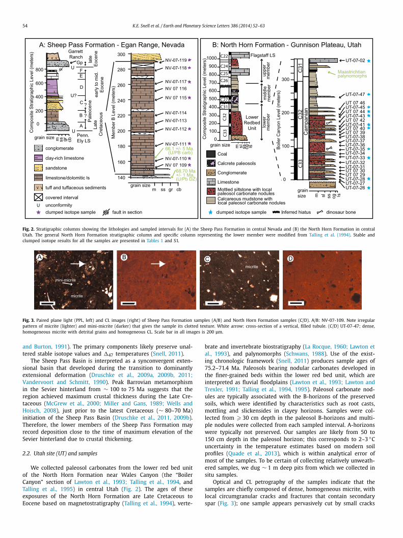
We collected lacustrine carbonate samples from Member B ofthe Sheep Pass Formation type section (Fig. 2). Member B isLate Cretaceous to late Paleocene in age, based on biostratigra-phy, palynology, detrital zircon U–Pb, and U–Pb dating of car-bonate (Druschke et al., 2009a, 2009b; Fouch, 1979; Good, 1987;Swain, 1999). Using this chronology, our samples range in age from66.7 to 59.9 Ma (Snell, 2011). Member B comprises dominantlytan to light brown microbial limestone beds (Fouch, 1979; Kellogg,1964; Winfrey, 1960). The lower part is composed dominantly ofmudstone and wackestone, whereas the middle part also containsinversely-graded units with laminated micrite beds capped by algalstromatolites and/or thin grainstone beds with local ripple cross-stratification. The upper part is locally dolomitic and siliceous,and contains ostracodes, charophytes, bivalves, calcite-filled ver-tical branching tubes, polygonal dessication cracks and wavy, ir-regular lamination throughout the unit (Fouch, 1979; Fouch et al.,1991). These features and clotted fabrics typical of microbial car-bonates, were also found in petrographic analysis of the samples(Snell, 2011). Branching tubes likely reflect the presence of aquaticplants, whereas dessication cracks indicate intermittent subaerialexposure (Fouch, 1979). These features suggest that Member B wasdeposited in a shallow-water lake setting, likely in the littoral tosub-littoral zone (Fouch, 1979; Fouch et al., 1991; Good, 1987;Winfrey, 1960).

Optical and cathodoluminescence (CL) petrography of the sam-ples reveals primary, secondary and altered components (Fig. 3).Clotted fabrics, burrows, micritic peloids, biogenic clasts and intra-clasts are common features of microbial limestones (Fouch andDean, 1982); we suggest these features are primary, depositionalattributes (Snell, 2011). In contrast, the anhedral, inequigranu-lar fabrics and speckled CL patterns of the microspars and spars,present as small patches within the samples, are typical recrys-tallization fabrics (Boggs and Krinsley, 2006; Flügel, 2004; Machel

54 K.E. Snell et al. / Earth and Planetary Science Letters 386 (2014) 52–63

Fig. 2. Stratigraphic columns showing the lithologies and sampled intervals for (A) the Sheep Pass Formation in central Nevada and (B) the North Horn Formation in centralUtah. The general North Horn Formation stratigraphic column and specific column representing the lower member were modified from Talling et al. (1994). Stable andclumped isotope results for all the samples are presented in Tables 1 and S1.

Fig. 3. Paired plane light (PPL, left) and CL images (right) of Sheep Pass Formation samples (A/B) and North Horn Formation samples (C/D). A/B: NV-07-109. Note irregularpattern of micrite (lighter) and mini-micrite (darker) that gives the sample its clotted texture. White arrow: cross-section of a vertical, filled tubule. (C/D) UT-07-47; dense,homogeneous micrite with detrital grains and homogeneous CL. Scale bar in all images is 200 μm.

and Burton, 1991). The primary components likely preserve unal-tered stable isotope values and �47 temperatures (Snell, 2011).

The Sheep Pass Basin is interpreted as a synconvergent exten-sional basin that developed during the transition to dominantlyextensional deformation (Druschke et al., 2009a, 2009b, 2011;Vandervoort and Schmitt, 1990). Peak Barrovian metamorphismin the Sevier hinterland from ∼ 100 to 75 Ma suggests that theregion achieved maximum crustal thickness during the Late Cre-taceous (McGrew et al., 2000; Miller and Gans, 1989; Wells andHoisch, 2008), just prior to the latest Cretaceous (∼ 80–70 Ma)initiation of the Sheep Pass Basin (Druschke et al., 2011, 2009b).Therefore, the lower members of the Sheep Pass Formation mayrecord deposition close to the time of maximum elevation of theSevier hinterland due to crustal thickening.

2.2. Utah site (UT) and samples

We collected paleosol carbonates from the lower red bed unitof the North Horn Formation near Wales Canyon (the “BoilerCanyon” section of Lawton et al., 1993; Talling et al., 1994, andTalling et al., 1995) in central Utah (Fig. 2). The ages of theseexposures of the North Horn Formation are Late Cretaceous toEocene based on magnetostratigraphy (Talling et al., 1994), verte-

brate and invertebrate biostratigraphy (La Rocque, 1960; Lawton etal., 1993), and palynomorphs (Schwans, 1988). Use of the exist-ing chronologic framework (Snell, 2011) produces sample ages of75.2–71.4 Ma. Paleosols bearing nodular carbonates developed inthe finer-grained beds within the lower red bed unit, which areinterpreted as fluvial floodplains (Lawton et al., 1993; Lawton andTrexler, 1991; Talling et al., 1994, 1995). Paleosol carbonate nod-ules are typically associated with the B-horizons of the preservedsoils, which were identified by characteristics such as root casts,mottling and slickensides in clayey horizons. Samples were col-lected from � 30 cm depth in the paleosol B-horizons and multi-ple nodules were collected from each sampled interval. A-horizonswere typically not preserved. Our samples are likely from 50 to150 cm depth in the paleosol horizon; this corresponds to 2–3 ◦Cuncertainty in the temperature estimates based on modern soilprofiles (Quade et al., 2013), which is within analytical error ofmost of the samples. To be certain of collecting relatively unweath-ered samples, we dug ∼ 1 m deep pits from which we collected insitu samples.

Optical and CL petrography of the samples indicate that thesamples are chiefly composed of dense, homogeneous micrite, withlocal circumgranular cracks and fractures that contain secondaryspar (Fig. 3); one sample appears pervasively cut by small cracks

K.E. Snell et al. / Earth and Planetary Science Letters 386 (2014) 52–63 55

that are filled with secondary spar (UT-07-44). Following previouswork (Budd et al., 2002; Driese and Mora, 1993; Snell et al., 2013;Wieder and Yaalon, 1982), we interpret the dense micrite as aprimary component that likely preserves unaltered stable isotopevalues and �47 temperatures (Snell, 2011).

The lower red bed unit of the North Horn Formation is thoughtto have been at low elevation during deposition because this unitmarks initiation of the Axhandle Piggyback Basin atop older Se-vier foreland basin strata (DeCelles and Coogan, 2006; Lawton andTrexler, 1991). Piggyback basins develop on active thrust sheetswhen new thrust ridges develop out past older thrust margins (Oriand Friend, 1984). Thus, at the inception of the Axhandle basin,the basin was likely at similar elevation to the low-elevation Sevierforeland, and was < 200 km west of the shoreline of the WesternInterior Seaway (WIS), which is marked by age-equivalent alternat-ing marine/non-marine sedimentary rocks in the Bookcliffs region(Willis, 2000).

2.3. Stable isotope geochemistry

2.3.1. Carbonate clumped isotope (�47) thermometryDuring carbonate formation, lower temperatures of mineral for-

mation increase “clumping” of 18O–13C in carbonate ions; theequation that describes this temperature dependence is used asa paleothermometer (Ghosh et al., 2006). Because measurement of13C18O16O2−

2 is currently impossible, CO2(g) created by phospho-ric acid digestion of calcium carbonate is measured instead (Ghoshet al., 2006). Variations in the abundance of doubly-substitutedisotopologues in such evolved CO2(g) (13C18O16O, mass-47) arereported as �47 and defined as the per mil deviation in the mea-sured mass 47-to-mass 44 ratio (R47

sample = M47sample/M44

sample) com-

pared to the expected R47 value for a stochastic distribution ofisotopes (Eiler and Schauble, 2004):

�47 =( R47

sample

R47stochastic

)× 1000 (1)

Stable carbon (δ13C) and oxygen isotope (δ18O) values (deter-mined simultaneously with every �47 value) as well as estimatesof �47 temperatures and the δ18O values of water (δ18Ow) fromwhich the carbonate formed, were produced for a subset of sam-ples collected from the Sheep Pass Formation and the North HornFormation. We report the carbon and oxygen isotope values fol-lowing standard delta notation as the per mil deviation of sample18O or 13C relative to the PDB standard 18O or 13C composition:δX = ((Rsample/Rstandard) − 1) × 1000, where Rsample and Rstandardare the ratios of the higher-mass isotope relative to the lower-massisotope for the sample and standard, respectively.

2.3.2. Sample preparation for �47 analysisWe milled ∼ 30–50 mg of sample powder for �47 analysis

from polished surfaces using a dental drill bit under a binocularmicroscope. We drilled aliquots of the micritic sections of all ofthe samples selected for �47 analysis. Where present in sufficientquantity, co-occurring secondary spars and carbonate cements inthe samples were drilled to establish formation temperatures ofsecondary fluids that interacted with the samples. To avoid drillingunwanted material (e.g., mixing of the secondary phases with theprimary micrite), we marked the areas free of secondary or alteredcarbonate on thin sections, then drilled the matching sites on thesample billets. Sample surfaces were drilled to a maximum depthof ∼ 1–2 mm. Once all the reliable powder was drilled from theinitial surface, the samples were re-planed and re-polished with alapidary wheel.

2.3.3. Analytical procedureSample powders (8–10 mg for 100% carbonate samples – lacus-

trine and vein calcite and standards – and 12–20 mg for paleosolcarbonates) were loaded and analyzed on a ThermoFinnegan MAT253 gas source isotope ratio mass spectrometer at Caltech (MS Iand II of Huntington et al., 2009) configured for automated CO2 gasgeneration, cleaning, and subsequent analysis following establishedprocedures and calculations (Eiler, 2007; Huntington et al., 2009;Passey et al., 2010; Wang et al., 2004). All samples were convertedto CO2(g) via phosphoric acid digestion at 90 ◦C, except samplesession 9 gases were generated at 25 ◦C. Carbonate δ18O (δ18Oc)values were calculated using an acid digestion fractionation factorfor 90 ◦C of 1.000821 (Swart et al., 1991). Five analyses that dis-played excess mass-48 (�48, defined similarly to �47 as the excessmass-48 relative to the abundance expected based on a stochas-tic distribution) were not used in the final dataset given that theymay also have contained anomalous mass-47 abundances (follow-ing Huntington et al., 2009). Four of the mass-48 excesses werethe results of analytical issues (e.g. large drifts in the isotopic ra-tios and failure of the GC liquid nitrogen regulation value), and thefifth mass-48 excess is likely a function of incomplete cleaning ofhydrocarbons or halocarbons that may produce isobaric interfer-ence.

2.3.4. Replication and analytical errorUncorrected �47 (�47,unc) values and the associated δ13C and

δ18O values produced for each gas are averages of 5–8 acquisi-tions of the gas which each comprise 7–10 cycles of 8-second peakintegration times for both the sample and reference gas analysisduring each cycle. Analytical precision (reported as one standarderror of the mean (1 s.e.)) for individual gas �47,unc values rangesfrom 0.005 to 0.025� (Table S1). We corrected the �47,unc val-ues (�47,corr) for non-linearity effects in the mass spectrometerusing the heated gas line, and corrected for changes in the heatedgas line since the original �47-temperature calibration using astretching factor (following Huntington et al., 2009 and Passey etal., 2010). Uncertainties for �47,corr values (±1 s.e.) include ana-lytical errors for the sample gases, and propagated errors associ-ated with the heated gas line (following Huntington et al., 2009;Snell, 2011 and Snell et al., 2013). Uncertainties for �47,corr valuesfor our samples range from 0.007 to 0.029� (Table S1).

We report final values relative to both the “in-house” Caltechscale (after applying an acid digestion correction of 0.081 to thesamples that were run at 90 ◦C) and to the Absolute ReferenceFrame (ARF) of Dennis et al. (2011). The robust way to convertto the ARF is to use heated gases and gases equilibrated with wa-ter at 25 ◦C to create transfer functions that convert the “in-house”values to the ARF. However, we analyzed these samples prior tothe development and adoption of this method and so there are noequilibrated gas data available for our dataset. Instead, we followeda modified version of a secondary approach outlined in Denniset al. (2011) that uses carbonate standard data to construct thetransfer functions used to convert our data to the ARF.

We compiled existing standard values that were converted tothe ARF via the equilibrated gas approach to determine acceptedARF values for all of our current standards (Hagit Carrara andTV01 – these accepted values are different than those quoted inDennis et al., 2011). We used these values and the secondaryapproach described in Dennis et al. (2011) to convert carbonatestandards to the ARF that are no longer used but were used dur-ing the generation of this dataset; these are listed in Table S1.We then created transfer functions for each sample session us-ing these standard values and the accepted value for the heatedgas intercept (Dennis et al., 2011); we used the in-house acid di-gestion corrected sample values to convert to the ARF (Table S1).We generated temperatures from the in-house Caltech �47 values

56 K.E. Snell et al. / Earth and Planetary Science Letters 386 (2014) 52–63

Table 1Whole-sample average stable isotope, �47 and temperature values for NV site samples (Sheep Pass Formation) and UT site samples (North Horn Formation) and Two MedicineFormation samples. Numbers in the sample code for the NV and UT samples stand for the year the sample was collected (“07”), then sample interval number (e.g. “35” or“109”). Numbers after the sample interval number for UT samples designate a specific nodule for that interval. “sp” indicates secondary spar. Altered samples were not usedin the paleoelevation reconstruction. Italics denote the samples used in the subset averages; average values are calculated as weighted averages, using the uncertainties asweighting factors. See Table S1 for all raw data.

SampleID

Age(Ma)

�47

(average)�47

(1 s.e.)AverageT (◦C)

T (◦C)(1 s.e.)

δ18Oc

(�, PDB)δ18Oc

(1 s.e.)δ13Cc

(�, PDB)δ13Cc

(1 s.e.)δ18Ow

(�, SMOW)δ18Ow

(1 s.e.)

Utah: Primary carbonateUT-07-26-1 75.16 0.605 0.019 34.5 4.9 −7.79 0.220 −8.67 0.474 −3.56 0.95UT-07-28-2 74.97 0.607 0.023 34.2 5.9 −7.54 0.144 −9.06 0.044 −3.36 1.13UT-07-33-1 74.02 0.576 0.010 42.1 3.2 −8.16 0.029 −8.21 0.006 −2.53 0.58UT-07-35-1 73.68 0.596 0.004 36.9 1.8 −8.01 0.130 −9.14 0.009 −3.32 0.36UT-07-40-1 72.79 0.591 0.020 38.1 5.2 −8.41 0.093 −8.11 0.017 −3.52 0.97UT-07-41-1 72.65 0.618 0.021 31.5 5.1 −8.02 0.117 −5.43 0.059 −4.38 1.00UT07-43-1 72.36 0.597 0.019 36.7 5.1 −9.15 0.094 −8.08 0.026 −4.51 0.96UT-07-47 71.45 0.584 0.017 40.0 4.7 −8.53 0.125 −8.79 0.100 −3.28 0.87Averages

all samples 73.39 37.4 3.2 −3.3 0.6subset average 71.90 38.5 2.3 −3.8 0.9

Utah: AlteredUT-07-28-1 74.97 0.576 0.016 42.1 4.5 −7.63 0.107 −8.97 0.023 −1.98 0.82UT-07-44 72.22 0.589 0.024 38.6 6.3 −8.75 0.070 −7.99 0.186 −3.76 1.17UT-07-02 69.69 0.536 0.010 53.3 3.7 −13.79 0.221 −0.39 0.089 −6.24 0.67

Utah:Secondary carbonateUT-07-28-2sp 74.97 0.613 0.021 32.8 5.4 −10.56 0.191 −8.11 0.179 −6.67 1.04UT-07-33-1sp 74.02 0.554 0.015 48.0 4.7 −13.54 0.024 −8.81 0.014 −6.88 0.82UT-07-41-1sp 72.65 0.610 0.000 33.5 1.5 −9.28 0.016 −5.92 0.025 −5.25 0.28UT-07-41 cement 72.65 0.591 0.020 38.1 5.4 −8.65 0.047 −5.97 0.101 −3.75 1.01UT-07-45 cement 72.09 0.537 0.006 52.8 3.0 −12.08 0.112 −7.40 0.271 −4.59 0.51

Nevada: Primary carbonateNV-07-109 66.73 0.646 0.010 25.0 2.8 −11.74 0.076 −2.59 0.034 −9.37 0.57NV-07-110 66.20 0.653 0.012 23.4 3.0 −11.65 0.037 −0.37 0.006 −9.60 0.61NV-07-112 64.39 0.653 0.012 23.5 3.1 −12.17 0.110 1.89 0.026 −10.12 0.63NV-07-115 62.44 0.630 0.005 28.7 1.8 −5.00 0.123 3.14 0.024 −1.88 0.38NV-07-117 61.32 0.651 0.006 24.0 2.1 −4.55 0.090 0.02 0.003 −2.38 0.44NV-07-118 60.07 0.620 0.007 31.1 2.2 −5.37 0.110 3.62 0.135 −1.78 0.43NV-07-119 59.95 0.647 0.013 24.8 3.2 −7.62 0.170 −1.47 0.004 −5.28 0.67Averages

all samples 63.01 26.5 3.2 −4.5 3.8subset average 66.47 24.3 1.1 −9.5 0.2

Nevada: Altered carbonateNV-07-111 65.32 0.596 0.026 37.0 6.7 −15.93 0.037 −0.30 0.010 −11.27 1.24

Nevada:Secondary carbonateNV-07-109-sp 66.73 0.570 0.012 43.7 3.7 −21.72 0.289 −2.22 0.016 −15.88 0.72NV-07-112sp 64.39 0.585 0.034 39.7 9.0 −24.57 0.177 7.35 0.471 −19.46 1.64

Montana: Two Medicine FormationTMA3-2 (lacustrine) ∼ 75 0.623 0.02 30.33 4.64 −10.77 0.08 −7.842 0.048 −7.35 0.90TM Lenoir1 (lacustrine) ∼ 75 0.614 0.04 32.44 8.92 −11.23 0.11 −7.026 0.062 −7.40 1.71TMB Caliche1 (paleosol) ∼ 75 0.629 0.03 28.95 6.75 −10.57 0.07 −8.535 0.072 −7.42 1.33

using the original Ghosh calibration (Ghosh et al., 2006); for theARF values, we used both the converted Ghosh and Dennis cali-brations (Dennis et al., 2011). A few of the older sample sessions,which have no standards with accepted ARF values independentlydetermined from the equilibrated gas approach, have large (∼ 5 ◦C)differences between the in-house and ARF temperatures. This likelyresults from iteratively back-calculating ARF values for older stan-dards with few sample sessions with sufficient overlap of new andold standards to make well-defined ARF values. These standardshave well-defined in-house values, however, so we base our in-terpretations on the �47 values and temperatures on the internalreference frame at Caltech. The later sample sessions that rely onstandards that have well-defined ARF values produce very small(< 1 ◦C) and consistent offsets between the internal and ARF tem-peratures, so our interpretations should be minimally affected bythis choice. Choice of calibration makes a large difference, however.The Dennis calibration is shallower than the Ghosh calibration, andcrosses over at 30–32 ◦C. Thus the cooler temperatures at the NVsite become colder while the warmer temperatures at the UT site

become hotter, creating a much larger temperature difference be-tween the sites. Given that the Ghosh calibration is the steepest ofthe calibrations, this means our elevation estimate is likely a min-imum estimate.

Using separate subsamples of the 30–50 mg aliquot of sam-ple powder, we produced 2–6 �47,corr, δ13C, and δ18Oc values foreach sample. From these replicate values, we generated weighted-average �47, δ13C and δ18Oc values and their associated uncer-tainties for each sample (Table 1). We calculated weighted av-erages to account for the errors associated with each replicate;the uncertainties for each measurement are the weighting factors,following Huntington et al. (2009). Standard error for weighted-average �47 values ranged from 0.0001 to 0.034�, with an av-erage error of 0.015� (Table 1). Temperatures were calculatedusing the weighted-average �47 values; final temperature error isbased on whole-sample error and the error associated with thepublished �47-to-temperature calibration line (Ghosh et al., 2006;Huntington et al., 2009). δ18Ow values were calculated for eachsample (using the calcite-to-water fractionation factor from Kim

K.E. Snell et al. / Earth and Planetary Science Letters 386 (2014) 52–63 57

Table 2Temperature differences and corresponding elevation estimates using different modern environmental temperature gradients, and different possible magnitudes of climatechange. Values in parentheses indicate ±1 s.e. Elevation estimates in bold (row three) are the elevations we suggest are most likely, while the elevation estimates that arebold and italicized (rows five and seven) indicate the maximum range of possible elevation given uncertainty associated with climate change and temperature gradient used.

Temperaturedifference(◦C)

Elevation (km), using a lapse rate of

4.2 ◦C/km 6 ◦C/km 8 ◦C/km

Subset averages (1) 14.2 (±2.6) 3.4 (±0.6) 2.4 (±0.4) 1.8 (±0.3)

All samples (2) 10.8 (±4.5) 2.6 (±1.1) 1.8 (±0.7) 1.4 (±0.6)

(1) −1.2 ◦C cooling 13.0 3.1 2.2 1.6(2) −1.2 ◦C cooling 9.6 2.3 1.6 1.2

(1) +4.7 ◦C warming 18.9 4.5 3.1 2.4(2) +4.7 ◦C warming 15.5 3.7 2.6 1.9

(1) −3.3 ◦C cooling 10.9 2.6 1.8 1.4(2) −3.3 ◦C cooling 7.5 1.8 1.3 0.9

Table 3δ18O values of carbonate from each marine basin and corresponding differences in δ18O of carbonate from each marine basin from the time of deposition at the UT siteto deposition at the NV site. The average δ18O difference for all three basins (as referred to in the text) is highlighted in bold. Ages correspond to the average age forthe youngest samples from UT site and the oldest samples from the NV site as defined in Table 1 (“subset averages”). “Min δ18O” and “max δ18O” values are minimumand maximum δ18O carbonate values for each marine basin within the range of ages allowed by uncertainties in the chronologic frameworks at the UT and NV sites. Thesubsequent values correspond to the amount of temperature change implied by each change in δ18O value. Values in bold italics indicate the maximum increase and decreasein δ18O of carbonate and temperature implied by the three marine records.

North Atlantic 1 s.d. Eq. Pacific 1 s.d. Southern Ocean 1 s.d. Average

UT (71.90 Ma) 0.6 0.2 0.0 0.2 0.4 0.1NV (66.5 Ma) 0.7 0.2 0.5 0.3 0.5 0.3

δ18O difference (�) 0.08 0.50 0.15 0.24Temp. difference (◦C) −0.4 −2.5 −0.7 −1.2

UT min δ18O 0.6 0.1 −0.1 0.2 0.1 0.1UT max δ18O 0.8 0.2 0.6 0.2 0.6 0.2NV min δ18O −0.1 0.1 0.0 0.2 −0.3 0.2NV max δ18O 0.7 0.2 0.6 0.3 0.6 0.1

Max increase (�) 0.2 0.2 0.7 0.3 0.5 0.2Max cooling (◦C) −0.8 1.2 −3.3 1.7 −2.7 0.8

Max decrease (�) −0.9 0.2 −0.6 0.3 −0.9 0.3Max warming (◦C) 4.6 1.2 3.0 1.6 4.7 1.3

and O’Neil, 1997) from the weighted-average δ18Oc value and theweighted-average �47 temperature specific to each sample. Errorsfor the calculated δ18Ow values include both δ18Oc and tempera-ture errors.

2.4. Estimating elevation

We compiled the �47 temperatures of the samples interpretedin Snell (2011) to preserve primary material (Table 1). We gen-erated a weighted-average temperature from the samples to de-termine a representative paleotemperature for each site (Table 1),using the uncertainties associated with each temperature as theweighting factor. We calculated a temperature difference betweenthe two sites from these representative temperatures (Table 2).We then applied these temperature differences to a range oftemperature-versus-elevation (T /km) relationships to estimate ele-vation (Tables 3 and 4). Errors were calculated using standard errorpropagation methods and the equation for unbiased variance forsmall sample sizes, as outlined in Huntington et al. (2009).

3. Results and discussion

3.1. Accounting for climate change

To account for effects of secular climate change on our paleoel-evation estimates, we must address the direction(s) and magnitudeof climate change that occurred during the ∼ 5.5 m.y. gap between

Table 4Temperature gradients and lapse rates that include regional lake surface water tem-perature gradients for different seasons as well as global and regional atmosphericlapse rates. Lake temperature data is from the southwestern USA, from 1979 to2007.

Type Value Citation

Temperature gradientsummer lake surface water −5.8 ◦C/km Huntington et al., 2010winter lake surface −4.8 ◦C/km Huntington et al., 2010modern lake carbonate �47 −4.2 ◦C/km Huntington et al., 2010

Atmospheric lapse rateglobal average atm. −6 ◦C/km Wolfe, 1992Arizona max air −6.8 ◦C/km Meyer, 1992Arizona min air −8 ◦C/km Meyer, 1992

the NV and UT sites. Ideally, we would evaluate this from high-resolution Campanian to Maastrichtian records from the westernCordillera, WIS and coastal Pacific Ocean (off the North Ameri-can coast) – the regions closest to our two sampling sites. Suchrecords do not exist, however, so we use benthic foraminiferalδ18O records through the time period of interest from three dif-ferent ocean basins (Barrera and Savin, 1999; Cramer et al., 2009;Friedrich et al., 2004; Huber et al., 2002; MacLeod et al., 2005;Wilf et al., 2003); ages for these records were adjusted to thetimescale of Gradstein et al. (2004).

Terrestrial paleoclimate may not respond linearly or consis-tently with the direction and magnitude of global climate changeimplied by the marine record. To justify our comparison to the

58 K.E. Snell et al. / Earth and Planetary Science Letters 386 (2014) 52–63

composite marine δ18O records, two conditions must be satisfied.The first is that high-latitude, deep ocean temperature changes(i.e. the benthic foraminiferal δ18O record) reasonably approximateglobal temperatures changes. This condition is met during ice-freetimes like the Late Cretaceous and Paleogene, albeit with some un-certainty (Hansen et al., 2008; Royer et al., 2012).

The second is that western U.S. temperatures track the direc-tion and magnitude of global temperature change during the lateCretaceous and early Cenozoic. Changes in land temperature areoften assumed to be amplified relative to changes in global tem-peratures (e.g. Royer et al., 2012). However, during the Paleocene–Eocene Thermal Maximum (the best characterized time periodwithin the Cretaceous/Early Cenozoic greenhouse), mean annualtemperature (MAT) and summer temperature changes from proxydata (5–7 ◦C; Fricke and Wing, 2004; Snell et al., 2013; Wing et al.,2005) are similar to temperature changes implied from the ben-thic δ18O record for the event (5–6 ◦C; Kennett and Stott, 1991;Zachos et al., 2001). Further, many climate model studies thatare cited as indicating amplification of land warming relative toglobal changes (e.g. Kump and Pollard, 2008; Lunt et al., 2010;Renssen et al., 2004; Sloan and Rea, 1996; Winguth et al., 2010),show only slight amplification of terrestrial temperature changes(0.5–1 ◦C) in western North America between 40◦N and 45◦N.Thus, we assume that for this place and time, the timing andmagnitude of the benthic δ18O record is a reasonable approxima-tion for the timing and magnitude of climate change that affectedour sample sites. However, more terrestrial temperature data fromwestern North America are necessary to further test this assump-tion.

The benthic δ18O records suggest global climate cooled dur-ing the Campanian and Maastrichtian (Barrera and Savin, 1999;Huber et al., 2002; MacLeod et al., 2005) with a pulse of warmingduring the latest Maastrichtian that may be associated with Dec-can Trap volcanism (Barrera and Savin, 1999; Huber et al., 2008;Thibault and Gardin, 2010; Wilf et al., 2003). A new clumpedisotope paleotemperature record from macrofossils in the WIS, al-though it is of low temporal resolution, supports this trend andsuggests ∼ 2 ◦C of cooling in the WIS from the Campanian to theMaastrichtian (Dennis et al., 2012). How the continental interiorof western North America responded to this cooling is unclear,however. A sparse MAT record dominantly from paleofloras fromthe southeastern United States suggests warming in North Americafrom later Campanian to ∼ middle Maastrichtian (Wolfe and Up-church, 1987). However, these temperatures may reflect regionalsea surface warming in the North Atlantic (MacLeod et al., 2005),rather than conditions in the WIS and western North America.

3.1.1. Choice of representative site temperatureTemperatures based on �47 thermometry for NV lacustrine

carbonates range from 23.4 ◦C to 31.1 ◦C, averaging 26.5 ± 3.2 ◦C(1 s.e.), while �47 temperatures from UT paleosol carbonates rangefrom 31.5 to 42.1 ◦C, averaging 37.4 ± 3.2 ◦C (1 s.e.; Figs. 4, 5 andTable 1). The temperature difference between the NV and UT sitesbased on averages of all the samples is 10.8 ± 4.5 ◦C (1 s.e.; Ta-bles 1, 2). However, this approach includes changes in temperaturethat occurred during as well as between the time of deposition ofthe samples. To avoid potential biases caused by averaging acrosssecular climate changes, we can improve our estimate of the ele-vation difference between the two sites by comparing averages ofa subset of samples from each site that are closest in age to eachother (hereafter “subset averages”). This produces site average tem-peratures that incorporate less long-term climate variability. Thesubset average temperatures are 24.3 ± 1.1 ◦C for the NV site and38.5 ± 2.3 ◦C for the UT site, yielding a temperature difference be-tween the two sites of 14.2 ± 2.6 ◦C (1 s.e.; Fig. 4B, Tables 1 and 2).This value is statistically indistinguishable from the difference be-

Fig. 4. (A) Plot of temperature difference versus elevation difference. The figureshows elevation estimates that result from applying a range of lapse rates to the13.2 ◦C temperature difference that remains after correcting for secular climatechange (see text). Red and black dashed lines show the range of elevation estimatesthat are possible from the influence of +4.7 or −3.3 ◦C of climate change (see text).The gray shaded region between the 4.2 and 6 ◦C/km lapse rates indicates the rangethat includes seasonal lake surface temperature gradients (Huntington et al., 2010).(B) Plot of individual �47 temperatures and the representative temperature for bothsites based on the samples closest in age. (For interpretation of the references tocolor in this figure legend, the reader is referred to the web version of this article.)

tween the averages of all data from each site. We prefer the subsetaverages, however, as they reduce the impact of secular changeson the temperature difference during the intervals of depositionat the two localities. In addition, they allow us to more cleanlyevaluate potential impacts of climate changes between the periodsof deposition at the localities. Finally, they avoid averaging poten-tial tectonic changes to the basins (e.g. elevation changes of thebasin bottoms) that may otherwise be incorporated if averagingover millions of years.

3.1.2. Correcting for climate changeWe correct for the remaining influence of secular climate

change on our record by considering the climate change that oc-curred, based on the marine δ18O record, during the ∼ 5.5 m.y.gap between deposition at the NV and UT sites. None of the sam-ples from either of our terrestrial records appear to temporallyoverlap with the interval of latest Cretaceous warming in marinerecords (Huber et al., 2008; Wilf et al., 2003). The marine δ18Ovalues from each record that correspond in age to the NV and UTsubset averages imply different amounts of cooling from the timeof deposition at the UT site to deposition at the NV site (Fig. 5).Averaging the estimates between the marine basins gives us a dif-ference of 0.24� (Fig. 5, Table 3). Assuming no change in theδ18O of seawater during this time, and using the approximate rela-tionship of −0.2�/◦C for the temperature-dependent fractionationbetween water and calcite (Kim and O’Neil, 1997), that δ18O differ-ence corresponds to ∼1.2 ◦C of cooling that may be a componentof our temperature difference (Fig. 5, Table 3). Thus, we attribute1.2 ◦C of our measured 14.2 ◦C temperature difference to secularclimate change, and attribute the remaining 13.0 ◦C to differentpaleoelevations of the two sites (Table 2).

Uncertainty in the estimated ages of our samples leads to un-certainty in our climate change correction. For example, we cannotrule out the possibility that the age of our UT subset is 70.5 Maand that the NV subset age could be 64.7 Ma; this correspondsto the greatest decrease in δ18O values (−0.9�) for any of thethree basins within the age uncertainties at each site (Fig. 5B). Wewould then have to account for 4.7 ◦C of warming in our eleva-tion estimate. In contrast, the greatest increase (+0.7� or 3.3 ◦Cof cooling) for any of the three basins occurs during the appar-ent ages of our subset averages. This value is part of the average

K.E. Snell et al. / Earth and Planetary Science Letters 386 (2014) 52–63 59

Fig. 5. Benthic foraminiferal δ18O records from the Late Cretaceous–Early Paleocene compared to our �47 temperature data. (A) Purple circles are �47 temperatures fromNV site samples, and blue diamonds are �47 temperatures for UT site samples. The horizontal gray bar delineates the latest Maastrichtian warming event. Purple and blueshading indicates age uncertainty for the average NV and UT site �47 temperature estimates, respectively. Small purple squares and blue triangles on each marine isotopetrend correspond temporally with the subset average temperature estimates from the NV and UT sites, respectively. The gray line in each marine record is the average trendcalculated from ∼ 1 Ma time bins; the lighter gray band behind shows the uncertainty of the average trend. (B) Simplified version of (A) (showing just the average δ18Otrends from the three marine records) to illustrate how we determined the climate change correction and uncertainties. The large symbols on the y-axis show the age of thesubset averages. The small symbols indicate the ages of the maximum and minimum δ18O values that occur within the age error windows for the UT and NV sites; we usethese δ18O values to define the maximum δ18O decrease/warming estimates (red arrow). The blue arrows show the δ18O changes for the ages of the subset averages; weused an average value of the δ18O changes across the three basins to make our climate change correction. Note that the maximum δ18O increase/cooling is the δ18O changein the Pacific basin (heavy blue arrow) that corresponds to the ages of the subset averages. (For interpretation of the references to color in this figure legend, the reader isreferred to the web version of this article.)

decrease we calculate above, but represents the maximum cool-ing that could influence our elevation estimates, assuming that themagnitude of marine climate change is similar to climate changein this part of western North America (Fig. 5). We adopt these val-ues (+4.7 ◦C/−3.3 ◦C) as the uncertainties associated with our cli-mate change correction. Support for our age estimates comes frombroadly favorable comparison of the temperature trends within ourNV and UT records with the global climate trends (Snell, 2011).However, refinement of the ages of the samples, particularly fromthe Sheep Pass section, will be required to reduce the uncertaintiesassociated with climate change.

3.2. Seasonal bias of carbonate growth

The temperature difference between the two sites is also sen-sitive to the seasonality of carbonate growth. We infer that boththe lacustrine carbonates and the paleosol carbonates reflect sum-mer temperatures, based on most recent studies of carbonate

clumped isotope temperatures recorded by modern lacustrine andsoil carbonates (Hough et al., submitted for publication; Hrenand Sheldon, 2012; Huntington et al., 2010; Passey et al., 2010;Quade et al., 2011). Summer formation appears to be a robustproperty of lake and soil carbonates in most non-tropical envi-ronments studied to-date, and presumably reflects summer algalblooms in lakes and preferential growth of soil carbonate in hotconditions, when soil waters evaporate. For the Utah site, sum-mer formation of paleosol carbonate is supported by findings fromFricke et al. (2010), which suggest that precipitation falls dom-inantly during the summer in this region during the Late Cre-taceous. Given similar inferred precipitation patterns during thePaleogene in NW Wyoming, Snell et al. (2013) argue for summerpaleosol carbonate formation based on comparison to modern pre-cipitation patterns in the Midwest and Great Plains of the U.S.,where nodular pedogenic carbonates form. This is further sup-ported by �47 thermometry of modern pedogenic carbonates fromWyoming and Nebraska (Hough et al., submitted for publication).

60 K.E. Snell et al. / Earth and Planetary Science Letters 386 (2014) 52–63

However, the dynamics within these environments may differ dur-ing the Late Cretaceous greenhouse climate. For example, if winterswere warmer than present in the Late Cretaceous, the time of yearwhen conditions were favorable for carbonate precipitation mayhave expanded. In such a scenario, �47 temperatures from our la-custrine carbonates would be cooler than the paleosol carbonatesin part because they incorporate carbonate that forms throughoutthe year, which would result in an overestimate of the paleoeleva-tion in Nevada.

Initial data sets presented here from the Campanian-agedTwo Medicine Formation in Montana support our suppositionthat coeval soil and lacustrine carbonate from a single locationrecord similar seasonal biases. The depositional setting of theTwo Medicine Formation, within the Late Cretaceous forelandbasin system in northwest Montana, was similar to the NorthHorn Formation of the Axhandle basin, and both display numer-ous red paleosol horizons developed in fluvial deposits (Rogers,1998). Additionally, the upper Two Medicine Formation contains alaterally extensive lacustrine interval that is composed of interbed-ded lacustrine carbonate and shale units (Foreman et al., 2011;Rogers, 1998). This ∼ 55 m thick sequence represents depositionin a perennial lake system that is grossly similar to Member B ofthe Sheep Pass Formation (Fouch, 1979; Rogers, 1998) and con-formably transitions into fluvial and overbank deposits. Carbonatesamples from the middle portion of the lacustrine interval andpedogenic nodules from soil horizons ∼ 30 m stratigraphicallyhigher, where deposition was fully alluvial (Foreman et al., 2011;Rogers, 1998) are ∼ 75 Ma based on radiometric ages within theformation (Foreman et al., 2011; Rogers et al., 1993). Althoughthis dataset is small, the temperature estimates from the two de-positional types are similar to each other within error (Table 1).Further work on diverse modern settings and additional recordswith co-occurring lacustrine and paleosol carbonates during thesetime periods will help reduce the uncertainties associated withpossible differences in seasonal bias.

3.3. Lapse rates and paleoelevation estimation

Environmental lapse rates (here defined as the change in airtemperature with elevation) vary in different regions and at dif-ferent spatial scales (Meyer, 1992; Wolfe, 1992). In addition,temperature-versus-elevation gradients in surface reservoirs likelakes (and the carbonate minerals that form within them) maynot equal atmospheric lapse rates, even though both record regu-lar temperature gradients with changing elevation (Huntington etal., 2010). We consider that the gradient of soil or lake temper-ature with altitude could have varied between 4.2 and 8.0 ◦C/km(Table 3), based on instrument records of lake water temperatureand carbonate clumped isotope temperatures for modern lake car-bonates in the present-day western United States (4.2–6 ◦C/km)(Huntington et al., 2010); the global average atmospheric lapserate (6 ◦C/km) (Wolfe, 1992); and regional atmospheric lapse ratesfrom the western United States for different seasons (∼ 6–8 ◦C/km)(Meyer, 1992). Application of these different environmental gradi-ents to the estimated temperature differences results in estimatesof the elevation difference between Nevada and Utah that rangeby up to 2.2 km (Fig. 4A and Table 2). In general, surface watersand lacustrine carbonate �47 temperatures preserve lower gradi-ents with altitude than the atmospheric lapse rates (Table 4), sowe suggest gradients relevant to the materials we have analyzedare most plausibly between 4.2 and 6 ◦C/km. It is also worth not-ing that studies suggest that lapse rates under warmer greenhouseclimate conditions will likely be shallower (if any change) than atpresent which would cause us to underestimate the elevation dif-ference (Poulsen and Jeffery, 2011).

Within this range of lapse rates, our data suggest that dur-ing the latest Cretaceous, the Sevier hinterland was ∼ 2.2–3.1 kmhigher than the Sevier foreland in Utah (Fig. 4, Table 2). If weinclude the uncertainty in our climate change correction (due touncertainties in the age estimates), the range of possible elevationdifferences increases to 1.8–4.5 km. In other words, given the un-certainties we treat explicitly, the lowest elevation estimates arejust less than 2 km, which overlaps with the highest end of therange of Lechler et al. (2013). As is apparent in Table 2, lowerelevations, similar to those of Lechler et al. (2013), could be con-sistent with our data. However, a lower elevation interpretationrequires that Cretaceous/Paleogene lapse rates were steeper thanmost modern lapse rates, which contrasts with Poulsen and Jeffery(2011); or the lakes in Sheep Pass system reflect MAT rather thansummer, contrary to studies of modern lake systems by Huntingtonet al. (2010) and Hren and Sheldon (2012); or the Sheep PassMember B lake carbonates formed in deep, cooler water, whichis contradicted by sedimentary evidence (e.g. Fouch, 1979; Fouchet al., 1991). Therefore, although we cannot rule out the possibil-ity of lower elevations, given that the factors that would lead ourdata to be consistent with substantially lower elevations for theSheep Pass members are not as likely given current understandingof the geologic setting, age and depositional processes, we believethe most plausible interpretation of our data is that the elevationat the time of deposition of the lower Sheep Pass formation was� 2 km.

Our estimate contrasts with the estimate of the Paleocene–Eocene paleoelevation of the Sheep Pass Basin (� 2 km) based ondata combined from the upper part of Member B with Members Cand D (Lechler et al., 2013). This difference may be the result ofseveral factors that are different in the Lechler et al. (2013) study,such as possible elevation decrease/change of the basin due to con-tinued extension during the ∼ 15 m.y. duration of Members B, Cand D; lack of a low elevation summer record to compare with;biases from the modern climate systems in the conversions usedto estimate MAT and/or some combination of these.

3.4. δ18O values of water and elevation

The estimated δ18Ow values for the NV subset average is ∼ 6�lower than the δ18Ow estimates from the UT samples (Table 1).Note that samples from the upper part of the NV site are muchheavier; this is consistent with the likelihood of greater evapora-tion implied by the increased localized dolomitization and indica-tions of occasional subaerial exposure (Fouch, 1979). Precipitationthat falls at the crest and on the leeward side of mountain rangesis 18O-depleted relative to the δ18O of the precipitation that fallson the windward side of the range due to the distillation of 18Oin moisture with progressive rainout as air masses travel up andover mountain ranges (Craig, 1961; Dansgaard, 1964). If precipita-tion tracks traveled from the WIS westward to our NV site, andusing the global average oxygen isotope lapse rate of −0.28�/100m (Poage and Chamberlain, 2002), this 6� difference implies anelevation difference of ∼ 2.1 km between the two sites.

However, δ18O values of precipitation and the water in reser-voirs like lakes and soils that track δ18O values of precipitation, aresubject to the effects of evaporation, as well as changes in temper-ature and moisture source (e.g. Rowley and Garzione, 2007). Forthe western interior of the United States during the Late Creta-ceous, these factors, especially oceanographic circulation patternsand moisture source, are difficult to constrain. The principle uncer-tainty in our estimate is that the moisture source(s) for the NV sitemay or may not be distilled from the same source(s) of moisture atthe UT site. Climate model results suggest that, during the Campa-nian, precipitation in the lowlands east of the Sevier hinterlands,and thus the δ18Ow values of our paleosol carbonates from cen-

K.E. Snell et al. / Earth and Planetary Science Letters 386 (2014) 52–63 61

tral Utah, was likely sourced from the WIS to the southeast duringthe summer (Fricke et al., 2010). In contrast, climate model resultssuggest the Sheep Pass area in east–central Nevada received mois-ture dominantly from the Pacific (Fricke et al., 2010) and this maybe especially true if the orogenic wedge front of the Sevier foldand thrust belt is elevated with respect to the hinterlands to west.In addition, although the oxygen isotope lapse rate is a relativelyrobust feature of orogenic belts, recent work suggests it may be aless robust characteristic of orogenic plateaus (Lechler and Niemi,2011; Quade et al., 2011) and so it is intriguing that this indepen-dent argument yields a result similar to that of the temperaturegradients.

3.5. Tectonic implications

The indication that central Nevada was likely � 2 km (withinplausible uncertainties) broadly supports the Nevadaplano hypoth-esis, i.e., that the Sevier hinterland was substantially elevated dur-ing the Late Cretaceous. If the Utah site was close to sea level(e.g. DeCelles and Coogan, 2006; Lawton and Trexler, 1991) andthe Sevier hinterland had low local relief (e.g. Armstrong, 1968),then our NV data indicate that elevation on the plateau was un-likely > 3.5 km, which is lower than the modern Tibetan Plateau(> 5 km) and Andean Altiplano (> 3.5 km). However, the occur-rence of megabreccia and boulder clast conglomerates, as wellas the localized provenance of detrital zircons within the SheepPass Formation suggest relief in the Sevier hinterland may havebeen substantial (Druschke et al., 2011, 2009b; Vandervoort andSchmitt, 1990). If true, and the Axhandle basin was > 500 m abovesea level, then our paleoelevation estimate would underestimatemean elevation, which might have approached altitudes seen to-day in the Andean Altiplano.

The elevation estimated here suggests that a thick crustal rootsupported high elevations during this time. Thus models thatsuggest thermal support of high elevations (e.g. Hyndman andCurrie, 2011) are likely not valid for this time period. However,simple isostatic calculations that use our paleoelevation estimate,crustal thickness estimates of 50-60 km for the Late Cretaceousand 30–35 km at present, and a range of crustal (2.7–2.8 kg/m3)and mantle (3.3–3.4 kg/m3) densities suggest that modern eleva-tions should be � 0 km. The current average elevation of the Basinand Range is greater than this, which implies that high eleva-tions at present are supported differently. This could be achievedby a number of mechanisms that allow for moderate net reduc-tion of elevation (Clark, 2007; Lachenbruch and Morgan, 1990),including addition of some other form of lithospheric mass to com-pensate (e.g. Block and Royden, 1990; Furlong and Fountain, 1986;Lachenbruch and Morgan, 1990), and by thermal support like thatsuggest by Hyndman and Currie (2011). Determining exactly howand when this change occurred will require more paleoelevationestimates during the Cenozoic.

4. Conclusions

Our study suggests that the paleoelevation of central Nevadaduring the Late Cretaceous was � 2 km. Uncertainties associatedwith our dataset allow this to be an overestimate, but require thatour inferences about thermal lapse rates, the season or depth offormation of Sheep Pass carbonate, or the relationship of terrestrialtemperature change relative to marine temperature change are in-correct. If our assumptions are confirmed by further studies, ourdata support interpretations of a high elevation plateau in the Se-vier hinterland during the Late Cretaceous. Our estimate providesindependent support for crustal thickness estimates of 50–60 km(Coney and Harms, 1984; DeCelles, 2004), and thus provides sup-port for models of Cenozoic tectonics that require over-thickened

crust in the Sevier hinterland during the Late Cretaceous (Joneset al., 1998). We note that this study provides a paleoelevationestimate for a single window of time (∼ latest Maastrichtian).Thus, our results cannot confirm a mechanism for specific eventsrestricted to the Late Cretaceous, such as uplift associated withmantle delamination during the Late Cretaceous (Wells and Hoisch,2008). However, our data provide a constraint that must be met bybroader models of the tectonic evolution of the western Cordillera.

Acknowledgements

We thank T. Wright for assistance in the field and B. Wernickefor helpful discussions. We also thank three anonymous review-ers for their critical and helpful comments and suggestions, whichimproved this manuscript. Funding for this study was provided byNSF Tectonics grant EAR-0838576 to P.L.K. and grants to J.M.E. fromNSF.

Appendix A. Supplementary material

Supplementary material related to this article can be found on-line at http://dx.doi.org/10.1016/j.epsl.2013.10.046.

References

Armstrong, R.L., 1968. Sevier Orogenic Belt in Nevada and Utah. Geol. Soc. Am.Bull. 79, 429–458.

Armstrong, R.L., Ward, P., 1991. Evolving geographic patterns of Cenozoic magma-tism in the North-American Cordillera – the temporal and spatial associationof magmatism and metamorphic core complexes. J. Geophys. Res. B Solid EarthPlanets 96, 13201–13224.

Barrera, E., Savin, S.M., 1999. Evolution of late Campanian–Maastrichtian marine cli-mates and oceans. Spec. Pap., Geol. Soc. Am. 332, 245–282.

Block, L., Royden, L.H., 1990. Core complex geometries and regional scale flow inthe lower crust. Tectonics 9, 557–567.

Boggs, S., Krinsley, D., 2006. Application of Cathodoluminescence Imaging to theStudy of Sedimentary Rocks. Cambridge University Press.

Budd, D.A., Pack, S.M., Fogel, M.L., 2002. The destruction of paleoclimatic isotopicsignals in Pleistocene carbonate soil nodules of Western Australia. Palaeogeogr.Palaeoclimatol. Palaeoecol. 188, 249–273.

Clark, M.K., 2007. The significance of paleotopography. In: Paleoaltimetry: Geo-chemical and Thermodynamic Approaches. Mineralogical Society of America,pp. 1–21.

Coney, P.J., Harms, T.A., 1984. Cordilleran metamorphic core complexes – Cenozoicextensional relics of Mesozoic compression. Geology 12, 550–554.

Craig, H., 1961. Isotopic variations in meteoric waters. Science 133, 1702–1703.Cramer, B.S., Toggweiler, J.R., Wright, J.D., Katz, M.E., Miller, K.G., 2009. Ocean

overturning since the Late Cretaceous: Inferences from a new benthicforaminiferal isotope compilation. Paleoceanography 24, PA4216. http://dx.doi.org/10.1029/2008pa001683.

Dansgaard, W., 1964. Stable isotopes in precipitation. Tellus 16, 436–467.DeCelles, P.G., 2004. Late Jurassic to Eocene evolution of the Cordilleran thrust belt

and foreland basin system, western USA. Am. J. Sci. 304, 105–168.DeCelles, P.G., Coogan, J.C., 2006. Regional structure and kinematic history of the

Sevier fold-and-thrust belt, central Utah. Geol. Soc. Am. Bull. 118, 841–864.Dennis, K.J., Affek, H.P., Passey, B.H., Schrag, D.P., Eiler, J.M., 2011. Defining an abso-

lute reference frame for ‘clumped’ isotope studies of CO2. Geochim. Cosmochim.Acta 75, 7117–7131.

Dennis, K.J., Cochran, J.K., Landman, N.H., Schrag, D.P., 2012. The climate of the LateCretaceous: new insights from the application of the carbonate clumped isotopethermometer to Western Interior Seaway macrofossil. Earth Planet. Sci. Lett. 362,51–65. http://dx.doi.org/10.1016/j.epsl.2012.11.036.

Dickinson, W.R., 2002. The basin and range province as a composite extensionaldomain. Int. Geol. Rev. 44, 1–38.

Driese, S.G., Mora, C.I., 1993. Physicochemical environment of pedogenic carbonateformation in Devonian vertic paleosols, central Appalachians, USA. Sedimentol-ogy 40, 199–216.

Druschke, P., Hanson, A.D., Wells, M.L., 2009a. Structural, stratigraphic, andgeochronologic evidence for extension predating Palaeogene volcanism in theSevier hinterland, east–central Nevada. Int. Geol. Rev. 51, 743–775.

Druschke, P., Hanson, A.D., Wells, M.L., Gehrels, G.E., Stockli, D., 2011. Paleogeo-graphic isolation of the Cretaceous to Eocene Sevier hinterland, east–centralNevada: Insights from U–Pb and (U–Th)/He detrital zircon ages of hinterlandstrata. Geol. Soc. Am. Bull. 123, 1141–1160.

62 K.E. Snell et al. / Earth and Planetary Science Letters 386 (2014) 52–63

Druschke, P., Hanson, A.D., Wells, M.L., Rasbury, T., Stockli, D.F., Gehrels, G., 2009b.Synconvergent surface-breaking normal faults of Late Cretaceous age within theSevier hinterland, east–central Nevada. Geology 37, 447–450.

Eiler, J.M., 2007. “Clumped-isotope” geochemistry – The study of naturally-occurring,multiply-substituted isotopologues. Earth Planet. Sci. Lett. 262, 309–327.

Eiler, J.M., Schauble, E., 2004. (OCO)–O18–C13–O16 in Earth’s atmosphere. Geochim.Cosmochim. Acta 68, 4767–4777.

Ernst, W.G., 2010. Young convergent-margin orogens, climate, and crustal thickness-A Late Cretaceous–Paleogene Nevadaplano in the American Southwest? Litho-sphere 2, 67–75.

Flügel, E., 2004. Microfacies of Carbonate Rocks: Analysis, Interpretation and Appli-cation. Springer-Verlag.

Foreman, B.Z., Fricke, H.C., Lohmann, K.C., Rogers, R.R., 2011. Reconstructing paleo-catchments by integrating stable isotope records, sedimentology, and taphon-omy: a Late Cretaceous case study (Montana, United States). Palaios 26,545–554.

Fouch, T.D., 1979. Character and paleogeographic distribution of upper Cretaceous(?) and Paleogene nonmarine sedimentary rocks in east–central Nevada. In: Ar-mentrout, J.M., Cole, M.R., TerBest Jr., H. (Eds.), Pacific Coast PaleogeographySymposium, no. 3. Pacific Section. Society of Economic Paleontologists and Min-eralogists, pp. 97–111.

Fouch, T.D., Dean, W.E., 1982. Lacustrine environments. Mem.- Am. Assoc. Pet. Geol.31, 87–114.

Fouch, T.D., Lund, K., Schmitt, J.G., Good, S.C., Hanley, J.H., 1991. Late Cretaceous (?)and Paleogene sedimentary rocks and extensional (?) basins in the region ofthe Egan and Grant Ranges, and White River and Railroad Valleys, Nevada –their relation to Sevier and Laramide contractional basins in the southern RockyMountains and Colorado Plateau. In: Geology of White River Valley, the GrantRange, eastern Railroad Valley and western Egan Range. Nevada Petroleum So-ciety, Nevada, pp. 15–23.

Fricke, H.C., Foreman, B.Z., Sewall, J.O., 2010. Integrated climate model – oxygenisotope evidence for a North American monsoon during the Late Cretaceous.Earth Planet. Sci. Lett. 289, 11–21.

Fricke, H.C., Wing, S.L., 2004. Oxygen isotope and paleobotanical estimates of tem-perature and δ18O-latitude gradients over North America during the earlyEocene. Am. J. Sci. 304, 612–635.

Friedrich, O., Herrle, J.O., Kossler, P., Hemleben, C., 2004. Early Maastrichtian sta-ble isotopes: changing deep water sources in the North Atlantic? Palaeogeogr.Palaeoclimatol. Palaeoecol. 211, 171–184.

Furlong, K.P., Fountain, D.M., 1986. Continental crustal underplating – thermal con-siderations and seismic-petrologic consequences. J. Geophys. Res. B Solid EarthPlanets 91, 8285–8294.

Ghosh, P., Adkins, J., Affek, H., Balta, B., Guo, W.F., Schauble, E.A., Schrag, D., Eiler,J.M., 2006. C13–O18 bonds in carbonate minerals: A new kind of paleother-mometer. Geochim. Cosmochim. Acta 70, 1439–1456.

Good, S.C., 1987. Mollusc-based interpretations of lacustrine paleoenvironments ofthe sheep pass formation (Latest Cretaceous to Eocene) of East Central Nevada.Palaios 2, 467–478.

Gradstein, F.M., Ogg, J.G., Smith, A.G., 2004. A Geologic Time Scale 2004. CambridgeUniversity Press, Cambridge.

Hansen, J., Sato, M., Kharecha, P., Beerling, D., Berner, R., Masson-Delmotte, V., Pa-gani, M., Raymo, M., Royer, D.L., Zachos, J.C., 2008. Target atmospheric CO2:Where should humanity aim? Open Atmos. Sci. J. 2, 217–231.

Horton, T.W., Sjostrom, D.K., Abruzzese, M.J., Poage, M.A., Waldbauer, J.R., Hren, M.,Wooden, J., Chamberlain, C.P., 2004. Spatial and temporal variation of Cenozoicsurface elevation in the Great Basin and Sierra Nevada. Am. J. Sci. 304, 862–888.

Hough, B.G., Fan, M., Passey, B.H., submitted for publication. Clumped and oxygenisotope evidence for summer formation of soil carbonate in Wyoming and west-ern Nebraska, U.S.A. Earth Planet. Sci. Lett.

House, M.A., Wernicke, B.P., Farley, K.A., 2001. Paleo-geomorphology of the SierraNevada, California, from (U–Th)/He ages in apatite. Am. J. Sci. 301, 77–102.

Hren, M.T., Sheldon, N.D., 2012. Temporal variations in lake water temperature: pa-leoenvironmental implications of lake carbonate δ18O and temperature records.Earth Planet. Sci. Lett. 337–338, 77–84.

Huber, B.T., Macleod, K.G., Tur, N.A., 2008. Chronostratigraphic framework for up-per Campanian–Maastrichtian sediments on the Blake nose (subtropical NorthAtlantic). J. Foraminiferal Res. 38, 162–182.

Huber, B.T., Norris, R.D., MacLeod, K.G., 2002. Deep-sea paleotemperature record ofextreme warmth during the Cretaceous. Geology 30, 123–126.

Humphreys, E.D., 1995. Post-Laramide removal of the Farallon Slab, Western UnitedStates. Geology 23, 987–990.

Huntington, K.W., Eiler, J.M., Affek, H.P., Guo, W., Bonifacie, M., Yeung, L.Y., Thi-agarajan, N., Passey, B., Tripati, A., Daeron, M., Came, R., 2009. Methods andlimitations of ‘clumped’ CO2 isotope (�47) analysis by gas-source isotope ratiomass spectrometry. J. Mass Spectrom. 44, 1318–1329.

Huntington, K.W., Wernicke, B.P., Eiler, J.M., 2010. Influence of climate change anduplift on Colorado Plateau paleotemperatures from carbonate clumped isotopethermometry. Tectonics 29, TC3005.

Hyndman, R.D., Currie, C.A., 2011. Why is the North America Cordillera high? Hotbackarcs, thermal isostasy, and mountain belts. Geology 39, 783–786.

Jones, C.H., Sonder, L.J., Unruh, J.R., 1998. Lithospheric gravitational potential energyand past orogenesis: Implications for conditions of initial basin and range andLaramide deformation. Geology 26, 639–642.

Kellogg, H.E., 1964. Cenozoic stratigraphy and structure of the Southern Egan Range,Nevada. Geol. Soc. Am. Bull. 75, 949–968.

Kennett, J.P., Stott, L.D., 1991. Abrupt deep-sea warming, palaeoceanographicchanges and benthic extinctions at the end of the Paleocene. Nature 353,225–229.

Kent-Corson, M.L., Sherman, L.S., Mulch, A., Chamberlain, C.P., 2006. Cenozoic to-pographic and climatic response to changing tectonic boundary conditions inWestern North America. Earth Planet. Sci. Lett. 252, 453.

Kim, S., O’Neil, J.R., 1997. Equilibrium and nonequilibrium oxygen isotope effects insynthetic carbonates. Geochim. Cosmochim. Acta 61, 3461–3475.

Kump, L.R., Pollard, D., 2008. Amplification of cretaceous warmth by biological cloudfeedbacks. Science 320, 195.

La Rocque, A., 1960. Molluscan faunas of the Flagstaff formation of central Utah.Geol. Soc. Am. Mem. 78, 100.

Lachenbruch, A.H., Morgan, P., 1990. Continental extension, magmatism and eleva-tion – formal relations and rules of thumb. Tectonophysics 174, 39–62.

Lawton, T.F., Talling, P.J., Hobbs, R.S., Trexler Jr, J.H., Weiss, M.P., Burbank, D.W., 1993.Structure and stratigraphy of upper Cretaceous and Paleogene Strata (NorthHorn Formation), Eastern San Pitch Mountains, Utah: sedimentation at the Frontof the Sevier Orogenic Belt. U.S. Geol. Surv. Bull. 1787.

Lawton, T.F., Trexler, J.H., 1991. Piggyback basin in the Sevier Orogenic Belt, Utah –implications for development of the thrust wedge. Geology 19, 827–830.

Lechler, A.R., Niemi, N.A., 2011. Controls on the spatial variability of modern mete-oric δ18O: empirical constraints from the western US and East Asia and impli-cations for stable isotope studies. Am. J. Sci. 311, 664–700.

Lechler, A.R., Niemi, N.A., Hren, M.T., Lohmann, K.C., 2013. Paleoelevation estimatesfor the northern and central proto-basin and range from carbonate clumped iso-tope thermometry. Tectonics 32, 295–316. http://dx.doi.org/10.1002/tect.20016.

Lunt, D.J., Valdes, P.J., Dunkley Jones, T., Ridgwell, A., Haywood, A.M., Schmidt, D.N.,Marsh, R., Maslin, M., 2010. CO2-driven ocean circulation changes as an ampli-fier of Paleocene–Eocene thermal maximum hydrate destabilization. Geology 38,875–878.

Machel, H.G., Burton, E.A., 1991. Factors governing cathodoluminescence in calciteand dolomite and their implications for studies of carbonate diagenesis. SEPMShort Course Notes 25, 37–57.

MacLeod, K.G., Huber, B.T., Isaza-Londono, C., 2005. North Atlantic warming duringglobal cooling at the end of the Cretaceous. Geology 33, 437–440.

McGrew, A.J., Peters, M.T., Wright, J.E., 2000. Thermobarometric constraints on thetectonothermal evolution of the East Humboldt Range metamorphic core com-plex. Nevada. Geol. Soc. Am. Bull. 112, 45–60.

Meyer, H.W., 1992. Lapse rates and other variables applied to estimating paleoalti-tudes from Fossil Floras. Palaeogeogr. Palaeoclimatol. Palaeoecol. 99, 71–99.

Miller, E.L., Gans, P.B., 1989. Cretaceous crustal structure and metamorphism in thehinterland of the Sevier Thrust Belt, Western United-States Cordillera. Geol-ogy 17, 59–62.

Mix, H.T., Mulch, A., Kent-Corson, M.L., Chamberlain, C.P., 2011. Cenozoic migrationof topography in the North American Cordillera. Geology 39, 87–90.

Molnar, P., Chen, W.P., 1983. Focal depths and fault plane solutions of earthquakesunder the Tibetan Plateau. J. Geophys. Res. 88, 1180–1196.

Ori, G.G., Friend, P.F., 1984. Sedimentary basins formed and carried piggyback onactive thrust sheets. Geology 12, 475–478.

Passey, B.H., Levin, N.E., Cerling, T.E., Brown, F.H., Eiler, J.M., 2010. High-temperatureenvironments of human evolution in East Africa based on bond ordering in pa-leosol carbonates. Proc. Natl. Acad. Sci. USA 107, 11245–11249.

Poage, M.A., Chamberlain, C.P., 2002. Stable isotopic evidence for a Pre-MiddleMiocene rain shadow in the western Basin and Range: Implications for the pa-leotopography of the Sierra Nevada. Tectonics 21, 1034.

Poulsen, C.J., Jeffery, M.L., 2011. Climate change imprinting on stable isotopic compo-sitions of high-elevation meteoric water cloaks past surface elevations of majororogens. Geology 39, 595–598.

Poulsen, C.J., Pollard, D., White, T.S., 2007. General circulation model simulationof the δ18O content of continental precipitation in the middle Cretaceous:A model-proxy comparison. Geology 35, 199–202.

Quade, J., Breecker, D.O., Daeron, M., Eiler, J.M., 2011. The paleoaltimetry of Tibet:An isotopic perspective. Am. J. Sci. 311, 77–115.

Quade, J., Eiler, J., Daëron, M., Achyuthan, H., 2013. The clumped isotope geother-mometer in soil and paleosol carbonate. Geochim. Cosmochim. Acta 105, 92.

Renssen, H., Beets, C.J., Fichefet, T., Goosse, H., Kroon, D., 2004. Modeling the climateresponse to a massive methane release from gas hydrates. Paleoceanography 19.

Rogers, R.R., 1998. Sequence analysis of the upper Cretaceous two medicine andJudith river formations, Montana: Nonmarine response to the Claggett andBearpaw marine cycles. J. Sediment. Res. 68, 615–631.

Rogers, R.R., Swisher, C.C., Horner, J.R., 1993. 40Ar/39Ar age and correlation of thenonmarine two medicine formation (Upper Cretaceous), northwestern Montana,USA. Can. J. Earth Sci. 30, 1066–1075.

Rowley, D.B., Garzione, C.N., 2007. Stable isotope-based paleoaltimetry. Annu. Rev.Earth Planet. Sci. 35, 463–508.

K.E. Snell et al. / Earth and Planetary Science Letters 386 (2014) 52–63 63

Royer, D.L., Pagani, M., Beerling, D.J., 2012. Geobiological constraints on Earth systemsensitivity to CO2 during the Cretaceous and Cenozoic. Geobiology 10, 298–310.

Saltus, R.W., Thompson, G.A., 1995. Why is it downhill from Tonopah to Las Ve-gas? A case for mantle plume support of the high northern Basin and Range.Tectonics 14, 1235–1244.

Schwans, P., 1988. Stratal packages at the subsiding margin of the Cretaceousforeland basin, Utah. unpublished PhD dissertation. The Ohio State University,Columbus, OH. 447 pp.

Sloan, L.C., Rea, D.K., 1996. Atmospheric carbon dioxide and early Eocene climate:A general circulation modeling sensitivity study. Palaeogeogr. Palaeoclimatol.Palaeoecol. 119, 275–292.

Snell, K.E., 2011. Paleoclimate and Paleoelevation of the western US Cordillera, Earthand Planetary Sciences. University of California, Santa Cruz. 201 pp.

Snell, K.E., Thrasher, B.L., Eiler, J.M., Koch, P.L., Sloan, L.C., Tabor, N.J., 2013. Hot sum-mers in the Bighorn Basin during the early Paleogene. Geology 41, 55–58.

Swain, F.M., 1999. Fossil nonmarine Ostracoda of the United States. Dev. Palaeontol.Stratigr. 16, 401.

Swart, P.K., Burns, S.J., Leder, J.J., 1991. Fractionation of the stable isotopes of oxygenand carbon in carbon-dioxide during the reaction of calcite with phosphoric-acid as a function of temperature and technique. Chem. Geol. 86, 89–96.

Talling, P.J., Burbank, D.W., Lawton, T.F., Hobbs, R.S., Lund, S.P., 1994. Magnetostrati-graphic chronology of Cretaceous-to-Eocene thrust belt evolution, Central Utah,USA. J. Geol. 102, 181–196.

Talling, P.J., Lawton, T.F., Burbank, D.W., Hobbs, R.S., 1995. Evolution of latestCretaceous–Eocene nonmarine deposystems in the Axhandle piggyback basin ofcentral Utah. Bull. Geol. Soc. Am. 107, 297–315.

Thibault, N., Gardin, S., 2010. The calcareous nannofossil response to the end-Cretaceous warm event in the Tropical Pacific. Palaeogeogr. Palaeoclimatol.Palaeoecol. 291, 239–252.

Vandervoort, D.S., Schmitt, J.G., 1990. Cretaceous to Early Tertiary paleogeographyin the hinterland of the Sevier Thrust Belt, East–Central Nevada. Geology 18,567–570.

Wang, Z.G., Schauble, E.A., Eiler, J.M., 2004. Equilibrium thermodynamics of multi-ply substituted isotopologues of molecular gases. Geochim. Cosmochim. Acta 68,4779–4797.

Wells, M.L., Hoisch, T.D., 2008. The role of mantle delamination in widespread LateCretaceous extension and magmatism in the Cordilleran orogen, western UnitedStates. Geol. Soc. Am. Bull. 120, 515–530.

Wieder, M., Yaalon, D.H., 1982. Micromorphological fabrics and developmentalstages of carbonate nodular forms related to soil characteristics. Geoderma 28,203–220.

Wilf, P., Johnson, K.R., Huber, B.T., 2003. Correlated terrestrial and marine evidencefor global climate changes before mass extinction at the Cretaceous–Paleogeneboundary. Proc. Natl. Acad. Sci. USA 100, 599–604.

Willis, A., 2000. Tectonic control of nested sequence architecture in the Sego Sand-stone, Neslen Formation and Upper Castlegate Sandstone (Upper Cretaceous),Sevier Foreland Basin, Utah, USA. Sediment. Geol. 136, 277–317.

Winfrey, W.M., 1960. Stratigraphy, correlation, and oil potential of the Sheep Passformation, east–central Nevada. In: Intermountain Association of Petroleum Ge-ologists Eleventh Annual Field Conference Proceedings. Salt Lake City, Utah,pp. 126–133.

Wing, S.L., Harrington, G.J., Smith, F.A., Bloch, J.I., Boyer, D.M., Freeman, K.H., 2005.Transient floral change and rapid global warming at the Paleocene–Eoceneboundary. Science 310, 993–996.

Winguth, A., Shellito, C., Shields, C., Winguth, C., 2010. Climate response at the Pa-leocene–Eocene thermal maximum to greenhouse gas forcing – a model studywith CCSM3. J. Climate 23, 2562–2584.

Wolfe, J.A., 1992. An analysis of present-day terrestrial lapse rates in the westernconterminous United States and their significance to paleoaltitudinal estimates.U.S. Geol. Surv. Bull. 1964, 35.

Wolfe, J.A., Forest, C.E., Molnar, P., 1998. Paleobotanical evidence of Eocene andOligocene paleoaltitudes in midlatitude western North America. Geol. Soc. Am.Bull. 110, 664–678.

Wolfe, J.A., Upchurch, G.R., 1987. North-American nonmarine climates and vege-tation during the Late Cretaceous. Palaeogeogr. Palaeoclimatol. Palaeoecol. 61,33–77.

Zachos, J., Pagani, M., Sloan, L., Thomas, E., Billups, K., 2001. Trends, rhythms, andaberrations in global climate 65 Ma to present. Science 292, 686–693.

Date Type n Sample spec #'s δ47 δ47 Δ47, unc Δ47, unc δ48 Δ48 Δ47, HG corr Δ47, HG corr Δ47,ACID Corr * Δ47, STD Corr Δ47 Δ47, STD Corr Δ47, ARF Caltech Temp ARF Temp ARF TempID (‰, WG) 1 s.e. (‰, WG) 1 s.e. (‰, WG) (‰, WG) (‰, HG) (‰, HG) (‰, HG) (‰, STD) (‰, HG) 1 s.e. (‰) Ghosh Ghosh Dennis

unstretched stretched stretched accepted, 25C (°C) (°C) (°C)SS9 - August, 2009 (manual processing, Caltech MS1, acid digestion @ 25°C, standard corrected and ARF adjusted using CM05)

08/04/09 heated gas 8 Heated Mix 2581 9.433 0.007 -0.720 0.008 42.19 7.498 -0.002 -0.002 N.A. 0.000 0.02008/06/09 heated gas 8 Heated EBOC 2613 25.28 0.010 -0.557 0.009 80.27 14.17 0.011 0.011 N.A. 0.000 0.03408/07/09 heated gas 8 Heated BOC 2645 -2.695 0.006 -0.809 0.006 11.98 2.137 0.025 0.026 N.A. 0.000 0.02508/10/09 standard 8 CM05 2669 20.05 0.009 -0.275 0.009 36.18 6.747 0.342 0.358 N.A. 0.371 0.371 0.028 0.409 116.0 118.9 283.108/11/09 heated gas 8 Heated BOC 2685 -2.667 0.010 -0.853 0.010 12.47 2.507 -0.019 -0.020 N.A. 0.000 0.02608/11/09 heated gas 8 Heated EBOC 2709 22.91 0.009 -0.599 0.008 75.77 13.57 -0.009 -0.009 N.A. 0.000 0.03108/12/09 heated gas 8 Heated Mix 2717 10.86 0.008 -0.709 0.006 43.86 7.520 -0.005 -0.005 N.A. 0.000 0.02008/12/09 sample 7 UT-07-44 2733 2.725 0.007 -0.246 0.006 19.06 4.611 0.536 0.561 N.A. 0.574 0.021 0.622 42.4 45.3 57.808/12/09 sample 8 UT-07-44 2743 2.702 0.004 -0.253 0.005 18.71 4.297 0.529 0.553 N.A. 0.567 0.020 0.615 44.4 47.3 61.808/12/09 heated gas 8 Heated Mix 2751 -9.865 0.010 -0.916 0.010 3.739 0.869 -0.014 -0.014 N.A. 0.000 0.034

SS10 - January, 2010 (autoline, Caltech MS2, acid digestion @ 90°C, standard corrected and ARF adjusted using CM05, NBS-19 and Hagit Carrera)2010-1-14 heated gas 8 Heated EBOC 396 22.62 0.017 -0.179 0.010 114.5 52.50 -0.002 -0.002 -0.002 0.000 0.0112010-1-16 heated gas 8 Heated EBOC 538 24.04 0.011 -0.130 0.011 119.3 54.83 0.011 0.012 0.012 0.000 0.0122010-1-18 heated gas 7 Heated EBOC 645 22.39 0.018 -0.184 0.007 114.8 52.37 -0.001 -0.001 -0.001 0.000 0.0092010-1-18 standard 8 NBS-19 653 17.68 0.017 -0.055 0.010 46.75 22.10 0.247 0.278 0.359 0.351 0.352 0.011 0.389 126.3 128.8 338.12010-1-19 sample 8 UT-07-47 669 0.070 0.012 -0.300 0.007 21.27 10.26 0.450 0.506 0.587 0.578 0.010 0.617 41.4 46.6 60.42010-1-19 sample 8 NV-07-109 702 2.892 0.021 -0.160 0.010 8.019 3.946 0.518 0.583 0.664 0.655 0.011 0.695 22.9 28.4 26.62010-1-19 heated gas 8 Heated BOC 710 -2.975 0.016 -0.820 0.011 18.03 8.650 0.007 0.008 0.008 0.000 0.0132010-1-19 standard 6 CM05 719 18.34 0.035 -0.005 0.013 49.38 23.55 0.281 0.316 0.397 0.389 0.371 0.014 0.427 107.3 110.7 244.82010-1-20 heated gas 8 Heated BOC 772 -2.561 0.016 -0.827 0.011 20.32 9.962 -0.010 -0.011 -0.011 0.000 0.0132010-1-20 standard 8 CM05 780 18.38 0.011 -0.028 0.014 50.03 24.06 0.257 0.289 0.370 0.361 0.371 0.015 0.399 120.9 123.7 308.02010-1-21 sample 8 UT-07-47 812 0.189 0.021 -0.290 0.018 22.59 11.37 0.457 0.513 0.594 0.586 0.019 0.625 39.4 44.6 56.52010-1-21 heated gas 8 Heated EBOC 829 25.42 0.015 -0.113 0.012 126.8 58.65 -0.008 -0.009 -0.009 0.000 0.0142010-1-22 standard 8 CM05 846 18.24 0.017 -0.028 0.010 49.38 23.66 0.260 0.292 0.373 0.365 0.371 0.011 0.403 118.9 121.8 297.92010-1-22 heated gas 8 Heated BOC 904 -2.535 0.011 -0.814 0.008 19.68 9.388 0.003 0.003 0.003 0.000 0.0112010-1-23 standard 7 Hagit Carrara 941 18.34 0.016 -0.033 0.010 47.56 22.23 0.253 0.285 0.366 0.357 0.352 0.011 0.395 122.9 125.6 319.02010-1-24 heated gas 7 Heated BOC 968 -2.975 0.010 -0.836 0.008 17.50 8.363 -0.009 -0.010 -0.010 0.000 0.0112010-1-24 sample 8 NV-07-109 976 2.953 0.011 -0.166 0.012 8.378 4.180 0.511 0.574 0.655 0.647 0.013 0.686 24.7 30.2 29.82010-1-24 sample 8 NV-07-109 1010 2.997 0.009 -0.175 0.009 8.251 3.850 0.501 0.563 0.644 0.636 0.011 0.675 27.3 32.8 34.3

SS11a - June 2010 (autoline, Caltech MS2, acid digestion @ 90°C, standard corrected and ARF adjusted using Hagit Carrera and Carmel Chalk)2010-5-31 standard 7 CM05 6272 18.09 0.009 -0.071 0.011 45.18 19.94 0.262 0.295 0.376 0.385 0.371 0.012 0.424 109.4 112.2 251.22010-5-31 sample 7 UT-07-28-1 6280 1.215 0.012 -0.285 0.008 23.91 10.72 0.438 0.493 0.573 0.581 0.010 0.637 40.7 41.6 50.72010-5-31 sample 7 UT-07-28-2 6288 1.119 0.012 -0.268 0.013 23.71 10.40 0.457 0.514 0.594 0.602 0.015 0.660 35.2 36.1 40.32010-6-1 sample 7 UT-07-28-2sp 6296 -1.343 0.011 -0.301 0.009 12.38 5.468 0.481 0.541 0.621 0.630 0.012 0.690 28.7 29.4 28.52010-6-1 sample 7 UT-07-35-1 6304 0.361 0.011 -0.288 0.012 21.27 9.281 0.455 0.512 0.592 0.600 0.013 0.658 35.8 36.7 41.42010-6-1 sample 7 UT-07-28-1 6312 1.076 0.018 -0.284 0.014 23.09 9.968 0.442 0.498 0.578 0.586 0.016 0.642 39.5 40.3 48.32010-6-1 sample 7 UT-07-28-2 6321 1.141 0.018 -0.242 0.023 23.44 10.08 0.482 0.543 0.623 0.631 0.024 0.692 28.4 29.1 27.82010-6-1 standard 7 CM05 6331 18.07 0.012 -0.090 0.012 44.00 18.77 0.244 0.274 0.355 0.363 0.371 0.014 0.401 119.8 122.9 303.72010-6-1 heated gas 7 Heated BOC 6339 -2.784 0.015 -0.848 0.008 16.47 6.834 -0.034 -0.038 -0.0382010-6-1 standard 7 CM05 6357 18.09 0.014 -0.064 0.016 43.90 18.67 0.269 0.303 0.384 0.392 0.371 0.017 0.431 106.1 108.7 236.42010-6-2 sample 7 NV-07-119 6373 8.686 0.012 -0.066 0.010 23.56 10.27 0.484 0.545 0.625 0.633 0.012 0.694 27.8 28.5 26.92010-6-2 sample 7 UT-07-28-2sp 6385 -1.355 0.016 -0.333 0.009 12.25 5.218 0.449 0.505 0.585 0.594 0.012 0.651 37.5 38.3 44.52010-6-2 sample 8 UT-07-35-1 6395 0.402 0.007 -0.292 0.006 20.79 8.732 0.450 0.506 0.586 0.595 0.009 0.652 37.2 38.1 44.02010-6-2 sample 7 NV-07-109-sp 6403 -6.798 0.014 -0.473 0.014 -26.79 -12.01 0.434 0.489 0.569 0.577 0.016 0.633 41.7 42.6 52.62010-6-2 sample 8 NV-07-119 6413 8.704 0.010 0.010 0.009 23.28 10.09 0.560 0.630 0.710 0.718 0.011 0.787 10.0 10.4 -2.62010-6-2 heated gas 8 Heated EBOC 6422 27.26 0.012 -0.133 0.010 122.0 49.76 -0.011 -0.013 -0.0132010-6-3 standard 8 Carmel Chalk 6431 11.71 0.007 0.020 0.005 35.92 15.50 0.501 0.564 0.645 0.653 0.644 0.008 0.715 23.4 24.0 19.22010-6-3 sample 8 NV-07-110 6440 5.261 0.012 -0.121 0.012 8.105 3.634 0.508 0.572 0.652 0.660 0.013 0.723 21.9 22.5 16.72010-6-3 sample 8 NV-07-111 6449 0.780 0.013 -0.276 0.012 -7.104 -2.968 0.457 0.514 0.594 0.602 0.014 0.661 35.2 36.1 40.32010-6-3 sample 8 UT-07-41-1(A) 6458 4.171 0.009 -0.201 0.009 21.29 9.187 0.453 0.510 0.590 0.598 0.011 0.656 36.3 37.2 42.32010-6-3 sample 8 UT-07-41-1sp 6467 2.184 0.011 -0.237 0.010 16.66 7.347 0.463 0.521 0.601 0.610 0.012 0.668 33.5 34.3 37.12010-6-3 sample 7 NV-07-110 6478 5.246 0.015 -0.128 0.015 7.671 3.242 0.501 0.565 0.645 0.653 0.017 0.715 23.5 24.1 19.32010-6-3 heated gas 7 Heated BOC 6487 -2.606 0.015 -0.826 0.016 17.24 7.159 -0.016 -0.018 -0.0182010-6-4 sample 8 NV-07-111 6497 0.758 0.009 -0.264 0.008 -7.201 -3.021 0.469 0.528 0.608 0.617 0.010 0.676 31.8 32.6 34.02010-6-4 standard 7 Hagit Carrara 6520 18.25 0.013 -0.059 0.013 44.43 19.30 0.270 0.304 0.385 0.393 0.352 0.014 0.433 105.3 107.9 232.82010-6-4 sample 8 UT-07-45 cement 6529 -2.777 0.014 -0.413 0.016 5.871 2.555 0.401 0.452 0.532 0.540 0.018 0.593 51.9 53.1 73.72010-6-4 sample 8 UT-07-41 cement 6538 2.638 0.013 -0.232 0.010 18.97 8.451 0.458 0.516 0.596 0.604 0.012 0.662 34.9 35.7 39.72010-6-4 sample 8 UT-07-41-1(B) 6547 3.991 0.010 -0.172 0.009 21.30 9.202 0.487 0.548 0.628 0.636 0.011 0.697 27.2 27.8 25.72010-6-4 sample 8 UT-07-41-1sp 6558 2.194 0.011 -0.237 0.010 16.52 7.246 0.463 0.522 0.602 0.610 0.012 0.668 33.5 34.3 37.02010-6-5 hg 7 Heated EBOC 6567 26.67 0.011 -0.150 0.010 120.1 49.05 -0.015 -0.017 -0.0172010-6-5 sample 7 UT-07-41 cement 6612 2.593 0.011 -0.239 0.012 18.89 8.449 0.451 0.508 0.588 0.596 0.014 0.654 36.8 37.6 43.12010-6-6 standard 7 Carmel Chalk 6621 11.73 0.011 0.016 0.011 35.95 15.53 0.496 0.559 0.640 0.648 0.644 0.012 0.710 24.6 25.2 21.22010-6-6 sample 8 NV-07-119 6630 8.537 0.010 -0.048 0.011 23.15 10.20 0.506 0.569 0.649 0.658 0.012 0.720 22.4 23.0 17.62010-6-6 sample 8 UT-07-40-1sp 17 -5.416 0.011 -0.499 0.014 0.713 0.408 0.377 0.425 0.505 0.513 0.016 0.563 60.3 61.6 92.42010-6-6 sample 7 UT-07-40-1 26 1.002 0.008 -0.265 0.008 19.95 8.657 0.462 0.521 0.601 0.609 0.010 0.667 33.7 34.5 37.52010-6-6 hg 7 Heated BOC 6641 -2.716 0.010 -0.829 0.009 17.12 7.008 -0.016 -0.018 -0.0182010-6-7 sample 8 UT-07-26-1 6668 0.911 0.006 -0.277 0.006 22.35 9.800 0.452 0.509 0.589 0.597 0.009 0.655 36.5 37.3 42.62010-6-7 standard 8 CM05 6677 17.95 0.012 -0.109 0.010 43.28 18.29 0.227 0.255 0.336 0.344 0.371 0.012 0.380 129.9 133.3 367.5

SS11b - June 2010 (autoline, Caltech MS1, acid digestion @ 90°C, standard corrected and ARF adjusted using Hagit carrera)06/01/10 standard 8 Carmel Chalk 876 11.22 0.011 -0.197 0.011 23.78 4.059 0.515 0.548 0.629 0.644 0.644 0.016 0.713 25.5 24.4 19.906/02/10 heated gas 8 Heated EBOC 38 26.29 0.017 -0.597 0.015 81.47 12.80 0.004 0.004 0.00406/04/10 standard 8 Hagit Carrara 63 17.58 0.016 -0.412 0.011 28.90 4.720 0.253 0.269 0.350 0.365 0.352 0.017 0.409 119.2 119.1 283.92010-6-8 standard 7 Hagit Carrara 112 17.67 0.008 -0.415 0.007 29.01 4.677 0.250 0.266 0.347 0.361 0.352 0.014 0.405 120.9 120.9 292.92010-6-8 sample 7 UT-07-26-1 123 0.707 0.012 -0.276 0.012 14.86 2.791 0.514 0.547 0.628 0.642 0.019 0.712 25.8 24.8 20.52010-6-8 sample 7 NV-07-112sp 131 -0.897 0.012 -0.318 0.012 -25.31 -3.317 0.484 0.514 0.595 0.610 0.020 0.677 33.4 32.4 33.72010-6-8 heated gas 8 Heated BOC 139 -3.535 0.013 -0.829 0.012 10.63 2.543 -0.008 -0.008 -0.0082010-6-14 sample 5 NV07-112 billet 2 149 6.746 0.008 -0.211 0.008 4.192 0.994 0.534 0.568 0.649 0.663 0.015 0.735 21.2 20.1 12.82010-6-14 sample 8 NV07-117 billet 1 160 12.81 0.011 -0.183 0.010 23.03 4.304 0.518 0.550 0.631 0.646 0.016 0.716 25.0 23.9 19.12010-6-14 sample 8 UT07-43-1 170 0.202 0.011 -0.306 0.009 13.00 3.370 0.487 0.518 0.599 0.614 0.018 0.681 32.4 31.4 31.92010-6-15 sample 7 UT07-28-2 181 0.793 0.007 -0.279 0.007 15.64 3.004 0.511 0.543 0.624 0.639 0.016 0.708 26.7 25.6 21.92010-6-15 standard 6 Carmel Chalk 189 11.19 0.006 -0.205 0.006 23.98 4.322 0.507 0.540 0.621 0.635 0.644 0.013 0.704 27.4 26.4 23.32010-6-15 sample 8 NV-07-117 202 12.98 0.006 -0.180 0.005 24.08 5.003 0.520 0.553 0.634 0.648 0.013 0.718 24.5 23.4 18.32010-6-16 sample 7 NV-07-112 216 6.859 0.009 -0.219 0.009 4.728 1.204 0.525 0.558 0.639 0.654 0.015 0.724 23.2 22.2 16.22010-6-16 sample 7 UT-07-43-1 224 0.095 0.014 -0.334 0.015 11.51 2.118 0.460 0.489 0.570 0.585 0.021 0.649 39.8 38.8 45.42010-6-16 heated gas 8 Heated EBOC 241 25.91 0.015 -0.607 0.013 81.38 13.57 -0.003 -0.003 -0.00306/22/10 standard 8 Carmel Chalk 270 11.32 0.011 -0.187 0.009 23.96 4.073 0.524 0.557 0.638 0.653 0.644 0.015 0.723 23.5 22.4 16.506/22/10 standard 8 Hagit Carrara 302 17.70 0.011 -0.422 0.008 29.32 4.876 0.242 0.258 0.339 0.353 0.352 0.015 0.397 125.0 125.0 315.306/24/10 hg 8 BOC 357 -4.153 0.013 -0.814 0.010 9.357 1.884 0.011 0.012 0.012

SS12 - February-March 2011 (autoline, Caltech MS2, acid digestion at 90°C, moving heated gas line processing; ARF adjusted using Hagit Carrera and TV01)2011-2-28 heated gas 8 Heated EBOC 699 20.815 0.011 -0.295 0.010 90.78 34.383 0.0098 0.0098 0.00982011-2-28 standard 8 Hagit Carrara 727 17.943 0.013 -0.1 0.012 41.675 17.108 0.2746 0.279 0.36 0.3504 0.352 0.020 0.405 126.6 120.9 293.22011-2-28 heated gas 8 Heated BOC 736 -4.662 0.019 -0.974 0.017 12.08 4.974 -0.0166 -0.0166 -0.01662011-2-28 standard 8 TV01 745 11.383 0.016 0.052 0.015 19.103 8.434 0.5945 0.6033 0.6843 0.6755 0.662 0.020 0.749 18.6 17.4 8.42011-2-28 standard 8 TV01 754 11.297 0.017 0.011 0.016 18.695 8.008 0.5552 0.563 0.644 0.6358 0.662 0.021 0.707 27.3 25.9 22.32011-3-1 standard 8 Hagit Carrara 763 17.989 0.026 -0.106 0.024 43.147 18.44 0.263 0.2665 0.3475 0.3398 0.352 0.029 0.394 132.5 126.4 323.62011-3-1 heated gas 8 Heated EBOC 773 18.613 0.012 -0.364 0.011 93.585 39.574 -0.0125 -0.0125 -0.01252011-3-1 standard 8 Hagit Carrara 783 18.009 0.026 -0.077 0.024 45.248 20.505 0.2892 0.2927 0.3737 0.3673 0.352 0.029 0.423 117.8 112.6 253.12011-3-2 standard 8 TV01 792 11.348 0.020 0.044 0.019 20.498 9.805 0.585 0.5915 0.6725 0.6668 0.662 0.023 0.739 20.4 19.2 11.32011-3-2 sample 7 NV-07-119 802 8.237 0.013 -0.058 0.012 22.85 10.436 0.5649 0.5708 0.6518 0.6469 0.017 0.718 24.8 23.4 18.22011-3-2 sample 8 UT-07-40 810 0.761 0.017 -0.319 0.016 19.114 8.268 0.5025 0.5074 0.5884 0.5842 0.022 0.652 39.9 38.0 43.92011-3-2 sample 8 UT-07-41-1 819 3.837 0.012 -0.204 0.012 21.328 9.659 0.536 0.5408 0.6218 0.6184 0.018 0.688 31.4 29.8 29.12011-3-2 heated gas 8 Heated BOC 5 -3.299 0.014 -0.954 0.013 16.254 6.917 -0.0227 -0.0227 -0.02272011-3-3 standard 8 TV01 16 11.291 0.009 0.034 0.010 19.73 9.08 0.5741 0.5785 0.6595 0.6577 0.662 0.016 0.730 22.4 21.1 14.42011-3-3 sample 8 UT-07-43-1 34 0.024 0.016 -0.354 0.015 18.46 9.07 0.4901 0.4932 0.5742 0.5741 0.021 0.641 42.5 40.6 48.72011-3-3 sample 8 UT-07-26-1 43 0.633 0.013 -0.309 0.013 23.798 11.735 0.5192 0.522 0.603 0.6038 0.019 0.673 34.9 33.2 35.22011-3-3 heated gas 8 Heated EBOC 52 18.117 0.017 -0.353 0.017 101.275 47.363 -0.0009 -0.0009 -0.00092011-3-3 standard 8 Hagit Carrara 61 18.025 0.010 -0.083 0.009 48.086 23.209 0.2705 0.2716 0.3526 0.3552 0.352 0.018 0.410 124.1 118.5 280.92011-3-4 sample 8 UT-07-44 70 0.903 0.012 -0.315 0.010 19.382 9.044 0.5074 0.5091 0.5901 0.5936 0.018 0.662 37.5 35.7 39.62011-3-4 sample 8 UT-07-28-2 79 0.692 0.018 -0.305 0.016 24.351 11.746 0.5237 0.5251 0.6061 0.6105 0.022 0.680 33.3 31.7 32.42011-3-4 sample 8 16-92 88 1.222 0.014 -0.327 0.014 8.188 3.827 0.4876 0.4885 0.5695 0.5748 0.020 0.642 42.3 40.4 48.42011-3-4 sample 8 UT-07-45 cement 97 -2.282 0.017 -0.459 0.016 6.839 3.202 0.4532 0.4538 0.5348 0.541 0.023 0.606 51.7 49.5 66.22011-3-4 heated gas 8 Heated BOC 106 -2.82 0.013 -0.93 0.013 18.807 8.951 -0.002 -0.002 -0.0022011-3-4 standard 8 TV01 115 11.303 0.014 0.042 0.012 21.192 10.504 0.5765 0.5764 0.6574 0.6654 0.662 0.017 0.738 20.7 19.5 11.82011-3-5 sample 8 NV-07-109-sp 124 -7.521 0.013 -0.579 0.012 -33.203 -17.386 0.4825 0.482 0.563 0.5719 0.024 0.639 43.1 41.2 49.82011-3-5 sample 7 NV-07-115 142 15.702 0.020 0.133 0.017 36.465 18.329 0.5342 0.533 0.614 0.6246 0.022 0.695 29.9 28.4 26.62011-3-5 heated gas 8 Heated EBOC 152 18.053 0.012 -0.327 0.012 103.275 49.878 0.0146 0.0146 0.01462011-3-5 standard 8 Hagit Carrara 161 17.942 0.008 -0.084 0.007 50.066 25.298 0.2596 0.2587 0.3397 0.3518 0.352 0.017 0.406 125.9 120.2 289.52011-3-6 sample 8 UT-07-44 171 0.378 0.016 -0.311 0.016 21.045 11.204 0.532 0.5296 0.6106 0.6235 0.022 0.694 30.2 28.6 27.12011-3-6 sample 8 UT-07-28-2-sp 180 -1.467 0.012 -0.37 0.010 13.213 6.872 0.5263 0.5236 0.6046 0.6182 0.019 0.688 31.4 29.9 29.22011-3-6 sample 8 NV-07-112-sp 189 -1.4 0.011 -0.426 0.010 -46.219 -25.197 0.4691 0.4664 0.5474 0.5617 0.019 0.628 45.9 43.8 55.02011-3-6 heated gas 8 Heated BOC 207 -2.474 0.011 -0.922 0.011 20.38 9.764 0.0056 0.0056 0.00562011-3-6 standard 8 TV01 216 11.406 0.009 0.044 0.010 22.371 11.554 0.5703 0.5658 0.6468 0.663 0.662 0.016 0.735 21.3 20.0 12.62011-3-7 sample 8 NV-07-118 (brown) 225 15.856 0.014 0.125 0.015 35.072 17.394 0.5215 0.5171 0.5981 0.6148 0.021 0.684 32.2 30.6 30.62011-3-7 sample 8 NV-07-115 234 15.738 0.012 0.142 0.012 38.288 20.137 0.541 0.536 0.617 0.6343 0.019 0.705 27.6 26.2 22.92011-3-7 sample 8 UT-07-41-1 243 3.758 0.019 -0.205 0.017 24.336 12.791 0.5436 0.5382 0.6192 0.6369 0.021 0.708 27.1 25.6 21.92011-3-7 heated gas 8 Heated EBOC 252 19.334 0.015 -0.299 0.015 110.144 54.995 -0.0073 -0.0073 -0.00732011-3-7 standard 8 Hagit Carrara 261 18.043 0.025 -0.057 0.023 50.918 26.017 0.2715 0.2684 0.3494 0.3678 0.352 0.028 0.423 117.6 112.4 252.02011-3-7 standard 8 Hagit Carrara 270 17.889 0.014 -0.095 0.011 49.732 25.044 0.2369 0.2341 0.3151 0.3337 0.352 0.019 0.387 136.0 129.7 343.52011-3-8 sample 8 UT-07-43-1 279 0.22 0.018 -0.34 0.018 20.063 10.323 0.5144 0.5079 0.5889 0.6077 0.023 0.677 34.0 32.3 33.52011-3-8 sample 8 UT-07-26-1 288 0.635 0.019 -0.333 0.017 24.94 12.827 0.5096 0.5028 0.5838 0.6028 0.023 0.672 35.2 33.5 35.62011-3-8 sample 8 NV-07-118 (brown) 298 15.901 0.015 0.145 0.014 35.742 18.37 0.532 0.5242 0.6052 0.6243 0.020 0.694 30.0 28.5 26.82011-3-8 heated gas 8 Heated BOC 307 -2.937 0.013 -0.928 0.012 20.144 10.279 0.0234 0.0234 0.0234

Table S1: Raw Δ47 and Δ48 data for all samples, standards and heated gases

SS13 - April, 2011(autoline, Caltech MS2, acid digestion @ 90°C, Standard corrected using TV01, ARF adjusted using TV01 and hagit carrera)2011-4-11 heated gas 8 Heated BOC 54 -3.986 0.013 -0.945 0.013 15.06 7.320 0.005 0.005 0.0052011-4-11 standard 8 Hagit Carrara 62 18.19 0.010 -0.051 0.009 55.81 30.54 0.290 0.292 0.373 0.378 0.352 0.015 0.420 112.3 113.7 258.02011-4-12 sample 8 NV-07-119 70 8.416 0.018 -0.044 0.018 27.59 14.80 0.565 0.569 0.650 0.655 0.020 0.722 22.9 22.6 16.92011-4-12 sample 8 UT-07-41-1 78 3.999 0.024 -0.215 0.023 27.44 15.46 0.516 0.519 0.600 0.606 0.025 0.668 34.4 34.3 37.02011-4-12 sample 8 UT-07-40-1 86 0.855 0.011 -0.335 0.007 25.22 14.09 0.482 0.485 0.566 0.572 0.012 0.631 43.2 43.2 53.72011-4-12 standard 8 TV01 94 11.16 0.013 0.030 0.013 22.46 11.77 0.564 0.567 0.648 0.654 0.662 0.016 0.721 23.2 22.9 17.32011-4-12 sample 8 UT-07-33-1 102 0.995 0.016 -0.321 0.016 25.11 13.55 0.492 0.495 0.576 0.581 0.019 0.641 40.6 40.6 48.72011-4-12 sample 8 UT-07-33-1sp 110 -5.300 0.012 -0.511 0.011 0.707 0.203 0.475 0.477 0.558 0.564 0.018 0.623 45.2 45.2 57.72011-4-12 heated gas 8 Heated EBOC 118 18.86 0.015 -0.327 0.013 116.3 61.06 -0.005 -0.005 -0.0052011-4-13 standard 8 Hagit Carrara 126 18.17 0.013 -0.052 0.011 55.81 30.56 0.289 0.291 0.372 0.378 0.352 0.016 0.419 112.8 114.2 260.22011-4-13 sample 8 UT-07-28-2 134 0.999 0.017 -0.319 0.017 28.92 15.74 0.494 0.497 0.578 0.584 0.019 0.644 40.0 39.9 47.52011-4-13 standard 8 TV01 158 11.45 0.009 0.040 0.009 24.36 13.35 0.567 0.570 0.651 0.656 0.662 0.013 0.724 22.7 22.4 16.52011-4-13 sample 8 UT-07-33-1 166 1.014 0.023 -0.335 0.022 25.20 13.55 0.477 0.480 0.561 0.567 0.024 0.626 44.5 44.5 56.32011-4-13 heated gas 8 Heated BOC 174 -3.613 0.016 -0.945 0.013 19.61 10.64 -0.005 -0.005 -0.0052011-4-14 standard 8 TV01 182 11.59 0.018 0.062 0.014 24.24 13.04 0.585 0.588 0.669 0.675 0.662 0.017 0.743 18.8 18.4 10.02011-4-14 sample 8 UT-07-33-1sp 190 -5.267 0.014 -0.532 0.013 -0.148 -0.720 0.453 0.456 0.537 0.542 0.019 0.599 51.3 51.4 70.22011-4-14 sample 8 NV-07-109-sp 198 -7.583 0.015 -0.583 0.016 -37.05 -21.21 0.465 0.468 0.549 0.555 0.022 0.612 47.8 47.9 63.02011-4-14 sample 8 NV-07-110 206 5.136 0.019 -0.153 0.019 9.451 5.138 0.546 0.549 0.630 0.636 0.021 0.701 27.3 27.0 24.32011-4-14 heated gas 8 Heated EBOC 222 17.23 0.017 -0.362 0.017 110.9 58.26 0.005 0.005 0.0052011-4-15 standard 8 Hagit Carrara 230 18.17 0.020 -0.075 0.018 53.99 28.74 0.267 0.268 0.349 0.355 0.352 0.021 0.395 124.2 126.0 320.92011-4-15 sample 8 NV-07-111 246 0.624 0.012 -0.349 0.010 -9.841 -5.610 0.475 0.477 0.558 0.564 0.015 0.623 45.3 45.3 57.72011-4-15 sample 8 NV-07-115 254 15.91 0.014 0.136 0.014 41.17 22.55 0.539 0.543 0.624 0.629 0.017 0.694 28.8 28.6 27.02011-4-15 sample 8 UT-07-41 cement 262 2.778 0.020 -0.289 0.019 22.41 11.76 0.475 0.477 0.558 0.564 0.021 0.623 45.2 45.2 57.62011-4-15 sample 8 UT-07-45 cement 270 -2.590 0.029 -0.472 0.018 8.236 4.831 0.440 0.443 0.524 0.529 0.021 0.585 55.2 55.3 78.52011-4-15 heated gas 8 Heated BOC 278 -2.793 0.011 -0.929 0.011 22.33 12.36 -0.012 -0.012 -0.0122011-4-16 standard 8 TV01 286 11.37 0.012 0.044 0.011 25.27 14.35 0.572 0.576 0.657 0.662 0.662 0.014 0.730 21.4 21.1 14.32011-4-16 sample 8 UT-07-26-1 294 1.435 0.027 -0.284 0.025 28.04 16.49 0.517 0.520 0.601 0.607 0.027 0.670 34.1 34.0 36.52011-4-16 sample 7 UT-07-28-1 302 0.739 0.017 -0.361 0.017 28.68 16.03 0.459 0.462 0.543 0.549 0.020 0.606 49.5 49.6 66.42011-4-16 sample 8 UT-07-35-1 310 0.088 0.020 -0.336 0.020 24.64 13.07 0.502 0.505 0.586 0.591 0.022 0.653 38.0 37.9 43.72011-4-16 sample 8 NV-07-117 318 13.12 0.015 0.088 0.012 42.04 22.85 0.569 0.572 0.653 0.659 0.015 0.726 22.2 21.9 15.72011-4-16 heated gas 8 Heated EBOC 326 19.05 0.012 -0.324 0.011 118.0 62.35 -0.006 -0.006 -0.0062011-4-16 standard 8 Hagit Carrara 336 18.10 0.020 -0.062 0.020 54.12 29.04 0.282 0.283 0.364 0.370 0.352 0.024 0.411 116.4 117.9 278.02011-4-17 sample 8 UT-07-40-1 344 0.915 0.013 -0.321 0.013 24.35 13.16 0.495 0.497 0.578 0.584 0.017 0.645 39.9 39.8 47.32011-4-17 sample 8 UT-07-28-1 352 0.816 0.020 -0.343 0.021 27.28 14.56 0.475 0.477 0.558 0.564 0.023 0.623 45.2 45.2 57.62011-4-17 sample 8 UT-07-47 360 0.053 0.024 -0.314 0.022 24.42 13.66 0.525 0.528 0.609 0.615 0.024 0.678 32.2 32.0 32.92011-4-17 sample 8 UT-07-41 cement 368 2.598 0.024 -0.299 0.023 23.10 12.57 0.470 0.473 0.554 0.559 0.025 0.617 46.5 46.6 60.32011-4-17 heated gas 8 Heated EBOC 376 17.76 0.010 -0.346 0.011 111.3 58.48 0.007 0.007 0.0074/17/11 standard 8 TV01 384 11.62 0.013 0.051 0.012 24.46 13.39 0.572 0.576 0.657 0.662 0.662 0.015 0.730 21.4 21.1 14.4

2011-4-18 sample 8 UT-07-02 392 3.246 0.020 -0.296 0.019 1.477 0.677 0.455 0.458 0.539 0.544 0.021 0.601 50.7 50.8 69.02011-4-18 sample 8 NV-07-111 400 0.601 0.014 -0.341 0.013 -10.41 -6.104 0.483 0.486 0.567 0.573 0.017 0.632 42.9 42.9 53.12011-4-18 sample 8 NV-07-112 409 7.017 0.019 -0.098 0.013 8.447 4.840 0.550 0.553 0.634 0.639 0.016 0.705 26.5 26.2 22.92011-4-18 sample 8 UT-07-28-2 417 1.153 0.014 -0.314 0.012 29.15 15.78 0.495 0.498 0.579 0.584 0.016 0.645 39.8 39.7 47.12011-4-18 heated gas 8 Heated BOC 425 -2.607 0.013 -0.898 0.013 21.68 11.64 0.014 0.014 0.014

SS14 - May, 2011 (autoline, Caltech MS1, acid digestion @ 90°C, Standard corrected using TV01, ARF adjusted using TV01 and hagit carrera)5/15/11 heated gas 8 Heated BOC 669 -3.089 0.007 -0.829 0.012 11.47 2.512 -0.002 -0.002 -0.0025/16/11 heated gas 8 Heated EBOC 760 19.08 0.005 -0.639 0.007 68.72 14.91 -0.003 -0.003 -0.0035/18/11 heated gas 8 Heated BOC 877 -3.126 0.007 -0.821 0.007 11.43 2.616 0.006 0.006 0.0065/18/11 standard 8 TV01 896 11.49 0.006 -0.127 0.007 14.55 3.542 0.575 0.607 0.688 0.655 0.662 0.008 0.723 23.0 22.5 16.65/18/11 sample 8 TMA3-2 914 -1.318 0.006 -0.277 0.005 8.435 2.376 0.535 0.565 0.646 0.612 0.007 0.679 32.9 31.8 32.55/19/11 standard 8 Hagit Carrara 934 17.82 0.006 -0.357 0.009 32.19 7.664 0.290 0.307 0.388 0.354 0.352 0.010 0.415 124.5 116.2 269.65/20/11 sample 8 TMA3-2 997 -1.116 0.005 -0.284 0.008 8.888 2.563 0.526 0.555 0.636 0.603 0.009 0.670 35.2 34.0 36.55/20/11 heated gas 8 Heated EBOC 1015 18.95 0.006 -0.644 0.009 69.10 15.66 -0.006 -0.007 -0.00705/20/11 heated gas 8 Heated BOC 1031 -2.886 0.007 -0.831 0.007 12.25 3.023 -0.005 -0.006 -0.0065/20/11 standard 8 TV01 1033 11.28 0.004 -0.128 0.010 14.29 3.521 0.575 0.607 0.688 0.655 0.662 0.010 0.723 23.0 22.4 16.65/21/11 standard 8 Hagit Carrara 1051 17.68 0.006 -0.358 0.007 32.07 7.727 0.290 0.306 0.387 0.354 0.352 0.008 0.414 124.8 116.5 271.05/21/11 heated gas 8 Heated EBOC 1115 18.64 0.006 -0.655 0.011 68.52 15.11 -0.015 -0.0165/22/11 heated gas 8 Heated EBOC 1171 18.24 0.008 -0.620 0.009 67.77 15.74 0.023 0.025

SS15 - June, 2011 (autoline, Caltech MS2, acid digestion @ 90°C, Standard corrected using TV01, ARF adjusted using TV01 and hagit carrera)6/06/2011 heated gas 8 Heated BOC 117 -3.448 0.009 -0.902 0.009 12.83 3.888 0.007 0.007 0.007 0.0096/06/2011 heated gas 8 Heated EBOC 133 18.51 0.005 -0.632 0.020 75.67 22.408 -0.038 -0.038 -0.038 0.0206/07/2011 standard 8 TV01 141 11.40 0.007 -0.120 0.018 16.10 5.127 0.576 0.567 0.648 0.652 0.662 0.018 0.731 23.7 20.8 13.96/07/2011 standard 8 Carmel Chalk 149 11.43 0.014 -0.106 0.016 29.28 9.225 0.589 0.579 0.660 0.665 0.644 0.016 0.745 20.9 18.0 9.46/07/2011 standard 8 Hagit Carrara 157 18.00 0.008 -0.323 0.010 36.25 11.301 0.278 0.273 0.354 0.358 0.352 0.010 0.410 122.5 118.2 279.66/07/2011 heated gas 8 Heated BOC 167 -3.742 0.008 -0.896 0.010 11.71 3.524 0.017 0.017 0.017 0.0106/08/2011 heated gas 8 Heated EBOC 199 16.89 0.006 -0.591 0.012 71.45 22.114 0.026 0.025 0.025 0.0126/08/2011 standard 8 TV01 207 11.46 0.006 -0.119 0.007 16.50 5.438 0.576 0.567 0.648 0.652 0.662 0.007 0.731 23.7 20.8 13.96/08/2011 heated gas 8 Heated BOC 231 -3.204 0.007 -0.944 0.014 13.93 4.395 -0.039 -0.038 -0.038 0.0146/09/2011 sample 6 TMA3-2 263 -1.356 0.008 -0.314 0.007 8.838 2.777 0.565 0.556 0.637 0.641 0.007 0.719 26.2 23.2 17.9

SS16 - June, 2011 (autoline, Caltech MS1, acid digestion @ 90°C, Standard corrected and ARF adjusted using TV01 and hagit carrera)06/13/11 heated gas 8 Heated EBOC 794 16.803 0.005 -0.606 0.011 67.042 18.427 0.019 0.019 0.019 0.02106/13/11 standard 8 TV01 803 11.355 0.011 -0.156 0.008 16.108 5.343 0.535 0.545 0.626 0.648 0.662 0.020 0.718 24.5 23.5 18.306/13/11 standard 8 Hagit Carrara 812 17.724 0.006 -0.381 0.011 34.747 10.268 0.232 0.237 0.318 0.340 0.352 0.021 0.384 132.4 131.5 355.26/14/2011 heated gas 8 Heated BOC 821 -2.598 0.005 -0.868 0.010 13.297 4.058 -0.007 -0.007 -0.007 0.02106/14/11 heated gas 8 Heated EBOC 855 17.329 0.007 -0.631 0.009 69.122 18.195 -0.013 -0.013 -0.013 0.02006/14/11 heated gas 8 Heated BOC 864 -3.031 0.007 -0.885 0.009 12.762 3.775 -0.019 -0.019 -0.019 0.02006/15/11 heated gas 8 Heated EBOC 908 18.494 0.006 -0.601 0.014 70.078 18.393 0.003 0.003 0.084 0.02306/15/11 standard 8 TV01 928 11.323 0.006 -0.138 0.014 15.208 4.427 0.553 0.563 0.644 0.667 0.662 0.023 0.738 20.5 19.5 11.76/16/2011 heated gas 8 Heated BOC 955 -3.704 0.007 -0.863 0.012 10.709 2.917 0.011 0.011 0.011 0.02206/16/11 heated gas 8 Heated EBOC 984 17.381 0.006 -0.606 0.007 67.561 17.755 0.011 0.011 0.011 0.02006/17/11 standard 8 TV01 1030 11.323 0.009 -0.113 0.012 15.331 4.507 0.578 0.589 0.670 0.693 0.662 0.022 0.766 15.1 14.1 3.106/17/11 heated gas 8 Heated BOC 1040 -3.440 0.006 -0.887 0.007 12.279 3.239 -0.016 -0.016 -0.016 0.02006/17/11 sample 8 TM Lenoir 1049 -1.176 0.005 -0.330 0.010 7.057 2.135 0.513 0.523 0.604 0.626 0.021 0.694 29.5 28.5 26.806/18/11 heated gas 8 Heated EBOC 1095 17.786 0.005 -0.631 0.010 70.983 18.878 -0.018 -0.019 -0.019 0.02106/19/11 standard 8 Hagit Carrara 1123 17.839 0.005 -0.362 0.007 33.796 9.185 0.250 0.255 0.336 0.358 0.352 0.020 0.403 122.7 121.8 298.006/19/11 sample 8 TM "B" Caliche 1 1141 -1.659 0.006 -0.327 0.011 9.278 2.754 0.523 0.533 0.614 0.636 0.021 0.705 27.2 26.2 22.806/19/11 heated gas 8 Heated BOC 1161 -2.914 0.004 -0.857 0.010 12.319 3.359 0.008 0.009 0.009 0.02106/19/11 standard 8 TV01 1173 11.386 0.004 -0.139 0.011 15.422 4.411 0.551 0.562 0.643 0.665 0.662 0.021 0.736 20.8 19.8 12.306/20/11 standard 8 TV01 1192 11.270 0.005 -0.161 0.009 14.958 4.143 0.531 0.541 0.622 0.644 0.662 0.020 0.713 25.5 24.4 19.9

SS16 - July, 2011 (autoline, Caltech MS2, acid digestion @ 90°C, Standard corrected and ARF adjusted using TV01 and hagit carrera)7/18/11 heated gas 8 Heated BOC 532 -2.818 0.007 -0.911 0.013 14.11 4.715 0.008 0.008 0.008 0.0197/18/11 standard 8 TV01 542 11.44 0.005 -0.073 0.008 17.08 6.097 0.590 0.574 0.655 0.657 0.662 0.014 0.730 22.6 21.0 14.27/19/11 standard 8 Carrara Marble 566 17.89 0.006 -0.288 0.013 37.81 13.09 0.260 0.253 0.334 0.335 0.352 0.018 0.382 135.0 132.5 361.47/19/11 heated gas 8 Heated EBOC 582 26.69 0.006 -0.392 0.013 105.4 35.18 -0.002 -0.002 -0.002 0.0217/19/11 sample 8 TM "B" Caliche 598 -1.917 0.008 -0.369 0.014 10.47 3.979 0.534 0.520 0.601 0.602 0.020 0.671 35.3 33.6 35.87/19/11 standard 8 TV01 606 11.41 0.005 -0.085 0.010 17.05 6.147 0.579 0.563 0.644 0.646 0.662 0.016 0.718 25.1 23.4 18.3

7/20/2011 sample 8 TM Lenoir 1 614 -1.137 0.007 -0.374 0.017 8.186 3.096 0.515 0.501 0.582 0.584 0.022 0.651 40.0 38.3 44.37/20/11 sample 8 TMA3-2 622 -1.283 0.007 -0.326 0.012 9.723 3.533 0.565 0.550 0.631 0.633 0.018 0.704 28.0 26.4 23.27/20/11 heated gas 8 Heated BOC 630 -2.946 0.007 -0.914 0.012 13.78 4.744 0.007 0.007 0.007 0.0187/20/11 standard 8 Carrara Marble 638 17.90 0.007 -0.277 0.010 38.26 13.52 0.270 0.263 0.344 0.345 0.352 0.017 0.393 129.3 126.8 325.97/21/11 heated gas 8 Heated EBOC 672 27.36 0.004 -0.397 0.009 109.0 37.21 -0.018 -0.018 -0.018 0.0197/21/11 standard 8 TV01 680 11.62 0.005 -0.062 0.008 17.96 6.695 0.598 0.582 0.663 0.665 0.662 0.015 0.739 20.9 19.3 11.5

7/22/2011 heated gas 8 Heated BOC 721 -3.018 0.007 -0.924 0.012 14.08 4.834 -0.002 -0.002 -0.002 0.0187/22/11 standard 8 Carrara Marble 729 18.04 0.010 -0.244 0.008 39.15 14.34 0.301 0.293 0.374 0.375 0.352 0.016 0.425 113.9 111.6 248.57/22/11 sample 8 TM "B" Caliche 1 745 -1.636 0.009 -0.338 0.010 10.65 3.895 0.559 0.545 0.626 0.627 0.017 0.698 29.4 27.7 25.57/22/11 sample 8 TM Lenoir 1 753 -0.910 0.005 -0.377 0.016 7.879 2.484 0.508 0.494 0.575 0.576 0.021 0.643 41.9 40.1 47.97/22/11 sample 8 TMA3-2 761 -1.084 0.008 -0.315 0.010 10.62 4.151 0.572 0.557 0.638 0.639 0.016 0.711 26.5 24.9 20.6

7/23/2011 heated gas 8 Heated EBOC 778 28.82 0.007 -0.341 0.008 114.7 39.70 0.011 0.011 0.011 0.0197/23/11 standard 8 TV01 786 11.90 0.010 -0.072 0.006 18.77 7.183 0.583 0.568 0.649 0.650 0.662 0.013 0.723 24.1 22.5 16.77/23/11 heated gas 8 Heated BOC 810 -3.033 0.006 -0.931 0.009 14.55 5.242 -0.009 -0.008 -0.008 0.0177/24/11 standard 8 carrrara Marble 842 18.03 0.005 -0.235 0.011 39.36 14.57 0.310 0.302 0.383 0.384 0.352 0.017 0.435 109.5 107.2 230.17/24/11 heated gas 8 Heated EBOC 877 29.49 0.008 -0.336 0.011 118.1 41.62 0.004 0.004 0.004 0.0207/24/11 standard 7 TV01 885 11.40 0.017 -0.066 0.013 17.68 6.778 0.598 0.582 0.663 0.665 0.662 0.018 0.739 20.9 19.3 11.5

7/25/2011 sample 8 TM "B" Caliche 893 -1.806 0.009 -0.305 0.016 11.14 4.571 0.596 0.580 0.661 0.662 0.021 0.736 21.4 19.8 12.307/25/11 heated gas 8 Heated EBOC 926 28.71 0.009 -0.350 0.014 116.7 41.43 0.004 0.004 0.004 0.022

Accepted standard values for CaltechStandard Caltech ARF n

CM05 (UCSC Carrera) 0.371 0.409 7Carmel Chalk 0.644 0.719 6Hagit Carrera 0.352 0.403 76

TV01 0.662 0.733 97NBS-19 0.352 0.384 *Dennis et al. 2011 value, adjusted to .092 acid digestion correction

Heated gas 0 0.027 *Dennis et al., 2011*These Δ47 values were used to converted to the absolute reference frame of Dennis et al., 2011, following the secondary reference frame approach and the accepted values listed above, except for values from SS9 which were converted using the stretched, non-acid digestion corrected values (samples run at 25°C)