Multi-level bootstrap analysis of stable clusters in resting-state fMRI

This article appeared in a journal published by Elsevier. The attachedcopy is furnished to the author for internal non-commercial researchand education use, including for instruction at the authors institution

and sharing with colleagues.

Other uses, including reproduction and distribution, or selling orlicensing copies, or posting to personal, institutional or third party

websites are prohibited.

In most cases authors are permitted to post their version of thearticle (e.g. in Word or Tex form) to their personal website orinstitutional repository. Authors requiring further information

regarding Elsevier’s archiving and manuscript policies areencouraged to visit:

http://www.elsevier.com/copyright

http://www.elsevier.com/copyright

Author's personal copy

Multi-level bootstrap analysis of stable clusters in resting-state fMRI

Pierre Bellec a,⁎, Pedro Rosa-Neto a, Oliver C. Lyttelton a, Habib Benali b,c, Alan C. Evans a

a McConnell Brain Imaging Center, Montreal Neurological Institute, McGill University, Montréal, Québec, Canadab Inserm, UMR_S 678, Laboratoire d'Imagerie Fonctionnelle, Paris, Francec UPMC Univ Paris 06, UMR_S 678, Laboratoire d'Imagerie Fonctionnelle, Paris, France

a b s t r a c ta r t i c l e i n f o

Article history:Received 12 November 2009Revised 13 February 2010Accepted 28 February 2010Available online 10 March 2010

Keywords:BootstrapClusteringFunctional MRIHierarchical clusteringk-MeansMulti-level analysisResting-state networksStability analysis

A variety of methods have been developed to identify brain networks with spontaneous, coherent activity inresting-state functional magnetic resonance imaging (fMRI). We propose here a generic statisticalframework to quantify the stability of such resting-state networks (RSNs), which was implemented withk-means clustering. The core of the method consists in bootstrapping the available datasets to replicate theclustering process a large number of times and quantify the stable features across all replications. Thisbootstrap analysis of stable clusters (BASC) has several benefits: (1) it can be implemented in a multi-levelfashion to investigate stable RSNs at the level of individual subjects and at the level of a group; (2) it providesa principled measure of RSN stability; and (3) the maximization of the stability measure can be used as anatural criterion to select the number of RSNs. A simulation study validated the good performance of themulti-level BASC on purely synthetic data. Stable networks were also derived from a real resting-state studyfor 43 subjects. At the group level, seven RSNs were identified which exhibited a good agreement with theprevious findings from the literature. The comparison between the individual and group-level stability mapsdemonstrated the capacity of BASC to establish successful correspondences between these two levels ofanalysis and at the same time retain some interesting subject-specific characteristics, e.g. the specificinvolvement of subcortical regions in the visual and fronto-parietal networks for some subjects.

© 2010 Elsevier Inc. All rights reserved.

Introduction

Functional magnetic resonance imaging (fMRI) provides a mea-sure of the vascular consequences of neuronal activity in the wholebrain. In a seminal work on resting-state fMRI, Biswal et al. (1995)demonstrated that the spontaneous fMRI fluctuations exhibited asignificant level of spatial coherence within the sensorimotornetwork. Since this initial experiment, functional connectivityanalysis has been used to investigate other brain resting-statenetworks (RSNs), such as the visual, auditory and default-modenetworks (Perlbarg and Marrelec, 2008). The RSNs identified in fMRIwere found to be largely consistent with other measurements of thebrain organization such as task-evoked activations (Toro et al., 2008;Smith et al., 2009), diffusion imaging (Damoiseaux and Greicius,2009), maps of anatomical connectivity derived using retrogradetracers in macaques (Vincent et al., 2007; Margulies et al., 2009) andelectrophysiology either on the scalp (Laufs et al., 2003) or on thecortex (Shmuel and Leopold, 2008). The possibility opened by resting-state fMRI to fully characterize the functional organization of the brainwith a single and simple experiment already proved very useful in

both clinical and basic neuroscience and is quickly growing popular(Fox and Raichle, 2007; Greicius, 2008; Broyd et al., 2009).

A variety of algorithms have been proposed to automatically identifyRSNs in fMRI, including principal component analysis (Zhong et al.,2009), independent component analysis (ICA) (McKeown et al., 1998)and various clustering algorithms such as k-means (Baumgartner et al.,1998), hierarchical clustering (Cordes et al., 2002), normalized cut-graph (vandenHeuvel et al., 2008), self-organizingmaps andneural gas(Meyer-Baese et al., 2004). The cost function or the heuristic thatactually drove these techniques varied across methods and imple-mentations, yet they all resulted in a set of spatial maps which wereloosely termed RSNs. An important word of caution is that ICA andclustering algorithmswould find RSNs in randomly generated datasets.As a consequence, it is critical to verify that the RSNs derived in aparticular experiment are real in an objective manner (Smith andDubes, 1980). Unfortunately, RSNs derived in fMRI cannot be easilyvalidated against some “ground truth” results, simply because there isno imaging technique other than fMRI and positron emission tomog-raphy that can access functional networks distributed in the wholehuman brain. As an alternative, it was proposed early in the clusteringliterature (Raghavan, 1982) to address the following question: howstable would the RSNs be if the experiment was to be replicated? Thatquestion actually entails two challenges. First, it may not be possible toreplicate the experiment at all, or at least not a large number of times.Recently, some test–retest database has been used to investigate the

NeuroImage 51 (2010) 1126–1139

⁎ Corresponding author.E-mail address: [email protected] (P. Bellec).

1053-8119/$ – see front matter © 2010 Elsevier Inc. All rights reserved.doi:10.1016/j.neuroimage.2010.02.082

Contents lists available at ScienceDirect

NeuroImage

j ourna l homepage: www.e lsev ie r.com/ locate /yn img


reproducibility of RSNs (Chen et al., 2008; Shehzad et al., 2009; Zuoet al., 2010) and, even though five sessions at most were acquired,the collection of such database represented a considerable effort. Asmost study will scan the subjects only once, some statistical techniquesneed to circumvent the actual replications of the datasets. Second,some measures have to be derived in order to quantify the stablefeatures of the replicated RSNs. This task is difficult because the orderof the RSNs is generally arbitrary within each particular experiment,preventing the direct comparison of RSNs across replications.

A number of stability methods were developed in the context ofgroup analysis of ICA results in fMRI, see (Calhoun et al., 2009) for acomprehensive review on this issue. These methods were all based ona generic technique called component matching. Component match-ing is performed by applying a clustering algorithm to an ensemble ofRSNs generated through multiple experiments. Each one of theresulting clusters is composed of RSNs from all experiments whichshared similar spatial distributions. A voxelwise t-test could then beused to identify the stable regions within each cluster of RSNs,yielding one stable RSN per cluster. Esposito et al. (2005) and De Lucaet al. (2006) applied component matching to study the stability ofRSNs across different subjects. The stable RSNs thus formed a group-level summary of the individual results. To assess the stability of thesegroup-level RSNs, Perlbarg et al. (2008) generated multiple surrogategroups using bootstrap resampling of the subjects in the population.Component matching was then applied to the replicated group-levelRSNs in order to study their stability across the surrogate groups. Asimilar approach (Damoiseaux et al., 2006; Smith et al., 2009) wasemployed for group-level RSNs generated through tensorial ICA(Beckmann and Smith, 2005). The stability methods based on com-ponent matching unfortunately suffers from two limitations. First, inthe works we just reviewed, it was not possible to derive individualmaps corresponding to each of the group-level RSNs. Some group-level ICA techniques have the potential to establish correspondencesbetween individual and group-level analysis, i.e. back-reconstructionin temporally-concatenated group ICA (Calhoun et al., 2009) or dual-regression (Filippini et al., 2009). However, and despite some initialattempts (Himberg et al., 2004), the stability of the individual mapsthemselves was not assessed unless some test–retest databasewas available (Zuo et al., 2010). Deriving stable individual counter-parts to the group-level RSNswould be of particular interest in clinicalapplications, where the RSNs could serve of biomarkers for variousdiseases (Greicius, 2008). A second limitation of component matchingis that the stability is measured within a cluster of RSNs that werematched precisely because of their large spatial similarity. Suchcircularity in the definition of the stability yields an upward bias thathas recently been evidenced and needs to be corrected using anadditional statistical procedure (Langers, 2010).

In this paper, we propose a new framework called bootstrapanalysis of stable clusters (BASC) to study the stability of RSNs infMRI. Assessing stability is a central issue for exploratory methods ingeneral, whether it be a component analysis or any type of clusteringtechnique. We focussed here on the k-means clustering algorithm todemonstrate the feasibility of BASC because of the low computa-tional cost of this technique. Our statistical approach is still versatileand could be applied to any algorithm working on individual timeseries. BASC belongs to the family of cluster ensemble methods, see(Fred and Lourenço, 2008) for a review, and is more specifically ageneralization of the evidence accumulation algorithm (Fred and Jain,2005). The originality of our approach is to provide a probabilisticformulation of the stability measure of the clustering process. In linewith approaches developed in the field of phylogenetic analysis (Kerrand Churchill, 2001; Suzuki and Shimodaira, 2006), the stabilitymeasure can be estimated both for individual and group fMRI datasetsusing well-adapted bootstrap methods. The group-level BASC isactually based on the results of the individual-level BASC, making thisapproach analogous to the hierarchical multi-level framework used

for general linear model analysis where parameter and uncertaintyestimates are passed from one level of the analysis to the other(Woolrich et al., 2004). It is moreover possible to combine both levelsof analysis by generating individual stability maps associated witheach group-level RSN. BASC also provides a principled way to selectthe parameters of the clustering algorithm, by maximizing a globalstability contrast measure. The ability of the multi-level BASC methodto accurately control for the stability of the RSNs was investigatedusing fully synthetic groups of fMRI time series. The method was thenapplied to a real 43 subject database of resting-state fMRI in order tocompare the identified stable group RSNs to those previously reportedin the literature. The individual stability maps associated with eachgroup RSN were examined to demonstrate the ability of BASC toestablish a successful correspondence between individual-level andgroup-level analysis.

Methods

We start by introducing the principle of BASC in a very generalsetting, before considering the particular context of individual-leveland group-level fMRI time series. A procedure to generate maps ofcluster stability for both levels of analysis is then provided. Strategiesto choose the parameters of the multi-level BASC method arepresented and the conditions of validity of the bootstrap approxima-tion are discussed.

Bootstrap analysis of stable clusters (BASC)

In the most generic terms, a clustering algorithm is an operationwhich takes a dataset y as input and produces a partition P of thespace into K non-overlapping subsets called clusters. Themost famousexample of a clustering process in neuroscience is arguably theexperiment performed by Brodmann (Brodmann, 1909), in whichcase the dataset y was a map of the cortical layers derived with Nisslstain, and the partition P was the subdivision of the cortex intoBrodmann's areas. The clustering was done in a subjective mannerbased on the observed features of the cortical layers. In modern days,this operation can be performed by one of the many automatedclustering algorithms that have been proposed in the literature, see(Jain, 2010) for an excellent review. Such a clustering operation ϕattempts to optimize the similarity of the data associated within theregions of each cluster in some sense which depends on the employedalgorithm.

To assess statistically the random variations that might occur inthe clustering results, the partition P is modeled as one sample of astochastic process consisting of two distinct steps:

Y→fy→

ϕΦ yð Þ: ð1Þ

The first step of the process is the generation of the dataset y, which istypically done through a complex procedure such as an fMRIacquisition. This is formalized by assuming that y is a sample of arandom variable Y with probability distribution function (pdf) f. Thesecond step is the application of the clustering algorithm ϕ to y,resulting in a partition which is represented through an adjacencymatrix Φ(y) where Φi,j(y) equals 1 if the regions i and j belong to thesame cluster in the partition and equals 0 otherwise. The clusteringprocess ϕ may itself have some stochastic behaviour, e.g. somealgorithms are based on a random initialization.

The (pairwise) stability of a stochastic clustering process can becaptured through the probability that a given pair of regions i and jbelong to the same cluster:

Si;j = Pr Φi;j yð Þ = 1 jY→fy

� �: ð2Þ

1127P. Bellec et al. / NeuroImage 51 (2010) 1126–1139


The matrix S, called the stability matrix, quantifies the stable fea-tures of the stochastic clustering process. It is however not itself aclustering, in the sense that it does not provide a partition of the spaceinto stable clusters. The key idea of the evidence accumulationalgorithm (Fred and Jain, 2005) was to formulate the search for stableclusters as a clustering problem on the stability matrix. Stable clusterscould indeed be defined as a partition of the space composed ofregions that had a high probability of being clustering together, i.e.high values in the matrix S. Many clustering algorithms, e.g. hier-archical agglomerative clustering (HAC), could be applied directlyon an arbitrary similarity matrix and were thus suitable to solve thisproblem.

It may not be possible in general to derive a closed expression forthe stability matrix because the pdf f and the clustering process ϕ donot follow simple parametric forms. Instead, if drawing independentsamples (y(b))b=1

B from Y was possible, the stability matrix S could beapproximated by Monte-Carlo estimation, which would simplyconsist of the average of all the sampled adjacency matrices:

SMCi;j = B−1 ∑

B

b=1Φi;j y bð Þ� �

≐Si;j; ð3Þ

where ≐means that the two terms are asymptotically equal as B tendstoward infinity. This approximation of the stabilitymatrix was alreadyproposed by several authors under different names (Ben-Hur et al.,2002; Fred and Jain, 2005; Steinley, 2008; Fred and Lourenço, 2008),even though the relationship with the probabilistic formulation inEq. 2 was not made explicitly.

In many applications, including individual fMRI resting-state data,it is not possible to derive independent data samples (y(b))b=1

B for Bgreater than 10, and it may even be that B=1. The Monte-Carloestimate of stability from Eq. (3) would not achieve a reasonablyaccurate approximation in such situation. It may however be possibleto resort to a non-parametric estimation of the distribution f in orderto derive an estimate of the stability. The bootstrap is such a non-parametric technique which comes in different variations, adaptedto different types of data structure (Efron and Tibshirani, 1994). Thebootstrap uses a single data sample y in order to build an approxi-mation f y of the pdf f. It is then possible to derive a bootstrap esti-mation of the stability matrix:

Sbooti;j = Pr Φi;j y Tð Þ� �

= 1 jy→fyy Tð Þ

!: ð4Þ

As for the real pdf f, the bootstrap pdf f y does not generally have aclosed, analytical form. The pdf f y is rather defined implicitly througha procedure to draw independent samples from f y . The classicalbootstrap estimator is therefore a Monte-Carlo approximation ofŜboot:

Si;j = B−1 ∑B

b=1Φi;j y ⁎bð Þ� �

≐ Sbooti;j ; ð5Þ

where (y(⁎b))b=1B are B independent samples drawn from fy using

bootstrap.

Individual-level BASC

In the case of individual fMRI time series, the dataset y is atime×space array of size T×R, where T is the number of time pointsand R is the number of regions. The data-generating process of thetime series involves scanning a real subject in resting-state and anumber of preprocessing steps performed on the raw fMRI volumes.Amongst the large collection of existing clustering algorithmsavailable to search for individual clusters, we decided to investigate

the behaviour of the k-means algorithm1 because it is very standardand fast to derive. The k-means algorithm directly applies to the timeseries and has a single parameter: the number of clusters K.

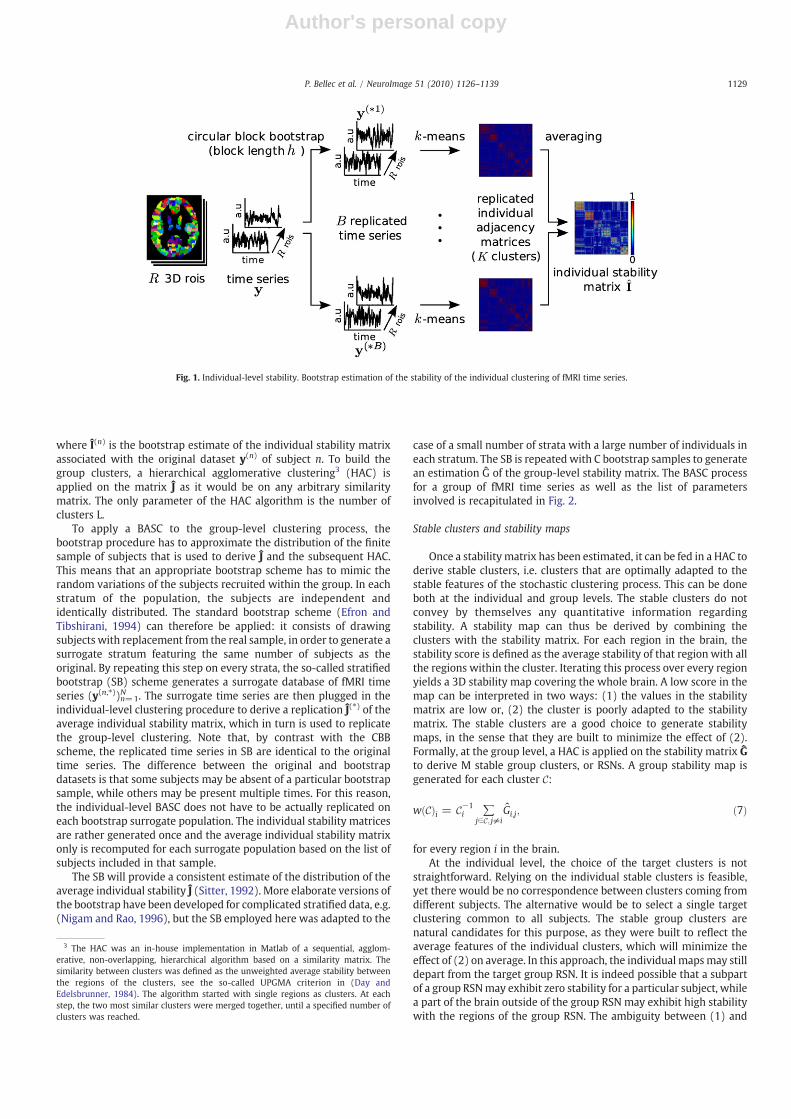
In order to build a non-parametric approximation of the data-generating process, it is important to note that the fMRI time seriesexhibit dependencies in both time and space (Bullmore, 2000). Thismakes the most standard version of the bootstrap non-applicable, yeta variant called circular block bootstrap (CBB) (Efron and Tibshirani,1994) is adapted to this case. The CBB draws independently temporalblocks of length h from the time series y to respect the temporaldependencies in the data. A block falling at the end of the time series iscompleted by points from the beginning, hence the “circular” in CBB.The resampled time blocks are pasted together in order to form asurrogate time series y(⁎) with the same temporal dimension as theoriginal. The same time blocks are used for all the regions to preservespatial correlation and CBB formally leads to consistent confidenceintervals of spatial correlations (Lahiri, 2003). This scheme has beendemonstrated to be efficient in replicating the distribution of spatialcorrelations in real fMRI time series (Bellec et al., 2008). As the k-means algorithm is driven by the spatial correlation present in thedata, that scheme should provide a well-behaved approximation ofthe individual stability. By applying the bootstrap approximation ofEq. 5, an individual stability matrix Î is estimated using B bootstrapsamples generated through CBB.2 Note that, for each replication of theindividual clustering process, some new bootstrap surrogate timeseries are generated and a k-means algorithm is applied based onrandom initial points. As such, the bootstrap stability integrates allsources of random variations, mixing the generation of the datasetwith the potential algorithmic variability. The BASC process forindividual time series as well as the list of parameters involved isrecapitulated in Fig. 1.

Group-level BASC

At the group level, an fMRI database is a collection of datasets(y(n))n=1

N acquired on a group of N different subjects. The subjectsare recruited in the study following a data-generating process whichcontrols for some factors of non-interest, e.g. the group is balancedregarding the number of men and women or the number of left- andright-handed subjects. A subpopulation of subjects that fits a particularprofile regarding those factors is called a stratum, e.g. right-handedwomen. Within each of the strata, the subjects are simply independentsamples of a population that meet some general criterion, e.g. healthysubjects with no history of psychological disorder within a certain agerange.

We now describe a procedure to build a group-level clustering thatwill give an accurate picture of the most stable features of theindividual-level clusterings. The key idea of the EAC algorithm, whichis to run a clustering algorithm on the stability matrix in order todefine stable cluster maps, can be applied to this end. Specifically, agroup-level cluster should be composed of pairs of regions thatmaximize the average probability of belonging to the same cluster atthe individual level. This last quantity is captured by the averageindividual stability matrix Ĵ:

Ji;j = N−1 ∑N

n=1I

nð Þi;j ; ð6Þ

1 The clustering algorithm was an in-house implementation in Matlab of a k-meansclassification, as described in (Duda et al., 2000). The centroids of the clusters wereinitialized using a random subset of the time series. Whenever a cluster became emptyin the classification process, it was replaced by the singleton time series located thefurther away from its centroid. To avoid falling too often in local minima, the k-meanswas actually iterated 5 times with different initializations and the result with thelowest within-cluster inertia was selected.

2 In Eq. 5 the stability matrix is denoted by a generic notation S, yet some specificnotations I and G are introduced for the individual- and group-level stability matrices.

1128 P. Bellec et al. / NeuroImage 51 (2010) 1126–1139


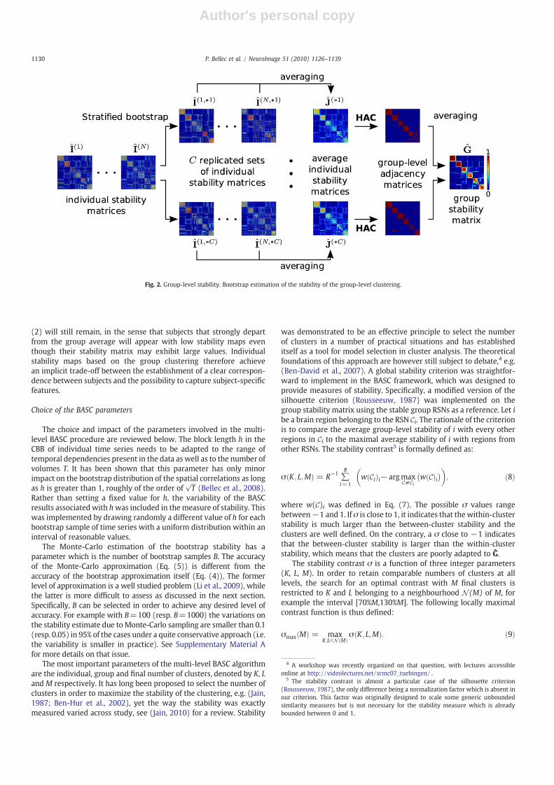
where Î(n) is the bootstrap estimate of the individual stability matrixassociated with the original dataset y(n) of subject n. To build thegroup clusters, a hierarchical agglomerative clustering3 (HAC) isapplied on the matrix Ĵ as it would be on any arbitrary similaritymatrix. The only parameter of the HAC algorithm is the number ofclusters L.

To apply a BASC to the group-level clustering process, thebootstrap procedure has to approximate the distribution of the finitesample of subjects that is used to derive Ĵ and the subsequent HAC.This means that an appropriate bootstrap scheme has to mimic therandom variations of the subjects recruited within the group. In eachstratum of the population, the subjects are independent andidentically distributed. The standard bootstrap scheme (Efron andTibshirani, 1994) can therefore be applied: it consists of drawingsubjects with replacement from the real sample, in order to generate asurrogate stratum featuring the same number of subjects as theoriginal. By repeating this step on every strata, the so-called stratifiedbootstrap (SB) scheme generates a surrogate database of fMRI timeseries (y(n,⁎))n=1

N . The surrogate time series are then plugged in theindividual-level clustering procedure to derive a replication Ĵ(⁎) of theaverage individual stability matrix, which in turn is used to replicatethe group-level clustering. Note that, by contrast with the CBBscheme, the replicated time series in SB are identical to the originaltime series. The difference between the original and bootstrapdatasets is that some subjects may be absent of a particular bootstrapsample, while others may be present multiple times. For this reason,the individual-level BASC does not have to be actually replicated oneach bootstrap surrogate population. The individual stability matricesare rather generated once and the average individual stability matrixonly is recomputed for each surrogate population based on the list ofsubjects included in that sample.

The SB will provide a consistent estimate of the distribution of theaverage individual stability Ĵ (Sitter, 1992). More elaborate versions ofthe bootstrap have been developed for complicated stratified data, e.g.(Nigam and Rao, 1996), but the SB employed here was adapted to the

case of a small number of strata with a large number of individuals ineach stratum. The SB is repeated with C bootstrap samples to generatean estimation Ĝ of the group-level stability matrix. The BASC processfor a group of fMRI time series as well as the list of parametersinvolved is recapitulated in Fig. 2.

Stable clusters and stability maps

Once a stability matrix has been estimated, it can be fed in a HAC toderive stable clusters, i.e. clusters that are optimally adapted to thestable features of the stochastic clustering process. This can be doneboth at the individual and group levels. The stable clusters do notconvey by themselves any quantitative information regardingstability. A stability map can thus be derived by combining theclusters with the stability matrix. For each region in the brain, thestability score is defined as the average stability of that region with allthe regions within the cluster. Iterating this process over every regionyields a 3D stability map covering the whole brain. A low score in themap can be interpreted in two ways: (1) the values in the stabilitymatrix are low or, (2) the cluster is poorly adapted to the stabilitymatrix. The stable clusters are a good choice to generate stabilitymaps, in the sense that they are built to minimize the effect of (2).Formally, at the group level, a HAC is applied on the stability matrix Ĝto derive M stable group clusters, or RSNs. A group stability map isgenerated for each cluster C:

w Cð Þi = C−1i ∑

j∈C; j≠iGi;j; ð7Þ

for every region i in the brain.At the individual level, the choice of the target clusters is not

straightforward. Relying on the individual stable clusters is feasible,yet there would be no correspondence between clusters coming fromdifferent subjects. The alternative would be to select a single targetclustering common to all subjects. The stable group clusters arenatural candidates for this purpose, as they were built to reflect theaverage features of the individual clusters, which will minimize theeffect of (2) on average. In this approach, the individual mapsmay stilldepart from the target group RSN. It is indeed possible that a subpartof a group RSNmay exhibit zero stability for a particular subject, whilea part of the brain outside of the group RSN may exhibit high stabilitywith the regions of the group RSN. The ambiguity between (1) and

3 The HAC was an in-house implementation in Matlab of a sequential, agglom-erative, non-overlapping, hierarchical algorithm based on a similarity matrix. Thesimilarity between clusters was defined as the unweighted average stability betweenthe regions of the clusters, see the so-called UPGMA criterion in (Day andEdelsbrunner, 1984). The algorithm started with single regions as clusters. At eachstep, the two most similar clusters were merged together, until a specified number ofclusters was reached.

Fig. 1. Individual-level stability. Bootstrap estimation of the stability of the individual clustering of fMRI time series.



(2) will still remain, in the sense that subjects that strongly departfrom the group average will appear with low stability maps eventhough their stability matrix may exhibit large values. Individualstability maps based on the group clustering therefore achievean implicit trade-off between the establishment of a clear correspon-dence between subjects and the possibility to capture subject-specificfeatures.

Choice of the BASC parameters

The choice and impact of the parameters involved in the multi-level BASC procedure are reviewed below. The block length h in theCBB of individual time series needs to be adapted to the range oftemporal dependencies present in the data as well as to the number ofvolumes T. It has been shown that this parameter has only minorimpact on the bootstrap distribution of the spatial correlations as longas h is greater than 1, roughly of the order of

ffiffiffiT

p(Bellec et al., 2008).

Rather than setting a fixed value for h, the variability of the BASCresults associated with hwas included in the measure of stability. Thiswas implemented by drawing randomly a different value of h for eachbootstrap sample of time series with a uniform distribution within aninterval of reasonable values.

The Monte-Carlo estimation of the bootstrap stability has aparameter which is the number of bootstrap samples B. The accuracyof the Monte-Carlo approximation (Eq. (5)) is different from theaccuracy of the bootstrap approximation itself (Eq. (4)). The formerlevel of approximation is a well studied problem (Li et al., 2009), whilethe latter is more difficult to assess as discussed in the next section.Specifically, B can be selected in order to achieve any desired level ofaccuracy. For example with B=100 (resp. B=1000) the variations onthe stability estimate due to Monte-Carlo sampling are smaller than 0.1(resp. 0.05) in 95% of the cases under a quite conservative approach (i.e.the variability is smaller in practice). See Supplementary Material Afor more details on that issue.

The most important parameters of the multi-level BASC algorithmare the individual, group and final number of clusters, denoted by K, LandM respectively. It has long been proposed to select the number ofclusters in order to maximize the stability of the clustering, e.g. (Jain,1987; Ben-Hur et al., 2002), yet the way the stability was exactlymeasured varied across study, see (Jain, 2010) for a review. Stability

was demonstrated to be an effective principle to select the numberof clusters in a number of practical situations and has establisheditself as a tool for model selection in cluster analysis. The theoreticalfoundations of this approach are however still subject to debate,4 e.g.(Ben-David et al., 2007). A global stability criterion was straightfor-ward to implement in the BASC framework, which was designed toprovide measures of stability. Specifically, a modified version of thesilhouette criterion (Rousseeuw, 1987) was implemented on thegroup stability matrix using the stable group RSNs as a reference. Let ibe a brain region belonging to the RSN Ci. The rationale of the criterionis to compare the average group-level stability of i with every otherregions in Ci to the maximal average stability of i with regions fromother RSNs. The stability contrast5 is formally defined as:

σ K; L;Mð Þ = R−1 ∑R

i=1w Cið Þi− argmax

C≠Ciw Cð Þi� ��

; ð8Þ

where w(C)i was defined in Eq. (7). The possible σ values rangebetween−1 and 1. If σ is close to 1, it indicates that the within-clusterstability is much larger than the between-cluster stability and theclusters are well defined. On the contrary, a σ close to −1 indicatesthat the between-cluster stability is larger than the within-clusterstability, which means that the clusters are poorly adapted to Ĝ.

The stability contrast σ is a function of three integer parameters(K, L, M). In order to retain comparable numbers of clusters at alllevels, the search for an optimal contrast with M final clusters isrestricted to K and L belonging to a neighbourhood N (M) of M, forexample the interval [70%M,130%M]. The following locally maximalcontrast function is thus defined:

σmax Mð Þ = maxK;L∈N Mð Þ

σ K; L;Mð Þ: ð9Þ

4 A workshop was recently organized on that question, with lectures accessibleonline at http://videolectures.net/srmc07_tuebingen/.

5 The stability contrast is almost a particular case of the silhouette criterion(Rousseeuw, 1987), the only difference being a normalization factor which is absent inour criterion. This factor was originally designed to scale some generic unboundedsimilarity measures but is not necessary for the stability measure which is alreadybounded between 0 and 1.

Fig. 2. Group-level stability. Bootstrap estimation of the stability of the group-level clustering.



The final number of clusters Mopt is selected as the one whichmaximizes σmax, and the individual and group parameters Kopt andLopt are selected as the one maximizing σ(K,L,Mopt) in the neighbour-hood N (Mopt).

Validity of the BASC approximation of stability

An important question regarding the BASC approach is the validityof the bootstrap estimate of the stability matrix. More specifically,would the estimator defined in Eq. (5) be unbiased, i.e. would thestatistical expectation of the estimator be equal to the real stabilitymeasure defined in Eq. (2). There is a large literature regarding thetheoretical asymptotical properties of bootstrap estimators (Shao andTu, 1995). Unfortunately, those results are applicable under relativelystrict conditions: the statistic would have to be a smooth function ofthe mean. In our case, the statistic of interest is the adjacency matrixresulting of a clustering algorithm, which departs from the “smoothfunction of the mean” category. The available theoretical results arethus quite limited (Field andWelsh, 2007). The standard bootstrap forindependent data seems efficient in practice to estimate the stabilityin hierarchical clustering (Suzuki and Shimodaira, 2006), even thoughbias-correction techniques (Shimodaira, 2004) improve the behav-iour. Acknowledging this current theoretical limitation of BASC, weresorted to bootstrap schemes that had an established satisfactorybehaviour regarding the spatial dependencies of the surrogatebootstrap data. We also investigated the accuracy of BASC empiricallyon Monte-Carlo simulations of synthetic fMRI time series. Thisvalidation step would be necessary in any case, as the theoreticalresults hold asymptotically, i.e. with the number of time samples Tand the number of subjects N tending towards infinity. Monte-Carlosimulations with synthetic datasets allow the behaviour of themethod to be assessed for finite T and N.

Experiments on simulated time series

Simulation model

Themulti-level BASCmethod has been evaluated on fully syntheticdatasets. At the group level, brain regions were grouped into non-overlapping clusters formed of a fixed number of regions. Individualclusters were generated by applying a random perturbation of the

group-level clusters. More specifically, regions of the brains weretreated as points on a circle. The group-level clusters were thusviewed as regular portions on the circle. Individual clusters weregenerated by randomly moving the edges between clusters. At theindividual level, regions within a cluster were generated by adding asignal common to all regions, called cluster time series, and a noisefollowing a Gaussian distribution independent in space and time withzero mean and unit variance. Each cluster time series was a sample ofan auto-regressive process of order 1, with parameter a=0.5, T=100samples and a variance σc

2 common to all clusters. The free param-eters of the simulations were the following:

• The number of clusters Λ.• The number of regions per group cluster Γ.• The variance of cluster time series σc

2 (or equivalently the signal-to-noise ratio, SNR).

• The number of subjects N.• The parameter p which defined the stability of the cluster edgesposition across subjects (a small p corresponded to a largevariability).

Some preliminary experiments were done to determine eightdifferent scenarios corresponding to various difficulties in terms ofclustering stability, see Supplementary Materials B. The parametersvalues of the different scenarios were Λ=5, Γ=20, SNR in {−10,−5},N in {5, 20} and p in {0.4, 0.1}.

Selection of the number of clusters

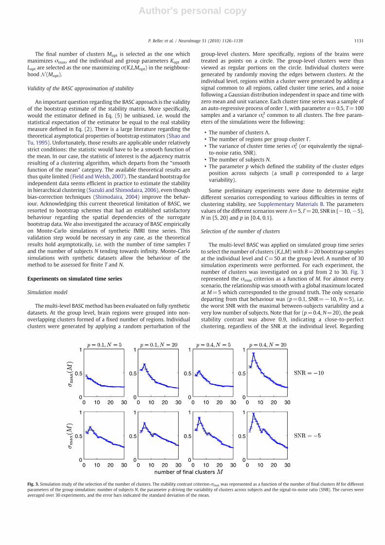
The multi-level BASC was applied on simulated group time seriesto select the number of clusters (K,L,M) with B=20 bootstrap samplesat the individual level and C=50 at the group level. A number of 30simulation experiments were performed. For each experiment, thenumber of clusters was investigated on a grid from 2 to 30. Fig. 3represented the σmax criterion as a function of M. For almost everyscenario, the relationshipwas smoothwith a global maximum locatedat M=5 which corresponded to the ground truth. The only scenariodeparting from that behaviour was (p=0.1, SNR=−10, N=5), i.e.the worst SNR with the maximal between-subjects variability and avery low number of subjects. Note that for (p=0.4, N=20), the peakstability contrast was above 0.9, indicating a close-to-perfectclustering, regardless of the SNR at the individual level. Regarding

Fig. 3. Simulation study of the selection of the number of clusters. The stability contrast criterion σmax was represented as a function of the number of final clusters M for differentparameters of the group simulation: number of subjects N, the parameter p driving the variability of clusters across subjects and the signal-to-noise ratio (SNR). The curves wereaveraged over 30 experiments, and the error bars indicated the standard deviation of the mean.



the final number of clusters M, the correct value M=5 was the mostselected value in every scenario but for (p=0.1, SNR=−10, N=5),where it was M=2. With N=20 subjects, the correct number ofclusters M was selected in more than 80% of the simulations,regardless of p and the SNR. The same behaviour was observed onthe group number of clusters L. The individual number of clusters Khad a much more widespread selection profile, even for (p=0.4,N=20). The most frequently selected values were {5,6,7}, but therange of selected number of clusters actually covered 2 to 8. Thisresult is not actually an issue as the optimal number of individualclusters may not exactly match the real number of clusters extractedat the group level. This simulation study demonstrated that thestability contrast criterionwas able to correctly identify the number ofclusters at the group level in a reliable fashion as soon as the numberof subjects was larger than 20.

Accuracy of the group-level stability estimation

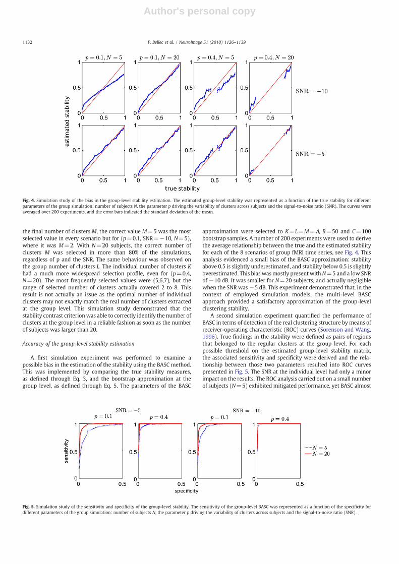
A first simulation experiment was performed to examine apossible bias in the estimation of the stability using the BASC method.This was implemented by comparing the true stability measures,as defined through Eq. 3, and the bootstrap approximation at thegroup level, as defined through Eq. 5. The parameters of the BASC

approximation were selected to K=L=M=Λ, B=50 and C=100bootstrap samples. A number of 200 experiments were used to derivethe average relationship between the true and the estimated stabilityfor each of the 8 scenarios of group fMRI time series, see Fig. 4. Thisanalysis evidenced a small bias of the BASC approximation: stabilityabove 0.5 is slightly underestimated, and stability below 0.5 is slightlyoverestimated. This bias wasmostly present withN=5 and a low SNRof −10 dB. It was smaller for N=20 subjects, and actually negligiblewhen the SNR was−5 dB. This experiment demonstrated that, in thecontext of employed simulation models, the multi-level BASCapproach provided a satisfactory approximation of the group-levelclustering stability.

A second simulation experiment quantified the performance ofBASC in terms of detection of the real clustering structure by means ofreceiver-operating characteristic (ROC) curves (Sorenson and Wang,1996). True findings in the stability were defined as pairs of regionsthat belonged to the regular clusters at the group level. For eachpossible threshold on the estimated group-level stability matrix,the associated sensitivity and specificity were derived and the rela-tionship between those two parameters resulted into ROC curvespresented in Fig. 5. The SNR at the individual level had only a minorimpact on the results. The ROC analysis carried out on a small numberof subjects (N=5) exhibited mitigated performance, yet BASC almost

Fig. 4. Simulation study of the bias in the group-level stability estimation. The estimated group-level stability was represented as a function of the true stability for differentparameters of the group simulation: number of subjects N, the parameter p driving the variability of clusters across subjects and the signal-to-noise ratio (SNR). The curves wereaveraged over 200 experiments, and the error bars indicated the standard deviation of the mean.

Fig. 5. Simulation study of the sensitivity and specificity of the group-level stability. The sensitivity of the group-level BASC was represented as a function of the specificity fordifferent parameters of the group simulation: number of subjects N, the parameter p driving the variability of clusters across subjects and the signal-to-noise ratio (SNR).



behaved as a perfect classifier with N=20 subjects. This suggestedthat the statistical power of BASC as a detector of group-levelclustering structures should be satisfactory in the conditions ofapplication of most fMRI studies.

Experiment on a real resting-state fMRI database

Data acquisition

The multi-level BASC was applied on the younger subjects (ageranging from 19 to 44 years) of a neuroimaging database collected bythe International Consortium for Brain Mapping (ICBM) and madepublicly available as part of the 1000-connectome project.6 A cohort ofN=43 healthy volunteers (21 men, 22 women) participated in thisstudywhichwas approved by the local ethics committee. Subjects hadno history of neurological or psychiatric disorders. Three functionalruns were acquired for each subject under resting-state conditions i.e.the subjects were asked to remain still, eyes closed, and to refrainfrom any overt activity. For each functional run, 138 brain volumes ofBOLD signals were recorded on a 1.5 T Siemens scanner using a 2Dechoplanar BOLD MOSAIC sequence and the following parameters:TR/TE=2 s/50 ms, 64×64 matrix with a 4×4 mm2 resolution, 23contiguous axial slices covering the cortex but not the cerebellum,slice thickness=4 mm, flip angle=90 ° and an 8-channel coil. A high-resolution anatomical T1-weighted scan was also acquired: TR/TE=0.022 s/0.0092 s, 256×256 matrix with a 1×1 mm2 resolution,176 contiguous sagittal slices covering the whole brain, slicethickness=1 mm, flip angle=30 °.

Data preprocessing

The fMRI database was preprocessed using the pipeline imple-mented in the package called neuroimaging analysis kit7 (NIAK). Thethree first volumes of each run were suppressed to allow themagnetisation to reach equilibrium. Each dataset was corrected ofinter-slice difference in acquisition time, rigid body motion, slow timedrifts (high-pass filter with a 0.01 Hz cut-off) and physiological noise(Perlbarg et al., 2007). Slow time drifts and physiological noise

correction were implemented in an attempt to reduce the spatiallycorrelated noise present in the fMRI time series, which may introducestable clusters unrelated to neural activity. Data-driven noisecorrection strategies have been reported to improve the detection ofRSNs and are increasingly popular in functional connectivity analysis(Giove et al., 2009; Weissenbacher et al., 2009).

The following strategywas implemented to transform the individualbrains into a common space of analysis. For each subject, the meanmotion-corrected volume of all the datasets was coregistered with a T1individual scan using Minctracc8 (Collins et al., 1994), which was itselfnon-linearly transformed to the Montreal Neurological Institute (MNI)non-linear template using the CIVET9 pipeline (Zijdenbos et al., 2002).The functional volumes were resampled in the MNI space at a 2 mmisotropic resolution and spatially smoothed with a 6 mm isotropicGaussian kernel. The spatial smoothingwas implemented in an attemptto minimize the residual variability in anatomy and functionalorganization of individual brain in stereotaxic space.

In order to limit the computational burden of the bootstrapanalysis, a region-growing algorithm (Bellec et al., 2006) was appliedto the concatenated time series of every subjects in order to derive acommon segmentation of the brain into small functionally homoge-neous regions. To limit the memory demand, the region growingwas applied independently in each of the 116 areas of the AAL tem-plate (Tzourio-Mazoyer et al., 2002). The resulting regions werespatially connected with roughly equal size, which was set to thesmallest value that would lead to amenable computations, i.e. a sizeof 800 mm3 translating into 1191 regions covering the grey matter.The average time series within each region was derived after cor-rection to a zero temporal mean and unit variance, and thenconcatenated across all the fMRI datasets for each subject. Thisprocess resulted into individual time series with T=405 time points10

and R=1191 regions.

Choice of BASC parameters

The block length for CBB of individual time series was selectedrandomly at each bootstrap sample in the interval ([10,30]). BASCwas

6 http://www.nitrc.org/projects/fcon_1000/.7 http://wiki.bic.mni.mcgill.ca/index.php/NiakFmriPreprocessing.

8 http://wiki.bic.mni.mcgill.ca/index.php/MinctraccManPage.9 http://wiki.bic.mni.mcgill.ca/index.php/CIVET.

10 (138 volumes − 3 dummy scans)×3 runs=405 time points per subject.

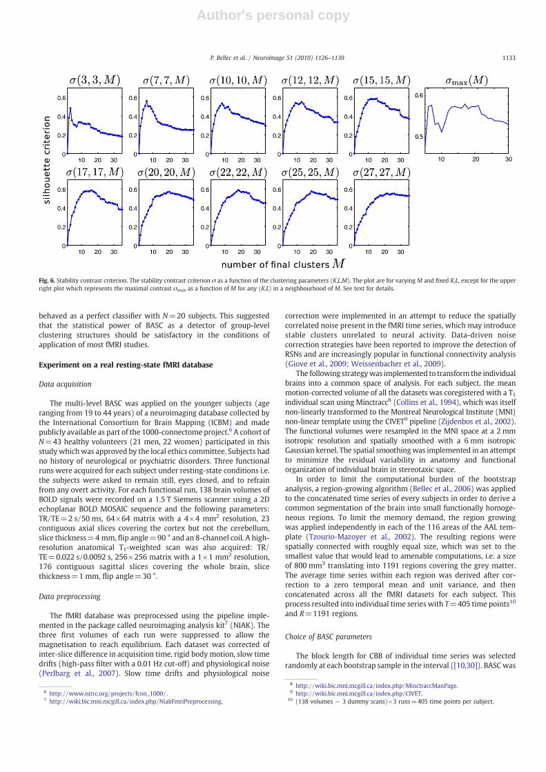
Fig. 6. Stability contrast criterion. The stability contrast criterion σ as a function of the clustering parameters (K,L,M). The plot are for varying M and fixed K,L, except for the upperright plot which represents the maximal contrast σmax as a function of M for any (K,L) in a neighbourhood of M. See text for details.



first applied in order to select the number of clusters with a smallnumber B=30 of bootstrap samples at the individual level andC=250 bootstrap samples at the group level. Fig. 6 presented thestability contrast σ as a function of the number of final clustersM, on agrid of 5 to 30, with different choices of (K,L). The σ curves weresmooth and the global maximum was achieved for M close to theemployed K. The locally maximal contrast σmax was also smooth, butdid not present a clear global maximum. Instead, the first localmaximum at M=7 was followed by a plateau in the range 12 to 21.This result demonstrated that more than one stable clusteringstructure could be identified in resting-state fMRI data. The purposeof this article being to illustrate the mechanics of the multi-level BASCrather than investigating such multi-scale architecture, we reportedthe results for a single M corresponding to the first local maximum.

Group-level stable clusters

To derive stability maps with high accuracy, the multi-level BASCwas applied a second time with B=200 bootstrap samples at theindividual level and C=1000 at the group level for the followingnumber of clusters (K=8,L=7,M=7). The group-level stabilitymatrix exhibited a very high stability contrast (σmax(7)=0.59), whichgraphically translated into yellow–red diagonal squares (within-clusters stability) on a deep blue background, see Fig. 7a. Thedendrogram representation of the HAC applied on the group-levelstability matrix showed that most of the merging between regionsoccurred at a very high level of stability, above 0.9, see Fig. 7b. Amatrix representation of the RSNs was derived by coding every pairsof regions within a given cluster with a specific color (Fig. 7c). EachRSN of Fig. 7c was associated with a group of brain regionsrepresented in Fig. 7d. Some RSNs were strikingly similar to thosereported previously using group-level ICA (Damoiseaux et al., 2006):a sensorimotor network (RSN3), a visual network (RSN6); thedefault-mode network (RSN7). The bilateral temporal RSN2 resem-bled a component from (Damoiseaux et al., 2006), yet the correspon-dence was not clear due to differences in the employed field of views.The fronto-parietal network (RSN4) included regions involved in

working-memory tasks, and has often been reported splitted into twoleft and right subnetworks (Damoiseaux et al., 2006). The RSN5,comprising ventro-frontal cortex, the thalami and the striatum, alsoappeared like a merging of two components reported by (Damoiseauxet al., 2008). RSN1 included some ventro-medial cortex and anteriorcaudate, yet it also included regions around the cerebellar tentoriumindicating that it might have been corrupted by residual physiologicalnoise.

Stability maps

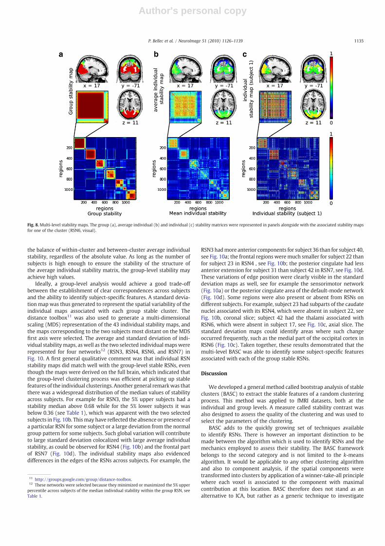
For each stable group RSN, the average group stability matrix wastranslated into a stability map, as illustrated for RSN6 in Fig. 8a. Thesame process was applied with the average individual stability matrix(Fig. 8b) and each of the 43 individual stability matrices (Fig. 8c). For aregion i, the associated value of the stabilitymapwas the average of allcolumns j≠ i of row i in the stability matrix, where j belonged to thetarget cluster. Note that the stability score was represented only forthe regions inside the cluster in Fig. 8, but could actually be derived forevery brain region.

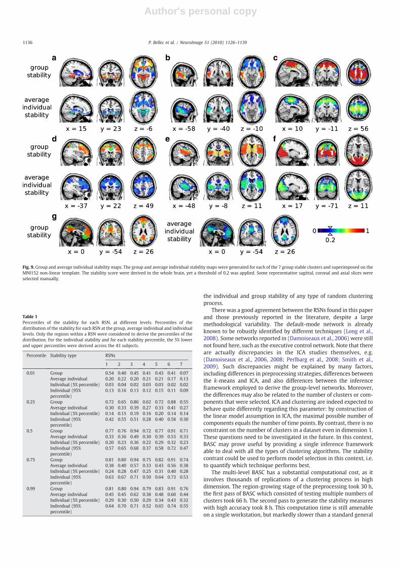
The group and average individual stability maps for the 7 RSNswere presented in Fig. 9. The maps were derived on the whole brain,yet only the values higher than 0.2 were represented and super-imposed to an average structural scan to facilitate the identification ofanatomical landmarks. The percentiles of the distribution of thesestability maps within each RSN were reported in Table 1. At the grouplevel, the two most stable RSNs were the visual and sensorimotor(respective median 0.91 and 0.94). The remaining RSNs had com-parable levels of group stability (median ranging from 0.71 to 0.77).The observed average individual stability was markedly smaller, witha median of 0.49 and 0.53 for the two most stables, and a medianranging from 0.3 to 0.36 for the other RSNs. It was interesting to notethat a relatively low level of average individual stability could result ina high level of group stability, e.g. in the striatum Fig. 9e. The gradientobserved on the individual average stability of the sensorimotor alsoresulted in a plateau of high stability at the group level 9c. This resultillustrated the fact that the group-level clustering was based on

Fig. 7. Partition of the brain into stable group-level networks. The group-level stability matrix (a) underwent a hierarchical clustering which was represented as a dendrogram(b) andwas used to generate a partition intoM=7 clusters. These clusters were color-coded in matrix form (c), see text for details, and the same color code was applied to representthe brain regions associated with each cluster, superimposed with theMNI152 non-linear template (d). Some representative sagittal, coronal and axial slices were selectedmanually.



the balance of within-cluster and between-cluster average individualstability, regardless of the absolute value. As long as the number ofsubjects is high enough to ensure the stability of the structure ofthe average individual stability matrix, the group-level stability mayachieve high values.

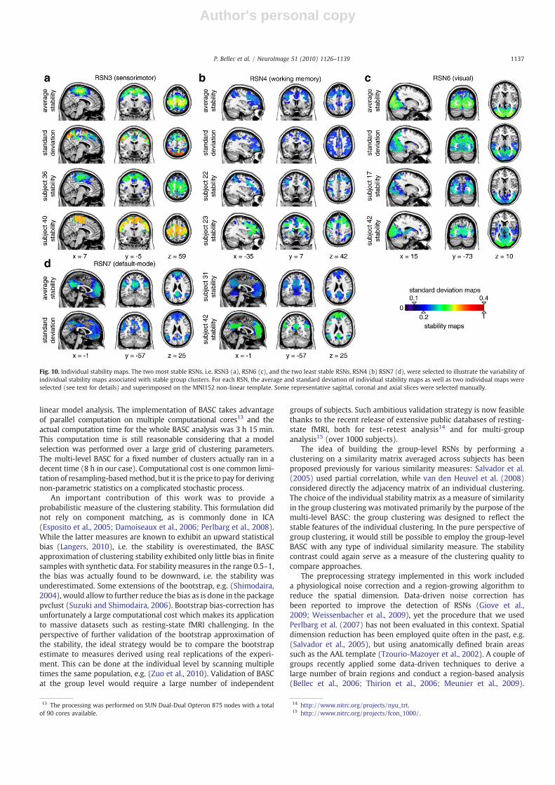
Ideally, a group-level analysis would achieve a good trade-offbetween the establishment of clear correspondences across subjectsand the ability to identify subject-specific features. A standard devia-tion map was thus generated to represent the spatial variability of theindividual maps associated with each group stable cluster. Thedistance toolbox11 was also used to generate a multi-dimensionalscaling (MDS) representation of the 43 individual stability maps, andthe maps corresponding to the two subjects most distant on the MDSfirst axis were selected. The average and standard deviation of indi-vidual stabilitymaps, as well as the two selected individualmapswererepresented for four networks12 (RSN3, RSN4, RSN6, and RSN7) inFig. 10. A first general qualitative comment was that individual RSNstability maps did match well with the group-level stable RSNs, eventhough the maps were derived on the full brain, which indicated thatthe group-level clustering process was efficient at picking up stablefeatures of the individual clusterings. Another general remarkwas thatthere was a widespread distribution of the median values of stabilityacross subjects. For example for RSN3, the 5% upper subjects had astability median above 0.68 while for the 5% lower subjects it wasbelow 0.36 (see Table 1), which was apparent with the two selectedsubjects in Fig. 10b. Thismay have reflected the absence or presence ofa particular RSN for some subject or a large deviation from the normalgroup pattern for some subjects. Such global variation will contributeto large standard deviation colocalized with large average individualstability, as could be observed for RSN4 (Fig. 10b) and the frontal partof RSN7 (Fig. 10d). The individual stability maps also evidenceddifferences in the edges of the RSNs across subjects. For example, the

RSN3hadmore anterior components for subject 36 than for subject 40,see Fig. 10a; the frontal regions weremuch smaller for subject 22 thanfor subject 23 in RSN4 , see Fig. 10b; the posterior cingulate had lessanterior extension for subject 31 than subject 42 in RSN7, see Fig. 10d.These variations of edge position were clearly visible in the standarddeviation maps as well, see for example the sensorimotor network(Fig. 10a) or the posterior cingulate area of the default-mode network(Fig. 10d). Some regions were also present or absent from RSNs ondifferent subjects. For example, subject 23 had subparts of the caudatenuclei associated with its RSN4, which were absent in subject 22, seeFig. 10b, coronal slice; subject 42 had the thalami associated withRSN6, which were absent in subject 17, see Fig. 10c, axial slice. Thestandard deviation maps could identify areas where such changeoccurred frequently, such as the medial part of the occipital cortex inRSN6 (Fig. 10c). Taken together, these results demonstrated that themulti-level BASC was able to identify some subject-specific featuresassociated with each of the group stable RSNs.

Discussion

We developed a general method called bootstrap analysis of stableclusters (BASC) to extract the stable features of a random clusteringprocess. This method was applied to fMRI datasets, both at theindividual and group levels. A measure called stability contrast wasalso designed to assess the quality of the clustering and was used toselect the parameters of the clustering.

BASC adds to the quickly growing set of techniques availableto identify RSNs. There is however an important distinction to bemade between the algorithm which is used to identify RSNs and themechanics employed to assess their stability. The BASC frameworkbelongs to the second category and is not limited to the k-meansalgorithm. It would be applicable to any other clustering algorithmand also to component analysis, if the spatial components weretransformed into clusters by application of a winner-take-all principlewhere each voxel is associated to the component with maximalcontribution at this location. BASC therefore does not stand as analternative to ICA, but rather as a generic technique to investigate

11 http://groups.google.com/group/distance-toolbox.12 These networks were selected because they minimized or maximized the 5% upperpercentile across subjects of the median individual stability within the group RSN, seeTable 1.

Fig. 8.Multi-level stability maps. The group (a), average individual (b) and individual (c) stability matrices were represented in panels alongside with the associated stability mapsfor one of the cluster (RSN6, visual).



the individual and group stability of any type of random clusteringprocess.

There was a good agreement between the RSNs found in this paperand those previously reported in the literature, despite a largemethodological variability. The default-mode network is alreadyknown to be robustly identified by different techniques (Long et al.,2008). Some networks reported in (Damoiseaux et al., 2006) were stillnot found here, such as the executive control network. Note that thereare actually discrepancies in the ICA studies themselves, e.g.(Damoiseaux et al., 2006, 2008; Perlbarg et al., 2008; Smith et al.,2009). Such discrepancies might be explained by many factors,including differences in preprocessing strategies, differences betweenthe k-means and ICA, and also differences between the inferenceframework employed to derive the group-level networks. Moreover,the differences may also be related to the number of clusters or com-ponents that were selected. ICA and clustering are indeed expected tobehave quite differently regarding this parameter: by construction ofthe linear model assumption in ICA, the maximal possible number ofcomponents equals the number of time points. By contrast, there is noconstraint on the number of clusters in a dataset even in dimension 1.These questions need to be investigated in the future. In this context,BASC may prove useful by providing a single inference frameworkable to deal with all the types of clustering algorithms. The stabilitycontrast could be used to perform model selection in this context, i.e.to quantify which technique performs best.

The multi-level BASC has a substantial computational cost, as itinvolves thousands of replications of a clustering process in highdimension. The region-growing stage of the preprocessing took 30 h,the first pass of BASC which consisted of testing multiple numbers ofclusters took 66 h. The second pass to generate the stability measureswith high accuracy took 8 h. This computation time is still amenableon a single workstation, but markedly slower than a standard general

Table 1Percentiles of the stability for each RSN, at different levels. Percentiles of thedistribution of the stability for each RSN at the group, average individual and individuallevels. Only the regions within a RSN were considered to derive the percentiles of thedistribution. For the individual stability and for each stability percentile, the 5% lowerand upper percentiles were derived across the 43 subjects.

Percentile Stability type RSNs

1 2 3 4 5 6 7

0.01 Group 0.54 0.40 0.45 0.41 0.43 0.41 0.07Average individual 0.20 0.22 0.20 0.21 0.21 0.17 0.13Individual (5% percentile) 0.03 0.04 0.02 0.03 0.03 0.02 0.02Individual (95%percentile)

0.13 0.16 0.13 0.12 0.15 0.11 0.09


0.42 0.55 0.51 0.28 0.40 0.58 0.30


0.57 0.65 0.68 0.37 0.58 0.72 0.47


0.63 0.67 0.71 0.50 0.64 0.73 0.53


0.64 0.70 0.71 0.52 0.65 0.74 0.55

Fig. 9. Group and average individual stability maps. The group and average individual stability maps were generated for each of the 7 group stable clusters and superimposed on theMNI152 non-linear template. The stability score were derived in the whole brain, yet a threshold of 0.2 was applied. Some representative sagittal, coronal and axial slices wereselected manually.



linear model analysis. The implementation of BASC takes advantageof parallel computation on multiple computational cores13 and theactual computation time for the whole BASC analysis was 3 h 15 min.This computation time is still reasonable considering that a modelselection was performed over a large grid of clustering parameters.The multi-level BASC for a fixed number of clusters actually ran in adecent time (8 h in our case). Computational cost is one common limi-tation of resampling-basedmethod, but it is the price to pay for derivingnon-parametric statistics on a complicated stochastic process.

An important contribution of this work was to provide aprobabilistic measure of the clustering stability. This formulation didnot rely on component matching, as is commonly done in ICA(Esposito et al., 2005; Damoiseaux et al., 2006; Perlbarg et al., 2008).While the latter measures are known to exhibit an upward statisticalbias (Langers, 2010), i.e. the stability is overestimated, the BASCapproximation of clustering stability exhibited only little bias in finitesamples with synthetic data. For stability measures in the range 0.5–1,the bias was actually found to be downward, i.e. the stability wasunderestimated. Some extensions of the bootstrap, e.g. (Shimodaira,2004), would allow to further reduce the bias as is done in the packagepvclust (Suzuki and Shimodaira, 2006). Bootstrap bias-correction hasunfortunately a large computational cost which makes its applicationto massive datasets such as resting-state fMRI challenging. In theperspective of further validation of the bootstrap approximation ofthe stability, the ideal strategy would be to compare the bootstrapestimate to measures derived using real replications of the experi-ment. This can be done at the individual level by scanning multipletimes the same population, e.g. (Zuo et al., 2010). Validation of BASCat the group level would require a large number of independent

groups of subjects. Such ambitious validation strategy is now feasiblethanks to the recent release of extensive public databases of resting-state fMRI, both for test–retest analysis14 and for multi-groupanalysis15 (over 1000 subjects).

The idea of building the group-level RSNs by performing aclustering on a similarity matrix averaged across subjects has beenproposed previously for various similarity measures: Salvador et al.(2005) used partial correlation, while van den Heuvel et al. (2008)considered directly the adjacency matrix of an individual clustering.The choice of the individual stability matrix as a measure of similarityin the group clustering was motivated primarily by the purpose of themulti-level BASC: the group clustering was designed to reflect thestable features of the individual clustering. In the pure perspective ofgroup clustering, it would still be possible to employ the group-levelBASC with any type of individual similarity measure. The stabilitycontrast could again serve as a measure of the clustering quality tocompare approaches.

The preprocessing strategy implemented in this work includeda physiological noise correction and a region-growing algorithm toreduce the spatial dimension. Data-driven noise correction hasbeen reported to improve the detection of RSNs (Giove et al.,2009; Weissenbacher et al., 2009), yet the procedure that we usedPerlbarg et al. (2007) has not been evaluated in this context. Spatialdimension reduction has been employed quite often in the past, e.g.(Salvador et al., 2005), but using anatomically defined brain areassuch as the AAL template (Tzourio-Mazoyer et al., 2002). A couple ofgroups recently applied some data-driven techniques to derive alarge number of brain regions and conduct a region-based analysis(Bellec et al., 2006; Thirion et al., 2006; Meunier et al., 2009).

13 The processing was performed on SUN Dual-Dual Opteron 875 nodes with a totalof 90 cores available.

14 http://www.nitrc.org/projects/nyu_trt.15 http://www.nitrc.org/projects/fcon_1000/.

Fig. 10. Individual stability maps. The two most stable RSNs, i.e. RSN3 (a), RSN6 (c), and the two least stable RSNs, RSN4 (b) RSN7 (d), were selected to illustrate the variability ofindividual stability maps associated with stable group clusters. For each RSN, the average and standard deviation of individual stability maps as well as two individual maps wereselected (see text for details) and superimposed on the MNI152 non-linear template. Some representative sagittal, coronal and axial slices were selected manually.



Because of its computational cost, the preprocessing of fMRI timeseries was not included in the bootstrap replication of the clusteringand its impact on stability was therefore not assessed by BASC. As apreliminary experiment to test the robustness of the BASC results todifferent choices of preprocessing strategies, the identification of thegroup stable RSNs reported in this manuscript was replicated withtwo other preprocessing strategies, see Supplementary Material C.Our conclusions were that excluding the physiological noise cor-rection (CORSICA) and the spatial smoothing from the preprocessinghad only a marginal influence on the stable group clusters. Thechoice of the template of brain areas used to constrain the regiongrowing had a more pronounced effect, notably through the seg-mentation of the grey matter, yet most features of the clusteringwere retained. This suggested that the BASC group results werereasonably robust to the choice of the preprocessing strategy.Assessing the impact of various preprocessing strategies on themulti-level BASC results more thoroughly will be an important areafor future work.

An interesting finding that was not further investigated in thiswork was the existence of stable clusters at multiple spatial scales, i.e.with different numbers of clusters. A recent article (Smith et al., 2009)has reported about 45 RSNs with consistent ICA maps at the group-level. Our results suggest that there may be many numbers of clusterswhere local maxima of clustering stability can be identified. While thecurrent view of RSNs is focussed on a few widespread networks, theorganization of RSNs at finer spatial scales may also inform us oncritical aspects of the brain functional architecture.

The BASC method naturally extends to perform group comparison.There are currently only a few techniques available to compare theRSNs patterns across group, e.g. (Calhoun et al., 2004; Sui et al., 2009).The present work concentrated on a single group, but the differencebetween the average individual-level stability matrices derived ontwo distinct groups of subjects would allow to test for differences inthe underlying clustering structures. The group-level clusteringwould then search for groups of brain regions with a large differencein stability between the two groups.

The ability of the multi-level BASC to provide individual stabilitymaps associated with group-level RSNs is a key feature for clinicalapplications. For example, it has been shown that the overlap betweensome individual default-mode network maps and a group templateallowed to differentiate between patients with Alzheimer's diseaseand healthy controls (Greicius et al., 2004). This result howeverrequired to select a default-mode network component for eachsubject on the basis of an a priori template. The BASCmethod providesa fully automated alternative which applies on an arbitrary largenumber of networks. As was illustrated in the present work, theindividual stability maps derived from group RSNs provide a well-defined correspondence of RSNs across subjects while allowing toextract some substantial subject-specific features.

Acknowledgments

Part of this work was presented at the 15th annual meeting of theorganization for human brain mapping (Bellec et al., 2009). Theauthors would like to thank Samir Das for editing an earlier version ofthis manuscript and to acknowledge the work of the InternationalConsortium for Brain Mapping16 (ICBM) fMRI community in creatingthe resting-state database. The acquisition of the ICBM resting-statedatabase was supported by NIH grant 9P01EB001955-11. Thecomputational resources used to perform the data analysis wereprovided by CLUMEQ17, which is funded in part by NSERC (MRS),FQRNT, and McGill University.

Appendix A. Supplementary data

Supplementary data associated with this article can be found, inthe online version, at doi:10.1016/j.neuroimage.2010.02.082.

References

Baumgartner, R., Windischberger, C., Moser, E., 1998. Quantification in functionalmagnetic resonance imaging: fuzzy clustering vs. correlation analysis. Magn.Reson. Imaging 16 (2), 115–125.

Beckmann, C.F., Smith, S.M., 2005. Tensorial extensions of independent componentanalysis for multisubject fMRI analysis. NeuroImage 25 (1), 294–311.

Bellec, P., Marrelec, G., Benali, H., 2008. A bootstrap test to investigate changes in brainconnectivity for functional MRI. Stat. Sin. 18, 1253–1268.

Bellec, P., Perlbarg, V., Jbabdi, S., Pélégrini-Issac, M., Anton, J., Doyon, J., Benali, H., 2006.Identification of large-scale networks in the brain using fMRI. NeuroImage 29 (4),1231–1243.

Bellec, P., Rosa-Neto, P., Benali, H., Evans, A.C., 2009. Multi-level bootstrap analysis ofstable clusters (BASC) in resting-state fMRI. Proceedings of the Human BrainMapping 2009 Annual Meeting, San Francisco: NeuroImage, vol. 47, p. S123.

Ben-David, S., Pál, D., Simon, H., 2007. Stability of k-means clustering. 20th AnnualConference on Learning Theory, COLT 2007, San Diego, CA, USA; June 13–15, 2007,vol. 4539/2007. Springer, Berlin/Heidelberg, pp. 20–34.

Ben-Hur, A., Elisseeff, A., Guyon, I., 2002. A stability based method for discoveringstructure in clustered data. Pacific Symposium on Biocomputing, pp. 6–17.

Biswal, B., Yetkin, F.Z., Haughton, V.M., Hyde, J.S., 1995. Functional connectivity in themotor cortex of resting human brain using echo-planar MRI. Magn. Reson. Med. 34(4), 537–541.

Brodmann, K., 1909. Vergleichende Lokalisationslehre der Grosshirnrinde in ihrenPrinzipien dargestellt auf Grund des Zellenbaues. Johann Ambrosius Barth Verlag,Leipzig.

Broyd, S.J., Demanuele, C., Debener, S., Helps, S.K., James, C.J., Sonuga-Barke, E.J., 2009.Default-mode brain dysfunction in mental disorders: a systematic review.Neurosci. Biobehav. Rev. 33 (3), 279–296.

Bullmore, E., 2000. How good is good enough in path analysis of fMRI data? NeuroImage11 (4), 289–301.

Calhoun, V.D., Adali, T., Pekar, J.J., 2004. A method for comparing group fMRI data usingindependent component analysis: application to visual, motor and visuomotortasks. Magn. Reson. Imaging 22 (9), 1181–1191.

Calhoun, V.D., Liu, J., Adal, T., 2009. A review of group ICA for fMRI data and ICA for jointinference of imaging, genetic, and ERP data. NeuroImage 45 (1), S163–S172.

Chen, S., Ross, T.J., Zhan, W., Myers, C.S., Chuang, K.-S.S., Heishman, S.J., Stein, E.A., Yang,Y., 2008. Group independent component analysis reveals consistent resting-statenetworks across multiple sessions. Brain Res. 1239, 141–151.

Collins, D.L., Neelin, P., Peters, T.M., Evans, A.C., 1994. Automatic 3D intersubjectregistration of MR volumetric data in standardized talairach space. J. Comput.Assist. Tomogr. 18 (2), 192–205.

Cordes, D., Haughton, V., Carew, J.D., Arfanakis, K., Maravilla, K., 2002. Hierarchicalclustering to measure connectivity in fMRI resting-state data. Magn. Reson.Imaging 20 (4), 305–317.

Damoiseaux, J.S., Beckmann, C.F., Arigita, S.J., Barkhof, F., Scheltens, P., Stam, C.J., Smith,S.M., Rombouts, S.A., 2008. Reduced resting-state brain activity in the “defaultnetwork” in normal aging. Cereb. Cortex 18 (8), 1856–1864 (New York, N.Y.: 1991).

Damoiseaux, J.S., Greicius, M.D., 2009. Greater than the sum of its parts: a review ofstudies combining structural connectivity and resting-state functional connectiv-ity. Brain Struct. Funct. 213 (6), 525–533.

Damoiseaux, J.S., Rombouts, S.A., Barkhof, F., Scheltens, P., Stam, C.J., Smith, S.M.,Beckmann, C.F., 2006. Consistent resting-state networks across healthy subjects.Proc. Natl Acad. Sci. USA 103 (37), 13848–13853.

Day, W.H., Edelsbrunner, H., 1984. Efficient algorithms for agglomerative hierarchicalclustering methods. J. Classif. 1 (1), 7–24.

De Luca, M., Beckmann, C.F., De Stefano, N., Matthews, P.M., Smith, S.M., 2006. fMRIresting state networks define distinct modes of long-distance interactions in thehuman brain. NeuroImage 29 (4), 1359–1367.

Duda, R.O., Hart, P.E., Stork, D.G., 2000. Pattern Classification, 2nd Edition. Wiley-Interscience.

Efron, B., Tibshirani, R.J., 1994. An Introduction to the Bootstrap. Chapman and Hall/CRC.

Esposito, F., Scarabino, T., Hyvarinen, A., Himberg, J., Formisano, E., Comani, S., Tedeschi,G., Goebel, R., Seifritz, E., Disalle, F., 2005. Independent component analysis of fMRIgroup studies by self-organizing clustering. NeuroImage 25 (1), 193–205.

Field, C.A., Welsh, A.H., 2007. Bootstrapping clustered data. J. R. Stat. Soc. BMethodol. 69(3), 369–390.

Filippini, N., MacIntosh, B.J., Hough, M.G., Goodwin, G.M., Frisoni, G.B., Smith, S.M.,Matthews, P.M., Beckmann, C.F., Mackay, C.E., 2009. Distinct patterns of brainactivity in young carriers of the apoe-epsilon4 allele. Proc. Natl Acad. Sci. USA 106(17), 7209–7214.

Fox, M.D., Raichle, M.E., 2007. Spontaneous fluctuations in brain activity observed withfunctional magnetic resonance imaging. Nat. Rev. Neurosci. 8 (9), 700–711.

Fred, A., Lourenço, A., 2008. Cluster ensemble methods: from single clusterings tocombined solutions. Supervised and Unsupervised Ensemble Methods and theirApplications, pp. 3–30.

Fred, A.L.N., Jain, A.K., 2005. Combining multiple clusterings using evidence accumu-lation. IEEE Trans. Pattern Anal. Mach. Intell. 27 (6), 835–850.

16 http://www.loni.ucla.edu/ICBM/.17 http://www.clumeq.mcgill.ca/.



Giove, F., Gili, T., Iacovella, V., Macaluso, E., Maraviglia, B., 2009. Images-basedsuppression of unwanted global signals in resting-state functional connectivitystudies. Magn. Reson. Imaging 27 (8), 1058–1064.

Greicius, M., 2008. Resting-state functional connectivity in neuropsychiatric disorders.Curr. Opin. Neurol. 24 (4), 424–430.

Greicius, M.D., Srivastava, G., Reiss, A.L., Menon, V., 2004. Default-mode networkactivity distinguishes Alzheimer's disease from healthy aging: evidence fromfunctional MRI. Proc. Natl Acad. Sci. USA 101 (13), 4637–4642.

Himberg, J., Hyvarinen, A., Esposito, F., 2004. Validating the independent components ofneuroimaging time series via clustering and visualization. NeuroImage 22 (3),1214–1222.

Jain, A., 1987. Bootstrap technique in cluster analysis. Pattern Recogn. 20 (5), 547–568.Jain, A.K., 2010. Data clustering: 50 years beyond k-means. Pattern Recognition Letters

31, 651–666.Kerr, M.K., Churchill, G.A., 2001. Bootstrapping cluster analysis: assessing the reliability

of conclusions from microarray experiments. Proc. Natl Acad. Sci. USA 98 (16),8961–8965.

Lahiri, S.N., 2003. Resampling Methods for Dependent Data, 1st Edition. Springer.Langers, D.R.M., 2010. Unbiased group-level statistical assessment of independent

component maps by means of automated retrospective matching. Hum. BrainMapp. 31 (5), 727–742.

Laufs, H., Krakow, K., Sterzer, P., Eger, E., Beyerle, A., Salek-Haddadi, A., Kleinschmidt, A.,2003. Electroencephalographic signatures of attentional and cognitive defaultmodes in spontaneous brain activity fluctuations at rest. Proc. Natl Acad. Sci. USA100 (19), 11053–11058.

Li, J., Tai, B.C., Nott, D.J., 2009. Confidence interval for the bootstrap P-value andsample size calculation of the bootstrap test. J. Nonparametric Stat. 21 (5),649–661.

Long, X.Y., Zuo, X.N., Kiviniemi, V., Yang, Y., Zou, Q.H., Zhu, C.Z., Jiang, T.Z., Yang, H.,Gong, Q.Y., Wang, L., Li, K.C., Xie, S., Zang, Y.F., 2008. Default mode network asrevealed with multiple methods for resting-state functional MRI analysis.J. Neurosci. Methods 171 (2), 349–355.

Margulies, D.S., Vincent, J.L., Kelly, C., Lohmann, G., Uddin, L.Q., Biswal, B.B., Villringer,A., Castellanos, F.X., Milham, M.P., Petrides, M., 2009. Precuneus shares intrinsicfunctional architecture in humans and monkeys. Proc. Natl Acad. Sci. USA 106 (47),20069–20074.

McKeown, M.J., Makeig, S., Brown, G.G., Jung, T.P., Kindermann, S.S., Bell, A.J., Sejnowski,T.J., 1998. Analysis of fMRI data by blind separation into independent spatialcomponents. Hum. Brain Mapp. 6 (3), 160–188.

Meunier, D., Lambiotte, R., Fornito, A., Ersche, K.D., Bullmore, E.T., 2009. Hierarchicalmodularity in human brain functional networks. Front. Neuroinformatics 3.

Meyer-Baese, A., Wismueller, A., Lange, O., 2004. Comparison of two exploratorydata analysis methods for fMRI: unsupervised clustering versus independentcomponent analysis. IEEE transactions on information technology in biomedi-cine: a publication of the IEEE Engineering in Medicine and Biology Society, 8(3),pp. 387–398.

Nigam, A.K., Rao, J.N.K., 1996. On balanced bootstrap for stratified multistage samples.Stat. Sin. 6, 199–214.

Perlbarg, V., Bellec, P., Anton, J.-L., Pélégrini-Issac, M., Doyon, J., Benali, H., 2007.CORSICA: correction of structured noise in fMRI by automatic identification of ICAcomponents. Magn. Reson. Imaging 25 (1), 35–46.

Perlbarg, V., Marrelec, G., 2008. Contribution of exploratory methods to theinvestigation of extended large-scale brain networks in functional MRI: method-ologies, results, and challenges. Int. J. Biomed. Imaging 218519. doi:10.1155/2008/218519.

Perlbarg, V., Marrelec, G., Doyon, J., Pélégrini-Issac, M., Lehericy, S., Benali, H., 2008.NEDICA: detection of group functional networks in fMRI using spatial independentcomponent analysis. 5th IEEE International Symposium on Biomedical Imaging:From Nano to Macro, 2008. ISBI 2008, pp. 1247–1250.

Raghavan, V.V., 1982. Approaches for measuring the stability of clustering methods.SIGIR Forum 17 (1), 6–20.

Rousseeuw, P., 1987. Silhouettes: a graphical aid to the interpretation and validation ofcluster analysis. J. Comput. Appl. Math. 20 (1), 53–65.

Salvador, R., Suckling, J., Coleman, M.R., Pickard, J.D., Menon, D., Bullmore, E., 2005.Neurophysiological architecture of functional magnetic resonance images ofhuman brain. Cereb. Cortex 15 (9), 1332–1342.

Shao, J., Tu, D., 1995. The Jackknife and Bootstrap. Springer.Shehzad, Z., Kelly, A.M.C., Reiss, P.T., Gee, D.G., Gotimer, K., Uddin, L.Q., Lee, S.H.,

Margulies, D.S., Roy, A.K., Biswal, B.B., Petkova, E., Castellanos, F.X., Milham, M.P.,2009. The resting brain: unconstrained yet reliable. Cereb. Cortex 19 (10),2209–2229.

Shimodaira, H., 2004. Approximately unbiased tests of regions using multistep-multiscale bootstrap resampling. Ann. Stat. 32 (6), 2616–2641.

Shmuel, A., Leopold, D.A., 2008. Neuronal correlates of spontaneous fluctuations in fMRIsignals in monkey visual cortex: implications for functional connectivity at rest.Hum. Brain Mapp. 29 (7), 751–761.

Sitter, R.R., 1992. A resampling procedure for complex survey data. J. Am. Stat. Assoc. 87(419), 755–765.

Smith, S.M., Fox, P.T., Miller, K.L., Glahn, D.C., Fox, P.M., Mackay, C.E., Filippini, N.,Watkins, K.E., Toro, R., Laird, A.R., Beckmann, C.F., 2009. Correspondence of thebrain's functional architecture during activation and rest. Proc. Natl Acad. Sci. USA106 (31), 13040–13045.

Smith, S.P., Dubes, R., 1980. Stability of a hierarchical clustering. Pattern Recogn. 12 (3),177–187.

Sorenson, J.A., Wang, X., 1996. ROC methods for evaluation of fMRI techniques. Magn.Reson. Med. 36 (5), 737–744.

Steinley, D., 2008. Stability analysis in k-means clustering. Br. J. Math. Stat. Psychol. 61,255–273.

Sui, J., Adali, T., Pearlson, G.D., Clark, V.P., Calhoun, V.D., 2009. A method for accurategroup difference detection by constraining the mixing coefficients in an ICAframework. Hum. Brain Mapp. 30 (9), 2953–2970.

Suzuki, R., Shimodaira, H., 2006. Pvclust: an R package for assessing the uncertainty inhierarchical clustering. Bioinformatics 22 (12), 1540–1542.

Thirion, B., Flandin, G., Pinel, P., Roche, A., Ciuciu, P., Poline, J.B., 2006. Dealing with theshortcomings of spatial normalization: multi-subject parcellation of fMRI datasets.Hum. Brain Mapp. 27 (8), 678–693.

Toro, R., Fox, P.T., Paus, T., 2008. Functional coactivation map of the human brain. Cereb.Cortex 18 (11), 2553–2559.

Tzourio-Mazoyer, N., Landeau, B., Papathanassiou, D., Crivello, F., Etard, O., Delcroix, N.,Mazoyer, B., Joliot, M., 2002. Automated anatomical labeling of activations in SPMusing a macroscopic anatomical parcellation of the MNI MRI single-subject brain.NeuroImage 15 (1), 273–289.

van den Heuvel, M., Mandl, R., Hulshoff, 2008. Normalized cut group clustering ofresting-state fMRI data. PLoS ONE 3 (4), e2001+.

Vincent, J.L., Patel, G.H., Fox, M.D., Snyder, A.Z., Baker, J.T., Van Essen, D.C., Zempel, J.M.,Snyder, L.H., Corbetta, M., Raichle, M.E., 2007. Intrinsic functional architecture inthe anaesthetized monkey brain. Nature 447 (7140), 83–86.

Weissenbacher, A., Kasess, C., Gerstl, F., Lanzenberger, R., Moser, E., Windischberger, C.,2009. Correlations and anticorrelations in resting-state functional connectivityMRI: a quantitative comparison of preprocessing strategies. NeuroImage 47 (4),1408–1416.

Woolrich, M.W., Behrens, T.E., Beckmann, C.F., Jenkinson, M., Smith, S.M., 2004.Multilevel linear modelling for fMRI group analysis using Bayesian inference.NeuroImage 21 (4), 1732–1747.

Zhong, Y.,Wang, H., Lu, G., Zhang, Z., Jiao, Q., Liu, Y., 2009. Detecting functional connectivityin fMRI using PCA and regression analysis. Brain Topogr. 22 (2), 134–144.

Zijdenbos, A.P., Forghani, R., Evans, A.C., 2002. Automatic “pipeline” analysis of 3-D MRIdata for clinical trials: application tomultiple sclerosis. IEEE Trans. Med. Imaging 21(10), 1280–1291.

Zuo, X.-N., Kelly, C., Adelstein, J.S., Klein, D.F., Castellanos, F.X., Milham, M.P., 2010.Reliable intrinsic connectivity networks: test–retest evaluation using ICA and dualregression approach. NeuroImage 49 (3), 2163–2177.


Multi-level bootstrap analysis of stable clusters in resting-state fMRI

Documents

Transcript of Multi-level bootstrap analysis of stable clusters in resting-state fMRI