NeuroImage 54 (2011) 875–891

Contents lists available at ScienceDirect

NeuroImage

j ourna l homepage: www.e lsev ie r.com/ locate /yn img

Network modelling methods for FMRI

Stephen M. Smith a,⁎, Karla L. Miller a, Gholamreza Salimi-Khorshidi a, Matthew Webster a,Christian F. Beckmann a,b, Thomas E. Nichols a,c, Joseph D. Ramsey d, Mark W. Woolrich a,e

a FMRIB (Oxford University Centre for Functional MRI of the Brain), Dept. Clinical Neurology, University of Oxford, UKb Department of Clinical Neuroscience, Imperial College London, UKc Departments of Statistics and Manufacturing, Warwick University, UKd Department of Philosophy, Carnegie Mellon University, Pittsburgh, PA, USAe OHBA (Oxford University Centre for Human Brain Activity), Dept. Psychiatry, University of Oxford, UK

⁎ Corresponding author. Fax: +44 1865 222 717.E-mail address: steve@fmrib.ox.ac.uk (S.M. Smith).

1053-8119/$ – see front matter © 2010 Elsevier Inc. Aldoi:10.1016/j.neuroimage.2010.08.063

a b s t r a c t

a r t i c l e i n f o

Article history:Received 22 May 2010Revised 19 August 2010Accepted 25 August 2010Available online 15 September 2010

Keywords:Network modellingFMRICausality

There is great interest in estimating brain “networks” from FMRI data. This is often attempted by identifying aset of functional “nodes” (e.g., spatial ROIs or ICA maps) and then conducting a connectivity analysis betweenthe nodes, based on the FMRI timeseries associated with the nodes. Analysis methods range from very simplemeasures that consider just two nodes at a time (e.g., correlation between two nodes' timeseries) tosophisticated approaches that consider all nodes simultaneously and estimate one global networkmodel (e.g.,Bayes net models). Many different methods are being used in the literature, but almost none has beencarefully validated or compared for use on FMRI timeseries data. In this work we generate rich, realisticsimulated FMRI data for a wide range of underlying networks, experimental protocols and problematicconfounds in the data, in order to compare different connectivity estimation approaches. Our results showthat in general correlation-based approaches can be quite successful, methods based on higher-orderstatistics are less sensitive, and lag-based approaches perform very poorly. More specifically: there are severalmethods that can give high sensitivity to network connection detection on good quality FMRI data, in particular,partial correlation, regularised inverse covariance estimation and several Bayes net methods; however,accurate estimation of connection directionality is more difficult to achieve, though Patel's τ can be reasonablysuccessful. With respect to the various confounds added to the data, the most striking result was that the useof functionally inaccurate ROIs (when defining the network nodes and extracting their associated timeseries)is extremely damaging to network estimation; hence, results derived from inappropriate ROI definition (suchas via structural atlases) should be regarded with great caution.

l rights reserved.

© 2010 Elsevier Inc. All rights reserved.

Introduction

Neuroimaging is used to studymany aspects of the brain's functionand structure; one area of rapidly increasing interest is themapping offunctional networks. Suchmapping typically starts by identifying a setof functional “nodes”, and then attempts to estimate the set ofconnections or “edges” between these nodes. In some cases, thedirectionality of these connections is estimated, in an attempt to showhow information flows through the network.

There are many ways to define network nodes. In the case ofelectrophysiological data, the simplest approach is to either consider eachrecorded channel as a node, or instead use spatial sources after sourcereconstruction (spatial localisation) has been carried out. In the case ofFMRI, nodes are often defined as spatial regions of interest (ROIs), forexample, as obtained frombrain atlases or from functional localiser tasks.

Alternatively, independent component analysis (ICA) canbe run todefineindependent components (spatial maps and associated timecourses),which can be considered network nodes, although the extent to whichthis makes sense depends on the number of components extracted (theICA dimensionality). If a low number of components is estimated(Kiviniemi et al., 2003), then it makes more sense to think of eachcomponent itself as a network. This will often include several non-contiguous regions, all having the same timecourse according to the ICAmodel, and hence within-component network analysis is not possiblewithout further processing, such as splitting the components and re-estimating each resulting node's timeseries. Furthermore, between-component network analysis is quite possibly not reasonable, as eachcomponent will in itself constitute a gross, complex functional system.However, if a higher numberof components is estimated (Kiviniemi et al.,2009), these are more likely to be smaller, isolated regions (functionalparcels), which canmore sensibly be then considered as nodes for use innetwork analysis.

Once the nodes are defined, each has its own associated time-course. These are then used to estimate the connections between

1 Although this neural model does not include neural lags as an explicit distinctprocess, the effect of the within-node dynamics (exponential temporal decay) is tocreate a lag between the input and output of every node. We verified this bygenerating a simple network of 4 nodes, with A→B→C→D, and a single impulse inputapplied into A. Each node's output neural timeseries was indeed a blurred and delayedversion of the previous node, with the delay controlled directly by σ. We also testedwhether replacing the neural and haemodynamic forward model with simple shiftsand linear HRF convolutions affected any of our final results, and found no significantdifferences. Finally, we tested that the neural lags were as expected by confirming thatGranger causality, applied to the neural timeseries, gave correct network edgedirections.

876 S.M. Smith et al. / NeuroImage 54 (2011) 875–891

nodes—in general, the more similar the timecourses are between anygiven pair of nodes, the more likely it is that there is a functionalconnection between those nodes. Of course, correlation (between twotimeseries) does not necessarily imply either causality (in itself it tellsone nothing about the direction of information flow), or whether thefunctional connection between two nodes is direct (there may be athird node “in-between” the two under consideration, or a third nodemay be feeding into the two, without a direct connection existingbetween them). This distinction between apparent correlation andtrue, direct functional connection (sometimes referred to as thedistinction between functional and effective connectivity respectively;Friston, 1994) is very important if one cares about correctlyestimating the network. For example, in a 3-node network whereA→B→C, and with external inputs (or at least added noise that feedsaround the network) for all nodes, then all three nodes' timeserieswill be correlated with each other, so the “network estimationmethod” of simple correlation will incorrectly estimate a triangularnetwork. However, another simple estimation method, partialcorrelation, can correctly estimate the true network; this works bytaking each pair of timeseries in turn, and regressing out the thirdfrom each of the two timeseries in question, before estimating thecorrelation between the two. If B is regressed out of A and C, there willno longer be any correlation between A and C, and hence the spuriousthird edge of the network (A–C) is correctly eliminated.

The question of directionality is also often of interest, but in generalis harder to estimate than whether a connection exists or not. Forexample, many methods, such as the two mentioned above (fullcorrelation and partial correlation) give no directional information atall. The methods that do attempt to estimate directionality fall intothree general classes. The first class is “lag-based”, the most commonexample being Granger causality (Granger, 1969). Here it is assumedthat if one timeseries looks like a time-shifted version of the other,then the one with temporal precedence caused the other, giving anestimation of connection directionality. The second class is based onthe idea of conditional independence, and generally starts byestimating the (zero-lag) covariance matrix between all nodes'timeseries (hence such methods are based on the same raw measureof connectivity as correlation-based approaches—but attempt to gofurther in utilising this matrix to drawmore complex inferences aboutthe network). Such methods may look at the probability of pairs ofvariables conditional on sets of other variables; for example, Bayes netmethods (Ramsey et al., 2010) in general estimate directionality byfirst orienting “unshielded colliders” (paths of the form A→B←C) andthen drawing inferences based on algorithm-specific assumptionsregardingwhat further orientations are implied by these colliders. Thethird class of methods utilises higher order statistics than just thecovariance; for example, Patel's pairwise conditional probabilityapproach (Patel et al., 2006) looks at the probability of A given B,and B given A, with asymmetry in these probabilities beinginterpreted as indicating causality.

A large number of network estimation methods have been used inthe neuroimaging literature, with varying degrees of validation. Thecloser a given modality's data is to the underlying neural sources, thesimpler it is to interpret the data and analyses resulting from it. In thecase of FMRI, the data is a relatively indirect measure of the neuralactivity, being distanced from the underlying sources by manyconfounding stages, particularly the nonlinear neuro-vascular cou-pling that adds (generally unknown amounts of) significant blurringand delay to the neural signal (Buxton et al., 1998). This means thatvery careful validation is necessary before network estimationmethods applied to FMRI data can be safely interpreted, and,unfortunately, it is too often the case that careful, sufficiently rich,validation is not carried out before real data is analysed andinterpreted. Several approaches have been applied to electrophysio-logical data, and have beenwell validated for that application domain;however, because FMRI data is so much further removed from the

underlying sources of interest than is generally the case with thevarious electrophysiological modalities, FMRI-specific validations areof particular importance. We concentrate solely on FMRI data in thispaper. We simulate resting FMRI data, although the results will also ingeneral be relevant for task FMRI (in fact, the input timings generatedin the simulations could equally be viewed as simulating an event-related task FMRI experiment).

The purpose of this work is to apply a rich biophysical FMRI modelto a range of network scenarios, in order to provide a thoroughsimulation-based evaluation of many different network estimationmethods. We have compared their relative sensitivities to finding thepresence of a direct network connection, their ability to correctlyestimate the direction of the connection, and their robustness againstvarious problems that can arise in real data. We find that some of themethods in common use are not effective approaches, and even caneasily give erroneous results.

Methods: Simulations

Networks of varied complexity were used to simulate rich, realisticBOLD timeseries. The simulations were based upon the dynamiccausal modelling (DCM; Friston et al., 2003) FMRI forward model,which uses the nonlinear balloon model (Buxton et al., 1998) for thevascular dynamics, sitting on top of a neural network model. We nowdescribe in detail how our simulations were generated. Specificsimulation parameters given are true in general for most of theevaluations, except where particular evaluations change one param-eter in order to investigate its effect on network estimability—forexample, in one particular evaluation the haemodynamic lagvariability was removed.

Each node has an external input that is binary (“up” or “down”)and generated based on a Poisson process that controls the likelihoodof switching state. Neural noise/variability of standard deviation 1/20of the difference in height between the two states is added. The meandurations of the states were 2.5 s (up) and 10 s (down), with theasymmetry representing longer average “rest” than “firing” durations;the final results did not depend strongly on these choices (forexample, reducing these durations by a factor of 3 made almost nodifference to the final results). These external inputs into each nodecan be viewed equivalently as either a signal feeding directly into eachnode, or as noise appearing at the neural level.

The neural signals propagate around the network using the DCMneural network model, as defined by the A network matrix:

z = σAz + Cu ð1Þ

where z is the neural timeseries, ż is its rate of change, u are theexternal inputs and C the weights controlling how the external inputsfeed into the network (often just the identity matrix). The off-diagonal terms in A determine the network connections betweennodes, and the diagonal elements are all set to -1, to model within-node temporal decay; thus σ controls both the within-node (neural)temporal inertia/smoothing and the neural lag between nodes.1 Theoriginal DCM forward model includes a prior on σ that results in amean 1 s lag between neural timeseries from directly connectednodes; this unrealistically long lag was originally coded into DCM for

2 4 6 8 10 12x104−0.1

0

0.1

0.2

0.3

0.4

0.5

0.6

neural timeseries (sampled every 5ms)

0 50 100 150 200−6

−4

−2

0

2

4

6

8

BOLD FMRI timeseries (sampled every 3s)

0.5 1 1.5 2x104−0.1

0

0.1

0.2

0.3

0.4

0.5

0.6

neural timeseries (expanded sub−section)

10 20 30 40 50−6

−4

−2

0

2

4

6

8

BOLD FMRI timeseries (expanded sub−section)

0 1 2 3 4 5 6x10410−4

10−2

100

102

104

106

neural timeseries power spectra

0 20 40 60 800

20

40

60

80

100

100

BOLD FMRI timeseries power spectra

data1data2

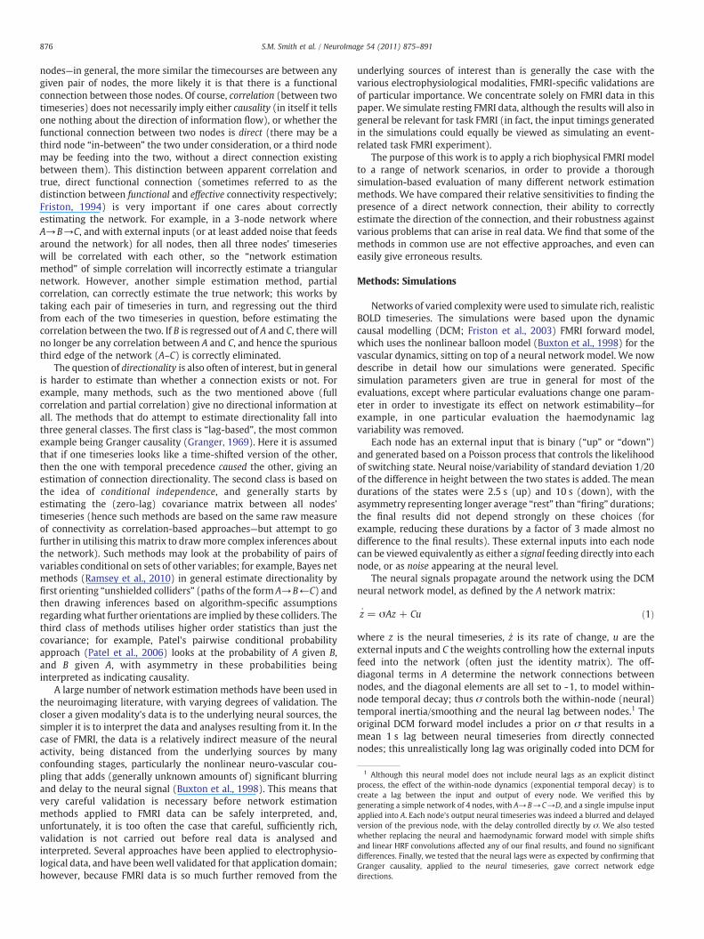
Fig. 1. Example simulated neural and FMRI BOLD timeseries, for a simple 2-node network, where node 1 feeds into node 2 with strength 0.4, and both nodes have random externalinputs as described in the main text. The y-axis units are arbitrary. Blue shows the neural/BOLD data at node 1, and orange shows node 2.

877S.M. Smith et al. / NeuroImage 54 (2011) 875–891

practical algorithmic purposes in the Bayesian modelling. Althoughthis is not a problem when DCM is applied to real data (as the dataoverwhelms this weak prior), it produces unrealistic lags in asimulation based on this model. Hence we changed this to a morerealistic time constant, resulting in a mean neural lag of approx-imately 50 ms. This is chosen to be towards the upper end of themajority of neural lags generally seen,2 in order to evaluate lag-basedmethods in a best-case scenario, while remaining realistic. (Thereason for not also testing the lag-based methods with lower, morerealistic neural lags is that, as seen below, even with a relatively longlag of 50 ms, performance of these methods is poor.)

Each node's neural timeseries was then fed through the nonlinearballoon model for vascular dynamics responding to changing neuraldemand. The amplitude of the neural timeseries were set so that theamount of nonlinearity (nonlinearity here being potentially withrespect both to changing neural amplitude and duration) matchedwhat is seen in typical 3 T FMRI data, and BOLD % signal changeamplitudes of approximately 4% resulted (relative to mean intensityof simulated timecourses). The balloon model parameters were ingeneral set according to the priormeans in DCM. However, it is knownthat the haemodynamic processes vary across brain areas andsubjects, resulting in different lags between the neural processesand the BOLD data, with variations of up to at least 1 s (Handwerkeret al., 2004; Chang et al., 2008). We therefore added randomness intothe balloon model parameters at each node, resulting in variations inHRF (haemodynamic response function) delay of standard deviation0.5 s. This is towards the lower end of the variability reported in theliterature, in order to evaluate lag-based methods in a best-casescenario while remaining reasonably realistic. Finally, thermal whitenoise of standard deviation 0.1–1% (of mean signal level) was added.

2 de Pasquale et al. (2010) note that intrahemispheric delays are typically 5–10 ms,while Ringo et al. (1994) note that unmyelinated interhemispheric fibres can result indelays of up to 300 ms, but in many long fibres are between 5 and 35 ms. Event-related potentials are often reported as being a few hundred milliseconds, but this isgenerally the delay between external stimulation and the response generated by ahigher cognitive area; hence, this period will typically have involved communicationbetween several distinct functional units, and is unlikely to reflect a single network“connection” that is of interest for investigation with imaging-based networkmodelling.

The BOLD data was sampled with a TR of 3 s (reduced to 0.25 s in afew simulations), and the simulations comprised 50 separaterealisations (or “subjects”), all using the same simulation parameters,except for having randomly different external input timeseries,randomly different HRF parameters at each node (as describedabove) and (slightly) randomly different connection strengths asdescribed below. Each “subject's” data was a 10-min FMRI session(200 timepoints) in most of the simulations. Example simulatedneural and FMRI BOLD timeseries can be seen in Fig. 1, for a simple 2-node network, where node 1 feeds into node 2 with strength 0.4, andboth nodes have external inputs as described above.

The main network topologies are shown in Fig. 2. The firstnetwork, S5, was 5 nodes in a ring (though not with cyclic causality—see arrows within the figure), with one independent external inputper node, and connection strengths set randomly to have mean 0.4,standard deviation 0.1 (with maximum range limited to 0.2:0.6). S10took two networks like S5, connected via one link only (a simple“small-world” network). S50 used 10 sub-networks, again with“small-world” topology. Each N-node network can also be repre-sented as an N×N connection matrix (see examples in Fig. 2), whereeach element (i,j) determines the presence of a connection from nodei to node j, and directed connections are represented by asymmetry inthe elements—if (i,j) is nonzero and (j,i) is zero, then there isdirectionality from node i to node j.

Our evaluations looked at the distribution of estimated networkresults over the 50 simulated subjects, to estimate false-positive andfalse-negative rates for the various methods tested. Some aspects ofour simulation framework are similar to that used to evaluate the“greedy equivalence search” (GES) network modelling method inRamsey et al. (2010). One difference is that, whereas Ramsey et al.(2010) developed and tested methodology for explicit cross-subjectnetwork modelling, we concentrate here on evaluating networkmodelling methods for single subject (single session) datasets, andonly utilise multiple subjects' datasets in order to characterisevariability of results across multiple random instantiations of thesame underlying network simulation. There is also a similar approachto simulated data generation inWitt andMeyerand (2009), where theDCM forward model is used to generate a simple 3 node network,with evaluation of DCM, structural equation modelling and autore-gressive modelling (including Granger causality). In Marrelec et al.

Fig. 2. The main network topologies fed into the FMRI data simulations. For each network graph the corresponding connection matrix is shown, where an element in the upperdiagonal of the matrix implies a directed connection from a lower-numbered node to a higher-numbered one.

878 S.M. Smith et al. / NeuroImage 54 (2011) 875–891

(2009) there is another somewhat similar simulation of BOLDtimeseries, using a large-scale neural model of seven network nodesunder different task conditions, followed by linear haemodynamicconvolution; this is used to investigate the performance of partialcorrelation, and compare against structural equation modelling.

Methods: Network modelling methods tested

We now give a brief description of each of the methods tested.Where minor variants of each main method (including alternativechoices in controlling parameters) performed universally worse thanother variants, we exclude the unsuccessful variants from furtherconsideration in the paper, in order to maximise the clarity ofpresentation. We describe all variants tested (including descriptionsof those that were rejected) within this section.

Not tested: DCM and SEM

There are two major network modelling approaches which wehave not included in this paper—dynamic causal modelling (DCM;Friston et al., 2003) and structural equation modelling (SEM; Wright,1920; McIntosh and Gonzales-Lima, 1994). The primary reason for theexclusion of both methods is mathematical and computationalfeasibility—neither method is able to effectively search across thefull range of possible network topologies, as well as both beingmathematically poorly conditioned when attempting to fit the mostgeneral (unconstrained) network model to data. In general, bothapproaches need (at most) a few potential networks to behypothesised and compared with their respective modellingapproaches, though see Freenor and Glymour (2010) for early workon searching over DCM models.

The second reason why DCM is not appropriate here is that we areinterested in modelling resting as well as task FMRI data. While thereis some early work on stochastic DCMs that may be able to addressthis (Daunizeau et al., 2009), established DCM methods require that

the “input” timings be specified in advance—something that is clearlynot known for resting data.

Correlation and Partial correlation

The simplest measure of pairwise similarity between two time-series is covariance. If the timeseries are normalised to unit variancethis measure becomes (normalised) correlation, which we will referto as Full correlation, to distinguish this from partial correlation.

We also evaluated full correlation, applied after bandpass filteringall timeseries data, to investigate if certain BOLD frequency bandscontain more useful information for connectivity modelling. We didthis because both the signal and the noise are potentially frequency-dependent (for example, the haemodynamics reduce the power in thesignal at the highest frequencies). We first filtered the data keepingthe lower and (separately) upper halves of the full frequency range,and also filtered the data into eight bands, each covering 1/8th of thefull frequency range. Results from most frequency bands performedless well than using the unfiltered data, with network connectionsensitivity becoming increasingly poorer at higher frequencies. Thetwo frequency bands that did show some interesting results were thebottom-half of the range (bandpass1/2) and the second-lowest of theeight frequency bands (bandpass2/8).

Partial correlation refers to the normalised correlation betweentwo timeseries, after each has been adjusted by regressing out allother timeseries in the data (all other network nodes). One attractivefeature of doing this is that it attempts to distinguish direct fromindirect connections, as discussed above. Partial correlation has beenadvocated (e.g., Marrelec et al., 2006, where light regularisation of thepartial correlation matrix is applied using an uninformative prior), asbeing a good surrogate for SEM, which makes sense if one thinks ofSEM as being a multiple regression where the data is related to itselfvia a network matrix, the link being that parameter estimation in amultiple regression framework is always driven by the unique(orthogonal) components of any given regressor within the model.

879S.M. Smith et al. / NeuroImage 54 (2011) 875–891

Regularised inverse covariance

An efficient way to estimate the full set of partial correlations is viathe inverse of the covariance matrix (Marrelec et al., 2006). Under theconstraint that this matrix is expected to be sparse, regularisation canbe applied, for example, using the Lassomethod (Banerjee et al., 2006;Friedman et al., 2008). This shrinks entries that are close to zero morethan those that are not, and can be useful in the context of Bayes nets/graphical models. For example, this method (which we refer to asICOV: Inverse COVariance) is expected to be useful when there are alimited number of observations at each node, such as with shorterFMRI scanning sessions.

If we consider a continuum of methods, with one extreme beingpure pairwise methods (e.g., full correlation) and the other extremeglobal network modelling approaches (e.g., Bayes nets), then partialcorrelation (which uses all nodes' data in its calculations) sitssomewhere in the middle, with ICOV also being intermediate, but alittle closer to the more global modelling extreme. SEM could bethought of as being one option at the global modelling extreme, wheremore sophisticated/explicit modelling allows (under certain modelassumptions) the estimation of model aspects such as the involve-ment of “latent variables” (external inputs which are not directlymeasured, but inferred from the viewed data).

We use an implementation of ICOV referred to as L1precision(www.cs.ubc.ca/~schmidtm/Software/L1precision.html), whichrequires the setting of the regularisation-controlling parameter λ.We tested a range of λ values: 5, 10, 20, 50, 100, and 200 (higher λgives greater regularisation).3 Final results showed that values of 10,20, 50, and 200 never gave the best results, and so were discarded,keeping the values of 5 and 100. We also tested the value of 0 (noregularisation), to confirm that this gave the same results as partialcorrelation, which indeed was the case, and hence this was notreported on below.

Mutual information

Mutual information (MI) (Shannon, 1948) quantifies the sharedinformation between two variables, and can reflect both linear andnonlinear dependencies. It is calculated by comparing the individualand joint histograms, and is high when one variable predictscharacteristics of the other. AsMI is sensitive to higher order statisticsthan is correlation (which only considers second order), this measuremay be able to detect some forms of network connectivity thatcorrelation cannot.

We used the implementation in the Functional ConnectivityToolbox (Zhou et al., 2009) (groups.google.com/group/fc-toolbox).As well as estimating mutual information, we also estimated PartialMI, for each pair of timecourses after all other timecourses in a givendataset were regressed out of the pair of interest.

Granger causality and related lag-based measures

Granger causality (Granger, 1969) defines a statistical interpreta-tion of causality in which A is said to cause B if knowing the past of Acan help predict B better than knowing the past of B alone. This isimplemented using multivariate vector autoregressive modelling(MVAR). Early use of Granger causality for neuroimaging data canbe found in Goebel et al. (2003) and Roebroeck et al. (2005). There hasbeen some criticism of this approach (e.g., Friston, 2009), in part dueto the lack of a biologically based generative model, but also withspecific problems raised such as the likelihood of spurious estimated

3 The L1precision code does not enforce scale invariance for the covariance vs. λ; hencewe utilised the following call to this code, in order to normalise the overall scaling of thecovariance, and adjust λ accordingly. Use of this call allows the reader to interpret the λvalues quoted here correctly: icov=L1precisionBCD(cov(X)/mean(diag(cov(X))), λ/1000)

“causality” being in fact caused by systematic differences across brainregions in haemodynamic lag (this being a problem for FMRI, but notin general for more direct electrophysiological modalities).

We tested four implementations of Granger causality. For the first,we used the “Causal Connectivity Analysis” toolbox (Seth, 2010)(www.anilseth.com). This implements “conditional” Granger causal-ity (Geweke, 1984), where “one variable causes a second variable ifthe prediction error variance of the first is reduced after including thesecond variable in the model, with all other variables included in bothcases” (Guo et al., 2008). As this requires the specification of the“model order” (number of recent timepoints to include in theautoregressive model) we tested (separately) the use of 1, 2, 3, 10and 20 previous observations. These results are referred to below asGranger Anwhere n is the model order. The toolbox also allows for theestimation of “partial” Granger causality (Guo et al., 2008), whichattempts to further reduce the deleterious effects of latent (unre-corded) confounding processes by making greater utilisation of theoff-diagonal covariance matrix terms than the “conditional” approachdoes.

The second implementation that we tested was pairwiseGranger causality estimation, using the Bayesian InformationCriterion to estimate the model order, up to a specified maximum(www.mathworks.co.kr/matlabcentral/fileexchange/25467-granger-causality-test). We again set the maximum lags considered to 1, 2, 3,10 and 20 (though in this case, the model order chosen by the use ofBIC may well be less than the maximum allowed). This set of tests isreferred to as Granger Bn.

The third and fourth implementations that we tested were fromthe BioSig toolbox (biosig.sourceforge.net): DC (“directed Grangercausality”) and GGC (“Geweke's Granger causality”). We tested thesame range of maximumMVARmodel orders as listed above, and alsodid this with the other lag-based methods from BioSig mentionedbelow. GGC can be restricted to be applied to frequencies of interest inthe data; we found that the highest frequencies gave the best resultsand so report just a single set of results (for each MVARmodel order),taken from the top end of the data frequencies.

The default Granger measure of causality for A causing B is an F-statistic FAB, and the measure for the reverse causality is FBA. InRoebroeck et al. (2005) it is suggested that a more robust variant ofthe Granger causality measure for A causing B is to subtract the twomeasures, i.e., use FAB−FBA. We therefore tested this “causality-difference” measure for all of the above Granger evaluations, inaddition to the raw direction measures. (In our directionalityevaluations we did in any case subtract the two directions' estimatesfor all measures, rendering this unnecessary for those tests, but thatdoes not fully remove the value of adding in the above differencemeasures, to allow connection strength to be evaluated separately fornon-differenced and differenced Granger measures.)

We also tested Partial directed coherence (PDC), which measuresthe “relationships (direction of information flow) between multivar-iate time series based on the decomposition of multivariate partialcoherences computed frommultivariate autoregressivemodels…[thisreflects] a frequency-domain representation of the concept of Grangercausality” (Baccalá and Sameshima, 2001). We used the implemen-tation of PDC in the BioSig toolbox. PDC is a function of the frequencies(in the data) that are investigated; we found that all frequenciesexcept the very highest gave identical results, and so only report oneset of results (for each MVAR model order) for PDC.

Directed transfer function (DTF) is another frequency-domainmethod that “describes propagation between channels furnishing atthe same time information about their directions and spectralcharacteristics. It makes possible the identification of situationswhere different frequency components are propagating differently”(Kamiński et al., 1997). We used the implementation in BioSig. Aswith PDC, DTF is a function of the frequencies investigated in the data;again we found the results almost identical across frequencies, with a

880 S.M. Smith et al. / NeuroImage 54 (2011) 875–891

slight preference for the higher frequencies, and hence only reportone set of results (for eachMVARmodel order) for DTF.We also testeda “modified version” of DTF implemented in BioSig (“ffDTF”), but thisgave the same results as DTF, so we do not report further on thismethod.

All of the BioSig-based measures gave equivalent or better resultswhen run pairwise, compared with feeding in the entire sets of allnodes' timeseries; hence we only report the pairwise results below.

An extra pre-processing option for lag-based methodologies is todetrend, demean and normalise to unit temporal standard deviationall timecourses before passing them into causality estimation. Werepeated all of the above tests with such pre-processing included, butfound that this made no appreciable difference to any results, and sodiscarded those evaluations from further consideration.

From all of the Granger evaluations, using the “causality-difference” measures were never better than the raw directionalmeasures, although in many cases they were very similar. Wetherefore do not report these further. From the Granger A tests, wefound that the “partial” Granger causality evaluations were alwayssimilar to or worse than the “conditional” measures, so we do notpresent those in our detailed results below. The 2 and 10 model orderevaluations for Granger A were discarded as they did not perform aswell as the other choices. In the Granger B tests, all results wereidentical across different maximum model orders, implying that theBIC was always dictating a model order of 1; we thus discarded allhigher-order tests. For GGC we kept model orders 1 and 10, as theothermodel orders never performed as well. All data frequencies from0.01 to 0.1 Hz were similar, with 0.01 Hz performing slightly better,and so we kept only the GGC results from 0.01 Hz filtering. For DC, wediscardedmodel orders of 1 and 20, as these did not perform aswell asorders 2, 3, and 10. For PDC we discarded model orders of 2 and 20,and for DTF, we discarded 1, 2 and 20, in both cases because theynever performed as well as other model orders.

Coherence

Two signals are said to be coherent if they have constant relativephase, or, equivalently, if their power spectra correlate, for a giventime and/or frequency window. This measure is therefore insensitiveto a fixed lag between two timeseries. Coherence is typically eitherestimated for a single (often narrow) frequency range, or estimatedwithin multiple frequency ranges, with the multiple results thencombined with each other.

We tested two implementations of coherence. For the first we usedwavelet transform coherence from the Crosswavelet and WaveletCoherence Matlab toolbox (Grinsted et al., 2004) (www.pol.ac.uk/home/research/waveletcoherence). This allows the estimation ofcoherence between two signals as a function of both time andfrequency, and was used recently in Chang and Glover (2010) toinvestigate nonstationary effects in resting FMRI data. Continuouswavelet transforms are used to estimate phase-locked behaviour intwo timeseries, and we average our different coherence measuresover all estimated time windows. We estimate mean (over time)coherence for 0.15 Hz (close to the highest possible frequency),0.017 Hz (close to the lowest), average over all frequencies, averageover 25–50% of the frequency range, and average over the lower halfof the frequency range; these are referred to as Coherence A1 to A5respectively. For measures 3–5 we also estimated the 95th percentile(across the entire set of values from all times and frequencies withinthe ranges described) instead of the mean. We did this in the hopethat we might show increased sensitivity to nonstationarities in theBOLD data (in the simulation where we generated nonstationarycorrelations); however Coherence A3 (mean over all frequencies)always performed better than the other options, so the rest werediscarded.

The second implementation of coherence that we used was thatprovided in the Functional Connectivity Toolbox mentioned above.This estimates the normalised cross-spectral density at a range offrequencies (up to Nyquist). We tested the same set of frequenciesand frequency ranges as above, though we do not have separatemeasurements at separate timepoints (as we set the time window forspectral estimation to be equal to the timeseries length); these arereferred to as Coherence B1–5. Coherence B3 (mean over allfrequencies) always performed better than the other options, so therest were discarded.

Generalised synchronisation

Generalised (or nonlinear) synchronisation “evaluates synchronyby analysing the interdependence between the signals in a state spacereconstructed domain” (Dauwels et al., 2010). We used theimplementation available at www.vis.caltech.edu/~rodri/programs/synchro.m, which provides three related measures of nonlinearinterdependence utilising generalised synchronisation; for detaileddescriptions of these measures and the differences between them, seeQuian Quiroga et al. (2002) and Pereda et al. (2005). These arereferred to in our results as Gen Synch S/H/N. We found thatmethodsHand N always gave very similar results, so we just report H below.

The three primary measures generated by the generalisedsynchronisation code are directional. In Quian Quiroga et al. (2002)there is discussion of the interpretability of asymmetries in thesedirectional measures. It is stated that the “asymmetry can giveinformation about driver-response relationships, but can also reflectthe different dynamical properties of the data”, and indeed, we didoften find that the direction of the asymmetry was not consistentacross the three tested synchronisation measures.

We used the default parameters of embedding dimension=10,number of nearest neighbours=10, Theiler correction=50. Wetested the effects of doubling and halving each of these parameters;this caused either unchanged or worse network estimation perfor-mance, so we left these default values unchanged. With respect to thetime lag parameter, we tested both the default of 2, and also testedtime lag=1 (hence the numbers 2 and 1 in our results below).

Because the three measures are directional, we also averaged bothdirections' measures as a further test of connection strength, but thisdid not improve any results, and so is not reported on further. Finally,we also estimated Gen Synch measures for each pair of timecoursesafter all other timecourses in a given dataset were regressed out of thepair of interest, but this did not improve results, so we do not reportfurther on those tests.

Patel's conditional dependence measures

The conditional dependence proposed in Patel et al. (2006) simplylooks at an imbalance between P(x|y) and P(y|x), to arrive at ameasure of connectivity/causality. This makes most sense (as a datamodel) when applied to fundamentally binarised data, however it canalso be applied to continuous data. Here we mapped each timeseriesinto the range 0:1, by limiting data under the 10th percentile to 0, anddata over the 90th percentile to 1, and linearly mapping data inbetween to the range 0:1. We then calculate the conditionaldependencies directly from these “normalised” timeseries. There aretwo measures that can be derived from the conditional dependences:κ, a measure of connection strength, and τ, a measure of connectiondirectionality.

As well as the results based on the continuous data, we alsobinarised the timeseries at a range of thresholds (0.25, 0.5, 0.75, 0.9)after mapping the data into the range 0:1 as discussed above. Each ofthese resulted in a separate evaluation. We found that binarisation at0.25, 0.5 and 0.9 always performed worse or equal to binarisation at0.75 or no binarisation, so these results were discarded.

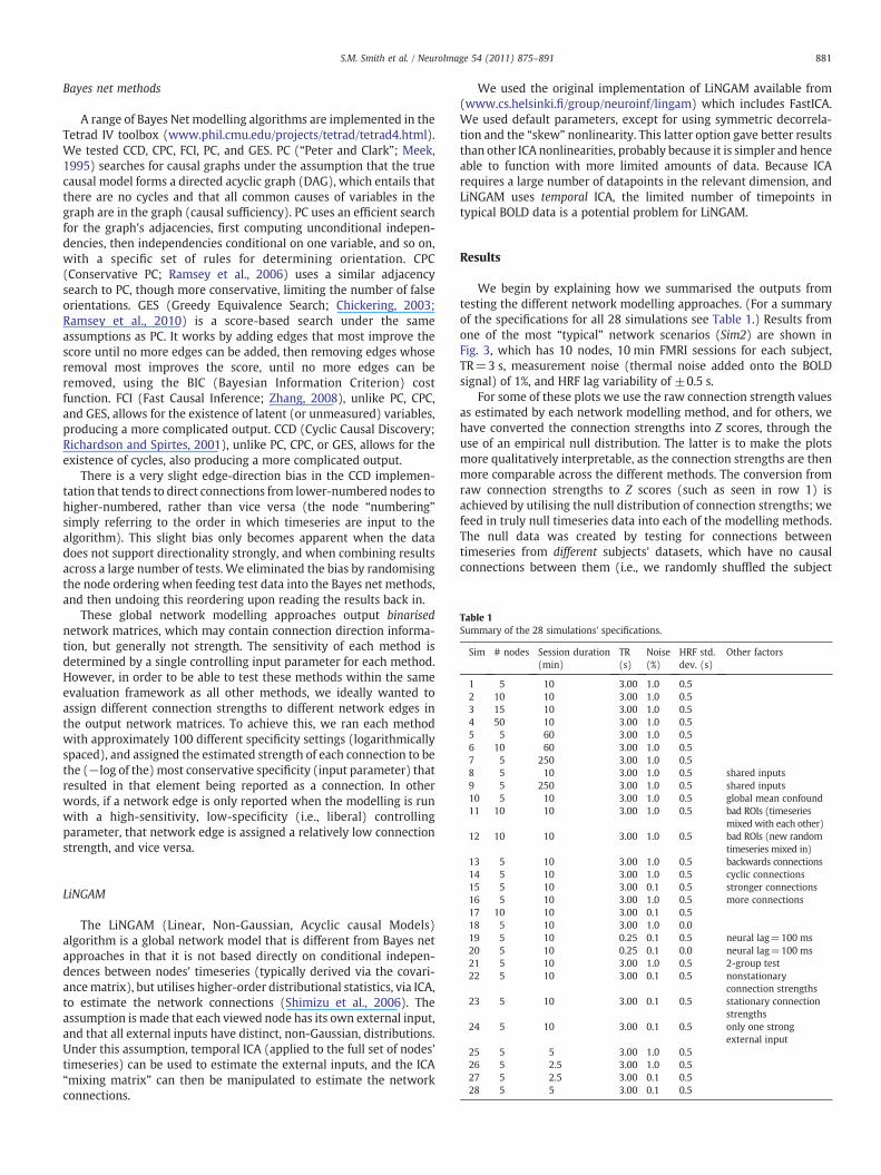
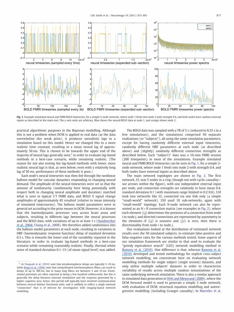
Table 1Summary of the 28 simulations' specifications.

Sim # nodes Session duration(min)

TR(s)

Noise(%)

HRF std.dev. (s)

Other factors

1 5 10 3.00 1.0 0.52 10 10 3.00 1.0 0.53 15 10 3.00 1.0 0.54 50 10 3.00 1.0 0.55 5 60 3.00 1.0 0.56 10 60 3.00 1.0 0.57 5 250 3.00 1.0 0.58 5 10 3.00 1.0 0.5 shared inputs9 5 250 3.00 1.0 0.5 shared inputs10 5 10 3.00 1.0 0.5 global mean confound11 10 10 3.00 1.0 0.5 bad ROIs (timeseries

mixed with each other)12 10 10 3.00 1.0 0.5 bad ROIs (new random

timeseries mixed in)

881S.M. Smith et al. / NeuroImage 54 (2011) 875–891

Bayes net methods

A range of Bayes Net modelling algorithms are implemented in theTetrad IV toolbox (www.phil.cmu.edu/projects/tetrad/tetrad4.html).We tested CCD, CPC, FCI, PC, and GES. PC (“Peter and Clark”; Meek,1995) searches for causal graphs under the assumption that the truecausal model forms a directed acyclic graph (DAG), which entails thatthere are no cycles and that all common causes of variables in thegraph are in the graph (causal sufficiency). PC uses an efficient searchfor the graph's adjacencies, first computing unconditional indepen-dencies, then independencies conditional on one variable, and so on,with a specific set of rules for determining orientation. CPC(Conservative PC; Ramsey et al., 2006) uses a similar adjacencysearch to PC, though more conservative, limiting the number of falseorientations. GES (Greedy Equivalence Search; Chickering, 2003;Ramsey et al., 2010) is a score-based search under the sameassumptions as PC. It works by adding edges that most improve thescore until no more edges can be added, then removing edges whoseremoval most improves the score, until no more edges can beremoved, using the BIC (Bayesian Information Criterion) costfunction. FCI (Fast Causal Inference; Zhang, 2008), unlike PC, CPC,and GES, allows for the existence of latent (or unmeasured) variables,producing a more complicated output. CCD (Cyclic Causal Discovery;Richardson and Spirtes, 2001), unlike PC, CPC, or GES, allows for theexistence of cycles, also producing a more complicated output.

There is a very slight edge-direction bias in the CCD implemen-tation that tends to direct connections from lower-numbered nodes tohigher-numbered, rather than vice versa (the node “numbering”simply referring to the order in which timeseries are input to thealgorithm). This slight bias only becomes apparent when the datadoes not support directionality strongly, and when combining resultsacross a large number of tests. We eliminated the bias by randomisingthe node ordering when feeding test data into the Bayes net methods,and then undoing this reordering upon reading the results back in.

These global network modelling approaches output binarisednetwork matrices, which may contain connection direction informa-tion, but generally not strength. The sensitivity of each method isdetermined by a single controlling input parameter for each method.However, in order to be able to test these methods within the sameevaluation framework as all other methods, we ideally wanted toassign different connection strengths to different network edges inthe output network matrices. To achieve this, we ran each methodwith approximately 100 different specificity settings (logarithmicallyspaced), and assigned the estimated strength of each connection to bethe (−log of the) most conservative specificity (input parameter) thatresulted in that element being reported as a connection. In otherwords, if a network edge is only reported when the modelling is runwith a high-sensitivity, low-specificity (i.e., liberal) controllingparameter, that network edge is assigned a relatively low connectionstrength, and vice versa.

13 5 10 3.00 1.0 0.5 backwards connections14 5 10 3.00 1.0 0.5 cyclic connections15 5 10 3.00 0.1 0.5 stronger connections16 5 10 3.00 1.0 0.5 more connections17 10 10 3.00 0.1 0.518 5 10 3.00 1.0 0.019 5 10 0.25 0.1 0.5 neural lag=100 ms20 5 10 0.25 0.1 0.0 neural lag=100 ms21 5 10 3.00 1.0 0.5 2-group test22 5 10 3.00 0.1 0.5 nonstationary

connection strengths23 5 10 3.00 0.1 0.5 stationary connection

strengths24 5 10 3.00 0.1 0.5 only one strong

external input25 5 5 3.00 1.0 0.526 5 2.5 3.00 1.0 0.527 5 2.5 3.00 0.1 0.528 5 5 3.00 0.1 0.5

LiNGAM

The LiNGAM (Linear, Non-Gaussian, Acyclic causal Models)algorithm is a global network model that is different from Bayes netapproaches in that it is not based directly on conditional indepen-dences between nodes' timeseries (typically derived via the covari-ancematrix), but utilises higher-order distributional statistics, via ICA,to estimate the network connections (Shimizu et al., 2006). Theassumption is made that each viewed node has its own external input,and that all external inputs have distinct, non-Gaussian, distributions.Under this assumption, temporal ICA (applied to the full set of nodes'timeseries) can be used to estimate the external inputs, and the ICA“mixing matrix” can then be manipulated to estimate the networkconnections.

We used the original implementation of LiNGAM available from(www.cs.helsinki.fi/group/neuroinf/lingam) which includes FastICA.We used default parameters, except for using symmetric decorrela-tion and the “skew” nonlinearity. This latter option gave better resultsthan other ICA nonlinearities, probably because it is simpler and henceable to function with more limited amounts of data. Because ICArequires a large number of datapoints in the relevant dimension, andLiNGAM uses temporal ICA, the limited number of timepoints intypical BOLD data is a potential problem for LiNGAM.

Results

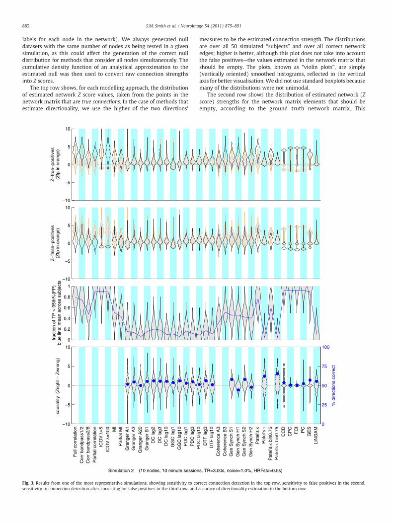
We begin by explaining how we summarised the outputs fromtesting the different network modelling approaches. (For a summaryof the specifications for all 28 simulations see Table 1.) Results fromone of the most “typical” network scenarios (Sim2) are shown inFig. 3, which has 10 nodes, 10 min FMRI sessions for each subject,TR=3 s, measurement noise (thermal noise added onto the BOLDsignal) of 1%, and HRF lag variability of ±0.5 s.

For some of these plots we use the raw connection strength valuesas estimated by each network modelling method, and for others, wehave converted the connection strengths into Z scores, through theuse of an empirical null distribution. The latter is to make the plotsmore qualitatively interpretable, as the connection strengths are thenmore comparable across the different methods. The conversion fromraw connection strengths to Z scores (such as seen in row 1) isachieved by utilising the null distribution of connection strengths; wefeed in truly null timeseries data into each of the modelling methods.The null data was created by testing for connections betweentimeseries from different subjects' datasets, which have no causalconnections between them (i.e., we randomly shuffled the subject

882 S.M. Smith et al. / NeuroImage 54 (2011) 875–891

labels for each node in the network). We always generated nulldatasets with the same number of nodes as being tested in a givensimulation, as this could affect the generation of the correct nulldistribution for methods that consider all nodes simultaneously. Thecumulative density function of an analytical approximation to theestimated null was then used to convert raw connection strengthsinto Z scores.

The top row shows, for each modelling approach, the distributionof estimated network Z score values, taken from the points in thenetwork matrix that are true connections. In the case of methods thatestimate directionality, we use the higher of the two directions'

−10

−5

0

5

10

Z−

true

−po

sitiv

es(Z

fp in

ora

nge)

−10

−5

0

5

10

Z−

fals

e−po

sitiv

es(Z

tp in

ora

nge)

0

0.2

0.4

0.6

0.8

1

frac

tion

of T

P >

95t

h%(F

P)

blue

line

: mea

n ac

ross

sub

ject

s

−10

−5

0

5

10

caus

ality

(Z

right

− Z

wro

ng)

Simulation 2 (10 nodes, 10 minute session

Ful

l cor

rela

tion

Cor

r ba

ndpa

ss1/

2C

orr

band

pass

2/8

Par

tial c

orre

latio

nIC

OV

λ=

5IC

OV

λ=

100 MI

Par

tial M

IG

rang

er A

1G

rang

er A

3G

rang

er A

20G

rang

er B

1D

C la

g2D

C la

g3D

C la

g10

GG

C la

g1G

GC

lag1

0P

DC

lag1

PD

C la

g3

Fig. 3. Results from one of the most representative simulations, showing sensitivity to cosensitivity to connection detection after correcting for false positives in the third row, and

measures to be the estimated connection strength. The distributionsare over all 50 simulated “subjects” and over all correct networkedges; higher is better, although this plot does not take into accountthe false positives—the values estimated in the network matrix thatshould be empty. The plots, known as “violin plots”, are simply(vertically oriented) smoothed histograms, reflected in the verticalaxis for better visualisation.We did not use standard boxplots becausemany of the distributions were not unimodal.

The second row shows the distribution of estimated network (Zscore) strengths for the network matrix elements that should beempty, according to the ground truth network matrix. This

s, TR=3.00s, noise=1.0%, HRFstd=0.5s)

PD

C la

g10

DT

F la

g3D

TF

lag1

0C

oher

ence

A3

Coh

eren

ce B

3G

en S

ynch

S1

Gen

Syn

ch H

1G

en S

ynch

S2

Gen

Syn

ch H

2

Pat

el’s

κP

atel

’s τ

Pat

el’s

κ b

in0.

75P

atel

’s τ

bin0

.75

CC

DC

PC

FC

IP

CG

ES

LiN

GA

M

0

25

50

75

100

% d

irect

ions

cor

rect

rrect connection detection in the top row, sensitivity to false positives in the second,accuracy of directionality estimation in the bottom row.

4 Our tests require running each Bayes net method many thousands of times, whichis why we had to exclude these from our 50-node testing; however, if only needing tobe run once (i.e., on real data), the Bayes net methods are in general usable,completing on 50 nodes in less than an hour, and, judged qualitatively, performingwell.

883S.M. Smith et al. / NeuroImage 54 (2011) 875–891

distribution of “false positive” (FP) values should ideally be non-overlapping with the TP distribution, for successful methods. In thetop row the TP distribution is shown in black, with the FP distributionshown in orange, for ease of comparison, and vice versa in row 2.

The fact that the FP values shown in row 2 are not all zero-meanunit-standard-deviation (as one might expect from the fact that thevalues have been all converted to Z scores using the null distributionderived from truly null data) reflects the fact that the presence of trueconnections will often induce increased false positive estimation(indirect connections). For example, note that the FP distribution forFull correlation is higher than that for Partial correlation, because thelatter takes steps to reduce the estimation of indirect (FP)connections.

Row 3 combines the information from the top two rows—it showsthe fraction of true positives that are estimated with higherconnection strengths than the 95th percentile of the false positivedistribution. This is therefore a measure of the success in separatingthe TP from the FP estimated connection strengths. The FP-basedthreshold is estimated separately for each subject, and the number ofTP values above this counted, and then divided by the total number oftrue connections. The violin-plot distributions are thus showingvariation across subjects. We do not need to use the Z scores here, butuse the raw values, for greater accuracy. The blue line plots the meanof the distributions of TP fraction. As this value will be discussedmanytimes in the following text, we shall refer to this mean fractional rateof detecting true connections as “c-sensitivity”; this is the mostimportant, quantitative evaluation of how sensitive the differentmethods are to estimating the presence of a network connection (asopposed to its directionality).

The general story regarding c-sensitivity told by this particularsimulation is reasonably reflective of our simulations in general.Partial correlation, ICOV and the Bayes net methods performexcellently, with a c-sensitivity of more than 90%. Full correlationand Patel's κ perform a little less well.MI, Coherence and Gen Synch aresignificantly less sensitive, with a c-sensitivity of about 50%. The lag-based methods (Granger, etc.) perform extremely poorly, with c-sensitivity of under 20%. LiNGAM also performs poorly, as it requires alarger number of timepoints to function well.

Row 4 presents results of the connection directionality estimation.For each true connection (positive element in the true networkmatrix), we took the estimated connection strength for that element(i,j) and subtracted the corresponding estimated strength in thereverse direction (j,i). The violin-plot distributions of subtracted-Z areover all true connections and over all subjects. A distribution showinga majority of positive values designates success in estimatingdirectionality (causality). The blue dots indicate the overall percent-age of causality directions that are correct, with 50% being the level ofchance. We shall refer to this mean fractional rate of detecting thecorrect directionality of true connections as “d-accuracy”. Somemethods (e.g., Full correlation) only output symmetric networkmatrices, hence no results are shown for these methods.

Again, the general story told by this particular simulation isreasonably reflective of many of our simulations. None of themethodsis very accurate, with Patel's τ performing best at estimatingdirectionality, reaching nearly 65% d-accuracy, all other methodsbeing close to chance.

We now discuss various sets of simulations, each testing a differentaspect of real-world data and experimental designs. The full set ofplots is included in the Supplementary Information; in the text belowwe summarise the relevant findings from each simulation.

Basic simulation results

We start with a set of basic experimental/data scenarios. Asdiscussed above, Sim2 has 10 nodes, 10 min FMRI sessions for eachsubject, TR=3 s, final added noise of 1%, and HRF variability of ±0.5 s.

Sim1 is the same, but with just 5 nodes. These two simulations arereferred to frequently in the following sections, as “baselines” againstwhich to compare the various changes we make in the networkscenarios. Sim3 is also the same, but with 15 nodes, organised in 3clusters of 5 nodes. Sim4 is the same, but with 50 nodes, as shown inFig. 2.

The Sim2 results were summarised above; in particular, Partialcorrelation, ICOV and the Bayes net methods perform excellently, witha c-sensitivity of above 90%, while at the other end of the spectrum,lag-based methods (Granger, etc.) perform extremely poorly, detect-ing less than 20% of true network connections. None of the methods isvery accurate at estimating directionality, with Patel's τ performingbest, reaching nearly 65% d-accuracy. The results with 5 and 15 nodesare extremely similar to those with 10.

With 50 nodes, the Bayes Net methods and Granger A were toocomputationally intensive to be practical in our testing, and so are notreported.4 Full correlation, ICOV λ=100 and Patel's κ all performexcellently, at over 90% c-sensitivity. Full correlation performs slightlybetter than Partial correlation (just over 80%), which is not verysurprising as now the overall fraction of indirect connections is lowerthan with the smaller networks, aiding full correlation's results, whilethe number of timeseries to regress out of each pair being tested bypartial correlation is much larger than with the smaller networks,which presumably removes more signal from each pair. However,with increased regularisation from the higher λ of 100, ICOVwas ableto ameliorate this, and perform better than Full correlation. Nomethods gave impressive results in estimating directionality.

Sim17 shows results from the 10 node scenario, but this time withreduced noise added to the BOLD data—just 0.1%. This reduction inamplitude of noise by a factor of 10 reflects what onemight achieve byaveraging timeseries over multiple voxels—in the case of thermalnoise that is spatially uncorrelated, averaging over just 100 voxelswould be expected to give this reduction. Thismight, for example, be aresult of defining a spatial ROI, or by utilising one component'stimecourse from ICA, which in effect is averaging timecourses overvoxels present in a given component's spatial map. Somewhatsurprisingly, the results are very similar to Sim2, suggesting that (atleast in the range 0.1–1%), the exact amount of noise in the data doesnot significantly affect network estimation). Slight exceptions are thatMI and Coherence B3 have an increased c-sensitivity of 78%; clearlythese measures benefit more than others from reduced noise levels,but they are still significantly less sensitive than the best methods,which have now reached as high as 97% c-sensitivity.

Effect of FMRI session length

We now consider the effect of varying the FMRI session length.Sim5 contains 5 nodes and 60-min sessions (in reality this would notbe very pleasant for the subjects, but in general is possible).Comparing this with Sim1, we see that most methods have improvedsensitivity, with all methods except for LiNGAM and the majority ofthe lag-based methods achieving better than 80% c-sensitivity. Thesingle lag-based result that reaches 80% is Granger A3; however, fromthe fact that the d-accuracy in this case is almost no better thanchance, we must conclude that it is not the lag-based causalityinformation that is driving this result, but simply the fact thatcorrelation between timeseries is bleeding into the Granger causalitymeasure (see further investigation of this effect below).

With respect to the estimation of directionality, the lag-basedmethods are still performing poorly with the hour-long sessions.

884 S.M. Smith et al. / NeuroImage 54 (2011) 875–891

LiNGAM has now improved to 77%, with the increased number oftimepoints starting to help the temporal ICA to function well. Patel's τis largely unchanged, with all other methods still under 70% d-accuracy. We also simulated hour-long sessions for 10 nodes (Sim6).The results are very similar to those for 5 nodes, though LiNGAM isreduced slightly, to 67%.

When we increased the sessions further, to just over 4 h (Sim7),LiNGAMwas able to achieve the highest d-accuracy across all methodsin all of our tests (90%). Patel's τ bin0.75 was also impressive (79%),with CCD at 71%.

The Gen Synch H directionality is well below chance (making asignificant number of directionality estimates in the wrong direction).As discussed above, asymmetry in the Gen Synchmeasures is expectedto be potentially driven by other factors than just the underlyingcausality, and this appears to be the case here.

Sim25 contains 5-min sessions, and Sim28 has 5-min sessions withnoise reduced to 0.1%. The reduced session time does not greatly affectthe results, but does reduce estimation quality a little, with the bestapproaches still being Partial correlation, ICOV and the Bayes netmethods (c-sensitivity 70–78%). With the reduced noise level, resultsimproved towards the values seen in Sim1 (84–89%). As with Sim1,directionality estimation is not very impressive from any of themethods. This pattern develops further with 2.5-min sessions; Sim26contains 2.5-min sessions, with the same best three methods havingc-sensitivity 57-59%, and Sim27 has 2.5-min sessions with noise 0.1%,with the same best three methods having 71–76%.

To summarise the dependence of the best methods' c-sensitivityon session duration, for the 5 nodes, 1% BOLD noise case:60 min:100%, 10 min:95%, 5 min:77%, 2.5 min:59%.

Effect of global additive confound

The first “problem” that we introduced into the data was a globaladditive confound—adding the same random timeseries to all nodes'BOLD timeseries. There has been much discussion in the literatureregarding the nature of the global mean timeseries (i.e., whether it isprimarily valid neural-related signal, or uninteresting non-neuralphysiological confound) and whether it should be subtracted beforeany further analyses (Fox et al., 2009). The general consensus wouldcurrently appear to be that as many specific confounds as possibleshould be removed from the data (e.g., by estimating signal in whitematter and cerebrospinal fluid (CSF), and regressing this out of alltimeseries), but there is not clear agreement as to whether globaltimeseries removal should be carried out.

Here we investigated the effect of an additive global timeseriesconfound. From a real resting-FMRI dataset (36 subjects' 4D dataconcatenated temporally in a common space), we estimated thetimeseries from approximately 100 functional parcels. The data hadoriginally been “cleaned” through the use of confound regressorsderived from CSF and white matter masks, as well as head motionparameters. Further, we discarded ICA components which wereclearly artefactual. We took the mean of all 100 timecourses, andestimated the standard deviation of this, std(mean(Ti)). We thenestimated the mean of the standard deviations of each individualtimecourse, mean(std(Ti)). The ratio std(mean(Ti))/mean(std(Ti))was approximately 0.3, whereas in pure random noise data it wouldbe expected to be around 1 =

ffiffiffiffiffiffiffiffiffi

100p

=0.1, roughly suggesting an upperlimit to the additive global effect of approximately 20% of the raw datastandard deviation.

Initial results with a global mean confound having 20% of theamplitude of the “uncorrupted” data showed, somewhat surprisingly,almost no change in the final c-sensitivity and d-accuracy results, sowe increased the confound fraction to 50%, generating Sim10. Theresults are still almost unchanged, compared with Sim1, suggestingthat the potential presence of a global confound is not a problem.However, looking at the separate distributions of TP and FP values, we

see that for some methods the distributions are significantly shiftedupwards, as one would expect from adding in a global confound. Thisis particularly noticeable for Full correlation, not surprisingly. Becauseboth TP and FP distributions are shifted upwards, the c-sensitivityresults do not show a significant worsening, and this raises a potentialproblem in our interpretation of these results (and later use of certainnetwork modelling methods); if we do not already know what theglobal confound signal is, we cannot adjust for the altered FPdistribution, and hence cannot achieve the c-sensitivity results seen.We are only able, here, to estimate c-sensitivity because we alreadyknowwhat the ground truth is, but in real experiments we would not.However, all is not lost—we can see that with other modellingmethods (in particular the methods that performed the best in thebasic simulations—Partial correlation, ICOV and the Bayes netmethods), there is not a significant shift in the raw TP and FPdistributions. This is not surprising—for example, partial correlationwill be expected to remove (some fraction of) the global confoundfrom any pair of timeseries before they are correlated, because it ispresent in all the other timeseries (Marrelec et al., 2006). Theseresults and considerations provide added strength to the argument forusing these approaches, as opposed to (e.g.) Full correlation.

In those simulations that add confounding processes into the data,we did not regenerate the null distributions for the connectivitymeasures, but used those derived from the matched simulationswithout the confounds. We did this in order to make the TP and FP Zscore distributions more easily comparable across simulations, butthis has no effect on the quantitative measures of success (c-sensitivity and d-accuracy).

Effect of shared inputs

The next “problem” that we introduced into the data wasmixing ofthe external inputs feeding into the network. So far we have assumedthat each viewed node has its own independent external input. Theseinputs can be thought of as neuronal “noise”, or as distinct sensoryinputs, or as inputs from other parts of the brain not included in theset of viewed nodes. In the case of the latter two scenarios, there is thereal possibility that an external input could feed into more than oneviewed node, which could be expected to have a deleterious effect onthe network modelling, if this “sharing” of inputs is not modelled(Larkin, 1971). For example, this could arise if one has imaged (orconsidered) only certain parts of the brain.

Sim8 simulates this problem. In the previous simulations, theexternal inputs feed into the viewed nodes with strength 1; in thissimulation, in addition, each external input may feed into any otherviewed node with strength 0.3, with the random probability of thisoccurring being 20% for any one possible connection between externalinput and viewed node. The results, compared with Sim1, show thatthe presence of shared inputs is quite deleterious to all estimationmethods. Partial correlation and ICOV λ=5 fall respectively to 69% and67% c-sensitivity, with all other methods being below 60%. Thedirectionality estimates, however, are largely unchanged from theSim1 results.

Sim9 applies the same sharing of inputs to 4-h sessions. Comparedwith Sim7, We see all methods' c-sensitivity fall, but particularly theBayes net methods, which fall to less than 40%. However, the methodsthat showed the best directionality estimation results in Sim7(LiNGAM and Patel's τ bin0.75) still performed quite well (78% and73% respectively).

Effect of inaccurate ROIs

The next problem we considered is the effect of mixing the BOLDtimeseries with each other. Whereas the previous section discussedthe mixing of inputs, this is in effect a mixing of outputs from the datasimulation. This scenario would arise, for example, if the spatial ROIs

885S.M. Smith et al. / NeuroImage 54 (2011) 875–891

used to extract average timeseries for a brain region did not matchwell the actual functional boundaries. This is very likely to happen tosome extent when using predefined ROIs that are not derived fromthe data, for example when using atlas-based ROIs.

Sim11 simulates 10 nodes, and for each node's timeseries, mixes in arelatively small amountof oneothernode's timeseries (randomly chosen,but the same for all subjects), in proportion 0.8:0.2. The results areextremely bad—every method gives lower than 20% c-sensitivity.

A less serious related scenario is when we have incorrect ROIs, butthese just result in mixing in of signals from brain areas not alreadypresent in the set of ROIs used. For example, if the ROIs are spreadsparsely across the brain and not touching each other, then incorrect ROIspecification will in general not mix them together, but will mix in new,unrelated signals. Sim12 shows the effects of mixing in unrelatedtimeseries into each timeseries of interest (achieved, for each subject,by using data from another subject), again in the ratio of 0.8:0.2. In thiscase the additional “confounds” have almost no effect at all on thenetworkmodelling,with the results looking almost identical to Sim2. Thisis not very surprising, given that we have already established that theresults arenot very sensitive to addednoise,which is effectively allweareadding here (albeit with more temporal structure than previously).

Effect of backwards connections

It is rarely the case that two brain regions are connected in onedirection only; there will generally be connections in both directions,including those with “negative” connection strengths (implyinginhibition). However, it is not clear, in terms of gross, averagedbehaviour of information flow around a network, whether thepresence of backwards connections is in practice relevant. It is veryhard also to know how to insert such connections into our simulations—for example, how strong should the backwards connections be, andshould they be positive or negative? In the absence of clear answers tothese questions, we chose, somewhat arbitrarily, to randomly selecthalf of the forwards connections, and add into those a negativebackwards connection of equal average strength (0.4±0.1).

These results are reported in Sim13. Compared with Sim1, all theapproaches that were performing well have heavily reduced sensi-tivity, with the best methods being the Bayes Net approaches, at 64%c-sensitivity. Interestingly, Coherence, Gen Synch andMI are no longersignificantly worse than the correlation measures, ICOV and Patel's κ,all being around 50–55% c-sensitivity; this presumably is because theformer set of methods are relatively robust against the potentiallymore complex relationships induced by the backward connections. Nomethods performed well at estimating directionality in this simula-tion (maximum d-accuracy being 62%), where estimated direction-ality is compared against the positive, “forward” connection direction—though of course, the interpretation in the cases where a backwardsconnection is present is difficult.

Effect of cyclic connections

Sim14 shows the results from reversing the direction of theconnection between nodes 1 and 5 in the 5 node simulation. Thisgenerates “cyclic causality”, which is theoretically a problem for manyof the global networkmodelling approaches such as most of the Bayesnet methods, as this breaks their modelling assumptions.

Somewhat surprisingly, compared with Sim1, this change makesvirtually no difference to any of the c-sensitivity measures. It doesreduce the d-accuracy values, although these were already low inSim1.

Effect of more connections

Sim16 shows the effect of using a denser set of connections in the 5node simulation. As well as the original 5 out of 10 possible network

edges, we add in a further two more, leaving just 3 “missing” edges.This therefore simulates the scenario of a very highly connected smallnetwork. The results are very similar to Sim1, with a slight reductionin c-sensitivity in the best methods. There is also very little change inthe d-accuracy results.

Effect of stronger connections, and investigation of lag-baseddirectionality estimation

Sim15 shows the effect of increasing the strength of the networkconnections to a mean of 0.9 instead of 0.4. We set the noise to be0.1%, so these results should be compared against Sim17. In this casethe previously most sensitive methods (Partial correlation, ICOV andthe Bayes net methods) remain relatively unchanged in c-sensitivity,falling to 90–95%. Full correlation and Patel's κ fall further, to around60%—presumably the increased connection strengths have increasedthe sensitivity to detection of indirect connections. MI, Coherence andGen Synch are relatively unchanged, although notably, Partial MI isincreased to 85%, presumably because it is less sensitive to indirectconnections than MI. Lag-based methods are still performing verypoorly, the best reaching 34% c-sensitivity. With respect to estimatingdirectionality, Patel's τ, has increased to 78%, with Gen Synch rising to68%.

The lag-based methods have improved d-accuracy, with amaximum of 72% for GGC lag-10 and DC lag-10. However, the factthat the existence of the connections was only estimated with amaximum c-sensitivity of 34% suggests that the directionality resultsmay not be trustworthy (i.e. truly reflecting an estimation of causalitybased on lag). In order to investigate more interpretably whetherconcern here is justified, we simulated a two-node network (node 1feeding into node 2), with otherwise the same parameters as Sim15.The results were consistent with the above finding; some Grangermethods gave only chance-level results (e.g., Granger A1), but mostgave a reasonable level of correct directionality estimation. However,when we reduced the neural lag to 0 and re-ran the simulation, theresults were qualitatively unchanged—the Granger methods that hadpreviously reported the “correct” causal direction continued to do so,despite the absence of any lag between the two neural timeseries.Furthermore, when we returned the lag to 50 ms, but now increasedthe added noise to 1.5% for the first node only, the estimated causalitydirection then became negative (i.e., the wrong direction wasestimated) for all Granger methods. All of these results werereplicated if we replaced the DCM forward model (includingnonlinear dynamics) with a simple shift for the neural lag, followedby linear haemodynamic convolution. Unfortunately this demon-strates how the interaction of haemodynamic smoothing andmeasurement noise renders the lag-based methods generally unre-liable for FMRI data. Gen Synch at model order 1 also showed the sameproblems as seen with Granger, but did not show this with modelorder 2.

Effect of having only one strong external input

Sim24 is the same as Sim15 (strong connections and low noise),except that all nodes apart from node 1 had their external inputstrengths reduced from 1 to 0.1. With this reduction in external inputsand the low noise level, this simulation is passing the one primaryexternal source around the network with very little disturbance fromother sources or noise. The results become poor—none of themethodshad a c-sensitivity greater than 50%, and none had a d-accuracygreater than 61%. One hopes that this particular simulation is not toorepresentative of reality! In general every node is so highly correlatedwith every other node that it is hard for the methods to distinguishdirect from indirect connections. Of the methods that have so far beenperforming the best, Partial correlation and ICOV λ=5do still generateamongst the best results (c-sensitivity 46–48%), but not better than

886 S.M. Smith et al. / NeuroImage 54 (2011) 875–891

MI, Coherence and Gen Synch; the Bayes net models perform badly(27%).

Sensitivity to connection strength changes

Sim21 tests how sensitive the different methods are at detectingchanges in connection strength across different subjects. In this casewe started with the Sim1 simulation, but halved the strength of thenetwork connections in 25 of the 50 subjects. We then performed atwo-group t-test on the raw TP connection strength measures. Thistest is of relevance to researchers wishing to discriminate betweensubjects on the basis of network connectivity, for example comparingpatients vs. controls.While we have only evaluated “univariate” groupcomparisons here (i.e., testing each edge independently from eachother), there is a good chance that a more sensitive general approachto network change detection will be “multivariate” (i.e., using alledges simultaneously to find patterns of change).

The most sensitive method was Patel's κ, with t=7.4. Othersensitive methods, with tN5, were Full correlation, Partial correlation,ICOV, Gen Synch and most of the Bayes net methods.

Effect of nonstationary connection strength

Sim22 and Sim23 investigate the effect of nonstationarity ofconnection strength between nodes. At the neural level, there isevidence of connection strength varying over time (Popa et al., 2009;de Pasquale et al., 2010); this was investigated for FMRI data in Changand Glover (2010).

In Sim23, we used 5 nodes, noise of 0.1%, strong connections (mean0.9) and reduced strength of 0.3 for all external inputs apart fromnode 1. There was no nonstationarity present in this simulation.Partial correlation and ICOV perform the best, at around 80% c-sensitivity, but the Bayes net methods do not perform so well, fallingto 60%. For directionality estimation, Patel's τ and Gen Synch performreasonably, having d-accuracy of around 70%.

Sim22 is the same as Sim23, except that the connection strength ismodulated over time by additional random processes. The strength ofconnection between any two connected nodes is either unaffected, orreduced to zero, according to the state of a random external bistableprocess that is unique for that connection. The transition probabilitiesof this modulating input are set such that the mean duration ofinterrupted connections is around 30 s and the mean time of fullconnections is about 20 s. The results are quite similar to Sim22, themain difference being that the Bayes net methods improve quite a bit,achieving the highest c-sensitivity (78%), slightly ahead of Partialcorrelation and ICOV (both at 73%). We had expected that perhaps oneof the Coherence measures would show particular value (comparedwith other methods) when faced with nonstationarity, but this wasnot the case. The directionality estimates are largely unchanged,though many of the lag-based methods reverse the mean estimateddirectionality, another example of problematic inference usingtemporal lag with FMRI.

Effect of HRF variability and low TR

A common criticism of lag-based methods for FMRI is that anyneural lag information is likely to be a) swamped by the haemody-namic smoothing and b) rendered inestimable because of variabilitiesin haemodynamic-induced delays. Our results so far support theseviews, in that there is no evidence of the lag-based methods workingon realistic simulated FMRI data. In the following simulations, weattempted to push the parameters of the simulations in different waysto give the lag-based methods even better chances of succeeding(though at the risk of becoming rather unrealistic in representing realbiology, experimental design and FMRI acquisitions).

Sim18 is the same as Sim1, except that we have removed allhaemodynamic lag variability. The results are unchanged—all lag-based methods still perform very poorly both with respect to c-sensitivity and d-accuracy.

Sim19 reduces the TR to 0.25 s (currently impractical to achieve inwhole-brain FMRI, but achievable for a few slices of data), sets thenoise to 0.1% and increases the neural lag to 100 ms. HRF variability isset to 0.5 s. Sim20 is identical, except that the HRF variability isremoved. The results in the two cases are quite similar. The highest c-sensitivity is achieved by Partial correlation, ICOV and GES (95–99%),but some of the Granger approaches are close behind, achieving up to89%, and giving impressive d-accuracy results. Because of our resultsdescribed above (and because it is suspicious that including HRF delayvariability that is large compared with the neural lag does not greatlyaffect results), we ran simpler, two-node simulations, starting withthe same simulation parameters as in Sim19 and Sim20. Whenincluding HRF variability, we still found that lag=0 results gave thesame “correct” causality, and that adding extra noise (as little as0.15%) onto node 1 reversed the estimated causality direction. Inthese very-low-TR, low-noise, 2-node tests, it is not until we removeall HRF variability, or increase the neural lag to 0.3 s, that we start tosee stronger (correct) causality estimation than the lag=0 results,and, even in these cases, simply adding extra noise onto node 1 stillreverses the estimated causality direction in the majority of tests. Wealso found similar general problems with Gen Synch.

Summary across all simulations

Table 1 summarises the specifications for all 28 simulations, andFigs. 4 and 5 show summaries of the dependence of all methods' c-sensitivity and d-accuracy on the different simulation parameters.Simulations 4 and 21 were excluded from these calculations (the formerbecause not all methods were run in that case, and the latter because itwas used to test group-difference performance rather than group-meanperformance). For each modelling method, and for each “subject”, amultiple regression was fit to the 28 simulations' c-sensitivity and(separately) d-accuracy values, with the different simulation parametersas model covariates. We used binary indicator variables for the caseswhere complex changes were applied, such as in the “global meanconfound” case. Simulations 19 and 20 reduced TR and increased neurallag, so the effects of these are not separable, and the third regressormodels both effects together. Themodelfittingwas carriedout separatelyfor each of the 50 “subjects”, and the parameter estimates from eachregression were then summarised across subjects in terms of their effectsize (mean/standard deviation). The distribution of the data is probablynot Gaussian, and the relationship to certain covariates not likely to belinear, but the final summary statistic (combining across subjects) is stillwell-conditioned, and at least gives a semi-quantitative view of therelative strengths and signs of thedependencies. The results aremostly asone would expect; for example, session duration correlates strongly andpositively with c-sensitivity for virtually all methods. For the mostsuccessfulmethods, sessionduration ismore important thanTR,which inturn is more important than noise level (the fact that neural lag was alsovaried alongwith the TR is not relevant in these cases). Somepatterns aremore complex, such as the effect of the number of nodes and the additionof a global mean confound. The effect of bad ROIs is notable as beingparticularly deleterious to the results from almost all methods. Withrespect todirectionality, themost striking result is the strongdependencyof the most successful methods on session duration.

We conclude with two figures that summarise the overall perfor-mances of the different network modelling methods across all simula-tions (except Sim4, which was not run for all methods). For each class ofmethod we take the best result, for each simulation, over all variants ofthat method (for example, putting all the Bayes net methods togetherinto a single class). This creates a slight bias in favour of those methodswithmanyvariants tested (although ingeneral not in a significantway, as

Granger A1

Granger A3

Granger A20

Granger B1

DC lag2

DC lag3

DC lag10

GGC lag1

GGC lag10

PDC lag1

PDC lag3

PDC lag10

DTF lag3

DTF lag10

Gen Synch S1

Gen Synch H1

Gen Synch S2

Gen Synch H2

Patel’s τPatel’s τ bin0.75

CCD

CPC

FCI

PC

GES

LiNGAM

# no

des

sess

ion

dura

tion

TR

/ ne

ural

lag

nois

e

HR

F s

td. d

ev.

shar

ed in

puts

glob

al m

ean

conf

ound

bad

RO

Is (

mix

ed)

bad

RO

Is (

not m

ixed

)

back

war

ds c

onne

ctio

ns

cycl

ic c

onne

ctio

ns

stro

nger

con

nect

ions

mor

e co

nnec

tions

nons

tatio

nary

- s

tatio

nary

only

one

str

ong

inpu

t

2

1.5

1

0.5

0

-0.5

-1

-1.5

-2

Fig. 5. Dependence of all methods' d-accuracy on simulation parameters. For eachmethod a multiple regression was fit, with the different simulation parameters ascovariates. This was done separately for each of the 50 “subjects”, and then theparameter estimates were summarised across subjects, with the colour scale showingstatistical effect size (mean/standard deviation).

# no

des

sess

ion

dura

tion

TR

/ ne

ural

lag

nois

e

HR

F s

td. d

ev.

shar

ed in

puts

glob

al m

ean

conf

ound

bad

RO

Is (

mix

ed)

bad

RO

Is (

not m

ixed

)

back

war

ds c

onne

ctio

ns

cycl

ic c

onne

ctio

ns

stro

nger

con

nect

ions

mor

e co

nnec

tions

nons

tatio

nary

−st

atio

nary

only

one

str

ong

inpu

t

Full correlationCorr bandpass1/2Corr bandpass2/8Partial correlation

ICOV λ=5ICOV λ=100

MIPartial MI

Granger A3Granger A20

Granger B1DC lag2DC lag3

DC lag10GGC lag1

GGC lag10PDC lag1PDC lag3

PDC lag10DTF lag3

DTF lag10Coherence A3Coherence B3Gen Synch S1Gen Synch H1Gen Synch S2Gen Synch H2

Patel’s κPatel’s τ

Patel’s κ bin0.75 Patel’s τ bin0.75

CCDCPCFCIPC

GESLiNGAM

Granger A1

-2

-1.5

-1

-0.5

0

0.5

1

1.5

2

Fig. 4. Dependence of all methods' c-sensitivity on simulation parameters. For eachmethod a multiple regression was fit, with the different simulation parameters ascovariates. This was done separately for each of the 50 “subjects”, and then theparameter estimates were summarised across subjects, with the colour scale showingstatistical effect size (mean/standard deviation).

887S.M. Smith et al. / NeuroImage 54 (2011) 875–891

most variants of a given class of method performed similarly), but allowsus to create simple summaryfigures. Fig. 6 shows the summary results forall methods' sensitivity to correctly detecting the presence of a networkconnection. The thick black line shows the median result across thesimulations. Fig. 7 shows the summary results for allmethods' accuracy indetecting network connection direction. Again the thick black line showsthe median result across simulations. The grey line shows theapproximate level above which accuracy is significantly better thanchance, i.e., the 95th percentile of the appropriate binomial distribution(the level shown is correct for 50 subjects×5 connections, and falls veryslightly for larger numbers of nodes). Patel's τ performs the best overall,and LiNGAM is the onlymethod to achieve over 80% accuracy (in the caseof the longest timeseries). As discussed above,we have to doubtwhethertheGen Synch andGranger results here are valid results drivenby the trueunderlying causality (as opposed to confounding asymmetries in thetimeseries characteristics).

Discussion

Although some of the different data scenarios generated quitevariable sets of results, a general picture does emerge, that should beapplicable across a large fraction of real FMRI experiments.

With respect to estimating the presence of a network connection,the overall results suggest that the “Top-3” (Partial correlation, ICOVand the Bayes net methods) often perform excellently, with asensitivity of more than 90% on “typical” data. The Bayes net methods

are as good as, or slightly better than, Partial correlation and ICOV inmany scenarios, but do not seem to be in general quite as robust whenfaced with certain problematic scenarios. Partial correlation and ICOVoften give very similar results, but with an increasing number ofnodes, the regularisation in ICOV starts to show some benefit, as longas λ is increased accordingly. Full correlation and Patel's κ perform alittle less well than the Top-3 on typical data, and often suffer morewhen faced with problematic scenarios. MI, Coherence and Gen Synchare significantly less sensitive, often detecting less than 50% of trueconnections. Lag-based methods (Granger, PDC and DTF) performextremely poorly, with c-sensitivity of under 20%. LiNGAM performspoorly for “typical-length” FMRI timeseries, as it requires a largernumber of timepoints to function well.

The sensitivity of detecting thepresenceof anetwork connectiondoesdepend on the length of the FMRI sessions, but already achieving (for thebest methods) 95% with 10 min sessions. To summarise the dependenceof the best methods' c-sensitivity on session duration, for the 5 nodes, 1%BOLD noise case: 60 min:100%, 10 min:95%, 5 min:77%, 2.5 min:59%.

With respect to the estimation of network connection direction-ality, high levels of accuracy are harder to achieve than just estimatingthe presence of the connection. For “typical” datasets, none of themethods is very accurate, though Patel's τ does achieve around 70%accuracy (one should bear in mind that 50% is chance level). Overall,this method performed better than all others.We can hope to improveon this accuracy in direction estimation, particularly through mini-mising noise levels and maximising session duration. Lag-basedmethods and general synchronisation often give spurious direction-ality estimation, driven by other factors in the data than the neural lag

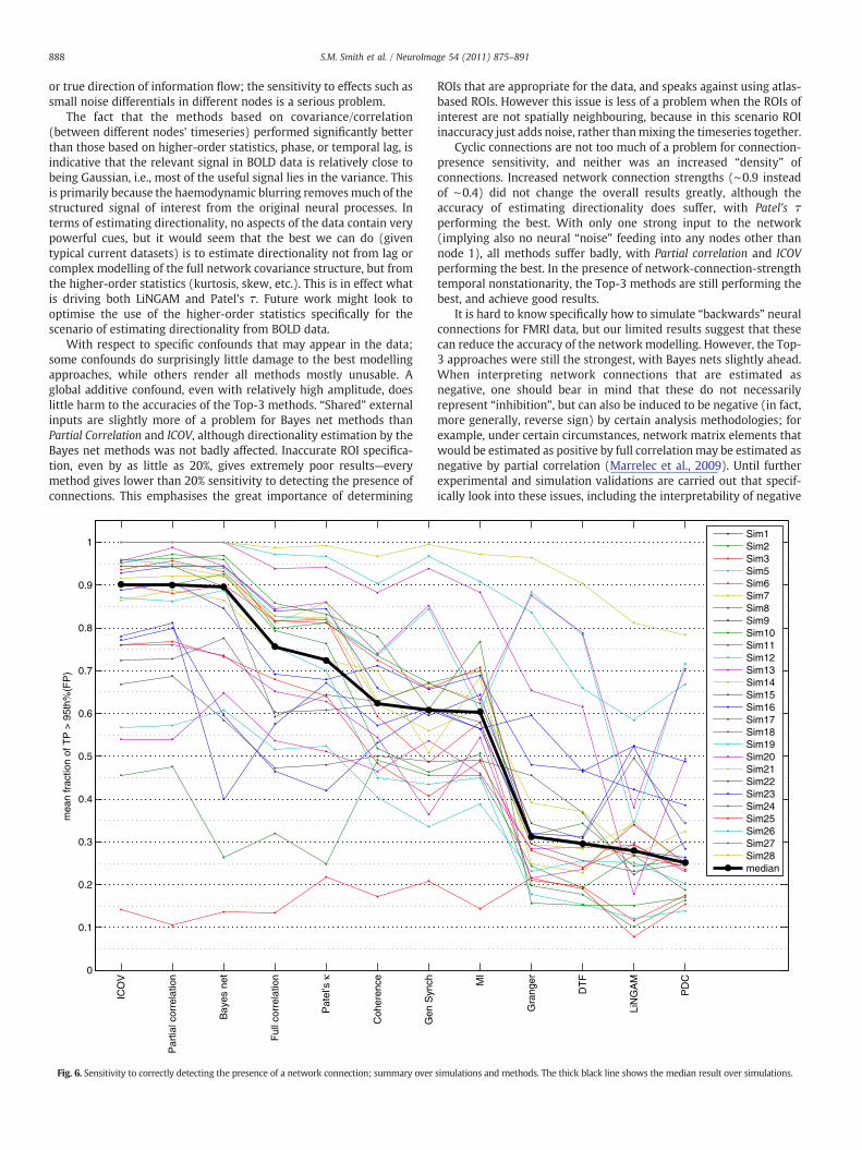
888 S.M. Smith et al. / NeuroImage 54 (2011) 875–891

or true direction of information flow; the sensitivity to effects such assmall noise differentials in different nodes is a serious problem.

The fact that the methods based on covariance/correlation(between different nodes' timeseries) performed significantly betterthan those based on higher-order statistics, phase, or temporal lag, isindicative that the relevant signal in BOLD data is relatively close tobeing Gaussian, i.e., most of the useful signal lies in the variance. Thisis primarily because the haemodynamic blurring removesmuch of thestructured signal of interest from the original neural processes. Interms of estimating directionality, no aspects of the data contain verypowerful cues, but it would seem that the best we can do (giventypical current datasets) is to estimate directionality not from lag orcomplex modelling of the full network covariance structure, but fromthe higher-order statistics (kurtosis, skew, etc.). This is in effect whatis driving both LiNGAM and Patel's τ. Future work might look tooptimise the use of the higher-order statistics specifically for thescenario of estimating directionality from BOLD data.

With respect to specific confounds that may appear in the data;some confounds do surprisingly little damage to the best modellingapproaches, while others render all methods mostly unusable. Aglobal additive confound, even with relatively high amplitude, doeslittle harm to the accuracies of the Top-3 methods. “Shared” externalinputs are slightly more of a problem for Bayes net methods thanPartial Correlation and ICOV, although directionality estimation by theBayes net methods was not badly affected. Inaccurate ROI specifica-tion, even by as little as 20%, gives extremely poor results—everymethod gives lower than 20% sensitivity to detecting the presence ofconnections. This emphasises the great importance of determining

0

0.1

0.2

0.3

0.4

0.5

0.6

0.7

0.8

0.9

1

mea

n fr

actio

n of

TP

> 9

5th%

(FP

)

ICO

V

Par

tial c

orre

latio

n

Bay

es n

et

Ful

l cor

rela

tion

Pat

el’s

κ

Coh

eren

ce

Gen

Syn

ch

Fig. 6. Sensitivity to correctly detecting the presence of a network connection; summary over

ROIs that are appropriate for the data, and speaks against using atlas-based ROIs. However this issue is less of a problem when the ROIs ofinterest are not spatially neighbouring, because in this scenario ROIinaccuracy just adds noise, rather thanmixing the timeseries together.

Cyclic connections are not too much of a problem for connection-presence sensitivity, and neither was an increased “density” ofconnections. Increased network connection strengths (∼0.9 insteadof ∼0.4) did not change the overall results greatly, although theaccuracy of estimating directionality does suffer, with Patel's τperforming the best. With only one strong input to the network(implying also no neural “noise” feeding into any nodes other thannode 1), all methods suffer badly, with Partial correlation and ICOVperforming the best. In the presence of network-connection-strengthtemporal nonstationarity, the Top-3 methods are still performing thebest, and achieve good results.

It is hard to know specifically how to simulate “backwards” neuralconnections for FMRI data, but our limited results suggest that thesecan reduce the accuracy of the network modelling. However, the Top-3 approaches were still the strongest, with Bayes nets slightly ahead.When interpreting network connections that are estimated asnegative, one should bear in mind that these do not necessarilyrepresent “inhibition”, but can also be induced to be negative (in fact,more generally, reverse sign) by certain analysis methodologies; forexample, under certain circumstances, network matrix elements thatwould be estimated as positive by full correlationmay be estimated asnegative by partial correlation (Marrelec et al., 2009). Until furtherexperimental and simulation validations are carried out that specif-ically look into these issues, including the interpretability of negative

MI

Gra

nger

DT

F

LiN

GA

M

PD

C

Sim1Sim2Sim3Sim5Sim6Sim7Sim8Sim9Sim10Sim11Sim12Sim13Sim14Sim15Sim16Sim17Sim18Sim19Sim20Sim21Sim22Sim23Sim24Sim25Sim26Sim27Sim28median

simulations and methods. The thick black line shows the median result over simulations.

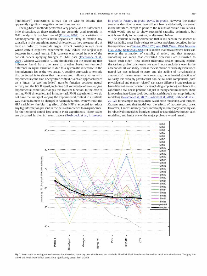
889S.M. Smith et al. / NeuroImage 54 (2011) 875–891

(“inhibitory”) connections, it may not be wise to assume thatapparently significant negative connections are real.

The lag-based methods performed very poorly, and this deserves alittle discussion, as these methods are currently used regularly inFMRI analysis. It has been noted (Friston, 2009) that variations inhaemodynamic lag across brain regions are likely to swamp anycausal lag in the underlying neural timeseries, as they are generally atleast an order of magnitude larger (except possibly in rare caseswhere certain cognitive experiments may induce the largest lagsbetween functional units). This concern was noted in one of theearliest papers applying Granger to FMRI data (Roebroeck et al.,2005), where it was stated: “…one should rule out the possibility thatinfluence found from one area to another based on temporaldifference in signal variation is due to a systematic difference in thehemodynamic lag at the two areas. A possible approach to excludethis confound is to show that the measured influence varies withexperimental condition or cognitive context.” Such an approach relieson a linear (or well-modelled) transfer function between neuralactivity and the BOLD signal, including full knowledge of how varyingexperimental condition changes this transfer function. In the case ofresting FMRI timeseries, and in many task FMRI experiments, we donot have the luxury of varying the experimental context in a suitableway that guarantees no changes in haemodynamics. Even without theHRF variability, the blurring effect of the HRF is expected to reduceany lag information present in the neural timeseries to insignificance,for the temporal neural lags seen in most experiments. These issuesare discussed further in recent papers (Roebroeck et al., in press-a,

40

50

60

70

80

90

caus

ality

: %

of c

orre

ct d

irect

ion

estim

ates

Pat

el’s

τ

Gen

Syn

ch

Gra

nger

Bay

es n

et

Fig. 7. Accuracy in detecting network connection direction; summary over simulations andshows the level above which accuracy is significantly better than chance.

in press-b; Friston, in press; David, in press). However the majorconcerns described above have still not been satisfactorily answeredin the literature, except to point to the results of certain simulations,which would appear to show successful causality estimation, butwhich are likely to be spurious, as discussed below.

The spurious causality estimation that is still seen in the absence ofHRF variability most likely relates to various problems described in theGranger literature (Tiao andWei, 1976;Wei, 1978;Weiss, 1984;Nalatoreet al., 2007; Nolte et al., 2008); it is known that measurement noise canreverse the estimation of causality direction, and that temporalsmoothing can mean that correlated timeseries are estimated to“cause” each other. These known theoretical results probably explainthe various problematic results we saw in our simulations even in theabsence of HRF variability, such as the estimation of causality evenwhenneural lag was reduced to zero, and the adding of (small/realisticamounts of) measurement noise reversing the estimated direction ofcausality. It is certainly possible that non-neural noise components (bothphysiological and scanner-related) can cause different image regions tohave different noise characteristics (including amplitude), and hence thisconcern is a real one in practice, not just in theory and simulations. Thereis hope that these issues couldbeameliorated throughmore sophisticatedmodelling (Nalatore et al., 2007; Havlicek et al., 2010; Deshpande et al.,2010a), for example, using Kalman-based noise modelling, and throughGranger measures that model out the effects of lag-zero covariance.However, it seems unlikely that (uncertainty in) haemodynamic lag canbe robustly distinguished from lags causedbyneural delays through suchmodelling, and hence one of the major problems would remain.

PD

C

LiN

GA

M

DT

F

Sim1Sim2Sim3Sim5Sim6Sim7Sim8Sim9Sim10Sim11Sim12Sim13Sim14Sim15Sim16Sim17Sim18Sim19Sim20Sim21Sim22Sim23Sim24Sim25Sim26Sim27Sim28p=0.05median

methods. The thick black line shows the median result over simulations. The grey line

890 S.M. Smith et al. / NeuroImage 54 (2011) 875–891

Previously published simulations suggesting successful estimation oflag-based causality in FMRI data most likely suffer from the variousproblems discussed above, including: not adding HRF variability into thesimulation, adding neural lags that are unrealistically long for themajority of neural connections, and not testing whether reducing theneural lag to zero in the simulations shows spurious causality. Forexample, in Deshpande et al. (2010b), the causality graphs, worryingly,oftendonot fall to zero for zeroneural lag, and the results in general seemto only support robust (safe) causality estimation for neural lags ofhundreds of milliseconds. Furthermore, in their four-node networksimulations, two of the four connectionswere apparently simulatedwithlags of tens of seconds.5 Another example is Havlicek et al. (2010), wherean impressive methodology is developed that aims to deal withnonstationary effects in the data. The authors begin by testing theirmethodology against simulated data; however, the simulations areproblematic, as an unrealistically long lag (2 s) is inserted between thesimulated timeseries, themethod is not tested against zero-lag simulateddata (to confirm that null data gives a null result), and it is not shownwhether the method can distinguish between neural lags and varyinghaemodynamic lags across regions.

Although our results suggest that in general lag-basedmethods are notuseful when applied to FMRI data, this is not to say that they can neverwork with carefully generated and interpreted FMRI data. It is possiblethat for those (relatively rare) functional connections whose effectiveneural lags are greater than 100 ms, then with very low TR (probablylimiting thefield-of-view) andhighSNR, and if thehaemodynamic lag canbe accurately pre-characterised for each region of interest and for everyexperimental context of relevance, then in theory lag-based neuralcausality from FMRI data may be estimable. For example, David et al.(2008) show that lag-based causality can give reasonable results afterdeconvolving the HRF, with the timing of the HRF estimated through theuse of electrophysiological data acquired simultaneously. In anotherexample, Rogers et al. (2010) show that neural lags as short as 100 msshould be estimable between two areas from the BOLD timecourses in thecase when the two areas in question have (presumably) identical HRFs(left and right V1), and using high field strength (7 T) and low TR(250 ms).

By generating realistic simulated data we are able to test differentmethods' sensitivities to detecting network connections, comparingestimated results against the ground truth used to drive thesimulations. We have thus been able to control not only the “fullnull” false positive rate of connection detection in the absence of anytrue positives, but also correct for the (generally increased) rate of falsepositives induced by the presence of true connections (i.e., evaluatingthe specificity of each method in distinguishing direct from indirectconnections). When a network modelling method is applied to new,real data, it is important to be able to estimate the significance ofestimation connections (whether considering connection presence,strength or directionality). For methods where the two kinds of nulldistributions particularly diverge (e.g., full correlation), it canpotentially be hard tomake accurate inference, as the null distributionin the presence of true connections may be hard to estimate. Certainnetwork scenarios will exacerbate this problem, as seen in our results,such as increasing connection strengths and density of connections.The use of surrogate data (“null data” generated to have similarcharacteristics to the real data) may help, possibly in conjunctionwitha network simulation such as those utilised in this work; however,valid surrogate data can be difficult to generate, as seen for example inthe (surrogate-corrected) problematic results in Deshpande et al.(2010b), described above. The methods that gave the best resultsoverall in our tests beat the “second-best” methods (such as full

5 It is clear from consideration of Figs. 1 and 2 that for two of the four networkconnections, the neural lags are of the same order as the lengths of the timeseries, soeither the neural lags are tens of seconds, or the timeseries are too short to bemeaningful. In either case, the network simulation results are not easily interpretable.

correlation) primarily because they were the most successful atdistinguishing direct from indirect connections, and for the samereason their “full null” distributions need the least correction whentrue connections are present (making it easier to achieve validinference on their outputs when applied to real data). Closely relatedto these questions is whether any given method's own estimates ofstatistical significance (for example, p-values derived from parametricassumptions regarding a method's estimated connection strength ordirectionality) are accurate. We have not needed to utilise anymethod's own associated (or “built-in”) approach for estimatingspecificity, because we have been able to use the ground truths toestimate false-positive rates empirically; it would be interesting toinvestigate whether different methods' own claimed p-values areaccurate, but this is outside the scope of this paper (and of course canbe confounded, for some methods, by the additional false positivesthat can be induced by true positives, as discussed above).

We have not considered any specific multi-subject modellingapproaches here (for example, as seen in Ramsey et al., 2010), as wehave concentrated on evaluating the different modelling methodswhen used to estimate functional brain networks from single subjectdatasets; we felt that this is a primary question of interest, needingsome clear answers before considering possible multi-subject mod-elling approaches. A question will arise as to whether the methods(such as LiNGAM) that require a relatively large number of timepointsto function well would give good results simply by concatenatingtimeseries across subjects; this may prove to be the case, althoughsuch an approach would then restrict the ability to use simplemethods (such as cross-subject mixed-effects modelling of theestimated network parameters) to determine the reliability of thegroup-estimated network.

To conclude, we have carried out a complex, rich, quantitative setof simulations with a realistic model for FMRI timeseries; we haveinvestigated a wide range of analysis methodologies in order todetermine which are the most sensitive at detecting direct networkfunctional connections and the direction of information flow carriedby them. We have included various problematic elements in thesimulations, in order to evaluate the robustness of the variousnetwork modelling methods. Our results show that lag-basedapproaches perform very poorly. However there are several methodsthat can give high sensitivity to network connection estimation ongood quality FMRI data, in particular partial correlation, regularisedinverse covariance estimation and several Bayes net methods. Withrespect to estimating connection directionality, Patel's τ can bereasonably successful.

All simulated BOLD timeseries and ground-truth networkmatricesare freely available from www.fmrib.ox.ac.uk/analysis/netsim—theauthors will be interested to receive feedback on the simulations,methods tested and results, and will post updates on this website.

Supplementarymaterials related to this article can be found online atdoi:10.1016/j.neuroimage.2010.08.063.

Acknowledgments

We are very grateful to: Gopikrishna Deshpande for helpfuldiscussions, Aslak Grinsted for providing the Crosswavelet and WaveletCoherence toolbox, Chandler Lutz for providing the pairwise Grangercausality code, Alard Roebroeck for helpful discussions, Alois Schlögl forproviding the BioSig toolbox,Mark Schmidt for providing the regularisedinverse covariance code (and for helpful discussions), Anil Seth forproviding the Causal Connectivity Analysis toolbox (and for helpfuldiscussions), Shohei Shimizu, Patrik Hoyer and Aapo Hyvärinen forproviding LiNGAM/FastICA (and for helpful discussions), Rodrigo QuianQuiroga for providing the generalised synchronisation code (and forhelpful discussions) and Dongli Zhou for providing the FunctionalConnectivity toolbox. We would like to make clear that any negativeresults or discussions resulting fromrelativelypoorperformanceof anyof

891S.M. Smith et al. / NeuroImage 54 (2011) 875–891

the methods tested here do not imply any criticism of the originalmethods themselves or their implementations in the various toolboxes;this paper is purely aiming to investigate the performance of the variousmethodswhen applied to FMRI data. Many of themethodswere originallydesigned toworkwith other types of datawith different signal and noisecharacteristics; however, we have felt it important to test all of thesemethods specifically for FMRI data, because they are being used by theFMRI community.

References

Baccalá, L., Sameshima, K., 2001. Partial directed coherence: a new concept in neuralstructure determination. Biol. Cybern. 84 (6), 463–474.

Banerjee, O., El Ghaoui, L., d'Aspremont, A., Natsoulis, G., 2006. Convex optimizationtechniques for fitting sparse Gaussian graphical models. Proceedings of the 23rdInternational Conference on Machine Learning. ACM, p. 96.

Buxton, R., Wong, E., Frank, L., 1998. Dynamics of blood flow and oxygenation changesduring brain activation: the balloon model. Magn. Reson. Med. 39, 855–864.

Chang, C., Glover, G., 2010. Time-frequency dynamics of resting-state brain connectivitymeasured with fMRI. Neuroimage 50, 81–98.

Chang, C., Thomason, M., Glover, G., 2008. Mapping and correction of vascularhemodynamic latency in the BOLD signal. Neuroimage 43, 90–102.

Chickering, D., 2003. Optimal structure identification with greedy search. J. Mach.Learn. Res. 3, 507–554.

Daunizeau, J., Friston, K., Kiebel, S., 2009. Variational Bayesian identification andprediction of stochastic nonlinear dynamic causal models. Phys. D NonlinearPhenom. 238 (21), 2089–2118.

Dauwels, J., Vialatte, F., Musha, T., Cichocki, A., 2010. A comparative study of synchronymeasures for theearlydiagnosisofAlzheimer'sdiseasebasedonEEG.Neuroimage49(1),668–693.

David, O., in press. fMRI connectivity, meaning and empiricism: Comments on:Roebroeck et al. The identification of interacting networks in the brain using fMRI:model selection, causality and deconvolution. NeuroImage, Corrected Proof:–.

David, O., Guillemain, I., Saillet, S., Reyt, S., Deransart, C., Segebarth, C., Depaulis, A.,2008. Identifying neural drivers with functional MRI: an electrophysiologicalvalidation. PLoS Biol. 6 (12), e315.

de Pasquale, F., Della Penna, S., Snyder, A., Lewis, C., Mantini, D., Marzetti, L., Belardinelli, P.,Ciancetta, L., Pizzella, V., Romani, G., Corbetta, M., 2010. Temporal dynamics ofspontaneousMEG activity in brain networks. Proc. Natl Acad. Sci. 107 (13), 6040–6045.

Deshpande, G., Sathian, K., Hu, X., 2010. Assessing and compensating for zero-lagcorrelation effects in time-lagged Granger causality analysis of fMRI. IEEE Trans.Biomed. Eng. 57 (6), 1446–1456.

Deshpande, G., Sathian, K., Hu, X., 2010. Effect of hemodynamic variability on Grangercausality analysis of fMRI. Neuroimage 52 (3), 884–896.

Fox, M., Zhang, D., Snyder, A., Raichle, M., 2009. The global signal and observedanticorrelated resting state brain networks. J. Neurophysiol. 101 (6), 3270–3283.

Freenor, M. and Glymour, C., 2010. Searching the DCM model space, and somegeneralizations. NeuroImage. In submission.

Friedman, J., Hastie, T., Tibshirani, R., 2008. Sparse inverse covariance estimation withthe Graphical Lasso. Biostat 9 (3), 432–441.

Friston, K., 1994. Functional and effective connectivity in neuroimaging: a synthesis.Hum. Brain Mapp. 2, 56–78.

Friston, K., 2009. Causal modelling and brain connectivity in functional magneticresonance imaging. PLoS Biol. 7 (2), e1000033.

Friston, K., in press. Dynamic causal modeling and Granger causality. Comments on: Theidentification of interacting networks in the brain using fMRI: model selection,causality and deconvolution. NeuroImage, Corrected Proof:–.

Friston, K.J., Harrison, L., Penny, W., 2003. Dynamic causal modelling. Neuroimage 19 (3),1273–1302.

Geweke, J.F., 1984. Measures of conditional linear dependence and feedback betweentime series. J. Am. Stat. Assoc. 79 (388), 907–915.

Goebel, R., Roebroeck, A., Kim, D.-S., Formisano, E., 2003. Investigating directed corticalinteractions in time-resolved fMRI data using vector autoregressive modeling andGranger causality mapping. Magn. Reson. Imaging 21 (10), 1251–1261.

Granger, C.W.J., 1969. Investigating causal relations by econometric models and cross-spectral methods. Econometrica 37 (3), 424–438.

Grinsted, A., Moore, J., Jevrejeva, S., 2004. Application of the cross wavelet transform andwavelet coherence to geophysical time series. Nonlinear Processes Geophys. 11 (5/6),561–566.

Guo, S., Seth, A.K., Kendrick, K.M., Zhou, C., Feng, J., 2008. Partial Granger causality—eliminating exogenous inputs and latent variables. J. Neurosci. Meth. 172 (1), 79–93.

Handwerker, D., Ollinger, J., D'Esposito, M., 2004. Variation of BOLD hemodynamic responsesacross subjects and brain regions and their effects on statistical analyses. Neuroimage 21,1639–1651.

Havlicek, M., Jan, J., Brazdil, M., Calhoun, V.D., 2010. Dynamic Granger causality basedon Kalman filter for evaluation of functional network connectivity in fMRI data.NeuroImage 53 (1), 65–77.

Kamiński, M., Blinowska, K., Szelenberger, W., 1997. Topographic analysis of coherenceand propagation of EEG activity during sleep and wakefulness. Electroencephalogr.Clin. Neurophysiol. 102 (3), 216–227.

Kiviniemi, V., Kantola, J.-H., Jauhiainen, J., Hyvärinen, A., Tervonen, O., 2003.Independent component analysis of nondeterministic fMRI signal sources. Neuro-image 19, 253–260.

Kiviniemi, V., Starck, T., Remes, J., Long, X., Nikkinen, J., Haapea, M., Veijola, J., Moilanen,I., Isohanni, M., Zang, Y.-F., Tervonen, O., 2009. Functional segmentation of the braincortex using high model order group PICA. Hum. Brain Mapp. 30 (12), 3865–3886.

Larkin, P., 1971. This Be The Verse. New Humanist. August.Marrelec, G., Kim, J., Doyon, J., Horwitz, B., 2009. Large-scale neural model validation of

partial correlation analysis for effective connectivity investigation in functionalMRI. Hum. Brain Mapp. 30 (3), 941–950.

Marrelec, G., Krainik, A., Duffau, H., Pélégrini-Issac, M., Lehéricy, S., Doyon, J., Benali, H.,2006. Partial correlation for functional brain interactivity investigation infunctional MRI. Neuroimage 32, 228–237.

McIntosh, A., Gonzales-Lima, F., 1994. Structural equation modeling and its applicationto network analysis in functional brain imaging. Hum. Brain Mapp. 2, 2–22.

Meek, C., 1995. Causal inference and causal explanation with background knowledge.Proceedings of the 11th Annual Conference on Uncertainty in Artificial Intelligence,pp. 403–410.

Nalatore, H., Ding, M., Rangarajan, G., 2007. Mitigating the effects of measurement noiseon Granger causality. Phys. Rev. E 75 (3), 31123.1–31123.10.

Nolte, G., Ziehe, A., Nikulin, V., Schlögl, A., Krämer, N., Brismar, T., Müller, K., 2008.Robustly estimating the flow direction of information in complex physical systems.Phys. Rev. Lett. 100 (23), 234101.1–234101.4.

Patel, R., Bowman, F., Rilling, J., 2006. A Bayesian approach to determining connectivityof the human brain. Hum. Brain Mapp. 27, 267–276.

Pereda, E., Quiroga, R., Bhattacharya, J., 2005. Nonlinear multivariate analysis ofneurophysiological signals. Prog. Neurobiol. 77 (1–2), 1–37.

Popa, D., Popescu, A., Paré, D., 2009. Contrasting activity profile of two distributedcortical networks as a function of attentional demands. J. Neurosci. 29 (4),1191–1201.

Quian Quiroga, R., Kraskov, A., Kreuz, T., Grassberger, P., 2002. Performance of differentsynchronization measures in real data: a case study on electroencephalographicsignals. Phys. Rev. E 65 (4), 41903.

Ramsey, J., Hanson, S., Hanson, C., Halchenko, Y., Poldrack, R., Glymour, C., 2010. Sixproblems for causal inference from fMRI. Neuroimage 49 (2), 1545–1558.

Ramsey, J., Zhang, J., Spirtes, P., 2006. Adjacency-faithfulness and conservative causalinference. Proceedings of the 22nd Annual Conference on Uncertainty in ArtificialIntelligence.

Richardson, T., Spirtes, P., 2001. Automated discovery of linear feedback models. In:Glymour, C., Cooper, G. (Eds.), Computation, Causation, and Causality. MIT Press.

Ringo, J., Doty, R., Demeter, S., Simard, P., 1994. Time is of the essence: a conjecture thathemispheric specialization arises from interhemispheric conduction delay. Cereb.Cortex 4, 331–343.

Roebroeck, A., Formisano, E., Goebel, R., 2005. Mapping directed influence over thebrain using Granger causality and fMRI. Neuroimage 25 (1), 230–242.

Roebroeck, A., Formisano, E., and Goebel, R., in press. Reply to Friston and David: Aftercomments on: The identification of interacting networks in the brain using fMRI:model selection, causality and deconvolution. NeuroImage, Corrected Proof:–.

Roebroeck, A., Formisano, E., and Goebel, R., in press. The identification of interactingnetworks in the brain using fMRI: model selection, causality and deconvolution.NeuroImage, Corrected Proof:–.

Rogers, B.P., Katwal, S.B., Morgan, V.L., Asplund, C.L., Gore, J.C., 2010. Functional MRI andmultivariate autoregressive models. Magnetic Resonance Imaging 28 (8),1058–1065.

Seth, A.K., 2010. AMATLAB toolbox for Granger causal connectivity analysis. J. Neurosci.Meth. 186 (2), 262–273.

Shannon, C., 1948. Amathematical theory of communication. Bell Syst. Tech. J. 27, 379–423.Shimizu, S., Hoyer, P.O., Hyvärinen, A., Kerminen, A., 2006. A linear non-Gaussian acyclic

model for causal discovery. J. Mach. Learn. Res. 7, 2003–2030.Tiao, G., Wei, W., 1976. Effect of temporal aggregation on the dynamic relationship of

two time series variables. Biometrika 63 (3), 513–523.Wei, W., 1978. The effect of temporal aggregation on parameter estimation in

distributed lag model. J. Econometrics 8 (2), 237–246.Weiss, A., 1984. Systematic sampling and temporal aggregation in time series models. J.

Econometrics 26 (3), 271–281.Witt, S., Meyerand, M., 2009. The effects of computational method, data modeling, and

TR on effective connectivity results. Brain Imaging Behav. 3, 220–231.Wright, S., 1920. Correlation and causation. J. Agric. Res. 20, 557–585.Zhang, J., 2008. On the completeness of orientation rules for causal discovery in the

presence of latent confounders and selection bias. Artif. Intell. 172, 1873–1896.Zhou, D., Thompson, W.K., Siegle, G., 2009. MATLAB toolbox for functional connectivity.

Neuroimage 47 (4), 1590–1607.