Mechanism and Machine Theory VoL 14, pp. 179-188 0094-114X/7910801-01791502,00/0 © Pergamon Press Ltd., 1979. Printed in Great Britain

Contribution of the Forming of Computer Methods for Automatic Modelling of Spatial Mechanisms Motionst

M. Vukobratovi(:$

and

V. PotkonJak§

Received 16 March 1978; for publication 28 November 1978

Abstract In this paper is presented the common basic features of the method for automatic setting of dynamic equations of active spatial mechanisms in the form of open chains. The paper is divided into two pads. In the first part, beside the theoretical basis of the computer methods, the version at the basis of the fundamental theorems of mechanics is presented. Second part of the paper contains the new result, relating to the procedures based on Gibbs--Appel's and Lagrange's equations. Finally is given the comparison of the three method's efficiency, representing the complete possibility for computer forming of the dynamic differential equations of spatial active chains.

Brief Review of Methods METHODS FOR forming mathematical models of active mechanisms in principle can be classified into three basic groups:

Models formed on the basis of the Newton and Euler equations and the principal theorems of mechanics of systems.

Models based on Lagrange's equations. Models formed on the basis of acceleration "energy", or Gibs function. The intention of this paper is not to present the details of all existing methods for the

forming of the mathematical models of motion of active mechanisms. Instead of more extensive review, here are only mentioned all important, up to date results in this field of research.

Fletcher, Rongved and Yu [1] studied the motion of a satellite, consisting of two rigid bodies, connected by universal joint and being under load due to gravitation. The model can be simply extended for the case when torques due to driving engines are also acting in the joints.

Hooker and Margulies[2] initiated by the preceding work, studied the general case when n + 1 bodies were connected by means of joints with 1 or 2 rotational degrees-of-freedom.

Roberson and Wittenburg[3] in their approach have defined the body system as a graph, utilizing the known graph properties. The system is limited to the form of a topological branch and every two bodies are connected by a joint, so that the system consists of n bodies and n - 1 joints. Isomorphism between the rigid body system and the graph is created in such that the mass centers of the bodies form a set of graph nodes X = {xl . . . . . x,} and the set U = {ul . . . . . u,} of the graph branches is defined as the set of joints, connecting the bodies. Mapping of F(x)~X is defined by directing of the graph (Fig. 1).

Interest of this method stays notably in representing system topology. Method by Hooker[4] renders a new possibility of eliminating constraints, which are

representing a serious difficulty in obtaining the equations of motion.

tThis work has been supported by lnstitut of Mathematics, Beograd, Yugoslavia. SMihailo Pupin lnstitut, Beograd, Yugoslavia. §Electrical Engineering Faculty, Beograd, Yugoslavia.

179

180

x!

Rgure 1. Example of body system and corresponding graph.

The method proposed by Likins[5], represents a more direct application of the preceding method. Even more, without restricting the problem generality, it simplifies the enumeration of the bodies in the kinematic chain, of the joints and unit vectors of the rotational axes.

Likins supposes that "exploding" of the complex joint with several degrees-of-freedom into several joints with 1 degree-of-freedom has already been performed. This approach enables simplification of the equations, proposed by Hooker[4] and enables Likins to present the rotational motion of the system by means of a matrix equation. This approach is suitable for computer simulation of a system of joint-connected bodies in the form of a topological branch, having only rotational relative movements.

Wittenburg has generalized method[3] onto systems, having a structure of a topological branch, the joints of which enable rotational motion to r~ degrees-of-freedom and translatory motion to tj degrees-of-freedom 16] (rj and tj = 1, 2 or 3).

The method is very general. It stays rather theoretical and does not yield some explicit matrix procedure for obtaining of equations.

Uicker proposed a method based on Lagrange's equations for studying the behaviour of articulated systems of arbitrary structure (with arbitrary number of closed chains)[8]. The author supposed that the joints enable either rotational or translatory motion, so this method can be regarded as general.

Kahn has applied Uicker's method for obtaining analytically the motion equations of a three-segment body system, linked rotationally[9, 10].

Bejszy and Lewis have tried to apply Uicker's method to analytically obtaining motion equations of the telescopic manipulator with a gripper having three degrees-of-freedom.

Bejszy[l 1] has obtained analytically the expressions for kinetic and potential energy. The obtained expressions are extremely complex and the author proposes that they be simplified by decoupling the motion of the manipulator itself and the gripper.

Lewis[12] proposes simplification in the calculation of certain coefficients of Lagrange's equations.

Independently from the previous works, Koronev[13] proposed a method for setting equations of articulated systems, having structure of a topological branch. This method deals with the connections only in the later phase of calculation, when the equations of the free system have been obtained in the Lagrange's form. The author starts by writing the quadratic form of the body system kinetic energy in function of the 6 coordinates defining body position and orientation. These equations represent the mathematical model of the whole free system in function of 6n coordinates. These 6n coordinates are valid for the real system, under the condition that to the generalized forces due to external forces and moments are added the generalized forces due to connections. The mentioned connections are taken into account via h equations in the set of 6n previous equations. After eliminating the generalized connection forces, the system reduces to 6n-h Lagrange's equations of the real system. This method is of theoretical interest only and does not yield any possibility of obtaining some matrix form during setting of equations.

Renaud[14, 15] derives motion equations for a system of n + 1 bodies, forming a branch structure relative to the reference body O, with the coordinate system O0. Permitted relative movements of the neighbouring bodies are rotation and translation. The method has treated quite systematically all phases of setting differential equations of kinematic chains. About the suibatility of the method in practical application cannot be said anything more reliable.

Popov et a/.[16] proposed the method for setting differential equations of motion for a system consisting of n + 1 bodies and n joints. Each joint permits turning with respect to one of the axes corresponding to the coordinate system, connected with the support of mechanism.

181

Based on Newton's equations, the equations for forces acting on bodies of mechanism are derived. The equations are expressed in projections onto the axes of fixed system.

Method is very suitable for computer and directly applicable for the forming of complete dynamic equations of open kinematic chains. Equations of motion derived in this way give the possibility relativeily simple analytical linearization, necessary in the analysis of stability, synthesis of optical regulator, etc.

In the following text of this paper the procedures will be exposed on which the authors have worked. These procedures belong to the basic categories of the approach, mentioned at the very beginning of this paper. Besides that of the computer realization of the algorithm for the forming of dynamic equations based on the general theorems of mechanics, for the first time in this paper will be exposed the new algorithm and its computer realization for automatic forming of mathematical models for the case of open kinematic chains. This algorithm is based on Lagrange's equations and recurrent relations. Also for the first time new version of the algorithm is exposed, very convenient for computer realization, based on the "energy" of acceleration.

Part I

Method of Basic Theorems of Mechanics

Introductory Consideration THE FORMING of mathematical models of arbitrary complex spatial mechanism by "hand" procedure produce unlimited possibilities of errors. The transferring of this task to computers and automatic forming of differential equations represent the central point of this paper. The final goal in the forming of mathematical models of active articulated mechanisms is the setting of general computer algorithm, onto which the next demands are imposed. It is only necessary to give the information about the kinematic scheme, the parameters of the mechanism and the problem which has to be solved.

On the basis of these informations the algorithm has to: "Assemble" the mechanism according to the kinematic scheme; Calculate the positions, velocities and accelerations; Set the differential equations of motion; Integrate the equations of motion with imposed specific conditions on the basis of elaborated iterative procedure.

These features of the algorithm for automatic forming of mathematical models are neces- sary for the minimum two reasons. First reason lies in the impossibility to choose some unique configuration of the robot. In the function of the concrete situation it is useful to analyse different kinematic schemes in order to select the appropriate model. Thus, the demand for the automatic forming of the equations is of dominant significance for the success of such analysis. The second reason lies in the necessity to control robots and manipulators in real time. The forming of dynamic equations on the basis of such concept and the on-line calculation of dynamics contribute directly to the synthesis of the control algorithms for practical use.

The first algorithm which satisfies these demands appeared independently in the papers [17, I8]. While the first approach appeared in connection with the dynamic analysis of manipulators[17], the second one is generated in the course of the synthesis of artificial anthropomorphic gait[18]. In order to estimate the essential points of these mentioned methods, as well as the methods which based on them, their basic statements will be exposed.

Dynamic equations of open active mechanisms can be represented in matrix form with the system of differential equations

w4 = P + v (1)

182

where q is column-matrix of generalized coordinates; P is column-matrix of driving forces and torques, P = [P= . . . . . p,]r: W is inertia matrix, a square matrix whose elements are a function of generalized coordinates: V is column-matrix, which is a function of generalized coordinates and velocities.

Explicit dependency of W and V on state coordinates (generalized coordinates and velocities) is extremely complex. It is more reasonable to calculate numerically W and V for the different time section. Thus, the essential quality of the method consists in the forming of the mathematical model for one time-instant. From such a system and in the function of the task, calculate the accelerations for the known driving forces or the driving forces for the known accelerations. In the case of known driving forces the accelerations (1) can be calculated. Their values can be considered constant in the sufficient small time interval At. Then, by simple integration, new values of the state vector can be calculatedt

l q(to + At) = ~ ii(to)At 2 + c~(to)At + q-to)

q(to + At) = q(to) +/](to)At. (2)

Now, the forming of the system repeats. In this manner the forming and the integration of the system are executed simultaniosly.

Kinematic Relations

The calculation of matrices W and V is performed in the process of "circling" of the chain[19,20]. In each iteration to the chain is adjoint one new member and then, for the new system the matrices W and V calculated. For these calculations it is necessary to know recurrent relations for velocities and accelerations of c.o.g., as well as the angular velocities and accelerations of the members of mechanism. Let us consider the joint with I degree-of-freedom about the axis ei (Fig. 2), where T~ is c.o.g, of ith member and q~ is generalized coordinate corresponding to the ith degree-of-freedom. This coordinate can be defined as the angle of joint rotation, or the angle between the projections of vectors -rH,i and r, onto the plane and acceleration of c.o.g., and with toi and ~i angular velocity and acceleration of the ith mechanism member. Then the known relations of mechanics are valid

g.O i = (.Oi_l "k ( l ie i

v i = v i - i - g o i - i x r i - i , i + ¢0i × r .

ei = e H +/~ei + q,~oi-~ x ei

w~ = w;_= - ei-= x r~_,.~ - t o l l x ( t a i l x r H j ) + e; x r . + ¢oj x (co; x r . ) .

(3)

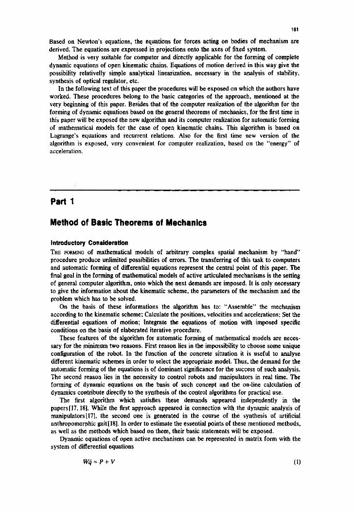
For the joints with one translation along axis e~ (Fig. 3), the generalized coordinate q~ can be defined as qj = IA;A';I. A~ is fixed point in relation to the j - lth member: A'; is fixed point in relation to the/ th member.

Now, the recurrent relations are ca~ = ca~_i: v~ = v j_ l - ¢a~_j x r j_ t . i + =oi x r~j + qje~

ej = e~-l: wj=wj_l-e~_=xrj_m.~-oJj_lx(o~j_jxri_,.j)+(ejxr~j+cojx(~o~Xr~i) + ( ~ e j + 2,~j_, x ej,~j). (4)

Rgure 2. S c h e m e o f r e v o l u t e j o i n t .

tValid for Euler's method of integration.

Tj

*'j'H

rli = r;t +lllq t

183

R g u r e 3. S c h e m e of translat ion joint.

Further, to each member one coordinate system is connected, with its axes along the principal axes of inertia. Let us introduce the symbols: at is vector in fixed coordinate system; it is same vector expressed in the system connected to the ith member; gi is same vector in the system of the ( i - 1)th member.

Both the vector and matrix calculus will be utilized in the lines to come. Let us, therefore, introduce the following designations. For instance, a designates a vector, and a designates a column-matrix corresponding to that vector, a will be used in the vector calculus, and a in matrix one, It will be evident from the relevant text which values are in question.

Let us define the transient matrices from the system of the ith member to the fixed system and from the system of the (i - 1)th member to the system of the ith member, i.e.

ai = A l i i ; i i = ALi-lgi (5)

Transient matrix At can be calculated after the addition of member i to the kinematic chain. Let us consider the revolute joint. As aH is known, r~-u = A~-tPH,~, e~ = Ai-let known too.

Now, the vectors a~ and i~ can be calculated

- e i X (ri_ U X el) ei X (re X ~) a, = I - l l - I = 1-11-1 (6)

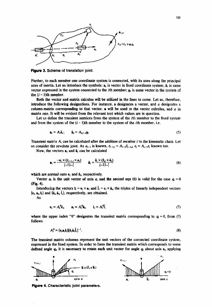
which are normal onto e~ and &b respectively. Vector a~ is the unit vector of axis a, and the second eqn (6) is valid for the case q~ = 0

(Fig. 4). Introducing the vectors !~ = ei x ai and Ji = et x i i , the triples of linearly independent vectors

{et, ai, Ii} and {~i, it, li}, respectively, are obtained. As

et = A°&t, a, - - A°i,, I, = Ai°li (7)

where the upper index "0" designates the transient matrix corresponding to qt = 0, from (7) follows

A~ ° = [e~ail~][~iiiii]-'. (8)

The transient matrix columns represent the unit vectors of the connected coordinate system, expressed in the fixed system. In order to form the transient matrix which corresponds to some defined angle qh it is necessary to rotate each unit vector for angle qi about axis ei, applying

II r;i 0 ~ q r ~ r , - , ~ ri+l,i

' ilx(~'i~ x 3i1 i q~=O

al axis a al ~ axis a

Figure 4. Character ist ic joint parameters.

184

Rodrig's formula

Q~j = qq cos q~ + (1 - cos qi)(e~qq)ei + ei × q.. sin q~ (9)

where q~i is jth column of matrix A ° (unit vector before rotation) and Qq is column of transient matrix Ai (unit vector after rotation). Thus, the transient matrix is formed

Ai = [Q. Qn Qis]. (I0)

For linear joints it is necessary to perform only "assembling" of members. Analogously, the transient matrix A~-Li - -~ - A~.~_~ can be determined. Now, it is possible to calculate the matrices W and V which determine the mathematical model for some given time section.

In this paper will be presented three methods for the calculation of these matrices.

M e t h o d of B a s i c T h e o r e m s

Let us consider the mentioned open active mechanism with revolute and linear joints. Let the indicator s~ determine the type of joint (s~ = 0 for revolute joint, and s~ = 1 for linear joint). In this case the recurrent formulas (3) and (4) can be put in compact form

toi = t o l l + q i e i ( l - si)

v t -- v i - i - to/-I × r i - i . i + ¢oi X r~i + il le~i, r~i = rii + eiq.~li

el = ei-i + ( itiei + ClitOi-~ x el)(l - si)

Wi ----- Wi-I -- e i - I X ri_l, i - t o i - i X ( t o i - i X ri_l , i) + ~i X r~ + tel × (to~ × r~) + (//ie~ + 2to~_t × e:ll)sl

V0 ----- tOO = e0 = w0 = O.

(11)

(12)

(13)

04)

The driving torque in rotational joint i is given as E u = E u • el, and the driving force in linear joint j as Vf = Pi F 'ej.

Let us consider the revolute joint Al and fictiously interrupt the chain in joint I. The action of the rejected part of the mechanism (in this case the support) can be substituted with the reaction force Rl and the one moment Met, normal to the axis of rotation et. On the other part of mechanism we can apply the theorem of kinetic momentum with respect to point Am. After transformation, it follows

o r

n n n

r/")x m i w i + X M i = p U + M e l + ~ : r i ° ) × m i g i = 1 i=! i = l

~ [ri (l) × miwi - ri ") × m;g] + ~ Mi = Pi u + Mm i = l i = 1

(15)

(16)

where, - (" - ri = A I T i (Fig. 5a), mi is mass of ith member, Mi is change of kinetic momentum of ith member about c.o.g. Ti defined as

M / = A i l ~ i

where M~ represents the expression on the left side of Euler's equations

~1/1 i = T i i i -- ( Titoi) X tel

(17)

(18)

where J~ is tensor of inertia of ith member. After scalar multiplication (16) by el, it follows

n

[(ri ") x miwi)e, - (rl ") x mig)el] + ~, Miel = PI ~. i = l i = l

(19)

RK

P~ + / _.- / / Tx+a. ~ "

1/ 1 - ~ K+I

MR. Ax

/ /

t , t Rx / "-\ / /

\ / A~÷, ~ 6 m

A~

185

(a)

F'Iguro 5. Genoralizod forces of mechanism.

(b)

Now, let us consider the revolute joint At and interrupt it fictiously in the same joint Ak. Let us consider the part of chain towards the free end. Let us introduce again the reactions Rk, Mat(Mat _L eD. Now, the theorem of kinetic momentum can be applied approximately on the considered pa_q of s],stem and with respec t to [he point At.

When we apply [he theorem and multiply the result by et, it follows

II n

[(r[t) x miw,)ek- (r i ( t )× re,g) • et] + i=~ M, "ek = p u (20)

where r/(k) = AtT~, Fig. 5(a). Thus, for p revolute joints we have p scalar equations. Let us consider now the linear joint At. Let us again interrupt fictiously the chain in point At

and substitute the rejected part of system with the reaction Rt, normal onto the translatory axis et and with the moment M~, Fig. 5(b). Let us apply the theorem of c.o.g, movement for the part of the system towards the free end

n n

re,w, = Pt F + i~= mig + Rk. (21)

After scalar multiplication (21) with ek it follows

PI

~ [miw,ek - migek] = Pk F. (22)

For q linear joints we get q scalar equations. Totally, by the application of theorem of kinetic momentum and of theorem of c.o.g, motion we get p + q = n scalar equations. Now it is necessary to show how to reduce these equations to form (1).

Let us designate with [1 the matrix of dimension 3 x n the columns of which, in the ith iteration, are the coefficients of the generalized accelerations in the expression for wi, and with O the matrix of dimension 3 x 1 which contains the free term of the same expression. Thus

w, = fl/j + 0 (23)

where q = [qt . . . . . q.]T. Let us introduce the symbols for the columns

1"1 = [ . a / . . . / 3 / 0 . . . 0 ] ; 0 = [8'] . (24)

With F designate the matrix, the columns of which are the coefficients of the generalized accelerations in the expression for ei, and with O the matrix which contains the free atom, i.e.

E, = F/j + 4,. (25)

Introduce the symbols for the columns

F = [ a / . . . a / O . . . O]; ~ = [I,i]. (26)

186

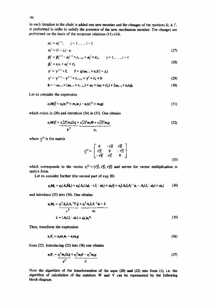
In each iteration to the chain is added one new member and the changes of the matrices l), 0, F, & performed in order to satisfy the presence of the new mechanism member. The changes are performed on the basis of the recurrent relations (11)-(14).

a / = a / - ' , / = 1 . . . . . i - I

at i = (1 - st)" ei

A' = #/-'- a/-' × r,-,,t + a/x ~,: /= l ..... i-I

I J / = eisi + a / x r;t

7 ' = 7 i-~ + f, f = clt(~ot-] x et)(1 - st)

y ' = 7 t- ' - y t-~ x r,-,.t + 1' t x ~i + h

h = - t a t - , x (tat-t x r t - u ) + tat x (tat x r~) + 2cat-, x elslql.

Let us consider the expression

e i M ~ = e j (r# ) x m,wt ) - ei(r~ °') x mtg)

which exists in (20) and introduce (24) in (31). One obtains

e jM~ = eT'-'i)m,fJ::l + eT'.Ci)mtO + eT '~ 'ma

b ~ ut

where r~ °) is the matrix

(27)

(28)

(29)

(30)

(31)

(32)

Then, transform the expression

ejFj = elmiwi - ejm~g (36)

from (22). Introducing (23) into (36) one obtains

etF t = e]Trfl i~q "J- ejTmtO -- ejTmig.

d • ~,

Now the algorithm of the transformation of the eqns (20) and (22) into form (1), i.e. the algorithm of calculation of the matrices W and V can be represented by the following block-diagram.

(35)

(37)

k = ( & ( J , • o~,) x ~ , ) e j ~

ejMt = ejT AjJtAf 'F ii + eTA.,JiA-' ~ - k

c ~ u2

and introduce (25) into (34). One obtains

ejM~ = ej(A~I~I~) = ej[A~(J~ - (J~" ~ ) × ~ ) ] = ej[A~I~Af-~F.~ - A d j , " ~ ) × ~ ] (34)

• ~-. -- rl~l )

0 (33)

which corresponds to the vector r~ °)= {r~ ), r~ ), rg )} and serves for vector multiplication in matrix form.

Let us consider further (the second part of exp 20)

GEOMETRY j MASSES ,TENSOR OF INERTIA/ VECTORS o.,

t i.-0 ® i--i .I

CALCULATION OF TRANSIENT MATRIX Ai , I

r', ® ACCO O,.O TO 1=7- 0) I' !

I j=l, . , i L ' V /

(TRANSL.) =1 . ~ :O (ROT.)

CALCULATION OF VECTOR-

MATRIX d AND SCALAR v

ADDITION OF VECTOR d WITH j - t h row OF

MATRIX W , i . e .

Wjm:Wjm. d m ; m : l ~ . . , n

ADDITION v WITH j - - t h

ELEMENT OF VECTOR-MATRIX

V , i , n . Vj :V j * v

CALCULATION OF VECTOR-

MATRIX b, c AND SCALARS

Ul : U 2

1 ADDITION OF VECTOR c, b

WITH j - t h row OF

MATRIX W , i , e.

Wjm= Wjm.Cm* brn ; m=1:..,n

ADOmON u I ,u 2 WITH j - t h

ELEMENT OF VECTOR- MATRIX

V . i . e . V j : V j , u l , u z

I I d

V: -V

y no :®

\-,v / Figure 6. Block-diagram for the forming of model.

187

References I. H. J. Fletcher, L. Rongved and E. Y. Yu, Dynamics analysis of a two-body gravitationally oriented satellite. The Bell

System Technical Journal, pp. 2239--2266 (1963). 2. W. W. Hooker and G. Margulius, The dynamic attitude equations for a n-body satellite. J. Astronaut. Sci. XlI(4),

123-128 (1965). 3. R. E. Roberson and J. Wittenburg, A dynamical formalism for an arbitrary number of interconnected rigid bodies, with

reference to the problem of satellite attitude control. 3rd IFAC-Cong. Session 46, Paper 46 D, (1966). 4. W. W. Hooker, A set of r dynamical attitude equations for an arbitrary n-body satellite having r rotational degrees of

freedom. A/AA J. 8(7) (1970). 5. P. V. Likins, Passive and semi-active attitude stabilizations-flexible spacecraft, AGARD, LS, 45, 71, Panel 3b (1971). 6. J. Wittenburg, Automatic for non linear equations of motion for systems with many degrees of freedom. Euromech 38

Coloquium. Louvain La Neuve, Belgium (1973). 7. F. Ossenberg, Equations of motion of multiple body systems with translational and rotations of motion of freedom.

Euromech 38 Colloquium. Louvain La Neuve, Belgium (1973). 8. J. J. Uicker, Dynamic behaviour of spatial linkages. Trans. ASME, No. 68 Mech, 5, pp. 1-15 (1968).

188

9. M. E. Kahn, The Near Minimum Time Control of Open Loop Articulated Kinematic Chains. Stanford University, Ph.D. Engineering Mechanical (1970).

10. M. E. Kahn and B. Roth, The near minimum time control of open loop articulated kinematic chains, Trans. ASME. J. Dynamic Systems Measurement and Control pp. 164-172 (1971).

I 1. A. K. Bejczy, Robot Arm Dynamic and Control. JET Propulsion Laboratory NASA Technical Memorandum 33-669 (1974).

12. R. A. Lewis, Autonomous Manipulation on a Robot: Summary of Manipulator Software Functions. JET Propulsion Laboratory. NASA Technical Memorandum 33-679 (1974).

13. G. V. Koronev, Movements of a man to reach a specified goal. Automatika i Telemehanika, No. 6, pp. 131-142 0972).

14. A. Liegeois and M. Renaud, Modele matematique des systemes mecaniques articules en rue de commande automa- tique de leurs mouvements. C.R.A.S.T. 278, Series B (1974).

15. 15. M. Renaud, Energie cinetique d'un bras mecanique articule. Note Interne LAAS, SMA 74.1.09 (1974). 16. E. P. Popov, A. F. Veres~agin, A. M. Ivikin, A. G. Leskov and V. S. Medvedov, Design of robot control using dynamic

models of manipulator devices. Proc. VI IFAC Syrup. on Automatic Control in Space. U.S,S.R. (1974). 17. Yu. Stepanenko, A method of analyzing lever space mechanisms (in Russian). Mehanika Maschin, Vol. 23. Moscow

(197o). 18. D. Juri~:i~ and M. Vukobratovi~, Mathematical modelling of bipedal walking system. ASME, 72-WA/BHF-13, Winter

Annual Meeting (1972). 19. M. Vukobratovi~ and Yu. Stepanenko, Mathematical models of general antropomorphic systems. Math. Bias. Vol. 17

(1973). 20. Yu. Stepanenko and M. Vukobratovi~, Dynamics of articulated open-chain active mechanisms. Math. Biosciences, Vol. 28,

No. 112 (1976). 21. M. Vukobratovi6, Dynamics of active articulated mechanisms and synthesis of artificial motion. Mechanism and Machine

Theory, Vol. 13, No. 1 (1978).

merTRAG Z~ F O ~ V~g REC~HOD TM ~ £UTOI~TISCHES UOnel".T.r~'~w~ DER B I r B R ~ G VO~ AEEIVHi 2 A ~ l i ~ u r ~ o ~ . . . . .

K. Vukob=atovio und V. Potkon~ak

~ u ~ a m s u n ~ - I , . aufsa~z werden d i e gemeinsaaen Grundei~ensohaf ten der Methoden fU~ dan automat isohe £ u f s t e l l e n d~na~lsoher Gleichungen yon ak t iven 2 a u ~ e c h a - nismen mit of fenen Ket ten v o ~ g o s t e l l t . Y.m ez s t en Te£1 des £ufsa~zes wird - zu- e a t e n mit den ~heo~et isohen Grundlagen de~ Reohne~nethoden - d i e Version au_f dar Basin de~ fundamentalen Theoreme der MeohaDik gezelgt. De~ ~welte Tell ent-

hilt dan neue Result&t in Verblndung mit den Ifethoden, die auf den Gibbs-£ppel-

sohen und Lagrangesohen Glelchungen be~uhen. Am Ende wird die WIrksamkeit de~

drel Hethoden ver~llchent und zwa~ hinelohtlich ih~er kompletten M~gllohkelten

zum £ufstellen der d,Tnamischen Differentlalglelchungen aktlver Ra~ketten mlt-

t e l s Reohner,