arX

iv:0

706.

1975

v1 [

astr

o-ph

] 1

3 Ju

n 20

07

Proper Motions in the Galactic Bulge: Plaut’s Window

Katherine Vieira, Dana I. Casetti-Dinescu,

Astronomy Department, Yale University, P.O. Box 208101, New Haven, CT 06520

vieira,dana@astro.yale.edu

Rene A. Mendez,

Depto. de Astronomia, Universidad de Chile, Casilla 36-D, Santiago, Chile

rmendez@das.uchile.cl

R. Michael Rich

Division of Astronomy, University of California, 8979 Math Sciences, Los Angeles, CA.

90095-1562

rmr@astro.ucla.edu

Terrence M. Girard, Vladimir I. Korchagin and William van Altena

Astronomy Department, Yale University, P.O. Box 208101, New Haven, CT 06520

girard,vik,vanalten@astro.yale.edu

Steven R. Majewski

Department of Astronomy, University of Virginia, P.O. Box 400325, Charlottesville, VA

22904-4325

srm4n@didjeridu.astro.virginia.edu

Sidney van den Bergh

National Research Council of Canada, Herzberg Institute of Astrophysics, 5071 West

Saanich Road, Victoria, BC V9E 2E7

sidney.vandenBergh@nrc-cnrc.gc.ca

ABSTRACT

– 2 –

A proper motion study of a field of 20′ × 20′ inside Plaut’s low extinction

window (l,b)=(0o,−8o), has been completed. Relative proper motions and pho-

tographic BV photometry have been derived for ∼ 21, 000 stars reaching to

V ∼ 20.5 mag, based on the astrometric reduction of 43 photographic plates,

spanning over 21 years of epoch difference. Proper motion errors are typically 1

mas yr−1 and field dependent systematics are below 0.2 mas yr−1.

Cross-referencing with the 2MASS catalog yielded a sample of ∼ 8700 stars,

from which predominantly disk and bulge subsamples were selected photometri-

cally from the JH color-magnitude diagram. The two samples exhibited different

proper-motion distributions, with the disk displaying the expected reflex solar

motion as a function of magnitude. Galactic rotation was also detected for stars

between ∼2 and ∼3 kpc from us. The bulge sample, represented by red giants,

has an intrinsic proper motion dispersion of (σl, σb) = (3.39, 2.91) ± (0.11, 0.09)

mas yr−1, which is in good agreement with previous results, and indicates a ve-

locity anisotropy consistent with either rotational broadening or tri-axiality. A

mean distance of 6.37+0.87−0.77 kpc has been estimated for the bulge sample, based

on the observed K magnitude of the horizontal branch red clump. The metal-

licity [M/H ] distribution was also obtained for a subsample of 60 bulge giants

stars, based on calibrated photometric indices. The observed [M/H ] shows a

peak value at [M/H ] ∼ −0.1 with an extended metal poor tail and around 30%

of the stars with supersolar metallicity. No change in proper motion dispersion

was observed as a function of [M/H ]. We are currently in the process of obtain-

ing CCD UBV RI photometry for the entire proper-motion sample of ∼ 21, 000

stars.

Subject headings: astrometry — stars: kinematics — Galaxy: bulge, disk —

catalogs

1. Introduction

The bulge of the Milky Way remained hidden for a long time, due to obscuration by

dust, until radio, infrared, X-ray and gamma-ray observations revealed some of its proper-

ties. Despite substantial efforts to probe its structure, dynamics and stellar populations,

a clear evolutionary picture for the bulge is still not in hand. The stellar populations of

the triaxial bulge form a dynamically old and relaxed structure in equilibrium, however, the

bulge might still accrete debris from an infalling dwarf galaxy, and can also be affected by the

influence of the bar, which was presumably formed by a disk instability. Last but not least,

– 3 –

there is observational evidence for recent star formation at the very nucleus of our Galaxy.

Hence, studies of the age and metallicity distribution of the bulge stars are fundamental to

understanding the structure and formation of all galaxies, including the Milky Way. Our

galaxy’s bulge plays a critical role in this regard, because it is the nearest central spheroid

close enough to allow detailed studies of the individual stars. This makes possible as well to

perform a close inspection of the kinematics in the center of our galaxy, that can be used to

model the gravitational potential and the distribution of mass, visible and dark.

The bulge can be described as an oblate ellipsoid, with a 2 kpc major axis and axis

ratios of 1.0:0.6:0.4 (Rich 1998). It consists of mostly old stars (ages > 9 Gyr) with a

range of metallicities (−1 < [Fe/H] < 0.5) and average metallicity a little under solar

([Fe/H] = −0.2). Recent studies show that the bulge has higher [O/Fe] than both thick and

thin disk (Zoccali et al. 2006), which suggest that it formed as a prototypical old spheroid,

before the disk and more rapidly. Within the bulge there are about 2 × 1010M⊙ of stars

that produce a luminosity of L ∼ 5 × 109L⊙ (Sparke & Gallagher 2000, pp. 25), and a

supermassive black hole with a mass of 4×106M⊙ (Ghez et al. 2005). Recent star formation

has been observed in the inner part of the bulge, possibly induced by the bar funneling gas

into the nuclear region. Coexisting with the bulge is the bar, a long thin structure of 4

kpc half length and ∼ 100 pc scale height, constrained to the plane at a position angle of

43o.0± 1o.8, as revealed by the red clump stars observed along different lines of sight in the

inner Galaxy. In contrast, the bulge is a fatter triaxial structure with a ∼ 500 pc scale height

and a position angle of 12o.6 ± 3o.2 (Cabrera-Lavers et al. 2007).

Low extinction windows towards the Galactic bulge provide the only possible oppor-

tunity to measure the kinematics of the stars in the optical range, either through radial

velocities or proper motions. Baade’s Window at (l,b)=(1o,-4o) is the best known example

of such a field, and a list of several others can be found in Dominici et al. (1999), Blanco &

Terndrup (1989) and Blanco (1988). These low-extinction windows are still limited by dust

extinction and large zenith distance as seen from northern hemisphere, so that only a few

studies involving radial velocities and proper motions have been made.

For the radial velocity investigations, several measurements have been made. For ex-

ample, Tyson & Rich (1991) used optical spectra from 33 carbon stars, and found a radial

velocity dispersion σr = 110± 14 km s−1, which decreased from 131 km s−1 at low Galactic

latitude to 81 km s−1 for the higher latitudes. Minniti (1996) measured σr = 71.9± 3.6 km

s−1 using 194 bulge K giants located at (l, b) = (8o, 7o). More recently, Rich et al. (2007)

presented the first results of an ongoing large scale radial velocity survey of the Galactic

bulge using M giants. They observe a gradient in σr vs. Galactic longitude, that goes from

about 75 km s−1 at |l| = 10 up to about 110 km s−1 at l = 0. Other works, like Kohoutek &

– 4 –

Pauls (1995) and Zijlstra et al. (1997), relied on planetary nebulae (PNe) as the most lumi-

nous objects among the old stellar population to trace the kinematics of the bulge. Zijlstra

et al. (1997) found σr = 114 km s−1, though they say that a bias may exist in their sample

since many of their PNe are located far from the bulge. Beaulieu et al. (2000) has analyzed

a sample of 373 PNe and measured radial velocities dispersion, which ranged from about 60

km s−1 to 110 km s−1 for |l| < 15 , but were smaller for fields beyond that region in galactic

langitude. It is still unclear if these observed trends reflect a gradient in the bulge rotation

or are just produced by disk contamination.

The first proper motion investigation of the Galactic bulge was made by Spaenhauer et

al. (1992) and since then a few additional studies have been made, as we will detail later in

this paper. All proper motion investigations of the bulge, including the one we present in

this paper, more or less agree on a velocity dispersion based on proper motions of around

σl =150 km s−1 and σb =110 km s−1 in Galactic longitude and latitude respectively. The

observed anisotropy σl/σb has been explained by the effect of bulge rotation on the observed

stellar velocities, which produces an apparent increase of σl in an intrinsically isotropic

oblate rotator body (Zhao et al. 1996). It is also found that more metal rich stars have a

larger apparent anisotropy σl/σb, a smaller σb, and σr > σb when compared to metal poor

stars. This latter result has been explained as evidence of a fast-rotating and intrinsically

anisotropical bar component (Soto et al. 2006). As suggested by Zhao et al. (1996), the

bulge probably consists of several co-spatial stellar populations with different kinematics

and/or density distributions, but on average the whole sample turns out to agree well with

the oblate rotator model.

One of the least studied low extinction windows is the so-called Plaut’s window, at

(l,b)=(0o,-8o)1, named after Lukas Plaut, who was involved for many years in the search

and study of RR Lyrae variables located in relatively unobscured regions in the Sagittarius-

Scorpius section, when working in the Groningen-Palomar Variable Star Survey (Plaut 1973,

Blaauw 2004). One of the many results of his work, was finding that the distance to the

Galactic center was around 8.7 kpc, less than the value of 10 kpc generally assumed at that

time (Oort & Plaut 1975).

Plaut’s low extinction window (E(B − V ) = 0.25 ± 0.05 mag, van den Berg & Herbst

1974), has smaller reddening and is less crowded than Baade’s window, giving us the oppor-

tunity to study the kinematical properties of the bulge minor axis, at approximately 1 kpc

south of the Galactic center, in the transition zone between the metal-rich Galactic bulge and

the metal-poor halo. In a preliminary study, Mendez et al. (1996) derived relative proper

1 (RA, DEC) = (18h18m8 s

. 32,−32o51′35 ”. 7)

– 5 –

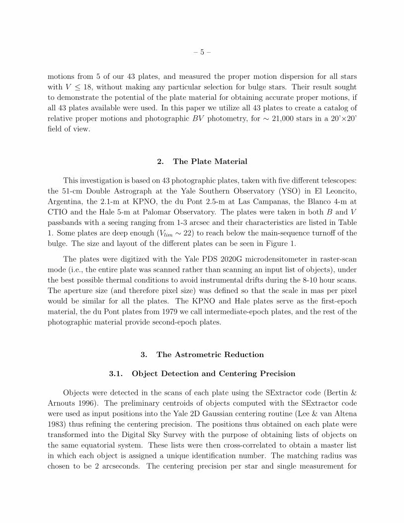
motions from 5 of our 43 plates, and measured the proper motion dispersion for all stars

with V ≤ 18, without making any particular selection for bulge stars. Their result sought

to demonstrate the potential of the plate material for obtaining accurate proper motions, if

all 43 plates available were used. In this paper we utilize all 43 plates to create a catalog of

relative proper motions and photographic BV photometry, for ∼ 21,000 stars in a 20’×20’

field of view.

2. The Plate Material

This investigation is based on 43 photographic plates, taken with five different telescopes:

the 51-cm Double Astrograph at the Yale Southern Observatory (YSO) in El Leoncito,

Argentina, the 2.1-m at KPNO, the du Pont 2.5-m at Las Campanas, the Blanco 4-m at

CTIO and the Hale 5-m at Palomar Observatory. The plates were taken in both B and V

passbands with a seeing ranging from 1-3 arcsec and their characteristics are listed in Table

1. Some plates are deep enough (Vlim ∼ 22) to reach below the main-sequence turnoff of the

bulge. The size and layout of the different plates can be seen in Figure 1.

The plates were digitized with the Yale PDS 2020G microdensitometer in raster-scan

mode (i.e., the entire plate was scanned rather than scanning an input list of objects), under

the best possible thermal conditions to avoid instrumental drifts during the 8-10 hour scans.

The aperture size (and therefore pixel size) was defined so that the scale in mas per pixel

would be similar for all the plates. The KPNO and Hale plates serve as the first-epoch

material, the du Pont plates from 1979 we call intermediate-epoch plates, and the rest of the

photographic material provide second-epoch plates.

3. The Astrometric Reduction

3.1. Object Detection and Centering Precision

Objects were detected in the scans of each plate using the SExtractor code (Bertin &

Arnouts 1996). The preliminary centroids of objects computed with the SExtractor code

were used as input positions into the Yale 2D Gaussian centering routine (Lee & van Altena

1983) thus refining the centering precision. The positions thus obtained on each plate were

transformed into the Digital Sky Survey with the purpose of obtaining lists of objects on

the same equatorial system. These lists were then cross-correlated to obtain a master list

in which each object is assigned a unique identification number. The matching radius was

chosen to be 2 arcseconds. The centering precision per star and single measurement for

– 6 –

well-measured stars is listed in Table 1. This number was estimated from the unit weight

error of coordinate transformations of pairs of plates taken with the same telescope at the

same epoch.

3.2. Photographic Photometry

We have obtained BV photographic photometry by calibrating the instrumental magni-

tudes from each plate with 26 photoelectric standards from van den Bergh & Herbst (1974).

The magnitude of each object is given by the mean of all determinations and its formal

error is computed from the scatter of the determinations. Outliers are eliminated in an

iterative process that is based on the estimated scatter of the measurements. The BV color-

magnitude diagran (CMD) and the photometric errors in the visual passband as a function

of V magnitude are shown in Figure 2, left and right panels respectively. The solid line in

the right panel of Fig. 2 represents the moving median of the V -magnitude errors. Thus,

the formal photometric errors are ∼ 0.1 mag for well-measured stars and between 0.2 and

0.3 mag for stars fainter than V = 18.

Due to the high reddening, photometry in the bulge is typically done in the V and I

bands. The only CCD BV photometry available in the bulge is given by Terndrup (1988) in

both the Baade and Plaut windows. By comparing the CMD from Terndrup (1988, their Fig.

4) with ours, we find qualitative agreement for the main features: the giant branch of the

bulge (B−V > 0.85 and V < 17), the main sequence of foreground disk stars (B−V < 0.85

and V < 17), and a low-density, blue horizontal branch of metal poor stars in the bulge

(V ∼ 16 and −0.1 ≤ B − V ≤ 0.4).

Our main reason for obtaining calibrated photographic photometry is to have (B − V )

colors that are crucial in modeling color terms in the astrometric reductions. Color terms are

generally due to differential atmospheric color refraction which, in this work, is very large for

the 1st epoch plates, because they were taken in the northern hemisphere at zenith distances

of ∼ 60◦.

3.3. Determination of Relative Proper Motions

The proper motions were computed using the central plate overlap method described

in Girard et al. (1989). This procedure provides differential proper motions by modeling all

plates into one master plate in an iterative process. The stars that are used to compute the

plate model span a given magnitude and color range, and they define the reference system.

– 7 –

For our case, these stars are a collection of disk and bulge stars; therefore the proper motions

are on a relative reference system. Only a few galaxies were identified on a handful of plates,

and thus, at this point, we are not able to provide a good measurement for the zero point of

the proper-motion system (i.e., provide absolute proper motions).

Before modeling the plates into the reference plate, a set of corrections was applied to

the positions. First, we corrected the positions for optical field angle distortion (OFAD) for

the plates taken with telescopes with previous astrometric studies. Thus the CTIO, duPont

and Hale plates were precorrected using the distortion coefficients from Chiu (1996) and

from Cudworth & Rees (1991). The center of distortion was taken to be the tangent point

of each plate.

The second correction is the well-kown magnitude equation, a systematic bias introduced

during long exposures due to inaccurate guiding and the nonlinearity of the photographic

plates (see e.g., Kozhurina-Platais et al. 1995; Guo et al. 1993; Girard et al. 1998). In

this study there are neither stars with negligible intrinsic proper-motion dispersion such as

stars in clusters which are used to model the proper-motion magnitude equation (e.g., Guo

et al. 1993), nor multiple images of different magnitudes per single star, such as the South-

ern Proper-Motion Program (Girard et al. 1998) uses to correct its magnitude equation.

Therefore, our approach to model and correct for magnitude equation is different than in

the above-mentioned studies, and has to rely on an assumption about the collection of plates.

The assumption is that for a large set of plates taken with the same telescope at the same

epoch, the variation in magnitude equation is random and therefore the average magnitude

equation over the whole set of plates is zero. In our case, this approach is suitable for the

modern du Pont plates, and for the old KPNO plates as these sets have many plates (Table

1) that can help build statistics. Thus, we have first considered the modern du Pont plates.

All modern du Pont plates were transformed into one from the same set (what we call the

‘assigned plate’), which is the deepest, and taken at the smallest hour angle. The plate

model is a polynomial that has up to 4th order terms in the coordinates, and a linear color

term when needed. A plot of residuals as a function of magnitude reflects the difference in

magnitude equation, between the plate being studied and the assigned plate. The residu-

als as a function of magnitude were determined for all modern du Pont plates (except for

the assigned plate itself) and then averaged to determine a single curve which, under our

assumption, represents the assigned plate’s magnitude equation. Once the assigned plate

was corrected for it, all other du Pont plates were placed onto this presumably magnitude

equation-free system. A similar procedure was applied to the KPNO plates. We then calcu-

lated a preliminary catalog of proper motions based only on the modern du Pont plates and

the old KPNO plates. This proper-motion system is presumably free of magnitude equa-

tion. Subsequent iterations of the proper motion catalog, included the intermediate-epoch

– 8 –

du Pont plates, then the CTIO and YSO plates, and finally the Hale plates. Magnitude

trends for these latter sets of plates determined from their mapping into the preliminary

magnitude-equation free system were interpreted as magnitude equation and corrected for

accordingly. The correction was determined and applied for each individual plate, before

they were introduced into the proper-motion solution.

The proper motion for each star was computed using a least-squares linear fit of position

as a function of time. Measures that differed by more than 0.2 arseconds from the best-fit

line were discarded from the solution. Individual proper-motion errors were computed from

the formal error of the slope as determined by the scatter of the residuals about the best-fit

line.

Since the x, y coordinate system is aligned with right ascension and declination, the

proper motions thus obtained are in the equatorial system. These were transformed to the

Galactic coordinate system to facilitate their kinematical interpretation discussed in the

following section. Initially our catalog had data for ∼ 31,000 stars, covering 30′ × 30′ on the

sky, but inadequately modeled OFAD obvious at the edges of the field restricted the final

catalog to 21,660 stars in an area of 20′ × 20′. As expected, proper-motion errors increase

with V -magnitude, due to lower S/N. In Figure 3 we show our proper-motion errors as a

function of magnitude. The solid line indicates a moving median for the whole sample.

Well-measured stars have proper-motion errors of ∼ 0.5 mas yr−1. Internal estimates of the

proper motion field dependent systematics are below 0.2 mas yr−1.

Since our goal is to accurately determine the intrinsic proper-motion dispersion of the

bulge (see following section), we must first determine an accurate estimate of our proper-

motion errors. The values shown in Fig. 3 are formal error estimates determined when

calculating the proper-motions, and they may not necessarily reflect the true errors. To

better estimate the proper-motion errors we divided our plates into two independent sets

and then created two proper-motion catalogs. A comparison of the proper-motion differences

between these two catalogs, indicated that the true errors are larger by 6% in µlcosb, and

by 10% in µb than our formal errors. We have therefore applied these values as corrections

to the formal proper-motion errors, and these adjusted errors are the ones we list in our

catalog.

4. Results

A cross-reference was made between our catalog and the 2MASS Catalog (Cutri et al.

2003), so we could use the infrared photometry to cleanly separate bulge from foreground

– 9 –

disk stars. Since 2MASS does not go as deep as our catalog, we ended up with 8721 matched

stars, which represent ∼ 90% of the 2MASS detections in the field. For this sample, our

(adjusted) proper-motion errors are typically 0.5 mas yr−1 in each coordinate.

Figure 4 shows the infrared J vs. J − H diagram for our Plaut’s window sample. It is

similar to that of Zoccali et al. (2003), for (l,b)=(0.277,-6.167), except for a slight correction

due to differential reddening and extinction. Both CMDs use 2MASS photometry. In Figure

4, the Red Giant Branch (RGB) is mostly populated by bulge red giants and can be easily

distinguished. There is also visible what looks like a slightly bluer and brighter thin sequence

of a few stars running parallel to the RGB stars. Some of these stars probably belong to

the metal-poor population of the bulge, but disk giants are also present in this part of the

CMD. As pointed out by Zoccali et al. (2003) and seen in our CMD as well, the Horizontal

Branch (HB) red clump of the bulge can be easily seen at J ∼13.5 and J −H ∼0.6, merged

with the bottom of the RGB. Due to a combination of differential reddening, metallicity

dispersion and depth effect, the HB has a large magnitude spread. Just below the HB red

clump, a second grouping of points, the RGB bump, is seen at J ∼14 and J − H ∼0.6.

Foreground main sequence stars belonging to the disk are located in the almost vertical

sequence extending upwards (J ≤ 16) and bluewards (0.0 ≤ J −H ≤ 0.45), widely dispersed

along the line of sight (Ng & Bertelli 1996). Another vertical sequence can be distinguished

at J − H ∼0.6 for J <13, which corresponds to the disk red clump of stars, dispersed in

magnitude as a result of their large spread in distance and reddening (Zoccali et al. 2003)

From Fig. 4, we selected 482 bulge stars, by using the decontaminated bulge sample

of Zoccali et al. 2003 (their figure 6c) as a template. We also separated a sample of 1851

disk main sequence stars by selecting those with 0.0 ≤ J − H ≤ 0.45 and J ≤ 16. Each

population is expected to have its own kinematical characteristics, and this is indeed observed

in Figure 5, where the bulge sample easily stands out from the disk samples, in the µl cos b

distribution. Since the disk sample is populated by blue stars and the bulge sample by

red ones, we considered the possibility of a residual color term producing a different mean

motion between the chosen samples. This possibility was discarded since an uncorrected

color term of this size on the individual plates would have been so large that it would have

been obvious, but no such effect was seen.

4.1. The disk sample

The disk stars selected from the infrared CMD, have a limited color range around

B − V ∼ 0.7, therefore we can consider the observed visual magnitude as a rough indicator

of distance. A plot of their proper motions components as a function of visual magnitude

– 10 –

(Figure 6) reveals a trend consistent with the projection of the reflex solar motion in the

observed proper motions. A residual magnitude equation was discarded as the cause of this

trend, since the bulge sample, which has visual magnitude in the same range [12.5,15.5],

does not exhibit any trend in its proper motions.

We then proceeded to compare our disk proper motion data with the expected projection

of the solar motion on the stellar proper motions. Simple geometry and distance determines

this projection, as stated by eqs. (31) and (32) from Mignard (2000):

µl cos b =u⊙ sin l − v⊙ cos l

4.74d(1)

µb =u⊙ cos l sin b + v⊙ sin l sin b − w⊙ cos b

4.74d(2)

where µl cos b and µb are given in mas yr−1, d is the distance to the star in kiloparsecs, and

(u⊙, v⊙, w⊙) are the components of the solar motion with respect to the Local Standard of

Rest (LSR), measured in km s−1. An arbitrary zero-point must be added to our relative

proper motions, to account for the mean motion of our reference frame with respect to

the Sun. After this, the proper motions will only contain the solar motion plus the stellar

motions, with respect to the LSR.

In Figure 7, we plot equations (1) and (2) for the predicted values of solar motion

by Dehnen & Binney (1998) (for a zero dispersion population), Mignard (2000) (for K0-K5

stars) and Abad et al. (2003) (for eπ/π < 0.33), to be compared with our data. The distance

in equations (1) and (2) has been converted to an apparent magnitude V by assuming that

the stars have an absolute magnitude of MV = 5.25. This value of MV was taken from

the observational HR diagram of Perryman et al. (1997), for main sequence stars having

B − V = 0.7. A linear correction of 0.1 mags kpc−1 was added to the computed apparent V

magnitude, to account for extinction effects.2

For µl cos b, both Abad et al. (2003) and Mignard (2000) produce good fits to our

data, while there is a disagreement with Dehnen & Binney (1998). The main difference in

the velocity of the reflex solar motion between these three studies, is in the v⊙-component

(Galactic rotation direction), which is approximately 5 km s−1, 15 km s−1 and 20 km s−1

for the three references cited, respectively. This velocity component defines the solar motion

projection onto µl cos b at l = 0, as stated by eq. (1). The apparent change in the solar

motion depending on the sample of stars chosen to measure it, is a well known effect which

reflects the fact that stars have kinematics related to their ages. For instance, Dehnen &

2Total extinction in the Plaut’s Window is AV = 3.1E(B − V ) = 0.775 ± 0.155 ∼ 0.8 mags, following

Cardelli et al. (1989).

– 11 –

Binney (1998) find that v⊙ ≈ 25 km s−1 for stars with B − V ∼ 0.7, and putting this value

into the above equation improves the fit significantly. All three papers more or less agree on

their values of u⊙ and w⊙, and their predictions match our points in µb closely. For stars

fainter than V ∼ 16.7 (J ∼ 15.2), the observed trend in µl cos b changes. At this distance

(∼ 2 kpc), the reflex solar motion has decreased sufficiently so that Galactic rotation begins

to be noticed in µl cos b. We will explore this subject in more detail later in the section 5.2.

No change is seen in µb, which is consistent with the expectation that no vertical motion is

present in either the disk or the bulge.

4.2. The bulge sample

Regarding the bulge, the intrinsic proper motion dispersion can be calculated from the

observed proper motions (Figure 8), corrected by the contribution of the estimated errors.

Following Spaenhauer et al. (1992)

1

n − 1

n∑

i=1

(µi − µ)2 = σ2 +1

n

n∑

i=1

ǫ2µ (3)

where σ is the intrinsic dispersion, ǫµ is the (adjusted) proper-motion error estimate, and

n is the number of stars in the sample. For our bulge sample of 482 stars, we derive an

intrinsic dispersion of (σl, σb) = (3.39, 2.91)± (0.11, 0.09) mas yr−1. The observed anisotropy

σl/σb = 1.17 ± 0.05 has been explained as a “rotational broadening” due to integration

over the line of sight of an intrinsically isotropic bulge (Zhao et al. 1996). Nevertheless,

theoretically speaking, the observed anisotropy could also be produced by an intrinsically

larger azimuthal dispersion of a nonrotating bulge.

Our result compares fairly well with previous studies (Table 2), though it is clear that

we obtained the one of the highest dispersions of all proper motion investigations of the bulge

(Figure 9, bold purple point). An increased value of the observed velocity dispersion could

be due to some contamination from halo stars at Plaut’s location. For example, Minniti

(1996) measured σr = 113.5±14.4 km s−1 in a sample of 31 “pure” halo giants ([Fe/H]≤-1.5)

located at about 1.5 kpc from the Galactic center at (l, b) = (8o, 7o). Assuming R⊙ = 8 kpc

as the mean distance to these halo giants, and given that the halo is isothermal (Minniti

1996), then σr can be translated into a proper motion dispersion, which will be ∼3 mas yr−1.

A few halo stars contaminating the bulge sample may increase the real bulge dispersion. In

our case, several runs of the Besancon Model of the Galaxy (Robin et al. 2003, 2004) at

Plaut’s Window position, simulating the data we have observed and the sample we have

selected, suggest that this contamination is in fact zero.

– 12 –

The comparison of all proper motion dispersions of the bulge as seen in Figure 9, relies

on a simple but powerful assumption: that all samples are located at the same mean distance,

usually R⊙, which may well not be the case, since the bulge has a non-neglibigle depth and

its orientation also implies that we might be observing at different distances according to the

position. For example, a velocity dispersion of 100 km s−1 corresponds to a proper motion

dispersion of ∼ 2.6 mas yr−1 for a distance of 8 kpc, but for stars at 6 kpc from us, the

proper motion dispersion will be measured as ∼ 3.5 mas yr−1. Their difference, 0.9 mas

yr−1, is far larger than the errors achieved in the most recent papers about the bulge proper

motion dispersion, so such a difference may well be observed. Therefore, our high value of

(σl, σb) could then be explained if our sample of stars happens to be in the closer side of the

bulge.

The only distance indicator available to us in Plaut’s Window is the bulge HB red

clump, easily visible at J ∼ 13.49, H ∼ 12.87 and K ∼ 12.67 (Figure 10). As explained

by Ferraro et al. (2006), the absolute K magnitude of the helium-burning red clump stars

is mainly influenced by metallicity and shows little dependence with age. When working

with relatively old metal-rich populations, it is then possible to use this feature as a distance

indicator. Extensive research on this topic has also been done using Hipparcos, OGLE and

HST data (Paczynski & Stanek 1998, Stanek & Garnavich 1998, Udalski et al. 1998). Based

on the measurements of six metal-rich (−0.9 < [Fe/H] < −0.3) clusters, Ferraro et al.

(2006) found MRCK = −1.40± 0.2, where the uncertainty adopted is a conservative estimate

of the age and metallicity effects for the population used to compute it.

Getting a distance modulus is then straightforward, once the value of the extinction

in the K-band is given, which though known to be small, could significantly change the

measured distance, particularly in the highly extincted fields close to the Galactic center.

AK can be estimated from AV = 0.775 ± 0.155 and Cardelli et al. (1989) extinction laws:

AK/AV = 0.114 ± 0.04. From these, AK = 0.09 ± 0.05 magnitudes, and from the measured

observed KRC = 12.67 ± 0.2, we can obtain the the distance modulus. Nevertheless we

decided to go a bit further, since the availability of a catalogue by Frogel et al. (1990),

allowed us to directly measure AK . Frogel at al. (1990) have a list of 90 M giants located

in the Plaut’s Window, with derredened JHK in the CTIO/CIT system, H2O, CO and

bolometric magnitudes, and spectral types. Conversion of their JHK into the 2MASS

system was done through Carpenter (2001) color transformations. A total of 55 stars were

crossmatched3 between our data and Frogel at al. (1990). The resulting measured extinction

in the K-band is AK = 0.05 ± 0.003 magnitudes, which is still within the error bars of the

3Thanks to a private communication with one of Frogel et al. (1990) coauthors, Dr. Donald Terndrup,

since positional information has not been published.

– 13 –

value above, though this one is far more precise and comes directly from observed stars in

the field. In any case, this additional exercise proved to be good to confirm numbers and also

to obtain spectral types for the 55 stars subsample, which are going to be of great value for

future developments of this project. This latter value of AK = 0.05 ± 0.003 will be adopted

for the rest of this work.

Therefore we conclude that the mean distance modulus of our 482 bulge stars is

KRC − MRCK − AK = 12.67 − (−1.40) − 0.05 ±

√0.22 + 0.22 + 0.0032 = 14.02 ± 0.28

or equivalently ∼ 6.37+0.87−0.77 kpc, which means we are looking ∼ 885 pc south of the Galactic

plane. If we assume R⊙ = 7.52 kpc (Nishiyama et al. 2006), a value that was also obtained

by using the HB red clump as a distance indicator, then our bulge sample is located ∼ 1.21

kpc closer than the Galactic rotation axis. Using the larger and most referred value of

R⊙ = 8.00 kpc, stresses the fact that our sample is significantly closer than R⊙, but this

shorter distance still makes possible for these stars to be part of the bulge. Indeed, based

on the bulge density model of Zhao (1996)4, it is straightforward to compute that the bulge

density at the location of our sample is ∼ 8% of the highest central value. Additionally, if

we use d = 6.37 kpc to convert the proper motion dispersion into a velocity dispersion, we

obtain (σ(vl), σ(vb)) = (102.30, 87.76) ± (3.32, 2.85) km s−1, which compares well with the

prediction by Zhao (1996) of (σ(vl), σ(vb)) ∼ (115, 80) km s−1, as obtained from his Figure

6 (lower panel).

The measured velocity dispersions can also be used to estimate the rotational velocity

at Plaut’s location. Using Zhao et al. (1996) equations (1) and (2), we obtain 52.57 ± 8.02

km s−1. This value is in agreement with the bulge rotation curve as measured by several

authors, including for example Izumiura et al. (1994), who used SiO masers at 7o < |b| < 8o

and measured Vrot = 50.8 ± 14.2 km s−1R kpc−1, where R is the distance from the Galactic

rotation axis, and also Tiede & Terndrup (1999), who obtained Vrot = 53.3 ± 9.3 km s−1R

kpc−1, using stars with V − I > 1.2 and I < 16.5, located at l = −8, +8 and b = −6. More

recent results by Rich et al. (2007) suggest though, that the bulge may not have a solid

body rotation. Radial velocities of M giants observed on a strip of fields at b = −4, indicate

that for |l| < 3o, the bulge rotation curve has a slope of roughly 100 km s−1 kpc−1, and

beyond that region in galactic longitude, the rotational velocity flattens out to about ∼ 45

4Zhao (1996) uses a triaxial structure with a gaussian radial profile and boxy intrinsic shape, to describe

the bulge. He calls this model bar, but it is what we currently call a triaxal bulge. The scale lenghts in Zhao

(1996) are a = 1.49, b = 0.58 and c = 0.40 kpc in the x, y and z axis respectively, assuming R⊙ = 8 kpc. In

his model, the bulge has a position angle of 20o, “close to the value of 13.4o found by Dwek et al. (1995)”

and it has an effective axis ratio of 1:0.6:0.4.

– 14 –

km s−1. Since this last result suggests a much higher rotation speed at a lower |b|, then a

possible gradient in the bulge rotation could explain all these observational results in the

same scenario. In any case, this subject is still not resolved. If we consider for example,

Izumiura et al. (1995) results using SiO masers at |l| < 15o and 3o < |b| < 15o, excluding

strips at 4o < |b| < 5o and 7o < |b| < 8o, they found a higher rotational rate of Vrot = 73.5

km s−1R kpc−1. Disk contamination and/or small numbers has been considered as a factor

to explain such high rates (Rich et al. 2007)

4.2.1. Bulge BHB stars

In addition to the RGB bulge sample, we also explored the kinematics of another stellar

population that lives in the bulge, the blue horizontal branch (BHB) of metal poor stars.

They can be seen in the optical BV CMD of Figure 2, as a low-density feature at −0.5 <

B − V < 0.45 and 15 < V < 17, comprising a total of 103 stars. Their proper motion

distribution looks a bit noisier but very similar to the observed for the bulge RGB stars

sample in Figure 5, which makes a very good case for these stars being bona fide members of

the bulge, despite the fact that this sample is almost five times smaller than the bulge RGB

one. Three of the BHB stars have very high proper motions. Once these stars are discarded,

the measured proper motion dispersion is (σl, σb) = (4.23, 3.48) ± (0.30, 0.25) mas yr−1, a

result which is about 6 to 7 sigmas away from the dispersion obtained with the bulge RGB

stars. Halo contamination, more probable in this part of the CMD, could be responsible for

this higher value. The observed anisotropy is σl/σb = 1.22 ± 0.12, which is within the error

bars of the anisotropy measured with bulge RGB stars. Taking this number as a face value

indicates that proper motion anisotropy does not change with metallicity, as observed by

Spaenhauer et al. 1992. These numbers must be taken with caution though, since several

factors affect them, including small numbers, halo contamination and even MS disk stars

contamination, since our optical photographic photometry is not precise enough to select a

clean sample.

4.3. Metallicity distribution in the bulge: proper motions vs. [M/H]

We have also explored the metallicity distribution of our bulge sample, by using the

method explained in Zoccali et al. (2003). A family of hyperbolas in the plane (MK , (V −K)0)

represent the upper RGBs of globular clusters that have a range of metallicities. An inversion

of the hyperbolas produces a value of metallicity for each star. This method required using

our V photographic magnitude with the K magnitude from 2MASS, and despite the lower

– 15 –

precision of our optical photometry, the dispersion in V −K was similar to the one observed

in Figure 12 of Zoccali et al. (2003), which uses CCD data alone.

Due to the high sensitivity of V −K to metallicity, it is very important to make the best

possible reddening correction. Once again, based on Cardelli et al. (1989) extinction law for

AV , and our measurement of AK , we obtain: E(V −K) = AV −AK = 3.1∗E(B−V )−0.05 =

3.1 ∗ 0.25 − 0.05 = 0.73 magnitudes. Coming back to Zoccali et al. (2003), we have applied

the corresponding inversion of their equation (1), to get [M/H ] for each star in the bulge

sample. Following the recommendations of that paper, only stars fainter than MK = −4.5

and (V − K)0 > 2.8 were considered for the inversion, which left us with a subsample of 60

stars. Results can be seen in Figure 11, that can be compared with Figures 9 and 12 from

Zoccali et al. (2003). Despite our small number statistics, the similarity between the plots

is very good. A histogram of the metallicities obtained is shown in Figure 12, displaying the

distribution peak at [M/H ] ∼ −0.1 with a somewhat extended metal poor tail, and ∼ 30%

of the stars with supersolar metallicity, i.e. [M/H ] > 0. Again, the results are similar to

those observed in Zoccali et al. (2003), which are plotted in gray. Since the slightly bluer

and brighter sequence of few stars parallel to the RGB visible in our Figure 4 is not included

in the bulge sample, it is possible that some few bulge metal poor stars are missing in Figure

12. If they are included, the overall distribution of [M/H] does not change significantly,

since these few stars - if calibrated using the hyperbolas method described above - have

−1 < [M/H ] < −0.3, and they would smooth the histogram in that section of it. This

would in effect make our histogram more alike to the one obtained by Zoccali et al. (2003).

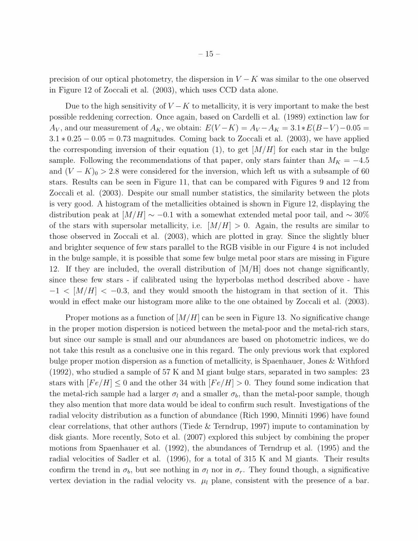
Proper motions as a function of [M/H ] can be seen in Figure 13. No significative change

in the proper motion dispersion is noticed between the metal-poor and the metal-rich stars,

but since our sample is small and our abundances are based on photometric indices, we do

not take this result as a conclusive one in this regard. The only previous work that explored

bulge proper motion dispersion as a function of metallicity, is Spaenhauer, Jones & Withford

(1992), who studied a sample of 57 K and M giant bulge stars, separated in two samples: 23

stars with [Fe/H] ≤ 0 and the other 34 with [Fe/H] > 0. They found some indication that

the metal-rich sample had a larger σl and a smaller σb, than the metal-poor sample, though

they also mention that more data would be ideal to confirm such result. Investigations of the

radial velocity distribution as a function of abundance (Rich 1990, Minniti 1996) have found

clear correlations, that other authors (Tiede & Terndrup, 1997) impute to contamination by

disk giants. More recently, Soto et al. (2007) explored this subject by combining the proper

motions from Spaenhauer et al. (1992), the abundances of Terndrup et al. (1995) and the

radial velocities of Sadler et al. (1996), for a total of 315 K and M giants. Their results

confirm the trend in σb, but see nothing in σl nor in σr. They found though, a significative

vertex deviation in the radial velocity vs. µl plane, consistent with the presence of a bar.

– 16 –

On this whole issue, an improved selection of BHB stars from our catalog, based on CCD

photometry, would be ideal to study their kinematics and better assess if these observed

changes are indeed real or not. Our paper provides the first kinematic link ever between

BHB and metal rich bulge stars.

We certainly agree that extreme caution must be taken when photometrically selecting

bulge stars, because even when kinematic information is available to improve the selection of

bona fide bulge members, confusion is still very possible, particularly when observing deep

into the Galactic center. In the next section we will thoroughly discuss this issue.

5. Discussion

5.1. Proper motion dispersion at different locations on the bulge

The recent availability of proper motion data in numerous locations on the bulge, and

the observation of what looks like trends in proper motion dispersion according to (l, b)

(Kozlowski et al. 2006, Rattenbury et al 2007), have prompted the idea that these results

may reflect intrinsic kinematic features of the bulge. For example, Kozlowski et al. (2006)

found a systematic variation of σl vs. b as measured by bulge main sequence (MS) stars

(Figure 9, upper panel right, blue points). Previous results by results by Zocalli et al. (2001)

and Kuijken & Rich (2002), both using MS bulge stars as well, do not deviate significantly

from the trend observed by Kozlowski et al. (2006) (Figure 9, upper panel right, green

points). On the other hand, Spaenhauer et al. (1992) and Feltzing & Johnson (2002), who

used RGB stars as tracers of the bulge, found larger values of σl that significantly deviate

from the observed trend above, and are in agreement with our high value of σl, within the

error bars (Figure 9, upper panel right, yellow points). More recently, Rattenbury et al.

2007, using a sample -supossedly- dominated by bulge HB red clump giants, have also found

correlations in σl vs. b (Figure 9, upper panel right, red points), that follow Kozlowski et al.

(2006) results . On the other hand, Rattenbury et al. 2007 also observe a trend in σl vs. l

(Figure 9, upper panel left, orange points), which has not seen by any previous work on the

bulge.

Regarding σb (see Figure 9, lower panel left), we found a large value that marginally

follows the trend of MS bulge stars, as seen by Kozlowski et al. (2006) in σb vs. l. Other

authors’ results agree as well, except for Rattenbury et al. 2007, who observe systematic

changes in σb, which are larger and offset from the rest of the proper motion works. Mendez

et al. (1996), (Figure 9 lower panel, black point), who also studied proper motions in Plaut’s

Window, but using all stars with V ≤ 18 and proper-motion errors less than 1 mas yr−1,

– 17 –

found essentially the same result as ours. This was initially surprising, since the Mendez et

al. (1996) sample is certainly dominated by disk foreground stars, but their result is just

a convolution of the real disk velocity dispersion along distance, plus the presence of real

bulge stars, and it is also affected by the proper motion errors of the fainter stars. Indeed,

a velocity dispersion of ∼ 30 km s−1 for the thin disk foreground stars will show up with

a proper motion dispersion of ∼ 3.2 mas yr−1 and ∼ 1.6 mas yr−1 for stars at around 2

and 4 kpc from the Sun, respectively. Thick disk stars also contribute, although they are

significantly less in number, but they have two times larger dispersion than thin disk stars.

In the case of the observed trends in Rattenbury et al. 2007, we would like to call the

attention to the fact that their selection of bulge stars, an ellipse centered on the HB clump

as seen in the V I CMD, is a poor criterion since disk contamination in this part of the

CMD is rather important. Indeed the clump is produced by bulge stars, but the presence

of an important smooth distribution of disk giants in that same magnitude and color range,

undermines their selection and therefore their the final results. The HB red clump is clearly

visible in our data as well, and we also studied the proper motion distribution of these stars.

We found that their mean motion was in the mean point between the mean motion of the

bright blue nearby disk and the mean motion of the red distant bulge. This clearly reveals

the strong mix of these populations at this location in the CMD. We also obtained these

mixed results when selecting stars in the AGB red bump. On top of that, except for the

proper motion data obtained from space (see Table 2), trustable ground-based proper motion

requires an extended baseline of at least a couple of decades, in order to achieve the accuracy

needed to properly assess the bulge kinematics. Numerous positions for a star within a short

period of time, as in the case of the OGLE-II data used in Rattenbury et al. 2007, may

improve its precision, but not its accuracy. Therefore, we consider that their results might be

affected by systematics related to both, their selection criteria as well as their short baseline.

In the case of Kozlowski et al. (2006), the observed trends in dispersion for bulge MS

stars, are explained as follows:

σl: Its value increases toward b = 0 due to (i) Disk contamination or (ii) Higher rotation

rate. Any of these two factors can broaden σl.

σb: Its value increases toward l = 0 due to (iii) An increase in metal poor stars on the

minor axis. It has been observed that metal poor stars have larger σb and σl/σb closer

to one (less anisotropy).

Of the three possible hypotheses, (i), (ii) and (iii) above, we will discuss disk contamination

in more detail, since the other two topics - higher rotation rate and the distribution of metal

poor stars - are beyond the scope of this paper.

– 18 –

5.2. Disk contamination in proper motions

Disk contamination can be estimated from the distribution of observed proper motions,

as long as all kinematic effects involved are taken into account. Previous studies did not

deal with this issue, since they only accounted for the proper motion shifts between bulge

and foreground stars as due to disk kinematics. In this paper we have done our best effort

to quantify all the observed trends in the proper motions, to better understand what they

mean and where they come from. So, for example, the effect of disk contamination on the

measured bulge σl, when coming from nearby stars can be easily guessed from our Figure

5: disk star proper motions are biased towards positive values of µl, due to the reflex solar

motion. If a bulge sample has nearby disk contamination, it will probably show a skewness

in its proper motion histogram and the measured dispersion σl will be artificially higher, like

for example in Figure 6 of Kozlowski et al. (2006). Since our bulge sample does not exhibit

any skewness, this gives us confidence that disk contamination in our sample is actually

small.

This diagnosis is valid of course only for nearby disk stars, on which the reflex solar

motion is the largest kinematic trend affecting these stars. For more distant stars, beyond

∼ 2 kpc, we have to consider what Galactic rotation does to their proper motion distribution,

on both its mean value as well as on its dispersion. To better understand this issue, we must

evaluate how differential galactic rotation projects onto the proper motions along distance.

For this, we selected the rotation curve measured by Zabolotskikh, Rastorguev & Dambis

(2003), who used a variety of young stellar systems plus HI and HII gas, assuming R⊙ = 7.5

kpc. This value of R⊙ is very close to R⊙ = 7.52 kpc measured by Nishiyama (2006) using

HB red clump stars.

The rotation curve in Figure 1 of Zabolotskikh, Rastorguev & Dambis (2003), can be

easily transformed to observed proper motions µl vs. V , by subtracting the Sun’s rotational

velocity, V (R⊙) = 206 ± 10 km s−1, and transforming those observed velocities into proper

motions, according to the distance. Extinction effects must also be taken into account.

Figure 14 shows the reflex solar motion (A03, long-dashed curve) and the galactic rotation

(short-dashed curve) as seen in the observed proper motions, individually and then added

up (gray curve). The mean µl observed in our disk star sample, shifted by an amount to fit

the gray curve, is also shown for comparison. Though it is clear that galactic rotation will

shift the mean µl to more negative values for stars fainter than V ∼ 16.7, the final result

once solar motion is considered, can not reproduce the observed drop in the stellar proper

motions of these faint and therefore distant stars. One important issue here though, is that

for galactocentric distances R < 6 kpc, Zabolotskikh, Rastorguev & Dambis (2003) use only

HI and HII data to measure the rotation curve. It is well known that the gas disk in the

– 19 –

Milky Way has a smaller velocity dispersion and therefore a higher circular velocity than the

stellar disk. Similarly younger stellar populations have more rotational support than older

ones, which lag behind. This is the so-called asymmetric drift in the solar neighborhood

(see for example Vallenari et al. 2006), and has been also observed in external disk galaxies

(Vega Beltran et al. 2001). Our sample of disk stars with B − V ∼ 0.7 are mostly dwarf

G5 to K0-type, so it is expected that they have a higher velocity dispersion and therefore

a slower circular velocity around the Galactic center, when compared to the gas disk. This

can explain why our disk stars exhibit a larger drop in their observed mean µl, than what is

seen in the gas.

If we were able to see deeper inside the Galaxy, a more negative mean µl would be

observed, down to the point where it could get close to the observed “negative” mean µl of

the bulge (See Figures 5 and 6). The proximity between the observed mean proper motion of

the bulge and the disk, will depend of course on how far we are observing from the Galactic

rotation axis. It has also been observed that old disk stars increase their velocity dispersion

as they get closer to the Galactic center. Lewis & Freeman (1989) measured radial velocities

for 600 old disk K giants, at different locations in l for 2o < |b| < 5o (See their Table I).

Based on these data, they computed the velocity dispersion along the azimuthal direction

σϕ, as a function of galactocentric distance R. For example, for R = 3 kpc, σϕ ∼ 65 km s−1

(R⊙ = 8.5 kpc was assumed in their paper). For l = 0, σϕ = 4.74σld, with d being distance.

Hence, following the example for R = 3 kpc, d = 8.5 − 3.0 = 5.5 kpc and σl is ∼ 2.5 mas

yr−1. This value of disk dispersion is still smaller than the bulge dispersion but not small

enough to stand out as a secondary peak in a histogram of proper motions, particularly

when the disk mean µl is also getting closer to the bulge’s mean motion. Therefore, when

sampling deep into these parts of the Galaxy, disk contamination might actually decrease

rather than increase the observed bulge σl, as measured by eq. (3). This problem can be of

special importance in very small deep fields of view, when it is more probable to have disk

contamination from distant stars than from nearby.

In order to further explore this idea, we decided to run the Besancon Model of the

Galaxy (Robin et al. 2003, 2004) on a homogeneous grid of points covering the pointings

studied in the Kozlowski et al. (2006) investigation. For the model data, we used the same

constraints of their paper: 30”×30” field of view, 0.5≤ V-I ≤3.0 and 18 ≤ I ≤ 21.5. We also

assumed an extinction suitable to reproduce the I vs. V − I CMD published in their paper.

We found that contamination from disk stars in the sample selected, ranged from 10% to

15%. It was observed indeed that for the fields closer to the Galactic plane, and therefore

more heavily extincted, the sample selection criterion of 18 ≤ I ≤ 21.5 allows some of the

disk stars brighter than the bulge turn off point to make it into the sample, but in all cases

more than 80% of the disk stars were located at distances d > 5 kpc. Disk stars alone showed

– 20 –

dispersions typically 2 to 5 times smaller than those of bulge stars and their mean motion

was close enough to the mean motion of the bulge, to make the whole sample σl as much as

5% to 10% smaller than the real bulge dispersion in most cases, when measured following

eq. (3). When examining the µl histograms though, it was possible to see in a few fields

closer to the galactic plane, a slight skewness that was indicative of the presence of more

than one single population. In general, the effect of the contaminanion from distant disk

stars was to “move” the bulge mean motion to a more positive value, artificially reducing the

real bulge σl, when using eq. (3) for the whole sample. These decrements represent 2 to 3

times the dispersion errors quoted by Kozlowski et al. (2006), which means that they could

- marginally - be observed when compared to the dispersion of a truly pure bulge sample.

More important, disk contamination never increased the bulge dispersion, and we did not

find evidence of it producing systematic changes in σl or σb as a function of l or b, either.

Therefore, for these small deep fields of view, with a data selection as the one explained

above, we could actually expect a reduction - if observable at all - rather than an increase, in

the observed bulge σl, due to distant disk contamination, since the nearby disk stars - which

would broaden σl - are very few compared to their far more numerous distant counterparts.

It is necessary to carefully evaluate the proper motion histograms, and check for possible

overlapping distributions of stellar proper motions, as long as a good number of data points

allows trustable statistics. On the other hand, nearby disk contamination is easy to detect

and correct for, by examining the proper motion histograms and looking for outliers in the

positive side of the µl histogram. Also, taking note of the extinction effects is key in order to

avoid disk contamination, particularly when selecting samples by fixed cuts in magnitude.

Hence, we think that if these two factors had been considered more carefully in Kozlowski

et al. (2006), the gradient in σl might actually dissapear. In any case, more observations

towards the Galactic plane should shed light on this issue, to check not only for a gradient

in the bulge rotation, which has been proposed as another possible cause of this trend, but

also to discard systematic effects or errors.

5.3. Final remarks

The selection of bulge stars for kinematic studies is usually done through photometry

cuts, aiming to select a particular population that is known to belong to this part of the

galaxy. What population is chosen to study the bulge depends, between other things, on

the quality and depth of the photometric data, shallower photometry allows a reliable iden-

tification of only the brightest features of the bulge stellar population in the CMD. But the

increasing amount of data coming from CCD observations and surveys, is opening another

– 21 –

possibility, studying the bulge faint MS stars. Extreme care must be taken in this case, be-

cause such a selection may include either nearby intrinsically faint stars, which will broaden

σl over large fields of view, or may include many distant disk stars which could decrease σl,

specially when observing deep into the galactic center. In this last case, if proper motions

are available for a large enough number of stars, those can be used to separate bulge from

foreground stars, particularly faint disk stars, as was done in Kuijken & Rich (2002), where

only stars with µl well in the negative side were selected as bulge stars. Such a kinematic

selection can be done, being of course aware of the biases that such sampling may introduce

in the data.

When looking for the right place to measure the bulge proper motion dispersion, we need

to deal with at least three interplaying factors: disk contamination, bulge stellar density and

obviously interstellar extinction. The place with the higher density of bulge stars, i.e. the

galactic plane l = 0, happens to have also the highest proportion of disk contamination

and extinction. Getting away from the plane to avoid disk stars and dust, without loosing

that many bulge stars, is then the way to go. The minor axis actually looks like the ideal

location for such observations, though surely this subject can be quantitatively determined

either thru analytical models or numerical simulations of the bulge and disk. In any case

though, extinction maps are the main tool to search and find low extinction windows, but

it is advisable to focus searches on those places where disk contamination is minimal.

As we have concluded before, our apparent high values of dispersion can be easily

explained by the closeness of our bulge sample. The line of sight at the Plaut’s Window,

(l, b) = (0,−8), crosses the bulge so that we sample the highest stellar density at the tangent

point of an isodensity curve. This tangent point is obviously closer than R⊙, and the farther

you go off the Galactic plane, the closer you sample mean distance will be. Assuming that all

bulge proper motion dispersions can be straightforwardly compared, based on the assumption

that all samples lie at the same mean distance, may be a source of mistakes, even worst, a

source of systematic errors. Interestingly, one of the ways to measure the orientation and

shape of the Galactic bar was precisely by looking at the systematic changes in the observed

magnitude of red clump stars along Galactic longitude (Stanek et al. 1997, Cabrera-Lavers

et al. 2007). But none of the systematic changes observed by Kozlowski et al. (2006) and

Rattenbury et al. (2007) can be explained by the bar orientation, since the trend in σb vs l

goes in the wrong direction. It is known that the bar is closer towards positive l, therefore,

we should observe (if possible at all) a decreasing σb towards l = 0, due to the increasing

distance.

It is also very critical to understand the effects of the solar motion and galactic rotation

on both the mean proper motion and its dispersion, since disk contamination has different

– 22 –

effects according to distance. In our case, for example, disk stars are mostly nearby fore-

ground, so in order to measure the relative motion of the disk with respect to the bulge,

we need to correct the reflex solar motion, which in turn requires distances to be computed.

Only for the MS disk stars we may use photometric distances, which also happen to be not

precise enough to do so. Nevertheless, a first estimate of this can be obtained from the

proper motion histograms, as depicted in Figure 5, where the bulge sample stands out from

the disk samples, in the µl cos b distribution. For redder nearby disk stars though, no option

is left to estimate distances. If an accurate solar motion correction were feasible, it would

be possible to convert our proper motions, from relative to absolute, for those disk stars

having photometric distances. Once we have completed our CCD photometry we expect to

properly examine this issue. Last but not least, the presence of the long thin bar and its

signature in the proper motion space, is a wholly unexplored subject of study in its own

right. Therefore, we consider that more proper motion studies using RGB bulge stars, which

are easier to observe and photometrically to select, should be done at different locations

around the bulge, before stating any further conclusions regarding kinematical trends in the

bulge.

6. Conclusions

We have measured proper motions of ∼ 21,000 stars brighter than V ∼ 20.5 in the low

extinction Plaut’s Window, that covers 20’ × 20’. The catalog contains α, δ, l,b, relative

proper motions in Galactic coordinates with their respective errors, optical photometry V ,

B − V based on our photographic plates, and 2MASS ID’s with their corresponding near

infrared magnitudes J, H, K and errors, when available.

Using infrared 2MASS photometry we have separated disk and bulge stars. Nearby disk

dwarf stars clearly show the signature of the reflex solar motion. Our determinations of the

bulge proper motion dispersion, though the highest measured in the bulge so far, it is still

in good agreement with previous results. Such a high value is explained by the relatively

close bulge sample that we selected, i.e. the brightest RGB stars. The mean distance to

this sample has been estimated to be 6.37 kpc, based on the observed K magnitude of the

bulge HB red clump. Based on this, the measured velocity dispersion is in good agreement

with the theoretical expected values for a steady-state triaxial bulge. The observed values

of proper motion anisotropy and metallicity distribution are limilar to previously published

values. No changes in dispersion were seen as function of metallicity. An independent small

sample of presumably mostly BHB bulge stars was also studied. This sample showed a higher

dispersion in both l and b, but the same anisotropy σl/σb than the RGB bulge sample. Our

– 23 –

paper provides the first kinematic link ever between BHB and metal rich bulge stars.

We also explored the effect that solar motion and galactic rotation have in the observed

mean proper motion and the proper motion dispersion, particularly along galactic longitude,

according to distance. We concluded that large field-of-view shallow surveys of the bulge,

mostly contaminated by nearby faint disk stars, may observe an artificially high σl, due to

the reflex solar motion component in the observed stellar proper motions. On the other side,

deeper small field-of-view shots of the bulge, may suffer the opposite effect: a lower σl, due

to (i) small dispersion of disk stars and (ii) mean motion of disk stars gets closer to the

mean motion of bulge stars, due to galactic rotation effects. Additionally, the fact that the

Galactic bulge has a non negligible depth and orientation, makes it important to consider

distance effects, when comparing proper motion dispersions along different locations in the

bulge.

A catalog containing the relative proper motions will soon be available at the Yale

Astrometry Group web page at http://www.astro.yale.edu/astrom/, and also in the electronic

edition of AJ. Samples of it can be seen in Tables 3 and 4. We are now processing CCD

observations of Plaut’s Window, to obtain more accurate UBV RI photometry, that will

allow us to make full use of the ∼21,000 precise proper motions. This will then be the most

complete, extended and precise investigation of the Galactic bulge proper motions using

ground based data, and its final results will be close in precision to those using HST data,

not going as deep but covering a much wider area on the sky, which allows us to simultaneosly

address the study of several components of the Milky Way.

This work has been supported by NSF grants AST-0407292, AST-0407293 and AST

0406884. Rene Mendez acknowledges support by the Chilean Centro de Astrofısica FONDAP

(no. 15010003). We would like to express our appreciation to the observers who took the

photographic plates and made this investigation possible: Sidney van der Bergh, William

Herbst, Jeremy Mould, Steven Majewski, Oscar Saa and Mario Cesco. K. Vieira also express

her thanks to Dr. Donald Terndrup who kindly gave her the positional information on a set

of M stars observed by Frogel et al. (1990). This publication makes use of data products from

the Two Micron All Sky Survey, which is a joint project of the University of Massachusetts

and the Infrared Processing and Analysis Center/California Institute of Technology, funded

by the National Aeronautics and Space Administration and the National Science Foundation.

REFERENCES

Abad, C. et al. 2003, A&A, 397, 345

– 24 –

Bertin, E. & Arnouts, S. 1996, A&AS, 117, 393

Beaulieu, S. et al. 2000, AJ, 120, 855

Blaauw, A. 2004, ARA&A, 42, 1

Blanco, V. M. 1988, AJ, 95, 1400

Blanco, V. M. & Terndrup, D. M. 1989, AJ, 98, 843

Cabrera-Lavers A. et al. 2007, astro-ph/0702109v1 (submitted to A&A)

Cardelli, J. A., Clayton, G. C. & Mathis, J. S. 1989, AJ, 345, 245

Carpenter J. M. 2001, AJ, 121, 2851

Chiu, L. 1976, PASP, 88, 803

Cudworth, K. M. & Rees, R. F. 1991, PASP, 103, 400

Cutri, R. M. et al. 2003, 2MASS All Sky Catalog of point sources (Pasadena: IPAC/Caltech)

Dehnen, W. & Binney J. 1998, MNRAS, 298, 387

Dominici, T. P. et al. 1999, A&AS, 136, 261

Dwek E. et al. 1995, ApJ, 445, 716

Feltzing, S. & Johnson, R. A. 2002, A&A, 385, 67

Ferraro, F. R., Valenti, E. & Origlia, L. 2006, AJ, 649, 243

Frogel, J. A. et al. 1990, AJ, 353, 494

Ghez, A. M. et al. 2005, ApJ, 620, 744

Girard, T. M. et al. 1989, AJ, 98, 227

Girard, T. M. et al. 1998, AJ, 115, 855

Guo, X. et al. 1993, AJ, 105, 2182

Izumiura, H. et al. 1994, ApJ, 437, 419

Izumiura, H. et al. 1995, ApJ, 453, 837

Kohoutek, L. & Pauls, R. 1995, A&AS, 111, 493

Kozhurina-Platais, V. et al. 1995, AJ, 109, 672

Kozlowski, S. et al. 2006, MNRAS, 370, 435

Kuijken, K. & Rich, R. M. 2002, AJ, 124, 2054

Lee, J. F. & van Altena W. 1983, AJ, 88, 1683

Lewis, J. R. & Freeman, K. C. 1989, AJ, 97, 139

– 25 –

Mendez, R. A. et al. 1996, ASP Conf. Series, 102, 345

Mignard, F. 2000, A&A, 354, 522

Minniti, D. 1996, ApJ, 459, 579

Ng, Y. K. & Bertelli, G. 1996, A&A, 315, 116

Nishiyama, S. et al. 2006, astro-ph/0607408v1 (accepted to ApJ)

Oort, J. & Plaut, L. 1975, A&A, 41, 71

Paczynski, B. & Stanek, K. Z. 1998, ApJ, 494, L219

Perryman, M. A. C. et al. 1997, A&A, 323, L49

Plaut, L. 1973, A&AS, 12, 351

Rattenbury, N. J. et al. 2007, arXiv:0704.1619 v1

Rich, R. M. 1990, ApJ, 362, 604

Rich, R. M. 1998, in IAU Symp. 184, The Central Regions of the Galaxy and Galaxies, ed.

Y. Sofue, (Dordrecht: Kluwer), 11

Rich, R. M. et al. 2007, AJ, 658, L29

Robin, A. C. et al. 2003, A&A, 409, 532

Robin, A. C. et al. 2004, A&A, 416, 157

Sadler, E. M., Rich, R. M. & Terndrup, D. M. 1996, AJ, 112, 171

Soto, M., Rich, R. M. & Kuijken, K. 2006, astro-ph/0611433v1 (submitted to ApJ Letters)

Tiede, G. P. & Terndrup, D. M. 1997, AJ, 113, 321

Tiede, G. P. & Terndrup, D. M. 1999, AJ, 118, 895

Tyson, N. D. & Rich, R. M. 1991, ApJ, 367, 547

Sparke, L. & Gallagher, J. 2000, Galaxies in the Universe (Cambridge: Cambridge University

Press)

Spaenhauer, A., Jones, B. F. & Whitford, A. E. 1992, AJ, 103, 297

Stanek, K. Z. et al., 1997, AJ, 477, 163

Stanek, K. Z. & Garnavich, P. M. 1998, ApJ, 503, L131

Terndrup, D. M. 1988, AJ, 96, 884

Terndrup, D. M., Sadler, E. M. & Rich, R. M. 1995, AJ, 110, 1174

Udalski, A. et al. 1998, Acta Astronomica, 48, 1

Vallenari, A. et al. 2006, A&A, 451, 125

– 26 –

van den Bergh, S. & Herbst, E. 1974, AJ, 79, 603

Vega Beltran, J, C. et al. 2001, A&A 374, 394

Zabolotskikh, M. V., Rastorguev, A. S. & Dambis, A. K. 2003, Communications of the

Konkoly Observatory, Hungary. Proceedings of the conference: “The interaction of

stars with their environment II”, held at the Eotvos Loriand University, Budapest,

Hungary, May 15-18, 2003, ed. Cs. Kiss, M. Kun, V. Konyves, p. 167-172

Zhao, H. 1996, MNRAS, 283, 149

Zhao, H., Rich R. M. & Biello, J. 1996, AJ, 470, 506

Zijlstra, A. A., Acker, A. & Walsh, J. R. 1997, A&AS, 125, 289

Zoccali, M. et al., 2001, AJ, 121, 2638

Zoccali, M. et al., 2003, A&A, 399, 931

Zoccali, M. et al., 2006, astro-ph/0609052v2 (accepted to A&A)

This preprint was prepared with the AAS LATEX macros v5.2.

– 27 –

Table 1. Photographic plate material

Telescope Epoch Observer Emulsion # of Plates Scale Centering Precisiona b c

KPNO 1972 vdB 103aO,D 13 12.70 18

Hale 1973 vdB&H 103aO,D 7 11.12 86

duPont 1979 JRM IIaO, IIIaF 5 10.92 28

duPont 1992-93 SRM IIaD, 103aO,D 12 10.92 28

CTIO 1993 OSAA IIIaJ 4 18.59 19

YSO 1993 MRC 103aO 2 55.10 112

a Observer: vdB=S. van der Bergh, vdB&H=S. van der Bergh & W. Herbst, JRM=J. Mould,

SRM=S. Majewski, OSAA=O. Saa, MRC=M. Cesco.

b Measured in arcsec mm−1

c Measured in milli-arcseconds

–28

–

Table 2. Dispersion Measurements in the bulge

Author l,b Detector FOV Target # of stars ∆T Sample Resultsa b c d e f g h i

S92 1.02,-3.93 plates 2’5 - 6’ NGC6522 427 33 B ≤ 19, (B − V )0 > 1 3.20,2.80 ± 1.00,1.00

annulus

M96 0.00,-8.00 plates 30’×30’ PW ∼5000 21 V≤18 3.38,2.78 ± 0.03,0.03

Z01 5.25,-3.02 WFPC2 2’×2’ NGC6553 1400 4 V-I redder than 2.63,2.06 ± 0.29,0.21

given line

F02 1.14,-4.12 WFPC2 2’×2’ NGC6528 500 6 V < 19, V − I > 1.6 3.27,2.54 ± 0.27,0.17

K02 1.13,-3.77 WFPC2 2’×2’ BW 3252 6 µl < −2, |µb| < 3 2.94,2.63 ± 0.05,0.05

K02 1.25,-2.65 WFPC2 2’×2’ SGR I 3867 6 µl < −2, |µb| < 3 3.24,2.85 ± 0.05,0.05

K06 2.10,-3.40 ACS/HRC+ 30”×30” BW 15254 4-8 18 < IF814W < 21.5 2.84,2.62 ± 0.11,0.04

WFPC2 ×35 fields

R07 1.83,-2.92 OGLE-II 14”×57” b = −4 577736 4 Red Clump Giants 2.98,2.61 ± 0.03,0.03

2K×2K CCD ×45 fields −8 < l < 10

This 0.00,-8.00 plates 20’×20’ PW 482 21 Red Giant Branch 3.39,2.91 ± 0.11,0.09

paper

–29

–a S92 = Spaenhauer et al. 1992, M96 = Mendez et al. 1996, Z01 = Zoccali et al. 2001, F02 = Feltzing & Johnson 2002, K02 =

Kuijken & Rich 2002, K06 = Kozlowski et al. 2006, R07 = Rattenbury et al. 2007

b Target position in Galactic coordinates. For K06 and R07, an average position of the 35 fields is shown.

c WFPC2 = HST Wide Field Planetary Camera 2. ACS/HRC= HST Advanced Camera for Surveys/High Resolution Camera.

d FOV=Field of View

e PW=Plaut’s Window, BW=Baade’s Window

g Epoch difference in years

i Proper motion dispersion, σ(µl) cos b, σ(µb) and their errors, all in mas/yr. For K06 and R07, results are given for the mean

position

– 30 –

Fig. 1.— Approximate spatial coverage and layout of the digitized plates. Axes are measured

in arcminutes.

– 31 –

Fig. 2.— Left: Optical CMD for the stars in Plaut’s Window. Right: Photometric error in

V vs. V magnitude for the same stars. The solid line is the median error computed over a

0.4 mag interval.

– 32 –

Fig. 3.— Proper motion errors vs. V magnitude, for stars in Fig. 2. The solid line is the

median error computed over a 0.25 mag interval.

– 33 –

Fig. 4.— 2MASS Infrared CMD for stars in common with our study. Disk stars were selected

as those having 0.0 ≤ J − H ≤ 0.45 and J ≤ 16. Bulge stars are indicated by the black

points on the RGB.

– 34 –

Fig. 5.— Upper: Histogram of µl cos b for three samples of disk stars as well as the bulge

stars. Lower: Same for µb. These are generalized histograms constructed using a gaussian

kernel of width 0.5 mas/yr.

– 35 –

Fig. 6.— Proper motion for the disk stars vs. V magnitude (as an indicator of distance).

Solid line: Mean proper motion over a 0.5 magnitude interval. The observed trend of larger

proper motion for the brighter (closer) stars, corresponds to the projection of the reflex solar

motion.

– 36 –

Fig. 7.— Reflex solar motion projected on the observed mean proper motion. Upper panel:

The black and gray lines depict the solid line in the upper panel of Figure 6, plus an arbitrary

shift in µl cos b to fit Abad et al. (2003) and Dehnen & Binney (1998) respectively. Lower

panel: The black line depicts the solid line in the lower panel of Figure 6. No shift was

required in µb to fit the curves.

– 37 –

Fig. 8.— Lower left: Vector-point diagram for the bulge stars. Upper left: Histogram of

µl cos b for bulge stars. Lower right: Histogram of µb for bulge stars.

– 38 –

Fig. 9.— Comparison of different proper motion investigations of the bulge. Results using

MS bulge stars are in blue (Kozlowski et al. 2006) and green (Zoccali et al. 2001, and

Kuijken & Rich 2002). Results using RGB bulge stars are plotted in yellow (Spaenhauer et

al. (1992), and Feltzing & Johnson (2002)). Results using the HB red clump (Rattenbury

et al. 2007) are plotted in red. The result from our study is plotted in bold purple. The

Mendez et al. (1996) result is plotted in black and has been shifted slightly to the right in

the upper panels, to distinguish it from our result. Some error bars in the upper right and

lower left panels are omitted for clarity purposes.

– 39 –

12 13 14 150

0.1

0.2

0.3J=13.49

J (mag)

12 13 14 150

0.1

0.2

0.3H=12.87

H (mag)

12 13 14 150

0.1

0.2

0.3K=12.67

K (mag)

Fig. 10.— Histogram of the Plaut’s Window catalog in the JHK 2MASS bands, for stars

with 0.45 < J − H < 0.8. The HB Red clump is easily observed as the brighter peak in the

histograms. The vertical line marks the mean observed magnitude of the red clump stars.

The second fainter peak corresponds to the RGB bump. A gaussian kernel of 0.2 mags width

was used to compute the histograms.

– 40 –

0 5 10

-4

-6

-8

0 5 10

0

-2

-4

-6

-8

Fig. 11.— V K CMD of bulge giants compared with the analytical RGB templates for

different metallicities, from Zoccali et al. (2003). The leftmost curve corresponds to [M/H ] =

−1.0. [M/H ] increases by 0.2 dex for the curves on the right. Insert on the upper left side is

a zoom-out of the same plot, showing all 482 bulge stars data. Only stars with MK > −4.5

and (V −K)0 > 2.8 were used to determine the metallicity distribution, as shown in Figure

12.

– 41 –

-2 -1 0 1

0

0.5

1

[M/H]

Fig. 12.— Metallicity distribution of a subsample of 60 RGB bulge stars in the Plaut’s

Window, as measured from Zoccali et al. (2003) hyperbolas calibration from Figure 11.

Only stars with MK > −4.5 and (V − K)0 > 2.8 were used to determine the metallicity

distribution. In gray, metallicity distribution of bulge giants from Zoccali et al. (2003). Both

histograms have been normalized for comparison.

– 42 –

-20

-10

0

-2 -1 0 1

-20

-10

0

[M/H]

Fig. 13.— Proper motion as a function of metallicity, for a subsample of 60 RGB bulge stars

in the Plaut’s Window. No visible trend is noticed in the proper motions, nor a significant

change in dispersion between metal-poor and metal-rich stars.

– 43 –

12 14 16 18-10

-8

-6

-4

-2

0

2

V (mag)

Galactic Rotation (Zabolotskikh et al. 2003)

Solar Motion (Abad et al. 2003)

Fig. 14.— Disk kinematics in the observed proper motion of our disk sample. The long-

dashed line is the reflex solar motion as measured by A03. The short-dashed line is the

differential galactic rotation as observed in µl as a function of V , based on Zabolotskikh,

Rastorguev & Dambis (2003) rotation curve of the Milky Way. The gray line is the sum of

the long- and the short-dashed lines. The solid line is the mean µl observed over 0.5 mag

intervals for our disk sample, shifted vertically to fit the gray line.

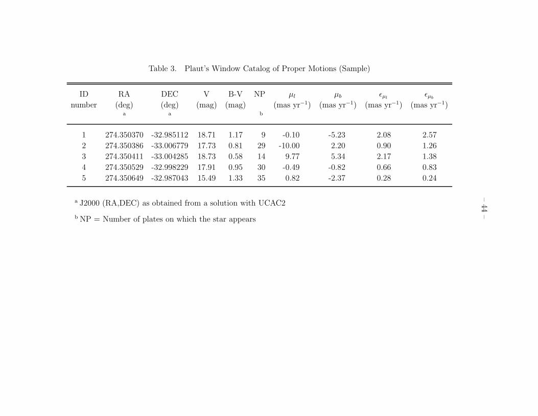
–44

–

Table 3. Plaut’s Window Catalog of Proper Motions (Sample)

ID RA DEC V B-V NP µl µb ǫµlǫµb

number (deg) (deg) (mag) (mag) (mas yr−1) (mas yr−1) (mas yr−1) (mas yr−1)a a b

1 274.350370 -32.985112 18.71 1.17 9 -0.10 -5.23 2.08 2.57

2 274.350386 -33.006779 17.73 0.81 29 -10.00 2.20 0.90 1.26

3 274.350411 -33.004285 18.73 0.58 14 9.77 5.34 2.17 1.38

4 274.350529 -32.998229 17.91 0.95 30 -0.49 -0.82 0.66 0.83

5 274.350649 -32.987043 15.49 1.33 35 0.82 -2.37 0.28 0.24

a J2000 (RA,DEC) as obtained from a solution with UCAC2

b NP = Number of plates on which the star appears

–45

–

Table 4. Plaut’s Window stars with 2MASS data (Sample)

ID 2MASS ID J ǫJ H ǫH K ǫK Population Duplicate

number number (mag) (mag) (mag) (mag) (mag) (mag) index match IDa b

18104 18184517-3242053 15.906 0.065 15.471 0.100 15.501 0.000 2

18106 18184517-3245568 15.854 0.098 14.238 0.000 14.275 0.000 0 18116

18111 18184518-3300268 14.756 0.062 14.388 0.089 14.462 0.093 2

18116 18184517-3245568 15.854 0.098 14.238 0.000 14.275 0.000 0 18106

18121 18184521-3241494 11.684 0.022 10.860 0.022 10.627 0.019 1

a Population index: 0=Undetermined, 1=Bulge RGB, 2=Disk MS. An index value of 0 means that no

population was explicitly assigned to the star

b ID of another Plaut’s star that was cross-referenced to the same 2MASS star. Our frames have better

resolution than 2MASS.