University of ZurichZurich Open Repository and Archive

Winterthurerstr. 190

CH-8057 Zurich

http://www.zora.uzh.ch

Year: 2008

Nonlinear dynamic causal models for fMRI

Stephan, K E; Kasper, L; Harrison, L M; Daunizeau, J; den Ouden, H E M;Breakspear, M; Friston, K J

Stephan, K E; Kasper, L; Harrison, L M; Daunizeau, J; den Ouden, H E M; Breakspear, M; Friston, K J (2008).Nonlinear dynamic causal models for fMRI. NeuroImage, 42(2):649-662.Postprint available at:http://www.zora.uzh.ch

Posted at the Zurich Open Repository and Archive, University of Zurich.http://www.zora.uzh.ch

Originally published at:NeuroImage 2008, 42(2):649-662.

Stephan, K E; Kasper, L; Harrison, L M; Daunizeau, J; den Ouden, H E M; Breakspear, M; Friston, K J (2008).Nonlinear dynamic causal models for fMRI. NeuroImage, 42(2):649-662.Postprint available at:http://www.zora.uzh.ch

Posted at the Zurich Open Repository and Archive, University of Zurich.http://www.zora.uzh.ch

Originally published at:NeuroImage 2008, 42(2):649-662.

Nonlinear dynamic causal models for fMRI

Abstract

Models of effective connectivity characterize the influence that neuronal populations exert over eachother. Additionally, some approaches, for example Dynamic Causal Modelling (DCM) and variants ofStructural Equation Modelling, describe how effective connectivity is modulated by experimentalmanipulations. Mathematically, both are based on bilinear equations, where the bilinear term modelstheeffect of experimental manipulations on neuronal interactions. The bilinear framework, however,precludes an important aspect of neuronal interactions that has been established with invasiveelectrophysiological recording studies; i.e., how the connection between two neuronal units is enabled orgated by activity in other units. These gating processes are critical for controlling the gain ofneuronalpopulations and are mediated through interactions between synaptic inputs (e.g. by means ofvoltage-sensitive ion channels). They represent a key mechanism for various neurobiological processes,including top-down (e.g. attentional) modulation, learning and neuromodulation.This paper presents anonlinear extension of DCM that models such processes (to second order) at theneuronal populationlevel. In this way, the modulation of network interactions can be assigned to an explicit neuronalpopulation. We present simulations and empirical results that demonstrate the validity and usefulness ofthis model. Analyses of synthetic data showed that nonlinear and bilinear mechanisms can bedistinguished by our extended DCM. When applying the model to empirical fMRIdata from a blockedattention to motion paradigm, we found that attention-induced increases in V5 responses could be bestexplained as a gating of the V1→V5 connection by activity in posterior parietal cortex. Furthermore, weanalysed fMRI data from an event-related binocular rivalry paradigm and found that interactionsamongst percept-selective visual areas were modulated by activity in themiddle frontal gyrus. In bothpractical examples, Bayesian model selection favoured the nonlinear models over corresponding bilinearones.

NONLINEAR DYNAMIC CAUSAL MODELS FOR FMRI

Klaas Enno Stephan1,2*, Lars Kasper3, Lee M. Harrison1, Jean Daunizeau1, Hanneke E.M. den

Ouden1, Michael Breakspear3, Karl J. Friston1

1 Wellcome Trust Centre for Neuroimaging, Institute of Neurology, University College London, 12 Queen

Square, London WC1N 3BG, UK. 2 Centre for the Study of Social and Neural Systems (CSSN), Institute for Empirical Research in Economics,

University of Zurich, Switzerland. 3 The Black Dog Institute, University of New South Wales, Prince of Wales Hospital, Hospital Road, Randwick

NSW 2031.

* Corresponding author:

Tel. +44-207-8337472

Fax +44-207-8131420

e-mail: k.stephan@fil.ion.ucl.ac.uk

Running head: Nonlinear Dynamic Causal Models for fMRI

Keywords: effective connectivity, DCM, Bayesian model selection, synaptic plasticity,

gain control, attention, binocular rivalry

Abstract: 290 words

Main text: 6,572 words

Figures: 10

Tables: 0

2

ABSTRACT

Models of effective connectivity characterize the influence that neuronal populations exert over each

other. Additionally, some approaches, for example Dynamic Causal Modelling (DCM) and variants of

Structural Equation Modelling, describe how effective connectivity is modulated by experimental

manipulations. Mathematically, both are based on bilinear equations, where the bilinear term models

the effect of experimental manipulations on neuronal interactions. The bilinear framework, however,

precludes an important aspect of neuronal interactions that has been established with invasive

electrophysiological recording studies; i.e., how the connection between two neuronal units is enabled

or gated by activity in other units. These gating processes are critical for controlling the gain of

neuronal populations and are mediated through interactions between synaptic inputs (e.g. by means of

voltage-sensitive ion channels). They represent a key mechanism for various neurobiological

processes, including top-down (e.g. attentional) modulation, learning and neuromodulation.

This paper presents a nonlinear extension of DCM that models such processes (to second order) at the

neuronal population level. In this way, the modulation of network interactions can be assigned to an

explicit neuronal population. We present simulations and empirical results that demonstrate the

validity and usefulness of this model. Analyses of synthetic data showed that nonlinear and bilinear

mechanisms can be distinguished by our extended DCM. When applying the model to empirical fMRI

data from a blocked attention to motion paradigm, we found that attention-induced increases in V5

responses could be best explained as a gating of the V1→V5 connection by activity in posterior

parietal cortex. Furthermore, we analysed fMRI data from an event-related binocular rivalry paradigm

and found that interactions amongst percept-selective visual areas were modulated by activity in the

middle frontal gyrus. In both practical examples, Bayesian model selection favoured the nonlinear

models over corresponding bilinear ones.

3

INTRODUCTION

Models of effective connectivity, i.e. the causal influences that system elements exert over another, are

essential for studying the functional integration of neuronal populations and for understanding the

mechanisms that underlie neuronal dynamics (Friston 2002; Horwitz et al. 1999). In the past, a variety

of models have been proposed for inferring effective connectivity from neuroimaging data, including

regression-based models like psycho-physiological interactions (PPI; Friston et al. 1997), structural

equation modelling (SEM; McIntosh & Gonzalez-Lima 1994; Büchel & Friston 1997; Bullmore et al.

2000), multivariate autoregressive models (MAR; Harrison et al. 2003; Roebroeck et al. 2005) and

dynamic causal modelling (DCM; Friston et al. 2003).

DCM is a general framework for inferring processes and mechanisms at the neuronal level from

measurements of brain activity with different techniques, including fMRI (Friston et al. 2003),

EEG/MEG (David et al. 2006) and frequency spectra based on local field potentials (Moran et al.

2008). In contrast to other models of effective connectivity, DCM does not operate on the measured

time-series directly. Instead, it combines a model of the hidden neuronal dynamics with a forward

model that translates neuronal states into predicted measurements. For fMRI, DCM is based on

bilinear differential equations describing neuronal population dynamics, which are combined with a

hemodynamic forward model. Since its original description (Friston et al. 2003), a number of

methodological developments have improved and extended DCM for fMRI, e.g. Bayesian model

selection amongst alternative DCMs (Penny et al. 2004a), precise sampling from predicted responses

(Kiebel et al. 2007), additional states at the neuronal level (Marreiros et al. 2008) and a refined

hemodynamic model (Stephan et al. 2007a). In this paper, we describe a novel DCM for fMRI that

enables one to model a class of nonlinear neuronal processes, which are important for a variety of

cognitive processes, including learning and attention.

Effective connectivity is inherently context-dependent and dynamic: there is a lot of evidence that the

functional coupling amongst neuronal populations changes as a function of processing demands (for

reviews, see McIntosh 2000; Stephan 2004). Therefore, models of effective connectivity are typically

used to infer whether the functional coupling is modulated by experimental manipulations; e.g. task

demands (Mechelli et al. 2003; McIntosh et al. 1994; Sonty et al. 2007; Stephan et al. 2007b), stimulus

properties (Fairhall & Ishai 2007; Haynes et al. 2005), learning (Büchel et al. 1999; McIntosh et al.

1998), drugs (Honey et al. 2003) or TMS (Lee et al. 2003). As discussed by Penny et al. (2004b), to

characterize context-dependent changes in coupling, early models of effective connectivity divided the

data into condition-specific subsets and applied separate linear models to each subset; later

developments used bilinear equations, allowing known input functions (which represent the

experimentally controlled context variable) to change connection strengths (see Fig. 1).

4

The bilinear model has two important limitations. First, the neuronal origin of the modulatory

influence is not specified. Second, it may not be the most appropriate framework for modelling fast

changes in effective connectivity, which are mediated by nonlinear effects at the level of single

neurons. These mechanisms are instances of "short-term synaptic plasticity" (STP), an umbrella term

for a range of processes which alter synaptic strengths with time constants in the range of milliseconds

to minutes; e.g. NMDA-controlled rapid trafficking of AMPA receptors (Malinow & Malenka 2002),

synaptic depression/facilitation (Zucker & Regehr 2002) or "early LTP" (Frey & Morris 1998) 1. All

these processes are driven by the history of prior synaptic activity and are thus nonlinear (Zucker &

Regehr 2002).

A particularly interesting mechanism, which relies on STP is "neuronal gain control" (Freeman 1979).

This is a general and fundamental mechanism for a large range of processes, including eye and limb

movements, spatial perception and, perhaps most significantly, attention (Salinas & Thier 2000).

Neuronal gain, i.e. the response of a given neuron N1 to presynaptic input from a second neuron N2,

depends on the history of inputs that N1 receives from other neurons, e.g. a third neuron N3. Such a

nonlinear modulation or "gating" of the N2→ N1 connection by N3 has been shown to have the same

mathematical form across a large number of experiments (e.g. Chance et al. 2002; McAdams &

Maunsell 1999a, 1999b; Larkum et al. 2004; for review, see Salinas & Sejnowski 2001): the change in

the gain of N1 results from a multiplicative interaction among the synaptic inputs from N2 and N3, i.e. a

second-order nonlinear effect. Biophysically, neuronal gain control can arise through various

mechanisms that mediate interactions among synaptic inputs, occurring close in time but not

necessarily in the same dendritic compartment. These neurophysiological mechanisms are described

in more detail in the Discussion.

Critically, the bilinear framework precludes a representation, at the neuronal level, of the mechanisms

described above. As stated in the original DCM paper (Friston et al. 2003), in order to model

processes like neuronal gain control and synaptic plasticity properly, one needs "to go beyond bilinear

approximations to allow for interactions among the states. This is important when trying to model

modulatory or nonlinear connections such as those mediated by backward afferents that terminate

predominantly in the supragranular layers and possibly on NMDA receptors."

One might wonder, however, whether these nonlinearities can be neglected in models of fMRI data,

due to the fact that (i) fMRI records the responses of large neuronal populations, whose ensemble

activity can often be well characterised by linear approximations (despite the highly nonlinear

behaviour of individual neurons; Deco et al. 2007), and that (ii) the hemodynamic transfer function,

which has low-pass filtering properties, may destroy most or all of the nonlinearities (that occur over

1 We do not consider long-term processes of synaptic plasticity, like long-term potentiation (LTP), here. These processes, which require major structural remodelling of the synapses and are thus slow, are difficult to observe in a single imaging session and are therefore typically investigated by comparing estimates of effective connectivity across sessions.

5

short periods of time). Therefore, an important question is whether nonlinear and bilinear modulatory

processes can be distinguished reliably in fMRI data and, if so, how much can be gained in practice by

using nonlinear, as opposed to bilinear, models of effective connectivity. In this technical paper,

which establishes the nonlinear framework for DCM, we perform analyses of both synthetic and

empirical data to address these questions. First, we use synthetic data and Bayesian model selection

(BMS) to demonstrate that nonlinear and bilinear mechanisms of generating fMRI data can be reliably

distinguished, even at reasonably high levels of observation noise. Second, we apply both nonlinear

and bilinear DCMs to two empirical fMRI studies. Theses studies look at attention and binocular

rivalry; processes for which nonlinear mechanisms have been proposed on the basis of

electrophysiological recordings. Using BMS, we demonstrate that, in both cases, nonlinear DCMs are

superior to corresponding bilinear DCMs.

METHODS

Bilinear Dynamic Causal Modelling (DCM)

DCM for fMRI is based on an input-state-output model of deterministic neuronal dynamics in a

system of n interacting brain regions. In this model, neuronal population activity of each region is

represented by a single state variable and is perturbed by experimentally controlled (and therefore

known) inputs u. DCM models the temporal change of the neuronal state vector x around the system's

resting state (i.e., x0=0, u0=0), using a bilinear Taylor series approximation to any nonlinear function

),( uxf that governs the dynamics of the system:

xuuxfu

ufx

xff

dtdxuxf

∂∂∂

+∂∂

+∂∂

+≈

=

2

)0,0(

),( (1)

Importantly, this series is truncated to include only a second-order (bilinear) term describing

interactions between neuronal states x and inputs u. Given m known inputs, one can parameterise this

equation with 0=

∂∂=u

xfA , ii uxfB ∂∂∂= 2)( , and

0=∂∂=

xufC to obtain a form that lends

itself to a direct neurophysiological interpretation:

CuxBuAdtdxuxf

m

i

ii +⎟

⎠

⎞⎜⎝

⎛ +== ∑=1

)(),( (2)

6

In this bilinear differential equation, the matrix A represents the fixed (context-independent or

endogenous) strength of connections between the modelled regions, and the matrices )(iB represent

the modulation of these connections (e.g. due to learning, attention, etc.) induced by the ith input ui as

an additive change. Finally, the C matrix represents the influence of direct (exogenous) inputs to the

system (e.g. sensory stimuli).

Nonlinear DCM

To model nonlinear interactions amongst the n states of the system, one can extend the Taylor series in

Eq. 1 to be second order in the states, i.e.

221)0,0(

),(

2

2

22 xxfxu

uxfu

ufx

xff

dtdxuxf

∂∂

+∂∂

∂+

∂∂

+∂∂

+≈

= (3)

Setting 0

2

2)(

21

=∂∂

=uj

j

xfD ( )nj ≤≤1 makes Eq. 3 equivalent to:

CuxDxBuAdtdxuxf

m

i

n

j

jj

ii +⎟⎟

⎠

⎞⎜⎜⎝

⎛++== ∑ ∑

= =1 1

)()(),( 4)

Here, the D(j) matrices encode which of the n regions gate which connections in the system.

Specifically, any non-zero entry )( jklD indicates that responses of region k to inputs from region l

depend on activity in region j. Figure 1 schematically juxtaposes bilinear and nonlinear DCMs, and

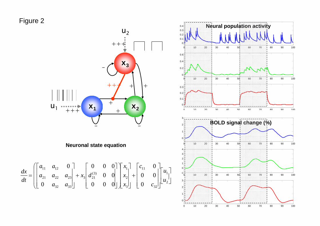
Figure 2 shows a simple example of a nonlinear DCM, illustrating the sort of dynamics, both at the

neuronal and hemodynamic level this sort of model exhibits.

[Figure 1: comparison of bilinear and nonlinear DCMs]

[Figure 2: example of a simple nonlinear DCM]

To explain regional BOLD responses, DCM for fMRI combines the models of neuronal dynamics

described above with a hemodynamic model. This model, which was originally described by Buxton

et al. (1998) and extended by Friston et al. (2000), comprises a set of differential equations linking

changes in neuronal population activity to changes in vasodilatation, blood flow, blood volume v and

deoxyhemoglobin content q; the predicted BOLD signal is a nonlinear function of the last two state

variables. In this work, we use the most recent formulation of this hemodynamic model as described

in Stephan et al. (2007a).

7

Together, the neuronal and hemodynamic state equations yield a deterministic forward model with

hidden states. For any given combination of parameters Κ,,,, DCBA⊇θ and inputs u, the

measured BOLD response y is modelled as the predicted BOLD signal ( )θ,uh plus a linear mixture

of confounds Xβ (e.g. signal drift) and Gaussian observation error e:

( ) eXuhy ++= βθ, (5)

Parameter estimation and stability

In DCM, parameter estimation employs a Bayesian scheme, with empirical priors for the

hemodynamic parameters and zero-mean shrinkage priors for the coupling parameters (see Friston

2002 and Friston et al. 2003 for details). The Gaussian observation error in Eq. 5 is modelled as a

linear combination of covariance components Q controlled by hyperparameters λ, i.e.,

( )∑ ii QNe )exp(,0~ λ . Briefly, the posterior moments of the parameters are updated iteratively

using variational Bayes under a fixed-form Laplace approximation, )(θq , to the conditional density

)|( yp θ ; similarly for )|( yp λ These updates are achieved through gradient ascent on a free-

energy bound on the log-evidence, )|( mypF ≤ for any model m, specified by a priori constraints

on which connections exist (see below and Friston et al. 2007). Two aspects are particularly

important. First, the use of informed priors condition the objective function by suppressing local

minima that are far away from the prior mean and facilitates identification of its global maximum by

gradient ascent schemes. Second, once the estimation scheme moves into a domain of parameter

space in which dynamics become unstable, i.e. runaway excitation, the value of the objective function

will necessarily decrease. The gradient ascent in DCM, however, rejects any updates that decrease the

objective function: in this case, the algorithm will return to the previous estimate and reduce its step-

size, using temporal regularisation (see Friston et al. 2007 for details); this regularisation scheme is

similar to (but more robust than) a Levenberg-Marquardt algorithm. This is repeated until the update

yields parameter estimates in a stable domain of parameter space and the objective function starts to

increase again. This ensures that one obtains parameter estimates for which the modelled system

dynamics are stable.

Integration of the nonlinear state equations

Even though stability is guaranteed, there may be parts of parameter space for which evaluation of the

state equations during integration encounters numerical problems. For example, some of the state

equations in the hemodynamic model contain roots (see appendix); for negative values of

hemodynamic states like blood volume and deoxyhemoglobin content2, evaluating these roots will

2 Note that negative values of the hemodynamic states would be physically meaningless; e.g. there is no such thing as a negative blood volume.

8

result in complex numbers. In order to prevent such cases, it is useful to transform the hemodynamic

states into log space; this guarantees that they will always have positive values and places formal

constraints on the support of these non-negative states. This transformation is described in the

appendix.

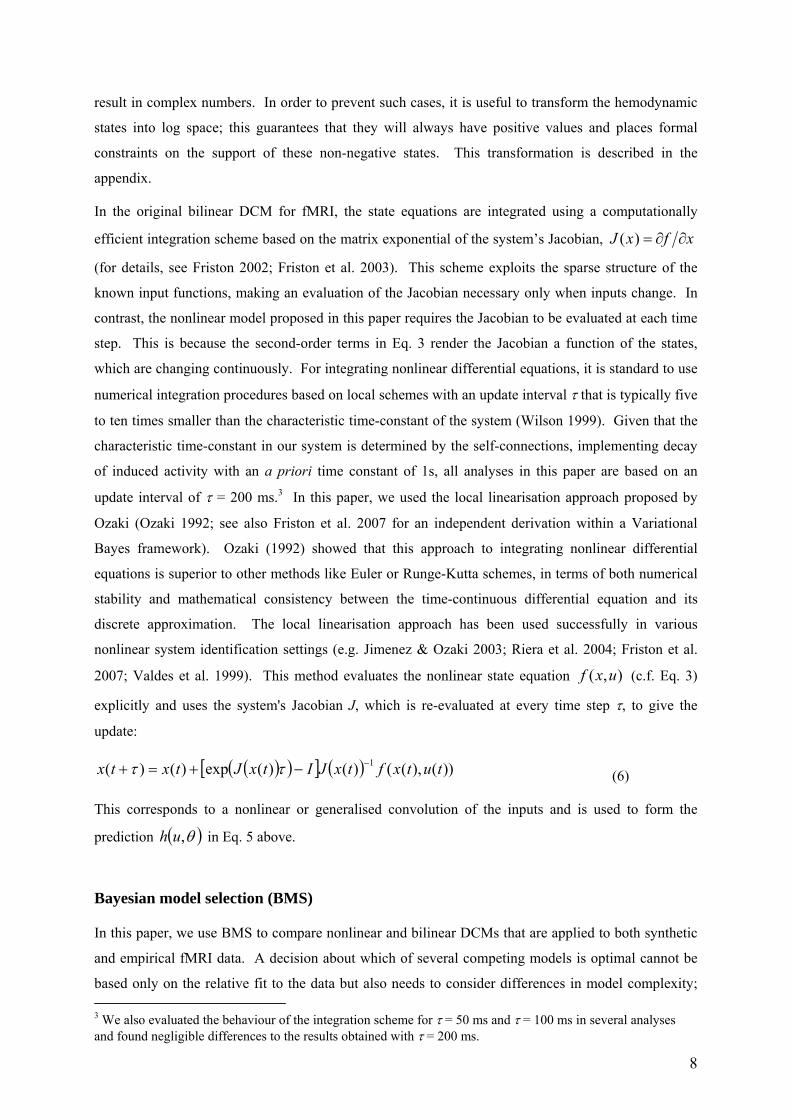
In the original bilinear DCM for fMRI, the state equations are integrated using a computationally

efficient integration scheme based on the matrix exponential of the system’s Jacobian, xfxJ ∂∂=)(

(for details, see Friston 2002; Friston et al. 2003). This scheme exploits the sparse structure of the

known input functions, making an evaluation of the Jacobian necessary only when inputs change. In

contrast, the nonlinear model proposed in this paper requires the Jacobian to be evaluated at each time

step. This is because the second-order terms in Eq. 3 render the Jacobian a function of the states,

which are changing continuously. For integrating nonlinear differential equations, it is standard to use

numerical integration procedures based on local schemes with an update interval τ that is typically five

to ten times smaller than the characteristic time-constant of the system (Wilson 1999). Given that the

characteristic time-constant in our system is determined by the self-connections, implementing decay

of induced activity with an a priori time constant of 1s, all analyses in this paper are based on an

update interval of τ = 200 ms.3 In this paper, we used the local linearisation approach proposed by

Ozaki (Ozaki 1992; see also Friston et al. 2007 for an independent derivation within a Variational

Bayes framework). Ozaki (1992) showed that this approach to integrating nonlinear differential

equations is superior to other methods like Euler or Runge-Kutta schemes, in terms of both numerical

stability and mathematical consistency between the time-continuous differential equation and its

discrete approximation. The local linearisation approach has been used successfully in various

nonlinear system identification settings (e.g. Jimenez & Ozaki 2003; Riera et al. 2004; Friston et al.

2007; Valdes et al. 1999). This method evaluates the nonlinear state equation ),( uxf (c.f. Eq. 3)

explicitly and uses the system's Jacobian J, which is re-evaluated at every time step τ, to give the

update:

( )( )[ ] ( ) ))(),(()()(exp)()( 1 tutxftxJItxJtxtx −−+=+ ττ (6)

This corresponds to a nonlinear or generalised convolution of the inputs and is used to form the

prediction ( )θ,uh in Eq. 5 above.

Bayesian model selection (BMS)

In this paper, we use BMS to compare nonlinear and bilinear DCMs that are applied to both synthetic

and empirical fMRI data. A decision about which of several competing models is optimal cannot be

based only on the relative fit to the data but also needs to consider differences in model complexity; 3 We also evaluated the behaviour of the integration scheme for τ = 50 ms and τ = 100 ms in several analyses and found negligible differences to the results obtained with τ = 200 ms.

9

i.e., the number of free parameters and the functional form of the generative model (Pitt & Myung

2002). Penalizing for model complexity is important because as complexity increases, model fit

increases monotonically, but at some point the model will start fitting noise that is specific to the

particular data (i.e., "over-fitting"). Models that are too complex are less generalisable across multiple

realizations of the same underlying generative process. Therefore, under the condition that all models

are equally likely a priori, the question “what is the optimal model?” can be reformulated as “what is

the model that represents the best balance between fit and complexity?” This is the model that

maximizes the model evidence:

∫= θθθ dmpmypmyp )|(),|()|( (7)

Here, the integration subsumes the number and conditional dependencies among free parameters as

well as the functional form ),,( θuxf of the generative model. Unfortunately, this integral cannot

usually be solved analytically, therefore approximations must be used (Penny et al. 2004a; Friston et

al. 2007). In this study, we use the variational free-energy, F. As detailed elsewhere (Stephan et al.,

in preparation), this has the advantage over other approximations that its complexity term not only

accounts properly for the effective degrees of freedom of the model but also for posterior covariance

(or dependency) among the parameters. This is important when comparing models whose likelihood

functions have different functional forms (e.g. nonlinear vs. bilinear). F is a lower bound on the log

model evidence such that

[ ]),|(),()|(ln mypqKLmypF θθ−= (8)

Here, KL denotes the Kulback-Leibler divergence (Kullback & Leibler 1951) between an

approximating posterior density )(θq and the true posterior, ),|( myp θ . F is the free-energy bound

on the log-evidence above and serves as the objective function for inversion. After convergence of the

estimation, the divergence is minimised and )|(ln mypF ≈ . An equivalent decomposition of F is in

terms of accuracy and complexity:

[ ])(),(),|(log θθθ pqKLmypFq−= (9)

where )(θp and )(θq represent the prior and approximate posterior densities, respectively. This

demonstrates that F embodies the two opposing requirements of a good model: that it explains the data

accurately (i.e., its log likelihood is high) and is as simply as possible (i.e., uses a minimal number of

parameters whose posterior densities deviate minimally from their prior; see Penny et al. 2007;

Stephan et al. 2007a).

Finally, to quantify the relative goodness of two models mi and mj, one can either report the

differences in their log-evidences or their Bayes factor (BF):

10

)exp()|()|(

jij

iij FF

mypmypBF −≈= (10)

Synthetic data

We assessed the sensitivity of our nonlinear model using simulated data with known properties. In

particular, we were interested in assessing its ability to distinguish nonlinear from bilinear processes.

For this purpose, we generated synthetic fMRI data, using a three-area model based on either nonlinear

(Fig. 3A) or bilinear state equations (Fig. 3B), and adding observation noise such that the resulting

time-series had either a high or low signal-to-noise ratio (SNR = 5 or 2, respectively)4. We then used

both nonlinear and bilinear models to estimate the parameters from each noisy data set. This resulted

in four sets of fitted models, under which the models used to generate the data and to estimate the

parameters were identical (i.e., nonlinear models fitted to time-series generated from nonlinear models

and bilinear models fitted to time-series generated from bilinear models) and another four sets of fitted

models in which they were not (i.e., bilinear models fitted to time-series generated from nonlinear

models and nonlinear models fitted to time-series generated from bilinear models). Each set of models

comprised 20 synthetic BOLD time-series for each of the three areas; overall, 160 models were fitted

and evaluated. Notably, all numerical procedures, including the integration schemes, were identical

for generation and inversion of all models.

The nonlinear model is shown in Fig. 3A. An irregular sequence of 25 delta functions or events

(randomly located within a 100 second time window) served as driving input u1 to region x1 and a box-

car function (two blocks with 25s duration) as driving input u2 to region x3. The output from x3

modulated the strength of the x1→x2 connection. We sampled the resulting BOLD time-series with a

sampling frequency of 1Hz over a period of 100 seconds and added Gaussian observation noise as

described above. The bilinear model (Fig. 3B) was identical in terms of connectivity structure and

inputs, except that the nonlinear modulation of the x1→x2 connection was omitted and replaced by a

bilinear modulation of the same connection by input u2. As a consequence, the modulatory processes

represented by nonlinear and bilinear models were qualitatively similar, and both models contained the

same number of free parameters; the key difference was the modulation of a connection by an

exogenous input (bilinear) or a hidden neuronal state (nonlinear).

With this factorial simulation set-up, we asked two questions. First, can nonlinear and bilinear

mechanisms underlying the modulation of connectivity be differentiated reliably on the basis of

BOLD time series? This question was addressed by Bayesian model selection, comparing the

evidence for the correct generative model against the evidence for the incorrect one. Second, how

4 Here, SNR=2 means that the standard deviation of the added observation noise equals half the standard deviation of the noise-free BOLD signal. It should be noted that the time-series entering a DCM are typically low in noise since they result from a singular value decomposition of the time-series across neighbouring voxels (c.f. Friston et al. 2003).

11

well are the true values of the modulatory parameters estimated in the presence of noise? We assessed

this by checking if the true parameter values fell within the 95% confidence interval based on the

sample density of the maximum a posteriori (MAP) parameter estimates over the 20 realisations. This

is a quite severe test, because the true value could easily lie within the 95% posterior confidence

interval of each realisation but the mode of the posterior density (the MAP estimate) might be

systematically smaller than the true value (due to the effects of shrinkage priors).

[Figure 3: nonlinear and bilinear DCMs used for simulating data]

Analyses of empirical fMRI data

Attention to visual motion

To demonstrate the face validity of our nonlinear DCM, we analysed a single subject fMRI dataset

from an experiment on attention to visual motion (Büchel et al. 1998). These data have been used in

previous analyses of effective connectivity (Büchel & Friston 1997; Friston & Büchel 2000; Friston et

al. 2003; Harrison et al. 2003; Marreiros et al. 2008; Penny et al. 2004a,b); a full description of the

experimental paradigm can be found in Büchel & Friston (1997). Both this study, and the study

below, had local ethics approval and participants gave informed consent. Briefly, subjects were

studied with an fMRI block design under four different conditions: fixating centrally (F), passively

viewing stationary dots (S), passively viewing radially moving dots (N) and attending to radially

moving dots (A), trying to detect putative velocity changes that actually never occurred, thus keeping

physical stimulation identical. Echo planar imaging data were acquired at 2 Tesla using a Siemens

Magnetom Vision whole body MRI system (TE = 40ms, TR = 3.22 seconds, matrix size = 64x64x32,

voxel size 3x3x3mm). Omitting dummy conditions (to allow for magnetic saturation effects) and

concatenating the data across four sessions, the dataset comprises 360 whole-brain volumes. As in

Friston et al. (2003), the conventional SPM analysis included three regressors: "photic" (conditions S

+ N + A), "motion" (conditions N + A), and "attention" (condition A). Regional time-series

representing primary visual cortex (V1), motion-sensitive area V5 and posterior parietal cortex (PPC)

were extracted by computing the principal eigenvariates from all voxels within spheres of 8 mm

radius. These spheres were centred on local maxima of suitable contrasts in a conventional SPM

analysis (V1: photic; V5: motion, masked inclusively by attention; PPC: attention).

We inverted a series of three-area DCMs representing either bilinear or nonlinear mechanisms and

compared these models using Bayesian model selection. Each of these models encoded a specific

mechanism for the attention-induced increase in V5 response that was observed in the SPM analysis

(see Fig. 6 for a summary of all models). We then used Bayesian model selection to investigate

whether there was sufficient information in the measured fMRI data to enable reliable differentiation

between bilinear and nonlinear models of attentional modulation. Additionally, we performed a

12

posterior density analysis of the modulatory parameters in the optimal model to quantify our certainty

that an attention-induced increase in V5 activity was mediated by modulation of afferent connections

to V5.

Binocular rivalry

To illustrate the use of nonlinear DCMs in a different empirical setting, we analysed a binocular

rivalry fMRI data set. This experiment was a 2×2×2 factorial generalisation of the binocular rivalry

experiment by Tong et al. (1998), the three factors being percept (face vs. house), rivalry (binocular

rivalry vs. non-rivalry), and motion (rocking vs. stationary stimuli). Specifically, subjects wore red-

blue dichromatic glasses and viewed a red house and blue face (or vice versa) in 30 sec blocks,

separated by 16 sec fixation intervals. In each block the stimuli were presented on a TFT-screen,

viewed via a mirror, either in a superimposed fashion (inducing binocular rivalry) or in a sequential

(non-rivalling) manner. During rivalry blocks, subjects were asked to indicate by button press when

they experienced a transition from a face to a house percept or vice versa. In each non-rivalry block,

the stimuli were presented sequentially with the timings as reported in a previous rivalry block (i.e.

replay); again subject reported perceptual transitions, which were yoked to the rivalry blocks. As

motion is known to influence the duration of stable percepts during binocular rivalry, our third

experimental factor concerned the use of stationary and rocking stimuli. The latter stimuli were

rocked continuously between extremes of 72 degrees from the vertical meridian (one cycle per

second). In the analysis presented in this methodological paper, however, we entirely focus on the

rivalry × percept interaction and ignore any effects of motion.

Echo planar imaging data were acquired using a 3 Tesla Philips Achieva whole body MRI scanner (TE

= 30ms, TR = 2.014s, matrix size 112x100x26, zero-filled to 128x128x26, voxel size 1.875x1.875x4.5

mm3) in four sessions. Omitting dummy scans (to allow for magnetic saturation effects) and

concatenating the data across four sessions, this dataset comprises 1136 whole-brain volumes. Here,

we report DCM results from a 22 year old female subject. A complete analysis of the group data will

be reported in a future paper.

Data were realigned to the first image, co-registered and normalized to the MNI template in SPM5.

Conventional SPM analysis used a general linear model with regressors for each of the eight

conditions in the factorial design, using two basis functions per regressor (a canonical hemodynamic

response function and its temporal derivative to account for slice-timing errors). Regions of interest

were identified using the appropriate contrasts from our factorial design and included the

parahippocampal place area (PPA), the fusiform face area (FFA) and the middle frontal gyrus (MFG).

The DCMs we considered allowed for full reciprocal connectivity among all three regions with

modulation of the lateral connections between the PPA and FFA. As above, these were based on

experimental (exogenous) inputs (bilinear) or top-down effects form MFG (nonlinear).

13

RESULTS

Simulated data

As described above, we assessed the sensitivity of our nonlinear model to the difference between

bilinear and nonlinear effects, using simulated data with known properties. We ran four sets of

simulations, i.e. for each combination of SNR and model type. This resulted in 80 synthetic datasets

to which we fitted both the correct model type (which had been used to generate the data) and the

incorrect model type. The results are summarized in Fig. 4 and Fig. 5: Amongst all 80 model

comparisons, there were only five cases in which there was higher evidence for the wrong model (Fig.

4), and in each of these cases the superiority of the wrong model was marginal, not even reaching the

conventional threshold for "positive" evidence, i.e. BF ≥ 3 (Kass & Raftery 1995). In contrast,

positive evidence for the correct model was obtained for 13 out of 20 datasets in the worst case

(nonlinear model, low SNR; Fig. 4A) and for 20 out of 20 datasets in the best case (bilinear model,

high SNR; Fig. 4D). Moreover, the overall (pooled) evidence for the correct model was very strong in

all four sets of simulations: group Bayes factors (GBF) ranged between 1014 and 1075 in favour of the

correct model, and average Bayes factors (ABF; the geometric mean of GBF) ranged between 5.6 and

6170 in favour of the correct model (Fig. 4; note that for scaling reasons this figure shows the log-

transformed Bayes factors, i.e. the relative log-evidence between models). Altogether, these results

demonstrate that, under the levels of SNR used in this analysis, bilinear and nonlinear mechanisms

underlying modulation of connection strengths can be differentiated.

Second, for moderate noise levels (SNR = 5), the 95% confidence intervals for both the nonlinear (D)

and bilinear (B) modulatory parameters contained the true values, thus demonstrating the robustness of

our estimates (Fig. 5). For high noise levels (SNR = 2), however, we observed a significant deviation

of both nonlinear and bilinear modulatory parameter estimates from their true values, generally

shrinking towards their prior expectation of zero (p<0.05). This result is due to the shrinkage priors on

the modulatory parameters, )1,0()( Ndp ij = , whose influence on the posterior estimates increases

with signal noise. The same shrinkage effect has been observed in previous simulation studies of

bilinear DCMs (Kiebel et al. 2007). This means that for noisy data, as expected, inversion of both

nonlinear and bilinear DCMs will yield conservative estimates of modulatory parameters.

[Fig. 4: BMS of correct and incorrect DCMs for synthetic data sets]

[Fig. 5: MAP estimates for synthetic data sets]

14

Empirical data

Attention to motion

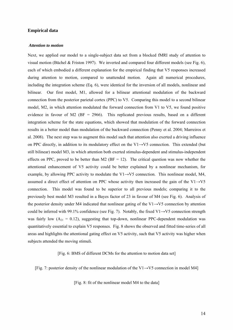
Next, we applied our model to a single-subject data set from a blocked fMRI study of attention to

visual motion (Büchel & Friston 1997). We inverted and compared four different models (see Fig. 6),

each of which embodied a different explanation for the empirical finding that V5 responses increased

during attention to motion, compared to unattended motion. Again all numerical procedures,

including the integration scheme (Eq. 6), were identical for the inversion of all models, nonlinear and

bilinear. Our first model, M1, allowed for a bilinear attentional modulation of the backward

connection from the posterior parietal cortex (PPC) to V5. Comparing this model to a second bilinear

model, M2, in which attention modulated the forward connection from V1 to V5, we found positive

evidence in favour of M2 (BF = 2966). This replicated previous results, based on a different

integration scheme for the state equations, which showed that modulation of the forward connection

results in a better model than modulation of the backward connection (Penny et al. 2004; Marreiros et

al. 2008). The next step was to augment this model such that attention also exerted a driving influence

on PPC directly, in addition to its modulatory effect on the V1→V5 connection. This extended (but

still bilinear) model M3, in which attention both exerted stimulus-dependent and stimulus-independent

effects on PPC, proved to be better than M2 (BF = 12). The critical question was now whether the

attentional enhancement of V5 activity could be better explained by a nonlinear mechanism, for

example, by allowing PPC activity to modulate the V1→V5 connection. This nonlinear model, M4,

assumed a direct effect of attention on PPC whose activity then increased the gain of the V1→V5

connection. This model was found to be superior to all previous models; comparing it to the

previously best model M3 resulted in a Bayes factor of 23 in favour of M4 (see Fig. 6). Analysis of

the posterior density under M4 indicated that nonlinear gating of the V1→V5 connection by attention

could be inferred with 99.1% confidence (see Fig. 7). Notably, the fixed V1→V5 connection strength

was fairly low (A21 = 0.12), suggesting that top-down, nonlinear PPC-dependent modulation was

quantitatively essential to explain V5 responses. Fig. 8 shows the observed and fitted time-series of all

areas and highlights the attentional gating effect on V5 activity, such that V5 activity was higher when

subjects attended the moving stimuli.

[Fig. 6: BMS of different DCMs for the attention to motion data set]

[Fig. 7: posterior density of the nonlinear modulation of the V1→V5 connection in model M4]

[Fig. 8: fit of the nonlinear model M4 to the data]

15

Binocular rivalry

As a second demonstration of nonlinear DCMs, we present an analysis of a single subject fMRI data

set acquired during an event-related binocular rivalry paradigm. Binocular rivalry arises when two

different stimuli are projected separately to the two eyes; the subject then experiences a single percept

at a time, and this percept fluctuates between the two competing stimuli with a time constant in the

order of a few seconds. While there is no clear consensus about the mechanisms that underlie this

phenomenon, it has been suggested that binocular rivalry (i) depends on nonlinear mechanisms and (ii)

may arise from modulation of connections amongst neuronal representations of the competing stimuli

by feedback connections from higher areas (see Blake & Logothetis 2002).

We acquired fMRI data during a factorial paradigm in which face and house stimuli were presented

either during binocular rivalry or during a matched non-rivalry (i.e. replay) condition. For the subject

studied here, the conventional SPM analysis showed a rivalry × percept interaction in both the right

fusiform face area (FFA) and the right parahippocampal place area (PPA): in FFA, the face vs. house

contrast was higher during non-rivalry than during rivalry; conversely, in PPA the house vs. face

contrast was higher during non-rivalry than during rivalry (both p<0.05, small-volume corrected).5

Additionally, testing for a main effect of rivalry, we replicated previous findings (Lumer et al. 1997)

that several prefrontal regions, including the right middle frontal gyrus (MFG), showed higher activity

during rivalry than during non-rivalry conditions.

These SPM results motivated a nonlinear DCM in which the connections between face- and house-

selective regions (i.e. FFA and PPA) were modulated by the activity in a source that was sensitive to

the degree of rivalry in the visual input (i.e. MFG). The structure of the resulting DCM (along with

the MAP estimates for all parameters) is shown in Fig. 9A. First, the fixed (intrinsic) connection

strengths between FFA and PPA are negative in both directions, i.e. FFA and PPA exert a mutual

negative influence on each other, when the system is not perturbed by inputs (i.e. during fixation); this

could be regarded as a "tonic" or "baseline" reciprocal inhibition. Much more important, however, is

that during the presentation of visual stimuli this competitive interaction between FFA and PPA is

modulated by activity in the middle frontal gyrus (MFG), which showed higher activity during rivalry

vs. non-rivalry conditions. As shown in Fig. 9B, our confidence about the presence of this nonlinear

modulation is very high (99.9%) for both connections. All parameter estimates are shown in Fig. 9A;

they provide a straightforward mechanistic explanation for the rivalry × percept interaction that was

found in both FFA and PPA in the SPM analysis. According to the model, activity levels in the MFG

determine the magnitude of the face vs. house activity differences in FFA and PPA by controlling the

influence that face-elicited activations and house-elicited deactivations of FFA have on PPA (and vice 5 This result is in contradiction to the findings by Tong et al. (1998) who reported that activity in FFA and PPA did not differ between rivalry and non-rivalry conditions. This discrepancy might arise due to various reasons. For example, Tong et al. (1998) used a separate localiser scan whereas our design embedded the localiser contrast into a fully factorial design. See Friston et al. (2006) and Saxe et al. (2006) for a discussion on the differences between these two approaches.

16

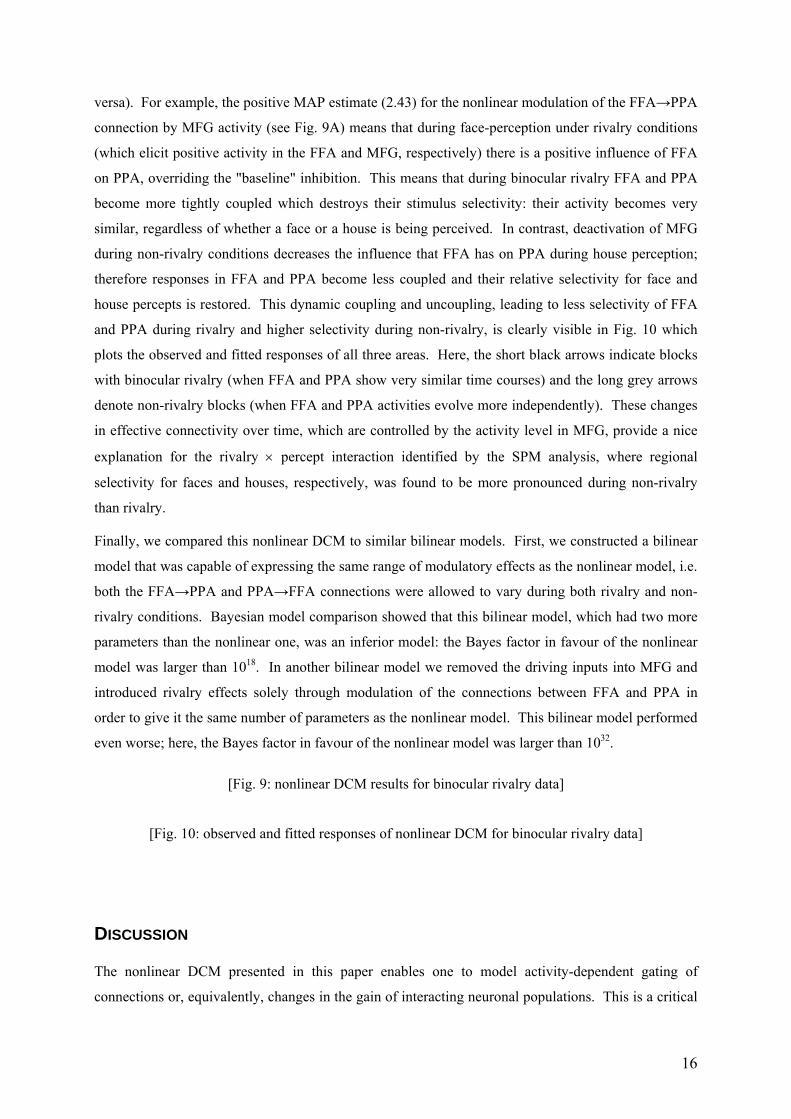
versa). For example, the positive MAP estimate (2.43) for the nonlinear modulation of the FFA→PPA

connection by MFG activity (see Fig. 9A) means that during face-perception under rivalry conditions

(which elicit positive activity in the FFA and MFG, respectively) there is a positive influence of FFA

on PPA, overriding the "baseline" inhibition. This means that during binocular rivalry FFA and PPA

become more tightly coupled which destroys their stimulus selectivity: their activity becomes very

similar, regardless of whether a face or a house is being perceived. In contrast, deactivation of MFG

during non-rivalry conditions decreases the influence that FFA has on PPA during house perception;

therefore responses in FFA and PPA become less coupled and their relative selectivity for face and

house percepts is restored. This dynamic coupling and uncoupling, leading to less selectivity of FFA

and PPA during rivalry and higher selectivity during non-rivalry, is clearly visible in Fig. 10 which

plots the observed and fitted responses of all three areas. Here, the short black arrows indicate blocks

with binocular rivalry (when FFA and PPA show very similar time courses) and the long grey arrows

denote non-rivalry blocks (when FFA and PPA activities evolve more independently). These changes

in effective connectivity over time, which are controlled by the activity level in MFG, provide a nice

explanation for the rivalry × percept interaction identified by the SPM analysis, where regional

selectivity for faces and houses, respectively, was found to be more pronounced during non-rivalry

than rivalry.

Finally, we compared this nonlinear DCM to similar bilinear models. First, we constructed a bilinear

model that was capable of expressing the same range of modulatory effects as the nonlinear model, i.e.

both the FFA→PPA and PPA→FFA connections were allowed to vary during both rivalry and non-

rivalry conditions. Bayesian model comparison showed that this bilinear model, which had two more

parameters than the nonlinear one, was an inferior model: the Bayes factor in favour of the nonlinear

model was larger than 1018. In another bilinear model we removed the driving inputs into MFG and

introduced rivalry effects solely through modulation of the connections between FFA and PPA in

order to give it the same number of parameters as the nonlinear model. This bilinear model performed

even worse; here, the Bayes factor in favour of the nonlinear model was larger than 1032.

[Fig. 9: nonlinear DCM results for binocular rivalry data]

[Fig. 10: observed and fitted responses of nonlinear DCM for binocular rivalry data]

DISCUSSION

The nonlinear DCM presented in this paper enables one to model activity-dependent gating of

connections or, equivalently, changes in the gain of interacting neuronal populations. This is a critical

17

mechanism in various neurobiological processes, including top-down modulation (e.g. by attention),

learning and effects exerted by neuromodulatory transmitters.

Biophysically, neuronal gain control can arise through various mechanisms of short-term synaptic

plasticity (STP) that result from interactions among synaptic inputs arriving close in time, but not

necessarily at the same dendritic compartment. For example, two major mechanisms are known to

induce very fast changes in connection strengths, without inducing lasting structural alterations of

synapses. The first one is non-linear dendritic integration of inputs due to voltage-dependent ion

channels, e.g. non-inactivating dendritic sodium conductances (Schwindt & Crill 1995). The second

mechanism is synaptic depression/facilitation (Abbott et al. 1997; Abbott & Regehr 2004). Other

mechanisms, although not relying on lasting structural synaptic changes, are likely to induce them; e.g.

activation of dendritic calcium conductances by back-propagating action potentials (Larkum et al.

2004) and amplification of neuronal responses by activation of NMDA conductances (Fox et al. 1990).

Finally, gain control is also affected strongly by various neuromodulatory transmitters that are known

to regulate synaptic plasticity (Gu 2002; Katz 2003), including noradrenalin (Ego-Stengel et al. 2002),

serotonin (Hurley & Pollak 2001) and acetylcholine (De Bruyn et al. 1986).

A few previous studies of effective connectivity have modelled changes in connection strength as a

function of activity in a different region (Friston et al. 1995; Büchel & Friston 1997: Friston et al.

1997; Friston & Büchel 2000). However, all of these studies differed in two crucial points to the

approach presented here. First, they operated directly on the measured BOLD time-series and could

not disambiguate whether nonlinearities arose from neuronal or from hemodynamic causes. In

contrast, the present model distinguishes between nonlinearities in the BOLD signal that are due to

neuronal and hemodynamic processes, respectively (c.f. Friston et al. 2003 and Stephan et al. 2007a).

A partial exception is the approach suggested by Gitelman et al. (2003), which can be used to compute

interaction terms used in psycho-physiological and physio-physiological interaction analyses of fMRI

data. In this approach, a deconvolution procedure is applied to BOLD data prior to Hadamard

multiplication. However, neither the deconvolution procedure nor the regression-based model of

effective connectivity in this approach affords the same flexibility and realism as combining nonlinear

neuronal state equations with a hemodynamic forward model as presented in this article. A second

critical difference is that all previous models were essentially variants of the general linear model and

thus remained linear in the parameters; nonlinearities were only accounted for by including regressors

or predictor variables that resulted from multiplication of two time-series.

Since its introduction a few years ago (Friston et al. 2003), DCM has already enjoyed widespread

application to fMRI data, resulting in more than thirty published studies to date. We expect that

nonlinear DCMs will further extend the practical applications of DCM. As exemplified by the two

examples in this paper, nonlinear mechanisms can, at least sometimes, better explain empirically

measured fMRI responses than linear ones. We would like to emphasise though that neither example

in this methodological paper is meant to provide an exhaustive treatment of questions on neuronal gain

18

modulation during attention or on nonlinear mechanisms during binocular rivalry. These examples are

only meant to lend face validity to our approach and provide anecdotal illustrations of the sort of

insights that can be gained with nonlinear DCMs. Similarly, the hierarchical sequence of comparisons

we employed for the attention-to-motion dataset is very useful for that particular analysis but does not

necessarily represent a blueprint for other DCM analyses; instead, the exact model comparison

strategy should always be tailored to the specific questions entailed by the model space examined.

A particularly exciting prospect is that nonlinear DCMs provide a good starting point for directly

embedding computational models (e.g. of learning processes) into physiological models (c.f. Stephan

2004). This is addressed by ongoing work in our group, with a focus on how neuromodulatory

transmitters shape synaptic plasticity during learning.

ACKNOWLEDGMENTS

This work was funded by the Wellcome Trust. We thank the attendees of the Brain Connectivity

Workshop 2007 at Barcelona and Brain Modes 2007 at Berlin for helpful discussions and John-Dylan

Haynes for help with the binocular rivalry stimuli. Special thanks to John "The Healer" Nugus for

invaluable support.

Software note

The MATLAB code implementing the method described in this paper will be made freely available as

part of the open-source software package SPM (http://www.fil.ion.ucl.ac.uk/spm) upon acceptance of

this paper.

19

APPENDIX – LOG-TRANSFORMATION OF HEMODYNAMIC STATE EQUATIONS

Classically, the hemodynamic model in DCM consists of the following differential equations in which

x is the neuronal state vector, κ is the rate constant of vasodilatory signal decay, γ is the rate constant

of flow-induced feedback regulation, τ is the mean transit time of venous blood, α is the resistance of

the venous balloon, and E0 is the resting oxygen extraction fraction (see Friston et al. 2000 and

Stephan et al. 2007a for details):

Changes in vasodilatory signalling s: )1( −−−= fγκsxdtds

(A1)

Changes in blood flow f: sdtdf

= (A2)

Changes in venous blood volume v: /αvfdtdvτ 1−= (A3)

Changes in deoxyhemoglobin content q: vqv

EEf

dtdq f

ατ /1

0

/10 )1(1

−−−

= (A4)

To ensure positive values of the hemodynamic states and thus numerical stability of the parameter

optimization scheme (see main text), we convert these equations, such that all hemodynamic states

},,,{ qvfsz = are in log space by applying the chain rule after a change of variables, zz ln~ = . That

is, for any given state variable z with the state equation )(zFdtdz

= :

zzF

dtdz

dzzd

dtzd

zzzz

)()ln(~

)~exp(ln~

==

⇒=⇔= (A5)

This means that ))(~exp()( tztz = is always positive, ensuring a proper support for these non-negative

states and numerical stability when evaluating the state equations during parameter estimation.

Applied to the four hemodynamic state equations in DCM (Eqs. A1 to A4), this transformation gives:

sfsx

dtsd )1(~ −−−=

γκ (A6)

fs

dtfd=

~ (A7)

20

vvf

dtvd

τ

α/1~ −= (A8)

qvqv

EEf

dtqd

f

τ

α/1

0

/10 )1(1

~ −−−

= (A9)

It is important to note that this log-transformation does not affect the model parameters, only the

hemodynamic states (which must have positive values due to their physical nature; e.g. there is no

such thing as a negative blood volume). This is because it is only the optimisation scheme that

operates on the log transformed states. In contrast, when evaluating the BOLD output equation (c.f.

Stephan et al. 2007a), the log-hemodynamic states are exponentiated. In other words, after each step

of the optimisation scheme, we use )(tz to compute the predicted BOLD signal at time t, not )(~ tz .

21

REFERENCES

Abbott LF, Varela JA, Sen K, Nelson SB (2002) Synaptic depression and cortical gain control. Science 275, 220-224.

Abbott LF, Regehr WG (2004) Synaptic compuation. Nature 431, 796-803.

Blake R, Logothetis NK (2002) Visual competition. Nat. Rev. Neurosci. 3, 13-21.

Büchel C, Friston KJ (1997) Modulation of connectivity in visual pathways by attention: cortical interactions evaluated with structural equation modelling and fMRI. Cereb. Cortex 7, 768-778.

Büchel C, Josephs O, Rees G, Turner R, Frith CD, Friston KJ (1998) The functional anatomy of attention to visual motion. A functional MRI study. Brain 121, 1281-94.

Büchel C, Coull JT, Friston KJ (1999) The predictive value of changes in effective connectivity for human learning. Science 283, 1538-1541.

Bullmore E, Horwitz B, Honey G, Brammer M, Williams S, Sharma T (2000) How good is good enough in path analysis of fMRI data? NeuroImage 11, 289-301.

Buxton RB, Wong EC, Frank LR (1998) Dynamics of blood flow and oxygenation changes during brain activation: the Balloon model. Magn. Reson. Med. 39, 855-864.

Chance FS, Abbott LF, Reyes AD (2002) Gain modulation from background synaptic input. Neuron 35, 773-782.

David O, Kiebel SJ, Harrison LM, Mattout J, Kilner JM, Friston KJ (2006) Dynamic causal modelling of evoked responses in EEG and MEG. NeuroImage 30, 1255-1272.

De Bruyn EJ, Gajewski YA, Bonds AB (1986) Anticholinesterase agents affect contrast gain of the cat cortical visual evoked potential. Neurosci. Lett. 71, 311-316.

Deco G, Jirsa VK, Robinson PA, Breakspear M, Friston, KJ (2008) The dynamic brain: From spiking neurons to neural masses and cortical fields. PLoS Comput. Biol., submitted.

Ego-Stengel V, Bringuier V, Shulz DE (2002) Noradrenergic modulation of functional selectivity in the cat visual cortex: an in vivo extracellular and intracellular study. Neuroscience 111, 275-289.

Fairhall SF, Ishai A (2007) Effective connectivity within the distributed cortical network for face perception. Cereb. Cortex 17, 2400-2406.

Fox K, Sato H, Daw N (1990) The effect of varying stimulus intensity on NMDA-receptor activity in cat visual cortex. J. Neurophysiol. 64, 1413-1428.

Freeman WJ (1979) Nonlinear gain mediating cortical stimulus-response relations. Biol. Cybern. 33, 237-247.

Frey U, Morris RGM (1998) Synaptic tagging: implications for late maintenance of hippocampal long-term potentiation. Trends Neurosci. 21, 181-188.

Friston KJ, Ungerleider LG, Jezzard P, Turner R (1995) Characterizing modulatory interactions between areas V1 and V2 in human cortex: A new treatment of functional MRI data. Hum. Brain Mapp. 2, 211-224.

22

Friston KJ, Büchel C, Fink GR, Morris J, Rolls E, Dolan RJ (1997) Psychophysiological and modulatory interactions in neuroimaging. NeuroImage 6, 218-229.

Friston KJ, Büchel C (2000) Attentional modulation of effective connectivity from V2 to V5/MT in humans. Proc. Natl. Acad. Sci. U. S. A. 97, 7591-7596.

Friston KJ, Mechelli A, Turner R, Price CJ (2000) Nonlinear responses in fMRI: the Balloon model, Volterra kernels, and other hemodynamics. NeuroImage 12, 466-477.

Friston KJ (2002) Beyond phrenology: What can neuroimaging tell us abut distributed circuitry? Ann. Rev. Neurosci. 25, 221-250.

Friston KJ (2002) Bayesian estimation of dynamical systems: An application to fMRI. NeuroImage 16, 513-530.

Friston KJ, Harrison L, Penny W (2003) Dynamic causal modelling. NeuroImage 19, 1273-1302.

Friston KJ, Rotshtein P, Geng JJ, Sterzer P, Henson RN (2006) A critique of functional localisers. NeuroImage 30, 1077-1087.

Friston KJ, Mattout J, Trujillo-Barreto N, Ashburner A, Penny WD (2007) Variational free energy and the Laplace approximation. NeuroImage 34, 220-234.

Gitelman DR, Penny WD, Ashburner J, Friston KJ (2003) Modeling regional and psychophysiologic interactions in fMRI: the importance of hemodynamic deconvolution. NeuroImage 19, 200-207.

Gu Q (2002) Neuromodulatory transmitter systems in the cortex and their role in cortical plasticity. Neuroscience 111, 815-835.

Harrison LM, Penny W, Friston KJ (2003) Multivariate autoregressive modelling of fMRI time series. NeuroImage 19, 1477-1491.

Haynes JD, Tregellas J, Rees G (2005) Attentional integration between anatomically distinct stimulus representations in early visual cortex. Proc. Natl. Acad. Sci. USA 102, 14925-14930.

Horwitz B, Tagamets BA, McIntosh AR (1999) Neural modelling, functional brain imaging, and cognition. Trends Cogn. Sci. 3, 91-98.

Honey GD, Suckling J, Zelaya F, Long C, Routledge C, Jackson S, Ng V, Fletcher PC, Williams SCR, BrownJ, Bullmore ET (2003) Dopaminergic drug effects on physiological connectivity in a human cortico-striato-thalamic system. Brain 126, 1767-1281.

Hurley LM, Pollak GD (2001) Serotonin effects on frequency tuning of inferior colliculus neurons. J. Neurophysiol. 85, 828-842.

Jimenez JC, Ozaki T (2003) Local linearization filters for non-linear continuous-discrete state space models with multiplicative noise. Int. J. Control. 76, 1159–1170.

Kass RE, Raftery AE (1995) Bayes factors. J. Am. Stat. Assoc. 90, 773-795.

Katz PS (2003) Synaptic gating: The potential to open closed doors. Current Biol. 13, R554–R556.

Kiebel SJ, Klöppel S, Weiskopf N, Friston KJ (2007) Dynamic causal modeling: a generative model of slice timing in fMRI. Neuroimage 34, 1487-1496.

Kullback S, Leibler RA (1951) On information and sufficiency. Ann. Math. Stat. 22, 79-86.

23

Larkum ME, Senn W, Lüscher HR (2004) Top-down dendritic input increases the gain of layer 5 pyramidal neurons. Cereb. Cortex. 14, 1059-1070.

Lee L, Siebner HR, Rowe JB, Rizzo V, Rothwell JC, Frackowiak RSJ, Friston KJ (2003) Acute remapping within the motor system induced by low-frequency repetitive transcranial magnetic stimulation. J. Neurosci. 23, 5308-5318.

Malinow R, Malenka RC (2002) AMPA receptor trafficking and synaptic plasticity. Annu. Rev. Neurosci. 25:103-126.

Marreiros AC, Kiebel SJ, Friston KJ (2008) Dynamic causal modelling for fMRI: A two-state model. NeuroImage 39, 269-278.

McAdams CJ, Maunsell JH (1999a) Effects of attention on the reliability of individual neurons in monkey visual cortex. Neuron 23, 765-773.

McAdams CJ, Maunsell JH (1999b) Effects of attention on orientation-tuning functions of single neurons in macaque cortical area V4. J. Neurosci. 19, 431-441.

McIntosh AR, Gonzalez-Lima F (1994) Structural equation modelling and its application to network analysis in functional brain imaging. Hum. Brain Mapp. 2, 2-22.

McIntosh AR, Grady CL, Ungerleider LG, Haxby JV, Rapoport SI, Horwitz B (1994) Network analysis of cortical visual pathways mapped with PET. J. Neurosci. 14, 655-666.

McIntosh AR, Cabeza RE, Lobaugh NJ (1998) Analysis of neural interactions explains the activation of occipital cortex by an auditory stimulus. J. Neurophysiol. 80, 2790-2796.

McIntosh AR (2000) Towards a network theory of cognition. Neural Netw. 13, 861-870.

Mechelli A, Price CJ, Noppeney U, Friston KJ (2003) A dynamic causal modeling study on category effects: bottom-up or top-down mediation? J. Cogn. Neurosci. 15, 925-934.

Moran RJ, Stephan KE, Kiebel SJ, Rombach N, O’Connor WT, Murphy KJ, Reilly RB, Friston KJ (2008) Bayesian estimation of synaptic physiology from the spectral responses of neural masses. NeuroImage, in press.

Ozaki T (1992) A bridge between nonlinear time series models and nonlinear stochastic dynamical systems: A local linearization approach. Statistica Sin. 2, 113-135.

Penny WD, Kiebel SJ, Friston KJ (2007) Variational Bayes. In: Statistical parametric mapping: The analysis of functional brain images (Friston KJ, ed), pp.303-312. Amsterdam: Elsevier.

Penny WD, Stephan KE, Mechelli A, Friston KJ (2004a) Comparing dynamic causal models. NeuroImage 22, 1157-1172.

Penny WD, Stephan KE, Mechelli A & Friston KJ (2004b) Modelling functional integration: a comparison of structural equation and dynamic causal models. NeuroImage 23, S264-274.

Pitt MA, Myung IJ (2002) When a good fit can be bad. Trends Cogn. Sci. 6, 421-425.

Riera JJ, Watanabe J, Kazuki I, Naoki M, Aubert E, Ozaki T, Kawashima R (2004) A state-space model of the hemodynamic approach: nonlinear filtering of BOLD signals. NeuroImage 21, 547-567.

Roebrock A, Formisano E, Goebel R (2005) Mapping directed influences over the brain using Granger causality and fMRI. NeuroImage 25, 230-242.

24

Salinas E, Thier P (2000) Gain modulation: a major computational principle of the central nervous system. Neuron 27, 15-21.

Salinas E, Sejnowski TJ (2001) Gain modulation in the central nervous system: where behavior, neurophysiology, and computation meet. Neuroscientist 7, 430-440.

Saxe R, Brett M, Kanwisher N (2006) Divide and conquer: A defense of functional localizers. NeuroImage 30, 1099-1096.

Schwindt PC, Crill WE (1995) Amplification of synaptic current by persistent sodium conductance in apical dendrite of neocortical neurons. J. Neurophysiol. 74, 2220-2224.

Sonty SP, Mesulam MM, Weintraub S, Johnson NA, Parrish TB, Gitelman DR (2007) Altered effective connectivity within the language network in primary progressive aphasia. J. Neurosci. 27, 1334-1345.

Stephan KE (2004) On the role of general system theory for functional neuroimaging. J. Anat. 205, 443-470.

Stephan KE, Weiskopf N, Drysdale PM, Robinson PA, Friston KJ (2007a) Comparing hemodynamic models with DCM. NeuroImage 38, 387-401.

Stephan KE, Marshall JC, Penny WD, Friston KJ, Fink GR (2007b) Inter-hemispheric integration of visual processing during task-driven lateralization. J. Neurosci. 27, 3512-3522.

Tong F, Nakayama K, Vaughan JT, Kanwisher N (1998) Binocular rivalry and visual awareness in human extrastriate cortex. Neuron 21, 753-759.

Valdes PA, Jimenez JC, Riera J, Biscay R, Ozaki T (1999) Nonlinear EEG analysis based on a neural mass model. Biol. Cybern. 81, 415-424.

Wilson H (1999) Spikes, Decisions and Actions. The Dynamical Foundations of Neuroscience. Oxford: Oxford University Press.

Zucker RS, Regehr WG (2002) Short-term synaptic plasticity. Annu. Rev. Physiol. 64, 355-405.

25

FIGURE LEGENDS

Figure 1

This figure shows schematic examples of bilinear (A) and nonlinear (B) DCMs, which describe the

dynamics of a neuronal state vector x. In both equations, the matrix A represents the fixed (context-

independent or endogenous) strength of connections between the modelled regions, the matrices )(iB

represent the context-dependent modulation of these connections, induced by the ith input ui, as an

additive change, and the C matrix represents the influence of direct (exogenous) inputs to the system

(e.g. sensory stimuli). The new component in the nonlinear equations are the D(j) matrices, which

encode how the n regions gate connections in the system. Specifically, any non-zero entry )( jklD

indicates that the responses of region k to inputs from region l depend on activity in region j.

Figure 2

The right panel shows synthetic neuronal and BOLD time-series that were generated using the

nonlinear DCM shown on the left. In this model, neuronal population activity x1 (blue) is driven by

irregularly spaced random events (delta-functions). Activity in x2 (green) is driven through a

connection from x1; critically, the strength of this connection depends on activity in a third population,

x3 (red), which receives a connection from x2 but also receives a direct input from a box-car input. The

effect of nonlinear modulation can be seen easily: responses of x2 to x1 become negligible when x3

activity is low. Conversely, x2 responds vigorously to x1 inputs when the x1→x2 connection is gated by

x3 activity. Strengths of connections are indicated by symbols (-: negative; +: weakly positive; +++:

strongly positive).

Figure 3

The nonlinear (A) and bilinear (B) DCM used for generation of synthetic data. As in Fig. 2, the first

input (u1) comprises an irregular sequence of random events (delta-functions), whereas the second

input (u2) corresponds to a box-car function. Strengths of connections are annotated as in Fig. 2.

Figure 4

This figure summarises the results of the Bayesian model comparisons between correct and incorrect

models applied to synthetic data generated by nonlinear and bilinear models (shown by Fig. 3), under

two levels of noise. The first two plots (A, B) contain the results for data with low signal-to-noise

(SNR=2), and the last two plots (C, D) show the results for data with high signal-to-noise (SNR=5).

26

Plots A and C show the log evidence differences between the nonlinear (NL) model and the bilinear

(BL) model for 20 synthetic data sets generated by a nonlinear model. Conversely, plots B and D

show the log evidence differences between the NL model and the BL model for data generated by a

BL model. The dashed horizontal lines indicate a log evidence difference of ≈1.1, corresponding to a

Bayes factor of ≈3 which is classically regarded as "positive" evidence for one model over another

(Kass & Raftery 1995). The solid horizontal lines denote a log evidence difference of ≈3,

corresponding to a Bayes factor of ≈20 which is conventionally considered to represent "strong"

evidence for one model over another (Kass & Raftery 1995). It can be seen that in the majority of

cases the correct model is identified as superior with at least positive evidence.

Figure 5

This figure plots the results of our analysis how well the true values of nonlinear and bilinear

modulatory parameters can be estimated in the presence of noise. We assessed this by checking if the

true parameter values fell within the 95% confidence interval based on the sample density of the

maximum a posteriori (MAP) parameter estimates over 20 synthetic data sets. The four plots in this

figure show the MAP estimates of modulatory parameters, obtained from fitting nonlinear models

(upper row) or bilinear models (lower row) to synthetic data generated by the same type of model.

The left column contains the results for data with low signal-to-noise (SNR=2), whereas the right

column contains the results for high signal-to-noise data (SNR=5). The true values of the modulatory

parameters are indicated by the dashed lines (nonlinear models: D = 1; bilinear models: B = 0.3). The

dotted lines indicated the average MAP estimates across data sets. In the low SNR case the true

values of both the nonlinear and bilinear modulatory parameters were not contained in the 95%

confidence interval of the respective estimates (nonlinear: 0.806 ± 0.063; bilinear: 0.261 ± 0.022).

This overly conservative estimation of the modulatory parameters is due to the effect of the zero-mean

shrinkage priors in DCM and has been observed in previous simulations (Kiebel et al. 2007). In

contrast, in the high SNR case the true values of both the nonlinear and bilinear modulatory

parameters fell within the 95% confidence interval of the respective estimates (nonlinear: 0.957 ±

0.072; bilinear: 0.286 ± 0.016).

Figure 6

Summary of the model comparison results for the attention to motion data set. For reasons of clarity,

we do not display a bilinear modulation of the V1→V5 connection by motion, which is present in

every model. The best model was a nonlinear one (model M4), in which attention-driven activity in

posterior parietal cortex (PPC) was allowed to modulate the V1→V5 connection. BF = Bayes factor.

27

Figure 7

(A) Maximum a posteriori estimates of all parameters in the optimal model for the attention to motion

data (model M4, see Fig. 6). PPC = posterior parietal cortex. (B) Posterior density of the estimate for

the nonlinear modulation parameter for the V1→V5 connection. Given the mean and variance of this

posterior density, we have 99.1% confidence that the true parameter value is larger than zero or, in

other words, that there is an increase in gain of V5 responses to V1 inputs that is mediated by PPC

activity.

Figure 8

Fit of the nonlinear model to the attention to motion data (model M4, see Figs. 4 and 5). Dotted lines

represent the observed data, solid lines the responses predicted by the nonlinear DCM. The increase in

the gain of V5 responses to V1 inputs during attention is clearly visible.

Figure 9

(A) The structure of the nonlinear DCM fitted to the binocular rivalry data, along with the maximum a

posteriori estimates of all parameters. The intrinsic connections between FFA and PPA are negative in

both directions; i.e. FFA and PPA mutually inhibited each other. This may be seen as an expression,

at the neurophysiological level, of the perceptual competition between the face and house stimuli.

This competitive interaction between FFA and PPA is modulated nonlinearly by activity in the middle

frontal gyrus (MFG), which showed higher activity during rivalry vs. non-rivalry conditions. (B) Our

confidence about the presence of this nonlinear modulation is very high (99.9%), for both connections.

Figure 10

Fit of the nonlinear model in Fig. 9A to the binocular rivalry data. Dotted lines represent the observed

data, solid lines the responses predicted by the nonlinear DCM. The upper panel shows the entire time

series. The lower panel zooms in on the first half of the data (dotted box). One can see that the

functional coupling between FFA (blue) and PPA (green) depends on the activity level in MFG (red):

when MFG activity is high during binocular rivalry blocks (BR; short black arrows), FFA and PPA are

strongly coupled and their responses are difficult to disambiguate. In contrast, when MFG activity is

low, during non-rivalry blocks (nBR; long grey arrows), FFA and PPA are less coupled, and their

activities evolve more independently.

bilinear DCM

CuxDxBuAdtdx m

i

n

j

jj

ii +⎟⎟

⎠

⎞⎜⎜⎝

⎛++= ∑ ∑

= =1 1

)()(CuxBuAdtdx m

i

ii +⎟

⎠

⎞⎜⎝

⎛+= ∑

=1

)(

Bilinear state equation

u1

u2

nonlinear DCM

Nonlinear state equation

u2

u1

Figure 1

0 10 20 30 40 50 60 70 80 90 100

0

0.1

0.2

0.3

0.4

0 10 20 30 40 50 60 70 80 90 1000

0.2

0.4

0.6

0 10 20 30 40 50 60 70 80 90 100

0

0.1

0.2

0.3

Neural population activity

0 10 20 30 40 50 60 70 80 90 100

0

1

2

3

0 10 20 30 40 50 60 70 80 90 100-1

0

1

2

3

4

0 10 20 30 40 50 60 70 80 90 100

0

1

2

3

BOLD signal change (%)

x1 x2u1

x3

u2

–

– –

++

++++

+++

+++

+

⎥⎦

⎤⎢⎣

⎡

⎥⎥⎥

⎦

⎤

⎢⎢⎢

⎣

⎡+

⎥⎥⎥

⎦

⎤

⎢⎢⎢

⎣

⎡

⎟⎟⎟

⎠

⎞

⎜⎜⎜

⎝

⎛

⎥⎥⎥

⎦

⎤

⎢⎢⎢

⎣

⎡+

⎥⎥⎥

⎦

⎤

⎢⎢⎢

⎣

⎡=

2

1

32

11

3

2

1)3(

213

3332

232221

1211

00

00

00000000

0

0

uu

c

c

xxx

dxaaaaa

aa

dtdx

Neuronal state equation

Figure 2

x1 x2u1

x3

u2

–

– –

++

++

+

+

+

x1 x2u1

x3

u2

–

– –

++

++

+

+

+

A B

Figure 3

-2

-1

0

1

2

3

4

5

6

1 2 3 4 5 6 7 8 9 10 11 12 13 14 15 16 17 18 19 20

Synthetic data sets

Log

evid

ence

diff

eren

ce

-1

0

1

2

3

4

5

6

1 2 3 4 5 6 7 8 9 10 11 12 13 14 15 16 17 18 19 20

Synthetic data sets

Log

evid

ence

diff

eren

ce

0

2

4

6

8

10

12

14

16

1 2 3 4 5 6 7 8 9 10 11 12 13 14 15 16 17 18 19 20

Synthetic data sets

Log

evid

ence

diff

eren

ce

0

2

4

6

8

10

12

14

16

1 2 3 4 5 6 7 8 9 10 11 12 13 14 15 16 17 18 19 20

Synthetic data sets

Log

evid

ence

diff

eren

ce

Figure 4

A

B

C

D

Low SNR High SNR

Dat

a ge

nera

ted

by

nonl

inea

r mod

elD

ata

gene

rate

d by

bi

linea

r mod

el

0

0.05

0.1

0.15

0.2

0.25

0.3

0.35

0.4

0.45

1 2 3 4 5 6 7 8 9 10 11 12 13 14 15 16 17 18 19 20

Synthetic data sets

MA

P es

timat

e

0

0.2

0.4

0.6

0.8

1

1.2

1.4

1 2 3 4 5 6 7 8 9 10 11 12 13 14 15 16 17 18 19 20

Synthetic data sets

MA

P es

timat

e

0

0.05

0.1

0.15

0.2

0.25

0.3

0.35

0.4

0.45

1 2 3 4 5 6 7 8 9 10 11 12 13 14 15 16 17 18 19 20

Synthetic data sets

MA

P es

timat

e

0

0.2

0.4

0.6

0.8

1

1.2

1 2 3 4 5 6 7 8 9 10 11 12 13 14 15 16 17 18 19 20

Synthetic data sets

MA

P es

timat

e

Figure 5

A

B

C

D

Low SNR High SNR

Dat

a ge

nera

ted

& fi

tted

by n

onlin

ear m

odel

Dat

a ge

nera

ted

& fi

tted

by b

iline

ar m

odel

modulation of back-ward or forward connection?

additional drivingeffect of attentionon PPC?

bilinear or nonlinearmodulation offorward connection?

V1 V5stim

PPCM2

attention

V1 V5stim

PPCM1

attention

V1 V5stim

PPCM3 attention

V1 V5stim

PPCM4 attention

BF = 2966

M2 better than M1

M3 better than M2BF = 12

M4 better than M3

BF = 23

Figure 6

V1 V5stim

PPC

attention

motion

-2 -1 0 1 2 3 4 50

0.1

0.2

0.3

0.4

0.5

0.6

0.7

0.8

%1.99)|0( 1,5 => yDp PPCVV

1.25

0.13

0.46

0.39

0.26

0.50

0.26

0.10MAP = 1.25

Figure 7

A B

V1V5PPC

observedfitted

motion &attention

motion &no attention

static dots

Figure 8

FFA PPA

MFG

-0.80

-0.31

faces houses faces houses

rivalry non-rivalry

1.05 0.08

0.300.51

2.43 2.41

0.04 -0.03 0.02 0.06

0.02 -0.03

-2 -1 0 1 2 3 4 5 6 70

0.1

0.2

0.3

0.4

0.5

0.6

0.7

-2 -1 0 1 2 3 4 5 6 70

0.1

0.2

0.3

0.4

0.5

0.6

0.7

%9.99)|0( , => yDp MFGFFAPPA

%9.99)|0( , => yDp MFGPPAFFA

Figure 9

A B

BR nBR

FFAPPAMFG

time (s)

Figure 10