Accounting for nonlinear BOLD effects in fMRI: parameter estimates and a model for prediction in...
13
Accounting for nonlinear BOLD effects in fMRI: parameter estimates and a model for prediction in rapid event-related studies Tor D. Wager, a, * Alberto Vazquez, b Luis Hernandez, b and Douglas C. Noll b a Department of Psychology, Columbia University, 1190 Amsterdam Avenue, New York, NY 10027, USA b University of Michigan, Ann Arbor, MI 48109, USA Received 19 July 2004; revised 9 October 2004; accepted 2 November 2004 Available online 4 January 2005 Nonlinear effects in fMRI BOLD data may substantially influence estimates of task-related activations, particularly in rapid event- related designs. If the BOLD response to each stimulus is assumed to be independent of the stimulation history, nonlinear interactions create a prediction error that may reduce sensitivity. When stimulus density differs among conditions, nonlinear effects can cause artifactual differences in activation. This situation can occur in rapid event-related designs or when comparing blocks of unequal lengths. We present data showing substantial nonlinear history effects for stimuli 1 s apart and use estimates of nonlinearities in response magnitude, onset time, and time to peak to form a low-dimensional parameterization of these nonlinear effects. Our estimates of non- linearity appear relatively consistent throughout the brain, and these estimates can be used to form adjusted linear predictors for future rapid event-related fMRI studies. Adjusting the linear model for these known nonlinear effects results in a substantially better model fit. The biggest advantages to using predictors adjusted for known nonlinear effects are (1) higher sensitivity at the individual subject level of analysis, (2) better control of confounds related to nonlinear effects, and (3) more accurate estimates of design efficiency in experimental fMRI design. D 2004 Elsevier Inc. All rights reserved. Keywords: fMRI; Event-related studies; Nonlinear effects Introduction Several studies have demonstrated the existence of nonlinear- ities in blood oxygen level-dependent (BOLD) fMRI data (Birn et al., 2001; Boynton et al., 1996; Buxton et al., 1998; Friston et al., 2000; Huettel and McCarthy, 2001; Vazquez and Noll, 1998). These nonlinearities are believed to arise from both nonlinearities in the vascular response, believed to be caused primarily by viscoelastic properties of blood vessels (Buxton et al., 1998; Vazquez and Noll, 1998, 2002), and nonlinearities at the neuronal level, such as the adaptive behavior of neuronal activity (Kileny et al., 1980; Logothetis, 2003; Logothetis et al., 2001; Wilson et al., 1984). Models of the underlying physiological changes that induce nonlinearities in the observed signal have been developed, primarily with the goal of understanding the nature of the BOLD response (Buxton and Frank, 1997; Buxton et al., 1998; Vazquez and Noll, 1998). Estimation methods (Cohen, 1997; Friston et al., 1998, 2000) have also been developed that may be used to model nonlinearities in functional experiments. Nonlinearity is an important issue in the design of experiments, and in the analysis of both blocked and event-related fMRI data under certain conditions (we present some scenarios below). In experimental design, the solution to the optimal stimulus spacing for an event-related design depends on the magnitude of nonlinear stimulus effects (Wager and Nichols, 2003). In a truly linear system, the efficiency of detecting a difference between conditions (e.g., Task A–Task B) increases without bound as the interstimulus interval approaches zero (e.g., Josephs and Henson, 1999), which is clearly not true of BOLD data (discussed further in Wager and Nichols, 2003). The true sensitivity is limited by nonlinear saturation in the BOLD signal, and to develop maximally sensitive experimental designs we must have a reasonably accurate model of the saturation. Virtually all work on experimental fMRI design assumes linear responses (Birn et al., 2002; Liu, 2004; Liu and Frank, 2004; Liu et al., 2001; Mechelli et al., 2003), or at least a very simple nonlinear model (Wager and Nichols, 2003), and would benefit from a simple approximate characterization of expected nonlinear responses. Nonlinear effects are largely ignored in neuroscientific and psychological studies using BOLD fMRI due possibly to several reasons. First, the finding that BOLD responses were approx- imately linear over a range of stimulus durations promised to greatly simplify analysis (Boynton et al., 1996). Nonlinearities are believed to be relatively small compared to the overall BOLD effects for events spaced more widely than 2 s (Buckner, 1998), although some studies have found fairly substantial saturation effects (17–25%) at 5 s (Miezin et al., 2000). Second, most work on development of expected hemodynamic responses has focused on determining canonical responses to single stimuli rather than 1053-8119/$ - see front matter D 2004 Elsevier Inc. All rights reserved. doi:10.1016/j.neuroimage.2004.11.008 * Corresponding author. E-mail address: [email protected] (T.D. Wager). Available online on ScienceDirect (www.sciencedirect.com). www.elsevier.com/locate/ynimg NeuroImage 25 (2005) 206 – 218
Transcript of Accounting for nonlinear BOLD effects in fMRI: parameter estimates and a model for prediction in...
www.elsevier.com/locate/ynimg
NeuroImage 25 (2005) 206–218
Accounting for nonlinear BOLD effects in fMRI: parameter estimates
and a model for prediction in rapid event-related studies
Tor D. Wager,a,* Alberto Vazquez,b Luis Hernandez,b and Douglas C. Nollb
aDepartment of Psychology, Columbia University, 1190 Amsterdam Avenue, New York, NY 10027, USAbUniversity of Michigan, Ann Arbor, MI 48109, USA
Received 19 July 2004; revised 9 October 2004; accepted 2 November 2004
Available online 4 January 2005
Nonlinear effects in fMRI BOLD data may substantially influence
estimates of task-related activations, particularly in rapid event-
related designs. If the BOLD response to each stimulus is assumed to
be independent of the stimulation history, nonlinear interactions
create a prediction error that may reduce sensitivity. When stimulus
density differs among conditions, nonlinear effects can cause
artifactual differences in activation. This situation can occur in rapid
event-related designs or when comparing blocks of unequal lengths.
We present data showing substantial nonlinear history effects for
stimuli 1 s apart and use estimates of nonlinearities in response
magnitude, onset time, and time to peak to form a low-dimensional
parameterization of these nonlinear effects. Our estimates of non-
linearity appear relatively consistent throughout the brain, and these
estimates can be used to form adjusted linear predictors for future
rapid event-related fMRI studies. Adjusting the linear model for these
known nonlinear effects results in a substantially better model fit. The
biggest advantages to using predictors adjusted for known nonlinear
effects are (1) higher sensitivity at the individual subject level of
analysis, (2) better control of confounds related to nonlinear effects,
and (3) more accurate estimates of design efficiency in experimental
fMRI design.
D 2004 Elsevier Inc. All rights reserved.
Keywords: fMRI; Event-related studies; Nonlinear effects
Introduction
Several studies have demonstrated the existence of nonlinear-
ities in blood oxygen level-dependent (BOLD) fMRI data (Birn et
al., 2001; Boynton et al., 1996; Buxton et al., 1998; Friston et al.,
2000; Huettel and McCarthy, 2001; Vazquez and Noll, 1998).
These nonlinearities are believed to arise from both nonlinearities
in the vascular response, believed to be caused primarily by
viscoelastic properties of blood vessels (Buxton et al., 1998;
Vazquez and Noll, 1998, 2002), and nonlinearities at the neuronal
1053-8119/$ - see front matter D 2004 Elsevier Inc. All rights reserved.
doi:10.1016/j.neuroimage.2004.11.008
* Corresponding author.
E-mail address: [email protected] (T.D. Wager).
Available online on ScienceDirect (www.sciencedirect.com).
level, such as the adaptive behavior of neuronal activity (Kileny et
al., 1980; Logothetis, 2003; Logothetis et al., 2001; Wilson et al.,
1984). Models of the underlying physiological changes that induce
nonlinearities in the observed signal have been developed,
primarily with the goal of understanding the nature of the BOLD
response (Buxton and Frank, 1997; Buxton et al., 1998; Vazquez
and Noll, 1998). Estimation methods (Cohen, 1997; Friston et al.,
1998, 2000) have also been developed that may be used to model
nonlinearities in functional experiments.
Nonlinearity is an important issue in the design of experiments,
and in the analysis of both blocked and event-related fMRI data
under certain conditions (we present some scenarios below). In
experimental design, the solution to the optimal stimulus spacing
for an event-related design depends on the magnitude of nonlinear
stimulus effects (Wager and Nichols, 2003). In a truly linear
system, the efficiency of detecting a difference between conditions
(e.g., Task A–Task B) increases without bound as the interstimulus
interval approaches zero (e.g., Josephs and Henson, 1999), which
is clearly not true of BOLD data (discussed further in Wager and
Nichols, 2003). The true sensitivity is limited by nonlinear
saturation in the BOLD signal, and to develop maximally sensitive
experimental designs we must have a reasonably accurate model of
the saturation. Virtually all work on experimental fMRI design
assumes linear responses (Birn et al., 2002; Liu, 2004; Liu and
Frank, 2004; Liu et al., 2001; Mechelli et al., 2003), or at least a
very simple nonlinear model (Wager and Nichols, 2003), and
would benefit from a simple approximate characterization of
expected nonlinear responses.
Nonlinear effects are largely ignored in neuroscientific and
psychological studies using BOLD fMRI due possibly to several
reasons. First, the finding that BOLD responses were approx-
imately linear over a range of stimulus durations promised to
greatly simplify analysis (Boynton et al., 1996). Nonlinearities are
believed to be relatively small compared to the overall BOLD
effects for events spaced more widely than 2 s (Buckner, 1998),
although some studies have found fairly substantial saturation
effects (17–25%) at 5 s (Miezin et al., 2000). Second, most work
on development of expected hemodynamic responses has focused
on determining canonical responses to single stimuli rather than
T.D. Wager et al. / NeuroImage 25 (2005) 206–218 207
exploring interactions among them. Finally, existing models such
as the Volterra series (Friston et al., 1998, 2000) require fitting a
large number of parameters, which may not be practical for many
multicondition fMRI experiments due to overfitting and loss of
power. In addition, the interpretation of parameter estimates with
such models becomes more problematic.
Nonlinearities in the BOLD response may be of more practical
concern for neuroscientists and psychologists than is generally
recognized. They pose the biggest problem in rapid ER designs,
which have become much more popular in the literature due to
their potential for more specific psychological and neuroscientific
inference, including linking BOLD activity to specific psycho-
logical events within trials and estimating the relative latency of
responses to different events (Henson et al., 2002; MacDonald et
al., 2000; Miezin et al., 2000; Wagner et al., 1998). In a rapid ER
design, events of various types are presented in random or
pseudo-random order, and temporal stochasticity is often intro-
duced into the design. Ignoring nonlinearities in several exper-
imental scenarios could have severe negative consequences for
the validity of the study. We expand briefly on several of these
scenarios below.
Scenario 1: comparing blocks of different lengths or events in
rapid designs that are not carefully balanced
In a simple, periodic task–control block design, the shape and
overall magnitude of the BOLD response to a stimulation block of
closely spaced events is highly determined by nonlinearities in the
BOLD response. Correctly modeling the shape of the response to a
stimulation block requires a model of nonlinear effects. If the
blocks are of equal durations, the expected nonlinearities are also
equivalent and do not pose a serious problem; but if blocks are of
unequal durations, problems in interpreting activations can arise. If
blocks are of unequal durations (e.g., 20 s periods for condition A,
and 10 s periods for B), differences in the nonlinear contribution to
measured responses in each block can produce artifactual
activations. Because the magnitude of the observed BOLD signal
is a nonlinear function of both the time on task and the magnitude
of neuronal responses, and if the time on task is not matched, it
becomes very difficult to interpret observed BOLD differences in
terms of neuronal activity differences. This problem is alluded to in
discussions of bduty cycle,Q which highlight the difficulties in
making inferences if the time on task is not known (Hernandez et
al., 2002). A concrete illustration of how false-positives may be
created and how the same principle applies to rapid ER designs is
provided in the discussion and in Fig. 7.
Scenario 2: comparing temporally adjacent periods
Many investigators study processes that are extended in time,
such as working memory (e.g., D’Esposito et al., 1999; Haxby et
al., 2000). In a working memory trial, stimuli are typically
presented for study, and participants must maintain memories of
these stimuli over a delay interval. A typical frontal cortex
response looks like a large rise following study, which decreases
and plateaus during the delay interval (Haxby et al., 2000). Is the
region responsive during study, maintenance, or both? Is it more
responsive during study than maintenance, as the largest BOLD
signal change immediately follows study? Without a good model
of nonlinearity, it is impossible to interpret the relative magnitudes
of the study- and delay-related signals.
Scenario 3: individual activation and individual differences
Rapid ER designs may offer a substantial increase in detection
power for individual subjects, even when nonlinearities are not
accounted for (Burock et al., 1998). A simple nonlinear model
could further provide increased detection sensitivity in individual
participants by providing better fits to time course data. In addition,
accounting for nonlinear effects may provide more accurate
estimates of an individual’s true response magnitude, improving
the accuracy of correlations between activation and performance
across participants. (The latter is true primarily when the stimulus
sequences, and thus nonlinear effects, differ across individuals.)
Scenario 4: comparing subpopulations of trials separated post hoc
Another case in which nonlinear effects should be accounted
for is when performance in an ER-fMRI design is correlated with
brain activation on a trial-by-trial basis, or trials are otherwise
separated on the basis of performance. Recent examples come
from the literature on cognitive interference (e.g., Kerns et al.,
2004) and success of long-term memory encoding (e.g., Davachi
and Wagner, 2002). In these cases, estimates of response
magnitude to individual trials or subpopulations of trials are
expected to be much more accurate if nuisance effects due to
stimulation history are parsed out. In addition, confounds due to
stimulation history can be avoided.
As an example, suppose a researcher is interested in trial–
history effects (e.g., Kerns et al., 2004)—that is, whether the
magnitude of activation on a trial (X) depends on whether
preceding trials were of type I or C. Thus, the researcher’s
hypothesis is that the neural response to X is greater for C–X
than I–X. Linear modeling, either with a known HRF shape or
deconvolution, assumes that the responses to the preceding trial
(C or I) can be separated from the response to X, and any
observed BOLD differences in X are neural and of psycho-
logical interest. However, what happens if the response to I is
greater than to C, and that response carries over to produce
nonlinear saturation in the response to X? Such effects can be
substantial (17–25%) for trials spaced as far as 5 s apart (Miezin
et al., 2000). In this case, nonlinearities would decrease
responses to I–X more than C–X, creating a C–X N I–X effect.
Kerns et al. (2004) tested just such a hypothesis with trials spaced
3 s apart. They found the expected effect, C–X N I–X, in a region
of anterior cingulate cortex known to show I N C responses
(MacDonald et al., 2000). Thus, it is reasonable to ask whether the
observed effects were neural or vascular in origin. In experimental
paradigms for which this confound cannot be removed by altering
the design, incorporating a good model of nonlinearity into the
analysis can help ameliorate the problem.
The current study
In this paper, we attempt to characterize nonlinear effects in
visual and motor cortex as an empirical function of stimulus
history. We find substantial nonlinearities in the magnitude, peak
delay, and dispersion of the hemodynamic response at an ISI of 1
s, which poses a serious problem for rapid ER designs at short
ISIs. We find that these nonlinear effects are relatively consistent
throughout the brain areas tested and develop a set of linear
equations approximating their form. These equations are used to
create a modified convolution that allows the response magnitude,
T.D. Wager et al. / NeuroImage 25 (2005) 206–218208
onset delay, and peak delay to vary as a function of the position
of the stimulus relative to others of the same type. Thus, as in
forms of linear modeling in common practice (e.g., Friston et al.,
1995a), one linear predictor for each event type is fit to the data;
but our predictors are constructed taking into account nonlinear
interactions of the form we observe experimentally. In essence,
this process is a low-dimensional parameterization of nonlinear
effects. The modified predictors can then be used in the GLM
framework (e.g., Friston et al., 1995b), producing a more accurate
prediction of the response than the prediction provided without
accounting for nonlinearity.
We find that the adjusted linear model is more accurate than the
standard GLM at capturing the variation in the observed signal. In
addition, it can be used to provide more meaningful predictions of
the response to a continuous stimulation epoch that are less
dependent on an arbitrary chosen sampling resolution.
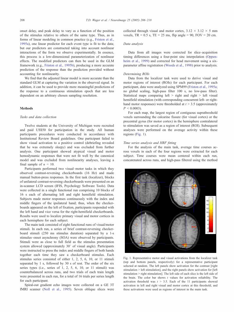
Fig. 1. Representative motor and visual activations from the localizer task
(top and bottom panels, respectively) for a representative participant
selected at random. The left panels show activation for the contrast [right
stimulation N left stimulation], and the right panels show activation for [left
stimulation N right stimulation]. The left side of each slice is the left side of
the brain. The color bar shows t values for activation reliability. The
activation threshold was t N 3.5. Each of the 11 participants showed
activation in left and right visual and motor cortex at this threshold, and
these activations were used as regions of interest in the main task.
Methods
Tasks and data collection
Twelve students at the University of Michigan were recruited
and paid US$50 for participation in the study. All human
participants procedures were conducted in accordance with
Institutional Review Board guidelines. One participant failed to
show visual activation to a positive control (debriefing revealed
that he was extremely sleepy) and was excluded from further
analysis. One participant showed atypical visual and motor
hemodynamic responses that were not fit well by the canonical
model and was excluded from nonlinearity analyses, leaving a
final sample of n = 10.
Participants performed two visual–motor tasks in which they
observed contrast-reversing checkerboards (16 Hz) and made
manual button-press responses. In the first task (localizer), blocks
of unilateral contrast-reversing checkerboards were presented on an
in-scanner LCD screen (IFIS, Psychology Software Tools). Data
were collected in a single functional run comprising 10 blocks of
16 s each of alternating left and right hemifield stimulation.
Subjects made motor responses continuously with the index and
middle fingers of the ipsilateral hand; thus, when the checker-
boards appeared on the left of fixation, participants responded with
the left hand and vice versa for the right-hemifield checkerboards.
Results were used to localize primary visual and motor cortices in
each hemisphere for each subject.
The main task consisted of eight functional runs of visual/motor
stimuli. In each run, a series of brief contrast-reversing checker-
board stimuli (250 ms stimulus duration) separated by a 1-s
stimulus–onset asynchrony (SOA) were observed by participants.
Stimuli were as close to full field as the stimulus presentation
system allowed (approximately 308 of visual angle). Participants
were instructed to press the index and middle fingers of both hands
together each time they saw a checkerboard stimulus. Each
stimulus series consisted of either 1, 2, 5, 6, 10, or 11 stimuli
separated by 1 s, followed by 30 s of rest. The order of the six
series types (i.e., series of 1, 2, 5, 6, 10, or 11 stimuli) was
counterbalanced across runs, and two trials of each train length
were presented in each run, for a total of 16 trials per series length
for each participant.
Spiral-out gradient echo images were collected on a GE 3T
fMRI scanner (Noll et al., 1995). Seven oblique slices were
collected through visual and motor cortex, 3.12 � 3.12 � 5 mm
voxels, TR = 0.5 s, TE = 25 ms, flip angle = 90, FOV = 20 cm.
Data analysis
Data from all images were corrected for slice–acquisition
timing differences using a four-point sinc interpolation (Oppen-
heim et al., 1999) and corrected for head movement using a six-
parameter affine registration (Woods et al., 1998) prior to analysis.
Determining ROIs
Data from the localizer task were used to derive visual and
motor regions of interest (ROIs) for each participant. For each
participant, data were analyzed using SPM99 (Friston et al., 1995a;
no global scaling, high-pass filter 100 s, no low-pass filter).
Statistical maps comparing left N right and right N left visual
hemifield stimulation (with corresponding concurrent left- or right-
hand motor responses) were thresholded at t N 3.5 (approximately
P b 0.0003).
For each map, the largest region of contiguous suprathreshold
voxels surrounding the calcarine fissure (for visual cortex) or the
precentral gyrus (for motor cortex) in the hemisphere contralateral
to stimulation was saved as a region of interest (ROI). Subsequent
analyses were performed on the average activity within these
regions (Fig. 1).
Time series analysis and HRF fitting
For the analysis of the main task, average time courses acQ
ross voxels in each of the four regions were extracted for each
subject. Time courses were mean centered within each run,
concatenated across runs, and high-pass filtered using the method

T.D. Wager et al. / NeuroImage 25 (2005) 206–218 209
of SPM99 at 0.0118 Hz (85 s). Individual observations were
excluded that were more than three standard deviations from the
mean of the filtered time series. Activity was averaged across
trials of each series type, omitting outlier values casewise, for
each ROI (Fig. 2).
To compare series of different lengths, difference waveforms
for three comparisons—2 stimulations vs. 1, 6 vs. 5, and 11 vs.
10—were calculated. These difference waveforms represent the
residual signal of the 2nd, 6th, and 11th stimulus in the sequence.
A canonical hemodynamic response function (implemented in
SPM, http://www.fil.ion.ucl.ac.uk/spm/ (Friston et al., 1995b), with
free parameters for magnitude (height), onset delay, and time to
peak, was fit to the difference waveforms for each pair of
conditions to determine the residual magnitude, onset delay, and
peak delay of the response to the nth stimulus (i.e., 2nd, 6th, or
11th). Fitting was performed with the Levenberg–Marquardt
method (Press et al., 1992; Miezin et al., 2000).
The resulting parameter values for height, onset time, and peak
delay were averaged across subjects to obtain group estimates for
each ROI. These parameter estimates varied as a function of the
position of the stimulus in the series, indicating that height, onset
time, and peak delay are nonlinear with respect to stimulation
history. HRF parameter estimates for each condition within
participant were analyzed using factorial repeated measures
Fig. 2. BOLD responses averaged across trials and participants for each region of
solid or dashed lines, respectively, and the difference between these waveforms w
responses to the 6th and 11th stimulus in a series were estimated by subtractin
respectively. Subtractions were performed on individual trial-averaged data, and the
nonlinearity (e.g., a brandom effectsQ analysis). The high-frequency noise observab
related pulsatility that would be aliased into the task frequency at longer TRs.
ANOVA, with functional region (visual vs. motor), hemisphere
(left vs. right), and stimulus position in series (1st, 2nd, 6th, or
11th) as factors.
We chose to approximate the form of these nonlinearities
across regions using a biexponential model, which provides a
canonical, mathematical description of the nonlinearity (one can
think of this as choosing an exponential basis set to describe the
nonlinear behavior in height, onset, and peak delay of the HRF).
Thus, a biexponential function was fit to the average extracted
parameter estimates across participants and brain regions (Fig.
4B), using a standard nonlinear least squares algorithm (lsqcur-
vefit.m) in Matlab 6.1. The function was of the form:
y ¼ Ae�ax þ Be�bx ð1Þ
with free parameters A and a, B and b describing the scaling
(allowed to be positive or negative) and exponent of two
exponential curves. The fitted biexponential curve describes the
nonlinear change in BOLD magnitude, onset time, and peak
delay as a function of stimulation history.
We found that a biexponential model was necessary to fit the
data, as onset and time to peak parameters varied nonmonotonically
with stimulus history; a single exponential model is always
monotonic and is therefore inadequate. Although a monoexponen-
interest. Responses to series of one or two visual stimuli are shown in red
as used to estimate the residual response to the second stimulus. Residual
g the solid from the dashed green (sixth) and blue waveforms (eleventh),
error across participants was used as the error term in statistical analyses of
le in the waveforms is centered around 1 Hz and is likely due to heartbeat-

Fig. 3. Effects of varying predicted hemodynamic response (HRF) height
(top panel), time to onset (middle panel), and time to peak (bottom panel) of
the canonical SPM99 HRF. An HRF with these three free parameters was fit
to trial-averaged data using nonlinear least squares. Starting estimates are
the default SPM99 values, shown in blue. Time to onset and time to peak
are not orthogonal, but together they capture much of the observed
variability in HRF latency and width. Fits with more free parameters (e.g.,
dispersion, height-to-undershoot ratio) were obtained, but they contributed
T.D. Wager et al. / NeuroImage 25 (2005) 206–218210
tial curve might be adequate for the height parameter, we were
concerned with accurately predicting the form of the response rather
than fitting the simplest possible model, so the biexponential model
is a better choice. Two advantages of the biexponential are that it
provides both a good fit to the data and reasonable values if
extrapolated beyond the range of data collected. The fits asymptote
at 0 or some constant value as stimulus position approaches infinity.
This property is physiologically plausible: the effects of stimulus
position in the series will become negligible as the physiological
system evolves toward steady state. That is, if there have been no
recent stimuli, a stimulus will affect BOLD responses to successive
ones, but if stimulation has been occurring for a long time (e.g., 1
min), one additional second of stimulation will have little effect on
ensuing BOLD responses. (This simplification, however, may cause
the model to underestimate the BOLD response with such long
stimulation times; thus, the model is most useful for event-related
designs and shorter epochs.) For time to peak, the model was fit to
centered data and the mean time to peak was added as a constant to
the equation; thus, the time to peak approaches the canonical HRF
value as the system approaches steady state (Fig. 3).
Comparison of nonlinear with linear model and balloon model
To compare the impact of observed nonlinearities on model
fits, we used a modified linear convolution that takes into account
stimulation history. The linear regressors of this model were
constructed by adjusting the height, time to onset, and time to
peak of the predicted HRF for each stimulus using the equations
produced by the biexponential fitting (see Results). We compare
this dadjustedT linear model against two benchmarks, the standard
linear model and the predicted response of the balloon model
(Buxton et al., 1998; Friston et al., 2000; Figs. 5 and 6), as well as
the standard linear model in terms of their mean squared error
(MSE). The balloon model was fit to the aggregate data using a
nonlinear least squares algorithm in Matlab (Mathworks Inc.,
Natick MA). The blood flow response amplitude, duration, and
delay were designated as free parameters of the model, in addition
to a blood volume hysteresis parameter and a BOLD response
amplitude parameter.
little additional explanatory power and are not further reported.Results
Visual and motor activation
In the blocked localizer run, all subjects showed activity in
discrete regions of visual cortex (around the calcarine fissure) and
motor cortex (in the precentral sulcus/gyrus) at the threshold of t N
3.5. As expected, right hemisphere activations were produced by
the left N right stimulation comparison, and vice versa for left
hemisphere activations. These four regions (right and left visual
and motor regions) were used as ROIs in the event-related analysis.
The average responses in each region for each trial type, a
stimulus series of either 1, 2, 5, 6, 10, or 11 stimuli, across trials
and participants are shown in Fig. 2. In the figure, solid lines show
responses for trains of 1, 5, and 10 stimuli. Dashed lines show
responses for 2, 6, and 11 stimuli.
Estimates of nonlinearity
Results for ANOVA on response magnitudes showed that the
first stimulus produced the largest response, with each successive
stimulus position tested producing a smaller activation. Percent
signal changes were 0.66%, 0.44%, 0.33%, and 0.20% for the
1st, 2nd, 6th, and 11th events. The main effects of stimulus
position (F = 11.73, MSE = 2.02, P b 0.001 with Huynh–Feldt
correction for nonsphericity) and linear trend in stimulus position
(F = 31.27, MSE = 5.04, P b 0.001) were significant. Due to
the unequal intervals chosen for stimulus position (1st, 2nd, 6th,
and 11th), the linear trend actually signifies a nonlinear (e.g.,
exponential) decrease in response magnitude as a function of
prior stimulation history. The trend could equivalently be
interpreted as larger than expected activation for brief events
(Birn et al., 2001), but we prefer to frame the effects in terms of
smaller activations for repeated events (response saturation),
reflecting an underlying neural and/or vascular hysteresis
(Buxton and Frank, 1997; Vazquez and Noll, 1998).
No other main effects or interactions were significant (max F
across all other effects = 2.03, P = 0.18), with the exception of
quadratic trends in the region � stimulus position (F = 3.84, P =
0.07) and hemisphere � stimulus position (F = 4.04, P = 0.06)
interactions. These effects suggest that in visual cortex, the
response decreased more than in motor cortex for the second
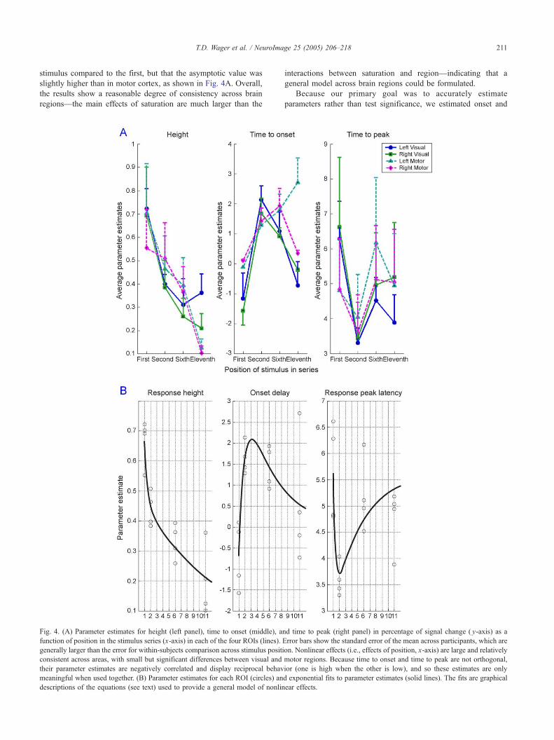
T.D. Wager et al. / NeuroImage 25 (2005) 206–218 211
stimulus compared to the first, but that the asymptotic value was
slightly higher than in motor cortex, as shown in Fig. 4A. Overall,
the results show a reasonable degree of consistency across brain
regions—the main effects of saturation are much larger than the
Fig. 4. (A) Parameter estimates for height (left panel), time to onset (middle), a
function of position in the stimulus series (x-axis) in each of the four ROIs (lines).
generally larger than the error for within-subjects comparison across stimulus positi
consistent across areas, with small but significant differences between visual and
their parameter estimates are negatively correlated and display reciprocal behav
meaningful when used together. (B) Parameter estimates for each ROI (circles) an
descriptions of the equations (see text) used to provide a general model of nonlin
interactions between saturation and region—indicating that a
general model across brain regions could be formulated.
Because our primary goal was to accurately estimate
parameters rather than test significance, we estimated onset and
nd time to peak (right panel) in percentage of signal change ( y-axis) as a
Error bars show the standard error of the mean across participants, which are
on. Nonlinear effects (i.e., effects of position, x-axis) are large and relatively
motor regions. Because time to onset and time to peak are not orthogonal,
ior (one is high when the other is low), and so these estimates are only
d exponential fits to parameter estimates (solid lines). The fits are graphical
ear effects.
T.D. Wager et al. / NeuroImage 25 (2005) 206–218212
peak delay parameters only for conditions within participants
showing significant activation to the nth stimulus (e.g., 6 vs. 5
stimuli produces a positive BOLD activation), on the basis that
estimating response delay is not meaningful if there is no
significant activation. The delay parameters that could be mean-
ingfully estimated were used in prediction, and mean values for
onset and peak delay are shown in Fig. 4A. The resulting missing
values in the data set made ANOVA analysis of delay difficult, as
there were not enough cases (10 subjects) with valid latency
estimates for all conditions (4) in all regions (4), which may cause
overestimation of the degrees of freedom. However, for com-
pleteness, we report ANOVA results here with missing values
replaced with across-subjects means.
ANOVA results for onset delay showed a later onset delay for
motor regions than visual ones, as expected (F = 6.51, MSE =
5.66, P b 0.03), a nonmonotonic effect is stimulus position (F =
4.79, MSE = 10.23, P b 0.01), and an interaction between visual/
motor region, hemisphere, and stimulus position (F = 4.86, MSE =
2.70, P b 0.03) caused by the late onset for left motor cortex after
prolonged stimulation (Fig. 4A, center panel). No other effects
were significant. Results for time-to-peak showed a significant
interaction between visual/motor and hemisphere (F = 7.69, MSE =
1.14, P = 0.02), with later time-to-peak for motor than visual
regions only in the left hemisphere. No other effects were
significant, although the effect of stimulus position showed a trend
(F = 2.75, P = 0.06). The nonmonotonic effects of delay and time-
to-peak in opposite directions suggests that the effects may be
related to collinearity between the regression parameters for onset
delay and time to peak. Thus, fitted responses for later stimuli in a
sequence tend to begin later and rise slightly faster, but the result is
little overall change in the delay of the response.
Equations for predicted nonlinearity
Biexponential fits to the nonlinearity estimates are shown in
Fig. 4B. Three equations were derived that predict relative BOLD
magnitude, onset delay, and peak delay as a function of stimulation
history (of repeated brief 1 s stimulations). All of these equations
give parameter values as a function of the stimulus position in a
sequence of stimuli, and they are given below:
m ¼ 1:7141e�2:1038x þ 0:4932e�0:0770x ð2Þ
d ¼ � 13:4097e�1:0746x þ 4:8733e�0:1979x ð3Þ
p ¼ 37:5445e�2:6760x � 3:2046e�0:2120x þ 5:6344 ð4Þ
where m is the stimulus magnitude, as a proportion of the
canonical HRF height with no stimulation history, d is the onset
delay of the canonical SPM99 HRF in s, and p is the time to peak
of the BOLD response in s. These equations constitute the core of
our predictive model, and we use these equations to perform a
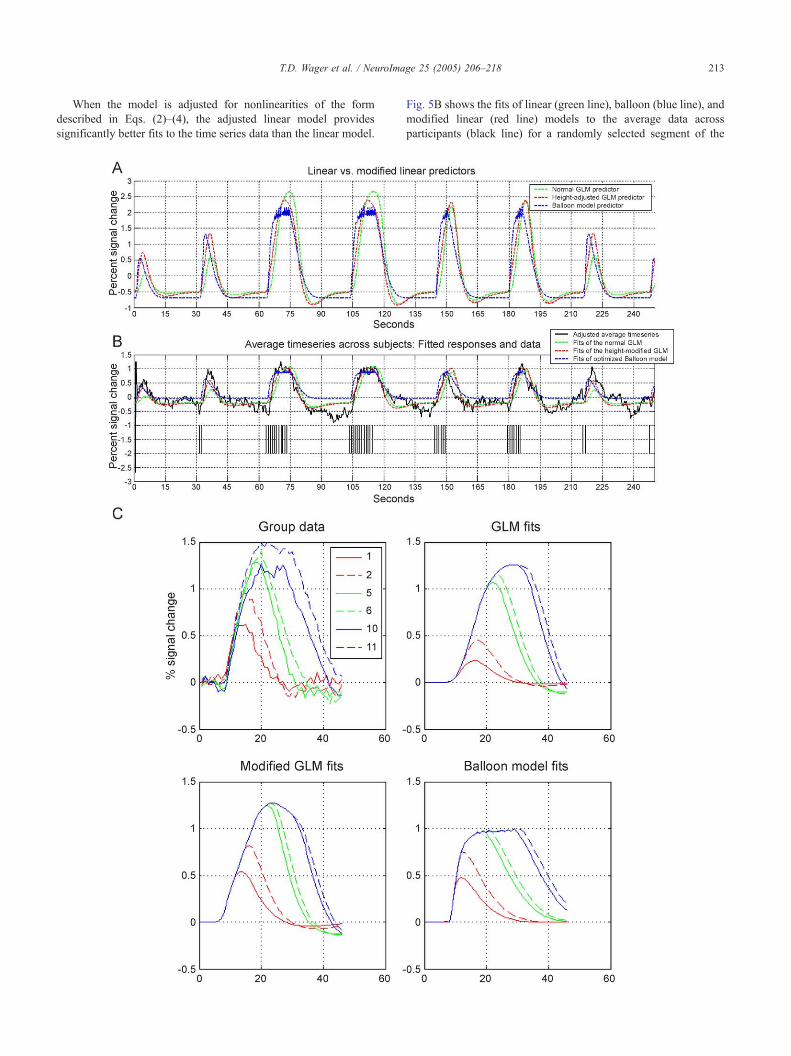
Fig. 5. (A) Predicted responses to stimulation in the first 4 min of the main exp
nonlinearity estimates (red), and the balloon model (blue). Deflections show the
in that order. Of interest is the relative magnitude of the responses to stimulati
(black line) for the three models to the same series as in A. Vertical black lines
response to brief trains (one or two stimuli) because the relative heights of shor
and balloon fits are more accurate. (C) Panels show the group average data (t
particular series length, as in Fig. 2. The length of each series is shown in the le
trains of stimuli.
modified convolution of the stimulus sequence as a function of
prior stimuli that have recently occurred. The full form of the
hemodynamic response, which assumes the shape of the difference
of two gamma functions using modified shape (p) and offset (d)
parameters, is:
f tð Þ ¼ m xð Þ
max
�t�d xð Þð Þp xð Þ�1
e�ktRl
0tp xð Þ�1e�kdt
�
� t � d xð Þð Þp xð Þ�1
e�ktRl0tp xð Þ�1e�kdt
� 1
6
t � d xð Þð Þ15e�ktRl
0t15d�kdt
!!ð5Þ
where t is the time following stimulus onset at some arbitrary divisor
of the TR (e.g., 16 samples per TR); x is the position in the stimulus
sequence (e.g., 1 is the first time a stimulus occurs in a given time
frame); and k is a constant scaling parameter equal to the TR / the
sampling resolution. The first term is a scaling parameter for the
magnitude of the response. The second term describes the gamma
function for the positive BOLD response, normalized by its integral,
minus the gamma function describing the undershoot (scaled to 1/6
the height of the positive response and also normalized).
This function is identical to that implemented in SPM in
spm_hrf.m, with p as the first input parameter and d as the sixth,
except that the gamma shape and offset parameters d and p are
allowed to vary nonlinearly as a function of x. An implementation
that uses the nonlinearity parameters described here is available
from the authors (see author note).
Note that the magnitude parameter (m) asymptotes at 0 for large
x. Therefore, our approximations predict a zero response magnitude
for long blocks of stimulation. Because of this, and because the
frequency of neural responses is unknown for blocks of continuous
stimulation, these equations may not be appropriate for modeling
long block designs (e.g., N30 consecutive stimuli).
Modified linear compared with linear and balloon model
predictors
Fig. 5A shows the predicted responses for three models: the
linear (green line), balloon (blue line), and modified linear (using
Eqs. (2)–(4); red line). The critical difference between the linear
and other models is the relative predicted response magnitude of
short stimulus trains (e.g., one or two stimuli followed by rest)
compared with long trains (e.g., 10 or 11 stimuli). The linear model
predicts that the relative height of these will differ by a factor of
approximately 4.6. After adjusting for observed nonlinearities
using the equations (red line), the relative predicted height differs
by a factor of approximately 2.3. The balloon and modified linear
models agree closely, although the rise time for the balloon model
is somewhat faster.
eriment for the linear model (green), the modified linear model using our
predicted responses to series of 1, 2, 11, 10, 6, 5, 2, and 1 visual stimulus,
on series of different lengths. (B) Model fits to the group-averaged data
below the fits show the stimulation onsets. The linear model underfits the
t and long trains are not captured well by the linear model. Both adjusted
op left) and model fits (remaining panels) averaged over all stimuli of a
gend. The GLM predictors (top right) underestimate the response to short
T.D. Wager et al. / NeuroImage 25 (2005) 206–218 213
When the model is adjusted for nonlinearities of the form
described in Eqs. (2)–(4), the adjusted linear model provides
significantly better fits to the time series data than the linear model.
Fig. 5B shows the fits of linear (green line), balloon (blue line), and
modified linear (red line) models to the average data across
participants (black line) for a randomly selected segment of the
T.D. Wager et al. / NeuroImage 25 (2005) 206–218214
data. Fig. 5C shows the average data across regions (top left panel)
and the fits for the GLM (top right), modified GLM (bottom left),
and balloon model (bottom right), averaged over series of each
length. The figures illustrate that the ordinary GLM fit underfits the
response to short series (one- and two-stimulus sequences). We
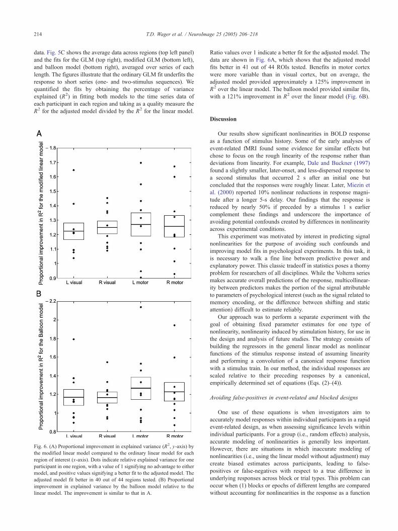
quantified the fits by obtaining the percentage of variance
explained (R2) in fitting both models to the time series data of
each participant in each region and taking as a quality measure the
R2 for the adjusted model divided by the R2 for the linear model.
Fig. 6. (A) Proportional improvement in explained variance (R2, y-axis) by
the modified linear model compared to the ordinary linear model for each
region of interest (x-axis). Dots indicate relative explained variance for one
participant in one region, with a value of 1 signifying no advantage to either
model, and positive values signifying a better fit to the adjusted model. The
adjusted model fit better in 40 out of 44 regions tested. (B) Proportional
improvement in explained variance by the balloon model relative to the
linear model. The improvement is similar to that in A.
Ratio values over 1 indicate a better fit for the adjusted model. The
data are shown in Fig. 6A, which shows that the adjusted model
fits better in 41 out of 44 ROIs tested. Benefits in motor cortex
were more variable than in visual cortex, but on average, the
adjusted model provided approximately a 125% improvement in
R2 over the linear model. The balloon model provided similar fits,
with a 121% improvement in R2 over the linear model (Fig. 6B).
Discussion
Our results show significant nonlinearities in BOLD response
as a function of stimulus history. Some of the early analyses of
event-related fMRI found some evidence for similar effects but
chose to focus on the rough linearity of the response rather than
deviations from linearity. For example, Dale and Buckner (1997)
found a slightly smaller, later-onset, and less-dispersed response to
a second stimulus that occurred 2 s after an initial one but
concluded that the responses were roughly linear. Later, Miezin et
al. (2000) reported 10% nonlinear reductions in response magni-
tude after a longer 5-s delay. Our findings that the response is
reduced by nearly 50% if preceded by a stimulus 1 s earlier
complement these findings and underscore the importance of
avoiding potential confounds created by differences in nonlinearity
across experimental conditions.
This experiment was motivated by interest in predicting signal
nonlinearities for the purpose of avoiding such confounds and
improving model fits in psychological experiments. In this task, it
is necessary to walk a fine line between predictive power and
explanatory power. This classic tradeoff in statistics poses a thorny
problem for researchers of all disciplines. While the Volterra series
makes accurate overall predictions of the response, multicollinear-
ity between predictors makes the portion of the signal attributable
to parameters of psychological interest (such as the signal related to
memory encoding, or the difference between shifting and static
attention) difficult to estimate reliably.
Our approach was to perform a separate experiment with the
goal of obtaining fixed parameter estimates for one type of
nonlinearity, nonlinearity induced by stimulation history, for use in
the design and analysis of future studies. The strategy consists of
building the regressors in the general linear model as nonlinear
functions of the stimulus response instead of assuming linearity
and performing a convolution of a canonical response function
with a stimulus train. In our method, the individual responses are
scaled relative to their preceding responses by a canonical,
empirically determined set of equations (Eqs. (2)–(4)).
Avoiding false-positives in event-related and blocked designs
One use of these equations is when investigators aim to
accurately model responses within individual participants in a rapid
event-related design, as when assessing significance levels within
individual participants. For a group (i.e., random effects) analysis,
accurate modeling of nonlinearities is generally less important.
However, there are situations in which inaccurate modeling of
nonlinearities (i.e., using the linear model without adjustment) may
create biased estimates across participants, leading to false-
positives or false-negatives with respect to a true difference in
underlying responses across block or trial types. This problem can
occur when (1) blocks or epochs of different lengths are compared
without accounting for nonlinearities in the response as a function

T.D. Wager et al. / NeuroImage 25 (2005) 206–218 215
of stimulation length, or (2) when events are compared that differ
in their densities or frequencies of occurrence (if events can occur
closer than 2–3 s apart). The following is an example to illustrate a
problematic block design. Fig. 7 shows the simulated response to a
block design with unequal block durations without taking non-
linearity into account. The btrue data,Q shown in black, is based on
the canonical SPM HRF modified using our nonlinearity estimates
(Eqs. (2)–(4)). The blue lines are the linear model predictors. The
bneural responseQ underlying both conditions is exactly the same, a
unit response every 0.5 s, evenly distributed across both block
types. Because the blocks for two conditions to be compared (A
and B) are of unequal lengths (10 and 20 s), the predicted height
for the longer block is of greater magnitude than the shorter one.
When the linear model is fit to the data, it finds a difference in
bactivityQ between conditions A and B (panel 3), corresponding to
beta values of 0.30 and 0.25 for A and B. However, this difference
is not related to underlying neural activity in A vs. B but rather to
inaccuracies in the relative scaling of the two predictors in a model
that does not account for stimulation history effects.
This principle also extends to event-related (ER) designs that
compare different trial types. In a rapid ER design, events of
various types are presented in random or pseudo-random order, and
temporal stochasticity is often introduced into the design. These
properties produce designs that have groups of uneven numbers of
events closely spaced in time. If the trial types differ in their
density with respect to time, nonlinear saturation will also differ,
and the same neuronal activity to each trial type may translate into
different estimates of BOLD response magnitude. At best, the
residual error in the model fit will increase. At worst, if the event
spacing (and thus the magnitude of nonlinear interactions) differs
among event types, analysis may yield false-positive results.
Sources of nonlinearity and prediction of BOLD response
Nonlinearity in BOLD responses can come from a number of
sources. At the single neuron level, the firing in response to
stimulation varies over time and is usually not a linear or time-
invariant function of the stimulus intensity (e.g., Logothetis, 2003).
At short (within stimulus) or long (across minutes or days) time
delays, habituation and sensitization of neurons to particular
stimuli often occur (Kileny et al., 1980; Logothetis, 2002; Wilson
et al., 1984). From a psychological point of view, the response to a
stimulus can vary based on a number of adaptive mechanisms that
result in a nonlinear neuronal firing pattern, including the
development of a strategy, learning new information, and changes
in attention or alertness during the task (Raichle et al., 1994).
Even in the case of near-linear neuronal responses, the vascular
response is clearly nonlinear, an effect attributed to the viscoelastic
properties of the blood vessels. Several groups have contributedwith
theoretical models of nonlinearity based on auxiliary measurements
of blood flow, oxygen saturation, and other parameters (Buxton and
Frank, 1997; Buxton et al., 1998; Mandeville et al., 1999; Vazquez
and Noll, 1998). Perhaps the most popular model is the one
presented by Buxton et al. (1998), in which the response is
characterized as a function of the oxyhemoglobin quantity in the
vessels. The vessels’ elastic properties allow their diameter to
increase up to a point when there is blood flow surge, like the one
expected following neuronal activation, and slowly return to their
original size afterward. When two stimuli are presented close
together, the vessels’ diameter is still dilated close to it maximum
capacity by the time the second stimulus is presented, and thus the
response to the second stimulus is smaller and has a slightly different
shape. This effect was included in the estimation of the balloon
model parameters where it is directly related to the poststimulus
undershoot. However, the estimation routine did not predict a strong
poststimulus undershoot (Fig. 5). While the balloon model explains
some of the nonlinearity in the data (as shown in Fig. 5), it is also
evident that there remains residual nonlinearities not explained by
this venous volume effect and likely to represent nonlinearities at the
metabolic and/or neuronal level.
A simple model of canonical nonlinearity
Nonlinearity in BOLD responses can come from a number of
sources: neural, vascular, psychophysical, and psychological (e.g.,
Kileny et al., 1980; Logothetis, 2002, 2003; Raichle et al., 1994;
Wilson et al., 1984). Whatever the source of nonlinearities,
however, if the goal is accurate prediction of the BOLD response,
it is only necessary to measure the end product of nonlinear
physiological effects on the BOLD response itself. This consid-
eration has motivated the Volterra series formulation of Friston et
al. (1998, 2000), which dlinearizesT sequence effects into a
number of linear predictors, and produces very accurate model
fits to data, at the cost of statistical power of the overall model,
and in particular, the psychological parameters of interest.
Calculating nonlinear effects using our model is computationally
efficient, and they can be easily incorporated into the linear
modeling framework without using up additional degrees of
freedom in the model.
Limitations of the current study
Several studies have pointed out that nonlinear effects may differ
among brain regions (Birn et al., 2001; Huettel and McCarthy,
2001). We also found some such effects, with small but consistent
differences in nonlinear saturation between visual and motor
regions. Using an overall average estimate of nonlinear effects
prospectively, as we suggest here, is most meaningful if those
nonlinearities do not vary with brain region. We find that the overall
saturation effects occur in approximately the same form, and these
overall effects are several times larger than the saturation � region
interactions; thus, we suggest that using the canonical estimates for
nonlinear responses we propose may provide a reasonable first-
order approximation to estimating nonlinearities. However, the
model will provide a poorer fit to brain regions that exhibit
noncanonical saturation effects.
The situation is analogous to the difficulties posed by using a
canonical estimate of the HRF at all (e.g., Friston et al., 1995a),
although this has become common practice in many laboratories.
The shape of the hemodynamic response itself is not consistent
throughout the brain (Marrelec et al., 2003; Rajapakse et al., 1998),
but the canonical form provides a first-order approximation. We
provide a bcanonicalQ first-order estimate for nonlinear effects.
While nonlinearities surely differ to some degree across brain
regions, we hope to provide an average starting point that will
reasonably approximate nonlinear effects.
An alternative, or complementary, approach might be to add
predictors that represent stimulation history to the design matrix
and thus fit a parameter for magnitude � history effects in each
brain voxel (this is a simplification of the full Volterra approach).
The current estimates could complement this approach if they are
used as priors in a Baysian model estimation framework (e.g.,
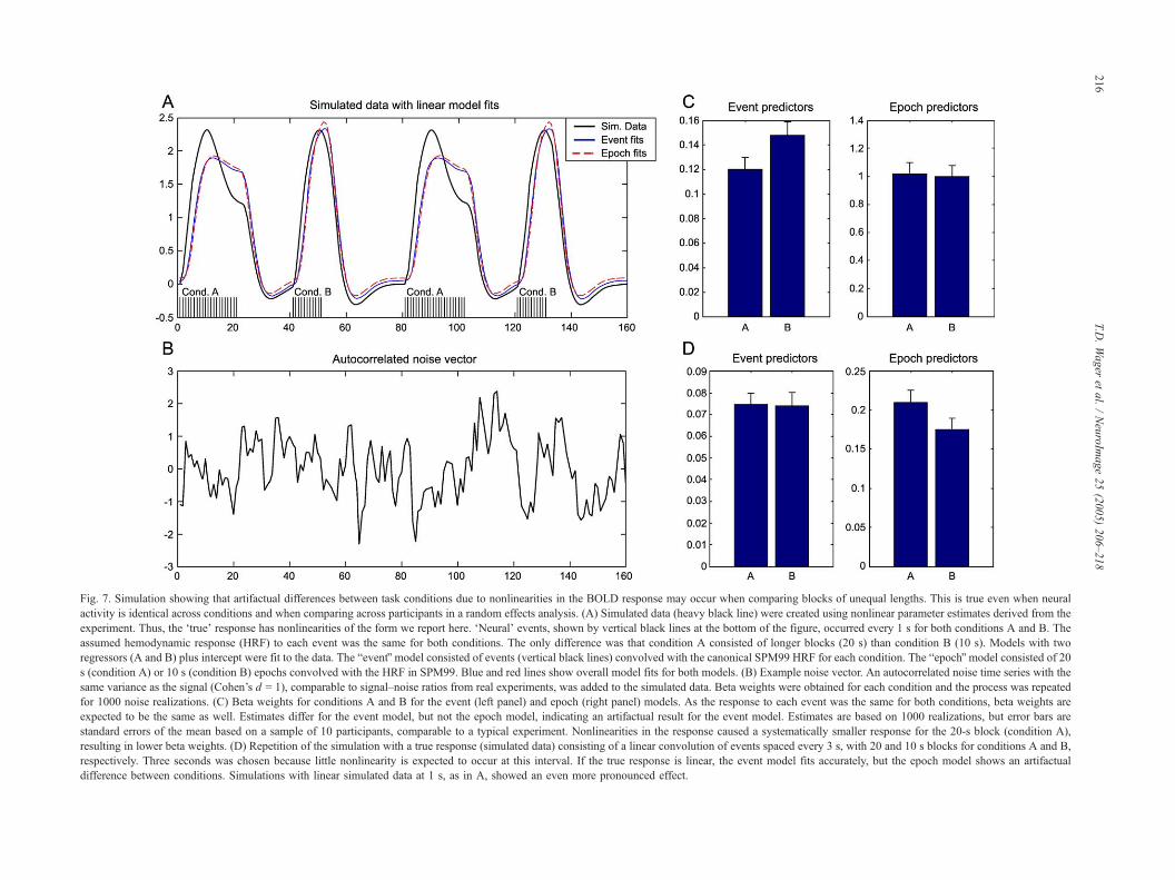
Fig. 7. Simulation showing that artifactual differences between task conditions due to nonlinearities in the BOLD response may occur when comparing blocks of unequal lengths. This is true even when neural
activity is identical across conditions and when comparing across participants in a random effects analysis. (A) Simulated data (heavy black line) were created using nonlinear parameter estimates derived from the
experiment. Thus, the dtrueT response has nonlinearities of the form we report here. dNeuralT events, shown by vertical black lines at the bottom of the figure, occurred every 1 s for both conditions A and B. The
assumed hemodynamic response (HRF) to each event was the same for both conditions. The only difference was that condition A consisted of longer blocks (20 s) than condition B (10 s). Models with two
regressors (A and B) plus intercept were fit to the data. The beventQ model consisted of events (vertical black lines) convolved with the canonical SPM99 HRF for each condition. The bepochQ model consisted of 20
s (condition A) or 10 s (condition B) epochs convolved with the HRF in SPM99. Blue and red lines show overall model fits for both models. (B) Example noise vector. An autocorrelated noise time series with the
same variance as the signal (Cohen’s d = 1), comparable to signal–noise ratios from real experiments, was added to the simulated data. Beta weights were obtained for each condition and the process was repeated
for 1000 noise realizations. (C) Beta weights for conditions A and B for the event (left panel) and epoch (right panel) models. As the response to each event was the same for both conditions, beta weights are
expected to be the same as well. Estimates differ for the event model, but not the epoch model, indicating an artifactual result for the event model. Estimates are based on 1000 realizations, but error bars are
standard errors of the mean based on a sample of 10 participants, comparable to a typical experiment. Nonlinearities in the response caused a systematically smaller response for the 20-s block (condition A),
resulting in lower beta weights. (D) Repetition of the simulation with a true response (simulated data) consisting of a linear convolution of events spaced every 3 s, with 20 and 10 s blocks for conditions A and B,
respectively. Three seconds was chosen because little nonlinearity is expected to occur at this interval. If the true response is linear, the event model fits accurately, but the epoch model shows an artifactual
difference between conditions. Simulations with linear simulated data at 1 s, as in A, showed an even more pronounced effect.
T.D.Wager
etal./NeuroIm
age25(2005)206–218
216

T.D. Wager et al. / NeuroImage 25 (2005) 206–218 217
Friston and Penny, 2003; Penny et al., 2003; Smith et al., 2003;
Woolrich et al., 2004).
Another limitation of the study is that nonlinear effects were
estimated using an ISI of 1 s throughout the experiment, which is
suitable for fast ER designs with interstimulus intervals around this
length. For example, average response times are near 1 s for many
cognitive tasks. This poses a serious limitation, however, as we
cannot provide quantitative estimates of nonlinearity at other delay
times (e.g., 3–4 s typical of many event-related paradigms). The
problem can be approximately solved by assuming a linear or
exponential decrease in nonlinear saturation with increasing ISI, as
the response is known to be very near linear at ISIs of greater than
5 s (Miezin et al., 2000).
Acknowledgments
We would like to thank John Jonides and Tom Nichols for
helpful discussions and comments on the experiment. This
research was supported by grant MH60655 to the University of
Michigan (John Jonides, P.I.). Software implementing the
modified convolution and nonlinearity equations is available
from http://www.columbia.edu/cu/psychology/tor/ or by e-mailing
References
Birn, R.M., Saad, Z.S., Bandettini, P.A., 2001. Spatial heterogeneity of the
nonlinear dynamics in the FMRI BOLD response. NeuroImage 14 (4),
817–826.
Birn, R.M., Cox, R.W., Bandettini, P.A., 2002. Detection versus estimation
in event-related fMRI: choosing the optimal stimulus timing. Neuro-
Image 15 (1), 252–264.
Boynton, G.M., Engel, S.A., Glover, G.H., Heeger, D.J., 1996. Linear
systems analysis of functional magnetic resonance imaging in human
V1. J. Neurosci. 16 (13), 4207–4221.
Buckner, R.L., 1998. Event-related fMRI and the hemodynamic response.
Hum. Brain Mapp. 6 (5–6), 373–377.
Burock, M.A., Buckner, R.L., Woldorff, M.G., Rosen, B.R., Dale, A.M.,
1998. Randomized event-related experimental designs allow for
extremely rapid presentation rates using functional MRI. NeuroReport
9 (16), 3735–3739.
Buxton, R.B., Frank, L.R., 1997. A model for the coupling between
cerebral blood flow and oxygen metabolism during neural stimulation.
J. Cereb. Blood Flow Metab. 17 (1), 64–72.
Buxton, R.B., Wong, E.C., Frank, L.R., 1998. Dynamics of blood flow and
oxygenation changes during brain activation: the balloon model. Magn.
Reson. Med. 39 (6), 855–864.
Cohen, M.S., 1997. Parametric analysis of fMRI data using linear systems
methods. NeuroImage 6 (2), 93–103.
D’Esposito, M., Postle, B.R., Jonides, J., Smith, E.E., 1999. The neural
substrate and temporal dynamics of interference effects in working
memory as revealed by event-related functional MRI. Proc. Natl. Acad.
Sci. U. S. A. 96 (13), 7514–7519.
Dale, A.M., Buckner, R.L., 1997. Selective averaging of rapidly presented
individual trials using fMRI. Hum. Brain Mapp. 5, 329–340.
Davachi, L., Wagner, A.D., 2002. Hippocampal contributions to episodic
encoding: insights from relational and item-based learning. J. Neuro-
physiol. 88 (2), 982–990.
Friston, K.J., Penny, W., 2003. Posterior probability maps and SPMs.
NeuroImage 19 (3), 1240–1249.
Friston, K.J., Frith, C.D., Turner, R., Frackowiak, R.S., 1995. Character-
izing evoked hemodynamics with fMRI. NeuroImage 2 (2), 157–165.
Friston, K.J., Holmes, A.P., Poline, J.B., Grasby, P.J., Williams, S.C.,
Frackowiak, R.S., et al., 1995. Analysis of fMRI time-series revisited.
NeuroImage 2 (1), 45–53.
Friston, K.J., Josephs, O., Rees, G., Turner, R., 1998. Nonlinear event-
related responses in fMRI. Magn. Reson. Med. 39 (1), 41–52.
Friston, K.J., Mechelli, A., Turner, R., Price, C.J., 2000. Nonlinear
responses in fMRI: the balloon model, Volterra kernels, and other
hemodynamics. NeuroImage 12 (4), 466–477.
Haxby, J.V., Petit, L., Ungerleider, L.G., Courtney, S.M., 2000.
Distinguishing the functional roles of multiple regions in distributed
neural systems for visual working memory. NeuroImage 11 (2),
145–156.
Henson, R.N., Price, C.J., Rugg, M.D., Turner, R., Friston, K.J., 2002.
Detecting latency differences in event-related BOLD responses:
application to words versus nonwords and initial versus repeated face
presentations. NeuroImage 15 (1), 83–97.
Hernandez, L., Wager, T.D., Jonides, J., 2002. Introduction to functional
brain imaging. In: Wixted, J., Pashler, H. (Eds.), Stevens Handbook of
Experimental Psychology, vol. 4. John Wiley and Sons, Inc., New
York, pp. 175–221.
Huettel, S.A., McCarthy, G., 2001. Regional differences in the refractory
period of the hemodynamic response: an event-related fMRI study.
NeuroImage 14 (5), 967–976.
Josephs, O., Henson, R.N., 1999. Event-related functional magnetic
resonance imaging: modelling, inference and optimization. Philos.
Trans. R. Soc. London, B Biol. Sci. 354 (1387), 1215–1228.
Kerns, J.G., Cohen, J.D., MacDonald III, A.W., Cho, R.Y., Stenger, V.A.,
Carter, C.S., 2004. Anterior cingulate conflict monitoring and adjust-
ments in control. Science 303, 1023–1027.
Kileny, P., Ryu, J.H., McCabe, B.F., Abbas, P.J., 1980. Neuronal
habituation in the vestibular nuclei of the cat. Acta Oto-Laryngol. 90
(3–4), 175–183.
Liu, T.T., 2004. Efficiency, power, and entropy in event-related fMRI with
multiple trial types. Part II: design of experiments. NeuroImage 21 (1),
401–413.
Liu, T.T., Frank, L.R., 2004. Efficiency, power, and entropy in event-
related FMRI with multiple trial types. Part I: theory. NeuroImage 21
(1), 387–400.
Liu, T.T., Frank, L.R., Wong, E.C., Buxton, R.B., 2001. Detection power,
estimation efficiency, and predictability in event-related fMRI. Neuro-
Image 13 (4), 759–773.
Logothetis, N.K., 2002. The neural basis of the blood–oxygen-level-
dependent functional magnetic resonance imaging signal. Philos. Trans.
R. Soc. London, B Biol. Sci. 357 (1424), 1003–1037.
Logothetis, N.K., 2003. The underpinnings of the BOLD functional
magnetic resonance imaging signal. J. Neurosci. 23 (10), 3963–3971.
Logothetis, N.K., Pauls, J., Augath, M., Trinath, T., Oeltermann, A., 2001.
Neurophysiological investigation of the basis of the fMRI signal.
Nature 412 (6843), 150–157.
MacDonald III, A.W., Cohen, J.D., Stenger, V.A., Carter, C.S., 2000.
Dissociating the role of the dorsolateral prefrontal and anterior cingulate
cortex in cognitive control. Science 288 (5472), 1835–1838.
Mandeville, J.B., Marota, J.J., Ayata, C., Zaharchuk, G., Moskowitz, M.A.,
Rosen, B.R., et al., 1999. Evidence of a cerebrovascular postarteriole
windkessel with delayed compliance. J. Cereb. Blood Flow Metab. 19
(6), 679–689.
Marrelec, G., Benali, H., Ciuciu, P., Pelegrini-Issac, M., Poline, J.B., 2003.
Robust Bayesian estimation of the hemodynamic response function in
event-related BOLD fMRI using basic physiological information. Hum.
Brain Mapp. 19 (1), 1–17.
Mechelli, A., Price, C.J., Henson, R.N., Friston, K.J., 2003. Estimating
efficiency a priori: a comparison of blocked and randomized designs.
NeuroImage 18 (3), 798–805.
Miezin, F.M., Maccotta, L., Ollinger, J.M., Petersen, S.E., Buckner, R.L.,
2000. Characterizing the hemodynamic response: effects of presentation
rate, sampling procedure, and the possibility of ordering brain activity
based on relative timing. NeuroImage 11 (6 Pt. 1), 735–759.
T.D. Wager et al. / NeuroImage 25 (2005) 206–218218
Noll, D.C., Cohen, J.D., Meyer, C.H., Schneider, W., 1995. Spiral K-space
MR imagingof cortical activation. J.Magn.Reson. Imaging 5 (1), 49–56.
Oppenheim, A.V., Schafer, R.W., Buck, J.R., 1999. Discrete-Time Signal
Processing, 2nd ed. Prentice Hall, Upper Saddle River, NJ.
Penny, W., Kiebel, S., Friston, K., 2003. Variational Bayesian inference for
fMRI time series. NeuroImage 19 (3), 727–741.
Press, W.H., Teukolski, S.A., Vetterling, W.T., Flannery, B.P., 1992.
Numerical Recipes in C: The Art of Scientific Computing. Cambridge
University Press, New York.
Raichle, M.E., Fiez, J.A., Videen, T.O., MacLeod, A.M., Pardo, J.V., Fox,
P.T., et al., 1994. Practice-related changes in human brain functional
anatomy during nonmotor learning. Cereb. Cortex 4 (1), 8–26.
Rajapakse, J.C., Kruggel, F., Maisog, J.M., von Cramon, D.Y., 1998.
Modeling hemodynamic response for analysis of functional MRI time-
series. Hum. Brain Mapp. 6 (4), 283–300.
Smith, M., Putz, B., Auer, D., Fahrmeir, L., 2003. Assessing brain
activity through spatial Bayesian variable selection. NeuroImage 20
(2), 802–815.
Vazquez, A.L., Noll, D.C., 1998. Nonlinear aspects of the BOLD response
in functional MRI. NeuroImage 7 (2), 108–118.
Vazquez, A., Noll, D., 2002. A fluid mechanical approach to modeling
hemodynamics in fMRI. Paper presented at the 10th Annual Mtg. of the
Int. Soc. of Magn. Reson. in Med., Honolulu, HI.
Wager, T.D., Nichols, T.E., 2003. Optimization of experimental design in
fMRI: a general framework using a genetic algorithm. NeuroImage 18
(2), 293–309.
Wagner, A.D., Schacter, D.L., Rotte, M., Koutstaal, W., Maril, A., Dale,
A.M., et al., 1998. Building memories: remembering and forgetting of
verbal experiences as predicted by brain activity. Science 281 (5380),
1188–1191.
Wilson, C.L., Babb, T.L., Halgren, E., Wang, M.L., Crandall, P.H., 1984.
Habituation of human limbic neuronal response to sensory stimulation.
Exp. Neurol. 84 (1), 74–97.
Woods, R.P., Grafton, S.T., Holmes, C.J., Cherry, S.R., Mazziotta, J.C.,
1998. Automated image registration: I. General methods and intra-
subject, intramodality validation. J. Comput. Assist. Tomogr. 22,
141–154.
Woolrich, M.W., Jenkinson, M., Brady, J.M., Smith, S.M., 2004. Fully
Bayesian spatio-temporal modeling of FMRI data. IEEE Trans. Med.
Imag. 23 (2), 213–231.