Behavioral/Cognitive

Quantifying the Microvascular Origin of BOLD-fMRI fromFirst Principles with Two-Photon Microscopy and anOxygen-Sensitive Nanoprobe

Louis Gagnon,1,2 Sava Sakadzic,1 Frederic Lesage,3 Joseph J. Musacchia,1 XJoel Lefebvre3, Qianqian Fang,1

Meryem A. Yucel,1 Karleyton C. Evans,1 Emiri T. Mandeville,1 Julien Cohen-Adad,3 Jonathan R. Polimeni,1

Mohammad A. Yaseen,1 Eng H. Lo,1 Douglas N. Greve,1 Richard B. Buxton,5 Anders M. Dale,4,5 Anna Devor,1,4,5

and David A. Boas1,2

1Athinoula A. Martinos Center for Biomedical Imaging, Department of Radiology, Massachusetts General Hospital, Harvard Medical School, Charlestown,Massachusetts 02129, 2Harvard-MIT Division of Health Sciences and Technology, Cambridge, Massachusetts 02139, 3Department of Electrical Engineering,Ecole Polytechnique de Montreal, Montreal, Quebec, Canada H3C 3A7, and Departments of 4Neurosciences and 5Radiology, UC San Diego, La Jolla,California 92093

The blood oxygenation level-dependent (BOLD) contrast is widely used in functional magnetic resonance imaging (fMRI) studies aimedat investigating neuronal activity. However, the BOLD signal reflects changes in blood volume and oxygenation rather than neuronalactivity per se. Therefore, understanding the transformation of microscopic vascular behavior into macroscopic BOLD signals is at thefoundation of physiologically informed noninvasive neuroimaging. Here, we use oxygen-sensitive two-photon microscopy to measurethe BOLD-relevant microvascular physiology occurring within a typical rodent fMRI voxel and predict the BOLD signal from firstprinciples using those measurements. The predictive power of the approach is illustrated by quantifying variations in the BOLD signalinduced by the morphological folding of the human cortex. This framework is then used to quantify the contribution of individualvascular compartments and other factors to the BOLD signal for different magnet strengths and pulse sequences.

Key words: BOLD-fMRI; modeling; Monte Carlo; two-photon microscopy

IntroductionFunctional magnetic resonance imaging (fMRI)-based on theblood oxygenation level-dependent (BOLD) response (Ogawa etal., 1990; Kwong et al., 1992) has become a widely used tool forexploring brain function, and yet the neurophysiological basis ofthis technique remains poorly understood (Logothetis, 2008;Kim and Ogawa, 2012). The BOLD signal arises from the orches-trated microscopic activity of the underlying neuronal networksbut does not reflect this activity directly (Logothetis, 2008).Rather, the signal measured depends on microscopic magnetic

field perturbations arising from changes in oxygenation andblood volume in the cortical microvasculature (Uludag et al.,2009; Buxton, 2010), which are themselves driven by neurovas-cular coupling (i.e., changes in blood flow and oxygen consump-tion associated with neuronal and glial activity). By itself,understanding neurovascular coupling has been a very active areaof research since the beginning of fMRI (Attwell et al., 2010).Separately, understanding the transformation of microscopicvascular dilation and oxygenation into macroscopic BOLD sig-nals is an important step toward the physiological interpretationof BOLD (Buxton, 2010). Specifically, understanding how indi-vidual vascular compartments are reflected in the BOLD signaland quantifying volume and oxygenation effects individually for dif-ferent pulse sequences and for different magnetic field strengths iscritical for a physiologically informed choice of sequence parame-ters, for the development of new quantitative fMRI methods to mea-sure the cerebral metabolic rate of oxygen (CMRO2), for thedevelopment of high-field fMRI technologies and for the interpreta-tion of neuroimaging data in the context of vascular diseases. Nev-ertheless, achieving these goals has been challenging because of thedifficulty of measuring vessel geometry and blood oxygenation inindividual microvascular compartments during cerebral activation.Typically, these quantities are rather assumed, which significantlyreduces our accuracy to compute the individual contributions men-tioned above (Buxton, 2010).

Received Aug. 25, 2014; revised Dec. 26, 2014; accepted Jan. 14, 2015.Author contributions: L.G., S.S., F.L., Q.F., K.C.E., E.H.L., R.B.B., A.M.D., A.D., and D.A.B. designed research; L.G.,

S.S., F.L., Q.F., K.C.E., E.T.M., J.C.-A., J.R.P., M.A.Yucel, D.N.G., R.B., A.M.D., A.D., and D.A.B. performed research; L.G.,S.S., J.J.M., J.L., M.A.Yaseen, J.C.-A., J.R.P., M.A. Yucel, D.N.G., A.M.D., A.D., and D.A.B. analyzed data; L.G., J.C.-A.,J.R.P., R.B., A.D., and D.A.B. wrote the paper.

This work was supported by NIH Grants P41RR14075, R01NS057476, R00NS067050, R01NS057198, andR01EB000790, American Heart Association Grant 11SDG7600037, and the Advanced Multimodal NeuroImagingTraining Program (R90DA023427 to L.G.). We thank Elfar Adalsteinsson, Jerrold Boxerman, Jean Chen, Audrey Fan,Valerie Griffeth, Sune Jesperson, David Kleinfeld, Joseph Mandeville, Leif Ostergaard, Axel Pries, Bruce Rosen, AaronSimon, Vivek Srinivasan, Bojana Stefanovic, and Larry Wald for fruitful discussions.

The authors declare no competing financial interests.Correspondence should be addressed to Dr Louis Gagnon, Massachusetts General Hospital, Charlestown, MA.

E-mail: lgagnon@nmr.mgh.harvard.edu.L. Gagnon’s present address: Department of Electrical Engineering, Ecole Polytechnique de Montreal, Montreal,

QC, Canada H3C 3A7.DOI:10.1523/JNEUROSCI.3555-14.2015

Copyright © 2015 the authors 0270-6474/15/353663-13$15.00/0

The Journal of Neuroscience, February 25, 2015 • 35(8):3663–3675 • 3663

Here, we overcome this difficulty by taking advantage of re-cent advances in multiphoton microscopy (Finikova et al., 2008;Sakadzic et al., 2010; Devor et al., 2011; Lecoq et al., 2011; Parpa-leix et al., 2013) to measure microvascular geometry and oxygendistribution in vivo in rodents, at rest and during forepaw stim-ulation. These physiological measurements were then used topredict the BOLD signal from first principles and our bottom-upapproach was validated against experimental fMRI measure-ments at several levels. Accounting for the real geometry andoxygen distribution of the microvasculature, our framework al-lowed us to quantify the variations in the BOLD signal producedby the complex folding of the human cortex. These variationswere then measured experimentally, demonstrating the predic-tive power of our model. Furthermore, our bottom-up approachallowed us to reverse engineer the content of the BOLD signal(i.e., quantify its phenomenological origin for different magnetstrengths, pulse sequences, and sequence parameters, as well asthe orientation of the cortical sheet relative to the magnetic field)directly without the need of traditional assumptions about cere-brovascular physiology.

Materials and MethodsBaseline measurements of pO2 and angiographyAll experimental procedures were approved by the Massachusetts Gen-eral Hospital Subcommittee on Research Animal Care. We anesthetizedC57BL/6 mice (male, 25–30 g, n � 6) by isoflurane (1–2% in a mixture ofO2 and air) under constant temperature (37°C). A cranial window withthe dura removed was sealed with a 150-�m-thick microscope coverslip.During the experiments, we used a catheter in the femoral artery tomonitor the systemic blood pressure and blood gases and to administerthe two-photon dyes. During the measurement period, mice breathed amixture of O2, and air under the 0.7–1.2% isoflurane anesthesia. Imagingwas performed using a custom built two-photon microscope (Sakadzic etal., 2010) and two-photon enhanced oxygen-sensitive phosphorescentdye PtP-C343 (Finikova et al., 2008). The time-domain measurements ofphosphorescence lifetimes were performed following the proceduresoutlined by Sakadzic et al., (2010), Devor et al. (2011), and Parpaleix et al.(2013). Approximately 400 pO2 measurements were collected in variousmicrovascular segments down to 450 �m from the cortical surface. Theconversion between pO2 and oxygen saturation of hemoglobin (SO2)was performed using the Hill equation with Hill coefficients specific forC57BL/6 mice (h � 2.59 and P50 � 40.2; Uchida et al., 1998).

After collecting the pO2 measurements, we obtained structural imagesof the cortical vasculature by labeling the blood plasma with dextran-conjugated fluorescein (FITC) at 500 nM concentration. We acquired600 � 600 � 662 �m stacks of the vasculature with 1.2 � 1.2 � 2.0 �mvoxel sizes under a 20� Olympus objective (NA � 0.95). The baselinepO2 measurements were recently published by Sakadzic et al. (2014).

Functional measurements on rodentsRationale for using both rats and mice. All baseline measurements wereperformed on mice while all functional measurements were performedon rats. Our motivation was to maximize both the quality of the dataacquired and the feasibility of our analysis. On one hand, using mice forbaseline measurements allowed us to take advantage of the powerfultwo-photon pO2 measurement technology (Finikova et al., 2008;Sakadzic et al., 2010), which is more difficult on rats due to the largerblood pool. Moreover, the angiograms are easier to graph on mice, whichis critical for our vascular anatomical network (VAN) model approach.On the other hand, using rats for functional data resulted in highersignal-to-noise ratio for the parameters measured (especially arterial di-lation and BOLD-fMRI). A recent work performed a detailed topologicalanalysis of the cortical microvasculature of rodents and concluded thatthe topology of cortical vessels is very similar for mice and rats (Blinder etal., 2010). This analysis strongly supports our hypothesis that rats andmice datasets can be mixed together without affecting substantially theresults of our work.

Stimulus. All experimental procedures were approved by the Univer-sity of California at San Diego Institutional Animal Care and Use Com-mittee. Sprague-Dawley rats (130 –200 g) were anesthetized as describedpreviously (Devor et al., 2007, 2008). The stimulation lasted 2 s andconsisted of a train of six electrical pulses (3 Hz, 300 �s, 1 mA) with aninterstimulus interval of 20 –25 s. The intensity was adjusted to providestimulation below the movement threshold. Stimulation was presentedusing a separate computer that also acquired transistor–transistor logic(TTL) timing signals for data acquisition (“trigger out” TTLs for eachline or frame during two-photon acquisition and for each slice duringfMRI) using a National Instruments IO DAQ interface controlled by ahome-written software in MATLAB. The TTL data were used to deter-mine the timing of each line/frame/slice relative to the stimulus onsetduring data analysis performed in MATLAB.

Two-photon measurements of arterial dilation. Two-photon micros-copy was performed on rats (n � 19) as described by Devor et al. (2008).Fluorescein-conjugated dextran (FD-2000; Sigma-Aldrich) in physio-logical saline was injected intravenously (Nishimura et al., 2006). Imageswere obtained with an Ultima two-photon microscopy system from Prai-rie Technologies using 4� (Olympus XLFluor4X/340, NA � 0.28) and40� (Olympus, NA � 0.8) objectives. Line scans up to 1 mm long wereacquired across multiple vessels (up to 6) with a scan rate of 80 –170 Hz.The pixel resolution was 0.5 �m or less. Diving arterioles were measuredin the frame mode at 5– 8 frames/s. These measurements were previouslypublished (Tian et al., 2010).

Confocal measurements of pO2. Confocal microscopy was performedon rats (n � 10) as described by Yaseen et al. (2011). A solution ofOxyphor R2 dye (Oxygen Enterprises) in saline was administeredthrough the femoral vein to yield a concentration of 40 �mol/L in thebloodstream. At each location, phosphorescence was excited for 100 ms.The resultant phosphorescence emission decay profile was collected at 50MHz sampling rate for 500 ms. Fifty decay profiles were averaged for eachmeasurement (�30 ms per point measurement). The decay lifetime wascalculated and converted to pO2 (Sakadzic et al., 2009). The temporalresolution was 0.5–1 s depending on the number of points measured perinterval. These measurements were previously published (Yaseen et al.,2011).

fMRI. MRI was performed on rats (n � 10) on a 7T/21 cm BioSpec70/30 USR horizontal bore scanner (Bruker) as described previously(Tian et al., 2010). BOLD functional data were acquired using a single-shot gradient-echo echo planar imaging pulse sequence with the follow-ing parameters: TE � 10 ms, flip angle � 30°, matrix � 80 � 80, slicethickness � 1 mm, TR � 1 s, five adjacent slices. The data and the laminaranalysis procedure used was previously published (Tian et al., 2010).

Graphing and meshing the angiogramsTo estimate vessel diameters, to label vessel types and to compute statis-tics across the angiogram, such as branching order from pial vessels, amathematical representation of the vasculature must be obtained. Thismathematical representation is termed a graph and consists of nodesinterconnected by segments.

Structural images based on FITC-labeled blood plasma were used toconstruct a graph of the microvascular network for each animal. A 3 �3 � 3 median filter was used to enhance vessel contrast. We created thegraphs and performed image processing using a suite of custom-designedtools in MATLAB (MathWorks). Initial steps involved running the VIDAsuite (Tsai et al., 2009). The graphs were then inspected and manualcorrections were applied until all segments in the field of view becomeinterconnected (single group). Vessel diameter was estimated at eachgraph node by thresholding the image at a low value of �2% of themaximum image intensity, considering lines through the node pointoriented every 3° in the local plane perpendicular to the vessel axis, andfinding the minimum distance from vessel edge to vessel edge (Fang et al.,2008).

A three-dimensional mask of the vasculature was obtained from theangiogram and the graph and a mesh of the vasculature was generatedusing the software iso2mesh (Fang and Boas, 2009).

3664 • J. Neurosci., February 25, 2015 • 35(8):3663–3675 Gagnon et al. • Reverse-Engineering BOLD-fMRI

Vessel-type identificationArterioles and venules were labeled manually by following them from thepial surface into the cortical depth. The identification of the pial arteri-oles and venules was done based on pO2 measurements and their mor-phology, where surface pial arteries tend to be straighter, thinner, andgradually branching into smaller vessels, and can be easily distinguishedfrom surface pial veins, which are more curvy, thicker, and branchinginto vessels of all calibers. Capillaries were typically identified a fewbranches away from the diving arterioles based on their diameter (�8�m) and morphology. The Floyd–Warshall algorithm was then used tocalculate branching orders of individual vascular segments with respectto main pial vessels, which were manually identified.

Vascular anatomical network modelRationale. The complete set of measurements required to acquire theangiogram and the pO2 distribution at rest takes �45 min. It was there-fore not possible to measure all vessel sizes and the entire pO2 distribu-tion at every time point during functional activation with short stimulus,which are the typical stimulus length used in human event-related fMRIexperiments. To model the BOLD signal accurately, we aimed at recon-structing changes in vessel size and oxygenation with a temporal resolu-tion of �1 s, which is 3 orders of magnitude faster than what the currenttechnology can achieve. To overcome this limitation, we instead focusedon measuring a single parameter at a time (i.e., vessel diameters or pO2

changes) during functional activation. Together with a VAN model,these functional measurements allowed us to reconstruct oxygenationchanges in all vessel segments contained in the field-of-view (600 �600 � 662 �m) with very good temporal resolution (�0.1 s), which wasnot achievable with the actual microscope technology alone.

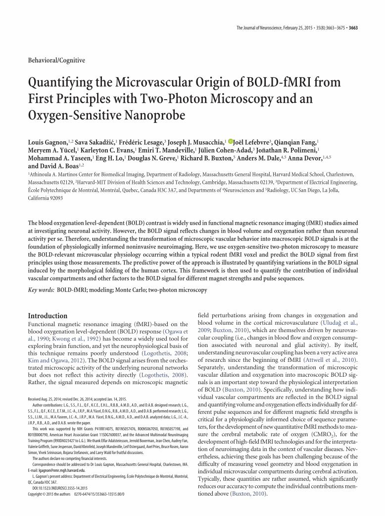
Overview. An overview of the entire modeling procedure is illustratedin Figure 1. Vessel dilation in the arterial compartment is an active pro-cess mediated by the release of vasodilatory agents and therefore thesemeasurements were used as inputs to perturb the VAN model fromsteady-state during functional activation. Flow changes and volumechanges can then be computed in all vascular segments assuming a pas-sive compliance model for the capillary and the venous bed. Knowing theflow and volume changes allowed us to compute the changes in oxygen-ation in all the vessels assuming a �Flow/�CMRO2 coupling ratio. Toensure the accuracy and realism of this approach, the simulated oxygen-ation changes were then compared with partial pO2 measurements dur-

ing functional activation. For all six vascular networks constructed, thisapproach gave very good agreement between the simulated and the mea-sured functional changes.

Steady-state VAN. The goal here was to reconstruct the resting distri-bution of oxygen in all vessels. This distribution was then compared withthe pO2 distribution measured experimentally to confirm its realism.This steady-state distribution was then perturbed during functionalactivation.

The oxygenation level in the vasculature was globally determined bytwo competing parameters, which are blood flow and the cerebral met-abolic rate of oxygen (CMRO2). Higher blood flow increases oxygen-ation while higher CMRO2 decreases it. In steady-state, these twoparameters are related by the following:

CMRO2 � CBF � OEF � Ca, (1)

where OEF is the oxygen extraction fraction and Ca is the arterial bloodoxygen content given by the following:

Ca � paO2� � 4HctCHbSaO2, (2)

where � � 1.27 � 10 3 �mol/ml/mmHg is the solubility of oxygen, CHb

� 5.3 �mol/ml is the hemoglobin content of blood and Hct � 0.4 is thehematocrit in arteries. OEF was computed directly for each animal usingour two-photon measurements as follows:

OEF �SaO2 � SvO2

SaO2. (3)

Baseline CBF in rodents has been previously measured with positronemission tomography (PET) and fMRI, and is well documented in theliterature (Wehrl et al., 2010; Zheng et al., 2010). Wehrl et al. (2010)reported a value of 75 ml/100 g/min over the cortex using PET, whereasZheng et al. (2010) reported a value of 125 ml/100 g/min with a 15%variation over the cortex using fMRI. We therefore fixed CBF to obtain aperfusion of 100 ml/100 g/min in our volumes. CMRO2 was then com-puted for each animal using Equation 1, and values obtained for eachanimal are shown in Table 1.

Capillary segments cut by the limits of the field-of-view were removedto obtain a closed graph between the pial arteries and the pial veins. Thisprocedure was previously used by (Lorthois et al., 2011a,b) and wasshown to result in accurate flow distributions.

The resistance for each segment was calculated using Poiseuille’s lawcorrected for hematocrit as described by Pries et al. (1990). Flow speedsin inflowing pial arteries were calculated based on the perfusion assumed(100 ml/100 g/min) and the arterial diameters. Blood pressure boundaryconditions for pial veins were set using values from (Lipowsky, 2005) andthe blood flow distribution was finally computed using the matrix equa-tions given by Boas et al. (2008), together with velocity boundary condi-tions for inflowing arteries and the blood pressure boundary conditionsfor outflowing veins. The arterial pressures calculated with this methodagreed with the experimental arterial pressures reported by Lipowsky(2005).

Finite-element oxygen advection was then performed individually foreach animal using the computed blood flow distribution and the inflow-ing arterial pO2 given in Table 1 for each animal. The pO2 was initializedeverywhere to 10 mmHg and oxygen advection was run with constantinputs (including uniform CMRO2 across the extravascular space) until

Figure 1. Overview of the modeling framework. Green arrows represent validations of themodel against experimental measurements.

Table 1. Physiological parameters for mice

ID paO2 (mmHg) pvO2 (mmHg) saO2 (%) svO2 (%) OEF (%) CMRO2 (�mol/ml/min)

1 109 44 92 58 36.9 2.282 94 43 88 54 38.6 2.323 107 60 93 67 28.0 1.724 116 57 93 66 29.0 1.815 118 60 94 68 27.7 1.736 109 41 91 58 36.2 2.23Mean 108.8 50.8 91.8 61.8 32.7 2.02SD 8.5 9.1 2.1 5.9 5.0 0.26

Gagnon et al. • Reverse-Engineering BOLD-fMRI J. Neurosci., February 25, 2015 • 35(8):3663–3675 • 3665

steady-state was achieved (typically after 15 s in the model time). Thedetails of the finite element algorithm used can be found in our previouspaper (Fang et al., 2008).

VAN model during functional activation. The arterial dilation traceswere used as inputs to compute changes in blood flow and blood volumeas described by Boas et al. (2008). An intracranial pressure of 10 mmHgwas assumed and the compliance parameter was set to 1 for bothcapillaries and veins (Boas et al., 2008).

Oxygenation changes during functional activation was then computedusing the same advection code (Fang et al., 2008) by keeping pO2 in thearterial inflowing nodes constant and using the updated flow and volumevalues at each time point. CMRO2 was increased following a temporalprofile corresponding the averaged arterial dilation trace with a peakamplitude corresponding to a relative change three times lower com-pared with the relative change in blood flow, giving a �Flow/�CMRO2

coupling ratio of 3 (Huppert et al., 2007; Dubeau et al., 2011).

fMRI simulationsOverview. The BOLD signal is a measure of the transverse magnetizationof nuclear spins. In gradient echo (GRE) BOLD, two processes contributeto the decay of the signal: dipole-dipole coupling (spin-spin interac-tions), as well as dephasing induced by microscopic and macroscopicfield inhomogeneities in the local magnetic field (Yablonskiy andHaacke, 1994). The relaxation constant embedding these two processes istermed T2*. In spin echo (SE) BOLD, the effect of field inhomogeneities isreversed around larger vessels (veins) using a 180° refocusing pulse. Therelaxation constant in this case is termed T2. A contributor to the localmagnetic field inhomogeneities is the presence of deoxyhemoglobin inthe vasculature, which is paramagnetic. During functional activation,variations in vessel size and oxygenation level affect the geometry and theamplitude of these magnetic field inhomogeneities and therefore affectT2*. Furthermore, the oxygenation level affects spin–spin coupling andtherefore T2.

The challenges in modeling BOLD are: (1) to compute the magneticfield inhomogeneities at every time point and (2) to keep track of spin-spin decay (T2 effect). These tasks require exact knowledge of the micro-vascular geometry and the deoxyhemoglobin content in each vesselsegment at every time point.

Computing magnetic field inhomogeneities. We used a numericalmethod previously described (Koch et al., 2006; Pathak et al., 2008) tocompute the magnetic field inhomogeneities. The SO2 volumes wereresampled to 1 � 1 � 1 �m and converted to a susceptibility shift volume� using the following:

� � �0Hct�1 � SO2�, (4)

where �0 � 4� � 0.264 � 10 �6 is the susceptibility difference betweenfully oxygenated and fully deoxygenated hemoglobin (Christen et al.,2011) and Hct is the hematocrit that was assumed to be 0.3 in capillariesand 0.4 in arteries and veins (Griffeth and Buxton, 2011).

Assuming that the magnetic field inhomogeneities are small, themethod uses perturbation theory and the inhomogeneities across theentire volume are computed by convolving the susceptibility shift vol-ume � with the geometrical factor for the magnetic field inhomogeneityinduced by a unit cube as follows:

�Bcube � � 6

��1

3

a3

r3�3cos2� � 1�B0, (5)

where a represents the grid size (1 �m) and r and � are the polar coordi-nates. This procedure allowed computation of the magnetic field inho-mogeneities across the entire vascular volume Binhom(x).

T2 and T2* volumes. In addition to magnetic field inhomogeneity, T2

and T2* volumes are required to accurately model the fMRI signals. T2

and T2* values (in seconds) along the vasculature were computed usingthe formulas obtained by fitting experimental measurements and givenin as follows (Uludag et al., 2009):

T2,vessel � �12.67B02�1 � SO2�

2 � 2.74B0 � 0.6��1, (6)

T2,vessel� � �A � C�1 � SO2�

2��1, (7)

where A and C are constants (in seconds �1) which depend on the exter-nal magnetic field B0 and given in Table 2.

In the tissue (outside the vessels), T2 and T2* (in seconds) were com-puted using the formulas given as follows (Uludag et al., 2009):

T2,tissue � �1.74B0 � 7.77��1, (8)

T2,vessel� � �3.74B0 � 9.77��1. (9)

Monte Carlo simulation of nuclear spins. Water protons experience diffu-sion in cortical tissue, which was simulated with Monte Carlo simula-tions (Boxerman et al., 1995a; Martindale et al., 2008). The positions of10 7 protons were initialized uniformly in the three-dimensional volume.Each proton experienced a random walk for a period of TE sec. Thediffusion coefficient was set to 1 � 10 �5 cm 2 /s (Pathak et al., 2008) andthe time step dt was set to 0.2 � 10 �3 sec. At each time step, the positionx � (x1 x2 x3) of each proton was updated using

x1 � x1 � N�0, 2Ddt�, (10)

x1 � x2 � N�0, 2Ddt�, (11)

x1 � x3 � N�0, 2Ddt�. (12)

Protons reaching a vessel wall were bounced back, such that all protonsstayed outside the vessels for the duration of the simulation. The MRsignal was computed at each time step by averaging the contribution of allN protons as follows:

S�t� � Re� 1

N�i�1

N

e�n�t�� , (13)

where the generalized phase (including both precession and relaxation)was updated every time step using:

�n,extra �t� � �k�1

t/dt

�j�B�x�k�� � T2,tissue �x�k��, (14)

where � is the hydrogen proton precession frequency, j the imaginaryunit, and:

�B� x�k�� � �B inhom�x�k�� � �Bgradients�x�k��, (15)

with �Binhom the magnetic field homogeneity computed above and�Bgradients is the field homogeneity introduced by the spatial gradient. ForSE signal, the imaginary part of the phase was inverted at TE/2

�n�TE/ 2� � conj��n�TE/2��. (16)

We note that only the extravascular protons were modeled, which con-stitute the dominant source of the signal at high fields (Uludag et al.,2009). This method was adopted since there is no current microscopicway of modeling accurately the intravascular signal. The numericalmethod produces relatively uniform magnetic fields inside the vascula-ture, while in reality there are very strong dipolar fields arising aroundred blood cells that are tumbling around and water molecules are ex-changed between red blood cells and the plasma.

This procedure is repeated at each desired time point during the func-tional activation. The relative signal changes was computed by compar-ing the signal obtained at each time point to the signal obtained at t � 0and converted to a percentage change.

Table 2. Empirical constants for T2* of blood

B0 � 1.5T A � 6.5 C � 251.5T B0 � 3T A � 13.8 C � 1813T B0 � 4T A � 30.4 C � 2624T B0 � 4.7T A � 41 C � 319B0 � 4.7T A � 100 C � 500

3666 • J. Neurosci., February 25, 2015 • 35(8):3663–3675 Gagnon et al. • Reverse-Engineering BOLD-fMRI

Calculation of the angular dependence of BOLDTo quantify the angular dependence of the BOLD response, we com-pared the BOLD signal changes simulated at different �z values with theBOLD signal changes simulated at �z � 0°. The difference was convertedto a percentage with respect to �z � 90°, as follows:

diff ��z� � 100 ��S�z � �S�z�90�

�S�z�90�. (17)

With this definition, a variation of 40% indicates that the BOLD signalchange for �z � 0° is 40% stronger compared with the BOLD signalchange for �z � 90°.

Experimental BOLD measurements on humanBOLD during hypercapnia. All experimental procedures were approvedby the Massachusetts General Hospital. Healthy subjects (n � 5) wereenrolled in the study. Written consent was received from each subjectbefore the experiment. During fMRI scanning, subjects breathedthrough a SCUBA-like mouth-piece attached to a specialized breathingcircuit that enabled steady-state levels of end-tidal pCO2 (Banzett et al.,2000). The end-tidal pCO2 was measured at the mouthpiece continu-ously during each fMRI scan via MRI-compatible capnograph (Capstar-100, CWE) to verify the target levels of end-tidal pCO2. Hypercapnia wasachieved by adding CO2 to the inspirate. Each subject received two 2 minblocks hypercapnia during which end-tidal pCO2 was maintained at a levelof 8 mmHg above the subject’s baseline pCO2 value. The hypercapnic blockswere interleaved with 3 min blocks at baseline pCO2 (normocapnia).

Combined ASL-BOLD data were collected simultaneously at 3T dur-ing the gas manipulations. BOLD images were extracted from the timeseries and corresponded to the control images. Sequence parameterswere TR � 3000 ms, IR-1 � 600 ms, IR-2 � 1800 ms, TE � 13 ms, flipangle � 90°, Res � 3.4 � 3.4 � 6.0 mm, 6 slices. An anatomical T1-weighted scan (MPRage) was also collected (Res � 1 � 1 � 1.2 mm).These measurements were previously published (Yucel et al., 2014).

Angular analysis. BOLD data were analyzed using Freesurfer. Motioncorrection and slice-timing correction were applied. No smoothing wasused. BOLD signal changes between normocapnic and hypercapnic con-ditions were computed across the six slices.

A complete cortical surface reconstruction of the anatomical scan wasperformed with Freesurfer using the recon-all function. An additionalcortical surface was generated midway in the gray matter and the anglebetween the normal to this surface and B0 was computed as previouslydescribed (Cohen-Adad et al., 2012). The BOLD signal volumes werethen interpolated on this surface, leading to a series of voxels contain-ing both �z and BOLD change values. The data were pruned by select-ing only voxel with a BOLD response between 0% and 10%. Voxelswith BOLD response larger than 10% were probably located insidelarge pial vessels and did not contain cortical tissue. These voxels weretherefore rejected from the analysis. Voxels with negative BOLD re-sponses were potentially strongly contaminated with noise and werealso rejected from the analysis.

The pruned data point were binned based on �z at every four degreesbetween 0° and 180° and the average BOLD change for each bin wascomputed. The variation in BOLD change with respect to BOLD changeat �z � 90° was computed using Eq. 17.

Individual contributions to the BOLD signalThe individual contributions to the BOLD signal were computed at thepeak of the activation, which occurred between 3.5 and 4 s (depending onthe animal) after the start of the stimulus. For each field strength, TE wasset to T2,tissue

* for GRE and to T2, tissue for SE as shown in the Table 3.Arteries, capillaries, and veins contributions. To compute the contribu-

tion of an individual vascular compartment (e.g., the capillaries), twodifferent simulations were performed. In the first one, the oxygenationvolume (with dilated vessels) computed with the VAN at the peak of thefunctional activation was used. The signal obtained (termed total BOLDresponse) was compared with the signal obtained using the oxygenationvolume (with baseline vessel size) at t � 0. In the second simulation, weconstructed a new volume by using baseline (values at t � 0) oxygenationand vessel size for arteries and veins, but peak values for oxygenation and

vessel sizes for capillaries. The signal obtained (termed capillary BOLDsignal change) in this case was also compared with the same baselinesignal computed using baseline oxygenation and vessel size everywhere.To compute the individual contribution of the capillaries, the capillaryBOLD signal change was divided by the total BOLD signal change andconverted to percentage. This procedure was repeated for arteries andveins, and for all field strengths.

Blood volume changes and oxygenation changes contributions. To com-pute the contribution of cerebral blood volume (CBV) changes, twosimulations were performed. In the first one, both the oxygenationchanges and vessel diameter changes given from the VAN models weretaken into account. In the second one, only the oxygenation changes weretaken into account, whereas the vessel diameters were kept constant. Thenet CBV contribution was computed as the difference between the stan-dard and the oxygenation only signals normalized to the standard signal(in percentage). A negative CBV contribution indicates that the BOLDsignal produced would be higher with no vessel dilation (only oxygenationchanges). The negative CBV contribution occurs because dilation of vesselscontaining deoxyhemoglobin increase the total amount of deoxyhemoglo-bin in a given fMRI voxel which reduces the signal measured.

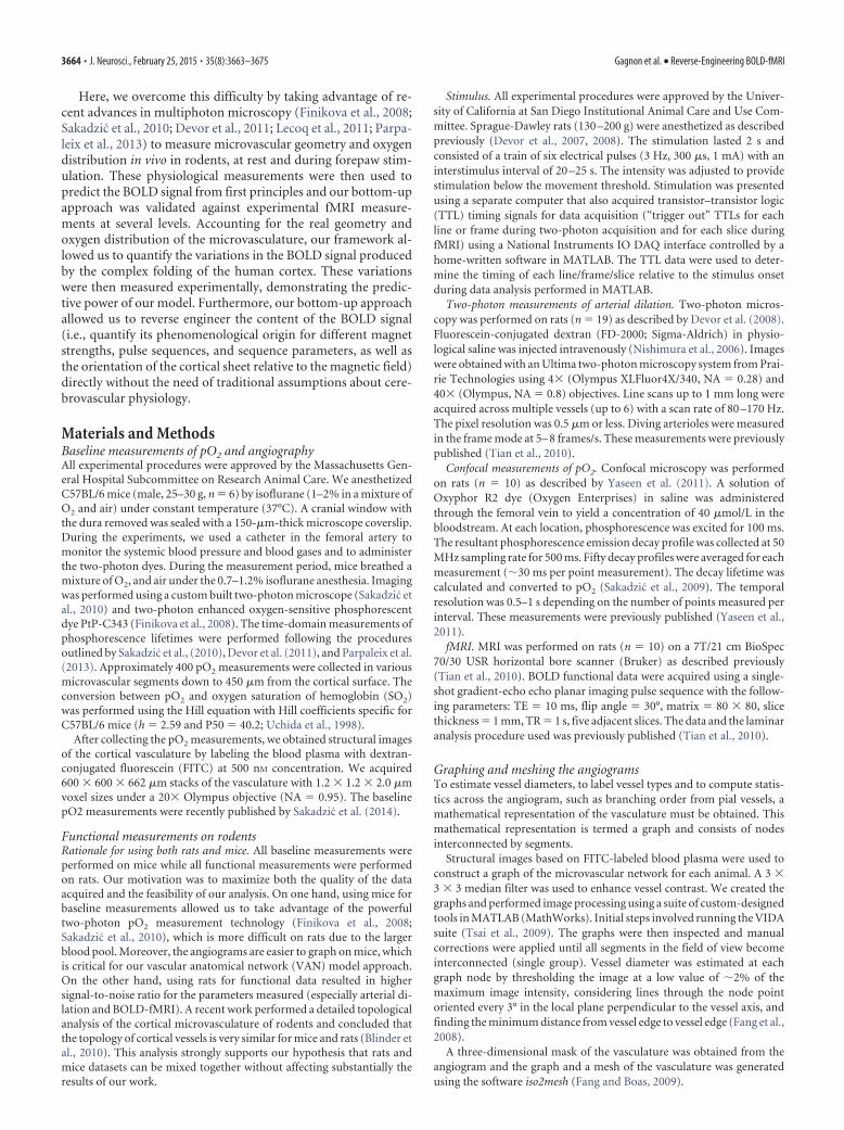
ResultsReconstruction of realistic vascular networks and baselineoxygen distributionTo reconstruct baseline oxygen distribution across real vascularnetworks, two-photon microscopy was performed first on a set ofanesthetized mice (n � 6) as described in Materials and Methods.Briefly, an intravascular oxygen-sensitive nanoprobe (PtP-C343)was injected for the pO2 measurements followed by the injectionof FITC for angiography. The angiogram for a representativeanimal is shown in Figure 2A. Unfortunately, the power of thistechnology can only be exploited on rodents. Although it isknown that the arteries/veins ratio varies between rodents andprimates (Hirsch et al., 2012), it is assumed here that the oxygendistribution along the different microvascular compartments ofthe cortex is similar between rodents and humans. With thisassumption, modeling the BOLD signal over real rodent data repre-sent a significant improvement over previous models based on ran-dom cylinder distributions (Boxerman et al., 1995b; Uludag et al.,2009) or uniform oxygen distributions (Christen et al., 2011).

To reconstruct microvascular oxygenation with sufficientspatiotemporal resolution to accurately model the BOLD signalin each animal (n � 6), six VAN models were created (i.e., one foreach animal; Fang et al., 2008; Blinder et al., 2013; see Materialsand Methods). Angiograms were graphed using a suite ofcustom-built computer programs (Fang et al., 2008; Tsai et al.,2009) and a mesh of the vasculature was then created (Fang et al.,2008). Each vessel segment was identified as an artery, a capillaryor a vein as shown in Figure 2B. The blood flow distribution (Fig.2C) was obtained for each animal after computing the resistanceof all vascular segments on each graph and assuming global per-fusion (see Materials and Methods). For this purpose, capillarysegments cut by the limits of the field-of-view were removed toobtain a closed graph between the pial arteries and the pial veins.

Table 3. T2* and T2 values for tissue at different B fields

Field (T) T2,tissue� (ms) T2,tissue (ms)

1.5 65 963.0 48 774.7 37 627.0 28 509.4 22 41

11.7 19 3514.0 16 31

Gagnon et al. • Reverse-Engineering BOLD-fMRI J. Neurosci., February 25, 2015 • 35(8):3663–3675 • 3667

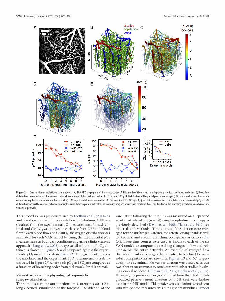
This procedure was previously used by Lorthois et al., (2011a,b)and was shown to result in accurate flow distributions. OEF wasobtained from the experimental pO2 measurements for each an-imal, and CMRO2 was derived in each case from OEF and bloodflow. Given blood flow and CMRO2, the oxygen distribution wassimulated for each VAN model by using the experimental pO2

measurements as boundary conditions and using a finite elementapproach (Fang et al., 2008). A typical distribution of pO2 ob-tained is shown in Figure 2D and compared against the experi-mental pO2 measurements in Figure 2E. The agreement betweenthe simulated and the experimental pO2 measurements is dem-onstrated in Figure 2F, where both pO2 and SO2 are compared asa function of branching order from pial vessels for this animal.

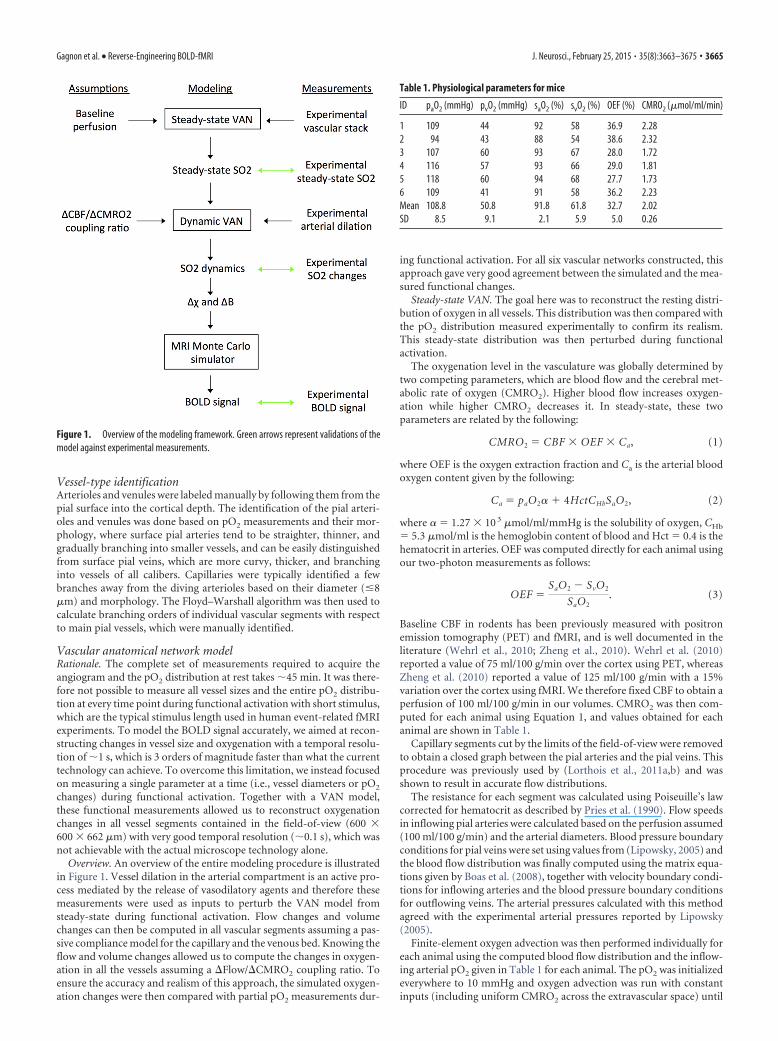
Reconstruction of the physiological response toforepaw stimulationThe stimulus used for our functional measurements was a 2-s-long electrical stimulation of the forepaw. The dilation of the

vasculature following the stimulus was measured on a separatedset of anesthetized rats (n � 19) using two-photon microscopy aspreviously described (Devor et al., 2008; Tian et al., 2010; seeMaterials and Methods). Time courses of the dilation were aver-aged for the surface pial arteries, the arterial diving trunk as wellfor the first and second branching precapillary arterioles (Fig.3A). These time courses were used as inputs to each of the sixVAN models to compute the resulting changes in flow and vol-ume across the entire networks. An example of averaged flowchanges and volume changes (both relative to baseline) for indi-vidual compartments are shown in Figures 3B and 2C, respec-tively, for one animal. No venous dilation was observed in ourtwo-photon measurements, consistent with other studies involv-ing a cranial window (Hillman et al., 2007; Lindvere et al., 2013).However, the pressure changes computed from the VAN modelsproduced passive venous dilations of 1–2% that were furtherused in the fMRI model. This passive venous dilation is consistentwith two-photon measurements during short stimulus (Drew et

Figure 2. Construction of realistic vascular networks. A, TPM FITC angiogram of the mouse cortex. B, FEM mesh of the vasculature displaying arteries, capillaries, and veins. C, Blood flowdistribution simulated across the vascular network assuming a global perfusion value of 100 ml/min/100 g. D, Distribution of the partial pressure of oxygen (pO2) simulated across the vascularnetwork using the finite element method model. E, TPM experimental measurements of pO2 in vivo using PtP-C343 dye. F, Quantitative comparison of simulated and experimental pO2 and SO2

distributions across the vascular network for a single animal. Traces represent arterioles and capillaries (red) and venules and capillaries (blue) as a function of the branching order from pial arterioles andvenules, respectively.

3668 • J. Neurosci., February 25, 2015 • 35(8):3663–3675 Gagnon et al. • Reverse-Engineering BOLD-fMRI

al., 2011) under a reinforced thinned skull window (Drew et al.,2010), which could potentially produce a picture of activationcloser to the one occurring in noninvasive human fMRI studies.

Given changes in flow and volume, we computed changes inoxygen saturation for the six VAN models assuming a �Flow/�CMRO2 ratio of 3, which is the typical value measured in ro-dents for short stimulations (Huppert et al., 2007; Dubeau et al.,2011). Simulated SO2 changes for a single animal are shown inFigure 3D for different vascular compartments. For validation,SO2 measurements during functional stimulation were per-formed in pial vessels with confocal microscopy on a separate setof rats (n � 10) under the same experimental conditions (Yaseenet al., 2011). A good agreement between the simulations and theexperimental measurements was obtained for both arteries andveins as demonstrated in Figure 3E, where the average is taken acrossall six animals for the simulations and all 10 animals for the experi-mental values. These results validate our initial assumption of ablood flow change three times larger than the CMRO2 change anddemonstrate the realism of our VAN modeling approach. An exam-ple of changes in SO2 across the entire vasculature (Fig. 3F) is shownat different time points following the forepaw stimulus in Figure 3G.

Modeling fMRI signals from first principlesThe BOLD signal is a measure of the transverse magnetization ofnuclear spins. In GRE BOLD, the signal decays to zero due tospin–spin interactions, as well as dephasing induced by magneticfield inhomogeneities. In SE BOLD, most of the later process isreversed using a 180° refocusing pulse. The presence of deoxyhe-moglobin in the vasculature gives rise to microscopic magneticfield perturbations within the cortical tissue (upon its introduc-tion in the strong field of the MR scanner) and therefore contrib-utes to local magnetic field inhomogeneities. During increasedneuronal activity, variations in vessel size and oxygenation levelaffect the geometry and the amplitude of these magnetic fieldinhomogeneities and therefore affect the GRE signal. The oxy-genation level in the vessels also affects spin–spin coupling andtherefore the SE signal.

Requirements to model the BOLD signal from first principles(diffusion of water molecules through the distorted magneticfield created by the deoxyhemoglobin distribution) are theknowledge of the exact geometry and size of the cerebral micro-vasculature, as well as the deoxyhemoglobin content in these mi-crovessels. The difficulty in measuring these two quantities has

Figure 3. Modeling the physiological response to forepaw stimulus. A, TPM experimental measurements or arterial dilation following forepaw stimulus. B, Simulated flow changes, (C) simulatedvolume changes, and (D) simulated SO2 changes (all relative to baseline) in the different vascular compartments. E, Comparison of simulated SO2 changes (n � 6 animals) with experimental SO2

changes (n � 10 animals) measured in pial vessels during a forepaw stimulus with confocal microscopy. F, Vessel type. G, Spatiotemporal evolution of simulated SO2 changes following forepawstimulus.

Gagnon et al. • Reverse-Engineering BOLD-fMRI J. Neurosci., February 25, 2015 • 35(8):3663–3675 • 3669

led researchers to use alternative approaches including simplify-ing the geometry of the vessel network with straight cylinders(Boxerman et al., 1995a; Martindale et al., 2008), simplifying theoxygen distribution in the microvasculature to uniform SO2

(Pathak et al., 2008; Christen et al., 2011), or to use top-downmodels (Yablonskiy and Haacke, 1994; Davis et al., 1998; Uludaget al., 2009). The VAN modeling approach presented here pro-vides accurate two-photon measurements of the relevant physi-ological quantities, vessel geometry and oxygen content; andtherefore, presents a unique opportunity to model the BOLDsignal with a high level of detail and accuracy.

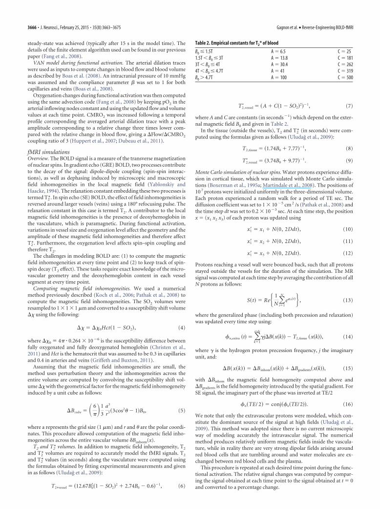
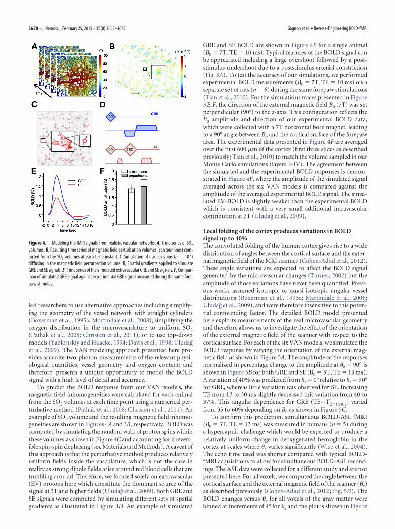
To predict the BOLD response from our VAN models, themagnetic field inhomogeneities were calculated for each animalfrom the SO2 volumes at each time point using a numerical per-turbative method (Pathak et al., 2008; Christen et al., 2011). Anexample of SO2 volume and the resulting magnetic field inhomo-geneities are shown in Figures 4A and 3B, respectively. BOLD wascomputed by simulating the random walk of proton spins withinthese volumes as shown in Figure 4C and accounting for irrevers-ible spin-spin dephasing (see Materials and Methods). A caveat ofthis approach is that the perturbative method produces relativelyuniform fields inside the vasculature, which is not the case inreality as strong dipole fields arise around red blood cells that aretumbling around. Therefore, we focused solely on extravascular(EV) protons here which constitute the dominant source of thesignal at 3T and higher fields (Uludag et al., 2009). Both GRE andSE signals were computed by simulating different sets of spatialgradients as illustrated in Figure 4D. An example of simulated

GRE and SE BOLD are shown in Figure 4E for a single animal(B0 � 7T, TE � 10 ms). Typical features of the BOLD signal canbe appreciated including a large overshoot followed by a post-stimulus undershoot due to a poststimulus arterial constriction(Fig. 3A). To test the accuracy of our simulations, we performedexperimental BOLD measurements (B0 � 7T, TE � 10 ms) on aseparate set of rats (n � 6) during the same forepaw stimulations(Tian et al., 2010). For the simulations traces presented in Figure3E,F, the direction of the external magnetic field B0 (7T) was setperpendicular (90°) to the z-axis. This configuration reflects theB0 amplitude and direction of our experimental BOLD data,which were collected with a 7T horizontal bore magnet, leadingto a 90° angle between B0 and the cortical surface of the forepawarea. The experimental data presented in Figure 4F are averagedover the first 600 �m of the cortex (first three slices as describedpreviously; Tian et al., 2010) to match the volume sampled in ourMonte Carlo simulations (layers I–IV). The agreement betweenthe simulated and the experimental BOLD responses is demon-strated in Figure 4F, where the amplitude of the simulated signalaveraged across the six VAN models is compared against theamplitude of the averaged experimental BOLD signal. The simu-lated EV-BOLD is slightly weaker than the experimental BOLDwhich is consistent with a very small additional intravascularcontribution at 7T (Uludag et al., 2009).

Local folding of the cortex produces variations in BOLDsignal up to 40%The convoluted folding of the human cortex gives rise to a widedistribution of angles between the cortical surface and the exter-nal magnetic field of the MRI scanner (Cohen-Adad et al., 2012).These angle variations are expected to affect the BOLD signalgenerated by the microvascular changes (Turner, 2002) but theamplitude of those variations have never been quantified. Previ-ous works assumed isotropic or quasi-isotropic angular vesseldistributions (Boxerman et al., 1995a; Martindale et al., 2008;Uludag et al., 2009), and were therefore insensitive to this poten-tial confounding factor. The detailed BOLD model presentedhere exploits measurements of the real microvascular geometryand therefore allows us to investigate the effect of the orientationof the external magnetic field of the scanner with respect to thecortical surface. For each of the six VAN models, we simulated theBOLD response by varying the orientation of the external mag-netic field as shown in Figure 5A. The amplitude of the responsesnormalized in percentage change to the amplitude at �z � 90° isshown in Figure 5B for both GRE and SE (B0 � 3T, TE � 13 ms).A variation of 40% was predicted from �z � 0° relative to �z � 90°for GRE, whereas little variation was observed for SE. IncreasingTE from 13 to 30 ms slightly decreased this variation from 40 to37%. This angular dependence for GRE (TE�T2

*, tissue) variedfrom 35 to 60% depending on B0 as shown in Figure 5C.

To confirm this prediction, simultaneous BOLD-ASL fMRI(B0 � 3T, TE � 13 ms) was measured in humans (n � 5) duringa hypercapnic challenge which would be expected to produce arelatively uniform change in deoxygenated hemoglobin in thecortex at scales where �z varies significantly (Wise et al., 2004).The echo time used was shorter compared with typical BOLD-fMRI acquisitions to allow for simultaneous BOLD-ASL record-ings. The ASL data were collected for a different study and are notpresented here. For all voxels, we computed the angle between thecortical surface and the external magnetic field of the scanner (�z)as described previously (Cohen-Adad et al., 2012; Fig. 5D). TheBOLD changes versus �z for all voxels of the gray matter werebinned at increments of 4° for �z and the plot is shown in Figure

Figure 4. Modeling the fMRI signals from realistic vascular networks. A, Time series of SO2

volumes. B, Resulting time series of magnetic field perturbation volumes (contour lines) com-puted from the SO2 volumes at each time instant. C, Simulation of nuclear spins (n � 10 7)diffusing in the magnetic field perturbation volume. D, Spatial gradients applied to simulateGRE and SE signals. E, Time series of the simulated extravascular GRE and SE signals. F, Compar-ison of simulated GRE signal against experimental GRE signal measured during the same fore-paw stimulus.

3670 • J. Neurosci., February 25, 2015 • 35(8):3663–3675 Gagnon et al. • Reverse-Engineering BOLD-fMRI

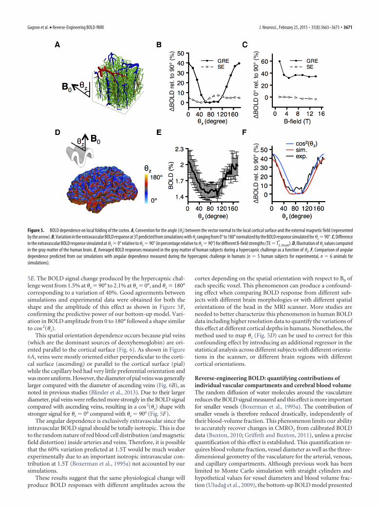
5E. The BOLD signal change produced by the hypercapnic chal-lenge went from 1.5% at �z � 90° to 2.1% at �z � 0°, and �z � 180°corresponding to a variation of 40%. Good agreements betweensimulations and experimental data were obtained for both theshape and the amplitude of this effect as shown in Figure 5F,confirming the predictive power of our bottom-up model. Vari-ation in BOLD amplitude from 0 to 180° followed a shape similarto cos 2(�z).

This spatial orientation dependence occurs because pial veins(which are the dominant sources of deoxyhemoglobin) are ori-ented parallel to the cortical surface (Fig. 6). As shown in Figure6A, veins were mostly oriented either perpendicular to the corti-cal surface (ascending) or parallel to the cortical surface (pial)while the capillary bed had very little preferential orientation andwas more uniform. However, the diameter of pial veins was generallylarger compared with the diameter of ascending veins (Fig. 6B), asnoted in previous studies (Blinder et al., 2013). Due to their largerdiameter, pial veins were reflected more strongly in the BOLD signalcompared with ascending veins, resulting in a cos2(�z) shape withstronger signal for �z � 0° compared with �z � 90° (Fig. 5F).

The angular dependence is exclusively extravascular since theintravascular BOLD signal should be totally isotropic. This is dueto the random nature of red blood cell distribution (and magneticfield distortion) inside arteries and veins. Therefore, it is possiblethat the 60% variation predicted at 1.5T would be much weakerexperimentally due to an important isotropic intravascular con-tribution at 1.5T (Boxerman et al., 1995a) not accounted by oursimulations.

These results suggest that the same physiological change willproduce BOLD responses with different amplitudes across the

cortex depending on the spatial orientation with respect to B0 ofeach specific voxel. This phenomenon can produce a confound-ing effect when comparing BOLD response from different sub-jects with different brain morphologies or with different spatialorientations of the head in the MRI scanner. More studies areneeded to better characterize this phenomenon in human BOLDdata including higher resolution data to quantify the variations ofthis effect at different cortical depths in humans. Nonetheless, themethod used to map �z (Fig. 5D) can be used to correct for thisconfounding effect by introducing an additional regressor in thestatistical analysis across different subjects with different orienta-tions in the scanner, or different brain regions with differentcortical orientations.

Reverse-engineering BOLD: quantifying contributions ofindividual vascular compartments and cerebral blood volumeThe random diffusion of water molecules around the vasculaturereduces the BOLD signal measured and this effect is more importantfor smaller vessels (Boxerman et al., 1995a). The contribution ofsmaller vessels is therefore reduced drastically, independently oftheir blood-volume fraction. This phenomenon limits our abilityto accurately recover changes in CMRO2 from calibrated BOLDdata (Buxton, 2010; Griffeth and Buxton, 2011), unless a precisequantification of this effect is established. This quantification re-quires blood volume fraction, vessel diameter as well as the three-dimensional geometry of the vasculature for the arterial, venous,and capillary compartments. Although previous work has beenlimited to Monte Carlo simulation with straight cylinders andhypothetical values for vessel diameters and blood volume frac-tion (Uludag et al., 2009), the bottom-up BOLD model presented

Figure 5. BOLD dependence on local folding of the cortex. A, Convention for the angle (�z) between the vector normal to the local cortical surface and the external magnetic field (representedby the arrow). B, Variation in the extravascular BOLD response at 3T predicted from simulations with �z ranging from 0° to 180° normalized by the BOLD response simulated for �z �90°. C, Differencein the extravascular BOLD response simulated at �z � 0° relative to �z � 90° (in percentage relative to �z � 90°) for different B-field strengths (TE � T2, tissue

* ). D, Illustration of �z values computedin the gray matter of the human brain. E, Averaged BOLD responses measured in the gray matter of human subjects during a hypercapnic challenge as a function of �z. F, Comparison of angulardependence predicted from our simulations with angular dependence measured during the hypercapnic challenge in humans (n � 5 human subjects for experimental, n � 6 animals forsimulations).

Gagnon et al. • Reverse-Engineering BOLD-fMRI J. Neurosci., February 25, 2015 • 35(8):3663–3675 • 3671

here provides an experimental measure of these three quantitiesand therefore allows us to compute the contribution of individualvascular compartments to the BOLD signal directly without anyfurther assumption regarding these three parameters.

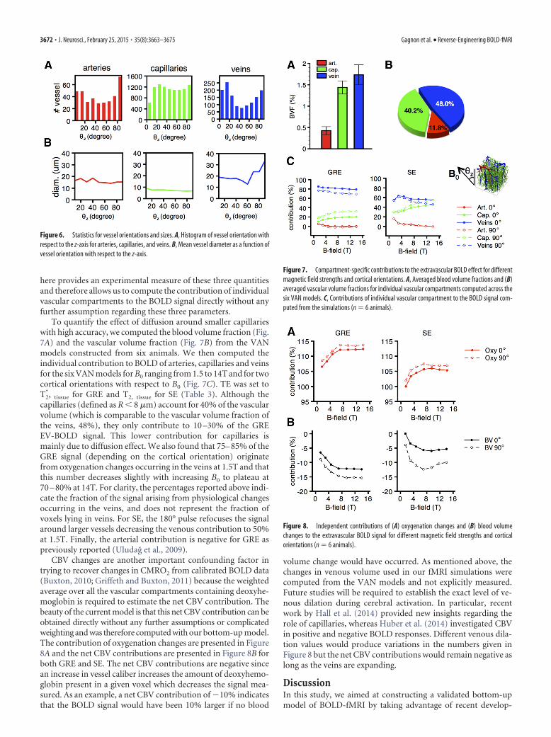
To quantify the effect of diffusion around smaller capillarieswith high accuracy, we computed the blood volume fraction (Fig.7A) and the vascular volume fraction (Fig. 7B) from the VANmodels constructed from six animals. We then computed theindividual contribution to BOLD of arteries, capillaries and veinsfor the six VAN models for B0 ranging from 1.5 to 14T and for twocortical orientations with respect to B0 (Fig. 7C). TE was set toT2

*, tissue for GRE and T2, tissue for SE (Table 3). Although thecapillaries (defined as R 8 �m) account for 40% of the vascularvolume (which is comparable to the vascular volume fraction ofthe veins, 48%), they only contribute to 10 –30% of the GREEV-BOLD signal. This lower contribution for capillaries ismainly due to diffusion effect. We also found that 75– 85% of theGRE signal (depending on the cortical orientation) originatefrom oxygenation changes occurring in the veins at 1.5T and thatthis number decreases slightly with increasing B0 to plateau at70 – 80% at 14T. For clarity, the percentages reported above indi-cate the fraction of the signal arising from physiological changesoccurring in the veins, and does not represent the fraction ofvoxels lying in veins. For SE, the 180° pulse refocuses the signalaround larger vessels decreasing the venous contribution to 50%at 1.5T. Finally, the arterial contribution is negative for GRE aspreviously reported (Uludag et al., 2009).

CBV changes are another important confounding factor intrying to recover changes in CMRO2 from calibrated BOLD data(Buxton, 2010; Griffeth and Buxton, 2011) because the weightedaverage over all the vascular compartments containing deoxyhe-moglobin is required to estimate the net CBV contribution. Thebeauty of the current model is that this net CBV contribution can beobtained directly without any further assumptions or complicatedweighting and was therefore computed with our bottom-up model.The contribution of oxygenation changes are presented in Figure8A and the net CBV contributions are presented in Figure 8B forboth GRE and SE. The net CBV contributions are negative sincean increase in vessel caliber increases the amount of deoxyhemo-globin present in a given voxel which decreases the signal mea-sured. As an example, a net CBV contribution of �10% indicatesthat the BOLD signal would have been 10% larger if no blood

volume change would have occurred. As mentioned above, thechanges in venous volume used in our fMRI simulations werecomputed from the VAN models and not explicitly measured.Future studies will be required to establish the exact level of ve-nous dilation during cerebral activation. In particular, recentwork by Hall et al. (2014) provided new insights regarding therole of capillaries, whereas Huber et al. (2014) investigated CBVin positive and negative BOLD responses. Different venous dila-tion values would produce variations in the numbers given inFigure 8 but the net CBV contributions would remain negative aslong as the veins are expanding.

DiscussionIn this study, we aimed at constructing a validated bottom-upmodel of BOLD-fMRI by taking advantage of recent develop-

Figure 6. Statistics for vessel orientations and sizes. A, Histogram of vessel orientation withrespect to the z-axis for arteries, capillaries, and veins. B, Mean vessel diameter as a function ofvessel orientation with respect to the z-axis.

Figure 7. Compartment-specific contributions to the extravascular BOLD effect for differentmagnetic field strengths and cortical orientations. A, Averaged blood volume fractions and (B)averaged vascular volume fractions for individual vascular compartments computed across thesix VAN models. C, Contributions of individual vascular compartment to the BOLD signal com-puted from the simulations (n � 6 animals).

Figure 8. Independent contributions of (A) oxygenation changes and (B) blood volumechanges to the extravascular BOLD signal for different magnetic field strengths and corticalorientations (n � 6 animals).

3672 • J. Neurosci., February 25, 2015 • 35(8):3663–3675 Gagnon et al. • Reverse-Engineering BOLD-fMRI

ment in quantitative two-photon microscopy of microvascularpO2. Our modeling framework was validated against experimen-tal data at several levels including the physiological and the bio-physical level. Our model improved upon previous work byconsidering the real geometry of the microvasculature, as well asits real baseline deoxyhemoglobin distribution. The importanceof this realism is twofold. First, our model provided a predictionof the magnitude of the effect of local cortical folding on theBOLD signal. It predicted signal variations up to 40% at 3T withTE � 13 ms. Taking into account this confounding effect in theanalysis of BOLD data could significantly improve the quantifi-cation of fMRI in terms of physiological changes. The amplitudeof the cortical-folding variations predicted from our model wasfurther validated against experimental BOLD recordings on hu-mans, demonstrating the predictive power of our model. Second,this realism allowed us to compute with high accuracy the con-tribution of individual compartment and the net blood volumecontribution to the BOLD signal, two important confoundingfactors when estimating CMRO2 changes from calibrated BOLDdata, without having to assume blood volume fraction, vesselsize, network geometry, or oxygen content of the individual vas-cular compartments.

As mentioned in Materials and Methods, an important as-sumption was necessary to model the physiological response toforepaw stimulation i.e., a coupling ratio for �Flow/�CMRO2 of3 was assumed. To validate this assumption, the simulated SO2

changes were compared with experimental SO2 changes andgood agreement were obtained. Nevertheless, we performed asensitivity analysis to test the impact of this assumption on theresults reported in this manuscript. We varied the �Flow/�CMRO2 coupling ratio from 2 to infinity (i.e., no changes inCMRO2) in the VAN modeling and resimulated the BOLD re-sponse with each of the resulting SO2 distributions. Although theamplitude of the BOLD response varied from 1 to 3% (whichrepresents a variation of �50% compared with the 2% BOLDresponse obtained with a �Flow/�CMRO2 coupling ratio of 3),neither the relative variations in the BOLD response produced bythe local cortical folding nor the relative contributions of individ-ual vascular compartments varied by �10% by varying the as-sumed �Flow/�CMRO2 coupling ratio. This occurred becausealthough the mean SO2 change of the voxel varied with the�Flow/�CMRO2 ratio, the relative SO2 changes between the dif-ferent compartments were less variable. We also introduced 30%heterogeneity in the amplitude of the dilation traces used as in-puts to the VAN to test the impact of heterogeneous dilation.Similarly, neither the relative variations in the BOLD responseproduced by the local cortical folding nor the relative contribu-tions of individual vascular compartments varied by �5%. Thisoccurred because heterogeneous dilation influenced the SO2 dis-tribution mostly in the arterial compartment and the firstbranches of the capillary compartment, which are not stronglyrepresented in the BOLD response.

Although increasing the level of complexity can improve thepredictive power of a model, as was the case here, this procedureoften reduces its invertibility. A drawback of the complexbottom-up model presented here is that the high number of pa-rameters and their non-uniqueness prevent the model to be in-verted (i.e., one cannot recover oxygenation changes and vesseldilation in all compartments from a simple BOLD trace). Be-cause an invertible BOLD model is required to recoverCMRO2 changes from flow and BOLD traces in the calibratedBOLD approach, researchers rely on the simplified top-downmodel originally proposed by Davis et al. (1998), which has

never been validated against microscopic physiological mea-surements. By simulating macroscopic BOLD responses fromdifferent realistic physiological states, the detailed bottom-upmodel proposed here will provide a validated foundation totest and potentially improve the accuracy of the calibratedBOLD approach to recover CMRO2 changes from combinedflow and BOLD data.

The need for an accurate model describing the transformationof microscopic vascular dilation and oxygenation into macro-scopic fMRI signals has increased recently with the developmentof magnetic resonance fingerprinting (MRF; Ma et al., 2013). InMRF, a pseudorandomized acquisition is used which causes thesignals from different tissues to have a unique signal evolutiontermed “fingerprint”. Following the acquisition, a pattern recog-nition algorithm is used to match the fingerprints to a predefineddictionary of predicted signal evolutions. This dictionary is con-structed from an fMRI model predicting the macroscopic fMRIsignal detected from the microscopic properties of the underlyingtissue. Recently, MRF has been used to reconstruct blood oxygen-ation and blood volume simultaneously (Christen et al., 2014).The MRF dictionary used in this case was constructed from aMonte Carlo fMRI model with simplified vascular geometry andoxygen content. The bottom-up model presented here will pro-vide a validated framework to validate and potentially improvethis MRF dictionary by accounting for the real geometry andoxygenation of cortical microvasculature.

ReferencesAttwell D, Buchan AM, Charpak S, Lauritzen M, Macvicar BA, Newman EA

(2010) Glial and neuronal control of brain blood flow. Nature 468:232–243. CrossRef Medline

Banzett RB, Garcia RT, Moosavi SH (2000) Simple contrivance “clamps”end-tidal PCO(2) and PO(2) despite rapid changes in ventilation. J ApplPhysiol 88:1597–1600. Medline

Blinder P, Shih AY, Rafie C, Kleinfeld D (2010) Topological basis for therobust distribution of blood to rodent neocortex. Proc Natl Acad SciU S A 107:12670 –12675. CrossRef Medline

Blinder P, Tsai PS, Kaufhold JP, Knutsen PM, Suhl H, Kleinfeld D (2013)The cortical angiome: an interconnected vascular network with nonco-lumnar patterns of blood flow. Nat Neurosci 16:889 – 897. CrossRefMedline

Boas DA, Jones SR, Devor A, Huppert TJ, Dale AM (2008) A vascular ana-tomical network model of the spatio-temporal response to brain activa-tion. Neuroimage 40:1116 –1129. CrossRef Medline

Boxerman JL, Bandettini PA, Kwong KK, Baker JR, Davis TL, Rosen BR,Weisskoff RM (1995a) The intravascular contribution to fMRI signalchange: Monte Carlo modeling and diffusion-weighted studies in vivo.Magn Reson Med 34:4 –10. CrossRef Medline

Boxerman JL, Hamberg LM, Rosen BR, Weisskoff RM (1995b) MR contrastdue to intravascular magnetic susceptibility perturbations. Magn ResonMed 34:555–566. CrossRef Medline

Buxton RB (2010) Interpreting oxygenation-based neuroimaging signals:the importance and the challenge of understanding brain oxygen metab-olism. Front Neuroenergetics 2:8. CrossRef Medline

Christen T, Zaharchuk G, Pannetier N, Serduc R, Joudiou N, Vial JC, Remy C,Barbier EL (2011) Quantitative MR estimates of blood oxygenationbased on T2*: A numerical study of the impact of model assumptions.Magn Reson Med 67:1458 –1468. CrossRef Medline

Christen T, Pannetier NA, Ni WW, Qiu D, Moseley ME, Schuff N, ZaharchukG (2014) MR vascular fingerprinting: a new approach to compute cere-bral blood volume, mean vessel radius, and oxygenation maps in thehuman brain. Neuroimage 89:262–270. CrossRef Medline

Cohen-Adad J, Polimeni JR, Helmer KG, Benner T, McNab JA, Wald LL,Rosen BR, Mainero C (2012) T2* mapping and B0 orientation-dependence at 7T reveal cyto- and myeloarchitecture organization of thehuman cortex. Neuroimage 60:1006 –1014. CrossRef Medline

Davis TL, Kwong KK, Weisskoff RM, Rosen BR (1998) Calibrated func-tional MRI: mapping the dynamics of oxidative metabolism. Proc NatlAcad Sci U S A 95:1834 –1839. CrossRef Medline

Gagnon et al. • Reverse-Engineering BOLD-fMRI J. Neurosci., February 25, 2015 • 35(8):3663–3675 • 3673

Devor A, Sakadzic S, Saisan PA, Yaseen MA, Roussakis E, Srinivasan VJ,Vinogradov SA, Rosen BR, Buxton RB, Dale AM, Boas DA (2011)“Overshoot” of O2 is required to maintain baseline tissue oxygenation atlocations distal to blood vessels. J Neurosci 31:13676 –13681. CrossRefMedline

Devor A, Tian P, Nishimura N, Teng IC, Hillman EM, Narayanan SN, UlbertI, Boas DA, Kleinfeld D, Dale AM (2007) Suppressed neuronal activityand concurrent arteriolar vasoconstriction may explain negative bloodoxygenation level-dependent signal. J Neurosci 27:4452– 4459. CrossRefMedline

Devor A, Hillman EM, Tian P, Waeber C, Teng IC, Ruvinskaya L, Shalin-sky MH, Zhu H, Haslinger RH, Narayanan SN, Ulbert I, Dunn AK, LoEH, Rosen BR, Dale AM, Kleinfeld D, Boas DA (2008) Stimulus-induced changes in blood flow and 2-deoxyglucose uptake dissociatein ipsilateral somatosensory cortex. J Neurosci 28:14347–14357.CrossRef Medline

Drew PJ, Shih AY, Driscoll JD, Knutsen PM, Blinder P, Davalos D, Akasso-glou K, Tsai PS, Kleinfeld D (2010) Chronic optical access through apolished and reinforced thinned skull. Nat Methods 7:981–984. CrossRefMedline

Drew PJ, Shih AY, Kleinfeld D (2011) Fluctuating and sensory-induced va-sodynamics in rodent cortex extend arteriole capacity. Proc Natl Acad SciU S A 108:8473– 8478. CrossRef Medline

Dubeau S, Ferland G, Gaudreau P, Beaumont E, Lesage F (2011) Cerebro-vascular hemodynamic correlates of aging in the Lou/c rat: a model ofhealthy aging. Neuroimage 56:1892–1901. CrossRef Medline

Fang QFQ, Boas DA (2009) Tetrahedral mesh generation from volumetricbinary and grayscale images. Proc IEEE Int Symp Biomed Imaging 2009:1142–1145.

Fang Q, Sakadzic S, Ruvinskaya L, Devor A, Dale AM, Boas DA (2008) Ox-ygen advection and diffusion in a three-dimensional vascular anatomicalnetwork. Opt Express 16:17530 –17541. CrossRef Medline

Finikova OS, Lebedev AY, Aprelev A, Troxler T, Gao F, Garnacho C, Muro S,Hochstrasser RM, Vinogradov SA (2008) Oxygen microscopy by two-photon-excited phosphorescence. Chemphyschem 9:1673–1679. CrossRefMedline

Griffeth VE, Buxton RB (2011) A theoretical framework for estimating ce-rebral oxygen metabolism changes using the calibrated-BOLD method:modeling the effects of blood volume distribution, hematocrit, oxygenextraction fraction, and tissue signal properties on the BOLD signal. Neu-roimage 58:198 –212. CrossRef Medline

Hall CN, Reynell C, Gesslein B, Hamilton NB, Mishra A, Sutherland BA,O’Farrell FM, Buchan AM, Lauritzen M, Attwell D (2014) Capillarypericytes regulate cerebral blood flow in health and disease. Nature 508:55– 60. CrossRef Medline

Hillman EM, Devor A, Bouchard MB, Dunn AK, Krauss GW, Skoch J, BacskaiBJ, Dale AM, Boas DA (2007) Depth-resolved optical imaging and mi-croscopy of vascular compartment dynamics during somatosensory stim-ulation. Neuroimage 35:89 –104. CrossRef Medline

Hirsch S, Reichold J, Schneider M, Szekely G, Weber B (2012) Topology andhemodynamics of the cortical cerebrovascular system. J Cereb Blood FlowMetab 32:952–967. CrossRef Medline

Huber L, Goense J, Kennerley AJ, Ivanov D, Krieger SN, Lepsien J, Trampel R,Turner R, Moller HE (2014) Investigation of the neurovascular cou-pling in positive and negative BOLD responses in human brain at 7T.Neuroimage 97:349 –362. CrossRef Medline

Huppert TJ, Allen MS, Benav H, Jones PB, Boas DA (2007) A multicom-partment vascular model for inferring baseline and functional changes incerebral oxygen metabolism and arterial dilation. J Cereb Blood FlowMetab 27:1262–1279. CrossRef Medline

Kim SG, Ogawa S (2012) Biophysical and physiological origins of bloodoxygenation level-dependent fMRI signals. J Cereb Blood Flow Metab32:1188 –1206. CrossRef Medline

Koch KM, Papademetris X, Rothman DL, de Graaf RA (2006) Rapid calcu-lations of susceptibility-induced magnetostatic field perturbations for invivo magnetic resonance. Phys Med Biol 51:6381– 6402. CrossRefMedline

Kwong KK, Belliveau JW, Chesler DA, Goldberg IE, Weisskoff RM, PonceletBP, Kennedy DN, Hoppel BE, Cohen MS, Turner R (1992) Dynamicmagnetic resonance imaging of human brain activity during primary sen-sory stimulation. Proc Natl Acad Sci U S A 89:5675–5679. CrossRefMedline

Lecoq J, Parpaleix A, Roussakis E, Ducros M, Goulam Houssen Y, Vinogra-dov SA, Charpak S (2011) Simultaneous two-photon imaging of oxygenand blood flow in deep cerebral vessels. Nat Med 17:893– 898. CrossRefMedline

Lindvere L, Janik R, Dorr A, Chartash D, Sahota B, Sled JG, Stefanovic B(2013) Cerebral microvascular network geometry changes in response tofunctional stimulation. Neuroimage 71:248 –259. CrossRef Medline

Lipowsky HH (2005) Microvascular rheology and hemodynamics. Micro-circulation 12:5–15. CrossRef Medline

Logothetis NK (2008) What we can do and what we cannot do with fMRI.Nature 453:869 – 878. CrossRef Medline

Lorthois S, Cassot F, Lauwers F (2011a) Simulation study of brain bloodflow regulation by intracortical arterioles in an anatomically accuratelarge human vascular network. Part I: methodology and baseline flow.Neuroimage 54:1031–1042. CrossRef Medline

Lorthois S, Cassot F, Lauwers F (2011b) Simulation study of brain bloodflow regulation by intracortical arterioles in an anatomically accuratelarge human vascular network. Part II: flow variations induced by globalor localized modifications of arteriolar diameters. Neuroimage 54:2840 –2853. CrossRef Medline

Ma D, Gulani V, Seiberlich N, Liu K, Sunshine JL, Duerk JL, Griswold MA(2013) Magnetic resonance fingerprinting. Nature 495:187–192. CrossRefMedline

Martindale J, Kennerley AJ, Johnston D, Zheng Y, Mayhew JE (2008) The-ory and generalization of Monte Carlo models of the BOLD signal source.Magn Reson Med 59:607– 618. CrossRef Medline

Nishimura N, Schaffer CB, Friedman B, Tsai PS, Lyden PD, Kleinfeld D(2006) Targeted insult to subsurface cortical blood vessels using ultra-short laser pulses: three models of stroke. Nat Methods 3:99 –108.CrossRef Medline

Ogawa S, Lee TM, Kay AR, Tank DW (1990) Brain magnetic resonanceimaging with contrast dependent on blood oxygenation. Proc Natl AcadSci U S A 87:9868 –9872. CrossRef Medline

Parpaleix A, Goulam Houssen Y, Charpak S (2013) Imaging local neuronalactivity by monitoring PO2 transients in capillaries. Nat Med 19:241–246.CrossRef Medline

Pathak AP, Ward BD, Schmainda KM (2008) A novel technique for model-ing susceptibility-based contrast mechanisms for arbitrary microvasculargeometries: the finite perturber method. Neuroimage 40:1130 –1143.CrossRef Medline

Pries AR, Secomb TW, Gaehtgens P, Gross JF (1990) Blood flow in micro-vascular networks: experiments and simulation. Circ Res 67:826 – 834.CrossRef Medline

Sakadzic S, Yuan S, Dilekoz E, Ruvinskaya S, Vinogradov SA, Ayata C, BoasDA (2009) Simultaneous imaging of cerebral partial pressure of oxygenand blood flow during functional activation and cortical spreading de-pression. Appl Opt 48:D169 –D177. CrossRef Medline

Sakadzic S, Roussakis E, Yaseen MA, Mandeville ET, Srinivasan VJ, Arai K,Ruvinskaya S, Devor A, Lo EH, Vinogradov SA, Boas DA (2010) Two-photon high-resolution measurement of partial pressure of oxygen incerebral vasculature and tissue. Nat Methods 7:755–759. CrossRefMedline

Sakadzic S, Mandeville ET, Gagnon L, Musacchia JJ, Yaseen MA, Yucel MA,Lefebvre J, Lesage F, Dale AM, Eikermann-Haerter K, Ayata C, SrinivasanVJ, Lo EH, Devor A, Boas DA (2014) Large arteriolar component ofoxygen delivery implies a safe margin of oxygen supply to cerebral tissue.Nat Commun 5:5734. CrossRef Medline

Tian P, Teng IC, May LD, Kurz R, Lu K, Scadeng M, Hillman EM, De Cre-spigny AJ, D’Arceuil HE, Mandeville JB, Marota JJ, Rosen BR, Liu TT,Boas DA, Buxton RB, Dale AM, Devor A (2010) Cortical depth-specificmicrovascular dilation underlies laminar differences in blood oxygen-ation level-dependent functional MRI signal. Proc Natl Acad Sci U S A107:15246 –15251. CrossRef Medline

Tsai PS, Kaufhold JP, Blinder P, Friedman B, Drew PJ, Karten HJ, LydenPD, Kleinfeld D (2009) Correlations of neuronal and microvasculardensities in murine cortex revealed by direct counting and colocaliza-tion of nuclei and vessels. J Neurosci 29:14553–14570. CrossRefMedline

Turner R (2002) How much cortex can a vein drain? Downstream dilutionof activation-related cerebral blood oxygenation changes. Neuroimage16:1062–1067. CrossRef Medline

3674 • J. Neurosci., February 25, 2015 • 35(8):3663–3675 Gagnon et al. • Reverse-Engineering BOLD-fMRI

Uchida K, Reilly MP, Asakura T (1998) Molecular stability and function ofmouse hemoglobins. Zoo Sci 15:703–706. CrossRef

Uludag K, Muller-Bierl B, Ugurbil K (2009) An integrative model for neu-ronal activity-induced signal changes for gradient and spin echo func-tional imaging. Neuroimage 48:150 –165. CrossRef Medline

Wehrl HF, Judenhofer MS, Maier FC, Martirosian P, Reischl G, Schick F,Pichler BJ (2010) Simultaneous assessment of perfusion with [15O] wa-ter PET and arterial spin labeling MR using a hybrid PET/MR device. ProcIntl Soc Mag Reson Med 18:715.

Wise RG, Ide K, Poulin MJ, Tracey I (2004) Resting fluctuations in arterialcarbon dioxide induce significant low frequency variations in BOLD sig-nal. Neuroimage 21:1652–1664. CrossRef Medline

Yablonskiy DA, Haacke EM (1994) Theory of NMR signal behavior in mag-

netically inhomogeneous tissues: the static dephasing regime. MagnReson Med 32:749 –763. CrossRef Medline

Yaseen MA, Srinivasan VJ, Sakadzic S, Radhakrishnan H, Gorczynska I, WuW, Fujimoto JG, Boas DA (2011) Microvascular oxygen tension andflow measurements in rodent cerebral cortex during baseline conditionsand functional activation. J Cereb Blood Flow Metab 31:1051–1063.CrossRef Medline

Yucel MA, Evans KC, Selb J, Huppert TJ, Boas DA, Gagnon L (2014) Vali-dation of the hypercapnic calibrated fMRI method using DOT-fMRI fu-sion imaging. Neuroimage 102:729 –735. CrossRef Medline

Zheng B, Lee PT, Golay X (2010) High-sensitivity cerebral perfusion map-ping in mice by kbGRASE-FAIR at 9.4 T. NMR Biomed 23:1061–1070.CrossRef Medline

Gagnon et al. • Reverse-Engineering BOLD-fMRI J. Neurosci., February 25, 2015 • 35(8):3663–3675 • 3675