Préparée à l’Ecole Normale Supérieure

Bootstrap Methods for Multi-Task Dependency Parsing

in Low-resource Conditions

Soutenue par

KyungTae LimLe 24 février 2020

École doctorale no540

Transdisciplinairelettres/sciences

Spécialité

Sciences du langage

Composition du jury :

Pascal AmsiliUniversité Sorbonne Nouvelle Président du jury

Benoît CrabbéUniversité de Paris Rapporteur

Claire GardentCNRS & Université de Lorraine Rapporteure

Barbara PlanckIT University of Copenhagen Examinatrice

Thierry PoibeauCNRS & École Normale Supérieure Directeur de thèse

Daniel ZemanCharles University Examinateur

Bootstrap Methods for Multi-Task Dependency Parsing in

Low-resource Conditions

by

KyungTae Lim

AbstractDependency parsing is an essential component of several NLP applications owing itsability to capture complex relational information in a sentence. Due to the wideravailability of dependency treebanks, most dependency parsing systems are built us-ing supervised learning techniques. These systems require a significant amount ofannotated data and are thus targeted toward specific languages for which this typeof data are available. Unfortunately, producing sufficient annotated data for low-re-source languages is time- and resource-consuming. To address the aforementionedissue, the present study investigates three bootstrapping methods, namely, (1) multi-lingual transfer learning, (2) deep contextualized embedding, and (3) co-training. Mul-tilingual transfer learning is a typical supervised learning approach that can transferdependency knowledge using multilingual training data based on multilingual lexicalrepresentations. Deep contextualized embedding maximizes the use of lexical featuresduring supervised learning based on enhanced sub-word representations and languagemodel (LM). Lastly, co-training is a semi-supervised learning method that leveragesparsing accuracies using unlabeled data. Our approaches have the advantage of re-quiring only a small bilingual dictionary or easily obtainable unlabeled resources (e.g.,Wikipedia) to improve parsing accuracy in low-resource conditions. We evaluated ourparser on 57 official CoNLL shared task languages as well as on Komi, which is a lan-guage we developed as a training and evaluation corpora for low-resource scenarios.The evaluation results demonstrated outstanding performances of our approaches inboth low- and high-resource dependency parsing in the 2017 and 2018 CoNLL sharedtasks. A survey of both model transfer learning and semi-supervised methods forlow-resource dependency parsing was conducted, where the effect of each methodunder different conditions was extensively investigated.

I

Méthodes d’amorçage pour l’analyse en dépendances de

langues peu dotées

par

KyungTae Lim

RésuméNote : Le résumé étendu en français se trouve en annexe, à la section (B.1)

L’analyse en dépendances est une composante essentielle de nombreuses applica-tions de TAL (Traitement Automatique des Langues), dans la mesure où il s’agit defournir une analyse des relations entre les principaux éléments de la phrase. La plu-part des systèmes d’analyse en dépendances sont issus de techniques d’apprentissagesupervisées, à partir de grands corpus annotés. Ce type d’analyse est dès lors lim-ité à quelques langues seulement, qui disposent des ressources adéquates. Pour leslangues peu dotées, la production de données annotées est une tâche impossible leplus souvent, faute de moyens et d’annotateurs disponibles. Afin de résoudre ceproblème, la thèse examine trois méthodes d’amorçage, à savoir (1) l’apprentissagepar transfert multilingue, (2) les plongements vectoriels contextualisés profonds et(3) le co-entrainement. La première idée, l’apprentissage par transfert multilingue,permet de transférer des connaissances d’une langue pour laquelle on dispose de nom-breuses ressources, et donc de traitements efficaces, vers une langue peu dotée. Lesplongements vectoriels contextualisés profonds, quant à eux, permettent une représen-tation optimale du sens des mots en contexte, grâce à la notion de modèle de langage.Enfin, le co-entrainement est une méthode d’apprentissage semi-supervisée, qui per-met d’améliorer les performances des systèmes en utilisant les grandes quantités dedonnées non annotées souvent disponibles pour les différentes langues visées. Nosapproches ne nécessitent qu’un petit dictionnaire bilingue ou des ressources non éti-quetées faciles à obtenir (à partir de Wikipedia par exemple) pour améliorer la pré-cision de l’analyse pour des langues où les ressources disponibles sont insuffisantes.Nous avons évalué notre analyseur syntaxique sur 57 langues à travers la participa-tion aux campagnes d’évaluation proposées dans le cadre de la conférence CoNLL.Nous avons également mené des expériences sur d’autres langues, comme le komi,une langue finno-ougrienne parlée en Russie : le komi offre un scénario réaliste pourtester les idées mises en avant dans la thèse. Notre système a obtenu des résultats trèscompétitifs lors de campagnes d’évaluation officielles, notamment lors des campagnesCoNLL 2017 et 2018. Cette thèse offre donc des perspectives intéressantes pour letraitement automatique des langues peu dotées, un enjeu majeur pour le TAL dansles années à venir.

II

Acknowledgments

I am extremely happy and fortunate to have met all the members of Lattice. Words

can’t express my deep appreciation to my supervisor, Thierry. He is not only an

adviser for me but more of a life mentor. Thierry (patiently) guided and helped me

continuously to grow all through out my PhD. Back in the first year of my Phd, I only

pursued to focus on improving implementation skills by participating in the CoNLL

shared task. Thierry guided me in the right path along with a conducive environment.

And through his help and non-stop effort, I had reached my dream on the shared task.

I have a good memory of the ACL 2017 conference; I was in Vancouver to present

our shared task results there and met many brilliant researchers who participated in

the same shared task. They are professionals not only in the technical aspect but also

incredibly passionate to share their ideas. It motivated me to be one of them and I

also wanted to share my ideas with them by publishing conference papers. I knew it

is not easy to publish an article in a good conference, but it was much harder than

I expected. Sometimes, I got frustrated and too emotional. Whenever I get overly

emotional, Thierry encouraged me and helped me find out the reason why I started

all of these and that thought kept me motivated. Thanks to him. He was kind and

understanding every time I’m not quite myself and when I needed a person to lean

on.

I also want to thank my doctoral committee members, Benjamin and Remi. Their

thoughtful comments and wisdom led me to getting accepted in a CICLing paper. I

also would like to give thanks to Jamie and Jay-Yoon in CMU, who gave me most

of the ideas for the Co-training work for AAAI conference paper. Thanks, Niko and

Alex, they always make me crazy in parsing low-resource languages.

I’m grateful for many LATTICE lab members: Loïc, Pablo, Martine, Sophie, Clé-

ment, Frédérique, Fabien, and others. Whenever I’m in trouble, they have always

supported me. Most of you know, it is tough to make a living in Paris as an inter-

national student aged over 30. Back in 2017, when I first came to Paris, many lab

members helped me to find accommodation, helped me to study French, and even

III

tried to search a French class for my wife.

During my time as a student, I was fortunate to have many friends and professors

to support me. I would like to give special thanks to the Paris NLP study group:

Djame, Benoît, Éric, Benjamin, Pedro, Gael, Clementine, and others. I have learned

not only NLP theories but also a way of thinking from a linguistic point of view from

them, and the fun memories such as our regular beer time will be cherished forever

and ever.

Finally, I wouldn’t be where I am today without the support of my family. I have

always kept in mind a lot of sacrifices and commitment from my parents and my wife.

I want to thank everyone and say that I love you with all my heart. My journey with

my wife in Paris will always be an unforgettable memory until the end of my life.

IV

Contents

1 Introduction 1

1.1 Research Questions . . . . . . . . . . . . . . . . . . . . . . . . . . . . 3

1.2 Contributions . . . . . . . . . . . . . . . . . . . . . . . . . . . . . . . 6

1.3 Thesis Structure . . . . . . . . . . . . . . . . . . . . . . . . . . . . . . 7

1.4 Publications Related to the Thesis . . . . . . . . . . . . . . . . . . . 9

2 Background 11

2.1 Syntactic Representation . . . . . . . . . . . . . . . . . . . . . . . . . 11

2.2 Dependency Parsing . . . . . . . . . . . . . . . . . . . . . . . . . . . 17

2.2.1 Transition-based Parsing . . . . . . . . . . . . . . . . . . . . . 19

2.2.2 Graph-based Parsing . . . . . . . . . . . . . . . . . . . . . . . 23

2.2.3 Neural Network based Parsers . . . . . . . . . . . . . . . . . . 24

2.2.4 A Typical Neural Dependency Parser: the BIST-Parser . . . . 29

2.2.5 Evaluation Metrics . . . . . . . . . . . . . . . . . . . . . . . . 34

2.3 Transfer Learning for Dependency Parsing . . . . . . . . . . . . . . . 35

2.4 Semi-Supervised Learning for Dependency Parsing . . . . . . . . . . . 39

3 A Baseline Monolingual Parser, Derived from The BIST Parser 41

3.1 A Baseline Parser Derived from the BIST Parser . . . . . . . . . . . 43

3.2 Experiments during the CoNLL 2017 Shared Task . . . . . . . . . . . 47

3.2.1 The CoNLL 2017 Shared Task . . . . . . . . . . . . . . . . . . 49

3.2.2 Experimental Setup . . . . . . . . . . . . . . . . . . . . . . . . 50

3.2.3 Results . . . . . . . . . . . . . . . . . . . . . . . . . . . . . . . 51

V

3.3 Summary . . . . . . . . . . . . . . . . . . . . . . . . . . . . . . . . . 55

4 A Multilingual Parser based on Transfer Learning 56

4.1 Our Approach . . . . . . . . . . . . . . . . . . . . . . . . . . . . . . . 59

4.2 A Multilingual Dependency Parsing Model . . . . . . . . . . . . . . . 61

4.2.1 Cross-Lingual Word Representations . . . . . . . . . . . . . . 62

4.2.2 Cross-Lingual Dependency Parsing Model . . . . . . . . . . . 64

4.3 Experiments on Komi and Sami . . . . . . . . . . . . . . . . . . . . . 67

4.3.1 Experiment Setup . . . . . . . . . . . . . . . . . . . . . . . . . 67

4.3.2 Results . . . . . . . . . . . . . . . . . . . . . . . . . . . . . . . 68

4.4 Experiments on The CoNLL 2017 data . . . . . . . . . . . . . . . . . 70

4.4.1 Experiment Setup . . . . . . . . . . . . . . . . . . . . . . . . . 70

4.4.2 Results . . . . . . . . . . . . . . . . . . . . . . . . . . . . . . . 73

4.5 Summary . . . . . . . . . . . . . . . . . . . . . . . . . . . . . . . . . 75

5 A Deep Contextualized Tagger and Parser 76

5.1 Multi-Attentive Character-Level Representations . . . . . . . . . . . 79

5.2 Deep Contextualized Representation (ELMo) . . . . . . . . . . . . . 86

5.3 Deep Contextualized Tagger . . . . . . . . . . . . . . . . . . . . . . . 88

5.3.1 Two Taggers from Character Models . . . . . . . . . . . . . . 89

5.3.2 Joint POS Tagger . . . . . . . . . . . . . . . . . . . . . . . . . 90

5.3.3 Experiments and Results . . . . . . . . . . . . . . . . . . . . . 91

5.4 A Deep Contextualized Multi-task Parser . . . . . . . . . . . . . . . . 97

5.4.1 Multi-Task Learning for Tagging and Parsing . . . . . . . . . 100

5.4.2 Experiments on The CoNLL 2018 Shared Task. . . . . . . . . 103

5.4.3 Results and Analysis . . . . . . . . . . . . . . . . . . . . . . . 106

5.5 Summary . . . . . . . . . . . . . . . . . . . . . . . . . . . . . . . . . 115

6 A Co-Training Parser on Meta Structure 116

6.1 Parsing on Meta Structure . . . . . . . . . . . . . . . . . . . . . . . . 119

6.1.1 The baseline Model . . . . . . . . . . . . . . . . . . . . . . 121

VI

6.1.2 Supervised Learning on Meta Structure (meta-base) . . . . 123

6.2 Parsing on Co-Training . . . . . . . . . . . . . . . . . . . . . . . . . . 124

6.2.1 Co-meta . . . . . . . . . . . . . . . . . . . . . . . . . . . . . 125

6.2.2 Joint Semi-Supervised Learning . . . . . . . . . . . . . . . . . 126

6.3 Experiments . . . . . . . . . . . . . . . . . . . . . . . . . . . . . . . . 127

6.3.1 Data Sets . . . . . . . . . . . . . . . . . . . . . . . . . . . . . 127

6.3.2 Evaluation Metrics . . . . . . . . . . . . . . . . . . . . . . . . 127

6.3.3 Experimental Setup . . . . . . . . . . . . . . . . . . . . . . . . 128

6.4 Results and Analysis . . . . . . . . . . . . . . . . . . . . . . . . . . . 129

6.4.1 Results in Low-Resource Settings . . . . . . . . . . . . . . . . 132

6.4.2 Results in High-Resource Settings . . . . . . . . . . . . . . . . 137

6.5 Summary . . . . . . . . . . . . . . . . . . . . . . . . . . . . . . . . . 139

7 Multilingual Co-Training 141

7.1 Integration of Co-Training and Multilingual Transfer Learning . . . . 142

7.2 Experiments . . . . . . . . . . . . . . . . . . . . . . . . . . . . . . . . 143

7.2.1 Preparation of Language Resources . . . . . . . . . . . . . . . 143

7.2.2 Experiments strategies . . . . . . . . . . . . . . . . . . . . . . 144

7.3 Results . . . . . . . . . . . . . . . . . . . . . . . . . . . . . . . . . . . 144

7.4 Summary . . . . . . . . . . . . . . . . . . . . . . . . . . . . . . . . . 146

8 Conclusion 147

8.1 Summary of the Thesis . . . . . . . . . . . . . . . . . . . . . . . . . . 147

8.2 Discussion over the Research Questions of the Thesis . . . . . . . . . 148

8.3 Perspectives . . . . . . . . . . . . . . . . . . . . . . . . . . . . . . . . 153

A Universal Dependency 155

A.1 The CoNLL-U Format . . . . . . . . . . . . . . . . . . . . . . . . . . 155

A.2 Tagsets . . . . . . . . . . . . . . . . . . . . . . . . . . . . . . . . . . 157

B Résumé en français de la thèse 160

B.1 Introduction . . . . . . . . . . . . . . . . . . . . . . . . . . . . . . . . 160

VII

B.2 État de l’art . . . . . . . . . . . . . . . . . . . . . . . . . . . . . . . . 166

B.3 Mise au point d’un modèle lexical multilingue . . . . . . . . . . . . . 169

B.3.1 Préparation de ressources linguistiques . . . . . . . . . . . . . 170

B.3.2 Projection de plongements de mots pour obtenir une ressource

multilingue . . . . . . . . . . . . . . . . . . . . . . . . . . . . 170

B.3.3 Corpus annotés au format Universal Dependencies . . . . . . . 172

B.4 Modèle d’analyse en dépendances crosslingue . . . . . . . . . . . . . . 172

B.4.1 Architecture du système d’analyse . . . . . . . . . . . . . . . . 173

B.4.2 Modèle d’analyse . . . . . . . . . . . . . . . . . . . . . . . . . 174

B.5 Expériences . . . . . . . . . . . . . . . . . . . . . . . . . . . . . . . . 175

B.6 Résultats et analyse . . . . . . . . . . . . . . . . . . . . . . . . . . . . 178

B.7 Conclusion . . . . . . . . . . . . . . . . . . . . . . . . . . . . . . . . . 182

References 188

VIII

List of Figures

2-1 Syntactic representation of the sentence ‘‘The big dog chased the cat’’.

On the left a constituent analysis, on the right the dependency analysis. 12

2-2 An example of English Universal Dependency corpus . . . . . . . . . 17

2-3 Representation of the structure of the sentence ‘‘I prefer the morning

flight through Denver” using a dependency representation. The goal

of a parser is to produce this kind of representation for unseen sen-

tences, i.e., find relations among words and represent these relations

with directed labeled arcs. We call this a typed dependency structure

because the labels are drawn from a fixed inventory of grammatical

relations. (taken from Stanford Lecture: https://web.stanford.

edu/\protect\unhbox\voidb@x\penalty\@M\{}jurafsky/slp3/

15.pdf) . . . . . . . . . . . . . . . . . . . . . . . . . . . . . . . . . 18

2-4 Basic transition-based parser. (taken from Stanford Lecture: https:

//web.stanford.edu/\protect\unhbox\voidb@x\penalty\

@M\{}jurafsky/slp3/15.pdf) . . . . . . . . . . . . . . . . . . . 19

2-5 An example of a dependency tree and the transitions-based parsing

process (taken from (Zhang et al., 2019)) . . . . . . . . . . . . . . . . 21

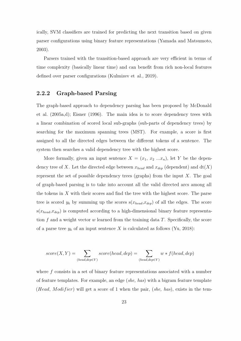
2-6 An example of a graph-based dependency parsing (taken from (Yu,

2018)) . . . . . . . . . . . . . . . . . . . . . . . . . . . . . . . . . . . 25

2-7 An example of binary feature representations (from https://blog.

acolyer.org/2016/04/21/the-amazing-power-of-word-vectors/) 26

2-8 An example of the continuous representations (same source as for the

previous figure). . . . . . . . . . . . . . . . . . . . . . . . . . . . . . . 26

IX

2-9 An example of the skip-gram model. Here, it predicts the center (focus)

word ‘‘learning” based on the context words (same source as for the

previous figure). . . . . . . . . . . . . . . . . . . . . . . . . . . . . . 27

2-10 Illustration of the neural model scheme of the graph-based parser when

calculating the score of a given parse tree (this figure and caption

are taken from the original paper (Kiperwasser and Goldberg, 2016a)).

The parse tree is depicted below the sentence. Each dependency arc

in the sentence is scored using an MLP that is fed by the BiLSTM

encoding of the words at the arc’s end points (the colors of the arcs

correspond to colors of the MLP inputs above), and the individual arc

scores are summed to produce the final score. All the MLPs share the

same parameters. The figure depicts a single-layer BiLSTM, while in

practice they use two layers. When parsing a sentence, they compute

scores for all possible n2 arcs, and find the best scoring tree using a

dynamic-programming algorithm. . . . . . . . . . . . . . . . . . . . . 31

2-11 Illustration of multilingual transfer learning in NLP (the figure is based

from (Jamshidi et al., 2017)) . . . . . . . . . . . . . . . . . . . . . . . 37

2-12 ’’How the transfer learning transfers knowledge in parsing?’’. A parser

learns the shared parameters (Wd) based on supervised-learning. Since

the learning is a data-driven task with inputs, source language can

affect to tune the parameter (Wd) for the target language (the figure

is taken from (Yu et al., 2018). . . . . . . . . . . . . . . . . . . . . . 38

X

3-1 Overall system structure for training language models. (1) Embed-

ding Layer: vectorized features that are feeding into Bidirectional

LSTM. (2) Bidirectional-LSTM: train representation of each to-

ken as vector values based on bidirectional LSTM neural network. (3)

Multi-Layer Perceptron: build candidate of parse trees based on

trained(changed) features by bidirectional LSTM layer, and then cal-

culate probabilistic scores for each of candidates. Finally, if it has

multiple roots, revise it or select the best parse tree. . . . . . . . . . 44

4-1 An example of the cross-lingual representation learning method be-

tween English (Source Language) and French (Target Language) . . . 63

4-2 An example of our cross-lingual dependency parsing for Russian (Source

Language) and Komi (Target Language) . . . . . . . . . . . . . . . . 66

5-1 An example of the word-based character model with a single attention

representation (Dozat et al., 2017b) . . . . . . . . . . . . . . . . . . . 83

5-2 An example of the word-based character model with three attention

representations. . . . . . . . . . . . . . . . . . . . . . . . . . . . . . . 84

5-3 (A) Structure of the tagger proposed by Dozat et al. (2017b) using a

word-based character model and (B) structure of the tagger proposed

by Bohnet et al. (2018a) using a sentence-based character model with

meta-LSTM. . . . . . . . . . . . . . . . . . . . . . . . . . . . . . . . . 85

5-4 Overall structure of our contextualized tagger with three different clas-

sifiers. . . . . . . . . . . . . . . . . . . . . . . . . . . . . . . . . . . . 90

5-5 An example of the procedure to generate a weighted POS embedding. 91

5-6 Overall structure of our multi-task dependency parser. . . . . . . . . 101

6-1 An example of word similarity captured by different Views (from CS224N

Stanford Lecture: http://web.stanford.edu/class/cs224n/) 121

XI

6-2 Overall structure of our baseline model. This system generates word-

and character-level representation vectors, and concatenates them as

a unified word embedding for every token in a sentence. To trans-

form this embedding into a context-sensitive one, the system encodes

it based on the individual BiLSTM for each tagger and parser. . . . 122

6-3 Overall structure of our Co-meta model. The system consists of three

different pairs of taggers and parsers that are trained using limited

context information. Based on the input representation of the word,

character, and meta, each model draws a differently shaped parse tree.

Finally, our co-training module induces models to learn from each other

using each model’s predicted result. . . . . . . . . . . . . . . . . . . 124

6-4 An example of the label selection method for ensemble and voting. 133

6-5 Evaluation results for Chinese (zh_gsd) based on different sizes of

the unlabeled set and proposed models. We apply ensemble-based

Co-meta with the fixed size of 50 training sentences while varying

the unlabeled set size. . . . . . . . . . . . . . . . . . . . . . . . . . . 134

6-6 Evaluation results for Chinese (zh_gsd) based on the different sizes

of the train set and proposed models. We apply ensemble based

Co-meta with the fixed size of 12k unlabeled sentences while varying

training set size. . . . . . . . . . . . . . . . . . . . . . . . . . . . . . 136

7-1 The overall structure of our Co-metaM model. This system gener-

ates word- and character-level representation vectors and concatenates

them into a unified word embedding for every token in a sentence. The

word-level representation can be a multilingual embedding as proposed

in Section 4.2. Thus, this system can train a dependency model, using

both labeled and unlabeled resources from several languages. . . . . 142

A-1 An example of tokenization of Universal Dependency . . . . . . . . . 155

A-2 An example of syntactic annotation of Universal Dependency . . . . . 156

XII

B-1 Architecture du réseau de neurones . . . . . . . . . . . . . . . . . . . 174

XIII

List of Tables

3.1 Official results with rank. (number): number of corpora . . . . . . . 50

3.2 Official results with monolingual models (1). . . . . . . . . . . . . . 52

3.3 Official results with monolingual models (2). . . . . . . . . . . . . . 53

3.4 Relative contribution of the different representation methods on the

English development set (English_EWT). . . . . . . . . . . . . . . . 54

3.5 Contribution of the multi-source trainable methods on the English de-

velopment set (English_EWT). . . . . . . . . . . . . . . . . . . . . . 54

4.1 Dictionary sizes and size of bilingual word embeddings generated by

each dictionary. . . . . . . . . . . . . . . . . . . . . . . . . . . . . . . 64

4.2 Labeled attachment scores (LAS) and unlabeled attachment scores

(UAS) for Northern Sami (sme) . . . . . . . . . . . . . . . . . . . . . 68

4.3 The highest results of this experiment (FinnishSami model) compared

with top 3 results for Sami from the CoNLL 2017 Shared Task. . . . 69

4.4 Labeled attachment scores (LAS) and unlabeled attachment score (UAS)

for Komi (kpv). We doesn’t conduct training for ‘‘kpv + eng + rus”

language combination because of unrealistic training scenario (It takes

more than 40GB memory for training) . . . . . . . . . . . . . . . . . 69

XIV

4.5 Languages trained by a multilingual model. Embedding model: ap-

plied languages that were used for making multilingual word embed-

dings. Bilingual Dic: resources to generate bilingual dictionaries

Training corpora: Training corpora that were used. 7 languages:

English, Italian, French, Spanish, Portuguese, German, Swedish. (num-

ber): the number of multiplication to expand the total amount of corpus. 72

4.6 Official experiment results with rank. (number): number of corpora . 74

4.7 Official experiment results processed by multilingual models. . . . . 74

5.1 Hyperparameter Details . . . . . . . . . . . . . . . . . . . . . . . . . 93

5.2 universal part-of-speech (UPOS) tagging results compared with the

best performing team (winn) of each treebank for the ST. Columns

denotes the size of training corpus Size, and our joint (join), joint with

ELMo (joinE), concatenated (conc) and ELMo only (elmo) models.

The symbols ∗ represents the result applied the ELMo embedding and+ represents the result applied an ensemble. . . . . . . . . . . . . . . 94

5.3 eu_bdt (Basque) tagging results by the number of attention heads n

of the word and sentence-based character embedding. Here, word

and sent denote models which trained taggers only word and sen-

tence-based character representations (as described in (5.1)) . . . . . 97

5.4 Overall experiment results based on each group of corpora. . . . . . . 106

5.5 Official experiment results for each corpus, where tr (Treebank), mu

(Multilingual) and el (ELMo) in the column Method denote the feature

representation methods used (see Section 5.4.1). . . . . . . . . . . . . 107

5.6 Official experiment results for each corpus, where tr (Treebank), mu

(Multilingual) and el (ELMo) in the column Method denote the feature

representation methods used (see Section 5.4.1). . . . . . . . . . . . . 108

5.7 Languages trained with multilingual word embeddings and their rank-

ing. . . . . . . . . . . . . . . . . . . . . . . . . . . . . . . . . . . . . 110

XV

5.8 Relative contribution of the different representation methods on the

overall results. . . . . . . . . . . . . . . . . . . . . . . . . . . . . . . . 111

5.9 UAS and LAS on English(en_ewt) corpus for each model, with ELMo

(elmo), character (char), and pre-trained word embeddings (ext)

over only unknown words. . . . . . . . . . . . . . . . . . . . . . . . . 112

5.10 Official evaluation results on three EPE task (see https://goo.gl/

3Fmjke). . . . . . . . . . . . . . . . . . . . . . . . . . . . . . . . . . 113

6.1 Hyperparameter Details . . . . . . . . . . . . . . . . . . . . . . . . . 128

6.2 LAS and UPOS scores of M (meta) model output on the test set using

50 training sentences and unlabeled sentences based using Co-meta,

meta-base, and our baseline model (Lim et al., 2018a). We report

meta-base to decompose the performance gain into the gains due to

meta-base (supervised) and Co-meta (SSL). *Kazakh only has 31

labeled instances. Thus we use only 31 sentences and its unlabeled data

are sourced from Wikipedia whereas other languages take the unlabeled

data from the given training corpus after removing label information. 130

6.3 LAS and UPOS scores of M (meta) model on the test set using 100

training sentences. We see that Co-meta takes over baseline for

Finnish, unlike the results in Table 6.2 (50 sentences used) . . . . . . 131

6.4 LAS on the Greek(el_bdt) corpus for each model, with the average

confidence score g(y) comparing M (word) and M (char) over the entire

test set using 100 training sentences. . . . . . . . . . . . . . . . . . . 132

6.5 Scores of Co-meta with the ensemble method on different domains

of unlabeled data with 100 training sentences. . . . . . . . . . . . . . 135

6.6 LAS for the English (en_ewt) corpus for each model, with the external

language models with the entire train set. . . . . . . . . . . . . . . . 137

XVI

6.7 LAS for the Chinese (zh_gsd) corpus for each model, with BERT–

Multilingual embedding using the entire training set. We observe much

higher improvements than for English showed (see Table 6.6), probably

because zh_gsd has a relatively small training set (3,997) and larger

character sets than the training set (12,543) of en_ewt. . . . . . . . . 138

7.1 Dictionary sizes and size of bilingual word embeddings generated from

each dictionary. . . . . . . . . . . . . . . . . . . . . . . . . . . . . . . 144

7.2 Labeled attachment scores (LAS) and unlabeled attachment scores

(UAS) for Northern Sami (sme) based on the use of the training corpora145

7.3 Comparison with top four results for Sami from the CoNLL 2017

Shared Task and our multilingual model trained on Sami and Finnish

corpora. . . . . . . . . . . . . . . . . . . . . . . . . . . . . . . . . . . 146

B.1 Taille des dictionnaires et des plongements de mots liés générés à partir

des différents dictionnaires (il s’agit de dictionnaires de formes fléchies,

ce qui explique que la taille du dictionnaire finnois-same du nord soit

par exemple différente de celle du dictionnaire same du nord-finnois). 171

B.2 Meilleurs résultats (officiels) pour le same lors de la tâche commune

CoNLL 2017 et résultat obtenu par le LATTICE lors de cette même

évaluation . . . . . . . . . . . . . . . . . . . . . . . . . . . . . . . . . 177

B.3 Évaluation de l’analyse du same du nord (sme) : scores LAS (labeled

attachment scores) et UAS (unlabeled attachment scores), c’est-à-dire

scores calculés en prenant en compte l’étiquette de la relation (score

LAS, colonne de gauche), et sans elle (score UAS, colonne de droite).

La première ligne sme (20) réfère à l’expérience utilisant uniquement

sur les vingt phrases annotées de same disponibles pour l’entraînement.

Les autres lignes montrent les résultats avec différentes combinaisons

de corpus annotés : anglais (eng) et finnois (fin). Pour chaque corpus,

le nombre de phrases utilisées est indiqué entre parenthèses. . . . . . 179

XVII

B.4 Évaluation de l’analyse syntaxique du komi. La première ligne kpv

(10) réfère à l’expérience utilisant uniquement les dix phrases annotées

de komi disponibles pour l’entraînement. Les autres lignes montrent

les résultats avec différentes combinaisons de corpus annotés : anglais

(eng), russe (rus), et finnois (fin). Pour chaque corpus, le nombre de

phrases utilisées est indiqué entre parenthèses. . . . . . . . . . . . . 180

XVIII

Chapter 1

Introduction

Thus far, natural language processing (NLP) has mainly focused on a small number

of languages for which different kinds of resources are available. The gradual devel-

opment of the Web, as well as of social media, has revealed the need to deal with

more languages which, in turn, present new challenges. For example, it is clear that

languages exhibit a large diversity of features, particularly concerning morphological

and syntactic complexity, and NLP tools (e.g., part-of-speech taggers and dependency

parsers) which must tackle this diversity to yield acceptable performance. In this con-

text, developing systems for low-resource languages is a crucial issue for NLP.

Parsing is the process of analyzing the syntactic structure of sentences. The struc-

ture of a sentence corresponds to the arrangement of the words within the sentence.

This can be expressed as a set of dependencies: each word in the sentence (except the

main verb) depends on another one (the subject of a sentence depends on the verb,

the determiner in a noun phrase depends on the noun, and so on). All these relations

can be formalized as relations between couple of words, a head (i.e. the verb) and a

dependent (i.e. the noun that is the subject of the verb). The main element of the

sentence (generally, the verb) has no head and is called the root of the sentence.

Syntax encodes the relations between the words in the sentence, and therefore, it

is the first step towards semantics. Parsing, the automatic analysis of the syntactic

structure of the sentence, is thus important for downstream NLP tasks, such as named

entity recognition (Kazama and Torisawa, 2008), discourse understanding (Sagae,

1

2009), or information extraction (Fares et al., 2018b). The traditional approach to

parsing was to manually develop rules encoding the grammar of the language, but

in practice, this leads to rather poor results. A large set of rules is hard to produce

and to maintain, generally provides a limited coverage, and more importantly, often

leads to inconsistencies because different phenomena may appear and interact in a

same sentence.

In this context, machine learning and the availability of annotated corpora pro-

vided a relevant alternative approach to parsing. More than 20 years ago, most NLP

systems were built using supervised learning techniques (Weiss et al., 2015b; Straka

et al., 2016; Ballesteros et al., 2016a). These systems observe large annotated corpora

to identify regularities and acquire (‘‘learn’’) a model that can reproduce the observed

annotation as accurately as possible. This model can then be applied to unseen data

and provide syntactic annotations (the task known as parsing) over unseen data.

However, this strategy implies that large amounts of annotated data are available:

the approach is thus well suited for languages for which this type of data exists. Un-

fortunately, producing enough annotated data for accurate parsing is known to be

time- and resource-consuming. A known problem is the lack of resources (particu-

larly annotated corpora) for most languages. As a recent example, the 2018 CoNLL

Shared Task considered around 57 languages; these included approximately all the

languages for which sufficient syntactically annotated data are available in the Univer-

sal Dependency format. This was probably the most ambitious parsing challenge ever

undertaken with regard to language diversity. However, the figure of 57 languages

should be viewed in the context of 6,000 languages in the world: even if we consider

only the languages for which written data are available, the 57 languages targeted at

CoNLL 2018 represent a fraction of all languages in the world.

Therefore, there is no accurate parser for several languages for which this kind of

technology would be useful, and the lack of resources constitutes a bottleneck that is

hard to overcome.

2

1.1 Research Questions

As we have just seen, for dependency parsing, (A) the monolingual and (B) su-

pervised approach based on syntactically annotated corpora has long been the most

popular one. However, because of recent developments involving (A) multilingual

feature representations and (B) semi-supervised methods, which allow NLP sys-

tems to learn from unlabeled data, more accurate NLP models, even for low resource

languages, can now be developed. This leads to two main research questions:

• (A) What are the benefits of multilingual models for parsing, especially in low

resource scenarios?

• (B) Can we make use of unlabeled data for parsing, especially in low resource

scenarios?

Although one can sometimes find limited data (such as a list of words or a small

dictionary) for low-resource languages, more substantial unlabeled data (e.g., from

Wikipedia) can often be obtained, as well as annotated data from other languages

that are typologically or geographically related1. We detail these questions in the

remainder of this section.

Question A: What are the benefits of multilingual models for parsing,

particularly in low resource scenarios? We know that multilingual approaches

to parsing have yielded encouraging results for both low- (Ammar et al., 2016b) and

high-resource scenarios (Guo et al., 2015b). Generally, the multilingual approach

can be implemented in two ways. The first approach involves projecting annotations

available for a high-resource language onto a low-resource language using a parallel

corpus, while the second aims at producing a cross-lingual transfer model that can

work for several languages using transfer learning. (Guo et al., 2016) and (Ammar

et al., 2016b) have conducted multilingual parsing studies on Indo-European lan-

guages using this second approach. They demonstrated that a multilingual model1Geography also plays a role. This is known as contact linguistics: two languages that are in close

contact, through a community of bilingual speakers (or not bilingual), will often share a commonvocabulary, at least some borrowings, and often even syntactic structures.

3

can yield better results than several monolingual models (one per language) for dif-

ferent European languages. Specifically, (Ammar et al., 2016b) made an artificial

low-resource scenario that uses only 50 training sentences to investigate the perfor-

mance of their multilingual approach. However, their approach relied on the existence

of a massive parallel corpus, as their experiment was based on Europarl2. Thus, the

problem of low-resource languages that do not have a massive parallel corpus remains

unaddressed. This raises two sub-questions which are as follows:

• (A-1) Is parallel data a requirement for multilingual parsing? (Section 4.2)

• (A-2) How can we bootstrap a system when no parallel corpus is available?

(Section 4.2 and 4.3)

In order to investigate and answer these questions, we propose a simple but pow-

erful method for creating a dependency parsing model when no annotated corpus or

parallel corpus is available for training. Our approach requires only a small bilin-

gual dictionary and a manual annotation of a handful of sentences. It is assumed

that the performance we obtain with this approach depends largely on the set of

languages used to train the model. Therefore, we developed several models using

genetically related and non-related languages, so as to gain a better understanding

of the limitations or possibilities of model transfer across different language families.

Question B: Can we make use of unlabeled data for parsing, especially

in low resource scenarios? This question is related to semi-supervised learning,

i.e., the ability to learn from annotated and also from non-annotated data conjointly.

Two major semi-supervised approaches have been proposed for parsing: self-training

(McClosky et al., 2006; Sagae, 2010) and co-training (Sarkar, 2001; Sagae, 2009; Zhang

et al., 2012; Yu, 2018). The goal of co-training is to train multiple learners (parsers in

our case) based on different ‘‘views” that can subsequently be applied on unlabeled

data. A view in NLP typically corresponds to a specific level of analysis (such as

character-based and token-based). The successful use of co-training depends on the2www.statmt.org/europarl

4

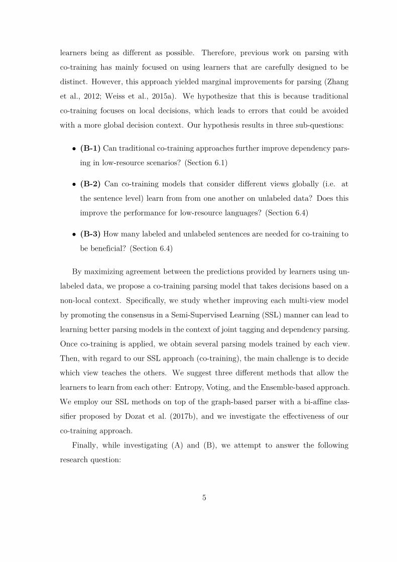
learners being as different as possible. Therefore, previous work on parsing with

co-training has mainly focused on using learners that are carefully designed to be

distinct. However, this approach yielded marginal improvements for parsing (Zhang

et al., 2012; Weiss et al., 2015a). We hypothesize that this is because traditional

co-training focuses on local decisions, which leads to errors that could be avoided

with a more global decision context. Our hypothesis results in three sub-questions:

• (B-1) Can traditional co-training approaches further improve dependency pars-

ing in low-resource scenarios? (Section 6.1)

• (B-2) Can co-training models that consider different views globally (i.e. at

the sentence level) learn from from one another on unlabeled data? Does this

improve the performance for low-resource languages? (Section 6.4)

• (B-3) How many labeled and unlabeled sentences are needed for co-training to

be beneficial? (Section 6.4)

By maximizing agreement between the predictions provided by learners using un-

labeled data, we propose a co-training parsing model that takes decisions based on a

non-local context. Specifically, we study whether improving each multi-view model

by promoting the consensus in a Semi-Supervised Learning (SSL) manner can lead to

learning better parsing models in the context of joint tagging and dependency parsing.

Once co-training is applied, we obtain several parsing models trained by each view.

Then, with regard to our SSL approach (co-training), the main challenge is to decide

which view teaches the others. We suggest three different methods that allow the

learners to learn from each other: Entropy, Voting, and the Ensemble-based approach.

We employ our SSL methods on top of the graph-based parser with a bi-affine clas-

sifier proposed by Dozat et al. (2017b), and we investigate the effectiveness of our

co-training approach.

Finally, while investigating (A) and (B), we attempt to answer the following

research question:

5

• (C) What are the benefits of simultaneously applying the two proposed ap-

proaches, (A) multilingual and (B) SSL, as multilingual SSL models? (Section

7.2)

1.2 Contributions

Considering the aforementioned challenges, the contributions of this thesis are (1)

the development and analysis of a new multi-source trainable dependency parser, (2)

the investigation of SSL methods using unlabeled data, and (3) the creation of new

resources for low-resource languages.

• Proposal for a new multi-source trainable parser. The major contribu-

tion of this study is the description of a new multilingual dependency parser

that integrates multilingual word embeddings. Concerning word embeddings,

we show that the bilingual word mapping approach (Artetxe et al., 2016a) can

be extended to cope with multilingual data. With this parsing model, we partic-

ipated in the official CoNLL 2017 and 2018 shared tasks that required to parse

57 languages, including low-resource ones (Zeman et al., 2018b). Our parser

regularly ranked among the 5 best systems for parsing, and also achieved the

best performance in the so called ‘‘extrinsic evaluation” (especially for informa-

tion extraction) (Fares et al., 2018a). The parser3 and POS-tagger4 are publicly

available.

• Investigation of SSL for parsing. The study investigates whether co-train-

ing is beneficial in both low- and high-resource conditions. As SSL methods

use unlabeled (uncertain) data, their performance must be investigated based

on the resource used. We experimented with diverse conditions by changing

the amount and domains of unlabeled data and the effect of all these variables

on the proposed model. Our experiments on joint parsing with SSL methods

resulted in three sub-contributions: (1) the proposal of a new formulation for3https://github.com/jujbob/multilingual-bist-parser4https://github.com/jujbob/Utagger

6

co-training that leverages consensus promotion in addition to multi-views. (2)

the analysis of the relative performance of each multi-view model. (3) the ex-

ploration of different semi-supervised scenarios, where the amount and domains

of unlabeled data vary.

• Creation of language resources. New resources were developed over the

course of the thesis. With Niko Partanen, we created a new corpus for Komi

with syntactic information encoded in the Universal Dependencies format5, as

well as bilingual dictionaries, multilingual word embeddings for Komi and Sami,

and a parser for the language, based on the multilingual approach described

above. All these resources are available for free in public repositories6. These

languages are interesting for at least three reasons: (1) they are typical of a

large number of languages for which very few resources exist, specifically no

annotated corpus but raw corpora in large enough quantities; (2) they are mor-

phologically-rich languages, which makes them hard to process; and (3) they

are supported by an active community of users that is very positive towards

language technology development. We had the chance to work with Niko Par-

tanen, a specialist of Finno-Ugric languages, especially Komi and Sami, during

the course of the thesis.

1.3 Thesis Structure

Each of the chapters 3-6 present a new parsing model that is an increment over the

previous one. Chapter 3 presents our baseline model based on monolingual lexical

representations. Chapter 4 extends the baseline model to a multilingual one. Chapter

5 describes a more complex version of this model, adding character-level and deep

contextualized representations, that improve out-of-vocabulary (i.e., unknown words

that appear in the testing data) processing. Finally, Chapter 6 integrates the co-train-

ing strategy intended to utilize unlabeled data. Each chapter presents the main idea5github.com/langdoc/UD_Komi-Zyrian6See github.com/jujbob/multilingual-bist-parser, and github.com/jujbob/multilingual-models.

7

of the chapter, technical developments, experimental results, and a brief discussion

of these results. The structure of the thesis, including Background and Conclusion,

is as follows:

• In Chapter 2, we first describe in detail the background information from

previous works. This chapter introduces the idea of dependency parsing along

with the two main algorithms: graph- and transition-based parsing. Then, we

discuss the more recent deep neural network techniques for developing parsers

with an example of the Bi-directional Long Short Term Memory (BIST) parser,

which considers contextualized information. We then introduce an overview of

the corpora and evaluation metrics used for dependency parsing. In Section 2.2

and 2.3, we present the transfer learning and co-training approaches, which are

fundamental for our parser.

• In Chapters 3 and 4, we introduce our multilingual parsing approach. We

first present an overview of our approach in Chapter 3 with a baseline model,

before detailing the multilingual resource representation used, in Chapter 4. In

section 4.3, we present our multilingual approach to Komi. As we have seen

before (Section 1.2), Komi offers a realistic and relevant use case as a low re-

source language with no annotated corpora available for training. We also detail

the annotated corpora that were developed to test the method in Section 4.3.1.

Moreover, we present the details of our participation in the CoNLL 2017 shared

task with our parser. In Section 3.2 and 4.4, we compare the performance of

our parser with other parsers that applied mono- and multilingual approaches.

• In chapter 5, we introduce deep contextualized representations. We begin by

discussing the most recent sub-word representations in Section 5.1, as well as

a deep contextual representation method, Embeddings from Language Models

(ELMo), which is an approach aiming at learning contextualized word vectors

(Section 5.2). Then, we detail our implementation of these representations.

Specifically, we describe the feature extraction and representation methods for

our POS tagger (Section 5.3) and parser, based on multi-task joint learning (Sec-

8

tion 5.4). Finally we provide an analysis of the experimental results obtained

on the CoNLL 2018 shared task data (Section 5.4.2).

• In chapter 6, we introduce our experiments with a semi-supervised approach.

We first discuss the effect of multi-view learning in Section 6.1. Then, we intro-

duce co-training, along with the multi-view structure in Section 6.2, Then, we

describe our experiments performed on unlabeled data from different domains

and sizes in Section 6.4.

• In chapter 7, we describe a parser that can simultaneously apply the proposed

multilingual and semi-supervised approaches. In Section 7.1, we propose a pro-

jection method that can integrate multilingual and semi-supervised approaches.

The experiment is detailed in Section 7.2, and the results are presented in Sec-

tion 7.3.

• In chapter 8, we summarize our thesis along with providing answers to the

questions raised in the Introduction.

1.4 Publications Related to the Thesis

There are seven publications based on this thesis, and the code used for all experiments

is publicly available on https://github.com/jujbob. The work described in

Chapter 4 has given birth to four different publications:

• KyungTae Lim, Niko Partanen, and Thierry Poibeau. Analyse syntaxique de

langues faiblement dotées à partir de plongements de mots multilingues. Traite-

ment Automatique des Langues (2018), volume 59, pages 67-91.

• Niko Partanen, KyungTae Lim, Michael Rießler, and Thierry Poibeau. De-

pendency parsing of code-switching data with cross-lingual feature representa-

tions. In Proceedings of the Fourth International Workshop on Computatinal

Linguistics of Uralic Languages. (2018). pages 117.

9

• KyungTae Lim, Niko Partanen, and Thierry Poibeau. 2018. Multilingual

Dependency Parsing for LowResource Languages: Case Studies on North Sami

and Komi-Zyrian. In Proceedings of the Eleventh International Conference on

Language Resources and Evaluation (LREC 2018). Miyazaki, Japan.

• KyungTae Lim, and Thierry Poibeau A System for Multilingual Dependency

Parsing based on Bidirectional LSTM Feature Representations. Proceedings of

the CoNLL 2017 Shared Task: Multilingual Parsing from Raw Text to Univer-

sal Dependencies (2017). pages 63-70.

The work described in Chapter 5 has given birth to two different publications:

• KyungTae Lim, Stephen McGregor and Thierry Poibeau. Joint Deep Charac-

ter-Level LSTMs for POS Tagging. Proceedings of the Twentieth International

Conference on Computational Linguistics and Intelligent Text Processing (CI-

CLing 2019), (Accepted)

• KyungTae Lim, Cheoneum Park, Changki Lee and Thierry Poibeau. SEx

BiST: A Multi-Source Trainable Parser with Deep Contextualized Lexical Repre-

sentations. Proceedings of the CoNLL 2018 Shared Task: Multilingual Parsing

from Raw Text to Universal Dependencies (2018)

The work described in Chapter 6, dependency parsing with a semi-supervised

learning (co-training), has given birth to a publication:

• KyungTae Lim Jay-Yoon Lee, Jaime Carbonell, and Thierry Poibeau. Semi–

Supervised Learning on Meta Structure: Multi-Task Tagging and Parsing in

Low-Resource Scenarios. Proceedings of the Thirty-Fourth AAAI Conference

on Artificial Intelligence (AAAI 2020), (Accepted)

10

Chapter 2

Background

In this chapter, we introduce the notion of dependency parsing. We describe the

main algorithms, datasets and evaluation metrics used in the field.

2.1 Syntactic Representation

Syntax refers to the set of rules that govern the relations between words within a

sentence (and therefore the structure of this sentence), in a given language. This do-

main is of crucial importance for natural language processing, since it is mandatory

to first establish the relations between words in order to then capture the meaning

of a sequence of words. Any advanced natural language application (e.g., informa-

tion extraction, question-answering, etc.) requires some kind of syntactic analysis to

produce accurate outputs.

A sentence can be hierarchically decomposed into logical groups of words, like a

noun phrase (a group of words around a noun) and a verb phrase (idem, around a

verb), until individual words are reached. This process is called ’’constituent analysis”

(or ’’phrase analysis’’) (Chomsky and Lightfoot, 2002)1. An alternative is a depen-

dency analysis (or ’’dependency representation’’), where each word in the sentence is

directly linked to another one, called the head (the word than depends on the head

is called a dependent) (Tesnière, 1959; De Marneffe et al., 2006; de Marneffe and1http://en.wikipedia.org/wiki/Phrase_structure_grammar

11

Figure 2-1: Syntactic representation of the sentence ‘‘The big dog chased the cat’’.On the left a constituent analysis, on the right the dependency analysis.

Manning, 2008; Nivre et al., 2016a)2. Generally the verb is the main element in the

sentence (it is the only element that does not have a head in the sentence). With a

dependency analysis, the main constituents of the sentence are not directly visible (as

opposed to a constituent-base analysis), but the relations between the main lexical

elements in the sentence (i.e., the arguments of the verb) are more directly accessible.

Let’s take a simple example, with the sentence ‘‘The big dog chased the cat’’. A

phrase-based representation of this sentence is shown on the left of Figure 2-1. In

this figure, the terminal and non-terminal nodes are categorized with tags such as:

NP (Noun phrase), VP (Verb phrase), Art (article), Adj (adjective), N (noun), and V

(verb). The constituent structure and the labels can also be represented in a labeled

bracketed structure, as follows:

• Input : The big dog chased the cat

• Representation: [NP The big dog NP] [VP chased [NP the cat NP] VP]3

A dependency representation of ‘‘The big dog chased the cat” would the one in

the right of Figure 2-1. In this example, we can see that both the subject (dog) and

the object (cat) are directly linked to the verb (chased) This structure has only ter-

minal nodes, which means there is no distinction between terminal and non-terminal2http://en.wikipedia.org/wiki/Dependency_grammar, Lucien Tesnière, Professor for Compara-

tive Linguistics at the University of Montpellier from 1937 to his death in 1954, is the undoubtedfather of dependency

3This example is taken from: http://www.ilc.cnr.it/EAGLES96/segsasg1/node44.html

12

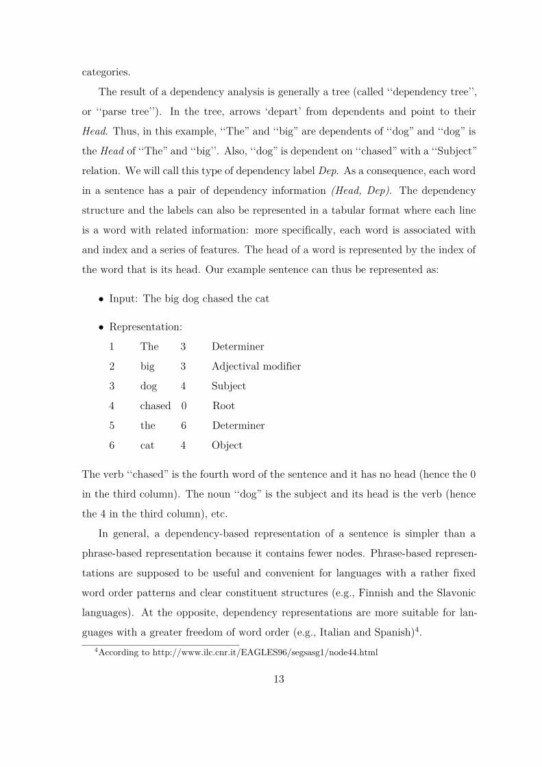
categories.

The result of a dependency analysis is generally a tree (called ‘‘dependency tree’’,

or ‘‘parse tree’’). In the tree, arrows ‘depart’ from dependents and point to their

Head. Thus, in this example, ‘‘The” and ‘‘big” are dependents of ‘‘dog” and ‘‘dog” is

the Head of ‘‘The” and ‘‘big’’. Also, ‘‘dog” is dependent on ‘‘chased” with a ‘‘Subject”

relation. We will call this type of dependency label Dep. As a consequence, each word

in a sentence has a pair of dependency information (Head, Dep). The dependency

structure and the labels can also be represented in a tabular format where each line

is a word with related information: more specifically, each word is associated with

and index and a series of features. The head of a word is represented by the index of

the word that is its head. Our example sentence can thus be represented as:

• Input: The big dog chased the cat

• Representation:

1 The 3 Determiner

2 big 3 Adjectival modifier

3 dog 4 Subject

4 chased 0 Root

5 the 6 Determiner

6 cat 4 Object

The verb ‘‘chased” is the fourth word of the sentence and it has no head (hence the 0

in the third column). The noun ‘‘dog” is the subject and its head is the verb (hence

the 4 in the third column), etc.

In general, a dependency-based representation of a sentence is simpler than a

phrase-based representation because it contains fewer nodes. Phrase-based represen-

tations are supposed to be useful and convenient for languages with a rather fixed

word order patterns and clear constituent structures (e.g., Finnish and the Slavonic

languages). At the opposite, dependency representations are more suitable for lan-

guages with a greater freedom of word order (e.g., Italian and Spanish)4.4According to http://www.ilc.cnr.it/EAGLES96/segsasg1/node44.html

13

The task consisting in automatically (i.e., by means of a computer) analyzing

the structure of sentences in a given language is called parsing. The main idea is

to automatically produce, from a sentence taken in input, a tree structure encoding

the relations among words in the sentence. Different parsers have been developed

to produce a constituent-based analysis, as well as a dependency analysis. A parser

that follows phrase structure principles is thus called a phrase structure parser (con-

stituency parser). At the opposite, a parser that follows dependency principles is

called a dependency parser.

Initially, the parsing community primarily focused on constituency parsing sys-

tems; as a result, a number of high accuracy constituency parsers have been intro-

duced, such as the Collins Parser (Collins, 2003), the Stanford PCFG Parser (Klein

and Manning, 2003), and the Berkeley Parser (Petrov and Klein, 2007). In the

past decade, dependency-based systems have gained more attention (McDonald and

Pereira, 2006; Nivre, 2004; Bohnet, 2010; Martins et al., 2013), as they have better

multilingual capacity and are supposed to be more efficient. All the experiments

described in this thesis have been done within the dependency framework.

In the following section, we will concentrate on the recent developments in the

field, especially the Universal dependencies initiative, and then recent dependency

parsing algorithms (Section 2.2).

Universal Dependency Representation

Several syntactic dependency representations have been proposed during the last

decade. As said on the Universal Dependencies (UD) website, UD ‘‘is a project that

is developing cross-linguistically consistent treebank annotation for many languages,

with the goal of facilitating multilingual parser development, cross-lingual learning,

and parsing research from a language typology perspective. The annotation scheme

is based on an evolution of (universal) Stanford dependencies (De Marneffe et al.,

2006; de Marneffe and Manning, 2008; De Marneffe et al., 2014), Google universal

part-of-speech tags (Petrov and McDonald, 2012), and the Interset interlingua for

14

morphosyntactic tagsets (Zeman, 2008)”5.

The Stanford Dependencies framework was originally invented in 2005 as a practi-

cal way to encode English syntax and help natural language understanding (NLU) ap-

plications. The annotation scheme was then extended as the main annotation scheme

for the dependency analysis of English (De Marneffe et al., 2006). This schema has

then been adapted to several other languages such as Chinese (Chang et al., 2009),

Italian (Bosco et al., 2013), or Finnish (Haverinen et al., 2014).

Meanwhile, the 2006 CoNLL shared task dealt with multilingual dependency pars-

ing McDonald and Nivre (2007a). The goal of this shared task was to evaluate depen-

dency parsing for 13 languages. The annotations used for each language was different,

hence the need to define a common format so as to make the comparison of the results

possible. Google decided to develop its own tag set in 2006 for the evaluation done

in the framework of the 2006 CoNLL shared task (Buchholz and Marsi, 2006). The

Google universal tag set also served to convert other tag sets developed in different

places, in multilingual contexts.

At some point, each treebank was annotated using some specific tools, with dif-

ferent tagsets, even for the same task. This led researchers to propose a conversion

method, for different tagsets, with the aim of making these tagsets reusable. (Zeman,

2008) proposed a universal approach ‘‘Interset” that converts different tagsets from a

source language to a target language. This universal tagset later served as a basis for

the Universal Dependency standard, especially for language-specific morphological

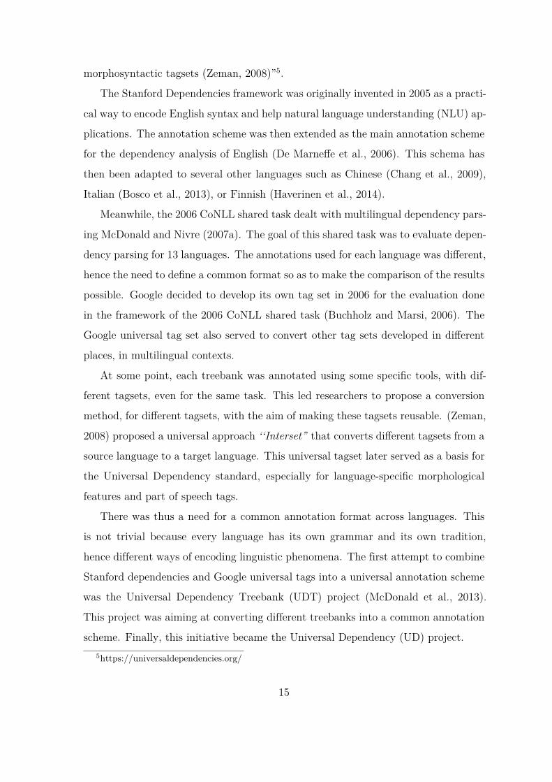
features and part of speech tags.

There was thus a need for a common annotation format across languages. This

is not trivial because every language has its own grammar and its own tradition,

hence different ways of encoding linguistic phenomena. The first attempt to combine

Stanford dependencies and Google universal tags into a universal annotation scheme

was the Universal Dependency Treebank (UDT) project (McDonald et al., 2013).

This project was aiming at converting different treebanks into a common annotation

scheme. Finally, this initiative became the Universal Dependency (UD) project.5https://universaldependencies.org/

15

In this study, we use Universal Dependencies (UD), which is a framework provid-

ing a consistent syntactic annotation scheme (including parts of speech, morpholog-

ical features, and syntactic dependencies) across different human languages. UD is

an open community effort with over 200 contributors who have so far produced more

than 100 treebanks in over 70 languages.

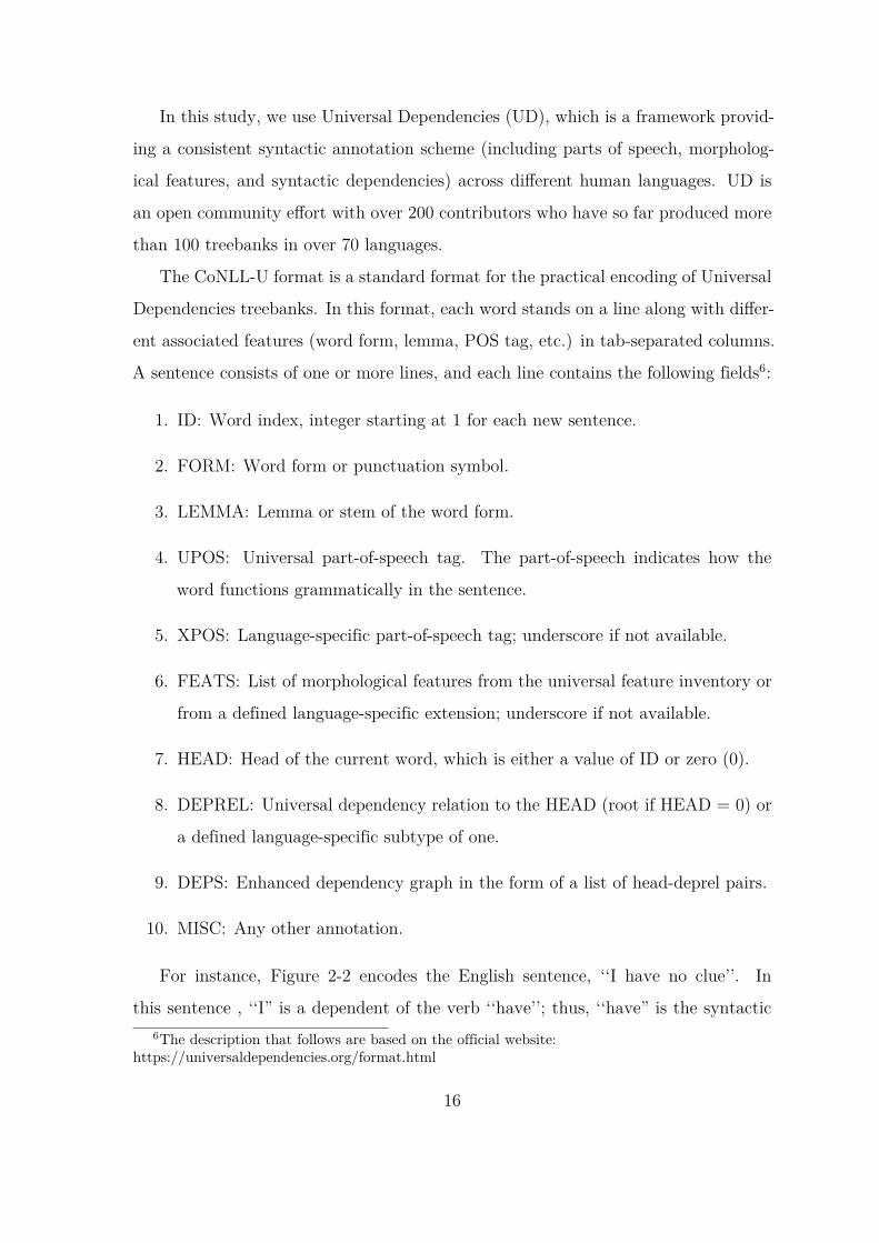
The CoNLL-U format is a standard format for the practical encoding of Universal

Dependencies treebanks. In this format, each word stands on a line along with differ-

ent associated features (word form, lemma, POS tag, etc.) in tab-separated columns.

A sentence consists of one or more lines, and each line contains the following fields6:

1. ID: Word index, integer starting at 1 for each new sentence.

2. FORM: Word form or punctuation symbol.

3. LEMMA: Lemma or stem of the word form.

4. UPOS: Universal part-of-speech tag. The part-of-speech indicates how the

word functions grammatically in the sentence.

5. XPOS: Language-specific part-of-speech tag; underscore if not available.

6. FEATS: List of morphological features from the universal feature inventory or

from a defined language-specific extension; underscore if not available.

7. HEAD: Head of the current word, which is either a value of ID or zero (0).

8. DEPREL: Universal dependency relation to the HEAD (root if HEAD = 0) or

a defined language-specific subtype of one.

9. DEPS: Enhanced dependency graph in the form of a list of head-deprel pairs.

10. MISC: Any other annotation.

For instance, Figure 2-2 encodes the English sentence, ‘‘I have no clue’’. In

this sentence , ‘‘I” is a dependent of the verb ‘‘have’’; thus, ‘‘have” is the syntactic6The description that follows are based on the official website:

https://universaldependencies.org/format.html

16

Figure 2-2: An example of English Universal Dependency corpus

head (Head) of ‘‘I’’, with a ‘‘Subject” relation (Dep). Additionally, ‘‘I” is a pronoun

(PRON in UPOS), but was also considered as a proper noun (PRP) in XPOS. ‘‘I” has

additional morphological features: the word s considered nominative (Case=Nom),

singular (Number=Sing), first person (Person=1). UD has 37 unified (standard)

different possible relations (described as Dep in Section 2.1), as well as 17 Universal

Part-Of-Speech (UPOS) tags, regardless of languages. The definition of tagsets for

UPOS and Dep, the differences between UPOS and XPOS, the definition of Words,

Tokens, and Empty Nodes with syntactic annotation examples are given in Appendix

A.

2.2 Dependency Parsing

Dependency parsing consists in automatically analyzing the grammatical structure of

a sentence following the dependency framework. The system thus has to establish,

for each word in a sentence, whats its head can be.

The task is an essential component of many NLP applications because of its ability

to capture complex relational information within the sentence. Figure 2-3 shows a

dependency analysis of the sentence, ‘‘I prefer the morning flight through Denver’’.

Basically, a dependency structure consists of dependency arcs. Each arc is a relation

between a Head, wh, and one or more dependent words, wm; each arc is labeled Dep

to define the relation between wm and wh.

For instance, in Figure 2-3, an arc is directed from ‘‘prefer” to ‘‘I’’, ‘‘prefer” is

the Head and ‘‘I” is the Modifier with the relation ‘‘nsubj” (subject). Because the

17

Figure 2-3: Representation of the structure of the sentence ‘‘I prefer the morningflight through Denver” using a dependency representation. The goal of a parseris to produce this kind of representation for unseen sentences, i.e., find relationsamong words and represent these relations with directed labeled arcs. We call this atyped dependency structure because the labels are drawn from a fixed inventory ofgrammatical relations. (taken from Stanford Lecture: https://web.stanford.edu/~jurafsky/slp3/15.pdf)

dependency structure represents the overall syntactic structure for a sentence, it is

widely used for tasks ranging from named entity recognition (Kazama and Torisawa,

2008), to discourse understanding (Sagae, 2009), and information extraction (Fares

et al., 2018b).

Several approaches have been proposed for dependency parsing, but all of them

can be said to be graph-based or transition-based (McDonald and Nivre, 2007b, 2011).

Transition-based parsing considers parsing as a classification task, aiming at predict-

ing the next transition given the current configuration, in one left-to-right sweep over

the input. Parsing is thus made through a series of local decisions performed thanks

to greed search algorithms applied over the whole parsed tree.

At the opposite, graph-based parsing tries to find maximum spanning trees (MST)

based on global optimization to find the best possible tree. A MST is an edge-weighted

undirected graph that ‘‘connects all the vertices together, without any cycles and with

the maximum possible total edge weight”7. In the following sub-sections, we detail the

notions of Transition-based parsing (Section 2.2.1) and Graph-based parsing (Section

2.2.2).

Recently, neural networks and continuous representation models have played a7https://en.wikipedia.org/wiki/Minimum_spanning_tree

18

Figure 2-4: Basic transition-based parser. (taken from Stanford Lecture: https://web.stanford.edu/~jurafsky/slp3/15.pdf)

major role in most NLP areas, leading to significant improvements for many NLP

tasks. Parsing has seen the same evolution, and all state of the art systems nowadays

are based on a neural network approach, aka deep learning. This approach has been

introduced for both transition-based and graph-based parsers. Since we will mainly

focus on neural network based parsing in the rest of this thesis, I will briefly summarize

modern neural network structures that have been used in parsing in Section 2.2.3. I

will also describe a neural dependency parser called BI-directional Long Short Term

Memory (BIST) parser, as it is a very popular, state of the art system for parsing

(Kiperwasser and Goldberg, 2016a) in Section 2.2.4.

2.2.1 Transition-based Parsing

As already said, transition-based parsing considers parsing as a classification task,

aiming at predicting the next transition given the current configuration, in one left–

to-right sweep over the input. At each step, the algorthm has to choose between one

19

of several possible transitions (actions). The idea is to reduce parsing to a classifica-

tion problem: the algorithm has to predict the next parsing action, i.e., produce one

arc at a time.

Transition-based dependency parsing is a popular approach to the problem (Nivre,

2003; Yamada and Matsumoto, 2003). It is generally based on a shift-reduce parsing

strategy (Veenstra and Daelemans, 2000; Black et al., 1993), which parses the input

text in one forward pass over the text (generally a left-to-right pass over the text).

In fact, the process of the transition action is almost identical to a greedy search

problem. Typically, transition actions can be configured to use different transition

systems and the algorithm performs one transition at a time in a deterministic fashion

until the system reaches the final configuration. We thus can say that the goal of

transition-based parsing is to search for the optimal sequence of actions, thanks to

a classifier trained to take into account local configurations. Parser configurations

generally represent the current state of the parser, as presented in Figure 2-4. A

parsing configuration for a sentence w = (w1…wn) consists of three components: (1)

a buffer containing the words of w, (2) a stack containing the words of w, (3) a set of

dependency relations. The transition action is decided by taking into account these

three features.

Different transition configurations have been proposed, but in this study, we

mainly use the Arc-Standard system which is the most popular and has been ap-

plied to many neural-based parsers. Figure 2-5 shows the structure and an example

of transition-based parsing with the Arc-standard algorithm. This approach employs

a context-free grammar, a stack, and a buffer that contains the tokens to be parsed.

In the initial stage, all the words are in the buffer, the stack is empty, and the depen-

dency relation is empty. In Figure 2-5-(B), the pre-defined transitions consist of three

discrete actions (LEFT-ARC, RIGHT-ARC, and SHIFT, see below for explanations).

‘‘In the standard approach to transition-based parsing, the operators used to produce

new configurations are surprisingly simple and correspond to the intuitive actions one

might take in creating a dependency tree by examining the words in a single pass

20

Figure 2-5: An example of a dependency tree and the transitions-based parsing pro-cess (taken from (Zhang et al., 2019))

over the input from left to right”8. Possible actions include:

• Assign the current word as the head of some previously seen word

• Assign some previously seen word as the head of the current word

• Or postpone doing anything with the current word, adding it to a store for later

processing.

To make these actions more precise, let’s imagine we have three transition oper-

ators that will operate on the top two elements of the stack:8This paragraph and the following six items are taken from the Stanford lecture,

https://web.stanford.edu/ jurafsky/slp3/14.pdf

21

• LEFTARC: Assert a head-dependent relation between the word at the top of

the stack and the word directly beneath it; remove the lower word from the

stack (e.g., the fourth line of Figure 2-5-(B))

• RIGHTARC: Assert a head-dependent relation between the second word on

the stack and the word at the top; remove the word at the top of the stack (e.g.

the last line of Figure 2-5-(B)).

• SHIFT: Remove the word from the front of the input buffer and push it onto

the stack (e.g., the second line of Figure 2-5-(B)).

To classify the transition at each step, the parser should be able to see the sur-

rounding context of the target word that is at the top of the stack. This context

information can be created as templates, by taking into account N-gram based lin-

guistic features from the training data. Generally, a set of extracted features from the

training data is called the feature template. An example of a bigram feature template,

(‘‘she-has’’, LEFT-ARC) can be made by the given example of Figure 2-5-(A) if it

is found in a training sentence. Based on this template, when the top two elements

of the stack are ‘‘She” and ‘‘has” and if there is a template of the same pair, the

system returns 1, otherwise 0 as a binary representation of a configuration (e.g., a

one-hot vector [0, 1, 0, 0, 0]). Several templates from training data can be applied,

such as trigrams, and the system also considers other combinations of Stack-Buffer

pair. For example, when the top of the Stack-Buffer pair is “has” and “lung” and

there is a template corresponding to the same pair, the system returns 1, otherwise

0 (e.g., a one-hot vector [0, 0, 0, 1, 0]). This binary representation is widely used

as a feature representation method because lexical features can be easily represented

as a single vector (e.g., a one-hot vector [0, 1, 0, 1, 0]) using several templates. The

system then needs to compute a learnable parameter (a weight vector learned from

the training data) w such as a linear model (e.g., w[0,1,0,1,0] +b) to classify the tran-

sition actions. In the domain, Support Vector Machine classifiers (SVMs) have been

applied before the neural approach became more popular. A SVM is a classifier that

maximizes the margin between the target transition and the other transitions. Specif-

22

ically, SVM classifiers are trained for predicting the next transition based on given

parser configurations using binary feature representations (Yamada and Matsumoto,

2003).

Parsers trained with the transition-based approach are very efficient in terms of

time complexity (basically linear time) and can benefit from rich non-local features

defined over parser configurations (Kulmizev et al., 2019).

2.2.2 Graph-based Parsing

The graph-based approach to dependency parsing has been proposed by McDonald

et al. (2005a,d); Eisner (1996). The main idea is to score dependency trees with

a linear combination of scored local sub-graphs (sub-parts of dependency trees) by

searching for the maximum spanning trees (MST). For example, a score is first

assigned to all the directed edges between the different tokens of a sentence. The

system then searches a valid dependency tree with the highest score.

More formally, given an input sentence X = (x1, x2 ...xn), let Y be the depen-

dency tree of X. Let the directed edge between xhead and xdep (dependent) and dt(X)

represent the set of possible dependency trees (graphs) from the input X. The goal

of graph-based parsing is to take into account all the valid directed arcs among all

the tokens in X with their scores and find the tree with the highest score. The parse

tree is scored yk by summing up the scores s(xhead,xdep) of all the edges. The score

s(xhead,xdep) is computed according to a high-dimensional binary feature representa-

tion f and a weight vector w learned from the training data T . Specifically, the score

of a parse tree yk of an input sentence X is calculated as follows (Yu, 2018):

score(X,Y ) =∑

(head,dep∈Y )

score(head, dep) =∑

(head,dep∈Y )

w ∗ f(head, dep)

where f consists in a set of binary feature representations associated with a number

of feature templates. For example, an edge (she, has) with a bigram feature template

(Head, Modifier) will get a score of 1 when the pair, (she, has), exists in the tem-

23

plate, otherwise 0. After scoring the possible parse trees dt(X), the parser outputs

the dependency tree ybest with the highest-score. Figure 2-6 shows an example of a

sentence parsed with a basic graph-based parser. During training, the parser uses

an online algorithm to learn the weight vector w from the input T . At each training

step, only one training instance is considered, and w is updated after each step (Yu,

2018).

The MST parser (McDonald and Pereira, 2006) was one of the most popular graph-

based parsers before the advent of neural networks. It has been later improved by

(McDonald and Pereira, 2006; Koo and Collins, 2010) to include more lexical features.

The Turbo (Martins et al., 2013) and Mate (Bohnet, 2010) graph-based parsers also

showed relatively accurate performance before the new era of Neural-based parsing.

2.2.3 Neural Network based Parsers

Neural network based dependency parsing has been proposed by (Titov and Hender-

son, 2010; Attardi et al., 2009). Parsers following this approach have continuously

achieved the best performance over the last five years. While this new generation of

parsers have dramatically changed (1) feature representation methods and (2) contex-

tualization methods, parsing algorithms themselves are still either transition-based

(Chen and Manning, 2014a; Dyer et al., 2015; Weiss et al., 2015b; Andor et al., 2016;

Kiperwasser and Goldberg, 2016a) or graph-based (Kiperwasser and Goldberg, 2016a;

Dozat and Manning, 2016).

Feature Representations of Neural Net based Systems

The biggest difference between traditional parsing systems and neural network based

systems is thus the feature representation method. Traditionally, conventional sys-

tems have adopted binary feature representations: the value of each feature is thus

either 0 or 1 (e.g., a one-hot vector [0, 1, 0, 0, 0]) as shown in Figure 2-7. The

representation of word vectors based on binary feature representations is orthogonal9;9For example, a vector v is an orthogonal vector when imposing the constraint vvT = 1

24

Figure 2-6: An example of a graph-based dependency parsing (taken from (Yu, 2018))

thus, there is no natural notion of similarity in a set of one-hot vectors. For instance,

the dot product of two vectors “Queen” and “Woman” is 0 (orthogonal) in Figure 2-7.

At the opposite, the neural network based approaches represent features as continu-

ous representations (e.g., [0.99, 0.99, 0.05, 0.7]) as shown in Figure 2-8. Continuous

representations are based on the analysis of the distributions of words in very large

corpora. In this context words are mapped to fix size vectors of real numbers. Con-

tinuous representations entail simpler system architectures, because they eliminate

the need for feature templates (e.g., a bigram feature template for Head-Modifier

mentioned in the previous section) that were previously necessary to calculate the

similarity between words.

25

Figure 2-7: An example of binary feature representations (from https://blog.acolyer.org/2016/04/21/the-amazing-power-of-word-vectors/)

Figure 2-8: An example of the continuous representations (same source as for theprevious figure).

26

Figure 2-9: An example of the skip-gram model. Here, it predicts the center (focus)word ‘‘learning” based on the context words (same source as for the previous figure).

Word embedding is currently the most popular continuous representation. The

main idea is to represent semantic similarities between words based on their distri-

butional properties. Specifically, this approach aims at mapping each word in the

training corpus with a vector whose content is filled with information coming from

regularities in the context of the word under study (thanks to a supervised-learning

process during training). The resulting vector captures both syntactic and semantic

information. For example, the system may identify that “man” and “boy” appear

in similar contexts, whereas “man” and “cartridge” do not. Therefore “man” and

“boy” will get very similar representations (very similar vectors), whereas “man” and

“cartridge” will be very different. So “man” and “boy” are very close from a semantic

point of view, whereas “man” and “cartridge” are not. Word embeddings are useful

in that they reduce the feature sparsity problem by representing all the information in

a fixed dimensional space, in opposition to traditional binary representation methods

that usually represent different token(s) combination by different independent feature

spaces as an additional dimension; thus, are highly sparse.

Another advantage of neural network based parsing is that the system allows the

usage of pre-trained word embeddings. Pre-trained word embeddings are embeddings

that have been trained on very large unlabeled corpora. The main idea of the pre-

trained word embedding is to learn context information by predicting the words that

surround it. For instance, Figure 2-9 describes the prediction of the center word

“learning”, using context words based on the skip-gram model (Mikolov et al., 2013b).

The output of this system is a vector that contains probabilities of the appearance

27

of other words in the context of the input word. This means that the model learns

to predict a word’s company, and it carries the statistical strength of the words.

Applying the pre-trained word embedding is a huge advantage for the parser when

compared to the model that uses word embeddings only. There has been a lot of

investigation on the pre-trained word embeddings (Mikolov et al., 2013b; Pennington

et al., 2014), and mostly reported large performance gains could be achieved by using

it.

Contextualizing Methods

Even though we also use continuous representations for sequences of words, these rep-

resentations do not directly take into account contextual information because each

token is just transferred as a vector. The meaning of a word is however polysemic

(context-dependent); their embeddings should also consider various contextual mean-

ings. The main reason for this is that word embeddings, including pre-trained word

embeddings, do not consider word order during training. Considering word order into

word representations has been an issue ever since word embeddings took off because it

is a way to address the polysemy problem. For example, given two sentences (A) “Go

to the bank and get some money” and (B) “We could see some fishes from the bank

of the river”, the word representation for “bank” will always be the same regardless

of its meaning. In reality, the vector representing any word should change depending

on the words around it.

In order to address this problem, Long-Short Term Memory (LSTM) can deal with

sequences of words and can take into account the previous words to produce context-

dependent representations. LSTM process entire sequences of data based on time

series (e.g., sentences or speech). LSTM has a memory cell and three gates (input,

output, and forget gates). Among them, the memory cell remembers parameter values

over arbitrary time intervals10. The three gates have their own learnable parameters

and regulate the flow of information into and out of the memory cell. The memory

cell for each sequence can thus control contextual information.10https://en.wikipedia.org/wiki/Long_short-term_memory

28

Many current parsers have adopted contextualized representation methods that

transform simple word embeddings into contextual ones (still encoded as vectors).

Bidirectional Long-Short Term Memory (BiLSTM) is a good example of a contex-

tualized representation method. BiLSTM is a neural network structure that “learns

bidirectional long-term dependencies between time steps of sequence data”11. In

NLP, BiLSTM is used to transform a sequence of embeddings as contextualized em-

beddings. Once the system transforms a word embedding into a contextualized one

using a BiLSTM, it is fed into a classifier, as we have seen for graph-based parsing. In

the case of transition-based parsing, the classifier predicts a new transition for each

token. In the case of graph-based parsing, it looks for the best possible maximum

spanning tree. By making information about the sentence-level context available to

local-level word representations, BiLSTM is assumed to mitigate error propagation

for transition-based parsers and widen the feature scope beyond individual word pairs

for graph-based parsers (Kulmizev et al., 2019).

2.2.4 A Typical Neural Dependency Parser: the BIST-Parser

At the beginning of this work in 2017, The BIST parser (Kiperwasser and Goldberg,

2016a) was one of the most popular neural dependency parsers. One of the main

features of the BIST parser was to replace the hand-crafted feature functions used to

build feature templates by continuous representations, as discussed in the previous

section. The BIST parser also used BiLSTM as a contextualized feature function.

From this point of view, this parser is typical of what we have just described, and

it will serve as a basis for our own work. In what follows, we thus give a shorty

description of this parser, following (Kiperwasser and Goldberg, 2016a).

Given an input sentence s with words s = (w1, . . . , wn) together with a set of gold

labels g = (g1, . . . , gn), where each g consists of Head y and Dep ℓ (its dependency

relation with Head), the parser associates each word wi with embedding vectors e(wi),11This expression is taken from

https://www.mathworks.com/help/deeplearning/ug/long-short-term-memory-networks.html

29

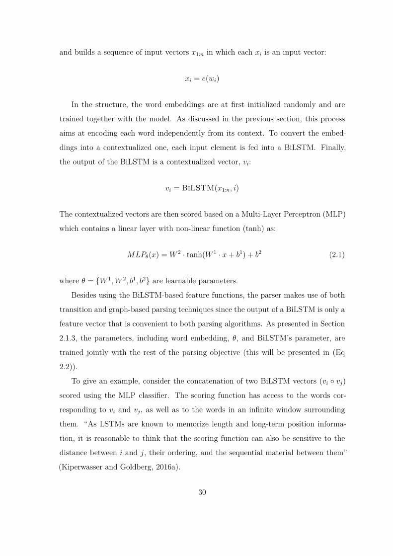
and builds a sequence of input vectors x1:n in which each xi is an input vector:

xi = e(wi)

In the structure, the word embeddings are at first initialized randomly and are

trained together with the model. As discussed in the previous section, this process

aims at encoding each word independently from its context. To convert the embed-

dings into a contextualized one, each input element is fed into a BiLSTM. Finally,

the output of the BiLSTM is a contextualized vector, vi:

vi = BiLSTM(x1:n, i)

The contextualized vectors are then scored based on a Multi-Layer Perceptron (MLP)

which contains a linear layer with non-linear function (tanh) as:

MLPθ(x) = W 2 · tanh(W 1 · x+ b1) + b2 (2.1)

where θ = {W 1,W 2, b1, b2} are learnable parameters.

Besides using the BiLSTM-based feature functions, the parser makes use of both

transition and graph-based parsing techniques since the output of a BiLSTM is only a

feature vector that is convenient to both parsing algorithms. As presented in Section

2.1.3, the parameters, including word embedding, θ, and BiLSTM’s parameter, are

trained jointly with the rest of the parsing objective (this will be presented in (Eq

2.2)).

To give an example, consider the concatenation of two BiLSTM vectors (vi ◦ vj)

scored using the MLP classifier. The scoring function has access to the words cor-

responding to vi and vj, as well as to the words in an infinite window surrounding

them. “As LSTMs are known to memorize length and long-term position informa-

tion, it is reasonable to think that the scoring function can also be sensitive to the

distance between i and j, their ordering, and the sequential material between them”

(Kiperwasser and Goldberg, 2016a).

30

LSTMf

xthe

concat

LSTMf

xbrown

concat

LSTMf

xfox

concat

LSTMf

xjumped

concat

LSTMf

x∗

concat

LSTM bs0

LSTM bs1

LSTM bs2

LSTM bs3

LSTM bs4

Vthe Vbrown Vfox Vjumped V∗

MLP MLP MLP MLP

+

Figure 2-10: Illustration of the neural model scheme of the graph-based parser whencalculating the score of a given parse tree (this figure and caption are taken from theoriginal paper (Kiperwasser and Goldberg, 2016a)). The parse tree is depicted belowthe sentence. Each dependency arc in the sentence is scored using an MLP that isfed by the BiLSTM encoding of the words at the arc’s end points (the colors of thearcs correspond to colors of the MLP inputs above), and the individual arc scores aresummed to produce the final score. All the MLPs share the same parameters. Thefigure depicts a single-layer BiLSTM, while in practice they use two layers. Whenparsing a sentence, they compute scores for all possible n2 arcs, and find the bestscoring tree using a dynamic-programming algorithm.

31

As discussed in the previous section, there are two major parsing algorithms: the

graph and transition-based parsing. Since our parser that will be presented in this the-

sis is a Graph-based parser, here, we introduce the graph-based BIST parser. Graph-

based BIST parser applies the common structured prediction paradigm proposed by

(Taskar et al., 2005):

predict(s) = argmaxy∈Y(s) scoreglobal(s, y)

scoreglobal(s, y) =∑

part∈y

scorelocal(s, part)

Here s denotes an input sequence and it is transformed the corresponding sequence

of vectors x1:n. Then, the system needs to search for the highest-scoring parse tree y

(as presented in the graph-based parser) in the space Y(s) of valid dependency trees

over s. Following the graph-based parsing algorithm, this parser keeps all local scores

for each part of the graph to make the search tractable. This is done by decomposing

the score of a tree as the sum of the score based on its head-modifier arcs (h,m):

parse(s) = argmaxy∈Y(s)

∑(h,m)∈y

score(ϕ(s, h,m)

)where score is an MLP classifier presented above, each h and m are the (possible)

head-modifier arcs, and ϕ(s, h,m) denotes a feature function following:

ϕ(s, h,m) = BiLSTM(x1:n, h) ◦BiLSTM(x1:n,m)

The parser uses a simple feature function that the concatenation of two BiLSTM

32

vectors, vhead and vmodifier. The final model, then:

parse(s) = argmaxy∈Y(s) scoreglobal(s, y)

= argmaxy∈Y(s)

∑(h,m)∈y

score(ϕ(s, h,m)

)= argmaxy∈Y(s)

∑(h,m)∈y

MLP (vh ◦ vm)

vi = BiLSTM(x1:n, i)

The overall structure of the parser is presented in Figure 2-10.

As an objective function, this parser uses a margin-based objective, “which means

a function intended to give a higher score to the correct tree y compared to all the

other competing trees at a given step of the parsing process. This objective function

is aiming to maximize the margin between the score of the gold tree y and the highest

scoring incorrect tree y′” (Kiperwasser and Goldberg, 2016a). They define a hinge

loss with respect to a gold tree y as:

max(0, 1−max

y′ =y

∑(h,m)∈y′ MLP (vh ◦ vm)

+∑

(h,m)∈y MLP (vh ◦ vm))

(2.2)

Note that the objective function only compares between the gold label y and y′, and

the predicted tree scores are calculated by MLP presented in Eq 2.1. Every predicted

label in a graph (sentence) can generate losses by comparing the gold label, and it is

computed by the sum of multiple neural networks as∑

(h,m)∈y′ MLP (vh ◦ vm). Based

on the hinge loss, the system computes the gradients of the parameters used for the

BiLSTM encoder, MLP, and word embeddings, and finally updates the parameters

using the gradients.

In order to predict the dependency label ℓ based on the predicted parse tree, the

BIST parser first predicts the best-predicted arc (head) following predict(s) and then

predicts the labels based on each predicted arc. This is done by another MLP classifier

33

for predicting dependency labels as:

label(h,m) = argmaxℓ∈labels MLPLabel(vh ◦ vm)[ℓ]

In the same way, the margin based hinge loss is applied for the dependency label

prediction with another hinge loss. Finally, the BIST parser builds a dependency

parsing model using a treebank in a supervised manner.

2.2.5 Evaluation Metrics

Different metrics have been proposed for dependency parsing. Here we propose to

keep four metrics that capture different aspects of the problem. None of these metrics

is more important than the others. The four main metrics are12:

• UAS (unlabeled attachment score) is used to evaluate the structure of a depen-

dency graph. It measures the extent to which the structure of the parsed tree

is correct, without taking into account the labels on the different links in the

tree.

• LAS (labeled attachment score) is the same as UAS, but takes into account

dependency labels.

• MLAS (morphology-aware labeled attachment score) extended LAS with the

evaluation of POS tags and morphological features.

• BLEX (bi-lexical dependency score); combines content-word relations with lemma-

tization (but not with tags and features).

Basically, word segmentation results must be reflected in the evaluation metrics

since the systems do not have access to gold-standard segmentation, “and identifying

the words is a prerequisite for dependency evaluation”13. In this work, however, we

use gold segmentation results to focus on the tagging and parsing tasks only.12http://universaldependencies.org/conll18/evaluation.html13http://universaldependencies.org/conll18/evaluation.html

34

In this study, we mainly report UAS and LAS scores because these are now the

most popular metrics. We can thus compare our results with those obtained by

many previously proposed parsers. Specifically, Labeled Attachment Score (LAS) is

a standard evaluation metric in dependency parsing since it reflects the percentage of

words that are assigned both the correct syntactic head and the correct dependency

label. Specifically, LAS is composed of two different scores. “Precision (P) is the

number of correct relations divided by the number of system-produced nodes; recall

(R) is the number of correct relations divided by the number of gold-standard nodes.

We then define LAS as the F1 score = 2PR / (P+R)”14. Following the 2017 and

2018 shared task guidelines, for scoring purposes, only universal dependency labels

will be taken into account in the evaluation. “This means that language-specific

subtypes such as acl:relcl (relative clause), a subtype of the universal relation acl

(adnominal clause), will be truncated to acl both in the gold standard”15 and in the

parser output during evaluation. Beyond the CoNLL shared task, parsers are however

still encouraged to output language-specific relations (e.g., predicting acl:relcl rather

than only acl), if they can predict them, as it makes the parsers more useful beyond

the shared task.

2.3 Transfer Learning for Dependency Parsing

Building a new annotated corpus is a resource- and time-consuming, as discussed

in Chapter 1. However, most NLP systems are now based on supervised learning

techniques, which means large training corpora are needed. This is especially the

case for Taggers and parsers, but we know that annotated resources are lacking for

most languages. Transfer learning has thus been investigated as a way to cope with

the problem of the lack of data for training.

Transfer learning aims at improving learning in a target language or domain by14This example is taken from official CoNLL shared task website,

http://universaldependencies.org/conll18/evaluation.html15This means both acl and acl:relcl become predictions during evaluation as presented in

http://universaldependencies.org/conll18/evaluation.html

35

leveraging knowledge from a source language or domain. The source can be (A)

multiple languages from which one wants to extract information or (B) different types

of sub-tasks contributing to a more general goal. For example, knowledge included in a

word embedding obtained after training a POS tagger could also be useful to recognize

Named Entity (NER). Since the goal of NER is to recognize sequences of words (such

as person, organization, and place names, most of them being POS:nouns), storing

knowledge gained while solving the POS problem could be helpful for NER.

Using external, pre-trained word embeddings for parsing is one of the most com-

mon transfer learning approaches. For instance, pre-trained word embeddings trained

by Word2Vec (Mikolov et al., 2013b) leverages dependency parsing performance, as

discussed in Section 2.2.3. This type of transfer learning has been recently applied

to most NLP tasks because of its ability to handle unseen in the training set (Guo

et al., 2015b)16.

Using a slightly different approach, Figure 2-11 shows that a system trained with

English data can help improve a model for French, due to the fact that some kind of

knowledge is shared across different languages (transfer of type A). As for dependency

parsing, Figure 2-12 describes training a dependency parser for French using both an

English and a French treebank, thanks to a shared neural network with the learnable

parameter Wd. Due to the fact that this shared parameter is trained by two different

languages, it captures syntactic features taking into account both languages. This

method can be helpful when one wants to augment the quantity of data available

for training in one of the languages considered, and is possible because of the shared

POS tagsets coming from UD (Ammar et al., 2016d).

As discussed above, one way to cope with the lack of training data is a multilin-

gual approach, which makes it possible to use different corpora in different languages

as training data. In most cases, for instance, in the CoNLL 2017 shared task (Zeman

et al., 2017a), the teams that have adopted this approach used a multilingual delexi-

calized parser (i.e., a multilingual parser trained without taking into account lexical16For example, the pre-trained word embeddings trained from Wikipedia are often useful since

they contain large coverage vocabularies for numerous languages.

36

Figure 2-11: Illustration of multilingual transfer learning in NLP (the figure is basedfrom (Jamshidi et al., 2017))

features but POS tags). It is however evident that delexicalized parsing cannot cap-

ture contextual features that depend on the meaning of words within the sentence.

The delexicalized model can thus not fully take into account (multilingual) lexical

information because languages have different word distributions (and then also differ-

ent word representations). For example, ‘en:dog’ and ‘fr:chien’ are represented with

different vectors even though the two words have the same meaning (Ammar et al.,

2016c). This raises the need for creating multilingual lexical representations.

To address this problem, we will propose in Chapter 4 a dependency parser with a

multilingual word representation that implements both (A) a multilingual transfer ap-

proach and (B) integrates pre-trained word embeddings. In the following section, we

will present the notion of multilingual dependency parsing based on transfer learning.

Multilingual Dependency Parsing

Multilingual dependency parsing consists in defining a parser that can parse several

languages using the same model. The idea is that a model trained with different

languages will benefit from more data and may recognize similarities across languages,

leading to a better coverage of rare phenomena.

Three major approaches have been suggested: 1) projection of cross-lingual anno-

tations, 2) joint modeling, and 3) cross-lingual representation learning (Guo et al.,

37

Figure 2-12: ’’How the transfer learning transfers knowledge in parsing?’’. A parserlearns the shared parameters (Wd) based on supervised-learning. Since the learningis a data-driven task with inputs, source language can affect to tune the parameter(Wd) for the target language (the figure is taken from (Yu et al., 2018).

2015b). The main idea of the cross-lingual annotation projection approach is to

project syntactic annotations through word alignments from a source language onto

a target language (Mann and Yarowsky, 2001; Tiedemann, 2014). For example, let’s

take a pair of sentences from a parallel corpus between a source language L1 and a

target language L2; and let’s imagine we have a syntactic analysis of the L1 sentence.

The predicted annotations in L1 are then mapped onto the sentence in L2, based

on word alignment. In a similar manner, the joint modeling approach is carried out

using projected dependency information for grammar inductions (Liu et al., 2013b)

or is based on a previous rule-based system (Naseem et al., 2010, 2012).

The cross-lingual representation learning method is focused on learning cross-

lingual features by aligning (or mapping) feature representations (e.g., embedding)

between the source and target languages. In general, cross-lingual representation

learning can be divided into two approaches depending on whether or not the parser

uses lexicalized features (e.g. word embedding). Due to the fact that it is rela-

tively easy to train a parser using supervised learning, many existing cross-lingual

representation learning studies have been conducted with the delexicalized approach

using POS tag-sets and word sequences (McDonald et al., 2011, 2013; Dozat et al.,

38

2017b). Such an approach includes training a dependency model with the source lan-

guage (e.g., English), then process the target language (e.g., French) using the model

trained according to the source language. Meanwhile, the lexicalized approach is able

to adapt diverse lexical features while in training. The features adapted for depen-

dency parsing include cross-lingual word cluster features (Täckström et al., 2012b),

multilingual word embeddings (Guo et al., 2015b, 2016; Ammar et al., 2016c,b) and

language identification embeddings (Naseem et al., 2012; Ammar et al., 2016b).

In Section 4.2.1, we will present our method for building multilingual word em-

bedding between two languages and we will discuss the impact of the approach in

Section 4.3 and 4.4.

2.4 Semi-Supervised Learning for Dependency Pars-

ing

Semi-supervised learning is a machine learning approach that makes use of both

labeled and unlabeled data for training. Over the past few years, unlabeled data has

been more and more widely used for parsing tasks, since it is easily obtained.

Two semi-supervised approaches, self-training (McClosky et al., 2006) and co-

training (Sarkar, 2001), use auto-parsed data as additional training data (Yu, 2018).

Self-training is the oldest semi-supervised learning approach. The idea is first to train

a supervised model based on labeled data only, and then analyze unlabeled data to

generate more labeled examples as input for the supervised learning algorithm. On

the contrary, co-training trains multiple models using different sets of features (e.g.,

words and characters) and generates labeled examples using unlabeled data. These

semi-supervised approaches make it possible for the parser to learn from its own

annotation, or from the annotations of other parsers.

Other techniques include word clustering (Koo et al., 2008) and word embedding

(Bengio et al., 2003), which are produced using large amounts of unlabeled data,

as discussed in the previous section. The output of these training processes can be

39

used as features or inputs for parsers as a pre-trained embedding17. Both groups of

techniques have been effective on syntactic parsing tasks (Reichart and Rappoport,

2007; Sagae and Tsujii, 2010; Yu et al., 2011; Weiss et al., 2015a). In this study, we

will propose in Chapter 6 to use a co-training approach to bootstrap our dependency

parser using unlabeled data.

17Pre-trained word embeddings can be classified as a kind of semi-supervised learning approachbecause it is trained with unlabeled data

40

Chapter 3

A Baseline Monolingual Parser,

Derived from The BIST Parser

In this chapter, we present our baseline parser, derived from the state-of-the-art BIST

parser (Kiperwasser and Goldberg, 2016a). The BIST parser is a standard parser

trainable on monolingual data, as presented in the previous section. Normally such

systems take as input an annotated corpus, along with word embeddings, language

specific dictionaries and other knowledge sources. This monolingual parsing approach

has yield state-of-the-art performance especially for resource-rich languages, when a

huge quantity of annotated corpora is available like for English or French (Chen and

Manning, 2014a; Kiperwasser and Goldberg, 2016a). Thus, it is natural to investigate

a standard, monolingual approach first, which can then be extended to integrate more

complex features.

In order to train a monolingual parsing model, many parsers use Universal Depen-

dency (UD) treebanks (see section 2.2). For many languages, one can find more than

one UD treebank, and these treebanks generally differ in several aspects. For exam-

ple, treebanks available for French include material from different language variants,

domains, and genres (one even find treebanks with spoken material). These treebanks

are called “heterogeneous treebanks” (Stymne et al., 2018), and the parsers dedicated

to these heterogeneous treebanks are called “multi-source” (Lim et al., 2018a; Stymne

et al., 2018).

41

However, many existing parsers, including the BIST parser, are trainable on a

single treebank. The easiest way to combine several treebanks for a language is

simply to concatenate the training treebanks as a single file. This concatenation

method showed better results than the case using a single treebank but did not allow

the parser to learn treebank-specific phenomena (Das et al., 2017).

In this chapter, we first describe the development of a traditional monolingual

system. This will be our baseline parser that will gradually be extended with addi-

tional features so as to deal with various complex linguistic situations. The baseline

parser extends the monolingual BIST parser as a multi-source trainable one, able to

take into account the specificities of heterogeneous treebanks. We thus add, for each

item of the language model, a reference to the treebank it has been trained on, so

as to take into account treebank-specific linguistic phenomena. This is done using a

one-hot scheme. It allows us to get a better model than the default option consisting

in simply learning from concatenated data.

We used this baseline dependency parser for the CoNLL 2017 UD Shared Task

called “Multilingual Parsing from Raw Text to Universal Dependencies”1. We ob-

tained satisfactory results as the system ranked 5th out of 33 teams and achieved

70.93 overall LAS score over the 81 test corpora (measured using macro-averaged

LAS F1 score)2. It also shows that the system is highly flexible and adaptable since

it was possible to get a state-of-the-art parser for all these languages in only a few

weeks.

In the following sections we will detail the architecture of our system (section 3.1).

We will also provide a description of the CoNLL shared task (section 3.2.1) along

with our results for this task (section 3.2.3).1http://universaldependencies.org/conll17/2For the For the evaluation campaign we also used multilingual models that will be presented in

the following chapter. This LAS score is 5.3 points lower than the score of the winner.

42

3.1 A Baseline Parser Derived from the BIST Parser

We want to develop a flexible parser, able to analyze a wide variety of languages.

Multi-source trainable parsers (i.e., parsers working with heterogeneous treebanks)

are especially flexible, and they are known to perform a lot better than monolin-

gual parsers in high-resource scenarios (Stymne et al., 2018). This is why we chose

to develop a multi-source trainable parser, based on the graph-based approach (see

Chapter 2, Section 2.2.1): we chose the BIST parser (Kiperwasser and Goldberg,

2016a), a state of the art parser freely available online.

As presented in Section 2.2.4, the BIST parser uses bidirectional Long Short Term

Memory (LSTM) feature representations thanks to two neural network layers (Kiper-

wasser and Goldberg, 2016a). In order to select the best relation and head for each

token in a sentence, this parser links the output of the bidirectional LSTM with the

Multi-Layer Perceptron (MLP) thanks to one neural layer (please, refer to Section

2.2.4). Here we adapt the same feature representation and MLP but different training

features and decision models.

In order to adapt the parser to a multi-source trainable approach, we add new

parameters and new features to the training algorithm, notably the possibility to use

pre-trained word embeddings and a one-hot encoding to encode domain of treebanks.

One-hot encoding is a binary feature representation (e.g. a one-hot vector [0, 1, 0,

0, 0]), as shown in section 2.2.3. The idea is to add a treebank one-hot encoding as

an additional feature while training with several treebanks. It allows the model to

focus on treebank specificities directly. For instance, there are two different English

UD treebanks, English_EWT and English_Partut. English_EWT is made of blog,

social, review, and email texts. In contrast, English_Partut based on data originated

from Wikipedia. The one-hot encoding scheme can make the training data to which

a sentence belongs between English_EWT and English_Partut as a binary feature

(e.g. 0 for EWT 1 for Partut). Finally, the parser can be trained on heterogeneous

treebanks depending on the parameters chosen for training (e.g. 0 for EWT 1 for

Partut). An overview of the overall architecture is given in Figure 3-1. Details on

43

Figure 3-1: Overall system structure for training language models. (1) EmbeddingLayer: vectorized features that are feeding into Bidirectional LSTM. (2) Bidirec-tional-LSTM: train representation of each token as vector values based on bidi-rectional LSTM neural network. (3) Multi-Layer Perceptron: build candidateof parse trees based on trained(changed) features by bidirectional LSTM layer, andthen calculate probabilistic scores for each of candidates. Finally, if it has multipleroots, revise it or select the best parse tree.

word embeddings along with the number of dimensions considered are given below.

• Word: randomly generated word embedding (100)

• XPOS: language-specific part-of-speech tags (25)

• UPOS: universal part-of-speech tags (25)

• External embedding1: pretrained word embedding (100)

• External embedding2: pretrained word embedding that is replaced with

Word (100)

• one-hot encoding: one-hot encoding of the treebank ID (65)

Word refers to word embeddings (vectors) learnt using the provided training cor-

pora. Both XPOS and UPOS3 are POS embeddings learnt from the training cor-

pora. The content of Word and POS is set randomly (randomly initialized) when the

training phase starts. In addition, two external word embeddings are added to the

representations of words, one is concatenated with the Word vector additionally, and3Please, refer to Section 2.1.1 or http://universaldependencies.org/format.html

44

the other is used to replace the Word vector. The reason why we adapt two different

embeddings is that it shows better results in handling unseen data or those data that

do not participate in the training phase. Generally, pre-trained word embeddings

trained by different raw texts (contexts) possibly have different sizes of vocabular-

ies. Thus, applying multiple pre-trained embeddings is better to handle unseen data.

In contrast, adding pre-trained word embeddings requires more computing resources

(e.g. GPU memory) and training time. In addition, we have found that if we use

two external word embeddings, replacing one word embedding as the Word made

better results than concatenating two pre-trained word embeddings based on exper-

iments. For example, let Word be generated randomly as a 100-dimensional vector

and External1 and let External2 be pretrained word embeddings made from different

resources with a 100-dimensional vector. If we just add External1 to an additional

word embedding, then final word embedding would be Word+External1 (200 dimen-

sions) based on concatenation. However, if we add just External2 as an additional

word embedding, Word is deleted because it is replaced with External2 so that final

word embedding could be External2 (100 dimensions). If both are used, final word

embedding could be External1 + External2 (Word is deleted because of External2).

As mentioned above, training a monolingual model in our system without multi-

sources (i.e., without several treebanks from different domains or different languages)

is very similar to training a standard BIST-parser model. However, we made one

additional modification to the original approach.

Multiple roots: The BIST parser can generate multiple roots for a given sen-

tence. This is not a problem in general but for parsing UD, we need to provide only

one single root per sentence. Not detecting the right root for a sentence leads to

major errors so the problem had to be addressed carefully.

We chose to develop a simple algorithm: when the parser returns multiple roots,

our system revises the overall sentence analysis so as to select one single primary

root and other previous roots become links pointing to the new head node. Choosing

the primary root is the result of an empirical process depending on the language

considered (i.e., taking into account language-specific word order). For example, the

45

primary root is the first head node in the case of an English sentence and the last one

in the case of a Korean sentence because English is SVO whereas Korean is SOV4.

This very simple trick improved the LAS scores by 0.17 overall F1-measure on the

development set of UD2.0 data (Nivre et al., 2017a).

Let’s remind the reader that the basic token representation in our parser is as

follows. Given a sentence made of tokens s=(t1,t2,..tn), the ith token ti is represented

by a vector vi, which is the result of the concatenation (◦) of a word embedding

wi, XPOS embedding xpi, UPOS embedding upi, External embedding1 e1i, External

embedding2 e2i and one-hot encoding embedding ohi of ti (see Section 2.2.4, for a

more detailed description of the feature representation used in the BIST parser):

vi = wi ◦ xpi ◦ upi ◦ e1i ◦ e2i ◦ ohi

wi = WORD(ti; θw)

xpi = XPOS(ti; θxp)

upi = UPOS(ti; θup)

e1i = EXT1(ti; θe1)

e2i = EXT2(ti; θe2)

ohi = HOT (ti; θoh)

where θ = {w, xp, up, oh} are learnable parameters randomly initialized during train-

ing. Additionally, the two pre-trained word embeddings, θ = {e1, e2}, are initialized

using the external word embeddings provided by Facebook (Bojanowski et al., 2016b)

and by the shared task organizer5, respectively. These two pre-trained embeddings

can be formalized through a set of word forms (key) and corresponding vectors (value),

as presented in Figure 2-8; thus, we can use this representation as a key-value lookup

table during training. Finally, the parser transforms the sequence of shared lexical

representation vi into a context-sensitive vector contextualized by BiLSTM with a4For example, the sentence ‘‘I love you” is translated in Korean ‘‘나는 너를 사랑한다”, where

‘나는’ is Subject, ‘너를’ is Object, and ‘사랑한다’ is Verb5http://universaldependencies.org/conll17/data.html

46

hidden layer r0 as:

h(head)i = BiLSTM(r

(head)0 , (v1, .., vn))i

h(dep)i = BiLSTM(r

(dep)0 , (v1, .., vn))i

The system uses the vector h(head)i to predict Head thanks to a Multi-layer Per-

ceptron (MLP) classifier, and h(dep)i for Dep thanks to another MLP classifier, as

presented in Section 2.2.4. During training, the system adjusts the parameters of the

network θ that maximize the probability P (yj|xj, θ) from the training set T based on

the conditional negative log-likelihood loss B_loss(θ). Thus,

B_loss =∑

(xj ,yj)∈T

− logP (yj|xj, θ) (3.1)

y = arg maxy

P (y|xj, θ)

where (xj, yj) ∈ T denotes an element from the training set T , y a set of gold labels

(lHead, lDep), and y a set of predicted labels. This model is subsequently used as the

baseline model.

During the CoNLL shared task, we used the same MLP classifier to score all the

possible Head and Modifier pairs Y = (h,m), following the strategy originally defined

for the BIST parser (see Section 2.2.4). We then select the best dependency graph

based on Eisner’s algorithm (Eisner and Satta, 1999). This algorithm tries to find

the maximum spanning tree among all the possible graphs (see Section 2.2.2).

3.2 Experiments during the CoNLL 2017 Shared

Task

A shared task is a popular way to evaluate the evolution of performance for a given

domain in computer science. A shared task is an evaluation campaign around a

predefined task (or set of tasks), for which some material is publicly distributed. All

the participants have access to the data following a precise time frame, and should

47

submit their results before a predefined deadline, so that the results and the different

approaches can then be compared. There has been, for example, recently very popular

challenges in image and video analysis. More specifically, the ImageNet Large Scale

Visual Recognition Challenge (ILSVRC)6 has been at the origin of huge progress

in image recognition. These challenges are especially important to identify relevant

approaches, measure relative performance and define new challenges beyond state of

the art.

In NLP, several competitions have also been organized since the 1990s, for example

in information extraction or machine translation. More recently and since 1999, the

annual CoNLL conference (Computational Natural language Learning7) has proposed

different challenges every year and some of the tasks have been especially popular.

The task organizers provide training and test data, which allows participating systems

to be evaluated and compared in a systematic way. The 2017 shared task dealt with

dependency parsing for 49 languages8.

We participated in this CoNLL 2017 UD Shared Task on “Multilingual Parsing,

from Raw Text to Universal Dependencies”9. The task offered a very relevant testbed

to compare our approach with systems developed by other competing teams. The fact

that the CoNLL 2017 Shared Task included different scenarios (low and high resource

languages, more than 49 languages covered, etc.) also made this evaluation scheme

very relevant for us. For this competition, we developed two different approaches,

based on monolingual and multilingual models. Since the approach with multilingual

models will be described in the following chapter, we just detail here our results

concerning our monolingual approach (we used this strategy for 40 of the 49 languages

considered for the 2017 shared task).6http://image-net.org/challenges/LSVRC/2016/index7https://www.conll.org/previous-tasks8Previous shared tasks have been devoted to chunking (1999, 2000), clausing (2001), named entity

recognition (2002, 2003), semantic role labeling (2004, 2005), dependency parsing (2006, 2007), jointparsing of syntactic and semantic dependencies (2008, 2009), hedge detection (2010), co-referenceresolution (2011, 2012), grammatical error correction (2013, 2014), and shallow discourse parsing(2015, 2016)

9http://universaldependencies.org/conll17/

48

3.2.1 The CoNLL 2017 Shared Task

The goal of the CoNLL 2017 shared task was to evaluate dependency parsers following

a real-world setting (starting from raw texts). The task was also intended to evaluate

the results for many typologically different languages. The evaluation even included

“surprise” languages for which there was no or very little training data. This challenge

was possible because of the Universal Dependencies initiative (UD): UD has made

available treebanks for many languages using a cross-linguistically consistent anno-

tation scheme (as presented in Section 2.1.2). For the Shared Task, the Universal

Dependencies version 2 (UD v2) has been used (Nivre et al., 2017b) which consists of

55 big treebanks, 14 PUD treebanks, 8 small treebanks, 4 surprise language treebanks.

• The “big” treebanks (55): Each corpus in this category has more than 2,000

annotated sentences available for training.

• The “small” treebanks (8): Each corpus in this category has between 20 and

1,000 annotated sentences available for training. It includes French ParTUT,

Galician TreeGal, Irish, Kazakh, Latin, Slovenian SST, Uyghur and Ukrainian.

• The “surprise” treebanks (4): Each corpus in this category has less than

20 annotated sentences available for training. Data for four languages were

provided (Buryat, Kurmanji Kurdish, North Sami and Upper Sorbian).

• The “PUD” treebanks (14): PUD refers to Parallel UD data. The PUD

treebank consists of 1,000 sentences in 14 languages (15 K to 27 K words, de-

pending on the language), which were randomly picked from online newswire

and Wikipedia.

As is usual in UD, there may be more than one training and development treebank

for certain languages. Typically, the different treebanks come from different sources

and different domain. Thus, for parsing the new Parallel UD (PUD) treebanks, it is

possible to use training data from a different domain. The four “surprise” languages

with a reduced amount of training data (20 sentences) were published one week before

49

Corpus LAS UAS Rank(LAS) Rank(UAS) UDpipe(LAS)Overall (81) 70.93 76.75 5 5 68.35Big treebanks (55) 75.79 80.55 5 5 73.04PUD treebanks (14) 70.77 77.64 4 4 68.33Small treebanks (8) 54.78 64.99 4 5 51.80Surprise language (4) 36.93 48.66 12 15 37.07English_PUD 82.38 85.77 2 2 78.95Russian_PUD 72.03 79.31 2 2 68.31Spanish 85.22 88.40 2 3 81.47

Table 3.1: Official results with rank. (number): number of corpora

the beginning of the evaluation phase only. The point of having surprise languages

was to encourage participants to investigate transfer methods and flexible approaches

that can be adapted to a new domain in a few days only (Zeman et al., 2017a). The

standard evaluation metric of the competition is the Unlabeled Attachment Score

(UAS) and Labeled Attachment Score (LAS) presented in Section 2.2.4.

To ease reproducibility, the CoNLL Shared Task was hosted on the TIRA platform

(Potthast et al., 2014)10. TIRA implements a proper solution that ensures blind

evaluation and an airlock for data. For example, a participant can run his parser on

the TIRA platform (server) but cannot see the test data and the result of parsing.

3.2.2 Experimental Setup

The results reported here concerns our baseline parser with monolingual models (Sec-

tion 3.1). Since the input of the shared task is raw text (plain text), it is thus necessary

to first implement or have access to pre-processing tools such as a tokenizer and POS

tagger. UDPipe baseline models (Straka et al., 2016) were provided for teams who

did not wish to develop their own pre-processing modules. We chose this option and

all our preprocessing modules were taken from UDPipe. We used the following mod-

ules: word segmentation, tokenization and morphological analysis (lemmas, UPOS,

XPOS and FEATS).10http://www.tira.io/

50

3.2.3 Results

Overall results. Table 3.1 and 3.2 show the official results using the F1-measure

computed by the official evaluation metric for the CoNLL 2017 Shared task11. Our sys-

tem achieved 70.93 F1 (LAS) on the overall 81 test sets and ranked 5th out of 33 teams.

Our results were generally better than those obtained by UDPipe1.1 (Straka et al.,

2016) with a significant margin (on average our system was 2.58 LAS point above

UDPipe1.1). When looking at the results on the PUD corpora, our system avoids

over-fitting issues because of the different domains used during training. Specifically,

performance gaps are narrowed when considering only PUD test sets (for example, our

system ranked second best for processing English_PUD and Russian_PUD), which

is encouraging for practical applications.

Contributions of the Different System Components to the General results.

To analyze the effect of the proposed representation methods on parsing, we evaluated

four different models with different components. In our baseline model, each token

is represented by a vector vi, which is the concatenation (◦) of a word embedding

wi, XPOS embedding xpi, UPOS embedding upi, External embedding1 e1i, External

embedding2 e2i, and one-hot encoding embedding ohi. Where wi is a randomly

initialized word vector, e1i and e2i are pre-trained word vectors, and xpi and upi

are POS vectors predicted by UDpipe1.1 (since we did not implement a specific POS

tagger, as said above). In this scenario, we deactivated each of representation in

turn during training, so as to investigate the impact of each feature individually.

The results are shown in Table 3.4, where ex denotes the use of the external word

embedding, and xp and up denote XPOS and UPOS representations, respectively. We

observe that each representation improves the overall results. This is especially true

regarding LAS when using external embeddings (ex), which means this representation

has a positive effect on relation labeling. Interestingly, the impact of the two different

POS features is almost identical when comparing the model between −ex, xp and

−ex, up. This is because UPOS for English treebanks is simply based on XPOS; thus,11http://universaldependencies.org/conll17/results.html

51

Corpus LATTICE BaselineArabic_PUD 47.13 43.14Arabic 68.54 65.3Bulgarian 85.6 83.64Catalan 86.83 85.39Czech-CAC 84.77 82.46Czech_PUD 80.86 79.8Czech 83.68 82.87Old_Church_Slavonic 60.81 62.76Danish 76.47 73.38Danish_PUD 71.45 66.53German 75.09 69.11Greek 81.13 79.26English-LinES 76.17 72.94English_PUD 82.38 78.95English 78.91 75.84Spanish-AnCora 86.87 83.78Spanish_PUD 79.87 77.65Spanish 85.22 81.47Estonian 62.93 58.79Basque 72.13 69.15Persian 82.63 79.24Finnish-FTB 79.44 74.03Finnish_PUD 80.82 78.65Finnish 77.11 73.75French_PUD 76.55 73.63French-Sequoia 83.7 79.98French 82.83 80.75Irish 64.39 61.52Galician 80.68 77.31Gothic 60.55 59.81Ancient_Greek-PROIEL 60.58 65.22Ancient_Greek 51.5 56.04Hebrew 61.24 57.23Hindi_PUD 50.94 50.85Hindi 86.99 86.77

Table 3.2: Official results with monolingual models (1).

52

Corpus LATTICE BaselineCroatian 80.96 77.18Hungarian 68.49 64.3Indonesian 76.6 74.61Italian_PUD 86.49 83.7Japanese_PUD 77.41 76.28Japanese 73.98 72.21Korean 72.35 59.09Latin-ITTB 74.33 76.98Latin-PROIEL 55.04 57.54Latin 51.95 43.77Latvian 64.49 59.95Dutch-LassySmall 75.67 78.15Dutch 70.6 68.9Norwegian-Bokmaal 85.55 83.27Norwegian-Nynorsk 84.57 81.56Polish 85.94 78.78Portuguese-BR 88.56 85.36Portuguese_PUD 76.56 73.96Romanian 81.93 79.88Russian_PUD 72.03 68.31Russian-SynTagRus 87.9 86.76Russian 78.42 74.03Slovak 79.23 72.75Slovenian 84.52 81.15Swedish-LinES 78.15 74.29Swedish_PUD 73.4 70.62Swedish 81.07 76.73Turkish_PUD 34.82 34.53Turkish 58.89 53.19Uyghur 34.94 34.18Ukrainian 63.63 60.76Urdu 79.26 76.69Vietnamese 39.87 37.47Chinese 61.94 57.4Average 73.13 70.45

Table 3.3: Official results with monolingual models (2).

53

Representation Methods UAS LASbaseline 83.17 80.64−ex 82.04 79.77−ex, xp 81.86 79.50−ex, up 81.68 79.52−ex, xp, up 81.09 79.12

Table 3.4: Relative contribution of the different representation methods on theEnglish development set (English_EWT).

Training Corpus Method UAS LASEnglish_EWT single-source 83.17 80.64English_Partut single-source 76.98 74.81English_EWT + English_Partut multi-source 83.89 81.34English_EWT + English_Partut concatenation 83.42 80.95

Table 3.5: Contribution of the multi-source trainable methods on the English devel-opment set (English_EWT).

two tagsets are very similar, as said in Section 2.2 (Figure 2-2). However, we observe

a slight improvement when applying the two POS features at the same time rather

than just using one of them (compare for example the two models −ex, xp and −ex).

Impact on Multi-Source Training. Another characteristic of our baseline parser

is the possibility to integrate multi-source treebanks (treebanks from different do-

mains). The one-hot encoding embedding ohi makes it possible to deal effectively

with several treebanks at the same time (the embedding is trained to recognize the

domain specificities of each treebank, as presented in Section 3.1). To investigate the

impact on the multi-source training method, we have conducted an evaluation using

different corpora in English. The results are shown in Table 3.5, where we compare

the performance of the parser with one or two different treebanks for the same lan-

guage (English). The Method column corresponds to the strategy used for the model:

ohi corresponds to the concatenation approach, and ohi to our multi-source proposal.

We observe that our multi-source approach works fine for English for example, with a

gain of 0.39 LAS score compared to the more traditional approach based on the con-

catenation method. The impact of multi-source learning will be further investigated

in the next chapter, along with our multilingual approach.

54

3.3 Summary

In this chapter, we have described our baseline system for dependency parsing that

has been tested over the 81 Universal Dependency corpora provided for the CoNLL

2017 shared task. Our parser mainly extends the monolingual BIST parser as a

multi-source trainable parser. We proposed two main extensions to the original BIST

parser: (1) the use of one-hot encoding to encode the notion of the source (domain

and language of the treebank), (2) a simple but effective way to solve the multiple

roots problem of the original BIST parser. Our system ranked 5th and achieved 70.93

overall F1-measure over the 81 test corpora provided for evaluation during the CoNLL

evaluation campaign (CoNLL 2017 shared task on Dependency parsing).

55

Chapter 4

A Multilingual Parser based on

Transfer Learning

Developing systems for low-resource languages is a crucial issue for Natural Language

Processing (NLP). Most NLP systems are built using supervised learning techniques

(Weiss et al., 2015b; Straka et al., 2016; Ballesteros et al., 2016a). These systems

require a large amount of annotated data and are thus targeted toward specific lan-

guages for which this kind of data exists. Unfortunately, producing enough annotated

data is known to be time- and resource-consuming, which means that annotated data,

especially of the type required for parsing, is lacking for most languages. To take a

recent example, the 2017 CoNLL shared task presented in the previous section, con-

cerned around 49 languages, roughly all of the languages for which enough syntac-

tically annotated data was available in the Universal Dependency format. This was

probably the most ambitious parsing challenge ever undertaken with regard to lan-

guage diversity, but the figure of 49 languages should be viewed relative to the 7,000

languages in the world. Even if one includes only those languages for which written

data is available, the 49 languages targeted at CoNLL 2017 cover only a fraction of

all the world’s languages.

When it comes to parsing, the supervised, monolingual approach based on syntac-

tically annotated corpora has long been the most common one. As presented in the

previous chapter, our baseline parser, a multi-source trainable parser, is also mono-

56

lingual even though it can take heterogeneous (multiple) treebanks for one language

as training data. It would be possible to turn our baseline parser into a multilingual

one using a delexicalized approach (an approach that does not take into account lex-

ical features), but this strategy does not give as good results as a lexicalized parser.

Thanks to recent developments involving cross-lingual feature representation meth-

ods and neural network models (as discussed in Section 2.2.3), it is now possible to

develop accurate multilingual models even for low resource languages.

Multilingual or cross-lingual parsing models are models able to parse several lan-

guages. These models are generally trained using parallel corpora or multilingual

treebanks from several, generally closely related languages (e.g. English, German

and Swedish). The multilingual approach can be implemented in two ways.

• The first one involves projecting annotations available for a high-resource lan-

guage onto a low-resource language using a parallel corpus that is aligned at

the token level. For example, let’s take a pair of sentences between a source

language L1 and a target language L2. The system first tries to parse the L1

sentence. Then, the predicted annotations are mapped from L1 onto L2 based

on word alignment information (the system tries to identify in L2 what word

corresponds to a given word in L1). This method produces a new annotated

dependency treebank using parallel corpora.

• The second method aims at producing a cross-lingual parsing model based on

the model transfer learning approach using several languages. Model transfer

learning is a method that improves learning in the target domain by leverag-

ing knowledge from the source domain. For example, model transfer learning

methods improve the parsing performance on a low-resource target language

L1 based on annotated data from other (source) languages L2. This method

typically utilizes cross-lingual resources such as parallel corpora (see Section

2.3).

Guo et al. (2016) and Ammar et al. (2016b) have conducted multilingual parsing

studies for Indo-European languages using the lexicalized transfer approach. They

57

demonstrate that a lexicalized transfer model yield better results than delexicalized

models for different European languages. However, their approach relies on the exis-

tence of a massive parallel corpus, as their experiment was based on Europarl.1 Thus

the problem of low-resource languages remains unaddressed, especially in cases when

no parallel corpus is available. In this chapter, we propose a simple but efficient

method for creating a dependency parsing model when (almost) no annotated corpus

or parallel corpus is available for training. Our approach requires only a small bilin-

gual dictionary and the manual annotation of a handful of sentences. We assume that

the performance one can obtain with this approach depends largely on the set of lan-

guages used to train the model. This is why we have developed several models using

genetically related and non-related languages, so as to gain a better understanding

of the limitations or possibilities of model transfer across different language families.

In this chapter, we introduce a new parser that extends our baseline parser, with

an additional multilingual lexical representation that will be presented in Section 4.2.

The parser has been used for the CoNLL 2017 shared task on multilingual parsing.

Following the previous section where the results obtained by our monolingual parser

have been presented, we detail here our results for 13 languages using multilingual

models. We are working with languages for which, until very recently, no Universal

Dependency corpus was available: North Sami2 and Komi-Zyrian, henceforth Komi.3

(in this thesis, we use ISO 639-3 codes to refer to the languages in tables.) This alone

does not make them low-resource languages, but they are still poorly equipped with

regard to NLP tools. Sami language technology has been in active development for

a longer time in the Giellatekno project of the University of Tromsø,4, but in the

case of Komi, resources have just recently begun to emerge. Work has also been

done on these languages within the framework of language documentation; however,

with the exception of a few individual projects (Blokland et al., 2015; Gerstenberger

et al., 2016), this field has generally not paid much attention to the use of NLP tools.1A parallel corpus of Indo-European languages, mainly used for machine translation:

www.statmt.org/europarl2glottolog.org/resource/languoid/id/nort26713glottolog.org/resource/languoid/id/komi12684giellatekno.uit.no

58

The same scenario applies to many other low-resource languages. However, despite

the lack of resources, we observe that the amount of written data in these languages

has grown rapidly in the past years, thanks to the activity of Komi users over the

Internet and also thanks to large digitalization projects. This means we can now easily

build word embeddings, as the only resource needed for these is a sufficiently large

amount of text. An additional contribution of this work is the new resources that

have been produced. We have created a new UD-type corpus for Komi5 (version 0.1

used in this study), as well as bilingual dictionaries, multilingual word embeddings for

Komi and Sami, and a multilingual parser, all of which are freely available in public

repositories.67

The structure of this chapter is as follows. We first provide an overview of our

approach (Section 4.1) before detailing the multilingual word representation used

(Section 4.2.1) and our parsing model (Section 4.3.2). We then describe a series of

experiments aiming at validating the approach (Section 4.3) before presenting an

analysis of our results in the CoNLL shared task (Section 4.4).

4.1 Our Approach

It is by definition not possible to get large scale training data and resources for a low

resource language. Therefore, new techniques adapted to this situation have to be

found. In this section, we will first study the multilingual approach to parsing using

Sami and Komi languages and then generalize this process with other low-resource

languages that were proposed within the CoNLL shared task.

Our aim is to test whether it is possible to use knowledge included in annotated

data from resource-rich languages to train an accurate parser for the target language,

exploiting structural similarities between source and target languages. The languages

used for training must thus be selected with the assumption that language may have

highly related languages that will contain such structural similarities and make it5github.com/langdoc/UD_Komi-Zyrian6github.com/jujbob/multilingual-bist-parser7github.com/jujbob/multilingual-models

59

possible to develop an accurate parser in the target language.

Our work with Northern Sami was initially motivated by it being one of the sur-

prise languages in the CoNLL 2017 Shared Task (presented in Section 3.2.1). After

the shared task ended, a larger training corpus became available in the dev-branch

of the UD_North_Sami GitHub repository of the Universal Dependencies project8,

which enabled us to carry out the broader evaluation. With Komi-Zyrian, the sit-

uation is essentially the same as it was with North Sami before the recent release

of the new corpus: we have 85 manually annotated examples that can be used for

training and testing. The training and testing set was created manually for Komi

for the purpose of this study, but it has been currently expanded. This Komi-Zyrian

treebank is included in the Universal Dependencies project since 2018.

Our expectation is that the match rate between Russian and Komi-Zyrian should

be exceptionally high, as there has been such a long history of contact between these

languages, leading to a variety of morphosyntactic changes in Komi (Leinonen, 2006).

North Sami has a complex contact relationship with Finnish, but in addition to

this, it is also a closely genetically related language (Aikio, 2012). From this point of

view, one could expect Finnish to perform well in parsing both Komi and North Sami,

although the similarities between these languages have not been studied in great detail

from the perspective of syntax and dependency structures. Other types of experiments

have also been conducted using this approach, for example, by using a Komi-Zyrian–

Russian multilingual model to parse data that contains both languages in the form

of code-switching: in these tests, the parser has been shown to be able to analyze

language-specific constructions when they occur within same utterance (Partanen

et al., 2018b). This case study and analysis about code-switching is presented in

(Lim et al., 2018b).8github.com/UniversalDependencies/UD_North_Sami

60

4.2 A Multilingual Dependency Parsing Model

We want to extend our baseline parser working as a multilingual trainable parser

that takes training data from several languages. Let’s assume that we need to parse

a resource-poor language (Komi) that has no training corpus; our baseline parser

can possibly train a multilingual parsing model using other languages’ treebanks (En-

glish, French). In this case, lexical features, however, are useless for parsing Komi

sentences because it did not learn any Komi lexicons from the training data (English,

French). This is a typical multi-source cross-lingual delexicalized parsing approach

(Rosa, 2015) when parsing Komi. In general, delexicalized cross-lingual parsing ap-

proaches have been applied using only POS features for many parsers (Dozat et al.,

2017b; Shi et al., 2017a; Das et al., 2017). This approach can also be applied for our

baseline parser presented in the previous section. For instance, the parser can only

take UPOS embeddings as an input representation and then train a parsing model

using treebanks from languages that have a similar POS order (e.g. Russian for

Komi). However, in terms of availability of language resources, lexical features (e.g.

words) deliver both syntactic and semantic information beyond non-lexical features

(e.g. POS). Therefore, cross-lingual word representation learning that assimilates

word representations based on two different languages is considered the best choice

for low-resource languages.

The cross-lingual representation learning method is focused on learning cross-

lingual features by aligning (or mapping) feature representations (e.g. embedding)

between the source and target languages (see Section 2.3.1). Let’s assume that we

have cross-lingual word embeddings in which vocabularies with the same meaning are

mapped between two languages. For instance, ‘Dog’ (English) and ‘Chien’ (French)

are mapped with the same word representation (e.g. a vector: [0.17, 0.15]) in the cross-

lingual word embeddings. Since words in the mapped embedding are represented by

the same vector, the system does not need to worry for its word form. Then we

can use English treebanks for training a French parsing model with lexical features.

The remaining questions we then need to investigate are (1) how to build cross-

61

lingual word representations that take into account two different languages in a single

representation space (vector space), and (2) how to adapt the cross-lingual word

representations in order to build a cross-lingual dependency parsing model on top of

our baseline parser.

4.2.1 Cross-Lingual Word Representations

Cross-lingual word representations (cross-lingual word embeddings) are one of the

most popular approaches for building multilingual lexical representations. Various

approaches have been investigated for the training of cross-lingual word embeddings

mainly for resource-rich languages. Moreover, most of these approaches relied on the

existence of a parallel corpus, especially for languages from the Indo-European family

(Ammar et al., 2016b; Guo et al., 2016). As we discussed earlier, however, this study

focuses on parsing in low-resource language data. Thus, we are constrained by the

fact that there is no parallel corpus and no larger annotated dataset for training a

dependency parser for the low-resource languages. However, it must be noted that

even for low-resource languages, we need raw texts as the minimum resource to train

a word embedding. In this study, we trained a monolingual embedding by using raw

text available in the public domain. The Komi texts used have been taken from

the National Library of Finland’s Fenno-Ugrica collection9, and proofread versions of

those Public Domain texts are available in FU-Lab’s portal Komi Nebögain10. Niko

Partanen has created a list of books included both in Fenno-Ugrica and FU-Lab11, and

the currently available data adds up to one million tokens. For the contact language

Russian we have used pre-trained Wikipedia word embeddings published by Facebook

and described in (Bojanowski et al., 2016c). Since the Komi and Sami Wikipedias

are relatively small, we have also trained larger word embeddings using FastText (it

is an open-source for training word embedding. (Bojanowski et al., 2016b)).

In a similar manner to the low-resource constraints, Artetxe et al. (2017) sug-9https://fennougrica.kansalliskirjasto.fi

10http://komikyv.org11https://github.com/langdoc/kpv-lit

62

Figure 4-1: An example of the cross-lingual representation learning method betweenEnglish (Source Language) and French (Target Language)

gested a powerful method for projecting two monolingual embeddings in a single

vector space with almost no bilingual data. Traditionally, the projection (or map-

ping) method for word embeddings requires a large parallel corpus or a bilingual

dictionary in order to map two different word embeddings in a distributional space

(Artetxe et al., 2016a; Guo et al., 2015b). However, (Artetxe et al., 2017) showed a

possible method for mapping two different embeddings based on the linear transfor-

mation approach with just 25 pairs of vocabularies but with almost no degradation

of performance. The main idea in this method is to project two embeddings trained

by different languages based on the linear transformation with bilingual word pairs.

The projection method can be described as follows with an example of Figure

4-1. Let X and Y be the source and target word embedding matrix so that xi refers

to ith word embedding of X and yj refers to jth word embedding of Y. And let

D is a binary matrix, where Dij = 1, if xi and yj are aligned. Our goal is then to

find a transformation matrix W such that Wx approximates y. For instance, the

system approximates W that makes the dot product between ‘dog’ ([0.34,0.28]) and

the parameter W have the same vector value as ‘chien’ ([0.81,0.14]), as shown in

Figure 4-1. This is done by minimizing the sum of squared errors following Artetxe

et al. (2017).

(1)

arg minW

m∑i=1

n∑j=1

Dij∥xiW − yi∥2

63

Bilingual pairs Bi-dictionary Bi-embeddingFinnish--Komi 12,879 2.3GBFinnish--North Sami 12,398 2.4GBKomi--English 8,746 7.5GBNorth Sami--Finnish 10,541 2.4GBRussian--Komi 12,354 5.7GB

Table 4.1: Dictionary sizes and size of bilingual word embeddings generated by eachdictionary.

We followed Artetxe et al. (2017) mapping idea to train a cross-lingual word

embedding based on a bilingual dictionary. To build cross-lingual word embedding,

we separately created a mapping system from our parser. This system takes three

inputs (two pre-trained embeddings and a bilingual dictionary) and produces a cross-

lingual word embedding. Specifically, when our mapping system returns the best-

approximated W based on a bilingual dictionary in a supervised manner, it transforms

our monolingual embedding to cross-lingual ones using W. The mapping method is

relatively simple to apply in our case because once we have a bilingual dictionary

available, converting the dictionary as D is not a problem. The size of the dictionary

used for training for Komi-Russian is described in Table 4.1. Those dictionaries

and projected word embedding are accessible in a public repository.12 Dictionary

is extracted from Jack Rueter’s Komi-Zyrian dictionaries that have translations to

several languages.13 In the case of the CoNLL 2017 shared task data, the projected

language pairs are shown in Table 4.5 and we will discuss more in Section 4.4.

4.2.2 Cross-Lingual Dependency Parsing Model

As discussed in the previous section, the major idea of the cross-lingual representation

learning method is to take aligned features, especially syntactic and lexical features.

Since the Universal Dependencies (UD) (Nivre et al., 2017a) model provides cross-

linguistically consistent grammatical annotation, we do not need to consider aligning

syntactic features among the languages (e.g., POS tags, dependency tags). However,12https://github.com/jujbob/multilingual-models13https://victorio.uit.no/langtech/trunk/words/dicts/kpv2X/src

64

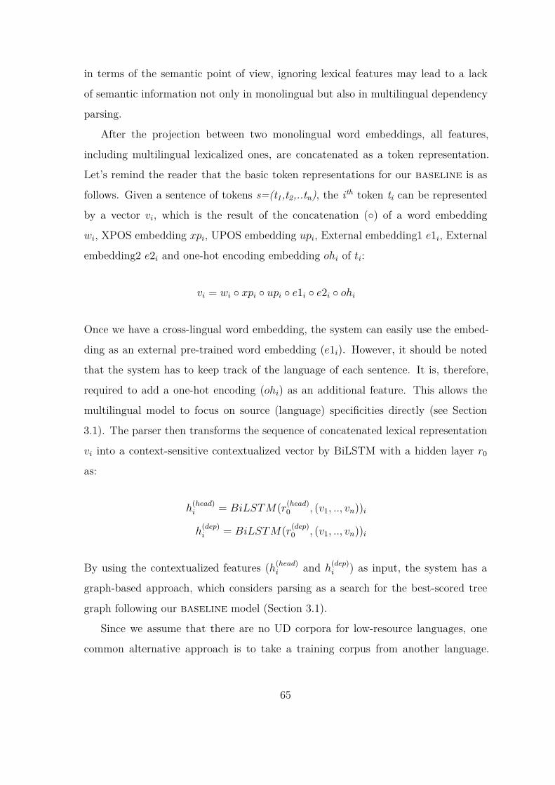
in terms of the semantic point of view, ignoring lexical features may lead to a lack

of semantic information not only in monolingual but also in multilingual dependency

parsing.

After the projection between two monolingual word embeddings, all features,

including multilingual lexicalized ones, are concatenated as a token representation.

Let’s remind the reader that the basic token representations for our baseline is as

follows. Given a sentence of tokens s=(t1,t2,..tn), the ith token ti can be represented

by a vector vi, which is the result of the concatenation (◦) of a word embedding

wi, XPOS embedding xpi, UPOS embedding upi, External embedding1 e1i, External

embedding2 e2i and one-hot encoding embedding ohi of ti:

vi = wi ◦ xpi ◦ upi ◦ e1i ◦ e2i ◦ ohi

Once we have a cross-lingual word embedding, the system can easily use the embed-

ding as an external pre-trained word embedding (e1i). However, it should be noted

that the system has to keep track of the language of each sentence. It is, therefore,

required to add a one-hot encoding (ohi) as an additional feature. This allows the

multilingual model to focus on source (language) specificities directly (see Section

3.1). The parser then transforms the sequence of concatenated lexical representation

vi into a context-sensitive contextualized vector by BiLSTM with a hidden layer r0

as:

h(head)i = BiLSTM(r

(head)0 , (v1, .., vn))i

h(dep)i = BiLSTM(r

(dep)0 , (v1, .., vn))i

By using the contextualized features (h(head)i and h

(dep)i ) as input, the system has a

graph-based approach, which considers parsing as a search for the best-scored tree

graph following our baseline model (Section 3.1).

Since we assume that there are no UD corpora for low-resource languages, one

common alternative approach is to take a training corpus from another language.

65

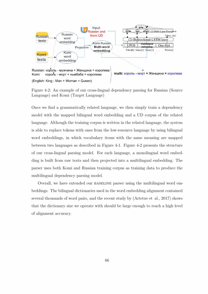
Figure 4-2: An example of our cross-lingual dependency parsing for Russian (SourceLanguage) and Komi (Target Language)

Once we find a grammatically related language, we then simply train a dependency

model with the mapped bilingual word embedding and a UD corpus of the related

language. Although the training corpus is written in the related language, the system

is able to replace tokens with ones from the low-resource language by using bilingual

word embeddings, in which vocabulary items with the same meaning are mapped

between two languages as described in Figure 4-1. Figure 4-2 presents the structure

of our cross-lingual parsing model. For each language, a monolingual word embed-

ding is built from raw texts and then projected into a multilingual embedding. The

parser uses both Komi and Russian training corpus as training data to produce the

multilingual dependency parsing model.

Overall, we have extended our baseline parser using the multilingual word em-

beddings. The bilingual dictionaries used in the word embedding alignment contained

several thousands of word pairs, and the recent study by (Artetxe et al., 2017) shows

that the dictionary size we operate with should be large enough to reach a high level

of alignment accuracy.

66

4.3 Experiments on Komi and Sami

We conducted a series of experiments on Sami and Komi. For Sami, we tested dif-

ferent language combinations for the cross-lingual model. All the experiments were

carried out using 20 training sentences in Sami, as was the case for the 2017 CoNLL

Shared Task, which means these results can be compared to the ones in the official

CoNLL evaluation. For Komi, no annotated corpus was available, but we designed

ten different experiments, again exploring different language combinations for the

cross-lingual model. The experiments for Komi are representative of an extremely

low-resource scenario, which is quite common, meaning the approach can be reused

for a wide variety of other languages.

4.3.1 Experiment Setup

Training Corpus. We used the corpora available in the Universal Dependency 2.0

format (Nivre et al., 2017a) to train and test all the models except for Komi. Since

there was no UD 2.0 Komi corpus, we used 10 sentences for training and 75 sentences

for testing (this corpus was designed specifically for this study). Following previous

works by (Guo et al., 2015b) and (Zhang and Barzilay, 2015), we used gold POS

sets for training and testing for Komi. For Sami, however, the teams in the CoNLL

Shared Task used preprocessed POS tags produced by UDpipe. In order to maintain

the same conditions as in the Shared Task, we also used the preprocessed POS tagging

sets to compare with others in Table 4.3.

Training Conditions. Since we wanted to explore low-resource scenarios (even in

the case of Sami, for which larger data now exists), we assumed that there had been

no development data for parameter tuning following the CoNLL shared task, and

we restricted all training experiments to run just one epoch with the training corpus

without early stopping (i.e. the 5th-low of column titled “Case” in Table 4.2 runs only

12,563 iterations). Similar restrictions have also been suggested by (Ammar et al.,

2016d), who proposed running one epoch, and by (Guo et al., 2016), who proposed

67

Case Training corpus LAS UAS1 sme (20) 32.96 46.852 eng (12,217) 32.72 50.443 fin (12,543) 40.74 54.244 sme (20) + eng (12,217) 46.54 61.615 sme (20) + fin (12,543) 51.54 63.06

Table 4.2: Labeled attachment scores (LAS) and unlabeled attachment scores (UAS)for Northern Sami (sme)

restricting iterations to 20,000 for low-resource scenarios. However, when training a

model with multilingual training data, the size of training corpora for low-resource

languages is comparably smaller than for high-resource languages (e.g. Komi has 10

sentences but Russian has 3,850). Following the previous work of (Guo et al., 2016),

we iterated 20 times more for low-resource training data than for high-resource. In

Table 4.2 and Table 4.4, the sizes of the training sets used are provided in brackets.

4.3.2 Results

Comparison with the CoNLL Shared Task. We used the same training en-

vironments in these experiments as for the CoNLL Shared Task (the same training

sets and no development set). Moreover, in order to guarantee similar experimen-

tal conditions, we allowed the training models to run just one epoch, following (Guo

et al., 2016). Table 4.3 reports the official 2017 CoNLL results. C2L2 (Cornell Univ.)

obtained the best performance for Sami with a delexicalized transfer approach (us-

ing a Finnish training corpus and a corpus of 20 Sami sentences as a development

set for parameter tuning without lexicalized features). IMS (Stuttgart) used a delex-

icalized transfer approach with a very large training corpus based on 40 different

training corpora in UD, obtaining the second-best result. Compared with the result

of the Shared Task, it seems that our Finnish–Sami approach (lexicalized cross-lingual

transfer parsing with resources from relevant languages) can be effective for parsing

low-resource languages. However, additional language features and the application of

the ensemble mechanism also seem to be very important. This is due to the fact that

the team C2L2 outperform others with more than 6.4 percent of LAS score based

68

Team LAS UASC2L2 (Ithaca) 48.96 58.85

IMS (Stuttgart) 40.67 51.56HIT-SCIR (Harbin) 38.91 52.51

This work 42.50 54.94

Table 4.3: The highest results of this experiment (FinnishSami model) comparedwith top 3 results for Sami from the CoNLL 2017 Shared Task.

Case Training corpus LAS UAS1 kpv (10) 22.33 51.782 eng (12,217) 44.47 59.293 rus (3,850) 53.85 71.294 fin (12,543) 48.22 66.985 kpv (10) + eng (12,217) 50.47 66.236 kpv (10) + rus (3,850) 53.1 69.987 kpv (10) + fin (3,850) 53.66 71.298 kpv (10) + fin (12,543) 55.16 73.739 kpv (10) + eng (12,217) + fin (12,543) 52.5 68.5710 kpv (10) + rus (3,850) + fin (12,543) 56.66 71.86

Table 4.4: Labeled attachment scores (LAS) and unlabeled attachment score (UAS)for Komi (kpv). We doesn’t conduct training for ‘‘kpv + eng + rus” language com-bination because of unrealistic training scenario (It takes more than 40GB memoryfor training)

on character-level representations as additional features and an ensemble mechanism

composed of three different dependency parsers (these two methods will be presented

in the next chapter).

Analysis. All the experiments we conducted using Finnish for training obtained

better results than other language combinations (i.e. English for Sami and Russian

and English for Komi in Table 4.4). This means that transferring knowledge from

genetically related languages is, at least in our case, a very efficient method for parsing.

This is true in the case of Sami and Finnish, but also in the case of Finnish and Komi,

which is arguably more distantly related to one another than Finnish and Sami. A

contact language can also be of significant help in improving the results with a low-

resource language, as can be seen in the case of Russian and Komi.

Word order must be one factor that limits the applicability of just the English

model, as all other languages analyzed allow rather flexible ordering. Interestingly, the

69

results obtained using English data show that simply selecting the largest available

word embedding can possibly lead to a better result than a monolingual model (e.g,

only Komi), but the different multilingual models were also very comparable with

that. As the English result improved when the training corpus was smaller, simply

adding more data in one language would not alone enable the corpus to outperform

smaller or better selected mixed models.

Even in cases where the LAS scores (i.e. labels of the syntactic dependencies)

were not significantly different, there was often greater variation in the UAS scores

(unlabeled dependencies). This means that although the actual labels may not have

been assigned correctly, the basic relations were found and the root was correctly

recognized. It is also worth noting that the highest UAS scores were obtained with

the Komi–Finnish pair, although the Komi–Russian–Finnish multilingual model gave

the best overall result. Our results show that adding even a small number of target-

language example sentences (e.g. Komi) into a parser that uses bilingual word embed-

dings can improve the result significantly. The size of the available training corpus

is very important, and the quality of the bilingual dictionaries used to align word

embeddings is also crucial.

4.4 Experiments on The CoNLL 2017 data

In the previous section, we showed some results with two languages, North Sami and

Komi-Zyrian, for which, until very recently, no Universal Dependency corpus was

available. In this section, we present additional results from the CoNLL 2017 shared

task using our baseline parser. This task offers a very relevant testbed to compare

our approach with systems developed by other competing teams. Experiments with

13 languages are presented, especially low-resource languages.

4.4.1 Experiment Setup

Our experiments were conducted using multilingual models integrated to our baseline

system (Section 3.1) for 13 languages with different conditions, as follows:

70

Surprise Languages and Kazakh. There were four surprise languages provided

for evaluation within the CoNLL 2017 shared task: Buryat, Kurmanji, North Sámi

and Upper Sorbian (all in the Universal Dependency format). Less than 30 sentences

were provided for training, and Kazakh (although not considered a surprise language)

also had 30 sentences for training. We divided the training corpus in half: half of

the data were set apart for development and never used for training. We applied our

multilingual parsing approach for the languages with two main external resources.

1. (Word embeddings). The first step to build the multilingual model is finding

topologically similar languages. Thus, we selected three languages for each

surprise language in order to be able to derive the multilingual word embeddings.

The choice of languages was based on the Word Atlas of Language Structures14

and on advice from linguists.

2. (Bilingual Dictionary). For some languages, we were able to find bilingual

dictionaries from OPUS15. When no corpus was available, we used Swadesh

lists from Wikipedia. Swadesh lists are composed of 207 bilingual words that

are supposed to be “basic concepts for the purposes of historical-comparative

linguistics”16.

Finally, we transformed both embeddings in a single vector space using these

two lexical resources (the embedding and dictionary). Table 4.5 shows details about

the selected pairs of languages and the different sources used for our dictionaries.

From these resources, we trained a multilingual model and after testing with the

development set apart for each pair of candidate languages, we picked up the best

candidate for the different surprise languages and for Kazakh.

14The Word Atlas of Language Structures provides information about different languages in theworld (family, latitude and longitude, see http://wals.info).

15http://opus.lingfil.uu.se/16https://en.wikipedia.org/wiki/Swadesh_list

71

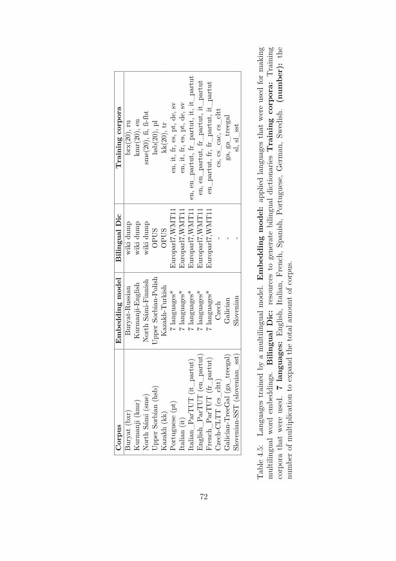
Cor

pus

Em

bedd

ing

mod

elB

iling

ual

Dic

Tra

inin

gco

rpor

aB

urya

t(b

xr)

Bur

yat-

Rus

sian

wik

idum

pbr

x(20

),ru

Kur

man

ji(k

mr)

Kur

man

ji-En

glish

wik

idum

pkm

r(20

),en

Nor

thSá

mi(

sme)

Nor

thSá

mi-F

inni

shw

ikid

ump

sme(

20),

fi,fi-

fbt

Upp

erSo

rbia

n(h

sb)

Upp

erSo

rbia

n-Po

lish

OPU

Shs

b(20

),pl

Kaz

akh

(kk)

Kaz

akh-

Tur

kish

OPU

Skk

(20)

,tr

Port

ugue

se(p

t)7

lang

uage

s*Eu

ropa

rl7,W

MT

11en

,it,

fr,e

s,pt

,de,

svIt

alia

n(it

)7

lang

uage

s*Eu

ropa

rl7,W

MT

11en

,it,

fr,e

s,pt

,de,

svIt

alia

n_Pa

rTU

T(it

_pa

rtut

)7

lang

uage

s*Eu

ropa

rl7,W

MT

11en

,en_

part

ut,f

r_pa

rtut

,it,

it_pa

rtut

Engl

ish_

ParT

UT

(en_

part

ut)

7la

ngua

ges*

Euro

parl7

,WM

T11

en,e

n_pa

rtut

,fr_

part

ut,i

t_pa

rtut

Fren

ch_

ParT

UT

(fr_

part

ut)

7la

ngua

ges*

Euro

parl7

,WM

T11

en_

part

ut,f

r,fr

_pa

rtut

,it_

part

utC

zech

-CLT

T(c

s_cl

tt)

Cze

ch-

cs,c

s_ca

c,cs

_cl

ttG

alic

ian-

Tre

eGal

(ga_

tree

gal)

Gal

icia

n-

ga,g

a_tr

eega

lSl

oven

ian-

SST

(slo

veni

an_

sst)

Slov

enia

n-

sl,sl_

sst

Tab

le4.

5:La

ngua

ges

trai

ned

bya

mul

tilin

gual

mod

el.

Em

bedd

ing

mod

el:

appl

ied

lang

uage

sth

atw

ere

used

for

mak

ing

mul

tilin

gual

wor

dem

bedd

ings

.B

iling

ual

Dic

:re

sour

ces

toge

nera

tebi

lingu

aldi

ctio

narie

sT

rain

ing

corp

ora:

Tra

inin

gco

rpor

ath

atw

ere

used

.7

lang

uage

s:En

glish

,It

alia

n,Fr

ench

,Sp

anish

,Po

rtug

uese

,G

erm

an,

Swed

ish.

(num

ber)

:th

enu

mbe

rof

mul

tiplic

atio

nto

expa

ndth

eto

tala

mou

ntof

corp

us.

72

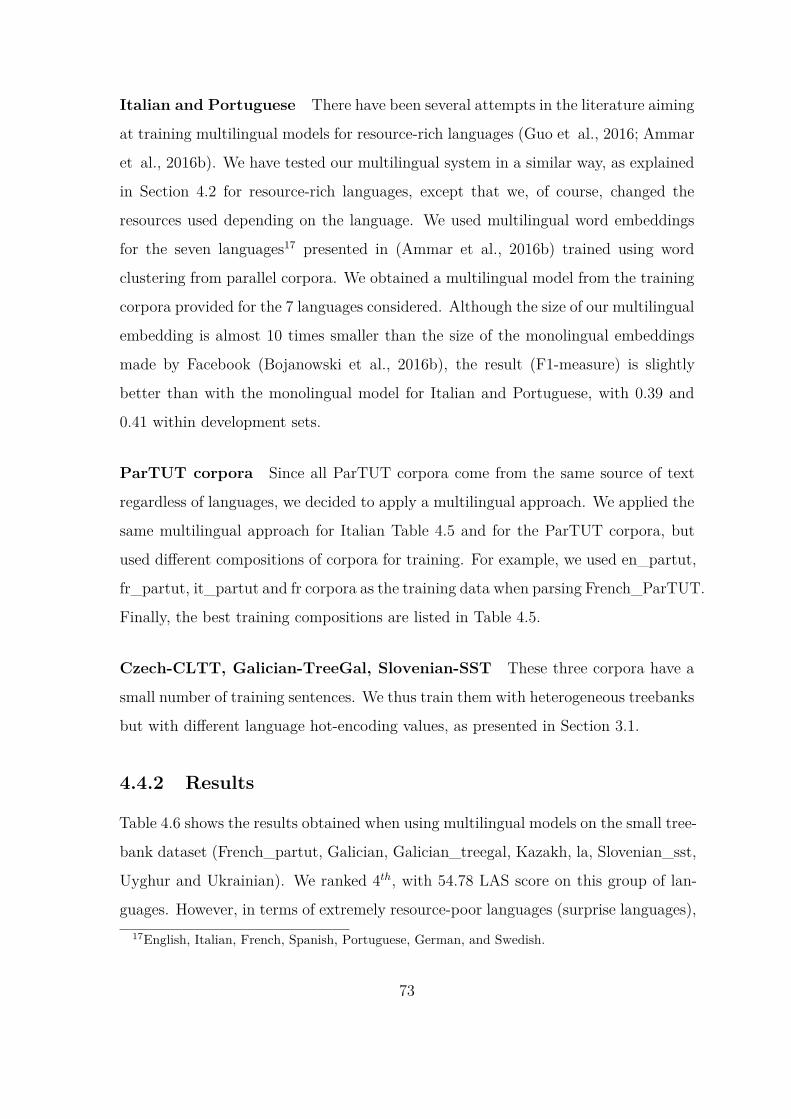
Italian and Portuguese There have been several attempts in the literature aiming

at training multilingual models for resource-rich languages (Guo et al., 2016; Ammar

et al., 2016b). We have tested our multilingual system in a similar way, as explained

in Section 4.2 for resource-rich languages, except that we, of course, changed the

resources used depending on the language. We used multilingual word embeddings

for the seven languages17 presented in (Ammar et al., 2016b) trained using word

clustering from parallel corpora. We obtained a multilingual model from the training

corpora provided for the 7 languages considered. Although the size of our multilingual

embedding is almost 10 times smaller than the size of the monolingual embeddings

made by Facebook (Bojanowski et al., 2016b), the result (F1-measure) is slightly

better than with the monolingual model for Italian and Portuguese, with 0.39 and

0.41 within development sets.

ParTUT corpora Since all ParTUT corpora come from the same source of text

regardless of languages, we decided to apply a multilingual approach. We applied the

same multilingual approach for Italian Table 4.5 and for the ParTUT corpora, but

used different compositions of corpora for training. For example, we used en_partut,

fr_partut, it_partut and fr corpora as the training data when parsing French_ParTUT.

Finally, the best training compositions are listed in Table 4.5.

Czech-CLTT, Galician-TreeGal, Slovenian-SST These three corpora have a

small number of training sentences. We thus train them with heterogeneous treebanks

but with different language hot-encoding values, as presented in Section 3.1.

4.4.2 Results

Table 4.6 shows the results obtained when using multilingual models on the small tree-

bank dataset (French_partut, Galician, Galician_treegal, Kazakh, la, Slovenian_sst,

Uyghur and Ukrainian). We ranked 4th, with 54.78 LAS score on this group of lan-

guages. However, in terms of extremely resource-poor languages (surprise languages),17English, Italian, French, Spanish, Portuguese, German, and Swedish.

73

Corpus LAS UAS Rank(LAS) Rank(UAS) UDpipe(LAS)Overall (81) 70.93 76.75 5 5 68.35Small treebanks (8) 54.78 64.99 4 5 51.80Surprise language (4) 36.93 48.66 12 15 37.07

Table 4.6: Official experiment results with rank. (number): number of corpora

Corpus LATTICE-Multi LATTICE-Mono UDpipeBuryat 27.08 19.7 31.5Kurmanji 41.71 37.59 32.35North Sámi 28.39 25.89 30.6Upper Sorbian 50.54 41.23 53.83Kazakh 22.11 19.98 24.51Italian 87.75 87.98 85.28Portuguese 84.08 84.08 82.11English-ParTUT 80.45 77.62 73.64French-ParTUT 83.26 80.66 77.38Italian-ParTUT 84.09 80.36 -Czech-CLTT 75.45 74.85 71.64Galician-TreeGal 68.01 67.75 65.82Slovenian-SST 49.94 48.06 46.45

Table 4.7: Official experiment results processed by multilingual models.

74

we have ranked only 12th, with 36.93 LAS score. This is slightly lower than the UD-

Pipe1.1 baseline model: we assume this is the result of using half of the corpus for

training surprise languages (as presented in Section 4.4.1). In contrast, when we used

all the training data for training, we obtained a 43.71 LAS score (3rd rank, unofficial

result).

Table 4.7 shows a comparison of the performance of the monolingual vs multilin-

gual model of our parser. When we compare monolingual models for surprise lan-

guages with multilingual ones, we see an improvement between 2.5 and 9.31 points.

The same kind of improvement can be observed for the ParTUT group. In this case,

the multilingual approach improves performance by almost 3 points. A further anal-

ysis for the impact of the multilingual model will be discussed in Section 5.4.1 and

7.2.

4.5 Summary

In this chapter, we have presented a multilingual approach to parsing that is effective

for languages with few resources and no syntactically annotated corpora available for

training. We have shown that our multilingual models provide better results than

monolingual ones. Adding training material from other languages usually did not

decrease the parsing result. It should, however, be noted that the relative size of

the different corpora used for training seems to be relevant, since using corpora that

are too imbalanced may weaken the result. A more detailed analysis of the results,

beyond the LAS and UAS scores, is most likely needed in order to determine the

exact influences of different language pairs or combinations. It remains a question for

further study whether the improvements observed here are actually attributable to

the genetic relationship between the language, or if the same result could be obtained

by simply selecting languages that are otherwise typologically similar.

75

Chapter 5

A Deep Contextualized Tagger and

Parser

Natural language processing (NLP) has been long focused on English and a few other

languages that were economically (or, more rarely, strategically) profitable. The

gradual development of the Web, as well as of social media, has revealed the need to

deal with more languages which, in turn, offer new technological challenges. It is, for

example, clear that languages exhibit a large diversity of morphological complexity

and NLP tools must tackle this diversity in order to obtain acceptable performance

beyond English (e.g., on agglutinative or polysynthetic languages). In this context,

feature representation methods that capture morphological complexities have been

an essential element for neural dependency parsing. As discussed in the previous

chapter, methods such as Feed Forward Neural Network (FFN) (Chen and Manning,

2014a) or LSTM-based contextualized representations (Kiperwasser and Goldberg,

2016a; Ballesteros et al., 2016a) have been proposed to provide fine-grained token

representations and make it possible to develop accurate parsers. However, word-

level representations, focusing only on word forms, have two serious limitations:

• A Lack of sub-word information: Word-level representations cannot cap-

ture sub-word information effectively because they focus only on word forms.

For example, humans can capture several sub-word information from the word

76

“delexicalized” such as (1) “de” used to indicate privation, removal, and separa-

tion, (2) “ed” represented the tense of the verb. However this is not possible if

one does not look for sub-word information.

• Out-of-vocabulary words: Out-of-vocabulary words are unknown words, be-

cause they were not present in the training corpus. Word-level representations

without external lexical resources (e.g. a pre-trained embedding) are weak to

handle these words. For example, if “delexicalized” was not part of the training

corpus, the system then cannot figure out its deep context during parsing.

To address the lack of sub-word information, character-level representation meth-

ods have become a crucial component offering better feature representations for pars-

ing (Zeman et al., 2017b; Dozat et al., 2017b). Formally, character-level representa-

tions (character embeddings) are trained using a sequence of characters, unlike word

embedding trained using a sequence of words. This representation is capable of cap-

turing sub-word information in a token or a sentence (this will be presented in the

following section). These sub-words can make it easier to represent inflection, com-

mon prefixes and suffixes and are thus well-suited for morphologically rich languages1.

To handle the out-of-vocabulary word issue, we also use a pre-trained word embed-

ding. Generally, such an embedding, trained using massive raw texts (e.g. Wikipedia,

OpenCrawl) can deliver more information than a randomly initialized word embed-

ding (see Section 2.2.3 and 3.1). However, even with all these resources, we are still

unable to model ambiguity since a word form is associated with one representation,

and only one. For example, pre-trained word embeddings do not consider word order2.

For example, given two sentences (A) “I am walking on the bank of the river” and (B)

“I have to put some money in the bank”, the representation for “bank” will always

be the same though it appears in different contexts. The need for contextualized

word representations taking into account context information, pushed the use of Lan-

guage Model (LM) (i.e., word representation that takes into account word order). An1For example, a word can have multiple forms, making it harder to find and look up in the

dictionary since by default a system has no rule to normalize or analyze unknown word forms.2For example, word embedding trained by Wor2Vec can predict neighboring words within a

window regardless of their order during training

77

LM representation (embedding) is a contextualized word representation that learns

word representations by trying to predict the next word in a sentence (details will be

presented in Section 5.2).

To train contextualized representations, LM representation methods need to keep

context information based on word order to predict the next word. Applying LSTM

has been one of the popular approaches to build contextualized LM embeddings be-

cause of its memory cell (see Section 2.3). In NLP, LMs, which are trained by LSTM

that captures both context-sensitive syntactic and semantic information, have been

initially called deep contextualized LM (Peters et al., 2017)3. Deep contextualized

representations generally denote embeddings generated by deep contextualized LMs.

Since these LMs are also trained using massive text corpora by taking into account

contextual information, they have yield better performance in handling unseen words

than pre-trained word embedding (Peters et al., 2017).

Following previous proposals promoting a model transfer approach with lexicalized

feature representations (Guo et al., 2016; Ammar et al., 2016b; Lim and Poibeau,

2017b), we propose a deep contextualized tagger and parser, respectively. This system

consists of a multi-source trainable system using three different lexical representations

as follows:

• Multi-attentive character level representations: A context sensitive

character-level representation that takes into account several subword infor-

mation.

• ELMo representation: A deep contextualized representation integrating

abundant contexts gathered from external resources (raw texts) (Peters et al.,

2018).

• Multilingual word representation: A multilingual word representation ob-

tained by the projection of several pre-trained monolingual embeddings into a

unique semantic space (presented in the previous chapter).3There are, however, several models that are also called deep contextualized LM that apply

different neural network techniques.

78

In general, the impact of each representation depends on the task considered.

Previous studies have evaluated the impact of representations over several tasks such

as POS tagging, dependency parsing, constituency parsing, named entity recognition,

question answering, etc (Peters et al., 2017; Devlin et al., 2018). Here we focus on

syntax-related tasks, especially POS tagging and dependency parsing to investigate

the effectiveness of the proposed representations.

The POS tagging task is a token classification task that predicts the part-of-speech

of each word in context. It is a convenient way to evaluate a system that has to deal

with morphological diversity. As presented in the previous section, POS tagging is

crucial for the dependency parsing task. Most state-of-the-art parsers require the text

to be tagged before parsing. We will thus investigate how well additional contextu-

alized representations produce syntactically consistent tagging outputs. Second, we

test our contextualized representations through parsing, to see whether our contex-

tualized representation is positive for parsing. Finally, we report our results of the

CoNLL 2018 shared task using this parser.

The structure of this chapter is as follows. We first describe sub-word and LM

representation methods (Section 5.1 and 5.2) and then present our POS tagger (Sec-

tion 5.3) and our parser (Section 5.4). Our parser is open source and available at:

https://github.com/jujbob/.

5.1 Multi-Attentive Character-Level Representa-

tions

We want to add sub-word information to our parser, because this is relevant to

represent inflections, including common prefixes and suffixes, and is thus well-suited

for dependency parsing.

A character-level word representation is a word embedding produced by charac-

ter representations for a word. This is an essential component of NLP tools because

of their ability to capture potentially complex morphological information (Kim et al.,

79

2016; Yu and Vu, 2017). Let’s remind the readers that, traditionally, a character-

level word representation learned using Long Short-Term Memory (LSTM) units

takes a sequence of characters as input and returns an encoded vector (Ballesteros

et al., 2015). Recently, studies on character models have focused on enriching fea-

ture representations by stacking more neural layers (Shi et al., 2017a), applying an

attention mechanism (this will be presented in the following section) (Cao and Rei,

2016), and appending a Multi-Layer Perceptron (MLP) to the output of recurrent

networks (Dozat et al., 2017b). This approach has obtained the best performance

for POS tagging and dependency parsing in the CoNLL 2017 (Zeman et al., 2017a)

and 2018 (Zeman et al., 2018c) shared task. However, despite their benefits, most

of these systems also have clear shortcomings, like their (lack of) representation of

unknown words. Moreover, the application of several character models, capable of

capturing different lexical characteristics, has not been fully explored so far. This is

because most of the time when two character models such as LSTM and BiLSTM-

based character representations are learned separately, they mostly capture the same

kind of features as other methods, and thus do not have a real positive influence on

the results.

Here we propose a new approach that aims at offering a more accurate representa-

tion. This is done through two complementary devices: i) a sub-word analysis, geared

to recognize morpheme-like information and ii) a contextual model taking into con-

sideration the sentential framing of a word, which is especially useful for the analysis

of unknown words (context is sometimes enough tot predict accurately the meaning

of an unknown word). In order to do this, we need to combine two different charac-

ter embeddings. One is a context independent word-based character representation

(Shi et al., 2017a), and the other is a context sensitive sentence-based character rep-

resentation (Alberti et al., 2017; Bohnet et al., 2018a) (These will be presented in

the following sub-section). We use joint training techniques to induce two character

embeddings focusing on different aspects of sub-word information. This new tech-

nique has the advantage of capturing not only locally optimized character features

but also globally optimized features, regardless of the language type. In the following

80

sub-sections, we introduce two LSTM-based character models with our self-attentive

approach.

Basic notions

• A character(-level) representation: an embedding for a character.

• A character-level word representation: a word embedding generated from

character representations.

• A sentence-based character representation: a character-level word repre-

sentation generated from a sequence of characters in a sentence.

• A word-based character representation: a character-level word represen-

tation generated from a sequence of characters in a word.

For example, given an input sentence s of length n with characters s=(ch1, . , chn),

our system creates a sequence of sentence-based character embeddings chs1:n, initially

encoded as random vectors. Since a sentence s is composed of m words such that

s=(w1, . , wm), and each word wi can be decomposed into a sequence of characters

wi=(chi1, . , chk), the system also creates a set of sequences of word-based character

embeddings ch1:m1:k . Note that two character embeddings, such as chs

1:n and ch1:m1:k , do

not refer to the same vector since the system is initialized randomly. A character can

thus be represented by two different embeddings.

In this section, we will use lowercase italics for vectors and uppercase italics for

matrices. The characters w and W denote parameters that the system has to learn.

Also, semicolons denote the concatenation of two vectors, and ConcatRow denotes

the concatenation of matrices by rows. We maintain this convention when indexing

and stacking; so hi is the i-th vector of matrix H, and matrix H is the stack of all

vectors hi.

81

Context Insensitive Word-based Character Model

A sentence consists of a sequence of characters; likewise a word also consists of a

sequence of characters. Therefore, there are at least two ways to build character-level

word embeddings using LSTM. Let’s call a word-based character model a method

that generates a representation based on a word (and thus not on the full sentence).

In general, word-based character vectors are obtained by running a BiLSTM (Dozat

et al., 2017b) over the k characters chi1:k of a word wi:

f(wc)j , b

(wc)j = BiLSTM(r

(wc)0 , (chi

1, .., chik))j

h(wc)j = [f

(wc)j ; b

(wc)j ]

Here, f (wc)j is the forward-pass hidden layer of the BiLSTM for character j of a word,

b(wc)j the backward pass, and h

(wc)j the concatenation of the two. Previous studies

have shown that the last encoded character f(wc)k represents a summary of all the

information from the input character sequence (Shi et al., 2017a) because the output

of the LSTM keeps track of the contextual information (see Section 2.3). However,

taking the last encoded character as an embedding is often omitted in the earlier

parts of the sequence once the entire sequence has been processed. This happens

because the last encoded embedding f(wc)k (vector) is a fixed size of the vector and

becomes a bottleneck to summarize long sequences into a single vector. The attention

mechanism was born to address this problem. The idea of attention is to use all the

intermediate states H(wc)i to build the context vector. Generally, an attention method

establishing relations between different parts of a single sequence to extract a specific

representation is called self-attention. The self-attention method involves applying

a linear transformation (Cao and Rei, 2016) over the matrix of character encodings

82

Figure 5-1: An example of the word-based character model with a single attentionrepresentation (Dozat et al., 2017b)

H(wc)i = h

(wc)1:k , for which attention weights a

(wc)i are calculated as follows4:

a(wc)i = Softmax(w(wc)H

(wc)i )

c(wc)i = a

(wc)i H

(wc)i

Here w(wc) is a linear transformation parameter. The self-attention weight a(wc)i

intuitively corresponds to the most informative characters of word wi for the task

being learned. Passing the encoded character vector H(wc)i of each word through its

attention weights a(wc)i , we obtain the character-level word-vector as c(wc)

i . Figure 5-1

is an illustration of the word-based character model, including the attention weights

a(wc)i and the encoded character vector H

(wc)i . Dozat et al. (2017b) suggest to con-

catenate the last encoded vector f(wc)k with the attention vector a

(wc)i H

(wc)i in order

to capture both the summary and sub-word information in one go for tagging (see

Figure 5-3-(A)). However, as Lin et al. (2017) suggest, self-attention based represen-

tations tend to focus on a specific component of the sequence. To alleviate this, we

propose multi-head attention character-level word embeddings, which reflect various

character-level features of a word by applying multiple attention weights as a matrix4Here, we use lowercase italics for vectors and uppercase italics for matrices. So a set of hidden

state H(wc)i is a matrix stacked on m characters.

83

Figure 5-2: An example of the word-based character model with three attentionrepresentations.

A(wc)i rather than as a vector a

(wc)i :

A(wc)i = Softmax(W (wc) tanh(D(wc)H

(wc)i ))

c(wc)i = ConcatRow(A

(wc)i H

(wc)i ) (5.1)

By applying an attention parameter matrix W (wc), rather than a vector w(wc),

and a non-linear function with a weight parameter D(wc), the attention weight can

reflect several aspects of sub-word information. For example, a successfully trained

attention weight W (wc) could recognize two different morphemes: “in” and “er” from

the word “infer”, as presented in Figure 5-2. We, however, do not know which sub-

word will exactly be captured during training because the system only tries to adjust

the attention parameters W based on the prediction errors (Lin et al., 2017). The

effectiveness of the multi-attentive model will be discussed in Section 5.3.

Context Sensitive Sentence-based Character Model

The model we have just described is effective at capturing sub-word information, but

cannot capture contextual information beyond word boundaries (e.g. because the

model just takes a word as input, it cannot take into account the context of this

word). The overall context can be modeled by considering the whole sentence as a

sequence of characters. The sentence-based character model is a model that builds a

word representation based on the sequence of characters corresponding in a sentence.

84

Figure 5-3: (A) Structure of the tagger proposed by Dozat et al. (2017b) using aword-based character model and (B) structure of the tagger proposed by Bohnet et al.(2018a) using a sentence-based character model with meta-LSTM.

The sentence-based character model is thus a context sensitive model (Bohnet et al.,

2018a).

Alberti et al. (2017) used a sentence-based character representation trained by a

LSTM model for dependency parsing and achieved state of the art results for morpho-

logically rich languages. In tagging, Bohnet et al. (2018a) showed that a sentence-

based character model that processes all the characters of a sentence at once is better

at keeping context information for unseen data than a token-based one for tagging.

Figure 5-3-(B) shows the structure of sentence-based model. This model obtained the

best POS parsing results during the 2018 CoNLL shared task.

We propose to extend these previous approaches with a self-attention sentence-

based word embedding, composed of three parts:

1. Encoding. A single encoding is generated from the entire sequence of charac-

ters corresponding to a sentence using a BiLSTM:

h(sc)j = BiLSTM(r

(sc)0 , (chs

1, .., chsn))j

2. Slicing. The output of the BiLSTM is sliced from the start index sidx(wi) to

85

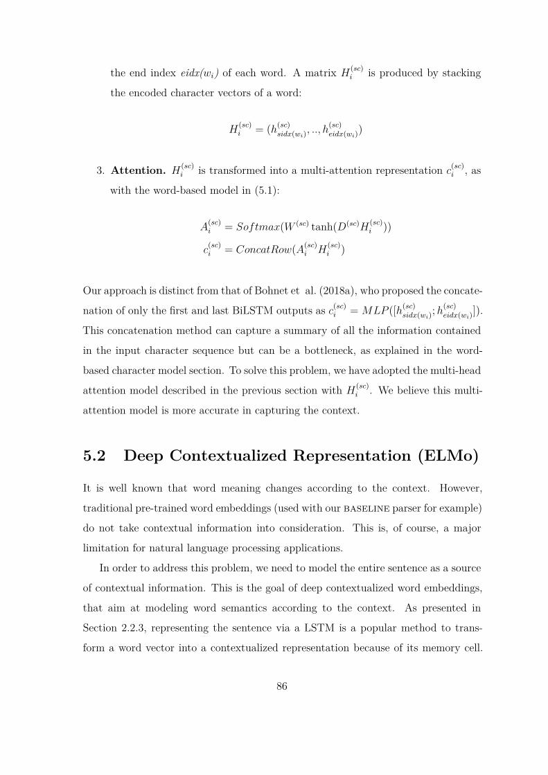
the end index eidx(wi) of each word. A matrix H(sc)i is produced by stacking

the encoded character vectors of a word:

H(sc)i = (h

(sc)sidx(wi)

, .., h(sc)eidx(wi)

)

3. Attention. H(sc)i is transformed into a multi-attention representation c

(sc)i , as

with the word-based model in (5.1):

A(sc)i = Softmax(W (sc) tanh(D(sc)H

(sc)i ))

c(sc)i = ConcatRow(A

(sc)i H

(sc)i )

Our approach is distinct from that of Bohnet et al. (2018a), who proposed the concate-

nation of only the first and last BiLSTM outputs as c(sc)i = MLP ([h(sc)sidx(wi)

;h(sc)eidx(wi)

]).

This concatenation method can capture a summary of all the information contained

in the input character sequence but can be a bottleneck, as explained in the word-

based character model section. To solve this problem, we have adopted the multi-head

attention model described in the previous section with H(sc)i . We believe this multi-

attention model is more accurate in capturing the context.

5.2 Deep Contextualized Representation (ELMo)

It is well known that word meaning changes according to the context. However,

traditional pre-trained word embeddings (used with our baseline parser for example)

do not take contextual information into consideration. This is, of course, a major

limitation for natural language processing applications.

In order to address this problem, we need to model the entire sentence as a source

of contextual information. This is the goal of deep contextualized word embeddings,

that aim at modeling word semantics according to the context. As presented in

Section 2.2.3, representing the sentence via a LSTM is a popular method to trans-

form a word vector into a contextualized representation because of its memory cell.

86

ELMo (Embedding from Language Model) is a deep contextualized word representa-

tion that aims at modeling complex characteristics of word use such as syntax and

semantics (Peters et al., 2018). These word embeddings are learned functions of the

internal states of LSTM, pre-trained on a large text corpus as explained in Section 5.1.

This contextualized embedding is a new technique for word representation that has

achieved state-of-the-art performance across a wide range of language understanding

tasks. This approach is able to capture both subword and contextual information.

From a technical point of view, ELMo can be used as a function that provides a

deep contextualized word representation based on the entire input sentence using

pre-trained LSTM.

Following Peters et al. (2018), we trained our deep contextualized word represen-

tations with a BiLSTM using the officially provided ELMo trainer5 and used ELMo

embeddings as an additional word embedding. Our ELMo embeddings have been

trained as follows:

Ri = {xLMi ,←→h LM

i,j | = 1, ..., L}

= {hLMi,j | = 0, ..., L}

(5.2)

ELMoi = E(Ri; Θ) = γL∑

j=0

sjhLMi,j (5.3)

To train ELMo embeddings, large quantities of raw text, as well as a pre-trained

word embedding, are required. We used the permitted pre-trained word embeddings

and raw texts provided by the CoNLL shared task organizer6. The transformation

of a sentence given the pre-trained word embedding is the first step of training. In

(5.2), xLMi and hLM

i,0 are pre-trained word embeddings corresponding to the tokens

of a sentence. We then contextualize the sequence of embeddings using BiLSTM.←→h LM

i,j denotes a contextualized LSTM vector consisting of a multi-layered bidirec-

tional LSTM and hLMi,j is a concatenated vector composed of xLM

i and ←→h LMi,j . Here,

5https://allennlp.org/elmo6http://universaldependencies.org/conll17/data.html

87

each hLMi,j is an individual contextualized embedding so we need to transform it as

a unified embedding. Finally, we compute our model with all the BiLSTM layers

weighed to generate a unified embedding using softmax. In (5.3), sj denotes the

softmax weight and γ is the scalar parameter to scale the embedding during training.

Following Peters et al. (2018), we used a 1024 dimensions ELMo embedding for our

tagger and parser.

5.3 Deep Contextualized Tagger

Since our input is raw text, it is first necessary to implement or have access to pre-

processing tools such as a tokenizer and a POS tagger. It is, in particular, crucial to

get an accurate POS tagger since POS tags are often used as a non-lexical feature

(Che et al., 2018). It has also been observed that tagging accuracy directly affects

parsing performance. We thus first investigate a POS tagger to see the impact of

our proposed contextualized representations and then introduce our parser in the

following section.

In this section, we describe our POS tagger, integrating the contextualized repre-

sentations we have just detailed, using Joint Many-Task learning (JMT). JMT is a

subfield of machine learning in which multiple learning tasks are solved at the same

time. JMT enriches context-sensitive feature representations by learning different

tasks with shared parameters (Hashimoto et al., 2016). For example, we can train a

tagger and parser at the same time with shared word representations in order to cap-

ture two different task-specific word representations. This approach may also consist

in training several classifiers for the same task. For example, Figure 5-3-(B) shows

the structure of a meta-Tagger that applies a JMT approach to a single POS tagging

task (Bohnet et al., 2018a). The Meta-Tagger separately trains a word-based and

a character-based POS tagger without sharing parameters and then joins the two

models via another middle-layer BiLSTM and MLP, which is used as the final classi-

fier. The system thus integrates three different taggers trained from different kinds of

information (character, word, character+word). However, the concatenation method

88

(that concatenates character and word features before contextualizing them, see Fig-

ure 5-3-(A)), has been the most popular approach recently. This model generally has

only one tagger.

The concatenation method often tends to rely on a specific feature (e.g. word)

and ignores the other features (e.g. character) during training (Lin et al., 2017). In

this context, the Meta-Tagger offers the advantage of learning contextual information

because each tagger struggles to identify the best features within the limited character

and word features. Because the middle-layer BiLSTM has access to two different

contexts that are captured by two different taggers, it is called meta-BiLSTM. The

meta-BiLSTM approach seems to be particularly effective at balancing the application

of word- and sentence-based features.

Following Bohnet et al. (2018a), we train two character-level taggers and then

combine them through a meta-BiLSTM tagger. As said above, we use each sentence

and word-based character embedding rather than only one ultimate embedding: this

makes it possible to take advantage of both the meta-BiLSTM model and JMT since

we are then using two character-level models. Since each separate tagger trained

on an individual classifier, each tagger struggles to identify the best features within

the limited sentence and word-based character features. Figure 5-4 shows the overall

structure of our contextualized tagger.

5.3.1 Two Taggers from Character Models

To take advantage of the meta-LSTM, our system builds two POS taggers using the

two different word embeddings generated from the sentence (c(sc)i ) and the word-based

(c(wc)i ) character model, as described in Section 5.1. To enrich word-level information,

for each character model, the system concatenates a shared word embedding w(e)i ini-

tialized with a pre-trained word embedding (Bojanowski et al., 2016a) and an ELMo

embedding e(el)i (Peters et al., 2018) in case we have one available, and then passes

it through another BiLSTM layer, whose output is g(sc)i and g

(wc)i for sentence-based

and word-based representations respectively. Finally, for sentence-based embeddings,

we apply a MLP classifier with a weight parameter Q(sc) including a bias term b(sc)

89

Figure 5-4: Overall structure of our contextualized tagger with three different classi-fiers.

to classify the best candidate POS:

p(sc)i = Q(sc)MLP (g

(sc)i ) + b(sc)

y(sc)i = arg max

jp(sc)i,j (5.4)

p(wc)i = Q(wc)MLP (g

(wc)i ) + b(wc)

y(wc)i = arg max

jp(wc)i,j (5.5)

Performing the same operation for the word-based embeddings as well, we predict

two POS tags y(sc)i and y

(wc)i .

5.3.2 Joint POS Tagger

To create joint representations that learn to combine the output of the two taggers,

we transform the two tagging results as a weighted POS label embedding h(pos)i as

follows:

l(sc)i =

U∑j=1

P (y(sc)i = j|p(sc)i )pos(j)

h(pos)i = [l

(sc)i ; l

(wc)i ] (5.6)

90

Figure 5-5: An example of the procedure to generate a weighted POS embedding.

Here U is the number of possible POS tags, P (y(sc)i = j|p(sc)i ) denotes the prob-

ability that the j-th POS tag is assigned to a word wi, and pos(j) is a randomly

initialized POS vector (presented in our baseline model). For example, Figure 5-5

shows a weighted POS embedding for a token pi. A weighted POS embedding for pi

is the weighted sum of POS embedding based on its probability P (y(sc)i = j|p(sc)i ). We

generate a joint embedding h(pos)i by concatenating two weighted POS features [l(sc)i

; l(wc)i ]. With the classifier proposed in (5.4) taking the joint vector h

(pos)i in input,

the system predicts another POS tag y(pos)i from two weighted POS features. Note

that the system only uses tokenized sentences as input, and the weighted POS are

predicted at training time. Where meta-Tagger (Bohnet et al., 2018a) trains three

taggers using separate optimizations, we trained our taggers simultaneously using a

single Adam-optimizer (Kingma and Ba, 2014)7, with a summed cross-entropy loss for

each tagger. This approach has the advantage of passing error propagation directly

to the shared word embedding w(e).

5.3.3 Experiments and Results

In this section, we present our experimental setting and the results of our model

on the CoNLL 2018 shared task (ST) dataset. This is a similar shared task to the

one presented in Section 3.2 (CoNLL 2017) but, for 2018, the organizers expanded

the number of languages from 49 to 57. The focus of the task was not only the

evaluation of syntactic dependency parsers but also included the evaluation of POS7This is a stochastic approximation of gradient descent optimization,

https://en.wikipedia.org/wiki/Stochastic_gradient_descent

91

tagger. Moreover, it is obvious that POS tagging directly affects parsing (a word with

a wrong tag cannot be rightly analyzed during parsing). We compare our UPOS8

results with the official CoNLL 2018 results for this task.9

Data Sets

We evaluate our model on the Universal Dependency 2.2 corpora provided for the

CoNLL ST (the development set is issued only for parameter tuning with the pro-

vided evaluation metric) (Zeman et al., 2018a). In order to compare our experiments

with the official 2018 CoNLL results, we use here the permitted pre-trained word em-

beddings for Japanese and Chinese10 and other languages (Bojanowski et al., 2016a),

and ELMo embeddings trained by Lim et al. (2018a). We tested our approach on 12

test treebanks from 8 different languages with different character sets to investigate

the impact of these character sets on our approach.

Since the input of the shared task was raw texts (plain texts), it is thus necessary

to first implement a word tokenizer. After the shared task, the tokenization results of

the best performing team have been officially provided by the ST organizer for further

investigation11. By using the tokenized results of each team as an input, it is directly

possible to compare the tagging results of each team. As our input test data, we use

the word tokenization result of the best performing model for each treebank in order

to compare with them directly. Note that when the baseline tokenizer (Straka et al.,

2016) is used for preprocessing, this largely affects the results since tokenization has a

direct and massive impact on tagging performance. Among our dataset, five treebanks

have no training data available, but for these cases at least one large training treebank

in a different domain is available. This offers an excellent opportunity to explore the

ability of our joint character model to deal with unseen data. Also, note that ELMo

has been trained by a sentence-based character model using external resources. In

the end, this gives us the opportunity to investigate three different character models8Universal Part-Of-Speech tags presented in Section 2.1.19http://universaldependencies.org/conll18/results-upos.html

10http://hdl.handle.net/11234/1-198911http://hdl.handle.net/11234/1-2885

92

Table 5.1: Hyperparameter DetailsComponent valuechi (char) Dim. 100h(pos)i (weighed POS) Dim. 200

W,Q,D (parameters) Dim. 300e(el)i (ELMo) Dim. 1024h(wc) (word-based) output Dim. 300h(sc) (sentence-based) output Dim. 300No. BiLSTM layers 2MLP output Dim. 300Dropout 0.3Learning rate 0.002β1, β2 0.9, 0.99Epoch 300Batch size 32Gradient clipping 5.0

effectively.

Experimental Setup

We applied the same hyperparameter settings as Smith et al. (2018a) for BiLSTM

dimensions, the MLP, the optimizer including β, and the learning rate to compare our

results with them on the similar environments. Table 5.1 presents our hyperparameter

settings. We set 300 dimensions for the parameters W and D in (5.1) and Q in (5.4).

The same dimensionality is applied to the sentence-based character model and the

word-based model. In training, we run over the entire training data as an epoch

with a batch size of 32 randomly chosen sentences. We save the model with the best

performance on the dev set within 300 epochs.

Results

Table 5.2 shows the results on the test sets of each treebank, compared with the best

performance winn as reported in the official ST results. The join column represents

our model jointly trained by the two different character-level representations described

in Section 5.3.2, and the joinE column is the join model enhanced with ELMo

93

Table 5.2: universal part-of-speech (UPOS) tagging results compared with the bestperforming team (winn) of each treebank for the ST. Columns denotes the size oftraining corpus Size, and our joint (join), joint with ELMo (joinE), concatenated(conc) and ELMo only (elmo) models. The symbols ∗ represents the result appliedthe ELMo embedding and + represents the result applied an ensemble.

Test set Train set Size winn joinE elmo join conczh_gsd (Chinese) zh_gsd 3997 91.94∗ 93.29 92.47 91.97 91.81ja_gsd (Japanese) ja_gsd 7164 92.97∗ 93.12 93.01 92.99 92.83en_ewt (English) en_ewt 12543 95.94∗+ 95.99 95.81 95.65 95.39en_lines en_lines 1022 97.06∗+ 97.45 96.76 96.57 96.39en_gum en_gum 981 96.44∗+ 96.45 96.25 96.08 95.95fr_gsd (French) fr_gsd 14554 96.97 97.18 97.04 97.04 96.85ko_gsd (Korean) ko_gsd 27410 96.33∗ 96.58 96.15 96.21 96.17en_pud (English) en_ewt 0(12543) 96.21∗+ 96.08 96.17 95.90 95.78ja_mod (Japanese) ja_gsd 0(7125) 54.60 54.70 54.61 54.67 54.55cs_pud (Czech) cs_pdt 0(68495) 97.17 - - 97.21 96.81sv_pud (Swedish) sv_l+t 0(7479) 94.28+ - - 94.29 94.09fi_pud (Finnish) fi_tdt 0(12217) 97.65+ - - 97.67 97.50

embeddings, as described in Section 5.3.1.

Overall, our joinE model achieves state-of-the-art results compared with the of-

ficial results published for the ST, except in the case of en_pud, where the best per-

forming model applied both ELMo and an ensemble of different models (Lim et al.,

2018a). Even without the application of ELMo, our join model shows comparable

results with models which did use ELMo embeddings (marked ∗) (Che et al., 2018)

and an ensemble (marked +) (Lim et al., 2018a).

As one can see in Table 5.2, the last five test treebanks have no training data, but

there exist large treebanks in different domains for these languages. For example, the

en_pud (genre: news) test treebank does not have specific training treebanks but has

alternative training treebanks from a different domain such as en_ewt (genre: blog,

reviews). We can thus investigate to which extent our joint character model is helpful

for handling unseen data. We tested those five PUD treebanks with models trained on

other training corpora (en_ewt, ja_gsd, cs_pdt, sv_l+t (sv_talbanken+sv_lines),

and fi_tdt), in line with other approaches to the ST (Lim et al., 2018a; Smith et al.,

2018a). We can see that our results are comparable for handling cross-domain data

when compared to other systems on the PUD treebanks.

94

Impact of the joint learning mechanism. To investigate whether our joint

model brings some benefit compared to a simple concatenation approach, we test a

disjoint model conc where a word embedding is defined simply as a concatenation

of embeddings for different levels of representation:

h(pos)i = [c

(sc)i ; c

(wc)i ;w

(e)i ]

This model then trains a single tagger without our joint learning method (please

refer to Figure 5-3-(A)). As our empirical result demonstrate in Table 5.2, the join

model always yields better performance than the conc model.

It should be noted that the shared word embedding w(e) produced by our joint

learning procedure leads to consistent improvements not only for the joint model

but also for the two character-based models. When we use the shared word embed-

ding only for the sentence-based or word-based character models, the performance

decreases by an average of 0.05-0.20 absolute points over the three taggers. We ob-

serve almost identical results with the multi-task learning approach for training a

tagger and a parser simultaneously with or without shared embeddings (Hashimoto

et al., 2016).

Impact of ELMo. Although the best performing system (Smith et al., 2018a) for

universal part-of-speech (UPOS) tagging in ST outperformed the macro-average score

over all the treebanks, with a 0.72 gap over the second-ranked team, some teams who

have used ELMo got the best score on many languages. It is thus necessary to extend

the evaluation by using the same ELMo embedding, as applied in ST12. To investigate

the performance of previously proposed taggers with ELMo, we evaluated the elmo

model, which is a simple concatenation model with a single classifier presented in

Figure 5-3-(A). This model produces a single tagger based on concatenation of ELMo,12https://github.com/jujbob/multilingual-models

95

word-based character, and word embedding as:

h(pos)i = [c

(wc)i ; e

(el)i ;w

(e)i ] (5.7)

In Table 5.2, the elmo model generally yields better performance than our join

model but not for joinE. We found a relatively significant gap between elmo and

joinE in tagging Chinese and Korean but not the same in English and French. As

reported by (Smith et al., 2018b), we assume that languages that have a bigger

character set benefit more from the character embeddings, especially when it is trained

with external data.

There is some indication that in the less-resourced conditions, ELMo is more in-

fluential than the dynamically trained character embeddings. This is because ELMo

is trained on various resources, external to the task; in contrast, our character models

are trained only on limited training data, and thus struggle to learn deep contexts

(see the size and performance gaps between join and joinE on zh_gsd).

Impact of the self-attention approach. Table 5.3 demonstrates the effective-

ness of the multi-head attention component for the word and sentence-based char-

acter models (as described in Eq.(5.1)). Here, n represents the number of attention

heads presented in Figure 5-2 (the number of rows allocated to the matrix Ai), with

additional columns providing traction for the model to focus on different semantic

components of the word under study.

We see at least marginal improvements when expanding from a single-head n=1

to double-head n=2 for all models, and then to triple-head n=3 for the word and

join models. Here, the applied model n=1 is the popular single head model proposed

by (Dozat et al., 2017b). We observe a negative impact when expanding beyond 5

rows for all models. This is because, as Lin (Lin et al., 2017) shows, each additional

attention-score a(wc)i tends to focus on the same part of a sequence, even though it

requires an n-times higher dimensional space.

96

Table 5.3: eu_bdt (Basque) tagging results by the number of attention heads n ofthe word and sentence-based character embedding. Here, word and sent denotemodels which trained taggers only word and sentence-based character representations(as described in (5.1))

# of head n=1 n=2 n=3 n=5word 96.04 96.17 96.19 96.12sent 96.24 96.26 96.21 96.17join 96.39 96.40 96.43 96.35

5.4 A Deep Contextualized Multi-task Parser

In the previous section, we have presented an approach based on contextualized

word representations for POS tagging. We have seen that two lexical representa-

tions (character-based and ELMo representations) play a crucial role for the task.

We can thus assume that, beyond tagging, these representations will also be helpful

for parsing. A common approach consists then in chaining these two components:

first a tagger is applied to assign a POS tag to each word, then the parser use s this

information to parse the sentence (i.e. provide s syntactic analysis of the sentence).

We can however ask ourselves whether there is a better way to deal with the two tasks

at the same time, or not. In this section, we present a multi-task learning scenario

that handles tagging and parsing simultaneously.

Multi-task learning is a machine learning approach in which several learning tasks

are solved at the same time. Recent breakthroughs in multi-task learning have made

it possible to effectively perform different tasks with a shared lexical representation

model (Hashimoto et al., 2016). In NLP, this approach has been widely used to learn

joint models performing tagging and parsing simultaneously, and most state-of-the-

art (SOTA) parsing models now use a multi-task strategy (Che et al., 2018; Smith

et al., 2018a; Lim et al., 2018a).

In general, given an input sentence s and a set of gold labels y = (l1, l2...ln), where

each li consists of gold labels for tagging (pos(gold)) and parsing (head(gold), dep(gold)),

the goal of the multi-task structure is to train a joint model that can provide at the

same time a POS tagger and a dependency parser.

The multi-task architecture of our parser is based on the multilingual baseline

97

parser presented in the previous chapter, with the addition of the two feature repre-

sentations presented in section 5.1 (character-level models) and 5.2 (ELMo). Let’s

remind the reader that the basic token representations for our multi-task parser is as

follows. Given a sentence of tokens s = (t1, t2, ..tn), the ith token ti can be represented

by a vector xi, which is the result of the concatenation (◦) of a word vector wi and a

word-based character-level vector ci of ti:

xi = ci ◦ wi

ci = CHAR(ti; θc)(seeEq(5.1))

wi = WORD(ti; θw)

when the approach is monolingual, wi corresponds to the external word embeddings

provided by Facebook (Bojanowski et al., 2016b). We have also seen in the previous

chapter (see Section 4.2.1) an alternative approach based on multilingual embeddings

that have proven useful for example when only little data was available for training.

To enhance the system and be able to capture sub-word information, we propose now

to concatenate a character-level word embedding ci with word embedding wi. For our

parsing task, we applied word-based character representations presented in Section

5.1 for character-level word vector ci. On top of the character and word embedding,

we want to enhance our word representation with three different information here:

• ELMo representation: we concatenate ELMo embedding directly to word

embedding xi from the encoding layer as:

ei = ELMoi (see Eq(5.3))

xi = ci ◦ wi ◦ ei

we want to enhance our parser with deeply contextualized word embeddings to

handle unknown words. The ELMo embedding trained with raw texts is a word

representation that is known to handle accurately unknown words, as presented

in Section 5.3.

• Treebank Representation: Following the strategy used for our baseline

98

parser, we use a treebank representation strategy to encode language-specific

features. In other words, each language has its own set of specific lexical

features. For languages with several training corpora (e.g., French-GSD and

French-Spoken) available in the Universal Dependency repository, our parser

computes an additional feature vector taking into account corpus specificities

at the word level. Following the recent work of Stymne et al. (2018), who

proposed a similar approach for treebank representation and showed a 12 di-

mensional vector is sufficient for treebank representation, we chose to use the

same size of treebank representation. This representation tri is concatenated

with the token representation xi:

tri = Treebank(ti; θtr)

xi = ci ◦ wi ◦ ei ◦ tri

We used this approach (treebank representation) for 24 corpora, and its effec-

tiveness will be discussed in the evaluation section.

• Multilingual Representation: As presented in Section 4.2, our baseline

parser can take multilingual word embedding to train multilingual dependency

models. Thanks to the multilingual word embedding, we have shown in the

previous chapter that we can train a multilingual parsing model even for low-

resource languages with no or very little data available for training. For this

kind of situation, our approach makes it possible to infer knowledge from other

related languages. We concatenate multilingual word embeddings with word

representation wi as follows:

mwi = Multilingual(ti; θmw) (please refer to e1i in Section 4.2.2)

xi = ci ◦ wi ◦ ei ◦ tri ◦ mwi

We used this multilingual embedding approach mostly to train the nine low-

resource languages of the Universal Dependency 2.2 data sets (Nivre et al.,

2018), for which only a handful of annotated sentences were provided in the

CoNLL 2018 shared task.

99

Finally, we generate an encoded token representation xi. This representation con-

tains different features depending on the resource availability for each language, as

presented in Table 5.6.

5.4.1 Multi-Task Learning for Tagging and Parsing

In this section, we describe our Part-Of-Speech (POS) tagger and dependency parser

using the encoded token representation xi implementing a Multi-Task Learning (MTL)

strategy (Zhang and Yang, 2017). To build our multi-task-based tagger and parser,

we first need to predict a POS tag since it is among the most important features for

our parser.

Part-Of-Speech Tagger

We apply the elmo model POS tagger that has a single classifier presented in Eq(5.7)

of Section 5.3.3. This tagger is based on a combination of features (a word-based

character embedding, a word embedding, and an elmo embedding). However, the

attention mechanism for this word-based character embedding ci and word wi embed-

ding are focusing only on a limited number of features within the token, it is thus

needed to contextualize by a BiLSTM, as a way to capture the overall context of the

sentence. Finally, a token is encoded as a vector gi:

gi = BiLSTM (pos)(g0, (x1, .., xn))i

We transform the token vector gi into a vector of the desired dimensionality by

a MLP with a bias term to classify the best candidate of universal part-of-speech

(UPOS):

pi = W (p)MLP (gi) + b(p)

y(pos)i = arg max

jpij

Finally, we randomly initialize the UPOS embedding as pi and map the predicted

100

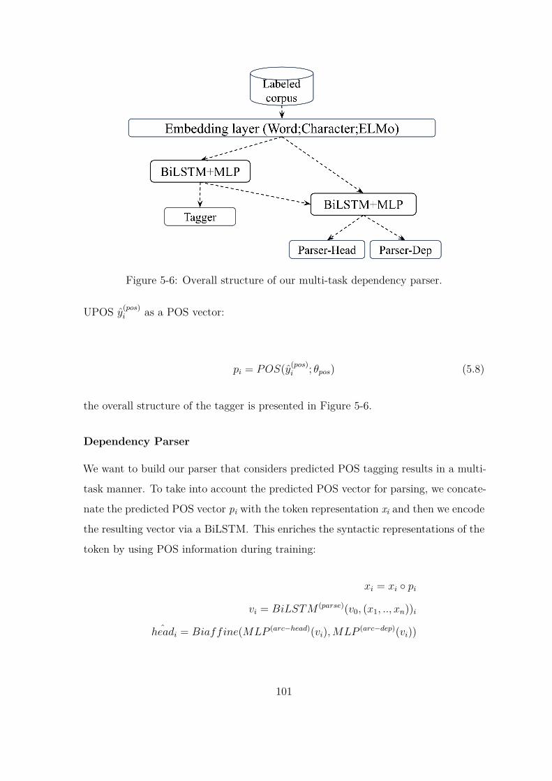
Figure 5-6: Overall structure of our multi-task dependency parser.

UPOS y(pos)i as a POS vector:

pi = POS(y(pos)i ; θpos) (5.8)

the overall structure of the tagger is presented in Figure 5-6.

Dependency Parser

We want to build our parser that considers predicted POS tagging results in a multi-

task manner. To take into account the predicted POS vector for parsing, we concate-

nate the predicted POS vector pi with the token representation xi and then we encode

the resulting vector via a BiLSTM. This enriches the syntactic representations of the

token by using POS information during training:

xi = xi ◦ pi

vi = BiLSTM (parse)(v0, (x1, .., xn))i

ˆheadi = Biaffine(MLP (arc−head)(vi),MLP (arc−dep)(vi))

101

vi is the final contextualized embedding that is only used for the dependency parsing

task. In order to predict a parsed tree following a graph-based parsing approach, we

need to know the probability of word i being the head of word j given the contex-

tualized embedding vi:n = V . Since word i can be both the head of word j and a

modifier of j, we transform the representation vi into two different representations us-

ing MLP as MLP (arc−head)(vi) (a vector to represent the head) and MLP (arc−dep)(vi)

(a vector to represent the modifier). Following Dozat and Manning (2016), we use a

Biaffine13 classifier (Appendix B) to score all the possible head and modifier pairs

Y = (h,m). We then select the best dependency graph based on Eisner’s algorithm

(Eisner and Satta, 1999). This algorithm tries to find the Maximum Spanning Tree

(MST) among all the possible graphs (a more detailed example described in Section

2.2.2):

arg maxvalid Y

∑(h,m)∈Y

ScoreMST (h,m)

With this algorithm, it has been observed that parsing results (for some sentences)

can have multiple roots, which is not a desirable feature. We thus follow an empirical

method in order to select a unique root based on the word order of the sentence, as

already proposed in Section 3.1 to ensure tree well-formedness. After the selection

of the best-scored tree, another bi-affine classifier is applied for the classification of

relation labels, based on the predicted tree:

ˆdepi = Biaffine(MLP (rel−head)(vi),MLP (rel−dep)(vi))

The overall structure of the parser is presented in Figure 5-6. To train our parser

with a supervised learning approach, we need to have an objective (loss) function

to feedback (backpropagate) errors by comparing the correct label and the predicted

label. We train our tagger and parser simultaneously using a single objective function13Here we use a usual linear transformation such as Wx + b, where W is a weight matrix, x is

an input vector and b is a bias. Wx+ b is an affine transformation, and it can be applied twice, asW (Wx+ b) + b. This corresponds to a biaffine.

102

with penalized terms:

loss = αCrossEntropy(p, p(gold))

+ βCrossEntropy( ˆhead, head(gold))

+ γCrossEntropy( ˆdep, dep(gold))

where ˆhead and ˆdep refer to the predicted head (Head) and dependency label (Dep)

results. CrossEntorpy14 measures the performance of a classification model by com-

paring two probability distributions such as ˆhead and head(gold) whose output is a

probability value between 0 and 1.

Since UAS (a score that considers only the head search procedure) directly affects

LAS, we assume that focusing on UAS would be more relevant than focusing on

LAS for parsing unseen data, as well as other corpora from low-resource languages.

Therefore, we gave more weight to the parameters predicting ˆhead than ˆdep and p,

because ˆhead directly affects UAS. We set α = 0.1, β = 0.7 and γ = 0.2.

5.4.2 Experiments on The CoNLL 2018 Shared Task.

The goal of the CoNLL 2018 shared task (ST) was to evaluate dependency parsers

following a real-world setting. For example, input for the task was just raw text with-

out annotation. The task was also intended to evaluate parsing many typologically

different languages, including low resource ones. We participated in this CoNLL 2018

UD Shared Task on “Multilingual Parsing, from Raw Text to Universal Dependencies”

(Zeman et al., 2018b). As presented in Section 3.2, the task offered a very relevant

testbed for comparing our results with systems developed by other competing teams.

In 2018, 7 languages were added to the task compared to 2017. The task concerned

82 UD treebanks, covering over 57 languages.14https://en.wikipedia.org/wiki/Cross_entropy

103

Implementation Details

Following the CoNLL 2017 shared task, we chose to train both monolingual and

multilingual models, not only for parsing but also for tagging. In the monolingual case,

we simply used the available Universal Dependency 2.2 corpora for training (Zeman

et al., 2018a). In the second case, for the multilingual approach, as both multilingual

word embeddings and corresponding training corpora (in the Universal Dependency

2.2 format) were needed for our approach as presented in the previous chapter, we

concatenated the corresponding available Universal Dependency 2.2 corpora in order

to artificially create multilingual training corpora.

The number of epochs was set to 200, with one epoch processing the entire training

corpus in each language and with a batch size of 32. We then picked the best two

performing models to parse the test corpora on the TIRA (Potthast et al., 2014)

evaluation platform (see Section 3.2.1). The two models were used as an ensemble

run (this will be described in the Testing subsection).

Hyperparameters. Each deep learning parser has a number of hyperparameters

that can boost the overall performance of the system. In our implementation, most

hyperparameter settings are identical to those of our baseline parser, except, of

course, those concerning the additional features we have just introduced. We use

100 dimensional character-level word representations with a 300 dimensional MLP, as

presented in Section 5.4.1, and for treebank representation, we use a 12 dimensional

vector. We set the learning-rate to 0.002 with Adam optimization.

Multilingual Embeddings. With the same approach as the one presented in

the previous chapter, we trained multilingual embedding models for nine low-resource

languages. Table 5.7 gives the list of languages for which we adopted this approach,

along with the language used for knowledge transfer. We selected language pairs

based on previous studies (Lim and Poibeau, 2017b; Lim et al., 2018b; Partanen

et al., 2018a) for Buryat (bxr), Kazakh (kk), Kurmanji (kmr), North Sami (sme),

and Upper Sorbian (hsb), and the others where chosen based on the public availability

of bilingual dictionaries (this explains why we chose to map several languages with

104

English, even when there was no real linguistically motivated reason to do so). Since

we could not find any pre-trained embeddings for Naija (pcm_nsc), for this case,

we applied a delexicalized parsing approach (see Section 4.2) based on an English

monolingual model.

ELMo. We applied ELMo embeddings to train specific models for five languages:

Korean, French, English, Japanese, and Chinese. ELMo embeddings were pre-trained

using the CoNLL resources provided15. We used AllenNLP16 which is a publicly

available piece of software allowing to train ELMo models. We included ELMo only

at the level of the input layer to make use of an additional feature representation

for both training and inference as shown in Figure 5-6. We set up dropout to 0.5

and used 1024 dimensions for the ELMo embedding layer in our model to prevent

overfitting based on our empirical experiments17 on our training data.

Testing with an Ensemble

All the tests were done on the TIRA platform provided by the shared task organizers.

Since the input of the shared task is raw text (plain text), it is thus necessary to first

implement or have access to pre-processing tools such as a sentence boundary detec-

tor and tokenizer. UDPipe baseline models Straka et al. (2016) were provided (esp.

for pre-processing) for teams who did not wish to develop their own pre-processing

modules. We chose this option and all our preprocessing modules (a sentence bound-

ary detector and tokenizer) were taken from UDPipe except for the UPOS tagger and

dependency parser.

During the test phase, an ensemble mechanism needs what is called ”seeds”. The

seeds are integers randomly produced by the Python random library and used to

initialize the parameters used during training as θ:

y = softmax(∑

seedi∈V P (yseedi |x, θseedi)).

We chose to train our models with two different “seeds”. Generally, an ensemble15http://hdl.handle.net/11234/1-198916https://github.com/allenai/allennlp17Overfitting is a modeling error which occurs when a model is too closely fit to a training set of

data than a testing set

105

Corpus UAS LAS Rank(UAS) Rank(LAS) BASE(LAS)Overall (82) 78.71 73.02 2 4 65.80Big treebanks only (61) 85.36 80.97 4 7 74.14PUD treebanks only (5) 76.81 72.34 3 3 66.63Small treebanks only (7) 75.67 68.12 2 3 55.01Low-resource only (9) 37.03 23.39 4 5 17.17

Table 5.4: Overall experiment results based on each group of corpora.

mechanism combines the best performing models obtained from different seeds, so as

to ensure robustness and efficiency.

In our case, due to a lack of GPU, we selected two best performing model on the

development set based on the use of two different seeds, respectively. Finally, the

two best performing models produced by each seed were put together to form the

ensemble model. This improved the performances by up to 0.6 points, but further

improvements could be expected by testing with a larger set of seeds. There could

be a further performance increase by using only the best performing models trained

using different seeds (This will be discussed in the next chapter).

Hardware Resources

The training process for all the dependency parsing models with i) the ensemble and

ii) ELMo was done using respectively 32 CPUs and 7 GPUs (Geforce 1080Ti), in

approximately two weeks. The memory usage of each model depends on the size of

the external word embeddings (3GB RAM by default plus the amount needed for

loading the external embeddings). In the testing phase on the TIRA platform, we

submitted our models separately, since testing with a model trained with ELMo takes

around three hours. Testing took 46.2 hours for the 82 corpora using 16 CPUs and

16GB RAM.

5.4.3 Results and Analysis

In this section, we discuss the results of our system and the relative contributions of

the different features to the global results.

106

Corpus Method UAS(Rank) LAS(Rank)af_afribooms 87.42 (7) 83.72 (8)grc_perseus tr 79.15 (4) 71.63 (8)grc_proiel tr 79.53 (5) 74.46 (8)ar_padt 75.96 (8) 71.13 (10)hy_armtdp tr, mu 53.56 (1) 37.01 (1)eu_bdt 85.72 (7) 81.13 (8)br_keb tr, mu 43.78 (3) 23.65 (5)bg_btb 92.1 (9) 88.02 (11)bxr_bdt tr, mu 36.89 (3) 17.16 (4)ca_ancora 92.83 (6) 89.56 (9)hr_set 90.18 (8) 84.67 (9)cs_cac tr 93.43 (2) 91 (2)cs_fictree tr 94.78 (1) 91.62 (3)cs_pdt tr 92.73 (2) 90.13 (7)cs_pud tr 89.49 (7) 83.88 (9)da_ddt 85.36 (8) 80.49 (11)nl_alpino tr 90.59 (2) 86.13 (5)nl_lassysmall tr 87.83 (2) 84.02 (4)en_ewt tr, el 86.9 (1) 84.02 (2)en_gum tr, el 88.57 (1) 85.05 (1)en_lines tr, el 86.01 (1) 81.44 (2)en_pud tr, el 90.83 (1) 87.89 (1)et_edt 86.25 (7) 82.33 (7)fo_oft tr, mu 48.64 (9) 25.17 (17)fi_ftb tr 89.74 (4) 86.54 (6)fi_pud tr 90.91 (4) 88.12 (6)fi_tdt tr 88.39 (6) 85.42 (7)fr_gsd tr, el 89.5 (1) 86.17 (3)fr_sequoia tr, el 91.81 (1) 89.89 (1)fr_spoken tr, el 79.47 (2) 73.62 (3)gl_ctg tr 84.05 (7) 80.63 (10)gl_treegal tr 78.71 (2) 73.13 (3)de_gsd 82.09 (8) 76.86 (11)got_proiel 73 (6) 65.3 (8)el_gdt 89.29 (8) 86.02 (11)he_htb 66.54 (9) 62.29 (9)hi_hdtb 94.44 (8) 90.4 (12)hu_szeged 80.49 (8) 74.21 (10)zh_gsd tr, el 71.48 (5) 68.09 (5)id_gsd 85.03 (3) 77.61 (10)ga_idt 79.13 (2) 69.1 (4)

Table 5.5: Official experiment results for each corpus, where tr (Treebank), mu(Multilingual) and el (ELMo) in the column Method denote the feature representationmethods used (see Section 5.4.1).

107

Corpus Method UAS(Rank) LAS(Rank)it_isdt tr 92.41 (6) 89.96 (8)it_postwita tr 77.52 (6) 72.66 (7)ja_gsd tr, el 76.4 (6) 74.82 (6)ja_modern 29.36 (8) 22.71 (8)kk_ktb tr, mu 39.24 (15) 23.97 (9)ko_gsd tr, el 88.03 (2) 84.31 (2)ko_kaist tr, el 88.92 (1) 86.32 (4)kmr_mg tr, mu 38.64 (3) 27.94 (4)la_ittb tr 87.88 (8) 84.72 (8)la_perseus tr 75.6 (3) 64.96 (3)la_proiel tr 73.97 (6) 67.73 (8)lv_lvtb tr 82.99 (8) 76.91 (11)pcm_nsc tr, mu 18.15 (21) 11.63 (18)sme_giella tr, mu 76.66 (1) 69.87 (1)no_bokmaal 91.4 (5) 88.43 (11)no_nynorsk tr 90.78 (8) 87.8 (11)no_nynorsklia tr 76.17 (2) 68.71 (2)cu_proiel 77.49 (6) 70.48 (8)fro_srcmf 91.35 (5) 85.51 (7)fa_seraji 89.1 (7) 84.8 (10)pl_lfg tr 95.69 (8) 92.86 (11)pl_sz tr 92.24 (9) 88.95 (10)pt_bosque 89.77 (5) 86.84 (7)ro_rrt 89.8 (8) 84.33 (10)ru_syntagrus tr 93.1 (4) 91.14 (6)ru_taiga tr 79.77 (1) 74 (2)sr_set 90.48 (10) 85.74 (11)sk_snk 86.81 (11) 82.4 (11)sl_ssj tr 87.18 (10) 84.68 (10)sl_sst tr 63.64 (3) 57.07 (3)es_ancora 91.81 (6) 89.25 (7)sv_lines tr 85.65 (4) 80.88 (6)sv_pud tr 83.44 (3) 79.1 (4)sv_talbanken tr 89.02 (4) 85.24 (7)th_pud tr, mu 0.33 (21) 0.12 (21)tr_imst 69.06 (7) 60.9 (11)uk_iu 85.36 (10) 81.33 (9)hsb_ufal tr, mu 54.01 (2) 43.83 (2)ur_udtb 87.4 (7) 80.74 (10)ug_udt 75.11 (6) 62.25 (9)vi_vtb 49.65 (6) 43.31 (8)

Table 5.6: Official experiment results for each corpus, where tr (Treebank), mu(Multilingual) and el (ELMo) in the column Method denote the feature representationmethods used (see Section 5.4.1).

108

Overall results.

The official evaluation results are given in Table 5.4. Our system achieved 73.02 LAS

(4th out of 26 teams) and 78.71 UAS (2nd out of 26). The comparison of our results

with those obtained by other teams shows that there is room for improvement regard-

ing preprocessing. For example, our system is 0.86 points below HIT-SCIR (Harbin)

for sentence segmentation and 1.03 for tokenization (HIT-SCIR obtained the best

overall results). Those two preprocessing tasks (sentence segmentation and tokeniza-

tion) affect tagging and parsing performance directly. As a result, our parser ranked

second on small treebanks (LAS), where most teams used the default segmenter and

tokenizer, avoiding the differences in this aspect. In contrast, we achieved 7th on the

big treebanks, probably because there is a more significant gap (1.72) when compared

to the best performing team at the tokenization level. Also, during the testing phase,

we chose not to adjust the weight parameters (α, β, γ) of the objective function pre-

sented in the previous section. We set α = 0.1, β = 0.7 and γ = 0.2 because we

assumed that focusing on UAS (β) would be helpful for low-resource languages. This

choice made our results on big treebanks suffer a bit (7th) compared to those we

obtained on Small and PUD treebanks (3th) regarding LAS. This also explains the

gap between the UAS and LAS scores in our overall results. When we set α = 0.1,

β = 0.2 and γ = 0.7 to focus more on LAS score, we get better LAS performance and

we are then ranked 5th on the big treebanks.

Effect of Treebank Representation on Performance.

Results with treebank representation (corpora marked tr in column Method in Table

5.6) exhibit relatively better performance than those without it, since tr makes it

possible to capture corpus-oriented features. Results were positive not only for small

treebanks (e.g., cs_fictree and ru_taiga) but also for big treebanks (e.g., cs_cac and

ru_syntagrus). Treebank representation with ELMo is the best for parsing English

and French.

109

Language Corpus Projected languages UAS LAS(Armenian) hy_armntdp Greek 1 1(Breton) br_keb English 3 5(Buryat) bxr_bdt Russian 3 4(Faroese) fo_oft English 9 17(Kazakh) kk_ktb Turkish 15 9(Kurmanji) kmr_mg English 3 4(Naija) pcm_nsc - 21 18(North Sami) sme_giella Finnish+Russian 1 1(Thai) th_giella English 21 21(Upper Sorbian) hsb_ufal Polish 2 2

Table 5.7: Languages trained with multilingual word embeddings and their ranking.

Effect of Multilingual Approach on Performance.

As described in Section 5.4.1, we applied our multilingual approach to most of the

low-resource languages. Table 5.7 shows results of our multilingual models. The best

result is obtained for hy_armtdp, while sme_giella and hsb_ufal also gave satisfactory

results. We only applied the delexicalized approach to pcm_nsc since we could not

find any pre-trained embeddings for this language. We got a relatively poor result for

pcm_nsc, despite testing different strategies and different feature combinations (we

assume that the English model is not fit for it).

Additionally, we found that character-level representation is not always helpful,

even in the case of some low-resource languages. When we tested kk_ktb (Kazakh)

trained with a Turkish corpus, with multilingual word embeddings and character-

level representations, the performance dramatically decreased. We suspect this has

to do with the writing systems (Arabic versus Latin), but this should be further

investigated.

North Sami (sme_giella) is another exceptional case since we chose to use a mul-

tilingual model trained with three different languages. Although Russian and Finnish

do not use the same writing system, applying character and treebank representation

improved the results. This is probably because the size of the training corpus for

sme_giella is around 900 sentences, which seems to be enough to capture its main

characteristics.

110

Representation Methods UAS LASbaseline 81.79 78.45+em 83.39 80.15+em, tr 83.67 80.64+em, el 85.47 82.72+em, tr, el 85.49 82.93

Table 5.8: Relative contribution of the different representation methods on theoverall results.

Effect of ELMo Representation on Performance.

We used ELMo embeddings for five languages: Korean, French, English, Japanese and

Chinese (marked with el in the method column in Table 5.6). The experiments with

ELMo models showed excellent overall performance. All the English corpora, fr_gsd

and fr_sequoia in French, and Korean ko_kaist obtained the best UAS scores. We

also obtained the best LAS score for English en_gum and en_pud, and for fr_sequoia

in French.

Contributions of the Different System Components to the General results.

In this chapter, we have presented several alternative representations. The primary

goal of our study is to investigate the effect of each proposed representation. In order

to do so, we evaluate four different models with different representations using the

English treebanks (en_ewt). We set our baseline model with a token representation

as xi = wi ◦ ci ◦ pi, where wi is a randomly initialized word vector, ci is a character-

level word vector and pi is a POS vector predicted by UDpipe1.1 (note that we did

not apply our 2018 POS tagger here, since it is trained jointly with the parser and

that affects the overall feature representation). We then initialized word vector wi

with external word embeddings provided by the CoNLL shared organizers. We also

re-run the experiment by adding treebank and ELMo representations. The results

are shown in Table 5.8 (em denotes the use of the external word embedding and tr

and el denotes treebank and ELMo representations, respectively.). We observe that

each representation improves the overall results. This is especially true regarding the

LAS score with ELMo (el), which means this representation has a positive effect on

111

Table 5.9: UAS and LAS on English(en_ewt) corpus for each model, with ELMo(elmo), character (char), and pre-trained word embeddings (ext) over only un-known words.

Representation Methods UAS LASbaseline 70.7 64.9+char 72.4 66.7+ext 73.2 68.0+elmo 75.2 70.6+char+ext 73.6 68.8+elmo+ext 75.1 70.5+elmo+char 75.6 71.1+elmo+char+ext 75.8 71.1

relation labeling.

Does Our Model Help Handle Unknown Words?

As presented in the introduction of this chapter, we want to enrich our parser with

contextualized word representations: we expect that these representations will help

handle issues related to Out-Of-Vocabulary (OOV) words. A more detailed OOV

analysis of the LAS scores is available in Table 5.9, based on a specific English corpus

(en_ewt) taken as an example. This corpus contains 204,585 tokens over 12,543

sentences for training and 25,096 tokens over 2,077 sentences for testing. Among

the tokens, 3.54 percent (889) is OOV, including letters, punctuation and sequences

such as “alt.animals.cat” and “ekrapels@esaibos.com”. We produced a unique parsing

model only trained with ELMo (elmo), character (char), and pre-trained word

(ext) representations to see the impact of each of these representations on the task.

In the end, we calculate the accuracy of the system only for OOV words (889) among

all tokens (25,096) based on the test treebank.

Among the three representations, ELMo always outperforms the baseline model,

and two proposing representations also improve performance: improvement of 5.7 LAS

points from ELMo, 1.8 from char, and 3.1 from the pre-trained word representations.

We can make three observations here. First, we observe that the model with the

lower performance, namely char in our example, always improves the overall perfor-

112

Task Precision Recall F1(Rank)Event Extraction 58.93 43.12 49.80 (1)

Negation Resolution 99.08 41.06 58.06 (12)Opinion Analysis 63.91 56.88 60.19 (9)

Task LAS MLAS BLEXIntrinsic Evaluation 84.66 (1) 72.93 (3) 77.62 (1)

Table 5.10: Official evaluation results on three EPE task (see https://goo.gl/3Fmjke).

mance when it is concatenated with other representations. For instance, char+elmo

and char+ext always yield better performance than the models trained without

char. This is because both ELMo and pre-trained word embeddings are trained on

corpus resources external to the task; in contrast, our character models are trained

only on the limited training data. Our system thus learns from both treebank-

dependent and independent (sub-) word information based on these representations.

Second, applying ELMo and pre-train word embedding at the same time does not

always bring a positive effect on the overall performance. We observe a slight drop in

performance when applying the two features at the same time rather than just using

one of them. We assume that they mostly capture the same kind of information,

and thus do not have a real positive influence on the results when they are applied

together. Finally, the absolute performance gain increases when we use less training

data. We trained three models that use 50, 25, and 10 percent of training sentences,

respectively, and compared our contextualized parser (elmo+char) and baseline.

We found that the performance gaps between the two models increase when using

less training data. We conjecture that the exposure to diverse vocabularies based on

elmo and ext is more influential in low-resource scenarios.

Extrinsic Parser Evaluation (EPE 2018)

When evaluating a parser, one should not take into account only intrinsic metrics

(such as the LAS score) but also consider real-world applications. Thus, participants

in the CoNLL shared task were invited to participate in downstream tasks, known as

113

the 2018 Extrinsic Parser Evaluation (EPE) campaign18 (Fares et al., 2018a), as a

way to confirm the applicability of the developed methods to practical tasks. Three

downstream tasks were proposed: biomedical event extraction, negation resolution

and opinion analysis (each task was run and evaluated independently from the others).

Related corpora were all in English. This part of the evaluation did not take into

account the ability of the different systems to deal with multiple languages at the

same time.

For this evaluation, participants were only required to send back to the organizers a

parsed version of the different corpora received as input, using a UD-type format (the

organizers then ran the different scripts related to the different tasks and computed the

corresponding results). We trained one single English model for the three tasks using

the three English corpora provided (en_lines, en_ewt, en_gum) without treebank

embeddings (tr), since we did not know which corpus embedding would perform

better. In addition, we did not apply our ensemble process on TIRA since it would

have been too time consuming.

Our results are listed in Table 5.10. They include an overall evaluation (overall

performance of the parser on the different corpora considered as a whole) (Nivre and

Fang, 2017) and three task-specific evaluations (i.e. results for the three different

tasks). In the intrinsic evaluation, we obtained the best LAS score among all the

participating systems, which confirms the portability of our approach across different

domains. As for the task-specific evaluations, we obtained the best result for event

extraction, but our parser did not perform so well on negation resolution and opinion

analysis. This means that specific developments would be required to properly address

the two tasks under consideration. Probably one way to get better results for these

tasks would be to take more semantic information into consideration.18http://epe.nlpl.eu/

114

5.5 Summary

In this chapter, we have presented two different systems based on a contextualized

approach: a tagger and a parser.

On the one hand, we have developed a tagger, integrating two different character-

level components: the first one limited to word boundaries, the second able to take

into account sentence-level information. By training two individual character models,

we have produced a tagger taking into account not only locally optimized character

information but also globally optimized information, regardless of the language types.

We have detailed our three main innovations: (1) A Multi-attention character model,

which makes the system able to capture several aspects of sub-word information. (2)

Joint POS representations to combine the two models’ states as a feature for final

tagger and (3) Contextual representation to capture contextual information from

external resources. This method is effective, leading to better results compared to

previously reported ones.

On the other hand, we described a deep contextualized parser that has been tested

over the 82 UD corpora provided for the CoNLLL 2018 shared task. Our system was

an extension of our baseline system, presented in the previous chapter, with three ad-

ditional contextual representations (multilingual word representation, character-level

representations, ELMo representation). It also included a multi-task learning process

able to simultaneously handle tagging and parsing. In this chapter, we have described

our three main innovations: (1) Multilingual word representations, which makes the

system to work both with a monolingual model and with a multilingual one. (2)

character-level representation to model subword-oriented lexical representations and

(3) Contextual representation to capture context information from external resources.

Our parser achieved 73.02 LAS score (4th over 26 teams), and 78.72 UAS score (2nd

out of 26), over the 82 test corpora of the evaluation. This shows that the approach is

accurate and effective in handling language diversity and different parsing situations

(with variable training conditions in particular).

115

Chapter 6

A Co-Training Parser on Meta

Structure

In the course of this thesis, we have proposed a multilingual transfer learning approach,

along with contextualized representations, to get a high accuracy dependency parser,

especially in low-resource scenarios. However, while the amount of labeled data is

small in low-resource languages, we often have access to larger sets of unlabeled data.

The question is then: how to leverage our supervised model using unlabeled data.

In this chapter, we expand our contextualized parser with a semi-supervised and a

multi-view learning approach.

Multi-view data consist of different manifestations of the same data, often in the

form of different features, and such data are abundant in real-world applications (Xu

et al., 2013). Color and texture information can be viewed as examples of multi-view

data in image processing whereas character-level representations, stem, prefix, and

suffix representations are examples of multi-view data in Natural Language Processing

(NLP). The use of multi-view data has resulted in considerable success in various

NLP problems. Combining different word representations at the character, token, or

sub-word levels has proven to be helpful for dependency parsing (Botha et al., 2017;

Andor et al., 2016), Part-of-Speech (POS) tagging (Plank et al., 2016), and other

NLP tasks.

As shown in the previous chapter, a simple but popular approach is to unify multi-

116

ple representations into a combined one through concatenation, averaging, or pooling.

For instance, our baseline model concatenates character and word embeddings before

contextualizing them via a LSTM. This approach is especially popular with neural

networks as it is very straightforward to concatenate multiple representations with-

out any modification of the model. All the aforementioned work also considered this

approach. However, the major problem of the simple input concatenation approach

is that it can lead to overfitting problems in low-resource conditions as the model

might ignore the specific statistical property of each view (Zhao et al., 2017).

As discussed in the previous chapter (in Section 5.3), recently, meta-BiLSTM

(Bohnet et al., 2018b) was proposed to extend the naive solution of concatenating

input representations in the context of POS tagging, and it showed superior perfor-

mance compared to simple view concatenation on input representations. meta-BiLSTM

builds a single-view model of each view (lower layer) and concatenates the series of

single-view-model outputs (i.e., the output of LSTMs) to form an input to the meta

layer, as shown in Figure 6-3. All the components of meta-BiLSTM (per-view mod-

els and meta layer) are trained jointly, as expressed in Eq.(6.2).

In this chapter, we first examine whether meta-BiLSTM can be beneficial in

the context of more complex tasks, namely multi-tasking for joint POS tagging and

dependency parsing. The study then proposes Co-meta, a semi-supervised approach,

to improve each single-view model through the consensus promotion of the multiple

single-view models on unlabeled data. The proposed Co-meta is motivated by co-

training (Blum and Mitchell, 1998), a classic approach similar to multi-view learning,

which enables the exploration of unlabeled data and is known to be helpful in low-

resource settings. Overall, co-training and many of its variants improve the multi-view

models by maximizing agreement between the multi-view models on unlabeled data,

and thus can improve performance in low-resource settings.

Thus, this study raises the question of whether classical co-training style ap-

proaches can further improve the meta-BiLSTM model in low-resource settings.

Specifically, we explore two questions: (1) can respective models from different views

learn from each other on unlabeled data? Moreover, (2) can this help the perfor-

117

mance of low-resource models? We study whether improving each multi-view model

by promoting the consensus in a Semi-Supervised Learning (SSL) fashion can lead to

learning better meta models in the context of joint tagging and dependency parsing.

Once we apply meta-BiLSTM, we obtain several parsing models trained by

each view. Then the main challenge that arises with regard to our SSL approach

(co-training) is to make a decision about which view teaches others. We suggest

three different methods for learning from each other, namely, Entropy, Voting, and

the Ensemble-based approach. We employ our SSL methods and meta-BiLSTM

on top of the graph-based parser with a bi-affine classifier proposed by (Dozat et al.,

2017b) (see Section 5.4), and investigate the effectiveness of our approach. To test the

hypothesis, we create both low- and high-resource scenario experiment setups using

the Universal Dependency 2.3 dataset (Zeman et al., 2018a). The proposed model

shows consistent improvement across the test cases, with an average of −0.9 ∼ +9.3

Labeled Attachment Score (LAS) gains in low-resource and 0.2 ∼ 1.1 in high-resource

settings, respectively. The study also investigates whether the proposed method varies

unlabeled data by changing the amount and varying the domains of unlabeled data,

and its effect on the proposed model. To sum up, our objectives in this study include:

1. The Proposal of a new formulation Co-meta that leverages consensus promotion

on top of a meta-BiLSTM model.

2. An Analysis of the relation of each multi-view model performance to that of

the meta model.

3. The Exploration of different semi-supervised scenarios, where the amount of

unlabeled data and the domains of unlabeled data are varying.

4. The Generalization of meta-BiLSTM and Co-meta by expanding an additional-

view model on top of the existing model using external word embedding.

118

Basic Notions

We define here a few notions that will play a crucial role in the remaining of this

chapter.

• A view: a feature

• Multi-view: several features (e.g. word, character, subwords, POS, etc)

• Multi-view learning: a machine learning approach that learns one function

to model each view and jointly optimizes all the functions to improve the gen-

eralization performance (Zhao et al., 2017).

• Multi-view model: a model trained by multi-view learning.

• meta-BiLSTM: a middle-layer BiLSTM that has access to two different con-

texts that are captured by two different views. It is a specific structure of

Multi-view learning.

• Co-training: a semi-supervised learning approach that trains multiple learners

(parsers in our case) based on different views, then these learners teach each

other using unlabeled data.

6.1 Parsing on Meta Structure

As discussed in Section 2.2.1, typically, the goal of dependency parsing is to derive

a tree structure for a sentence following a given dependency grammar (Nivre et al.,

2016a). Recent breakthroughs in multi-task learning have made it possible to effec-

tively perform different tasks with the same model. The multi-task approach enriches

context-sensitive feature representations by learning different tasks using shared pa-

rameters (Hashimoto et al., 2016). In NLP, this approach has been widely used to

learn joint models performing tagging and parsing simultaneously, and all state-of-

the-art (SOTA) models now use a multi-task structure. In general, given an input

sentence x = (w1, w2 ...wn) and a set of gold labels y = (l1, l2...ln), where each li

119

consists of labels for tagging (lPOS) and parsing (lHead, lDep), the goal of the multi-

task structure is to train a joint model that can provide at the simultaneously a POS

tagger and a dependency parser.

There are many variants of multi-task learning for tagging and parsing. These

variants consist in models sharing LSTM parameters between the tasks (Straka, 2018;

Che et al., 2018; Lim et al., 2018a). On top of this, recent systems trained with Lan-

guage Model (LM) representations have shown even better results. One of these

models, ELMo (Peters et al., 2018), which is trained with unsupervised textual rep-

resentations using BiLSTM (see Section 5.2). Models with ELMo obtained the best

performance in the 2018 CoNLL shared task (Che et al., 2018; Lim et al., 2018a).

Another more-recent and cutting-edge LM, BERT (Devlin et al., 2018), which is

trained by bidirectional transformers with a masked language model strategy, shows

outstanding results in parsing (Kondratyuk, 2019; Kulmizev et al., 2019). While

many variants exist, all these models basically produce a single parser and tagger

based on a single concatenated view. In contrast, (Bohnet et al., 2018b) proposed an

approach to build several POS taggers trained by individual lexical representations

and generated a multi-view model only for POS tagging. This multi-view model

proved that each model trained by individual views struggles to learn the best possi-

ble parameters because the information it has access to is limited. At the opposite,

because of the amount of information captured by the different parameters, the multi-

view model outperforms the concatenation model for tagging.

We cannot know the exact nature of the captured information but we can con-

jecture what is captured by the individual views. Figure 6-1 shows an example of

similar words captured by different views (word, char, and char+word sequence),

given an input word based on a LM task (ELMo). Given an input “richard”, each

word (LSTM-Word), char (LSTM-Char), and word+char (LSTM-Char)1 model pre-

dicts “jonathan”, “hard”, and “eduard” as the most similar word, respectively. We

observe that each word, char, and word+char model focus on semantic, syntactic,

and both features, respectively. We want to make full use of the three information1This model consists two LSTM that model a token as a character and as a word sequence.

120

Figure 6-1: An example of word similarity captured by different Views (from CS224NStanford Lecture: http://web.stanford.edu/class/cs224n/)

rather than only using a single concatenated information for our multi-task parser.

In this section, we first consider the baseline model introduced in the previous

chapter as a deep contextualized parser and extend it so as to get a multi-view model

structure following (Bohnet et al., 2018b).

6.1.1 The baseline Model

As it is known that using information from multiple views yield better performance,

most SOTA multi-task parsers use both word-level and character-level views to get a

lexical embedding v(wc)1:n from a sequence of n words w1:n. Most of these approaches

simply concatenate a word embedding v(w)i and the character-level embedding v

(c)i

of wi to form v(wc)i . For example, Figure 6-2 shows the multi-task parsing architec-

ture for low-resource scenarios proposed in the previous chapter. It obtained good

results on the CoNLL 2018 shared task (Zeman et al., 2018c). Specifically, the parser

transforms the sequence of shared lexical representation v(wc)i into a context-sensitive

121

Figure 6-2: Overall structure of our baseline model. This system generates word-and character-level representation vectors, and concatenates them as a unified wordembedding for every token in a sentence. To transform this embedding into a con-text-sensitive one, the system encodes it based on the individual BiLSTM for eachtagger and parser.

vector contextualized by a BiLSTM with a hidden layer r0 as:

h(pos)i = BiLSTM(r

(pos)0 , (v

(wc)1 , .., v(wc)

n ))i

h(dep)i = BiLSTM(r

(dep)0 , (v

(wc)1 , .., v(wc)

n ))i

The system uses vector h(pos)i to predict POS with a Multi-layer Perceptron (MLP)

classifier, and h(dep)i for Head and Dep with a bi-affine classifier (Dozat and Manning,

2016) (see Section 5.4). During training, it learns the parameters θ of the network that

maximize the probability P (yj|xj, θ) from the training set T based on the conditional

negative log-likelihood loss B_loss(θ). Thus,

B_loss =∑

(xj ,yj)∈T

− logP (yj|xj, θ) (6.1)

y = arg maxy

P (y|xj, θ)

where (xj, yj) ∈ T denotes an element from the training set T , y is a set of gold labels

(lPOS, lHead, lDep), and y is a set of predicted labels. This model2 is subsequently2As presented in the previous section, the parser achieved the 2nd and 4th ranks with regard to

122

used as the baseline model.

6.1.2 Supervised Learning on Meta Structure (meta-base)

In order to examine whether a multi-view learning approach similar to that of (Bohnet

et al., 2018b) would also be helpful to perform tagging and parsing jointly, we propose

the meta structure shown in Figure 6-3. We use baseline’s multi-task structure of

tagging and parsing as our default single-view model and call the overall system

meta-base.

We define a model M vi for each view vi ∈ V , where V is the set of all the views. For

example, Figure 6-3 contains different views for word, character, and meta levels, and

V is expressed as V = {word,char,meta}. Each model M vi consists of a BiLSTMvi

that contextualizes its view with a representation hvii for word wi, and an MLP

classifier to predict POS tag and a bi-affine classifier (Dozat and Manning, 2016) to

predict parsing outputs Head and Dep. As the input of each view, Mword and M char

consume the word- and character-level embedding, respectively, and Mmeta consumes

the concatenation of two models’ contextualized outputs as [hwordi ;hchar

i ]. Each M vi

is parameterized by the network parameter θvi, and the overall network parameter θ

is defined as the union of the network parameters of all views, that is, θ = ∪vi∈V θvi.

During the supervised learning phase, we train θ to maximize the probability

P (yj|xj, θ) for the input and labeled instance pair (xj, yj) in the training set T by

optimizing over the supervised loss (S_loss) as follows:

S_loss =∑

(xj ,yj)∈T

− logP (yj|xj, θ) (6.2)

which is simply the standard cross entropy loss, where logP (yj|xj, θ) stands for∑vi∈V logP (yj|xj, θ

vi) for brevity. Note that the predicted POS results are added

to the parser’s classifier as an embedding (learnable parameters) during training.

UAS and LAS, respectively, out of 26 teams in the CoNLL 2018 shared task.

123

Figure 6-3: Overall structure of our Co-meta model. The system consists of threedifferent pairs of taggers and parsers that are trained using limited context informa-tion. Based on the input representation of the word, character, and meta, each modeldraws a differently shaped parse tree. Finally, our co-training module induces modelsto learn from each other using each model’s predicted result.

6.2 Parsing on Co-Training

The standard multi-view learning approaches try to learn a model by jointly optimiz-

ing all the multi-view models arising from different views as opposed to combining

input level multi-view data. The most representative and one of the earliest multi-

view learning methods is co-training Blum and Mitchell (1998). Co-training is a

semi-supervised learning method that trains multiple models with different sets of

features (e.g. words and characters) and generates labeled examples for one another

using unlabeled data. It first trains a supervised model based on labeled data only.

It then makes some predictions for the unlabeled data to generate more labeled ex-

amples as input for the supervised learning algorithm. Since co-training generates

several predictions for a task, co-training and many of its variants (Nigam and Ghani,

2000; Muslea et al., 2002; Yu et al., 2011) try to maximize the mutual agreement of

multi-view models on unlabeled data promoting a consensus principle. The unified

model is said to have improved when each view provides some knowledge that the

other views do not possess; that is, when different views hold complementary informa-

124

tion. In this section, we propose a new semi-supervised learning (SSL) approach on

top of meta-base and call it Co-meta. We detail the proposed loss function (Section

6.2.2) for co-training while taking into account the provided meta structure.

6.2.1 Co-meta

Co-meta stands for the co-training approach on the meta structure. The main idea of

co-training is to augment training data with each model’s confident prediction on un-

labeled data so that each model can learn from other models’ predictions. While not

exactly following the co-training algorithm, we adopt the idea of one model teaching

other models. We propose to extract the best possible parsing result using the pre-

dictions from all the models as y∗ on a given instance x in unlabeled set U , and make

each single-view model learn from y∗ by optimizing over the proposed unsupervised

loss (C_loss) as follows:

C_loss = −∑

vi∈V \{meta}

∑x∈U

g(y∗, yvi) logP (y∗|x, θvi). (6.3)

Here, yvi = arg maxy P (y|x, θvi) stands for the best output for view vi and the

g(y∗, yvi) stands for the confidence score, which measures the confidence of yvi with

respect to y∗. The ways to obtain y∗ can be divided into three variants depending

on how one extracts y∗. We detail the notions of Entropy-based, Voting-based, and

Ensemble-based extraction.

• Entropy-based extraction selects the entire prediction of one model in one

view vi∗, as y∗ = yvi∗ , which has the highest confidence for its prediction score,

i.e. vi∗ = argmaxvi∈V P (yvi|x, θvi). In the entropy-based approach, the corre-

sponding view for y∗ only teaches other views and does not teach itself.

• Voting-based extraction selects the most popular label among the three

models for each word wm. When there is no agreement between the output of

each model, we select the prediction of M (meta).

125

• Ensemble-based extraction selects y∗ using an ensemble method, that is,

y∗ = softmax(∑

vi∈V P (yvi|x, θvi)).

In addition, we scale the loss function with the confidence score g(y∗, yvi), which

measures the similarity between the two arguments. The idea is to assess how much

confidence one should have in updating model θvi with instance y∗. We hypothesize

that if the prediction yvi has a similar structure to the extracted y∗, then the vi-view

model is aligned with the extracted output and thus can confidently learn from y∗. In

more detail, the confidence score g(yvi, yvj) is a simple agreement measure between

yvi, yvj normalized by the sentence length to range from 0 to 1. If two models predict

an identical output, the confidence score is 1. Note that we update the parameters

of each view but do not update the parameters of M (meta) using C_loss to avoid

overfitting.

A similar idea was explored by (Dong and Schäfer, 2011) in the context of self-

training but without the confidence score. In our experiments, all the models without

a confidence score showed a decrease of performance for all the three variants of y∗.

6.2.2 Joint Semi-Supervised Learning

While labeled data T is small in low-resource scenarios, we often have larger unlabeled

data U . We thus need to leverage the supervised model Eq.(6.2) using unlabeled data.

Since our C_loss only requires prediction result y, we can train both T and U as a

joint loss (J_loss) as follows:

J_loss =∑

(xj ,yj)∈T

− logP (yj|xj, θ) (6.4)

−∑vi∈V

∑xk∈U

g(y∗k, yvik ) logP (y∗k|xk, θ

vi)

where T ⊆ U might apply to U , T when using T without labels. During the joint

learning phase, we use the individual CrossEntropy objective function to compute all

126

the losses with an Adam-optimizer presented in the previous Chapter. In what follows,

let’s call Co-meta the training process with J_loss on the meta-LSTM structure.

6.3 Experiments

6.3.1 Data Sets

We evaluate Co-meta on the Universal Dependency 2.2 (Zeman et al., 2018a) test

set, which is applied in the previous section (Section 5.4.2), for nine languages. Our

testing languages are Ancient Greek, Chinese, Czech, English, Finnish, Greek, He-

brew, Kazakh, and Tamil, following the criteria from de Lhoneux et al. (2017), with

regard to typological variety, geographical distance, and the quality of the treebanks.

During training, we use pre-trained word embeddings3 and unlabeled data4 from the

CoNLL 2018 shared task to initialize our word embedding v(w) and the SSL presented

in the previous section. When we use Language Models, we take the pretrained mod-

els provided by Lim et al. (2018a) for ELMo and Google5 for BERT. We use the gold

segmentation result for the training and test data.

6.3.2 Evaluation Metrics

We use the Unlabeled Attachment Score (UAS) and the Labeled Attachment Score

(LAS) to evaluate our parsing performance (see Section 2.2.5). As for POS tagging,

we measure the percentage of words that are assigned the correct POS label. We

evaluate our tagger and parser based on the official evaluation metric provided by the

CoNLL 2018 shared task6.3http://hdl.handle.net/11234/1-19894https://lindat.mff.cuni.cz/repository/xmlui/handle/11234/1-1989#5https://github.com/google-research/bert6https://universaldependencies.org/conll18/evaluation.html

127

Table 6.1: Hyperparameter DetailsComponent valuev(c) (char) Dim. 100v(w) (word) Dim. 100v(elmo) Dim. 1024v(bert) (multi) Dim. 768v(bert) (base) Dim. 200h(word) (word) output Dim. 400h(char) (char) output Dim. 400No. BiLSTM layers 2MLP output (arc) Dim. 300MLP output (dep) Dim. 300MLP output (pos) Dim. 100Dropout 0.3Learning rate 0.002Learning rate (BERT) 0.00001β1, β2 0.9, 0.99Epoch 1,000Batch size (Base) 2Batch size (High-resource) 32Batch size (High-resource+BERT) 10Gradient clipping 5.0

6.3.3 Experimental Setup

For our evaluation, We sample the first 50 instances of the treebank for each language

from labeled data as a training set to test the low-resource scenario following (Guo

et al., 2016). In addition, we test our models on extremely low-resource scenarios

that use 5∼50 training sets to investigate the effect of our semi-supervised approach.

We borrow hyperparameter settings from the baseline and apply them on the single-

view layers in the meta-BiLSTM structure. Table 6.1 shows our hyperparameter

settings with the learning rate. In each epoch, we run over the training data with

a batch size of 2 and run only a batch from randomly chosen unsupervised data.

We evaluate our models on the test sets, and report the average of the three best

performing results, trained with different initial seeds, within 1,000 epochs. All the

reported scores without any mention are based on the scores from the meta-layer

output.

128

6.4 Results and Analysis

Our study has different goals: (1) study the impact of multi-view based learning,

meta-base Co-meta, on tagging and parsing in low-resource scenarios, (2) check

whether Co-meta can increase the consensus between single-view models and the

effect of this promoted consensus on the performance of each-view model and on the

overall meta-BiLSTM system, (3) study the effect of unlabeled data on Co-meta,

and finally (4) investigate to what extent the efficacy of Co-meta remains when the

approach is applied to high-resource scenarios.

129

Tab

le6.

2:LA

San

dU

POS

scor

esof

M(m

eta)

mod

elou

tput

onth

ete

stse

tus

ing

50tr

aini

ngse

nten

ces

and

unla

bele

dse

nten

ces

base

dus

ingCo-meta

,met

a-ba

se,a

ndou

rba

seli

nem

odel

(Lim

etal

.,20

18a)

.W

ere

port

met

a-ba

seto

deco

mpo

seth

epe

rform

ance

gain

into

the

gain

sdu

eto

met

a-ba

se(s

uper

vise

d)an

dCo-meta

(SSL

).*K

azak

hon

lyha

s31

labe

led

inst

ance

s.T

hus

we

use

only

31se

nten

ces

and

itsun

labe

led

data

are

sour

ced

from

Wik

iped

iaw

here

asot

her

lang

uage

sta

keth

eun

labe

led

data

from

the

give

ntr

aini

ngco

rpus

afte

rre

mov

ing

labe

linf

orm

atio

n.vo

ting

entr

opy

ense

mbl

em

eta-

base

base

line

corp

usun

labe

led

LAS

POS

LAS

POS

LAS

POS

LAS

POS

LAS

POS

cs_

cac

(Cze

ch)

2347

847

.479

.447

.479

.748

.781

.445

.979

.039

.474

.6fi_

ftb(F

inni

sh)

1498

121

.743

.222

.044

.721

.843

.521

.944

.622

.639

.2en

_ew

t(E

nglis

h)12

543

45.1

75.7

46.3

76.7

46.5

76.3

45.4

75.2

42.8

71.1

grc_

pers

eus

(Anc

ient

Gre

ek)

1146

030

.870

.131

.770

.931

.370

.730

.970

.429

.565

.8he

_ht

b(H

ebre

w)

5240

47.9

76.9

47.8

77.2

48.4

77.4

47.6

76.7

45.1

75.2

zh_

gsd

(Chi

nese

)39

9736

.170

.735

.170

.836

.971

.135

.170

.634

.868

.7el

_bd

t(G

reek

)11

6260

.084

.360

.683

.260

.584

.257

.882

.651

.780

.0ta

_tt

b(T

amil)

400

38.1

69.1

39.0

69.7

40.0

69.3

38.3

67.3

34.0

61.9

kk_

ktb

(Kaz

akh)

∗12

000∗

27.6

56.9

27.9

57.0

28.7

57.1

27.8

57.7

26.2

53.0

Ave

rage

-39

.469

.639

.870

.040

.370

.139

.069

.336

.265

.5

130

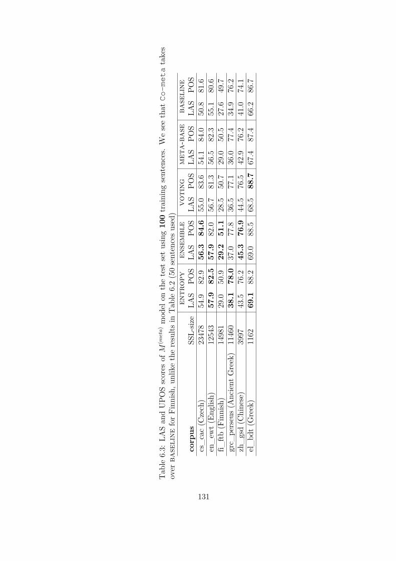
Tab

le6.

3:LA

San

dU

POS

scor

esof

M(m

eta)

mod

elon

the

test

set

usin

g10

0tr

aini

ngse

nten

ces.

We

see

that

Co-meta

take

sov

erba

seli

nefo

rFi

nnish

,unl

ike

the

resu

ltsin

Tab

le6.

2(5

0se

nten

ces

used

)en

trop

yen

sem

ble

voti

ngm

eta-

base

base

line

corp

usSS

L-siz

eLA

SPO

SLA

SPO

SLA

SPO

SLA

SPO

SLA

SPO

Scs

_ca

c(C

zech

)23

478

54.9

82.9

56.3

84.6

55.0

83.6

54.1

84.0

50.8

81.6

en_

ewt

(Eng

lish)

1254

357

.982

.557

.982

.056

.781

.356

.582

.355

.180

.6fi_

ftb(F

inni

sh)

1498

129

.050

.929

.251

.128

.550

.729

.050

.527

.649

.7gr

c_pe

rseu

s(A

ncie

ntG

reek

)11

460

38.1

78.0

37.0

77.8

36.5

77.1

36.0

77.4

34.9

76.2

zh_

gsd

(Chi

nese

)39

9743

.576

.245

.376

.944

.576

.542

.976

.241

.074

.1el

_bd

t(G

reek

)11

6269

.188

.269

.088

.568

.588

.767

.487

.466

.286

.7

131

Table 6.4: LAS on the Greek(el_bdt) corpus for each model, with the average con-fidence score g(y) comparing M (word) and M (char) over the entire test set using 100training sentences.

Method word char meta confidenceentropy 61.8 66.7 69.1 0.871ensemble 61.4 66.9 69.0 0.879without 57.6 65.2 67.4 0.799

6.4.1 Results in Low-Resource Settings

Impact of Multi-View Learning. Table 6.2 and Table 6.3 show the experimental

results of M (meta) on the test data of each language, with 50 and 100 training sentences,

respectively. We see that the proposed co-training method shows average performance

gains of −0.9 ∼ +9.3 LAS points in parsing and +1.7 ∼ +6.9 points in tagging

compared to baseline.

Note that the proposed meta-base approach also shows a LAS improvement of

−0.6 ∼ +6.5 for baseline as well. Breaking down the contribution of improvement,

Co-meta shows −0.3 ∼ +2.8 LAS improvement over meta-base and this improve-

ment is comparable to the improvement of meta-base over baseline.

Comparison of Co-meta Variants. When we compare the three proposed co-

training approaches, one can see that the ensemble approach seems to work better

than entropy, and voting is always worst. This is because the best-voted labels

for each token do not guarantee to get an optimal structure over the parse tree at

the sentence-level, since the voting model has a relatively high chance of learning

from the inconsistent graph that has multi-roots and cycling heads among tokens

(Kiperwasser and Goldberg, 2016a). Figure 6-4 describes the label selection method

of ensemble and voting for a token. ensemble makes a decision by taking into

account the probability of each possible label from the three models. On the contrary,

voting makes a local decision and selects the most popular label. We found that

both two methods make a local decision but voting made a lot more errors during

training.

Lastly, we also try running Co-meta experiments without confidence scores, i.e.,

132

Figure 6-4: An example of the label selection method for ensemble and voting.

we set the confidence score as 1. We find that, with this configuration, performance

always decreases in comparison to meta-base, and thus, we conclude that the pro-

posed confidence score plays a major role in stabilizing the Co-Train approach. Figure

6-5 presents the impact of our confidence score based on the size of unlabeled sen-

tences. We see positive gains using our confidence score when the number of unlabeled

sentences is more than 1200.

Interaction among the layers. More detailed per-layer analysis of the LAS scores

is available in Table 6.4 for the case of the Greek corpus. Among the three views,

char always outperforms word, and all the three views improve after using Co-meta:

improvements of +1.6-1.7 LAS point for meta, +1.5-1.7 for char and +3.8-4.2 for

word.

We can make three observations. First, we note that the model with lower perfor-

mance, namely word view in our example, always benefits the most from other better-

performing views. Second, the evolution of low-performing views towards better re-

sults has a positive effect on meta view, and thus on the overall performance. While

the score char increases by +1.5, meta increases by +1.7. If the lower-performing-

view model was not helping, then the improvement would be upper-bounded by the

performance gain of the higher-performing model. Note that we do not update the

meta layer θ(meta) when using Co-meta, and all the gains result from the improve-

ments of the single-view layers. Lastly, the confidence column shows that the

consensus increases, and thus, we can confirm that promoting consensus-philosophy

133

0 5000 10000 15000 20000 25000 30000The number of unlabeled sentences

35.5

36.0

36.5

LAS

scor

e

with confience scorewithout confience score

Figure 6-5: Evaluation results for Chinese (zh_gsd) based on different sizes of theunlabeled set and proposed models. We apply ensemble-based Co-meta with thefixed size of 50 training sentences while varying the unlabeled set size.

of Co-Train works as intended in Co-meta. In other words, higher confidence

denotes that models predict a similar tree structure by learning from each other.

Sensitivity to the Domain of the Unlabeled Set. In Table 6.5, we investigated

a more realistic scenario for our semi-supervised approach for two languages, Chinese

and Greek, by using out-of-domain data: Wikipedia and a crawled corpus. In the case

of Chinese, the crawled out-domain corpus shows better results than the in-domain

corpus for both entropy-based and ensemble-based Co-meta, by up to +1.1 UAS

and +0.9 POS points. In contrast, for Greek, the in-domain corpus (el_bdt) shows a

better result than the out-domain corpus even when the size of el_bdt is only about

13% of the others. We conjecture that as the Chinese has large character sets, the

exposure to diverse characters helps learning regardless of the domain.

Effect of Training Size on Performance. Table 6.2 shows positive results for

Co-meta given fixed size train data. However, would Co-meta be useful even with

extremely low resource scenarios (<50 sentences)? And also in a more favorable

scenario, when more resources are available for training (e.g. >1000 sentences)?

To answer these questions, we conducted an experiment using the zh_gsd (Chi-

134

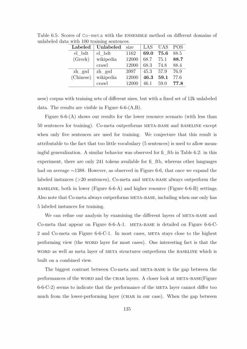
Table 6.5: Scores of Co-meta with the ensemble method on different domains ofunlabeled data with 100 training sentences.

Labeled Unlabeled size LAS UAS POSel_bdt el_bdt 1162 69.0 75.6 88.5(Greek) wikipedia 12000 68.7 75.1 88.7

crawl 12000 68.3 74.8 88.4zh_gsd zh_gsd 3997 45.3 57.9 76.9

(Chinese) wikipedia 12000 46.3 59.1 77.6crawl 12000 46.1 59.0 77.8

nese) corpus with training sets of different sizes, but with a fixed set of 12k unlabeled

data. The results are visible in Figure 6-6-(A,B).

Figure 6-6-(A) shows our results for the lower resource scenario (with less than

50 sentences for training). Co-meta outperforms meta-base and baseline except

when only five sentences are used for training. We conjecture that this result is

attributable to the fact that too little vocabulary (5 sentences) is used to allow mean-

ingful generalization. A similar behavior was observed for fi_ftb in Table 6.2: in this

experiment, there are only 241 tokens available for fi_ftb, whereas other languages

had on average ∼1388. However, as observed in Figure 6-6, that once we expand the

labeled instances (>20 sentences), Co-meta and meta-base always outperform the

baseline, both in lower (Figure 6-6-A) and higher resource (Figure 6-6-B) settings.

Also note that Co-meta always outperforms meta-base, including when one only has

5 labeled instances for training.

We can refine our analysis by examining the different layers of meta-base and

Co-meta that appear on Figure 6-6-A-1. meta-base is detailed on Figure 6-6-C-

2 and Co-meta on Figure 6-6-C-1. In most cases, meta stays close to the highest

performing view (the word layer for most cases). One interesting fact is that the

word as well as meta layer of meta structures outperform the baseline which is

built on a combined view.

The biggest contrast between Co-meta and meta-base is the gap between the

performances of the word and the char layers. A closer look at meta-base(Figure

6-6-C-2) seems to indicate that the performance of the meta layer cannot differ too

much from the lower-performing layer (char in our case). When the gap between

135

20 40 60 80 100

40

50

60

70UP

OS sc

ore

(A-1) UPOS Scores in low-resource

Co-metameta-basebaseline

20 40 60 80 100

10

20

30

40

LAS

scor

e

(A-2) LAS Scores in low-resource

Co-metameta-basebaseline

500 1000 1500 2000 2500 3000 3500 400088

90

92

94

UPOS

scor

e

(B-1) UPOS Scores in high-resource

Co-metameta-basebaseline

500 1000 1500 2000 2500 3000 3500 4000

65

70

75

80

LAS

scor

e

(B-2) LAS Scores in high-resource

Co-metameta-basebaseline

20 40 60 80 100

40

50

60

70

UPOS

scor

e

(C-1) UPOS Scores of Co-meta

metawordchar

20 40 60 80 100

30

40

50

60

70

UPOS

scor

e

(C-2) UPOS Scores of meta-base

metawordchar

Figure 6-6: Evaluation results for Chinese (zh_gsd) based on the different sizes ofthe train set and proposed models. We apply ensemble based Co-meta with thefixed size of 12k unlabeled sentences while varying training set size.

word and char becomes too large (>5 points), then the performance gain of meta

layer is parallel to that of char layer for train size of 10–50 even when the word

layer makes steeper performance gains. In contrast, the Co-meta’s meta layer from

Figure 6-6-C-1 shows more stable performance as the gap between char and word

is minimal as the two layers learn from each other.

To summarize from Table 6.2 and Figure 6-6, the proposed SSL approach is always

beneficial for the meta-BiLSTM structure when comparing the LAS scores between

Co-meta and meta-base. However, the meta-BiLSTM structure itself might not

136

Table 6.6: LAS for the English (en_ewt) corpus for each model, with the externallanguage models with the entire train set.

Model LM LAS UAS POSudpipe (Kondratyuk, 2019) - 86.97 89.63 96.29baseline (Lim et al., 2018a) - 86.82 89.63 96.31metabase - 86.95 89.61 96.19Co-meta - 87.01 89.68 96.17baseline (Lim et al., 2018a) ELMo 88.14 91.07 96.83metabase ELMo 88.28 91.19 96.90Co-meta ELMo 88.25 91.19 96.84udify (Kondratyuk, 2019) bert-multi 88.50 90.96 96.21uuparser (Kulmizev et al., 2019) bert-multi 87.80 - -baseline bert-multi 89.34 91.70 96.66metabase bert-multi 89.49 92.01 96.75Co-meta bert-multi 89.52 91.99 96.80Co-meta bert-base 89.98 92.25 97.03

benefit when too few tokens exist in the train set. In general, we hypothesis that for

the meta-BiLSTM structure to be useful, the train set should consist of more than

300 tokens (more than 20 sentences) to provide enough generalization information.

6.4.2 Results in High-Resource Settings

Although the lack of annotated resources for many languages has given rise to low-

resource approaches, there are also several languages for which we have plenty of

resources. We can thus examine whether our approach is also effective in more favor-

able settings, when large scale resources are available. A comprehensive overview is

shown in Table 6.6, 6.7, where different systems using no language model (first part

of the table), or ELMo (Peters et al., 2018) or BERT (Devlin et al., 2018) language

models are evaluated.

Table 6.6 includes a comparison of our results using the approach presented in this

chapter with four state-of-the-art systems. The first system is our baseline (intro-

duced in Section 6.1.1), which obtained the best LAS measure for English in the 2018

CoNLL shared task. The second is udpipe (Straka, 2018; Kondratyuk, 2019) which

was one of the best performing systems during the 2018 CoNLL shared task (best

137

Table 6.7: LAS for the Chinese (zh_gsd) corpus for each model, with BERT–Multilingual embedding using the entire training set. We observe much higher im-provements than for English showed (see Table 6.6), probably because zh_gsd hasa relatively small training set (3,997) and larger character sets than the training set(12,543) of en_ewt.

Model LM LAS UAS POSudpipe - 80.50 84.64 94.88baseline - 79.70 84.28 94.41metabase - 80.32 84.58 94.72Co-meta - 80.71 84.99 94.81udify bert-multi 83.75 87.93 95.35uuparser bert-multi 83.7 - -metabase bert-multi 83.90 88.07 96.07Co-meta bert-multi 84.21 88.39 96.07

MLAS score, that combines tagging and parsing, and 2nd for the average LAS score).

udpipe uses a multi-task learning approach with a loosely-joint LSTM layer between

tagger and parser. The third system is udify (Kondratyuk, 2019) (derived from ud-

pipe), where the LSTM layer is replaced with BERT embedding, which is in turn

fine-tuned during training. The fourth system is uuparser wherein concatenated

word, character and BERT embedding serves as an input, e.g., hi =[v(wc);v(bert)].

Effect of Co-meta On High-Resource Settings without LMs. By expanding

the baseline with our meta-LSTM and SSL approach, we observe a slight improve-

ment of up to 0.19 and 0.04 points against the baseline and udpipe, respectively.

In contrast, we find that both meta-base and Co-meta slightly underperform the

baseline in tagging, which goes against our intuition. One possible reason might be

that there is enough data to get accurate results using a supervised learning approach

while SSL suffers from unexpected surface sequences. Another evidence of this is that

SSL did not bring further improvement when using more than 10,000 training sen-

tences. In contrast, interestingly, Chinese (Table 6.7) for which we had a relatively

small train set (3,997), is positively affected by the SSL approach, with a gain of up

to +0.21 LAS points compared to udpipe, +1.12 points compared to baseline. We

assume that the main reason for this is the character set. Languages with a bigger

138

character set size and little training data gain more influence with SSL.

Effect of Co-meta On High-Resource Settings with LMs. While we train our

model with a LM, we concatenate the last layer of the LM embedding with the input

of the BiLSTM (meta) presented in the previous section. Finally, the input of our

meta model consists of three different contextualized features as [h(word)i ;h(char)

i ;v(lm)i ].

On average, adding a LM provides excellent results both for dependency parsing

and POS tagging, outperforming by large margins previous results obtained without

LMs (up to +1.27 LAS for ELMo and +2.97 for BERT). Furthermore, our parser

with Co-meta globally shows better results than the state-of-the-art parsers that use

ELMo (Lim et al., 2018a) and the BERT-Multilingual model (Kondratyuk, 2019).

However, it should be noted that the udify model used by (Kondratyuk, 2019) (that

includes Bert-Multilingual as a LM) was first trained with 75 different languages using

Universal Dependency corpora and then tuned for English, and it is not clear how

this training process affects the performance. Thus, we add the results of uuparser

and baseline with BERT to represent fine-tuning in a monolingual way only and

still found that co-meta+bert-multi yields better performance.

We generalized Co-meta by adding an additional view: LM embedding. We

conclude that Co-meta can, surprisingly, result in positive effects by more than +1–

+1.7 points compared to competing models and by +0.2 compared to the baseline

even in a high-resource setting, especially when a LM embedding is present.

6.5 Summary

In this chapter, we have proposed Co-meta, a SSL on multi-view learning strategy

using co-training methods. The proposed model is evaluated on the multi-task of

POS tagging and dependency parsing. In this setting, multi-view learning shows

a large improvement in comparison to a single model with a combined view in the

input level on all levels: low-, mid-, and high-resource settings with or without a LM

embedding. Furthermore, Co-meta is more stable and yields significant gains on low-,

139

and mid-resource settings and marginal gain in high-resource settings compared to

META-BASE, a multi-view learning model without SSL. The proposed entropy and

ensemble-based methods yield the best prediction among multi-views and update the

individual-view model based on a confidence score. This strategy is especially well

suited for low-resource scenarios, when only a very small sample of annotated data

is available, along with larger quantities of unlabeled data. Our experiment shows

statistically significant gains (−0.9 ∼ +9.3 points compared to the baseline), largely

due to the proper integration of unlabeled data in the learning process. Finally, this

chapter shows the performance of Co-meta varies as we change the size of labeled

and unlabeled dataset in the case of the el_bdt and zh_gsd corpora, so that we were

able to provide some comments on the chance that Co-meta would succeed or fail.

140

Chapter 7

Multilingual Co-Training

In Sections 4 and 6, we discussed two main bootstrap methods, multilingual transfer

learning and co-training. Although these two approaches have yielded outstanding

performance compared to the supervised monolingual model in low-resource scenar-

ios, several questions remain, including whether two bootstrap methods can work

together. No attempts have yet been made to apply both multilingual and semi-

supervised learning simultaneously owing to structural limitations. Because the pro-

posed transfer learning method based on multilingual token representations takes

several treebanks from several languages in input, some difficulties were encountered

when applying the semi-supervised learning approach using unlabeled data. For exam-

ple, we need to adjust the ratio between labeled and unlabeled data and also between

languages to avoid overfitting, especially when the languages have different character

sets. Recently, Kondratyuk (2019) proposed a multilingual approach based on the

multilingual BERT model. This parser can simultaneously learn from 75 languages

using 142 annotated treebanks and, of course, also parse 75 languages. Interestingly,

the parser showed state-of-the-art performance in low-resource languages because it

can capture sub-word information from similar languages by tuning the BERT lan-

guage model (parameter tuning). However, this approach does not consider the use

of unlabeled data for training.

In this chapter, we investigate how to integrate the two proposed methods and

we analyze the effect of this integration for parsing. This chapter is structured as

141

Figure 7-1: The overall structure of our Co-metaM model. This system generatesword- and character-level representation vectors and concatenates them into a unifiedword embedding for every token in a sentence. The word-level representation can bea multilingual embedding as proposed in Section 4.2. Thus, this system can train adependency model, using both labeled and unlabeled resources from several languages.

follows: we describe an approach that uses simultaneously multilingual and transfer

learning (presented in Chapter 4) and co-training (presented in Chapter 6) in Section

6.1. The evaluation results are presented in Section 6.3.

7.1 Integration of Co-Training and Multilingual

Transfer Learning

To evaluate the benefit of co-training, we use the same structure with Co-meta as

presented in Section 6.3. This model thus integrates three individual parsers based

on three different views (char, word, and meta-BiLSTM), and produces three

predicted parse trees (yword, ychar, ymeta) using unlabeled data. When the parser in-

tegrates the co-training approach (Semi-supervised learning), the best (predicted)

possible tree y∗ is generated using an ensemble, voting, and entropy-based method ap-

plied on the predictions of the three based parsers. To apply multilingual approaches

to Co-meta, a function that considers multilingual representations is required. As

mentioned in Section 4.2, a possible option is to use a cross-lingual word embedding

obtained after the projection of two monolingual embeddings via a bilingual dictio-

142

nary. The resulting cross-lingual embeddings are supposed to have similar vectors

for words with a similar meaning in two languages (e.g., English “dog” and French

“chien”). When a cross-lingual word representation is built using two languages, A

and B, the embedding can be directly applied to train the cross-lingual dependency

parser based on two training corpora from language A and B. Figure 7-1 shows the

structure of our system expanded from Co-meta with multilingual word representa-

tions. Since the system uses a multilingual word embedding, it can also take several

training corpora in the input. Notably, the character-level representation would be

monolingual when different writing systems are considered (e.g., Korean and French).

Hereinafter, we will call this multilingual Co-meta Co-metaM (Co-metaM is the mul-

tilingual variant of Co-meta).

7.2 Experiments

To quantify the effectiveness of Co-metaM in low-resource scenarios, we select Sami

and the cross-lingual word embeddings used in Section 4.3. Sami was one of the

low-resource languages proposed in the CoNLL shared task 2017 and only 20 anno-

tated sentences were provided fro training. However, in 2018, the number of training

sentences was expanded to 1,662 to ensure efficient testing for both high- and low-

resource scenarios. We used the same environmental settings presented in Section 6.4

(Co-meta), i.e. the hyper-parameter settings, dimension of LSTM, and learning rate

were kept the same.

7.2.1 Preparation of Language Resources

We used the lexical resources presented in Chapter 4, including the bilingual dictio-

naries and word embeddings. Table B.1 shows the sizes of the dictionaries used.

We used the pretrained Finnish FastText word embedding published by Facebook

(Bojanowski et al., 2016b), as presented in Section 4.3. As the Sami Wikipedia is

relatively small, we also trained larger word embeddings using FastText. When co-

training (presented in Section 6.2) was applied using unlabeled data, the unlabeled

143

Bilingual pairs Bi-dictionary Bi-embeddingFinnishNorth Sami 12,398 2.4GBNorth SamiEnglish 8,746 7.5GBNorth SamiFinnish 10,541 2.4GB

Table 7.1: Dictionary sizes and size of bilingual word embeddings generated fromeach dictionary.

data provided by the shared task organizer was used1. This unlabeled data also used

for training word embeddings as well.

7.2.2 Experiments strategies

We conducted a series of experiments on Sami. We tested different language combi-

nations to get a cross-lingual parsing model. All the experiments were carried out

using the 20 Sami sentences provided for training for the 2017 CoNLL Shared Task.

Therefore, these results can be compared to the ones in the official CoNLL evaluation.

As presented in Section 4.3, when training a model with multilingual data, the

size of the training corpora for low-resource languages is smaller than that for high-

resource languages. Following our previous work presented in Section 4.3, we iterated

for additional 20 times for low-resource training data as compared to the scenario of

high-resource. For example, when iterating 20 times using 20 Sami sentences, the

system iterates only one time using 12,543 Finnish sentences. When applying co-

training, we used the unlabeled data with batch size 2, as presented in the previous

section.

7.3 Results

Impact of the multilingual approach. Table 7.2 shows our experimental results

based on the different pairs of training data with the gold-tokenized input. The mul-

tilingual approach outperforms every monolingual approach. Additionally, the choice

of the language pairs is significant: compare for example sme+eng and sme+fin,1https://lindat.mff.cuni.cz/repository/xmlui/handle/11234/1-1989

144

Case Training corpus Model LAS UAS1 sme (20) Co-metaM without Co-training 32.96 46.852 eng (12,217) Co-metaM without Co-training 32.72 50.443 fin (12,543) Co-metaM without Co-training 40.74 54.244 sme (20) + eng (12,217) Co-metaM without Co-training 46.54 61.615 sme (20) + fin (12,543) Co-metaM without Co-training 51.57 63.06

4-1 sme (20) + eng (12,217) Co-metaM 46.97 61.445-1 sme (20) + fin (12,543) Co-metaM 53.80 66.76

Table 7.2: Labeled attachment scores (LAS) and unlabeled attachment scores (UAS)for Northern Sami (sme) based on the use of the training corpora

which yielded LAS scores of 46.54 and 51.57, respectively. In addition to the multilin-

gual approach, co-training has a positive effect on the overall performance, especially

for sme+fin (note though that this is not the case for sme+eng). We assume that

this difference is due to the different character sets and word order between the two

languages.

Comparison with the CoNLL Shared Task. We used the same environmental

settings in these experiments as for the CoNLL Shared Task (same training sets, no de-

velopment set and application of the baseline tokenizer). Table 7.3 reports the official

2017 CoNLL results with our multilingual model trained for Sami and Finnish. C2L2

(Cornell Univ.) obtained the best performance for Sami with a delexicalized transfer

approach (using a Finnish training corpus and a corpus of 20 Sami sentences as a

development set for parameter tuning without lexicalized features). IMS (Stuttgart)

used a delexicalized transfer approach with an exceptionally large training corpus

based on 40 different training corpora in UD, thereby obtaining the second-best re-

sult. Compared with the result of the Shared Task, our approach without co-training

(lexicalized cross-lingual transfer parsing with resources from relevant languages) can

be effective for parsing low-resource languages when observing the “Co-metaM with-

out co-training” model. When our multilingual parser is used with the co-training

approach (Co-metaM), the performance dramatically improves compared to the other

model, with an average LAS gain of +2.23 ∼ 7.25. Interestingly, it seems that the

multilingual approach is more important than co-training for Sami, if we compare the

145

Model LAS UASC2L2 (Ithaca) (Shi et al., 2017a) 48.96 58.85

IMS (Stuttgart) (Björkelund et al., 2017a) 40.67 51.56HIT-SCIR (Harbin) (Che et al., 2017a) 38.91 52.51

LATTICE (Paris) (Lim and Poibeau, 2017b) 28.39 42.72Co-metaM 49.73 59.89

Co-metaM without Co-training (unlabeled data) 47.50 58.94Co-metaM without multilingual training 45.16 57.17

Co-metaM without Co-training and multilingual training 41.48 53.61

Table 7.3: Comparison with top four results for Sami from the CoNLL 2017 SharedTask and our multilingual model trained on Sami and Finnish corpora.

individual contribution of each technique to Co-metaM.

7.4 Summary

In this chapter, we have presented a multilingual co-training approach for parsing

that is effective for languages having limited resources for training. We demonstrated

that our Co-metaM (Multilingual Co-training) model yields better results compared

to monolingual ones. We also found that a multilingual word embedding derived from

carefully selected related languages is more crucial than co-training (Semi-supervised

learning) for low-resource scenarios. With the careful selection of training data, it is

possible to enhance parsing results for low-resource languages.

146

Chapter 8

Conclusion

The present thesis mainly focused on bootstrapping methods for accurate dependency

parsing under low-resource conditions. Two approaches, namely, multilingual transfer

learning and co-training, were proposed.

8.1 Summary of the Thesis

In the course of this thesis, we have examined the different resources available for

parsing, including labeled treebanks, unlabeled treebanks, pre-trained word represen-

tations, and pre-trained language embeddings (ELMo, Bert). Our monolingual and

multilingual systems (described in chapter 3 and 4) make full use of these resources

in high resource scenarios. We also examined how knowledge can be transferred from

several languages to train low-resource languages. Additionally, co-training enabled

the use of unlabeled data as a training set.

In Chapter 4, we extended a monolingual parser to make it multilingual, based

on multilingual lexical representations. We showed that the bilingual word mapping

approach is effective with multilingual training sets. This approach is simple yet

powerful for creating a dependency parsing model when no annotated corpus or par-

allel corpus is available for training. Our approach requires only a small bilingual

dictionary and the manual annotation of a handful of sentences. We showed that the

performance one can obtain with this approach depends largely on the set of languages

147

used for training. This was done by investigating several models using genetically re-

lated and non-related languages to gain a better understanding of the limitations or

possibilities of model transfer across different language families. For example, we pre-

sented three multilingual models, namely, Komi-English, Komi-Finnish (genetically

related languages), and Komi-Russian (geographically related languages) models for

parsing. The best results were obtained with the Komi-Finish and Komi-Russian

models, which shows that language typology and geography play a role.

In Chapter 6, we proposed a co-training parsing model that can infer information

from unlabeled data. The primary idea was to augment the quantity of labeled

data with automatic methods. We showed that an automatic approach based on

the combination of different “views” (character-based analysis, token-based analysis,

etc.) provides good enough predictions to be able to generate a highly accurate

combined result, that in turn can be used as training data. To compute the confidence

of the predicted labels when the views are combined, we proposed three different

methods, namely, the entropy-, voting-, and ensemble-based score. This strategy

is especially well suited for low-resource scenarios, when only an exceedingly small

sample of annotated data is available, along with larger quantities of unlabeled data.

The proposed model showed consistent improvement across the different test cases

used. Moreover, the evaluations on various domains and languages demonstrated the

effectiveness and robustness of the proposed approach.

Based on our experiments, we can conclude by examining the different questions

raised in the introduction.

8.2 Discussion over the Research Questions of the

Thesis

(A) In the course of this thesis, we have shown that a multilingual approach

provides accurate results for parsing. This approach is especially suited for

low resource scenarios as it makes it possible to transfer knowledge from

148

a well-resourced language to a low resource one. However, the conditions

under which these experiments are carried out must be examined in detail.

We have shown that the multilingual transfer learning approach, which utilizes

annotated data from several languages, is advantageous for low-resource languages.

However, we also found that a careful selection of the related languages used for

the experiments is important for transfer learning. Specifically, in Section 4.1, we

investigated the multilingual transfer approach as a substitute for the more typical

monolingual approach. We proposed a method that compensates the lack of training

data with transfer learning, which enabled us to use different corpora in different

languages as training data. In most cases, for instance, in the CoNLL 2017 shared

task (Zeman et al., 2017a), the teams that adopted this approach used a multilingual

delexicalized parser (i.e. a multi-source parser trained without considering lexical

features). However, it is evident that delexicalized parsing cannot capture contextual

features that depend on the meaning of the words within the sentence. This led to

the creation of multilingual lexical representations. As discussed in Section 4.4, the

multilingual transfer learning approach based on multilingual word representations

showed better results than the delexicalized one under low-resource conditions. In

addition, the results on the CoNLL shared task demonstrated the good performance

of our multilingual approach for a wide variety of languages.

(A-1) Is parallel data required for multilingual parsing?

• We believe that parallel corpora are no longer needed when using a transfer

learning approach. Instead, monolingual raw texts can be used to train mono-

lingual word embeddings. As presented in Section 4.1, once we integrate a mul-

tilingual transfer learning approach to produce multilingual lexical resources,

we only need to map lexical resources among the languages. Traditionally, a

large parallel corpus or a bilingual dictionary is required to map two different

word embeddings into a joint distributional space (Artetxe et al., 2016a; Guo

et al., 2015b). However, (Artetxe et al., 2017) proposed a method for mapping

two different embeddings based on a linear transformation and using only 25

149

pairs of words, with almost no decrease of the quality of the result.

(A-2) How can we bootstrap a system when no parallel corpus is available?

• To answer this question, we have presented two different case studies, around

Komi (a Finno-Ugric language spoken in Russia) and five different low resource

languages used for evaluation during the CoNLL 2017 shared tasks (these lan-

guages were called “Surprise” languages because the languages and the data

were provided only a few days before the evaluation). In Sections 4.3 and 5.4

we suggested the use of a bilingual word embedding (integrating the vocabulary

of the language to be parsed and the vocabulary of another, linguistically re-

lated language, for which different resources including a treebank is available).

However, it must be noted that even for low-resource languages, raw texts are

required as the minimum resource to train a word embedding. This multilingual

lexicalized approach based on transfer learning achieved good results during the

CoNLL 2017 evaluation. In practice, larger bilingual dictionaries can be used

to improve the result; however, only 25 pairs of words are sufficient to align the

embeddings reasonably well.

(B) In this thesis, we also examined whether using unlabeled data for

parsing, especially in low resource scenarios, can improve the results.

There have been several semi-supervised learning (SSL) algorithms proposed for

parsing, and these algorithms generally obtained better results than the typical su-

pervised learning approach. Among these approaches, self-training (see Section 2.4),

which is based on concatenated lexical representations (e.g. concatenation of char and

word embeddings), is especially interesting. However, the main problem of this simple

concatenation approach is that it can lead to overfitting in low-resource conditions, as

the model may ignore the specific statistical properties of each lexical representation.

As presented in Chapter 6, we suggest the application of co-training on individual

models trained with limited features. Co-training is a semi-supervised approach that

trains multiple learners (parsers in our case) based on different features (views). The

150

views in our case refer to the word and character-level representations. Subsequently,

a single-view model is constructed that concatenate single-view-model outputs to

form the input of the meta layer. Because each parser struggles to identify the best

features within the limited character and word features, this method maximizes the

use of lexical features under low-resource conditions.

(B-1) Can traditional Co-Training approaches further improve dependency

parsing in low-resource scenarios?

• Based on our experimental results presented in Section 6.4, we see that the

proposed co-training approach is always advantageous for the meta-BiLSTM

structure that trains several different parsers simultaneously. We found up to

+9.3 LAS gains when comparing the LAS scores between our co-training model

and the baseline model. However, the meta-BiLSTM structure itself may

not benefit when extremely few tokens exist in the training set. In general,

we hypothesize that for the co-training structure to be useful, the training

set should include more than 300 tokens (more than 20 sentences) to provide

meaningful generalizations.

(B-2) Can co-training models that consider different views globally (i.e.

at the sentence level) learn from each other on unlabeled data? Does this

improve the performance for low-resource languages?

• To answer this question, we set three different parsers that consume individual

features (views) as input, namely char, word, and meta and subsequently

allowed these parsers teach each other using unlabeled data (in Section 6.3).

We found that the three models improved in terms of performance after using

co-training: improvement was 1.6-1.7 LAS point for meta, 1.5-1.7 for char,

and 3.8-4.2 for word for Chinese.

We report two observations. First, we note that the model (parser) with the

lowest performance, namely the word model in this example, always benefits

151

the most from the better-performing models. Second, the transition of low-

performing models into those yielding better results has a positive effect on

meta view, and consequently on the overall performance. While the score

char increases by 1.5, meta increases by 1.7. Without the assistance of low-

performing-view model, the improvement would have been upper-bounded by

the performance gain of the high-performing model.

(B-3) How many labeled and unlabeled sentences are needed for co-train-

ing to be beneficial?

• To answer this question, we presented an experiment in Section 5.4 using the

zh_gsd (Chinese) corpus with training sets of different sizes, but with a fixed

set of 12k unlabeled data. Our co-training model shows the best performance

over the baseline except when only five sentences were used for training. We

believe that this is attributable to the fact that an extremely small vocabulary

was used for meaningful generalization. However, once we expand the labeled

examples (>20 sentences), our co-training model always outperforms the other

models, both in low and high (<500 sentences) resource settings.

In Section 6.3, we investigated the performance gains depending on the use of

different domains of semi-supervised corpora. We evaluated on two languages,

Chinese and Greek, using out-of-domain data: Wikipedia and a crawled corpus.

In the case of Chinese, the crawled out-domain corpus shows better results

than the in-domain corpus by up to 1.1 UAS and 0.9 POS points. In contrast,

for Greek, the in-domain corpus (el_bdt) shows a better result than the out-

domain corpus even when the size of el_bdt is only approximately 13% of the

others. We determine that as Chinese has large character sets, the exposure to

diverse characters is advantageous during learning regardless of the domain.

(C) What is the effect on the results of our parser when the two proposed

approaches, (A) multilingual and (B) SSL, are simultaneously applied as

a multilingual SSL model?

152

• As discussed in Section 6.3, Co-metaM show much better results than the other

models, (1) without co-training, with 2.23 LAS, (2) without multilingual repre-

sentations, with 4.57 LAS, and (3) both co-training and multilingual approach,

with 8.29 LAS. Based on these experimental results, we determine that the

two proposed approaches lead to a performance improvement. Additionally,

the two methods demonstrated a positive synergy when working in cooperation

with one another.

8.3 Perspectives

In this thesis, we have shown that multilingual word embeddings can be used to train

a model that combines data from multiple languages. This seem to be particularly

useful for low-resource scenarios. We have for example conducted different experi-

ments around Komi: the strategy was mainly to use a knowledge transfer approach,

where some information is automatically derived from corpora in different languages.

We have designed experiments with different language pairs, and we have observed

that the language pair Finnish–Russian is one of the most accurate one for Komi.

This work has however some important limitations, the main one being that we do

not know in advance which language combination will give the best results in the end.

Although it is theoretically possible to build truly multilingual models (e.g., Finnish-

Komi-Russian), we found that a bilingual Finnish-Komi model performed best, based

on our tests on Komi. It could thus be useful to look at language typologies and see

if these typologies contain usable data and information for parsing.

Apart from the multilingual approach, co-training methods also improved perfor-

mance for dependency parsing in low-resource scenarios. However, it does not mean

that this approach always brings some benefit, because semi-supervised learning is

highly sensitive to parameter settings. For example, we observed that, with our co-

training method, the ratio of labeled vs unlabeled data for training should be adjusted

very precisely. More specifically, the method is prone to overfitting when one uses

too much unlabeled ones (vs labeled one). It would be both interesting and useful to

153

investigate this issue, and try to determine what proportion of labeled and unlabeled

date should be used for an optimal result, according to the context.

154

Appendix A

Universal Dependency

A.1 The CoNLL-U Format

Universal Dependencies (UD) is a framework for consistent annotation of grammar

and the annotation format is called CoNLL-U. The format contains parts of speech,

morphological features, and syntactic dependencies. The description of tagsets and

examples of tagging are based on the official website1.

In the CoNLL-U format, words are indexed with integers, while multiword tokens

are indexed with integer ranges like 1-2 or 4-7. Lines representing such tokens are

inserted before the first word in the range. Figure A-1 shows an example of tokenized

output of a sentence with multiword tokens.

Observing an example of syntactic annotation (Figure A-2), the UPOS field con-1https://universaldependencies.org/format.html

Figure A-1: An example of tokenization of Universal Dependency

155

Figure A-2: An example of syntactic annotation of Universal Dependency

tains a part-of-speech tag from the universal POS tag set, while the XPOS optionally

contains a language-specific part-of-speech tag, normally from a traditional, more

fine-grained tagset. If the XPOS field is used, the treebank-specific documentation

should define a mapping from XPOS to UPOS values (which may be context-sensitive

and refer to other fields as well). If no language-specific tags are available, the XPOS

field should contain an underscore for all words. The FEATS field contains a list of

morphological features, with vertical bar (|) as list separator and with underscore to

represent the empty list. All features should be represented as attribute-value pairs,

with an equals sign (=) separating the attribute from the value.

The HEAD (the 7th column in Figure A-2) and DEPREL (the 8th column in

Figure A-2) fields are used to encode a dependency tree over words. The DEPREL

value should be a universal dependency relation or a language-specific subtype of

such a relation (defined in the language-specific documentation). As in the case of

morphology, syntactic annotation is only provided for words, and tokens that are not

words have an underscore in both the HEAD and DEPREL fields.

The HEAD and DEPREL values define the basic dependencies which must be

strictly a tree. However, in addition to these basic dependencies, treebanks may

optionally provide an enhanced dependency representation that specifies additional

dependency relations, for example, when dependencies propagate over coordinate

structures. The enhanced dependency representation, which in general is a graph

and not a tree, is specified in the DEPS field, using a list of head-relation pairs. We

use colon (:) to separate the head and relation and (as usual) vertical bar (|) to

separate list items and underscore for the empty list. The list is to be sorted by the

index of the head: 4:nsubj|11:nsubj.

156

A.2 Tagsets

The Universal Dependency has 37 unified (standard) dependency relation tag sets as

follows:

1. acl: clausal modifier of noun (adjectival clause)

2. advcl: adverbial clause modifier

3. advmod: adverbial modifier

4. amod: adjectival modifier

5. appos: appositional modifier

6. aux: auxiliary

7. case: case marking

8. cc: coordinating conjunction

9. ccomp: clausal complement

10. clf: classifier

11. compound: compound

12. conj: conjunct

13. cop: copula

14. csubj: clausal subject

15. dep: unspecified dependency

16. det: determiner

17. discourse: discourse element

18. dislocated: dislocated elements

157

19. expl: expletive

20. fixed: fixed multiword expression

21. flat: flat multiword expression

22. goeswith: goes with

23. iobj: indirect object

24. list: list

25. mark: marker

26. nmod: nominal modifier

27. nsubj: nominal subject

28. nummod: numeric modifier

29. obj: object

30. obl: oblique nominal

31. orphan: orphan

32. parataxis: parataxis

33. punct: punctuation

34. reparandum: overridden disfluency

35. root: root

36. vocative: vocative

37. xcomp: open clausal complement

The Universal Dependency has 17 Universal Part-Of-Speech (UPOS) tag set as

follows:

158

1. ADJ: adjective

2. ADP: adposition

3. ADV: adverb

4. AUX: auxiliary

5. CCONJ: coordinating conjunction

6. DET: determiner

7. INTJ: interjection

8. NOUN: noun

9. NUM: numeral

10. PART: particle

11. PRON: pronoun

12. PROPN: proper noun

13. PUNCT: punctuation

14. SCONJ: subordinating conjunction

15. SYM: symbol

16. VERB: verb

17. X: other

159

Appendix B

Résumé en français de la thèse

B.1 Introduction

Le développement de systèmes automatiques, pouvant analyser avec succès des langues

faiblement dotées, est une question cruciale pour le traitement automatique des

langues (TAL). La plupart des systèmes d’analyse sont en effet fondés sur des

techniques d’apprentissage supervisé nécessitant de grandes quantités de données an-

notées : la disponibilité de tels corpus est une des conditions principales pour obtenir

des performances correctes, quelle que soit la tâche visée. Ce type de techniques est

donc bien adapté pour les quelques langues pour lesquelles on dispose de nombreuses

ressources en ligne (dictionnaires et surtout corpus annotés), mais l’approche laisse

aussi de nombreuses autres langues de côté, du fait de l’absence des ressources néces-

saires. Par ailleurs, produire des données annotées en grandes quantités demande

beaucoup de moyens (que ce soit au niveau humain ou financier). C’est évidem-

ment un problème majeur pour quantité de langues pour lesquelles ces données sont

quasi inexistantes et pour lesquelles on ne dispose pas des moyens nécessaires pour y

remédier.

Nous nous intéressons dans cet article au cas de l’analyse syntaxique (cet article

reprend en partie la présentation du système développé par le LATTICE pour la tâche

d’évaluation CoNLL 2017 (Lim and Poibeau, 2017a; Lim et al., 2018c))1. L’analyse1Le code source correspondant aux réalisations présentées dans cet article est intégralement

160

syntaxique est une tâche classique, fondamentale pour le TAL et nécessaire pour de

nombreuses applications dérivées. Les systèmes d’analyse syntaxique récents les plus

performants ou les plus emblématiques du domaine (Weiss et al., 2015b; Straka et al.,

2016; Ballesteros et al., 2016b), pour n’en citer que quelques-uns, reposent tous sur

l’approche décrite dans le paragraphe précédent, c’est-à-dire sur une approche par

apprentissage supervisé à partir de grands corpus annotés de la langue visée, souvent

l’anglais.

La communauté a toutefois bien conscience qu’il faut aller au-delà des quelques

langues bien dotées pour lesquelles on dispose de ressources en masse. D’une part

parce qu’il y a des besoins concrets pour d’autres langues : différentes communautés

linguistiques, en particulier celles liées à des langues minoritaires ou en danger, ont

conscience que l’avenir passe entre autres par l’informatisation des langues et la mise

au point d’outils performants, y compris pour le grand public. D’autre part, parce que

les langues moins bien dotées posent souvent des questions extrêmement intéressantes

sur le plan linguistique, et qui ont été trop longtemps négligées jusqu’ici. Les systèmes

entraînés seulement sur l’anglais ne donnent qu’une vision étriquée du TAL, visant

l’analyse d’une langue analytique à la morphologie extrêmement pauvre. Au-delà de

la quantité de données disponible, la prise en compte de la complexité linguistique,

notamment morphosyntaxique, est un autre élément fondamental.

Pour prendre un exemple récent, la tâche d’évaluation lors des conférences Com-

putational Natural Language Learning 2017 et 2018 (CoNLL shared task) (Zeman,

D. et al., 2017; Zeman et al., 2018b) portait sur environ cinquante langues (plus

précisément quarante-neuf en 2017 et cinquante-sept en 2018), soit à peu près toutes

les langues pour lesquelles des données annotées syntaxiquement sont disponibles en

quantité significative au format UD (Universal Dependencies) (Nivre et al., 2016b).

C’est probablement le défi d’analyse syntaxique le plus ambitieux jamais organisé de

ce point de vue, mais le chiffre de cinquante langues est à considérer en regard des six

mille langues estimées dans le monde. Et même si l’on ne considère que les langues

pour lesquelles des données écrites sont disponibles, les cinquante-sept langues de

disponible sur le site : https://github.com/jujbob.

161

CoNLL 2018 ne permettent de couvrir qu’un échantillon extrêmement restreint de ce

qui existe.

En ce qui concerne l’analyse syntaxique automatique, l’approche monolingue et

supervisée (c’est-à-dire par apprentissage automatique à partir de corpus annotés

représentatifs) est évidemment la plus répandue (l’alternative étant les systèmes re-

posant sur des grammaires entièrement élaborées à la main). Des chercheurs essaient

toutefois depuis un certain temps de concevoir des systèmes multilingues. L’approche

multilingue a donné des résultats encourageants aussi bien pour les langues faiblement

dotées (Guo et al., 2015a, 2016) que pour les langues déjà bien dotées, et disposant

déjà de ressources comme des dictionnaires et des corpus représentatifs (Ammar et al.,

2016a,d). Dans ce dernier cas, l’idée est de n’avoir à maintenir qu’un seul modèle

d’analyse et de pouvoir l’appliquer ensuite aux différentes langues constitutives du

modèle. L’approche multilingue a de plus un avantage, même pour les langues bien

dotées : en mettant ensemble plusieurs langues, on peut espérer mieux analyser cer-

tains mots ou certaines constructions rares sans dégrader les performances sur des

phénomènes plus classiques. Il semble donc y avoir toujours un gain possible.

Ainsi, Ammar et ses collègues (cf. références déjà citées) ont proposé des études

portant sur des langues indo-européennes pour lesquelles on dispose déjà de ressources

importantes. Ils ont démontré que l’approche via un modèle multilingue donne

généralement de meilleurs résultats que les modèles monolingues correspondants pour

les langues visées.

D’une manière générale, c’est surtout pour les langues moins bien dotées que

l’approche multilingue est intéressante. Cette approche peut en fait être mise en

œuvre de deux façons différentes. La première consiste à projeter des annotations

disponibles d’une langue donnée vers une langue peu dotée via un corpus parallèle.

Cette approche a été utilisée à plusieurs reprises (notamment dans les références déjà

citées (Guo et al., 2015a; Ammar et al., 2016d)), mais elle nécessite de disposer de

données parallèles en quantité suffisante, ce qui est souvent problématique. Le trans-

fert de connaissances nous semble aussi problématique en soi, dans la mesure où cela

suppose une relative similarité de structure entre les deux langues visées. Si les deux

162

langues sont trop différentes, l’approche fonctionnera mal, ce qui est insatisfaisant à la

fois sur le plan pratique et sur le plan théorique. La seconde approche, celle que nous

adoptons ici, vise à produire directement un modèle multilingue, pouvant fonction-

ner pour plusieurs langues, tout en relâchant les contraintes de structure (voir aussi

Scherrer et Sagot 2014 pour une expérience visant l’étiquetage morphosyntaxique de

langues non dotées par transfert depuis une langue dotée, sans utilisation de corpus

parallèles).

Dans cet article, nous proposons une approche d’analyse syntaxique utilisant des

méthodes à l’état de l’art pour des langues disposant de très peu de ressources

structurées (mais pour lesquelles des corpus bruts, c’est-à-dire non annotés, sont

disponibles). Notre approche ne nécessite qu’un petit dictionnaire bilingue (ou, a

minima, une liste élaborée manuellement de mots de la langue visée avec leur tra-

duction dans la langue cible) et l’annotation syntaxique (au format UD) manuelle

d’une poignée de phrases de la langue visée. Ces données peuvent être mises au point

en quelques heures seulement (moins d’une journée) par une personne connaissant la

langue en question. Comme souvent dans ce type de schéma, l’hypothèse que nous

faisons est qu’il est possible de transférer des connaissances d’une langue à l’autre

entre langues apparentées, mais nous ne faisons pas pour autant l’hypothèse d’une

similarité de structure stricte entre les langues. Le point principal est d’identifier

des éléments communs au niveau lexical, via des plongements de mots (word embed-

dings) multilingues. La source première de comparaison entre une phrase en langue

source et une phrase en langue cible est donc lexicale et sémantique, plus que syn-

taxique (même si la syntaxe joue aussi un rôle primordial, bien évidemment ; c’est

d’ailleurs pour cela que les langues choisies pour élaborer le modèle d’analyse doivent

être sélectionnées avec attention).

Nous faisons aussi l’hypothèse que les performances dépendent largement des

langues utilisées pour élaborer le modèle d’analyse. A priori, des langues de même

famille et, au sein d’une même famille, des langues étroitement apparentées sont

évidemment les meilleurs candidats a priori, mais les contacts linguistiques peuvent

aussi jouer un rôle. Il existe en effet de nombreux cas de langues où les locuteurs sont

163

tous au moins bilingues et s’expriment le plus souvent dans la langue « dominante »,

ce qui peut affecter largement leur langue maternelle. Ces phénomènes sont connus,

mais relativement peu étudiés, et le TAL peut aider à donner une base statistique

et quantitative à l’étude de ces phénomènes d’emprunts et de contagion linguistique.

Au cours de l’étude, nous détaillerons plusieurs modèles mettant en jeu des langues

génétiquement apparentées et non apparentées, afin de mieux comprendre les limites

ou les possibilités de transfert de modèles entre différentes familles de langues.

Afin de mener à bien nos expériences, nous nous penchons sur deux langues finno-

ougriennes peu dotées et ayant fait l’objet de peu de recherches en TAL jusqu’ici.

Le same du nord2 est une langue parlée par environ 20 000 personnes au nord de

la péninsule scandinave (Suède, Norvège, Finlande). Il existe une dizaine de langues

sames (25 000 à 30 000 locuteurs environ au total), mais le same du nord est de loin

la langue la plus répandue et celle qui est la mieux supportée par les autorités et

les médias (il existe des journaux, ainsi qu’une radio et des émissions de télévision

soutenues publiquement). Nous nous intéressons par ailleurs au komi-zyriène3 (parfois

abrégé en komi par la suite), une langue finno-ougrienne de Russie assez éloignée du

same. Quasiment tous les locuteurs komis parlent aussi le russe, qui est leur langue

essentielle de communication (souvent même entre locuteurs komis). Il y a environ

150 000 locuteurs komis.

Les deux langues (same du nord et komi) sont dans des situations différentes

mais possèdent aussi de nombreux points communs pour leur avenir : tous les locu-

teurs sont bilingues, ils utilisent essentiellement une autre langue de communication

(le russe pour les Komis, le finnois, le suédois ou le norvégien pour les Sames du

nord) et le komi comme le same du nord étaient dévalorisés jusqu’à récemment. La

situation a toutefois changé depuis les années 1980 : les communautés ont pris con-

science de l’importance de la préservation de leur langue maternelle, des campagnes

de numérisation ont permis de rendre disponibles les écrits existants (la production

écrite disponible s’étend sur un siècle environ) et surtout la langue est transmise2glottolog.org/resource/languoid/id/nort26713glottolog.org/resource/languoid/id/komi1268

164

activement aux enfants, au moins dans certaines régions et dans certaines commu-

nautés. Les Sames comme les Komis sont aujourd’hui convaincus de l’importance de

développer des outils informatiques pour aider à maintenir et développer leur langue.

Sur le plan informatique, la situation des deux langues n’est pas la même. Le cen-

tre d’analyse linguistique de l’université de Tromsø (projet Giellatekno4) développe

depuis plusieurs années des outils permettant la description des langues finno-ougriennes

en général, et du same en particulier. On dispose donc de dictionnaires électroniques

assez complets pour le same du nord, incluant les paradigmes de flexion et de conjugai-

son, ce qui permet d’un côté de générer l’essentiel des formes de la langue et de l’autre,

d’analyser dynamiquement des formes linguistiques complexes. Les outils d’analyse

(analyse morphosyntaxique et syntaxique) sont en revanche limités, l’approche de

l’équipe de Tromsø reposant uniquement sur des automates à nombre fini d’états

(éventuellement pondérés), mais sans recours à l’apprentissage automatique. Pour le

komi, la situation est beaucoup moins favorable que pour le same du nord. L’équipe

de Tromsø a commencé à décrire le komi mais les données disponibles restent rela-

tivement embryonnaires.

Il faut enfin noter que, fin 2017, un corpus annoté au format UD a été rendu

disponible pour le same du nord. Les données disponibles pour le same sont donc

aujourd’hui suffisamment massives pour pouvoir évaluer précisément des analyseurs

pour cette langue, mais aussi pour développer des analyseurs de manière tradition-

nelle, à partir d’un corpus d’entraînement important, comme lors de la campagne

CoNLL 2018. Pour le komi, la situation est très différente et il n’existait, à notre con-

naissance, aucun corpus syntaxiquement annoté pour cette langue au moment où nous

avons commencé nos expériences. Les quelques corpus électroniques disponibles sont

liés à des travaux réalisés à des fins de documentation linguistique (Blokland et al.,

2015; Gerstenberger et al., 2016) : ces corpus sont relativement petits et difficiles

d’utilisation dans une perspective de TAL. Notons enfin que ces langues disposent

de données numérisées en quantités relativement importantes, ce qui est utile pour

l’élaboration de plongements de mots et permet par ailleurs de compenser en partie4http://giellatekno.uit.no/

165

le manque de ressources.

L’article est structuré comme suit : nous présentons dans un premier temps l’état

de l’art en matière d’analyse syntaxique multilingue (section 2). Nous présentons en-

suite le modèle lexical mis au point pour nos expériences (section 3), puis l’architecture

du modèle d’analyse à base de réseaux de neurones bidirectionnels, dit BiLSTM (sec-

tion 4). Nous présentons ensuite le détail des expériences sur le same du nord et le

komi-zyriène (section 5), avant de finir par une discussion de ces résultats (section

6), une conclusion et quelques perspectives (section 7). Nous présentons enfin les

données mises au point pour le komi-zyriène (embryon de corpus annotés au format

Universal Dependencies), ainsi que quelques exemples en annexe à cet article.

B.2 État de l’art

Depuis les travaux pionniers de Hwa et al. 2005, de nombreux groupes se sont in-

téressés à la mise au point d’analyseurs syntaxiques multilingues, et/ou au transfert

de connaissances d’une langue à l’autre, que ce soit dans un cadre d’analyse syn-

taxique ou pour d’autres tâches, par exemple l’analyse morphosyntaxique. La plu-

part des méthodes supposent un corpus parallèle, avec des annotations d’un côté

(langue source), et non de l’autre (langue cible). La tâche repose alors le plus souvent

sur une stratégie de transfert d’étiquettes (c’est-à-dire d’annotations) d’une langue

à l’autre, en tenant compte des spécificités de chaque langue. D’autres approches

évitent le transfert direct en proposant des stratégies plus ou moins élaborées visant

tout d’abord à produire des représentations multilingues avancées, pour éviter les

problèmes de transfert d’information. L’apprentissage du parseur est alors réalisé

directement sur le modèle enrichi ainsi défini.

Comme on l’a dit, les approches reposant sur la projection d’annotations utilisent

un corpus parallèle annoté dans la langue source. Ces annotations sont projetées

sur le corpus en langue cible, à partir de quoi un analyseur syntaxique peut être

inféré par apprentissage automatique (Smith and Eisner, 2009; Zhao et al., 2009; Liu

et al., 2013a). Cette approche est efficace mais elle est principalement confrontée à

166

des problèmes liés à l’alignement des mots lors de l’étape de projection d’annotations.

Les méthodes proposées reposent sur des algorithmes de projection robustes prenant

en compte un contexte large (Das and Petrov, 2011), ou sur des ressources extérieures

comme Wikipédia (Kim et al., 2014) ou WordNet (Khapra et al., 2010), ou bien

encore sur la correction a posteriori de certaines étiquettes de manière heuristique

(Kim et al., 2010).

L’alternative consiste à élaborer directement des modèles d’analyse multilingues

grâce aux informations contenues dans des corpus parallèles, ou grâce à des con-

naissances extérieures, provenant en général de dictionnaires bilingues. L’approche

consiste à « apprendre » un modèle d’analyse unique, conjointement pour les deux

langues. Des règles, spécifiées ou non à la main, permettent ensuite d’adapter l’analyse

et de tenir compte des spécificités des langues considérées. En dehors de l’analyse

syntaxique, les modèles multilingues ont été appliqués à d’autres problèmes de traite-

ment automatique des langues, comme la reconnaissance des entités (Zhuang and

Zong, 2010) ou l’analyse des rôles sémantique (Kozhevnikov and Titov, 2012).

D’autres méthodes enfin empruntent aux deux approches précédentes pour créer

un modèle d’analyse hybride. Il s’agit alors de produire dans un premier temps une

représentation en grande partie indépendante des langues (ou plutôt mêlant les dif-

férentes langues dans un seul espace de représentation partagé) puis à « apprendre »

un analyseur à partir de cette représentation abstraite et « crosslingue » (Täckström

et al., 2012a). Différents types de ressources peuvent être utilisés dans ce cadre, no-

tamment des corpus parallèles et/ou des dictionnaires bilingues.

Les systèmes plus récents reposent quasi systématiquement sur la notion de plonge-

ment de mots (« word embeddings » en anglais). Comme précédemment, les systèmes

utilisent soit des dictionnaires soit des corpus bilingues, voire des documents paral-

lèles (des légendes d’images ou des pages Wikipédia, par exemple) comme source de

connaissances pour inférer un modèle bilingue. Une grande variété d’approches a pu

être proposée, mais plusieurs auteurs ont montré que ce sont les données utilisées

pour l’apprentissage, plus que l’architecture ou les algorithmes utilisés, qui ont une

influence majeure sur le résultat final (Levy et al., 2017; Ruder et al., 2017). En

167

gros, à partir des mêmes données, on obtient des résultats très similaires avec des

approches en apparence différentes, car dans les faits les algorithmes eux-mêmes sont

au final relativement similaires, quel que soit leur point de départ.

L’article de Ruder et al. 2017 présente en détail les méthodes fondées sur des

représentations lexicales riches. Trois approches sont possibles pour obtenir des

plongements de mots bilingues (ou multilingues si on généralise l’approche) : i) une

première approche consiste à obtenir des représentations sous forme de plongements

de mots indépendants pour les deux langues visées (selon la technique introduite par

Mikolov et al. 2013a par exemple), puis à mettre en relation les deux représentations

obtenues par projection d’un espace sémantique sur l’autre, comme par exemple dans

(Artetxe et al., 2016b) ; ii) élaborer directement un modèle bilingue à partir d’un

corpus dans lequel des phrases (voire des documents) des deux langues visées sont déjà

en rapport direct (corpus parallèle ou similaire) (Gouws and Søgaard, 2015; Gouws

et al., 2015) ou iii) utiliser un corpus parallèle et un espace sémantique pour chaque

langue simultanément (Luong et al., 2015), afin d’obtenir la représentation la plus

adéquate en fonction des données fournies en entrée au système.

La mise au point de plongements de mots bilingues et multilingues est un secteur

clé de la recherche en TAL à l’heure actuelle. Les tendances visent à réduire les

contraintes sur les données en entrée pour obtenir des approches rapides, efficaces et

surtout simples à mettre en œuvre. Ainsi, Artexte et al. 2017 montrent que quelques

dizaines (une cinquantaine environ) de couples de mots bien choisis sont suffisants

pour obtenir des plongements de mots bilingues de bonne qualité, au lieu des quelques

milliers utilisés dans les expériences précédentes. Une équipe de Facebook a même

récemment montré qu’on pouvait produire des plongements de mots bilingues sans

données parallèles ni thésaurus bilingue (Conneau et al., 2017). Cet article a eu

un relatif retentissement, mais ses conclusions doivent être nuancées, les résultats

n’étant satisfaisants que si les corpus utilisés sont très proches stylistiquement et

thématiquement (Vulić et al., 2018).

Dans cet article, nous utiliserons la première méthode qui est facile à mettre en

œuvre et qui semble obtenir des résultats très satisfaisants malgré sa simplicité. En ce

168

qui concerne l’architecture du système, nous nous inspirons de Guo et al. 2015a. La

principale différence est que Guo et ses collègues utilisent une approche délexicalisée

pour leur analyse, tandis que, conformément au système de Ammar et al. 2016a, nous

avons recours à des représentations multilingues riches pour l’analyse.

B.3 Mise au point d’un modèle lexical multilingue

Dans la mesure où les langues que nous souhaitons analyser sont finno-ougriennes,

nous nous tournons naturellement vers le finnois pour obtenir des connaissances per-

tinentes pour l’analyse. Le same du nord a été en contact depuis plusieurs siècles

avec le finnois et ce sont surtout deux langues étroitement liées sur le plan génétique

(Aikio, 2012, p. 67–69). Le komi est plus éloigné du finnois, mais le finnois reste la

langue la plus proche sur le plan linguistique pour laquelle on dispose de ressources

importantes. Nous nous sommes également intéressés au russe, sachant que le komi

est depuis longtemps en contact avec le russe, et que tous les locuteurs komis sont

bilingues (ils parlent aussi russe). On peut donc s’attendre à ce que le russe ait influ-

encé le komi et que ce soit une autre source de connaissances pertinente, les structures

copiées du russe étant fréquentes en komi, surtout à l’oral (Leinonen, 2006, p. 241).

Enfin, des expériences avec un corpus anglais seront aussi effectuées : l’anglais

n’a pas de lien génétique avec le komi ou le same, ce qui le rend intéressant comme

« langue de contrôle » (c’est-à-dire pour comparer les performances obtenues par

rapport à des langues de la même famille linguistique, par exemple). Il faut toutefois

faire attention aux expériences avec l’anglais : la masse de données disponible pour

cette langue permet souvent d’obtenir des résultats relativement corrects malgré tout,

la quantité permettant de suppléer partiellement au manque de qualité (ou du moins à

l’absence de similarité entre l’anglais et les langues visées lors de l’analyse). L’anglais

peut aussi avoir une influence bénéfique en apportant des éléments d’information

pertinents pour le niveau lexical-sémantique, ce qui est utile même pour une tâche

d’analyse syntaxique.

169

B.3.1 Préparation de ressources linguistiques

Comme nous l’avons déjà dit, pour les expériences qui suivent nous avons recours aux

lexiques bilingues disponibles sur le site Giellatekno5. Nous avons par ailleurs utilisé

les plongements de mots FastText proposés par Facebook en mai 2017 pour le finnois

et le russe (Bojanowski et al., 2016b). Il nous faut ensuite générer des plongements

de mots similaires pour le same et le komi. Pour ce faire, nous avons en premier lieu

recours au corpus Wikipédia, mais il s’agit d’un corpus relativement petit pour les

langues visées. Nous le complétons alors avec des corpus disponibles dans le domaine

public6. Nous produisons enfin les plongements de mots monolingues pour chacune

des langues considérées à partir du module FastText de Facebook.

B.3.2 Projection de plongements de mots pour obtenir une

ressource multilingue

Dans la section précédente, nous avons décrit comment nous avons obtenu des plonge-

ments de mots monolingues pour chaque langue considérée mais, logiquement, chacun

de ces plongements a son propre espace vectoriel. Afin d’obtenir des plongements de

mots bilingues (voire multilingues, en répétant l’opération plusieurs fois), c’est-à-dire

des plongements de mots partageant un espace vectoriel unique, nous utilisons la

méthode de transformation linéaire proposée par Artexte et al. 2016b. Pour effectuer

cette transformation, il est nécessaire d’avoir un petit lexique bilingue qui va perme-

ttre de définir des « points d’attache » entre les deux espaces vectoriels à mettre en

regard. Selon les comparaisons présentées dans Artexte et al. 2017, p. 457, la taille

des dictionnaires que nous utilisons ici est bien supérieure à ce qui est nécessaire pour

effectuer la mise en correspondance des deux espaces vectoriels des langues concernées5Les dictionnaires pour le same sont disponibles ici : http://dicts.uit.no/smedicts.

eng.html et les autres dictionnaires sont disponibles à l’adresse suivante : https://gtsvn.uit.no/langtech/trunk/words/dicts/. Tous ces dictionnaires sont relativement completset disponibles sous forme libre, avec une licence GNU GPLv3.

6Notamment les livres numérisés de la collection Fenno-Ugrica (https://fennougrica.kansalliskirjasto.fi/) qui ont été corrigés manuellement par le laboratoire d’appui à la pro-duction de ressources électroniques pour les langues régionales de Syktyvkar (http://komikyv.org/). Pour le same du nord, nous utilisons le corpus gratuit SIKOR (http://hdl.handle.net/11509/100), disponible avec une licence CC-BY 3.0.

170

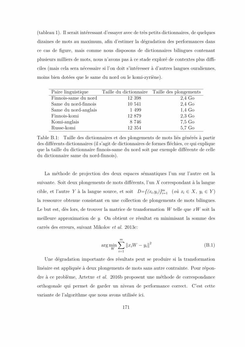
(tableau 1). Il serait intéressant d’essayer avec de très petits dictionnaires, de quelques

dizaines de mots au maximum, afin d’estimer la dégradation des performances dans

ce cas de figure, mais comme nous disposons de dictionnaires bilingues contenant

plusieurs milliers de mots, nous n’avons pas à ce stade exploré de contextes plus diffi-

ciles (mais cela sera nécessaire si l’on doit s’intéresser à d’autres langues ouraliennes,

moins bien dotées que le same du nord ou le komi-zyriène).

Paire linguistique Taille du dictionnaire Taille des plongementsFinnois-same du nord 12 398 2,4 GoSame du nord-finnois 10 541 2,4 GoSame du nord-anglais 1 499 1,4 GoFinnois-komi 12 879 2,3 GoKomi-anglais 8 746 7,5 GoRusse-komi 12 354 5,7 Go

Table B.1: Taille des dictionnaires et des plongements de mots liés générés à partirdes différents dictionnaires (il s’agit de dictionnaires de formes fléchies, ce qui expliqueque la taille du dictionnaire finnois-same du nord soit par exemple différente de celledu dictionnaire same du nord-finnois).

La méthode de projection des deux espaces sémantiques l’un sur l’autre est la

suivante. Soit deux plongements de mots différents, l’un X correspondant à la langue

cible, et l’autre Y à la langue source, et soit D={(xi,yi)}mi=1 (où xi ∈ X, yi ∈ Y )

la ressource obtenue consistant en une collection de plongements de mots bilingues.

Le but est, dès lors, de trouver la matrice de transformation W telle que xW soit la

meilleure approximation de y. On obtient ce résultat en minimisant la somme des

carrés des erreurs, suivant Mikolov et al. 2013c:

arg minW

m∑i=1

∥xiW − yi∥2 (B.1)

Une dégradation importante des résultats peut se produire si la transformation

linéaire est appliquée à deux plongements de mots sans autre contrainte. Pour répon-

dre à ce problème, Artetxe et al. 2016b proposent une méthode de correspondance

orthogonale qui permet de garder un niveau de performance correct. C’est cette

variante de l’algorithme que nous avons utilisée ici.

171

B.3.3 Corpus annotés au format Universal Dependencies

Nous avons également besoin de corpus annotés pour nos expériences, au moins pour

montrer leur apport quand ils sont disponibles. Nous avons utilisé des corpus pour

l’anglais, le finnois et le russe : tous provenaient de l’initiative Universal Dependencies

et peuvent être trouvés en ligne7.

B.4 Modèle d’analyse en dépendances crosslingue

Les analyseurs syntaxiques traditionnels emploient des méthodes d’apprentissage su-

pervisé fondées sur des séries de traits définis en grande partie manuellement. Le

développeur doit en fait définir des combinaisons pertinentes (feature functions) de

traits et de relations entre ceux-ci, afin que le système soit capable de déterminer les

relations entre têtes et dépendants8. La définition manuelle de ces combinaisons de

traits est une tâche difficile et en grande partie arbitraire, que tous les concepteurs

de systèmes cherchent à contourner.

Les systèmes récents à base de réseaux de neurones ont plutôt recours à des

méthodes automatiques permettant de simplifier le problème, en laissant le soin à

la machine de déterminer les combinaisons de traits pertinentes. Ainsi, Chen et

Manning 2014b ont proposé d’utiliser des classificateurs non linéaires intégrés dans

un modèle de réseau neuronal. Avec cette méthode, les caractéristiques lexicales

et non lexicales sont encodées dans des vecteurs qui peuvent être concaténés pour

alimenter un classificateur non linéaire. Cette approche présente deux avantages : i)

les classificateurs non linéaires ont globalement de meilleures performances que les7Sur le projet Universal dependencies, voir http://universaldependencies.org.

Nous avons utilisé les corpus arobés suivants, dans leur version 2.1 : https://github.com/UniversalDependencies/UD_English-EWT (anglais), https://github.com/UniversalDependencies/UD_Russian-GSD (russe) et https://github.com/UniversalDependencies/UD_Finnish-TDT (finnois).

8“Traditionally, state-of-the-art parsers rely on linear models over hand-crafted feature functions.The feature functions look at core components (e.g. “word on top of stack”, “leftmost child of thesecond-to- top word on the stack”, “distance between the head and the modifier words”), and arecomprised of several templates, where each template instantiates a binary indicator function overa conjunction of core elements (resulting in features of the form “word on top of stack is X andleftmost child is Y and ...”).” (Kiperwasser and Goldberg, 2016b).

172

classifieurs linéaires pour identifier les relations entre les éléments pertinents pour

l’analyse, et ii) cette approche réduit drastiquement le travail manuel dans la mesure

où le réseau de neurones se fonde essentiellement sur les caractéristiques calculées par

les classifieurs.

B.4.1 Architecture du système d’analyse

Notre approche est ici similaire à celle de Chen et Manning 2014b et de Kiperwasser et

Goldberg 2016b pour la partie analyse, mais nous utilisons des plongements de mots

multilingues, alors que nos prédécesseurs s’en tiennent à un système monolingue.

Représentations LSTM bidirectionnelles. Les progrès récents en TAL sont

largement dus à des représentations sous forme de traits portant des informations effi-

caces pour l’analyse des relations entre les mots de la phrase (Cho, 2015; Huang et al.,

2015). Une représentation LSTM bidirectionnelle (bi-LSTM) est un type de réseau

de neurones récurrent, où chaque élément dans la séquence à analyser est lui-même

représenté par un vecteur. L’algorithme procède en produisant des représentations

préfixes (dites forward car la phrase est analysée de gauche à droite) et des représenta-

tions suffixes (dites backward car la phrase est alors analysée de droite à gauche). Un

item est représenté par la concaténation de ses deux contextes, gauche et droit. Soit

par exemple la phrase t = (t1,t2,...,tn), dans laquelle le symbole ◦ dénote une opération

de concaténation. La fonction LSTM bidirectionnelle correspond à : BiLSTM(t1:n, i)

= LSTMForward(t1:i) ◦ LSTMBackward(ti:n).

L’architecture est exactement la même que celle du BIST-parser (Kiperwasser and

Goldberg, 2016b). Nous renvoyons donc le lecteur à cet article fondateur pour con-

naître les détails de l’architecture du système qui est de ce point de vue relativement

standard. Nous avons juste étendu cet analyseur de manière à le rendre multilingue,

ce qui oblige à prendre en compte des représentations contextuelles construites par le

module bi-LSTM multilingue (un code pour chaque mot, dit one hot encoding, permet

de déterminer la langue associée).

Représentation lexicale. Soit une phrase en entrée t = (t1,t2,...,tn), une forme

lexicale w, une étiquette morphosyntaxique correspondante p, un plongement de mots

173

Figure B-1: Architecture du réseau de neurones

obtenu préalablement xw et une valeur de codage de la langue concernée l, un mot ti

(token) est défini comme : ti = e(wi) ◦ e(pi) ◦ e(xwi) ◦ e(li), où e réfère au plonge-

ment de chaque trait et e(xwi) est le plongement de mots déjà présenté en section 3.

Nous ajoutons un code pour désigner la langue concernée, comme dit précédemment

(Naseem et al., 2012; Ammar et al., 2016a). La plupart des analyseurs monolingues

utilisent des traits comme e(wi) et e(pi), ainsi que d’autres éléments comme la dis-

tance entre la tête et le dépendant, ou d’autres traits spécifiques calculables à partir

du corpus UD. Notez enfin que ti de BiLSTM(t1:n, i) permet de stocker les contextes

forward et backward du LSTM.

B.4.2 Modèle d’analyse

Il existe deux approches principales en matière d’analyse syntaxique en dépendance.

La première est fondée sur la notion de transition (Nivre, 2004), l’autre sur la no-

tion de graphe (McDonald et al., 2005c). Nous utilisons ici une approche à base de

graphes héritée du BIST-parser. L’approche semble efficace pour les corpus au format

Universal Dependencies, et on renverra à Dozat et al. 2017a pour une comparaison

détaillée et argumentée des deux approches.

À partir des représentations des mots et de leurs annotations dans la couche BiL-

STM, le BIST-parser produit un arbre candidat pour chaque couple dépendant-mot-

tête. Les scores attachés aux différents arbres candidats sont ensuite calculés à l’aide

174

d’un perceptron multicouche (MLP), utilisé comme simple fonction de pondération

(scoring function). Enfin, le système choisit les meilleurs arbres d’analyse en dépen-

dance sur la base de la somme des scores attachés aux différents sous-arbres. Pour

plus d’informations sur le modèle à base de graphes et sur le modèle de pondéra-

tion d’arcs utilisé par le BIST-parser, voir (Taskar et al., 2005) et (McDonald et al.,

2005b).

B.5 Expériences

Nous présentons dans cette section les expériences que nous avons menées sur le same

du nord et sur le komi-zyriène.

Corpus disponibles. Le same était une des langues dites surprise language

de la campagne d’évaluation CoNLL 2017 : seulement vingt phrases étaient fournies

pour l’entraînement et les participants n’avaient que quelques jours pour produire

un système opérationnel. Le komi n’était pas inclus dans l’évaluation CoNLL 2017

mais nous avons choisi cette langue pour des raisons linguistiques (il s’agit d’une

langue finno-ougrienne, comme le same) et parce qu’elle correspond à un cas typique

de langue sous-dotée, comme on l’a vu dans l’introduction. Pour pouvoir mener à

bien nos expériences, nous avons produit un corpus annoté composé de dix phrases

komies pour l’entraînement et soixante-quinze phrases pour le test (ce corpus contient

aujourd’hui près de trois cents phrases et grossit régulièrement, mais moins d’une cen-

taine de phrases étaient disponibles au moment des expériences rapportées ici). Une

présentation du corpus komi et des problèmes d’annotation rencontrés est disponible

à la fin de cet article, en annexe.

Étiquettes morphosyntaxiques utilisées. Dans les expériences rapportées

ici, nous nous fondons sur les étiquettes (catégories morphosyntaxiques) fournies par

UDpipe (Straka et al., 2016) pour le same et, en l’absence d’analyseur morphosyn-

taxique disponible pour le komi, nous utilisons les étiquettes posées à la main pour

cette langue (gold). Lors de la campagne CoNLL 2017, l’analyse se fondait aussi sur

des étiquettes de référence pour le same du nord, mais nous préférons recourir ici à un

175

analyseur morphologique pour le same afin de rendre les conditions expérimentales

plus proches de la réalité. Nous n’utilisons pas de traits morphologiques autres que

ceux du corpus de référence ou ceux fournis par UDpipe pour le same.

Le fait d’utiliser des étiquettes morphosyntaxiques de référence est bien évidem-

ment quelque peu artificiel, mais permet de se focaliser uniquement sur le niveau syn-

taxique. Il n’en reste pas moins que la production d’analyseurs morphosyntaxiques

performants est évidemment une condition nécessaire pour produire des analyses en

situation réelle. La tâche commune CoNLL 2018 impliquait de développer une chaîne

complète allant du texte brut à l’analyse syntaxique, et l’expérience a montré que les

systèmes conservent ainsi des performances satisfaisantes. On renverra donc le lecteur

aux actes de la tâche commune CoNLL 2018 sur ce point (Zeman et al., 2018b).

Conditions d’entraînement du système. Comme nous voulons explorer des

scénarios pour des langues faiblement dotées, nous avons supposé que l’on ne dispo-

sait pas de données de développement permettant d’ajuster les paramètres du système

(même dans le cas du same, pour lequel il existe maintenant des données importantes,

notamment le corpus annoté syntaxiquement au format UD). Nous avons donc limité

les expériences, notamment lors de la phase d’apprentissage, en considérant toutes les

données disponibles une fois, sans arrêt anticipé, suivant Guo et al. 2016. D’autres

stratégies seraient possibles (plusieurs itérations en faisant varier les phrases utilisées

lors de l’apprentissage par exemple), mais le gain observé sur les résultats est min-

ime et souvent non significatif. Ce type d’approches pose en outre des problèmes

de réplicabilité et nous l’avons donc laissé de côté. Enfin, il faut noter que, pour

l’élaboration d’un modèle multilingue, les différentes sources de données sont de taille

très déséquilibrée. Pour pallier ce problème, et suivant les travaux antérieurs de Guo

et al. 2016, nous avons effectué vingt fois plus d’itérations pour les langues faiblement

dotées que pour les autres langues.

Comparaison avec la tâche commune CoNLL 2017. Nous avons utilisé les

mêmes conditions pour l’entraînement de notre système dans les expériences décrites

ici que pour la tâche commune CoNLL. En particulier nous n’avons pas de corpus de

développement (nous disposons juste de vingt phrases annotées pour le same et de

176

Équipe Score LAS Score UASC2L2 (Ithaca) 48,96 58,85

IMS (Stuttgart) 40,67 51,56HIT-SCIR (Harbin) 38,91 52,51

Notre système 28,39 42,72

Table B.2: Meilleurs résultats (officiels) pour le same lors de la tâche communeCoNLL 2017 et résultat obtenu par le LATTICE lors de cette même évaluation

dix phrases annotées pour le komi pour la mise au point du système, comme dit plus

haut).

Le tableau 2 présente les résultats obtenus par les trois meilleures équipes sur le

same lors de la tâche commune CoNLL 2017, ainsi que les résultats de notre propre

système. Il est évident, au vu de ces résultats, que notre système était alors loin d’être

aussi performant que les meilleurs systèmes sur le same, à savoir ceux de Cornell (Shi

et al., 2017b) , de Stuttgart (Björkelund et al., 2017b) ou de Harbin (Che et al.,

2017b).

Lors de CoNLL 2017, C2L2 (Cornell Univ.) a obtenu les meilleures performances

pour le same avec une approche par transfert délexicalisé (en utilisant un corpus de

finnois pour l’entraînement et un corpus de développement de vingt phrases en same

pour ajuster les paramètres du système, sans utilisation de traits lexicaux, c’est-à-dire

en se fondant uniquement sur les étiquettes morphosyntaxiques et non sur les mots

eux-mêmes). IMS (Stuttgart) a utilisé une approche similaire (approche par transfert

délexicalisé) en utilisant pour l’entraînement quarante corpus différents encodés au

format UD, et a ainsi obtenu le deuxième meilleur résultat.

Comparaison avec la tâche commune CoNLL 2018. Le same était à

nouveau une langue de test lors de la campagne d’évaluation CoNLL 2018. Le meilleur

système a obtenu les résultats suivants lors de la campagne 2018 : 69,87 LAS et 76,66

UAS. Ces résultats sont bien meilleurs que ceux rapportés pour l’évaluation CoNLL

2017 (tableau 2) ou même dans cet article (tableau 3), mais en 2018 des données

d’entraînement importantes étaient fournies pour le same (il s’agissait essentiellement

du corpus de same au format UD publié après la campagne d’évaluation 2017, comme

indiqué dans l’introduction). Il est donc important de souligner que les résultats

177

obtenus sur le corpus CoNLL 2018 ne sont en rien comparables avec les résultats

2017, où seules vingt phrases étaient disponibles pour la mise au point des systèmes.

Les résultats du meilleur système lors de la campagne d’évaluation CoNLL 2018

(69,87 LAS et 76,66 UAS) donnent malgré tout une idée de l’état de l’art pour

une langue à morphologie riche, comme le same, quand on dispose d’un corpus

d’entraînement moyennement volumineux. Ils permettent aussi d’avoir une idée de

l’écart de performance entre une langue pour laquelle on dispose de données annotées

et une langue pour laquelle on ne dispose pas de telles ressources (entre 10 et 15

points de différence environ), et aussi une idée de l’écart par rapport à l’anglais (là

aussi, entre 10 et 15 points de différence – ces chiffres sont évidemment à prendre

avec précaution car il faudrait faire d’autres expériences, avec d’autres langues et des

conditions expérimentales plus directement comparables pour obtenir des résultats

vraiment fiables). On confirme là, par l’observation, des résultats très évidents : une

langue synthétique à morphologie riche est plus complexe à analyser qu’une langue

analytique avec une complexité morphologique moindre, et un corpus d’entraînement

de grande taille est aussi un facteur majeur d’amélioration des performances. Pour le

reste, redisons-le : les résultats CoNLL 2018 ne sont en rien comparables aux résul-

tats 2017 du fait des conditions expérimentales radicalement différentes pour le same

lors de ces deux campagnes.

B.6 Résultats et analyse

Les résultats pour le same du nord sont donnés dans le tableau 3, et les résultats

pour le komi-zyriène dans le tableau 4. Les résultats du tableau 3 diffèrent de ceux

du tableau 2 car les expériences faites après la campagne CoNLL 2017 ont permis de

mieux utiliser les vingt phrases fournies pour la mise au point du système et surtout de

tester différentes combinaisons de langues afin d’identifier le modèle le plus performant

pour la tâche. On voit que le système de base est ainsi plus performant que le système

officiel ayant participé à CoNLL 2017, même sans ressources extérieures ni modèle

multilingue.

178

Corpus utilisés Score LAS Score UAS1 sme (20) 32,96 46,852 eng (12 217) 32,72 50,443 fin (12 543) 40,74 54,244 sme (20) + eng (12 217) 46,54 61,615 sme (20) + fin (12 543) 51,54 63,06

Table B.3: Évaluation de l’analyse du same du nord (sme) : scores LAS (labeledattachment scores) et UAS (unlabeled attachment scores), c’est-à-dire scores cal-culés en prenant en compte l’étiquette de la relation (score LAS, colonne de gauche),et sans elle (score UAS, colonne de droite). La première ligne sme (20) réfère àl’expérience utilisant uniquement sur les vingt phrases annotées de same disponiblespour l’entraînement. Les autres lignes montrent les résultats avec différentes combi-naisons de corpus annotés : anglais (eng) et finnois (fin). Pour chaque corpus, lenombre de phrases utilisées est indiqué entre parenthèses.

Globalement, les expériences que nous avons menées en utilisant le finnois comme

source de connaissances (en particulier pour élaborer des plongements de mots bilingues)

ont permis d’obtenir de meilleurs résultats qu’avec d’autres langues (on obtient de

meilleurs résultats avec le finnois qu’avec l’anglais pour l’analyse syntaxique du same

du nord, cf. tableau 3, et on obtient également de meilleurs résultats avec le finnois

qu’avec l’anglais pour l’analyse du komi, cf. tableau 4 – le russe est toutefois plus

performant pour analyser le komi que le finnois). Ceci semble indiquer d’une part

qu’il est possible d’inférer des connaissances linguistiques utiles pour l’analyse à partir

d’une langue tierce et, d’autre part, que la typologie et la situation linguistique jouent

un rôle (on obtient de meilleurs résultats sur le same ou le komi à partir du finnois ou

éventuellement du russe qu’à partir de l’anglais, même si les données utilisées pour

l’anglais sont largement plus volumineuses).

La stratégie de transfert de connaissances d’une langue vers l’autre a bien fonc-

tionné pour le finnois vis-à-vis du same, ce qui peut sembler logique car le finnois et

le same sont supposés relativement proches génétiquement parlant (mais n’importe

quel locuteur pourra aussi dire à quel point ces langues sont éloignées : il n’y a pas

d’intercompréhension, même limitée, et même le vocabulaire de base est très différent).

Le transfert fonctionne bien aussi pour le komi, alors que le komi est supposé plus

éloigné du finnois d’un point de vue génétique.

179

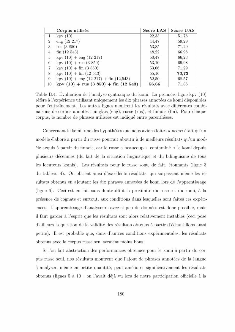
Corpus utilisés Score LAS Score UAS1 kpv (10) 22,33 51,782 eng (12 217) 44,47 59,293 rus (3 850) 53,85 71,294 fin (12 543) 48,22 66,985 kpv (10) + eng (12 217) 50,47 66,236 kpv (10) + rus (3 850) 53,10 69,987 kpv (10) + fin (3 850) 53,66 71,298 kpv (10) + fin (12 543) 55,16 73,739 kpv (10) + eng (12 217) + fin (12,543) 52,50 68,5710 kpv (10) + rus (3 850) + fin (12 543) 56,66 71,86

Table B.4: Évaluation de l’analyse syntaxique du komi. La première ligne kpv (10)réfère à l’expérience utilisant uniquement les dix phrases annotées de komi disponiblespour l’entraînement. Les autres lignes montrent les résultats avec différentes combi-naisons de corpus annotés : anglais (eng), russe (rus), et finnois (fin). Pour chaquecorpus, le nombre de phrases utilisées est indiqué entre parenthèses.

Concernant le komi, une des hypothèses que nous avions faites a priori était qu’un

modèle élaboré à partir du russe pourrait aboutir à de meilleurs résultats qu’un mod-

èle acquis à partir du finnois, car le russe a beaucoup « contaminé » le komi depuis

plusieurs décennies (du fait de la situation linguistique et du bilinguisme de tous

les locuteurs komis). Les résultats pour le russe sont, de fait, étonnants (ligne 3

du tableau 4). On obtient ainsi d’excellents résultats, qui surpassent même les ré-

sultats obtenus en ajoutant les dix phrases annotées de komi lors de l’apprentissage

(ligne 6). Ceci est en fait sans doute dû à la proximité du russe et du komi, à la

présence de cognats et surtout, aux conditions dans lesquelles sont faites ces expéri-

ences. L’apprentissage d’analyseurs avec si peu de données est donc possible, mais

il faut garder à l’esprit que les résultats sont alors relativement instables (ceci pose

d’ailleurs la question de la validité des résultats obtenus à partir d’échantillons aussi

petits). Il est probable que, dans d’autres conditions expérimentales, les résultats

obtenus avec le corpus russe seul seraient moins bons.

Si l’on fait abstraction des performances obtenues pour le komi à partir du cor-

pus russe seul, nos résultats montrent que l’ajout de phrases annotées de la langue

à analyser, même en petite quantité, peut améliorer significativement les résultats

obtenus (lignes 5 à 10 ; on l’avait déjà vu lors de notre participation officielle à la

180

tâche commune CoNLL 2017, où l’usage des vingt phrases fournies par défaut, et

le fait d’en réserver une partie ou non comme corpus de développement, pouvaient

avoir un effet très positif sur les résultats finaux). La taille des corpus bruts utilisés

pour l’obtention des plongements de mots, et les ressources annexes utilisées pour

l’acquisition de connaissances linguistiques jouent aussi un rôle important (on com-

parera ainsi les lignes 7 et 8, où le modèle est à chaque fois conçu à partir du finnois,

mais avec deux corpus de tailles différentes). C’est logiquement le corpus le plus

grand qui permet d’obtenir le modèle le plus performant. On peut aussi comparer

les performances relatives obtenues avec des modèles élaborés à partir du russe, du

finnois et de l’anglais : l’anglais, même avec un ensemble de phrases annotées très

supérieur, n’est pas vraiment compétitif sur le komi. Comme on l’a dit, ces résultats

sont toutefois fragiles et sont validés sur un corpus très petit. Il faut donc souhaiter

davantage d’études sur des langues variées, afin d’obtenir une meilleure vue des types

de résultats possibles en fonction des langues, des ressources et des algorithmes util-

isés.

Finalement, c’est le modèle élaboré à partir du finnois et du russe qui permet

d’obtenir les meilleurs résultats (et non celui élaboré à partir de l’anglais, même si

on dispose de plus de données pour l’anglais). Il semble bien que les langues choisies

pour l’apprentissage jouent un rôle, et il est important de choisir celles-ci en fonction

de critères linguistiques et typologiques.

On observe enfin que les scores UAS (c’est-à-dire sans tenir compte des étiquettes

de relations syntaxiques) varient légèrement plus que les scores LAS (scores avec les

étiquettes des relations syntaxiques), autrement dit les relations de base ont été trou-

vées et la racine correctement identifiée dans un certain nombre de cas, même quand

les étiquettes des relations n’ont pas été attribuées correctement. Il est intéressant de

noter que le modèle qui obtient le meilleur score UAS est le couple komi-finnois, même

si d’autres combinaisons (avec l’ajout du russe notamment) permettent d’obtenir les

meilleurs scores LAS.

181

B.7 Conclusion

Dans cet article, nous avons présenté une approche fondée sur l’utilisation de modèles

multilingues, afin de fournir une analyse syntaxique pour des langues disposant de

peu de ressources, et en particulier ne disposant pas de données annotées (à part

quelques phrases utilisées comme amorçage, dix à vingt phrases dans les expériences

menées ici et lors de la campagne CoNLL 2017). Nous avons montré que l’approche

suivie était efficace dans le cas du same et du komi, même si les performances restent

évidemment bien en deçà de ce que l’on peut obtenir avec un corpus d’entraînement

de grande taille, comme en témoignent nos résultats pour le same lors de la campagne

d’évaluation CoNLL 2018 (avec un corpus d’entraînement au format UD). Il s’agit

toutefois, à notre avis, d’un cadre intéressant pour aider à produire des corpus annotés

pour des langues peu dotées. Le cas du komi est à cet égard un cas d’étude intéressant,

dans la mesure où il s’agit d’une langue avec peu de ressources, mais avec des locuteurs

intéressés et demandeurs d’outils d’analyse automatique. Ce cadre pose toutefois un

problème d’évaluation, en l’absence de données de référence (gold standard).

Nous avons observé que les modèles multilingues permettent généralement d’améliorer

les performances par rapport à des modèles monolingues. Les langues génétiquement

liées semblent être la meilleure source de connaissances (le finnois est ainsi efficace

pour l’analyse du same comme du komi), mais la prise en compte de langues de con-

tact semble aussi pertinente (ainsi le russe pour l’analyse du komi), de même que des

langues pour lesquelles on dispose tout simplement de gros corpus (comme l’anglais).

Une meilleure compréhension de l’apport réel de chaque langue au processus global

serait intéressante pour permettre de définir une stratégie plus générale, et surtout

reproductible, concernant le développement et l’utilisation de modèles multilingues

pour l’analyse syntaxique.

182

Remerciements

Les auteurs remercient les trois relecteurs anonymes pour leurs suggestions, qui ont

permis de largement améliorer cet article. Les travaux décrits ont été en partie

effectués dans le cadre du projet LAKME, financé par l’université Paris Sciences

et Lettres (IDEX PSL référence ANR-10-IDEX-0001-02). Cette recherche a aussi

bénéficié du soutien d’un projet RGNF-CNRS entre le Lattice et l’université d’État

des sciences humaines de Russie.

Annexe : contribution à l’élaboration d’un corpus

arboré pour le komi

Afin de permettre l’évaluation de l’analyseur décrit dans cet article, un ensemble de

phrases en komi ont été annotées au format UD. Ce corpus comprend actuellement

environ trois cents phrases, et devrait en contenir mille prochainement. Une première

version de ce corpus a été incluse dans la distribution officielle Universal Dependencies

d’avril 20189. Au-delà de la réalisation d’un nouveau corpus arboré, plusieurs points

peuvent être soulignés, qui nous semblent relativement typiques du cas des langues

de terrain et des langues minoritaires.

Les données disponibles sont de deux types très différents. On a d’un côté des

sources écrites, parfois anciennes, écrites dans une langue relativement élaborée et lit-

téraire, parfois très éloignée de la langue quotidienne. De l’autre, on dispose de corpus

beaucoup plus modestes (en taille) correspondant à des enquêtes de terrain faites par

des linguistes. Ce matériau est précieux, car directement issu de travaux linguistiques,

il rend compte de la langue réellement utilisée par les locuteurs au quotidien, mais il

pose plusieurs difficultés. Des difficultés matérielles d’abord, dans la mesure où ces

données sont souvent encodées dans des formats particuliers, qui ne conviennent pas

directement à un traitement automatique ; des difficultés liées à la taille des corpus9Voir le site officiel de l’initiative Universal Dependencies : http://

universaldependencies.org.

183

existants, qui rendent difficile l’utilisation de techniques d’apprentissage artificiel par

exemple. Enfin, ces corpus sont représentatifs de l’oral : ils posent donc des prob-

lèmes particuliers et les outils mis au point pour l’écrit ne sont pas très performants

sur ce type de données.

Notre travail se situe dans le cadre d’un effort en cours en vue de fournir des

données annotées pour un certain nombre de langues finno-ougriennes. Des corpus

arborés sont déjà disponibles pour le finnois, l’estonien et le hongrois. L’année 2017 a

vu l’émergence d’un corpus arboré important pour le same du nord (produit en grande

partie automatiquement à partir des outils d’analyse mis au point à l’université de

Tromsø et non entièrement vérifié manuellement). Un corpus arboré est actuellement

en préparation pour l’erzya (langue mordve), ce qui permettra de couvrir à terme une

partie non négligeable des langues finno-ougriennes, même si des efforts seront encore

nécessaires pour les autres langues. Une tendance similaire est observée pour ce qui

concerne la réalisation de corpus arborés à partir du résultat d’enquêtes de terrain.

À notre connaissance, des projets existent par exemple pour le dargwa (langue du

Caucase), le pnar (langue austro-asiatique) et le shipibo-konibo (langue du Pérou).

En pratique...

La plupart des travaux sur la langue komie sont actuellement menés à Syktyvkar,

Russie (capitale de la République komie). Le FU-Lab, dirigé par Marina Fedina,

a en particulier numérisé un nombre important de livres komis (datant du début

du xxe siècle jusqu’à aujourd’hui), ceux libres de droits étant directement mis à

disposition en ligne. Ce corpus brut compte actuellement quarante millions de mots

et l’objectif à long terme est de numériser tous les livres publiés en komi-zyriène.

Le nombre total des publications est estimé à environ quatre mille cing cents livres,

auxquels il faut ajouter des dizaines de milliers de pages issues de journaux et de

revues. Pour la constitution de notre corpus, nous avons évidemment veillé à n’utiliser

que des textes libres de droits, afin d’en assurer une distribution aussi large et simple

que possible. Il est possible qu’à un stade ultérieur des matériaux moins standard

puissent être inclus dans la base de données, par exemple des textes issus de blogs et

184

de discussions en ligne, mais cela pose immédiatement des problèmes de droits et de

diffusion.

En dehors du projet mené à Syktyvkar, un des plus grands projets de recherche sur

le komi parlé a été un projet de documentation dirigé par Rogier Blokland (université

de Uppsala) en 2014-2016. Ce projet a abouti à un grand corpus en langue parlée

transcrite. Ces données sont précieuses, pour les raisons que nous avons données

supra, mais elles sont aussi problématiques car elles ne peuvent généralement pas être

diffusées directement dans le domaine public. Le corpus contient aussi des formes

dialectales, et comme le komi-zyriène écrit ne suit pas les principes utilisés pour les

transcriptions, il semble problématique de mélanger ce matériau avec les données is-

sues de sources écrites. Le corpus oral contient enfin de nombreuses phrases où le komi

est mêlé à du vocabulaire russe, les locuteurs pratiquant le code switching en perma-

nence. Cette langue est donc non standard, mais elle est par ailleurs scientifiquement

intéressante et pertinente.

À partir de ce point de départ, il a été décidé de créer deux corpus différents,

le premier avec les matériaux écrits et le deuxième avec les données orales issues

d’enquêtes de terrain.

Annotation syntaxique du corpus komi-zyriène au format UD

Pour l’annotation du corpus komi-zyriène, nous nous sommes inspirés de corpus ar-

borés existants et des consignes d’annotation liées, notamment celles ayant été con-

stituées pour le finnois, le same du nord et l’erzya, ainsi que pour le russe. Il s’agit

de langues proches du komi (langues de la même famille, à l’exception du russe), et il

nous semblait naturel d’aller voir du côté de ces langues en priorité. De fait, les con-

signes d’annotation ont facilement pu être transposées au komi et quasiment toutes

les configurations observées correspondaient à des cas de figure observés (mutatis

mutandis) dans au moins une de ces langues.

Le komi-zyriène présente malgré tout quelques particularités et différences qui

le distinguent de ces langues proches. Il existe notamment deux cas spatiaux large-

ment spécifiques au komi (en fait aux langues permiennes, branche des langues finno-

185

ougriennes qui regroupe le komi et l’oudmourte) : l’égressif et l’approximatif. Ces

deux cas expriment le mouvement depuis et vers une direction. Ils se distinguent

de l’élatif et de l’illatif (deux cas bien répandus dans l’ensemble des langues finno-

ougriennes) : l’élatif et l’illatif expriment aussi un mouvement depuis ou vers un lieu,

mais ils insistent justement sur ce point de départ ou d’arrivée, alors que l’égressif et

l’approximatif insistent davantage sur le mouvement, sans préciser le point de départ

ou d’arrivée.

L’exemple ci-dessous illustre précisément l’utilisation du cas approximatif, sans

aucun caractère égressif.

Il existe deux autres cas directionnels en komi, traditionnellement appelés pro-

latifs et transitifs, qui expriment le mouvement le long d’un chemin. Ceux-ci cor-

respondent assez bien au cas appelé « perlatif » du guide d’annotation au format

UD (Universal Dependencies), mais ce cas ne figure pas dans les exemples annotés

jusqu’ici. Plus généralement, ceci pose la question de la terminologie employée et de la

mise en rapport des cas (et plus généralement des notions linguistiques) à travers les

langues : nous pensons que le prolatif et le translatif correspondent au perlatif, mais

ceci mériterait sûrement une discussion approfondie. UD est en tout cas l’occasion

de s’interroger sur la terminologie en cours, les notions manipulées et les correspon-

dances entre langues. Il était à cet égard utile de garder un œil sur le russe lors de

l’annotation, dans la mesure où le komi emprunte certaines constructions au russe.

De plus, il semble souhaitable d’être, autant que faire se peut, cohérent et homogène

au niveau des annotations.

Le premier exemple illustre une situation typique où la date est exprimée en russe,

y compris au niveau du marquage morphologique et syntaxique.

186

Nous avons cherché ici à avoir une annotation comparable à celle de la structure

correspondante en russe. Ce choix diffère de ce qui a été fait pour la plupart des autres

langues, où les mots ou structures en langue étrangère sont généralement marqués en

tant que tels, et donc globalement plutôt mis de côté. Vu le bilinguisme de tous les

locuteurs komis qui se retrouve en partie dans les corpus, nous souhaitons avoir une

annotation qui intègre pleinement les passages en russe (y compris à l’intérieur d’une

même phrase en cas de code switching comme ici) et les considère comme faisant

pleinement partie du corpus komi.

Il faut toutefois noter que ceci peut aussi entraîner différents problèmes. Par

exemple, certaines structures (provenant du russe) auront un trait gender (exprimant

le genre grammatical), alors qu’il s’agit d’un trait morphologique étranger au komi.

Ceci est évidemment aussi un défi pour les outils de TAL et les analyseurs en général,

qui doivent gérer des situations linguistiques plus complexes que ce que l’on trouve

dans la plupart des grands corpus monolingues disponibles. C’est cette richesse qui

fait l’intérêt de ces langues trop longtemps laissées de côté.

187

Bibliography

Ante Aikio. An essay on Saami ethnolinguistic prehistory. In Riho Grünthal andPetri Kallio, editors, A Linguistic Map of Prehistoric Northern Europe, pages 63–117. Société Finno-Ougrienne, 2012.

Chris Alberti, Daniel Andor, Ivan Bogatyy, Michael Collins, Dan Gillick, LingpengKong, Terry Koo, Ji Ma, Mark Omernick, Slav Petrov, Chayut Thanapirom, ZoraTung, and David Weiss. Syntaxnet models for the CoNLL 2017 shared task. CoRR,abs/1703.04929, 2017. URL http://arxiv.org/abs/1703.04929.

Waleed Ammar, George Mulcaire, Miguel Ballesteros, Chris Dyer, and Noah A.Smith. Many languages, one parser. Transactions of the Assoc. for Comp. Linguis-tics (TACL), 4:431–444, 2016a.

Waleed Ammar, George Mulcaire, Miguel Ballesteros, Chris Dyer, and Noah A.Smith. One parser, many languages. CoRR, 2016b. URL http://arxiv.org/abs/1602.01595.

Waleed Ammar, George Mulcaire, Yulia Tsvetkov, Guillaume Lample, Chris Dyer,and Noah A Smith. Massively multilingual word embeddings. arXiv preprintarXiv:1602.01925, 2016c.

Waleed Ammar, George Mulcaire, Yulia Tsvetkov, Guillaume Lample, Chris Dyer,and Noah A Smith. Massively multilingual word embeddings. arXiv preprintarXiv:1602.01925, 2016d.

Daniel Andor, Chris Alberti, David Weiss, Aliaksei Severyn, Alessandro Presta, Kuz-man Ganchev, Slav Petrov, and Michael Collins. Globally normalized transition-based neural networks. CoRR, abs/1603.06042, 2016. URL http://arxiv.org/abs/1603.06042.

Mikel Artetxe, Gorka Labaka, and Eneko Agirre. Learning principled bilingual map-pings of word embeddings while preserving monolingual invariance. In Proceedingsof the 2016 Conference on Empirical Methods in Natural Language Processing,2016a.

Mikel Artetxe, Gorka Labaka, and Eneko Agirre. Learning principled bilingual map-pings of word embeddings while preserving monolingual invariance. In Proceedingsof the 2016 Conference on Empirical Methods in Natural Language Processing(EMNLP), Austin, USA, pages 2289–2294, 2016b.

188

Mikel Artetxe, Gorka Labaka, and Eneko Agirre. Learning bilingual word embeddingswith (almost) no bilingual data. In Proceedings of the 55th Annual Meeting of theAssociation for Computational Linguistics (Volume 1: Long Papers), pages 451–462,2017. URL aclweb.org/anthology/P17-1042.

Giuseppe Attardi, Felice Dell’Orletta, Maria Simi, and Joseph Turian. Accuratedependency parsing with a stacked multilayer perceptron. Proceedings of EVALITA,9:1–8, 2009.

Miguel Ballesteros, Chris Dyer, and Noah A. Smith. Improved transition-based pars-ing by modeling characters instead of words with lstms. CoRR, abs/1508.00657,2015. URL http://arxiv.org/abs/1508.00657.

Miguel Ballesteros, Yoav Goldberg, Chris Dyer, and Noah A. Smith. Training withexploration improves a greedy stack lstm parser. In Proceedings of the 2016 Con-ference on Empirical Methods in Natural Language Processing, pages 2005–2010,Austin, Texas, November 2016a. Association for Computational Linguistics. URLhttps://aclweb.org/anthology/D16-1211.

Miguel Ballesteros, Yoav Goldberg, Chris Dyer, and Noah A Smith. Training withexploration improves a greedy stack lstm parser. In Conf. on Empirical Methodsin Natural Language Processing (EMNLP), pages 2005–2010, Austin, 2016b. URLhttps://aclweb.org/anthology/D16-1211.

Yoshua Bengio, Réjean Ducharme, Pascal Vincent, and Christian Jauvin. A neuralprobabilistic language model. Journal of machine learning research, 3(Feb):1137–1155, 2003.

Anders Björkelund, Agnieszka Falenska, Xiang Yu, and Jonas Kuhn. Ims at theconll 2017 ud shared task: Crfs and perceptrons meet neural networks. In Pro-ceedings of the CoNLL 2017 Shared Task: Multilingual Parsing from Raw Text toUniversal Dependencies, pages 40–51, Vancouver, Canada, August 2017a. Associ-ation for Computational Linguistics. URL http://www.aclweb.org/anthology/K/K17/K17-3004.pdf.

Anders Björkelund, Agnieszka Falenska, Xiang Yu, and Jonas Kuhn. Ims at the conll2017 ud shared task: Crfs and perceptrons meet neural networks. In CoNLL 2017Shared Task: Multilingual Parsing from Raw Text to Universal Dependencies, pages40–51, Vancouver, 2017b.

Ezra Black, Fred Jelinek, John Lafferty, David M. Magerman, Robert Mercer, andSalim Roukos. Towards history-based grammars: Using richer models for prob-abilistic parsing. In Proceedings of the 31st Annual Meeting on Association forComputational Linguistics, ACL ’93, pages 31–37, Stroudsburg, PA, USA, 1993.Association for Computational Linguistics. doi: 10.3115/981574.981579. URLhttps://doi.org/10.3115/981574.981579.

189

Rogier Blokland, Marina Fedina, Ciprian Gerstenberger, Niko Partanen, MichaelRießler, and Joshua Wilbur. Language documentation meets language technology.In Septentrio Conference Series, pages 8–18, 2015.

Avrim Blum and Tom Mitchell. Combining labeled and unlabeled data with co-training. In Proceedings of the eleventh annual conference on Computational learn-ing theory, pages 92–100. ACM, 1998.

Bernd Bohnet. Very high accuracy and fast dependency parsing is not a contradiction.In Proceedings of the 23rd International Conference on Computational Linguistics,COLING ’10, pages 89–97, Stroudsburg, PA, USA, 2010. Association for Compu-tational Linguistics. URL http://dl.acm.org/citation.cfm?id=1873781.1873792.

Bernd Bohnet, Ryan T. McDonald, Gonçalo Simões, Daniel Andor, Emily Pitler, andJoshua Maynez. Morphosyntactic tagging with a meta-bilstm model over contextsensitive token encodings. CoRR, abs/1805.08237, 2018a. URL http://arxiv.org/abs/1805.08237.

Bernd Bohnet, Ryan T. McDonald, Gonçalo Simões, Daniel Andor, Emily Pitler, andJoshua Maynez. Morphosyntactic tagging with a meta-bilstm model over contextsensitive token encodings. CoRR, abs/1805.08237, 2018b. URL http://arxiv.org/abs/1805.08237.

Piotr Bojanowski, Edouard Grave, Armand Joulin, and Tomas Mikolov. Enrichingword vectors with subword information. CoRR, abs/1607.04606, 2016a. URL http://arxiv.org/abs/1607.04606.

Piotr Bojanowski, Edouard Grave, Armand Joulin, and Tomas Mikolov. Enrichingword vectors with subword information. arXiv preprint arXiv:1607.04606, 2016b.

Piotr Bojanowski, Edouard Grave, Armand Joulin, and Tomas Mikolov. Enrichingword vectors with subword information. CoRR, 2016c. URL http://arxiv.org/abs/1607.04606.

Cristina Bosco, Montemagni Simonetta, and Simi Maria. Converting italian tree-banks: Towards an italian stanford dependency treebank. In 7th Linguistic Anno-tation Workshop and Interoperability with Discourse, pages 61–69. The Associationfor Computational Linguistics, 2013.

Jan A. Botha, Emily Pitler, Ji Ma, Anton Bakalov, Alex Salcianu, David Weiss,Ryan T. McDonald, and Slav Petrov. Natural language processing with small feed-forward networks. CoRR, abs/1708.00214, 2017. URL http://arxiv.org/abs/1708.00214.

Sabine Buchholz and Erwin Marsi. Conll-x shared task on multilingual dependencyparsing. In Proceedings of the tenth conference on computational natural languagelearning, pages 149–164. Association for Computational Linguistics, 2006.

190

Kris Cao and Marek Rei. A joint model for word embedding and word morphology.CoRR, abs/1606.02601, 2016. URL http://arxiv.org/abs/1606.02601.

Pi-Chuan Chang, Huihsin Tseng, Dan Jurafsky, and Christopher D Manning. Dis-criminative reordering with chinese grammatical relations features. In Proceedingsof the Third Workshop on Syntax and Structure in Statistical Translation, pages51–59. Association for Computational Linguistics, 2009.

Wanxiang Che, Jiang Guo, Yuxuan Wang, Bo Zheng, Huaipeng Zhao, Yang Liu,Dechuan Teng, and Ting Liu. The hit-scir system for end-to-end parsing ofuniversal dependencies. In Proceedings of the CoNLL 2017 Shared Task: Mul-tilingual Parsing from Raw Text to Universal Dependencies, pages 52–62, Van-couver, Canada, August 2017a. Association for Computational Linguistics. URLhttp://www.aclweb.org/anthology/K/K17/K17-3005.pdf.

Wanxiang Che, Jiang Guo, Yuxuan Wang, Bo Zheng, Huaipeng Zhao, Yang Liu,Dechuan Teng, and Ting Liu. The hit-scir system for end-to-end parsing of universaldependencies. In CoNLL 2017 Shared Task: Multilingual Parsing from Raw Textto Universal Dependencies, pages 52–62, Vancouver, 2017b.

Wanxiang Che, Yijia Liu, Yuxuan Wang, Bo Zheng, and Ting Liu. Towardsbetter UD parsing: Deep contextualized word embeddings, ensemble, and tree-bank concatenation. In Proceedings of the CoNLL 2018 Shared Task: Multi-lingual Parsing from Raw Text to Universal Dependencies, pages 55–64, Brus-sels, Belgium, October 2018. Association for Computational Linguistics. URLhttp://www.aclweb.org/anthology/K18-2005.

Danqi Chen and Christopher D Manning. A fast and accurate dependency parserusing neural networks. In EMNLP, pages 740–750, 2014a.

Danqi Chen and Christopher D Manning. A fast and accurate dependency parserusing neural networks. In Conf. on Empirical Methods in Natural Language Pro-cessing (EMNLP), pages 740–750, Doha, 2014b.

Kyunghyun Cho. Natural language understanding with distributed representation.arXiv preprint, 2015. URL http://arxiv.org/abs/1511.07916.

Noam Chomsky and David W Lightfoot. Syntactic structures. Walter de Gruyter,2002.

Michael Collins. Head-driven statistical models for natural language parsing. Com-putational linguistics, 29(4):589–637, 2003.

Alexis Conneau, Guillaume Lample, Marc’Aurelio Ranzato, Ludovic Denoyer, andHervé Jégou. Word translation without parallel data. In Conf. International Con-ference on Learning Representations (ICLR), Toulon, 2017.

191

Ayan Das, Affan Zaffar, and Sudeshna Sarkar. Delexicalized transfer parsing for low-resource languages using transformed and combined treebanks. In Proceedings ofthe CoNLL 2017 Shared Task: Multilingual Parsing from Raw Text to UniversalDependencies, pages 182–190, 2017.

Dipanjan Das and Slav Petrov. Unsupervised part-of-speech tagging with bilingualgraph-based projections. In Conf. Assoc. for Comp. Linguistics (ACL), Portland,2011.

Miryam de Lhoneux, Sara Stymne, and Joakim Nivre. Old school vs. new school:Comparing transition-based parsers with and without neural network enhancement.In In Proceedings of the 15th Treebanks and Linguistic Theories Workshop, pages99–110, 2017.

Marie-Catherine de Marneffe and Christopher D. Manning. The stanford typeddependencies representation. In Coling 2008: Proceedings of the Workshop onCross-Framework and Cross-Domain Parser Evaluation, CrossParser ’08, pages1–8, Stroudsburg, PA, USA, 2008. ACL. ISBN 978-1-905593-50-7. URL http://dl.acm.org/citation.cfm?id=1608858.1608859.

Marie-Catherine De Marneffe, Bill MacCartney, Christopher D Manning, et al. Gen-erating typed dependency parses from phrase structure parses. In Lrec, volume 6,pages 449–454, 2006.

Marie-Catherine De Marneffe, Timothy Dozat, Natalia Silveira, Katri Haverinen,Filip Ginter, Joakim Nivre, and Christopher D Manning. Universal stanford de-pendencies: A cross-linguistic typology. In LREC, volume 14, pages 4585–4592,2014.

Jacob Devlin, Ming-Wei Chang, Kenton Lee, and Kristina Toutanova. Bert: Pre-training of deep bidirectional transformers for language understanding. arXivpreprint arXiv:1810.04805, 2018.

Cailing Dong and Ulrich Schäfer. Ensemble-style self-training on citation classification.In Proceedings of 5th international joint conference on natural language processing,pages 623–631, 2011.

Timothy Dozat and Christopher D. Manning. Deep biaffine attention for neuraldependency parsing. CoRR, abs/1611.01734, 2016. URL http://arxiv.org/abs/1611.01734.

Timothy Dozat, Peng Qi, and Christopher D. Manning. Stanford’s graph-based neu-ral dependency parser at the conll 2017 shared task. In CoNLL 2017 Shared Task:Multilingual Parsing from Raw Text to Universal Dependencies, pages 20–30, Van-couver, 2017a.

Timothy Dozat, Peng Qi, and Christopher D. Manning. Stanford’s graph-basedneural dependency parser at the CoNLL 2017 shared task. In Proceedings of

192

the CoNLL 2017 Shared Task: Multilingual Parsing from Raw Text to Univer-sal Dependencies, pages 20–30, Vancouver, Canada, August 2017b. ACL. URLhttp://www.aclweb.org/anthology/K/K17/K17-3002.pdf.

Chris Dyer, Miguel Ballesteros, Wang Ling, Austin Matthews, and Noah A. Smith.Transition-based dependency parsing with stack long short-term memory. CoRR,abs/1505.08075, 2015. URL http://arxiv.org/abs/1505.08075.

Jason Eisner and Giorgio Satta. Efficient parsing for bilexical context-free grammarsand head automaton grammars. In Proceedings of the 37th annual meeting ofthe Association for Computational Linguistics on Computational Linguistics, pages457–464. Association for Computational Linguistics, 1999.

Jason M Eisner. Three new probabilistic models for dependency parsing: An explo-ration. In Proceedings of the 16th conference on Computational linguistics-Volume1, pages 340–345. Association for Computational Linguistics, 1996.

Murhaf Fares, Stephan Oepen, Lilja Øvrelid, Jari Björne, and Richard Johansson.The 2018 Shared Task on Extrinsic Parser Evaluation. On the downstream utilityof English Universal Dependency parsers. In Proceedings of the 22nd Conferenceon Natural Language Learning, Brussels, Belgia, 2018a.

Murhaf Fares, Stephan Oepen, Lilja Øvrelid, Jari Björne, and Richard Johansson.The 2018 shared task on extrinsic parser evaluation: On the downstream utility ofEnglish universal dependency parsers. In Proceedings of the CoNLL 2018 SharedTask: Multilingual Parsing from Raw Text to Universal Dependencies, pages 22–33,Brussels, Belgium, October 2018b. ACL. URL http://www.aclweb.org/anthology/K18-2002.

Ciprian Gerstenberger, Niko Partanen, Michael Rießler, and Joshua Wilbur. Utilizinglanguage technology in the documentation of endangered Uralic languages. North-ern European Journal of Language Technology, 4:29–47, 2016. doi: 10.3384/nejlt.2000-1533.1643.

Stephan Gouws and Anders Søgaard. Simple task-specific bilingual word embeddings.In HLT-NAACL, pages 1386–1390. The Association for Computational Linguistics,2015.

Stephan Gouws, Yoshua Bengio, and Greg Corrado. Bilbowa: Fast bilingual dis-tributed representations without word alignments. In Proceedings of the 32nd In-ternational Conference on Machine Learning, volume 37 of Proceedings of MachineLearning Research, pages 748–756, Lille, France, 2015.

Jiang Guo, Wanxiang Che, David Yarowsky, Haifeng Wang, and Ting Liu. Cross-lingual dependency parsing based on distributed representations. In Conf. of theAssoc. for Comp. Linguistics (ACL), Beijing, 2015a.

193

Jiang Guo, Wanxiang Che, David Yarowsky, Haifeng Wang, and Ting Liu. Cross-lingual dependency parsing based on distributed representations. In Proceedings ofACL, 2015b.

Jiang Guo, Wanxiang Che, David Yarowsky, Haifeng Wang, and Ting Liu. A rep-resentation learning framework for multi-source transfer parsing. In AAAI, pages2734–2740, 2016.

Kazuma Hashimoto, Caiming Xiong, Yoshimasa Tsuruoka, and Richard Socher. Ajoint many-task model: Growing a neural network for multiple NLP tasks. CoRR,abs/1611.01587, 2016. URL http://arxiv.org/abs/1611.01587.

Katri Haverinen, Jenna Nyblom, Timo Viljanen, Veronika Laippala, Samuel Kohonen,Anna Missilä, Stina Ojala, Tapio Salakoski, and Filip Ginter. Building the essentialresources for finnish: the turku dependency treebank. Language Resources andEvaluation, 48(3):493–531, 2014.

Zhiheng Huang, Wei Xu, and Kai Yu. Bidirectional lstm-crf models for sequencetagging. arXiv preprint, 2015. URL http://arxiv.org/abs/1508.01991.

Rebecca Hwa, Philip Resnik, Amy Weinberg, Clara Cabezas, and Okan Kolak. Boot-strapping parsers via syntactic projection across parallel texts. Natural LanguageEngineering, 11(3):311–325, 2005. ISSN 1351-3249.

Pooyan Jamshidi, Miguel Velez, Christian Kästner, Norbert Siegmund, and PrasadKawthekar. Transfer learning for improving model predictions in highly config-urable software. In Proceedings of the 12th International Symposium on SoftwareEngineering for Adaptive and Self-Managing Systems, pages 31–41. IEEE Press,2017.

Jun’ichi Kazama and Kentaro Torisawa. Inducing gazetteers for named entity recog-nition by large-scale clustering of dependency relations. In proceedings of ACL-08,pages 407–415, 2008.

Mitesh M. Khapra, Saurabh Sohoney, Anup Kulkarni, and Pushpak Bhattacharyya.Value for money: Balancing annotation effort, lexicon building and accuracy formultilingual WSD. In Coling, pages 555–563, Beijing, 2010.

Seokhwan Kim, Minwoo Jeong, Jonghoon Lee, and Gary Geunbae Lee. A cross-lingual annotation projection approach for relation detection. In Coling, pages564–571, Beijing, 2010.

Seokhwan Kim, Minwoo Jeong, Jonghoon Lee, and Gary Geunbae Lee. Cross-lingualannotation projection for weakly-supervised relation extraction. ACM Transactionson Asian Language Information Proc. (TALIP), 13(1):3:1–3:26, February 2014.ISSN 1530-0226. doi: 10.1145/2529994. URL http://doi.acm.org/10.1145/2529994.

Yoon Kim, Yacine Jernite, David Sontag, and Alexander M Rush. Character-awareneural language models. In AAAI, pages 2741–2749, 2016.

194

Diederik P Kingma and Jimmy Ba. Adam: A method for stochastic optimization.arXiv preprint arXiv:1412.6980, 2014.

Eliyahu Kiperwasser and Yoav Goldberg. Simple and accurate dependency parsingusing bidirectional LSTM feature representations. Transactions of the Associationfor Computational Linguistics, 4:313–327, 2016a. URL https://transacl.org/ojs/index.php/tacl/article/view/885.

Eliyahu Kiperwasser and Yoav Goldberg. Simple and accurate dependency parsingusing bidirectional LSTM feature representations. Transactions of the Assoc. forComp. Linguistics (TACL), 4:313–327, 2016b.

Dan Klein and Christopher D Manning. Accurate unlexicalized parsing. In Pro-ceedings of the 41st Annual Meeting on Association for Computational Linguistics-Volume 1, pages 423–430. Association for Computational Linguistics, 2003.

Daniel Kondratyuk. 75 languages, 1 model: Parsing universal dependencies univer-sally. CoRR, abs/1904.02099, 2019. URL http://arxiv.org/abs/1904.02099.

Terry Koo and Michael Collins. Efficient third-order dependency parsers. In Proceed-ings of the 48th Annual Meeting of the Association for Computational Linguistics,ACL ’10, pages 1–11, Stroudsburg, PA, USA, 2010. Association for ComputationalLinguistics. URL http://dl.acm.org/citation.cfm?id=1858681.1858682.

Terry Koo, Xavier Carreras, and Michael Collins. Simple semi-supervised dependencyparsing. In Proceedings of ACL-08: HLT, pages 595–603, Columbus, Ohio, June2008. Association for Computational Linguistics. URL https://www.aclweb.org/anthology/P08-1068.

Mikhail Kozhevnikov and Ivan Titov. Cross-lingual bootstrapping for semantic rolelabeling. In xLiTe: Cross-Lingual Technologies, Lake Tahoe, 2012.

Artur Kulmizev, Miryam de Lhoneux, Johannes Gontrum, Elena Fano, and JoakimNivre. Deep contextualized word embeddings in transition-based and graph-based dependency parsing–a tale of two parsers revisited. arXiv preprintarXiv:1908.07397, 2019.

Marja Leinonen. The russification of Komi. Number 27 in Slavica Helsingiensia,pages 234–245. Helsinki University Press, 2006.

Omer Levy, Anders Søgaard, and Yoav Goldberg. A strong baseline for learningcross-lingual word embeddings from sentence alignments. In Conf. of the EuropeanChapter of the Assoc. for Comp. Linguistics (EACL), pages 765–774, Valence, 2017.

KyungTae Lim and Thierry Poibeau. A system for multilingual dependency pars-ing based on bidirectional LSTM feature representations. In CoNLL 2017 SharedTask: Multilingual Parsing from Raw Text to Universal Dependencies, pages 63–70,Vancouver, 2017a.

195

KyungTae Lim and Thierry Poibeau. A system for multilingual dependency parsingbased on bidirectional lstm feature representations. In Proceedings of the CoNLL2017 Shared Task: Multilingual Parsing from Raw Text to Universal Dependencies,pages 63–70, Vancouver, Canada, August 2017b. Association for ComputationalLinguistics. URL http://www.aclweb.org/anthology/K/K17/K17-3006.pdf.

KyungTae Lim, Cheoneum Park, Changki Lee, and Thierry Poibeau. SEx BiST: Amulti-source trainable parser with deep contextualized lexical representations. InProceedings of the CoNLL 2018 Shared Task: Multilingual Parsing from Raw Textto Universal Dependencies, pages 143–152, Brussels, Belgium, October 2018a. As-sociation for Computational Linguistics. URL http://www.aclweb.org/anthology/K18-2014.

KyungTae Lim, Niko Partanen, and Thierry Poibeau. Multilingual DependencyParsing for Low-Resource Languages: Case Studies on North Saami and Komi-Zyrian. In Nicoletta Calzolari (Conference chair), Khalid Choukri, ChristopherCieri, Thierry Declerck, Sara Goggi, Koiti Hasida, Hitoshi Isahara, Bente Maegaard,Joseph Mariani, Hélène Mazo, Asuncion Moreno, Jan Odijk, Stelios Piperidis, andTakenobu Tokunaga, editors, Proceedings of the Eleventh International Conferenceon Language Resources and Evaluation (LREC 2018), Miyazaki, Japan, May 7-12,2018 2018b. European Language Resources Association (ELRA). ISBN 979-10-95546-00-9.

KyungTae Lim, Niko Partanen, and Thierry Poibeau. Multilingual Dependency Pars-ing for Low-Resource Languages: Case Studies on North Saami and Komi-Zyrian.In Language Resource and Evaluation Conference (LREC), Miyazaki, 2018c.

Zhouhan Lin, Minwei Feng, Cícero Nogueira dos Santos, Mo Yu, Bing Xiang, BowenZhou, and Yoshua Bengio. A structured self-attentive sentence embedding. CoRR,abs/1703.03130, 2017. URL http://arxiv.org/abs/1703.03130.

Kai Liu, Yajuan Lü, Wenbin Jiang, and Qun Liu. Bilingually-guided monolingualdependency grammar induction. In Conf. of the Assoc. for Comp. Linguistics(ACL), pages 1063–1072, Sofia, 2013a.

Kai Liu, Yajuan Lü, Wenbin Jiang, and Qun Liu. Bilingually-guided monolingualdependency grammar induction. In ACL (1), pages 1063–1072, 2013b.

Thang Luong, Hieu Pham, and Christopher D Manning. Bilingual word represen-tations with monolingual quality in mind. In VS@ HLT-NAACL, pages 151–159,2015.

Gideon S Mann and David Yarowsky. Multipath translation lexicon induction viabridge languages. In Proceedings of the second meeting of the North AmericanChapter of the Association for Computational Linguistics on Language technologies,pages 1–8. Association for Computational Linguistics, 2001.

196

André Martins, Miguel Almeida, and Noah A. Smith. Turning on the turbo: Fastthird-order non-projective turbo parsers. In Proceedings of the 51st Annual Meetingof the Association for Computational Linguistics (Volume 2: Short Papers), pages617–622, Sofia, Bulgaria, August 2013. Association for Computational Linguistics.URL https://www.aclweb.org/anthology/P13-2109.

David McClosky, Eugene Charniak, and Mark Johnson. Reranking and self-trainingfor parser adaptation. In Proceedings of the 21st International Conference onComputational Linguistics and the 44th Annual Meeting of the Association forComputational Linguistics, ACL-44, pages 337–344, Stroudsburg, PA, USA, 2006.Association for Computational Linguistics. doi: 10.3115/1220175.1220218. URLhttps://doi.org/10.3115/1220175.1220218.

Ryan McDonald and Joakim Nivre. Characterizing the errors of data-driven de-pendency parsing models. In Proceedings of the 2007 Joint Conference on Em-pirical Methods in Natural Language Processing and Computational Natural Lan-guage Learning (EMNLP-CoNLL), pages 122–131, Prague, Czech Republic, June2007a. Association for Computational Linguistics. URL https://www.aclweb.org/anthology/D07-1013.

Ryan McDonald and Joakim Nivre. Characterizing the errors of data-driven de-pendency parsing models. In Proceedings of the 2007 Joint Conference on Em-pirical Methods in Natural Language Processing and Computational Natural Lan-guage Learning (EMNLP-CoNLL), pages 122–131, Prague, Czech Republic, June2007b. Association for Computational Linguistics. URL https://www.aclweb.org/anthology/D07-1013.

Ryan McDonald and Joakim Nivre. Analyzing and integrating dependency parsers.Comput. Linguist., 37(1):197–230, March 2011. ISSN 0891-2017. doi: 10.1162/coli_a_00039. URL http://dx.doi.org/10.1162/coli_a_00039.

Ryan McDonald and Fernando Pereira. Online learning of approximate dependencyparsing algorithms. In 11th Conference of the European Chapter of the Associationfor Computational Linguistics, Trento, Italy, April 2006. Association for Computa-tional Linguistics. URL https://www.aclweb.org/anthology/E06-1011.

Ryan McDonald, Koby Crammer, and Fernando Pereira. Online large-margin trainingof dependency parsers. In Proceedings of the 43rd Annual Meeting of the Associationfor Computational Linguistics (ACL’05), pages 91–98, Ann Arbor, Michigan, June2005a. Association for Computational Linguistics. doi: 10.3115/1219840.1219852.URL https://www.aclweb.org/anthology/P05-1012.

Ryan McDonald, Koby Crammer, and Fernando Pereira. Online large-margin trainingof dependency parsers. In Proceedings of the 43rd annual meeting on association forcomputational linguistics, pages 91–98. Association for Computational Linguistics,2005b.

197

Ryan McDonald, Fernando Pereira, Kiril Ribarov, and Jan Hajič. Non-projectivedependency parsing using spanning tree algorithms. In Conf. on Human LanguageTechnology and Empirical Methods in Natural Language Processing (HLT-EMNLP),pages 523–530, Stroudsburg, 2005c.

Ryan McDonald, Fernando Pereira, Kiril Ribarov, and Jan Hajič. Non-projectivedependency parsing using spanning tree algorithms. In Proceedings of the Con-ference on Human Language Technology and Empirical Methods in Natural Lan-guage Processing, HLT ’05, pages 523–530, Stroudsburg, PA, USA, 2005d. As-sociation for Computational Linguistics. doi: 10.3115/1220575.1220641. URLhttps://doi.org/10.3115/1220575.1220641.

Ryan McDonald, Slav Petrov, and Keith Hall. Multi-source transfer of delexicalizeddependency parsers. In Proceedings of the conference on empirical methods in nat-ural language processing, pages 62–72. Association for Computational Linguistics,2011.

Ryan T McDonald, Joakim Nivre, Yvonne Quirmbach-Brundage, Yoav Goldberg,Dipanjan Das, Kuzman Ganchev, Keith B Hall, Slav Petrov, Hao Zhang, OscarTäckström, et al. Universal dependency annotation for multilingual parsing. InACL (2), pages 92–97, 2013.

Tomas Mikolov, Kai Chen, Greg Corrado, and Jeffrey Dean. Efficient estimation ofword representations in vector space. Prépublication arXiv:1301.3781, 2013a.

Tomas Mikolov, Kai Chen, Greg Corrado, and Jeffrey Dean. Efficient estimation ofword representations in vector space. arXiv preprint arXiv:1301.3781, 2013b.

Tomas Mikolov, Quoc V Le, and Ilya Sutskever. Exploiting similarities among lan-guages for machine translation. 2013c.

Ion Muslea, Steven Minton, and Craig A Knoblock. Active+ semi-supervised learn-ing= robust multi-view learning. In ICML, volume 2, pages 435–442, 2002.

Tahira Naseem, Harr Chen, Regina Barzilay, and Mark Johnson. Using universallinguistic knowledge to guide grammar induction. In Proceedings of the 2010 Con-ference on Empirical Methods in Natural Language Processing, pages 1234–1244.Association for Computational Linguistics, 2010.

Tahira Naseem, Regina Barzilay, and Amir Globerson. Selective sharing for mul-tilingual dependency parsing. In Proceedings of the 50th Annual Meeting of theAssociation for Computational Linguistics: Long Papers-Volume 1, pages 629–637.Association for Computational Linguistics, 2012.

Kamal Nigam and Rayid Ghani. Analyzing the effectiveness and applicability ofco-training. In In Workshop on information and knowledge management, 2000.

198

Joakim Nivre. An efficient algorithm for projective dependency parsing. In Proceed-ings of the Eighth International Conference on Parsing Technologies, pages 149–160,Nancy, France, April 2003. URL https://www.aclweb.org/anthology/W03-3017.

Joakim Nivre. Incrementality in deterministic dependency parsing. In Proceedingsof the Workshop on Incremental Parsing: Bringing Engineering and CognitionTogether, pages 50–57. Association for Computational Linguistics, 2004.

Joakim Nivre and Chiao-Ting Fang. Universal dependency evaluation. In Proceedingsof the NoDaLiDa 2017 Workshop on Universal Dependencies (UDW 2017), pages86–95, 2017.

Joakim Nivre, Marie-Catherine de Marneffe, Filip Ginter, Yoav Goldberg, Jan Ha-jič, Christopher D. Manning, Ryan McDonald, Slav Petrov, Sampo Pyysalo, Na-talia Silveira, Reut Tsarfaty, and Daniel Zeman. Universal dependencies v1: Amultilingual treebank collection. In Proceedings of the Tenth International Con-ference on Language Resources and Evaluation (LREC 2016), pages 1659–1666,Portorož, Slovenia, May 2016a. European Language Resources Association. URLhttps://www.aclweb.org/anthology/L16-1262.

Joakim Nivre, Marie-Catherine de Marneffe, Filip Ginter, Yoav Goldberg, Jan Hajič,Christopher D. Manning, Ryan McDonald, Slav Petrov, Sampo Pyysalo, NataliaSilveira, Reut Tsarfaty, and Daniel Zeman. UDPipe: trainable pipeline for pro-cessing CoNLL-U files performing tokenization, morphological analysis, POS tag-ging and parsing. In Language Resources and Evaluation Conf. (LREC), Portorož,2016b.

Joakim Nivre, Željko Agić, Lars Ahrenberg, et al. Universal dependencies 2.0, CoNLL2017 shared task development and test data, 2017a. URL http://hdl.handle.net/11234/1-2184. LINDAT/CLARIN digital library at the Institute of Formal andApplied Linguistics, Charles University.

Joakim Nivre et al. Universal Dependencies 2.0, 2017b. URL http://hdl.handle.net/11234/1-1983. LINDAT/CLARIN digital library at the Institute of Formaland Applied Linguistics, Charles University, Prague, http://hdl.handle.net/11234/1-1983.

Joakim Nivre et al. Universal Dependencies 2.2, 2018. URL http://hdl.handle.net/11234/1-1983xxx. LINDAT/CLARIN digital library at the Institute of Formaland Applied Linguistics, Charles University, Prague, http://hdl.handle.net/11234/1-1983xxx.

Niko Partanen, KyungTae Lim, Michael Rießler, and Thierry Poibeau. Dependencyparsing of code-switching data with cross-lingual feature representations. In Pro-ceedings of the Fourth International Workshop on Computatinal Linguistics of UralicLanguages, pages 1–17, 2018a.

199

Niko Partanen, KyungTae Lim, Michael Rießler, and Thierry Poibeau. Depen-dency parsing of code-switching data with cross-lingual feature representations.In Tommi A. Pirinen, Michael Rießler, Jack Rueter, Trond Trosterud, and Fran-cis M. Tyers, editors, Proceedings of the 4th International Workshop on Compu-tational Linguistics for Uralic languages, ACL Anthology, pages 1–17. Associationfor Computational Linguistics, 2018b. URL http://aclweb.org/anthology/W/W18/W18-0201.pdf.

Jeffrey Pennington, Richard Socher, and Christopher D. Manning. Glove: Global vec-tors for word representation. In Empirical Methods in Natural Language Process-ing (EMNLP), pages 1532–1543, 2014. URL http://www.aclweb.org/anthology/D14-1162.

Matthew E. Peters, Waleed Ammar, Chandra Bhagavatula, and Russell Power.Semi-supervised sequence tagging with bidirectional language models. CoRR,abs/1705.00108, 2017. URL http://arxiv.org/abs/1705.00108.

Matthew E. Peters, Mark Neumann, Mohit Iyyer, Matt Gardner, Christopher Clark,Kenton Lee, and Luke Zettlemoyer. Deep contextualized word representations.CoRR, abs/1802.05365, 2018. URL http://arxiv.org/abs/1802.05365.

Slav Petrov and Dan Klein. Improved inference for unlexicalized parsing. In HumanLanguage Technologies 2007: The Conference of the North American Chapter ofthe Association for Computational Linguistics; Proceedings of the Main Conference,pages 404–411, 2007.

Slav Petrov and Ryan McDonald. Overview of the 2012 shared task on parsing theweb. 2012.

Barbara Plank, Anders Søgaard, and Yoav Goldberg. Multilingual part-of-speech tag-ging with bidirectional long short-term memory models and auxiliary loss. CoRR,abs/1604.05529, 2016. URL http://arxiv.org/abs/1604.05529.

Martin Potthast, Tim Gollub, Francisco Rangel, Paolo Rosso, Efstathios Stamatatos,and Benno Stein. Improving the reproducibility of PAN’s shared tasks: Plagiarismdetection, author identification, and author profiling. In Evangelos Kanoulas, Mi-hai Lupu, Paul Clough, Mark Sanderson, Mark Hall, Allan Hanbury, and ElaineToms, editors, Information Access Evaluation meets Multilinguality, Multimodal-ity, and Visualization. 5th International Conference of the CLEF Initiative (CLEF14), pages 268–299, Berlin Heidelberg New York, September 2014. Springer. ISBN978-3-319-11381-4. doi: 10.1007/978-3-319-11382-1\_{}22.

Roi Reichart and Ari Rappoport. Self-training for enhancement and domain adap-tation of statistical parsers trained on small datasets. In Proceedings of the 45thAnnual Meeting of the Association of Computational Linguistics, pages 616–623,Prague, Czech Republic, June 2007. Association for Computational Linguistics.URL https://www.aclweb.org/anthology/P07-1078.

200

Rudolf Rosa. Multi-source cross-lingual delexicalized parser transfer: Prague or stan-ford? In Proceedings of the Third International Conference on Dependency Lin-guistics (Depling 2015), pages 281–290, 2015.

Sebastian Ruder, Ivan Vulić, and Anders Søgaard. A survey of cross-lingual embed-ding models. Prépublication arXiv:1706.04902, 2017.

Kenji Sagae. Analysis of discourse structure with syntactic dependencies and data-driven shift-reduce parsing. In Proceedings of the 11th International Conference onParsing Technologies, IWPT ’09, pages 81–84, Stroudsburg, PA, USA, 2009. ACL.URL http://dl.acm.org/citation.cfm?id=1697236.1697253.

Kenji Sagae. Self-training without reranking for parser domain adaptation and itsimpact on semantic role labeling. In Proceedings of the 2010 Workshop on Do-main Adaptation for Natural Language Processing, DANLP 2010, pages 37–44,Stroudsburg, PA, USA, 2010. Association for Computational Linguistics. ISBN978-1-932432-80-0. URL http://dl.acm.org/citation.cfm?id=1870526.1870532.

Kenji Sagae and Jun-Ichi Tsujii. Dependency parsing and domain adaptation withdata-driven lr models and parser ensembles. In Trends in Parsing Technology, pages57–68. Springer, 2010.

Anoop Sarkar. Applying co-training methods to statistical parsing. In Proceed-ings of the Second Meeting of the North American Chapter of the Associationfor Computational Linguistics on Language Technologies, NAACL ’01, pages 1–8, Stroudsburg, PA, USA, 2001. Association for Computational Linguistics. doi:10.3115/1073336.1073359. URL https://doi.org/10.3115/1073336.1073359.

Yves Scherrer and Benoît Sagot. A language-independent and fully unsupervised ap-proach to lexicon induction and part-of-speech tagging for closely related languages.In Language Resources and Evaluation Conf. (LREC), Reykjavik, 2014.

Tianze Shi, Felix G. Wu, Xilun Chen, and Yao Cheng. Combining global modelsfor parsing universal dependencies. In Proceedings of the CoNLL 2017 SharedTask: Multilingual Parsing from Raw Text to Universal Dependencies, pages 31–39, Vancouver, Canada, August 2017a. Association for Computational Linguistics.URL http://www.aclweb.org/anthology/K/K17/K17-3003.pdf.

Tianze Shi, Felix G. Wu, Xilun Chen, and Yao Cheng. Combining global models forparsing universal dependencies. In CoNLL 2017 Shared Task: Multilingual Parsingfrom Raw Text to Universal Dependencies, pages 31–39, Vancouver, 2017b.

Aaron Smith, Bernd Bohnet, Miryam de Lhoneux, Joakim Nivre, Yan Shao, andSara Stymne. 82 treebanks, 34 models: Universal dependency parsing with multi-treebank models. In Proceedings of the CoNLL 2018 Shared Task: Multilin-gual Parsing from Raw Text to Universal Dependencies, pages 113–123, Brus-sels, Belgium, October 2018a. Association for Computational Linguistics. URLhttp://www.aclweb.org/anthology/K18-2011.

201

Aaron Smith, Miryam de Lhoneux, Sara Stymne, and Joakim Nivre. An investigationof the interactions between pre-trained word embeddings, character models and postags in dependency parsing. In Proceedings of the 2018 Conference on EmpiricalMethods in Natural Language Processing, pages 2711–2720, 2018b.

David A. Smith and Jason Eisner. Parser adaptation and projection with quasi-synchronous grammar features. In Conf. on Empirical Methods in Natural LanguageProcessing (EMNLP), pages 822–831, Singapour, 2009.

Milan Straka. UDPipe 2.0 prototype at CoNLL 2018 UD shared task. In Proceedingsof the CoNLL 2018 Shared Task: Multilingual Parsing from Raw Text to UniversalDependencies, pages 197–207, Brussels, Belgium, October 2018. Association forComputational Linguistics. URL http://www.aclweb.org/anthology/K18-2020.

Milan Straka, Jan Hajič, and Jana Straková. UDPipe: trainable pipeline for process-ing CoNLL-U files performing tokenization, morphological analysis, POS taggingand parsing. In Proceedings of the 10th International Conference on LanguageResources and Evaluation (LREC 2016), Portorož, Slovenia, 2016. European Lan-guage Resources Association. ISBN 978-2-9517408-9-1.

Sara Stymne, Miryam de Lhoneux, Aaron Smith, and Joakim Nivre. Parser trainingwith heterogeneous treebanks. In Proceedings of the 56th Annual Meeting of theAssociation for Computational Linguistics (Short Papers), Melbourne, Australia,2018.

Oscar Täckström, Ryan McDonald, and Jakob Uszkoreit. Cross-lingual word clustersfor direct transfer of linguistic structure. In Conf. of the North American chapterof the Assoc. for Comp. Linguistics (NAACL), pages 477–487, Montréal, 2012a.

Oscar Täckström, Ryan McDonald, and Jakob Uszkoreit. Cross-lingual word clustersfor direct transfer of linguistic structure. In Proceedings of the 2012 conference of theNorth American chapter of the association for computational linguistics: Humanlanguage technologies, pages 477–487. Association for Computational Linguistics,2012b.

Ben Taskar, Vassil Chatalbashev, Daphne Koller, and Carlos Guestrin. Learningstructured prediction models: A large margin approach. In Proceedings of the 22ndinternational conference on Machine learning, pages 896–903. ACM, 2005.

Lucien Tesnière. Eléments de syntaxe structurale. 1959.

Jörg Tiedemann. Rediscovering annotation projection for cross-lingual parser induc-tion. In COLING, pages 1854–1864, 2014.

Ivan Titov and James Henderson. A Latent Variable Model for Generative Depen-dency Parsing, pages 35–55. Springer Netherlands, Dordrecht, 2010. ISBN 978-90-481-9352-3. doi: 10.1007/978-90-481-9352-3_3. URL https://doi.org/10.1007/978-90-481-9352-3_3.

202

Jorn Veenstra and Walter Daelemans. A memory-based alternative for connectionistshift-reduce parsing. Technical report, 2000.

Ivan Vulić, Anders Søgaard, and Sebastian Ruder. On the limitations of unsupervisedbilingual dictionary induction. In Conf. of the Assoc. for Comp. Linguistics (ACL),Melbourne, 2018.

David Weiss, Chris Alberti, Michael Collins, and Slav Petrov. Structured trainingfor neural network transition-based parsing. CoRR, abs/1506.06158, 2015a. URLhttp://arxiv.org/abs/1506.06158.

David Weiss, Chris Alberti, Michael Collins, and Slav Petrov. Structured trainingfor neural network transition-based parsing. CoRR, abs/1506.06158, 2015b. URLhttp://arxiv.org/abs/1506.06158.

Chang Xu, Dacheng Tao, and Chao Xu. A survey on multi-view learning. CoRR,abs/1304.5634, 2013. URL http://arxiv.org/abs/1304.5634.

Hiroyasu Yamada and Yuji Matsumoto. Statistical dependency analysis with supportvector machines. In Proceedings of the Eighth International Conference on ParsingTechnologies, pages 195–206, 2003.

Jianfei Yu, Minghui Qiu, Jing Jiang, Jun Huang, Shuangyong Song, Wei Chu, andHaiqing Chen. Modelling domain relationships for transfer learning on retrieval-based question answering systems in e-commerce. In Proceedings of the EleventhACM International Conference on Web Search and Data Mining, pages 682–690.ACM, 2018.

Juntao Yu. Semi-supervised methods for out-of-domain dependency parsing. CoRR,abs/1810.02100, 2018. URL http://arxiv.org/abs/1810.02100.

Shipeng Yu, Balaji Krishnapuram, Rómer Rosales, and R Bharat Rao. Bayesianco-training. Journal of Machine Learning Research, 12(Sep):2649–2680, 2011.

Xiang Yu and Ngoc Thang Vu. Character composition model with convolutionalneural networks for dependency parsing on morphologically rich languages. CoRR,abs/1705.10814, 2017. URL http://arxiv.org/abs/1705.10814.

Dan Zeman et al. Universal Dependencies 2.2 – CoNLL 2018 shared task devel-opment and test data, 2018a. URL http://hdl.handle.net/11234/1-2184. LIN-DAT/CLARIN digital library at the Institute of Formal and Applied Linguistics,Charles University, Prague, http://hdl.handle.net/11234/1-2184.

Daniel Zeman. Reusable tagset conversion using tagset drivers. In LREC, volume2008, pages 28–30, 2008.

Daniel Zeman, Martin Popel, Milan Straka, Jan Hajič, Joakim Nivre, Filip Ginter,Juhani Luotolahti, Sampo Pyysalo, Slav Petrov, Martin Potthast, Francis Tyers,

203

Elena Badmaeva, Memduh Gökırmak, Anna Nedoluzhko, Silvie Cinková, Jan Ha-jič jr., Jaroslava Hlaváčová, Václava Kettnerová, Zdeňka Urešová, Jenna Kanerva,Stina Ojala, Anna Missilä, Christopher Manning, Sebastian Schuster, Siva Reddy,Dima Taji, Nizar Habash, Herman Leung, Marie-Catherine de Marneffe, ManuelaSanguinetti, Maria Simi, Hiroshi Kanayama, Valeria de Paiva, Kira Droganova,Hěctor Martínez Alonso, Hans Uszkoreit, Vivien Macketanz, Aljoscha Burchardt,Kim Harris, Katrin Marheinecke, Georg Rehm, Tolga Kayadelen, Mohammed At-tia, Ali Elkahky, Zhuoran Yu, Emily Pitler, Saran Lertpradit, Michael Mandl, JesseKirchner, Hector Fernandez Alcalde, Jana Strnadova, Esha Banerjee, Ruli Ma-nurung, Antonio Stella, Atsuko Shimada, Sookyoung Kwak, Gustavo Mendonça,Tatiana Lando, Rattima Nitisaroj, and Josie Li. CoNLL 2017 Shared Task: Mul-tilingual Parsing from Raw Text to Universal Dependencies. In Proceedings ofthe CoNLL 2017 Shared Task: Multilingual Parsing from Raw Text to UniversalDependencies. Association for Computational Linguistics, 2017a.

Daniel Zeman, Martin Popel, Milan Straka, Jan Hajic, Joakim Nivre, Filip Gin-ter, Juhani Luotolahti, Sampo Pyysalo, Slav Petrov, Martin Potthast, FrancisTyers, Elena Badmaeva, Memduh Gokirmak, Anna Nedoluzhko, Silvie Cinkova,Jan Hajic jr., Jaroslava Hlavacova, Václava Kettnerová, Zdenka Uresova, JennaKanerva, Stina Ojala, Anna Missilä, Christopher D. Manning, Sebastian Schus-ter, Siva Reddy, Dima Taji, Nizar Habash, Herman Leung, Marie-Catherinede Marneffe, Manuela Sanguinetti, Maria Simi, Hiroshi Kanayama, Valeria de-Paiva, Kira Droganova, Héctor Martínez Alonso, Çağrı Çöltekin, Umut Suluba-cak, Hans Uszkoreit, Vivien Macketanz, Aljoscha Burchardt, Kim Harris, Ka-trin Marheinecke, Georg Rehm, Tolga Kayadelen, Mohammed Attia, Ali Elkahky,Zhuoran Yu, Emily Pitler, Saran Lertpradit, Michael Mandl, Jesse Kirchner, Hec-tor Fernandez Alcalde, Jana Strnadová, Esha Banerjee, Ruli Manurung, AntonioStella, Atsuko Shimada, Sookyoung Kwak, Gustavo Mendonca, Tatiana Lando,Rattima Nitisaroj, and Josie Li. Conll 2017 shared task: Multilingual parsing fromraw text to universal dependencies. In Proceedings of the CoNLL 2017 Shared Task:Multilingual Parsing from Raw Text to Universal Dependencies, pages 1–19, Van-couver, Canada, August 2017b. Association for Computational Linguistics. URLhttp://www.aclweb.org/anthology/K/K17/K17-3001.pdf.

Daniel Zeman, Jan Hajič, Martin Popel, Martin Potthast, Milan Straka, Filip Ginter,Joakim Nivre, and Slav Petrov. CoNLL 2018 Shared Task: Multilingual Parsingfrom Raw Text to Universal Dependencies. In Proceedings of the CoNLL 2018Shared Task: Multilingual Parsing from Raw Text to Universal Dependencies, pages1–20, Brussels, Belgium, October 2018b. Association for Computational Linguistics.ISBN 978-1-948087-82-7.

Daniel Zeman, Jan Hajič, Martin Popel, Martin Potthast, Milan Straka, Filip Ginter,Joakim Nivre, and Slav Petrov. CoNLL 2018 shared task: Multilingual parsingfrom raw text to universal dependencies. In Proceedings of the CoNLL 2018 SharedTask: Multilingual Parsing from Raw Text to Universal Dependencies, pages 1–21,

204

Brussels, Belgium, October 2018c. ACL. URL http://www.aclweb.org/anthology/K18-2001.

Zeman, D. et al. Conll 2017 shared task: Multilingual parsing from raw text touniversal dependencies. In CoNLL 2017 Shared Task: Multilingual Parsing fromRaw Text to Universal Dependencies, pages 1–19, Vancouver, 2017.

Meishan Zhang, Wanxiang Che, Yijia Liu, Zhenghua Li, and Ting Liu. Hit depen-dency parsing: Bootstrap aggregating heterogeneous parsers. In Notes of the FirstWorkshop on Syntactic Analysis of Non-Canonical Language (SANCL), 2012.

Yaoyun Zhang, Firat Tiryaki, Min Jiang, and Hua Xu. Parsing clinical text usingthe state-of-the-art deep learning based parsers: a systematic comparison. BMCMedical Informatics and Decision Making, 19(3):77, Apr 2019. ISSN 1472-6947. doi:10.1186/s12911-019-0783-2. URL https://doi.org/10.1186/s12911-019-0783-2.

Yu Zhang and Qiang Yang. A survey on multi-task learning. arXiv preprintarXiv:1707.08114, 2017.

Yuan Zhang and Regina Barzilay. Hierarchical low-rank tensors for multilingualtransfer parsing. In In Proceedings of the 2015 Conference on Empirical Methodsin Natural Language Processing. Association for Computational Linguistics, 2015.

Hai Zhao, Yan Song, Chunyu Kit, and Guodong Zhou. Cross language dependencyparsing using a bilingual lexicon. In Conf. of the Assoc. for Comp. Linguistics(ACL), pages 55–63, 2009.

Jing Zhao, Xijiong Xie, Xin Xu, and Shiliang Sun. Multi-view learning overview:Recent progress and new challenges. Information Fusion, 38:43–54, 2017.

Tao Zhuang and Chengqing Zong. Joint inference for bilingual semantic role labeling.In Conf. on Empirical Methods in Natural Language Processing (EMNLP), pages304–314, Cambridge, USA, 2010.

205

MOTS CLÉS

Analyse en dépendances; analyse en déTransfert de connaissancespendances; représentations lexicales

multilingues.

RÉSUMÉ

L'analyse en dépendances est une composante essentielle de nombreuses applications de TAL (Traitement Automa-

tique des Langues), dans la mesure où il s'agit de fournir une analyse des relations entre les principaux éléments de la

phrase. La plupart des systèmes d'analyse en dépendances sont issus de techniques d'apprentissage supervisées, à

partir de grands corpus annotés. Ce type d'analyse est dès lors limité à quelques langues seulement, qui disposent des

ressources adéquates. Pour les langues peu dotées, la production de données annotées est une tâche impossible le plus

souvent, faute de moyens et d'annotateurs disponibles. Afin de résoudre ce problème, la thèse examine trois méthodes

d’amorçage, à savoir (1) l’apprentissage par transfert multilingue, (2) les plongements vectoriels contextualisés profonds

et (3) le co-entrainement. La première idée, l'apprentissage par transfert multilingue, permet de transférer des connais-

sances d'une langue pour laquelle on dispose de nombreuses ressources, et donc de traitements efficaces, vers une

langue peu dotée. Les plongements vectoriels contextualisés profonds, quant à eux, permettent une représentation opti-

male du sens des mots en contexte, grâce à la notion de modèle de langage. Enfin, le co-entrainement est une méthode

d'apprentissage semi-supervisée, qui permet d'améliorer les performances des systèmes en utilisant les grandes quan-

tités de données non annotées souvent disponibles pour les différentes langues visées. Nos approches ne nécessitent

qu'un petit dictionnaire bilingue ou des ressources non étiquetées faciles à obtenir (à partir de Wikipedia par exemple)

pour améliorer la précision de l'analyse pour des langues où les ressources disponibles sont insuffisantes. Nous avons

évalué notre analyseur syntaxique sur 57 langues à travers la participation aux campagnes d'évaluation proposées dans

le cadre de la conférence CoNLL. Nous avons également mené des expériences sur d'autres langues, comme le komi,

une langue finno-ougrienne parlée en Russie : le komi offre un scénario réaliste pour tester les idées mises en avant

dans la thèse. Notre système a obtenu des résultats très compétitifs lors de campagnes d'évaluation officielles, notam-

ment lors des campagnes CoNLL 2017 et 2018. Cette thèse offre donc des perspectives intéressantes pour le traitement

automatique des langues peu dotées, un enjeu majeur pour le TAL dans les années à venir.

ABSTRACT

Dependency parsing is an essential component of several NLP applications owing its ability to capture complex relational

information in a sentence. Due to the wider availability of dependency treebanks, most dependency parsing systems

are built using supervised learning techniques. These systems require a significant amount of annotated data and are

thus targeted toward specific languages for which this type of data are available. Unfortunately, producing sufficient an-

notated data for low-resource languages is time- and resource-consuming. To address the aforementioned issue, the

present study investigates three bootstrapping methods, namely, (1) multi-lingual transfer learning, (2) deep contextual-

ized embedding, and (3) Co-training. Multi-lingual transfer learning is a typical supervised learning approach that can

transfer dependency knowledge using multi-lingual training data based on multi-lingual lexical representations. Deep

contextualized embedding maximizes the use of lexical features during supervised learning based on enhanced sub-word

representations and language model (LM). Lastly, co-training is a semi-supervised learning method that leverages pars-

ing accuracies using unlabeled data. Our approaches have the advantage of requiring only a small bilingual dictionary

or easily obtainable unlabeled resources (e.g., Wikipedia) to improve parsing accuracy in low-resource conditions. We

evaluated our parser on 57 official CoNLL shared task languages as well as on Komi, which is a language we developed

as a training and evaluation corpora for low-resource scenarios. The evaluation results demonstrated outstanding per-

formances of our approaches in both low- and high-resource dependency parsing in the 2017 and 2018 CoNLL shared

tasks. A survey of both model transfer learning and semi-supervised methods for low-resource dependency parsing was

conducted, where the effect of each method under different conditions was extensively investigated.

KEYWORDS

Dependency Parsing; transfer learning; multilingual word representation.