OSPF Routing with Optimal Oblivious Performance Ratio

Under Polyhedral Demand Uncertainty∗

Aysegul Altın, Pietro Belotti, and Mustafa C. Pınar

Department of Industrial Engineering, Bilkent University, Ankara, Turkey

aysegula,mustafap@bilkent.edu.tr

Tepper School of Business, Carnegie Mellon University, Pittsburgh PA

belotti@andrew.cmu.edu

Abstract

We consider the best OSPF style routing problem in telecommunication networks, where

weight management is employed to get the optimal routing configuration with the minimum

oblivious ratio. We incorporate polyhedral demand uncertainty into the problem so that

the performance of each routing is assessed on its worst case congestion ratio for any feasible

traffic matrix in the polyhedron of demands. The problem is an accurate reflection of real

world IP networks not just because it considers the likelihood of having inaccurate demand

estimates but also because it models one of the main currently viable traffic forwarding

technologies, i.e., OSPF with equal load sharing. As the OSPF routing problem with

equal split is NP-hard even for a fixed demand matrix, the problem considered in the

paper is also very difficult. First, we prove that the optimal oblivious MPLS routing under

polyhedral traffic uncertainty can be obtained in polynomial time using a duality-based

reformulation. Then we consider the OSPF routing with ECMP in case of general traffic

uncertainty, and present a compact mixed-integer linear programming formulation based

on flow variables. We propose an alternative tree formulation along with a specialized

Branch-and-Price algorithm as an exact solution tool. Finally, we report and discuss test

results for several network instances.

Key words: OSPF, oblivious routing, traffic engineering, ECMP, branch-and-price,

traffic uncertainty, duality-based reformulation.

1 Introduction

The importance of effective traffic engineering for today’s highly information dependent econ-omy should not be underestimated. Hence, the configuration of an ‘effective’ routing strategyto achieve a high customer satisfaction and the efficient use of network resources is crucial.Different routing protocols like Multi-Protocol Label Switching (MPLS), Open Shortest PathFirst (OSPF), Border Gateway Protocol (BGP) etc. can be used to tell routers the best pathsto use whereas miscellaneous criteria can be used to determine these paths. We will consider theOSPF routing protocol with a ‘fairness’ criterion, which is about the optimization of networkutilization through a ‘fair’ allocation of the traffic load among the links of the available shortestpaths. Particularly, we look for a general OSPF routing strategy which is fair for a set of trafficdemands, i.e., an optimal oblivious OSPF routing scheme.

Open Shortest Path First (OSPF) is a link-state routing protocol developed for InternetProtocol (IP) networks in which routers send information to each other about the state oftheir adjacent links. Routers send the traffic between all nodes in an internetwork along the

∗Research supported through grant MISAG-CNR-1 jointly from TUBITAK, The Scientific and Technological

Research Institution of Turkey, and CNR, Consiglio Nazionale delle Ricerche, Italy.

1

corresponding shortest paths composed of available links of the underlying network. Theseshortest paths are determined based on a metric established prior to network operations. Thereare different approaches for determining these metrics. The traditional approach is to fix linkweights in advance based on some criteria like physical distances or the inverse of link capacities(Giovanni et al. [17]). On the other hand, the management of link weights so as to optimizea design and routing criterion is the focus of the most recent references (Parmar et al. [3],Tomaszewski et al. [5], Fortz and Thorup [6], Holmberg and Yuan [16], Pioro et al. [18], andWang et al. [24]).

The ‘fairness’ of a routing can be measured by the utilization (i.e., the fraction of capacityused by data flow) of the most congested link. If some flow is distributed among the links inproportion to their capacities such that none of them becomes the bottleneck link, then thismeasure would be small and the routing is relatively fair. On the other hand each routing isassessed irrespective of a specific traffic demand when there is a set of feasible demands ratherthan a single one. Such a routing is called oblivious since the path between every node pair ischosen independent of the current demand matrix. To sum up, the goal of oblivious routing isto find a set of fair routing paths for all source-sink pairs regardless of the demand matrix.

Since it is not likely for traffic engineers to estimate the traffic demands with certaintyin advance, considering some level of uncertainty in the definition of demand matrices wouldstrengthen the traffic engineering efforts. Applegate and Cohen [8] study oblivious routing inthe case of very limited information of traffic demands. More recently Belotti and Pınar [22]consider box and ellipsoidal uncertainty representations. They focus on the case where trafficdemand is assumed to have some lower and upper bounds as well as the case where the mean-covariance information of random demand is available. In the present paper, we consider thecase of polyhedral demand uncertainty where the possible traffic matrices are assumed to lie ina polyhedron, defined by a set of linear inequalities.

The problem considered in this paper is a best OSPF style routing problem. We incorporateweight management into our analysis based on the common belief that OSPF might lead tounsatisfactory network performance without a good traffic engineering. Naturally, the freedomof defining a clever weight setting to optimize any design criterion would not deteriorate theeffectiveness of OSPF. Moreover, we have used a general definition of the set of feasible trafficmatrices in deference to the difficulty of having an exact estimate of the demands in real life.Finally, we apply the Equal Cost Multi-Path Protocol (ECMP) rule, which complies with thecurrent forwarding technology. It is worth mentioning that these specifics of our problem makeour models practically feasible. Moreover, the added flexibility via weight management andgeneral demand definition improves the effectiveness of the OSPF routing.

There has been a lot of research to accomplish effective traffic engineering. Different routingstrategies as well as various ways to manage them have been proposed. However, given thedifficulty of the problem, some simplifications had to be made. The most common one isthe assumption of a given demand matrix. Then again there is agreement among researchersthat weight management is crucial to improve the performance of OSPF routing, and henceweight metric is not supposed to be given. Unfortunately, it is not trivial to determine ametric consistent with the capabilities of today’s traffic forwarding technology and thus variousstrategies for controlling the weight metric are proposed. Such a problem can be thought of asa particular inverse shortest path problem (Zhang et al [13], Burton et al. [14]).

Weight management under ECMP is NP-hard (Wang et al. [24], Pioro et al. [18], Fortz andThorup[6]) and the current technology does not support arbitrary load sharing. In order totackle this difficulty either single path routing assumption or a couple of alternative strategieslike the management of next hop selection or edge-based traffic engineering have been used.We cite Bley and Koch [2], Tomaszewski et al. [5], and Lin and Wang [11], as the examplesfor unsplit routing while we refer to Parmar et al. [3], Sridharan et al. [4] and Wang et al. [15]for the latter case. References Parmar et al. [3], Tomaszewski et al. [5], Giovanni et al. [17],Pioro et al. [18], and Brostrom and Holmberg [23] also show Mixed-Integer modeling examples

2

for incorporating the ECMP rule. In Bley and Koch [2], Pioro et al. [18], and Brostrom andHolmberg [23] a two-stage algorithm is used where the authors initially find an optimal routingscheme. Then, in the second step they look for a metric that is compatible with the pathsfound in the first step, namely a metric according to which these paths are shortest paths. Thedrawback of these approaches is that not all configurations are guaranteed to be realized asshortest paths. Although Wang et al. [24] shows that a class of routes with some property canbe converted to shortest-paths, still no complete description of admissible routing schemes isavailable. Alternatively, Parmar et al. [3], Fortz and Thorup [6], Lin and Wang [11], Giovanniet al. [17], and Wang et al. [24] prefer to consider the optimization of a design criterion and thelink metric, simultaneously.

To the best of our knowledge, there is no other work that combines general traffic uncer-tainty with the oblivious routing problem. We use duality-based reformulations to convertour originally semi-infinite models to their linear counterparts. Hence, we provide a compactlinear mixed-integer formulation based on flow variables for the best oblivious OSPF routingproblem under weight management. Furthermore, we present an alternative tree formulationusing destination-based multiple shortest paths as well as a solution tool based on a specializedBranch-and-Price algorithm, that is strengthened by the inclusion of cutting planes. Also, arelaxation of our flow formulation, which is an extension of the models of Applegate and Cohen[8] and Belotti and Pınar [22], can be used to model the MPLS routing under general demanduncertainty. Hence we show that optimal oblivious MPLS routing can be found in polynomialtime. As a result, we can discuss the relative performances of the oblivious OSPF routing andthe oblivious MPLS routing under a very general setting where any polyhedral definition oftraffic demands can be used. Therefore, we provide a concrete perspective to the discussionson the feasibility and effectiveness of these routing alternatives.

In summary, the present paper makes an important contribution in terms of modeling andapplicability of the results. We make no assumption of arbitrary split or known traffic demand,and hence sacrifice neither the practicality nor the generality of the model. Moreover, weavoid two-stage approaches, which do not guarantee to find a shortest path configuration.Furthermore, we focus on the efficient use of network resources so as to improve customersatisfaction by allocating the traffic demand “fairly” among the network links. Above all,we use compact MIP formulations to model this difficult problem and propose a specializedBranch-and-Price algorithm as an exact solution tool.

The rest of the paper is organized as follows. In Section 2 we make some basic definitions andexplain the performance measure we will use in our models to assess the goodness of differentroutings. Then in Section 3 we present our integer programming models for the obliviousrouting with general demand uncertainty. Consequently, we show how we incorporate OSPFrouting into our models in Section 4. Section 5 discusses our Branch-and-Price algorithm whilenumerical results are provided in Section 6. Finally we offer conclusions in Section 7.

2 Basic definitions and measures of performance

Consider the undirected graph G = (V, E). All edges h, k ∈ E are also referred to as links.For each link we have the associated directed pairs (h, k) and (k, h), which we call the arcsof G. We denote this set of directed node pairs by A. Moreover, we suppose that each linkh, k is assigned chk units of capacity, which is available for the total flow on h, k in bothdirections. The estimated traffic flow from the source node s ∈ V to the sink node t ∈ V isdst where we define the set of such directed source-sink pairs as Q = (s, t) : s, t ∈ V, s 6= t .The traffic matrix (TM) d = (dst)(s,t)∈Q shows the amounts of traffic flow between all directedsource-sink pairs. Although d is defined as a vector, the term traffic matrix is obiquitous in theTelecommunications literature, and we shall use the term matrix throughout to refer to vectord.

3

We denote the fraction of dst routed on the arc (h, k) by fsthk. Then the matrix f =

(fsthk)(h,k)∈A,(s,t)∈Q defines a routing if it satisfies the following conditions:

∑

k:h,k∈E

(fst

hk − fstkh

)=

1 h = s

−1 h = t

0 otherwise∀h ∈ V, (s, t) ∈ Q (1)

0 ≤ fsthk ≤ 1 ∀(h, k) ∈ A, (s, t) ∈ Q (2)

and we denote the set of all possible routings on G as Λ. Consequently, the traffic load assignedby f ∈ Λ to the undirected link h, k ∈ E for the traffic matrix d is Lf

d(hk) =∑

(s,t)∈Q dst(fsthk+

fstkh) whereas its utilization is Uf

d (hk) = Lfd(hk)/chk. The fairness of a routing, i.e., the measure

of how balanced the distribution of a traffic demand d is, can be measured by the maximumlink utilization of f (MaxUf

d ), that is:

MaxUfd = max

h,k∈EUf

d (hk).

Then, the problem of finding the routing with the minimum MaxUfd for a fixed TM d is

minf∈Λ

MaxUfd

and it can be modeled as follows:

min r (3)

s.t.∑

k:h,k∈E

(fst

hk − fstkh

)=

1 h = s

−1 h = t

0 otherwise∀h ∈ V,∀(s, t) ∈ Q (4)

r ≥∑

(s,t)∈Q

dst(fsthk + fst

kh)/chk ∀h, k ∈ E (5)

∑

(s,t)∈Q

dst(fsthk + fst

kh) ≤ chk ∀h, k ∈ E (6)

0 ≤ fsthk ≤ 1 ∀(h, k) ∈ A, (s, t) ∈ Q (7)

where (4) ensures that f is a routing and (5)-(6) imply the existence of a flow, which routes thetraffic matrix d respecting the capacity limitations. Notice that (5) and (6) together with theobjective of minimizing r imply that r ≤ 1, i.e., the traffic load of each link must be less thanits capacity. Therefore, (6) imposes that no link be overloaded.

3 Oblivious routing under polyhedral demand uncertainty

The optimal oblivious routing problem consists in finding a routing for each source-sink pair(s, t) ∈ Q independent of the traffic matrix d such that the maximum edge utilization is min-imized. In this case we have a set of traffic matrices D and the best routing is required tosupport any feasible traffic matrix d ∈ D in the most balanced way. Thus, oblivious routingyields a conservative strategy with a worst case approach when the demand is uncertain. As aresult, the ‘goodness’ of a routing is assessed based on a set of matrices where the maximumlink utilization of a routing f is the highest ratio it achieves over D, i.e., maxd∈D MaxUf

d .However, a more common approach is to use a measure of how close each f is to optimality forany traffic matrix d ∈ D (Applegate and Cohen [8], Belotti and Pınar [22]). Then the obliviousratio of f on the set D is

ORfD = max

d∈D

MaxUfd

BESTd

4

where BESTd is the smallest maximum link utilization ratio for d and is equal to the optimalsolution of the linear problem (3)-(7). As a result, the problem of finding the routing with thesmallest maximum link utilization for the set D of traffic demands becomes

minf∈Λ

maxd∈D

maxh,k∈E Ufd (hk)

BESTd. (8)

Notice that BESTd does not depend on h, k and hence maxh,k∈E Ufd (hk)

BESTdcan be written as

maxh,k∈EUf

d (hk)

BESTd. Then, we can swap the two max functions in (8) to have the equivalent

expression

minf∈Λ

maxh,k∈E

maxd∈D

Ufd (hk)

BESTd. (9)

In the sequel, we can model (9) as the following mathematical model:

min r (10)

s.t. r ≥ maxd∈D

∑(s,t)∈Q dst(fst

hk + fstkh)/chk

BESTd∀h, k ∈ E (11)

(1)− (2) (12)

where (12) ensures that f is a routing. Constraint (11) implies that for each link h, k ∈ E androuting f ∈ Λ, we have a maximization problem over D. Hence the definition of D is importantin modeling and solving (10)-(12).

Unlike the case with fixed traffic demands, although here d is not known it should not beconsidered as a variable of the optimization model (10)-(12). It is instead a variable of theinner optimization model on the right-hand side of constraint (11). Due to the max operatorin constraint (11), the model (10)-(12) is equivalent to a semi-infinite optimization model withone constraint (11) for each d ∈ D.

Another remark is useful here. In recent works on network design with uncertainty in thetraffic demand, there has been an interest towards the set D′ ⊆ D of so-called dominant demands(see Oriolo [12]), which are defined as those that suffice to describe the entire uncertainty set,or in other words, such that routing all demands in D′ implies that all demands in D arealso routable. For instance, in network design problems where capacity has to be installed toaccommodate a set of uncertain traffic demands, it is easy to prove that a demand d dominatesall d′ such that d′ ≤ d. A necessary and sufficient condition for dominance between trafficdemands has been given by Oriolo [12]. However, the same does not apply here because theobjective function of the inner optimization problem is not linear w.r.t. d, hence for two demands

d and d′ such that d′ ≤ d we cannot prove thatMaxUf

d′BESTd′

≤ MaxUfd

BESTd.

Bearing in mind that the demand uncertainty can be modeled in various ways, we willconsider the case of polyhedral uncertainty: traffic demand matrices are not known but aresupposed to belong to a polyhedron defined by some linear inequalities specifying the capacityof routers or bounds on the traffic flow between some node pairs etc. Consequently, we considerthe general traffic uncertainty model

D = d = (dst)(s,t)∈Q : Ad ≤ a, d ≥ 0, d 6= 0 (13)

where A ∈ RH×|Q| and a ∈ RH with H being the number of linear inequalities that defineD. We prove that the above semi-infinite optimization model can be reduced to its equivalentlinear counterpart by using LP duality. Firstly, notice that we can write (11) as

maxd∈D

∑

(s,t)∈Q

dst(fsthk + fst

kh)− rchkBESTd

≤ 0 ∀h, k ∈ E. (14)

5

Then the left-hand side of (14) is a maximization problem and we have the following model Phk

for each h, k ∈ E:

(Phk) max∑

(s,t)∈Q

dst(fsthk + fst

kh)− rωchk (15)

s.t.∑

j:s,j∈E

(gstsj − gst

js) = dst ∀(s, t) ∈ Q (16)

∑

j:i,j∈E

(gstij − gst

ji) = 0 ∀i ∈ V \ s, t, (s, t) ∈ Q (17)

∑

(s,t)∈Q

(gstij + gst

ji) ≤ ωcij ∀i, j ∈ E (18)

ω ≤ 1 (19)∑

(s,t)∈Q

astz dst ≤ az ∀z = 1, . . . , H (20)

gstij ≥ 0 ∀(i, j) ∈ A, (s, t) ∈ Q (21)

dst ≥ 0 ∀(s, t) ∈ Q (22)

ω ≥ 0 (23)

where ω = BESTd and the traffic polytope D is defined by H linear inequalities of the form(20). Applegate and Cohen [8] assume that, at the optimum of the inner optimization problem(12), BESTd = 1 and hence one of the arcs is assumed to be used to its full capacity in the worstcase. However, as Belotti and Pınar [22] show, this is not a valid assumption all the time. Theygive an example of the case where D = (dst)(s,t)∈Q is such that dst ≤ α

minh,k∈E chk

|Q| ∀(s, t) ∈ Q

with α < 1. Then none of the links would be used totally even if all demands were routed on thelink with the minimum capacity. Hence, we avoid such an assumption and use (15), (18), and(19) to model this feature of the problem. Moreover, constraints (16)-(19) ensure that there isa feasible flow g on G = (V,E) that routes demand d without violating the link capacities.

For a given r and routing f , Phk is a linear programming problem, and hence we can employduality to get the dual problem (DPhk) for each link h, k ∈ E. Consider the dual variablesπst

hk, σsti,hk, ηij,hk, χhk, and λhk

z of the constraints (16) - (20). If we let

Πsti,hk =

πsthk if i = s

0 if i = t

σsti,hk otherwise

∀i ∈ V, (s, t) ∈ Q,

then we have:

(DPhk) min χhk +H∑

z=1

azλhkz (24)

s.t. Πsti,hk −Πst

j,hk + ηij,hk ≥ 0 ∀(i, j) ∈ A, (s, t) ∈ Q (25)

−πsthk +

H∑z=1

astz λhk

z ≥ fsthk + fst

kh ∀(s, t) ∈ Q (26)

−∑

i,j∈E

cijηij,hk + χhk ≥ −rchk (27)

ηij,hk ≥ 0 ∀i, j ∈ E (28)

χhk ≥ 0 (29)

λhkz ≥ 0 ∀z = 1, ..,H (30)

We use DPhk and the duality theorems to reduce (11) to an equivalent set of linear inequalities.

6

Proposition 3.1. For the polyhedral traffic uncertainty model where D = d = (dst)(s,t)∈Q :Ad ≤ a, d ≥ 0, d 6= 0 the right-hand side of the constraint (11) for each h, k ∈ E can bereplaced with the equivalent inequality system (25)-(30) and the inequality

−χhk −H∑

z=1

azλhkz ≥ 0. (31)

Proof. Suppose D is subject to polyhedral uncertainty. For each link h, k ∈ E consider thefollowing LP problem (FPhk) :

min 0 : (25), (26), (27), (28), (29), (30), (31). (32)

Let gstij , dst, ω, and ψhk be the dual variables associated with constraints (25)-(27), and (31),

respectively. Consequently, the corresponding dual problem (FDhk) is

max−ωrchk +∑

(s,t)∈Q

dst(fsthk + fst

kh) (33)

s.t.∑

j:s,j∈E

(gstsj − gst

js) = dst ∀(s, t) ∈ Q (34)

∑

j:i,j∈E

(gstij − gst

ji) = 0 ∀i ∈ V \s, t, (s, t) ∈ Q (35)

∑

(s,t)∈Q

(gstij + gst

ji) ≤ ωcij ∀i, j ∈ E (36)

ω ≤ ψhk (37)∑

(s,t)∈Q

dstastz ≤ ψhkaz ∀z = 1, ..,H (38)

gstij ≥ 0 ∀(i, j) ∈ A, (s, t) ∈ Q (39)

dst ≥ 0 ∀(s, t) ∈ Q (40)

ω ≥ 0 (41)

ψhk ≥ 0 ∀h, k ∈ E. (42)

Without loss of generality, we can assume that ψhk > 0 since we would have the trivial solutionotherwise. Hence, if we scale each variable by ψhk such that gst

hk = gsthk/ψhk, dst = dst/ψhk, and

ω = ω/ψhk, then (33)-(42) reduces to (15)-(23) as we wanted to show.

Corollary 3.1. Assuming that the traffic demand set D is subject to polyhedral uncertainty,

7

solving the following LP yields the optimal oblivious routing on G = (V, E):

min r (43)

s.t.∑

k:h,k∈E

(fst

hk − fstkh

)=

1 h = s

−1 h = t

0 otherwise∀h ∈ V, (s, t) ∈ Q (44)

χhk +H∑

z=1

azλhkz ≤ 0 ∀h, k ∈ E (45)

Πsti,hk −Πst

j,hk + ηij,hk ≥ 0 ∀(i, j) ∈ A, (s, t) ∈ Q, h, k ∈ E (46)

−πsthk +

H∑z=1

astz λhk

z ≥ fsthk + fst

kh ∀(s, t) ∈ Q, h, k ∈ E (47)

−∑

i,j∈E

cijηij,hk + χhk ≥ −rchk ∀h, k ∈ E (48)

0 ≤ fsthk ≤ 1 ∀(h, k) ∈ A, (s, t) ∈ Q (49)

ηij,hk ≥ 0 ∀i, j, h, k ∈ E (50)

χhk ≥ 0 ∀h, k ∈ E (51)

λhkz ≥ 0 ∀z = 1, . . . , H, h, k ∈ E. (52)

An important issue that we need to highlight here is that the model (43)-(52) is a linearprogramming problem. Hence we proved that the optimal oblivious ratio for MPLS routingunder general traffic uncertainty can be computed in polynomial time by solving 43)-(52).

Before discussing how the OSPF routing protocol could be incorporated into the obliviousrouting problem, it would be useful to mention that there is no condition on how the routeswould be chosen to carry the feasible traffic matrices on G = (V,E) in the above model.Moreover, constraints (49) imply that the flow from s to t can be split in any fraction amongthe paths defined between them. However, this latter issue is not applicable with the currenttraffic engineering technology. The current approach is either to use a unique path for eachdemand dst or to split it equally among multiple paths. Besides, OSPF protocol is compatiblewith the current applications. Hence the inclusion of OSPF routing with the aim of ’fair’ trafficallocation is also important for the sake of applicability. This is discussed in the followingsection.

4 Modeling OSPF routing

Open Shortest Path First (OSPF) routing protocols route flow between node pairs along thecorresponding shortest paths defined with respect to some metric. The traditional approach is tofix this metric in advance and determine the shortest paths a priori. The more recent approachis to manage the OSPF metric to optimize a given design criteria. We also adopt this latterapproach since we believe in the necessity of good weight management to improve the OSPFperformance. Therefore, we consider OSPF routing with the goal of minimizing the obliviousratio r defined in (9), where BESTd is the oblivious ratio of the best non-OSPF routing, sincewe want to compare the performance of OSPF with that of the best non-constrained routing.

Naturally, there can be more than one shortest path between a pair of nodes. In terms ofrouting design, one option is to consider unsplittable routing such that each demand dst canbe routed on a unique path. However, using multiple paths would mostly improve the fairnessof work load distribution. To further clarify this issue, consider the simple example given inFigure 1. The numbers on each link are its weight and capacity, respectively. For example, thelink A,B is assigned a unit weight and 12 units of capacity, which is available for the trafficin both directions.

8

AC

B

(1,12)

(1,6)

(2,12)

AC

B

8

4

a) OSPF with single path b) OSPF with ECMP

(0.5,6) (0.5,6)D

D

2

4AC

B

42

4/3

4/3

8/324/3 D

4/3

Figure 1: Example for splittable vs unsplittable routing

Suppose that we have a fixed traffic matrix d where nodes A and C exchange some trafficwith dAC = 8 and dCA = 4. In this case, we can define 3 shortest paths between A and C in bothdirections. With unsplittable routing we would route each demand along a single path. Thenwe would have the situation shown in Figure 1a where the link A,C is used to its full capacityalthough the rest of the links are left idle. On the other hand, if we allow splittable routing,then we would have the case in Figure 1b where the utilization of all links are around 50%. Thelatter routing is more fair since all links would use almost equal fractions of their capacities.Hence rather than unsplittable routing, it would be better to apply Equal Cost Multi-Path(ECMP) routing in which the demand dst accumulated at some node i is split evenly amongall shortest paths between i and t. As a result, we model OSPF routing with ECMP. Twoformulations, namely the flow formulation and the tree formulation, will be presented in therest of this section.

4.1 Variables and parameters

Below we present two formulations to model OSPF routing. Integer variables θij define themetric used at each arc (i, j) and range between 1 and Θmax, which is a parameter of value655351. Although we only need the optimal values of the f and θ variables, some auxiliaryclasses of variables are needed. We define ρt

i as the shortest path distance between i and t

according to the metric defined by the θij variables. In order to impose ECMP constraints, weuse a variable ϕst

i which gives the fraction of flow that, after entering node i, is split amongdifferent outgoing arcs due to the ECMP rules. For example, in Figure 1b, for node B and thedemand from A to C we have ϕAC

B = 0.25 because the portion of flow from A to B is equallysplit on the two shortest paths from B to C. Similarly, ϕCA

C = 1/3 since there are three shortestpaths from C to A.

4.2 Flow formulation

To model OSPF routing, we must ensure that the demands are routed on the correspondingshortest paths. We can do so via a set of linear inequalities where the binary variable yt

ij

indicates if the arc (i, j) is on some shortest path destined to node t, i.e., if it is a shortest patharc for t. Note that OSPF is a source invariant routing scheme, and this is the reason why wedo not need an index for the source node s in y variables. Consequently, we use the constraints

fstij ≤ yt

ij ∀(i, j) ∈ A, (s, t) ∈ Q (53)

to relate y variables to flow variables. Moreover we include

ytij + ρt

j − ρti + θij ≥ 1 ∀(i, j) ∈ A, t ∈ V (54)

−ytij −

ρtj − ρt

i + θij

2Θmax≥ −1 ∀(i, j) ∈ A, t ∈ V (55)

1This is the common constant used in the literature when integer link weights are required.

9

to model OSPF routing. The Bellman conditions ρtj − ρt

i + θij ≥ 0, imposing non-negativereduced cost of arc (i, j) for the set of shortest paths destined to t, are dominated by constraints(54), and therefore are not included. If yt

ij = 1, then (i, j) is a shortest path arc for all demandsdestined to t and hence the Bellman condition must be satisfied with equality, as imposed by(54) and (55).

On the other hand, if some arc (i, j) is not a shortest path arc to t according to weightsθ, then its reduced cost must be at least 1 since we require θij ≥ 1. Lastly, any constantlarger than 2Θmax can be used in (55). Since for each link i, j ∈ E we have (i, j) ∈ A and(j, i) ∈ A, we use 2Θmax as mentioned in Holmberg and Yuan [16]. Although they explainthe reason for such a choice, we restate it here for the sake of completeness. Firstly, for somearc (j, i) we know ρt

i ≥ ρtj − θji by the Bellman conditions. As a result, for arc (i, j) we have

ρtj − ρt

i + θij ≤ ρtj − ρt

j + θji + θij ≤ 2Θmax. Finally, we need the following set of constraintssince we want to apply the ECMP rule to implement splittable routing:

fstij ≤ ϕst

i ∀(i, j) ∈ A, (s, t) ∈ Q (56)

1 + fstij − ϕst

i ≥ ytij ∀(i, j) ∈ A, (s, t) ∈ Q (57)

with the variable bounds

1 ≤ θij ≤ Θmax integer ∀(i, j) ∈ A (58)

ytij ∈ 0, 1 ∀(i, j) ∈ A, t ∈ V (59)

0 ≤ ϕsti ≤ 1 ∀i ∈ V, (s, t) ∈ Q. (60)

Constraints (56) and (57) impose that if demand dst is routed via some node i, then all arcsoriginating at i and contained in some shortest path to t should share the total flow accumulatedin i equally.

Corollary 4.1. The solution of the following linear MIP is the optimal oblivious OSPF routing

10

on G = (V, E) with equal load sharing under polyhedral demand uncertainty:

min r (61)

s.t.∑

k:h,k∈E

(fst

hk − fstkh

)=

1 h = s

−1 h = t

0 otherwise∀h ∈ V, (s, t) ∈ Q (62)

χhk +H∑

z=1

azλhkz ≤ 0 ∀h, k ∈ E (63)

Πsti,hk −Πst

j,hk + ηij,hk ≥ 0 ∀(i, j) ∈ A, (s, t) ∈ Q, h, k ∈ E (64)

−πsthk +

H∑z=1

astz λhk

z ≥ fsthk + fst

kh ∀(s, t) ∈ Q, h, k ∈ E (65)

−∑

i,j∈E

cijηij,hk + χhk ≥ −rchk ∀h, k ∈ E (66)

fstij ≤ yt

ij ∀(i, j) ∈ A, (s, t) ∈ Q (67)

ytij + ρt

j − ρti + θij ≥ 1 ∀(i, j) ∈ A, t ∈ V (68)

−ytij −

ρtj − ρt

i + θij

2Θmax≥ −1 ∀(i, j) ∈ A, t ∈ V (69)

fstij ≤ ϕst

i ∀(i, j) ∈ A, (s, t) ∈ Q (70)

1 + fstij − ϕst

i ≥ ytij ∀(i, j) ∈ A, (s, t) ∈ Q (71)

0 ≤ fsthk ≤ 1 ∀(h, k) ∈ A, (s, t) ∈ Q (72)

ηij,hk ≥ 0 ∀i, j, h, k ∈ E (73)

χhk ≥ 0 ∀h, k ∈ E (74)

λhkz ≥ 0 ∀z = 1, . . . , H, h, k ∈ E (75)

1 ≤ θij ≤ Θmax integer ∀(i, j) ∈ A (76)

ytij ∈ 0, 1 ∀(i, j) ∈ A, t ∈ V (77)

0 ≤ ϕsti ≤ 1 ∀i ∈ V, (s, t) ∈ Q. (78)

Notice that if we use the flow formulation (61)-(78) to model OSPF with ECMP we need2|E|(|V | + 1) + |V |3 additional variables, 2|E||V | of which are binary. Even for medium sizednetworks, the size of our formulation can get very large and the related solution time wouldbe too long. Hence the time required to solve these problems using MIP solvers is quite long.Therefore, we propose an alternative tree formulation, whose linear relaxation can be solved bycolumn generation, in the next section.

4.3 Alternative formulation

In this section we adopt an alternative approach where we use tree- rather than flow variablesto model OSPF routing. In this model each tree variable corresponds to an SP tree, which isa widely used structure in OSPF and IS-IS routing protocols. We give a brief explanation ofthese special structures in the following lines and later proceed with a discussion of our treeformulation in the rest of this section.

4.3.1 Shortest Paths Trees

A Shortest Paths Tree (SP tree) is an acyclic graph such that, for at least one metric, all andonly paths within the SP tree are the shortest ones. In other words, an SP tree T with respectto some node t (destination node) of the backbone graph G = (V, E) contains all shortest pathsfrom all other nodes of G to t for a given vector of link weights. Notice that if there are multiple

11

shortest paths from some node s ∈ V \ t to t, then all of them are included in T . Hence thestructure of an SP tree, i.e., the set of arcs it contains, is very much affected by the link metric.Therefore we need to underline that an SP tree T does not have to be a tree literally since it isthe union of some paths. As a result it is important to mention here that an SP tree is someacyclic subgraph of G, but not a tree in general.

4.3.2 Tree Formulation

In our problem formulation we use destination based SP trees and hence T shows how all thetraffic towards its destination node t should be routed on the arcs of the backbone graph. Inother words, each SP tree T defines a routing configuration for its root node. Thus, we wantonly one SP tree to be used for each t ∈ V . We model this requirement via binary τ t

T variables,which indicate whether the implicitly defined SP tree T is used to route all traffic flow endingat t or not. Bearing in mind that the number of paths in a graph can be exponential in numberwe define Ωt as the set of SP trees with destination t and Ωij as the set of SP trees containingarc (i, j). Consequently, we can ensure that a single SP tree would be used for each destinationby the constraint

∑

T∈Ωt

τ tT = 1 ∀t ∈ V. (79)

Moreover, we use the inequality

fstij ≤

∑

T∈Ωt∩Ωij

τ tT ∀(i, j) ∈ A, (s, t) ∈ Q (80)

to relate the τ variables to flow variables. Notice that (80) is analogous to (53) of the flowformulation. If some flow originated at s and destined to t is routed on arc (i, j), then this arcshould be a shortest path arc for t in any SP tree T that will be used for it. Hence the sum onthe right-hand side of (80) must be 1, which ensures that the SP tree for t contains (i, j).

Consequently, we include the OSPF constraints∑

T∈Ωt∩Ωij

τ tT + ρt

j − ρti + θij ≥ 1 ∀t ∈ V, (i, j) ∈ A (81)

−∑

T∈Ωt∩Ωij

τ tT −

ρtj − ρt

i + θij

2Θmax≥ −1 ∀t ∈ V, (i, j) ∈ A, (82)

which are analogous to (54) and (55), respectively. Note that the summations in (81) and (82)would be equal to one only for the shortest path arcs ensuring that their reduced costs are zero.The final set of constraints are the following ECMP constraints

fstij ≤ ϕst

i ∀(i, j) ∈ A, (s, t) ∈ Q (83)

1 + fstij − ϕst

i ≥∑

T∈Ωt∩Ωij

τ tT ∀(i, j) ∈ A, (s, t) ∈ Q (84)

with the variable bounds

1 ≤ θij ≤ Θmax integer ∀(i, j) ∈ A (85)

τ tT ∈ 0, 1 ∀t ∈ V, T ∈ Ωt (86)

0 ≤ ϕsti ≤ 1 ∀i ∈ V, (s, t) ∈ Q. (87)

The flow and tree formulations are analogous to each other, and the difference is how onetries to solve them. Before discussing our solution approach for the tree formulation, we shouldmake a remark here. As we have mentioned before, the SP trees are defined by the weightmetric θ, which is also a variable of our model. Hence, we know neither the number nor the

12

structure of SP trees explicitly in advance, and we can say the sets Ωt and Ωij are implicitlydefined.

Consequently, the oblivious routing model discussed in Proposition 3.1 can be combinedwith one of the flow or path OSPF models to find the optimal OSPF routing under ECMP rulesuch that the oblivious ratio is minimum.

5 A Branch-and-Price algorithm for exact solution

The number of paths in a graph depends on the structure of the graph, and it can be huge.So can be the number of variables in the tree formulation, hence we have decided to develop abranch-and-price (B&P) algorithm, which is a column generation integrated branch-and-boundtechnique. This method was initially discussed in Barnhart et al. [7] and it is an efficientapproach to cope with those models with a large number of variables. Basically, it is a modifiedbranch-and-bound (B&B) algorithm, which starts with a restricted LP relaxation (RLP0) withfewer variables than the original problem and applies column generation at each node of theB&B tree. The subproblem in a B&B node (RLPcurr) is optimal when no new columns can beadded to the problem and branching occurs if the integrality conditions are not satisfied by thecurrent solution. An application of the B&P algorithm in a VPN design problem can be foundin Altın et al. [1].

In our problem, we consider destination based SP trees comprising shortest paths to eachnode t ∈ V from all other nodes of the graph G = (V, E). Just like the number of paths in agraph, the number of SP trees can also be very large. Therefore it is wise to use Branch-and-Price to solve the tree formulation. We summarize the main steps of our B&P algorithm inFigure 2. The details of the application are addressed in the rest of this section.

As a final remark, note that we use the terms SP tree T destined at t and τ tT variable

interchangeably throughout this section.

5.1 Initialization

We start our B&P algorithm with a relaxed formulation RLP0, whose solution is feasible butnot necessarily optimal for the original problem. For the sake of completeness, we define RLP0

as follows:

13

algorithm B&P;input: an undirected graph G = (V, E), a traffic polytope D, a link capacity vector ~c ;output:the optimal oblivious ratio in the OSPF routing environment for the given input;

beginInitialize:

Find an initial set Ω0 of SP trees, i.e., τ tT variables;

Let Ω = Ω0; // Ω is the current set of SP treesLet S = root ; // S is the set of unevaluated B&B nodes, root is the root nodeLet UB = ∞; // UB is the best oblivious ratio obtained so far

while S 6= ∅ beginSelect nb ∈ S such that LB(nb) ≤ LB(n) ∀n ∈ S

Let S = S\nb;repeat

Optimize: Get z∗(nb, Ω);//optimal value of RLPcurr

Price:

For each t ∈ V beginSearch for a new τ t

Tvariable, i.e., an SP tree T destined to t;

If τ tT

has a promising reduced cost then beginAdd T to the current set of SP trees, i.e., Ω = Ω∪ T ;Update RLPcurr;

endend

until no new T can be foundIf current LP is feasible then begin

Let z∗ub(nb) be the upper bound obtained by approximationIf z∗ub(nb) < UB then begin

UB = z∗ub(nb)endIf the current optimal solution is not integral then begin

Branch:Select a fractional τ t

T variable and branch;Create two child nodes nr, nl and let S = S ∪ nr, nl

endendExtract B&B nodes that are fathomed by bound or infeasibility from S

endend

Figure 2: Summary of the B&P Algorithm for the Tree Formulation

14

min r (88)

s.t.∑

k:h,k∈E

(fst

hk − fstkh

)=

1 h = s

−1 h = t

0 otherwise∀h ∈ V, (s, t) ∈ Q (89)

χhk +H∑

z=1

azλhkz ≤ 0 ∀h, k ∈ E (90)

Πsti,hk −Πst

j,hk + ηij,hk ≥ 0 ∀(i, j) ∈ A, (s, t) ∈ Q, h, k ∈ E (91)

−πsthk +

H∑z=1

astz λhk

z ≥ fsthk + fst

kh ∀(s, t) ∈ Q, h, k ∈ E (92)

−∑

i,j∈E

cijηij,hk + χhk ≥ −rchk ∀h, k ∈ E (93)

∑

T∈Ω0t

τ tT = 1 ∀t ∈ V (94)

fstij ≤

∑

T∈Ω0t∩Ω0

ij

τ tT ∀(i, j) ∈ A, (s, t) ∈ Q (95)

∑

T∈Ω0t∩Ω0

ij

τ tT + ρt

j − ρti + θij ≥ 1 ∀t ∈ V, (i, j) ∈ A (96)

−∑

T∈Ω0t∩Ω0

ij

τ tT −

ρtj − ρt

i + θij

2Θmax≥ −1 ∀t ∈ V, (i, j) ∈ A (97)

fstij ≤ ϕst

i ∀(i, j) ∈ A, (s, t) ∈ Q (98)

1 + fstij − ϕst

i ≥∑

T∈Ω0t∩Ω0

ij

τ tT ∀(i, j) ∈ A, (s, t) ∈ Q (99)

1 ≤ θij ≤ Θmax integer ∀(i, j) ∈ A (100)

τ tT ∈ 0, 1 ∀t ∈ V, T ∈ Ω0

t (101)

0 ≤ ϕsti ≤ 1 ∀i ∈ V, (s, t) ∈ Q (102)

where Ω0t = Ω0 ∩ Ωt and Ω0

ij = Ω0 ∩ Ωij with the inital set of SP trees Ω0. Given constraints(94), we must have at least one SP tree for every node t ∈ V in Ω0 to ensure that each t isreachable from every other node of G = (V,E). Therefore, we need to construct Ω0 using somemetric. This metric can be such that each arc is assigned a unit weight or a value proportionalto the physical distance between its two endpoints. We prefer to use an inverse capacity weightsetting in which the weight of each arc is equal to the inverse of its capacity (this has been usedfor instance in some network operated by Cisco). This choice implies that Ω0 will be formed byconsidering the link capacities to some extent. Finally, notice that |Ω0| = |V | and we have oneτ tT variable for each t in RLP0. Hence we start with |V | binary variables, which is much less

than 2|E||V | of the flow formulation.

5.2 Pricing

In each node of the B&B tree, the linear programming problem is solved by generating thenecessary τ variables dynamically. Given a solution of RLPcurr which uses a subset of τ

variables, a pricing procedure is used to find a set of new τ variables whose reduced costis negative and which may therefore improve the current routing. In other words, we look forsome more promising routing strategies. Notice that the reduced cost of each τ t

T variable (redtT )

15

is

−ζt −∑

(i,j)∈T

υt

ij − ςtij +

∑

s∈V \t(νst

ij − κstij) +

∑

c∈cut(nb)

Bcøcij

, (103)

where ζt, νstij , υt

ij , ςtij , and κst

ij are the dual variables of the constraints (79),(80), (81), (82),and (84), respectively. Moreover, we take care of the dual variables for the branching rules byincluding Bcøc

ij in (103). In brief, suppose we are in the B&B node nb with cut(nb) being theset of cutting planes added for all ancestor nodes of nb. Then consider the SP tree T. If thearc (i, j) is contained in the SP tree T , then we would have øc

ij = 1 ∀c ∈ cut(nb) providedthat T appears in the cutting plane c. As a result, the dual variables Bc of the correspondingbranching rules will be included in the reduced cost of τ t

T .As we have expressed in Section 5.1, we start the B&P algorithm with an initial set Ω0

of SP trees. Then, as we generate new τ variables, we include the corresponding SP trees inour model, and update the set of currently available SP trees (Ω) accordingly. While redt

T isnonnegative for all SP trees, which are enumerated so far, i.e., ∀T ∈ Ω, if we can find a new τ t

Twith a negative reduced cost, then we can improve the current solution by simply routing alldemands destined to t on T .

To determine such SP trees we solve a shortest path problem for each destination nodet ∈ V with arc metric α on an auxiliary graph Gaux(t, α). Two important issues should behandled with care at this stage. First, the solution of the pricing problem must comply withthe definition of an SP tree, i.e., ECMP routing and integer arc weights must be ensured. Second,we can guarantee to have neither a nonnegative α nor an acyclic Gaux(t, α). Actually, it is verylikely that Gaux(t, α) has negative cycles. Hence we cannot use the well known shortest pathalgorithms like Djikstra or Bellman-Ford algorithms to solve the pricing problem. Therefore,for each destination node t, we solve the pricing problem to determine promising SP trees usingthe following MIP model PRt

z∗t = min∑

(i,j)∈A

αijyij (104)

s.t.∑

j:i,j∈E

(fsij − fs

ji) =

1 i = s

−1 i = t

0 otherwise∀i ∈ V, s ∈ V \t (105)

fsij ≤ ϕs

i ∀(i, j) ∈ A, s ∈ V \t (106)

1 + fsij − ϕs

i ≥ yij ∀(i, j) ∈ A, s ∈ V \t (107)

−yij − (ρj − ρi + θij

2Θmax) ≥ −1 ∀(i, j) ∈ A (108)

yij + ρj − ρi + θij ≥ 1 ∀(i, j) ∈ A (109)

0 ≤ fsij ≤ 1 ∀(i, j) ∈ A, s ∈ V (110)

0 ≤ ϕsi ≤ 1 ∀i ∈ V, s ∈ V (111)

1 ≤ θij ≤ Θmax integer ∀(i, j) ∈ A (112)

yij ∈ 0, 1 ∀(i, j) ∈ A (113)

ρi ≥ 0 ∀i ∈ V (114)

where the binary variable yij indicates if (i, j) is an SP arc for t whereas f, ϕ, ρ, and θ retaintheir definitions made in the original master problem. Moreover, we set

αij = −υtij + ςt

ij −∑

s∈V \t(νst

ij − κstij)−

∑

c∈cut(nb)

Bcønbij ∀(i, j) ∈ A

in the objective function. Consequently, since PRt contains the OSPF and the ECMP con-straints as we have discussed before, its solution is an SP tree T defined with respect to some

16

metric θ and its total length is z∗t =∑

(i,j)∈T∗ αij . Now, if z∗t < ζt then we have a new routingconfiguration whose inclusion could improve the current solution of the original problem. Hencewe add the SP tree T = (i, j) ∈ A : y∗ij = 1 destined at t to Ω. Note that we solve the pricingproblem for all nodes t ∈ V at each call of the Price routine in Figure 2.

5.3 Upper bound approximation

At each node nb of the B&B tree, we keep on pricing τ variables and reoptimizing the updatedRLPcurr problem until we cannot identify new SP trees. When we are done at nb we have alower bound LB(nb) on the optimal oblivious ratio r(nb) we could achieve under the same setof constraints defining nb. On the other hand, if we can find a feasible solution of the originalmaster problem, then this will be an upper bound (UB) on the optimal oblivious ratio r∗. Suchan information would be useful especially for those large instances that are difficult to solve tooptimality in reasonable time. As a result, we implement a simple method where we fix an SPtree for each destination node t ∈ V and solve the original problem with this specific routingplan. In brief, given the optimal solution of RLPcurr we have the optimal values for the τ t

T

variables. So, for each t ∈ V we pick the SP tree T ∗ destined at t such that τ tT∗ ≥ τ t

T ∀T ∈ Ωt,where Ωt is the set of currently known SP trees destined at t. Then we fix these τ t

T∗ variablesto 1 and solve the original master problem. If this routing strategy is viable, then we have anoblivious ratio zub(nb), which is an upper bound UB on the optimal oblivious ratio r∗. Anoverview of this method is provided in Figure 3.

5.4 Branching

The efficiency of the B&P algorithm is highly dependent on the effectiveness of the branchingrule. Moreover, the structure of the pricing problem should not be destroyed for the B&Pmethod to be applicable. Hence, we use a branching rule that exploits the problem structureto partition the solution space without complicating the pricing problem.

As we have mentioned in Figure 2, we use fractional τ tT variables to determine the restrictions

we impose in each branching step. This does not mean that we base our branching rule on thedichotomy of these variables. Such an approach would not be efficient since the algorithm mightget stuck to the same set of SP trees and loop. Suppose that we have used a branching rulesuch that τ t

T = 0 in one branch and τ tT = 1 in the other. The former condition means that the

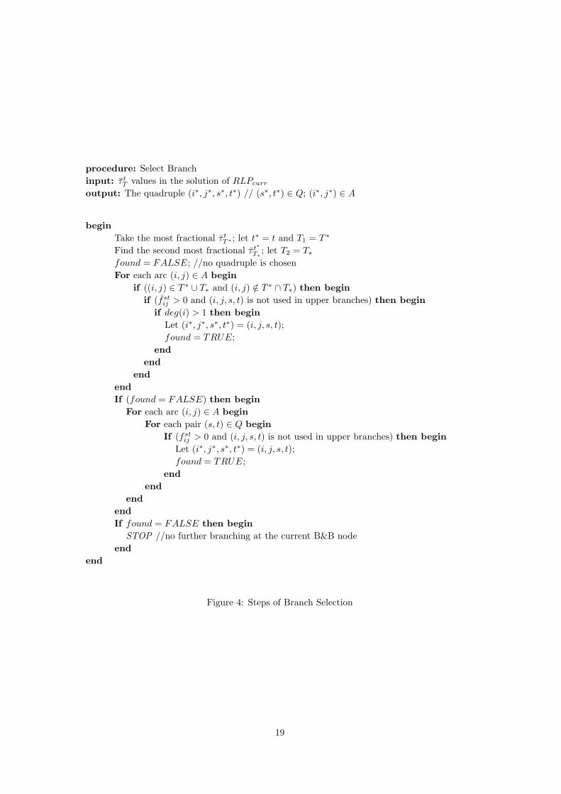
SP Tree T cannot be used for the destination node t. However, it is possible that PRt finds anSP Tree T with exactly the same set of arcs of T , i.e., T ≡ T . Consequently, we have decidedto create two subdivisions of the current problem based on an arc (i∗, j∗) being or not beingan SP arc for the demand ds∗t∗ of the pair (s∗, t∗). The procedure for selecting the quadruple(i∗, j∗, s∗, t∗) is explained in Figure 4.

When we are done with branch selection, we use the following rule to partition the solutionspace by creating two new nodes such that either of the following conditions holds:

• (i∗, j∗) is not an SP arc for the pair (s∗, t∗), i.e.,

fs∗t∗i∗j∗ = 0 (115)

• (i∗, j∗) is an SP arc for the pair (s∗, t∗), i.e.,

fs∗t∗i∗j∗ ≥

∑(k,i∗)∈A fst

ki∗

deg(i∗)− 1(116)

Notice that the summation on the right hand side of the inequality (116) is the total inflowfor node i∗. Moreover, suppose deg(i∗) arcs are incident to i∗. Then in order (i∗, j∗) to be anSP arc, we must have at least one incoming arc and at most deg(i∗)− 1 outgoing arcs for node

17

Procedure Upper Bound Approximationinput: Optimal values of the τ variables for RLPcurr, i.e.,τoutput: Upper bound UB on the optimal oblivious ratio r

beginFor each t ∈ V begin

Pick the largest τ tT∗ variable such that ¯τ t

T∗ ≥ τ tT ∀T ∈ Ωt

Let At be the set of SP arcs contained in T ∗

Get the fraction of demand routed on each arc (i, j) ∈ At by solving LPt:min 0

s.t.∑

(i,j)∈Atfs

ij −∑

(j,i)∈Atfs

ji =

1 i = s

−1 i = t

0 otherwise∀i ∈ V, s ∈ V \t

−fsij + ϕs

i = 0 ∀(i, j) ∈ At, s ∈ V \t0 ≤ fs

ij ≤ 1 ∀(i, j) ∈ At, s ∈ V \tfs

ij = 0 ∀(i, j) ∈ A\At, s ∈ V \t0 ≤ ϕs

i ≤ 1 ∀i ∈ V, s ∈ V \tLet σst

ij = fsij + fs

ji ∀i, j ∈ E, (s, t) ∈ Q

endSolve the following problem PUB to get an upper bound UB on r∗

z∗ub(nb) = min r

s.t. χhk +∑H

z=1 azλhkz ≤ 0 ∀h, k ∈ E

Πsti,hk −Πst

j,hk + ηij,hk ≥ 0 ∀(i, j) ∈ A; (s, t) ∈ Q; h, k ∈ E

−πsthk +

∑Hz=1 ast

z λhkz ≥ σst

ij ∀(s, t) ∈ Q; h, k ∈ E

ρtj − ρt

i + θij = 0 ∀(i, j) ∈ At, t ∈ V

ρtj − ρt

i + θij ≥ 0 ∀(i, j) ∈ A\At, t ∈ V

χhk ≥ 0 ∀h, k ∈ E

λhkz ≥ 0 ∀z = 1, .., H, h, k ∈ E

ηij,hk ≥ 0 ∀i, j ∈ E, h, k ∈ E

ρti ≥ 0 ∀i ∈ V, t ∈ V

1 ≤ θij ≤ Θmax integer ∀(i, j) ∈ A

r ≥ 1If z∗ub(nb) < UB then begin

Let UB = z∗ub(nb)end

end

Figure 3: Summary of the Upper Bound Approximation Method

18

procedure: Select Branchinput: τ t

T values in the solution of RLPcurr

output: The quadruple (i∗, j∗, s∗, t∗) // (s∗, t∗) ∈ Q; (i∗, j∗) ∈ A

beginTake the most fractional τ t

T∗ ; let t∗ = t and T1 = T ∗

Find the second most fractional τ t∗T∗ ; let T2 = T∗

found = FALSE; //no quadruple is chosenFor each arc (i, j) ∈ A begin

if ((i, j) ∈ T ∗ ∪ T∗ and (i, j) /∈ T ∗ ∩ T∗) then beginif (fst

ij > 0 and (i, j, s, t) is not used in upper branches) then beginif deg(i) > 1 then begin

Let (i∗, j∗, s∗, t∗) = (i, j, s, t);found = TRUE;

endend

endendIf (found = FALSE) then begin

For each arc (i, j) ∈ A beginFor each pair (s, t) ∈ Q begin

If (fstij > 0 and (i, j, s, t) is not used in upper branches) then begin

Let (i∗, j∗, s∗, t∗) = (i, j, s, t);found = TRUE;

endend

endendIf found = FALSE then begin

STOP //no further branching at the current B&B nodeend

end

Figure 4: Steps of Branch Selection

19

i∗. Hence in the most splitted case all arcs departing from node i∗ would be SP arcs and thetotal flow accumulated in i∗ will be splitted evenly among them according to the ECMP routingrule. This is why we have this constant in the denominator of (116).

Given the current B&B node nb and its associated relaxation RLPcurr, we create the two newnodes nr and nl by adding the constraints (115) and (116) to the current restricted problem aswell as the corresponding pricing problems PRt∗ . Additionally, we also impose the constraints

• Do not use SP trees containing arc (i∗, j∗), i.e.,∑

T∈Ωt∗∩Ωi∗j∗

τ t∗T = 0 (117)

• Do not use SP trees not containing arc (i∗, j∗), i.e.,∑

T∈Ω\(Ωt∗∩Ωi∗j∗ )

τ t∗T = 0 (118)

to create nr and nl, respectively. For both branches we just need to modify the upper boundsof the corresponding τ variables. Similarly, for nr we need to modify the upper bound of theflow variable whereas for nl we add a new constraint. Alternatively, together with the cuttingplane in (118), the result of the following proposition can also be used to define nr.

Proposition 5.1. Suppose that (i, j) is an SP arc for the pair (s, t). Then the fraction of dst

routed on (i, j) satisfies the condition

fstij ≥

1deg(s) ∗∏

l∈V \s,t:deg(l)>1(deg(l)− 1)(119)

Proof. Suppose that arc (i, j) is an SP arc for the demand pair (s, t). In the worst case thedemand dst originated at the source node s would visit all nodes in the graph G = (V, E) beforeit ceases at the destination node t and all arcs of G would be SP arcs. Then, for the sourcenode s we would have

fstsj =

1deg(s)

∀(s, j) ∈ A

whereas

fsthk =

∑(l,h)∈A fst

lh

(deg(h)− 1)∀(h, k) ∈ A, h ∈ V \s, t

for the rest of the graph. For example, suppose that SPst = (s, i), (i, j), (j, m), ...., (k, t) is ashortest path from s to t and all arcs incident to all nodes on this path are SP arcs. Then wehave

fstsi ≥

1deg(s)

fstij ≥

1deg(s) ∗ (deg(i)− 1)

fstjm ≥ 1

deg(s) ∗ (deg(i)− 1) ∗ (deg(j)− 1)...

fstkt ≥

1deg(s) ∗∏

l∈PATHsk(deg(l)− 1)

20

and hence

fstkt ≥

1deg(s) ∗∏

l∈V \s,t(deg(l)− 1)

where PATHsk is the set of nodes on the shortest path from s to k. The latter inequality isbased on the assumption that in the worst case dst would visit all nodes before it reaches itsdestination node.

In our computational experiments, we have used (119) rather than (116). This is mainlybecause our models are already difficult to solve and we do not want the increase the size ofcurrent problem as we go down the B&B tree. Moreover, unlike (116), the inequalities (119)ensure that the flow on an SP arc (i, j) is positive. We have observed that this difference hasimproved the performance of the B&P algorithm for the set of instances we have worked on.On the other hand, using (119) and (116) together would be useful especially for more dense orlarger instances since neither of them dominates the other one all the time.

6 Computational experiments

In order to test our models as well as the B&P algorithm, we have considered two well knowndemand uncertainty definitions. The common property of these approaches is that we do notmake any assumption about the distribution of the traffic demands or how pairwise demandsare correlated with each other.

For the rest of this section we let W ⊆ V be the set of demand and\or supply nodes, whichwe call terminal nodes. Moreover, Q = (s, t) : s, t ∈ W, s 6= t is the set of directed demandpairs with flow demands dst.

6.1 Hose model

This uncertainty model has been introduced by Duffield et al. [20] within the context of VirtualPrivate Network (VPN) design. In this approach the focus is on the outflow and inflow capacitiesof some special nodes, which are called VPN terminals, rather than the individual demands.Namely, the set of feasible demands is defined by some bounds on the total flow each terminalnode can send to and accept from the rest of the VPN terminals. Then the set of feasibledemand matrices with the Hose model is

D = d ∈ R|Q| :∑

t∈W\sdst ≤ b+

s ;∑

t∈W\sdts ≤ b−s ; dst ≥ 0 ∀(s, t) ∈ Q (120)

where b−s and b+s are the ingress and egress capacities of the terminal node s ∈ W , respectively.

Notice that this is more known as the asymmetric version of the Hose model, and that there is asymmetric version where an upper bound is given on the sum of all traffic demands originatingor ending in s.

6.2 Bertsimas-Sim (BS) uncertainty model

Consider the case where we have box constraints to define the lower and upper bounds on thepairwise flow demands. Since our models provide worst case guarantees we would get a veryconservative solution, which assumes that all demands can get their peak levels simultaneously.To overcome this problem we can use a positive integer parameter Γ to scale the trade offbetween the robustness of the model and the conservatism level of the solution. This is theapproach discussed within the context of robust optimization by Bertsimas and Sim in [9]and [10]. In our problem, Γ is the maximum number of pairs whose demands would change

21

simultaneously within their uncertainty limits so as to affect the solution adversely. Let usassume that demands dst range between d′st and d′st + dst (where dst > 0) and that not morethan Γ may differ from their nominal value d′st simultaneously. We can define each demandas dst = d′st + βstdst, where βst is a binary variable, and impose that

∑(s,t)∈Q βst ≤ Γ. Since

βst = dst−d′st

dst, if we relax integrality of β the BS uncertainty model defines the polyhedral set

of feasible demands as follows:

D = d ∈ R|Q| : d′st ≤ dst ≤ d′st + dst ∀(s, t) ∈ Q;∑

(s,t)∈Qdst−d′st

dst≤ Γ. (121)

6.3 Numerical results

We have performed numerical experiments on instances of various sizes to assess the performanceof our formulations and the B&P algorithm. We have also included MPLS routing in ourestimations to compare it to the OSPF routing with ECMP condition under weight management.Note that the MPLS oblivious performance ratio under general demand uncertainty is foundby solving the linear program (43)-(52), where we restrict neither the routing pattern nor howeach demand dst is shared among multiple paths between s and t. Therefore, MPLS routingdoes not perform worse than OSPF routing with ECMP. Nevertheless, it would be a goodbenchmark for us to comment on the oblivious ratios under OSPF environment since we havezmpls ≤ zospf where zmpls and zospf are the oblivious performance ratios for MPLS routingand OSPF routing with ECMP, respectively. Furthermore, Fortz and Thorup [6] compare theperformance of optimal OSPF routing with the optimal MPLS routing for a fixed TM and statethat their performances almost match in this case. However, we deal with oblivious routingwhere there is a set of feasible demands. To the best of our knowledge, there is no other referencecomparing oblivious MPLS routing with oblivious OSPF routing with weight management forsuch a general definition of feasible traffic matrices. Therefore, we believe it is important toextend this comparison to the case of a set of feasible demands rather than a single TM asApplegate and Cohen [8] also mention.

The instances bhvac, pacbell, eon, metro, and arpanet are well known instances studiedin the IEEE literature. On the other hand, Exodus (Europe), Abovenet (US), VNSL (India),and Telstra (Australia) are from the Rocketfuel project [21] for which we have the data forthe topology (|V | and |E|), the link weights (w), and the number of data packets enteringand leaving each node. For these instances we have assumed that the weight metric w obeythe inverse capacity weight setting where the weight of each link is inversely proportional to itscapacity, i.e., cij = 1/wij ∀i, j ∈ E. Moreover, since the information on real demand matricesis not made publicly available, we have used the Gravity model mentioned by Applegate andCohen [8] to generate the demand polyhedra D matching each instance. This approach is basedon the assumption that a demand dst is proportional to the product of a repulsion term Rs

associated with the source, and an attraction term At associated with the destination, which,for instance, can be set as the total observed outgoing and incoming traffic, respectively. Abase demand d is defined and the uncertainty polyhedron is constructed around d: we have thedata on the number of data packets incoming and outgoing for each node i, i.e., the repulsion(Ri) and attraction (Ai) parameters. Then the base demand for pair (s, t) is estimated usingthe relation dst = βRsAt, where β is computed in order for d to be feasible (i.e., to admit atleast one routing) and to choose how close d is to the boundary of the feasibility region. Let us

22

define ς ∈ [0, 1] such that β = ςυ∗ with

υ∗ = max υ (122)

s.t.∑

j:s,j∈E

(gstsj − gst

js) = υRsAt ∀(s, t) ∈ Q (123)

∑

j:i,j∈E

(gstij − gst

ji) = 0 ∀i ∈ V \ s, t, (s, t) ∈ Q (124)

∑

(s,t)∈Q

(gstij + gst

ji) ≤ cij ∀i, j ∈ E (125)

gstij ≥ 0 ∀(i, j) ∈ A, (s, t) ∈ Q. (126)

We fix a direction (the half-line dst = βRsAt) on which d must lie, and solve the LP aboveto find the most critical demand value, which is on the boundary of the feasibility region.Then, ς scales this value so that d is an inner point of the demand polyhedron if ς < 1. As aresult, (dst)(s,t)∈Q is a feasible traffic matrix for the current topology such that the maximumcongestion is no more than ς.

For the Hose and BS uncertainty models, we have determined the set of terminal nodesW among the busiest nodes, i.e., the ones with large Ri and Ai parameters. It should bementioned that our instances are dense instances in the sense that in all but two cases we have|Q|/|V | ≥ 0.33. Moreover, we have created 4 variants of each instance using different uncertaintyparameters p with values 1.1, 2, 5, 20 for the BS model. We will refer to each BS instanceusing the label (name,p), i.e., (nsf,2) is the nsf instance with uncertainty level p = 2. Largerp values imply higher variation in demand estimates. Hence the optimal oblivious ratio is alsoexpected to be larger for such cases. On the other hand, we have randomly picked a subsetS of W such that |S| = |W |/2. Then we have used b+

s = (∑

(s,t)∈Q dst)/1.1 ∀s ∈ S, b+s =

1.1(∑

(s,t)∈Q dst) ∀s ∈ W\S, b−s = 1.1(∑

(s,t)∈Q dst) ∀s ∈ S, and b−s = (∑

(s,t)∈Q dst)/1.1 ∀s ∈W\S as the outflow and inflow capacities of the terminal nodes in the Hose model. It is worthnoting that the uncertainty set is asymmetric in this case. This feature is believed to complicatethe problem based on the VPN design literature (Altın et al. [1]).

We have used AMPL to model the flow formulation as well as the MPLS routing and Cplex9.1 MIP solver to solve them. The B&P algorithm is implemented in C using MINTO (MixedINTeger Optimizer) [19] and Cplex 9.1 as LP solver. We have set a two hours time limitboth for AMPL and MINTO. Our test results for two uncertainty models discussed above aresummarized in Table 1 and Table 2 with:

• the instance characteristics, i.e., the name of the instance as well as the numbers of nodes,arcs, and terminals,

• the measure of the demand uncertainty p that we use in the creation of the test instancesfor the BS model. After getting an estimate of the average traffic demand (dst) for a pair(s, t), we set the corresponding d′st = dst/p and dst = (p− 1

p )dst.

• the solution ztree and total CPU time ttree of the B&P algorithm;

• the solution zflow and CPU time tflow of the flow formulation;

• the solution zmpls and CPU time tmpls for the MPLS routing;

All run times are given in seconds.The OSPF routing problem we focus on is clearly different from the regular OSPF routing

with fixed link metric. Applegate and Cohen [8] call this more complicated routing effort asbest OSPF style routing and mention that it is highly non-trivial. Therefore, it is not surprisingthat some instances could not be solved to optimality at the end of 2 hours time limit. Inthose cases for which we could find a feasible but not the optimal solution of the corresponding

23

problem we put a ∗ next to this upper bound. On the other hand, if no feasible solution isavailable, then the best lower bound obtained by solving the associated LP relaxation is givenin brackets. Furthermore, NoI means that we do not even have a feasible solution for the LPrelaxation, i.e., the Phase I problem could not be solved in 2 hours. Finally, MINTO couldnot solve some instances due to excessive memory requirements. We label such cases with MAunder the ttree column.

Note that the ztree, zflow, and zmpls columns provide a relative performance measure forthe corresponding routings. They indicate how much each routing deviates from the optimaloblivious routing for the corresponding D. Hence, as specified in our mathematical models thesevalues can be at least 1 where larger numbers imply larger deviation from the best possiblerouting tailored for that instance. Moreover, a value of 1 means that the perfectly obliviousrouting is found by solving the corresponding model. In other words, by using our optimizationtools we find a routing, which is the best tailored for any traffic matrix in the feasible set D.

Table 1 shows the results for the BS uncertainty model for 11 instances of 4 different levelsof uncertainty. As expected, the oblivious ratios never get smaller as the variability increases.MINTO and Cplex could solve 19 and 17 of these 44 instances to optimality in 2 hours, respec-tively. Moreover, in those cases where the tree formulation provides a worse upper bound thanthe flow formulation, B&P algorithm run less than 2 hours and had to stop due to memory allo-cation problems. Finally, our B&P method finds the perfectly oblivious OSPF routing for (ex-ample,1.1), (bhvac,1.1), (bhvac,2), (bhvac,5), (Abovenet,2), (Abovenet,5), and (Abovenet,20) inaround one minute. Cplex could only find very loose upper bounds for the Abovenet instancesand just lower bounds for the remaining four. Hence, we can say that it is worth implementinga specialized B&P algorithm for the BS uncertainty model. However, this problem has consid-erable memory requirements. Therefore, it is not likely to get very promising results for largeinstances within reasonable time limits neither with the tree nor with the flow formulation. Asa result, the performance of optimal oblivious OSPF routing with weight management is notexpected to be comparable with the performance of optimal oblivious MPLS routing for largecases.

A comparison of the OSPF and MPLS routings based on our test results should be made intwo stages. In the first step, we focus on the 24 instances for which we could find the optimalsolutions and compare the gap for the oblivious ratios. In 15 of them we could find the perfectlyoblivious routings with both routing protocols. For the remaining 9, the oblivious ratio of ourOSPF routing is 5.4% to 47% larger than that of the oblivious MPLS routing. An importantobservation here is that the gap between two alternatives does not improve with p. In otherwords for any network the deviation for OSPF at uncertainty level p is almost never less thanthe one for a smaller p. For example, consider the nsf instance for which the oblivious MPLSrouting performs strictly better in all of the four uncertainty levels. A comparison of the threerouting technologies, namely our best OSPF style routing, MPLS routing, and OSPF underinverse capacity weight setting with ECMP, for the nsf network is provided in Figure 5.

00.5

11.5

22.5

33.5

44.5

1.2

1.6 2

2.4

2.8

3.2

3.6 4 6 10 14 18 25

P

optim

al o

bliv

ious

rat

io inv-cap OSPF

best OSPF

MPLS

Figure 5: The change in the optimal solutions of the best OSPF style, MPLS, and inversecapacity weight routings for the network nsf for different values of p.

Firstly, notice the significant difference between the best OSPF style routing and the OSPF

24

in inverse capacity weight environment. This is a very good example to depict the benefitof using weight management. As is clear from Figure 5, weight management resulted in animprovement in the OSPF performance. A more concrete comparison of the three alternativerouting alternatives is given in Figure 6, which shows the gaps between the optimal performanceratios. We can say that inverse capacity OSPF routing is almost 100% worse than best OSPF inall higher uncertainty levels for the nsf network. On the other hand the gap between best OSPFand MPLS increases with p from 8% to 30%. Finally, due to the increasing demand uncertainty,the performances of MPLS, best OSPF, and inverse capacity OSPF routings degrade by 32%,43.6%, and 60.4%, respectively. The degradation in oblivious ratio with uncertainty is alreadyexpected. Additionally, these observations certify that the effect is more significant for bothOSPF routing strategies. However, we can say that weight management has also helped toreduce the impact of demand uncertainty on oblivious ratio to some extent.

0

0.2

0.4

0.6

0.8

1

1.2

1.2

1.6 2

2.4

2.8

3.2

3.6 4 6 10 14 18 25

p

gap

inv-cap OSPF vs best OSPF

best OSPF vs MPLS

Figure 6: Comparison of the best OSPF style routing with MPLS and OSPF under inversecapacity weight setting for the instance nsf for different values of p.

Finally, we compare the best upper bounds we obtain for the OSPF routing with the optimalsolutions for MPLS. The gaps are more variable for those instances and range from 3.7% to335.7%. Just like the previous comment, the deviation is larger for more uncertain as well asmore difficult2 instances.

The second traffic uncertainty model we focus on is the Hose model for which the test resultsare shown in Table 2. The most obvious comment we can make is that the management of theHose uncertainty model is more difficult than the BS model for both the OSPF and MPLSroutings. We can make such a comment based on the computation times. Moreover, for theinstances eon and arpanet we could not get even a feasible solution with neither the flow northe MPLS formulations. Hence, we believe it will be fair to focus on the other instances of theHose model while interpreting the numerical results.

The performances of the tree and flow formulations in terms of computation times are com-parable for relatively smaller instances like Exodus and VNSL where the optimal oblivious ratiosare found. Nonetheless, the B&P algorithm had to stop due to excessive memory requirementsfor nsf, example, and Telstra providing upper bounds on the optimal oblivious ratios of our bestOSPF style routing. These bounds are worse than the bounds provided by the flow formulationunder the same settings. On the other hand, the tree formulation is superior with respect tothe lower bounds found at the end of 2 hours.

The difference between the OSPF and MPLS routings is more evident for the Hose model.For Exodus we could find the perfectly oblivious routing with both protocols. However, thecomparison between the optimal solutions of the instances nsf, VNSL, example, and Telstrashows that the difference between the two alternatives are 31.8%, 6.6%, 85.4%, and 50%,respectively. In brief, the average gap between the optimal solutions of the two routing schemesis 34.8% for the Hose model and 6.5% for the BS model. Note that the Hose model relies onthe estimates for the total inflow and outflow capacities of the routers whereas for the BS casewe need an estimate for the lower and upper bounds on the individual demands. Thus we can

2We consider large and dense topologies as difficult instances. tmpls values are also indicators of the difficulty

level.

25

Instance N E W p ztree ttree zflow tflow zmpls tmpls

Exodus 7 12 7 1.1 1 0.06 1 0.048 1 0.0522 1 0.05 1 0.044 1 0.0485 1 0.05 1 0.044 1 0.03620 1 0.04 1 0.036 1 0.036

nsf 8 20 5 1.1 1.381* MA 1.05* 2 hrs 1.013 0.3682 2.299* MA 1.556 3821.53 1.44 0.7525 3.808* MA 1.904 94.33 1.423 0.98420 3.936* MA 1.976 241.1 1.462 1.054

VNSL 9 22 3 1.1 1.066 39.75 1.066 0.19 1 0.0162 1.066 3.61 1.066 0.14 1 0.0245 1.066 24.77 1.066 0.22 1 0.0220 1.066 9.24 1.066 0.296 1 0.02

example 10 30 4 1.1 1 0.11 (1) 2 hrs 1 0.2752 1 0.15 1 1900.19 1 0.4065 2.25* MA 1.82* 2 hrs 1.034 0.54720 2.575* MA 3.269* 2 hrs 1.079 0.775

metro 11 84 5 1.1 4.357* 2 hrs (1) 2 hrs 1 92.9692 (1.211) 2 hrs (1.211) 2 hrs 1.210 450.965 (2.192) 2 hrs (1.299) 2 hrs 1.299 4642.3420 (1.648) 2 hrs (1.306) 2 hrs 1.302 3577.76

bhvac 19 44 11 1.1 1 109.63 (1) 2 hrs 1 81.1772 1 120.03 (1.0004) 2 hrs 1 235 1 41.32 (1) 2 hrs 1 44.23420 (1.706) 2 hrs (1.001) 2 hrs 1.443 1130.53

Abovenet 19 68 5 1.1 1 12.78 1 60.78 1 12.4822 1 13.58 2.24284* 2 hrs 1 35.955 1 13.92 2.68684* 2 hrs 1 54.0620 1 16.31 5.3568* 2 hrs 1 46.35

Telstra 44 88 7 1.1 1 1.75 1 0.504 1 0.1562 1 1.79 1 0.414 1 0.1585 2.075* MA 1.054 2.56 1 0.15920 2.081* MA 1.886 2.39 1.283 0.181

pacbell 15 42 7 1.1 1.667* 2 hrs 1.283* 2 hrs 1.014 70.932 1.868* 2 hrs (1.249) 2 hrs 1.249 1345 (1.521) 2 hrs (1.489) 4403 sec 1.488 174.2920 (1.565) 2 hrs (1.541) 2 hrs 1.54 159.54

eon 19 74 15 1.1 (1) 2 hrs NoI 2 hrs NoI 2 hrs2 (1) 2 hrs NoI 2 hrs 4.433* 2 hrs5 (4.718) 2 hrs NoI 2 hrs NoI 2 hrs20 (6.411) 2 hrs NoI 2 hrs 6.87* 2 hrs

arpanet 24 100 10 1.1 (1.3133) 2 hrs NoI 2 hrs 1.017 492.852 (1.922) 2 hrs NoI 2 hrs 4.4* 2 hrs5 (4.993) 2 hrs NoI 2 hrs NoI 2 hrs20 (5.799) 2 hrs NoI 2 hrs NoI 2 hrs

Table 1: Results for the BS uncertainty model

26

say that the definition of the traffic polyhedra D is looser in the former3. Therefore, we believethat these average deviations between the two protocols support our remark that degredationof the network performance due to increased uncertainty is higher for OSPF routing.

Instance N E W ztree ttree zflow tflow zmpls tmpls

Exodus 7 12 7 1 0.04 1 0.052 1 0.031nsf 8 20 5 4* MA 2 2730.38 1.517 0.403

VNSL 9 22 3 1.0655 8.77 1.0655 0.296 1 0.16example 10 30 4 2.7* MA 2 2 hrs 1.079 0.424metro 11 84 5 (1.437) 2 hrs (1.302) 2 hrs 1.302 1657.832bhvac 19 44 11 (2.853) 2 hrs (1.515) 2 hrs (1.515) 2 hrs

Abovenet 19 68 5 (1.116) 2 hrs (1.116) 2 hrs 1.045 326.125Telstra 44 88 7 2.081* MA 1.925 1.224 1.283 0.084pacbell 15 42 7 (1.544) 2 hrs (1.543) 2 hrs 1.543 59.131

eon 19 74 15 (6.857) 2 hrs NoI 2 hrs NoI 2 hrsarpanet 24 100 10 (5.85) 2 hrs NoI 2 hrs NoI 2 hrs

Table 2: Results for the hose uncertainty model

Our final comment is about the benefit of considering a polyhedra of demands rather than

a single traffic matrix d of average demands. To make such a comparison we useMaxUf∗

d

BESTdwhere

f∗ is the optimal oblivious OSPF routing in a given instance and BESTd is the maximum linkutilization of the most fair routing, say fd, for the average demand d. First, note that such acomparison does not provide additional information in those instances where we could find theperfectly oblivious routing. We already know that the most fair routing for any traffic matrixin D is attained in such cases. Hence we focus on the remaining examples and we have observedthat it is not possible to make a conclusion that is valid for all cases. For example in the VNSLinstances the optimal routing for d, is different than f∗. This means that if we optimize justfor the mean demand and the current demand turns out to be a different one, then we mighthave fd perform significantly worse than f∗. On the other hand, for the nsf instances we haveobserved that fd ≡ f∗. As a result, we believe that optimizing just for the mean demands doesnot suffice to ensure the fair allocation of work load in all cases.

7 Conclusion

Current traffic engineering efforts are mostly based on the efficient use of network resources soas to route a given traffic matrix. In practice the demands are not likely to be known exactly.This is the main motivation of our work and we consider the case where the polyhedra of feasibledemands is defined by some system specific constraints. We incorporate this general uncertaintyinto the OSPF style routing problem. To comply with the current forwarding technology, wealso include the equal load sharing condition (ECMP) in our analysis. Furthermore, we employweight management to improve the network performance of OSPF. Given all these specifics ofthe problem we focus on the minimization of the maximum link congestion via a fair allocationof traffic among the network links. To our knowledge, our paper is the first work on such ageneral and practically defensible best OSPF style routing.

We have proposed two mixed integer models obtained by a duality-based reformulation forour problem. The first one is a compact formulation based on flow variables. Because thismodel gets large very rapidly even for medium sized problems, we have proposed an alternative

3Based on how we have determined b+s and b−s as well as d′st and dst for the Hose and BS instances respectively

given the same average pairwise demand estimates dst.

27

tree formulation based on special structured subgraphs of the backbone graph, i.e., SP trees.Moreover, we have proposed a B&P algorithm supported by cutting planes to solve this model.

We have tested our models and the B&P algorithm on two traffic uncertainty definitions,namely the Hose model and the BS model. We have presented a comparison of the two formula-tions in terms of the solution quality and computation times. We have observed that it pays tocreate a specialized B&P algorithm especially for the BS uncertainty case. Unfortunately, dueto excessive memory requirements of the algorithm, it had to stop before two hours time limitin some instances. Additionally, we have compared the OSPF style routing and the MPLS stylerouting for these two traffic polyhedra. First, we have realized that for the BS case the optimaloblivious ratios for both routing styles increase as the level of demand variability increases. An-other important observation is that the performance of OSPF routing degrades more than theMPLS routing as the demand uncertainty increases. To sum up, we believe that a polyhedraldefinition of the feasible set of demand matrices, which is accurate as far as possible, couldmake the OSPF performance get closer to the MPLS performance.

References

[1] A. Altın, E. Amaldi, P. Belotti, and M. C. Pınar, Provisioning virtual private networksunder traffic uncertainty. NETWORKS, 20, 1, 2007, pp. 100-115.

[2] A. Bley and T. Koch, Integer programming approaches to access and backbone IP-networkplanning. Tech. Report TR 02-41, Konrad-Zuse-Zentrum fur Informationstechnik, Berlin,2002.

[3] A. Parmar, S. Ahmed, and J. Sokol, An integer programming approach to the OSPFweight setting problem. submitted for publication, 2006.

[4] A. Sridharan, R. Guerin, and C. Diot, Achieving near-optimal traffic engineering solutionsfor current OSPF/IS-IS networks. IEEE INFOCOM 2003, San Francisco, CA, 2003.

[5] A. Tomaszewski, M. Pioro, M. Dzida, and M. Zagozdzon, Optimization of administrativeweights in IP networks using the branch-and-cut approach. Proceedings of INOC 2005,B2, pp. 393-400.

[6] B. Fortz and M. Thorup, Internet traffic engineering by optimizing OSPF weights. Pro-ceedings of IEEE INFOCOM 2000, pp. 519-528.

[7] C. Barnhart, E.L. Johnson, G.L. Nemhauser, M.W.P. Savelsbergh, P.H. Vance, Branch-and-price: column generation for solving huge integer programs. Operations Research, 46,1998, pp. 316-329.

[8] D. Applegate and E. Cohen, Making intra-domain routing robust to changing and un-certain traffic demands:Understanding fundamental tradeoffs. Proceedings of SIGCOMM’03, Karlsruhe, Germany, pp. 313-324.

[9] D. Bertsimas and M. Sim, Robust discrete optimization and network flows. MathematicalProgramming, Ser. B 98, 2003, pp. 43-71.

[10] D. Bertsimas and M. Sim, The price of robustness. Operations Research, 52, 2004, pp.35-53.

[11] F. Y. Lin and J. L. Wang, Minimax open shortest path first routing algorithms in networkssupporting SMDS service. Proc. IEEE Int. Conf. Communications(ICC), 2, 1993, pp. 666-670.

28

[12] G. Oriolo, Domination in traffic matrices. Available for download athttp://www.optimization-online.org/DB FILE/2004/09/952.pdf

[13] J. Zhang, Z. Ma, C. Yang, A column generation method for inverse shortest path problems.Mathematical Methods of Operations Research (ZOR) 41 (3), 1995, pp. 347-358.

[14] B. Burton, W. R. Pulleyblank, and Ph. L. Toint. The inverse shortest path problem withupper bounds on shortest path costs, In: P. Pardalos, D. W. Hearn, and W. H. Hager, eds.Network Optimization, Springer Lecture Notes in Economics and Mathematical Systems,450 (1997), 156–171.

[15] J. Wang, Y. Yang, L. Xiao, K. Nahrstedt, Edge-based traffic engineering for OSPF net-works. Computer Networks, in press.

[16] K. Holmberg and D. Yuan, Optimization of internet protocol network design and routing.NETWORKS, 43(1), 2004, pp. 39-53.

[17] L. De Giovanni, B. Fortz, and M. Labbe, A lower bound for the internet protocol networkdesign problem. Proceedings of INOC 2005, B2, pp. 401-408.

[18] M. Pioro, A. Szentesi. J. Harmatos, A. Juttner, P. Gajowniczek, and S. Kozdrowski, Onopen shortest path first related network optimization problems. Performance Evaluation,48, 2002, pp. 201-223.

[19] M.W.P. Savelsbergh, G.C. Sigismondi, G.L. Nemhauser. A functional description ofMINTO, a Mixed INTeger Optimizer. OR Letters 15 (1994), pp. 47-58.

[20] N. Duffield, P. Goyal, A. Greenberg, P. Mishra, K. Ramakrishnan, and J.E. van derMerive, A flexible model for resource management in virtual private networks. Proceedingsof ACM SIGCOMM, 1999, pp. 95-108.

[21] N. Springs, R. Mahajan, D. Wetherall, Measuring ISP topologies with Rocketfuel. Pro-ceedings of IEEE/ACM Transactions on Networking 12-1 (2004), pp. 2-16.

[22] P. Belotti and M.C. Pınar, Optimal oblivious routing under linear and nonlinear uncer-tainty, 2005, submitted to Optimization and Engineering. Available for download fromhttp://www.andrew.cmu.edu/user/belotti/papers/obl-stat.pdf

[23] P. Brostrom and K. Holmberg, Design of IP/OSPF networks using a Lagrangean heuristicon an in-graph based model. Proceedings of INOC 2005, B3, pp.702.

[24] Y. Wang, Z. Wang, and L. Zhang, Internet traffic engineering without full mesh overlaying.Proceedings of IEEE INFOCOM 2001, pp. 565-571.

29