Journal of Hydrology (2006) 330, 368–381

ava i lab le at www.sc iencedi rec t . com

journal homepage: www.elsevier .com/ locate / jhydro l

Hydrological forecasting uncertaintyassessment: Incoherence of the GLUE methodology

Pietro Mantovan a, Ezio Todini b,*

a Department of Statistics, University of Venice, Italyb Department of Scienze della Terra e Geologico-Ambientali, University of Bologna, Via Zamboni, 67, 40126 Bologna, Italy

Received 11 October 2004; received in revised form 10 April 2006; accepted 11 April 2006

Summary The aim of the paper is to demonstrate the incoherence, in terms of Bayesian infer-ence, of the generalized likelihood uncertainty estimation (GLUE) approach, introduced byBeven and Binley in 1992. This results into a reduced capacity of the technique to extract infor-mation, in other words to ‘‘learn’’, from observations. The paper also discusses the implica-tions of this reduced learning capacity for parameter estimation and hydrological forecastinguncertainty assessment, which has led to the definition of the ‘‘equifinality’’ principle. Thenotions of coherence for learning and prediction processes as well as the value of a statisticalexperiment are introduced. These concepts are useful in showing that the GLUE methodologydefines a statistical inference process, which is inconsistent and incoherent.

�c 2006 Elsevier B.V. All rights reserved.

KEYWORDSBayesian analysis;Coherence;Inconsistency;Inference process;Value of a statisticalexperiment;GLUE

0d

2

Introduction and scope

In the last decade, increased scientific interest had beenshown on parameter estimation as well as on the assessmentof parameter and forecasting uncertainty in hydrologicalmodels. As pointed out by Vrugt et al. (2005), hydrologicalmodels conceptualize and aggregate the complex, spatiallydistributed, and highly interrelated water, energy, and veg-etation processes in a watershed through relatively simplemathematical equations with model parameters that often

022-1694/$ - see front matter �c 2006 Elsevier B.V. All rights reserveoi:10.1016/j.jhydrol.2006.04.046

* Corresponding author. Tel.: +39 051 2094537; fax: +39 051094522.E-mail address: todini@tin.it (E. Todini).

do not represent directly measurable entities and musttherefore be estimated using input and output measure-ments. This inevitably leads to uncertain parameter esti-mates (and consequently to uncertain forecasts) due tostructural errors in the model schematisation, errors inthe input (such as for instance rainfall, temperature, andupstream inflows) and output measurements (generallydownstream discharges), errors in the initial conditions ofseveral state variables (such as for instance soil moisturecontent, the extent of saturated areas, and the accumu-lated snowpack). In addition, the parameter estimationphase is generally carried out only based upon the down-stream residuals, without really accounting for their tempo-ral correlation as well as their non–stationarity.

d.

Hydrological forecasting uncertainty assessment: Incoherence of the GLUE methodology 369

If the statistical properties of all these errors and resid-uals are not properly accounted for, biased parameterestimates are obtained together with wrong assessmentsof parameter estimate uncertainty as well as of forecast-ing uncertainty (Vrugt et al., 2005). Several methods haveappeared in the literature, which seek to provide mean-ingful confidence bands for parameter estimates in con-ceptual non-linear watershed models. These approachesrange from classical Bayesian techniques (Kuczera andParent, 1998; Thiemann et al., 2001; Vrugt et al.,2003a; Kavetski et al., 2003), to the pseudo-Bayesian(Beven and Binley, 1992; Freer et al., 1996), set theory(Keesman, 1990; Klepper et al., 1991; van Straten andKeesman, 1991; Vrugt et al., 2001), multiple criteria (Gup-ta et al., 1998; Yapo et al., 1998; Boyle et al., 2000;Vrugt et al., 2003b), and recursive model and parameteridentification techniques (Thiemann et al., 2001; Young,2001; Vrugt et al., 2002; Wagener et al., 2003) to accountfor non-stationarities in model residuals. Unfortunately,most of the previously mentioned approaches tend to con-sider the model uncertainty to be mostly produced byparameter uncertainty and use, as a measure of fit, afunction based on the model residuals. Essentially, themodel is assumed to be correct, and the parameter esti-mated conditional on this assumption. To overcome thisproblem and to incorporate a better treatment of the in-put, output, parameter and model structural uncertaintiesin hydrologic modeling, Vrugt (2004), Vrugt et al. (2005)proposed a simultaneous parameter optimization and dataassimilation (SODA) method, which combines the ShuffledComplex Evolution Metropolis (SCEM-UA) algorithm (Vrugtet al., 2003a), with an ensemble Kalman filter (Evensen,1994). Although the SODA approach seems to be of greatinterest, it is the belief of the authors that further re-search should be fostered into a more formal Bayesian ap-proach that would incorporate model, parameter, initialconditions uncertainty as well as non-stationarity and cor-relation into the model identification and parameter esti-mation process.

Following this line of thought, and for the sake of clar-ity, the present paper investigates certain aspects of oneof the previously mentioned techniques, the ‘‘generalisedlikelihood uncertainty estimation’’ (GLUE) method intro-duced by Beven and Binley (1992). The reason for this fo-cus is that GLUE has been interpreted as a Bayesianapproach (or more precisely as an extension of the Bayes-ian approach) and widely used over the past ten years toanalyse and estimate predictive uncertainty, particularlyin hydrological applications (Beven and Binley, 1992; Bev-en, 1993; Romanowicz et al., 1994; Freer et al., 1996;Franks and Beven, 1997; Zak et al., 1997). However, mostof the above mentioned authors, as well as many users allover the world, are apparently not aware that GLUE isinconsistent with the Bayesian inference process, whichinevitably leads to large overestimation of uncertainty,both for the parameter estimates and the resulting simu-lation forecasts. Users are apparently attracted by theease of use of GLUE, which provides in a single ready-made package, simple understandable ideas, workableinference techniques and a spurious sensation of freedomin relation to the strict rationale of statistical modellingand Bayesian inference.

Parameter estimation and/or predictiveuncertainty?

Before entering into a discussion of the GLUE approach, it isnecessary to clarify a fundamental concept fully embeddingthe Bayesian approach. In the classical Bayesian approach,the parameters of a model are not necessarily consideredas the representations of physically meaningful quantitieswhich have true (albeit unknown) values, but rather tempo-rary ‘‘dummy’’ or ‘‘convenient’’ quantities of uncertainnature (on which all our uncertainty is projected) to be mar-ginalized out by means of their posterior probability den-sity, which is obtained from observations via the Bayesianinference process.

Therefore, it is worthwhile clarifying the objective of ouruncertainty assessment. Is ‘‘parameter estimation’’ ourmain objective, or is it ‘‘prediction’’?

If the objective is ‘‘parameter estimation’’, we implic-itly assume that our parameters have a true albeit unknownvalue to be found, and this can be estimated once the pos-terior density has been derived, either in terms of the max-imum likelihood value or as the expected value. But theparameter estimation does not necessarily reflect the origi-nal Bayesian idea.

When the objective is ‘‘prediction’’, the Bayesian ap-proach ‘‘does not require’’ the estimation of a specificparameter value, but rather the estimation of ‘‘their entireposterior probability density’’ that expresses our uncer-tainty after sampling the observations. Maybe, it is worth-while bearing in mind that a ‘‘deterministic’’ quantity canbe represented as a delta of Dirac over its value, while anuncertain quantity requires either of the descriptions ofits probability distribution.

To clarify this concept, let us consider the following ob-servable random vector yi = (y1,y2, . . . ,yc)

T, c P 1, i =1,2, . . . ,n, of predictive interest, such as for instance, forc = 1, a time series of discharges or water stages at a down-stream section in a river, sampled at constant time stepsi = 1, . . . ,n, jointly observable with the predictor vectorxi = (x1,x2, . . . ,xk)

T, k P 1, i = 1,2, . . . ,n, such as for in-stance, for k = 1, a time series of precipitation. Under theconditional stochastic independence, let f(yijh,xi) be theconditional probability density function of the observablevector yi conditioned on the covariate vector xi and theparameter vector h. The conditional probability densityfunction f(yijh,xi) implicitly summarizes the modelleddependence of the observable random vector yi from thecovariate vector xi by the parameter vector h. This relationmay be explained, for instance, by the conditional expectedvalue:

Eðyijh; xiÞ ¼ lðh; xiÞ ¼ l1ðh; xiÞ; l2ðh; xiÞ; . . . ; lcðh; xiÞð ÞT;

i = 1,2, . . . ,n, where the conditional mean model l (h,xi) isidentified by the parameter vector h, the size of which issomehow related to the complexity of the conditional meanmodel and, as previously stated, not necessarily encapsulat-ing a physical meaning.

More explicitly, but in an equivalent way, the observablerandom vector yi can be assumed to be defined by a struc-tural part l(h,xi) modelling directly the expected depen-dence of the observable random vector yi from the

370 P. Mantovan, E. Todini

covariate vector xi by the parameter vector h composedwith an additive or multiplicative random error. From thedistribution of the random error, follows the conditional dis-tribution of the observable random vector yi.

The scope of the Bayesian inference is to derive from theuse of the historical observations (Yn,Xn), Yn = (y1,y2, . . . ,yn)

T, Xn = (x1,x2, . . . ,xn)T, a posterior probability density

for the parameter vector h, namely g(hjYn,Xn), with whichit will then be possible to marginalize out the conditionalityon the parameters. This involves integrating over H, the en-tire domain of existence of the parameters, the conditionalprobability density function f(ypjh,xp) of the observablevector yp conditioned on the covariate vector xp and theparameter vector h that identifies the specific model, to de-rive the predictive probability density for the pthobservation:

fðypjYn;Xn; xpÞ ¼Z

Hfðypjh; xpÞgðhjYn;XnÞdh; ð1Þ

which can be used to describe the predictive uncertaintyboth in ‘‘hindcast’’ mode, when p 6 n, and in ‘‘forecast’’mode for p > n.

From Eq. (1), note that the dependence of the predictiveprobability density on the uncertain parameters has beenmarginalized by taking its expected value on the basis ofthe posterior parameter density. A similar expression resultsif h belongs to a discrete parametric space. Of course, thepredictive probability density can be extended to more thatone next observation.

The concept on which Beven and Binley’s (1992) ap-proach is based, where ‘‘alternative models’’ (namely thesame model with alternative parameters) are consideredto have the same predictive value (the concept of ‘‘equif-inality’’), reflects this concept up to a certain point, in thesense that, when dealing with non-linear models, the typi-cal hydrological approach of using a model with fixedparameter values may lead to large predictive biases, whileby expressing Eq. (1) in discrete form, one should use anensemble of model predictions (one for each parametervector realization) averaged with its derived posteriorprobability mass. Unfortunately, GLUE on the one handdoes not provide a correct expression for Eq. (1) and, onthe other hand, produces extremely ‘‘flat’’ posterior prob-ability distributions that lead to unrealistically wide predic-tive uncertainties, as opposed to a correct application ofthe Bayesian inference approach, which leads to peakierposterior densities and smaller predictive uncertainties.As a matter of fact, one is supposed to make the hypothesisof ‘‘equifinality’’ at the onset of the Bayesian inferenceprocess, namely that all the models (one per parametervector realisation) have the same informative value, dueto our prior lack of knowledge (typically expressed by auniform prior distribution for the parameters). But then,by means of the observations, one aims to produce peakierposterior densities; so the real scope of the whole Bayesianprocess is to achieve ‘‘inequifinality’’ where some of themodels are more likely to be correct than others. The mostimportant aspect to be borne in mind (which should not beconfused with the concept of ‘‘equifinality’’) is that, in or-der to avoid predictive biases, following Eq. (1), one has totake into account and use all the model predictions,namely one per parameter vector realization (and not only

the one relevant to the most likely parameter values), andall the predictions have then to be averaged using the de-rived posterior probability function to marginalize out theuncertainty due to the lack of knowledge of the actualparameter values to be used.

Therefore, when dealing with the derivation of the pre-dictive probability, which is the main object of modelling(and in particular of hydrological modelling), the estimationof the parameter values is a false problem, since the fullpredictive uncertainty information will be encapsulated intothe derived posterior probability density of the parametersgiven the observations.

This brings us to the reason for this paper. As it willbe demonstrated in the following sections, GLUE doesnot allow for a correct estimation of the posterior prob-ability density, since the choice of the ‘‘less formal like-lihoods’’ highly reduces its capability to extractinformation from the observations and consequently itis not advisable to use GLUE for estimating the predictiveprobabilities on the basis of the resulting posterior prob-ability density.

The GLUE approach

As already noted, the generalised likelihood uncertaintyestimation technique was introduced by Beven and Binley(1992) starting from concepts that, although expressed indifferent terms, are quite similar to the Bayesian ones.According to Beven et al. (2000), GLUE ‘‘represents anextension of Bayesian or fuzzy averaging procedures toless formal likelihood or fuzzy measures’’. The conceptof ‘‘the less formal likelihood’’, which represents themain element of differentiation with the Bayesian infer-ence, is a remarkable aspect of the GLUE methodology.In theory, this concept was introduced to overcome theneed to advance detailed distribution functions of the ob-servable variables and/or of errors even in complex situa-tions, such as when there is more than one source oferrors, when the explicative models provided are complexor when the number of parameters used to realize a pro-cess of learning is high.

Unfortunately, as will be shown in the sequel, the use ofsuch less formal likelihoods results in GLUE loosing thelearning properties of the Bayesian inferential approach,and so the GLUE methodology is incoherent and inconsistentwith the statistical inference process. The loss of the learn-ing properties prevents the possibility of reducing theuncertainty down to a lower limit imposed by the structuralproperties of the model and the other sources of errors, byincreasing the number of observations. This inevitably re-sults in very ‘‘flat’’ parameter posterior densities, a factthat may have led to the emergence of the ‘‘equifinality’’principle. In reality, a proper Bayesian approach wouldeventually start from a flat non-informative prior distribu-tion with the aim at reaching an ‘‘inequifinality’’ condition,namely a ‘‘peaky’’ posterior density over the most likelyparameter sets, by adding the sampling information pro-vided by an increasing number of observations.

Although, according to Beven and Binley (1992), GLUEwas formulated in order to overcome uncertainties relevantto several sources of errors: ‘‘error due to poorly defined

Hydrological forecasting uncertainty assessment: Incoherence of the GLUE methodology 371

boundary conditions and input data; error associated withmeasurements used in model calibration; and error due todeficiencies in model structure’’; in reality it does not ac-count for them directly, but only indirectly through the sta-tistical properties of the model residuals. GLUE is in factconditional on model structure, on input errors and on ini-tial conditions, which are not taken as uncertain. Uncer-tainty is only considered to be generated by the lack ofknowledge of model parameter values as well as possiblyby the predictand observation errors, with the implicitassumption of additive errors, ‘‘perhaps after a suitabletransformation’’ (Beven and Freer, 2001), which can besummarised in Eq. (2), similar to what is generally done inthe Bayesian approach:

yi ¼ lðh; xiÞ þ ei; i ¼ 1; 2; . . . ; n; h 2 H; ð2Þ

where yi is the predictand at step i, xi is the predictor vec-tor incorporating all the input observations up to step i, h isone of the possible choices of the parameter vector and eiis an additive error term which will incorporate the mea-surement errors on the predictand, the model structure er-rors as well as all the errors generated by the lack ofknowledge of the ‘‘true’’, if any, or optimal parameterset. In reality, the choice of the additive error formulationgiven in Eq. (2) is not binding when the main objective isthe derivation of the predictive probability distribution gi-ven by Eq. (1).

Conversely, when the objective is ‘‘parameter’’ estima-tion, several problems may occur. Firstly, the formulationof Eq. (2) does not guarantee that all the parameters canbe properly estimated (the concept of ‘‘observability’’ thatcan be found in Gelb, 1974, and in several papers such as forinstance in Gupta and Sorooshian, 1983, and Sorooshian andGupta, 1983, may not be fulfilled), which implies that othersources of information should be used, not necessarily lim-iting ourselves to a downstream cross section water stage ordischarges of predictive interest. For instance, the recentavailability of distributed satellite measurements could beof great relevance by providing information on the extentof saturation surfaces or (hopefully in a nearby future) onthe soil moisture content, both highly related to the param-eters of the distributed hydrological models. Secondly, bynot directly accounting for the variability induced by theother sources of errors, such as for instance the measure-ment errors in xi, the input variables, the estimated param-eter values, due to the generally non-linear links betweenparameters and measurements in the hydrologic models,will inevitably be biased.

Therefore, two aspects must be clearly borne in mind allthroughout the paper:

(i) the focus of this work is the derivation of the predic-tive probability of a predictand (Eq. (1)) and

(ii) the parameters, although generally considered as‘‘deterministic’’ in a physically meaningful model ofgiven structure, encapsulate ‘‘all our uncertainties’’,thus becoming ‘‘uncertain’’ quantities. This impliesthat it is not necessary to estimate specific parametervalues (i.e., as the expected value or the most likelyone), but rather their posterior probability distribu-tion, which is the essential information required forassessing the predictive probability.

More details on points (i) and (ii) related to the inductivereasoning in statistical inference and its mathematical char-acterization can be found in de Finetti (1975, Chapters 11and 12).

The basic formulation

The GLUE formulation closely follows the classical Bayesianinference approach, from which it mainly differs in thechoice of the likelihood to be used, the so called ‘‘less for-mal likelihood’’, as well as in the discrimination betweenthe ‘‘behavioural’’ and the ‘‘non-behavioural’’ parameters.

The main steps in the GLUE methodology are

(1) the subjective choice of a parameters prior probabil-ity distribution;

(2) the use of a subjective ‘‘less formal likelihood’’;(3) the selection of the behavioural parameters;(4) the derivation of the parameters posterior probability

distribution via Monte Carlo sampling;(5) the derivation of the predictive probability

distribution.

All these points will be briefly described in the sequel.It is worthwhile noting that no parameter estimation is

included in GLUE. This is consistent with the objective ofcorrectly assessing the predictive uncertainty, given a spe-cific model structure, on the assumption that the parame-ter estimates are dummy quantities, incorporating not onlythe true (if any) unknown parameter value, but also theuncertainty deriving from all the possible sources (modelschematization, input and output data measurement er-rors, etc.).

The assumptions on the parameters prior toprobability distribution

In order to initiate the GLUE analysis, one has to assume aprior distribution for the parameters from which all theparameter sets hj, j = 1,2, . . . ,m, are drawn using a MonteCarlo type extraction.

The probability distribution assumed for h is invariably anon-informative multi-uniform distribution, where theparameters are initially assumed independent with uniformmarginal distributions, mostly describing their range of exis-tences, which is generally possible if the parameters arephysically meaningful. Although the real benefit of theBayesian approach stems from the possibility of startingthe inferential process from informative priors, the choiceof such a distribution is not strictly binding when dealingwith hydrological models within the frame of the Bayesianinference approach, particularly if the number of parame-ters is not large. In fact, in the case of hydrological modelsthe number of observations used to derive the posterior dis-tribution is generally so large that, provided that the infer-ence mechanism works properly and the number ofparameters is not excessive, the dependence on the priordistribution becomes marginal.

Unfortunately, as it will be demonstrated, this propertydoes not apply when using the less formal likelihoods de-fined in GLUE.

372 P. Mantovan, E. Todini

Less formal likelihood functions

If the classical likelihood functions (Box and Tiao, 1973)were assumed, there would be scarce or very little differ-ence between GLUE methodology and the Bayesian ap-proach to the statistical inference. In the Bayesianstatistical inference, the likelihood function is directly con-nected (proportional) to the probability density function ofthe observable random vector yi, conditional to the knowl-edge of the parameter vector h and the predictor vector xi(proper likelihood).

These probabilistic laws adopted to explain the observa-ble random vector, with the definition of an error model,are generally aimed at modelling the conditional expectedvalue and variance. They follow the physical laws governingthe phenomenon of the observable random vector yi (waterlevels, discharges, etc.) in its relation to the predictor vec-tor xi (precipitation, upstream inflows, etc.).

Alternatively, the ‘‘less formal likelihood’’ functionsintroduced in the GLUE methodology are conceived as func-tions of a synthesis of errors between the observed valuesand the values provided by the deterministic model.

To make the process steps clearer, a real-valued obser-vable random variable yi is considered in the following.

Given the acquired sampling observations (yn,Xn), ex-pressed in terms of the notation introduced in the secondsection, the following sampling values are considered forthe observable variable:

The sampling mean:

�y ¼ 1

n

Xni¼1

yi:

The sampling variance (sampling mean square error inthe absence of a model) is

s2n ¼1

n

Xni¼1ðyi � �yÞ2:

The sampling residual variance is

s2nðhÞ ¼1

n

Xni¼1

yi � lðh; xiÞ½ �2;

namely, the sampling mean square error estimated on thebasis of the values given by the model identified by theparameter vector h.

In a series of papers, the following less formal likelihoodfunctions of h, h 2 H, with H being the support (the domainof existence) of the parameter vector h, have been intro-duced and used in the literature.

For Nash and Sutcliffe efficiency criterion with shapingfactor N P 1 (see Freer et al., 1996):

L1ðh; yn;XnÞ,1� s2nðhÞ=s2n� �N

if h : s2nðhÞ 6 s2n;

0 if h : s2nðhÞ > s2n:

(

For inverse error variance with shaping factor N P 1 (seeBeven and Binley, 1992):

L2ðh; yn;XnÞ,½s2nðhÞ��N:

For exponential transformation of error variance withshaping factor N P 1 (see Freer et al., 1996):

L3ðh; yn;XnÞ, expf�Ns2nðhÞg;

as well as many others.In particular, the ‘‘less formal likelihood’’ based on

the Nash and Sutcliffe criterion plays a critical role inthe GLUE methodology: although not substantiated byfacts, it is believed to be connected to the equifinalityproperty of the models in hydrological and environmentalapplications, as well as with the GLUE approach itself(see Beven et al., 2000, section ‘‘Choosing a likelihoodmeasure’’). The possibility to introducing such less formallikelihood functions prevents the formulation of precisedistribution functions of the observable variables and/orof the errors in complex situations – the latter due tothe presence of many sources of error, to the complexityof the explicative models considered and to the high num-ber of parameters with which to build a learning process.Unfortunately, as it will be shown later, the use of lessformal likelihood functions generally leads to paradoxicalinferential results.

Note that the above – mentioned less formal likelihoodsare not defined to represent probability density functions,as usually defined in classical or Bayesian statistics, butrather their integral, the probability distribution function,and they are forced to be limited between 0 and 1 via re-normalization of the obtained values.

In the sequel, without loss of generality, if not otherwisespecified, a ‘‘less formal likelihood’’ is understood as one ofthe above three less formal likelihoods. As it will be shownlater, the use of such less formal likelihood functions is it-self a questionable aspect of the inferential methodologyunder review.

Behavioural parameters

Another important element in GLUE is the distinction be-tween behavioural and non-behavioural parameters,which in GLUE terminology are also called ‘‘models’’. Abehavioural parameter is that specification of the vectorh whose likelihood value exceeds a certain threshold. Thenon- behavioural parameters are not taken into accountin the inference process. Among the behavioural parame-ters, the attention is focused on a subset of effectiveparameters. An effective parameter is that specificationof the vector h whose likelihood value is high. The intro-duction of such a distinction in GLUE is in fact a conse-quence of the choice of the less formal likelihoods thatdo not guarantee that their domain of existence is posi-tive. This means that all the parameters inducing nega-tive values (or more in general values below athreshold) of the less formal likelihood will be considerednon-behavioural and dropped as done with L1ðh; yn;XnÞ.In reality, there is nothing wrong with using prior infor-mation to exclude points from the parameter space,but this should not be done on the basis of the likeli-hood, as in GLUE.

Although the distinction between behavioural and non-behavioural parameters may also lead to biased results,for the sake of clarity this problem will not be discussedin this paper in order to concentrate the attention of thereader on the most critical points.

Hydrological forecasting uncertainty assessment: Incoherence of the GLUE methodology 373

The derivation of the parameter posteriorprobability distribution via Monte Carlo sampling

In GLUE, similarly to what is generally done in the unconju-gate Bayesian inference approach, the parameter posteriorprobability distribution is obtained through the use of MonteCarlo simulation techniques. The assumption of a uniformprior probability density function for the parameter vectoron a limited support facilitates such simulations, and onlythe behavioural parameters and the corresponding valuesof the likelihood function are considered. In the case ofGLUE, it is important to note that forecasts are affectedonly by the set of models taken as ‘‘behavioural’’, and aspreviously pointed out, this conditioning to behaviouralparameters may lead to forecasting bias.

Following the GLUE procedure, a multi-uniform priorprobability distribution on the discrete space H is assumedfor the behavioural parameters h, and a large number m ofparameter sets hj 2 H, "j = 1,m are generated at random.The value of the less formal likelihood (generally chosenamong the ones introduced in section ‘‘Less formal likeli-hood functions’’) is then estimated for each specificparameter set hj and the results are then presented as‘‘dotty plots’’ after renormalizing the values between 0and 1 in order to obtain a function which would look sim-ilar to a probability distribution function. Note that, asmentioned in section ‘‘Less formal likelihood functions’’,given the choice of the less formal likelihoods, the GLUEprocedure provides a probability distribution function(not a probability density), which is then forced to be lim-ited between 0 and 1 via re-normalization of the obtainedvalues.

The derivation of the predictive probabilitydistribution

In the GLUE literature (Beven and Freer, 2001; Bevenet al., 2000), a predictive probability distribution is gi-ven. Unfortunately, even if the likelihood measure is aproper likelihood, it is not difficult to show that the pre-dictive probability given in the GLUE literature does notrepresent the predictive probability. As clearly pointedout by Krzysztofowicz (1999), the predictive probabilityfor the pth observation of interest, which is the probabil-ity of the observable value yp (not the model forecast) tobe greater or equal to a specific value y, can be ob-tained by marginalizing the effect of the model uncer-tainty by means of the posterior parameter distribution,to obtain:

fðypjYn;Xn; xpÞ ¼Z

Hfðypjh; xpÞgðhjYn;XnÞdh; ð3Þ

which involves the need of estimating P(yp 6 yjh,xp) theprobability of yp 6 y conditional to the model forecast (orhindcast). A similar expression is given if h belongs to a dis-crete parametric space. Of course, the predictive probabil-ity distribution can be expressed for more than one nextobservation.

It must be acknowledged that an equation similar to Eq.(3), given the multi-uniform prior, has been introduced asthe predictive probability estimate given in discrete form

in a more recent paper (Eq. (2) in Romanowicz and Beven,2003).

Bayesian incoherence and inconsistentlearning of GLUE

The required properties of a Bayesian inferenceprocess

The most important knowledge element in the Bayesianlearning process is the amount of information extractedfrom one or several experiments, which will be here calledthe ‘‘value’’ of the experiment(s). This ‘‘value’’ reflectsthe amount that a rational agent should be prepared topay to acquire new data.

There are two basic requirements that guarantee thesuccess of a Bayesian inference process: the first one isthe non-decreasing value with the increasing number ofexperiments (for instance, the number of sampling observa-tions); the second one is the equivalence of the experimen-tal value in terms of the number of experiments,irrespective of the order in which the experiments havebeen carried out or whether the results are presented insequential or batch form.

It will be shown that the inferential process based on theGLUE less formal likelihoods fails to guarantee these essen-tial properties.

Consistency and coherence in learning

A natural requirement for a statistical inference process isthe increasing value of experiment, with the increasingnumber n of sampling observations of the sampling experi-ment with results (yn,Xn).

In the Bayesian inferential approach, this property is ex-pressed by the Bayesian consistency, that is, by the asymp-totic properties of the posterior distribution, namely theconvergence in probability of the sequence of randomvariables {hn} with probability distribution functionGn(hj(yn,Xn)) (see Bernardo and Smith, 1994, 5.3 Asymptoticanalysis, p. 285 and following, and bibliographic refer-ences). Assuming that the ‘‘true model’’, for instance,the parameter vector h0, is included in the set of models(parameters) taken into consideration, under regular condi-tions, and referring to the above-mentioned bibliography,the sequence of random variables {hn} converges in proba-bility to h0. The convergence of the predictive probabilitydensity function f(ypj(yn,Xn),xp) to the limiting conditionalprobability density function f(ypjh0,xp) follows.

As it will be verified in the following sections, the use ofthe less formal likelihoods generally proposed and used inGLUE does not ensure the desired asymptotic consistencyproperty. In order to demostrate it, the property of ‘‘coher-ence’’ for a parametric inference process will be introducedsince an inferential process which is not coherent is alsoinevitably non-consistent.

The coherence property is here introduced to formalizethe assumption that the experimental value of the experi-mental observable matrix (yn+m,Xn+m) is higher than the in-cluded experimental observable matrix (yn,Xn) or (ym,Xm);

374 P. Mantovan, E. Todini

this is considered for each number n and m(n P 1, m P 1),with ynþm ¼ ðyTn ; yTmÞ

T and Xnþm ¼ ðXTn ;X

TmÞ

T.In order to make a complete analysis of the observed

cases, we assume n P 0, m P 0. For either n > 0 or m > 0,without loss of generality, the following probability distri-bution functions (pdf) for the parameter vector h areconsidered:

– prior: g0(h);– posterior: gn+m(hjyn+m,Xn+m).

The marginal probability distribution function of the ob-servable vector yn+m (predictive probability distributionfunction) is

FðynþmjXnþmÞ ¼ EG0ðhÞfFðynþmjh;XnþmÞg;

in correspondence with Xn+m, where EG0ðhÞfdðhÞg denote theexpected value of the measurable function d(Æ) of the ran-dom vector h, calculated by considering the prior probabil-ity distribution function G0(h), corresponding to the priordensity (or probability) function g0(h).

Let d[gn+m(Æjyn+m,Xn+m),g0(Æ)] be a non-negative real-val-ued and convex function, in the following said discrepancybetween posterior and prior pdf, where g0(Æ) is fixed andgn+m(Æjyn+m,Xn+m) is the argument variable of the function.

For instance, Chi-square discrepancy and Kullback–Lei-bler divergence between posterior and prior probabilitydensities, as well as the Frobenious norm of the differencebetween the posterior and the prior probability densityfunction may be considered (for the use of the Kullback–Leibler divergence in Bayesian statistics, see for instanceBernardo and Smith, 1994).

Let d[gn+m,g0] be the expected discrepancy:

d½gnþm; g0� ¼ EFðynþm jXnþmÞfd½gnþmð�jynþm;XnþmÞ; g0ð�Þ�g

that defines and measures the value of the experiment cor-responding to the observable vector yn+m.

EFðynþmjXnþmÞfdðynþmÞg denote the expected value of themeasurable function d(Æ) of the random vector yn+m, calcu-lated by considering the marginal probability distributionfunction F(yn+mjXn+m).

Of course, we assume the conditions of regularity whichensure the finiteness of the above mean value.

The following definition of coherence in learning for astatistical process of inference is proposed:

Definition 1. A statistical process of inference on param-eter vector h is defined as coherent in learning if

d½gnþm; g0� > maxfd½gn; g0�; d½gm; g0�g; ð4Þ

for all n P 1, m P 1.

The condition of coherence in learning corresponds tothe request of the experimental value d(n) = d[gn,g0] to beincreasing monotone in n, for n P 1. It should be noted thatthe expected discrepancy d[gn,g0] measures the value ofthe experiment concerning the observable vector yn, con-sidering the observable vector yn subordinate to the matrixXn.

The parametric inference processes that violate the con-dition of coherence in learning are called incoherent.

Now the sampling result yn might be understood as theunion of results (yn,ym), as ym varies among all possible re-sults. Thus the results (yn,ym) define a partition of yn. Thecoherence in learning still requires increasing samplinginformation as the partition of yn is refined.

It can be proved that

Proposition 1. The Bayesian process of inference onparameter vector h with a proper likelihood function iscoherent in learning according to the above definition.

Proposition 2. The Bayesian process of inference onparameter vector h with the GLUE less formal likelihoodfunctions is incoherent in learning according to the abovedefinition.

Predictive coherence may also be considered, in thiscase predictive probability density functions (or predictiveprobability functions) obtained before and after samplingare compared. It can be shown that Bayesian process ofparametric inference with proper likelihood is coherent alsoin prediction. Equivalence between learning and predictivecoherence for Bayesian process of parametric inference canbe proved. Coherence is necessary for consistency.

The proof of the above results can be found in Mantovanand Todini, 2004.

In section ‘‘A simulated experiment’’ Propositions 1 and2 are verified on the basis of a simulated experiment.

Equivalence between batch and sequential learning

In the Bayesian inference process, the equivalence betweenbatch, sequential learning as well as the sequential orderdescends from the basic definition and the symmetrical nat-ure of the proper likelihood

Lðh; ymþn;XmþnÞ ¼ fððymþn;XmþnÞjhÞ ¼ fððym;XmÞ; ðyn;XnÞjhÞ¼ fððym;XmÞjh; ðyn;XnÞÞfððyn;XnÞjhÞ¼ fððyn;XnÞjh; ðym;XmÞÞfððym;XmÞjhÞ:

If this property is not guaranteed, there is no uniquenessand therefore equivalence of the experimental value for agiven number of experiments. The less formal likelihoodsused in GLUE violate this property, which makes the pro-posed Bayesian updating (see for example Eq. (3) in Roman-owicz and Beven, 2003) non-unique and consequently ofdubious validity.

It is not difficult to acknowledge that when using theless formal likelihoods, the batch and the sequentiallearning are not equivalent for samples of dimensions nand m, respectively. This property is here demonstrated,without loss of generality, for the case of independentsamples.

For L1, the Nash and Sutcliffe criterion is based on theless formal likelihood, and assuming without loss of general-ity that L1 > 0, "h 2 H, N P 1,

L1ðh; ynþm;XnþmÞ 6¼L1ðh; yn;XnÞL1ðh; ym;XmÞ

given that

½1� s2nþmðhÞ=s2nþm�N 6¼ ½1� s2nðhÞ=s2n�

N½1� s2mðhÞ=s2m�N:

Hydrological forecasting uncertainty assessment: Incoherence of the GLUE methodology 375

For L2, the inverse error variance is based on the lessformal likelihood:

L2ðh; ynþm;XnþmÞ 6¼L2ðh; yn;XnÞL2ðh; ym;XmÞ

given that

½s2nþmðhÞ��N 6¼ ½s2nðhÞ�

�N½s2mðhÞ��N:

For L3, the exponential transformation of error varianceis based on the less formal likelihood:

L3ðh; ynþm;XnþmÞ 6¼L3ðh; yn;XnÞL3ðh; ym;XmÞ

given that

expf�Ns2nþmðhÞg 6¼ expf�Ns2nðhÞg expf�Ns2mðhÞg:

The non-equivalence of batch and sequential learning isalso acknowledged in Beven (2001, p. 253), where the fol-lowing statement is made:

‘‘. . . It has the disadvantage that if a period of calibrationis broken down into smaller periods, and the likelihoodsare evaluated and updated for each period in turn, formany likelihood measures the final likelihoods will be dif-ferent from using a single evaluation for the wholeperiod.’’

Unfortunately, this is not a technical disadvantage, but abasic requirement to an inference process.

A simulated experiment

The abc hydrological model

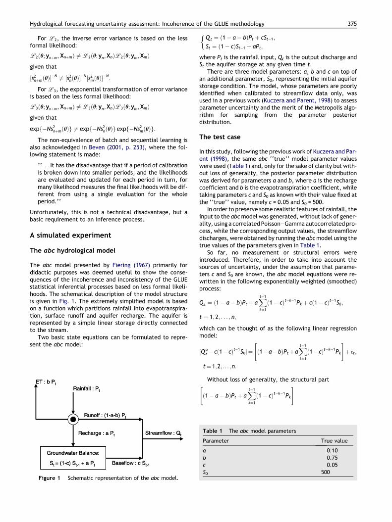
The abc model presented by Fiering (1967) primarily fordidactic purposes was deemed useful to show the conse-quences of the incoherence and inconsistency of the GLUEstatistical inferential processes based on less formal likeli-hoods. The schematical description of the model structureis given in Fig. 1. The extremely simplified model is basedon a function which partitions rainfall into evapotranspira-tion, surface runoff and aquifer recharge. The aquifer isrepresented by a simple linear storage directly connectedto the stream.

Two basic state equations can be formulated to repre-sent the abc model:

ET : b Pt

Rainfall : Pt

Runoff : (1-a-b) Pt

Recharge : a Pt Streamflow : Qt

Baseflow : c St-1

Groundwater Balance:

St = (1-c) St-1 + a Pt

ET : b PtRainfall : Pt

Runoff : (1-a-b) Pt

Recharge : a Pt Streamflow : Qt

Baseflow : c St-1

Groundwater Balance:

St = (1-c) St-1 + a Pt

Figure 1 Schematic representation of the abc model.

Qt ¼ ð1� a� bÞPt þ cSt�1;

St ¼ ð1� cÞSt�1 þ aPt;

�

where Pt is the rainfall input, Qt is the output discharge andSt the aquifer storage at any given time t.

There are three model parameters: a, b and c on top ofan additional parameter, S0, representing the initial aquiferstorage condition. The model, whose parameters are poorlyidentified when calibrated to streamflow data only, wasused in a previous work (Kuczera and Parent, 1998) to assessparameter uncertainty and the merit of the Metropolis algo-rithm for sampling from the parameter posteriordistribution.

The test case

In this study, following the previous work of Kuczera and Par-ent (1998), the same abc ‘‘true’’ model parameter valueswere used (Table 1) and, only for the sake of clarity but with-out loss of generality, the posterior parameter distributionwas derived for parameters a and b, where a is the rechargecoefficient and b is the evapotranspiration coefficient, whiletaking parameters c and S0 as known with their value fixed atthe ‘‘true’’ value, namely c = 0.05 and S0 = 500.

In order to preserve some realistic features of rainfall, theinput to the abcmodel was generated, without lack of gener-ality, using a correlated Poisson–Gammaautocorrelated pro-cess, while the corresponding output values, the streamflowdischarges, were obtained by running the abcmodel using thetrue values of the parameters given in Table 1.

So far, no measurement or structural errors wereintroduced. Therefore, in order to take into account thesources of uncertainty, under the assumption that parame-ters c and S0 are known, the abc model equations were re-written in the following exponentially weighted (smoothed)process:

Qt ¼ ð1� a� bÞPt þ aXt�1k¼1ð1� cÞt�k�1Pk þ cð1� cÞt�1S0;

t ¼ 1; 2; . . . ; n;

which can be thought of as the following linear regressionmodel:

½Q ot � cð1� cÞt�1S0� ¼ ð1�a�bÞPtþa

Xt�1k¼1ð1� cÞt�k�1Pk

" #þ et;

t¼ 1;2; . . . ;n:

Without loss of generality, the structural part

ð1� a� bÞPt þ aXt�1k¼1ð1� cÞt�k�1Pk

" #

Table 1 The abc model parameters

Parameter True value

a 0.10b 0.75c 0.05S0 500

376 P. Mantovan, E. Todini

is combined with the measurement error et in additive way.In the following, et was generated according to an autocor-related AR(1) Gaussian error model:

et ¼ aet�1 þ gt; t ¼ 1; 2; . . . ;

with a = 0.8; e0 , Normal(0,d2), with d2 = 8; and gt , Nor-mal(0,r2), with r2 = 8 and E{gtgj} = 0, "t 5 j, "j P 1;E{gte0} = 0, " t P 1.

The generation of the additive noise allowed computa-tion of the ‘‘observed’’ streamflow discharges Q o

t ,t = 1,2, . . . ,n.

For the error et given by the above AR(1) model, as t di-verges, we just have:

VarðetÞ ¼ r2=ð1� a2Þ;Corrðet; etþkÞ ¼ ak; k ¼ 1; 2; . . .

The autocorrelated Gaussian error model is usuallyadopted when the r.v. yi, i = 1,2, . . . ,n, is observable in sub-sequent equispatial time instants.

This model has also been widely used in hydrologicalstudies (see, for instance, Romanowicz et al., 1994, 1996).

In terms of the choice of the parameters prior to distri-bution, following the GLUE procedure, a uniform prior prob-ability distribution on a discrete space for parameters (a,b)is taken. Bearing in mind the continuity of mass constraint,which requires that a + b 6 1, the following discrete spacefor parameters (a,b) was considered:

H ¼ fðai; bjÞ : ai ¼ i=m; i ¼ 1; 2; . . . ;m;

bj ¼ j=m; j ¼ 1; 2; . . . ; ðm� iÞ=mg; m ¼ 100:

The proper likelihood function, in this case, given theautocorrelated AR(1) Gaussian error model, is the following:

Lðai;bjÞ,exp � 1

2Qo

n�l ai;bj;Pn

� �� �0R�1 Qo

n�lðai;bj;PnÞ� �� �

ð2pÞn=2½detðRÞ�1=2;

where Qon ¼ ðQ

o1;Q

o2; . . . ;Q o

nÞ0; Pn = (P1,P2, . . . ,Pn)

0; l(ai,bj,Pn) = (l1(ai,bj,P1),l2(ai,bj,P2), . . . ,ln(ai,bj,Pn)) 0; ltðai; bj;PtÞ ¼ ½ð1� a� bÞPt þ a

Pt�1k¼1ð1� cÞt�k�1Pk� þcð1� cÞt�1S0;

i = 1,100; j = 1,100; R = [r2/(1 � a2)]R(a), 0 < jaj < 1,r2 > 0; where R(a) is the so-called first order Markov matrix(see Basilevsky, 1983, p. 221):

RðaÞ ¼

1 a a2 . . . an�2 an�1

a 1 a . . . an�3 an�2

a2 a 1 . . . an�4 an�3

. . . . . . . . . . . . . . . . . .

an�2 an�3 an�4 . . . 1 a

an�1 an�2 an�3 . . . a 1

2666666664

3777777775:

The inverse matrix of R is a symmetric Jacobian matrixwhich can readily be computed (see Basilevsky, 1983, p.222).

The posterior probability function is then updated as thesample size increases both using the exact likelihood givenand with the less formal likelihoods proposed in GLUE.

Therefore, the sample size will be equal to n(i) = 50 Æ i,where i is the number of sample periods taken into accountto determine the posterior probability function,i = 1,2, . . . ,10.

The sample size on which the experiment was carried outis therefore equal to n(i) = 50 Æ i, where i = 1,2, . . . ,10 is thenumber of sample extensions successively taken into ac-count to determine the posterior probability function.

Results of the experiment

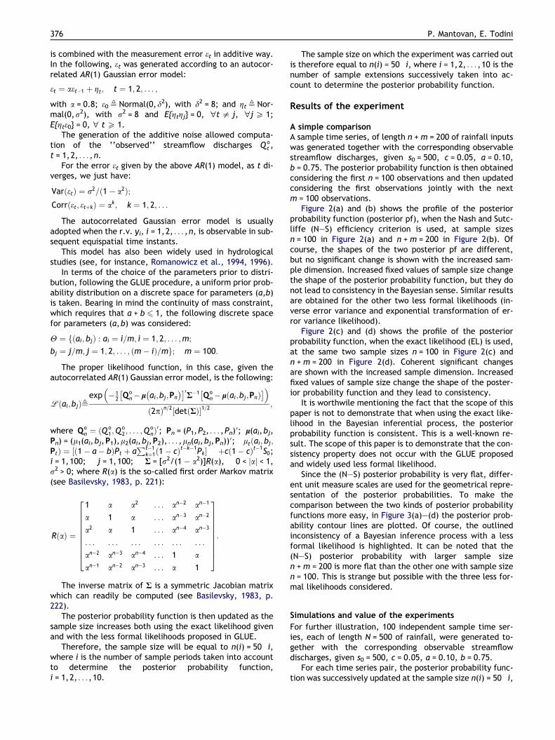
A simple comparisonA sample time series, of length n + m = 200 of rainfall inputswas generated together with the corresponding observablestreamflow discharges, given s0 = 500, c = 0.05, a = 0.10,b = 0.75. The posterior probability function is then obtainedconsidering the first n = 100 observations and then updatedconsidering the first observations jointly with the nextm = 100 observations.

Figure 2(a) and (b) shows the profile of the posteriorprobability function (posterior pf), when the Nash and Sutc-liffe (N–S) efficiency criterion is used, at sample sizesn = 100 in Figure 2(a) and n + m = 200 in Figure 2(b). Ofcourse, the shapes of the two posterior pf are different,but no significant change is shown with the increased sam-ple dimension. Increased fixed values of sample size changethe shape of the posterior probability function, but they donot lead to consistency in the Bayesian sense. Similar resultsare obtained for the other two less formal likelihoods (in-verse error variance and exponential transformation of er-ror variance likelihood).

Figure 2(c) and (d) shows the profile of the posteriorprobability function, when the exact likelihood (EL) is used,at the same two sample sizes n = 100 in Figure 2(c) andn + m = 200 in Figure 2(d). Coherent significant changesare shown with the increased sample dimension. Increasedfixed values of sample size change the shape of the poster-ior probability function and they lead to consistency.

It is worthwile mentioning the fact that the scope of thispaper is not to demonstrate that when using the exact like-lihood in the Bayesian inferential process, the posteriorprobability function is consistent. This is a well-known re-sult. The scope of this paper is to demonstrate that the con-sistency property does not occur with the GLUE proposedand widely used less formal likelihood.

Since the (N–S) posterior probability is very flat, differ-ent unit measure scales are used for the geometrical repre-sentation of the posterior probabilities. To make thecomparison between the two kinds of posterior probabilityfunctions more easy, in Figure 3(a)–(d) the posterior prob-ability contour lines are plotted. Of course, the outlinedinconsistency of a Bayesian inference process with a lessformal likelihood is highlighted. It can be noted that the(N–S) posterior probability with larger sample sizen + m = 200 is more flat than the other one with sample sizen = 100. This is strange but possible with the three less for-mal likelihoods considered.

Simulations and value of the experiments

For further illustration, 100 independent sample time ser-ies, each of length N = 500 of rainfall, were generated to-gether with the corresponding observable streamflowdischarges, given s0 = 500, c = 0.05, a = 0.10, b = 0.75.

For each time series pair, the posterior probability func-tion was successively updated at the sample size n(i) = 50 Æ i,

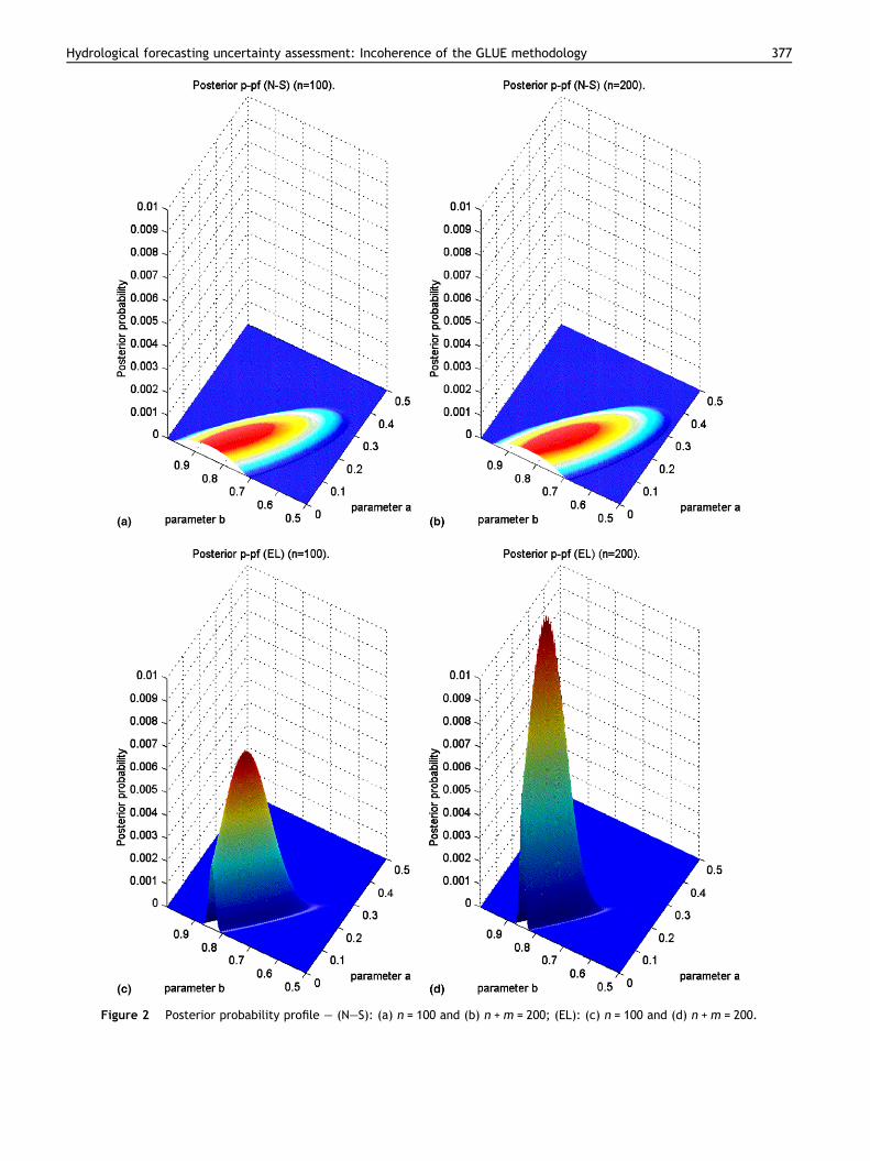
Figure 2 Posterior probability profile – (N–S): (a) n = 100 and (b) n +m = 200; (EL): (c) n = 100 and (d) n +m = 200.

Hydrological forecasting uncertainty assessment: Incoherence of the GLUE methodology 377

0 0.5 10

0.2

0.4

0.6

0.8

1

R-parameter a

ET

-par

amet

er b

0 0.5 10

0.2

0.4

0.6

0.8

1

R-parameter a

ET

-par

amet

er b

0 0.5 10

0.2

0.4

0.6

0.8

1

R-parameter a

ET

-par

amet

er b

0 0.5 10

0.2

0.4

0.6

0.8

1

R-parameter a

ET

-par

amet

er b

(a) (b)

(d)(c)

Posterior pf contour -(N-S) (n=100).

Posterior pf contour -(EL) (n=100).

Posterior pf contour -(N-S) (n=200).

Posterior pf contour -(EL) (n=200).

Figure 3 Posterior pf contour – (N–S): (a) n = 100 and (b) n +m = 200; (EL): (c) n = 100 and (d) n +m = 200.

378 P. Mantovan, E. Todini

where i = 1,2, . . .,10 is the number of sample extensionssuccessively taken into account to determine the posteriorprobability function.

The inconsistency of a Bayesian inference process with aless formal likelihood can still be shown by the discrepancyfunction as a specified measure of the value of theexperiment.

At every update step i, given the posterior probabilityfunction p(hjyn(i),Xn(i)), the Euclidean distance betweenthe posterior probability function p(hjyn(i),Xn(i)) and theprior one p0(h):

dðnðiÞÞ ¼Xh2HðpðhjynðiÞ;XnðiÞÞ � p0ðhÞÞ

2

" #1=2;

was computed, i = 1,2, . . . ,10. Then the 5th, 50th and 95thpercentiles of the distance d(n(i)) were determined on thebasis of the 100 independent sample time series generated,at the step of updating i = 1,2, . . . ,10.

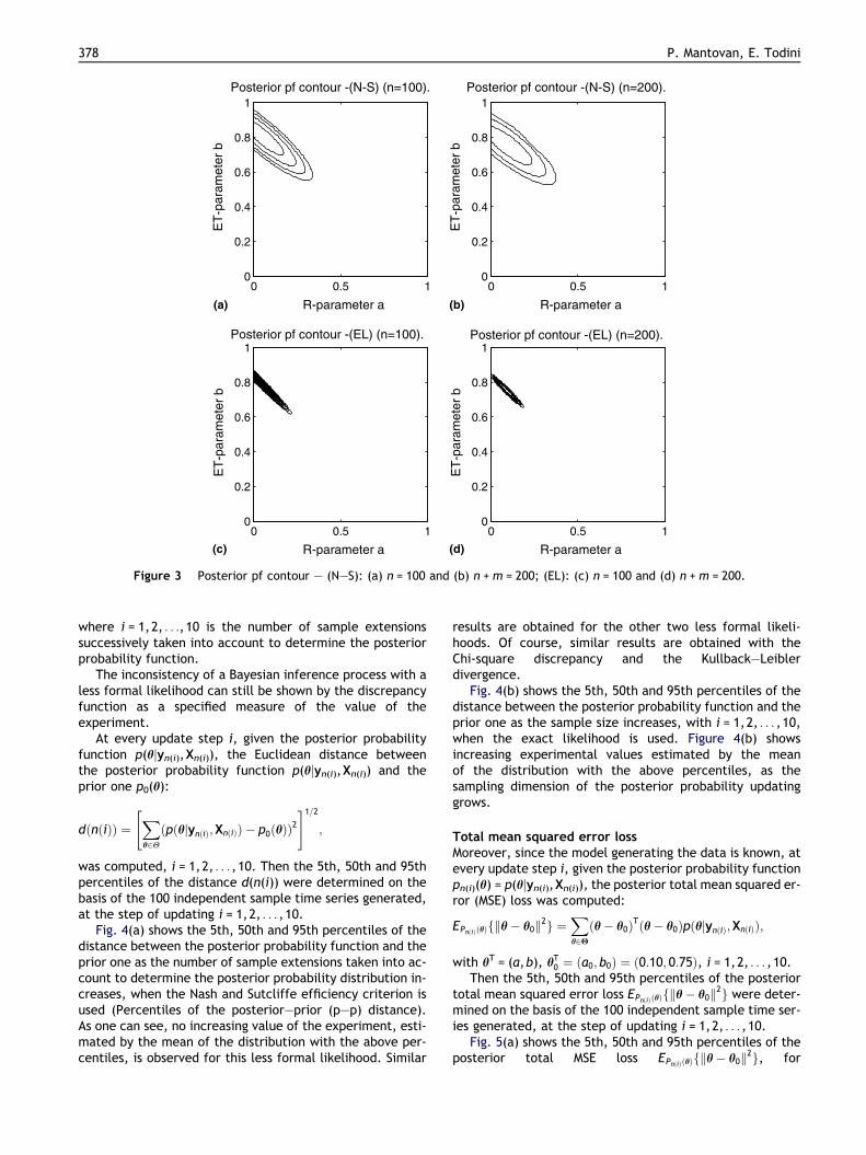
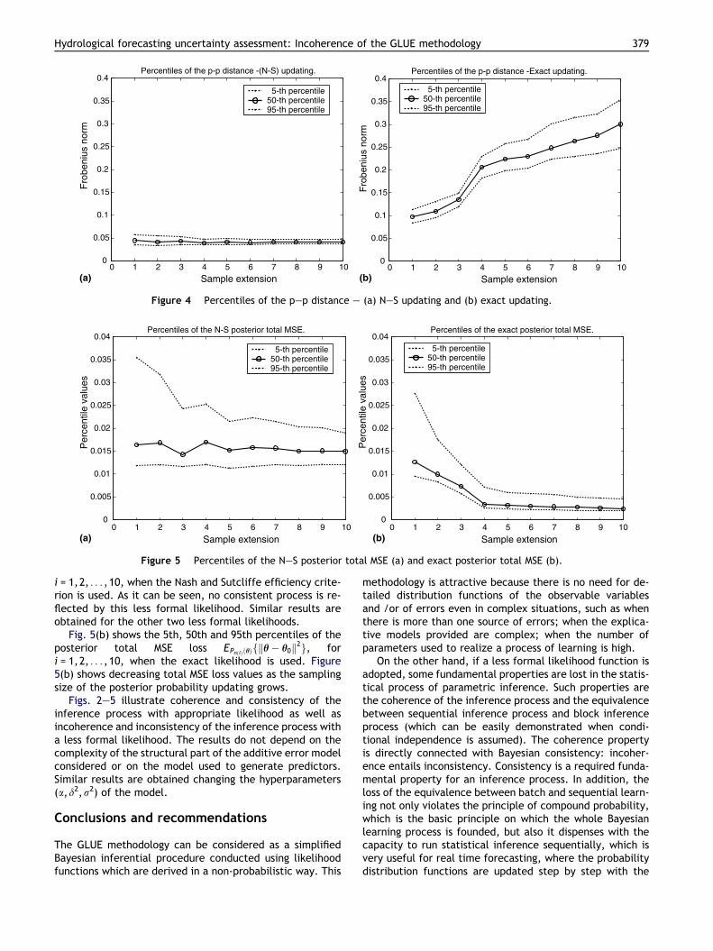
Fig. 4(a) shows the 5th, 50th and 95th percentiles of thedistance between the posterior probability function and theprior one as the number of sample extensions taken into ac-count to determine the posterior probability distribution in-creases, when the Nash and Sutcliffe efficiency criterion isused (Percentiles of the posterior–prior (p–p) distance).As one can see, no increasing value of the experiment, esti-mated by the mean of the distribution with the above per-centiles, is observed for this less formal likelihood. Similar

results are obtained for the other two less formal likeli-hoods. Of course, similar results are obtained with theChi-square discrepancy and the Kullback–Leiblerdivergence.

Fig. 4(b) shows the 5th, 50th and 95th percentiles of thedistance between the posterior probability function and theprior one as the sample size increases, with i = 1,2, . . . ,10,when the exact likelihood is used. Figure 4(b) showsincreasing experimental values estimated by the meanof the distribution with the above percentiles, as thesampling dimension of the posterior probability updatinggrows.

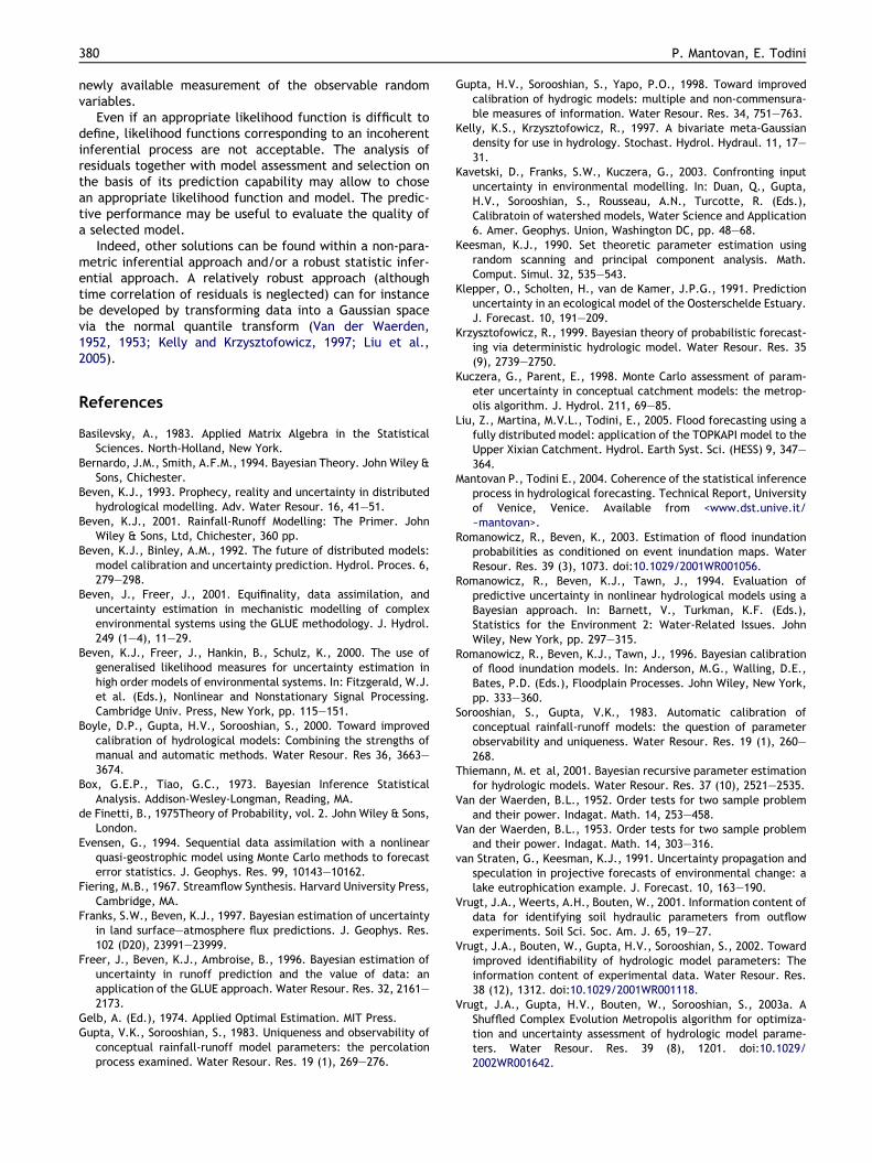
Total mean squared error lossMoreover, since the model generating the data is known, atevery update step i, given the posterior probability functionpn(i)(h) = p(hjyn(i),Xn(i)), the posterior total mean squared er-ror (MSE) loss was computed:

EPnðiÞðhÞfkh� h0k2g ¼Xh2Hðh� h0ÞTðh� h0ÞpðhjynðiÞ;XnðiÞÞ;

with hT = (a,b), hT0 ¼ ða0; b0Þ ¼ ð0:10; 0:75Þ, i = 1,2, . . . ,10.

Then the 5th, 50th and 95th percentiles of the posteriortotal mean squared error loss EPnðiÞðhÞfkh� h0k2g were deter-mined on the basis of the 100 independent sample time ser-ies generated, at the step of updating i = 1,2, . . . ,10.

Fig. 5(a) shows the 5th, 50th and 95th percentiles of theposterior total MSE loss EPnðiÞðhÞfkh� h0k2g, for

0 1 2 3 4 5 6 7 8 9 100

0.05

0.1

0.15

0.2

0.25

0.3

0.35

0.4 Percentiles of the p-p distance -(N-S) updating.

Sample extension

Fro

beni

us n

orm

5-th percentile50-th percentile95-th percentile

0 1 2 3 4 5 6 7 8 9 100

0.05

0.1

0.15

0.2

0.25

0.3

0.35

0.4 Percentiles of the p-p distance -Exact updating.

Sample extension

Fro

beni

us n

orm

5-th percentile50-th percentile95-th percentile

(a) (b)

Figure 4 Percentiles of the p–p distance – (a) N–S updating and (b) exact updating.

0 1 2 3 4 5 6 7 8 9 100

0.005

0.01

0.015

0.02

0.025

0.03

0.035

0.04 Percentiles of the N-S posterior total MSE.

Sample extension

Per

cent

ile v

alue

s

5-th percentile50-th percentile95-th percentile

0 1 2 3 4 5 6 7 8 9 100

0.005

0.01

0.015

0.02

0.025

0.03

0.035

0.04 Percentiles of the exact posterior total MSE.

Sample extension

Per

cent

ile v

alue

s 5-th percentile50-th percentile95-th percentile

(a) (b)

Figure 5 Percentiles of the N–S posterior total MSE (a) and exact posterior total MSE (b).

Hydrological forecasting uncertainty assessment: Incoherence of the GLUE methodology 379

i = 1,2, . . . ,10, when the Nash and Sutcliffe efficiency crite-rion is used. As it can be seen, no consistent process is re-flected by this less formal likelihood. Similar results areobtained for the other two less formal likelihoods.

Fig. 5(b) shows the 5th, 50th and 95th percentiles of theposterior total MSE loss EPnðiÞðhÞfkh� h0k2g, fori = 1,2, . . . ,10, when the exact likelihood is used. Figure5(b) shows decreasing total MSE loss values as the samplingsize of the posterior probability updating grows.

Figs. 2–5 illustrate coherence and consistency of theinference process with appropriate likelihood as well asincoherence and inconsistency of the inference process witha less formal likelihood. The results do not depend on thecomplexity of the structural part of the additive error modelconsidered or on the model used to generate predictors.Similar results are obtained changing the hyperparameters(a,d2,r2) of the model.

Conclusions and recommendations

The GLUE methodology can be considered as a simplifiedBayesian inferential procedure conducted using likelihoodfunctions which are derived in a non-probabilistic way. This

methodology is attractive because there is no need for de-tailed distribution functions of the observable variablesand /or of errors even in complex situations, such as whenthere is more than one source of errors; when the explica-tive models provided are complex; when the number ofparameters used to realize a process of learning is high.

On the other hand, if a less formal likelihood function isadopted, some fundamental properties are lost in the statis-tical process of parametric inference. Such properties arethe coherence of the inference process and the equivalencebetween sequential inference process and block inferenceprocess (which can be easily demonstrated when condi-tional independence is assumed). The coherence propertyis directly connected with Bayesian consistency: incoher-ence entails inconsistency. Consistency is a required funda-mental property for an inference process. In addition, theloss of the equivalence between batch and sequential learn-ing not only violates the principle of compound probability,which is the basic principle on which the whole Bayesianlearning process is founded, but also it dispenses with thecapacity to run statistical inference sequentially, which isvery useful for real time forecasting, where the probabilitydistribution functions are updated step by step with the

380 P. Mantovan, E. Todini

newly available measurement of the observable randomvariables.

Even if an appropriate likelihood function is difficult todefine, likelihood functions corresponding to an incoherentinferential process are not acceptable. The analysis ofresiduals together with model assessment and selection onthe basis of its prediction capability may allow to chosean appropriate likelihood function and model. The predic-tive performance may be useful to evaluate the quality ofa selected model.

Indeed, other solutions can be found within a non-para-metric inferential approach and/or a robust statistic infer-ential approach. A relatively robust approach (althoughtime correlation of residuals is neglected) can for instancebe developed by transforming data into a Gaussian spacevia the normal quantile transform (Van der Waerden,1952, 1953; Kelly and Krzysztofowicz, 1997; Liu et al.,2005).

References

Basilevsky, A., 1983. Applied Matrix Algebra in the StatisticalSciences. North-Holland, New York.

Bernardo, J.M., Smith, A.F.M., 1994. Bayesian Theory. John Wiley &Sons, Chichester.

Beven, K.J., 1993. Prophecy, reality and uncertainty in distributedhydrological modelling. Adv. Water Resour. 16, 41–51.

Beven, K.J., 2001. Rainfall-Runoff Modelling: The Primer. JohnWiley & Sons, Ltd, Chichester, 360 pp.

Beven, K.J., Binley, A.M., 1992. The future of distributed models:model calibration and uncertainty prediction. Hydrol. Proces. 6,279–298.

Beven, J., Freer, J., 2001. Equifinality, data assimilation, anduncertainty estimation in mechanistic modelling of complexenvironmental systems using the GLUE methodology. J. Hydrol.249 (1–4), 11–29.

Beven, K.J., Freer, J., Hankin, B., Schulz, K., 2000. The use ofgeneralised likelihood measures for uncertainty estimation inhigh order models of environmental systems. In: Fitzgerald, W.J.et al. (Eds.), Nonlinear and Nonstationary Signal Processing.Cambridge Univ. Press, New York, pp. 115–151.

Boyle, D.P., Gupta, H.V., Sorooshian, S., 2000. Toward improvedcalibration of hydrological models: Combining the strengths ofmanual and automatic methods. Water Resour. Res 36, 3663–3674.

Box, G.E.P., Tiao, G.C., 1973. Bayesian Inference StatisticalAnalysis. Addison-Wesley-Longman, Reading, MA.

de Finetti, B., 1975Theory of Probability, vol. 2. John Wiley & Sons,London.

Evensen, G., 1994. Sequential data assimilation with a nonlinearquasi-geostrophic model using Monte Carlo methods to forecasterror statistics. J. Geophys. Res. 99, 10143–10162.

Fiering, M.B., 1967. Streamflow Synthesis. Harvard University Press,Cambridge, MA.

Franks, S.W., Beven, K.J., 1997. Bayesian estimation of uncertaintyin land surface–atmosphere flux predictions. J. Geophys. Res.102 (D20), 23991–23999.

Freer, J., Beven, K.J., Ambroise, B., 1996. Bayesian estimation ofuncertainty in runoff prediction and the value of data: anapplication of the GLUE approach. Water Resour. Res. 32, 2161–2173.

Gelb, A. (Ed.), 1974. Applied Optimal Estimation. MIT Press.Gupta, V.K., Sorooshian, S., 1983. Uniqueness and observability of

conceptual rainfall-runoff model parameters: the percolationprocess examined. Water Resour. Res. 19 (1), 269–276.

Gupta, H.V., Sorooshian, S., Yapo, P.O., 1998. Toward improvedcalibration of hydrogic models: multiple and non-commensura-ble measures of information. Water Resour. Res. 34, 751–763.

Kelly, K.S., Krzysztofowicz, R., 1997. A bivariate meta-Gaussiandensity for use in hydrology. Stochast. Hydrol. Hydraul. 11, 17–31.

Kavetski, D., Franks, S.W., Kuczera, G., 2003. Confronting inputuncertainty in environmental modelling. In: Duan, Q., Gupta,H.V., Sorooshian, S., Rousseau, A.N., Turcotte, R. (Eds.),Calibratoin of watershed models, Water Science and Application6. Amer. Geophys. Union, Washington DC, pp. 48–68.

Keesman, K.J., 1990. Set theoretic parameter estimation usingrandom scanning and principal component analysis. Math.Comput. Simul. 32, 535–543.

Klepper, O., Scholten, H., van de Kamer, J.P.G., 1991. Predictionuncertainty in an ecological model of the Oosterschelde Estuary.J. Forecast. 10, 191–209.

Krzysztofowicz, R., 1999. Bayesian theory of probabilistic forecast-ing via deterministic hydrologic model. Water Resour. Res. 35(9), 2739–2750.

Kuczera, G., Parent, E., 1998. Monte Carlo assessment of param-eter uncertainty in conceptual catchment models: the metrop-olis algorithm. J. Hydrol. 211, 69–85.

Liu, Z., Martina, M.V.L., Todini, E., 2005. Flood forecasting using afully distributed model: application of the TOPKAPI model to theUpper Xixian Catchment. Hydrol. Earth Syst. Sci. (HESS) 9, 347–364.

Mantovan P., Todini E., 2004. Coherence of the statistical inferenceprocess in hydrological forecasting. Technical Report, Universityof Venice, Venice. Available from <www.dst.unive.it/~mantovan>.

Romanowicz, R., Beven, K., 2003. Estimation of flood inundationprobabilities as conditioned on event inundation maps. WaterResour. Res. 39 (3), 1073. doi:10.1029/2001WR001056.

Romanowicz, R., Beven, K.J., Tawn, J., 1994. Evaluation ofpredictive uncertainty in nonlinear hydrological models using aBayesian approach. In: Barnett, V., Turkman, K.F. (Eds.),Statistics for the Environment 2: Water-Related Issues. JohnWiley, New York, pp. 297–315.

Romanowicz, R., Beven, K.J., Tawn, J., 1996. Bayesian calibrationof flood inundation models. In: Anderson, M.G., Walling, D.E.,Bates, P.D. (Eds.), Floodplain Processes. John Wiley, New York,pp. 333–360.

Sorooshian, S., Gupta, V.K., 1983. Automatic calibration ofconceptual rainfall-runoff models: the question of parameterobservability and uniqueness. Water Resour. Res. 19 (1), 260–268.

Thiemann, M. et al, 2001. Bayesian recursive parameter estimationfor hydrologic models. Water Resour. Res. 37 (10), 2521–2535.

Van der Waerden, B.L., 1952. Order tests for two sample problemand their power. Indagat. Math. 14, 253–458.

Van der Waerden, B.L., 1953. Order tests for two sample problemand their power. Indagat. Math. 14, 303–316.

van Straten, G., Keesman, K.J., 1991. Uncertainty propagation andspeculation in projective forecasts of environmental change: alake eutrophication example. J. Forecast. 10, 163–190.

Vrugt, J.A., Weerts, A.H., Bouten, W., 2001. Information content ofdata for identifying soil hydraulic parameters from outflowexperiments. Soil Sci. Soc. Am. J. 65, 19–27.

Vrugt, J.A., Bouten, W., Gupta, H.V., Sorooshian, S., 2002. Towardimproved identifiability of hydrologic model parameters: Theinformation content of experimental data. Water Resour. Res.38 (12), 1312. doi:10.1029/2001WR001118.

Vrugt, J.A., Gupta, H.V., Bouten, W., Sorooshian, S., 2003a. AShuffled Complex Evolution Metropolis algorithm for optimiza-tion and uncertainty assessment of hydrologic model parame-ters. Water Resour. Res. 39 (8), 1201. doi:10.1029/2002WR001642.

Hydrological forecasting uncertainty assessment: Incoherence of the GLUE methodology 381

Vrugt, J.A., Gupta, H.V., Bastidas, L.A., Bouten, W., Sorooshian, S.,2003b. Effective and efficient algorithm for multi-objectiveoptimization of hydrologic models. Water Resour. Res. 39 (8),1214. doi:10.1029/2002WR001746.

Vrugt, J.A., Diks, C.G.H., Gupta, H.V., Bouten, W., Verstraten,J.M., 2005. Improved treatment of uncertainty in hydrologicmodeling: Combining the strengths of global optimization anddata assimilation. Water Resour. Res. 41, W01017. doi:10.1029/2004WR003059.

Vrugt, J.A., 2004. Towards improved treatment of parameteruncertainty in hydrologic modeling. Ph.D. Thesis of University ofAmsterdam, the Netherlands, ISBN:90-76894-46-9.

Wagener, T., McIntyire, N., Lees, M.J., Wheather, H.S., Gupta,H.V., 2003. Towards reduced uncertainty in conceptual rainfall-runoff modelling: Dynamic identifiability analysis. Hydrol. Proc.17, 455–476.

Yapo, P.O., Gupta, H.V., Soroosian, S., 1998. Multi-objective globaloptimization for hydrologic models. J. Hydrol. 204, 83–97.

Young, P.C., 2001. Data-based mechanistic modeling and validationof rainfall-flow processes. In: Anderson, M.G., Bates, P.G.(Eds.), Model Validation. John Wiley & Sons Ltd, Chichester,UK, pp. 117–161.

Zak, S.K. et al, 1997.Uncertainty in theestimationof critical loads: apractical methodology. Soil Water Air Pollut. 98, 297–316.