
volume ii paper iii hydrological monitoring final report
107
VOLUME II PAPER III HYDROLOGICAL MONITORING FINAL REPORT MARCH 2004 WUP-JICA TEAM
-
Upload
khangminh22 -
Category
Documents
-
view
0 -
download
0
Transcript of volume ii paper iii hydrological monitoring final report
VOLUME II
PAPER III
HYDROLOGICAL MONITORING
FINAL REPORT
MARCH 2004
WUP-JICA TEAM
Volume II: Supporting Report, Paper III: Hydrological MonitoringWUP-JICA, March 2004
TABLE OF CONTENTS
1. BACKGROUND .............................................................................................. III-1
2. ISSUES, APPROACHES AND GOALS........................................................ III-4
2.1 Issues ....................................................................................................... III-4
2.2 Related Projects and Possible Cooperative Activities ............................. III-5
2.3 Goals and Approaches ............................................................................. III-6
3. OBEJECTIVES AND AVITIVITIES............................................................ III-9
3.1 Objectives ................................................................................................ III-9
3.2 Activities.................................................................................................. III-9
4. DEVELOPMENT OF RATING CURVES ................................................... III-13
4.1 Previous Efforts for Development of Rating Curves............................... III-13
4.2 Results of Measurement .......................................................................... III-13
4.3 Determination of Rating Ranges ............................................................. III-15
4.4 Development of Discharge Rating Curves .............................................. III-17
5. FLOW MONITORING SYSTEM IN CAMBODIA .................................... III-21
5.1 Wet-season Flow Monitoring System ..................................................... III-21
5.2 Dry-season Flow Monitoring System...................................................... III-25
5.3 Recommendations for Future Monitoring System .................................. III-33
6. HYDROLOGICAL FUNCTIONS OF CAMBODIAN FLOODPLAINS .. III-34
6.1 Previous Study Results ............................................................................ III-34
6.2 Flow Balance along the Mekong Watercourses ...................................... III-37
6.3 Hydrological Functions of Cambodian Floodplains................................ III-42
REFERENCES ............................................................................................................. III-48
ANNEX I MEASUREMENT RESULTS.............................................................. AI-1
ANNEX II INDOOR TRAINNING ON FLOW DATA MANAGEMENT......... AII-1
III - i

Volume II: Supporting Report, Paper III: Hydrological MonitoringWUP-JICA, March 2004
LIST OF TABLES
Table 3.1 Major Hydrological Stations in Cambodia............................................ III-10 Table 4.1 Previous Discharge Records in/around Phnom Penh Area ................... III-13 Table 4.2 Rating Ranges and Inapplicable Durations of Rating Curves ............... III-17 Table 4.3 Representative Stations for Water Level Falls ...................................... III-18 Table 5.1 Wet-Season Monitoring Periods in Cambodia...................................... III-21 Table 5.2 Effects of Tidal Fluctuation to the Dry-Season Flow............................ III-25 Table 6.1 Flooding Functions between Kratie and Kompong Cham .................... III-38 Table 6.2 Estimated Flood Volume and Great Lake Storage................................ III-46
III - ii
Volume II: Supporting Report, Paper III: Hydrological MonitoringWUP-JICA, March 2004
LIST OF FIGURES
Fig. 1.1 Temporal Changes of Hydrological Monitoring................................... III-2 Fig. 2.1 Hydrological Monitoring Strategy in Cambodia................................... III-8 Fig. 3.1 Major Hydrological Stations in Cambodia ........................................... III-10 Fig. 3.2 Flow Situations and Selected Hydrological Stations/Sections.............. III-11 Fig. 3.3 Discharge Measurement Activities at Kompong Cham........................ III-11 Fig. 4.1 Measured Discharge Data versus Water Level ..................................... III-14 Fig. 4.2 Tidal Effects in the Dry Season at Selected Stations ............................ III-15 Fig. 4.3 Measured Discharge in the Dry Season in Phnom Penh Area .............. III-16 Fig. 4.4 Measured Discharge in the Dry Season versus Daily Water Level ...... III-16 Fig. 4.5 Measured Discharge in the Dry Season at Neak Luong........................ III-17 Fig. 4.6(1/2) Developed Discharge Rating Curves: Mekong Mainstream................. III-19 Fig. 4.6(2/2) Developed Discharge Rating Curves: Mekong Mainstream
and Bassac............................................................................................. III-20 Fig. 5.1(1/2) Computed Flow Hydrographs and Comparison between Estimated
and Observed Discharges at Phnom Penh Port: 2002 Wet Season ....... III-23 Fig. 5.1(2/2) Computed Flow Hydrographs and Comparison between Estimated
and Observed Discharges at Phnom Penh Port: Year 2003 .................. III-24 Fig. 5.2 Conseptual Dry-season Flow Monitoring System in/around
Phnom Penh Port................................................................................... III-26 Fig. 5.3 Flow Hydrograph of Kratie and Kompong Cham in the
2003 Dry Season ................................................................................... III-27 Fig. 5.4 Comparison of Flow Discharges of Kratie and Kompong Cham
in the 2003 Dry Season ......................................................................... III-27 Fig. 5.5 Hydraulic Model Calibration Results at Phnom Penh Port
for the 2003 Dry Season........................................................................ III-28 Fig. 5.6 Relation of Dry-Season Flows between Kompong Cham
and Chrui Chanvar (Phnom Penh Mekong) .......................................... III-29 Fig. 5.7 Simulated Hourly and Daily Average Dry-Season Flows
at Phnon Penh Port................................................................................ III-30 Fig. 5.8 Relation between Daily Average Dry-season and Gauge Height
at Phnom Penh Port............................................................................... III-30 Fig. 5.9 Comparison of Daily Average Dry-season Flows Computed by
the Hydraulic Model and Estimated by the Rating Curve at Phnom Penh Port............................................................................... III-30
Fig. 5.10 Estimated Diversion Rate to the Mekong Downstream at the Chak Tomuk Junction ................................................................. III-31
Fig. 5.11 Estimated Dry-season Flow in Phnom Penh Area ................................ III-32 Fig. 5.12 Future Dry-season Flow Monitoring System
in Phnom Penh Area ............................................................................. III-33 Fig. 6.1 Floodwater Balance Measured during the 1964 Flood ......................... III-35 Fig. 6.2 Annual Flood Hydrograph in 1964 ....................................................... III-35 Fig. 6.3 Flood Hydrograph in Cambodian Floodplains in the
2002 Wet Season................................................................................... III-37
III - iii
Volume II: Supporting Report, Paper III: Hydrological MonitoringWUP-JICA, March 2004
Fig. 6.4 Observed Water Level at Moat Khmung Bridge in 2002...................... III-38 Fig. 6.5 Flood Hydrograph Passing through the Moat Khmung Bridge
in 2002................................................................................................... III-39 Fig. 6.6 Longitudial Flow Changes along the Mekong Mainstream .................. III-40 Fig. 6.7 Relationship between Flood Discharges of Kompong Cham
and Chrui Chanvar ................................................................................ III-40 Fig. 6.8 Longitudial Flow Changes along the Tonle Sap ................................... III-41 Fig. 6.9 Longitudial Flow Changes along the Bassac River............................... III-42 Fig. 6.10 Flooding Situation in the Cambodian Floodplains................................ III-43 Fig. 6.11 Flood Balance between Kompong Cham and Phnom Penh
in the 2002 Wet Season......................................................................... III-44 Fig. 6.12 Flood Hydrographs at Konpong Cham in Recent Years
and Threshold Discharge of 25,000m3/s............................................... III-46 Fig. 6.13 Relation between Kg. Cham Flood Volume
and Great Lake Storage ......................................................................... III-47
III - iv
Volume II: Supporting Report, Paper III: Hydrological MonitoringWUP-JICA, March 2004
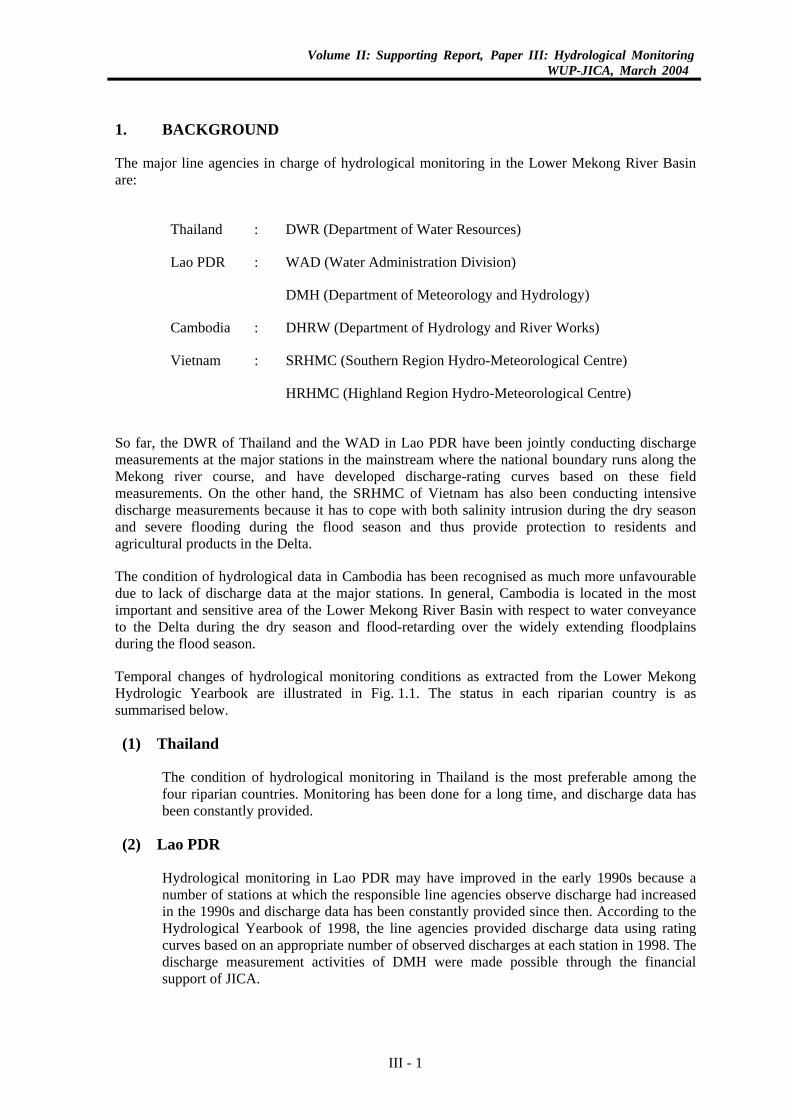
1. BACKGROUND
The major line agencies in charge of hydrological monitoring in the Lower Mekong River Basin are:
Thailand : DWR (Department of Water Resources)
Lao PDR : WAD (Water Administration Division)
DMH (Department of Meteorology and Hydrology)
Cambodia : DHRW (Department of Hydrology and River Works)
Vietnam : SRHMC (Southern Region Hydro-Meteorological Centre)
HRHMC (Highland Region Hydro-Meteorological Centre)
So far, the DWR of Thailand and the WAD in Lao PDR have been jointly conducting discharge measurements at the major stations in the mainstream where the national boundary runs along the Mekong river course, and have developed discharge-rating curves based on these field measurements. On the other hand, the SRHMC of Vietnam has also been conducting intensive discharge measurements because it has to cope with both salinity intrusion during the dry season and severe flooding during the flood season and thus provide protection to residents and agricultural products in the Delta.
The condition of hydrological data in Cambodia has been recognised as much more unfavourable due to lack of discharge data at the major stations. In general, Cambodia is located in the most important and sensitive area of the Lower Mekong River Basin with respect to water conveyance to the Delta during the dry season and flood-retarding over the widely extending floodplains during the flood season.
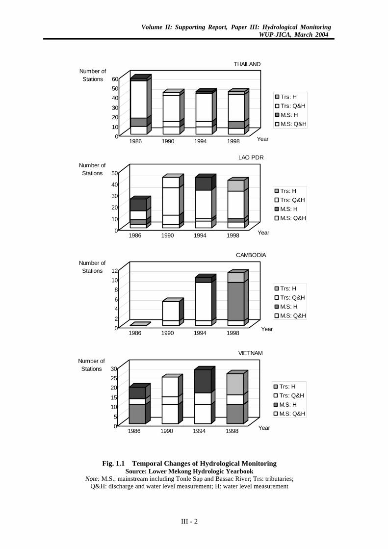
Temporal changes of hydrological monitoring conditions as extracted from the Lower Mekong Hydrologic Yearbook are illustrated in Fig. 1.1. The status in each riparian country is as summarised below.
(1) Thailand
The condition of hydrological monitoring in Thailand is the most preferable among the four riparian countries. Monitoring has been done for a long time, and discharge data has been constantly provided.
(2) Lao PDR
Hydrological monitoring in Lao PDR may have improved in the early 1990s because a number of stations at which the responsible line agencies observe discharge had increased in the 1990s and discharge data has been constantly provided since then. According to the Hydrological Yearbook of 1998, the line agencies provided discharge data using rating curves based on an appropriate number of observed discharges at each station in 1998. The discharge measurement activities of DMH were made possible through the financial support of JICA.
III - 1
Volume II: Supporting Report, Paper III: Hydrological MonitoringWUP-JICA, March 2004
010
2030
405060
Number ofStations
1986 1990 1994 1998 Year
THAILAND
Trs: HTrs: Q&HM.S: HM.S: Q&H
0
10
20
30
40
50Number ofStations
1986 1990 1994 1998 Year
LAO PDR
Trs: HTrs: Q&HM.S: HM.S: Q&H
02
46
81012
Number ofStations
1986 1990 1994 1998Year
CAMBODIA
Trs: HTrs: Q&HM.S: HM.S: Q&H
05
1015
202530
Number ofStations
1986 1990 1994 1998 Year
VIETNAM
Trs: HTrs: Q&HM.S: HM.S: Q&H
Fig. 1.1 Temporal Changes of Hydrological Monitoring
Source: Lower Mekong Hydrologic Yearbook Note: M.S.: mainstream including Tonle Sap and Bassac River; Trs: tributaries;
Q&H: discharge and water level measurement; H: water level measurement
III - 2
Volume II: Supporting Report, Paper III: Hydrological MonitoringWUP-JICA, March 2004
(3) Cambodia
After cessation of the political disturbance in Cambodia, the line agency commenced to reconstruct the completely damaged hydrological network. The number of hydrological stations had increased in the 1990s due to the technical and financial support of MRCS and other donors. However, the coverage area of stations is still insufficient, and discharge measurement activities have not been made enough to develop the rating curves of the major stations.
(4) Vietnam
The line agencies have been conducting intensive hydrological monitoring, including hourly discharge measurements of the mainstream, to cope with the salinity intrusion in the dry season. As for the severe flooding, the agencies have been monitoring the flooding situation over the Mekong Delta during the flood season.
In addition to the above, the riparian line agencies have pointed out issues that need to be addressed for sustainable monitoring, as summarised below.
(1) Thailand
The line agencies intend to upgrade the present monitoring system; for instance, from manual reading of staff gauges to automatic recorders. However, the agencies have been under budgetary constraint since the economic crisis in 1997.
(2) Lao PDR
The line agencies require training of their personnel such as hydrologists and observers, as well as financial support for equipment such as vehicles and boats for field operations. In addition, they are requesting technology transfer, in particular, on the use and operation of computer software and automatic recorders introduced by MRCS-related projects.
(3) Cambodia
The Cambodian line agency is confronted with the most serious issues. These are financial constraint due to shortage of government budget and lack of opportunity for human resources training. Thus, without the assistance of donors like the MRCS, the DHRW cannot continue with its monitoring activities and cannot also improve the capability of its staff on hydrological matters.
(4) Vietnam
The Mekong Delta in Vietnam is facing various problems such as water shortage and salinity intrusion in the dry season, severe and long-lasting flooding, and water acidity. To cope with these problems, the line agencies intend to upgrade the present monitoring system, including the upgrade of recording equipment, the establishment of integrated water quality monitoring network, the introduction of latest monitoring instruments, and the improvement of data transmission system utilising e-mail.
Taking into account the situations mentioned above and the limited capacity of the WUP-JICA Team to assist in the hydrological monitoring, the Team, therefore, decided to concentrate its resources on monitoring activities at the major stations within the Cambodian territory.
III - 3

Volume II: Supporting Report, Paper III: Hydrological MonitoringWUP-JICA, March 2004
2. ISSUES, APPROACHES AND GOALS
2.1 Issues
The issues to be addressed in the hydrological monitoring in Cambodia may be divided into three areas. These are:
(1) Physical Issues
The density of hydrological network in Cambodia is inadequate compared to the other riparian countries. Furthermore, the existing hydrological stations are decrepit, and the periodical renewal and repair of manual-reading gauges has not been completely made.
In the near future, various development projects such as irrigation improvement, hydropower generation, and bridge and road construction/improvement may be implemented to uplift the Cambodian economy and the people’s living standard. Hence, hydrological information/data will be needed for the proper design and evaluation of such development projects. It is, however, expected that these development projects may change the hydrological conditions of flooding as well as the low flow regimes, so that the abundant water-related resources including inland fishery, wetlands with rich biodiversity, and flood receding agriculture may be affected. To evaluate these effects, an appropriate hydrological observation network shall be established all over the country and, for this purpose, a master plan of hydrological network development, including classification and the phased development schemes of the network, should be established as early as possible.
Regarding hydrological data itself, the DHRW has been observing and providing water level data at its managing stations. The crucial issue, however, is the absolute lack of discharge data, because only the Stung Treng Station is continuously providing discharge data. Since Cambodia is situated in an important location of the Lower Mekong River Basin in geopolitical terms, it receives the excess water of the upper reaches in the wet season. Flooding starts at Kratie towards the lower reaches of the floodplains during floods. In the dry season, the water detained in the floodplains as well as the Tonle Sap Lake supplements the water for the Delta where the biggest water users on the mainstream live and utilize water. Thus, measuring and providing discharge data in the Cambodian territory is a crucial issue for the successful water management in the Lower Mekong River Basin.
(2) Institutional and Technical Issues
Technically, human resources development is indispensable for the sound operation and maintenance of the network. The issue related to this area may be subdivided into:
Shortage of skilled staff including observers
Lack of opportunity for practical training
Lack of budget to sustain the above activities
There is no institution in Cambodia that provides hydrologists and related technicians, as reported by the DHRW. Strengthening the institutions in water-related fields may unfortunately be beyond the scope of this Study. In spite of this situation, practical training could partially make up for the shortage of skill and experience. Thus, capacity building through practical training could be one of the solutions to these issues.
III - 4

Volume II: Supporting Report, Paper III: Hydrological MonitoringWUP-JICA, March 2004
The financial/budgetary issues are as discussed below.
(3) Financial Issues
The lack of budget for network operation and maintenance has been a critical issue to be addressed. For a short certain period, the project-basis support may be possible to sustain the monitoring activities. However, the problem would be the uncertainty on when the government can consolidate its budgetary self-support system for the sustainable monitoring. It might be a time-taking process in line with the economic growth of Cambodia.
For the time being, the related projects will have to supplement the shortage of budget through the project-basis support. The projects have to enhance the technical knowledge and skill of the DHRW staff through various kinds of training and workshop.
2.2 Related Projects and Possible Cooperative Activities
In a similar field of hydrological monitoring in Cambodia, two (2) projects have been implemented by the MRCS in parallel with this WUP-JICA Study (hereinafter called the WUP-JICA Project). The two projects, which are closely related to the WUP-JICA Project, are the “Appropriate Hydrological Network Improvement Project (AHNIP)” and “The Consolidation of Hydro-Meteorological Data and Multi-Functional Hydrologic Roles of Tonle Sap Lake and its Vicinities (TSLVP).”
(1) AHNIP
AHNIP began in April 2001 and will continue for five years. The project involves the line agencies concerned in hydro-meteorological monitoring. The project aims to collect real-time water level and discharge data and to handle, manage and share the data among the riparian countries and China with the improvement of 18 hydrological stations located mainly along the Lancang-Mekong mainstream. In Cambodia, the target telemetry stations under AHNIP are:
Stung Treng on the Mekong
Kratie on the Mekong
Kompong Luong in the Tonle Sap Lake
Prek Kdam on the Tonle Sap
The project emphasizes strengthening of the capacity of MRCS and the line agencies in dealing with real time data to implement the rules to be established for water sharing, environmental protection and damage mitigation. AHNIP had periodically held training and workshops as initially planned. The activities cover related subjects such as selection of equipment, train-the-trainer training and so on.
(2) TSLVP
TSLVP (Phase I) substantially started in February 2002 and was completed in March 2003. The project area covers the Tonle Sap Lake and the drainage basins of its tributaries, and the floodplains of the Mekong mainstream which extend from Kompong Cham down to Tan Chau and Chau Doc of the downstream ends along the Mekong and the Bassac, respectively. The major objectives of the project are:
III - 5

Volume II: Supporting Report, Paper III: Hydrological MonitoringWUP-JICA, March 2004
To evaluate the multifunctional hydrologic roles of the Tonle Sap Lake and vicinities
through improvement of hydro-meteorological and related topographic data/information.
To provide MRC projects and programmes, as well as the line agencies, with more accurate and updated hydrological data/information about the project area.
Under the TSLVP, twenty (20) hydrological stations have been installed in the floodplains to record floodwater rising and falling situations. All the gauges are automatic recorders with data loggers. Some of them started observation in 2001. All of the gauges have recorded water level fluctuations from the beginning of the wet season in 2002 until the driest period in 2003.
The TSLVP also measured discharges at passages of floodwaters toward the Tonle Sap Lake and the lower reaches of the project area. However, the discharge measurement activities excluded mainstream flow and were limited to the floodplain areas. Thus, some cooperative activities of the related project were needed to accomplish the objective of clarification of hydrological mechanism in the Cambodian floodplains throughout the year.
2.3 Goals and Approaches
The aim of the hydrological network is to provide timely, sufficient and reliable hydrological data/information. In addition, the activities of hydrological monitoring shall be kept up towards the future. Thus, the goal could be set up as to provide timely, sufficient and reliable hydrological data/information through a sustainable monitoring system.
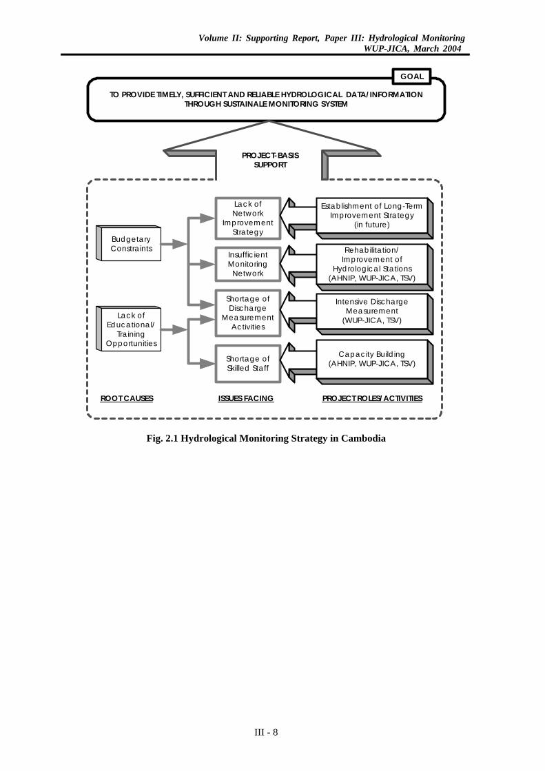
The difficulties to attain the goal are clear existence of root causes originating from socio-economic conditions of Cambodia. These are budgetary constraints of the government and lack of educational/training opportunities in the Cambodian educational system. The project-basis support cannot directly resolve such causes, but can tackle the derivative issues from the root causes during the project period. The effects of this approach might not cover the entire areas, but the following synergy effects among the projects could be expected:
The accumulated knowledge acquired during each project period can contribute to the capacity building.
The observed data/information contributed by the projects can remain as intellectual property so that organizational importance can accumulate.
The rehabilitated/improved hydrological network can be utilized in routine activities resulting in partial solution to the budgetary constraints.
To the project execution side, the hidden issues can be clearly identified in the course of the project so that the donors can prepare for the succeeding project to tackle the remaining issues.
Needless to say, to attain the goal is a time-taking process. The WUP-JICA had addressed the issues through the following approaches.
(1) Network Improvement and Rehabilitation/Improvement of Hydrological Stations
As described in Section 2.2, the WUP-JICA rehabilitated and improved the four (4) hydrological stations in Cambodia. In addition to the stations improved by AHNIP, the network covering the Mekong mainstream and Tonle Sap was properly formed.
III - 6

Volume II: Supporting Report, Paper III: Hydrological MonitoringWUP-JICA, March 2004
The remaining issues were to establish the long-term improvement strategy of the network and to rehabilitate and improve the hydrological network over the Cambodian territory following the strategy. These plan formulation and actual works may be realized in the near future under the succeeding project.
(2) Intensive Discharge Measurement
In order to develop the reliable rating curves at the selected stations, discharge data shall have to be measured as much as possible since flow condition might be different between wet and dry seasons due to tidal effect. To start the intensive discharge measurement, the following conditions shall be considered:
To avoid unnecessary overlapping among the related projects, the stations to conduct discharge measurement shall be carefully selected.
To collaborate on clarification of flow mechanisms in the floodplains with the TSV Project, the possible collaborative activities shall be determined in due consideration of the limitation of manpower and budget for the project.
(3) Capacity Building
Capacity building is an indispensable issue to tackle in order to obtain favourable results of discharge measurement. The discharge measurement will be made using ADCP (Acoustic Doppler Current Profiler), while the measurements in AHNIP and the TSV Project will be made with ADP (Acoustic Doppler Profiler). In this connection, frequent training has to be made in the following manner:
To impart knowledge on ADCP mechanism to the staff of the line agencies, explanatory indoor training shall be held at the initial stage.
To familiarize the staff on the operation and maintenance of ADCP, on-the-job field training shall be made to the staff together with experts of the Team as frequently as possible.
To share the acquired knowledge and experiences among the measuring staff, periodical training and meetings will be held between WUP-JICA and the TSV Project.
To evaluate the results and enhance the measuring activities, the training and meetings will be held in parallel with the progress of hydrological analysis utilizing the measured data.
The final products of the discharge measurement are reliable dataset of measured discharge and water level, and developed rating curves at the selected stations. In addition, the following was the final goal of the capacity building made by the WUP-JICA in connection with the discharge measurement:
For the DHRW itself, to continuously conduct the discharge measurement using ADCP and revise the rating curves based on the newly observed data after termination of the WUP-JICA Project.
Fig. 2.1 illustrates the conceptual relation among the goal, root causes and issues, and roles and activities of the projects as remedial measures.
III - 7
Volume II: Supporting Report, Paper III: Hydrological MonitoringWUP-JICA, March 2004
TO PROVIDE TIMELY, SUFFICIENT AND RELIABLE HYDROLOGICAL DATA/INFORMATIONTHROUGH SUSTAINALE MONITORING SYSTEM
GOAL
BudgetaryConstraints
Lack ofEducational/
TrainingOpportunities
Lack ofNetwork
ImprovementStrategy
InsufficientMonitoring
Network
Shortage ofDischarge
MeasurementActivities
Shortage ofSkilled Staff
Rehabilitation/Improvement of
Hydrological Stations(AHNIP, WUP-JICA, TSV)
Intensive DischargeMeasurement
(WUP-JICA, TSV)
Establishment of Long-TermImprovement Strategy
(in future)
Capacity Building(AHNIP, WUP-JICA, TSV)
PROJECT-BASISSUPPORT
ROOT CAUSES ISSUES FACING PROJECT ROLES/ACTIVITIES
Fig. 2.1 Hydrological Monitoring Strategy in Cambodia
III - 8
Volume II: Supporting Report, Paper III: Hydrological MonitoringWUP-JICA, March 2004
3. OBJECTIVES AND ACTIVITIES
3.1 Objectives
As discussed above, the hydrological monitoring under the WUP-JICA Project should concentrate on discharge measurements in Cambodia. Hence, the Team deliberately avoided overlapping and thus facilitate the collaborative works. The objectives of discharge measurement were:
(1) To develop the discharge rating curves at the major hydrological stations utilising the measured data of water level and discharge, so that hydrological balances along the Mekong River system can be easily understood for the water utilization programme throughout the entire system; and
(2) To clarify the flood retarding and succeeding water supplement functions of the floodplains including the Tonle Sap system, utilizing the discharge data simultaneously measured along the river courses, so that various related projects can utilise the water balance mechanisms of the Cambodian floodplains to evaluate the cause-effect relationships.
To achieve the former objective, continuous measurement activities were necessary at the points of major stations. Furthermore, it was indispensable to collaborate with the AHNIP by sharing the responsible stations.
To achieve the latter objective, periodical and frequent measurement activities were necessary at the selected river cross-sections following the river courses of the mainstream, the Tonle Sap, and the Bassac. It was also indispensable to collaborate with the MRC projects of the Tonle Sap and Vicinities (TSLVP).
3.2 Activities
The following activities were carried out in 2002/2003 and 2003/2004, in relation to hydrological monitoring:
(1) Discharge Measurements and Development of Discharge Rating Curves
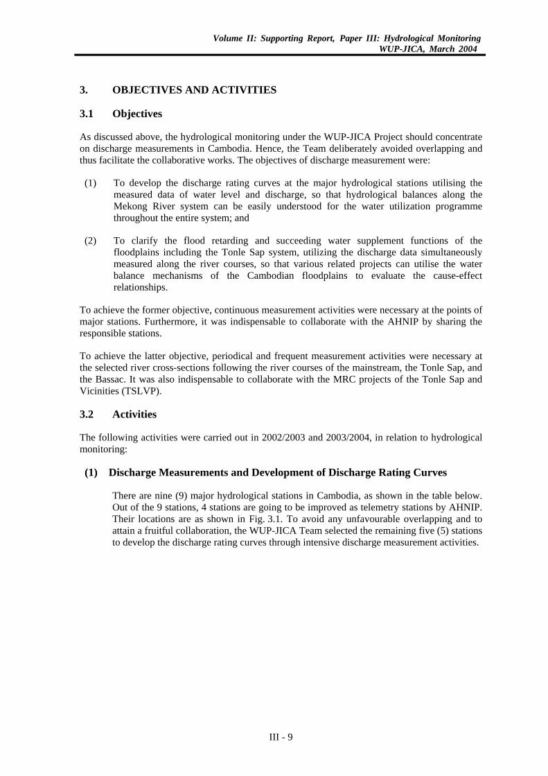
There are nine (9) major hydrological stations in Cambodia, as shown in the table below. Out of the 9 stations, 4 stations are going to be improved as telemetry stations by AHNIP. Their locations are as shown in Fig. 3.1. To avoid any unfavourable overlapping and to attain a fruitful collaboration, the WUP-JICA Team selected the remaining five (5) stations to develop the discharge rating curves through intensive discharge measurement activities.
III - 9
Volume II: Supporting Report, Paper III: Hydrological MonitoringWUP-JICA, March 2004
Table 3.1 Major Hydrological Stations in Cambodia
Station River/Lake Remarks Stung Treng Being improved under AHNIP Kratie Being improved under AHNIP Kompong Cham Mekong Churui Changvor Neak Luong Kompong Luong Tonle Sap Lake Being improved under AHNIP;
unnecessary to measure discharge Prek Kdam Tonle Sap Being improved under AHNIP Phnom Penh Port Chak Tomuk Bassac
Using the observed hydrological data of the above 5 stations, the flow conditions in the Chak Tomuk area at the junction of the Mekong, Tonle Sap and Bassac river systems have been clarified at the minimum. Clarification of this flow distribution mechanism would be useful for future water management following the water utilization rules to be formulated.
In due consideration of international river course management, crosschecking of data from the neighbouring countries has been indispensable. Even if intensive flow measurements were made at Tan Chau, Chau Doc and Vam Nao in Vietnam, the transparently crosschecked data observed in neighbouring countries would be useful for the acknowledgement among the riparian countries, in particular, during the dry season.
Stung Treng
Kratie
KompongLuong
PrekKdam
Kompong Cham
Chrui Changvar
Neak Luong
Phnom Penh Port
Chak Tomuk
AHNIP Stations
WUP-JICADischarge
Measuring Stations
Fig. 3.1 Major Hydrological Stations in Cambodia
III - 10
Volume II: Supporting Report, Paper III: Hydrological MonitoringWUP-JICA, March 2004
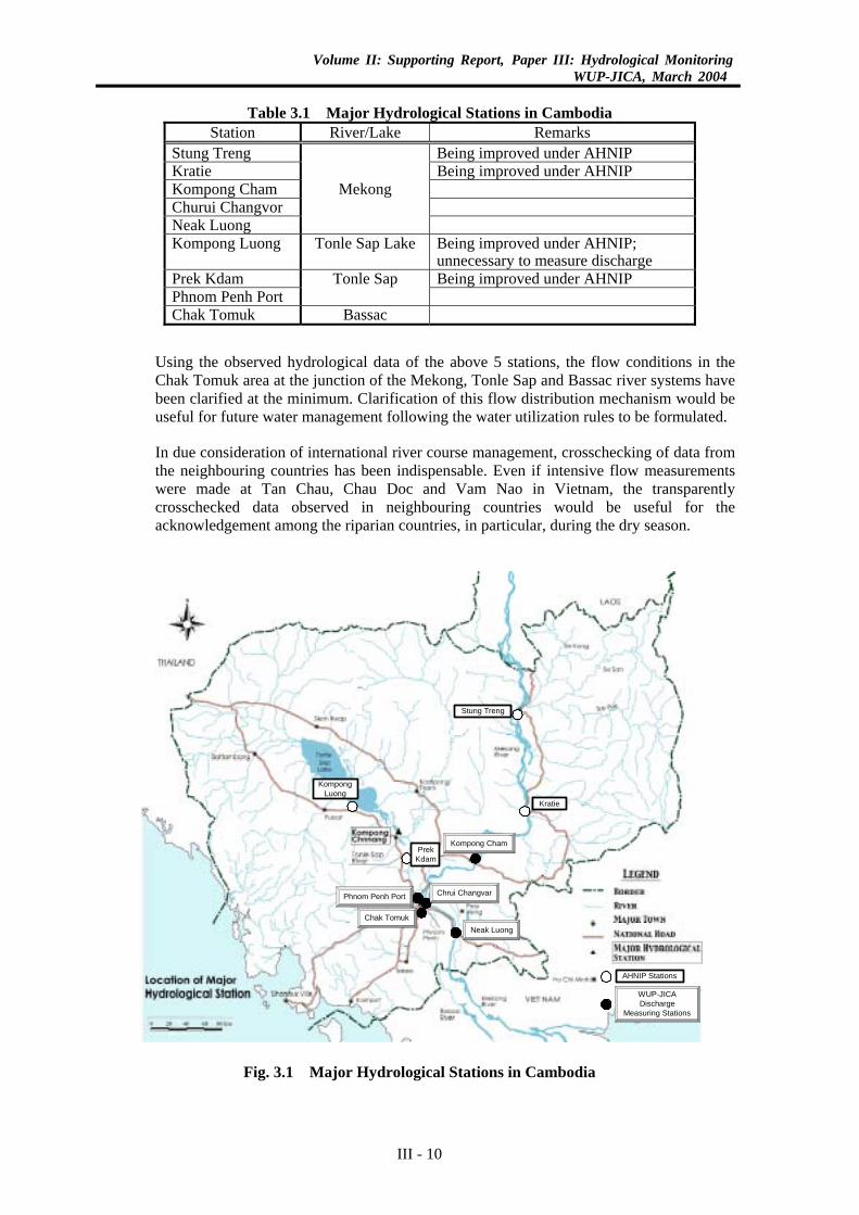
Kompong Cham
Flow of the Upstream
MEKONG RIVER
Overbanking Flooding during Flood Season
Chrui Changvar
Phnom Penh Port
Chak Tomuk
Neak Luong
TONLE SAP
MEKONG RIVER
BASSAC RIVER
Normal Flow or Reverse Flow
Flow Convergence and Divergence
Koh Norea
Fig. 3.2 Flow Situations and Selected Hydrological Stations/Sections
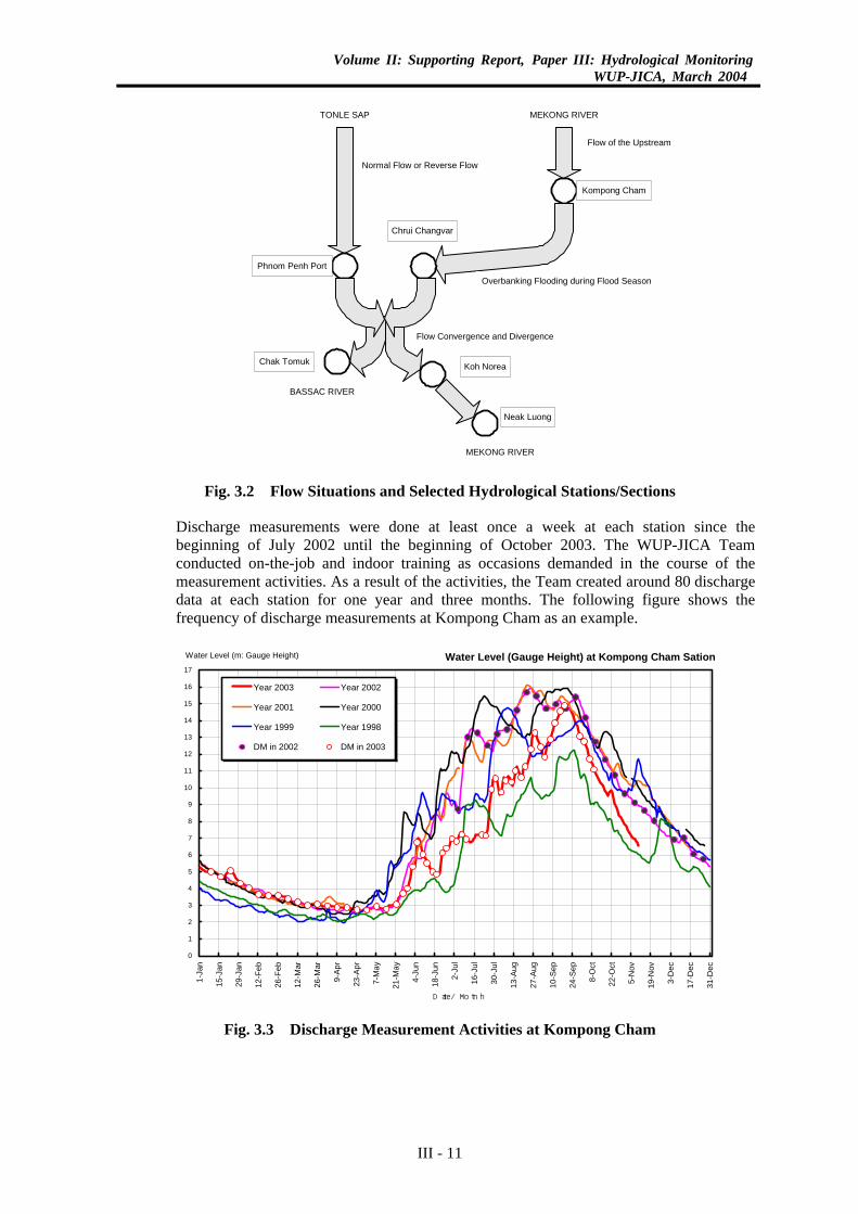
Discharge measurements were done at least once a week at each station since the beginning of July 2002 until the beginning of October 2003. The WUP-JICA Team conducted on-the-job and indoor training as occasions demanded in the course of the measurement activities. As a result of the activities, the Team created around 80 discharge data at each station for one year and three months. The following figure shows the frequency of discharge measurements at Kompong Cham as an example.
Water Level (Gauge Height) at Kompong Cham Sation
0
1
2
3
4
5
6
7
8
9
10
11
12
13
14
15
16
17
1-Ja
n
15-J
an
29-J
an
12-F
eb
26-F
eb
12-M
ar
26-M
ar
9-Ap
r
23-A
pr
7-M
ay
21-M
ay
4-Ju
n
18-J
un
2-Ju
l
16-J
ul
30-J
ul
13-A
ug
27-A
ug
10-S
ep
24-S
ep
8-O
ct
22-O
ct
5-N
ov
19-N
ov
3-D
ec
17-D
ec
31-D
ec
Date/Month
Water Level (m: Gauge Height)
Year 2003 Year 2002
Year 2001 Year 2000
Year 1999 Year 1998
DM in 2002 DM in 2003
Fig. 3.3 Discharge Measurement Activities at Kompong Cham
III - 11
Volume II: Supporting Report, Paper III: Hydrological MonitoringWUP-JICA, March 2004
(2) Coordinated Discharge Measurement
Coordinated discharge measurements were made, in particular, together with the Tonle Sap and Vicinities Project (TSLVP). One of the major objectives of TSLVP was to clarify the hydrological mechanisms of the Cambodian floodplains. On the other hand, one of the objectives of the WUP-JICA Project was to assist in the formulation of water utilization rules among the four countries. For this purpose, flow mechanisms including the dry-season flow shall have to be clarified in the Cambodian floodplains because these are very complicated in this area. Since the floodplains widely extend and the drainage systems including the Colmatage systems complicatedly developed on them, it might be a heavy burden for the project alone to tackle them and to create fruitful results. Thus, cooperative work was necessary in this field.
The work sharing between the two projects was determined based on the frequent discussions with the TSLV project team. As a result of the discussion, the WUP-JICA Team measured the discharges longitudinally along the river courses, while the TSLVP team made discharge measurements on the floodplains at the same time. The compiled results of the discharge measurements are presented in 6.2 to 6.3 of this paper as the Hydrological Functions of Cambodian Floodplains.
III - 12
Volume II: Supporting Report, Paper III: Hydrological MonitoringWUP-JICA, March 2004
4. DEVELOPMENT OF RATING CURVES
4.1 Previous Efforts for Development of Rating Curves
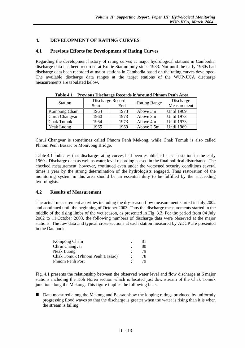
Regarding the development history of rating curves at major hydrological stations in Cambodia, discharge data has been recorded at Kratie Station only since 1933. Not until the early 1960s had discharge data been recorded at major stations in Cambodia based on the rating curves developed. The available discharge data ranges at the target stations of the WUP-JICA discharge measurements are tabulated below.
Table 4.1 Previous Discharge Records in/around Phnom Penh Area
Discharge Record Station Start End Rating Range Discharge Measurement
Kompong Cham 1964 1973 Above 3m Until 1969 Chrui Changvar 1960 1973 Above 3m Until 1973 Chak Tomuk 1964 1973 Above 4m Until 1973 Neak Luong 1965 1969 Above 2.5m Until 1969
Chrui Changvar is sometimes called Phnom Penh Mekong, while Chak Tomuk is also called Phnom Penh Bassac or Monivong Bridge.
Table 4.1 indicates that discharge-rating curves had been established at each station in the early 1960s. Discharge data as well as water level recording ceased in the final political disturbance. The checked measurement, however, continued even under the worsened security conditions several times a year by the strong determination of the hydrologists engaged. Thus restoration of the monitoring system in this area should be an essential duty to be fulfilled by the succeeding hydrologists.
4.2 Results of Measurement
The actual measurement activities including the dry-season flow measurement started in July 2002 and continued until the beginning of October 2003. Thus the discharge measurements started in the middle of the rising limbs of the wet season, as presented in Fig. 3.3. For the period from 04 July 2002 to 11 October 2003, the following numbers of discharge data were observed at the major stations. The raw data and typical cross-sections at each station measured by ADCP are presented in the Databook.
Kompong Cham : 81 Chrui Changvar : 80 Neak Luong : 79 Chak Tomuk (Phnom Penh Bassac) : 78 Phnom Penh Port : 79
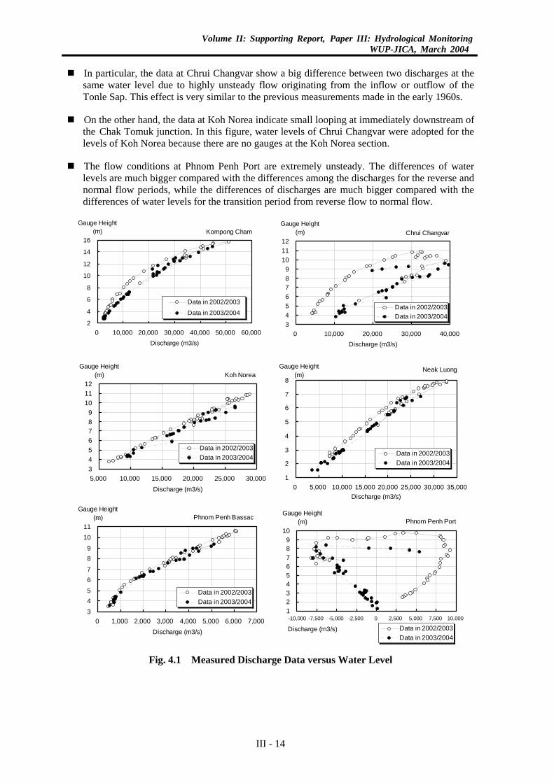
Fig. 4.1 presents the relationship between the observed water level and flow discharge at 6 major stations including the Koh Norea section which is located just downstream of the Chak Tomuk junction along the Mekong. This figure implies the following facts:
Data measured along the Mekong and Bassac show the looping ratings produced by uniformly progressing flood waves so that the discharge is greater when the water is rising than it is when the stream is falling.
III - 13
Volume II: Supporting Report, Paper III: Hydrological MonitoringWUP-JICA, March 2004
In particular, the data at Chrui Changvar show a big difference between two discharges at the
same water level due to highly unsteady flow originating from the inflow or outflow of the Tonle Sap. This effect is very similar to the previous measurements made in the early 1960s.
On the other hand, the data at Koh Norea indicate small looping at immediately downstream of the Chak Tomuk junction. In this figure, water levels of Chrui Changvar were adopted for the levels of Koh Norea because there are no gauges at the Koh Norea section.
The flow conditions at Phnom Penh Port are extremely unsteady. The differences of water levels are much bigger compared with the differences among the discharges for the reverse and normal flow periods, while the differences of discharges are much bigger compared with the differences of water levels for the transition period from reverse flow to normal flow.
Kompong Cham
2
4
6
8
10
12
14
16
0 10,000 20,000 30,000 40,000 50,000 60,000Discharge (m3/s)
Gauge Height(m)
Data in 2002/2003
Data in 2003/2004
Chrui Changvar
3456789
101112
0 10,000 20,000 30,000 40,000Discharge (m3/s)
Gauge Height(m)
Data in 2002/2003Data in 2003/2004
Phnom Penh Bassac
3456789
1011
0 1,000 2,000 3,000 4,000 5,000 6,000 7,000Discharge (m3/s)
Gauge Height(m)
Data in 2002/2003Data in 2003/2004
Phnom Penh Port
123456789
10
-10,000 -7,500 -5,000 -2,500 0 2,500 5,000 7,500 10,000
Discharge (m3/s)
Gauge Height(m)
Data in 2002/2003Data in 2003/2004
Koh Norea
3456789
101112
5,000 10,000 15,000 20,000 25,000 30,000Discharge (m3/s)
Gauge Height(m)
Data in 2002/2003Data in 2003/2004
Neak Luong
1
2
3
4
5
6
7
8
0 5,000 10,000 15,000 20,000 25,000 30,000 35,000Discharge (m3/s)
Gauge Height(m)
Data in 2002/2003Data in 2003/2004
Fig. 4.1 Measured Discharge Data versus Water Level
III - 14
Volume II: Supporting Report, Paper III: Hydrological MonitoringWUP-JICA, March 2004
4.3 Determination of Rating Ranges
According to the examination of measured discharges versus water levels as presented in Fig. 4.1, it may very difficult to develop the rating curves at Phnom Penh Port due to the strong and complicated effects of flow convergence and divergence at the Chak Tomuk junction. Thus, except for Phnom Penh Port on the Tonle Sap, the rating curves at the remaining 5 stations were developed using the observed data. In the process of development, the initial step was the determination of applicable range of rating curve, since hydrological data at these stations are strongly affected by tidal fluctuation in the low-flow period.
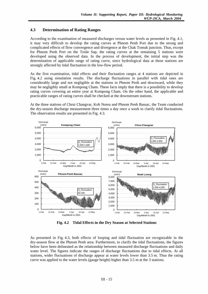
As the first examination, tidal effects and their fluctuation ranges at 4 stations are depicted in Fig. 4.2 using simulation results. The discharge fluctuations in parallel with tidal ones are considerably large and not negligible at the stations in Phnom Penh and downward, while they may be negligibly small at Kompong Cham. These facts imply that there is a possibility to develop rating curves covering an entire year at Kompong Cham. On the other hand, the applicable and practicable ranges of rating curves shall be checked at the downstream stations.
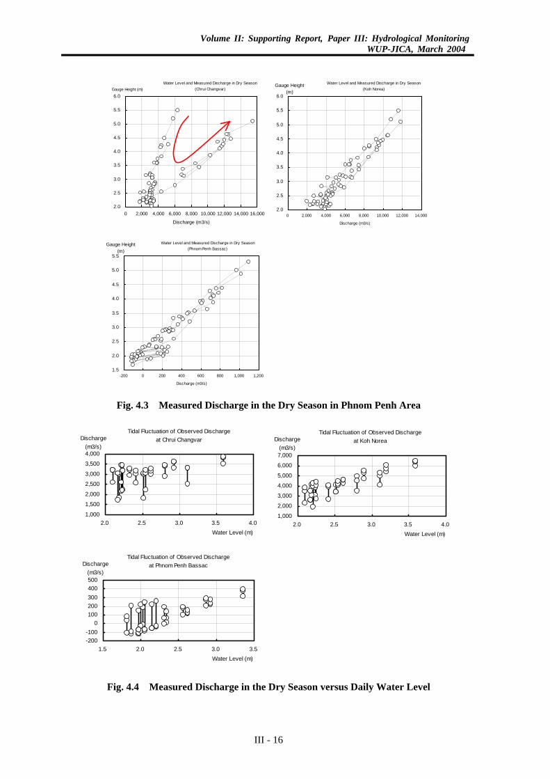
At the three stations of Chrui Changvar, Koh Norea and Phnom Penh Bassac, the Team conducted the dry-season discharge measurement three times a day once a week to clarify tidal fluctuations. The observation results are presented in Fig. 4.3.
Chrui Changvar
0
1,000
2,000
3,000
4,000
5,000
6,000
1-Feb 21-Feb 13-Mar 2-Apr 22-Apr 12-MayDay/Month in 2001
Discharge(m3/s)
Q_Fluctuation:1,000-2,500
Neak Luong
0
1,000
2,000
3,000
4,000
5,000
6,000
7,000
8,000
1-Feb 21-Feb 13-Mar 2-Apr 22-Apr 12-MayDay/Month in 2001
Discharge(m3/s)
Q_Fluctuation:1,000-4,000
Kompong Cham
0
1,000
2,000
3,000
4,000
5,000
6,000
1-Feb 21-Feb 13-Mar 2-Apr 22-Apr 12-MayDay/Month in 2001
Discharge(m3/s)
Q_Fluctuation:1,500-1,600
Phnom Penh Bassac
0
100
200
300
400
500
600
1-Feb 21-Feb 13-Mar 2-Apr 22-Apr 12-MayDay/Month in 2001
Discharge(m3/s)
Q_Fluctuation:50-200
Fig. 4.2 Tidal Effects in the Dry Season at Selected Stations
As presented in Fig. 4.3, both effects of looping and tidal fluctuation are recognizable in the dry-season flow at the Phnom Penh area. Furthermore, to clarify the tidal fluctuations, the figures below have been delineated as the relationship between measured discharge fluctuations and daily water level. The figures indicate the ranges of discharge fluctuations due to tidal effects. At all stations, wider fluctuations of discharge appear at water levels lower than 3.5 m. Thus the rating curve was applied to the water levels (gauge height) higher than 3.5 m at the 3 stations.
III - 15
Volume II: Supporting Report, Paper III: Hydrological MonitoringWUP-JICA, March 2004
Water Level and Measured Discharge in Dry Season(Chrui Changvar)
2.0
2.5
3.0
3.5
4.0
4.5
5.0
5.5
6.0
0 2,000 4,000 6,000 8,000 10,000 12,000 14,000 16,000
Discharge (m3/s)
Gauge Height (m)Water Level and Measured Discharge in Dry Season
(Koh Norea)
2.0
2.5
3.0
3.5
4.0
4.5
5.0
5.5
6.0
0 2,000 4,000 6,000 8,000 10,000 12,000 14,000
Discharge (m3/s)
Gauge Height(m)
Water Level and Measured Discharge in Dry Season(Phnom Penh Bassac)
1.5
2.0
2.5
3.0
3.5
4.0
4.5
5.0
5.5
-200 0 200 400 600 800 1,000 1,200
Discharge (m3/s)
Gauge Height(m)
Fig. 4.3 Measured Discharge in the Dry Season in Phnom Penh Area
Tidal Fluctuation of Observed Dischargeat Chrui Changvar
1,000
1,500
2,000
2,500
3,000
3,500
4,000
2.0 2.5 3.0 3.5 4.0Water Level (m)
Discharge(m3/s)
Tidal Fluctuation of Observed Dischargeat Koh Norea
1,000
2,000
3,000
4,000
5,000
6,000
7,000
2.0 2.5 3.0 3.5 4.0Water Level (m)
Discharge(m3/s)
Tidal Fluctuation of Observed Dischargeat Phnom Penh Bassac
-200-100
0100200300400500
1.5 2.0 2.5 3.0 3.5Water Level (m)
Discharge(m3/s)
Fig. 4.4 Measured Discharge in the Dry Season versus Daily Water Level
III - 16
Volume II: Supporting Report, Paper III: Hydrological MonitoringWUP-JICA, March 2004
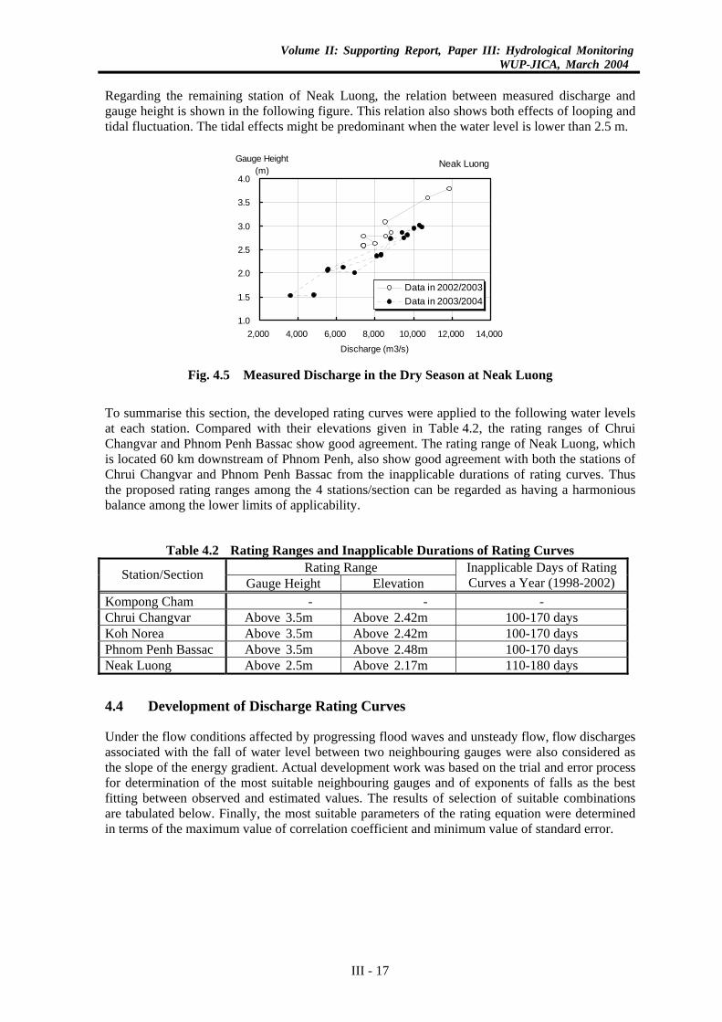
Regarding the remaining station of Neak Luong, the relation between measured discharge and gauge height is shown in the following figure. This relation also shows both effects of looping and tidal fluctuation. The tidal effects might be predominant when the water level is lower than 2.5 m.
Neak Luong
1.0
1.5
2.0
2.5
3.0
3.5
4.0
2,000 4,000 6,000 8,000 10,000 12,000 14,000
Discharge (m3/s)
Gauge Height(m)
Data in 2002/2003Data in 2003/2004
Fig. 4.5 Measured Discharge in the Dry Season at Neak Luong
To summarise this section, the developed rating curves were applied to the following water levels at each station. Compared with their elevations given in Table 4.2, the rating ranges of Chrui Changvar and Phnom Penh Bassac show good agreement. The rating range of Neak Luong, which is located 60 km downstream of Phnom Penh, also show good agreement with both the stations of Chrui Changvar and Phnom Penh Bassac from the inapplicable durations of rating curves. Thus the proposed rating ranges among the 4 stations/section can be regarded as having a harmonious balance among the lower limits of applicability.
Table 4.2 Rating Ranges and Inapplicable Durations of Rating Curves
Rating Range Station/Section Gauge Height Elevation
Inapplicable Days of RatingCurves a Year (1998-2002)
Kompong Cham - - - Chrui Changvar Above 3.5m Above 2.42m 100-170 days Koh Norea Above 3.5m Above 2.42m 100-170 days Phnom Penh Bassac Above 3.5m Above 2.48m 100-170 days Neak Luong Above 2.5m Above 2.17m 110-180 days
4.4 Development of Discharge Rating Curves
Under the flow conditions affected by progressing flood waves and unsteady flow, flow discharges associated with the fall of water level between two neighbouring gauges were also considered as the slope of the energy gradient. Actual development work was based on the trial and error process for determination of the most suitable neighbouring gauges and of exponents of falls as the best fitting between observed and estimated values. The results of selection of suitable combinations are tabulated below. Finally, the most suitable parameters of the rating equation were determined in terms of the maximum value of correlation coefficient and minimum value of standard error.
III - 17
Volume II: Supporting Report, Paper III: Hydrological MonitoringWUP-JICA, March 2004
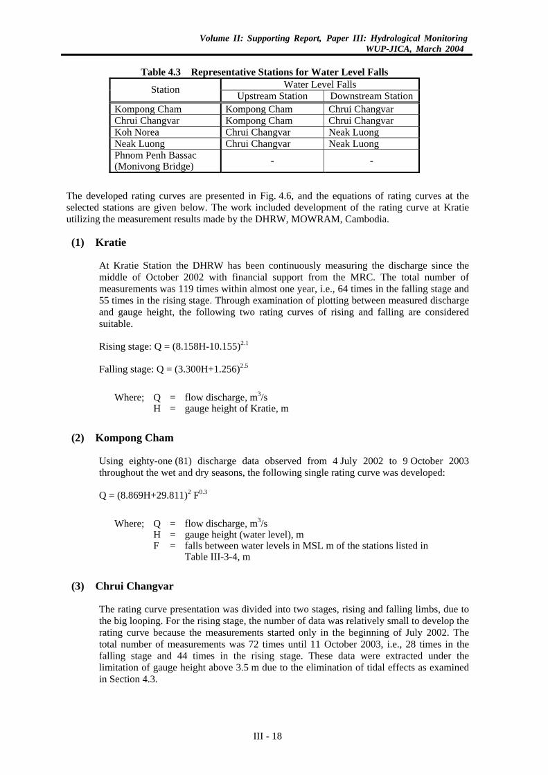
Table 4.3 Representative Stations for Water Level Falls
Water Level Falls Station Upstream Station Downstream Station Kompong Cham Kompong Cham Chrui Changvar Chrui Changvar Kompong Cham Chrui Changvar Koh Norea Chrui Changvar Neak Luong Neak Luong Chrui Changvar Neak Luong Phnom Penh Bassac (Monivong Bridge) - -
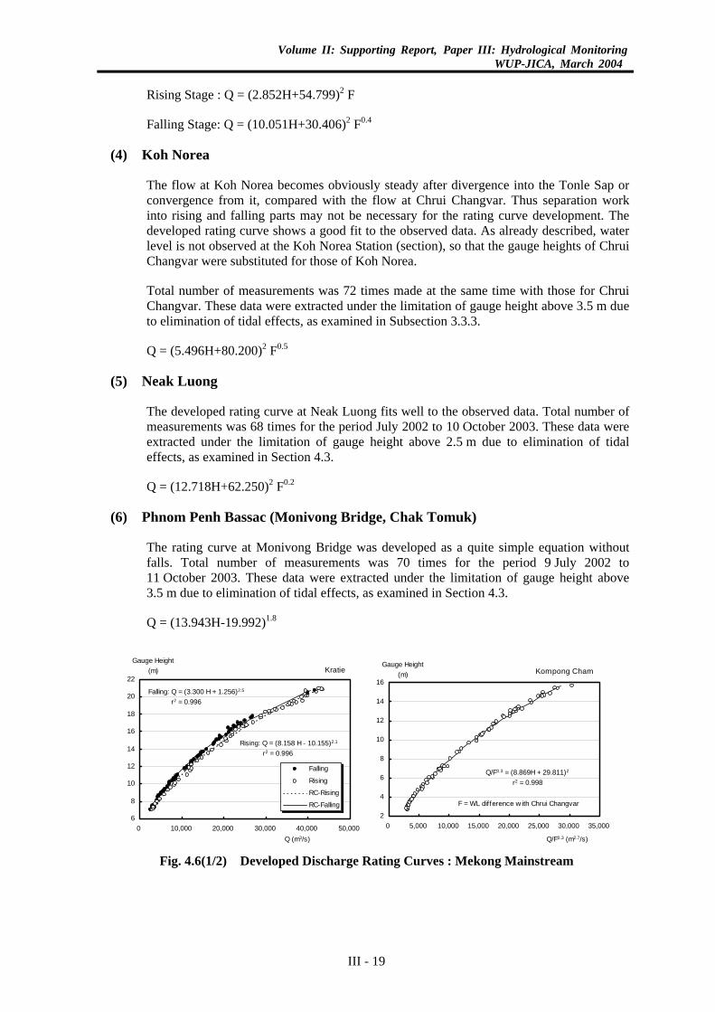
The developed rating curves are presented in Fig. 4.6, and the equations of rating curves at the selected stations are given below. The work included development of the rating curve at Kratie utilizing the measurement results made by the DHRW, MOWRAM, Cambodia.
(1) Kratie
At Kratie Station the DHRW has been continuously measuring the discharge since the middle of October 2002 with financial support from the MRC. The total number of measurements was 119 times within almost one year, i.e., 64 times in the falling stage and 55 times in the rising stage. Through examination of plotting between measured discharge and gauge height, the following two rating curves of rising and falling are considered suitable.
Rising stage: Q = (8.158H-10.155)2.1
Falling stage: Q = (3.300H+1.256)2.5
Where; Q = flow discharge, m3/s H = gauge height of Kratie, m
(2) Kompong Cham
Using eighty-one (81) discharge data observed from 4 July 2002 to 9 October 2003 throughout the wet and dry seasons, the following single rating curve was developed:
Q = (8.869H+29.811)2 F0.3
Where; Q = flow discharge, m3/s H = gauge height (water level), m F = falls between water levels in MSL m of the stations listed in
Table III-3-4, m
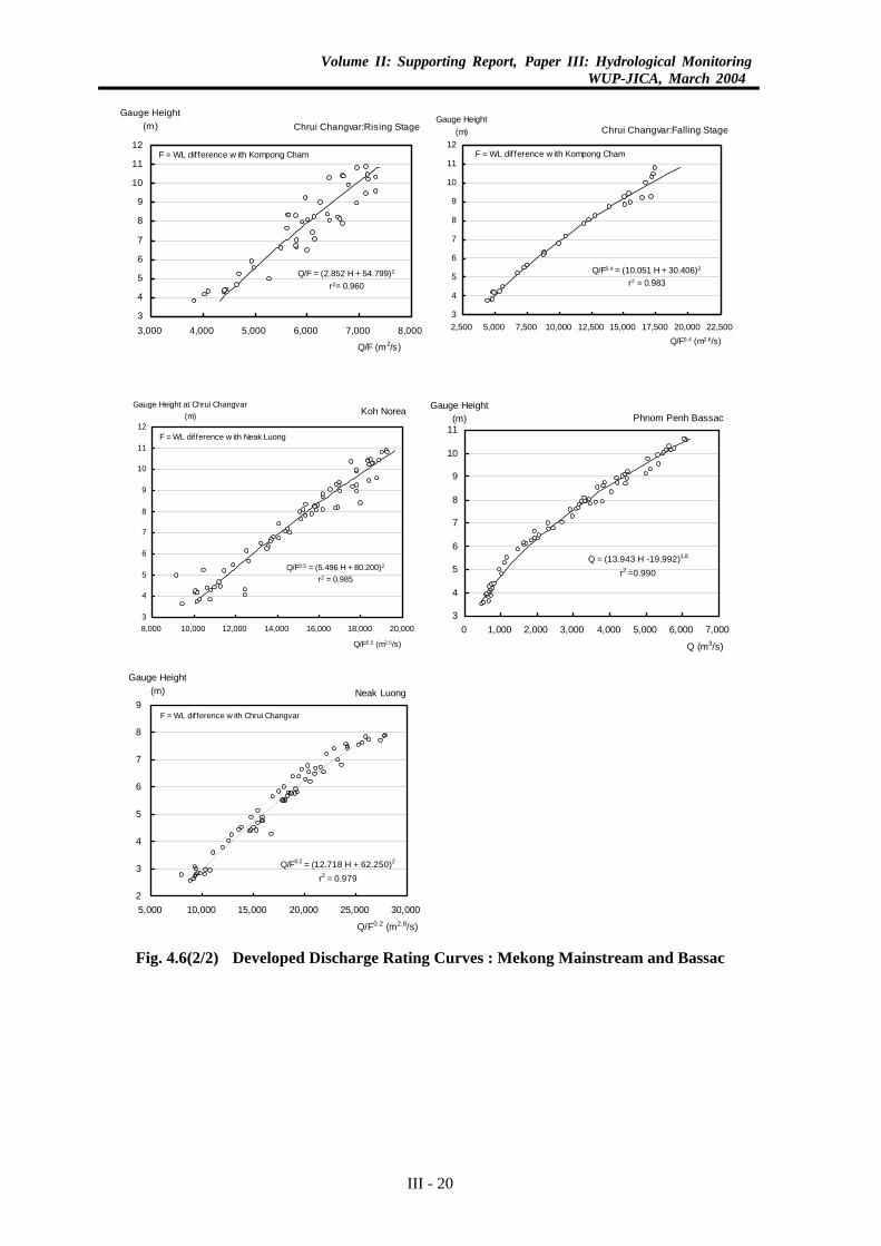
(3) Chrui Changvar
The rating curve presentation was divided into two stages, rising and falling limbs, due to the big looping. For the rising stage, the number of data was relatively small to develop the rating curve because the measurements started only in the beginning of July 2002. The total number of measurements was 72 times until 11 October 2003, i.e., 28 times in the falling stage and 44 times in the rising stage. These data were extracted under the limitation of gauge height above 3.5 m due to the elimination of tidal effects as examined in Section 4.3.
III - 18
Volume II: Supporting Report, Paper III: Hydrological MonitoringWUP-JICA, March 2004
Rising Stage : Q = (2.852H+54.799)2 F
Falling Stage: Q = (10.051H+30.406)2 F0.4
(4) Koh Norea
The flow at Koh Norea becomes obviously steady after divergence into the Tonle Sap or convergence from it, compared with the flow at Chrui Changvar. Thus separation work into rising and falling parts may not be necessary for the rating curve development. The developed rating curve shows a good fit to the observed data. As already described, water level is not observed at the Koh Norea Station (section), so that the gauge heights of Chrui Changvar were substituted for those of Koh Norea.
Total number of measurements was 72 times made at the same time with those for Chrui Changvar. These data were extracted under the limitation of gauge height above 3.5 m due to elimination of tidal effects, as examined in Subsection 3.3.3.
Q = (5.496H+80.200)2 F0.5
(5) Neak Luong
The developed rating curve at Neak Luong fits well to the observed data. Total number of measurements was 68 times for the period July 2002 to 10 October 2003. These data were extracted under the limitation of gauge height above 2.5 m due to elimination of tidal effects, as examined in Section 4.3.
Q = (12.718H+62.250)2 F0.2
(6) Phnom Penh Bassac (Monivong Bridge, Chak Tomuk)
The rating curve at Monivong Bridge was developed as a quite simple equation without falls. Total number of measurements was 70 times for the period 9 July 2002 to 11 October 2003. These data were extracted under the limitation of gauge height above 3.5 m due to elimination of tidal effects, as examined in Section 4.3.
Q = (13.943H-19.992)1.8
Kratie
6
8
10
12
14
16
18
20
22
0 10,000 20,000 30,000 40,000 50,000Q (m3/s)
Gauge Height(m)
Falling
Rising
RC-Rising
RC-Falling
Falling: Q = (3.300 H + 1.256)2.5
r2 = 0.996
Rising: Q = (8.158 H - 10.155)2.1
r2 = 0.996
Kompong Cham
2
4
6
8
10
12
14
16
0 5,000 10,000 15,000 20,000 25,000 30,000 35,000
Q/F0.3 (m2.7/s)
Gauge Height(m)
F = WL difference w ith Chrui Changvar
Q/F0.3 = (8.869H + 29.811)2
r2 = 0.998
Fig. 4.6(1/2) Developed Discharge Rating Curves : Mekong Mainstream
III - 19
Volume II: Supporting Report, Paper III: Hydrological MonitoringWUP-JICA, March 2004
Chrui Changvar:Rising Stage
3
4
5
6
7
8
9
10
11
12
3,000 4,000 5,000 6,000 7,000 8,000
Q/F (m2/s)
Gauge Height(m)
Q/F = (2.852 H + 54.799)2
r2= 0.960
F = WL difference w ith Kompong Cham
Chrui Changvar:Falling Stage
3
4
5
6
7
8
9
10
11
12
2,500 5,000 7,500 10,000 12,500 15,000 17,500 20,000 22,500Q/F0.4 (m2.6/s)
Gauge Height(m)
Q/F0.4 = (10.051 H + 30.406)2
r2 = 0.983
F = WL dif ference w ith Kompong Cham
Phnom Penh Bassac
3
4
5
6
7
8
9
10
11
0 1,000 2,000 3,000 4,000 5,000 6,000 7,000
Q (m3/s)
Gauge Height(m)
Q = (13.943 H -19.992)1.8
r2 =0.990
Koh Norea
3
4
5
6
7
8
9
10
11
12
8,000 10,000 12,000 14,000 16,000 18,000 20,000
Q/F0.5 (m2.5/s)
Q/F0.5 = (5.496 H + 80.200)2
r2 = 0.985
Gauge Height at Chrui Changvar(m)
F = WL difference w ith Neak Luong
Neak Luong
2
3
4
5
6
7
8
9
5,000 10,000 15,000 20,000 25,000 30,000
Q/F0.2 (m2.8/s)
Gauge Height(m)
Q/F0.2 = (12.718 H + 62.250)2
r2 = 0.979
F = WL difference w ith Chrui Changvar
Fig. 4.6(2/2) Developed Discharge Rating Curves : Mekong Mainstream and Bassac
III - 20
Volume II: Supporting Report, Paper III: Hydrological MonitoringWUP-JICA, March 2004
5. FLOW MONITORING SYSTEM IN CAMBODIA
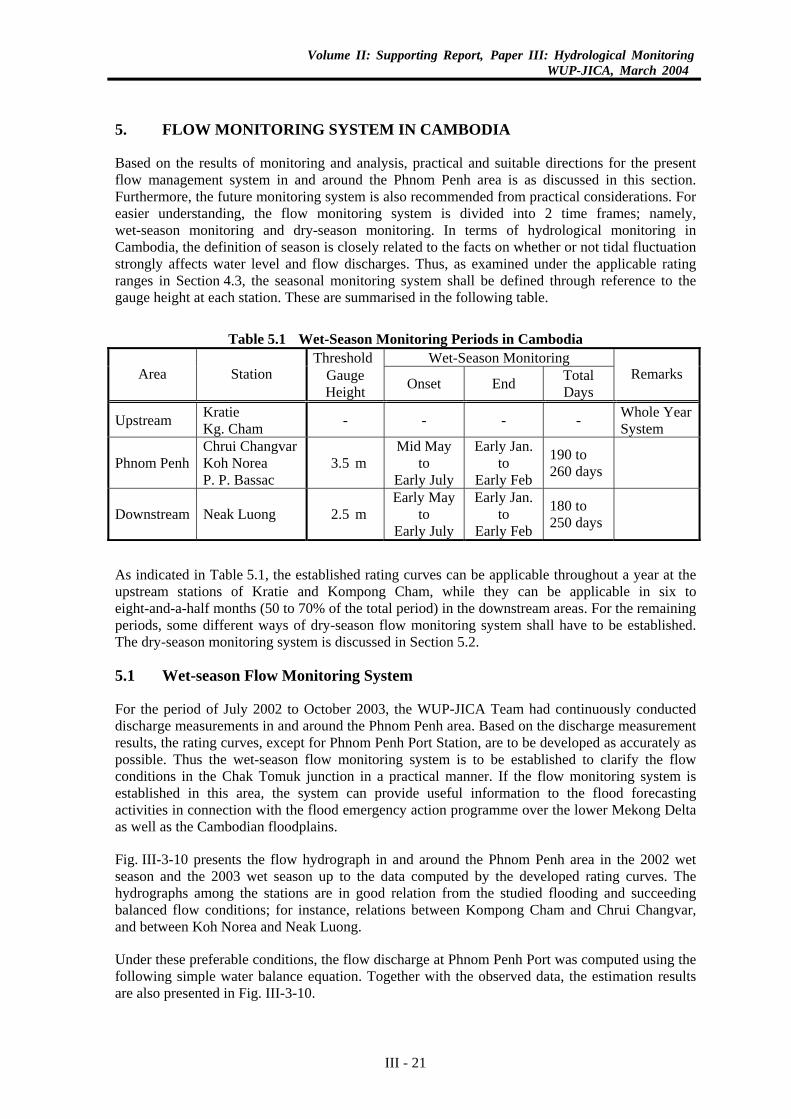
Based on the results of monitoring and analysis, practical and suitable directions for the present flow management system in and around the Phnom Penh area is as discussed in this section. Furthermore, the future monitoring system is also recommended from practical considerations. For easier understanding, the flow monitoring system is divided into 2 time frames; namely, wet-season monitoring and dry-season monitoring. In terms of hydrological monitoring in Cambodia, the definition of season is closely related to the facts on whether or not tidal fluctuation strongly affects water level and flow discharges. Thus, as examined under the applicable rating ranges in Section 4.3, the seasonal monitoring system shall be defined through reference to the gauge height at each station. These are summarised in the following table.
Table 5.1 Wet-Season Monitoring Periods in Cambodia
Threshold Wet-Season Monitoring Area Station Gauge
Height Onset End Total Days
Remarks
Upstream Kratie Kg. Cham - - - - Whole Year
System
Phnom Penh Chrui Changvar Koh Norea P. P. Bassac
3.5 m Mid May
to Early July
Early Jan.to
Early Feb
190 to 260 days
Downstream Neak Luong 2.5 m Early May
to Early July
Early Jan.to
Early Feb
180 to 250 days
As indicated in Table 5.1, the established rating curves can be applicable throughout a year at the upstream stations of Kratie and Kompong Cham, while they can be applicable in six to eight-and-a-half months (50 to 70% of the total period) in the downstream areas. For the remaining periods, some different ways of dry-season flow monitoring system shall have to be established. The dry-season monitoring system is discussed in Section 5.2.
5.1 Wet-season Flow Monitoring System
For the period of July 2002 to October 2003, the WUP-JICA Team had continuously conducted discharge measurements in and around the Phnom Penh area. Based on the discharge measurement results, the rating curves, except for Phnom Penh Port Station, are to be developed as accurately as possible. Thus the wet-season flow monitoring system is to be established to clarify the flow conditions in the Chak Tomuk junction in a practical manner. If the flow monitoring system is established in this area, the system can provide useful information to the flood forecasting activities in connection with the flood emergency action programme over the lower Mekong Delta as well as the Cambodian floodplains.
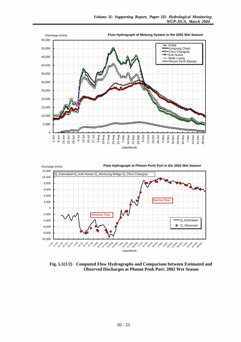
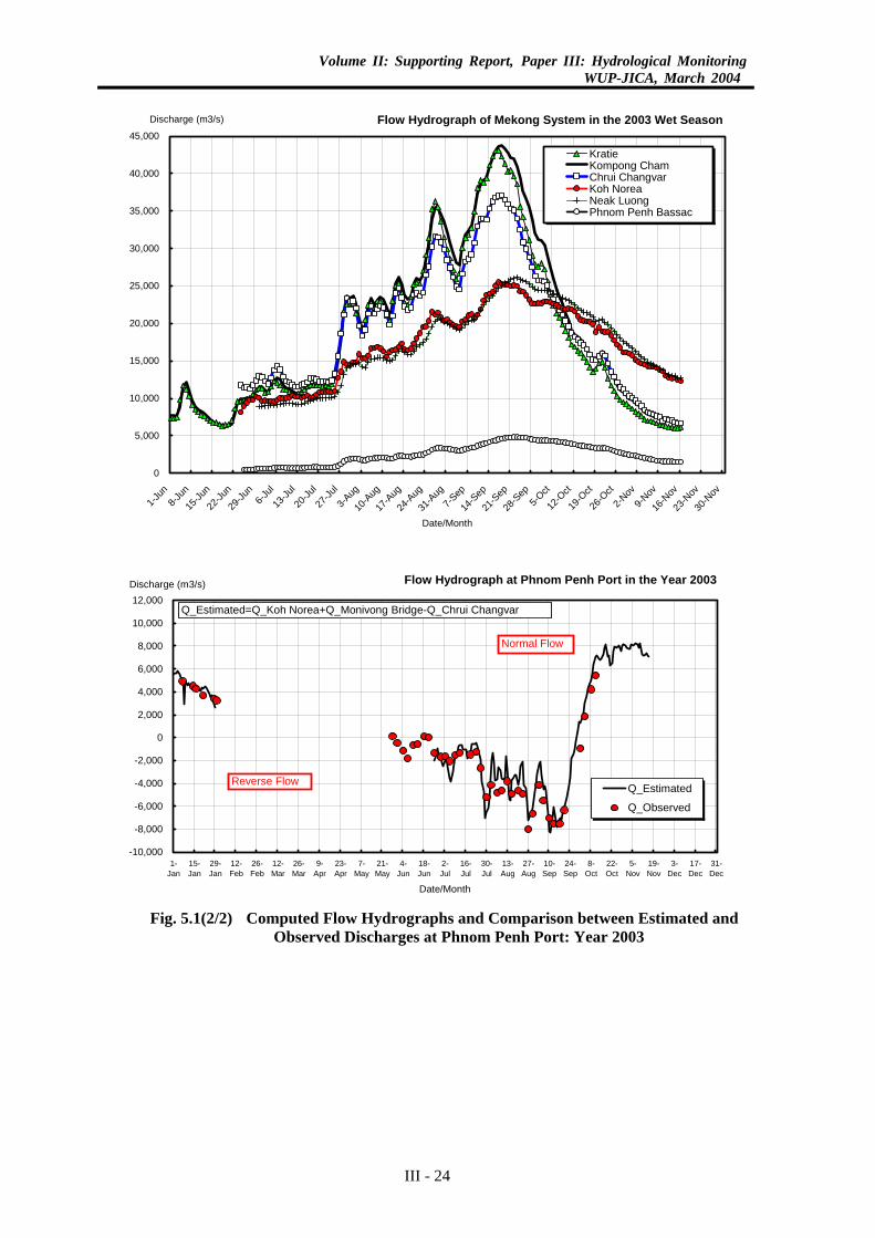
Fig. III-3-10 presents the flow hydrograph in and around the Phnom Penh area in the 2002 wet season and the 2003 wet season up to the data computed by the developed rating curves. The hydrographs among the stations are in good relation from the studied flooding and succeeding balanced flow conditions; for instance, relations between Kompong Cham and Chrui Changvar, and between Koh Norea and Neak Luong.
Under these preferable conditions, the flow discharge at Phnom Penh Port was computed using the following simple water balance equation. Together with the observed data, the estimation results are also presented in Fig. III-3-10.
III - 21

Volume II: Supporting Report, Paper III: Hydrological MonitoringWUP-JICA, March 2004
Phnom Penh Port Q = Koh Norea Q + Monivong Bridge Q- Chrui Changvar Q
This figure implies the possibilities for establishment of the wet-season monitoring system. Computed hydrograph shows a good fit to the observed discharges during the reverse flow period as well as the transition and normal flow period. Thus the computed flow can be practically utilized for estimation of the Tonle Sap flow in the wet season. In conclusion, the developed rating curves can be utilized for the wet-season flow monitoring system from Kratie down to Phnom Penh area in Cambodia, to clarify the flow rate not only at the station sites but also of divergence/convergence at the junction of the Chak Tomuk area.
III - 22
Volume II: Supporting Report, Paper III: Hydrological MonitoringWUP-JICA, March 2004
Flow Hydrograph of Mekong System in the 2002 Wet Season
0
5,000
10,000
15,000
20,000
25,000
30,000
35,000
40,000
45,000
50,000
55,000
1-Ju
n
8-Ju
n
15-J
un
22-J
un
29-J
un
6-Ju
l
13-J
ul
20-J
ul
27-J
ul
3-A
ug
10-A
ug
17-A
ug
24-A
ug
31-A
ug
7-S
ep
14-S
ep
21-S
ep
28-S
ep
5-O
ct
12-O
ct
19-O
ct
26-O
ct
2-N
ov
9-N
ov
16-N
ov
23-N
ov
30-N
ov
7-D
ec
14-D
ec
21-D
ec
28-D
ec
Date/Month
Discharge (m3/s)
KratieKompong ChamChrui ChangvarKoh NoreaNeak LuongPhnom Penh Bassac
Flow Hydrograph at Phnom Penh Port in the 2002 Wet Season
-10,000
-8,000
-6,000
-4,000
-2,000
0
2,000
4,000
6,000
8,000
10,000
12,000
1-Jun
8-Jun
15-Ju
n
22-Ju
n
29-Ju
n6-J
ul
13-Ju
l
20-Ju
l
27-Ju
l
3-Aug
10-A
ug
17-A
ug
24-A
ug
31-A
ug7-S
ep
14-S
ep
21-S
ep
28-S
ep5-O
ct
12-O
ct
19-O
ct
26-O
ct
2-Nov
9-Nov
16-N
ov
23-N
ov
30-N
ov7-D
ec
14-D
ec
21-D
ec
28-D
ec
Date/Month
Discharge (m3/s)
Q_Estimated
Q_Observed
Q_Estimated=Q_Koh Norea+Q_Monivong Bridge-Q_Chrui Changvar
Reverse Flow
Normal Flow
Fig. 5.1(1/2) Computed Flow Hydrographs and Comparison between Estimated and
Observed Discharges at Phnom Penh Port: 2002 Wet Season
III - 23
Volume II: Supporting Report, Paper III: Hydrological MonitoringWUP-JICA, March 2004
Flow Hydrograph of Mekong System in the 2003 Wet Season
0
5,000
10,000
15,000
20,000
25,000
30,000
35,000
40,000
45,000
1-Jun
8-Jun
15-Ju
n
22-Ju
n
29-Ju
n6-J
ul
13-Ju
l
20-Ju
l
27-Ju
l
3-Aug
10-A
ug
17-A
ug
24-A
ug
31-A
ug7-S
ep
14-S
ep
21-S
ep
28-S
ep5-O
ct
12-O
ct
19-O
ct
26-O
ct
2-Nov
9-Nov
16-N
ov
23-N
ov
30-N
ov
Date/Month
Discharge (m3/s)
KratieKompong ChamChrui ChangvarKoh NoreaNeak LuongPhnom Penh Bassac
Flow Hydrograph at Phnom Penh Port in the Year 2003
-10,000
-8,000
-6,000
-4,000
-2,000
0
2,000
4,000
6,000
8,000
10,000
12,000
1-Jan
15-Jan
29-Jan
12-Feb
26-Feb
12-Mar
26-Mar
9-Apr
23-Apr
7-May
21-May
4-Jun
18-Jun
2-Jul
16-Jul
30-Jul
13-Aug
27-Aug
10-Sep
24-Sep
8-Oct
22-Oct
5-Nov
19-Nov
3-Dec
17-Dec
31-Dec
Date/Month
Discharge (m3/s)
Q_Estimated
Q_Observed
Q_Estimated=Q_Koh Norea+Q_Monivong Bridge-Q_Chrui Changvar
Reverse Flow
Normal Flow
Fig. 5.1(2/2) Computed Flow Hydrographs and Comparison between Estimated and Observed Discharges at Phnom Penh Port: Year 2003
III - 24

Volume II: Supporting Report, Paper III: Hydrological MonitoringWUP-JICA, March 2004
5.2 Dry-season Flow Monitoring System
The discharge measurements continued even in the dry season of 2003 at the stations of Kompong Cham, Chrui Changvar, Koh Norea, Phnom Penh Port and Phnom Penh Bassac. The area in and around Phnom Penh is geographically important for the future flow management following the Water Utilization Rules to be established in the near future, in particular, for the dry-season flow monitoring to manage the acceptable minimum monthly natural flow to the Delta. In order to properly and equitably manage the flow in the international watercourses, sufficient crosschecking to the downstream discharge observed in Vietnam is indispensable at the reliable hydrological stations.
Unfortunately the dry-season flows in the Cambodian floodplains are strongly affected by tidal fluctuation. Figs. 4.2 to 4.5 already presented the hourly fluctuation of discharges in the dry season in 2001 to 2003 through the hydraulic simulation and actual measurements. In Fig. 4.2, the most serious dry period in 2001 was from the end of April to the beginning of May. In this period, approximate discharge fluctuations at the major stations are as summarized in the following table.
Table 5.2 Effects of Tidal Fluctuation to the Dry-Season Flow
Station Average Flow (m3/s) Range of Fluctuation (m3/s) Fluctuation Rate (%)Kompong Cham 1,600 100 6 Chrui Changvar 2,000 1,500 75 Neak Luong 3,000 3,000 100 Phnom Penh Port 1,200 500 42 Monivong Bridge 100 150 150
Fluctuation ranges due to tidal effects are very wide at all stations except for Kompong Cham. The rating curve for the dry-season flow could be developed only at Kompong Cham based on the above simulation results.
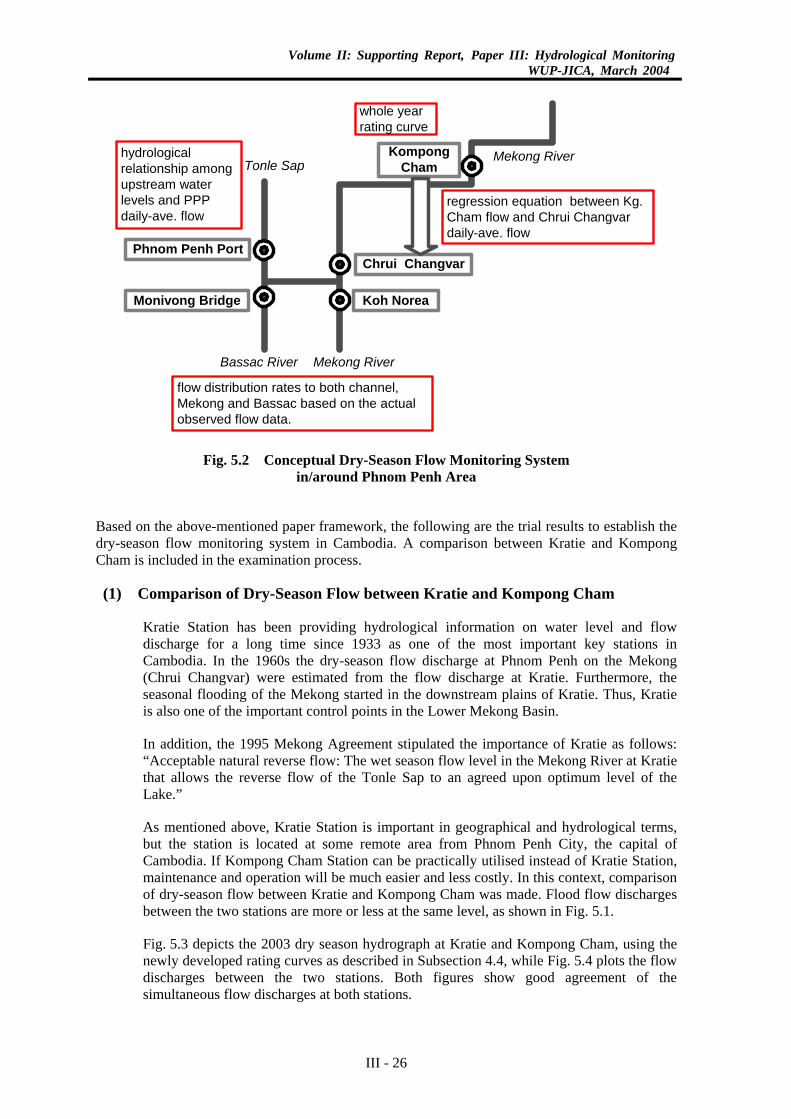
Prior to entrance of the 2003 dry season, the establishment of a dry-season flow monitoring system in this area was planned in the following process, in due consideration of the above-tabulated conditions:
(1) Discharge measurement activities will be continued at Kompong Cham in the same manner as the 2002 wet season. Then the rating curve applicable for the whole year shall be developed.
(2) At four stations in the Chak Tomuk junction, frequent discharge measurements within a day will be conducted so as to estimate the daily average discharges.
(3) Regression equation will be developed between discharges at Kompong Cham and daily average discharges at Chrui Changvar. Finally, continuous daily average discharges at Chrui Changvar will be computed using the developed regression equation.
(4) Also, some hydrological relationship among upstream water levels in the Great Lake and daily average discharges at Phnom Penh Port will be developed for computation of continuous daily discharges at Phnom Penh Port.
(5) Using observed daily average discharges at Koh Norea and Monivong Bridge, flow distribution rates into both channels in the dry season will be determined.
Based on the above process, the conceptual dry-season flow monitoring system is as schematised in Fig. 5.2.
III - 25
Volume II: Supporting Report, Paper III: Hydrological MonitoringWUP-JICA, March 2004
whole yearrating curve
KompongCham
Chrui Changvar
Koh NoreaMonivong Bridge
Bassac River Mekong River
Tonle SapMekong River
Phnom Penh Port
regression equation between Kg.Cham flow and Chrui Changvardaily-ave. flow
hydrologicalrelationship amongupstream waterlevels and PPPdaily-ave. flow
flow distribution rates to both channel,Mekong and Bassac based on the actualobserved flow data.
Fig. 5.2 Conceptual Dry-Season Flow Monitoring System in/around Phnom Penh Area
Based on the above-mentioned paper framework, the following are the trial results to establish the dry-season flow monitoring system in Cambodia. A comparison between Kratie and Kompong Cham is included in the examination process.
(1) Comparison of Dry-Season Flow between Kratie and Kompong Cham
Kratie Station has been providing hydrological information on water level and flow discharge for a long time since 1933 as one of the most important key stations in Cambodia. In the 1960s the dry-season flow discharge at Phnom Penh on the Mekong (Chrui Changvar) were estimated from the flow discharge at Kratie. Furthermore, the seasonal flooding of the Mekong started in the downstream plains of Kratie. Thus, Kratie is also one of the important control points in the Lower Mekong Basin.
In addition, the 1995 Mekong Agreement stipulated the importance of Kratie as follows: “Acceptable natural reverse flow: The wet season flow level in the Mekong River at Kratie that allows the reverse flow of the Tonle Sap to an agreed upon optimum level of the Lake.”
As mentioned above, Kratie Station is important in geographical and hydrological terms, but the station is located at some remote area from Phnom Penh City, the capital of Cambodia. If Kompong Cham Station can be practically utilised instead of Kratie Station, maintenance and operation will be much easier and less costly. In this context, comparison of dry-season flow between Kratie and Kompong Cham was made. Flood flow discharges between the two stations are more or less at the same level, as shown in Fig. 5.1.
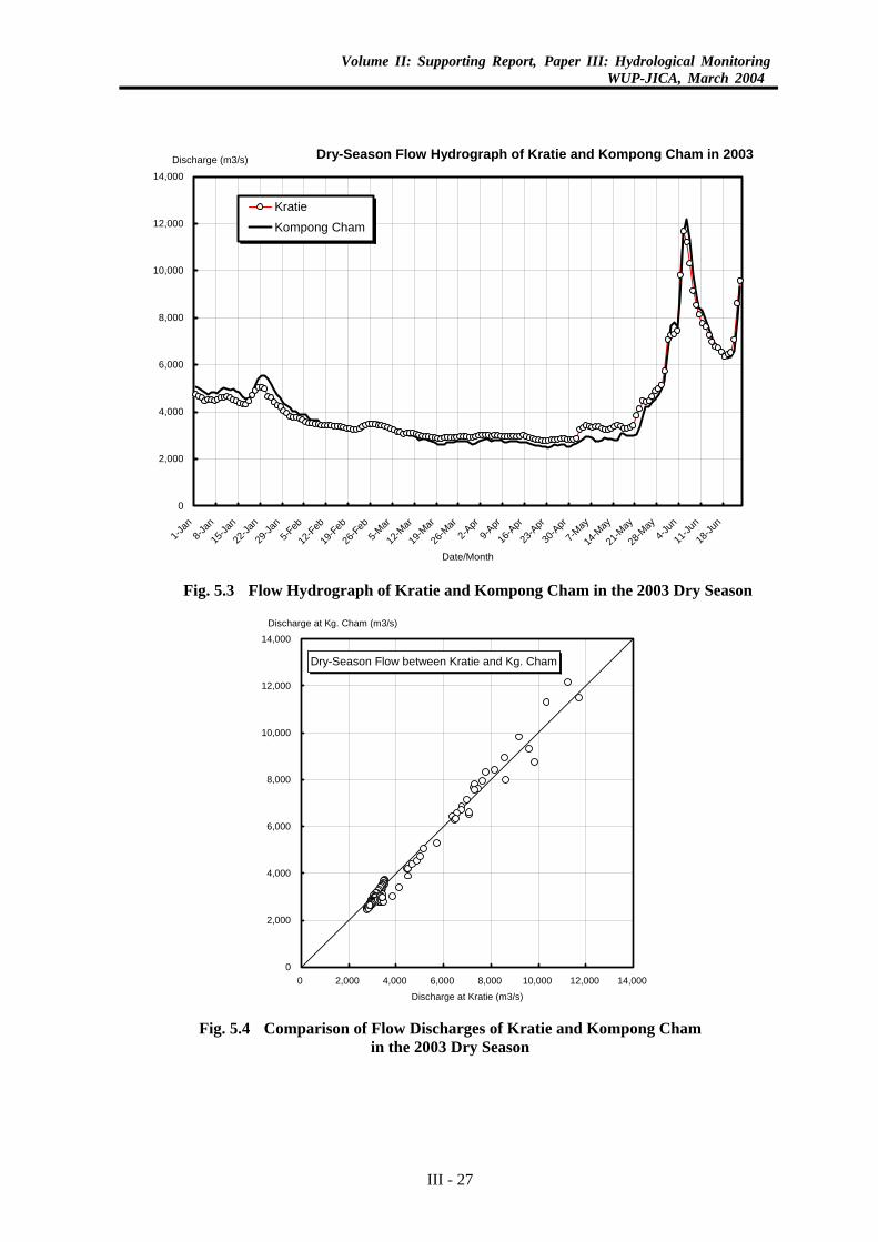
Fig. 5.3 depicts the 2003 dry season hydrograph at Kratie and Kompong Cham, using the newly developed rating curves as described in Subsection 4.4, while Fig. 5.4 plots the flow discharges between the two stations. Both figures show good agreement of the simultaneous flow discharges at both stations.
III - 26
Volume II: Supporting Report, Paper III: Hydrological MonitoringWUP-JICA, March 2004
Dry-Season Flow Hydrograph of Kratie and Kompong Cham in 2003
0
2,000
4,000
6,000
8,000
10,000
12,000
14,000
1-Jan
8-Jan
15-Ja
n
22-Ja
n
29-Ja
n5-F
eb
12-F
eb
19-F
eb
26-F
eb5-M
ar
12-M
ar
19-M
ar
26-M
ar2-A
pr9-A
pr
16-A
pr
23-A
pr
30-A
pr
7-May
14-M
ay
21-M
ay
28-M
ay4-J
un
11-Ju
n
18-Ju
n
Date/Month
Discharge (m3/s)
KratieKompong Cham
Fig. 5.3 Flow Hydrograph of Kratie and Kompong Cham in the 2003 Dry Season
Dry-Season Flow between Kratie and Kg. Cham
0
2,000
4,000
6,000
8,000
10,000
12,000
14,000
0 2,000 4,000 6,000 8,000 10,000 12,000 14,000
Discharge at Kratie (m3/s)
Discharge at Kg. Cham (m3/s)
Fig. 5.4 Comparison of Flow Discharges of Kratie and Kompong Cham
in the 2003 Dry Season
III - 27
Volume II: Supporting Report, Paper III: Hydrological MonitoringWUP-JICA, March 2004
In conclusion, the dry-season flows at Kompong Cham practically can be utilized as representative flows down to the Cambodian floodplains instead of the flows at Kratie, even though the flows at Kompong Cham are slightly affected by tidal fluctuations.
(2) Relationship of Dry-Season Flow between Kompong Cham and Chrui Changvar
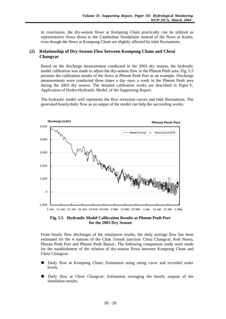
Based on the discharge measurement conducted in the 2003 dry season, the hydraulic model calibration was made to adjust the dry-season flow in the Phnom Penh area. Fig. 5.5 presents the calibration results of the flows at Phnom Penh Port as an example. Discharge measurements were conducted three times a day once a week in the Phnom Penh area during the 2003 dry season. The detailed calibration works are described in Paper V, Application of Hydro-Hydraulic Model, of the Supporting Report.
The hydraulic model well represents the flow recession curves and tidal fluctuations. The generated hourly/daily flow as an output of the model can help the succeeding works.
Phnom Penh Port
-1,000
0
1,000
2,000
3,000
4,000
5,000
1-Jan 11-Jan 21-Jan 31-Jan 10-Feb 20-Feb 2-Mar 12-Mar 22-Mar 1-Apr 11-Apr 21-Apr 1-May
Discharge [m3/s]
Model (hourly) Observed (ADCP)
Fig. 5.5 Hydraulic Model Calibration Results at Phnom Penh Port
for the 2003 Dry Season
From hourly flow discharges of the simulation results, the daily average flow has been estimated for the 4 stations of the Chak Tomuk junction: Chrui Changvar, Koh Norea, Phnom Penh Port and Phnom Penh Bassac. The following comparison study were made for the establishment of the relation of dry-season flows between Kompong Cham and Chrui Changvar:
Daily flow at Kompong Cham: Estimation using rating curve and recorded water levels.
Daily flow at Chrui Changvar: Estimation averaging the hourly outputs of the simulation results.
III - 28
Volume II: Supporting Report, Paper III: Hydrological MonitoringWUP-JICA, March 2004
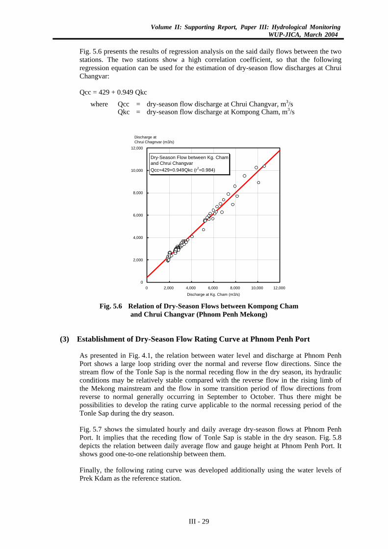
Fig. 5.6 presents the results of regression analysis on the said daily flows between the two stations. The two stations show a high correlation coefficient, so that the following regression equation can be used for the estimation of dry-season flow discharges at Chrui Changvar:
Qcc = 429 + 0.949 Qkc
where Qcc = dry-season flow discharge at Chrui Changvar, m3/s Qkc = dry-season flow discharge at Kompong Cham, m3/s
Dry-Season Flow between Kg. Chamand Chrui ChangvarQcc=429+0.949Qkc (r2=0.984)
0
2,000
4,000
6,000
8,000
10,000
12,000
0 2,000 4,000 6,000 8,000 10,000 12,000
Discharge at Kg. Cham (m3/s)
Discharge atChrui Chagnvar (m3/s)
Fig. 5.6 Relation of Dry-Season Flows between Kompong Cham
and Chrui Changvar (Phnom Penh Mekong)
(3) Establishment of Dry-Season Flow Rating Curve at Phnom Penh Port
As presented in Fig. 4.1, the relation between water level and discharge at Phnom Penh Port shows a large loop striding over the normal and reverse flow directions. Since the stream flow of the Tonle Sap is the normal receding flow in the dry season, its hydraulic conditions may be relatively stable compared with the reverse flow in the rising limb of the Mekong mainstream and the flow in some transition period of flow directions from reverse to normal generally occurring in September to October. Thus there might be possibilities to develop the rating curve applicable to the normal recessing period of the Tonle Sap during the dry season.
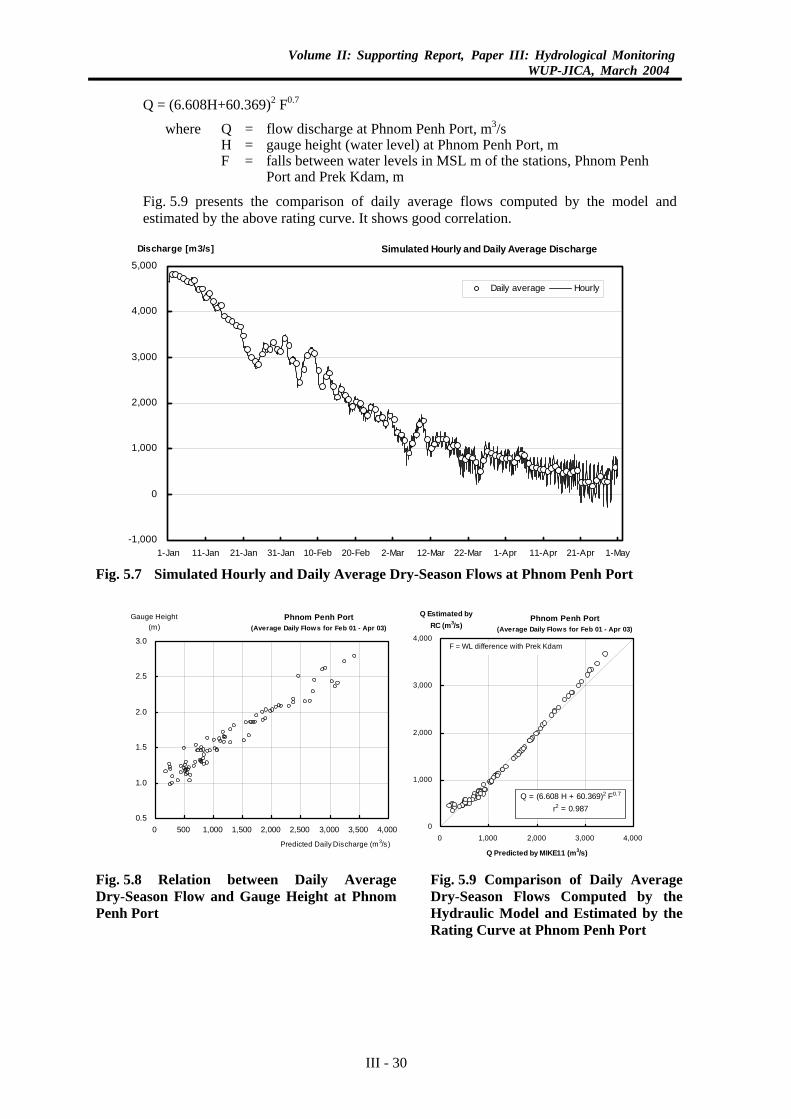
Fig. 5.7 shows the simulated hourly and daily average dry-season flows at Phnom Penh Port. It implies that the receding flow of Tonle Sap is stable in the dry season. Fig. 5.8 depicts the relation between daily average flow and gauge height at Phnom Penh Port. It shows good one-to-one relationship between them.
Finally, the following rating curve was developed additionally using the water levels of Prek Kdam as the reference station.
III - 29
Volume II: Supporting Report, Paper III: Hydrological MonitoringWUP-JICA, March 2004
Q = (6.608H+60.369)2 F0.7
where Q = flow discharge at Phnom Penh Port, m3/s H = gauge height (water level) at Phnom Penh Port, m F = falls between water levels in MSL m of the stations, Phnom Penh
Port and Prek Kdam, m
Fig. 5.9 presents the comparison of daily average flows computed by the model and estimated by the above rating curve. It shows good correlation.
Simulated Hourly and Daily Average Discharge
-1,000
0
1,000
2,000
3,000
4,000
5,000
1-Jan 11-Jan 21-Jan 31-Jan 10-Feb 20-Feb 2-Mar 12-Mar 22-Mar 1-Apr 11-Apr 21-Apr 1-May
Discharge [m3/s]
Daily average Hourly
Fig. 5.7 Simulated Hourly and Daily Average Dry-Season Flows at Phnom Penh Port
Phnom Penh Port(Average Daily Flows for Feb 01 - Apr 03)
0
1,000
2,000
3,000
4,000
0 1,000 2,000 3,000 4,000
Q Predicted by MIKE11 (m3/s)
Q Estimated byRC (m3/s)
F = WL difference with Prek Kdam
Q = (6.608 H + 60.369)2 F0.7
r2 = 0.987
Phnom Penh Port(Average Daily Flows for Feb 01 - Apr 03)
0.5
1.0
1.5
2.0
2.5
3.0
0 500 1,000 1,500 2,000 2,500 3,000 3,500 4,000
Predicted Daily Discharge (m3/s)
Gauge Height(m)
Fig. 5.8 Relation between Daily Average Dry-Season Flow and Gauge Height at Phnom Penh Port
Fig. 5.9 Comparison of Daily Average Dry-Season Flows Computed by the Hydraulic Model and Estimated by the Rating Curve at Phnom Penh Port
III - 30
Volume II: Supporting Report, Paper III: Hydrological MonitoringWUP-JICA, March 2004
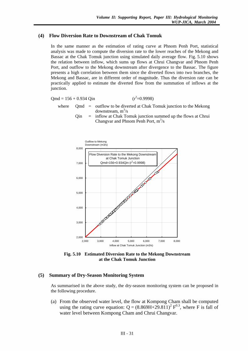
(4) Flow Diversion Rate to Downstream of Chak Tomuk
In the same manner as the estimation of rating curve at Phnom Penh Port, statistical analysis was made to compute the diversion rate to the lower reaches of the Mekong and Bassac at the Chak Tomuk junction using simulated daily average flow. Fig. 5.10 shows the relation between inflow, which sums up flows at Chrui Changvar and Phnom Penh Port, and outflow to the Mekong downstream after divergence to the Bassac. The figure presents a high correlation between them since the diverted flows into two branches, the Mekong and Bassac, are in different order of magnitude. Thus the diversion rate can be practically applied to estimate the diverted flow from the summation of inflows at the junction.
Qmd = 156 + 0.934 Qin (r2=0.9998)
where Qmd = outflow to be diverted at Chak Tomuk junction to the Mekong downstream, m3/s
Qin = inflow at Chak Tomuk junction summed up the flows at Chrui Changvar and Phnom Penh Port, m3/s
Flow Diversion Rate to the Mekong Downstreamat Chak Tomuk Junction
Qmd=156+0.934Qin (r2=0.9998)
2,000
3,000
4,000
5,000
6,000
7,000
8,000
2,000 3,000 4,000 5,000 6,000 7,000 8,000
Inflow at Chak Tomuk Junction (m3/s)
Outflow to MekongDownstream (m3/s)
Fig. 5.10 Estimated Diversion Rate to the Mekong Downstream
at the Chak Tomuk Junction
(5) Summary of Dry-Season Monitoring System
As summarised in the above study, the dry-season monitoring system can be proposed in the following procedure.
(a) From the observed water level, the flow at Kompong Cham shall be computed using the rating curve equation: Q = (8.869H+29.811)2 F0.3, where F is fall of water level between Kompong Cham and Chrui Changvar.
III - 31
Volume II: Supporting Report, Paper III: Hydrological MonitoringWUP-JICA, March 2004
(b) From the flow at Kompong Cham, the flow at Chrui Changvar shall be
computed using the regression equation: Qcc = 429 + 0.949 Qkc.
(c) From the observed water level, the normal receding flow at Phnom Penh Port shall be computed using the rating curve equation: Q = (6.608H+60.369)2 F0.7, where F is fall of water level between Prek Kdam and Phnom Penh Port.
(d) After summation of the flows at Chrui Changvar and Phnom Penh Port, the diversion rate to the Mekong downstream shall be computed using the regression equation: Qmd = 156 + 0.934 Qin
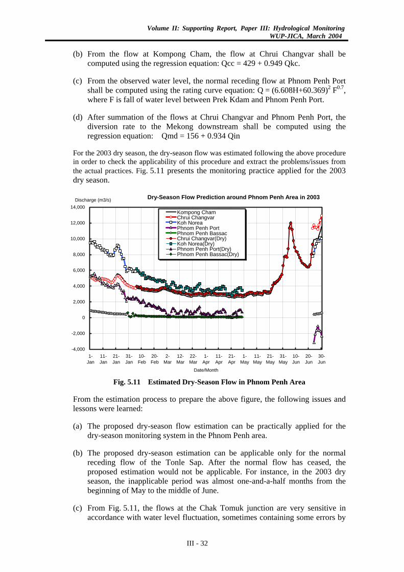
For the 2003 dry season, the dry-season flow was estimated following the above procedure in order to check the applicability of this procedure and extract the problems/issues from the actual practices. Fig. 5.11 presents the monitoring practice applied for the 2003 dry season.
Dry-Season Flow Prediction around Phnom Penh Area in 2003
-4,000
-2,000
0
2,000
4,000
6,000
8,000
10,000
12,000
14,000
1-Jan
11-Jan
21-Jan
31-Jan
10-Feb
20-Feb
2-Mar
12-Mar
22-Mar
1-Apr
11-Apr
21-Apr
1-May
11-May
21-May
31-May
10-Jun
20-Jun
30-Jun
Date/Month
Discharge (m3/s)
Kompong ChamChrui ChangvarKoh NoreaPhnom Penh PortPhnom Penh BassacChrui Changvar(Dry)Koh Norea(Dry)Phnom Penh Port(Dry)Phnom Penh Bassac(Dry)
Fig. 5.11 Estimated Dry-Season Flow in Phnom Penh Area
From the estimation process to prepare the above figure, the following issues and lessons were learned:
(a) The proposed dry-season flow estimation can be practically applied for the dry-season monitoring system in the Phnom Penh area.
(b) The proposed dry-season estimation can be applicable only for the normal receding flow of the Tonle Sap. After the normal flow has ceased, the proposed estimation would not be applicable. For instance, in the 2003 dry season, the inapplicable period was almost one-and-a-half months from the beginning of May to the middle of June.
(c) From Fig. 5.11, the flows at the Chak Tomuk junction are very sensitive in accordance with water level fluctuation, sometimes containing some errors by
III - 32
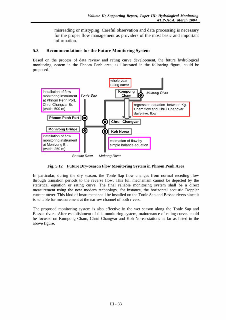
Volume II: Supporting Report, Paper III: Hydrological MonitoringWUP-JICA, March 2004
misreading or mistyping. Careful observation and data processing is necessary for the proper flow management as providers of the most basic and important information.
5.3 Recommendations for the Future Monitoring System
Based on the process of data review and rating curve development, the future hydrological monitoring system in the Phnom Penh area, as illustrated in the following figure, could be proposed.
whole yearrating curve
KompongCham
Chrui Changvar
Koh NoreaMonivong Bridge
Bassac River Mekong River
Tonle SapMekong River
Phnom Penh Port
regression equation between Kg.Cham flow and Chrui Changvardaily-ave. flow
installation of flowmonitoring instrumentat Phnom Penh Port,Chrui Changvar Br.(width: 500 m)
installation of flowmonitoring instrumentat Monivong Br.(width: 250 m)
estimation of flow bysimple balance equation
Fig. 5.12 Future Dry-Season Flow Monitoring System in Phnom Penh Area
In particular, during the dry season, the Tonle Sap flow changes from normal receding flow through transition periods to the reverse flow. This full mechanism cannot be depicted by the statistical equation or rating curve. The final reliable monitoring system shall be a direct measurement using the new modern technology, for instance, the horizontal acoustic Doppler current meter. This kind of instrument shall be installed on the Tonle Sap and Bassac rivers since it is suitable for measurement at the narrow channel of both rivers.
The proposed monitoring system is also effective in the wet season along the Tonle Sap and Bassac rivers. After establishment of this monitoring system, maintenance of rating curves could be focused on Kompong Cham, Chrui Changvar and Koh Norea stations as far as listed in the above figure.
III - 33
Volume II: Supporting Report, Paper III: Hydrological MonitoringWUP-JICA, March 2004
6. HYDROLOGICAL FUNCTIONS OF CAMBODIAN FLOODPLAINS
6.1 Previous Study Results
The most intensive discharge measurements for the period from 1963 to 1965 covering the Mekong Delta were made by SOGREA under the UNESCO Project. The locations for discharge measurement as well as water level observation covered almost all major flow paths of the branches of the Mekong River system encompassing those from Kratie to the downstream ends.
The primary objective of this discharge measurement campaign was to construct the mathematical simulation model of the Mekong Delta including the Cambodian floodplains. As anticipated, the target areas were too large and mobilization capacity was limited due to the insufficient transportation system. Thus inconsistencies and inconveniences in understanding the flow balance were encountered in the project. However, a part of the measured data is still very useful and helpful in understanding the water balance, in particular, during the flood season.
In this section, useful information is summarized below from the reports of the above-mentioned project.
Kratie to Chrui Changvar
Intensive discharge measurements were made during the 1964 flood season. In particular, discharge measurements were made at various points along the mainstream in the stretch from Kratie down to Chrui Changvar (Phnom Penh) for 4 days from September 29 to October 2. The results can be regarded as similar to the simultaneous measurements. Combining the discharge data tabulated in the hydrological yearbook, the results are schematised in Fig. 6.1. The figure characterizes the following flood conditions.
(1) Kratie to Kompong Cham
Along the mainstream from Kratie to Kompong Cham, the floodplains on the right bank are narrow and have no flood paths connecting with the lower floodplains. Thus the flood retarding capacity is relatively small. On the other hand, the hills on the left bank are situated further back from the river course and the area in-between is comparatively flat. At high water the floodplain between Chhlong and Kompong Cham (Tonle Bet) can act as a lateral outfall and as a wide flood path parallel to the Mekong.
Fig. 6.1 shows that the total discharge regulated was 3,650 m3/s, which was equivalent to 8% regulation of the Kratie flood discharge of 48,000 m3/s. Some 880 m3/s returned to the mainstream upstream of the Kompong Cham Station, and the discharge of 2,080 m3/s passed through the Moat Khmung Bridge site after regulation of the floodplain’s storage function.
The flood hydrographs of Kratie, Kompong Cham and Phnom Penh are depicted from the hydrologic yearbook in Fig. 6.2. The flood retarding effects cannot be detected from this figure due to insufficient reliability of rating curves.
III - 34
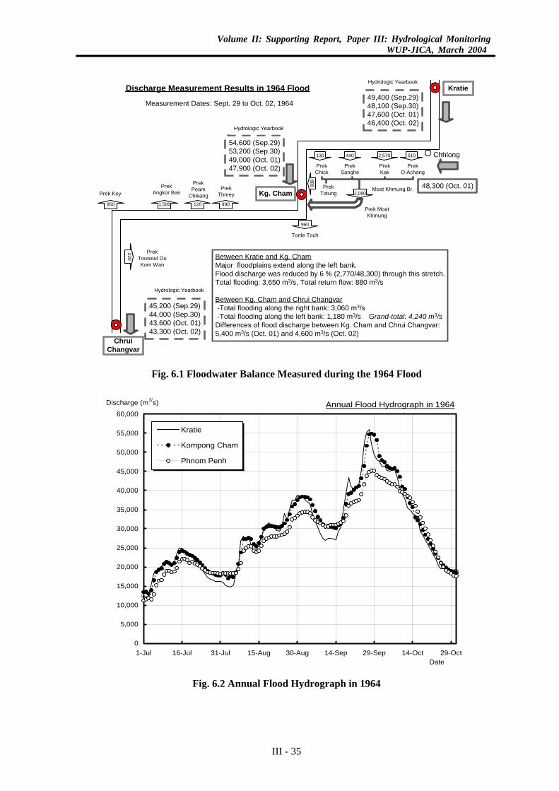
Volume II: Supporting Report, Paper III: Hydrological MonitoringWUP-JICA, March 2004
Kratie
Kg. Cham
Chhlong
ChruiChangvar
PrekO Achang
510
PrekKak
2,570
PrekSanghe
440
PrekChick
130
880
PrekTotung 2,080
Moat Khmung Br.
Prek MoatKhmung
960
Tonle Toch
490
PrekThmey
120
PrekPeam
Chikang950
Prek Koy
1,500
PrekAngkor Ban
220
PrekTouwoul OuKom Wan
Discharge Measurement Results in 1964 Flood
Measurement Dates: Sept. 29 to Oct. 02, 196449,400 (Sep.29)48,100 (Sep.30)47,600 (Oct. 01)46,400 (Oct. 02)
54,600 (Sep.29)53,200 (Sep.30)49,000 (Oct. 01)47,900 (Oct. 02)
48,300 (Oct. 01)
45,200 (Sep.29)44,000 (Sep.30)43,600 (Oct. 01)43,300 (Oct. 02)
Between Kratie and Kg. ChamMajor floodplains extend along the left bank.Flood discharge was reduced by 6 % (2,770/48,300) through this stretch.Total flooding: 3,650 m3/s, Total return flow: 880 m3/s
Between Kg. Cham and Chrui Changvar -Total flooding along the right bank: 3,060 m3/s -Total flooding along the left bank: 1,180 m3/s Grand-total: 4,240 m3/sDifferences of flood discharge between Kg. Cham and Chrui Changvar:5,400 m3/s (Oct. 01) and 4,600 m3/s (Oct. 02)
Hydrologic Yearbook
Hydrologic Yearbook
Hydrologic Yearbook
Fig. 6.1 Floodwater Balance Measured during the 1964 Flood
Annual Flood Hydrograph in 1964
0
5,000
10,000
15,000
20,000
25,000
30,000
35,000
40,000
45,000
50,000
55,000
60,000
1-Jul 16-Jul 31-Jul 15-Aug 30-Aug 14-Sep 29-Sep 14-Oct 29-OctDate
Discharge (m3/s)
Kratie
Kompong Cham
Phnom Penh
Fig. 6.2 Annual Flood Hydrograph in 1964
III - 35
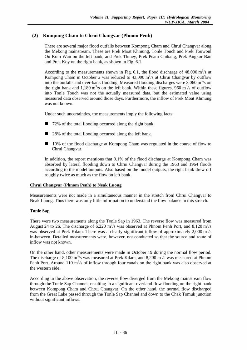
Volume II: Supporting Report, Paper III: Hydrological MonitoringWUP-JICA, March 2004
(2) Kompong Cham to Chrui Changvar (Phnom Penh)
There are several major flood outfalls between Kompong Cham and Chrui Changvar along the Mekong mainstream. These are Prek Moat Khmung, Tonle Touch and Prek Touwoul Ou Kom Wan on the left bank, and Prek Thmey, Prek Peam Chikang, Prek Angkor Ban and Prek Koy on the right bank, as shown in Fig. 6.1.
According to the measurements shown in Fig. 6.1, the flood discharge of 48,000 m3/s at Kompong Cham in October 2 was reduced to 43,000 m3/s at Chrui Changvar by outflow into the outfalls and over-bank flooding. Measured flooding discharges were 3,060 m3/s on the right bank and 1,180 m3/s on the left bank. Within these figures, 960 m3/s of outflow into Tonle Touch was not the actually measured data, but the estimated value using measured data observed around those days. Furthermore, the inflow of Prek Moat Khmung was not known.
Under such uncertainties, the measurements imply the following facts:
72% of the total flooding occurred along the right bank.
28% of the total flooding occurred along the left bank.
10% of the flood discharge at Kompong Cham was regulated in the course of flow to Chrui Changvar.
In addition, the report mentions that 9.1% of the flood discharge at Kompong Cham was absorbed by lateral flooding down to Chrui Changvar during the 1963 and 1964 floods according to the model outputs. Also based on the model outputs, the right bank drew off roughly twice as much as the flow on left bank.
Chrui Changvar (Phnom Penh) to Neak Luong
Measurements were not made in a simultaneous manner in the stretch from Chrui Changvar to Neak Luong. Thus there was only little information to understand the flow balance in this stretch.
Tonle Sap
There were two measurements along the Tonle Sap in 1963. The reverse flow was measured from August 24 to 26. The discharge of 6,220 m3/s was observed at Phnom Penh Port, and 8,120 m3/s was observed at Prek Kdam. There was a clearly significant inflow of approximately 2,000 m3/s in-between. Detailed measurements were, however, not conducted so that the source and route of inflow was not known.
On the other hand, other measurements were made in October 19 during the normal flow period. The discharge of 8,100 m3/s was measured at Prek Kdam, and 8,200 m3/s was measured at Phnom Penh Port. Around 110 m3/s of inflow through four canals on the right bank was also observed at the western side.
According to the above observation, the reverse flow diverged from the Mekong mainstream flow through the Tonle Sap Channel, resulting in a significant overland flow flooding on the right bank between Kompong Cham and Chrui Changvar. On the other hand, the normal flow discharged from the Great Lake passed through the Tonle Sap Channel and down to the Chak Tomuk junction without significant inflows.
III - 36
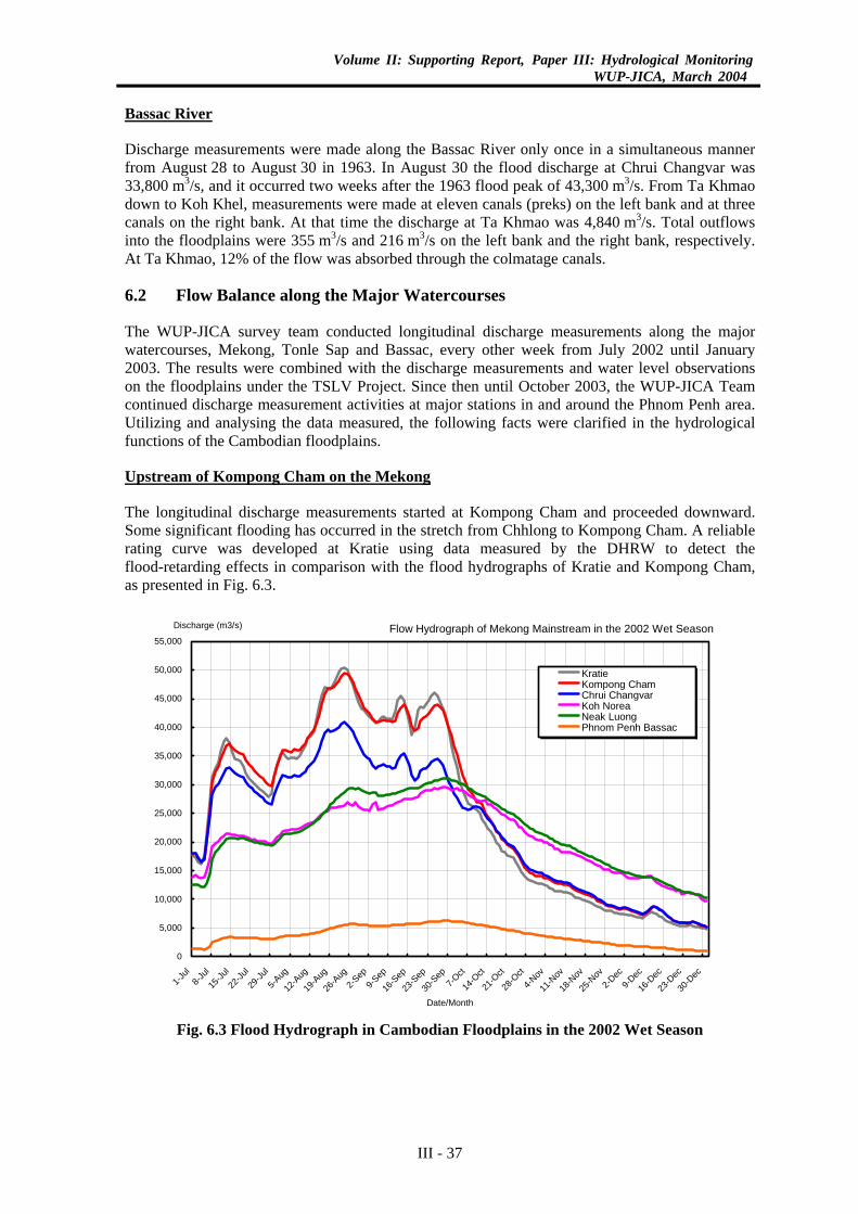
Volume II: Supporting Report, Paper III: Hydrological MonitoringWUP-JICA, March 2004
Bassac River
Discharge measurements were made along the Bassac River only once in a simultaneous manner from August 28 to August 30 in 1963. In August 30 the flood discharge at Chrui Changvar was 33,800 m3/s, and it occurred two weeks after the 1963 flood peak of 43,300 m3/s. From Ta Khmao down to Koh Khel, measurements were made at eleven canals (preks) on the left bank and at three canals on the right bank. At that time the discharge at Ta Khmao was 4,840 m3/s. Total outflows into the floodplains were 355 m3/s and 216 m3/s on the left bank and the right bank, respectively. At Ta Khmao, 12% of the flow was absorbed through the colmatage canals.
6.2 Flow Balance along the Major Watercourses
The WUP-JICA survey team conducted longitudinal discharge measurements along the major watercourses, Mekong, Tonle Sap and Bassac, every other week from July 2002 until January 2003. The results were combined with the discharge measurements and water level observations on the floodplains under the TSLV Project. Since then until October 2003, the WUP-JICA Team continued discharge measurement activities at major stations in and around the Phnom Penh area. Utilizing and analysing the data measured, the following facts were clarified in the hydrological functions of the Cambodian floodplains.
Upstream of Kompong Cham on the Mekong
The longitudinal discharge measurements started at Kompong Cham and proceeded downward. Some significant flooding has occurred in the stretch from Chhlong to Kompong Cham. A reliable rating curve was developed at Kratie using data measured by the DHRW to detect the flood-retarding effects in comparison with the flood hydrographs of Kratie and Kompong Cham, as presented in Fig. 6.3.
Flow Hydrograph of Mekong Mainstream in the 2002 Wet Season
0
5,000
10,000
15,000
20,000
25,000
30,000
35,000
40,000
45,000
50,000
55,000
1-Jul
8-Jul
15-Ju
l
22-Ju
l
29-Ju
l
5-Aug
12-A
ug
19-A
ug
26-A
ug2-S
ep9-S
ep
16-S
ep
23-S
ep
30-S
ep7-O
ct
14-O
ct
21-O
ct
28-O
ct
4-Nov
11-N
ov
18-N
ov
25-N
ov2-D
ec9-D
ec
16-D
ec
23-D
ec
30-D
ec
Date/Month
Discharge (m3/s)
KratieKompong ChamChrui ChangvarKoh NoreaNeak LuongPhnom Penh Bassac
Fig. 6.3 Flood Hydrograph in Cambodian Floodplains in the 2002 Wet Season
III - 37
Volume II: Supporting Report, Paper III: Hydrological MonitoringWUP-JICA, March 2004
Fig. 6.3 shows three flood peaks in the 2002 wet season. As summarized in the following table, the flooding functions of flood peak attenuation could be estimated as 900 to 2,240 m3/s. These functions are equivalent to 2 to 5% of flow discharge at Kratie.
Table 6.1 Flooding Functions between Kratie and Kompong Cham
in the 2002 Wet Season Flood Discharge (m3/s) Date
Kratie Kompong Cham Flood Attenuation
Rate (m3/s) August 24 50,300 49,400 900 September 13 45,460 43,480 1,980 September 25 45,980 43,740 2,240
In addition, the related hydrological data of project-based observations were obtained for this area. In the 2002 wet season, the improvement project of National Road No. 7 was implemented in the stretch from Kizuna Bridge to Suong under Japan’s Grant Aid Programme. Under this project, the water level over the project area was observed in the flood season.
Fig. 6.4 shows the observed water level at Moat Khmung Bridge during the floods in 2002. According to the report of the project office, reverse flow from the river mouth occurred in the initial stage of the flood season. Then normal downward flow occurred after full impoundment of floodwaters in the floodplains. The normal flow started on August 8, 2002, according to the report of the project office. This fact might be reasonable compared with the water levels at Kompong Cham and the Bridge as shown in Fig. 6.4.
Water Level in 2002 at Kompong Cham and Moat Khmung Br.
4
6
8
10
12
14
16
18
1-Jun
8-Jun
15-Ju
n
22-Ju
n
29-Ju
n6-J
ul
13-Ju
l
20-Ju
l
27-Ju
l
3-Aug
10-A
ug
17-A
ug
24-A
ug
31-A
ug7-S
ep
14-S
ep
21-S
ep
28-S
ep5-O
ct
12-O
ct
19-O
ct
26-O
ct
Date/Month
Water Level(Gauge Height in m)
Kompong Cham
Moat KhmungBr.
Fig. 6.4 Observed Water Level at Moat Khmung Bridge in 2002
Furthermore, the project office measured floodwater velocity at their major water level stations by a current meter during the 2000 floods. Thus the following procedures were taken for estimation of the flood hydrograph in 2002, utilizing the velocity measurement data:
III - 38
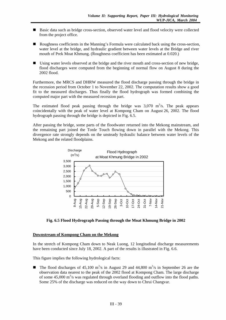
Volume II: Supporting Report, Paper III: Hydrological MonitoringWUP-JICA, March 2004
Basic data such as bridge cross-section, observed water level and flood velocity were collected
from the project office.
Roughness coefficients in the Manning’s Formula were calculated back using the cross-section, water level at the bridge, and hydraulic gradient between water levels at the Bridge and river mouth of Prek Moat Khmung. (Roughness coefficient has been estimated at 0.020.)
Using water levels observed at the bridge and the river mouth and cross-section of new bridge, flood discharges were computed from the beginning of normal flow on August 8 during the 2002 flood.
Furthermore, the MRCS and DHRW measured the flood discharge passing through the bridge in the recession period from October 1 to November 22, 2002. The computation results show a good fit to the measured discharges. Thus finally the flood hydrograph was formed combining the computed major part with the measured recession part.
The estimated flood peak passing through the bridge was 3,070 m3/s. The peak appears coincidentally with the peak of water level at Kompong Cham on August 26, 2002. The flood hydrograph passing through the bridge is depicted in Fig. 6.5.
After passing the bridge, some parts of the floodwater returned into the Mekong mainstream, and the remaining part joined the Tonle Touch flowing down in parallel with the Mekong. This divergence rate strongly depends on the unsteady hydraulic balance between water levels of the Mekong and the related floodplains.
Flood Hydrographat Moat Khmung Bridge in 2002
0500
1,0001,5002,0002,5003,0003,500
8-A
ug
15-A
ug
22-A
ug
29-A
ug
5-S
ep
12-S
ep
19-S
ep
26-S
ep
3-O
ct
10-O
ct
17-O
ct
24-O
ct
31-O
ct
7-N
ov
14-N
ov
21-N
ov
Discharge(m3/s)
Fig. 6.5 Flood Hydrograph Passing through the Moat Khmung Bridge in 2002
Downstream of Kompong Cham on the Mekong
In the stretch of Kompong Cham down to Neak Luong, 12 longitudinal discharge measurements have been conducted since July 18, 2002. A part of the results is illustrated in Fig. 6.6.
This figure implies the following hydrological facts:
The flood discharges of 45,100 m3/s in August 29 and 44,800 m3/s in September 26 are the observation data nearest to the peak of the 2002 flood at Kompong Cham. The large discharge of some 45,000 m3/s was regulated through overland flooding and outflow into the flood paths. Some 25% of the discharge was reduced on the way down to Chrui Changvar.
III - 39
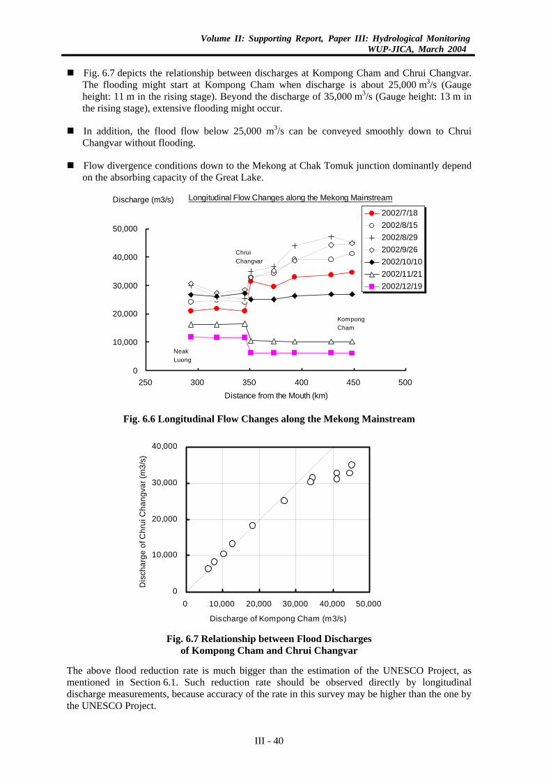
Volume II: Supporting Report, Paper III: Hydrological MonitoringWUP-JICA, March 2004
Fig. 6.7 depicts the relationship between discharges at Kompong Cham and Chrui Changvar.
The flooding might start at Kompong Cham when discharge is about 25,000 m3/s (Gauge height: 11 m in the rising stage). Beyond the discharge of 35,000 m3/s (Gauge height: 13 m in the rising stage), extensive flooding might occur.
In addition, the flood flow below 25,000 m3/s can be conveyed smoothly down to Chrui Changvar without flooding.
Flow divergence conditions down to the Mekong at Chak Tomuk junction dominantly depend on the absorbing capacity of the Great Lake.
Longitudinal Flow Changes along the Mekong Mainstream
0
10,000
20,000
30,000
40,000
50,000
250 300 350 400 450 500Distance from the Mouth (km)
Discharge (m3/s)2002/7/182002/8/152002/8/292002/9/262002/10/102002/11/212002/12/19
KompongCham
ChruiChangvar
NeakLuong
Fig. 6.6 Longitudinal Flow Changes along the Mekong Mainstream
0
10,000
20,000
30,000
40,000
0 10,000 20,000 30,000 40,000 50,000
Discharge of Kompong Cham (m3/s)
Dis
char
ge o
f Chr
ui C
hang
var (
m3/
s)
Fig. 6.7 Relationship between Flood Discharges
of Kompong Cham and Chrui Changvar
The above flood reduction rate is much bigger than the estimation of the UNESCO Project, as mentioned in Section 6.1. Such reduction rate should be observed directly by longitudinal discharge measurements, because accuracy of the rate in this survey may be higher than the one by the UNESCO Project.
III - 40
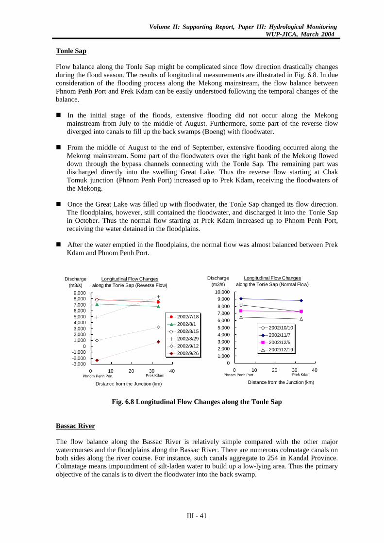
Volume II: Supporting Report, Paper III: Hydrological MonitoringWUP-JICA, March 2004
Tonle Sap
Flow balance along the Tonle Sap might be complicated since flow direction drastically changes during the flood season. The results of longitudinal measurements are illustrated in Fig. 6.8. In due consideration of the flooding process along the Mekong mainstream, the flow balance between Phnom Penh Port and Prek Kdam can be easily understood following the temporal changes of the balance.
In the initial stage of the floods, extensive flooding did not occur along the Mekong mainstream from July to the middle of August. Furthermore, some part of the reverse flow diverged into canals to fill up the back swamps (Boeng) with floodwater.
From the middle of August to the end of September, extensive flooding occurred along the Mekong mainstream. Some part of the floodwaters over the right bank of the Mekong flowed down through the bypass channels connecting with the Tonle Sap. The remaining part was discharged directly into the swelling Great Lake. Thus the reverse flow starting at Chak Tomuk junction (Phnom Penh Port) increased up to Prek Kdam, receiving the floodwaters of the Mekong.
Once the Great Lake was filled up with floodwater, the Tonle Sap changed its flow direction. The floodplains, however, still contained the floodwater, and discharged it into the Tonle Sap in October. Thus the normal flow starting at Prek Kdam increased up to Phnom Penh Port, receiving the water detained in the floodplains.
After the water emptied in the floodplains, the normal flow was almost balanced between Prek Kdam and Phnom Penh Port.
Longitudinal Flow Changesalong the Tonle Sap (Reverse Flow)
-3,000-2,000-1,000
01,0002,0003,0004,0005,0006,0007,0008,0009,000
0 10 20 30 40
Distance from the Junction (km)
Discharge(m3/s)
2002/7/182002/8/12002/8/152002/8/292002/9/122002/9/26
Phnom Penh Port Prek Kdam
Longitudinal Flow Changesalong the Tonle Sap (Normal Flow)
01,0002,0003,0004,0005,0006,0007,0008,0009,000
10,000
0 10 20 30 40
Distance from the Junction (km)
Discharge(m3/s)
2002/10/102002/11/72002/12/52002/12/19
Prek KdamPhnom Penh Port
Fig. 6.8 Longitudinal Flow Changes along the Tonle Sap
Bassac River
The flow balance along the Bassac River is relatively simple compared with the other major watercourses and the floodplains along the Bassac River. There are numerous colmatage canals on both sides along the river course. For instance, such canals aggregate to 254 in Kandal Province. Colmatage means impoundment of silt-laden water to build up a low-lying area. Thus the primary objective of the canals is to divert the floodwater into the back swamp.
III - 41

Volume II: Supporting Report, Paper III: Hydrological MonitoringWUP-JICA, March 2004
Fig. 6.9 illustrates the results of discharge measurements. As the flood discharge increases, the rate of discharge reduction also increases. When the peak discharge of 6,100 m3/s occurred at Monivong Bridge in September 26, 2100 m3/s of flow was absorbed by the floodplains through the canals in the stretch down to Koh Khel. Absorbed flow was equivalent to one-third of the peak discharge at Monivong Bridge. This rate was also much bigger than the one measured by the UNESCO Project.
Furthermore, diverted floodwaters did not return in this stretch even through the same canals according to the figure. The floodwaters diverted may have flown down the floodplains and discharged through the far downstream tributaries or canals.
Longitudinal Flow Changesalong the Bassac
0
1,000
2,000
3,000
4,000
5,000
6,000
7,000
0 10 20 30 40 50
Distance from the Junction (km)
Discharge (m3/s)2002/7/182002/8/152002/8/292002/9/262002/10/102002/11/212002/12/19
Koh Khel
Phnom PenhBassac
Ta Khmao
Fig. 6.9 Longitudinal Flow Changes along the Bassac River
6.3 Hydrological Functions of Cambodian Floodplains
Since the flooding conditions have been examined in the preceding section, the hydrological functions of the Cambodian floodplains will be described as a summary.
Flooding Conditions and Effects in the Cambodian Floodplains
By comparing the mainstream flow at Kompong Cham and the Tonle Sap flow, the flooding conditions in the Cambodian floodplains could be described as follows:
(1) At some time near the onset of the rising limb of the Mekong mainstream flow, the Tonle Sap changes its flow direction from normal to reverse during which stream water flows towards the Great Lake.
(2) When the water level at Kompong Cham becomes higher than 11 m in gauge height, flooding will start in the floodplains and reverse flow of the Tonle Sap starts to increase at the same time. At this moment, the discharge at Kompong Cham reaches at 25,000 m3/s.
(3) Further, the water level increases in the flood season. When it exceeds 12 m in gauge height at Kompong Cham, intensive flooding occurs over the floodplains. At this moment, the discharge reaches 30,000 m3/s.
(4) Flood peak on the Tonle Sap coincides with the peak on the mainstream.
III - 42
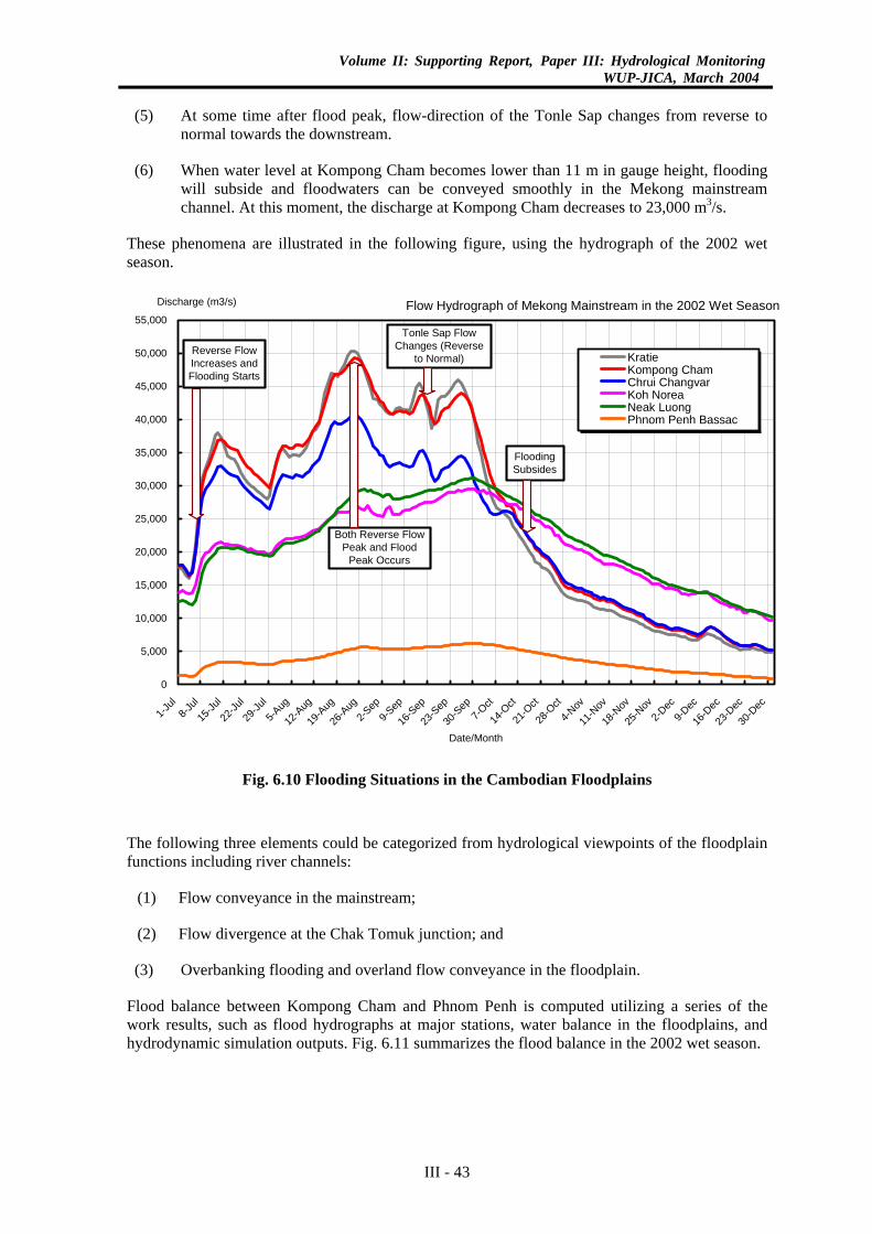
Volume II: Supporting Report, Paper III: Hydrological MonitoringWUP-JICA, March 2004
(5) At some time after flood peak, flow-direction of the Tonle Sap changes from reverse to
normal towards the downstream.
(6) When water level at Kompong Cham becomes lower than 11 m in gauge height, flooding will subside and floodwaters can be conveyed smoothly in the Mekong mainstream channel. At this moment, the discharge at Kompong Cham decreases to 23,000 m3/s.
These phenomena are illustrated in the following figure, using the hydrograph of the 2002 wet season.
Flow Hydrograph of Mekong Mainstream in the 2002 Wet Season
0
5,000
10,000
15,000
20,000
25,000
30,000
35,000
40,000
45,000
50,000
55,000
1-Jul
8-Jul
15-Ju
l
22-Ju
l
29-Ju
l
5-Aug
12-A
ug
19-A
ug
26-A
ug2-S
ep9-S
ep
16-S
ep
23-S
ep
30-S
ep7-O
ct
14-O
ct
21-O
ct
28-O
ct
4-Nov
11-N
ov
18-N
ov
25-N
ov2-D
ec9-D
ec
16-D
ec
23-D
ec
30-D
ec
Date/Month
Discharge (m3/s)
KratieKompong ChamChrui ChangvarKoh NoreaNeak LuongPhnom Penh Bassac
Both Reverse FlowPeak and Flood
Peak Occurs
Reverse FlowIncreases andFlooding Starts
Tonle Sap FlowChanges (Reverse
to Normal)
FloodingSubsides
Fig. 6.10 Flooding Situations in the Cambodian Floodplains
The following three elements could be categorized from hydrological viewpoints of the floodplain functions including river channels:
(1) Flow conveyance in the mainstream;
(2) Flow divergence at the Chak Tomuk junction; and
(3) Overbanking flooding and overland flow conveyance in the floodplain.
Flood balance between Kompong Cham and Phnom Penh is computed utilizing a series of the work results, such as flood hydrographs at major stations, water balance in the floodplains, and hydrodynamic simulation outputs. Fig. 6.11 summarizes the flood balance in the 2002 wet season.
III - 43
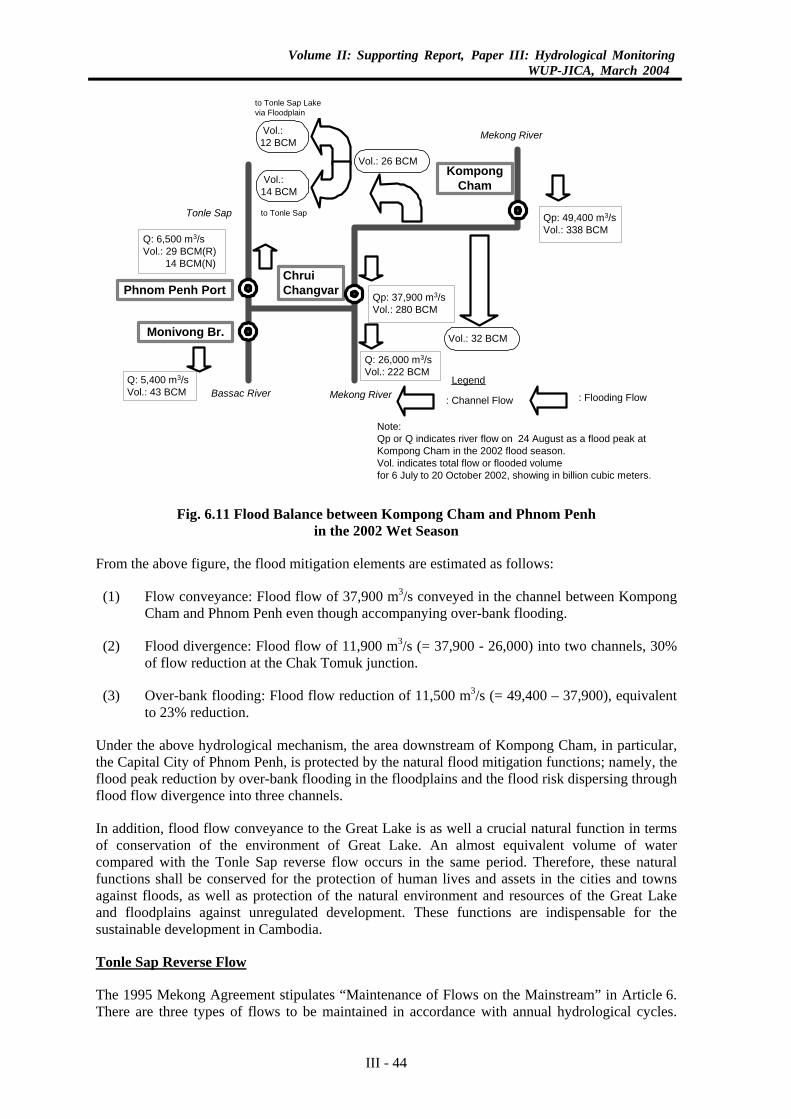
Volume II: Supporting Report, Paper III: Hydrological MonitoringWUP-JICA, March 2004
Qp: 49,400 m3/sVol.: 338 BCM
KompongCham
ChruiChangvar
Monivong Br.
Phnom Penh Port
Bassac River Mekong River
Tonle Sap
Mekong River
Qp: 37,900 m3/sVol.: 280 BCM
Vol.: 32 BCM
Q: 5,400 m3/sVol.: 43 BCM
Q: 6,500 m3/sVol.: 29 BCM(R) 14 BCM(N)
Vol.: 26 BCM
Vol.:14 BCM
Vol.:12 BCM
to Tonle Sap
to Tonle Sap Lakevia Floodplain
Legend
Note:Qp or Q indicates river flow on 24 August as a flood peak atKompong Cham in the 2002 flood season.Vol. indicates total flow or flooded volumefor 6 July to 20 October 2002, showing in billion cubic meters.
: Channel Flow : Flooding Flow
Q: 26,000 m3/sVol.: 222 BCM
Fig. 6.11 Flood Balance between Kompong Cham and Phnom Penh in the 2002 Wet Season
From the above figure, the flood mitigation elements are estimated as follows:
(1) Flow conveyance: Flood flow of 37,900 m3/s conveyed in the channel between Kompong Cham and Phnom Penh even though accompanying over-bank flooding.
(2) Flood divergence: Flood flow of 11,900 m3/s (= 37,900 - 26,000) into two channels, 30% of flow reduction at the Chak Tomuk junction.
(3) Over-bank flooding: Flood flow reduction of 11,500 m3/s (= 49,400 – 37,900), equivalent to 23% reduction.
Under the above hydrological mechanism, the area downstream of Kompong Cham, in particular, the Capital City of Phnom Penh, is protected by the natural flood mitigation functions; namely, the flood peak reduction by over-bank flooding in the floodplains and the flood risk dispersing through flood flow divergence into three channels.
In addition, flood flow conveyance to the Great Lake is as well a crucial natural function in terms of conservation of the environment of Great Lake. An almost equivalent volume of water compared with the Tonle Sap reverse flow occurs in the same period. Therefore, these natural functions shall be conserved for the protection of human lives and assets in the cities and towns against floods, as well as protection of the natural environment and resources of the Great Lake and floodplains against unregulated development. These functions are indispensable for the sustainable development in Cambodia.
Tonle Sap Reverse Flow
The 1995 Mekong Agreement stipulates “Maintenance of Flows on the Mainstream” in Article 6. There are three types of flows to be maintained in accordance with annual hydrological cycles.
III - 44
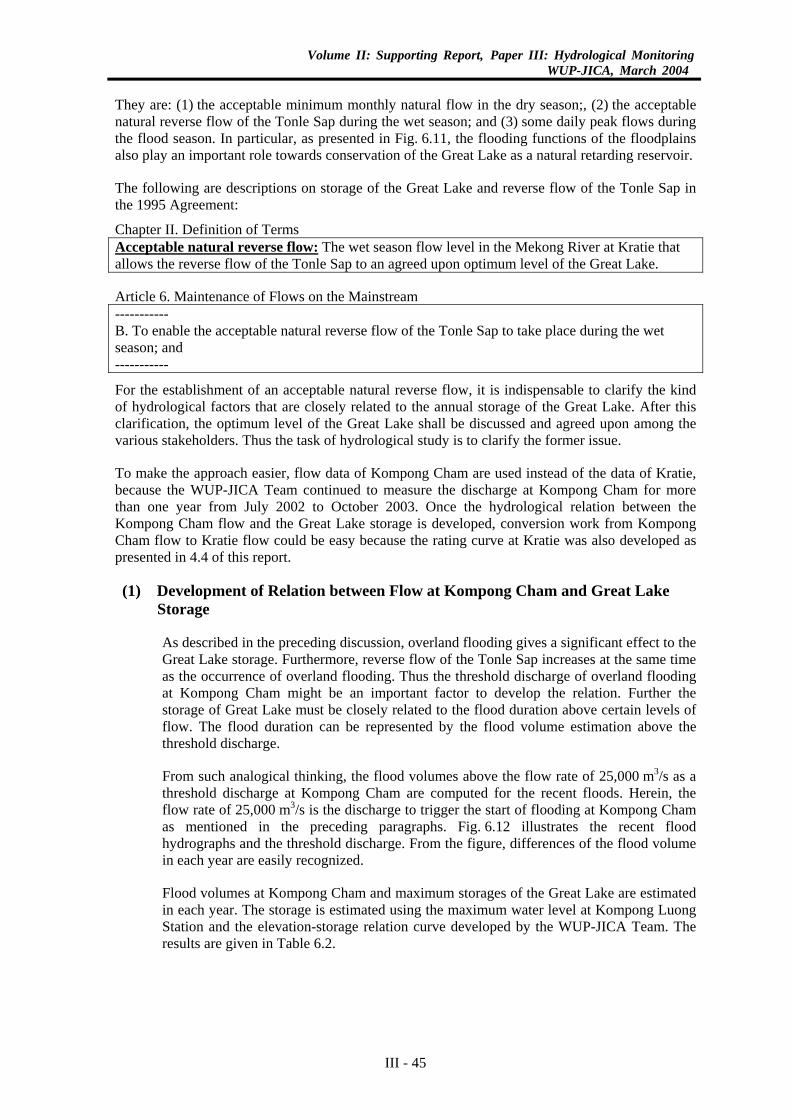
Volume II: Supporting Report, Paper III: Hydrological MonitoringWUP-JICA, March 2004
They are: (1) the acceptable minimum monthly natural flow in the dry season;, (2) the acceptable natural reverse flow of the Tonle Sap during the wet season; and (3) some daily peak flows during the flood season. In particular, as presented in Fig. 6.11, the flooding functions of the floodplains also play an important role towards conservation of the Great Lake as a natural retarding reservoir.
The following are descriptions on storage of the Great Lake and reverse flow of the Tonle Sap in the 1995 Agreement:
Chapter II. Definition of Terms Acceptable natural reverse flow: The wet season flow level in the Mekong River at Kratie that allows the reverse flow of the Tonle Sap to an agreed upon optimum level of the Great Lake. Article 6. Maintenance of Flows on the Mainstream ----------- B. To enable the acceptable natural reverse flow of the Tonle Sap to take place during the wet season; and -----------
For the establishment of an acceptable natural reverse flow, it is indispensable to clarify the kind of hydrological factors that are closely related to the annual storage of the Great Lake. After this clarification, the optimum level of the Great Lake shall be discussed and agreed upon among the various stakeholders. Thus the task of hydrological study is to clarify the former issue.
To make the approach easier, flow data of Kompong Cham are used instead of the data of Kratie, because the WUP-JICA Team continued to measure the discharge at Kompong Cham for more than one year from July 2002 to October 2003. Once the hydrological relation between the Kompong Cham flow and the Great Lake storage is developed, conversion work from Kompong Cham flow to Kratie flow could be easy because the rating curve at Kratie was also developed as presented in 4.4 of this report.
(1) Development of Relation between Flow at Kompong Cham and Great Lake Storage
As described in the preceding discussion, overland flooding gives a significant effect to the Great Lake storage. Furthermore, reverse flow of the Tonle Sap increases at the same time as the occurrence of overland flooding. Thus the threshold discharge of overland flooding at Kompong Cham might be an important factor to develop the relation. Further the storage of Great Lake must be closely related to the flood duration above certain levels of flow. The flood duration can be represented by the flood volume estimation above the threshold discharge.
From such analogical thinking, the flood volumes above the flow rate of 25,000 m3/s as a threshold discharge at Kompong Cham are computed for the recent floods. Herein, the flow rate of 25,000 m3/s is the discharge to trigger the start of flooding at Kompong Cham as mentioned in the preceding paragraphs. Fig. 6.12 illustrates the recent flood hydrographs and the threshold discharge. From the figure, differences of the flood volume in each year are easily recognized.
Flood volumes at Kompong Cham and maximum storages of the Great Lake are estimated in each year. The storage is estimated using the maximum water level at Kompong Luong Station and the elevation-storage relation curve developed by the WUP-JICA Team. The results are given in Table 6.2.
III - 45
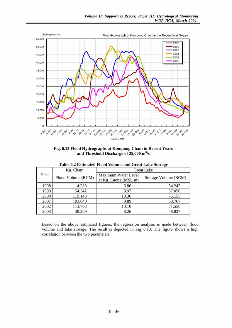
Volume II: Supporting Report, Paper III: Hydrological MonitoringWUP-JICA, March 2004
Flow Hydrograph of Kompong Cham in the Recent Wet Season
0
5,000
10,000
15,000
20,000
25,000
30,000
35,000
40,000
45,000
50,000
55,000
1-Jun
8-Jun
15-Ju
n
22-Ju
n
29-Ju
n6-J
ul
13-Ju
l
20-Ju
l
27-Ju
l
3-Aug
10-A
ug
17-A
ug
24-A
ug
31-A
ug7-S
ep
14-S
ep
21-S
ep
28-S
ep5-O
ct
12-O
ct
19-O
ct
26-O
ct
2-Nov
9-Nov
16-N
ov
23-N
ov
30-N
ov
Date/Month
Discharge (m3/s)
199819992000200120022003
Fig. 6.12 Flood Hydrographs at Kompong Cham in Recent Years
and Threshold Discharge of 25,000 m3/s
Table 6.2 Estimated Flood Volume and Great Lake Storage Kg. Cham Great Lake
Year Flood Volume (BCM) Maximum Water Level
at Kg. Luong (MSL m) Storage Volume (BCM)
1998 4.233 6.86 34.242 1999 54.342 8.97 57.050 2000 119.143 10.36 75.155 2001 103.640 9.89 68.767 2002 113.708 10.10 71.556 2003 38.209 8.26 48.837
Based on the above estimated figures, the regression analysis is made between flood volume and lake storage. The result is depicted in Fig. 6.13. The figure shows a high correlation between the two parameters.
III - 46
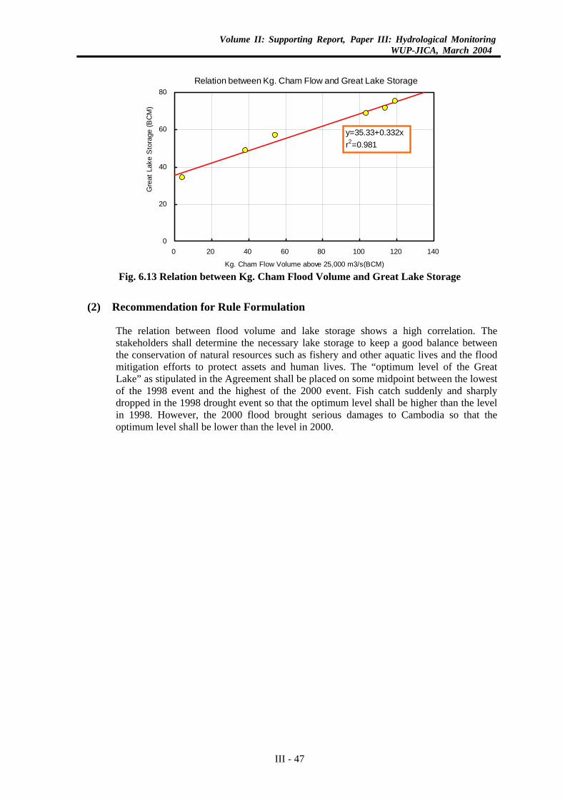
Volume II: Supporting Report, Paper III: Hydrological MonitoringWUP-JICA, March 2004
Relation between Kg. Cham Flow and Great Lake Storage
0
20
40
60
80
0 20 40 60 80 100 120 140
Kg. Cham Flow Volume above 25,000 m3/s(BCM)
Gre
at L
ake
Sto
rage
(BC
M)
y=35.33+0.332xr2=0.981
Fig. 6.13 Relation between Kg. Cham Flood Volume and Great Lake Storage
(2) Recommendation for Rule Formulation
The relation between flood volume and lake storage shows a high correlation. The stakeholders shall determine the necessary lake storage to keep a good balance between the conservation of natural resources such as fishery and other aquatic lives and the flood mitigation efforts to protect assets and human lives. The “optimum level of the Great Lake” as stipulated in the Agreement shall be placed on some midpoint between the lowest of the 1998 event and the highest of the 2000 event. Fish catch suddenly and sharply dropped in the 1998 drought event so that the optimum level shall be higher than the level in 1998. However, the 2000 flood brought serious damages to Cambodia so that the optimum level shall be lower than the level in 2000.
III - 47
Volume II: Supporting Report, Paper III: Hydrological MonitoringWUP-JICA, March 2004
REFERENCES
(1) MRC: Lower Mekong Hydrologic Yearbook, 1985-86, 1990, 1994 and 1998
(2) MRC: Strategic Master Scheme for Hydro-meteorological Network in the Mekong River Basin, 2001
(3) MRC: AHNIP workshop and training materials, 2001 and 2002-07-30
(4) MRC: Inception Report on the Consolidation of Hydro-meteorological Data and Multi-functional Hydrologic Roles of Tonle Sap Lake and its Vicinities, March 2002
(5) RD Instruments: WinRiver User’s Guide, International Version, 2001
(6) MRC: Analyses of Hydrological Data at Stations around the Great Lake and on Mekong, Bassac Rivers in 1960’s and from 1998 to 2000, Mission Report, June 2002
(7) The Committee for Coordination of Investigation of the Lower Mekong River Basin: Lower Mekong River Basin Discharge Data Prior to 1960
(8) The Committee for Coordination of Investigation of the Lower Mekong River Basin: Hydrologic Data Mekong River basin, 1961-1973
(9) UNESCO: Backwater Curves of the Upstream Mekong River, Mathematical Model of Mekong River Delta IV-1, 1966
(10) WMO: Manual on Stream Gauging, Volume II Computation of Discharge, Operational Hydrology Report No. 13, 1980
(11) UNESCO: Measurement Campaign 1963, 1964 and 1965, Mathematical Model of Mekong River Delta III-1, 2 and 4, 1966
(12) UNESCO: Mekong Delta Monograph, Mathematical Model of Mekong River Delta I, 1966
III - 48
Volume II: Supporting Report, Paper III: Hydrological MonitoringWUP-JICA, March 2004
ANNEX I MEASUREMENT RESULTS
MEASUREMENT RESULTS
Mekong Kompong Cham ........................................................................... AI-1 Roka Koy ...................................................................................... AI-8 Kong Tanong ................................................................................ AI-9 Prek Tamak .................................................................................. AI-10 Chrui Changvar ............................................................................ AI-11 Koh Norea .................................................................................... AI-18 Lvea Sa ........................................................................................ AI-24 Neak Luong .................................................................................. AI-25
Tonle Sap Prek Kdam ................................................................................... AI-32 Phnom Penh Port ......................................................................... AI-33
Bassc Monivong Bridge .......................................................................... AI-40 Ta Khmao ..................................................................................... AI-46 Koh Khel ....................................................................................... AI-47
MEASUREMENT RESULTS IN DRY SEASON Chrui Changvar ............................................................................ AI-48 Koh Norea .................................................................................... AI-51 Phnom Penh Port ......................................................................... AI-54 Monivong Bridge .......................................................................... AI-57
AI-i
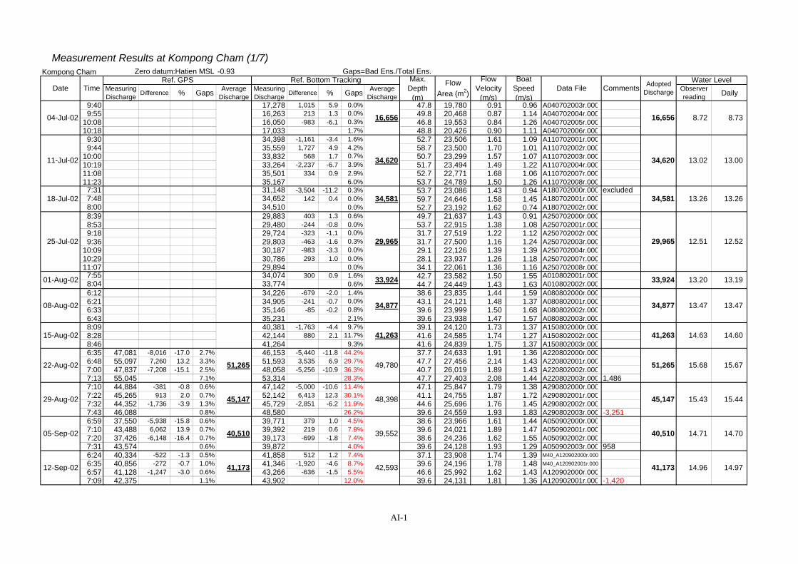
Measurement Results at Kompong Cham (1/7)Kompong Cham Zero datum:Hatien MSL -0.93 Gaps=Bad Ens./Total Ens.
MeasuringDischarge Difference % Gaps Average
DischargeMeasuringDischarge Difference % Gaps Average
DischargeObserverreading Daily
9:40 17,278 1,015 5.9 0.0% 47.8 19,780 0.91 0.96 A040702003r.0009:55 16,263 213 1.3 0.0% 49.8 20,468 0.87 1.14 A040702004r.000
10:08 16,050 -983 -6.1 0.3% 46.8 19,553 0.84 1.26 A040702005r.00010:18 17,033 1.7% 48.8 20,426 0.90 1.11 A040702006r.000
9:30 34,398 -1,161 -3.4 1.6% 52.7 23,506 1.61 1.09 A110702001r.0009:44 35,559 1,727 4.9 4.2% 58.7 23,500 1.70 1.01 A110702002r.000
10:00 33,832 568 1.7 0.7% 50.7 23,299 1.57 1.07 A110702003r.00010:19 33,264 -2,237 -6.7 3.9% 51.7 23,494 1.49 1.22 A110702004r.00011:08 35,501 334 0.9 2.9% 52.7 22,771 1.68 1.06 A110702007r.00011:23 35,167 6.0% 53.7 24,789 1.50 1.26 A110702008r.000
7:31 31,148 -3,504 -11.2 0.3% 53.7 23,086 1.43 0.94 A180702000r.000 excluded7:48 34,652 142 0.4 0.0% 59.7 24,646 1.58 1.45 A180702001r.0008:00 34,510 0.0% 52.7 23,192 1.62 0.74 A180702002r.0008:39 29,883 403 1.3 0.6% 49.7 21,637 1.43 0.91 A250702000r.0008:53 29,480 -244 -0.8 0.0% 53.7 22,915 1.38 1.08 A250702001r.0009:18 29,724 -323 -1.1 0.0% 31.7 27,519 1.22 1.12 A250702002r.0009:36 29,803 -463 -1.6 0.3% 31.7 27,500 1.16 1.24 A250702003r.000
10:09 30,187 -983 -3.3 0.0% 29.1 22,126 1.39 1.39 A250702004r.00010:29 30,786 293 1.0 0.0% 28.1 23,937 1.26 1.18 A250702007r.00011:07 29,894 0.0% 34.1 22,061 1.36 1.16 A250702008r.000
7:55 34,074 300 0.9 1.6% 42.7 23,582 1.50 1.55 A010802001r.0008:04 33,774 0.6% 44.7 24,449 1.43 1.63 A010802002r.0006:12 34,226 -679 -2.0 1.4% 38.6 23,835 1.44 1.59 A080802000r.0006:21 34,905 -241 -0.7 0.0% 43.1 24,121 1.48 1.37 A080802001r.0006:33 35,146 -85 -0.2 0.8% 39.6 23,999 1.50 1.68 A080802002r.0006:43 35,231 2.1% 39.6 23,938 1.47 1.57 A080802003r.0008:09 40,381 -1,763 -4.4 9.7% 39.1 24,120 1.73 1.37 A150802000r.0008:28 42,144 880 2.1 11.7% 41.6 24,585 1.74 1.27 A150802002r.0008:46 41,264 9.3% 41.6 24,839 1.75 1.37 A150802003r.0006:35 47,081 -8,016 -17.0 2.7% 46,153 -5,440 -11.8 44.2% 37.7 24,633 1.91 1.36 A220802000r.0006:48 55,097 7,260 13.2 3.3% 51,593 3,535 6.9 29.7% 47.7 27,456 2.14 1.43 A220802001r.0007:00 47,837 -7,208 -15.1 2.5% 48,058 -5,256 -10.9 36.3% 40.7 26,019 1.89 1.43 A220802002r.0007:13 55,045 7.1% 53,314 28.3% 47.7 27,403 2.08 1.44 A220802003r.000 1,4867:10 44,884 -381 -0.8 0.6% 47,142 -5,000 -10.6 11.4% 47.1 25,847 1.79 1.38 A290802000r.0007:22 45,265 913 2.0 0.7% 52,142 6,413 12.3 30.1% 41.1 24,755 1.87 1.72 A290802001r.0007:32 44,352 -1,736 -3.9 1.3% 45,729 -2,851 -6.2 11.9% 44.6 25,696 1.76 1.45 A290802002r.0007:43 46,088 0.8% 48,580 26.2% 39.6 24,559 1.93 1.83 A290802003r.000 -3,2516:59 37,550 -5,938 -15.8 0.6% 39,771 379 1.0 4.5% 38.6 23,966 1.61 1.44 A050902000r.0007:10 43,488 6,062 13.9 0.7% 39,392 219 0.6 7.9% 39.6 24,021 1.89 1.47 A050902001r.0007:20 37,426 -6,148 -16.4 0.7% 39,173 -699 -1.8 7.4% 38.6 24,236 1.62 1.55 A050902002r.0007:31 43,574 0.6% 39,872 4.0% 39.6 24,128 1.93 1.29 A050902003r.000 9586:24 40,334 -522 -1.3 0.5% 41,858 512 1.2 7.4% 37.1 23,908 1.74 1.39 M40_A120902000r.000
6:35 40,856 -272 -0.7 1.0% 41,346 -1,920 -4.6 8.7% 39.6 24,196 1.78 1.48 M40_A120902001r.000
6:57 41,128 -1,247 -3.0 0.6% 43,266 -636 -1.5 5.5% 46.6 25,992 1.62 1.43 A120902000r.0007:09 42,375 1.1% 43,902 12.0% 39.6 24,131 1.81 1.36 A120902001r.000 -1,420
14.96
29-Aug-02 45,147 15.43
05-Sep-02 40,510 14.71
45,147
42,593
15.68
33,924 13.20
15-Aug-02 41,263 14.6341,263
51,265
08-Aug-02 34,877 13.47
01-Aug-02
34,877
33,924
13.02
16,656
25-Jul-02 29,965 12.51
34,620
34,581
29,965
41,173
22-Aug-02 51,265
12-Sep-02
49,780
48,398
39,552
Date Time
04-Jul-02
18-Jul-02
11-Jul-02
8.73
13.00
13.26
Ref. GPS Ref. Bottom Tracking
16,656 8.72
34,581 13.26
34,620
Data File Comments AdoptedDischarge
Water Level
40,510
41,173
14.70
14.97
12.52
13.19
13.47
14.60
15.67
15.44
Max.Depth
(m)
FlowArea (m2)
FlowVelocity
(m/s)
BoatSpeed(m/s)
AI-1
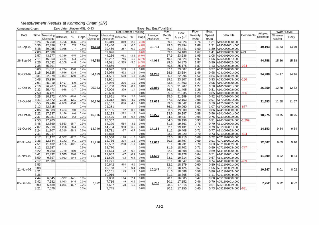
Measurement Results at Kompong Cham (2/7)Kompong Cham Zero datum:Hatien MSL -0.93 Gaps=Bad Ens./Total Ens.
MeasuringDischarge Difference % Gaps Average
DischargeMeasuringDischarge Difference % Gaps Average
DischargeObserverreading DailyDate Time
Ref. GPS Ref. Bottom TrackingData File Comments Adopted
Discharge
Water LevelMax.Depth
(m)
FlowArea (m2)
FlowVelocity
(m/s)
BoatSpeed(m/s)
6:26 36,750 -5,706 -15.5 0.6% 40,319 869 2.2 2.4% 39.1 24,024 1.76 1.31 A190902000r.0006:35 42,456 3,191 7.5 0.6% 39,450 -9 0.0 4.8% 39.6 23,894 1.68 1.31 A190902001r.0006:48 39,265 -3,035 -7.7 0.6% 39,459 -367 -0.9 2.3% 40.1 24,441 1.69 1.30 A190902002r.0007:00 42,300 0.6% 39,826 0.6% 39.1 24,108 1.67 1.41 A190902003r.000 4296:57 43,677 -2,386 -5.5 0.5% 44,286 -981 -2.2 16.9% 37.6 23,536 1.95 1.08 A260902000r.0007:11 46,063 2,471 5.4 0.5% 45,267 746 1.6 12.7% 40.1 23,624 1.97 1.06 A260902001r.0007:26 43,592 -2,109 -4.8 0.4% 44,521 -1,335 -3.0 14.3% 39.6 24,875 1.87 0.90 A260902002r.0007:38 45,701 2.0% 45,856 16.3% 40.6 25,175 1.87 1.13 A260902003r.000 -2246:00 31,851 -4,774 -15.0 0.4% 34,672 593 1.7 0.0% 37.1 23,687 1.49 0.97 A031002000r.0006:15 36,625 4,546 12.4 0.4% 34,079 -422 -1.2 0.0% 38.6 23,684 1.46 0.98 A031002001r.0006:31 32,079 -3,857 -12.0 0.4% 34,501 600 1.7 0.4% 36.1 22,996 1.52 0.84 A031002002r.0006:48 35,936 0.4% 33,901 0.0% 39.1 23,307 1.48 0.93 A031002003r.000 -1667:01 25,210 -1,497 -5.9 0.3% 27,036 276 1.0 0.0% 33.6 21,563 1.27 0.95 A101002000r.0007:16 26,707 1,234 4.6 0.3% 26,760 -249 -0.9 0.0% 35.6 21,707 1.27 0.78 A101002001r.0007:33 25,473 -948 -3.7 0.3% 27,009 379 1.4 0.0% 36.1 21,405 1.26 0.81 A101002002r.0007:50 26,421 0.3% 26,630 0.0% 35.6 21,835 1.23 0.85 A101002003r.000 -9066:28 18,972 -3,500 -18.4 0.4% 21,851 539 2.5 0.0% 35.6 21,389 1.06 0.92 A171002000r.0006:41 22,472 2,726 12.1 0.4% 21,312 -855 -4.0 0.0% 37.6 22,153 0.98 0.97 A171002001r.0006:55 19,746 -2,969 -15.0 0.3% 22,167 886 4.0 0.0% 33.6 20,642 1.08 0.79 A171002002r.0007:12 22,715 0.4% 21,281 0.0% 36.1 20,960 1.02 1.07 A171002003r.000 -6777:06 16,083 -1,454 -9.0 0.3% 18,185 52 0.3 0.0% 33.6 19,900 0.90 0.86 A241002000r.0007:22 17,537 1,156 6.6 0.4% 18,133 -292 -1.6 0.0% 33.6 20,387 0.88 0.96 A241002001r.0007:37 16,381 -1,522 -9.3 0.3% 18,425 68 0.4 0.0% 34.6 20,647 0.94 0.75 A241002002r.0007:53 17,903 0.4% 18,357 0.0% 34.6 20,196 0.93 0.91 A241002003r.000 -1,2996:48 12,360 -3,553 -28.7 0.3% 14,220 -514 -3.6 0.0% 31.6 19,361 0.75 0.70 A311002000r.0007:07 15,913 4,206 26.4 0.3% 14,734 953 6.5 0.0% 32.1 19,131 0.77 0.79 A311002001r.0007:24 11,707 -3,310 -28.3 0.3% 13,781 -97 -0.7 0.0% 31.1 19,408 0.71 0.77 A311002002r.0007:41 15,017 0.3% 13,878 0.0% 33.1 19,329 0.70 0.73 A311002003r.000 -4047:17 11,177 -1,367 -12.2 0.3% 12,568 -198 -1.6 0.0% 32.6 18,710 0.69 0.72 A071102000r.0007:36 12,544 1,142 9.1 0.3% 12,766 204 1.6 0.0% 30.6 18,797 0.69 0.91 A071102001r.0007:51 11,402 -1,155 -10.1 0.2% 12,562 -208 -1.7 0.0% 31.1 18,731 0.70 0.63 A071102002r.0008:12 12,557 0.3% 12,770 0.0% 31.6 18,702 0.71 0.90 A071102003r.000 -7476:22 9,763 -2,729 -28.0 0.0% 11,674 22 0.2 0.0% 32.1 18,808 0.63 0.69 A141102000r.0006:41 12,492 2,595 20.8 0.3% 11,652 -47 -0.4 0.0% 31.6 18,428 0.64 0.71 A141102001r.0006:59 9,897 -2,912 -29.4 0.3% 11,699 -72 -0.6 0.0% 33.1 19,314 0.62 0.67 A141102002r.0007:17 12,809 0.3% 11,771 0.0% 31.1 18,347 0.66 0.74 A141102003r.000 -4597:53 10,642 474 4.5 0.0% 32.1 18,879 0.60 0.80 A211102001r.0008:08 10,168 7 0.1 0.0% 32.1 18,125 0.57 1.05 A211102002r.0008:21 10,161 145 1.4 0.0% 31.6 18,586 0.58 0.86 A211102003r.0008:36 10,016 0.0% 31.1 18,365 0.57 1.11 A211102004r.0007:44 6,645 -937 -14.1 0.3% 7,880 164 2.1 0.0% 28.1 16,805 0.47 0.68 A051202000r.0007:42 7,582 1,093 14.4 0.3% 7,716 49 0.6 0.0% 30.1 17,152 0.46 0.70 A051202001r.0008:00 6,489 -1,081 -16.7 0.2% 7,667 -78 -1.0 0.0% 28.6 17,315 0.46 0.61 A051202002r.0008:21 7,570 0.3% 7,745 0.0% 30.1 17,155 0.45 0.73 A051202003r.000 -681
8.01 8.0221-Nov-02 10,247 10,247
8.64
9.0907-Nov-02 11,920
8.6214-Nov-02 11,240 11,699 11,699
12,667 12,667
10.75
9.64 9.64
10.75
9.10
31-Oct-02 13,749 14,153 14,153
24-Oct-02 16,976 18,275 18,275
12.78
26-Sep-02 44,758 15.36
26,859
14.17
26,859
03-Oct-02
44,758
10-Oct-02 25,953
19-Sep-02
34,288
39,764
44,983
34,123
40,193
11.67
40,193
11.68
12.72
14.73
34,288
17-Oct-02 20,976 21,653 21,653
05-Dec-02 7,072 7,752 7,752 6.92 6.92
14.70
15.38
14.16
AI-2
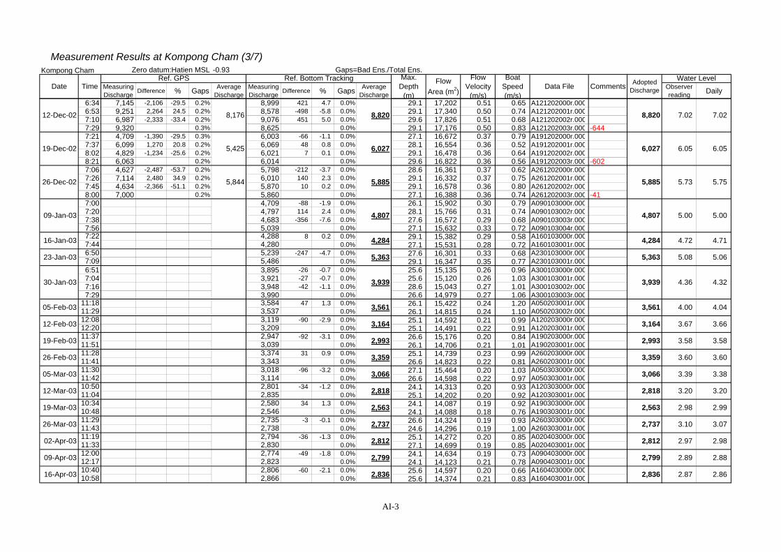
Measurement Results at Kompong Cham (3/7)Kompong Cham Zero datum:Hatien MSL -0.93 Gaps=Bad Ens./Total Ens.
MeasuringDischarge Difference % Gaps Average
DischargeMeasuringDischarge Difference % Gaps Average
DischargeObserverreading DailyDate Time
Ref. GPS Ref. Bottom TrackingData File Comments Adopted
Discharge
Water LevelMax.Depth
(m)
FlowArea (m2)
FlowVelocity
(m/s)
BoatSpeed(m/s)
6:34 7,145 -2,106 -29.5 0.2% 8,999 421 4.7 0.0% 29.1 17,202 0.51 0.65 A121202000r.0006:53 9,251 2,264 24.5 0.2% 8,578 -498 -5.8 0.0% 29.1 17,340 0.50 0.74 A121202001r.0007:10 6,987 -2,333 -33.4 0.2% 9,076 451 5.0 0.0% 29.6 17,826 0.51 0.68 A121202002r.0007:29 9,320 0.3% 8,625 0.0% 29.1 17,176 0.50 0.83 A121202003r.000 -6447:21 4,709 -1,390 -29.5 0.3% 6,003 -66 -1.1 0.0% 27.1 16,672 0.37 0.79 A191202000r.0007:37 6,099 1,270 20.8 0.2% 6,069 48 0.8 0.0% 28.1 16,554 0.36 0.52 A191202001r.0008:02 4,829 -1,234 -25.6 0.2% 6,021 7 0.1 0.0% 29.1 16,478 0.36 0.64 A191202002r.0008:21 6,063 0.2% 6,014 0.0% 29.6 16,822 0.36 0.56 A191202003r.000 -6027:06 4,627 -2,487 -53.7 0.2% 5,798 -212 -3.7 0.0% 28.6 16,361 0.37 0.62 A261202000r.0007:26 7,114 2,480 34.9 0.2% 6,010 140 2.3 0.0% 29.1 16,332 0.37 0.75 A261202001r.0007:45 4,634 -2,366 -51.1 0.2% 5,870 10 0.2 0.0% 29.1 16,578 0.36 0.80 A261202002r.0008:00 7,000 0.2% 5,860 0.0% 27.1 16,388 0.36 0.74 A261202003r.000 -417:00 4,709 -88 -1.9 0.0% 26.1 15,902 0.30 0.79 A090103000r.0007:20 4,797 114 2.4 0.0% 28.1 15,766 0.31 0.74 A090103002r.0007:38 4,683 -356 -7.6 0.0% 27.6 16,572 0.29 0.68 A090103003r.0007:56 5,039 0.0% 27.1 15,632 0.33 0.72 A090103004r.0007:22 4,288 8 0.2 0.0% 29.1 15,382 0.29 0.58 A160103000r.0007:44 4,280 0.0% 27.1 15,531 0.28 0.72 A160103001r.0006:50 5,239 -247 -4.7 0.0% 27.6 16,301 0.33 0.68 A230103000r.0007:09 5,486 0.0% 29.1 16,347 0.35 0.77 A230103001r.0006:51 3,895 -26 -0.7 0.0% 25.6 15,135 0.26 0.96 A300103000r.0007:04 3,921 -27 -0.7 0.0% 25.6 15,120 0.26 1.03 A300103001r.0007:16 3,948 -42 -1.1 0.0% 28.6 15,043 0.27 1.01 A300103002r.0007:29 3,990 0.0% 26.6 14,979 0.27 1.06 A300103003r.000
11:18 3,584 47 1.3 0.0% 26.1 15,422 0.24 1.20 A050203001r.00011:29 3,537 0.0% 26.1 14,815 0.24 1.10 A050203002r.00012:08 3,119 -90 -2.9 0.0% 25.1 14,592 0.21 0.99 A120203000r.00012:20 3,209 0.0% 25.1 14,491 0.22 0.91 A120203001r.00011:37 2,947 -92 -3.1 0.0% 26.6 15,176 0.20 0.84 A190203000r.00011:51 3,039 0.0% 26.1 14,706 0.21 1.01 A190203001r.00011:28 3,374 31 0.9 0.0% 25.1 14,739 0.23 0.99 A260203000r.00011:41 3,343 0.0% 26.6 14,823 0.22 0.81 A260203001r.00011:30 3,018 -96 -3.2 0.0% 27.1 15,464 0.20 1.03 A050303000r.00011:42 3,114 0.0% 26.6 14,598 0.22 0.97 A050303001r.00010:50 2,801 -34 -1.2 0.0% 24.1 14,313 0.20 0.93 A120303000r.00011:04 2,835 0.0% 25.1 14,202 0.20 0.92 A120303001r.00010:34 2,580 34 1.3 0.0% 24.1 14,087 0.19 0.92 A190303000r.00010:48 2,546 0.0% 24.1 14,088 0.18 0.76 A190303001r.00011:29 2,735 -3 -0.1 0.0% 26.6 14,324 0.19 0.93 A260303000r.00011:43 2,738 0.0% 24.6 14,296 0.19 1.00 A260303001r.00011:19 2,794 -36 -1.3 0.0% 25.1 14,272 0.20 0.85 A020403000r.00011:33 2,830 0.0% 27.1 14,699 0.19 0.85 A020403001r.00012:00 2,774 -49 -1.8 0.0% 24.1 14,634 0.19 0.73 A090403000r.00012:17 2,823 0.0% 24.1 14,123 0.21 0.78 A090403001r.00010:40 2,806 -60 -2.1 0.0% 25.6 14,597 0.20 0.66 A160403000r.00010:58 2,866 0.0% 25.6 14,374 0.21 0.83 A160403001r.000
5.00 5.0009-Jan-03 4,807 4,807
7.02 7.02
26-Dec-02 5,844 5,885 5,885 5.73 5.75
12-Dec-02 8,176 8,820 8,820
19-Dec-02 5,425 6,027 6,027 6.05 6.05
4.72 4.7116-Jan-03 4,284 4,284
5.08 5.0623-Jan-03 5,363 5,363
4.36 4.3230-Jan-03 3,939 3,939
05-Feb-03 3,561 3,561 4.00 4.04
3.67 3.6612-Feb-03 3,164 3,164
19-Feb-03 2,993 2,993 3.58 3.58
3.60 3.6026-Feb-03 3,359 3,359
05-Mar-03 3,066 3,066 3.39 3.38
3.20 3.2012-Mar-03 2,818 2,818
19-Mar-03 2,563 2,563 2.98 2.99
3.10 3.07
02-Apr-03 2,812 2,812 2.97 2.98
26-Mar-03 2,737 2,737
2.89 2.8809-Apr-03 2,799 2,799
16-Apr-03 2,836 2,836 2.87 2.86
AI-3
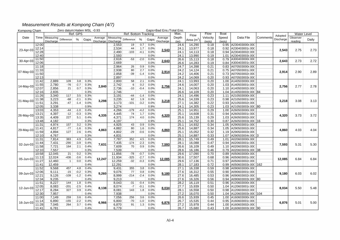
Measurement Results at Kompong Cham (4/7)Kompong Cham Zero datum:Hatien MSL -0.93 Gaps=Bad Ens./Total Ens.
MeasuringDischarge Difference % Gaps Average
DischargeMeasuringDischarge Difference % Gaps Average
DischargeObserverreading DailyDate Time
Ref. GPS Ref. Bottom TrackingData File Comments Adopted
Discharge
Water LevelMax.Depth
(m)
FlowArea (m2)
FlowVelocity
(m/s)
BoatSpeed(m/s)
12:00 2,553 19 0.7 0.0% 24.6 14,290 0.18 0.95 A230403000r.00012:14 2,534 44 1.7 0.0% 24.1 13,977 0.18 0.92 A230403001r.00012:28 2,490 -103 -4.1 0.0% 24.1 14,113 0.18 0.94 A230403002r.00012:40 2,593 0.0% 24.1 13,990 0.19 1.01 A230403003r.00011:50 2,616 -53 -2.0 0.0% 26.6 15,113 0.18 0.79 A300403000r.00012:06 2,669 0.0% 26.6 14,283 0.19 0.84 A300403001r.00011:18 2,964 26 0.9 0.0% 24.7 14,398 0.21 0.83 A070503000r.00011:33 2,938 80 2.7 0.0% 24.2 14,124 0.21 0.75 A070503001r.00011:50 2,858 -39 -1.4 0.0% 24.2 14,406 0.21 0.73 A070503002r.00012:13 2,897 0.0% 24.2 14,069 0.20 0.93 A070503003r.00011:42 2,889 109 3.8 0.3% 2,800 58 2.1 0.0% 24.1 13,993 0.20 1.00 A140503000r.00011:55 2,780 -76 -2.7 0.3% 2,742 6 0.2 0.0% 24.6 14,007 0.20 1.03 A140503001r.00012:07 2,856 21 0.7 0.3% 2,736 -10 -0.4 0.0% 24.1 14,063 0.20 1.10 A140503002r.00012:16 2,835 0.3% 2,746 0.0% 26.6 14,109 0.20 1.04 A140503003r.000 8411:26 3,340 117 3.5 0.3% 3,191 -44 -1.4 0.0% 24.1 14,496 0.23 1.11 A210503000r.00011:38 3,223 -68 -2.1 0.3% 3,235 62 1.9 0.0% 25.6 14,339 0.23 0.98 A210503001r.00011:51 3,291 -47 -1.4 0.0% 3,173 -101 -3.2 0.0% 27.1 14,382 0.22 0.93 A210503002r.00012:05 3,338 0.9% 3,274 0.9% 24.1 14,305 0.23 1.03 A210503003r.000 8013:03 4,353 -44 -1.0 0.4% 4,266 -179 -4.2 0.0% 25.1 14,951 0.29 1.00 A260503000r.00013:21 4,397 -12 -0.3 0.3% 4,445 74 1.7 0.0% 25.1 14,608 0.31 0.94 A260503001r.00013:35 4,409 227 5.1 0.4% 4,371 174 4.0 0.0% 25.6 15,139 0.29 1.03 A260503002r.00013:48 4,182 0.3% 4,197 0.9% 25.1 14,752 0.30 0.87 A260503003r.000 1611:31 4,974 157 3.2 0.3% 4,925 43 0.9 0.0% 25.1 14,932 0.34 1.05 A290503001r.00011:41 4,817 -77 -1.6 0.3% 4,882 80 1.6 0.0% 25.6 14,887 0.34 1.05 A290503002r.00011:59 4,894 127 2.6 0.4% 4,802 -29 -0.6 0.0% 25.1 15,052 0.32 1.19 A290503003r.00012:10 4,767 0.3% 4,831 0.0% 25.1 14,887 0.33 1.07 A290503004r.000 311:31 7,814 383 4.9 0.4% 7,787 352 4.5 0.0% 28.1 15,749 0.49 1.01 A020603000r.00011:44 7,431 -290 -3.9 0.4% 7,435 -174 -2.3 0.0% 28.1 16,088 0.47 0.94 A020603001r.00011:58 7,721 164 2.1 0.4% 7,609 70 0.9 0.0% 26.6 16,109 0.49 1.10 A020603002r.00012:10 7,557 0.3% 7,539 0.0% 28.6 16,186 0.46 0.79 A020603003r.000 3810:58 12,045 21 0.2 0.3% 11,856 -78 -0.7 0.0% 29.6 17,090 0.70 0.89 A050603000r.00011:13 12,024 -436 -3.6 0.4% 11,934 -325 -2.7 0.0% 30.6 17,507 0.68 0.96 A050603001r.00011:27 12,460 1 0.0 0.4% 12,259 -32 -0.3 0.0% 29.6 17,136 0.71 0.97 A050603002r.00011:41 12,459 0.4% 12,291 0.0% 28.1 17,183 0.72 0.99 A050603003r.000 16211:52 9,568 457 4.8 0.4% 9,431 355 3.8 0.0% 27.1 16,338 0.59 0.98 A090603000r.00012:06 9,111 -15 -0.2 0.3% 9,076 77 0.8 0.0% 27.6 16,312 0.55 0.90 A090603001r.00012:21 9,126 -109 -1.2 0.4% 8,999 -214 -2.4 0.0% 27.6 16,485 0.53 0.96 A090603002r.00012:34 9,235 0.4% 9,213 0.0% 27.6 16,326 0.56 0.94 A090603003r.000 8011:51 8,227 144 1.8 0.4% 8,043 -31 -0.4 0.0% 28.2 16,119 0.51 0.96 A120603000r.00012:05 8,083 -201 -2.5 0.4% 8,074 -7 -0.1 0.0% 27.7 15,939 0.50 1.04 A120603001r.00012:17 8,284 327 3.9 0.4% 8,081 143 1.8 0.0% 28.1 16,558 0.50 0.98 A120603002r.00012:30 7,957 0.4% 7,938 0.0% 27.2 16,070 0.50 1.04 A120603003r.000 10411:00 7,149 259 3.6 0.4% 7,056 256 3.6 0.0% 26.6 15,939 0.45 1.00 A160603000r.00011:14 6,890 -155 -2.2 0.4% 6,800 -70 -1.0 0.0% 26.7 15,535 0.44 0.95 A160603001r.00011:28 7,045 264 3.7 0.4% 6,870 91 1.3 0.0% 27.2 15,978 0.44 1.00 A160603002r.00011:41 6,781 0.4% 6,779 0.0% 26.7 15,680 0.43 1.00 A160603003r.000 90
16-Jun-03 6,966 6,876 6,876
5.50 5.48
5.01 5.00
12-Jun-03 8,138 8,034 8,034
6.84 6.84
09-Jun-03 9,260 9,180 9,180 6.03 6.02
05-Jun-03 12,247 12,085 12,085
3.08 3.1321-May-03 3,298 3,218 3,218
2.75 2.7323-Apr-03 2,543 2,543
30-Apr-03 2,643 2,643 2.73 2.72
07-May-03 2,914 2,914 2.90 2.89
14-May-03 2,840 2,756 2,756 2.77 2.78
26-May-03 4,335 4,320 4,320 3.73 3.72
4.03 4.0429-May-03 4,863 4,860 4,860
02-Jun-03 7,631 7,593 7,593 5.31 5.30
AI-4
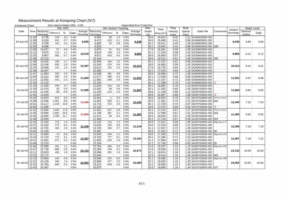
Measurement Results at Kompong Cham (5/7)Kompong Cham Zero datum:Hatien MSL -0.93 Gaps=Bad Ens./Total Ens.
MeasuringDischarge Difference % Gaps Average
DischargeMeasuringDischarge Difference % Gaps Average
DischargeObserverreading DailyDate Time
Ref. GPS Ref. Bottom TrackingData File Comments Adopted
Discharge
Water LevelMax.Depth
(m)
FlowArea (m2)
FlowVelocity
(m/s)
BoatSpeed(m/s)
11:26 6,736 218 3.2 0.4% 6,561 89 1.4 0.0% 26.6 15,814 0.43 1.11 A190603000r.00011:38 6,518 -241 -3.7 0.0% 6,472 -133 -2.1 0.0% 26.6 15,496 0.41 0.86 A190603001r.00011:53 6,759 151 2.2 0.4% 6,605 52 0.8 0.0% 26.1 15,511 0.43 1.09 A190603002r.00012:05 6,608 0.3% 6,553 0.0% 28.1 15,841 0.41 0.88 A190603003r.000 10811:59 10,027 57 0.6 0.4% 9,870 51 0.5 0.0% 27.6 16,391 0.59 1.00 A230603000r.00012:12 9,970 113 1.1 0.4% 9,819 148 1.5 0.0% 30.1 17,229 0.58 1.02 A230603001r.00012:25 9,857 -362 -3.7 0.4% 9,671 -433 -4.5 0.0% 28.6 16,800 0.57 1.06 A230603002r.00012:38 10,219 0.4% 10,104 0.0% 28.6 16,512 0.61 1.06 A230603003r.000 15211:49 10,426 180 1.7 0.4% 10,409 164 1.6 0.0% 30.1 17,197 0.61 0.98 A260603000r.00012:09 10,246 -302 -2.9 0.0% 10,245 -370 -3.6 0.0% 28.6 16,985 0.59 1.05 A260603001r.00012:24 10,548 141 1.3 0.4% 10,615 231 2.2 0.0% 27.6 16,725 0.64 1.14 A260603002r.00012:36 10,407 0.4% 10,384 0.0% 28.1 17,043 0.60 1.16 A260603003r.00011:47 11,954 342 2.9 0.4% 12,038 461 3.8 0.0% 28.6 16,966 0.72 1.05 A300603000r.00012:00 11,612 -390 -3.4 0.4% 11,577 -385 -3.3 0.0% 30.1 17,658 0.66 0.95 A300603001r.00012:14 12,002 -151 -1.3 0.3% 11,962 -188 -1.6 0.0% 29.1 17,107 0.72 0.84 A300603002r.00012:30 12,153 0.4% 12,150 0.0% 30.1 17,288 0.70 1.03 A300603003r.000 -211:19 11,918 444 3.7 0.5% 11,916 414 3.5 0.0% 28.1 16,982 0.70 1.19 A030703000r.00011:30 11,474 29 0.3 0.4% 11,502 68 0.6 0.0% 30.1 17,342 0.65 1.00 A030703001r.00011:44 11,445 -98 -0.9 0.4% 11,434 -113 -1.0 0.0% 28.6 17,108 0.66 1.12 A030703002r.00011:55 11,543 0.4% 11,547 0.0% 28.6 16,967 0.68 1.08 A030703003r.000 -514:24 12,870 814 6.3 0.4% 12,451 -1 0.0 0.0% 30.6 18,003 0.70 1.01 A070703000r.000 External compass
14:38 12,056 -1,061 -8.8 0.4% 12,452 -263 -2.1 0.0% 29.6 17,361 0.73 1.01 A070703001r.000 test14:51 13,117 1,419 10.8 0.4% 12,715 572 4.5 0.0% 30.1 17,730 0.74 0.97 A070703002r.00015:05 11,698 0.4% 12,143 0.0% 30.6 17,572 0.69 0.92 A070703003r.000 -511:42 13,334 2,344 17.6 0.5% 11,421 -317 -2.8 0.0% 29.1 17,210 0.67 1.27 A100703000r.000 External compass
11:55 10,990 -1,850 -16.8 0.4% 11,738 367 3.1 0.0% 19.6 17,099 0.67 1.01 A100703001r.000 test12:35 12,840 2,785 21.7 0.4% 11,371 -29 -0.3 0.0% 28.6 16,832 0.67 1.09 A100703003r.00012:48 10,055 0.4% 11,400 0.0% 28.1 17,129 0.67 0.95 A100703004r.000 32212:24 12,194 176 1.4 0.4% 12,142 116 1.0 0.0% 30.6 17,621 0.69 1.09 A200703000r.000 Mag.Var.4.7712:37 12,018 -773 -6.4 0.4% 12,026 -700 -5.8 0.0% 29.6 17,519 0.69 1.07 A200703001r.00012:49 12,791 362 2.8 0.4% 12,726 345 2.7 0.0% 31.1 17,947 0.73 1.09 A200703002r.00013:02 12,429 0.4% 12,381 0.0% 29.6 17,452 0.71 1.03 A200703003r.000 3913:11 12,650 -73 -0.6 0.0% 12,546 -156 -1.2 0.0% 29.6 17,393 0.73 1.16 A240703000r.000 Mag.Var.5.4413:24 12,723 772 6.1 1.2% 12,702 777 6.1 1.2% 29.1 17,285 0.71 1.04 A240703001r.00013:37 11,951 -271 -2.3 0.4% 11,925 -229 -1.9 0.0% 31.1 17,994 0.67 1.13 A240703002r.00013:48 12,223 0.4% 12,154 0.4% 31.1 17,700 0.68 0.93 A240703003r.000 5512:46 22,999 261 1.1 0.4% 22,754 465 2.0 0.0% 31.6 19,337 1.13 1.19 A280703000r.000 Mag.Var.4.5212:57 22,739 -885 -3.9 0.5% 22,289 -709 -3.2 0.0% 31.6 19,346 1.13 1.24 A280703001r.00013:11 23,623 452 1.9 0.5% 22,998 352 1.5 0.0% 32.1 19,674 1.16 1.26 A280703002r.00013:22 23,172 0.5% 22,646 0.0% 32.6 19,424 1.16 1.36 A280703003r.000 46212:10 23,983 -145 -0.6 0.5% 23,566 -132 -0.6 0.0% 32.1 19,686 1.19 1.31 A310703000r.000 Mag.Var.4.8812:21 24,128 345 1.4 0.5% 23,698 477 2.0 0.0% 32.1 19,935 1.15 1.33 A310703001r.00012:32 23,783 -584 -2.5 0.5% 23,221 -649 -2.8 0.0% 32.1 19,993 1.15 1.30 A310703002r.00012:43 24,367 0.5% 23,870 0.0% 32.6 19,895 1.19 1.34 A310703003r.000 477
10.09 10.06
31-Jul-03 24,065 23,589 24,065 10.55 10.54
28-Jul-03 23,133 22,672 23,133
7.18 7.2124-Jul-03 12,387 12,332 12,387
20-Jul-03 12,358 12,319 12,358 7.18 7.19
6.92 6.9210-Jul-03 11,805 11,483 11,483
07-Jul-03 12,435 12,440 12,440 7.22 7.24
6.41 6.41
4.84 4.83
23-Jun-03 10,018 9,866 9,866 6.12 6.12
19-Jun-03 6,655 6,548 6,548
26-Jun-03 10,407 10,413 10,413
30-Jun-03 11,930 11,932 11,932 6.97 6.98
03-Jul-03 11,595 11,600 11,600 6.81 6.83
AI-5
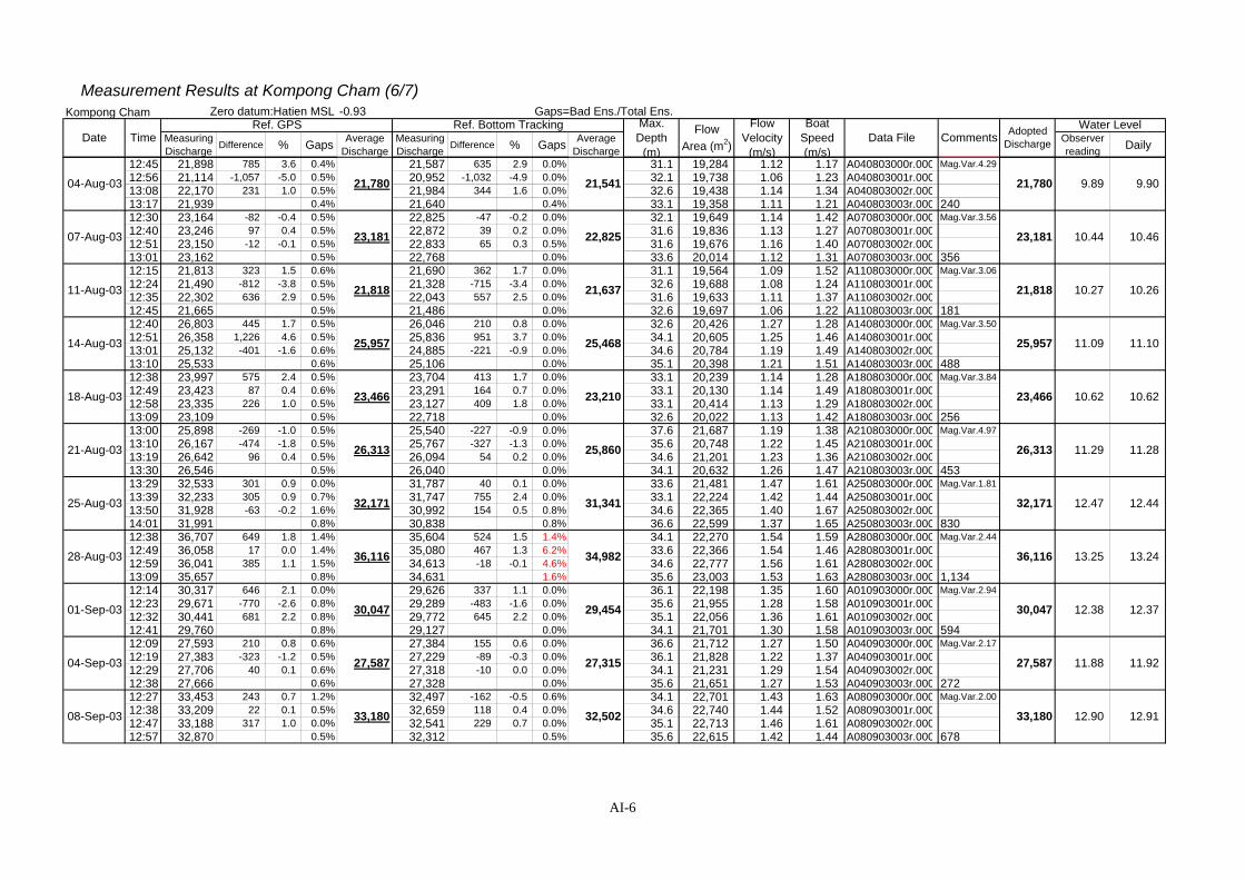
Measurement Results at Kompong Cham (6/7)Kompong Cham Zero datum:Hatien MSL -0.93 Gaps=Bad Ens./Total Ens.
MeasuringDischarge Difference % Gaps Average
DischargeMeasuringDischarge Difference % Gaps Average
DischargeObserverreading DailyDate Time
Ref. GPS Ref. Bottom TrackingData File Comments Adopted
Discharge
Water LevelMax.Depth
(m)
FlowArea (m2)
FlowVelocity
(m/s)
BoatSpeed(m/s)
12:45 21,898 785 3.6 0.4% 21,587 635 2.9 0.0% 31.1 19,284 1.12 1.17 A040803000r.000 Mag.Var.4.2912:56 21,114 -1,057 -5.0 0.5% 20,952 -1,032 -4.9 0.0% 32.1 19,738 1.06 1.23 A040803001r.00013:08 22,170 231 1.0 0.5% 21,984 344 1.6 0.0% 32.6 19,438 1.14 1.34 A040803002r.00013:17 21,939 0.4% 21,640 0.4% 33.1 19,358 1.11 1.21 A040803003r.000 24012:30 23,164 -82 -0.4 0.5% 22,825 -47 -0.2 0.0% 32.1 19,649 1.14 1.42 A070803000r.000 Mag.Var.3.5612:40 23,246 97 0.4 0.5% 22,872 39 0.2 0.0% 31.6 19,836 1.13 1.27 A070803001r.00012:51 23,150 -12 -0.1 0.5% 22,833 65 0.3 0.5% 31.6 19,676 1.16 1.40 A070803002r.00013:01 23,162 0.5% 22,768 0.0% 33.6 20,014 1.12 1.31 A070803003r.000 35612:15 21,813 323 1.5 0.6% 21,690 362 1.7 0.0% 31.1 19,564 1.09 1.52 A110803000r.000 Mag.Var.3.0612:24 21,490 -812 -3.8 0.5% 21,328 -715 -3.4 0.0% 32.6 19,688 1.08 1.24 A110803001r.00012:35 22,302 636 2.9 0.5% 22,043 557 2.5 0.0% 31.6 19,633 1.11 1.37 A110803002r.00012:45 21,665 0.5% 21,486 0.0% 32.6 19,697 1.06 1.22 A110803003r.000 18112:40 26,803 445 1.7 0.5% 26,046 210 0.8 0.0% 32.6 20,426 1.27 1.28 A140803000r.000 Mag.Var.3.5012:51 26,358 1,226 4.6 0.5% 25,836 951 3.7 0.0% 34.1 20,605 1.25 1.46 A140803001r.00013:01 25,132 -401 -1.6 0.6% 24,885 -221 -0.9 0.0% 34.6 20,784 1.19 1.49 A140803002r.00013:10 25,533 0.6% 25,106 0.0% 35.1 20,398 1.21 1.51 A140803003r.000 48812:38 23,997 575 2.4 0.5% 23,704 413 1.7 0.0% 33.1 20,239 1.14 1.28 A180803000r.000 Mag.Var.3.8412:49 23,423 87 0.4 0.6% 23,291 164 0.7 0.0% 33.1 20,130 1.14 1.49 A180803001r.00012:58 23,335 226 1.0 0.5% 23,127 409 1.8 0.0% 33.1 20,414 1.13 1.29 A180803002r.00013:09 23,109 0.5% 22,718 0.0% 32.6 20,022 1.13 1.42 A180803003r.000 25613:00 25,898 -269 -1.0 0.5% 25,540 -227 -0.9 0.0% 37.6 21,687 1.19 1.38 A210803000r.000 Mag.Var.4.9713:10 26,167 -474 -1.8 0.5% 25,767 -327 -1.3 0.0% 35.6 20,748 1.22 1.45 A210803001r.00013:19 26,642 96 0.4 0.5% 26,094 54 0.2 0.0% 34.6 21,201 1.23 1.36 A210803002r.00013:30 26,546 0.5% 26,040 0.0% 34.1 20,632 1.26 1.47 A210803003r.000 45313:29 32,533 301 0.9 0.0% 31,787 40 0.1 0.0% 33.6 21,481 1.47 1.61 A250803000r.000 Mag.Var.1.8113:39 32,233 305 0.9 0.7% 31,747 755 2.4 0.0% 33.1 22,224 1.42 1.44 A250803001r.00013:50 31,928 -63 -0.2 1.6% 30,992 154 0.5 0.8% 34.6 22,365 1.40 1.67 A250803002r.00014:01 31,991 0.8% 30,838 0.8% 36.6 22,599 1.37 1.65 A250803003r.000 83012:38 36,707 649 1.8 1.4% 35,604 524 1.5 1.4% 34.1 22,270 1.54 1.59 A280803000r.000 Mag.Var.2.4412:49 36,058 17 0.0 1.4% 35,080 467 1.3 6.2% 33.6 22,366 1.54 1.46 A280803001r.00012:59 36,041 385 1.1 1.5% 34,613 -18 -0.1 4.6% 34.6 22,777 1.56 1.61 A280803002r.00013:09 35,657 0.8% 34,631 1.6% 35.6 23,003 1.53 1.63 A280803003r.000 1,13412:14 30,317 646 2.1 0.0% 29,626 337 1.1 0.0% 36.1 22,198 1.35 1.60 A010903000r.000 Mag.Var.2.9412:23 29,671 -770 -2.6 0.8% 29,289 -483 -1.6 0.0% 35.6 21,955 1.28 1.58 A010903001r.00012:32 30,441 681 2.2 0.8% 29,772 645 2.2 0.0% 35.1 22,056 1.36 1.61 A010903002r.00012:41 29,760 0.8% 29,127 0.0% 34.1 21,701 1.30 1.58 A010903003r.000 59412:09 27,593 210 0.8 0.6% 27,384 155 0.6 0.0% 36.6 21,712 1.27 1.50 A040903000r.000 Mag.Var.2.1712:19 27,383 -323 -1.2 0.5% 27,229 -89 -0.3 0.0% 36.1 21,828 1.22 1.37 A040903001r.00012:29 27,706 40 0.1 0.6% 27,318 -10 0.0 0.0% 34.1 21,231 1.29 1.54 A040903002r.00012:38 27,666 0.6% 27,328 0.0% 35.6 21,651 1.27 1.53 A040903003r.000 27212:27 33,453 243 0.7 1.2% 32,497 -162 -0.5 0.6% 34.1 22,701 1.43 1.63 A080903000r.000 Mag.Var.2.0012:38 33,209 22 0.1 0.5% 32,659 118 0.4 0.0% 34.6 22,740 1.44 1.52 A080903001r.00012:47 33,188 317 1.0 0.0% 32,541 229 0.7 0.0% 35.1 22,713 1.46 1.61 A080903002r.00012:57 32,870 0.5% 32,312 0.5% 35.6 22,615 1.42 1.44 A080903003r.000 678
11.29 11.2821-Aug-03 26,313 25,860 26,313
18-Aug-03 23,466 23,210 23,466 10.62 10.62
10.44 10.4607-Aug-03 23,181 22,825 23,181
04-Aug-03 21,780 21,541 21,780 9.89 9.90
10.27 10.2611-Aug-03 21,818 21,637 21,818
14-Aug-03 25,957 25,468 25,957 11.09 11.10
12.47 12.4425-Aug-03 32,171 31,341 32,171
28-Aug-03 36,116 34,982 36,116 13.25 13.24
12.38 12.3701-Sep-03 30,047 29,454 30,047
04-Sep-03 27,587 27,315 27,587 11.88 11.92
08-Sep-03 33,180 32,502 33,180 12.90 12.91
AI-6
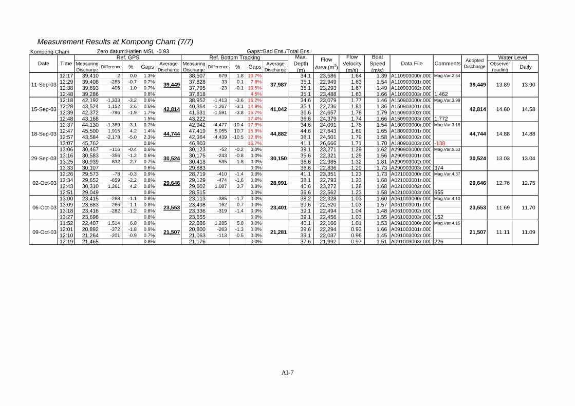
Measurement Results at Kompong Cham (7/7)Kompong Cham Zero datum:Hatien MSL -0.93 Gaps=Bad Ens./Total Ens.
MeasuringDischarge Difference % Gaps Average
DischargeMeasuringDischarge Difference % Gaps Average
DischargeObserverreading DailyDate Time
Ref. GPS Ref. Bottom TrackingData File Comments Adopted
Discharge
Water LevelMax.Depth
(m)
FlowArea (m2)
FlowVelocity
(m/s)
BoatSpeed(m/s)
12:17 39,410 2 0.0 1.3% 38,507 679 1.8 10.7% 34.1 23,586 1.64 1.39 A110903000r.000 Mag.Var.2.5412:29 39,408 -285 -0.7 0.7% 37,828 33 0.1 7.8% 35.1 22,949 1.63 1.54 A110903001r.00012:38 39,693 406 1.0 0.7% 37,795 -23 -0.1 10.5% 35.1 23,293 1.67 1.49 A110903002r.00012:48 39,286 0.8% 37,818 4.5% 35.1 23,488 1.63 1.66 A110903003r.000 1,46212:18 42,192 -1,333 -3.2 0.6% 38,952 -1,413 -3.6 16.2% 34.6 23,079 1.77 1.46 A150903000r.000 Mag.Var.3.9912:28 43,524 1,152 2.6 0.6% 40,364 -1,267 -3.1 14.9% 35.1 22,736 1.81 1.36 A150903001r.00012:39 42,372 -796 -1.9 1.7% 41,631 -1,591 -3.8 15.7% 36.6 24,657 1.78 1.79 A150903002r.00012:48 43,168 1.5% 43,222 17.4% 36.6 24,379 1.74 1.66 A150903003r.000 1,77212:37 44,130 -1,369 -3.1 0.7% 42,942 -4,477 -10.4 17.9% 34.6 24,091 1.78 1.54 A180903000r.000 Mag.Var.3.1812:47 45,500 1,915 4.2 1.4% 47,419 5,055 10.7 15.9% 44.6 27,643 1.69 1.65 A180903001r.00012:57 43,584 -2,178 -5.0 2.3% 42,364 -4,439 -10.5 12.8% 38.1 24,501 1.79 1.58 A180903002r.00013:07 45,762 0.8% 46,803 16.7% 41.1 26,666 1.71 1.70 A180903003r.000 -13813:06 30,467 -116 -0.4 0.6% 30,123 -52 -0.2 0.0% 39.1 23,271 1.29 1.62 A290903000r.000 Mag.Var.5.5313:16 30,583 -356 -1.2 0.6% 30,175 -243 -0.8 0.0% 35.6 22,321 1.29 1.56 A290903001r.00013:25 30,939 832 2.7 0.7% 30,418 535 1.8 0.0% 36.6 22,985 1.32 1.81 A290903002r.00013:33 30,107 0.6% 29,883 0.0% 36.6 22,836 1.29 1.73 A290903003r.000 37412:26 29,573 -78 -0.3 0.9% 28,719 -410 -1.4 0.0% 41.1 23,351 1.23 1.73 A021003000r.000 Mag.Var.4.3712:34 29,652 -659 -2.2 0.8% 29,129 -474 -1.6 0.0% 38.1 22,793 1.23 1.68 A021003001r.00012:43 30,310 1,261 4.2 0.8% 29,602 1,087 3.7 0.8% 40.6 23,272 1.28 1.68 A021003002r.00012:51 29,049 0.8% 28,515 0.0% 36.6 22,562 1.23 1.58 A021003003r.000 65513:00 23,415 -268 -1.1 0.8% 23,113 -385 -1.7 0.0% 38.2 22,328 1.03 1.60 A061003000r.000 Mag.Var.4.1013:09 23,683 266 1.1 0.8% 23,498 162 0.7 0.0% 39.6 22,520 1.03 1.57 A061003001r.00013:18 23,416 -282 -1.2 0.8% 23,336 -319 -1.4 0.0% 39.1 22,494 1.04 1.48 A061003002r.00013:27 23,698 0.8% 23,655 0.0% 39.1 22,456 1.03 1.55 A061003003r.000 15211:52 22,407 1,514 6.8 0.8% 22,086 1,285 5.8 0.0% 40.1 22,166 1.01 1.53 A091003000r.000 Mag.Var.4.1512:01 20,892 -372 -1.8 0.9% 20,800 -263 -1.3 0.0% 39.6 22,294 0.93 1.66 A091003001r.00012:10 21,264 -201 -0.9 0.7% 21,063 -113 -0.5 0.0% 39.1 22,037 0.96 1.45 A091003002r.00012:19 21,465 0.8% 21,176 0.0% 37.6 21,992 0.97 1.51 A091003003r.000 226
11.11 11.09
12.76 12.75
11.69 11.7006-Oct-03 23,553 23,401 23,553
09-Oct-03 21,507 21,281 21,507
02-Oct-03 29,646 28,991 29,646
29-Sep-03 30,524 30,150 30,524 13.03 13.04
14.60 14.5815-Sep-03 42,814 41,042 42,814
11-Sep-03 39,449 37,987 39,449 13.89 13.90
18-Sep-03 44,744 44,882 44,744 14.88 14.88
AI-7

Volume II: Supporting Report. Paper III: Hydrologic MonitoringWUP-JICA, March 2004
ANNEX II INDOOR TRAINING ON FLOW DATA MANAGEMENT
(25 NOVEMBER 2003)
1. OBJECTIVES
To provide participants with final outcomes of the WUP-JICA discharge measurement activities.
To share these outcomes and knowledge, in particular, focusing on future flow management in Cambodia.
To explore technical practices for the development of discharge rating curves using measured data.
To exchange views and issues on future flow management in Cambodia.
2. TENTATIVE PROGRAM
Venue: Third Floor, Building opposite MRCS
Time Activities
0830-0930
Opening and Objectives Clear Understanding of Hydrological Features of the Cambodian Floodplains through Discharge Measurement and Processing (Mr. MORISHITA Kanehiro)
0930-1015 Discharge Measurements and Data Processing (1) (Mr. HAMADA Yuichiro)
1015-1030 Coffee Break
1030-1115 Discharge Measurements and Data Processing (2) (Mr. HAMADA Yuichiro)
1115-1200 Theoretical Aspects of Program and Know-how on Input Data File Preparation (Mr. Khadananda LAMSAL)
1200-1330 Lunch
1330-1415 Procedure of Program Execution and Going through Output Data File(Mr. Khadananda LAMSAL)
1415-1430 Coffee Break
1430-1515 Demonstration of Program and Hands-on Session (Mr. Khadananda LAMSAL)
1515-1600 Question and Answer Closing
AII-1

Volume II: Supporting Report. Paper III: Hydrologic MonitoringWUP-JICA, March 2004
3. ATTENDANCE LIST
No. Name Organization Position 1 Long Saravuth DHRW,
MOWRAM Deputy Director of DHRW
2 Horn Sovanna - Chief of Hydrology Works Office3 So Im Monichoth - Chief of Forecast and Research
Office 4 Sam Sopheak - Deputy Chief of Hydrology
Works Office 5 Vin Bunpove - Technical Staff of Hydrology
Works Office 6 Khun Thoeun - Technical Staff of Hydrology
Works Office 7 Pot Pove - Technical Staff of Hydrology
Works Office 8 Yin Savuth - Technical Staff of Hydrology
Works Office 9 Sreng So Tha - Technical Staff of Hydrology
Works Office 10 Sok Saing Im MRCS Senior Hydrologist, Technical
Support Division 11 Chayanis
Manusthiparom - Operational Hydrologist,
Technical Support Division 11 MORISHITA Kanehiro WUP-JICA Team Leader 12 HAMADA Yuichiro - Hydrological Monitoring 13 Khadananda LAMSAL - Hydrologist,
MRC/NMC Coordinator
4. HANDOUTS FOR THE INDOOR TRAINING
Handout for Discharge Measurement and Data Processing
User Manual for Rating Curve Development Program
The handout and manual are attached in the following pages.
AII-2
Volume II: Supporting Report. Paper III: Hydrologic MonitoringWUP-JICA, March 2004
HANDOUT
FOR
DISCHARGE MEASUREMENT
AND DATA PROCESSING
25 NOVEMBER 2003
WUP-JICA TEAM
AII-3
Volume II: Supporting Report. Paper III: Hydrologic MonitoringWUP-JICA, March 2004
TABLE OF CONTENTS
1. CHARACTERISTICS OF ADCP DATA ..................................................... AII-5
1.1 Discharge Calculation ............................................................................. AII-5
1.2 ADCP Ensemble and Depth Cell ............................................................ AII-5
1.3 Data Error in the Result .......................................................................... AII-5
1.4 Supplementary Explanation .................................................................... AII-8
2. ADCP CALCULATION SYSTEM ............................................................... AII-9
2.1 Integrating GPS, External Compass and Depth Sounder ........................ AII-9
2.2 ADCP Calculation System ...................................................................... AII-9
2.3 Measurement Results Depending on External Equipment ....................... AII-11
3. PROCEDURE OF ADCP MEASUREMENT .............................................. AII-17
4. RULES FOR RESULT SELECTION ........................................................... AII-19
4.1 Summary Table ....................................................................................... AII-19
4.2 Setting for “Mag.Variation” ................................................................... AII-20
4.3 Rules for Result Selection ....................................................................... AII-22
AII-4
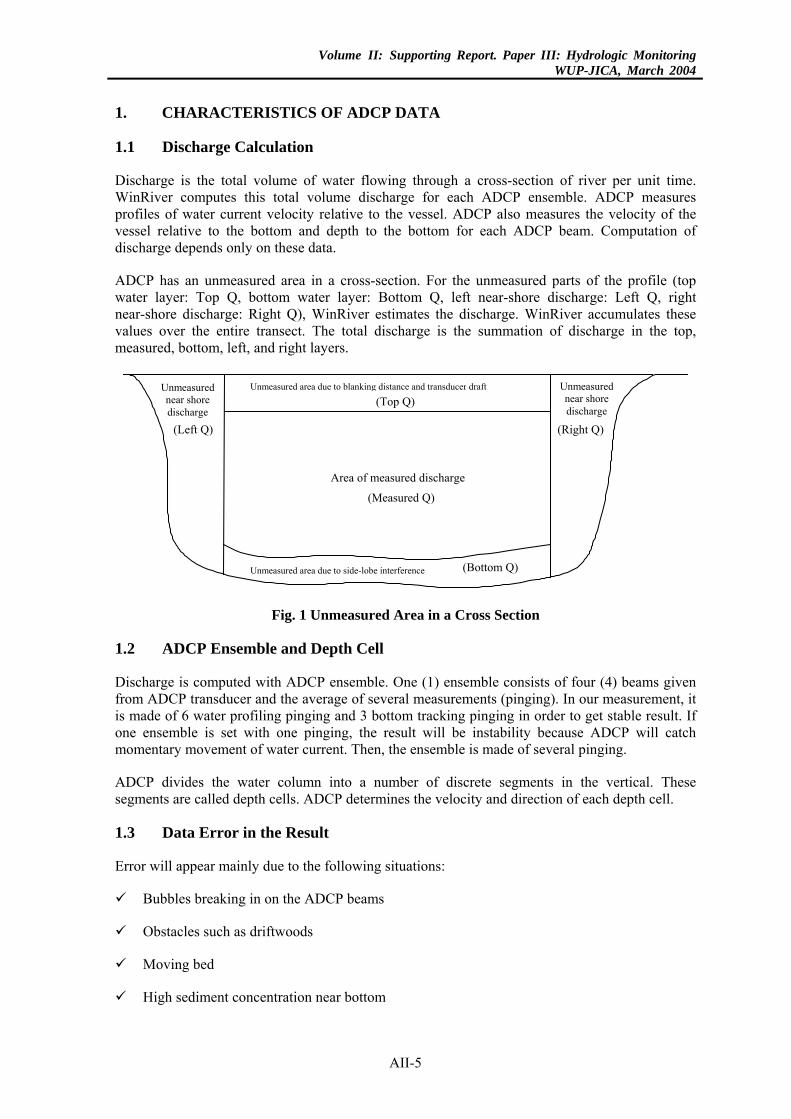
Volume II: Supporting Report. Paper III: Hydrologic MonitoringWUP-JICA, March 2004
1. CHARACTERISTICS OF ADCP DATA
1.1 Discharge Calculation
Discharge is the total volume of water flowing through a cross-section of river per unit time. WinRiver computes this total volume discharge for each ADCP ensemble. ADCP measures profiles of water current velocity relative to the vessel. ADCP also measures the velocity of the vessel relative to the bottom and depth to the bottom for each ADCP beam. Computation of discharge depends only on these data.
ADCP has an unmeasured area in a cross-section. For the unmeasured parts of the profile (top water layer: Top Q, bottom water layer: Bottom Q, left near-shore discharge: Left Q, right near-shore discharge: Right Q), WinRiver estimates the discharge. WinRiver accumulates these values over the entire transect. The total discharge is the summation of discharge in the top, measured, bottom, left, and right layers.
Unmeasured near shore discharge
Unmeasured near shore discharge
Unmeasured area due to blanking distance and transducer draft
(Top Q)
(Left Q) (Right Q)
Area of measured discharge
(Measured Q)
(Bottom Q)Unmeasured area due to side-lobe interference
Fig. 1 Unmeasured Area in a Cross Section
1.2 ADCP Ensemble and Depth Cell
Discharge is computed with ADCP ensemble. One (1) ensemble consists of four (4) beams given from ADCP transducer and the average of several measurements (pinging). In our measurement, it is made of 6 water profiling pinging and 3 bottom tracking pinging in order to get stable result. If one ensemble is set with one pinging, the result will be instability because ADCP will catch momentary movement of water current. Then, the ensemble is made of several pinging.
ADCP divides the water column into a number of discrete segments in the vertical. These segments are called depth cells. ADCP determines the velocity and direction of each depth cell.
1.3 Data Error in the Result
Error will appear mainly due to the following situations:
Bubbles breaking in on the ADCP beams
Obstacles such as driftwoods
Moving bed
High sediment concentration near bottom
AII-5
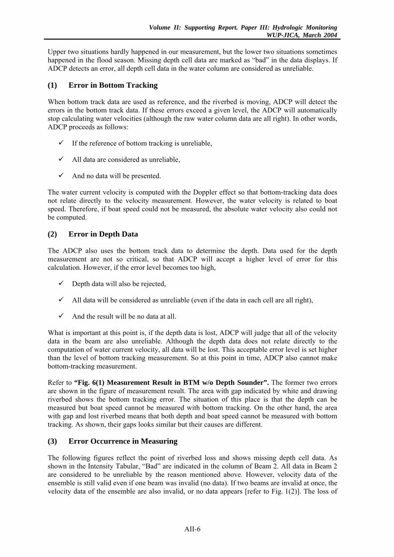
Volume II: Supporting Report. Paper III: Hydrologic MonitoringWUP-JICA, March 2004
Upper two situations hardly happened in our measurement, but the lower two situations sometimes happened in the flood season. Missing depth cell data are marked as “bad” in the data displays. If ADCP detects an error, all depth cell data in the water column are considered as unreliable.
(1) Error in Bottom Tracking
When bottom track data are used as reference, and the riverbed is moving, ADCP will detect the errors in the bottom track data. If these errors exceed a given level, the ADCP will automatically stop calculating water velocities (although the raw water column data are all right). In other words, ADCP proceeds as follows:
If the reference of bottom tracking is unreliable,
All data are considered as unreliable,
And no data will be presented.
The water current velocity is computed with the Doppler effect so that bottom-tracking data does not relate directly to the velocity measurement. However, the water velocity is related to boat speed. Therefore, if boat speed could not be measured, the absolute water velocity also could not be computed.
(2) Error in Depth Data
The ADCP also uses the bottom track data to determine the depth. Data used for the depth measurement are not so critical, so that ADCP will accept a higher level of error for this calculation. However, if the error level becomes too high,
Depth data will also be rejected,
All data will be considered as unreliable (even if the data in each cell are all right),
And the result will be no data at all.
What is important at this point is, if the depth data is lost, ADCP will judge that all of the velocity data in the beam are also unreliable. Although the depth data does not relate directly to the computation of water current velocity, all data will be lost. This acceptable error level is set higher than the level of bottom tracking measurement. So at this point in time, ADCP also cannot make bottom-tracking measurement.
Refer to “Fig. 6(1) Measurement Result in BTM w/o Depth Sounder”. The former two errors are shown in the figure of measurement result. The area with gap indicated by white and drawing riverbed shows the bottom tracking error. The situation of this place is that the depth can be measured but boat speed cannot be measured with bottom tracking. On the other hand, the area with gap and lost riverbed means that both depth and boat speed cannot be measured with bottom tracking. As shown, their gaps looks similar but their causes are different.
(3) Error Occurrence in Measuring
The following figures reflect the point of riverbed loss and shows missing depth cell data. As shown in the Intensity Tabular, “Bad” are indicated in the column of Beam 2. All data in Beam 2 are considered to be unreliable by the reason mentioned above. However, velocity data of the ensemble is still valid even if one beam was invalid (no data). If two beams are invalid at once, the velocity data of the ensemble are also invalid, or no data appears [refer to Fig. 1(2)]. The loss of
AII-6
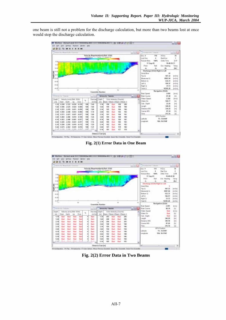
Volume II: Supporting Report. Paper III: Hydrologic MonitoringWUP-JICA, March 2004
one beam is still not a problem for the discharge calculation, but more than two beams lost at once would stop the discharge calculation.
Fig. 2(1) Error Data in One Beam
Fig. 2(2) Error Data in Two Beams
AII-7
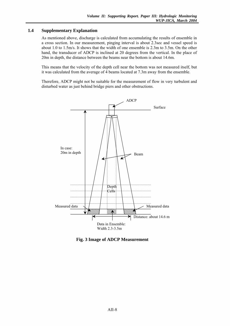
Volume II: Supporting Report. Paper III: Hydrologic MonitoringWUP-JICA, March 2004
1.4 Supplementary Explanation
As mentioned above, discharge is calculated from accumulating the results of ensemble in a cross section. In our measurement, pinging interval is about 2.3sec and vessel speed is about 1.0 to 1.5m/s. It shows that the width of one ensemble is 2.3m to 3.5m. On the other hand, the transducer of ADCP is inclined at 20 degrees from the vertical. In the place of 20m in depth, the distance between the beams near the bottom is about 14.6m.
This means that the velocity of the depth cell near the bottom was not measured itself, but it was calculated from the average of 4 beams located at 7.3m away from the ensemble.
Therefore, ADCP might not be suitable for the measurement of flow in very turbulent and disturbed water as just behind bridge piers and other obstructions.
In case: 20m in depth
Distance: about 14.6 m
Surface
Measured data Measured data
Beam
Depth Cells
ADCP
Data in Ensemble: Width 2.3-3.5m
Fig. 3 Image of ADCP Measurement
AII-8
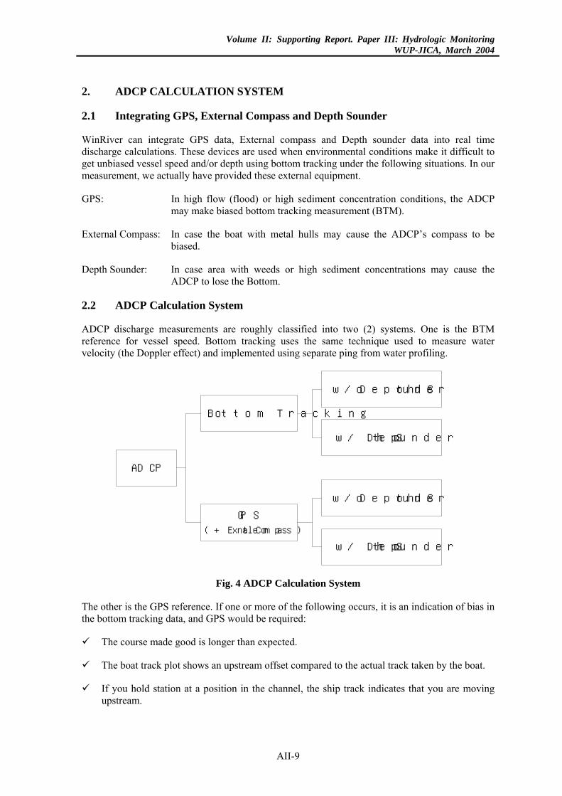
Volume II: Supporting Report. Paper III: Hydrologic MonitoringWUP-JICA, March 2004
2. ADCP CALCULATION SYSTEM
2.1 Integrating GPS, External Compass and Depth Sounder
WinRiver can integrate GPS data, External compass and Depth sounder data into real time discharge calculations. These devices are used when environmental conditions make it difficult to get unbiased vessel speed and/or depth using bottom tracking under the following situations. In our measurement, we actually have provided these external equipment.
GPS: In high flow (flood) or high sediment concentration conditions, the ADCP may make biased bottom tracking measurement (BTM).
External Compass: In case the boat with metal hulls may cause the ADCP’s compass to be biased.
Depth Sounder: In case area with weeds or high sediment concentrations may cause the ADCP to lose the Bottom.
2.2 ADCP Calculation System
ADCP discharge measurements are roughly classified into two (2) systems. One is the BTM reference for vessel speed. Bottom tracking uses the same technique used to measure water velocity (the Doppler effect) and implemented using separate ping from water profiling.
ADCP
Bottom Tracking
GPS(+ External Compass)
w/o Depth Sounder
w/ Depth Sounder
w/o Depth Sounder
w/ Depth Sounder
Fig. 4 ADCP Calculation System
The other is the GPS reference. If one or more of the following occurs, it is an indication of bias in the bottom tracking data, and GPS would be required:
The course made good is longer than expected.
The boat track plot shows an upstream offset compared to the actual track taken by the boat.
If you hold station at a position in the channel, the ship track indicates that you are moving upstream.
AII-9
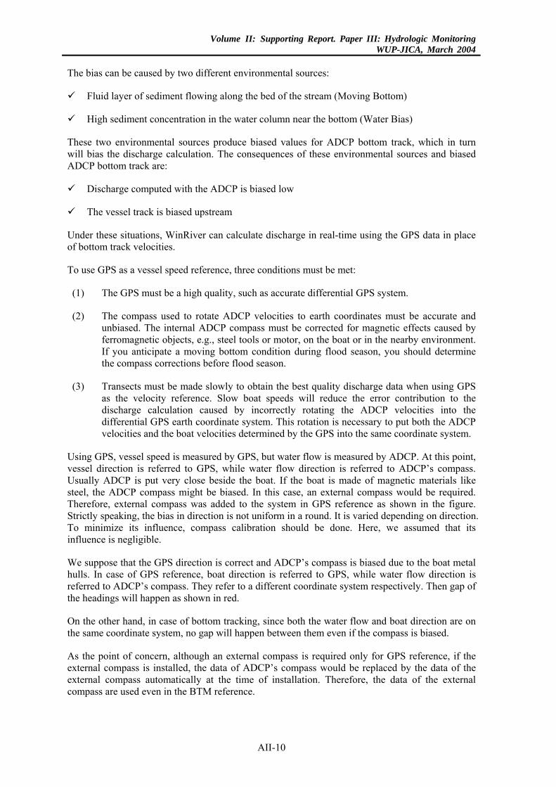
Volume II: Supporting Report. Paper III: Hydrologic MonitoringWUP-JICA, March 2004
The bias can be caused by two different environmental sources:
Fluid layer of sediment flowing along the bed of the stream (Moving Bottom)
High sediment concentration in the water column near the bottom (Water Bias)
These two environmental sources produce biased values for ADCP bottom track, which in turn will bias the discharge calculation. The consequences of these environmental sources and biased ADCP bottom track are:
Discharge computed with the ADCP is biased low
The vessel track is biased upstream
Under these situations, WinRiver can calculate discharge in real-time using the GPS data in place of bottom track velocities.
To use GPS as a vessel speed reference, three conditions must be met:
(1) The GPS must be a high quality, such as accurate differential GPS system.
(2) The compass used to rotate ADCP velocities to earth coordinates must be accurate and unbiased. The internal ADCP compass must be corrected for magnetic effects caused by ferromagnetic objects, e.g., steel tools or motor, on the boat or in the nearby environment. If you anticipate a moving bottom condition during flood season, you should determine the compass corrections before flood season.
(3) Transects must be made slowly to obtain the best quality discharge data when using GPS as the velocity reference. Slow boat speeds will reduce the error contribution to the discharge calculation caused by incorrectly rotating the ADCP velocities into the differential GPS earth coordinate system. This rotation is necessary to put both the ADCP velocities and the boat velocities determined by the GPS into the same coordinate system.
Using GPS, vessel speed is measured by GPS, but water flow is measured by ADCP. At this point, vessel direction is referred to GPS, while water flow direction is referred to ADCP’s compass. Usually ADCP is put very close beside the boat. If the boat is made of magnetic materials like steel, the ADCP compass might be biased. In this case, an external compass would be required. Therefore, external compass was added to the system in GPS reference as shown in the figure. Strictly speaking, the bias in direction is not uniform in a round. It is varied depending on direction. To minimize its influence, compass calibration should be done. Here, we assumed that its influence is negligible.
We suppose that the GPS direction is correct and ADCP’s compass is biased due to the boat metal hulls. In case of GPS reference, boat direction is referred to GPS, while water flow direction is referred to ADCP’s compass. They refer to a different coordinate system respectively. Then gap of the headings will happen as shown in red.
On the other hand, in case of bottom tracking, since both the water flow and boat direction are on the same coordinate system, no gap will happen between them even if the compass is biased.
As the point of concern, although an external compass is required only for GPS reference, if the external compass is installed, the data of ADCP’s compass would be replaced by the data of the external compass automatically at the time of installation. Therefore, the data of the external compass are used even in the BTM reference.
AII-10
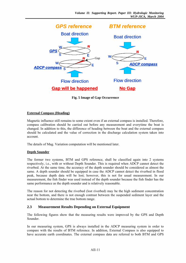
Volume II: Supporting Report. Paper III: Hydrologic MonitoringWUP-JICA, March 2004
GPS reference BTM referenceGPS reference BTM reference
E
W
S
EW
S
Boat direction
Flow direction
EW
S
Boat direction
Flow direction
ADCP compassADCP compass
GPSE
W
S E
W
S
EW
SEW
S
Boat direction
Flow direction
EW
SEW
S
Boat direction
Flow direction
ADCP compassADCP compass
GPS
N
N
N
Gap will be happened No Gap
NN
NN
NN
Gap will be happened No Gap
Gap
Fig. 5 Image of Gap Occurrence
External Compass (Heading)
Magnetic influence still remains to some extent even if an external compass is installed. Therefore, compass calibration should be carried out before any measurement and everytime the boat is changed. In addition to this, the difference of heading between the boat and the external compass should be calculated and the value of correction in the discharge calculation system taken into account.
The details of Mag. Variation computation will be mentioned later.
Depth Sounder
The former two systems, BTM and GPS reference, shall be classified again into 2 systems respectively, i.e., with or without Depth Sounder. This is required when ADCP cannot detect the riverbed. At the same time, the accuracy of the depth sounder should be considered as almost the same. A depth sounder should be equipped in case the ADCP cannot detect the riverbed in flood peak, because depth data will be lost; however, this is not for usual measurement. In our measurement, the fish finder was used instead of the depth sounder because the fish finder has the same performance as the depth sounder and is relatively reasonable.
The reason for not detecting the riverbed (lost riverbed) may be the high sediment concentration near the bottom, and there is not enough contrast between the suspended sediment layer and the actual bottom to determine the true bottom range.
2.3 Measurement Results Depending on External Equipment
The following figures show that the measuring results were improved by the GPS and Depth Sounder.
In our measuring system, GPS is always installed in the ADCP measuring system in order to compare with the results of BTM reference. In addition, External Compass is also equipped to have accurate earth coordinates. The external compass data are referred to both BTM and GPS
AII-11
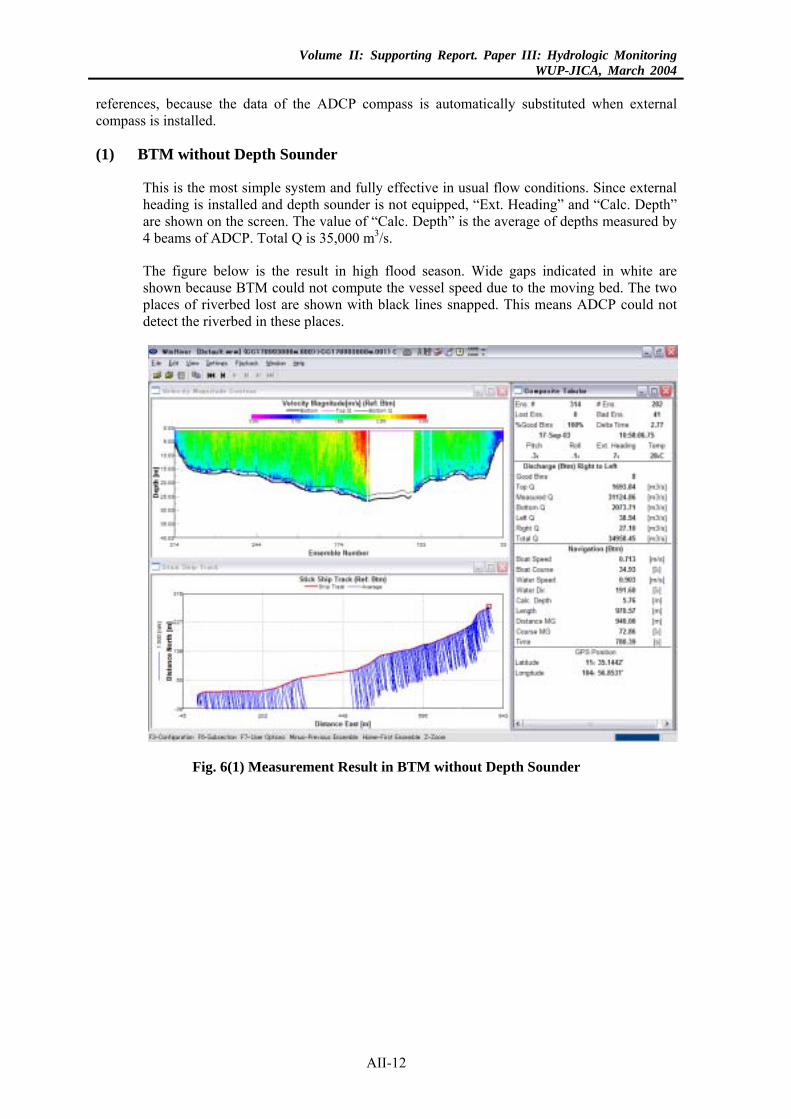
Volume II: Supporting Report. Paper III: Hydrologic MonitoringWUP-JICA, March 2004
references, because the data of the ADCP compass is automatically substituted when external compass is installed.
(1) BTM without Depth Sounder
This is the most simple system and fully effective in usual flow conditions. Since external heading is installed and depth sounder is not equipped, “Ext. Heading” and “Calc. Depth” are shown on the screen. The value of “Calc. Depth” is the average of depths measured by 4 beams of ADCP. Total Q is 35,000 m3/s.
The figure below is the result in high flood season. Wide gaps indicated in white are shown because BTM could not compute the vessel speed due to the moving bed. The two places of riverbed lost are shown with black lines snapped. This means ADCP could not detect the riverbed in these places.
Fig. 6(1) Measurement Result in BTM without Depth Sounder
AII-12
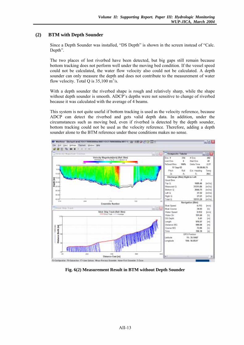
Volume II: Supporting Report. Paper III: Hydrologic MonitoringWUP-JICA, March 2004
(2) BTM with Depth Sounder
Since a Depth Sounder was installed, “DS Depth” is shown in the screen instead of “Calc. Depth”.
The two places of lost riverbed have been detected, but big gaps still remain because bottom tracking does not perform well under the moving bed condition. If the vessel speed could not be calculated, the water flow velocity also could not be calculated. A depth sounder can only measure the depth and does not contribute to the measurement of water flow velocity. Total Q is 35,100 m3/s.
With a depth sounder the riverbed shape is rough and relatively sharp, while the shape without depth sounder is smooth. ADCP’s depths were not sensitive to change of riverbed because it was calculated with the average of 4 beams.
This system is not quite useful if bottom tracking is used as the velocity reference, because ADCP can detect the riverbed and gets valid depth data. In addition, under the circumstances such as moving bed, even if riverbed is detected by the depth sounder, bottom tracking could not be used as the velocity reference. Therefore, adding a depth sounder alone to the BTM reference under these conditions makes no sense.
Fig. 6(2) Measurement Result in BTM without Depth Sounder
AII-13
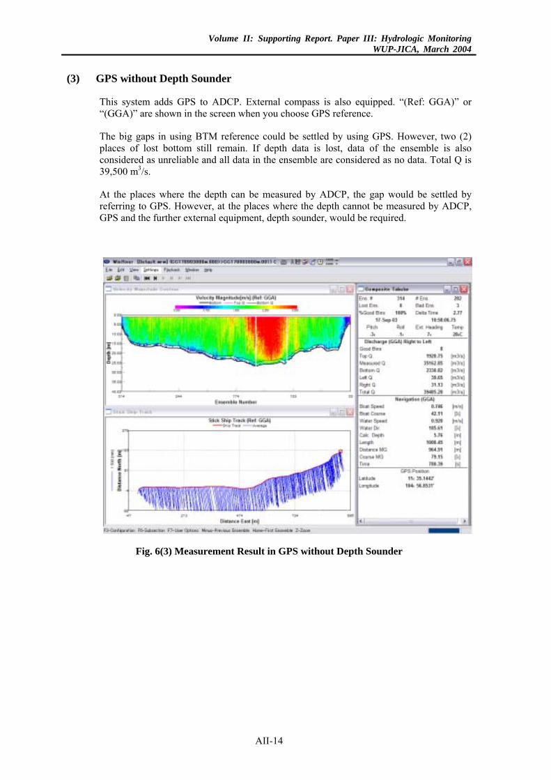
Volume II: Supporting Report. Paper III: Hydrologic MonitoringWUP-JICA, March 2004
(3) GPS without Depth Sounder
This system adds GPS to ADCP. External compass is also equipped. “(Ref: GGA)” or “(GGA)” are shown in the screen when you choose GPS reference.
The big gaps in using BTM reference could be settled by using GPS. However, two (2) places of lost bottom still remain. If depth data is lost, data of the ensemble is also considered as unreliable and all data in the ensemble are considered as no data. Total Q is 39,500 m3/s.
At the places where the depth can be measured by ADCP, the gap would be settled by referring to GPS. However, at the places where the depth cannot be measured by ADCP, GPS and the further external equipment, depth sounder, would be required.
Fig. 6(3) Measurement Result in GPS without Depth Sounder
AII-14
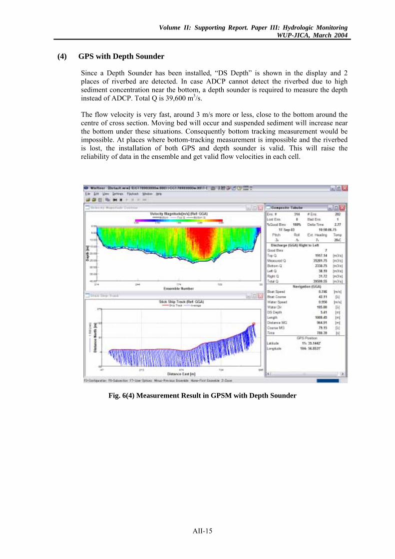
Volume II: Supporting Report. Paper III: Hydrologic MonitoringWUP-JICA, March 2004
(4) GPS with Depth Sounder
Since a Depth Sounder has been installed, “DS Depth” is shown in the display and 2 places of riverbed are detected. In case ADCP cannot detect the riverbed due to high sediment concentration near the bottom, a depth sounder is required to measure the depth instead of ADCP. Total Q is 39,600 m3/s.
The flow velocity is very fast, around 3 m/s more or less, close to the bottom around the centre of cross section. Moving bed will occur and suspended sediment will increase near the bottom under these situations. Consequently bottom tracking measurement would be impossible. At places where bottom-tracking measurement is impossible and the riverbed is lost, the installation of both GPS and depth sounder is valid. This will raise the reliability of data in the ensemble and get valid flow velocities in each cell.
Fig. 6(4) Measurement Result in GPSM with Depth Sounder
AII-15
Volume II: Supporting Report. Paper III: Hydrologic MonitoringWUP-JICA, March 2004
(5) Summary of Effectiveness of Each Measuring System
Considering the situation of error occurrence and so on mentioned above, the effectiveness of each measuring system is summarised as follows:
BTM without Depth Sounder => Total Q = 35,000 m3/s: This system is effective in usual flow conditions but it is not useful in high flow seasons when such situations as the moving bed will happen.
BTM with Depth Sounder => Total Q = 35,100 m3/s: This system is not very useful. When bottom tracking is used as the velocity reference, the depth sounder is not necessary. Besides, when a moving bed occurs, even if the riverbed is detected by the depth sounder, bottom tracking could not be used as the velocity reference.
GPS without Depth Sounder => Total Q = 39,500 m3/s: This system is effective in almost all conditions, but the riverbed will be lost. It is most preferable to install a depth sounder.
GPS with Depth Sounder => Total Q = 39,600 m3/s: This system is effective in any condition, but it is not necessary to use a depth sounder in usual measurements.
As to the measured discharges, there is a big difference of almost 10% between the discharge with BTM and that with GPS references. There are two main reasons for this big difference. One is the low estimation of discharge with BTM reference due to moving bed and the other is the error in the extrapolation of gaps in areas with widely changing water current velocity. As described before, the discharge estimated with BTM reference has the possibility to be low in the flood season, so that GPS should always be equipped in the measuring system.
On the other hand, the discharge difference between with and without depth sounder is quite small in both reference cases because the gaps due to missing depth data are very small compared with the former case so that any error would hardly occur. This happens only a few times a year, hence the influence of the depth error would be quite small. It may be preferable to equip a depth sounder in the system , but it is not indispensable.
AII-16
Volume II: Supporting Report. Paper III: Hydrologic MonitoringWUP-JICA, March 2004
3. PROCEDURE OF ADCP MEASUREMENT
The measuring team of DHRW has been doing measuring work for one year. Therefore, they know the measuring procedure very well and have enough skill on ADCP operation in any situation. However, since the WUP-JICA Team had conducted the data processing and examination of the measured data, the measuring team of DHRW is not yet familiar with data processing and examination. In future, the DHRW team should be able to execute all of the work from measuring to data processing by itself.
To confirm that the measuring procedure is understood, the whole of ADCP measurement procedure is herein mentioned once again. The ADCP measurement procedure is classified into 3 stages; namely, before, during and after measurement, and the action items in each stage are summarised in the table below. With regard to the action items after measurement, particular explanations are mentioned in the following chapter.
Table 1. Action Items of ADCP Measurement
Stage Action Items Special Note 1 Check instruments to be
brought Spare batteries for GPS receiver
(Only the GPS receiver uses different batteries)
Before Measurement
2 Calibration of External Compass
Select an extensive place where there is no big boat made of steel like a tanker and stilling water surface.
Do not put the magnetic instruments or tools near the external compass and ADCP.
Keep the boat stability during the calibration.
Check the connection port of computer (the compass calibration uses port #1).
After the calibration, put back the cable of ADCP to port #1.
1 Reading Water Level Read water level before and after the discharge measurement.
Read the middle value between highest and lowest to remove the wave influence.
Check water level with 2 persons at least.
During Measurement
2 Measuring Preparations Connect the necessary equipment (As for Depth sounder, judge its necessity by last measurement result.)
Setup the configuration file (Filename, Max. Depth expected, External Equipment connected, and Mag. Variation given previously will be used.)
AII-17
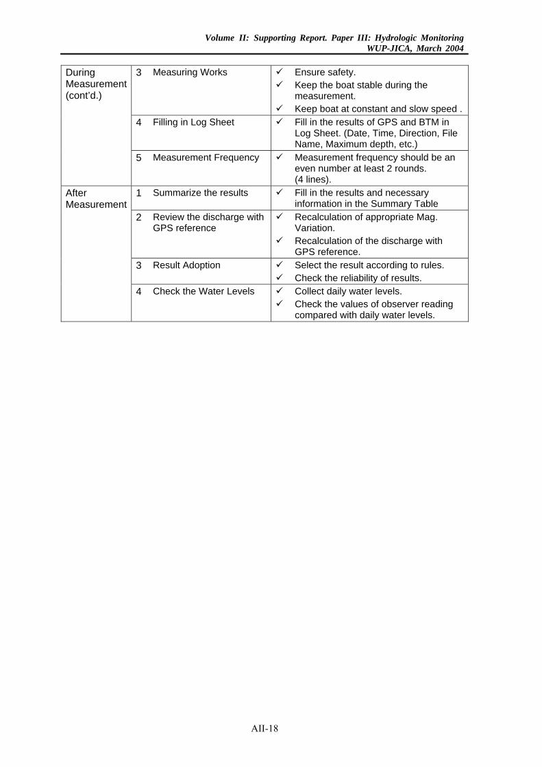
Volume II: Supporting Report. Paper III: Hydrologic MonitoringWUP-JICA, March 2004
3 Measuring Works Ensure safety.
Keep the boat stable during the measurement.
Keep boat at constant and slow speed .4 Filling in Log Sheet Fill in the results of GPS and BTM in
Log Sheet. (Date, Time, Direction, File Name, Maximum depth, etc.)
During Measurement (cont’d.)
5 Measurement Frequency Measurement frequency should be an even number at least 2 rounds. (4 lines).
1 Summarize the results Fill in the results and necessary information in the Summary Table
2 Review the discharge with GPS reference
Recalculation of appropriate Mag. Variation.
Recalculation of the discharge with GPS reference.
3 Result Adoption Select the result according to rules. Check the reliability of results.
After Measurement
4 Check the Water Levels Collect daily water levels. Check the values of observer reading
compared with daily water levels.
AII-18
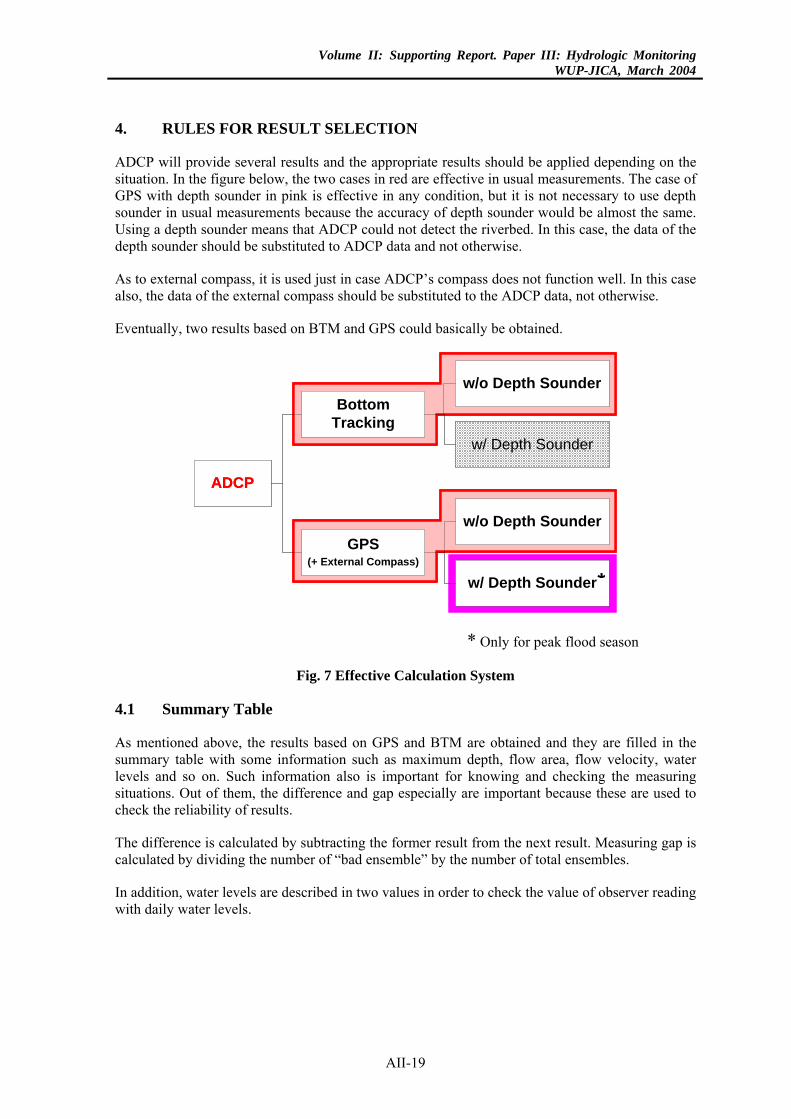
Volume II: Supporting Report. Paper III: Hydrologic MonitoringWUP-JICA, March 2004
4. RULES FOR RESULT SELECTION
ADCP will provide several results and the appropriate results should be applied depending on the situation. In the figure below, the two cases in red are effective in usual measurements. The case of GPS with depth sounder in pink is effective in any condition, but it is not necessary to use depth sounder in usual measurements because the accuracy of depth sounder would be almost the same. Using a depth sounder means that ADCP could not detect the riverbed. In this case, the data of the depth sounder should be substituted to ADCP data and not otherwise.
As to external compass, it is used just in case ADCP’s compass does not function well. In this case also, the data of the external compass should be substituted to the ADCP data, not otherwise.
Eventually, two results based on BTM and GPS could basically be obtained.
BottomTracking
GPS(+ External Compass)
w/o Depth Sounder
w/ Depth Sounder
w/o Depth Sounder
w/ Depth Sounde
BottomTracking
GPS(+ External Compass)
w/o Depth Sounder
w/ Depth Sounder
w/o Depth Sounder
w/ Depth Sounde
ADCPADCP
*
* Only for peak floo
Fig. 7 Effective Calculation System
4.1 Summary Table
As mentioned above, the results based on GPS and BTM are obtained and thesummary table with some information such as maximum depth, flow area, flolevels and so on. Such information also is important for knowing and checkisituations. Out of them, the difference and gap especially are important becausecheck the reliability of results.
The difference is calculated by subtracting the former result from the next result.calculated by dividing the number of “bad ensemble” by the number of total ense
In addition, water levels are described in two values in order to check the value owith daily water levels.
AII-19
rr
d season
y are filled in the w velocity, water ng the measuring these are used to
Measuring gap is mbles.
f observer reading
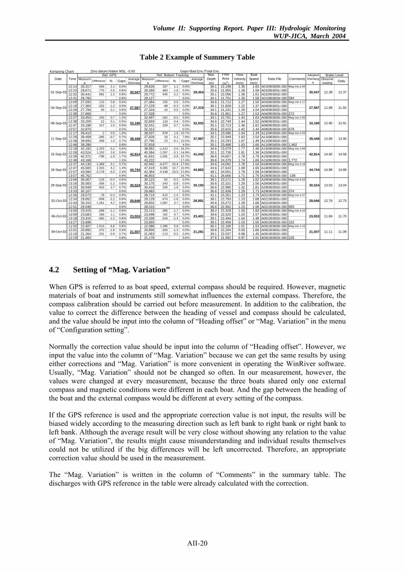
Volume II: Supporting Report. Paper III: Hydrologic MonitoringWUP-JICA, March 2004
Table 2 Example of Summery Table
Kompong Cham Zero datum:Hatien MSL -0.93 Gaps=Bad Ens./Total Ens.
Measuring Difference % Gaps Average
DischargMeasurin
g Difference % Gaps AverageDischarg
Observerreading Daily
12:14 30,317 646 2.1 0.0% 29,626 337 1.1 0.0% 36.1 22,198 1.35 1.60 A010903000r.000 Mag.Var.2.9412:23 29,671 -770 -2.6 0.8% 29,289 -483 -1.6 0.0% 35.6 21,955 1.28 1.58 A010903001r.00012:32 30,441 681 2.2 0.8% 29,772 645 2.2 0.0% 35.1 22,056 1.36 1.61 A010903002r.00012:41 29,760 0.8% 29,127 0.0% 34.1 21,701 1.30 1.58 A010903003r.000 59412:09 27,593 210 0.8 0.6% 27,384 155 0.6 0.0% 36.6 21,712 1.27 1.50 A040903000r.000 Mag.Var.2.1712:19 27,383 -323 -1.2 0.5% 27,229 -89 -0.3 0.0% 36.1 21,828 1.22 1.37 A040903001r.00012:29 27,706 40 0.1 0.6% 27,318 -10 0.0 0.0% 34.1 21,231 1.29 1.54 A040903002r.00012:38 27,666 0.6% 27,328 0.0% 35.6 21,651 1.27 1.53 A040903003r.000 27212:27 33,453 243 0.7 1.2% 32,497 -162 -0.5 0.6% 34.1 22,701 1.43 1.63 A080903000r.000 Mag.Var.2.0012:38 33,209 22 0.1 0.5% 32,659 118 0.4 0.0% 34.6 22,740 1.44 1.52 A080903001r.00012:47 33,188 317 1.0 0.0% 32,541 229 0.7 0.0% 35.1 22,713 1.46 1.61 A080903002r.00012:57 32,870 0.5% 32,312 0.5% 35.6 22,615 1.42 1.44 A080903003r.000 67812:17 39,410 2 0.0 1.3% 38,507 679 1.8 10.7% 34.1 23,586 1.64 1.39 A110903000r.000 Mag.Var.2.5412:29 39,408 -285 -0.7 0.7% 37,828 33 0.1 7.8% 35.1 22,949 1.63 1.54 A110903001r.00012:38 39,693 406 1.0 0.7% 37,795 -23 -0.1 10.5% 35.1 23,293 1.67 1.49 A110903002r.00012:48 39,286 0.8% 37,818 4.5% 35.1 23,488 1.63 1.66 A110903003r.000 1,46212:18 42,192 -1,333 -3.2 0.6% 38,952 -1,413 -3.6 16.2% 34.6 23,079 1.77 1.46 A150903000r.000 Mag.Var.3.9912:28 43,524 1,152 2.6 0.6% 40,364 -1,267 -3.1 14.9% 35.1 22,736 1.81 1.36 A150903001r.00012:39 42,372 -796 -1.9 1.7% 41,631 -1,591 -3.8 15.7% 36.6 24,657 1.78 1.79 A150903002r.00012:48 43,168 1.5% 43,222 17.4% 36.6 24,379 1.74 1.66 A150903003r.000 1,77212:37 44,130 -1,369 -3.1 0.7% 42,942 -4,477 -10.4 17.9% 34.6 24,091 1.78 1.54 A180903000r.000 Mag.Var.3.1812:47 45,500 1,915 4.2 1.4% 47,419 5,055 10.7 15.9% 44.6 27,643 1.69 1.65 A180903001r.00012:57 43,584 -2,178 -5.0 2.3% 42,364 -4,439 -10.5 12.8% 38.1 24,501 1.79 1.58 A180903002r.00013:07 45,762 0.8% 46,803 16.7% 41.1 26,666 1.71 1.70 A180903003r.000 -13813:06 30,467 -116 -0.4 0.6% 30,123 -52 -0.2 0.0% 39.1 23,271 1.29 1.62 A290903000r.000 Mag.Var.5.5313:16 30,583 -356 -1.2 0.6% 30,175 -243 -0.8 0.0% 35.6 22,321 1.29 1.56 A290903001r.00013:25 30,939 832 2.7 0.7% 30,418 535 1.8 0.0% 36.6 22,985 1.32 1.81 A290903002r.00013:33 30,107 0.6% 29,883 0.0% 36.6 22,836 1.29 1.73 A290903003r.000 37412:26 29,573 -78 -0.3 0.9% 28,719 -410 -1.4 0.0% 41.1 23,351 1.23 1.73 A021003000r.000 Mag.Var.4.3712:34 29,652 -659 -2.2 0.8% 29,129 -474 -1.6 0.0% 38.1 22,793 1.23 1.68 A021003001r.00012:43 30,310 1,261 4.2 0.8% 29,602 1,087 3.7 0.8% 40.6 23,272 1.28 1.68 A021003002r.00012:51 29,049 0.8% 28,515 0.0% 36.6 22,562 1.23 1.58 A021003003r.000 65513:00 23,415 -268 -1.1 0.8% 23,113 -385 -1.7 0.0% 38.2 22,328 1.03 1.60 A061003000r.000 Mag.Var.4.1013:09 23,683 266 1.1 0.8% 23,498 162 0.7 0.0% 39.6 22,520 1.03 1.57 A061003001r.00013:18 23,416 -282 -1.2 0.8% 23,336 -319 -1.4 0.0% 39.1 22,494 1.04 1.48 A061003002r.00013:27 23,698 0.8% 23,655 0.0% 39.1 22,456 1.03 1.55 A061003003r.000 15211:52 22,407 1,514 6.8 0.8% 22,086 1,285 5.8 0.0% 40.1 22,166 1.01 1.53 A091003000r.000 Mag.Var.4.1512:01 20,892 -372 -1.8 0.9% 20,800 -263 -1.3 0.0% 39.6 22,294 0.93 1.66 A091003001r.00012:10 21,264 -201 -0.9 0.7% 21,063 -113 -0.5 0.0% 39.1 22,037 0.96 1.45 A091003002r.00012:19 21,465 0.8% 21,176 0.0% 37.6 21,992 0.97 1.51 A091003003r.000 226
14.88 14.8818-Sep-03 44,744 44,882 44,744
12.90 12.9108-Sep-03 33,180 32,502 33,180
04-Sep-03 27,587 27,315 27,587 11.88 11.92
12.38 12.3701-Sep-03 30,047 29,454 30,047
Max.Depth
(m)
FlowArea(m2)
FlowVelocity
(m/s)
BoatSpeed(m/s)
Data File CommentsAdoptedDischarg
e
Water LevelRef. GPS Ref. Bottom TrackingDate Time
11-Sep-03 39,449 37,987 39,449 13.89 13.90
15-Sep-03 42,814 41,042 42,814 14.60 14.58
29-Sep-03 30,524 30,150 30,524 13.03 13.04
02-Oct-03 29,646 28,991 29,646 12.76 12.75
06-Oct-03 23,553 23,401 23,553 11.69 11.70
09-Oct-03 21,507 21,281 21,507 11.11 11.09
4.2 Setting of “Mag. Variation”
When GPS is referred to as boat speed, external compass should be required. However, magnetic materials of boat and instruments still somewhat influences the external compass. Therefore, the compass calibration should be carried out before measurement. In addition to the calibration, the value to correct the difference between the heading of vessel and compass should be calculated, and the value should be input into the column of “Heading offset” or “Mag. Variation” in the menu of “Configuration setting”.
Normally the correction value should be input into the column of “Heading offset”. However, we input the value into the column of “Mag. Variation” because we can get the same results by using either corrections and “Mag. Variation” is more convenient in operating the WinRiver software. Usually, “Mag. Variation” should not be changed so often. In our measurement, however, the values were changed at every measurement, because the three boats shared only one external compass and magnetic conditions were different in each boat. And the gap between the heading of the boat and the external compass would be different at every setting of the compass.
If the GPS reference is used and the appropriate correction value is not input, the results will be biased widely according to the measuring direction such as left bank to right bank or right bank to left bank. Although the average result will be very close without showing any relation to the value of “Mag. Variation”, the results might cause misunderstanding and individual results themselves could not be utilized if the big differences will be left uncorrected. Therefore, an appropriate correction value should be used in the measurement.
The “Mag. Variation” is written in the column of “Comments” in the summary table. The discharges with GPS reference in the table were already calculated with the correction.
AII-20
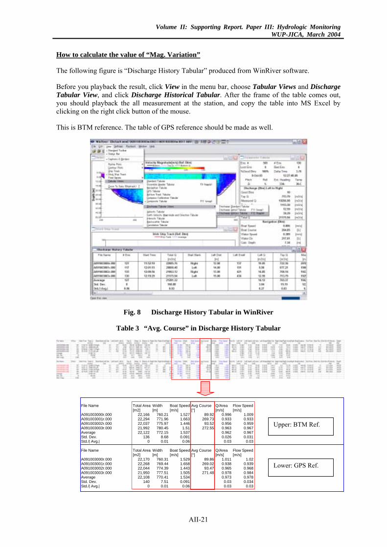
Volume II: Supporting Report. Paper III: Hydrologic MonitoringWUP-JICA, March 2004
How to calculate the value of “Mag. Variation”
The following figure is “Discharge History Tabular” produced from WinRiver software.
Before you playback the result, click View in the menu bar, choose Tabular Views and Discharge Tabular View, and click Discharge Historical Tabular. After the frame of the table comes out, you should playback the all measurement at the station, and copy the table into MS Excel by clicking on the right click button of the mouse.
This is BTM reference. The table of GPS reference should be made as well.
Fig. 8 Discharge History Tabular in WinRiver
Table 3 “Avg. Course” in Discharge History Tabular
File Name Total Area Width Boat Speed Avg Course Q/Area Flow Speed[m2] [m] [m/s] [°] [m/s] [m/s]
A091003000r.000 22,166 760.21 1.527 89.92 0.996 1.009A091003001r.000 22,294 771.96 1.663 269.73 0.933 0.933A091003002r.000 22,037 775.97 1.446 93.52 0.956 0.959A091003003r.000 21,992 780.45 1.51 272.55 0.963 0.967Average 22,122 772.15 1.537 0.962 0.967Std. Dev. 136 8.68 0.091 0.026 0.031Std./| Avg.| 0 0.01 0.06 0.03 0.03
File Name Total Area Width Boat Speed Avg Course Q/Area Flow Speed[m2] [m] [m/s] [°] [m/s] [m/s]
A091003000r.000 22,170 760.31 1.529 89.86 1.011 1.02A091003001r.000 22,268 769.44 1.658 269.02 0.938 0.939A091003002r.000 22,044 774.39 1.443 93.47 0.965 0.968A091003003r.000 21,950 777.51 1.505 271.48 0.978 0.984Average 22,108 770.41 1.534 0.973 0.978Std. Dev. 140 7.51 0.091 0.03 0.034Std./| Avg.| 0 0.01 0.06 0.03 0.03
Lower: GPS Ref.
Upper: BTM Ref.
AII-21
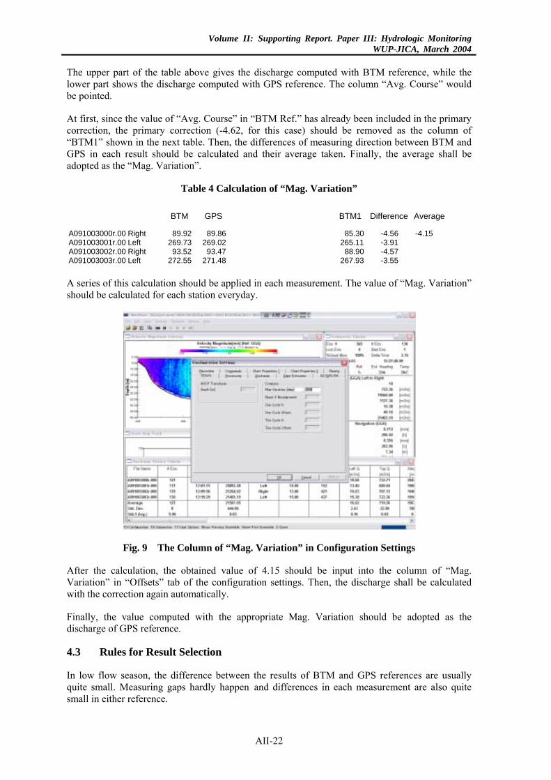
Volume II: Supporting Report. Paper III: Hydrologic MonitoringWUP-JICA, March 2004
The upper part of the table above gives the discharge computed with BTM reference, while the lower part shows the discharge computed with GPS reference. The column “Avg. Course” would be pointed.
At first, since the value of “Avg. Course” in “BTM Ref.” has already been included in the primary correction, the primary correction (-4.62, for this case) should be removed as the column of “BTM1” shown in the next table. Then, the differences of measuring direction between BTM and GPS in each result should be calculated and their average taken. Finally, the average shall be adopted as the “Mag. Variation”.
Table 4 Calculation of “Mag. Variation”
BTM GPS BTM1 Difference Average
A091003000r.00 Right 89.92 89.86 0.06 0.47 85.30 -4.56 -4.15A091003001r.00 Left 269.73 269.02 0.71 265.11 -3.91A091003002r.00 Right 93.52 93.47 0.05 88.90 -4.57A091003003r.00 Left 272.55 271.48 1.07 267.93 -3.55
A series of this calculation should be applied in each measurement. The value of “Mag. Variation” should be calculated for each station everyday.
Fig. 9 The Column of “Mag. Variation” in Configuration Settings
After the calculation, the obtained value of 4.15 should be input into the column of “Mag. Variation” in “Offsets” tab of the configuration settings. Then, the discharge shall be calculated with the correction again automatically.
Finally, the value computed with the appropriate Mag. Variation should be adopted as the discharge of GPS reference.
4.3 Rules for Result Selection
In low flow season, the difference between the results of BTM and GPS references are usually quite small. Measuring gaps hardly happen and differences in each measurement are also quite small in either reference.
AII-22
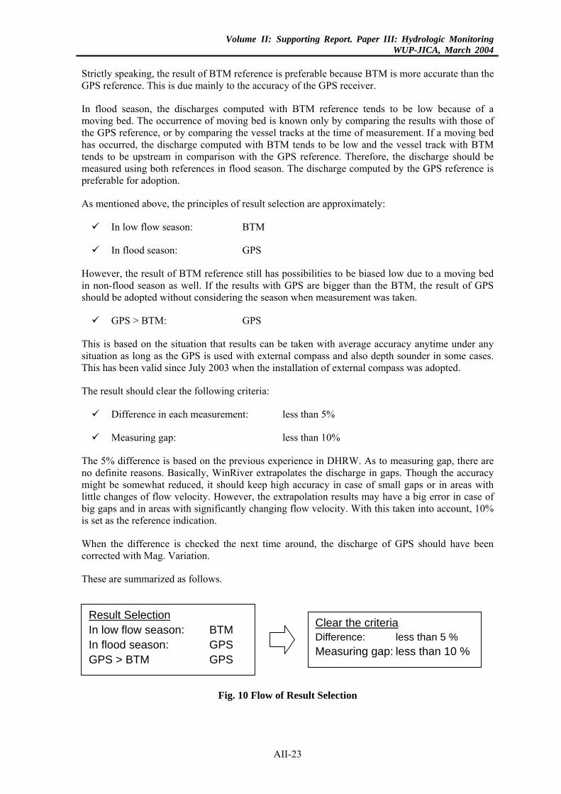
Volume II: Supporting Report. Paper III: Hydrologic MonitoringWUP-JICA, March 2004
Strictly speaking, the result of BTM reference is preferable because BTM is more accurate than the GPS reference. This is due mainly to the accuracy of the GPS receiver.
In flood season, the discharges computed with BTM reference tends to be low because of a moving bed. The occurrence of moving bed is known only by comparing the results with those of the GPS reference, or by comparing the vessel tracks at the time of measurement. If a moving bed has occurred, the discharge computed with BTM tends to be low and the vessel track with BTM tends to be upstream in comparison with the GPS reference. Therefore, the discharge should be measured using both references in flood season. The discharge computed by the GPS reference is preferable for adoption.
As mentioned above, the principles of result selection are approximately:
In low flow season: BTM
In flood season: GPS
However, the result of BTM reference still has possibilities to be biased low due to a moving bed in non-flood season as well. If the results with GPS are bigger than the BTM, the result of GPS should be adopted without considering the season when measurement was taken.
GPS > BTM: GPS
This is based on the situation that results can be taken with average accuracy anytime under any situation as long as the GPS is used with external compass and also depth sounder in some cases. This has been valid since July 2003 when the installation of external compass was adopted.
The result should clear the following criteria:
Difference in each measurement: less than 5%
Measuring gap: less than 10%
The 5% difference is based on the previous experience in DHRW. As to measuring gap, there are no definite reasons. Basically, WinRiver extrapolates the discharge in gaps. Though the accuracy might be somewhat reduced, it should keep high accuracy in case of small gaps or in areas with little changes of flow velocity. However, the extrapolation results may have a big error in case of big gaps and in areas with significantly changing flow velocity. With this taken into account, 10% is set as the reference indication.
When the difference is checked the next time around, the discharge of GPS should have been corrected with Mag. Variation.
These are summarized as follows.
Clear the criteria Difference: less than 5 % Measuring gap: less than 10 %
Result Selection In low flow season: BTM In flood season: GPS GPS > BTM GPS
Fig. 10 Flow of Result Selection
AII-23
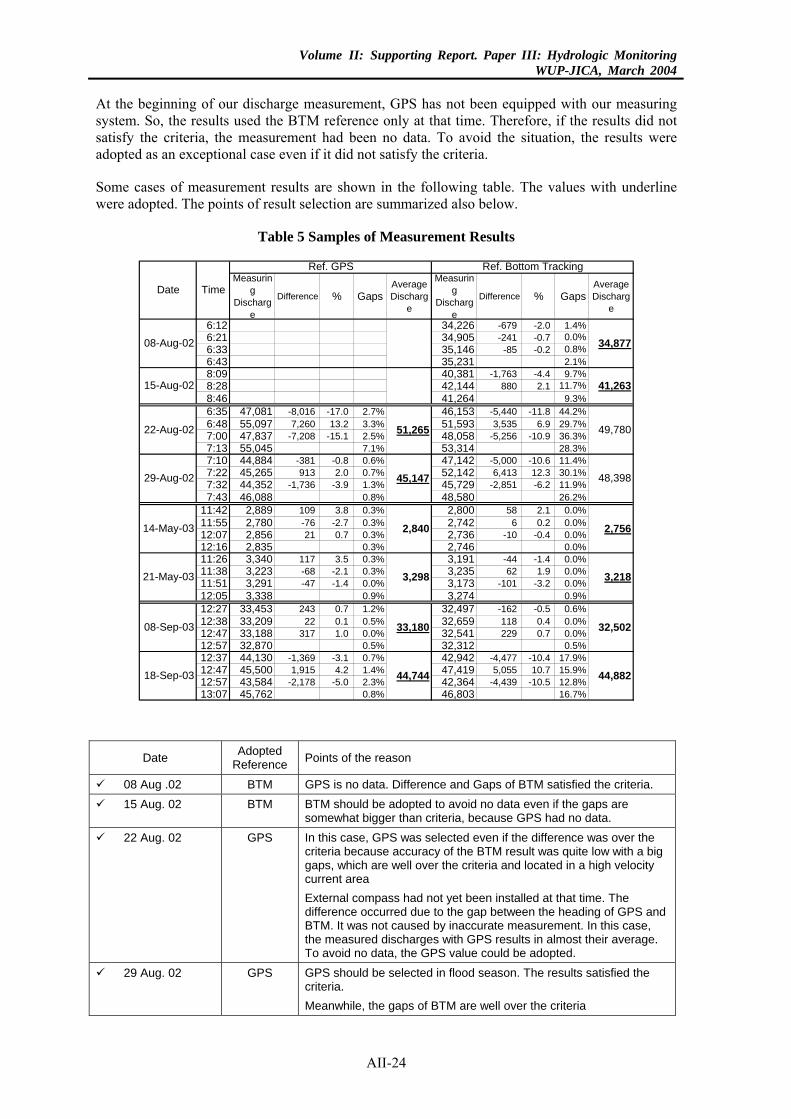
Volume II: Supporting Report. Paper III: Hydrologic MonitoringWUP-JICA, March 2004
At the beginning of our discharge measurement, GPS has not been equipped with our measuring system. So, the results used the BTM reference only at that time. Therefore, if the results did not satisfy the criteria, the measurement had been no data. To avoid the situation, the results were adopted as an exceptional case even if it did not satisfy the criteria.
Some cases of measurement results are shown in the following table. The values with underline were adopted. The points of result selection are summarized also below.
Table 5 Samples of Measurement Results
Measuring
Discharge
Difference % GapsAverageDischarg
e
Measuring
Discharge
Difference % GapsAverageDischarg
e
6:12 34,226 -679 -2.0 1.4%6:21 34,905 -241 -0.7 0.0%6:33 35,146 -85 -0.2 0.8%6:43 35,231 2.1%8:09 40,381 -1,763 -4.4 9.7%8:28 42,144 880 2.1 11.7%8:46 41,264 9.3%6:35 47,081 -8,016 -17.0 2.7% 46,153 -5,440 -11.8 44.2%6:48 55,097 7,260 13.2 3.3% 51,593 3,535 6.9 29.7%7:00 47,837 -7,208 -15.1 2.5% 48,058 -5,256 -10.9 36.3%7:13 55,045 7.1% 53,314 28.3%7:10 44,884 -381 -0.8 0.6% 47,142 -5,000 -10.6 11.4%7:22 45,265 913 2.0 0.7% 52,142 6,413 12.3 30.1%7:32 44,352 -1,736 -3.9 1.3% 45,729 -2,851 -6.2 11.9%7:43 46,088 0.8% 48,580 26.2%
11:42 2,889 109 3.8 0.3% 2,800 58 2.1 0.0%11:55 2,780 -76 -2.7 0.3% 2,742 6 0.2 0.0%12:07 2,856 21 0.7 0.3% 2,736 -10 -0.4 0.0%12:16 2,835 0.3% 2,746 0.0%11:26 3,340 117 3.5 0.3% 3,191 -44 -1.4 0.0%11:38 3,223 -68 -2.1 0.3% 3,235 62 1.9 0.0%11:51 3,291 -47 -1.4 0.0% 3,173 -101 -3.2 0.0%12:05 3,338 0.9% 3,274 0.9%12:27 33,453 243 0.7 1.2% 32,497 -162 -0.5 0.6%12:38 33,209 22 0.1 0.5% 32,659 118 0.4 0.0%12:47 33,188 317 1.0 0.0% 32,541 229 0.7 0.0%12:57 32,870 0.5% 32,312 0.5%12:37 44,130 -1,369 -3.1 0.7% 42,942 -4,477 -10.4 17.9%12:47 45,500 1,915 4.2 1.4% 47,419 5,055 10.7 15.9%12:57 43,584 -2,178 -5.0 2.3% 42,364 -4,439 -10.5 12.8%13:07 45,762 0.8% 46,803 16.7%
14-May-03 2,840
21-May-03 3,298 3,218
2,756
29-Aug-02 45,147 48,398
22-Aug-02 51,265 49,780
15-Aug-02 41,263
08-Aug-02 34,877
Ref. GPS Ref. Bottom Tracking
Date Time
08-Sep-03 33,180 32,502
18-Sep-03 44,744 44,882
Date Adopted Reference Points of the reason
08 Aug .02 BTM GPS is no data. Difference and Gaps of BTM satisfied the criteria. 15 Aug. 02 BTM BTM should be adopted to avoid no data even if the gaps are
somewhat bigger than criteria, because GPS had no data. 22 Aug. 02 GPS In this case, GPS was selected even if the difference was over the
criteria because accuracy of the BTM result was quite low with a big gaps, which are well over the criteria and located in a high velocity current area External compass had not yet been installed at that time. The difference occurred due to the gap between the heading of GPS and BTM. It was not caused by inaccurate measurement. In this case, the measured discharges with GPS results in almost their average. To avoid no data, the GPS value could be adopted.
29 Aug. 02 GPS GPS should be selected in flood season. The results satisfied the criteria. Meanwhile, the gaps of BTM are well over the criteria
AII-24
Volume II: Supporting Report. Paper III: Hydrologic MonitoringWUP-JICA, March 2004
14, 21 May 03 BTM In low flow season, The result of BTM is more accurate than the
GPS. (External compass had not been installed yet. If it were after the installation, GPS would be adopted.)
08, 18 Sep. 03 GPS GPS should be selected in flood season. Their results cleared the criteria.
Since the technique of the measuring team have progressed and the necessary external equipment have been installed, the accuracy of measurement has improved and the criteria should almost always be met at least in case of GPS reference.
If the result of GPS does not meet the criteria, it will cause a problem in setting of the Mag. Variation or the depth sounder will not be used when needed. In the former case, appropriate Mag. Variation should be calculated and then the discharge of GPS should be calculated again. In the latter case, the result should be rejected and measurement should be made again with the depth sounder.
References:
(1) Principles of Operation: A Practical Primer (RD Instruments)
(2) WinRiver User’s Guide International Version (RD Instruments)
AII-25

Volume II: Supporting Report. Paper III: Hydrologic MonitoringWUP-JICA, March 2004
AII-26
Volume II: Supporting Report. Paper III: Hydrologic MonitoringWUP-JICA, March 2004
Rating Curve Development Program
USERS MANUAL
25 NOVEMBER 2003
WUP-JICA TEAM
AII-27
Volume II: Supporting Report. Paper III: Hydrologic MonitoringWUP-JICA, March 2004
TABLE OF CONTENTS
1. INTRODUCTION ........................................................................................... AII-20
2. EQUATIONS USED FOR RATING CURVES ........................................... AII-29
2.1 Type 1 Equations .................................................................................... AII-29
2.2 Type 2 Equations .................................................................................... AII-30
3. SOLUTION FOR EQUATIONS ................................................................... AII-31
4. ACCURACY TEST OF RATING CURVE .................................................. AII-32
5. STAGE – DISCHARGE AND REFERENCE - H ....................................... AII-33
6. INPUT DATA FILE ........................................................................................ AII-33
7. EXECUTION OF PROGRAM ...................................................................... AII-35
8. OUTPUT DATA FILE ................................................................................... AII-37
8.1 Results File (Type 1 Equations) .............................................................. AII-39
8.2 Results File (Type 2 Equations) .............................................................. AII-40
9. EXPORT OF OUTPUT DATA FILE ........................................................... AII-43
AII-28
Volume II: Supporting Report. Paper III: Hydrologic MonitoringWUP-JICA, March 2004
LIST OF TABLES
Table 1 Input data file in text format ................................................................. AII-35 Table 2 Results file (Type -1 with all combinations of equations
tried for rating curve) ............................................................................ AII-39 Table 3 Results file (Type -1 with only good fitted equations
for rating curve) ...................................................................................... AII-40 Table 4 Results file (Type -2 with all combinations of equations
tried for rating curve) .............................................................................. AII-41 Table 5 Results file (Type -2 with only good fitted equations
for rating curve) ...................................................................................... AII-42 Table 6 Import of text results file in Excel ........................................................ AII-44
LIST OF FIGURES
Fig. 1 Regression analysis ............................................................................... AII-32 Fig. 2 Schematic diagram for gauge height and reference-H .......................... AII-33 Fig. 3 Preparation of data sheet and browsing of save-as –type
for text data file in Excel ....................................................................... AII-34 Fig. 4 Program executed in MS-DOS mode .................................................... AII-36 Fig. 5 Message wizard to select a program from list to open
results file .............................................................................................. AII-38 Fig. 6 Message wizard to select a program to open text results file ................ AII-38 Fig. 7 Message wizard to select the feature of data in result ........................... AII-43 Fig. 8 Adjustment of columns widths to open results file in Excel ................. AII-44
AII-29

Volume II: Supporting Report. Paper III: Hydrologic MonitoringWUP-JICA, March 2004
AII-30
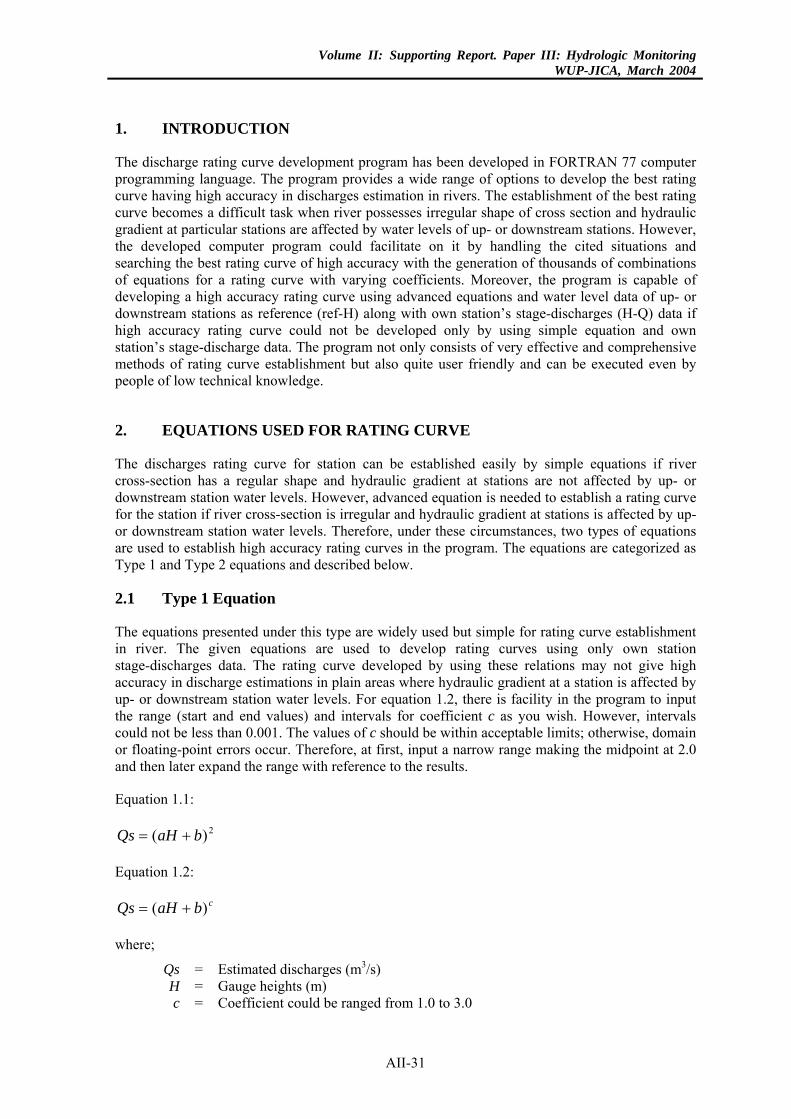
Volume II: Supporting Report. Paper III: Hydrologic MonitoringWUP-JICA, March 2004
1. INTRODUCTION
The discharge rating curve development program has been developed in FORTRAN 77 computer programming language. The program provides a wide range of options to develop the best rating curve having high accuracy in discharges estimation in rivers. The establishment of the best rating curve becomes a difficult task when river possesses irregular shape of cross section and hydraulic gradient at particular stations are affected by water levels of up- or downstream stations. However, the developed computer program could facilitate on it by handling the cited situations and searching the best rating curve of high accuracy with the generation of thousands of combinations of equations for a rating curve with varying coefficients. Moreover, the program is capable of developing a high accuracy rating curve using advanced equations and water level data of up- or downstream stations as reference (ref-H) along with own station’s stage-discharges (H-Q) data if high accuracy rating curve could not be developed only by using simple equation and own station’s stage-discharge data. The program not only consists of very effective and comprehensive methods of rating curve establishment but also quite user friendly and can be executed even by people of low technical knowledge.
2. EQUATIONS USED FOR RATING CURVE
The discharges rating curve for station can be established easily by simple equations if river cross-section has a regular shape and hydraulic gradient at stations are not affected by up- or downstream station water levels. However, advanced equation is needed to establish a rating curve for the station if river cross-section is irregular and hydraulic gradient at stations is affected by up- or downstream station water levels. Therefore, under these circumstances, two types of equations are used to establish high accuracy rating curves in the program. The equations are categorized as Type 1 and Type 2 equations and described below.
2.1 Type 1 Equation
The equations presented under this type are widely used but simple for rating curve establishment in river. The given equations are used to develop rating curves using only own station stage-discharges data. The rating curve developed by using these relations may not give high accuracy in discharge estimations in plain areas where hydraulic gradient at a station is affected by up- or downstream station water levels. For equation 1.2, there is facility in the program to input the range (start and end values) and intervals for coefficient c as you wish. However, intervals could not be less than 0.001. The values of c should be within acceptable limits; otherwise, domain or floating-point errors occur. Therefore, at first, input a narrow range making the midpoint at 2.0 and then later expand the range with reference to the results.
Equation 1.1:
2)( baHQs +=
Equation 1.2:
cbaHQs )( +=
where;
Qs = Estimated discharges (m3/s) H = Gauge heights (m) c = Coefficient could be ranged from 1.0 to 3.0
AII-31
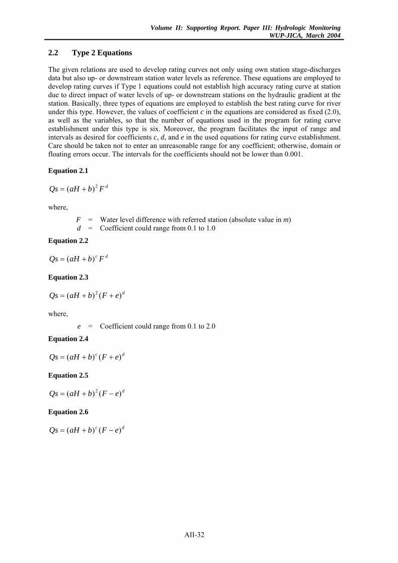
Volume II: Supporting Report. Paper III: Hydrologic MonitoringWUP-JICA, March 2004
2.2 Type 2 Equations
The given relations are used to develop rating curves not only using own station stage-discharges data but also up- or downstream station water levels as reference. These equations are employed to develop rating curves if Type 1 equations could not establish high accuracy rating curve at station due to direct impact of water levels of up- or downstream stations on the hydraulic gradient at the station. Basically, three types of equations are employed to establish the best rating curve for river under this type. However, the values of coefficient c in the equations are considered as fixed (2.0), as well as the variables, so that the number of equations used in the program for rating curve establishment under this type is six. Moreover, the program facilitates the input of range and intervals as desired for coefficients c, d, and e in the used equations for rating curve establishment. Care should be taken not to enter an unreasonable range for any coefficient; otherwise, domain or floating errors occur. The intervals for the coefficients should not be lower than 0.001.
Equation 2.1
dFbaHQs 2)( +=
where,
F = Water level difference with referred station (absolute value in m) d = Coefficient could range from 0.1 to 1.0
Equation 2.2
dc FbaHQs )( +=
Equation 2.3
deFbaHQs )()( 2 ++=
where,
e = Coefficient could range from 0.1 to 2.0
Equation 2.4
dc eFbaHQs )()( ++=
Equation 2.5
deFbaHQs )()( 2 −+=
Equation 2.6
dc eFbaHQs )()( −+=
AII-32
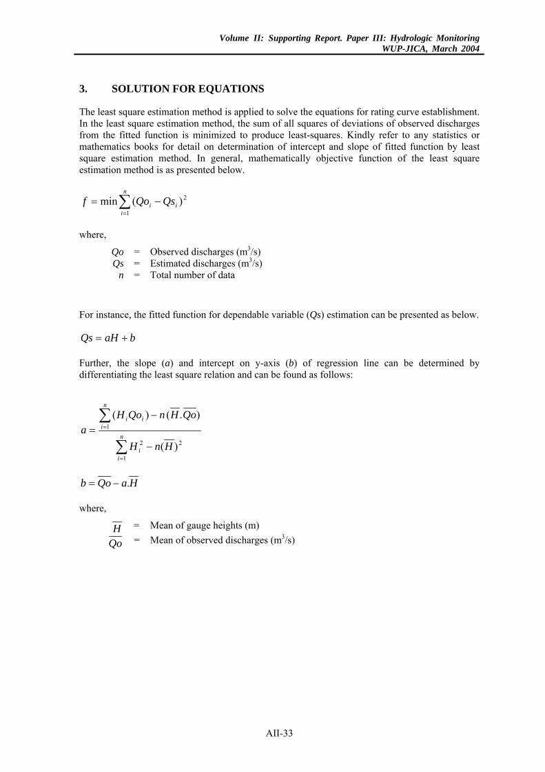
Volume II: Supporting Report. Paper III: Hydrologic MonitoringWUP-JICA, March 2004
3. SOLUTION FOR EQUATIONS
The least square estimation method is applied to solve the equations for rating curve establishment. In the least square estimation method, the sum of all squares of deviations of observed discharges from the fitted function is minimized to produce least-squares. Kindly refer to any statistics or mathematics books for detail on determination of intercept and slope of fitted function by least square estimation method. In general, mathematically objective function of the least square estimation method is as presented below.
2
1)(min i
n
ii QsQof −= ∑
=
where,
Qo = Observed discharges (m3/s) Qs = Estimated discharges (m3/s)
n = Total number of data
For instance, the fitted function for dependable variable (Qs) estimation can be presented as below.
baHQs +=
Further, the slope (a) and intercept on y-axis (b) of regression line can be determined by differentiating the least square relation and can be found as follows:
∑
∑
=
=
−
−=
n
ii
n
iii
HnH
QoHnQoHa
1
22
1
)(
).()(
HaQob .−=
where,
H = Mean of gauge heights (m)
Qo = Mean of observed discharges (m3/s)
AII-33
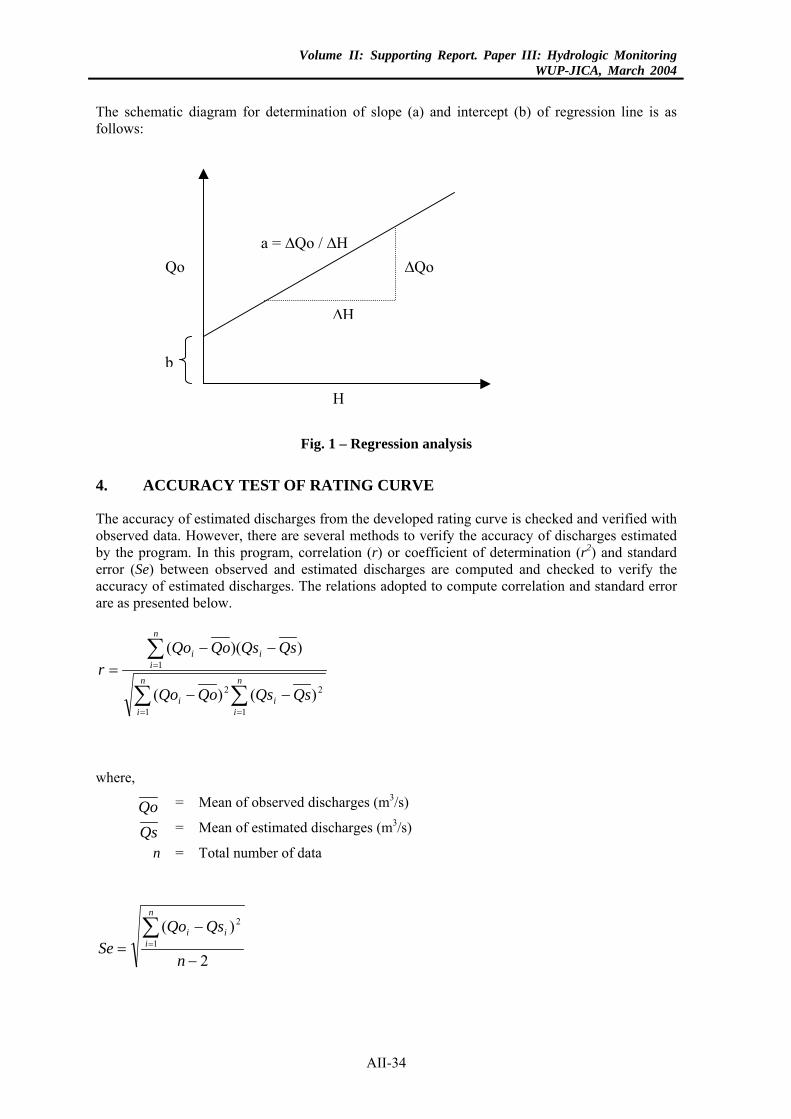
Volume II: Supporting Report. Paper III: Hydrologic MonitoringWUP-JICA, March 2004
AII-34
The schematic diagram for determination of slope (a) and intercept (b) of regression line is as follows:
Fig. 1 – Regression analysis
4. ACCURACY TEST OF RATING CURVE
The accuracy of estimated discharges from the developed rating curve is checked and verified with observed data. However, there are several methods to verify the accuracy of discharges estimated by the program. In this program, correlation (r) or coefficient of determination (r2) and standard error (Se) between observed and estimated discharges are computed and checked to verify the accuracy of estimated discharges. The relations adopted to compute correlation and standard error are as presented below.
∑ ∑
∑
= =
=
−−
−−=
n
i
n
iii
n
iii
QsQsQoQo
QsQsQoQor
1 1
22
1
)()(
))((
where,
Qo = Mean of observed discharges (m3/s)
Qs = Mean of estimated discharges (m3/s)
n = Total number of data
2
)(1
2
−
−=∑=
n
QsQoSe
n
iii
b
∆Qo
∆H
a = ∆Qo / ∆H
H
Qo
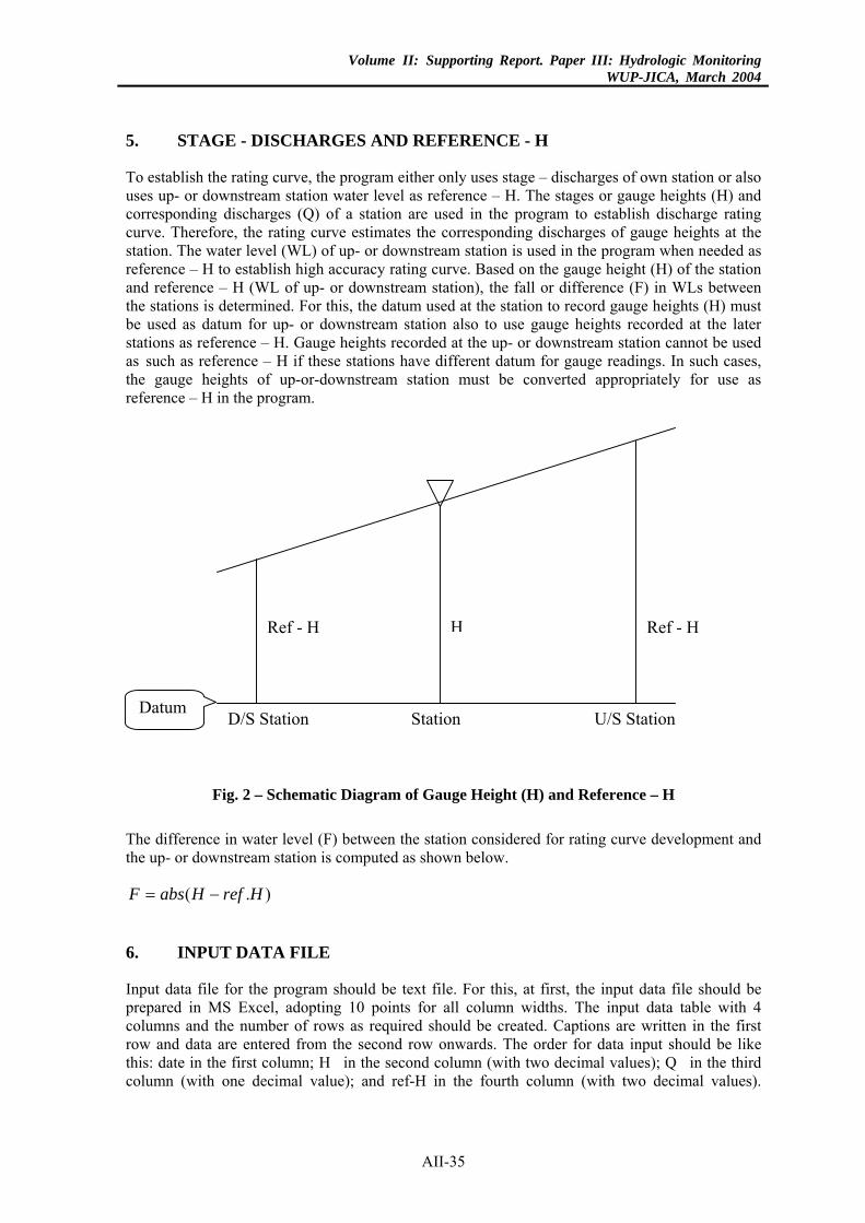
Volume II: Supporting Report. Paper III: Hydrologic MonitoringWUP-JICA, March 2004
5. STAGE - DISCHARGES AND REFERENCE - H
To establish the rating curve, the program either only uses stage – discharges of own station or also uses up- or downstream station water level as reference – H. The stages or gauge heights (H) and corresponding discharges (Q) of a station are used in the program to establish discharge rating curve. Therefore, the rating curve estimates the corresponding discharges of gauge heights at the station. The water level (WL) of up- or downstream station is used in the program when needed as reference – H to establish high accuracy rating curve. Based on the gauge height (H) of the station and reference – H (WL of up- or downstream station), the fall or difference (F) in WLs between the stations is determined. For this, the datum used at the station to record gauge heights (H) must be used as datum for up- or downstream station also to use gauge heights recorded at the later stations as reference – H. Gauge heights recorded at the up- or downstream station cannot be used as such as reference – H if these stations have different datum for gauge readings. In such cases, the gauge heights of up-or-downstream station must be converted appropriately for use as reference – H in the program.
HRef - H Ref - H
Datum D/S Station Station U/S Station
Fig. 2 – Schematic Diagram of Gauge Height (H) and Reference – H
The difference in water level (F) between the station considered for rating curve development and the up- or downstream station is computed as shown below.
).( HrefHabsF −=
6. INPUT DATA FILE
Input data file for the program should be text file. For this, at first, the input data file should be prepared in MS Excel, adopting 10 points for all column widths. The input data table with 4 columns and the number of rows as required should be created. Captions are written in the first row and data are entered from the second row onwards. The order for data input should be like this: date in the first column; H in the second column (with two decimal values); Q in the third column (with one decimal value); and ref-H in the fourth column (with two decimal values).
AII-35
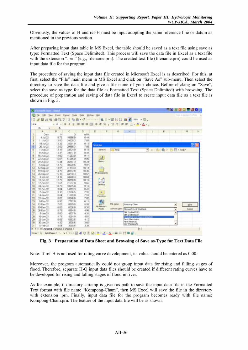
Volume II: Supporting Report. Paper III: Hydrologic MonitoringWUP-JICA, March 2004
Obviously, the values of H and ref-H must be input adopting the same reference line or datum as mentioned in the previous section.
After preparing input data table in MS Excel, the table should be saved as a text file using save as type: Formatted Text (Space Delimited). This process will save the data file in Excel as a text file with the extension “.prn” (e.g., filename.prn). The created text file (filename.prn) could be used as input data file for the program.
The procedure of saving the input data file created in Microsoft Excel is as described. For this, at first, select the “File” main menu in MS Excel and click on “Save As” sub-menu. Then select the directory to save the data file and give a file name of your choice. Before clicking on “Save”, select the save as type for the data file as Formatted Text (Space Delimited) with browsing. The procedure of preparation and saving of data file in Excel to create input data file as a text file is shown in Fig. 3.
Fig. 3 Preparation of Data Sheet and Browsing of Save as-Type for Text Data File
Note: If ref-H is not used for rating curve development, its value should be entered as 0.00.
Moreover, the program automatically could not group input data for rising and falling stages of flood. Therefore, separate H-Q input data files should be created if different rating curves have to be developed for rising and falling stages of flood in river.
As for example, if directory c:\temp is given as path to save the input data file in the Formatted Text format with file name “Kompong-Cham”, then MS Excel will save the file in the directory with extension .prn. Finally, input data file for the program becomes ready with file name: Kompong-Cham.prn. The feature of the input data file will be as shown.
AII-36
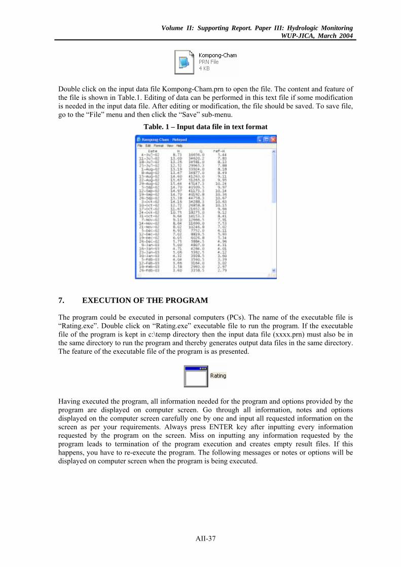
Volume II: Supporting Report. Paper III: Hydrologic MonitoringWUP-JICA, March 2004
Double click on the input data file Kompong-Cham.prn to open the file. The content and feature of the file is shown in Table.1. Editing of data can be performed in this text file if some modification is needed in the input data file. After editing or modification, the file should be saved. To save file, go to the “File” menu and then click the “Save” sub-menu.
Table. 1 – Input data file in text format
7. EXECUTION OF THE PROGRAM
The program could be executed in personal computers (PCs). The name of the executable file is “Rating.exe”. Double click on “Rating.exe” executable file to run the program. If the executable file of the program is kept in c:\temp directory then the input data file (xxxx.prn) must also be in the same directory to run the program and thereby generates output data files in the same directory. The feature of the executable file of the program is as presented.
Having executed the program, all information needed for the program and options provided by the program are displayed on computer screen. Go through all information, notes and options displayed on the computer screen carefully one by one and input all requested information on the screen as per your requirements. Always press ENTER key after inputting every information requested by the program on the screen. Miss on inputting any information requested by the program leads to termination of the program execution and creates empty result files. If this happens, you have to re-execute the program. The following messages or notes or options will be displayed on computer screen when the program is being executed.
AII-37
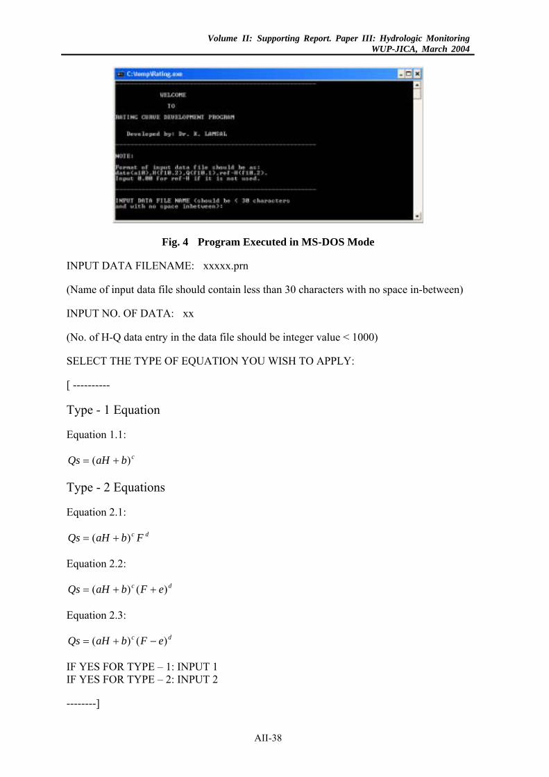
Volume II: Supporting Report. Paper III: Hydrologic MonitoringWUP-JICA, March 2004
Fig. 4 Program Executed in MS-DOS Mode
INPUT DATA FILENAME: xxxxx.prn
(Name of input data file should contain less than 30 characters with no space in-between)
INPUT NO. OF DATA: xx
(No. of H-Q data entry in the data file should be integer value < 1000)
SELECT THE TYPE OF EQUATION YOU WISH TO APPLY:
[ ----------
Type - 1 Equation
Equation 1.1:
cbaHQs )( +=
Type - 2 Equations
Equation 2.1:
dc FbaHQs )( +=
Equation 2.2:
dc eFbaHQs )()( ++=
Equation 2.3:
dc eFbaHQs )()( −+=
IF YES FOR TYPE – 1: INPUT 1 IF YES FOR TYPE – 2: INPUT 2
--------]
AII-38
Volume II: Supporting Report. Paper III: Hydrologic MonitoringWUP-JICA, March 2004
EITHER YOU CAN OUTPUT RESULTS OF ALL COMBINATIONS OF EQUATIONS TRIED FOR RATING CURVE OR CAN ONLY OUTPUT THE RESULTS OF FEW GOOD FITTED EQUATIONS:
[--------
IF YES FOR ALL COMBINATIONS: INPUT 1 IF YES FOR ONLY FEW GOOD FITTED EQUATIONS: INPUT 2
--------]
If yes for only few good fitted equations, then:
ENTER THE NO. OF THE GOOD FITTED EQUATIONS RESULTS YOU WANT TO OUTPUT IN THE RESULT FILE: xx
INPUT THE RANGE AND INTERVALS FOR COEFFICIENT – c (value of c could be ranged 1.0 – 3.0) INPUT THE STARTING VALUE OF – c: x.x INPUT THE INTERVALS FOR c VALUES: x.x INPUT THE END VALUE OF – c: x.x
INPUT THE RANGE AND INTERVALS FOR COEFFICIENT – d (value of d could be ranged 0.1 – 1.0) INPUT THE STARTING VALUE OF – d: x.x INPUT THE INTERVALS FOR d VALUES: x.x INPUT THE END VALUE OF – d: x.x
INPUT THE RANGE AND INTERVALS FOR COEFFICIENT – e (value of e could be ranged 0.1 – 2.0) INPUT THE STARTING VALUE OF – e: x.x INPUT THE INTERVALS FOR e VALUES: x.x INPUT THE END VALUE OF – e: x.x
After inputting all the information requested by the program on the screen then press ENTER to execute the program and wait until the message of “Please Wait! Program is Executing” displays on the screen. The message will not be displayed (cannot be noticed) if Type-1 equations are chosen, because computation completes so fast due to having simple equations and less numbers of iterations. In this way, the program could be run successfully and result files could be generated.
8. OUTPUT DATA FILE
The program automatically generates result or output data file taking the name of input data file. Suffixes like T1.res or T2.res will be given to result files. If Type-1 equations are chosen for rating curve then result file contains suffix T1.res. Similarly, if Type-2 equations are selected then result file contains suffix T2.res. For instance, if name of input data file is: Kompong-Cham.prn then output files will be named as: Kompong-Cham-T1.res or Kompong-Cham-T2.res. The program creates output data file as a text file, however, the output text file can read by Microsoft Excel and could be saved as Excel file for further editing purposes. The output data files are generated in the same directory where the execution file of the program and input data file are kept. Use Windows Explorer to browse the output data files. The features of the output data files are as shown below.
AII-39
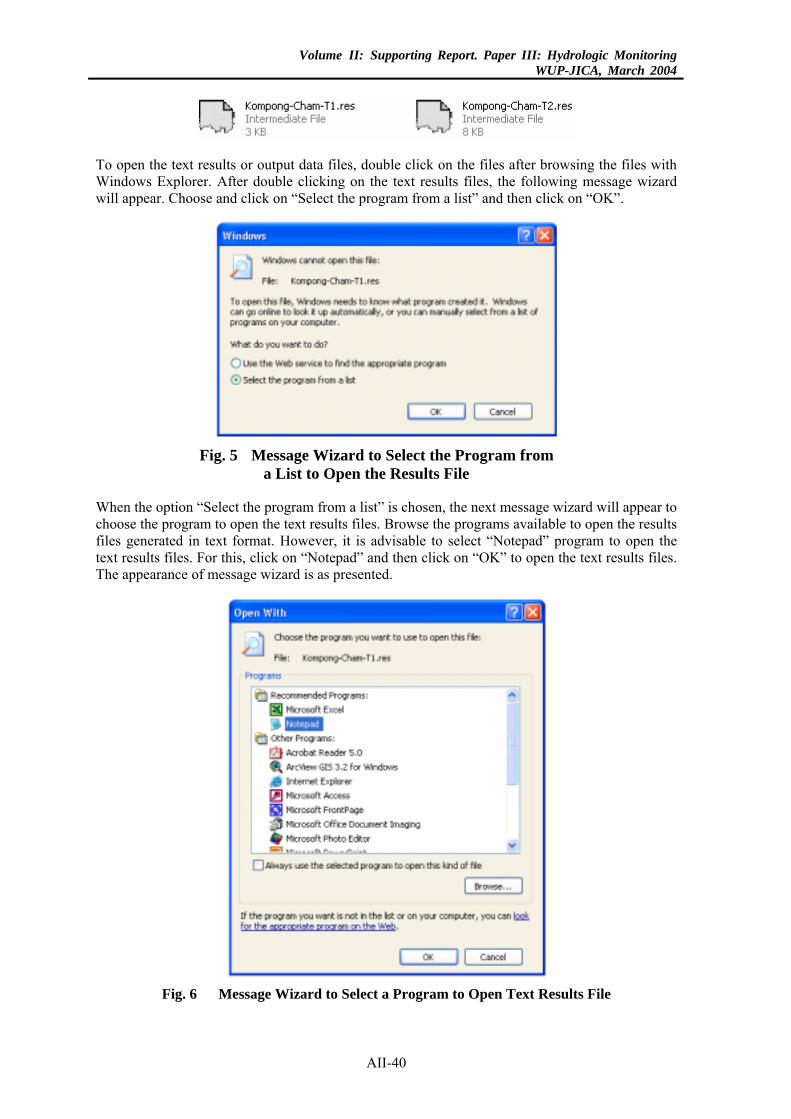
Volume II: Supporting Report. Paper III: Hydrologic MonitoringWUP-JICA, March 2004
To open the text results or output data files, double click on the files after browsing the files with Windows Explorer. After double clicking on the text results files, the following message wizard will appear. Choose and click on “Select the program from a list” and then click on “OK”.
Fig. 5 Message Wizard to Select the Program from
a List to Open the Results File
When the option “Select the program from a list” is chosen, the next message wizard will appear to choose the program to open the text results files. Browse the programs available to open the results files generated in text format. However, it is advisable to select “Notepad” program to open the text results files. For this, click on “Notepad” and then click on “OK” to open the text results files. The appearance of message wizard is as presented.
Fig. 6 Message Wizard to Select a Program to Open Text Results File
AII-40
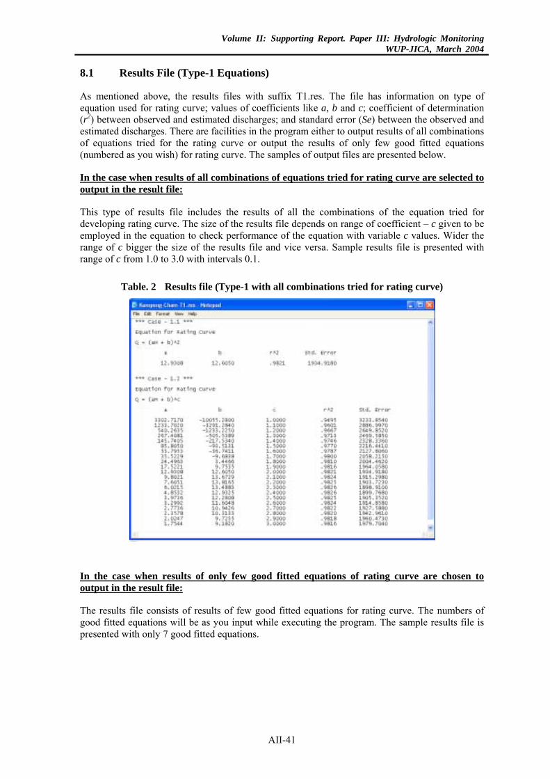
Volume II: Supporting Report. Paper III: Hydrologic MonitoringWUP-JICA, March 2004
8.1 Results File (Type-1 Equations)
As mentioned above, the results files with suffix T1.res. The file has information on type of equation used for rating curve; values of coefficients like a, b and c; coefficient of determination (r2) between observed and estimated discharges; and standard error (Se) between the observed and estimated discharges. There are facilities in the program either to output results of all combinations of equations tried for the rating curve or output the results of only few good fitted equations (numbered as you wish) for rating curve. The samples of output files are presented below.
In the case when results of all combinations of equations tried for rating curve are selected to output in the result file:
This type of results file includes the results of all the combinations of the equation tried for developing rating curve. The size of the results file depends on range of coefficient – c given to be employed in the equation to check performance of the equation with variable c values. Wider the range of c bigger the size of the results file and vice versa. Sample results file is presented with range of c from 1.0 to 3.0 with intervals 0.1.
Table. 2 Results file (Type-1 with all combinations tried for rating curve)
In the case when results of only few good fitted equations of rating curve are chosen to output in the result file:
The results file consists of results of few good fitted equations for rating curve. The numbers of good fitted equations will be as you input while executing the program. The sample results file is presented with only 7 good fitted equations.
AII-41
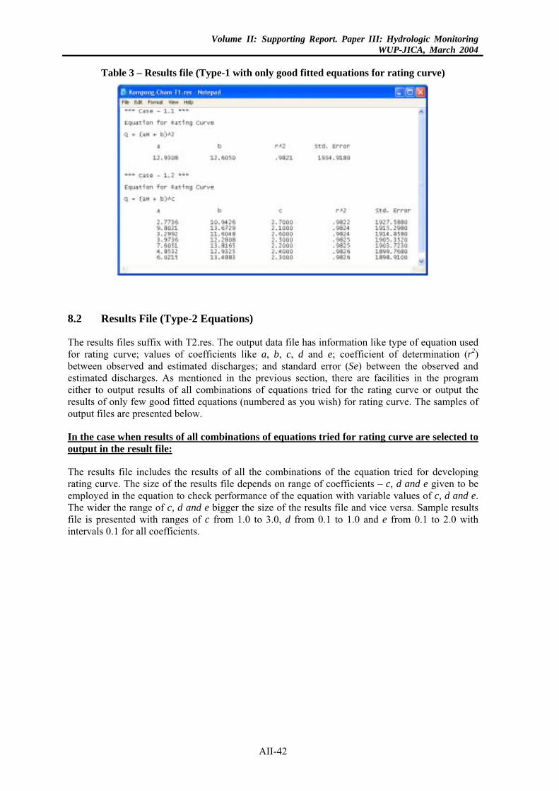
Volume II: Supporting Report. Paper III: Hydrologic MonitoringWUP-JICA, March 2004
Table 3 – Results file (Type-1 with only good fitted equations for rating curve)
8.2 Results File (Type-2 Equations)
The results files suffix with T2.res. The output data file has information like type of equation used for rating curve; values of coefficients like a, b, c, d and e; coefficient of determination (r2) between observed and estimated discharges; and standard error (Se) between the observed and estimated discharges. As mentioned in the previous section, there are facilities in the program either to output results of all combinations of equations tried for the rating curve or output the results of only few good fitted equations (numbered as you wish) for rating curve. The samples of output files are presented below.
In the case when results of all combinations of equations tried for rating curve are selected to output in the result file:
The results file includes the results of all the combinations of the equation tried for developing rating curve. The size of the results file depends on range of coefficients – c, d and e given to be employed in the equation to check performance of the equation with variable values of c, d and e. The wider the range of c, d and e bigger the size of the results file and vice versa. Sample results file is presented with ranges of c from 1.0 to 3.0, d from 0.1 to 1.0 and e from 0.1 to 2.0 with intervals 0.1 for all coefficients.
AII-42
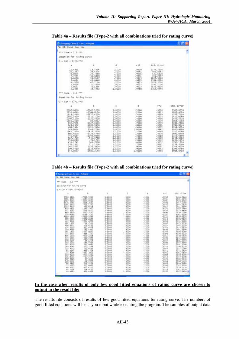
Volume II: Supporting Report. Paper III: Hydrologic MonitoringWUP-JICA, March 2004
Table 4a – Results file (Type-2 with all combinations tried for rating curve)
Table 4b – Results file (Type-2 with all combinations tried for rating curve)
In the case when results of only few good fitted equations of rating curve are chosen to output in the result file:
The results file consists of results of few good fitted equations for rating curve. The numbers of good fitted equations will be as you input while executing the program. The samples of output data
AII-43
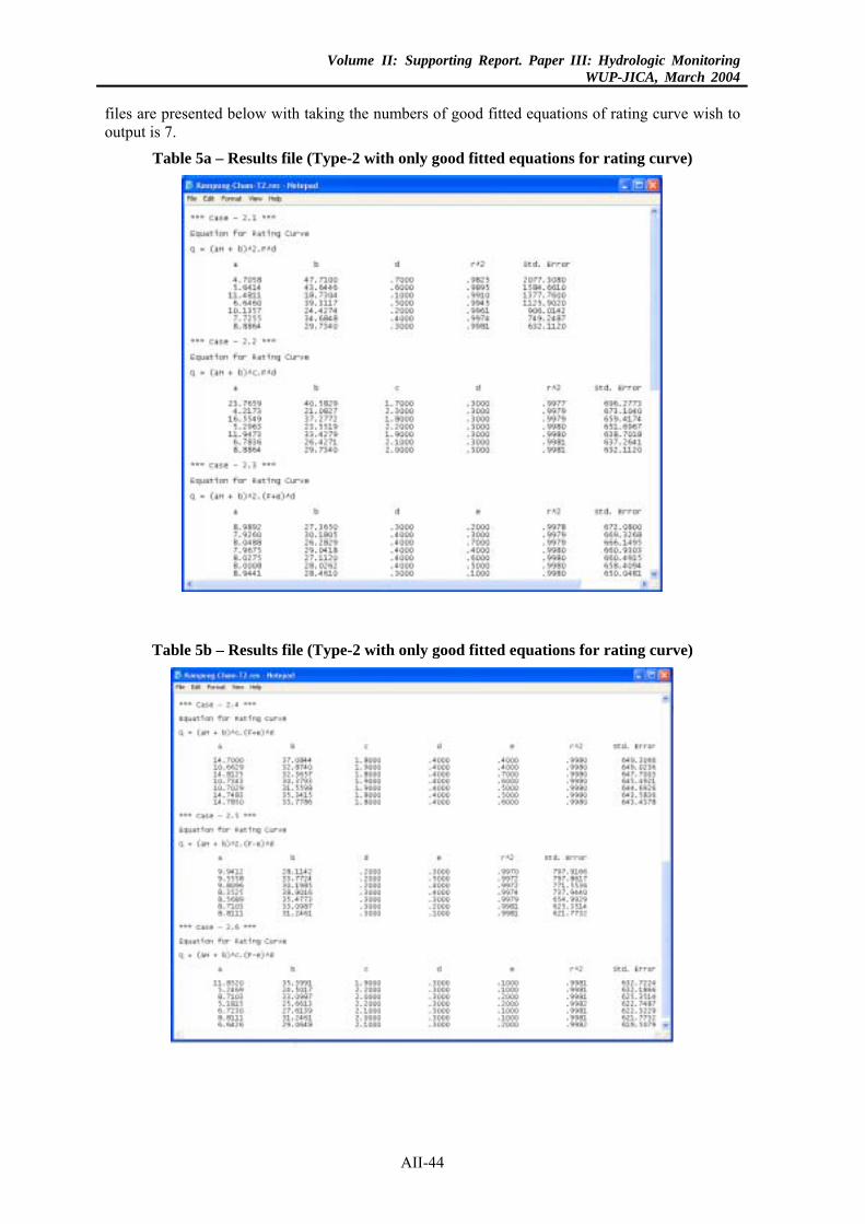
Volume II: Supporting Report. Paper III: Hydrologic MonitoringWUP-JICA, March 2004
files are presented below with taking the numbers of good fitted equations of rating curve wish to output is 7.
Table 5a – Results file (Type-2 with only good fitted equations for rating curve)
Table 5b – Results file (Type-2 with only good fitted equations for rating curve)
AII-44
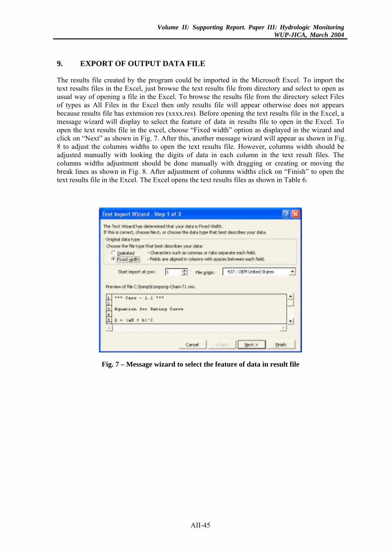
Volume II: Supporting Report. Paper III: Hydrologic MonitoringWUP-JICA, March 2004
9. EXPORT OF OUTPUT DATA FILE
The results file created by the program could be imported in the Microsoft Excel. To import the text results files in the Excel, just browse the text results file from directory and select to open as usual way of opening a file in the Excel. To browse the results file from the directory select Files of types as All Files in the Excel then only results file will appear otherwise does not appears because results file has extension res (xxxx.res). Before opening the text results file in the Excel, a message wizard will display to select the feature of data in results file to open in the Excel. To open the text results file in the excel, choose “Fixed width” option as displayed in the wizard and click on “Next” as shown in Fig. 7. After this, another message wizard will appear as shown in Fig. 8 to adjust the columns widths to open the text results file. However, columns width should be adjusted manually with looking the digits of data in each column in the text result files. The columns widths adjustment should be done manually with dragging or creating or moving the break lines as shown in Fig. 8. After adjustment of columns widths click on “Finish” to open the text results file in the Excel. The Excel opens the text results files as shown in Table 6.
Fig. 7 – Message wizard to select the feature of data in result file
AII-45
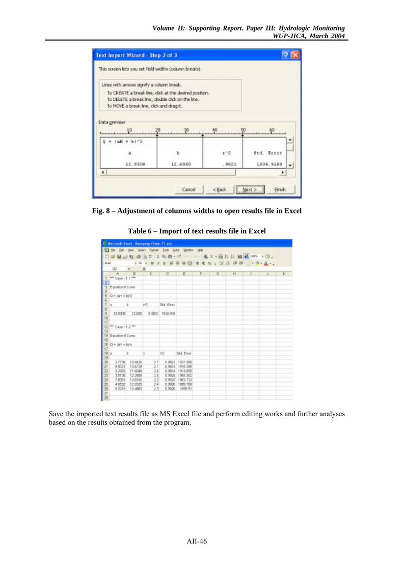
Volume II: Supporting Report. Paper III: Hydrologic MonitoringWUP-JICA, March 2004
Fig. 8 – Adjustment of columns widths to open results file in Excel
Table 6 – Import of text results file in Excel
Save the imported text results file as MS Excel file and perform editing works and further analyses based on the results obtained from the program.
AII-46