SANDIA REPORT SAND2009-7001 Unlimited Release Printed October 2009

Climate Uncertainty and Implications for U.S. State-Level Risk Assessment Through 2050 George Backus, Thomas Lowry, Drake Warren, Mark Ehlen, Anjelka Kelic, Geoffrey Klise, Verne Loose, Len Malczynski, Kevin Stamber, Vince Tidwell, Vanessa Vargas, and Aldo Zagonel Prepared by Sandia National Laboratories Albuquerque, New Mexico 87185 and Livermore, California 94550

Sandia is a multiprogram laboratory operated by Sandia Corporation, a Lockheed Martin Company, for the United States Department of Energy’s National Nuclear Security Administration under Contract DE-AC04-94AL85000.

Approved for public release; further dissemination unlimited.

2

Issued by Sandia National Laboratories, operated for the United States Department of Energy by Sandia Corporation. NOTICE: This report was prepared as an account of work sponsored by an agency of the United States Government. Neither the United States Government, nor any agency thereof, nor any of their employees, nor any of their contractors, subcontractors, or their employees, make any warranty, express or implied, or assume any legal liability or responsibility for the accuracy, completeness, or usefulness of any information, apparatus, product, or process disclosed, or represent that its use would not infringe privately owned rights. Reference herein to any specific commercial product, process, or service by trade name, trademark, manufacturer, or otherwise, does not necessarily constitute or imply its endorsement, recommendation, or favoring by the United States Government, any agency thereof, or any of their contractors or subcontractors. The views and opinions expressed herein do not necessarily state or reflect those of the United States Government, any agency thereof, or any of their contractors. Printed in the United States of America. This report has been reproduced directly from the best available copy. Available to DOE and DOE contractors from U.S. Department of Energy Office of Scientific and Technical Information P.O. Box 62 Oak Ridge, TN 37831 Telephone: (865) 576-8401 Facsimile: (865) 576-5728 E-Mail: reports@adonis.osti.gov Online ordering: http://www.osti.gov/bridge Available to the public from U.S. Department of Commerce National Technical Information Service 5285 Port Royal Rd. Springfield, VA 22161 Telephone: (800) 553-6847 Facsimile: (703) 605-6900 E-Mail: orders@ntis.fedworld.gov Online order: http://www.ntis.gov/help/ordermethods.asp?loc=7-4-0#online

3

SAND2009-7001 Unlimited Release

Printed October 2010

Climate Uncertainty and Implications for

U.S. State-Level Risk Assessment Through 2050

George Backus, Thomas Lowry, Drake Warren, Mark Ehlen, Anjelka Kelic, Geoffrey Klise, Verne Loose, Len Malczynski, Kevin Stamber, Vince Tidwell, Vanessa Vargas, and Aldo Zagonel

Sandia National Laboratories P.O. Box 5800

Albuquerque, New Mexico 87185-MS0370

Abstract Decisions for climate policy will need to take place in advance of climate science resolving all relevant uncertainties. Further, if the concern of policy is to reduce risk, then the best-estimate of climate change impacts may not be so important as the currently understood uncertainty associated with realizable conditions having high consequence. This study focuses on one of the most uncertain aspects of future climate change – precipitation – to understand the implications of uncertainty on risk and the near-term justification for interventions to mitigate the course of climate change.

We show that the mean risk of damage to the economy from climate change, at the national level, is on the order of one trillion dollars over the next 40 years, with employment impacts of nearly 7 million labor-years. At a 1% exceedance-probability, the impact is over twice the mean-risk value. Impacts at the level of individual U.S. states are then typically in the multiple tens of billions dollar range with employment losses exceeding hundreds of thousands of labor-years.

We used results of the Intergovernmental Panel on Climate Change’s (IPCC) Fourth Assessment Report 4 (AR4) climate-model ensemble as the referent for climate uncertainty over the next 40 years, mapped the simulated weather hydrologically to the county level for determining the physical consequence to economic activity at the state level, and then performed a detailed,

4

seventy-industry, analysis of economic impact among the interacting lower-48 states. We determined industry GDP and employment impacts at the state level, as well as interstate population migration, effect on personal income, and the consequences for the U.S. trade balance.

5

ACKNOWLEDGMENTS We acknowledge the additional efforts of Tim Trucano, David Robinson, Arnie Baker, Brian Adams, Elizabeth Richards, John Siirola, Mark Boslough, Mark Taylor, Ray Finely, Lillian Snyder, Dan Horschel, Jesse Roach, Marissa Reno, Laura Cutler, James P. Smith, (LANL), David Higdon (LANL), Joe Galewsky (UNM), Anna Weddington, William Fogelman, Jim Strickland, John Mitchiner, Howard Hirano, and James Perry. We graciously thank the Sandia LDRD offices for its financial support of this effort.

6

7

Table of Contents 

ACKNOWLEDGMENTS ............................................................................................................................ 5 

EXECUTIVE SUMMARY .......................................................................................................................... 9 

1.0  OVERVIEW ...................................................................................................................................... 21 

1.1 RELATIONSHIP TO PREVIOUS WORK .................................................................................................... 27 1.1.1 Impact Studies ............................................................................................................................ 28 1.1.2 Damage Functions ..................................................................................................................... 29 

1.2 DISCOUNT RATE ................................................................................................................................. 30 

2. APPROACH .......................................................................................................................................... 33 

2.1 UNCERTAINTY AND RISK .................................................................................................................... 35 2.1.1 Uncertainty Means Greater Risk ............................................................................................... 36 2.1.2 Risk Assessment ......................................................................................................................... 37 2.1.4 Second Order Uncertainty ......................................................................................................... 38 2.1.5 Interpolated Versus Extrapolated Risk ...................................................................................... 39 

2.2 INCLUSIONS AND OMISSIONS .............................................................................................................. 42 2.3 HISTORICAL AND FUTURE CONTINUITY .............................................................................................. 48 

3. CLIMATE UNCERTAINTY QUANTIFICATION AND ANALYSIS ............................................. 51 

3.1 CLIMATIC SAMPLING .......................................................................................................................... 52 3.1.1 Specification of Sampled Uncertainty ........................................................................................ 58 3.1.2 Motif Specification ..................................................................................................................... 60 

3.2 HYDROLOGIC IMPACTS ....................................................................................................................... 62 3.2.1 Water Availability ...................................................................................................................... 64 3.2.2 Agricultural Impacts .................................................................................................................. 75 3.2.3 Water Transfer Costs ................................................................................................................. 77 3.2.4 Base Case Water Availability .................................................................................................... 78 

3.3 MACROECONOMIC SIMULATION ......................................................................................................... 79 

4. ANALYSIS RESULTS ........................................................................................................................... 85 

4.1 NATIONAL IMPACTS ........................................................................................................................... 86 4.2 SECTORAL IMPACTS ............................................................................................................................ 95 4.3 THE IMPACT OF INTER-ANNUM VOLATILITY .....................................................................................102 4.4 STATE IMPACTS .................................................................................................................................104 

5.0 SUMMARY ..........................................................................................................................................117 

REFERENCES ..........................................................................................................................................119 

8

APPENDIX A: HYDROLOGY MODELING ........................................................................................137 

APPENDIX B: ECONOMIC IMPACT METHODOLOGY .................................................................143 

B.1 CLIMATE-TO-ECONOMY MODELING ASSUMPTIONS TO ADDRESS UNCERTAINTIES ..........................144 B.2. MODELING AGRICULTURAL IMPACTS ..............................................................................................144 

B.2.1 Impacts to Farming Industry ....................................................................................................144 B.3.2 Impacts to Industries that use Farm Output .............................................................................148 

B. 3 MODELING IMPACTS TO MUNICIPAL WATER USE ............................................................................152 B.4 MODELING IMPACTS TO POWER PRODUCTION ..................................................................................153 

B.4.1 Thermoelectric Power in States not Adjacent to an Ocean ......................................................153 B.4.2 Thermoelectric Power in States Adjacent to an Ocean ............................................................157 B.4.3 Hydroelectric Power.................................................................................................................159 

B.5 MODELING IMPACTS TO INDUSTRY AND MINING ..............................................................................161 B.5.1 Modeling Assumptions ..............................................................................................................161 

APPENDIX C: BASE CASE NORMALIZATION ...............................................................................173 

APPENDIX D: NATIONAL AND STATE REFERENCE VALUES ...................................................179 

APPENDIX E: 1% EXCEEDANCE PROBABILITY IMPACTS ........................................................185 

APPENDIX F: LOST FUNCTION FOR SMALL EXCEEDANCE-PROBABILITIES ....................211 

9

“What we anticipate seldom occurs; what we least expect generally happens.” -Benjamin Disraeli 1804-1881, British prime minister “We know we cannot wait for certainty. Failure to act because a warning isn’t precise enough is unacceptable. …if we wait, we might wait too long." -General Gordon R. Sullivan, USA (Ret.), Former Chief of Staff, U.S. Army, quoted from “National Security and the Threat of Climate Change” CNA 2007

EXECUTIVE SUMMARY

The uncertainty in climate change and in its impacts is of great concern to the international community. While the ever-growing body of scientific evidence substantiates climate change, the driving concern over climate change lies in its consequence to humanity. By the time the negative impacts of climate change significantly affect populations, it will be too late to prevent escalating damage. The greenhouse gases dominating the warming process, especial carbon dioxide, will produce enduring impact for over a millennium (Solomon 2009). Should climate change cross a self-perpetuating threshold where geophysical processes reinforce man-made climate change, the long term consequences could be existentially dire (Keller 2008). To a large extent, it is the uncertainty associated with climate change and its impacts that presents the greatest problem. If society knew how climate change would exactly unfold, it could readily decide the adaptation and mitigation activities it should undertake. But decades of climate science research indicate that an acceptable reduction in uncertainty may be unobtainable, and certainly not obtainable within the timeframe required to counter the worst effects of climate change (Roe 2008). There is a “long tail” to the probability that temperature will exceed the best estimates of its equilibrium value. (Hegerl 2007). The Intergovernmental Panel on Climate Change (IPCC) analyses, and the ensemble of model results they provide, are currently the generally recognized statement on the future of climate change. The variation among the climate models used for the IPCC assessment embodies the uncertainty most associated with climate forecasts. We used the uncertainty characterization implied by the ensemble of climate simulations to consider the risk across the range of probability for uncertain precipitation conditions, as it applies to individual U.S. states. We selected precipitation because it more directly affects economic activities and is more uncertain (implying more risk) than the commonly used temperature considerations. (Trenberth 2008, Allen 2002, Gleick 2001) The impacts from climate change are largely negative (IPCC 2007b). The uncertainty in future U.S. climate means that there are non-negligible, high-consequence, low probability, and abundant, lower-consequence, high-probability risks associated with climate change. In basic terms, risk is the product of consequence and the probability a

10

consequence will occur. Total risk (stated here as the mean or summary risk) of climate change is the summation of the spectrum of consequence over the full range of uncertainty. In the situation, where potential consequences threaten nations and humanity itself, the greater the uncertainty then the greater is the risk – and therefore the less justification for inaction to ignore such risks. The consequence of adverse conditions is often expressed in economic terms. Due to the manifest ambiguities of human behavior, the prediction of future economic conditions, and then the estimated impacts of added negative events, has much greater uncertainty than does the prediction of climate change. Yet, cost-benefit analyses for healthcare, social security, defense budget, and a myriad of additional national and individual choices take place daily. All use a referent picture of the future with which to compare alternative circumstances. Any prediction of state-level economies in 2050 through the use of computer models will almost certainly be highly inaccurate, but it is the only rational option available to inform decision making. An imprecise prediction can be useful to compare options under the assumption that 1) it is an adequate depiction of the future relative to the choices to be made, and more importantly, 2) it is a mutually agreed upon basis with which stakeholders can debate alternatives on a common ground. The same applies to climate change. The IPCC analyses, along with any limitations and nuanced caveats associated with their usage, represent the best, if not the only timely choice available. The IPCC analyses represent a de facto referent for debating the national and international response to the threat of climate change. In this study, we 1) use results from the ensemble of IPCC global climate model simulations to develop the distribution of potential climatic futures between 2010 and 2050 using a county-level hydrologic model, 2) determine how those conditions physically affect economic actively, and 3) use a macroeconomic model widely used among U.S. states for policy assessment to estimate the impact of climate change, in the absence of climate policy, over the full range of the precipitation uncertainty. Figure E.1 depicts this process.

Figure E.1. Analysis Process

Climate Change: Precipitation & Temperature conditions with uncertainty

(IPCC Model Ensemble)

IPCC A1B Scenario

Hydrological implications at the U.S./state level for water availability

(SNL Energy Water Model)

Referent U.S./State Hydrological Process

State-Level Economic consequences over time, despite adaptation

(REMI Macroeconomic model)

Referent U.S./State Economic Scenario

11

We use precipitation, one of the most uncertain of the climate model outputs, as the variable to characterize the primary uncertainty with which to link temperature and the frequency/intensity of future climatic conditions. It is a common practice in corporate environments to use scenario analyses that focus on the most uncertain considerations that also generally have the largest potential impact (Wilkinson 1995). If the U.S. had an inexhaustible supply of abundant clean energy with no risk of water shortages, adapting to higher temperatures does not seem overwhelming. The use of air conditioning within enclosed living and workspaces, not unlike what exists in cities with excessive cold, could set a tolerable upper limit on economic impacts. But under extreme conditions containing the complete absence of water needed for industry, people, or the energy sources that serve them, then severe economic impacts would occur. Within the 2010 to 2050 time frame this study addresses, there is a diminishing small probability of such extreme consequence. However, by selecting reduced-precipitation as the primary uncertainty, we can directly assess the tangible economic impacts over the full range of precipitation uncertainty. This study details the impacts from climate change on U.S. state and national–level economic activity for consumers and seventy industries. It determines the industry contribution to gross domestic product (GDP) and employment impacts at the state level, as well as interstate population migration, effects on personal income, and the consequences for U.S. trade balance. It does not attempt to apply a cost to human suffering or apply a cost to ecological damage beyond its effect on economic activity through 2050. It necessarily has consumers and industry responding (adapting) to the shifting economic and physical conditions created by climate change. Adaptation mitigates the economic impact that would otherwise occur and it is inextricably coupled within any integrated economic assessment. This analysis is based on historical response patterns of industry and consumers. We feel this is more realistic than simulating choice as if based on more commonly used economic assumptions of clairvoyant optimality. (Ackerman 2004). Economic studies often use discount rates either 1) to capture the ability to better accommodate adverse situations in the future because of greater access to resources or 2) to recognize that adversity in the present has a greater impact on human decision-making than those threats that are still in a distant future. Because of the current controversy in this area, the study estimates impact with a 0%, 1.5 %/yr and 3.0%/yr discount rate. The 1.5%/yr discount rate roughly corresponds to that used in the Stern Review. (Stern 2007) Other authors make a strong case for a 0% rate (Dasgupta 1999), while the 3%/yr rate more closely conforms to historical orthodoxy (USEPA 2000). To limit the amount of information, and when space can only warrant a single example of the impacts, the values reflect a 0% discount rate. Figure E.2 shows the estimate reduction in GDP over the period 2010-2050 at various levels of uncertainty. The analysis uses the concept of exceedance-probabilities to describe uncertainty. A exceedance-probability indicates the probability that a condition will exceed the value noted. For example, a 25% exceedance-probability indicates there is an estimated 25% chance the impact will be worse than indicated. The dashed lines

12

indicate the uncertainty-on-the-uncertainty associated with the climatic uncertainty at the 95% exceedance-probability. The values represent the total cost over the 40-year period. The hydrology and macroeconomic models are referents considered deterministic for the purposes of this type of analysis. The emphasis is solely on the impact of climatic uncertainty. The extreme risk, with an asymptotically zero percent probability of occurrence, is the possibly of losing most of the economy. At the country level, the Stern Review (Stern 2007) study is similar, except for the level of detail and U.S. focus, to this effort. This study does generate U.S. GDP impacts in 2050 comparable to those determined in the Stern Review: ~0.1% of GDP in 2050 at 50% exceedance-probabilities and ~0.2% of GDP in 2050 at the 5% exceedance-probabilities. (Page 2007) However the Stern Review includes noneconomic losses not contained in this study. Previous analyses, including the Stern Review, use aggregated, economy-level equations to estimate damage cost. Moreover, the estimates primarily capture only the direct impacts. The use of the combined industry level econometric and input-output methods, as used in this study, elucidate economic multiplier effects that capture added indirect impacts as damages flow through the economy to supplier and employees. The indirect effects are typically two to five times larger than the direct effects. Table E.1 shows the values associated with the mean-estimate line of Figure E.2. It also notes the summary risk or the approximate sum of consequence multiplied by the probability. Note the analysis only considers the impact of reduced precipitation. Even if there were abundant water on average, climate change forecasts still have a trend toward reduced precipitation that includes both drought and flood conditions. We do not include the cost of flooding in the assessment. Flooding is easier to accommodate than drought, with lesser costs, and are the subject of other studies (McKinsey 2009). The estimated GDP-loss risk is $1.2 trillion dollars through 2050.1 The forecast 50% exceedance-probability annual losses to the GDP are nearly $60 billion per year by 2050 and would exceed $130 billion per year in the 1% exceedance-probability case. At the national level, the summary risk is not dramatically larger than the 50% exceedance-probability estimate. At the individual state level, the difference varies much more widely.

Table E.1: GDP Impact and Summary Risk (2010-2050)

1 All costs are present in 2008 U.S. dollars.

99% 75% 50% 35% 25% 20% 10% 5% 1%

0.0% -$638.5 -$899.4 -$1,076.8 -$1,214.5 -$1,324.6 -$1,390.8 -$1,573.9 -$1,735.4 -$2,058.5

1.5% -$432.0 -$595.9 -$707.4 -$795.0 -$865.1 -$907.2 -$1,024.6 -$1,129.3 -$1,340.2

3.0% -$301.9 -$407.4 -$479.4 -$536.6 -$582.4 -$610.0 -$687.2 -$756.8 -$898.2

Change in National GDP (Billions of 2008$)

Discount rate

Cumulative Distribution PercentileSummary

Risk

-$1,204.8

-$790.3

-$534.5

13

Figure E.2: U.S. GDP impacts (2010-2050)

Figure E.3 shows the impact on employment measured in lost labor-years over the years 2010 to 2050, with Table E.2 showing the values. Total risk is nearly 7 million lost labor-years between 2010 and 2050. The annual job-loss for the 50% exceedance-probability is nearly 320,000 jobs. For the 1% exceedance-probability, the annual job-loss rises to nearly 700,000 jobs.

Table E.2: Employment Impact and Summary Risk (2010-2050).

U.S. GDP Risk from Climate (2010‐2050)‐$2,500

‐$2,300

‐$2,100

‐$1,900

‐$1,700

‐$1,500

‐$1,300

‐$1,100

‐$900

‐$700

‐$500

0%10%20%30%40%50%60%70%80%90%100%

Cumulative Probability Distribution

GDP Loss ( Billions 2008$)

Best Estimate

5%‐95% confidence

99% 75% 50% 35% 25% 20% 10% 5% 1%

-3,815 -5,463 -6,601 -7,468 -8,166 -8,587 -9,764 -10,819 -12,961

Change in Employment (Thousands)

Cumulative Distribution Percentile

Estimated Risk

-6,863

14

Figure E.3: U.S. Employment Impacts (2010-2050)

When water constraints limit economic production within the U.S., the alternative is to import the lost commodities, especially food. Figure E.4 shows the mean-estimate impact of climate change on the U.S. trade balance. This study is U.S. centric and assumes the Rest-of-the-World (ROW) can accommodate added U.S. demands for imports. Climate change may improve the agriculture and core industries of Canada and Russia, but recent studies indicate increased costs for agricultural products throughout the ROW (Nelson 2009).

Figure E.4: Trade balance Impacts (2010-2050)

‐15.0

‐14.0

‐13.0

‐12.0

‐11.0

‐10.0

‐9.0

‐8.0

‐7.0

‐6.0

‐5.0

‐4.0

‐3.0

0%10%20%30%40%50%60%70%80%90%100%

Employmen

t Loss         

(Million Labo

r‐Years)

Cumulative Probability Distribution

U.S. Labor Risk from Climate (2010‐2050)

Best Estimate

5%‐95% Confidence

15

Under the assumption of a functional ROW, the trade balance only expands by an additional $0.5B per year in the 50% probability-exceedance case, but at an extra $8B per year in the 1% probability exceedance case. Because climate change is predicted to increase the volatility of temperature and precipitation, the estimated impacts over time also show volatility. Figure E.5 shows the annual impact on national GDP as a function of uncertainty. Note again that the motif for the climate remains a constant in these analyses. The variation in annual climate conditions, and their economic impacts, may prove more problematic than the summary monetary impacts reflect.

Figure E.5: Annual U.S. GNP impacts from Climate Change

The employment variation depicted in Figure E.6 shows a similar pattern, although somewhat different because of diversity in amount of employment demanded per unit of output across industries.

-$160

-$140

-$120

-$100

-$80

-$60

-$40

-$20

$0

$20

2005 2010 2015 2020 2025 2030 2035 2040 2045 2050

GD

P C

han

ge

($B

, 200

8)

1% 5% 10%

20% 25% 35%

50% 75% 99%

National GDP ranges from $14.3T to $52.6T in the REMI standard regional control.

16

Figure E.6: Annual U.S. Employment Impacts from Climate Change

Figures E.7 and E.8 show the summary risk for GDP and employment risk at the state-level, respectively. This information conveys the impact of climate change with which state-level governments and business will contend. The GDP losses indicate what it would be worth to avoid climate change even within short-term planning horizons – that is, when mitigation is possible. Further, the employment losses indicate the pressures policymakers will experience to minimize climate change impacts. An example may help the understanding of the analysis results. Despite suffering relatively greater drought conditions on average relative to the rest of the nation, California shows improvements by 2050 because its economic impacts are relatively less than those of other states. This relative advantage occurs because some states have little flexibility in dealing with water shortages, for example because there is little agricultural irrigation from which water can be diverted. By and large, those states that already suffer water constraints (often due to irrigation loads combined with urban growth in arid regions) have processes in place to adjust to changes in water balances. Irrigation-water use can act as a buffer to water shortages, assuming the viability of food imports. The value added to the economy from certain types of industry is large compared to that for food production. Thus, the impact of reduced agriculture is partially compensated by the continued operation of high-value-added industry. In the near term and at higher exceedance-probabilities, California does incur largely negative impacts. Impacts change sign over time for many states. Pacific Northwest states show improvement with climate change due to expected increased precipitation. This study limits itself to the annual resolution of precipitation

-800,000

-700,000

-600,000

-500,000

-400,000

-300,000

-200,000

-100,000

0

2005 2010 2015 2020 2025 2030 2035 2040 2045 2050E

mp

loym

ent

Ch

ang

e

1% 5% 10%

20% 25% 35%

50% 75% 99%

National employment ranges from 178M to 276M in the REMI standard regional control.

17

levels (other than capturing monthly variation for agricultural assessments), and thus, does not capture the impact from lost snowpack water-storage in the Pacific Northwest. Consequently, the positive impacts shown could be an artifact of analysis assumption. On the other hand, migration to the Pacific Northwest may provide positive impacts even if hydropower declines.

Figure E.7: GDP Risk (2010-2050, $B, 0% Discount)

Figure E.8: Employment Risk (2010-2050, Thousand Employment-Years)

18

Lastly, Table E.3 shows the numerical values of 2010 through 2050 GDP impacts with all three discount rates. It also shows employment (2010-2050) and population migration (2050) impacts. Employment changes and population migration is a physical status, as opposed to the monetary one for GDP impacts and, as such, is not discounted. In the reverse of other studies, this study concentrated on what is unknown about climate change more than what is known. The uncertainty associated with climate change, combined with the consequence it entails, defines the risk from climate change. Further, the volatility of conditions over time means the risk assessment needed to go beyond a static analysis and address the dynamics of the impacts and the response. The uncertainty within the ensemble of IPCC simulations encompasses an accepted face of climate uncertainty. They do not, however, represent a formal quantification of uncertainty because they do not, for example address threshold conditions where self-reinforcing phenomena lead to as yet unrealized threats, nor do they contain detail on phenomena that could change our understanding of climate dynamics, such as, cloud formation. The formal characterization of climate uncertainty for refining the risk assessment is one of the next steps in improving the analysis presented here. A fundamental shortcoming of this study is its U.S.-centric focus. Understanding the U.S. risks from climate change is a necessary foundation for informed policy debate, but the climate change is global and global turmoil affects the U.S. Our analysis has assumed the Rest-of-the-World (ROW) fully accommodates climate change and that it can absorb a volatile U.S. export and import situation. The next phase of this work is its extension to include the ROW risks and their implications for U.S risks. All data used to generate the results, as well as all the detailed results themselves are available upon request. Citation: Backus, G. et.al.,, Climate Uncertainty and Implications for U.S. State-Level Risk-Assessment Through 2050, Sandia National Laboratories, SAND Report 2009-XXXX, Albuquerque, New Mexico. September 2009 For further information, contact: John Mitchiner Sandia National Laboratories P.O. Box 5800 Albuquerque, NM 87185 jlmitch@sandia.gov 505-844-7825

Jim Strickland Sandia National Laboratories P.O. Box 5800 Albuquerque, NM 87185 jhstric@sandia.gov 505-844-8421

19

Table E.3: Summary of State-Level Climate Risk (2010-2050)

0.0% 1.5% 3.0% 0.0% 1.5% 3.0%

United States -$1,204.8 -$790.3 -$534.5 -6,862.7 -0.6 Montana $0.9 $0.6 $0.4 12.8 2.9

Alabama -$29.2 -$18.9 -$12.6 -246.1 -10.8 Nebraska -$1.4 -$0.8 -$0.4 -4.4 2.5

Arizona -$69.0 -$45.8 -$31.2 -481.2 -14.8 Nevada -$38.7 -$26.2 -$18.1 -220.6 -2.8

Arkansas -$11.9 -$7.6 -$5.0 -96.8 -2.4 New Hampshire -$1.8 -$1.2 -$0.8 -12.1 2.6

California $25.1 $16.6 $11.5 152.0 115.7 New Jersey -$38.9 -$25.8 -$17.6 -205.9 3.6

Colorado $1.2 $0.4 $0.0 22.8 15.3 New Mexico -$26.1 -$17.9 -$12.7 -217.6 -8.3

Connecticut -$9.5 -$6.3 -$4.3 -36.4 4.7 New York -$122.9 -$80.5 -$54.4 -560.4 7.2

Delaware -$4.8 -$3.1 -$2.1 -30.3 0.0 North Carolina -$63.4 -$41.6 -$28.1 -492.4 -19.8

D.C. -$4.7 -$3.1 -$2.1 -15.5 0.5 North Dakota -$0.9 -$0.5 -$0.3 -5.4 0.8

Florida -$146.3 -$97.5 -$66.9 -1,242.4 -55.5 Ohio -$26.7 -$16.1 -$10.0 -167.7 1.7

Georgia -$102.9 -$67.7 -$45.9 -752.6 -40.0 Oklahoma -$38.0 -$25.2 -$17.2 -312.0 -15.3

Idaho $4.0 $2.5 $1.6 33.3 6.9 Oregon $19.4 $12.5 $8.3 152.7 20.5

Illinois -$10.1 -$5.1 -$2.5 -36.7 15.7 Pennsylvania -$64.6 -$42.4 -$28.7 -459.1 -7.7

Indiana -$21.8 -$12.9 -$7.8 -130.1 -4.0 Rhode Island -$0.7 -$0.5 -$0.3 -3.2 1.8

Iowa -$2.8 -$1.4 -$0.6 -10.3 3.1 South Carolina -$24.2 -$15.9 -$10.7 -235.4 -10.2

Kansas -$6.3 -$4.1 -$2.7 -43.5 2.3 South Dakota -$0.5 -$0.3 -$0.2 -2.1 1.3

Kentucky -$40.6 -$24.9 -$15.6 -289.6 -21.6 Tennessee -$58.5 -$37.3 -$24.4 -440.0 -23.0

Louisiana -$14.3 -$9.4 -$6.3 -119.4 -0.9 Texas -$137.8 -$91.0 -$61.9 -1,045.9 -28.5

Maine -$0.3 -$0.2 -$0.2 -4.4 2.5 Utah -$10.5 -$6.9 -$4.6 -72.2 2.2

Maryland -$23.7 -$15.6 -$10.5 -163.0 0.1 Vermont -$0.7 -$0.4 -$0.3 -5.5 1.0

Massachusetts -$9.0 -$5.9 -$4.1 -37.8 12.9 Virginia -$45.4 -$29.7 -$20.1 -314.2 -5.9

Michigan -$18.3 -$11.2 -$7.1 -107.7 7.1 Washington $26.6 $17.0 $11.2 190.7 29.5

Minnesota -$8.3 -$4.9 -$2.9 -36.8 7.6 West Virginia -$45.9 -$27.7 -$17.0 -306.4 -34.5

Mississippi -$7.3 -$4.7 -$3.1 -63.0 -0.8 Wisconsin -$6.2 -$3.7 -$2.2 -38.8 6.6

Missouri -$3.8 -$2.2 -$1.3 -22.7 8.3 Wyoming -$3.0 -$1.9 -$1.3 -19.2 -0.5

Change in Pop. (Thous. People)

Discount Rates Discount Rates

Summary of Climate Impacts (2010-2050)

Region

Change in GDP (Billions of 2008$)

Change in Empl. (Thous. Labor-Years)

Change in Pop. (Thous. People)

Region

Change in GDP (Billions of 2008$)

Change in Empl. (Thous. Labor-Years)

20

21

“No reasonable person will wait for certainty before he decides on action or inaction.” -Noam Chomsky, American philosopher 1968 All models are wrong but some are useful. -George Cox, Statistician, 1987

“I don’t think the American public understands [there's] a reasonably high probability some very bad things will happen. They fundamentally don’t understand that, because if they really felt that, then they would do something about it.” -Steven Chu, Secretary of Energy, December 20, 2008

1.0 OVERVIEW

Climate science in support of the Intergovernmental Panel on Climate Change (IPCC) efforts further establishes and defends the reality of climate change (Hegerl 2007). Associated uncertainty analyses seek to improve estimates of future conditions and reinforce confidence in predicted climate impacts. The IPCC Fourth Assessment Report (AR4) portrays the sense of confidence in terms of probability and likelihood.(CCSP 2007, IPCC 2006, Manning 2006) For example the discussion may note that ”for some regions, there are grounds for stating that the projected precipitation changes are likely or very likely. For other regions, confidence in the projected change remains weak.” (Christensen et. al. 2007). Other published uncertainty analyses focus on the impacts of the policies necessary to mitigate climate change (Barker 2006) and to what extent mitigation reduces climate change impacts (Washington 2009). In the effort described herein, we address climate change impact uncertainty in the context of risk assessment. From a climate policy perspective, the impetus to act comes from a comparison of the risk (cost) of inaction versus the cost of action for mitigation. The clearest analogy for this approach is the value of an insurance policy or a safety precaution. Most likely you will not suffer a traffic accident the next time you drive to work, but you should wear a seat belt nonetheless to manage the risk of those high-consequence, low probability events. You have high confidence your house will not burn down tonight, but you still carry homeowner’s insurance. Conversely, you would feel very uncomfortable sending you family on a plane that had a 10%, or even a 1% change of catastrophic failure. Yet, for climate science, the discussion revolves around justifying action through the high levels of certainty of when and where a climate impact will occur. In the realm of risk-assessment, conservative science's best estimates are considered “optimistic” rather that

22

“conservative.” Risk assessment as used here concentrates primarily on the implication for decisions of what remains unknown rather what is known.

Studies have shown that human judgment alone has little or no ability to estimate the future conditions of systems with feedback and delays (Sterman 2007, 2008). Coupled Atmospheric and Ocean Global-Circulation Models (AOGCMs) and macroeconomic forecasting models are the only means available to assess the dynamics and impacts of future climate change (Murphy 2004) . Because decisions for climate policy will need to take place in advance of climate science resolving all relevant uncertainties, the goal of risk assessment is to inform decision makers of the risks, on terms of cost, associated with inaction so that they can compare it to the cost of proposed policy interventions (i.e., action). Presuming there is still time to mitigate climate change, the anticipated future time window needed to effectively combat climate change and the delays in effective policy implementation means policymakers have no choice but to use the best currently information available, with all its limitations. The alternative to using AOGCMs and macroeconomic models is to use even less justifiable information.

Vast amounts of information and numerous studies detail the countless aspects of climate change. Just like everyone else, policymakers have competing demands on their finite time for innumerable priorities from healthcare to nuclear proliferation. Ensuring policymakers understand all the subtle features of climate change can only ensure information overload and policy paralysis. Unavoidably, the use of science to inform policy is a trade-off between the best information science can offer and the limiting, but more critical, realities of the societal decision making process. Policymakers do not have the time to argue which bit of today’s climate science is the best attempting a policy consensus. Climate science “consensus” does not lead to a policy “consensus” in immediate or direct manner. The future is inescapably uncertain, but without an choice of reference there is no anchor upon which policy makers can tackle the issues that challenge the interests of disparate stakeholders. The anchor is called the “referent.” While a referent is often based on extensive analysis, its policy relevant characterization is more important than its absolute accuracy. Only the most salient information applied to an acknowledged referent furthers the goal of supporting implementable policy. This effort attempts to define a risk assessment process that recognizes the uncertainty of climate science and the impacts of climate change while further balancing exacting science and the imperfect, yet effective application of it. The formal use of uncertainty quantification is a key component of impact evaluation and whose process is well established (Motatt 2008, Helton 2009). The consequence of adverse conditions is often expressed in economic terms. Due to the manifest ambiguities of human behavior, the prediction of future economic conditions, and then the estimated impacts of added negative events, has much greater uncertainty than does the prediction of climate change. Yet, cost-benefit analyses for healthcare, social security, defense budget, and a myriad of additional national and individual

23

choices take place daily. All use a referent picture of the future with which to compare alternative circumstances. Any prediction of state-level economies in 2050 through the use of computer models will almost certainly be highly inaccurate, but it is the only rational option available to inform current Sdecision making. An imprecise prediction can be useful to compare options under the assumption that 1) it is an adequate depiction of the future relative to the choices to be made, and more importantly, 2) it is a mutually agreed upon basis with which stakeholders can debate alternatives on a common ground. The same logic applies to climate change. The IPCC analyses, along with any limitations and nuanced caveats associated with their usage, represent the best, if not the only timely choice available. The IPCC analyses represent a de facto referent for debating the national and international response to the threat of climate change. In the economic and scientific literature, climate physical and consequent cost impacts often focus on the single dimension of temperature. (Nordhaus 1993, Page 2007) Costs are often estimated as linear or quadratic functions of temperature (Ackerman 2006, Tol 2002a). The impacts for temperature are generally indirect and through long chains of inferred relationships.

In this work we employ a detailed regional macroeconomic model using (highly) uncertain precipitation estimates from the existing ensemble of IPCC Program for Climate Model Diagnosis and Inter-comparison (PCMDI) runs. We only focus on the economic costs inclusive of adaptation, from the probabilistic reduction in annual precipitation, albeit with recognition of volatility and associated temperature conditions.

Viewing economic impacts through the lense of water availability and its hydrological implications allows a direct tangible analysis of impacts on the U.S. economy. As will be explained in detail in subsequent sections, this risk assessment study is composed of three components: 1) the selection and use of an uncertainty referent for U.S. regional climate change, 2) the U.S. state-level use of a hydrological model to map critical climate impacts to physical conditions that may affect the economy, and 3) the use of a mature, dynamic, state-level macroeconomic model to act as a referent for socioeconomic conditions and to capture interacting demographic and economic adjustments. We choose to use only annual uncertainty in precipitation for multiple reasons. First the, the precipitation estimates among the climate models for June-July-August and December-January-February can vary even in sign, but the annual values are much more consistent (Allen 2002, Seager 2008, Zhang 2009). Second, the volatility of precipitation is more important to agricultural produce than the actual level of precipitation. The volatility measures across the models do appear to be consistent (see section 3.2.1). Third, economic activities can generally accommodate or are relatively immune to seasonal differentiation. Fourth, the uncertainty in sign of impact among the climate models and the large amount of volatility and biases (compared to historical values) at the short time-constants (hours and months) largely disappears at the annual level (Sheffield 2008). In that this intra-seasonal aspect of uncertainty and volatility has minimal bearing on analysis herein, the validity of the risk assessment actually improves because the specification of uncertainty improves.

24

We estimated the macroeconomic impacts due to the probabilistically characterized reduction in precipitation from climate change. We endogenously simulated hydrological conditions and adaptation efforts to reduce future costs and maintain economic viability. The analysis explicitly details the interacting impacts across the 48-continental U.S. states (plus the District of Columbia) with detail across 70 economic sectors. We include dynamic (time-dependent) changes in costs, consumption, employment and migration. Our motivation is to add a perspective to the climate debate that uncertainty in impacts implies a greater risk rather than an excuse for inaction. While better science can reduce some of the uncertainty, this reduction will occur after the time frame for effective policy action. The selective use of salient science can inform policy, while detailed absorption of expert-level research cannot (NRC 2009). We show that the cost of inaction is large enough to justify significant consideration of policies that could minimize climate impacts for a cost comparable to the avoided damages.

This study does not attempt to apply costs to human suffering or ecological damage beyond its effect on economic activity through 2050. It necessarily has consumers and industry responding (adapting) to the shifting economic and physical conditions due to climate change. The adaptation mitigates the economic impact that would otherwise occur and it is inextricably tied together within any integrated economic assessment. This analysis is based on historical behavior patterns of industry and consumers (See sections 3.2 and 3.2). We feel this is more realistic than simulating choice as if based on economic assumptions of clairvoyant optimality (Manne 1995, Nordhaus 1996, Ackerman 2004). Nevertheless, the relative myopic nature of assumed human behaviors used in the analysis does create a horizon problem. Responses to climate made between now and 2050, such as the continued increase in the use of ground water or coastal development for access to (rising levels of) sea-water, could make the consequence of future climate change much worse – not because the climate is worse than expected but because prior actions have reduced the physical and societal resiliency to deal with it. All analyses in this study are based on the IPCC Special Report on Emissions Scenarios (SRES) A1B scenario. The IPCC considers A1B a “balanced” scenario of economic growth with expanding renewable energy use. We do not address variation in carbon dioxide (CO2) emissions or mitigation efforts by economic to reduce emissions.

The term “climate sensitivity” combines the concepts of how sensitive, for example, the global temperature is to greenhouse gas (GHG) concentrations and the uncertain range of temperature associated with a given concentration. While the best estimates of global warming (global mean temperature rise) by the year 2100 is on the order of 2 º to 3º Centigrade, the uncertainty is relatively large with the probability density function on climate sensitivity dominated by a ”long tail” where the probability of much more severe temperature impacts has significance. As shown in Figure 1.1, various studies have

25

attempted to define this uncertainty (Hegerl 2007). Other studies indicate that this uncertainty may be unavoidable not matter how good climate science or how sophisticated the computer simulation of climate become (Roe 2007).

Kundzewicz (2007) provides an extensive IPCC overview of the climate-modeling, hydrological, and economic considerations related to climate-induced changes in water resources.

Figure 1.1: The “Long Tail” of Climate Sensitivity

The combination of the probability and the consequence of climate change all along the probability distribution of climate sensitivity determines the estimated risk of climate change. The risk is then the value of insuring against the consequences (Weitzman 2007). Because the climate uncertainty is a stumbling block in addressing climate change, our goal is to estimate the risk using the existing understanding of climate sensitivity and thereby provide decision makers with the pivotal piece of information needed to weight intervention options.

As illustrated in Figure 1.2, the analysis starts with the A1B scenario using the uncertainty as derived from the PCMDI date sets. Specifically, we use the ensemble of

26

the 53 model runs that include precipitation data (Murphy 2004). Precipitation and temperature regimes associated with selected probability intervals combine with demands for water to determine water availability for selected industries within each state based on the referent macroeconomic forecast. The REMI macroeconomic model (REMI 2007) then determines the cost of adapting to reduce water use to match availability and determine consequent macroeconomic impacts due to revisions in the relative economic advantage of each state.

Figure 1.2: Overview of the Analysis Process

If the impact on the economy is so large that it in turn produces sizable impacts on the estimated water availability, then the REMI and the Hydrology modes can iterate until adequate convergence. In this study, the multiple iterations would only change the result of a single pass through the models on the order of a hundredths of a percent at the national GDP level. Therefore, reported values are from the single-pass results.

This analysis is U.S.-centric and only considers climate impacts within the U.S. It does not consider the impact of climate change on the rest of the world, nor the interaction of the these impacts with U.S. impacts. It has geographic resolution down to the state level to inform U.S. policymakers from government and corporate arenas on the risk of climate change in terms meaningful to them. In addition the study, only covers the period 2010 through 2050 to maintain a connection to the pragmatic time horizon upon which the numerous priorities of corporate, state and national policy will play out.

The discussion of the analysis will routinely contain reference to exceedance-probabilities. A exceedance-probability indicates the probability that a condition will

Climate Change: Precipitation & Temperature conditions with uncertainty

(IPCC Model Ensemble)

IPCC A1B Scenario

Hydrological implications at the U.S./state level for water availability

(SNL Energy Water Model)

Referent U.S./State Hydrological Process

State-Level Economic consequences over time, despite adaptation

(REMI Macroeconomic model)

Referent U.S./State Economic Scenario

27

exceed the value noted. For example, a10% exceedance-probability indicates there is an estimated 10% chance the impact will be worse than indicated.

1.1 Relationship to previous work

Many efforts have addressed the uncertainty in climate change projections (Roe 2007, Ramanathan 2008,Murphy 2004). Due to computer resource requirements, most of these analyses are performed on individual, often simplified, models. The PCMDI data set we use consists of the results from the 25 most accepted climate models. For risk assessment, we use these results as an ensemble (Palmer 2002). The uncertainty within a model is less than the uncertainty across the models (Giorgi 2000). For risk assessment the inferred uncertainty from the ensemble of models is then deemed appropriate (Tebaldi and Knutti 2007) , even for precipitation and hydrological assessments (Backlund 2008), and therefore used in the study reported here.

Several studies have combined macroeconomic analyses with climate models for sensitivity analyses, but the effort is largely to determine the sensitivity associated with forecasting uncertain GHG emissions (Webster 2003, Stott 2007, Prinn 1999, Sokolov 2009). Webster (2003) notes the need to include uncertainty quantification for decision making in regard to climate change.

The cost of climate change is routinely cast in the context of the cost to mitigate climate change (Baker 2006). This perspective is the context of the IPCC integrated assessments (IPCC 2007b) and that of many other researchers (IPCC2007a). In this study we do not consider mitigation responses or costs. Other studies consider risk assessment for adaptation (see Alkhaled 2007 for a review), but not as part of a macroeconomic response. A recent study (Parry 2009) argues that the costs of adaptation of significantly underestimated. The consulting firm McKinsey (2009) produced a detailed set of case studies to determine the adaptation costs for from a bottom up perspective the goes well beyond the technology detail of the study herein. Their study, like the one presented herein strives to inform the decision-making process for responses to climate change. The McKinsey work limits itself to the direct costs under aggressive implementation of technologies. Our study only considers a few core technological responses to reduced water availability, but follows the dynamics of both the direct and indirect flow of impacts through the economy.

The IPCC does consider the U.S. ecological and physical impacts of climate change, but does not quantify risk (IPCC 207d).

Additionally, many studies have addressed the impact of climate change, often at a global resolution (Tol 2002a, 2009). A few studies do include regional analyses that contain the U.S. The most visibly noted work is that of Nordhaus (1996, 2006) via his RICE model,

28

and Stern (2003) via the PAGE model (Hope 2006). The Nordhaus model is a clairvoyant optimization model using a much higher discount rate than that of the Stern Review (discussed below). Other than for our increased detail, the Stern Review is the most comparable to this study.

There are additional studies that consider the cost or physical impacts for particulate state and regions within the U.S. and, in particular, using hydrology as the conveyer of impacts (Vicuna 2009, Christensen 2004, Frei 2002, Chang 2003, Jha 2004, Hayhoe 2004, Dettinger 2004, Frederick 1999, Chen 2001, Gleick 2001, Stone 2001, Mauer 2005 Leung 2004, Mastrandrea 2009, State of New Mexico 2005). Mastrandrea (2009) also considers impacts across economic sectors down to the county level for California. Our study looks at the all individual lower-48 states including the District of Columbia, and their economic sectors interacting in response to the impact of climate change. A recent study does consider the region impact of climate change over the entire U.S., but the discussion is largely qualitative and not form a quantitative risk analysis perspective (Karl 2009). Another recent study notes that the impact of climate change (at a global level) may be significantly larger than previously estimated (Parry 2009). A more recent study provides numerous, location specific, test cases on the cost of adapting to climate change (McKinsey 2009).

The IPCC (IPCC 2007b) and Tol( 2007) provide a overview of the many efforts on forecasting the impact of climate change on natural and social systems.

1.1.1 Impact Studies

This work generates U.S. GDP impacts in 2050 comparable to those determined in the Stern Review (Stern 2007): ~0.1% at the 50% exceedance-probability and ~0.2% in the 5% exceedance-probability (Hope 2007). However, the Stern Review includes noneconomic losses not contained in this study. The work of Mendelsohn (2000) considered global impact that did include the U.S. as a studied region but derives a positive 0.1% impact on GDP within the 2050 timeframe. Previous analyses, including the Stern Review, have relatively simple, if not single equation, damage functions (defined below) that primarily capture only the direct impacts. The use of combined industry level econometric and input-output methods, as applied in this study, elucidate economic multiplier effects that capture added indirect impacts as damages flow through the economy to supplier and employees. The indirect impacts are typically two to five times larger than the direct impacts. The impacts of climate change have a large behavioral component. Consumers and industry will respond to impacts, as they occur, to mitigate the consequences to individuals or companies, but with associated costs. These adaptation costs are part and parcel of the realistic response to climate change. We contend that climate impacts, and the adaption to them, are inseparable with in a realistic analysis. Nonetheless, when

29

studies that do consider the impact in the absence of adaptive responses to them show a 0.4 % of GDP loss by 2050, growing to 1.73% by 2100. (Ackerman 2008). At a 17% exceedance probability, Ackerman (2009) determines a 2.6% of GDP impact in 2100. Tol (1998) presents the issues associated with the self consistency between cost (mostly in the domain of mitigation) and adaptation (often limited to energy-use improvements). Yohe (2007) provides a overview of damage and vulnerability analyses. The Ackerman (2008) study bases its analysis on the Hope (2007) study. Both the Ackerman and Hope studies present the 95% uncertainty confidence intervals on their analysis and thus do allow a comparison to the efforts report here.

Several efforts have considered the issues associated with the risk assessment on the physical impacts of climate-change precipitation uncertainty on regional conditions (New 2007). Others have considered the historical impact of precipitation variability as it applies to future climate change (Seager 2008)

1.1.2 Damage Functions

Analyses of the cost of climate change typically use equations called the damage function. These equations are often linear, quadratic or allometric functions of temperature (Tol 1995, 2002b; Ackerman 2006,Lampert 1996, Roughgarden 1999). Occasionally, researchers use multiple equations to estimate the climate change cost impacts for specific sectors (Mendelsohn 2000). The parameterization for such equations can be enumerative, where researches use specific cost studies, such as, the cost build sea walls to mitigate rising sea level, to estimates damage costs.( Tol 2002a). Another approach statistical where researchers use estimates based on comparing variations in costs across countries and time as climate conditions change (Nordhaus 2006).

We use a combined approach that utilizes engineering studies to estimate the cost of modifying processes to accommodate new climatic conditions as well as to use the statistically based knowledge of macroeconomic interactions within and across economic sectors (Ackerman 2008). A discussion of the engineering efforts are described in Appendix B. The statistical basis for the macroeconomic model is described in the REMI macroeconomic model documentation (REMI 2001).

Previous studies on climate change impacts generally focus on temperature change (Tol 2008, Hope 2007, Nordhaus 1996), as the primary uncertainty or sensitivity to climate change costs. In this study we only consider temperature as a condition associated with the precipitation pattern over time.

O’Brein shows that intra-country heterogeneity better delineates the economic impacts of climate change (O’Brien 2004 – via Tol 2009). The study herein has state resolution to explore this concern.

30

1.2 Discount Rate

Economic studies often use discount rates 1) to capture either the ability to better accommodate adverse situations in the future because of greater access to resources or 2) to recognize that adversity in the present has a greater impact on human decision-making than those threats that are still in a distant future. Because of the current controversy in applying discount rate, this the study estimates impacts with a 0%, 1.5 %/yr and 3.0%/yr discount rate. The 1.5% rate roughly corresponds to that used in the Stern Review. (Stern 2007) Other authors make a strong case for a 0% rate (Dasgupta 1999), while the 3%/yr rate more closely conforms to historical orthodoxy (USEPA 2000, OMB 2008). A more complete discussion of the various was to consider discounting is presented in Guo (2006).

If the quantity is, for example the change in GDP, then there is an argument to reduce the net present value of the future impact by the discount rate. The discount rate applies to monetary conditions. Generally, a discount rate is not applied to physical conditions such as human suffering. Analyses for determining the value of public investments often use the discount rate determined in OMB Circular 94 (OMB 2008). These values apply solely to public works project rather than long term more general, risk analyses. Nonetheless, the discounts rates for long term project are consistent with a 3% real discount rate.

The discount rate assumed in climate studies is often based on that defined by Ramsey or some minor variant thereof (Tol 2009, Nordhaus and Boyer 2000, and Stern 2007). The social discount rate “r” (Ramsey 1928) as used in such climate analyses (Ackerman 2007, Stern 2007) is represented by equation 1.1

Equation 1.1

Here “r” is the social rate or time preference (or the discount rate), ρ is the pure rate of time preference (PRTP), θ is the income elasticity of marginal utility of consumption (usually assumed to be unity- Cowell and Gardiner, 1999; OXERA, 2002, Ha-Duong 2004) and g is the growth rate in per capita consumption. Note, that if the expected economic growth rate were negative, then the discount rate could become negative (Dasgupta et al. 1999). Several authors argue that the PRTP should be 0.0 in the instances of where an investment is not made today to accommodate future conditions. (Broome 1992, Cline 1992, 2004) The Stern Review uses a PRTP approaching zero, arguing intergenerational equity and the risk of climate catastrophes (Stern 2007, Sterner 2008, Nordhaus 2007).

31

Several studies indicate the value θ is in the range of unity or more, however, no value has a solid basis from data (Buckholtz 2008). Saelen (2008) provides a broad discussion of the debate on θ’s value. Cline (1992) provides a relatively complete derivation of equation 1.1, but Cline’s derivation is based on absolute (or additive) costs. With precipitation as the primary uncertainty, the damage costs are proportional to the size of the economy and the justification for the consumption term of Equation 1.1 may be absent as noted below.

If the cost associated with climate change has an additive (subtractive) affect on the economy, then the emphasis on future, richer, generations having a better ability to cope with climate related costs may have some merit. (This approach disregards concerns that the ecological footprint of humankind indicates increasing consumption may be unsustainable even into the mid-term future) . If the cost is proportional to the existing economy, then the Cline (1992) derivation may not apply.

If the Utility (U) of consumption (C) is:

CKU Expression 1.2

where 0.0<α<1.0 and k is a constant, and if consumption is a share (S) of the economy and if the climate impacts are proportional (F) to the size of the economy, then the fractional change in utility is:

)/())1((/ CKCFSCKUU Equation 1.3

Or

FSUU / Equation 1.4

Because a power function (econometrically estimates as a log-linear function) commonly describes economic data and that monetary values are just an affine mathematical method of accounting, a 20% loss in consumption for Warren Buffet is the same proportional loss in utility as a 20% loss to minimum wage worker. Such a proportional loss is independent of the level of consumption and thus the utility is not a function of income levels. While it is possible to argue that increased temperature has additive (subtractive) impacts, this study shows the impact of reduced precipitation is clearly proportional. Therefore, the second term in the discount equation becomes questionable at best and possibly inapplicable. As such, only the PPFT term may have meaning and some economists rationalize values for it approximating zero. (Quiggin 2008)

Nonetheless, climate change analyses routinely use a discount rate of 3% or greater (Nordhaus and Boyer 2000) while Stern (2007) and Cline (2004) used a rate of approximately 1.5%. To be inclusive, Tol (2009) uses a range from 0% to 3%, but notes that these rates are the pure rate of time preference. We assume the range noted by Tol

32

but apply them as if they represent the actual social discount rate. To constrain the amount of information presented in this report, and when space warrants only a single example of the analyzed impacts, the values noted in this report reflect a 0% discount rate. There is a difference between a cost analysis used to determine the value of mitigation (e.g. Nordhaus) and the study here. This study is solely concerned with the impact of inaction today on deprivation in the future. It takes the perspective of the monetary and employment loss to individuals experiencing it at the future time. It is not associated with the value of an investment today to compensate for those costs. How the current society may want to respond to these costs, by preventing them from occurring or by direct financial compensation, is then in the realm of conventional discounting. That analysis is not part of this study. In the sense of divorcing the impacts on future individuals from the impacts on the present, this exercise starts with the ethical basis of the cost to those who will experience it. Broome (1992) notes that the social discount rate within this perspective is zero – even though it can be a positive value when deciding how to accommodate the cost. Davidson (2006) notes that in the of balance of investments from the damage-maker to compensate for lost consumption of the damage-bearer, the discount rate corresponds to the interest rate (typically less than 3%). However, from a regulatory and legal perspective, Davidson argues that the consumption rate of interest is zero (the second term in Equation 1.1) and therefore the social discount rate for establishing the value to future generation is a PRTP of less than one percent and close to zero. Weisbach and Sunstein (2008) detail the various legal arguments of this debate. The costs developed in this study are only the near-term costs of climate change; they do not reflect the accelerating risks of future (Hope and Albreth 2007). The damage estimates are the mean expected costs of climate change. They correspond to the payout for an insurance policy and, hence, do capture the value society places on avoiding a risk (Weitzman 2009). Conversely, the costs do not fall on aggregate society, but on a small subset of individuals who pay dearly in the proportional sense (IPCC 2007d). Alfred Marshall (1890) pointed out that an ordinary individual perceives a given cost much more heavily than does a rich individual. Therefore, casting a $1.2 trillion impact in the context of it percentage of total economic activity over the time period distorts the actual implications for those who locally experience the loss. The value also implies the much greater future losses perpetuated by the rapid growth in impacts realized even over the short time frame considered here.

33

2. APPROACH

Temperature is the common attribute used for estimating the impacts of climate change, but in this work, we address the much more uncertain attributes of precipitation as it, with temperature and the volatility in both, affect predicted economic activity and interstate human/business migration between 2010 and 2050. We uses the U.S. county-level hydrological model developed at Sandia National Laboratories and the PI+ macroeconomic model from Regional Economic Models Incorporated (REMI) configured at the 70 sector and continental US state level. Both the hydrological and the REM model have been used in the policy arena. We mapped each of the 53 PCMDI SRES A1B runs that include precipitation predictions at the continental U.S. (CONUS) county and state level for compatibility with the hydrological and macroeconomic models, respectively.

Precipitation is one of the most uncertain aspects within existing climate models. In scenario analyses for policy and planning, the most uncertain characteristic of the future with potentially the greatest consequence is generally selected as the pivotal component of the assessment process (Van de Heijen 1997, Ringland 1998, Wilkinson 1995). We use this logic as a justification to consider the currently poorly quantified uncertainty in precipitation as the primary driver of the risk assessment in this study. Several researchers note the need to confront policy assessment with the use of risk assessment based on the uncertainly embodied in simulation ensembles (Palmer 2002, Raisanen & Palmer 2001). The use of the ensemble uncertainty means that while no model has the ability to adequately predict future conditions, the uncertainty within the ensemble can support the process to use all the ensemble information in as useful manner as possible (Stainforth 2007b, Box 1987).

As such, our analysis highlights the climate risk associated with enduring, reduced precipitation within the CONUS. Although increased flooding (Milly et al, 2002) and changes in winter vs. summer precipitation (Gleick 2001) will have impacts, continued efforts in water management by local council and government bodies simply due to changing demographics (Trenberth 2008) and economic growth make it less clear what aspect of the impacts to directly associate with climate costs. While we do associate precipitation scenarios with the temperature profile generated by the AOGCMs, we do not include the costs of flooding in this analysis. Other studies have addressed flooding costs from climate change (McKinsey 2009) and they are typically less substantial than those we estimate here for reduced precipitation. Climate-induced precipitation changes are recognized to potentially cause large impacts (Gleick 2001)

As will be discussed later, we use the range of the projected national precipitation from the PCMDI ensemble over the years 2010 to 2050 as the uncertainty metric. We sample the probability distribution of precipitation based on the ensemble of model runs and

34

apply the implied reduction (or increase) in precipitation to each U.S. state, for the entire time period, based on the detailed forecasts of precipitation, temperature, frequency and intensity specified by the AOCGM simulation. The word “sample” is not meant to imply a random process for statistical analysis. The sampling is a purposeful progression to cover the input uncertainty range in a manner that ensures the analysis produces an ensemble of values adequately-dense numerically for estimating the risk over the output probability distribution.

This study did not attempt to characterize the full spectrum of the weather-frequency and weather-intensity uncertainty projected by the AOGCM modes as a consequence of climate change, but rather used a specific pattern, representative of the 10% exceedance-probability within the probability distribution. This pattern, called the motif, relates precipitation, temperature, frequency, and intensity across all scenarios. We take this approach because 1) there is not enough information in the PCMDI data set to fully specify the joint variation of precipitation and temperature temporally (Tebaldi and Sanso 2008), 2) the analysis shows the specific choice of the motif does not dominate the conclusion of the analysis (see section 4.3), and 3) other studies have also had to revert to selecting a motif to make the uncertainty analysis tractable (Hallegate 2006). By maintaining a self-consistent relationship among precipitation, temperature, frequency and intensity, we attempt to minimize the statistical concerns (or at least make them transparent) when sampling a single variable (precipitation) to reflect variability across multiple dimensions, in addition to propagating the uncertainty within simulation models (Hall 2007).

Our concern is to characterize the risk associated with the tail of the precipitation distribution rather than its “best estimate,” i.e., most likely value. The motif is not dramatically different from other patterns other models produce, but it does capture the impact of climate change volatility consistent with the temperature levels correlated with the precipitation. The chosen motif does contain a realizable sequence of how precipitation may increase or decrease in a given U.S. state compared to others. Over the full range of precipitation probability, the simulations of any U.S. state include both increased and decreased precipitation. As stated above, the IPCC data set is not extensive enough to allow the joint determination of a primary uncertainty (such as precipitation or temperature) and their associated frequency and intensity variation among state-level regions. Nonetheless, the motif produces only secondary impacts compared to the variation in long-term precipitation that the study uses as the primary uncertainty (See section 4.3). The motif does include the downward trend in average precipitation correlated with an increase in average temperature that is a fingerprint of climate change within the mid latitudes (Portmann 2009). It is true that the use of another motif may have changed our simulated relative precipitation increase or decrease at the state level, but certainly an analysis fully characterized the uncertainty in these features would increase the overall uncertainty, and thereby increase the potential for low-probability, high-consequence conditions, even

35

while it improved the credibility of best-estimate condition. The purpose of this study is to consider the risk profile among the states through the use of a referent socioeconomic forecast impacted by the climatic uncertainty from a referent set of climate simulations. When and if climate analyses and methods allow it, the process used in this study can accommodate fully quantified uncertainty in the motif. Given the urgency in developing a U.S. response to human-induced climate change, this study takes the approach that it is preferable to use the currently incomplete state of knowledge rather than wait for future climate research to supply a more precise picture.

We consider only added impacts between 2010 and 2050 because these represent the added costs of inaction of a time frame that capture the short and intermediate term interest of the political process and the constituency. The pre-2009 economic impacts have happened and are now part of the economy.

This study is only about future impacts through the year 2050. Certainly, impacts beyond 2051 are likely to be more severe and have large cost consequences. Hope and Alberth (2007) indicate costs at 5% exceedance-probability at 4% of U.S. GDP in the year 2100 and nearly 15% of GDP in the year 2200. Although the U.S. political process may eventually have the ability to tangibly address uncertainty in policy concerns to the year 2100 and beyond, immediate policy action needs a justification based on the tangible near-future costs of inaction.

The year 2050 cut-off presents “horizon effects” where more severe outcomes and costs to future generations remain obscured and absent from the cost calculation. The relatively myopic economic behaviors simulated in this study are consistent with historical behaviors (REMI 2007). The activities may be suboptimal from a longer-term perspective, but they do capture the costs of greatest relevance to current policymakers. In the absence of quantifying these near-term costs, the need to address climate change seems more remote and has a diluted sense of urgency.

The next few sections present the several considerations that characterize the foundation of the analysis.

2.1 Uncertainty and Risk

Current climate science continues to focus on emphasizing its assertion of anthropogenic-induced global climate change. While the majority of scientists and policymakers already accept the assertion as fact, the language of climate science, for example through the IPCC reporting process, continues to talk in terms of future climate-change phenomena as being very likely with a high degree of confidence. Their efforts are to provide a high degree of confidence that the reported phenomena are real and the current scientific best estimates are valid. The focus of the scientific endeavor is to improve confidence in the validity of conclusions drawn from data and simulations. Risk is

36

concerned with the opposite position. What is the chance that scientifically conservative estimates of climate change are actually optimistic? Therefore, in this work, we look at the tail the temperature and precipitation distributions rather than the most likely part of the distribution that is generally of most concern to scientists and policy makers. We concentrate on the tail of the distribution where there are small probability but realizable risks that the effects and consequence of climate change could be much more severe than predicted from the best estimates.

2.1.1 Uncertainty Means Greater Risk

Uncertainly is most commonly represented via a probability density function (PDF), sometimes simply called a probability distribution. From a statistical perspective, the density function captures the idea of how often to expect a given value compared to other values. When the uncertainty increases, there is more of a chance that a variable, such as the local temperature-rise, will have a value different from the most common values or mode. Figure 2.1 shows an illustrative PDF with the blue line having greater unceratinty that the red line. The blue line is above the red line in the right-side tail of the distribution. That is, there is a greater chance of the temperature occuring at extreme levels with the blue-line distribution. Figure 2.2 provides the same logic when there is more of a concern with the average (or mean) value of the distribution than the mode.

Figure 2.1: Probability w/const. mode Figure 2.2 Probability w/const. mean

In risk assessment, a useful perspective is with the use of the cumulative distribution function (CDF) as shown in Figure 2.3. It shows the probability of exceeding the value of concern. A CDF approach is commonly used for presenting the uncertainty in climate change (Knutti 2008a) and for assessing the risks form climate change (Schneider and Mastrandrea 2005, Mastrandrea and Schneider 2004) The Figure 2.3 transforms the uncertainty in Figure 2.2 to illustrate that the probability of the high temperatures stays

37

higher when there is a greater level of uncertainty. If the consequence of climate increases with temperature, then the risk (consequence multiplied by probability) remain significant even at extreme conditions. The greater the uncertainty, the greater is the risk.

Figure 2.3: Cumulative probability with uncertainty

2.1.2 Risk Assessment

We use the Kaplan and Garrick (1981) approach to risk quantification. Risk is defined in terms of answers to three questions: 1) What can happen?, (i.e., What can go wrong?), 2)How likely is it?, and 3) If it does happen, what are the consequences? Item 1 corresponds to specifying scenario under consideration, here defined as the climate change conditions characterized by the climatic condition at a stated exceedance-probability. Item 2 is the probably (p) as defined by the exceedance-probability, and item 3 is the consequence as determined by first developing the hydrological consequence of the climate conditions on water availability followed by the socioeconomic consequence on economic activity and demographics.

In a simulated situation Helton (1994) calculates the risk ss the sum of the consequences (C) for a probability interval multiplied by the range of probability interval (ΔP) associated with that consequence over all the simulations of probabilistic instantiation (n) over time (t).

∑ ∑ , ∆ Equation 2.1

In the situation of a financial cost, the discounted risk is then:

0.0

0.1

0.2

0.3

0.4

0.5

0.6

0.7

0.8

0.9

1.0

0 1 2 3 4 5 6 7 8

Temperature Sensitivity

Cu

mu

lati

ve

Pro

ba

bili

tyMore Uncertainty

Less Uncertianty

38

T n

trnPtnCRisk )1/()(*),( Equation 2.2

The integrated risk impact on demographics, for example, as measured with unemployment or migrated population, is not directly a financial quantity (also being primarily a zero-one situation of an individual being employed or not), and therefore not discounted over time. The risk is, in general, the integral of the consequence over the probability space (the continuum limit of Equation 2.2).

Our economic assessment of climate impacts uses an econometrically estimated macroeconomic model to which we explicitly add the costs of adaptation (impact mitigation) options for maintaining economic production and population needs. Other studies leave out adaptation (Ackerman 2006) or narrowly assume that the only goal of adaptation is to maintain current socioeconomic conditions. In our work, adaptation is what entities in the economy (consumers and companies) do to maintain economic viability, and hopefully continue to prosper, in a changing environment of climate-induced costs causing further changes in socioeconomic conditions.

With a fixed amount of water associated with each scenario, an increase in economic activity would require more than proportional increases in adaption costs. If the water availability were constant, say at 50%, but the economy were doubled, the cost to limit water use to 50% of normal would double. But is the absolute amount of water is fixed, a doubling of the economy means the economy-wide water availability (maintaining the initial 50% availability example,) is now only 25% and the entire economy has the costs to reduce water usage to that low level. The added costs of reducing water consumption by such a large degree would result in consumption growth becoming negative as local industry became noncompetitive or as water constraints simply impinge on economic or demographic growth. Because technological advance could reduce unit water consumption (within limits), we simply note that the increase in costs is nearly proportional to the reduction in water availability and hence growth would only increase costs in proportion to its impact on the discounted risk. In economic assessments where climate change affects economic activity in a proportional manner, (i.e., in those macroeconomic models containing input-output (I/O) tables or relatively inelastic choice functions across commodities of production or consumption), reduction in growth increases with the size of the economy. Once again, in this situation, the larger the economy, then the larger the impact of climate change.

2.1.4 Second Order Uncertainty

Second order uncertainty is the uncertainty in the uncertainty. We derive our first order and second order uncertainty distributions from the 53 PCMDI runs SRES A1B runs that

39

include the precipitation data required for such estimates. (See section 3.2). The second order uncertainty we mean here is that on the estimate of first order uncertainty, for example as formalized in the Probability Frequency characterization of Kaplan and Garrick (1981). It is the uncertainty on the estimate of the average response of the models. It is not necessarily a reflection of the uncertainty in actual future climatic conditions over what the simulation results imply as a best estimate. Undoubtedly, the ensemble of model runs we use does not reflect all the uncertainty associated with climate modeling. But the uncertainty across models in the ensemble we use is much more inclusive than that within fixed models because the ensemble represents a broader representation of epistemic uncertainty (for example, model structure uncertainty) that supplements the aleatory uncertainty from using differing model parameterization for calibration to match historical observations (Tebaldi 2007, Knutti 2008).

We do consider the second order uncertainty indicated within the data for climate in our analysis. This second order uncertainty could become very important on the tail of the distribution where there is a high consequence, and the probability of a condition can be much different than that associated with mean-estimate of the probability.

The summary GDP and employment impacts discussed later acknowledge this second-order uncertainty, but the emphasis is on the first order uncertainty to preserve the clarity of the assessment. our ability to address it, we minimize added complexity of presenting second order uncertainty and accentuate the use of the first order uncertainty for risk assessments integrating 1) climate phenomena, 2) physical implications for economic activity, and 3) the detailed characterization of socioeconomic impacts. For the purely pragmatic purpose of informing decision makers, we have purposely kept the complications of presenting second-order uncertainty secondary to a minimum.

2.1.5 Interpolated Versus Extrapolated Risk

As will be discussed more fully below, we make the highly uncertain variation in precipitation central to our analysis because it has the most direct impact on also highly uncertain socioeconomic consequences. We use the gamma distribution to describe the probability density function for precipitation (Groisman 1999). The statistical analysis of climate model results conforms well to the a priori assumption of gamma distributed precipitation. The Dismal Theorem, discussed below, contends that in the tail of the, for example, the temperature distribution, the consequence of climate change, may increase faster than the probability of those consequence declining, and thus the tip of the tail generates infinite risks. The gamma distribution has a lower value limit of 0.0 as the probability goes to zero. (See section 3.1). This fact constrains the upper value the distribution function can have as the probability goes to 0.0. Further, because this study is only the concerned with economic impacts, as opposed to human suffering,

40

the maximum value of the consequences is finite. We simulated the consequence between the 99% and 1% probabilities of exceedance. For the assessment in this study to be useful, risks associated with the extreme of the tail we did not simulate must not dominate the total risk. That means we must make sure the uncertainty in estimating the probability distribution function has limited impact on the calculation of the total risk. While we truncate the formal analysis at a1% exceedance probability, we separately extrapolate the results to 0% exceedance probability to determine the magnitude of it contribution to the total risk.

The estimated summary risk is the approximate sum (integral) of consequence multiplied by the probability (as in equations 2.1 and 2.2). The interpolated values are based on simulated estimates between 99% and 1% exceedance probabilities . The extrapolated value includes extrapolated estimates of the contribution to risk between 0% and 1% exceedance probabilities (very severe drought) and 99% to 100% exceedance probabilities (the largest amount of precipitation) the distribution encompasses.

The impacts from the 99% to 100% probability interval represents scenarios with the maximum precipitation the probability distribution justifies. Even in situations where there is abundant water on average, climate change still has a trend toward reduced precipitation, which still includes both drought and flood conditions. The higher exceedance-probability cases (>50%) represent conditions where there is more precipitation than estimated to occur on-average. The predicted climate change is toward generally dryer conditions, in the U.S, on average, on an annual basis. The high exceedance-probability cases may increase flooding, but the estimates we consider account for only those costs associated with the intermittent dry or drought periods that are part and parcel of the climate change increase in frequency and intensity of extreme weather. We do not include the cost of flooding in the assessment. Flooding is easier to accommodate than drought with lesser costs and these lesser costs are the subject of other studies (Frederick 2000). As such, the higher exceedance-probability costs change gradually above the 50% cases, and as such, the 100% exceedance-probability values are estimated by simple linear extrapolation.

The 0% to 1% probability interval is more problematic. Our estimation of its consequences has the sole purpose to illustrate inexact tail contributions to impacts do not dramatically affect the total risk estimate beyond the risk estimated with the interpolation approach. Because we only address economic impacts, the cost is limited to the near total loss of the entire GDP of the U.S. or a state. In the extreme, with a probability of occurrence approaching zero, there is the potential of possibly losing most of the economy. We select an upper limit of a 90% loss of the referent case the U.S. GDP which represents the GDP as if all areas of the U.S., in the most extreme case of minimal precipitation, had a climate comparable to New Mexico. This impact only occurs in the limit as the probability approaches zero in the impact distribution, and we assume that

41

the climatic conditions only grows to dominance over the last ten years of analysis horizon. These assumptions lead to the fraction of loss having the analytical form:

Fraction of GDP lost t 0.0168 e 1 2010 2050

Equation 2.3

The integral of Equation 2.3 and the reference GDP over time is the maximum cost (Cmax) of the loss in the asymptotically most extreme circumstance. The probability of this fractional loss and its attendant risk depends on how fast the tail of the probability distribution falls to zeo and how fast the cost rise with the risk variable, for example temperature or precipitation (Yohe 2009).

In many climate studies (Nordhaus 1996, Hope 2007) the cost of climate change impact are based solely on temperature change. The probability density function for the temperature change distribution is skewed to the right with a long slowly declining tail for larger temperature changes (Roe 2007, Ramanathan 2008). This tail of increasing temperature is the focal concern for climate-induced damage. Costs assessments that include ever increasing human suffering or loss of life are considered unbounded (Weitzman 2009). Therefore, the expected risk (the integral of cost as a function of temperature over the probability that is also a function of temperature) is unbounded. The recognition of this condition is called the Dismal Theorem (Weizman 2009). Because our analysis only focuses on the economic impact, its costs are bounded. The primary uncertainty is precipitation, which is bounded on its lower extreme by 0.0. Nonetheless, characterization of the damage function and how the probability goes to zero could still, in principle, dominate the estimate of expected risk.

The function we use to extrapolate the cost (C) or loss over the range of 1% to 0% exceedance-probability is shown in equation 2.4:

1/ α Equation 2.4

where α is the reciprocal of the a known loss (e.g. GDP loss at 1% exceeedance-probability) times its associated probably. The β is the reciprocal of Cmax. The α is much larger than the β. In the absence of the β, the lost would go to infinity as the probability goes to 0.0. The β limits the loss to the maximum it specifies. Appendix F describes how Equation 2.4 is also analogous to the extraction-cost trajectory for the consumption of a finite resource. In an analogous sense, climate change impacts are consuming the finite GDP. The Appendix discussion also notes Equation 2.4 is compatible with cumulative gamma distribution describing how fast the precipitation goes to zero and, concomitantly, how fast losses are increasing.

42

The contribution of the 0%-1% interval to the increase in the summary risk is on the order of 10% beyond the impact estimated with the interpolated approximation. For particular states the impact can be as high as 25% due to local growth rates significantly exceeding the national average. In the same vein, while all the interpolated impacts by state add up to the national impacts, the extrapolated values do not because of the heterogeneity of state growth rates affecting ultimate state GDPs compared to the aggregate (homogenous) national GDP value. The assessment of risk over the entire probability distribution (0% to 100%) of GDP impacts generates a complete statement of expected risk for informing policy debate.

2.2 Inclusions and Omissions

A simulation-based impact analysis, explicitly or implicitly, contains limiting assumption that can bias the results of the analysis. No finite analysis can address all possible features of a real-world system. A simulation is necessarily a simplification of the actual system it addresses. The simulation and the impact analysis does need to contain the salient features affecting the problem being addressed. In this section, we describe what is included and what is not included in the analysis. The simplifications may cause estimates of larger or smaller impacts than may actually occur. These effects are treated as biases and they may be deemed optimistic or conservative, depending on the perspective for using the results. In this effort, we attempted to balance the optimistic and conservative aspects of the analysis. The elements of damage associated with climate change described below attempt to address the classes of concerns noted by Tol (2002). Richardson (2009) notes other risks of climate change, many of which do not affect the U.S., such a hunger.

Economic Coverage: The analysis captures the interactions among the lower 48 states plus the District of Columbia. The analysis can then reconcile population migration and changes in industry-specific activities across states. We include the economic components noted in Table 2.1. However, we only explicitly simulate the impact of water availability on the industries shown below:

Agriculture/Farming Food Beverage Paper Petroleum and Coal Chemical

Primary Metal Mining Thermoelectric Power Generation Hydropower Municipal Water Utilities

43

Forestry and logging; Fishing, hunting, and trapping

Truck transportation; Couriers and messengers

Agriculture and forestry support activities; Other Transit and ground passenger transportation

Oil and gas extraction Pipeline transportation

Mining (except oil and gas) Scenic and sightseeing transportation; support activities

Support activities for mining Warehousing and storage

Utilities Publishing industries, except Internet

Construction Motion picture and sound recording industries

Wood product manufacturing Internet publishing and broadcasting; ISPs, search portals, and data processing; Other information services

Nonmetallic mineral product manufacturing Broadcasting, except Internet; Telecommunications

Primary metal manufacturing Monetary authorities - central bank; Credit intermediation and related activities; Funds, trusts, & other financial vehicles

Fabricated metal product manufacturing Securities, commodity contracts, investments

Machinery manufacturing Insurance carriers and related activities

Computer and electronic product manufacturing Real estate

Electrical equipment and appliance manufacturing Rental and leasing services; Lessors of nonfinancial intangible assets

Motor vehicles, bodies & trailers, and parts manufacturing Professional and technical services

Other transportation equipment manufacturing Management of companies and enterprises

Furniture and related product manufacturing Administrative and support services

Miscellaneous manufacturing Waste management and remediation services

Food manufacturing Educational services

Beverage and tobacco product manufacturing Ambulatory health care services

Textile mills Hospitals

Textile product mills Nursing and residential care facilities

Apparel manufacturing Social assistance

Leather and allied product manufacturing Performing arts and spectator sports

Paper manufacturing Museums, historical sites, zoos, and parks

Printing and related support activities Amusement, gambling, and recreation

Petroleum and coal product manufacturing Accommodation

Chemical manufacturing Food services and drinking places

Plastics and rubber product manufacturing Repair and maintenance

Wholesale trade Personal and laundry services

Retail trade Membership associations and organizations

Air transportation Private households

Rail transportation Separate National and State & Local Government Components

Water transportation Rest-of World Imports/Exports

Table 2.1: Economic Sector Detail

The impacts on all other economic sectors are due to interactions with the affected sectors. The noted sectors are those with significant water use and sensitivity to water availability. Ignoring the minor (water-using) industries may slightly underestimate economic impacts.

Dynamics: Our analysis is dynamic (follows the cause and effect responses, year by year) rather than static (an equilibrium result within a set time horizon). The simulated economic decisions are largely myopic rather than clairvoyant. They are based on past

44

behavior patterns rather than optimal choices. Some may argue this overestimates the economic impacts.

Extreme Events: We only focus on precipitation variation but do include the associated temperature variations. We do not include additional destructive extreme events such as flooding or wind storms. Flooding impacts are noted in other studies with expectations of new climate-related damages within the spectrum of historical values (Frederick 2000, Kunkel 1999, Changnon 2003). The lack of wind damage consideration could underestimate impacts but building-design regulation limits the potential for such damage. Because primary uncertainty used for the risk assessment is based on national precipitation levels mapped to state specific precipitation with a motif based on single model, it may modestly overestimate the reduction in precipitation and the impact in, for example, the central U.S. states. Nonetheless, the damage from destructive extreme events may be very large for low probability conditions, leading to the risk calculated in this study to be an underestimate.

Water Rights: We assume jurisdictional water rights ensure a distribution of shortages across affected regions rather than having local shortages disproportionally exacerbating downstream conditions. This may underestimate downstream impacts. On the other hand, we assume that industry and urban areas can purchase available water rights from agriculture and mining users. This may overestimate impacts on mining and agriculture, while underestimating the impacts on urban and industrial areas.

Local Effects: There may be unique local (county level) effects with much larger intensity than the state-level averages would indicate. These phenomena may underestimate impacts at the state level, but will probably stochastically average out at the regional level because the aggregate historical data does implicitly blend-in locale-specific data streams.

Technology: Our analysis attempts to portray the impact of climate change over the years 2010 to 2050 in the absence of climate policy initiatives. Autonomous and price-induced technology improvements that already reduce energy use may compensate for what would have been increased cooling loads due to climate change (Wilbanks 2008). To keep this analysis focused on a tractable referent-based assessment, energy (e.g. oil) price uncertainty was not included. Implicitly the assumption is that actual primary-energy prices have an increasing trend. For energy use, temperature and technology effects were assumed to mutually compensate toward no net impact.

Fuel-Use: We do include the impact on industry energy-use due to the loss of cooling or consumptive water if it leads to reduced industrial production. We implicitly concern ourselves with rising water temperature in the alternative cooling solutions through cost but do not include the minor changes in additional fuel use – under the assumption

45

autonomous energy efficiency improvements over the next 40 years will limit increased fossil fuel demands.

Temperature-Sensitive Energy-Use: We do not include increased energy use due to increase temperature for the same reasons noted above. Autonomous and price induced efficiency changes from future energy price increases. Future (un-modeled) energy price increases – possibly caused by increased energy demand due to climate change – would feed back on the economy to again reduce demand. Commercial substitution of cooling for heating with climate change may balance out and residential demands are more price sensitive (Wilbanks 2009).

Additionally, the increased temperature has defined identical values across all the simulated scenarios due to the motif specification (see Section 3.1.2). Temperature impacts do not increase the precipitation across scenario simulations and therefore do not contribute to the change in impact of the referent-defined SRES A1B scenario. Unlike other uncertainty analyses, we are not concerned with the uncertainty in temperature levels as a function of optimized mitigation or model parameter uncertainty. We start with the model scenarios across the multiple climate models and use them as an ensemble, as is.

Seal Level Rise: Because the analysis does not go beyond 2050, the impacts of sea level rise are neglected (Sokolov 2009). A review of coastal-facility and topological data indicate that the existing precautions are adequate to accommodate sea level rise and routine storm surge through 2050. In this context, we also do not include consideration of an increase in hurricane frequency over historical ranges.

Salt Water Intrusion: We do not include saltwater intrusion because the excess use of ground (and surface) water in the referent case contributes much more salt water intrusion than the minimal sea level rise prior to the year 2050.

Intra-Annum Dynamics: We focus these analyses on the lower precipitation end of the precipitation probability distribution. Thus, as noted previously, added costs from flooding are excluded. However, the analysis here is on an annual basis and does recognize the change in intra-annum precipitation. The primary consequence is to increase low-cost earthen-dam water storage for leveling out supply and demand imbalances over the year. These same procedures, with planning would limit flooding impacts to some extent. Other sections of this report provide expanded discussion of considerations for intra-annum impacts.

Cost of Water: If we compare the cost of obtain water via the purchase of water rights and note that the market should price the water at a comparable rate of cost as added storage, our calculations indicate that this cost is small compared to the cost of physically

46

accommodating reduce water availability. We show this in section 3.3.3. Applying the cost of both flood protection and added water storage could constitute double counting.

Ecological Loss: This effort does not attempt to capture the value of ecological loses nor does it consider pest and disease levels in agriculture or the ecosystem beyond those implied with historical temperature and precipitation.

Human Health: We also purposely avoid addressing the cost of potentially increased human disease levels due to climate change. Our purpose is to compare a referent forecast with uncertainty levels associated with climate. On one hand, it appears that the analysis of disease impacts are not yet sophisticated enough to quantify even initial confidence level in the estimates of changing disease conditions. Patz (2005) attempted quantification of the disease impacts, but the dominant U.S. disease risk is associated with flooding. On the other hand, health policy is currently a part of the national agenda and makes the consideration of a base case (no climate change) basis for future U.S. health conditions unquantifiable.

We do not consider the health impacts for increased pollution levels associated with climate change. These appear to be associated with temperature levels (Tol 200a). Although temperature and it variation is a component of this analysis, the uncertainty emphasis is on reduced precipitation. Further, it is unclear whether minimal adaptation efforts (i.e. minimal costs) could reduce this impact.

Lastly, for the U.S., there appear to be positive and negative estimates of health impacts due to climate change (Tol 2002b, Kunkel 1999). For example, warmer temperature may significantly reduce cardiovascular related deaths, and much drier conditions may reduce disease spread (Tol 2000a, Bosello 2006). As such, the net risk-adjusted impact of climate on healthcare will average the positive and negative risk for a value with an expected value close to 0.0.

Nonetheless even in the absence of explicitly estimating health impacts, the analysis here does show a significant impact on the healthcare system, primarily negative impacts due to lost employment and lost income that restricts the use of discretionary healthcare. Because this analysis addresses the impacts of climate change in the absence of any policy interventions, it does not assume the U.S. government will step in to fund this loss. Whether the government transfers the loss to itself or not, it is still a loss and it is so recognized in this analysis.

Tourism: We also leave out tourism considerations to focus on the core inter-industry and migration dynamics within the economy.

Insurance Costs: We explicitly leave out insurance costs but they are implicitly in the analysis. The analysis, in principle, determines the costs of such losses. An insurance

47

company mainly acts as a funds transfer agent, presumably having the funds from an industry paying for the intra-industry damage. The added complication of tracking intermediate cash-flows from some industry to the associated insurance company and then back again to the industry will not affect net results.

Rest-Of-The-World: Given the limitation that this is a CONUS-centric analysis, it does assume the rest of the world can and will (and indeed must to maintain the cash flows it requires for adaptation) accommodate U.S. import needs (especially food), and it does provide a comprehensiveness and detail other researchers suggest is important. (Tol 2002b, Niemi 20091, 2009b). Climate change may improve the agriculture and core industries of Canada, Russia, and elsewhere, but the combined impact of changing global trade and climate change on other countries is relatively unstudied. A recent study, however notes that global agricultural prices will rise with climate change (Nelson 2009). The adaptation in less developed countries (who are predicated to experience the brunt of climate change physical impacts) will require funds that are largely affected by their export (U.S. import) revenues. Assuredly global markets will change in the future with an assumption that cost will rise, but these uncertain conditions do not change the policy perspective this study engenders.

Internal Migration: Local intra-CONUS costs increase in comparison to areas that have lesser adaptation costs. Change in relative economic advantage causes product demands to change with the consequent expansion or contraction of companies. A portion of labor (population) migrates as employment options change. We include these dynamics in this study.

International Migration: Because international immigration is a policy decision, we did not assume any additional immigration or emigration above that in the referent forecast.

Dam Operations: Our study probably underestimates impacts of water availability from increased precipitation occurring out of phase with the snow-based storage design of the Pacific Northwest dam system. Other analyses seem to indicate that reduced water levels do not appear to reduce river transport capabilities, but does have an impact on hydroelectric power not captured in this analysis. (Miles 2000, Niemi 2009a, 2009b, Bull 2007, NRC 2008) Thus, our reported absence of negative impacts from climate change within the Pacific Northwest in the study here is more due to the simplification of analysis than the lack of such impacts. Such impacts are noted in University of Washington studies (Neimi 2009a, 2009b) and in the study “Impacts of Climate Change on the U.S.” (Glieck 2009). Some studies argue that a change in the operation of the dams, albeit with other ecological impacts, could maintain either electric generation or other water needs (Payne 2004). Under assumptions of operational inflexibility, the added Pacific Northwest electric costs are estimated in the University of Washington study (Neimi 2009a, 2009b).

48

Inventory and Investment Timing: We assume that the investment to adapt production with reduced water occurs within the year of recognized reduced water availability. This timeframe further implies adequate inventories to sustain demand during presumed short-term reduced production and that the production is made up over the remaining part of the year. The alternative would be to presume temporary product shortages with ensuing indeterminate analyses of how much price would vary due to hoarding and the existence of exaggerated construction and commodity cycles. We to do not have the ability to validly address these latter considerations.

Investments: Once an investment has been made to reduce water needs, only further reduction in availability would cause more investments. The production costs that are a consequence of the investments add to the future price and thus affect the future demand for the sector’s output in the particular state. Reduced output due to reduced demand would cause unemployment and population migration. Note that national accounting conventions (for example, the UN National System of Accounts or the U.S. National Income and Product Accounts) credits adaptation investments as an addition to GDP.

Alaska and Hawaii: Physical climatic impacts are only applied to the contiguous continental states. Alaska and Hawaii are not directly affected. However they do receive benefit from added demand and immigration from the directly affected states. These positive impacts are minor, although possibly understated, and are contained in the reported numbers at the national level.

Analysis Balance: The use of the fixed pattern of water and temperature volatility (motif) probably overestimates the damage costs at the high exceedance-probabilities where the volatility of precipitation may be more benign. Conversely, the analysis excludes 1) flooding costs that could be larger than noted in the existing studies and that disregard the potentially high levels of precipitation implied at the upper confidence extremes, and 2) cost from infrastructure-damaging extreme wind and hot weather. In contrast, the fixed motif does not capture worsening extreme weather at the lower exceedance-probabilities that could physically damage facilities. The net effect appears to tend toward a potential underestimate of costs due to extreme (low exceedance-probability) climate induce-weather that destroys productive capacity.

2.3 Historical and Future Continuity

The year 2009 is history. While AOGCM climate change analyses include impacts from 2000, those changes between 2000 and 2009 are already implicitly incorporated in the economy. The models that simulate the economy use the recent (weather-responsive) historical data in their construction and calibration. The consequence of GHG emissions through 2009 will have impact that may last millennia (Solomon 2009), and are an enduring component of present and future economic evolution. Therefore, from a

49

modeling perspective, the 2000-2009 consequences of climate have no additional impact on the hydrological and macroeconomic models. All future climate change must be in comparison to the average 2000-2009 values already incorporated as the new “normal” climate conditions implicit within the economic models.

The economic models do not explicitly consider climate change phenomena. Yet in their base-case forecasts, they do implicitly assume unchanging weather for every future year. In this study, we then only determine additional climate-induced risks occurring between 2010 and 2050. We use the climate ensemble average between 2000 and 2009 to represent the referent “normal” weather that underlies the referent macroeconomic projection in the absence of added climate change. We ramp-in the specified conditions of the sampled exceedance-probability over a five year transition period that starts from the (ensemble-average) 2009 historical values.

In this study, we use the IPCC climate model ensemble as the referent statement of the climatic future. In many versions of system dynamic and econometric (statistically-estimated) modeling, the models reproduce history and continue on in the future as a part of the analysis and validation (Meadows 1974, REMI 2007). The macroeconomic, hydrological, and climate referents must all be self-consistent. The climate model ensemble-average conditions between 2000 and 2009 are normalized to ensure they generate no impact on the macroeconomic model over history. The future variations in weather from the climate model projections are what define climate-impact scenarios. Similarly, the hydrology model output is normalized to generate no (new) shortages over the historical period. Implicitly, if there were historical shortages, these impacts are all ready implicitly “corrected for” in the macroeconomic model. The hydrology model determines the incremental changes in physical water, based on the results of the climate models, over the referent case macroeconomic assumptions. This maintenance of self-consistency across the chain of models for the purpose of determining comparative impacts acts as the primary foundation of the analysis.

50

51

3. CLIMATE UNCERTAINTY QUANTIFICATION AND ANALYSIS

For the globe, figure 3.1 shows the ensemble-mean percentage change in precipitation from recent historical values due to climate change for 15 AOGCM models under the SERS A1B scenario (IPCC) . The stipple marks show where 80% of the model agree on the sign of the change (Bates et. al, 2008). Precipitation in North American varies by geographical region and by the AOGCM, with annual ensemble mean precipitation projected to decrease in the Southwest but increase in much of the remaining areas (Bates et.al, 2008). Individual studies project both increases in extreme precipitation and droughts (Meehl 2000, Trenberth 2008). The AOGCMs in general, project larger changes in precipitation extremes than in mean precipitation. (Field et.al 2007, Kundzewicz 2008)

Figure 3.1 Precipitation Change (Bates et. al, 2008)

By and large, the ensemble mean shows increased drying over the Continental U.S. Individual models may indicate precipitation increases in some states while other models indicate decreases. In the risk assessment, we vary the precipitation over the entire range of the uncertain increased and decreased precipitation implied by the ensemble results. The available data do not allow an adequate consideration of joint probability impact from a change in national average precipitation and interstate deviation from the national trend. However, we do use a motif that relates national precipitation to state-level modeled temperature and precipitation volatility consistent with the overall trends shown in Figure 3.1. The motif is selected as a representative pattern corresponding to the 10% exceedance-probability that is also consistent with Figure 3.1. The precipitation patterns within the MIROC3 model in the PCMDI set matched this criterion. We use a motif combined with precipitation uncertainty because it captures the key elements of IPCC

52

data and its uncertainty. It acts as a pragmatic, nonetheless necessarily imperfect, referent that forms the foundation for climate-policy discussions. We use the REMI model as the referent for the socioeconomic impacts. It is widely used by state governments and corporations. Its forecast is based on the Department of Commerce’s official macroeconomic forecast (REMI 2007). Because the emphasis in this report is solely on the policy impact of climatic uncertainty, we define the macroeconomic model, as we do the hydrological model that connects the climatic information to the macroeconomic simulation, as deterministic for our purposes. In other words, all the uncertainty in this report stems from the climate change forecasts. We neglect all uncertainty in the hydrologic and macroeconomic models. This approach of isolating the impact of climate uncertainty from the other consequence calculations avoids the paralysis from compounding uncertainty Dessai (2004). The following sections describe how we use the PCMDI data set to create confidence in our sampling of that date set for use in uncertainty quantification and, ultimately, the risk assessment. The following sections also describe the determination of the hydrological impacts and socioeconomic assessment process. 3.1 Climatic Sampling

We used the SRS A1B scenarios because they represent a balance approach to future energy use more consistent with expectations despite the fact current GHG emissions exceed the A1F scenarios (Steffen 2009).

We use the ensemble of the 53 PCMDI A1B simulation runs as an appropriate (useful and relevant) referent for quantifying the climate uncertainty used in our study. The actual uncertainty is probably much larger that characterized by the ensemble (Jun 2008, Knutti 2008), and therefore the estimated summary risk (integral of probability-weighted consequences) underestimates the true risk value. The ensemble simulation results are publicly available for review and use from Lawrence Livermore Laboratory via the Internet (http://www-pcmdi.llnl.gov/ ). They stem from the IPCC authorized work on climate change. These IPCC analyses are the most visible and widely used source of information on potential climate change outcomes.

The PCMDI data does not contain an exhaustive uncertainty analysis for each individual contributing AOGCM model. Some contributing modeling groups did provide multiple simulation runs for the PCMDI that primarily capture the impact of alternative initial conditions. The ensemble of models does capture a significant degree of epistemic uncertainty (Knutti 2008, Tebaldi 2007). If the data set contained a more complete sensitivity analysis of the individual models, then the uncertainty within the ensemble would likely be even larger and the results of the risk analysis would therefore show larger costs. Studies note that the variation among different AOGCM models is much

53

greater than that solely within the models (Giorgi 2000, Knutti 2008, Murphy 2004). We adopt this observation as a general assumption. Therefore, the existing PCMDI data not only has the obvious value of actually existing, it contains a palatable level of uncertainty.

In other words, the PCMDI ensemble results for the SRES A1B scenarios are used as our representation of climate uncertainty, not because they are “right,” but because they can act as a acceptable referent for risk-informing decisions assessments and are use as such (Vicuna 2009). Our emphasis is neither on risk-informed policy nor on a strict risk-assessment. The terms risk-informing and risk-assessment often imply a sense of knowledge that is clearly not yet achieved for climate science. Decades in the future, the climate science may have the level of valid knowledge and sufficient accuracy required for risk-minimized policy making (Knutti 2008b), but climate policies need to be made long before the climate community comes to common agreement on their quantitative predictive uncertainty.

We accept the PCMDI model results as-is. That is, we do not question of analyze their validity in this study, or even recognize error biases in their forecasts. Consistent with our purposes of regional-impact risk-assessment, others note that the random selection and use of the models doe note result in significantly different conclusions (Pierce 2009). We are interested in the ensemble results as a rational and useful representation of climate uncertainty. By doing so we take advantage of the information within the ensemble and recognize that there is no consistent manner to correct for perceived error biases (Tebaldi and Knutti 2007, Jun 2008). Other researcher note that the relative uncertainty does provide the policy relevant information and is well supported across different studies. (Knutti 2008). We primarily focus on the variability in precipitation among the runs, but do, as discussed below, also use them for selecting a referent motif of future weather intensity and frequency. Researchers (Stainforth et.al. 2007a, Räisänen and Palmer 2001, Allen 2002) note that an ensemble still underestimates the full uncertainty of future climate, but that the information does have has value for guiding decision makers. The larger uncertainty would imply a greater risk than the estimates in the study here (Stainforth 2007b). Yet others indicate that the accuracy of climate modeling is improving to the point where the uncertainty is converging (Reicher 2008). That is the uncertainty remains but the calculation of its second order components produces meaningful results.

We did not use formal downscaling methods on the PCMDI simulation runs to the county level for three reasons. One is that downscaling is a sophisticated process that favors sophisticated science discussion over what must be a perspicuous policy discussion. Secondly, the added skill, that is, accuracy, that downscaling provides for improved forecasting remains an open question (Dibike 2005, Santoso 2008). And thirdly, a national policy discussion that depends on detailed local phenomena contradicts the

54

purpose of using models for informing national policy discussions. Downscaling is an approach that attempts to extend the resolution for the IPCC runs to a local scale consistent with historical statistical characterization. This methodology however, is highly dependent on the particular AOGCM used and it is not clear whether it produces additional information (Alkhaled 2007, Collins 2007) . For national policy efforts, the state level is the appropriate level of aggregation. Even if higher resolution supported more detailed heterogeneous information, it would be necessary to again aggregate the information to the state level for our purposes.

Current data indicates that the present trajectory for CO2 emissions exceeds even SRES A1F runs (Steffen 2009), but this work assumes that technology and future economic growth will maintain a trajectory more consistent with the less severe A1B scenarios.

Figure 3.1 shows the annual variation in nation-level precipitation across the 53 model A1B simulation runs. The points are calculated by summing the precipitation reported in each ensemble model simulation over the complete and partial grids that contain the area representing the United States.

Figure 3.1: Ensemble Precipitation

2010 2020 2030 2040 2050Year

15

20

25

30

35

40

45

50

Ave

rage

Nat

iona

l Pre

cipi

tatio

n by

Mod

el [

in/y

r]

55

If “f” is the fraction of the model gridding that is contained in an area (such as a state or the nation) and V is the value of any quantity estimated for that grid (such as precipitation or temperature at a specified time), then the average value V-bar (such as the national precipitation in Figure 3.1) is the sum over the gridding (g) and the modeled time instantiations (t) to the area (A) and time resolution (T) of interest:

, ∑ ∑ , , , Equation 3.1

A gamma distribution is commonly used to represent the precipitation probability distribution function (Groisman 1999, Watterson 2003). Figure 3.2 shows the projected cumulative probability of precipitation (inches/month) for New Mexico and New York over the years 2010 to 2050, as generated by the MIROC3 and CCSM3 models respectively.2 (See Randall 2007 and Meehl 2007 for a discussion of IPCC climate the models.) These calculations simply calculate the monthly precipitation of the two models for the areas representing the states of New Mexico and New York. The gridding of the models is mapped using whole and partial grids to cover the area of the state. The value in each modeled grid is taken as homogenous across the grid. The depicted state-values are the area-weighted sum for each month, ordered by values, and then portrayed as a cumulative probability distribution. Visually, the model’s results conform to expectation of a gamma distribution and have minimal estimated second-order uncertainty, as represented by the dashed linea around the 50% exceedance-probability solid line. Figure 3.3 shows the same states but with units of inches per year and only for the MIROC model results. In this case, the data of Figure 3.2 were additional summed over the 12 months of each year. Note the gamma function is still a reasonable representation, as one would expect. The distribution of precipitation as a function of time should be functionally invariant.

2 The statistical fitting of the PCMDI data to the gamma distribution was completed using MATLAB.

56

Figure 3.2: NM and NY Projected precipitation Distribution (in/mo)

Figure 3.3: NM and NY Projected Precipitation Distribution (in/year)

0 2 4 6 8 10

Simulated Precipitation, 2000-2050 [in/mo]

0.0

0.1

0.2

0.3

0.4

0.5

0.6

0.7

0.8

0.9

1.0

Prob

abili

ty

New MexicoNM DataNew YorkNY Data

NCAR CCSM 3.0 CDF for New Mexico and New York

0 2 4 6 8 10

Simulated Precipitation, 2001-2050 [in/mo]

0.0

0.1

0.2

0.3

0.4

0.5

0.6

0.7

0.8

0.9

1.0

Prob

abili

ty

New MexicoNM DataNew YorkNY Data

MIROC 3.2 MEDRES Run 2 CDF for New Mexico and New York

10 15 20 25 30 35 40 45 50 55 60

Simulated Precipitation, 2001-2050 [in/yr]

0.0

0.1

0.2

0.3

0.4

0.5

0.6

0.7

0.8

0.9

1.0

Prob

abili

ty

New MexicoNM DataNew YorkNY Data

MIROC 3.2 MEDRES Run 2 CDF for New Mexico and New York

57

Figure 3.4 shows the cumulative distribution of national level precipitation from all 53 model runs over the 2000 to 2050 timeframe.3 To generate this figure, we calculate the average inches per year for each ensemble model rather than just the MIROC and CCSM models used for Figure 3.3. We perform this calculation for the CONUS area rather than just an individual state, sum over all years to and including 2050, and calculate the annual average. It notes the 95% and 5% exceedance-probabilities via the dashed lines. Note the second order uncertainty is much larger than that for the individual models of Figures 3.2 and 3.4 The curve of Figure 3.4 is the curve we use as the primary uncertainty in national precipitation that we use to generate the scenarios for the risk assessment. The national level of precipitation determined at a given exceedance probability level (taken directly from the mean values –solid red line- of the exceedance-curve estimated for Figure 3.4) is mapped to the state level using state-to state differences within the MIROC model simulation we used as the referent for the volatility motif.

Figure 3.4: National Average Precipitation Cumulative Probability.

3 Some model data begins in 2001.

26 28 30 32 34 36 38 40

Average Precipitation [in/yr]

0.0

0.1

0.2

0.3

0.4

0.5

0.6

0.7

0.8

0.9

1.0

Prob

abili

ty

MODEL ENSEMBLE

58

Explained another way, a particular level of forecasted precipitation is associated with a particular AOGCM global model simulation run. An AOGCM divides the globe into gridded areas. The simulation run contains temperature and precipitation detail for each of the gridded areas simulated. We use a model’s gridded areas covering the U.S. and map them to the individual states, partitioning and aggregating area-specific data as appropriate. Thus, the national value translates to unique state level conditions for both precipitation and temperature for use in the subsequent hydrological component of the analysis.

Because our interest in economic impacts, economic-value or population weighting may seem more appropriate for aggregating the data to the national level for developing the probability distribution. However, any approach that uses anything other than the area-centric logic inherent in the actual AOGCM simulations generates distortions and inconsistencies in the statistical meaning of variables as the data flows from the hydrology simulation through the socioeconomic simulation.

3.1.1 Specification of Sampled Uncertainty

As noted above, we use the cumulative distribution of nation area-weighted average annual precipitation through the year 2050 as defined in Equation 2.1 to determine the precipitation to use in the scenarios for our risk assessment. For the hydrological analysis, the monthly conditions (for temperature and precipitation) associated with the climate model grids are first mapped to the county level to correspond to the detail of the hydrology model in the same manner as it was done for the states. The hydrology model also includes basin level specificity. The county hydrology results are then aggregated to the state level for input at the state-level macroeconomic analysis. Note that the state-level aggregation implies an assumption of homogeneity of economic activity within the state based on a homogenous assessment of state level water availability. However, the state level macroeconomic model also implies homogeneity within the state and therefore any hydrological data feed to the model must be at the state level for consistency. Nonetheless the macroeconomic model was also constructed using county level resolution which then implicitly captures the historical-average non-homogeneity of economic activity, and thereby the associated local water-availability considerations of where economic activity occurs within the state. The climate, hydrological and macroeconomic spatial-data resolution is therefore self-consistent for historical differences within the state. With the state level motif, the future differences across states change with time based on climate change, but the relative intra-state differences remain at their historical relationship. As noted in Section 2.2 above, intra-state considerations are outside the boundary of this study

We analyzed a series of scenarios at different exceedance-probabilities to estimate the distribution of socioeconomic impacts as a function of the changing state-level

59

precipitation. Our emphasis is on the lower end of the precipitation distribution tail centered at approximately a 10% exceedance-probability where damage costs begin to rise precipitously. Table 3.1 shows the national exceedance-probabilities selected from Figure 3.4, and mapped to state level detail. It also shows the corresponding nation-average precipitation and the ratio (multiplier) between it and the 50% exceedance-probability.

Table 3.1: Probability-Exceedance Sampling Scheme.

These percentage values correspond the 50% probability (solid line) of the cumulative distribution in Figure 4.4. We can estimate the second order uncertainty impact without performing additional scenario analyses by noting that every 50% probability uncertainty corresponds to a second-order uncertainty at the 95% and 5% exceedance-probability according to the values in Table 3.2. The 95% and 5% probability values are simply the exceedance probability resulting from the intersection a vertical line through the 50% probabilities as it passes through the 95% and 5% probability curves.

50% Level Second Order Probability Level Scenario

% Precip [in.] Lower 5% Upper 95%

1 % 25.777 0.250% 3.918% 5 % 27.542 2.102% 11.429% 10 % 28.516 5.187% 18.412% 20 % 29.726 12.626% 30.193% 25 % 30.194 16.741% 35.591% 35 % 31.017 25.478% 45.889% 50 % 32.135 39.424% 60.576% 75 % 34.158 64.408% 83.259% 99 % 39.463 96.081% 99.750%

Table 3.2 First Order to Second-Order Probability Map

Sample %

Precip [in.]

Multiplier (50% = 1.0)

1 % 25.777 0.8021 5 % 27.542 0.8571 10 % 28.516 0.8874 20 % 29.726 0.9250 25 % 30.194 0.9396 35 % 31.017 0.9652 50 % 32.135 1.0000 75 % 34.158 1.0629 99 % 39.463 1.2280

60

In all cases, the sample is the probabilistic instantiation over the complete 40 year period of interest with the frequency and intensity characteristics associated with its drought, flood, and temperature specification via the motif. As noted earlier, there is inadequate information to self-consistently vary the pattern of frequency and intensity for temperature and precipitation over the scenarios. We selected the model run (MIROC3) that closely approximate the 10% exceedance-probability as the referent motif. (The next section explains the motif further.) The single motif of the MIROC simulation run, by state, is used for all the scenarios. The MIROC model results fit within the mainstream envelope of climate (precipitation) forecasts from other models (Jun 2008, Milly 2005).

The analysis includes a five year transition period from the 2009 historical value to the specified conditions of the sampled exceedance-probability.

3.1.2 Motif Specification

Because the PCMDI database does not contain adequate information to determine the second-order uncertainty effects on precipitation frequency and intensity, we selected a pattern of inter-annual volatility near the 10% exceedance-probability as the referent motif (based on the MIROC3 simulation results in the PCMDI data set). It acts as the vehicle for comparison across the range of precipitation uncertainty. This approach is pragmatic, does not significantly affect the estimation on climate change impacts (see section 4.3), and has a history within climate impact analysis (Hallegatte 2006). Associated with the frequency and intensity of precipitation, the motif also then expresses the temperature (with volatility) relationship to precipitation.

More sophisticated studies could exercise the suite of models to extend this work by including frequency, intensity and secondary uncertainty, but such an effort would be prohibitively time consuming even on the next generation of supercomputers. Studies using a single model would not capture the range of both epistemic and aleatory uncertainty captured in the full suite of models (Tebaldi 2007).

Figure 3.5 shows what precipitation component of the national-level motif would look like. It is normalized (to give an average of unity) to the average of 2000-2009 period, with the volatility then measured as a percentage difference from the norm. . Each state has its individual motif for temperature and precipitation based on the mapping of the MIROC3 gridded, time-dependent data to the state area. State volatilities are larger than the national one. The relatively modest 40% swings in national-average precipitation implied Table 3.4 is then increased by the variation in the state motif to produce larger swings in drought (and flooding) conditions.

61

Figure 3.5: The national level motif for precipitation

Figure 3.6: Ensemble Temperature and Precipitation Relationship

2000 2010 2020 2030 2040 2050Year

-0.20

-0.15

-0.10

-0.05

0.00

0.05

0.10

0.15

0.20

% D

evia

tion

from

200

0-20

09 M

ean

8 10 12 14 16 18Average National Temperature 2010-2050 [oC]

27

28

29

30

31

32

33

34

35

36

37

38

39

40

Ave

rage

Nat

iona

l Pre

cipi

tatio

n 20

10-2

050

[in./y

r]

62

Temperature and precipitation are causally related in the climate science sense (Trenberth et. al, 2007). Historical trends appear to support increased North American precipitation, except in the Southwest (Trenberth et. al, 2007), as do individual AOGCM models (Christensen 2004). National-level precipitation versus temperature correlations within the model ensembles also show this relationship, but with greater variation The data points in Figure 3.6 show the nation-level averaged temperature over the 40 year period of interest compared to the national average level of precipitation of the same period for the same AOGCM model. The scatter plot of Figure 3.6 shows that the relationship of temperature and precipitation across all AOGCM models is complex, despite the numerical ability to generate a poorly-fitting line through the data. Nonetheless, Figure 3.5 does have a negative slope consistent with the rising temperatures (Portmann 2009).

We do not adjust the temperature aspects of the motif with the sampled precipitation levels. The qualitative relation between precipitation and the temperature in a state are maintained by a constant motif even though the precipitation is a proportional increase across all years. Any attempt to adjust the temperature in the absence of actually running the AOGCM would add inconsistency to the analysis. Moreover, as discussed below, temperature has a minimal affect on the total economic impacts reported

3.2 Hydrologic Impacts

We used the precipitation values in Figure 3.4 as a suitable approximation to define reduced water conditions probabilistically. The fitted (statistically estimated from model data) gamma distribution does include the secondary uncertainty (as depicted in Figure 3.4), but most of our analysis focuses on addressing the impacts along the best-estimate fit of the (first order uncertainty- solid) curve.

The hydrologic analysis determines the availability of water in the context of changing water supply and demand over time at the U.S. state level. The climate data describes the primary source of water via their estimated precipitation conditions. To be consistent, we used the referent (control) run of the REMI macroeconomic model discussed in section 3.3 as the basis for future economic activity which drives future water demand (usage). The hydrology model uses the time-dependent precipitation estimates to determine the adequacy of available water for the industrial activities. These availabilities are then converted to measures of the physical impact on industry operations and investments (as discussed in Section 3.3). We consider both usage and consumption, but the focus here is primarily on consumption as the limiting factor. Usage versus consumption are distinct concerns very important to hydrological analyses and the exact definition of water availability. Irrigation primarily consumes water. The cooling

63

of thermoelectric power plants and heavy-industry facilities, as well as hydropower is primarily a usage of water that allows further downstream consumption. Mining activities, although they extensively reuse water, are largely consumptive. Food and beverage industries are also consumptive. In determining water availability for thermoelectric generation plants, we do not count coastal facilities that operate on saline water. For agriculture, we consider irrigated and non-irrigated crop production with the recognition of temperature and volatility in addition to water conditions.

The Sandia Energy-Water model (see Appendix A) overlays a water basin level approach with a state level mapping. It determines water availability as a function of supply and demand. In broad terms, water availability becomes an issue when demand exceeds 40% to 50% of total water supply (Taylor 2009). Demand is a composite of agricultural (irrigation and non-irrigating farming, and livestock) uses, with separate municipal, industry (as an aggregate), mining, thermoelectric generation and hydropower needs. Chen (2001) takes this same modeling approach of comparing economic needs to water supply, but limited the study to a specific region rather than across whole nation.

For this analysis, we used a constant proportional relationship between precipitation and the fraction that becomes surface water. Ground-water usage specification is based on existing planning and policy trends (Solley 1993, 1998; Hutson 2005; Maupin 2005) through 2050 without assuming a complete loss of ground water resource by 2050.

Our concern is the impact of climate change relative to the referent case. Existing water rights are based on extensive historical precedence, and are unlikely to change dramatically over the analysis time frame and a focus on that concern would detract from the primary message of the analysis. The modeling also assumes, to the extent possible, the enforcement of interstate water rights. Thus a shortage in one state, because of defined water allocations, does not necessarily result in a shortage in the downstream state.

As is common for hydrological impact analysis, this work does not take into account day-to-day fluctuations (Bates et.al. 2008) although, as discussed below, intra-annual fluctuations are intrinsic to this analysis. The PCMDI ensemble does not show dramatic changes in overall CONUS precipitation over the 2010 to 2050 time horizon and the ensemble includes simulation runs that contain both decreases and increases in precipitation at the state level. The hydrologic model is assumed to be deterministic and valid for this analysis to isolate the impact of climate uncertainty. Other studies indicate the hydrological models contain less uncertainty than the climate models. (Giorgi 2000, Knutti 2008, Murphy 2004)

Despite the resulting introduction of error, our analysis has annual temporal resolution 1) to highlight major concepts, 2) to improve the understandability of results, 3) to avoid

64

the distraction from the primary results created by shorter timescales. Further, the uncertainty associated with climate models has better specificity at the annual level for the latitudes of interest here (Bader 2008, Dai 2006). As presented in section 4.3 below, we below, we enumerate the implication the annual resolution has on implied economic responses and damage-cost estimates.

3.2.1 Water Availability

For the agricultural impact analysis, we developed a probability density function for the standard precipitation index (SPI) to give an indication of the droughts content of the ensemble runs. The SPI is the ratio of the peak precipitation for any month in specified area, over the precipitation from a longer time period, for example a year. We varied the range of the SPI calculation from months to years and found the SPI ranking, as relevant to the purposes here to be relatively unaffected by the choice of time interval. We selected a SPI based on one year running-averages over the 40 years of the analysis to compare model rankings using the SPI drought index to those simply using annual precipitation. Within the 10% exceedance-probability region of the probability distribution that is our primary interest, the AOGCM simulated reductions in precipitation and increased drought (SPI) are positively correlated to a high degree. There is little or no change in the ranking of PCMDI simulations in using SPI as the criteria versus using precipitation. On the one hand, this means that the selection of the precipitation level (average water supply) for quantifying the uncertainty we use to select scenarios is comparable to the use of the SPI (drought). On the other hand, it means we can use the SPI of the selected motif for estimating crop productivity

The allocation of water under enduring climatic water shortages remains largely undefined. Water rights are fraught with complex legal, political, and social implications. The legal specifics of water rights vary widely from state to state. Agriculture often has grandfathered rights to water resources, yet under the currently increasing routine instances of limited water availability, compromises, purchases, and the transfer of rights commonly occur. In this study, we use a simple heuristic that assumes high-value (monetarily and politically) users can purchase rights, but only to the extent where the proportional shortage to other users, such as agriculture or mining, is twice that of the high-value users. For example, if there is a overall shortage on the order of 10%, where municipal and industry sectors experience a 7% shortfall, agriculture and mining sectors accept no more than a 14% shortfall. The difference in the allocation is associated with payments from the high value activities to the lower value activities to pay for the water transfer. (See Section 3.2.3 below.)

It is well beyond the scope of this study to consider the various possible scenarios that could be envisioned for water reallocation: e.g., pure market-based allocation, pro-rata sharing, or restructuring of the legal basis for water rights allocation based on priority of

65

use rather than priority of right or riparian link to land. Further, we recognize that there are significant differences in water allocation regimes between the eastern and western United States, as well as among the various states. For example, we use a uniform value of $1000 per acre-foot as the representative cost for delivered water, but this compensation assumption reflects a market structure that does not yet exist in many U.S. locations. The consideration of marginal and average values of water costs across geographical and jurisdictional entities, many of which don’t contain market mechanisms, is again well beyond the scope of this analysis. Additionally, it impossible to determine what would be the unique regulatory response in each state to the conditions tested in this analysis (Young 2005, Changnon 2005, Schlenker 2005). Therefore, we have selected a middle-ground that is transparent and pragmatic enough to allow an analysis, while producing acceptably realistic allocations. Frederick and Schwarz (2000) analyze future induced water shortages and ability to remove low value uses. Their reported costs for water are in the $400 to $1000 per acre-foot range.

Some states currently have abundant water, such as Minnesota. Other states, such as New Mexico, barely have adequate water. Figure 3.6 illustrates the hydrology-model estimated reduction in water availability in 2050 across the states for the different exceedance-probability scenarios. Water availability is the estimated ratio of water demand to water supply. Figure 3.6 shows an index measuring of water adequacy (or water availability) and has an upper value of unity. Because additional water does not improve economic production, the value does not exceed unity even in flooding conditions. A value of 1.0 means the water availability is minimally comparable to it historical value. New Mexico has increased water shortages in all cases. Washington-state fares much better.

Figure 3.7 shows the year 2050 water availability conditions for the high value sectors of municipalities, industry, and thermoelectric generation. States that have high levels of irrigated agriculture such as New Mexico suffer the burden indicated by the broad level of water availability. States with little existing water storage capability or irrigated agriculture compared to the high-value components of the economy, such as South Carolina, fare worse.

Mining is very susceptible to water availability (Morrison 2009). Mining as a producer of raw material has a lower value-added component than other industries (Goldsmith 2009) and could potentially improve its economic situation by selling its water rights. The consequence to its production levels in 2050 are shown in Figure 3.8. Agriculture irrigation is simulated to experience the same level of shortage as mining (in return for water payments).

Figure 3.9 conforms largely to Figure 3.6 and shows the impact of water availability (for usage) on hydroelectric generation in 2050 as a function of exceedance-probability.

66

The next series of tables show the inter-annual volitility in water availability at the 50% , 10%, and 1% exceedance-probabilities. The coloring goes from green (adequate water availability) to yellow (diminished availability) to red (significant shortages) to show how the volatility changes from year to year and causes more acute conditions at the lower exceedance-probabilities.

Figures 3.10 and 3.11 show the 50% exceedance-probability water availability for the high-value economic components and mining, respectively. The core economy encounters only modest availbility concerns. Mining has some years where its production would be affected.

Figures 3.12 and 3.13 show the 10% exceedance-probability situation, where Figures 3.14 and 3.5 show the 1% exceedance-probability conditions. At the 1% exceedance-probability, a large part of the economy has significant physical constraints due to water availability.

67

Figure 3.6: Normalized Water Availability (2050)

Figure 3.7: High-Value User Water-Availability (2050)

Municipal ‐ Industrial ‐ Thermoelectric Normalized Water Availability

0.65

0.70

0.75

0.80

0.85

0.90

0.95

1.00

AL AZ AR CA CO CT DE DC FL GA ID IL IN IA KS KY LA MEMDMA MI MNMS MO MT NE NV NH NJ NM NY NC ND OH OK OR PA RI SC SD TN TX UT VT VA WAWVWI WY

1% Case

5% Case

10% Case

20% Case

25% Case

35% Case

50% Case

75% Case

99% Case

Normalized Water Availability

0.5

0.6

0.7

0.8

0.9

1

1.1

1.2

1.3

AL AZ AR CA CO CT DE DC FL GA ID IL IN IA KS KY LA ME MD MA MI MN MS MO MT NE NV NH NJ NM NY NC ND OH OK OR PA RI SC SD TN TX UT VT VA WAWV WI WY

1% Case

5% Case

10% Case

20% Case

25% Case

35% Case

50% Case

75% Case

99% Case

68

99Figure 3.8: Mining Water Availability (2050)

Figure 3.9 Hydroelectric Water Availability (2050)

Mining  ‐ Normalized Water Availability

0.00

0.10

0.20

0.30

0.40

0.50

0.60

0.70

0.80

0.90

1.00

AL AZ AR CA CO CT DE DC FL GA ID IL IN IA KS KY LA MEMDMA MI MNMS MO MT NE NV NH NJ NM NY NC ND OH OK OR PA RI SC SD TN TX UT VT VA WAWVWI WY

1% Case

5% Case

10% Case

20% Case

25% Case

35% Case

50% Case

75% Case

99% Case

Hydroelectric Water Availability

0.50

0.55

0.60

0.65

0.70

0.75

0.80

0.85

0.90

0.95

1.00

AL AZ AR CA CO CT DE DC FL GA ID IL IN IA KS KY LA ME MD MA MI MN MS MO MT NE NV NH NJ NM NY NC ND OH OK OR PA RI SC SD TN TX UT VT VA WAWV WI WY

1% Case

5% Case

10% Case

20% Case

25% Case

35% Case

50% Case

75% Case

99% Case

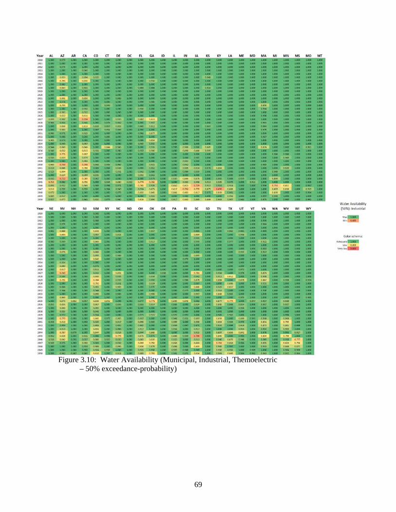
69

Figure 3.10: Water Availability (Municipal, Industrial, Themoelectric – 50% exceedance-probability)

70

Figure 3.11: Water Availability (Mining – 50% exceedance-probability)

71

Figur 3.12: Water Availability (Municipal, Industrial, Themoelectric – 10% exceedance-probability)

72

Figure 3:13 Water Availability (Mining – 10% exceedance-probability)

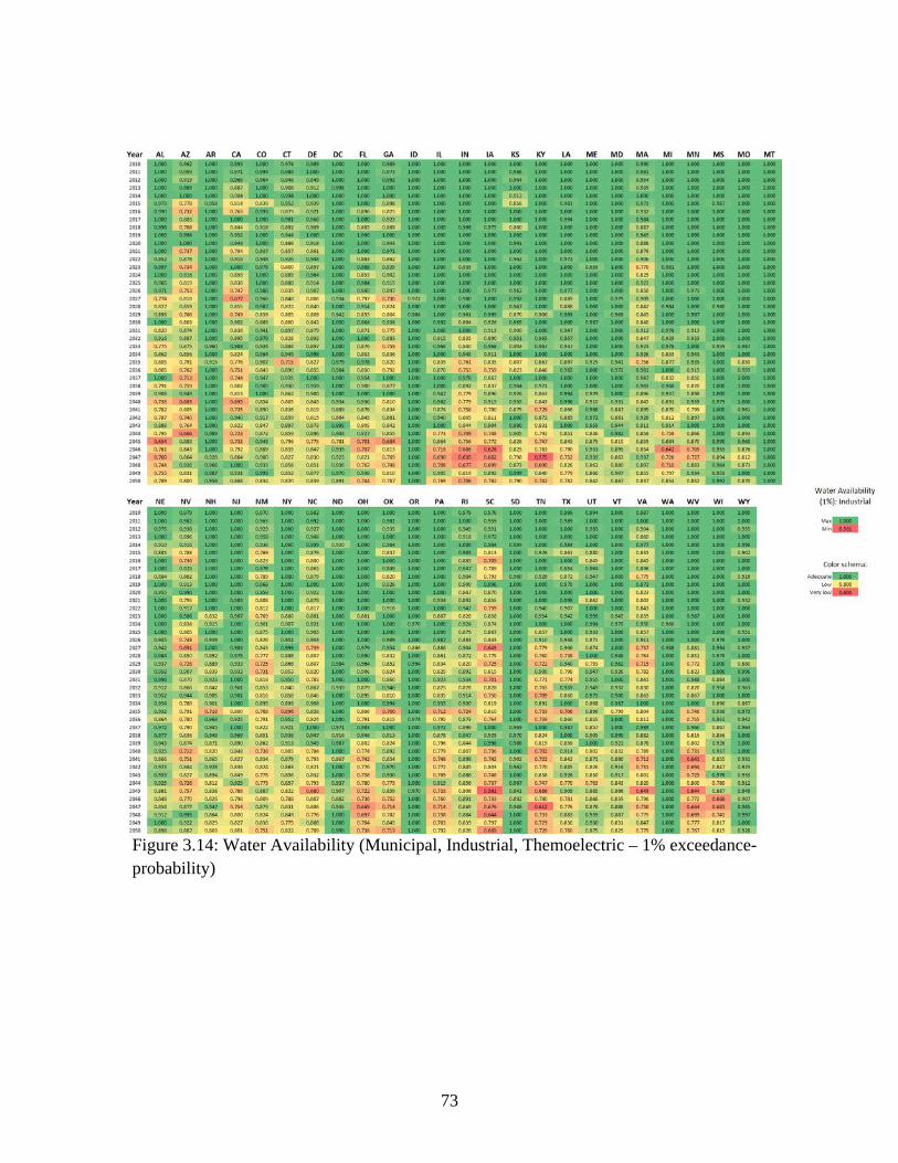
73

Figure 3.14: Water Availability (Municipal, Industrial, Themoelectric – 1% exceedance-probability)

74

Figure 3.15: Water Availability (Mining – 1% exceedance-probability)

75

3.2.2 Agricultural Impacts

The Sandia hydrological model contains an agriculture productivity component that estimates the impacts on agriculture from climate change. The algorithms are based on the work of McCarl et. al. (2008) and consider temperature and its standard deviation, precipitation and its standard deviation, and precipitation intensity. They also include recognition of soil types for 6 geographical regions covering the CONUS. Implicitly the model captures minor changes in farming practices (such as fertilizer use or crop rotation) in response to varying weather/climate conditions as implicitly embodied in the historical date. The statistical regression underlying the algorithms uses annual values to optimize predictive capability. This feature of using annual data ensures the McCarl work is compatible with this study. The McCarl work is designed to estimate the impact of climate change on agriculture. For this effort, the focus is on the comparison of realizable climate conditions with historical values. We use the agricultural algorithms to compare crop output across scenarios due to direct climate conditions between 2010 and 2050 combined with the re-allocation (or rights-purchase) of irrigation water away from agricultural activities toward higher value economic activities such as power generation, industrial needs, and municipal use. Because of their economic dominance, we use corn and soy as the representative crops upon which all agriculture is proportionally reduced in the economic portion of our analysis. The impact by state is based on its agricultural mix and the local impacts of climate. Other studies primarily look at one or only a couple of the terms included here (Schlenker 2005, 2006, Parry 1999, Iglesias 2000). More detailed dynamic simulations of agricultural impacts also exist (Williams 1984).

Because the McCarl study does include time-series as well as panel analyses of crop production within states, it implicitly captures technological and resource usage (such as the use of more or less fertilizer or modified planting regime) associated with variation in climatically-induced weather conditions

Reduced agricultural activity results in lost employment as well as lost demand for the intermediate products/goods used be agriculture. These impacts across sectors are readily simulated within the REMI PI+ model as will be discussed in section 3.4. Any reduction in agricultural produce is assumed to be made up with imports. The hydrological assessment of agriculture does include improvements in agriculture technology but does not assume an increased availability in agricultural acreage to augment reduced productivity due to climate change. In the reverse sense, we assume historical urban growth trends will cease and reduce the historical rate of farmland conversion in the future.

Figure 3.16 show an example of the impact of climate change on corn production, in this instance, at the 1% exceedance-probability. The change in colors helps visualize the variation in climate change impact across the years with state-specificity. The 50%

76

exceedance-probability impacts are not significantly different from the 1% exceedance-probability ones because of the fixed volatility of precipitation contained in the motif dominates the crop response. Crop impacts are small compared to other macroeconomic impacts from reduce precipitation.

Figure 3.16 Water Impacts (Corn -1% exceedance-probability)

77

3.2.3 Water Transfer Costs

Our analysis recognizes the practice of transferring water rights through contractual or policy means, typically from agricultural entities. While we do estimate these costs, they are not explicitly added to the macroeconomic analysis for three reasons. One reason is that the actual cost may not less substantial that estimated here, especially if policy interventions limit water transfer prices. Second, the climate change may reduce the economic viability of agricultural activities with a de-facto access in some years for water normally used for agriculture – as is currently the case when upstream or urban water usage exceeds the amount that would be formally associated with existing rights. Third and most importantly, a macroeconomic model categorizes economic activity by economic sector. If agriculture (or mining) sectors sold water rights, that activity is not related to added agricultural or mining activity, but rather as added “water-utility” activity where it is already accounted for in our analyses. Thus, in an economic sense, the “water sector” is merely buying and selling from itself. The cost of increased water delivery is endogenously captured (albeit, in the version of the REMI model we use all distribution utilities are lumped together as a single economic entity for each state). The cost of procuring water whether by new wells or new water rights is implicitly contained in the model logic. Therefore we do not attempt to explicitly make any exogenous, and potentially redundant, correction to the macroeconomic model simulation.

Figure 3.17: Water transfer Costs.

Simulation Total Costs for Transfers of Water 

from Mining and Agriculture

$1.0

$1.5

$2.0

$2.5

$3.0

$3.5

$4.0

$4.5

$5.0

0 20 40 60 80 100

Confidence Level

Billions of Cumulative

 2008$ 

78

To verify the adequacy of these assumptions, we estimate the cost of water transfer based on a cost of $1000 per acre-feet of deliverable water (as opposed to just water rights). This cost is consistent with existing transactions and with expectations over this timeframe (SeekingAlpha 2007, Frederick 2000 ). The aggregated national-level water transfer costs over the 2010-2050 period for varying exceedance-probabilities are shown in Figure 3.17. These cost are negligible compared the primary economic impacts.

3.2.4 Base Case Water Availability

When we apply the referent macroeconomic projection to the hydrology simulation in the absence of additional climate change, it shows that “normal” water supply will be inadequate to meet projected demand for water in several regions of the U.S. Other researchers also realize the potential for shortages even in an assumed business-as-usual environment (Frederick and Schwarz 2000, USEPA 2002, USGAO 2003, Karl 2009, NRC 2004, USBR 2005). This concern is widely appreciated (USBR 2005), but is not included in macroeconomic models because they are necessarily parameterized assuming physical conditions remain unchanged from historical values. Nonetheless, the macroeconomic forecast is solely use as a referent for assessing, in a comparative manner, future impacts from conditions different from those agreed upon for the referent projection. This use of a macroeconomic referent is the widely accepted pragmatic approach used in economic impact analyses for both policy planning and risk assessment. As such, the analysis presented here only considers water availability condition in excess of those beyond what would occur in the base case hydrology analysis. For reference, in appendix C, we present and summarize the implied impacts of water scarcity even in the absence of climate change.

79

3.3 Macroeconomic Simulation

For the economic component of our risk assessment, we use the Regional Economic Models Incorporated’s (REM 2007I) PI+ model. The pragmatic state-focused perspective of this work limits the study to the risk assessment between the years 2010 and 2050. The macroeconomic referent contained in PI+ is the U.S. Department of Commerce BEA forecast extended to 2050. This referent forecast and the REMI model are used within many states for policy and impact analysis.(REMI 2007, Treyz 2004) While the PI+ model does have a admirable track record for predictive accuracy, the use of the referent forecast is not based on its potential accuracy, but rather because it can act as a common basis for policy discussion – one that can avoid the energy and time consumption of debating whether it is right or wrong. Policy measures are invoked to avoid undesirable but anticipated outcome. The PI+ model is robust from a policy outcome perspective in that the differences it produces between a referent (i.e., a reasonable, acceptable but essentially arbitrarily selected control case) and intervention variants maintain a defendable relationship among “better” and “worse” alternatives.

The economic impact analysis consists of two steps. The first step is pre-modeling that transforms the estimated hydrological impacts into the relevant economic description that the REMI model can use to determine the implications across the entire U.S. economy. The second step is then the actual REMI simulation that determines the time dependent, interacting industry, and interacting state responses. Figure 3.18 depicts this process.

Figure 3.18: Data flow for the Economic Modeling

Sandia Hydrology Models

•Crop productivity

•Water availability

•Hydropower   Production

Sandia Hydrology Models

•Crop productivity

•Water availability

•Hydropower   Production

Climate‐to‐Economic Impact Model

•Changes in crop production

•Changes in industrial output, intermediate demand, and production costs

Climate‐to‐Economic Impact Model

•Changes in crop production

•Changes in industrial output, intermediate demand, and production costs

Macroeconomic Modeling

•National and regional changes in employment, GDP, and income

•Changes in regional population

Macroeconomic Modeling

•National and regional changes in employment, GDP, and income

•Changes in regional population

80

The REMI model is a time-dependent macroeconomic forecasting and policy analysis model.4 It is a mature and well- known model with documentation that includes exhaustive references, especially in regard to model evaluation (REMI 2007).5 The model is widely used by states and U.S. corporations as noted in its website.6 (www.remi.com). The REMI model integrates input-output, computable general equilibrium (CGE), econometric, and economic-geography methodologies. For this work we utilized the US model with state level detail for 70 economic sectors. The Input-Output aspect of the model captures inter-industry changes in demand and production. In the REMI model, the CGE aspect balances supply and demand through price, but the delays in response due to investments, population/business migration, and wage adjustments provide a more realistic simulation of the interactions across states across time. The econometric aspects ensure the model reflects the statistically estimated response characteristics of the individual states.

Figure 3.19 and 3.20 shows the overall structure of the PI+ model. The model contains five major blocks: (1) Output, (2) Labor and Capital Demand, (3) Population and Labor Supply, (4) Wages, Prices, and Costs, and (5) Market Shares. The access to factors of production such as labor and specialty commodities can affect how business can respond to local changes in conditions (e.g., due to climate change) by expanding operation in other states. The use of intermediate inputs from other industries ties the national and international economies together with cascading, interacting, multiplicative impacts as individual industries respond to climate change impacts.

Several industries are particularly susceptible to change in water availability and we explicitly simulate their adjustments to a changing climate and the consequences throughout the economy (Morrison 2009).

The industries most directly affected by reduced water availability are (see Appendix B):

Agriculture/Farming Food Beverage Paper Petroleum and Coal Chemical Primary Metal Mining Thermoelectric Power Generation

4 The description of the PI+ model in this section is based on material provided by REMI and used with permission. 5 The evaluations are comparisons to other methods or of prediction versus observations, but formal verification and validation methods are not fully developed. 6 See http://www.remi.com/index.php?page=by-sector&hl=en_US and www.remi.com

81

Hydropower Municipal Water Utilities

82

Figure 3.19: REMI PI+ Model Components and Linkages.

Figure 3.20: REMI PI+ Model Detail on Intermediate Demand and Factor Access

83

The specific pre-modeling effort forto map the hydrological impacts of climate change to the initiating impact on each industry is presented in Appendix B and a more detailed discussion is presented by Warren et.al (2009). To briefly summarize:

The changes in crop productivity from the hydrological model translate to changes in farm demand for secondary products (such as fertilizer) and reduced supply (leading to primarily to imports) for agricultural-product using sectors.

With water shortages, thermoelectric and industrial sectors using cooling-water convert to closed-cycle cooling or even to dry-cooling as conditions demand (Kelic 2009, Warren 2009). These changes increase the cost of producing output. Changes in the demand for their product due to increased costs then affects employment and the demand they previously had for products from other industrial sectors. This generates a spiral of impacts across industries, a story familiar during the recent financial crisis.

For coastal industries, we also consider conversion to saline-water use.

If reduced precipitation affects hydropower production, new generation is built endogenously, often in surrounding states to serve the otherwise unsatisfied demand for electricity.

For industrial consumptive uses of water, if efficiency improvements can adequately reduce water needs to match availability, production becomes constrained and declines.

Given the options for reduction in municipal water uses (e.g. not watering lawns and adding low-flow appliances) plus the general ability of municipal authorities to purchase water rights, the direct economic impact on municipal water consumers are estimated to be minimal.

If an industry already efficiently uses water, it has less capability to accommodate reduced water availability. It has already exercised the majority of options available, and its sensitivity to water shortages is greater than those industries that use water less efficiently. This consideration is particularly apparent in the mining industry.

Those regions that marginally have adequate water in the present have not yet developed storage and sophisticated water allocation (water rights) strategies. These areas immediately experience the impact of reduced water availability, even more so than those regions who currently deal with (accommodate) water limitations on a routine basis.

84

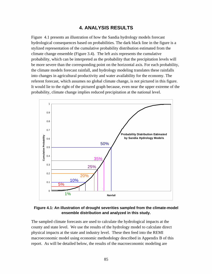
85

4. ANALYSIS RESULTS

Figure 4.1 presents an illustration of how the Sandia hydrology models forecast hydrological consequences based on probabilities. The dark black line in the figure is a stylized representation of the cumulative probability distribution estimated from the climate change ensemble (Figure 3.4). The left axis represents the cumulative probability, which can be interpreted as the probability that the precipitation levels will be more severe than the corresponding point on the horizontal axis. For each probability, the climate models forecast rainfall, and hydrology modeling translates these rainfalls into changes in agricultural productivity and water availability for the economy. The referent forecast, which assumes no global climate change, is not pictured in this figure. It would lie to the right of the pictured graph because, even near the upper extreme of the probability, climate change implies reduced precipitation at the national level.

Figure 4.1: An illustration of drought severities sampled from the climate-model ensemble distribution and analyzed in this study.

The sampled climate forecasts are used to calculate the hydrological impacts at the county and state level. We use the results of the hydrology model to calculate direct physical impacts at the state and industry level. These then feed into the REMI macroeconomic model using economic methodology described in Appendix B of this report. As will be detailed below, the results of the macroeconomic modeling are

0

0.1

0.2

0.3

0.4

0.5

0.6

0.7

0.8

0.9

1

Rainfall

Cu

mu

lati

ve P

rob

abili

ty

1%

5%10%

20%

25%

35%

Probability Distribution Estimated by Sandia Hydrology Models

50%

86

analyzed at the aggregate, national level and at the state level to gauge differences between different regions.

The REMI model is run on an annual basis for the years 2007 to 2050.7 Due to the recent global financial crisis, the revised historical estimates of economic may not exactly correspond to the referent macroeconomic forecast noted in Appendix D. Nonetheless, the numbers do remain a usable referent for a comparison of impact across different climate regimes. All costs are presented in 2008 U.S. dollars.

4.1 National Impacts

This section summarizes the national level risk assessment of climate change impacts. Figure 4.2 shows the values associated with the 50% probability (solid) line of Figure 3.4. It also notes the summary risk, that is the approximate sum (integral) of consequence multiplied by the probability. The interpolated value is based on the simulated values between 99% and 1% exceedance-probabilities. The extrapolated value includes extrapolated estimates of the contribution between 0% and 1% exceedance-probabilities (very severe) and 99% to 100% exceedance-probabilities (the largest amount of precipitation). As always, the analysis only considers the impact of reduced precipitation as justified in section 2.2. Even if there were abundant water on average, climate change still has a trend toward reduced precipitation which still includes both drought and flood conditions.

Table 4.1 present the value over different discount rates. The estimated GDP risk is estimated to be $1.2 trillion dollars through 2050 with 0% discount rate. The 50% exceedance-probability annual losses to the GDP are nearly $60 billion per year by 2050 and would exceed $130 billion per year at the 1% exceedance-probability. The annual data for the 1% probability exceedance case is presented in Appendix E.

7 Runs of the model assume that Keynesian closure rules are followed, which “[does] not use an interest rate mechanism to correct changes in U.S. employment that have been caused by an exogenous policy shock” (Source: Regional Economic Models, Inc. Description for “Closure Options”, “REMI PI+”, v. 1.0.114, March 24, 2009 build, 51 region, 70 sector model, Amherst, MA). The other options, which assume “coordination between fiscal and monetary policy makers resulting in interest rate adjustments that would immediately adapt to new policies, so that employment would be maintained at a constant rate” are deemed inappropriate, especially when the changes to the model will be caused by unpredictable changes in weather and climate.

87

Table 4.1: GDP Impact and Summary Risk (2010-2050)

Figure 4.2: U.S. GDP impacts (2010-2050)

The noted interpolated values are the risk using only the model-estimated costs between 1% and 99%. The extrapolated values include extrapolative estimates of the costs at over the 1% tails on each side of the distribution. Given the rapid increase in losses at the lower exceedance probabilities, and the existence of climate-induced loss even at 100% exceedance probability, the loss at the 50% exceedance probability only modestly underestimates the total risk. Figure 4.3 shows the impact on employment measured in lost labor-years over the years 2010 to 2050, with Table 4.2 showing the values. For the summary risk, the table only includes the interpolated values (99% to 1%). The analysis does not attempt to consider a widespread migration of unemployed population beyond U.S. borders possible at the 0%-1% extremes. Total risk is nearly 7 million lost labor-years between 2010 and 2050. The annual job loss for the 50% exceedance-probability is nearly 320,000. For the 1% exceedance-probability, job loss rises to nearly 700,000. The uncertainty in employment impact due to climatic uncertainty (at the 95% level) is only on the order of 10%.

U.S. GDP Risk from Climate (2010‐2050)‐$2,500

‐$2,300

‐$2,100

‐$1,900

‐$1,700

‐$1,500

‐$1,300

‐$1,100

‐$900

‐$700

‐$500

0%10%20%30%40%50%60%70%80%90%100%

Cumulative Probability Distribution

GDP Loss ( Billions 2008$)

Best Estimate

5%‐95% confidence

99% 75% 50% 35% 25% 20% 10% 5% 1%Inter-

polatedExtra-

polated

0.0% -$638.5 -$899.4 -$1,076.8 -$1,214.5 -$1,324.6 -$1,390.8 -$1,573.9 -$1,735.4 -$2,058.5 -$1,105.1 -$1,204.8

1.5% -$432.0 -$595.9 -$707.4 -$795.0 -$865.1 -$907.2 -$1,024.6 -$1,129.3 -$1,340.2 -$726.1 -$790.3

3.0% -$301.9 -$407.4 -$479.4 -$536.6 -$582.4 -$610.0 -$687.2 -$756.8 -$898.2 -$492.0 -$534.5

Estimated Risk

Change in National GDP ($B, 2008$)

Discount rate

Cumulative Distribution Percentile

88

Table 4.2: Employment Impact and Summary Risk (2010-2050).

Figure 4.3: U.S. Employment Impacts (2010-2050)

When water constraints limit economic production within the U.S., one alternative is to import the lost commodities, especially food. Figure 4.3 shows the impact of climate change on the U.S. trade balance, sans second order uncertainty intervals. This study is U.S. centric and assumes the Rest-the-World can accommodate added U.S. demands for imports. This analysis implicitly assumes that the Rest-of-the-World remains unchanged relative to its ability to import and export product at costs consistent with expectations. This assumption is assuredly unrealistic. Therefore, the components of uncertainty are not recognized in the analysis. Nonetheless, the Change in Net Exports (gross exports minus gross imports) appears to still capture the impacts of reduced U.S. production and competitiveness.

Under the assumption of a functional Rest of World, the trade balance only expands by an additional $0.5B per year in 2050 at the 50% exceedance-probability, but at an extra $8B per year at the 1% exceedance-probability. While mostly like being significantly

99% 75% 50% 35% 25% 20% 10% 5% 1%

-3,815 -5,463 -6,601 -7,468 -8,166 -8,587 -9,764 -10,819 -12,961

Change in Employment (Thousands)

Cumulative Distribution PercentileSummary

Risk

-6,863

U.S. Labor Risk from Climate (2010‐2050)‐15000

‐14000

‐13000

‐12000

‐11000

‐10000

‐9000

‐8000

‐7000

‐6000

‐5000

‐4000

‐3000

0%10%20%30%40%50%60%70%80%90%100%

Cumulative Probability Distribution

Employm

ent Loss       

(Thousands Labor‐Years)

Best Estimate

5%‐95% Confidence

89

underestimated, the trade balance risk over the 2010 to 2050 is over $25 billion dollars at a 0% discount rate. The value for other discount rates are shown in Table 4.3

Table 4.3: Balance of Trade Impacts (assuming an unchanged Rest-of-the-World

Figure 4.4: Trade Balance Impacts (2010-2050) (0% discount, Interpolated)

Table 4.4 shows the estimate of interpolated risks by industry at the national level. Due to construction, especially of power plants to augment lost hydroelectric capacity, utilities, electric equipment, and other manufacturing experience positive effects. Transportation sees a net neutral impact due to the added need for interstate trade, especially for food. Although highly uncertain, the textile industry appears to see a net

99% 75% 50% 35% 25% 20% 10% 5% 1%

0.0% $21.5 -$1.6 -$20.6 -$33.7 -$44.7 -$51.5 -$71.0 -$88.9 -$126.6

1.5% $16.9 $2.2 -$9.9 -$18.1 -$24.9 -$29.3 -$41.7 -$53.3 -$78.1

3.0% $13.5 $3.8 -$4.1 -$9.3 -$13.7 -$16.5 -$24.6 -$32.4 -$49.3 -$6.0

Discount rate

Cumulative Distribution PercentileSummary

Risk

Change in Net Exports (Billions of 2008$)

-$25.2

-$12.8

90

neutral impact due to the non-negligible migration of population to the relatively colder northern states.

Many professional services, including medial, see a drop because of unemployment constraining additional spending. Agriculture-dependent industries encounter substantial declines.

Table 4.4: Sector-Specific Risk at the National Level (0% discount rate, Interpolated)

National-Level Industry Impacts 2010-2050 (0% Discount, Billions 2008$)

Forestry and logging; Fishing, hunting -$0.6 Water transportation $0.0

Agriculture, forestry support activities; Other -$0.3 Truck transportation, couriers -$19.9

Oil and gas extraction -$9.4 Transit and ground passenger transportation -$0.6

Mining (except oil and gas) -$86.3 Pipeline transportation -$0.2

Support activities for mining -$7.3 Tourist transportation; support activities -$0.8

Utilities $13.6 Warehousing and storage -$2.1

Construction -$30.8 Publishing industries, except Internet -$12.4

Wood product manufacturing -$1.1 Motion picture and sound recording industries -$4.5

Nonmetallic mineral product manufacturing -$3.3 Internet publishing, Information services -$10.8

Primary metal manufacturing -$2.4 Broadcasting, Telecommunications -$28.1

Fabricated metal product manufacturing -$3.7 Monetary authorities, funds, trusts, financials -$34.1

Machinery manufacturing -$4.2 Securities, commodity contracts, investments -$39.9

Computer and electronic product mfg. -$10.3 Insurance carriers and related activities -$6.4

Electrical equipment and appliance mfg. $1.4 Real estate -$38.2

Motor vehicles, bodies & trailers, parts mfg. -$8.8 Rental and leasing services -$8.4

Other transportation equipment manufacturing -$1.6 Professional and technical services -$41.4

Furniture and related product manufacturing -$3.6 Management of companies and enterprises -$13.9

Miscellaneous manufacturing $1.4 Administrative and support services -$21.2

Food manufacturing -$82.3 Waste management and remediation services -$0.5

Beverage and tobacco product manufacturing -$29.4 Educational services -$2.2

Textile mills $0.0 Ambulatory health care services -$66.8

Textile product mills -$1.0 Hospitals -$5.5

Apparel manufacturing $0.8 Nursing and residential care facilities -$2.0

Leather and allied product manufacturing -$2.3 Social assistance -$2.0

Paper manufacturing -$2.5 Performing arts and spectator sports -$2.0

Printing and related support activities -$0.6 Museums, historical sites, zoos, and parks -$0.2

Petroleum and coal product manufacturing -$3.6 Amusement, gambling, and recreation -$5.9

Chemical manufacturing -$18.2 Accommodation -$3.8

Plastics and rubber product manufacturing -$4.5 Food services and drinking places -$19.9

Wholesale trade -$45.3 Repair and maintenance -$4.9

Retail trade -$127.2 Personal and laundry services -$11.2

Air transportation -$4.1 Membership associations and organizations -$2.0

Rail transportation -$3.2 Private households -$1.0

91

Table 4.5: Change in Employment-Years, GDP, and Disposable Personal Income: 2010 – 2050 (0% discount rate)

Table 4.5 adds an indication of the average percentage loss to the economy over the 40-year analysis timeframe. Costs rise significantly in the later years, with rapidly escalating cost in outlying years (Hope 2007). The year-2050 percentage impacts are typically 50% higher than the average over the 40-year period. Table 4.5 also distinguishes the agricultural from non-agricultural impacts on the economy, and it adds an estimate of Personal Disposable Income impacts. Although these economic impacts are a small fraction of overall economic activity of the period, they are substantial. Decreases in employment years range from a loss of 13.0.M in the least probable scenario to about 6.6M in the most probable, median scenario. GDP losses range from a loss of about $1.9T to a loss of about $0.9T. GDP losses due to crops is relatively small, ranging from a loss of $0.16T to a loss of $0.13T. As will be describe below in the sectoral analysis, GDP losses from the downstream industries that use crops is much greater than the direct losses. Losses in real disposable personal income range from about a $1.7T loss to a $1.0T loss. Losses in the most probable scenario remain substantial, as the economic impacts are about half as large as the lowest probability scenario.

Figures 4.5 to 4.8 examine the dynamics of these four variables. The paths of these variables are highly erratic, reflecting the high volatility of the year-to-year forecasts of the climate conditions. During all years except 2010—where impacts are nearly zero—impacts as a function of reduced exceedance probability are monotonic, becoming worse with simulations of greater drought severity. The 2010 values show an insightful artifact of the simulation. The initial response of investment and construction for adapting to climate change has a positive impact on the economy. This benefit is quickly outweighed

8 This calculation assumes that changes in soy and corn production can be used as proxies for total crop production and uses a ratio of 0.801 of change in GDP directly due to changes in crop production to corn and soy production. See Appendix B for the derivation of this ratio.

Run Employment U.S. GDP (no crops)

U.S. GDP (from crops)8

Real Disposable Years (k) Personal Income

1% -12,961 -0.15% -$1,899 -0.16% -$159 -0.01% -$1,727 -0.19%5% -10,819 -0.12% -$1,583 -0.13% -$152 -0.01% -$1,494 -0.16%

10% -9,764 -0.11% -$1,426 -0.12% -$148 -0.01% -$1,376 -0.15%20% -8,587 -0.10% -$1,247 -0.10% -$144 -0.01% -$1,241 -0.14%25% -8,166 -0.09% -$1,183 -0.10% -$142 -0.01% -$1,193 -0.13%35% -7,468 -0.08% -$1,076 -0.09% -$138 -0.01% -$1,113 -0.12%50% -6,601 -0.07% -$943 -0.08% -$134 -0.01% -$1,011 -0.11%

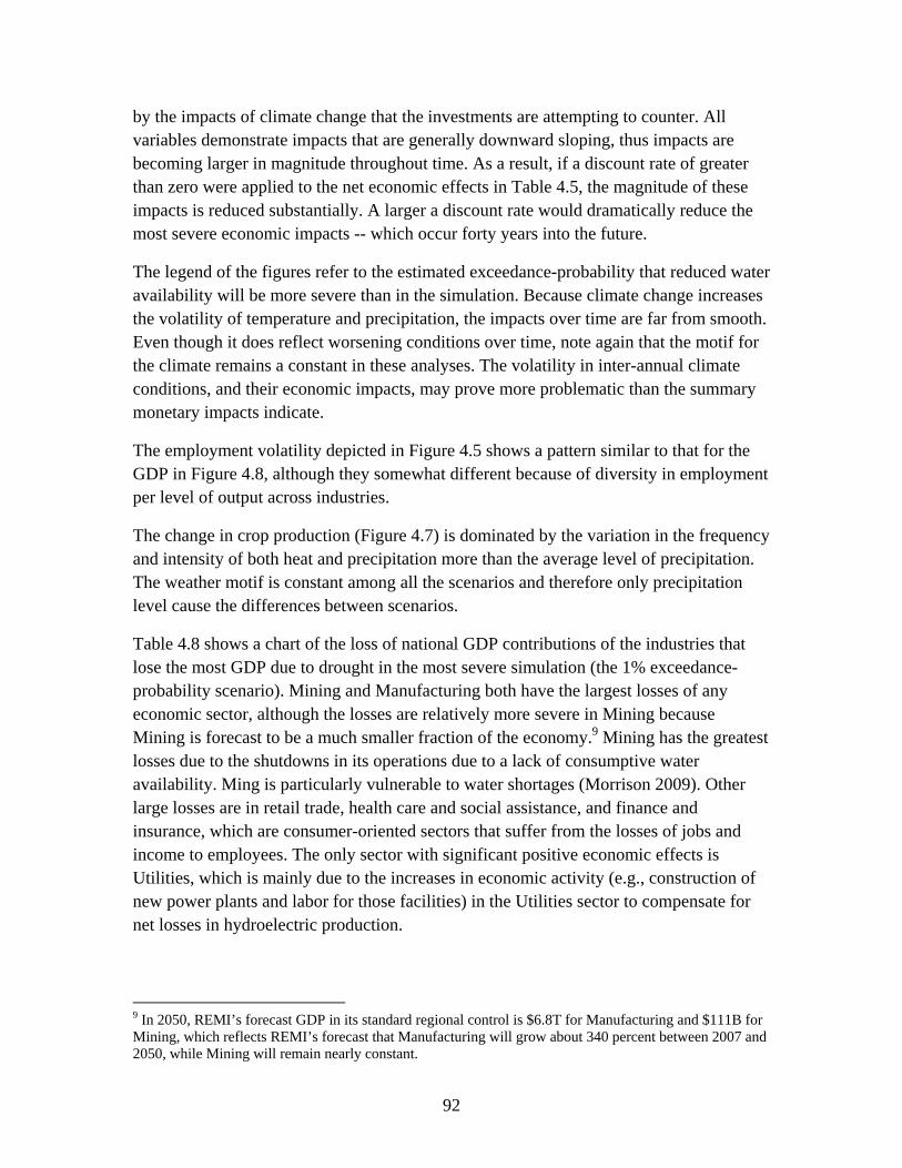
92

by the impacts of climate change that the investments are attempting to counter. All variables demonstrate impacts that are generally downward sloping, thus impacts are becoming larger in magnitude throughout time. As a result, if a discount rate of greater than zero were applied to the net economic effects in Table 4.5, the magnitude of these impacts is reduced substantially. A larger a discount rate would dramatically reduce the most severe economic impacts -- which occur forty years into the future.

The legend of the figures refer to the estimated exceedance-probability that reduced water availability will be more severe than in the simulation. Because climate change increases the volatility of temperature and precipitation, the impacts over time are far from smooth. Even though it does reflect worsening conditions over time, note again that the motif for the climate remains a constant in these analyses. The volatility in inter-annual climate conditions, and their economic impacts, may prove more problematic than the summary monetary impacts indicate.

The employment volatility depicted in Figure 4.5 shows a pattern similar to that for the GDP in Figure 4.8, although they somewhat different because of diversity in employment per level of output across industries.

The change in crop production (Figure 4.7) is dominated by the variation in the frequency and intensity of both heat and precipitation more than the average level of precipitation. The weather motif is constant among all the scenarios and therefore only precipitation level cause the differences between scenarios.

Table 4.8 shows a chart of the loss of national GDP contributions of the industries that lose the most GDP due to drought in the most severe simulation (the 1% exceedance-probability scenario). Mining and Manufacturing both have the largest losses of any economic sector, although the losses are relatively more severe in Mining because Mining is forecast to be a much smaller fraction of the economy.9 Mining has the greatest losses due to the shutdowns in its operations due to a lack of consumptive water availability. Ming is particularly vulnerable to water shortages (Morrison 2009). Other large losses are in retail trade, health care and social assistance, and finance and insurance, which are consumer-oriented sectors that suffer from the losses of jobs and income to employees. The only sector with significant positive economic effects is Utilities, which is mainly due to the increases in economic activity (e.g., construction of new power plants and labor for those facilities) in the Utilities sector to compensate for net losses in hydroelectric production.

9 In 2050, REMI’s forecast GDP in its standard regional control is $6.8T for Manufacturing and $111B for Mining, which reflects REMI’s forecast that Manufacturing will grow about 340 percent between 2007 and 2050, while Mining will remain nearly constant.

93

Figure 4.5: National Employment Impacts: 2010-2050

Figure 4.6: Change in National Disposable Personal Income (2008 USD): 2010-2050

-800,000

-700,000

-600,000

-500,000

-400,000

-300,000

-200,000

-100,000

0

2005 2010 2015 2020 2025 2030 2035 2040 2045 2050

Em

plo

ymen

t C

han

ge

1% 5% 10%

20% 25% 35%

50% 75% 99%

National employment ranges from 178M to 276M in the REMI standard regional control.

-$120

-$100

-$80

-$60

-$40

-$20

$0

2005 2010 2015 2020 2025 2030 2035 2040 2045 2050

Rea

l Dis

po

sab

le P

erso

nal

Inco

me

Ch

ang

e ($

B, 2

008)

1% 5% 10%

20% 25% 35%

50% 75% 99%

National Real Disposable Personal Income ranges from $11.0T to $39.2T in the REMI standard regional control.

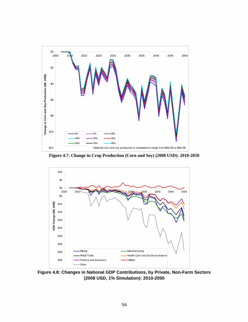
94

Figure 4.7: Change in Crop Production (Corn and Soy) (2008 USD): 2010-2050

Figure 4.8: Changes in National GDP Contributions, by Private, Non-Farm Sectors (2008 USD, 1% Simulation): 2010-2050

-$12

-$10

-$8

-$6

-$4

-$2

$0

2005 2010 2015 2020 2025 2030 2035 2040 2045 2050

Ch

ang

e in

Co

rn a

nd

So

y P

rod

uct

ion

($B

, 200

8)

1% 5% 10%

20% 25% 35%

50% 75% 99%

National corn and soy production is estimated to range from $69.2B to $89.2B.

-$45

-$40

-$35

-$30

-$25

-$20

-$15

-$10

-$5

$0

$5

$10

2005 2010 2015 2020 2025 2030 2035 2040 2045 2050

GD

P C

han

ge

($B

, 200

8)

Mining Manufacturing

Retail Trade Health Care and Social Assistance

Finance and Insurance Utilities

Other

95

4.2 Sectoral Impacts

This section explores the relative contributions of subcategories of inputs, running five categories of inputs variables into REMI: 1. Impacts to Farms, 2. Impacts to Industries that Use Farm Output, 3. Thermoelectric Production , 4. Hydroelectric Power and 5. Industry and Mining in separate REMI simulations. Additionally, the Industry and Mining category is run for a subcategory of variables without shutdowns for mining. All factor analysis simulations use the most extreme global climate change scenario that forecasts droughts that have a one percent chance of being exceeded in magnitude.

The goal of this factor analysis is to understand the relative contributions of different sets of input variables to aggregate results. This factor analysis was conducted using results from the hydrology assessment, which allocate water so that each sector absorbs a percentage of the deficit that is equal to that sector’s water demand in relation to the total demand.

REMI produces hundreds of output variables. This analysis concentrates on three of those variables: employment, gross domestic product (GDP—a measure of total value added), and real disposable personal income (income adjusted for taxes and changes in price levels). For each variable, two charts are presented. The first includes the first four (Farms, Farm Industry, Thermoelectric, and Hydroelectric) categories of input variables while the second includes two variants of the fourth (Industry and Mining) category: the full scenario and the scenario without shutdowns in the mining industry. This split was chosen because the industry variables produce much larger economic consequences than the other categories, and the mining shutdown variables (i.e., reductions in “Industry Sales / Exogenous Production”) have especially large effects.

Graphs of these output variables are presented in Figure 4.9 to Figure 4.12. In addition, the total changes between 2010 and 2050 is presented in Table 4.7 and the biggest percentage changes to states is shown in Table 4.8. These figures and tables show that the economic impacts of the farm variables are generally positive, but have the smallest magnitude. Part of this impact is the change toward more labor-intensive components of farming as crop production declines but with higher farm prices. The farm industry variables have a larger magnitude and are noisy with a decreasing trend.

96

Table 4.7 : Change in Labor-Years, GDP, and Disposable Personal Income: 2010 - 2050

The thermoelectric variables produce economic consequences of greater magnitude than the Farm variables and slightly smaller magnitude than the Hydroelectric variables. Positive spikes in GDP and employment occasionally occur, especially in the early years when investments in retrofits first begin, but these increases are often overwhelmed by the negative effects of increasing production costs in later years. The increases in production costs increase the price index throughout time, which results in a steadily decreasing level of Real Disposable Personal Income, reaching an annual loss of over $8B by 2050. Despite the net decrease of Real Disposable Personal Income of -$155B during this period, there is a slight net increase in GDP of $2B. However, that difference is due to investments in cooling retrofits that mitigate water shortages. If those retrofits were unnecessary, economic resources would be freed to be used more productively.

The only economic impacts that are generally positive are due to reductions in hydroelectric power production. Reductions to hydroelectric power increase the demand for alternate sources of power from the Utilities sector (as described further in Appendix B.). This increased demand causes increases to the economic variables as power plants are built, workers are hired to work in those plants, and fuel is purchased to power the plants, while the hydroelectric plants continue to operate with essentially the same labor and costs. The increases in economic activity highlights a problem—most familiar to economists who analyze disasters—with using aggregate measures of economic flows for consequence analysis: the lost service of hydroelectric power production is not measured in these economic flows, but the increased economic activity necessary to compensate for these losses is measured. If hydroelectric power production did not decrease, the economic resources utilized to create power from alternate sources could be used for other means (such as building luxury items) that would make consumers better off.

The Farm Industry input variables have the second highest magnitude to Employment and GDP, and the greatest impact to Real Disposable Personal Income. The annual loss in GDP reaches hovers around -$30B in the later years of the simulation, while the annual loss in Real Disposable Personal Income reaches -$40B.

Category Employment U.S. GDP Real Disposable1. Farm 216 0.0024% $21B 0.0017% $11B 0.0012%2. Farm-Demanding Ind. -5,286 -0.0594% -$719B -0.0598% -$887B -0.0976%3. Thermoelectric -91 -0.0010% $2B 0.0002% -$155B -0.0170%4. Hydroelectric 622 0.0070% $120B 0.0100% $47B 0.0052%5. Industry and Mining -8,428 -0.0946% -$1,324B -0.1101% -$746B -0.0820% -Not including shutdowns -1,641 -0.0184% -$285B -0.0237% -$197B -0.0217%

97

The Mining and Industry variables are generally of a much greater magnitude than the other categories of variables, except the magnitude of the losses to Real Disposable Personal Income is slightly less than it is for Farm Industry input variables. The maximum loss in annual GDP is about -$103B, while the maximum annual loss in any of the other three categories is about -$35B (for the Farm Industry). Partial and total shutdowns of mining and industry have a substantial negative effect on the output variables and are largely responsible for the substantial volatility of the output variables—when no shutdowns are included in the REMI simulation, all of the output variables decrease relatively smoothly. Because of the water allocation scheme, water availability to high-value industry never reaches low enough levels to cause industry shutdowns thus shutdowns only affect mining. From the perspective of an individual mining operation the sale of water right may represent a profitable option.

Reductions in water availability to mining cause relatively severe economic consequences because mining typically uses water efficiently. There are few opportunities for conservation without shutting down mining activity in states that are not adjacent to the ocean. All of the industries use a much greater share of their water for cooling, so they can conserve much greater portions of their consumption. Additionally, the industries are represented as an aggregate, so no industry begins shutting down production until all industries have made all possible cooling retrofits, thus raising the fraction of water that can be conserved through cooling retrofits.10

10 The smallest value of

itc% , which is the percentage of industrial consumption that can be conserved by

retrofitting cooling in states not adjacent to an ocean (see Section 0) is 32.4 percent. The median is 41.0%. For mining, on the other hand, this percentage is always 6 percent.

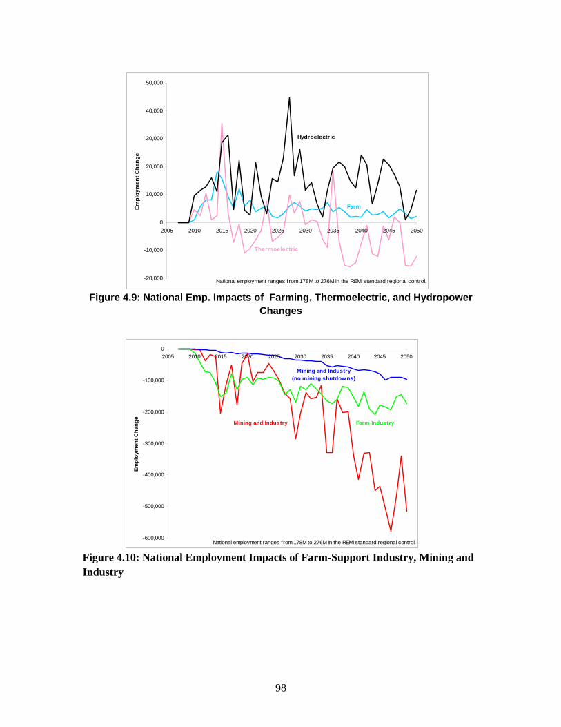
98

Figure 4.9: National Emp. Impacts of Farming, Thermoelectric, and Hydropower Changes

Figure 4.10: National Employment Impacts of Farm-Support Industry, Mining and Industry

-20,000

-10,000

0

10,000

20,000

30,000

40,000

50,000

2005 2010 2015 2020 2025 2030 2035 2040 2045 2050

Em

plo

ymen

t C

han

ge

Farm

Thermoelectric

National employment ranges from 178M to 276M in the REMI standard regional control.

Hydroelectric

-600,000

-500,000

-400,000

-300,000

-200,000

-100,000

0

2005 2010 2015 2020 2025 2030 2035 2040 2045 2050

Em

plo

ymen

t C

han

ge

Mining and Industry(no mining shutdowns)

Mining and Industry

National employment ranges from 178M to 276M in the REMI standard regional control.

Farm Industry

99

Figure 4.11: Change in National GDP (2008 USD), using Farm, Thermoelectric, and Hydroelectric Changes: 2010 – 2050.

Figure 4.12: Change in National GDP (2008 USD), Farm Industry, Mining and Industry Inputs: 2010 – 2050

-$8

-$6

-$4

-$2

$0

$2

$4

$6

$8

$10

2005 2010 2015 2020 2025 2030 2035 2040 2045 2050

GD

P C

han

ge

($B

, 200

8)

Farm

Thermoelectric

National GDP ranges from $14.3T to $52.6T in the REMI standard regional control.

Hydroelectric

Crops

-$105

-$85

-$65

-$45

-$25

-$5

$15

2005 2010 2015 2020 2025 2030 2035 2040 2045 2050

GD

P C

han

ge

($B

, 200

8)

Mining and Industry(no mining shutdowns)

Mining and Industry

National GDP ranges from $14.3T to $52.6T in the REMI standard regional control.

Farm Industry

100

Figure 4.13 shows that under extreme drought at the 1% exceedance-probability, water demand from municipal and high value-added industrial (with consequent demands for electric power) edges out agriculture and mining demand to a large extent (by a factor of 2 to 1 for the water allocation logic used in this analysis) . The difference between the mining line with and without shutdowns indicates the extent to which the unavailability of water to sustain operations affects the magnitude of total economic loss.

Figure 4.13: Change in National Real Disposable Personal Income (2008 USD), Using Farm, Farm Industry, Thermoelectric, Hydroelectric, and Mining and

Industry Inputs

Because the REMI model used for these simulations is a state-level model, it can measure regional economic consequences.

Table 4.8 lists the states with the largest percentage gains and losses in 2050 of population and real disposable personal income (both variables chosen because they change relatively smoothly and are measures of socio-economic dislocation). The relative magnitudes of the largest state-level changes in the different simulations are similar to the magnitudes of the national-level variables.

-$70

-$60

-$50

-$40

-$30

-$20

-$10

$0

$10

2005 2010 2015 2020 2025 2030 2035 2040 2045 2050

Rea

l Dis

po

sab

le P

erso

nal

Inco

me

Ch

ang

e ($

B, 2

008)

Mining and Industry(no mining shutdowns)

Mining and Industry

National Real Disposable Personal Income ranges from $11.0T to $39.2T in the REMI standard regional control.

Farm

Thermoelectric

Farm Industry

Hydroelectric

101

Table 4.8: States with Largest Percentage Changes in Population and Income: 2050

The largest losses are to West Virginia in the simulation that includes shutdowns of the mining industry. In this simulation, West Virginia loses 3.41 percent of its projected population and 4.11 percent of its projected real disposable personal income by 2050. This result is expected because a large fraction (8 percent of output11) of the West Virginia economy is mining, and according to the defined water allocation scheme, mining experiences twice the proportional reduction in water availability than the higher value-added industries.

For many of the categories of input variables, the largest gains and losses for Population and Real Disposable Personal Income are in states with large populations. For example, for the Industry and mining category, California gains over 58,200 residents by 2050, which is over twice as great as the second greatest increase (Florida, with a gain of about 27,500 residents). Based on the percentage gain compared to the baseline, however, California has the eighth largest gain (an increase of 0.10 percent). These gains in population come despite large losses in GDP (-$3.9B) and Real Disposable Personal Income (-$1.2B). Other states fare relatively worse and their residents choose to relocate. California, as the most populous state in the nation, is a likely destination of those emigrants. It also maintains a relative economic advantage compared to other states

11 In REMI’s standard regional control simulation, West Virginia’s total output in 2050 is $203B and its total output in mining is $16B.

Category Population Real Disposable Personal IncomeLargest Loss (Smallest Gain) 1. Farm 0.00% WY 0.00% WY 2. Farm-Demanding Industries -0.24% GA -0.38% GA 3. Thermoelectric -0.10% WV -0.15% WV 4. Hydroelectric -0.01% MD 0.00% IL 5. Industry and Mining -3.41% WV -4.11% WV -Not including mining shutdowns -0.05% IA -0.09% IA Largest Gain (Smallest Loss) 1. Farm 0.02% NE 0.02% NE 2. Farm-Demanding Industries 0.26% OR 0.16% OR 3. Thermoelectric 0.02% DE 0.00% DE 4. Hydroelectric 0.02% AZ 0.03% AZ 5. Industry and Mining 0.13% OR 0.01% OR -Not including mining shutdowns 0.02% OR -0.01% OR

102

dealing with the impacts of climate change in the long-term despite significant negative impacts in the short-term.

4.3 The Impact of Inter-Annum Volatility

An additional analysis was conducted using inputs to the Electricity Production Sector to explore how the volatility of the data, that is the motif, affects the average estimated macroeconomy impacts. The results from the simulation using the year-to-year hydrology forecasts is compared to a scenario created by linearly changing water availability to Electricity Production between 1 and the minimum of the 2010 to 2050 values for each state. The hydrology forecast used is the same data used in the previous subsection—the most extreme, with a one percent chance of the severity of the drought being exceeded.

Figure 4.14 shows the difference in national employment between the simulations and REMI’s standard regional control using the Sandia hydrology model’s simulated water availability and using a linear trend over time. When using the hydrology forecasts, year-to-year data is highly variable. Employment increases over 35,000 in 2015, while decreases nearly reach a loss of 16,000 jobs. When the simulation is conducted using a linear trend, increases in employment initially spike above 9,000, but then return to a relatively steady decrease of around -1,000 jobs.

Figure 4.14: Change in National Employment, using Simulated Thermoelectric Sector Water Availability Data: 2010 – 2050.

-20,000

-10,000

0

10,000

20,000

30,000

40,000

2005 2010 2015 2020 2025 2030 2035 2040 2045 2050

Em

plo

ymen

t C

han

ge

Thermoelectric(variable)

Thermoelectric(linear)

National employment ranges from 178M to 276M in the REMI standard regional control.

103

Figure 4.15 shows the change in GDP for the same simulations. The pattern is similar to the change in employment, except the magnitude of GDP changes become slightly larger in the second half of the simulation for both the variable and linear data.

Figure 4.15: Change in National GDP (2008 USD), using Simulated Thermoelectric Sector Water Availability Data: 2010 – 2050.

Figure 4.16 shows changes in Real Disposable Personal Income for the same simulations. Although the simulation using the hydrology forecasts continues to exhibit greater volatility than the simulation using the linear trend, it is much steadier than the path of employment or GDP using the hydrology forecasts.

Real Disposable Personal Income is driven by prices changes, which are affected by increases in production costs. These changes in the price index accumulate gradually over time, leading to a steady decrease in Real Disposable Personal Income. The volatility of the hydrology forecasts means that GDP fluctuates from year to year, which results in slight fluctuations of the variable forecast from the linear forecast. Furthermore, the variable forecast is slightly higher than the linear forecast because GDP in the variable forecast is higher than it is in the linear forecast in the earlier years of the simulation.

-$3

-$2

-$1

$0

$1

$2

$3

$4

$5

2005 2010 2015 2020 2025 2030 2035 2040 2045 2050GD

P C

han

ge

($B

, 200

8)

Thermoelectric(variable)

Thermoelectric(linear)

National GDP ranges from $14.3T to $52.6T in the REMI standard regional control.

104

Figure 4.16: Change in National Real Disposable Income (2008 USD), using Simulated Thermoelectric Sector Water Availability Data: 2010 – 2050.

In summary, the results of these simulations suggest that the economic consequences of global climate change—like any change that will have large year-to-year volatility—may cause more substantial year-to-year disruptions than climate change would cause if it followed a perfectly linear trend. Hallegate (2006) explores this issue more thoroughly. Additionally, the economic methodology (which assumes that firms make permanent retrofits to mitigate reductions in water availability) and the actions of the REMI model cause the variable simulation to have permanently lower levels of real disposable personal income.

4.4 State Impacts

The national-level results show that economic impacts for the entire nation are negative. However, this aggregate look at the economic impacts of drought induced by climate change may ignore important regional differences that create winners and losers. Examining regional differences are particularly pertinent for this analysis because drought caused by climate change will vary in severity across the country and different regions contain different mixes of industry, which will suffer to different extents from drought. For example, heavy consumers of water tend to cluster together near sources of water, thus there is little water-intensive industry in most Western, arid states.

-$12

-$10

-$8

-$6

-$4

-$2

$0

$2

2005 2010 2015 2020 2025 2030 2035 2040 2045 2050R

eal D

isp

osa

ble

Per

son

al In

com

e C

han

ge

($B

, 200

8)

Thermoelectric(variable)

Thermoelectric(linear)

National Real Disposable Personal Income ranges from $11.0T to $39.2T in the REMI standard regional control.

105

Table 4.10 shows the national and state level risk to GDP, employment and interstate population migration. The values are the integral of consequence-cost and consequence probability over the 2010 to 2050 period. The migration across states is often based on relative advantage. Even if a state economy is having difficulties, it may be having less difficulties than other states.

Figure 4.17 to Figure 4.22 show maps of state level impacts for GDP, employment population and corn for the total risk and 1% exceedance-probability conditions. The coloring scheme (green is good, yellow is neutral and red is bad) is based on the percentage impact relative to the state size. The impact values are presented in absolute terms.

These maps show that all states suffer negative economic impacts for all variables, except for three states in the Northwest (Washington, Oregon, Idaho) -- with Montana, California and Colorado showing benefits for the summary risk, but losses at the 1% exceedance-probability. These states have only slightly positive impacts. However, their slight gains are at the expense of the misfortune of others because these three states experience the largest increases in population (Figure 4.19), which transfers economic activity to these states. The gains the in Northwest states are also due to the increases in demand for Utilities that result from reduced hydroelectric power production. California, while suffering from the reduce precipitation in early years, prospers from the later-year population movements. Colorado prospers in the early years while there is still adequate water, but with losses mounting in the later years due to reduced water. Montana appears to be the only state that (slightly) benefits from both adequate water and population migration. Economic impacts are particularly severe in interior states that do not have the ability to substitute to desalinated water, and most acute in states like West Virginia with large concentrations of mining. For example, the GDP risk for West Virginia is estimated to be about 2.6 percent less than they would be without the consequences of drought.

Table 4.11 shows the state level impacts at the 1% exceedance-probability for comparison to summary risk in Table 4.10.

Figure 4.19 shows a map of state-level population changes in 2050. In a different mix from economic impacts, population impacts create a similar number of “winners” and “losers”. National population changes are not part of this analysis, so regional population changes are almost entirely the result of Americans moving from one state to another for economic reasons. There is a strong regional pattern with states in the Southeast and Southwest losing population and states on the West Coast, the western Midwest, and the Northeast gaining. Once again, interior states with the greatest concentrations of mining, such as West Virginia and Wyoming most affected.

106

States that gain population are not necessarily “winners” in a normative sense because greater population may have negative, non-monetary impacts that are not modeled within this study. For example, all states adjacent to the Atlantic Coast in the Northeast are gaining in population, but these states then become more susceptible to damage from extreme weather associated with global climate because of the large population concentrations (Changnon 2003).

Figure 4.20 through Figure 4.22 show the 1% exceedance-probability impacts. These are larger than total risk but comparable in most cases. For a few state, the results are dramatically different because the high exceedance-probability (>35%) impacts may actually show positive effects, such as in Colorado where there would still be adequate water with growing demand for goods from those states that are negatively affected earlier . Figure 4.23 shows the predicted change in value of corn and soy production across states at the 1% exceedance-probability. An evener strong regional pattern emerges with large percentage losses across all Southern, Southwest, and Eastern states. The Midwest, which produces most corn and soy, experiences only minor losses, while the Northwest experiences gains. States with 0.0% crop impact do not have recorded corn and soy production. The 1% exceedance-probability impacts can differ even in sign from the summary risk because the impacts can have different signs at different exceedance-probabilities, especially in the central latitude states where precipitation goes from sufficient to insufficient as the exceedance-probability decreases. Further, the relative advantage among the states can shift when states negatively affected at high exceedance-probabilities relatively improve in the lower exceedance-probabilities as the states around them experience negative impacts as well. Despite suffering relatively greater drought conditions on average relative to the rest of the nation, California shows improvements because its economic impacts are relatively less than those of other states. This relative advantage occurs because some states have little flexibility in dealing with water shortages, for example because there is little agricultural irrigation from which water can be diverted. By and large, those states that already suffer water constraints (often due to irrigation loads combined with urban growth in arid regions) have processes in-place to adjust to changes in water balances. Irrigation-water use can act as a buffer to water shortages, assuming the viability of food imports. The value added to the economy from certain types of industry is large compared to that for food production. Thus, the impact of reduced agriculture is partially compensated by the continued operation of high-value-added industry. The California case is particularly illuminating. In the early year of climate change it suffers significantly from the reduce precipitation and in the later years achieves relative advantage. There are time-dependent dynamics among several states where the geographical movement of the precipitation conditions and the change in relative advantage cause a reversal of cost and benefit from climate change over the 40 years. Similarly, high exceedance probability conditions may show benefits or losses the reverse with lower probability exceedance conditions.

107

The Pacific Northwest states show improvement with climate change due to expected increased precipitation.. This study limits itself to the annual resolution of precipitation levels (other than capturing monthly variation for agricultural assessments), and thus, does not capture the impact from lost snowpack water-storage in the Pacific Northwest. Consequently, the shown positive impacts could be an artifact of analysis assumptions. On the other hand, migration to the Pacific Northwest may provide positive impacts even if hydropower declines with residual added requirements for water storage.

108

Figure 4.9: National and State Level Risk 2010-2050

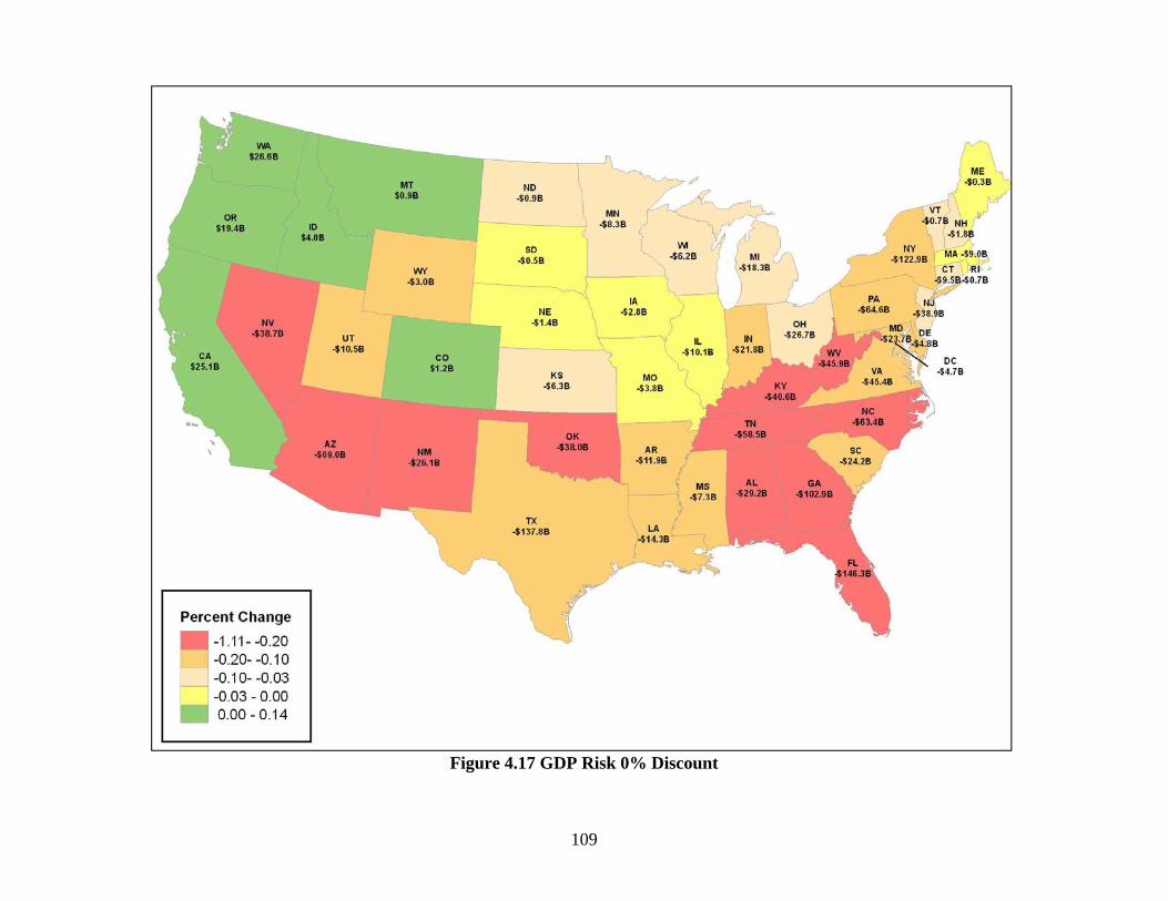
109

Figure 4.17 GDP Risk 0% Discount

110

Figure 4.18: Employment Risk (Employment-Years, 0% Discount)

111

Figure 4.19: Population 2050 Risk

112

Figure 4.20: Net change in state contribution to GDP 2010-2050, 1% Simulation

113

Figure 4.21: Net change in Employment-Years, 2010-2050, 1% Simulation

114

Figure 4.22: Change in 2050 Population, 1% Simulation

115

Figure 4.23: Net change in the value of corn and soy production, 2010-2050 (states with no recorded production are in white), 1% simulation

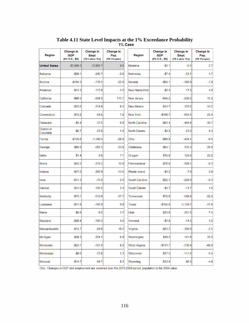
116

Table 4.11 State Level Impacts at the 1% Exceedance Probability

117

5.0 SUMMARY

We have used the uncertainty in future levels of precipitation associated with climate change as a input to a hydrological analysis that we could than use to estimate economic impacts. We used the uncertainty inferred from the IPCC climate model ensemble to estimate the economic costs of predicted climate change for various exceedance-probabilities. The integration of the costs over the full range of probability then characterizes the actual risk from climate change relative to GDP. The value of the loss, on the order of a trillion $ for the nation, represents an upper limit on how much society should be willing to pay for a successful mitigation of climate change, even over the near term. Our risk assessment only considers the loss in the absence of mitigation or any other climate policy. Schaeffer (2008) considers the risk assessment of the mitigation efforts. Consideration of longer-term (post 2050)impacts would imply even larger costs, but more temporally distant considerations are difficult for constituencies to accept with a sense of urgency.

The state level impact are far from uniform with some states experiencing significant swing depending on the specific probability of risk and large disparities compared to other states. Population and employment change produce similar disparities among the states. The integrated analysis of detailed climatic, hydrological, and economic impacts at the resolution of counties, states, and industries across the range of exceedance probabilities required for a meaningful risk assessment presents is relatively complex process. This study however indicates the losses associated with the 50% exceedance probability only modestly underestimate the value of the total risk over the existing PCMDI ensemble. This relationship is most probably not robust. As advances in climate modeling modify the understanding of best-estimate impacts and the uncertainty characteristics of the simulations, the total risk could be much larger than that associated with the 50% exceedance probability.

118

119

REFERENCES

Ackerman F, Stanton E (2008) Climate change and the U.S. Economy: The costs of inaction. Stockholm Environment Institute-US Center, Tufts University, http://www.seib.org/climate-and-energy/US_Costs_of_Inaction.doc, Cited September 2, 2009

Ackerman, F, and IJ Finlayson, (2006) “The Economics of Inaction on Climate Change: A Sensitivity Analysis, Global Development And Environment Institute, Working Paper No. 06-07, Tufts University, Medford MA

Ackerman, F. and K. Gallagher (2004). The Flawed Foundations of General Equilibrium: critical essays on economic theory, Routledge, London and New York

Ackerman F, EA Stanton, C Hope, S Alberth, (2009),”Did the Stern Review underestimate US and global climate damages?, Energy Policy, Volume 37, Issue 7

Alkhaled AA, AM Michalak and JW Bulkley, (2007) “ Applications of Risk Assessment in the Development of Climate Change Adaptation Policy”,World Environmental and Water Resources Congress 2007, Tampa Florida, American Society of Civil Engineers

Allen, M. R. & Ingram, W. J. (2002), Constraints on future changes in climate and the hydrological cycle. Nature 419, 224–232.

Backlund, P, A Janetos, D Schimel, (2008), “ The effects of climate change on agriculture, land resources, water resources, and biodiversity in the United States,” Synthesis and Assessment Product 4.3. Washington, DC: U.S. Environmental Protection Agency, Climate Change Science Program. 240 p.

Bader, D. C., C. Covey, W. J. Gutowski, Jr., I. M. Held, K. E. Kunkel, R. L. Miller, R. T. Tokmakian, and M. H. Zhang. 2008. Climate Models: An Assessment of Strengths and Limitations. U.S. Climate Change Science Program, Synthesis and Assessment Product (SAP) 3.1, http://downloads.climatescience.gov/sap/sap3‐1/sap3‐1‐final‐all.pdf.

Barker, Terry, Mahvash S. Qureshi, and Jonathan Koehler. 2006. The Costs of Greenhouse-Gas Mitigation with Induced Technological Change: a Meta-Analysis of Estimates in the Literature. Cambridge, UK: 4CMR, Cambridge Centre for Climate Change Mitigation Research, University of Cambridge.

120

Bates, B.C., Z.W. Kundzewicz, S. Wu, and J.P. Palutikof (eds.), 2008: Climate Change and Water. Technical paper of the Intergovernmental Panel on Climate Change. IPCC Secretariat, Geneva, Switzerland, 210 pp.

Bosello F., R. Roson, RSJ. Tol, (2006), “ Economy-wide estimates of the implications of climate change: Human health,” Ecological Economics, Volume 58, Issue 3, Pages 579-591.

Box, GEP, NR Draper (1987). Empirical Model-Building and Response Surfaces. Wiley. pp. p. 424.

Broome, J. (1992). Counting the cost of global warming. White Horse Press, Cambridge, UK.

Bull, S.R., D.E. Bilello, J. Ekmann, M.J. Sale, and D.K. Schmalzer, 2007: Effects of climate change on energy production and distribution in the United States. In: Effects of Climate Change on Energy Production and Use in the United States [Wilbanks, T.J., V. Bhatt, D.E. Bilello, S.R. Bull, J. Ekmann, W.C. Horak, Y.J. Huang, M.D. Levine, M.J. Sale, D.K. Schmalzer, and M.J. Scott (eds.)]. Synthesis and Assessment Product 4.5. U.S. Climate Change Science Program, Washington, DC, pp. 45-80.

CCSP (2009) “Best Practice Approaches for Characterizing, Communicating, and Incorporating Scientific Uncertainty in Decisionmaking.” [Morgan, G., H. Dowlatabadi, M. Henrion, D. Keith, R. Lempert, S. McBrid, M. Small, and T. Wilbanks (eds.)]. Synthesis and Assessment Product 5.2. US Climate Change Science Program, National Oceanic and Atmospheric Administration, Washington DC.

Chang, H., 2003: Basin hydrologic response to changes in climate and land use: the Conestoga River basin, Pennsylvania. Phys. Geogr., 24, 222-247.

Changnon, S.A., (2005) “Economic impacts of climate conditions in the United States: past, present, and future – an editorial essay.” Climatic Change, 68, 1-9.

Changnon, SA, (2003) “Shifting Economic Impacts from Weather Extremes in the United States: A Result of Societal Changes, Not Global Warming,” Natural Hazards, Springer Netherlands, Volume 29, Number 2

Chi-Chung Chen, C , D Gillig and BA McCarl (2001), “Effects of Climatic Change on a Water Dependent Regional Economy: A Study of the Texas Edwards Aquifer,” Climatic Change, Springer Netherlands, Volume 49, Number 4

121

Christensen, N.S.,A.W.Wood, N. Voisin, D.P. Lettenmaier and R.N. Palmer, 2004: The effects of climate change on the hydrology and water resources of the Colorado River basin. Climatic Change, 62, 337-363.

Christensen, J.H., B. Hewitson, A. Busuioc, A. Chen, X. Gao, I. Held, R. Jones, R.K. Kolli, W.-T. Kwon, R. Laprise, V. Magaña Rueda, L. Mearns, C.G. Menéndez, J. Räisänen, A. Rinke, A. Sarr and P. Whetton, 2007: Regional Climate Projections. In: Climate Change 2007: The Physical Science Basis. Contribution of Working Group I to the Fourth Assessment Report of the Intergovernmental Panel on Climate Change [Solomon, S., D. Qin, M. Manning, Z. Chen, M. Marquis, K.B. Averyt, M. Tignor and H.L. Miller (eds.)]. Cambridge University Press, Cambridge, United Kingdom and New York, NY, USA.

Cline, W. R. (1992). The Economics of Global Warming. Washington DC, Institute of International Affairs.

Cline, W. R. (2004). Meeting the challenge of global warming. Global Crises, Global Solutions. B. Lomborg. New York, Cambridge University Press.

Collins, M, (2007) “Ensembles and probabilities: a new era in the prediction of climate change,” Phil. Trans. R. Soc. A, vol. 365 no. 1857

Cowell, F. A. and K. Gardiner (1999). Welfare Weights, STICERD, London School of Economics.

Crovelli, RA, (1993) “ Probability & Statistics for Petroleum Resource Assessment. US Geological Survey, Denver

Dai,. A, 2006: Precipitation characteristics in eighteen coupled climate models. J. Climate, 19, 4605–4630.

Dasgupta , P., K.G Mäler and S. Barrett (1999). Intergenerational equity, social discount rates, and global warming. Discounting and Intergenerational Equity. P. R. Portney and J. P. Weyant. Washington, DC, Resources for the Future..

Davidson, M.D. (2006). A Social Discount Rate For Climate Damage to Future Generations Based on Regulatory Law, Climatic Change, 76, 55-72.

Dessai, S. and Hulme, M. (2004) Does climate adaptation policy need probabilities? Climate Policy 4, 107–128

122

Dettinger, M.D., D.R. Cayan, M.K. Meyer and A.E. Jeton, 2004: Simulated hydrologic responses to climate variations and change in the Merced, Carson, and American River basins, Sierra Nevada, California, 1900–2099. Climatic Change, 62, 283-317.

Dibike, Y.B. and P. Coulibaly, 2005: Hydrologic impact of climate change in the Saguenay watershed: comparison of downscaling methods and hydrologic models. J. Hydrol., 307, 145-163.

Feeley TJ, L Green, JT Murphy, J Hoffmann, and BA Carney, (2005), DOE/FE’s Power Plant Water Management R&D Program Summary, Department of Energy/Office of Fossil Energy’s Power Plant Water Management R&D Program, Washington DC, July 2005, http://www.netl.doe.gov/technologies/coalpower/ewr/pubs/IEP_Power_Plant_Water_R&D_Final_1.pdf

Field, C.B., L.D. Mortsch,, M. Brklacich, D.L. Forbes, P. Kovacs, J.A. Patz, S.W. Running and M.J. Scott, (2007), “ North America. Climate Change 2007: Impacts, Adaptation and Vulnerability.” Contribution of Working Group II to the Fourth Assessment Report of the Intergovernmental Panel on Climate Change, M.L. Parry, O.F. Canziani, J.P. Palutikof, P.J. van der Linden and C.E. Hanson, Eds., Cambridge University Press, Cambridge, UK, 617-652.

Frederick KD, GE Schwarz, (1999), “Socioeconomic Impacts Of Climate Change On U.S. Water Supplies,” Journal of the American Water Resources Association, vol. 35, no. 6

Frederick KD, GE Schwarz, (2000) “Socioeconomic Impacts of Climate Variability and Change on U.S. Water Resources,” Discussion Paper 00–21, Resources for the Future, DC.

Frei, A., R.L. Armstrong, M.P. Clark and M.C. Serreze, 2002: Catskill mountain water resources: vulnerability, hydroclimatology and climate change sensitivity. Ann. Assoc. Am. Geogr., 92, 203-224.

Giorgi, F. & Francisco, R.(2000) Evaluating uncertainties in the prediction of regional climate change. Geophys. Res. Lett. 27, 1295–1298.

Glieck, PH et.al., (2001), Climate Change Impacts on the United States: The Potential Consequences of Climate Variability and Change, National Assessment Synthesis Team (NAST), Cambridge University Press, Cambridge, UK, and New York, 612 pp. http://www.usgcrp.gov/usgcrp/Library/nationalassessment/>

123

Goldsmith T, (2009), Mine when the going gets tough: Review of global trends in the mining industry Price Waterhouse Coopers, Melbourne

Ghosh TK and MA Prelas, (2009) “Hubbert Peak Theory,” Chapter 10 , in Energy Resources and Systems , Volume 1: Fundamentals and Non-Renewable Resources, Springer Netherlands

Groisman, P.Ya. et al., 1999. Changes in the probability of heavy precipitation: important indicators of climatic change. Climatic Change 42, 243–283.

Guo J, CJ Hepburn, RSJ. Tol, D Anthoff, (2006), “Discounting and the social cost of carbon: a closer look at uncertainty,” Environmental Science & Policy, Volume 9, Issue 3

Ha-Duong, M. and N. Treich (2004). "Risk aversion, intergenerational equity and climate change." Environmental and Resource Economics 28: 195-207.

Hall, J , G Fu and J Lawry, (2007) “Imprecise probabilities of climate change: aggregation of fuzzy scenarios and model uncertainties,” Climatic Change, Springer Netherlands, Volume 81, Numbers 3-4, pp 265-281.

Hallegattea,S , J Hourcadec, and P Dumas (2007), “Why economic dynamics matter in assessing climate change damages: Illustration on extreme events,” Ecological Economics, Volume 62, Issue 2.

Hayhoe, K., D. Cayan, C.B. Field, P.C. Frumhoff, E.P. Maurer, N.L. Miller, S.C. Moser, S.H. Schneider, K.N. Cahill, E.E. Cleland, L. Dale, R. Drapek, R.M. Hanemann, L.S. Kalkstein, J. Lenihan, C.K. Lunch, R.P. Neilson, S.C. Sheridan and J.H. Verville, 2004: Emissions pathways, climate change, and impacts on California. P. Natl. Acad. Sci. USA, 101, 12422-12427.

Helton J.C., 1994, Treatment of Uncertainty in Performance Assessments for Complex Systems, Risk Analysis, Vol. 14, No. 4, 1994

Helton JC, (2009), “Conceptual and computational basis for the quantification of margins and uncertainty,”, SAND2009-3055, Sandia National Laboratories, Albuquerque

Hegerl, G.C., F. W. Zwiers, P. Braconnot, N.P. Gillett, Y. Luo, J.A. Marengo Orsini, N. Nicholls, J.E. Penner and P.A. Stott, 2007: Understanding and Attributing Climate Change. In: Climate Change 2007: The Physical Science Basis. Contribution of Working Group I to the Fourth Assessment Report of the Intergovernmental Panel on Climate Change [Solomon, S., D. Qin, M. Manning, Z. Chen, M. Marquis, K.B. Averyt, M. Tignor and H.L. Miller (eds.)]. Cambridge University Press, Cambridge, United Kingdom and New York, NY, USA.

124

Hope, C., 2006. The marginal impact of CO2 from PAGE2002: an integrated assessment model incorporating the IPCC’s five reasons for concern. Integrated Assessment 6 (1):19–56.

Hubbert M K, (1982) “Techniques of Prediction as Applied to the Production of Oil and Gas, ” In Oil and Gas Supply Modelling, S I Gass (ed ) National Bureau of Standards Special Publication 631, Washington DC

Hutson, SS, NL Barber, JF Kenny, KS Linsey, DS Lumia, and MA Maupin, (2005) “Estimated Use of Water in the United States in 2000,” Circular 1268, U.S. Geological Survey, Denver

Iglesias, A., Rosenzweig, C., Pereira, D., 2000. Prediction spatial impacts of climate in agriculture in Spain. Global Environmental Change 10, 69–80.

IPCC (Intergovernmental Panel on Climate Change) Contribution of Working Group III to the Fourth Assessment Report, 2007a, B. Metz, O.R. Davidson, P.R. Bosch, R. Dave, L.A. Meyer (eds), Climate Change 2007: Mitigation of Climate Change, Cambridge University Press, Cambridge, United Kingdom and New York, NY, USA.

IPCC (Intergovernmental Panel on Climate Change) Contribution of Working Group II to the Fourth Assessment Report, 2007b, M.L. Parry, O.F. Canziani, J.P. Palutikof, P.J. van der Linden and C.E. Hanson, Eds. Climate Change 2007: Impacts, Adaptation and Vulnerability, Cambridge University Press, Cambridge, UK, 976 pp

IPCC (Intergovernmental Panel on Climate Change) Contribution of Working Group I to the Fourth Assessment Report (2007c), Solomon, S., D. Qin, M. Manning, Z. Chen, M. Marquis, K.B. Averyt, M. Tignor and H.L. Miller (eds.). Climate Change 2007: The Physical Science Basis, Cambridge University Press, Cambridge, United Kingdom, 996 pp.

IPCC (Intergovernmental Panel on Climate Change) Field, C.B., L.D. Mortsch,, M. Brklacich, D.L. Forbes, P. Kovacs, J.A. Patz, S.W. Running and M.J. Scott, 2007d : North America. Climate Change 2007: Impacts, Adaptation and Vulnerability. Contribution of Working Group II to the Fourth Assessment Report, M.L. Parry, O.F. Canziani, J.P. Palutikof, P.J. van der Linden and C.E. Hanson, Eds., Cambridge University Press, Cambridge, UK, 617-652.

Jha, M., Z.T. Pan, E.S. Takle and R. Gu, 2004: Impacts of climate change on streamflow in the Upper Mississippi River Basin: a regional climate model perspective. J. Geophys. Res. – Atmos., 109(D9), D09105.

125

Jun, M, R Knutti, DW Nychka, “Spatial Analysis to Quantify Numerical Model Bias and Dependence,” Journal of the American Statistical Association, 2008

Kaplan, S, and B. J. Garrick. (1981) “On the Quantitative Definition of Risk,” Risk Analysis. 1, 11-27.

Karl T, Melillo J, Peterson T, Hassol SJ, eds. 2009. Global Climate Change Impacts in the United States.Cambridge Univ.Press. http://www.globalchange.gov/usimpacts (accessed 20 June 2009)

Kelic A, V Loose, V Vargas, and E Vugrin, (2009), “Energy and Water Sector Policy Strategies for Drought Mitigation,” SAND 2009-1360, Sandia National Laboratories, Albuquerque, New Mexico.

Keller K., G Yohe and M Schlesinger (2008), "Managing the risks of climate thresholds: uncertainties and information needs ," Climatic Change, Springer Netherlands, Volume 91, Numbers 1-2

Knutti, R. (2008b). “Should we believe model predictions of future climate change?,” Philosophical Transactions of The Royal Society A 366(1885): 4647–4664.

Knutti, R., et al. (2008a), A review of uncertainties in global temperature projections over the twenty-first century, J. Climate, in press.

Kuik, O.J., B. Buchner, M. Catenacci, A. Goria, E. Karakaya and R.S.J. Tol (2006), Methodological Aspects of Recent Climate Change Damage Cost Studies, FNU-122 (Submitted: Climate Policy)

Kundzewicz, Z.W., L.J. Mata, N.W. Arnell, P. Döll, P. Kabat, B. Jiménez, K.A. Miller, T. Oki, Z. Sen, and I.A. Shiklomanov, 2007: Freshwater resources and their management. In: Climate Change 2007: Impacts, Adaptation and Vulnerability. Contribution of Working Group II to the Fourth Assessment Report of the Intergovernmental Panel on Climate Change [Parry, M.L., O.F. Canziani, J.P. Palutikof, P.J. van der Linden, and C.E. Hanson (eds.)]. Cambridge University Press, Cambridge, UK, and New York, pp. 173-210.

Kunkel KE, RA Pielke Jr, SA Changnon (1999), Temporal Flunctuations and Climate Extremes that Cause Economic and Human Health Impacts: A Review - Bulletin of the American Meteorological Society, v. 80, n. 6.

Lempert RJ, ME Schlesinger and SC. Bankes, (1996), “When we don't know the costs or the benefits: Adaptive strategies for abating climate change,” Climatic Change , Springer Netherlands, Volume 33, Number 2

126

Leung, L.R., Y. Qian, X. Bian, W.M. Washington, J. Han and J.O. Roads, 2004: Mid-century ensemble regional climate change scenarios for the western United States. Climatic Change, 62, 75-113.

Manne, A,R Mendelsohn, R Richels, , 1995. "MERGE : A model for evaluating regional and global effects of GHG reduction policies," Energy Policy, Elsevier, vol. 23(1), pages 17-34.

Manning M (2006) The treatment of uncertainties in the Fourth IPCC Assessment Report. Advances in Climate Change Research 2(1):13–21

Marshall, A.: 1890, Principles of Economics, Macmillan and Co., Ltd., London.

Mastrandrea MD, Schneider SH (2004) Probabilistic integrated assessment of ‘‘dangerous’’ climate change. Science 304:571–575.

Mastrandrea, MD, et. al. (2009), Current And Future Impacts Of Extreme Events In California, California Climate Change Center, CEC500-2009-026-D

Maurer, E.P. and P.B.Duffy, 2005:Uncertainty in projections of stream flow changes due to climate change in California. Geophys. Res. Lett., 32, L03704.

Matott, L. S., J. E. Babendreier, and S. T. Purucker (2009), Evaluating uncertainty in integrated environmental models: A review of concepts and tools, Water Resour. Res., 45, W06421

Maupin MA and NL Barber,(2005) “Estimated Withdrawals from Principal Aquifers in the United States, 2000, Circular 1279, U.S. Geological Survey, Denver

McKinsey (2009). Shaping climate-resilient development. A framework for decision-making. Report of the Economics of Adaptation Working Group, http://www.mckinsey.com/clientservice/Social_Sector/our_practices/Economic_Development/Knowledge_Highlights/~/media/Images/Page_Images/Offices/SocialSector/PDF/ECA%20%20%20Shaping%20Climate%20Resilent%20Development%20%20%20Report%20Only.ashx

Meadows DL, et. al., 1974, Dynamics of growth in a finite world, Wright-Allen Press, Boston

Meehl, G. A. (2000), “ Trends in Extreme Weather and Climate Events: Issues Related to Modeling Extremes in Projections of Future Climate Change,” Bulletin- American Meteorological Society, VOL 81; PART 3, pages 427-436

127

Meehl, G.A., T.F. Stocker, W.D. Collins, P. Friedlingstein, A.T. Gaye, J.M. Gregory, A. Kitoh, R. Knutti, J.M. Murphy, A. Noda, S.C.B. Raper, Watterson, I.G. A.J. Weaver and Z.-C. Zhao, 2007: Global Climate Projections. In: Climate Change 2007: The Physical Science Basis. Contribution of Working Group I to the Fourth Assessment Report of the Intergovernmental Panel on Climate Change [Solomon, S., D. Qin, M. Manning, Z. Chen, M. Marquis, K.B. Averyt, M. Tignor and H.L. Miller (eds.)]. Cambridge University Press, Cambridge, United Kingdom and New York, NY, USA.

Mendelsohn, R.O., W. Morrison, M.E. Schlesinger, and N.G. Andronova (2000), “Country-specific market impacts of climate change”, Climatic Change, 45, 553-569.

Miles EL , AK Snover, AF Hamlet , B Callahan , D Fluharty (2000), “ Pacific Northwest Regional Assessment: The Impacts Of Climate Variability And Climate Change On The Water Resources Of The Columbia River Basin,” Journal of the American Water Resources Association, Volume 36, Issue 2

Milly, P.C.D., K.A. Dunne and A.V. Vecchia, 2005: Global pattern of trends in streamflow and water availability in a changing climate. Nature, 438, 347-350.

Morrison et al.(2009) , “Water Scarcity and Climate Change: Growing Risks for Businesses and Investors.” Ceres and Pacific Institute Report , CERES, Boston.

Murphy, J. M. et al. (2004), “Quantification of modelling uncertainties in a large ensemble of climate change simulations,” Nature 430, 768–-772

Nelson GC, et.al. (2009), Climate Change: Impact on Agriculture and Costs of Adaptation, International Food Policy Research Institute, Washington, D.C., September 2009, http://www.ifpri.org/publication/climate-change-impact-agriculture-and-costs-adaptation

Niemi E. (2009a), "An Overview of Potential Economic Costs to Washington of a Business-As-Usual Approach to Climate Change," The Program on Climate Economics, Climate Leadership Initiative, Institute for a Sustainable Environment, University of Oregon, Portland

Niemi E. (2009b), "An Overview of Potential Economic Costs to Oregon of a Business-As-Usual Approach to Climate Change," The Program on Climate Economics, Climate Leadership Initiative, Institute for a Sustainable Environment, University of Oregon, Portland

New, MI, A Lopez, S Dessai and R Wilby (2007), “ Challenges in using probabilistic climate change information for impact assessments: an example from the water sector,” Phil. Trans. R. Soc. A, vol. 365 no. 1857

128

Nordhaus WD, (1993) Rolling the DICE: an optimal transition path for controlling greenhouse gases, Resource and Energy Economics 15, 27–50.

Nordhaus WD and Z. Yang, (1996) RICE: a regional dynamic general equilibrium model of optimal climate-change policy, American Economic Review 86(4) 741–765.

Nordhaus W, J Boyer (2000) Warming the world: economic models of climate change, MITPress, Cambridge, MA, USA

Nordhaus WD (2006), "Geography and macroeconomics: New data and new findings", PNAS vol. 103 no. 10 3510-3517

Nordhaus WD (2007) A Review of the Stern Review on the Economics of Climate Change, Journal of Economic Literature, Volume: 45,Issue: 3

NRC.2009. Informing Decisions in a Changing Climate. Panel on Strategies and Methods for Climate-Related Decision Support, Committee on the Human Dimensions of Global Change. Washington, DC: The National Academies Press.

NRC, (2008) "Potential Impacts of Climate Change on U.S.Transportation," Special Report 290, Committee on Climate Change and U.S. Transportation, National Research Council, Washington DC, National Academies Press

NRC, (2004), “Confronting the Nation’s Water Problems: The Role of Research” National Research Council, National Academies Press, Washington, DC.

OXERA Consulting Ltd. (2002). A social time preference rate for use in long-term discounting. Report to Office of the Deputy Prime Minister, Department for Transport, and DEFRA, London, UK

Palmer, T. N. (2002). "The economic value of ensemble forecasts as a tool for risk assessment: From days to decades." Quarterly Journal of the Royal Meteorological Society 128(581): 747-774.

Parry, M.L., Fischer, C., Livermore, M., Rosenzweig, C., Iglesias, A., 1999. Climate change and world food security: a new assessment. Global Environmental Change 9, S51–S67.

Parry, M, N Arnell, P Berry, D Dodman, S Fankhauser, C Hope, S Kovats, R Nicholls, D Satterthwaite, R Tiffin, T Wheeler (2009), Assessing the costs of adaptation to climate change: A review of the UNFCCC and other recent estimates. International Institute for Environment and Development and Grantham Institute for Climate Change, London.

129

Patz JA,(2002) A human disease indicator for the effects of recent global climate change,PNAS, vol. 99 no. 20 12506-12508

Payne, J.T., A.W. Wood, A.F. Hamlet, R.N. Palmer and D.P. Lettenmaier, 2004: Mitigating the effects of climate change on the water resources of the Columbia River basin. Climatic Change, 62, 233-256.

Pierce DW, Barnett TP, Santer BD, Gleckler PJ(2009) Selecting global climate models for regional climate change studies. Proc Nat Acad Sci USA 106:8441–8446.

Portmann, PW, S Solomon and GC Hegerl. (2009), Spatial and seasonal patterns in climate change, temperatures, and precipitation across the United States,” PNAS, vol. 106 no. 18.

Prinn R., H. Jacoby, A. Sokolov, C. Wang, X. Xiao, Z. Yang, R. Eckhaus, P. Stone, D. Ellerman, J. Melillo, J. Fitzmaurice, D. Kicklighter, G. Holian and Y. Liu, (1999), “ Integrated Global System Model for Climate Policy Assessment: Feedbacks and Sensitivity Studies,” Climatic Change, Springer Netherlands, Issue Volume 41, Numbers 3-4.

Quiggin, John (2008) Stern and his critics on discounting and climate change: An editorial essay. Climatic Change, 89 3-4: 195-205.

Räisänen, J., and T.N. Palmer, 2001: A Probability and Decision-Model Analysis of a Multimodel Ensemble of Climate Change Simulations. J. Climate, 14, 3212–3226.

Ramanathan V, Feng Y (2008) On avoiding dangerous anthropogenic interference with the climate system: Formidable challenges ahead. Proc Natl Acad Sci USA 105:14245–14250.

Ramsey, F. P. (1928). "A mathematical theory of saving." The Economic Journal 138(152): 543-59.

Randall, D.A., R.A. Wood, S. Bony, R. Colman, T. Fichefet, J. Fyfe, V. Kattsov, A. Pitman, J. Shukla, J. Srinivasan, R.J. Stouffer, A. Sumi and K.E. Taylor, 2007: Cilmate Models and Their Evaluation. In: Climate Change 2007: The Physical Science Basis. Contribution of Working Group I to the Fourth Assessment Report of the Intergovernmental Panel on Climate Change [Solomon, S., D. Qin, M. Manning, Z. Chen, M. Marquis, K.B. Averyt, M.Tignor and H.L. Miller (eds.)]. Cambridge University Press, Cambridge, United Kingdom and New York, NY, USA.

Reichler,T, J Kim, (2008) “ How Well Do Coupled Models Simulate Today's Climate?,” Bulletin of the American Meteorological Society, Volume 89, Issue 3

130

REMI (2007) REMI Policy Insight: Model Documentation. Version 9.5, Regional Economic Models, Inc., Amherst, MA, Available at; http://www.remi.com/index.php?page=documentation&hl=en_US

Richardson, K, W Steffen, et. al.,(2009) Synthesis Report from Climate Change: Global Risks, Challenges & Decisions, Copenhagen 2009, 10-12 March University of Copenhagen

Ringland, G, 2006, Scenario Planning: Managing for the Future, Wiley & Sons, NY

Roe, GH and MB Baker, (2007) “Why Is Climate Sensitivity So Unpredictable?,”, Science, AAAS, 26 October 2007 318: 629-632

Roughgarden T, and SH Schneider.(1999), “ Climate Change Policy: Quantifying Uncertainties for Damages and Optimal Carbon Taxes.,” Energy Policy 27:415-429.

Saelen, H, G Atkinson, S Dietz, J Helgeson, C Hepburn (2008), “Risk,inequality and time in the welfare economics of climate change: is the workhorse model underspecified?” Department of Economics, University of Oxford, Discussion Paper 400, http://www.economics.ox.ac.uk/research/WP/pdf/paper400.pdf

Santoso H. M Idinoba, P Imbach (2008) ,“Climate Scenarios: What we need to know and how to generate them,” Working Paper No. 45, Center for International Forestry Research (CIFOR), Indonesia

Schaeffer M, T Kram, M Meinshausen, DP. van Vuuren, and WL Harec, (2008), “ Near-linear cost increase to reduce climate-change risk,” PNAS December 30, 2008 vol. 105 no. 52 20621-20626

Schlenker,W.,W.M. Hanemann andA.C. Fisher, 2005:Will U.S. agriculture really benefit from global warming? Accounting for irrigation in the hedonic approach. Am. Econ. Rev., 95, 395-406.

Schlenker, W and Roberts, MJ.(2006) , Estimating the Impact of Climate Change on Crop Yields: The Importance of Non-Linear Temperature Effects (September 2006). Available at SSRN: http://ssrn.com/abstract=934549

Schneider SH, and M D. Mastrandrea (2005) Probabilistic assessment of “dangerous” climate change and emissions pathways PNAS November 1, 2005 vol. 102 no. 44 15728-15735

131

Seager, R., A. Tzanova and J. Nakamura, 2008: Drought in the Southeastern United States: Causes, variability over the last millennium and the potential for future hydroclimate change, Journal of Climate, Submitted

SeekingAlpha (2007) "T. Boone Pickens Invests in Water - Should You?", http://seekingalpha.com/article/24410-t-boone-pickens-invests-in-water-should-you

Sheffield, J., and E. F. Wood. 2008. Projected changes in drought occurrence under future global warming from multimodel, multiscenario, IPCC AR4 simulations. Climate Dynamics 31:79–105. .

Sokolov A, Stone P, Forest C, Prinn R, Sarofim M, et al. (2009) Probabilistic forecast for 21st century climate based on uncertainties in emissions (without policy) and climate parameters. Journal of Climate: In Press

Solley, WB, RR Pierce and HA Perlman, (1998) Estimates Use of Water in the United States in 1995,” Circular 1200, U.S. Geological Survey, Denver

Solley, WB, RR Pierce and HA Perlman, (1993) Estimates Use of Water in the United States in 1990, Circular 1081, US Geological Survey, Denver

Solomon, S., et. al. (2009), Irreversible climate change due to carbon dioxide emissions, PNAS, January 28, 2009, doi: 10.1073/pnas.0812721106

Stainforth, D.A, M.R Allen, E.R Tredger and L.A Smith, (2007a) “ Confidence, uncertainty and decision-support relevance in climate predictions,” Phil. Trans. R. Soc. A 15 August 2007 vol. 365 no. 1857 2145-2161

Stainforth1,DA, TE Downing, R Washington, A Lopez and M New, (2007b) “Issues in the interpretation of climate model ensembles to inform decisions,” Phil. Trans. R. Soc. A 15 August 2007 vol. 365 no. 1857 2163-2177

State Of New Mexico (2005), “Potential Effects Of Climate Change On New Mexico,” Agency Technical Work Group, State Of New Mexico

Steffen, W., 2009: Climate Change 2009: Faster Change and More Serious Risks. Report to the Department of Climate Change, Australian Government.

Sterman JD and LB Sweeney, (2007) Understanding public complacency about climate change: adults’ mental models of climate change violate conservation of matter,Climatic Change, Springer Netherlands, Volume 80, Numbers 3-4

132

Sterman JD, (2008),"Risk Communication on Climate: Mental Models and Mass Balance, "Science, AAAS, Vol. 322. no. 5901

Stern, Nicholas. 2007. The Economics of Climate Change: The Stern Review. Cambridge and New York: Cambridge University Press.

Sterner, T, UM Persson (2008), An Even Sterner Review: Introducing Relative Prices into the Discounting Debate, Review of Environmental Economics and Policy, Advance Access published online on April 23, 2008

Stone,M.C., R.H. Hotchkiss, C.M. Hubbard, T.A. Fontaine, L.O.Mearns and J.G.Arnold, 2001: Impacts of climate change on Missouri River Basin water yield. J.Am. Water Resour. As., 37, 1119-1129. (north = increased agri production and water)

Stott, P. A. & Forest, C. E. Ensemble climate predictions using climate models and observational constraints. Phil. Trans. R. Soc. A 365, 2029–2052 (2007).

Taylor, R. G. (2009) Rethinking water scarcity: the role of storage. EOS – Trans. Am. Geophys. Union, Vol. 90, no. 28

Tebaldi C., and R Knutti (2007) “The use of the multi-model ensemble in probabilistic climate projections,” Phil. Trans. R. Soc. A 2007 365, 2053-2075

Tebaldi, C. and Sanso, B. (2008). \Joint Projections of Temperature and Precipitation Change from Multiple Climate Models: A Hierarchical Bayes Approach." Journal of the Royal Statistical Society: Series A. Volume 172 Issue 1, Pages 83 – 106

Tol, Richard S. J. 2009. The Economic Effects of Climate Change. Journal of Economic Perspectives. Volume 23, Issue 2.

Tol, RSJ, (2002a) “Estimates of the Damage Costs of Climate Change. Part 1: Benchmark Estimates”, Journal Environmental and Resource Economics, Springer Netherlands, Volume 21

Tol, RSJ, (2002b) “Estimates of the Damage Costs of Climate Change. Part 1: Benchmark Estimates”, Journal Environmental and Resource Economics, Springer Netherlands, Volume 21

Trenberth, K. E., 2008: The impact of climate change and variability on heavy precipitation, floods and droughts. Encyclopedia of Hydrological Sciences. M. H. Anderson, Ed. J. Wiley and Sons, Ltd. Chichester, UK.

133

Treyz F., and G. Treyz, (2004),” The Evaluation of Programs aimed at Local and Regional Development: Methodology and Twenty Years of Experience using REMI Policy Insight, “ Chapter 7 in Evaluating Local Economic and Employment Development: How to Assess What Works among Programmes and Policies,” Organization for Economic Cooperation and Development (OECD), Paris

U.S. Bureau of Reclamation, (2005) ”Water 2025: Preventing Crises and Conflict in the West.” U.S. Bureau of Reclamation, Washington, DC.

U. S. Environmental Protection Agency (2000), Guidelines for Preparing Economic Analysis, Washington D.C.

U.S. Environmental Protection Agency, 2002: The Clean Water and Drinking Water Infrastructure Gap Analysis. EPA-816-R-02-020. U.S. Environmental Protection Agency, Washington, DC, 50 pp. http://www.epa.gov/safewater/gapreport.pdf

U.S. General Accounting Office, 2003: Freshwater Supply: States’ Views of How Federal Agencies Could Help Them Meet the Challenges of Expected Shortages. GAO-03-514. General Accounting Office, Washington, DC, 110 pp. http://www.gao.gov/new.items/d03514.pdf

US Office of Management and Budget, (2008), 2009 Discount Rates for OMB Circular No. A-94, Washington DC, http://www.whitehouse.gov/omb/assets/omb/memoranda/fy2009/m09-07.pdf

van der Heijden, K (2005), Scenarios: The Art of Strategic Conversation, Wiley & Sons,NY

Vicuna, S., J.A. Dracup, J.R. Lund, L.L. Dale and E.P. Maurer, 2009, Basin Scale Water Systems Operations under Climate Change Hydrologic Conditions: Methodology and Case Studies, Water Resources Research (submitted 2/10/2009)

Warren, D., M. Ehlen, V. Loose, and V. Vargas, (2009) Estimates of the Long-Term U.S. Economic Impacts of Global Climate Change-Induced Drought, Computational Economics Group, Infrastructure and Economic Systems Analysis Department, Sandia National Laboratories, Albuquerque, NM, September 1, 2009

Washington, W. M., R. Knutti, G. A. Meehl, H. Teng, C. Tebaldi, D. Lawrence, L. Buja, and W. G. Strand (2009), How much climate change can be avoided by mitigation?, Geophys. Res. Lett., 36, L08703, doi:10.1029/2008GL037074.

134

Watterson, I. G., and M. R. Dix (2003), Simulated changes due to global warming in daily precipitation means and extremes and their interpretation using the gamma distribution, J. Geophys. Res., 108(D13), 4379, doi:10.1029/2002JD002928.

Webster, M., et.al, 2003: Uncertainty analysis of climate change and policy response. Climate Change, 61, 295–320.

Weisbach, David A. and Sunstein, Cass R., ( 2008) Climate Change and Discounting the Future: A Guide for the Perplexed (August 12, 2008). Reg-Markets Center Working Paper No. 08-19; Harvard Public Law Working Paper No. 08-20; Harvard Law School Program on Risk Regulation Research Paper No. 08-12. Available at SSRN: http://ssrn.com/abstract=1223448

Weitzman ML, (2007) “A Review of the Stern Review on the Economics of Climate Change”, Journal of Economic Literature, Volume: 45, Issue: 3

Weitzman, ML,(2009) “On Modeling and Interpreting the Economics of Catastrophic Climate Change,” The Review of Economics and Statistics, Vol. 91, No. 1, Pages 1-19

Wilbanks, T.J., V. Bhatt, D.E. Bilello, S.R. Bull, J. Ekmann, W.C. Horak, Y.J. Huang, M.D. Levine, M.J. Sale, D.K. Schmalzer, and M.J. Scott (eds.) (2008), Effects of Climate Change on Energy Production and Use in the United States. Synthesis and Assessment Product 4.5. U.S. Climate Change Science Program, Washington, DC, pp. 45-80.

Wilkinson L,(1995) "How to Build Scenarios: Planning for Long Fuse, Big Bang Problems in an Era of Uncertainty." Wired (Special Edition, Scenarios: The Future of the Future): 74-81.

Williams J.R, Renard K.G, Dyke P.T. (1984) EPIC—a new model for assessing erosion's effect on soil productivity. J. Soil Water Conservation.8:381–383.

Yohe, G.W., R.D. Lasco, Q.K. Ahmad, N.W. Arnell, S.J. Cohen, C. Hope, A.C. Janetos, and R.T. Perez, 2007: Perspectives on climate change and sustainability. In: Climate Change 2007: Impacts, Adaptation and Vulnerability. Contribution of Working Group II to the Fourth Assessment Report of the Intergovernmental Panel on Climate Change [Parry, M.L., O.F. Canziani, J.P. Palutikof, P.J. van der Linden, and C.E. Hanson (eds.)]. Cambridge University Press, Cambridge, UK, and New York, pp. 811-841.

Yohe, Gary, and Richard S.J. Tol. 2009. Precaution and a Dismal Theorem: Implications for Climate Policy and Climate Research. In Risk Management in Commodity Markets, edited by H. Geman. New York: Wiley Press. Forthcoming.

135

Young, R.A., 2005: Determining the Economic Value of Water: Concepts and Methods. Resources for the Future Press, Washington, District of Columbia, 300 pp.

Zhang Y, Dulière V, Mote P, Salathé Jr EP (2009) Evaluation of WRF and HadRM Mesoscale Climate Simulations over the United States Pacific Northwest. Journal of Climate: In Press

136

137

APPENDIX A: HYDROLOGY MODELING

The hydrologic model was adapted from modules embedded in the broader decision support framework for integrated energy-water planning and management depicted in Figure A.1 (Tidwell et al. 2009). Elements borrowed for this study pertain to the simulation of future water demands as well as the identification of regions of potential future water stress. These simulations are possible at each of four reference scales (e.g., national, state, county, and watershed).

Figure A1: The SNL Hydrology Model (subset of modules used for this study)

Water demand is individually calculated according to six different use sectors: municipal (including domestic, public supply, and commercial), industrial, electrical power production, agriculture, mining and livestock. Water use and consumption are tracked

138

separately as are the resulting return flows. Water use statistics published by the U.S. Geological Survey (USGS) serve as the primary data source for the analysis. Specifically, data from the 1985, 1990, and 1995 campaigns provide the most comprehensive picture of water use in the U.S., and hence form the basis of this analysis (USGS 1985, 1990, 1995).

Municipal water use/consumption is modeled at the county level and subsequently aggregated to the state level. 1995 water use values serve as the initial conditions for the model. Future water use/consumption rates are calculated as the product of the per capita water use/consumption and the population. Population growth projections are based on REMI output while per capita water use/consumption rates are extrapolated according to regression equations fitted to the published USGS water use/consumption rates. The maximum change in the per capita water use/consumption is capped at ±20% simply to reflect the fact that changes beyond this level generally require structural change to the system.

Water demand in the industrial, mining, and livestock sectors is handled in a similar fashion to municipal; however, use/consumption rates are calculated as the product of Gross State Product and the associated water intensity (e.g., gallon/$GSP). GSP projections are based on REMI output.

Increases in thermoelectric water demand are modeled as the product of new power plant capacity and the water use rate per kWh. For consistency in this project, projections of new capacity are taken directly from REMI. Thermoelectric water use rates are assumed to equal the 2004 average for produced power. The model distinguishes the use of ocean versus fresh water for cooling.

Water demands in the agricultural sector consider both farms/conveyance losses as well as the direct consumptive use of the crop itself. Estimated losses are taken directly from published USGS data. Crop consumptive losses are calculated as the product of historical average irrigation rates for specific crop types and the associated irrigated acreage (USDA 2008).

Key to this analysis is determining at what point a region will begin experiencing water stress. That is, at what point with the available water supply be insufficient to meet all projected water demands. This requires some measure of the available water supply; however, detailed water supply values for each region of the U.S. are currently unavailable and their calculation is well beyond the scope of this project. As such, a proxy to water supply is used which is based on the long-term mean gauged flow, as are available at the USGS four-digit hydrologic unit classification level (USGS 2009). These long term averages are further modified by sequentially subtracting increases in consumptive water use from upstream basins (to account for the effect of growing water

139

use on the availability of water). The model does include projections on the use of ground water and implicitly considers jurisdiction rights on downstream water usage. For this analysis, the ratio of runoff to precipitation is assumed adequately constant to determine water availability. Although studies do indicate changes in this ratio the statistics remain inconclusive (Sheffield 2007, Steager 2008) and the changes inconsequential relative to impacts considered in this study.

To project potential water stress at the state level the ratio of water supply to projected demand is calculated. Where this ratio is less than 2 the state is assumed to be using essentially as much water as is available in a normal year. In this case any new water use or drought would immediately result in water shortage (Taylor 2009). States in this class are listed in Table A1. Further, states with a supply/demand ratio between 2 and 10 are assumed to experience a water shortage anytime the supply drops below 60% of the long term average. Finally, all other states are assumed to experience shortages only when the supply drops below 40% of average.

Each year, climate data is passed to the hydrologic model to determine where water stress will occur. Where precipitation ratios (current/normal) fall below the above thresholds, water shortages are initiated. Shortages are not evenly distributed across the sectors, but rather are weighted more heavily toward agriculture, mining and livestock. Specifically, 2/3 of the proportional water shortage burden is shouldered by agriculture, mining and livestock (each administered according to their relative share of the demand). These shortages are calculated as a ratio of desired water use and passed to REMI for evaluation of the economic impacts.

Within the hydrologic model, the impacts of water shortage on crop yield are calculated. Yield calculations are based on a model developed by McCarl et al. (2008). The model is empirically based on the historical impact of climate changes of the crop yield distribution, considering temperature, precipitation, variance of intra-annual temperature, a constructed index of rainfall intensity, and PDSI. Rainfed crops are obviously assumed to depend solely on precipitation, while irrigated crops depend on both irrigation and rainfall. Modeled precipitation and the other noted parameter come directly from the climate model while the percent irrigation is based on the severity of water shortage in the state.

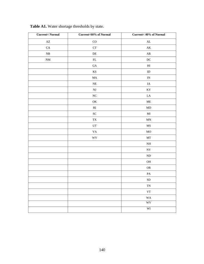
140

Table A1. Water shortage thresholds by state.

Current< Normal Current<60% of Normal Current< 40% of Normal

AZ CO AL

CA CT AK

NB DE AR

NM FL DC

GA HI

KS ID

MA IN

NE IA

NJ KY

NC LA

OK ME

RI MD

SC MI

TX MN

UT MS

VA MO

WY MT

NH

NY

ND

OH

OR

PA

SD

TN

VT

WA

WV

WI

141

References

McCarl, B.A., X. Villavicencio, and X. Wu, Climate change and future analysis: Is stationarity dying? American Journal of Agricultural Economics, 90(5), 1241-1247, 2008.

Stewart, D.W., A. Rea and D.M Wolock, USGS Streamgages Linked to the Medium Resolution NHD Geospatial Data Presentation Form: Vector Digital Data, US Geological Survey DS-195, data available at: http://water.usgs.gov/GIS/metadata/usgswrd/XML/streamgages.xml#stdorder, accessed April 2007.

Taylor, R. G. (2009) Rethinking water scarcity: the role of storage. EOS – Trans. Am. Geophys. Union, Vol. 90, no. 28

Tidwell, V.C., P.H. Kobos, L. Malczynski, G. Klise and W. Hart, Decision Support for Integrated Water-Energy Planning, SAND Report SAND2009-xxxx, Sandia National Laboratories, Albuquerque, NM, 2009.

U.S. Department of Agriculture, Census of Agriculture, available at http://www.agcensus.usda.gov/Publications/2002/index.asp, acquired in June 2008.

U.S.G.S. (U.S. Geological Survey), 1985, 1990, 1995. Water Use in the United States, Available at http://water.usgs.gov/watuse/ Accessed in November, 2008.

142

143

APPENDIX B: ECONOMIC IMPACT METHODOLOGY

This section is derived from:

Warren, D., M. Ehlen, V. Loose, and V. Vargas, Estimates of the Long-Term U.S. Economic Impacts of Global Climate Change-Induced Drought, Computational Economics Group, Infrastructure and Economic Systems Analysis Department, Sandia National Laboratories, Albuquerque, NM, September 1, 2009

The economic impact methodology was designed to answer two economic questions:

1. What does a physical climate change mean economically? 2. How can this change be modeled in a macroeconomic model?

To answer the first question, we used th eforecasts of hydrological change reported by the hydrology models noted earlier. Table B1 lists the types of hydrological change forecast by these models; each of these annual variables was forecast by state and over the 2010 to 2050 period.

Table B1: Variables Used to Report Hydrological Impact Forecasts.

Variable Description

itx, Relative production (compared to a base year) for crop x (both irrigated and

nonirrigated crop production, combined)

itH Fraction of normal water availability for municipal consumption

itE

Fraction of normal water availability for thermoelectric generation consumption

itHP Fraction of normal hydroelectric power production

itI Fraction of normal water availability for industrial consumption

itM Fraction of normal water availability for mining consumption

As described below, these hydrology impacts were translated to direct economic impacts by developing a set of assumptions about the direct economic impacts of each, modeling these impacts, and then using publicly available data to quantify the actual direct economic effects. These direct effects were then input into the REMI model to estimate the total (direct plus indirect) economic impacts over the 2010 to 2050 period.

144

B.1 Climate-to-Economy Modeling Assumptions to Address Uncertainties

This effort did not exogenously adjust the technological assumptions inherent in the control (referent) forecast. Additionally it maintained the price elasticity relationships to infer consumer response to rising prices through substitution of the use of more efficient technologies.

To translate each hydrological change into a direct economic impact, a set of economic assumptions, models, and calculations were made, by type of change and the sectors in which they occur. Each is described now, in turn, beginning first with two assumptions that apply across all non-farming sectors.

To simplify the economic methodology and to reduce uncertainties, two assumptions apply to the non-farming sectors:

1. We assumed to that investment could be made quickly as condition warranted, such as to impose close-cycle cooling systems or even dry-cooling. We further assumed that these modification could happen without the significant shut-down of capacity. States that are adjacent to oceans will have access to desalinated water.

2. Retrofits to conserve water are made instantly. In reality, there may be some delays in producing machinery for the retrofits, which could lead to short term shutdowns of facilities in the various sectors. These shutdowns will likely be relatively minor, so they are ignored.

B.2. Modeling Agricultural Impacts

To model the effects of changes in agricultural productivity on the U.S. economy, separate strategies were developed estimate the impacts to (1) farm industries and their suppliers and (2) non-farm industries that use farm outputs as inputs to their own production.

B.2.1 Impacts to Farming Industry

As with all of the climate-to-economy modeling, the estimates of direct economic impact need to be variables that can be input directly in to the REMI model. The REMI model does not endogenously simulate framing activity,12 but it does includes a Translator Module that allows users to model impacts to sectors not explicitly captured in the model,

12 This is an assumption inherent in the REMI model. It may be justified economically because a principal factor in agricultural production is land, which—unlike capital or labor—is immobile. Furthermore, agricultural markets are international in scope, thus much of the supply and demand and agricultural markets is largely exogenous to the United States.

145

such as the farming sector. For each state and year in the simulation period, the module takes as an input the change in the total value of production for that industry and ‘translates’ it into impacts to a broader set of industries. For farm industries, the module calculates estimates of the changes in government spending, farm employment, farm compensation, and intermediate demand to 65 other industries within the state. These translated variables are then used as the inputs to the REMI model. The reduction in output is based on the change in agricultural productivity/output produced by the hydrology model

Modeling Assumptions

Given that the farming industry is complex and that behaviors of individual farmers depend on a wide range of factors that are hard to capture with the REMI Translator Module, a number of simplifying assumptions were made.

The climate-based changes in hydrology only impact agricultural production to the combined irrigated and non-irrigated crops as forecast by the Sandia hydrology models. We do not, for example, incorporate price-based decisions by farmers to produce or not produce crops. The hydrology models implicitly contain the many physical factors and human factors (e.g., differences in fertilizer applications due to fertilizer prices), and they incorporate some factors like soil productivity and, to some extent, farmers’ decisions about when to apply fertilizer and how much to apply based upon changes in rainfall.

The changes in corn and soybean production are considered representative of cereal corps. Corn and soybean farming have the greatest shares of production. According to the National Agricultural Statistics Service, in 2008 the production of corn for grain was $47.4bil and the production of soybeans was $27.4bil. By comparison, the production of all “field and miscellaneous crops” was $134bil, the production of “34 major vegetables” was $10.4bil, and fruit production was $16.5bil.13 The third largest crop is hay ($18.8bil), whose productivity is not modeled within the Sandia hydrology models. Changes to crops other than cereal crops were neglected.

Absolute and relative crop prices will be held constant over time. Agricultural commodity prices actually fluctuate on a day-to-day basis based upon events in world commodity markets. By affecting agricultural productivity, global climate change will affect global commodity prices. It is uncertain whether agricultural

13 Source: U.S. Department of Agriculture, National Agriculture Statistics Service, Crop Values 2008 Summary, February 2009, http://usda.mannlib.cornell.edu/usda/nass/CropValuSu/2000s/2009/CropValuSu-02-13-2009.pdf, http://usda.mannlib.cornell.edu/usda/nass/CropValuSu/2000s/2009/CropValuSu-02-13-2009.zip.

146

commodities will be more or less expensive due to global climate change;14 therefore, we assumed that relative global prices do not change.

The only agricultural and water-use substitutions made are those predicted by the hydrology regression models. There are no additional substitutions made on the economics portion of the modeling. In reality, there are a wide range of substitutions that individual farmers make: for example, crops are often rotated; farmers may change the mix of crops in response to price changes or expectations in productivity, may install irrigation systems or choose not to use existing irrigation systems, may bring land in and out of cultivation, and may alter the timing of plantings and fertilizer applications. This analysis considers the reduction in production the dominant impact. The production loss due to climate change is implicitly mitigated through the assumption from the hydrology model for maximizing production under changing weather conditions. Therefore, any addition changes that are outside the scope of this effort are presumed secondary.

Agriculture production technologies follow the exogenous growth pattern estimated by REMI through annual changes in its Translator Module. Overall output in corn and soybeans is assumed to grow at the same rate as REMI’s (exogenous) forecast of increases in farm GDP. This assumption implicitly assumes that the ratio of GDP to production remains constant throughout time.

Climate change does not affect livestock farming directly. In reality, livestock farming may be impacted by changes in the price of feed, changes in the productivity of forage eaten by grazing livestock, and water used in livestock farming and manufacturing.15 Industrial livestock production may be affected indirectly through impacts to the food manufacturing industry.

Climate change will not affect forestry. While it is likely that climate change will impact forest productivity, it is not currently modeled in the Sandia hydrology models, hence it is ignored in these economic models. We have assumed that given the long time constants in silvaculture and the 2050 time horizon of this run, the important impacts on the forestry industry (other than increase fire destruction, also neglected) occur in timeframes beyond this analysis

Modeling Procedures

Since the output of the translator is proportional to the magnitude of the inputs, a standard set of impacts were developed by calculating the translator outputs per $1 million chang, 14 A global model of agricultural productivity response to climate change may provide a better idea of whether agricultural commodities will become more or less expensive. Even with such a model, there will remain many factors that will lead to substantial uncertainty about the overall effect of climate change on commodity prices. 15 Water use is less than one percent of all U.S. water use (Source: USGS “Estimated Use of Water in the United States in 2000” http://pubs.usgs.gov/circ/2004/circ1268/).

147

first approximation allowed automated calculation of REMI inputs (and consistent with the observed operation of the translator); otherwise, inputs would have had to be entered manually for each of the regions.

Estimates of corn productivity from the Sandia hydrology models were used to estimate changes in REMI’s grain farming industry and changes in soybean productivity in REMI’s oilseed farming industry. Changes in production values (measured in aggregate dollars across the state) for each crop, x, (which were be entered into the REMI model via the Translator) were calculated as

farmb

farmti

bxi

txi

bxi

txi

tx GDP

GDPYYYY ,,,,, )1( ,

where

itxY , = the change in production for crop x in state i,16

itxY , = the value of production in year t,

ibxY , = the average production in the baseline period (an average of 2006 to

2008 data17),

itx, = the relative production of crop x in year t in state i to the baseline

production (an output of the hydrology models),

farmtGDP = REMI’s (exogenous) forecast of national farm GDP in year t, and

farmbGDP = REMI’s (exogenous) forecast of national farm GDP in the baseline

period (an average of 2006 to 2008).

16 Taken as the average of 2006 through 2008 data (Source: United States Department of Agriculture, National Statistics Service, “Crop Values 2008 Summary,” February, 2009, http://usda.mannlib.cornell.edu/usda/nass/CropValuSu/2000s/2009/CropValuSu-02-13-2009.pdf, http://usda.mannlib.cornell.edu/usda/nass/CropValuSu/2000s/2009/CropValuSu-02-13-2009.zip , accessed May 27, 2009. 17 Source: U.S. Department of Agriculture, National Agriculture Statistics Service, Crop Values 2008 Summary, February 2009, http://usda.mannlib.cornell.edu/usda/nass/CropValuSu/2000s/2009/CropValuSu-02-13-2009.pdf, http://usda.mannlib.cornell.edu/usda/nass/CropValuSu/2000s/2009/CropValuSu-02-13-2009.zip.

148

To create variables that can be used to model in REMI, Yx,ti was converted to millions of

dollars and multiplied by the 68 variables produced by the REMI translator, for each state and year in the forecast period.

B.3.2 Impacts to Industries that use Farm Output

In addition to directly impacting agriculture, changes in agricultural productivity will impact the downstream users of agricultural farm output. These users are modeled directly within REMI except for the intermediate inputs they purchase from the exogenous farm industry.

Modeling Assumptions

Modeling the effects to these downstream users requires a number of assumptions in addition to those listed above.

The actual amount that the users of the commodity pay to obtain the commodity includes the cost of transportation. Although this “economic geography” process is modeled in most industries in REMI, once again it does not apply to the exogenous farm industry. In this case, the net price of these food commodities is assumed to include transportation costs. If production in a state decreases, then net prices are assumed to increase due to the higher costs necessary to transport the commodities.

The degree to which an industry is affected by net price changes of farm production is proportional to the total requirements of that industry that originates from the farm industry. Table B2 shows BEA industries that have total requirements of $0.05 or more for each dollar of production, which has been chosen as the cutoff for industries that will be modeled in this paper. Changes in net price will change the production costs for the industries shown in the right column of Table B2.

We assumed that changes in productivity of corn and soy production, when averaged together using a weighted average based upon baseline production of the two crops by state, serve as proxies for changes in productivity for all farm inputs within a state.

To estimate the direct GDP contribution of crop production, we estimated the ratio of GDP directly due to crop production to production of corn and soybeans. Between 2006 and 2008, national corn and soybean production averaged $58.1B (2000 USD) and crop production averaged $126.0B.18 During the same time, the

18 Source: United States Department of Agriculture, National Statistics Service, “Crop Values 2008 Summary,” February, 2009, http://usda.mannlib.cornell.edu/usda/nass/CropValuSu/2000s/2009/CropValuSu-02-13-2009.pdf,

149

average estimated (exogenous) farm GDP in REMI was $87.9B. In 2006, the measured output in livestock was $112.1B).19 Therefore, the estimated ratio is [$126.0B/($112.1B+$126.0B)*$87.9B]/$58.1B=0.801.

REMI’s projected changes in technology in industries that use farm products as inputs account for REMI’s forecast changes in food production technologies. Therefore, only the changes in productivity measured by the hydrology models (i.e., not REMI’s forecast increases in farm GDP) are used to calculate changes in production costs.

Final demand from consumers for farm output is small (personal consumption expenditures are $52.9 B compared to industry output of $294.8 B), Most consumer demand for farm production comes by way of demand for the production of the industries shown in Tabl3 B2 (e.g., personal consumption expenditures for Food and Beverage and Tobacco Products are $482.5 B compared to industry output of $722.2 B and personal consumption from Food Services and Drinking Places is $497.8 B compared to industry output of $614.1 B20). Therefore, we did not model changes in the net prices of farm production that directly affect consumers, while recognizing that REMI will endogenously model impacts to consumers via these other industries.

http://usda.mannlib.cornell.edu/usda/nass/CropValuSu/2000s/2009/CropValuSu-02-13-2009.zip , accessed May 27, 2009. 19 Source: Bureau of Labor Statistics, 2008, “Industry output and employment projections to 2016”, Monthly Labor Review, November 2007, pp. 53-85, http://www.bls.gov/opub/mlr/2007/11/art4full.pdf, accessed August 10, 2009. 20 Source: U.S. Census Bureau, Bureau of Economic Analysis, “The Use of Commodities by Industries after Redefinitions” for 2007, summary level. (http://www.bea.gov/industry/iotables/table_list.cfm?anon=82430), accessed May 27, 2009

150

Table B2: Industries with total requirements from farms of at least $0.05 per $1 of output.21

IO Code BEA Industry Name

Requirement for $1 Output (

xR ) REMI

Industry/Industries

111CA Farms $1.18 N/A

311FT Food and beverage

and tobacco products

$0.31 #19: Food manufacturing,

#20: Beverage and tobacco product mfg.

113FF Forestry, fishing, and

related activities

$0.10 #2: Agriculture and forestry support activities;

Other

722 Food services and

drinking places $0.07 #62:Food services and

drinking places

Modeling Procedures

Because farm production is a basic input for most of the production in the industries in Table B2, it is difficult to substitute to other inputs. An increase in the net costs of farm production will look like an exogenous increase in production costs in these industries (because the farm industry is not modeled endogenously in REMI). Therefore, increased net costs to these industries were modeled by increasing the Production Cost variable in REMI, which is “used when a specific policy will affect the cost of doing business in a region without directly changing the relative costs of factor inputs.”22 Farm input is not included as a factor input in REMI.

We assumed that if farm production within a state changes, the changes are compensated by imports or exports via rail transportation. Table B3 shows some average costs of shipping grain by rail, as well as the price of each crop. The “% Rail” column indicates the cost of the rail transportation relative to the price and can be thought of as the increase in net price if a firm had to obtain these grains via rail instead of on-site. With

21 Source: U.S. Census Bureau, Bureau of Economic Analysis, “BEA Industry-by-Industry Total Requirements after Redefinitions,” 2007 summary-level table, accessed May 27, 2009 22 Source: Regional Economic Models, Inc. Variable description for “Production Cost”, “REMI PI+”, v. 1.0.114, March 24, 2009 build, 51 region, 70 sector model, Amherst, MA

151

this data as a guide, we assumed that production costs will increase or decrease by a factor of 20% of the decrease or increase of agricultural production in the state.

Table B3: Average Cost to Ship Grain by Rail.23

Grain Avg. Rail Cost

Per Bushel July 2010 Price

Per Bushel % Rail

Corn $0.99 $4.75 21%

Soybeans $1.04 $9.87 11%

We used the following equation to estimate the change in production costs caused by changes in agricultural production in state i:24

ibsoy

ibcorn

ibsoy

itsoy

ibcorn

itcorn

xi

txYY

YYRPC

,,

,,,,,

*)1(*)1(*%20%

,

where

PC%x,ti = the percentage change in production costs for industry x

Rx = the total requirements of industry x for farm products to produce a

dollar of outputs,

itx, = the relative production of crop x in year t in state i to the baseline

production (an output of the hydrology models), and

ibxY , = the average production in the baseline period (an average of 2006

to 2008 data25)..

23 USDA “Grain Transportation Report”, May 14, 2009, www.ams.usda.gov/GTR), July 2010 futures price (closing price on 5/19/2009 on Chicago Mercantile Exchange, http://www.cmegroup.com/), and calculation of the rail costs as a percentage of the futures price. 24 In states without either corn or soybean production, this term is assumed to be zero. 25 Source: U.S. Department of Agriculture, National Agriculture Statistics Service, Crop Values 2008 Summary, February 2009, http://usda.mannlib.cornell.edu/usda/nass/CropValuSu/2000s/2009/CropValuSu-02-13-2009.pdf, http://usda.mannlib.cornell.edu/usda/nass/CropValuSu/2000s/2009/CropValuSu-02-13-2009.zip.

152

The term PC%x,ti was entered into REMI as the change in the “Production Cost (share)”

variable for the appropriate industry.

B. 3 Modeling Impacts to Municipal Water Use

Municipal water use is one output from the Sandia hydrology model that is not modeled directly in the economics model because review indicates that there are many opportunities for substantial municipal water conservation that will be inexpensive and have little effect on the livability of a region. Modeling municipal water in REMI is relatively difficult: while there is a Utilities sector within REMI, municipal water utilities are not modeled explicitly in the 67-sector version used in this analysis. Therefore, a number of assumptions need to be made to model the effects of water shortages to municipal water utilities.

B. 3.1 Modeling Assumptions

Drought-induced water conservation is relatively easy to conduct. For example, the

EPA estimates that 30% of household water is used for outdoor watering (and this is higher in arid regions),26 suggesting that a significant fraction of water consumption would be eliminated in time of drought. Also, the American Water Works Association estimates that 30% of household water could be saved if all homes installed common water-saving features.27 Finally, 60% (or more) of household water use could be cut fairly painlessly with current, affordable technology.

Municipal water losses of greater than 60% would have to be made up with more extreme conservation measures, such as developing new no- or low-water technologies, increased conservation measures (e.g., shorter showers, less frequent clothes washing, disposable dishware, eliminating car washes, closing golf courses, or population migration).28

26 Environmental Protection Agency, WaterSense, “Outdoor Water Use in the United States”, http://www.epa.gov/watersense/pubs/outdoor.htm, accessed May 27, 2009. 27 American Water Works Association, “Water Use Statistics”, http://www.drinktap.org/consumerdnn/Default.aspx?tabid=85, accessed May 27, 2009. 28 As for minimum water requirements, the USAID recommends 20 to 40 liters per person per day, while a separate study recommends a Basic Water Requirement right of 50 l/p/d (17% of average U.S. household use and 9% of average California household use). (Source: Peter H. Gleick, 1996, “Basic Water Requirements for Human Activities: Meeting Basic Needs”, Water International, v. 21, pp. 83-92.) This could probably be reduced by more efficient technologies (like composting toilets).

153

Many technologies exist that may help provide long-term sources of municipal water. For example, rain harvesting technology, water treatment, desalination, and water pipelines could be used to increase supply. We assumed that the use of technology remains the same as today, except that desalination may be increased near the coasts (see next bullet). Because the use of these technologies will mitigate the effects of reduced water supplies, this assumption provides a conservative bound to the simulation.

B.4 Modeling Impacts to Power Production

Although water consumption in agricultural irrigation is highest, thermoelectric power production is the sector with the largest U.S. water withdrawals29, albeit with only 3% of the national consumption.30 As a result, water shortages could be expected to have significant impacts on electricity supplies. Technology exists that eliminates water consumption in thermoelectric generation, thus this technology is a backstop technology in the event of water shortages. In states adjacent to oceans, desalinated water used in evaporative cooling systems and ocean water used in once-through cooling systems provide an even cheaper alternative. We modeled REMI the effect of water shortages on electricity production by increasing the costs of generating electricity, to reflect the increased costs of the backstop technology.

Additional impacts to power production result from changes in water volumes in rivers and streams that change available hydroelectric power production. We modeled these changes by changing demand for alternate sources of electricity production in REMI.

B.4.1 Thermoelectric Power in States not Adjacent to an Ocean

In-land plant do not have the option to use ocean water and therefore need to reduce the dependence on water availability (e.g. river flow) conditions

Modeling Assumptions

Thermoelectric power was responsible for 48 percent of water withdrawals in 2000.31 However, much of that water (91 percent) is used in once-through cooling, where most water is returned to the source where it originated, at a higher

29 (Source: Susan S. Hutson, Nancy L. Barber, Joan F. Kenny, Kristin S. Linsey, Deborah S. Lumia, and Molly A. Maupin, 2004, “Estimated Use of Water in the United States in 2000,” USGS Cicular 1268, Revised Feb. 2005. http://pubs.usgs.gov/circ/2004/circ1268/.) Consumption is higher in agriculture because 91 percent of thermoelectric withdrawals are used in once-through cooling, which consumes very little water. 30 Feeley TJ, L Green, JT Murphy, J Hoffmann, and BA Carney, (2005), DOE/FE’s Power Plant Water Management R&D Program Summary, Department of Energy/Office of Fossil Energy’s Power Plant Water Management R&D Program, Washington DC, July 2005, http://www.netl.doe.gov/technologies/coalpower/ewr/pubs/IEP_Power_Plant_Water_R&D_Final_1.pdf 31 Ibid.

154

temperature, thus it is not consumed. The remainder of water is used in closed-loop cooling systems where most of the water is evaporated, hence consumed.

Due to climate change, it is possible that some freshwater sources for once-through cooling will no longer have sufficient volume. Hydroelectric power may be similarly affected by volume reductions, which may necessitate additional supplies of power from alternate sources such as thermoelectric power. We include the imcpat of developing the alternative production facilities.

Climate change may also increase the temperature of water and air, which may decrease the cooling efficiency of thermoelectric power plants. Additionally, “warmer water discharged from power plants can alter species composition in aquatic ecosystems“32 Temperature changes in water are not considered by the Sandia hydrology models, so economic effects of these changes are not considered. The impact of efficiency variance is small compared to the cost increases already assumed.

A third type of cooling is air-cooled (dry) cooling. This technology is a backstop because it consumes little water, but instead works similarly to air refrigeration by removing heat from steam and transferring it to the ambient air with fans. We assumed that only when faced with water shortages, electricity producers will retrofit to dry cooling. A large portion of thermoelectric power generation is converting to combined-cycle,33 much of which can more easily use use dry cooling (and in the event of water shortages, an even greater share will be dry cooling) due to the reduced cooling needs these plants.

We used an estimate of the additional cost of dry cooling through calculations made by Powers Engineering for retrofitting generation in California.34 They perform calculations for a hypothetical plant that find the increased cost of generation of converting from once-through cooling to a wet tower will be between $0.0013 to $0.0039/kilowatt hour (kWh) (against a wholesale price of $0.07/kWh) depending on the capacity utilization of the plant. They also cite projections that dry cooling retrofits would cost 25% more than wet tower retrofits, which means that the range would be $0.0016 to $0.0049/kWh. These calculations assume a 7 percent interest rate and 100 percent debt financing. A more realistic mix with 55 percent debt financing, 45 percent equity financing (taxed at 50 percent) and property taxes triples the cost to $0.0048 to $0.0147/kWh.

32 Source: U.S. Global Climate Change Research Program, 2009, Global Climate Change Impacts in the United States, Cambridge University Press (p. 56) 33 Source: Powers Engineering, “Once-Through Cooling and Energy”, http://www.cacoastkeeper.com/assets/pdf/Energy_OTC_Fact_Sheet.pdf, accessed on May 27. 34 Ibid.

155

Retrofits have the additional effect of making power production less efficient. Power Engineering estimates that cooling will reduce the efficiency of the plant and cost an additional 1-2 percent for retrofitting to wet, closed-loop cooling, but they do not recommend a value for dry cooling, which is more energy intensive. A power consultant35 identifies increases of 1.9 percent for production costs when retrofitting wet, closed-loop cooling and 4.9 percent for dry cooling. Assuming that wholesale prices of $0.07/kWh can be used as costs and multiplying those prices by 4.9 percent increases the cost by $0.00343/kWh.

Adding the increased capital costs increases the cost of retrofits to results in a range of $0.00823 to $0.01813/kWh. We assumed the high end of the range is correct and assume that retrofits to dry cooling will cost an additional $18.13/megawatt hour (MWh).

An alternative backstop technology is gas turbines. However, they tend to be relatively expensive to use due to high natural gas prices and have low capacity utilization rates because they are used mainly to serve peak demand. Therefore, we assumed that power producers will not switch to gas turbines for the purpose of mitigating water shortages.

We assumed that once retrofits have been implemented, the electric power in the state will be able to fully operate with the reduced level of water consumption, at the increased costs in future years.

Different states have different mixes of once-through cooling, so they will be affected differently by water shortages. For example, all cooling in many arid states is wet, closed-loop due to a lack of water volume necessary for once-through cooling.36 However, we assumed that water shortages will affect power generation of generation technologies that commonly consume water (i.e., fueled by coal, natural gas, nuclear, other, other biomass, other gases, petroleum, and wood and derived fuels) in proportion to the state’s water shortage. This is a conservative estimate for four reasons. First, wet, closed-loop cooling consumes a much greater amount of water than does once-through cooling for the same power production. It is likely that wet, closed-loop cooling would be converted first to dry cooling, which would reduce a large fraction of water consumption but affect relatively little power production. For example, we estimated that in Texas wet,

35 Source: John S. Maulbetsch, Maulbetsch Consulting, “Water Conserving Cooling Status and Needs”, July 25, 2006, accessed at http://www.sandia.gov/energy-water/West/Maulbetsch.pdf accessed on May 27, 2009. 36 Calculated from EIA’s “Annual Steam-Electric Plant Operation and Design Data (EIA-767)” (http://www.eia.doe.gov/cneaf/electricity/page/eia767.html, accessed May 27, 2009) using data from 2005.

156

closed-loop cooling consumes 97 percent of all water consumed for cooling, but is used to produce only 62 percent of power.37 Our conservative assumption assumes that a 97 percent reduction in available water will necessitate that 97 percent of generation be retrofitted—likely an overestimate. Second, some portion of power production in each state, especially power produced with natural gas, already uses dry cooling, thus less power generation within the state needs to have its cooling retrofitted. Third, retrofits would first occur for plants that operate at a high capacity utilization rate, thus the average capital costs of the retrofit will be lower than these estimates for mild water shortages. Fourth, plants that use ocean water as their source are unlikely to need to be retrofitted because they are consuming salt water from a source that is expected to increase in volume.

Modeling Procedures

The additional production cost of electric power in each state, i, and each year, t, is calculated as38

Yti $18.13(1Et

i)Xi ,

where

Eti = the fraction of normal demand for water by electric power producers that

is satisfied, and

X i = the total power production, in MWh, of production in the state in 2007 for

power fueled by coal, natural gas, nuclear, other, other biomass, other gases, petroleum, and wood and derived fuels.

Because producers can permanently operate with a reduced supply of water following

retrofits, Et1i Et

i . (If this identity does not hold in the input data, it will be adjusted so

that any year has, at most, as much water availability as the previous year.) In years

where the electric power available for electricity production decreases (i.e. Eti Et1

i )

investment in cooling retrofits will be measured by39

37 Ibid. 38 Source: 2007 Net Generation by State by Type of Producer by Energy Source (EIA-906), http://www.eia.doe.gov/cneaf/electricity/epa/epa_sprdshts.html, accessed May 27, 2009 39 Powers Engineering’s calculations (Source: Powers Engineering, “Once-Through Cooling and Energy”, http://www.cacoastkeeper.com/assets/pdf/Energy_OTC_Fact_Sheet.pdf, accessed on May 27.) for a retrofit

157

INti $71.35(Et1

i Eti)Xi ,

which assumes that all investments are made immediately.

REMI model contains a “Cap and Trade Scenario” testing capability that provides guidance in modeling the economic impacts of cap and trade policies. Because cap and trade is likely to impact the electric power generation sector, the scenario suggests manipulating utility costs. An increase in production costs due to retrofitting equipment in order to reduce water use is a similar cost increase.

Utility costs are changed by increasing the production costs for the utilities sector. Specifically, we increased the “Production Cost (amount)” of the utilities sector by the

amount (Yti) determined by the above equation. During years where producers must

invest in retrofitting technologies, this additional demand (INti from the above equation)

was invested. This amount was entered into REMI using “Investment Spending (amount)” in “Producer’s Durable Equipment.” However, this allocates demand generically in a way that overly favors production in industries like “Computer and Electronic Product Manufacturing.” REMI’s Translator Module was used to adjust these numbers for different types of equipment such as “Industrial Equipment.” However, like the translator for agriculture, the equipment translator produces many variables (up to 65) that are slightly different for each region. We calculated that on net, around 60 percent of additional demand goes to “Machinery manufacturing” and 33 percent goes to “Electrical equipment and appliance manufacturing.” To simplify calculations, we assumed that two-

thirds of INti goes to “Machinery manufacturing” and one-third goes to “Electrical

equipment and appliance manufacturing” via the “Exogenous Final Demand (amount)” variable.

B.4.2 Thermoelectric Power in States Adjacent to an Ocean

Power plant near the ocean can directly use saline water, can ship the water inland, or convert desalinate water.

Modeling Assumptions

In states that adjacent to oceans, water shortages to electric power were assumed to be mitigated by using once-through cooling with saline ocean water or desalinating water

from once-through to wet-tower cooling are $100,000/MW of capacity. Using their estimate that dry cooling costs 25 percent more, this becomes $125,000/MW. Using the low-end capacity of 20 percent (8,760 hours x 0.20 = 1,752 kWh/year), this averages to $71.35/MWh.

158

and using it in wet-tower cooling. We assumed that thermoelectric generation plants in a state will conserve water by switching wet-tower cooling systems to desalinated water during water shortages.

Desalination is a proven technology. Therefore, we assumed that any state on a coast has access to desalinated water as a backstop before water shortages become too severe. (In addition, states not on the coast may have access to desalinated brackish water, but we ignored this possibility because it will affect a relatively small population.) In these states, the main consideration for modeling is the increased cost of the desalination.

Desalinating saline water is more expensive than surface or ground water. A National Academies study40 cites the current price of water in San Diego as $0.24/m3 but the cost of desalination as between $0.64 and $1.04/m3. A review of cost estimates for various technologies conducted at SNL41 found estimates from 23 studies. For sea water these estimates range from $0.27 to $6.56/m3; however, the high range is an outlier. Removing one study puts the upper estimate at $1.86/m3. We assumed that upper estimate is correct and using desalinated water will increase cost by $1.62/m3.

A study of water use by thermoelectric plants finds that the mean withdrawals per kWh of electricity for evaporative cooling is between 4.54 and 4.95 cubic decimeters for kWh, depending on the technology used.42 Taking the larger value, we assumed a value of 4.95m3/MWh. Thus the additional cost of using desalinated water in wet-tower cooling is $9.21/MWh. Because the cost of using desalinated water is about half the cost of converting to dry cooling ($9.21/MWh vs. $18.13/MWh) conservation of water will likely occur by substituting to desalinated water.

Modeling Procedures

The additional production cost of electric power in each state, i, and each year, t, is calculated by

Yti $9.21(1Et

i)Xi ,

40 Source: National Research Council Committee on Advancing Desalination Technology, Desalination: A National Perspective, The National Academies Press, Washington, D.C. http://www.nap.edu/catalog.php?record_id=12184 41 Source: James E. Miller, “Review of Water Resources and Desalination Technologies,” SAND 2003-0800, http://www.prod.sandia.gov/cgi-bin/techlib/access-control.pl/2003/030800.pdf 42 Source: Yang, Xiaoying and Benedykt Dziegielewski, 2007, “Water Use by Thermoelectric Power Plants in the United States,” Journal of the American Water Resources Association, v 43(1), pp. 160-169.

159

where

Eti = the fraction of normal demand for water by electric power producers that

is satisfied, and

X i = the total power production, in MWh, of production in the state in 2007 for

power fueled by coal, natural gas, nuclear, other, other biomass, other gases, petroleum, and wood and derived fuels.43

In states where cooling retrofits were necessary to conserve water, electricity production could permanently operate with less water. However, in the case of states adjacent to oceans, electricity producers may use desalinated water in one year and return to fresh water in following years when the shortages are less severe.

As before, we increased the “Production Cost (amount)” of the utilities sector by the

amount (Yti) determined by the above equation. In addition, “Industry Sales/Exogenous

Production (amount)” for the Utilities industry is increased by Yti to account for the

increased water production that the power generators require from water utilities that provide desalinated water. Increases in production in REMI automatically trigger investment in the industry, thus REMI will automatically account for investments that are made to build desalination capacity.

B.4.3 Hydroelectric Power

Hydroelectric plants,are fully dependent on water flow. The enduring loss of water requires the construction of new renewable energy, fossil, or nuclear powered facilities.

Modeling Assumptions

Drought conditions will change rainfall, thus changing volumes of water flowing through rivers and streams. Hydroelectric power creates electricity from the potential energy in water, so lesser/greater volumes of water reduce/increase the amount of power that a hydroelectric plant can generate.

43 Source: 2007 Net Generation by State by Type of Producer by Energy Source (EIA-906), http://www.eia.doe.gov/cneaf/electricity/epa/epa_sprdshts.html, accessed May 28, 2009.

160

We approximated the marginal cost of producing hydroelectric power at zero because the major costs of producing hydroelectric power are about the same regardless of how much power the plant actually produces. Capital costs to build hydroelectric power generation are sunk costs, thus the cost is the same no matter how much power is produced. Labor costs are relatively small, and the same amount of labor will be required from workers such as guards and operators, no matter the level of power production. Hydroelectric power does not use a costly fuel source as thermoelectric power does. Therefore, changes to hydroelectric power, alone, were assumed not have any aggregate macroeconomic impact.

Changes to hydroelectric power production will have a macroeconomic impact through substitutions away from or to other forms of production with a greater marginal cost. We assumed that reductions in hydroelectric power lead to an equally large increase in demand for thermoelectric power, while decreases in hydroelectric power lead to an equally large decrease in demand for thermoelectric power within the state where the hydroelectric power is produced. These changing demands will change production levels, but not necessarily within the same state—power can be imported or exported outside the region.

We assumed a monetary value for changes in demand of $138.13/MWh, which is equal to the cost of new coal power generation ($120/MWh)44 plus the costs of retrofits to dry cooling towers ($18.13/MWh—a conservative assumption because cooling “retrofits” will likely be cheaper to implement when designed into new construction.)

We did not calculate any changes to demand for other sectors. In reality, an increase in demand for Utilities, for example, could reduce demand for other sectors due to price and income effects. However, modeling at this detailed level is beyond the scope of this report. By assuming that there are no changes to demand in other sectors due to changes in demand for Utilities, we are making a bounding assumption about the maximum possible impact.

44 LAZARD, 2008, Levelized Cost of Energy Analysis—Version 2.0, June, 2008, http://www.narucmeetings.org/Presentations/2008%20EMP%20Levelized%20Cost%20of%20Energy%20-%20Master%20June%202008%20(2).pdf, accessed June 24, 2009) and a transmission and distribution cost of $20/MWh (source: Northwest Power and Conservation Council, 2009, “Appendix B: Draft Economic Forecast,” February 13, 2009, http://www.nwppc.org/library/2009/2009-03.pdf, accessed June 24, 2009).

161

Modeling Procedures

Changes in the demand for alternate sources of power due to changes in hydroelectric production is modeled in the REMI model as a change in the “Exogenous Final Demand (amount)” variable to the Utilities sector. To satisfy changes in demand, REMI will change production and investment in capital stock (e.g., increasing capital stock if thermoelectric power plants are needed) in a state and its neighbors.

The change in “Exogenous Final Demand (amount)” for the Utilities sector in state i and year t is calculated as

iHP

it

it XHPD )1(13.138$

where

itHP = the fraction of normal hydroelectric power production in state i and

year t and,

iHPX = the total hydroelectric power production, in MWh, in the state in

2007.45

B.5 Modeling Impacts to Industry and Mining

Of all the major sectors of water withdrawal (5 percent of U.S. water withdrawals or greater), industry is the smallest (5 percent of all water withdrawals), after thermoelectric power (48 percent), irrigation of agriculture (34 percent), and public water supplies (11 percent).46 Mining, whose water availability will be modeled separately from the aggregate of other industries, consumes less than one percent of all water.

B.5.1 Modeling Assumptions

A USGS report47 provides information about aggregate withdrawals of water for all industries and mining, but does not break down the numbers by industry or provide data on how much water is consumed (e.g., evaporated or incorporated into a product) or

45 Source: 2007 Net Generation by State by Type of Producer by Energy Source (EIA-906), http://www.eia.doe.gov/cneaf/electricity/epa/epa_sprdshts.html, accessed May 28, 2009. 46 Source: Susan S. Hutson, Nancy L. Barber, Joan F. Kenny, Kristin S. Linsey, Deborah S. Lumia, and Molly A. Maupin, 2004, “Estimated Use of Water in the United States in 2000,” USGS Cicular 1268, Revised Feb. 2005. http://pubs.usgs.gov/circ/2004/circ1268/ 47 Ibid.

162

returned to its source, such as with once-through cooling. Statistics Canada provides a large number of tables with a large breadth of data based on surveys of industrial and mining users of water.48 We assumed that the water use of Canadian industries mirrors that of U.S. industries, proportionally. This assumption is reasonable because the two countries user similar technologies and the industries are both classified using the North American Industry Classification System (NAICS). (Because temperatures in the United States are generally warmer than in Canada, it is possible that more U.S. industrial water is used for cooling. In the bullets below, a greater amount of cooling means that there are more opportunities for conservation by converting to dry cooling, thus assuming that the United States and Canada use the same proportions for cooling is a conservative assumption.)

The USGS report says that food, paper, chemicals, refined petroleum, and primary metals are the largest industrial users of water, and they provide separate data for the mining industry. The Statistics Canada survey reports similar findings, but also includes Beverage and Tobacco manufacturing as a significant consumer of water. These six industries account for 87 percent of all industrial (non-mining) consumption of water. We focused on these industries.

The data provided to us from the hydrologists’ models provides the percentage of normal consumption that can be provided by water supplies. Therefore, we assumed that there is plenty of water to withdraw, but only a limited amount of this water can be consumed. The remainder of the water must be treated and returned to water supplies where it can be withdrawn, and ultimately consumed, by other users.

A summary of pertinent statistics for the Statistics Canada survey is provided in Table B4. Only 13.5 percent of water intake is actually consumed. The remainder of the water is for:

Food. Disclosure problems make it difficult to clearly see what is happening in the data. It is likely that a large portion of the food industry’s water consumption is used for “Sanitary Service”, most likely in the animal processing industries. This water is probably relatively difficult to conserve, but it can be treated or transferred to irrigation use. Surface discharge is very small, probably because it is difficult to treat. It is likely that most of the discharge becomes irrigation water. (The italics indicate undisclosed data that we have imputed by assuming that 29 percent of water intake is used for cooling, as it is in the beverage and tobacco industry.)

48 Source: Statistics Canada, 2008, “Industrial Water Use 2005”, Catalogue no. 16-401-X, March 2008, http://www.statcan.gc.ca/pub/16-401-x/16-401-x2008001-eng.pdf

163

Beverage and Tobacco. This industry’s consumption rate is the highest of all at 51 percent. The high percentage is likely due to the fact that water comprises the majority of most beverages.

Paper. This industry’s consumption rate is only 5 percent, and it discharges 89 percent of its intake to the surface, and it spends a lot of money doing this. There is very little it can do to conserve because it consumes so little and is already spending a lot to treat water.

Petroleum and Coal. This industry is based on the transformation of petroleum and coal into usable products (i.e., it does not include extraction). It has a consumption rate of 12 percent. Much of this is likely due to evaporation as 87 percent of the water is used for cooling, condensing, and steam. This 12 percent could be conserved using similar technologies as in electricity generation.

Chemicals. Chemicals consume a relatively high amount of water, probably because the water is used in chemical reactions or as a solute. There is no conservation opportunity with this use of water. A large portion of water is used for cooling, condensing, and steam (80 percent) so there are opportunities to conserve water here by using similar technologies as in electricity generation.

Primary Metals. Primary metals manufacturing uses a moderate amount of water in cooling, condensing, and steam (hence there are moderate conservation opportunities) and returns a relatively large percentage of water (80 percent) in surface discharge.

Mining. Statistics Canada surveys only “Mining (Except Oil and Gas)”. Surface discharge is 98 percent of withdrawals. Consumption is -37 percent because mining often “generates” water when mines are below the water table. If the intake is adjusted by adding “Mine Water”, the total intake is 674.9mil cubic meters and consumption is 7 percent. The recycling rate is 448%, meaning that the same water is used over and over again. Since mining consumes so little water and it already has a high recycling rate, there are few conservation opportunities.

The USGS study of water use in the United States includes oil and gas in its mining data. This data is much more limited than the Canadian data and covers only a subset of states. The data reports that mining uses 2,250 thousand acre-feet per year of fresh water and 1,660 thousand acre-feet of saline water. Of this saline water, 1,260 thousand acre-feet per year is ground water.

164

Information about the output of Canadian industries is included in Table B5. We assumed that U.S. industries use water at the same rate, per amount of output, as Canadian industries (i.e., the right column of Table B5is representative of U.S. industries). Due to a lack of information about water use in Oil and Gas Extraction, we assumed that the industry has the same water-use characteristics as Mining (Except Oil and Gas).

To calculate the costs of retrofitting cooling systems to dry cooling systems, we assumed that the costs per amount of water consumption saved are the same as in the electric power industry. We assumed that the maximum percentage of water that can be conserved by retrofitting cooling systems in each industry is equal to the amount of water used in cooling divided by the total intake. This ranges from 6 percent for mining to 87 percent for petrochemicals and coal. As before, we assumed a value of the aforementioned 4.95m3/MWh for the amount of water used by thermoelectric plants for evaporative cooling.49 We used the previous value of retrofitting power generation plants of $18.13/MWh. Dividing by the value from the previous bullet equals an additional cost of $3.66/m3 for water saved by retrofitting to dry cooling.50

We used the previous value of investment necessary to retrofit power generation plants of $71.35/MWh. Dividing by 4.95m3/MWh equals an investment cost of $14.41/m3 for water conserved by retrofitting to dry cooling. As with electric power, any cooling retrofits that occur will reduce industrial requirements for water in future years.

We assumed that once the maximum amount of water has been conserved by retrofitting to dry cooling, additional water is not easily conserved because it often goes into production or is otherwise lost in the production process. Water will have to be obtained through desalination or otherwise firms will have to shut down production to conserve any remaining water. Desalination is available to firms in states that are adjacent to an ocean at an increased cost of $1.62/m3 (for the reasons noted previously). Because the increased cost of using desalinated water is much cheaper than the increased cost of retrofitting to dry cooling, we assumed that firms will use desalinated water to adjust to the shortfall in water. Firms in all industries will conserve water in the same proportion

(e.g., if the available water is a fraction Iti of normal demand, all firms will have access to

that fraction.)

In states not adjacent to an ocean, we assumed that all industries will initially retrofit cooling systems to conserve water. For simplification purposes, industries will retrofit according to a linear function that is proportional to the industry’s consumption of water

49 Source: Yang, Xiaoying and Benedykt Dziegielewski, 2007, “Water Use by Thermoelectric Power Plants in the United States,” Journal of the American Water Resources Association, v 43(1), pp. 160-169. 50 This is slightly more expensive than the $1.62/m3 increase for desalinated water used earlier. Thus, it may be slightly cheaper for a wet, closed-loop cooling system to use desalinated water rather than retrofitting. However, the cooling in these data is an aggregate of both wet, closed-loop and once-through.

165

for cooling purposes multiplied by the water shortfall.51 Once all retrofits have been performed, if the retrofits have not conserved enough water, industries will shut down in equal proportions. This is a conservative assumption because industries are likely to shut down according to how intensively they use water for non-cooling purposes (based upon water consumption per dollar of output), with the most intensive industries shutting down first. Calculations of these intensities are shown in Table B5..

51 The implication of this assumption is that different industries will conserve water at different rates depending upon the intensity at which they consume water for cooling.

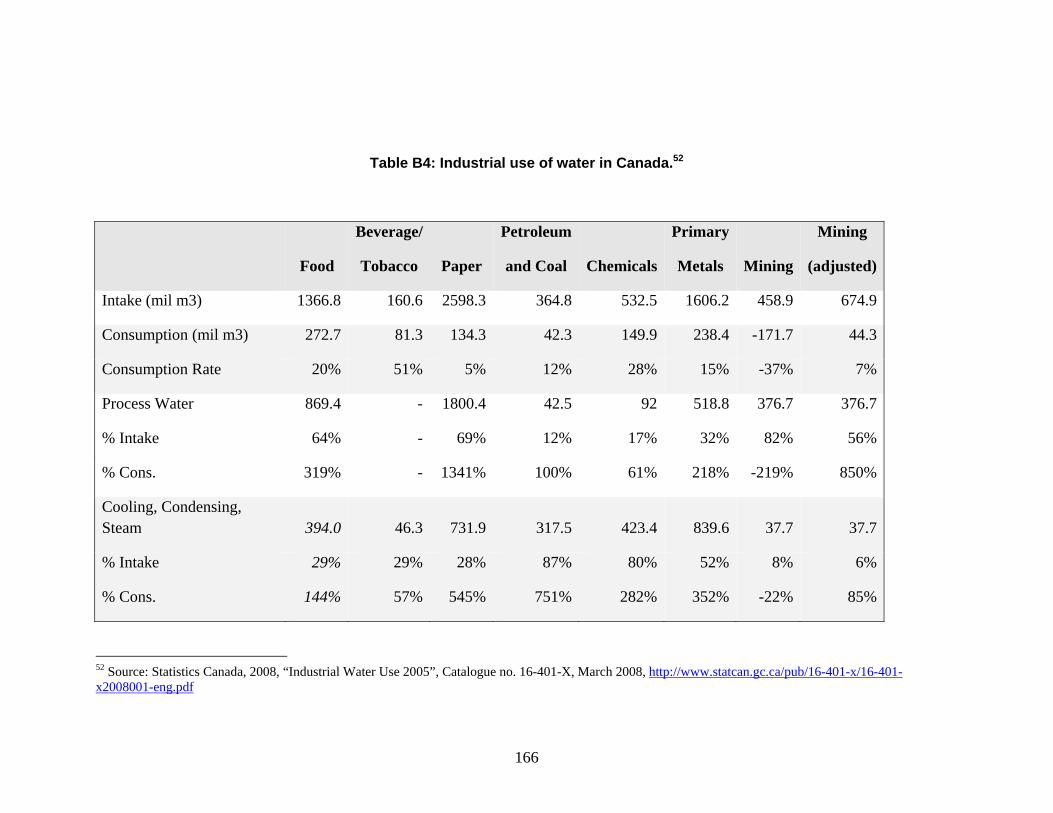
166

Table B4: Industrial use of water in Canada.52

Food

Beverage/

Tobacco Paper

Petroleum

and Coal Chemicals

Primary

Metals Mining

Mining

(adjusted)

Intake (mil m3) 1366.8 160.6 2598.3 364.8 532.5 1606.2 458.9 674.9

Consumption (mil m3) 272.7 81.3 134.3 42.3 149.9 238.4 -171.7 44.3

Consumption Rate 20% 51% 5% 12% 28% 15% -37% 7%

Process Water 869.4 - 1800.4 42.5 92 518.8 376.7 376.7

% Intake 64% - 69% 12% 17% 32% 82% 56%

% Cons. 319% - 1341% 100% 61% 218% -219% 850%

Cooling, Condensing, Steam 394.0 46.3 731.9 317.5 423.4 839.6 37.7 37.7

% Intake 29% 29% 28% 87% 80% 52% 8% 6%

% Cons. 144% 57% 545% 751% 282% 352% -22% 85%

52 Source: Statistics Canada, 2008, “Industrial Water Use 2005”, Catalogue no. 16-401-X, March 2008, http://www.statcan.gc.ca/pub/16-401-x/16-401-x2008001-eng.pdf

167

Non-cooling

Consumption

(mil m3) 53

2005 Output $CAN mil (2002) 54

Output in

$USD mil (2008)

55

Non-cooling Consumption m3/$M USD

output

Food Manufacturing

194.1 $71,028 $102,330 1,897

Beverage and Tobacco Product Manufacturing

57.9 $13,901 $20,027 2,889

Paper Manufacturing

96.5 $33,546 $48,330 1,996

Petroleum and Coal Product Manufacturing

5.5 $59,228 $85,330 64

Chemical Manufacturing

30.7 $54,659 $78,747 390

Primary Metal Manufacturing

113.8 $49,790 $71,733 1,586

Table B5: Non-Cooling Consumption Rates Compared to Industry Output.

53 Ibid. 54 Source: Statistics Canada, “National economic accounts: Input-output”, “Input and output, by industry and commodity, M-level aggregation”, 2005 total outputs per industry, http://www.statcan.gc.ca/nea-cen/list-liste/io-es-eng.htm, accessed May 28, 2009. 55 Converted to 2005 Canadian dollars by multiplying by 1.099 (112.27/102.13) (Source: NationalMaster, “Time Series > Economy > GDP deflator > Canada”, http://www.nationmaster.com/time.php?stat=eco_gdp_def-economy-gdp-deflator&country=ca-canada, accessed May 28, 2009), converted to 2005 USD by multiplying by 1.21 (2005 exchange rate and PPP equivalence, Source: International Comparison Project. (2008) “Tables of Results”, World Bank, Washington, D.C., http://siteresources.worldbank.org/ICPINT/Resources/icp-final-tables.pdf, accessed May 28, 2008), and converted by 2008 USD by multiplying by 1.08 (122.422/113.026, Source: EconStats, “Implicit Price Deflator, BEA release: 04/29/2009”, http://www.econstats.com/gdp/gdp__a4.htm, accessed May 28, 2009.).

168

Cooling % Intake

Consumption

(mil m3)

2005 Output

$CAN mil (2002)

Output in

$USD mil (2008)

Consumption m3/$M USD

output

Food Manufacturing

29% 272.7 $71,028 $102,330 2,665

Beverage and Tobacco Product Manufacturing

29% 81.3 $13,901 $20,027 4,059

Paper Manufacturing

28% 134.3 $33,546 $48,330 2,779

Petroleum and Coal Product Manufacturing

87% 42.3 $59,228 $85,330 496

Chemical Manufacturing

80% 149.9 $54,659 $78,747 1,904

Primary Metal Manufacturing

52% 238.4 $49,790 $71,733 3,323

Mining (adjusted) 6% 44.3 $24,351 $35,083 1,263

Table B6: Total consumption.56

B.5.2 Modeling Procedures

The following outline the equations that will be used to determine impacts from water shortages in industry, using the assumptions generated in the previous bullets.

States not Adjacent to an Ocean

These states will first retrofit industrial cooling systems to conserve water. If additional water conservation is necessary, industries will need to halt some production. For each state i and year t, a fraction of water consumption that can be saved through dry-cooling retrofits is calculated by weighting each industry’s cooling water intake as follows, using data from Table B6and REMI’s standard regional control outputs :

56 Based on calculations in Table B4 and B5.

169

%cti

%c fWIfYf ,ti %cbWIbYb,t

i %cpWIpYp,ti %ceWIeYe,t

i %ccWIcYc,ti %cmWImYm,t

i

WIfYf ,ti WIbYb,t

i WIpYp,ti WIeYe,t

i WIcYc,ti WImYm,t

i

where

f, b, p, e, c, and m represent the six non-mining industries,

xc% = the percentage of consumption assumed to be used in cooling

xWI = the water intensity of each industry i

txY , = the output of industry x (in millions of 2008 USD, from REMI’s standard regional

control).

Because mining is disaggregated from the Sandia hydrology model data, its value is simply 6 percent.

Production costs in each industry will increase by:

PCx,ti

(1 Iti) /%c t

i$3.66%cxWIxYx,t

i

$3.66%cxWIxYx,ti

(1 Iti) %c t

i

(1 Iti) %c t

i

where

itI = the fraction of usual water demanded that is available to all industries.

For mining, which includes both Mining (Except Oil and Gas) and Oil and Gas Extraction, this equation simplifies to:

06.0)1(

06.0)1(

126306.066.3$

126306.066.3$06.0/)1(

,

,

,

it

it

itm

itm

iti

tmM

M

Y

YMPC

where

itM = the fraction of usual water demanded that is available to mining.

170

Increases in production costs, itxPC , , are entered into REMI as increases in “Production Cost

(amount)” for the appropriate industry. Investment in cooling-system retrofits will be made until

all industrial cooling systems have been retrofitted (i.e., itc% has been conserved. Investment is

based upon previous retrofits in the following equations:

otherwise

IcI

cII

YWIccI

YWIcII

IN it

it

it

it

it

it

itxxx

it

it

itxxx

it

it

itx )1(%)1(

%)1()1(

0

%41.14$)]%1([

%41.14$)(

1

1

,1

,1

,

and for mining:

otherwise

MM

MM

YM

YMM

IN it

it

it

it

itx

it

itx

it

it

itm )1(06.0)1(

06.0)1()1(

0

126306.041.14$)]06.01([

126306.041.14$)(

1

1

,1

,1

,

The first case occurs when water availability is lower than the previous year but still higher than the maximum amount that can be conserved with cooling retrofits. The second case occurs when water availability is lower than the previous year and lower than the maximum that can be conserved with cooling system retrofits. The third case occurs when water availability increases or decreases further below the maximum retrofitting conservation amount. Because the industry can operate with less water every year to the point where all possible retrofits have been made,

Iti max It1

i ,(1%c ti)

and

Mti max Mt1

i ,(1 0.06) .

(Input data may need to be adjusted for this identity to hold).

171

As with investments for dry-cooling retrofits for electric power generation, we assumed that two-

thirds of itxIN , goes to “Machinery manufacturing” and one-third goes to “Electrical equipment

and appliance manufacturing” via the “Exogenous Final Demand (amount)” variable.

When water availability is below the level that can satisfy industry needs through cooling-system

retrofits (e.g.it

it cI %)1( ) firms will need to shut down some portion of production to conserve

water. We assumed that firms will reduce their output in proportion to the amount that the water shortage exceeds the level that can be conserved with cooling system conservation. This can be represented as:

it

it

itx

it

it

it

itx cIYccIY %)1()%1/()%1( ,,

for mining, this simplifies to:

06.0)1()06.01/()06.01( ,, it

itm

it

itm MYMY

This change in output will be modeled in REMI as a change to “Industry Behavior” through

reduced “Industry Sales/Exogenous Production (amount)” of itxY , . An alternative strategy is to

target Firm Sales through “Firm Behavior”, which allows “displacement due to competition in the local and nearby markets and the national market”, whereas “Industry Behavior” leads to an exogenous change that will not be compensated for by other firms increasing their production levels. Although it is likely that firms in regions of the country with abundant water would increase production to take up the slack created by water shortages, REMI does not include water availability as a variable; many of the firms picking up the slack in a REMI simulation would be within the same region, which is unrealistic if production is reduced due to water shortages. Thus choosing “Industry Behavior” is the more conservative assumption.

States Adjacent to an Ocean

The hydrology model first attempts to purchase water right to mitigate the impact or reduce regional water availability. Once this option is exhausted, these states will conserve water by purchasing desalinated water with a cost of $1.62/m3 for water conserved. The increase in production costs for each industry will be based upon the industry’s water intensity for water

172

consumption and the industry output. This can be represented asitxx

it

itx YWIIPC ,, )1(62.1$ . This equation assumes that each industry loses the same

fraction )1( itI of its normal water demanded. The whole amount of the change in production

costs will be applied as increased production costs for industry x and a fraction of the amount,itc% , will be applied to increased production in the utility industry to correspond to increased

production of desalinated water.

173

APPENDIX C: BASE CASE NORMALIZATION

Even in the absence of climate change, economic and population growth will lead to water constraints (USEPA 2002, USGAO 2003, Karl 2009). These impacts are not typically part of referent macroeconomic forecasts. We show the impacts here for completeness. The analysis in the body of the text does not include these impacts, but rather maintains the concept of a referent and only includes differences beyond what the base-case considers. The color coded tables note the water availability for municipal utilities, industry, and thermoelectric facilities (Table C1) and for mining (Table C2). Note precipitation and thus hydrology is assumed constant over the entire time period. The change in water availability is solely due to demand exceeding a constant supply. The estimated impacts that would occur for GDP and employment are noted in Figure C3 and C4, respectively. Table C1 shows the impacts numerically. Note that the impacts are relatively small compared the low exceedance-probability climate impacts but they are comparable to the high consequence 99% exceedance-probability results in the main text.

National GDP loss is $316B (2008$) at a 0% discount rate and $114B at a 3% discount rate.

174

Figure C1: Municipal, industry and thermoelectric water availability

175

Figure C2: Mining Water Availability

176

Figure C3: National GDP Impacts

Figure C4: National Employment Impacts

Base

-250,000

-200,000

-150,000

-100,000

-50,000

0

2010 2015 2020 2025 2030 2035 2040 2045 2050

Em

plo

ymen

t C

han

ge

National employment ranges from 178M to 276M in the REMI standard regional control.

Base-$45

-$40

-$35

-$30

-$25

-$20

-$15

-$10

-$5

$0

2000 2005 2010 2015 2020 2025 2030 2035 2040 2045 2050G

DP

Ch

ang

e ($

B, 2

008)

National GDP ranges from $14.3T to $52.6T in the REMI standard regional control.

177

Table C1: Base Case Impacts

178

179

APPENDIX D: NATIONAL AND STATE REFERENCE VALUES (REMI Base Case Control Run)

This section simply notes the referent macroeconomic values for comparison to the impacts (changes) noted in the main text. Table D1 summarizes the national values. Tables D2 to D4 show state-level GDP, Employment, and Population, respectively. Table D5 shows the sum of key variables from 2010 to 2050 for comparison to summary-risk values in the main text.

REMI Summary - National

2007 2025 2050

National GDP ($B) $14,396.5 $23,304.3 $52,577.0

Employment (1K People) 181,668.7 201,023.2 275,903.9

Personal Income ($B) $14,285.9 $38,129.8 $185,936.6

Population (1K People) 301,697.4 356,252.5 431,634.3

Table D1: National Summary Values

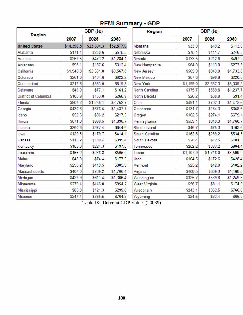
180

Table D2: Referent GDP Values (2008$)

181

Table D2: Referent Employment Values

Region

2007 2025 2050 2007 2025 2050

United States 181,668.7 201,023.2 275,903.9 Montana 648.2 691.3 946.3

Alabama 2,629.7 2,667.1 3,633.6 Nebraska 1,260.0 1,293.1 1,688.0

Arizona 3,427.1 4,277.7 7,142.0 Nevada 1,653.3 1,995.6 3,041.7

Arkansas 1,629.6 1,656.0 2,206.3 New Hampshire 872.4 1,032.7 1,518.1

California 20,858.1 25,805.3 42,573.6 New Jersey 5,250.7 6,044.3 7,817.8

Colorado 3,241.5 3,797.3 5,001.3 New Mexico 1,118.7 1,199.4 1,639.6

Connecticut 2,291.6 2,716.3 3,598.3 New York 11,279.2 14,183.8 19,805.2

Delaware 554.0 620.3 817.5 North Carolina 5,401.3 5,723.9 7,632.1

District of Columbia 819.5 897.2 1,095.0 North Dakota 492.6 506.1 691.2

Florida 10,781.8 12,110.2 16,457.8 Ohio 6,991.9 6,940.1 8,721.5

Georgia 5,499.9 6,081.5 7,886.2 Oklahoma 2,184.1 2,164.7 2,550.3

Idaho 919.1 1,035.8 1,554.2 Oregon 2,327.4 2,681.6 4,031.8

Illinois 7,744.8 8,043.8 9,579.3 Pennsylvania 7,430.0 7,971.3 10,368.3

Indiana 3,785.0 3,706.4 4,816.5 Rhode Island 631.3 706.8 962.1

Iowa 2,053.0 2,072.1 2,757.7 South Carolina 2,484.8 2,590.7 3,446.4

Kansas 1,876.0 1,911.6 2,424.0 South Dakota 564.3 577.7 792.8

Kentucky 2,462.9 2,427.0 3,131.0 Tennessee 3,795.7 3,995.6 5,442.4

Louisiana 2,510.1 2,505.0 3,224.4 Texas 13,795.8 15,031.5 19,580.4

Maine 857.1 932.0 1,324.4 Utah 1,626.4 1,877.9 2,807.3

Maryland 3,460.6 3,808.8 4,834.7 Vermont 437.9 498.9 732.3

Massachusetts 4,299.5 5,276.1 7,712.2 Virginia 4,929.5 5,246.5 6,390.4

Michigan 5,596.7 5,500.6 7,221.2 Washington 3,947.0 4,469.7 5,985.1

Minnesota 3,620.7 3,956.9 5,269.7 West Virginia 941.2 952.4 1,249.6

Mississippi 1,555.6 1,561.5 2,135.7 Wisconsin 3,658.2 3,640.9 4,615.5

Missouri 3,739.4 3,830.2 4,798.1 Wyoming 384.5 387.3 482.2

REMI Summary - Employment

RegionEmployment (1K People) Employment (1K People)

182

Table D3: Referent Population Values

183

Table D4. REMI Control Totals Over 2010-2050 For Comparison to Main-Text Impacts.

184

185

APPENDIX E: 1% EXCEEDANCE PROBABILITY IMPACTS

National and State

This section provides the detailed national and state information at the 1% exceedance-probability level for a more in-depth look at the impacts and their volatility by state and industry over time. Note that some states experience a change in the sign of impacts (from positive to negative or vice versa) . A state may initially have adequate water but later-year reduced-precipitation finally has an impact. Conversely, initial negative impacts from reduced precipitation may give way to positive impacts if surrounding states are negatively affected by a larger degree in later years. Figure E1 shows the GDP impacts for industry at the national level by decade. Figure E2 provides the contribution of GDP per state by decade. Figures E3 and E4 illustrate the yearly changes and highlight the volatility, as well as the potential change in the sign of impacts for some states. Figure E5 shows the employment impacts per state by decade. Finally, Figures E6 through E24 display the impact for each state by industry-group with decadal resolution.

186

Table E1: Change in the GDP Contribution by Industry (1% case)

187

Table E2: Change in the GDP Contribution by State (1% case)

188

Table E3: Change in GDP Contribution by State and Year

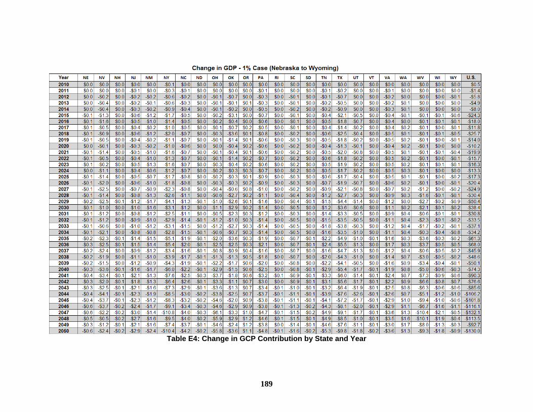
189

Table E4: Change in GCP Contribution by State and Year

190

Table E5: Change in Employment by State (1% Case)

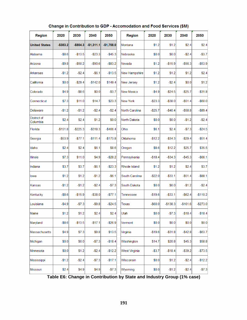
191

Table E6: Change in Contribution by State and Industry Group (1% case)

192

Table E7: Change in Contribution by State and Industry Group (continued)

193

Table E8: Change in Contribution by State and Industry Group (continued)

194

Table E9: Change in Contribution by State and Industry Group (continued)

195

Table E10: Change in Contribution by State and Industry Group (continued)

196

Table E11: Change in Contribution by State and Industry Group (continued)

197

Table E12: Change in Contribution by State and Industry Group (continued)

198

Table E13: Change in Contribution by State and Industry Group (continued)

199

Table E14: Change in Contribution by State and Industry Group (continued)

200

Table E15: Change in Contribution by State and Industry Group (continued)

201

Table E16: Change in Contribution by State and Industry Group (continued)

202

Table E17: Change in Contribution by State and Industry Group (continued)

203

Table E18: Change in Contribution by State and Industry Group (continued)

204

Table E19: Change in Contribution by State and Industry Group (continued)

205

Table E20: Change in Contribution by State and Industry Group (continued)

206

Table E21: Change in Contribution by State and Industry Group (continued)

207

Table E22: Change in Contribution by State and Industry Group (continued)

208

Table E23: Change in Contribution by State and Industry Group (continued)

209

Table E24: Change in Contribution by State and Industry Group (continued)

210

211

APPENDIX F: LOST FUNCTION FOR SMALL EXCEEDANCE-

PROBABILITIES

Section 2.1.5 considers the problem of extrapolating the result between the 99% and 1% exceedance probability intervals and the 1% to 0% intervals. The 1% to 0% interval is potentially problematic if the value of risk (probability multiplied by consequence) is either not convergent or has a value in excess of that explicitly simulated for the 99% to 1% exceedance probability range. Section 2.1.5 justifies a functional form for extrapolation based on logical argument and analogy. This appendix simply expands on the underlying analogy of using the logic of a finite resource depletion to represent how the costs of climate change “deplete” the finite GDP.

In the absence of technological change, the concept of rising costs as a function of the reduced probability of finding additional (finite) resources emulates the consideration here of rising climate costs as extreme climatic conditions have diminishing probability.

Historically, the finding rate (R) for a finite resource was often approximated by na exponentially decreasing function, for example, the barrel of oil found per foot as a function of cumulative drilling feet (x) (Ghosh 2009, Hubbert 1982, Covelli 1993):

Expression F1

The cost (C) of finding new resources then exponentially rises as the inverse of the finding rate.

Expression F2

Per Expression F1, the finding rate is a random variable whose values conform to an exponentially declining probability distribution. The change in the probability (p) of finding a new unit of oil per foot of drilling is just a scaling of the exponentially declining finding rate in terms of, for example, feet drilled.

Expression F3

Analogously, the temperature increase from climate change is comparable to the drilling activity (the tail of the distribution of temperature is well approximated by an exponential function); and the exponential cost function corresponds to the exponential damage-function approach recommended by Weitzman (2009). For this analogy to hold in a mathematical sense and establish a finite risk, the probability must fall no slower than exponentially. The tail of the gamma distribution of precipitation falls faster than the exponential function. Thus, the gamma distribution used to capture the uncertainty in precipitation due to climate change meets this criteria.

212

The integral of expression F1, represent the total use of a resource from 0% to 100% of its initial base, while the integration of expression F3 captures the same concept. That is, the total finding of the resource with infinite drilling is the entire resource bases, and by the time the probability of finding more of the resource goes to zero, the entire resource base has been exhausted. Equation F1 integrates to 100% of the resource base. Equation F3 integrate to 100% of the probability of finding the resource.

The resource exploited (E) is the integral of expression F1 and a proportionality constant (K1):

Equation F4

Or

1 Equation F5

The integral from zero to infinity is the entire resource base (B):

∞ Equation F6

Therefore:

1 Equation F7

Or:

1 Equation F8

Define (1-B/E) as the fraction of the resource remaining (F). It is also the probability (p) of how much of the resource remains to be found at a given level of total drilling.

Equation F9

Equations F1 and F3 are equivalent and we have used the two equations containing both the finding rate and the probability to make functions of the finding rate (x) into functions of the probability (p). Therefore, the integral of expressions F1 and F3 allows the transformation of expression F2 from a function of feet-drilled into a function of probability. Expression F2 becomes an equation with the use of a proportional constant K2. Substituting Equation F9 for the exponential term of Expression F2 gives:

/ Equation F10

In the more general case:

213

1/ Expression F11

Although this exercise used a concrete example of feet-drilled, the logic applies to any set of relationships where the probability of an occurrence declines exponentially, the consequence increases exponentially, and the integral of all occurrences has a specified finite value (such GDP in the actual concern of this study).

If Cmax is the asymptotic maximum cost value as probability goes to 0.0, then we can modify equation F10 to become:

1/ α Equation F12

where α is the reciprocal of the a known cost times its associated probably. The β is the reciprocal of Cmax. We can formally derive the function form of the denominator of Equation F12 but here simply state that has the required mathematical characteristics for our purposes.

As noted in Section 2.1.3, the maximum lost is assumed to be 90% of the GDP. From section 4 of the main text, the simulated 1% exceedance-probability loss is in the range of tenths to single digit percentage of GDP for the nation and individual states. In using the 1% exceedance-probability cost for determining α, empirically and definitionally α is much larger than β.

Equation F12 is the analytical function used for extrapolating costs within the interval of 1% and 0% exceedance-probability.

214

215

Distribution

2 MS9018 Central Technical Files 8944 1 MS0899 Technical Library 4536 (electronic copy) 1 MS0123 D. Chavez, LDRD Office 1011

216