Subtropical Dipole Modes Simulated in a Coupled General Circulation Model

YUSHI MORIOKA AND TOMOKI TOZUKA

Department of Earth and Planetary Science, Graduate School of Science, The University of Tokyo, Tokyo, Japan

SEBASTIEN MASSON AND PASCAL TERRAY

LOCEAN/IPSL, Universite Pierre et Marie Curie, Paris, France

JING-JIA LUO

Research Institute for Global Change, JAMSTEC, Yokohama, Japan

TOSHIO YAMAGATA

Department of Earth and Planetary Science, Graduate School of Science, The University of Tokyo, Tokyo, Japan

(Manuscript received 19 July 2011, in final form 26 December 2011)

ABSTRACT

The growth and decay mechanisms of subtropical dipole modes in the southern Indian and South Atlantic

Oceans and their impacts on southern African rainfall are investigated using results from a coupled general

circulation model originally developed for predicting tropical climate variations. The second (most) dominant

mode of interannual sea surface temperature (SST) variations in the southern Indian (South Atlantic) Ocean

represents a northeast–southwest oriented dipole, now called subtropical dipole mode. The positive (nega-

tive) SST interannual anomaly pole starts to grow in austral spring and reaches its peak in February. In austral

late spring, the suppressed (enhanced) latent heat flux loss associated with the variations in the subtropical

high causes a thinner (thicker) than normal mixed layer thickness that, in turn, enhances (reduces) the

warming of the mixed layer by the climatological shortwave radiation. The positive (negative) pole gradually

decays in austral fall because the mixed layer cooling by the entrainment is enhanced (reduced), mostly owing

to the larger (smaller) temperature difference between the mixed layer and the entrained water. The in-

creased (decreased) latent heat loss due to the warmer (colder) SST also contributes to the decay of the

positive (negative) pole. Although further verification using longer observational data is required, the present

coupled model suggests that the South Atlantic subtropical dipole may play a more important role in rainfall

variations over the southern African region than the Indian Ocean subtropical dipole.

1. Introduction

Southern Africa (Africa south of the equator in gen-

eral) experiences most of the annual rainfall in austral

summer and its interannual variation has a significant

socioeconomic impact on the regional society. A number

of studies have been devoted to investigate its possible

link with the El Nino–Southern Oscillation (ENSO) in

the Pacific (Ropelewski and Halpert 1987; Lindesay 1988;

Mason 1995; Reason et al. 2000; Richard et al. 2000).

However, they are not sufficient to explain all of the in-

terannual variability. Recently, much attention has been

paid to studying impacts from regional sea surface tem-

perature (SST) anomalies in the southern Indian and

South Atlantic Oceans (Walker 1990; Mason 1995;

Reason 1998; Reason and Mulenga 1999; Behera and

Yamagata 2001; Reason 2001; Fauchereau et al. 2009).

This is clearly seen in Fig. 1a, showing the correlation

between the SST anomalies and the southern African

rainfall index (SARI) (Richard et al. 2000), defined as

area-averaged land rainfall anomalies south of 108S

during 1960–2008. The SST anomalies in the south-

western (northeastern) region of the southern Indian

and South Atlantic Oceans are positively (negatively)

Corresponding author address: Toshio Yamagata, Department

of Earth and Planetary Science, Graduate School of Science, The

University of Tokyo, 7-3-1, Hongo, Bunkyo-ku, Tokyo 113-0033,

Japan.

E-mail: yamagata@eps.s.u-tokyo.ac.jp

15 JUNE 2012 M O R I O K A E T A L . 4029

DOI: 10.1175/JCLI-D-11-00396.1

� 2012 American Meteorological Society

correlated with the SARI, representing a clear dipole

structure. This dipole pattern is also obtained even when

rainfall indices are defined using the rainfall anomaly

south of 58 or 158S.

The existence of this dipole pattern was first identified

in the southern Indian Ocean by Behera et al. (2000).

Using observations and a reanalysis dataset, Behera and

Yamagata (2001) revealed that the SST anomalies asso-

ciated with the named Indian Ocean subtropical dipole

(IOSD) reach their peak in February owing to the latent

heat flux anomalies associated with the variations in the

Mascarene high. This important role of the latent heat

flux anomalies was also supported by calculating a mixed

layer heat balance with a constant thickness (Suzuki et al.

2004; Hermes and Reason 2005).

Another dipole of SST anomalies in the South At-

lantic is known as the South Atlantic subtropical dipole

(SASD). Using a singular value decomposition (SVD)

analysis, Venegas et al. (1997) first showed the exis-

tence of dipole SST anomalies in the South Atlantic

and its link with variations in the sea level pressure (SLP).

Later, Fauchereau et al. (2003) suggested that the SST

anomalies associated with the SASD are mostly due to

the latent heat flux anomalies linked with the southward

migration and strengthening of the St. Helena high. The

importance of the latent heat flux anomalies was also dis-

cussed using ocean assimilation data (Sterl and Hazeleger

2003) or outputs from an ocean general circulation model

(OGCM) (Colberg and Reason 2007).

However, all of these studies on the IOSD and SASD

were based on a discussion of the heat balance in a box

with a constant mixed layer thickness. Since the mixed

layer depth undergoes significant seasonal and inter-

annual variations in the subtropics, those studies may

have serious defects. Indeed, Morioka et al. (2010, 2011)

have recently revealed the significance of interannual

variations in the mixed layer thickness on the growth of

SST anomalies associated with the IOSD and SASD,

respectively. They indicated that warming of the mixed

layer by climatological shortwave radiation is enhanced

(reduced) because of the thinner (thicker) than normal

mixed layer over the positive (negative) SST anomaly

pole. However, these results were based on the outputs

from an OGCM in which the surface heat fluxes were

calculated by the bulk formula using the atmospheric

reanalysis data and the simulated SST. As a result, some

effects of the SST anomaly on surface heat fluxes are

neglected. For instance, the positive SST anomaly pole

in reality acts to enhance the moisture (temperature) of

air near the ocean surface and reduce the latent (sensi-

ble) heat loss from the ocean. To reveal the air–sea in-

teraction processes involving the IOSD and SASD in

more detail, it is necessary to use a coupled general

circulation model (CGCM).

Furthermore, impacts of the subtropical dipole modes

on the southern African rainfall are still unclear. Using

outputs of an atmospheric general circulation model

(AGCM), Reason (2001, 2002) showed that the positive

SST anomaly of positive IOSDs enhances the rainfall

in austral summer via anomalous moisture convergence

associated with the low SLP anomalies generated over

the positive SST anomaly pole. To understand variations

of the southern African rainfall related to air–sea inter-

action involving the IOSD, a one-tier approach using a

CGCM may also be necessary. Using observational and

reanalysis data, Vigaud et al. (2009) suggested a poten-

tial impact of the dipole SST anomalies in the South

Atlantic on the rainfall anomalies during austral sum-

mer. Since the 1979–2000 data period used in their study

is too short, only one positive SASD event and three

negative SASD events are selected in their composite

analysis, which is not sufficient to examine the link be-

tween the SASD and rainfall variations.

Therefore, the present study investigates the growth

and decay of subtropical dipole modes using outputs

from a 500-yr integration of a CGCM and examines

their impact on the southern African rainfall. This paper

is organized as follows. A brief description of the data

and the CGCM is given in the next section. The seasonal

variation of observed and simulated SST and mixed layer

depth in the southern Indian Ocean is discussed in section

3. In section 4, we compare the observed and simulated

IOSD and SASD. The mixed layer heat balance over the

SST anomaly poles for the positive IOSD is investigated

in section 5. In section 6, the impacts of the positive IOSD

and SASD on the southern African rainfall in austral

summer are examined. The final section summarizes the

main results and discusses the difference in the position

FIG. 1. Correlation between the (a) observed and (b) simulated

SARI and SST anomalies: correlations exceeding 90% confidence

level by a two-tailed t test are shaded.

4030 J O U R N A L O F C L I M A T E VOLUME 25

of SST anomaly poles associated with the subtropical

dipole modes between the observations and model.

2. Model and data

We use monthly mean outputs from a CGCM devel-

oped at the Frontier Research Center for Global Change

(FRCGC) called the Scale Interaction Experiment-

FRCGC (SINTEX-F) model (Luo et al. 2003). The

SINTEX-F model has been developed from the original

European SINTEX model under the Japan–European

Union collaboration (Gualdi et al. 2003; Guilyardi et al.

2003) and a more detailed model description is provided

by Luo et al. (2005). The oceanic component is based on

the reference version 8.2 of Ocean Parallelise (OPA)

(Madec et al. 1998). Its horizontal resolution is 0.58–28,

with the meridional resolution increasing up to 0.58 near

the equator, and it has 31 vertical levels with 19 levels in

the upper 500 m. The vertical eddy viscosity and diffu-

sivity are calculated from a 1.5-order turbulent closure

scheme (Blanke and Delecluse 1993), and the Gent and

McWilliams (1990) scheme is included for the isopycnal

mixing. Sea ice cover in the model is given by observed

monthly climatology.

The atmospheric component of the model is the latest

version of the ECHAM4 (Roeckner et al. 1996). Our

configuration is based on a T106 Gaussian grid and 19

levels in the hybrid sigma-pressure vertical. Surface tur-

bulent heat flux is calculated by a bulk aerodynamic

formula in which the drag coefficients for momentum and

heat depend on the moist bulk Richardson number and

roughness length (Louis 1979). For cumulus convection,

the bulk mass flux formula of Tiedtke (1989) is used.

The atmospheric and oceanic fields are coupled every

2 h by the Ocean Atmosphere Sea Ice Soil (OASIS) 2.4

coupler (Valcke et al. 2000). The surface current mo-

mentum is directly passed to the atmosphere through

a vertical viscosity term in its momentum equation. The

initial condition of the ocean is from the Levitus annual

mean climatologies with zero velocities. For the atmo-

sphere, a 1-yr run forced with the observed monthly

climatological SST is used. To obtain a sufficient number

of SASD and IOSD events for a discussion of their rel-

ative impact on the southern African rainfall, the coupled

model is integrated for 520 years. Considering the near-

surface oceanic adjustment time, we analyze outputs from

the last 500 years.

For comparison, we use the monthly mean observed

SST data from the Hadley Centre sea ice and sea surface

temperature (HADISST) (Rayner et al. 2003), gridded

data with 18 3 18 resolution, and we analyze the period

during 1960–2008 because of few observations in the

southern Indian and South Atlantic Oceans before the

1960s. To derive the mixed layer depth, we use the monthly

climatology of ocean temperature available from the

World Ocean Atlas 2009 (WOA09) (Locarnini et al.

2010; http://www.nodc.noaa.gov), which has 24 levels in

the vertical with 18 3 18 horizontal resolution. We also

use the horizontal wind at 850 hPa from the National

Centers for Environmental Prediction–National Center

for Atmospheric Research (NCEP–NCAR) reanalysis

dataset (Kalnay et al. 1996). It has a 2.58 3 2.58 hori-

zontal resolution and covers the same period. Regarding

precipitation, we use the gridded monthly rainfall data,

provided by the University of Delaware (Legates and

Willmott 1990), from 1960 to 2008 with a horizontal

resolution of 0.58 in both longitude and latitude. For all

of these data the interannual anomalies are calculated

by subtracting the monthly mean climatology after re-

moving a linear trend using a least squares fit.

The correlation between the simulated SARI and SST

interannual anomalies is shown in Fig. 1b. The model

reproduces northeast–southwest oriented dipoles in the

South Atlantic and southern Indian Oceans rather well.

The simulated IOSD and SASD are compared with the

observed ones in Fig. 2. The IOSD in the observation is

captured by the second EOF mode (Fig. 2a), whereas in

the model it is captured by the first EOF mode (Fig. 2b).

The pattern correlation between them is 0.88 and is re-

markably high. This is superior compared with other

CGCMs as shown by Kataoka et al. (2012). Therefore,

the model has high skill in simulating the SST pattern

associated with the IOSD. On the other hand, both ob-

served and simulated SASD are detected as the first EOF

mode (Figs. 2c,d). Although the northeast–southwest

orientation of the poles is well simulated, the position of

the positive pole in the model is shifted toward higher

latitudes by 108; the pattern correlation is 0.76. Also, the

percentage of the explained variance in the model for

the IOSD (SASD) is 20.2% (19.2%) and is in good

agreement with 21.0% (20.4%) in the observation. The

second EOF mode with a monopole pattern simulated in

the southern Indian Ocean and the South Atlantic ex-

plains 14.6% and 14.0% of the total variance, respectively,

and is sufficiently separated from the first mode (North

et al. 1982).

Furthermore, we have defined positive (negative) event

years as years when the normalized principal component

during austral summer (in Fig. 2) exceeds one (minus one)

standard deviation. This leads to 9 (7) positive IOSD

(SASD) events during 49 years in the observation and 74

(76) positive IOSD (SASD) events during 500 years in the

model. The frequency of occurrence for the observed pos-

itive IOSDs (SASDs), 18.8% (14.6%), is well reproduced in

the model, 14.8% (15.2%). Thus, the use of this model for

analyses of the IOSD and SASD may be validated.

15 JUNE 2012 M O R I O K A E T A L . 4031

3. Validation of simulated seasonal variabilityin the subtropical region

In this section, we explore the seasonal variation of the

SST and mixed layer depth in the subtropical region to

help understand its interannual variation. Since results

obtained in the South Atlantic are almost similar, we

discuss only the seasonal variation in the southern In-

dian Ocean. Both observed and simulated SST averaged

over the southwestern pole (338–438S, 458–658E), de-

fined in Fig. 2b, show a clear annual cycle with their

maximum in February (Fig. 3a), whereas those over the

northeastern pole (178–278S, 758–958E) reach their peak

in March (Fig. 3b). To investigate this seasonal SST

variation, we use the tendency of the mixed layer tem-

perature Tm averaged over the box of each pole:

›Tm

›t5

Qnet 2 qd

rcpH2 um � $Tm 2

DT

Hwe 1 res (1)

(Qiu and Kelly 1993; Moisan and Niiler 1998). The first

term on the right-hand side indicates the contribution

from the surface heat flux, where Qnet is the net surface

heat flux, qd is the downward solar insolation penetrating

through the mixed layer bottom (Paulson and Simpson

1977), r (51027 kg m23) is the density of the seawater, cp

(54187 J kg21 K21) is the specific heat of the seawater,

and H is the mixed layer depth, defined as the depth at

which temperature is 0.58C lower than the SST. Here qd is

negligible compared to Qnet because only less than 5% of

the shortwave radiation can penetrate the mixed layer

depth, even when the mixed layer is thinnest in austral

summer. The second term indicates the horizontal ad-

vection, where um denotes the horizontal velocity aver-

aged in the mixed layer. The third term is the entrainment

term, where DT ([Tm 2 T2H220m) represents the tem-

perature difference between the mixed layer and the

entrained water; we use the water temperature at 20 m

below the mixed layer base as the temperature of en-

trained water, as in Yasuda et al. (2000). Also,

we

([›H/›t 1 $ � um

H) is the entrainment velocity and

is assumed to vanish when it becomes negative (Kraus

and Turner 1967; Qiu and Kelly 1993). The residual

term, res, consists of diffusion, detrainment, and other

FIG. 2. Spatial patterns of the (a) second EOF mode of SST anomalies from HADISST and (b) first EOF mode of

SST anomalies from SINTEX-F model in the southern Indian Ocean, and the first EOF mode of SST anomalies from

(c) HADISST and (d) the model in the South Atlantic (8C). Negative values are shaded, and percentage of the

explained variance is shown. The boxes over the positive and negative poles in the upper left (right) panel are defined

as 308–408S, 508–708E (338 and 438S, 458 and 658E) and 158–258S, 858–1058E (178 and 278S, 758 and 958E). The boxes

over the positive and negative poles in the lower left (right) panel are defined as 308–408S, 108–308W (408 and 508S, 238

and 438W) and 158–258S, 08–208W (168 and 268S, 08 and 208W).

4032 J O U R N A L O F C L I M A T E VOLUME 25

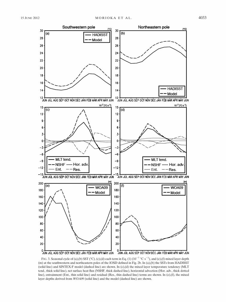
FIG. 3. Seasonal cycle of (a),(b) SST (8C), (c),(d) each term in Eq. (1) (1027 8C s21), and (e),(f) mixed layer depth

(m) at the southwestern and northeastern poles of the IOSD defined in Fig. 2b. In (a),(b) the SSTs from HADISST

(solid line) and SINTEX-F model (dashed line) are shown. In (c),(d) the mixed layer temperature tendency (MLT

tend., thick solid line), net surface heat flux (NSHF, thick dashed line), horizontal advection (Hor. adv., thick dotted

line), entrainment (Ent., thin solid line) and residual (Res., thin dashed line) terms are shown. In (e),(f), the mixed

layer depths derived from WOA09 (solid line) and the model (dashed line) are shown.

15 JUNE 2012 M O R I O K A E T A L . 4033

neglected oceanic processes such as high frequency

variability.

The monthly climatology of each term in Eq. (1) over

the southwestern (northeastern) pole is shown in Fig.

3c (Fig. 3d). The warming of the mixed layer over the

southwestern (northeastern) pole from November to

February (from October to March) is mostly due to the

contribution from the net surface heat flux. Among its

four components, the contribution from shortwave radi-

ation is dominant (figure not shown). The shallow mixed

layer also contributes to enhanced warming of the mixed

layer by shortwave radiation (Figs. 3e,f). The contribu-

tion from shortwave radiation over the southwestern

(northeastern) pole decreases from March to September

(from April to September), explaining most of the mixed

layer cooling. Also, cooling of the mixed layer by en-

trainment occurs when the mixed layer deepens (Figs.

3e,f). The mixed layer depth in the model at the south-

western (northeastern) pole becomes deepest in September

(August) and its seasonal variation is well simulated.

4. Validation of simulated interannual variability inthe subtropical region: Subtropical dipole modes

To identify the key feature of the observed and simu-

lated SST anomalies associated with the IOSD and SASD,

we introduce IOSD and SASD indices, defined by the

difference in the SST anomalies between the boxes over

the southwestern and northeastern poles (Figs. 2a–d).

Each of the observed and simulated IOSD (SASD)

indices shows a high correlation, above 0.9, with the

principal component of its EOF mode in Figs. 2a,b (Figs.

2c,d). The monthly standard deviations of the observed

and simulated IOSD and SASD indices are largest in

austral summer (Figs. 4a,b), indicating a strong phase

locking of their interannual variation to austral summer.

This allows us to define IOSD (SASD) events as years

when the observed IOSD (SASD) index averaged in

austral summer exceeds one standard deviation. This

leads to eight positive IOSD (SASD) events: 1960/61,

1965/66, 1967/68, 1973/74, 1975/76, 1980/81, 1981/82, and

1998/99 (1961/62, 1965/66, 1975/76, 1979/80, 1980/81,

1981/82, 1996/97, and 1998/99; see Morioka et al. 2011).

In the model simulation for 500 years, we find 75 (74)

positive IOSD (SASD) events exceeding one standard

deviation for the model. Hereafter, we define year 0 as

the year when the subtropical dipole event develops and

year 1 the following year.

The evolution of the observed and simulated com-

posite SST anomalies for the positive IOSD is shown in

Fig. 5. Both positive and negative SST anomaly poles

start to grow from austral spring, reach their peak in

austral summer, and decay in austral fall. The pattern

correlation between the observed and simulated SST

anomalies in the peak phase of December (0)–February

(1) is 0.81. A similar evolution of the positive and neg-

ative poles associated with the positive SASD is found

(Fig. 6). However, the pattern correlation between the

observed and simulated SST anomalies in austral sum-

mer is relatively low at 0.63. This may be mostly due to

FIG. 4. Monthly standard deviation of (a) IOSD and (b) SASD indices (8C) from HADISST (dashed line) and

SINTEX-F model (solid line). The error bar indicates one standard deviation calculated using 10 different 49-yr

periods.

4034 J O U R N A L O F C L I M A T E VOLUME 25

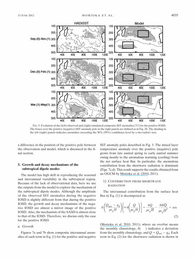
a difference in the position of the positive pole between

the observation and model, which is discussed in the fi-

nal section.

5. Growth and decay mechanisms of thesubtropical dipole modes

The model has high skill in reproducing the seasonal

and interannual variability in the subtropical region.

Because of the lack of observational data, here we use

the outputs from the model to explore the mechanism of

the subtropical dipole modes. Although the amplitude

of the observed SST anomalies during the negative

IOSD is slightly different from that during the positive

IOSD, the growth and decay mechanisms of the nega-

tive IOSD are almost a mirror image of the positive

IOSD. Also, the mechanism of the SASD is almost close

to that of the IOSD. Therefore, we discuss only the case

for the positive IOSD.

a. Growth

Figures 7a and 7b show composite interannual anom-

alies of each term in Eq. (1) for the positive and negative

SST anomaly poles described in Fig. 5. The mixed layer

temperature anomaly over the positive (negative) pole

grows from late austral spring to early austral summer

owing mostly to the anomalous warming (cooling) from

the net surface heat flux. In particular, the anomalous

contribution from the shortwave radiation is dominant

(Figs. 7c,d). This result supports the results obtained from

an OGCM by Morioka et al. (2010, 2011).

1) CONTRIBUTION FROM SHORTWAVE

RADIATION

The interannual contribution from the surface heat

flux in Eq. (1) is decomposed as

dQnet 2 qd

rcpH

!"[ d

Q

rcpH

!#5

dQ

rcpH2

dHQ

rcpH2

1 res

(2)

(Morioka et al. 2010, 2011), where an overbar means

the monthly climatology, d( � � � ) indicates a deviation

from the monthly climatology, and Q 5 Qnet 2 qd. Each

term in Eq. (2) for the shortwave radiation is shown in

FIG. 5. Evolution of the (left) observed and (right) simulated composite SST anomalies (8C) for the positive IOSD.

The boxes over the positive (negative) SST anomaly pole in the right panels are defined as in Fig. 2b. The shading in

the left (right) panels indicates anomalies exceeding the 90% (99%) confidence level by a two-tailed t test.

15 JUNE 2012 M O R I O K A E T A L . 4035

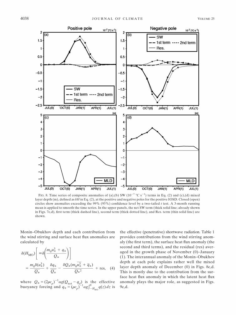
Figs. 8a,b. Over the positive (negative) pole the anom-

alous contribution from the shortwave radiation is due

mostly to the second term on the rhs of Eq. (2), indicating

that warming of the mixed layer by the climatological

shortwave radiation is enhanced (suppressed) by a thin-

ner (thicker) than normal mixed layer, as shown in Fig. 8c

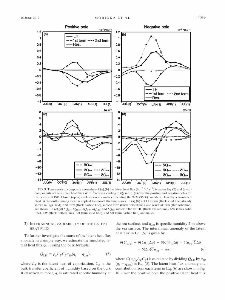
(Fig. 8d). On the other hand, cooling of the mixed layer

by the climatological latent heat loss in Fig. 9a (Fig. 9b) is

enhanced (suppressed) by the same mixed layer thickness

anomaly and this cancels out the decreased (increased)

latent heat loss in the first term of Eq. (2) as suggested in

Fig. 9c (Fig. 9d).

Regarding the oceanic role, the residual term contrib-

utes to cooling (warming) the mixed layer anomalously in

Fig. 7a (Fig. 7b). Besides the effects of the high frequency

variability, this may be related to the fact that the cooling

of the mixed layer by detrainment and diffusion is en-

hanced (reduced) by the thinner (thicker) than normal

mixed layer. On the other hand, the contribution from

horizontal advection due to the oceanic circulation is very

small. This may be due to the fact that the SST anomaly

poles associated with the IOSD are located off the strong

Agulhas return current.

The significant role of interannual variations in the mixed

layer thickness was overlooked in previous studies by Suzuki

et al. (2004) and Hermes and Reason (2005) because they

calculated the mixed layer heat balance assuming a constant

thickness. This important point was already demonstrated

by the OGCM studies (Morioka et al. 2010, 2011).

2) INTERANNUAL VARIABILITY OF THE MIXED

LAYER DEPTH

The interannual anomaly in the mixed layer thickness

is the key to the evolution of the tendency anomaly in

the mixed layer temperature in Eq. (2). This mixed layer

FIG. 6. As in Fig. 5 but for the positive SASD. (right) The boxes over the positive (negative) SST anomaly pole are

defined as in Fig. 2d.

4036 J O U R N A L O F C L I M A T E VOLUME 25

thickness anomaly may be linked with wind stirring and

surface heat flux anomalies. To clarify each contribution

quantitatively, we calculate a diagnostic value of the

mixed layer depth during a shoaling phase, called the

Monin–Obukhov depth:

HMO 5

"m0u3

* 1ag

rcp

ð0

2HMO

q(z) dz

#ag

2rcp

(Qnet 2 qd)

,

(3)

(Kraus and Turner 1967; Qiu and Kelly 1993). Here m0

is a coefficient for the efficiency of wind stirring, and we

use m0 5 0.5 (Davis et al. 1981). The frictional velocity

u*

is defined by u* [ (raCDu210/r)1/2, where ra (51.3

kg m23) is the density of air, CD (50.00125) is the drag

coefficient, and u10 is the wind speed at 10-m height.

Also, a (50.00025) is the thermal expansion coefficient,

and q(z) is the downward solar insolation (Paulson

and Simpson 1977). The interannual anomaly of the

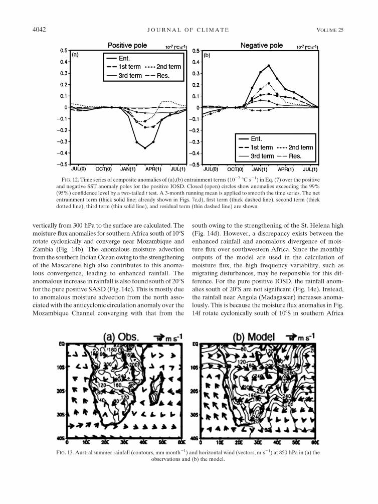
FIG. 7. Time series of composite anomalies of (a),(b) the mixed layer temperature tendency (1027 8C s21) terms

in Eq. (1) and (c),(d) components of the net surface heat flux (1027 8C s21) terms in Eq. (1) over the positive and

negative poles for the positive IOSD. Closed (open) circles show anomalies exceeding the 99% (95%) confidence

level by a two-tailed t test. A 3-month running mean is applied to smooth the time series. In the upper panel, the

mixed-layer temperature tendency (MLT tend., thick solid line), net surface heat flux (NSHF, thick dashed line),

horizontal advection (Hor. adv., thick dotted line), entrainment (Ent., thin solid line) and residual (Res., thin

dashed line) terms are shown. In the lower panel, the short wave radiation (SW, thick solid line), long wave

radiation (LW, thick dotted line), latent heat flux (LH, thin solid line) and sensible heat flux (SH, thin dashed line)

terms are shown.

15 JUNE 2012 M O R I O K A E T A L . 4037

Monin–Obukhov depth and each contribution from

the wind stirring and surface heat flux anomalies are

calculated by

d(HMO)

"[d

m0u3* 1 q*Q*

!#

5m0d(u3

*)

Q*

1dq*Q*

2dQ*(m0u3

*1 q*)

Q*2

1 res, (4)

where Q* 5 (2rcp)21ag(Qnet 2 qd) is the effective

buoyancy forcing and q* 5 (rcp)21agÐ 0

2HMOq(z) dz is

the effective (penetrative) shortwave radiation. Table 1

provides contributions from the wind stirring anom-

aly (the first term), the surface heat flux anomaly (the

second and third terms), and the residual (res) aver-

aged in the growth phase of November (0)–January

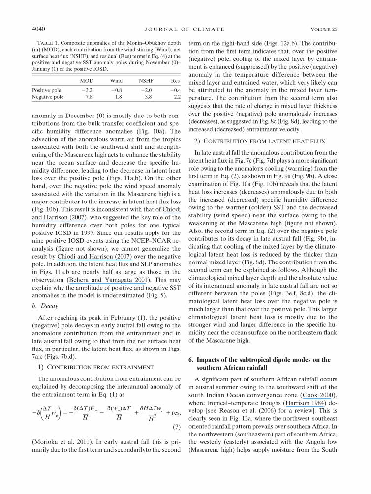
(1). The interannual anomaly of the Monin–Obukhov

depth at each pole explains rather well the mixed

layer depth anomaly of December (0) in Figs. 8c,d.

This is mostly due to the contribution from the sur-

face heat flux anomaly in which the latent heat flux

anomaly plays the major role, as suggested in Figs.

9c,d.

FIG. 8. Time series of composite anomalies of (a),(b) SW (1027 8C s21) terms in Eq. (2) and (c),(d) mixed

layer depth (m), defined as dH in Eq. (2), at the positive and negative poles for the positive IOSD. Closed (open)

circles show anomalies exceeding the 99% (95%) confidence level by a two-tailed t test. A 3-month running

mean is applied to smooth the time series. In the upper panels, the net SW term (thick solid line; already shown

in Figs. 7c,d), first term (thick dashed line), second term (thick dotted line), and Res. term (thin solid line) are

shown.

4038 J O U R N A L O F C L I M A T E VOLUME 25

3) INTERANNUAL VARIABILITY OF THE LATENT

HEAT FLUX

To further investigate the cause of the latent heat flux

anomaly in a simple way, we estimate the simulated la-

tent heat flux QLH using the bulk formula:

QLH 5 raLECEu10(qs 2 q2m), (5)

where LE is the latent heat of vaporization, CE is the

bulk transfer coefficient of humidity based on the bulk

Richardson number, qs is saturated specific humidity at

the sea surface, and q2m is specific humidity 2 m above

the sea surface. The interannual anomaly of the latent

heat flux in Eq. (5) is given by

d(QLH) 5 d(Cu10Dq) 5 d(C)u10Dq 1 d(u10)CDq

1 d(Dq)Cu10 1 res, (6)

where C(5raL

EC

E) is calculated by dividing QLH by u10

(qs 2 q2m) in Eq. (5). The latent heat flux anomaly and

contribution from each term in Eq. (6) are shown in Fig.

10. Over the positive pole the positive latent heat flux

FIG. 9. Time series of composite anomalies of (a),(b) the latent heat flux (1027 8C s21) terms in Eq. (2) and (c),(d)

components of the surface heat flux (W m22) corresponding to dQ in Eq. (2) over the positive and negative poles for

the positive IOSD. Closed (open) circles show anomalies exceeding the 99% (95%) confidence level by a two-tailed

t test. A 3-month running mean is applied to smooth the time series. In (a),(b) net LH term (thick solid line; already

shown in Figs. 7c,d), first term (thick dashed line), second term (thick dotted line), and residual term (thin solid line)

are shown. In (c),(d) dQnet, dQSW, dQLW, dQLH, and dQSH indicate the NSHF (thick dashed line), SW (thick solid

line), LW (thick dotted line), LH (thin solid line), and SH (thin dashed line) anomalies.

15 JUNE 2012 M O R I O K A E T A L . 4039

anomaly in December (0) is mostly due to both con-

tributions from the bulk transfer coefficient and spe-

cific humidity difference anomalies (Fig. 10a). The

advection of the anomalous warm air from the tropics

associated with both the southward shift and strength-

ening of the Mascarene high acts to enhance the stability

near the ocean surface and decrease the specific hu-

midity difference, leading to the decrease in latent heat

loss over the positive pole (Figs. 11a,b). On the other

hand, over the negative pole the wind speed anomaly

associated with the variation in the Mascarene high is a

major contributor to the increase in latent heat flux loss

(Fig. 10b). This result is inconsistent with that of Chiodi

and Harrison (2007), who suggested the key role of the

humidity difference over both poles for one typical

positive IOSD in 1997. Since our results apply for the

nine positive IOSD events using the NCEP–NCAR re-

analysis (figure not shown), we cannot generalize the

result by Chiodi and Harrison (2007) over the negative

pole. In addition, the latent heat flux and SLP anomalies

in Figs. 11a,b are nearly half as large as those in the

observation (Behera and Yamagata 2001). This may

explain why the amplitude of positive and negative SST

anomalies in the model is underestimated (Fig. 5).

b. Decay

After reaching its peak in February (1), the positive

(negative) pole decays in early austral fall owing to the

anomalous contribution from the entrainment and in

late austral fall owing to that from the net surface heat

flux, in particular, the latent heat flux, as shown in Figs.

7a,c (Figs. 7b,d).

1) CONTRIBUTION FROM ENTRAINMENT

The anomalous contribution from entrainment can be

explained by decomposing the interannual anomaly of

the entrainment term in Eq. (1) as

2dDT

Hwe

� �52

d(DT)we

H2

d(we)DT

H1

dHDTwe

H2

1 res.

(7)

(Morioka et al. 2011). In early austral fall this is pri-

marily due to the first term and secondarilyto the second

term on the right-hand side (Figs. 12a,b). The contribu-

tion from the first term indicates that, over the positive

(negative) pole, cooling of the mixed layer by entrain-

ment is enhanced (suppressed) by the positive (negative)

anomaly in the temperature difference between the

mixed layer and entrained water, which very likely can

be attributed to the anomaly in the mixed layer tem-

perature. The contribution from the second term also

suggests that the rate of change in mixed layer thickness

over the positive (negative) pole anomalously increases

(decreases), as suggested in Fig. 8c (Fig. 8d), leading to the

increased (decreased) entrainment velocity.

2) CONTRIBUTION FROM LATENT HEAT FLUX

In late austral fall the anomalous contribution from the

latent heat flux in Fig. 7c (Fig. 7d) plays a more significant

role owing to the anomalous cooling (warming) from the

first term in Eq. (2), as shown in Fig. 9a (Fig. 9b). A close

examination of Fig. 10a (Fig. 10b) reveals that the latent

heat loss increases (decreases) anomalously due to both

the increased (decreased) specific humidity difference

owing to the warmer (colder) SST and the decreased

stability (wind speed) near the surface owing to the

weakening of the Mascarene high (figure not shown).

Also, the second term in Eq. (2) over the negative pole

contributes to its decay in late austral fall (Fig. 9b), in-

dicating that cooling of the mixed layer by the climato-

logical latent heat loss is reduced by the thicker than

normal mixed layer (Fig. 8d). The contribution from the

second term can be explained as follows. Although the

climatological mixed layer depth and the absolute value

of its interannual anomaly in late austral fall are not so

different between the poles (Figs. 3e,f, 8c,d), the cli-

matological latent heat loss over the negative pole is

much larger than that over the positive pole. This larger

climatological latent heat loss is mostly due to the

stronger wind and larger difference in the specific hu-

midity near the ocean surface on the northeastern flank

of the Mascarene high.

6. Impacts of the subtropical dipole modes on thesouthern African rainfall

A significant part of southern African rainfall occurs

in austral summer owing to the southward shift of the

south Indian Ocean convergence zone (Cook 2000),

where tropical–temperate troughs (Harrison 1984) de-

velop [see Reason et al. (2006) for a review]. This is

clearly seen in Fig. 13a, where the northwest–southeast

oriented rainfall pattern prevails over southern Africa. In

the northwestern (southeastern) part of southern Africa,

the westerly (easterly) associated with the Angola low

(Mascarene high) helps supply moisture from the South

TABLE 1. Composite anomalies of the Monin–Obukhov depth

(m) (MOD), each contribution from the wind stirring (Wind), net

surface heat flux (NSHF), and residual (Res) terms in Eq. (4) at the

positive and negative SST anomaly poles during November (0)–

January (1) of the positive IOSD.

MOD Wind NSHF Res

Positive pole 23.2 20.8 22.0 20.4

Negative pole 7.8 1.8 3.8 2.2

4040 J O U R N A L O F C L I M A T E VOLUME 25

Atlantic (southern Indian Ocean). Although the simulated

rainfall over Mozambique, South Africa, and Lesotho

(Congo basin) is larger (smaller) than observed, the spatial

patterns of the low-level wind and associated rainfall over

southern Africa are simulated in the model (Fig. 13b).

To study the relative influence of the SASD and IOSD

on austral summer rainfall over southern Africa, we

classify the years of subtropical dipole modes into three

groups: co-occurrence of the SASD and IOSD, pure

SASD, and pure IOSD. Here we define years with both

SASD and IOSD indices exceeding one (minus one)

standard deviation as co-occurring positive (negative)

SASD and IOSD events. When only the SASD (IOSD)

index exceeds 61 standard deviation, it is defined as the

pure SASD (IOSD) event. This procedure leads to 5 (19)

events for the co-occurrence of the positive SASD and

IOSD, 3 (55) pure positive SASDs, and 3 (56) pure positive

IOSDs in the observation (model). Similarly, 5 (26) events

for the co-occurrence of the negative SASD and IOSD, 6

(47) pure negative SASDs, and 2 (53) pure negative IOSDs

in the observation (model) are obtained. Since the number

of the observed events for each group is not enough to

discuss their composites, we only discuss the positive SASD

and IOSD in the model here. We note that the mechanism

of the simulated rainfall anomalies for the negative events

is close to a mirror of that for the positive events.

The austral summer rainfall slightly increases south

of 158S when the positive SASD and IOSD co-occur

(Fig. 14a). In particular, the positive rainfall anomalies

near Mozambique and Zambia are statistically significant.

To investigate the mechanism of the rainfall anomalies,

the anomalous moisture flux and its divergence integrated

FIG. 10. Time series of composite anomalies of LH (thick solid line; already shown in Figs. 9c,d) and each con-

tribution from the wind speed at 10 m (thick dashed line), specific humidity difference near the surface (thick dotted

line), transfer coefficient (thin solid line), and residual (thin dashed line) terms in Eq. (6) over (a) positive and

(b) negative poles for the positive IOSD (W m22). Closed (open) circles show anomalies exceeding the 99% (95%)

confidence level by a two-tailed t test. A 3-month running mean is applied to smooth the time series.

FIG. 11. Composite anomalies of (a) LH (W m22) and (b) SLP (hPa) averaged during November (0)–January (1) of

the positive IOSD. The anomalies exceeding 99% confidence level by two-tailed t test are shaded.

15 JUNE 2012 M O R I O K A E T A L . 4041

vertically from 300 hPa to the surface are calculated. The

moisture flux anomalies for southern Africa south of 108S

rotate cyclonically and converge near Mozambique and

Zambia (Fig. 14b). The anomalous moisture advection

from the southern Indian Ocean owing to the strengthening

of the Mascarene high also contributes to this anoma-

lous convergence, leading to enhanced rainfall. The

anomalous increase in rainfall is also found south of 208S

for the pure positive SASD (Fig. 14c). This is mostly due

to anomalous moisture advection from the north asso-

ciated with the anticyclonic circulation anomaly over the

Mozambique Channel converging with that from the

south owing to the strengthening of the St. Helena high

(Fig. 14d). However, a discrepancy exists between the

enhanced rainfall and anomalous divergence of mois-

ture flux over southwestern Africa. Since the monthly

outputs of the model are used in the calculation of

moisture flux, the high frequency variability, such as

migrating disturbances, may be responsible for this dif-

ference. For the pure positive IOSD, the rainfall anom-

alies south of 208S are not significant (Fig. 14e). Instead,

the rainfall near Angola (Madagascar) increases anoma-

lously. This is because the moisture flux anomalies in Fig.

14f rotate cyclonically south of 108S in southern Africa

FIG. 12. Time series of composite anomalies of (a),(b) entrainment terms (1027 8C s21) in Eq. (7) over the positive

and negative SST anomaly poles for the positive IOSD. Closed (open) circles show anomalies exceeding the 99%

(95%) confidence level by a two-tailed t test. A 3-month running mean is applied to smooth the time series. The net

entrainment term (thick solid line; already shown in Figs. 7c,d), first term (thick dashed line), second term (thick

dotted line), third term (thin solid line), and residual term (thin dashed line) are shown.

FIG. 13. Austral summer rainfall (contours, mm month21) and horizontal wind (vectors, m s21) at 850 hPa in (a) the

observations and (b) the model.

4042 J O U R N A L O F C L I M A T E VOLUME 25

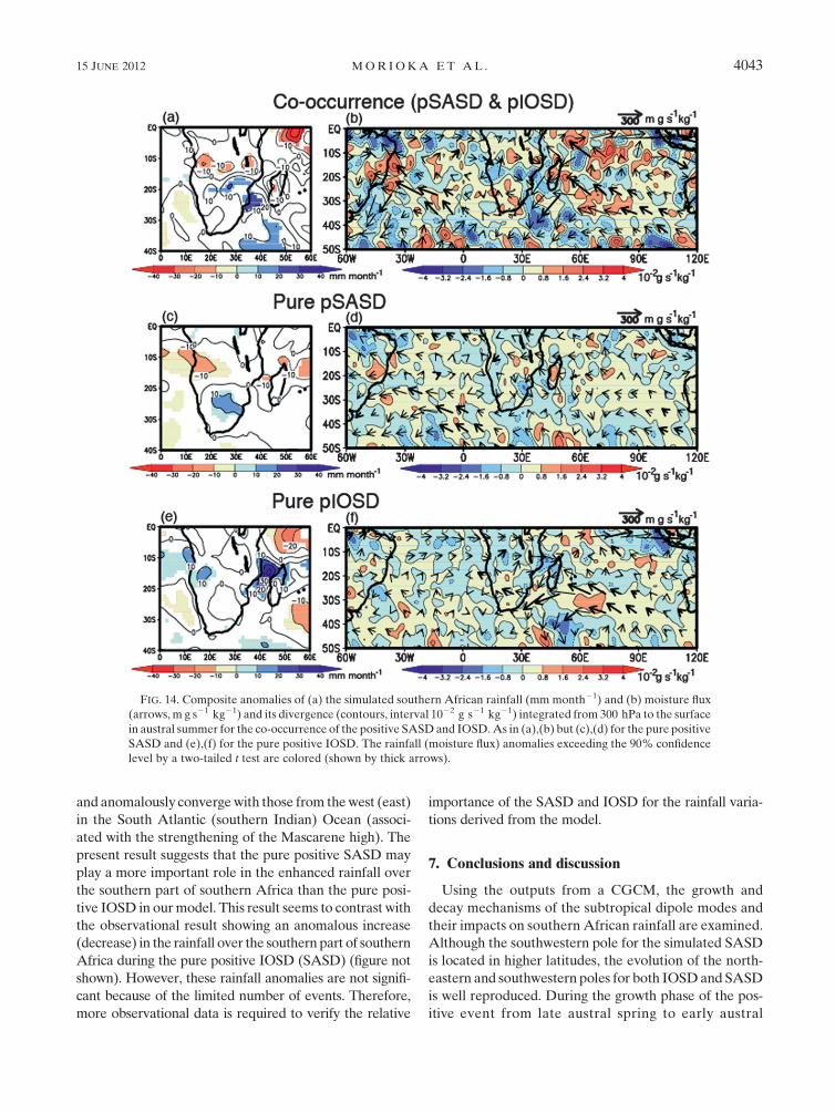
and anomalously converge with those from the west (east)

in the South Atlantic (southern Indian) Ocean (associ-

ated with the strengthening of the Mascarene high). The

present result suggests that the pure positive SASD may

play a more important role in the enhanced rainfall over

the southern part of southern Africa than the pure posi-

tive IOSD in our model. This result seems to contrast with

the observational result showing an anomalous increase

(decrease) in the rainfall over the southern part of southern

Africa during the pure positive IOSD (SASD) (figure not

shown). However, these rainfall anomalies are not signifi-

cant because of the limited number of events. Therefore,

more observational data is required to verify the relative

importance of the SASD and IOSD for the rainfall varia-

tions derived from the model.

7. Conclusions and discussion

Using the outputs from a CGCM, the growth and

decay mechanisms of the subtropical dipole modes and

their impacts on southern African rainfall are examined.

Although the southwestern pole for the simulated SASD

is located in higher latitudes, the evolution of the north-

eastern and southwestern poles for both IOSD and SASD

is well reproduced. During the growth phase of the pos-

itive event from late austral spring to early austral

FIG. 14. Composite anomalies of (a) the simulated southern African rainfall (mm month21) and (b) moisture flux

(arrows, m g s21 kg21) and its divergence (contours, interval 1022 g s21 kg21) integrated from 300 hPa to the surface

in austral summer for the co-occurrence of the positive SASD and IOSD. As in (a),(b) but (c),(d) for the pure positive

SASD and (e),(f) for the pure positive IOSD. The rainfall (moisture flux) anomalies exceeding the 90% confidence

level by a two-tailed t test are colored (shown by thick arrows).

15 JUNE 2012 M O R I O K A E T A L . 4043

summer, the southward migration and strengthening of

the subtropical high suppresses (enhances) latent heat

flux loss over the southwestern (northeastern) pole

through a decrease in the specific humidity difference and

increase in the near-surface stability (the increase in the

near-surface wind speed). This induces a thinner (thicker)

than normal mixed layer, which enhances (suppresses)

warming of the mixed layer by climatological shortwave

radiation, leading to the generation of the positive (neg-

ative) SST anomaly pole. This contradicts previous results

by Suzuki et al. (2004) and Hermes and Reason (2005),

who suggested the importance of latent heat flux anom-

alies by calculating the heat balance for a constant mixed

layer thickness. Therefore, we have demonstrated that

the seasonal and interannual variations in mixed layer

thickness play a key role in the growth of the dipoles.

The positive (negative) pole decays in early austral

fall mostly because of the anomalous contribution from

entrainment and from the latent heat flux in late austral

fall. The cooling of the mixed layer by entrainment is

enhanced (suppressed) mainly by the larger (smaller)

temperature difference between the mixed layer and

entrained water owing to the warmer (colder) mixed

layer. Also, the warmer (colder) SST acts to enhance

(reduce) latent heat loss owing to the larger specific

humidity difference near the surface. These CGCM re-

sults not only support the OGCM results by Morioka

et al. (2010, 2011) but also clarify the cause of the latent

heat flux anomalies, which play an important role in

generating the mixed layer thickness anomalies during

growth of the subtropical dipole modes.

In addition, the coupled model results reveal the sig-

nificant impact of the subtropical dipole modes on

southern African rainfall in austral summer. The rainfall

over southern Africa increases anomalously when the

positive IOSD and SASD co-occur or when the positive

SASD occurs independently of the positive IOSD. This

is mostly because of the anomalous convergence of

moisture flux linked with the strengthening of the Mas-

carene high and/or St. Helena high. However, the rainfall

anomalies for the pure positive IOSD are not significant

in the subtropical region except in Angola and Mada-

gascar. Although further verification using a longer ob-

servational database is required, the present coupled

model suggests that the positive SASD may have more

impact on the rainfall variations over southern Africa

than the positive IOSD.

The interannual variations of the Mascarene high and

St. Helena high play an important role in rainfall vari-

ability over southern Africa as well as in the evolution of

the subtropical dipole modes. Although other climate

modes such as ENSO also influence rainfall variability,

resolving the variability of the subtropical highs may

lead to an improvement of prediction skill for southern

African rainfall through better prediction of the sub-

tropical dipole modes. However, the center of SLP

anomalies in the South Atlantic associated with the

positive SASD is simulated with a southward shift by 108

(Fig. 15). This may be the major cause of model bias in

the position of the positive SST anomaly pole for the

SASD (Fig. 6). The SLP anomalies in midlatitudes are

accompanied by anomalies in the upper troposphere,

and those are due to the propagation of stationary

Rossby waves. The stationary wavenumber at 200 hPa

in austral summer is calculated by KS 5 (bM/UM)1/2,

where bM is the effective beta and UM is the Mercator

projection of the basic zonal velocity (Hoskins and

Karoly 1981). The maximum stationary wavenumber,

which indicates the stationary Rossby waveguide, is

simulated for higher latitudes between 508 and 608S in

the South Atlantic (Figs. 15a,b). This is related to the

difference of the polar front jet between the reanalysis

data and the model (Figs. 15c,d). The amplitude and

location of the polar front jet in austral summer are

strongly influenced by the SST front through the for-

mation of storm tracks (Nakamura and Shimpo 2004;

Sampe et al. 2010). The SST front is clearly located

around 458S in observations, whereas that in the model is

broadly located between 408 and 508S because of its low

resolution (Figs. 15e,f). This may make the simulated

polar front jet broader and weaker. Also, since the sim-

ulated SST in mid high latitudes of the South Atlantic is

warmer than observed by 28C, the stronger meridional

temperature gradient due to this warm SST bias may

enhance baroclinicity near the surface to accelerate the

westerlies in the upper troposphere. This will provide

a favorable condition for the southward shift of the polar

front jet between 508 and 608S. Thus, improvement of the

SST bias in the model is required for accurate simulation

of the variation in the subtropical high.

The major cause of interannual variation in the sub-

tropical high remains unclear. Several studies discussed

its possible link with air–sea interaction inside the basin

or remote forcings by ENSO, the Indian Ocean dipole,

and Antarctic circumpolar waves in midlatitudes (Behera

and Yamagata 2001; Fauchereau et al. 2003; Colberg et al.

2004; Hermes and Reason 2005; Terray 2011). However,

none of these studies evaluated the relative influence of

those climate modes on the variation in the subtropical

high. Also, recent studies by Wang (2010a,b) suggested that

the subtropical dipole mode exists as a thermodynamical

coupled mode, which is linearly independent of ENSO and

the southern annular mode. In this regard, further studies

using an AGCM and/or CGCM are required to determine

the source of the variations in the subtropical high in more

detail.

4044 J O U R N A L O F C L I M A T E VOLUME 25

Acknowledgments. The authors thank Drs. Simon

Mason and Takafumi Miyasaka for their helpful com-

ments. The SINTEX-F model was run on the Earth Sim-

ulator of the Japan Agency for Marine-Earth Science and

Technology (JAMSTEC). Constructive comments pro-

vided by two anonymous reviewers helped us to improve

the earlier manuscript. The present research is supported

by the Japan Science and Technology Agency/Japan In-

ternational Cooperation Agency through the Science and

Technology Research Partnership for Sustainable De-

velopment (SATREPS). Also, the first author is supported

by a research fellowship from the Japan Society for the

Promotion of Science (JSPS) and the JSPS Institutional

Program for Young Researcher Overseas Visits.

REFERENCES

Behera, S. K., and T. Yamagata, 2001: Subtropical SST dipole

events in the southern Indian Ocean. Geophys. Res. Lett., 28,327–330.

——, P. S. Salvekar, and T. Yamagata, 2000: Simulation of interannual

SST variability in the tropical Indian Ocean. J. Climate, 13, 3487–

3499.

Blanke, B., and P. Delecluse, 1993: Variability of the tropical At-

lantic Ocean simulated by a general circulation model with

two different mixed-layer physics. J. Phys. Oceanogr., 23,

1363–1388.

Chiodi, A. M., and D. E. Harrison, 2007: Mechanisms of sum-

mertime subtropical southern Indian Ocean sea surface tem-

perature variability: On the importance of humidity anomalies

and the meridional advection of water vapor. J. Climate, 20,

4835–4852.

Colberg, F., and C. J. C. Reason, 2007: Ocean model diagnosis of

low-frequency climate variability in the South Atlantic region.

J. Climate, 20, 1016–1034.

——, ——, and K. Rodgers, 2004: South Atlantic response to

El Nino-Southern Oscillation induced climate variability in an

ocean general circulation model. J. Geophys. Res., 109, C12015,

doi:10.1029/2004JC002301.

Cook, K. H., 2000: The South Indian Ocean convergence zone and

interannual rainfall variability over southern Africa. J. Climate,

13, 3789–3804.

Davis, R. E., R. de Szoeke, and P. Niiler, 1981: Variability in the

upper ocean during MILE. Part II: Modeling the mixed layer

response. Deep-Sea Res., 28, 1453–1475.

Fauchereau, N., S. Trzaska, Y. Richard, P. Roucou, and P. Camberlin,

2003: Sea-surface temperature co-variability in the southern At-

lantic and Indian Oceans and its connections with the atmo-

spheric circulation in the Southern Hemisphere. Int. J. Climatol.,

23, 663–677, doi:10.1002/joc.905.

FIG. 15. (a),(b) Stationary wavenumber Ks (in 1/a m21, where a is the earth’s radius), (c),(d) zonal wind speed (m s21)

at 200 hPa, and (e),(f) meridional gradient of SST (1025 8C m21) in austral summer. In the upper and middle panels the

stationary wavenumber and zonal wind speed derived from NCEP–NCAR reanalysis and the SINTEX-F model are

shown; in the lower panel the meridional gradient of SST from (e) HADISST and (f) the model is shown.

15 JUNE 2012 M O R I O K A E T A L . 4045

——, B. Pohl, C. J. C. Reason, M. Rouault, and Y. Richard, 2009:

Recurrent daily OLR patterns in the Southern Africa/

Southwest Indian Ocean region, implications for South Af-

rican rainfall and teleconnections. Climate Dyn., 32, 575–

591.

Gent, P. R., and J. C. McWilliams, 1990: Isopycnal mixing in ocean

circulation models. J. Phys. Oceanogr., 20, 150–155.

Gualdi, S., A. Navarra, E. Guilyardi, and P. Delecluse, 2003: As-

sessment of the tropical Indo-Pacific climate in the SINTEX

CGCM. Ann. Geophys., 46, 1–26.

Guilyardi, E., P. Delecluse, S. Gualdi, and A. Navarra, 2003:

Mechanisms for ENSO phase change in a coupled GCM.

J. Climate, 16, 1141–1158.

Harrison, M. S. J., 1984: A generalized classification of South Af-

rican summer rain-bearing synoptic systems. J. Climatol., 4,

547–560.

Hermes, J. C., and C. J. C. Reason, 2005: Ocean model diagno-

sis of interannual coevolving SST variability in the South

Indian and South Atlantic Oceans. J. Climate, 18, 2864–

2882.

Hoskins, B. J., and D. J. Karoly, 1981: The steady linear response

of a spherical atmosphere to thermal and orographic forcing.

J. Atmos. Sci., 38, 1179–1196.

Kalnay, E., and Coauthors, 1996: The NCEP/NCAR 40-Year Re-

analysis Project. Bull. Amer. Meteor. Soc., 77, 437–471.

Kataoka, T., T. Tozuka, Y. Masumoto, and T. Yamagata, 2012:

The Indian Ocean subtropical dipole mode simulated in the

CMIP3 models. Climate Dyn., doi:10.1007/s00382-011-1271-2,

in press.

Kraus, E. B., and J. S. Turner, 1967: A one-dimensional model of

the seasonal thermocline: II. The general theory and its con-

sequences. Tellus, 19, 98–106.

Legates, D. R., and C. J. Willmott, 1990: Mean seasonal and spatial

variability in gauge-corrected, global precipitation. Int. J. Clima-

tol., 10, 111–127.

Lindesay, J. A., 1988: Southern African rainfall, the Southern

Oscillation and a Southern Hemisphere semi-annual cycle.

J. Climatol., 8, 17–30.

Locarnini, R. A., A. V. Mishonov, J. I. Antonov, T. P. Boyer, H. E.

Garcia, O. K. Baranova, M. M. Zweng, and D. R. Johnson,

2010: Temperature. Vol. 1, World Ocean Atlas 2009, NOAA

Atlas NESDIS 68, 184 pp.

Louis, J. F., 1979: A parametric model of vertical eddy fluxes in the

atmosphere. Bound.-Layer Meteor., 17, 187–202.

Luo, J. J., S. Masson, S. Behera, P. Delecluse, S. Gualdi, A. Navarra,

and T. Yamagata, 2003: South Pacific origin of the decadal

ENSO-like variation as simulated by a coupled GCM. Geophys.

Res. Lett., 30, 2250, doi:10.1029/2003GL018649.

——, ——, E. Roeckner, G. Madec, and T. Yamagata, 2005: Re-

ducing climatology bias in an ocean–atmosphere CGCM with

improved coupling physics. J. Climate, 18, 2344–2360.

Madec, G., P. Delecluse, M. Imbard, and C. Levy, 1998: OPA 8.1

ocean general circulation model reference manual. Tech. Note

11, LODYC/IPSL, 91 pp.

Mason, S. J., 1995: Sea-surface temperature—South African

rainfall associations, 1910-1989. Int. J. Climatol., 15, 119–

135.

Moisan, J. R., and P. P. Niiler, 1998: The seasonal heat budget of

the North Pacific: Net heat flux and heat storage rates (1950–

1990). J. Phys. Oceanogr., 28, 401–421.

Morioka, Y., T. Tozuka, and T. Yamagata, 2010: Climate variability

in the southern Indian Ocean as revealed by self-organizing

maps. Climate Dyn., 35, 1059–1072.

——, ——, and ——, 2011: On the growth and decay of the sub-

tropical dipole mode in the South Atlantic. J. Climate, 24,

5538–5554.

Nakamura, H., and A. Shimpo, 2004: Seasonal variations in

the Southern Hemisphere storm tracks and jet streams

as revealed in a reanalysis dataset. J. Climate, 17, 1828–

1844.

North, G. R., T. L. Bell, R. F. Cahalan, and F. J. Moeng, 1982:

Sampling errors in the estimation of empirical orthogonal

functions. Mon. Wea. Rev., 110, 699–706.

Paulson, C. A., and J. J. Simpson, 1977: Irradiance measurements

in the upper ocean. J. Phys. Oceanogr., 7, 952–956.

Qiu, B., and K. A. Kelly, 1993: Upper-ocean heat balance in the

Kuroshio Extension region. J. Phys. Oceanogr., 23, 2027–

2041.

Rayner, N. A., D. E. Parker, E. B. Horton, C. K. Folland,

L. V. Alexander, D. P. Rowell, E. C. Kent, and A. Kaplan,

2003: Global analyses of sea surface temperature, sea ice, and

night marine air temperature since the late nineteenth cen-

tury. J. Geophys. Res., 108, 4407, doi:10.1029/2002JD002670.

Reason, C. J. C., 1998: Warm and cold events in the southeast

Atlantic/southwest Indian Ocean region and potential impacts

on circulation and rainfall over southern Africa. Meteor. At-

mos. Phys., 69, 49–65.

——, 2001: Subtropical Indian Ocean SST dipole events and

southern African rainfall. Geophys. Res. Lett., 28, 2225–

2227.

——, 2002: Sensitivity of the southern African circulation to dipole

sea-surface temperature patterns in the South Indian Ocean.

Int. J. Climatol., 22, 377–393, doi:10.1002/joc.744.

——, and H. Mulenga, 1999: Relationships between South African

rainfall and SST anomalies in the southwest Indian Ocean. Int.

J. Climatol., 19, 1651–1673.

——, R. J. Allan, J. A. Lindesay, and T. J. Ansell, 2000: ENSO and

climatic signals across the Indian Ocean basin in the global

context: Part I, interannual composite patterns. Int. J. Clima-

tol., 20, 1285–1327.

——, W. Landman, and W. Tennant, 2006: Seasonal to decadal pre-

diction of southern African climate and its links with variability

of the Atlantic Ocean. Bull. Amer. Meteor. Soc., 87, 941–955.

Richard, Y., S. Trzaska, P. Roucou, and M. Rouault, 2000: Modi-

fication of the southern African rainfall variability/ENSO re-

lationship since the late 1960s. Climate Dyn., 16, 883–895.

Roeckner, E., and Coauthors, 1996: The atmospheric general cir-

culation model ECHAM-4: Model description and simulation

of present-day climate. Max-Planck-Institut fur Meteorologie

Rep. 218, 90 pp.

Ropelewski, C., and M. S. Halpert, 1987: Global and regional scale

precipitation patterns associated with the El Nino/Southern

Oscillation. Mon. Wea. Rev., 115, 1606–1626.

Sampe, T., H. Nakamura, A. Goto, and W. Ohfuchi, 2010: Signif-

icance of a midlatitude SST frontal zone in the formation of

a storm track and an eddy-driven westerly jet. J. Climate, 23,

1793–1814.

Sterl, A., and W. Hazeleger, 2003: Coupled variability and air-sea in-

teraction in the South Atlantic Ocean. Climate Dyn., 21, 559–571.

Suzuki, R., S. K. Behera, S. Iizuka, and T. Yamagata, 2004: Indian

Ocean subtropical dipole simulated using a coupled general

circulation model. J. Geophys. Res., 109, C09001, doi:10.1029/

2003JC001974.

Terray, P., 2011: Southern Hemisphere extra-tropical forcing:

A new paradigm for El Nino-Southern Oscillation. Climate

Dyn., 36, 2171–2199.

4046 J O U R N A L O F C L I M A T E VOLUME 25

Tiedtke, M., 1989: A comprehensive mass flux scheme for cumulus

parameterization in large-scale models. Mon. Wea. Rev., 117,

1779–1800.

Valcke, S., L. Terray, and A. Piacentini, 2000: The OASIS coupler

user’s guide version 2.4. Tech. Rep. TR/CMGC/00-10, CER-

FACS, 85 pp.

Venegas, S. A., L. A. Mysak, and D. N. Straub, 1997: Atmosphere–

ocean coupled variability in the South Atlantic. J. Climate, 10,2904–2920.

Vigaud, N., Y. Richard, M. Rouault, and N. Fauchereau, 2009:

Moisture transport between the South Atlantic Ocean and

southern Africa: Relationships with summer rainfall and as-

sociated dynamics. Climate Dyn., 32, 113–123.

Walker, N. D., 1990: Links between South African summer

rainfall and temperature variability of the Agulhas and

Benguela current systems. J. Geophys. Res., 95, 3297–

3319.

Wang, F., 2010a: Thermodynamic coupled modes in the tropical

atmosphere–ocean: An analytical solution. J. Atmos. Sci., 67,

1667–1677.

——, 2010b: Subtropical dipole mode in the Southern Hemisphere:

A global view. Geophys. Res. Lett., 37, L10702, doi:10.1029/

2010GL042750.

Yasuda, I., T. Tozuka, M. Noto, and S. Kouketsu, 2000: Heat bal-

ance and regime shifts of the mixed layer in the Kuroshio

Extension. Prog. Oceanogr., 47, 257–278.

15 JUNE 2012 M O R I O K A E T A L . 4047