University of Tennessee, KnoxvilleTrace: Tennessee Research and CreativeExchange

Doctoral Dissertations Graduate School

8-2007

Analysis of Simulated Electromyography (EMG)Signals Using Integrated Computer Muscle ModelMohammad Abdul AhadUniversity of Tennessee - Knoxville

This Dissertation is brought to you for free and open access by the Graduate School at Trace: Tennessee Research and Creative Exchange. It has beenaccepted for inclusion in Doctoral Dissertations by an authorized administrator of Trace: Tennessee Research and Creative Exchange. For moreinformation, please contact trace@utk.edu.

Recommended CitationAhad, Mohammad Abdul, "Analysis of Simulated Electromyography (EMG) Signals Using Integrated Computer Muscle Model. " PhDdiss., University of Tennessee, 2007.https://trace.tennessee.edu/utk_graddiss/111

To the Graduate Council:

I am submitting herewith a dissertation written by Mohammad Abdul Ahad entitled "Analysis ofSimulated Electromyography (EMG) Signals Using Integrated Computer Muscle Model." I haveexamined the final electronic copy of this dissertation for form and content and recommend that it beaccepted in partial fulfillment of the requirements for the degree of Doctor of Philosophy, with a major inElectrical Engineering.

Mohammad Ferdjallah, Major Professor

We have read this dissertation and recommend its acceptance:

Aly Fathy, Michael J. Roberts, Jack F. Wasserman

Accepted for the Council:Dixie L. Thompson

Vice Provost and Dean of the Graduate School

(Original signatures are on file with official student records.)

To the Graduate Council: I am submitting herewith a dissertation written by Mohammad Abdul Ahad entitled “Analysis of Simulated Electromyography (EMG) Signals Using Integrated Computer Muscle Model”. I have examined the final electronic copy of this dissertation for form and content and recommend that it be accepted in partial fulfillment of the requirements for the degree of Doctor of Philosophy, with a major in Electrical Engineering. Mohammad Ferdjallah, Major Professor We have read this dissertation And recommend its acceptance: Aly Fathy Michael J. Roberts Jack F. Wasserman Accepted for the Council: Carolyn Hodges Vice Provost and Dean of the Graduate School

(Original signatures are on file with official student records)

ANALYSIS OF SIMULATED ELECTROMYOGRAPHY (EMG) SIGNALS

USING INTEGRATED COMPUTER MUSCLE MODEL

A Thesis Presented For the

Doctor of Philosophy Degree

The University of Tennessee, Knoxville

Mohammad Abdul Ahad August 2007

Dedicated to my parents

ii

Acknowledgement

There are a number of people that I need to mention without whose help this work would

never have seen the light. First of all, my academic advisor Dr. Mohammed Ferdjallah

whose constant encouragement and thoughtful guidance were key to the success of this

dissertation. He introduced me to this fascinating world of Bioengineering and taught me

all the basics of this interesting field. He made me a thinker, writer and scientist. I

would also like to thank the committee members Drs Aly Fathy, Michael Roberts and

Jack Wasserman who in different situations, helped and guided me for the successful

completion of this dissertation. I’m grateful to my group members Moshiur Rahman and

Abdullah Zaman for their technical and moral support. I would also like to thank Ashraf

and many other friends for their encouragement. All of my family members especially

my late brother-in-law Abul Mansur were a source of constant encouragement and their

confidence in me was unwavering. Last but not the least, I thank my wife Faiza, who

always believed in me and supported me through thick and thin.

iii

Table of Contents

Chapter 1 ........................................................................................................................... 1 1. Motivation and Problem Statement ............................................................................ 1

1.1 Introduction......................................................................................................... 1 1.2 Application of EMG Signal ..................................................................................... 3 1.3 Techniques of EMG Acquisition ............................................................................. 4 1.4 System Development of Multichannel EMG............................................................ 7

1.4.1Front-end Instrumentation .................................................................................. 7 1.4.2 Filtering stage..................................................................................................... 9 1.4.3 Building of the Front-end Interface ................................................................. 10

1.5 Review of the Previous Research on EMG....................................................... 13 1.6 Problem Statement ............................................................................................ 16

Chapter 2 ......................................................................................................................... 22 2. Muscle Physiology...................................................................................................... 22

2.1 Introduction............................................................................................................. 22 2.2 Muscle Fibers.......................................................................................................... 24

2.2.1 Endplate ........................................................................................................... 25 2.2.2 Tendon ............................................................................................................. 28 2.2.3 Muscle Fiber Diameter ............................................................................. 29 2.2.4 Muscle Fiber Numbers and Distribution................................................... 29

2.3 Nervous System ...................................................................................................... 30 2.3.1 Motor Units...................................................................................................... 30 2.3.2 Motor Unit Numbers................................................................................. 34 2.3.3 Innervations Ratio..................................................................................... 34

2.4 Biophysical Phenomenon of Action Potential ........................................................ 35 Chapter 3 ......................................................................................................................... 41 3. Muscle Computer Model............................................................................................ 41

3.1 Introduction........................................................................................................... 41 3.2 Muscle Modeling .............................................................................................. 41 3.2.1 Analytical Expression of the Transmembrane Current Source........................ 53 3.2.2 Effects of Endplate and Tendons ..................................................................... 57

3.3 Algorithm Used for SFAP Modeling...................................................................... 58 3.4 Results and Discussion ........................................................................................... 60 3.5 Effect of Fat and Skin ............................................................................................ 76 3.6 Results..................................................................................................................... 82 3.7 Conclusion .............................................................................................................. 85

Chapter 4 ......................................................................................................................... 89 4. The Motor Neuron Pool Model.................................................................................. 89

4.1 Introduction.......................................................................................................... 89 4.2 Motor Unit Distribution .......................................................................................... 90 4.3 Motor Unit Recruitment.................................................................................... 91

4.3.1 Relative Threshold of the Motor Units ..................................................... 95

iv

4.4 Motor Unit Firing.............................................................................................. 96 4.4.1 Minimum Frequency................................................................................. 98 4.4.3 Force-Firing Frequency Relationship ....................................................... 99 4.4.4 Peak frequency........................................................................................ 100 4.4.5 Variation of Inter-pulse-interval (IPI)..................................................... 100

4.5 Recruitment and Firing Frequency Interaction ..................................................... 103 Chapter 5 ....................................................................................................................... 106 5. EMG Generation....................................................................................................... 106

5.1 Introduction........................................................................................................... 106 5.2 Methods................................................................................................................. 109 5.3 Results and Discussion ......................................................................................... 114

5.3.1 EMG Force Relationship ............................................................................... 115 4.3.2 Force EMG-Spectral Relationship................................................................. 124

Chapter 6 ....................................................................................................................... 130 6. Age Related Muscle Remodeling ............................................................................. 130

6.1 Introduction........................................................................................................... 130 6.1.1 Clinical Importance of CMAP Parameters .................................................... 133

6.2 Muscle Simulation and Data Analysis................................................................. 135 6.3 Results............................................................................................................. 139 6.3 Conclusion ........................................................................................................... 148 6.4 Effects of Aging on EMG Signal Generation ...................................................... 148 6.5 Methods................................................................................................................. 150 6.6 Results and Discussion ......................................................................................... 153

Chapter 7 ....................................................................................................................... 162 7. Conclusion and Recommendations For Future Work .......................................... 162

7.1 Conclusion ............................................................................................................ 162 7.2 Future Recommendations ..................................................................................... 165 References................................................................................................................... 167 Vita.............................................................................................................................. 181

v

List of Tables

Table 2-1: Difference between different types of fibers in a muscle................................ 26 Table 2-2: Characteristics of two types of motor units..................................................... 31 Table 2-3: Total number of motor units in different group of muscle and total number of

muscle fibers in a motor unit. ................................................................................... 36 Table 3-1: Simulation parameters used for modeling single fiber action potential.......... 61 Table 4-1: Simulated CMAP metrics in 50 trials for anterior tibialis muscle .................. 93 Table 5-1: Comparison of different model parameters of Fuglevand’s model and the

model developed in this study................................................................................. 108 Table 5-2: Different types of fiber and fiber type concentration for both young and old

................................................................................................................................. 110 Table 6-1: Diameter and fiber type concentration for Bicep Brachii for both young and

old ........................................................................................................................... 136 Table 6-2: CMAP metrics simulated for 50 trials for three different muscles ............... 140

vi

List of Figures

Figure 1.1: Double differential technique for EMG acquisition......................................... 6 Figure 1.2: A block diagram for surface EMG acquisition technique................................ 8 Figure 1.3: A Sallen and Key type Butterworth filter....................................................... 11 Figure 1.4: Frequency response of the Butterworth filter................................................. 12 Figure 2.1: Different layers of a muscle [40].................................................................... 23 Figure 2.2: Structure of the muscle endplate .................................................................... 27 Figure 2.3: A complete neuromuscular system................................................................. 32 Figure 2.4: Innervation number of the different motor units in a muscle......................... 37 Figure 2.5: Distribution of number of different types of motor units in a muscle............ 38 Figure 2.6: Different phases of an action potential generated inside the fiber ................. 40 Figure 3.1: A single fiber action potential model ............................................................. 43 Figure 3.2: A muscle core conductor model..................................................................... 55 Figure 3.3: An extracellular action potential .................................................................... 62 Figure 3.4: A 3-D representation of the extracellular action potential ............................. 63 Figure 3.5: Impulse response of the volume conductor.................................................... 65 Figure 3.6: SFAPs at different depth from the recording surface..................................... 66 Figure 3.7: SFAPs at different depth from the recording surface. (ye=15-30mm)........... 67 Figure 3.8: Effects of fiber to recording electrode distance on the peak to peak amplitude

of SFAPs ................................................................................................................... 68 Figure 3.9: Effects of recording electrode distance in the z-direction on SFAPs............. 70 Figure 3.10: Effects of recording electrode distance in the x-direction on SFAPs........... 71 Figure 3.11: Relationship between peak to peak amplitude of SFAPs with the fiber

diameter..................................................................................................................... 73 Figure 3.12: Effects of fiber diameter on SFAPs.............................................................. 74 Figure 3.13: A differential SFAP derived from two monopolar SFAPs........................... 75 Figure 3.14: Four-layer concentric cylindrical model ...................................................... 77 Figure 3.15: Two dimensional potential distribution in spatial domain at a) muscle and b)

at skin ........................................................................................................................ 83 Figure 3.16: Two dimensional potential distribution in spatial frequency domain at a)

muscle and b) at skin................................................................................................. 84 Figure 3.17: Two-dimensional potential distribution in spatial domain at a) muscle and b)

at skin ........................................................................................................................ 86 Figure 3.18: Effects of different depth of fat on volume conductor ................................. 87 Figure 4.1: Motor unit distribution inside a muscle with 100 motor units. Type-I are blue

and Type-II are red.................................................................................................... 92 Figure 4.2: Relative recruitment thresholds for 200 motor units in an arbitrary muscle.. 97 Figure 4.3: IPI variation for five different motor units in a motor unit pool of 200 for a

force of 30%MVC................................................................................................... 104 Figure 5.1: A block diagram of the EMG generation ..................................................... 107 Figure 5.2: Simulated applied force to the muscle in %MVC........................................ 111 Figure 5.3: Distribution of the recruited motor units for various input force levels....... 113

vii

Figure 5.4: EMG signal for 2 seconds recorded in the monopolar electrode at ............. 116 Figure 5.5: EMG signal for 2 seconds recorded in the monopolar electrode at ............. 117 Figure 5.6: EMG signal spectrum recorded in the monopolar electrode at .................... 118 Figure 5.7: EMG signal spectrum recorded in the monopolar electrode at 20 %MVC

when there are external fat or skin tissues .............................................................. 119 Figure 5.8: Relationship between EMG RMS value with the level of force generated. a)

in muscle b) on skin ................................................................................................ 120 Figure 5.9: Relationship between EMG ARV with the level of force generated. a) in

muscle b) on skin .................................................................................................... 121 Figure 5.10: Experimental result of the RMS-force relationship of first dorsal

interosseous muscle [85]......................................................................................... 123 Figure 5.11: Relationship between the contraction force and mean and frequency when

no fat and skin lies above the muscle...................................................................... 126 Figure 5.12: Relationship between the contraction force and median frequency when no

fat and skin lies above the muscle........................................................................... 127 Figure 5.13: : Relationship between the contraction force and mean frequency when fat

and skin lies above the muscle................................................................................ 128 Figure 5.14: Relationship between the contraction force and median frequency when fat

and skin lies above the muscle................................................................................ 129 Figure 6.1: Different parameters of the CMAP wave shape........................................... 132 Figure 6.2: Behavior of change in strength during aging process .................................. 134 Figure 6.3: a) A sigmoid function, b) Curve fitting of the aging process....................... 138 Figure 6.4: CMAP wave shapes during aging ................................................................ 141 Figure 6.5: CMAP peak to peak amplitude during aging ............................................... 142 Figure 6.6: CMAP area under curve during aging.......................................................... 143 Figure 6.7: CMAP mean frequency during aging........................................................... 144 Figure 6.8: CMAP rise time during aging ...................................................................... 145 Figure 6.9: Tibialis Anterior muscle............................................................................... 147 Figure 6.10: Force firing frequency relationship in both young and elderly, redrawn from

[25].......................................................................................................................... 152 Figure 6.11: Generated EMG signals for a) young and b) elderly at 100% MVC ......... 154 Figure 6.12: Generated EMG signal spectrum for a) young and b) elderly at 100% MVC

................................................................................................................................. 155 Figure 6.13: Normalized EMG-force relationship for both young and elderly in tibialis

anterior muscle........................................................................................................ 156 Figure 6.14: Comparison of a) ARV and b) RMS of the EMG for young and elderly at

50% MVC ............................................................................................................... 158 Figure 6.15: Comparison of a) mean and b) median frequency of the EMG for young and

elderly at 50% MVC ............................................................................................... 159 Figure 6.16: Comparison of ARV of the simulated and experimental EMG of a) young

and b) elderly at 100% MVC.................................................................................. 160 Figure 6.17: Figure 6.17: Comparison of a) median frequency of the simulated and

experimental EMG of a) young and b) elderly at 100% MVC............................... 161

viii

CHAPTER 1

1. Motivation and Problem Statement

1.1 Introduction Electromyography (EMG) is a technique used to study the activity of muscle through

detection and analysis of the electrical signals generated during muscular contractions.

Electromyographic activity is recorded from skeletal muscles to obtain information about

their anatomy and physiology. Electromyography, in interplay with various anatomical

techniques, provides the present knowledge of the structural organization and the nervous

control of muscle. EMG is the prime source of information about the status of the

neuromuscular system, and EMG has developed into a diagnostic tool that allows the

clinician to follow changes in nerve and muscle caused by neuromuscular diseases.

EMG provides both invasive and noninvasive means for the study of muscular functions

[1, 2]. It is also useful in interpreting pathologic states of musculoskeletal or

neuromuscular systems [3, 4]. In particular, EMG offers valuable information

concerning the timing of muscular activity and its relative intensity [5, 6]. Standard

EMG is typically recorded from fine wire or two surface electrodes placed at discrete

sites over a muscle or muscle belly. Currently surface grid electrode EMG is widely

used.

The cell bodies of these neurons reside in the brainstem and spinal cord. The interfacing

fiber between motor neuron and muscle is called axon. At the distal end, an axon divides

1

into many terminal branches. Each terminal branch innervates a group of muscle fibers.

When a nerve signal approaches the end of an axon, it spreads out over all its terminal

branches and stimulates all the muscle fibers supplied by them. So, all the excited

muscle fibers contract almost simultaneously. Since they behave as a single functional

unit, one nerve fiber and all the muscle fibers innervated by it are called a motor unit

(MU) [7, 8]. Generally, the muscle fibers of a motor unit are distributed throughout

muscle rather than being clustered together. The fine control of the muscle force is

performed through the intricate mechanism and interaction of the brain and muscle.

During contraction, these motor units are recruited systematically and the recruited motor

units discharge in a train of pulses in a complex manner [9, 10]. The recorded EMG is

the temporal summation of all the recruited motor unit action potential trains. Because

movement is controlled by motor unit activity, an understanding of motor unit physiology

can have a significant impact on the evaluation and treatment of movement disorders.

The neuromuscular system is an intricate physiological organization of brain, nerve and

muscle. These neural control properties are not well understood mostly because of the

experimental difficulties in quantifying the neural input to the muscle. Moreover, the

muscle itself is a complex system. It is necessary to address these complexities as

accurately as possible. Understanding of these complex systems facilitates the

understanding of EMG generation, which is a highly complex signal by itself.

2

1.2 Application of EMG Signal The main reason for the interest in EMG signal analysis is in clinical diagnosis and

biomedical applications. EMG is used clinically for the diagnosis of neurological and

neuromuscular problems. The shapes and firing rates of motor unit action potentials

(MUAPs) in EMG signals provide an important source of information for the diagnosis

of neuromuscular disorders. The field of management and rehabilitation of motor

disability is identified as one of the important application areas. It is used diagnostically

by gait laboratories and by clinicians trained in the use of biofeedback or ergonomic

assessment. EMG is also used in many types of research laboratories, including those

involved in biomechanics, neuromuscular physiology, movement disorders, postural

control, physical therapy, and many others. Electromyography signals can also be used

for Evolvable Hardware Chip (EHW) development, and modern human computer

interaction [11]. Moreover, EMG covers nerve conduction studies - testing the electrical

function of nerves in the limbs. The most frequent reason for nerve conduction studies is

to look for evidence of a trapped nerve. Carpal tunnel syndrome is the type of nerve

entrapment most frequently seen in clinical neurophysiology. Nerve conduction testing is

also used to test for and evaluate a whole range of other nerve disorders. If a limb is

injured, this technique can be used to test for nerve damage. The studies can give

valuable information about which nerves are involved and how severely they have been

injured. Nerve conduction studies are also used in the diagnosis of peripheral

neuropathies. This is a group of conditions in which, instead of a single nerve being

involved, there is a generalised abnormality of the nerves in the limbs. Nerve conduction

3

studies in these cases may show several types of abnormality - slowing of nerve

conduction or a decrease in the size of the electrical signals or both. The exact pattern of

these abnormalities will help to classify the type of peripheral neuropathy.

1.3 Techniques of EMG Acquisition Fine wire needle electrode and surface electrodes are two ways to collect EMG data.

Fine wire electrodes require a needle for insertion into the belly of the muscle. The

advantages of fine wire electrodes are an increased bandwidth, a more specific pick-up

area, ability to test deep muscles, isolation of specific muscle parts of large muscles, and

ability to test small muscles which would be impossible to detect with a surface electrode

due to cross-talk. But there are some disadvantages using the fine wire electrodes. The

needle insertion causes discomfort. This discomfort can increase the tightness or

spasticity in the muscles. The electrodes are less repeatable as it is very difficult to place

the needle in the same area of the muscle each time. On the other hand, with the surface

electrodes there is minimal pain with application, they are more reproducible, easy to

apply, and they are very good for movement applications. The disadvantages of surface

electrodes are that they have a large pick-up area and therefore, have more potential for

cross talk from adjacent muscles. Nevertheless the surface grid electrode technology is

becoming popular now a days.

There are two techniques for surface electrode EMG that are widely used. They are,

differential electrode and surface grid electrode configuration. Because the EMG signal

is low in amplitude with respect to other ambient signals on the surface of the skin, it is

4

convenient to detect it with a differential configuration. That is, two detection surfaces

are used and the two detected signals are subtracted prior to being amplified. In this

differential configuration, the shape and area of the detection surfaces and the distance

between the detection surfaces are important factors because they affect the amplitude

and the frequency content of the signal. The differential arrangement acts as a comb

band-pass filter to the electrical signal seen by the detection surfaces. The Double

differential technique is widely used to reduce and possibly eliminate crosstalk in the

EMG signal detected with surface electrodes. This technique consists of using a surface

electrode having three detection surfaces equally spaced apart. Figure 1 shows the

configuration of a double-differential surface electrode technique. Two differential

signals are obtained from detection surfaces 1 and 2, and detection surfaces 2 and 3.

Then a differential signal is obtained from these two. Thus, the EMG signal undergoes

two levels of differentiation. This procedure has the advantage of decreasing

considerably the pick-up volume of the three-bar electrode, thus filtering out the signals

from further distances often corresponding to those emanating from other muscles.

Single Motor unit analysis is a key attraction of multichannel surface grid electrode

EMG. Moreover, multichannel EMG allows the construction of higher order

electrode montages for spatial filtering, which facilitate the study and mapping of

muscle’s spatial functional properties [12]. Multichannel surface EMG provides spatial

or topographical information from a muscle. A Myoelectric signal recorded over the

muscle surface changes with the anatomical position of that muscle. Single-site

recording thus do not have the complete information of the investigated muscle and

5

+

-

+ -

+ -

Electrode-1

Electrode-2

Electrode-3 Double differential

EMG

Figure 1.1: Double differential technique for EMG acquisition

6

may lead to erroneous interpretation of the EMG signals and eventually unnecessary

surgery especially in the case of Carpometacarpal (CMC) degenerative joint disease

(DJD), which is very common in the aging hands [13]. Thus the multichannel grid

electrode EMG system has promising future in electro-diagnostic research.

1.4 System Development of Multichannel EMG Figure 1.2 shows a block diagram of multichannel EMG acquiring technique. This EMG

unit uses a 60-channel configuration for EMG data collection. EMG signals are on the

order of milivolt; hence they are vulnerable to many types of electronic noise. A pre-

amplification stage is necessary to enhance the performance of the filtering stage. EMG

data are needed to be amplified and filtered out for further processing. So a front-end

instrumentation consisting of an amplifier and a lowpass filter has been designed [14].

60 steel (6X10grid) pins are inserted into a 8cmX8cm plastic paper so that these pins are

insulated from each other. Each individual electrode has a diameter of 1mm and these

pins are placed 2.5mm apart from each other. 60-channel bus-type ribbon cable is used

to connect those pins to the front-end instrument.

1.4.1Front-end Instrumentation

A pre-amplification stage is necessary to enhance the performance of the filtering stage.

For pre-amplification, a power instrumentation amplifier (Burr-Brown’s INA2126) is

used. This dual (two amplifier in a single chip) precision instrumentation amplifier is

7

DAQ MUX

Front-end Instrumentation

Computer

Grid array

Figure 1.2: A block diagram for surface EMG acquisition technique

8

capable of accurate, low noise differential signal acquisition. Its two-op-amp design

provides excellent performance with very low quiescent current. This combined with

wide operating voltage range of ±13.5V to ±18V, makes it ideal for portable

instrumentation and data acquisition systems. Gain can be set from 5V/V to 10000V/V

with a single external resistor Rg using the following gain equation:

ginin

o

RK

VVVG 805+=−

=−+

(1)

The gain was set by an external resistor to 120 with common-mode rejection of 94 dB

and 9 KHz of bandwidth.

1.4.2 Filtering stage An ideal lowpass filter passes all frequencies below its cutoff frequency with a uniform

gain and phase change. It also totally suppresses all frequencies above the cutoff

frequency. Although the realization of such a filter is impossible, practical filters can be

designed and implemented to satisfy at least the most crucial design requirements. A

filter design, which provides the maximum degree of pass-band flatness is the

Butterworth design. The Butterworth filter has a gain characteristic, which rolls off

slowly near the cutoff, approaching the asymptotic slope only at frequencies well above

the cutoff. Moreover, the Butterworth is the design which least affects the phase of those

signals whose spectral components all fall within the pass-band of the filter. The Sallen

and Key circuit whose simplicity, stability and ease of adjustment have made it an

extremely popular circuit as a basic low-pass filter will be used for this filter design,

9

which is shown in Figure 3. The operational amplifier in the circuit is actually the pre-

amplification stage described above and thus the filter is designed at the top of the

amplifier. The operational amplifier is configured in the voltage-follower configuration,

which has a closed loop gain of unity, very high input impedance and nearly zero output

impedance. For an ideal operational amplifier, the input resistance of its terminals is

infinite. Therefore, the sum of the two entering currents at each terminal must be zero.

The voltage transfer function of this circuit, using the Laplace Transform, can be

expressed as:

in

o

VVsH =)(

1)()(1

21221212 +++

=RRsCRRCCs

(2)

The following nominal values can be calculated for a 2500Hz cutoff frequency:

R1=R2=R=100KΩ and C1=900pf and C2=450pf

The small values of the capacitors C1 and C2 ensure linearity and stability of the filter.

Since the filter is designed as follower for the pre-amplifier, which has very low output

resistance (<<1Ω), the value of the resistance R1 is less affected. Consequently the cutoff

frequency as well as the performance of the filter is not affected. Figure 4 shows the

frequency response of the filter described above.

1.4.3 Building of the Front-end Interface After the pre-signal processing in the front-end instrument, the data are passed through

the multiplexer. We used the AMUX-64T of National Instrument, which is a front-end

Analog multiplexer that quadruples the number of analog input signals that can be

10

+

_

C1

R1 R2

C2

Vin

Vo

Figure 1.3: A Sallen and Key type Butterworth filter

11

0

0 500 1000 1500 2000 2500 3000-35

-30

-25

-20

-15

-10

-5

Frequency, (Hz)

Gai

n, (

dB

)

fc

Figure 1.4: Frequency response of the Butterworth filter

12

digitized with a National Instruments DAQ board. The AMUX-64T has 16 separate four-

to-one analog multiplexer circuits and has 64 single-ended or 32 differential channels. It

can be powered by the computer through the DAQ board or with a 5V battery.

The Data Acquisition Board used is the National Instrument’s AT-MIO-16E-1 which

delivers high-performance, reliable data acquisition capabilities to meet a wide range of

application requirements. It has a 12- bit resolution with 16 single-ended analog inputs.

The maximum sampling rate it can provide is 1.5 MS/s. This device features both analog

and digital triggering capability, as well as two 12-bit analog outputs, two 24-bit 20MHz

counter/timers and 8 digital I/O lines.

The whole EMG mapping system circuit board has been developed using the following

connection between all the modules as shown below. The EMG signals acquired through

the grid electrodes are amplified and filtered out by the front-end instrumentation. These

analog signals are then received by the DAQ board through the MUX circuitry and

converted to digital signals to be processed by the computer.

1.5 Review of the Previous Research on EMG A number of investigators worked mostly on the development of generating the single

muscle fiber action potential. Several approaches have been presented to simulate the

extra-cellular potential by volume conduction theory [5, 15, 16]. In 1947, Loerente de

No [6] first introduced the idea of intercellular and extra cellar potential. In 1969, Paul

13

Rosenfalck [17] first presented the mathematical analysis of the spread of action potential

within nerve and muscle fibers. Based on Maxwell’s field equation, he developed the

relationship between the extra cellular and intracellular potential. In 1974, Plonsey [16]

formulated this relationship as a free space source-sink relationship. In 1981, Andreassen

et al [18] extended this model by approximating the muscle structure with an anisotropic

volume conductor model. In 1983, Nandedkar and Stalberg [19] introduced a line source

model with a simplified approach of the transfer function of the medium. They utilized

the concept of potential produced by a point source located at the origin of cylindrical

coordinate system. In 1990, Gootzen et al [20] reported the influence of the finite

dimension of volume conductor and fiber length on single-fiber action potential. Their

described model is found to be capable of generating a surface motor unit action

potential, which showed a very good resemblance with measured signal. In 1999,

Merletti et al [21] investigated the relationship between the parameters of the active

motor unit by using mathematical model of surface electromyographic signal. In 2001,

Farina et al [22] proposed a new model of EMG signal generation and detection by

describing the volume conductor as an inhomogeneous and anisotropic medium

constituted by muscle, fat and skin tissue. He presented the transfer function in the form

of two-dimensional filter function. Later on, most of the modeling studies were focused

around the precise representation of multiple layer volume conductor model [2,11].

Not too many researchers worked on the development of the motor unit pool in a muscle

mostly because there was lack of information about the motor unit physiology although

there has been an extensive amount of literature devoted to investigating the various

14

properties of a motor unit. These studies have demonstrated that the histochemical,

morphological and physiological properties of motor units vary across the motor unit

pool of a muscle (23, 24, 25). These studies have also found that the properties of the

motor unit pool vary dramatically between different muscles by their number, size and

recruitment threshold. However, the muscle fibers belonging to a motor unit feature

many common characteristics (23). The fibers of a motor unit are scattered throughout a

broad region of muscle and intermingled with fibers belonging to many other motor

units (23). Henneman and his colleagues [25] demonstrated that there is a unique

relationship between motoneuron size and the motor unit’s recruitment threshold, which

is well known as size principle that states that in a pool of motor units, recruitment occurs

in the order of increasing size of the motor unit during contractions. It has been

demonstrated that variable inputs to the motor unit pool allow the nervous system to vary

the rate coding and recruitment strategies used during any specific task [24, 26, 27].

Several investigators have also proposed that the rate coding and recruitment strategies

used during a specific task can be altered with training (28, 29, 30). The firing rates of

earlier recruited motor units are greater than those of later recruited motor units at any

given force value [31, 32]. However, some others found the opposite characteristics in

some muscles.

During the past century a large number of mathematical models have been developed to

gain a better understanding of the various neurornuscular factors, which result in the

mechanical output of muscle. These models vary widely from models of single cross-

bridge interactions to models of complex kinematical movements involving large

15

numbers of muscles [33]. Kernell [34] employed a relatively simple computational

algorithm to imitate experimentally-observed recruitment and firing rate behaviors in a

small pool of motoneurons. In 1988, Stein et al [35] presented the intrinsic motoneuron

properties in more mechanistic models. While reporting on the EMG signal generation,

some common assumptions were made which seem contrary to the known experimental

results. Some [36, 37] researchers assumed the same shape for all motor unit action

potential whereas others [19,38] thought all motor units discharged in the same

frequency. In 1993, Fuglevand et al [31] and Stashuk [32] presented a more realistic

model than others but did not incorporate the effect of different types of fibers, which

influence the EMG generation significantly. Their model also did not consider the

multilayer model of human muscle.

1.6 Problem Statement An EMG is the recorded electrical signals, which represent the activities of skeletal

muscle due to the stimulation by nerves. Muscle fibers are organized into many

functional units, which are called motor units. A single-fiber action potential is the

recorded extra cellular potential due to the propagation of the transmembrane current

through the muscle fiber. The motor unit action potential is the summation of all the

single fiber action potentials belonging to that motor unit. During contraction, the

nervous system controls the number and patterns of motor unit recruitment as well as

their rate and pattern of discharge from a pool of the motor units in a muscle group.

16

EMG is the temporal addition of all motor unit potentials at each of the motor unit’s

recruitment and firing frequency level.

By extensive survey of the current literature of experimental findings on motor unit

physiology, it becomes necessary to incorporate and utilize all the latest findings in

developing a muscle model for EMG generation. A muscle model developed with

rigorous detail of the physiological behavior will be highly beneficial in clinical

neuromuscular assessment. A good amount of research is dedicated to the development

of EMG signal decomposition techniques. However without a reliable and a

comprehensive model of muscle EMG generation, clinical representation of the outcome

of these researches will not be accurate.

Thus, the main objective of this dissertation is to develop simulation techniques for EMG

generation using a muscle model. A muscle model for EMG generation consists of two

separate models. The first required model is a single-fiber action potential model to

generate motor unit action potential and the other is a motor unit pool model, which will

predict the motor unit recruitment and the firing frequency of each of the motor units for

a certain level of force on the muscle. So the specific aims for this dissertation are as

follows:

1. A single muscle fiber action potential model

2. Motor unit pool model

3. EMG generation using the single fiber action potential model and the motor unit

pool model for various recruitments and firing frequency patterns

17

4. Analyze the generated EMG amplitude and spectrum for change in various

physiological and recording factors and also for aging

Chapter Two presents a brief discussion about the muscle physiology and the conception

of motor unit. For any biological system design, it is critically important to understand

the physiological behavior of the system. This is also true for skeletal muscle and its

modeling. Different constituent parts of muscle as well as motor unit are described. The

distribution and size of motor units inside a muscle and the distribution and size of

muscle fibers inside a motor unit are also discussed based on recent conceptual

development of the motor unit physiology, which is the most fascinating and complicated

issue to describe while developing a muscle model. This chapter also describes the

biophysical and bio-chemical phenomena of the generation and propagation of action

potentials inside a muscle fiber.

To develop a muscle model, it is essential to model a single-muscle fiber action potential

using mathematical representations of muscle fiber’s intercellular potential and muscle’s

electrophysiological behavior. Chapter Three provides an analytical solution of the

single fiber action potential for muscle in the absence of fat and skin layer and also for

multilayer model with fat and skin. The following physiological factors and the factors

related to the recording of the potential affect the modeling of a single fiber action

potential:

Distribution of diameter of the muscle fibers

Distribution of endplate and tendon of the fibers

18

Finite length of the fiber

Thickness of fat and skin tissue layers

Spatial configuration and localization of the recording electrodes

Distance of the muscle fiber and the recording electrode

Sampling frequency

By considering these factors, a simulation algorithm is developed to generate a profile of

single fiber muscle action potential using published anatomical and clinical data.

As EMG is the summation of all the recruited motor unit action potentials at their firing

frequencies, it is necessary to predict each of the motor unit’s recruitment level and

pattern and the rate at which each of them fires. Chapter Four describes a motor unit

pool model, which predicts the motor unit recruitment and the firing rate pattern. The

model requires following physiological considerations:

Number of motor units in a muscle and the physiological phenomenon of total

number of fibers innervated by each motor unit

Spatial distribution pattern of each motor unit and the fibers inside the motor unit

Different types of fiber, their diameter and percentage concentration in a muscle

Recruitment pattern of motor units (spatial coding)

Firing rate and pattern of each motor unit (temporal coding)

The related data about the motor unit physiology were collected from published

experimental medical work. A general motor unit pool model is developed to

accommodate any change of above physiological factors.

19

In Chapter Five, models described in chapter three and four are utilized to generate EMG

signals during voluntary contraction. The contraction is assumed to rise linearly in one

second at a particular level and remain at that level for remaining time of the simulation.

The generated EMG signal is temporal addition of each motor unit action potential trains.

For a different level of voluntary contraction, the EMG signals are generated to

investigate the relationship between force and different parameters of EMG signal and its

spectrum. Various recruitment patterns and different firing frequency distribution

behavior are tested using the model for steady-state contraction level. Results are

verified with the published experimental results.

Application of the EMG model and the validation of the model with the published

experimental results are described in Chapter Six. Neuromuscular system behavior

during aging is assessed and the muscle model developed in earlier chapter is remodeled

for the age related alterations in the muscle structure and physiologic behavior. For

comparison, both young and elderly muscle of tibialis anterior has been simulated for

EMG generation. Changes in the EMG parameters in aging muscle are also analyzed and

compared with that of young muscle.

In this chapter, a human aging process model is also developed, which shows how with

age, humans lose the strength. Using this model, the effects of aging on compound

muscle action potential (CMAP), which is the addition of all the muscle fiber action

potential in a muscle group, is analyzed. Different CMAP metrics such as peak-to-peak

amplitude, area under the curve, rise time and mean frequency of the CMAP waveform

20

are analyzed and compared between young and elderly persons. The changing patterns of

these metrics during aging are investigated.

Finally a conclusion is made in Chapter Seven, which summarizes the work in this

dissertation and discusses the limitations of this muscle EMG model. Future

recommendation is also provided to overcome the shortcomings of this work and a

discussion is made of the future applications that this model can offer.

21

CHAPTER 2

2. Muscle Physiology

2.1 Introduction Virtually all of our dynamic interactions with the environment involve muscle tissue.

Muscle helps us to posture, to produce force to work in our daily life. Three types of

muscle tissues exist in human body. They are skeletal striated muscle, 2) cardiac striated

muscle and, 3) smooth non-striated muscle. Without these muscle tissues, nothing in the

body would move. Skeletal muscle tissue moves the body by pulling on bones of the

skeleton, making it possible for us to do our daily work. Cardiac muscle tissue pushes

blood through the circulatory system. Smooth muscle tissue pushes fluids and solids

along the digestive tract, regulates the diameters of small arteries, and performs a variety

of other functions. In particular, skeletal muscles do the following functions:

1. Produce skeletal movement

2. Maintain posture and body position

3. Maintain body temperature

4. Support soft tissues

5. Guard entrances and exits

Three layers of connective tissue are part of each muscle [39, 40]: (1) an outer

epimysium, (2) a central perimysium, and (3) an inner endomysium. These are shown in

Figure 2.1. The entire muscle is surrounded by the epimysium dense layer of collagen

22

Figure 2.1: Different layers of a muscle [40].

23

fibers. The epimysium separates the muscle from surrounding tissues and organs. The

connective tissue fibers of the perimysium divide the skeletal muscle into a series of

compartments, each containing a bundle of muscle fibers called a fascicle. Within a

fascicle, the delicate connective tissue of the endomysium surrounds the individual

skeletal muscle fibers and interconnects adjacent muscle fibers. Scattered between the

endomysium and the muscle fibers are satellite cells, embryonic stem cells that function

in the repair of damaged muscle tissue. At each end of the muscle, the collagen fibers of

the epimysium, perimysium, and endomysium come together to form a bundle known as

a tendon. Tendons usually attach skeletal muscles to bones. Any contraction of the

muscle will exert a pull on its tendon and thereby on the attached bone. Skeletal muscles

contract only under stimulation from the central nervous system. Axons, or nerve fibers,

penetrate the epimysium, branch through the perimysium, and enter the endomysium to

innervate individual muscle fibers. Skeletal muscles are often called voluntary muscles,

because we have voluntary control over their contractions.

2.2 Muscle Fibers A muscle fiber is a single cell of a muscle. Muscle fibers contain many myofibrils, the

contractile unit of muscles. Muscle fibers are long and a single fiber can reach a length

of 30 cm. Skeletal muscle fibers can be divided into two basic types, type-I (slow-twitch

fibers) and type-II (fast twitch fibers). They can also be grouped according to what kind

of tissue they are found in, namely, skeletal muscle, cardiac muscle and smooth muscle

[41, 42, 43]. Type-I muscle fibers (slow-oxidative fibers) use primarily cellular

24

respiration and as a result, have relatively high endurance. To support their high-

oxidative metabolism, these muscle fibers typically have large amount of myoglobin,

many mitochondria, and many blood capillaries, generate ATP by aerobic system, thus

known as oxidative fiber. Type-I muscle fibers are typically found in muscles of animals

that require endurance.

Type-II muscle fibers use primarily anaerobic metabolism and have relatively low

endurance. These muscle fibers are typically used during tasks requiring short bursts of

strength, such as sprints or weightlifting. Type-II muscle fibers cannot sustain

contraction for significant lengths of time and get fatigued faster. There are two sub

classes of type-II muscle fibers. They are type-IIA (fast oxidative) and type-IIB (fast

glycolytic). Type IIB tire the fastest and are the prevalent type in sedentary individuals.

Some research suggests that these subtypes can switch with training to some degree.

Table 2.1 shows all the properties of different types of fibers.

2.2.1 Endplate Skeletal muscle fibers contract only under the control of the nervous system.

Communication between the nervous system and a skeletal muscle fiber occurs at a

specialized intercellular connection known as a neuromuscular junction (Figure 2.2), or

myoneural junction. A single axon branches within the perimysium to form a number of

fine branches. Each branch ends at an expanded synaptic terminal. The cytoplasm of the

synaptic terminal contains mitochondria and vesicles filled with molecules of

acetylcholine, or ACh. Acetylcholine is a neurotransmitter, a chemical released by a

25

Table 2-1: Difference between different types of fibers in a muscle

Muscle Properties Type-I fiber

Type-IIA fiber Type-IIB fiber

Contraction time

Slow Fast Very fast

Size of motor neuron

Small Large Very large

Resistance to fatigue

High Intermediate Low

Activity used for Aerobic long term Anaerobic short term

Anaerobic

Force Production

Low High Very high

Mitochondria density

High High Low

Oxidative capacity

High High Low

26

Figure 2.2: Structure of the muscle endplate

27

neuron to change the membrane properties of another cell. In this case, the release of

ACh from the synaptic terminal can alter the permeability of the sarcolemma and trigger

the contraction of the muscle fiber. The synaptic cleft, a narrow space, separates the

synaptic terminal of the neuron from the opposing sarcolemmal surface. This surface,

which contains membrane receptors that bind ACh, is known as the motor end plate. The

endplate is that specialized region between the motor nerve terminal and the muscle fiber

that mediates neuromuscular transmission. Therefore, the endplate region on the muscle

fiber contains some receptors. When these receptors are activated successfully, the result

is an endplate potential. An action potential is generated right after the endplate potential

is generated and this action potential spreads down the length of the muscle fiber. As the

action potential travels down the muscle fiber membrane, the contractile apparatus is

activated in turn. The endplate zone in a healthy muscle is fairly homogeneous in that the

endplates are usually at the mid portion along the length of the muscle fibers. This may

vary depending on the shape of the muscle. Such positioning of the endplates allows

greater efficiency in the bidirectional spread of the action potential along the length of the

muscle fiber membrane. The mean position of the endplates is defined as a percentage p

of a basic muscle length L (default values: p = 50%). Endplates are generally considered

as scattered and normally distributed around this mean position. The default distribution

has been taken as Gaussian with zero mean, SD = 1mm, range = ±3.

2.2.2 Tendon A tendon (or sinew) is a tough band of fibrous connective tissue that connects muscle to

bone. They are similar to ligaments except that ligaments join one bone to another.

28

Tendons are designed to withstand tension. Tendons connect muscles to bones. A

combination of tendons and muscles can only exert a pulling force. The distribution of

the location of tendons at the end of the fiber is homogeneous.

2.2.3 Muscle Fiber Diameter Different types of fibers have different fiber diameters. In most of the muscle,

histochemical analysis showed that type-II fiber diameter is bigger than the type-I fiber

diameter. Muscle fiber diameter differs from muscle to muscle as well. The range of

fiber diameter varies from 25 μm to 110 μm in different skeletal muscles. The

distribution of fiber diameter is Gaussian inside a motor unit [44]. Lange et al. (45.)

showed that the spread in MFCV followed a normal (Gaussian) distribution in the biceps

brachii at different contraction levels (0-100% MVC) of short duration (1.5 s).

2.2.4 Muscle Fiber Numbers and Distribution Muscle fiber numbers vary according to the size of the muscle. The bigger the muscle,

the bigger the number of fibers in that muscle is. However type-I and type-II fiber

number differ in a muscle and differ from muscle to muscle as well. For example in

Bicep Brachii muscle group of young adults, 50% of the total fiber is type-I and 50% is

type-II, whereas in Tibialis Anterior muscle, only 28% of the total number of fibers is

type-I and the remaining are type-II fibers [46, 47]. Fibers are distributed uniformly

throughout the muscle cross section.

29

2.3 Nervous System The nervous system is both the controlling and communications system of the body. This

system consists of a large number of excitable connected cells called neurons that

communicate with different parts of the body by means of electrical signals, which are

rapid and specific. The nervous system consists of three main parts: the brain, the spinal

cord and the peripheral nerves. The neurons are the basic structural unit of the nervous

system and vary considerably in size and shape. Neurons are highly specialized cells that

conduct messages in the form of nerve impulses from one part of the body to another.

Neurons are branches into smaller neurons to innervate the muscle fibers.

2.3.1 Motor Units Motor units are the functional block of the muscular system. The force that a muscle

produces depends on the percentage of the number of motor units that are active at that

time. The motor unit (MU) is a part of the neuromuscular system that contains an

anterior horn cell, its axon, and all of the muscle fibers that it innervates (Figure2.3),

including the axon's specialized point of connection to the muscle fibers, the

neuromuscular junction at the endplate. As motoneuron branches and innervates muscle

fibers, one motoneuron innervates either type-I or type-II fibers. Thus motor unit could

be either type-I or type-II category. Characteristics of two types of motor units are shown

in Table 2.2. All muscles consist of a number of motor units and the fibers belonging to a

motor unit are dispersed and intermingle amongst fibers of other units. The muscle fibers

belonging to one motor unit can be spread throughout part, or most of the entire muscle,

depending on the number of fibers and size of the muscle. When a motor neuron is

30

Table 2-2: Characteristics of two types of motor units

Characteristics

Type-I motor unit Type-II motor unit

Properties of neuron cell diameter

Small Large

Conduction velocity Fast Very fast

Ease of excitability High Low

Number of fibers Few Many

Fiber diameter Moderate Larger

Force of unit Low High

Contraction velocity Moderate Fast

Fatigability Low High

31

Figure 2.3: A complete neuromuscular system

32

activated, all of the muscle fibers innervated by the motor neuron are stimulated and

contract. The activation of one motoneuron will result in a weak but distributed muscle

contraction. The activation of more motor neurons will result in more muscle fibers

being activated, and therefore a stronger muscle contraction. This also result is the ability

of the muscle to make various patterns of contraction under the control of the upper

motor neurons in the central nervous system (CNS) [48]. Groups of motor units often

work together to coordinate the contractions of a single muscle. The output of a single

motor unit is referred to as "all or none". This means that either all fibers in the unit

contract or none do. The number of muscle fibers within each unit can vary [Table 2.3].

The bigger unit of the thigh muscles such as the gastrocnemious muscle can have

thousands of fibers in each unit whereas eye muscles might have ten. In general, the

number of muscle fibers innervated by a motor unit is a function of a muscle's need for

refined motion. Muscles requiring more refined motion have motor units that innervate

fewer muslce fibers. Motor units are distributed randomly inside the muscle [24].

Within a muscle, the ratio of the diameter of smaller and the bigger motor units can

vary up to 1:10. The most consistant finding in the motor unit physiology is that motor

unit properties have skewed nature of distribution [49]. Thus, it can be stated that most

of the motor units will have smaller diameters and very few will have bigger diameters

and this relationship can be expressed by the following equation:

i

nR

i edd.)ln(

min= (3)

where,

di = diameter of the ith motor unit

33

dmin = diameter of the smallest motor unit

R = ratio of biggest and the smallest motor unit diameter

n = number of motor units

2.3.2 Motor Unit Numbers The number of motor units also varies with the size of the muscle. In human skeletal

muscles, motor unit numbers can vary from 50 motor units in smaller muscle to 900

motor units in the larger muscle groups.

2.3.3 Innervations Ratio The numbers of fibers innervated by each motoneuron differ from each other in a muscle.

The innervation ratio indicates the average number of muscle fibers that, under normal

conditions with respond to the action potential discharged by a single motor neuron. The

data suggest that smaller muscles, such as the intrinsic hand muscles, tend to have lower

innervation ratios. There is a negative correlation between the values of the innervation

ratio and how finely movement can be controlled. In muscles where innervation ratios

are low, it is possible to produce very fine motion. This is because each neuron is

responsible for only a small increment in force. On the other hand, when the innervation

ratio is large, each neuron can initiate a very large step in force. The variation in

innervation ratios is one of the most significant factors that contribute to differences in

motor unit force [50, 51, 52]. Such a distribution can be represented as an exponential

form as [24, 49] (Figure 2.4):

34

inR

i aey.)ln(

= (4)

where: yi is the force or innervation number of motor unit i

a is the force or innervation number for the smallest unit

R is the ratio of the innvervation numbers for the largest and the smallest units

n is the total number of motor units

Figure 2.5 shows the number of motor units that innervate the different fiber types.

Although the muscle (for example Tibialis Anterior) is comprised of 70% type-I and 30%

type-II fibers, 396 motor units are of type-I and only 34 of them are type-II motor units in

a pool of 430 motor units.

2.4 Biophysical Phenomenon of Action Potential

Each muscle or nerve cell has membranes, which introduces a structural barrier to limit

the movement of some ions, but permits others to diffuse freely from in and out of the

cell. This selective permeability creates a potential difference across the membrane. At

resting muscle there are more sodium (Na+) and chloride (Cl-) ions in the extra cellular

fluid outside the cell than inside the cell and excess amount of potassium (K+) ions and

proteins in the intracellular fluid within the cell than that of extra cellular medium [53].

At resting potential some potassium channels are open but the voltage-gated sodium

channels are closed. Even though no net current is flowing, the major ion species moving

35

Table 2-3: Total number of motor units in different group of muscle and total number of muscle fibers in a motor unit.

Name of muscle group

Number of motor units Number of fibers/motor unit

Bicep brachii 750 774 Tibialis Anterior 445 562 Gastrocnemius 580 1720

First dorsal interosseous

119

340

36

Figure 2.4: Innervation number of the different motor units in a muscle

37

Figure 2.5: Distribution of number of different types of motor units in a muscle

38

across the membrane is potassium, thus pulling the resting potential close to the K+

equilibrium potential. The potential difference that exists across the membrane of all

cells is usually negative inside the cell with respect to the outside. The membrane is said

to be polarized. The potential difference across the membrane at rest is called the resting

and is approximately –90 mV in neurons, with the negative sign indicating that the inside

of the cell is negative with respect to the outside.

A local membrane depolarization caused by an excitatory stimulus causes some voltage-

gated sodium channels in the neuron cell surface membrane to open and therefore Na+

ions diffuse in through the channels along their electrochemical gradient. Being

positively charged, they begin a reversal in the potential difference across the membrane

from negative to positive-inside.

As Na+ ions enter and the membrane potential becomes less negative, more sodium

channels open, causing an even greater influx of Na+ ions. This is an example of positive

feedback. As more sodium channels open, the sodium current dominates over the

potassium leak current and the membrane potential becomes positive inside.

As voltage-gated potassium channels open, there is a large outward movement of K+ ions

driven by the potassium concentration gradient and initially favored by the positive-

inside electrical gradient. As K+ ions diffuse out, this movement of positive charge

causes a reversal of the membrane potential to negative-inside and repolarization of the

neuron back towards the large negative-inside resting potential. Figure (2.6) shows an

action potential and all its phases.

39

-100

-80

-60

-40

-20

0

20

40

60 peak

resting potential (-90mV)

depolarization

repolarization

Figure 2.6: Different phases of an action potential generated inside the fiber

40

CHAPTER 3

3. Muscle Computer Model

3.1 Introduction The quantitative description of intracellular and extracellular fields of a single circular

cylindrical fiber, resulting from the propagation of an action potential is of obvious

interest in electro-physiology. A mathematical analytical model of muscle fiber action

potential is the first step in the modeling of the muscle and thus simulation and analysis

of EMG signals. The analytic modeling technique enhances the application of EMG

signal, reduces the complexity of performing tedious and expensive experimental

measurements. Analytical solutions are valuable to determine the theoretical dependence

of the solution on specific parameters of the system. It reduces the computational time

and thus accelerates the development of different DSP algorithm for post processing of

measured signals.

3.2 Muscle Modeling Electromyography (EMG) provides noninvasive means for the study of muscular

functions during biofeedback training, activities of sports or daily living. It is also useful

in interpreting pathologic states of musculoskeletal or neuromuscular systems. Surface

myoelectric signals (SEMG) are recorded in motor nerve conduction studies, fatigue

studies and in kinesiologic studies. A surface motor unit action potential (MUAP) is the

summation of the spatially and temporally dispersed action potentials of individual

41

muscle fibers belonging to the motor unit within the uptake area of the recording surface

electrode [19, 55]. Compound muscle action potentials (CMAPs) represent the

summation of a number of motor unit action potentials [56]. For modeling the motor unit

action potentials, it is essential to simulate a single fiber action potential [19,57]. Several

approaches have been investigated and documented. Models based on the mathematical

expression describing the single fiber action potential using volume conduction theory

are very complex and computationally time consuming [58, 59]. In simplified models,

the transmembrane current have been approximated as dipole or tripole sources

propagating from the neuromuscular endplate toward the tendons [20]. The dipole model

generated only biphasic potentials, whereas the transmembrane current profile is usually

triphasic. The tripole model is found to be unsuitable when the electrode is very close to

the muscle fiber. Nonetheless, the later model has been used in larger muscle models

considering the transmembrane current as discrete point sources along the axis of the

muscle fiber for a finite fiber within a finite volume conductor [20]. The influence of the

finite dimensions of the volume conductor, however, has small effects on the amplitudes

of SMUPs. The volume conductor discrimination diminishes when motor units are

farther from the detecting electrode [20]. Consequently, a less computationally

demanding model, which consists of a line source model within a finite fiber length and

an infinite homogenous volume conductor, is used in this study. Figure 3.1 shows a

muscle model where fibers are randomly distributed inside motor units. The fibers are

assumed to lie inside the motor unit as parallel to the surface of the muscle. The isotropic

layers of fat and skin tissues lie above the anisotropic layers of muscle. The size and

42

Figure 3.1: A single fiber action potential model

Termination Zone

Tendon Neuromuscular Endplate

y Single Muscle Fiber

z

Innervation Zone

Termination Zone

43

distribution of individual muscle fibers are adapted from anatomical and clinical data.

The assumptions used in deriving a single fiber action potential are as follows:

Muscle is infinitely extended radially

Muscle Fiber is cylindrical

Radius of the fiber is much smaller than the length of the fiber

There is no capacitive effect on the volume conductor

Muscle fibers lie parallel to the surface of the muscle

The time-varying fields associated with electromyographic currents are considered low-

frequency fields, and thus, the wavelength of the harmonic fields is considerably larger

than the dimensions of human muscles. The electrical field distribution can be

approximated by a static field satisfying the time-varying boundary conditions. For a

region with homogeneous conductivity σ the relationship between field potential, ϕ and

volume source density, IV can be stated using Poisson’s equation as:

VI−=∇∇ )..( ϕσ (5)

ie.σ

ϕ VI−=∇2 (6)

Where 2

2

2

2

2

22

zyx ∂∂

+∂∂

+∂∂

=∇ is a three dimensional differential operator.

A linear differential equation written in the general form is as follows:

)()()( xfxuxL = (7)

where L(x) is a linear differential operator,

44

(8) )(........)()( 01

1 taDtaDxL nn

n +++= −−

and u(x) is the unknown function and f(x) is a known non-homogeneous term.

Solution of equation (8) can be written as:

)()()( 1 xfxLxu −= (9)

where L-1 is the inverse of the differential operator L. Since L is a differential operator, it

is reasonable to expect its inverse to be an integral operator and the usual properties of

inverse hold,

ILLLL == −− 11 (10)

where I is the identity operator. More specifically we define the inverse operator as:

∫== − ')'()';()( 1 dxxfxxGfLxu (11)

where the kernel G(x; x′) is the Green’s function associated with the differential operator

L.

Let , a three dimensional differential operator. So the potential of the Poisson’s

equation (6) can be written as:

2∇=L

)(1

σϕ VIL −= − (12)

So by using equation (12), we can write:

(13) ∫= )'()'()';()( pdVpIppGp Vϕ

So Green’s function gives the potential at the point p due to a point charge at the point p′

based on the assumption of quasi-stationary condition, which means that wave

propagation effects, capacitive effects and inductive effect can be ignored in the

calculation of potential.

45

An important special case of Poisson’s equation occurs when the source density IV is zero

everywhere in a region of interest i.e. sources lie outside or at the boundary of this

identified region. In the case of muscle fiber, the sources are concentrated on the

membrane of the active fiber, and in this case Poisson’s equation becomes Laplace’s

equation, which is:

(14) 02 =∇ ϕ

i.e., 0),,(),,(),,(2

2

22

2=

∂∂

+∂

∂+

∂∂

zzyx

yzyx

xzyx ϕϕϕ (15)

This equation can be written in cylindrical coordinates as:

0),(1),(1),(),( 2

2

2

2

22

22 =

∂∂

+∂∂

+∂

∂+

∂∂

=∇z

zrrr

zrrr

zrzr ϕθϕϕϕϕ ; (16)

Assuming rotational symmetry, we get:

0),(),(1),(),( 2

2

2

22 =

∂∂

+∂

∂+

∂∂

=∇z

zrr

zrrr

zrzr ϕϕϕϕ (17)

where 22 yxr +=

Taking Fourier Transform of Equation (17) only along the z-axis, we get:

0),(),(1),( 22

2=Φ−

∂Φ∂

+∂Φ∂ ωωωω r

rr

rrr (18)

Here Φ is the notation for Fourier transforms of extracellular field φ and ω is the spatial

angular frequency corresponding to z-axis. The spatial angular frequency is related to the

angular frequency k by:

kπω 2= (19)

46

The boundary condition to be satisfied by φ is given by the membrane current im:

e

m

ar

zir

zrσ

ϕ )(),(−=

∂∂

=

(20)

The general solution of the Equation (14) can be represented by Bessel function as shown

by [60]:

)().()().(),( 0201 ωωωωω rKCrICr +=Φ (21)

where In and Kn are modified Bessel functions and C1(ω) and C2(ω) are functions to be

determined from the boundary conditions. The solution of the equation can be found

utilizing the properties of Bessel functions. Before proceeding towards the solution of

Equation (21), the field of isotropic extracellular medium, it is important to address the

anisotropic behavior of the extracellular medium or the volume conductor of the muscle.

Muscle fibers are separated by thin layers of extracellular fluid and each fiber is

surrounded by a membrane. Extracellular fluid has high conductivity compared to the

conductivity of the membranes. As a result, action potential currents running

perpendicular to the fibers are forced to flow mainly in the narrow extracellular space

between the fibers. Consequently, the extracellular medium is not adequately described

by a uniform conductivity σe. An exact calculation of the potential around a muscle fiber

in situ would require calculation of the currents in the narrow interstitial spaces

surrounding the fiber and the currents in the membranes of the nearby fibers, taking

electrical properties of passive membranes into account. This is only possible when

numerical methods are employed. It is too complicated geometrical to be tractable by

analytical methods. However, an approximate solution can be obtained if the

extracellular medium is considered homogenous but anisotropic, i.e., with different

47

conductivities in parallel and perpendicular directions, which are σz and σr respectively.

Thus the conductivity of anisotropic extracelllular medium can be written as:

(22) ⎥⎥⎥

⎦

⎤

⎢⎢⎢

⎣

⎡=

z

r

r

e

σσ

σσ

000000

Thus Laplace’s equation for the single fiber field calculation can be rewritten as:

0),,(),,(),,(2

2

22

2=

∂∂

+∂

∂+

∂∂

zzyx

yzyx

xzyx

zrrϕσϕσϕσ (23)

0),,(),,(),,(2

2

22

2=

∂∂

+∂

∂+

∂∂

∴z

zyxy

zyxx

zyx

r

z ϕσσϕϕ (24)

Let r

zPσσ

= , the ratio of longitudinal and radial conductivity. Transferring Equation (24)

in the cylindrical co-ordinate system as:

( ) ( ) ( ) 0,,1,

2

2

2

2

2

2=

∂∂

+∂

∂⋅+

∂∂

zzrP

rzr

rrzr ϕϕϕ (25)

Taking Fourier transform along z-axis to represent Equation (25) in the spatial frequency

domain, we get:

( ) ( ) ( ) ( ) 0,,1,

, 22

2

2

22 =Φ−

∂Φ∂

⋅+∂Φ∂

=Φ∇ zzzz

z rPrr

rrrr ωω

ωωω (26)

This is similar to equation (18) and the solution of which can be given again using the

modified Bessel function as follows [60]:

( ) ( ) ( ) ( ) ( )zzzzz PrKCPrICr ωωωωω 0201, +=Φ (27)

The potential distribution is a continuous decay function with respect to the radius of the

cylindrical volume and it approaches to zero at ∞→r . Since for ∞→0I ∞→r , the

48

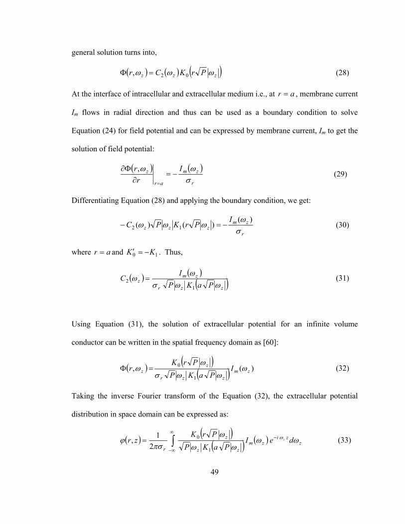
general solution turns into,

( ) ( ) ( )zzz PrKCr ωωω 02, =Φ (28)

At the interface of intracellular and extracellular medium i.e., at ar = , membrane current

Im flows in radial direction and thus can be used as a boundary condition to solve

Equation (24) for field potential and can be expressed by membrane current, Im to get the

solution of field potential:

( ) ( )

r

zm

ar

z Ir

rσωω

−=∂

Φ∂

=

, (29)

Differentiating Equation (28) and applying the boundary condition, we get:

r

zmzzz

IPrKPC

σω

ωωω)(

)()( 12 −=− (30)

where ar = and . Thus, 10 KK −=′

( ) ( )( )zzr

zmz PaKP

IC

ωωσω

ω1

2 = (31)

Using Equation (31), the solution of extracellular potential for an infinite volume

conductor can be written in the spatial frequency domain as [60]:

( ) ( )( ) )(,

1

0zm

zzr

zz I

PaKPPrK

r ωωωσ

ωω =Φ (32)

Taking the inverse Fourier transform of the Equation (32), the extracellular potential

distribution in space domain can be expressed as:

( ) ( )( ) ( )∫

∞

∞−

−= zzi

zmzz

z

rdeI

PaKPPrK

zr z ωωωω

ωπσ

ϕ ω

1

0

21, (33)

49

Equation (33) can be solved by evaluating Bessel’s function, K0 and K1 and discrete

Fourier transform of the membrane current Im. Moreover, the FFT can be applied directly

to Equation (32) to solve the inverse Fourier transform to get φ(r,z). Although this

technique can readily be applied, it is important and handy to derive a straight-forward

and simple expression for the extracellular field potential for better understanding. For

this purpose, we can write the Equation (32) as:

( ) ( ) ( )zmzz IrWr ωωω ⋅=Φ ,, (34)

where, ( ) ( )( )zzr

zz PaKP

PrKrW

ωωσ

ωω

1

0, = (35)

Using the Inverse Fourier Transform and the convolution property on Equation (34) we

find [60,19]:

∫∞

∞−

−== dsszrwsizizrwzr mm ),().()(*),(),(ϕ (36)

where, ‘*’ denotes the convolution operator and w(r,z) is called the weighting function or

the transfer function of the volume conductor. This function is similar to the Green’s

function in Equation (13).

Thus the extracellular potential φ(r, z) can be calculated by convolving the weighting

function h(r, z) with the membrane current im(z). As the radial distance r is increased the

weighting function gets broadened and diminished in amplitude with the effect that the

extracellular potential also is broadened and diminished in amplitude. The weighting

function W in Equation (35) can be redefined by introduction of an approximation to the

50

weighting function. Transmembrane current flows due to the intracellular potential

generated between inside and outside the cell. In human muscle, it is found that the

intracellular potential is a low frequency field, which is less than 10 KHz in frequency

domain. This frequency is equivalent to 2500 cycle/m in spatial frequency domain.

Thus,

2500.22 ππω ≤= kz rad/sec. (37)

The average diameter of human muscle fiber is 55 μm or radius a = 28 μm, which gives:

610.28.2500.2 −≤ πωza

i.e., 44.0≤zaω (38)

Thus the intercellular potential or the membrane current is zero for frequency more than

10 KHz or

0)( ≅zmI ω for 44.0>zaω (39)

Introducing this condition, the weighting function can be approximated as:

( ) ( )( ) 44.0'

'''1,

1

0 ≤= zzz

z

rz afor

aKaraK

rH ωωω

ωσ

ω (40)

where Paa =' and Prr =' . From the behavior of the first-order modified Bessel

function it is found that the value ( ) 1'' 1 →zz aKa ωω for 0' →za ω . For 44.0=zaω ,

( ) 86.0'' 1 =zz aKa ωω . So, ignoring around 14% error it can be assumed that

( ) 1'' 1 ≈zz aKa ωω for 44.0' ≤za ω . This approximation turns the weighting function

as:

51

( ) ( zr

z raKrW ωσ

ω '1, 0≈ ) (41)

or by [60], 22)(

12

),(zr

azrwr +′

=σ

(42)

Thus we finally get the equation for the extracellular potential from Equation (45):

zdzzr

siazr

r

z

m

r′

′−+

= ∫∞

∞− 22 )(

)(2

),(

σσσ

ϕ (43)

The denominator of Equation (43) can be identified as the distance R between the

integration point on the fiber axis and the observation point (Figure

3.2), i.e.,

),0( zP ′=′ ),( zrP =

22 )()( zzrPPR ′−+′=′−= (44)

Thus Equation (46) can be written as:

zdRziazr m

r′

′= ∫

∞

∞−

)(2

),(σ

ϕ (45)

From the line source model, we know that total membrane current for a section of the

fiber can be denoted as a point source. Again, the potential V (p) from a point source i0 at

the point P′ in an infinite volume conductor with conductivity σe is:

Ri

pVe

0

41)(πσ

= (46)

Accordingly, the potential φ(r,z) from a line source on the center of the fiber is:

∫∞

∞−

′′=

Rzdzia

zr m

e

)(.24

1),(π

πσϕ (47)

52

zdRzia m

r′

′= ∫

∞

∞−

)(2σ

(48)

which is same as Equation (45). Thus Equation (45) is equivalent to concentrating the

membrane current as a line source on the center of the fiber.

3.2.1 Analytical Expression of the Transmembrane Current Source The ionic currents in the membrane create electrical potentials inside and outside the

membrane. The transmembrane current is usually considered as the bioelectrical source

of SFAPs. In an approximating description, the current can be represented by a current

tripole along the fiber axis [61]. Alternatively, the shape of the intracellular action

potential (IAP) can be approximated by a synthetic Gaussian curve [62] or a quasi-

continuous function [19, 63]. A discrepancy is always seen between the actual

experimental action potential and the simulated one. One of the origins of discrepancy

might be an erroneous description of the source. Benno K. van Veen et al [64], studied

different sources. First, an analytical description of the intercellular action potential was

used. Furthermore, an experimental intercellular potential, a special experimental surface

action potential, and a measured transmembrane current scaled to their experimental

situation were applied. The results for the experimental IAP were comparable to those

with the analytical IAP. The best agreement between experimental and simulated data

was found for a measured transmembrane current as source, but differences are still

apparent.

The core conductor model applies to a situation where a cylindrical fiber is surrounded by

53

a cylindrical conductor. If a and b are the radius of the muscle fiber and the surrounding

medium respectively, then the resistance per unit length r is given by:

21a

ri

i πσ= (49)

Applying Ohm’s law to a cross section of the fiber (Figure 3.2) gives:

)(.)(

zirdz

zdvii

i −= (50)

Kirchhoff’s law applied to a cross section of the fiber gives:

dz

zdizia i

m)(

)(..2 −=π

2

2 )(2.

dzzvda

i iim

σ=⇒ (51)

Thus the transmembrane current is then calculated as the second derivative of the

intercellular potential. The extracellular action potential from a single muscle fiber is

generated by the depolarized and repolarized transmembrane current [61, 65]. The

extracellular field can be described either by the intercellular potential or the

transmembrane current. Andreassen and Rosenfalck have suggested a mathematical

representation of the intercellular action potential from a precise experimental setup. If

the muscle fiber is parallel to the z axis and the neuromuscular endplate is located at z =

0, then the intracellular potential Vm at a particular point z and time t is given by [65]:

(52) BezAzV zm −= −λλ 3)()(

Where is the profile of the intracellular action potential along the length of the muscle

fiber in the z direction, and A=96, a suitable constant to fit the amplitude of the action

potential and B is the resting potential of –90mV and λ = 1. Thus the transmembrane

mV

54

y im

Figure 3.2: A muscle core conductor model

z

x a

ie

b

55

potential becomes:

9096)( 3 −= −zm ezzV (53)

Modification of Rosenfalck's model by dividing the time scale by two (or λ = 2)

enhanced the peak-to-peak voltage of the transmembrane current (proportional to the

second derivative of the intercellular potential). After this transformation, the simulated

data of Nandedkar and Stalberg [19] matched the experimental data. Their empirical

equation was:

90768)( 23 −= − zm ezzV (54)

However, after this transformation, their intercellular potential had a duration that was

never obtained from experiments [64]. Nevertheless, in this study, Rosenfalck’s

empirical model of intercellular potential will be used to derive the transmembrane

current for the source description of the surface EMG. As described earlier, the

transmembrane current is proportional to the second derivative of the intracellular

potential:

]66[96.

2

)(.

2)(

23

2

2

zzzea

zzVa

zi

zi

mim

+−=

=

−σ∂

∂σ

(55)

where σi is the intracellular conductivity, a is the muscle fiber radius. In the particular

case where the extra-cellular medium is considered infinite with cylindrical anisotropy,

the potential recorded at the surface of the model when a current source travels along the

muscle fiber from the neuromuscular endplate toward the tendons can be approximated

as:

56

( )[ ]

∫ ′′−+

′+′−=

−2

1 22

22

)(

6696*),(z

z

r

z

z

r

i zdzzr

ezzazr

σσσ

σϕ (56)

3.2.2 Effects of Endplate and Tendons At the neuromuscular endplate and muscle fiber endings, the transmembrane current is

constrained by the excitation and extinction principles. To account for the finite

dimensions of muscle fibers and volume conductor distortions, the excitation and the

extinction of the action potential are described as current sources at the neuromuscular

endplate and fiber endings. These compensating current sources are calculated such as

the total current is zero over the active part of the fiber.

(57) ∫ =fiber

m 0dz)t,z(i

The model is described by a fiber with length L and diameter d which is located at a

depth of ye from the surface of the skin. The endplate is located at the center of the fiber

with normal distribution with the innervation zone with a radius of re. Similarly the

tendons, which are located at the two ends of the fiber, are also distributed uniformly

within a radius of rt. The conduction velocity, vc, for each fiber is calculated as a linear

function of the fiber diameter d (μm), by the empirical formula [19]:

)25(05.02.2 −+= dvc (58)

57

3.3 Algorithm Used for SFAP Modeling Following are the steps that are utilized to model a single fiber action potential.

1. Select a sampling frequency, fs usually 25khz.

2. Spatial frequency is deduced from fs using

1000*s

c

fv

z =Δ [Δz is in mm], vc is the conduction velocity of the action potential

in the muscle fiber which is related to the fiber diameter by Equation (58).

3. Thus for a length of ‘L’ fiber, total numbers of points Npt needed for the action

potential [these points are from endplate to one side of tendon] is calculated as

zLNptΔ

=*2

4. Total number of points to generate the action potential in the endplate zone is Nev.

As Plonsy has shown that it takes 5ms for an action potential to generate before it

starts propagating. Thus Nev is calculated as

dt

Nev5

=

where 1000*1

sfdt = (dt in ms) and Nev is rounded towards zero.

5. A coordinate system is chosen with center of the coordinate system located at the

center of the endplate location of the fiber.

6. Recording electrode position is selected as (xe, ye, ze) where the user selects the

position of the electrode.

58

7. The next step in SFAP modeling is to define the action potential source as

transmembrane current im(z). The samples of im(z) is obtained from the analytic

model of intracellular potential derived by Rosenfalk which is

9096)( 3 −= − zm ezzV

where d = diameter of the fiber, σi & σr are the intercellular and radial

conductivities of the muscle

8. Volume conductor calculation: transfer function of volume conductor depends on

the distances between the action potential source location and electrode positions.

Transfer function of the volume conductor is

222 )()(){(

1

esesesz

r zzyyxxh

−±−+−

=

σσ

Action potential recorded at point (xe, ye, ze) is due to two currents flowing from

the endplate towards the tendons in ±z direction. Thus Transfer function for both

side of the endplate needs to be calculated separately.

9. The extracellular potential V1 is calculated as the convolution of the

transmembrane current and the volume conductor transfer function h. The

number of discrete values in h is Npt. The length of discrete convolution is (Npt +

Nev –1). Another way of simulating extra cellular action potential is to take

product of Fast Fourier transform of im (z) & h (x,y,z,t) and taking the inverse FFT

gives the generated extra cellular potential due to the propagation of action

potential.

59

10. Compensation of endplate and tendon effect: generations of action potential at

endplate and extinction at tendons have effects on recorded potential at electrode.

To eliminate these effects, im (z) at each step (from 1 to Npt) are multiplied by h(x,

y, z) and h(x, y, z0 +,Npt Δ z) to get compensation at endplate V2 and at tendon

V3 respectively so the final single fiber action potential (SFAP) is:

132 VVVVsfap −+=

3.4 Results and Discussion In this section, a single fiber action potential model has been described using the finite

length and radially-infinite volume conductor. A single fiber action potential has been

simulated using the techniques described above. The volume conductor is assumed only

conductive and any capacitive or inductive effects of the volume conductor are neglected.

The simulation parameters used for the generation of the single fiber action potential is

shown in Table 3.1. A single fiber action potential and its spectrum are shown in Figure

3.3 for the electrode position at xe = 0, ye = 10mm and ze = 20mm. A 3-D figure of the

action potential is also shown in Figure 3.4. The surface action potential (SFAP) can be

biphasic or triphasic and it depends on the position of the recording electrode as will be

discussed next. The magnitude of a single fiber action potential is in the range of

microvolt and has power signal component not more than 500 Hz. It is of practical as

well as simulation concerns to consider the distance of the source fiber and the recording

electrode and also the effect of the volume conductor on the shape and behavior of the

60

Table 3-1: Simulation parameters used for modeling single fiber action potential

Simulation Parameters Values Used

Sampling frequency

25 KHz

Fiber length

150mm

Fiber diameter (d)

Variable, mainly from 50-80 μm

Endplate location and distribution

At the middle of the fiber with a radius of 5mm

Tendon location and distribution

At the end of the fiber with a radius of 5mm

0.33 Sm-1σz

0.063 Sm-1σr

1.01 Sm-1σi

Conduction velocity

)25(05.02.2 −+= dvc

61

Figure 3.3: An extracellular action potential

62

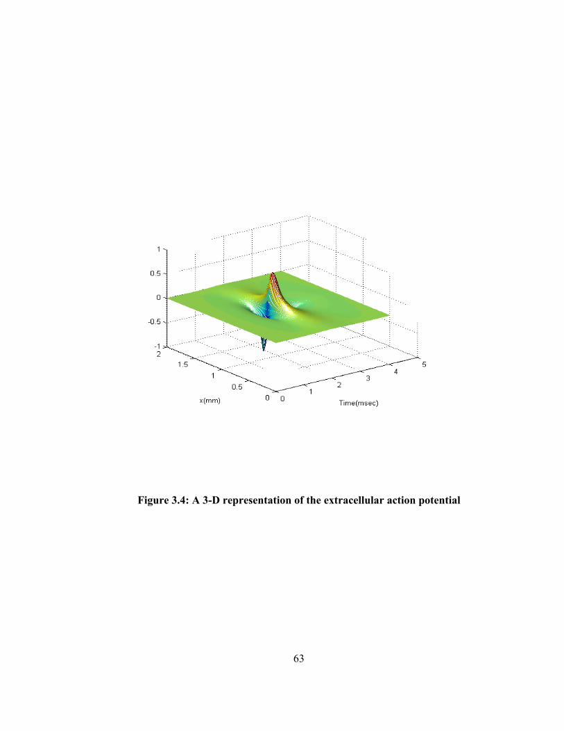
Figure 3.4: A 3-D representation of the extracellular action potential

63

recorded action potential. Both needle electrode and surface (either monopole or

differential or grid electrode) electrode can be simulated using the model. Distances

close to the muscle fibers can only be accomplished through the use of needle and fine

wire electrodes. To see the effect of depth of fiber from the surface, the action potential

is generated for fibers at different depth from the surface where the electrode is placed at

(xe,ze) = (0,10mm) ie, a monopolar electrode 10mm away from the origin which is also

the intersecting point of the endplate zone. At large distances from the muscle fibers, the

effects of the neuromuscular endplate and the fiber endings alter the shape of the

simulated action potential generated at the surface of the muscle fiber. At closer

distances from the muscle fiber, the effects of the volume conductor are minimized since

the filter function of the volume conductor approximates the impulse function. Figure

3.5 shows the impulse response of the volume conductor. Figure 3.6 and Figure 3.7 show

respectively the volume conductor effect on the shape of recorded potential very close to

the fiber located at a distance from 4mm to 10mm and further away from the fiber such

as from 15mm to 30mm from the muscle surface. It is visible that the closer the

recording electrode is, the bigger the amplitude of the action potential and the amplitude

diminishes as the electrode moves further away from the source fiber. Also it is

noticeable that the shape changes from triphasic to biphasic when the fiber-electrode

distance increases. Thus, the recording electrode cannot detect signals after a certain

fiber-electrode distance where the detected signal amplitudes are close to the system

noise level. Figure 3.8 shows the diminishing peak to peak amplitude as fiber electrode

distance increases. At this point of discussion, the model is described without fat and

64

Figure 3.5: Impulse response of the volume conductor

65

Figure 3.6: SFAPs at different depth from the recording surface

66

Figure 3.7: SFAPs at different depth from the recording surface. (ye=15-30mm)

67

Figure 3.8: Effects of fiber to recording electrode distance on the peak to peak amplitude of SFAPs

68

skin and we will see later that this fat and skin will further deteriorate this signal pick up

for the fiber-electrode distance.

EMG signals are not only affected by the fiber-electrode distance or the depth of the fiber

from the surface, but also by the spatial position of the electrode on the surface.

Simulations have been performed for electrodes in different positions along the z-

direction while the fiber is at a constant depth from the surface and xe = 0. Results are

shown in Figure3.9. It has been found that, the further the electrode from the origin of

the recording surface, the smaller the peak to peak of the action potential becomes or in

other words the smaller the energy of the detected signal becomes. But not until a certain

position, does the detected signal amplitude become larger again. Because, the behavior

of the volume conductor transfer function is parabolic with the increasing ze. Moreover,

the switch from biphasic to triphasic in the shape of the action potential is also seen as the

electrode moves away from the origin of the recording surface. Another significant

phenomenon is the shift in the peak of the action potential towards right as it occurs when

the electrode moves further from the origin. Another set of simulation is performed for

the electrodes that are moving further out in the x-direction on the surface while keeping

the depth of the fiber and the z-directional position of the electrode constant. Figure 3.10

illustrates the behavior of this action potential with the changing position of the electrode

in the x-direction.

As expected, the magnitude of the signal diminishes when the electrode is further away

from the origin of the measuring surface. One significant attribute is that the peak of the

69

Figure 3.9: Effects of recording electrode distance in the z-direction on SFAPs

70

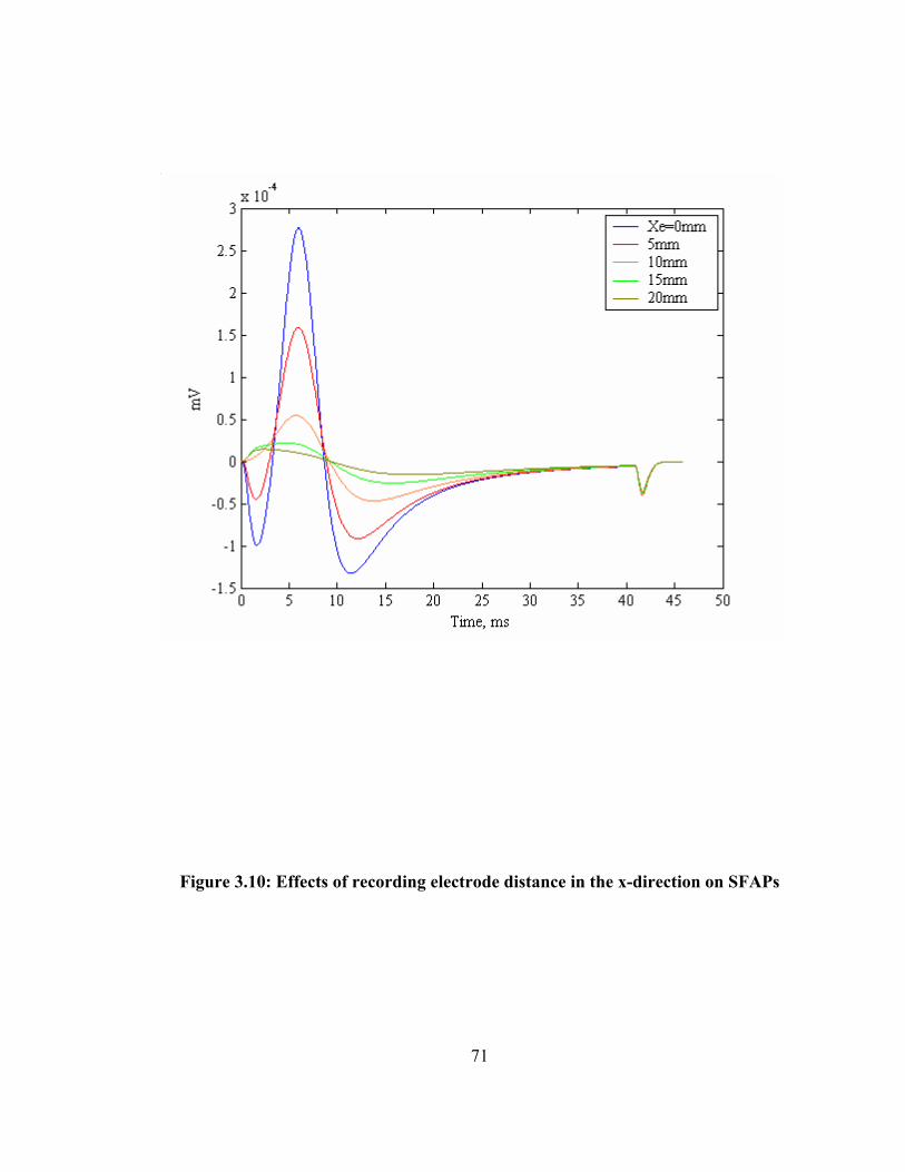
Figure 3.10: Effects of recording electrode distance in the x-direction on SFAPs

71

signals at different xe does not move to the right as was seen in the z-directional change.

Change in phase, that is change from tirphasic to biphasic is also seen when xe increases.

Next phase of simulation has been done to see the effect of fiber diameter in the shape of

recorded action potential. Figure 3.11 depicts the behavior of the peak to peak amplitude

of the SFAP with the increase of fiber diameter. As conduction velocity is linearly

proportionate to the fiber diameter and SFAP is also proportionate to the conduction

velocity, it turns out that peak to peak amplitude varies linearly with the increasing fiber

diameter. Figure 3.12 shows the change in shape and magnitude of the SFAP with the

changing fiber diameter. As stated earlier, peak to peak amplitude increases linearly with

the increase of diameter and also spatially gets tightened with the increase in diameter.

No change in phase is observed due to the change in diameter.

Another important aspect of the surface action potential is of the combination of

electrodes that are used for the EMG recording. As described in chapter one, differential

electrodes are widely used for surface EMG recording. In Figure 3.13, a differential

SFAP is recorded for two electrodes situated at ze = 10 and ze = 20mm with other

parameters kept constant. As shown in Figure 3.14, the differential SFAP is the

difference between the signals recorded at the two electrodes. Interesting feature of this

simulation is that, although the signal in each electrode is biphasic, the differential signal

has turned out to be triphasic or it could be vice versa as well.

72

Figure 3.11: Relationship between peak to peak amplitude of SFAPs with the fiber diameter

73

Figure 3.12: Effects of fiber diameter on SFAPs

74

Figure 3.13: A differential SFAP derived from two monopolar SFAPs

75

3.5 Effect of Fat and Skin Surface EMG is widely used because of its ease of operation and also its usefulness of

acquiring global information from the surface of the muscle. In surface EMG it is

essential to take consideration of the effect of fat and skin on EMG measurement and also

in the modeling of EMG generation. In between muscle fibers and the surface electrodes,

there are two additional tissue layers- fat and skin exist. Though the fat and skin layers

are two different tissues and have different conductivity, both mediums are isotropic.

The effects of highly resistive skin and adipose fat tissues can be simulated to depict the

influence of each physiological parameter on the surface EMG signals. These

subcutaneous tissue layers of fat and skin cause attenuation and spatial widening of the

surface EMG signals. In this section, the volume conductor model that is described in the

previous section will be extended to incorporate fat and skin layers at the top of muscle

tissue and the potential distribution on the top of skin surface will be calculated following

the procedure described in [66] and [67].

Figure 3.14 shows a Four-layer concentric cylindrical model that represents a large inner

cylinder of muscular anisotropic tissue, an intermediate layer of subcutaneous fat and an

outer layer of skin, both as an isotropic medium. The complete muscle structure is

situated in the medium of air. It is assumed that the muscle and the fat tissue has

interface at y = 0, fat and skin has at y = y1 and skin and air at y = y2. To develop the

simulation model the position of muscle fiber is considered parallel along z-axis in the

76

y

Longitudinal

Skin

Air

Fat

Muscle

y

Muscle

Motor Unit

Muscle Fiber

Fat

Skin

Figure 3.14: Four-layer concentric cylindrical model

77

superficial area of muscle. As shown earlier, the potential in the anisotropic muscle

medium can be expressed using the Laplace equation as:

( ) mmuscle izyxz

Pyx

=⎥⎦

⎤⎢⎣

⎡

∂∂

+∂∂

+∂∂ ,,2

2

2

2

2

2ϕ (59)

where r

zPσσ

=

However, for the fat and skin medium, rz σσ = . Thus Laplace equations for fat and skin

layer can be written as:

( ) 0,,2

2

2

2

2

2=⎥

⎦

⎤⎢⎣

⎡

∂∂

+∂∂

+∂∂ zyx

zyx fatϕ (60)

( ) 0,,2

2

2

2

2

2=⎥

⎦

⎤⎢⎣

⎡

∂∂

+∂∂

+∂∂ zyx

zyx skinϕ (61)

In the multiple layer muscle model, current can be considered continuous along y

direction and electric field can be considered continuous along x and z direction at the

interface of two different layers. As shown in Figure 3.14, muscle layer and fat and skin

layer has a boundary at y = 0. Thus at the boundaries, the following conditions hold:

0

)(0 ==

∂∂

=∂

∂

y

muscleymuscle

y

fatfat yy

ϕσ

ϕσ

00 ==

∂∂

=∂

∂

y

muscle

y

fat

xxϕϕ

11 yy

fatfat

yy

skinskin yy

== ∂

∂=

∂∂ ϕ

σϕ

σ

78

11 yy

fat

yy

skin

xx== ∂

∂=

∂∂ ϕϕ

02

=∂

∂

= yy

skin

yϕ (62)

22 yy

air

yy

skin

xx == ∂∂

=∂

∂ ϕϕ

00 ==

∂∂

=∂

∂

y

muscle

y

fat

zzϕϕ

11 yy

fat

yy

skin

zz== ∂

∂=

∂∂ ϕϕ

Taking the two dimensional Fourier transform of the Equations (59), (60) and (61) in x

and z direction, we get:

mzxmusclezx IyPy

=⎥⎦

⎤⎢⎣

⎡−−

∂∂ ),,(22

2

2ωωϕωω (63)

0),,(222

2=⎥

⎦

⎤⎢⎣

⎡−−

∂∂

zxfatzx yy

ωωϕωω (64)

0),,(222

2=⎥

⎦

⎤⎢⎣

⎡−−

∂∂

zxskinzx yy

ωωϕωω (65)

Let 22zxya Pωωω += and 22

zxyi ωωω += , thus the above Equations become:

( ) mzxmuscleya Iyy

=⎥⎦

⎤⎢⎣

⎡−

∂∂ ωωϕω ,,2

2

2 (66)

79

( ) 0,,22

2=⎥

⎦

⎤⎢⎣

⎡−

∂∂

zxfatyi yy

ωωϕω (67)

( ) 0,,22

2=⎥

⎦

⎤⎢⎣

⎡−

∂∂

zxskinyi yy

ωωϕω (68)

Solutions of the above ordinary differential equations can be given as:

(69) yaya yyzxmuscle eBeAy ωωωωϕ −+= 11),,(

(70) yiyi yyzxfat eBeAy ωωωωϕ −+= 22),,(

(71) yiyi yyzxskin eBeAy ωωωωϕ −+= 33),,(

Boundary conditions in the spatial frequency domain can be expressed as:

0

)(0

),,(),,(

==∂

∂=

∂

∂

y

zxmuscleymuscle

y

zxfatfat y

yy

y ωωϕσ

ωωϕσ

( ) ( ) 00,,,,

=== yzxmuscleyzxfat yy ωωϕωωϕ

11

),,(),,(

yy

zxfatfat

yy

zxskinskin y

yy

y

== ∂

∂=

∂∂ ωωϕ

σωωϕ

σ (72)

0),,(

2

=∂

∂

= yy

zxskinskin y

y ωωϕσ

( ) ( ) 22 ,,,, yyzxairyyzxskin yy==

= ωωϕωωϕ

Thus the six coefficients of the above potential solutions can be evaluated from the six

boundary conditions described above. Substitution of these coefficients provides the

80

potential distribution for each layer. At those layers, potential distribution in 2D spatial

frequency domain can be expressed as:

( ) ( ) ( ) ( )( ) ( ) ( )( )( ) ( )sfcyayisfcyayi

sfyicsfyicy

r

zmzx ttRttR

ttRttRe

Iya

,,,,,,,,cosh1cosh1

,0,21

0

ωωαωωαωω

σω

ωωϕ ω

+

−−+++= − (73)

( ) ( ) ( )( ) ( )sfcyayisfcyayi

syiy

r

zmzx ttRttR

te

Iy ya

,,,,,,,,,cosh2

,1,21

0

ωωαωωαω

σω

ωωϕ ω

+= − (74)

( ) ( )( ) ( )sfcyayisfcyayi

y

r

zmzx ttRttR

eI

y ya

,,,,,,,,12

,2,21

0

ωωαωωασω

ωωϕ ω

+= − (75)

where α1 and α2 for a specific value of frequency are,

( ) ( ) ( ){ } ( ){ }[ ]sfyybyasfycsfcyay ttRttRttR ++++= ωωωωωωα tanhcosh1,,,,1 (76)

( ) ( ) ( ){ } ( ){ }[ ]sfyybyasfycsfcyay ttRttRttR −+−−= ωωωωωωα tanhcosh1,,,,2 (77)

fat

skinc

r

fatbrymuscle RandR

σσ

σσ

σσ === ,)( (78)

The above three potential equations will provide the potential distribution on various

region of the multi-layer model. The transfer function of the isotropic layers of fat and

skin can be obtained by dividing the potential at the top of skin by the potential of the

muscle region. In other words, the total transfer function of the intermediate tissue layers

is a cascade of transfer function of anisotropic and isotropic medium. Thus, the transfer

function of the fat and skin layer can be written as:

),0,(),2,(

),(&zx

zxzxskinfat

yH

ωωϕωωϕ

ωω = (79)

81

( ) ( ) ( )( ) ( ) (( ))sfycsfyczxskinfat ttwRttwR

wwH−−+++

=cosh1cosh1

2,& (80)

Where xx fπω 2= and zz fπω 2= are the spatial angular frequency in x (perpendicular to

the fiber) and z (parallel to the fiber) directions, 22zxy ωωω += in the direction of

distance between muscle and electrode, is the conductivity ratio between skin and fat,

and are thickness of fat and skin respectively. The solution of potential distribution

in the space domain can be obtained by taking the two dimensional inverse Fourier

transform. So the final action potential equation will be the inverse Fourier transforms of

the product of H

cR

ft st

fat&skin and Φ (r,ω).

(81) )).,(( &1

skiinfattotal HrF ωϕ Φ= −

3.6 Results The existence of these subcutaneous layers substantially effect the potential profile

generated by an excited muscle fiber. So while using surface electrodes, it is essential to

take consideration of the effect of fat and skin. The effects of subcutaneous fat and skin

on the recorded surface action potential can be analyzed by simulating the potential

distribution at different layers. Figure 3.15 shows the two-dimensional potential

distribution in spatial domain at muscle and at the skin surface from a fiber parallel to

skin at a depth of 2 mm in the muscle. Thickness of fat and skin are assumed to be 3mm

and 1mm respectively. From the comparison of Figure 3.15a and Figure3.15b it can be

stated that the isotropic layers cause attenuation and spatial widening of the signal.

Figure 3.16 shows the characteristics of simulated potential in two-dimensional spatial

82

Figure 3.15: Two dimensional potential distribution in spatial domain at a) muscle and b) at skin

83

Figure 3.16: Two dimensional potential distribution in spatial frequency domain at a) muscle and b) at skin

84

frequency domain. Isotropic fat and skin layer behaves as a low pass filter obstructing to

pass any high frequency component that might be with the generated action potential.

Figure 3.17 shows the comparison of the simulated action potential at muscle and at skin,

which shows clearly the reduction in signal amplitude. The variation in thickness of fat

and skin layer, which is expected among different people, also has effect on the surface

action potential. Figure 3.18 shows the spatial characteristics of the fat and skin layer

transfer function along z direction with the variation of fat thickness, tf form 3 mm to 9

mm while skin thickness is 1mm. The location of the source and other

electrophysiological parameters are kept unchanged. Increase in fat thickness decreases

the cutoff frequency of the low pass volume conductor of the fat and skin layer. Also

seen from the figure is the attenuation that is increased when the fat thickness increased.

3.7 Conclusion In this section, first a single fiber action potential model is described and its analytical

solution for calculating the potential due to the propagating action potential in the fiber is

given. The solution is based on line source model representation of the transmembrane

current. The fiber is assumed parallel to the skin surface although in reality the fiber

might be curve shape. An algorithm to simulate SFAP is given and the effects of

electrode to fiber distance and electrode orientation on the SFAP measurement have been

discussed. In the second part of this chapter, a multi-layer muscle model is described

which includes muscle as well as fat and skin tissues as concentric cylinder. Effect of

these two isotropic mediums on SFAP has been illustrated by generating the potential

85

Figure 3.17: Two-dimensional potential distribution in spatial domain at a) muscle and b) at skin

86

Figure 3.18: Effects of different depth of fat on volume conductor

87

distribution on each medium. Spatial widening and signal attenuation of the SFAP are

the two distinct effects that took place while fat and skin layers are incorporated to the

single fiber action potential model.

88

CHAPTER 4

4. The Motor Neuron Pool Model

4.1 Introduction

There is a huge collection of literature on motor unit physiology and its behavior, which

underscores the variability of motor unit functions during voluntary contraction.

Nonetheless, some principles have emerged that have enabled us to reduce the observed

variability and to examine the mechanisms used by the nervous system in the control of

movement. The central nervous system (CNS) can increase the strength of muscle

contraction by the following:

• Increasing the number of active motor units (i.e., spatial recruitment)

• Increasing the firing rate at which individual motor units fire to optimize the

summated tension generated (i.e., temporal recruitment or rate coding)

The nervous system acts in a complex fashion to control the force generated by our

skeletal muscle by using intricate and systematic procedure of recruiting a number of

motor units and controlling their corresponding firing frequencies. Functionally, the

critical point in the modulation of motor-neuron recruitment and discharge is whether a

given synaptic input generates sufficient current at the soma to recruit the cell. This has

been called the effective synaptic current. During muscle contraction, these effective

89

synaptic current inputs from various sources of nervous system activate the required

motor units. Firing frequency or the frequency of activation of the motor units depends

on the amount of force needed to produce and also dependent on the type of contractions.

The behavior of the motor unit recruitment and the firing frequency is not yet well

understood among the physiologists for various muscle activities. Nevertheless, this

chapter tries to use the current available published rules of motor unit behavior during

constant voluntary contraction. Using these experimental results, a motor unit pool

model has been developed here. A motor neuron pool model predicts the number of

motor units that is recruited from a pool of motor units in a muscle as a function of force

and recruitment threshold and also the pattern of recruiting as the force increases and

remains constant at certain amount of maximum voluntary contraction. The model also

incorporates a firing frequency for each of the motor unit as a function of force as well.

It also limits each of motor unit’s minimum and maximum firing frequency and the

variation in the steady state firing frequency. This model does not predict the recruitment

and firing frequency for fatiguing contraction or the transient behavior of the contraction.

4.2 Motor Unit Distribution

As described in Chapter two, motor units are distributed randomly inside the muscle. In

this chapter, a generic motor unit pool model is developed. If muscle radius, number of

motor units, number of fibers per motor unit, different fiber concentration and fiber

diameter is known, then muscle cross sectional surface is divided into number of small

square areas whose one side is equal to the maximum fiber diameter and total number of

90

areas are equal to total number of fibers in that muscle. Each square area is numbered as

‘1’ or ‘2’ as type-I and type-II fiber respectively. Motor unit center point is randomly

selected inside this cross sectional surface and each motor unit is filled with the required

number of fibers using the equation described in Chapter Two (Equation 4). Figure 4.1

shows the random distribution of the motor units inside a muscle. To analyze the effect

of random distribution of the motor units, compound muscle action potential (CMAP,

discussed in detail in Chapter Six), which is the summation of all the single fiber action

potential in a muscle, is simulated for 50 trials for tibialis anterior muscle. Results show

that, different metrics of CMAP such as peak to peak amplitude, area under the curve and

rise time are differently affected [68]. Table 4.1 shows these metrics as mean and

standard deviation.

As muscle in a motor unit is comprised of many motor units with different diameters,

conduction velocities differ among the muscle fibers in a motor unit. A Gaussian

distribution of the fiber diameter is assumed within a motor unit [44]. The last two

variations factor will not be used in the simulation of the single fiber action potential.

They will be used while motor unit pool as well as motor unit action potential model is

developed.

4.3 Motor Unit Recruitment Recruitment is defined as the successive activation of the motor units with increasing

strength of voluntary muscle contraction. It is a complex process that is under central

91

Figure 4.1: Motor unit distribution inside a muscle with 100 motor units. Type-I are blue and Type-II are red

92

Table 4-1: Simulated CMAP metrics in 50 trials for anterior tibialis muscle

Area under the curve Peak to peak Muscle Rise time (mV) (mV.ms)

Tibialis Anterior

16.19 1.23 1.39 (SD = 0.72) (SD = 0.14) (SD = 0.03)

93

nervous system control. Motor unit recruitment results in a strong efficient muscle

contraction. Patterns of recruitment may differ between various types of motor

activation. But for most of the cases, the recruitment order follows the ‘size principle’,

which states that, smaller motor units will be recruited earlier than the larger motor units

[69, 70, 71]. The size principle refers to alpha motoneuron size relative to its order of

recruitment in a population of motor units that comprises the fundamental organizational

units of a muscle. The soma of alpha motoneurons varies in size, accounting for some of

the differences between type-I and type-II motor unit. Dendritic volume (i.e. number of

excitatory synapses on the neuronal soma) is constant in the two types of alpha

motoneurons. Therefore, smaller type-I motoneurons have relatively greater excitatory

input given their smaller membrane size. In contrast, type-II alpha motoneurons have a

larger membrane, but given the same number of excitatory inputs, they have a lower

excitatory potential. When the muscle is activated initially, the first motor units to be

recruited are small in size and weak in the degree of tension they can generate. Starting

with the smallest motor units, progressively larger units are recruited with increasing

strength of muscle contraction. The result is an orderly addition of sequentially larger

and stronger motor units resulting in a smooth increase in muscle strength. The

recruitment sequence is thus to begin with slow type I motor units, to progress to type II

units that first include moderate type IIA and to end with fast type IIB, which are active

only at relatively high force output.

94

4.3.1 Relative Threshold of the Motor Units An individual motor unit is not active until the level of muscle contraction or the

excitatory input current to the motoneurons is above some minimal level, which is termed

its recruitment threshold. Once a motor unit is active it remains active throughout a

contraction as long as the force created remains above its recruitment threshold. In

accordance with the ‘size principle’, the earlier recruited motor units will have smaller

recruitment threshold and later recruited motor units will have larger threshold. In other

words, smaller motor units need smaller excitatory synaptic input currents than the larger

ones. As suggested by Fuglevand [31], a Poisson distribution of recruitment thresholds

similar to the distribution of motor unit territories adequately reflects the distribution of

thresholds of the motor units and the size principle suggested by Henneman [72]. For

ease of simulation procedure if the recruitment thresholds are assigned in the unit of

percentage of maximal voluntary contraction (MVC), then the exponential equation that

describes the Poisson distribution of recruitment thresholds is as follows [32]:

inR

i e.)ln(

minηη = (82)

where,

ηi is the recruitment threshold of the ith motor unit in units of %MVC

ηmin is the minimum recruitment threshold

R is the ratio of the maximum to minimum recruitment threshold

n is the total number of motor units in the muscle

95

This equation will result in many motor units having a relatively smaller recruitment

threshold and fewer motor units having larger recruitment thresholds. ηmin is arbitrarily

set at 1. Thus any voluntary contraction that produces a total synaptic excitatory current

of Ii, the motor units, which have thresholds greater that Ii will not be activated. The

range or the ratio (R) of recruitment threshold is chosen from published physiological

condition of the muscle and the desired level of voluntary contractions. Figure 4.2 shows

the relative recruitment thresholds for 200 motor units in an arbitrary muscle where the

recruitment threshold range is 60.

4.4 Motor Unit Firing The rate at which motor units produce action potentials during contraction is called the

firing frequency. Motor unit firing or the rate coding is one of the two neural methods

that the nervous system adopts during contraction of the muscle. Motor units have been

found to modulate their firing rates in unison and simultaneously. The firing rate of

motor units is not constant, even during constant force contractions rather it fluctuates.

The firing rates of earlier recruited motor units are greater than those of later recruited

motor units at any given force value [31, 32]. At a force reversal, the firing rates of high

threshold motor units reduce their firing rates before the low threshold motor units. The

fluctuations in a force output of a muscle during a constant-force contraction are caused

by the fluctuations in the firing rates of the motor units. The firing rates of the motor

units decrease during a constant-force isometric contraction. These phenomena suggest

96

Figure 4.2: Relative recruitment thresholds for 200 motor units in an arbitrary muscle

97

that the motor units have a net excitation, which acts through a common input. The most

likely location of this common input is the anterior horn cell. The control to the muscle is

not designed to generate constant-force contractions. Motor unit firing frequency is

characterized by four parameters, namely, minimum firing frequency, peak firing

frequency, force and firing frequency relationship and interpulse interval of the firing

action potentials. In the human body, smaller muscles are generally involved in

performing accurate movements. Such movements require small incremental changes in

force. In contrast, large muscles are generally involved in either producing large forces

or in controlling posture. Large muscles generally do not require finer force gradation to

accomplish their task. Thus, the firing rates of such muscles do not require continual

regulation and do not possess the highly dynamic characteristics seen in smaller muscles.

4.4.1 Minimum Frequency

The motor units with a low threshold in sustained contraction had a low minimum

frequency. The higher the threshold of the unit in sustained contraction, the higher was

its minimum frequency. However, when excited simultaneously, all motor units will

have the same minimum firing frequency irrespective of their threshold excitation. When

the exerted force remains at the threshold level for any motor unit, then that motor unit

will fire in the minimum frequency. For most of the human skeletal muscle the minimum

frequency is found in between 7 to12 Hz.

98

4.4.3 Force-Firing Frequency Relationship

The steady state injected current to the motoneurons and its firing frequency shows a

linear relationship. The gain of this linear relationship is constant for all motor units in a

muscle and independent of motor unit recruitment threshold. Therefore, if the excitation

current exceeds the motor unit threshold, the motor unit firing will be linearly

proportionate to the applied current. However, this frequency for a particular motor unit

does have saturation at its peak frequency (which will be discussed next) from where the

firing frequency does not increase with the increase of the input excitation. The firing

rate can be modeled to increase linearly with the increased force above the recruitment

threshold for a particular motor unit. The equation can be written as follows [31]:

)( ii VCmmffFF η−+= (83)

where, mff = minimum firing frequency

VC = voluntary contraction level in %MVC

ηi is the recruitment threshold of the ith motor unit in units of %MVC

m is the rate at which the firing rate changes with changes in simulated level of

contraction

The value of m can be chosen from the experimental result. Usually the value of m of

0.75 is used to simulate the firing behavior of smaller muscles while a value of 0.25 is

typically used to simulate larger muscles [32].

99

4.4.4 Peak frequency In voluntary contraction, it was found that, after a certain force exerted to a muscle, the

firing frequency does not increase [73]. This saturation in firing frequency is called the

peak or maximum firing frequency. It was also found that earlier recruited motor units

have higher peak frequency than the later recruited motor units. However there are

contradictory findings too where higher threshold units had higher peak frequency than

that of the lower threshold motor units. In the literature, the reported peak frequency is

20-50 Hz, although some researchers even found 100 Hz of peak frequency [74]. The

peak firing rate has been modeled as an inversely proportionate to the recruitment

thresholds [31]:

max(max)max η

ηii RFFFF −= ` (84)

where, FFmax = maximum or peak firing frequency

FFi(max) = peak firing frequency of the first motor unit

R = Difference in peak firing rates between the first and last units recruited

ηi = recruitment threshold for the ith unit

ηmax = recruitment threshold of the highest or the last motor unit 4.4.5 Variation of Inter-pulse-interval (IPI) Interpulse interval (IPI) is the time difference between two successive action potentials.

IPI variation expresses the pulse-to-pulse variation. At constant force, the firing

frequency of a motor unit varies around a mean value with a fixed covariance. This

100

variation varies with age and muscle although for a muscle, this value is constant for all

the motor units in that muscle. Analysis of motor unit discharge trains has indicated that

IPIs resemble a random process with a Gaussian probability distribution function where

the mean and the standard deviation of IPI distributions are related in such a way that the

coefficient of variation remains relatively constant with changes in mean IPI [25, 71, 75,

76, 77, 78, 79]. For a given motor unit, the variation of IPIs was observed to increase

with decreasing firing rate. Equation (83) can be written as:

)(11

1,,ii

jiji VCmmffFFttIPI

η−+==−= − (85)

To simulate the stochastic nature of motoneuron discharge, the IPI predicted by the above

equation can be assumed equivalent to the mean IPI (IPImean). In a normally distributed

population, the deviation from the mean can be expressed as:

σmeanIPIX

X−

= (86)

where, X can be represented as the value of IPI in a train of action potentials with a

standard deviation of σ. Equation (86) can be written as:

IPIXIPIX mean =+= .σ (87)

So the equation (87) becomes:

XIPIttIPI meanjiji .1,, σ+=−= − (88)

i.e, XIPItt meanjiji .1,, σ++= − (89)

As the coefficient of variation (cv) remains constant and

101

μσ

=cv or cv.μσ = , where μ is the mean. Equation (89) becomes

XcvIPIIPItt meanmeanjiji ..1,, ++= − (90)

For each discharge, X has randomly selected from a Gaussian distribution with known

mean and standard deviation using Box-Muller transformation method. It allows us to

transform uniformly distributed random variables, to a new set of random variables with

a Gaussian (or Normal) distribution. The most basic form of the transformation looks

like:

)22cos()1ln(2(1 xxy π−= (91)

)22sin()1ln(2(2 xxy π−= (92)

where x1 and x2 are derived from a uniform distribution of [0 1]. The polar form of the

Box-Muller transformation is both faster and more robust numerically. The algorithmic

description of it is:

1. Generate two uniformly distributed random numbers x1 and x2.

2. Add the square of each of the random numbers until the sum w, is less than or

equal to 1.

3. )/))ln(.2(( www −= .

4. The new Gaussian distributed number is wxy *11= .

102

where random numbers are uniformly distributed in [0,1]. Substituting the value of y1

for X in equation (90) will give the interpulse interval between two successive action

potentials. The equation can be solved recursively to get all the interpulse intervals in a

train of action potentials. Figure 4.3 shows the IPI variation for five different motor units

in a motor unit pool of 200 for a force of 30%MVC.

4.5 Recruitment and Firing Frequency Interaction Considerable anatomical and functional coupling exists among the motor units within a

muscle. This behavior has been studied extensively in animals as well as in humans by

providing external electrical and mechanical stimuli to sensory receptors in the muscle.

The force produced by a muscle during a voluntary contraction depends on the number of

active motor units and the rate at which those units discharge action potentials. This

interaction between recruitment and firing rate provides an apparently simple strategy for

providing smooth force output. Upon recruitment of a new motor unit it may be desirable

to produce an increase in muscle force, which is less than the minimal incremental

contribution of the new motor unit. One way to achieve this goal is to decrease the firing

rates of the motor units, which are already active, so as to diminish their contribution to

the total force output when the new motor unit is recruited. Thus, compensatory

decreases of the firing rates of previously activated motor units will enable the muscle to

produce a smoother force output during recruitment. This effect becomes more important

as the newly recruited motor units provide an increasingly stronger twitch contribution.

103

MU-1

MU-50

MU-100

MU-150

MU-200

Figure 4.3: IPI variation for five different motor units in a motor unit pool of 200 for a force of 30%MVC

104

Thus, in general, motor units recruited later should have a stronger effect on the firing

rates of previously-activated motor units.

The distribution of net synaptic input currents on a motor neuron pool varies as a function

of task. Thus it means that the nervous system determines a priori whether a contraction

will involve shortening or lengthening of a muscle and develops appropriate commands

by varying the pattern of synaptic inputs [24]. The relative contribution of motor unit

recruitment and firing frequency to increase force varies across the working range of the

muscle. Recruitment dominates at low forces, whereas rate coding is more significant at

high forces. For most muscles, the recruitment of motor units continues up to forces of

around 80% of maximum contraction, which means that the remaining 20% is achieved

solely by variation of discharge rate of the motor unit action potential [24, 80, 81, 82, 83].

Thus in the initial force build up, recruitment is the primary process that a muscle

undertakes, whereas, when the force reaches its maximum, discharge rate becomes

important to maintain the force.

105

CHAPTER 5

5. EMG Generation

5.1 Introduction Electromyography (EMG) signal is the summation of all activated motor unit action

potential trains for a given force applied to the muscle. Both single fiber action potential

model and motor neuron pool model are required to be utilized to develop EMG signal

for any type of contraction and force level. Figure 5.1 shows a block diagram of the

EMG generation using the developed models. Motor unit activation and firing pattern

depends on the applied task on the muscle. The tasks can be voluntary isometric (when

tension develops but load does not move and muscle does not shorten), voluntary isotonic

(when muscle shortens and load moves) or electrically elicited contraction when all the

motor units in a muscle are activated synchronously. In this study, only the voluntary

isometric contraction has been considered with a ramp contraction. A motor unit pool

model will predict the number and timing of the motor unit recruitment. A single fiber

action potential model will be utilized to find each activated motor unit action potential,

which, is the summation of all the single fiber action potentials belonging to that motor

unit. Finally the motor unit pool model will predict the firing frequency and the variation

of that frequency for each activated motor unit. Table 5.1 shows the comparison of the

distinct features of this EMG generation model with that of Fuglevand’s model.

106

Motor unit action

potential

Motor unit action

potential train

Σ

.

.

.

.

MU-1

MU-2

MU- n

Figure 5.1: A block diagram of the EMG generation

107

Table 5-1: Comparison of different model parameters of Fuglevand’s model and the model developed in this study.

Modeling Parameters

Fuglevand’s Model

New Model

Modeling of current source

Dipole representation Line source current representation

Multilayer volume conductor model

No Yes

Motor unit type distribution

All same type Distributed as Type-I and Type-II motor units

Muscle excitation Excitation synaptic currents Force as a voluntary contraction

Recruitment range Narrow range (< 50%) and At 60% MVC Broad range (>70%) of

excitation Minimum firing rate Constant for all motor units Increased linearly with

force

ISI variability Constant for all motor units Decreased linearly with force

108

5.2 Methods Using the single fiber action potential model and the motor unit pool model, any human

skeletal muscle can be simulated for EMG generation. In this study, tibialis anterior

muscle will be used for simulation. The size and length of this muscle for average young

person have been collected from [84]. Fiber diameter range and distribution for different

types of fiber and fiber type concentration have been shown in Table 5.2. Number of

motor unit and average number of fiber per motor unit are shown in Table 2.2. All other

required parameters have been adopted from the published journals and applied to the

models that have been developed in this work for EMG generation. As stated earlier, a

ramp voluntary contraction has been applied as a force or excitation for the motor neuron

pool model, which increases to the level of simulated %MVC in one second and stays at

that level for another three seconds without getting fatigued. As it is not the intent to

analyze the effect of fatigue in this dissertation, it is assumed that maximum voluntary

contraction for the simulated period of time will not cause any fatigue in the muscle.

Figure 5.2 shows the ramp force and its constant stay at contraction level. Thus the

developed EMG signal is constant force EMG without consideration of fatigue. The

muscle is simulated for 5%, 10% and for every 10% increment until the maximum

voluntary contraction or 100%MVC. Recruitment level is set at 60%MVC, which means

that all motor units in the muscle will be activated when the contraction reach at 60% of

MVC. In other words, at 60% of MVC the highest threshold motor unit will be recruited.

Thus the range for the recruitment threshold has been set from 1 to 60. The first or the

lowest threshold motor unit will have threshold limit of 1%MVC and the last or the

109

Table 5-2: Different types of fiber and fiber type concentration for both young and old

Young subjects Old subjects

Type-I Type-IIA Type-I Type-IIA

Muscle Type

% d μm

% d μm

% d μm

% d μm

Bicep Brachii

45.0 ±3.0

65.4 ±7.0

31.0 ±3.4

71.5 ±7.0

48.0 ±5.0

58.4 29.0 ±5.0 ±7.0

60.9 ±5.0

Tibialis Anterior

76.0 ±7.0

70.9 22.7 98.9 84.1 71.8 15.2 80.0 ±6.5 ±7.0 ±7.8 ±5.0 ±6.6 ±3.0 ±4.0

110

0

10

20

30

40

50

0 1 2 3

Time, sec

%M

VC

4

0

20

40

60

80

100

120

0 1 2 3

Time, sec

%M

VC

4

Figure 5.2: Simulated applied force to the muscle in %MVC

111

highest threshold motor unit will have threshold limit of 60%MVC. Thus at 50%MVC,

for example, the number of recruited motor units can be found using the Equation (80),

which is calculated as 411 or more than 95% of the total motor units. Figure 5.3 shows

the distribution of the recruited motor units for various input force levels. Both unipolar

and bipolar differential electrode has been simulated. The unipolar electrode is situated

10mm away from the center of neuromuscular endplate of the muscle in the z-direction

on the surface whereas two electrodes 10mm and 20mm away from the endplate were

simulated for differential setting. EMG signal will be simulated and analyzed for the

case when there are no subcutaneous tissues in the model (mimicking needle electrode

EMG) and also when fat and skin layer lies above the muscle tissue (surface EMG).

EMG signals are random in nature. A raw EMG burst cannot be reproduced a second

time by its precise shape. Four parameters of the EMG signal and its spectrum are

usually used to describe the content of EMG signals. These are root mean square value

(RMS) and average rectified value (ARV) for the time varying signal and mean and

median frequency for the power spectrum of the EMG signal. The mean value of the

rectified EMG over a time interval T is defined as average rectified value (ARV) and is

computed as the integral of the rectified EMG over the time interval T divided by T.

ARV relates to information about the area under the selected signal epoch. RMS reflects

the mean power of the signal. The equations used for the calculation of RMS and ARV

are described below:

∫=T

dttxT

RMS0

2 )(1 (93)

112

0

50

100

%MVC

Num

ber o

f m

10 20 30 40 50 60

150

200

250

otor

uni

t…...

Figure 5.3: Distribution of the recruited motor units for various input force levels

113

dttxT

ARVT

.)(1

0∫= (94)

where x(t) is the time varying EMG signal for a time T. The mean frequency estimates

the mean of frequencies in the frequency spectrum of the EMG signal. Median frequency

is defined as the frequency that divides the power spectrum in two regions having the

same amount of power or area under the power spectrum. Following are the equations

used to calculate the mean and median frequency:

∫

∫∞

∞

=

0

0

).(

.).(

dffP

dfffPfmean (95)

Median frequency, fmed when (96) ∫ ∫∞

=med

med

f

f

dffPdffP0

)()(

where P(f) is the spectral density function which is the Fast Fourier Transform (FFT) of a

epoch of the EMG signal x:

(97) 2)]([)( xFFTfP =

In this study, EMG signals are generated and analyzed for the muscle model considering

1) muscle in the absence of fat and skin layer and 2) muscle with subcutaneous fat and

skin layer.

5.3 Results and Discussion EMG signal is the result of many physiological, anatomical and technical factors. To use

the signal effectively, it is first necessary to understand as much as possible the sources

114

of, and the influences on, the signal, which have somewhat been discussed in part in the

previous chapters. Figure 5.4 and Figure 5.5 show respectively the EMG signal for 2

seconds recorded in the monopolar electrode at 20 %MVC when there are no external fat

or skin tissues and when the subcutaneous fat and skin layer exists on the top of the

muscle. These figures show the initial build up of the EMG amplitude as the force in

ramp builds up in one second. Figure 5.6 and Figure 5.7 show the frequency spectrum of

the EMG signal at 20% MVC for the above two cases.

5.3.1 EMG Force Relationship Figure 5.8 illustrates the behavior of the RMS values of the EMG signal generated for

various levels of voluntary contraction. In both cases of the model, the relationship is

curvilinear although until 60% of MVC, EMG RMS magnitude increases linearly with

the increase in input contraction with a slope higher than the slope by which the RMS

amplitude increase from 60% to 100% of MVC. Behavior of average rectified value

(ARV) with force is also similar to that of the RMS of the EMG, which is shown in

Figure 5.9. For first linear increment (0-60%MVC) of the EMG force curve, the

explanation could be as follows: When a motor unit is recruited, it contributes quanta of

force to the muscle contraction. However, the contribution to the EMG signal amplitude

is dependent on the proximity of the detection surfaces of the electrode to the nearest

fibers of the recruited motor unit - the nearer the fibers, the greater the contribution [85].

Thus, the vector representing the incremental increase may increase or decrease the

instantaneous slope of the force-EMG signal relationship. For the second part of the

linearity (60-100%MVC), the EMG amplitude is increased slightly as at 60% MVC all

115

Figure 5.4: EMG signal for 2 seconds recorded in the monopolar electrode at

20 %MVC when there are no external fat or skin tissues

116

Figure 5.5: EMG signal for 2 seconds recorded in the monopolar electrode at

20 %MVC when there are external fat or skin tissues

117

Figure 5.6: EMG signal spectrum recorded in the monopolar electrode at

20 %MVC when there are no external fat or skin tissues

118

Figure 5.7: EMG signal spectrum recorded in the monopolar electrode at 20 %MVC when there are external fat or skin tissues

119

0.1

0.2

0.3

0.4

0.5

0.6

0 20 40 60 80

Force, %MVC

RM

S, m

100

V

(a)

0.1

0.2

0.3

0.4

0.5

0 20 40 60 80 100

Force, %MVC

RM

S, m

V

(b)

Figure 5.8: Relationship between EMG RMS value with the level of force generated. a) in muscle b) on skin

120

(a)

0

0.2

0.4

0.6

0.8

0 20 40 60 80

Force, %MVC

AR

V, m

100

V

(b)

0.1

0.2

0.3

0.4

0.5

0 20 40 60 80

Force, %MVC

AR

V, m

100

V

Figure 5.9: Relationship between EMG ARV with the level of force generated. a) in muscle b) on skin

121

of the motor unit in the muscle were recruited and no other motor units are recruited after

that. Thus the muscle maintains that EMG amplitude and increases by the increased

firing frequency of the recruited motor units due to the increased level of contraction

(motor unit firing frequency increases linearly with the applied force).

Most of the practical observation is that the amplitude of the EMG signal generally increases as

the force and/or contraction velocity of the muscle increases [85]. Figure 5.10 illustrates the

experimental result of the RMS-force relationship of first dorsal interosseous muscle. In fact

this relationship is not rigid for all muscles and there are many factors that cause the

relationship to be nonrigid. As the amplitude of the surface EMG signal is a random variable,

the instantaneous value of the amplitude is not monotonic with respect to the force value.

Furthermore, the estimate of the signal amplitude will vary as a function of force due to

intrinsic anatomical and physiological factors. The detection electrode size and placement

plays an important role on the amplitude of the EMG signal. If the newly recruited motor unit

is located close to the electrode, then the relative increase of the EMG signal will be greater

than the corresponding increase of the force because the new MUAP will contribute more than

an average unit of energy to the EMG signal. However that is not the case when newly

recruited motor unit is located far away from the electrode. The control strategy, described in

terms of firing rate dynamics and recruitment range used by the central nervous system (CNS)

to control different muscles can also affect the EMG-force relationship. In the case of

surface electromyography, cross talk, which is unwanted signal from the neighboring muscles

can contaminate the recorded signal for a specific muscle and thus affect the force EMG

amplitude relationship.

122

Figure 5.10: Experimental result of the RMS-force relationship of first dorsal interosseous muscle [85]

123

4.3.2 Force EMG-Spectral Relationship Figure 5.11 and Figure 5.12 depict the relationship between the contraction force and

mean and median frequency respectively for muscle in the absence of fat and skin.

Figure 5.13 and Figure 5.14 show the relationship between the force and mean and

median frequency respectively when a subcutaneous layer of fat and skin exists. Mean

and median frequency increase linearly until 60%MVC of voluntary contraction. After

that level both mean and median frequency of the simulated EMG fluctuates from the

value at 60%MVC. In practical situations, it is also found that, mean and median

frequency increase with the increase of force.

There are two main properties of the EMG signal that can affect the frequency spectrum:

1) the firing behavior of the motor units, and 2) the shape of the motor unit action

potential (MUAP). The dominant effect of the firing rate of the motor unit is limited to

the frequency neighborhood of the value of the average firing rate (15 to 25 Hz). The

second harmonics of the firing rates are considerably smaller than the first harmonics and

they occur at double the frequency of the first harmonics, where they are overwhelmed

by the energy of the MUAP shapes [85]. The variance of the firing rates will determine

the broadness of the frequency peak representing the firing rate, therefore, any influence

will be limited to the same region. However, the shape of the MUAP is the determining

factor of any change in frequency spectrum of the EMG signal. In chapter three,

different parameters involving the change in MUAP are described. If the isometric

contraction is maintained at constant force, recruitment of the motor units is unlikely to

occur and the average size of the active muscle fibers remains constant. Thus, for a

124

constant-force isometric contraction, the only factors that affect the MUAP are the

conduction velocity and the depolarization zone of the muscle fibers. The conduction

velocity of the muscle fiber is proportional to its diameter. Therefore, muscles with

larger diameter fibers, such as those generally belonging to higher threshold motor units,

will have greater average conduction velocities which, in turn, will shift the frequency

spectrum towards the high frequency range and consequently increase the value of the

median frequency. Both mean and median frequency increases linearly until 60% of

MVC due to the increase in higher threshold motor units and consequently Type-II motor

units recruitment.

The amount of subcutaneous (fatty) tissue between the electrode and the active fibers

determines the amount of spatial filtering to which the signal is subjected. The greater

the thickness of the tissue, the greater is the low-pass filtering. Thus, additional

subcutaneous tissue reduces the value of the median frequency. Simulated results justify

this statement, as the subcutaneous layer reduces the mean and median frequency (some

%) from that of the muscle without fat and skin.

Moreover it is important to note that, electrode location and orientation, electrode

configuration are also important factors influencing the EMG spectrum. The distance

between the electrodes determines the bandwidth of the filtering characteristics of the

differential electrode configuration. Therefore, when the frequency spectrum parameters

are compared among contractions, the same electrode configuration and dimensions must

be used.

125

100

120

140H

z

0

20

40

60

80

0 20 40 60 80 100

Force, %MVC

Mea

n Fr

eq,

Figure 5.11: Relationship between the contraction force and mean and frequency when no fat and skin lies above the muscle

126

50

60

70

eq, H

z

20

30

40

0 20 40 60 80 100

Force, %MVC

Mea

n Fr

Figure 5.12: Relationship between the contraction force and median frequency when no fat and skin lies above the muscle

127

10

30

50

70

0 20 40 60 80 100

Force, %MVC

Med

ian

Freq

,90

110

Hz

Figure 5.13: : Relationship between the contraction force and mean frequency when fat and skin lies above the muscle

128

20

30

40

50

0 20 40 60 80 100

Force, %MVC

Med

ian

Freq

60

70

, Hz

Figure 5.14: Relationship between the contraction force and median frequency when fat and skin lies above the muscle

129

CHAPTER 6

6. Age Related Muscle Remodeling

6.1 Introduction Since impairment of skeletal muscle function leads to disability and loss of

independence, it is important to understand the basic cellular mechanism underlying

muscle dysfunction in the elderly. This knowledge is essential to optimize rehabilitation

and preventive strategies for this population, which by the year of 2030 will increase by

107% for the age group of 65 years and 133% for the age group of 85 years as predicted

by the US Census Bureau [86]. In addition, the percentages of older people with

disabilities in activities of daily living and of older people requiring institutionalization

for disabilities are expected to remain similar to current levels over the next 30 years,

although these statistics vary by ethnicity. This means that the number of people

requiring institutionalization for disabilities will increase substantially. As humans grow

older, their skeletal muscles loose the strength and the capacity to generate force due to

skeletal muscle mass reductions. This is known as sarcopenia [87, 88]. Some

investigators have suggested that the loss of muscle mass is primarily due to the loss in

the number of muscle fibers and to a lesser extent, a reduction in muscle fiber size [89,

90]. Most researchers, however, reported that age related muscle atrophy results from

fiber atrophy rather than a loss of muscle fibers [91,92,93,94,95]. In addition to the

decrease in skeletal muscle mass due to the atrophy of the muscle fibers, the muscles of

130

elderly subjects (65-83 years of age) contain less contractile tissues (Type-II) and more

noncontractile tissues (Type-I) when compared with the skeletal muscle of younger

subjects (26-44 years of age). Consequently, elderly people may lack strength and force

production. In recent reviews, it is also found that the size of Type-I fibers does not

change substantially with age, but Type-II fibers undergo selective atrophy [86,87,96].

In attempt to understand the aging skeletal muscle, this section investigates the effects of

the physiologic changes that occur during aging on computer generated compound

muscle action potentials (CMAPs) of Bicep Brachii muscle group. CMAP are used in the

motor conduction studies. Figure 6.1 shows different parameters of the CMAP wave

shape. These parameters are:

(a) Latency: Latency is the time delay for the CMAP to rise to its peak. Latency can also

be expressed as rise time, which indicates the rise of the CMAP from 5% to 95% of its

peak amplitude.

(b) Amplitude: The amplitude of the evoked motor response carries important

information. Amplitude is dependent on the number of axons that conduct impulses from

the stimulus point to the muscle, the number of functioning motor endplates and muscle

volume. Peak to peak amplitude is often calculated which is the summation of the

positive and negative peaks.

(c) Area under the curve: Area represents a combination of amplitude and duration. It

reflects the number and synchrony of the muscle fibers activated. A prolongation of the

duration can cause a decrease in the amplitude and may be misinterpreted as a conduction

block. Area under the curve is calculated as total area of the CMAP on the time scale.

131

CHAPTER 1 TIME, MS Rise

time

95% of peak Peak

to peak 5% of peak

Figure 6.1: Different parameters of the CMAP wave shape

132

(d) Duration: The duration reflects the synchrony of individual muscle fiber discharges.

If there is a significant difference in the conduction velocity among nerve fibers, the

duration will be prolonged. Mean frequency is also used as a CMAP parameter instead

of duration, which describes the mean of the frequency content in the CMAP spectrum.

6.1.1 Clinical Importance of CMAP Parameters Amplitude: Some neuromuscular disease such as axonal neuropathies, which affect

repiratory function may cause a reduction in the amplitude of the CMAP. Therefore

quantification of amplitude of the CMAP is sometimes more relevant than measuring the

phrenic nerve conduction. Area under the action potential will also be used instead of

amplitude only.

Duration and latency: Duration in the measured CMAP can indicate the muscle slowing

or nerve conduction block. In the nerve conduction of thener muscle, it is found that

thener muscle with degenerative joint disease (DJD) in the hand of elderly people shows

larger duration in the CMAP than those of healthy hand of the elderly.

The nonlinear behavior of the physiologic changes during aging is adapted from the work

of Robert Schwartz on Sarcopenia and physical performance in old age [97] which is

shown if Figure 6.2. Behavior of CMAPs and its metrics such as peak to peak amplitude,

area under the curve, rise time and mean frequency during aging have been computed and

analyzed. The physiologic data such as the number of motor units in a muscle group,

133

0

20

40

0 20 40 60 80 100

Age, (Years)

Vig

or

60

80

100

120, %

Figure 6.2: Behavior of change in strength during aging process

134

number of fibers per motor unit, diameter, length and percentile concentration of different

types of fiber in a motor unit were adapted from the published clinical data [98, 99].

Hypothesis:

1. Most of the researchers said that type-I fiber diameter does not change

substantially.

2. Almost every researcher agreed that type-II fiber diameter decreases substantially

during aging.

3. Almost every researcher agreed that type-II fiber concentration decreases in old

people.

4. Some researchers said type-I concentration remains same whereas some said it

increases during aging.

5. Some researchers said number of fibers does not change substantially during

aging whereas some said it decreases during aging

6.2 Muscle Simulation and Data Analysis Muscle fiber action potentials and surface electrodes were simulated to describe the

physiological changes that occur during aging. The characteristics of simulated

composite action potentials (CMAPs) metrics for Bicep Brachii muscle group were

investigated. Table 6.1 shows the documented percentile concentration of Type-I and

Type-II fibers and their corresponding diameters for this muscle group for both young

(age 22-44) and old (age 65-83) population for bicep brachii and also for tibialis anterior.

135

Table 6-1: Diameter and fiber type concentration for Bicep Brachii for both young and old

Young subjects Old subjects Type-I Type-IIA Type-I Type-IIA

% d μm

% d μm

% d % d μm μm

45.0±3 65.4±7 31.0±3.4 71.5±7 48.0±5 58.4±5 29.0±7 60.9±5

136

The muscle model consisted of Type-I, Type-IIA and Type-IIB fibers, which were

distributed randomly inside the muscle model. We assumed that Type-IIA and Type-IIB

had same percentile concentration. Fiber diameters were generated randomly using their

corresponding mean and standard deviation values. A linear relationship described in

Equation (57) was used to calculate the conduction velocity for each fiber. Two surface

electrodes, 10 and 20 mm away from the muscle motor point, were simulated to record

the monopolar as well as differential CMAPs at a sampling frequency of 25 KHz.

Simulations for bicep brachii muscle group in young subjects were performed in 50 trials

to investigate the effects of uniform random distribution of the fibers within the cross

section of the muscle model. To observe the effects of physiological changes on the

CMAPs during aging, simulations were also performed when fiber diameter, Type-I and

Type-II fiber concentration and total number of fibers in bicep brachii muscle changed

from the values of young subjects (20 years) to that of elderly subjects (80 years) using

the nonlinear curve of physiological changes described in [97]. In attempt to simulate

this aging behavior, it is required that the aging curve is described by an empirical

equation. For this, the aging curve is fitted using MATLAB (Figure 6.3). First of all, the

aging curve behaves as a sigmoid function as follows:

xey

−+=

11 (98)

The shape of the sigmoid function is shown in Figure 6.3. The coefficients of this

sigmoid function are derived while fitting the curve exactly. The equation that describes

the aging curve is as follows:

137

0

0.25

0.5

0.75

1

-4 -3 -2 -1 0 1 2 3

x

y

4

(a)

(b)

Figure 6.3: a) A sigmoid function, b) Curve fitting of the aging process

138

cbx

cbx

deaeky

+−

+−

++

=11 (99)

where, the coefficients are:

075.00.218.533.104.27

=====

kdcba

6.3 Results CMAPs were simulated for both young and elderly subjects using physiologic data for

Bicep Brachii muscle group. Peak to peak amplitude, area under the curve, rise time, and

mean frequency of these CMAPs have been calculated. Table 6.1 shows the mean and

standard deviation values of these CMAP metrics, which were calculated from 100 trials

for the three different muscles of young subjects for single electrode position.

Figure 6.4 shows the CMAP plots of bicep muscle during aging. The CMAP wave

shapes for young and elderly subjects are shown in this figure for visual comparison.

Figure 6.5 illustrates the changes in the CMAP peak to peak amplitude during simulated

aging. Peak to peak amplitude of the CMAP decreased in the same fashion as the

nonlinear aging curve. Figure 6.6 and figure 6.7 shows the area under the curve and

mean frequency of the CMAP of bicep, which also decreased in the same fashion. Rise

time was calculated as the time for CMAP to increase from 5% to 95% of its positive

139

Table 6-2: CMAP metrics simulated for 50 trials for three different muscles

CGAP Metrics

Bicep Brachii Vastus Leteralis Tibialis Anterior

Peak to Peak Amp (mV)

23.85±0.21 31±0.41 18±0.16

Area under the Curve

(mVms)

2.12±0.04 3.24±0.02 1.68±0.02

Rise Time 1.1±0.01 1.03±0.01 0.93±0.01 (ms)

Mean Frequency 91.80±0.08 84.88±0.07 (Hz)

59.36±0.04

140

-15

-10

-5

00 5 10 15 20

Time, ms

m

5

10

15 young

elderly

V

Figure 6.4: CMAP wave shapes during aging

141

12141618

10 20 30 40 50 60 70 80 90

Age, (Years)

Peak

to p

eak

a 2022242628

mpl

itude

(mV

)

Figure 6.5: CMAP peak to peak amplitude during aging

142

1

1.2

1.4

1.6

10 20 30 40 50 60 70 80 90

Age, (Years)

Are

a un

der c

urve

1.8

2

2.2

, (M

v.m

s)

Figure 6.6: CMAP area under curve during aging

143

80

83

10 20 30 40 50 60 70 80 90

Age, (Years)

Mea

n Fr

86

89

92

95eq

uenc

y, (H

z)

Figure 6.7: CMAP mean frequency during aging

144

1

1.1

1.2

10 20 30 40 50 60 70 80 90

Age, (Years)

Rise

Ti

1.3

1.4

1.5

me

(ms)

Figure 6.8: CMAP rise time during aging

145

peak amplitude. Figure 6.9 shows the rise time of CMAP, which increases, in the

opposite pattern of the nonlinear aging curve during aging.

In the elderly subjects, the simulated CMAPs had reduced amplitude, area under curve

and mean frequency as compared to that of young subjects, whereas rise time, of the

compound action potential were higher in elderly than those of the young population.

These CMAP metrics were investigated when the number of Type-I muscle fiber

increased from the corresponding values of young subjects to those in elderly subjects.

It was found that, peak to peak amplitude decreased with aging. This was expected as

amplitude of CMAP depends on the fiber diameter. With age both Type-I and Type-II

fiber suffer atrophy, which lead to reduction in diameter and size of the fibers. As we

assumed linear conversion of Type-II fiber to Type-I during the aging process, amplitude

decline of CMAP followed the same pattern of the nonlinear aging curve. Area under the

curve is the area under the CMAP plot and therefore it also decreased in the same

fashion.

For the investigated muscle group, rise time increased with age. This result is consistent

with the pathological changes that occur during aging as Type-II fiber, known as fast

twitch fiber, concentration decreases during aging. Mean frequency varies linearly with

the conduction velocity. During aging process, Type-II fiber, which has bigger diameter

than that of Type-I fiber, decreased. As fiber diameter is proportional to conduction

velocity, the mean frequency decreased during the aging process.

146

Figure 6.9: Tibialis Anterior muscle

147

6.3 Conclusion The objectives of this study were to investigate the effects of physiological changes on

the computer generated composite action potentials in the aging skeletal muscles. The

aging process was simulated as the change of fiber diameter, total number of fibers and

Type-I and Type-II fiber concentration changes from the values of young subjects to that

of elderly subjects using the nonlinear physiological changes described by Robert

Schwartz. The computer muscle model designed in this study allowed to simulate this

aging process successfully. CGAPs of elderly subjects produced smaller peak to peak

amplitude, area under the CGAP curve and mean frequency and substantially higher rise

time of the CGAPs than those of young subjects. The results found in this study illustrate

the implications of the physiological changes that occur in the aging skeletal muscles.

6.4 Effects of Aging on EMG Signal Generation In the previous section, the pathological changes that occurred during aging of human

muscles have been described. As CMAP is the summation of all the muscle fiber action

potentials in a muscle group at one sudden instance of muscle excitation, the simulation

for the aging process above did not consider the motor unit function such as recruitment

and firing frequency during aging. However, in voluntary contraction, it is necessary to

consider motor unit remodeling during aging process. The vast bulk of research in this

area has been done on identifying the changes in the morphological [100], physiological

[101], and histochemical [102] properties of the motor unit (MU) with age. Zeynep Erim

148

et al [103] described three novel observations regarding the firing behavior of aged motor

units.

1) Among elderly subjects, there is a decrease in the common fluctuations of firing

frequency i.e. IPI variation that are observed among the firing rates of motor units in the

young.

2) The linear relationship observed between the firing rate and recruitment threshold of

young subjects is also seen in the elderly. In young subjects, at any point in a given

submaximal contraction, earlier recruited motor units have higher firing rates than later-

recruited units. But in aged subjects this dependency of firing rate on recruitment rank is

compromised.

3) The progressive decrease observed in the firing rates of concurrently active motor

units in constant-force contractions in the young is not seen in the aged.

In addition to these findings, EMG of the muscle of elderly people has

decreased average firing rates probably reflecting the slowing of the muscle,

decreased number of motor units or α-motoneurons

a shift in recruitment thresholds toward lower force levels in line with the shift toward

type I fibers, and

multiphasic action potential shapes which indicates the reinnervation process that

takes place during aging.

Taken as a whole, these findings indicate significant age-related modifications in the

control properties of human motor units. Although the number of α-motoneurons

decrease and as a result number of motor units decrease, the muscle fibers belonging to

the deceased motor unit are often reinnervated by one of the existing motor units [86,

149

104]. Therefore, although there is a reduction in the number of motor units, some motor

units specially the low force type-I units become larger. This reorganization probably

impairs the ability of elderly persons to perform finely controlled tasks, including

maintaining steady submaximal forces [24, 105, 106]. The reinervation of denervated

type-II muscle fibers by neighboring type-I motor units has also been implicated in the

increase co-expression of type-I and type-II myosin heavy chain iso-forms observed in

the skeletal muscle of older individuals [86]. In the light of the significant changes in the

properties of the elements of a motor unit, it can be hypothesized that the control aspects

of the motor unit would be modified as an adaptive or compensatory mechanism to

preserve force production. EMG signals from young and elderly are expected to be

significantly different due to pathological changes and changes in motor unit functioning

strategy. In this section, EMG signals will be generated for both young and elderly using

the model described in Chapter Four. The purposes of these simulations are to utilize the

developed EMG model on describing aging effect on the EMG signals and verify the

result with the published data on EMG for both young and old people.

6.5 Methods Tibialis Anterior muscle group has been selected for the simulation of EMG generation

for both the young and the elderly. Figure 6.9 shows the tibialis anterior muscle group

located at the right below the knee and thus an important muscle group for posture and

balance control. Aging people are vulnerable to falling due to the lack of balance control.

Thus Tibialis Anterior muscle has always been an object of interest for the clinicians and

150

gerontologists. The physiological data, such as number of motor units, number of fibers

per motor unit, percentage of fiber types and their diameter for both the young and the

elderly are collected from the published data [47, 84, 107]. Motor unit firing and

recruitment properties for young and old have been adopted from the work of Connelly

D.M et al [108]. The average age group for the young is 20 years and for the elderly it is

80 years. It has been found that, even in aging muscle, recruitment order follows the size

principle during voluntary contractions [47, 109, 110]. The force-firing rate curve is

redrawn from [108] which is shown in Figure 6.10. Minimum firing rate in the elderly

decreased from 8.14 Hz of young to 4.18 Hz. The slope of the linear curve for the young

is 0.3 and for the elderly is 0.27. As stated earlier, variation in the inter pulse interval

(IPI) of the firing frequencies is less in the old than in the young. The covariance of the

IPI variation is estimated as 0.25 for young and 0.20 for elderly [108]. It is estimated in

[111] that about 60% motor neuron die out at the age 80 years and older. Out of these

neurons, type-II motor units are vastly affected. All these physiological changes are

incorporated in the model developed in Chapter Four and applied in Chapter Five. In this

section, simulation has been performed for both young and elderly for 5% to 100% of the

maximum voluntary contraction. Only a monopolar electrode, which is situated 10mm

away from the center of the endplate zone, has been simulated for EMG generation for

both populations. Also in simulation, only muscle with fat and skin has been considered.

151

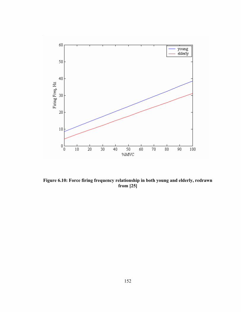
Figure 6.10: Force firing frequency relationship in both young and elderly, redrawn from [25]

152

6.6 Results and Discussion The purpose of these simulations is to verify the proposed model with the published

experimental data and also describe the effect of aging on the EMG signals. Because of

the motor unit distribution effects described in Chapter Five, all simulations have been

performed 10 times. Figure 6.11 shows the generated EMG signal for the elderly along

with the signal for the young at 100% MVC. The frequency spectrum for both these

signals are shown in Figure 6.12 for visual comparison. These figures show that, for

elderly, the EMG signal has less high frequency contents than that of young, mainly

because elderly has fewer fast type-II fibers, which has smaller duration of the action

potential than the type-I. On the other hand, in the EMG of elderly, the magnitude of the

lower frequency contents in the range of 30-40Hz is larger than that of the young. The

muscles of elderly has more type-I motor units of bigger size due to the re-enervation of

the muscle fibers, which fires more frequently than the type-II motor units that is seen in

larger amount in the muscle of young. Thus the magnitude of the frequency content in

the range of 30-40 Hz, which is the average peak firing frequency of type-I motor units,

is higher in the tibialis anterior muscle of elderly.

Force-EMG relationship of the anterior tibialis muscle of elderly is also similar to that of

young, although the slope of this linear force EMG behavior is bigger in the muscles of

young than that of elderly. Figure 6.13 depicts this behavior. This behavior is expected

as during aging, muscle fibers are lost mostly of type-II, which are bigger size than that

of type-I and which produces larger force. Figure 6.14 shows the comparison of different

153

(a)

(b)

Figure 6.11: Generated EMG signals for a) young and b) elderly at 100% MVC

154

(a)

(b)

Figure 6.12: Generated EMG signal spectrum for a) young and b) elderly at 100% MVC

155

0

0.4

0.8

0 20 40 60 80

Force, %MVC

Nor

mal

ized

EM

1.2

1.6

G R

MS…

..

Elderly

Young

Linear(Young)Linear(Elderly)

Figure 6.13: Normalized EMG-force relationship for both young and elderly in tibialis anterior muscle

156

time variable parameters of EMG between young and elderly tibialis muscle. Mean and

median frequency of the EMG signals for both young and elderly are compared in Figure

6.15.

To verify the simulation results, experimental work of Yamada et al [112] on young and

elderly is adopted. Although the exact experimental parameters were not known, the

different physiological parameters for young (20 year old) and elderly (80 year old) are

for the average young and old subjects that were adopted from the published data

described in this chapter and the earlier chapters. Figure 6.16 illustrates the simulated

average rectified value (ARV) and the experimental value for young and elderly subjects

respectively at the maximum voluntary contraction. Comparison and statistical analysis

shows that simulated and experimental results are not significantly different ( 05.0<p ,

two tailed, paired). Similarly, median frequency for both young and elderly are

compared in Figure 6.17 for simulated and experimental results. These results also show

that there is no significant difference ( 05.0<p ) between simulated and the experimental

results.

157

(a)

(b)

Figure 6.14: Comparison of a) ARV and b) RMS of the EMG for young and elderly at 50% MVC

0

100

200

300

400

500

uV

Young

Elderly

0

100

200

300

400

500

uV

Young

Elderly

158

(a)

(b)

Figure 6.15: Comparison of a) mean and b) median frequency of the EMG for young and elderly at 50% MVC

0

10

20

30

40

50

60

70

Hz Young

Elderly

0

10

20

30

40

50

60

Hz Young

Elderly

159

(a)

(b)

Figure 6.16: Comparison of ARV of the simulated and experimental EMG of a) young and b) elderly at 100% MVC

350

375

400

425

450

uV

Simulated

Experimental

100

200

300

400

uV

SimulatedExperimental

160

(a)

30

40

50

60

70

80

Hz Simulated

Experimental

(b)

Figure 6.17: Figure 6.17: Comparison of a) median frequency of the simulated and experimental EMG of a) young and b) elderly at 100% MVC

20

30

40

50

60

70

Hz Simulated

Experimental

161

CHAPTER 7

7. Conclusion and Recommendations For Future Work

7.1 Conclusion

An EMG generation algorithm has been developed in this study using two separate

models. The first model describes an extracellular single fiber action potential

calculation and thus motor unit action potential, which is the summation of all the single

fiber action potential in a motor unit. The second model is a motor neuron pool model

which is a mathemetical description of brain muscle interaction. This model describes

the nature of motor unit recruitment and their discharge rate during contraction.

Although these two models were not necessarily original in design, the techniques

followed to develop the motor neuron pool model algorithm using the accurate and most

up to date motor unit physiology will facilitate the application of this model in several

areas of biomedical research. One of the application of this EMG generation model has

been shown in remodeling of human muscle during aging.

Difference between most of the single fiber action potential generation technique lie in

the representation of the membrane current in different mathemetical forms. In this

study, line source model which considers the transmembrane current as discrete point

sources along the axis of the muscle fiber for a finite fiber was utilized to derive the

162

analytical solution of extracellular action potential. The effects of anisotropic muscle

volume conductor were investigated for fibers located in different distances from the

recording surface. These findings show that, muscle volume conductor attenuate and can

also shift the phase of the recorded potential. Moreover different electrode orientations

have been simulated to analyze their effects on extracellular action potentials. A

multilayer model, which includes fat and skin at the top of the muscle, described by

Farina [66], was also incorporated in the model of single fiber action potential. These

isotropic mediums act as low pass filter and cause further attenuation of the signal that

was recorded at the muscle with the increasing fat and skin layer. This single fiber model

readily provides the motor unit action potential, which is the summation of all the muscle

fiber action potentials innervated by the motor unit.

Motor units are mostly two types: type-I and type-II and they have structural and

functional differences. In the motor unit pool model, these two types of motor units are

distributed randomly inside a hypothetical muscle and each of them were assigned a

motor unit diameter and total number of fibers innervated, based on some rules from the

published experimental findings. The percentage of different types of motor units in a

muscle differ from muscle to muscle and this difference depends on the functionality of a

specific muscle. Some rules have been reported in the earlier work about the recruitment

order of motor units and the discharge behavior and pattern of the recruited motor units.

Recent experimental findings validate some of the earlier concept and at the same time

invalidate some of the hypothesis regarding motor unit physiology that were used in the

EMG simulation by some researchers. In this study, a unique algorithm has been

163

presented which incorporates motor units as two different types of motor units rather than

assigning the same diameter for all the motor unit fibers that was used in the earlier EMG

simulation. Excitation input currents to the population of motoneurons are simulated in

the form of voluntary isometric contraction to the muscle, and all the muscle input output

relationships are described in the form of voluntary contraction as input and generated

EMG signals as output. Simulation was performed for the tibialis anterior muscle to

generate EMG signal when the input contraction is increased linearly until the simulated

level of contraction in one second and stayed in that contraction level for remaining three

seconds without fatigue. Temporal and spectral behavior of simulated EMG signals for

various input forces were investigated. The experimental finding of the force-EMG

magnitude (RMS and ARV) relation is linear for most of the muscle atleast until 80% of

maximum voluntary contraction (MVC). Similar results were also found in the

simulation results which showed the linear force-EMG relation until the highest

recruitment threshold level that was set 60% MVC for this simulation. Thus this

simulation supports the agreement between the researchers that recruitment thresholds are

spread in a broader range of muscle contraction. Mean and median frequency were also

found increasing with the increasing force although there is not unique relationship

between them. These results are also in agreement with the experimental findings. All

these simulation results suggest that overall, the model produces simulated EMG signals

which closely resemble the real signals.

The utility of an EMG signal model is dependent on the degree of rigor and detail it

possesses. As the model developed in this study is based on recently found physiological

164

behavior, it will be useful to address many neuropathological situations that undergo

subtle pathological changes. One of the major pathological changes is seen in the muscle

of elderly people. Thus the developed model was utilized to address these changes and

their effects on the EMG signals. Tibialis anterior muscle was selected for the simulation

of both young and elderly muscle using the published pathological data for both groups.

Simulation showed significant changes between temporal and spectral parameters of the

EMG signal of young and elderly. The results were verified with the published

experimental data for both population. An aging process model was also developed in

this study, which describes the pattern of changes in the compound muscle action

potential (CMAP) wave shape and different metrics of CMAP during aging.

7.2 Future Recommendations

EMG signal in this study was developed for isometric voluntary contraction in which,

muscle length does not change with the contraction. There are not enough data available

about the physiological behavior of the muscle when the length of the muscle changes.

Moreover, very little is known about the motor unit recruitment and firing rate in the high

level of tension to the muscle. These information are necessary to model the EMG

generation technique for its general use.

Recorded EMG signals are decomposed in its constituent parts to analyze the signals.

Many researches are underway to develop techniques to decompose the EMG signals.

The EMG model developed in this study provides the expected output signal for various

165

input force to the muscle thus can be easily employed to assess the qualitative and

quantitative reliability of the decomposition techniques.

In this study only one application has been shown of this EMG model. Several other

neuromuscular conditions such as muscle fatigue, Parkinson desease, Cerebral Palsy and

many others can easily be modeled using the model described in this dissertation.

The EMG model described here can also be improved by modeling the single fiber action

potential for actual shape of the muscle rather than considering all fibers parallel to the

surface of the muscle.

166

REFERENCES

167

[1] G. A. Bekey, C Chang, J Perry, M.M. Hoffer,”Pattern recognition of multiple

EMG signals applied to the description of human gait,” Proceedings of IEEE, 65:

674-689, 1977.

[2] Boisset S, Matson MS, “Quantitative Relationship Between Surface EMG and

Intramuscular Electromyographic Activity in Voluntary Movement,” Amer J Phys

Med, 51: 285-295, 1972.

[3] S. Boisset, F Goubel, “Integrated electromygraphy activity and muscle work,” J

Applied Physiol, 35:695-702, 1972.

[4] R. Plonsey, “The active fiber in a volume conductor,” IEEE Trans Biomed Eng,

21:371-381, 1974

[5] DiFabio PP, “Reliability of Computerized Surface Electromyography for

Determining the Onset of Muscular Activity,” Physical Therapy, 67:43-48, 1987.

[6] Lorente de No, “A Study of Nerve Physiology,” Studies from the Rockefeller

Institute for Medical Research, 132:384-477, 1947.

[7] Binder M.D and Mendell L.M., ‘The Segmental Motor System”, Oxford, UK:

Oxford Univ. Press, 1990.

[8] Burke R.E., “Motor units: anatomy, physiology and functional organization. In:

Handbook of Physiology. The Nervous System, Motor Control. Bethesda,

MD:Am. Physiological Society, sect.1, vol.II, part 1, pp. 345-422, 1981.

[9] Adam L, Datta A.K., Guz A., “Synchronization of motor unit firing during

different respiratory and postural tasks in human sternocleidomastoid muscle: J

Physiol (Land), 413: 213-231, 1989.

168

[10] Adrian E.D., Bronk D.W., “The discharge of impulses in motor nerve fibers, Part-

II. The frequency of discharge in reflex and voluntary contractions”, J. Physiol

(land), 67:119-151, 1929.

[11] M.B.I. Raez, M.S. Hussain and F. Mohd-Yasin, “Techniques of EMG signal

analysis: detection, processing, classification and applications”, Biol. Proced.

Online, 8:11-35, 2006.

[12] Lapatki BG, Van Dijk JP, Jonas IE, Zwarts MJ, Stegeman DF, “A thin, flexible

multielectrode grid for high density surface EMG”, Journal Appl. Physiol.,

96:327-336, 2004.

[13] Mohammed Ferdjallah, Jacqueline J. Wertsch, Mohammad A. Ahad, Gulapar

Phongsamart and Kevin C. McGill, “Nerve Conduction Topography in Geriatric

Hand Assessment,” Journal of Rehabilitation Research and Development, vol. 42,

no. 6, pp 1-7, 2005.

[14] Mohammad A. Ahad, Abdullah Al Zaman, Mohammed Ferdjalllah and Gerald F.

Harris, “Multichannel Grid Electrode Interface for EMG Mapping,” Proc. in IEEE

Midwest Symp. on Circuits and Systems, Cincinnati, OH, 2005, pp. 1770-1773,

2005

[15] Plonsey R, “Actions Potentials Sources and their Volume Conductor Fields,”

Proceedings of the IEEE, 65: 601-611, 1977.

[16] Plonsey R, “The Active Fiber in a Volume Conductor,” IEEE Trans Biomed Eng,

vol. 21, pp. 371-381, 1974.

[17] Rosenfalck P, “Intra- and Extracellular Potential Fields of Active Nerve and

Muscle Fibers,” Acta Physiol. Scan., suppl. 321, 1969

169

[18] Andreassen S, Rosenfalck A, “Ralationship of Intracellular and Extracellular

Action Potentials of Skeletal Muscle Fibers,” CRC Crit Rev. in Bioengineering,

6:267-306, 1981.

[19] Nandedkar SD, Stalberg E, “Simulation of Single Muscle Fiber action Potentials,”

Med Biol Eng Computing, vol. 21, pp. 158-165, 1983.

[20] Gootzen THJM, Stegeman DF, Van Oosterom A, “Finite Limb Dimensions and

Finite Muscle Length in a Model for the Generation of Electromyographic

Signals,” Electroenceph Clin Neurophysiol, vol. 81:152-162, 1991.

[21] Merletti R, Conte LL, Avignone E, Guglielminotti P, “Modeling of Surface

Myoelectric Signals – Part I: Model Implementation,” IEEE Trans Biomed Eng,

46: 810-820, 1999.

[22] Farina D, Merletti R, “A Novel Approach for Precise Simualtion of the EMG

Signal Detected by Surface Electrode,” IEEE Trans Biomed Eng, 48:637-646,

2001.

[23] Burke, R.E., “Motor units: anatomy, physiology, and functional organization. In:”

Brookhart, J.M., Mountcastle, V.B.. Brooks. V.B.. Geiger, S.R., eds. Handbook of

Phvsiologv. Bethesda, MD: American Physiological Society. 345-422, 1981.

[24] Enoka, R.M., “Morphologicai features and activation patterns of motor units”,

Journal of Clinical Neurophysiolo,oy, 12, 53 8-559, 1995

[25] Henneman, E., & Mendell, L.M., “Functional organization of the motoneuron pool

and its inputs. In J.M Brookhart, V.V. Mountcatle (Eds.) Handbook of Phyiology:

Section 1 The Nevous System (pp 423-507) Berthesda, Maryland, American

Physiological Society, 1981.

170

[26] Heckman, C.J., & Binder, M.D., Computer simulation of the steady-state input-

output function of the cat medial gastrocnernius motor-neuron pool. Journal of

Neurophvsiology, 65,952-967, 1991

[27] Kemell, D., & Hultborn, H., “Synaptic effects on recruitrnent gain: a mechanism

of importance for the input-output relations of motoneurone pools”, Brain

Research. 507, 176- 179

[28] Bernardi, M., Solomonow, M., Nguyen, G., Smith, A., & Baratta, R.(1996).Motor

unit recruitment strategy changes with skill acquisition. European Journal of

Applied Physiol., 74:52-59, 1996.

[29] Enoka R.M, Neural adaptations with chronic physical activity. Journal of

Biomechanics. 30, (5),447-455, 1997.

[30] Sale GD, Neural adaptation to resistance training. Medicine in Science and, Sports

and Exercise, 20, (5), s 135- 145,. 1988

[31] Fuglevand A.J., Winter D.A., Patla A.E., “Models of recruitment and rate coding

organization in motor unit pool”, J. Neurophysiol., 70:2470-2488, 1993

[32] Stashuk D.W., “Simulation of electromyographic signal”, J. Electromyogr.

Kinesil., 3:157-173, 1993.

[33] Zajac, F.E. “Muscle and tendon: properties, models, scaling, and application to

biomechanics and motor control”, Critical Reviews in Biomedical Engineering, -

17, (4), 359-411, 1989

[34] Kernell,D., “The adaptation and the relation between discharge frequency and

current strength of cat lumbosacral motoneurons stimulated by long-lasting

injected currents.”, Acta Physiol. Scand., 65:65-73, 1965.

171

[35] Stein R.B., French A.S., Mannard A. and Yemm R. “New methods for analyzing

motor function in man and animals”, Brain Res, 40:187-192, 1972

[36] Goldberg L.J., and Derfler B., “Relationship among recruitment order, spike

amplitude and twirch tension of single motor units in human masseter”, J.

Neurophysiol., 40:879-890, 1977.

[37] Harrison, P.J., “The relationship between the distribution of motor unit mechanical

properties and the force due t recruitment and to rate coding for the generation of

muscle force”, Brain Res. 264: 311-315, 1983.

[38] Pan Z.S., Zhang Y., Parker P.A., “Motor unit power spectrum and firing rate”,

Med. Biol. Eng. Comput., 27:14-18, 1989.

[39] Martini R, “Anatomy Physiology”, Prentice Hall Inc, 2000

[40] http://www.bergen.org/ACADEMY/Bio/molbio/AAMB5_Lesson/STRIATEDMU

SC/MusclePage1.html

[41] Buchthal F., Guld C. and Rosenfalck P., “Multielectrode study of the territory of a

motor unit”, Acta Physiol. Scand., 39:83-104, 1957.

[42] Gath I., Stalberg E., “On the measurement of fiber density in human muscles”,

Electroenceph. Clin. Neurophysiol., 54:699-706, 1982.

[43] Lexell J., Taylor C.C., and Sjostrom M., “What is the cause of the ageing

atrophy?”, J. Neurol. Sci. 84:275-294, 1988.

[44] Duchene J. and Hogrel J., “A model of EMG generation”, IEEE Trans. On

Biomed. Engg., 47:192-201, 2000.

172

[45] Lange F, Van Weerden TW, and Van Der Hoeven JH, “A new surface

electromyography analysis method to determine spread of muscle fiber conduction

velocities”, J Appl Physiol 93: 759-764, 2002

[46] C. S. Klein, G. D. Marsh, R. J. Petrella, “Muscle Fiber Number in the Biceps

Brachii Muscle of Young and Old Men,” Muscle & Nerve, vol. 28, pp. 62-68,

2003.

[47] Porter M.M., Stuart S., Lexell J., “Capilary supply of the tibialis anterior muscle in

young and healty and moderately active men and women”, J. appl. Phyisiol.

92:1451-1457, 2002.

[48] Gordon T, Pattullo M.C., “Plasticity of muscle fiber and motor unit types”,

Holloszy JO, ed, Exercise and sport sciences reviews. Vol. 21. Baltimore:

Williams & Wilkins, pp. 331-362, 1993

[49] Enoka R.M., Fuglevand A. J., “Motor unit physiology: some unresolved issues”,

Muscle Nerve, 34:4-17, 2001.

[50] Fordon D.A., Enoka R. M., Stuart D. G., “Motor unit force potentiation in adult

cats during a standard fatigue test”, J. Physiol. (Lond), 421:569-582, 1990.

[51] Kanda K., Hashizume K., “Factors causing difference in force output among motor

units in the rat medial gastrocnemius muscle”, J. Physiol. (Lond), 448:677-695,

1992.

[52] Totosy de Zepetnek J., Zung H.V., Erdebil S., Gordon T., “Innervation ratio is an

important determinant of force in normal and reinnervated rat tibialis anterior

muscles”, J. Neuro-physiol., 67:1385-1403, 1992.

[53] http://en.wikipedia.org/wiki/Action_potential

173

[54] http://www.fortunecity.com/greenfield/buzzard/387/actionpot.htm

[55] Albers BA, Rutten WL, DE Jonge W, “Microscopic and macroscopic volume

conduction in skeletal muscle tissue: Applied to simulation of single muscle fiber

action potentials”, Medical & Biological Engineering Computing, 26:605-610,

1988

[56] Brown WF, Strong MJ, Snow R, “Methods of estimiating numbers of motor units

in biceps brachialis muscles and losses of motor unit with aging”, Muscle &

Nerve, 11:423-432, 1988

[57] Barker AT, Brown BH, Freston IL, “Modeling of an active nerve fiber in a finite

volume conductor and its application to the calculation of surface action

potentials”, IEEE Trans on Biomedical Engineering, 26:53-56, 1979.

[58] Gath I, Stalberg E, “On the volume conduction in human skeletal muscle: In situ

measurements”, Electro-encephalgraphy & Clinical Neurophysiology, 43:106-110,

1977

[59] Gath I, Stalberg E, “The calculated radial decline of the extracellular action

potential compared with in situ measurements in the human brachialis biceps

muscle”, Electro-encephalgraphy & Clinical Neurophysiology, 44:547-552, 1978

[60] Andreassen S, Rosenfalck A, “Ralationship of Intracellular and Extracellular

Action Potentials of Skeletal Muscle Fibers,” CRC Critical Reviews in

Bioengineering, vol. 6, pp. 267-306, 1981.

[61] Rosenfalck P, “Intra- and Extracellular Potential Fields of Active Nerve and

Muscle Fibers,” Acta Physiol. Scan., suppl. 321, 1969

174

[62] Fleisher, S. M., “Comparative analysis of modelled extracellular potentials”, Med.

& Biol. Eng. & Comput. 22:440-447, 1984

[63] Albers, B A., Rutten WLC., Wallinga-de Jonge W. and Boom HBK, “Microscopic

and macroscopic volume conduction in skeletal muscle tissue, applied to

simulation of single fibre action potentials”, Med. & Bio. Eng. & Comput.

26:605-610, 1988.

[64] Benno K. van Veen, Wolters H, Wallinga W, Rutten WLC,and Boom HBK, “The

bioelectrical source in computing single muscle fiber action potentials”, Journal of

Biophysics, 64:1492-1498, 1993

[65] R. Plonsey, “Actions potential sources and their volume conductor fields,”

Proceeding of the IEEE, vol. 65, pp. 601-611, 1977

[66] Faina D, Rainoldi A, “Compensation of the Effect of Sub-cutaneous Tissue Layers

on Surface EMG: A Simulation Study,” Medical Engineering and Physics, vol. 22.

pp. 487-496, 1999.

[67] Rahman, MM, “Analysis of 2D spatial filtering of simulated muscle action

potential using grid arrays”, MS thesis, University of Tennessee, 2005.

[68] Mohammad A. Ahad, Jacqueline J. Wertsch and Mohammed Ferdjallah, “Effect of

Motor Unit Distribution on Computer Generated Action Potential” Muscle &

Nerve, 2006; 34:530.

[69] Riek S. and Bawa P. “Recruitment of motor units in human forearm extensor”, J

Neurophysiol., 68:100-108, 1992

175

[70] Zajac F.E., Faden J.S., “ Relationship among recruitment order, axonal conduction

velocity, and muscle unit properties of type-identified motor units in cat plantaris

muscle”, J Neurophysiol., 53:1303:1322, 1985.

[71] Nordstrom M.A., Miles T.A., “Discharge variability and characterization of motor

units in a heterogeneous muscle (Flexor digitorum longus) of cat”, Comp. Neurol,

128:475-498, 1966.

[72] Henneman E., “Functional organization of motoneuron pools: the size principle”,

Integration in the Nervous System, edited by H. Asunuma and V.J. Wilson.

Tokyo: Igaku Shion, pp. 13-25, 1979.

[73] Monster AW, Chan H., “Isometric force production by motor units of extensor

digitorum communis muscle in man”, Journal of Neurophysiol, 40:1432-1443,

1977.

[74] Grimby L, Hannerz K, “Firing rate and recruitment order of toe extensor motor

units in different models of voluntary contraction”, Journal of Physiol (land),

264:865-879, 1977.

[75] Gilchrist J.M., Perrone M., and Ross J., “Dynamical analysis of neuromuscular

transmission jitter”, Muscle Nerve, 18:685-692, 1995.

[76] De Luca C.J., Forrest W.J., “Some properties of motor unit action potential trains

recorded during constant force isometric contractions in man”, Kybernetik,

12:160-168, 1973.

[77] Shiavi R., Negin M., “Stochastic properties of motoneuron activity and the effect

of muscle length”, Biol. Cybern, 19: 231-237, 1975.

176

[78] Clamann H.P., “Statistical analysis of motor unit firing patterns in a human

skeletal muscle”, Biophys. J, 9:1233-1251, 1969.

[79] Lago P. and Jones N.B., “Effect of motor unit firing time statistics on EMG

spectra”, Med. Biol. Eng. Comput., 15:648-655, 1977.

[80] Grimby L, Hannerz K, “Firing rate and recruitment order of toe extensor motor

units in different models of voluntary contraction”, Journal of Physiol (land),

264:865-879, 1977.

[81] Kukulka CG, Clamann HP, “Comparison of the recruitment and discharge

properties of motor units in human brachial biceps and adductor pollicis during

isometirc contraction”, Brain Res, 219:45-55, 1981.

[82] De Luca CJ, LeFever RS, McCue MP, Xenakis AP, “Behavior of human motor

units in different muscles during linearly varying contraction”, Journal of Physiol

(Lond), 329:113-128, 1982.

[83] Kernell D and Sjoholm H., “Recruitment and firing rate modulation of motor unit

tension in a small muscle of the cat’s foot”, 98:57-72, 1975.

[84] Jakobson F, Borg K, Edstrom L, Grimby L, “Use of motor units in relation of

muscle fiber type and size in men”, Muscle & Nerve, 11:1211-1218, 1988.

[85] http://www.health.uottawa.ca/biomech/courses/apa4311/biomec~3.htm#force

[86] G. N. Williams, M. J. Higgins, M. D. Lewek, “Aging skeletal muscle: Physiologic

changes and the effects of training”, Physical Therapy, 82, 62-68, 2002.

[87] M. A. Rogers, W. J. Evans, Changes in Skeletal Muscle with Aging: Effects of

exercise Training, Exerc Sport Sci Rev, 21, 65-102, 1993.

177

[88] W. R. Frontera, V. A. Hughes, R. A. Fielding, Aging of skeletal muscle: A 12 year

longitudinal study, Journal for Applied Physiology, 88, 1321-1326, 2000.

[89] A. C. Hooper, Length, diameter and number of ageing skeletal muscle fibers,

Gerontology, 27, 121-126, 1981.

[90] J. Lexell, C. C. Taylor, M. Sjostrom, What is the cause of the ageing atrophy?

Total number, size and proportion of different fiber types studied in whole Vastus

Lateralis Muscle from 15 to 83 year-old men, Journal of Neurol Sci, 84, 275-294,

1988.

[91] W. F. Brown, M. J. Strong, R. Snow, Methods for estimating numbers of motor

units in biceps-brachialis muscles and losses of motor units with aging, Muscle &

Nerve 11, 423-432, 1988.

[92] J. Lesell , C. C. Taylor, Variability in muscle fiber areas in whole human

Quadriceps Muscle: Effects of increasing age, Journal of Anatomy, 174, 239-249,

1991.

[93] J. A. Kent-Braun, A. V. Ng, K. Young, Skeletal Muscle Contractile and

Noncontractile Components in Young and Older Women and men, Journal for

Applied Physiology, 88, 662-668, 2000.

[94] P. G. Arabadjis, R. R. Heffner, D. R. Jr, Pendergast, “Morphologic and functional

alterations in Aging Rat Muscle”, Journal of Neuropathol Exp Neurol, 49, 600-

609, 1990.

[95] M. Brown, Change in fiber size, not number, in aging skeletal muscle, Age

Ageing, 16, 244-248, 1987.

178

[96] M. M. Porter, A. A. Vandervoort, J. Lexell, “Aging of human muscle: structure,

function and adaptability”, Scand J Med Sci Sports, 5, 129-142, 1995.

[97] R. S. Schwartz, Sarcopenia and physical performance in old age: Introduction,

Muscle and Nerve, supp 5,pp. 10-12, and 1997.

[98] C. S. Klein, G. D. Marsh, R. J. Petrella, Muscle Fiber Number in the Biceps

Brachii Muscle of Young and Old Men, Muscle & Nerve, 28, 62-68, 2003.

[99] G. Goldspink, Malleability of the motor system: A comparative approach, Journal

of Experimental Biology, 115, 375-391, 1985.

[100] Kanda, K., and Hashizume, K. Changes in properties of the medial gastrocnemius

motor units in aging rats. J. Neurophysiol. 61: 737-746, 1989.

[101] Roos, M. R., Rice, C. L., and Vandervoort, A. A. Age-related changes in motor

unit function. Muscle Nerve 20: 679-690, 1997.

[102] Ansved, T., and Larsson, L. Effects of aging on the motor unit. Prog. Neurobiol.

45: 397-458, 1995.

[103] Zeynep Erim, M. Faisal Beg, David T. Burke, and Carlo J. de Luca, “Effects of

Aging on Motor-Unit Control Properties”, J Neurophysiol 82: 2081-2091, 1999.

[104] Campbell M.L, McComas AJ, Petito F., “Physiological changes in ageing

muscles”, Journal of Neurol Neurosurg Psychiatry, 36:174-182, 1973.

[105] Galganski ME, Fuglevand AJ, Enoka RM, “Reduced control of motro output in

human hand muscle of elderly subjects during submaximal contractions”, Journal

of Neurophysiol, 69:2108-2115, 1993.

[106] Keen DA, Yue GH, Enoka RM, “Training-related enhancement in the control of

motor output in elderly humans”, Journal of Applied Physiol, 77:2648-2658, 1994.

179

[107] Jakobson F, Borg K, Edstrom L, Grimby L., “Use of motor units in relation of

muscle fiber type and size in man”, Muscle Nerve, 11:1211-1218, 1988.

[108] Connelly D.M., Rice CL, Roos MR, “Motor unit firing rates and contractile

properties in tibialis anterior of young and old men”, J. applied Physiol, 87:843-

852, 1999.

[109] Sale DG, “Neural adaptation to resistance training”, Med Sci Sports Exerc,

85:319-331, 1988.

[110] Duchateau J, Hainaut K, “Effects of immobilization on contractile properties,

recruitment and firing rates of human motor units”, Journal of Physiol (Lond),

422:55-65, 1990.

[111] McNeil CJ, Doherty TJ, Stashuk DW and Rice CL, “Motor unit number estimates

in the tibialis anterior muscle of young, old, and very old men”, Muscle Nerve,

31:461-467, 2005

[112] Yamada H et al, “Effect of aging on EMG variables during fatiguing isometric

contraction”, Journal Human Ergol, 29:7-14, 2000.

180

VITA Mohammad Abdul Ahad, the son of Late Abdul Munaf and Mrs. Feroza Begum, was

born in Chittagong, Bangladesh. Upon completion of preliminary schooling from St.

Mary’s School, he went to Collegiate School, Chittagong and Chittagong College for

high schooling. He secured 13th and 17th position in the combined merit list in Secondary

School Certificate and Higher Secondary School Certificate Examinations respectively.

He earned his Bachelor degree in Electrical and Electronic Engineering from the

prestigious Bangladesh University of Engineering and Technology (BUET), Dhaka

Bangladesh. He joined the University of Tennessee, Knoxville in Master’s program of

Electrical Engineering in 1999. He continued his higher studies in the same University

and the same department and is going to get his Ph.D. in Summer 2007. He is joining the

Harvard Medical School as a post-doctoral fellow from August 2007.

181