Hysteresis in electric dipole monolayers
31
ELSEVIER Journal of Electrostatics 32 (1994) 183-213 Journal of ELECTROSTATICS Hysteresis in electric dipole monolayers Silvano Cincotti *'a, Mauro Parodi b, Alessandro Chiabrera b Istituto di Elettrotecnica, Universitf~ di Cagliari, piazza D'Armi, 09123 Cagliari, Italy b Dipartimento di Ingegneria Biofisica ed Elettronica, Universit3 di Genova, via Opera Pia lla, 16145 Genova, Italy (Received August 17, 1993; accepted October 28, 1993) Abstract The possibility of hysteretic behaviours in plane monolayers of electric dipoles is investigated. The basic tool for this study is a model where the electric dipoles can rotate around the nodes of a plane rhombic grid and the electric interactions among dipoles are properly simplified (Union Jack approximation). In the ideal case of an infinitely extending monolayer, the model yields analytical solutions both for the spatially periodical equilibrium orientations of dipoles and for their stability under the influence of an external electric field. On this basis, a set of hysteresis cycles dealing with different physical situations is obtained and discussed. Then, the much more realistic and complex case of finite-size dipole monolayers is considered and the hysteresis cycles are obtained by computer calculations. The degree of similarity of these numerical results with the analytical ones of the corresponding infinitely extending monolayers puts into evidence the prediction capabilities of such simple model. 1. Introduction A very important topic in molecular electronics is the study of the behaviour of molecular assemblies. The main efforts of this study are devoted to finding molecular structures that can process information at a molecular scale I-1-4]. Generally speak- ing, two approaches are possible. The first aims at showing that molecules are equivalent to logic gates so as to apply, at microscopic level, the set of methodologies available from circuit theory. The second aims at finding molecular assemblies that can collectively process information. In this case, the main characteristic of the systems is a large number of elementary microstructures with a short-range interac- tion for all of them. Thus, these molecular assemblies can correspond to intrinsic parallel computational machines spatially distributed. * Corresponding author. 0304-3886/94/$07.00 © 1994 Elsevier Science B.V. All rights reserved. SSDI 0304-3886(93)E0041-F
Transcript of Hysteresis in electric dipole monolayers

ELSEVIER Journal of Electrostatics 32 (1994) 183-213
Journal of
ELECTROSTATICS
Hysteresis in electric dipole monolayers
Silvano Cincotti *'a, Mauro Parodi b, Alessandro Chiabrera b
Istituto di Elettrotecnica, Universitf~ di Cagliari, piazza D'Armi, 09123 Cagliari, Italy b Dipartimento di Ingegneria Biofisica ed Elettronica, Universit3 di Genova, via Opera Pia lla, 16145 Genova,
Italy
(Received August 17, 1993; accepted October 28, 1993)
Abstract
The possibility of hysteretic behaviours in plane monolayers of electric dipoles is investigated. The basic tool for this study is a model where the electric dipoles can rotate around the nodes of a plane rhombic grid and the electric interactions among dipoles are properly simplified (Union Jack approximation). In the ideal case of an infinitely extending monolayer, the model yields analytical solutions both for the spatially periodical equilibrium orientations of dipoles and for their stability under the influence of an external electric field. On this basis, a set of hysteresis cycles dealing with different physical situations is obtained and discussed. Then, the much more realistic and complex case of finite-size dipole monolayers is considered and the hysteresis cycles are obtained by computer calculations. The degree of similarity of these numerical results with the analytical ones of the corresponding infinitely extending monolayers puts into evidence the prediction capabilities of such simple model.
1. Introduction
A very important topic in molecular electronics is the study of the behaviour of molecular assemblies. The main efforts of this study are devoted to finding molecular structures that can process information at a molecular scale I-1-4]. Generally speak- ing, two approaches are possible. The first aims at showing that molecules are equivalent to logic gates so as to apply, at microscopic level, the set of methodologies available from circuit theory. The second aims at finding molecular assemblies that can collectively process information. In this case, the main characteristic of the systems is a large number of elementary microstructures with a short-range interac- tion for all of them. Thus, these molecular assemblies can correspond to intrinsic parallel computational machines spatially distributed.
* Corresponding author.
0304-3886/94/$07.00 © 1994 Elsevier Science B.V. All rights reserved. SSDI 0304-3886(93)E0041-F
184 S. Cincotti et al./Journal of Electrostatics 32 (1994) 183-213
Both approaches rely on the set of methods and results achieved by a proper modelling. As an example, considerable efforts have been directed towards an accu- rate characterization of physisorbed monolayers (e.g. lipid monolayers assembled via the Langmuir-Blodgett technique [5]) and chemisorbed monolayers (e.g. activated octadecyl trichlorosilane on glass [6]). In both cases, molecules can be modelled by an electric dipolar head covalently connected to a tail. The dipoles are thought as responsible for the mutual orientations of the heads, while the interactions among the tails are thought as responsible for the film formation [7, 8].
The main objective of this paper is to explore if a monolayer of electric dipoles offers intrinsic "memory" capabilities, due to dipole interactions. This is a prerequisite for the potential use of these monolayers as molecular information processors.
The study of the electrical organization properties of a dipole monolayer when no exogenous electric field is applied was the main objectives of our previous modelling activity [9-11].
The spatially periodical equilibrium configurations that spontaneously originate in an infinitely extending plane monolayer were found by using a continuous model [9] and then two discrete models [10, 11].
Both discrete models consider the dipoles free to rotate in the monolayer plane. The centres of the dipoles are fixed at the nodes of a lattice which is rhombic in the general case [11]. A proper simplification of the interaction mechanism (the so-called Union Jack approximation) leads to obtain the characteristics of the basic periodical equilib- rium configurations and the stability criteria for all the values of the angles of the rhombic lattice [11].
In this work, the effects of an exogenous, uniform electric field in the monolayer plane are assessed. This is done by properly generalizing the Union Jack model. For ease of exposition, the description of the generalization process is followed by a summary of the main results obtained in [11]. The equations for this new model show that the main effect of an exogenous electric field on the above-said infinitely extending lattice is to induce a hysteretic behaviour. Thanks to its overall simplicity, the model enables one to formulate the main results through closed-form (though approximate) expressions. A set of hysteresis cycles, corresponding to different values of the lattice angle and to particular orientations of the electric field, is then described and discussed.
A model that is more closely related to a real monolayer should take into account many other factors. One of them is very general and lies in the finite dimensions of the real monolayer; this factor causes the lack of spatial periodicity of the equilibrium configurations. Another factor stems from other forces experienced by the dipoles, e.g., positional forces due to steric reasons and random forces associated with thermal fluctuation. As to the latter factor, we limit ourselves to observing that the overall simplicity of the model should allow the inclusion of some other kind of force, while maintaining part of the model handiness. Moreover, the energy and stability terms discussed in this paper for the equilibrium configurations may be important to estimate the effects of thermal fluctuation.
The former factor is explicitly taken into account, and the hysteresis cycles in a lattice of finite dimensions are obtained by appropriate computer simulations. Then,

S. Cincotti et al./Journal of Electrostatics 32 (1994) 183- 213 185
11
d
Fig. 1. The rhombic grid.
these cycles are compared with those given by the model for the corresponding infinite lattice. The similarities between the two sets of results make the model a suitable investigation tool also for finite-size lattices.
2. The rhombic lattice
The rhombic mesh-grid shown in Fig. 1 presents the basic elements of the model• Each mesh is defined by the angle ~ between the ~ and r/axes and by the length d of its sides. The variations in y can range between 0 ° and 90 °, without loss of generality. In general, the grid is assumed to extend infinitely in the ~ and r/directions. Each node of the grid is defined either by a pair of integer numbers (i,j) associated with the ~, r/ coordinates or by the position vector r w Choosing the diagonals of the rhombic mesh as orthogonal coordinate system (x, y), r~ can be written as
r 0 = d~o, (1)
where
~i~ = [(~ - j ) ~ / 1 - (i + j)u u21' u = c o s ½r. (2)
Each node (i,j) is the barycentre of a dipole m o that lies in the x, y plane and forms an angle 0ij with the x axis, as shown in Fig. 2. All dipoles have the same modulus #, so

186 S. Cincotti et al./Journal o f Electrostatics 32 (1994) 183-213
Fig. 2. A dipole of the grid.
we can write
cos 0is m i j : [,(mis, ~tliJ = L sin Oij 3 " (3)
The general parameters are d, ?, g and the dielectric permittivity e of the medium. The position of each dipole is defined by r u, and its orientation by 0i s. The electric interaction energy W~ z between two dipoles m o and mk~ can be written in the following form:
w k,_ 1 ( t iS 41W'[riS rkll 3 (mis , mkt > _ 3 ( r i j - - rkt, mi_._j>(ri__Z~ - -- r k l , m u > - - Iris - - rkll 2 '
(4)
where the brackets ( > denote the scalar product. When a dipole m~j interacts with a generic set I o of other dipoles, the resulting
interaction energy W~ i of m~j with these dipoles is
rata E ] i ]
Thus, the energy Wxe associated with a set .o.¢e of interacting dipoles can be written as
2 m,i~_~
When each m o can rotate about its fixed barycenter (i, j) under the influence of all the other dipoles in the grid, Iij should include all the dipoles except m O. As widely shown in [-11], approximate equations for the dipoles' behaviour can be obtained restricting I o to contain only the first eight dipoles surrounding miI (Union J a c k approximation).
We further assume that an exogenous uniform electric field g is present in the plane of the grid. Then, the resulting energy to be considered for the study of the equilibrium

S. Cincotti et al./Journal o f Electrostatics 32 (1994) 183- 213 187
orientations of the dipoles is
W = Wa~- IE, ~, m,~> (7) tn~j ~ .go
and these orientations are the solutions 0ij of the non-linear system of equilibrium equations
0W - - = O. (8)
Generally speaking, the number of Eqs. (8) equals the number of elements of .Y. Taking into account expressions (4)-(8), they can be written in the equivalent form
vi~ - E, d 0 i ~ / = 0, (9)
where
1 ~ 1 { <rij--rk,,m,J>(rrk,)} (10) ~ij ~ ~ m lij I riJ "~ Fkll 3 l'nkl - - 3 iFij--'__- ~i.kl I ~, ij - -
depends on the angles Ou of the set lij. In each equation, then, the number of unknowns is fixed by the size of the set I~ chosen to take into account the interaction of mij with the other dipoles. When I~ is the Union Jack set, such a number is nine.
For E - 0 (i.e. for W ~- W~), the periodical equilibrium configurations of an infinite lattice of dipoles have been extensively studied [10, 11]. It has been shown that the equilibrium equations originated within the Union Jack approximation allow a good predictive capability concerning both the orientations of the dipoles in the plane and their energy levels and stability. Some of those results constitute an important tool for a right interpretation of hysteretic phenomena, and will be summarized in the next sections. However, it is important to consider both infinite and finite structures and to compare the related results as far as possible because, in any practical application, the effect of the monolayer boundaries must be taken into account. To this end, an average energy term W0 is now defined for both kinds of structures. 1. In the case of infinite structures, for which dipoles are organized according to
spatially periodical configurations, let .Yp denote the minimum set of dipoles where all the periodical features of the basic configurations can be found, and let Np denote the number of its dipoles. Then we define
Wo = ~ , Wij - E, mij , (11) i" mi
thus assigning Wo the meaning of average energy per dipole in each tessera of the periodic mosaic. In this paper, as will be shown later on, the tessera is a rhomb of side d, and Np = 4.
2. When a finite-size array .elf of dipoles is considered, spatially periodical equilibrium distributions are not expected anymore. In this case, all the set ~f of Nf dipoles

188
i-i
S. Cincotti et al./Journal of Electrostatics 32 (1994) 183 213
d
i i+l
Fig. 3. The Union Jack approximation.
must be considered, and 14/o is defined as
W o = ~ 2 l~iJ - E, 2 miJ , (12) mije.~f \ mij~.~f / fl
again, Wo turns out to be the average energy per dipole so that the two definitions are closely related.
3. The Union Jack approximation
As anticipated, the electrical interactions of any dipole mij of the grid with the other dipoles are neglected outside the rhombic boundary connecting the eight nodes in Fig. 3.
Then the set I o is defined as
Iij = {mi +_ 1.j, mi. j + 1 ,mi_ l . j +_ 1 ,n l i+ t . j + 1 }.
For ease of writing, we introduce the following unit vectors:
ax, at, a¢ = x / 1 - U2ax + uar, a, 1 = - x / 1 u2ax + uar (13)
oriented as the corresponding axes x, y, ~, r/shown in Fig. 1. Now, taking into account expressions (4) and (5), it is not difficult to show that the energy term W~j can be expressed in the form
/~2 W/j ~- ~ [ (? t i i_ l , j -4- ?hi+l,j)TB1 +(?tl l- 1 , j - 1 + ?~Ii+I,j+I)TB2
+ (ttli.j_ 1 + I?ii.j+l)Tn3 + ( /~ti+l . j_ 1 + t t l i - l . j+l )Tn4] t t l i j (14)

S. Cincotti et al./Journal of Electrostatics 32 (1994) 183-213 189
which includes the normalized dipole moments defined by (3). The matrices BI-B4 are obtained as
B1 = I - 3 a ~ a ~ ,
1 B2 = 8 ~ ( I - 3ayarX),
Ba = I - 3a~a~,
1 B, = (2 lx/-i-S-~_ u2)3 (1 - 3a~aT), (15)
where I is the identity matrix and the transposed vectors are row vectors. The matrices B , - B 4 are completely equivalent to those given in [-11]. The expres-
sions for their elements, which are reported in Appendix I, differ from those in [11] due to the choice of the rhomb diagonals as reference axes.
For the sake of compactness, we denote by ~T the bracketed term [- ] of expression (14) and we introduce the following energy and f ield terms, which depend on the physical parameters of the grid of dipoles
f12 Wo Wo = 4~ed a , Eo = - - (16)
Then expression (14) can be written in the much more compact form
W,j = Wo(~j, ,h~j)
and the equilibrium equations (9) become
dOij / = 0 (17)
where/~ = E / E o is the normalized electric field. Now, since
^ d,hi~ \ mij , - - ) = 0
dOij /
the vector (~ij - F.) in Eq. (17) must be proportional to rhij. As a consequence, the equilibrium equations can be written in the much more suitable form
Bl (mi -1 , j -Jr- mi+ l,j) -~- B2(l~i- l , j -1 '~ mi+l,j-i- 1) "4- B3(tni,j-1 + thi,j+ 1)
"~- n4(mi+l , j -1 + ll~li- 1,j+ 1) -- /~ = KIhi.s, (18)
where K is a real number. Both the value and the sign of K have very important physical meanings. Two of
them have been extensively discussed in [11], i.e. a. when E = 0, the interaction energy W o at equilibrium is proportional to K via the
multiplicative factor Wo; b. any equilibrium configuration when E = 0 is stable only when K is a negative
quantity.

190 S. Cincotti et al./Journal o f Electrostatics 32 (1994) 183- 213
The proof of the second statement has been given in [10, 11]. In the present context, it can be viewed as one of the results of a much more general discussion that will be developed later on.
We shall now consider the basic spatially periodical equilibrium configurations. As stated before, they represent the spontaneous tendency of electric dipoles to get organized into regular structures, even in the absence of an exogenous electric field. The knowledge of such configurations is very important as it is the basis for the theoretical tools and allows one to introduce the concepts necessary to analyse hysteretic phenomena. For these reasons, some of the results reported in [11] are briefly summarized in the next section.
4. Spatially periodical equilibrium configurations for E = 0
4.1. First-order periodicity configurations
This term labels the cases where all dipoles are parallel to m~j. The equilibrium equations (18), with E - - 0 and m k t = mij for mkz e lij, become
~T-/(1)mlj ~--- K(1)ttlij, (19)
where
I 1 Kx (I) = 2 6u ~ - 4 + 8u 3
K~I) 2 ~2 6u z 1 Y L 4U3
0 l Kr~, ~ , (20)
4(1 ---u2) 3/2 '
1 1 + 8(1 - u2) 3/2 " (21)
The diagonal structure of ~utl) immediately suggests that, at equilibrium, all dipoles are oriented along either the long diagonal of the rhomb ("energy" K~ ~)) or the short one ("energy" Kx~I)), as shown in Figs. 4(a) and (b), respectively.
Each of these equilibrium configurations is stable when the related "energy" term K(x I) or K~ l~ is negative. The plots nf k-~I) r,-~i) v.-Lx ,--y vs. the grid angle V as calculated by expression (21) are displayed by the dashed-line curves of Fig. 5. The continuous lines represent the same terms as they follow from a slightly refined numerical calculation [11]. This improves the prediction accuracy for meaningful grid angles, such as
= 60 ° (hexagonal lattice) and V = 90 °, where Kx tIJ and K~ I) must be rigorously equal for geometrical reasons.
4.2. Second-order periodicity configurations
This term labels two different cases, which are briefly described in the following.
S. Cincott i et al . /Journal o f Electrostatics 32 (1994) 1 8 3 - 2 1 3
J
(a)
191
(b)
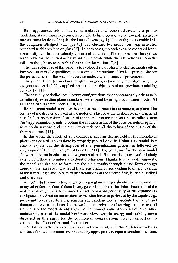
Fig. 4. First-order dipole patterns. (a) long diagonal direction; (b) short diagonal direction.
Case 1. In the first case, the dipole orientations alternate in both grid directions 4, q. This means that, in the Union Jack
m i ~ 1, j ~ - - m i j ,
m i , j ± 1 ~ - - m i j ,
n l i _ l , j +_ l -~- m i j ,
m i + l , j + 1 ~ m U.
The equilibrium equations (18) with E - 0 take on the form
~ ( I I ) ~ i j ~--- K O I ) t ~ l i j ,
where
(22)
(23)
[-K(II) ~(n) = 2 ( - B1W Be - Ba q- B4) = L 0
E 1 1 ] K~ (II)=2 4 - 6 u 2 + 8 u 3 4 ( 1 - u 2 ) 3/2 '
E 1 l j .-yK(ll) = 2 6u 2 - 2 - ~ + 8(1 - - / , /2)3/2
II)]' (24)
(25)
Again, the only equilibrium directions are the diagonals of the rhomb. The equilib- rium configurations corresponding to the energy terms K~ u) and K~ m are shown in Figs. 6(a) and (b), respectively, while the energy terms k-(m and K~ u) are plotted vs. m y
(with the same notes given for the curves of Fig. 5) in Fig. 7.

192 S. Cincotti et al./Journal o['Electrostatics 32 (1994) 183 213
400
20£
0
-20(
-40(
.600 I
-80C
0
/ i
/ / (1)
-2(
3(
I i I I I ~ I i I t
10 20 30 40 50 60 70 80 90
3'
Fig. 5. Plot of the "energy" terms K(l) and ]~(1) vs. ~. Dashed lines: expressions (21). Continuous lines: . L x - ~ y
computer results (see text).
(a)
Fig. 6. Second-order dipole patterns. (a) long diagonal direction; (b) short diagonal direction.
Negative sign values are attained only for the Kx (II) curve and in the range e [0 °, 81 ° r. Thus, stable second-order periodical configurations, as defined by (22),
can occur only when dipoles are oriented along the short diagonal of the rhomb, as shown in Fig. 6(b), provided that 7 is included in the above-mentioned range.

S. Cincotti et al./Journal o f Electrostatics 32 (1994) 183-213 193
40ff
200
0
-200
-400
-600
-800
0
~ ' I ' I i i I I i
, d I )
II I x 0
- 10
, I , , , , , 2° y , '°, ~ yv , ' ° , ]° ,~ 10 20 30 40 50 60 70 80 90
3'
Fig. 7. Plot of the "energy" terms Kx tlI) and Kr ~uJ vs. y. Dashed lines: expressions (25). Continuous lines: computer results (see text).
C a s e 2 . When the dipole orientations alternate only in one or the other of the grid directions C, q, i.e. when one of the following two definitions is assumed:
C-variation
m i ± 1,l = - - rail, m k , j ± 1 = m k j , (26)
q-variation
m k . j + 1 = - - m k j , m i + a.z = m i t , (27)
the equilibrium matrix generated by Eqs. (18) for E -- 0 is not diagonal anymore, and the orientations of the dipoles at equilibrium do not coincide with the x, y directions of the rhomb diagonals anymore.
The main features of the above configurations can be briefly summarized by considering the C-variation case, for which the equilibrium equations become
~ l h i j = K t I I ) l h i j , (28)
where t2 is a symmetric, non-diagonal matrix given by
t2 = 2 ( - B1 - B2 + B3 - B4). (29)
The eigenvectors of ~2 are not ax, ay anymore. Then we choose to define them as
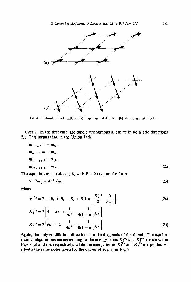
Fcos,q, + 9o°) l s = L s i n a j r = Lsin(6 + 90o) j (30)
where 6 is the orientation angle of s with respect to the x-axis. The function 6(y) is given in Fig. 8(a), and the terms K} II) and K~ II) vs. y are plotted in Fig. 8(b).
194 S. Cincotti et al./Journal of Electrostatics 32 (1994) 183- 213
10 20 30 40 ~ 50 60 70 80 90
135
130
125
120
115
i10 '
105
100
95
90
(b)
700
60O
500
400
300
200
100
0
-10£
-20(
-30£
0
' I ' I ' I I I I I
\ ,of t . . . . . .
~ (If) o | | )
( a )
I I i I , I I I i I I I I I i
10 20 30 40 -it 50 60 70 80 90
Fig. 8. (a) Plot of the functions 6(7) defining the directions s and v (expression (30)). (b) Plot of the "energy" terms K~ m and Kv ([I) vs. "~. Dashed lines: results from the Union Jack approximation. Continuous lines: computer results (see text).
Since the sign of K (II) is always positive, the equilibrium configurations generated by v are unstable, hence they are of no interest in this context. On the contrary, the s configurations are always stable. One of them is presented in Fig. 9.
The ~/-variation case can be treated in a very similar way. It can be easily shown that the expression for the 12 matrix differs from (29) only in the signs of B1 and 83. Moreover, it can be shown r l l ] that, in this case, the angle 3' for the s and v eigenvectors is related to the 6 angle in the previous case via the very simple relation
6 ' = 1 8 0 ° - 6. ( 3 1 )
The eigenvalues K~ tII) and K~ If) are the same as in the previous case (Fig. 8(b)). Stable configurations are then associated only with the s eigenvector. An example is given in Fig. 10.

S. Cincotti et al./Journal of Electrostatics 32 (1994) 183-213 195
Fig. 9. Second-order stable l-configuration (26) for ~, = 45 ° (3 = 102.5°).
Fig. 10. Second-order stable ~/-configuration (27) for ~, = 45 ° (6 = 77.5°).
The discussion concerning second-order periodicity configurations can be con- tc'~m K~II~ cluded by comparing the curves --x and that can be obtained by the accurate
approach described in [11]. It turns out that
K(II) < K.-(u) for ~ [ 0 , 6 0 ° [ ,
K~ m < K~ n) for 7~]60°,90°].
Some general remarks can now be made on the whole set of results reported in this section. These results point out that a rhombic grid individuates some preferred directions in which the electric dipoles can align even when E -- 0. Such directions are anisotropy directions and are associated with various stable equilibrium configura- tions, whose multiplicity is the basis for a hysteretic behaviour [12, 13]. Strictly speaking, the periodicity characteristic of the equilibrium configurations should be possible only in an infinitely extending lattice [9]. From this point of view, the results obtained represent rather a crude basis for the study of the real case of a lattice with a finite number of nodes, but with the advantage that, thanks to definitions (22), (26), (27) and to the Union Jack approximation, the investigation reduces to a limited set of variables. This advantage becomes more evident when an exogenous electric field E is introduced, and the stability limits of each basic configuration are assessed. This topic is addressed in the next section.
5. Spatially periodical equilibrium configurations for E # 0
Let us suppose now that an exogenous electric field E is present in the lattice plane. When E is uniform, i.e. it is independent of the node coordinates (i,j), the resulting energy for a generic set ~ of dipoles is given by expression (7). However, in order to study the stability of periodical equilibrium configurations under the influence of E, two important simplifications can be introduced.
196 S. Cincotti et al./Journal of Electrostatics 32 (1994) 183-213
A A A m4 _ , / m 3 ~..f- . . . . . . . . . . . /~v ma
/ / / / /
/ / / /
/ l ~ i / / / ' ^
A A /ma /- /- /-
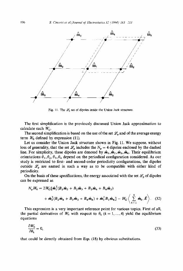
Fig. 11. The ~ep set of dipoles inside the Union Jack structure.
The first simplification is the previously discussed Union Jack approximation to calculate each W w
The second simplification is based on the use of the set Lap and of the average energy term Wo defined by expression (11).
Let us consider the Union Jack structure shown in Fig. 11. We suppose, without loss of generality, that the set Lap includes the Np = 4 dipoles enclosed by the dashed line. For simplicity, these dipoles are denoted by n~l, th2, n~3, th4. Their equilibrium orientations 01,02, 03,04 depend on the periodical configuration considered. As our study is restricted to first- and second-order periodicity configurations, the dipoles outside ~p are named in such a way as to be compatible with either kind of periodicity.
On the basis of these specifications, the energy associated with the set Lap of dipoles can be expressed as
NpWo = 2WG[ml^T(Blm2^ + B2m3 + Ba/h4 + B4/ti3)
+ m 2 (B2m 4 + Bath 3 + Balh4) + lh~Bltha] -- ~ thk,/~ (32) k=l
This expression is a very important reference point for various topics. First of all, the partial derivatives of Wo with respect to Ok (k = 1 ..... 4) yield the equilibrium equations
dWo - - = 0 , ( 3 3 ) 8Ok
that could be directly obtained from Eqs. (18) by obvious substitutions.

S. Cincotti et al./Journal of Electrostatics 32 (1994) 183-213 197
Then, the Hessian matrix
n = LaOk aO,_l' k, l = 1 . . . . . 4, (34)
which must be positively defined for any stable equilibrium configuration, yields the range of E values for which any configuration stability holds and the s w i t c h i n g values from any equilibrium configuration to another.
The above choice for Lf v and the representation of Wo as a function of four independent variables 01 . . . . ,04 is an approximation which might seem rather crude at first sight. As it will appear in the following, however, theoretical investigations of H become impracticable for larger sets of Ok. Moreover, theoretical estimations in the literature are often based on more drastic assumptions [14, 15].
Owing to the simplicity of the resulting expressions, the discussion about stability is explicitly developed for the case in Section 4.1 and case 1 in Section 4.2 when the exogenous electric field E is directed in the main direction ax of the short rhomb diagonal. The cases when E is oriented along a r or in an i n t e r m e d i a t e direction can be studied in a similar way, so they are not explicitly considered. For the same reasons and because the "main" directions s and v change with ~, the theoretical expressions for case 2 in Section 4.2 are not reported. It should be stressed, however, that the numerical evaluation of the stability range is very simple in this case, too. This statement will become apparent in the next section, where some hysteresis cycles in periodical structures are presented.
1. In the case of first-order dipole configurations, the equilibrium equations (33) take on the equivalent form
~/(I)/1~ - - /~ = 0C/~I, (35)
which generalizes Eq. (19) for /~ ~ 0. The matrix ~(~) is the same as in Eq. (19), and thk = rh (k = 1 . . . . . 4). The term :t is a real constant.
The elements of the Hessian matrix at the equilibrium position are easily calculated. For instance, we have
= wo [ - - E ) ] = w o ( -
and the structure of the Hessian matrix turns out to be
- e - A ( 3 6 ) H = W~ - A - ~ t "
D - N
The expressions for the terms A, D, N are reported in Appendix II. Owing to the symmetries of matrix H, its four eigenvalues are the solutions of the
two second-order equations [16]
(2 + ~ - D) 2 - (N + A) 2 = 0,
(2 + ~ + D ) 2 - - ( N - - A ) 2 = 0. (37)
198 S. Cincotti et al./Journal of Electrostatics 32 (1994) 183 213
When all the eigenvalues are positive, H is positively defined and the equilibrium configuration is stable.
In the particular case where th = ax (short diagonal of the rhomb), Eq. (35) yields
i.e. /~ =/~ax and
/((l) /~.
K~ I ) - ~ 0 = (38)
(39)
At the same time, the terms A, D, N are defined by the polynomial expressions reported in the final part of Appendix II.
Substituting these expressions and expression (39) into Eqs. (37) amounts to relat- ing the eigenvalues 2~ (k = 1, ..., 4) to the field/~ and to the lattice parameter u. Rather tedious, though direct, calculations show that all the 2k's are positive when/~ is subject to the following constraint:
I 1 1 ] for uE]0.9128,1], / ~ > 2 6 u 2 - 4 8u 3 8(1--u)3/2 i.e. 7E[0°,48°[,
[ 3 3 ] for u~[1/x/~,0.9128 [, ff~ > 2 12u z - 6 + 8u ~ 8(1 - u) 3/2 i.e. ),E]48°,90°]. (40)
The value 7 = 48° is obviously approximate, as are the K~ ~) and Kr (I) values obtained through the Union Jack approximation. It should be stressed, however, that the second inequality is that usually proposed in the literature, with no conditions on the lattice angle y [14]. As pointed out in [15], this lack of information occurs when stability is investigated taking W0 as a function of only one independent variable 0. Finally, we remark that, with !/, = ax, the general expression (32) gives rise to the following expression for the normalized average energy 1~o:
Wo - Wo _ ± r , - ( l )2 , , -x - /~. ( 4 1 ) WG
When th = - ax, both the I~o and the constraint expressions are dual to those given above.
2. In the case of the second-order configurations defined by
th3 = Ihl = lh,
th2 = th4 = - th, (42)
the equilibrium equations can be written as
7"(n)th - / ~ = ~11h,
(43)

S. Cincotti et al./Journal o f Electrostatics 32 (1994) 183- 213 199
The structure of the Hessian matrix at equilibrium takes on the general form
I i ° N - ~2 A D
H = W o A - ~ 1 N "
D N - - O~ 2
(44)
The terms A, D, N are defined in Appendix II as in the previous case. Again, the four eigenvalues are the solutions of two second-order equations, i.e.
(4 + ~l -- D)(2 + ~2 - D) - (N + A) 2 -- 0,
(4 + ~l + D)(2 + ~2 + D) -- (N -- A) 2 = 0. (45) When d l = ax, Eqs. (43) yield
/~ = IKx(II )o- ~1
FK m) _ E=-L xO
thus giving E- - /~ax
K (II) E, ~1 ~l ~ x - -
~2 = K~n) + /~ .
0 IE]E ,II, lll x ° 1((II) - - OC 1 0
--rk'(n) -- ~2 0 = 0 J '
and
(46)
(47)
Substituting these expressions and those for A, D, N (see Appendix II) into (45), the discussion on the eigenvalues 2k (k = 1 . . . . . 4) can be developed by performing the same steps as in the previous case. The final result is that all the 2k'S are positive, provided that
1 lu)3l 2 for u eqx/~/2, 11-, I/~1 < 2 4 - 6u 2 8u s 8(1 i.e. 7e ]0° ,60° [ ,
I/~1 = 0 for ~ > 60 °. (48)
Thus the stability of this configuration is compatible with an exogenous electric field /~ # 0 for lattice angles ~ in the range ] 0 °, 60 ° [. For completeness, it is worth noting that the model predicts stability with/~ ~ 0 up to ~ = 63 °, provided that IEI fulfils a second inequality, more restrictive than (48), between 60 ° and 63 °. This result is not significant, as it concerns the range of V values for which the coarseness of the Union Jack approximation is maximum [11].
Owing to (42), the sum of the dipole moments mk of the set .£~p (k = 1 . . . . . 4) is equal to zero. Then, for n~ = as, the normalized average energy ffZo is constant for any value
200 S. Cincotti et al./Journal of Electrostatics 32 (1994) 183 213
of/~ in the stability range defined by (48). Direct calculations yield
I~o 1 z~nl (49)
When y ranges between 60 ° and 90 °, the second-order periodical configurations whose stability can hold also for/~ ~ 0 are those defined by (26) and (27). This could be easily verified by numerical evaluations over the related Hessian matrix. Some results will be reported in the next section.
6. Hysteresis cycles in spatially periodical structures
On the basis of the results reported in the previous section, the set £Pp shown in Fig. 11 is considered. The exogenous electric field is directed (except for one specific case) along the short diagonal of the rhombic structure, i.e. E = Exax. The hysteresis cycles can be generated by a computer according to the following steps: 1. Let /~ = 0 and let the "initial" components of the orientation vector
0 ~°) = [0~ °) 02 t°) 0t3 °) 0~4°)] r be assigned randomly. 2. With the given /~ and the "initial" vector 0 t°), the vector 0 of the equilibrium
orientations is found by searching for the minimum value of Wo. Then, the average vector
P = ~ ~hk = Pxax + P~,ay k=l
is calculated. 3. The value of/~x is changed by a "small" amount, according to the criterion given in
step 4. Then the just found vector 0 is taken as the new 0 t°) and another step 2 begins.
4. Starting from /~x = 0, positive increments are given until a value/~u is reached which is larger than the "threshold" value yielding P = ax. Then /~ is reduced down to the opposite value - /~u and finally incremented until the value/~M is reached again.
A first group of results dealing with values of 7 lower than 60 ° is shown in Figs. 12-14. Set (a) of the figures shows the hysteresis cycles P~ = P~(/~x). Owing to the directions assumed for /! and to the values of ~ chosen for these examples, P y - - 0 everywhere. The first- and second-order periodical configura- tions involved in these hysteretic processes have the dipoles directed along the short diagonal, like the electric field. This is the reason for the abrupt changes in Px, which occur when /~x leaves the range of stability of a second-order (BC, G " G segments) or of a first-order configuration (FG' or FG and IL' or IL segments). These threshold values o f / ~ are those given in expressions (48) and (40), respectively.
The set (b) of figures presents the corresponding behaviour of the normalized average energy I~o (see expressions (41) and (49)).
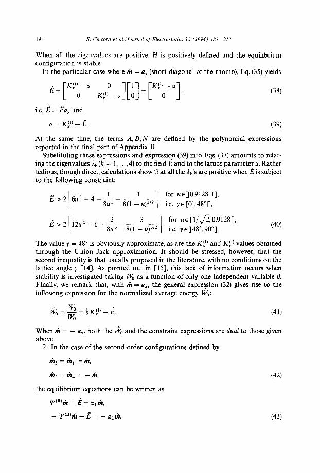
S. Cincotti et al./Journal of Electrostatics 32 (1994) 183- 213 201
1.0
0.5
px .0
- o . 5 ~
(a) - l o
-60 -40 -20 20 40 60 Ex
wo_ 0 f ....
, I , I , i I i I , I
-60 -40 -20 20 40 60 Ex
Fig. 12. Hysteresis curves in an infinitely extending lattice with ~ = 20 ° and E ---/~xax. (a) plot of the average dipole component Px vs./~x; (b) plot of the corresponding average energy I~0.
Taking/~x = 0 and giving random initial orientations to the dipoles (step 1), the self-organizing capability of the structure provides the second-order periodical config- uration discussed in the previous sections. Then, at point A, I~o = K~n)/2 (expression (49)).
This value remains constant until/~x causes the BC transition to the first-order configuration with Px = + 1. Here I~o depends linearly on/~x, as in expression (41). Starting from C, the path followed along this right line is C --) D ~ C ~ F. At point F, the first-order configuration with P---a~ is not stable anymore, and a transition occurs. For y = 20 ° and y = 30 ° (Figs. 12 and 13), the "landing-place" of this

202 S. Cincotti et al./Journal of Electrostatics 32 (1994) 183- 213
ex .0
-0.5
(a) -1.o
-1¢
A
wo -2C
p i i
1.0 . . . . . . . . . . . . F ; C : D
0 . 5 . . . . . . . . . . . . . . . . . . . . : . . . . . . . . .
(3" Ai L'
-3(3
H G , i , i
-30 -20 -10
(b) _ , ~
30
i
Ex i
10 20 30
' i i i ' i ' L
-20 -10 0 10 20 30 A
Ex
Fig. 13. Hysteresis curves in an infinitely extending lattice with y = 30 ° and /~ =/~xax. (a) plot of the average dipole component Px vs . /~ ; (b) plot of the corresponding average energy I~o.
transition is the second-order configuration which holds in the segment G'G", after which a transition G"G to the first-order P = - a x configuration occurs. When 7 = 50 ° (Fig. 14), the transition from Px = + 1 to Px = - 1 is direct (FG segment). This happens because, when 7 is higher than about 48 °, the energy level at point G is higher than that at point A. As a consequence, in the abrupt transition from F, the straight line of the energy for Px = - 1 is met before the horizontal line Wo = ½ K~ n) of the second-order configuration.
We finally observe that, owing to (41), the value of I~o at point M is ½Kt~ l). The remaining elements in the figures are obvious and need no comments.

S. Cincotti et al./Journal of Electrostatics 32 (1994) 183- 213 2 0 3
i i i
1.0 . . . . . . ; . . . . . . : . . . . . . : . . F
0.5 . . . . . . . . . . . . . . . . . . . . . . .
PxO.O
-0.5 . . . . . . . . . . . . . . . . . . . . . .
-1.0 H G
( a ) -10.0' -7.5 ' -5.0 ' -2.5 '
i
L : C D
A ............ !iiiiii
0.0 A
Ex
. . . . . . . . . Z . . . . . ~ . . . . .
2.5 5.0 7.5 10.0
0
-2
-4
A
W o - 5
-8
-10
(b)-1.~;io '
' ' ' I
F M I
i i i ~ ! i B i . . . . . . ! . . . . ! i A, ! . . . . . . i . . . . . . ! . . . .
. . . . ! i i i ic i . . . .
-7.5 -5.0 -2.5 0.0 2.5 5.0 7.5 10.0 A
Ex
Fig. 14. Hysteresis curves in an infinitely extending lattice with y = 50 ° a n d E = / ~ x a x . (a) plot of the average dipole component P= vs. Ex; (b) plot of the corresponding average energy I~0.
The second group of results was obtained by using the value 7 = 75° for the lattice angle. As previously stated, this value of 7 is included in the range ] 60 °, 90°[, where the only second-order configurations that can keep stable under the influence of an external field are those defined by (26) and (27). The orientation angle defining the vectors s and ~ for configuration (26) is equal to 130 °, and that for (27) is equal to 50 ° .
Instead of assuming the external field E to be directed in either of these "main" directions, we chose, as possible directions, each of the lattice diagonals and studied

204 S. Cincotti et al./Journal o f Electrostatics 32 (1994) 183- 213
(a)
(b)
(c)
- 2 . 5
-3.0
P,
~ ] '0 -3 .5
-4.0
-4.5
-5.0
, , , , . , • , , ~ , , . , • , . , ,
. . . . . F C D 10 :
o~ ! B! i
- 1 . [ - . . . . . . . .
Ex
0 . 2
-5 -4 -3 -2 -1 0 A 1 2 3 4 5
E×
" ! ! ! ! ! , ! i~! ' ! !
-5 -4 -3 "2 -1 0 /~. 1 2 3 4
Ex
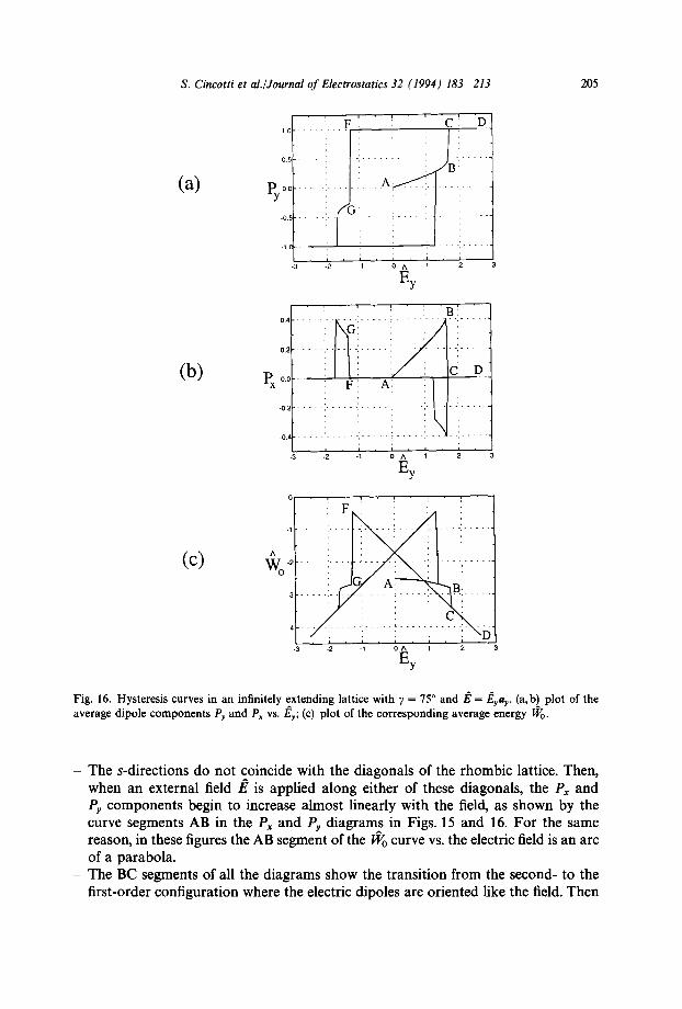
Fig. 15. Hysteresis curves in an infinitely extending lattice with 7 = 7 5o and/~ =/~xax. (a,b) plot of the average dipole components Px and Py vs./~x. (c) plot of the corresponding average energy 1~o.
the hysteresis curves as summarized in the following:
1. E =/~=ax (Fig. 15): curves P~ = Px(/~); Pr = Py(/~); I~o = 1~o(/~);
2. /~ =/~ya r (Fig. 16): curves Py = Py(/~y); P~ = P=(/~r); I~o = l~o(/~y);
Most of the comments are valid for both sets of results and are made in the following. - When E = 0, the electric dipoles get organized along the s-direction of either of the
second-order distributions defined by Eqs. (26) and (27), respectively. Then, at point A, Px = Py = 0 and #o = 1 ld(ll)2,,,~ -,,~ -- 2.54.
S. Cincotti et al./Journal of Electrostatics 32 (1994) 183-213 205
(a)
1.0
0 .5
p y O , C
.0.. =
-1 .(
-3 - 2 2
C
i A!
L d L
l L , l -1 0 A 1
Ey
D
(b)
O.Z
05
P X 0.0
-0.2
-0.4
-3 i i , i i
-2 -1 0 A 2
Ey
(c) A
Wo -~
- 3
- 4
• ] - ! • , - , • ,
-2 - 0 A 1
Ey
^ A
Fig. 16. Hysteresis curves in an infinitely extending lattice with 7 = 75° and E = Eyay. (a,b) plot of the average dipole components Py and Px vs./~y; (c) plot of the corresponding average energy Wo.
- The s-directions do not coincide with the diagonals of the rhombic lattice. Then, when an external field /~ is applied along either of these diagonals, the Px and Py components begin to increase almost linearly with the field, as shown by the curve segments AB in the Px and Py diagrams in Figs. 15 and 16. For the same reason, in these figures the AB segment of the 1~o curve vs. the electric field is an arc of a parabola.
- The BC segments of all the diagrams show the transition from the second- to the first-order configuration where the electric dipoles are oriented like the field. Then

2 0 6 S. Cincotti et al./Journal of Electrostatics 32 (1994) 183- 213
the end-transition point C is associated with the value Px = + 1 in Fig. 15(a) and with Py = + 1 in Fig. 16(a). The corresponding values in Figs. 15(b) and 16(b) are Py = 0 and Px = 0, respectively.
- Starting from C, the C ~ D ~ C ~ F segments represent the behaviours of Px, Py and I~o for the first-order dipole configurations. The FG segment shows the transition to the second-order configuration. The field va lue /~ at point F (Fig. 15) is easily calculated by the second expression (40). The corresponding expression for the /~y threshold value can be obtained by studying the Hessian matrix (36) for th --- at, but it is not reported here for brevity.
The remaining segments of the curves are so evidently related to those discussed above that no further comments are required.
We conclude this section by observing that, in the curves in Figs. 15 and 16, the only single hysteresis loop centred in the origin of the coordinates belongs to the Py(/~r) curve shown in Fig. 16(a). This is due to the positions of the F and A points in the (/~, Wo) planes in Figs. 15(c) and 16(c).
7. Hysteresis cycles in finite lattices - Conclusions
A refined model of a real two-dimensional structure requires that further physical elements be taken into account. In this respect, the Union Jack approach is only the first step towards this direction. The structural simplicity of the model presented in this paper is important to preserve some handiness when further refinements are introduced. Moreover, this model proves an effective investigation tool even when the hysteretic behaviour of finite-size lattice structures is studied. Generally speaking, finite structures are much more realistic than infinite ones, but they are more difficult to study. The main reason is that the end-effects on the dipoles at the boundaries do not allow spatially periodical equilibrium configurations. The lack of this simplifying mechanism in the study of the hysteretic behaviour compels one to take into account each dipole of the structure and its interactions with the other dipoles. This task must be accomplished via computer simulation (although the Union Jack can be used to approximate the interaction mechanism) and the number of dipoles of the lattice is limited by the available computer power.
The cases considered in the following deal with a rhombic lattice £~r with 11 x 11 dipoles. The ), values and the field orientations are the same as taken in the previous section for the periodical solutions. The energy term Wo = We lgZo is defined by expression (12) where the W~ i terms of the boundary dipoles take into account the absence of dipoles outside the finite grid.
The average dipole moment is given by
e = ~ L ,J (50) f Ihlj e ~ f
where Nf = 121. Apart from these specifications, the logical steps performed to obtain the hysteresis curves are the same as defined for the infinite lattice cases. For any given

S. Cincotti et al,/Journal of Electrostatics 32 (1994) 183- 213 207
/~, the equilibrium dipole configuration corresponding to the minimum of l~o was searched for by using the following simple approach [17]: - out of the equilibrium position, each dipole rh o is thought of as being subject to
both the torsional moment - aWo/00 u and a viscosity term, while the angular acceleration term is neglected. Thus, the "dynamic" equation for any dipole is
aO~j a Wo v - - (51)
Ot OOij'
1.0 . . . . . . . . . 5 . . . . ',r . . . .
0 . 5 . . . . . . . . . . . . . . . . . . . . . . . . . . . . . . . . . . . . .
-0.5 ~
( a ) -1.o , ! , i i i
-40 -20 20 40
Ex 0 ,
-20 . . . . . . . . . . . . . . . .
A
wo-4° ........ i -60 . . . . . . . .
(b) -80 ' ' ' I
-40 -20 0 20 40 A
Ex A ^
Fig. 17. Hysteresis curves in a finite-size lattice (11 x 11) dipoles with ? = 20 ° and E = E~ax. T h e (a) and (b) plots correspond to those shown in Fig. 12 for the infinite lattice case.

208 S. Cincotti et al./Journal of Electrostatics 32 (1994) 183- 213
0 i i i ! ! 0.5
r
xo0 iiii -0.5
(a) , 0 i , , , , i , J i
-15 -10 -5 0 5 10 15 A
E×
' ' ' ', I ', !
- 5 - i
-10
W o -15
-20
(b) -2s
-15 -10 -5 5 10 15 A
E x
Fig. 18. Hysteresis curves in a finite-size lattice (11 x 11) dipoles with y = 30 ° and E =/~xax. The (a) and (b) plots correspond to those shown in Fig. 13 for the infinite lattice case.
where v is the viscosity coefficient. This means that
- - = - _< 0 (52) dt v 0,
i.e. the energy Wo decreases over time until a minimum value is reached at which all the torsional moments annihilate and the equilibrium equations in the lattice are fulfilled;
- the above results outline an approximate numerical procedure to generate a dis- crete set of values Wo converging to a minimum. In the procedure, the Are angles

S. Cineotti et al./Journal of Electrostatics 32 (1994) 183-213 209
1 . 0
0 . 5
Pxo.o
- 0 . 5
(a) - 1 . o
, , i , i , , i , I
- 6 - 4 - 2 0 2 4 6 A
E×
i i ~ i i i i
- 2 - - - : . . . . . . . ~ . . . . . . . , . . . . . . : . . . . . . ~ . . . . . . . : . . . . . . . , " ' ' "
- 3 . . . . i . . . . . . . : . . . . . . . : . . . . : . . . . . . . : . . . . . . . :
- 4 . . . . ! . . . . . . . i . . . . . . . . . . . . i . . . . . . . i -
. . . . . . . . . . . i : : . . . . . . . !
i:i ( b ) - 9 " ~ , i , ' 2 , ~ , ~ , ~ , ~
A
Ex
Fig. 19. Hysteresis curves in a finite-size lattice (11 x 11) dipoles with ~, = 50 ° and E = E~a=. The (a) and (b) plots correspond to those shown in Fig. 14 for the infinite lattice case.
0 u are updated via an approximate solution of the Nf Eqs. (51) (e.g. by multistep methods such as Forward Euler (FE), Backward Euler (BE), or Trapezoidal (TR)).
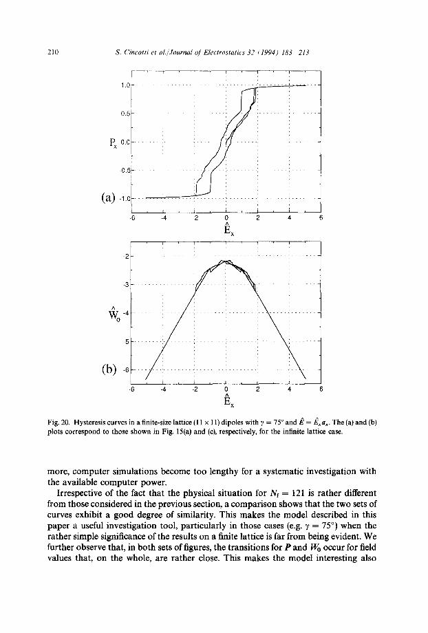
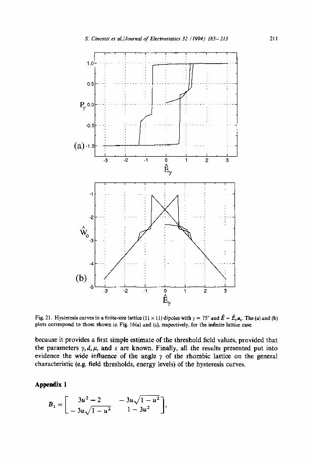
The set of Figs. 17-21 shows the results. For the sake of comparison, the correspond- ing curves in the case of an infinitely extending lattice are indicated in the figure captions.
Owing to the very small size Nf of the lattice, all the transitions appear as the sequence of a certain number of steps. The smoothness of the curves obviously increases with Nf. Unfortunately, when Nf becomes of the order of one thousand or
210 S. Cincotti et al./Journal of Electrostatics 32 (1994) 183 213
1.0
0.5
Px 0.0
-0.5
(a)-1.o
-6
-2
-3
A
Wo4
-5
(b) -6
-6
i T I $ I
, i i , i , i , i , -4 -2 0 2 4 6
A
Ex i i I i
I I I i I I l " - ~ -4 -2 0 2 4 6
A
Ex
Fig. 20. H yste r e s i s c u r v e s in a f ini te-s ize latt ice (11 x 11) d i p o l e s w i th ? = 75 ° a n d E =/]~ax. The (a) and (b) p l o t s c o r r e s p o n d to t h o s e s h o w n in Fig. 15(a) and (c), respect ive ly , for the inf inite latt ice case .
more, computer simulations become too lengthy for a systematic investigation with the available computer power.
Irrespective of the fact that the physical situation for Nf = 121 is rather different from those considered in the previous section, a comparison shows that the two sets of curves exhibit a good degree of similarity. This makes the model described in this paper a useful investigation tool, particularly in those cases (e.g. 7 = 75°) when the rather simple significance of the results on a finite lattice is far from being evident. We further observe that, in both sets of figures, the transitions for P and Wo occur for field values that, on the whole, are rather close. This makes the model interesting also
S. Cincotti et al./Journal of Electrostatics 32 (1994) 183- 213 211
1.o
0.5
pyO.O -0.5
( a ) -1.0
I i i i 1 i
. . . . . . , . . . . . . . , . . . . . . . . , . . _
i , i , i , i , i , i , i
-3 -2 -1 0 1 2 3 A Ey
-2
A
Wo -3
-4
(b) -5
ii -3 -2 -1 2 3
A Ey
Fig. 21. Hysteresis curves in a finite-size lattice (11 x 11) dipoles with ? = 75 ° and E =/~yay. The (a) and (b) plots correspond to those shown in Fig. 16(a) and (c), respectively, for the infinite lattice case.
because it provides a first simple estimate of the threshold field values, provided that the parameters ?, d, #, and e are known. Finally, all the results presented put into evidence the wide influence of the angle ? of the rhombic lattice on the general characteristic (e.g. field thresholds, energy levels) of the hysteresis curves.
Appendix I
3u 2 - 2 - 3 u x / 1 - u 2 1 B I = _ 3 u x / l _ u 2 1 - - 3 u 2 '
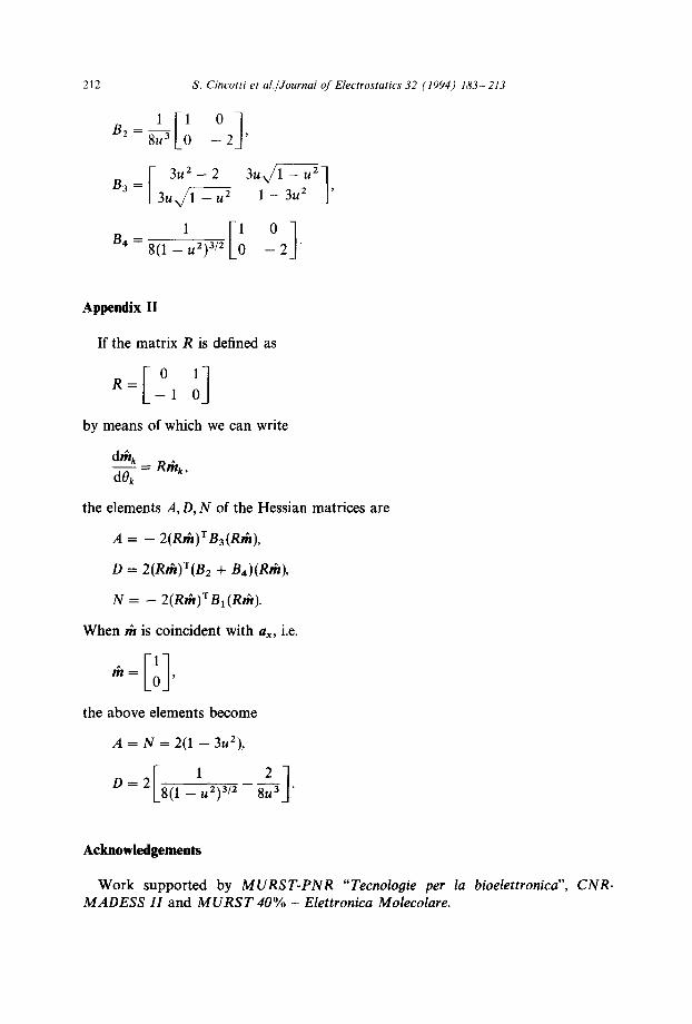
212 S. Cincotti et al./Journal of Electrostatics 32 (1994) 183- 213
E,o o] B2 = 8 ~ - 2 '
= [ 3 u 2 - 2 3ux/1 - u21 B3 L3ux/1 _ u 2 1 - 3u 2 '
1 [lo01 B 4 - 8(1 - u2) a/2 - 2 "
Appendix II
If the matrix R is defined as
I°ll R = - 1 0
by means of which we can write
d,hk - - - - R ~ k , dOk
the elements A, D, N of the Hessian matrices are
A = - 2(Rth)TBa(Rth) ,
D = 2(Rlh)~(B2 + B, ) (R th) ,
N = - 2(Rth)TBI(Rth).
When th is coincident with ax, i.e.
the above elements become
.4 = N = 2(1 - 3u2),
D = 2 8 ( 1 - u 2 ) 3/2 8u 3 "
Acknowledgements
W o r k suppor ted by M U R S T - P N R "Tecnologie per la bioelettronica", M A D E S S I I and M U R S T 40% - Elettronica Molecolare.
C N R .

S. Cincotti et al./Journal of Electrostatics 32 (1994) 183-213 213
References
[1] M. La Breeque, Circuits and devices a molecule wide, National Science Foundation MOSAIC, 20 (1989) 16-27.
[2] M. Parodi, B. Bianco and A. Chiabrera, Toward molecular electronics: Self-screening of molecular wires, Cell Biophys., 7 (1985) 215-235.
[3] A. Chiabrera, E. Di Zitti, F. Costa and G.M. Bisio, Physical limits of integration and information processing in molecular systems, J. Phys. D: Appl. Phys., 22 (1989) 1571-1579.
[4] A. Chiabrera, E. Di Zitti and G.M. Bisio, Molecular information processing and physical constraints in computation, Chemtronics, 5 (1991) 17-22.
[5] G. Roberts, Langmuir-Blodgett Films, Plenum Press, New York, 1990. [6] E. Sabatani, I. Rubinstein, R. Maoz and J. Sagiv, Organized self-assembling monolayers on electrodes,
J. Electroanal. Chem., 219 (1987) 365-371. [7] L. Netzer, R. Iscovici and J. Sagiv, Adsorbed monolayers versus Langmuir-Blodgett monolayers
- - Why and how? I: From monolayer to multilayer by adsorption, Thin Solid Films, 99 (1983) 235-241.
[8] L. Netzer, R. Iscovici and J. Sagiv, Adsorbed monolayers versus Langmuir-Blodgett monolayers - - Why and how? II: Characterization of built-up films constructed by stepwise adsorption of individual monolayers, Thin Solid Films, 100 (1983) 67-76.
[9] M. Parodi, S. Cincotti and A. Chiabrera, A continuous model of the interactions among electric dipoles, J. Electrostatics, 26 (1991) 47-64.
[10] S. Cincotti, M. Parodi and A. Chiabrera, Modelling of dipole monolayers as cellular arrays, J. Mol. Liq., 50 (1991) 73-92.
[11] S. Cincotti, M. Parodi and A. Chiabrera, Surface organization of dipole monolayers, J. Mol. Liq., 51 (1992) 89-113.
[12] L. Landau and E. Lifsits, Electrodynamics of Continuous Media, Pergamon Press, Oxford, 1960. [13] D. Pescetti, Memory phenomena in hysteretic systems, 4th Italian Workshop on Parallel Architec-
tures and Neural Networks, Salerno, Italy, May 8-10, 1991. [14] M.I. Kaganov and V.M. Tsukernik, The Nature of Magnetism, Mir, Moscow, 1985. [15] W.F. Brown, Failure of the local-field concept for hysteresis calculations, J. Appl. Phys., 33 (1962)
1308-1309. [16] H.D. Ikramov, Linear Algebra, Mir, Moscow, 1983. [17] A. Chiabrera, S. Cincotti, A. De Gloria, E. Di Zitti and M. Parodi, From electrical interactions among
dipoles to cellular automata: A model, 12th Int. Conf. IEEE Eng. in Med. and Biol. Soc., Philadelphia, USA, November 1-4, 1990.