arX

iv:c

ond-

mat

/970

9075

v1 5

Sep

199

7

MAGNETIC DIPOLE ABSORPTION OF RADIATION

IN SMALL CONDUCTING PARTICLES

Michael Wilkinson1 and Bernhard Mehlig2

Isaac Newton Institute for Mathematical Sciences,University of Cambridge,

20, Clarkson Road,Cambridge, CB3 0EH,

United Kingdom,

Paul N. Walker

Laboratoire de Physique des Solides, associe au CNRSUniversite Paris-Sud

91405 OrsayFrance

Abstract

We give a theoretical treatment of magnetic dipole absorption of electromagneticradiation in small conducting particles, at photon energies which are large compared tothe single particle level spacing, and small compared to the plasma frequency. We discussboth diffusive and ballistic electron dynamics for particles of arbitrary shape.

The conductivity becomes non-local when the frequency is smaller than the frequencyωc characterising the transit of electrons from one side of the particle to the other, but inthe diffusive case ωc plays no role in determining the absorption coefficient. In the ballisticcase, the absorption coefficient is proportional to ω2 for ω ≪ ωc, but is a decreasingfunction of ω for ω ≫ ωc.

1 Permanent address: Department of Physics and Applied Physics, John AndersonBuilding, University of Strathclyde, Glasgow, G4 0NG, Scotland, U.K.

2 Permanent address: Max-Planck-Institut fur Physik komplexer Systeme, NothnitzerStr. 38, 01187 Dresden, Germany

1. Introduction

For sufficiently low frequencies, the interaction of small conducting particles withelectromagnetic radiation is dominated by absorption rather than scattering. The classicaltheory of the interaction of electromagnetic radiation with spherical particles of uniformcomposition was considered by Mie [1]; the theory encompasses conducting particles witha complex dielectric constant, which is often modelled by the Drude theory [2]. If theparticles are small compared to both the wavelength and the electromagnetic skin depthof the radiation, the dominant contributions to the absorption are called the electric andmagnetic dipole terms [3]. In both cases the absorption is due to Joule or Ohmic heatingcaused by electrical currents flowing through the particle: the electric dipole term is dueto currents which establish electrical polarisation of the particle, and the magnetic dipoleterm is due to eddy currents induced by variation of the magnetic field.

At frequencies below the plasma frequency, the electric field is screened from theinterior of the particle, but the magnetic field can penetrate the whole of the particle.Although magnetic effects are negligible in atomic absorption processes, they could becomesignificant when the number of atoms in the particle sufficiently large that most of theatoms are screened from the electric field. In fact, magnetic dipole absorption is oftenthe dominant absorption process in suspensions of small metal particles [4]. Very few ofthe many theoretical papers on absorption of radiation by small particles have consideredthe magnetic dipole contribution, some exceptions are [5,6] which consider magnetic dipoleabsorption in the context of effective medium theories. Because it is typically the dominantcontribution, it is appropriate to consider the problem of magnetic dipole absorption insome detail.

The Mie theory is restricted to spherical particles in which the dynamics of the chargecarriers is diffusive, and quantum mechanical effects are ignored. In this paper we willgive the first theoretical treatment of magnetic dipole absorption going beyond the Mietheory: we will consider both diffusive electron dynamics (for which the particles are char-acterised by their bulk conductivity), and ballistic electron motion (in which the particleis smaller than the bulk mean free path of the conduction electrons). Our approach allowsfor arbitrary particle geometries, and we give careful consideration to the fact that theconductivity is non-local when the particles are very small: quantum mechanical effectsare included using a semiclassical approach. The paper complements [7-9], which gave acomparably comprehensive treatment of electric dipole absorption.

We do not explicitly consider the structures in the absorption close to the singleparticle level spacing which were originally considered by Gorkov and Eliashberg [10].These structures are determined by repulsion between energy levels and the appropriatetool to analyse them is random matrix theory. Their full characterisation requires anestimate of a mean-square matrix element, which was not given correctly in [10]. Ourresults for the low-frequency limit provide the correct estimate of this quantity for magneticdipole absorption.

Sections 2 to 4 will be concerned with various aspects of the formulation of the prob-lem, discussing respectively the relation between the absorption of radiation and correlationfunctions of the electron motion, the criteria for a self-consistent solution of the equationsdetermining the electric field driving the eddy currents, and the definition and semiclassicalestimation of the non-local conductivity which is required to determine the self-consistentfield. Our semiclassical estimates for the non-local conductivity are closely related to ex-pressions given by Argaman [11]. In section 5 we develop the theory for magnetic dipoleabsorption in particles with diffusive electron motion, assuming that the electric field isknown. This calculation also yields the form of the non-local conductivity applicable to the

diffusive case: in section 6 we consider the solution for the self-consistent field, and discussresults for some specific geometries. Our formula for the non-local conductivity is identicalto one given by Serota and co-workers [12,13], who used diagrammatic techniques. Ourderivation is more direct and requires fewer assumptions: we discuss this point further insection 6.

Our approach uses a semiclassical estimate described in [14], which relates meansquared matrix elements to classical correlation functions. We might expect that thereshould be features in the absorption spectrum which are related to the characteristictimescale for decay of classical correlations, in this case the typical time for a particleto cross the particle: the importance of this timescale was emphasised by Thouless [15],and in the case of diffusive electron motion, we will refer to the characteristic frequencyscale ωc = D/a2 as the Thouless frequency (D is the diffusion constant and a is the charac-teristic size of the particle). Another reason for expecting ωc to play a role in determiningthe absorption coefficient is that the conductivity is non-local when ω is not large comparedto ωc. We find however that ωc plays no role in the final expression for the absorptioncoefficient.

We consider the case of ballistic electron motion in section 7. We are only able to gainlimited information about this case: we find that the absorption coefficient is proportionalto ω2 at frequencies small compared to ωc = vF/a, and that it is a decreasing function offrequency for ω ≫ ωc.

Our conclusions are in many ways parallel to those for electric dipole absorption. Inballistic systems, it was found [7,8] that the electric dipole absorption has resonances inthe absorption coefficient with a frequency scale ωc = a/vF, where vF is the velocity at theFermi energy. By contrast, in the case of diffusive electron motion, it was found [9] thatthere is no structure in the absorption coefficient at the frequency scale ωc = D/a2.

Finally, we remark that there is a large literature concerned with the effects of timedependent magnetic fluxes on metallic loops: when the magnetic flux varies sinusoidally,the absorption of energy by the loop is a special case of the magnetic dipole absorptionwhich we consider here. Most of the papers on this topic are concerned with quantum sizeeffects analogous to those considered by Gorkov and Eliashberg [10]: two recent works inthis area are [16] and [17].

2. Formulation of the problem

The absorption of radiation is usually described by an extinction coefficient γ(ω),which is defined as the fractional loss of intensity per unit length of sample, divided bythe volume fraction F occupied by the particles. We will express our results in terms ofthe rate of absorption of energy 〈dE/dt〉 within a single particle. If the amplitude of theelectric and magnetic fields are E0 are B0 respectively, the intensity of the radiation isI = 1

2 ǫ0 E20 = 1

2µ0B20 , and the relationship between γ and 〈dE/dt〉 is therefore

γ =2

V ǫ0cE20

⟨

dE

dt

⟩

, (2.1)

where V is the volume of a single particle. In this paper we will define the absorptioncoefficient α(ω) as the rate of absorption of energy for a single particle, divided by theelectric field intensity:

α(ω) =1

E20

⟨

dE

dt

⟩

=1

c2B20

⟨

dE

dt

⟩

. (2.2)

The normalisation with respect to electric (rather than magnetic) field intensity is used tofacilitate comparison with the results in [7-9].

The particle will be considered to consist of a static potential well which traps a gasof non-interacting fermions (electrons), initially with occupation probability f(E) (whichwould be identified with the Fermi-Dirac distribution). In a quantum mechanical calcula-tion the rate of absorption of energy is determined by the Fermi golden rule. This statesthat the rate of transition under the action of a periodic perturbation with frequency ωand matrix elements ∆Hnm, from a state with energy En, to a quasi-continuum of finalstates with energies close to Em = En + hω is

R =π

2hg(Em)〈|∆Hnm|2〉ω (2.3)

where g(Em) is the density of final states and 〈|∆Hnm|2〉ω is the mean-square matrixelement for transitions from En to states close to Em. The energy absorbed by an electronmaking an upward transition is hω. The rate of absorption of energy is therefore

⟨

dE

dt

⟩

= hω

∫

dE g(E)R(E) [f(E)− f(E − hω)] ∼ Rgh2ω2 (2.4)

where the approximate equality is applicable in the limit where hω and kT are both largecompared to the mean level spacing, but small compared to other energy scales: in theright hand expression both g and R are evaluated at the Fermi energy.

The mean-square matrix element can be estimated semiclassically [14]:

〈|∆Hnm|2〉ω =1

2πhg

∫ ∞

−∞

dt exp(iωt)〈∆H(t)∆H(0)〉E (2.5)

where 〈∆H(t)∆H(0)〉E is the microcanonical autocorrelation function of the classical ob-servable corresponding to ∆H, evaluated at energy E. Combining this result with (2.4),the absorption coefficient can be expressed in terms of the classical autocorrelation func-tion of the perturbation ∆H(r,p). The resulting expression can also be written in terms

of the classical change in energy of the individual electrons due to the perturbation: thechange in energy of an electron following a trajectory r(t),p(t) is

∆E(t) =

∫ t

0

dt′∂H

∂t(r(t′),p(t′)) . (2.6)

Combining this result with (2.5), the rate of absorption of energy by the electron gas is

⟨

dE

dt

⟩

=g

2

d

dt

⟨

∆E(t)2⟩

(2.7)

where 〈∆E(t)2〉 is the variance of the change in the single-electron energies.In our problem the perturbation is a sinusoidally varying electromagnetic field, spec-

ified by a vector potential A(r) exp(iωt), and a scalar potential Φ(r) exp(iωt). The com-ponent of the perturbation of the Hamiltonian which is quadratic in A can be neglectedwhen calculating the leading order absorption coefficient; the remaining terms are

∆H =e

2me(p.A + A.p) + eΦ . (2.8)

In discussing the magnetic dipole absorption, it is given that the magnetic field is

B(t) = ∇∧ A = B0 exp[iωt] . (2.9)

The fluctuating magnetic field induces an electric field E, which is given by

E = −∂A∂t

+ ∇Φ . (2.10)

The Hamiltonian admits a set of gauge transformations (A,Φ) → (A′,Φ′) = (A,Φ) +(∇µ, ∂tµ) which leave the electric and magnetic fields unchanged. We will assume that thegauge has been chosen so that Φ = 0. Physically, the electric field is not uniquely definedby the magnetic field, and must be determined by a self-consistent condition, which wediscuss in section 3.

3. Self-consistent choice of the vector potential

3.1 Self-consistent electric field

The eddy currents induced by the fluctuating magnetic will themselves generate amagnetic field. We will consider only the case of extremely small particles, for which thisadditional magnetic field is negligible. We therefore assume that the magnetic field issimply the externally applied field, B(t) = B0 exp[iωt]e3. The electric field is required touniquely determine the perturbation of the Hamiltonian. In this section we will discussthe self-consistent calculation of the electric field.

In discussions of the Zeeman effect in atomic physics, the perturbation of the Hamil-tonian representing the magnetic field is conventionally taken to be proportional to thecomponent of the angular momentum operator along the direction of the field. It is natu-ral to ask why a more involved procedure is used here, but is unnecessary for the Zeemanproblem or for calculation of static magnetic susceptibility. At the end of this section weshow that the angular momentum operator gives the correct answer in the limit where thefrequency approaches zero, but not in general.

The electric field satisfies the Maxwell equations

∇∧ E =∂B

∂t, ∇.E =

ρ

ǫ0. (3.1)

The electric field causes a current density j to flow within the particle. We will assume thata linear response theory is valid, but in general the current may be a non-local function ofthe electric field: we will write

j(r, t) =

∫

dr′∫ t

−∞

dt′ σ(r, r′; t− t′)E(r′, t′) (3.2)

where σ is the non-local conductance tensor. We will also write this relation in the form

j(r, ω) =

∫

dr′ σ(r, r′;ω)E(r′, ω) ≡ σE(r, ω) (3.3)

where the second equality defines an operator σ which maps the electric field E(r, ω) non-locally into the current field j(r, ω). For a monochromatic perturbation, the charge densityis

ρ = − i

ω∇. j . (3.4)

Combining these results, we find the following equation for the electric field

∇. j′ = 0, j′ = (σ − iωǫ0)E . (3.5)

This equation must be supplemented by a boundary condition in order to uniquely deter-mine the electric field. This is

n. j = 0 (3.6)

where n is a unit vector normal to the boundary: this condition represents the fact thatcharges cannot enter or leave the sample.

3.2 Representation of the field in terms of potentials

It will be convenient to write the electric field in terms of a vector and a scalarpotential:

E = ∇∧ψ + ∇φ . (3.7)

We will only consider in detail cases where the field ψ(r) is of the form

ψ = ψ(x, y)e3 . (3.8)

This form is appropriate when the conducting particle is two dimensional, lying in theplane z = 0, for three dimensional particles in the form of general cylinders aligned withthe z axis, and can be extended to spheres and some other non-cylindrical geometries.Substituting (3.7), (3.8) into the Maxwell equations, we find that ψ satisfies Poissons’sequation in the form

∇2ψ = iωB0 . (3.9)

We will always choose ψ(x, y) to satisfy the condition that ψ = 0 on the boundary. Hav-ing uniquely specified ψ(x, y), equations (3.5) and (3.6) are transformed into a equationsdetermining the scalar potential φ.

In some cases a local, isotropic conductivity Σ(ω) will provide an adequate description.In this case, the condition (3.5) reduces to the requirement that ∇.E = 0, in which casethe electric field can be written in the form

E = ∇∧ψ + ∇φ, ∇2φ = 0 . (3.10)

The boundary condition corresponding to (3.6) is then satisfied by taking a solution forwhich ψ = 0 and φ = 0 on the boundary: the latter condition implies that φ = 0 every-where.

3.3 A remark on the low-frequency limit

After having described the approach used to define the correct perturbation, we willnow show that any form of the electric field which has a uniform value of ∇ ∧ E givesthe correct value of the absorption coefficient in the limit ω → 0. According to (2.7), theabsorption coefficient is proportional to the variance of the change in the single particleenergy. The change of the single-particle energy can be written

∆E(t) =

∫

dr.E =

∫ t

t0

dt′dr

dt′.E(r(t′)) = iω

∫ t

t0

dt′dr

dt′.A(r(t′)) . (3.11)

Consider the effect of making a transformation A → A′ = A + ∇ϕ on the absorptioncoefficient. The change in the single particle energy is transformed to ∆E′:

∆E′ = ∆E + iω

∫ t

dt′ exp(iωt′)dr

dt.∇ϕ

= ∆E + iω

∫ t

t0

dϕ[r(t′)] exp(iωt′) ≡ ∆E + iωX(t, ω) . (3.12)

If ω = 0, the correction X(t) introduced by the transformation is simply

X(t, 0) =

∫ t

t0

dt′dr

dt.∇ϕ = ϕ[r(t)] − ϕ[r(t0)] (3.13)

which remains bounded as t→ ∞. For finite ω the correction X(t, ω) satisfies

〈X2(t, ω)〉 = t

∫ ∞

−∞

dτ exp(iωt)

⟨

dϕ

dt(τ)

dϕ

dt(0)

⟩

+O(1) ≡ Γ(ω)t+O(1) (3.14)

provided the correlation function of dϕ/dt decays faster than τ−1. Comparison with (3.13)shows that the coefficient Γ(ω) approaches zero as ω → 0, implying that the gauge depen-dent contribution to the absorption coefficient vanishes in the limit ω → 0.

4. Semiclassical theory for non-local conductivity

4.1 General formula

We will use a semiclassical analysis for the non-local conductivity σ(r, r′, ω). Wewill first consider the problem in rather abstract terms: we will discuss a HamiltonianH(r,p, X), where X is a time-dependent parameter. The Hamiltonian determines themotion of particles in a gas with phase space density ρ(r,p, t). The phase space densitysatisfies the Liouville equation ∂tρ = {ρ,H}. A solution can be written in the form

ρ(r,p; t) = f(H(r,p;X)−EF)

−X∫ t

−∞

dt′∂H

∂X(r(t′),p(t′);X)

∂f

∂E(H(r,p;X −EF) +O(X2) . (4.1)

Formally, this is an expansion in the velocity of the perturbation, X: the results will bevalid for all frequncies, because the amplitude of the perturbation is infinitesimal.

The leading order Weyl or Thomas-Fermi estimate of the density of states of a quan-tum system states that the density of quantum states is (2πh)−d in classically accessibleregions of phase space. We will therefore multiply the above solution by this factor, andtake f(E) to be the Fermi-Dirac function.

Our Hamiltonian, H = (p− eA)2/2me + V has a time dependent vector potential, sothat we can write

X∂H

∂X=∂H

∂A.E =

e

mep.E . (4.2)

The resulting current is

j(r, t) =e

me

∫

dp p ρ(r,p, t) . (4.3)

The current flowing in response to the electric field E(r, t) is therefore

ji(r, t) =e2

(2πh)dm2e

∑

j

∫ t

−∞

dt′∫

dp pi∂f

∂EPj(r,p; t′ − t) Ej(R(r,p; t′ − t)

=e2

(2πh)dm2e

∑

j

∫ t

−∞

dt′∫

dp

∫

dr′∂f

∂Epi Pj(r,p; t′−t) δ[r′−R(r,p; t−t′)] Ej(r

′, t′) (4.4)

where Pi(r,p; τ), Ri(r,p, τ) are the ith components of the momentum and position at timeτ for a trajectory which starts at (r,p) at time t = 0. The components of the non-localconductivity tensor are therefore

σij(r, r′; t) =

e2

(2πh)dm2e

∫

dp

∫

dr′∂f

∂Epi Pj(r,p; t′) δ[r′ − R(r,p; t− t′)] . (4.5)

We can write this result in a simpler form

σij(r, r′, t) =

e2

(2πh)dm2e

⟨

pi(r, t)pj(r′, 0)

⟩

(4.6)

where the angle brackets denote an average over the initial momenta, defined by (4.5).We will consider the evaluation of this quantity for diffusive motion in section 6; next weconsider the case of ballistic motion.

4.2 Results specific to ballistic systems

Equation (4.5) can also be expressed as a sum over classical trajectories which travelbetween r and r′:

σij(r, r′, t) =

e2

(2πh)dm2e

∑

paths

[

det

(

∂Rk

∂pl

)

]−1

(pinit)j(pfin)i . (4.7)

In the low temperature limit the term ∂f/∂E reduces to a delta function, and this expres-sion becomes a sum of delta functions δ(t− τj), where the τj are the times of trajectoriesfrom r to r′ at the Fermi energy EF.

It is more convenient to consider the frequency dependent non-local conductivity: ifthe electric field is E(r) exp(iωt), then the current can be written in the form

ji(r, t) = exp(iωt)∑

j

∫

dr′σij(r, r′;ω) Ej(r

′) (4.8)

Comparing with (4.4) and (4.5), we find

σij(r, r′;ω) =

∫

dτ exp(iωτ) σij(r, r′; τ)

=e2

(2πh)2m2e

∑

paths

∫

dτ exp(iωτ)

∫

dθ pi(θ) p′j(θ) δ(r

′ − R(r,p; τ)) (4.9)

where in the second line we have specialised to the case of two dimensions, and θ is theinitial angle of the trajectory. Performing the integrations, we find

σij(r, r′;ω) =

e2

(2πh)2m2e

∑

paths

[

det

(

∂2R

∂τ∂θ

)]−1

pi(θ) p′j(θ) exp(iωτk) (4.10)

where the sum runs over all trajectories which travel from r to r′ in time τk at the Fermienergy. This general expression can be specialised in a variety of ways. We remark that ithas a rather simple form for billiards with boundaries consisting of only straight edges. Inthis case the times τk are proportional to the lengths Lk of the trajectories, and becausethere is no focusing or de-focusing of bundles of trajectories when they bounce off theboundary, the form of the determinant is very simple: we find

σij(r, r′;ω) =

e2

(2πh)2m2e

pF

∑

k

L−1k n

(k)i n

(k)j′ exp(iωLkme/pF) (4.11)

where ni, n′j are the components of a unit vector in respectively the initial and final

directions of the trajectory. As an example, the case of a square billiard is illustrated infigure 1. The formula also gives the non-local conductivity in free space, with only thedirect trajectory included.

We close this section by remarking that in the limit ω → ∞ the non-local conductivitybecomes a very rapidly varying function of r′, except for when the path length of thetrajectory is very short. Unless the electric field is a rapidly varying function of position,the dominant contribution to (4.4) comes from the region where r′ is close to r, implying

that a local conductivity Σij(r, ω) will give an adequate description. When r′ is close to r,the non-local conductivity can be approximated by (4.11), with only the direct trajectoryincluded. The local conductivity is then obtained as follows:

Σij(ω) =e2pF

(2πh)2m2e

∫

dR1

Rexp(iωmeR/pF)ni n

′j

=ie2p2

F

2πh2meωδij =

iNe2

meωδij (4.12)

where N is the electron density per unit volume. This result is precisely the same as thehigh frequency limit of the Drude formula for the conductivity.

5. Absorption coefficient for diffusive electrons

5.1 Preliminary comments

In the present section we calculate the absorption coefficient α(ω) for systems withdiffusive electron motion, using (2.6) and (2.7), assuming that the self-consistent electricfield is known. We show that the absorption coefficient can be written as a sum of twoterms. The first term describes a classical bulk contribution. The second term introducesboundary contributions which could modify the absorption coefficient at frequencies belowωc = D/a2.

We begin by briefly discussing the classical expression for the absorption coefficient:it is natural to compare the final answer with this result. The rate of absorption of energyis given by integrating the rate of Joule heating j.E over the volume of the particle. Thecurrent density j is proportional to the local electric field: j = Σ0E = iωΣ0A where Σ0 isthe bulk conductivity of the metal. We therefore have

α(ω) =1

2Σ0E20

∫

dr |j|2 =Σ0ω

2

2E20

∫

drA2 =ne2Dω2

2c2B20

∫

dr A2 (5.1)

where n is the density of states per unit volume, n = dN/dE = g/V . The boundarycondition for the electric field is determined by the fact that the current must be tangentialto the boundary. Unless there is a constant biasing magnetic field present, E is alignedwith j. This implies that E.n = 0 at all points on the boundary (where n is a unit vectornormal to the boundary).

Equation (2.5) suggests that the absorption coefficient might exhibit deviations fromclassical behaviour at frequencies small compared to the Thouless frequency ωc = a2/D,which is the inverse of the time taken for an electron to diffuse across the sample. Inthe following, we give a semiclassical treatment of the absorption coefficient with diffusiveelectron motion. There are two distinct but related issues which must be addressed here.Firstly, for a given electric field E(r), does the absorption coefficient exhibit any structuresat the Thouless energy? Secondly, is the self consistent solution for the electric fielddifferent above and below the Thouless frequency? In this section we consider the firstof these issues. In section 6 we will show how one of the results below can be used todetermine the non-local conductance, and consider the determination of the self consistentfield in greater detail.

5.2 Calculation of the energy absorbed

Our calculation is based upon (2.6) and (2.7). Because the instantaneous velocity isnot well defined for a diffusive trajectory, we will divide the trajectory of the electron intofinite segments, in which the electron travels from rn to rn+1 with a uniform velocity, ina fixed time increment δt. The rn are chosen from an ensemble of random walks confinedwithin the boundary of the particle. The change in the single-electron energy is

∆E(t) = Re

[

ieω

∫ t

0

dt′ exp(iωt)A(r).dr

dt′

]

= Re

[

ieωN−1∑

n=0

exp(iωtn)A(rn).δrn

]

(5.2)

where t = N δt, tn = (n + 12)δt, δrn = rn+1 − rn, and the quantity A is defined by the

requirement that each term in the sum equals the contribution to the integral from the

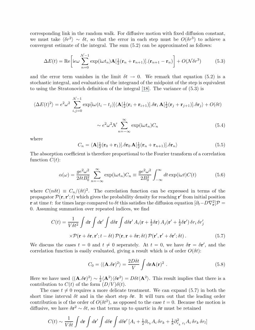
corresponding link in the random walk. For diffusive motion with fixed diffusion constant,we must take 〈δr2〉 ∼ δt, so that the error in each step must be O(δr3) to achieve aconvergent estimate of the integral. The sum (5.2) can be approximated as follows:

∆E(t) = Re

[

ieωN−1∑

n=0

exp(iωtn)A[ 12(rn + rn+1)].(rn+1 − rn)

]

+O(N δr3) (5.3)

and the error term vanishes in the limit δt → 0. We remark that equation (5.2) is astochastic integral, and evaluation of the integrand of the midpoint of the step is equivalentto using the Stratonovich definition of the integral [18]. The variance of (5.3) is

〈∆E(t)2〉 = e2ω2N−1∑

i,j=0

exp[iω(ti − tj)]〈A[ 12 (ri + ri+1)].δri A[ 12 (rj + rj+1)].δrj〉 +O(δt)

∼ e2ω2N∞∑

n=−∞

exp(iωtn)Cn (5.4)

whereCn = 〈A[ 12 (r0 + r1)].δr0 A[ 12 (rn + rn+1)].δrn〉 (5.5)

The absorption coefficient is therefore proportional to the Fourier transform of a correlationfunction C(t):

α(ω) =ge2ω2

2δtB20

∞∑

n=−∞

exp(iωtn)Cn ≡ ge2ω2

2B20

∫ ∞

−∞

dt exp(iωt)C(t) (5.6)

where C(nδt) ≡ Cn/(δt)2. The correlation function can be expressed in terms of the

propagator P(r, r′; t) which gives the probability density for reaching r′ from initial positionr at time t: for times large compared to δt this satisfies the diffusion equation [∂t−D∇2

r]P =

0. Assuming summation over repeated indices, we find

C(t) =1

V δt2

∫

dr

∫

dr′∫

dδr

∫

dδr′Ai(r + 12δr)Aj(r

′ + 12δr

′) δri δr′j

×P(r + δr, r′; t− δt)P(r, r + δr; δt)P(r′, r′ + δr′; δt) . (5.7)

We discuss the cases t = 0 and t 6= 0 seperately. At t = 0, we have δr = δr′, and thecorrelation function is easily evaluated, giving a result which is of order O(δt):

C0 = 〈(A.δr)2〉 =2Dδt

V

∫

drA(r)2 . (5.8)

Here we have used 〈(A.δr)2〉 ∼ 12 〈A2〉〈δr2〉 = Dδt〈A2〉. This result implies that there is a

contribution to C(t) of the form (D/V )δ(t).The case t 6= 0 requires a more delicate treatment. We can expand (5.7) in both the

short time interval δt and in the short step δr. It will turn out that the leading ordercontribution is of the order of O(δt2), as opposed to the case t = 0. Because the motion isdiffusive, we have δr2 ∼ δt, so that terms up to quartic in δr must be retained

C(t) ∼ 1

V δt

∫

dr

∫

dr′∫

dδr

∫

dδr′ [Ai + 12∂rk

Ai δrk + 18∂

2r

krlAi δrk δrl]

×[A′j + 1

2∂r′

kA′

j δr′k + 1

8∂2r′

kr′

lA′

j δr′k δr

′l] δri δr

′j

×[P(r, r′; t) − ∂tP(r, r′; t) δt+ ∂rkP(r, r′; t) δrk + 1

2∂2rkrl

P(r, r′; t)δrkδrl]

×P(r, r + δr; δt)P(r′, r′ + δr′; δt) . (5.9)

The terms containing ∂tP(r, r′; t) can be dropped when there are more than two factorsof δr. The integrals over products of the δr can now be separated out to give

C(t) =1

V δt2

∫

dr

∫

dr′{

AiAj [P − ∂tP δt]〈δri〉〈δr′j〉

+[ 12A′

j∂rkAi P + 1

2A′

j∂rk(PAi) − 1

2A′

j∂rkAi P]〈δriδrk〉〈δr′j〉

+[ 12Ai∂rkA′

j P]〈δr′jδr′k〉〈δri〉

+[ 18Ai∂2rkrl

A′j P + 1

2AiA′j∂

2rkrl

P]〈δriδrkδrl〉〈δr′j〉

+[ 12Ai∂

2rkrl

A′j P]〈δr′jδr′kδr′l〉〈δri〉

+[ 14∂rlAj∂rk

Ai P + 12Ai∂rl

Aj∂rkP]〈δriδrk〉〈δr′lδr′j〉

}

(5.10)

where 〈δr〉 =∫

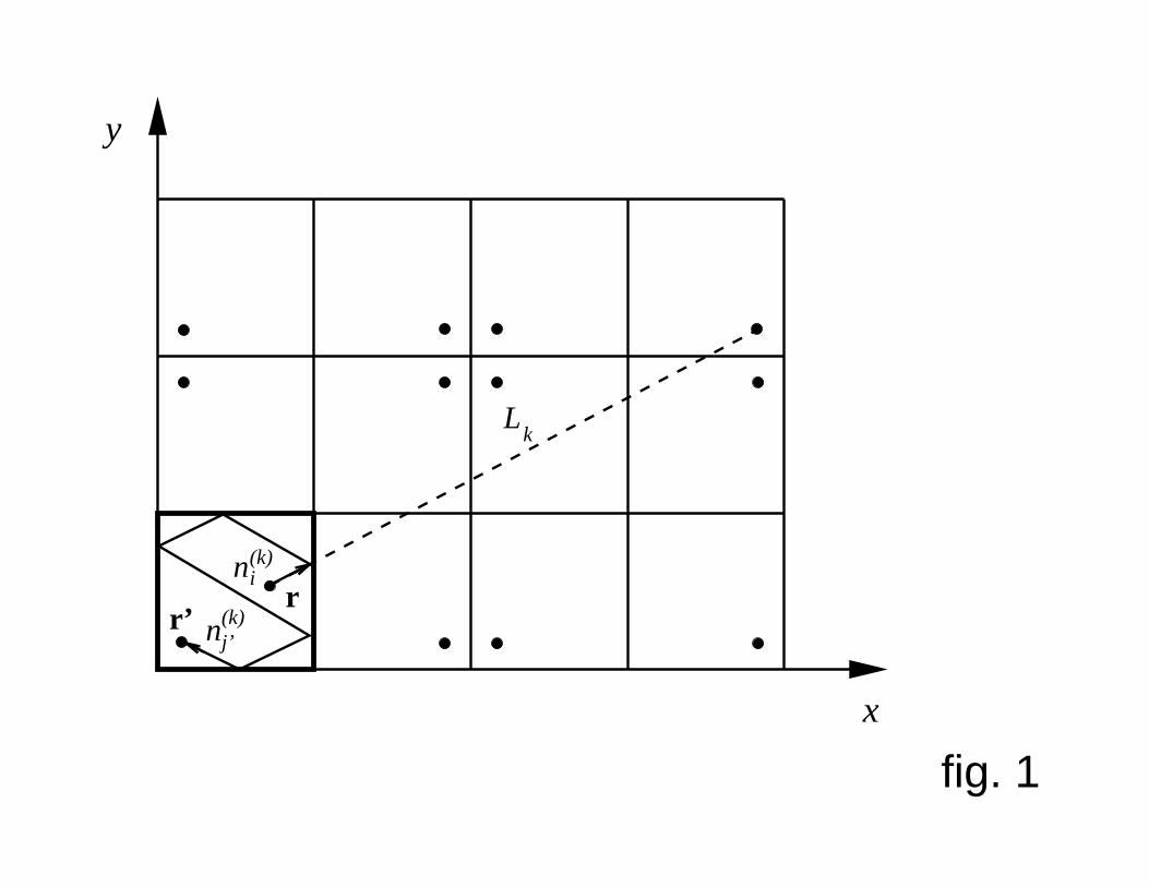
dδr δr P(r,r + δr; δt). Now consider the form of these integrals when δt issufficiently small. The propagator P(r, r+δr; δt) is small unless δr is small. When r is notclose to the boundary, this propagator can be approximated by a function of the distancetravelled, P0(|δr|, δt): because the steps are assumed to be independent, the variance 〈δr2〉averaged over this distribution can be identified with 2dDδt (where d is the dimensionalityof space). When r is close to the boundary, a solution satisfying the boundary conditionn.∇P = 0 is constructed by the method of images. We denote the image of the sourcepoint r by r∗. The diffusion propagator is then

P(r, r + δr; δt) ∼ P0(|δr|, δt) + P0(|δr + r− r∗|, δt) . (5.11)

Since δt is small compared to the time to traverse the particle, the second term onlycontributes for points r close to the surface, which can thus be considered locally flat.We then introduce a local coordinate system arranged so that the nearest boundary pointdefines the origin. In two dimensions, the surface tangent is given by the line x = 0, andthe normal by y = 0. the point r lies at (x, 0), and r∗ = (−x, 0) (figure 2).

The average 〈δri〉 vanishes unless r is close to the boundary, in which case the meandisplacement is inwards, and its projection in the direction perpendicular to the surface is

〈δx〉x =

∫ ∞

0

dx′(x′ − x)[f(x′ − x) + f(x′ + x)] (5.12)

where f(x) is the projection of the distribution P0(|δr|) onto the x axis

f(x) =

∫

dr P0(|δr|, δt) δ(x− |δr|) (5.13)

which satisfies∫ ∞

−∞

dx x2f(x) = 2Dδt . (5.14)

Equations (5.12) and (5.14) show that the mean inward displacement 〈δx〉x is of typicalmagnitude

√Dδt, in a layer of depth

√Dδt next to the boundary, and negligible elsewhere.

The weight w of these inward displacements is clearly ∼ Dδt. We define

w ≡ limL→∞

∫ L

0

dx〈δx〉x . (5.15)

We evaluate w by sustituting (5.12), then making a change of variables X = x′ + x,X ′ = x′ − x. The integral is written as the sum of two integrals, one over the domainX ≤ L, |X ′| ≤ X , which vanishes because of a symmetry, and another integral whichinvolves only f(X ′) in the limit L→ ∞: we find w = Dδt, which implies that

∫

drFi(r)〈δri〉 = −Dδt∫

dsiFi (5.16)

for any vector field F, where dsi are the components of a vector element of the surface.When evaluating the integrals over 〈δriδrj〉 we can approximate these terms by 2Dδtδij ,

because the second term in (5.14) is significant only in a narrow layer of width√Dδt. The

terms containing averages of δr3 make no contribution at order δt2. Retaining only theleading order terms, we find the following contribution for t 6= 0:

C(t) =D2

V

∫

dr

∫

dr′ ∂r

i

Ai(r) ∂r′

jAj(r

′)P(r, r′; t)

−2D2

V

∫

dsi

∫

dr′Ai(r) ∂r′

jAj(r

′)P(r, r′; t)

+D2

V

∫

dsi

∫

ds′j Ai(s)Aj(s′)P(s, s′; t) . (5.17)

After integrating by parts, and adding the delta function contribution from t = 0, we find

C(t) = Dδ(t)

∫

drAiAi −D2

V

∫

dr

∫

dr′AiAj ∂2rir′

jP(r, r′; t) (5.18)

Before Fourier transforming this expression to determine the absorption coefficient, we willintroduce a convenient expression for the propagator:

P(r, r′; t) =∑

α

χα(r)χα(r′) exp(−Dk2αt) (5.19)

where the χα(r) are solutions of the Helmholz equation [∆+k2α]χα = 0, satisfying the Neu-

mann boundary condition ni∂riχα = 0. Using this result, we find the following expression

for the absorption coefficient

α(ω) = Kω2

[∫

drA2 −∑

α

D2k2α

(Dk2α)2 + ω2

∣

∣

∣

∣

∫

drAi∂riχα

∣

∣

∣

∣

2]

(5.20)

where

K =ge2D

B20

=Σ0

B20

. (5.21)

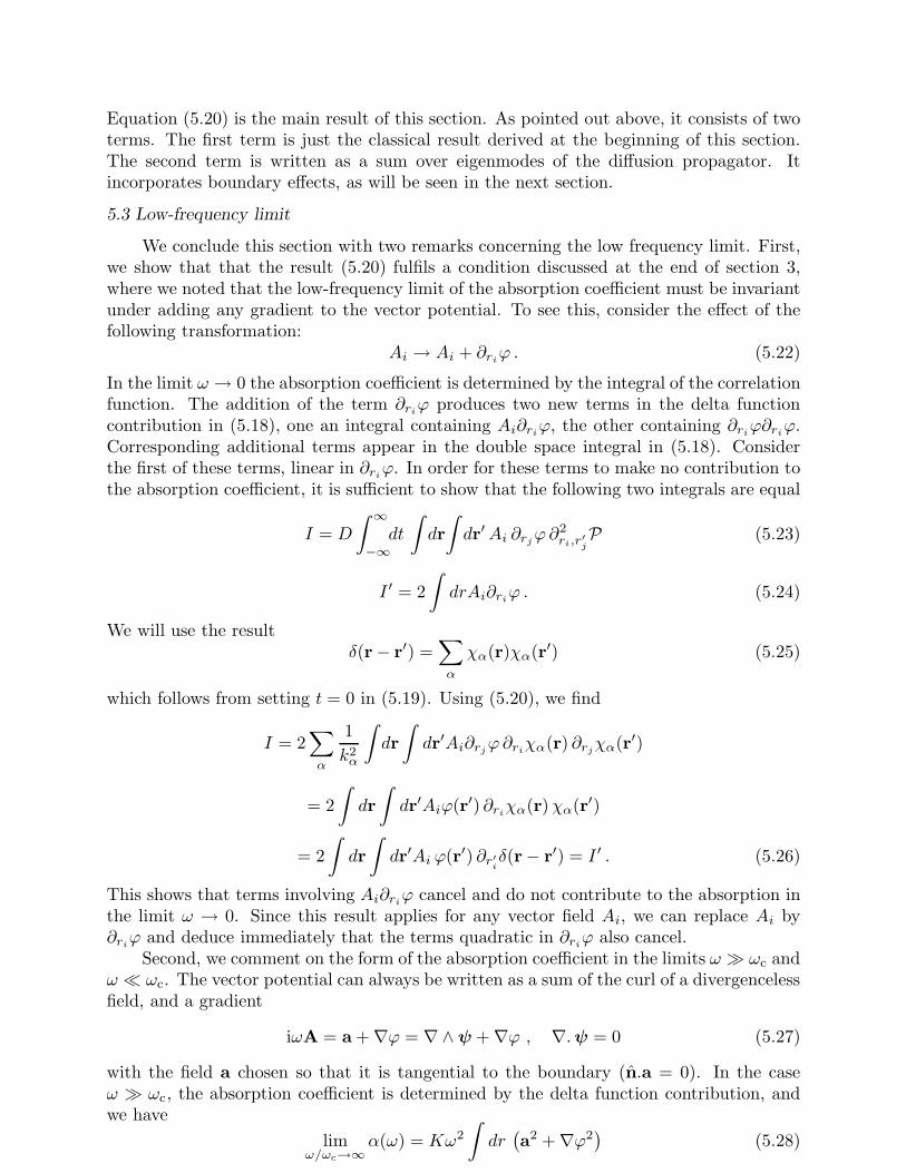
Equation (5.20) is the main result of this section. As pointed out above, it consists of twoterms. The first term is just the classical result derived at the beginning of this section.The second term is written as a sum over eigenmodes of the diffusion propagator. Itincorporates boundary effects, as will be seen in the next section.

5.3 Low-frequency limit

We conclude this section with two remarks concerning the low frequency limit. First,we show that that the result (5.20) fulfils a condition discussed at the end of section 3,where we noted that the low-frequency limit of the absorption coefficient must be invariantunder adding any gradient to the vector potential. To see this, consider the effect of thefollowing transformation:

Ai → Ai + ∂riϕ . (5.22)

In the limit ω → 0 the absorption coefficient is determined by the integral of the correlationfunction. The addition of the term ∂ri

ϕ produces two new terms in the delta functioncontribution in (5.18), one an integral containing Ai∂ri

ϕ, the other containing ∂riϕ∂ri

ϕ.Corresponding additional terms appear in the double space integral in (5.18). Considerthe first of these terms, linear in ∂ri

ϕ. In order for these terms to make no contribution tothe absorption coefficient, it is sufficient to show that the following two integrals are equal

I = D

∫ ∞

−∞

dt

∫

dr

∫

dr′Ai ∂rjϕ∂2

ri,r′

jP (5.23)

I ′ = 2

∫

drAi∂riϕ . (5.24)

We will use the resultδ(r− r′) =

∑

α

χα(r)χα(r′) (5.25)

which follows from setting t = 0 in (5.19). Using (5.20), we find

I = 2∑

α

1

k2α

∫

dr

∫

dr′Ai∂rjϕ∂ri

χα(r) ∂rjχα(r′)

= 2

∫

dr

∫

dr′Aiϕ(r′) ∂riχα(r)χα(r′)

= 2

∫

dr

∫

dr′Ai ϕ(r′) ∂r′

iδ(r− r′) = I ′ . (5.26)

This shows that terms involving Ai∂riϕ cancel and do not contribute to the absorption in

the limit ω → 0. Since this result applies for any vector field Ai, we can replace Ai by∂riϕ and deduce immediately that the terms quadratic in ∂ri

ϕ also cancel.Second, we comment on the form of the absorption coefficient in the limits ω ≫ ωc and

ω ≪ ωc. The vector potential can always be written as a sum of the curl of a divergencelessfield, and a gradient

iωA = a + ∇ϕ = ∇∧ψ + ∇ϕ , ∇.ψ = 0 (5.27)

with the field a chosen so that it is tangential to the boundary (n.a = 0). In the caseω ≫ ωc, the absorption coefficient is determined by the delta function contribution, andwe have

limω/ωc→∞

α(ω) = Kω2

∫

dr(

a2 + ∇ϕ2)

(5.28)

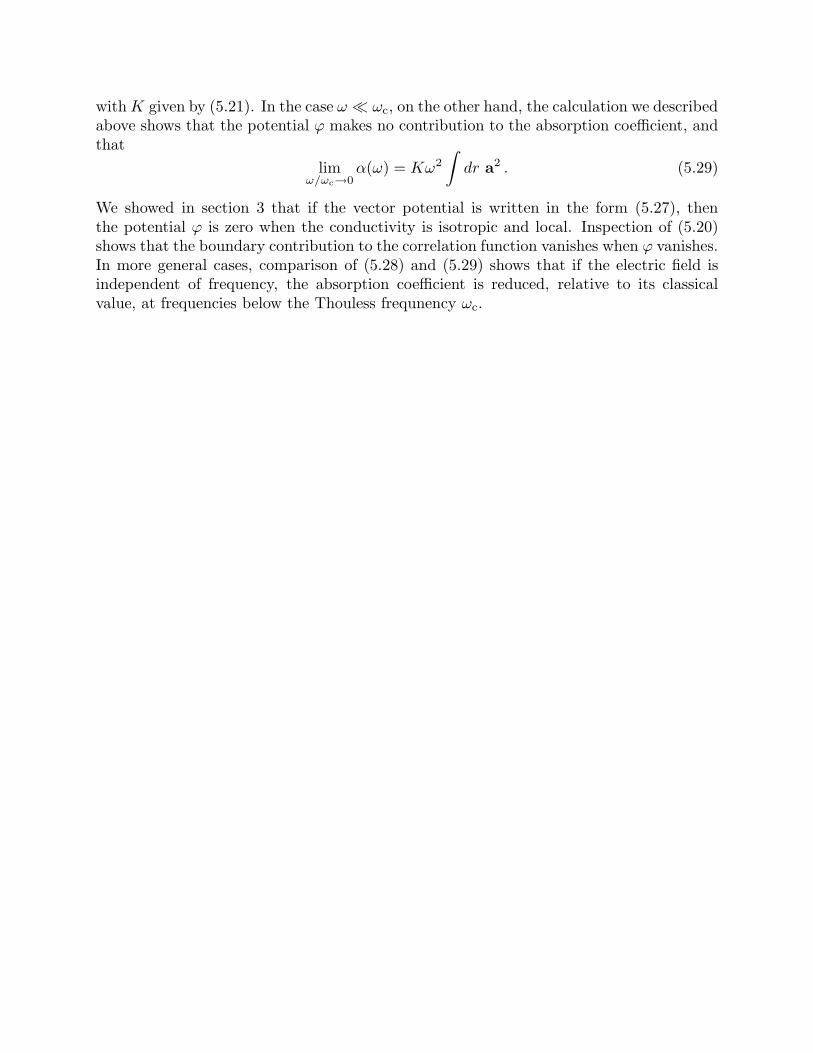
withK given by (5.21). In the case ω ≪ ωc, on the other hand, the calculation we describedabove shows that the potential ϕ makes no contribution to the absorption coefficient, andthat

limω/ωc→0

α(ω) = Kω2

∫

dr a2 . (5.29)

We showed in section 3 that if the vector potential is written in the form (5.27), thenthe potential ϕ is zero when the conductivity is isotropic and local. Inspection of (5.20)shows that the boundary contribution to the correlation function vanishes when ϕ vanishes.In more general cases, comparison of (5.28) and (5.29) shows that if the electric field isindependent of frequency, the absorption coefficient is reduced, relative to its classicalvalue, at frequencies below the Thouless frequnency ωc.

6. Self-consistent electric field: diffusive case

6.1 Non-local conductance

We can deduce the non-local conductivity from the results of the previous section intwo ways. We could use (4.6) as the definition of the conductivity, and evaluate it bysetting A(r) = δ(r− R)ei in (5.5), so that

σij(R,R′; t) =

e2

(2πh)dδt2〈δ(R− r)δriδ(R

′ − r′)δrj〉 . (6.1)

Alternatively, if we write the absorption coefficient in terms of the non-local conductivityin the form

α(ω) =1

2E20

∫

dr

∫

dr′∫

dτ exp[iωτ ] σij(r, r′, ω)Ei(r)Ej(r

′) (6.2)

the kernel σij(r, r′; t) is deduced from (5.18). By either route we find

σ(r, r′; t) = Σ0

[

δijδ(r− r′)δ(t) −D∂2rir′

jP(r, r′; t)

]

(6.3)

where Σ0 is the bulk conductivity, and P(r, r′, t) is the propagator, given by (5.19).This form for the non-local conductivity was originally given in ref. [13] (and in the

DC limit in ref. [12]). The argument in these earlier papers involves the diagrammaticanalysis of disorder averaged perturbation theory, and in the case of [13] it appeals to asupersymmetric formalism. We believe that our derivation is more direct, and also morecompelling. Our derivation considers the effect of the surface explicitly, whereas it is notclear from the diagrammatic analysis that there are not additional contributions whicharise from integrating fields over the surface of the sample. Our derivation also dealsexplicitly with the fact that the trajectories are discontinuous, and we show explicitly howthe correct evaluation is related to the Stratonovitch definition of the integral over thetrajectory.

6.2 Self-consistent solution

The self-consistent electric field has to be chosen to satisfy (3.5). First we remarkthat in the case of diffusive electron motion, the term containing ǫ0 is negligible, and canbe dropped. Estimating the magnitude of σ by the bulk conductance Σ0 = ne2D, andnoting that the bulk plasma frequency scale is ω2

p ∼ Ne2/meǫ0, we see that this term isnegligible provided ω ≫ ωs, where ωs is the elastic scattering rate. This is consistent withthe assumptions that the electron motion is diffusive.

We therefore wish to determine an electric field for which ∇.(σE) = 0; more explicitlywe require

Σ0 ∂ri

∫

dt exp(iωt)

∫

dr′[

Ei(r′)δ(r− r′)δ(t) −D∂2

rir′

jP(r, r′; t) Ej(r

′)]

= 0 . (6.4)

Substituting for the propagator using (5.19), we find

0 = Σ0

[

∂riEi −

∑

α

D2k2α

D2k4α + ω2

∂ri

∫

dr′∂riχα(r)∂r′

jχα(r′)Ej(r

′)

]

= Σ0 ∂riEi + Σ0

∑

α

D2k4α

D2k4α + ω2

χα(r)

∫

dr′ ∂rjχα(r′)Ej(r

′)

= Σ0 ∂riEi − Σ0

∑

α

D2k4α

D2k4α + ω2

χα(r)[

∫

dr′ χα(r′)∂r′

jEj(r

′)

−∫

dsi χα(s)Ei(s)]

. (6.5)

This equation has a solution where ∇.E = 0 everywhere, with E tangential to the bound-ary. The classical solution for an isotropic local conductance satisfies these conditions. Weconclude that, at least in the case where there is no static biasing magnetic field applied,the electric field configuration is independent of frequency.

6.3 Calculation of the absorption coefficient

We have shown that the electric field distribution is independent of frequency: we cantherefore use the solution of the form (3.7), (3.8), with φ = 0, and with ψ tangential to theboundary. Referring to (5.21) we observe that, after integrating by parts, the integrals areseen to vanish because the field A is divergenceless and is tangential at the boundary. Itfollows that the summation in (5.21) vanishes, and that the absorption coefficient is givenby the classical expression (5.1), at all relevant frequencies.

We conclude by describing a useful approach to calculating the field ψ, satisfyingPoisson’s equation (3.9). The solution can be obtained from a Green’s function G(r, r′)satisfying ∇2G = −δ(r− r′). A suitable Green’s function is

G(r, r′) =∑

n

ξn(r)ξn(r′)

k2n

(6.6)

where the ξn(r) and k2n are eigenfunctions and eigenvalues of the Helmholtz equation,

[∇2 + k2n]ξn = 0, solved with the Dirichlet boundary condition ξn(r) = 0. The field ψ(r)

is then obtained by applying this Green’s function to the source term iωB0 appearing in(3.9). In two dimensions, the absorption coefficient can then be written in terms of the ξnas follows

α(ω) =Σ0

2E20

∫

dr∣

∣∇ψ∣

∣

2= − Σ0

2E20

∫

dr ψ∇2ψ∗ = iωΣ0B0

2E0)2

∫

dr ψ . (6.7)

Using the Green’s function (6.6) to obtain ψ, we have

α(ω) =Σ0ω

2

2c2

∑

n

1

k2n

∣

∣

∣

∣

∫

dr ξn(r)

∣

∣

∣

∣

2

. (6.8)

This is a very general expression for the classical magnetic dipole absorption coefficientin particles with diffusive electron motion, expressed in terms of solutions of the twodimensional Helmholtz equation. As it stands, equation (6.8) is valid for two-dimensionalparticles.

We note that the eigenfunctions ξn(r) obey Dirichlet boundary conditions and thatthe absorption coefficient for a given geometry can be significantly reduced by applyingcuts orthogonal to the boundary: the main contribution to the sum in (6.8) comes from theground state and the low-lying states and the corresponding eigenvalues are increased by

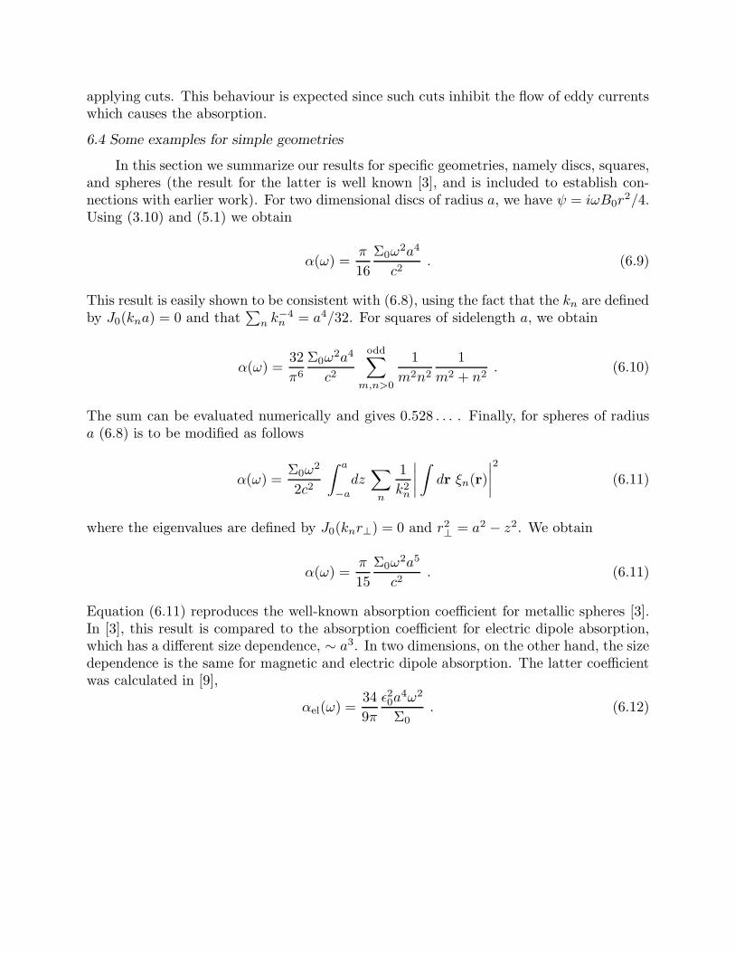
applying cuts. This behaviour is expected since such cuts inhibit the flow of eddy currentswhich causes the absorption.

6.4 Some examples for simple geometries

In this section we summarize our results for specific geometries, namely discs, squares,and spheres (the result for the latter is well known [3], and is included to establish con-nections with earlier work). For two dimensional discs of radius a, we have ψ = iωB0r

2/4.Using (3.10) and (5.1) we obtain

α(ω) =π

16

Σ0ω2a4

c2. (6.9)

This result is easily shown to be consistent with (6.8), using the fact that the kn are definedby J0(kna) = 0 and that

∑

n k−4n = a4/32. For squares of sidelength a, we obtain

α(ω) =32

π6

Σ0ω2a4

c2

odd∑

m,n>0

1

m2n2

1

m2 + n2. (6.10)

The sum can be evaluated numerically and gives 0.528 . . . . Finally, for spheres of radiusa (6.8) is to be modified as follows

α(ω) =Σ0ω

2

2c2

∫ a

−a

dz∑

n

1

k2n

∣

∣

∣

∣

∫

dr ξn(r)

∣

∣

∣

∣

2

(6.11)

where the eigenvalues are defined by J0(knr⊥) = 0 and r2⊥ = a2 − z2. We obtain

α(ω) =π

15

Σ0ω2a5

c2. (6.11)

Equation (6.11) reproduces the well-known absorption coefficient for metallic spheres [3].In [3], this result is compared to the absorption coefficient for electric dipole absorption,which has a different size dependence, ∼ a3. In two dimensions, on the other hand, the sizedependence is the same for magnetic and electric dipole absorption. The latter coefficientwas calculated in [9],

αel(ω) =34

9π

ǫ20a4ω2

Σ0. (6.12)

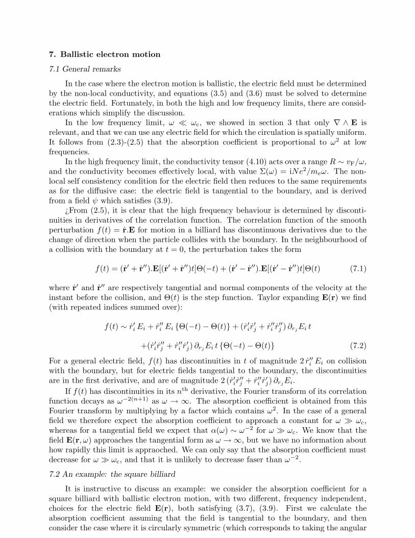
7. Ballistic electron motion

7.1 General remarks

In the case where the electron motion is ballistic, the electric field must be determinedby the non-local conductivity, and equations (3.5) and (3.6) must be solved to determinethe electric field. Fortunately, in both the high and low frequency limits, there are consid-erations which simplify the discussion.

In the low frequency limit, ω ≪ ωc, we showed in section 3 that only ∇ ∧ E isrelevant, and that we can use any electric field for which the circulation is spatially uniform.It follows from (2.3)-(2.5) that the absorption coefficient is proportional to ω2 at lowfrequencies.

In the high frequency limit, the conductivity tensor (4.10) acts over a range R ∼ vF/ω,and the conductivity becomes effectively local, with value Σ(ω) = iNe2/meω. The non-local self consistency condition for the electric field then reduces to the same requirementsas for the diffusive case: the electric field is tangential to the boundary, and is derivedfrom a field ψ which satisfies (3.9).

¿From (2.5), it is clear that the high frequency behaviour is determined by disconti-nuities in derivatives of the correlation function. The correlation function of the smoothperturbation f(t) = r.E for motion in a billiard has discontinuous derivatives due to thechange of direction when the particle collides with the boundary. In the neighbourhood ofa collision with the boundary at t = 0, the perturbation takes the form

f(t) = (r′ + r′′).E[(r′ + r′′)t]Θ(−t) + (r′ − r′′).E[(r′ − r′′)t]Θ(t) (7.1)

where r′ and r′′ are respectively tangential and normal components of the velocity at theinstant before the collision, and Θ(t) is the step function. Taylor expanding E(r) we find(with repeated indices summed over):

f(t) ∼ r′iEi + r′′i Ei {Θ(−t) − Θ(t)} + (r′ir′j + r′′i r

′′j ) ∂rj

Ei t

+(r′ir′′j + r′′i r

′j) ∂rj

Ei t {Θ(−t) − Θ(t)} (7.2)

For a general electric field, f(t) has discontinuities in t of magnitude 2 r′′i Ei on collisionwith the boundary, but for electric fields tangential to the boundary, the discontinuitiesare in the first derivative, and are of magnitude 2 (r′ir

′′j + r′′i r

′j) ∂rj

Ei.

If f(t) has discontinuities in its nth derivative, the Fourier transform of its correlationfunction decays as ω−2(n+1) as ω → ∞. The absorption coefficient is obtained from thisFourier transform by multiplying by a factor which contains ω2. In the case of a generalfield we therefore expect the absorption coefficient to approach a constant for ω ≫ ωc,whereas for a tangential field we expect that α(ω) ∼ ω−2 for ω ≫ ωc. We know that thefield E(r, ω) approaches the tangential form as ω → ∞, but we have no information abouthow rapidly this limit is appraoched. We can only say that the absorption coefficient mustdecrease for ω ≫ ωc, and that it is unlikely to decrease faser than ω−2.

7.2 An example: the square billiard

It is instructive to discuss an example: we consider the absorption coefficient for asquare billiard with ballistic electron motion, with two different, frequency independent,choices for the electric field E(r), both satisfying (3.7), (3.9). First we calculate theabsorption coefficient assuming that the field is tangential to the boundary, and thenconsider the case where it is circularly symmetric (which corresponds to taking the angular

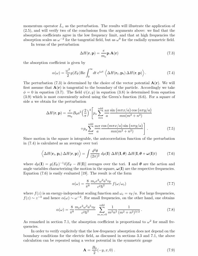
momentum operator Lz as the perturbation. The results will illustrate the application of(2.5), and will verify two of the conclusions from the arguments above: we find that theabsorption coefficients agree in the low frequency limit, and that at high frequencies theabsorption scales as ω−2 for the tangential field, but as ω0 for the radially symmetric field.

In terms of the perturbation

∆H(r,p) =e

mep.A(r) (7.3)

the absorption coefficient is given by

α(ω) =ω2

2g(EF)Re

∫ ∞

0

dt eiωt⟨

∆H(rt,pt) ∆H(r,p)⟩

. (7.4)

The perturbation (7.3) is determined by the choice of the vector potential A(r). We willfirst assume that A(r) is tangential to the boundary of the particle. Accordingly we takeφ = 0 in equation (3.7). The field ψ(x, y) in equation (3.8) is determined from equation(3.9) which is most conveniently solved using the Green’s function (6.6). For a square ofside a we obtain for the perturbation

∆H(r,p) =e

meB0a

2( 2

π

)4[

px

odd∑

mn

nπ

a

sin(

mπx/a)

cos(

nπy/a)

mn(m2 + n2)

+py

odd∑

mn

mπ

a

cos(

mπx/a)

sin(

nπy/a)

mn(m2 + n2)

]

. (7.5)

Since motion in the square is integrable, the autocorrelation function of the perturbationin (7.4) is calculated as an average over tori

⟨

∆H(rt,pt) ∆H(r,p)⟩

=

∫

d2θ

(2π)2dµ(I) ∆H(I, θ) ∆H(I, θ + ω(I)t) (7.6)

where dµ(I) = g(EF)−1δ[EF − H(I)] averages over the tori. I and θ are the action andangle variables characterizing the motion in the square, ω(I) are the respective frequencies.Equation (7.6) is easily evaluated [19]. The result is of the form

α(ω) =8

π8

mee2ω2a5vF

c2h2 f(ω/ωc) (7.7)

where f(z) is an energy-independent scaling function and ωc = vF/a. For large frequencies,f(z) ∼ z−4 and hence α(ω) ∼ ω−2. For small frequencies, on the other hand, one obtains

α(ω) =8

π8

mee2ω2a5vF

c2h2

odd∑

m,n>0

1

m2n2

1

(m2 + n2)3/2. (7.8)

As remarked in section 7.1, the absorption coefficient is proportional to ω2 for small fre-quencies.

In order to verify explicitely that the low-frequency absorption does not depend on theboundary conditions for the electric field, as discussed in sections 3.3 and 7.1, the abovecalculation can be repeated using a vector potential in the symmetric gauge

A =B0

2(−y, x, 0) . (7.9)

We note that this choice of the vector potential does note satisfy tangential boundaryconditions. The corresponding perturbation is

∆H(r,p) =e

mep.A =

eB0

2meLz . (7.10)

For small frequencies we find again the result (7.8), thus verifying explicitly that theboundary conditions do not influence the low-frequency absorption. For high frequencies,on the other hand, we find α(ω) ∼ ω0, as predicted in the previous section.

8. Acknowledgements

We are grateful to the organisers of the program on ‘Quantum Chaos and DisorderedSystems’ for inviting us to the Newton Institute. The work of BM was supported by theMax Planck Institute for Physics of Complex Systems, and that of MW was supportedby a research grants from the EPSRC, reference GR/H94337 and GR/L02302. PNWwas working at Strathclyde University when this project was started, where his work wassupported by an EPSRC grant; he is currently supported by a EU fellowship.

References

[1] G. Mie, Ann. Physik., 25, 377, (1908).

[2] N. W. Ashcroft and N. D. Mermin, Solid State Physics, Philadelphia: Saunders College,(1976).

[3] E. M. Lifshitz and L. P. Pitaevskii, Statistical Physics, Part 2, (Volume 9 of Landauand Lifshitz Course of Theoretical Physics), Oxford: Pergamon, (1980).

[4] D. B. Tanner, A. J. Sievers and R. A. Buhrman, Phys. Rev., B11, 1330-41, (1975).

[5] D. Stroud and F. P. Pan, Phys. Rev., B17, 1602-10, (1978).

[6] G. L. Carr, S. Perkowitz, and D. B. Tanner, in Infrared and Millimeter Waves, 13, 169,ed. K. J. Button, Academic Press, (1985).

[7] E. J. Austin and M. Wilkinson, J. Phys.: Condens. Matter, 5, 8461-8484, (1993).

[8] M. Wilkinson and E. J. Austin, J. Phys.: Condens. Matter, 6, 4153-4166, (1994).

[9] B. Mehlig and M. Wilkinson, J. Phys.: Condens. Matter, 9, 3277-90, (1997).

[10] L. P. Gorkov and G. M. Eliashberg, Zh. Eksp. Teor. Fiz., 48, 1407, (1965) (transl.

Sov. Phys. JETP, 21, 940, (1965)).

[11] N. Argaman, Phys. Rev., B47, 4440, (1993).

[12] C. L. Kane, R. A. Serota and P. A. Lee, Phys. Rev., B37, 6701-10, (1988).

[13] R. A. Serota, J. Yu and Y. H. Kim, Phys. Rev., B42, 9724-7, (1990).

[14] M. Wilkinson, J. Phys., A20, 2415, (1987).

[15] D. J. Thouless, Phys. Rep., 13, 93, (1974).

[16] A. Kamenev and Y. Gefen, Int. J. Mod. Phys., B9, 751-802, (1995).

[17] B. Reulet, M. Ramin, H. Bouchiat and D. Mailly, Phys. Rev. Lett., 75, 124-27,(1996).

[18] N. G. van Kampen, Stochastic processes in physics and chemistry, Amsterdam: NorthHolland, (1981).

[19] B. Mehlig, Phys. Rev., B55, R10193, (1997).

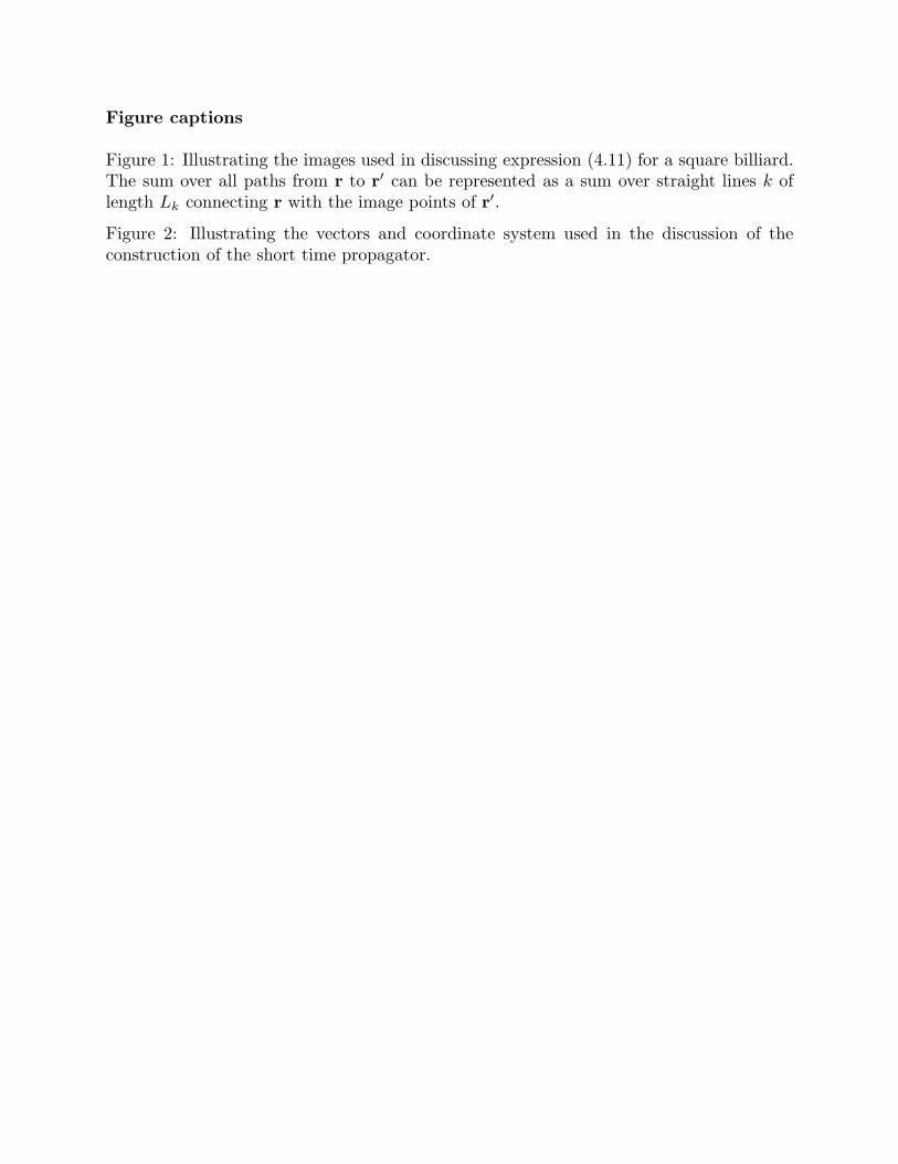
Figure captions

Figure 1: Illustrating the images used in discussing expression (4.11) for a square billiard.The sum over all paths from r to r′ can be represented as a sum over straight lines k oflength Lk connecting r with the image points of r′.

Figure 2: Illustrating the vectors and coordinate system used in the discussion of theconstruction of the short time propagator.

(k)i

n(k)j’

n���������

���������

��������������������������������������������������������������������������������������������������������������������������������������������������������������������������������������������������������������������������������������������������������������������������������������������������������������������������������������������������������������������������������������������������������������������������������������������������������������������������������������������������������������������������������������������������������������������������������������������������������������������������������������������������������������������������

��������������������������������������������������������������������������������������������������������������������������������������������������������������������������������������������������������������������������������������������������������������������������������������������������������������������������������������������������������������������������������������������������������������������������������������������������������������������������������������������������������������������������������������������������������������������������������������������������������������������������������������������������������������������������

Lk

x

y

fig. 1

rr’

fig.2

r’

r*r

x

y