arX

iv:0

806.

0167

v2 [

phys

ics.

geo-

ph]

24

Mar

200

9

J Geod.DOI 10.1007/s00190-009-0304-7

Precise geodesy with the Very Long Baseline Array

Leonid Petrov · David Gordon · John Gipson · Dan MacMillan ·

Chopo Ma · Ed Fomalont · R. Craig Walker · Claudia Carabajal

Received: 01 June, 2008/ Accepted: 26 January 2009c© Springer-Verlag 2009

Abstract We report on a program of geodetic mea-

surements between 1994 and 2007 which used the Very

Long Baseline Array and up to 10 globally distributed

antennas. One of the goals of this program was to mon-itor positions of the array at a 1 millimeter level of

accuracy and to tie the VLBA into the International

Terrestrial Reference Frame. We describe the analysis

of these data and report several interesting geophys-ical results including measured station displacements

due to crustal motion, earthquakes, and antenna tilt.

In terms of both formal errors and observed scatter,

these sessions are among the very best geodetic VLBI

experiments.

Keywords VLBI · coordinate systems · platetectonics · VLBA

L. Petrov,ADNET Systems Inc./NASA GSFC, Code 610.2, Greenbelt, MD20771 USAE-mail: Leonid.Petrov@lpetrov.net

D. Gordon, J. Gipson, D. MacMillanNVI Inc./NASA GSFC, Code 698, Greenbelt, MD 20771 USA

C. MaNASA GSFC, Code 698, Greenbelt, MD 20771 USA

E. Fomalont,National Radio Astronomy Observatory, 520 Edgemont Rd,Charlottesville, VA 22903–2475, USA

R. C. WalkerNational Radio Astronomy Observatory, P. O. Box O, Socorro,NM 87801 USA.

C. Carabajal

Sigma Space Corporation/NASA GSFC, Code 698, Greenbelt,MD 20771 USA

Published online: 28 February 2009

1 Introduction

The method of very long baseline interferometry (VLBI),

first proposed by Matveenko et al. (1965), is a techniqueof computing the cross-power spectrum of a signal from

radio sources digitally recorded at two or more radiote-

lescopes equipped with independent frequency gener-

ators. This spectrum is used in a variety of applica-

tions. One of the many ways of utilizing information inthe cross-power spectrum is to derive a group interfer-

ometric delay (Takahashi et al. 2000; Thompson et al.

2001). It was shown by Shapiro and Knight (1970) that

group delays can be used for precise geodesy. The firstdedicated geodetic experiment, on January 11, 1969,

yielded 1 meter accuracy (Hinteregger et al. 1972). In

the following decades VLBI technology flourished, sen-

sitivities and accuracies were improved by several or-

ders of magnitude, and arrays of dedicated antennaswere built. Currently, VLBI activities for geodetic ap-

plications are coordinated by the International VLBI

Service for Geodesy and Astrometry (IVS) (Schluter

and Behrend 2007).

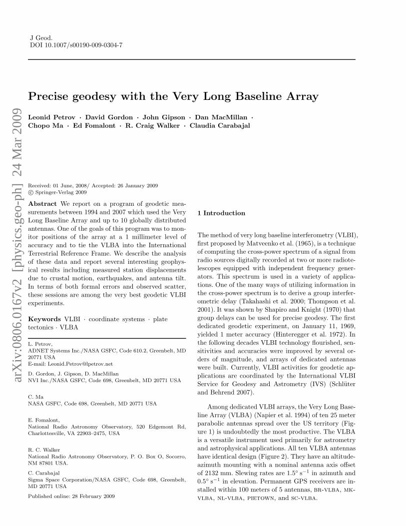
Among dedicated VLBI arrays, the Very Long Base-

line Array (VLBA) (Napier et al. 1994) of ten 25 meter

parabolic antennas spread over the US territory (Fig-

ure 1) is undoubtedly the most productive. The VLBA

is a versatile instrument used primarily for astrometryand astrophysical applications. All ten VLBA antennas

have identical design (Figure 2). They have an altitude-

azimuth mounting with a nominal antenna axis offset

of 2132 mm. Slewing rates are 1.5 s−1 in azimuth and0.5 s−1 in elevation. Permanent GPS receivers are in-

stalled within 100 meters of 5 antennas, br-vlba, mk-

vlba, nl-vlba, pietown, and sc-vlba.

2

Fig. 1 Positions of the antennas of the Very Long Baseline Array

Phase referencing for detection of weak radio sources

and for proper motion and parallax measurements are

used in about half of all VLBA sessions. Accuracies

on the order of 10 microarcseconds using source–to–calibrator separations of around one degree are achieved

in the best current observations. Such accuracies need

to be supported by the underlying geometric model and

its input parameters, including the station and sourcecatalogs and the Earth orientation parameters (EOP).

A future goal is to improve on this accuracy by a factor

of 2 or more. To achieve 10 microarcsecond accuracy on

a 4000 km baseline, a delay accuracy after calibration of

0.2 mm or 0.6 ps is required for any effects that cannotbe reduced by integration. Phase referencing over a one

degree source–to–calibrator separation reduces model

errors by a factor of 57, requiring the model parameters

to be accurate to around 1 cm. Higher accuracies aredesired to deal with the cumulative effect of several mo-

del parameters, to meet future goals, or to allow larger

source–to–calibrator separations.

Use of the Global Positioning System (GPS) can

provide very high quality time series of site positions.

Averaging these time series over several years can pro-

vide sub-mm estimates of the phase center positions ofthe GPS antennas, but this precision cannot be trans-

ferred to the reference points of the VLBI antennas for

several reasons. First, measurements of the tie vector

between the GPS phase center and the reference pointof a radiotelescope introduce an additional uncertainty

at a level of 3 mm or higher. Second, systematic errors

of the GPS technique, such as phase center variations,

multi-path, scale errors, and orbital errors, may cause

biases in measurement of the phase center at a level

of tens of mm. Third, a nearby GPS receiver may not

experience the same localized effects as the VLBI an-tenna, such as settling or tilting of the support struc-

ture. According to Ray and Altamimi (2005) (Table 4 in

their paper), the root mean square (rms) of differences

between coordinates of VLBI reference points derivedfrom analysis of VLBI observations and from analysis

of GPS observations plus ties measurements among 25

pairs of GPS/VLBI sites are 6 mm for the horizontal

components and 13 mm for the vertical components

after removal of the contribution of 14 Helmert trans-formation parameters fitted to the differences.

The best way for determining positions of the an-

tenna reference points is to derive them directly from

dedicated geodetic VLBI observations on the VLBA

array. Uncertainties of better than 1 mm are easilyachieved. Since the motion of these antenna reference

points cannot be predicted precisely, geodetic observa-

tions need to be repeated on a regular basis in order to

sustain that high precision.

The importance of precise position monitoring was

recognized during the design of the VLBA and eachantenna began to participate in geodetic VLBI obser-

vations soon after it was commissioned. Between July

1994 and August 2007, there were 132 dedicated 24

hour dual band S/X VLBI sessions under geodesy andabsolute astrometry programs with a rate of 6–24 ses-

sions per year. During each session, all ten VLBA an-

tennas and up to 10 other geodetic VLBI stations par-

3

ticipated. In this paper we present the geodetic results

from this campaign. In section 2 we describe the goals

of the observations, scheduling strategies and the hard-

ware configuration. In section 3 we describe the algo-

rithm for computing group delays from the output ofthe FX VLBA correlator and validation of the post-

correlator analysis procedure. The results and the error

analysis are presented in sections 4 and 5. Concluding

remarks are given in section 6.

2 Observing sessions

The primary goal of these geodetic VLBI observations

was to derive an empirical mathematical model of themotions of the antenna reference points. The antenna

reference point is the projection of antenna’s moving

axis (the elevation axis for altitude-azimuth mounts) to

the fixed axis (the azimuthal axis for altitude-azimuth

mounts). This mathematical model can be used for re-duction of astronomical VLBA observations as well as

for making inferences about the geophysical processes

which cause this motion. A secondary goal was to es-

timate the precise absolute positions of many compact

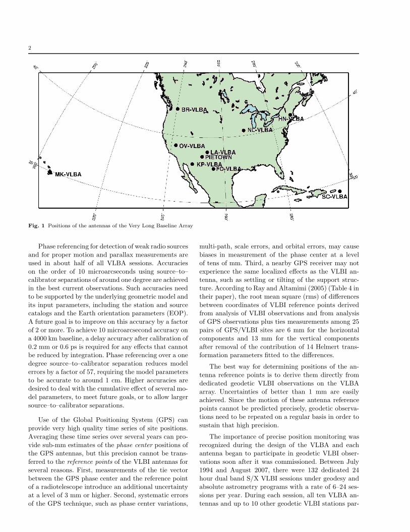
Fig. 2 The VLBA station pietown is in the background. Thepermanent GPS receiver pie1 is in the foreground.

radio sources not previously observed under absolute

astrometry programs, for use as phase referencing cali-

brators. Other goals, not discussed here, include mon-

itoring a list of ∼ 400 selected sources and producing

time series of source coordinate estimates and imagesfor improving the source position catalogue (A. Fey

et al. (2009), paper in preparation) and for studying

source structure changes (Piner et al. 2007; Kovalev et

al. 2008).

The observing sessions were typically 24 hours long.

The radio sources observed were distant active galactic

nuclei at distances of a gigaparsec scale1 with contin-

uum radio emission from regions of typically 0.1–10 mil-liarcsecond in size.

VLBA geodetic observations use the dual frequency

S/X mode, observing simultaneously at S and X bands,centered around 2.3 and 8.6 GHz. This is enabled by a

dichroic mirror permanently positioned over the S band

receiver, reflecting higher frequency radiation towards

a deployable reflector leading to the X band receiver.The system equivalent flux densities (SEFD) of VLBA

antennas are in the range of 350–400 Jy when using

the dual-frequency S/X system. From each receiver,

four frequency channels 4 MHz wide before April 1995

and 8 MHz thereafter, were recorded over a largespanned bandwidth to provide precise measurements

of group delays. The sequence of frequencies (called IF)

was selected to minimize sidelobes in the delay reso-

lution function and to reduce adverse effects of radiointerference. The sequence was slightly adjusted over

the 14 year period of observations in accordance with

changes in the interference environment. The frequency

sequence used in the session of 2007.08.01 is presented

in Table 1.

Table 1 The range of frequencies in the observing session of2007.08.01, in MHz.

IF1 2232.99 2240.99

IF2 2262.99 2270.99IF3 2352.99 2360.99IF4 2372.99 2380.99IF5 8405.99 8413.99IF6 8475.99 8483.99IF7 8790.99 8798.99IF8 8895.99 8903.99

2.1 Scheduling

Among the 132 observing sessions, 97 can be charac-

terized as global geodetic sessions and 35 as absolute

astrometry sessions. They differ in scheduling strategy.

1 1 gigaparsec ≈ 3.2 · 109 light years ≈ 3 · 1025 m

4

A wider list of 150–250 sources was observed in each

astrometry session while a shorter list of ∼100 objects

was observed in each geodesy session.

2.1.1 Scheduling of astrometric sessions

Two lists of sources were observed in astrometry ses-

sions: a list of 150–200 target sources and a list of 30–80

tropospheric calibrators. Selection of tropospheric cali-brators was based on two criteria: a) the compactness

at both X and S band, i.e. the ratio of the median cor-

related flux density at baselines longer than 5000 km to

the median correlated flux density at baselines shorter

than 900 km, must be greater than 0.5; b) the corre-lated flux density at baselines longer than 5000 km must

be greater than 0.4 Jy at both X and S bands. These

sources are frequently observed in other IVS geodetic

programs.

Target sources were scheduled for 1–3 scans, i.e. the

period of time when antennas are on source and record

the data, in a sequence that seeks to minimize slewing

time needed for pointing all antennas to the next source.

In the astrometry sessions, normally all antennas simul-taneously observe the same object for the same dura-

tion. Scan durations were determined on the basis of

the predicted correlated flux density and the SEFDs to

get SNRs of the multi-band fringe amplitude greaterthan 20. The typical scan durations were 40–480 s.

The sequence of target sources was interrupted ev-

ery 1.5 hours, to observe 3–5 tropospheric calibrators.

The tropospheric calibrators were scheduled in such a

way that at each station, at least one calibrator was ob-served in the ranges of [7, 20] elevation, [20, 50] ele-

vation, and above 50 elevation. The purpose of includ-

ing tropospheric calibrators was a) to reliably estimate

the zenith path delay of the neutral atmosphere in the

least squares (LSQ) solution, and b) to link the posi-tions of new or rarely observed target sources with those

of frequently observed calibrators. Astrometric sched-

ules were prepared with the NRAO software package

SCHED. The efficiency of these schedules, i.e. the ra-tio of time on source to the total time of the observing

session is typically ∼70%.

2.1.2 Scheduling of geodetic sessions

The geodetic sessions involved ∼15–20 geographically

dispersed antennas with varying sensitivities. At any

given time, few sources, if any, are visible by the entire

network. Hence, in contrast to the astrometric sessions,at any instant different subsets of antennas will be ob-

serving different sources, and the integration time will

vary from antenna to antenna in order to reach the

required SNR. The minimum elevation angle for sched-

uled observations for all antennas in the geodetic VLBA

sessions is set to 5 degrees.

These sessions were scheduled using the automatic

scheduling mode of the SKED program. The schedulersets up some general parameters that govern how the

schedule is generated. The scheduler then generates all

or part of the schedule and examines it for problems,

such as prolonged gaps in the schedule when a station isidle. The scheduling parameters can be adjusted to min-

imize problems. The schedule can also be modified by

adding or deleting observations. In its automatic mode,

SKED generates a sequence of scans using the following

algorithm:

1. SKED determines the current schedule time by

looking at the latest time any station was sched-

uled, and taking the earliest of these times.

2. SKED updates the logical source-station visibility

table for the current time. The rows of this table cor-respond to sources and the columns to stations. If a

source is visible at a station, the location is marked

as true, else it is false. Any row that has two or more

true entries corresponds to a possible scan.This ta-ble is modified by the so-called “Major Options”

which control which scans are actually considered.

The important major options are: A) MinBetween.

If a source has been observed more recently than

MinBetween, it is marked as down at all stations.This prevents strong sources from being observed

too frequently. B) MaxSlew. If the slew time for

an antenna is longer than MaxSlew, the source is

marked as down for the station. C) MinSubNetSize.If the number of stations which can see a given

source is smaller than MinSubNetSize, the source

is marked as down at all stations.

3. SKED scores scans based on their effect on Sky

Coverage or Covariance optimizations. The userhas the option of choosing which, with Sky Coverage

the usual choice. A) For Sky Coverage, SKED cal-

culates, for each station, the angular distance of the

source from all previous scans over some time in-terval. It finds the minimum angular distance, and

averages over all stations. This is the sources’ sky-

coverage score. The larger the score, the larger the

hole that will be filled by observing this source.

B) For Covariance optimization, prior to schedul-ing, the scheduler specifies a set of parameters to

be estimated, and a subset to optimize. For exam-

ple, you might estimate atmosphere at each station,

clocks at all but the reference station, and EOP, butyou are only interested in optimizing EOP. Scans

are ranked by the decrease in the sum of the formal

errors of the optimized parameters when the con-

5

sidered scan is added to the schedule. C) In either

case, the top X% of scans are kept for further consid-

eration, where X% is user settable, and is typically

30–50%. The smaller X% is, the more important the

initial ranking.4. Lastly the top X% scans are ranked by a set of “Mi-

nor Options”. There are 15 Minor Options, each cor-

responding to some possible desirable feature of the

scan. For each scan, SKED calculates the weightedsum of the minor options in use. The scan with the

highest overall score is scheduled. A description of

all of the Minor Options and how the score is cal-

culated is beyond the scope of this paper. The Mi-

nor Options typically used for scheduling geodeticVLBA experiments, and their effect on the scan se-

lection follows. A) EndScan prefers scans which end

soonest. B) NumObs prefers scans with more obser-

vations, i.e., with more stations. C) StatWt prefersscans involving certain stations. This is a way of

increasing the number of observations at weak sta-

tions, or stations that are poorly connected to the

network. D) StatIdle prefers scans which involve

stations which have been idle. This reduces gaps inthe schedule. E) Astrometric and F) SrcEvnmodes

are discussed below.

When SKED is done scheduling a scan, it checks to

see if there is more time left, in which case it returns toStep 1. If not, it returns control to the scheduler.

Geodetic VLBA experiments have two goals absent

from other geodetic VLBI sessions: 1) The inclusion

of “requested” sources for which precise positions have

been requested by the astronomical community; and

2) The desire to image all (or most) of the sourcesin each experiment. These lead to the development of

Astrometric mode and SrcEvn modes in SKED. In

Astrometric mode the user specifies minimum and

maximum observing targets for a list of sources. SKEDpreferentially selects scans involving sources which are

below their targets, and discriminates against scans in-

volving sources which are above their targets. SrcEvn

mode was introduced because SKED has a tendency

to select strong sources with good mutual visibility. IfSrcEvn mode is turned on, SKED will preferentially

schedule sources that are under-observed compared to

their peers. This is one way of ensuring that weak

sources, or sources with low mutual visibility, are ob-served a sufficient number of times so that they can be

imaged. The efficiency of geodetic schedules is typically

45–60%.

2.2 Session statistics

The distribution of sessions over time is presented in Ta-

ble 2. In each session 7,000–34,000 pairs of S/X group

delays were evaluated, for a total of 1,737 947 values.

The ten VLBA stations and 20 other non-VLBA sta-tions took part in the observing campaign, with from 9

to 20 stations in each session. The frequency of station

participation in sessions is shown in Table 3. Among

4412 observed sources, at least two usable S/X pairs ofgroup delays were determined for 3090 objects.

Table 2 Statistics of VLBA sessions

Year # geodetic # astrometricsessions sessions

1994 3 11995 12 21996 16 81997 6 51998 6 01999 6 02000 6 02001 6 02002 6 22003 6 02004 6 42005 6 72006 7 52007 5 1

3 Correlation and post-correlation analysis of

observations

Observations at individual stations were recorded onmagnetic tapes or, since 2007, on Mark 5 disc packs.

Cross-correlation of the raw data was performed on the

VLBA correlator (Benson 1995; Walker 1995), in So-

corro, N.M., USA. The correlator uses the GSFC pro-gram Calc and the station clock offsets with respect to

UTC measured with GPS clocks to compute theoreti-

cal delays to each station. Each station’s bit stream is

offset by these delays during the correlation. The resul-

tant correlator output is the amplitudes and residualphases as functions of time (visibility points) for each

station, referenced to a common point that lies close to,

but not necessarily coincident with the geocenter.

Most geodetic VLBI experiments are correlated us-

ing Mark 4 correlators (Whitney et al. 2004). Their out-

put is processed using the Fourfit program developed at

MIT Haystack Observatory. Since this program cannothandle the output from the FX correlators, we used

the AIPS software package (Greisen 2003) for further

processing.

6

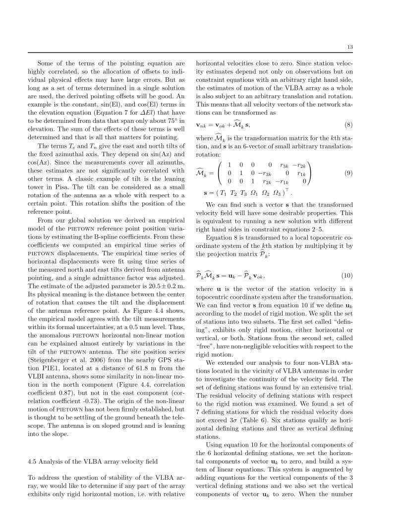
Table 3 Statistics of observing session per station. (1) IVS sta-tion name; (2) geocentric latitude; (3) longitude, positive towardseast; (4) Number of observing sessions under geodesy and astrom-

etry with the VLBA array.

(1) (2) (3) (4)

pietown +34.122 251.880 132la-vlba +35.592 253.754 130kp-vlba +31.783 248.387 129br-vlba +47.939 240.316 128ov-vlba +37.046 241.722 128fd-vlba +30.466 256.055 126hn-vlba +42.741 288.013 126mk-vlba +19.679 204.544 124nl-vlba +41.580 268.425 123sc-vlba +17.645 295.416 117westford +42.431 288.511 59kokee +21.992 200.334 57gilcreek +64.830 212.502 56onsala60 +57.220 11.925 50wettzell +48.954 12.877 50medicina +44.328 11.646 46nyales20 +78.856 11.869 38tsukub32 +35.922 140.087 31hartrao −25.738 27.685 28ggao7108 +38.833 283.173 24tigoconc −36.658 286.974 21nrao20 +38.245 280.160 20matera +40.459 16.704 19hobart26 −42.611 147.440 6kashim34 +35.772 140.657 6algopark +45.763 281.927 5noto +36.691 14.989 4zelenchk +43.595 41.565 3svetloe +60.367 29.781 2urumqi +43.279 87.178 1

3.1 Using AIPS to process geodesy experiments

Additional processing is required to evaluate the geode-

tic/astrometric VLBI observables of group delays and

phase delay rates. The initial calibrations are:

1. Small amplitude corrections for the correlator statis-

tics are applied while reading the raw data into an

AIPS data base.2. The reference point of each IF channel is moved

from the lower frequency edge to the center fre-

quency of the channel, along with an adjustment

to the frequency in the AIPS data base. This re-

duces edge effects, resulting in a small improvementin determination of the group delays.

3. Bad antenna and frequency channels are flagged

out, as necessary.

4. At the VLBA stations, relative phase and delay off-sets are applied to the visibility points using mea-

sured phase calibration tone phases. For both VLBA

and non-VLBA stations, manual phase offsets are

applied.2 The phase offsets are determined by fringe

fitting a reference scan on a compact radio source to

determine the relative instrumental phase and resid-

ual group delay for each individual IF. These phases

are removed from the entire data set, equivalent tosetting the single band and multiband residual de-

lays to zero at the scan used for the calibration.

The heart of the reduction process is the fringe fit-

ting of the data using AIPS task FRING. Data for each

scan, baseline, frequency band and IF channel are pro-

cessed separately, and the following parameters are de-termined: the average phase at some fiducial time near

the center of the scan; the average phase rate with time

(fringe rate); and the average phase rate with frequency

(single-band delay) by finding the maximum of the 2D

Fourier-transform of visibility data (Takahashi et al.2000) and subsequent LSQ fit. An SNR cutoff of about

3 is generally used in order to omit noisy solutions for

relatively weak sources3.

For those observations in which all of the IF chan-

nels have a detection, an AIPS program called MBDLY

computes the average phase for the reference frequencyand the average phase slope with frequency (so-called

multi-band delay or group delay) that best fits the in-

dividual IF phases obtained from FRING. The individ-

ual IF solutions for the single-band delay and the fringerate are averaged over all IFs. Checks of the quality of

the group delays are obtained by the spread of the in-

dividual single-band delays, the fringe rates, and the

phase scatter between each measured IF phase versusthe best-fit group delay. Observations with large devi-

ations are flagged as low quality and generally are not

used in the analysis.

The results from FRING and MBDLY give the

phase, single-band delay, fringe-rate, and group delay

for a fiducial time near the middle of each scan for eachbaseline and each frequency band. These quantities rep-

resent the residual values with respect to the correlator

model for the observation. When these data are added

to that of the correlator model, the results become the

total phase delay, total single-band delay, total fringe-rate and total group delay, respectively. These total val-

ues are independent of the correlator model.

The correlator model is attached to the correlator

output. For each source and each antenna, it is repre-

sented by a six-order polynomial for every two minuteinterval, so that its value can be determined at any

time with rounding errors below 0.1 ps. It contains

2 The non-VLBA stations have phase calibration systems, buttheir phases could not be captured in real time, nor extractedduring correlation as is done on the Mark 4 correlators.

3 The AIPS cookbook can be found on the Web athttp://www.aips.nrao.edu/cook.html

7

three parts: the geometric delay based on the a pri-

ori source position, antenna locations, and the Earth

orientation parameters; an a priori atmospheric delay;

and the clock offset with respect to UTC determined by

GPS at each individual station. The time-tag associatedwith the correlator model and the residual parameters

is earth-center oriented. That is, the parameters are

referenced to the time when the wavefront intercepts

a fiducial point chosen at the coordinate system originin order to facilitate the correlation process. The total

quantities are then determined by adding the baseline

residual parameters to the correlator model difference

for the appropriate antenna-pair, interpolated to the

scan reference time.The total observables are continuous functions of

time. Further geodetic and astrometric analysis requires

discrete values of observable quantities, one per scan

and per baseline, thereafter called observations, withtime-tags associated with the arrival of the wavefront at

the reference antenna of the baseline. These observables

can differ by as much as 20 ms from the quantities with

Earth-centered time-tags. AIPS task CL2HF is used to

combine the correlator models and residuals at two sta-tions and compute the observables with the reference

antenna time-tags. For convenience, the time-tags are

chosen to be on an integer second, and a common time-

tag is set to all observations in a scan. CL2HF per-forms this transformation, computes the fringe ampli-

tude SNRs, delay, and rate uncertainties. CL2HF writes

out an “HF” extension AIPS file which contains the

total quantities as well as many other derived quanti-

ties needed for further analysis. Finally, the AIPS taskHF2SV converts the data in the HF extension file to a

binary form that is consistent with Mark 3 correlator

output.

3.2 Validation of the post-correlation analysis

procedure

For the first few years, the VLBA/AIPS processed ses-

sions were freely mixed with Mark 4/Fourfit processedsessions, with few noticeable effects. However, two dis-

crepancies were noticed between results from the two

data sets. 1) The horizontal position of the onsala sta-

tion shifted by approximately 3 mm between the two

sets of data and 2) scatter of source position series forsouthern sources differed at a level of 0.2–1.0 mas. The

shift in onsala’s position was found to be the result of

a strong azimuthal dependence of instrumental delay in

the cable, not seen at other sites. It showed up becausemeasured phase calibration was not used for onsala in

the VLBA/AIPS processing. The source statistics dif-

ference was found to be due to an incorrect accounting

in program CL2HF of the total number of bits read

from the station tapes at the VLBA correlator. When

this was corrected, the “southern source” problem dis-

appeared.

A direct comparison of delays and rates processedby the AIPS software package versus the Haystack

Fourfit software package was strongly desired. To make

such a comparison, the tapes from 8 stations in the

rdv22 VLBA session (2000 July 6–7) were saved andsent to Haystack Observatory, where they were corre-

lated on the Mark 4 correlator and fringed using the

program Fourfit. To minimize the differences in process-

ing, a single set of phase calibration phases was used in

both the AIPS and Fourfit processing. Two databaseswere made of the same baselines processed through the

two independent systems, with matching time tags. The

regular Calc/Solve analysis was then performed on each

to eliminate any bad data points. The observed delaysand rates were differenced and tabulated by baseline.

There were constant offsets for each baseline due to

differences in single band calibration, and differences

in 2π ambiguity shifts. Such delay differences get ab-

sorbed into the clock adjustments and do not affect thegeodetic or astrometric results. After removal of these

constant differences, weighted root mean square (wrms)

differences at X-band were computed by baseline. These

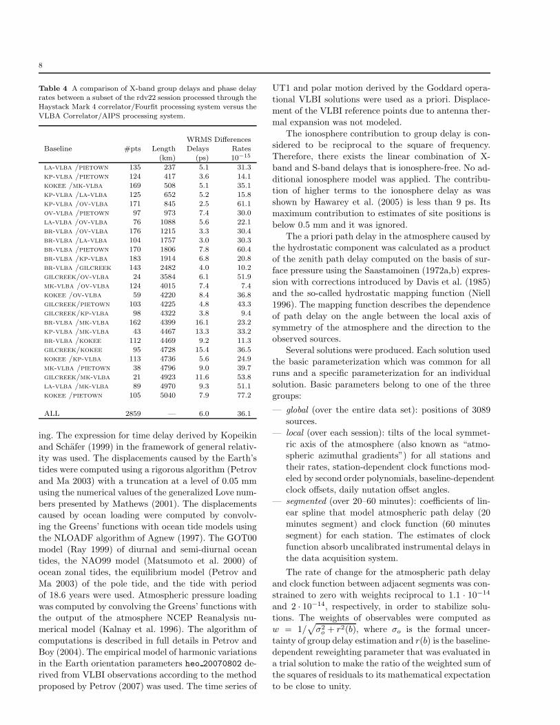
are given in Table 4. The wrms differences range fromas little as 2.5 ps on the kp-vlba/ov-vlba baseline,

up to 16.1 ps on the br-vlba/mk-vlba baseline. The

wrms over all baselines is only 6.0 ps, equivalent to

1.8 mm. By comparison, the average delay formal er-

rors are 7.7 ps on kp-vlba/ov-vlba and 17.3 ps onbr-vlba/mk-vlba. In a similar comparison between

the Mark 3 and Mark 4 correlators and post-processing

software at Bonn University, Nothnagel et al. (2002)

found an average wrms difference of 21.1 ps on 6 longintercontinental baselines.

4 Geodetic analysis

In our analysis we used all available VLBI observationsfrom August 03, 1979 through October 04, 2007, in-

cluding 132 observing sessions with the VLBA. The

differences between the observed ionosphere-free linear

combinations of dual-frequency group delays and theo-

retical group delays are used in the right hand side ofthe observation equations in the least squares parame-

ter estimation procedure.

Computation of theoretical time delays in general

follows the approach outlined in the IERS Conven-tions (McCarthy and Petit, Eds 2004) and presented

in detail by Sovers et al. (1998) with some minor re-

finements. The most significant ones are the follow-

8

Table 4 A comparison of X-band group delays and phase delayrates between a subset of the rdv22 session processed through theHaystack Mark 4 correlator/Fourfit processing system versus the

VLBA Correlator/AIPS processing system.

WRMS DifferencesBaseline #pts Length Delays Rates

(km) (ps) 10−15

la-vlba /pietown 135 237 5.1 31.3kp-vlba /pietown 124 417 3.6 14.1kokee /mk-vlba 169 508 5.1 35.1kp-vlba /la-vlba 125 652 5.2 15.8kp-vlba /ov-vlba 171 845 2.5 61.1ov-vlba /pietown 97 973 7.4 30.0la-vlba /ov-vlba 76 1088 5.6 22.1br-vlba /ov-vlba 176 1215 3.3 30.4br-vlba /la-vlba 104 1757 3.0 30.3br-vlba /pietown 170 1806 7.8 60.4br-vlba /kp-vlba 183 1914 6.8 20.8br-vlba /gilcreek 143 2482 4.0 10.2gilcreek/ov-vlba 24 3584 6.1 51.9mk-vlba /ov-vlba 124 4015 7.4 7.4kokee /ov-vlba 59 4220 8.4 36.8gilcreek/pietown 103 4225 4.8 43.3gilcreek/kp-vlba 98 4322 3.8 9.4br-vlba /mk-vlba 162 4399 16.1 23.2kp-vlba /mk-vlba 43 4467 13.3 33.2br-vlba /kokee 112 4469 9.2 11.3gilcreek/kokee 95 4728 15.4 36.5kokee /kp-vlba 113 4736 5.6 24.9mk-vlba /pietown 38 4796 9.0 39.7gilcreek/mk-vlba 21 4923 11.6 53.8la-vlba /mk-vlba 89 4970 9.3 51.1kokee /pietown 105 5040 7.9 77.2

ALL 2859 — 6.0 36.1

ing. The expression for time delay derived by Kopeikin

and Schafer (1999) in the framework of general relativ-ity was used. The displacements caused by the Earth’s

tides were computed using a rigorous algorithm (Petrov

and Ma 2003) with a truncation at a level of 0.05 mm

using the numerical values of the generalized Love num-

bers presented by Mathews (2001). The displacementscaused by ocean loading were computed by convolv-

ing the Greens’ functions with ocean tide models using

the NLOADF algorithm of Agnew (1997). The GOT00

model (Ray 1999) of diurnal and semi-diurnal oceantides, the NAO99 model (Matsumoto et al. 2000) of

ocean zonal tides, the equilibrium model (Petrov and

Ma 2003) of the pole tide, and the tide with period

of 18.6 years were used. Atmospheric pressure loading

was computed by convolving the Greens’ functions withthe output of the atmosphere NCEP Reanalysis nu-

merical model (Kalnay et al. 1996). The algorithm of

computations is described in full details in Petrov and

Boy (2004). The empirical model of harmonic variationsin the Earth orientation parameters heo 20070802 de-

rived from VLBI observations according to the method

proposed by Petrov (2007) was used. The time series of

UT1 and polar motion derived by the Goddard opera-

tional VLBI solutions were used as a priori. Displace-

ment of the VLBI reference points due to antenna ther-

mal expansion was not modeled.

The ionosphere contribution to group delay is con-sidered to be reciprocal to the square of frequency.

Therefore, there exists the linear combination of X-

band and S-band delays that is ionosphere-free. No ad-

ditional ionosphere model was applied. The contribu-tion of higher terms to the ionosphere delay as was

shown by Hawarey et al. (2005) is less than 9 ps. Its

maximum contribution to estimates of site positions is

below 0.5 mm and it was ignored.

The a priori path delay in the atmosphere caused bythe hydrostatic component was calculated as a product

of the zenith path delay computed on the basis of sur-

face pressure using the Saastamoinen (1972a,b) expres-

sion with corrections introduced by Davis et al. (1985)and the so-called hydrostatic mapping function (Niell

1996). The mapping function describes the dependence

of path delay on the angle between the local axis of

symmetry of the atmosphere and the direction to the

observed sources.Several solutions were produced. Each solution used

the basic parameterization which was common for all

runs and a specific parameterization for an individual

solution. Basic parameters belong to one of the threegroups:

— global (over the entire data set): positions of 3089

sources.

— local (over each session): tilts of the local symmet-

ric axis of the atmosphere (also known as “atmo-spheric azimuthal gradients”) for all stations and

their rates, station-dependent clock functions mod-

eled by second order polynomials, baseline-dependent

clock offsets, daily nutation offset angles.— segmented (over 20–60 minutes): coefficients of lin-

ear spline that model atmospheric path delay (20

minutes segment) and clock function (60 minutes

segment) for each station. The estimates of clock

function absorb uncalibrated instrumental delays inthe data acquisition system.

The rate of change for the atmospheric path delay

and clock function between adjacent segments was con-

strained to zero with weights reciprocal to 1.1 · 10−14

and 2 · 10−14, respectively, in order to stabilize solu-tions. The weights of observables were computed as

w = 1/√

σ2o + r2(b), where σo is the formal uncer-

tainty of group delay estimation and r(b) is the baseline-

dependent reweighting parameter that was evaluated ina trial solution to make the ratio of the weighted sum of

the squares of residuals to its mathematical expectation

to be close to unity.

9

4.1 Baseline analysis

In the preliminary stage of data analysis, in addition

to basic parameters we estimated the length of each

baseline at each session individually. The purpose of

this solution was to determine possible non-linearity in

station motion, to detect possible outliers, and to evalu-ate statistics related to systematic errors. The baseline

length is invariant with respect to a linear coordinate

transformation that affects all the stations of the net-

work. Therefore, changes in baseline lengths are relatedto either physical motion of one station with respect to

another or to systematic errors specific to observations

at the stations of the baseline.

We present in Figures 4.1–4.1 examples of length

evolutions for a very stable intra-plate baseline and fora rapidly stretching inter-plate baseline.

Fig. 3 Residual lengths of the intra-plate baseline hn-vlba/fd-vlba with respect to the average value of 3 623 021.2526 m. Thewrms 3.7 mm.

Fig. 4 Residual lengths of the inter-plate baseline mk-vlba/sc-vlba with respect to the average value of 8 611 584.6972 m. Thewrms 9.2 mm.

As we see, the tectonic motion has shifted station

mk-vlba, located on the fast Pacific plate, by morethan 0.5 meters over the existence of the array.

No significant outliers, and no jumps exceeding 2 cm

were found in examining plots of the baseline length

evolution. Significant non-linear motion was found only

on baselines with station pietown (Figure 5). Analy-

sis of GPS data from the permanent IGS station PIE1

located within 61.8 m of the VLBI station (Figure 2)

does not show a similar pattern.

4.2 Global analysis

The purpose of the global solution is to determine the

best model of station motion. In general, the model of

motion of the kth station can be represented in this

form:

rk = rok + rk t +

nk∑

j=1−m

fkj Bmj (t; t1−m,k, . . . tnk,k) +

nh∑

i

(hc

ki cos(αi + ωit) + hski sin(αi + ωit)

).

(1)

Here rok is the position of the kth station at the ref-

erence epoch when t=0, rk is the linear station velocity,

Bmj (t; t1−m,, . . . , tnk,k) is the B-spline of mth degree de-

fined on a knot sequence t1−m,k, . . . , tnk,k that is unique

for each station and not necessarily equidistant with the

jth pivotal element. Properties of B-spline function are

discussed in full details in de Boor (1978); Nurnberger(1989). The first two terms in 1 describe the linear sta-

tion motion, the last one describes harmonic motion,

and the third term describes the non-linear, anharmonic

motion with possible discontinuities caused by seismic

events or antenna repair.

The parameters of the non-linear model of motion

for selected sites, the frequencies of harmonic site po-sition variations, the degree of the B-splines, and the

sequences of knots on which the B-splines are defined,

were selected manually. Several trial solutions were

made, and the series of the baseline length estimateswere scrutinized. The parameters of the non-linear mo-

del were adjusted until the plots of residuals showed no

systematics. The stations for estimation of harmonic

position variations were selected on the basis of their

observational history. Only those stations that partici-pated in observations at least once every three months

for at least three years were selected to avoid strong

correlation between estimates of harmonic site position

variations and other parameters.

We estimated non-linear anharmonic motion at 18

stations, including two VLBA stations pietown andmk-vlba. The degree of B-spline was 0 for mk-vlba

and 2 for pietown. The epochs of B-spline knots are

presented in Table 5.

10

Table 5 Epochs of knots of B-spline for modeling a non-linearanharmonic motion of two VLBA stations.

pietown 1988.09.08 mk-vlba 1993.07.19pietown 1993.03.01 mk-vlba 2000.04.02pietown 1996.01.01 mk-vlba 2006.10.15pietown 1998.01.01 mk-vlba 2007.08.10pietown 2000.01.01pietown 2002.01.01pietown 2004.01.01pietown 2007.08.10

We ran a special global solution4, where in addition

to parameters estimated in the previous solution, we

estimated as global parameters quantities rok, rk for allstations, quantities hc

ki,hski for all VLBA stations and

25 selected sites, and quantities fkj for five stations.

The polar motion, UT1, and their first time derivatives

were also estimated.

4.3 Required minimum constraints

Equations of light propagation are differential equations

of the second order. Their solution does not allow deter-mining specific coordinates of sources and stations, but

rather a family of coordinate sets. Boundary conditions

should be formulated either implicitly or explicitly in

the form of constraints in order to select an elementfrom these sets. These boundary conditions cannot in

principle be determined from the observations. Thus,

observations alone are not sufficient to evaluate station

positions and source coordinates. Coordinates are de-

termined from observations in the form of observationequations and boundary conditions in the form of con-

straint equations.

Expressions for VLBI path delays are invariant with

respect to a group of coordinate transformation thatinvolves translation and rotation of site positions at a

reference epoch, their first time derivatives, and rota-

tion of source coordinates. In order to remove the rank

deficiency, we imposed constraints in the form

ns∑

k

(∆rok × rok)/|rok| = const

ns∑

k

∆rok = const

ns∑

k

(∆rk × rok)/|rok| = const

ns∑

k

∆rk = const

q∑

a

∆sa × sa = const,

(2)

where sa is the coordinate vector of ath source, ns is the

number of stations that participate in constraints, and q

is the number of sources that participate in constraints.

4 Listing of this solution is available athttp://astrogeo.org/vlbi/solutions/2007d adv

The pairs of parameters rok, fki and rk, fki are lin-

early dependent, and pairs of parameters fki,hcki, and

fki,hski may be highly correlated depending on frequen-

cies. In order to avoid rank deficiency of a system of

observation equations, the following decorrelation con-straints are to be imposed for each frequency of the

harmonic constituents:

m−1∑

j=1−m

fj

+∞∫

−∞

Bmj (t) cos ωi t dt = const

m−1∑

j=1−m

fj

+∞∫

−∞

Bmj (t) sin ωi t dt = const.

(3)

Decorrelation constraints between the estimates of

B-spline coefficients, the estimate of mean site position

rok and linear velocity rk (in the case if the degree ofB-spline m > 0) are to be imposed as well:

m−1∑

j=1−m

fj

+∞∫

−∞

Bmj (t) dt = const

m−1∑

j=1−m

fj

+∞∫

−∞

t Bmj (t) dt = const.

(4)

The integrals 3–4 can be evaluated analytically

(Nurnberger 1989).

Similar to coordinates, the adjustments of harmonic

variations in coordinates are invariant with respect to

a group of transformations that involve translation androtation. In order to remove the rank deficiency asso-

ciated with this group of transformations, we imposed

the following constraints:

ns∑

k

(hcki × rk)/|rk| = const

nh∑

k

hcki = const

ns∑

k

(hski × rk)/|rk| = const

nh∑

k

hski = const.

(5)

In our solutions, we set the constants in equations 2–

5 to zero.

4.4 Motion of the reference point due to antenna

instability

The residuals of time series of baseline length estimates

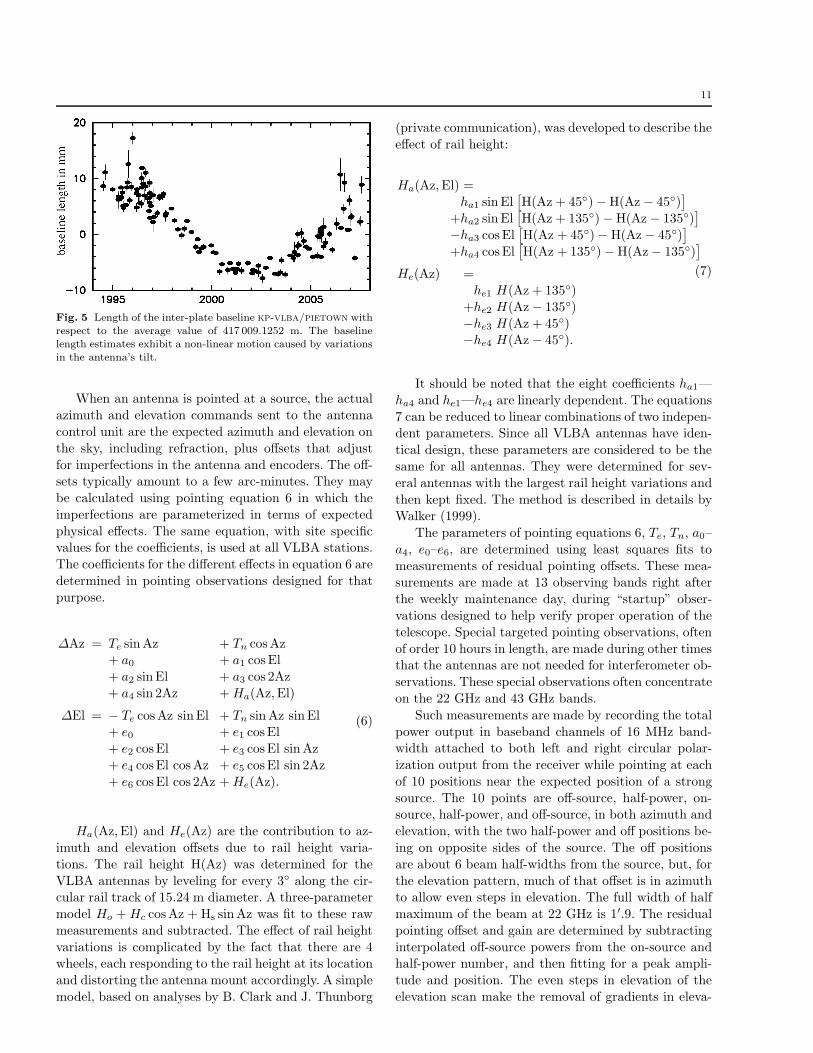
with station pietown with respect to a linear fit show

a significant systematic behavior. In our efforts to un-derstand the origin of this behavior, we investigated the

effect of variations of up to 4′ in the antenna’s tilt, made

evident from pointing measurements.

11

Fig. 5 Length of the inter-plate baseline kp-vlba/pietown withrespect to the average value of 417 009.1252 m. The baselinelength estimates exhibit a non-linear motion caused by variationsin the antenna’s tilt.

When an antenna is pointed at a source, the actual

azimuth and elevation commands sent to the antenna

control unit are the expected azimuth and elevation on

the sky, including refraction, plus offsets that adjust

for imperfections in the antenna and encoders. The off-sets typically amount to a few arc-minutes. They may

be calculated using pointing equation 6 in which the

imperfections are parameterized in terms of expected

physical effects. The same equation, with site specificvalues for the coefficients, is used at all VLBA stations.

The coefficients for the different effects in equation 6 are

determined in pointing observations designed for that

purpose.

∆Az = Te sin Az + Tn cosAz+ a0 + a1 cosEl

+ a2 sin El + a3 cos 2Az

+ a4 sin 2Az + Ha(Az, El)

∆El = − Te cosAz sin El + Tn sin Az sin El+ e0 + e1 cosEl

+ e2 cosEl + e3 cosEl sin Az

+ e4 cosEl cosAz + e5 cosEl sin 2Az

+ e6 cosEl cos 2Az + He(Az).

(6)

Ha(Az, El) and He(Az) are the contribution to az-

imuth and elevation offsets due to rail height varia-

tions. The rail height H(Az) was determined for the

VLBA antennas by leveling for every 3 along the cir-cular rail track of 15.24 m diameter. A three-parameter

model Ho + Hc cosAz + Hs sin Az was fit to these raw

measurements and subtracted. The effect of rail height

variations is complicated by the fact that there are 4wheels, each responding to the rail height at its location

and distorting the antenna mount accordingly. A simple

model, based on analyses by B. Clark and J. Thunborg

(private communication), was developed to describe the

effect of rail height:

Ha(Az, El) =ha1 sin El

[H(Az + 45) − H(Az − 45)

]

+ha2 sin El[H(Az + 135) − H(Az − 135)

]

−ha3 cosEl[H(Az + 45) − H(Az − 45)

]

+ha4 cosEl[H(Az + 135) − H(Az − 135)

]

He(Az) =

he1 H(Az + 135)

+he2 H(Az − 135)

−he3 H(Az + 45)−he4 H(Az − 45).

(7)

It should be noted that the eight coefficients ha1—

ha4 and he1—he4 are linearly dependent. The equations

7 can be reduced to linear combinations of two indepen-dent parameters. Since all VLBA antennas have iden-

tical design, these parameters are considered to be the

same for all antennas. They were determined for sev-

eral antennas with the largest rail height variations and

then kept fixed. The method is described in details byWalker (1999).

The parameters of pointing equations 6, Te, Tn, a0–

a4, e0–e6, are determined using least squares fits to

measurements of residual pointing offsets. These mea-surements are made at 13 observing bands right after

the weekly maintenance day, during “startup” obser-

vations designed to help verify proper operation of the

telescope. Special targeted pointing observations, often

of order 10 hours in length, are made during other timesthat the antennas are not needed for interferometer ob-

servations. These special observations often concentrate

on the 22 GHz and 43 GHz bands.

Such measurements are made by recording the total

power output in baseband channels of 16 MHz band-width attached to both left and right circular polar-

ization output from the receiver while pointing at each

of 10 positions near the expected position of a strong

source. The 10 points are off-source, half-power, on-source, half-power, and off-source, in both azimuth and

elevation, with the two half-power and off positions be-

ing on opposite sides of the source. The off positions

are about 6 beam half-widths from the source, but, for

the elevation pattern, much of that offset is in azimuthto allow even steps in elevation. The full width of half

maximum of the beam at 22 GHz is 1′.9. The residual

pointing offset and gain are determined by subtracting

interpolated off-source powers from the on-source andhalf-power number, and then fitting for a peak ampli-

tude and position. The even steps in elevation of the

elevation scan make the removal of gradients in eleva-

12

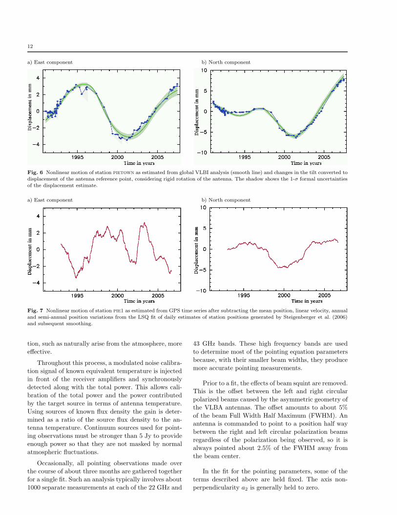
a) East component b) North component

Fig. 6 Nonlinear motion of station pietown as estimated from global VLBI analysis (smooth line) and changes in the tilt converted todisplacement of the antenna reference point, considering rigid rotation of the antenna. The shadow shows the 1-σ formal uncertaintiesof the displacement estimate.

a) East component b) North component

Fig. 7 Nonlinear motion of station pie1 as estimated from GPS time series after subtracting the mean position, linear velocity, annualand semi-annual position variations from the LSQ fit of daily estimates of station positions generated by Steigenberger et al. (2006)and subsequent smoothing.

tion, such as naturally arise from the atmosphere, more

effective.

Throughout this process, a modulated noise calibra-

tion signal of known equivalent temperature is injected

in front of the receiver amplifiers and synchronouslydetected along with the total power. This allows cali-

bration of the total power and the power contributed

by the target source in terms of antenna temperature.

Using sources of known flux density the gain is deter-

mined as a ratio of the source flux density to the an-tenna temperature. Continuum sources used for point-

ing observations must be stronger than 5 Jy to provide

enough power so that they are not masked by normal

atmospheric fluctuations.

Occasionally, all pointing observations made overthe course of about three months are gathered together

for a single fit. Such an analysis typically involves about

1000 separate measurements at each of the 22 GHz and

43 GHz bands. These high frequency bands are used

to determine most of the pointing equation parameters

because, with their smaller beam widths, they produce

more accurate pointing measurements.

Prior to a fit, the effects of beam squint are removed.This is the offset between the left and right circular

polarized beams caused by the asymmetric geometry of

the VLBA antennas. The offset amounts to about 5%

of the beam Full Width Half Maximum (FWHM). Anantenna is commanded to point to a position half way

between the right and left circular polarization beams

regardless of the polarization being observed, so it is

always pointed about 2.5% of the FWHM away from

the beam center.

In the fit for the pointing parameters, some of the

terms described above are held fixed. The axis non-

perpendicularity a2 is generally held to zero.

13

Some of the terms of the pointing equation are

highly correlated, so the allocation of offsets to indi-

vidual physical effects may have large errors. But as

long as a set of terms determined in a single solution

are used, the derived pointing offsets will be good. Anexample is the constant, sin(El), and cos(El) terms in

the elevation equation (Equation 7 for ∆El) that have

to be determined from data that span only about 75 in

elevation. The sum of the effects of these terms is welldetermined and that is all that matters for pointing.

The terms Te and Tn give the east and north tilts of

the fixed azimuthal axis. They depend on sin(Az) andcos(Az). Since the measurements cover all azimuths,

these estimates are not significantly correlated with

other terms. A classic example of tilt is the leaning

tower in Pisa. The tilt can be considered as a small

rotation of the antenna as a whole with respect to acertain point. This rotation shifts the position of the

reference point.

From our global solution we derived an empirical

model of the pietown reference point position varia-

tions by estimating the B-spline coefficients. From these

coefficients we computed an empirical time series of

pietown displacements. The empirical time series ofhorizontal displacements were fit using time series of

the measured north and east tilts derived from antenna

pointing, and a single admittance factor was adjusted.

The estimate of the adjusted parameter is 20.5±0.2 m.Its physical meaning is the distance between the center

of rotation that causes the tilt and the displacement

of the antenna reference point. As Figure 4.4 shows,

the empirical model agrees with the tilt measurements

within its formal uncertainties, at a 0.5 mm level. Thus,the anomalous pietown horizontal non-linear motion

can be explained almost entirely by variations in the

tilt of the pietown antenna. The site position series

(Steigenberger et al. 2006) from the nearby GPS sta-tion PIE1, located at a distance of 61.8 m from the

VLBI antenna, shows some similarity in non-linear mo-

tion in the north component (Figure 4.4, correlation

coefficient 0.87), but not in the east component (cor-

relation coefficient -0.73). The origin of the non-linearmotion of pietown has not been firmly established, but

is thought to be settling of the ground beneath the tele-

scope. The antenna is on sloped ground and is leaning

into the slope.

4.5 Analysis of the VLBA array velocity field

To address the question of stability of the VLBA ar-

ray, we would like to determine if any part of the array

exhibits only rigid horizontal motion, i.e. with relative

horizontal velocities close to zero. Since station veloc-

ity estimates depend not only on observations but on

constraint equations with an arbitrary right hand side,

the estimates of motion of the VLBA array as a whole

is also subject to an arbitrary translation and rotation.This means that all velocity vectors of the network sta-

tions can be transformed as

vnk = vok + Mk s, (8)

where Mk is the transformation matrix for the kth sta-

tion, and s is an 6-vector of small arbitrary translation-

rotation:

Mk =

1 0 0 0 r3k −r2k

0 1 0 −r3k 0 r1k

0 0 1 r2k −r1k 0

(9)

s = ( T1 T2 T3 Ω1 Ω2 Ω3 )⊤

.

We can find such a vector s that the transformed

velocity field will have some desirable properties. Thisis equivalent to running a new solution with different

right hand sides in constraint equations 2–5.

Equation 8 is transformed to a local topocentric co-

ordinate system of the kth station by multiplying it bythe projection matrix Pk:

PkMk s = uk − Pk vok, (10)

where u is the vector of the station velocity in atopocentric coordinate system after the transformation.

We can find vector s from equation 10 if we define uk

according to the model of rigid motion. We split the set

of stations into two subsets. The first set called “defin-ing”, exhibits only rigid motion, either horizontal or

vertical, or both. Stations from the second set, called

“free”, have non-negligible velocities with respect to the

rigid motion.

We extended our analysis to four non-VLBA sta-tions located in the vicinity of VLBA antennas in order

to investigate the continuity of the velocity field. The

set of defining stations was found by an extensive trial.

The residual velocity of defining stations with respectto the rigid motion was examined. We found a set of

7 defining stations for which the residual velocity does

not exceed 3σ (Table 6). Six stations qualify as hori-

zontal defining stations and three as vertical defining

stations.Using equation 10 for the horizontal components of

the 6 horizontal defining stations, we set the horizon-

tal components of vector uk to zero, and build a sys-

tem of linear equations. This system is augmented byadding equations for the vertical components of the 3

vertical defining stations and we also set the vertical

components of vector uk to zero. When the number

14

Table 6 Station local topocentric velocities with respect to therigid North American plate. Units: mm/yr. The quoted uncer-tainties are re-scaled 1-σ standard errors. The last column indi-

cates whether the station was used as defining for horizontal (h)or vertical (v) motion of the plate.

Station Up East North Def

br-vlba 0.0± 0.1 1.9± 0.3 -0.3± 0.4 vfd-vlba 1.2± 1.0 0.4± 0.2 -0.1± 0.2 hhn-vlba 0.2± 0.3 -0.1± 0.2 -0.1± 0.2 hvkp-vlba 2.3± 1.0 -0.2± 0.2 0.1± 0.2 hla-vlba 1.3± 0.8 0.0± 0.3 0.0± 0.2 hmk-vlba 0.9± 1.1 -55.0± 1.4 52.5± 1.1nl-vlba -1.1± 0.5 0.0± 0.2 0.1± 0.3 hov-vlba 2.0± 0.8 -6.0± 0.3 5.0± 0.4pietown 2.1± 0.9 -0.4± 0.3 -1.5± 0.3sc-vlba -1.2± 1.2 19.0± 0.8 5.3± 0.4gilcreek 3.0± 1.4 4.0± 0.6 -10.2± 0.7ggao7108 -0.9± 0.5 -0.4± 0.3 -0.5± 0.3kokee 2.7± 1.0 -54.3± 1.3 52.9± 1.2westford -0.3± 0.3 -0.1± 0.2 0.0± 0.2 hv

of equations exceeds 6, the system becomes redundant.

We solve it by LSQ with a full weight matrix W :

W =(Pa Cov(vo,v

⊤

o ) P⊤

a + A)−1

, (11)

where Pa is a block-diagonal matrix formed from matri-

ces Pk, A is a diagonal reweighting matrix with an ad-ditive correction to weights. Values of (0.4 mm/year)2

for both horizontal and vertical velocity components,

corresponding to a conservative measure of errors, were

used in the matrix A in our solution.

Then, transformation 10 and the rotation to the lo-

cal topocentric coordinate system were applied to both

defining and free stations. The covariance matrix for

velocity estimates of free stations was computed as:

Cov(vn,v⊤

n) = Pa Cov(vo,v⊤

o) P⊤

a

+ PaMCov(s, s⊤)M⊤ P⊤

a

(12)

and for defining stations as

Cov(vn,v⊤

n) = Pa Cov(vo,v⊤

o ) P⊤

a

+ PaMCov(s, s⊤)M⊤ P⊤

a

+ Pa Cov(s, s⊤)MW Cov(vo,v⊤

o) P⊤

a

+ Pa Cov(vo,v⊤

o) W M⊤Cov(s, s⊤) P⊤

a.

(13)

The latter expression takes into account statistical

dependence of the a priori velocity vo and the vector s.

The results are presented in Table 6. It is remarkablethat there exists a set of 6 stations spread over distances

of 1–3 thousand kilometers with an average residual

horizontal velocity of only 0.2 mm/yr.

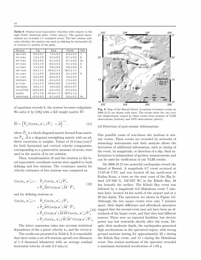
Fig. 8 Map of the Hawaii Island. Locations of seismic events on2006.10.15 are shown with stars. The arrows show the mk-vlbasite displacement caused by these events from analysis of VLBIobservations (bottom) and GPS observations (above).

4.6 Detection of post-seismic deformations

One possible cause of non-linear site motions is seis-

mic events. These events are recorded by networks of

seismology instruments and their analysis allows thederivation of additional information, such as timing of

the event, its magnitude, or direction of a slip. Such in-

formation is independent of geodesy measurements and

can be used for verification of our VLBI results.

On 2006.10.15 two powerful earthquakes struck the

Island of Hawaii. A magnitude 6.7 event occurred at

17:07:48 UTC and was located 16 km north-west of

Kailua Kona, a town on the west coast of the Big Is-

land (19.820 N, 156.027 W) in the Kiholo Bay, 38km beneath the surface. The Kiholo Bay event was

followed by a magnitude 6.0 Makuhona event 7 min-

utes later, located 44 km north of the airport and at a

20 km depth. The epicenters are shown in Figure 4.6.Although the two major events were only 7 minutes

apart, their depth difference and aftershock epicenters

suggest that the second event may not have been an af-

tershock of the larger event, and that they had different

sources. There were no reported fatalities, but electricpower was lost statewide shortly after the event. De-

spite their moderate depth, the earthquakes generated

high accelerations in the epicentral region, with strong

ground motions lasting for approximately 20 s duringthe Kiholo Bay event, and 15 s during the Mahuhona

event. One station northeast of the epicenter recorded

a maximum horizontal acceleration of 1.03 g.

15

The largest historical earthquakes in Hawaii have

occurred beneath the flanks of Kilauea, Mauna Loa, and

Hualalai volcanoes, when stored compressive stresses

from magma intrusions into their adjacent rift zones

were released. Their sources are related to near-horizontalbasal decollements at approximately 10 km depth, which

separate the emplaced volcanic material from the older

oceanic crust. In contrast, the Kiholo Bay event was

considered tectonic, rather than volcano related. Deeper,30–40 km deep, earthquakes like this result from a long-

term geologic response to flexural fracture of the un-

derlying lithosphere from the load of the island mass

(Chock 2006). They are the result long term accumula-

tion and release of lithospheric flexural stresses causedby the island-building process.

The distance from the epicenter of the Kailua Konaevent to the mk-vlba station is 62 km. No structural

damage was reported. As a response to the event, an

additional observing session was added to the schedule

on 2006.11.08 in order to detect possible post-seismic

deformation. Preliminary analysis early in 2007 did notfind any position changes exceeding 1 cm.

We reanalyzed the dataset and parameterized non-linear motion with the B-spline of the zeroth degree

with two knots: at 1994.07.08 (beginning observations)

and 2006.10.15 17:07:48. Using these two estimates of

B-spline coefficients and their covariance matrices, we

computed the displacement vector:

Up = –7.7 ± 1.3 mm

East = –10.0 ± 0.4 mm

North = 1.5 ± 0.4 mm

where the quoted uncertainties are unscaled 1-σ for-

mal errors. The vertical and west displacements look

very significant. However, the presence of outliers may

cause an artificial jump and various systematic corre-lated errors may cause estimates of uncertainties to be

unreliable.

In order to check the robustness of the solution, weperformed two tests: an observation decimation test and

a knot shift test. In the observation decimation test we

ran two solutions. The first solution used only the odd

observations, while the second solution used only theeven observations. The data used in these solutions are

independent. This test checks the contribution of ran-

dom errors uncorrelated at time scale of the interval be-

tween observations, typically 5–10 minutes. The differ-

ence in estimates of the displacement was only 0.14 mmin the vertical component and 0.06 mm in the horizon-

tal component.

In the knot shift test we made 21 trial solutions

which differed only by epochs of the B-spline knots. In

each trial solution we shifted the epoch of the knot six

months backward with respect to the previous. The pro-

cedure for computing theoretical path delay for these

trial solutions incorporated the estimate of the displace-

ment at 2006.10.15 17:07:48 epoch from the initial so-

lution. The rms of the time series of displacement esti-mates at epochs with no reported seismic events were

2.1 mm for the vertical and 1.3 mm for the horizontal

component of the mk-vlba displacement vector. We

consider these statistics as a measure of the robustnessof the estimates of the displacement vector. Both tests

support our claim that VLBI observations detected a

displacement of station mk-vlba caused by the seismic

event at 2006.10.15 at the confidence level of 99.5%.

Since there is a GPS receiver named MKEA located

88 meters from the VLBA station mk-vlba, we ex-

amined the GPS site motion series to determine the

corresponding co-seismic offset. For the analysis, weused the MKEA daily position time series generated

by JPL (M. Heflin, 2007, personal communication). We

obtained the following estimate for the co-seismic dis-

placement vector:

Up = –6.3 ± 0.9 mm

East = –9.9 ± 0.4 mmNorth = 3.5 ± 0.2 mm

Here, the uncertainties are unscaled 1-sigma formal

errors. This is reasonable because the position repeata-

bilities computed from the position time series are close

to the formal uncertainties of the daily estimates. TheVLBI and GPS vertical and east displacements are con-

sistent within their 1-sigma error bars but the 2 mm

difference in the north displacement is too large to be

explained by the formal uncertainties.

4.7 Harmonic variations in site positions

The technique of estimation of harmonic variations in

site positions directly from the analysis of group delays

was developed by Petrov and Ma (2003). It was shown

in that study that many stations exhibit position varia-tions that are attributed to mismodeled harmonic non-

tidal signals. The purpose of estimating the harmonic

site position variations was to remove those remain-

ing signals. We estimated sine and cosine amplitudes of

variations in all three components of site position vec-tors at annual (Sa), semi-annual (SSa), diurnal (S1),

and semi-diurnal (S2) frequencies for all VLBA and 25

other non-VLBA stations. The seasonal signal is caused

by unaccounted hydrology loading, by errors in annualamplitudes of the NMF mapping function that lead

to systematic errors in tropospheric path delay model-

ing, and possibly other effects. Sun-synchronous diurnal

16

Table 7 Amplitudes of vertical component of harmonic varia-tions of VLBA station positions in mm.

Station annual semi-annual diurnal semi-diurnal

br-vlba 8.0 ± 0.3 3.3 ± 0.3 1.0 ± 0.2 0.5 ± 0.2fd-vlba 1.8 ± 0.3 1.8 ± 0.3 0.4 ± 0.2 1.5 ± 0.2hn-vlba 5.4 ± 0.3 2.3 ± 0.3 1.5 ± 0.3 1.0 ± 0.3kp-vlba 1.7 ± 0.3 1.8 ± 0.3 0.2 ± 0.2 0.8 ± 0.2

la-vlba 1.0 ± 0.3 3.2 ± 0.2 1.3 ± 0.2 0.9 ± 0.2mk-vlba 2.5 ± 0.4 2.5 ± 0.4 0.8 ± 0.3 2.5 ± 0.3nl-vlba 4.1 ± 0.3 3.6 ± 0.3 0.8 ± 0.2 0.2 ± 0.2ov-vlba 2.7 ± 0.3 2.0 ± 0.3 1.1 ± 0.2 0.9 ± 0.2pietown 1.8 ± 0.3 0.8 ± 0.3 1.1 ± 0.2 1.2 ± 0.2sc-vlba 2.6 ± 0.5 3.0 ± 0.5 0.5 ± 0.4 1.3 ± 0.4

Table 8 Amplitudes of horizontal component of harmonic vari-ations of VLBA station positions in mm.

Station annual semi-annual diurnal semi-diurnal

br-vlba 0.8 ± 0.1 0.3 ± 0.1 0.3 ± 0.1 0.2 ± 0.1fd-vlba 1.4 ± 0.1 0.1 ± 0.1 0.2 ± 0.1 0.1 ± 0.1hn-vlba 0.9 ± 0.1 0.2 ± 0.1 0.2 ± 0.1 0.1 ± 0.1kp-vlba 1.5 ± 0.1 0.3 ± 0.1 0.4 ± 0.1 0.2 ± 0.1la-vlba 1.1 ± 0.1 0.3 ± 0.1 0.3 ± 0.1 0.1 ± 0.1

mk-vlba 0.8 ± 0.2 0.4 ± 0.2 0.8 ± 0.1 0.3 ± 0.1nl-vlba 0.7 ± 0.1 0.2 ± 0.1 0.2 ± 0.1 0.2 ± 0.1ov-vlba 1.2 ± 0.1 0.2 ± 0.1 0.5 ± 0.1 0.3 ± 0.1pietown 1.5 ± 0.1 0.2 ± 0.1 0.3 ± 0.1 0.3 ± 0.1sc-vlba 0.7 ± 0.2 0.9 ± 0.2 0.4 ± 0.1 0.3 ± 0.1

variations can be caused by thermal variations, by sys-

tematic errors in tropospheric path delay, or unmodelednon-tidal ocean loading.

In order to evaluate the robustness of the estimates

at low frequencies, we performed two tests: the obser-

vation decimation test and the dummy frequency test.We examined the differences in estimates of sine and

cosine amplitudes from the observation decimation test

and compared them with the formal uncertainties of

the estimates. The differences are within 1-sigma for-

mal uncertainty.

In the second test we estimated site position varia-

tions at a frequency of 2.5 · 10−7 rad s−1, corresponding

to a period of 0.8 year where no harmonic signal is ex-

pected. The average amplitude found for the verticaldisplacements for the ten VLBA stations is 1.2 mm,

and 0.2 mm for the horizontal displacements. These es-

timates should be considered as the upper limit of un-

certainties, since the observed harmonic signal at fre-

quency 2.5 · 10−7 rad s−1 is affected by both systematicerrors and real displacements at this frequency, caused

by anharmonic, broad-band site position displacements.

We see that the combined contribution of seasonal

position variation, unaccounted for in the theoreticalmodel, can reach 1 cm for the vertical component of

VLBA stations and 1.5 mm for the horizontal compo-

nent and is statistically significant for most of the sta-

tions at the 95% confidence level. Unaccounted diurnal

position variations are at the level of 1–2 mm.

5 Error analysis

Uncertainties of estimated parameters can be evaluated

using the law of error propagation under the assump-

tion that the unmodeled contribution to group delay

is due to random uncorrelated errors with known vari-

ance. The parameter estimation procedure provides es-timates of these errors based on the SNR of fringe

amplitudes. These errors are labeled as formal errors

and they are considered as lower limits of accuracy.

Formal uncertainties of the site position estimates ofthe VLBA stations from our global solution are in the

range of 0.5–1.0 mm for vertical components and 0.2–

0.5 mm for horizontal components. Formal uncertain-

ties of the VLBA site velocity estimates are in the range

of 0.07–0.1 mm/yr for vertical components and 0.04–0.05 mm/yr for horizontal components.

Many factors contribute to an increase of errors.

Among them are underestimated uncertainties of groupdelays due to phase instability of the data acquisition

system, unmodeled instrumental errors, unaccounted

atmospheric fluctuations, correlations between observa-

tions, and unaccounted environmental effects.

Another measure of accuracy is an observation dec-

imation test. Since the two datasets have independent

random errors, the root mean square of differences be-tween estimates from these solutions divided by

√2 pro-

vides a measure of accuracy that is independent of esti-

mates of the uncertainty of each individual observation.

However, many other factors that affect the results,such as mismodeled delay in the neutral atmosphere,

are common in the two subsets. To examine the influ-

ence of these factors, we ran a session decimation test

and used every second observing session. In the observa-tion decimation test, matrices of observation equations

were almost identical, but the data were affected by the

same systematic errors. In the session decimation test,

systematic errors were more independent, but the ma-

trices of observation equations have larger differences.

The statistics of differences are given in Table 9. In

the absence of systematic errors, both decimation tests

would give close results. Analysis of the statistics showssignificant discrepancies between the decimation tests.

Estimates of site positions and velocities in solutions

where every second observation is removed are a fac-

tor of 2–3 closer to each other than in solutions whereevery second session is removed. This is an indication

that systematic errors on the time scale of several min-

utes — the typical time between observations — are

17

Table 9 Formal uncertainties and rms of differences of two dec-imation tests for estimates of site positions and site velocities.The estimates are given for horizontal and vertical components

separately.

Statistics Position Velocitymm mm/yr

v h v h

Formal σ 0.7 0.3 0.11 0.04Observation decimation 0.3 0.06 0.04 0.02Session decimation 1.4 0.3 0.09 0.06

Table 10 The rms of differences in pole coordinates estimatesbetween the VLBI results and the GPS time series igs00p03.erp.Only data after 1997.0 are used. Comparison is made separatelyfor VLBA sessions in astrometric mode (only 10 VLBA stations)and VLBA sessions in geodetic mode (10 VLBA stations plus3–10 non-VLBA stations).

Sessions X-pole Y-pole

VLBA, Astrometric mode 0.87 nrad 1.15 nradVLBA, Geodetic mode 0.54 nrad 0.43 nradIVS sessions in 2006–2007 0.39 nrad 0.47 nrad

correlated. The session decimation test suggests that

estimates of the vertical site position errors should be

scaled by a factor of 2. This scaling may be related to

unaccounted errors in modeling the contribution of the

neutral atmosphere.

We also estimated Earth orientation parameters inour solutions. Comparison of our EOP estimates with

independent GPS time series igs00p03.erp5 gives us

another measure of the accuracy of our results. We com-

puted the rms of differences in pole coordinates forsessions in astrometric mode and sessions in geodetic

modes. Only sessions after 1997 were used for this com-

parison, since GPS estimates prior to this date are not

very accurate. As we see from Table 10, the VLBA es-

timates of pole coordinates from geodetic observationsare approximately as close to GPS results as ones from

regular IVS sessions. However, the EOP from astromet-

ric sessions divert from the GPS time series by a factor

of 2 larger than the EOP from geodetic VLBI sessions.

A baseline length repeatability test provides another

measure of solution accuracy. For each baseline, a seriesof lengths was obtained. Empirical non-linear site po-

sition variations described above were applied as a pri-

ori. A plot of the baseline length repeatability of VLBA

baselines is presented in Figure 5. For comparison, base-line length repeatability at non-VLBA baselines is also

shown.

A linear model of baseline lengths was fit to each

series, and the wrms of the deviations from the linear

model, the baseline length repeatability, was computed

for each baseline. The plot of baseline length repeatabil-

5 Available atftp://cddisa.gsfc.nasa.gov/gps/products/igs00p03.erp.Z

Fig. 9 Baseline length repeatability as a function of baselinelength. Solid disks shows estimates of baseline length repeata-

bility between VLBA sites, circles shows repeatability betweennon-VLBA sites.

ity shows that the scatter in baseline lengths estimates

between VLBA sites is less than the scatter in base-

line length between dedicated geodetic VLBI stations.

The set of wrms was fit by a function√

A2 + (B · L)2

where L is the mean baseline length. Coefficients A andB, which represent the average baseline length repeata-

bility, are a measure of accuracy. For the VLBA base-

lines, A = 1.6 mm, B=0.9 ppb, for non-VLBA baselines

A=2.0 mm, B=1.4 ppb. Growth of the baseline lengthrepeatability with the baseline length for both sets of

data reflects the impact of the contribution of unmod-

eled path delay in the neutral atmosphere, which affects

the site position vertical component to a greater extent

than the horizontal one (Davis et al. 1985).

The results of error analysis allow us to concludethat the errors of predicted site positions for any epoch

within the time range of observations, [1994, 2008], are

in the range of 2–3 mm for the vertical component

and 0.4–0.6 mm for the horizontal component. The pre-dicted positions, based on the adjusted parameters of

the site motion model, includes mean site positions at

the reference epoch, site velocities, and coefficients of

the harmonic and B-spline models. The estimates of

errors for the vertical coordinates were derived fromthe formal errors by inflating by a factor of 2, as the

session decimation test suggests. In the absence of new

observations, the predicted errors in site position will

grow by a factor of 2 by 2020 as is shown in Figure 5,provided no motion other than harmonic position vari-

ations and linear velocities, i.e. that no seismic events,

or unmodeled variable tilt, will happen in the future.

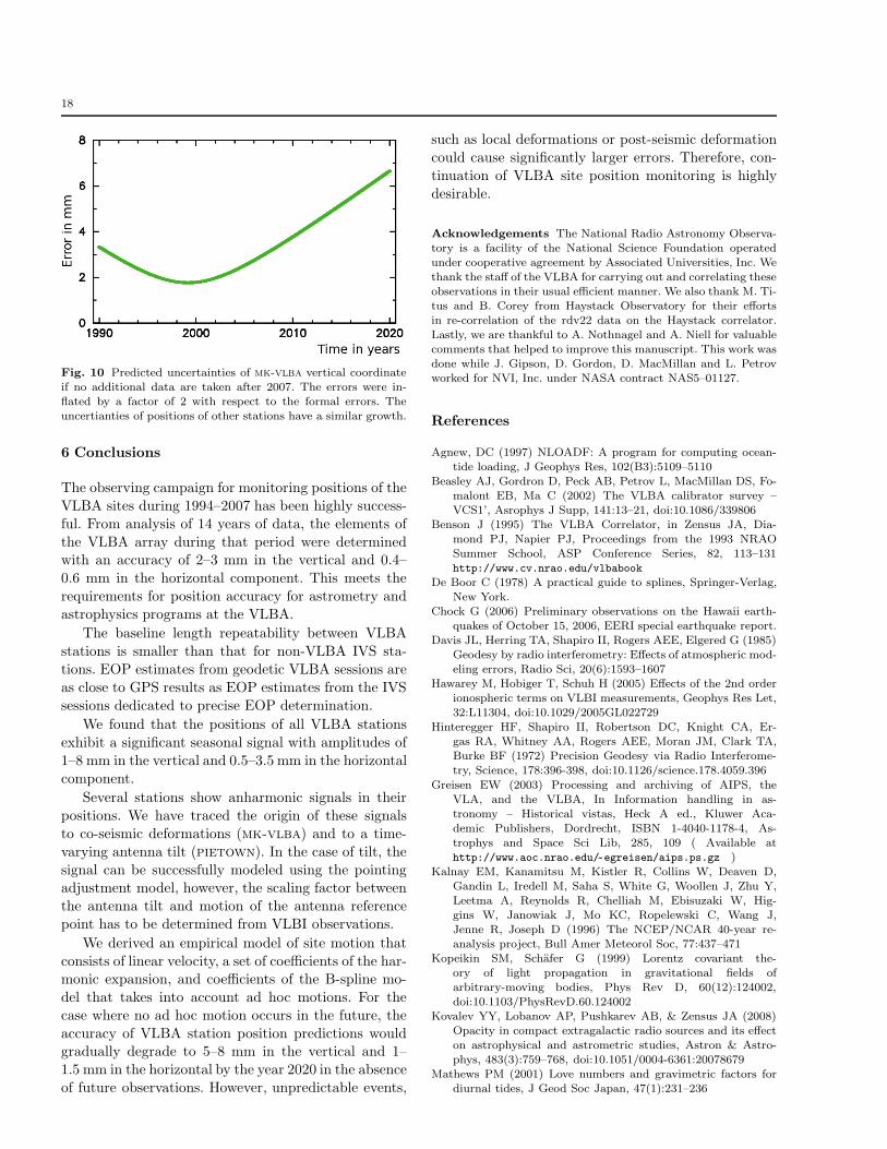
18

Fig. 10 Predicted uncertainties of mk-vlba vertical coordinateif no additional data are taken after 2007. The errors were in-flated by a factor of 2 with respect to the formal errors. Theuncertianties of positions of other stations have a similar growth.

6 Conclusions

The observing campaign for monitoring positions of the

VLBA sites during 1994–2007 has been highly success-

ful. From analysis of 14 years of data, the elements of

the VLBA array during that period were determinedwith an accuracy of 2–3 mm in the vertical and 0.4–

0.6 mm in the horizontal component. This meets the

requirements for position accuracy for astrometry and

astrophysics programs at the VLBA.

The baseline length repeatability between VLBA

stations is smaller than that for non-VLBA IVS sta-

tions. EOP estimates from geodetic VLBA sessions are

as close to GPS results as EOP estimates from the IVS

sessions dedicated to precise EOP determination.

We found that the positions of all VLBA stations

exhibit a significant seasonal signal with amplitudes of

1–8 mm in the vertical and 0.5–3.5 mm in the horizontal

component.

Several stations show anharmonic signals in their

positions. We have traced the origin of these signals

to co-seismic deformations (mk-vlba) and to a time-

varying antenna tilt (pietown). In the case of tilt, the

signal can be successfully modeled using the pointingadjustment model, however, the scaling factor between

the antenna tilt and motion of the antenna reference

point has to be determined from VLBI observations.

We derived an empirical model of site motion that

consists of linear velocity, a set of coefficients of the har-monic expansion, and coefficients of the B-spline mo-

del that takes into account ad hoc motions. For the

case where no ad hoc motion occurs in the future, the

accuracy of VLBA station position predictions wouldgradually degrade to 5–8 mm in the vertical and 1–

1.5 mm in the horizontal by the year 2020 in the absence

of future observations. However, unpredictable events,

such as local deformations or post-seismic deformation

could cause significantly larger errors. Therefore, con-

tinuation of VLBA site position monitoring is highly

desirable.

Acknowledgements The National Radio Astronomy Observa-tory is a facility of the National Science Foundation operatedunder cooperative agreement by Associated Universities, Inc. Wethank the staff of the VLBA for carrying out and correlating theseobservations in their usual efficient manner. We also thank M. Ti-tus and B. Corey from Haystack Observatory for their effortsin re-correlation of the rdv22 data on the Haystack correlator.Lastly, we are thankful to A. Nothnagel and A. Niell for valuablecomments that helped to improve this manuscript. This work wasdone while J. Gipson, D. Gordon, D. MacMillan and L. Petrovworked for NVI, Inc. under NASA contract NAS5–01127.

References

Agnew, DC (1997) NLOADF: A program for computing ocean-tide loading, J Geophys Res, 102(B3):5109–5110

Beasley AJ, Gordron D, Peck AB, Petrov L, MacMillan DS, Fo-malont EB, Ma C (2002) The VLBA calibrator survey –VCS1’, Asrophys J Supp, 141:13–21, doi:10.1086/339806

Benson J (1995) The VLBA Correlator, in Zensus JA, Dia-mond PJ, Napier PJ, Proceedings from the 1993 NRAOSummer School, ASP Conference Series, 82, 113–131http://www.cv.nrao.edu/vlbabook

De Boor C (1978) A practical guide to splines, Springer-Verlag,New York.

Chock G (2006) Preliminary observations on the Hawaii earth-quakes of October 15, 2006, EERI special earthquake report.

Davis JL, Herring TA, Shapiro II, Rogers AEE, Elgered G (1985)Geodesy by radio interferometry: Effects of atmospheric mod-eling errors, Radio Sci, 20(6):1593–1607

Hawarey M, Hobiger T, Schuh H (2005) Effects of the 2nd orderionospheric terms on VLBI measurements, Geophys Res Let,32:L11304, doi:10.1029/2005GL022729

Hinteregger HF, Shapiro II, Robertson DC, Knight CA, Er-gas RA, Whitney AA, Rogers AEE, Moran JM, Clark TA,Burke BF (1972) Precision Geodesy via Radio Interferome-try, Science, 178:396-398, doi:10.1126/science.178.4059.396

Greisen EW (2003) Processing and archiving of AIPS, theVLA, and the VLBA, In Information handling in as-tronomy – Historical vistas, Heck A ed., Kluwer Aca-demic Publishers, Dordrecht, ISBN 1-4040-1178-4, As-trophys and Space Sci Lib, 285, 109 ( Available athttp://www.aoc.nrao.edu/~egreisen/aips.ps.gz )

Kalnay EM, Kanamitsu M, Kistler R, Collins W, Deaven D,Gandin L, Iredell M, Saha S, White G, Woollen J, Zhu Y,Leetma A, Reynolds R, Chelliah M, Ebisuzaki W, Hig-gins W, Janowiak J, Mo KC, Ropelewski C, Wang J,Jenne R, Joseph D (1996) The NCEP/NCAR 40-year re-analysis project, Bull Amer Meteorol Soc, 77:437–471

Kopeikin SM, Schafer G (1999) Lorentz covariant the-ory of light propagation in gravitational fields ofarbitrary-moving bodies, Phys Rev D, 60(12):124002,doi:10.1103/PhysRevD.60.124002

Kovalev YY, Lobanov AP, Pushkarev AB, & Zensus JA (2008)Opacity in compact extragalactic radio sources and its effecton astrophysical and astrometric studies, Astron & Astro-phys, 483(3):759–768, doi:10.1051/0004-6361:20078679

Mathews PM (2001) Love numbers and gravimetric factors fordiurnal tides, J Geod Soc Japan, 47(1):231–236

19

Matsumoto K, Takanezawa T, Ooe M (2000) Ocean tide mod-els developed by assimilating TOPEX/POSEIDON altime-ter data into hydrodynamical model: a global model and a

regional model around Japan, J Oceanography, 56:567–581Matveenko LI, Kardashev NS, & Sholomitsky GB (1965) On

an interferometer with very long baseline, Izvestija VysshihUchebnyh Zavedenij, Radiofizika, 8:651–654 (In Russian).English translation: Large base-line radio interferometers,Radiophysics and Quantum Electronics, 8(4): 461-463, 1965,doi: 10.1007/BF01038318

McCarthy DD and Petit G, Eds (2004) IERS Conventions 2003IERS Technical Note, No. 32, Frankfurt am Main: Verlag desBundesamts fur Kartographie und Geodasie

Napier PJ, Bagri DS, Clark BG, Rogers AEE, Romney JD,Thompson AR, Walker RC (1994) The Very Long BaselineArray, Proc IEEE, 82(5):658–671

Niell AE, (1996) Global mapping functions for the atmospheredelay at radio wavelengths, J Geophys Res, 100:3227–3246

Nothnagel A, Bromorzki O, Campbell J, Muskens A,Rottmann H, Rottman I (2002) Comparison of the outputof repeated Mark III and Mark IV correlation results. InIVS 2002 general meeting proceedings, ed Vandenberg N &Baver KD, 107–112

Nurnberger G (1989) Approximation by spline functions,Springer, New York.

Petrov L and Ma C (2003), Study of harmonic site position vari-ations determined by VLBI, J Geophys Res, 108(B4), 2190,doi: 10.1029/2002JB001801

Petrov L and Boy JP (2004) Study of the atmospheric pres-sure loading signal in VLBI observations, J Geophys Res,109:B03405, doi:10.1029/2003JB002500

Petrov L (2007) The empirical Earth rotation model fromVLBI observations, Astron & Astrophys, 467(1):359–369,doi:10.1051/0004-6361:20065091

Piner BG, Mahmud M, Fey AL, Gospodinova K (2007) Rel-ativistic jets in the radio reference frame image database.I. Apparent Speeds from the First 5 Years of Data, Astron J,133(5):2357–2388, doi:10.1086/514812

Ray RD (1999) A global ocean tide model from TOPEX/ POSEI-DON altimetry: GOT99.2, NASA/TM-1999-209478, Green-belt USA

Ray J and Altamimi Z (2005) Evaluation of co-location ties relat-ing the VLBI and GPS reference frames, J. Geod, 79:189–185,doi:10.1007/s00190-005-0456-z

Saastamoinen J (1972a) Contributions to the theory of atmo-spheric refraction, Bull Geod, 105:279–298

Saastamoinen J (1972b) Introduction to practical computationof astronomical refraction. Part II Bull Geod, 106:383–397

Shapiro II, Knight CA (1970) Geophysical applications of long-

baseline radio interferometry. In Earthquake displacementfield and the rotation of the Earth, ed. Beck A, Reidel,Dordecht, 284

Schluter W, Behrend D (2007) The international VLBI service forgeodesy and astrometry (IVS): current capabilities and futureprospects, J Geod, 81(4–5):379–387, doi:10.1007/s00190-006-0131-z

Sovers OJ, Fanselow JL, Jacobs CS (1998) Astrometryand geodesy with radio interferometry: experiments,models, results, Rev Modern Phys, 70(4):1393–1454,doi:10.1103/RevModPhys.70.1393

Steigenberger P, Rothacher M, Dietrich R, Fritsche M, A. Rulke,Vey S (2006): Reprocessing of a global GPS network. J Geo-phys R, 111, B05402, doi: 10.1029/2005JB003747

Takahashi F, Kondo R, Takahashi Y, Koyama Y (2000) Very longbaseline interferometer, Ohmsha, Ltd, Tokyo

Thompson AR, Moran JM, Swenson GW (2001) Interferometryand synthesis in radio astronomy, Wiley & Sons, Inc.

Walker RC (1999) Pointing improvements using rail

height information, VLBA test memo 61, Na-tional Radio Astronomy Observatory, Socorro, USAhttp://www.vlba.nrao.edu/memos/test/test61memo.ps

Walker RC (1995) What the VLBA Can Do For You, in Zen-sus JA, Diamond PJ, Napier PJ, Proceedings from the 1993NRAO Summer School, ASP Conference Series, 82, 133–157http://www.cv.nrao.edu/vlbabook

Whitney AR, Cappallo R, Aldrich W, Anderson B, Bos A,Casse J, Goodman J, Parsley S, Pogrebenko S, Schilizzi R& Smythe D (2004) Mark 4 VLBI Correlator: Ar-chitecture and algorithms, Radio Sci, 39, RS1007doi:10.1029/2002RS002820