
thesis_reo.pdf - UC Berkeley Ultracold Atomic Physics
174
Creating, imaging, and exploiting collective excitations of a multicomponent Bose-Einstein condensate by Ryan Ewy Olf A dissertation submitted in partial satisfaction of the requirements for the degree of Doctor of Philosophy in Physics in the Graduate Division of the University of California, Berkeley Committee in charge: Professor Dan M. Stamper-Kurn, Chair Professor Alexander Pines Associate Professor Hartmut H¨ affner Fall 2015
-
Upload
khangminh22 -
Category
Documents
-
view
1 -
download
0
Transcript of thesis_reo.pdf - UC Berkeley Ultracold Atomic Physics

Creating, imaging, and exploiting collective excitations of a multicomponentBose-Einstein condensate
by
Ryan Ewy Olf
A dissertation submitted in partial satisfaction of the
requirements for the degree of
Doctor of Philosophy
in
Physics
in the
Graduate Division
of the
University of California, Berkeley
Committee in charge:
Professor Dan M. Stamper-Kurn, ChairProfessor Alexander Pines
Associate Professor Hartmut Haffner
Fall 2015

Creating, imaging, and exploiting collective excitations of a multicomponentBose-Einstein condensate
Copyright 2015by
Ryan Ewy Olf

1
Abstract
Creating, imaging, and exploiting collective excitations of a multicomponent Bose-Einsteincondensate
by
Ryan Ewy Olf
Doctor of Philosophy in Physics
University of California, Berkeley
Professor Dan M. Stamper-Kurn, Chair
Ultracold atomic gas systems provide a remarkably versatile platform for studying a widerange of physical phenomena, from analogue particle physics and gravity, to the emergenceof subtle and profound order in many body and condensed matter systems. In addition,ultracold atomic gas systems can be used to perform a range of precision measurements,from time keeping to variations in the fine structure constant. In this dissertation, I describeour efforts to build a new apparatus capable testing a range of techniques for performingprecision measurements in a magnetic storage ring for cold, possibly Bose-condensed, lithiumand rubidium atoms. Next, I briefly touch upon our explorations of spin vortices in aferromagnetic rubidium Bose-Einstein condensate before presenting an exhaustive accountof our work using free-particle-like magnon excitations of the ferromagnetic gas to cool itand measure its temperature in a never-before-seen regime of low entropy. Using magnons asa thermometer, we measure temperatures as low as one nanokelvin in gases with an entropyper particle of about one thousandth of the Boltzmann constant, 0.001 kB. I conclude bypresenting the details of our procedure for calculating the entropy of our coldest, lowestentropy gases in the regime where the local density approximation does not apply.

i
To my family, for every advantage they have afforded me
ii
Contents
Contents ii
List of Figures v
List of Tables viii
1 Introduction 11.1 Purpose of this dissertation . . . . . . . . . . . . . . . . . . . . . . . . . . . 11.2 Prologue . . . . . . . . . . . . . . . . . . . . . . . . . . . . . . . . . . . . . . 11.3 Why ultracold AMO? . . . . . . . . . . . . . . . . . . . . . . . . . . . . . . . 21.4 Outline: An empty room . . . . . . . . . . . . . . . . . . . . . . . . . . . . . 4
2 Dual-species apparatus 62.1 Overview . . . . . . . . . . . . . . . . . . . . . . . . . . . . . . . . . . . . . . 62.2 Dual species oven . . . . . . . . . . . . . . . . . . . . . . . . . . . . . . . . . 6
2.2.1 Pressures and conductance . . . . . . . . . . . . . . . . . . . . . . . . 82.2.2 Temperature control . . . . . . . . . . . . . . . . . . . . . . . . . . . 102.2.3 Iterating on the design . . . . . . . . . . . . . . . . . . . . . . . . . . 12
2.3 Dual species Zeeman slower . . . . . . . . . . . . . . . . . . . . . . . . . . . 142.3.1 Optimizing the slower length . . . . . . . . . . . . . . . . . . . . . . . 142.3.2 Dual-species slower design . . . . . . . . . . . . . . . . . . . . . . . . 182.3.3 Designing the slower windings . . . . . . . . . . . . . . . . . . . . . . 212.3.4 Winding the slower . . . . . . . . . . . . . . . . . . . . . . . . . . . . 242.3.5 Testing the slower . . . . . . . . . . . . . . . . . . . . . . . . . . . . . 25
3 Microfabricating a magnetic ring trap 283.1 Electroplating . . . . . . . . . . . . . . . . . . . . . . . . . . . . . . . . . . . 303.2 Planarization . . . . . . . . . . . . . . . . . . . . . . . . . . . . . . . . . . . 323.3 Singularization, Annealing, and Testing . . . . . . . . . . . . . . . . . . . . . 353.4 Chip stack bonding . . . . . . . . . . . . . . . . . . . . . . . . . . . . . . . . 373.5 Mounting, thermal testing, and in situ monitoring . . . . . . . . . . . . . . . 393.6 Moving on . . . . . . . . . . . . . . . . . . . . . . . . . . . . . . . . . . . . . 41

iii
4 Spin vortices 43
5 Thermometry and cooling with magnons 455.1 The challenge of low entropy . . . . . . . . . . . . . . . . . . . . . . . . . . . 495.2 Cooling at low entropy . . . . . . . . . . . . . . . . . . . . . . . . . . . . . . 515.3 First cooling: a benchmark for improvements . . . . . . . . . . . . . . . . . . 535.4 Momentum space focusing . . . . . . . . . . . . . . . . . . . . . . . . . . . . 55
5.4.1 Experimental procedure . . . . . . . . . . . . . . . . . . . . . . . . . 575.4.2 Simulating the magnetic focusing lens . . . . . . . . . . . . . . . . . . 585.4.3 Calibrating MSF . . . . . . . . . . . . . . . . . . . . . . . . . . . . . 605.4.4 Practical considerations and limits of MSF . . . . . . . . . . . . . . . 62
5.5 Imaging . . . . . . . . . . . . . . . . . . . . . . . . . . . . . . . . . . . . . . 655.5.1 Focusing the imaging system . . . . . . . . . . . . . . . . . . . . . . . 675.5.2 Calibrating the imaging system . . . . . . . . . . . . . . . . . . . . . 675.5.3 Magnification . . . . . . . . . . . . . . . . . . . . . . . . . . . . . . . 685.5.4 Gain and efficiency . . . . . . . . . . . . . . . . . . . . . . . . . . . . 695.5.5 Polarization, cross-section, and optical pumping . . . . . . . . . . . . 695.5.6 Pulse duration and intensity . . . . . . . . . . . . . . . . . . . . . . . 715.5.7 Dealing with high OD . . . . . . . . . . . . . . . . . . . . . . . . . . 735.5.8 Tracking photons . . . . . . . . . . . . . . . . . . . . . . . . . . . . . 73
5.6 Characterizing the optical trap . . . . . . . . . . . . . . . . . . . . . . . . . 765.7 Measuring the trap depth . . . . . . . . . . . . . . . . . . . . . . . . . . . . 775.8 Leveling the ODT . . . . . . . . . . . . . . . . . . . . . . . . . . . . . . . . . 805.9 Setting up a state-dependent trap . . . . . . . . . . . . . . . . . . . . . . . . 825.10 Noise performance and trap depth limits . . . . . . . . . . . . . . . . . . . . 835.11 Magnetic field gradient control . . . . . . . . . . . . . . . . . . . . . . . . . . 855.12 Purging magnons from the trap (for cycled cooling) . . . . . . . . . . . . . . 895.13 State purification and preparation . . . . . . . . . . . . . . . . . . . . . . . . 915.14 Data and data management . . . . . . . . . . . . . . . . . . . . . . . . . . . 935.15 Temperature fitting . . . . . . . . . . . . . . . . . . . . . . . . . . . . . . . . 95
5.15.1 Masking the condensate . . . . . . . . . . . . . . . . . . . . . . . . . 965.15.2 Selecting a fit . . . . . . . . . . . . . . . . . . . . . . . . . . . . . . . 98
5.16 Thermalization . . . . . . . . . . . . . . . . . . . . . . . . . . . . . . . . . . 1015.16.1 Real-space magnon thermalization . . . . . . . . . . . . . . . . . . . . 106
5.17 State dependent trap . . . . . . . . . . . . . . . . . . . . . . . . . . . . . . . 1075.18 Error analysis . . . . . . . . . . . . . . . . . . . . . . . . . . . . . . . . . . . 109
5.18.1 Statistical error . . . . . . . . . . . . . . . . . . . . . . . . . . . . . . 1095.18.2 Systematic error . . . . . . . . . . . . . . . . . . . . . . . . . . . . . 112
5.19 Temperature extrapolation . . . . . . . . . . . . . . . . . . . . . . . . . . . . 1135.20 Optimizing cycled decoherence cooling . . . . . . . . . . . . . . . . . . . . . 1155.21 Two types of cooling . . . . . . . . . . . . . . . . . . . . . . . . . . . . . . . 1155.22 Benefits of a square well potential . . . . . . . . . . . . . . . . . . . . . . . . 117

iv
5.23 Thermometry and cooling results . . . . . . . . . . . . . . . . . . . . . . . . 118
6 Calculating the entropy per particle 1246.1 Numerical objective . . . . . . . . . . . . . . . . . . . . . . . . . . . . . . . . 1246.2 Discretizatation strategy . . . . . . . . . . . . . . . . . . . . . . . . . . . . . 1256.3 The Hermite mesh . . . . . . . . . . . . . . . . . . . . . . . . . . . . . . . . 1296.4 Solving a simple 1D problem . . . . . . . . . . . . . . . . . . . . . . . . . . . 1306.5 Higher dimensions . . . . . . . . . . . . . . . . . . . . . . . . . . . . . . . . 1316.6 Comparing to the Thomas-Fermi limit in 2D . . . . . . . . . . . . . . . . . . 1346.7 Simulating our (harmonic) trap . . . . . . . . . . . . . . . . . . . . . . . . . 1376.8 Entropy in our harmonic trap . . . . . . . . . . . . . . . . . . . . . . . . . . 1416.9 The trap is not harmonic . . . . . . . . . . . . . . . . . . . . . . . . . . . . . 1436.10 Adjustments to the chemical potential . . . . . . . . . . . . . . . . . . . . . 147
7 The future 148
A Winding the slower 149
B Chip fabrication proposal 152
Bibliography 156

v
List of Figures
1.1 Lab then and now. . . . . . . . . . . . . . . . . . . . . . . . . . . . . . . . . . . 4
2.1 The vacuum chamber . . . . . . . . . . . . . . . . . . . . . . . . . . . . . . . . . 72.2 Dual-species oven and parameters . . . . . . . . . . . . . . . . . . . . . . . . . . 82.3 Self-latching relay . . . . . . . . . . . . . . . . . . . . . . . . . . . . . . . . . . . 112.4 Original oven design . . . . . . . . . . . . . . . . . . . . . . . . . . . . . . . . . 122.5 Schematic of zeeman slower . . . . . . . . . . . . . . . . . . . . . . . . . . . . . 132.6 Capturable fraction in simulated slower . . . . . . . . . . . . . . . . . . . . . . . 162.7 Estimated slow flux in single-species slower . . . . . . . . . . . . . . . . . . . . . 182.8 Dual-species slower design with three sections . . . . . . . . . . . . . . . . . . . 192.9 Dual-species slower trade-offs . . . . . . . . . . . . . . . . . . . . . . . . . . . . 202.10 Slower winding and target field . . . . . . . . . . . . . . . . . . . . . . . . . . . 222.11 Design field and acceleration required . . . . . . . . . . . . . . . . . . . . . . . . 242.12 Close-up of the slower windings . . . . . . . . . . . . . . . . . . . . . . . . . . . 252.13 Measured slower field . . . . . . . . . . . . . . . . . . . . . . . . . . . . . . . . . 262.14 Numerical optimization of slower parameters . . . . . . . . . . . . . . . . . . . . 26
3.1 Overview of the microfabricated chip design . . . . . . . . . . . . . . . . . . . . 283.2 Photos of the curvature coil electroplating . . . . . . . . . . . . . . . . . . . . . 323.3 Planarization scheme . . . . . . . . . . . . . . . . . . . . . . . . . . . . . . . . . 323.4 The chip after wet etch . . . . . . . . . . . . . . . . . . . . . . . . . . . . . . . . 343.5 CMP chuck and machine in action . . . . . . . . . . . . . . . . . . . . . . . . . 343.6 CMP results . . . . . . . . . . . . . . . . . . . . . . . . . . . . . . . . . . . . . . 363.7 Chip resistance pre- and post-anneal. . . . . . . . . . . . . . . . . . . . . . . . . 363.8 Resistance curves without and with a short . . . . . . . . . . . . . . . . . . . . . 373.9 Chip stack bonding . . . . . . . . . . . . . . . . . . . . . . . . . . . . . . . . . . 383.10 Our best, fully-assembled ring trap coils. . . . . . . . . . . . . . . . . . . . . . . 383.11 Mounting and heat sinking the chip stack . . . . . . . . . . . . . . . . . . . . . 393.12 Thermal cycling curves for the chips . . . . . . . . . . . . . . . . . . . . . . . . 40
5.1 What does entropy look like? . . . . . . . . . . . . . . . . . . . . . . . . . . . . 485.2 Effective potentials for various spin excitations . . . . . . . . . . . . . . . . . . . 50

vi
5.3 Magnon cooling and thermometry protocols . . . . . . . . . . . . . . . . . . . . 525.4 Preliminary cycled decoherence cooling data . . . . . . . . . . . . . . . . . . . . 535.5 Principle of momentum space focusing . . . . . . . . . . . . . . . . . . . . . . . 565.6 Experimental sequence for momentum space focusing . . . . . . . . . . . . . . . 585.7 Simulating momentum space focusing . . . . . . . . . . . . . . . . . . . . . . . . 595.8 Calibrating momentum space focusing . . . . . . . . . . . . . . . . . . . . . . . 615.9 The expansion of the condensate . . . . . . . . . . . . . . . . . . . . . . . . . . 635.10 Schematic of optical trap and imaging system . . . . . . . . . . . . . . . . . . . 665.11 Calibrating the top imaging magnification . . . . . . . . . . . . . . . . . . . . . 695.12 Side imaging light polarization and pulse duration . . . . . . . . . . . . . . . . . 705.13 Features of the repump beams can appear on the atoms. . . . . . . . . . . . . . 725.14 Saturation of the optical depth . . . . . . . . . . . . . . . . . . . . . . . . . . . 755.15 A new, more harmonic, trap . . . . . . . . . . . . . . . . . . . . . . . . . . . . . 765.16 Cross section through the center of combined optical/gravitational potential . . 775.17 Fitting optical trap parameters . . . . . . . . . . . . . . . . . . . . . . . . . . . 785.18 Contour plots of tilted trap potentials . . . . . . . . . . . . . . . . . . . . . . . 805.19 Calibrating the circularly polarized trap . . . . . . . . . . . . . . . . . . . . . . 825.20 Heating rate and trap lifetime in the optical dipole trap . . . . . . . . . . . . . . 845.21 Magnetic field gradients and the elevator . . . . . . . . . . . . . . . . . . . . . . 865.22 Stabilized magnetic fields . . . . . . . . . . . . . . . . . . . . . . . . . . . . . . 885.23 Initial scheme for purging magnons . . . . . . . . . . . . . . . . . . . . . . . . . 895.24 Purging magnons from the trap . . . . . . . . . . . . . . . . . . . . . . . . . . . 905.25 Our scheme to remove majority atoms from MSF images . . . . . . . . . . . . . 925.26 Data structures for data analysis . . . . . . . . . . . . . . . . . . . . . . . . . . 945.27 Masking the condensate automatically . . . . . . . . . . . . . . . . . . . . . . . 975.28 Assortment of fits varying the mask size . . . . . . . . . . . . . . . . . . . . . . 985.29 The “fit maker” interface . . . . . . . . . . . . . . . . . . . . . . . . . . . . . . . 1005.30 Thermalization of magnons in a magnetic gradient . . . . . . . . . . . . . . . . 1025.31 Thermalization of magnons created at various trap depths . . . . . . . . . . . . 1035.32 Thermalization of magnons created in a non-degenerate sample before a several
second ramp to a final trap depth . . . . . . . . . . . . . . . . . . . . . . . . . . 1045.33 Saturation of the thermal gas . . . . . . . . . . . . . . . . . . . . . . . . . . . . 1055.34 Magnons imaged in situ . . . . . . . . . . . . . . . . . . . . . . . . . . . . . . . 1075.35 Temperatures in a state-dependent trap . . . . . . . . . . . . . . . . . . . . . . 1085.36 Temperatures from fits with and without uncertainty weighting . . . . . . . . . 1105.37 Comparing expected and actual errors . . . . . . . . . . . . . . . . . . . . . . . 1115.38 Reduced Chi-square statistics of the fits . . . . . . . . . . . . . . . . . . . . . . 1125.39 Temperatures in the zero-magnon limit . . . . . . . . . . . . . . . . . . . . . . . 1145.40 Optimizing cycled decoherence cooling . . . . . . . . . . . . . . . . . . . . . . . 1165.41 Combining magnon-assisted evaporation and cycled decoherence cooling . . . . . 1175.42 The critical number for magnon condensation . . . . . . . . . . . . . . . . . . . 1185.43 Thermometry and cooling results . . . . . . . . . . . . . . . . . . . . . . . . . . 119

vii
5.44 Lowest temperatures versus effective trap depth . . . . . . . . . . . . . . . . . . 1205.45 A closer look at decoherence cooling . . . . . . . . . . . . . . . . . . . . . . . . 123
6.1 The Hermite basis Lagrange functions and mesh points . . . . . . . . . . . . . . 1296.2 The energy and excitations in a harmonic trap . . . . . . . . . . . . . . . . . . . 1326.3 Sample kinetic energy matrices in 1D and 2D . . . . . . . . . . . . . . . . . . . 1336.4 The Thomas-Fermi limit with transverse harmonic confinement . . . . . . . . . 1356.5 Spectrum of the cylindrical Thomas-Fermi condensate in three dimensions . . . 1366.6 The ground state in our trap . . . . . . . . . . . . . . . . . . . . . . . . . . . . . 1376.7 Excitation spectrum with zero longitudinal wave vector in our trap, modeled as
harmonic . . . . . . . . . . . . . . . . . . . . . . . . . . . . . . . . . . . . . . . 1386.8 Excitation spectrum versus longitudinal wave vector in our trap, modeled as
harmonic . . . . . . . . . . . . . . . . . . . . . . . . . . . . . . . . . . . . . . . 1396.9 Entropy at the longitudinal center of the trap at the lowest depth setting . . . . 1406.10 The calculated peak density in our trap . . . . . . . . . . . . . . . . . . . . . . . 1416.11 Entropy density, entropy per particle, and linear atom density in a harmonic trap
with our trap frequencies . . . . . . . . . . . . . . . . . . . . . . . . . . . . . . . 1426.12 Line profiles of the excitation densities through the center of the real non-harmonic
trap . . . . . . . . . . . . . . . . . . . . . . . . . . . . . . . . . . . . . . . . . . 1436.13 Two approaches to dealing with the lack of confinement in the anharmonic trap 1446.14 The energy spectra and entropy density in the anharmonic trap . . . . . . . . . 146
A.1 Winding the slower . . . . . . . . . . . . . . . . . . . . . . . . . . . . . . . . . . 150

viii
List of Tables
3.1 POLI-500 DC settings . . . . . . . . . . . . . . . . . . . . . . . . . . . . . . . . 35
5.1 Entropy per particle in some reference systems . . . . . . . . . . . . . . . . . . . 465.2 Optical trap parameters . . . . . . . . . . . . . . . . . . . . . . . . . . . . . . . 79
6.1 Summary of different entropy per particle estimates . . . . . . . . . . . . . . . . 145

ix
Acknowledgments
While most of the experiments described herein took place in a literal vacuum, this workwas performed far away from any figurative one. I am indebted to so many people for somany reasons that it seems futile to attempt to enumerate them. Nonetheless, I would beremiss if I did not at least try.
First and foremost, I acknowledge my wife, partner, and friend, Kayte, and our lovingfamily—Glenn, Jeanne, Bob, Kathleen, DJ, Will, and Kelly—for their unending support andencouragement, even as the years turned into nearly a decade. While our poodle, Lucy, cats,Linus and Charlie, and step-dog, Alabama, cannot read, write, or speak English, they wouldwant to know meow, *stomp* *stomp* *bite*, woof, meow, Bank of America *low growl*,*long stare*.
I acknowledge our housemates over these years, who have shared both my triumphs andmy struggles: Linda Strubbe, David Strubbe, Will Coulter, Andre Wenz, Todd Gingrich,Pat Shaffer, Grant Rotskoff, and Sydney Schreppler.
I acknowledge the considerable support, patience, confidence, and guidance of my adviserDan Stamper-Kurn, from whom I have learned so much. The members of the Stamper-Kurngroup, ever changing, have proven to be first-class colleagues, friends, and mentors, andI could not have made it through graduate school without their varied contributions. Itherefore acknowledge Lorraine Sadler, Kevin Moore, Deep Gupta, Mukund Vengalattore,Tom Purdy, Kater Murch, Sabrina Leslie, Jennie Guzman, Dan Brooks, Thierry Botter,Nathan Brahms, Gyu-Boong Jo, Friedhelm Serwane, Vincent Klinkhamer, Claire Thomas,Nicolas Spethmann, Maryrose Barrios, Tom Barter, Jonathan Kohler, Zephy Leung, JustinGerber, Severin Daiss, and Daniel Tatum.
I am especially indebted to everyone who worked on my experimental apparatus, called“E4” in Stamper-Kurn lab speak. For this, I acknowledge in particular Toni Ottl, MichaelSolarz, Enrico Vogt, Jo Daniels, Gabe Dunn, Sean Lourette, Holger Kadau, Eric Copen-haver, Fang Fang, and especially Ed Marti, who many have referred to as my “lab wife”over the preceding many years. His inventiveness, work ethic, and passion for science wereindispensable during my graduate career, and his willingness to put up with my quirks and(strange?) sense of humor were rivaled only my “real wife.”
I acknowledge members of the larger physics community at Berkeley, including admin-istrators and support staff—especially Anne Takizawa, Katalin Markus, Eleanor Crump,Stephen Pride-Raffel, and Anthony Vitan—and faculty, especially the members and support-ers of the AMO community—Hartmut Haffner, Holger Muller, and Hitoshi Muryama—aswell as my committee member Alex Pines.
Finally, I acknowledge the members—undergrad, grad, and postdoc—of the CompassProject, who helped me better understand my place in the Scientific community, and howto make that community more inclusive and equitable.

1
Chapter 1
Introduction
1.1 Purpose of this dissertation
The modern dissertation serves many purposes. First and foremost, it documents the au-thor’s innovations and novel contributions to his or her field, fulfilling the requirements fora Ph.D. My first priority is to accomplish this to the satisfaction of my committee members.
Equally important, though, at least among my experimental colleagues, a thesis docu-ments the process behind the most substantive and summary figures, which are typicallypublished in journal articles. For projects that did not ultimately lead to results, the disser-tation serves to mark important lessons learned and sets signposts for future work. Thus,when results or details can be readily found elsewhere, I will generally defer to the mostsuitable reference. The bulk of this dissertation focuses on process and intermediate results,some of which paved the way to publication and some of which did not.
Finally, a good dissertation documents important toy models and “tricks of the trade”—be they technical or practical—that enabled or facilitated the work being discussed. Whilenot necessarily original work, these tricks and toys constitute a significant part of the produc-tivity advantage a Nth-year student enjoys over a first-year. Thus, primarily with youngerpractitioners in mind, this dissertation will, at some points, take a pedagogical turn.
1.2 Prologue
I began my journey to this dissertation some years ago in the summer of 2006. I hadgraduated from Caltech in 2005 without much in the way of plans and moved to Berkeleywith my wife Kayte, who would complete her Ph.D. here at Berkeley in 2009. I had enjoyedmajoring in physics, but I had never really found my research groove and I wasn’t sure thatgraduate school was for me. I took a year to try new things, and to step away from theinsular world of elite academics.
Obviously, I ultimately made the questionable decision of pursuing a Ph.D. in physics,but the experiences of that year have proven to have enduring value. Apropos to this thesis,

CHAPTER 1. INTRODUCTION 2
I spent a fair amount of time at the Exploratorium, eventually as a volunteer, and my hoursthere there have helped me to better understand (or at least frame) what makes science sointeresting to me.
I had been to the Exploratorium, San Francisco’s “museum of science, art, and humanperception,” many times as a kid, but I don’t recall ever feeling as much awe at the wondersof nature as when I returned after graduating from Caltech. Far from diminishing theexperience, budding scientific expertise put myriad interactive experiments into perspective.Questions streamed through my mind, and I felt like I could have spent days wandering themuseum, pen and paper in tow, weaving threads of curiosity into a satisfying blanket. Eventoday, it’s not infrequent that I notice something new, or perhaps something old, but in anew light, even with a familiar exhibit. With the right tools, deep science can be found indeceptively simple packages.
At some base level, the brain— mine, at least— does not distinguish between discov-eries that are novel and discoveries that are merely new-to-me. Anyone with a frontier—and everyone has a frontier— can be an explorer. At the Exploratorium, as in real life, ahandmade musical instrument, a lens, or a slinky can be someone’s Large Hadron Collider.However, even as the reward centers of the brain crave novelty of any stripe, the Ph.D. isnot just about a human’s knowledge, it’s about human knowledge.
Keeping eyes on that prize—discovering something truly new—has been a huge challengefor me. Ultimately, it’s been a very rewarding one. In part, the reward has been goalsachieved, uncovering some small bits of new knowledge and giving it to the world. But inpart, the reward has been due to a surprise turn: an education that has been, like many ofthe most sought after quantum states, narrow in one sense, but incredibly broad in another.
1.3 Why ultracold AMO?
According to the United Nations, 44% of the world’s population lives within 150 km of thecoast [60], far more than would be expected if population were distributed randomly, but farfewer than might be expected if proximity to ocean were paramount to the viability of humanlife. The coast is generally convenient to have nearby, but not necessarily vital. Especiallyastonishing to me, though, is that even if one nullifies the practical amenities that the nearbyocean provides—food and transport are widely available even inland these days—the coaststill draws us. The coast provides a diversity of ecologies, climates, and topographies thatfeed our competing needs for variety and integration. Our own San Francisco Bay area isa paragon of the compelling dynamics of life on the edge, at the confluence of mountains,plains, sea, river, and estuary.
Like our University, ultracold atomic physics sits at a multitude of appealing, if lesspoetic, interfaces:

CHAPTER 1. INTRODUCTION 3
classical quantumwave particle
statistical dynamicalmany-body condensed matter
N -dimensions N + 1-dimensionsnon-equilibrium equilibrium or steady-state
SO(3) S2 × U(1)/Z2
... ...
These junctions avail us access to an unusually wide array of canonical physical models.Moreover, by meeting these models at the edge of applicability, our community of scientistspushes these models to their breaking points and watches them wash up on the shores of theirneighbors. Deep physical puzzles like emergence and universality are nowhere more apparent,and tantalizingly deconstructable, than in cold-atom systems, where one can observe ananalogue of Hawking radiation [84], a Higgs mode [17], and topologically-driven quantum Hallconductivity [30] in apparatuses that, even to most physicists, are nearly indistinguishable.
These features make systems comprised of cold, trapped atoms an attractive place to lookfor scientific breakthroughs1, and there has been ample funding to support ambitious researchprograms around the world, leading to the sort of consistent growth that makes the academicjob market abnormally viable. Beyond academia, the practical side of AMO puts cold atomsand cold atom analogues to work in strange places—clocks, precision sensors, computers,and computer networks—to great success. The practical work of building and running acold atom experiment relies on a wide range of technical skills, leaving its practitioners witha range of (hopefully) employable engineering skills, in addition to scientific ones.
A scientists’s tools can be both boon and burden: Abraham Maslow was speaking ofscientists when he coined the aphorism, “it is tempting, if the only tool you have is a hammer,to treat everything as if it were a nail.” [51] We must not be too attached to our favoritemodels and tools. One of the privileges of pursing a Ph.D. is the freedom to hammer in ascrew a few times, and to deal with the fallout. The diversity of tools and models employedin ultracold AMO guarantees countless such opportunities for young practitioners. Seeingthe need for new, better tools takes practice, and it’s something we get to practice a lot.
For the curious, technically minded young physicist, life in AMO can provide quite aneducation. Here, indeed, simple ingredients come together to yield remarkable depth.

CHAPTER 1. INTRODUCTION 4
Figure 1.1: Lab then and now. Over several years, the empty lab (left) was filled withequipment and experimental apparatus (right), much of it custom built and designed.
1.4 Outline: An empty room
The story of this dissertation begins with an empty room, Fig. 1.1, left2, and an ambitiousvision. While the details of our long-term experimental goals were not entirely clear, theimmediate technical goals of our apparatus were sufficient to get us running. Building onprevious work in our group [23], we wanted to design and build a new apparatus for trappingultracold, possibly Bose-condensed, rubidium and lithium in a ring-shaped potential. Themagnetic potential, and the magnetic environment, would be well controlled so that opposingobjectives could be achieved: the ring would encircle a large area (we would shoot for roughly1 mm diameter, but the exact size would be adjustable in situ) and the trapping potentialwould be level enough to allow a Bose-Einstein condensate to fill it.
The team that Dan assembled to lead the experimental effort initially consisted entirely oftwo inexperienced young students: myself and Ed Marti. The two of us would work togetherclosely for nearly eight years. A year after Ed and I began work on the experiment, withapparatus design and construction underway, we were joined by a talented postdoc, ToniOttl. Over several years, the three of us, with assistance from a few others, most notably
1I estimate that there has been, on average, approximately one new research article based on trappedatoms in Science or Nature each week since I began watching these journals carefully in 2006. This wouldcorrespond to nearly 1 out of every 30 articles that these journals publish! Nobel prizes have been awardedto achievements related to trapped atoms at a similar rate. In the last 20 years, 4 years have yielded suchprizes, corresponding to 1 in 15 science Nobels (or 1 in 20 if you count Economics as a science).
2A minor detail: the empty room shown is actually the second empty room we encountered. Constructionon the experiment began in one empty room before relocating to another.
CHAPTER 1. INTRODUCTION 5
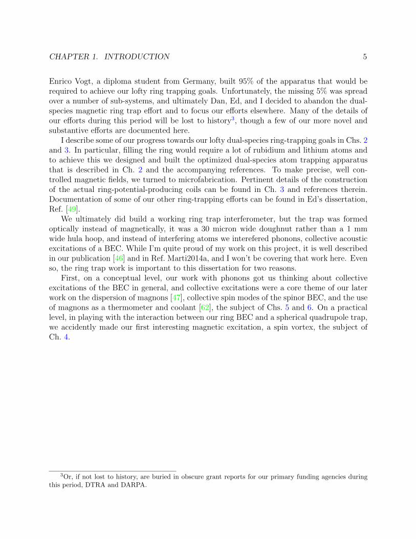
Enrico Vogt, a diploma student from Germany, built 95% of the apparatus that would berequired to achieve our lofty ring trapping goals. Unfortunately, the missing 5% was spreadover a number of sub-systems, and ultimately Dan, Ed, and I decided to abandon the dual-species magnetic ring trap effort and to focus our efforts elsewhere. Many of the details ofour efforts during this period will be lost to history3, though a few of our more novel andsubstantive efforts are documented here.
I describe some of our progress towards our lofty dual-species ring-trapping goals in Chs. 2and 3. In particular, filling the ring would require a lot of rubidium and lithium atoms andto achieve this we designed and built the optimized dual-species atom trapping apparatusthat is described in Ch. 2 and the accompanying references. To make precise, well con-trolled magnetic fields, we turned to microfabrication. Pertinent details of the constructionof the actual ring-potential-producing coils can be found in Ch. 3 and references therein.Documentation of some of our other ring-trapping efforts can be found in Ed’s dissertation,Ref. [49].
We ultimately did build a working ring trap interferometer, but the trap was formedoptically instead of magnetically, it was a 30 micron wide doughnut rather than a 1 mmwide hula hoop, and instead of interfering atoms we interefered phonons, collective acousticexcitations of a BEC. While I’m quite proud of my work on this project, it is well describedin our publication [46] and in Ref. Marti2014a, and I won’t be covering that work here. Evenso, the ring trap work is important to this dissertation for two reasons.
First, on a conceptual level, our work with phonons got us thinking about collectiveexcitations of the BEC in general, and collective excitations were a core theme of our laterwork on the dispersion of magnons [47], collective spin modes of the spinor BEC, and the useof magnons as a thermometer and coolant [62], the subject of Chs. 5 and 6. On a practicallevel, in playing with the interaction between our ring BEC and a spherical quadrupole trap,we accidently made our first interesting magnetic excitation, a spin vortex, the subject ofCh. 4.
3Or, if not lost to history, are buried in obscure grant reports for our primary funding agencies duringthis period, DTRA and DARPA.

6
Chapter 2
Dual-species apparatus
2.1 Overview
All of the fundamental physics relating to the experiments reported in this dissertation takeplace in a relatively small volume—at most a cubic millimeter, for example in the time-of-flight expansion of a barely degenerate gas, but typically much less than that, less than 0.0001cubic millimeters—but as is quite common in experimental science, the entire apparatus forallowing and observing that physics occupies a much larger space. Most of our apparatus isquite standard, with individual components well described in a variety of places. The basicsof laser cooling and trapping are covered in detail in Metcalf and van der Straten [57]. Ourdual-species oven design was based on Stan and Ketterle [81] and Stan [80]. For detailedguidance on assembling a BEC system, we like Lewandowski et al. [40]. Our optical trappingprocedure was inspired heavily by Lin et al. [43]. Finally, several other theses from our groupdescribe constructing apparatus very similar to our own, either because ours was built intheir shadow [26], or because ours was built contemporaneously and benefited from manymutual exchanges of ideas [24].
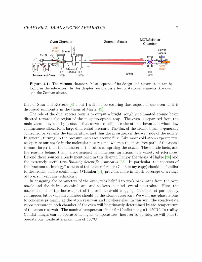
Finally, my close collaborator in designing, building, characterizing, and using the presentapparatus has covered many of its aspects in Marti [49]. Fig. 2.1 shows an overview of thevacuum system employed in this work. In this chapter, I will focus on two areas of the system:the dual-species oven and Zeeman slower. The accompanying optical setup is discussed inMarti [49] and will not be discussed here, except as necessary to understand the Zeemanslower. Details of the apparatus relevant to particular experiments will be covered in theirrespective chapters.
2.2 Dual species oven
The original design for our oven is based heavily on the work of Stan and Ketterle [81], withminor modifications pertaining to the substitution of rubidium (in our system) for sodium(in his). The nozzle design in our oven has seen several iterations and is quite distinct from
CHAPTER 2. DUAL-SPECIES APPARATUS 7
Gat
e Va
lve
Oven Chamber Zeeman Slower MOT/ScienceChamber
Rb Li
ColdMirrorDifferential
Pumping10 cmTwo-element Oven
IonPump
SlowerLasers
IonPump
ShutterExit Nozzle
ColdPump
IonPump
Figure 2.1: The vacuum chamber. Most aspects of its design and construction can befound in the references. In this chapter, we discuss a few of its novel elements, the ovenand the Zeeman slower.
that of Stan and Ketterle [81], but I will not be covering that aspect of our oven as it isdiscussed sufficiently in the thesis of Marti [49].
The role of the dual species oven is to output a bright, roughly collimated atomic beamdirected towards the region of the magneto-optical trap. The oven is separated from themain vacuum system by a nozzle that serves to collimate the atomic beam and whose lowconductance allows for a large differential pressure. The flux of the atomic beam is generallycontrolled by varying the temperature, and thus the pressure, on the oven side of the nozzle.In general, turning up the pressure increases atomic flux. Like most cold atom experiments,we operate our nozzle in the molecular flow regime, wherein the mean free path of the atomsis much larger than the diameter of the tubes comprising the nozzle. These basic facts, andthe reasons behind them, are discussed in numerous variations in a variety of references.Beyond those sources already mentioned in this chapter, I enjoy the thesis of Higbie [26] andthe extremely useful text Building Scientific Apparatus [58]. In particular, the contents ofthe “vacuum technology” section of this later reference (Ch. 3 in my copy) should be familiarto the reader before continuing. O’Hanlon [61] provides more in-depth coverage of a rangeof topics in vacuum technology.
In designing the parameters of the oven, it is helpful to work backwards from the ovennozzle and the desired atomic beam, and to keep in mind several constraints. First, thenozzle should be the hottest part of the oven to avoid clogging. The coldest part of anycontiguous bit of vacuum chamber should be the atomic reservoir. We want gas-phase atomsto condense primarily at the atom reservoir and nowhere else. In this way, the steady-statevapor pressure in each chamber of the oven will be primarily determined by the temperatureof the atom reservoir. The nominal temperature limit for Conflat flanges is 450C. In reality,Conflat flanges can be operated at higher temperatures, however to be safe, we will plan tooperate our nozzle at a maximum of 450C.

CHAPTER 2. DUAL-SPECIES APPARATUS 8
Rb Li 10 cm
Rb reservoirT~200ºC
Li reservoirT~400ºC
intermediate nozzleT~450ºC
C~0.01 L/s
oven nozzle heaterT~450ºC
Rb angeT~250ºC
mixing chamberP~10-4 to10-3 Torr
Li angeT~425ºC
oven nozzle angeT~450ºC
oven nozzleC~2 L/s
P~0.
1 To
rr
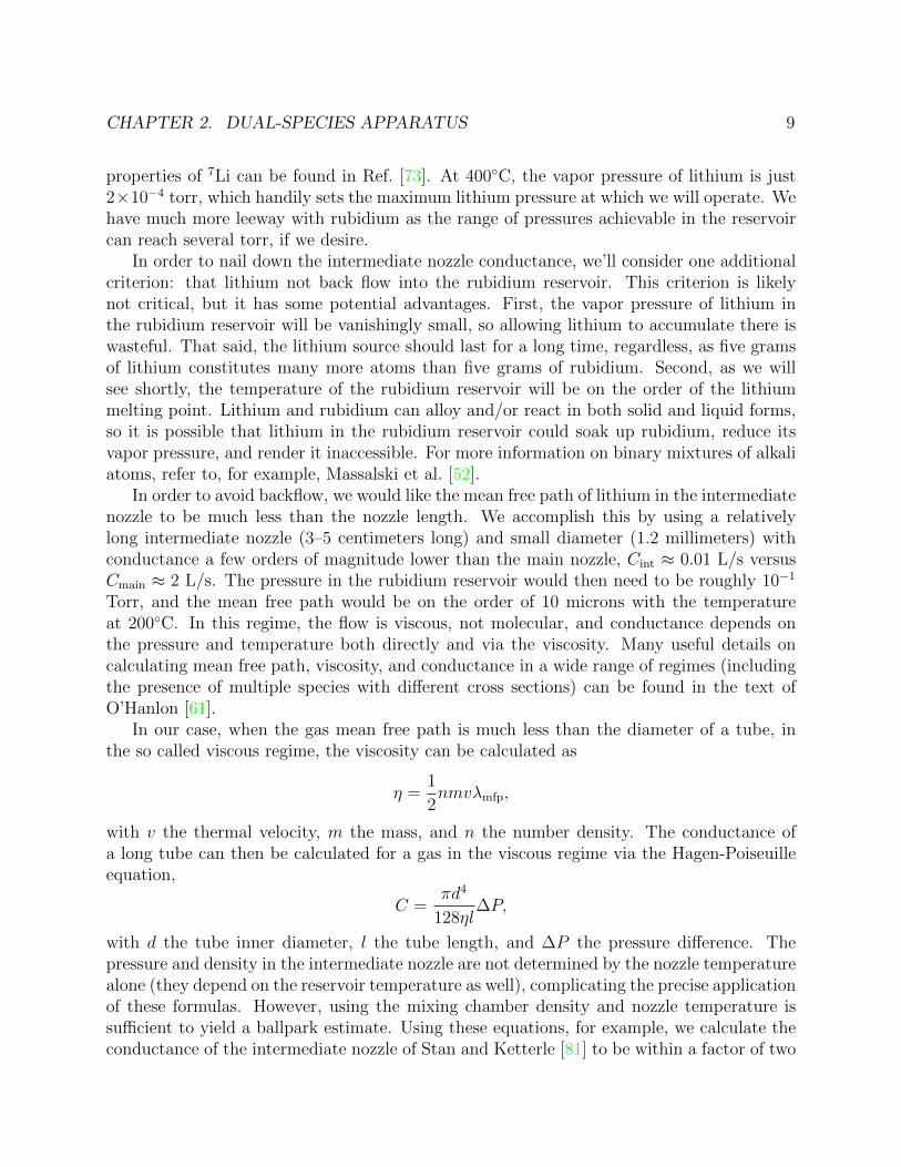
Figure 2.2: The dual-species oven and parameters. Approximate operating pressures,temperatures, and conductances are indicated. Band heaters are shown in dark red. Across section of the cold surface is shown in orange and is maintained at around -15C. Thenozzle is attached to a copper mount (shown in red) that is press-fit into a steel nipple. Theoven nozzle heater is placed around the nipple and heat is conducted to the nozzle throughthe copper. Water cooling coils, indicated in blue, keep the heat from the oven from heatingthe rest of the vacuum chamber. Oven insulation is schematically represented by the dottedblack line.
2.2.1 Pressures and conductance
As covered in the thesis of Marti [49], we want to operate with a mean free path λmfp & 1 cmin the mixing chamber, which is attached directly to the lithium reservoir. This impliespartial pressures for both rubidium and lithium in the range of 10−4–10−3 Torr in the mixingchamber. The lithium partial pressure is controlled directly by the lithium reservoir temper-ature. The equilibrium rubidium partial pressure in the mixing chamber (P
(mix)Rb ) depends
on the conductance of the intermediate (Cint) and main (Cmain) nozzles and the rubidium
pressure in its reservoir (P(res)Rb ):
P(res)Rb Cint = P
(mix)Rb Cmain.
Here we have assumed that the pressure in the mixing chamber is negligible compared tothe pressure in the rubidium reservoir, and similarly that the pressure outside the oven isnegligible compared to the pressure in the mixing chamber.
Vapor pressure curves for the alkali elements can be found in many places. The CRCHandbook [41] has comprehensive data, while the particular properties of 6Li and 87Rbare conveniently cataloged online by Gehm [20] and Steck [82], respectively. The optical
CHAPTER 2. DUAL-SPECIES APPARATUS 9
properties of 7Li can be found in Ref. [73]. At 400C, the vapor pressure of lithium is just2×10−4 torr, which handily sets the maximum lithium pressure at which we will operate. Wehave much more leeway with rubidium as the range of pressures achievable in the reservoircan reach several torr, if we desire.
In order to nail down the intermediate nozzle conductance, we’ll consider one additionalcriterion: that lithium not back flow into the rubidium reservoir. This criterion is likelynot critical, but it has some potential advantages. First, the vapor pressure of lithium inthe rubidium reservoir will be vanishingly small, so allowing lithium to accumulate there iswasteful. That said, the lithium source should last for a long time, regardless, as five gramsof lithium constitutes many more atoms than five grams of rubidium. Second, as we willsee shortly, the temperature of the rubidium reservoir will be on the order of the lithiummelting point. Lithium and rubidium can alloy and/or react in both solid and liquid forms,so it is possible that lithium in the rubidium reservoir could soak up rubidium, reduce itsvapor pressure, and render it inaccessible. For more information on binary mixtures of alkaliatoms, refer to, for example, Massalski et al. [52].
In order to avoid backflow, we would like the mean free path of lithium in the intermediatenozzle to be much less than the nozzle length. We accomplish this by using a relativelylong intermediate nozzle (3–5 centimeters long) and small diameter (1.2 millimeters) withconductance a few orders of magnitude lower than the main nozzle, Cint ≈ 0.01 L/s versusCmain ≈ 2 L/s. The pressure in the rubidium reservoir would then need to be roughly 10−1
Torr, and the mean free path would be on the order of 10 microns with the temperatureat 200C. In this regime, the flow is viscous, not molecular, and conductance depends onthe pressure and temperature both directly and via the viscosity. Many useful details oncalculating mean free path, viscosity, and conductance in a wide range of regimes (includingthe presence of multiple species with different cross sections) can be found in the text ofO’Hanlon [61].
In our case, when the gas mean free path is much less than the diameter of a tube, inthe so called viscous regime, the viscosity can be calculated as
η =1
2nmvλmfp,
with v the thermal velocity, m the mass, and n the number density. The conductance ofa long tube can then be calculated for a gas in the viscous regime via the Hagen-Poiseuilleequation,
C =πd4
128ηl∆P,
with d the tube inner diameter, l the tube length, and ∆P the pressure difference. Thepressure and density in the intermediate nozzle are not determined by the nozzle temperaturealone (they depend on the reservoir temperature as well), complicating the precise applicationof these formulas. However, using the mixing chamber density and nozzle temperature issufficient to yield a ballpark estimate. Using these equations, for example, we calculate theconductance of the intermediate nozzle of Stan and Ketterle [81] to be within a factor of two

CHAPTER 2. DUAL-SPECIES APPARATUS 10
of the measured value. The viscosity of rubidium in our nozzle is expected to be roughly2× 10−5 Poise. In practice, we have a lot of latitude in the rubidium temperature and willoptimize both rubidium and lithium atom flux by turning all the knobs at our disposal.
2.2.2 Temperature control
Once the nozzles are fixed and the physical design of the oven fixed, maintaining the tem-perature of the oven becomes a primary concern. We follow Stan and Ketterle [81] and useMi-Plus band heaters with built-in thermocouples from TEMPCO to heat the oven chamberin multiple places, shown in red in Fig. 2.4. The Mi-Plus heaters can be ordered in a range ofpeak powers (the peak power is obtained by driving them with 120V AC), sizes, and geome-tries. Two relevant geometries that we consider are one-piece, two-piece, and expandable.Two-piece or expandable heaters should be used where a one-piece band heater cannot beslid in place. However, we have found that 1.5 inch 2.75 inch one-piece heaters and can bestretched and wrapped directly onto 1.5 inch vacuum nipples and 2.75 inch flanges withoutbreaking them, if necessary.
We found elementary order-of-magnitude calculations of heat flow to be sufficient todetermine the required power of each heater. For the most part, any underestimate of therequired heater power can be fixed with additional insulation. Overestimates can be correctedby reducing the voltage to the heater or by pulse-width-modulation, which in our case isautomatically performed by PID controllers that stabilize the temperature as measured atthe heaters. The main concern one should have in choosing heaters and insulation is thatthe requisite thermal gradients can be maintained in the oven.
For example, in our oven design, we may wish for the rubidium reservoir to be maintainedat 150–175C while the intermediate nozzle temperature is fixed at 450C by the desire toprevent lithium accumulation. Heat will flow from the nozzle through the steel to the ru-bidium flange and reservoir. Maintaining the appropriate thermal gradient will require asufficiently powerful heater on the intermediate nozzle and a sufficiently small amount of in-sulation around the rubidium reservoir and flange. A rough calculation using the parametersof steel and the heat flow equation
Q =kA∆T
L,
with Q the heat flow rate, k ≈ 21 W/m·K the thermal conductivity, ∆T the temperaturedifference, and L and A the steel tube length and cross sectional area, respectively, withequal amounts of radiation and convective heat loss from the rubidium flange and reservoir,convinced us that a 300 W heater on the nozzle flange would be more than sufficient. It’s notnecessarily bad to have too much power. Keep in mind, though, that the fuses and cablesthat power the heaters need to be sized according to the peak power in order to handle morepeak current.
Based on our experience with the heaters and insulation, roughly one half watt per degreecelsius desired, as well as good fiberglass insulation, seems to be sufficient for maintainingtemperature. We went a little overkill and used 300 W and 400 W heaters for the nozzle
CHAPTER 2. DUAL-SPECIES APPARATUS 11
AC in
Poweron/o
red
90V
5 kΩ
(Solid-state) relay
50 kΩ
5 kΩ
green
90V
5 kΩ AC out
neutral
neutral
Turn onAC out(latch)
lineline
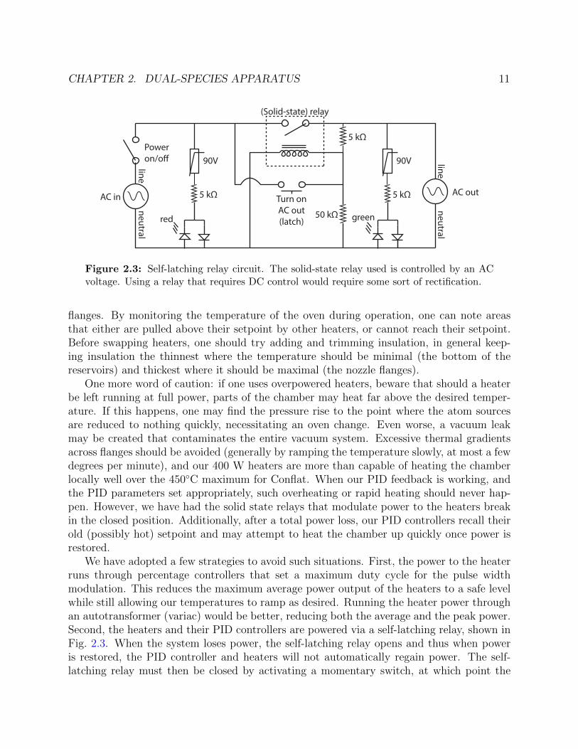
Figure 2.3: Self-latching relay circuit. The solid-state relay used is controlled by an ACvoltage. Using a relay that requires DC control would require some sort of rectification.
flanges. By monitoring the temperature of the oven during operation, one can note areasthat either are pulled above their setpoint by other heaters, or cannot reach their setpoint.Before swapping heaters, one should try adding and trimming insulation, in general keep-ing insulation the thinnest where the temperature should be minimal (the bottom of thereservoirs) and thickest where it should be maximal (the nozzle flanges).
One more word of caution: if one uses overpowered heaters, beware that should a heaterbe left running at full power, parts of the chamber may heat far above the desired temper-ature. If this happens, one may find the pressure rise to the point where the atom sourcesare reduced to nothing quickly, necessitating an oven change. Even worse, a vacuum leakmay be created that contaminates the entire vacuum system. Excessive thermal gradientsacross flanges should be avoided (generally by ramping the temperature slowly, at most a fewdegrees per minute), and our 400 W heaters are more than capable of heating the chamberlocally well over the 450C maximum for Conflat. When our PID feedback is working, andthe PID parameters set appropriately, such overheating or rapid heating should never hap-pen. However, we have had the solid state relays that modulate power to the heaters breakin the closed position. Additionally, after a total power loss, our PID controllers recall theirold (possibly hot) setpoint and may attempt to heat the chamber up quickly once power isrestored.
We have adopted a few strategies to avoid such situations. First, the power to the heaterruns through percentage controllers that set a maximum duty cycle for the pulse widthmodulation. This reduces the maximum average power output of the heaters to a safe levelwhile still allowing our temperatures to ramp as desired. Running the heater power throughan autotransformer (variac) would be better, reducing both the average and the peak power.Second, the heaters and their PID controllers are powered via a self-latching relay, shown inFig. 2.3. When the system loses power, the self-latching relay opens and thus when poweris restored, the PID controller and heaters will not automatically regain power. The self-latching relay must then be closed by activating a momentary switch, at which point the

CHAPTER 2. DUAL-SPECIES APPARATUS 12
Rb Li Rb Li10 cma b c
Figure 2.4: Original oven design (left) and improved oven design incorporating lessonslearned (right). (a) Fewer flanges are used, and the flanges present are oriented horizontallyto avoid alkali accumulation. The flanges are farther from the reservoirs, allowing themto be heated more. (b) The intermediate nozzle is welded in place, avoiding the manifoldissues associated with the original double-sided flange. (c) The nozzle assembly includes alarger gap between the nozzle heater and the high vacuum chamber, reducing the thermalgradient across the flange that affixes the oven to the oven chamber.
relay will close and remain closed. In practice, the self-latching relay that I built only opensupon power failure when a load is attached, seemingly because of some quirks of the solidstate relay. This is fine for turning off power to the PID controller and heaters, but in generalis an unwanted bug. Using a spring-loaded mechanical relay in the same circuit would be anobvious improvement.
2.2.3 Iterating on the design
Several drawbacks to the initial oven design were revealed over a few years of operation, whichincluded several catastrophic leaks. While we eventually switched to a less fraught single-species rubidium oven for the bulk of the work described in this dissertation, we designedand built an updated dual-species oven that incorporates several important improvements.A cross sectional schematic of the updated design is shown in Fig. 2.4. The problems weencountered, and proposed solutions incorporated, are discussed below.
First, lithium is well known to react slowly with copper gaskets. Thus, it is commonplaceto use nickel gaskets at flanges with substantial lithium exposure. Nickel is not an idealgasket material, however, as it is much less pliable than copper. This makes nickel gasketsless forgiving of knife-edge imperfections and, in our experience, repeated cycles of thermalexpansion and contraction. The updated oven design minimizes the number of flanges andtheir exposure to lithium. In this design, only one flange is exposed to lithium at a modestpressure, and this flange does not have to transmit any torque. A nickel gasket can safely beused for this flange. Importantly, the flange that affixes the oven to the vacuum system andtransmits a torque is “outside” the oven. A normal copper gasket, or better, a silver coatedcopper gasket (so that it is less likely to stick to the steel when it is time to replace it), can

CHAPTER 2. DUAL-SPECIES APPARATUS 13
vx
x
vx
x
vx
x
atom beam
MOT
Zeeman slower
z
x
LD Lz LM
slowing light
MOT
Initial Final... ... with transverseheating
vz
Ato
m
ux
vmax √Lz
oven
Figure 2.5: Schematic of zeeman slower. Atoms have a Maxwell-Boltzmann velocitydistribution in the oven. The atoms that emerge from the oven are collimated and those witha longitudinal velocity vz < vmax are slowed and cooled by scattering light in the Zeemanslower. As the atoms travel towards the MOT, their transverse phase space distributionevolves owing to both the passage of time and light scattering. Some fraction of the atomswill have a longitudinal velocity and transverse position such that they can be be capturedby the MOT.
be used there.Our original design included a double-sided flange in the construction of the intermediate
nozzle. This required using long threaded bolts to affix the adjoining oven parts, and thesebolts had to apply pressure to two different knife edges, one of which required a nickel gasket.Long bolts expand more than short ones when thermally cycled, and the requirement thatstrong force be applied to two knife edges made this junction particularly troublesome.When the nickel gasket originally used at the lithium side of the double-sided flange failed,we replaced it with a softer silver-coated copper gasket. However, the orientation of theflange at the intermediate nozzle allowed liquid lithium to accumulate in a cold spot andthe copper gasket was eaten away slowly in spite of its silver coating. The new oven designavoids the double-sided flange. Instead, an intermediate nozzle is welded in place.
Finally, the nozzle assembly incorporates a longer gap between where the nozzle is heatedand the rest of the vacuum system. This allows the large thermal gradient between the ovennozzle heater and the vacuum system to be more gradual. As a result, the flange affixingthe oven should experience less thermal stress.

CHAPTER 2. DUAL-SPECIES APPARATUS 14
2.3 Dual species Zeeman slower
The basics a Zeeman slower are well described in a number of the aforementioned sources [57,26]. Please refer to one of these resources for an overview of the basic operating principles.In this section, I will only briefly mention the basic elements of a Zeeman slower that aremost relevant to the design and construction of our novel dual-species design.
A schematic of a single-species Zeeman slower is shown in Fig. 2.5, which illustrates someof the essential trade offs in Zeeman-slower design. An ideal slower decelerates an atom atsome fraction η of the maximum deceleration amax, which is given for a saturated atom by
amax = ~kΓ/2m = vrΓ/2,
for an atom of mass m slowed by a counter-propagating laser of wavenumber k on a transitionwith linewidth Γ. The recoil velocity is vr. Increasing the length of the slowing regionincreases the length over which deceleration can occur, and thus the maximum velocity thatwill be entrained in the slower. For a slowing length Lz the maximum velocity entrained is
vmax =√v2f + 2ηamaxLz,
where vf is the velocity of the slowed atoms at the exit of the slower. Since the number fluxof atoms in the atomic beam rises initially like the velocity cubed, there is generally someadvantage to be had by increasing the slower length above zero. On the other hand, as theslower is lengthened, the solid angle subtended by the MOT decreases, reducing the numberof atoms in the beam with the appropriate trajectory for capture. Transverse heating ofthe atomic beam owing to spontaneous emission may also reduce the number atoms with atrajectory suitable for capture.
2.3.1 Optimizing the slower length
For heavy atoms like rubidium, transverse heating can more or less be ignored in slowerdesign, making the resulting calculation of ideal slower length essentially a problem of ge-ometry, as in Higbie [26]. For lighter atoms, transverse heating cannot be ignored, as wewill see, and it can be important to account for its effects. We optimize the slower lengthby considering the slow (capturable) atom flux at the MOT. To calculate the slow flux, weconsider the effect of the slower on two main factors: the transverse phase space and thelongitudinal velocity distributions. We begin by considering a single-species slower.
To model the transverse phase space, illustrated in Fig. 2.5, we will derive equations forits first and second moments. The first moments, which correspond to the mean transversevelocity, are trivially zero, so we focus on the second moments only. Using the definitionof the expected value 〈〉 and the relationship between the phase space variables (in onedimension), vx = ∂tx, with ∂t a short hand for the partial time derivative, we can derive a

CHAPTER 2. DUAL-SPECIES APPARATUS 15
simple differential relationship between the second moments,
∂t⟨x2⟩
(t) = 2 〈xvx〉 (t) (2.1)
∂t 〈xvx〉 (t) =⟨v2x
⟩(t) + 〈x∂tvx〉 (t)
∂t⟨v2x
⟩(t) = r(t)(∆v)2,
where r(t) is the rate of photon scattering and ∆v is the root mean square transverse velocityimparted by each scattering event. The term 〈x∂tvx〉 can be non-zero, for example whenthe transverse beam profile is inhomogeneous and the scattering rate depends on transverseposition. For simplicity we will ignore such effects for now, effectively modeling the coolingbeam as translation invariant in the transverse plane. When r(t) is constant, Eqs. (2.1) areeasy to solve analytically. One can account for initial atomic beam distributions that havenonzero higher moments (i.e. are not Gaussian) by the appropriate convolution of the initialbeam and a narrow Gaussian kernel propagated via Eqs. (2.1); however, for simplicity wewill consider beams that are initially Gaussian and can be described by the second momentsdirectly. The estimated capturable flux is sensitive to assumptions about the initial beamand the slowing process, a fact that has some implications for the manner in which weoperate the slower.
To solve Eqs. (2.1) for the transverse phase space distribution at the MOT of atoms witha particular longitudinal velocity vf < vz < vmax, we break the trajectory into three phases:first, the atoms travel ballistically from the oven nozzle into the slower, with r(t) = 0, for atime t1 such that
vzt1 = Ld + Lz − (v2z − v2
f )/(2amaxµ).
Here, Ld is the distance between the oven nozzle and start of the slower, and the later termsaccount for the fact that an atom with initial velocity vz < vmax will travel in the slower forsome distance before it is Zeeman shifted into resonance with the cooling light. Second, oncethe atoms are brought into resonance with the cooling light, they scatter light at a constantrate as they are slowed, with r(t) = ηΓ/2, for a time
t2 = (vz − vf )/(vrr(t)).
Finally, the atoms once again travel with r(t) = 0 from the end of the slower to the positionof the MOT during a time t3 = Lm/vf . Atoms with vz < vf travel the whole length of theslower ballistically. The capturable fraction of atoms with initial longitudinal velocity vz isthen computed by comparing the marginal probability of a slowed atom having a positionwithin the capture range of the MOT to that of an unslowed ballistic atom from the samebeam. Assuming a Gaussian atomic beam, integrating the phase space distribution is trivialand the capturable fraction f takes a trivial form:
f(vz) =
(erf
(MOT size√2 〈x2〉 (vz)
)/ erf
(MOT size√2 〈x2〉0 (vz)
))2
. (2.2)

CHAPTER 2. DUAL-SPECIES APPARATUS 16
0 50 100 150 200 250 300
0.2
0.4
0.6
0.8
1.0
vz (m/s)
Capturablefraction
(a) Rubidium
0 200 400 600 800 1000 1200
0.2
0.4
0.6
0.8
1.0
vz (m/s)
(b) Lithium
Figure 2.6: Capturable fraction without transverse cooling (dotted/dashed lines) andwith transverse cooling and with variable initial beam sizes (narrow beam: violet, broadbeam: red, in reverse rainbow order). Dotted curve neglects transverse heating. Withouttransverse cooling, the reduction in the capturable fraction is dominated by the reductionof the longitudinal velocity without a commensurate reduction in the transverse velocity.This “blooming” effect can be minimized by focusing the slower beam on the oven aperture,effectively cooling the transverse motion in proportion to the longitudinal motion. The solidrainbow curves have such transverse cooling applied. The presumed distance between theslower and the MOT is 10 cm, each atom is presumed to slow at 0.7amax, and the finalvelocities are vf = 30 m/s for rubidium and vf = 90 m/s for lithium.
Here, “MOT size” refers to the transverse extent over which atoms with longitudinal velocityless than vf will be entrained in the MOT. Typically, this size is taken to be roughly thesize of the beams that form the MOT. An assumption inherent in this formula is thatthere is a sharp cutoff in the transverse direction between 100% and 0% of atoms withspeed vf being captured. In reality, there is not a sudden cut-off, but we have found thissimplifying assumption to yield actionable results nonetheless. More nuanced expressionsfor the capturable fraction that consider a more detailed model of the MOT can certainlybe produced, but considering the level of approximation employed in our treatment thus far,they are unlikely to contribute much additional actionable information.
Fig. 2.6 shows some sample capturable fractions and highlights the importance of someamount of transverse cooling of the atomic beam. With longitudinal cooling only, the beamblooms dramatically because the ratio
√〈v2x〉/vz increases as the slower reduces vz. As shown
by comparing the dotted and dashed curves, even for the lighter lithium, this sort of beamblooming dominates transverse heating in the reduction of capturable flux. Zeeman slowersare typically operated with a slowing laser that is focused near the oven aperture, applying,in the ideal case, transverse and longitudinal cooling in (at least) equal proportion.
The effect of slowing in the presence of such transverse cooling, which we model by assign-ing our atom beam zero initial transverse velocity, is indicated by the rainbow colored curves

CHAPTER 2. DUAL-SPECIES APPARATUS 17
in Fig. 2.6. The different colors correspond to different initial (spatial) beam sizes. Here,the reduction of the capturable flux is due to transverse heating. Under the assumptionsof our simple model, the effects of transverse heating exhibit a strong dependence on themodel parameters. For beams with initial Gaussian width much larger than the MOT (notphysically realistic), transverse heating has little effect in our model, as atoms are equallylikely to be redirected toward the MOT as away from it. On the other hand, for very small,focused atomic beams (such as those emerging from a very small aperture), a substantialamount of transverse heating must take place before any atoms are lost. The true physicalsituation inside our slower lies between these extremes, as the extent of the atomic beamand the cooling laser are both finite. The most physically relevant atomic beam size thatworks with our model is thus initially slightly smaller than the MOT, giving the “worst case”dark blue curves. Numerical simulations of the slowing process can allow one to implementmore elaborate models, allowing, for example, atoms to exit the cooling beam and ceasescattering, or to have spatially dependent scattering rates. For estimating the ideal slowerlength, however, such simulations are almost certainly overkill, as we have found that in-cluding more sophisticated physical models beyond what we have already presented changesthe ideal lengths by relatively small amounts, even if it does shed better light on the overallatom flux that can be expected.
We are now ready to estimate the impact of the slower on the capturable flux by combin-ing our model slower with a model oven. We take the model oven to operate with a pressureof P = 2× 10⁻⁴ Torr at T = 400K and to have a thin round aperture with 5 mm diameter.The flux emitted into solid angle πθ2 at velocity vz is then, using the Maxwell-Boltzmannvelocity distribution [35],
I(vz) = πθ2nAvz
(m
2πkBT
)3/2
v2z exp
(−mv2
z
2kBT
), (2.3)
where A is the aperture area and n is the atom density in the oven at pressure P and temper-ature T . With πθ2 set to the solid angle subtended by the MOT at the oven aperture, andtherefore a function of the slower length, the estimated capturable flux N can be calculatedas
N =
∫ ∞0
I(vz)f(vz)dvz. (2.4)
Note that when the lithium and rubidium partial pressures are equal, as we are assuming,the total lithium flux emerging from the oven far exceeds the rubidium flux emerging fromthe oven owing to the higher average velocity of the lithium atoms at the same temperature.As noted in Sec. 2.2, the lithium and rubidium partial pressure, and thus the correspondingnumber fluxes, can be varied independently.
Estimated slow fluxes for a single species slower are shown in Fig. 2.7 for particular designparameters. Notably, we consider a slower with initial dead length of only 10 cm. In general,some amount of dead space, wherein the atoms are not being slowed, is required to allow

CHAPTER 2. DUAL-SPECIES APPARATUS 18
Rubidium
Lithium
0 20 40 60 80 1001×1010
5×10101×1011
5×10111×1012
5×10¹²
Slower length (cm)
Slowflux(1/s)
0 20 40 60 80 1005×1011
1×10¹²
5×10¹²
1×10¹³
Slower length (cm)
Figure 2.7: (Left) Estimated slow flux for single species slower as a function of slowerlength Lz, with slowing efficiency η = 0.7, Ld = 10 cm, Lm = 10 cm, final velocities vf forrubidium and lithium of 30 m/s and 90 m/s, respectively, and oven parameters describedin the text. The dotted curve indicates the slow flux of lithium in a slower optimized forrubidium. (Right) The slow fluxes from the left panel (solid lines) are compared to the slowfluxes that would be estimated without accounting for transverse heating (dashed lines). Inour simple model, transverse heating reduces the optimal lithium slower length considerably.
room for vacuum hardware in between the atomic beam nozzle and the Zeeman slower1.Our initial chamber design did not account for a second differential pumping stage, whichincreases the dead length. Notably, operating a slower designed for rubidium does increasethe capturable lithium flux by some amount, but is far inferior to a dedicated lithium slowerand strongly favors rubidium flux over lithium flux2. In the next section we talk aboutimproving the lithium performance of a primarily rubidium-focused slower.
2.3.2 Dual-species slower design
Our main innovation in slower design is to take advantage of the large differential in amax
between rubidium and lithium by adding slowing sections that (ideally) impact lithiumwithout impacting rubidium, as shown in the annotated magnetic field profile in Fig. 2.8.Because of more pronounced transverse heating of lithium, and because it can be sloweda great deal in a small amount of space, additional slowing of lithium at the end of therubidium slower provides the greatest returns in terms of slow lithium flux with the leastcost in slow rubidium flux. With the parameters modeled in Fig. 2.9, the model predictsthat slow lithium flux jumps 3.5 times by the addition of an optimized 3 cm section at theend of the rubidium slower. The rubidium flux drops by a mere 15% with the same addition.
While the stage III slower provides a generous return, its length is limited by the require-ment that rubidium cease its slowing and that lithium be slowed effectively by the stage II
1Recently, a permanent magnet Zeeman slower has been developed [44] that can be placed in vacuumvery close to the atomic beam nozzle, allowing a very short dead space and thus a very short optimal length.
2Recall that owing to its smaller amax, a slower optimized for lithium cannot slow rubidium.

CHAPTER 2. DUAL-SPECIES APPARATUS 19
20 40 60 80
200
400
600
800
Distance in slower (cm)
Mag
netic
el
d (G
auss
)
Slow Li
Slow Rb and Li
Slo
w L
i
Stage I Stage II Stage III
Figure 2.8: Dual-species slower design with three sections. Section I (shown as 18 cmlong) slows lithium only. Section II (here 61 cm long) slows rubidium primarily, but lithiumcomes along for the ride. Section III (merely 2 cm long) slows lithium only. The kink in thefield going from section II to III is important. In order for rubidium to exit the slower withthe desired final velocity, its velocity must be unable to track the change in the magneticfield at that spot. This places limits on the length of the final lithium slower section, asdiscussed in the text.
slower. This condition may seem at first glance to be trivially satisfied owing to the fact thata
(Rb)max < a
(Li)max, but it is not, because if the velocities of lithium and rubidium are different, the
acceleration required for the velocity to follow a particular magnetic field will be different.Rather than thinking about dv/dt we need to consider dv/dz = (1/v)× dv/dt.
The requirement that rubidium not be slowed in the stage III slower can be expressed as
ηa(Li)max/v
(Li)III > a(Rb)
max /(ηv(Rb)III ), (2.5)
where we have written vIII for the velocity of rubidium/lithium at the end of stage II/beginningof stage III. We have used the fact that the stage III magnetic field is designed to slow lithiumat a rate ηa
(Li)max and, for simplicity, we have arbitrarily imposed a requirement that the accel-
eration required to slow rubidium exceed its maximum value by a factor of 1/η. In derivingEq. (2.5), note that the magnetic moments of lithium and rubidium in their optically-pumpedstates are the same. Likewise, the requirement that lithium be slowed in stage II takes thesimilar form
ηa(Li)max/v
(Li)III > ηa(Rb)
max /v(Rb)III . (2.6)
For 0 < η < 1, both Eq. (2.6) and Eq. (2.5) are satisfied if Eq. (2.5) is.
Using the fact that v(Rb)III = v
(Rb)f and v
(Li)III =
√v
(Li)2f + 2ηa
(Li)maxLIII, the restriction on the

CHAPTER 2. DUAL-SPECIES APPARATUS 20
Rubidium (composite)
Lithium (composite)
Lithium (optimal)
0 5 10 15 20 251×1010
5×10101×1011
5×10111×1012
5×10¹²
Lithium slower length (cm)
Slowflux(1/s)
0 5 10 15 20 2540
45
50
55
60
Lithium slower length (cm)
OptimalRblength
(cm)
Figure 2.9: Dual-species slower trade-offs. (Left) Slow flux of rubidium and lithium isplotted as a function of total lithium slower length. Lithium length is applied first to thestage III slower, up to its maximum length, indicated by the vertical dashed gray line.Additional length is allocated to the stage I slower. Rubidium slower (stage II) length is setto maximize rubidium flux at the particular slower length. The stage II length is plottedat the right. Adding lithium sections to the rubidium slower decreases the rubidium flux,but over a wide range of parameters the fractional gain in slow lithium flux far exceeds thecost in rubidium. The lithium performance of the dual-species slower does not approachthat of a slower optimized for lithium alone. Parameters used here are η = 0.7, Ld = 10 cm,Lm = 10 cm, and final velocities vf for rubidium and lithium of 30 m/s and 90 m/s,respectively, and oven parameters described in the text.
length of stage III can be written
LIII <η3a
(Li)maxv
(Rb)f
2a(Rb)2max
−v
(Li)2f
2ηa(Li)max
. (2.7)
In essence, this condition is meant to guarantee that the kink in the desired magnetic fieldat the interface of section II and III is sufficiently large. In reality, the slope of the magneticfield cannot be made to increase abruptly. In the physical design of our slower, we will haveto make sure it changes fast enough. Like the factors η in the designed rate of deceleration,the margin 1/η in Eq. (2.5) is meant to help accommodate the differences between an idealand an actual slower.
Even with a limit on the length of section III, increasing the total length of the lithiumslower, by including section I, may be advantageous, as shown in Fig. 2.9. Section I offersan additional benefit that will be apparent in Sec. 2.3.3: some of the coils that produce thefield for section I can be made large, such that their field extends into the oven chamber. Tosome extent, this allows additional slowing of lithium without increasing the total length ofthe slower; rather, dead space at the beginning of the slower is reduced. In addition, it isadvantageous for a rubidium Zeeman slower to operate on top of a large, at least 250 G biasfield, at which point the excited state hyperfine structure is in the Paschen-Back regime, inorder to reduce the likelihood that an atom is pumped to a dark state [57]. Lithium, which
CHAPTER 2. DUAL-SPECIES APPARATUS 21
reaches the Paschen-Back regime at much lower field, might as well be slowed as the biasfield is ramped on.
2.3.3 Designing the slower windings
Now that we have a decent model that allows us to weigh the effect of various choices ofslower lengths and parameters η, which determine the magnetic field profile Btarget(z), weconsider what sort of slower we can actually build. Our general approach to this problem isto try certain parameters, producing a target magnetic field profile, and then see if we canexpect to build an approximation of that profile that is “good enough” by playing with amodel of the magnetic field produced by an achievable configuration of coils and currents.
We found it helpful to break down what constitutes “good enough” into a manageablelist of quantitative metrics. The key ingredients are as follows.
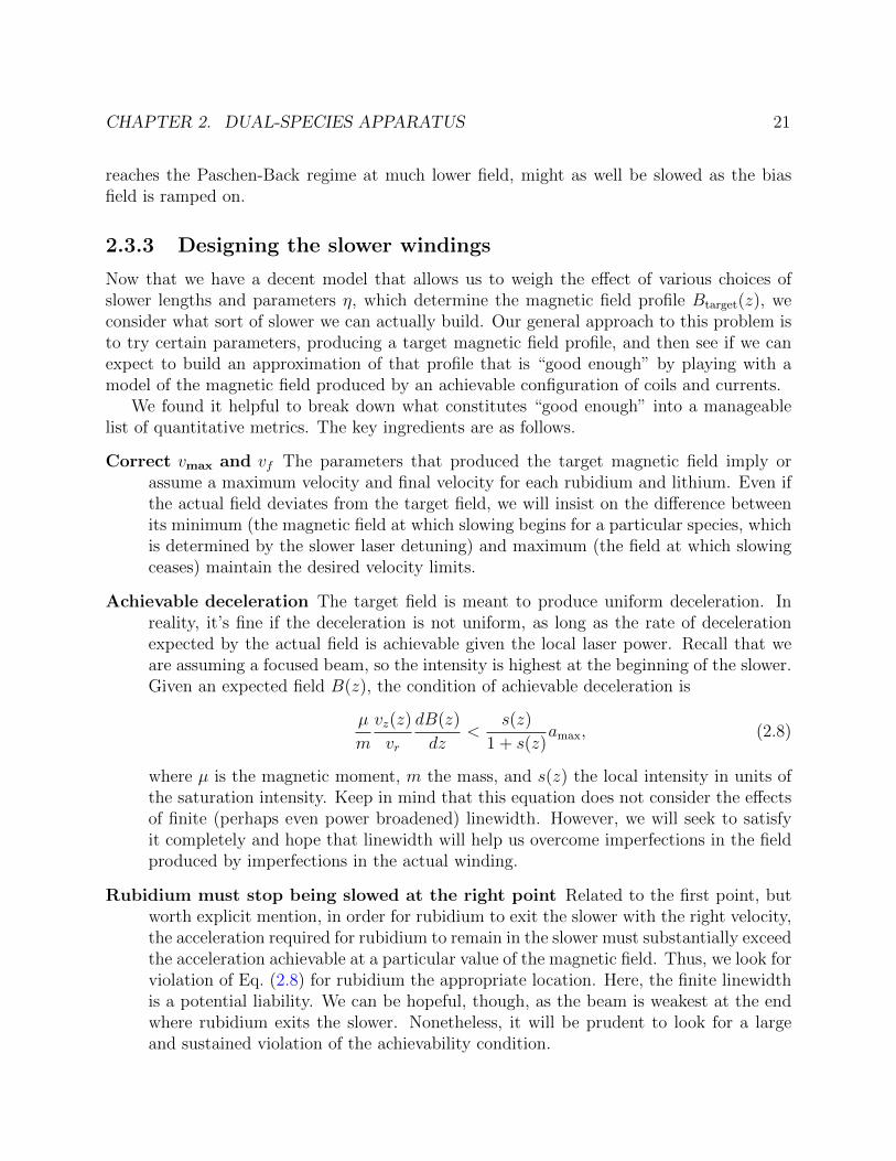
Correct vmax and vf The parameters that produced the target magnetic field imply orassume a maximum velocity and final velocity for each rubidium and lithium. Even ifthe actual field deviates from the target field, we will insist on the difference betweenits minimum (the magnetic field at which slowing begins for a particular species, whichis determined by the slower laser detuning) and maximum (the field at which slowingceases) maintain the desired velocity limits.
Achievable deceleration The target field is meant to produce uniform deceleration. Inreality, it’s fine if the deceleration is not uniform, as long as the rate of decelerationexpected by the actual field is achievable given the local laser power. Recall that weare assuming a focused beam, so the intensity is highest at the beginning of the slower.Given an expected field B(z), the condition of achievable deceleration is
µ
m
vz(z)
vr
dB(z)
dz<
s(z)
1 + s(z)amax, (2.8)
where µ is the magnetic moment, m the mass, and s(z) the local intensity in units ofthe saturation intensity. Keep in mind that this equation does not consider the effectsof finite (perhaps even power broadened) linewidth. However, we will seek to satisfyit completely and hope that linewidth will help us overcome imperfections in the fieldproduced by imperfections in the actual winding.
Rubidium must stop being slowed at the right point Related to the first point, butworth explicit mention, in order for rubidium to exit the slower with the right velocity,the acceleration required for rubidium to remain in the slower must substantially exceedthe acceleration achievable at a particular value of the magnetic field. Thus, we look forviolation of Eq. (2.8) for rubidium the appropriate location. Here, the finite linewidthis a potential liability. We can be hopeful, though, as the beam is weakest at the endwhere rubidium exits the slower. Nonetheless, it will be prudent to look for a largeand sustained violation of the achievability condition.

CHAPTER 2. DUAL-SPECIES APPARATUS 22
20 40 60 80
200
400
600
800
Position (cm)
Fiel
d (G
auss
)
Figure 2.10: Slower winding and target field on same linear position scale. The mainsection consists of two layers of double-diameter hollow core wire with up to sixteen layersof narrow gauge solid wire on top. The large diameter windings shown at the left are the“stretch” coils that extend the section I field into the oven chamber. The section III fieldis aided by a high-current “boost” winding, shown in blue to the right. The field peak issharpened by the high current “anti-gradient” winding, shown in green to the right.
We modeled our physical slower by considering a configuration of closed loops of wirein various positions and with various currents. In reality, we constructed our slower fromhelical windings; the closed loop approximation should be good as long as the coil spacingis much less than the coil diameter. To assist in finding a configuration of coils that isgood enough, it helps to have additional constraints. These constraints should incorporatephysical restrictions in the slower winding. To get a sense of the constraints we employed,take a look at the winding pattern we ultimately used in our slower, shown with the targetfield in Fig. 2.10.
We chose to have five distinct sets of coils. The main section of the slower would comprisetwo sets of coils: one set composed of 1/8 inch wire and another of 1/16 inch wire. Up totwo layers of the 1/8 inch diameter hollow wire would be spaced at multiples of 1/7 inchand covered by up to sixteen layers of 1/16 inch wire, which would be spaced at multiples of1/14 inch. The 1/8 inch base layer of coils were to be wound on a one inch outer-diametertube. Each subsequent layer would rest on the layer below, giving the layers 1/8 or 1/16 inchspacing in the radial direction. A key constraint imposed on these windings was that everycoil be placed on top of another coil. Gaps in the winding were allowed only on exposedlayers. In addition, the average winding pitch was constrained to increase from left to right,as shown in the zoomed in regions of Fig. 2.10. All of the wire in the main section wasdesigned to operate at the same current, but in optimizing the winding pattern the currentrequired was allowed to vary between five and ten amperes. Water can be run through the1/8 inch hollow layers to prevent some of the heat generated by the slower windings fromconducting through to the vacuum chamber.

CHAPTER 2. DUAL-SPECIES APPARATUS 23
A large diameter coil was included in the coil optimization routine. The first layer of this“stretch” coil was fixed at an inner diameter of five inches in order to allow the magneticfield to stretch into the oven or differential pumping region. Up to six layers of winding with1/8 inch wire were allowed in the stretch section. The axial position of the stretch coils wereconstrained to limit the overlap with the main section. The designed stretch coil current,like the inner diameter, was constrained to be five times the current in the main section,reducing the number of free parameters and increasing the speed of finding the optimizedwinding pattern.
The final two sets of coils are meant to facilitate the fast rise in magnetic field at theend of the slower. The “boost” coil consisted of up to two layers of the 1/8 inch wire woundon top of the two layers of 1/8 inch wire from the main section. In retrospect, winding theboost directly on the 1 inch tube would have been a better choice, allowing the field slopeto change more abruptly and making it easier to stop slowing rubidium. The boost coilcurrent was allowed to reach several hundred amperes. The final coil is the “anti-gradient”coil, which is wrapped on 1.5 inch tube that can fit over the mini-flange that connects theslower vacuum tube to the MOT chamber. The anti-gradient coil consisted of three turns of1/8 inch wire running up to 200 amperes.
The particular pattern of winding for the main and stretch coils, along with the currentsof all of the coils, was optimized using an iterative algorithm that involved adding andremoving turns of simulated wire in various places, subject to constraints already mentioned,and varying the currents in order to minimize a target function. The target function weighedfive criteria:
1. The squared difference between the target field and calculated field,
2. The condition that the acceleration required, Eq. (2.8), was achievable as necessary inthe three stages,
3. The condition that rubidium cease accelerating at the appropriate place,
4. The condition that the gradient field at the MOT be minimal, and
5. The condition that the field reaches the right maximum value so that the final velocityof lithium is correct.
Condition 4, in retrospect, was not important as the gradient due to the slower can be madeto add constructively with the gradient of the MOT coil, and does not hurt the operation ofthe MOT. We would not include it if we were to perform the optimization again. The biasfield of the slower is canceled by compensation coils.
Each of the terms in the target function was weighted empirically to assist the algorithmin finding a suitable local minimum. Once a winding and current set were found, tweakswere made by hand to further optimize the field (e.g. increase the likelihood of rubidiumceasing deceleration at the expense of larger gradient field at the MOT) and to make thewinding pattern easier to produce (e.g. make the spacing more even so that fewer changes

CHAPTER 2. DUAL-SPECIES APPARATUS 24
0 20 40 60 80
0
200
400
600
800
Position (cm)
Field
(Gauss
)
Rubidium
Lithium
0 20 40 60 800.0
0.2
0.4
0.6
0.8
1.0
1.2
Position (cm)
Accelerationrequired/amax
Figure 2.11: Design field (left) and acceleration required (right). (Left) The target fieldis shown in solid blue, and the calculated field from the coil winding is shown in dashedorange. (Right) The acceleration required is expressed in terms of amax for each species.Divisions between the sections, based on the target values of the magnetic field, ratherthan the design lengths L, are shown as vertical dashed lines. The maximum accelerationachievable given the laser power, assuming a minimum intensity I/Isat = 2.5 10 cm pastthe end of the slower, at the presumed position of the MOT, is shown in solid dark gray.As desired, the acceleration required of rubidium exceeds the maximum possible under thesimple model that does not account for finite linewidth or transverse variation in the laserpower.
in spacing would be required). Throughout the optimization process, we kept tabs on aplot of the acceleration required and a comparison of the actual and target field, as shownin Fig. 2.11. The target field parameters ultimately employed included a 5 cm transitionregion between stage I and stage II in which the target field did not change. Additionally,the design parameter η varied from section to section. The parameters were LI = 18 cm,LII = 61 cm, LIII = 2.6 cm, ηI = 0.78, ηII = 0.67, and ηIII = 0.68. Lithium and rubidiumfinal velocities vf were 40 m/s and 30 m/s, respectively. We later realized that higher finalvelocities up to 100 m/s for lithium could have been used.
2.3.4 Winding the slower
The ambitious nature of the dual-species slower requires precise winding. The main innova-tion that we employed to reach the desired precision was the use of the threading functionalityof a lathe in laying each turn of wire. In the process of winding the main and boost sec-tions of the slower, which are wrapped on a single tube, the threading gears were alwaysengaged and the turns of the chuck (performed by hand rather than by motor) were carefullycounted. In this manner, each layer of wire could be absolutely referenced to a particular“home” position of the compound tool holder.
The use of the lathe’s threading facility was inspired by the fortuitous fact that both seven

CHAPTER 2. DUAL-SPECIES APPARATUS 25
1/4 1/2 3/4 full
Figure 2.12: An overview of the first half of the wound slower. One-quarter, one-half,three-quarter, and full density turns are clear.
and fourteen threads-per-inch are standard pitches for 1-1/4” and 7/16” bolts, respectively,and are thus among the limited options built-in to larger imperial lathes. The standardsquare cross section magnet wire used in our group (hollow conductor kapton-wrapped mag-net wire from S&W Wire) happens to be about 1/8” wide. In considering ways of makingmore precise magnetic fields, I noted the compatibility of 1/8” wire with a seven-per-inchpitch and, furthermore, was able to find square magnet wire with approximately 1/16” width(14 AWG square conductor wire with polyimide enamel from MWS Wire Industries), com-patible with 14-per-inch pitch. Furthermore, half density windings of the thinner wire couldbe achieved. Using the thinner wire allows more layers with different numbers and pitchesof turns in the same space, and allows finer control of the turn density. The procedure forwinding the slower is detailed in Appendix A. A snapshot of the precise winding is shown inFig. 2.12
2.3.5 Testing the slower
Before installing the slower, it is very helpful to run a few tests. Resistance measurementsbetween unconnected conductors can reveal shorts (oops!) and four-point resistance mea-surements of the various contiguous layers will serve as a baseline for future reference. Dropsin resistance over time could indicate shorts between layers. It’s also important to make anaccurate measurement of the magnetic fields generated by the various coils, both as a test forshorts between layers and also to aid in simulating the function of the slower, if necessary.
We used F.W. Bell transverse and axial hall probes to measure the magnetic field atcentimeter intervals along the center of the coils. As expected, the field is mostly axial.The magnetic field measurements were performed in a differential manner with DC currentswitched on and off at each position. The main set of coils, including the 1/8” base layer,is composed of seven different pieces of conductor. The field due to each conductor wasmeasured separately to allow for the possibility of optimizing the operation of the slower byrunning slightly different currents through the different conductors that comprise the mainsection. The boost, stretch, and anti-gradient coils were measured separately as well.
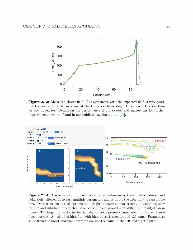
CHAPTER 2. DUAL-SPECIES APPARATUS 26
0 20 40 60 80
0
200
400
600
800
Position (cm)
Field
(Gauss
)
Figure 2.13: Measured slower field. The agreement with the expected field is very good,but the measured field curvature at the transition from stage II to stage III is less thanwe had hoped for. Details on the performance of our slower, and suggestions for furtherimprovements, can be found in our publication, Marti et al. [48].
Boost current (A)
Boost current (A)
Mai
n cu
rren
t (A
)
slow ux
LiRb
Figure 2.14: A screenshot of our numerical optimization using the simulated slower andfields (left) allowed us to vary multiple parameters and estimate the effect on the capturableflux. Data from our actual optimization (right) showed similar trends, but aligning slowlithium and rubidium flux with a large boost current proved more difficult in reality than intheory. The large purple dot in the right-hand plot represents large rubidium flux with zeroboost current. An island of high flux with high boost is seen around 125 amps. Parametersaside from the boost and main currents are not the same in the left and right figures.

CHAPTER 2. DUAL-SPECIES APPARATUS 27
With the field well measured, the performance of the slower can be simulated numericallyin great detail—accounting for beam inhomogeneity and finite linewidth, for example—allowing one to vary a wide range of parameters to assist in finding suitable settings. Wefound that including the magnetic fields produced by the MOT in the simulations of theslower improved their ability to predict our observed loading rates. Ultimately, the proof ofthe slower is in its performance in loading a real MOT. The measured fields of our slower, itsreal-world performance, and suggestions for future improvements based on lessons learnedsince its original design are detailed in our publication, Marti et al. [48]. A screenshot ofsome of our numerical optimizations, in which many simulated parameters are varied, andMOT fluorescence data tracking a similar variation in parameters, is shown in Fig. 2.14.
Our goal of producing a stage III that slows lithium but not rubidium was only partlyachieved. Operating in dual species mode as intended, we were unable to find settings thatproduced a large rubidium flux with exit velocities low enough to be captured by the MOT,owing to the limited field curvature at the transition from stage II to III. New slower designsbased on this concept would do well to place more emphasis on increasing the curvature inthis region, perhaps with smaller boost coils or by placing the boost coils further from themain coils, as suggested in our publication.
The slower works very well as a single-species slower—no stretch, boost, or anti-gradientcurrents required—as very few compromises were made in its rubidium performance in theeffort to accommodate lithium, and the smooth field and aggressive deceleration payoff inthe rubidium flux. Other than producing the data for Marti et al. [48], the slower has beenoperated in rubidium-only mode for all of the experiments described in this work. In thismode, only the main sections of the slower are powered. The stretch, boost, and anti-gradientcoils remain, but are idle.

28
Chapter 3
Microfabricating a magnetic ring trap
The initial goal for our team was to trap and condense atoms in a magnetic ring trap, buildingupon work that had been done along these lines in our group on a different apparatus [23].In contrast to that work, which employed hand-wound millimeter-scale coils with sufficientmagnetic field inhomogeneity to preclude filling a ring with a BEC, our experiment wouldbuild upon the micro-fabrication expertise developed by members of our group’s atom chipexperiment [70] to produce coils capable of trapping atoms in an extremely flat potentialwith a circular minimum.
Antibias
Curv
atur
e
450
500
550
|B| (Gauss)
-0.5-1.0 0.5 1.0x (mm)
Antibias
Curvature
2 mm
7.8 mm
2 mm (spacer)
525 um
27 turns / 120 um deep50um wire / 10 um wall
21 turns / 120 um deep20um wire / 10 um wall
Figure 3.1: Overview of the microfabricated chip design, including labeled crosssectionof the assembled stack of four chips, magnetic field profiles, and schematic of the overallassembly.

CHAPTER 3. MICROFABRICATING A MAGNETIC RING TRAP 29
The basic requirements and design of the microfabricated chips were worked out by ourpostdoc Anton Ottl, and are shown in Fig. 3.1. Prior to my assuming a role in the fabricationprocess, two members of our research group, Tom Purdy and Dan Brooks, had developedand demonstrated a process for micro-machining deep (100s of microns), high-aspect ratio(>10:1) and sub-micron positioned through-silicon features on double-sided silicon wafers.Preliminary work had been done on copper plating and planarizing these microfabricatedchips, though these aspects of the process were largely undeveloped. Tom had been able toshow very promising proof-of-concept electroplating of the larger, lower-aspect-ratio (2.5:1)antibias coils. The metalization process we employ leaves metal on the surfaces of the chips,which must be removed. Tom had demonstrated the ability to remove this metal in antibiaschips with copper on one side.
An overview of the project goals and status as it stood when I assumed the lead, producedas part of a request for proposal in an attempt to outsource the chip fabrication project toTeledyne Scientific, can be found in Appendix B. Several aspects of the chip fabrication hadyet to be developed completely. In particular:
1. Consistent void-free copper filling of the high-aspect-ratio “wires” (6:1) on the curva-ture chip had not been achieved.
2. A compatible planarization process for removal of excess copper had not been developedfor the curvature chips.
3. Planarization of double-sided chips had not been achieved.
4. Post-processing procedures (e.g. annealing of plated copper) were largely unexplored.
5. The methods and procedure for the assembly and precise alignment of chips into a coilstack was required.
6. Destructive and non-destructive methods of testing the electrical and mechanical ro-bustness of the chips required refinement and further development.
7. Operational capabilities and limitations (i.e. current carrying, heat sinking and distri-bution, handling) needed to be determined.
The unique nature of our chip coils (large, high-aspect-ratio, high density features dis-tributed over a large area of both sides of the silicon) place them in a regime which has beensparsely explored by industry and academia. The development of our process has thereforebeen guided by a combination of prior research on thin (nanometer scale) films and on sparse100 nanometer to 10 micron-scale high-aspect ratio features.
The development of an appropriate process was further complicated by the fact that wehad a very limited number of quality samples from the first (micro-machining) stages ofproduction, necessitating excessive care on ensuring a high yield on these samples. Tomwas available to introduce me to many aspects of the chip fabrication procedure, but the

CHAPTER 3. MICROFABRICATING A MAGNETIC RING TRAP 30
knowledge and skill required to micro-machine quality double-sided chips remained his alone.Thus, most process development was done on stand-in chips differing in key ways fromthe actual production samples. In most cases, single sided chips were used at first. Theprocess was then extrapolated to double-sided chips and tested on discarded and early-stage(often with shallower features) or defective (with broken sidewalls, for example) double-sided chips. A “best effort” would then be performed on the production samples. In an idealscenario, many identical production chips would have been available for testing and processdevelopment, allowing for more parallel testing and more accurate indication of the processefficacy.
The details of the chip micro-machining procedure, as well as the specific parameters ofthe electroplating process that we developed for both the curvature and antibias wafers can befound in Appendix A of Purdy [70]. In this chapter, I will touch on a few of the challengesthat we overcame in developing the electroplating recipe, including some suggestions forfurther improvement. Mainly, though, I will report on subsequent stages of development,including our planarization, annealing, chip verification and testing, and bonding procedures.Preliminary measurements of the thermal capabilities of the completed chip stack are alsoreported.
3.1 Electroplating
Before the electroplating process is to begin, a metal layer (or two) is deposited onto thesilicon-oxide substrate. In our case, a thin layer of titanium serves as an intermediary betweenthe silicon-oxide and a layer of copper. The metal layers serve two main purposes. First, thecopper serves as a seed on which more copper can be deposited by electrochemical means.Second, the metal serves to provide electrical connectivity between all areas where we desirecopper to grow.
There are two basic strategies for electroplating deep features. The most straight-forwardway is to deposit copper (or electrically connect) only the bottom of the future wires andgrow the copper in a bottom-up fashion. This approach works when all of the wires canbe joined with minimal electrical resistance such that the growth rate in all of the wires isnearly the same. The other approach is to coat all of the surfaces with a seed layer andgrow copper everywhere, even where it will not be wanted eventually. This approach has theadvantage of great electrical conductivity, and is useful in cases like ours where the wires arevery long (so that the resistance of a seed layer lying within them would be large) or wheremany features that require copper are electrically isolated. The challenge of this approachis filling deep features completely, without voids. In order for this to be done, the copper inthe trenches needs to grow from the side in, with a preference for faster growth deep in thetrenches.
The electroplating procedure that we developed was based on the work of Sun et al. [85].There, 10 micron square by 70 micron deep vias were filled with copper using a commercialplating apparatus, a homemade plating solution, and special current sequence involving a
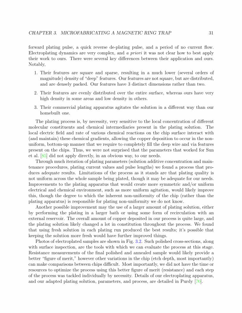
CHAPTER 3. MICROFABRICATING A MAGNETIC RING TRAP 31
forward plating pulse, a quick reverse de-plating pulse, and a period of no current flow.Electroplating dynamics are very complex, and a priori it was not clear how to best applytheir work to ours. There were several key differences between their application and ours.Notably,
1. Their features are square and sparse, resulting in a much lower (several orders ofmagnitude) density of “deep” features. Our features are not square, but are distributed,and are densely packed. Our features have 3 distinct dimensions rather than two.
2. Their features are evenly distributed over the entire surface, whereas ours have veryhigh density in some areas and low density in others.
3. Their commercial plating apparatus agitates the solution in a different way than ourhomebuilt one.
The plating process is, by necessity, very sensitive to the local concentration of differentmolecular constituents and chemical intermediaries present in the plating solution. Thelocal electric field and rate of various chemical reactions on the chip surface interact with(and maintain) these chemical gradients, allowing the copper deposition to occur in the non-uniform, bottom-up manner that we require to completely fill the deep wire and via featurespresent on the chips. Thus, we were not surprised that the parameters that worked for Sunet al. [85] did not apply directly, in an obvious way, to our needs.
Through much iteration of plating parameters (solution additive concentration and main-tenance procedures, plating current values and pulse lengths) we found a process that pro-duces adequate results. Limitations of the process as it stands are that plating quality isnot uniform across the whole sample being plated, though it may be adequate for our needs.Improvements to the plating apparatus that would create more symmetric and/or uniformelectrical and chemical environment, such as more uniform agitation, would likely improvethis, though the degree to which the inherent non-uniformity of the chip (rather than theplating apparatus) is responsible for plating non-uniformity we do not know.
Another possible improvement may the use of a larger amount of plating solution, eitherby performing the plating in a larger bath or using some form of recirculation with anexternal reservoir. The overall amount of copper deposited in our process is quite large, andthe plating solution likely changed a lot in constitution throughout the process. We foundthat using fresh solution in each plating run produced the best results; it’s possible thatkeeping the solution more fresh would have further improved things.
Photos of electroplated samples are shown in Fig. 3.2. Such polished cross-sections, alongwith surface inspection, are the tools with which we can evaluate the process at this stage.Resistance measurements of the final polished and annealed sample would likely provide abetter “figure of merit,” however other variations in the chip (etch depth, most importantly)can make comparisons between chips difficult. Most importantly, we did not have the time orresources to optimize the process using this better figure of merit (resistance) and each stepof the process was tackled individually by necessity. Details of our electroplating apparatus,and our adapted plating solution, parameters, and process, are detailed in Purdy [70].

CHAPTER 3. MICROFABRICATING A MAGNETIC RING TRAP 32
Figure 3.2: Photos of the curvature coil electroplating. (Left) A polished cross sectionof the wires in the curvature coil shows voids. (Center) Using our best known parameters,void-free filling has been achieved, at least in the section of the chip shown here. Extremecopper overfilling in this section of the chip was deemed necessary to insure adequate copperfilling in the large pads of the chip. In retrospect, overfilling with so much copper may nothave been prudent, as removing such a thick layer of copper poses a challenge. (Right) Thesurface of the chip as it appears during electroplating.
1 micron silicon dioxide Silicon substrate copper
20 micronfragile features!!Copper over plated
50-150 microns
Have Want Want Avoid
Figure 3.3: Planarization scheme and photos of some common pitfalls of purely mechan-ical polishing: (top to bottom) surface shorts, cracking of wire sidewalls, and wholesaledelamination of copper.
3.2 Planarization
The plating procedure we developed leaves 50–100 microns of copper on the surfaces of thechip (really the “chip” at this stage is a quarter wafer containing several individual coils).This excess copper must be removed while preserving delicate silicon features and copperbelow the surface of the chip. This process is complicated by several factors:
1. Chips with copper on both sides do not have a flat reference surface and copper is notevenly distributed on the surfaces. Thus, purely mechanical polishing that does notdistinguish between Cu and Si or Si-oxide will tend to remove a substantial amount ofmaterial below the chip surface.

CHAPTER 3. MICROFABRICATING A MAGNETIC RING TRAP 33
2. Each side of the wafer may have a different amount of copper because of differencesin the duration of plating. Ideally, this factor could be minimized by more consistentplating.
3. The wafer must be mounted to a chuck to be polished, and standard (reversible)mounting procedures involve hot wax bonding. Thermal expansion and bowing ofthe piece during temperature cycling may result due to different thermal expansionproperties of Si and Cu, and due to different amounts of Cu on different sides of thechip. Thermal stress on the Cu-Si surface can cause delamination of copper from thissurface and/or damage to delicate silicon features.
4. Traditional mechanical lapping procedures are rough on the thin Si walls.
Photos illustrating some of the effects of these complications are shown in Fig. 3.3. Thesesort of poor polishing results lead us towards developing a chemical-mechanical polishing(CMP) process for our chips.
CMP, when done right, can allow for highly selective and highly planar material removal.In the ideal case for our application, the CMP process would be unable to remove any Sior Si-oxide while gently removing only copper that is in contact with the polishing surface.The way in which this ideal is approximately achieved is an active area of research [88, 75],but it can be schematically thought of as a competition between several processes. First, achemical reaction dissolves copper, removing small amounts of copper from the surfaces of thechip and quickly dissolving any copper particulates that have been removed by mechanicalmeans. Second, a slow reaction passivates the copper surface, inhibiting its chemical removal.Third, slight mechanical agitation removes the passivating layer, along with small amountsof copper, allowing the chemical etch to continue in abraded areas. The resulting effectis that copper areas that are not in contact with the polishing pad are protected by thepassivation reaction, but that copper in contact with the pad is removed quickly by thecombined chemical and mechanical process. Ideally, the Si and Si-oxide parts of the chipare affected only by the mechanical aspects of polishing, which can be minimized when theprimary means of copper removal is chemical.
After a lot of trial and error and in consultation with CMP experts in industry andin other departments at Berkeley—notably Professor Fiona Doyle and former students ofhers, Shantanu Tripathi, now at Intel, and graduate student Seungchoun Choi, along withProfessor David Dornfield’s graduate student Joshua Chien—we found an effective CMPslurry and process for our double sided chips. This process is detailed in the rest of thissection.
First, excess copper on the surface of the chips is reduced from 100–200 microns to 10–50microns by a purely chemical wet copper etch process. Reducing the thickness of the copperlayers not only reduces the CMP time (the CMP process removes material slowly), but itreduces the stresses on the surface of the chip during CMP and during the thermal cyclingemployed in mounting. The primary reason the chips have so much additional copper onthe surface in the first place is that the narrow wire features accumulate copper at a much

CHAPTER 3. MICROFABRICATING A MAGNETIC RING TRAP 34
Figure 3.4: Chip after wet etch. The area around the pads, which were masked by superglue, is etched at an accelerated rate.
chuck
handle wafer
polishedpiece
Figure 3.5: CMP chuck and machine in action. The chuck (left) consists of an aluminummount with inset region for the handle wafer. The handle wafer has space in the center forthe piece to be polished (shown) and consists of a 4 inch wafer with slightly thinned waferpieces epoxied around the edges. The chip is affixed to the center of the handle wafer withbonding wax.
higher rate than the large-area pads used for connecting the leads to the surface. In orderto bring the level of copper in the pads to the level of the silicon substrate, the rest of thechip must accumulate an excess. The pads, though, have only a tiny excess. Thus, duringthe initial chemical removal of excess copper, the large interconnection pads are protectedby covering them with super glue, so they are not etched.
The wet procedure employs a commercial etchant, Aluminum Etchant Type A fromTransene Co., Inc., heated to 50C. We etch the chips one side at a time by covering thenon-etched side with Kapton tape. The etch speed is roughly 3 microns/minute. The etchtime is varied in order to leave 10–50 microns of copper on the surface of the chips and,most importantly, above the chip wires. Interestingly, we observe the etch rate is acceleratedaround the masked (super glue-covered) regions, as shown in Fig. 3.4.
Next, we employ our CMP procedure to remove the remaining excess copper. We use aG&P Technology POLI-500 DC Chemical-Mechanical Polisher with a custom chuck, shownin Fig. 3.5. The general procedure for using the polisher can now be found in chapter 10.3

CHAPTER 3. MICROFABRICATING A MAGNETIC RING TRAP 35
table on 90 rpm oscil on DI offhead1 on 60 rpm slurry 1 on slurry 2 offhead2 off 0 rpm head1 down head2 uppressure 100 g/cm2
slurry flow 100 mL/min
Table 3.1: POLI-500 DC settings. The piece to be polished is affixed to head1.
of the Marvell Nanolab manual [50] (though I don’t believe this document existed when ourwork was underway), and include our procedure for conditioning the IC1000 polishing pad.The POLI-500 settings we settled on are shown in Tab. 3.1.
The slurry that ended up working best for us consisted of (per liter deionized water) 10–20 grams 0.3 micron alumina abrasive powder, 7.5 grams glycine, 0.15 grams benzotriazole(BTA), 50 milliliter of 30% hydrogen peroxide, with smaller amounts of abrasive used forthe final stages of planarization. In this slurry, BTA plays the role of an inhibitor [34],reducing the chemical etching of copper by the hydrogen peroxide and glycine, and allowingthe copper to be polished with minimal “dishing” of the copper beyond the Si or Si-oxidesurface, as shown in the profiles in Fig. 3.6.
In order to polish both sides of the chips, we first run the CMP on one side using ouroptimized slurry. The chip is mounted using a low-temperature bonding wax with onlymoderate hardness (MWM070 from South Bay Technologies) to reduce thermal expansionstresses. Not all surface copper is removed from this side. We cease CMP when polishingappears to be uneven and Si-oxide is exposed on part of the wafer. Si-oxide can be identifiedby its deep blue or Newton ring rainbow coloration. We then continue CMP on the secondside. When polishing appears uneven, the wafer/wax/chuck assembly is temperature cycledto relieve strain on the wafer caused by the thermal expansion. This periodic re-seating ofthe polished piece by temperature cycling is critical to obtaining uniform polishing of double-sided samples. Polishing continues on the second side until all surface copper is removed.Finally, CMP is resumed on the other side, temperature cycling as necessary, until all of thesurface copper is removed.
3.3 Singularization, Annealing, and Testing
The polished chips were inspected and photographed under a microscope for defects acquiredduring the polishing and plating steps. An ASIQ profilometer can produce a surface profile offeatures & 10 microns in size with sub-nanometer precision, allowing us to evaluate “dishing”and surface quality. Sample microscope images and ASIQ profiles are shown in Fig. 3.6.
Next, the chips were “singularized,” that is, the individual coils were cut out from thequarter-wafer of similar coils that have been processed thus far. The singularization processwas performed on an Esec dicing saw. The dicing procedure is well described in Purdy [70],Appendix A, section 1.5.

CHAPTER 3. MICROFABRICATING A MAGNETIC RING TRAP 36
200 micron
1 m
icro
n
Figure 3.6: CMP results. Top left, even polishing of one side of the curvature chips isindicated by the mostly intact oxide layer. The oxide is originally one micron in thickness.Right, elevation profiles of the annulus (top) and leads (bottom) show sub-micron dishingof the copper and sidewall features. Bottom left, a close up of one of the polished coils.
4.0
3.5
3.0
2.5
2.0
1.5
1.0
0.5
0.0
Resi
stan
ce (Ω
)
302520151050Coil winding number (outside in)
Pre-annealPost-anneal
Figure 3.7: Chip resistance pre- and post-anneal.

CHAPTER 3. MICROFABRICATING A MAGNETIC RING TRAP 37
2500
2000
1500
1000
500
0
Res
ista
nce
(mΩ
)
403020100Point along winding (half-turns)
50
-50
Res
idua
l
With short2500
2000
1500
1000
500
0
Res
ista
nce
(mΩ
)
50403020100Point along winding (half-turns)
2
-2
Res
idua
l
No shorts
Figure 3.8: Resistance curves without and with a short. Fits are to a quadratic polynomial.
Annealing of the plated copper can reduce stresses within the copper and on the silicon aswell as decrease the resistance of the copper. For thin films, at least, the reduced resistancearises more quickly than the bulk restructuring than the copper crystal, and can actually beachieved with a relatively short low temperature anneal [10]. This is good because heatingour chips too much can cause the copper to pop out of the silicon owing to the differencesin thermal expansion. Therefore, we do a 250–300C anneal of the polished chips for severalhours in a nitrogen atmosphere. We have seen this reduce the resistivity of the copper byapproximately 10%, as shown in Fig. 3.7. The resistance can be accurately measured byfour-point probe, where probes are placed with the aid of a micro-motion stage under amicroscope.
Such four point resistance measurements, taken at various (and numerous) positionsalong the turns of the polished chips, provide a non-destructive window into the quality ofthe chips at this point in the process. If the depth of the etching on the chips is knownand approximately uniform, such measurements provide an indication of local electroplatingquality and can indicate the presence and location of shorts between turns of the coils. Shorts,while undesired, need not pose too much of a problem if they are sufficiently large that theycompletely “cut out” a single turn of the coil, and can for the most part be compensated forwith a small amount of extra current. A four point resistance measurement as a function ofcurrent across a short could determine the robustness of the short by measuring, essentially,it’s heating via resistance rise.
3.4 Chip stack bonding
We bonded the stack of four chips together using a low-viscocity, heat-curing, non-conductiveepoxy on a home-built temperature-controlled micro-manipulation stage. The chip stack wasback-illuminated with infrared light. Each of the chips had alignment markings that could be

CHAPTER 3. MICROFABRICATING A MAGNETIC RING TRAP 38
Figure 3.9: Chip stack bonding. (Left) Alignment marks of two chips, as seen throughthe chips, are nearly in alignment. (Right) A cross section of the bonded chips reveals asub-10 micron wide interface between the two chips.
Figure 3.10: Our best, fully-assembled ring trap coils.
viewed through the stack on a microscope-mounted camera. First we bonded the outer pairsof coils, one curvature and one anti-bias coil. During the bonding and alignment process,etalon fringes were generated by the narrow gap between chips and served as an indicator ofparallelism.
Then, as shown in Fig. 3.1 and in Appendix B, the two sides of the stack were bondedand aligned with a 2 mm spacer in between. The spacer was made of highly-parallel piecesof silicon. We did not precisely measured the alignment precision of our bonding setup, butI estimate it is the range of 10 microns. The parallelism across the chips was on the orderof 5-10 microns, which was the thickness of the epoxy layer. Images of alignment marks inalignment and of the bonded interface, with annotated scale bars, are shown in Fig. 3.9.
We measured the thermal conductivity through a stack of chips and found that a thinlayer of non-condutive epoxy more effectively transfers heat than a thicker thermally con-ductive epoxy, by about a factor of two. This was likely because all surfaces are very smoothand thus the 50 micron-scale silver particles present in many thermally conductive epoxiescould not do their typical job of filling in the cracks.
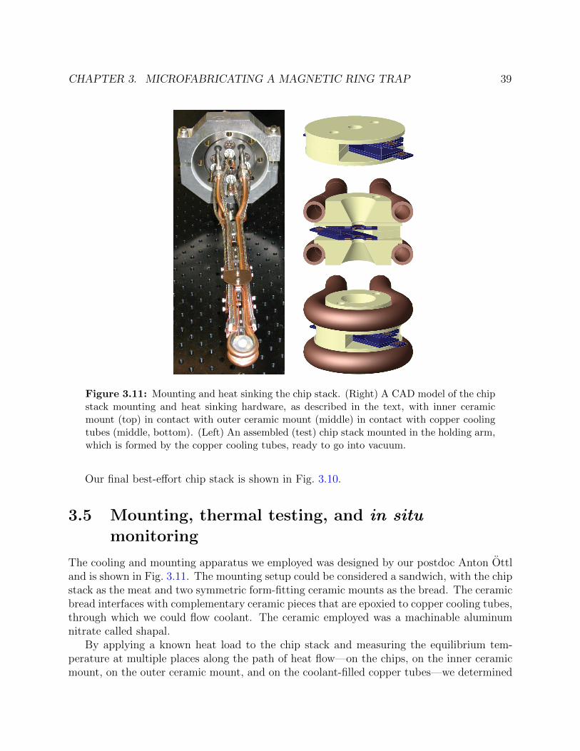
CHAPTER 3. MICROFABRICATING A MAGNETIC RING TRAP 39
Figure 3.11: Mounting and heat sinking the chip stack. (Right) A CAD model of the chipstack mounting and heat sinking hardware, as described in the text, with inner ceramicmount (top) in contact with outer ceramic mount (middle) in contact with copper coolingtubes (middle, bottom). (Left) An assembled (test) chip stack mounted in the holding arm,which is formed by the copper cooling tubes, ready to go into vacuum.
Our final best-effort chip stack is shown in Fig. 3.10.
3.5 Mounting, thermal testing, and in situ
monitoring
The cooling and mounting apparatus we employed was designed by our postdoc Anton Ottland is shown in Fig. 3.11. The mounting setup could be considered a sandwich, with the chipstack as the meat and two symmetric form-fitting ceramic mounts as the bread. The ceramicbread interfaces with complementary ceramic pieces that are epoxied to copper cooling tubes,through which we could flow coolant. The ceramic employed was a machinable aluminumnitrate called shapal.
By applying a known heat load to the chip stack and measuring the equilibrium tem-perature at multiple places along the path of heat flow—on the chips, on the inner ceramicmount, on the outer ceramic mount, and on the coolant-filled copper tubes—we determined

CHAPTER 3. MICROFABRICATING A MAGNETIC RING TRAP 40
8
6
4
2
0
Anti-
bias
resis
tanc
e Ω
-200 -100 0 100RTD Temperature ºC
8
6
4
2
0
Curvature resistance Ω
8
6
4
2
0
Ant
i-bia
s re
sist
ance
Ω
-200 -100 0 100RTD Temperature °C
8
6
4
2
0
Curvature resistance Ω
Figure 3.12: Thermal cycling curves for two different pairs of chips, each with a bias andanti-bias coil. The chips tested on the left appear more robust than the ones on the right,as indicated by the lack of hysteresis. The first points in each series of measurements areindicated with the large right-pointing triangle, while the final point is indicated by thelarge square.
the heat sinking capabilities of our chip stack and the cooling/mounting apparatus in whichit sits. In particular, we determined the thermal bottlenecks.
Overall, we measured a temperature rise at the chips of 1C per Watt. The thermalbottleneck was the interface between our outer ceramic mount and the copper tubing. Heattransfer at the interfaces between the chips and the inner ceramic mount, as well as betweenthe inner and outer ceramic mounts, was facilitated by thin graphite sheets. Graphite hasexcellent thermal conduction only in-plane, so the graphite sheets were kept thin. Thesethermal joints were overall very effective at transmitting heat. On the other hand, theinterface between the outer ceramic mounts and the copper tubing relied upon thermallyconductive epoxy.
Regardless, with the setup as-is, we determined that we should be able to constantly runour target current, four amps, through each chip with a temperature rise of 150C. Thistemperature rise would be acceptable if we were to cool the chips to -60C with methanol,which was within our capability. With a modest two-fold improvement of the ceramic-copperjunction the estimated temperature rise would be reduced to 75C, which would be both moremanageable and leave a greater margin for error. Still, we had a lot of doubt as to whetherthe chips could survive repeated cycles of temperature variation.
Thus, we investigated the question of what sort of temperature cycling our chip stackcan stand, at least in the short term. To do this, we temperature cycled the chips by flowingvarious amounts of current while monitoring the resistance and temperature of the coils.Changes of the resistance with temperature are normal, and can be predicted if assumptionsabout the distribution of resistivity in the copper wire are made, but hysteresis or changes inresistance at a given temperature after cycling can indicate structural changes and failure of

CHAPTER 3. MICROFABRICATING A MAGNETIC RING TRAP 41
the stack. Preliminary data tracking the resistance of two different pairs of chip coils as thetemperature was cycled are shown in Fig. 3.12. The data suggested that chip resistance overtime may be a good indicator of robustness and possible failure. Preliminary measurementsof the radio-frequency transfer function of early versions of the chips were also performed.Such transfer function measurements could also be tracked over time and may serve asadditional indicators of chip quality and reveal shorts or other material changes over time.
3.6 Moving on
Because of issues with other aspects of the apparatus, most notably the magnetic transportof cold atoms into the area where the chips were to be placed, and because of the factthat we only managed to assemble one chip stack that we deemed suitable for use in ourapparatus, we abandoned efforts to use the microfabricated chips in our actual apparatus.We deemed the substantial effort required to fully realize the magnetic transport throughthe tight apertures imposed by the holding arm and the chip stack not to be worthwhile,as the likelihood that the chip stack would fail in some way upon installation and repeatedtemperature cycling was substantial. Without a backup stack, such a failure would make allof that additional effort for naught.
As true believers in the sunk cost fallacy, we decided to move on. The “best-effort” chipstack shown in Fig. 3.10 remains in a drawer in the lab, and we decided to pursue ringtrap and spinor physics in the MOT chamber, in spite of the fact that this chamber lackedsome important features that might have been desired of a top-tier apparatus. Desirable, butmissing features included plentiful optical access, an RF antenna, and magnetic field control.Nonetheless, we made it work, as evidenced in Marti [49] and the rest of this dissertation.
Were we to continue towards our initial goal of trapping atoms in the magnetic ring trap,our next step would have been to measure the magnetic fields produced by the assembledstack of chips. We began development of a system for accurately measuring the fields of thechip stack that I will briefly describe.
First, we obtained a sensitive magnetic field probe from Micro Magnetics with a spatialresolution of must a few microns. We mounted this probe on a 3D micro-translation stagefrom Newport so that we could sample the magnetic field in the region of the chip stackwith high resolution and precision. The magnetic probe was linear and sensitive only atfields much less than one Gauss, which meant we could not simply map the field at anythingapproaching our process currents. Our plan, which we never implemented, was to put themagnetic sensor in loop with a compensation coil. This compensation coil would be largeenough to provide a very uniform magnetic field in the region of the chip stack and wouldbe driven with a precision current source such that the magnetic field at the position of thesensor be precisely canceled. The relevant magnetic field signal would be the current throughthe compensation coil.
In order to mitigate the effects of large near-DC magnetic field noise, our plan was todrive both the chip stack and the compensation coils with AC currents. Owing to differences

CHAPTER 3. MICROFABRICATING A MAGNETIC RING TRAP 42
in complex impedance, the phases of the driving currents of the chips and the compensationcoil might would likely have needed to vary. We never got around to deciding on a concreteimplementation for the phase-locked AC driving currents.

43
Chapter 4
Spin vortices
Though we abandoned our efforts to place atoms in an ultra-smooth magnetic storage ring,we did not abandon ring shaped traps all together. Our explorations of Bose condensed 87Rbin a 30 µm diameter optical ring trap are detailed in our publication, Ref. [46] and in Ch. 3of Marti [49]. In this work, we characterized the collective modes of the scalar BEC orderparameter— phonons—and showed how they could potentially be used to perform accurateand bias-free rotation measurements, even in an imperfect trap. While we did not havesufficient signal-to-noise to measure a rotation signal, we performed a detailed experimentaland theoretical analysis of the noise in our system and demonstrated that it operated atthe atom shot noise limit. Our signal was limited primarily by unexpectedly large dampingrates, which we now attribute to finite-temperature effects.
The bias-free nature of our phonon gyroscope has its origin in the fact that the trappedBEC is irrotational at low energy: The order parameter, the phase of the condensate, mustbe single-valued, and thus rotation, which corresponds to an accumulated phase around aclosed contour within the condensate, must be quantized.
The order parameter(s) of spinor condensates admit a wide range of interesting structures[31], some of which are topologically non-trivial. In future versions of this chapter we willsummarize our work creating, imaging, and characterizing interesting spinor structures. Ourmain focus will be on the spin vortex in a ferromagnetic condensate, which is topologicallynon-trival in the magnetization space but trivial in the larger order parameter space.
While not officially part of my dissertation, my plan is to release an updated version ofthis chapter1 wherein I discuss the following topics:
• Making the first spin vortex.
• Varying the vortex core size.
• Analyzing the topological character of the spin vortex.
1Try the Stamper-Kurn group website http://ultracold.physics.berkeley.edu or the ArXiV pre-printserver http://www.arxiv.org.

CHAPTER 4. SPIN VORTICES 44
• Comparing the stability of the spin vortex with similar looking spin structures withoutrotation.
• Accounting for missing transverse magnetization in the imaged spin vortices
• Improvements to the experimental apparatus that would be necessary to improve uponthis work.
At the time of this writing, a discussion of our imaging techniques and images of some ofour spin vortices can be found in Ch. 4 of [49].
Ultimately, our work on spin vortices was put on hold to make the aforementioned im-provements to the apparatus. While many of these improvements were made (some arediscussed in Ch. 5), we never returned to the spin vortices. Instead, we initiated a pro-ductive investigation of an even simpler excitation of the spinor condensate: the magnon, aGoldstone mode associated with symmetry breaking of the ferromagnetic order parameter.Eventually, a return to the study of spin vortices using the techniques that we developedmight prove quote fruitful.
The basics of magnons are discussed and experimentally validated in Ch. 5 of [49]. Inthe following chapter, I use these properties of magnons to extend accurate thermometry ofthe BEC into new regimes of low entropy. I also show how magnons can be used to cool aspin-polarized BEC.

45
Chapter 5
Thermometry and cooling withmagnons
The low [56, 38], even (gasp!) negative [9] temperatures reached in ultracold atomic andmolecular [66] systems are deservedly praised, sometimes even in the popular press (cf.Ref. [16]), for allowing experimenters to “access new regimes of physical phenomena.” How-ever, the emphasis in this archetypal phrase is almost always misplaced. The key phraseshould really be new access rather than new physical phenomena. Most of the strangequantum phenomena the cold atom community explores are quite common. A paper ti-tled “Cooling to 0.002 times the Fermi temperature” could represent a huge technologicaland scientific breakthrough in cold quantum gases, but would be rather unremarkable if thecooling in question was performed by placing a block of aluminum in a typical householdrefrigerator1.
New access to phenomena that exist in a wide range of materials is very appealing. Inexchange for a massive effort in cooling technology, ultracold atomic gases have providedexperimenters with a remarkable window into the quantum world, allowing time- and space-resolved readout and control of archetypal many-body and condensed matter systems. Still,in spite of their name, relative to relevant physical energies, many ultracold gases mightbe considered quite hot relative to solid-state systems of interest. The entropy per particle(S/N), rather than the temperature, is the pertinent parameter when comparing physicallysimilar systems with different length and energy scales. See Table 5.1 for a sample of S/Nin various systems.
In some simple cases, the entropy per particle can be calculated in a straightforward way.For non-interacting harmonically trapped quantum degenerate Bose and Fermi gases, for
1In solid aluminum, the electron Fermi temperature TF ∼ 135,000 K.

CHAPTER 5. THERMOMETRY AND COOLING WITH MAGNONS 46
System Temperature S/N (kB)Nitrogen gas 300 K 22
Rubidium (metal) 300 K 8.8Water 300 K 8.4
Sodium (metal) 300 K 6.1Ideal Fermi gas, harmonic TF 4.2Ideal Bose gas, harmonic Tc 3.6
Aluminum 300 K 3.0Ideal Bose gas, box Tc 1.3Two-level systems ∞ 0.7
Diamond 300K 0.28Ideal Fermi gas, harmonic 0.05× TF 0.25
Ideal Bose gas, box 0.3× Tc 0.2Ideal Bose gas, harmonic 0.3× Tc 0.1
Aluminum 77 K 0.06Aluminum 2 K 0.0001
Table 5.1: Table of entropy per particle in some reference systems. Even when entropyper particle cannot be calculated from first principles, the measured entropy per mole, or“standard molar entropy,” can be be looked up at for certain substances and a specifiedtemperature in chemical tables.
example,
(S/N)Bose = kB × 4ζ(4)
ζ(3)
(T
Tc
)3
(5.1)
(S/N)Fermi = kB ×π2
2
T
TF−O(T/TF )3, (5.2)
where ζ is the Riemann zeta function. For strongly interacting Bose gases deep in theBogoliubov phonon regime, and, in general, for a medium that supports phonon excitations,such as a crystal lattice well below the Debye temperature2,
(S/N)phonon = kB × γ2π2
45n~3c3(kBT )3 , (5.3)
where c is the speed of sound, n is the number density of the medium and γ the numberof phonon polarizations (one for BEC, three for a crystal). In the general case where theequation of state is not known, or must be calculated numerically, as in Ch. 6, estimating theentropy per particle is either not quite as straightforward or simply impossible. Regardless,using these simple relations, the 500 pK sodium gas of Ref. [38] has an entropy per particleS/N ∼ 1.5 kB, about that of the same sodium cooled as a solid to liquid nitrogen temperature.
2Note that the Debye temperatures of the alkali are quite low. For rubidium it is 56 K.

CHAPTER 5. THERMOMETRY AND COOLING WITH MAGNONS 47
At first glance, (weakly interacting) gaseous and (strongly interacting) solid sodium mayseem too dissimilar for the entropy per particle to provide a meaningful comparison, butbecause of the manner in which experiments on ultracold atoms are often performed, thisis not necessarily the case. Weakly interacting gases are routinely transformed, ideallyadiabatically, into strongly interacting lattice-trapped systems [22, 3, 65, 86, 78] where thephysics of solids are at the forefront. Without powerful techniques for reducing the entropyin optical lattices, which have largely, though not entirely [4], remained elusive [53], theentropy of the initially prepared gas sets a lower bound on the entropy that can subsequentlybe achieved in the transformed system.
Entropies per particle in the 0.5–few kB range commonly reached in cold atom exper-iments have been sufficient to implement quantum simulators exploring a range of funda-mental effects, including the superfluid to Mott insulator transition of the Bose-Hubbardmodel and the universal dynamics of Fermi gases at the BEC-BCS crossover [8]. However,the entropy required to reach the regimes of non-trivial (e.g. antiferromagnetic or frustrated)magnetic ordering in multi-component Bose-Hubbard [1, 11] and Fermi-Hubbard [64] sys-tems is expected to be just beyond what is commonly achieved. At even lower entropy,perhaps a few orders of magnitude lower than has been achieved with cold atoms thus far,with fractional filling of the lattice, such systems may be important to understanding the d-wave superconductivity known to exist in the cuprates [29]. Nobody knows the full richness(or not) of the multi-component Hubbard models at partial filling, and whether exotic super-fluid/superconducting phases exist somewhere in them, because they remain theoreticallyintractable. To be able to simulate them, then, would be a Very Big Deal.
Why does a small amount of entropy spoil some quantum phases and not others? Iam not aware of a good discussion of this question, but I can offer a few thoughts. Somesystems display quantum behavior at high entropy owing to entropy compartmentalization.For example, in a BEC, the non-condensed fraction can carry a large amount of entropy overa wide range of low energy modes, leaving a zero entropy condensate. The non-condensedfraction interacts weakly with the condensate, making the distinction between condensedand non-condensed fractions quite stark. In other systems, such as Mott insulating states,strong localization allows entropy to be compartmentalized spatially, for example, at theedge of the Mott lobes. The center of a Mott lobe may appear to have quite low entropy.
Interesting spin models often present different situation, as they frequently rely on thefact that spins are not localized, and interactions between spins necessarily constitute adominant energy scale. In “strongly correlated” systems, interesting states may requirecorrelations that build up over long distances, and perhaps it doesn’t take many thermalfluctuations to disrupt the long-range quantum ones. In Fig. 5.1, the “spin” pattern isrevealed at S/N = 0.1 kB. If, however, “Berkeley” were more spread out, or had largerquantum fluctuations, it might still be obscured. In addition, the number of degrees offreedom in spin systems is typically quite small. For a two-component spin system with onespin per site, the maximum entropy is S/N = kB×ln 2 ≈ 0.7 kB. Clearly, to reach an orderedphase, the entropy needs to be less than the maximum. Little is known about the microscopicphysics behind the d-wave superconducting states, but in solid state systems they appear with

CHAPTER 5. THERMOMETRY AND COOLING WITH MAGNONS 48
(a) S/N = 2.77 kB (b) S/N = 1 kB (c) S/N = 0.1 kB (d) S/N = 0.001 kB
Figure 5.1: What does entropy look like? In general, it’s not easy to determine, let alone“see”, the entropy in a system. Here is a special case. Each of these images is 200 by 200pixels, and each pixel can independently take on one of 16 grayscale values. When all valuesare equally likely, the entropy per pixel is log(16) ≈ 2.77 kB. In digital images, entropy ismore frequently measured in bits: log2(16) = 4 bits per pixel. If not all colors are equallylikely—here white is favored as the entropy is reduced—the expected entropy per pixel isthe average S/N =
∑i pi log(1/pi), where pi is the probability of a pixel having color i. At
lower entropy, a message may emerge from the “thermal” noise if the contrast of this figureis high enough. This message has some noise of its own, however not all noise is thermal!Incidentally, the GIF format does a good job of compressing these images, with the overallfile size tracking closely to the true average entropy per pixel.
less doping (i.e. less filling) and at lower temperatures than the antiferromagnetic phases.The greatest promise of quantum simulation using cold atoms hinges on accessing models
about which theory has been able to say very little, and in order to do this, experimentersneed to be able to reliably create and characterize samples with lower entropy than hasbeen done before. In this chapter, I describe our experimental efforts exploring coolingand thermometry of a highly degenerate bulk ferromagnetic F=1 Bose gas using collectivespin excitations known as magnons [27]. Our study reveals that forced evaporative coolingcan produce gases an order of magnitude colder than had been commonly thought, as lowas T/Tc ≈ 0.02 in our experiments, which we estimate (see Ch. 6) corresponds to S/N ∼0.001 kB at equilibrium. Our thermometry is remarkably precise, operating near fundamentalnoise limits, and could pave the way for precision studies of thermodynamics at low entropy.In addition, we demonstrate a novel cooling method, cycled decoherence cooling, a form ofdemagnetization cooling, that does not rely on lowering the trap depth, and that we findcan reach S/N ∼ 0.3 kB. With technical improvements, it may be able to reduce the entropyeven further. Producing low entropy bulk gases does not solve the problem of producing lowentropy gases in optical latices, however, the ability to create and characterize such samplesis a substantial step forward.

CHAPTER 5. THERMOMETRY AND COOLING WITH MAGNONS 49
5.1 The challenge of low entropy
Both thermometry and cooling rely on distinguishing the excitations that differentiate asystem from its ground state. At very low entropy per particle the system is very nearits ground state and detecting (or removing) these minor differences becomes difficult, asdoing so requires very high sensitivity to small and rare fluctuations in the state of thesystem as well as detailed knowledge of the ground state. For example, the temperatureof an ideal gas is manifest entirely in the variance in its kinetic degrees of freedom. Athigh temperatures, crudely sampling the velocity of the constituent particles is sufficientto establish the temperature. At sufficiently low temperature (and entropy), however, thevariations in velocities can get arbitrarily small, and so arbitrarily precise measurementswould be required. Likewise, reducing the entropy of such a gas in isolation requires avelocity dependent force or the selective removal of its most energetic constituents.
In a weakly interacting Bose gas with harmonic confinement, the situation is not im-proved, as the number of non-condensed atoms, Nth drops very quickly below the conden-sation temperature, Nth/N ≈ (T/Tc)
3, so that not only does the variation in the kineticmotion decrease, so does the number of atoms with varying motion. For weakly interactinggases at temperatures comparable to the chemical potential, kBT . µ, the kinetic degreesof freedom acquire a collective phonon-like character, and can no longer be characterized bytheir velocity. In this regime, it becomes increasingly difficult to distinguish thermal fluctu-ations from quantum ones [74, 84], and it is not obvious on theoretical grounds [63, 45, 33]that evaporative cooling should continue to function.
While direct measurements of the system itself may not readily yield its temperature,thermometry may still be possible by placing the system in thermal contact with a systemthat would exhibit considerably higher entropy at the same temperature. Additionally, unlessthe thermometer is prepared at the same temperature as the system in question before beingplaced in thermal contact, the thermometer can be expected to change the temperature of thesystem it is measuring. For a highly degenerate ferromagnetic condensate, spin excitationscan constitute such a thermometer.
Spin excitations can constitute an excellent thermometer for several key reasons. First,in most of the commonly used ultracold gases, collisions that change the projection of thegas magnetization along the magnetic quantization axis essentially do not occur. Thus,the number of spin excitations created out of an initially polarized gas can be controlledprecisely. In particular, the number of spin excitations created can be made to be as largeas possible while still keeping the number of spin excitations below the critical number fortheir condensation at equilibrium. In addition, in the presence of a weak magnetic field,spin excitations that differ in magnetic moment from the majority spin component can beaddressed spectroscopically or separated from the majority component by a magnetic fieldgradient, allowing them to be imaged with high signal to noise independent of the majoritygas by common techniques, as in Ch. 4.
Any spin or pseudo-spin excitation that thermalizes at constant (pseudo-)magnetizationmight make an excellent thermometer, but magnons have some advantages over generic spin
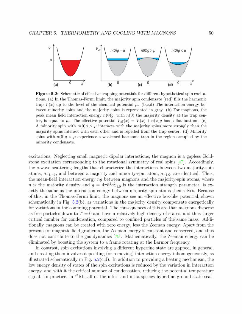
CHAPTER 5. THERMOMETRY AND COOLING WITH MAGNONS 50
V
x
µ
(a) (b)
Ve
x
n(0)g = µ n(0)g > µ n(0)g < µ
(c) (d)0 0 0 0
Figure 5.2: Schematic of effective trapping potentials for different hypothetical spin excita-tions. (a) In the Thomas-Fermi limit, the majority spin condensate (red) fills the harmonictrap V (x) up to the level of the chemical potential µ. (b,c,d) The interaction energy be-tween minority spins and the majority spins is represented in gray. (b) For magnons, thepeak mean field interaction energy n(0)g, with n(0) the majority density at the trap cen-ter, is equal to µ. The effective potential Veff(x) = V (x) + n(x)g has a flat bottom. (c)A minority spin with n(0)g > µ interacts with the majority spins more strongly than themajority spins interact with each other and is repelled from the trap center. (d) Minorityspins with n(0)g < µ experience a weakened harmonic trap in the region occupied by theminority condensate.
excitations. Neglecting small magnetic dipolar interactions, the magnon is a gapless Gold-stone excitation corresponding to the rotational symmetry of real spins [47]. Accordingly,the s-wave scattering lengths that characterize the interactions between two majority-spinatoms, a−1,−1, and between a majority and minority-spin atom, a−1,0, are identical. Thus,the mean-field interaction energy ng between magnons and the majority-spin atoms, wheren is the majority density and g = 4π~2a2
−1,0 is the interaction strength parameter, is ex-actly the same as the interaction energy between majority-spin atoms themselves. Becauseof this, in the Thomas-Fermi limit, the magnons see an effective box-like potential, shownschematically in Fig. 5.2(b), as variations in the majority density compensate energeticallyfor variations in the confining potential. The consequences of this are that magnons disperseas free particles down to T = 0 and have a relatively high density of states, and thus largercritical number for condensation, compared to confined particles of the same mass. Addi-tionally, magnons can be created with zero energy, less the Zeeman energy. Apart from thepresence of magnetic field gradients, the Zeeman energy is constant and conserved, and thusdoes not contribute to the gas dynamics [79]. Mathematically, the Zeeman energy can beeliminated by boosting the system to a frame rotating at the Larmor frequency.
In contrast, spin excitations involving a different hyperfine state are gapped, in general,and creating them involves depositing (or removing) interaction energy inhomogeneously, asillustrated schematically in Fig. 5.2(c,d). In addition to providing a heating mechanism, thelow energy density of states of the spin excitations is reduced by the variation in interactionenergy, and with it the critical number of condensation, reducing the potential temperaturesignal. In practice, in 87Rb, all of the inter- and intra-species hyperfine ground-state scat-

CHAPTER 5. THERMOMETRY AND COOLING WITH MAGNONS 51
tering lengths are nearly equal [89], and the temperature at which magnons should have adistinct advantage over hyperfine pseudo-spin excitations is quite low, on the order of a fewpercent of the chemical potential. Thermometry using co-trapped pseudo-spin impurities isa common technique in Fermi gas systems [72, 59, 77, 54].
5.2 Cooling at low entropy
The same characteristics that make spin excitations a good thermometer—high relativeenergy and entropy per particle—enable them to cool the majority gas in two distinct ways.First, spin excitations created in a degenerate Bose gas can decrease its temperature by aprocess known as decoherence [39] or demagnetization [19, 56] cooling. Immediately afterthe RF pulse that creates the magnons is applied, the minority spin population has thesame energy and momentum distribution as the initially polarized degenerate Bose gas,with a large condensed fraction, which carries no energy above the chemical potential, anda small normal fraction, which carries on the order of kBT of energy per particle. Uponthermalization, the normal fraction within the minority spin gas increases, bounded fromabove by its critical number for condensation, and the energy and entropy of the minorityspins increases. The energy gained by the minority is energy lost by the majority, as,for magnons, the entire process occurs at constant energy, neglecting from the effects ofmagnetic field inhomogeneities and dipolar interactions. After thermalization, the magnonscan be expelled from the sample and the process of decoherence cooling can be repeated.We call this “cycled decoherence cooling.”
This cooling process can also be understood as a form of demagnetization cooling. Themajority gas and the magnon gas are the longitudinal and transverse magnetization, re-spectively, of a magnetized gas. Transverse magnetization is created by slightly tipping themagnetization of the longitudinally polarized gas. While the longitudinal magnetization isconserved owing to the symmetry breaking applied magnetic field, the transverse magneti-zation is allowed to dissipate at constant energy.
In Fermi gas systems, a similar process would lead to heating as the minority spins wouldbe created with relatively high average energy (some fraction of the majority Fermi energy)and equilibrate to a lower average energy (some fraction of the much smaller minority Fermienergy). Energy lost by the minority spins is, more or less, energy gained by the majority,leading to heating overall. Thus, to perform thermometry using spin excitations in Fermigases, the spins are typically allowed to equilibrate at higher temperature before evaporatingto the final trap depth. It turns out that this sort of evaporation protocol can also lead toenhanced cooling in bosons by increasing the efficacy of evaporative cooling.
Forced evaporative cooling from a trap with an effective trap depth Ueff kBT has acooling power proportional to the number of thermal excitations with excitation energiesabove Ueff . In a weakly interacting single-component degenerate Bose gas, the numberof thermal excitations is determined by the temperature and is independent of the totalparticle number, fixing the evaporative cooling rate. By seeding the gas with additional

CHAPTER 5. THERMOMETRY AND COOLING WITH MAGNONS 52
Condensate fractionCondensate fractionmF=-1
mF=0
create magnonspump with Image/magnetizewith RFmicrowaves with light
Inte
grat
ed c
olum
n de
nsity
T=1.6 nK
T=16.2 nK
T=54.4 nK
Trap
dep
th
Time
ViVf tevap teq thold Time tevap teq thold
T=3.1 nK
T=11.1 nK
T=53.6 nK
Trap depth/kB (nK)
B
a
b
c
d
ge f
cycled cooling
25 ± 10130 ± 20
590 ± 40
0 5 10Wavenumber (µm-1)
-5-10 0 5 10-5-10 0 5 10-5-10
35 ± 10130 ± 20
590 ± 40
35 ± 10130 ± 20
590 ± 40
200 µm
Figure 5.3: Schematic illustration of magnon cooling and thermometry protocols withsample thermometry data. Magnons are created via a RF pulse in a spin-polarized gas atthe final trap depth (a, b) or at an intermediate trap depth (c, d). The magnetized gascan be viewed schematically as an arrow, initially pointed in the direction of an appliedmagnetic field. Introducing magnons corresponds to tilting the gas magnetization. Unlikethe longitudinal magnetization, the transverse magnetization is not conserved, and as themagnon population loses coherence, the average transverse magnetization dissipates. This isindicated schematically by the magnetization arrow losing its tilt. The incoherent transversemagnetization is indicated by the fuzzy background arrows. Equivalently, the magnonscan be viewed as an admixture of mF=0 atoms whose coherence dissipates quickly at theintermediate trap depth and slowly at the final trap depth. Magnons created at the final trapdepth cool the gas via magnon decoherence cooling, which can repeated in the same sampleas cycled magnon decoherence cooling. Magnons created at the intermediate trap depthimprove the efficiency of forced evaporation. In both cases, the magnons serve as a sensitivethermometer. As the gas is cooled, the majority gas (or, equivalently, longitudinal spincomponent) becomes highly condensed and the temperature signal is lost (e). In contrast,the magnons (mF=0 component or minority gas) provide a relatively large temperaturesignal even at low temperatures (f,g).

CHAPTER 5. THERMOMETRY AND COOLING WITH MAGNONS 53
0 5 10 15 20 25 300
10
20
30
40
50
60
70
Pulses
Tem
pera
ture
(nK)
0 5 10 15 20 25 300
0.1
0.2
0.3
0.4
0.5
0.6
0.7
T/T c
Figure 5.4: Sample preliminary cycled decoherence cooling data. Top row images show themajority condensate and thermal cloud atoms in time-of-flight. The bottom row of imagesshows the corresponding distribution of minority atoms. The graph shows the absoluteand relative (to the critical temperature Tc) temperatures extracted from the majorityatoms. The estimates of temperature are not well calibrated and the critical temperatureis unreliable owing to large uncertainty in the trap frequencies and trap anharmonicity.Regardless, cooling is clearly working and shows real promise.
spin excitations at constant total particle number, the total number of thermal excitations,and thus the evaporative cooling power, increases. We call this sort of cooling “magnonassisted evaporation.” Once again, in Fermi gases, a different situation presents itself, as theexcitations of the minority spins will in general have much lower energy than the excitationsof the majority, and will not contribute to evaporation. Our cooling and thermometryschemes are illustrated schematically in Fig. 5.3.
In this chapter, we discuss the details of our implementation of sensitive and accurate low-entropy thermometry using magnons, as well as our efforts characterizing the two differentmagnon cooling schemes. As most of the most salient scientific results are in our publication,Ref. [62], the focus of this chapter will be the experimental and behind-the-scenes details andevolution of that work. It will probably help the reader to be familiar with that referencebefore proceeding.
5.3 First cooling: a benchmark for improvements
Our first attempts at doing cycled decoherence cooling went remarkably smoothly. Forreasons of history and convenience (we had microwaves set up and not RF) we chose tocool by mixing in a small amount of F=2 into the polarized F=1 condensate using a brief

CHAPTER 5. THERMOMETRY AND COOLING WITH MAGNONS 54
microwave pulse. That cooling was occurring was evident immediately from the in situimages of the majority gas. Even at this early stage, it seemed that a magnetic field gradientwas important in achieving thermalization in a finite amount of time. An example of ourpreliminary cooling data are shown in Fig. 5.4.
The preliminary data were very promising, but indicated a need for substantial improve-ment to be quantitatively convincing. For example, we had little confidence in the estimatedtemperature and critical temperature. To do accurate thermometry, lots of things need towork right and be well calibrated. There are many things to cross-check to assure us thatwe’re moving towards reliable measurements, or not.
The BEC critical temperature for an ideal non-interacting Bose gas in a harmonic trapdepends on several quantities that we need to calibrate accurately:
kBTc = ~ω(N
ζ(3)
)1/3
. (5.4)
Here, ω = (ωxωyωz)1/3 is the geometric mean of the trapping frequencies, N is the number
of atoms, and ζ is the Riemann zeta function. We can experimentally produce a cloudwith temperature T = Tc by finding settings at which a small condensate barely forms. Ifeverything is well calibrated, we should find that the Tc calculated using Eq. 5.4 and ourmeasurements of N and ω agrees well with our estimate of the temperature of the cloud.The equality should hold over a range of Tc and N .
In the Thomas-Fermi regime, the chemical potential, µ, is another quantity that can allowus to find consistency between our parameters, relating the trap frequencies, condensatenumber, and the in situ size of the condensate:
µ =1
2mω2
iR2i =
ω
2
(15~2Nca (mω)1/2
)2/5
, (5.5)
with Ri the condensate radius along the direction with trap frequency ωi, and Nc the con-densate number.
Finally, we can measure temperature by different methods, and these methods shouldagree in regimes where they are valid. For example, near Tc we can measure the temperatureof our gas by imaging its size as a function of the time following its release from the opticaltrap (“time-of-flight” or TOF) along two different axes, with two independently calibratedimaging systems.
Our first attempts at cooling with magnons clearly showed a gas getting colder, but ex-actly how much we could not be sure, as the thermometry failed several of these consistencychecks. This spurred us to make a range of changes to our thermometry, imaging, and trap-ping setups. In the next sections I will describe many of the calibrations and improvementsto our apparatus that ultimately enabled our final study.

CHAPTER 5. THERMOMETRY AND COOLING WITH MAGNONS 55
5.4 Momentum space focusing
In a non-interacting, non-degenerate classical gas (obeying Boltzmann statistics), the tem-perature is manifest in both spatial and momentum degrees of freedom separately. At everypoint in position space, the momentum distribution is identical, apart from a multiplicativeconstant, and likewise for points in momentum space, as is easily seen from the separa-bility of the Hamiltonian entering the exponential of the classical phase-space probabilitydistribution function:
P (x,p) = e(µ/kBT−V (x)/kBT−p2/2mkBT)/Z. (5.6)
Unwanted degrees of freedom can essentially be ignored, as integrating over them yieldstrivial multiplicative factors.
For a gas at or near quantum degeneracy, the Boltzmann distribution in Eq. (5.6) isreplaced by the appropriate Bose or Fermi distribution, and the separability of real-spaceand momentum-space distributions is no longer obvious. However, the dependence of themomentum distribution on the trapping potential turns out to take a fairly simple form, atleast for potentials that are well described by a single power law (e.g. box and harmonic).In the case of bosons, integrating over j quadratic degrees of freedom yields a probabilityfor the remaining quadratic degrees of freedom s of
P (s) ∝ gj/2
(e(µ/kBT−(c·s)2/kBT)
), (5.7)
where c is a vector of coefficients for the s degrees of freedom, e.g.√
1/2m for momentumdegrees of freedom, and gj/2 is the Bose function or polylogarithm of order j/2. The sig-nature of the integrated degrees of freedom (e.g. the trapping potential if we are observingonly momentum degrees of freedom) is in the order of the polylogarithm and, indirectly, thechemical potential µ. µ appears in Eq. (5.6) but is irrelevant to the shape of the probabilitydistribution; it’s a multiplicative factor. In Eq. (5.7), however, µ appears inside the polylog-arithm, and can affect the overall shape of the probability distribution. Note that gj(z) ≈ zfor z 1 and thus far from quantum degeneracy, or at sufficiently large c ·s, Boltzmann-likestatistics prevail.
In-trap (position-space) images of non-condensed gases thus provide direct access tothe temperature, provided one knows the potential V . However, in situ images are rarelyused for thermometry for several reasons. First, in the presence of a condensate, the non-condensed part of the gas may be largely obscured, and high optical density makes imagingsuch distributions challenging. Even in the absence of a condensate, tightly confining trapspush the relevant temperature signal to small length scales where imaging may be lesssensitive. Finally, the temperature signal is sensitive to the details of the trapping potential,which may be poorly constrained.
Time-of-flight measurements are the thermometric workhorse of the cold-atom commu-nity and overcome many of the limitations of in situ thermometry. In most imaging setups,

CHAPTER 5. THERMOMETRY AND COOLING WITH MAGNONS 56
x
p
x
p
x
p
x
p
x
pp
x x
p
φ=0 φ=π/4 φ=3π/8 φ=π/2
Figure 5.5: Principle of momentum space focusing. The action of a harmonic oscillator isto rotate a system in phase space, shown here with one space and one momentum dimensionversus the harmonic oscillator phase φ = ωt. A few points with the same in situ (φ = 0)momentum are marked with yellow dots. The imaged distribution, at the top of eachcolumn, shows only position space. The dashed axes show the positions of the initial axesrotated through angle φ. At φ = π/2, points with the same momenta converge to the samereal-space coordinate.
the signal-to-noise for temperature measurements increases with free expansion time (forsome time, at least) and the expanding cloud asymptotically approaches a shape that re-flects its momentum distribution.
Momentum space focusing [87, 76] (MSF) takes time-of-flight one step further in yieldingpure momentum-space distributions in an adjustable (and perhaps signal-to-noise optimized)time, removing most of the dependence on the trap geometry from temperature calculations.For magnons, which can experience an effective trapping potential that varies with theirtemperature (which is related to how much of the trap they explore beyond the edge of themajority condensate) [18], this feature is quite attractive.
The key insight involved in MSF is that harmonic motion manifests as rotation in phasespace (with coordinates appropriately scaled), and thus a distribution of momenta manifestsas a distribution of positions after a quarter cycle (rotation in phase space by π/2), and viceversa, as shown in Fig. 5.5. Atoms with initial momentum p will converge on real-space pointxp = p/mω, where ω is the harmonic trap frequency. By releasing our atoms from theirtrap into a two-dimensional isotropic harmonic magnetic potential, with the symmetry axiscoincident with the imaging axis, the atoms’ in situ in-plane momentum distribution willappear after a quarter cycle, neglecting interactions after the trapping light is extinguished.
In the following subsections, I will describe how we implement and characterize MSF inour system.

CHAPTER 5. THERMOMETRY AND COOLING WITH MAGNONS 57
5.4.1 Experimental procedure
Two-dimensional confinement is provided by the same coils that produce the sphericalquadrupole3 and bias fields for the MOT. Near the center of the quadrupole field, the fieldproduced can be written in terms of the offset and gradients as
B(r) = B0 + JBr, (5.8)
where B0 is the bias field, and JB is the Jacobian matrix of partial derivatives of B. For thequadrupole, in a basis with the z-axis aligned with the vertical symmetry axis, this Jacobianhas a simple diagonal form:
JB =
∂xBx 0 00 ∂yBy 00 0 ∂zBz
=
−B′/2 0 00 −B′/2 00 0 B′
, (5.9)
where we write B′ for the vertical gradient ∂zBz. The trapping potential for a spin-polarizedatom with magnetic moment µ and bias field B0 = B0z oriented along the z-axis is
V (r) = µ|B| ≈ µ
(Bo + zB′ +
x2 + y2
2
B′2
4Bo
), (5.10)
where the approximation assumes B0 dominates the other terms in parenthesis. The in-planecurvature of V implies a harmonic trapping frequency ω2 = µB′2/4mB0. The quadrupoleand bias field are configured such that atoms in the |F = 1,mF = −1〉 and |F = 2,mF = 1, 2〉states are confined by the field curvature and supported against gravity by the field gradient.
The MSF sequence begins 5 ms after the optical trapping light is extinguished. Duringthis time, the purging and state preparation (Sec. 5.13) sequences are completed and theatoms we wish to image are in the |F = 2,mF = 1〉 state and in free fall under the influenceof gravity. At this point we quickly ramp on the bias field B ≈ 36 G over 500µs. B′ risesmore slowly from zero to B′ ≈ 42 G/cm with an exponential time constant of roughly 5 ms.This gradient overcompensates for gravity (mg = µ×30.4 G/cm) in order to slow the fallingatoms to a stop. After approximately 45 ms, the atoms are stopped (Fig. 5.6b) and B′ isset to 30.4 G/cm in concert with B in order to maintain a constant transverse curvature ofB′′ ≈ 12 G/cm2, which corresponds to a transverse trapping frequency of ω ≈ 2π × 3 rad/s.Calibrations, discussed below in Sec. 5.4.3, will reveal a more precise version of this number.
With the magnetic field so configured, the vertical field gradient opposes gravity, lev-itating the center of mass of the cloud at a constant height. Nonetheless, the atoms arefree to continue their expansion in the vertical direction, as motion along the vertical axis isunconfined. I will have more to say about this in Sec. 5.4.4.
3Aside: Etymologically, multipoles are assembled from a hodgepodge of prefixes of Greek and Latinorigin. Pole can swing both ways. Multi comes from Latin; the Greek would by poly. Mono and di areGreek, while quad is Latin and Octo can go either way. For higher-order moments, people tend to steertowards the Greek, as in tetrakaidecapole for the fourteenth moment.

CHAPTER 5. THERMOMETRY AND COOLING WITH MAGNONS 58
0
10
20
30
Bias
fiel
d (G
)
010203040
Gra
dien
t (G
/cm
)
0 10 20 30 40 50 60 70 80 90 1000
1
2
3
Trap
freq
uenc
y (H
z)
Time (ms)
Stop
Levitate
Image
(a)
10.2
10.0
9.8
9.6
9.4
9.2
9.0
Clo
ud p
ositi
on (m
m)
5550454035302520
Time halting gradient is applied (ms)
Stopping time = 44.1 ms
(b)
Figure 5.6: Experimental sequence for MSF. (a) Gradient and bias fields are first config-ured to slow and stop the falling cloud. Blue traces show measured coil currents plotted asmagnetic fields. The gradient coil ramps up exponentially with a weak 2 ms time constantand dominant 11 ms time constant (red fit). As soon as the atoms are stopped (b), thefields are reconfigured to levitate the cloud until it is focused. The MSF trap frequency isheld roughly constant.
One complication that we need to consider carefully is that the ramps of the gradientfield are slow, limited by the slew rate and bandwidth of the driving power supply, as shownin Fig. 5.6a and Fig. 5.7a. At one point early in developing MSF on our apparatus weoptimized the gradient field turn-on using the resonant switch in order to have appropriatefield curvature established within a few milliseconds, however we realized later that thesesettings were never used for subsequent calibrations and data. To figure out the impact, orlack thereof, of non-constant field curvature during MSF, we simulate the process using theexperimentally measured field ramps. These simulations will verify that MSF behaves as weexpect, and will guide our calibrations.
5.4.2 Simulating the magnetic focusing lens
The results of simulating the magnetic focusing lens with our measured gradient and biascoil ramps are summarized in Fig. 5.7. The only free parameter in these simulations isthe equilibrium magnetic trap frequency, ω0 = 2π × 3.05 rad/s, which I adjust to achievefocusing at the observed time tfoc = 97 ms. The focusing trap is assumed to be harmonic

CHAPTER 5. THERMOMETRY AND COOLING WITH MAGNONS 59
0 25 50 75 95 125 150
0
2
4
Time (ms)T
rap
freq
. (H
z)
−600
−400
−200
0
200
400
600
Ato
m p
ositi
on (
µm)
0
200
400
600
800
20 n
K c
loud
wid
th (
µm)
0 0.1 0.2 0.3 0.4 0.5 0.6 0.7 0.8 0.9 1Accumulated phase/π
(a)
100
101
102
−0.10
0.10.2
Temperature (nK)
Fra
ctio
nal e
rror
0
100
200
300
400
500
600
Foc
usin
g po
sitio
n (m
icro
n)
T∝ω02
T∝ωfoc2 ∝ 1/ T
foc2
T∝ωeff2 =(ω
foc/0.88)2
(b)
Figure 5.7: Simulation results for MSF with our measured field ramps and focusing timeof 94 ms. (a) The gradient (red) and bias coil currents (teal) in arbitrary units, alongwith inferred magnetic trap frequency (black), are shown in the top panel. The middlepanel shows the real-space trajectories of atoms with different momenta (different colors)originating from different locations in the cloud. The bottom panel shows width of a 20nK cloud with different initial sizes (different colors). (b) The simulated real-space focusingposition of atoms with various energies (blue dots) are plotted in the top panel along with thefocusing positions that would be expected in a SHO with various frequencies. Fractionalerrors of the different SHO models, shown in the bottom panel, are constant. In theseplots, for simplicity, representative momenta and temperatures are related by the relationp2/2m = 2kBT .
and isotropic with time-varying trap frequency ω(t) in both transverse directions, and thelongitudinal direction is ignored.
The simulations show several important features of the 2d-harmonic focusing lens. First,the magnetic lens is free of aberration in spite of the time varying frequency. Individualmomenta focus to a point (lines with the same color in Fig. 5.7a cross at a point), anddifferent momenta focus at the same time (all colors cross themselves at the same time).

CHAPTER 5. THERMOMETRY AND COOLING WITH MAGNONS 60
Further, the time at which the momenta focus is close to, but not quite, the time atwhich the oscillator phase θ(t) =
∫ t0ω(τ)dτ = π/2, as it would be for a perfect turn-on.
Importantly, the focusing time tfoc corresponds to the time at which the cloud width achievesa local minimum. For our cloud, with one very long axis, this local minimum is quite sharp.tfoc can thus be readily measured, as done in Fig. 5.8. Note that the focusing time does notcoincide with the global maximum of the width of small clouds, as it does in the constant ωcase.
Finally, the simulation shows in Fig. 5.7b that the real-space positions at which differentmomenta focus are well described by the simple harmonic oscillator (SHO) model with asingle effective momentum-independent frequency ωeff = ωfoc/0.88 such that xp = p/mωeff .Thus, in spite of the varying curvature of the magnetic lens, the momentum space imagesit produces are faithful to the simple model presented above, with one simple adjustment.Computing temperatures using ωfoc = 2π/4tfoc, instead of ωeff would lead one to underesti-mate temperatures by 25%.
5.4.3 Calibrating MSF
The key parameters in MSF are the magnification, 1/mωeff , which allows us to infer momentafrom real-space data, and the focusing time, tfoc, at which we should take images in orderto find the momentum distribution in focus. Because these two parameters are related,knowing one of them is sufficient.4 Nonetheless, we can boost our confidence, and precision,by measuring both parameters quasi-independently.
The focusing time tfoc is perhaps the easiest parameter to pin down. The long axis ofthe condensate focuses very tightly, making the focusing point easy to spot to within a fewmilliseconds by eye. The focusing time can also be easily extracted from non-condensedgases, so long as the focused size is smaller than the initial spatial extent of the gas. Inthis limit, the cloud size has a minimum that can easily be fit. The colder the gas—thesmaller the focused size—the sharper the minimum. Furthermore, neglecting effects of theexpanding condensate and misalignment of the focusing plane (see Sec. 5.4.4), the size ofthe non-condensed gas should be equal in all directions at the focusing time. Sample datafor these calibrations are shown in Fig. 5.8a. With tfoc = 97 ± 3 ms, and including 0.5%uncertainty in the ratio ωfoc/ωeff , we find ωeff = 2π × 2.9± 0.1 rad/s.
Measuring ωeff directly, without the help of a simulation, is easy if one knows a priorithe momentum distribution and an approximate value of tfoc: simply look at the spatialdistribution around the focusing time and use the relation xp = p/mωeff . Thus, accuratelymeasuring the temperature via a traditional method, such as time-of-flight, can serve tocalibrate MSF directly. We would prefer, however, to measure ωeff without reference totemperatures, as this allows us to gain confidence in the temperatures measured by MSFand time-of-flight by their mutual agreement.
4In principle, ω0 would also be sufficient information to fully calibrate MSF. However, in our system, ob-serving more than a single oscillation in the MSF trap proved difficult, owing to persistent vertical expansionand residual vertical motion of the gas.

CHAPTER 5. THERMOMETRY AND COOLING WITH MAGNONS 61
74 79 84 89 94 99 104 109 114 ms
130
120
110
100
90
80
Clo
ud s
ize
(m
)
120115110105100959085807570
Time (ms)
Minimum: 97.6 ms
(a)
1250
1200
1150
1100
1050
Pos
ition
in M
SF
(m
)
5004003002001000Time (ms)
800
750
Pos
ition
in s
itu (
m)
ωi = 2π × 37.5 ± 0.2 rad/sAi = 8.3 ± 0.2 µmφ = 0τ = 248 ± 55 ms ωi = 2π × 37.68 ± 0.02 rad/s
Am = 106. ± 2 µmφ = π × 0.48 ± 0.03τ = 235 ± 8 ms
(b)
Figure 5.8: Calibrating MSF. (a) The time at which the vertical size of the condensatereaches a minimum can be discerned easily by eye (top). The focusing time tfoc of thenon-condensed atoms shows a distinct minimum as well, even if it is hard to see by eye.Coupled to simulations, these measurements allow us to determine the magnification ofMSF. (b) The magnification of MSF is measured directly by fitting in-trap center-of-massoscillations in situ and in MSF to an exponentially decaying sinusoid. The decay timesτ and oscillation frequencies ωi are the same, but the oscillations differ in phase by π/2,the expected phase difference between real-space and momentum-space quadratures of thesame oscillation, and they have different amplitudes. The frequency associated with theMSF magnification is ωeff = ωiAi/Am. Vertical axes are shown on the same scale.
Rather, in Fig. 5.8b we illustrate another (related) way of measuring ωeff by comparingthe amplitude and phase of center-of-mass oscillations measured in situ and in MSF. Ineffect, we are measuring the in-trap velocity and mapping it to a position in MSF, but byconsidering the amplitude of oscillation we have a straightforward way of averaging manymeasurements. Given the amplitude Ai and frequency ωi of in-trap motion, the maximumcenter of mass momentum is pi = mAiωi. This maximum momentum maps via MSF tothe maximal position xp − x0 = Am = pi/mωeff , with Am the measured amplitude of theoscillations as imaged in momentum space. Thus, ωeff = ωiAi/Am. Our calibration yieldsωeff = 2π × 2.8± 0.2 rad/s.

CHAPTER 5. THERMOMETRY AND COOLING WITH MAGNONS 62
This calibration depends only weakly on the chosen value of tfoc. The center-of-massmotion is quite small, and the MSF trap is nearly centered on the atoms during all phasesof the in-trap oscillation. Thus, even with the field ramps as slow as they are, as can be seenfrom the trajectories that begin near zero in Fig. 5.7a, the center-of-mass velocity reachesa quadratic turning point near tfoc. Therefore, we can consider this direct measurementof ωeff independent of the one obtained from tfoc and average the two values, weighting byuncertainty.
As it stands, the measurement based on tfoc dominates the weighted average, but wegain confidence knowing that the two measurements agree with each other. The directmeasurement of ωeff could be repeated, or even better, more points could sampled at earlytimes of the in situ oscillation to reduce the uncertainty in our determination of Ai. The3% uncertainty in our measurement of ωeff is the primary source of systematic uncertaintyin the temperature measurements.
5.4.4 Practical considerations and limits of MSF
So far, we have been relying on two assumptions that merit further scrutiny. First, we haveassumed that the momenta of the atoms are fixed when we release them from the opticaltrap, and that the momenta we observe in MSF correspond to the momenta in situ. Forweakly interacting atoms, for example non-degenerate alkali atoms, this assumption is typi-cally very good. Clouds composed exclusively of such atoms expand nearly ballistically andisotropically. However, the interactions between atoms in the condensate are not negligible,and interactions between the condensed and non-condensed parts of the gas may not be ei-ther. In addition, we have mostly ignored the vertical axes of MSF, imaging, and the opticaltrap, and we have tacitly assumed they are well aligned to each other. Poor alignment ofthese axes, and the expansion of the condensate along one or more of them—aggravated byinteractions—can broaden the momentum signal anisotropically, as discussed below.
For a large condensate deep in the Thomas-Fermi regime, the change in the velocityof the condensate atoms is well described by a hydrodynamic theory [14]. In particular,upon being released from confinement, a condensate expands most rapidly in the directionin which it had been most tightly confined, with radii growing as Ri(t) = Ri(0)bi(t). Thescaling parameters bi, with i ∈ x, y, z, satisfy the equation
bi =ω2i
bibxbybz, (5.11)
where ωi are the (extinguished) trap frequencies. To understand intuitively why the conden-sate expands rapidly along the tight axis, recall that the phase of the trapped Thomas-Fermicondensate in equilibrium is uniform, evolving at a rate θ = µ(0) = µ(ρ)+V (ρ), where ρ is aradial coordinate and the minimum of the trapping potential is V (0). The interaction energyvaries across the cloud, but the sum of the interaction and potential energy is constant5, and
5Reminder: in the Thomas-Fermi approximation one ignores the kinetic energy of the ground state.

CHAPTER 5. THERMOMETRY AND COOLING WITH MAGNONS 63
100
101
102
103
Con
dens
ate
radi
us (
µm)
10−2
10−1
100
101
102
10−3
10−2
10−1
100
101
Time (ms)
Edg
e ve
loci
ty (
µm/m
s)
x−axisy−axisz−axis
(a)
1 1.2 1.4 1.6 1.8 210
−3
10−2
10−1
100
101
102
Optical trap setpoint (V)
Effe
ctiv
e te
mpe
ratu
re (
nK)
(b)
Figure 5.9: The expansion of the condensate. (a) Interaction energy turns into kineticenergy after the optical trap is turned off, shown here for the case of optical trap setpointVODT = 2. The magnons might inherit this velocity, which, via the relation mv2
RMS/2 =kBT , corresponds to a temperature, shown in (b), where vRMS is the RMS velocity of thecondensate after 100 ms.
hence the phase evolves at the same rate everywhere. When the trapping potential is sud-denly turned off, this is no longer the case, and the phase accumulates most rapidly wherethe interaction energy µ(x) is largest. A phase gradient develops and is most steep whereµ(x) changes most rapidly: along the direction of (formerly) tightest confinement. In a su-perfluid, a gradient in phase corresponds to a velocity. An equivalent semi-classical pictureis that the interaction energy constitutes a type of potential energy, and thus the expansionforce is proportional to its gradient, allowing the interaction energy to be reduced as quicklyas possible.
Our optical trap is highly anisotropic, and the condensate expansion is predominantlydirected along the vertical axis. This can be a nice feature, as it means the image of thecondensate in momentum space is quite small, allowing narrow momentum distributionsto be seen unobscured. However, the vertical expansion is not without side effects. First,the optical density of the condensate increases dramatically as its shadow on our cameragets smaller; we make no attempt to accurately count condensate atoms in MSF. Second,a condensate expanding at 5 µm/ms (see Fig. 5.9a) will be nearly 500 µm long at thefocusing time. The Rayleigh range of our approximately 8µm-resolution imaging system
CHAPTER 5. THERMOMETRY AND COOLING WITH MAGNONS 64
is around 250 µm and thus it is unsurprising that MSF images with a condensate includeaberration at and around the location of the condensate. Finally, if the tight z-axis of theoptical trap does not coincide precisely with the unconfined axis of MSF, a component ofthe condensate’s “vertical” expansion may be present in the transverse momentum signal,causing the condensate to appear larger or more anisotropic than it really is.
The simple Thomas-Fermi hydrodynamic theory applies only to the condensate; in gen-eral, it’s not particularly useful in quantitatively understanding the interactions betweencondensed and normal gases6. Nonetheless, to the extent that the condensate can be consid-ered a medium for excitations—magnons or non-condensed atoms—we can imagine that, inthe worst case, the expanding medium imparts its own additional expansion velocity onto itsexcitations. Thus, the additional velocity acquired by the condensate during MSF serves asan upper bound on the additional velocity obtained by the normal atoms, neglecting interac-tions between only normal atoms. In service as a thermometer, this extra velocity impartedby the condensate has the potential to set limits on the temperatures we might be able tomeasure, and so it is worth estimating this effect, as in Fig. 5.9b.
In our system, all three axes—MSF, imaging, and optical trap—would ideally be alignedto gravity and thus closely coincide. The spherical quadrupole coils used in MSF were roughlyaligned to gravity upon their installation, but there is likely some residual tilt. A small tiltaround an in-plane axis by an angle θ would rotate the plane in which focusing occurs aroundthat same axis by 3θ, but would not lead to any other more onerous aberrations. To calculatethis, consider a variation on Eq. (5.8) with the quadrupole coils rotated around the x-axis,
B(r) = B0z +Rx(θ)JBRTx (θ)r, (5.12)
where B is written in the gravity-referenced coordinates, and JB is diagonal in the rotatedcoil-referenced coordinates. Once again, write the trapping potential V as in Eq. (5.10) andcompute the Hessian (curvature) matrix H of V ,
Hij =∂2V
∂xi∂xj,
evaluated at the origin and keeping terms up to O(θ). Unlike in the case of perfect alignment,H is not diagonal in the gravity-referenced basis. However, the trapping frequencies, theeigenvalues of H, are unaltered, while the axes of oscillation/no confinement, the eigenvectorsof H, are rotated from the gravity-referenced basis by an angle 3θ.
The imaging axis can easily be well aligned to gravity: when viewed from above, fallingatoms should not vary in their transverse position. The optical trap can also be aligned wellto gravity, especially in the direction of the long axis of the condensate, where our procedurefor leveling is most sensitive (see Sec. 5.8). However, at the lowest temperatures explored inthis work, the anisotropy of the momentum signal seems to be the most sensitive probe of the
6Ref. [32] has a well written section on the ways in which normal and condensed fluids can interact.Though much work has surely advanced the state of the art in this area, this reference suffices as a first passfor many experimenters.

CHAPTER 5. THERMOMETRY AND COOLING WITH MAGNONS 65
optical trap alignment in the tight in-plane direction. Thus for two reasons—broadening ofthe momentum distribution from in-plane condensate expansion and additional broadeningfrom out-of-plane expansion projected into the imaging plane—we will use the temperaturemeasured along the long axis of the optical trap as our primary thermometer. Regardless,misalignment should never cause us to underestimate the temperature.
5.5 Imaging
To extract quantitative, accurate temperatures from our images, we need to make sure ourimages accurately represent the distribution of the atoms we wish to image. Taking andinterpreting absorption images of atoms is so integral to most ultracold atom experimentsthat most of the salient points have been detailed countless times. On the other hand,because imaging systems are so common, it is easy to take many important aspects of theiroperation for granted. Regardless, in the course of conducting this research we found thatunderstanding our imaging process was both essential and non-trivial.
Our apparatus has two imaging systems, shown in Fig. 5.10, oriented at right angles toeach other. The side imaging system has a wide field of view, roughly 1 cm across, andis used primarily for atom counting and calibrating the atoms’ vertical position. The topimaging system has a narrower field of view, roughly 2 mm across, and is the source of mostof our quantitative data. All of the imaging relevant to this study was performed with lightresonant with the F = 2 → F ′ = 3 cycling transition of the D2-line. The camera used forimaging from the top is an Andor Ixon 885 EMCCD camera (with EM, electron multiplier,turned off), while the camera used for the side is a Stingray CCD camera by Allied VisionTechnologies.
One salient feature of our top imaging system is that the primary objective is set backfrom the vacuum chamber to allow a MOT mirror to slide in under it. This reduces the res-olution of the imaging along this axis to about 8–10µm, but has some advantages. Notably,with the MOT mirror out of the way, there is space to place a removable pick-off mirror thatplaces the focus of the imaging system outside the chamber. The pick-off mirror is mountedon a Thorlabs KB1X1 kinematic base, allowing it be replaced with a high degree of accuracy.This has proved very useful in aligning optical paths that enter or exit the chamber fromtop.
If the imaging system is well aligned to the atoms, optical targets or cameras can beaccurately placed in the corresponding image plane outside of the chamber by moving theminto the focus of the imaging system. Once a target is so positioned, the target can be used asa proxy for the atoms in future alignments. This allows us to change aspects of our imagingsystem quite quickly. For example, once a target is placed, and an image of it is saved withthe position of the atoms noted, lenses could be reconfigured to change the magnificationand subsequently realigned to the target in real time. Aligning to the atoms directly mightinvolve a lengthy search through the alignment parameter space with one observation every

CHAPTER 5. THERMOMETRY AND COOLING WITH MAGNONS 66
Broadband mirror
Translation stageSigma SGSP20-85
200 mmThorlabs AC508-200-B
800 mm
Ixon 885+camera
2x 100 mm
atoms
AR-coated viewport
Removable pick-o mirror
(optional)top-down beams
Opticaltarget
λ/4 plate
PBS
removable razor bladefor frame transfer
top imaging light
Figure 5.10: Optical trap and imaging system. The ODT axis, side imaging axis, andtop imaging axis are oriented at right angles to each other. The focal position of the topimaging system can be scanned by translating a lens on a translation stage, though thechange in magnification with focal position must be accounted for. A beam pick off pointis a useful feature of this system. Several features of the imaging system are not used inmost of this work described in this chapter, including an intermediate focal plane for a razorblade and a cube for overlaying additional trapping or manipulation beams from the top.
twenty seconds. Alternatively, if a camera is placed at the secondary image plane, top-downbeams can be readily aligned and focused on the “atoms.”
It is not always trivial to find the focal plane in which the target should be placed, though;one needs something sharp to focus on, and whatever this thing is should be illuminatedwith light near the imaging wavelength of 780 nm. Optical test patterns with features atmany different length scales, back lit by a diffused 780 nm laser, can be roughly placed byhand, and brought into fine alignment with a 2D or 3D translation stage. Cameras are moredifficult to align, as the sensor surface is typically very smooth and reflective, leaving fewfeatures to focus on. In this case, we roughly find the imaging focus by illuminating a pieceof paper with small type with diffuse laser light. Type on the paper should reveal itself whenthe paper is near the appropriate position, and the combination of letters seen can serve toindicate the portion of the paper that is being imaged. With this location noted, the camerasensor is positioned to roughly this spot and likewise illuminated. At this point, one hopesthat there is dust on the sensor that can be discerned and brought into focus. Some sensors

CHAPTER 5. THERMOMETRY AND COOLING WITH MAGNONS 67
also have lines that can be discerned if illuminated properly.
5.5.1 Focusing the imaging system
We focus our imaging system in situ using the procedure described in Ch. 4 of Guzman[24]. In short, this procedure involves imprinting a spin winding of known wave vectork onto the BEC by applying a magnetic field gradient to a condensate with a coherenttransverse magnetization (or transverse pseudo-spin). We then use our spin-selective imaging(described in Refs. [49, 47]) to image a single component of the spin winding, which shouldhave features with 100% contrast at the specified k. By noting the contrast of these featuresin our images for different values of k, we determine the modulation transfer function of ourimaging system. We can then adjust lenses in our imaging system to optimize the modulationtransfer function.
It is important to note that it is not sufficient to bring a single sharp feature, such as anarrow BEC, or a single wave vector into focus. In a real imaging system with aberrations,one can bring some length scales into greater focus at the expense of others. In addition, theTalbot effect will cause features with a narrow range of wave vectors to appear with highcontrast when the imaging system is focused on any of several planes aside from the plane ofthe condensate. A rough focus can be found by looking at long length scale features wherethe Talbot effect can be mostly ignored owing to the finite extent of the condensate.
In many of our experiments we image the atoms after they have been released fromthe trap. In many cases, the atoms fall out of the focus of our imaging system, such asafter momentum space focusing or after several milliseconds of time-of-flight. Thus, we runthe MTF calibration procedure at a few times of flight. The resulting focal positions areconsistent with a simple model that adjusts the lens position in accord with the expectedatom position:
lens position at time t = in situ lens position− ct2.
The calibrated constant c ≈ 0.064 mm/ms2 incorporates the acceleration due to gravity aswell as the imaging system magnification.
Once the focus is calibrated in time-of-flight, we can focus any cloud by observing itsposition from the side, relating this position to that of a condensate dropped in time-of-flight,and setting the focusing lens accordingly. We checked the vertical position of our atoms afterMSF and adjusted the focal position employed during MSF every day (or more) to assurethat the images we used for thermometry were in focus.
5.5.2 Calibrating the imaging system
The images we want to end up with are three-dimensional: two in-plane spatial dimensions,along with an number coordinate. We derive the number of atoms imaged by pixel i, Ni, bycombining data from three exposures.7 An exposure of the atoms back-lit by a light pulse
7 Exhaustive treatments of quantitative absorption imaging are available in Refs. [32] and [49].

CHAPTER 5. THERMOMETRY AND COOLING WITH MAGNONS 68
of duration t yields a number of “counts,” arbitrary units delivered by the camera’s ADC,n′a (“a” for absorption). An exposure of empty space back-lit by a light pulse of the sameduration yields n′b counts (“b” for bright field). An image without imaging light and withoutatoms yields nd (“d” for dark field). nd is non-zero primarily because of background lightin our lab, but also because of noise on the CCD and offset in the camera readout. Thisbackground is subtracted to yield nb/a = n′b/a − nd, and the number of atoms is
Ni =A
σ0
lognbna
+2
Γtqg(nb − na), (5.13)
where A = (pixel size/magnification)2 is the real area imaged by the pixel, σ0 is the res-onant cross-section for the imaging light on the atomic transition, Γ is the line-width ofthe transition, q is the quantum efficiency of the CCD (photon to photo-electron conversionfactor), and g is the “gain” of the camera readout (photo-electron to ADC count conversionfactor). The first term dominates at low intensities, I Isat, and represents a regime inwhich the atoms scatter a certain fraction of photons that pass through them. The secondterm dominates at high intensities and represents a regime in which the atoms are saturatedby the imaging light and scatter a fixed number of photons at a rate Γ/2.
Our side imaging system operates in the regime I Isat (Sec. 5.5.6), and thus only thefirst term is relevant. Improper calibration will lead to errors in overall atom counting. Ourtop imaging system operates with I ∼ Isat, and thus both terms need to be calibrated. Inthis case, because the intensity of the imaging light varies across our field of view, failureto properly calibrate both terms in Eq. (5.13) can lead to errors in the column densitythat vary with position, which can bias the temperature measurements. Fortunately, in theend, we have a powerful way to check that our system is working: we can verify that ouratom counting is independent of imaging intensity, and that our atom number counting isconsistent between the two independent imaging paths.
5.5.3 Magnification
Calibrating the magnification from the side is quite straightforward. We release a cloud ofatoms from the trap and watch it fall. Since gravity acts in the plane of our imaging, wecan be sure that, neglecting magnetic or electric effects, the position of the cloud’s center-of-mass will change in accordance with a well-known uniform acceleration. Vertical magneticgradients can skew this measurement and are difficult for us to measure in our setup owingto our trap geometry. By dropping clouds composed of mF=− 1, mF=0, and mF=1 atoms,we can deduce the presence of gradients that act with force greater than about 1% that ofgravity. In our system, no such gradients were detected.
To calibrate the magnification from the top, we employ an optical micrometer with 25µmdivisions placed in the pick-off path. The magnification changes slightly with focal position,so the apparent size of the micrometer needs to be measured in a range of focal positions, asshown in Fig. 5.11b. The fractional change in length scale over the range of focal positions

CHAPTER 5. THERMOMETRY AND COOLING WITH MAGNONS 69
(a)
1.78
1.76
1.74
1.72
1.70
1.68
1.66
1.64Pix
el s
ize/
mag
nific
atio
n (m
icro
n)
80706050403020Focusing lens position (mm)
(b)
Figure 5.11: Calibrating the top imaging magnification. At several positions of the fo-cusing lens we bring the micrometer into focus by translating it and measure the apparentsize of the pixels on the CCD.
is around 7%, which, if unaccounted for, would lead to errors in inferred temperatures andatom numbers of up to 14%.
5.5.4 Gain and efficiency
The gain-efficiency product qg in Eq. (5.13) represents the conversion rate of photons in theimage plane to A/D counts in the digital output of the camera. Gain and efficiency have dif-ferent effects on the noise of the imaging system—a fact employed by camera manufacturersto determine the gain of the ADC for individually calibrated cameras—but for the purposesof atom counting the product is important.
The procedure we use is straightforward. First, we focus or iris the imaging beam sothat it is small enough to fit on the measurement surface of an optical power meter near theatoms—before and/or after the vacuum viewports—and on the camera sensor. The inferredoptical power at the atoms can be turned into a photon flux and compared to the rate atwhich counts accumulate on the camera. The resulting value of qg should be consistent withthe value estimated from the camera’s specified gain and approximate quantum efficiency,combined with reasonable optical losses between the atoms and the camera, as it is in ourcase.
5.5.5 Polarization, cross-section, and optical pumping
The D1 and D2 lines in alkali atoms are very well characterized. In the case of 87Rb, therelevant numbers are all contained in Ref. [82]. The main thing for us to do is to make

CHAPTER 5. THERMOMETRY AND COOLING WITH MAGNONS 70
6x10⁶
5
4
3
2
1
0
Infe
rred
ato
m n
umbe
r
20015010050Wave plate position (degrees)
(a)
6x10⁶
5
4
3
2
1
0
Infe
rred
ato
m n
umbe
r
10.09.08.07.0Imaging laser detuning (arb)
σ-
σ+
(b)
1.0
0.8
0.6
0.4
0.2
Sca
led
atom
num
ber
10008006004002000Imaging pulse length ( s)
σ-
σ+
(c)
Figure 5.12: Side imaging light polarization and pulse duration. (a) Having the rightimaging light polarization is important to accurate atom counting. Fortunately, calibratingthe polarization is straight forward. (b) The maximum atom signal for opposite circularpolarizations differ as a consequence of slow optical pumping by the low-intensity imaginglight. (c) In this case, accurate atom numbers require long imaging pulses. Pulses can bemade shorter by increasing the pulse intensity as described in the text. Atom number isscaled by the maximum atom number.
sure that our atoms and light are polarized in accordance with the assumptions implicitin the cross-section and line-width we are using. In our case, we assume that the atomsare optically pumped into the stretched state (with respect to the quantization axis set bythe imaging light, to which we also align a small applied magnetic field to simplify opticalpumping), and that the light is circularly polarized.
In alkali atoms, the strongest transition (largest cross-section) is the stretch-state transi-tion with the appropriate circularly polarized light. Thus, as shown in Fig. 5.12a for the side

CHAPTER 5. THERMOMETRY AND COOLING WITH MAGNONS 71
imaging system, we can verify that the imaging light is polarized properly by maximizing theatom signal with respect to the optical polarization, controlled in our case by the orientationof a λ/4-plate following a polarizing cube.
The difference in the maximum signal for atoms initially (before any repump is applied)in the |F = 1,mF = −1〉 and |F = 1,mF = +1〉 states is due a breakdown in our assumptionthat the atoms are quickly pumped into the stretch state and scatter most of the photons thatcontribute to our signal from this state. In the case of the side imaging system, with lightintensity far below the saturation intensity, each atom only scatters a handful of photons,and the rate at which atoms scatter on the weaker optical pumping transitions, as well astheir initial Zeeman sublevel, is important. We can reduce the impact of the uncontrolledscattering rate during optical pumping by making the atoms scatter more photons either byusing longer imaging pulses or more intense imaging light. In the case of the side imagingsystem, we place a ND filter in the imaging path after the atoms to avoid saturating thecamera. We do not observe any problems with optical pumping in the top imaging setup,which can use more intense light without saturating the camera sensor, owing to the highermagnification.
5.5.6 Pulse duration and intensity
There are both practical and fundamental considerations involved in choosing an imagingpulse duration and intensity. For our purposes, the following factors were considered mostimportant.
Signal to noise Probably the most fundamental consideration is signal to noise. AppendixA of Marti [49] includes a discussion of signal and noise in resonant absorption imaging,ultimately concluding that, everything else being constant and in the limit of lowoptical density (na ∼ nb), the noise is minimized at intensity I = Isat, with δN ≥√
16A/(qσ0Γτ). Equality in this relation is achieved in a system where photon shotnoise is the dominant source of noise. By this consideration alone, the pulse length τshould be maximized. The condition na ∼ nb may seem to make this analysis moot—don’t we care most about noise when and where atoms are present?—but it doesn’t.In optically dense regions, the dominant noise source is likely to be atom shot noise,rather than photon shot noise.
Laser detuning drifts Imaging near saturation, as already mentioned in Sec. 5.5.2, meansthat the calibration of the imaging system is important to avoid errors that are cor-related with light intensity. The validity of the calibration, however, depends on theimaging light being on resonance. We found that in our system, our laser lock set pointcould drift on the order of 1–2 MHz, enough to noticeably change the apparent numberof atoms and, more importantly, their spatial distribution. Imaging at lower powers,perhaps with longer pulses to increase the signal to noise, can reduce sensitivity to

CHAPTER 5. THERMOMETRY AND COOLING WITH MAGNONS 72
Figure 5.13: The inferred atom column density (left) and the repump beam profile (right).Red circles are for spatial reference and mark the same area. The wings of the atom columndensity should be smooth. Instead, they have structure that correlates with the repumpintensity. Using microwaves to repump removes these features. We note that the repumpand imaging beam have the same spatial structure, and in some cases the imaging beamcan be the source of such features.
these drifts8. Regardless, during data acquisition, we had to take care to check thelock drift regularly and recenter it around zero as necessary.
Camera dynamic range Longer laser pulses with more photons increase the signal tonoise, but the camera can only count so many photons per pixel. To have reliableimages, it’s important the none of the camera pixels in the region of interest aresaturated by any of the imaging pulses.
Atom motion Each time an atom scatters a photon, its momentum changes. On average,scattering N photons leaves an atom with momentum p‖ = N~k momentum along
the direction of the imaging laser, and p⊥ =√N~k transverse to that direction. The
longitudinal motion and Doppler shift limit the time the atoms remain in focus and thenumber of photons that can be scattered, respectively. The transverse motion causesthe image to blur. In imaging small sharp features, such as the edge of a Thomas-Fermiprofile, it’s important to verify that imaging pulses are sufficiently short to capture thedesired level of detail. In our system, we found that changing from imaging pulses of200 µs at I ∼ Isat/4 to 40 µs at I ∼ Isat was important to bring the calculated Thomas-Fermi radii in accord with the one observed in in situ images of the condensed gas, perEq. (5.5).
8At very high powers, above saturation intensity, power broadening may also help alleviate the effect ofdrifts, though we have not explored this option.

CHAPTER 5. THERMOMETRY AND COOLING WITH MAGNONS 73
5.5.7 Dealing with high OD
In our work with phonons, described in our publication (Ref. [46]) and Ch. 3 of Marti [49],we imaged optically dense samples by repumping a fraction of the total number of atomsusing off-resonant repumping light. Off-resonant, not merely low intensity, light was key tothis scheme, because it guaranteed that the gas appear nearly transparent to the repumpinglight, allowing for the gas to be uniformly excited. The excitation, however, can only bemade as uniform as the excitation beam. In the phonon work, the gas was sufficiently smallthat this condition was well met. In the present work, wherein we image thermal magnonsin momentum space, the clouds can cover a substantial portion of the repumping beam, andunless the cloud is fully excited to the F = 2 state, which in the case of high OD may not bedesired, the spatial profile of the repump impacts the apparent spatial profile of the atoms.On longer length scales, this can bias temperature measurements. At shorter length scales,fringes on the repumping beam add unwanted noise, as in Fig. 5.13.
In this work, we employed a microwave repump instead of an optical repump, even whenimaging spin-polarized samples for which the state selectivity of the microwaves is not needed.In free space, the microwave field is uniform at scales smaller than its wavelength (λ ∼ 4.5 cm)and even on resonance interacts weakly with the gas, such that even the largest condensateshave negligible optical depth and are excited uniformly. There are some downsides to usingmicrowaves for repumping the atoms before imaging that should be considered. Chief amongthese are:
• The microwave excitation is sensitive to the magnetic field direction and strength, soinhomogeneous magnetic fields can cause inhomogeneous excitations. Thus, magneticfields need to be well characterized and controlled.
• The absence of a dark state makes fully repumping a sample less automatic and lessrobust.
• The time it takes to repump is typically longer with microwaves (100-400 µs in oursystem) than with resonant light (< 50µs in our top imaging setup).
5.5.8 Tracking photons
Eq. (5.13) relies on an assumption that all of the counts present at a pixel correspondto photons that were present in the appropriate area of the image plane, converted via astochastic process with the quantum efficiency of the camera and nearly perfectly by thegain of the ADC. This assumption can be violated in a number of ways. Relevant to thiswork were variations in dark counts, vignetting, and light scattering between the atoms andthe camera.

CHAPTER 5. THERMOMETRY AND COOLING WITH MAGNONS 74
Dark counts
Dark counts are generally well dealt with in cold atom experiments, in which frames typicallyhave thousands of photo-electrons, by subtracting the dark image. This process is notperfect though. The dark levels in each frame have fundamental variations from shot-to-shot which means that dark counts cannot be perfectly subtracted. This is a very importantconsideration in applications with long exposures and low light levels. In our system, photonshot noise should dominate this noise source. However, beyond the fundamental issues, wediscovered that our camera seemed to have considerably more dark counts in the first frameacquired (the one with atoms) than in subsequent frames, and that the dark counts werenot uniformly distributed, leading to a non-uniform bias in the distribution of atoms. We’renot sure where these dark counts came from—they did not seem to be related to the roomlights—but we were able to get rid of them by reading out a throwaway frame before thetypical imaging sequence. When it is not acquiring, our camera is supposed to be continuallyflushing the CCD so that dark counts don’t accumulate. Evidently in our camera this processwas not ironclad. Fortunately, the solution was straightforward.
Vignetting
In vignetting, well described in Ref. [40] as it pertains to fluorescence imaging, the effectiveaperture varies with position in the image plane. In fluorescence imaging the problem hereis obvious, as the solid angle over which photons are collected, which relates to the aperturesize and position, is a key parameter in estimating the number of scattered photons andhence the number of scatterers. If the aperture varies spatially, getting smaller at the edgeof the image, the inferred spatial distribution of scatterers will be skewed.
This effect can also be present in absorption imaging. Recall that according to the opticaltheorem, the total cross section of a scatterer is related to the forward scattering amplitude,σtot ∝ =(f(0)). The k = 0 component of the atoms’ shadow has all of the informationon their total cross section, or number. Non-zero k components of the shadow, or forwardscattered light, contain the spatial information and are key to allowing the imaging system toreconstruct how atoms are distributed. Young students often wonder why the imaging lensesneed to be so much larger than the imaging beam; this is why. The solid-angle over whichforward-scattered light is captured, or equivalently the numerical aperture, is an importantparameter in the resolution of the imaging system regardless of whether images are capturedwith absorption or fluorescence. If vignetting is present, even though the total atom numberinformation may be intact, the inferred spatial distribution of atoms can be skewed.
Light scattering after atoms
Light scattering between the atoms and the camera has two main effects. If the scatteredphotons leave the imaging system, the scattering effectively reduces the quantum efficiency ofthe camera, perhaps in a spatially dependent way. At low light levels, where the calibration ofthe camera gain and efficiency is not important, this has only minor impact on the noise. At

CHAPTER 5. THERMOMETRY AND COOLING WITH MAGNONS 75
0 1 2 30
50
100
150
200
250
300
Inferred OD
Posi
tion
(µm
)
Figure 5.14: Saturation of the OD. Scattered light after atoms limits the maximum ODthat can be inferred and can lead to under counting atoms in dense areas. In this image(left frame), the condensate OD is given a “flat top.” (Right frame) A slice through theimage (red) is compared to a harmonic guide to the eye (dashed gray line).
higher light levels this could lead to spatially dependent calibration errors and, in principle,bias quantitative analysis if the errors are correlated in some way.
More onerous in our system was light that scattered after the atoms and remained withinthe imaging system, leading to counts at a pixel that cannot be blocked by the atoms imagedby that pixel. This effect is contained within the description of image analysis in the appendixA. to Ref. [32], in which the first term of our Eq. (5.13) is recast as, with our labeling,
nanb
= e−Niσ0/A + si(1− e−Niσ0/A
), (5.14)
where si is the fraction of photons at pixel i that are present owing to scattering after theimage plane, and is presumed to be small. The quantity Niσ0/A is the optical density.With si = 0 and I Isat, this equation is equivalent to Eq. (5.13). If one calculates theoptical density in the usual way as − log(na/nb), the effect of non-zero si is manifest in a fewimportant ways. First, the maximum optical depth that can be inferred is − log(si), reducingthe dynamic range. Moreover, the number of atoms in each pixel will be underestimatedwith the degree of error getting more severe when there are more atoms and also when lightintensity is lower. This can lead, for example, to peaked atom distributions getting flattened,as shown in Fig. 5.14, which is a problem if one is trying to measure temperatures accurately.
In principle, one could measure the si and take them into account in calculating Ni. Wewere able to reduce si to a suitable level by cleaning the optics in the imaging path. Inparticular, dust accumulates on horizontal optics, such as the chamber’s top viewport, andneeds to be removed from time to time. We use a shop vac for this purpose. At the timethe data of Fig. 5.14 were taken, these optics had not been cleaned in several years.

CHAPTER 5. THERMOMETRY AND COOLING WITH MAGNONS 76
100 µmyx
Figure 5.15: A condensate in the new, more harmonic, trap. Condensate profile before hadclear non-harmonic structure, as seen in Fig. 5.14 where the condensate outline is not round.The condensate in the new trap, shown here, has a harmonic profile, but narrow directionsare broadened slightly by our imaging resolution and, if we are not careful, imaging pulseduration.
5.6 Characterizing the optical trap
With imaging and MSF well characterized and calibrated, we begin to have confidence inthe momentum distributions and atom numbers we measure. However, for the pieces to fittogether in Eqs. (5.4) and (5.5), it’s also important to have a well characterized trap. Forour trap, this means measuring the harmonic trap frequencies as a function of the opticalpower and verifying that the trap is, in fact, sufficiently harmonic.
For a sufficiently cold condensate to which the Thomas-Fermi approximation shouldapply, an easy first pass at characterizing the trap is to image the atom density in situ andto compare its profile with the one expected for a harmonic trap,
n(x, y) ∝(µ− ω2
xx2
2−ω2yy
2
2
)3/2
,
where the column density n is the integral of the full density along the z-axis. A discrepancybetween the measured and expected size of the condensate could indicate anharmonicity,though it is also important to note that such a discrepancy could also be indicative of otherissues, such as imaging pulses that are too long, poor imaging resolution, or an out-of-focusimaging system. Other indications of anharmonicity include heavily damped center-of-massoscillations and oscillation frequencies that vary with amplitude.
The optical trap we used for many of the preliminary cooling and thermometry experi-ments had significant anharmonicity, probably owing to the exceptionally weak focus alongthe x-axis coupled to the exceptionally strong focus along the z-axis. The anharmonicitycan even be seen by eye in the shape of the condensate shown in Fig. 5.14. For such a trap,the trap minimum is determined by the position of the z-focus, and the position of the beamfocus along x is difficult to determine. Ideally, the lens responsible for forming the ODTtransforms short length-scale structure in the collimated trapping beam into long length-scale structure at the beam focus, and vice versa. Thus, ideally, the atoms, confined nearthe center of the focused beam, are not exposed to the short length-scale crud that is presenton the collimated laser beam. However, if the focus is poorly determined or too weak, thedesired short and long length-scale decomposition might not occur. Additionally, the ratio

CHAPTER 5. THERMOMETRY AND COOLING WITH MAGNONS 77
-40 -20 20 40z [μm]
2000
4000
6000
V [nK]
-40 -20 20 40z [μm]
2000
4000
6000
V [nK]
-6 -4 -2 0 2 4 6 8z [μm]
10
20
30
-6 -4 -2 0 2 4
10
20
30
40
50
(a) (b)
Figure 5.16: Cross section through the center of combined optical/gravitational potentialat (a) low trap depth and (b) higher trap depth along the vertical axis. Dashed red lineshows the harmonic potential corresponding to the curvature at the trap minimum. Insetsshow region near the trap minimum. Gray patch highlights a typical chemical potentialfor the given trap parameters, showing extent of a BEC in our experiments. When thechemical potential is a significant fraction of the trap depth, the condensate extends beyondthe harmonic region at the very center of the trapping potential, both with gravity (shown)and without (not shown).
of trap depth to peak optical intensity increases as the z-focus becomes tighter, which meansthat at constant trap depth and temperature, the extent of the transverse optical potentialexplored by the atoms increases as the z-focus becomes tighter, possibly exposing the atomsto the more aberrant parts of the beam.
Characterizing such a trap is more complicated than just measuring trap frequencies,so we swapped out some lenses in our system to make the z-focus less aggressive and thex-focus more so. The resulting trap is long and narrow (and still quite thin vertically),and much more harmonic, as indicated by the condensate Thomas-Fermi profile and in-traposcillations. A condensate in the modified trap is shown in Fig. 5.15. Importantly, in theupdated trap, Eqs. (5.4) and (5.5) are satisfied. Having a well-calibrated trap potential isalso very useful in calibrating the trap depth, as we shall see.
5.7 Measuring the trap depth
We infer the trap depth using a model of the trapping potential, including the effects ofgravitational and optical forces, wherein beam parameters are set to values consistent withobserved trapping frequencies and measurements of the trapping light.
The model for the trap includes the optical potential of a Gaussian focus and the linear

CHAPTER 5. THERMOMETRY AND COOLING WITH MAGNONS 78
0 0.25 0.5 0.75 1 1.25 1.50
250
500
750
1000
1250
1500
Optical power set point (Volts)
Tra
p de
pth
(nK
)
0 0.25 0.5 0.75 1 1.25 1.50
1000
2000
3000
4000
AC
Sta
rk s
hift
(nK
)
(a)
0
100
200
300
ωz/2
π (H
z)
0
1
2
ωy/2
π (H
z)
0 500 1000 1500 20000
10
20
30
Trap depth (nK)
ωx/2
π (H
z)
0 50 100 150
100
150
0 100 2000.5
1
0 100 20016182022
(b)
Figure 5.17: Fitting trap parameters. We use the measured trap frequencies to fit thepeak AC stark shift, beam waists, and Rayleigh length. The resulting model predictionsare shown in red for (a) the trap depth and (b) trap frequencies, where the light red patchis the error in the estimate implied by the fit. The blue line in the central panel of (b) isthe predicted ωy based on the Rayleigh range implied by the beam waist wz.
potential of gravity
Utrap =−U0√
1 + (y/yRz)2√
1 + (y/yRx)2
exp
(−2z2
w2z
(1 + (y/yRz)
2) +−2x2
w2x
(1 + (y/yRx)
2))−mgz,
(5.15)where the trapping laser beam propagates along the y-axis, U0 is the maximum opticalpotential depth (peak AC Stark shift), and wz (wx) and yRz (yRx) are the beam waistand Rayleigh length, respectively, along the z-axis (x-axis). For an ideal Gaussian focus,yRz = πw2
z/λ. For our trap, wz wx and thus a good approximation is to take yRx →∞.Including the effects of gravity, the trapping potential no longer has a global minimum,
as shown in Fig. 5.16, and at low enough power does not even have a local minimum. Whena local minimum exists, the trap frequencies are related to the curvature of the trap potential

CHAPTER 5. THERMOMETRY AND COOLING WITH MAGNONS 79
Parameter Fit or inferred value Measured valueBeam waist, wx 210 µm ∼200 µmBeam waist, wz 22 µm ∼25 µm
Peak AC Stark shift, U0 -3000 nK/VOptical power 145 mW/V (at atoms) 133 mW/V (after chamber)
Table 5.2: Trap parameters. The beam waists, wx and wz, along with peak AC Starkshift, U0, are fit to the Gaussian beam model with gravity, using the measured trap fre-quencies. From these fits, the optical power is derived from the expected AC stark shift,152µK/(mW/µm2).
at the local minimum, which is shifted downward by gravity,
mω2i =
d2Utrap
dx2i
∣∣∣∣x=0,y=0,z=zmin
, (5.16)
and the trap depth is just the difference between the potential at the local maximum andthe local minimum,
U = Utrap|x=0,y=0,z=zmax− Utrap|x=0,y=0,z=zmin
. (5.17)
The main parameters of our model are the beam waists and optical potential depth, U0(V ),as a function of the optical power set point (in volts). The inputs to our model are themeasured trap frequencies along all three axes, ωi(V ), where i ∈ x, y, z, as a function ofthe optical power set point.
The vertical trap frequencies depend on the vertical beam waist and optical potentialdepth only, so we first fit for wz and U0(V ) using the measured ωz. Next, we fit for wxusing the measured ωx, holding wz and U0(V ) constant. In principle, this determines yRz,however we can also choose to fit for yRz using the measured ωy; the difference is minor.Fig. 5.17 shows the trap frequency data and resulting fits. The middle panel of Fig. 5.17bshows the fit-free estimate of ωy in blue, while the estimate with yRz as a free-parameter isshown in red. In estimating trap depth and trap frequencies, we use the model with fittedyRz, though the difference is negligible, especially at low trap depths.
As a check of consistency, we compare our inferred trap parameters to what we expectbased on our knowledge of atomic physics and what we can measure about the trappingbeam. Tab. 5.2 compares fitted/inferred and calculated/measured values. It’s difficult tomake precise measurements of the trapping laser beam before it enters the chamber, as it islarger than any of our cameras in the vertical direction in order to make a tight focus, andoptical access is limited. Still, the beam waists we infer are consistent from what we expectfrom rough measurements of the beam size and focal length.
We measured the optical power as a function of set point voltage after the chamber, andwe found the relationship to be stable and linear. The measured slope varied by about 2%over many months (within our measurement error), and the zero-power voltage was fixed

CHAPTER 5. THERMOMETRY AND COOLING WITH MAGNONS 80
y-position [µm]
z-po
sitio
n [µ
m]
Trap
pot
enta
il ab
ove
min
imum
[nK]
Tilt: 0.005°
Tilt: 0°
Tilt: 0.01°
(a)
0°
0.01°0.005°
Tilt: 0°
Tilt: 0.05°
Tilt: 0.5°
x-position [µm]
-10 0 10 20
5101520253035
-300 -150 0 150 300
5
10
15
20
0°0.05°0.5°
x-position [µm]
y-position [µm]
(b) (c)
Figure 5.18: (a,b) Contour plots show the combined gravitational and optical potentialthat confines the atoms at very low trap depth. The optical focus is at the origin, but thetrap minimum is offset, primarily along the z-axis. Minimum trap depth and center positionare sensitive to trap tilt along both y- (a) and x-axes (b), but much more so along y, wherethe trap local minimum disappears entirely at a few hundredths of a degree tilt. The trappotential along the lip of the trap (red, blue, and green lines in [a] and [b]) is shown in (c).
by our transimpedance amplifier. The measured slope was about 10% less than the valueinferred from the trap frequencies and the expected AC stark shift of the 1064 nm laser on87Rb in its ground state. The discrepancy is likely accounted for by additional losses as thebeam exits the chamber, the difficulty of capturing the full beam power on a meter (owingto the large beam size), and the calibration of our high-power optical power meter.
5.8 Leveling the ODT
Our procedure for leveling the ODT in situ9 takes advantage of the extreme sensitivity ofthe trap depth and the position of the trap minimum to tilts, as shown in Fig. 5.18. Theoptical table on which our experiment rests floats on air cushions, and the precise heightand tilt of the table as a whole can be adjusted. The tilt can also drift over time, so thisprocedure had to be repeated at regular intervals.
First, we choose a trap setting V2 that is as low as possible, but that reliably still has acondensate present. We evaporate to V2 and then ramp the trap back up to V1 V2 over a
9This procedure is relevant for a trap that is already mostly aligned. Upon the initial installation, or ifthe trap is strongly tilted, a different procedure needs to be used.
CHAPTER 5. THERMOMETRY AND COOLING WITH MAGNONS 81
few seconds. With these settings, we take an image of this condensate and mark its centerwith a persistent cross hairs in our imaging software, for future reference. With the trap atV1, the optical potential dominates gravity along the in-plane dimensions, so the cross hairsmarks the optical trap center. Next, we evaporate to V2 and image the condensate. If thecondensate center has shifted with respect to trap center, we assume gravity is pulling it andcan work out which way the trap is tilted based on how the directions in the image relate tothe physical world. In our setup, conveniently, “up” is parallel, roughly, to the propagationof the trapping laser.
The trap tilt can be adjusted using optics, but if we are well aligned through the centerof all the optics, there is no single knob that will level the trap without potentially makingsomething else worse, e.g. the vertical position of the trap relative to the chamber. Thefloating table lets us adjust the trap tilt without changing the relative alignment of anyother components of the apparatus. Ideally, the optical beam was installed very close toparallel to the table, with the table level to gravity (using a sensitive bubble level), and onlysmall tweaks are needed. This was the case in our experiment.
The floating table has three adjustment points, one on each of three legs. The fourthleg is self-adjusting to maintain the constraint that all four corners are supported. Oncewe know about which axis we want to tilt the table, we need to figure out which knob toturn (i.e. which corner to adjust). There are three axes about which the table can tilt, eachpassing through two of the adjustment knobs. No axis runs through the self-adjusting leg.To rotate around one of these three axes, we tweak the knob at the leg that does not definethe axis.
The self-adjusting leg cannot be entirely ignored. It is important that as the table isadjusted, the self-adjusting leg be able to respond by either raising or lowering. Therefore, itshould not be at a limit of its range of motion. If it reaches a limit, which can be ascertainedby inspecting the leg, the height of the table can be adjusted by turning all three adjustmentknobs in equal measure.
Once a tweak has been made, we reinspect the condensate at V2. If it is centered, wemove on, if not, further tweaks may be needed. If the condensate is well centered at V2, thetrap may be further leveled at a lower trap depth V3 using the same procedure. At verylow trap depths and when the chemical potential is a large fraction of the trap depth, thenumber of atoms in the condensate may be a more sensitive probe of the trap alignment.Thus, to reach a final precise alignment we optimize the tilt of the trap (along both x andy) for condensate number.
Fig. 5.18 reveals something interesting about the trap at low depth/high chemical po-tential: the trap depth varies substantially as a function of the in-plane position. Along they-axis, the lip of the trap is lowest at the edges, where the density if lowest. The oppositeis true along x. In our work, including our published write-up of this work [62], we havetypically reported the trap depth as would be measured vertically through the center of thegas (at x = y = 0). However, the minimum energy required for an atom to leave the trapmay be substantially (as a fraction) less than the trap depth defined in that manner. Theaverage energy of an atom lost is probably somewhere in between.

CHAPTER 5. THERMOMETRY AND COOLING WITH MAGNONS 82
0.2 0.3 0.4 0.5 0.6 0.7 0.80.2
0.3
0.4
0.5
0.6
0.7
0.8
0.9
1
Control voltage (circular)
Equ
ival
ent c
ontr
ol v
olta
ge (
linea
r)
(a)
Control voltage (circular)
Tra
p de
pth
(nK
)
0.69 0.71 0.730
20
40
60
80
100
120
140
(b)
Figure 5.19: Calibrating the circularly polarized trap. (a) We use the observed trapfrequencies of atoms in the |mF=1〉 (red) and |mF=−1〉 (blue) states to relate voltagecontrol levels of the circularly polarized trap, and thus the AC Stark shifts, to the well-calibrated linear trap. The fractional difference in the slopes for ±1 atoms is 0.025, closeto the expected value of 2 × 0.011 = 0.022. (b) The resulting trap depths are shown,with the lowest control voltage setting used in this work indicated by the vertical dashedgray line. Dashed black line is the trap depth for atoms in the |mF=0〉 state. Light coloredpatches show the systematic error carried over from the (linear) trap depth calibration. Darkcolored patches are an additional (independent, essentially negligible) systematic error fromthe calibration in (a).
5.9 Setting up a state-dependent trap
Most of our experiments are done with linearly polarized trap light, which couples equallyto the atoms regardless of their Zeeman state (ignoring the small tensor stark shift). Forsome experiments, however, we will want to vary the trap depth for atoms in different states.One way to achieve this is with magnetic field gradients. However, our apparatus lacks theability to control gradients and bias fields independently, possibly leading to complications.Another approach is to use circularly polarized trap light, which we calculate can apply adifferential Stark shift of about 1.1% between atoms in the |mF=0〉 and |mF= ± 1〉 statesif the spin quantization axis of the atoms (defined by a bias magnetic field) aligns with thequantization axis of the light. In our case, the bias magnetic field and optical trap axes arenearly aligned.
The differential Stark effect, measured to be about 1.2% in our system, is small comparedto what can be achieved with magnetic field gradients, however a small fractional changein Stark shift can translate into a large fractional change in trap depth when the trap isshallow, around 30% at our lowest trap depths, as shown in Fig. 5.19. With the samecircular polarization, and all other experimental parameters fixed, we can change the trap

CHAPTER 5. THERMOMETRY AND COOLING WITH MAGNONS 83
potential of the majority atoms, by using either |mF=1〉 or |mF=−1〉 atoms, while keepingthe trapping potential for the |mF=0〉 atoms constant.
Changing the trap polarization from linear to circular is straightforward, but with thechange in polarization, the relations between ODT control voltage, optical power, and ACStark shift are no longer known. However, a single scaling parameter captures the effects ofall of these uncertainties, as the trap geometry is unaltered. Thus, to calibrate the circularlypolarized trap, we measure the trap frequency for atoms in the |mF= ± 1〉 states at twodifferent control voltages.
5.10 Noise performance and trap depth limits
The optical trap level is maintained by a home built PI controller. The setpoint is establishedby the 13-bit DAC of our National Instruments PXI-6723 control card. With outputs rangingfrom −10 V to +10 V, this card gives us 2.4 mV resolution in defining the set point. Thetrap level is measured by picking off a fraction of the trapping light after it passes throughthe chamber and focusing it onto a Hamamatsu S11499 photodiode connected to a SRSSR570 current preamplifier. The trap level is adjusted by varying the diffracted opticalpower through an AOM via a variable RF attenuator that adjusts the driving power.
The SRS preamplifier is an expensive solution to a simple problem, but it allows us toeasily tune various parameters—bias voltage, transimpedance gain, and bandwidth— foroptimal stability, noise, and dynamic range. We examined the performance of our feedbackloop by measuring the noise on an out-of-loop photodiode with and without feedback. Wefound that very few of the knobs we could tune had much impact on the noise, as measuredwith a fast FFT spectrum analyzer. The largest improvement to our setup was replacing anolder Thorlabs photodiode with the Hamamatsu, which is optimized for the infrared. Ulti-mately, integral gain and transimpedance gain were set to give the largest possible dynamicrange (trap levels are varied from 7–8 V to less than 1 V in a typical experiment) and tomake the trap level stable over its entire range of operation.
This latter requirement turns out to dictate a level of feedback gain that is just sufficientfor the trap to reach its highest setpoint10. The open loop response of the optical trap levelis non-linear owing to the variable RF attenuator and AOM. If the integral gain is set toohigh, the optical trap power can oscillate as the level is changed within a certain window,even if it is stable in another window. We monitor the optical power on an oscilloscope tomake sure it is not manifestly unstable.
In spite of the unsophisticated manner in which we optimize our optical trap, we find itto be very stable. At the lowest trap depths, the stability of the temperature we measuresuggests the trap level is stable to much better than the 2.4 mV resolution of our controlcard, which corresponds to a nearly 20% change in trap depth at our lowest values. More-
10Recall that a real integrator can only integrate up to a finite level before saturating, and so the DCgain of the feedback loop is not, in fact, infinite, as it would be for an ideal integrator.

CHAPTER 5. THERMOMETRY AND COOLING WITH MAGNONS 84
0 5 10 1540
50
60
70
80
Tem
pera
ture
(nK
)
Hold time (s)
0 5 10 1501234
Ato
ms/1
05
(a)
0 500 10000
20
40
60
Trap Depth (nK)
Lifetim
e (
s)
(b)
Figure 5.20: Heating rate and trap lifetime in the optical dipole trap. (a) The gas iscooled via cycled decoherence cooling from the temperature indicated by the dashed grayline and then allowed to heat. Two repetitions of the experiment are shown in green andblue, with temperatures extrapolated to zero magnon number using the slopes derived fromthe data of Sec. 5.19. During heating, no magnons are present. The solid line shows theexpected heating based on peak scattering rate. The dotted line is based on heating at twicethe expected scattering rate. (b) The lifetime of the majority (red) and magnon (blue) gasat different trap depths, along with statistical error in the measured lifetimes. Black dottedand solid line are inverse scattering rates from (a).
over, lifetime and heating rates seem to be nearly consistent (within a factor of 2) with afundamental process: spontaneous scattering from the far-detuned trap.
Each photon scattered in the trap should deposit its recoil energy, ER = 97 nK, in thegas at a rate that varies with the AC Stark shift U , ignoring counter-rotating terms,
Rsc ≈ ΓU/~∆
,
with Γ the excited state linewidth and ∆ the detuning [83, 67] of the trap light from therelevant atomic resonance. Fig. 5.20a shows the temperature of the gas as it sits in theoptical trap at constant power with evaporative cooling turned off by precooling with cycledmagnon decoherence cooling. The heating rate that we observe is consistent with abouttwice the rate expected owing to spontaneous scattering from the optical trap 11. This resultsuggests the heating rate could be improved somewhat, but it is approaching a fundamentallimit given the current trap.
The source of additional heating beyond scattering from the ODT is not known. Possiblesources include three-body collisions, optical intensity fluctuations, magnetic field noise, andmechanical noise. Three body decay is evident in the initial atom number decay after optical
11Initially we thought the heating rate equaled the expected value, but more careful calibration causedus to correct our temperature estimates upwards, yielding the present estimate.

CHAPTER 5. THERMOMETRY AND COOLING WITH MAGNONS 85
evaporation but is generally not seen at longer times. The number of atoms present duringheating does seem to decline initially before leveling off, as shown in the inset of Fig. 5.20a.
We also measured the lifetime of the gas in the trap, which after initial three-body decay,was consistently 35-45 seconds and consistent with one-body loss. One might expect to loseone atom for each Utrap worth of energy deposited 12, however this is not what we observe.For example, as shown in Fig. 5.20b, at a trap depth of 1000 nK, the lifetime of roughly40 s is consistent with losing one atom for every two scattered photons, since the solid blackline corresponds to a scattering rate of half the observed value. Two scattered photonscorresponds to about 200 nK, rather than the 1000 nK that the simple model predicts, onceagain indicating some additional heating.
Historical note: we initially performed the experiment of Fig. 5.20a in which magnonspresent during the hold time and found that the temperature seemed to equilibrate to amuch lower value than expected. This prompted us to perform the experiments that revealedmagnon-assisted evaporative cooling.
5.11 Magnetic field gradient control
In many ways, our experiments depend on reliable, repeatable control of magnetic fields.Unfortunately, as mentioned in Sec. 3.6, the chamber where we do science was not designedwith exquisite control of magnetic fields in mind. Typically, in a sensitive experiment likeours, one would at minimum like to have control over all three bias fields and all five (in-dependent) gradients. Our experiment, however, can only control one gradient via a singlespherical-quadrupole-producing coil. However, as described well in Sec. 4.4.2 of Ref. [49], weare able to control the magnetic field gradients seen by our atoms by canceling one in-planegradient and maintaining a magnetic bias field along the direction of the other in-plane gra-dient. Our scheme has the benefit of not requiring any additional coils beyond the ones usedfor our MOT, but the disadvantage that it constrains the bias fields that we can apply andcouples external bias field fluctuations to gradient fluctuations.
Sensitivity to bias fields is somewhat onerous because in general, environmental bias fieldsfluctuate much more than gradients. This can be mitigated by operating with higher biasfields, which reduce the effect of background fluctuations on the orientation of the overallfield. However, at high bias fields, the Zeeman energy increases and the RF fields requiredto drive transitions between Zeeman states are at a higher frequency. Unfortunately, asour (improvised) science chamber does not have an integrated internal RF antenna, weresort to coupling RF into our system from the outside, and in this configuration higherfrequencies are more strongly attenuated, reducing the reliability with which they can drivemagnetic transitions. High bias fields also increase the quadratic Zeeman shifts, which canbe undesirable. By acquiring data when the magnetic environment is most quiet (late nighton weekends when the elevators are not moving), we have been able to control gradients tobetter than 1 mG/cm.
12Atom lifetimes measured in the magnetic trap exceed several minutes.

CHAPTER 5. THERMOMETRY AND COOLING WITH MAGNONS 86
B2 B1 G 3 5Floor of elevator
30 micron
0 10 20 40 feet
Our experiment
Elevators
Figure 5.21: Top: The floor plan of Birge subbasement, indicating the location of ourexperiment table and the elevators. Bottom: Magnetic field gradients are measured byRamsey interferometry with a 20 ms time between pulses. The magnetic field gradientpresent at the atoms varies from roughly 10 mG/cm to 25 mG/cm as the nearby freightelevator moves from the subbasement to the top floor.
We were able to improve on this situation by implementing active magnetic field stabi-lization of the slowly varying bias fields. To do this, a reference measurement is taken of themagnetic field value at a particular time in the experimental sequence where the fields underexperimental control are stable in a “reference” configuration, for example during opticalevaporation. The field is measured by a magnetometer placed near the atoms, but externalto the chamber. Then, in subsequent runs of the experiment, the currents through large biascoils are adjusted to maintain the reference field value as long as the applied experimentalfields are in the reference configuration. If the experiment requires fields to deviate fromthe reference configuration (e.g. to change the magnetic field gradient), the current throughthe bias coils is held constant at the last best value. The magnetic environment relevant tothe experiment is thus held constant from run to run, even as the elevators move or faraway

CHAPTER 5. THERMOMETRY AND COOLING WITH MAGNONS 87
superconducting magnets are slowly cycled.To perform field stabilization, we use six coils in three pairs oriented along the axes of our
optical table. The coils are large and rectangular, varying from 1–2 m across. Pairs are 1–3m apart, with each pair controlled by a 0–10 amp, 0–25 V Kepco ATE power supply. Eachcoil is centered as well as possible on the location of the atoms in the chamber. Ideally, thesecoils would be in a Helmholtz configuration, however, as these coils were added after thechamber was constructed and were designed to minimally disturb a functioning experiment,the members of each coil pair are not equidistant from the plane of the atoms and theirdimensions were allowed to deviate from the ideal. The number of windings in each coilwas set such that the same common current (max 10 amp) and voltage (max 25 V) couldcause each pair to generate a maximum field large enough to compensate bias field driftsup to about 0.03 Gauss with minimal magnetic field gradient at the position of the trappedatoms. Thus, opposing coils that were not equidistant from the atoms necessitated differentnumbers of windings. In the end, each coil was composed of 4–13 windings of 18 AWG wire.Winding the wire in situ was facilitated by using a single-turn of ribbon cable and joiningthe ends with the ribbon offset by one.
Three-axes of magnetic field control requires (at least) a three-axis measurement of thefield. We achieve this by placing a Bartington Mag690 three-axis fluxgate magnetometeroutside the main chamber, axes aligned with the coils. The magnetometer is close enough tothe position of the atoms that the stabilization field is roughly constant in the space betweenthem. This magnetometer can accurately measure fields up to 1 Gauss in magnitude. Thus,it’s important that the reference field at the magnetometer not exceed this value.
The output of the magnetometer, ±10 V full scale for each of three channels, is filteredby active double-pole ∼20 Hz low-pass filters and digitized by a 16-bit Texas InstrumentsADS7825 ADC. The power supplies are each controlled by a 0–1 V analog voltage, which wegenerate with three MAX541 16-bit DACs. In between the ADC and DACs sits an ArduinoAVR-based microcontroller system, which can sample the ADC and write to the DACs at arate of roughly 50 Hz for each channel while running a control and feedback logic loop. TheArduino is programmed to accept two digital control inputs that set it to either
(a) hold its analog output at the most recent value;
(b) measure a reference field and update the reference set point;
(c) feedback to the control voltages to achieve and maintain the reference field set point;or
(d) hold its analog output at a predetermined fixed value, typically zero amps.
The arduino also accepts commands over a serial interface that allow the set points to bemanually adjusted and to manually tweak or override the current settings for both (a) and(d) control scenarios.
Much of our experimental sequence was optimized with no stabilization fields, so webegin our experimental sequence (MOT loading, magnetic evaporation, and initial loading

CHAPTER 5. THERMOMETRY AND COOLING WITH MAGNONS 88
π/2 pulse, no feedback π/2 pulse, with feedback
Figure 5.22: With feedback on, the bias magnetic field is more stable, and thus RFtransitions are more stable. Here the populations of the three Zeeman states are shownafter a 300 µs π/2 pulse, with the elevator in motion between experimental cycles.
of the optical trap) with the stabilization fields off, which corresponds to stabilization controlconfiguration (d). After the ODT is loaded, during the initial optical evaporation and aswe adjust the bias field and gradients to their reference values, we set the stabilizationcoils to configuration (a), which causes the stabilization field to ramp over 100 ms fromzero Amperes to the current that last achieved the reference set point. Once the referencefields are stable, we enter configuration (c) to compensate for any changes to the magneticfield environment. We continue feedback until the experiment compels us to change thefields from the reference configuration, at which time we switch back to (a). Wheneverthe reference field configuration is changed or recalibrated, we set the stabilization currentsto three Amperes. This assures that field variations can be tracked in future runs of theexperiment by our stabilization coils, which are driven by unipolar power supplies. Oncethe reference levels are recalibrated, the reference field level is saved as the new set point byrunning the experiment with stabilization configuration (b) instead of (c).
With the stabilization coils integrated into the experimental sequence, bias fields are wellstabilized at the one second timescale to better than 1 mG at the atoms. As a result, theapplied, or rather, mostly canceled magnetic field gradients are quite stable—we can easilymaintain an in-plane gradient of less than 0.5 mG/cm—from run to run and even day to day.The stability of the bias field means that RF transitions are much more stable, as shownanecdotally in Fig. 5.22.
Long RF pulses (>500 µs) are still limited by higher-frequency noise and sub-mG vari-ations of the bias field at the atoms. The dominant source of higher-frequency noise is inphase with the line voltage and can largely be eliminated by synchronizing critical RF pulseswith the 60 Hz line. Regardless, such pulses need to be recalibrated frequently.

CHAPTER 5. THERMOMETRY AND COOLING WITH MAGNONS 89
|F=1〉
|mF=−1〉|0〉
|1〉
|F=2〉
|F ′=3〉
∆
Ωµ
Ωopt Γ
(a) The atomic level picture.
|F=1〉
|e〉 ≈ |F=2〉+Ω2
opt
Γ2 |F ′=3〉∆
ΩµΓeff ≈ Γ
Ω2opt
Γ2
(b) Dressed state picture.
Figure 5.23: Our initial scheme for purging magnons as a level diagram (a) and viewedin a schematic dressed-state picture (b). There is a second dressed state that is unresolvedin this picture, wherein the optical transition is not saturated.
5.12 Purging magnons from the trap (for cycled
cooling)
Our strategy for purging magnons from the trap has evolved over time. Our usual methodof purging atoms is illustrated in Fig. 5.23a. We simultaneously apply resonant microwavesto transfer atoms to the F=2 ground-state manifold and imaging light to cycle atoms onthe F=2→ F ′=3 transition, causing them to accumulate sufficient momentum to leave thetrap. However, in general, the dynamics of a three-level quantum system with two drivesand dissipation is not trivial, and perhaps it’s not surprising that this scheme for purgingatoms can have some side effects and limitations.
In the limit that the optical drive is resonant and large compared to the microwavedrive, but still small enough to avoid saturating the optical transition, Γ Ωopt Ωµ, wecan consider the |F=2〉 states to be lightly dressed by the optical field, admixing a smallamount of the excited |F ′=3〉 states. The resulting admixture has an effective line widthand decay rate Γeff , as shown in Fig. 5.23b. The microwave drive that we apply during purgeis resonant with atoms in the |mF=0〉 state and is detuned for atoms in the |mF=−1〉 stateby ∆ = ωL ≈ 100 kHz, the Larmor frequency. In this simplified scenario, where we also note∆ Ωµ, the ratio of “bad” scattering to “good” scattering is
R−1
R0
≈ΓeffΩ2
µ/(4∆2)
ΓeffΩ2µ/Γ
2eff
=Γ2
eff
4∆2. (5.18)
Thus, if we are willing to excite 1,000 magnons before we excite a majority atom, then wewould limit Γeff . 5 kHz. This requires Ωopt . 50 kHz, about 1/100 of the saturation intensity(which is about 6 MHz). Conveniently, our maximum microwave Rabi frequency is roughly
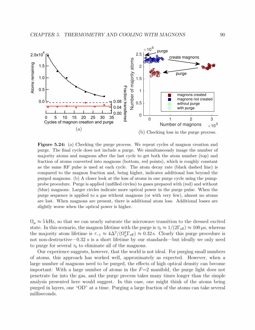
CHAPTER 5. THERMOMETRY AND COOLING WITH MAGNONS 90
2.0x10⁶
1.5
1.0
0.5
0.0
Ato
ms
rem
aini
ng
35302520151050Cycles of magnon creation and purge
0.080.040.00
Fraction transferred(a)
Number of magnons×10
5
0 1 2 3
Num
be
r of
ma
jority
ato
ms
×106
0
0.5
1
1.5
2
2.5create magnons
purge
purge
magnons createdmagnons not createdwithout purgewith purge
(b) Checking loss in the purge process.
Figure 5.24: (a) Checking the purge process. We repeat cycles of magnon creation andpurge. The final cycle does not include a purge. We simultaneously image the number ofmajority atoms and magnons after the last cycle to get both the atom number (top) andfraction of atoms converted into magnons (bottom, red points), which is roughly constantas the same RF pulse is used at each cycle. The atom decay rate (black dashed line) iscompared to the magnon fraction and, being higher, indicates additional loss beyond thepurged magnons. (b) A closer look at the loss of atoms in one purge cycle using the pump-probe procedure. Purge is applied (unfilled circles) to gases prepared with (red) and without(blue) magnons. Larger circles indicate more optical power in the purge pulse. When thepurge sequence is applied to a gas without magnons (or with very few), almost no atomsare lost. When magnons are present, there is additional atom loss. Additional losses areslightly worse when the optical power is higher.
Ωµ ≈ 5 kHz, so that we can nearly saturate the microwave transition to the dressed excitedstate. In this scenario, the magnon lifetime with the purge is τ0 ≈ 1/(2Γeff) ≈ 100µs, whereasthe majority atom lifetime is τ−1 ≈ 4∆2/(Ω2
µΓeff) ≈ 0.32 s. Clearly this purge procedure isnot non-destructive—0.32 s is a short lifetime by our standards—but ideally we only needto purge for several τ0 to eliminate all of the magnons.
Our experience suggests, however, that the world is not ideal. For purging small numbersof atoms, this approach has worked well, approximately as expected. However, when alarge number of magnons need to be purged, the effects of high optical density can becomeimportant: With a large number of atoms in the F=2 manifold, the purge light does notpenetrate far into the gas, and the purge process takes many times longer than the simpleanalysis presented here would suggest. In this case, one might think of the atoms beingpurged in layers, one “OD” at a time. Purging a large fraction of the atoms can take severalmilliseconds.

CHAPTER 5. THERMOMETRY AND COOLING WITH MAGNONS 91
Also, in this approach to purging, it is important that the light driving the opticaltransition be close to resonance, as even weak driving can result in a considerable AC Starkshift of the |F=2〉 levels. Such a shift could reduce the detuning from resonance of undesirablescattering events and decrease the rate of desirable scattering. Finally, our top-imaging beamtypically operates near saturation intensity, and it is difficult to cut the intensity reliablyby two orders of magnitude without feedback, so generally purging works best with our sideimaging beam, which operates far below saturation intensity.
We were able to increase the reliability and robustness of the purging procedure by im-plementing a pump-probe procedure, rather than driving microwave and optical transitionssimultaneously. In this scenario, we purge by first pumping the atoms with an (approximate)microwave π-pulse. Then we apply imaging light for a brief period, 50–150 µs depending onthe optical depth of the atoms, to push the atoms out of the trap. To account for imperfectπ-pulses, the procedure can be repeated several times. This purge procedure can be fasterthan our original method and is more robust to drifts in laser frequency and power. Thefinal cooling data for our publication were acquired using the pump-probe purge method.
5.13 State purification and preparation
Atoms in the |F=1,mF=− 1〉 state, our majority gas, are magnetically trappable, and theirpresence in the imaging field of view can introduce unwanted aberration in our images ofthe magnon momentum distribution. Even if they remain 6.8 GHz out of resonance withthe imaging light, their high density and moderate polarizability makes them an excellentlens that can cast a formidable shadow. Therefore, in order to image small numbers ofmagnons accurately, we begin an optimized purge process, similar to the one applied totrapped magnons in Sec. 5.12, but with microwaves resonant with the |F=1,mF=− 1〉 →|F=2,mF=0〉 transition, removing the majority atoms from the field of view. The purgeprocess begins about one millisecond after extinguishing the optical trapping light.
Purging majority atoms from the field of view presents some additional challenges beyondthose encountered in purging the magnons. Unlike the trapped the magnon gas, the majorityatoms are extremely dense, so considerations of high optical density are not just footnotes,they are front and center. The OD in the center of our BEC can easily exceed 50. In addition,the majority atoms far outnumber the magnons, and thus the constraints on the ratio ofdesirable to undesirable scattering events, such as that given for magnons in Eq. (5.18), aremore severe.
We have used two different majority-atom purge procedures. The first procedure is avariation on the pump-probe purge that we adapted for use on the majority atoms. In thispurge process, forces due to optical scattering remove the atoms from field of view. Thesecond procedure relies on the magnetic field gradient used in MSF to push the majorityatoms from the field of view. In this latter process, the majority atoms are transferred to amagnetically anti-trapped state. In the next few paragraphs I detail both of these purgingprocedures and discuss their relative merits.

CHAPTER 5. THERMOMETRY AND COOLING WITH MAGNONS 92
|F=1〉
|mF=−1〉|0〉
|1〉
|F=2〉
π
(a) Before levitation, pump |mF=− 1〉 to anti-trapped state.
|F=1〉
|mF=−1〉|0〉
|1〉
|F=2〉
LZ sweep
(b) Then transfer |mF=0〉 to magnetically trap-pable state.
Mag
netic
el
d (k
Hz
w.r.
t. re
sona
nce)
Resonance0
-20
20
0.5 1.0 0.5 ms Time
(c) The magnetic field bias during the Landau-Zener (LZ) sweep.
Figure 5.25: Our ultimate scheme to remove |mF=− 1〉 atoms from the imaging fieldof view and to make |mF=0〉 atoms compatible with momentum space focusing. Denselydotted levels are magnetically trappable.
The pump-probe optical majority purge Most of our data were acquired using avariation on the pump-probe purge, with alternating microwave (pump) and optical (probe)pulses. To reduce the optical depth, we used a pump power and pulse length that transferredonly a fraction of the |mF=− 1〉 atoms into the F=2 manifold in each pump-probe cycle.The microwave pulses, probe power, probe duration, and number of pump-probe cycles couldbe varied to purge reliably while losing as few |mF=0〉 atoms as possible.
In spite of this our attempts at optimization, the purge process removed between 10% and40% of the |mF=0〉 atoms, depending on the number of majority atoms being purged andon the particular mood of the experiment. These losses could possibly have been reduced bywaiting longer before the purge sequence, at which point the density would be lower, or byusing a magnetic field gradient to separate the clouds in momentum space. However, doingeither of these things would have changed the timing of our momentum space focusing andimaging procedure, which we had already carefully calibrated. Crucially, the atom loss doesnot visibly impact the momentum of the minority atoms that remain. In counting magnons,we have to consider these losses.
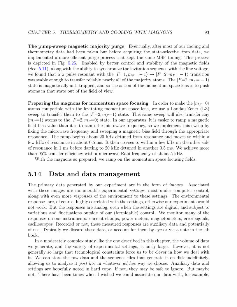
CHAPTER 5. THERMOMETRY AND COOLING WITH MAGNONS 93
The pump-sweep magnetic majority purge Eventually, after most of our cooling andthermometry data had been taken but before acquiring the state-selective trap data, weimplemented a more efficient purge process that kept the same MSF timing. This processis depicted in Fig. 5.25. Enabled by better control and stability of the magnetic fields(Sec. 5.11), along with the ability to synchronize the levitation sequence with the line voltage,we found that a π pulse resonant with the |F=1,mF=− 1〉 → |F=2,mF=− 1〉 transitionwas stable enough to transfer reliably nearly all of the majority atoms. The |F=2,mF=− 1〉state is magnetically anti-trapped, and so the action of the momentum space lens is to pushatoms in that state out of the field of view.
Preparing the magnons for momentum space focusing In order to make the |mF=0〉atoms compatible with the levitating momentum space lens, we use a Landau-Zener (LZ)sweep to transfer them to the |F=2,mF=1〉 state. This same sweep will also transfer any|mF=1〉 atoms to the |F=2,mF=0〉 state. In our apparatus, it is easier to ramp a magneticfield bias value than it is to ramp the microwave frequency, so we implement this sweep byfixing the microwave frequency and sweeping a magnetic bias field through the appropriateresonance. The ramp begins about 20 kHz detuned from resonance and moves to within afew kHz of resonance in about 0.5 ms. It then crosses to within a few kHz on the other sideof resonance in 1 ms before darting to 20 kHz detuned in another 0.5 ms. We achieve morethan 95% transfer efficiency with a microwave Rabi frequency of about 5 kHz.
With the magnons so prepared, we ramp on the momentum space focusing fields.
5.14 Data and data management
The primary data generated by our experiment are in the form of images. Associatedwith these images are innumerable experimental settings, most under computer control,along with even more responses of the environment to these settings. The environmentalresponses are, of course, highly correlated with the settings, otherwise our experiments wouldnot work. But the responses are analog, even when the settings are digital, and subject tovariations and fluctuations outside of our (formidable) control. We monitor many of theresponses on our instruments: current clamps, power meters, magnetometers, error signals,oscilloscopes. Recorded or not, these measured responses are auxiliary data and potentiallyof use. Typically we discard these data, or account for them by eye or via a note in the labbook.
In a moderately complex study like the one described in this chapter, the volume of datawe generate, and the variety of experimental settings, is fairly large. However, it is notgenerally so large that technological constraints force us to be clever in how we deal withit. We can store the raw data and the sequence files that generate it on disk indefinitely,allowing us to analyze it post hoc in whatever ad hoc way we choose. Auxiliary data andsettings are hopefully noted in hard copy. If not, they may be safe to ignore. But maybenot. There have been times when I wished we could associate our data with, for example,

CHAPTER 5. THERMOMETRY AND COOLING WITH MAGNONS 94
Figure 5.26: Some tables used to store data and analysis results. In the top row, twosnapshots show tables that store experimental parameters and quantities pulled directlyfrom primary data files derived from momentum space images and side images. There maybe multiple images of from the side associated with each momentum space image, or viceversa. In the bottom left table, multiple different fits are applied to each piece of momentumspace data, each yielding different derived quantities, such as temperature and condensatefraction. In the bottom right table, multiple different temperature results with differentsettings are combined to yield an extrapolated and/or average temperature.
the magnetic field measured in the lab at the moment it was acquired. However, the needhas never been pressing enough to make it so, and the way we manage our data does nottrivially lend itself to such coordination.
The ability to decide after the fact how to deal with primary data, and thus secondaryand aggregated data that our analysis may generate, is a valuable luxury. Even though wemay analyze the data as they come in, we frequently realize that the experiment is not whatwe think it is, and we are free to approach the data from an entirely different angle at alater time. Regardless, the way we organize data and analysis can have a big impact onour ability to tease out the patterns and trends they contain, on our ability to adapt themto testing evolving hypotheses, and on the way in which preexisting software tools can beapplied to them.
In some ways, choosing how to manage data is akin to choosing a programming languagefor a project. A sensible default is to adapt what has been done before, or to use the toolswith which one is familiar. In the programming space, in some senses— such as “Turingcompleteness”—all choices are equivalent. As a practical matter though, in terms of whatsorts of things are easy, fast, or efficient, such choices can matter a great deal. In thesections that follow, the data, analysis, and results of our study will rightly take center

CHAPTER 5. THERMOMETRY AND COOLING WITH MAGNONS 95
stage. However, the manner in which data and analysis were managed and stored will bea minor character, moving the story along. Let me introduce, briefly, that minor characternow.
The primary data, the images, are acquired by edcam [2], a home built MATLAB-basedimage acquisition program. Edcam does basic processing of absorption images and producesfiles containing the inferred column density, as well as the raw image frames, should they beneeded. These data files are stored on disk with a name determined by the operator, andare typically organized by date.
Information about the primary data, including metadata, such as variables relevant tothe experimental sequence that generated a primary data file, and analysis results, werestored in an impromptu relational database [90] built on MATLAB’s table data structure.A relational database makes a lot of sense for much of our data because there are strongrelationships between different aspects of the data. For example, one or more images ofthe momentum space distribution of the atoms may be related to one or more images of theatoms from the side (to determine the atom number) and one or more images of the atoms insitu, all acquired with the same experimental parameters. These different pieces of primarydata may be the source of many different derived quantities, such as the temperature orchemical potential. Additional quantities can be derived from these derived quantities, andso on, such as an average or extrapolated temperature. By taking care to structure the datain an intelligent way, writing code to analyze the data, perhaps in unforeseen ways, canbecome a lot easier.
Relational databases, along with other (possibly) relevant types of data managementsystems and concepts, are often covered in “programming for scientists”-type courses, suchas Berkeley’s “Python computing for science” [71]. Materials are often available online.Though such courses often focus on a particular programming environment, the principlesof data management are quite general and might fill a much needed gap in the formaleducation of many experimental physicists. Keeping the many types of data in mind whenbuilding a new experiment might allow one to easily integrate environmental responses andother process data with the primary data, potentially allowing variability to be reduced viapost-selection or more sophisticated data modeling.
5.15 Temperature fitting
Atom column momentum densities np are fit to a Bose-enhanced momentum distributionnp = b+ Agj(e
x), with gj the Bose function (polylogarithm) of order j and the argument
x = α− (pw − pw0)2/2mkBTw − (pt − pt0)2/2mkBTt. (5.19)
For non-degenerate gases, α = µ/kBT is a free parameter of the fit, along with the zeroof momentum (pw0, pt0), the background level b, peak level A, and temperatures Tw and Ttalong the weak and tight in-plane axes of the optical trap, respectively. For degenerate gases,α = 0. If necessary, we also add a term that allows for a linear background gradient.

CHAPTER 5. THERMOMETRY AND COOLING WITH MAGNONS 96
Generally, Tw = Tt within the error of the fit. However, at low temperatures, severaleffects cause Tt be an unreliable estimate of the gas temperature. Although the conden-sate expands primarily along the unfocused vertical direction, at very low temperatures thecondensate expansion along the more tightly confined in-plane direction can be manifest(Fig. 5.9b). Also, the tilt of the trap in the tight direction is more difficult to calibrate, lead-ing to a (fictitious) systematic upward shift in the apparent Tt by the mechanism explainedin Sec. 5.4.4. Finally, Eq. (5.19) is expected to describe a Bose gas under the assumptionthat the semiclassical condition kBT ~ω holds along both the tight and weak axes of thetrap. However, in our system ~ωw, ωt/kB ∼ 0.05, 1 nK, and thus at the lowest tempera-tures we achieve this approximation is not valid along the tight axis. Thus, while we fit thefull two-dimensional momentum densities to Eq. (5.19), throughout this work we estimatetemperatures by T = Tw alone.
5.15.1 Masking the condensate
Eq. (5.19) describes the normal component of the gas only, so we must exclude regions ofthe column density that include condensed atoms. Our final data set consists of nearly 5000images with condensates and non-condensates of different shapes and sizes. Automatingmuch of the fitting process, including finding and masking the condensate, if one is present,was quite important. Our procedure for masking a condensate is shown, in part, in Fig. 5.27.The algorithm for establishing the condensate mask is approximately as follows:
Compute the curvature of the image A Laplacian of a Gaussian (LoG) filter is appliedto the image of the atom column density. The standard deviation of the Gaussianfilter can be adjusted but is generally set to roughly twice the imaging resolution. Theresulting image gives the curvature, Ci, of the smoothed image at each pixel i.
Mark points below a curvature threshold The distribution of curvature values differsmarkedly when a condensate is present and when one is not, as shown in Fig. 5.27band 5.27c. Without a condensate, the distribution of curvatures is approximatelysymmetric. With a condensate, a long tail of negative curvatures is present. Candi-date condensate pixels are established by marking pixels with a curvature less than−max(Ci)/β, where β is a tunable constant of order unity that sets the sensitivity ofthe threshold.
Unmark regions less than a minimum size Noise in our images can cause isolated pix-els or small groups of pixels to be tagged in regions where there is no condensate, oreven no atoms. Thus, we unmark candidate pixels that are part of a group of candi-date pixels smaller than a certain size, using the standard “closing” image morphologyoperation. We used a threshold radius of 3 pixels. We call the resulting marked pixelsthe mask.
Expand the mask To make sure the mask covers the whole condensate, we expand itby a variable amount using a “dilation” operation. We may want to mask a region

CHAPTER 5. THERMOMETRY AND COOLING WITH MAGNONS 97µ
m
700
800
900
1000
1100
1200
1300
µm
600 800 1000
0
2
4
6
8
10
−0.025
−0.02
−0.015
−0.01
−0.005
0
0.005
−1
0
1
2
3
4
−1.5
−1
−0.5
0
0.5
1
1.5
2
(a)
−0.01 −0.002 0 0.0020
200
400
Curvature
Occu
rence
s
(b)
−0.002 −0.001 0 0.001 0.0020
200
400
Curvature
Occu
ren
ces
(c)
Figure 5.27: Masking the condensate automatically. (a) Top row: the image of the trans-verse momentum distribution, with color scale indicating density (left) and its curvature(right). Bottom row: The mask (left) and expanded mask (right) are shown in dark blue,superimposed on the transverse momentum density distribution. The distribution of cur-vatures is also shown both with (b) and without (c) a condensate. The masking thresholdcalculated from the distributions is indicated by the vertical blue line. Insets show thecorresponding transverse momentum density distributions. Color scales assign dark red tomaximum unmasked density or curvature in each image.
much larger than the condensate, for example to just fit the wings of the momentumdistribution, so the amount by which we expand the mask may be quite large.
Merge with minimum mask Even if there is no condensate detected, we may want tomask the central part of the distribution. Thus, we combine the automatically deter-mined mask with an adjustable minimum-size mask centered on the density distribu-tion.
This masking procedure has been remarkably successful at finding the condensate in a widerange of our data, including momentum space, in situ, and time-of-flight images. The tuningconstants have proven to be quite robust, and require only minor tweaks depending on thedata.

CHAPTER 5. THERMOMETRY AND COOLING WITH MAGNONS 98
0 0.25 0.5 0.750
5
10
Infe
rred tem
pera
ture
(nK
)
0 0.25 0.5 0.75 10
5
10
15
Normalized mask momentum radius
0 1 2 30
0.5
1
1.5
2
Figure 5.28: Assortment of fits varying the mask size. Fits using the Bose function g2
are in red while fits using g1/2 are in blue. The mask size (x-axis) is normalized by thestandard deviation of the selected fit, which is indicated by the square box. The first twoframes are typical of samples with a condensate present, while the last frame is typical ofsamples without a condensate. Notice that both functions underestimate the temperatureat smaller mask sizes (when a condensate is partially unmasked). At intermediate masksizes, where the Bose-enhanced parts of the non-condensed distribution are present, the g1/2
fits tend to overestimate the temperature. Fits with g2 generally converge to the correcttemperature (as indicated by the wings of the distribution, which are insensitive to the fitfunction employed) at smaller mask sizes.
5.15.2 Selecting a fit
In order to have reliable temperature estimates, we must verify that the temperature isinsensitive to the size of the masked exclusion region. Thus we fit each image multiple timeswith masks of varying size. In addition, it is not clear a priori which Bose function weshould be fitting to. At high temperatures, kBT µ, the non-condensed atoms (includingmagnons) have little overlap with the condensate, and the statistics should be those of atomsin a harmonic trap. In such a case, the function g2 should describe the momentum columndensity. At low temperatures, when kBT µ, the magnons are confined to the region ofthe condensate and see an effective “square well” potential, implying a momentum columndensity approaching g1/2. However, g1/2(ex) diverges unphysically as ex → 1, and ex = 1 atthe center of a quantum-degenerate gas. This incongruity suggests that some other physicsshould keep the unphysical g1/2 behavior from being realized. For example, weak interactionsand finite size should prevent a true divergence. In addition, more recent work in our labon the condensation of magnons suggests that the timescales for true equilibration of themagnons at the longest length scales is longer than the lifetime of our gas.
Fortunately, the high-momentum tails of the momentum distribution np are insensitive tothe particular Bose function employed (gj(e
x)→ ex as ex → 0). Thus, it is important to makesure that some of our fits include only the high-momentum data points. In addition, we will

CHAPTER 5. THERMOMETRY AND COOLING WITH MAGNONS 99
also fit our data with two candidate Bose functions, g1/2 and g2. We can then determine whichBose function best applies to our data by seeing which function most consistently estimatesthe temperature and magnon number as the mask size is varied. If we determine the properBose function, we can increase our signal to noise by including more low-momentum data inthe fits while maintaining temperature consistency with the unbiased high-momentum tailsof the distribution.
Both g2 and g1/2 tend to underestimate the temperature when the mask is very smalland parts of the condensate are included in the fitting region. As the mask grows, thetemperature predicted by g2 tends to rise before it plateaus. In contrast, as the mask sizegrows, the temperature implied by g1/2 will tend to rise above the asymptotic temperaturevalue before converging on the true temperature from above. In both cases, once the maskis too large, the fits become unreliable as the signal to noise drops to zero. This behaviorcan be seen in the examples of Fig. 5.28 and in panel 10 of Fig. 5.29, where the temperaturepredicted by g2 (red points) and g1/2 (blue points) are shown versus mask size.
In general, when fitting condensed samples, g2 seems to converge to the true temperaturevalue faster than g1/2. Often, especially at low temperatures, they converge equally well.The fact that g2 underestimates and g1/2 overestimates the temperature when the centralpart of the degenerate distribution is included in the fit suggests that j ∼ 1 or 3/2 mightfit the data better. Indeed, in our ongoing (as of this writing) work exploring magnoncondensation, this seems to be the case. While the choice of Bose function is not critical inestimating the temperature using the tails of the momentum distribution, it can impact theinferred condensate fraction a great deal. The more highly peaked Bose functions—thosewith smaller j—tend to ascribe more of the atoms in the central region to the non-condensedfraction.
Much of our thermometry data were obtained by imaging entirely non-condensed sam-ples. Far from degeneracy, both g2 and g1/2 are equally good at describing the momentumdistribution. This is the typical case for much of our data, including the third panel inFig. 5.28. Even for samples approaching degeneracy, we noticed once again that in generalg2 seemed to describe the observed distribution better than g1/2, even at low temperatures.This behavior is a bit puzzling and is being investigated in more detail in ongoing work. Ihypothesize a partial explanation: First, as mentioned previously, the timescales required toachieve thermal equilibrium at long length scales seem to be quite slow in our system. Thishas also been observed in other experiments in our lab [25] and elsewhere [15]. The result ofthis may be that at long length scales, where the difference between g1/2 and g2 behavior ismanifest, the gas is unaware, in some sense, that it is approaching degeneracy. In addition,when kBT < µ and g1/2 may be expected to apply, the effects of trap anharmonicity in thevertical direction become relevant, softening the box somewhat. Regardless, for this study,reliable temperatures could be obtained by yielding to the well-thermalized long length scales(e.g. high momentum), as necessary.
Our procedure for efficiently fitting and examining the fits leverages the relational datastorage described briefly at the end of Sec. 5.14. When data were initially acquired, thelocation of the primary data files and the experimental parameters are entered into a table

CHAPTER 5. THERMOMETRY AND COOLING WITH MAGNONS 100
400 600 800 1000 1200 1400 1600
500
600
700
800
900
1000
1100
0 200 400 600 800 0100200300400500600700 400 600 800 1000 1200 1400 1600
500
600
700
800
900
1000
1100
0
200
400
600
800
−20
0
20
40
60
80
100
120
140
10 20 30 40 50 600
5
10
15
20
25
0
100
200
300
400
500
600
700
050100150 400 600 800 1000 1200 1400 1600
500
600
700
800
900
1000
1100
> ‘> am4 22> am4 20> save> am4 0> save> am4 16> save> save> save> save> save
File: MAG_0135.matcurrent ID: − 618vODT: 1tRF: 80tHF: 4.00vortex: 2Tx: 15.6778Ty: 14.5592uB: −0.1463CondFrac: 0.4181r2: 0.1934stdev: 0.3968sROI: []hold fit: 0auto fav: 0
s|idx|cnd| polylog|m1| m2|m3|m4|l| Tx| Ty| N| cFrac| muBet| r2| sdev|fv|masky| 18| 0| g_two|10|1.0| 3|28|0|15.68|14.56|34572| 0.4181|−0.1463| 0.1934| 0.3968| 0|40.96n| 1| 0| g_two|10|1.0| 3|22|0|14.71|13.86|34236| 0.3917|−0.0025| 0.2588| 0.3974| 0|34.24y| 2| 0| g_two|10|1.0| 3|12|0|10.80|10.35|32480| 0.3436|−0.0000| 0.3982| 0.4007| 0|23.93y| 3| 0|g_onehalf|10|1.0| 3| 0|0| 5.35| 3.90|23809|−0.1017|−0.0001| 0.6474| 0.4415| 0|12.73y| 4| 0|g_onehalf|10|1.0| 3|10|0|22.05|20.12|35083| 0.1329|−0.0002| 0.4351| 0.3994| 0|22.13y| 5| 0| g_two|10|1.0| 3| 6|0| 8.43| 7.73|30828| 0.3087|−0.0004| 0.4979| 0.4080| 0|17.83y| 6| 0| g_two|10|1.0| 3| 8|0| 9.22| 8.66|31466| 0.3207|−0.0003| 0.4673| 0.4043| 0|19.63y| 7| 0| g_two|10|1.0| 3|10|0|10.02| 9.59|32034| 0.3329|−0.0001| 0.4277| 0.4020| 0|22.13y| 8| 0| g_two|10|1.0| 3|18|0|13.13|12.55|33608| 0.3747|−0.0031| 0.3103| 0.3981| 0|29.98y| 9| 0|g_onehalf|10|1.0| 3|18|0|18.22|17.25|34768| 0.3370|−0.1593| 0.3112| 0.3979| 0|29.98y| 10| 0|g_onehalf|10|1.0| 3|22|0|16.81|15.79|34646| 0.3815|−0.4010| 0.2589| 0.3974| 0|34.24y| 11| 0|g_onehalf|10|1.0| 3|26|0|15.80|14.72|34570| 0.4152|−0.8897| 0.2146| 0.3970| 0|38.49y| 12| 1| g_two|10|1.0| 3|24|0|15.53|14.52|34520| 0.4002| 0.0000| 0.2324| 0.3972| 0|36.72y| 13| 0| g_two|10|1.0| 3|24|0|15.45|14.45|34485| 0.4003|−0.0038| 0.2324| 0.3972| 0|36.72y| 14| 1| g_two|10|1.0| 3|32|0|16.36|14.93|34665| 0.4144| 0.0000| 0.1642| 0.3966| 0|44.51y| 15| 0| g_two|10|1.0| 3|32|0|15.83|14.47|34600| 0.4304|−0.3129| 0.1643| 0.3966| 0|44.51y| 16| 0| g_two|10|1.0| 3|34|0|15.79|14.39|34601| 0.4368|−0.4770| 0.1461| 0.3964| 0|46.98y| 17| 1| g_two|10|1.0| 3|36|0|16.64|15.07|34705| 0.4195| 0.0000| 0.1330| 0.3963| 0|48.75y| 19| 0| g_two|10|1.0| 3|36|0|15.56|14.12|34588| 0.4510|−1.3824| 0.1331| 0.3963| 0|48.75y| 20| 1| g_two|10|1.0| 3|44|0|16.70|14.89|34697| 0.4178| 0.0000| 0.0842| 0.3959| 1|57.23y| 21| 0|g_onehalf|10|1.0| 3|30|0|15.65|14.41|34573| 0.4305|−1.2768| 0.1781| 0.3968| 0|42.74y| 22| 1| g_two|10|1.0| 3|16|0|13.45|12.81|33908| 0.3679| NaN| 0.3339| 0.3985| 0|28.20y| 23| 0|g_onehalf|10|1.0| 3|14|0|19.51|18.25|34867| 0.2954|−0.0701| 0.3612| 0.3985| 0|26.41y| 24| 0|g_onehalf|10|1.0| 3|36|0|15.73|14.27|34607| 0.4485|−1.9095| 0.1331| 0.3963| 0|48.75y| 25| 0|g_onehalf|10|1.0| 3|46|0|16.37|14.49|34674| 0.4536|−1.6147| 0.0724| 0.3958| 0|59.69y| 26| 1| g_two|10|1.0| 3| 0|0| 4.02| 3.07|25464| 0.2069| NaN| 0.6248| 0.4554| 0|12.19
21
3 4
5 6
7 8
910
11
1213
Figure 5.29: The “fit maker” was used to check fits, apply new fits, and select the favoritefit for each datum. This makeshift GUI is just an interactive MATLAB figure window.Panels 1–3: The original transverse momentum distribution and integrated profiles withintegrated fits. The mask used for the fit is superimposed on the momentum distribution.Panels 4–6: Corresponding momentum distributions and integrated profiles with the maskeddata excluded. These panels show only the data used to produce the fit. Panels 7–9: Theimplied condensate column density and integrated profiles are obtained by subtracting thefitted non-condensed density. Panel 10: A graphical summary of the different fits performedon this datum shows the temperature vs. mask size. The three different colors differ inparameters other than mask size. Red and green points use g2 Bose function with degeneracyparameter α free and fixed to zero respectively. Blue points use g1/2 function and α free.The currently displayed fit is marked with a circle. The favorite fit is marked with a square.Clicking on a data point selects it for display. Panel 11: Numerical summary of differentsaved fit results and parameters. Panel 12: Information on the experimental parametersused for this datum, as well as a few fit highlights and configuration parameters of thefit maker. Panel 13: A command line allows new fits to be generated and saved, for fitsto be selected as favorite, for navigation between data, and for settings of the fit makerto be changed. Time saving settings included automatically selecting the last-viewed fitas favorite and locking the fit settings while navigating between different data so that, forexample, good fit settings do not need to be reentered manually for each item of relateddata.

CHAPTER 5. THERMOMETRY AND COOLING WITH MAGNONS 101
and marked as new. A simple script is called to examine any new data and to add astandard battery of desired fits (which depend on the experimental parameters) to anothertable. Another script monitors this table of fits and would-be fits for unprocessed rows andcalls the fitting routine to fill in any missing fit results. Each fit can take several seconds toperform, and at times, such as when a new battery of fits is to be applied to all of the data,many thousands of new fits might need to be performed. With the data tables stored on acentral server, the fitting routine can easily be parallelized. To make viewing and recallingfits faster, the results of calls to the fit procedure are cached in a hash table whose key isuniquely determined from the data and fit settings.
While our fitting routing is quite robust and well automated, picking a particular set offit parameters that produce the best unbiased fit is not. We need to check that the choiceof Bose function and mask size are reasonable and that the fit results don’t have a strongdependence on particular, somewhat arbitrary, choices. In some data, we need to decidewhether to compensate for a linear background, or not; we may need to decide whether tofix the degeneracy parameter α (owing to the presence of a condensate), and to be sure thischoice does not bias the data. And we need to do this for several thousand different images.To make this process relatively easy, we built a simple tool for browsing the data whileadding, comparing, and selecting fits: the “fit maker,” shown in Fig. 5.29. The fit makershows a summary of all of the fits that have been performed on a particular image along withdetails and views of a particular fit. It includes a capability to add new fits with varyingparameters, and to select a particular “favorite” fit for use in subsequent analysis. All of thedata and fits employed in this work were examined and selected using the fit maker.
5.16 Thermalization
In order to function as a thermometer and to cool the gas, the magnons have to be able toexchange energy with the majority gas at a rate sufficient to achieve a suitable approximationof thermal equilibrium. When kBT > µ, the thermal excitations of the majority gas dispersequadratically, similarly to the magnons, and the magnon gas would be expected to thermal-ize in step with the majority gas itself. However, when kBT < µ, the thermal excitationsof a homogeneous Bose-Einstein condensate are linearly-dispersing phonons, and thus ther-malization of the magnons with the majority gas requires collisions between quasi-particleswith very different dispersion.
We found that an applied magnetic field gradient could expedite thermalization betweeninitially coherent spin components. With no gradient (though a small background curvatureremains, roughly 50 mG/cm2 along the long axis of the trap), the out-of-equilibrium two-component condensate can persist for several seconds when the temperature is sufficientlylow. A less dramatic demonstration of the effects of a magnetic field gradient is shown inFig. 5.30, where the “melting” of the condensate is shown to be expedited by moderategradients. The optimal gradient to achieve thermalization in our system is moderate, on theorder of 0.2–2 mG/cm, depending on the temperature of the gas. We avoid larger gradients

CHAPTER 5. THERMOMETRY AND COOLING WITH MAGNONS 102
Hold time (ms)10 50 90 130 170 210
Gra
dien
tLow
High
Medium
Figure 5.30: Images of the magnon gas in situ at an intermediate temperature in anolder trap geometry are shown with varying magnetic field gradient and hold time. Atshort times, a dense condensate is seen, reflecting the in situ distribution of the initiallyspin-polarized gas. In the presence of low gradients (top row), the dense condensate persiststo later times, “melting” slowly. Higher gradients initially facilitate faster melting, as thecondensate moves more quickly towards the edge of the trap. When the gradient is toolarge, however, the magnons re-condense in a reduced trap volume.
for several reasons. First, a large gradient has the potential to deposit extra energy in thecondensate, leading to atom loss and low-order collective motion of the gas that takes timeto dissipate. Additionally, recall that the magnons have an effective magnetic moment [47],so a gradient that is large compared to the temperature of the gas divided by the size ofthe trap reduces the trap volume for magnons by confining the magnons to the edge of thetrap, lowering the magnon condensation temperature. This effect can be seen in Fig. 5.30,wherein the condensate is seen not to melt at the larger gradients.
A gradient of 0.2 mG/cm corresponds to an energy of approximately h×10 Hz = kB×0.5nK across the longest dimension of our gas and was sufficient to produce a saturated non-condensed fraction of the |mF=0〉 state in 100–2000 ms, depending on the temperature of thegas. Thermalization of magnons created out of a degenerate gas at different temperaturesare shown in Fig. 5.31. In this thermalization experiment, the total time after the end ofthe evaporation ramp is constant, so that effects of thermalization of the entire gas followingevaporative cooling are removed.
When magnons are created at an intermediate trap depth before the final evaporation

CHAPTER 5. THERMOMETRY AND COOLING WITH MAGNONS 103
200 400 600 800
0
20
40
60
80
100
0
5
10
0
0.5
1
1.5
0 200 400 600 8000
100
200
300
400
Ato
m lin
ear
density (
µm
−1)
0
10
20
30
40
Tem
pera
ture
(nK
)
0
5
10
15
20
25
Non−
condensed
magnons/1
03
−500 0 500 1000
0
200
400
600
800
y−axis momentum position (µm)10
−210
−110
010
10
50
100
150
Thermalization time (s)
10−2
10−1
100
101
0
100
200
300
Figure 5.31: Thermalization of magnons of magnons created at trap depths of kB×35 nK(top row), kB × 210 nK (second row), and kB × 1275 nK (bottom row), with total timefollowing evaporative cooling ramp held constant. In the first column, integrated profiles(blue-green lines) and fits to the thermal component (red lines) are offset for clarity. Thepoints corresponding to each fit in column one are marked by same-color circles in thesecond and third columns. Several features of magnon thermalization can be seen here. Atthe lowest trap depth, the temperature cannot be determined until after nearly one secondof thermalization, at which point the temperature has reached steady-state and does notdepend on the number of magnons. At this trap depth, the number of magnons does notseem to saturate (likely due to high loss rates) and the peak number of magnons seemsto vary with the size of the initial magnon condensate. At the intermediate trap depth,the temperature can just barely be determined from the initial momentum distribution.Note the scatter in initial temperatures owing to the very low signal. The temperaturereflected by the magnons initially rises by an amount inversely proportional to the numberof magnons created, but the final temperature achieved is lower when more magnons arecreated owing to decoherence cooling. In contrast to the low trap depth case, the thermalmagnon number saturates to a value independent of the initial condensate number, as longas the initial condensate number is sufficiently large. At high trap depth, similar patterns ofthermalization occur, but are more pronounced. The initial temperature is well determined.At this trap depth, we typically do not create enough magnons to saturate the thermal gas.
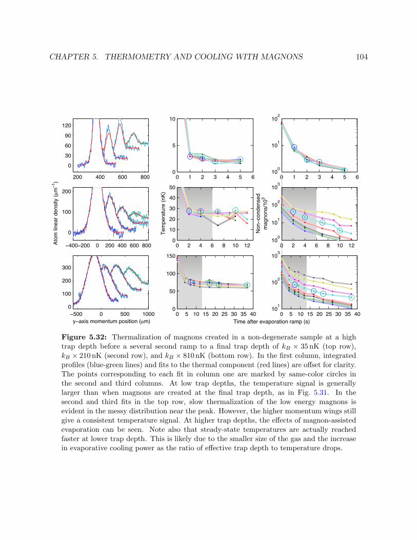
CHAPTER 5. THERMOMETRY AND COOLING WITH MAGNONS 104
200 400 600 800
0
30
60
90
120
0 1 2 3 4 5 60
5
10
0 1 2 3 4 5 6100
101
102
−400−200 0 200 400 600 800
0
100
200
Atom
line
ar d
ensi
ty (μ
m−1
)
0 2 4 6 8 10 120
10
20
30
40
50
Tem
pera
ture
(nK)
0 2 4 6 8 10 12100
101
102
103
Non
−con
dens
edm
agno
ns/1
03
−500 0 500 10000
100
200
300
y−axis momentum position (μm)0 5 10 15 20 25 30 35 40
0
50
100
150
Time after evaporation ramp (s)0 5 10 15 20 25 30 35 40
101
102
103
Figure 5.32: Thermalization of magnons created in a non-degenerate sample at a hightrap depth before a several second ramp to a final trap depth of kB × 35 nK (top row),kB × 210 nK (second row), and kB × 810 nK (bottom row). In the first column, integratedprofiles (blue-green lines) and fits to the thermal component (red lines) are offset for clarity.The points corresponding to each fit in column one are marked by same-color circles inthe second and third columns. At low trap depths, the temperature signal is generallylarger than when magnons are created at the final trap depth, as in Fig. 5.31. In thesecond and third fits in the top row, slow thermalization of the low energy magnons isevident in the messy distribution near the peak. However, the higher momentum wings stillgive a consistent temperature signal. At higher trap depths, the effects of magnon-assistedevaporation can be seen. Note also that steady-state temperatures are actually reachedfaster at lower trap depth. This is likely due to the smaller size of the gas and the increasein evaporative cooling power as the ratio of effective trap depth to temperature drops.
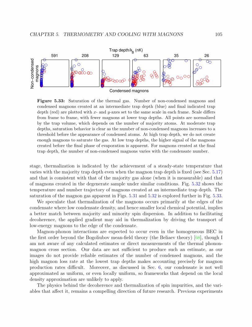
CHAPTER 5. THERMOMETRY AND COOLING WITH MAGNONS 105
591
Non−
condensed
magnons
208 129
Condensed magnons
63 35 26
Trap depth/kB (nK)
Figure 5.33: Saturation of the thermal gas. Number of non-condensed magnons andcondensed magnons created at an intermediate trap depth (blue) and final indicated trapdepth (red) are plotted with x- and y-axes set to the same scale in each frame. Scale differsfrom frame to frame, with fewer magnons at lower trap depths. All points are normalizedby the trap volume, which depends on the number of majority atoms. At moderate trapdepths, saturation behavior is clear as the number of non-condensed magnons increases to athreshold before the appearance of condensed atoms. At high trap depth, we do not createenough magnons to saturate the gas. At low trap depths, the higher signal of the magnonscreated before the final phase of evaporation is apparent. For magnons created at the finaltrap depth, the number of non-condensed magnons varies with the condensate number.
stage, thermalization is indicated by the achievement of a steady-state temperature thatvaries with the majority trap depth even when the magnon trap depth is fixed (see Sec. 5.17)and that is consistent with that of the majority gas alone (when it is measurable) and thatof magnons created in the degenerate sample under similar conditions. Fig. 5.32 shows thetemperature and number trajectory of magnons created at an intermediate trap depth. Thesaturation of the magnon gas apparent in Figs. 5.31 and 5.32 is explored further in Fig. 5.33.
We speculate that thermalization of the magnons occurs primarily at the edges of thecondensate where low condensate density, and hence smaller local chemical potential, impliesa better match between majority and minority spin dispersion. In addition to facilitatingdecoherence, the applied gradient may aid in thermalization by driving the transport oflow-energy magnons to the edge of the condensate.
Magnon-phonon interactions are expected to occur even in the homogeneous BEC inthe first order beyond the Bogoliubov mean-field theory (the Beliaev theory) [68], though Iam not aware of any calculated estimates or direct measurements of the thermal phonon-magnon cross section. Our data are not sufficient to produce such an estimate, as ourimages do not provide reliable estimates of the number of condensed magnons, and thehigh magnon loss rate at the lowest trap depths makes accounting precisely for magnonproduction rates difficult. Moreover, as discussed in Sec. 6, our condensate is not wellapproximated as uniform, or even locally uniform, so frameworks that depend on the localdensity approximation are unlikely to apply.
The physics behind the decoherence and thermalization of spin impurities, and the vari-ables that affect it, remains a compelling direction of future research. Previous experiments

CHAPTER 5. THERMOMETRY AND COOLING WITH MAGNONS 106
on degenerate F=1 87Rb gases have found magnetic field inhomogeneity to facilitate deco-herence and thermalization of spin populations, typically on timescales of several 10’s–100’sof milliseconds [12, 39, 37]. In our work on contrast interferometry with magnons, we ob-served coherence between magnons in different momentum states out to several hundredmilliseconds [47] with a negligible gradient. However, none of these experiments claim tohave operated in the highly-degenerate phonon-dominated regime kBT < µ. On the otherhand, in strongly-interacting Fermi gases, decoherence of spin impurities has been well char-acterized and is limited by a fundamental lower-bound on the spin diffusivity, ~/m [5, 36].Thus, in contrast to weakly interacting Bose systems such as ours, in the strongly interactingFermi gas, the role of the gradient in driving diffusive spin transport is well understood.
5.16.1 Real-space magnon thermalization
When the magnons are initially created, their real-space distribution matches that of theharmonically trapped majority gas. However, at low temperatures, the equilibrium spatialdistribution of non-interacting (dilute) magnons is that of free particles confined to a box.To observe the transition, we imaged magnons in situ as they thermalized. Indeed, in thedata shown in Fig. 5.34, the faint shadows of the gas at long equilibration times do seemflatter than the initial profile. Unfortunately, the combination of low signal owing to atomloss and the small width of the cloud in this data set make a quantitative demonstration ofthe flat magnon potential difficult. In more recent work, we have observed in situ profilesof thermalized magnons that demonstrably match the predicted profile of magnons in abox better than magnons in a harmonic trap by employing a trap with rounder transversedimensions [18].
Initially, our in situ observations of magnon thermalization showed a lot of unexpectedclumping of the magnons, as shown in the left panel of Fig. 5.34. Further investigationrevealed the presence of vortices in the majority gas (the vortices could be seen in themajority gas after a long time of flight as density dips in the condensate distribution). Byevaporating more slowly, we could eliminate the vortices, and the degree of clumping ofthe magnons during thermalization was greatly reduced, as shown in the right panel ofFig. 5.34. The reason that some clumpiness remains, even without vortices, is a mystery,though it could be related to the emergence of a length scale that appears in many of ourgroup’s experiments on condensation in spin mixtures [25].
Much of our data in which magnons are created in a degenerate sample at the final trapdepth have been acquired using similar evaporation parameters to those where we observedvortices. To determine whether vortices impact the temperature indicated by the magnons,we repeated some of our previous experiments with vortex-free evaporation ramps. Otherthan the in situ character of the thermalizing magnons, the presence of vortices does notseem to matter.

CHAPTER 5. THERMOMETRY AND COOLING WITH MAGNONS 107
Time (s)0 0.2 0.4 0.6 0.8 1 2 3 4 6
Time (s)0 0.2 0.4 0.6 0.8 1 2 3 4 6
Fast evaporation Slow evaporation
Figure 5.34: Magnons are created in a degenerate gas at low temperature and imagedin situ. When the majority gas contains vortices owing to a fast evaporation ramp, themagnons clump as they thermalize. Without vortices, the magnons clump much less. Thedistribution of magnons at long times should be more uniform as their 3-D density isexpected to be constant in the trapping volume.
5.17 State dependent trap
Our data show clearly that the magnon gas thermalizes and reaches a steady-state tempera-ture. However, we need to verify that the temperature reached by the magnons reflects energyexchange with the majority gas and not just independent evaporation and self-thermalizationof the magnons. To do this, we vary the trapping potential depth of the majority gas, andthus its temperature, while holding the trapping potential depth of the magnons constant.
Varying the trapping potential depth of the majority gas changes the number of majorityatoms and thereby changes the chemical potential and effective trap depth of the magnons,which is the potential energy depth minus the chemical potential, Ueff = U − µ. If themagnons thermalize independent of the majority gas then we expect the magnon temperatureto vary in proportion to their effective trap depth, even when the trap potential depthis constant. On the other hand, if the magnons thermalize with the majority atoms, themagnon temperature should vary with the majority atom trap depth. Fortunately, these twocompeting effects—self- and co-thermalization—pull the magnon temperature in oppositedirections.
Fig. 5.35 shows clearly that co-thermalization is the dominant effect, as at constantmagnon trap potential depth the magnon temperature varies counter to the effective magnontrap depth and with the majority atom effective trap depth (and trap potential depth).However, the data also suggest that the temperature reflected by the magnons is not strictlyproportional to the estimated majority atom effective trap depth. There are several possibleexplanations for this that might warrant further study.

CHAPTER 5. THERMOMETRY AND COOLING WITH MAGNONS 108
0 20 40 60 800
1
2
3
4
5
Majority atom effective trap depth/kB (nK)
Tem
pera
ture
(n
K)
0 20 40 60 80Magnon effective trap depth/k
B (nK)
Figure 5.35: Temperatures indicated by the magnon momentum distribution in the state-dependent trap have a positive correlation with the majority effective trap depth and anegative correlation with the magnon effective trap depth at constant magnon trappingpotential depth. Here, same-color data connected by a dashed line were acquired at thesame magnon trapping potential depth, but with varying majority atom trapping potentialdepth that was either lower (squares), higher (circles), or the same (diamonds) as themagnon potential depth. Different majority atom numbers result in different effective trapdepths for the magnons even when the trapping potential depth is constant. The magnitudeof the temperature changes is discussed in the main text. Vertical error bars show standarderror of the mean over several measurements and horizontal error bars show systematicuncertainty in the trap depth predicted by the model of Sec. 5.7.
First, variations in the temperature at the same majority atom trap depth (but varyingmagnon effective trap depth) could be due to magnon assisted evaporation, which we havedocumented at higher trap depths. We have not observed that temperature varies with thenumber of magnons at these low trap depths, however, the dynamics of evaporation at suchlow trap depths is not well understood, and it is possible that magnon-assisted evaporationdoes occur but saturates at low magnon numbers. Second, the trap depth itself is notprecisely calibrated, or even well defined, at such low trap depths. The systematic errorin our estimates of trap depth are proportionally large. Moreover, as explored in Sec. 5.8,the trap depth is not constant across the trap and can be very sensitive to tilts. The datadisplayed in Fig. 5.35 was acquired with a tilt in the less-sensitive short in-plane axis thatwas noticeable in the momentum-space expansion of the cloud orthogonal to the directionused to infer temperatures.

CHAPTER 5. THERMOMETRY AND COOLING WITH MAGNONS 109
5.18 Error analysis
5.18.1 Statistical error
One of the powerful features of our magnon thermometer is that its high signal-to-noise ratioallows us to estimate temperatures from a single image. In essence, each magnon indepen-dently samples the collective momentum distribution, and each image of the gas constitutesthe results of hundreds to hundreds-of-thousands of identical, simultaneous experiments,giving us a formidable atomic signal, as well as atom shot noise. Each individual atom isprobed by a large, random number of photons, yielding a large optical signal, along with theinevitable13 photon shot noise. Our camera is sensitive, but relies on stochastic quantum andthermal processes that can introduce additional noise. Finally, technical noise—includingdust and vibrations—has the potential to further spoil our precious temperature signal. Thenoise in our imaging system is dominated by photon shot noise [49] and when imaging asufficient number of atoms, the atom distribution can be determined at the atom shot noiselimit, at least at moderate length scales [46].
By default, our temperature fits do not take noise into account. In effect, this means thatthe fitting algorithm, which is based on a non-linear least-squares optimization (MATLAB’snlinfit), assumes that the error on each pixel is equal and drawn from a normal distribution.However, this is not the case. While the imaging noise is roughly equal across the fittingregion insofar as the imaging beam intensity is roughly constant across the region, the atomshot noise varies considerably. We need to verify that ignoring the variation in error is notbiasing our fits. In addition, when errors are not explicitly included in the fitting routine, thefitting routine must determine from the data and the fit itself what size of a deviation fromthe least-squares result is statistically meaningful, or not, once again employing assumptionsthat may not hold up.
To better understand the uncertainty of our temperature estimates, and to verify that thefits are not systematically shifted by having done the bulk of our fits without specifying thepixel-by-pixel errors, we perform two additional fits. First, we refit the lowest temperaturedata using our selected fit settings with noise-weighted errors. We estimate the noise at pixeli as
Var (ni) = σ2i = ni + Var (nj) ,
where ni is the estimated number of atoms in pixel i obtained from the previous non-noise-weighted fit and the nj are a selection of column densities obtained from pixels withoutatoms present, but with comparable imaging optical power. The first term accounts foratom shot noise and the second for imaging noise, which is dominated by photon shot noise.As shown in Fig. 5.36, the temperature estimates with and without noise weighting are notsubstantially different.
Next we use the results of this fit to construct a simulated image that is perfectly describedby our model. To do this, we use the parameters of the fit to produce a (noiseless) column
13Unless we can somehow use highly squeezed states for imaging.

CHAPTER 5. THERMOMETRY AND COOLING WITH MAGNONS 110
−3 −2 −1 0 1 2 30
10
20
30
40
Num
ber
of fits
Shift of temperature (in standard errors)
Figure 5.36: The difference between temperature estimates from fits with and withoutuncertainty weighting is minor for the 271 lowest temperatures, generally much less thanthe uncertainty in the fit itself.
density profile. We then add to each pixel independent Gaussian noise with variance σ2i and
refit the resulting (noisy) data. The errors on the parameters of the fit of the simulateddata can be compared to the errors on the parameters of the fit to our actual data. Ifour experimental data are well described by our model, and their noise is as expected, thesimulated and actual fits should be essentially identical. Note that our noise model neglectscorrelations in the atom shot noise between different pixels, which might be the case owingto finite imaging resolution. The experimental and simulated errors are compared in the leftpanel of Fig. 5.37.
We can also analytically estimate what the error in our temperature estimates should begiven our noise in the limit that each pixel represents an independent measurement of themomentum distribution and that all parameters of the fit except the temperature are fixed.Obviously, this later requirement is not entirely valid, and in reality the variances of andcovariances between different fit parameters probably cannot be ignored. Still, in this simplelimit, the expected error in the temperature estimated from pixel i is derived from the fitfunction np as
Var (Ti) = Var (ni) /
(∂np∂T
)2
.
The overall variance in the parameter T estimated from a weighted average over the indi-vidual measurements (i.e. each pixel) would then be
Var (T ) = 1/∑i
Var (Ti)−1 . (5.20)
The calculated and experimental uncertainties are compared in the left panel of Fig. 5.37.The calculated error is suggestively close to a factor of two less than the experimental andsimulated errors. It is not surprising that the calculated error is less given the assumptionsmade in the calculation, but one might wonder if a factor of two is missing somewhere. Ina careful examination, none was found.

CHAPTER 5. THERMOMETRY AND COOLING WITH MAGNONS 111
10−2
10−1
100
10−2
10−1
100
Experim
enta
l te
mpera
ture
unce
rtain
ty (
nK
)
Simulated temperature uncertainty (nK)
10−2
10−1
100
10−2
10−1
100
Calculated temperature uncertainty (nK)
Tem
pera
ture
(nK
)
1
2
3
4
5
6
7
Figure 5.37: Comparison of experimental, calculated, and simulated statistical uncertaintyin the single-shot temperature estimates. In the left panel, the uncertainty derived fromour actual data assuming atom shot noise and photon-dominated imaging noise matcheswell with that derived from perfect simulated data perturbed by the assumed noise. In theright panel, the simple model of uncertainty described in the test underestimates the actualnoise observed by a factor of two. The dashed gray line has a slope of two, the solid grayline has a slope of one.
The temperatures were measured many times at each trap depth, and if the error esti-mates given by our fitting routine are correct, they should accurately reflect the variation inthe independent repeated experiments. In statistics, a simple (and like much in statistics,much abused) test of such consonance is the reduced Chi-square statistic,
χ2red =
1
N − 1
∑i
(Ti − T )2
Var (Ti).
χ2red ∼ 1 when the individual variances Var(Ti) are consistent with the scatter of the (assumed
to be independent) data. Here, N − 1 is the number of degrees of freedom, N measurementsless one degree of freedom to determine the uncertainty-weighted average temperature T .For example, if the Ti are independent and drawn from identical normal distributions withknown standard deviation σ =
√Var (Ti), the numerator is just N − 1 times the unbiased
estimate of σ2 and the expected sum would be one.As shown in Fig. 5.38, at the lowest temperatures that we access, the scatter of the data
are consistent with the uncertainty assigned by the fitting routine, with the χ2red hovering
around unity. One outlier shows gives a χ2red ∼ 4. Closer inspection reveals this deviation to
be due to a few fits with uncommonly low error, but differing estimates of the temperature.Regardless, in all cases, using weighed and unweighted means give very similar temperatures.At higher temperatures, a weighted mean no longer describes the data as the temperature
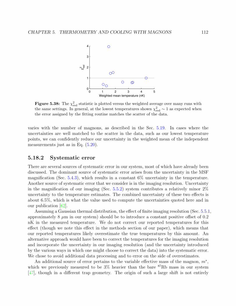
CHAPTER 5. THERMOMETRY AND COOLING WITH MAGNONS 112
Weighted mean temperature (nK)
χ2 re
d
0 1 2 3 4 50
1
2
3
4
Figure 5.38: The χ2red statistic is plotted versus the weighted average over many runs with
the same settings. In general, at the lowest temperatures shown χ2red ∼ 1 as expected when
the error assigned by the fitting routine matches the scatter of the data.
varies with the number of magnons, as described in the Sec. 5.19. In cases where theuncertainties are well matched to the scatter in the data, such as our lowest temperaturepoints, we can confidently reduce our uncertainty in the weighted mean of the independentmeasurements just as in Eq. (5.20).
5.18.2 Systematic error
There are several sources of systematic error in our system, most of which have already beendiscussed. The dominant source of systematic error arises from the uncertainty in the MSFmagnification (Sec. 5.4.3), which results in a constant 6% uncertainty in the temperature.Another source of systematic error that we consider is in the imaging resolution. Uncertaintyin the magnification of our imaging (Sec. 5.5.2) system contributes a relatively minor 2%uncertainty to the temperature estimates. The combined uncertainty of these two effects isabout 6.5%, which is what the value used to compute the uncertainties quoted here and inour publication [62].
Assuming a Gaussian thermal distribution, the effect of finite imaging resolution (Sec. 5.5.1,approximately 8 µm in our system) should be to introduce a constant positive offset of 0.2nK in the measured temperature. We do not correct our reported temperatures for thiseffect (though we note this effect in the methods section of our paper), which means thatour reported temperatures likely overestimate the true temperatures by this amount. Analternative approach would have been to correct the temperatures for the imaging resolutionand incorporate the uncertainty in our imaging resolution (and the uncertainty introducedby the various ways in which one might choose to correct the data) into the systematic error.We chose to avoid additional data processing and to error on the side of overestimates.
An additional source of error pertains to the variable effective mass of the magnon, m∗,which we previously measured to be 3% heavier than the bare 87Rb mass in our system[47], though in a different trap geometry. The origin of such a large shift is not entirely

CHAPTER 5. THERMOMETRY AND COOLING WITH MAGNONS 113
known. Some amount of the shift, 0.3% can be accounted for by considering interactionsone order beyond the usual mean-field Bogoliubov theory (the Bilaev theory) [68]. Wesuspect the remaining portion may owe something to dipolar interactions. Regardless, itis not obvious how this shift in the magnon mass affects the interpretation of the MSFdata. Do the MSF data reveal the in situ momentum distribution? In such a case theshifted effective mass m∗ should be used to infer the temperature from the momentumwidth: A momentum p implies E = p2/2m∗. Do the MSF data reveal the in situ velocitydistribution? In this case, E = m∗v2/2 and the momentum revealed by MSF would needto be corrected to account for the mass difference between the in situ magnons and thefree atoms undergoing MSF. Perhaps neither momentum nor velocity is conserved, and thechange in magnon momentum requires a dynamic description akin to the hydrodynamictheory discussed above. My intuition is that the magnon momentum is conserved as thecondensate density drops after the trap is extinguished, and that the effective mass shouldbe used to infer the temperature. However, we use the bare mass of 87Rb in all of ourestimates. We did not consider this affect in our initial analysis, and so it is not included inour estimates of the systematic error, though it probably should be. While not necessarilynegligible, the systematic error due to the uncertainty in the magnon mass (and how toincorporate it), around 3%, would not be a dominant source of systematic error.
5.19 Temperature extrapolation
At higher temperatures, the presence of magnons clearly impacts the temperature. In suchcases, we can still obtain a reliable and low-uncertainty estimate of the temperature of themajority gas without magnons by extrapolating the temperature signal to the zero-magnonlimit. The way we do this in practice involves two steps, shown in Fig. 5.39.
In most of our data sets, we obtain temperatures with varying numbers of magnonsand with varying hold times after evaporation (in the case that magnons are created at anintermediate trap depth) or after magnon creation (in the case that magnons are created ina degenerate sample at the final trap depth). The first step in our extrapolation procedureis to select the hold times at which the temperature is constant and at which sufficientmagnons are present for reliable temperature fits. These data can then be aggregated andthe variation of temperature with magnon number fit to a line. The zero-magnon interceptand its uncertainty are taken to be the magnon-free estimate of the majority gas temperatureand the uncertainty of this estimate.
We perform a similar process to estimate T/Tc of the majority gas, in general withdifferent hold times, as T/Tc and T are not in general constant at the same hold times. Infact, T/Tc generally rises as atoms are lost, while T remains constant. We select hold timeswhere T/Tc is roughly constant and minimal.
Along with our measurements of T and T/Tc, we also quote the number of atoms andquantities derived from it, such as the chemical potential µ. The atom number, however,decreases slowly with hold time, so there are a range of atom numbers we could reasonably

CHAPTER 5. THERMOMETRY AND COOLING WITH MAGNONS 114T
(nK
)
40
50
60
70
Time (s)
T/T
c
0 20 400.4
0.5
0.6
0 10 20 30
Non−condensed
magnons/104
Time (s)
10−2
10−1
100 0 5 10 15
Non−condensed
magnons/104
Magnons created before... ...and after evaporation
Figure 5.39: Extrapolating the temperature T and ratio of temperature to majoritycondensation temperature Tc to the zero magnon limit at a trap depth of kB × 590 nK. Toobtain reliable, low-noise limits, we perform the extrapolation on data acquired at severalhold times where T (T/Tc) is constant. The first (third) column shows T (T/Tc) as afunction of hold time after the final evaporation (after magnon creation, with constanthold after evaporation). Different colored points and connecting lines indicate differentinitial magnon numbers. The vertical colored bars highlight the data used in the second(fourth) column, where T (T/Tc) is plotted versus the number of non-condensed magnons.The circle points are colored to indicate the hold time at which they were acquired, withcolors matched to the bars in the first (third) columns. The linear fit to T (T/Tc), anduncertainties derived from the extrapolation, are indicated by the solid line and error barsat end points. The extrapolated T (T/Tc) and uncertainty is the left end point and errorbar. The mean and standard deviation of the mean are indicated by the dashed black lineand error bars on the end points. The linear extrapolation describes the data better thana simple mean.

CHAPTER 5. THERMOMETRY AND COOLING WITH MAGNONS 115
state with each measurement. In general, when we quote a single number, we chose thelargest measured atom number relevant to both the extrapolation of T and Tc. The range ofchoices for atom number is typically less than the systematic uncertainty we assign to ouratom number estimates.
5.20 Optimizing cycled decoherence cooling
Several experimental parameters can affect the efficacy of cycled decoherence cooling, includ-ing the number of magnons created at each cycle, the thermalization time following magnoncreation, and the magnetic field gradient. These parameters might not be constant from cycleto cycle. For example, as temperatures are lowered, the number of magnons created shoulddrop with the critical number for magnon condensation. We optimized cycled decoherencecooling several cycles at a time by varying the parameters and plotting the resulting T/Tcand majority atom number achieved, as in Fig. 5.40. The best parameters are those wherethe slope of T/Tc versus majority atom number is steepest with the additional cycles. Forsimplicity, we did not optimize the gradient degree of freedom, but rather chose a gradientsufficiently small that the magnon box was effectively flat even at the lowest temperaturesreached by decoherence cooling.
In the end, we found that fairly simple heuristics could be applied to roughly optimizecycled decoherence cooling without searching the entire parameter space. At each cycle ofdecoherence cooling, the number of magnons created should be small such that no magnoncondensate persists upon thermalization. The thermalization time should be as short as pos-sible such that only a negligible magnon condensate persists. In practice, we optimize coolingfour to ten cycles at a time, breaking cooling into several stages with different parameters.
5.21 Two types of cooling
When we initially undertook our exploration of magnon decoherence cooling, we did notforesee the phenomenon of magnon-assisted evaporation. Our original protocols for bothcooling and thermometry only included producing magnons at the final trap depth in thedegenerate sample. It was only upon investigating heating rates in the trap that I suspectedan additional cooling effect due to the evaporation of magnons.
The heating experiment involved performing cycled decoherence cooling to a sufficientlylow temperature that evaporative cooling would cease. Magnons produced in the final stepof cooling were retained for a variable number of seconds in order to probe the temperatureof the gas as it heated in its trap. Surprisingly, I found the temperature to level-off at a lowervalue than the initial value reached by (non-magnon-assisted) evaporation. I hypothesizedthat the magnons improved the power of evaporative cooling, and our experiments in whichwe produce magnons at an intermediate trap depth proved that to be the case.

CHAPTER 5. THERMOMETRY AND COOLING WITH MAGNONS 116
20
40
60
80
T (n
K)
4 6 8 10 12 140.4
0.5
0.6
0.7
0.8
Majority atoms remaining after nine cycles/105
T/T c
Coo
ling
cycl
e ho
ld ti
me
(ms)
100
200
300
400
500
600
700
800
900
1000
Figure 5.40: Optimizing cycled decoherence cooling at a trap depth of kB × 810 nK afternine cycles of cooling. The solid black point is the T (top) or T/Tc (bottom) achieved afterone cycle of magnon creation and thermalization. The sizes of the open circles indicatethe length of the RF pulse used to create magnons in each cycle, with longer RF pulsesindicated as larger circles. Longer RF pulses convert more atoms to magnons in each cycle,leading to fewer majority atoms, but also potentially more cooling. Data points are colorcoded by the thermalization time employed in each cycle. Short thermalization times canbe effective when the RF pulses are short. Longer thermalization times are needed whenthe RF pulses are longer. An optimal parameter choice would be to use the steepest slope,indicated by the dotted gray arrows. To continue the optimization, parameters are selectedfor the first nine cycles and new parameters are tried in subsequent cycles, generating asimilar plot.
Initially, the discovery of magnon-assisted evaporation challenged our straightforwardinterpretation of our previously acquired magnon-decoherence data. Could the cooling weobserved just be magnon-assisted evaporation turning on with the introduction of magnons?To tease apart the two types of cooling, we combined them, as shown in Fig. 5.41a. In thisexperiment, we evaporate with a large number of non-degenerate magnons present. Uponwaiting some time at the final trap depth, we purge the non-degenerate magnons and begincycled magnon decoherence cooling wherein the number of magnons created each cycle isless than the number of magnons that survived evaporation. As a result the power of anymagnon-assisted evaporation is reduced. Regardless, decoherence cooling proceeds to lowerthe temperature as expected.
When magnons are first created at the final trap depth, it is likely that, initially, somemagnon-assisted evaporation does occur along with magnon decoherence cooling. This isevident in Fig. 5.41b, which plots the energy removed per magnon as indicated by the slopesof the temperature extrapolation described in Sec. 5.19, wherein single pulses with varying

CHAPTER 5. THERMOMETRY AND COOLING WITH MAGNONS 117
0 10 20 30 400
20
40
60
80
100
T (
nK
)
Hold after evaporation ramp (s)
(a)
0.1 1
−10
−8
−6
−4
−2
0
2
kBT/µ
∆E
per
magnon/k
BT
(b)
Figure 5.41: (a) Combining magnon-assisted evaporation and cycled decoherence cooling.Evaporation is performed with magnons present. Trajectories in which a variable numbermagnons are held at the final trap depth (points with lines between them) are comparedto trajectories in which these magnons are removed from the trap and cycled decoherencecooling is applied using a smaller number of magnons than had been removed (filled circularpoints). Cycled decoherence cooling continues to cool the sample despite fewer magnonsbeing present to assist in evaporation. (b) The energy removed per magnon for a singlecycle of magnons created before (red) and after (blue) the final evaporation ramp in unitsof kBT are derived from the slopes and uncertainty of the extrapolated temperature versusmagnon number. Decoherence cooling applies only to the blue data, while magnon-assistedevaporation applies primarily to the red data. Additional magnon-assisted evaporationlikely also applies to the blue data, especially when kBT > µ.
numbers of magnons perform varying amounts of decoherence cooling or magnon-assistedevaporation. At higher temperatures, the energy removed per magnon in magnon-assistedevaporation is on the order of 4–6 kBT . At similar temperatures, the energy removed permagnon when magnons are created in the degenerate sample rises to 6–8 kBT , consistentwith a 3 kBT contribution from decoherence cooling in addition to some contribution frommagnon-assisted evaporation.
5.22 Benefits of a square well potential
The fact that magnons disperse like free massive particles, as opposed to harmonicallytrapped or massless particles, can substantially benefit the signal to noise achievable bythe magnon thermometer. This is shown dramatically in Fig. 5.42, where it is shown thatthe number of non-condensed magnons from which we derive our temperature signal at very

CHAPTER 5. THERMOMETRY AND COOLING WITH MAGNONS 118
102
103
104
105
106
102
103
104
105
106
Num
ber
of non−
condensed m
ag
no
ns
For a harmonic trop
102
103
104
105
106
For a square well trap
T/µ
0.511.522.5
Estimated critical number for magnon condensation
Figure 5.42: The number of non-condensed magnons estimated from fits over a widerange of data from our data set is compared the critical number for magnon condensationas computed for magnons confined to a harmonic trap with trapping frequencies derivedfrom our optical trap and for magnons confined to a square well with volume equal tothe calculated volume of the majority condensate under the Thomas-Fermi approximation.Runs with magnons created before the final evaporation ramp are plotted as dots while runswith magnons created at the final trap depth are plotted as open circles. Color varies withthe ratio of the measured temperature to the calculated chemical potential of the majoritygas.
low temperatures is more than an order of magnitude more than the maximum number ofnon-condensed particles that we would expect to exist in the harmonically trapped majoritygas. Rather, the maximum number of non-condensed magnons scales very much like theprediction for particles confined in a flat box.
In the present work, we do not have as high confidence in our estimates of the non-condensed magnon number as we do the temperature. Unlike our estimates of temperature,the estimates of non-condensed magnon number can be shifted systematically by the incorrectBose function in the fits of the transverse momentum distribution, as discussed in Sec. 5.15.2.We are exploring in better detail the characteristics of magnon condensation and thermalposition/momentum distributions in ongoing work.
5.23 Thermometry and cooling results
Details of the results of our experiments and analysis are covered in Ref. [62], so here weinclude just a brief summary. Fig. 5.43 shows the temperature and level of degeneracyreached by evaporative cooling only, magnon decoherence cooling, and magnon assisted
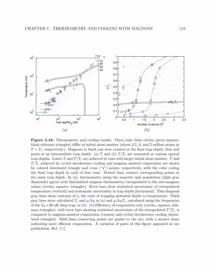
CHAPTER 5. THERMOMETRY AND COOLING WITH MAGNONS 119
7 10
45302014
η
Tc
μ/kb
Trap depth/kB (nK)
Tem
pera
ture
(nK)
101 102 103 104
100
101
102
103
(a)
Number of atoms/106
T/T
c
µ/kb T
c
0.5 1 1.5 2 2.5 3 3.50
0.1
0.2
0.3
0.4
0.5
0.6
0.7
0.8
0.9
1
(b)
Figure 5.43: Thermometry and cooling results. Three runs (blue circles, green squares,black sideways triangles) differ in initial atom number (about 2.5, 3, and 5 million atoms atT = Tc, respectively). Magnons in black run were created at the final trap depth, blue andgreen at an intermediate trap depth. (a) T and (b) T/Tc are measured at various opticaltrap depths. Lower T and T/Tc are achieved in runs with larger initial atom number. T andT/Tc achieved by cycled decoherence cooling and magnon assisted evaporation are shownby colored downward triangle and cross (“x”) points, respectively, with the color codingthe final trap depth in each of four runs. Dotted lines connect corresponding points atthe same trap depth. In (a), thermometry using the majority spin population (light graydiamonds) agrees with thermalized magnon thermometry extrapolated to the zero-magnonvalues (circles, squares, triangles). Error bars show statistical uncertainty of extrapolatedtemperature (vertical) and systematic uncertainty in trap depth (horizontal). Thin diagonalgray lines show contours of η, the ratio of trapping potential depth to temperature. Thickgray lines show calculated Tc and µ/kB in (a) and µ/kBTc, calculated using the frequenciesof the kB×60 nK deep trap, in (b). (b) Efficiency of evaporation only (circles, squares, side-ways triangles), with error bars showing statistical uncertainty of the extrapolated T/Tc, iscompared to magnon-assisted evaporation (crosses) and cycled decoherence cooling (down-ward triangles). Solid lines connecting points are guides to the eye, with a steeper slopeindicating more efficient evaporation. A variation of parts of this figure appeared in ourpublication, Ref. [62].
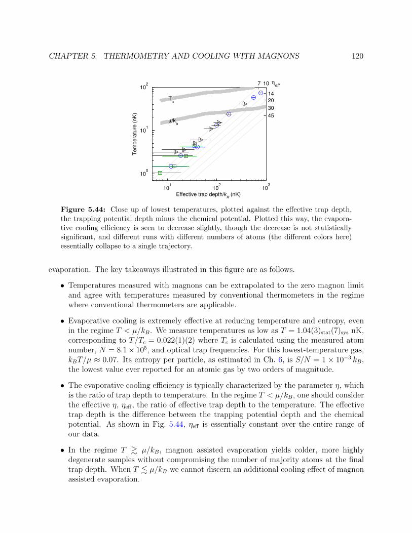
CHAPTER 5. THERMOMETRY AND COOLING WITH MAGNONS 120
7 10
45
30
20
14
ηeff
Tc
µ/kb
Effective trap depth/kB (nK)
Tem
pera
ture
(nK
)
101
102
103
100
101
102
Figure 5.44: Close up of lowest temperatures, plotted against the effective trap depth,the trapping potential depth minus the chemical potential. Plotted this way, the evapora-tive cooling efficiency is seen to decrease slightly, though the decrease is not statisticallysignificant, and different runs with different numbers of atoms (the different colors here)essentially collapse to a single trajectory.
evaporation. The key takeaways illustrated in this figure are as follows.
• Temperatures measured with magnons can be extrapolated to the zero magnon limitand agree with temperatures measured by conventional thermometers in the regimewhere conventional thermometers are applicable.
• Evaporative cooling is extremely effective at reducing temperature and entropy, evenin the regime T < µ/kB. We measure temperatures as low as T = 1.04(3)stat(7)sys nK,corresponding to T/Tc = 0.022(1)(2) where Tc is calculated using the measured atomnumber, N = 8.1× 10⁵, and optical trap frequencies. For this lowest-temperature gas,kBT/µ ≈ 0.07. Its entropy per particle, as estimated in Ch. 6, is S/N = 1× 10−3 kB,the lowest value ever reported for an atomic gas by two orders of magnitude.
• The evaporative cooling efficiency is typically characterized by the parameter η, whichis the ratio of trap depth to temperature. In the regime T < µ/kB, one should considerthe effective η, ηeff , the ratio of effective trap depth to the temperature. The effectivetrap depth is the difference between the trapping potential depth and the chemicalpotential. As shown in Fig. 5.44, ηeff is essentially constant over the entire range ofour data.
• In the regime T & µ/kB, magnon assisted evaporation yields colder, more highlydegenerate samples without compromising the number of majority atoms at the finaltrap depth. When T . µ/kB we cannot discern an additional cooling effect of magnonassisted evaporation.

CHAPTER 5. THERMOMETRY AND COOLING WITH MAGNONS 121
• Cycled decoherence cooling allows low temperatures and entropy to be reached in adeep trap. We reach an temperatures as low as T ≈ 22 nK, corresponding to η ∼ 30,in a kB × 700 nK deep trap.
• The efficiency of cycled decoherence cooling, in terms of the number of atoms sacrificedto reach a desired temperature or entropy, is much lower than that of evaporativecooling. This makes sense, as each atom lost by evaporation carries away an energy ofroughly ηkBT while each atom lost in decoherence cooling carries away roughly 3 kBTplus the chemical potential.
• In our experiments, decoherence cooling saturates at temperatures T ∼ µ/kB in spite ofour initial expectations that decoherence cooling should be most effective in this regimebecause the gas heat capacity drops quickly as it becomes increasingly degenerate. Wesuspect the discrepancy lies in the slow speed of thermalization in this regime, whichresults in the magnons being unable to remove energy faster than it is deposited byheating processes.
• Magnon decoherence cooling can only barely reduce the entropy at T/Tc ∼ 0.9. Thisis consistent with our expectation that the entropy should only be reduced by thedecoherence cooling process for T/Tc < 0.96.
To derive this limit, consider that in an ideal Bose gas in a harmonic trap withgeometric-mean frequency ω, the following relations for the saturated thermal atomnumber Nth, energy E, and heat capacity C, at the temperature T , apply:
Nth = ζ(3)
(kBT
~ω
)3
(5.21a)
E = 3 ζ(4)(kBT )4
(~ω)3=
3ζ(4)
ζ(3)kBTNth (5.21b)
C =dE
dT= 12kB
ζ(4)
ζ(3)Nth. (5.21c)
Suppose we transfer dN > 0 atoms to the minority spin state (where dN is far belowthe critical number for magnon condensation), let them thermalize, and eject them. Tolowest order, the majority gas loses energy dE = −3kBTdN , and thus the temperaturechanges by dT = dE/C = −3(kBT )/C dN . The non-condensed fraction changes as,
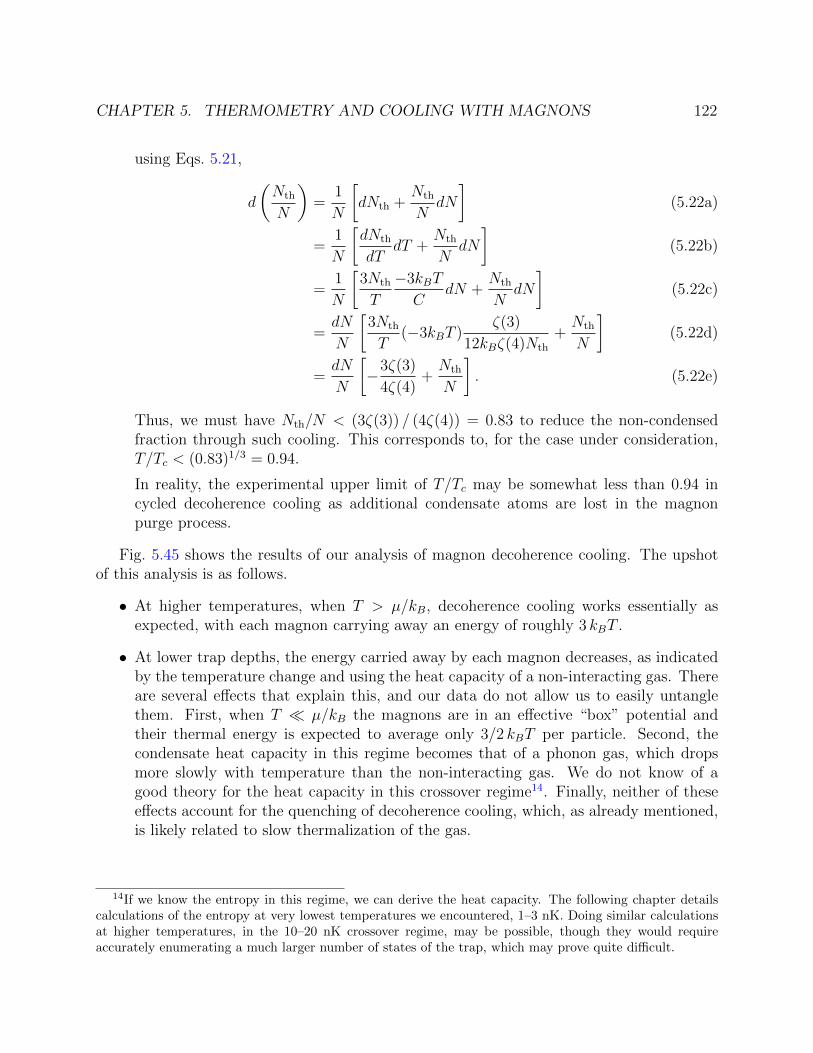
CHAPTER 5. THERMOMETRY AND COOLING WITH MAGNONS 122
using Eqs. 5.21,
d
(Nth
N
)=
1
N
[dNth +
Nth
NdN
](5.22a)
=1
N
[dNth
dTdT +
Nth
NdN
](5.22b)
=1
N
[3Nth
T
−3kBT
CdN +
Nth
NdN
](5.22c)
=dN
N
[3Nth
T(−3kBT )
ζ(3)
12kBζ(4)Nth
+Nth
N
](5.22d)
=dN
N
[−3ζ(3)
4ζ(4)+Nth
N
]. (5.22e)
Thus, we must have Nth/N < (3ζ(3)) / (4ζ(4)) = 0.83 to reduce the non-condensedfraction through such cooling. This corresponds to, for the case under consideration,T/Tc < (0.83)1/3 = 0.94.
In reality, the experimental upper limit of T/Tc may be somewhat less than 0.94 incycled decoherence cooling as additional condensate atoms are lost in the magnonpurge process.
Fig. 5.45 shows the results of our analysis of magnon decoherence cooling. The upshotof this analysis is as follows.
• At higher temperatures, when T > µ/kB, decoherence cooling works essentially asexpected, with each magnon carrying away an energy of roughly 3 kBT .
• At lower trap depths, the energy carried away by each magnon decreases, as indicatedby the temperature change and using the heat capacity of a non-interacting gas. Thereare several effects that explain this, and our data do not allow us to easily untanglethem. First, when T µ/kB the magnons are in an effective “box” potential andtheir thermal energy is expected to average only 3/2 kBT per particle. Second, thecondensate heat capacity in this regime becomes that of a phonon gas, which dropsmore slowly with temperature than the non-interacting gas. We do not know of agood theory for the heat capacity in this crossover regime14. Finally, neither of theseeffects account for the quenching of decoherence cooling, which, as already mentioned,is likely related to slow thermalization of the gas.
14If we know the entropy in this regime, we can derive the heat capacity. The following chapter detailscalculations of the entropy at very lowest temperatures we encountered, 1–3 nK. Doing similar calculationsat higher temperatures, in the 10–20 nK crossover regime, may be possible, though they would requireaccurately enumerating a much larger number of states of the trap, which may prove quite difficult.

CHAPTER 5. THERMOMETRY AND COOLING WITH MAGNONS 123
0 2 4 6 8 100
20
40
60
80
100
120
Non−condensed magnons removed/105
Tem
pera
ture
(nK
)
Trap depth/kB : 1,250 nK
800 nK
600 nK200 nK
0 50
5
10
Magnons imaged/105
Ato
ms lost/10
5
kBT/µ
∆E
per
magnon/k
BT
0 1 2 3
−3
−1.5
0
Figure 5.45: A closer look at decoherence cooling. (Left) Magnons are created at the finaltrap depth and cool the gas as they thermalize. Thermalized magnons can be removed fromthe trap and the cooling process repeated before measuring the temperature by imaging themomentum distribution of the thermalized magnons. Each non-condensed magnon removedfrom the trap takes energy from the gas. Here, decoherence cooling trajectories are plottedversus cumulative number of magnons removed at several trap depths, coded by colorsthat correspond to those of Fig. 5.43. Closed circles show temperatures after a single cycleof decoherence, but with varying numbers of magnons. Some additional magnon-assistedevaporative cooling may also be present. Open triangles show repeated cycles of magnoncreation, thermalization, and purge, with representative error bars on first and last trianglesgiving statistical error over several repetitions. Solid lines show zero-free-parameter theorypredictions assuming each non-condensed magnon removes 3 kBT energy. Solid patchesindicate the range of predictions included within the uncertainty in the cumulative numberof magnons removed. (Center) We image 75%±10% of the magnons present after each cycleof decoherence cooling. From these magnons, we extract the temperature. In a separaterun, we also extract the total number of atoms remaining in the trap. Here we comparethe number of atoms lost along each cycled cooling trajectory to the cumulative number ofmagnons imaged. If atom loss were due only to removing magnons, the number of atomslost would lie in the gray region, which accounts for the ∼75% efficiency of our magnonimaging sequence. Instead, the cumulative number of atoms lost in each decoherence coolingtrajectory is larger than this owing to additional atom losses unrelated to decoherencecooling, such as finite trap lifetime and 3-body loss. The dotted line represents 100%magnon imaging efficiency and no additional atom loss. (Right) The amount of energyremoved by each magnon, in units of kBT , is plotted versus the ratio of µ/kBT , where eachpoint is based on an estimate of the slope over 4 consecutive triangle points in the left frame.We observe that the net energy carried away by the magnons vanishes when T . µ/kB. Avariation of parts of this figure appeared in our publication, Ref. [62].
124
Chapter 6
Calculating the entropy per particle
The entropy per particle of a Bose-Einstein condensate deep in the phonon regime, whereT µ/kB, can be calculated using the standard relations for Planck-distributed phonons,Eq. (5.3), provided one can make the local density approximation. For the gas of Ch. 5 atthe lowest entropy settings, the chemical potential is µ ≈ kB × 15 nK, the speed of soundis c =
√µ/m, and density is n = µ × m/(4π~2a), with a the scattering length, and this
calculation yields S/N ≈ 1.5× 10⁻⁵ at the point of highest density at the center of our trapat T = 1.04 nK. This naive calculation underestimates the entropy in our gas.
We cannot rely on the local density approximation to calculate the entropy per particlebecause the thermal phonon wavelength λ = hc/kBT ≈ 50µm is far larger than the trans-verse Thomas-Fermi radii of the condensed gas (15µm, 2.5µm). To understand the entropy,we will have to estimate numerically the spectrum of excitations along these dimensions.However, since the condensate radius along the longest axis is large (around 300 µm), wecan apply a one-dimensional local density approximation to determine the entropy. In thischapter I detail and build confidence in this important calculation.
6.1 Numerical objective
In general, the entropy S and number of atoms N in a Bose gas at equilibrium temperatureT and with chemical potential µ can be calculated as [69]
S/kB =∑i
(εi − µ) /kBT
e(εi−µ)/kBT − 1− log
(1− e(µ−εi)/kBT
)(6.1a)
N =∑i
1
e(εi−µ)/kBT − 1, (6.1b)
where the many-body excitation spectrum of the gas is εi. For example, plugging in thespectrum of single-particle excitations in a harmonic trap one can derive the well-knownformula for the entropy of a Bose gas in a harmonic trap. These formula are accurate even

CHAPTER 6. CALCULATING THE ENTROPY PER PARTICLE 125
in the presence of interactions, provided one accounts for interactions properly in derivingthe εi.
The excitation spectrum of a weakly interacting (with s-wave interactions) trapped Bosegas is typically well described by the zero-temperature Gross-Pitaevskii theory [69], whereinthe ground state order parameter Ψ0 satisfies the time-independent Gross-Pitaevskii equa-tion, (
T + V (x)− µ+ g |Ψ0(x)|2)
Ψ0(x) = 0, (6.2)
with the kinetic energy operator T = −~2∇2/2m, confining potential V , and the interactionparameter g = 4π~2a/m. The condensate density is n = |Ψ0|2. Note that in the limit g → 0Eq. (6.2) reduces to the time-independent Schrodinger equation for a single particle, with µthe energy eigenvalue. Also, the solution Ψ0 is not necessarily unique; Ψ0 = 0 is always atrivial solution.
For a particular static solution Ψ0(x), the small amplitude excitations can be written
Ψ(x, t) =
(Ψ0(r) +
∑i
[ui(r)e−iωit + v∗i (r)eiωit
])e−iµt/~,
where “∗” denotes complex conjugation, and the Bogoliubov amplitudes u and v satisfy thecoupled eigenvalue equations
~ωiui(r) =(T + V − µ+ 2g |Ψ0(r)|2
)ui(r) + gΨ0(r)2vi(r)
−~ωivi(r) =(T + V − µ+ 2g |Ψ0(r)|2
)vi(r) + gΨ∗0(r)2ui(r). (6.3)
Once again, in the limit g → 0 these equations are equivalent to the Schrodinger equationwith eigenvalue ~ωi +µ. The excitation energies relevant to Eqs. (6.1) are thus εi = ~ωi +µ.
This is our challenge: derive the spectrum of excitations of our gas in our trap, and employEqs. (6.1) to calculate S/N . Our approach is to numerically solve Eq. (6.2) for the groundstate order parameter Ψ0 and then to plug this into the eigenvalue equations Eqs. (6.3) topull out the excitation spectrum. To begin, we need a way to discretize the relevant equationssuch that the solutions we obtain are sufficiently accurate and the numerics tractable.
6.2 Discretizatation strategy
The naıve way of discretizing involves choosing a Cartesian grid xi with spacing ∆xbetween points, on which one will define the spatially varying functions Ψi = Ψ(xi) andVi = V (xi). The kinetic energy operator can then be approximated using finite-differences.To do this, one defines the one-dimensional difference operator ∂x,
∂xΨj = Ψ(xj + ∆x/2)−Ψ(xj −∆x/2),
so that∂2xΨj = Ψj+1 − 2Ψj + Ψj−1,

CHAPTER 6. CALCULATING THE ENTROPY PER PARTICLE 126
and relates it to the one-dimensional derivative operator ∇x via the translation operator,
Ψ(xj + ∆x/2) = e∆x∇x/2Ψ(xj).
The difference operator can then be written
∂x = e∆x∇x/2 − e−∆x∇x/2 = 2 sinh (∆x∇x/2) ,
allowing one to solve and expand to find
∇2x =
(∂2x − ∂4
x/12 + ∂6x/90 +O(∂x)
8)/(∆x)2.
This expression allows the kinetic energy operator T to be written as a matrix to arbitraryaccuracy (if one employs an arbitrary number of mesh points). The Gross-Pitaveskii equationcan then be written in a discrete form as∑
i
(Tij + Viδij + g |Ψi|2 δij
)Ψi = µΨj. (6.4)
Formulated in this way, it is not obvious what assumptions and approximations aremade in the discretization, and what their impact might have on the numerics. It shouldbe clear that the approximation to the derivative ∇x in terms of a truncated series of finitedifferences ∂x depends on the finite differences being small. More generally, recall that theGross-Pitaevskii equation can be derived by minimizing the energy functional
E =
∫ (~2
2m|∇Ψ0(x)|2 + V (x) |Ψ0(x)|2 +
g
2|Ψ0(x)|4
)dx (6.5)
with respect to the conjugate order parameter Ψ∗0, with the constraint that particle numberis conserved. The accuracy of the finite difference method relates to the precision with whichthe integral in the energy functional (and also the particle number) can be approximated bya rectangle-rule sum: ∫
f(x)dx→∑i
f(xi)∆x.
The energy of a particular configuration Ψi computed via the rectangle rule may overes-timate or underestimate the true minimum energy. While with a small enough grid spacingthis approximation can be very good, as we shall see, there are more nuanced discretizationsthat lead to a sum rule that achieves a higher degree of accuracy with fewer mesh points.
First, let’s consider another common way to discretize an equation: in function space viaa basis approximation. To discretize using N orthonormal basis functions φi, we write
Ψ(x) =∑i
Ψiφi(x). (6.6)

CHAPTER 6. CALCULATING THE ENTROPY PER PARTICLE 127
For convenience, we will once again consider a one-dimensional problem. We plug Eq. (6.6)into Eq. (6.2), multiply on the left by φ∗j(x), and integrate to obtain the expression
∫dx φ∗j(x)×
∑i
T + V (x) + g
∣∣∣∣∣∑k
Ψkφk(x)
∣∣∣∣∣2Ψiφi(x) = µ
∑i
Ψiφi(x)
, (6.7)
which we write more concisely as∑i
(Tij + Vij + gIij) Ψi = µΨj. (6.8)
The matrices T and V only need to be computed once (for time-independent problems),however the non-linear interaction matrix I needs to be computed for any change to theweights Ψi. Thus, solving Eq. (6.8) using an interative procedure like Newton’s methodrequires N multiplications of a different N × N matrix at every step, as with the finitedifference approach. However, in the present basis function approach, calculating each N×Nmatrix requires an explicit numerical integration:
Iij =
∫dx φ∗j(x)φi(x)
∣∣∣∣∣∑k
Ψkφk(x)
∣∣∣∣∣2
. (6.9)
This integration can be performed to arbitrary precision, regardless of the number of basisfunctions employed.
An advantage of the basis function approach over the finite difference approach is thatthe solution Ψ(x) is defined at every point x, and thus the energy of the configurationcomputed via Eq. (6.5) constitutes of a lower bound of the true ground state energy, asin a variational calculation. In addition, with the proper choice of basis, a relatively smallnumber of basis functions may be required to achieve high accuracy. Regardless, it appearsthat the computational requirements—many many numerical integrations of Eq. (6.9) atevery iteration—are quite high. The basis approach allows us to understand explicitly theassumed interaction energy and order parameter in all space, but at the cost of making localinformation cumbersome to calculate.
It turns out that the integral Eq. (6.9) can be calculated quite painlessly and accuratelywith the appropriate choice of basis functions, allowing us to combine the best of the finitedifference and basis function approach. Suppose we choose orthonormal basis functions fiand mesh points xi such that
fi(xi) = λ−1/2i δij (6.10)
and writeΨ(hx) =
∑i
Ψiλ1/2fi(x),

CHAPTER 6. CALCULATING THE ENTROPY PER PARTICLE 128
where Ψi ≡ Ψ(hxi) and h is a scale factor that allows us to fit the range of xi to the regionin which we want to find Ψ (i.e. hx is dimensionless). Then, remarkably, integrals involvingΨ can be computed very accurately via the quadrature rule∫
dxF (x) ≈∑i
λiF (xi). (6.11)
In fact, this quadrature rule gives exact results for inner products of functions proportionalto the fi, such as the order parameter. With this basis, many of the virtues of finite differencereturn, for example the potential energy and the interaction energy are well approximatedas diagonal matrices,
Vij =
∫dx f ∗j (x)V (hx)fi(x) ≈
∑k
λkf∗j (xk)V (hxk)fi(xk) = V (hxi)δij ≡ Viδij
Iij ≈∑k
λkf∗j (xk)
∣∣∣∣∣∑l
Ψlfl(xk)
∣∣∣∣∣2
fi(xk) = |Ψi|2 δij, (6.12)
and while the kinetic energy matrix T is clearly not diagonal, we will chose functions fisuch that it can be easily computed exactly. Note that with the scale factor, the condensatedensity is integrated as
n0 =
∫dx′ |Ψ(x′)|2 =
∫dx h |Ψhx|2 ≈
∑i
λih |Ψi|2 . (6.13)
With this straight-forward construction, called the Lagrange mesh method [6, 7]—theclass of functions fi, which vanish at all mesh points except one, are called generallycalled Lagrange functions— the discrete Gross-Pitaevskii equation reads∑
i
(Tij/h
2 + Viδij + g |Ψi|2 δij)λ
1/2i Ψi = µλ
1/2j Ψj, (6.14)
where the scale factor h is needed to scale the kinetic energy to match the scaled orderparameter. Once we have chosen our Lagrange functions, the equations we need to solve areno more complicated than those of Eq. (6.4), but we have gained some important features.
First, like in the finite difference case, we only need to keep track of the value of theorder parameter Φ(hx) at the mesh points x ∈ xi. However, in contrast to the finite-difference approach, the order parameter implied by the weights Ψi is defined everywhere.As a result, the kinetic energy can be calculated exactly. In addition, the Lagrange meshcomes with a quadrature rule that permits a wide range of relevant integrals, including theinteraction energy, to be approximated with a high degree of accuracy using fewer meshpoints. Thus, the solutions to Eq. (6.14) are closely related to a variational solution toEq. (6.5) on the chosen basis. The Lagrange-mesh method is closely related to a broaderclass of discretization schemes known as “discrete variable representations,” about whichmuch has been written [42].

CHAPTER 6. CALCULATING THE ENTROPY PER PARTICLE 129
-6 -4 -2 0 2 4 6
0.0
0.5
1.0
Figure 6.1: The Hermite basis Lagrange functions fi (colored curves)with 10 mesh pointsand quadrature weights λi (black points) shown above their mesh points. As desired,only one basis function is non-zero at each mesh point. The mesh points are more closelyspaced near the origin. Such spacing is well suited to problems where the kinetic energy islargest near the origin.
6.3 The Hermite mesh
A key part of the success of the numerical methods we employ in this section is the selectionof the right basis functions, and in the Lagrange mesh approach, their accompanying gridpoints. Different problems, with different boundary conditions, coordinate systems, andpotentials will demand different bases. For the anisotropic harmonic oscillator, a mesh basedon the Hermite polynomials with Gaussian weighting is particularly well suited. Recall thatorthogonal polynomials are typically orthogonal with respect to a particular weighted innerproduct. For the Hermite polynomials Hn,∫ ∞
−∞dxHm(x)Hn(x)e−x
2
=√π 2nn! δnm.
For g = 0 and with a harmonic potential, the solutions to Eq. (6.2) are in fact Hermitepolynomials with Gaussian weighting, and these basis functions should constitute a perfectvariational foundation.
The general procedure for constructing the Lagrange functions and mesh points from abasis of orthogonal polynomials can be found in the Refs. [6] and [7], including the partic-ular case of the Hermite mesh. The procedure is straightforward, with the N mesh pointsxi corresponding to the zeros of the Nth Hermite polynomial and the basis functions con-structed from particular prescribed linear combinations of the remaining N basis functions:
fj(x) = λ1/2j
N−1∑i=0
χ∗i (xj)χi(x) =χN(x)
(x− xj)χ′N (xi), (6.15)

CHAPTER 6. CALCULATING THE ENTROPY PER PARTICLE 130
with χi(x) the ith normalized, exponentially weighted Hermite polynomial. Care must betaken with the second, compact form for fj in Eq. (6.15) because the singular denominatorat x = xj can cause issues in finite-precision calculations. The quadrature weights are givensimply by
λi = 2/ (χ′N(xi))2.
The 10 Lagrange interpolating functions fi corresponding to a mesh with 10 points areshown along with the weights λi in Fig. 6.1. Finally, the kinetic energy matrix for theHermite mesh can be written explicitly and exactly as
2m
~2Tij =
(4N − 1− 2x2
i )/6 i = j
(−1)i−j (2(xi − xj)−2 − 1/2) i 6= j. (6.16)
If this seems like a lot of work to create a grid for a calculation, don’t be fooled. Theonly results we actually require for our calculation are the mesh points, weights, and kineticenergy matrix. The interpolating functions are only needed if we want to understand thecharacter of our solution in between, or outside, the mesh points.
6.4 Solving a simple 1D problem
To illustrate the method and to check our numerics, we solve Eq. (6.14) in one dimension withvery low atomic density and with harmonic confinement, in which case interactions shouldbe negligible and the resulting energies and excitation vectors should be those of a quantumharmonic oscillator. Solved with the constraint of constant (low) density, the ground stateenergy µ should be simply ~ω/2. As written, Eq. (6.14) is non-linear matrix equation forΨ0 where µ is specified. In order to allow µ to be a free parameter and to constrain theatom number n (in the 1D case, the atom number is really a 1D linear density), we add anadditional equation: ∑
i
hλi |Ψ0|2 − n = 0. (6.17)
We then solve the system of equations via Newton’s method. In practice, this is achieved byusing Mathematica’s FindRoot or MATLAB’s fzero.
Once the ground state Ψ0 and energy µ are determined, we plug them into Eq. (6.3)along with the matrices T and V . The resulting equation is linear in the u and v, and so itseigenvalues and eigenvectors can be computed via standard exact or approximate methods.Note that u and v must be solved for simultaneously, and thus the matrix equation mustcombine both lines of Eq. (6.3) and is thus twice as large in each dimension as the gridon which u, v, and Ψ0 are discretized. In spite of the great deal of structure present inthis matrix—its eigenvalues come in positive/negative pairs and it is anti-symmetric, forexample—there do not seem to be extraordinarily efficient exact or approximate methodsfor its diagonalization, as there are for Hermitian and real-symmetric matrices.

CHAPTER 6. CALCULATING THE ENTROPY PER PARTICLE 131
The choices we have to make in solving for the Ψ0 and µ are two: we must choose thenumber of grid points N and the scaling h of the grid. For convenience, we calculate theexcitations and excitation energies on the same grid as we use in solving for the ground state.However, it is possible to choose different N and h for these two problems, as the value ofΨ0 is determined everywhere by the interpolating Lagrange functions. Choosing a new gridfor the eigenvalue problem would simply involve resampling Ψ0 at the new grid points withhigh accuracy using the functions fi.
To develop a sense of the role of the grid scaling h, we solve the problem using severalvalues and compare the estimated excitation energies to their exact values in each case. Incalculating the entropy, our primary concern is to compute system’s energy levels accuratelyup to several times higher than the thermal energy. The spatial extent of the Nth harmonicoscillator wave function scales as N1/2, so to be able to accurately describe high (comparedto N) energy excitations the mesh should grow accordingly. Thus, we scale the mesh suchthat hxN = sxho
√N , where xN is the Nth (largest) mesh point and xho =
√~/mω is the
harmonic oscillator length. The energy and excitation vectors are shown for N = 50 andthree values of s in Fig. 6.2.
With the proper scaling, it is not surprising that most of the energies and excitationvectors are reproduced exactly1. With s = 1.5 the spectrum is very accurate out pastthe 40th (of 50) eigenvalue. From Fig. 6.2b, we can derive a useful heuristic for findinga grid scaling: On one hand, the grid should be large enough in extent to fully containthe eigenvectors. The discretization forces the excitation functions to zero just beyond theedge of the grid, and if the exact solutions are not zero there, the energy implied by ourinterpolation will differ from the exact solution. If the mesh is too small, increasing thenumber of sample points will be of limited use in gaining additional accuracy. On the otherhand, making the grid too large in extent will mean that the mesh does not have sufficientresolution to describe the excitation vectors. In such a case, adding more sample points(with the mesh extent constant) should benefit the calculation.
6.5 Higher dimensions
Solving problems in higher dimensions is relatively straightforward. In understanding thevarious options for simulating in higher dimensions, I found the thesis of McPeake [55] tobe helpful. Here, we will continue to focus on Cartesian coordinates and the Hermite mesh,but bear in mind that for problems with cylindrical or spherical symmetry, other coordinatesystems and meshes based on other Lagrange functions may be more suitable. To extend ourcurrent approach into two dimensions, we construct two one-dimensional meshes, perhapswith different numbers of mesh points, Nx and Ny, and different scalings, hx and hy, andcombine them. The coordinate grid is a straight-forward outer product of the two 1D meshes,in the usual Cartesian style.
1Indeed, for some scaling, the basis is constructed of the exact solutions, and the exact energies shouldbe recovered.

CHAPTER 6. CALCULATING THE ENTROPY PER PARTICLE 132
0 10 20 30 40 50
1020304050607080
0 10 20 30 40 5010-16
10-11
10-6
10-1
Energy
/ħω
Residu
al/ħω
Index
(a)(b)
Figure 6.2: (a) The energy of excitations in a harmonic trap, in units of the harmonicoscillator energy ~ω, are taken from the zero and positive eigenvalues of Eq. (6.3) discretizedwith N = 50 mesh points and scale h such that hxN = sxho
√N , where xN is the Nth
(largest) mesh point, xho =√
~/mω is the harmonic oscillator length, and s = 0.5, 1.5, 2for the blue, orange, and green curves and points, respectively. The red line is the exactharmonic oscillator solution. The residuals show the difference between the calculated andexact results. (b) The probability densities corresponding the ground state (blue), 5th(orange), 20th (green), and 42nd (red) excitations, calculated as |u(x) + v∗(x)|2, for eachof the scalings. The frame border colors are coded to the mesh scaling, in accord with (a).Lagrange interpolating functions are used to infer the value of the excitation functions inbetween grid points. The x-axes have different scalings; the blue ground state curve is thesame width in all cases. The top panel has a well scaled mesh and captures the details ofthe exact excitation vectors well. The benefits of a well chosen basis are evident in the wayfeatures between grid points are well described. In the second panel, the mesh is too largeand detail is lost in the center of the mesh. Wiggles are missing or are not of full height inthe green and red curves. In the third panel, the mesh is too small.

CHAPTER 6. CALCULATING THE ENTROPY PER PARTICLE 133
-10
-5
0
5
10
Figure 6.3: A sample kinetic energy matrix for 1D 8 point mesh (left) and 2D 8× 8 mesh(right). Matrix elements that are identically zero are left white. The 2D matrix is quitesparse.
The most natural way to formulate our equation is probably to consider our state vectoras a rank-2 tensor and our Hamiltonian as rank-4 tensors, or something like that. In practice,though, we need to flatten everything into the same sort of matrix equation that we hadin the 1D case, so that we can compute eigenvalues and solve the appropriate system ofequations using the usual well-worn tools. There is not a unique way to do this, but thereare lots of ways that don’t work. I made a few errors in my first attempt at setting up theright equations in 2D, so for the sake of posterity I present my explicit construction.
First, we assign a linear index to each Cartesian point. To do this, we construct amapping from linear index i to Cartesian indices (α, β). I will refer to this map a few times,so let’s give it a name, g(i), g : i → (α, β). This part is very straightforward; just numberthe grid points going down the columns first, for example. With this map, we can associateeach index of our state vector Ψi with a Cartesian point (xα, yβ). Easy so far.
Constructing the diagonal interaction and potential energy matrices I and V is similarlystraightforward, for example Vii = V (xα, yβ). Constructing the appropriate linearly indexedform of a non-diagonal matrix, such as the kinetic energy matrix, is a little more tricky.First we construct the appropriate 1D kinetic energy matrices, T (x) and T (y). From these,the linearly indexed 2D kinetic energy matrix can be generated, with g(i) = (α, β) andg(j) = (κ, λ), as
Tij =h2
h2x
T (x)α,κδβ,λ +
h2
h2y
T(y)β,λδα,κ,
where h = hxhy is the 2D scaling parameter. The state vector has NxNy entries, and thekinetic energy matrix is NxNy × NxNy, which means that for larger meshes the matricesget large. Fortunately, T is quite sparse, which can substantially speed up calculations andreduce memory usage. With the relevant matrices and state vector constructed, solving the2D problem is exactly like solving the 1D problem, with one caveat. If the size of the mesh is

CHAPTER 6. CALCULATING THE ENTROPY PER PARTICLE 134
large, finding the exact eigenvalues of the resulting matrix Eq. (6.3) might be prohibitivelyslow. In this case, the desired number of approximate eigenvalues can be found via iterativemethods.
6.6 Comparing to the Thomas-Fermi limit in 2D
The Gross-Pitaevskii ground state can be computed trivially in the Thomas-Fermi limit, andin the case of 2D harmonic confinement with cylindrical symmetry, the excitations can becomputed analytically [28]. With ω the transverse trap frequency, the collective excitationsof the trapped sample are given by
εnm = ~ω√
2n2 + 2n |m|+ 2n+ |m|, n ≥ 0 ∈ Z, m ∈ Z.
To test the accuracy of our numerics, and to further understand the key parametersinvolved, we use our numerical procedure to compute the ground state and spectrum for aharmonically trapped system with transverse confinement, deep in the Thomas-Fermi regime,with µ/ω ≈ 250. We use Nx = Ny = 50 points for each dimension of the mesh (2,500 totalmesh points) and set the scaling parameters hx and hy such that the largest mesh pointsits at 1.4 times the Thomas-Fermi radius. Cuts through the center of the resulting groundstate density and excitation densities are shown in Fig. 6.4 along with a comparison of thecalculated and exact energy spectrum.
The basis functions are clearly not as ideally suited to describing the Thomas-Fermidistribution as they are to the harmonic oscillator distribution, as small additional wigglescan be seen in the interpolation. The mesh points themselves fall perfectly on a Thomas-Fermi profile, which suggests that the ripples seen in the interpolation are related to thequadrature rule imperfectly approximating the integrated interaction and potential energies.In essence, the quadrature approximation seems to result in the ripples being ignored by thepotential and interaction energy terms. The energy of the ripples is included in the kineticenergy of the ground state, but in the Thomas-Fermi limit the kinetic energy is negligiblecompared to the interaction energy.
Once again, we see good agreement with the expected spectrum result as long as theexcitation vector amplitudes vanish before they reach the edge of the mesh. The excitationsshow a little bit of additional ripple between mesh points as well. The ripples evidently havenegligible effect on the energy.
We can transform this 2D problem into a 3D problem easily, as long as we are happywith the third dimension remaining unconfined. To do this, we promote our 2D groundstate solution to 3D by the trivial transformation Ψ0(x, y, z) = Ψ0(x, y), that is, without anydependence on the third dimension. Next, we adjust slightly the ansatz from which Eq. (6.3)is derived, writing the excitations u and v as
u(x, y)→ u(x, y)e−ikz, v(x, y)→ v(x, y)e−ikz.

CHAPTER 6. CALCULATING THE ENTROPY PER PARTICLE 135
-1.5 -1.0 -0.5 0.0 0.5 1.0 1.5 -1.5 -1.0 -0.5 0.0 0.5 1.0 1.5
Harmonic
Exact TF
Numeric result
0 50 100 150 2000
2
4
6
8
10
-1.5 -1.0 -0.5 0.0 0.5 1.0 1.5
Ener
gy/ħω
Index x-axis position/TF radius
x-axis position/TF radius
Inde
x
(a) (b)
(c)(d)
0
20
40
60
80
100
120
Figure 6.4: The Thomas-Fermi limit with transverse harmonic confinement. (a) Sectionof the ground state density |Ψ0|2 through the trap center. (b) Slices through the trap centerof a few low lying excitations, shown as |Ψ|2 − |Ψ0|2, where Ψ = Ψ0 + u + v∗, includingthe center of mass mode (blue), scissors mode (green), and two quadrupole modes (red andgold). The excitions plotted in this manner illustrate the motion of the whole gas undereach excitation. (c) The computed excitation spectrum matches the exact result for the first100 lowest lying excitations. The chemical potential has been subtracted from the energy ofthe Thomas-Fermi and computed excitations. (d) Slices of the first 120 excitation vectorsare shown as |u+ v∗|2, which highlights the probability density of the excitation. Theexcitations are generally concentrated in regions of low or zero condensate density. As inthe harmonic case, the energy of the excitations deviates when the excitation vectors retainsome amplitude near the edge of the mesh (blue curves are plotted behind red curves).

CHAPTER 6. CALCULATING THE ENTROPY PER PARTICLE 136
E= μ
2mk
[π/ ]
/ℏω
Figure 6.5: Spectrum of the cylindrical Thomas-Fermi condensate in three dimensionsshowing the lowest 50 transverse excitations at each longitudinal wavenumber, color codedin order of energy. The initial slope of the pure longitudinal excitation is consistent with theexpected phonon dispersion, with effective harmonic channel speed of sound c =
õ/2m,
until the phonon wavelength approaches the transverse diameter, at k = 1/2. Even athigher wavenumbers, crossings with the transverse excitations seem to be evident.
The resulting eigenvalue equation, which keeps terms to linear order in u and v, is the sameas before, but with the substitution
µ→ µ− ~2k2/2m. (6.18)
We obtain the 3D excitation spectrum in the unconfined limit by computing the eigenvaluesof the adjusted eigenvalue equation with a range of longitudinal wavenumbers k. The 3Dspectrum of excitations for the cylindrical harmonically trapped gas in the Thomas-Fermilimit is shown in Fig. 6.5, where the expected speed of sound is seen in the low energylongitudinal excitations.
As we move into numerical territory without precise results to compare to, we can nowunderstand how to be confident in our results. First, we should rely only on ranges of theenergy spectrum where the excitation vectors are fully contained by the mesh and do not havesuch high frequency wiggles that the mesh cannot accommodate them. This later conditioncan be tested for by increasing the mesh density and looking for improved accuracy. Based onour experiences in two extreme limits—Thomas-Fermi and non-interacting—we will choosea scale such that the largest mesh point along either axis satisfies
xmax = max(1.4xTF, 1.5√Nx xho), (6.19)
with xTF and xho the Thomas-Fermi radius and harmonic oscillator lengths, respectively,and Nx the number of mesh points. This heurstic for defining the mesh scale will allow usto find the ground state and excitation spectrum at a range of densities.

CHAPTER 6. CALCULATING THE ENTROPY PER PARTICLE 137
-2 -1 0 1 20
1
2
3
4
x/TF radius
Density
(1013/cm3)
-3 -2 -1 0 1 2 30
1
2
3
4
z/TF radius
Density
(1013/cm3)
Figure 6.6: Slices through the center of the condensate density along x (left) and z (right).Our solution is in blue, while the Thomas-Fermi and harmonic ground state densities, withthe same total number of atoms, are shown in yellow and green respectively. Horizontalaxes are scaled by the Thomas-Fermi radius in the appropriate direction, x or z.
6.7 Simulating our (harmonic) trap
We are primarily interested in the spectrum of our gas at the lowest trap depth settings,where we achieved the lowest T/Tc. This trap has trap frequencies (ωx, ωy, ωz) = 2π ×(18, 0.78, 109) rad/s and on average we achieved a temperature of 1.04 nK with 8.1 × 10⁵
atoms. Clearly, no axis of our trap is unconfined. Can we simulate the full 3D trap?Simulating the full 3D trap is computationally prohibitive for us. The weak axis trap
frequency corresponds to a lowest energy of 0.03 nK. Using the 1D Thomas-Fermi energyspectrum,
εn = ~ω√n(n+ 1)/2, n ≥ 1 ∈ Z,
we can estimate that in order to compute energies up to ten times the temperature ofinterest, we would need to have nearly 500 accurate eigenvalues along the z axis alone. Inthe Thomas-Fermi limit, which is most valid along the z axis, this would require a mesh witha few thousand points along one axis. By contrast, we expect that 50 mesh points should besufficient along x and 20 points more than sufficient along z. The full 3D calculation wouldthen require on the order of a million mesh points. While not impossible to deal with, as thematrices involved would be quite sparse, the resulting calculations would take a very longtime on a personal computer.
Instead, we will make use of Eq. (6.18) to turn a 2D solution into a quasi-3D solution,employing what is known as the local density approximation (LDA). Under the LDA, weassume that properties like the entropy and energy can be defined locally, and that globalproperties can be estimated by integrating slowly varying local ones. For this sort of descrip-tion to make sense, the density of the gas should change slowly compared to the wavelengthof the thermal excitations. At 1 nK, the thermal phonon wavelength at the center of ourtrap is about 50µm. This is larger than either of the x or z dimensions, but much shorter

CHAPTER 6. CALCULATING THE ENTROPY PER PARTICLE 138
Harmonic1D TFOur result
0 50 100 150 200 250 3000
10
20
30
40
50
Index
Ene
rgy/
k B(n
K)
0 10 20 30 40 500
5
10
15
20
25
Index
-2 -1 0 1 2
x/TF radius
-3 -2 -1 0 1 2 3
z/TF radius
0
25
50
75
100
125
150
Inde
x
(a) (b)
(c) (d)
Figure 6.7: Spectrum of our trap, modeled as harmonic, with the longitudinal wavenumberk = 0. (a) The 300 lowest energy excitations are enumerated and compared to those ofa 2D anisotropic harmonic oscillator and of two independent 1D Thomas-Fermi gases ofthe appropriate sizes. The chemical potential µ is included in the energy of the calculatedand TF spectra in order to emphasize the interaction energy compared to the harmonicoscillator estimate. (b) Only the first 50 energies are shown. The lowest energies match theTF model exactly, as the lowest energies are excitations along x only. At higher energies, noagreement should be expected. (c,d) Slices of the eigenvectors, plotted as |u+ v∗|2, alongthe x and z axes, respectively.
than the weakly confined y dimension, which has a Thomas-Fermi radius of roughly 340µm.Near the edge of the trap, along y, the speed of sound drops and the thermal wavelengthgets shorter. The thermal de Broglie wavelength for free particles is about 10 µm. Thissituation lends itself well to the LDA.
We begin by looking at the spectrum of excitations at the (longitudinal) trap center. Todo this, we use Nx = 50 and Nz = 20 mesh points along x and z, respectively. We set thechemical potential to the value predicted in the Thomas-Fermi limit, µ/kB ≈ 14.5 nK. Thescaling factors employ the heuristic Eq. (6.19), which leads to scaling limited by the harmonicoscillator term along both axes. The 2D spectrum (longitudinal wavenumber k = 0) andeigenvectors are shown in Fig. 6.7. The eigenspectrum initially has a Thomas-Fermi-likecharacter, with the excitation vectors concentrated at the edge of the gas and the energies

CHAPTER 6. CALCULATING THE ENTROPY PER PARTICLE 139
k<<1
k=1
lowest mode second mode
2π/k
2π/k
TF radius along x
xy
(a) (b)
E= μ2 m k2 + ℏ
2 k2
2 m 2
0 1 2 3 4 5 60
5
10
15
20
25
30
Wavenumber k [2π/TF radius along x]
Energy/ℏω
x
Figure 6.8: (a) Spectrum of our trap, modeled as harmonic, with the longitudinalwavenumber plotted in units of 2π/xtf , with xtf the Thomas-Fermi radius along x. Thedotted line shows the 1D Boboliubov dispersion. As energy levels cross the Bogoliubovdispersion from above, they tend to become degenerate with other levels. (b) One suchdegeneracy is visualized by plotting a 2D cross section of the density excitation, plotted as|Ψ|2 − |Ψ0|2, in the xy plane. Axes are not to scale. At low k, the lowest mode is a purelongitudinal excitation, with slightly higher amplitude at the edge of the gas than in themiddle. The second mode energy is dominated by a dipole excitation along x that is con-centrated near the edge of the gas. When k is higher, such that the longitudinal wavelengthis on the order of the Thomas-Fermi radius along x, the longitudinal excitations are highlylocalized at the edges of the gas. The excitations confined at each edge are uncoupled, andcan have any relative phase, leading to the degeneracy.
growing somewhat like a simple model that adds the energy of two independent 1D Thomas-Fermi gases. At higher energies, however, the energy grows more like a that of harmonicoscillator, and the excitation vectors look more like those of the harmonic oscillator. Onlythe first 50 or so eigenvalues will be needed to enumerate energies up to ten times thetemperature (above the chemical potential).
The quasi-3D spectrum at the trap center is shown in Fig. 6.8. At low longitudinalwavenumber k, the lowest energy excitations scale with k as expected for phonons in atransverse harmonic channel. At higher values of k, the energy spectrum bends upwardsin accord with the expected Bogoliubov dispersion. The spectrum has many interestingfeatures. For example, as the longitudinal excitations become shorter in wavelength, lowerenergy transverse excitations form degenerate groups.
To calculate the entropy per particle, we first calculate the entropy per length. To dothis, we select some scale length L and calculate the energy spectrum for each k = jπ/L,j ∈ 0,±1,±2, ..., up to some cutoff kmax. The entropy S can then be calculated usingEq. (6.1a), where one must be careful to recall that the computed energy eigenvalues arealready relative to the chemical potential, and the entropy per length is simply S/L. Note

CHAPTER 6. CALCULATING THE ENTROPY PER PARTICLE 140
T=1 nK
T=2 nK
T=3 nK
0.1 0.5 1 5 101.×10-5
5.×10-51.×10-4
5.×10-40.001
0.005
Maximum energy included/kB (nK)
Entropyperparticle/kB
(a)
kBϵmin≈0.05 nK
kBϵmin≈0.1 nK
∝T2
0.01 0.05 0.10 0.50 110-8
10-7
10-6
10-5
10-4
0.001
0.010
Temperature (nK)
Entropyperparticle/kB
(b)
Figure 6.9: Entropy at the longitudinal center of the trap at the lowest depth setting.Entropy per particle is plotted against (a) the maximum energy eigenvalue considered and(b) the temperature, with two different values of εmin (see text). In (a), kBεmin ≈ 0.1 nK.Including eigenvalues up to ten times the temperature is more than sufficient to saturatethe entropy estimate.
that the ground state is excluded from the sum in Eq. (6.1a). The entropy per particle canthen be found by dividing S/L by the total 1D density n = nth + n0: S/N = S/(Ln), wherethe non-condensed 1D density is nth = N/L, with N given by Eq. (6.1b), once again withthe ground state excluded, and the condensate density is given by Eq. (6.13).
The entropy per particle at the longitudinal trap center is shown in Fig. 6.9 as botha function of temperature and a function of the maximum energy included in the sum ofEq. (6.1a). The entropy largely saturates after energies roughly five times the temperatureare included. In general we calculate energies up to ten times the temperature. This thresholdenergy dictates the number of eigenvalues we need to calculate at each value of k, as well asthe maximum longitudinal wave vector kmax. In Fig. 6.9b, it is notable that in the regimeof temperatures between 0.2 nK and 2.5 nK the entropy per particle grows like the squareof the temperature. This may be due to the fact that the thermal excitations of the gas areeffectively 2D. The lowest energy excitation along the tight z axis corresponds to roughly 5nK, which is largely frozen out in this temperature range.
If one is not careful, the length L employed in the discretization of k can affect theestimate of the entropy. The lowest energy above the ground state that our calculationconsiders corresponds to a longitudinal excitation with wavenumber kmin = π/L. In orderfor the entropy estimate to be independent of L, the variation in the relative occupations ofthe lowest lying states should be small. Equivalently, the energy of the lowest lying state,εmin = ckmin in regions with a condensate, the c the longitudinal speed of sound, shouldbe much less than the temperature, kBεmin T . For our calculations, we use L such thatkBεmin ≈ 0.1 nK. As seen clearly in Fig. 6.9b, lowering εmin does not change the entropyestimate at 1 nK.

CHAPTER 6. CALCULATING THE ENTROPY PER PARTICLE 141
TF
Ideal Bose
0 5 10 150
10
20
30
40
μ/kB (nK)Peakdensity
(μm
-3)
Figure 6.10: The calculated peak density in our trap as a function of µ is compared tothe Thomas-Fermi and non-interacting ideal Bose gas predictions.
6.8 Entropy in our harmonic trap
We can now calculate the total entropy of our gas in a harmonic trap with the trap frequenciescorresponding to our lowest trap depth settings, with T = 1.04 nK, by using the local densityapproximation and by assuming that the chemical potential varies in accordance with theThomas-Fermi limit along the long y axis. To do this, we calculate the entropy and numberof atoms as in Sec. 6.7 at a range of chemical potentials, yielding the entropy and numberdensity as functions of µ: S
L(µ) and N
L(µ). We then write the total entropy of the gas as
S =
∫ ∞−∞
S
L
(µmax −
1
2ω2yy
2
)dy, (6.20)
and the total number of atoms as
N =
∫ ∞−∞
N
L
(µmax −
1
2ω2yy
2
)dy, (6.21)
where µmax is chosen to yield the experimentally measured value of N . The entropy perparticle of the gas is then S/N . We need the Thomas-Fermi approximation along y in orderto define the way the chemical potential varies with trapping potential. We do not need torely on the Thomas-Fermi approximation along x and z, however, and the peak chemicalpotential µmax may not take on its Thomas-Fermi value. In fact, as shown in Fig. 6.10,for a given value of µ, the atom density is generally somewhat less than the Thomas-Fermiprediction. As µ increases, the Thomas-Fermi approximation becomes more valid.
The range of µ at which we calculate the number and entropy densities clearly needs toinclude µmax. In principle, there is no lower bound chemical potential implied by the limitsof integration on Eqs. (6.20) and (6.21). In practice, as shown in the left hand panels ofFig. 6.11, both number density and entropy density fall off exponentially for µ < ~ωx/2 +~ωz/2, and thus the integrals can be truncated (or extrapolated) without consequence.
While the overall entropy per particle is significantly higher than the expectation for anon-interacting Bose gas—we calculate S/N ≈ 0.0012 whereas with the same atom number

CHAPTER 6. CALCULATING THE ENTROPY PER PARTICLE 142
-10 -5 0 5 10 1510-510-40.001
0.010
0.100
1
μ/kB (nK)
Entropydensity
(kB/μm)
-10 -5 0 5 10 1510-6
0.001
1
1000
μ/kB (nK)
Lineardensity
λ(1/μm)
S/N ∝ λ-1
10-6 0.001 1 1000
0.001
0.010
0.100
1
10
Linear density λ (μm-1)
S/N
(kB)
-10 -5 0 5 10 15
0.001
0.010
0.100
1
10
μ/kB (nK)
S/N
(kB)
Figure 6.11: Entropy density, entropy per particle, and linear atom density in a harmonictrap with our trap frequencies. The gas becomes quantum degenerate for µ > ~ωx/2 +~ωz/2 ≈ kB × 3 nK. The entropy density is roughly constant in the condensed region,consistent with the expectation for an ideal Bose gas. The entropy and atom density bothfall off exponentially at negative µ.
and temperature in the non-interacting limit we would expect S/N ∼ 0.00003—in manyways, the entropy behaves similarly in the non-interacting and interacting gases. For ex-ample, in the degenerate non-interacting gas, the entropy is independent of the total atomnumber, and thus the entropy per particle varies like 1/N (in Eq. (5.1) note that T 3
c ∝ N).In our interacting gas, the entropy per particle drops only slightly faster than 1/N in theregion of degeneracy. Equivalently, entropy density is roughly constant as µ varies in theregime of degeneracy.
The overall entropy per particle and the entropy per particle at the one-dimensional(along y) trap center are within a factor of two of each other. As noted in Sec. 6.7, theentropy at the trap center scales with the square of the temperature around 1 nK. Indeed,we can verify that varying the temperature by 10% changes the overall entropy by 20%.Thus, our estimate of the entropy, to one significant digit, is not affected by the systematicand statistical error in our thermometer. It is likewise not affected by the atom numberuncertainty at this level of precision, as the peak µ scales weakly with the atom number.

CHAPTER 6. CALCULATING THE ENTROPY PER PARTICLE 143
-2 -1 0 1 2
x/TF radius
Densityorenergy
-2 -1 0 1 2
z/TF radius
Densityorenergy
Figure 6.12: Line profiles of the excitation densities through the center of the trap, shownas |u+ v∗|2, with the profile of the trapping potential superimposed. The zero-level of thedensities is shown roughly at the chemical potential level of the trapping potential. Alongthe x axis the potential is nearly harmonic. Along the z axis the trapping potential isnot harmonic and many of the excitations are unconfined, with non-negligible amplitudebeyond the lip of the trap.
6.9 The trap is not harmonic
We have calculated an estimate of the entropy per particle at equilibrium in a harmonictrap with trap frequencies corresponding to those in our system at the lowest trap depth.However, as shown clearly in Secs. 5.8 and 5.7, the optical trap deviates significantly fromharmonicity in the region where the condensate is confined when the chemical potential isa considerable fraction of the trap depth, as it is at the settings we are considering. Howmight taking the anharmonicity of the trap into account affect our estimate of the entropy?
Estimating the entropy in the anharmonic trap is complicated by a few factors. Firstand foremost, the gravity-tilted optical trap is not confining and lacks a global minimum.Irrespective of this, by setting the initial guess for the ground state such that it has noamplitude beyond the Thomas-Fermi radius, Newton’s method has no problem finding thenecessary meta-stable ground state Ψ0. The excitation spectrum, however, includes manystates that are clearly not confined, as shown in Fig. 6.12. These states pose a problembecause their energies are not reliable—the excitations are clearly not contained to themesh—and regardless, atoms occupying these states would quickly leave the trap.
We will take two main approaches to work around this issue. One approach is to post-select excitations that do not have significant amplitude outside the confining region of thetrap. Physically, this approach may be justified by noting that because these states couplestrongly to the continuum, the lifetime of atoms in these states would be short, and thusat steady state they are likely to be less occupied than their energy (which we don’t trustanyway) might suggest. In taking this approach, we decide how much excitation density wepermit to be unconfined, and reject energy levels that exceed this threshold. The metric

CHAPTER 6. CALCULATING THE ENTROPY PER PARTICLE 144
-4 -2 0 2 4 6 810-4
0.001
0.010
0.100
1
Energy above effective trap depth/kB (nK)
Fractionunconfined
(a)
-2 -1 0 1 2
x/TF radius
Densityorenergy
-2 -1 0 1 2
z/TF radius
Densityorenergy
(b)
Figure 6.13: Two approaches to dealing with the lack of confinement in the anharmonictrap. (a) By computing a measure of the confinement (see text) associated with the calcu-lated excitations, we can exclude from our entropy estimate states that fall below a certainthreshold of confinement. Here we show the unconfined fraction f of the first 100 statesat µ/kB ≈ 15 nK and with longitudinal k = 0, plotted against the energy of the statereferenced to the effective trap depth. Many states with energy larger than the effectivetrap depth are confined; such states are excited predominantly in the mostly-harmonic xdirection. One of the thresholds that we use is indicated by the dashed line. (b) Alterna-tively, we can make the anharmonic trap confining by adding a wall at the trap lip. Theline profiles shown are analogous to those of Fig. 6.12.

CHAPTER 6. CALCULATING THE ENTROPY PER PARTICLE 145
Approach S/NHarmonic trap 0.0012
Anharmonic wall 0.0012Anharmonic f = 0.1 0.0012
Anharmonic f = 0.02 0.0011Anharmonic f = 0.01 0.0011
Table 6.1: Summary of different entropy per particle estimates. There is not much varia-tion.
we use to gauge the level of unconfinement is the fraction of the excitation density that isbeyond the lip of the trap, in the continuum C:
f =
∫~x∈C d~x |u(~x) + v∗(~x)|2∫~xd~x |u(~x) + v∗(~x)|2
.
The unconfined fraction f is shown for the first 100 excitations in Fig. 6.13a. The choiceof f is somewhat arbitrary, but fortunately the outcome is not particularly sensitive to thischoice.
Another approach is to restore confinement while preserving most of the anharmonicityof the trap. There are many ways to do this. One naıve and simple approach is illustrated inFig. 6.13b: add a hard wall at the trap lip. The ground state in this trap is unchanged, butthe excitations are confined. With this approach, we can calculate the entropy as we do withany other trap, with no postselection of the computed excited states. In either approach tocalculating with anharmonicity, we continue to approximate the trap as harmonic along thelong axis y and we assume that the trap geometry along x and z does not depend on they coordinate. With this assumption in place, we need only vary µ to estimate the entropydensity at various points along the y axis.
The entropy estimated by taking account anharmonicity in any of these ways is essentiallyunchanged over the harmonic case, as seen in Tab. 6.1. The entropy is dominated by thelowest energy excitations—longitudinal phonons and a few of the lowest lying transverseexcitations. As shown in Fig. 6.14, the lowest energies are nearly identical in the harmonicand anharmonic traps. The entropy density is generally somewhat higher in the anharmonictrap than in the harmonic one, but not enough to make a large difference overall.
It is interesting and important to note the difference in entropy density between the twoanharmonic approaches at high chemical potential. When using the postselection procedure,the entropy density drops rather quickly above a particular value of µ. This should makesense, as the zero point energy of the excitations is the chemical potential, and thus withlarger µ the excitations need less energy to leave the trap. At larger µ, the effective trapdepth is lower. At smaller µ, the effective trap depth increases and more excitations canbe considered confined. Here we see the significance of our assumption that the transversetrap geometry, and hence the trap potential depth, is constant, regardless of the value of the

CHAPTER 6. CALCULATING THE ENTROPY PER PARTICLE 146
Harmonic
Wall
f=0.1
0 500 1000 1500 2000 2500 3000 35000
2
4
6
8
10
Energy index for μ≈15 nK
Energy/kB(nK)
-10 -5 0 5 10 150.0
0.5
1.0
1.5
2.0
μ/kB (nK)
Entropydensity
(kB/μm)
Figure 6.14: (Left) The energy spectra calculated in the anharmonic trap, with two dif-ferent approaches to the confinement problem, are compared to the results in the harmonictrap. At low energy, the difference between traps is small. (Right) The entropy densityis plotted against the chemical potential, for the same traps. The anharmonic trap hasslightly higher entropy density in general. The postselection procedure causes the entropydensity to drop when the the chemical potential is large.
longitudinal coordinate y. In fact, as seen clearly in Fig. 5.18, the trap depth is not constantalong the y axis. In fact, the trap potential depth decreases away from the trap center. Asa result, we are likely overestimating the entropy away from the trap center.
Why not vary the transverse trap potential with µ? This is certainly possible, thoughbecause we do not know ahead of time the peak chemical potential µmax that results inthe correct total number of atoms, we may have to repeat the calculation a few times withdifferent µmax. But our first guess at µmax is likely to be good, as the peak values of µ thatwe find generally don’t deviate much from the Thomas-Fermi prediction. One could do thiscalculation, and it is very likely to find a slightly smaller estimate for the entropy.
We have not done this version of the calculation, though, because we would rather es-timate the entropy as conservatively as is reasonable. It is not obvious how states that arecoupled to the continuum should contribute to the entropy at steady state. Based on thehigh per-atom loss rate in our trap at the lowest trap depths, we know that at steady-statemany atoms do occupy states that are coupled to the continuum, and these states are likelyto have lower occupancy than the temperature might suggest. Fully accounting for the effectof continuous evaporation in the estimated entropy likely requires machinery that is beyondthe scope of this work.

CHAPTER 6. CALCULATING THE ENTROPY PER PARTICLE 147
6.10 Adjustments to the chemical potential
In our work we generally report Tc and µ as calculated by standard formulas for Bose gasesin the non-interacting and Thomas-Fermi limits, respectively. In particular,
kBTc = ~ω(N
ζ(3)
)1/3
(6.22)
µ =~ω2
(15Na
aω
)2/5
, (6.23)
where ω is the geometric mean trap frequency and aω =√~/(mω) is the associated harmonic
oscillator length. Several effects can shift the true values of Tc and µ. These simulationsallow us to estimate some of them.
The value of µ is shifted by two main effects. In the Thomas-Fermi approximation, kineticenergy is neglected compared to the interaction energy. As a result, Eq. (6.23) underestimatesthe true value of µ for finite values of Na/aω [13]. In addition, the anharmonicity of thevertical trapping potential results in a larger trap volume than predicted by ω, skewing thecalculated value of µ upward. Our calculation of the trap entropy via µmax takes into accountboth of these opposing effects and estimates the peak value of µ to be shifted upwards bybarely more than 1% of the harmonic Thomas-Fermi value, with each effect contributing nomore than a 5% shift when considered individually.
The value of Tc is likewise shifted by two main effects: trap anharmonicity and interac-tions. Both effects are expected to be small. Trap anharmonicity should reduce Tc, similarlyto µ, by a few percent at the very lowest trap depths. At higher trap depths, the anhar-monicity is reduced. Interactions are estimated to produce a fractional shift [21] in Tc of
δTcTc
= −1.32a
aωN1/6 ≈ −0.02. (6.24)
The resulting combined shift is on the order of the systematic uncertainty in our temperaturemeasurements.

148
Chapter 7
The future
The future of our experimental apparatus is bright as a new crew of smart and motivatedpersonnel have taken over as its stewards. It takes years to learn the ins and outs of anapparatus as complex (and haphazard?) as ours, but already my colleague Fang Fang hasshown an exceptional ability to produce impressive and compelling data. The work she haslead, already mentioned as Ref. [18], to be published soon, continues our work with magnonsby exploring the details of their condensation, or as it turns out quasi-condensation. In thatwork, we leverage our ability to fully image the gas magnetization to map the emergence of amagnon condensate phase as a function of temperature and other experimental parameters.As we expected from our other work with magnons, magnons do indeed condense in a box-likepotential. In our most recent work, we can see a clear crossover from harmonic to box-likecondensation as a function of the ratio of temperature to chemical potential.
The new members of our experimental team are already looking beyond magnons to animproved apparatus capable of producing molecules of rubidium and lithium, eventually inan optical lattice. This work involves reviving some of our early dual-species efforts and,likely, a major overhaul of our main vacuum chamber and the surrounding optics. I will notbe an integral part of that effort, but I look forward to seeing many impressive results in thefuture.

149
Appendix A
Winding the slower
The procedure for winding contiguous (single-wire) layers of the slower was roughly as follows.The general idea is that positions along the slower are referenced to particular point, thehome position, which we place at the end of the main section of the slower, in terms of turnsof the chuck with the fourteen-per-inch threading gears engaged. All of the windings on aparticular piece of stock are referenced to the same home position. Here a one inch outerdiameter tube hosts the base layer of coils (1/8 inch wire) on which are wound the mainsection (1/16 inch wire, to the “left” of the home position) and the boost coils (1/8 inchwire, to the “right” of the home position). The stretch coils and the anti-gradient coils areon separate pieces of stock with a larger OD.
To begin winding a layer with a new conductor, the starting position for the first turn ofwire is identified in terms of the number of fourteen-per-inch turns from the home position.The chuck and slower are then rotated the appropriate number of turns, with the threadinggears engaged at fourteen-per-inch, to bring the winding tool into position. The startingposition of the layer is then marked with an indelible felt-tip marker. To protect againstshorts, the prior layer of wire is coated with a single layer of kapton tape, and to hold thenew layer in position, the kapton tape is coated with a thin layer of thermally conductiiveepoxy. We used JB Weld.
Before affixing the wire, we consider how to achieve the appropriate winding pitch. Thedesign of the slower necessitated turns of the thin wire with one-quarter density (shownin the winding diagram, Fig. 2.10, as one coil every four slots), which could not be madewith the lathe directly. Such turns require some manual intervention; however appropriatepositioning of the lathe tool (always moved by turning the chuck with gears engaged) is stillimportant. In this case, rotate the chuck (no wire attached) to bring the winding tool tothe point at which half- or single-density windings commence. Then, set the gears to theclosest approximation of quarter-density that is available (we used half-density) and turn thechuck backwards a number of full rotations equal to the number of quarter-density turns.Next, affix the new wire lead, which passes through the winding tool, at the previouslymarked starting position with a padded hose clamp. At this point, the winding tool and thewire position on the slower do not line up precisely. Next, turn the chuck to lay down the

APPENDIX A. WINDING THE SLOWER 150
a
dcb
Figure A.1: Winding the slower. (a) An overview of the first half of the wound slower.One-quarter, one-half, three-quarter, and full density turns are clear. (b) Close-up of the aretaining ring used to step the number of layers. (c) The slower being wound on the lathe.The wire spool was supported (support not shown) and allowed to freely rotate to reducetension on the wire. Tension could be controlled by the winding tool. (d) The winding tool,made of delrin, had a slot for both the 1/16 inch and 1/8 wire. The slot precisely positionedthe wire on the slower and kept it properly oriented.
appropriate number of quarter-density turns. Using the underlying layers as a guide, adjustthe spacing of the fresh-laid wire to approximate one-quarter density. The winding tool ispresently in position to begin laying half- or single-density turns, and the wire and windingtool should line up precisely. Change gears as necessary and continue laying down turnsaccording to the winding diagram, using the threading functionality of the lathe to guidethe wire placement.
When quarter-density turns are not required, no shenanigans are needed and the wire canbe affixed directly at the position of the winding tool when it is set to the starting position.If multiple layers are to be put on top of one another such that the number of layers jumpsat the starting position by more than one, a retaining ring should be affixed gently at thestarting position. Such a ring has a slot for the lead wire to pass through and abuts the firstturn on the layer. When using such a ring, be careful with the wire insulation. Delrin orteflon rings are ideal. Excessive tension on the wire lead should be avoided. Set the gears

APPENDIX A. WINDING THE SLOWER 151
for the appropriate winding density and begin counting turns of the chuck.Each run of wire in the main section of the slower includes at least one out-and-back.
The taper in the number of turns makes getting leads out easy, as shown in Fig. A.1. Alarge retaining ring is fixed at the home position at the end of the main section to allow thewire at this position to stack. If all is done right, the left-to-right (low field to the left) layershould reach the stop at the home position after the correct number of turns. The directionof travel of the lathe tool is then reversed, and the next layer is placed in similar, but reverse,fashion. Of course, when laying wire, the chuck is always turned in the same direction; onlythe direction of travel of the lathe tool is changed.
After our first (few) attempts at winding the slower, we discovered shorts between someof the layers. The polyimide enamel coating of the small wire was not as robust as the kaptontape coating of the larger wire (even though kapton is made of polyimide). Shorts are avoidedby wrapping a layer of kapton tape between layers and by maintaining the tension with whichthe wire is wound to just above the level where the wire is held in place and lays flat. Shortsare found by two techniques. Shorts between layers produced by separate conductors canbe identified by finite conductivity between conductors where there should be none. Shortsbetween layers composed of the same conductor can be found by anomalous (low) resistancebetween ends of the conductor, or by abrupt changes in the measured magnetic field.

152
Appendix B
Chip fabrication proposal
An overview of the chip fabrication project goals, and its status when I assumed the leadrole on the project, can be found in the following three pages. This document was developedas part of a request for proposal in an attempt to outsource the chip fabrication projectto Teledyne Scientific. The document overstates slightly our capability (at the time) withrespect to electroplating and planarization—in reality, we could only reliably achieve void-free electroplating of the larger, lower-aspect-ratio bias chips, and we had only attemptedto remove excess copper material from chips with copper on one side—but it is a helpfuloverview of the project nonetheless.
Teledyne’s proposal came back indicating, essentially, that their capabilities with regardto fabrication roughly matched our own, and that they had little to no experience with theparts of the project that we had yet to figure out, namely the metalization, lapping andpolishing of copper, and bonding of the final chip stack. For a few hundred thousand dollars,they would be willing to make a “best effort” attempt at developing a successful process andproducing the desired product, but they could make no guarantees. The time frame theyproposed, if I recall correctly, was roughly a year.

APPENDIX B. CHIP FABRICATION PROPOSAL 153
Introduction: For our new experiment where we want to create a magnetic ring trap for ultracold atoms, we need very precise magentic fields., i.e. magnet coils. These can be achieved by microfabricated chip coils, controlling its dimensions to the required degree of precision on the order of one micrometer. For the specific magnetic field configu-ration, we require four distinct double-sided chip coils with very high aspect-ratio microfabricated wires (120 um deep) to carry ~4A. Furthermore we would need some bonding/stacking of these 4 chip coils on a micron level, where two of these chip coils need to be bonded together, respectively and subsequently bonded with a 2mm thick thermally conductive spacer (sapphire? silicon?). However, we should differentiate between these two fabrication steps. In the first phase we are looking for getting a number (maybe 2-10 wafers) of these microfabricated chip coils cut into dies. We will try to perform the bonding/stacking ourselves in the lab with thermally conductive epoxy. However, both quality and quantity is probably improved if we can also outsource this step. Therefore, in parallel to our own effort, Teledyne should also work on this second phase, which involves die bonding (potentially with Au thermal compression bonding) and wire/lead attachments. But let us first define the requirements on the chips themselves.
To introduce our terminology we like to call the smaller coils “Curvature Coils” and the larger ones “Antibias Coils”. For one assembly we need two Curvature Coils of opposite helicity and two Antibias Coils of opposite helicity. Their dimensions are the following:
Curvature Coils Antibias Coils
Number of Turns 21 27Wire Width [um] 20 50Wall Thickness [um] 10 10Trench Depth [um] 120 120ID [mm] 2 4.5OD [mm] 3.3 7.9
The dies carrying these coils should have a thickness of ~525 um. Their size is about 28.6 x 8 mm. The exact dimensions and location of the spiral coils are depicted below. In the center of each coil we need a hole through the substrate for optical access. Furthermore the location of the soldering pads is off-axis to allow one corner to be cut out, which facili-tates solder connections in the bonded final assembly. The location of alignment marks (chip-to-chip and stack-to-stack) is indicated as small squares. This is where we can have backside illumination with IR light for chip glueing in our lab.
15.875
3.175
4
12.700
8
Ø 3.380
12.70015.875
4
3.175
8
Ø 1.730
This page should define the basic requirements we have on these chip coils. Hopefully without biasing you too much, on the next page, however, we would like to show you some examples of the chips that were made in the Berkeley Microlab by Tom Purdy and Dan Brooks from silicon with electroplated copper. But in principle our coils could be made with other materials, different processes, order of processes, etc. The finished chip coils have to withstand temperatures of ~200C for several days (vacuum bakeout ~30C/h) and -80C (daily cycle from/to room temperature in ~ 1h) whithout mechanical failure, i.e. cracking and plastic deformation of the conductor spirals.
Chip Coil Specifications: In general, each of these four different coils is a microstructured conductor on a substrate formed by two flat spirals connected through the chip substrate by a via. A schematic drawing of a single chip coil is shown here without the substrate. Leads coming in on the top surface from a soldering pad (not shown), spiraling inward in about 20 turns (counter-clockwise in this example), connected to the other side through the substrate by the via, spiraling outwards again (also counter-clockwise when viewed form the other side), and leading out in parallel to the incoming lead to a second solder pad on the bottom side of the substrate surface.
~ 100 um

APPENDIX B. CHIP FABRICATION PROPOSAL 154
Masks: We do have masks for 4” wafers made by photo-sciences with mirrrored, clear drawn features (material 5090CRSL, product code F10CS5090). There is one mask per Curvature/Antibias coil for holes that are etched all the way through (via, central hole, L-shaped cut to break off one corner plus alignment marks) and one mask each for patterning the features (spiral, leads, solder pads plus alignement marks). The “features masks” are for front + backside and opposite helicites are already integrated. A fifth mask was made with 50 x 50 um squares (10 um in between) for Au thermal compression bonding. The data format is DXF and GDSII. I will send along those files for you. Maybe you could use them in the fabrication, maybe we/you will have to draw new masks.Deep Etching: First the holes were etched almost all the way through (-120um) before the actual features were etched down about 120um on each side. For the central hole only a 70 um rim was etched to avoid to much contamination. Etching has to be very accurate, because it leaves behind very high-aspect ratio features (walls between turns are 10 x 120um).
Insulation: Before backfilling the trenches with copper an insulating thermal oxide layer (1um) was put on. How can we specify and measure the leakage current between turns an from the top to the bottom spiral? Would it be possible to bias the substrate?
Adhesion: To improve adhesion the leads were spread out in parallel and addditional “anchors” around the soldering pad were implemented. Do you have other ideas on how to improve adhe-sion? (How) can we specify it?Lapping/polishing: Can you do double-sided wafer polishing? Or would you have to cut the dies first and then do the polishing? Please note the drastic differences in local densities (areas of very high and very low copper). So far Tom has achieved surface roughnesses across the coil of 100’s of nanometers. Which tolerances could you meet?
Central Hole: If you have the capabilities to drill (etch, machine) the central hole as one of the last steps in the fabrication process this could be advantageous. It would eliminate the copper layer on its sidewalls seen in our chips. The dimension and position of this hole are less critical. It is only for optical access.
Tolerances: What are reasonable tolernaces you can achieve in the alignment of the front and backside masks? What will be your tolerances on the smoothness of the bottom of the etched trenches?The via is offset from the last turn to accomodate its size (60 x 120 um). However, if you could make the via as slim as 20um it could be integrated in the last turn! This would allow us for instance to increase the size of the central hole and have a larger NA for optical access.
Plating: The growing (electroplating) process has to be done in a way that leaves no voids in the high-aspect ratio trenches and the vias. What could be the tolerances on defects (not visible on the surface) from the growing process (most likely reflecting the roughness of the etched trenches)? Can you analyze it by taking cross-sections or do you have other means?
2
1.5
1
5
0
resi
stan
ce [Ω
]
2018161412108642number of turns
resistance along turns1.0
0.9
0.8
0.7
0.6
0.5
surface roughness [μm]
800700600500400distance [μm]
Add-ons: Is it possible (and would it make sense) to put an insulation layer on top of the chips? Out of curiousity, how difficult would it be to integrate additional gadgets, like a platinum temperature sensor, a Hall probe or a microwave patch antenna at 6.8 GHz?

APPENDIX B. CHIP FABRICATION PROPOSAL 155
2 mm
7.8 mm
2 mm (spacer)
525 um
27 turns / 120 um deep50um wire / 10 um wall
21 turns / 120 um deep20um wire / 10 um wall
Chip Bonding/Stacking: Each chip coil has its own electrical connections. There is no current flowing between different chips. But for our magnet coil arrangement one Curvature coil chip and one Antibias coil chip need to be bonded together, respectively and the two pairs need to be bonded together with a 2mm thermally conductive spacer for the final assembly. A cross-section of the complete stack is also shown below.
Curvature (-)
spacer
Curvature (+)
Antibias (+)
Antibias (-)
Antibias (+)Curvature (-)
Curvature (+)Antibias (-)
The order of the 4 distinct coils (from top to bott-tom) is the following: Antibias (+) - Curvature (-) - spacer - Curvature (+) - Antibias (-), where the +/- denotes left/right handed coils. The leads for the Anti-bias coils face the same way, so do the leads of the Curvature coils, but in the opposite direction. The order is unique and given/labelled by the key-shaped markers next to the soldering pad.
Bonding between chips could either be done by gold thermal com-pression bonding or glueing with a thermally conductive insulating and ultra-high vacuum compatible epoxy.. Differential thermal expansion coefficients will be a critical issue (temperature range: -80C - 200C) and electrical shorting between chips, i.e. coils has to be avoided. Moreover, flatness, i.e. parallelity between the coils is very important.
The Spacer should be thermally conductive, of similar thermal expansion coefficient and should have very close tolerances on the parallelism of its faces. We thought about sapphire, but e.g. Si or any other suited material should also be ok. The bonding should be stable (there will be no mechanical forces on the stack) whithout inducing too much stress through the temperature cycles.
Wire attachment: Do you have the capabilities to already attach wires/leads to the solder pads? The process and the flying leads (~1”) have to be ultra-high vacuum compatible and be able to carry ~4A.
Alignment marks (50 x 50 um squares) for chip-to-chip and stack-to-stack bonding would be available in diagonal corners on our masks. What would be reasonable tolerances for your alignement and bonding processes?

156
Bibliography
[1] Ehud Altman et al. “Phase diagram of two-component bosons on an optical lattice”.In: New J. Phys. 5.1 (Sept. 2003), pp. 113–113. issn: 1367-2630. doi: 10.1088/1367-2630/5/1/113.
[2] amoberkeley / edcam — Bitbucket. url: https://bitbucket.org/amoberkeley/edcam (visited on 06/19/2015).
[3] W S Bakr et al. “Probing the superfluid-to-Mott insulator transition at the single-atomlevel”. In: Science 329.5991 (July 2010), pp. 547–50. issn: 1095-9203. doi: 10.1126/science.1192368.
[4] Waseem S Bakr et al. “Orbital excitation blockade and algorithmic cooling in quantumgases”. In: Nature 480.7378 (Dec. 2011), pp. 500–3. issn: 1476-4687. doi: 10.1038/nature10668.
[5] A B Bardon et al. “Transverse demagnetization dynamics of a unitary Fermi gas”. In:Science 344.6185 (May 2014), pp. 722–4. issn: 1095-9203. doi: 10.1126/science.1247425.
[6] D Baye and P-H Heenen. “Generalised meshes for quantum mechanical problems”.In: J. Phys. A. Math. Gen. 19.11 (Aug. 1986), pp. 2041–2059. issn: 0305-4470. doi:10.1088/0305-4470/19/11/013.
[7] Daniel Baye. “Lagrange-mesh method for quantum-mechanical problems”. In: Phys.status solidi 243.5 (Apr. 2006), pp. 1095–1109. issn: 0370-1972. doi: 10.1002/pssb.200541305.
[8] Immanuel Bloch, Jean Dalibard, and Sylvain Nascimbene. “Quantum simulations withultracold quantum gases”. In: Nat. Phys. 8.4 (Apr. 2012), pp. 267–276. issn: 1745-2473.doi: 10.1038/nphys2259.
[9] S. Braun et al. “Negative Absolute Temperature for Motional Degrees of Freedom”.In: Science 339.6115 (Jan. 2013), pp. 52–55. issn: 0036-8075. doi: 10.1126/science.1227831.
[10] SH Brongersma and E Richard. “Two-step room temperature grain growth in electro-plated copper”. In: J. Appl. Phys. 86.7 (1999), p. 3642.

BIBLIOGRAPHY 157
[11] B. Capogrosso-Sansone et al. “Critical entropies for magnetic ordering in bosonic mix-tures on a lattice”. In: Phys. Rev. A 81.5 (May 2010), p. 053622. issn: 1050-2947. doi:10.1103/PhysRevA.81.053622.
[12] Ming-Shien Chang et al. “Coherent spinor dynamics in a spin-1 Bose condensate”. In:Nat. Phys. 1.2 (Oct. 2005), pp. 111–116. issn: 1476-0000. doi: 10.1038/nphys153.
[13] Franco Dalfovo, Stefano Giorgini, and Sandro Stringari. “Theory of Bose-Einstein con-densation in trapped gases”. In: Rev. Mod. Phys. 71.3 (Apr. 1999), pp. 463–512. issn:0034-6861. doi: 10.1103/RevModPhys.71.463.
[14] F Dalfovo et al. “Nonlinear dynamics of a Bose condensed gas”. In: Phys. Lett. A 227.3-4 (Mar. 1997), pp. 259–264. issn: 03759601. doi: 10.1016/S0375-9601(97)00069-8.
[15] S. De et al. “Quenched binary Bose-Einstein condensates: Spin-domain formation andcoarsening”. In: Phys. Rev. A 89.3 (Mar. 2014), p. 033631. issn: 1050-2947. doi: 10.1103/PhysRevA.89.033631.
[16] Jesse Emspak. “Molecules Reach Coldest Temperature Ever”. In: Sci. Am. (2015).
[17] Manuel Endres et al. “The ’Higgs’ amplitude mode at the two-dimensional super-fluid/Mott insulator transition”. In: Nature 487.7408 (July 2012), pp. 454–8. issn:1476-4687. doi: 10.1038/nature11255.
[18] Fang Fang et al. “Condensing magnons in a degenerate ferromagnetic spinor Bose gas”.In: (Nov. 2015), p. 5. arXiv: 1511.05193.
[19] M. Fattori et al. “Demagnetization cooling of a gas”. In: Nat. Phys. 2.11 (Oct. 2006),pp. 765–768. issn: 1745-2473. doi: 10.1038/nphys443.
[20] ME Gehm. Properties of 6Li. 2003. url: http://www.physics.ncsu.edu/jet/
techdocs/pdf/PropertiesOfLi.pdf (visited on 08/18/2015).
[21] S. Giorgini, L. Pitaevskii, and S. Stringari. “Condensate fraction and critical temper-ature of a trapped interacting Bose gas”. In: Phys. Rev. A 54.6 (Dec. 1996), R4633–R4636. issn: 1050-2947. doi: 10.1103/PhysRevA.54.R4633.
[22] Markus Greiner et al. “Quantum phase transition from a superfluid to a Mott insulatorin a gas of ultracold atoms”. In: Nature 415.6867 (Jan. 2002), pp. 39–44. issn: 0028-0836. doi: 10.1038/415039a.
[23] S. Gupta et al. “Bose-Einstein Condensation in a Circular Waveguide”. In: Phys. Rev.Lett. 95.14 (Sept. 2005), p. 143201. issn: 0031-9007. doi: 10.1103/PhysRevLett.95.143201.
[24] Jennie Sara Guzman. “Explorations of Magnetic Phases in F = 1 87Rb Spinor Con-densates”. PhD thesis. University of California, Berkeley, 2012.
[25] J. Guzman et al. “Long-time-scale dynamics of spin textures in a degenerate F = 1 87Rb spinor Bose gas”. In: Phys. Rev. A 84.6 (Dec. 2011), p. 063625. issn: 1050-2947.doi: 10.1103/PhysRevA.84.063625.

BIBLIOGRAPHY 158
[26] James Michael Higbie. “First Steps toward Precision Measurements using Multicompo-nent Bose-Einstein Condensates of 87Rb”. PhD thesis. University of California, Berke-ley, 2005.
[27] Tin-Lun Ho. “Spinor Bose Condensates in Optical Traps”. In: Phys. Rev. Lett. 81.4(July 1998), pp. 742–745. issn: 0031-9007. doi: 10.1103/PhysRevLett.81.742.
[28] Tin-Lun Ho and Michael Ma. “Quasi 1 and 2d Dilute Bose Gas in Magnetic Traps:Existence of Off-Diagonal Order and Anomalous Quantum Fluctuations”. en. In: J.Low Temp. Phys. 115.1-2 (Apr. 1999), pp. 61–70. issn: 1573-7357. doi: 10.1023/A:1021894713105.
[29] W. Hofstetter et al. “High-Temperature Superfluidity of Fermionic Atoms in OpticalLattices”. In: Phys. Rev. Lett. 89.22 (Nov. 2002), p. 220407. issn: 0031-9007. doi:10.1103/PhysRevLett.89.220407.
[30] Gregor Jotzu et al. “Experimental realization of the topological Haldane model withultracold fermions”. In: Nature 515.7526 (Nov. 2014), pp. 237–240. issn: 0028-0836.doi: 10.1038/nature13915.
[31] Yuki Kawaguchi et al. “Topological Excitations in Spinor Bose-Einstein Condensates”.In: Prog. Theor. Phys. Suppl. 186 (June 2010), pp. 455–462. issn: 0375-9687. doi:10.1143/PTPS.186.455. arXiv: 1006.5839.
[32] W. Ketterle, D. S. Durfee, and D. M. Stamper-Kurn. “Making, probing and under-standing Bose-Einstein condensates”. In: (Apr. 1999), p. 90. arXiv: 9904034 [cond-mat].
[33] Wolfgang Ketterle and N.J. Van Druten. “Evaporative Cooling of Trapped Atoms”.In: ed. by Benjamin Bederson and Herbert Walther. Vol. 37. Advances In Atomic,Molecular, and Optical Physics. Academic Press, 1996, pp. 181–236. doi: http://dx.doi.org/10.1016/S1049-250X(08)60101-9.
[34] In Kwon Kim et al. “Effect of corrosion inhibitor, benzotriazole, in Cu slurry on Cupolishing”. In: Jpn. J. Appl. Phys. 47.1 (2008), pp. 108–112. issn: 00214922. doi:10.1143/JJAP.47.108.
[35] Charles Kittel and Herbert Kroemer. Thermal Physics. W. H. Freeman, 1980, p. 473.isbn: 0716710889.
[36] Marco Koschorreck et al. “Universal spin dynamics in two-dimensional Fermi gases”.In: Nat. Phys. 9.7 (May 2013), pp. 405–409. issn: 1745-2473. doi: 10.1038/nphys2637.
[37] J. Kronjager et al. “Evolution of a spinor condensate: Coherent dynamics, dephasing,and revivals”. In: Phys. Rev. A 72.6 (Dec. 2005), p. 063619. issn: 1050-2947. doi:10.1103/PhysRevA.72.063619.
[38] A E Leanhardt et al. “Cooling Bose-Einstein condensates below 500 picokelvin”. In:Science 301.5639 (Sept. 2003), pp. 1513–5. issn: 1095-9203. doi: 10.1126/science.1088827.

BIBLIOGRAPHY 159
[39] H. J. Lewandowski et al. “Decoherence-Driven Cooling of a Degenerate Spinor BoseGas”. In: Phys. Rev. Lett. 91.24 (Dec. 2003), p. 240404. issn: 0031-9007. doi: 10.1103/PhysRevLett.91.240404.
[40] H. J. Lewandowski et al. “Simplified System for Creating a Bose–Einstein Condensate”.In: J. Low Temp. Phys. 132.5 (2003), pp. 309–367. issn: 0022-2291. doi: 10.1023/A:1024800600621.
[41] David R. Lide, ed. CRC Handbook of Chemistry and Physics, 84th Edition, 2003-2004.Vol. 53. Taylor & Francis, 2003, p. 2616. isbn: 0849304849. doi: 10.1136/oem.53.7.504.
[42] J. C. Light and T. Carrington. “Discrete-Variable Representations and their Utiliza-tion”. In: Adv. Chem. Phys. Ed. by I. Prigogine and Stuart A. Rice. Vol. 114. Advancesin Chemical Physics. Hoboken, NJ, USA: John Wiley & Sons, Inc., Jan. 2000. Chap. 4,pp. 263–310. isbn: 9780470141731. doi: 10.1002/9780470141731.ch4.
[43] Y. -J. Lin et al. “Rapid production of 87 Rb Bose-Einstein condensates in a combinedmagnetic and optical potential”. In: Phys. Rev. A 79.6 (June 2009), p. 063631. doi:10.1103/PhysRevA.79.063631. arXiv: 0904.3314.
[44] T.H. Loftus, A. Vitouchkine, and L. Hollberg. Permanent magnet axial field zeemanslower. US Patent 8,710,428. Apr. 2014.
[45] O. Luiten, M. Reynolds, and J. Walraven. “Kinetic theory of the evaporative coolingof a trapped gas”. In: Phys. Rev. A 53.1 (Jan. 1996), pp. 381–389. issn: 1050-2947.doi: 10.1103/PhysRevA.53.381.
[46] G. Edward Marti, Ryan Olf, and Dan M. Stamper-Kurn. “Collective excitation in-terferometry with a toroidal Bose-Einstein condensate”. In: Phys. Rev. A 91.1 (Jan.2015), p. 013602. issn: 1050-2947. doi: 10.1103/PhysRevA.91.013602. arXiv: arXiv:1210.0033.
[47] G. Edward Marti et al. “Coherent Magnon Optics in a Ferromagnetic Spinor Bose-Einstein Condensate”. In: Phys. Rev. Lett. 113.15 (Oct. 2014), p. 155302. issn: 0031-9007. doi: 10.1103/PhysRevLett.113.155302.
[48] G. Edward Marti et al. “Two-element Zeeman slower for rubidium and lithium”. In:Phys. Rev. A 81.4 (Apr. 2010), p. 043424. issn: 1050-2947. doi: 10.1103/PhysRevA.81.043424.
[49] George Edward Marti. “Scalar and Spinor Excitations in a Ferromagnetic Bose-EinsteinCondensate”. PhD thesis. University of California, Berkeley, 2014.
[50] Marvell Nanofabrication Laboratory Manual. url: https://nanolab.berkeley.edu/labmanual/labmantoc.shtml (visited on 09/27/2015).
[51] Abraham H. Maslow. The Psychology of Science: A Reconnaissance. 1st. New York:Harper & Row, 1966. isbn: 0976040239.

BIBLIOGRAPHY 160
[52] T.B. Massalski et al. Binary Alloy Phase Diagrams. American Society for Metals, 2001.isbn: 9780871704030.
[53] D C McKay and B DeMarco. “Cooling in strongly correlated optical lattices: prospectsand challenges”. In: Reports Prog. Phys. 74.5 (May 2011), p. 054401. issn: 0034-4885.doi: 10.1088/0034-4885/74/5/054401.
[54] D McKay and B DeMarco. “Thermometry with spin-dependent lattices”. en. In: NewJ. Phys. 12.5 (May 2010), p. 055013. issn: 1367-2630. doi: 10.1088/1367-2630/12/5/055013.
[55] Dermot McPeake. “Superfluidity, collective excitations and nonlinear dynamics ofBose-Einstein condensates”. Thesis. Queen’s University, Belfast, 2002.
[56] Patrick Medley et al. “Spin Gradient Demagnetization Cooling of Ultracold Atoms”.In: Phys. Rev. Lett. 106.19 (May 2011), p. 195301. issn: 0031-9007. doi: 10.1103/PhysRevLett.106.195301.
[57] Harold J. Metcalf and Peter van der Straten. Laser Cooling and Trapping. SpringerScience & Business Media, 1999, p. 323. isbn: 0387987282.
[58] John H. Moore et al. Building Scientific Apparatus. Cambridge University Press, 2009.isbn: 1139478656.
[59] S. Nascimbene et al. “Exploring the thermodynamics of a universal Fermi gas”. In: Na-ture 463.7284 (Feb. 2010), pp. 1057–1060. issn: 0028-0836. doi: 10.1038/nature08814.
[60] UN-Oceans. UN Atlas of the Oceans. url: http://www.oceansatlas.org/.
[61] John F. O’Hanlon. A User’s Guide to Vacuum Technology. John Wiley & Sons, 2005,p. 536. isbn: 0471467154.
[62] Ryan Olf et al. “Thermometry and cooling of a Bose gas to 0.02 times the condensationtemperature”. In: Nat. Phys. 11.9 (May 2015), pp. 720–723. arXiv: 1505.06196.
[63] Abraham J. Olson, Robert J. Niffenegger, and Yong P. Chen. “Optimizing the efficiencyof evaporative cooling in optical dipole traps”. In: Phys. Rev. A 87.5 (May 2013),p. 053613. issn: 1050-2947. doi: 10.1103/PhysRevA.87.053613.
[64] Thereza Paiva et al. “Fermions in 3D Optical Lattices: Cooling Protocol to ObtainAntiferromagnetism”. In: Phys. Rev. Lett. 107.8 (Aug. 2011), p. 086401. issn: 0031-9007. doi: 10.1103/PhysRevLett.107.086401.
[65] Belen Paredes et al. “Tonks-Girardeau gas of ultracold atoms in an optical lattice”. In:Nature 429.6989 (May 2004), pp. 277–81. issn: 1476-4687. doi: 10.1038/nature02530.
[66] Jee Woo Park, Sebastian A. Will, and Martin W. Zwierlein. “Ultracold Dipolar Gasof Fermionic Na 23 K 40 Molecules in Their Absolute Ground State”. In: Phys. Rev.Lett. 114.20 (May 2015), p. 205302. issn: 0031-9007. doi: 10.1103/PhysRevLett.114.205302.
BIBLIOGRAPHY 161
[67] C. J. Pethick and H. Smith. Bose-Einstein Condensation in Dilute Gases. CambridgeUniversity Press, 2002, p. 402. isbn: 0521665809.
[68] Nguyen Thanh Phuc, Yuki Kawaguchi, and Masahito Ueda. “Beliaev theory of spinorBose–Einstein condensates”. In: Ann. Phys. 328 (Jan. 2013), pp. 158–219. issn: 00034916.doi: 10.1016/j.aop.2012.10.004.
[69] Lev. P. Pitaevskii and S. Stringari. Bose-Einstein Condensation. Oxford UniversityPress, 2003, p. 382. isbn: 0198507194.
[70] Thomas P. Purdy. “Cavity QED with Ultracold Atoms on an Atom Chip”. PhD thesis.University of California, Berkeley, 2009.
[71] Python Learning Resources. url: http://python.berkeley.edu/learning%7B%5C_%7Dresources.html (visited on 06/19/2015).
[72] C.A. Regal and D.S. Jin. “Experimental Realization of the BCS-BEC Crossover with aFermi Gas of Atoms”. In: Adv. At. Mol. Opt. Phys. 54 (2007), pp. 1–79. issn: 1049250X.doi: 10.1016/S1049-250X(06)54001-7.
[73] Craig J Sansonetti et al. “Absolute transition frequencies and quantum interference ina frequency comb based measurement of the (6,7)Li D lines”. In: Phys. Rev. Lett. 107.2(July 2011), p. 023001. issn: 1079-7114. doi: 10.1103/PhysRevLett.107.023001.
[74] R. Schley et al. “Planck Distribution of Phonons in a Bose-Einstein Condensate”.In: Phys. Rev. Lett. 111.5 (July 2013), p. 055301. issn: 0031-9007. doi: 10.1103/
PhysRevLett.111.055301.
[75] S. Seal, S. C. Kuiry, and B. Heinmen. “Effect of glycine and hydrogen peroxideon chemical-mechanical planarization of copper”. In: Thin Solid Films 423.2 (2003),pp. 243–251. issn: 00406090. doi: 10.1016/S0040-6090(02)00989-6.
[76] I Shvarchuck et al. “Bose-Einstein Condensation into Nonequilibrium States Studiedby Condensate Focusing”. In: Phys. Rev. Lett. 89.27 (Dec. 2002), p. 270404.
[77] F. M. Spiegelhalder et al. “Collisional Stability of K 40 Immersed in a Strongly Inter-acting Fermi Gas of Li 6”. In: Phys. Rev. Lett. 103.22 (Nov. 2009), p. 223203. issn:0031-9007. doi: 10.1103/PhysRevLett.103.223203.
[78] I. Spielman, W. Phillips, and J. Porto. “Mott-Insulator Transition in a Two-DimensionalAtomic Bose Gas”. In: Phys. Rev. Lett. 98.8 (Feb. 2007), p. 080404. issn: 0031-9007.doi: 10.1103/PhysRevLett.98.080404.
[79] Dan M. Stamper-Kurn and Masahito Ueda. “Spinor Bose gases: Explorations of sym-metries, magnetism and quantum dynamics”. In: (May 2012), p. 57. arXiv: 1205.1888.
[80] Cladiu A. Stan. “Experiments with Interacting Bose and Fermi Gases”. PhD thesis.Massachusetts Institute of Technology, 2005, pp. 1–204.
[81] Cladiu A. Stan and Wolfgang Ketterle. “Multiple species atom source for laser-coolingexperiments”. In: Rev. Sci. Instrum. 76 (2005), pp. 1–5. issn: 00346748. doi: 10.1063/1.1935433. arXiv: 0503192 [physics].

BIBLIOGRAPHY 162
[82] Daniel A. Steck. Rubidium 87 D Line Data. url: http://steck.us/alkalidata/.
[83] Daniel Adam Steck. Quantum and Atom Optics. 2011. url: http : / / steck . us /
teaching.
[84] Jeff Steinhauer. “Observation of self-amplifying Hawking radiation in an analogueblack-hole laser”. In: Nat. Phys. 10.11 (Oct. 2014), pp. 864–869. issn: 1745-2473. doi:10.1038/nphys3104.
[85] Jian-Jun Sun et al. “High-Aspect-Ratio Copper Via Filling Used for Three-DimensionalChip Stacking”. en. In: J. Electrochem. Soc. 150.6 (June 2003), G355. issn: 00134651.doi: 10.1149/1.1572154.
[86] S Trotzky et al. “Time-resolved observation and control of superexchange interactionswith ultracold atoms in optical lattices”. In: Science 319.5861 (Jan. 2008), pp. 295–9.issn: 1095-9203. doi: 10.1126/science.1150841.
[87] S. Tung et al. “Observation of the Presuperfluid Regime in a Two-Dimensional BoseGas”. In: Phys. Rev. Lett. 105.23 (Dec. 2010), p. 230408. issn: 0031-9007. doi: 10.1103/PhysRevLett.105.230408.
[88] Ling Wang and Fiona M Doyle. “Mechanisms of Passivation of Copper in CMP Slur-ries Containing Peroxide and Glycine”. In: Mater. Res. 767 (2003), pp. 1–10. issn:02729172. doi: 10.1149/1.1615611.
[89] Artur Widera et al. “Precision measurement of spin-dependent interaction strengthsfor spin-1 and spin-2 87 Rb atoms”. In: New J. Phys. 8.8 (Aug. 2006), pp. 152–152.issn: 1367-2630. doi: 10.1088/1367-2630/8/8/152.
[90] Wikipedia. Relational database. 2015. url: https://en.wikipedia.org/?title=Relational%7B%5C_%7Ddatabase.