1

Multi-level Image Segmentation based on FuzzyEntropy and Differential Evolution

Soham Sarkara,∗, Sujoy Paula, Saptarshi Polleya, Ritambhar Burmana,Swagatam Dasb,∗∗

aElectronics and Telecommunication Engineering Department, Jadavpur University,Kolkata 700032,India

bElectronics and Communication Sciences Unit, Indian Statistical Institute, Kolkata700108,India

Abstract

This paper presents a multi-level image thresholding approach, using fuzzy par-

tition and entropy theory. Automatic image segmentation is considered as one

of the most challenging domain in image processing and pattern recognition ap-

plications. Efficiency of multilevel thresholding techniques lies in the fact that,

how accurately it can actually split the image into multiple segments. Over

the ages fuzzy partition on 1-D histogram has been employed successfully in

bi-level image segmentation to improve the separation between object and the

background. Here a fuzzy based approaches is adopted in multi-level image

segmentation scenario using entropy based thresholding approach. A contem-

porary meta-heuristic - Differential evolution is being attempted in this paper

to improve the computational time and complexity of the proposed algorithm.

The outcomes are also compared with Shannon entropy, both visually and sta-

tistically in order to establish the perceptible difference in image quality. A set

of state-of-art image quality assessment matrices are also applied in order to

measure the effectiveness of the proposed scheme.

Keywords: Multilevel Image Segmentation, Fuzzy Entropy, Differential

∗Corresponding author∗∗Principal corresponding author

Email addresses: sarkar.soham@gmail.com (Soham Sarkar),swagatam.das@isical.ac.in (Swagatam Das)

Preprint submitted to Elsevier January 15, 2013

Evolution, Constrained Optimization, CWSSIM, MSSIM

1. Introduction

Image segmentation, the technique to discriminate objects from its back-

ground at pixel level, is no doubt, the most important part of image analysis.

Over the years segmentation is being applied as a basic step for several com-

puter vision applications like feature extraction, pattern recognition, identifica-

tion, image registration etc. However automatic separation between objects and

background remains the key aspect of the success of the method. Even today

it stands as the most difficult and intriguing domain in the field of image pro-

cessing and pattern recognition. Image segmentation, done via bi-level thresh-

olding, subdivides the image into two homogeneous regions, based on texture,

histogram, and edge etc. Scientific literature depict several image segmentation

processes, such as grey level thresholding, interactive pixel classification, neural

network based approaches, edge detection, and fuzzy based segmentation etc.

[1, 2, 3, 4, 5, 6, 7].

Gray level global thresholding has been a popular one. There are many

techniques available for this purpose e.g. entropy based global thresholding

Kapur et al., 1985 [8]; Sahoo et al., 1988 [9]; Pal, 1996 [10]; Li, 1993 [11];

Rosin, 2001 [12]. The principal assumption of entropy based global threshold-

ing stands on the segregation of the image histogram into the summation of

two regions, namely- object and background. Further, techniques like Shannon

entropy, Renyis entropy, Tsallis Entropy provides the scope for investigating the

process of efficient separation of the image between objects and background.

Image segmentation, done via multilevel thresholding, splits the image into

different classes by selecting multiple threshold points. Otsu (1979) [13] de-

veloped a non-parametric multi-level image segmentation algorithm which was

later modified by Kapur et al [8]. None the less, it was unable to overcome

3

the demerits of longer computational time and complexity. Other than these,

the fidelity of these methods for automatic separation between multiple classes

persists as a vital concern to the researchers. Later, in 1972 [14]Luca and

Termini tried a modification to solve this problem and introduced fuzzy parti-

tion technique for image segmentation. A visible trend of the researches shows

that this fuzzy based approach got widely popular among the researcher for

bi-level thresholding, whereas its application in multi-level thresholding sce-

nario remains unattended. Notably, in 2001 Zhao et al. [15] ] first applied

a multi-level approach; outcome of his work was not much encouraging. He

defined three membership functions for 3-level thresholding i.e. dark, medium

and bright. Then derived a necessary condition for maximizing the objective

function, which was as following pbright = pmedium = pdark = 1/3.Based on this

paper, in 2003 Tao et al. [16] proposed a 3-level fuzzy entropy based image seg-

mentation technique, where he partitioned the image into dark, grey and white

regions by using 3 different membership functions, Z-function , F-function and

S-function, respectively. The threshold values were obtained by maximizing the

total entropy. This is how it became a problem of optimization. Tao used a

Global Optimization technique, namely- Genetic Algorithm. Since then, several

researchers applied different algorithms and optimization techniques to find out

the sets of optimal thresholds, aided by maximizing the fuzzy entropy. Even

these results were not much encouraging.

To pursue with the present research interest a fuzzy-entropy based multi-

level image segmentation process ,boosted by Differential Evolution is proposed

in this paper. So far it has been well established that multi-level thresholding al-

gorithms based on DE are superior to all conventional meta-heuristics in terms

of convergence, speed, and accuracy [17, 18]. Thorough investigation reveals

that DE outperforms GA and PSO when it is applied in multi-level threshold-

ing based image segmentation problems [19, 20]. A generalized fuzzy entropy

based thresholding technique for multilevel image segmentation has been pre-

sented here using the same membership functions as Zhao et al. Here, DE

4

is preferred for lesser computational time and accurate results. Results are

tested against Shannons entropy. Both visual and statistical comparison of the

segmented images, are provided. Statistical comparison done via state of art

Image Quality Assessment (IQA) metrics like- Mean Structural Similarity In-

dex Measurement Index (MSSIM), Complex wavelet structural similarity index

(CW-SSIM), Feature Similarity Index Measurement(FSIM) and Gradient Sim-

ilarity Measurement, given to prove the superiority of the proposed scheme.

This paper has been organized as the following: - In section 2 a brief in-

troduction to fuzzy entropy and multi-level fuzzy entropy, based on probability

partition and its mathematical formulations are presented. Following this a

constraint Differential Evolution is being discussed in Section 3. Section 4 deals

with the discussion on the object-quality matrices and their mathematical con-

structions. In section 5, the test findings of our proposed method, developed on

some benchmark images, are included along with their statistical analysis. And

in section 6 we have presented our conclusion and future works.

2. Concept of Multilevel Fuzzy Entropy

Let f (m, n) be the gray value of the pixel located at the point (m,n). In a

digital image D ∈ f(m,n)|m ∈ 1, 2, . . . ,M, n ∈ 1, 2, . . . , N of size M×N ,

let the histogram be h(x) for x ∈ 0, 1, 2, . . . , L− 1, where L = 256 for a 8 bit

image. For convenience, we denote the set of all gray levels 0, 1, 2, . . . , 255 as

G :

f(m,n) ∈ G ∀(m,n) ∈ D

Dk = (m,n) : f(m,n) = k, k ∈ (m,n) (1)

where k = 0, 1, 2, . . . , L− 1

Let H = h0, h1, h2, . . . , hL−1 is the normalized histogram of the image and

hk ≥ 0,∑L−1

k=0 = 1

5

hk =nk

M ×N(2)

where nk denotes the number of pixels in Dk and⋃L−1

k=0 Dk ∈ D.∏L = D0, D1, D2, . . . , DL−1 is a probability partition of D with a proba-

bilistic distribution

pk = P (Dk) = hk, for k = 0, 1, 2, . . . , L− 1 (3)

2.1. 3 level Segmentation

In multilevel segmentation let (t1, t2, . . . , tn) will subdivide the image into

(n+1 ) segments. Hence we define two thresholds t1, t2 for 3- level image seg-

mentation

2.1.1. Probability Partition

Original image is partitioned into 3 classes E1, E2 and E3 , representing dark,

medium and bright regions respectively by using two threshold values.∏

L =

E1, E2, E3 is an unknown probability partition of D whose probability distri-

butions can be defined as

p1 = P (E1), p2 = P (E2), p3 = P (E3) (4)

2.1.2. Fuzzy C-Partition

A classical set A can be defined as a collection of element that can either

belong to or not belongs to set A.Whereas as according to fuzzy set, which is

an extension of classical set, an element can partially belongs to a set A.A can

be defined as

A = (x, µA(x)|x ∈ X

where , 0 ≤ µA(x) ≤ 1 and µA(x) is called the membership function, which

measures the closeness of x to A.

6

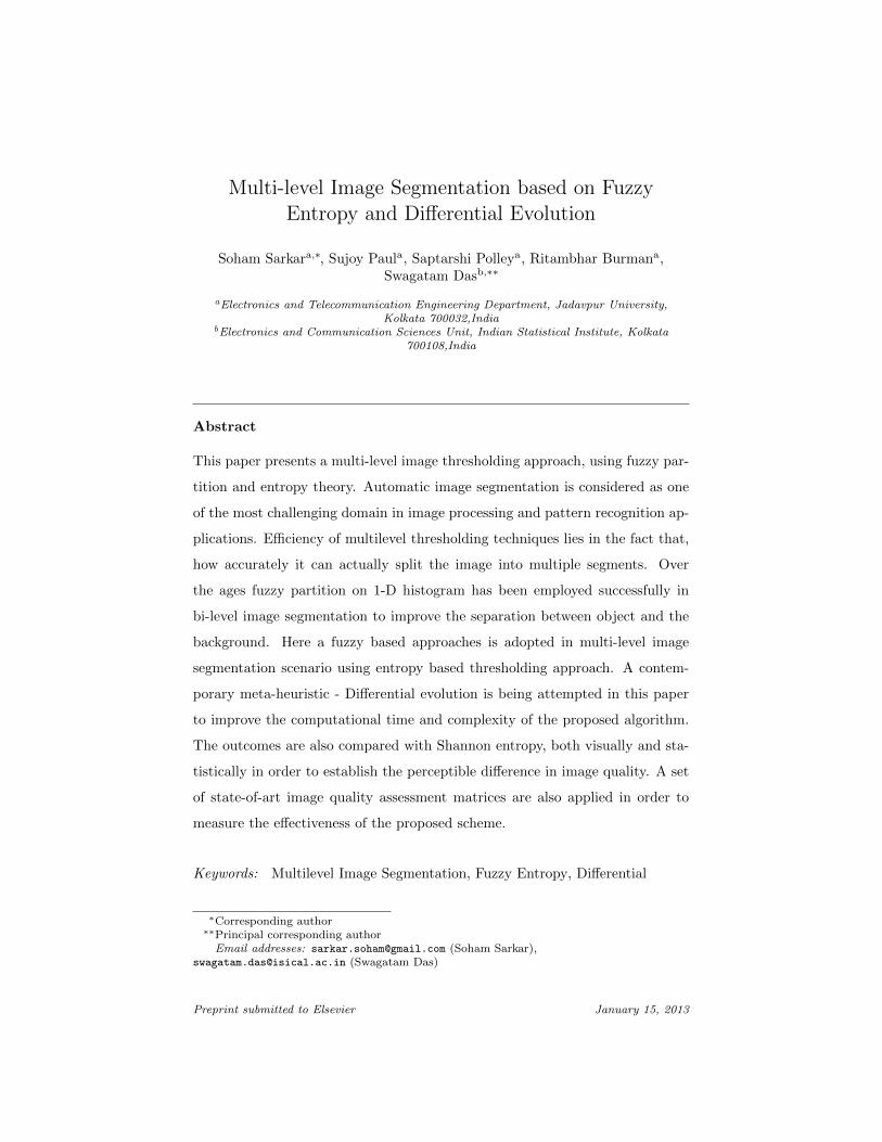
For simplicity trapezoidal membership function is used in this paper to esti-

mate the membership of µ1, µ2, µ3 of an image with 256 gray values,representing

three segmented regions.The membership function have four parameter, namely

a1, c1, a2, c2.

where 0 ≤ a1 ≤ c1 ≤ a2 ≤ c2 ≤ 255, are four unknown parameters.For each

k = 0, 1, 2, . . . , 255, let

Dk1 = (m,n) : 0 < f(m,n) ≤ t1, (m,n) ∈ Dk

Dk2 = (m,n) : t1 < f(m,n) ≤ t2, (m,n) ∈ Dk

Dk3 = (m,n) : t2 < f(m,n) < 255, (m,n) ∈ Dk

Then the following equation can be derived by assuming partition probability

and conditional probability are same for a particular region

p1 =

255∑k=0

pk ∗ µ1(k)

p2 =

255∑k=0

pk ∗ µ2(k)

p3 =

255∑k=0

pk ∗ µ3(k)

(5)

µ1, µ2 and µ3 are membership function 3 regions , represent dark, medium and

bright classes respectively.For simplicity a trapezoidal membership function is

used in this paper. The ideal membership function is displayed in Figure. 1.

µ1(k) =

1 k ≤ a1

k−c1a1−c1 a1 < k ≤ c1

0 k > c1

(6a)

7

µ2(k) =

0 k ≤ a1

k−a1

c1−a1a1 < k ≤ c1

1 c1 < k ≤ a2

k−c2a2−c2 a2 < k ≤ c2

0 k > c2

(6b)

µ3(k) =

1 k ≤ a2

k−a2

c2−a2a2 < k ≤ c2

1 k > c2

(6c)

Figure 1: Fuzzy membership function for 3 - level segmentation

2.1.3. Maximum Fuzzy Entropy

The maximum Fuzzy Entropy for each segment can be defined by

H1 = −255∑k=0

pk ∗ µ1(k)

p1∗ ln

(pk ∗ µ1(k)

p1

)H2 = −

255∑k=0

pk ∗ µ2(k)

p2∗ ln

(pk ∗ µ2(k)

p2

)H3 = −

255∑k=0

pk ∗ µ3(k)

p3∗ ln

(pk ∗ µ3(k)

p3

) (7)

8

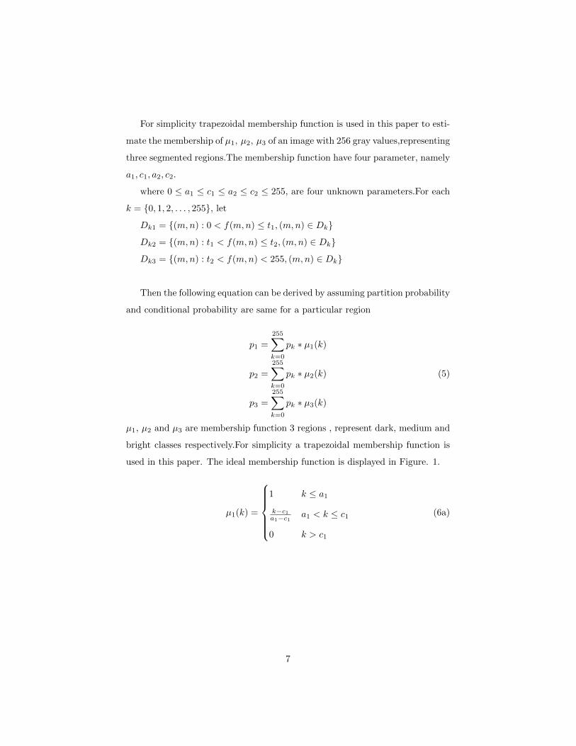
The optimal values of parameters can be found by maximizing the total entropy

H(a1, c1, a2, c2) = Argmax[H1 +H2 +H3]. (8)

A constrained Differential Evolution us used in this paper to find the opti-

mum value of the parameters and also to maintain the order of the parameters

. The two thresholds values,named as t1, t2 is determined by using a1, c1, a2, c2.

t1 =1

2(a1 + c1), t2 =

1

2(a2 + c2) (9)

2.2. (n+1)- level segmentation

Similar to the 3-level thresholding approach (n+1 )level thresholding is also

designed in this paper.t1, t2, . . . tn thresholds are used to subdivide the image

into (n+1) segments.

2.2.1. Fuzzy C-Partition

The same trapezoidal membership function is also used in (n+1)-level thresh-

olding to estimate the membership of (n+1) segmented regions, µ1, µ2, . . . , µn+1

bu using n threshold values.The membership function have 2× n unknown pa-

rameter, namely a1, c1, . . . , an, cn.where 0 ≤ a1 ≤ c1 ≤ . . . ≤ a3 ≤ c3 ≤ 255.For

each k = 0, 1, 2, . . . , 255, let

Dk1 = (m,n) : 0 < f(m,n) ≤ t1, (m,n) ∈ Dk

Dk2 = (m,n) : t1 < f(m,n) ≤ t2, (m,n) ∈ Dk

...

Dk(n+1) = (m,n) : tn < f(m,n) < 255, (m,n) ∈ Dk

Then the following equation can be derived by assuming partition probability

and conditional probability are same for a particular region

9

p1 =

255∑k=0

pk ∗ µ1(k)

p2 =

255∑k=0

pk ∗ µ2(k)

...

pn+1 =

255∑k=0

pk ∗ µn+1(k)

(10)

And the membership function for (n+1) level segmentation is calculated as

follows

µ1(k) =

1 k ≤ a1

k−c1a1−c1 a1 < k ≤ c1

0 k > c1

(11a)

µn(k) =

0 k ≤ an−1

k−an−1

cn−1−an−1an−1 < k ≤ cn−1

1 cn−1 < k ≤ ank−cnan−cn an < k ≤ cn

0 k > cn

(11b)

...

µn+1(k) =

1 k ≤ ank−an

cn−anan < k ≤ cn

1 k > cn

(11c)

The ideal membership trapezoidal function for (n+1) - level segmentation

is shown in Figure. 2

10

Figure 2: Fuzzy membership function for (n+1) - level segmentation

2.2.2. Maximum Fuzzy Entropy

The maximum Fuzzy Entropy for each segment of (n+1) - level segmentation

can be defined by

H1 = −255∑k=0

pk ∗ µ1(k)

p1∗ ln

(pk ∗ µ1(k)

p1

)H2 = −

255∑k=0

pk ∗ µ2(k)

p2∗ ln

(pk ∗ µ2(k)

p2

)...

Hn+1 = −255∑k=0

pk ∗ µn+1(k)

pn+1∗ ln

(pk ∗ µn+1(k)

pn+1

)(12)

The optimal values of parameters can be found by maximizing the total entropy

H(a1, c1, . . . , an, cn) = Argmax[H1 +H2 + . . .+Hn+1]. (13)

A constrained Differential Evolution is also used here to optimize the equa-

tion no (13) . Similar with two level thresholding the n no of threshold values

is determined by using a1, c1, . . . , an, cn.

t1 =1

2(a1 + c1), t2 =

1

2(a2 + c2), . . . tn =

1

2(an + cn) (14)

11

3. Differential Evolution(DE)

DE, a population-based global optimization algorithm, was proposed by

Storn in 1997 [17]. The ith individual (parameter vector) of the population

at generation (time) t is a D-dimensional vector containing a set of D optimiza-

tion parameters:

−→Z l(t) = [Zi,1(t), Zi,2(t), . . . , Zi,D(t)] (15)

In each generation to change the population members−→Z l(t) (say), a donor

vector−→Y l(t) is created. It is the method of creating this donor vector that

distinguishes the various DE schemes. In one of the earliest variants of DE,

now called DE/rand/1 scheme, to create−→Y l(t) for each ith member, three other

parameter vectors (say the r1, r2, and r3−th vectors such that r1, r2, r3 ∈ [1, NP ]

and r1 6= r2 6= r3 ) are chosen at random from the current population. The donor

vector−→Y l(t) is then obtained multiplying a scalar number F with the difference

of any two of the three. The process for the jth component of the ith vector

may be expressed as,

−→Y l,j(t) = Zr1,j(t) + F.(Zr2,j(t)− Zr3,j(t)) (16)

A binomial crossover operation takes place to increase the potential diver-

sity of the population. The binomial crossover is performed on each of the D

variables whenever a randomly picked number between 0 and 1 is within the Cr

value. In this case the number of parameters inherited from the mutant has a

(nearly) binomial distribution. Thus for each target vector−→Z l(t), a trial vector

−→R l(t) is created in the following fashion:

−→R i,j(t) =

−→Y i,j(t) if randj(0, 1) ≤ Cr orj = rn(i)

−→Z i,j(t) if randj(0, 1) > Cr orj 6= rn(i)

(17)

For j = 1, 2, . . . , D and randj(0, 1) ∈ [0, 1] is the jth evaluation of a uniform

random number generator. rn(i) ∈ [1, 2, . . . , D] is a randomly chosen index to

ensures that−→R l(t) gets at least one component from

−→Z l(t). Finally ’selection’

12

is performed in order to determine which one between the target vector and

trial vector will survive in the next generation i.e. at time t = t + 1. If the trial

vector yields a better value of the fitness function, it replaces its target vector

in the next generation; otherwise the parent is retained in the population:

−→Z l(t+ 1) =

−→R l(t) if f(

−→R l(t)) ≤ f(

−→Z l(t))

−→Z l(t) if f(

−→R l(t)) > f(

−→Z l(t))

(18)

Here in this paper a constrained DE is used to maintain order of the fuzzy

parameter.As it is maximization problem , the function is by 100 if any of the

parameter value is found similar with other.

−→Z l(t+ 1) =

−→Z l(t)− 100 if a1 = c1 = a2 = c2 = a3 = c3

−→Z l(t) otherwise

(19)

4. Results

The simulations are performed with MATLAB R2011b in a workstation

with Intel Core i3 3.2 GHz processor. For testing and analysis, 8 images

are used from the Berkeley Segmentation Dataset and Benchmark (obtain-

able from http://www.eecs.berkeley.edu/Research/Projects/CS/vision/

bsds/).The original gray scale image and its histograms are shown in Figure. 3

Segmented images fs(x, y)are formed as gray scale images by using the following

equation and the achieved threshold values.

fs(x, y) = k × bL− 1

n+ 1c if tk−1 < f(x, y) ≤ tk (20)

where n is the no of thresholds and k = 1, 2, . . . , n+ 1

The effectiveness of the fuzzy based approach is established by compar-

ing the results with Shannon entropy in terms of both graphical and statistical

analysis.Performance of proposed method is tested with the help of several well-

known image quality assessment matrices like Mean Structural Similarity Index

13

1.(a) 1.(b)

2.(a) 2.(b)

3.(a) 3.(b)

4.(a) 4.(b)

5.(a) 5.(b)

Figure 3: Test Images: 1.14037 2. 37073 3. 55067 4. 65010 5. 23084. (a) original gray scale

Image and (b) histogram of the respective images

14

Measurement Index (MSSIM),Feature similarity (FSIM) index , Gradient Sim-

ilarity Measurement(GSM) and Complex Wavelet Structural Similarity Index

Measurement(CW-SSIM).

SSIM method , a spatial domain technique to evaluating image quality, con-

siders image degradation as perceived change in structural information [21].Given

original image as x = xi|i = 1, 2, . . .M and segmented image as y = yi|i =

1, 2, . . .M, the SSIM index can be defined as

SSIM(x, y) =(2µxµy + C1)(2σxy + C2)

(µ2xµ

2y + C1)(σ2

x + σ2y + C2)

(21)

where µ, σ are the sample mean intensity of the images , standard deviation

or co-variance of original image and segmented image,and C1 and C2 are two

positive stabilizing constants,respectively.In this paper mean SSIM (MSSIM)

index to evaluate the overall image quality. MSSIM can be defined as

MSSIM(x, y) =1

M

M∑j=1

SSIM(xj , yj) (22)

FSIM is used to measure the similarity between original image and seg-

mented image mainly according to its low-level features like Phase Congru-

ency (PC) and Image Gradient Magnitude (GM) [22].The FSIM for two images

f1(x), f2(x) can be defined as

FSIM(x, y) =

∑x∈Ω SL(x).PCm(x)∑

x∈Ω PCm(x)(23)

where Ω means the whole image in spatial domain.PCm is the maximum of

PC1, PC2 denoting the PC component of f1(x), f2(x) respectively.

SL(x) = SPC(x).SG(x), is combination of similarity of PC , i.e.SPC(x) and

similarity of GM , i.e. SG(x).SPC(x), SG(x) is measured for f1(x), f2(x) as

SPC(x) =2PC1.PC2 + T1

PC21 + PC2

1 + T1(24)

15

SG(x) =2G1.PC2 + T2

G21 +G2

1 + T2(25)

T1, T2 are positive constants.Here T1 = 0.85 and T2 = 160

GSM is a IQA emphasis on gradient similarity [23].If gx, gy are the gradient

values for the central pixel of the images x and y ,then GSM is calculated as

follows

g(x, y) =2(1−R) +K

2 + (1−R)2 +K(26)

where R =|gx−gy|

max(gx,gy) , K = C4

max(gx,gy)2 and C4 is a small constant to avoid

the denominator being zero.

CW-SSIM index is a image similarity measurement technique is developed

to measure local phase in complex wavelet domain[24].As local phase pattern

contains more structural information than local magnitude, the CW-SSIM is

designed to separate phase from magnitude distortion measurement and impose

more penalty to inconsistent phase distortions.Let cx = cx,i|i = 1, 2, . . . N

and cy = cy,i|i = 1, 2, . . . N are two sets of coefficients extracted at the same

spatial location in the same wavelet sub-bands of original image and segmented

image respectively. The CW-SSIM can be defined as

CWSSIM(cx, cy) =2|∑N

i=1 cx,ic∗x,i|+K∑N

i=1 cx,i|2 +∑N

i=1 c2y,i +K

(27)

A constraint differential evolution is applied here to achieve lesser compu-

tational time. The parametric setup of DE is given in Table. 1. Results are

acquired for 3 - level and 4- level segmentation. The acquired threshold value for

3 and 4 level segmentation and the value of the parameters for the membership

function are displayed in Table. 2 and Table. 3 respectively. The membership

functions are exhibited in Figure 4. 3 - level segmented gray scale images ac-

quired by Shannon entropy and fuzzy entropy using the threshold values given

16

Table 1: Experimental set up for DE/rand/1

Parameter V alue

No. of Runs 50

No. of Iteration in each run 500

D 2 and 3 depending on number of thresholds

NP 10×D

Min val Minimum value of histogram

Max val Maximum value of histogram

F 0.5

CR 0.9

Table 2: Threshold values obtained for 3 level segmentation

Image ShanonEntropy FuzzyEntropy a1 c1 a2 c2

14037 128 198 89 217 0 177 178 255

37073 84 147 57 173 0 114 115 230

55067 97 149 94 181 54 133 134 228

65010 118 185 63 191 0 126 127 255

23084 101 174 74 202 0 148 149 255

Table 3: Threshold values obtained for 4 level segmentation

Image ShanonEntropy FuzzyEntropy a1 c1 a2 c2 a3 c3

14037 91 142 201 67 157 218 0 133 134 180 181 255

37073 83 130 182 58 129 199 0 116 117 141 142 255

55067 95 130 195 63 128 176 0 126 127 128 129 223

65010 68 125 188 63 127 192 0 125 126 128 129 255

23084 71 126 183 66 134 196 0 132 133 135 136 255

17

1.(c) 1.(d)

2.(c) 2.(d)

3.(c) 3.(d)

4.(c) 4.(d)

5.(c) 5.(d)

Figure 4: Test Images: 1.14037 2. 37073 3. 55067 4. 65010 5. 23084. (c) membership

function for 3 - level and (d) membership function for 4 - level

18

1.(e) 1.(f)

2.(e) 2.(f)

3.(e) 3.(f)

4.(e) 4.(f)

5.(e) 5.(f)

Figure 5: Test Images: 1. 14037 2. 37073 3. 55067 4. 65010 5. 23084. (e) 3 - Level Shanon

Entropy, (f) 3 - Level Fuzzy Entropy.

19

in Table. 2 are shown in Figure. 5 . It is clearly visible from the images that

fuzzy entropy performs significantly better than Shannon entropy. Interestingly,

for some images differences are much profound. In Figure. 5 .1. (e) the ob-

ject on the top of the hill in not visible , whereas it is clearly distinguishable

against the hill and sky in Figure. 5. 1.(f) using fuzzy entropy. The plain is

glaringly visible from its shadow and the runway in Figure. 5. 2.(f), which is

not that much prominent in Figure. 5. 2.(e) using Shannon entropy. Figure.

5. 3. (a) is supposedly a very critical image for segmentation. As well as, in

this case fuzzy entropy (Figure. 5.3.(f)) performs better than Shannon entropy(

Figure. 5. 3.(e)) . The best improvement of results could be noticed in Figure.

5. 4. (f), where the trees, house, lake and shadows in the water are distinctly

separable. However using Shannon entropy in Figure. 5. 4.(e) the results are

utterly inseparable. In Figure. 5. 5.(f) also the the circuits are more visible in

comparison with Figure. 5. 5.(e).

Similar kind of improvement of outcomes could be observed in Figure. 6

for 4 - level segmentation using fuzzy entropy over Shannon entropy, specially

in g 1.(h) where the lake is better visible than Figure. 6. 1. (g). In Figure.

6. 3. (h) it clearly exhibits a better separation in comparison to Figure. 6.

3. (g) .The outcomes of Figure. 5 and Figure. 6. are well supported by the

results of statistical analysis which is given in Table. 4. It done via performance

evolution matrices. The best results are displayed in bold letters. Here too the

fuzzy entropy outperforms the Shannon entropy to a great extent.

5. Conclusion

It can be concluded from the above discussion that Fuzzy entropy based

thresholding methods for multi-level segmentation performs significantly bet-

ter than Shannon based approaches .Fuzzy entropy based thresholding tech-

niques delivers satisfactory results in case of visual comparison. This claims

are doubtlessly established via state-of-art image quality assessments metrics

20

1.(g) 1.(h)

2.(g) 2.(h)

3.(g) 3.(h)

4.(g) 4.(h)

5.(g) 5.(h)

Figure 6: Test Images: 1. 14037 2. 37073 3. 55067 4. 65010 5. 23084. (g) 4 - Level Shanon

Entropy and (h) 4 - Level Shanon Entropy

21

Table 4: Image quality assessment matrices for 3 level segmentation

3− Level 4− Level

Image Metrices Shanon Fuzzy Shanon Fuzzy

14037

MSSIM

FSIM

GSM

CW-SSIM

0.1190

0.6291

0.9557

0.6784

0.3372

0.6372

0.9624

0.7505

0.3144

0.6621

0.9632

0.8291

0.4221

0.7121

0.9704

0.8879

37073

MSSIM

FSIM

GSM

CW-SSIM

0.5857

0.6938

0.9609

0.7703

0.6302

0.7066

0.9648

0.8398

0.6143

0.7354

0.9699

0.9054

0.6605

0.7428

0.9722

0.9580

55067

MSSIM

FSIM

GSM

CW-SSIM

0.4566

0.7757

0.9712

0.5999

0.5007

0.7957

0.9741

0.6210

0.4897

0.7956

0.9763

0.6844

0.7430

0.8425

0.9829

0.8147

65010

MSSIM

FSIM

GSM

CW-SSIM

0.1419

0.557

0.9373

0.7884

0.4616

0.6171

0.9411

0.8323

0.4866

0.6953

0.9586

0.9138

0.5208

0.6996

0.9605

0.9287

23084

MSSIM

FSIM

GSM

CW-SSIM

0.3451

0.6544

0.9433

0.8671

0.4448

0.6637

0.9470

0.8888

0.5078

0.7188

0.9595

0.9326

0.5378

0.7282

0.9616

0.9533

22

like MSSIM, FSIM, GSM and CW-SSIM. Hence use of this metrics in image

segmentation circumstances is also justified.Undisputedly, DE adds speed and

accuracy to this algorithm. However, a better constrained DE or other upgraded

variants of DE could be used to attain better performance. Also several other

membership functions could be tested for better separation of the segmented

regions. More image performance metrics could be used in future to prove the

competence of segmentation algorithms. Lastly, 2-D histogram based approach

could be implemented in order to get improved outcomes.

6. References

References

[1] E.M.Riseman , M.A.Arbib, Survey: computational techniques in the visual

segmentation of static scenes, Comput. Vision Graphics Image Process. 6

(1977), 221 - 276 .

[2] J.S.Weszka, A survey of threshold selection techniques, CGIP. 7 ( 1978),

259 - 265.

[3] K.S.Fu , J.K.Mui, A survey on image segmentation, Pattern Recognition.

13 ( 1981) , 3 - 16.

[4] R.M.Haralharick , L.G.Shapiro, Survey: image segmentation techniques,

CVGIP. 29 (1985), 100 - 132.

[5] V.I.Borisenko, A.A.Zlatotol , I.B.Muchnik, Image segmentation (state of

the art survey), Automat.Remote Control. 48 (1987), 837 - 879.

[6] P.K.Sahoo, S.Soltani, A.K.C.Wong , Y.C.Chen, A survey of thresholding

techniques , CVGIP . 41 (1988) , 233 - 260.

[7] N. R. Pal , S. K. Pal, A review on image segmentation, Pattern Recognition.

26 (9) (1993), 1277 - 1294, .

23

[8] J.N. Kapur, P.K.Sahoo, A.K.C Wong, A new method for gray-level picture

thresholding using the entropy of the histogram , Comput. Vision Graphics

Image Process. 29 (1985) , 273 - 285.

[9] A.K.C.Wong,P.K. Sahoo, A gray-level threshold selection method based

on maximum entropy principle, IEEE Trans. Systems Man Cybernet. 19

(1989) , 866 - 871.

[10] N. R. Pal, On minimum cross entropy thresholding, Pattern Recognition.

29 (4) (1996) , 575 - 580.

[11] C.H. Li,C.K. Lee, Minimum cross entropy thresholding ,Pattern Recogni-

tion. 26 (1993), 617 - 625.

[12] P.L. Rosin, Unimodal thresholding, Pattern Recognition. 34 (2001), 2083 -

2096.

[13] Otsu,A threshold selection method for grey level histograms,IEEE Trans-

actionsonSystem,ManandCybernetics SMC. 9 (1) (1979), 62 - 66.

[14] A.D. Luca, S. Termini, Definition of a non probabilistic entropy in the

setting of fuzzy sets theory, Inf. contr. 20 (1972), 301 - 315.

[15] M.S. Zhao, A.M.N. Fu, H. Yan, A technique of threelevel thresholding

based on probability partition and fuzzy 3-partition, IEEE Trans. Fuzzy

Systems 9 (3) (2001), 469 - 479.

[16] W.B. Tao , J.W. Tian, J. Liu, Image segmentation by three-level thresh-

olding based on maximum fuzzy entropy and genetic algorithm, Pattern

Recognition Letters. 24 (2003), 3069 - 3078.

[17] R. Storn, K. Price, Differential evolution - a simple and efficient heuristic for

global optimization over continuous spaces, Journal of Global Optimization

11 (1997), 341 - 359.

24

[18] S. Das, , P. N. Suganthan, Differential evolution - a survey of the state-of-

the-art, IEEE Transactions on Evolutionary Computation. 15 (1) (2011),

4 - 31.

[19] S. Sarkar, G. R. Patra, S. Das, A Differential Evolution Based Approach

for Multilevel Image Segmentation Using Minimum Cross Entropy Thresh-

olding, SEMCCO LNCS. 7076 (2011), 51 - 58.

[20] S. Sarkar, S. Das, S. S. Chaudhuri, Multilevel Image Thresholding Based on

Tsallis Entropy and Differential Evolution,SEMCCO LNCS. 7677 (2012),

17 - 24.

[21] Z. Wang, A. Bovik, H. Sheikh, E. Simoncelli, Image quality assessment:

From error visibility to structural similarity,IEEE Transactions on Image

Processing. 13 (4) (2004), 600 612.

[22] Lin Zhang, Lei Zhang, Xuanqin Mou, David Zhang, FSIM: A feature sim-

ilarity index for image quality assessment, IEEE Transactions on Image

Processing. 20(8) (2011), 2378 - 2386.

[23] J. Zhu, N. Wang, Image Quality Assessment by Visual Gradient Similarity.

IEEE Transactions on Image Processing, 21 (3) (2012), 919 - 933.

[24] M. P. Sampat, Z. Wang, S. Gupta, A. C. Bovik, M. K. Markey, Complex

wavelet structural similarity: A new image similarity index. IEEE Trans-

actions on Image Processing, 18 (11)(2009), 2385 2401.

25