Progress curve analysis for enzyme and microbial kinetic reactions using explicit solutions based on...

www.elsevier.com/locate/jmicmeth

Journal of Microbiological Methods 5

Progress curve analysis for enzyme and microbial kinetic reactions

using explicit solutions based on the Lambert W function

Chetan T. Goudara,*, Steve K. Harrisb,1, Michael J. McInerneyb, Joseph M. Suflitab

aProcess and Technology Development, Bayer HealthCare, Biological Products Division, 800 Dwight Way, B56-A, Berkeley,

CA 94710, United StatesbDepartment of Botany and Microbiology, Institute for Energy and the Environment, University of Oklahoma, Norman,

OK 73019, United States

Received 23 December 2003; received in revised form 30 June 2004; accepted 30 June 2004

Available online 16 September 2004

Abstract

We present a simple method for estimating kinetic parameters from progress curve analysis of biologically catalyzed

reactions that reduce to forms analogous to the Michaelis–Menten equation. Specifically, the Lambert W function is used to

obtain explicit, closed-form solutions to differential rate expressions that describe the dynamics of substrate depletion. The

explicit nature of the new solutions greatly simplifies nonlinear estimation of the kinetic parameters since numerical techniques

such as the Runge–Kutta and Newton–Raphson methods used to solve the differential and integral forms of the kinetic

equations, respectively, are replaced with a simple algebraic expression. The applicability of this approach for estimating Vmax

and Km in the Michaelis–Menten equation was verified using a combination of simulated and experimental progress curve data.

For simulated data, final estimates of Vmax and Km were close to the actual values of 1 AM/h and 1 AM, respectively, while the

standard errors for these parameter estimates were proportional to the error level in the simulated data sets. The method was also

applied to hydrogen depletion experiments by mixed cultures of bacteria in activated sludge resulting in Vmax and Km estimates

of 6.531 AM/h and 2.136 AM, respectively. The algebraic nature of this solution, coupled with its relatively high accuracy,

makes it an attractive candidate for kinetic parameter estimation from progress curve data.

D 2004 Published by Elsevier B.V.

Keywords: Kinetics; Lambert W function; Michaelis–Menten equation; Nonlinear parameter estimation; Progress curve analysis

0167-7012/$ - see front matter D 2004 Published by Elsevier B.V.

doi:10.1016/j.mimet.2004.06.013

* Corresponding author. Tel.: +1 510 705 4851; fax: +1 510

705 5451.

E-mail address: [email protected] (C.T. Goudar).1 Current address: U.S. Geological Survey, 3215 Marine St.,

Suite E-129, Boulder, CO 80303, United States.

1. Introduction

The Michaelis–Menten equation has been widely

used to describe the kinetics of enzyme-catalyzed

reactions (Michaelis and Menten, 1913). Applications

also include non-growing microbial suspensions

where substrate consumption takes place in the

9 (2004) 317–326

C.T. Goudar et al. / Journal of Microbiological Methods 59 (2004) 317–326318

absence of active microbial growth (Betlach and

Tiedje, 1981; Pauli and Kaitala, 1997; Suflita et al.,

1983). Awide variety of data analysis techniques have

been developed to obtain the kinetic parameters Vmax

and Km, the maximal rate, and half-saturation con-

stant, respectively (Atkins and Nimmo, 1975; Nimmo

and Atkins, 1974; Duggleby, 1995). The most widely

used approach is graphical where the Michaelis–

Menten equation is linearized by algebraic manipu-

lation. This linear equation is subsequently plotted as

a straight line in rectangular coordinates and the

parameters Vmax and Km are estimated by linear least

squares analysis. Graphical methods of kinetic anal-

ysis of substrate–velocity data pairs are well known

(Cornish-Bowden, 1995) and include the direct linear

plot that does not involve any algebraic manipulations

(Eisenthal and Cornish-Bowden, 1974; Cornish-

Bowden, 1975). While graphical methods possess

the unique advantage of providing a visual representa-

tion of experimental data, their parameter estimates can

be very inaccurate. This is primarily because a linear

transformation of an inherently nonlinear equation,

such as the Michaelis–Menten expression, distorts the

error in the measured variables and this can subse-

quently impact estimates of the salient kinetic param-

eters (Cornish-Bowden, 1995; Robinson, 1985;

Leatherbarrow, 1990; Duggleby, 1991).

Some of the limitations described above can be

avoided through the coupling of nonlinear parameter

estimation techniques and progress curve analysis.

This approach involves the use of substrate depletion/

product accumulation determinations over time rather

than initial velocity–substrate concentration data pairs

to estimate Vmax and Km (Duggleby, 1994, 1995;

Duggleby and Morrison, 1977; Duggleby and Wood,

1989; Fernley, 1974; Zimmerle and Frieden, 1989). In

addition to the potential for obtaining improved

parameter estimates, this method is consistent with

most experimental designs that typically involve

monitoring either substrate or product concentration

over time. Despite the obvious advantages of progress

curve analyses as described elsewhere (Duggleby,

1995; Robinson, 1985), this method is not commonly

used for kinetic parameter estimation. This is because

of the computational difficulties associated with

progress curve analysis. The integral form of the

Michaelis–Menten equation is implicit in the substrate

concentration. As a result, numerical approaches such

as bisection and Newton–Raphson methods are

necessary to compute substrate concentration in the

integrated Michaelis–Menten equation (Duggleby,

1995). Alternatively, substrate concentration must be

calculated by numerically integrating the differential

form of the Michaelis–Menten equation (Zimmerle

and Frieden, 1989; Duggleby, 1994, 2001). Kinetic

parameter estimation in the Michaelis–Menten equa-

tion is a multidimensional approach that involves

using one of the numerical techniques described

above to solve the Michaelis–Menten equation fol-

lowed by an iterative estimation of the kinetic

parameters Vmax and Km using an appropriate non-

linear optimization routine. Implementation of a

robust nonlinear kinetic parameter estimation

approach can be difficult when there is inadequate

experience in numerical techniques and computer

programming. We believe a simplification in kinetic

parameter estimation from progress curve data can

make this approach more appealing to a wider group

of experimentalists.

While the implicit nature of the Michaelis–Menten

equation presents computational difficulties, the first

truly explicit solution of the Michaelis–Menten

equation was derived only recently through the use

of computer algebra (Schnell and Mendoza, 1997) and

we have independently verified that this solution can

be used to accurately calculate substrate concentration

(Goudar et al., 1999). The availability of this explicit

solution of the Michaelis–Menten expression has

significant implications for simplifying estimation of

Vmax and Km through progress curve analysis.

Specifically, this approach replaces numerical solution

of a differential/nonlinear equation with the evaluation

of a simple algebraic expression that provides highly

accurate values of the substrate concentration. The

algebraic nature of this solution coupled with its

relatively high accuracy makes it an attractive

candidate for use in nonlinear kinetic parameter

estimation from progress curve data.

In the present study, we present a brief derivation

of the explicit solution for the Michaelis–Menten

equation and illustrate its application for estimating

Vmax and Km from simulated and experimental

substrate concentration data. We also show that this

approach is general and can be applied to any kinetic

expression that can be reduced to a form analogous to

the Michaelis–Menten equation. We have developed a

C.T. Goudar et al. / Journal of Microbiological Methods 59 (2004) 317–326 319

suite of computer programs in MATLAB (The Math-

works, Natick, MA) that use this explicit solution for

kinetic parameter estimation and these programs are

available free of charge for academic use from the

corresponding author.

2. Theory

The Michaelis–Menten equation in the differential

form can be used to describe the dynamics of substrate

depletion as

dS

dt¼ � VmaxS

Km þ Sð1Þ

where S is the substrate concentration, and Vmax and

Km are the maximal rate and Michaelis half saturation

constant, respectively. Eq. (1) can be readily inte-

grated to obtain the integral form of the Michaelis–

Menten equation

KmlnS0

S

�þ S0 � S ¼ Vmaxt

�ð2Þ

where S0 is the initial substrate concentration. Eq. (2)

is nonlinear and clearly implicit with respect to the

substrate concentration. Hence, numerical approaches

such as bisection and Newton–Raphson methods are

necessary to calculate S. In order to obtain the explicit

form of Eq. (2), we rearrange to form

S þ Kmln Sð Þ ¼ S0 þ Kmln S0ð Þ � Vmaxt ð3Þ

Substituting /=S/Km in Eq. (3) results in

/Km þ Kmln /Kmð Þ ¼ S0 þ Kmln S0ð Þ � Vmaxt ð4Þ

Dividing Eq. (4) by Km and rearranging results in

/ þ ln /ð Þ ¼ S0

Km

þ lnS0

Km

�� Vmaxt

Km

�ð5Þ

The left hand side of Eq. (5) is analogous to the

Lambert W function (Corless et al., 1996).

W xð Þ þ ln W xð Þf g ¼ ln xð Þ ð6Þ

where W is the Lambert W function and x the

argument of W. From Eqs. (5) and (6), an expression

for / may be obtained as

/ ¼ WS0

Km

expS0 � Vmaxt

Km

�� ð7Þ

As /=S/Km, Eq. (7) can be written in terms of S as

S ¼ KmWS0

Km

expS0 � Vmaxt

Km

�� ð8Þ

Eq. (8), derived from Eq. (2), explicitly relates the

substrate concentration to the initial substrate con-

centration, S0, and the kinetic parameters Vmax and

Km. Substrate concentrations can be readily esti-

mated from Eq. (8) which is a simple algebraic

expression.

While the above derivation of the explicit solution

has been for the Michaelis–Menten equation, it is

equally applicable to several other kinetic models that

reduce to forms analogous to the Michaelis–Menten

equation. For instance, inhibition reaction me-

chanisms such as competitive, uncompetitive, non-

competitive and mixed inhibition can all be reduced to

forms that are analogous to Eq. (1) with different

definitions of Vmax and Km. Hence, they all have

explicit closed-form solutions similar to Eq. (8) that

can be used for progress curve analysis.

3. Materials and methods

3.1. Evaluating W

There are several methods for computing the value

of W as defined by Eq. (6) (Barry et al., 1995a,b;

Fritsch et al., 1973). These algorithms are extremely

robust and fairly simple to use with one method

(Fritsch et al., 1973) converging in a single iteration.

The FORTRAN source code implementing the

method in Fritsch et al. (1973) is presented in the

original publication while that for the method in Barry

et al. (1995a) can be obtained from http://www.netlib.

org/toms/743. In the present study, we have used the

MAPLER (Waterloo Maple) implementation of the W

function as described in Corless et al. (1996).

http://www.netlib.org/toms/743


3.2. Substrate depletion data

To illustrate the applicability of Eq. (8) for

estimating Vmax and Km through progress curve

analysis, simulated substrate concentration data were

generated from Eq. (8) using S0=10 AM, Vmax=1.0

AM/h and Km=1.0 AM. For the resulting error-free

substrate depletion data to more realistically repre-

sent experimental observations, noise of known type

and magnitude was introduced. Normally distributed

error with a mean of zero and standard deviation

ranging from 1% to 4% of the magnitude of the

initial substrate concentration (10 AM) was gener-

ated using a pseudo-random number generator. This

noise was added to the error-free substrate concen-

tration data obtained from Eq. (8) and the resulting

data set was used for estimating Vmax and Km using

nonlinear least squares.

Experimental hydrogen depletion data were

obtained with sewage sludge that was collected

from the primary digestor at the municipal treat-

ment plant in Norman, OK. Hydrogen partitioning

was mass transfer limited in incubations of undi-

luted sludge. To overcome this, sludge was

centrifuged at 15,000�g for 20 min. The resulting

supernatant was used as a diluent to make a sludge

preparation (10%) that was not mass transfer

limited. Diluted sludge (0.5 l) was transferred to a

2-l Erlenmeyer flask under constant sparging with

N2/CO2 (80%/20%). The flask was stoppered,

placed at 37 8C and constantly stirred. Hydrogen

(50 ml) was injected into the headspace of the flask

to begin the assay. Hydrogen consumption was

monitored by periodically removing headspace

samples and analyzing them by gas chromatography

(RGA3 Gas Analyzer, Trace Analytical, Sparks,

MD).

3.3. Initial kinetic parameter estimates through

linearization

Given the iterative nature of nonlinear least squares

analysis, initial estimates of the parameters are

necessary. These initial estimates are typically

obtained through linearization of the original non-

linear equation and it is important that they be as

accurate as possible since the final solution can be

impacted. The integrated Michaelis–Menten can be

linearized in three different ways (Robinson and

Characklis, 1984)

t

ln S=S0ð Þ ¼ 1

Vm

S0 � Sð Þln S=S0ð Þ þ Km

Vm

ð9Þ

S0 � Sð Þln S=S0ð Þ ¼ Vm � Km

tln S=S0ð Þ ð10Þ

t

S0 � Sð Þ ¼ Km

Vm

ln S=S0ð ÞS0 � Sð Þ þ 1

Vm

ð11Þ

and standard linear least squares can be used to obtain

estimates of Vmax and Km from Eqs. (9)–(11). These

initial estimates were subsequently used as starting

points for estimating Vmax and Km through nonlinear

least squares analysis as described in the following

section.

3.4. Nonlinear kinetic parameter estimation

Nonlinear kinetic parameter estimation involves

minimizing the residual sum of squares error (RSSE)

between experimental and calculated substrate con-

centration data.

Minimize RSSE ¼Xni¼1

�Sexp� �

i� Scalð Þi

2

ð12Þ

where (Sexp)i is the ith experimental substrate

concentration and (Scal)i is the ith calculated substrate

concentration in a total of i observations. Initial

estimates of Vmax and Km obtained from Eqs. (9)–(11)

were used in Eq. (8) to calculate the first set of

substrate concentration data. Subsequently, a compar-

ison was made between the experimental and calcu-

lated substrate concentrations and the RSSE was

computed from Eq. (12). The kinetic parameters were

iteratively updated using the Levenberg–Marquardt

method (Marquardt, 1963) until the RSSE in Eq. (12)

was minimized.

3.5. Computer implementation

Computer programs have been developed that

implement the parameter estimation approach outlined


in Sections 3.3 and 3.4. Experimental S versus t data

are first used to obtain initial estimates of Vmax and

Km from Eqs. (9)–(11). These initial estimates are

subsequently used to obtain final estimates of Vmax

and Km using nonlinear least squares. The output from

this analysis includes detailed statistics regarding

quality of the fit and graphical representation of the

fit to experimental data along with a plot of the

residuals. Finally, three-dimensional visualization of

the error surface in the Vmax and Km space along with

contour plots for the RSSE can be obtained. This

visualization allows observation of local minima on

the error surface and helps determine if the true global

minimum has actually been reached during nonlinear

parameter estimation.

4. Results

4.1. Lambert W function

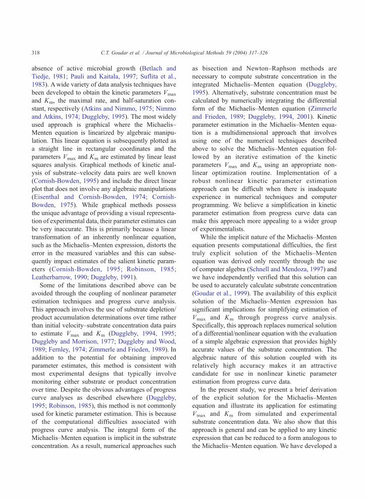
A plot of the Lambert W function as defined by Eq.

(8) is shown in Fig. 1 for real values of W. From Eq.

(8), the argument of the W function, x, corresponds to

Fig. 1. The three real branches of the Lambert W function. {(o),

xN0, Region 1; (n), �1/ebxb0 and 0NWN�1, Region 2; (4), �1/

ebxb0 and Wb�1, Region 3}.

S0Km

exp S0�Vmax tKm

�. The W function has three distinct

branches depending upon the values of x. For xN0, W

is positive and has a unique value (Region 1). For x

values in the range of �1/ebxb0, two solutions exist

on either side of W=�1 (Regions 2 and 3, respec-

tively). An examination of the above expression for x

indicates that x is always positive as Km and S0 are

always positive suggesting that unique values of W

exist for all x values of interest when applying this

solution to the Michaelis–Menten equation.

4.2. Kinetic Parameter Estimation from Simulated

Data

Simulated substrate concentration data along with

the theoretical predictions corresponding to the best fit

kinetic parameters are shown in Fig. 2. Significant

scatter in simulated substrate depletion curves is seen

for errors with standard deviations of 3% and 4% as

might be encountered in actual progress curve experi-

ments Despite the increased scatter, final estimates of

Vmax and Km were very close to the actual values of

1.0 AM/h and 1.0 AM, respectively. However, the

standard errors for both Vmax and Km increased with

increasing noise levels suggesting that greater uncer-

tainty is associated with the final estimates of the

kinetic parameters as error is amplified. The magni-

tude of the increase in standard errors for Vmax and Km

was similar to the increase in the standard deviation of

the error introduced in the simulated substrate

depletion curves.

The standard errors for Km were approximately

six-fold higher than those for Vmax at all the four noise

levels (Fig. 2) indicating higher uncertainty in the Km

estimates. Contour plots of the RSSE in the Vmax and

Km space are shown in Fig. 3 where the inner most

contours which represent the region of lowest RSSE,

extend over a wide range of Km values and only over

a very narrow range of Vmax values. This suggests

substantially lower sensitivity of the RSSE to Km

values and is consistent with the higher standard

errors for Km estimates.

High parameter correlation can adversely affect

parameter determination and must be taken into

account while assessing the quality of model fit to

experimental data. The off-diagonal element of the

parameter correlation matrix was 0.968 for all cases

indicating significant correlation between Vmax and

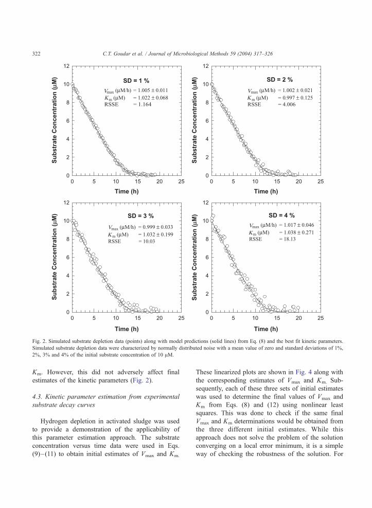
Fig. 2. Simulated substrate depletion data (points) along with model predictions (solid lines) from Eq. (8) and the best fit kinetic parameters.

Simulated substrate depletion data were characterized by normally distributed noise with a mean value of zero and standard deviations of 1%,

2%, 3% and 4% of the initial substrate concentration of 10 AM.


Km. However, this did not adversely affect final

estimates of the kinetic parameters (Fig. 2).

4.3. Kinetic parameter estimation from experimental

substrate decay curves

Hydrogen depletion in activated sludge was used

to provide a demonstration of the applicability of

this parameter estimation approach. The substrate

concentration versus time data were used in Eqs.

(9)–(11) to obtain initial estimates of Vmax and Km.

These linearized plots are shown in Fig. 4 along with

the corresponding estimates of Vmax and Km. Sub-

sequently, each of these three sets of initial estimates

was used to determine the final values of Vmax and

Km from Eqs. (8) and (12) using nonlinear least

squares. This was done to check if the same final

Vmax and Km determinations would be obtained from

the three different initial estimates. While this

approach does not solve the problem of the solution

converging on a local error minimum, it is a simple

way of checking the robustness of the solution. For

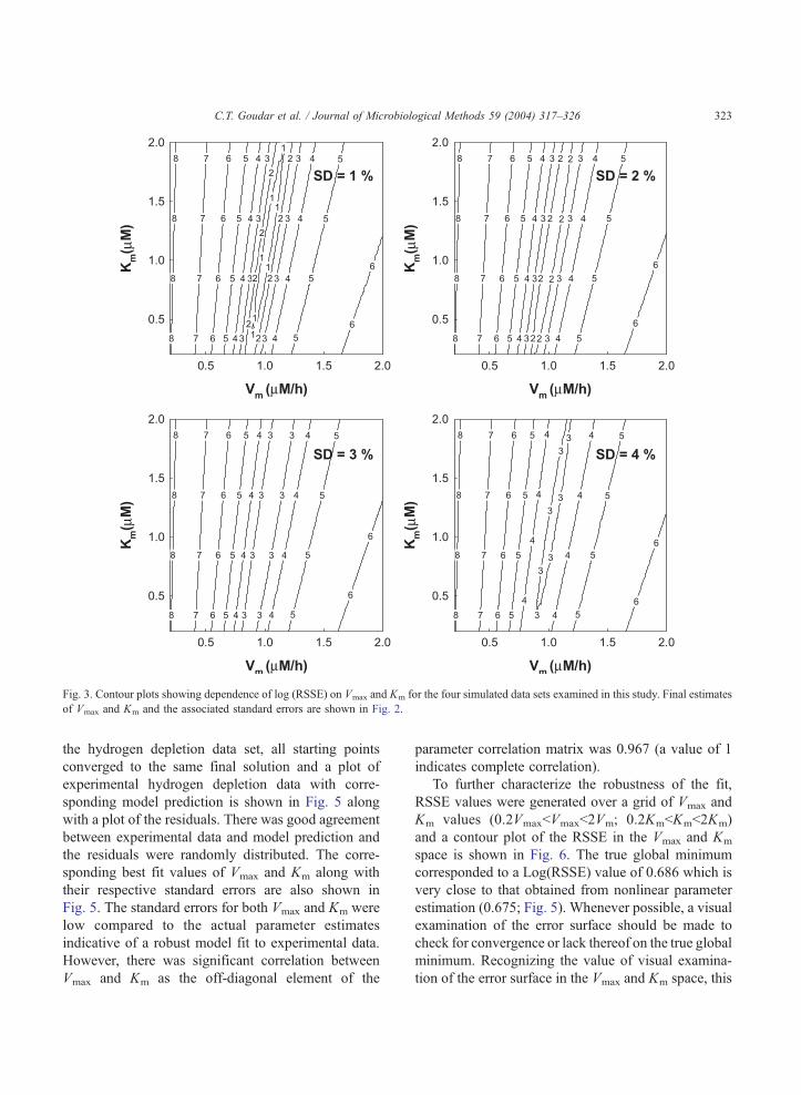
Fig. 3. Contour plots showing dependence of log (RSSE) on Vmax and Km for the four simulated data sets examined in this study. Final estimates

of Vmax and Km and the associated standard errors are shown in Fig. 2.


the hydrogen depletion data set, all starting points

converged to the same final solution and a plot of

experimental hydrogen depletion data with corre-

sponding model prediction is shown in Fig. 5 along

with a plot of the residuals. There was good agreement

between experimental data and model prediction and

the residuals were randomly distributed. The corre-

sponding best fit values of Vmax and Km along with

their respective standard errors are also shown in

Fig. 5. The standard errors for both Vmax and Km were

low compared to the actual parameter estimates

indicative of a robust model fit to experimental data.

However, there was significant correlation between

Vmax and Km as the off-diagonal element of the

parameter correlation matrix was 0.967 (a value of 1

indicates complete correlation).

To further characterize the robustness of the fit,

RSSE values were generated over a grid of Vmax and

Km values (0.2VmaxbVmaxb2Vm; 0.2KmbKmb2Km)

and a contour plot of the RSSE in the Vmax and Km

space is shown in Fig. 6. The true global minimum

corresponded to a Log(RSSE) value of 0.686 which is

very close to that obtained from nonlinear parameter

estimation (0.675; Fig. 5). Whenever possible, a visual

examination of the error surface should be made to

check for convergence or lack thereof on the true global

minimum. Recognizing the value of visual examina-

tion of the error surface in the Vmax and Km space, this

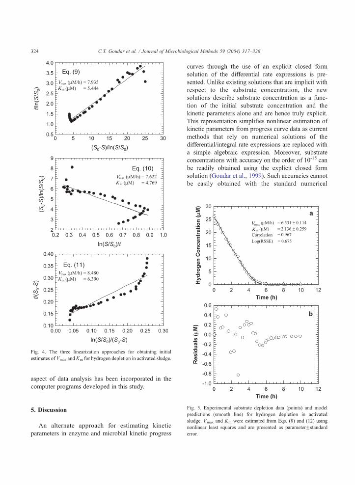
Fig. 4. The three linearization approaches for obtaining initial

estimates of Vmax and Km for hydrogen depletion in activated sludge.


aspect of data analysis has been incorporated in the

computer programs developed in this study.

Fig. 5. Experimental substrate depletion data (points) and mode

predictions (smooth line) for hydrogen depletion in activated

sludge. Vmax and Km were estimated from Eqs. (8) and (12) using

nonlinear least squares and are presented as parameterFstandard

error.

5. Discussion

An alternate approach for estimating kinetic

parameters in enzyme and microbial kinetic progress

curves through the use of an explicit closed form

solution of the differential rate expressions is pre-

sented. Unlike existing solutions that are implicit with

respect to the substrate concentration, the new

solutions describe substrate concentration as a func-

tion of the initial substrate concentration and the

kinetic parameters alone and are hence truly explicit.

This representation simplifies nonlinear estimation of

kinetic parameters from progress curve data as current

methods that rely on numerical solutions of the

differential/integral rate expressions are replaced with

a simple algebraic expression. Moreover, substrate

concentrations with accuracy on the order of 10-15 can

be readily obtained using the explicit closed form

solution (Goudar et al., 1999). Such accuracies cannot

be easily obtained with the standard numerical

l

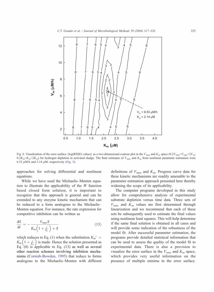
Fig. 6. Visualization of the error surface {log(RSSE) values} as a two-dimensional contour plot in the Vmax and Km space (0.2VmaxbVmaxb2Vm;

0.2KmbKmb2Km) for hydrogen depletion in activated sludge. The final estimates of Vmax and Km from nonlinear parameter estimation were

6.53 AM/h and 2.14 AM, respectively (Fig. 5).


approaches for solving differential and nonlinear

equations.

While we have used the Michaelis–Menten equa-

tion to illustrate the applicability of the W function

based closed form solution, it is important to

recognize that this approach is general and can be

extended to any enzyme kinetic mechanism that can

be reduced to a form analogous to the Michaelis–

Menten equation. For instance, the rate expression for

competitive inhibition can be written as

dS

dt¼ � VmaxS

Km 1þ iKc

þ S

� ð13Þ

which reduces to Eq. (1) when the substitution KmV¼Km 1þ i

Kc

�is made. Hence the solution presented as

Eq. (8) is applicable to Eq. (13) as well as several

other reaction schemes involving inhibition mecha-

nisms (Cornish-Bowden, 1995) that reduce to forms

analogous to the Michaelis–Menten with different

definitions of Vmax and Km. Progress curve data for

these kinetic mechanisms are readily amenable to the

parameter estimation approach presented here thereby

widening the scope of its applicability.

The computer programs developed in this study

allow for comprehensive analysis of experimental

substrate depletion versus time data. Three sets of

Vmax and Km values are first determined through

linearization and we recommend that each of these

sets be subsequently used to estimate the final values

using nonlinear least squares. This will help determine

if the same final solution is obtained in all cases and

will provide some indication of the robustness of the

model fit. After successful parameter estimation, the

programs provide detailed statistical information that

can be used to assess the quality of the model fit to

experimental data. There is also a provision to

visualize the error surface in the Vmax and Km space,

which provides very useful information on the

presence of multiple minima in the error surface.


The computer programs developed in this study are

intuitive and extremely easy to use.

6. Conclusions

Solution of both the differential and integral forms

of the Michaelis–Menten and analogous equations

has traditionally required the use of numerical

techniques which adds to the complexity of nonlinear

parameter estimation from progress curve data. In the

present study, we present a simpler alternate approach

that uses explicit, closed-from solutions of the

differential rate equations. Applicability of the

explicit solutions for progress curve analysis was

verified using both simulated and experimental

substrate depletion data. The simplicity and accuracy

of the Lambert W function based solutions should

increase the appeal of progress curve analysis for

estimating kinetic parameters in the Michaelis–

Menten and similar rate expressions. Computer

programs have been developed that perform all the

analyses presented in this study and are available free

of charge for academic use from the corresponding

author.

References

Atkins, G.L., Nimmo, I.A., 1975. A comparison of seven methods

for fitting the Michaelis–Menten equation. Biochem. J. 149,

775.

Barry, D.A., Barry, S.J., Culligan-Hensley, P.J., 1995. Algorithm

743: A Fortran routine for calculating real values of the W-

function. ACM Trans. Math. Softw. 21, 172.

Barry, D.A., Culligan-Hensley, P.J., Barry, S.J., 1995. Real values of

the W-function. ACM Trans. Math. Softw. 21, 161.

Betlach, M.R., Tiedje, J.M., 1981. Kinetic explanation for

accumulation of nitrite, nitric oxide, and nitrous oxide during

bacterial denitrification. Appl. Environ. Microbiol. 42, 1074.

Corless, R.M., Gonnet, G.H., Hare, D.E., Jeffrey, D.J., Knuth, D.E.,

1996. On the Lambert W function. Adv. Comput. Math. 5, 329.

Cornish-Bowden, A., 1975. The use of the direct linear plot for

determining initial velocities. Biochem. J. 149, 305.

Cornish-Bowden, A., 1995. Fundamentals of Enzyme Kinetics.

Portland Press, London.

Duggleby, R.G., 1991. Analysis of biochemical data by nonlinear

regression. Is it a waste of time. TIBS 16, 51.

Duggleby, R.G., 1994. Analysis of progress curves for enzyme-

catalyzed reactions: application to unstable enzymes, coupled

reactions and transient-state kinetics. Biochim. Biophys. Acta

1205, 268.

Duggleby, R.G., 1995. Analysis of enzyme progress curves by non-

linear regression. Methods Enzymol. 249, 61.

Duggleby, R.G., 2001. Quantitative analysis of the time course of

enzyme catalyzed reactions. Methods 24, 168.

Duggleby, R.G., Morrison, J.F., 1977. The analysis of progress

curves for enzyme-catalysed reactions by non-linear regression.

Biochim. Biophys. Acta 481, 297.

Duggleby, R.G., Wood, C., 1989. Analysis of progress curves for

enzyme-catalyzed reactions. Biochem. J. 258, 397.

Eisenthal, R., Cornish-Bowden, A., 1974. The direct linear plot. A

new graphical procedure for estimating enzyme kinetic param-

eters. Biochem. J. 139, 715.

Fernley, H.N., 1974. Statistical estimation in enzyme kinetics. The

integrated Michaelis–Menten equation. Eur. J. Biochem. 43,

377.

Fritsch, F.N., Shafer, R.E., Crowley, W.P., 1973. Algorithm 443:

Solution of the transcendental equation wew=x. Commun. ACM

16, 123.

Goudar, C.T., Sonnad, J.R., Duggleby, R.G., 1999. Parameter

estimation using a direct solution of the integrated Michaelis–

Menten equation. Biochim. Biophys. Acta 1429, 377.

Leatherbarrow, R.J., 1990. Using linear and nonlinear regression to

fit biochemical data. TIBS 15, 455.

Marquardt, D.W., 1963. An algorithm for least squares estimation of

nonlinear parameters. J. Soc. Ind. Appl. Math. 11, 431.

Michaelis, L., Menten, M.L., 1913. Die kinetik der invertinwirkung.

Biochem. Z. 49, 333.

Nimmo, I.A., Atkins, G.L., 1974. A comparison of two methods for

fitting the integrated Michaelis–Menten equation. Biochem. J.

141, 913.

Pauli, A.S., Kaitala, S., 1997. Phosphate uptake kinetics by

Acinetobacter isolates. Biotechnol. Bioeng. 53, 304.

Robinson, J.A., 1985. Determining microbial kinetic parameters

using nonlinear regression analysis. Advantages and limitations

in microbial ecology. Adv. Microb. Ecol. 8, 61.

Robinson, J.A., Characklis, W.G., 1984. Simultaneous estimation of

Vmax, Km and the rate of endogenous substrate production (R)

from substrate depletion data. Microb. Ecol. 10, 165.

Schnell, S., Mendoza, C., 1997. Closed form solution for time-

dependent enzyme kinetics. J. Theor. Biol. 187, 207.

Suflita, J.M., Robinson, J.A., Tiedje, J.M., 1983. Kinetics of

microbial dehalogenation of haloaromatic substrates in meth-

anogenic environments. Appl. Environ. Microbiol. 45.

Zimmerle, C.T., Frieden, C., 1989. Analysis of progress curves by

simulations generated by numerical integration. Biochem. J.

258, 381.

Progress curve analysis for enzyme and microbial kinetic reactions using explicit solutions based on...

Documents

Transcript of Progress curve analysis for enzyme and microbial kinetic reactions using explicit solutions based on...