Virginia Commonwealth University Virginia Commonwealth University

VCU Scholars Compass VCU Scholars Compass

Theses and Dissertations Graduate School

2016

Chemometric Curve Resolution for Quantitative Liquid Chemometric Curve Resolution for Quantitative Liquid

Chromatographic Analysis Chromatographic Analysis

Daniel W. Cook Virginia Commonwealth University

Follow this and additional works at: https://scholarscompass.vcu.edu/etd

Part of the Analytical Chemistry Commons

© The Author

Downloaded from Downloaded from https://scholarscompass.vcu.edu/etd/4362

This Dissertation is brought to you for free and open access by the Graduate School at VCU Scholars Compass. It has been accepted for inclusion in Theses and Dissertations by an authorized administrator of VCU Scholars Compass. For more information, please contact libcompass@vcu.edu.

Chemometric Curve Resolution for Quantitative Liquid Chromatographic Analysis

A dissertation submitted in partial fulfillment of the requirements for the degree of Doctor of

Philosophy in Chemistry at Virginia Commonwealth University

By

Daniel Wesley Cook

Bachelor of Science in Chemistry, Randolph-Macon College, 2011

Director: Sarah C. Rutan

Professor, Department of Chemistry

Virginia Commonwealth University

Richmond, VA

June 2016

ii

Acknowledgements

My journey toward my doctoral degree would never have been possible if not for the

copious amounts of support and guidance I have received from those around me. First, I must

thank Dr. Sarah Rutan, my PhD advisor, for her constant support and mentoring. Aside from her

many direct contributions to my research and introducing me to the field of chemometrics, she

has pushed me to become the best scientist I can be. Many thanks are due to our collaborator Dr.

Dwight Stoll at Gustavus Adolphus College, St Peter, MN, for providing many helpful

discussions both about my work and about chromatography in general as well as much of the

experimental data I have utilized in my research.

My parents, Glen and Tina Cook, have always been advocates for my continued

education and have always provided any and all types of support to my wife and me as we

completed our respective educations. I am forever indebted to them. I would also like to thank

my sister, Carrie Leone, for always setting the bar high when it came to school. Without having

to keep up with her, my drive to succeed in my education would have been missing.

Last, and certainly not least, I am forever grateful for the love and support of my wife,

Dr. Amy Cook. Even as she completed her education and intensive residency, she has always

supported my goals and never allowed me to give up both during my undergraduate and graduate

studies. None of this would have been possible without her.

iii

Table of Contents

Acknowledgements ......................................................................................................................... ii

List of Tables ................................................................................................................................ vii

List of Figures .............................................................................................................................. viii

List of Abbreviations .................................................................................................................... xii

List of Variables .............................................................................................................................xv

Abstract ....................................................................................................................................... xvii

Chapters

1. Overview of Objectives ............................................................................................................1

2. Liquid Chromatography .........................................................................................................5

2.1. Fundamentals of Liquid Chromatography ..........................................................................5

2.2. Basics of Two-Dimensional Liquid Chromatography ......................................................11

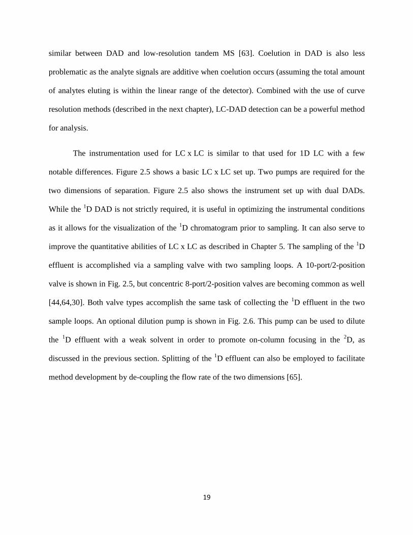
2.2.1. Instrumentation ......................................................................................................18

3. Chemometric Techniques for Liquid Chromatography ....................................................23

3.1. Traditional Preprocessing Techniques ..............................................................................24

3.2. Multiway Curve Resolution Methods ...............................................................................27

3.2.1. Data Structure ........................................................................................................27

3.2.2. Parallel Factor Analysis (PARAFAC) ...................................................................28

iv

3.2.3. Multivariate Curve Resolution (MCR) ..................................................................31

3.2.3.1. Alternating Least Squares (ALS) ...............................................................33

4. Peak Capacity Enhancements Enabled By Chemometric Curve Resolution...................37

4.1. Introduction .......................................................................................................................37

4.2. Methods ............................................................................................................................39

4.2.1. Design of Experiments ...........................................................................................39

4.2.2. Multivariate Curve Resolution-Alternating Least Squares ....................................42

4.2.3. Monte-Carlo Simulations .......................................................................................43

4.2.4. Modeling ................................................................................................................43

4.3. Results and Discussion .....................................................................................................44

4.3.1. Effective Peak Capacity in MCR-ALS ..................................................................48

4.4. Conclusions.......................................................................................................................49

5. Two-Dimensional Assisted Liquid Chromatography .........................................................51

5.1. Introduction .......................................................................................................................51

5.2. Strategy .............................................................................................................................56

5.2.1. Instrumental Setup .................................................................................................56

5.3. Experimental .....................................................................................................................57

5.3.1. Simulated Datasets .................................................................................................57

5.3.2. Experimental Datasets ...........................................................................................60

5.3.3. MCR-ALS ..............................................................................................................63

5.3.4. Calibration..............................................................................................................63

5.4. Results...............................................................................................................................64

5.4.1. Simulated Data .......................................................................................................64

v

5.4.2. Experimental Data .................................................................................................68

5.4.3. Combined 2DALC (c2DALC) ...............................................................................70

5.5. Conclusions.......................................................................................................................75

6. Comparison of Curve Resolution Strategies in LC x LC: Application to the Analysis of

Furanocoumarins in Apiaceous Vegetables.........................................................................79

6.1. Furanocoumarins ..............................................................................................................79

6.2. Experimental .....................................................................................................................83

6.2.1. Plant Extracts .........................................................................................................83

6.2.2. Chromatographic Conditions .................................................................................84

6.2.3. Data Analysis .........................................................................................................85

6.3. Results...............................................................................................................................87

6.3.1. Comparison of Integration Methods ......................................................................88

6.3.2. Comparison of Curve Resolution Strategies ..........................................................91

6.3.3. Vegetable Results (from 2D Manual) ....................................................................92

6.4. Conclusions.......................................................................................................................93

7. Conclusions and Future Work ..............................................................................................95

7.1. Reflections on Chapter 4 ..................................................................................................95

7.2. Reflections on Chapter 5 ..................................................................................................96

7.3. Reflections on Chapter 6 ..................................................................................................97

7.4. Outlook and Future Work .................................................................................................99

List of References ........................................................................................................................101

Appendix A ..............................................................................................................................115

vi

Appendix B ..............................................................................................................................123

Vita ...............................................................................................................................................127

vii

List of Tables

Table 2.1. Comparison of different combinations for LC x LC ....................................................15

Table 4.1. Factor levels for full-factorial experimental design .....................................................40

Table 4.2. Predictors used in building prediction model...............................................................44

Table 4.3. Coefficients and errors for predictive model of calibration quality .............................45

Table 5.1. Literature reports of quantitation in LC x LC ..............................................................53

Table 5.2. Relative concentrations of samples in the simulated dataset .......................................59

Table 5.3. Concentrations of samples in the experimental dataset ...............................................61

Table 5.4. Quantitation methods studied in this work ...................................................................65

viii

List of Figures

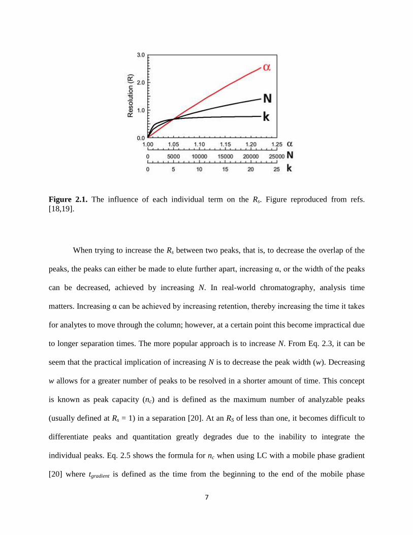
Figure 2.1. The influence of each individual term on the Rs. Figure reproduced from refs

[18,19] ..............................................................................................................................................7

Figure 2.2. Van Deemter plot and individual term contributions to the van Deemter curve

(black). Hmin and uopt represent the minimum plate height at the optimum linear velocity. ............9

Figure 2.3. Three modes of two dimensional LC. (A) shows the 1D chromatogram and the

collection of the 1D effluent samples across the

1D chromatogram. Each box represents a single

aliquot collected in a single sample loop. (B) shows the resulting chromatograms from each of

the methods. MHC and sLC x LC result in two separate chromatograms for each of the two 1D

windows collected. LC x LC results in a single comprehensive 2D chromatogram. ....................13

Figure 2.4. Diagram comparing cases of low fractional coverage (A) and high fractional

coverage (B). Each dot represents an analyte peak. Low fractional coverage is often a

consequence of correlated retention between the two separations causing peaks to elute along a

diagonal line across the separation space. ......................................................................................17

Figure 2.5. Diagram representing a typical setup for LC x LC, with a 10-port/2-position valve.

The dashed outlines on the dilution pump and 1D DAD indicate these components are optional.20

Figure 2.6. Folding of instrumental data into a 2D chromatogram. Data is collected as a string of 2D chromatograms as shown in (A) separated by the dashed lines. These

2D chromatograms are

aligned perpendicular to the 1D time axis as shown in (B). Typically this 2D chromatogram is

visualized as a contour plot as shown in (C). .................................................................................21

Figure 3.1. The instrumental signal (A) consists of the analytical signal (B), the background (C),

and the noise (D). Adapted from Matos et al. [72] and Amigo et al.[10]. ....................................24

Figure 3.2. Data structures resulting from instrumental techniques of increasing complexity.

Adapted from Olivieri [80]. ...........................................................................................................28

Figure 3.3. Graphical depiction of the PARAFAC model (Eq. 3.1) with two components.

Adapted from Bro [82]...................................................................................................................29

ix

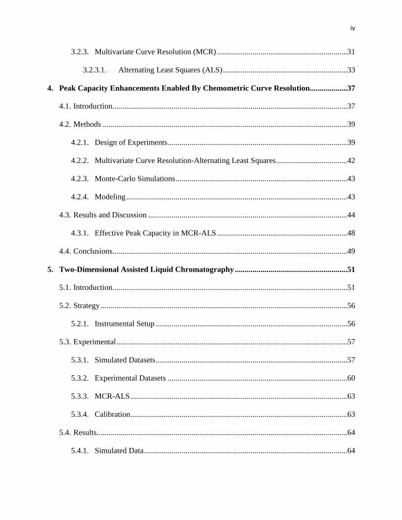
Figure 3.4. (A) depicts the MCR model graphically for a LC-DAD dataset with I time points, J

wavelengths, and N components representing the data. The yellow areas represent how each

point in the raw data (X) is represented by the chromatographic (C) and spectral (S) profiles and

error (E). Figure inspired by Rutan et al. [11]. (B) shows an example of a 2-compound

spectrochromatogram resolved into two pure analyte chromatographic and spectral profiles. .....32

Figure 3.5. Rearrangement of a multisample LC-DAD dataset into a single matrix for MCR

analysis. λ represents the spectral dimension, while t represents the time dimension. (A) This

graphic depicts the process graphically while (B) shows the process with realistic chromatograms

with the wavelength axis going into the page. ...............................................................................33

Figure 3.6. Scree plot for estimating the number of components for MCR-ALS. The possible

break point occurs at 4 components indicating a starting point of 4 components for MCR-ALS. 34

Figure 4.1. Simulated spectra used to create simulated datasets. The similarity of the spectra to

the reference spectra (black) as measured by 2

rspectra are 0.50 (blue), 0.95 (red), and

0.98 (green). ...................................................................................................................................41

Figure 4.2. Examples of simulated chromatograms at varying S/N and RS values. Each color

represents one of the five different samples in each dataset. .........................................................42

Figure 4.3. Predicted calibration quality (2

rcal ) versus RS at S/N = 100 (A), 50 (B), and 26 (C).

The dotted line represents a threshold rcal2 of 0.999, above which represents a satisfactory

calibration curve.............................................................................................................................46

Figure 4.4. Calculated minimum resolution required for quantitation ( '

sR ; defined at 2rcal

=

0.999) as a function of S/N. Each line represents a different spectral correlation (2

rspectra ) as

shown in the legend. Values in the gray area are below the range of the model and thus are

extrapolated values.........................................................................................................................47

Figure 5.1. Overall strategy for analyzing LC x LC-DAD data using 2DALC ...........................55

Figure 5.2. Instrumental setup for LC x LC with dilution and dual DAD detectors. Reproduced

from Stoll et al. [59] with permission. ...........................................................................................57

Figure 5.3. Representative chromatograms and spectra from the data analyzed in this work. The

left column is the simulated data under high dilution conditions and experimental data is shown

in the right column. A and B show the 2D chromatograms (at 200 nm) with a box around the

actual section analyzed (the colorbars indicate the intensities in mAU). C and D show the 1D

chromatograms (at 200 nm) and E and F show the pure spectra of the compounds. The peak

resolution in both chromatographic dimensions is 0.5 (before undersampling) in A and C. See

experimental section for chromatographic conditions. .................................................................62

x

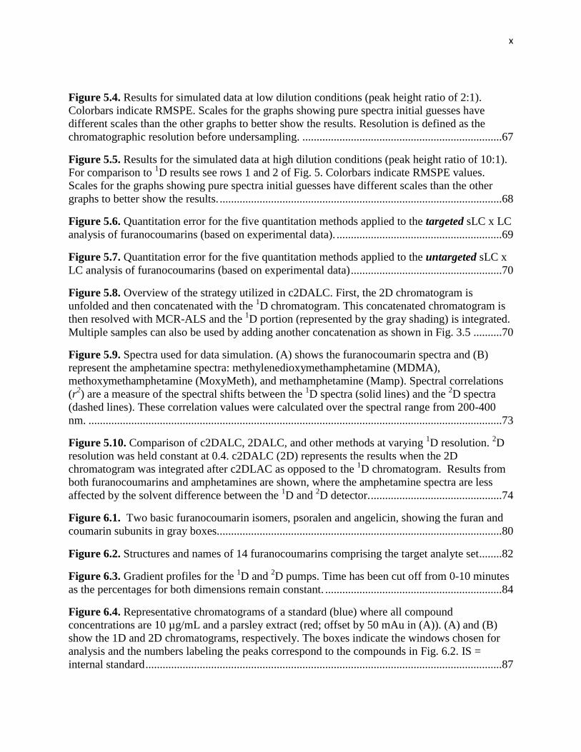
Figure 5.4. Results for simulated data at low dilution conditions (peak height ratio of 2:1).

Colorbars indicate RMSPE. Scales for the graphs showing pure spectra initial guesses have

different scales than the other graphs to better show the results. Resolution is defined as the

chromatographic resolution before undersampling. ......................................................................67

Figure 5.5. Results for the simulated data at high dilution conditions (peak height ratio of 10:1).

For comparison to 1D results see rows 1 and 2 of Fig. 5. Colorbars indicate RMSPE values.

Scales for the graphs showing pure spectra initial guesses have different scales than the other

graphs to better show the results. ...................................................................................................68

Figure 5.6. Quantitation error for the five quantitation methods applied to the targeted sLC x LC

analysis of furanocoumarins (based on experimental data). ..........................................................69

Figure 5.7. Quantitation error for the five quantitation methods applied to the untargeted sLC x

LC analysis of furanocoumarins (based on experimental data) .....................................................70

Figure 5.8. Overview of the strategy utilized in c2DALC. First, the 2D chromatogram is

unfolded and then concatenated with the 1D chromatogram. This concatenated chromatogram is

then resolved with MCR-ALS and the 1D portion (represented by the gray shading) is integrated.

Multiple samples can also be used by adding another concatenation as shown in Fig. 3.5 ..........70

Figure 5.9. Spectra used for data simulation. (A) shows the furanocoumarin spectra and (B)

represent the amphetamine spectra: methylenedioxymethamphetamine (MDMA),

methoxymethamphetamine (MoxyMeth), and methamphetamine (Mamp). Spectral correlations

(r2) are a measure of the spectral shifts between the

1D spectra (solid lines) and the

2D spectra

(dashed lines). These correlation values were calculated over the spectral range from 200-400

nm. .................................................................................................................................................73

Figure 5.10. Comparison of c2DALC, 2DALC, and other methods at varying 1D resolution.

2D

resolution was held constant at 0.4. c2DALC (2D) represents the results when the 2D

chromatogram was integrated after c2DLAC as opposed to the 1D chromatogram. Results from

both furanocoumarins and amphetamines are shown, where the amphetamine spectra are less

affected by the solvent difference between the 1D and

2D detector. ..............................................74

Figure 6.1. Two basic furanocoumarin isomers, psoralen and angelicin, showing the furan and

coumarin subunits in gray boxes....................................................................................................80

Figure 6.2. Structures and names of 14 furanocoumarins comprising the target analyte set ........82

Figure 6.3. Gradient profiles for the 1D and

2D pumps. Time has been cut off from 0-10 minutes

as the percentages for both dimensions remain constant. ..............................................................84

Figure 6.4. Representative chromatograms of a standard (blue) where all compound

concentrations are 10 µg/mL and a parsley extract (red; offset by 50 mAu in (A)). (A) and (B)

show the 1D and 2D chromatograms, respectively. The boxes indicate the windows chosen for

analysis and the numbers labeling the peaks correspond to the compounds in Fig. 6.2. IS =

internal standard .............................................................................................................................87

xi

Figure 6.5. Graphical representation of integration methods compared. (A) shows a MCR-ALS

resolved LC x LC chromatogram. (B) and (C) show the rearranged LC x LC chromatogram with

summation and manual integration, respectively. The shaded area represents the area calculated

for quantitation. The percent difference in calculated peak area for these two chromatograms is

9.9%. The integration methods are identical for 1D LC, without the rearrangement of the

resolved chromatograms. ...............................................................................................................89

Figure 6.6. Comparison of MCR-ALS approaches. (A) shows the results when the peaks are

manually integrated. (B) shows when the resolved chromatograms are integrated over the entire

component. .....................................................................................................................................90

Figure 6.7. Concentration (C) of detected furanocoumarins in the three vegetables as calculated

with manual integration of the 2D chromatogram. The box represents the median and the 1st and

3rd

quartiles. Each point represents the average concentration in each sample (n = 2). Only

compounds which were found to be present in at least one vegetable type are shown. ................93

xii

List of Abbreviations

1D first dimension

1D one-dimensional

2D second dimension

2D two dimensional

2DALC two-dimensional assisted liquid chromatography

2D-LC two-dimensional liquid chromatography

8-MOP 8-methoxypsoralen

ALS alternating least squares

°C degree Celsius

C18 octadecyl carbon chain

c2DALC combined two-dimensional assisted liquid chromatography

CBP 4-chlorobenzophenone

COW correlation optimized warping

DAD diode array detector

EFA evolving factor analysis

EMG exponentially modified Gaussian

GRAM generalized rank annihilation method

HILIC hydrophilic interaction liquid chromatography

IEC ion exchange chromatography

IKSFA iterative key set factor analysis

xiii

IOPA iterative orthogonal projection approach

HTLC high temperature liquid chromatography

HPLC high performance liquid chromatography

HSM hydrophobic subtraction model

LC liquid chromatography (used interchangeably with high performance liquid

chromatography)

LC x LC comprehensive two dimensional liquid chromatography

LCCC liquid chromatography under critical conditions

Mamp methamphetamine

MCR multivariate curve resolution

MDMA methylenedioxymethamphetamine

MHC multiple heartcutting two-dimensional liquid chromatography

MoxyAmp methoxyamphetamine

MS mass spectrometer or mass spectrometry

MS/MS tandem mass spectrometry

OBGC orthogonal background correction

OPA orthogonal projection approach

PARAFAC parallel factor analysis

PARAFAC2 parallel factor analysis version 2

PCA principal components analysis

PLS partial least squares

QuEChERS quick, easy, cheap, effective, rugged, safe (acronym for extraction method)

RMSPE root mean square percent error

RP reversed phase liquid chromatography

%RSD percent relative standard deviation

xiv

SE standard error

SEC size exclusion chromatography

SIMPLISMA simple-to-use interactive self-modeling mixture analysis

sLC x LC selective comprehensive two-dimensional liquid chromatography

UHPLC ultra-high performance liquid chromatography

UV ultraviolet light

Vis visible light

xv

List of Variables

α chromatographic selectivity

<β> broadening correction factor

λ wavelength

σ standard deviation

θ angle

A coefficient representing eddy diffusion in the van Deemter equation

A matrix representing sample profiles in PARAFAC

B coefficient representing longitudinal diffusion in the van Deemter equation

C coefficient representing resistance to mass transfer in the van Deemter equation

OR concentration

C matrix representing chromatographic profiles in MCR-ALS and PARAFAC

E residual error after MCR-ALS or PARAFAC fitting

fcoverage fractional coverage of the two dimensional separation space

H height equivalent of a theoretical plate

I number of data points in the chromatographic dimension

J number of data points in the spectral dimension

K number of samples represented in a data array

k retention factor

L column length

xvi

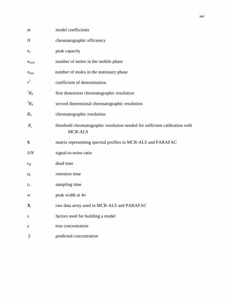
m model coefficients

N chromatographic efficiency

nc peak capacity

nmob number of moles in the mobile phase

nstat number of moles in the stationary phase

r2 coefficient of determination

1RS first dimension chromatographic resolution

2RS second dimensional chromatographic resolution

RS chromatographic resolution

'

sR threshold chromatographic resolution needed for sufficient calibration with

MCR-ALS

S matrix representing spectral profiles in MCR-ALS and PARAFAC

S/N signal-to-noise ratio

tM dead time

tR retention time

tS sampling time

w peak width at 4σ

X raw data array used in MCR-ALS and PARAFAC

x factors used for building a model

y true concentration

y predicted concentration

Abstract

CHEMOMETRIC CURVE RESOLUTION FOR QUANTITATIVE LIQUID

CHROMATOGRAPHIC ANALYSIS

By Daniel Wesley Cook

A dissertation submitted in partial fulfillment of the requirements for the degree of Doctor of

Philosophy at Virginia Commonwealth University

Virginia Commonwealth University, 2016

Director: Sarah C. Rutan, Professor, Department of Chemistry

In chemical analyses, it is crucial to distinguish between chemical species. This is often

accomplished via chromatographic separations. These separations are often pushed to their limits

in terms of the number of analytes that can be sufficiently resolved from one another, particularly

when a quantitative analysis of these compounds is needed. Very often, complicated methods or

new technology is required to provide adequate separation of samples arising from a variety of

fields such as metabolomics, environmental science, food analysis, etc.

An often overlooked means for improving analysis is the use of chemometric data

analysis techniques. Particularly, the use of chemometric curve resolution techniques can

mathematically resolve analyte signals that may be overlapped in the instrumental data. The use

of chemometric techniques facilitates quantitation, pattern recognition, or any other desired

analyses. Unfortunately, these methods have seen little use outside of traditionally chemometrics

focused research groups. In this dissertation, we attempt to show the utility of one of these

methods, multivariate curve resolution-alternating least squares (MCR-ALS), to liquid

chromatography as well as its application to more advanced separation techniques.

First, a general characterization of the performance of MCR-ALS for the analysis of

liquid chromatography-diode array detection (LC-DAD) data is accomplished. It is shown that

under a wide range of conditions (low chromatographic resolution, low signal-to-noise, and high

similarity between analyte spectra), MCR-ALS is able to increase the number of quantitatively

analyzable peaks. This increase is up to five-fold in many cases.

Second, a novel methodology for MCR-ALS analysis of comprehensive two-dimensional

liquid chromatography (LC x LC) is described. This method, called two dimensional assisted

liquid chromatography (2DALC), aims to improve quantitation in LC x LC by combining the

advantages of both one-dimensional and two dimensional chromatographic data. We show that

2DALC can provide superior quantitation to both LC x LC and one dimensional LC under

certain conditions.

Finally, we apply MCR-ALS to an LC x LC analysis of fourteen furanocoumarins in

three apiaceous vegetables. The optimal implementation of MCR-ALS and subsequent

integration was determined. For these data, simply performing MCR-ALS on the two

dimensional chromatogram and manually integrating the results proved to be the superior

method. These results demonstrate the usefulness of these curve resolution techniques as a

compliment to advanced chromatographic techniques.

1

Chapter 1: Overview of Objectives

With the ever increasing need to analyze complex chemical samples, analysis methods

must constantly evolve. These complex analyte mixtures arise from a wide range of fields such

as food science, environmental science, metabolomics [1], proteomics [2,3], and many others.

These fields can produce samples with well over 1,000 analytes with multiple classes of analytes

present [4–6]. Commonly, innovations in instrumental technology and instrumental methods

drive the field of analytical separations; however, innovations in data analysis techniques can

also offer powerful tools to complement existing instrumental methods.

Liquid chromatography (LC) has advanced greatly in the few decades since its inception.

Both advances in the theoretical understanding and practical innovations have enabled its

widespread adoption and today it is one of the most widely used techniques for chemical

analysis. Chapter 2 presents a brief overview of the fundamentals of liquid chromatography and

describes comprehensive two-dimensional liquid chromatography (LC x LC) [7,8], a particularly

promising innovation in the field of separation science. LC x LC allows for a much greater

number of analytes to be separated due its use of two coupled chromatographic separations with

different selectivities. Even with advanced LC instrumentation and methods, the number of

analytes able to be separated in a single analysis is finite and overlap of analyte signals is still

common, particularly when short analysis times are desired and/or complex samples are being

2

analyzed. These peak overlaps along with other instrumental effects can degrade the quantitative

performance of these methods [9].

The objective of the research described in the following chapters was to utilize

chemometric techniques to improve quantitative liquid chromatographic analyses by extracting

underlying quantitative information from data that may be corrupted by background, noise,

interfering species, and other instrumental effects. The chemometric curve resolution techniques

discussed in the following chapters mathematically resolve analyte signals from one another and

from background and noise by analyzing the data holistically. Most traditional data analysis

techniques rely on single-channel detection (i.e., a single wavelength or mass-to-charge value),

even if multiple channels of data are collected from the instrument. Data from multichannel

detectors are often visualized and analyzed at a single wavelength in the case of ultraviolet-

visible (UV-Vis) detection or an extracted ion chromatogram in the case of mass spectrometric

(MS) detection. Chemometric curve resolution techniques use the complete data by treating them

as higher order data arrays, making use of the full spectral dimension in the data (e.g., ultraviolet

visible or mass spectra) [10]. Descriptions of these curve resolution methods and other

chemometric treatments of chromatographic data are presented in Chapter 3.

Three major goals guide the work described in the following chapters. First, many curve

resolution techniques have been used in the literature without a detailed study on the abilities and

limitations of these methods. We aim to characterize one such technique called multivariate

curve resolution-alternating least squares (MCR-ALS) [11,12]. While used extensively in the

literature, MCR-ALS has yet to find widespread use in routine analyses outside of traditionally

chemometric research laboratories. This is possibly due to the misperception that it is difficult to

implement and does not provide a significant advantage for chromatographic analyses. In

3

Chapter 4 it is demonstrated that MCR-ALS does provide a clear advantage and can produce up

to a five-fold increase in effective peak capacity, a measure of the maximum number of

analyzable peaks in a given separation. This is demonstrated over a range of conditions using a

design of experiments approach allowing for the generation of an approximate model of the

quantitative performance of MCR-ALS.

The second goal of this work was to investigate the use of MCR-ALS to improve the

quantitative abilities of LC x LC. LC x LC aims to resolve analyte signals by adding a second

dimension of chromatography. While this can provide significantly higher peak capacities, it can

come at the cost of quantitative performance. Thus far in the literature the quantitative

performance of LC x LC has typically been inferior to that of traditional one-dimensional (1D)

chromatography. This is attributed to effects introduced during the transfer of the first dimension

(1D) effluent to the second dimension (

2D) of separation. Therefore, quantitative information is

preserved in the 1D separation. The work described in Chapter 5 aims to extract the quantitative

information of the 1D separation with the assistance of the

2D separation. This is done by

utilizing the greater separation of peaks in the 2D to improve MCR-ALS analysis of the

1D

separation, containing severely overlapped chromatographic peaks. This approach is named two-

dimensional assisted liquid chromatography (2DALC).

Finally, our third goal was to demonstrate the use of MCR-ALS in a relevant, real-world

LC x LC analysis. Chapter 6 describes the analysis of furanocoumarins from apiaceous

vegetables with LC x LC and MCR-ALS. Furanocoumarins are a class of compounds of great

interest due to their high bioactivity including interactions with the liver enzymes responsible for

the metabolism of many pharmaceuticals[13,14]. In order to investigate the physiological effects

from the consumption of these vegetables, it is crucial to determine the levels at which the

4

compounds are present within certain vegetables. To determine the best method for obtaining the

concentrations of these compounds in vegetable samples, three implementations of MCR-ALS

were investigated, as well as two strategies for the subsequent peak integration step. It was found

that for this data set, LC x LC quantitation was competitive with that of one-dimensional LC

when MCR-ALS was used. It was also found that, while tedious, manual integration of the

resolved chromatographic peaks yielded superior quantitative results.

Through the work described in the following chapters, it is clear that MCR-ALS has great

potential for improving quantitative liquid chromatographic performance. Through the ability to

handle peak overlap, MCR-ALS can enable the use of shorter analysis times of more complex

samples; however, rather than MCR-ALS being considered an alternative to improved

separations, MCR-ALS should be thought of as a complementary technique that allows good

separations to be made even better. This is shown by its applicability to LC x LC where MCR-

ALS can assist in the quantitation of analytes while simultaneously increasing peak capacity

even further than with LC x LC alone. Chapter 7 draws conclusions from the work presented

here and provides future directions for this work.

5

Chapter 2: Liquid Chromatography

2.1. Fundamentals of Liquid Chromatography

Liquid chromatography (LC) is one of the most widely used methods of chemical

analysis. LC separates analytes based on their interactions with a mobile phase and a stationary

phase, either through partitioning or adsorption. These interactions differentially retard analytes

giving rise to separation. These interactions are dictated by three main properties of the

molecules: electrical charge, molecular size, or polarity [15]. The discussion below will focus on

polarity; however, many of the concepts apply equally well to electrical charge. Also in this

discussion and the following chapters, high performance or high pressure liquid chromatography

(HPLC) will be used interchangeably with LC as it will be the focus of the work presented here.

HPLC, rather than gravity-fed chromatography, forces the mobile phase through the stationary

phase at higher pressure [16].

Separation in LC is driven by the differential retention of each analyte on the stationary

phase. The extent of this retention can be quantified by a metric called the retention factor, k.

This value is equal to the ratio of moles of analyte in the stationary phase, nstat, to the moles of

analyte in the mobile phase, nmob, as shown in Eq. 2.1. Experimentally, it can be calculated based

on the time it takes for the analyte to elute from the column, also known as retention time (tR),

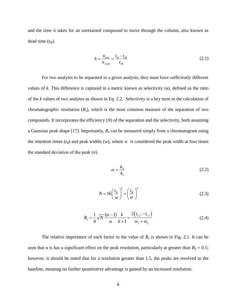
6

and the time it takes for an unretained compound to move through the column, also known as

dead time (tM).

stat R M

mob M

n t tk

n t

(2.1)

For two analytes to be separated in a given analysis, they must have sufficiently different

values of k. This difference is captured in a metric known as selectivity (α), defined as the ratio

of the k values of two analytes as shown in Eq. 2.2. Selectivity is a key term in the calculation of

chromatographic resolution (Rs), which is the most common measure of the separation of two

compounds. It incorporates the efficiency (N) of the separation and the selectivity, both assuming

a Gaussian peak shape [17]. Importantly, Rs can be measured simply from a chromatogram using

the retention times (tR) and peak widths (w), where w is considered the peak width at four times

the standard deviation of the peak (σ).

2

1

k

k (2.2)

2 2

16 R Rt tN

w

(2.3)

,2 ,1

1 2

21 ( 1)

4 1

r r

s

t tkR N

k w w

(2.4)

The relative importance of each factor in the value of Rs is shown in Fig. 2.1. It can be

seen that α is has a significant effect on the peak resolution, particularly at greater than RS = 0.5;

however, it should be noted that for a resolution greater than 1.5, the peaks are resolved to the

baseline, meaning no further quantitative advantage is gained by an increased resolution.

7

Figure 2.1. The influence of each individual term on the Rs. Figure reproduced from refs.

[18,19].

When trying to increase the Rs between two peaks, that is, to decrease the overlap of the

peaks, the peaks can either be made to elute further apart, increasing α, or the width of the peaks

can be decreased, achieved by increasing N. In real-world chromatography, analysis time

matters. Increasing α can be achieved by increasing retention, thereby increasing the time it takes

for analytes to move through the column; however, at a certain point this become impractical due

to longer separation times. The more popular approach is to increase N. From Eq. 2.3, it can be

seem that the practical implication of increasing N is to decrease the peak width (w). Decreasing

w allows for a greater number of peaks to be resolved in a shorter amount of time. This concept

is known as peak capacity (nc) and is defined as the maximum number of analyzable peaks

(usually defined at Rs = 1) in a separation [20]. At an RS of less than one, it becomes difficult to

differentiate peaks and quantitation greatly degrades due to the inability to integrate the

individual peaks. Eq. 2.5 shows the formula for nc when using LC with a mobile phase gradient

[20] where tgradient is defined as the time from the beginning to the end of the mobile phase

8

gradient. This equation assumes a random distribution of peaks from the beginning to the end fo

the mobile phase gradient.

4

gradient gradient

c

t tn

w (2.5)

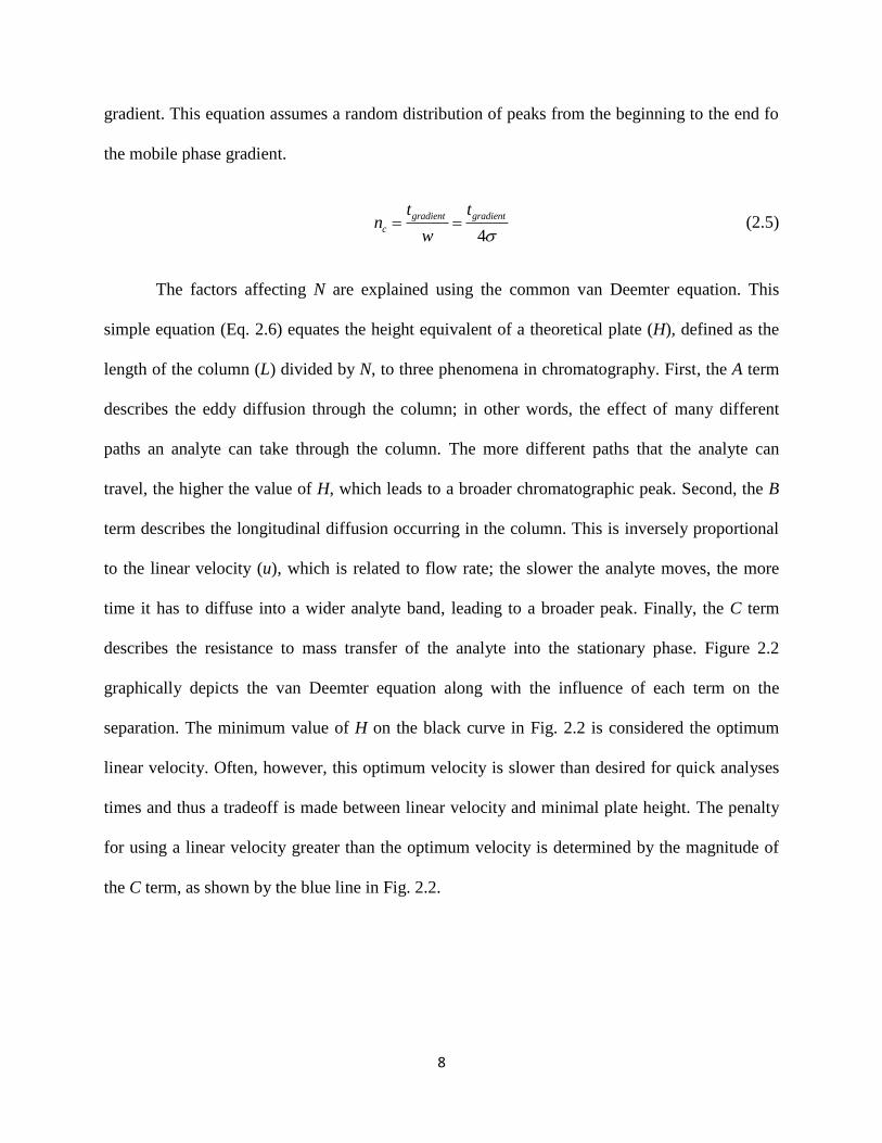
The factors affecting N are explained using the common van Deemter equation. This

simple equation (Eq. 2.6) equates the height equivalent of a theoretical plate (H), defined as the

length of the column (L) divided by N, to three phenomena in chromatography. First, the A term

describes the eddy diffusion through the column; in other words, the effect of many different

paths an analyte can take through the column. The more different paths that the analyte can

travel, the higher the value of H, which leads to a broader chromatographic peak. Second, the B

term describes the longitudinal diffusion occurring in the column. This is inversely proportional

to the linear velocity (u), which is related to flow rate; the slower the analyte moves, the more

time it has to diffuse into a wider analyte band, leading to a broader peak. Finally, the C term

describes the resistance to mass transfer of the analyte into the stationary phase. Figure 2.2

graphically depicts the van Deemter equation along with the influence of each term on the

separation. The minimum value of H on the black curve in Fig. 2.2 is considered the optimum

linear velocity. Often, however, this optimum velocity is slower than desired for quick analyses

times and thus a tradeoff is made between linear velocity and minimal plate height. The penalty

for using a linear velocity greater than the optimum velocity is determined by the magnitude of

the C term, as shown by the blue line in Fig. 2.2.

9

Figure 2.2. Van Deemter plot and individual term contributions to the van Deemter curve

(black). Hmin and uopt represent the minimum plate height at the optimum linear velocity.

B

H A Cuu

(2.6)

L

HN

(2.7)

The major contributing factor to all three terms in the van Deemter equation is the

column. Column manufacturers are constantly innovating to create new packing materials in

order to increase the efficiency of the columns. Traditionally, the silica particles used for packing

are fully porous particles; recently, however, superficially porous, or core shell, particles are

becoming very popular [21]. These particles consist of a solid core with a porous outer shell. The

main implications of this are a decrease in the C term (i.e., increasing the speed of mass transfer)

and a decrease in the A term due to improved column packing [22]. A decrease in the C term

lowers the slope of the blue curve in Fig. 2.2, which allows for an increase in linear velocity with

lesser effects on H. Monolithic columns, consisting of a solid rod of porous silica or other

material, also have this same advantage [23]. Decreasing particle size has been found to

significantly increase efficiency as well. Not only do these small particles increase the speed of

10

mass transfer, they also pack more uniformly, decreasing the A term, eddy diffusion. However,

this comes at the cost of higher backpressure, leading to a need for ultra-high performance liquid

chromatography (UHPLC), with pressures up to 1000 bar (14,500 psi) or more.

While chromatographic technologies are constantly improving, increasing column

efficiency and leading to higher peak capacities, other approaches must be considered. In

addition, increased peak capacities may not solve the problem of co-elution, which is common

between analytes with similar chemical properties, such as isomers. In these cases, improved

selectivity is required. Harnessing the different selectivities of two columns in one analysis

presents a powerful separation method. Mixed mode columns, which consist of two

functionalities, such as anion exchange and octadecyl carbon chains (C18), on a single column

provide separation based on both ion exchange and polarity [24]. This type of column provides

different α values for many compounds, but does not provide an increased peak capacity and

necessitates the purchase (or synthesis) of a new column whenever a different selectivity is

desired. Recently, we published a method for the synthesis of stationary phase gradients which

allow for the fine tuning of chromatographic selectivity [25]. These stationary phase gradients

were created on in-house synthesized monolithic columns by infusing an aminosilane

functionalizing reagent through a bare-silica column creating a column with both amine and

silica surface functionalities. The surface coverage and gradient steepness of the functional

groups on the column support can be easily controlled by varying the time of infusion and

concentration of reagent. This approach can be also extended to multiple functionalities, such as

phenyl and C18 [26]. Although this approach makes tuning the selectivity of these columns

simpler, the in-house synthesis of columns does not reach the same efficiencies as

commercialized columns.

11

Another approach is the coupling of two or more separate columns. This can be

accomplished in two main ways: serial connections or multidimensional coupling. Serially

connected columns consist of two or more columns connected end-to-end, providing added

selectivity. These columns can simply been connected with a piece of tubing; however, this

potentially adds significant dead volume, leading to broadening of the chromatographic peaks.

Commercialized versions of serially connected column, such as the POPLC® system (Bischoff

Analysentechnik, DE), use specialized column “segments” which connect to one another with no

additional tubing, thus eliminating the majority of dead volume between the columns. Still, the

additional connections can prove to be problematic [27] and the column choices are limited by

the offerings of a single manufacturer. Another approach, and the one focused on in Chapters 5

and 6, is two-dimensional liquid chromatography (2D-LC), in which two columns are coupled in

an orthogonal manner.

2.2. Basics of Two-Dimensional Liquid Chromatography (2D-LC)

The 2D-LC technique combines two individual separations into a single analysis in order

to provide greater separation power for a greater number of compounds due to its increased

selectivity and increased peak capacities. The coupling of two separations is accomplished via a

sampling valve placed between the two columns. This sampling valve collects a pre-defined

volume of effluent from the first dimension (1D) column and then injects it onto the second

dimension (2D) column. This is described further in the section 2.2.1. This sampling and

2D

separation can occur in two main ways. In heart-cutting methods, a single section of the 1D

chromatogram, often fully encompassing the peak(s) of interest, is collected in a single aliquot

and transferred to the 2D column [28,29]. This creates a

1D chromatogram and a single

2D

chromatogram. Multiple heart-cutting (MHC) methods do this for two (or more) sections of the

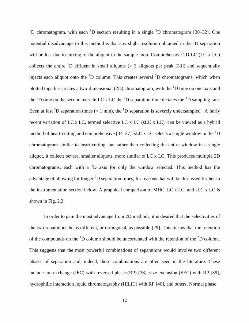
12

1D chromatogram, with each

1D section resulting in a single

2D chromatogram [30–32]. One

potential disadvantage to this method is that any slight resolution obtained in the 1D separation

will be lost due to mixing of the aliquot in the sample loop. Comprehensive 2D-LC (LC x LC)

collects the entire 1D effluent in small aliquots (> 3 aliquots per peak [33]) and sequentially

injects each aliquot onto the 2D column. This creates several

2D chromatograms, which when

plotted together creates a two-dimensional (2D) chromatogram, with the 1D time on one axis and

the 2D time on the second axis. In LC x LC the

2D separation time dictates the

1D sampling rate.

Even at fast 2D separation times (< 1 min), the

1D separation is severely undersampled. A fairly

recent variation of LC x LC, termed selective LC x LC (sLC x LC), can be viewed as a hybrid

method of heart-cutting and comprehensive [34–37]. sLC x LC selects a single window in the 1D

chromatogram similar to heart-cutting, but rather than collecting the entire window in a single

aliquot, it collects several smaller aliquots, more similar to LC x LC. This produces multiple 2D

chromatograms, each with a 1D axis for only the window selected. This method has the

advantage of allowing for longer 2D separation times, for reasons that will be discussed further in

the instrumentation section below. A graphical comparison of MHC, LC x LC, and sLC x LC is

shown in Fig. 2.3.

In order to gain the most advantage from 2D methods, it is desired that the selectivities of

the two separations be as different, or orthogonal, as possible [29]. This means that the retention

of the compounds on the 1D column should be uncorrelated with the retention of the

2D column.

This suggests that the most powerful combinations of separations would involve two different

phases of separation and, indeed, these combinations are often seen in the literature. These

include ion exchange (IEC) with reversed phase (RP) [38], size-exclusion (SEC) with RP [39],

hydrophilic interaction liquid chromatography (HILIC) with RP [40], and others. Normal phase

13

Figure 2.3. Three modes of 2D-LC. (A) This diagram shows the 1D chromatogram and the

collection of the 1D effluent samples across the

1D chromatogram. Each box represents a single

aliquot collected in a single sample loop. Here, two peaks are selected for further analysis using

MHC or sLC x LC. (B) These plots show the resulting chromatograms for each of the methods.

MHC and sLC x LC result in two separate chromatograms for each of the two 1D windows

collected. LC x LC results in a single comprehensive 2D chromatogram.

has also been used with RP [41]; however, solvent compatibility between the two separations

must be considered. For example, normal phase LC uses highly non-polar organic solvents with

increasing polarity to elute compounds. RP LC uses highly aqueous solvents with decreasing

solvent polarity to elute compounds. Ignoring potential solvent immiscibility issues, if

compounds elute from the 1D normal phase column in non-polar solvents and are injected onto

14

the 2D RP column, no retention (or minimal retention) will be observed. To circumvent these

issues, complex methods are required. On the other hand, a very popular choice is the use of two

RP separations [7,42–44]. While an increase in retention correlation is seen, the plethora of

different RP column chemistries commercially available often allows for sufficient orthogonality

between the two dimensions. Online selection tools are available to assist in the selection of

orthogonal columns. HPLCcolumns.org [45], for example, makes use of the hydrophobic

subtraction model (HSM) of selectivity [46] to compare over 600 commercially available RP

columns from over 30 different manufacturers. By incorporating empirical values for

hydrophobicity, steric effects, hydrogen bond acidity and basicity, and cation-exchange activity,

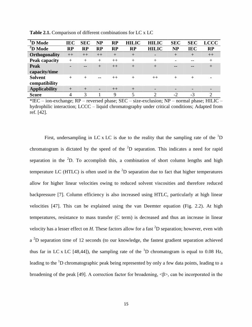
this website calculates a similarity value between two columns. In their primer to LC x LC, Carr

and Stoll attempt to compare different mode combinations according to several factors [42]. A

portion of their table is reproduced here in Table 2.1. While the scoring is somewhat subjective,

it presents a good overall picture of the different combinations. From this table, it can be seen

that while the combination of two RP separations suffers slightly from lack of orthogonality, it is

superior to all other combinations, particularly in terms of the wide range of compounds able to

be analyzed by RP separations as well as the peak capacity per unit time of RP separations.

For the work in the following chapters, only comprehensive LC x LC and sLC x LC with

RP conditions in both dimensions will be considered. LC x LC provides a significant increase in

separation space allowing more peaks to be detected in a given analysis time. In terms of peak

capacity, LC x LC provides an ideal 2D peak capacity (nc,2D) equal to the product of the two

individual separations’ peak capacities (1nc and

2nc); however, this 2D peak capacity is impacted

by two major factors: peak broadening due to the undersampling of the 1D chromatographic peak

and correlated retention between the two columns.

15

Table 2.1. Comparison of different combinations for LC x LC

1D Mode IEC SEC NP RP HILIC HILIC SEC SEC LCCC

2D Mode RP RP RP RP RP HILIC NP IEC RP

Orthogonality ++ ++ ++ + + - + + ++

Peak capacity + + + ++ + + - -- +

Peak

capacity/time

- -- + ++ + + -- -- +

Solvent

compatibility

+ + -- ++ + ++ + + -

Applicability + + - ++ + - - - -

Score 4 3 1 9 5 2 -2 -3 2

*IEC – ion-exchange; RP – reversed phase; SEC – size-exclusion; NP – normal phase; HILIC –

hydrophilic interaction; LCCC – liquid chromatography under critical conditions; Adapted from

ref. [42].

First, undersampling in LC x LC is due to the reality that the sampling rate of the 1D

chromatogram is dictated by the speed of the 2D separation. This indicates a need for rapid

separation in the 2D. To accomplish this, a combination of short column lengths and high

temperature LC (HTLC) is often used in the 2D separation due to fact that higher temperatures

allow for higher linear velocities owing to reduced solvent viscosities and therefore reduced

backpressure [7]. Column efficiency is also increased using HTLC, particularly at high linear

velocities [47]. This can be explained using the van Deemter equation (Fig. 2.2). At high

temperatures, resistance to mass transfer (C term) is decreased and thus an increase in linear

velocity has a lesser effect on H. These factors allow for a fast 2D separation; however, even with

a 2D separation time of 12 seconds (to our knowledge, the fastest gradient separation achieved

thus far in LC x LC [48,44]), the sampling rate of the 1D chromatogram is equal to 0.08 Hz,

leading to the 1D chromatographic peak being represented by only a few data points, leading to a

broadening of the peak [49]. A correction factor for broadening, <β>, can be incorporated in the

16

definition of nc,2D. Davis, Stoll, and Carr define <β> as shown in Eq. 2.8 [49], where ts is the

sampling time and 1σ is the

1D peak width before sampling.

2

11 0.21 st

(2.8)

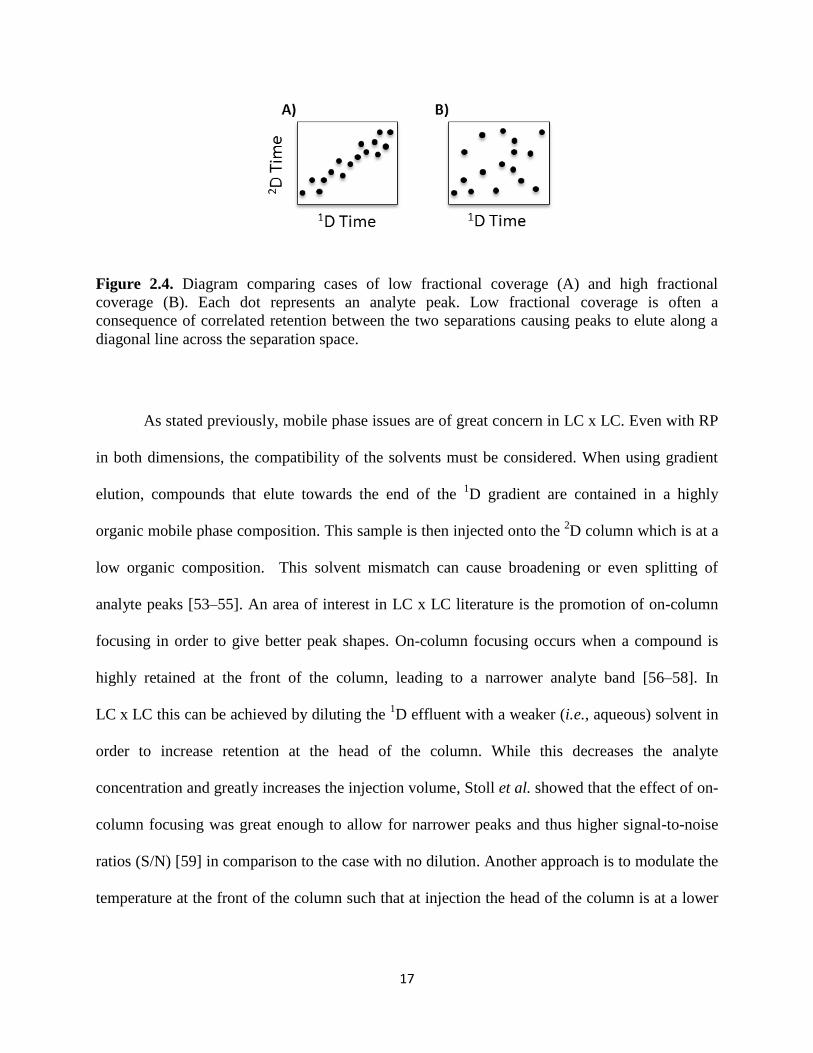
Correlated retention is also a major factor when estimating peak capacity. When retention

in both dimensions of separation is strongly correlated, the chromatographic peaks elute along a

diagonal line across the 2D separation space. If the two separations are completely uncorrelated,

or orthogonal, the peaks appear evenly spread across the separation space. As stated previously,

the combination of two RP separations will never be completely orthogonal and thus the

separation space will always be under-utilized. The extent of this under-utilization of the

separation space is captured in a metric called fractional coverage (fcoverage) and can be estimated

via many different methods [50,51]. Figure 2.4 shows the cases of high and low fcoverage.

Typically, low fractional coverage is a result of the peaks falling along a diagonal line across the

2D separation space, however it can also be caused by weak retention in one dimension of the

separation, leading to elution along a horizontal or vertical line in the 2D chromatogram. Eq. 2.9

incorporates both fcoverage and <β> into the calculation of nc,2D [52].

1 2

,2

1c D c c coveragen n n f

(2.9)

17

Figure 2.4. Diagram comparing cases of low fractional coverage (A) and high fractional

coverage (B). Each dot represents an analyte peak. Low fractional coverage is often a

consequence of correlated retention between the two separations causing peaks to elute along a

diagonal line across the separation space.

As stated previously, mobile phase issues are of great concern in LC x LC. Even with RP

in both dimensions, the compatibility of the solvents must be considered. When using gradient

elution, compounds that elute towards the end of the 1D gradient are contained in a highly

organic mobile phase composition. This sample is then injected onto the 2D column which is at a

low organic composition. This solvent mismatch can cause broadening or even splitting of

analyte peaks [53–55]. An area of interest in LC x LC literature is the promotion of on-column

focusing in order to give better peak shapes. On-column focusing occurs when a compound is

highly retained at the front of the column, leading to a narrower analyte band [56–58]. In

LC x LC this can be achieved by diluting the 1D effluent with a weaker (i.e., aqueous) solvent in

order to increase retention at the head of the column. While this decreases the analyte

concentration and greatly increases the injection volume, Stoll et al. showed that the effect of on-

column focusing was great enough to allow for narrower peaks and thus higher signal-to-noise

ratios (S/N) [59] in comparison to the case with no dilution. Another approach is to modulate the

temperature at the front of the column such that at injection the head of the column is at a lower

18

temperature, which increases retention and focuses the analytes [60]. This has been applied

mostly to capillary LC due to the low thermal mass of capillary columns.

2.2.1. Instrumentation

High performance liquid chromatography requires the use of a high pressure pump to

deliver the analyte mixture and mobile phase to the column where the analytes are separated.

After separation, the analytes are detected using a detector suitable for the target analytes, often a

diode array detector (DAD) or a mass spectrometer (MS). The choice of detector is crucial to the

success of the analysis. Mass spectrometers are available with varying levels of mass resolution

and have become a powerful detector in terms of both selectivity and sensitivity. When tandem

mass spectrometry (MS/MS) is utilized, sensitivity and selectivity are enhanced even further

along with the ability to obtain structural information about the compounds being analyzed.

Mass spectrometers, however, are costly compared to alternatives such as DADs and require

much more upkeep and maintenance. Issues with ion suppression are also commonly present in

MS when multiple compounds coelute [61,62]. This occurs when two compounds enter the

ionization source (e.g., electrospray ionization) and one compound negatively affects the

ionization of the second compound. The exact mechanism of this process is not fully understood.

The most common cause of ion suppression is interferences in the sample; however, ion

suppression can also be caused by compounds introduced during sample preparation or even

from tubing on the instrument [62]. These effects can lead to a drastic decrease in instrument

sensitivity towards certain compounds in the sample. DADs, which measure the ultraviolet-

visible absorption of analytes, are much more inexpensive and robust, but can suffer from lower

sensitivity and lower selectivity due to the broad absorption bands of most organic compounds.

Stoev and Stoyanov have shown, however, that the reliability of compound identification is

19

similar between DAD and low-resolution tandem MS [63]. Coelution in DAD is also less

problematic as the analyte signals are additive when coelution occurs (assuming the total amount

of analytes eluting is within the linear range of the detector). Combined with the use of curve

resolution methods (described in the next chapter), LC-DAD detection can be a powerful method

for analysis.

The instrumentation used for LC x LC is similar to that used for 1D LC with a few

notable differences. Figure 2.5 shows a basic LC x LC set up. Two pumps are required for the

two dimensions of separation. Figure 2.5 also shows the instrument set up with dual DADs.

While the 1D DAD is not strictly required, it is useful in optimizing the instrumental conditions

as it allows for the visualization of the 1D chromatogram prior to sampling. It can also serve to

improve the quantitative abilities of LC x LC as described in Chapter 5. The sampling of the 1D

effluent is accomplished via a sampling valve with two sampling loops. A 10-port/2-position

valve is shown in Fig. 2.5, but concentric 8-port/2-position valves are becoming common as well

[44,64,30]. Both valve types accomplish the same task of collecting the 1D effluent in the two

sample loops. An optional dilution pump is shown in Fig. 2.6. This pump can be used to dilute

the 1D effluent with a weak solvent in order to promote on-column focusing in the

2D, as

discussed in the previous section. Splitting of the 1D effluent can also be employed to facilitate

method development by de-coupling the flow rate of the two dimensions [65].

20

Figure 2.5. Diagram representing a typical setup for LC x LC, with a 10-port/2-position valve.

The dashed outlines on the dilution pump and 1D DAD indicate these components are optional.

In LC x LC only two sampling loops are required due to the fact that as one loop is being

filled with 1D effluent, the contents of the second loop are being delivered to the

2D column. The

valve switches and these loops switch roles. sLC x LC requires a more complex sampling valve

setup. sLC x LC collects many aliquots of the 1D effluent and stores them in sample loops rather

than immediately injecting them onto the 2D column. This allows for fast sampling of the

1D

separation and longer separations on the 2D column. Because of this, ten or more sampling loops

are required. These are typically configured in what is sometimes called a “sampling deck [66]”

or a “parking deck [30].” The instruments typically contain two of these sampling decks, where

each one is used for a single peak window. This allows for a selected peak window to be

sampled 10 or more times, which allows for a much faster 1D sampling rate than allowed in

comprehensive LC x LC.

Data are collected at the 2D DAD as a sequence of

2D chromatograms, corresponding to

the 2D separation of each sampled volume of the

1D effluent. In order to visualize these data as a

2D chromatogram, the sequence of 2D chromatograms must be folded into a 2D chromatogram

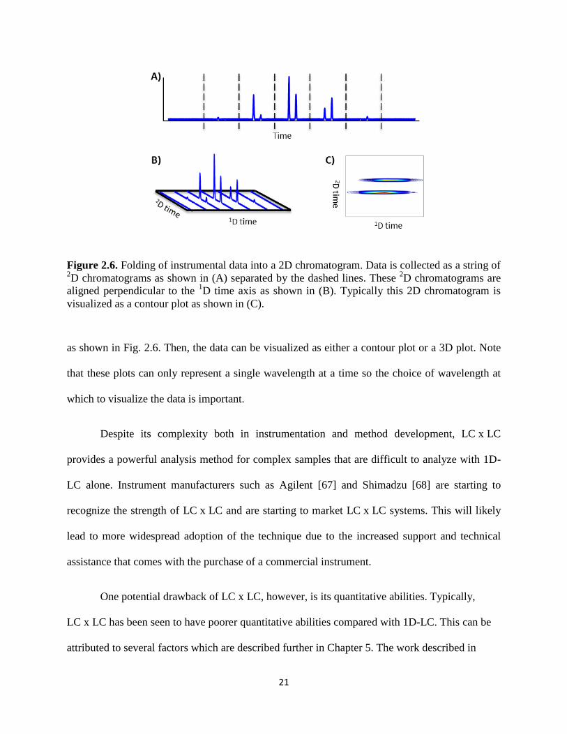
21

Figure 2.6. Folding of instrumental data into a 2D chromatogram. Data is collected as a string of 2D chromatograms as shown in (A) separated by the dashed lines. These

2D chromatograms are

aligned perpendicular to the 1D time axis as shown in (B). Typically this 2D chromatogram is

visualized as a contour plot as shown in (C).

as shown in Fig. 2.6. Then, the data can be visualized as either a contour plot or a 3D plot. Note

that these plots can only represent a single wavelength at a time so the choice of wavelength at

which to visualize the data is important.

Despite its complexity both in instrumentation and method development, LC x LC

provides a powerful analysis method for complex samples that are difficult to analyze with 1D-

LC alone. Instrument manufacturers such as Agilent [67] and Shimadzu [68] are starting to

recognize the strength of LC x LC and are starting to market LC x LC systems. This will likely

lead to more widespread adoption of the technique due to the increased support and technical

assistance that comes with the purchase of a commercial instrument.

One potential drawback of LC x LC, however, is its quantitative abilities. Typically,

LC x LC has been seen to have poorer quantitative abilities compared with 1D-LC. This can be

attributed to several factors which are described further in Chapter 5. The work described in

22

Chapters 5 and 6 aims to apply chemometric curve resolution to the analysis of LC x LC data in

order to improve the quantitative abilities of LC x LC. These curve resolution methods are

described in the following chapter.

23

Chapter 3: Chemometric Techniques for Liquid Chromatography

Portions of this chapter adapted, with permission, from D.W. Cook, S.C. Rutan, Chemometrics

for the analysis of chromatographic data in metabolomics investigations, J. Chemom. 28 (2014)

681-687.

While LC is a powerful analysis technique, the data obtained from such analyses are

often complex and necessitate the use of advanced data analysis techniques. Chemometrics

provides many useful data analysis tools by utilizing mathematical concepts to solve chemical

problems. Svante Wold, widely considered one of the fathers of chemometrics, defined

chemometrics as “How to get chemically relevant information out of measured chemical data,

how to represent and display this information, and how to get such information into data [69].”

This definition encompasses both post-acquisition analysis of the data as well as pre-acquisition

design of experiments in order to collect data that contains the most information pertinent to the

goal of analysis.

Post-acquisition data analysis can be divided further into preprocessing and pattern

recognition. Pattern recognition aims to find underlying trends in the data for easier visualization

of the data or for more targeted purposes such as discriminating between two sample groups

(e.g., healthy versus diseased individuals). This includes methods such as principal components

analysis (PCA), partial least squares (PLS) [70], and cluster analysis, to name a few [71].

24

3.1. Traditional Preprocessing Methods

Preprocessing methods are often employed prior to pattern recognition in order to remove

unwanted contributions to the data to reveal relevant signals in those data. Chromatographic data

consist of three main contributions to the instrumental signal as shown in Fig. 3.1. Figure 3.1.A.

depicts the chromatogram obtained instrumentally. This is an combination of the analytical

signal, background, and noise (Figs 3.1.B,C,D, respectively). Background and noise reduction

methods are among the most common preprocessing techniques. These aim to eliminate the

background and noise signals from the raw data leaving only the analytical signal. This

analytical signal contains the information about the compounds analyzed and thus the

information that is relevant to the analysis.

To remove the background, several methods of baseline correction have been developed.

The most commonly used method in currently available software packages is curve fitting [10].

Figure 3.1. The instrumental signal (A) consists of the analytical signal (B), the background (C),

and the noise (D). Adapted from Matos et al. [72] and Amigo et al. [10].

25

This approach attempts to estimate the baseline by fitting a curve under each peak based

on the area around the base of each peak. These fits can be global fits, or can be localized, which

may provide a better fit but may not be continuous between segments [10]. When analyzing

complex samples this approach can be problematic; if the chromatogram does not have baseline

resolution around many of the peaks, it can be difficult to fit a suitable curve to estimate the

baseline. Background correction methods have also been proposed for LC x LC. Often, these

background methods extend 1D methods to 2D chromatograms. Filgueira, et al. extended

traditional 1D background correction methods (median filtering and polynomial fitting) to

LC x LC chromatograms [73]. Their method, named orthogonal background correction (OBGC),

applies the selected method at each extracted 1D chromatogram (at each

2D time point). This

implementation is orthogonal to how the data is collected (individual 2D chromatograms). The

authors found this to be a very effective and easy to implement method.

Most noise reduction techniques make use of the fact that noise in data is typically high-

frequency with low peak widths. The most well-known form of noise reduction is smoothing.

This is often performed with Savitzky-Golay smoothing in which a few data points are captured

in a window and those points are multiplied by a set of coefficients and summed [74]. The new

value replaces the original center point of the window. The window is moved through the data,

multiplying the data points within each window by the coefficients at each step. A popular

variation on this is matched filtering in which the coefficients used in each window are set to

match the expected peak shape [75,76]. For example, in chromatography, the analytical signal is

expected to be a Gaussian peak shape so the matched filter is set to be a Gaussian peak with a

similar peak width. Danielsson et al. proposed using a second-derivative Gaussian peak as the

26

filter [77]. By using the second-derivative, linear background contributions are reduced to zero,

essentially performing background subtraction and noise reduction in the same step.

Once background and noise contributions are removed from the data, peaks must be

detected to allow for further analyses. It is most often desired to detect peaks in an automated

fashion particularly in complex samples and/or with a large number of samples. Two major

approaches to peak detection are the use of derivatives and peak fitting. When the first-derivative

of a chromatographic peak is taken, the zero-crossing point corresponds to the peak maximum.

The peak width can be estimated using the second-derivative, where two zero-crossing points

exist near the edges of a chromatographic peak [9]. Peak fitting can also be used for peak

detection. In this approach the user or software uses a fixed peak model and optimizes the fit of

the model to the data. Gaussian peak models are often used [10]; however, most

chromatographic peaks exhibit non-Gaussian characteristics due to tailing and sometimes

fronting. Very often, an exponentially modified Gaussian (EMG) model is employed due to its

ability to model a tailing chromatographic peak [78]. A multitude of other peak models are also

available which may fit peaks better depending on the data being fit. Almost 90 of these models

have been compiled by Di Marco and Bombi [79]. Determination of the peak shape can be a

tedious “guess-and-check” process, particularly if the peaks do not conform to a Gaussian or

EMG shape. In cases where peak overlap is severe it is particularly difficult, if not impossible to

choose determine the best peak shape. Amigo et al. demonstrated that in some cases, two peak

shape models seem to fit the data equally well, but it is impossible to know which model better

explains the true underlying peak shape [10]. Peak fitting methods are known as hard models in

that the model is set and the parameters are estimated to best fit this model. A more flexible

method is known as soft modeling, or self-modeling. These methods are explained in section 3.2.

27

3.2. Multiway Curve Resolution Methods

Most traditional methods treat the data using a single or a few detector channel(s) (i.e. a

single wavelength or mass-to-charge value); however, this approach can exclude important

information that may be contained in other channels such as other analytes or information about

the background. Multiway curve resolution analyses treat the full spectrum and the

chromatographic dimension as a single array of data from which components can be extracted.

These components ideally correspond to each compound present in the sample. These methods

can accomplish background and noise reduction by treating them as one or more extra

component(s) in the data. In theory these can greatly simplify analysis by eliminating the need

for multiple algorithms for each preprocessing step, which may affect the results of one another.

Often, these methods eliminate the need for separate peak picking algorithms as well because

each compound is ideally contained in a separate component. These components can then be

utilized for the further pattern recognition steps. Two of the most widely used curve resolution

methods are parallel factor analysis (PARAFAC) and multivariate curve resolution-alternating

least squares (MCR-ALS).

3.2.1. Data Structure

In order to apply multiway methods of analysis to the entire dataset, the data must be organized

into a single data array. These arrays are classified by the number of dimensions they contain,

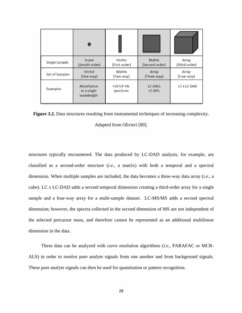
resulting from the instrumental measurement. Figure 3.2 depicts the types of data

28

Figure 3.2. Data structures resulting from instrumental techniques of increasing complexity.

Adapted from Olivieri [80].

structures typically encountered. The data produced by LC-DAD analysis, for example, are

classified as a second-order structure (i.e., a matrix) with both a temporal and a spectral

dimension. When multiple samples are included, the data becomes a three-way data array (i.e., a

cube). LC x LC-DAD adds a second temporal dimension creating a third-order array for a single

sample and a four-way array for a multi-sample dataset. LC-MS/MS adds a second spectral

dimension; however, the spectra collected in the second dimension of MS are not independent of

the selected precursor mass, and therefore cannot be represented as an additional multilinear

dimension in the data.

These data can be analyzed with curve resolution algorithms (i.e., PARAFAC or MCR-

ALS) in order to resolve pure analyte signals from one another and from background signals.

These pure analyte signals can then be used for quantitation or pattern recognition.

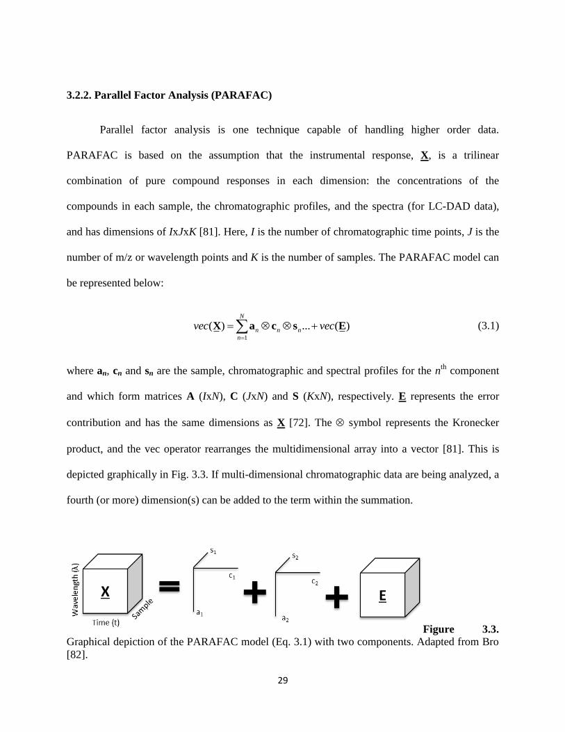
29

3.2.2. Parallel Factor Analysis (PARAFAC)

Parallel factor analysis is one technique capable of handling higher order data.

PARAFAC is based on the assumption that the instrumental response, X, is a trilinear

combination of pure compound responses in each dimension: the concentrations of the

compounds in each sample, the chromatographic profiles, and the spectra (for LC-DAD data),

and has dimensions of IxJxK [81]. Here, I is the number of chromatographic time points, J is the

number of m/z or wavelength points and K is the number of samples. The PARAFAC model can

be represented below:

1

( ) ... ( )

X a c s EN

n n n

n

vec vec (3.1)

where an, cn and sn are the sample, chromatographic and spectral profiles for the nth

component

and which form matrices A (IxN), C (JxN) and S (KxN), respectively. E represents the error

contribution and has the same dimensions as X [72]. The symbol represents the Kronecker

product, and the vec operator rearranges the multidimensional array into a vector [81]. This is

depicted graphically in Fig. 3.3. If multi-dimensional chromatographic data are being analyzed, a

fourth (or more) dimension(s) can be added to the term within the summation.

Figure 3.3.

Graphical depiction of the PARAFAC model (Eq. 3.1) with two components. Adapted from Bro

[82].

30

The PARAFAC model is trilinear (when analyzing third-order data such as LC-DAD)

which restricts its use to data whose retention times do not shift between runs. This is a strict

requirement in LC where retention time shifts can occur due to slight inconsistencies in flow rate

and mobile phase gradient as well as column aging. If shifts in retention occur, an alignment

step, such as correlation optimized warping (COW) [83], is required, or an algorithm such as

PARAFAC2 can be used, which attempts to handle retention time shifts within the model.

Bortolato and Oliveri showed, however, that PARAFAC2 did not perform well when interferents

were present [84]. Several algorithms exist for fitting the PARAFAC model to obtain the sample,

chromatographic, and spectral profiles. These include generalized rank annihilation method

(GRAM) and alternating least squares (ALS) [81,82].

Khakimov et al. [85] employed PARAFAC2 for the analysis of LC-MS data in a study of

a plant’s resistance to insects. With the exception of splitting the chromatograms into smaller

segments to decrease data complexity, no preprocessing steps were performed. Combining the

results of PARAFAC with pattern recognition, these authors were able to correlate four

previously reported compounds and five previously unknown compounds to the plants’

resistance to insects.

Synovec and colleagues have used PARAFAC extensively for the analysis of two

dimensional gas chromatography (GC)-MS data [86–89]. After processing raw chromatograms

in LECO ChromaTOF software [90], PARAFAC was used to resolve the chromatograms for the

purpose of quantification. Their approach consists of a pattern recognition step to find the peaks

that change the most between samples, then using ChromaTOF software to match mass spectra

31

to a library. Finally, the relative concentrations of the analytes of interest were found using peak

areas determined with PARAFAC [86]. They were able to identify 26 metabolites that differed

between yeast metabolizing glucose and yeast metabolizing ethanol, with ratios ranging from

0.02 to 67 for the compounds [88], as well as identifying 63 metabolites between 5 strains of

yeast and correlating them with RNA data to create pathways which could be compared across

strains [86].

Due to the trilinearity requirement, PARAFAC is difficult to implement in LC x LC.

Retention time shifts are very common in both separation dimensions. In the second dimension,

retention time shifts mainly occur due to misalignments of the 2D chromatograms. This is very

often due to slight variations in the valve timing. In the first dimension, slight retention time

shifts are amplified by the undersampling of the 1D separation. Due to these requirements, it is

often very difficult to implement PARAFAC in LC x LC, and often LC, analyses. PARAFAC

can also be time consuming do to the computational demands compared to other techniques. For

datasets with many samples, this can be another potential disadvantage.

3.2.3. Multivariate Curve Resolution (MCR)

Another method of curve resolution which is much more flexible is called multivariate

curve resolution (MCR). MCR is a based on a bilinear model, rather than the trilinear model of

PARAFAC, which makes MCR impervious to retention time shifting. The only requirement of

MCR is that the spectral profiles of each analyte do not vary over the dataset. DAD is a very

reproducible method which almost always meets this requirement, whereas other method such as

mass spectrometry can have slight variations in spectra between each chromatographic time

points.

32

The MCR model is shown in Eq. 3.2 and Fig. 3.4, where X is the raw data matrix (as

described in the previous section) and C and S are matrices consisting of the pure analyte (and

background) chromatographic and spectral profiles, respectively.

X CS ET (3.2)

Figure 3.4. (A) This graphic depicts the MCR model for a LC-DAD dataset with I time points, J

wavelengths, and N components representing the data. The yellow areas represent how each

point in the raw data (X) is represented by the chromatographic (C) and spectral (S) profiles and

error (E). Figure inspired by Rutan et al. [11]. (B) This graphic shows an example of a 2-

compound spectrochromatogram resolved into two pure analyte chromatographic and spectral

profiles.

Unlike PARAFAC, which can accept higher order data structures, MCR requires a matrix

as input. For a single LC-DAD run, the data are contained in a matrix which fits the MCR model;

however, when multiple samples are used, the data must be rearranged from a three-way array to

a matrix. As shown in Fig. 3.5, this is accomplished by concatenating the chromatograms from

each sample end-to-end along the time dimension to create a single augmented time dimension

33

while retaining the spectral dimension. This matrix can then be used for MCR-ALS analysis.

After analysis the data is then re-folded to determine the component profiles in each sample.

Similar to a multi-sample dataset, LC x LC-DAD adds another dimension to the data,

creating a third-order data array, or a four-way array when multiple samples are analyzed. This

requires two rearrangement steps. First, the two separation dimensions are unfolded to a single

time dimension consisting of the 2D chromatograms appended to one another similar to how the

data are collected (see Fig. 2.6). Then, the time and sample dimensions are unfolded to a single

dimension as depicted in Fig. 3.5. This results in a single spectral dimension and a single

augmented time dimension which can be analyzed via MCR-ALS.

Figure 3.5. Rearrangement of a multisample LC-DAD dataset into a single matrix for MCR

analysis. λ represents the spectral dimension, while t represents the time dimension. (A) This

graphic depicts the process graphically while (B) shows the process with realistic chromatograms

with the wavelength axis going into the page.

3.2.3.1. Alternating Least Squares (ALS)

Data collected from the instrument are represented by X in Eq. 3.2 but the goal of MCR

is to obtain the chromatographic and spectral profiles for each analyte and background

34

contribution, contained in the C and S matrices, respectively. To accomplish this, an alternating

least squares (ALS) methodology is most often used. ALS works by solving Eq 3.2 for C and S

alternatively using least squares solutions as shown in Eqs. 3.3 and 3.4.

1( )C XS S ST (3.3)

1( )S C C CXT T (3.4)

Before the ALS process can begin, a number of components (the number of columns in C

and S) must be chosen and an initial guess, or estimate, must be obtained for either C or S as a

starting point for ALS. The selection of the correct number of components is data dependent and

often multiple numbers of components are tested for the best MCR-ALS performance. Scree

plots, shown in Fig. 3.6., can offer a starting point for this determination. These plots are

obtained from the singular values (from a singular value decomposition) of the data plotted

versus the number of components [71]. A break or a shoulder in the trend can indicate a

reasonable starting point for determining the number of components.

Figure 3.6. Scree plot for estimating the number of components for MCR-ALS. The possible

break point occurs at 4 components indicating a starting point of 4 components for MCR-ALS.

35

The initial guess is typically derived from the raw data. Several methods have been

developed for this purpose. If an initial guess of the chromatographic profiles, C, is desired,

evolving factor analysis is a popular choice [91,92]. Most often, however, an initial guess of the

spectral profiles, S, is preferred. All of the methods for obtaining an initial guess of S involve

extracting individual spectra from the raw data. The methods differ in how this is accomplished.

Methods include SIMPLISMA [93,94], iterative key set factor analysis (IKSFA) [95,96], and

iterative orthogonal projection approach (IOPA) [9,97], which is used throughout the work

presented in the following chapters. IOPA, developed previously in our lab [9,97], builds off the

previously developed orthogonal projection approach (OPA) [98,99] which extracts a set of

spectra that represent the most different, or orthogonal, spectra in the dataset by defining a

dissimilarity metric. This dissimilarity metric is defined as the determinant of a matrix containing

the set of spectra for the initial guess. IOPA adds an iterative step in which each spectrum in the

initial guess is replaced by each spectrum in the raw data to maximize the orthogonality between

the spectra set used for the initial guess. If some or all of the analyte spectra are known a priori,

they can be used in the initial guess; however, OPA is still performed to obtain initial estimates

of the background and potential interferent spectra [9].

Once the initial guess is obtained, it is used in either Eq. 3.3 or 3.4 to initiate ALS. ALS

alternatively solves for C and S until either a predefined number of iterations is met or a solution

is converged upon as defined by a minimum change in fit error (E in Eq. 3.2). A defining factor

of ALS is that every time an updated estimate of C or S is calculated, the column vectors

contained in these matrices are subjected to constraints. Mathematically, a wide range of possible

solutions are possible for Eqs. 3.3 and 3.4, a problem often referred to as rotational ambiguity. A

much smaller range of solutions are physically reasonable, however. For instance, analyte

36

chromatographic and spectral profiles cannot be negative. To drive the ALS solutions to

physically reasonable solutions, constraints are imposed. These constraints, which are typically

only applied to components (columns in C and S) that correspond to true analyte signals, most

commonly include non-negativity, unimodality, normalization, and spectral selectivity. Non-

negativity replaces any negative values with zeros, recognizing that concentration values and

spectral intensities of chemical species cannot be negative. Unimodality recognizes that well-

behaved, spectrally distinct analytes should only produce a single maximum in their

chromatographic profiles. Unimodality eliminates any secondary maxima. Selectivity allows for

any known values to be input into the C and/or S matrices. This is most often used in the spectral

profiles to incorporate the knowledge that most analytes will not absorb at higher wavelengths

and therefore the absorbance values at those wavelengths should be zero. It has been observed

that spectral selectivity greatly helps in resolving analyte signals from background signals

[100,101]. Selectivity can also be used in the chromatographic dimension or the sample

dimension. Sample selectivity is especially useful when blanks are present in the dataset, and it is

desired to set an analyte signal to zero in that sample. Normalization of the spectra solves the

problem of intensity ambiguity. That is, normalization ensures that any intensity information is

contained in the chromatographic profiles rather than the spectral profiles, allowing for

quantitation based on the chromatographic profiles.

In the next chapter, we will explore the advantages of applying MCR-ALS to LC-DAD

data, particularly in terms of its ability to increase the number of quantitatively analyzable peaks

in a chromatogram.

37

Chapter 4: Peak Capacity Enhancements Enabled By Chemometric Curve Resolution

4.1. Introduction

When developing chromatographic methods, the primary goal is often to increase the

separation between analytes in order to facilitate further analysis. Sufficient separation is

particularly important when quantitation is the final goal of the analysis in order to enable the

precise and accurate recovery of peak areas (or peak height). Typically, the extent of separation

is defined by chromatographic resolution (RS) as discussed in Chapter 2 and the ideal separation

ability is estimated by peak capacity (nc). By definition, peak capacity is defined as the number

of peaks that can be separated at a RS of 1.0 in an analysis [20]. As discussed in Chapter 3, curve

resolution methods such as multivariate curve resolution (MCR-ALS) can resolve overlapping

chromatographic peaks, allowing for quantitative analysis at low RS.

Optimization of the chromatographic conditions is a crucial step in developing a

chromatographic method; however, method development can be time consuming and may still

not lead to satisfactory results. Similar attention to the application of chemometric approaches to

enhance the analysis is often not considered as carefully. These methods can assist in both

qualitative and quantitative analysis. MCR-ALS has been reported in the literature as early as 26

years ago [102,103] and has been utilized in a multitude of papers in many fields since then.

Specifically, MCR-ALS has been applied to liquid chromatographic (LC) data for various

38

applications including, but not limited to, environmental analyses [104–106], omics studies

[107–109], detection of biomarkers [110,111], food analyses [92,112,113], and pharmaceutical

analyses [114–116]. Several software packages for MCR-ALS are available including a program

by Tauler and colleagues [117,118] and the ALS package for the R programming environment

by Mullen [119]. Commercial chemometric programs are also available which include MCR-

ALS such as the PLS toolbox (Eigenvector Research, Inc., Manson, WA), which works through

the MATLAB programming environment.

Despite the demonstrated utility of MCR-ALS, it has yet to find widespread use in

chromatography outside of literature reports. It is our belief that this is due to an assumption that

MCR-ALS (and other chemometric techniques) are overly complex and difficult to implement.

There have also been very few papers characterizing the performance of MCR-ALS and other

curve resolution techniques and demonstrating their potential in everyday analyses. Davis,

Rutan, and Carr [120] investigated the use of chemometrics to analyze LC x LC data in a

theoretical study involving statistical overlap theory [121,122] and multivariate selectivity [123].

Multivariate selectivity is related to the quantitative precision that can be obtained when using

PARAFAC [82]. In that work, the authors found that in a separation space with a peak capacity

of 100 with 200 randomly positioned peaks actually present, 120 peaks would be able to be

analyzed quantitatively if PARAFAC were to be used. In comparison, only 20 peak maxima

were able to be identified in the chromatograms without chemometric assistance. That work

provided a detailed theoretical demonstration of the potential advantages of chemometrics, but

no curve resolution was actually performed and no experimental deviations from ideality

(background, retention time shifts, etc.) were considered. Fraga, Bruckner, and Synovec also

investigated the use of chemometric curve resolution in two dimensional separations, but with

39

generalized rank annihilation method (GRAM) [124]. They found that, on average, the number

of analyzable peaks was increased by a factor of two; however, no spectral information was

utilized in that work, relying solely on the additional information provided by a second

dimension of separation. This work also neglected the influence of background on the

performance of the curve resolution techniques, which may be significant in many cases.

There is a need for a general characterization of MCR-ALS performance over a range of

conditions in order to provide general guidelines of when it can provide an advantage in an

analysis. In the work in this chapter, LC-DAD data have been simulated under a range of

conditions with real instrumental background signals and analyzed with MCR-ALS. Then,

quantitation was performed and a model of quantitative MCR-ALS performance was created.

4.2. Methods

All simulated data creation and MCR-ALS analyses were performed in MATLAB

(R2013a, Mathworks, Inc., Natick, MA, USA). MCR-ALS was performed using an in-house

program. Modeling was performed using JMP statistical software (version 12.0.1, SAS Institute,

Inc. Cary, NC, USA).

4.2.1. Design of Experiments

To investigate the effects of different factors on the quantitative performance of MCR-ALS,

simulated LC-DAD data were created varying the signal-to-noise ratio (S/N), the

chromatographic resolution (RS) and the spectral similarity as measured by the coefficient of

determination ( 2rspectra

). A three factor, three level full-factorial experimental designs was created

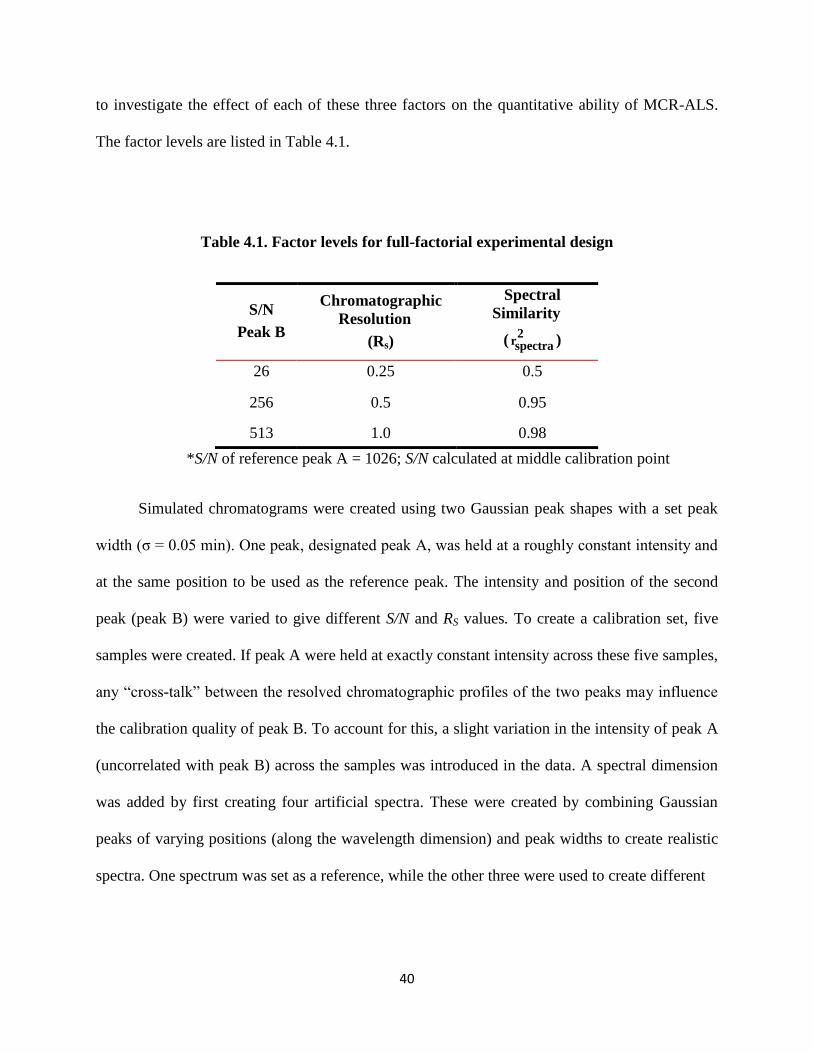
40

to investigate the effect of each of these three factors on the quantitative ability of MCR-ALS.

The factor levels are listed in Table 4.1.

Table 4.1. Factor levels for full-factorial experimental design

S/N

Peak B

Chromatographic

Resolution

(Rs)

Spectral

Similarity

(2

rspectra )

26 0.25 0.5

256 0.5 0.95

513 1.0 0.98

*S/N of reference peak A = 1026; S/N calculated at middle calibration point

Simulated chromatograms were created using two Gaussian peak shapes with a set peak

width (σ = 0.05 min). One peak, designated peak A, was held at a roughly constant intensity and

at the same position to be used as the reference peak. The intensity and position of the second

peak (peak B) were varied to give different S/N and RS values. To create a calibration set, five

samples were created. If peak A were held at exactly constant intensity across these five samples,

any “cross-talk” between the resolved chromatographic profiles of the two peaks may influence

the calibration quality of peak B. To account for this, a slight variation in the intensity of peak A

(uncorrelated with peak B) across the samples was introduced in the data. A spectral dimension

was added by first creating four artificial spectra. These were created by combining Gaussian

peaks of varying positions (along the wavelength dimension) and peak widths to create realistic

spectra. One spectrum was set as a reference, while the other three were used to create different

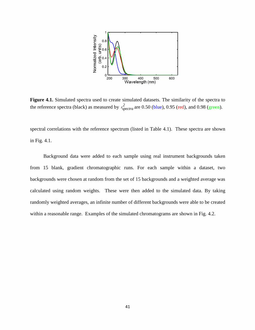
41

Figure 4.1. Simulated spectra used to create simulated datasets. The similarity of the spectra to

the reference spectra (black) as measured by 2

rspectra are 0.50 (blue), 0.95 (red), and 0.98 (green).

spectral correlations with the reference spectrum (listed in Table 4.1). These spectra are shown

in Fig. 4.1.

Background data were added to each sample using real instrument backgrounds taken

from 15 blank, gradient chromatographic runs. For each sample within a dataset, two

backgrounds were chosen at random from the set of 15 backgrounds and a weighted average was

calculated using random weights. These were then added to the simulated data. By taking

randomly weighted averages, an infinite number of different backgrounds were able to be created

within a reasonable range. Examples of the simulated chromatograms are shown in Fig. 4.2.

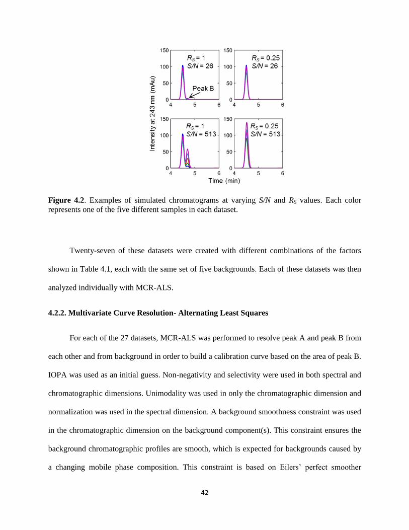
42

Figure 4.2. Examples of simulated chromatograms at varying S/N and RS values. Each color

represents one of the five different samples in each dataset.

Twenty-seven of these datasets were created with different combinations of the factors

shown in Table 4.1, each with the same set of five backgrounds. Each of these datasets was then

analyzed individually with MCR-ALS.

4.2.2. Multivariate Curve Resolution- Alternating Least Squares

For each of the 27 datasets, MCR-ALS was performed to resolve peak A and peak B from

each other and from background in order to build a calibration curve based on the area of peak B.

IOPA was used as an initial guess. Non-negativity and selectivity were used in both spectral and

chromatographic dimensions. Unimodality was used in only the chromatographic dimension and

normalization was used in the spectral dimension. A background smoothness constraint was used

in the chromatographic dimension on the background component(s). This constraint ensures the

background chromatographic profiles are smooth, which is expected for backgrounds caused by

a changing mobile phase composition. This constraint is based on Eilers’ perfect smoother

43

algorithm [125] which requires a single value be input to determine the extent of smoothing. In

order to remove any peak-like features in the background, this value was set high to effectively

“over-smooth” the background chromatographic profiles.. For all analyses, except in cases where

S/N was 26, three components were used. For the cases S/N was 26, five components were

needed to sufficiently resolve peak from the background.

After MCR-ALS resolution, the area of peak B was calculated for each sample by

summing all intensities in the resolved chromatogram of peak B and a calibration curve was

built. From this calibration the quality of fit was calculated using the coefficient of determination

of the calibration curve ( 2rcal

).

4.2.3. Monte-Carlo Simulations

After the MCR-ALS analyses of the 27 datasets, the set of background chromatograms

was changed to a new, randomly generated set of backgrounds produced in the same manner as

the previous set. The entire process was repeated including creation of datasets and MCR-ALS.

This process was repeated a total of 50 times to give 50 replicates for each of the 27

combinations of factors, each with a slightly different background.

4.2.4. Modeling

From the calibration curves, the coefficient of determination ( 2rcal

) was calculated. A

model was built using the average 2rcal

from each combination of factors (n = 50) as the response

variable and S/N, RS, and 2

rspectra as the predictors. Before building the model, both the spectral

and calibration r2

variables were converted to angles using Eq. 4.1 [126]. Using angles (θ) rather

than r2 as the model variables allows for greater sensitivity particularly at higher values of r

2

44

where a difference between 0.9 and 0.999 is mathematically small, but very meaningful in terms

of fit quality. In terms of angles the difference between these two values is 10-fold. Of note is the

inverse relationship between r2 and θ.

2 2cosr (4.1)

A model was built including independent terms and interaction terms, to predict the

quality of the calibration using the three predictors. The generic model is shown in Eq. 4.2,

where b represents the intercept, the m values represent the coefficients, and the x terms are the

predictors, defined in Table 4.2. Only terms whose coefficients were statistically significant

(p<0.05) were included in the final model.

3 3 3

log1,2,3 1 2 31 1 1

b m x m x x m x x xi i ij i jcal i i j

(4.2)

Table 4.2. Predictors used in building prediction model

i or j x

1 log(θspectra)

2 log(S/N)

3 log(RS)

4.3. Results and Discussion

A model was built with S/N, RS, and θspectra as predictors and θcal as the response variable

as shown in Eq. 4.2 and Table 4.2. All terms were log-scaled to ensure no negative predicted

values. Each independent term and cross-term was evaluated for its significance in affecting the

45

model using significance testing. Terms with p-values < 0.05 were included in the final model.

The terms included are listed in Table 4.3 along with their corresponding coefficient (m),

standard error (SE), and p-value. To interpret this model, it is important to remember the inverse

relationship between r2 and θ. A larger θcal indicates a worse 2

rcal

for the calibration curve and a

larger θspectra indicates more dissimilar spectra. As shown in Table 4.3, θspectra has an inverse

relationship with θcal; as the spectra corresponding to peaks A and B become more dissimilar, the

calibration fit quality improves, as expected. Similarly, S/N and RS have inverse relationships

with θcal; as the peak becomes less intense and the peaks become more overlapped, the

calibration fit quality worsens. Several cross-terms were also found to be statistically significant

including a quadratic term for θspectra as well as all of the interaction terms between the

predictors.

Table 4.3. Coefficients and errors for predictive model of calibration quality

Term* m SE p-value

Intercept 1.15 0.11 <0.0001

θspectra -1.670 0.075 <0.0001

S/N -0.646 0.030 <0.0001

RS -0.35 0.15 0.0331

(θspectra)² -1.70 0.34 <0.0001

θspectra *S/N 0.47 0.10 0.0001

θspectra * RS -2.00 0.30 <0.0001

S/N* RS 0.50 0.12 0.0007

(θspectra)² *RS -4.3 1.4 0.0061

θspectra *S/N* RS 1.46 0.39 0.0016

*All variables are log-scaled; cross-terms are mean centered

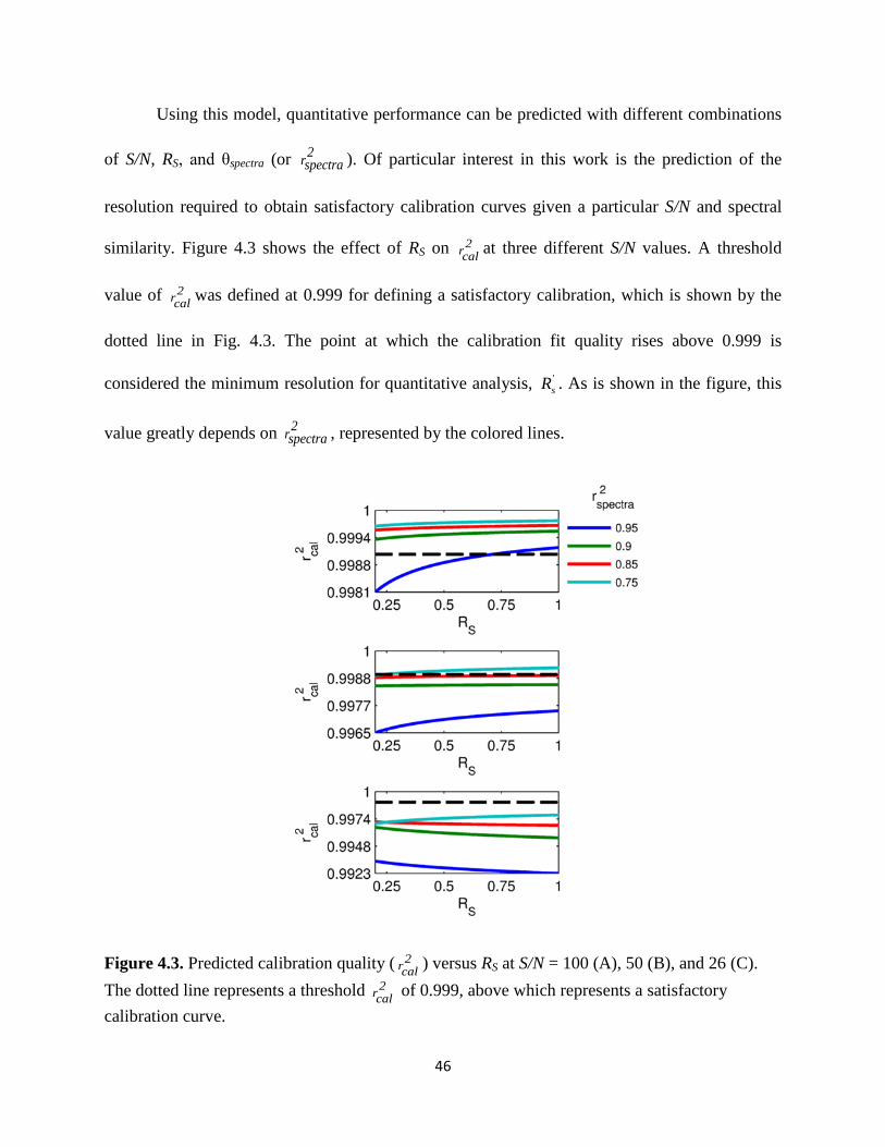
46

Using this model, quantitative performance can be predicted with different combinations

of S/N, RS, and θspectra (or 2

rspectra ). Of particular interest in this work is the prediction of the

resolution required to obtain satisfactory calibration curves given a particular S/N and spectral

similarity. Figure 4.3 shows the effect of RS on 2rcal

at three different S/N values. A threshold

value of 2rcal

was defined at 0.999 for defining a satisfactory calibration, which is shown by the

dotted line in Fig. 4.3. The point at which the calibration fit quality rises above 0.999 is

considered the minimum resolution for quantitative analysis, '

sR . As is shown in the figure, this

value greatly depends on 2

rspectra , represented by the colored lines.

Figure 4.3. Predicted calibration quality ( 2rcal

) versus RS at S/N = 100 (A), 50 (B), and 26 (C).

The dotted line represents a threshold 2rcal

of 0.999, above which represents a satisfactory

calibration curve.

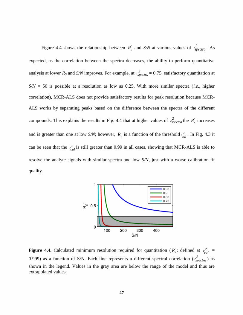
47

Figure 4.4 shows the relationship between '

sR and S/N at various values of 2

rspectra . As

expected, as the correlation between the spectra decreases, the ability to perform quantitative

analysis at lower RS and S/N improves. For example, at 2

rspectra = 0.75, satisfactory quantitation at

S/N = 50 is possible at a resolution as low as 0.25. With more similar spectra (i.e., higher

correlation), MCR-ALS does not provide satisfactory results for peak resolution because MCR-

ALS works by separating peaks based on the difference between the spectra of the different

compounds. This explains the results in Fig. 4.4 that at higher values of 2

rspectra the '

sR increases

and is greater than one at low S/N; however, '

sR is a function of the threshold 2rcal

. In Fig. 4.3 it

can be seen that the 2rcal

is still greater than 0.99 in all cases, showing that MCR-ALS is able to

resolve the analyte signals with similar spectra and low S/N, just with a worse calibration fit

quality.

Figure 4.4. Calculated minimum resolution required for quantitation ( '

sR ; defined at 2rcal

=

0.999) as a function of S/N. Each line represents a different spectral correlation (2

rspectra ) as

shown in the legend. Values in the gray area are below the range of the model and thus are

extrapolated values.

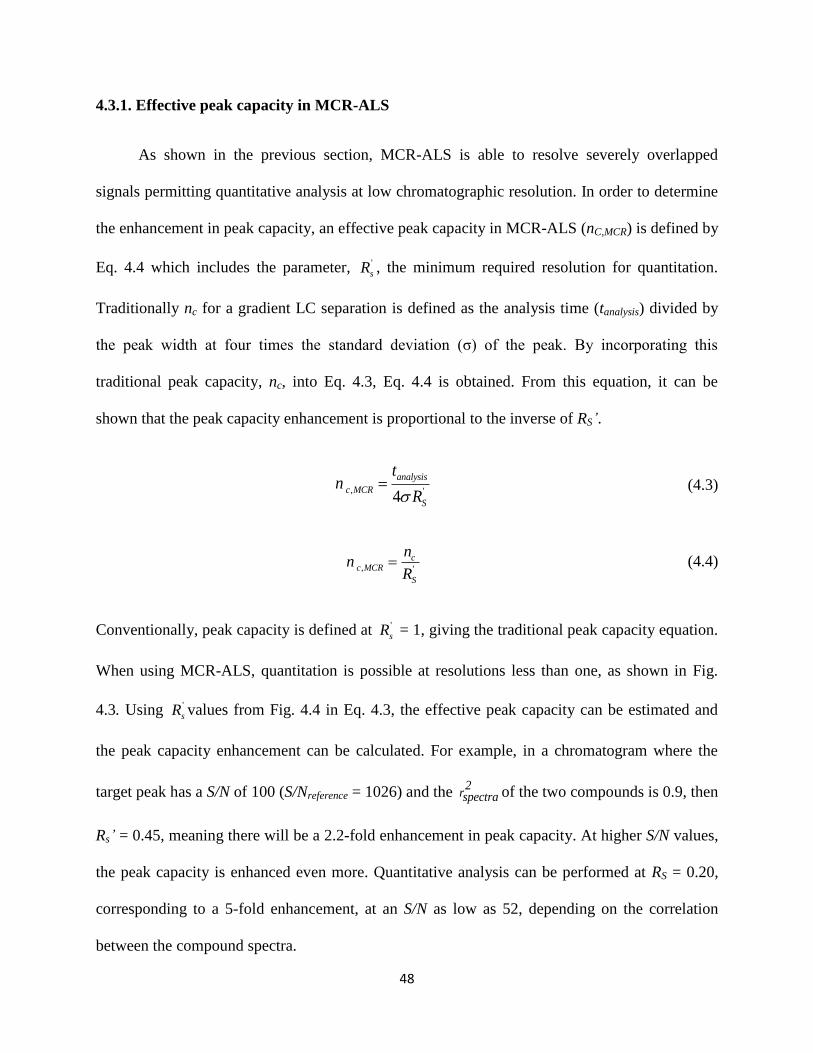
48

4.3.1. Effective peak capacity in MCR-ALS

As shown in the previous section, MCR-ALS is able to resolve severely overlapped

signals permitting quantitative analysis at low chromatographic resolution. In order to determine

the enhancement in peak capacity, an effective peak capacity in MCR-ALS (nC,MCR) is defined by

Eq. 4.4 which includes the parameter, '

sR , the minimum required resolution for quantitation.

Traditionally nc for a gradient LC separation is defined as the analysis time (tanalysis) divided by

the peak width at four times the standard deviation (σ) of the peak. By incorporating this

traditional peak capacity, nc, into Eq. 4.3, Eq. 4.4 is obtained. From this equation, it can be

shown that the peak capacity enhancement is proportional to the inverse of RS’.

, '4

analysis

c MCR

S

tn

R (4.3)

, '

cc MCR

S

nn

R (4.4)

Conventionally, peak capacity is defined at '

sR = 1, giving the traditional peak capacity equation.

When using MCR-ALS, quantitation is possible at resolutions less than one, as shown in Fig.

4.3. Using '

sR values from Fig. 4.4 in Eq. 4.3, the effective peak capacity can be estimated and

the peak capacity enhancement can be calculated. For example, in a chromatogram where the

target peak has a S/N of 100 (S/Nreference = 1026) and the 2

rspectra of the two compounds is 0.9, then

Rs’ = 0.45, meaning there will be a 2.2-fold enhancement in peak capacity. At higher S/N values,

the peak capacity is enhanced even more. Quantitative analysis can be performed at RS = 0.20,

corresponding to a 5-fold enhancement, at an S/N as low as 52, depending on the correlation

between the compound spectra.

49

4.4. Conclusions

While MCR-ALS has been well documented in the literature, it has not yet become a

standard tool in the analytical chemist’s arsenal. In the work presented here, three crucial factors

impacting the performance of MCR-ALS – S/N, RS, and2

rspectra – were varied and the potential for

peak capacity enhancement in quantitative LC-DAD analysis was evaluated. It was found that

MCR-ALS significantly increased the effective peak capacity. In many cases, the number of

quantitatively analyzable peaks was increased by a factor of five or more compared to the

traditional peak capacity at a resolution of one. This has the potential to significantly impact

analyses by reducing the need for long analysis times and/or complicated methods to completely

separate analyte peaks for subsequent quantification. The data simulated in this work included no

pure standards. Previous work in our lab found that including pure standards in the data structure

submitted to MCR-ALS improves the performance by providing a better initial guess to initiate

the ALS algorithm [9].

In this work MCR-ALS was applied to LC-DAD data; however, the technique is broadly

applicable to other instrumental methods including LC x LC, LC-MS, various spectroscopies,

etc. Based on the results here, MCR-ALS can be expected to perform even better with increased

peak separation (as in LC x LC) or with decreased spectral correlation (as in high resolution

mass spectrometry). We believe that the ability of MCR-ALS to quantify significantly

overlapped analyte peaks along with its relative ease-of-use lends itself well to being utilized

much more often in the analytical laboratory for both routine and complex analyses.

50

This page intentionally left blank

51

Chapter 5: Two-Dimensional Assisted Liquid Chromatography

This chapter has been adapted, with permission, from D.W. Cook, S.C. Rutan, D.R. Stoll, P.W.

Carr. Two dimensional assisted liquid chromatography – a chemometric approach to improve

accuracy and precision of quantitation in liquid chromatography using 2D separation, dual

detectors, and multivariate curve resolution, Anal. Chim. Acta 859 (2014) 87-95

Section 5.4.3 was adapted from D.W. Cook, S.C. Rutan, D.R. Stoll. 2016 in preparation for

submission to Chemom. Intell. Lab. Syst.

5.1. Introduction

The increasing need for the analysis of complex samples necessitates the development of

new analytical techniques and data analysis strategies. Particularly in “-omic” type applications,

these samples can contain several hundred to several thousands of compounds [4]. For these

applications traditional 1D chromatography is being pushed to its limits in regards to peak

capacity, particularly when analysis time is limited. Many of these applications require analyte

quantitation not merely detection. To do this the analytes must be adequately resolved in order

to accurately determine how much is present in the sample [101].

Comprehensive two-dimensional liquid chromatography (LC x LC) can provide a

significant advantage over one-dimensional liquid chromatography (1D-LC) in terms of

resolving power. Ideally, the theoretical peak capacity for a two-dimensional (2D) separation is

52

equal to the product of the peak capacities of each separation dimension; however, this peak

capacity is significantly smaller than ideal due to undersampling and lack of orthogonality

between the two dimensions as discussed in Chapter 2. Despite these limitations Stoll, Wang,

and Carr determined through both theoretical and experimental studies that when separation

times are greater than 10 minutes and the 2D separation is conducted sufficiently rapidly, LC x

LC has superior effective peak capacity as compared to 1D-LC [48,52,65,127]. While multi-

dimensional chromatography has definite advantages in terms of peak capacity and peak capacity

per unit time, the precision and accuracy of these methods compared to 1D chromatography

often are not considered. Indeed, multi-dimensional liquid chromatography methods often suffer

in terms of quantitative performance in comparison to their traditional 1D counterparts [101].

Stoll et al. reported percent relative standard deviations (%RSD) for two dimensional (2D) peak

areas ranging from 0.7% to upwards of 15% with most falling between 1.5% and 7% when

manual peak integration was employed [59]. In another paper, Stoll et al. compared the precision

of 1D-LC and LC x LC and found that the 2D peak areas were on average seven-fold less precise

based on the %RSD [52]. Kivilompolo et al. reported %RSDs for peak volumes ranging from

3%-13% for antioxidants in wines and juices [128]. Dugo et al. were able to quantify more

polyphenols in red wines due to the increased resolving power of LC x LC; however, for the

compounds detected in both LC x LC and 1D-LC, the %RSD in LC x LC was 12-fold higher

than in 1D-LC [129]. A summary of these results is presented in Table 5.1. While the

quantitative ability of LC x LC is improving with improved instrumentation and methods, poor

quantitation still remains an issue and is unlikely to completely disappear without even more

complex instrumentation and methods.

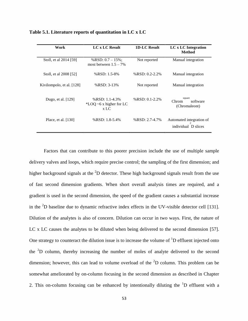
53

Table 5.1. Literature reports of quantitation in LC x LC

Work LC x LC Result 1D-LC Result LC x LC Integration

Method

Stoll, et al 2014 [59] %RSD: 0.7 – 15%;

most between 1.5 – 7%

Not reported Manual integration

Stoll, et al 2008 [52] %RSD: 1.5-8% %RSD: 0.2-2.2% Manual integration

Kivilompolo, et al. [128] %RSD: 3-13% Not reported Manual integration

Dugo, et al. [129] %RSD: 1.1-4.3%

*LOQ ~6 x higher for LC

x LC

%RSD: 0.1-2.2% Chrom

square

software

(Chromaleont)

Place, et al. [130] %RSD: 1.8-5.4% %RSD: 2.7-4.7% Automated integration of

individual 2

D slices

Factors that can contribute to this poorer precision include the use of multiple sample

delivery valves and loops, which require precise control; the sampling of the first dimension; and

higher background signals at the 2D detector. These high background signals result from the use

of fast second dimension gradients. When short overall analysis times are required, and a

gradient is used in the second dimension, the speed of the gradient causes a substantial increase

in the 2D baseline due to dynamic refractive index effects in the UV-visible detector cell [131].

Dilution of the analytes is also of concern. Dilution can occur in two ways. First, the nature of

LC x LC causes the analytes to be diluted when being delivered to the second dimension [57].

One strategy to counteract the dilution issue is to increase the volume of 1D effluent injected onto

the 2D column, thereby increasing the number of moles of analyte delivered to the second

dimension; however, this can lead to volume overload of the 2D column. This problem can be

somewhat ameliorated by on-column focusing in the second dimension as described in Chapter

2. This on-column focusing can be enhanced by intentionally diluting the 1D effluent with a

54

weak solvent before delivery to the second dimension. This is useful for avoiding injection

broadening on the 2D column caused by the delivery of the

1D effluent in a stronger solvent

[59,35]. The amount of dilution needed is dependent on the analytes and should be optimized to

avoid unnecessary loss of the signal-to-background caused by the loss of signal intensity.

Sampling of the 1D separation can also cause a loss of S/N due to the division of a single

chromatographic peak into three or more peaks.

Even given the superior peak capacity of LC x LC, many analytes may still be poorly

resolved in complex samples, making quantification difficult. Another approach for improving

peak resolution is to use a curve resolution technique, such as MCR-ALS. Using MCR-ALS,

Bailey et al. were able to detect 18 peaks in a separation space which had a calculated

chromatographic peak capacity of only 5 using a DAD detector [101]. Curve resolution can

essentially improve resolution without increasing the complexity of instrumentation, while

maintaining the inherent quantitative abilities of the instrument. This is demonstrated in Chapter

4 where MCR-ALS was shown to resolve chromatographic peaks with a resolution of less than

0.25 depending on the spectra similarity and S/N. While curve resolution methods work well for

moderate to significantly overlapped peaks, they can fail when peaks are severely or completely

overlapped and have low S/N. This is shown in Fig. 4.3, where the performance of MCR-ALS

began to degrade at resolutions as high as 0.5 if the spectral similarity between the analytes was

very high (2

rspectra > 0.9). Having the additional chromatographic resolution provided by

LC x LC can potentially create a powerful technique when both LC x LC and MCR-ALS are

combined.

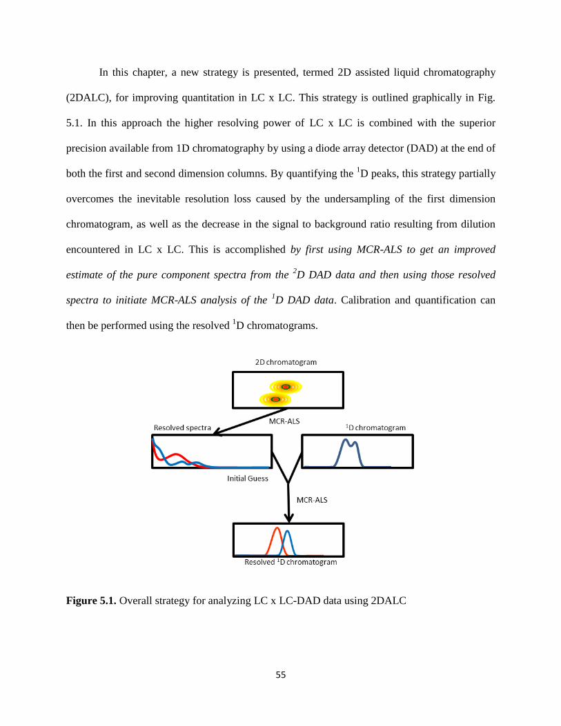
55

In this chapter, a new strategy is presented, termed 2D assisted liquid chromatography

(2DALC), for improving quantitation in LC x LC. This strategy is outlined graphically in Fig.

5.1. In this approach the higher resolving power of LC x LC is combined with the superior

precision available from 1D chromatography by using a diode array detector (DAD) at the end of

both the first and second dimension columns. By quantifying the 1D peaks, this strategy partially

overcomes the inevitable resolution loss caused by the undersampling of the first dimension

chromatogram, as well as the decrease in the signal to background ratio resulting from dilution

encountered in LC x LC. This is accomplished by first using MCR-ALS to get an improved

estimate of the pure component spectra from the 2D DAD data and then using those resolved

spectra to initiate MCR-ALS analysis of the 1D DAD data. Calibration and quantification can

then be performed using the resolved 1D chromatograms.

Figure 5.1. Overall strategy for analyzing LC x LC-DAD data using 2DALC

56

5.2. Strategy

Figure 5.1 shows the overall strategy developed here. First, the 2D chromatogram is

analyzed with MCR-ALS to obtain resolved spectra of the real chemical components. Then,

these spectra are used to initialize MCR-ALS on the 1D chromatographic data to obtain the

resolved 1D chromatograms. Calibration is performed with these resolved

1D chromatograms in

order to assess the quantitative performance of this strategy.

5.2.1 Instrumental Setup

As discussed in Chapter 2, LC x LC commonly uses one detector at the end of the 2D

column, which, after rearranging the data gives the 2D chromatogram. For this work, a

multichannel detector is also needed at the end of the 1D column as shown in Fig. 5.2. In this

case, both detectors were diode array detectors (DAD); however, this strategy should work with

other multichannel detectors as well as long as the two detectors are identical. With this setup,

both a 1D chromatogram from the

1D DAD and a 2D chromatogram from the

2D DAD can be

produced. The addition of a detector after the first dimension will induce peak broadening due to

added extra column volume; however, under the conditions of this experiment we estimate that

the 1D detector will add at most a few percent to the

1D peak width prior to sampling (assuming a

flow cell contribution of 1 µL2). When this is compared to the broadening of

1D peaks due to its

undersampling [49] , it is evident that the contribution of the 1D detector to the effective

1D peak

width is very minor. As discussed in the previous section, pre-dilution with a weak solvent was

also employed in this setup as shown in Fig. 5.2.

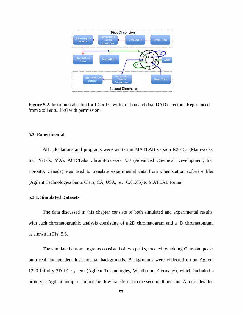
57

Figure 5.2. Instrumental setup for LC x LC with dilution and dual DAD detectors. Reproduced

from Stoll et al. [59] with permission.

5.3. Experimental

All calculations and programs were written in MATLAB version R2013a (Mathworks,

Inc. Natick, MA). ACD/Labs ChromProcessor 9.0 (Advanced Chemical Development, Inc.

Toronto, Canada) was used to translate experimental data from Chemstation software files

(Agilent Technologies Santa Clara, CA, USA, rev. C.01.05) to MATLAB format.

5.3.1. Simulated Datasets

The data discussed in this chapter consists of both simulated and experimental results,

with each chromatographic analysis consisting of a 2D chromatogram and a 1D chromatogram,

as shown in Fig. 5.3.

The simulated chromatograms consisted of two peaks, created by adding Gaussian peaks

onto real, independent instrumental backgrounds. Backgrounds were collected on an Agilent

1290 Infinity 2D-LC system (Agilent Technologies, Waldbronn, Germany), which included a

prototype Agilent pump to control the flow transferred to the second dimension. A more detailed

58

description of the instrumentation can be found in Allen et al. [44]. Mobile phases in both

dimensions were water as the A solvent and acetonitrile as the B solvent. The first dimension

consisted of an SB-C18 column (30 mm x 4.6 mm; 5 µm; Agilent Technologies, Little Falls, DE)

maintained at 40 °C and a flow rate of 0.500 mL/min. A gradient from 5%-95% B over 10

minutes was used for a 15 minute time of analysis. The 1D effluent

was split to 0.05 mL/min (see

reference [65] for more details about splitting) and directed to a pair of 40 µL sample loops

connected to an 8-port valve. The sample loops were alternatively filled with 1D effluent and

then the effluent was delivered to the 2D column by switching the valve position. The cycle time

was 12 sec and the gradient was 0%-100% B over 9 s. The second dimension consisted of a

Poroshell 120 C18 column (30 mm x 2.1 mm; 2.7 µm; Agilent Technologies, Little Falls, DE)

maintained at 80 °C with a flow rate of 3 mL/min.

For 2D chromatograms, Gaussian peaks were used in the second dimension (sampled at

0.0250 sec intervals) and sampled Gaussian peaks were used in the first dimension (sampled at

12 second intervals), using an in-house MATLAB program [132]. Two separate sets of simulated

data, differing in only the amount of dilution of the 1D effluent before delivery to the

2D column,

were created. The peak heights and widths were chosen to approximately match experimental

data obtained for an amphetamine mixture. For low dilution conditions, the peak height ratio

between 1D and

2D chromatograms was 2:1. For high dilution, the ratio was 10:1. The

chromatographic resolution of the peaks was varied from 0.01 to 1 in both dimensions. At each

resolution, 15 “samples” were created at varying concentrations including 9 calibration samples,

4 test samples, and 2 blanks. These concentrations are listed in Table 5.2. The spectra for the two

analytes were taken from pure samples of 3-methoxyamphetamine (MoxyAmp) and 3,4-

methylenedioxy-N-methylamphetamine (MDMA). The similarity of each compound’s spectra to

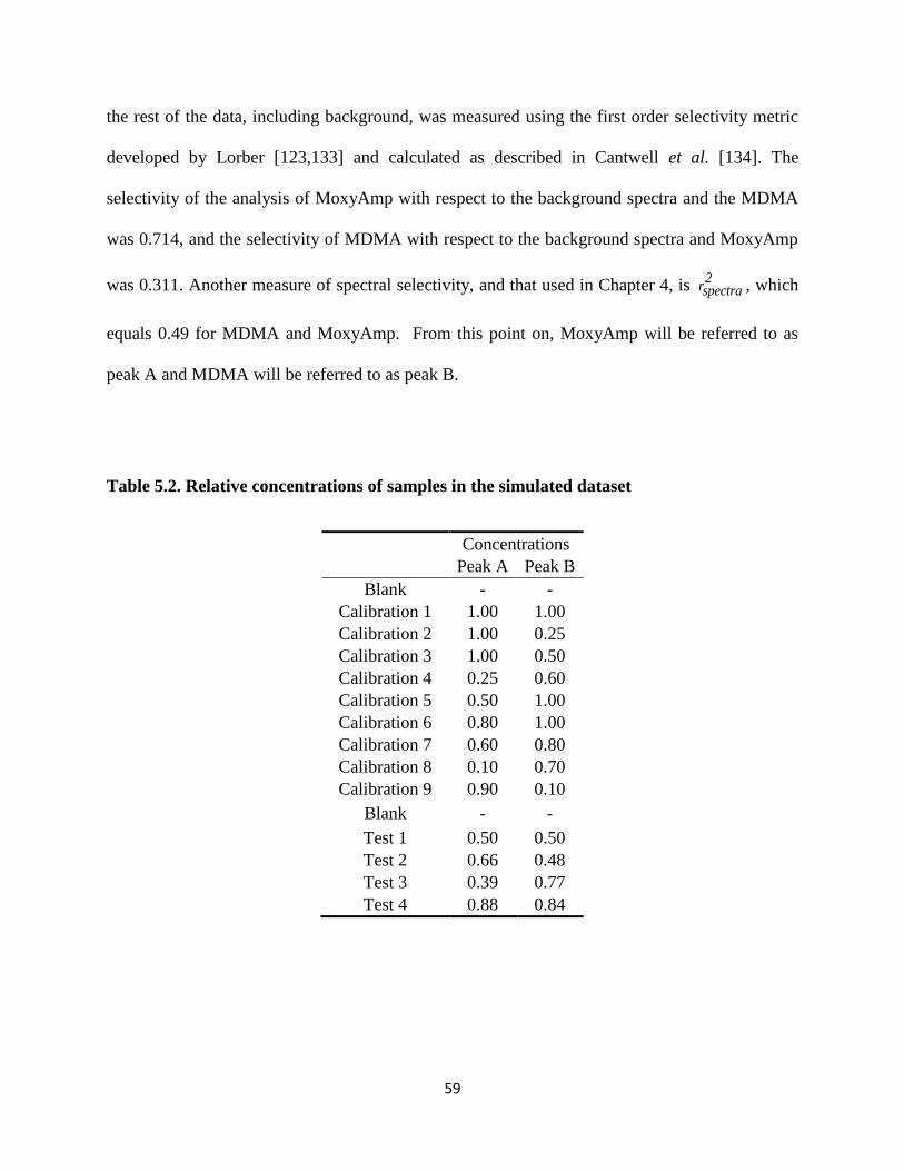
59

the rest of the data, including background, was measured using the first order selectivity metric

developed by Lorber [123,133] and calculated as described in Cantwell et al. [134]. The

selectivity of the analysis of MoxyAmp with respect to the background spectra and the MDMA

was 0.714, and the selectivity of MDMA with respect to the background spectra and MoxyAmp

was 0.311. Another measure of spectral selectivity, and that used in Chapter 4, is 2

rspectra , which

equals 0.49 for MDMA and MoxyAmp. From this point on, MoxyAmp will be referred to as

peak A and MDMA will be referred to as peak B.

Table 5.2. Relative concentrations of samples in the simulated dataset

Concentrations

Peak A Peak B

Blank - -

Calibration 1 1.00 1.00

Calibration 2 1.00 0.25

Calibration 3 1.00 0.50

Calibration 4 0.25 0.60

Calibration 5 0.50 1.00

Calibration 6 0.80 1.00

Calibration 7 0.60 0.80

Calibration 8 0.10 0.70

Calibration 9 0.90 0.10

Blank - -

Test 1 0.50 0.50

Test 2 0.66 0.48

Test 3 0.39 0.77

Test 4 0.88 0.84

60

5.3.2. Experimental Datasets

The experimental data consisted of selective LC x LC (denoted sLC x LC) analyses of

three furanocoumarins – psoralen, angelicin, and 8-methoxypsoralen (8-MOP). The multivariate

selectivities of these compounds’ spectra were calculated to be 0.160, 0.204, and 0.156,

respectively. The pairwise 2

rspectra values for the furanocoumarin spectra were: psoralen/8-MOP

0.91; psoralen/angelicin, 0.95; and 8-MOP/angelicin, 0.89. The data consisted of three mixtures

and three pure calibration standards for each compound. The concentrations of the components

in each sample are listed in Table 5.3. In this work, sLC x LC separations of the furanocoumarins

were performed using an Agilent 1290 Infinity 2D-LC system (Agilent Technologies,

Waldbronn, Germany). Mobile phases in both dimensions were 10 mM phosphoric acid as the A

solvent and acetonitrile as the B solvent. The 1D separations were carried out on a Poroshell 120

PFP (100 mm x 2.1 mm i.d.; Agilent Technologies, Little Falls, DE) column maintained at 40 °C

with a flow rate of 0.15 mL/min and a 5 µL injection. A gradient was used with the following

conditions: 40%-55% B from 0-6 min; 55%-95% from 6-7 min; 95%-40% from 7-7.01 min; and

held at 40% until 9 min. The 1D effluent was sampled six times at 5-sec intervals starting at 3.75

min into 40 µL loops following dilution with water at 0.25 mL/min. Each 1D effluent sample was

then delivered sequentially to the 2D column, which was a Zorbax SB-C18 (30 mm x 2.1 mm i.d;

3.5 µm; Agilent Technologies, Little Falls, DE) column maintained at 60 °C with a flow rate of

2.5 mL/min under isocratic conditions (17.5% B) over 45 sec. For a more detailed description of

the implementation of sLC x LC, the reader is referred to Stoll et al. [37].

61

Table 5.3. Concentrations of samples in the experimental dataset

Concentrations (mg L

-1)

Angelicin Psoralen 8-MOP

Blank - - -

Blank - - -

Mix 1 4.0 1.5 6.0

Mix 2 6.0 4.0 1.5

Mix 3 1.5 6.0 4.0

Psoralen Standard - 1.0 -

Psoralen Standard - 2.5 -

Psoralen Standard - 7.0 -

8-MOP Standard - - 1.0

8-MOP Standard - - 2.5

8-MOP Standard - - 7.0

Angelicin Standard 1.0 - -

Angelicin Standard 2.5 - -

Angelicin Standard 7.0 - -

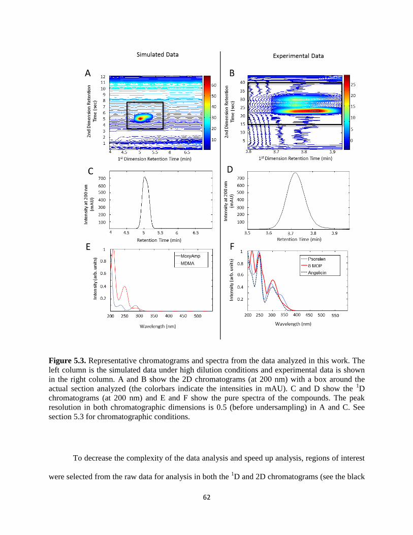
62

Figure 5.3. Representative chromatograms and spectra from the data analyzed in this work. The

left column is the simulated data under high dilution conditions and experimental data is shown

in the right column. A and B show the 2D chromatograms (at 200 nm) with a box around the

actual section analyzed (the colorbars indicate the intensities in mAU). C and D show the 1D

chromatograms (at 200 nm) and E and F show the pure spectra of the compounds. The peak

resolution in both chromatographic dimensions is 0.5 (before undersampling) in A and C. See

section 5.3 for chromatographic conditions.

To decrease the complexity of the data analysis and speed up analysis, regions of interest

were selected from the raw data for analysis in both the 1D and 2D chromatograms (see the black

63

boxes in Figs. 5.3.A and 5.3.B). Before MCR-ALS analysis, the data must be augmented as

described in Chapter 3.

5.3.3. MCR-ALS

MCR-ALS was performed using an in-house algorithm adapted from a previously

described algorithm [135]. The code is reproduced in Appendix A. Non-negativity was applied

as a constraint for the 1D and

2D chromatograms, unimodality was used for the

1D

chromatograms, and spectral selectivity was used to set absorbances at the longer wavelengths to

zero in the 2D chromatograms to assist in the differentiation of the signal from the background

[101]. These constraints were applied only to the components which represented real chemical

compounds; background components were not constrained.

5.3.4. Calibration

The resolved 1D chromatograms were integrated over the full retention time range to

obtain the peak area. This gave acceptable results because of the complete resolution of the

signals from each other and from the background. For the resolved 2D chromatograms, Savitzky-

Golay second-derivative peak detection was employed to deal with the incomplete resolution of

the analyte signals from the background signal. This was implemented using a Savitzky-Golay

second-derivative smoothing [74,75] and then finding the peak start and end points based on a

noise threshold in the second derivative. A window size of 19 points for the simulated

chromatograms and 115 points for the experimental chromatograms for the second derivative

smoothing was used, and the noise threshold was set at 0.0025 mAU. The peak area was then

determined by summing the signal above a linear baseline created between these points in the

MCR-resolved chromatogram. The areas of the calibration samples were then used to create a

64

calibration curve. The peak areas of the test samples were then used to estimate the predictive

ability of this method, measured by root mean squared percentage error (RMSPE) as defined by

Eq. 5.1 [136], where yi is the true concentration, ŷ is the calculated concentration from the

calibration curve, and n is the number of samples.

𝑅𝑀𝑆𝑃𝐸 =√∑(

𝑦𝑖−��

𝑦𝑖)2

𝑛× 100% (5.1)

5.4. Results

5.4.1 Simulated Data

Chromatograms were simulated to investigate the effect of peak resolution on the

quantitative capabilities of 2DALC for both low dilution and high dilution conditions. RMSPE

was used to compare the quantitative ability of 2DALC to the four alternative methods listed in

Table 5.4. Examples of the 1D and 2D data are shown in Figs. 5.3A and 5.3C, and the results are

summarized in Figs. 5.4 and 5.5. These figures show the RMSPE as a function of both the first

and second dimension resolutions. The bottom left corner of each panel in Figs. 5.4 and 5.5

shows the RMSPE for the case where no resolution is achieved in either the first or second

dimension, and the top right corner of each panel shows the RMSPE for the case of high

resolution in both dimensions. As expected, there is a clear trend where the performances of all

of the methods improve as the resolution in both dimensions improves.

65

Table 5.4. Quantitation methods studied in this work

Method Chromatogram used

for quantitation

Method of obtaining initial guess

1D-IOPA

1D IOPA

1D-Pure

1D

Pure analyte spectra with OPA estimated

backgrounds

2DALC 1D

2D resolved spectra with OPA estimated

backgrounds

2D-IOPA 2D IOPA

2D-Pure 2D Pure analyte spectra with OPA estimated

backgrounds

When the two methods of resolving 1D chromatograms are compared (rows 1 and 2 in

Fig. 5.4), it can be seen that IOPA begins to degrade at resolutions less than 0.3 versus using the

pure spectra, where quantitative results can be achieved even when peaks are almost completely

overlapped, (represented as a resolution of 0.01 in Fig. 5.4 and 5.5). A similar pattern is observed

when the two methods of resolving 2D chromatograms are compared (rows 4 and 5 in Fig. 5.4

and rows 2 and 3 in Fig. 5.5). For peak A, as long as one dimension has a resolution greater than

0.4, the RMSPE is similar to that obtained using pure spectra as initial guesses. For peak B, the

results are similar at low dilution; however, at high dilution 2D-IOPA fails to give acceptable

quantitative results at any 1D resolution if the

2D resolution is low. In low dilution conditions

(Fig. 5.4) the RMSPE is almost equal between peak A and peak B. In the high dilution

conditions (Fig. 5.5) peak B has higher RMSPE values, which is consistent with the higher

relative residual background in the resolved chromatographic profile due to the lower

multivariate selectivity of this peak relative to the background and peak A (0.311 vs. 0.714 for

peak A). In addition, some of the points in the 2D graphs do not follow the trends seen for peak

A under the high dilution conditions. We attribute this to the difficulty in obtaining accurate peak

66

areas due to the low S/N, despite using peak detection to assist in the differentiation of peaks

from residual noise in the resolved components.

2DALC is superior to 2D-IOPA (row 3 vs. row 4 in Fig. 5.4 and row 1 vs row 2 in Fig.

5.5). Under the low dilution conditions, the difference is small, but for higher dilution conditions,

the advantage of quantitation in 2DALC is clear. Both peaks have poorer quantitation in 2D-

IOPA when the resolution is less than 0.5 in both dimensions. Peak B has poorer quantitation at

all resolutions when 2D-IOPA is used. There are also more inconsistencies in the patterns of both

peaks, owing to the lower S/N in the 2D chromatogram. When 2DALC is used, quantitative

performance is slightly better under low dilution conditions (compared to high dilution, compare

row 3 of Fig. 5.4 to row 1 of Fig. 5.5), whereas the extent of dilution has a much bigger impact

on the quantitative performance of 2D-IOPA (compare row 4 of Fig. 5.4 to row 2 of Fig. 5.5).

Based on this we conclude that 2DALC is less sensitive to variations in S/N at the 2D detector.

2DALC also has advantages over 1D-IOPA (row 2 in Fig. 5.4). At

1D resolution of 0.25

1D-IOPA begins to fail. When the

2D resolution is greater than that of the

1D resolution, the

spectrum obtained from the 2D chromatogram provides a better initial guess than IOPA analysis

of the 1D data, and therefore provides better quantitation under both low and high dilution

conditions. The exception is when 1D resolution is greater than 0.25; in this case IOPA is able to

obtain a sufficiently accurate initial guess from the 1D chromatographic data leading to results

that are equivalent to those obtained using 2DALC.

67

Figure 5.4. Results for simulated data at low dilution conditions (peak height ratio of 2:1).

Colorbars indicate RMSPE. Scales for the graphs showing pure spectra initial guesses have

different scales than the other graphs to better show the results. Resolution is defined as the

chromatographic resolution before undersampling.

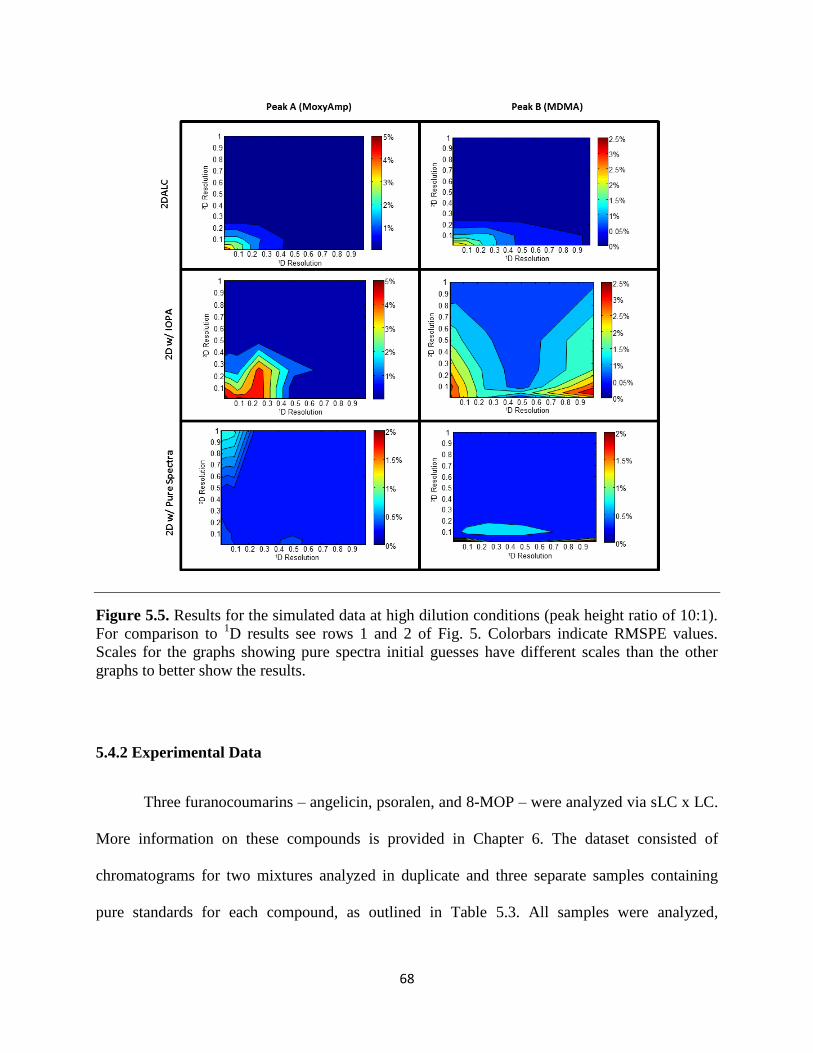
68

Figure 5.5. Results for the simulated data at high dilution conditions (peak height ratio of 10:1).

For comparison to 1D results see rows 1 and 2 of Fig. 5. Colorbars indicate RMSPE values.

Scales for the graphs showing pure spectra initial guesses have different scales than the other

graphs to better show the results.

5.4.2 Experimental Data

Three furanocoumarins – angelicin, psoralen, and 8-MOP – were analyzed via sLC x LC.

More information on these compounds is provided in Chapter 6. The dataset consisted of

chromatograms for two mixtures analyzed in duplicate and three separate samples containing

pure standards for each compound, as outlined in Table 5.3. All samples were analyzed,

69

representing a targeted analysis, in which the compounds present in the mixture are known ahead

of time. The corresponding 2D and 1D chromatograms for one of the mixtures are shown in Figs.

5.3B and 5.3D, respectively. The results of this analysis are shown in Fig. 5.6. We observe that

the RMSPE values for the 1D-IOPA and

1D-pure methods are almost equivalent, and superior to

all other methods shown. This is because IOPA easily finds almost pure spectra from the

standards to use as an initial guess. This indicates that when all of the compounds being analyzed

are known, 2D chromatography does not provide an advantage over 1D chromatography for

quantitation, when the spectra of the overlapped components are distinguishable and no

spectrally similar interferents are present. In other words, spectral resolution along with the

improved precision of 1D chromatography provides the necessary quantitative information

without the need for the additional chromatographic resolution provided by the 2D column, as

long as pure standards of the target compounds are available.

Figure 5.6. Quantitation error for the five quantitation methods applied to the targeted sLC x LC

analysis of furanocoumarins (based on experimental data).

Often, such as in the case of “discovery” type metabolomics investigations, the analytes

are not known prior to analysis; this is known as an untargeted analysis. To investigate this type

of problem, the analysis of the furanocoumarin sLC x LC data was repeated, but without using

0

5

10

15

20

% R

MSP

E

Psoralen

8-MOP

Angelicin

70

the data for the pure standard samples; this meant that there were no calibration standards

included in the analysis. Therefore, the quantitative performance of the different methods was

estimated by dividing the peak area by the concentration of the analyte in the mixture. The

percent relative standard deviation (% RSD) was then calculated. As seen in Fig. 5.7, 1D-IOPA

now gives the worst results due to the inability to obtain a sufficiently accurate initial guess, due

to the severe overlap of compounds. Both 2D methods give similar results, with angelicin having

a very good % RSD, but psoralen and 8-MOP still having a very poor % RSDs. The best results

in the “untargeted” analysis are given by the 1D-pure method; however, this method is only used

for comparison because pure spectra are not available prior to analysis in the untargeted case.

2DALC has the next best % RSD, being much better than both 2D-IOPA and 1D-IOPA. In this

case, 1D-IOPA gives the worst results.

Figure 5.7. Quantitation error for the five quantitation methods applied to the untargeted sLC x

LC analysis of furanocoumarins (based on experimental data).

5.4.3. Combined 2DALC (c2DALC)

An alternative approach to 2DALC was also investigated. In this variant, 2DALC was

modified to perform the MCR-ALS analyses on the 1D and the 2D chromatograms

simultaneously. This approach was named combined 2DALC (c2DALC). This method makes

0

10

20

30

40

50

60

% R

SD

Psoralen

8-MOP

Angelicin

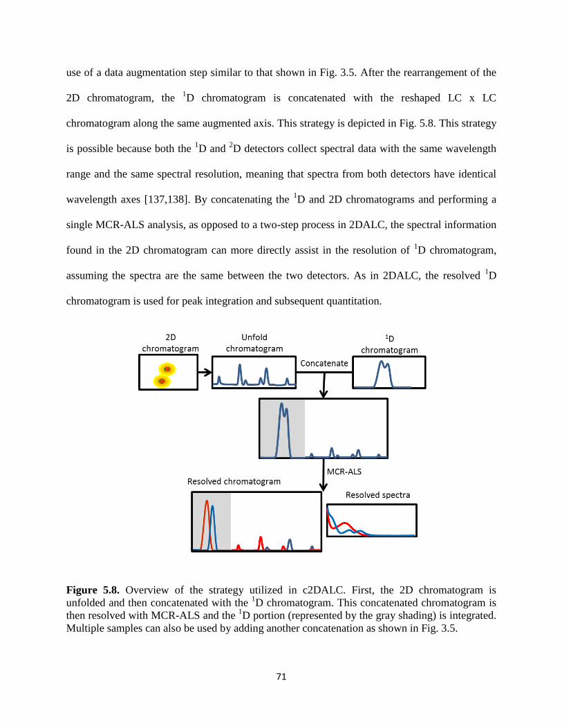
71

use of a data augmentation step similar to that shown in Fig. 3.5. After the rearrangement of the

2D chromatogram, the 1D chromatogram is concatenated with the reshaped LC x LC

chromatogram along the same augmented axis. This strategy is depicted in Fig. 5.8. This strategy

is possible because both the 1D and

2D detectors collect spectral data with the same wavelength

range and the same spectral resolution, meaning that spectra from both detectors have identical

wavelength axes [137,138]. By concatenating the 1D and 2D chromatograms and performing a

single MCR-ALS analysis, as opposed to a two-step process in 2DALC, the spectral information

found in the 2D chromatogram can more directly assist in the resolution of 1D chromatogram,

assuming the spectra are the same between the two detectors. As in 2DALC, the resolved 1D

chromatogram is used for peak integration and subsequent quantitation.

Figure 5.8. Overview of the strategy utilized in c2DALC. First, the 2D chromatogram is

unfolded and then concatenated with the 1D chromatogram. This concatenated chromatogram is

then resolved with MCR-ALS and the 1D portion (represented by the gray shading) is integrated.

Multiple samples can also be used by adding another concatenation as shown in Fig. 3.5.

72

The assumption that the spectra of the compounds will be identical between the two

detectors is often incorrect. Because a molecule’s spectral properties are often influenced by its

solvent environment [139], it can be expected that spectral shifts may occur between the 1D and

the 2D detectors. As the molecules elute off of each column, they will be contained in a certain

solvent composition and therefore a certain solvent polarity. Most often the mobile phase

composition during the elution of a compound from the 1D column will be different than that

from the 2D column. Even if the polarity difference is slight, spectral shifts may occur. To

investigate the effect of these spectral shifts, data were simulated as described in section 5.3.1.

One dataset was created with furanocoumarin spectra and the other was created with

amphetamine spectra, which show less pronounced solvent effects on their spectra. The

amphetamine spectra are also more dissimilar to each other compared to the furanocoumarin

spectra. As demonstrated in Chapter 3, this will have an effect on all of the implementations of

MCR-ALS tested here. The spectra used for the 1D and the 2D chromatograms were taken from

MCR-ALS resolved experimental data from the 1D and

2D detector, respectively. This allowed

the use of realistic spectral shifts in the data. As shown in Fig. 5.9, the furanocoumarin spectra

have more pronounced spectral shifts than the amphetamine spectra. The chromatographic

resolution in the second dimension (2RS) was held constant at 0.4 and the first dimension

resolution (1RS) was varied to determine what effect resolution had on the performance of the

methods tested.

Both datasets were analyzed with c2DALC, 2DALC, 1D-IOPA, and 2D-IOPA. The

results are shown in Fig. 5.10 with 1RS values of 0.2, 0.3, and 0.5. In addition to integrating the

1D chromatogram in c2DALC as discussed above, the 2D chromatogram was also integrated.

73

Figure 5.9. Spectra used for data simulation. (A) shows the furanocoumarin spectra and (B)

represent the amphetamine spectra: methylenedioxymethamphetamine (MDMA),

methoxymethamphetamine (MoxyMeth), and methamphetamine (Mamp). Spectral correlations

(r2) are a measure of the spectral shifts between the

1D spectra (solid lines) and the

2D spectra

(dashed lines). These correlation values were calculated over the spectral range from 200-400

nm.

These results are labeled c2DALC (2D) in Fig. 5.10. In general, as 1RS decreases, the

performance of 1D-IOPA improved, as expected. This trend generally held for 2DALC and

c2DALC as well; however, the %RSD was generally higher for c2DALC versus 2DALC. For

these data, 2D-IOPA most often performed the best at low 1RS, with a few exceptions; this is

most likely due to sufficient resolution of the compounds in the second dimension (2RS

= 0.4) for

MCR-ALS analysis. The trends seen in the angelicin plot are mostly different than the other

compounds. This is most likely due to the fact that the angelicin elutes in the middle of psoralen

and 8-MOP in the 2D separation causing peak overlap on both sides of the peak. In the

1D

74

Figure 5.10. Comparison of c2DALC, 2DALC, and other methods at varying 1D resolution.

2D

resolution was held constant at 0.4. c2DALC (2D) represents the results when the 2D

chromatogram was integrated after c2DLAC as opposed to the 1D chromatogram. Results from

both furanocoumarins and amphetamines are shown, where the amphetamine spectra are less

affected by the solvent difference between the 1D and

2D detector.

chromatogram, angelicin elutes last, possibly explaining the low %RSD values for 1D IOPA.

Another interesting trend shown in Fig. 5.10 is that of c2DALC when the 2D chromatogram is

integrated (labeled as c2DALC (2D)), rather than integrating the 1D chromatogram. For many of

the compounds, the %RSD values are lowest for c2DALC (2D) at low 1RS values and increase as

1RS increases. This is the opposite trend as c2DALC (where the

1D chromatogram is integrated).

The goal of c2DALC is the simultaneous optimization of the 1D and 2D chromatograms. Ideally,

the optimal solution would match the true peak profiles for both the 1D and 2D chromatograms

75

(i.e., %RSD close to zero for both chromatograms); however, the opposing trends suggest that at

low values of 1RS, c2DALC is optimizing the fit based on the 2D spectra whereas at higher

values of 1RS c2DALC is optimizing based on the

1D spectra. Due to this finding, and the

observation that c2DALC did not provide a significant advantage over 2DALC, we decided not

to pursue c2DALC for further analyses, such as those in Chapter 6.

5.5. Conclusions

A new method of quantitation in LC x LC based on the use of multivariate detection with

a DAD in both dimensions has been developed. This method, 2DALC, uses MCR-ALS analysis

of the 2D chromatogram to obtain a better initial guess for the component spectra for subsequent

MCR-ALS analysis of the 1D chromatogram than would be obtained using the

1D detector data

alone. For targeted analyses, where the spectra of all detected compounds are known prior to

analysis, use of the 1D chromatography with pure spectra to initiate MCR-ALS is superior to all

other methods tested, including all 2D methods. However, in contrast to untargeted analyses,

where an initial guess of the analyte spectra must be extracted from the chromatograms for the

unknown sample, 2DALC provides the best quantitation. Further, although not investigated in

this work, we believe that 2DALC will provide quantitative advantages in targeted analysis in

which unknown interferences overlap the target analytes. Based on simulated chromatograms,

when the 1D peak resolution is less than 0.3, 2DALC gives better quantitation than the other,

more conventional methods of data analysis tested (i.e., improved the accuracy by up to 14-fold

compared to 1D-LC and up to 3.8-fold compared to LC x LC with a single multivariate detector).

As chromatographic resolution improves, the quantitative performance of 2DALC and the

conventional methods converge. The superiority of 2DALC over traditional IOPA-based

methods increases as chromatographic resolution decreases. Additionally, 2DALC performs

76

increasingly better compared to other methods as sample dilution between the two separation

dimensions of 2D-LC increases.

The performance of 2DALC depends on the spectral dissimilarity between the

compounds themselves, and between the compounds and the background. The more similar the

spectra, the harder it is for MCR-ALS to resolve severely overlapped peaks, even with the

assistance of a second dimension of separation. This changes the threshold chromatographic

resolution, below which point an advantage is gained by using 2DALC. This observation also

depends on the degree of dilution between the first and second dimension separations. The use

of 2DALC for high dilution cases provides better quantitation compared to quantitation based on

the 2D detector signal because of the lower S/N in the

2D chromatogram. Even in low dilution

cases, the background in the 2

D detector signal is still worse than the 1D signal. The experimental

data shown here involved a relatively high level of dilution. For other, more hydrophobic

analytes, less dilution might be required, which should lead to improved performance from the

MCR-ALS analysis of the 2D chromatogram [35]. It was shown that 2DALC is less sensitive to

the amount of dilution, and therefore is recommended whenever dilution of any magnitude is

applied. The results shown for simulated 2DALC also represent an optimistic case in which the

spectra are identical between the two detectors. While this is often not the case, the experimental

data confirmed that 2DALC can still provide a quantitative advantage.

A combined 2DALC approach was also investigated in which the 1D and 2D

chromatograms were simultaneously resolved with the goal of improving 2DALC due to a more

direct application of the 2D spectra to the 1D MCR-ALS analysis. It was found, however, that the

effects of different solvent compositions on the analyte spectra at the two separate diode array

detectors degraded the performance of c2DALC. While in cases of minimal spectral shifts,

77

c2DALC may provide a slight advantage over 2DALC; however, since it was found that even

slight shifts greatly affect c2DALC, it was not tested in further analyses.

2DALC is a simple way to improve the accuracy and precision in the LC x LC analysis

of compounds present in complex samples by combining LC x LC equipped with dual DADs

and chemometrics, where neither method alone provides the desired quality of quantitation.

78

This page intentionally left blank

79

Chapter 6: Comparison of Curve Resolution Strategies in LC x LC: Application to the

Analysis of Furanocoumarins in Apiaceous Vegetables

This chapter adapted from D.W. Cook, M.L. Burnham, D.C. Harmes, D.R. Stoll, S.C. Rutan,

Multivariate curve resolution-alternating least squares analysis of high resolution liquid

chromatography-mass spectrometry data, 2016 in preparation for submission to Chemom. Intell.

Lab. Syst.

6.1. Furanocoumarins

Many naturally occurring compounds in foods we eat are considered bioactive, with

either positive or negative effects on our bodies. The complexity of the interactions of these

compounds with our bodies very often means that these compounds can affect multiple

biological pathways simultaneously, sometimes with both positive and negative effects. Many

times the difference between beneficial and harmful effects is dependent on the concentration of

the compound. In pharmaceuticals, medications must be dosed as to maximize the positive

effects while minimizing the negative effects (i.e., side-effects). In foods it is also important to

understand the effect of different compounds and their concentration-dependent interactions

within the body.

One class of compounds known to have significant biological activity is

furanocoumarins, found in significant levels in citrus fruits and apiaceous vegetables. As their

80

name suggests, furanocoumarins are defined by their structure of coumarin with a fused furan

ring as shown in Fig. 6.1. The two common furanocoumarin isomers, psoralen and angelicin, are

also shown in Fig. 6.1. Most furanocoumarins can be classified as a derivative of one of these

two base structures.

Figure 6.1. Two basic furanocoumarin isomers, psoralen and angelicin, showing the furan and

coumarin subunits in gray boxes.

Furanocoumarins are of great interest because of their interaction with the P450 enzymes

found in the liver. P450 enzymes play a crucial role in the metabolism of many medicines and

endogenous compounds. The interaction of furanocoumarins with these enzymes can have major

implications on a medication’s effectiveness. One well-known effect, known colloquially as the

“grapefruit juice effect,” is caused by furanocoumarins, namely bergamottin, interacting with the

CYP3A4 enzyme. This enzyme is one of the most common P450s involved in the metabolism of

many widely used medications such as statins, some blood-pressure drugs, and some anti-anxiety

medications, to name a few [140]. Traditionally, grapefruit juice has been contraindicated with

statin use, due to the increased bioavailability of the statins resulting from the decreased

metabolism by the CYP3A4 enzyme [14]. Furanocoumarins are also known to cause

photosensitivity, a condition sometimes called bartender or margarita dermatitis due to the rash

that outdoor bartenders can develop from handling citrus fruits.

81

While often associated with their negative effects, furanocoumarins’ biological activity

can often be harnessed for powerful medical treatments. Using grapefruit juice to inhibit

CYP3A4 has been shown to increase bioavailability of a cancer therapeutic [141]. The

photosensitizing effect of psoralen has been incorporated with ultra-violet therapy to increase its

efficacy for diseases such as eczema, psoriasis, cutaneous T-cell lymphoma and others [142].

The inhibition of procarcinogen activation has also been studied. Procarcinogens are compounds

that have the potential to become carcinogenic after activation by enzymes such as P450s. By

inhibiting these enzymes by consumption of furanocoumarin rich foods, procarcinogen

activation may be suppressed [143]. Finally, bergamottin has been proposed for treating

overdoses of acetaminophen by inhibiting the conversion of excess acetaminophen to a toxic

metabolite via the P450 enzymes [144].

Due to the important bioactivity of furanocoumarins, it is crucial to develop methods that

are able to quantitatively analyze their presence in foods. Because of the complex sample matrix

that is present in food analysis, it is necessary to employ more advanced analysis techniques. In

this case, LC x LC is used to provide separation of the target analytes from the matrix,

interfering compounds, and one another. Due to the complexity and relevance of furanocoumarin

analysis, it was chosen for testing quantitation using different implementations of MCR-ALS for

LC x LC-DAD data. Fourteen furanocoumarins were targeted in three apiaceous vegetables –

parsley, parsnips, and celery. The structures and abbreviations of the fourteen targeted

furanocoumarins are shown in Fig. 6.2.

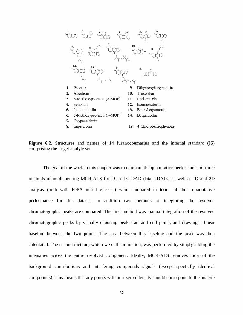
82

Figure 6.2. Structures and names of 14 furanocoumarins and the internal standard (IS)

comprising the target analyte set

The goal of the work in this chapter was to compare the quantitative performance of three

methods of implementing MCR-ALS for LC x LC-DAD data. 2DALC as well as 1D and 2D

analysis (both with IOPA initial guesses) were compared in terms of their quantitative

performance for this dataset. In addition two methods of integrating the resolved

chromatographic peaks are compared. The first method was manual integration of the resolved

chromatographic peaks by visually choosing peak start and end points and drawing a linear

baseline between the two points. The area between this baseline and the peak was then

calculated. The second method, which we call summation, was performed by simply adding the

intensities across the entire resolved component. Ideally, MCR-ALS removes most of the

background contributions and interfering compounds signals (except spectrally identical

compounds). This means that any points with non-zero intensity should correspond to the analyte

83

signal. By summing all intensities, this should provide a simple alternative to the tedious manual

integration approach.

6.2. Experimental

LC x LC analyses, including sample preparation, were carried out in the lab of Dwight

Stoll at Gustavus-Adolphus College. Fourteen furanocoumarin compounds, listed in Fig. 6.2,

along with one internal standard, 4-chlorobenzophenone (CBP) were analyzed. Samples of three

apiaceous vegetable types – parsley, parsnip, and celery – were then analyzed for the presence

and concentration of these 14 target compounds.

6.2.1. Plant Extracts

Samples of parsley, parsnips, and celery were purchased from a local grocery store and

were provided by Sabrina Trudo and colleagues at the University of Arkansas. Sample

preparation was accomplished using a QuEChERS methodology [145,146]. In general, the

QuEChERS method entails the following steps: homogenization of sample with acetonitrile and

internal standard, buffering and phase separation with salts, centrifugation and extraction of

organic phase, and sample clean-up with dispersive solid phase extraction. For the vegetables in

this work, samples were prepared combining 5.0 g of wet vegetable matter with 10 mL of water

and 10 mL of acetonitrile (ACN) with 0.1% acetic acid. This mixture was then homogenized in

an Ultra Turrax T25 Homogenizer (IKA Laboratories, Wilmington, NC) for 3 min. A 1 g portion

of sodium acetate and 4 g of magnesium sulfate were added to the homogenate and hand-mixed

by inversion for 2 min. Samples were then centrifuged at 3,000 rpm for 5 min at room

temperature which resulted in three distinct layers: ACN, vegetable matter, and aqueous.

Following centrifugation, 1.8 mL of the supernatant (i.e. the ACN layer) was transferred to a 2

84

mL dispersive solid extraction (dSPE) tube (United Science 20 CarbonX QuEChERS; Center

City, MN; part number 05040114) to remove highly non-polar compounds such as pigments and

lipids from the extract. Water was added to the dSPE tube to 10% of total volume to improve

retention of undesirable non-polar compounds and tubes were vortexed with a Mini Vortex

(VWR Part Number 12620-852, Radnor, PA) at the maximum speed setting. Samples were again

centrifuged at 6,000 rpm for 30 sec and the supernatant was transferred to a HPLC vial and

diluted 1:2 with water prior to LC analysis.

6.2.2. Chromatographic Conditions

The LC x LC analyses were performed on modules from the Agilent Technologies 1290

Infinity line (Agilent Technologies. Waldbronn, Germany). Samples were injected using an

autosampler (Model G4226A). First and second dimension flows were generated using binary

pumps (Model G4220A); a quaternary pump (Model DEQAT00023) was used to dilute 1D

effluent. Thermostated column compartments were used in both dimensions (Model G1316C)

and nominally identical diode-array UV detectors (DADs) (Model G4212A) were used at the

outlets of the 1D and

2D columns. Low dispersion flow cells (800 nL volume, Model G4212-

60038) were used in both the 1D and

2D DAD detectors. At the outlet of the 1D flow cell a

pressure relief valve (Model G4212-60022) was used to protect the cell from breaking due to

downstream pressure. A 2-position 8-port Duo-valve (Model 5067-4214) fitted with two 80 µL

stainless-steel loops mounted on an external valve drive (Model G1170A) was used to transfer

fractions of 1D effluent to the

2D column. The 2D-LC instrument was controlled by OpenLab

Chromatography Data System (Agilent Technologies. Rev. C.01.07).

85

The 1D separation was performed using an Agilent Poroshell 120 PFP (100 mm x 2.1 mm

i.d.) column with 5 mF sodium phosphate at pH 6 (A) and methanol (B). The unit milliformal

(mF) used here indicates the amount of sodium phosphate added to solution rather than the

amount of phosphate species that exists in solution after dissociation. A gradient was used with

the following conditions: 45-45-75-100-100-45-45 % B from 0-12.5-29.5-31.5-33-33.01-36 min;

this is shown in Fig. 6.3. The temperature was held at 20°C and the flow rate was 0.25 mL/min

from 0-7.5 min and 0.125 mL/min from 7.51 to 36 min. Beginning at 7.0 min, the 1D effluent

was diluted with 20 mM phosphoric acid in water at 0.15 mL/min to promote focusing of the

analyte bands at the inlet of the 2D column [19]. The diluted effluent was collected in 80 µL

sample loops before injection on the 2D column.

The 2D separation was performed from 7.5-36 min using an Agilent Zorbax SB-C18

rapid resolution high definition (RRHD) (50 mm x 3.0 mm i.d., 1.8 µm) column using 20 mM

phosphoric acid in water (A) and acetonitrile (B) as mobile phase components. The temperature

was held at 50°C and the flow rate was 2.5 mL/min. The 2D mobile phase was held isocratic at

42% B until 12.5 min and then a shifted gradient was employed as shown in Fig. 6.3.

6.2.3. Data Analysis

All computation was performed on a Dell Precision T3600 with an Intel Xeon E5-1620

CPU at 3.60 GHz and 32.0 GB of RAM. Data files were converted from Agilent .D format to

MATLAB .mat format files using ACD/Lab Spectrus Processor (Advanced Chemical

Development, Inc., Toronto, Canada). All other computational analysis was performed in

MATLAB version R2013a (Mathworks, Inc., Natick, MA).

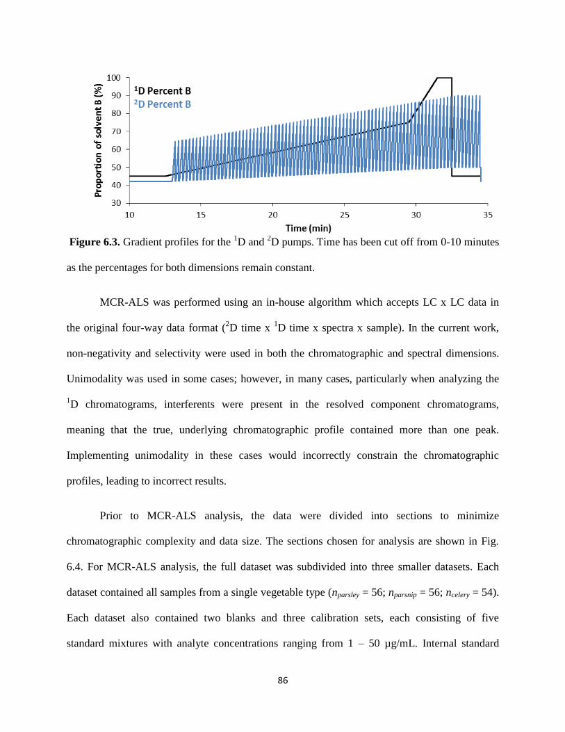
86

Figure 6.3. Gradient profiles for the 1D and

2D pumps. Time has been cut off from 0-10 minutes

as the percentages for both dimensions remain constant.

MCR-ALS was performed using an in-house algorithm which accepts LC x LC data in

the original four-way data format (2D time x

1D time x spectra x sample). In the current work,

non-negativity and selectivity were used in both the chromatographic and spectral dimensions.

Unimodality was used in some cases; however, in many cases, particularly when analyzing the

1D chromatograms, interferents were present in the resolved component chromatograms,

meaning that the true, underlying chromatographic profile contained more than one peak.

Implementing unimodality in these cases would incorrectly constrain the chromatographic

profiles, leading to incorrect results.

Prior to MCR-ALS analysis, the data were divided into sections to minimize

chromatographic complexity and data size. The sections chosen for analysis are shown in Fig.

6.4. For MCR-ALS analysis, the full dataset was subdivided into three smaller datasets. Each

dataset contained all samples from a single vegetable type (nparsley = 56; nparsnip = 56; ncelery = 54).

Each dataset also contained two blanks and three calibration sets, each consisting of five

standard mixtures with analyte concentrations ranging from 1 – 50 µg/mL. Internal standard

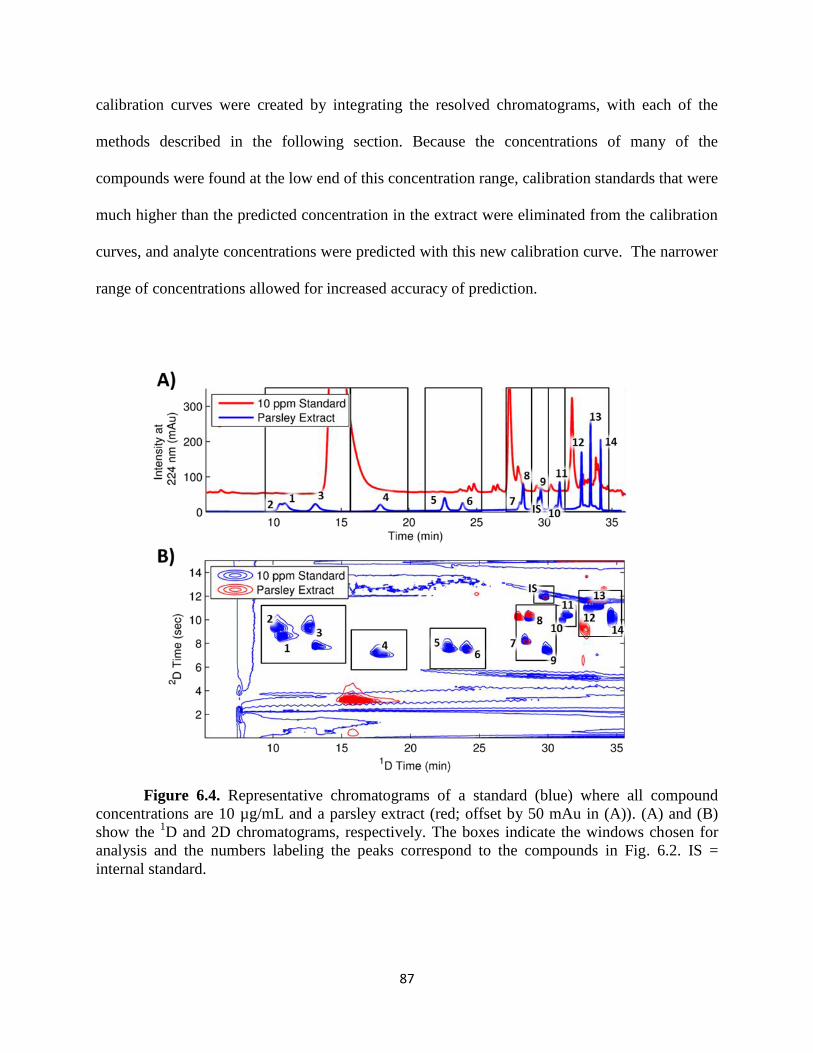
87

calibration curves were created by integrating the resolved chromatograms, with each of the

methods described in the following section. Because the concentrations of many of the

compounds were found at the low end of this concentration range, calibration standards that were

much higher than the predicted concentration in the extract were eliminated from the calibration

curves, and analyte concentrations were predicted with this new calibration curve. The narrower

range of concentrations allowed for increased accuracy of prediction.

Figure 6.4. Representative chromatograms of a standard (blue) where all compound

concentrations are 10 µg/mL and a parsley extract (red; offset by 50 mAu in (A)). (A) and (B)

show the 1D and 2D chromatograms, respectively. The boxes indicate the windows chosen for

analysis and the numbers labeling the peaks correspond to the compounds in Fig. 6.2. IS =

internal standard.

88

MCR-ALS was performed on the data using three strategies: 1D, 2D, and 2DALC. The

1D analysis corresponds to MCR-ALS being applied to only the

1D chromatogram, collected at

the 1D detector. Likewise, the 2D analysis corresponds to MCR-ALS being applied to only the

2D chromatogram, collected at the 2D detector. Both of these methods used IOPA as the initial

guess. Finally, 2DALC is the strategy described in Chapter 5, utilizing both the 1D and 2D

chromatograms.

6.3. Results

Extracts from the three vegetable types – parsley, parsnips, and celery – were analyzed

via LC x LC. Using diode array detectors (DAD) placed at the end of both the 1D and

2D

columns, both 1D and 2D chromatograms were collected. This allowed for the comparison of

quantitative performance of 1D and 2D chromatography. Representative chromatograms from

both a standard and a parsley extract are shown in Fig. 6.4. From this, it can be seen that, as

expected, the peaks are separated much better in the 2D chromatogram; however, interferents are

still present. It is also important to note that lower level interferents in the 2D may not been seen

in the 2D chromatogram due to the contour plot style in which minor peaks may not be seen.

6.3.1. Comparison of Integration Methods

Ideally, MCR-ALS completely resolves the pure analyte signals from the background and

noise. This would allow for the integration over the entire pure analyte component. This is

simply a summation of the total signal intensity contained in the resolved chromatographic

profile of each component as shown in Fig. 6.5B. Unfortunately, MCR-ALS with DAD data

rarely eliminates background and noise completely. This complicates the summation process by

including residual background producing an overestimate of peak

89

Figure 6.5. Graphical representation of integration methods compared. (A) shows a

MCR-ALS resolved LC x LC chromatogram. (B) and (C) show the rearranged LC x LC

chromatogram with summation and manual integration, respectively. The shaded area represents

the area calculated for quantitation. The percent difference in calculated peak area for these two

chromatograms is 9.9%. The results from the two integration methods are identical for 1D LC.

area. In contrast, manual integration is performed by visually estimating the peak start and end

points, drawing a linear baseline between those points, and integrating the peak area between that

baseline and the peak as shown in Fig. 6.5C.

To compare manual integration to simple summation, resolved chromatographic profiles for both

the calibration set and the unknown samples were integrated using both methods. Calibration

curves were constructed and the concentrations in the samples were predicted. Since the samples

were run in duplicate, the differences between the duplicates can be taken as a measure of the

precision of each integration method. Figure 6.6 displays the sum of these differences across all

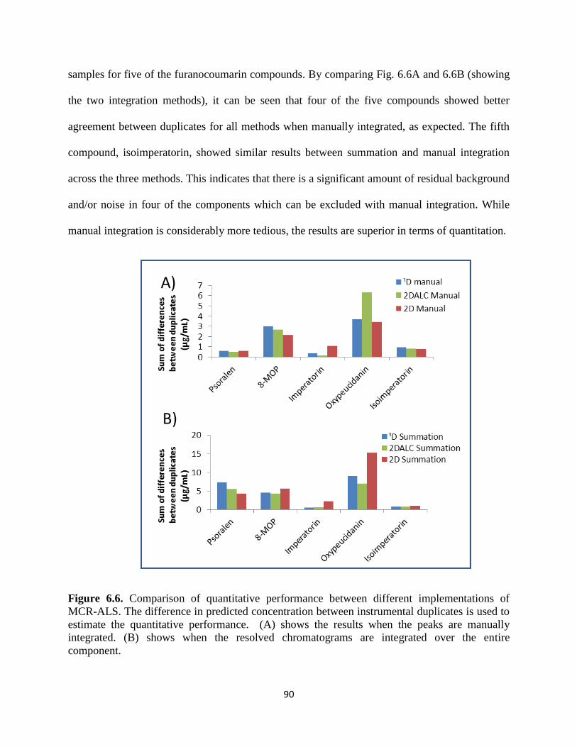
90

samples for five of the furanocoumarin compounds. By comparing Fig. 6.6A and 6.6B (showing

the two integration methods), it can be seen that four of the five compounds showed better

agreement between duplicates for all methods when manually integrated, as expected. The fifth

compound, isoimperatorin, showed similar results between summation and manual integration

across the three methods. This indicates that there is a significant amount of residual background

and/or noise in four of the components which can be excluded with manual integration. While

manual integration is considerably more tedious, the results are superior in terms of quantitation.

Figure 6.6. Comparison of quantitative performance between different implementations of

MCR-ALS. The difference in predicted concentration between instrumental duplicates is used to

estimate the quantitative performance. (A) shows the results when the peaks are manually

integrated. (B) shows when the resolved chromatograms are integrated over the entire

component.

91

6.3.2. Comparison of Curve Resolution Strategies

In addition to manual versus summation approaches, it is important to understand the

performance of the three methods tested – 1D, 2D, and 2DALC. Figure 6.6 compares the

agreement between duplicates for the three methods tested. Figure 6.6A shows the comparison

when employing manual integration. When comparing the 1D and 2D data analysis, the results

are similar, with the 2D analysis having better agreement between the duplicates for 8-MOP and

isoimperatorin, while the duplicates for imperatorin agree better with 1D analysis. However, note

that these differences are not very large. Overall, 1D and 2D are similar due to the ability of

manual integration to exclude interferents and background. Figure 6.6B shows the results for the

summation approach. Overall the agreement is worse than for manual integration due to the

residual background that occurs in all methods. For most of the compounds the 1D analysis has

better agreement than the 2D analysis, with the exception of psoralen, which eluted early and had

more interferents that may not have been completely resolved with MCR-ALS. Interestingly,

when manual integration was applied, 2DALC had the best agreement only for imperatorin;

however, for the summation approach, 2DALC performed the best or was equal to the best

method for all but psoralen, most likely due to less residual background. For summation, any

slight errors in MCR-ALS analysis would be overshadowed by residual noise, but when manual

integration is employed, the small differences between resolution results obtained using the

different methods become more evident.

For the best quantitative results, it is shown that 2D with manual integration is the best

method for this data set; however, this process can be very time consuming. If the summation

approach is to be utilized the 1D data provides superior results due to the fact that the signal-to-

background ratio is higher in the 1D chromatograms. This is, however, limited to cases in which

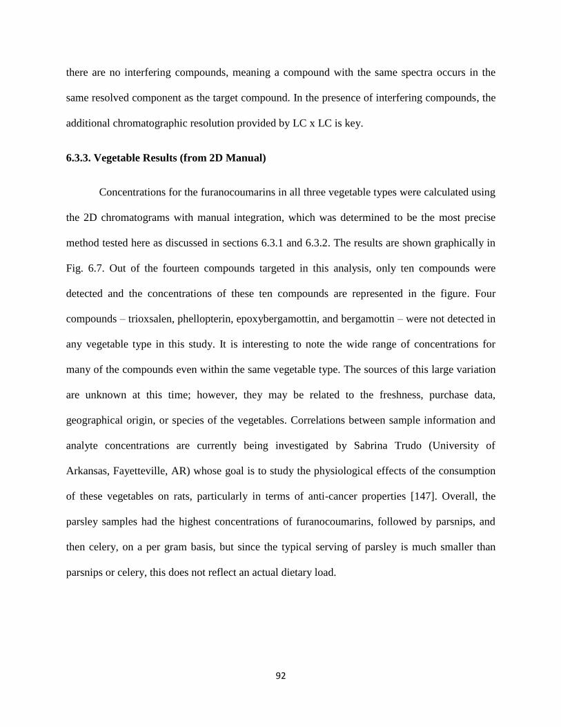
92

there are no interfering compounds, meaning a compound with the same spectra occurs in the

same resolved component as the target compound. In the presence of interfering compounds, the

additional chromatographic resolution provided by LC x LC is key.

6.3.3. Vegetable Results (from 2D Manual)

Concentrations for the furanocoumarins in all three vegetable types were calculated using

the 2D chromatograms with manual integration, which was determined to be the most precise

method tested here as discussed in sections 6.3.1 and 6.3.2. The results are shown graphically in

Fig. 6.7. Out of the fourteen compounds targeted in this analysis, only ten compounds were

detected and the concentrations of these ten compounds are represented in the figure. Four

compounds – trioxsalen, phellopterin, epoxybergamottin, and bergamottin – were not detected in

any vegetable type in this study. It is interesting to note the wide range of concentrations for

many of the compounds even within the same vegetable type. The sources of this large variation

are unknown at this time; however, they may be related to the freshness, purchase data,

geographical origin, or species of the vegetables. Correlations between sample information and

analyte concentrations are currently being investigated by Sabrina Trudo (University of

Arkansas, Fayetteville, AR) whose goal is to study the physiological effects of the consumption

of these vegetables on rats, particularly in terms of anti-cancer properties [147]. Overall, the

parsley samples had the highest concentrations of furanocoumarins, followed by parsnips, and

then celery, on a per gram basis, but since the typical serving of parsley is much smaller than

parsnips or celery, this does not reflect an actual dietary load.

93

Figure 6.7. Concentration (C) of detected furanocoumarins in the three vegetables as calculated

with manual integration of the 2D chromatogram. The box represents the median and the 1st and

3rd

quartiles. Each point represents the average concentration of instrumental duplicates in each

sample. Only compounds which were found to be present in at least one vegetable type are

shown. The total numbers of samples analyzed were: nparsley = 56; nparsnip = 56; ncelery = 54.

6.4. Conclusions

When quantitative analysis is performed it is important to consider the impact of all steps

on the analysis. This is especially true when chemometric techniques are performed on the data.

Here, several strategies for MCR-ALS analysis for LC x LC were compared along with the

subsequent integration methods. In most cases 2DALC performed similarly to resolving the 1D

94

chromatogram by itself. Even though spectral shifts were present, the two-step strategy of

2DALC allowed for the 2D spectra to be further optimized for the resolution of the

1D

chromatogram.

As expected, manual integration was superior to summation approaches; however, this

approach is time consuming for studies involving many samples and for 2D chromatograms in

which several 2D peaks must be integrated for a single chromatogram. If summation is to be

used, the 1D chromatogram gave better agreement between replicates, but caution must be used

so that interfering peaks are not included in the component window being summed. It is possible

that the resolved chromatograms could be submitted to peak detection for a more automated

method of excluding residual background [130]. Depending on the performance of the peak

detection algorithm, results from this approach may approach those obtained from manual

integration. This would facilitate the use of the 2D chromatographic data to obtain superior

quantitative results.

95

Chapter 7: Conclusions and Future Work

As defined in Chapter 1, three main goals were set for the work in this dissertation: 1) to

characterize the abilities and limitations of MCR-ALS for LC-DAD data; 2) to improve

quantitative abilities of LC x LC through the use of a novel implementation of MCR-ALS; and

3) to demonstrate the utility of MCR-ALS for real-world LC x LC analyses. Work was

performed towards these goals in Chapters 4-6.

7.1. Reflections on Chapter 4

Goal 1 was addressed in Chapter 4 where MCR-ALS was implemented on data over a

wide range of conditions such as varying S/N, Rs, and spectral similarity. An effective peak

capacity was defined where the number of analyzable peaks within a separation was defined by a

calculated threshold RS rather than a RS of one. It was found that even when the target peak was

of low intensity (i.e. low S/N) and was overwhelmed by a coeluting peak, excellent quantitation

was achieved even at RS values less than 0.25. This was particularly true when analyte spectra

were sufficiently dissimilar. These values corresponded to an up to five-fold increase in effective

peak capacity. This finding clearly demonstrates the potential of MCR-ALS to improve

separations. This work is particularly meaningful due to the inclusion of background

contributions to the simulated data, which is often neglected in similar literature reports.

96

While we believe these results to be representative of expected experimental results,

future work may include the validation of this work with the use of experimental data. By

collecting experimental data under a range of conditions such as varying mobile phase

composition and different analyte concentrations, the chromatographic resolution and S/N can be

controlled. Spectral similarity can be controlled through the careful selection of different analyte

pairs. While significantly more involved than the simulated data sets used in Chapter 4, a smaller

range of data (within the ranges used in the simulations) would be able to be used in order to

validate the simulation results, rather than creating a full model.

The approach used in Chapter 4 can also be used as the basis for a comprehensive

comparison between MCR-ALS and other curve resolution techniques such as PARAFAC and

PARAFAC2. For this comparison, retention time shifting should be added as an additional

parameter because these shifts are known to affect the performance of PARAFAC [4].

7.2. Reflections on Chapter 5

The second goal was addressed in Chapter 5. A new implementation of MCR-ALS was

developed for LC x LC data in which data from two detectors were utilized to take advantage of

the resolution of the 2D separation and the quantitative superiority of the 1D separation. It was

found that a clear advantage was present for the simulated data, particularly when dilution was

significant. At 1D peak resolutions of less 0.3, 2DALC provided a clear advantage. While no

spectral shifts were incorporated in this data, the experimental data clearly showed that for the

untargeted analyses, 2DALC did provide better quantitation for two of the three compounds.

c2DALC was also investigated; however, it was found that even minor spectral shifts greatly

affected the results and thus, we decided not to pursue c2DALC further. It is important to note

97

that while 2DALC was proven effective in this data, it may not always be superior to 2D or 1D

chromatography alone, as seen in Chapter 5; however, the ability to obtain 1D and 2D

chromatograms from an LC x LC analysis gives the analyst the ability to choose the best method

for each analyte. Each of the three methods – 1D-IOPA, 2D-IOPA, and 2DALC – are relatively

simple to run, giving the analyst the opportunity to evaluate which method is best for the given

data. It is very possible that certain compounds that are not strongly overlapped in the 1D may

work better with 1D-IOPA while other overlapped compounds in the same analysis may work

better with 2DALC or 2D-IOPA, depending on the resolution in the 2D separation.

The work in this chapter also showed two types of analyses: targeted and untargeted. The

targeted analysis showed that when standards are available for all compounds, MCR-ALS was

able to provide excellent calibration and prediction errors. Future work should investigate the

intermediate case in which only some of the compounds are known prior to analysis. This would

represent the case in which unknown compound spectra would need to be estimated from the raw

data, while known compound spectra are also included in the analysis.

7.3. Reflections on Chapter 6

In Chapters 4 and 5, mostly simulated data were created in order to control

chromatographic parameters such as RS, S/N, and spectral similarity. This allowed us to

investigate the effect of each of these parameters individually, which would have been difficult

to completely control with experimental data. In order to demonstrate the applicability to real-

world analyses, we tested methods of MCR-ALS analysis on a targeted analysis of

furanocoumarins from three apiaceous vegetables: parsley, parsnips, and celery. The LC x LC

data were analyzed using the three methods outlined in Chapter 5: 1D-IOPA, 2DALC, and 2D-

98

IOPA. It was found that for this data set all three methods tested performed approximately

equally in terms of the precision of quantitation. 2D-IOPA had the advantage that it was able to

separate chromatographically overlapped, spectrally identical interferents from the target

compounds, which MCR-ALS is unable to do. As discussed in Chapter 4, MCR-ALS requires a

minimal level of spectral dissimilarity and chromatographic resolution in order to resolve

overlapped analyte signals. Manual integration was also found to provide greater quantitative

precision over the summation approach despite MCR-ALS removing most of the background.

This suggests that the quantitative abilities in LC x LC are comparable to 1D-LC for these data

when MCR-ALS is utilized. These findings are impressive when compared to many of the

previous literature reports of quantitation in LC x LC. Because of this, we used 2D-IOPA with

manual integration to quantify all 14 furanocoumarins. We were able to detect 10 of the 14

furanocoumarins at varying concentrations. Overall, the concentrations were low and often lower

than the lowest calibration point; however, an estimate of concentration was able to be

calculated. The concentrations of each furanocoumarin were found to vary greatly even within a

single vegetable type. This may be due to vegetable freshness, specific plant species,

geographical origin, or a plethora of other factors. It may also be due to natural, random

variations, which would be a significant finding itself. Studies of correlations of the

concentrations with exact sample information are ongoing. These samples will also be used to

study the physiological effects of these compounds on rats. Although not performed in this work,

peak detection may provide an alternative to manual integration that performs better than the

summation approach, but still in a semi-automated fashion. The peak detection approach in

Chapter 5 may work; however, selection of parameters for this approach (noise threshold,

99

window size, etc.) can still be tedious. Future work may provide a more automated peak

detection method that can complement our work presented here.

7.4. Outlook and Future Work

It is clear from the work presented in this dissertation, along with the body of work in the

literature, that MCR-ALS and other curve resolution techniques have the potential to greatly

impact the field of separation science. While widespread adoption of these techniques has yet to

occur, it is undeniable that these methods provide valuable tools for the analytical chemist.

While the identification power of diode array detection has been shown previously [63]

and has been shown in the previous chapters to be particularly powerful in terms of quantitation

using MCR-ALS, curve resolution with mass spectrometric detection must be explored due to

the increasing adoption of both low and high resolution mass spectrometry. Currently in our

laboratory and in a select few other labs, work is being performed towards this aim

[109,148,149]. One major impediment to MCR-ALS analysis of LC-high resolution MS data is

the immense size of the data. LC-DAD analysis collect UV-Vis spectra which typically contain

100-200 data points per spectrum corresponding to a wavelength range of approximately 190-

600 nm sampled at 2-4 nm intervals. High resolution MS (HRMS) produces several orders of

magnitude more data points. For example, a mass range of 100-1000 amu at a 0.001 amu

precision, gives 9 x 105

data points per mass spectrum. In our lab, we implement a data reduction

strategy that allows us to exclude many of these masses corresponding to background and noise

[149]. By employing a binning strategy which initially reduces the precision to unit mass, MCR-

100

ALS can be performed to resolve masses corresponding to true chemical compounds and discard

the remaining masses. Using this limited range of masses, a second binning process takes place,

this time to 0.1 amu bins. MCR-ALS is performed on this data and once again any masses not

corresponding to compounds are discarded. This process continues until the final precision level

is reached as dictated by the instrument’s capabilities.

Automation should also be a key focus of curve resolution research moving forward. As

with any technique, MCR-ALS can always be improved upon; however, if it is difficult to

implement due to the need for experience and knowledge of computer programming, these

techniques will never find widespread use. It is our belief that MCR-ALS is developed to a point

that with automation of certain steps (component determination, application of constraints, etc)

rather than optimization of the algorithm should be a major focus of research. Some work has

been performed in other groups towards this goal, specifically on the determination of the

number of components [150–152]; however, these methods can overestimate the number of

components [97] and still may require several iterations of MCR-ALS with different numbers of

components to find the optimal fit. While not completely automated, graphical user interfaces

(GUI) have been developed for MCR-ALS analysis. One of the more popular MCR-ALS GUIs

was developed by Jaumot, de Juan, and Tauler [118] which simplify the MCR-ALS process by

eliminating the need for programming experience, but still requires a certain level of expertise

and experience on the part of the user to determine the number of components and properly

apply constraints. With further automation of these steps and subsequent commercialization of

MCR-ALS packages, we believe MCR-ALS can become a standard tool in the analytical

chemist’s arsenal.

101

List of References

102

List of References

[1] W. Weckwerth, Metabolomics: an integral technique in systems biology, Bioanalysis. 2

(2010) 829–836. http://www.future-science.com/doi/abs/10.4155/bio.09.192 (accessed

January 2, 2014).

[2] Z. Zhang, S. Wu, D.L. Stenoien, L. Paša-Tolić, High-Throughput Proteomics, Annu. Rev.

Anal. Chem. 7 (2014) 427–454. doi:10.1146/annurev-anchem-071213-020216.

[3] X. Zhang, A. Fang, C.P. Riley, M. Wang, F.E. Regnier, C. Buck, Multi-dimensional

liquid chromatography in proteomics-A review, Anal. Chim. Acta. 664 (2010) 101–113.

doi:10.1016/j.aca.2010.02.001.

[4] D.W. Cook, S.C. Rutan, Chemometrics for the analysis of chromatographic data in

metabolomics investigations, J. Chemom. 28 (2014) 681–687. doi:10.1002/cem.2624.

[5] A. Zhang, H. Sun, P. Wang, Y. Han, X. Wang, Modern analytical techniques in

metabolomics analysis., Analyst. 137 (2012) 293–300. doi:10.1039/c1an15605e.

[6] M.F. Almstetter, P.J. Oefner, K. Dettmer, Comprehensive two-dimensional gas

chromatography in metabolomics., Anal. Bioanal. Chem. 402 (2012) 1993–2013.

doi:10.1007/s00216-011-5630-y.

[7] D.R. Stoll, X. Li, X. Wang, P.W. Carr, S.E.G. Porter, S.C. Rutan, Fast, comprehensive

two-dimensional liquid chromatography., J. Chromatogr. A. 1168 (2007) 3–43.

doi:10.1016/j.chroma.2007.08.054.

[8] J.C. Giddings, Two-dimensional separations: concept and promise, Anal. Chem. 56

(1984) 1258A–1270A. doi:10.1021/ac00276a003.

[9] D.W. Cook, S.C. Rutan, D.R. Stoll, P.W. Carr, Two dimensional assisted liquid

chromatography – a chemometric approach to improve accuracy and precision of

quantitation in liquid chromatography using 2D separation, dual detectors, and

multivariate curve resolution, Anal. Chim. Acta. 859 (2014) 87–95.

doi:10.1016/j.aca.2014.12.009.

[10] J.M. Amigo, T. Skov, R. Bro, ChroMATHography: solving chromatographic issues with

mathematical models and intuitive graphics., Chem. Rev. 110 (2010) 4582–605.

103

doi:10.1021/cr900394n.

[11] S.C. Rutan, A. de Juan, R. Tauler, Introduction to Multivariate Curve Resolution, in: S.D.

Brown, R. Tauler, B. Walczak (Eds.), Compr. Chemom., Elsevier, 2009: pp. 249–259.

doi:10.1016/B978-044452701-1.00046-6.

[12] A. de Juan, J. Jaumot, R. Tauler, Multivariate Curve Resolution (MCR). Solving the

mixture analysis problem, Anal. Methods. 6 (2014) 4964. doi:10.1039/c4ay00571f.

[13] L. Guo, Y. Yamazoe, Inhibition of cytochrome P450 by furanocoumarins in grapefruit

juice and herbal medicines, 25 (2004) 129–136.

[14] J.W. Lee, J.K. Morris, N.J. Wald, Grapefruit Juice and Statins., Am. J. Med. 129 (2015)

26–29. doi:10.1016/j.amjmed.2015.07.036.

[15] Waters, HPLC Separation Modes, (2016). http://www.waters.com/waters/en_US/HPLC-

Separation-Modes/nav.htm?cid=10049076&locale=en_US (accessed May 12, 2016).

[16] L.R. Snyder, J. Kirkland, Introduction to Modern Liquid Chromatography, Second, John

Wiley & Sons, Inc., Hoboken, NJ, USA, 1979. http://doi.wiley.com/10.1002/0470055529.

[17] C.F. Poole, The Essence of Chromatography, First, Elsevier B.V., Amsterdam, The

Netherlands, 2003.

[18] Y. Mao, Selectivity Optimization in Liquid Chromatography Using the Thermally Tuned

Tandem Column (T3C) Concept, University of Minnesota, 2001.

[19] Chromatographic Selectivity, Sigma-Aldrich. (2016).

http://www.sigmaaldrich.com/analytical-chromatography/hplc/learning-

center/chromatographic-selectivity.html (accessed April 25, 2016).

[20] U.D. Neue, Peak capacity in unidimensional chromatography, J. Chromatogr. A. 1184

(2008) 107–130. doi:10.1016/j.chroma.2007.11.113.

[21] N. Tanaka, D. V. McCalley, Core-Shell, Ultrasmall Particles, Monoliths, and Other

Support Materials in High-Performance Liquid Chromatography, Anal. Chem. 88 (2016)

279–298. doi:10.1021/acs.analchem.5b04093.

[22] F. Gritti, G. Guiochon, Mass transfer mechanism in liquid chromatography columns

packed with shell particles: Would there be an optimum shell structure?, J. Chromatogr.

A. 1217 (2010) 8167–8180. doi:10.1016/j.chroma.2010.10.075.

[23] G. Guiochon, Monolithic columns in high-performance liquid chromatography., J.

Chromatogr. A. 1168 (2007) 101–68; discussion 100. doi:10.1016/j.chroma.2007.05.090.

[24] T. Alvarez-Segura, J.R. Torres-Lapasió, C. Ortiz-Bolsico, M.C. García-Alvarez-Coque,

Stationary phase modulation in liquid chromatography through the serial coupling of

columns: A review, Anal. Chim. Acta. 923 (2016) 1–23. doi:10.1016/j.aca.2016.03.040.

104

[25] V.C. Dewoolkar, L.N. Jeong, D.W. Cook, K.M. Ashraf, S.C. Rutan, M.M. Collinson,

Amine Gradient Stationary Phases on In-House Built Monolithic Columns for Liquid

Chromatography, Anal. Chem. (2016) acs.analchem.6b00895.

doi:10.1021/acs.analchem.6b00895.

[26] L.N. Jeong, S.G. Forte, S.C. Rutan, Simulation of elution profiles in liquid

chromatography: II. Stationary Phase Gradients, Prep. Submiss. to J. Chromatogr. A.

(2016).

[27] C. Ortiz-Bolsico, J.R. Torres-Lapasi??, M.J. Ruiz-??ngel, M.C. Garc??a-??lvarez-Coque,

Comparison of two serially coupled column systems and optimization software in

isocratic liquid chromatography for resolving complex mixtures, J. Chromatogr. A. 1281

(2013) 94–105. doi:10.1016/j.chroma.2013.01.064.

[28] C. Lee, J. Zang, J. Cuff, N. McGachy, T.K. Natishan, C.J. Welch, et al., Application of

Heart-Cutting 2D-LC for the Determination of Peak Purity for a Chiral Pharmaceutical

Compound by HPLC, Chromatographia. 76 (2013) 5–11. doi:10.1007/s10337-012-2367-

5.

[29] H. Malerod, E. Lundanes, T. Greibrokk, Recent advances in on-line multidimensional

liquid chromatography, Anal. Methods. 2 (2010) 110. doi:10.1039/b9ay00194h.

[30] M. Pursch, S. Buckenmaier, Loop-based multiple heart-cutting two-dimensional liquid

chromatography for target analysis in complex matrices, Anal. Chem. 87 (2015) 5310–

5317. doi:10.1021/acs.analchem.5b00492.

[31] D.R. Stoll, Recent advances in 2D-LC for bioanalysis., Bioanalysis. 7 (2015) 3125–42.

doi:10.4155/bio.15.223.

[32] Y. Ouyang, Y. Zeng, Y. Rong, Y. Song, L. Shi, B. Chen, et al., Profiling Analysis of Low

Molecular Weight Heparins by Multiple Heart-Cutting Two Dimensional

Chromatography with Quadruple Time-of-Flight Mass Spectrometry, Anal. Chem. 87

(2015) 8957–8963. doi:10.1021/acs.analchem.5b02218.

[33] R.E. Murphy, M.R. Schure, J.P. Foley, Effect of Sampling Rate on Resolution in

Comprehensive Two-Dimensional Liquid Chromatography, Anal. Chem. 70 (1998) 1585–

1594. doi:10.1021/ac971184b.

[34] S.R. Groskreutz, M.M. Swenson, L.B. Secor, D.R. Stoll, Selective comprehensive

multidimensional separation for resolution enhancement in high performance liquid

chromatography. Part II: applications., J. Chromatogr. A. 1228 (2012) 41–50.

doi:10.1016/j.chroma.2011.06.038.

[35] S.R. Groskreutz, M.M. Swenson, L.B. Secor, D.R. Stoll, Selective comprehensive multi-

dimensional separation for resolution enhancement in high performance liquid

chromatography. Part I: principles and instrumentation., J. Chromatogr. A. 1228 (2012)

31–40. doi:10.1016/j.chroma.2011.06.035.

105

[36] D.R. Stoll, D.C. Harmes, J. Danforth, E. Wagner, D. Guillarme, S. Fekete, et al., Direct

Identification of Rituximab Main Isoforms and Subunit Analysis by Online Selective

Comprehensive Two-Dimensional Liquid Chromatography–Mass Spectrometry, Anal.

Chem. 87 (2015) 8307–8315. doi:10.1021/acs.analchem.5b01578.

[37] E.D. Larson, S.R. Groskreutz, D.C. Harmes, I.C. Gibbs-Hall, S.P. Trudo, R.C. Allen, et

al., Development of selective comprehensive two-dimensional liquid chromatography

with parallel first-dimension sampling and second-dimension separation--application to

the quantitative analysis of furanocoumarins in apiaceous vegetables., Anal. Bioanal.

Chem. 405 (2013) 4639–53. doi:10.1007/s00216-013-6758-8.

[38] D.R. Stoll, P.W. Carr, Fast, comprehensive two-dimensional HPLC separation of tryptic

peptides based on high-temperature HPLC, J. Am. Chem. Soc. 127 (2005) 5034–5035.

doi:10.1021/ja050145b.

[39] G.J. Opiteck, J.W. Jorgenson, M.A. Moseley, R.J. Anderegg, Two-Dimensional

Microcolumn HPLC Coupled to a Single-Quadrupole Mass Spectrometer for the

Elucidation of Sequence Tags and Peptide Mapping, J. Microcolumn Sep. 10 (1998) 365–

375. http://www.scopus.com/inward/record.url?eid=2-s2.0-

0000262232&partnerID=tZOtx3y1.

[40] V. Elsner, S. Laun, D. Melchior, M. Köhler, O.J. Schmitz, Analysis of fatty alcohol

derivatives with comprehensive two-dimensional liquid chromatography coupled with

mass spectrometry, J. Chromatogr. A. 1268 (2012) 22–28.

doi:10.1016/j.chroma.2012.09.072.

[41] P. Dugo, T. Kumm, M.L. Crupi, A. Cotroneo, L. Mondello, Comprehensive two-

dimensional liquid chromatography combined with mass spectrometric detection in the

analyses of triacylglycerols in natural lipidic matrixes, J. Chromatogr. A. 1112 (2006)

269–275. doi:10.1016/j.chroma.2005.10.070.

[42] P.W. Carr, D.R. Stoll, Two-Dimensional Liquid Chromatography: Principles, Practical

Implementation and Applications. Primer., 2015.

[43] D. Li, C. Jakob, O. Schmitz, Practical considerations in comprehensive two-dimensional

liquid chromatography systems (LCxLC) with reversed-phases in both dimensions., Anal.

Bioanal. Chem. 407 (2014) 153–67. doi:10.1007/s00216-014-8179-8.

[44] R.C. Allen, B.B. Barnes, I.A. Haidar Ahmad, M.R. Filgueira, P.W. Carr, Impact of

reversed phase column pairs in comprehensive two-dimensional liquid chromatography.,

J. Chromatogr. A. 1361 (2014) 169–177. doi:10.1016/j.chroma.2014.08.012.

[45] P. Boswell, D.R. Stoll, HPLC Columns, (n.d.). http://www.hplccolumns.org (accessed

April 27, 2016).

[46] L.R. Snyder, J.W. Dolan, P.W. Carr, The hydrophobic-subtraction model of reversed-

phase column selectivity, J. Chromatogr. A. 1060 (2004) 77–116.

doi:10.1016/j.chroma.2004.08.121.

106

[47] C. V. McNeff, B. Yan, D.R. Stoll, R.A. Henry, Practice and theory of high temperature

liquid chromatography, J. Sep. Sci. 30 (2007) 1672–1685. doi:10.1002/jssc.200600526.

[48] L.W. Potts, D.R. Stoll, X. Li, P.W. Carr, The impact of sampling time on peak capacity

and analysis speed in on-line comprehensive two-dimensional liquid chromatography., J.

Chromatogr. A. 1217 (2010) 5700–9. doi:10.1016/j.chroma.2010.07.009.

[49] J.M. Davis, D.R. Stoll, P.W. Carr, Effect of first-dimension undersampling on effective

peak capacity in comprehensive two-dimensional separations., Anal. Chem. 80 (2008)

461–73. doi:10.1021/ac071504j.

[50] S.C. Rutan, J.M. Davis, P.W. Carr, Fractional coverage metrics based on ecological home

range for calculation of the effective peak capacity in comprehensive two-dimensional

separations., J. Chromatogr. A. 1255 (2012) 267–76. doi:10.1016/j.chroma.2011.12.061.

[51] G. Semard, V. Peulon-Agasse, A. Bruchet, J.P. Bouillon, P. Cardinaël, Convex hull: A

new method to determine the separation space used and to optimize operating conditions

for comprehensive two-dimensional gas chromatography, J. Chromatogr. A. 1217 (2010)

5449–5454. doi:10.1016/j.chroma.2010.06.048.

[52] D.R. Stoll, X. Wang, P.W. Carr, Comparison of the practical resolving power of one- and

two-dimensional high-performance liquid chromatography analysis of metabolomic

samples., Anal. Chem. 80 (2008) 268–78. doi:10.1021/ac701676b.

[53] N.E. Hoffman, S.-L. Pan, A.M. Rustum, Injection of eluites in solvents stronger than the

mobile phase in reversed-phase liquid chromatography, J. Chromatogr. A. 465 (1989)

189–200. doi:10.1016/S0021-9673(01)92657-3.

[54] B.J. Holland, X.A. Conlan, P.S. Francis, N.W. Barnett, P.G. Stevenson, Overcoming

solvent mismatch limitations in 2D-HPLC with temperature programming of isocratic

mobile phases, Anal. Methods. 8 (2016) 1293–1298. doi:10.1039/C5AY02528A.

[55] K. Horváth, J.N. Fairchild, G. Guiochon, Detection issues in two-dimensional on-line

chromatography, J. Chromatogr. A. 1216 (2009) 7785–7792.

doi:10.1016/j.chroma.2009.09.016.

[56] M.J. Mills, J. Maltas, W.J. Lough, Assessment of injection volume limits when using on-

column focusing with microbore liquid chromatography, J. Chromatogr. A. 759 (1997) 1–

11. doi:10.1016/S0021-9673(96)00753-4.

[57] F. Bedani, P.J. Schoenmakers, H.-G. Janssen, Theories to support method development in

comprehensive two-dimensional liquid chromatography--a review., J. Sep. Sci. 35 (2012)

1697–711. doi:10.1002/jssc.201200070.

[58] Y. Oda, N. Asakawa, T. Kajima, Y. Yoshida, T. Sato, On-line determination and

resolution of verapamil enantiomers by high-performance liquid chromatography with

column switching, J. Chromatogr. A. 541 (1991) 411–418. doi:10.1016/S0021-

9673(01)96013-3.

107

[59] D.R. Stoll, E.S. Talus, D.C. Harmes, K. Zhang, Evaluation of detection sensitivity in

comprehensive two-dimensional liquid chromatography separations of an active

pharmaceutical ingredient and its degradants, Anal. Bioanal. Chem. (2014) 13–15.

doi:10.1007/s00216-014-8036-9.

[60] S.R. Groskreutz, S.G. Weber, Temperature-assisted on-column solute focusing: A general

method to reduce pre-column dispersion in capillary high performance liquid

chromatography, J. Chromatogr. A. 1354 (2014) 65–74.

doi:10.1016/j.chroma.2014.05.056.

[61] D.A. Volmer, L.L. Jessome, Ion Suppression: A Major Concern in Mass Spectrometry,

LCGC North Am. 24 (2006) 498–510.

[62] A. Furey, M. Moriarty, V. Bane, B. Kinsella, M. Lehane, Ion suppression; A critical

review on causes, evaluation, prevention and applications, Talanta. 115 (2013) 104–122.

doi:10.1016/j.talanta.2013.03.048.

[63] G. Stoev, A. Stoyanov, Comparison of the Reliability of the Identification with Diode

Array Detector and Mass Spectrometry, J. Chromatogr. A. 1150 (2007) 302–311.

doi:10.1016/j.chroma.2006.12.026.

[64] E.S. Talus, K.E. Witt, D.R. Stoll, Effect of pressure pulses at the interface valve on the

stability of second dimension columns in online comprehensive two-dimensional liquid

chromatography., J. Chromatogr. A. 1378C (2015) 50–57.

doi:10.1016/j.chroma.2014.12.019.

[65] M.R. Filgueira, Y. Huang, K. Witt, C. Castells, P.W. Carr, Improving peak capacity in

fast online comprehensive two-dimensional liquid chromatography with post-first-

dimension flow splitting., Anal. Chem. 83 (2011) 9531–9. doi:10.1021/ac202317m.

[66] D.R. Stoll, D.C. Harmes, J. Danforth, E. Wagner-Rousset, D. Guillarme, S. Fekete, et al.,

Direct identification of rituximab main isoforms and subunit analysis by online selective

comprehensive two-dimensional liquid chromatography – mass spectrometry, Anal.

Chem. (2015) 150706002756001. doi:10.1021/acs.analchem.5b01578.

[67] Agilent, 1290 Infinity II 2D-LC Solution, (2016). http://www.agilent.com/en-

us/products/liquid-chromatography/extended-lc-systems-workflow-solutions/2d-lc-

solution/1290-infinity-ii-2d-lc-solution.

[68] Shimadzu, Nexera-e Comprehensive Two -Dimensional Liquid Chroamtograph, (2016).

http://www.ssi.shimadzu.com/products/product.cfm?product=nexera-e.

[69] S. Wold, Chemometrics; what do we mean with it, and what do we want from it?,

Chemom. Intell. Lab. Syst. 30 (1995) 109–115. doi:10.1016/0169-7439(95)00042-9.

[70] R.G. Brereton, G.R. Lloyd, Partial least squares discriminant analysis: taking the magic

away, J. Chemom. (2014) n/a–n/a. doi:10.1002/cem.2609.

108

[71] M. Otto, Chemometrics, 2nd ed., Wiley-VCH, 2007.

[72] J.T. V Matos, R.M.B.O. Duarte, A.C. Duarte, Trends in data processing of

comprehensive two-dimensional chromatography: state of the art., J. Chromatogr. B.

Analyt. Technol. Biomed. Life Sci. 910 (2012) 31–45.

doi:10.1016/j.jchromb.2012.06.039.

[73] M.R. Filgueira, C.B. Castells, P.W. Carr, A simple, robust orthogonal background

correction method for two-dimensional liquid chromatography., Anal. Chem. 84 (2012)

6747–52. doi:10.1021/ac301248h.

[74] A. Savitzky, M.J.E. Golay, Smoothing and Differentiation of Data by Simplified Least

Squares Procedures., Anal. Chem. 36 (1964) 1627–1639. doi:10.1021/ac60214a047.

[75] D.F. Thekkudan, S.C. Rutan, Denoising and Signal-to-Noise Ratio Enhancement:

Classical Filtering, Elsevier, 2009. doi:10.1016/B978-044452701-1.00098-3.

[76] M. Fredriksson, P. Petersson, M. Jörntén-Karlsson, B.-O. Axelsson, D. Bylund, An

objective comparison of pre-processing methods for enhancement of liquid

chromatography-mass spectrometry data., J. Chromatogr. A. 1172 (2007) 135–50.

doi:10.1016/j.chroma.2007.09.077.

[77] R. Danielsson, D. Bylund, K.E. Markides, Matched filtering with background suppression

for improved quality of base peak chromatograms and mass spectra in liquid

chromatography–mass spectrometry, Anal. Chim. Acta. 454 (2002) 167–184.

doi:10.1016/S0003-2670(01)01574-4.

[78] E. Grushka, D. Israeli, Characterization of overlapped chromatographic peaks by the

second derivative. The limit of the method, Anal. Chem. 62 (1990) 717–721.

doi:10.1021/ac00206a014.

[79] V.B. Di Marco, G.G. Bombi, Mathematical functions for the representation of

chromatographic peaks., J. Chromatogr. A. 931 (2001) 1–30.

http://www.ncbi.nlm.nih.gov/pubmed/11695512.

[80] A.C. Olivieri, Analytical advantages of multivariate data processing. One, two, three,

infinity?, Anal. Chem. 80 (2008) 5713–20. doi:10.1021/ac800692c.

[81] A. Smilde, R. Bro, P. Geladi, Multi-way Analysis: Applications in the Chemical

Sciences, Wiley, New York, 2004.

[82] R. Bro, PARAFAC. Tutorial and applications, Chemom. Intell. Lab. Syst. 38 (1997) 149–

171. doi:10.1016/S0169-7439(97)00032-4.

[83] G. Tomasi, F. van den Berg, C. Andersson, Correlation optimized warping and dynamic

time warping as preprocessing methods for chromatographic data, J. Chemom. 18 (2004)

231–241. doi:10.1002/cem.859.

109

[84] S.A. Bortolato, A.C. Olivieri, Chemometric processing of second-order liquid

chromatographic data with UV–vis and fluorescence detection. A comparison of

multivariate curve resolution and parallel factor analysis 2, Anal. Chim. Acta. 842 (2014)

11–19. doi:10.1016/j.aca.2014.07.007.

[85] B. Khakimov, J.M. Amigo, S. Bak, S.B. Engelsen, Plant metabolomics: resolution and

quantification of elusive peaks in liquid chromatography-mass spectrometry profiles of

complex plant extracts using multi-way decomposition methods., J. Chromatogr. A. 1266

(2012) 84–94. doi:10.1016/j.chroma.2012.10.023.

[86] E.M. Humston, K.M. Dombek, B.P. Tu, E.T. Young, R.E. Synovec, Toward a global

analysis of metabolites in regulatory mutants of yeast., Anal. Bioanal. Chem. 401 (2011)

2387–402. doi:10.1007/s00216-011-4800-2.

[87] R.E. Mohler, K.M. Dombek, J.C. Hoggard, K.M. Pierce, E.T. Young, R.E. Synovec,

Comprehensive analysis of yeast metabolite GC x GC-TOFMS data: combining

discovery-mode and deconvolution chemometric software., Analyst. 132 (2007) 756–67.

doi:10.1039/b700061h.

[88] R.E. Mohler, K.M. Dombek, J.C. Hoggard, E.T. Young, R.E. Synovec, Comprehensive

two-dimensional gas chromatography time-of-flight mass spectrometry analysis of

metabolites in fermenting and respiring yeast cells., Anal. Chem. 78 (2006) 2700–9.

doi:10.1021/ac052106o.

[89] R.E. Mohler, B.P. Tu, K.M. Dombek, J.C. Hoggard, E.T. Young, R.E. Synovec,

Identification and evaluation of cycling yeast metabolites in two-dimensional

comprehensive gas chromatography-time-of-flight-mass spectrometry data., J.

Chromatogr. A. 1186 (2008) 401–11. doi:10.1016/j.chroma.2007.10.063.

[90] ChromaTOF® Software, (n.d.). http://www.leco.com/products/separation-

science/software-accessories/chromatof-software.

[91] H.R. Keller, D.L. Massart, Evolving factor analysis, Chemom. Intell. Lab. Syst. 12 (1992)

209–224. doi:10.1016/0169-7439(92)80002-L.

[92] R. Wehrens, E. Carvalho, D. Masuero, A. de Juan, S. Martens, High-throughput

carotenoid profiling using multivariate curve resolution., Anal. Bioanal. Chem. 405 (2013)

5075–86. doi:10.1007/s00216-012-6555-9.

[93] W. Windig, J. Guilment, Interactive self-modeling mixture analysis, Anal. Chem. 63

(1991) 1425–1432. doi:10.1021/ac00014a016.

[94] F.C. Sánchez, D.L. Massart, Application of SIMPLISMA for the assessment of peak

purity in liquid chromatography with diode array detection, Anal. Chim. Acta. 298 (1994)

331–339. doi:10.1016/0003-2670(94)00283-5.

[95] K.J. Schostack, E.R. Malinowski, Preferred set selection by iterative key set factor

analysis, Chemom. Intell. Lab. Syst. 6 (1989) 21–29. doi:10.1016/0169-7439(89)80062-0.

110

[96] H.P. Bailey, S.C. Rutan, Chemometric resolution and quantification of four-way data

arising from comprehensive 2D-LC-DAD analysis of human urine, Chemom. Intell. Lab.

Syst. 106 (2011) 131–141. doi:10.1016/j.chemolab.2010.07.008.

[97] R. Allen, S. Rutan, Alignment and quantification of peaks using parallel factor analysis

for comprehensive two-dimensional liquid chromatography–diode array detector data sets,

Anal. Chim. Acta. 723 (2012) 7–17. doi:10.1016/j.aca.2012.02.019.

[98] F.C. Sánchez, J. Toft, B. van den Bogaert, D.L. Massart, F. Sanchez, Orthogonal

projection approach applied to peak purity assessment, Anal. Chem. 68 (1996) 79–85.

doi:10.1021/ac950496g.

[99] F.C. Sanchez, S.C. Rutan, M.D.G. Garcfa, D.L. Massart, Resolution of multicomponent

overlapped peaks by the orthogonal projection approach , evolving factor analysis and

window factor analysis, Chemom. Intell. Lab. Syst. 36 (1997) 153–164.

[100] C. Tistaert, Y. Vander Heyden, Bilinear decomposition based alignment of

chromatographic profiles., Anal. Chem. 84 (2012) 5653–60. doi:10.1021/ac300735a.

[101] H.P. Bailey, S.C. Rutan, P.W. Carr, Factors that affect quantification of diode array data

in comprehensive two-dimensional liquid chromatography using chemometric data

analysis., J. Chromatogr. A. 1218 (2011) 8411–22. doi:10.1016/j.chroma.2011.09.057.

[102] R. Tauler, B. Kowalski, S. Fleming, Multivariate Curve Resolution Applied to Spectral

Data from Multiple Runs of an Industrial Process, Anal. Chem. 65 (1993) 2040–2047.

doi:10.1021/ac00063a019.

[103] R. Tauler, D. Barceló, Multivariate Curve Resolution Applied to Liquid Chromatography

Diode Array Detection, Trends Anal. Chem. 12 (1993) 319–327.

[104] R.L. Pérez, G.M. Escandar, Liquid chromatography with diode array detection and

multivariate curve resolution for the selective and sensitive quantification of estrogens in

natural waters, Anal. Chim. Acta. 835 (2014) 19–28. doi:10.1016/j.aca.2014.05.015.

[105] H.P. Bailey, S.C. Rutan, D.R. Stoll, Chemometric analysis of targeted 3DLC-DAD data

for accurate and precise quantification of phenytoin in wastewater samples., J. Sep. Sci. 35

(2012) 1837–43. doi:10.1002/jssc.201200053.

[106] E. Peré-Trepat, S. Lacorte, R. Tauler, Solving liquid chromatography mass spectrometry

coelution problems in the analysis of environmental samples by multivariate curve

resolution., J. Chromatogr. A. 1096 (2005) 111–22. doi:10.1016/j.chroma.2005.04.089.

[107] I. Sánchez Pérez, M.J. Culzoni, G.G. Siano, M.D. Gil García, H.C. Goicoechea, M.

Martínez Galera, Detection of unintended stress effects based on a metabonomic study in

tomato fruits after treatment with carbofuran pesticide. Capabilities of MCR-ALS applied

to LC-MS three-way data arrays., Anal. Chem. 81 (2009) 8335–46.

doi:10.1021/ac901119h.

111

[108] J. Omar, M. Olivares, J.M. Amigo, N. Etxebarria, Resolution of co-eluting compounds of

Cannabis Sativa in comprehensive two-dimensional gas chromatography/mass

spectrometry detection with Multivariate Curve Resolution-Alternating Least Squares.,

Talanta. 121 (2014) 273–80. doi:10.1016/j.talanta.2013.12.044.

[109] E. Gorrochategui, J. Casas, C. Porte, S. Lacorte, R. Tauler, Chemometric strategy for

untargeted lipidomics: biomarker detection and identification in stressed human placental

cells., Anal. Chim. Acta. 854 (2015) 20–33. doi:10.1016/j.aca.2014.11.010.

[110] R.S. Moazeni-Pourasil, F. Piri, A. Ghassempour, M. Jalali-Heravi, The use of

multivariate curve resolution methods to improve the analysis of muramic acid as bacterial

marker using gas chromatography-mass spectrometry: an alternative method to gas

chromatography-tandem mass spectrometry., J. Chromatogr. B. Analyt. Technol. Biomed.

Life Sci. 949-950 (2014) 1–6. doi:10.1016/j.jchromb.2013.12.032.

[111] A.M. De Llanos, M.M. De Zan, M.J. Culzoni, A. Espinosa-Mansilla, F. Cañada-Cañada,

A.M. De La Peña, et al., Determination of marker pteridines in urine by HPLC with

fluorimetric detection and second-order multivariate calibration using MCR-ALS, Anal.

Bioanal. Chem. 399 (2011) 2123–2135. doi:10.1007/s00216-010-4071-3.

[112] V. Boeris, J.A. Arancibia, A.C. Olivieri, Determination of five pesticides in juice, fruit

and vegetable samples by means of liquid chromatography combined with multivariate

curve resolution, Anal. Chim. Acta. 814 (2014) 23–30. doi:10.1016/j.aca.2014.01.034.

[113] P.L. Pisano, M.F. Silva, A.C. Olivieri, Anthocyanins as markers for the classification of

Argentinean wines according to botanical and geographical origin. Chemometric

modeling of liquid chromatography-mass spectrometry data, Food Chem. 175 (2015) 174–

180. doi:10.1016/j.foodchem.2014.11.124.

[114] K. De Braekeleer, A. De Juan, D.L. Massart, Purity assessment and resolution of

tetracycline hydrochloride samples analysed using high-performance liquid

chromatography with diode array detection, J. Chromatogr. A. 832 (1999) 67–86.

doi:10.1016/S0021-9673(98)00985-6.

[115] R. Rajkó, P.R. Nassab, P. Szabó-Révész, Self-modeling curve resolution method applied

for the evaluation of dissolution testing data: A case study of meloxicam-mannitol binary

systems, Talanta. 79 (2009) 268–274. doi:10.1016/j.talanta.2009.03.068.

[116] C.M. Teglia, M.S. Camara, H.C. Goicoechea, Rapid determination of retinoic acid and its

main isomers in plasma by second-order high-performance liquid chromatography data

modeling, Anal. Bioanal. Chem. 406 (2014) 7989–7998. doi:10.1007/s00216-014-8268-8.

[117] R. Tauler, A. de Juan, J. Jaumot, Multivariate Curve Resolution, (n.d.).

http://www.mcrals.info/ (accessed April 7, 2016).

[118] J. Jaumot, A. de Juan, R. Tauler, MCR-ALS GUI 2.0: New features and applications,

Chemom. Intell. Lab. Syst. 140 (2015) 1–12. doi:10.1016/j.chemolab.2014.10.003.

112

[119] K.M. Mullen, ALS: Multivariate Curve Resolution Alternating Least Squares, (2015).

https://cran.r-project.org/web/packages/ALS/index.html (accessed April 7, 2016).

[120] J.M. Davis, S.C. Rutan, P.W. Carr, Relationship between selectivity and average

resolution in comprehensive two-dimensional separations with spectroscopic detection., J.

Chromatogr. A. 1218 (2011) 5819–28. doi:10.1016/j.chroma.2011.06.086.

[121] B.M.R. Schure, J.M. Davis, S.I. Volume, The Simple Use of Statistical Overlap Theory in

Chromatography, (2015).

[122] J.M. Davis, J.C. Giddings, Statistical theory of component overlap in multicomponent

chromatograms, Anal. Chem. 55 (1983) 418–424. doi:10.1021/ac00254a003.

[123] N.J. Messick, J.H. Kalivas, P.M. Lang, Selectivity and Related Measures for nth-Order

Data., Anal. Chem. 68 (1996) 1572–9. doi:10.1021/ac951212v.

[124] C.G. Fraga, C.A. Bruckner, R.E. Synovec, Increasing the Number of Analyzable Peaks in

Comprehensive Two-Dimensional Separations through Chemometrics, Anal. Chem. 73

(2001) 675–683. doi:10.1021/ac0010025.

[125] P.H.C. Eilers, A Perfect Smoother, Anal. Chem. 75 (2003) 3631–3636.

doi:10.1021/ac034173t.

[126] J.L. Rodgers, W.A. Nicewander, Thirteen Ways to Look at the Correlation Coefficient,

Am. Stat. 42 (1988) 59 – 66. doi:10.2307/2685263.

[127] Y. Huang, H. Gu, M. Filgueira, P.W. Carr, An experimental study of sampling time

effects on the resolving power of on-line two-dimensional high performance liquid

chromatography., J. Chromatogr. A. 1218 (2011) 2984–94.

doi:10.1016/j.chroma.2011.03.032.

[128] M. Kivilompolo, V. Obůrka, T. Hyötyläinen, Comprehensive two-dimensional liquid

chromatography in the analysis of antioxidant phenolic compounds in wines and juices.,

Anal. Bioanal. Chem. 391 (2008) 373–80. doi:10.1007/s00216-008-1997-9.

[129] P. Dugo, F. Cacciola, P. Donato, D. Airado-Rodríguez, M. Herrero, L. Mondello,

Comprehensive two-dimensional liquid chromatography to quantify polyphenols in red

wines., J. Chromatogr. A. 1216 (2009) 7483–7. doi:10.1016/j.chroma.2009.04.001.

[130] B.J. Place, M.J. Morris, M.M. Phillips, L.C. Sander, C. a Rimmer, Evaluation of the

impact of peak description on the quantitative capabilities of comprehensive two-

dimensional liquid chromatography., J. Chromatogr. A. 1368 (2014) 107–15.

doi:10.1016/j.chroma.2014.09.060.

[131] R.C. Allen, M.G. John, S.C. Rutan, M.R. Filgueira, P.W. Carr, Effect of background

correction on peak detection and quantification in online comprehensive two-dimensional

liquid chromatography using diode array detection., J. Chromatogr. A. 1254 (2012) 51–

61. doi:10.1016/j.chroma.2012.07.034.

113

[132] D.F. Thekkudan, S.C. Rutan, P.W. Carr, A study of the precision and accuracy of peak

quantification in comprehensive two-dimensional liquid chromatography in time., J.

Chromatogr. A. 1217 (2010) 4313–27. doi:10.1016/j.chroma.2010.04.039.

[133] A. Lorber, Error propagation and figures of merit for quantification by solving matrix

equations, Anal. Chem. 58 (1986) 1167–1172. doi:10.1021/ac00297a042.

[134] M.T. Cantwell, S.E.G. Porter, S.C. Rutan, Evaluation of the multivariate selectivity of

multi-way liquid chromatography methods, J. Chemom. 21 (2007) 335–345.

doi:10.1002/cem.1055.

[135] E. Bezemer, S.C.S. Rutan, Analysis of three- and four-way data using multivariate curve

resolution-alternating least squares with global multi-way kinetic fitting, Chemom. Intell.

Lab. Syst. 81 (2006) 82–93. doi:10.1016/j.chemolab.2005.10.005.

[136] R.J. Hyndman, A.B. Koehler, Another look at measures of forecast accuracy, Int. J.

Forecast. 22 (2006) 679–688. doi:10.1016/j.ijforecast.2006.03.001.

[137] P. Cutler, P.J. Gemperline, A. de Juan, Experimental monitoring and data analysis tools

for protein folding: study of steady-state evolution and modeling of kinetic transients by

multitechnique and multiexperiment data fusion., Anal. Chim. Acta. 632 (2009) 52–62.

doi:10.1016/j.aca.2008.10.052.

[138] R. Tauler, M. Maeder, A. De Juan, S. Analyzed, D. Matrices, Q. Information, et al.,

Multiset Data Analysis : Extended Multivariate Curve Resolution, in: S.D. Brown, R.

Tauler, B. Walczak (Eds.), Compr. Chemom., Elsevier, 2009: pp. 473–505.

doi:10.1016/B978-044452701-1.00055-7.

[139] C. Reichardt, Solvent Effects on the Absorption Spectra of Organic Compounds, in:

Solvents Solvent Eff. Org. Chem., 3rd ed., Wiley-VCH, Weinheim, Germany, 2003: pp.

329–388.

[140] U.S.F. and D. Administration, Grapefruit Juice and Medicine May Not Mix, (2014).

http://www.fda.gov/ForConsumers/ConsumerUpdates/ucm292276.htm.

[141] E.E.W. Cohen, K. Wu, C. Hartford, M. Kocherginsky, K.N. Eaton, Y. Zha, et al., Phase I

studies of sirolimus alone or in combination with pharmacokinetic modulators in

advanced cancer patients., Clin. Cancer Res. 18 (2012) 4785–93. doi:10.1158/1078-

0432.CCR-12-0110.

[142] Psoriasis, Mayo Clin. (2015). http://www.mayoclinic.org/diseases-

conditions/psoriasis/basics/treatment/con-20030838 (accessed August 12, 2015).

[143] A.-Y. Kang, L.R. Young, C. Dingfelder, S. Peterson, Effects of furanocoumarins from

apiaceous vegetables on the catalytic activity of recombinant human cytochrome P-450

1A2., Protein J. 30 (2011) 447–56. doi:10.1007/s10930-011-9350-0.

[144] R. Baleni, Z. Bekker, A. Walubo, J.B. Du Plessis, Co-administration of fresh grape fruit

114

juice (GFJ) and bergamottin prevented paracetamol induced hepatotoxicity after

paracetamol overdose in rats, Toxicol. Reports. 2 (2015) 677–684.

doi:10.1016/j.toxrep.2015.05.004.

[145] M. Anastassiades, S.J. Lehotay, Fast and Easy Multiresidue Method Employing

Acetonitrile, J. AOAC Int. 86 (2003) 412–431.

[146] AOAC International, AOAC Official Method 2007.01 Pesticide Residues in Foods by

Acetonitrile Extraction and Partitioning with Magnesium Sulfate, Off. Methods Anal.

AOAC Int. 90 (2011) 17 – 26. http://lib3.dss.go.th/fulltext/E_content/1060-

3271/2007v90n2.pdf.

[147] J.K. Kim, D.D. Gallaher, C. Chen, D. Yao, S.P. Trudo, Apiaceous vegetable consumption

decreases PhIP-induced DNA adducts and increases methylated PhIP metabolites in the

urine metabolome in rats, J. Nutr. 145 (2015) 442–451. doi:10.3945/jn.114.202622.

[148] R. Tauler, E. Gorrochategui, J. Jaumot, R. Tauler, A protocol for LC-MS metabolomic

data processing using chemometric tools, Protoc. Exch. (2015).

doi:10.1038/protex.2015.102.

[149] M.M. Sinanian, D.W. Cook, S.C. Rutan, Multivariate Curve Resolution-Alternating Least

Squares Analysis of High Resolution Liquid Chromatography-Mass Spectrometry Data,

To Be Submitt. to Anal. Chem. (2016).

[150] S. Peters, H.-G. Janssen, G. Vivó-Truyols, A new method for the automated selection of

the number of components for deconvolving overlapping chromatographic peaks, Anal.

Chim. Acta. 799 (2013) 29–35. doi:10.1016/j.aca.2013.08.041.

[151] R. Bro, K. Kjeldahl, A.K. Smilde, H.A.L. Kiers, Cross-validation of component models:

A critical look at current methods, Anal. Bioanal. Chem. 390 (2008) 1241–1251.

doi:10.1007/s00216-007-1790-1.

[152] M. Wasim, R.G. Brereton, Determination of the number of significant components in

liquid chromatography nuclear magnetic resonance spectroscopy, Chemom. Intell. Lab.

Syst. 72 (2004) 133–151. doi:10.1016/j.chemolab.2004.01.008.

115

Appendix A

The MCR-ALS analyses in this work was performed in MATLAB using personal code

adapted from Robert Allen and Ernst Bezemer, previous graduate students in the Rutan group.

This code is located in Virginia Commonwealth University’s network R drive

(R:\CHEM\Rutan_lab\Dan\Dissertation\Cook_Toolbox) and is reproduced here.

als_DWCv5.m

This is the core function for applying MCR-ALS. It calls upon the function constrain_DWC.m

which is located within the same directory. The inputs ig and options are obtained using the

functions listed further in this Appendix.

function [r_opt,s_opt,IT,fit,conc_opt]=als_DWCv5(data,ig,iterations,options) %Adapted from Robert Allen's als_Xv4 %data consists of 4 dimensions of data in the following order: % 1st dim time, 2nd dim time, sample, spectra %ig consists of spectra x components %iterations is the maximum number of iterations %nn is nonnegativity where the 1st row is concentrations and 2nd row is % spectra %u is unimodality in which the 1st row is 1st dim and 2nd row is 2nd dim % u must also contain an extra column at the end specifying how to % implement unimodality %uTol is tolerance for unimodality %csel is chromatographic selectivity in the with the dimensions of: % 1D x 2D x sample x component or 1D x sample x component %ssel is spectral selectivity with the dimensions of: % spectra x component

%% Initialize data and options if size(size(data),2)==3 && size(data,2)>size(data,3) data=permute(data,[1 3 2]); end

if size(size(data),2)==4 && size(data,3)>size(data,4) data=permute(data,[1 2 4 3]); end

nn=options.NN; u=options.Uni; uTol=options.Utol; ssel=options.ssel; csel=options.csel; trilinearity=options.Trilinearity; smoothness=options.Smoothness;

if exist('constrain_DWC','file') == 0 error('Missing constrain_DWC file necessary to impose constraints')

116

end

if any(any(smoothness ~= 0)) && exist('whitsm','file') == 0 error(['Missing whitsm function - needed for smoothing.'... 'whitsm is part of Perfect Smoother']) end

if numel(ssel)==1 ssel=NaN(size(ig)); end

if numel(csel)==1 csel=NaN(size(data)); end

if size(nn,2) == 1 %if only a single number,duplicate it for all components nn=ones(2,size(ig,2)).*nn; end

if size(nn,1)==1 %If nn is only one row, duplicate it for second row nn(2,:)=nn(1,:); end

if size(size(data),2)==3 % If the data is 1D data

if size(u,2) == 1 u=[ones(1,size(ig,2)).*u 1]; end end

if size(size(data),2)==4 % If the data is 2D data

if size(u,2) == 1 u=[ones(1,size(ig,2)).*u 1]; end

if size(u,1) == 1 u(2,:)=u(1,:); end

end

%% Begin ALS comp=size(ig,2); S=ig; md=3; osq=inf; bsq=inf; dc=0; ssqX=sum(sum(sum(sum((data.^2)))));

for n=1:size(size(data),2)

117

dimensions(1,n)=size(data,n); end reshapesize=prod(dimensions(1,1:size(size(data),2)-1)); refoldsize=dimensions(:,1:end-1); if size(dimensions,2) ~= 3 && size(dimensions,2) ~=4 error('dimensionality of data is incorrect') end datars=reshape(data,reshapesize,dimensions(1,end));

h= waitbar(0,sprintf('0 out of %d iterations',iterations));

for IT=1:iterations C=datars*pinv(S'); %Solve for concentration profiles C=reshape(C,[refoldsize,comp]); %Constrain concentration profiles for a=1:comp for b=1:dimensions(1,end-1) %samples %If this is LCxLC data, we need to constrain %dimensions differently if size(dimensions,2) == 4 for c=1:dimensions(1,2) C(:,c,b,a)=constrain_DWC(C(:,c,b,a),nn(1,a),u(1,a),... u(1,comp+1),uTol,csel(:,c,b,a),smoothness(1,a)); end % To constrain 1st dimension, uncomment the next 4 lines %for c=1:dimensions(1,1) % C(c,:,b,a)=constrain_DWC(C(c,:,b,a),nn(1,a),u(2,a),... %u(2,comp+1),uTol,csel(c,:,b,a),smoothness); %end else if size(dimensions,2) == 3 C(:,b,a)=constrain_DWC(C(:,b,a),nn(1,a),u(1,a),... u(1,comp+1),uTol,csel(:,b,a),smoothness(1,a)); end end end if any(trilinearity == 1) if size(dimensions,2) == 3 [C,Ctril,conc]=apply_trilinearity1D(C,trilinearity); else if IT == 1 warndlg(['Trilinearity constraint is not defined'... '4-way data. Press OK to continue without'... 'trilinearity','Warning:Trilinearity']) end end end

end C=reshape(C,reshapesize,comp);

S=(pinv(C)*datars)'; %Solve for spectral profiles

%constrain spectral profiles for a=1:comp S(:,a)=constrain_DWC(S(:,a),nn(2,a),0,0,0,ones(size(ssel(:,a))),...

118

smoothness(2,a)); S(:,a)=S(:,a)/max(abs(S(:,a))); S(:,a)=constrain_DWC(S(:,a),nn(2,a),0,0,0,ssel(:,a),... smoothness(2,a));

end

T=C*S'; res=datars-T; ssq=sum(sum(sum(res.^2))); imp=(osq-ssq)/osq %Percent improvement if IT==1 imp=0; r_opt=C; s_opt=S; bsq=ssq; end if ssq<bsq dc=0; r_opt=C; s_opt=S; bsq=ssq; end if ssq<osq dc=0; end if ssq>osq dc=dc+1; end osq=ssq; if dc>md %If error increases 3 times, its divergent break end if abs(imp<1e-6)&&imp>0 break end

waitbar(IT/iterations,h,sprintf('%d of %d iterations',IT,iterations)) end

if exist('Ctril','var') %If trilinearity was imposed r_opt=Ctril; conc_opt = conc; end

r_opt=reshape(r_opt,[refoldsize,comp]);

fit=100*sqrt(bsq/ssqX);

waitbar(IT/iterations,h,sprintf('Completed!')) pause(0.5) close(h)

if size(ig,2)<5 for n=1:size(ig,2)

119

subplot(4,1,n);plot(r_opt(:,:,n)) end end if size(ig,2)<8 && size(ig,2)>4 for n=1:size(ig,2) subplot(8,1,n);plot(r_opt(:,:,n)) end end

if size(ig,2)<13 && size(ig,2)>7 for n=1:size(ig,2) subplot(6,2,n);plot(r_opt(:,:,n)) end end

if size(ig,2)<17 && size(ig,2)>12 for n=1:size(ig,2) subplot(8,2,n);plot(r_opt(:,:,n)) end end end

function [C_out,Ctril,conc]=apply_trilinearity1D(C,components)

C_out=C; Ctril=C; tril_comp = find(components == 1); conc=NaN(size(C,2),size(C,3));

for k=tril_comp %for each component [Cnorm,~,weights]=normalize(C(:,:,k),1); profile_average=zeros(size(C,1),1);

for j=1:size(C,2) %for each sample profile_average = profile_average + Cnorm(:,j)*weights(:,j); end profile_average = profile_average./sum(weights(:,j));

C_out(:,:,k)=profile_average*weights; conc(:,k)=weights; Ctril(:,:,k)=repmat(profile_average,1,size(C,2)); end

end

initialguess.m

initialguess.m performs IOPA to extract a set number of spectra for use in als_DWCv5.m. If the

input variable ‘ncomponents’ is left blank a Scree plot is created and the user is prompted to

choose the number of components. This function calls iopav2.m which is located in the same

directory.

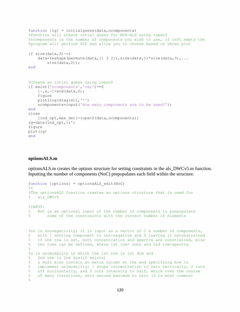
120

function [ig] = initialguess(data,ncomponents) %Function will create intial guess for MCR-ALS using iopav2 %ncomponents is the number of components you wish to use, if left empty the %program will perform SVD and allow you to choose based on Skree plot

if size(data,3)~=1 data=reshape(permute(data,[1 3 2]),size(data,1)*size(data,3),... size(data,2)); end

%Create an intial guess using iopav2 if exist('ncomponents','var')==0 [~,s,~]=svd(data,0); figure plot(log(diag(s)),'*') ncomponents=input('How many components are to be used?'); end close [ind_opt,max_det]=iopav2(data,ncomponents); ig=data(ind_opt,:)'; figure plot(ig) end

optionsALS.m

optionsALS.m creates the options structure for setting constraints in the als_DWCv5.m function.

Inputting the number of components (NoC) prepopulates each field within the structure.

function [options] = optionsALS_edit(NoC) %% %The optionsALS function creates an options structure that is used for % als_DWCv5

%INPUT: % NoC is an optional input of the number of components to prepopulate % some of the constraints with the correct number of elements

%nn is nonnegativity; it is input as a vector of 1 x number of components, % with 1 setting component to non-negative and 0 leaving it unconstrained % If one row is set, both concentration and spectra are constrained, else % two rows can be defined, where 1st row= conc and 2nd row=spectra % %u is unimodality in which the 1st row is 1st dim and % 2nd row is 2nd dim(if exists) % u must also contain an extra column at the end specifying how to % implement unimodality; 1 drops concentration to zero vertically, 2 cuts % off horizontally, and 3 cuts intensity to half, which over the course % of many iterations, sets second maximum to zero (3 is most common) %

121

%uTol is tolerance for unimodality; 1 allow no increase after intial maximum, % 1.1 allows 10% increase, etc. % %csel is chromatographic selectivity in the with the dimensions of: % time x sample x component or 1D time x 2D time x sample x component % %ssel is spectral selectivity with the dimensions of: % spectra x component %Trilinearity sets components to be trilinear. Row vector with sample % number of elements as components. 1 sets trilinear, 0 leaves it % unconstrained. Trilinearity is only defined at this point for 3-way % data %Smoothness constrains components to be smooth, based on Eiler's perfect % smoother. First row is concentration, second row is spectra

if ~exist('NoC','var') NoC=1; end

field1='NN'; value1=zeros(1,NoC);

field2='Uni'; value2=zeros(1,NoC+1); value2(:,end)=3;

field3='Utol'; value3=1;

field4='ssel'; value4=NaN;

field5='csel'; value5=NaN;

field6='Trilinearity'; value6=zeros(1,NoC);

field7='Smoothness'; value7=zeros(2,NoC);

options=struct(field1,value1,field2,value2,field3,value3,field4,value4,field5

,value5,field6,value6,field7,value7);

end

122

This page intentionally left blank

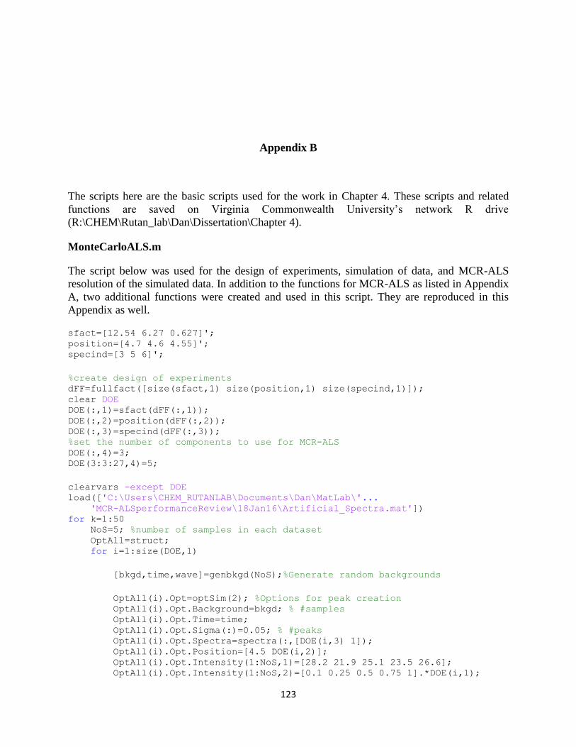
123

Appendix B

The scripts here are the basic scripts used for the work in Chapter 4. These scripts and related

functions are saved on Virginia Commonwealth University’s network R drive

(R:\CHEM\Rutan_lab\Dan\Dissertation\Chapter 4).

MonteCarloALS.m

The script below was used for the design of experiments, simulation of data, and MCR-ALS

resolution of the simulated data. In addition to the functions for MCR-ALS as listed in Appendix

A, two additional functions were created and used in this script. They are reproduced in this

Appendix as well.

sfact=[12.54 6.27 0.627]'; position=[4.7 4.6 4.55]'; specind=[3 5 6]';

%create design of experiments dFF=fullfact([size(sfact,1) size(position,1) size(specind,1)]); clear DOE DOE(:,1)=sfact(dFF(:,1)); DOE(:,2)=position(dFF(:,2)); DOE(:,3)=specind(dFF(:,3)); %set the number of components to use for MCR-ALS DOE(:,4)=3; DOE(3:3:27,4)=5;

clearvars -except DOE load(['C:\Users\CHEM_RUTANLAB\Documents\Dan\MatLab\'... 'MCR-ALSperformanceReview\18Jan16\Artificial_Spectra.mat']) for k=1:50 NoS=5; %number of samples in each dataset OptAll=struct; for i=1:size(DOE,1)

[bkgd,time,wave]=genbkgd(NoS);%Generate random backgrounds

OptAll(i).Opt=optSim(2); %Options for peak creation OptAll(i).Opt.Background=bkgd; % #samples OptAll(i).Opt.Time=time; OptAll(i).Opt.Sigma(:)=0.05; % #peaks OptAll(i).Opt.Spectra=spectra(:,[DOE(i,3) 1]); OptAll(i).Opt.Position=[4.5 DOE(i,2)]; OptAll(i).Opt.Intensity(1:NoS,1)=[28.2 21.9 25.1 23.5 26.6]; OptAll(i).Opt.Intensity(1:NoS,2)=[0.1 0.25 0.5 0.75 1].*DOE(i,1);

124

end clear bkgd

for i=1:size(DOE,1) %Simulate peaks [peaks,results(i).profiles,results(i).res]=peakSim(OptAll(i).Opt); results(i).spectra=OptAll(i).Opt.Spectra; results(i).intensity=OptAll(i).Opt.Intensity; %results(i).peaks=peaks; n=DOE(i,4);

ig=initialguess(reshape(permute(peaks,[1 3 2]),size(peaks,1)*... size(peaks,3),size(peaks,2)),n);

%number of components ALSopt=optionsALS(n); %Options for MCR-ALS ALSopt.NN(1:2)=1; ALSopt.Uni(1:2)=1; ALSopt.ssel=NaN(113,n); ALSopt.ssel(40:end,1:2)=0; ALSopt.csel=NaN(size(peaks,1),size(peaks,3),n); ALSopt.csel([1:190 700:end],:,1:2)=0; ALSopt.Smoothness(1,3:end)=10e4;

%Rearrange intial guess to match the order of the real spectra rearr=corrcoef(cat(2,ig,results(i).spectra)).^2; rearr=rearr(1:n,n+1:n+size(results(i).spectra,2));

for j=1:size(rearr,2) [x,y]=find(rearr == max(max(rearr))); rearrx(y)=x; rearr(:,y)=0;rearr(x,:)=0; end %Rearrage ig to match spectra order x=1:size(ig,2);x(rearrx)=[];ig=ig(:,[rearrx x]);

[results(i).r_opt,results(i).s_opt,~,results(i).fit]=... als_DWCv5(peaks,ig,10000,ALSopt);

%rearrange s_opt and r_opt to match real spectra order rearr=corrcoef(cat(2,results(i).s_opt,results(i).spectra)).^2; rearr=rearr(1:n,n+1:n+size(results(i).spectra,2));

for j=1:size(rearr,2) [x,y]=find(rearr == max(max(rearr))); rearrx(y)=x; rearr(:,y)=0;rearr(x,:)=0; end x=1:size(results(i).s_opt,2);x(rearrx)=[]; results(i).s_opt=results(i).s_opt(:,[rearrx x]); results(i).r_opt=results(i).r_opt(:,:,[rearrx x]); results(i).quant=squeeze(sum(results(i).r_opt)); end eval(['results' num2str(k) '=results;'])

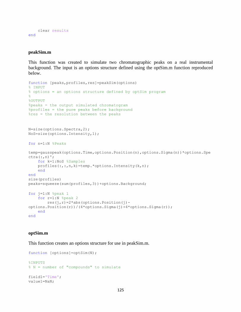
125

clear results end

peakSim.m

This function was created to simulate two chromatographic peaks on a real instrumental

background. The input is an options structure defined using the optSim.m function reproduced

below.

function [peaks,profiles,res]=peakSim(options) % INPUT % options = an options structure defined by optSim program % %OUTPUT %peaks = the output simulated chromatogram %profiles = the pure peaks before background %res = the resolution between the peaks

N=size(options.Spectra,2); NoS=size(options.Intensity,1);

for n=1:N %Peaks

temp=gausspeak(options.Time,options.Position(n),options.Sigma(n))*options.Spe

ctra(:,n)'; for k=1:NoS %Samples profiles(:,:,n,k)=temp.*options.Intensity(k,n); end end size(profiles) peaks=squeeze(sum(profiles,3))+options.Background;

for j=1:N %peak 1 for r=1:N %peak 2 res(j,r)=2*abs(options.Position(j)-

options.Position(r))/(4*options.Sigma(j)+4*options.Sigma(r)); end end

optSim.m

This function creates an options structure for use in peakSim.m.

function [options]=optSim(N);

%INPUTS % N = number of "compounds" to simulate

field1='Time'; value1=NaN;

126

field2='Position'; value2=NaN(1,N);

field3='Sigma'; value3=NaN(1,N);

field4='Intensity'; value4=NaN(1,N);

field5='Spectra'; value5=NaN;

field6='Background'; value6=NaN;

options=struct(field1,value1,field2,value2,field3,value3,field4,value4,field5

,value5,field6,value6);

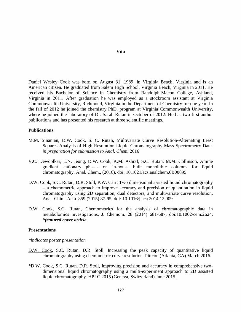
127

Vita

Daniel Wesley Cook was born on August 31, 1989, in Virginia Beach, Virginia and is an

American citizen. He graduated from Salem High School, Virginia Beach, Virginia in 2011. He

received his Bachelor of Science in Chemistry from Randolph-Macon College, Ashland,

Virginia in 2011. After graduation he was employed as a stockroom assistant at Virginia

Commonwealth University, Richmond, Virginia in the Department of Chemistry for one year. In

the fall of 2012 he joined the chemistry PhD. program at Virginia Commonwealth University,

where he joined the laboratory of Dr. Sarah Rutan in October of 2012. He has two first-author

publications and has presented his research at three scientific meetings.

Publications

M.M. Sinanian, D.W. Cook, S. C. Rutan, Multivariate Curve Resolution-Alternating Least

Squares Analysis of High Resolution Liquid Chromatography-Mass Spectrometry Data.

in preparation for submission to Anal. Chem. 2016

V.C. Dewoolkar, L.N. Jeong, D.W. Cook, K.M. Ashraf, S.C. Rutan, M.M. Collinson, Amine

gradient stationary phases on in-house built monolithic columns for liquid

chromatography. Anal. Chem., (2016), doi: 10.1021/acs.analchem.6B00895

D.W. Cook, S.C. Rutan, D.R. Stoll, P.W. Carr, Two dimensional assisted liquid chromatography

– a chemometric approach to improve accuracy and precision of quantitation in liquid

chromatography using 2D separation, dual detectors, and multivariate curve resolution,

Anal. Chim. Acta. 859 (2015) 87-95, doi: 10.1016/j.aca.2014.12.009

D.W. Cook, S.C. Rutan, Chemometrics for the analysis of chromatographic data in

metabolomics investigations, J. Chemom. 28 (2014) 681-687, doi:10.1002/cem.2624.

*featured cover article

Presentations

*indicates poster presentation

D.W. Cook, S.C. Rutan, D.R. Stoll, Increasing the peak capacity of quantitative liquid

chromatography using chemometric curve resolution. Pittcon (Atlanta, GA) March 2016.

*D.W. Cook, S.C. Rutan, D.R. Stoll, Improving precision and accuracy in comprehensive two-

dimensional liquid chromatography using a multi-experiment approach to 2D assisted

liquid chromatography. HPLC 2015 (Geneva, Switzerland) June 2015.

128

S. C. Rutan, P. W. Carr, J.M. Davis, D.W. Cook, R.C. Allen, B.B. Barnes, M.F. Filgueria.

Fundamental issues in quantitative analysis in multi-dimensional liquid chromatography

– The Good, the Bad and the Ugly. Pittcon (New Orleans, LA) March 2015

*D.W. Cook, S.C. Rutan, Chemometric approach to improve accuracy and precision of

quantitation in two-dimensional liquid chromatography using dual detectors and

multivariate curve resolution. Chemometrics in Analytical Chemistry (Richmond, VA)

June 2014.