NOTE TO USERS - CURVE | Carleton University Research ...

NOTE TO USERS

This reproduction is the best copy available.

®

UMI

Reproduced with permission of the copyright owner. Further reproduction prohibited without permission.

HEAT PIPE PERFORMANCE ENHANCEMENT THROUGH

COMPOSITE WICK DESIGN

By

George S. Franchi

A thesis submitted to

the Faculty of Graduate Studies and Research

in partial fulfillment of

the requirements for the degree of

Master o f Applied Science

Ottawa-Carleton Institute for

Mechanical and Aerospace Engineering

Department of

Mechanical and Aerospace Engineering

Carleton University

Ottawa, Ontario

July, 2006

© Copyright by George S. Franchi, 2006


Library and Archives Canada

Bibliotheque et Archives Canada

Published Heritage Branch

395 Wellington Street Ottawa ON K1A 0N4 Canada

Your file Votre reference ISBN: 978-0-494-33631-1 Our file Notre reference ISBN: 978-0-494-33631-1

Direction du Patrimoine de I'edition

395, rue Wellington Ottawa ON K1A 0N4 Canada

NOTICE:The author has granted a nonexclusive license allowing Library and Archives Canada to reproduce, publish, archive, preserve, conserve, communicate to the public by telecommunication or on the Internet, loan, distribute and sell theses worldwide, for commercial or noncommercial purposes, in microform, paper, electronic and/or any other formats.

AVIS:L'auteur a accorde une licence non exclusive permettant a la Bibliotheque et Archives Canada de reproduire, publier, archiver, sauvegarder, conserver, transmettre au public par telecommunication ou par I'lnternet, preter, distribuer et vendre des theses partout dans le monde, a des fins commerciales ou autres, sur support microforme, papier, electronique et/ou autres formats.

The author retains copyright ownership and moral rights in this thesis. Neither the thesis nor substantial extracts from it may be printed or otherwise reproduced without the author's permission.

L'auteur conserve la propriete du droit d'auteur et des droits moraux qui protege cette these.Ni la these ni des extraits substantiels de celle-ci ne doivent etre imprimes ou autrement reproduits sans son autorisation.

In compliance with the Canadian Privacy Act some supporting forms may have been removed from this thesis.

While these forms may be included in the document page count, their removal does not represent any loss of content from the thesis.

Conformement a la loi canadienne sur la protection de la vie privee, quelques formulaires secondaires ont ete enleves de cette these.

Bien que ces formulaires aient inclus dans la pagination, il n'y aura aucun contenu manquant.

i * i

CanadaReproduced with permission of the copyright owner. Further reproduction prohibited without permission.

Abstract

This study examines the enhancement of heat pipe thermal performance through the

employment of composite wicks. These wicks were fabricated from a biporous structure

comprised of fine metal powders, sintered onto layers of coarse pore copper mesh. Wick

structures were conceived to exploit both the effects o f enhanced evaporation heat

transfer at the liquid/vapour interface and the extension of the capillary limit. A number

of composite wick heat pipe configurations were fabricated and tested to assess

performance improvements in comparison to conventional designs. Tests were conducted

in horizontal, gravity assisted and against gravity conditions to determine whether these

designs were orientation dependent. At various heat inputs, some configurations achieved

thermal performance levels over three times higher than those of conventional heat pipes.

During against gravity tests, virtually all composite designs outperformed the

conventional heat pipe at all heat inputs. These results clearly demonstrated that heat pipe

performance was substantially improved through composite wick design.

111


Acknowledgements

Who to thank and where to begin? I think I will start by offering a warm-hearted thanks

to my supervisor, Professor Huang, for providing guidance and inspiration for this

milestone in my career. I will never forget the kind words and wisdom you imparted to

me, not only in matters of engineering, but more importantly towards all aspects o f life

involving integrity and honesty. Long after the classroom lectures and experiments have

faded from memory, these most important o f qualities will endure. Thank you, Professor.

Many thanks to the Department of Mechanical and Aerospace Engineering for the

financial assistance awarded to me, without which I could not have completed this

endeavour. I am also indebted to Materials and Manufacturing Ontario, Acrolab and

INCO for their invaluable aid during this research program. For their technical support

and expertise, I would like to extend my appreciation to Stephan Biljan, Steve Truttmann,

Fred Barrett and Gary Clements. To my heat pipe research colleagues Feng Cai and

Michel Garcia, thank you both for your advice and experience. I avoided countless

difficulties and pitfalls from your hard-earned knowledge.

Most importantly, I want to thank my family. Try as I may, I could never hope to find

words eloquent enough to express my gratitude. You mean the world to me, and I love

you with all my heart.

iv


Table of Contents

Abstract......................................................................................................................................... iii

Acknowledgements......................................................................................................................iv

Table of Contents..........................................................................................................................v

List of Tables................................................................................................................................ x

List of Figures............................................................................................................................. xii

1 Introduction.................................................................................................................................1

1.1 History.................................................................................................................................. 1

1.2 Applications........................................................................................................................3

1.2.1 Electronics cooling.................................................................................................... 3

1.2.2 Aerospace.....................................................................................................................5

1.2.3 Pipelines.......................................................................................................................6

1.3 Operation............................................................................................................................. 7

1.4 Enhanced Heat Transfer with Composite W icks............................................................ 8

1.5 Objective and Approach................................................................................................... 9

2 Theory....................................................................................................................................... 11

2.1 Capillary Limit................................................................................................................11

2.1.1 Surface tension and capillary pressure................................................................... 12

2.1.2 Liquid pressure drop................................................................................................ 17

2.1.3 Vapour pressure drop...............................................................................................21

2.1.4 Hydrostatic pressure................................................................................................ 22

2.1.5 General expression for the capillary limit..............................................................23

v


2.2 Sonic Limit........................................................................................................................23

2.3 Boiling Limit.....................................................................................................................24

2.4 Entrainment Lim it............................................................................................................31

2.5 Graphical Representation of Heat Transfer Limitations............................................. 33

2.6 Prediction of Thermal Performance...............................................................................34

2.6.1 Equivalent thermal resistance network..................................................................35

2.6.2 Heat pipe operating temperature............................................................................ 41

2.6.3 Effective thermal conductivity of wicks............................................................... 42

3 Heat Pipe Design......................................................................................................................46

3.1 Working Fluid Selection................................................................................................. 46

3.2 Container........................................................................................................................... 50

3.3 Wick Design......................................................................................................................54

3.3.1 Metal screens............................................................................................................55

3.3.2 Axial grooves............................................................................................................ 58

3.3.3 Sintered metal wicks................................................................................................ 62

3.3.4 Composite wicks...................................................................................................... 67

4 Experimental Procedure..........................................................................................................74

4.1 Container and Wick M aterials....................................................................................... 74

4.2 Wick Configurations........................................................................................................78

4.2.1 Homogeneous w icks................................................................................................ 80

4.2.2 Composite wicks.......................................................................................................81

4.3 Heat Pipe Design and Manufacture...............................................................................84

4.3.1 Design...................................................................................................................... 85

vi


4.3.2 Wick cutting.............................................................................................................. 89

4.3.3 Degreasing and deoxidizing.................................................................................... 90

4.3.4 Metal powder application....................................................................................... 91

4.3.5 Rolling and insertion................................................................................................95

4.3.6 Sintering.....................................................................................................................97

4.3.7 Fluid charging and sealing.....................................................................................100

4.4 Heat Pipe Test R ig ......................................................................................................... 102

4.4.1 Heater and annulus................................................................................................. 103

4.4.2 Cooling jacket and chiller..................................................................................... 106

4.4.3 Insulation.................................................................................................................108

4.4.4 Instrumentation.......................................................................................................110

4.4.5 Data acquisition system .......................................................................................114

4.5 Test Procedure................................................................................................................117

4.5.1 Heat pipe preparation............................................................................................. 117

4.5.2 Orientations............................................................................................................. 121

4.5.3 Testing and data collection................................................................................... 123

4.5.4 Data reduction program .........................................................................................126

5 Results and Discussion......................................................................................................... 128

5.1 Summary of Tests Performed.......................................................................................128

5.2 Scanning Electron Microscopy.....................................................................................129

5.2.1 Configuration A ......................................................................................................130

5.2.2 Configuration H ...................................................................................................... 131

5.2.3 Configuration K ...................................................................................................... 133

vii


5.2.4 Configuration B ......................................................................................................134

5.2.5 Configuration E.......................................................................................................137

5.2.6 Configuration 1........................................................................................................139

5.2.7 Configuration J .......................................................................................................140

5.2.8 Configuration L .......................................................................................................142

5.3 Effective Thermal Conductivity and Maximum Heat Input Rate..........................143

5.3.1 Configuration A ......................................................................................................144

5.3.2 Configuration H ......................................................................................................147

5.3.3 Configuration K ......................................................................................................150

5.3.4 Configuration B ......................................................................................................155

5.3.5 Configuration E.......................................................................................................164

5.3.6 Configuration J .......................................................................................................170

5.3.7 Configuration L.......................................................................................................177

5.3.8 Summary of composite wicks with highest thermal performance................... 185

5.3.9 Uncertainty analysis............................................................................................... 187

6 Conclusions and Recommendations................................................................................... 194

6.1 Remarks on Results........................................................................................................194

6.2 Remarks on Manufacturing...........................................................................................196

6.3 Remarks on Testing.......................................................................................................197

6.4 Concluding W ords......................................................................................................... 197

Appendix A Heat Pipe Design Calculations..........................................................................199

Appendix B Fluid Charging.................................................................................................... 211

Appendix C Cooling Jacket Drawings...................................................................................214

viii


Appendix D Data Acquisition Program.................................................................................226

Appendix E “thermalPerformance” Program ....................................................................... 230

Appendix F Additional Performance Results....................................................................... 237

7 References.............................................................................................................................. 260

ix


List of Tables

Table 2-1: Effective Pore Radii of Simple Wicks [16].......................................................... 17

Table 2-2: Wetted Perimeter for Various Wicks [1].............................................................. 32

Table 2-3: Heat Pipe Thermal Resistances [10].....................................................................36

Table 2-4: Effective Thermal Conductivities of Various Wicks [1]..................................44

Table 3-1: Heat Pipe Working Fluids and Their Corresponding Temperature Ranges [10]

...............................................................................................................................................47

Table 3-2: Material/Working Fluid Compatibility Data [38]............................................... 50

Table 3-3: Values for n, m and B of the Initial Stage Sintering Equation [56]..................66

Table 4-1: Copper Tubing Properties [68], [69], [70 ]........................................................... 75

Table 4-2: 100-Mesh Copper Screen Properties [1], [68]......................................................76

Table 4-3: Properties of Metco 55 Copper Powder [71]........................................................76

Table 4-4: Properties of Nickel Powder [73].......................................................................... 78

Table 4-5: Summary of Wick Identification........................................................................... 79

Table 4-6: Conventional Heat Pipe Design Specifications....................................................88

Table 4-7: Band Heater Properties..........................................................................................104

Table 4-8: Properties o f Delrin® [68]..................................................................................... 106

Table 4-9: Properties o f Refrigerated Recirculation Chiller [74].......................................108

Table 4-10: Properties of Insulation [68]............................................................................... 109

Table 4-11: Thermocouple Properties [75]............................................................................I l l

Table 4-12: Multimeter Properties [76]................................................................................. 112

Table 4-13: Thermistor Properties [75]................................................................................. 113

x


Table 4-14: Flowmeter Properties [77].................................................................................. 113

Table 4-15: Properties of Thermocouple Modules [78 ]......................................................114

Table 4-16: Properties of Analog Input Module [79].......................................................... 115

Table 4-17 : Properties of Network Module [80]..................................................................115

Table 4-18: Properties o f OMEGATHERM® [81]...............................................................120

Table 5-1: List of Heat Pipe Tests..........................................................................................129

Table 5-2: Thermal Performance Summary for A 7..............................................................147

Table 5-3: Thermal Performance Summary for H 3..............................................................150

Table 5-4: Thermal Performance Summary for K1 and K 2 ................................................ 155

Table 5-5: Thermal Performance Summary for Runs 1 and 2 of B8.................................. 164

Table 5-6: Thermal Performance Summary for E 7 ..............................................................170

Table 5-7: Thermal Performance Summary for J 3 ...............................................................176

Table 5-8: Summary of Findings from Cao et al. [67 ]........................................................ 181

Table 5-9: Maximum Heat Input Rate Comparison, Against Gravity............................... 183

Table 5-10: Thermal Performance Summary for L 2 ............................................................184

Table 5-11: Measurement Uncertainties Used in Equation ( 5-5 ) .....................................189

Table 5-12: Uncertainty Summary for Heat Pipe B8............................................................190

XI


List of Figures

Figure 1-1: Heat Pipe Cooling System for a Mobile Pentium 4 Chip [4].............................3

Figure 1-2: Module Heat Flux Rise versus Time [8].............................................................. 4

Figure 1-3: Pipeline Support with Integrated Heat Pipes for Permafrost Preservation [14]

................................................................................................................................................. 7

Figure 1-4: Schematic Diagram of a Heat Pipe [15]................................................................8

Figure 2-1: Wetting Meniscus Geometry at Liquid/Vapour Interface [16]........................13

Figure 2-2: Geometry of Meniscus in a Cylindrical Tube [16]........................................... 14

Figure 2-3: Capillary Limit versus Effective Pore Radius for Copper Mesh Wicks [17] 16

Figure 2-4: Permeability versus Effective Pore Radius for Copper Mesh Wicks [17].......19

Figure 2-5: Tortuosity of Coarse Pores (Left) Compared to Fine Pores (Right)...............19

Figure 2-6: Heat Flux versus Excess Temperature [20].......................................................21

Figure 2-7: Gravity Assisted Operation, <j> Negative............................................................ 22

Figure 2-8: Heat Transfer Modes 1 and 2 in the Evaporator [1 ] ..........................................25

Figure 2-9: Heat Transfer Modes 3 and 4 in the Evaporator [1 ] ..........................................26

Figure 2-10: Pool Boiling Curve for Plane Surface Submerged Under Water [1 ]............ 27

Figure 2-11: Heat Flux versus Excess Temperature [28]......................................................30

Figure 2-12: Heat Flux versus Excess Temperature for Wicks with Vapour Channels [23]

...............................................................................................................................................31

Figure 2-13: Heat Transfer Limitations as a Function of Temperature [16]...................... 34

Figure 2-14: Thermal Resistance Network of a Heat Pipe [30]............................................35

Figure 2-15: Simplified Thermal Resistance Network [10]..................................................37

xii


Figure 2-16: Estimation o f Heat Pipe Operating Temperature [10].................................... 42

Figure 2-17: Thermal Conductivity for Heat Transfer in (a) Parallel and (b) Series [1].. 43

Figure 3-1: Variation of Liquid Transport Factor with Temperature [5]........................48

Figure 3-2: Heat Pipe Container and Wick Dimensions................................................... 51

Figure 3-3: Wick Pore Radius (nm) versus Permeability (jum2) [39]............................. 54

Figure 3-4: Plain Wire Screen Weave (Left), Twill Screen Weave (Right) [40]..........56

Figure 3-5: Metal Screen Wick Dimensions.......................................................................57

Figure 3-6: Cross-section of Heat Pipe with Rectangular Axial Grooves [45]............. 58

Figure 3-7: Friction Factor Reynolds Number Product for Rectangular Passages [16]... 61

Figure 3-8: Phases during Sintering Process......................................................................63

Figure 3-9: Neck Formation in Sintered Bronze Powder [55]......................................... 64

Figure 3-10: Surface Diffusion versus Volume Diffusion [58]............................................65

Figure 3-11: Thin Film Evaporation in Porous Structures [61]............................................69

Figure 3-12: Composite Metal Powder Wick [60].................................................................70

Figure 3-13: Triangular Grooves (a) without and (b) with Fine Pores [46]....................... 71

Figure 3-14: Wang and Catton’s Results [46]........................................................................ 73

Figure 4-1: Spherical Copper Powder Morphology...........................................................77

Figure 4-2: Filamentary Nickel Powder M orphology.......................................................78

Figure 4-3: Schematics of Configuration A (Left) and Configurations H and K (Right). 80

Figure 4-4: Liquid/Vapour Interface Covered with Metal Powder, Configurations B and I

82

Figure 4-5: Wall/Wick and Liquid/Vapour Interfaces Covered with Metal Powder,

Configurations E and J .......................................................................................................83

xiii


Figure 4-6: Metal Powder Applied throughout Wick Thickness, Configuration L ........... 84

Figure 4-7: Schematic of Mesh Weave [28]........................................................................... 87

Figure 4-8: Model for Required Width of Mesh.....................................................................89

Figure 4-9: Wick Cutting Tools................................................................................................90

Figure 4-10: End P lugs.............................................................................................................. 91

Figure 4-11: Homogeneous Copper Metal Powder Heat Pipe Manufacturing Assembly 92

Figure 4-12: Metal Powder Application Patterns for Configurations B, E, I and J ........... 93

Figure 4-13: Spray Patterns for Configurations L and H .......................................................93

Figure 4-14: Nickel Powder Sprayed Wick, Configuration B .............................................. 94

Figure 4-15: Composite Copper Wick Manufacturing.......................................................... 95

Figure 4-16: Configuration J with Rolling Tools...................................................................96

Figure 4-17: Placement of End Plugs for Wick Centering....................................................97

Figure 4-18: Nickel Powder, Sintered at 800°C for 1.5 Hours............................................. 98

Figure 4-19: Copper Powder, Sintered at 850°C for 1 H our................................................ 98

Figure 4-20: Nickel Powder, Sintered at 940°C for 1 H our................................................. 99

Figure 4-21: Heat Pipe Test Rig Schematic...........................................................................103

Figure 4-22: Dimensions of Copper Annulus Half...............................................................105

Figure 4-23: Heater and Annulus Assembly..........................................................................105

Figure 4-24: Cooling Jacket.....................................................................................................107

Figure 4-25: Insulation Covering Cooling Jacket and H eater............................................ 110

Figure 4-26: Thermocouple Locations on Heat Pipe........................................................... 111

Figure 4-27: Thermocouple Attachment................................................................................ 118

Figure 4-28: Teflon Tape Seal................................................................................................ 118

xiv


Figure 4-29: Clamped Cooling Jacket on Orientation Pedestal.......................................... 119

Figure 4-30: Thermal Paste Application................................................................................ 120

Figure 4-31: Heater Assembly Secured to Evaporator Section.......................................... 121

Figure 5-1: Configuration A ...................................................................................................130

Figure 5-2: Configuration H ...................................................................................................131

Figure 5-3: Configuration H, Higher Magnification............................................................132

Figure 5-4: Sintering in Nickel Powder................................................................................ 132

Figure 5-5: Configuration K ...................................................................................................133

Figure 5-6: Neck Formation in Configuration K .................................................................134

Figure 5-7: Liquid/Vapour Interface of Configuration B ...................................................135

Figure 5-8: Increased Surface Area in Configuration B ......................................................136

Figure 5-9: Sintering between Nickel Powder and Copper M esh......................................137

Figure 5-10: Configuration E ...................................................................................................138

Figure 5-11: Wall/Wick Interface of Configuration E ......................................................... 138

Figure 5-12: Configuration 1....................................................................................................139

Figure 5-13: Liquid/Vapour Interface of Configuration 1....................................................140

Figure 5-14: Configuration J ....................................................................................................141

Figure 5-15: Wall/Wick Interface of Configuration J...........................................................142

Figure 5-16: Horizontal and Gravity Assisted Effective Thermal Conductivities for A7

............................................................................................................................................. 145

Figure 5-17: Axial Temperature Distribution of A7, Against Gravity Operation............146

Figure 5-18: Against Gravity Effective Thermal Conductivity Results for A7.............. 146

xv


Figure 5-19: Horizontal and Gravity Assisted Effective Thermal Conductivities for H3

............................................................................................................................................. 149

Figure 5-20: Against Gravity Effective Thermal Conductivity Results for H3...............149

Figure 5-21: Horizontal and Gravity Assisted Results for Configuration K ................... 151

Figure 5-22: Against Gravity Effective Thermal Conductivity Results for K1 and K 2. 152

Figure 5-23: Axial Temperature Distribution for K l, Against Gravity............................153

Figure 5-24: Comparison of Horizontal Thermal Performance between B8 and A 7 156

Figure 5-25: Comparison of Gravity Assisted Thermal Performance between B8 and A7

.............................................................................................................................................158

Figure 5-26: Against Gravity Thermal Performance Comparison between B8, A7 and H3

160

Figure 5-27: Testing Repeatability for B8, Horizontal Orientation.................................. 161

Figure 5-28: Testing Repeatability for B8, Gravity Assisted Orientation........................162

Figure 5-29: Testing Repeatability for B8, Against Gravity Orientation.........................162

Figure 5-30: Comparison o f Horizontal Thermal Performance between E7 and A 7 165

Figure 5-31: Comparison of Gravity Assisted Performance between E7 and A 7 167

Figure 5-32: Against Gravity Performance Comparison between E7, A7 and H 3 168

Figure 5-33: Comparison o f Horizontal Performance between J3 and A7...................... 171

Figure 5-34: Comparison of Gravity Assisted Performance between J3 and A 7 173

Figure 5-35: Against Gravity Performance Comparison between J3, A7 and K l 174

Figure 5-36: Axial Temperature Distribution for J3, Against Gravity.............................175

Figure 5-37: Comparison o f Horizontal Performance between L2 and A 7..................... 178

Figure 5-38: Comparison o f Gravity Assisted Performance between L2 and A 7 181

xvi


Figure 5-39: Against Gravity Performance Comparison between L2, A7 and H 3 182

Figure 5-40: Best Performing Configurations, Horizontal Operation............................... 186

Figure 5-41: Best Performing Configurations, Gravity Assisted Operation..................... 186

Figure 5-42: Best Performing Configurations, Against Gravity Operation.......................187

Figure 5-43 Uncertainty for B8, Horizontal Orientation..................................................... 191

Figure 5-44: Uncertainty for B8, Gravity Assisted Orientation......................................... 191

Figure 5-45: Uncertainty for B8, Against Gravity Orientation........................................... 192

X V ll


1 Introduction

The need for progressively efficient, high performance heat transfer equipment in

electronics cooling, heat recovery systems and spacecraft thermal management has

produced numerous successful innovations. Perhaps the most remarkable o f these is the

heat pipe, a heat transfer device with a thermal conductivity much higher than any solid

material. Through vapourization and condensation heat transfer processes, very high heat

transfer rates with minimal variations in end-to-end temperature are possible. Since heat

pipes do not contain any moving parts, they have gained a reputation of exceptional

reliability, with the additional benefit of completely passive operation.

Although the heat pipe has proven itself a practical tool for thermal control, certain heat

transfer limitations hinder its capabilities. Coupled with industrial demands for greater

heat removal capacity in increasingly compact designs, conventional heat pipes have

often proven inadequate. Thus, to keep pace, the heat pipe must evolve. Since heat pipe

performance is intimately associated with heat transfer and fluid behaviour in porous

materials, advancement o f the art may very well depend on the application of enhanced,

porous engineering materials.

1.1 History

The historical development of the heat pipe began in 1836 with the United Kingdom

patent of the Perkins Tube, comprised of a closed tube containing a small amount of

water for the purpose of transferring heat [1], Although the Perkins Tube was not

1


technically a heat pipe, the operating principles and mechanism of heat transfer were

analogous. The first patent describing the modem day heat pipe was filed in 1944 by

Gaugler, who was working for General Motors at the time [1], This device, used in a

refrigeration unit, was made of an outer tube, a working fluid and a capillary structure to

pump the fluid against gravity.

The heat pipe was somewhat forgotten until its emergence as a viable system for

spacecraft thermal management. In 1964, the heat pipe was reinvented by Grover et al. at

Los Alamos National Laboratories during research for the United States Space Program

[1], [2], His experiments demonstrated the feasibility of heat pipes as high performance

heat transmission devices for space applications. It was Grover who first coined the name

“heat pipe”. Although these experiments renewed much interest in heat pipes, worldwide

research did not begin until after Cotter’s work on theoretical heat pipe analysis was

published in 1965 [3]. Heat pipe research centers were then established in the United

Kingdom, Italy and the former USSR.

Today, every developed country has contributed in some way to the development o f heat

pipe technology, with Russia and the United States leading the state-of-the-art. Heat pipes

are currently being used in a wide array of industries, ranging from electronics and space

exploration to petroleum pipelines. Industrial manufacturers are capable of heat pipe

production rates of 50 000 units per month [4], Research programs worldwide continue to

explore potential heat pipe applications, more advanced modeling techniques and new,

2


high performance materials. The heat pipe has become a universally accepted, reliable

thermal management tool with ample opportunity for research.

1.2 Applications

Heat pipe applications reflect their remarkable versatility. Microelectronics cooling and

spacecraft temperature control are two main areas where heat pipes are extensively used.

Other notable industrial uses include the preservation o f permafrost in pipeline

applications.

1.2.1 Electronics cooling

Electronics cooling represents the most widespread industrial use of heat pipes [5], The

higher performance electronics o f the early 1990’s demanded more efficient heat removal

devices. Laptop computer manufacturers first used heat pipes in 1994 to dissipate 6 W of

heat [6], By 1999, approximately 60% of all laptop computers employed heat pipes for

their cooling needs. Figure 1-1 shows a typical heat pipe and heat sink for laptop

computer thermal management.

Heat

source

Figure 1-1: Heat Pipe Cooling System for a Mobile Pentium 4 Chip [4]

3


Presently, Intel’s Mobile Pentium 4 processor requires 35 W of heat removal at a heat

'j

flux of 24 W/cm [7], and all manufacturers make use of heat pipe technology in their

laptops. Current designs capable of meeting this demand commonly use 3 to 6 mm

outside diameter copper/water heat pipes. However, the increasing trend towards higher

heat removal rates in more compact designs must be met with higher performance

thermal management devices. According to Moore’s Law, the performance of electronic

modules doubles approximately every 18 months [8], This in turn causes an exponential

growth in heat flux from the component surface, shown in Figure 1-2.

15

~ 10 £

5X

J3 »*-

IS 0)

01950 1960 1970 1980 1990 2000 2010

Year

Figure 1-2: Module Heat Flux Rise versus Time [8]

4

■ B ipolar

A CMOSIBM ES9000

Fujitsu VP2000

B M 3090S TCM

NTT B

Fujitsu M 780

IBM 3090 TCMrj

CDC Cyber 205

IBM3081 TCM _

U

Vacuum tube

IBM4381

IBM 360 FujitsuM 380™ ^ “ NEC LCM t

IBM 3iW IBM3033 -T litacb i s-810 ■ £ ® Honeywell DPS-88

A IBM RY5

A IBM RY6 A IBM RX4

t IBM RX3


Some electronic components produce heat fluxes greater than 100 W/cm2 [9] while

requiring operating temperatures lower than 120°C. Projected trends demand even higher

performance from the electronics thermal control industry. It is therefore necessary to

improve heat pipe performance to further enhance waste heat dissipation. Since heat pipe

performance is strongly dependent on the properties of its porous wick [10], numerous

research programs have taken aim at heat transfer augmentation through advancements in

wick design.

1.2.2 Aerospace

Aluminium-ammonia heat pipes are extensively used for aerospace and spacecraft

applications, due to their low weight penalty. Spacecraft thermal management also

includes the field of microelectronics and component temperature control.

Satellite isothermalisation is one instance where heat pipes have been particularly

indispensable. Thermal gradients resulting from external heating and cooling can be

minimized by redistributing heat from the hot side to the cold side, thus reducing

structural distortion. For example, if one side of a satellite faces the sun while the other

side faces deep space, solar radiation will heat one side while the other side reaches very

cold temperatures. This will impose significant thermal stresses on the satellite. To

counter this, thermal engineers have exploited the heat pipe’s nearly isothermal behaviour

with great success [1].

5


The Russian satellites MAGION 4 and 5, launched in 1995 and 1996 respectively, used

U-shaped heat pipes with sintered copper wicks and acetone as the working fluid [11].

These heat pipes, with a diameter o f 10 mm and length o f 0.6 m, were reported to

dissipate 60 W of heat. Another current project being conducted by NASA employs a

heat pipe for laser cooling. The Geoscience Laser Altimeter System (GLAS) uses remote

laser sensing for land topography. The laser requires 100 W of heat dissipation to

function. This is accomplished with a sintered nickel wick heat pipe, measuring 25 mm in

diameter and 150 mm in length [12].

1.2.3 Pipelines

Heat pipe technology is used in numerous additional applications. One important instance

deserving mention is perhaps the largest project to ever use heat pipes. Initiated by the

Alyeska Pipeline Service Company in 1974, construction o f the Trans-Alaska Pipeline

required the use of 130 000 heat pipes for the purpose of permafrost preservation around

vertical supports. This would ensure year-round structural stability of above-ground

pipeline sections. The heat pipe manufacturer, McDonnell Douglas, used 5 to 7.5 cm

diameter, steel-ammonia heat pipes with lengths varying from 9 to 23 m [13], These heat

pipes, shown in Figure 1-3, demonstrated heat removal rates of 300 W.

6


ripe

V ^rtt^n l *>1 1 p o rts

Figure 1-3: Pipeline Support with Integrated Heat Pipes for Permafrost Preservation [14]

1.3 Operation

A heat pipe essentially consists of a sealed container, a porous wicking material and a

working fluid. Air is evacuated from the container and an adequate amount o f working

fluid is added to fully saturate the wick. The container is then sealed and the heat pipe is

connected to a heat source and heat sink.

Heat pipes can be divided into three distinct sections: the evaporator, an adiabatic section

and the condenser. Heat addition takes place in the evaporator by conduction through the

container and wick. The working fluid then evaporates, absorbing its latent heat of

7


vapourization. A pressure difference causes the vapour to flow through the constant

temperature adiabatic section to the condenser. Here, it gives off its latent heat,

condensing into liquid. The porous wick then transports the fluid back to the evaporator

by capillary action where the cycle repeats itself. A schematic o f heat pipe components

and operation is shown below in Figure 1-4.

- V i i u h . i l \ ' . A l i e n

Liquid flow (capillary wick)

Liquid flow (capillary wick) A A A A

Vapor flow

Evaporator „ eatend cap

InDirection o f gravity

(evaporator)

» * *11 eat Out

(condenser)I

Condenser end cap

Figure 1-4: Schematic Diagram of a Heat Pipe [15]

1.4 Enhanced Heat Transfer with Composite Wicks

The wick is the essential element in heat pipe operation, since it provides the means for

continuous heat transfer. Two important parameters to consider during the wick design

stage are its pore size and liquid permeability. As will be presented in Section 2.1 , an

ideal wick would have small pores for high capillary pressure, along with high liquid

permeability to facilitate liquid flow. Most heat pipes have homogeneous wicks, that is,

wicks with one characteristic microstructure. This poses a problem, since a fine pore

8


structure, favourable for capillary pressure, increases the liquid path length through the

wick, resulting in a higher liquid pressure drop [1]. Conversely, a wick with high

permeability suffers from poor capillary pressure, yet possesses the advantage o f low

liquid pressure drops.

Thus, homogeneous wicks must balance capillary pumping pressure and liquid

permeability to achieve some compromise in performance. On the other hand, composite

wicks offer a solution to this anomaly. If a porous structure with both small and large

pores could be manufactured, both parameters may be satisfied simultaneously. The fine

pore layer would provide the means for high capillary pressure, while the large pore

layers would ensure high liquid permeability. Furthermore, the addition o f fine pores

should augment evaporation heat transfer due to a substantial increase in evaporative

surface area. Through these mechanisms, heat pipe performance should increase

significantly.

1.5 Objective and Approach

The objective of this research program is the enhancement o f heat pipe performance

through the development of composite wick structures. Moderate temperature heat pipes

are commonly employed in electronics cooling, therefore this is the intended field of

application. Heat transfer performance will be assessed based on the maximum heat

transfer rate along with the effective thermal conductivity of the heat pipe.

Composite wick heat pipes will be manufactured from large pore metal substrate

materials, combined with a secondary fine pore structure of metal powder. Manufacturing

9


techniques must be developed, including cleaning, application methods, heat pipe

fabrication, furnace processing and fluid charging. Various wick configurations will be

attempted to improve heat transfer performance. Following this, the design and

manufacture of a heat pipe test rig will be carried out, including instrumentation, controls

and data analysis software. Finally, composite wick heat pipe performance testing will be

carried out to quantify improvements in heat transfer in comparison to conventional

designs. Test variables will include heat input rates and gravitational orientation, since

these factors affect heat pipe performance.

10


2 Theory

Steady state heat pipe theory consists of hydrodynamic and heat transfer analyses. The

hydrodynamic analysis is concerned with the liquid pressure drop in the wick, as well as

the vapour pressure drop in the vapour passage. Heat transfer analyses are used to model

heat transport through the heat pipe [1]. Using a combination of these, theoretical heat

pipe performance can be predicted. However, numerous heat transfer limitations

constrain heat transport under certain circumstances. O f these, the limit with the lowest

heat transport capability will determine a heat pipe’s maximum performance. The major

limitations on a heat pipe’s heat transport capability are:

the capillary limit

• the sonic limit

• the boiling limit

. the entrainment limit

Although other less common heat transport limits exist, the above will be the focus of

discussion in this section.

2.1 Capillary Limit

A heat pipe’s wick provides the necessary flow path for the liquid to return from the

condenser to the evaporator. It also supplies the capillary pressure needed to pump the

fluid from one end to the other. Along the heat pipe, there exists a pressure gradient

11


between the vapour and the liquid at the liquid/vapour interface. This pressure gradient

forces the meniscus back into the wick, creating capillary pressure [16]. For proper heat

pipe operation, the maximum capillary pumping pressure provided by the wick (APC)

must be greater than or equal to the sum of the following pressure drops [5]:

The liquid pressure drop needed to transport the liquid from the condenser to the

evaporator through the wick (AP/)

The vapour pressure drop required to move the liquid from the evaporator to the

condenser through the vapour passage (APV)

The hydrostatic pressure due to gravity (APg)

This can be expressed mathematically as:

APC > AP, + APV + APg <2"1>

The above equation is referred to as the capillary limit and is the most significant

limitation to heat transport for moderate temperature heat pipes [10]. If this condition is

not satisfied, the wick will not be able to return the working fluid to the evaporator, and

evaporator dry out will occur [10].

2.1.1 Surface tension and capillary pressure

The phenomenon of surface tension is responsible for creating the capillary pressure

required to return the working fluid from the condenser to the evaporator. A molecule in

12


a liquid is attracted by other liquid molecules surrounding it. Since these forces are in

equilibrium, no resultant force acts on this molecule. However, if this molecule is placed

at the surface of the liquid, unbalanced attractive forces are imposed on it by the

molecules inside the liquid. Therefore, a resultant inward force acts to pull the surface

molecule in that direction. This has the effect of giving the liquid drop a shape of

minimum area. This attractive force per unit length is called surface tension, and is a

property of the fluid and the surrounding medium [5].

When a liquid is in contact with a solid medium, the liquid surface molecules experience

forces from the solid surface molecules as well as from the internal liquid molecules. If

attractive forces exist between the liquid and the solid, the liquid free surface will be

concave and the liquid “wets” the solid, as shown in Figure 2-1. Conversely, if these

forces are repulsive, the resultant liquid free surface will be convex and the liquid is

termed “non-wetting”.

Figure 2-1: Wetting Meniscus Geometry at Liquid/Vapour Interface [16]

13


If a perfectly wetting liquid is used such that the contact angle is zero, we obtain:

A Pc , m a x

2 c r ( 2 -5 )

Equation ( 2-5 ) is the expression for the maximum capillary pressure developed in a

cylindrical pore [1]. Other pore shapes yield similar results. For example, it can be shown

that a rectangular capillary tube with Ri = oo and R2 = W/2 produces a maximum

capillary pressure of:

A Pc , m a x

2 <T ( 2-6 )

W

where W is the width o f the tube. Generalizing the Laplace and Young Equation for any

pore geometry, we therefore obtain:

A P = — ( 2 - 7 )c,max

r eff

where reff is the “effective” pore radius. From Equation ( 2-7 ), one can appreciate how a

decrease in reff would influence the maximum capillary pressure. This effect is shown in

Figure 2-3, where the maximum capillary pressure of various copper mesh screens are

plotted versus their pore radii [17]. The capillary pressure increases dramatically for pore

radii smaller than 300 pm.

15


C aptaiy Limit n Eflectae P«fe Radius

2000

5. 1000

500

200 400 GOD BCD 1000 1200 1400 1600Eflbcliw poia radK Jraicioinsirae]

Figure 2-3: Capillary Limit versus Effective Pore Radius for Copper Mesh Wicks [17]

Values of reff for other simple pore geometries are listed in Table 2-1. For more complex

geometries, the effective pore radius must be determined experimentally.

16


Wick Structures Expressions for rtg

Cylindrical pores

Rectangular groove

Triangular groove

Parallel wires

Wire screens

Pack spheres

r.p = r r = radius of pores

rffl — w = groove width

_ W iv =■ groove width

* cos/? /?= half angle

r*g = w M' - wirc spacing

iv'+ d v u>= wire spacingr<u 7

z </„, * wire diameter

= 0 .4 1 r r, = sphere radius

Table 2-1: Effective Pore Radii of Simple Wicks [16]

2.1.2 Liquid pressure drop

Concerning the liquid pressure drop term (APt) o f Equation (2-1 ), liquid flow in the

wick is almost always laminar [5]. Since mass flow in the evaporator and the condenser

varies with axial position, an effective length (/^) for fluid flow is commonly used for

pressure drop calculations [1], [5], [16]:

, _ ; j e + l c ( 2-8 )l eff - ‘ a + 2

where la is the length of the adiabatic portion of the heat pipe, and 4 and lc are the lengths

of the evaporator and condenser sections respectively. Faghri simplifies the Continuity

17


and Momentum Equations to obtain an expression for the axial liquid pressure drop in the

wick [1]:

H m ‘ h it <2' 9 >

where m is the dynamic viscosity of the liquid, mi is the liquid mass flow rate, pi is the

liquid density, Aw is the cross-sectional area of the wick and K is the wick’s liquid

permeability. Equation ( 2-9 ) can also be expressed in terms of the evaporator heat input,

Qin-

. p _ P l Q J e f f ( 2 - 1 0 )

' ” p , a j >m k

where hfg is the latent heat o f vapourization of the working fluid. Equation ( 2-10 )

demonstrates that in order to minimize the liquid pressure drop term, the liquid

permeability of the wick should be as high as possible. However, liquid permeability

decreases rapidly with decreasing pore size, the smaller pore sizes being favourable for

high capillary pressure. Refer to Figure 2-4 for an illustration of this trend from

manufacturer’s data for copper mesh wicks [17].

18


PwnMMityvs B tetfrf Por* R?dta

400 800 BCD 1000 1200 1400 160QSfectlw pa® ra d ie pricmoieiree)

Figure 2-4: Permeability versus Effective Pore Radius for Copper Mesh Wicks [17]

This effect is primarily due to tortuosity, or an increase in the liquid flow path length

associated with the finer pores, which causes a larger liquid pressure drop [18]. Figure

2-5 illustrates this phenomenon.

Figure 2-5: Tortuosity of Coarse Pores (Left) Compared to Fine Pores (Right)

19


Here, the anomaly o f homogeneous wicks becomes evident: oftentimes a wick with one

characteristic pore size cannot simultaneously satisfy both high liquid permeability and

high capillary pressure [18]. However, some researchers have reported significant

performance improvements employing composite wicks containing large and small pores.

A study conducted by Canti et al. [20] characterized various stainless steel wicks based

on liquid permeability, capillary head and heat transfer performance. Wick configurations

in this study consisted of fused metal powder, metal screens or hybrid, layered

compositions of these two structures.

It was discovered that the hybrid wick possessed the best combination of liquid

permeability and capillary pressure. Additionally, this wick exhibited the highest heat

transfer performance when tested in against gravity operation. It was postulated that this

performance increase was attributable to the presence of the large pores from the metal

screen layers and the fine pores from the fused metal powder. The large pores allowed

high liquid permeability while the fine pores generated high capillary pressure. Results

from the most unfavourable heat transfer condition are shown in Figure 2-6, where heat

flux is plotted versus the temperature difference between the heater wall (Tw) and the

saturation temperature of the liquid (Ts) at atmospheric pressure. For this test, the heater

was positioned at its highest point above the water reservoir, such that the water was

required to travel through the wick against gravity towards the heat source. Clearly, the

hybrid wick demonstrated superior heat transfer performance in comparison to both

homogeneous wicks.

20


Hybrid4 0 -

CM

Metal screen • •20sCT

Metal powder10

35 453020 2S 4015105

Figure 2-6: Fleat Flux versus Excess Temperature [20]

2.1.3 Vapour pressure drop

The vapour pressure drop term of Equation ( 2 - 1 ), APV, can be approximated in

conventional heat pipes by assuming incompressible, laminar flow [1], [16]. One widely

used one-dimensional analysis proposed by Busse assumes laminar vapour flow and

constant vapour density [21]. An expression relating the vapour pressure drop to the

evaporator heat input is then obtained through:

_ ^M yQ iJeff (2-11)

where /iv is the vapour dynamic viscosity, pv is the vapour density and Rv is the vapour

space radius.

21


2.1.4 Hydrostatic pressure

The expression for the hydrostatic pressure term of Equation (2-1 ), APg, can be positive,

negative or zero depending on the orientation of the heat pipe. The hydrostatic pressure is

given by:

where pi is the density o f the liquid, g is the acceleration due to gravity, L, is the total

length of the heat pipe and </> is the angle between the heat pipe and the horizontal plane.

According to the sign convention of Equation (2 - 1 ), if the condenser is above the

evaporator, (f> is negative so that APg acts to decrease the right hand side o f the

inequality. See Figure 2-7 for a graphical representation. The liquid returning to the

evaporator will be aided by gravity, thus increasing the capillary limit. The converse is

true when the evaporator is above the condenser.

APg = p tgLt sin ^ ( 2-1 2 )

Heat out

<j> is negative counterclockwise

Figure 2-7: Gravity Assisted Operation, (j) Negative

22


2.1.5 General expression for the capillary limit

Combining Equations (2-1 ), ( 2-7 ), ( 2-10 ), ( 2-11) and ( 2-12 ), an expression for the

capillary limit of a conventional heat pipe is obtained:

For proper heat pipe operation, the above condition must be satisfied. If Equation ( 2-13 )

is violated, heat pipe dryout will occur. This is defined as the inability of the wick to

continuously supply liquid to the evaporator for heat transport. The onset of the capillary

limit can be detected by a sudden and continuous increase in evaporator wall temperature

[1]. If the heat input is not decreased at this point, the wick will dry out completely, and

heat pipe failure will ensue.

2.2 Sonic Limit

This heat transfer limitation occurs when the vapour velocity at the evaporator exit

approaches the local speed of sound [1]. When this happens, choked flow limits the

vapour mass flow rate. Accordingly, the heat transfer limit is also reached. Liquid metal

heat pipes are susceptible to this, particularly during transient startup. However, the sonic

limit is not as serious a failure as the capillary limit, since an increase in the evaporator

temperature will in turn increase the sonic limit. Conversely, decreasing the condenser

temperature will not increase the heat transfer rate under choked conditions. Thus, one

distinct sign associated with this type of failure is a high axial temperature gradient.

2 ( 7 > H iQ iJ e f f 8 H v Q iJ e f f

ref P ,A J fgK n p X h fg+ PigLt sin (f> (2 - 13)

23


The theoretical analysis is accomplished using the principles of conservation of mass,

momentum and energy. The relation between the maximum axial heat transport (Qs) at

unity Mach Number was first suggested by Levy [22]:

where p0 is the density of the vapour at the evaporator and Av is the area of the vapour

passage. The speed of sound, ca, is calculated with:

where Rvap is the vapour gas constant and T0 is the evaporator end cap temperature. The

where Cp is the specific heat of the vapour during a constant pressure process, and Cv is

the specific heat of the vapour during a constant volume process.

2.3 Boiling Limit

If the radial heat flux in the evaporator is too high, the heat pipe may exceed the boiling

limit. This phenomenon causes vapour bubbles to form in the wick, and if severe enough,

a vapour barrier will form between the heat pipe wall and the liquid. Very high

Q .

p c h f Ar o o fg v (2 -14)

(2 -15)

ratio o f specific heats, K , is given by:

K ' = (2 -16)

24


evaporator wall temperatures are observed when this limit is surpassed, since liquid

transport to the pipe wall has been effectively blocked by vapour entrapment in the wick

[ 1 1 -

Figure 2-8 and Figure 2-9 show the four modes of heat transfer progressively leading to

this type of failure. During the first mode, conduction and natural convection transfer

heat through the liquid saturated wick. In Mode 2, liquid starts receding into the pores of

the wick as the heat flux increases. If the capillary force is not high enough to deliver

liquid to the evaporator, dryout will occur at this stage. Here, conduction still controls

heat transfer.

vaporliquidwick

Mode 1 Mode 2Conduction-Convection Receding liquid

Figure 2-8: Heat Transfer Modes 1 and 2 in the Evaporator [1]

In Mode 3, nucleate boiling begins with the formation of vapour bubbles at the heat pipe

wall. These bubbles work through the wick and burst at the liquid/vapour interface.

Nucleate boiling does not necessarily pose a problem, so long as the vapour bubbles can

escape from the wick [23]. Indeed, many researchers have concluded that nucleate

25


boiling permits very high forced convective heat transfer rates [1], [24], However, this

heat transfer regime does not exist for very long. With higher temperature differences

between the wall and the vapour, heat transfer rates decrease. This is the onset o f Mode 4,

where film boiling arises. Here, larger quantities o f vapour are generated and may form

an insulating layer against the heat pipe wall if it cannot escape. As a result, liquid flow

to the wall is impeded, causing a rapid increase in wall temperature.

■i-:

I f f f

Mode 3 Nucleate boiling

/Bubble

nucleation

Formation o f vapour

blanket « e Mode 4

Film boiling (Boiling limit)

Figure 2-9: Heat Transfer Modes 3 and 4 in the Evaporator [1]

The above heat transfer modes are analogous to the phenomenon of boiling heat transfer.

In Figure 2-10, the different regimes that occur during boiling heat transfer are shown

through variations o f heat flux (q) versus excess temperature, or superheat (Tw - Tsat). The

excess temperature is defined as the difference between the surface or wall temperature

(Tw) and the saturation temperature of the fluid (Tsat) at a given pressure. From A to B,

free convection currents are responsible for heat transfer, moving liquid to the

liquid/vapour interface where evaporation can occur. This is comparable to Modes 1 and

2 of Figure 2-8.

26


StableFilm

BoilingRegion

PartialFilm

BoilingRegionNucleate

BoilingRegion

NaturalConvection

Region

Critical Heat Flux

Figure 2-10: Pool Boiling Curve for Plane Surface Submerged Under Water [1]

As the superheat is increased from B to C, nucleate boiling is initiated and the Critical

Heat Flux (CHF) is rapidly reached at C. This is similar to Mode 3 o f Figure 2-9. Most

notable here is the substantial increase in heat flux associated with relatively small

increments in superheat. This rapid increase may be attributable to intense agitation of the

fluid at the heat transfer surface [25], [26]. Thus, if a heat pipe can be induced to function

in the nucleate boiling regime, very high performance should result. However, if the

generated vapour cannot escape, film boiling, shown in Mode 4 of Figure 2-9, will

greatly reduce the heat pipe’s effectiveness. This corresponds to the even higher

superheat regions from C to D and D to E o f Figure 2-10. The formed vapour blanket acts

as an insulating layer, greatly increasing the radial temperature drop across the wick.

27


According to convention, nucleate boiling in heat pipe wicks must be avoided, since

precise control of this mode of heat transfer is unreliable [1], [16]. This process is

composed of two events: bubble initiation followed by bubble growth and motion. Small

bubbles are always present in the wick. However, for bubble growth and subsequent

failure to occur, vapour superheat is required. This occurs at a critical wall-to-vapour

temperature difference calculated by [1]:

where Tw is the heat pipe wall temperature, Tv is the vapour temperature, a is the surface

tension of the liquid, hfg is the latent heat of vapourization of the working fluid, p v is the

vapour density, Rb is the radius o f the vapour bubble and Rme„ is the radius of the

meniscus at the liquid/vapour interface. The meniscus radius is usually estimated to be

equal to the effective pore radius o f the wick (re/j), while Rb is commonly calculated by

where Tsa, is the saturation temperature of the working fluid, k/ is the liquid thermal

conductivity and qr is the radial heat flux. The specific volumes of the saturated vapour

I tand liquid are given by vv and v, respectively. In the absence o f sufficient experimental

AT = T - T =crit w v

2 o T v 1 1 "I (2 - 17)

men J

[27]:

(2-18)

data, Faghri [1] and Chi [16] suggest using a value on the order o f Rb = 10'7 for a

28


conventional heat pipe. To prevent bubble growth, a critical heat input rate (Qb) is related

to the boiling heat transfer limit. For cylindrical heat pipes, this limit is given by [1]:

& =2 7lL k , A T ■,e wick crit

I n(

(2 -19)

where Le is the length of the evaporator, Rj is the inner radius of the pipe wall and Rv is

the vapour space radius. The effective thermal conductivity of the saturated wick is

denoted kwick and depends on the thermal conductivities of both the solid wick and the

working fluid. More specific cases have been solved for various wick configurations.

These will be covered in Section 2.6.3.

Although nucleate boiling has traditionally been avoided, numerous researchers have

acknowledged its potential for heat pipe performance enhancement, [24], [28], Brautsch

and Kew performed experiments on metal screen wicks to study heat transfer processes

associated with the boiling and capillary limits. Tests were conducted in both submerged

pool boiling and against gravity modes. They found that at low heat fluxes, porous

structures increased heat transfer performance over bare surfaces. As pore size decreased,

heat transfer performance increased, particularly during against gravity operation.

Moreover, during against gravity operation, the maximum attainable heat flux increased

with the number of layers, however the heat transfer coefficient decreased due to an

increase in the thermal resistance across the wick [28], Results are shown in Figure 2-11.

Also notable here is the superior performance of the bare surface at higher heat fluxes.

29


Thus, it was concluded that porous surfaces improved heat transfer performance over

bare surfaces at low heat fluxes due to an increased number of nucleation sites. Higher

heat fluxes enabled the bare surface to outperform the porous structures, attributable to

vapour entrapment in the wicks.

1000

H

100

Bare surface A h = 55 mm, one layer A one layer, submerged ° h = 55 mm, three layers • three layers, submerged n h = 55 mm, five layers ■ five layers, submerged

10010Temperature difference T - T sat [KJ

Figure 2-11: Heat Flux versus Excess Temperature [28]

Mughal and Plumb conducted experiments on heat pipe wicks with various thicknesses

and configurations. Channels were cut into the wick to facilitate vapour evacuation

during nucleate boiling. Copper foam wicks with 7 and 15 vapour channels were

compared to a plain wick. They discovered that heat transfer was enhanced when vapour

channels were present, the highest performance being achieved by the 15-channel wick

[23]. Figure 2-12 displays Mughal and Plumb’s findings. There was a distinct increase in.

heat flux with an increase in the number o f vapour channels. This was credited to

30


nucleate boiling and the augmented egress o f vapour through vapour evacuation

channels. Therefore, they concluded that nucleate boiling increased heat transfer

performance and extended the boiling limit, provided the generated vapour was permitted

to escape from the wick.

5000-------------------------------------------- :^rrr---------------------------------------□ 15 Channels & 7 Channels

4000O No C hannels« ------------------------------------------------------------------------------------------Nucleate Boiling Curve , n n r

I a o o o o 3 “ “

2000(Q£ toooQS OOg J f c O O O 0

0 1 1 1 1----------0 2 4 6 a 10 12 14 16

Excess Temperature, °K

Figure 2-12: Heat Flux versus Excess Temperature for Wicks with Vapour Channels [23]

The mechanism responsible for this increase in performance is the decrease in the wick

temperature drop during nucleate boiling. Since conduction controls heat transfer at low

heat fluxes, there is a comparatively large temperature drop through the liquid saturated

wick. When nucleate boiling is encountered, this temperature drop is progressively

minimized due to intense liquid agitation from the movement of vapour bubbles.

2.4 Entrainment Limit

When the vapour velocity in the heat pipe is very high, shear forces at the liquid/vapour

interface can pull the liquid from the wick and into the vapour stream. This reduces the

31

Q2>OC

□ 15 Channels & 7 Channels O No C hannels

Nucleate Boiling Curve . n -,1

0 fP * . m

o


liquid flow to the evaporator resulting in diminished heat transport capacity. Cotter first

discovered this phenomenon in 1967 and proposed an operational limit based on a ratio

of inertial vapour forces to surface tension forces, known as the Weber Number [29], He

postulated that entrainment occurred when the Weber Number (We) equalled unity:

w 2 R h , « , P ^ 2 t ( 2-20)

where Rh,w is the hydraulic radius of the wick surface pore, pv is the vapour density and

w is the mean axial vapour velocity. The hydraulic radius of the wick surface pore is

given by:

o ( 2-2 1 )R h,w - p

where Aiv is the surface pore area and P is the wetted perimeter of the pore. Wetted

perimeter values for various simple wicks are listed in Table 2-2.

Wick Tvoe Wetted Perimeter, P Notes

Screen Rh,w = 0.5 W Wwire = wire spacing

Axial grooves Rh,w=W W = groove width

Packed spheres Rh,w= 0.205D D = sphere diameter

Table 2-2: Wetted Perimeter for Various Wicks [1]

32


In terms of heat transport capacity, the entrainment limit (Qent) is expressed as:

Q en t

l( X i

O Pv '

V2 ^ , w )

( 2-2 2 )

where Av is the vapour space area.

2.5 Graphical Representation of Heat Transfer Limitations

The above heat transfer limitations are represented schematically in Figure 2-13 . The

dotted lines represent extensions of the limitation lines beyond their effective segments.

For example, even though the capillary limit can be plotted from the onset of heat input

up to Point 3, it does not govern the heat transfer performance in this regime. Instead, the

sonic and entrainment limits control performance since they possess lower values here.

The maximum heat transport rate will be governed by the heat transfer limit with the

lowest numerical value. Generally, the low vapour pressures and high vapour velocities

encountered at startup trigger either the sonic or entrainment limits, while the capillary

and boiling limits restrain performance at higher temperatures.

33


Hgfl Tr?n$p<?rt lim it?

(1-2): Sonic (2-3): Entrainment (3-4): Capillary (4-5): Boiling

©Tem perature ►

Figure 2-13: Heat Transfer Limitations as a Function o f Temperature [16]

2.6 Prediction of Thermal Performance

Ultimately, a heat pipe designer’s goal is to achieve optimum thermal performance. This

could include a low axial temperature drop, high “effective” thermal conductivity or high

heat transfer rates. Invariably, realizing high thermal performance requires minimizing

the heat pipe’s overall thermal resistance. Like the capillary limit, this is also closely

related to wick design parameters. Even though a heat pipe may theoretically perform

well, its real-world performance can suffer greatly from high heat source and sink

resistances. Accordingly, source and sink resistances should also be minimized.

34


2.6.1 Equivalent thermal resistance network

By specifying wick conditions as well as heat source and sink parameters, the thermal

performance of a heat pipe can be predicted. Temperatures, effective thermal

conductivities and overall heat transfer coefficients can be estimated using an equivalent

thermal resistance network [30], [31]. A typical thermal resistance network is presented

in Figure 2-14.

AA/V

Heat Source Heat Sink

Figure 2-14: Thermal Resistance Network of a Heat Pipe [30]

The equivalent resistances are as follows:

R^Rg: External source and sink resistances

R2, Rg: Radial evaporator and condenser wall resistances

R3, R7: Radial evaporator and condenser wick resistances

35


R4, R-6: Radial evaporator and condenser liquid/vapour interface resistances

• R5: Axial vapour core thermal resistance

• Rio: Axial wall/wick resistance

Typical values for these resistances are listed in Table 2-3 for comparison.

Resistance Value f°C/W)

Ri R9On the same order o f magnitude as the overall

heat pipe resistance

R2,R8 K f1

R3, R7 101

R4, Re l(f5

r 5 10-8

R io 102-1 0 4

Table 2-3: Heat Pipe Thermal Resistances [10]

The vapour core resistance ( R 5 ) and the gas-liquid interface resistances (R 4 and Rt) are

small and are usually neglected [10], [31]. Moreover, the wall/wick axial resistance is

essentially infinite compared to all other resistances. Since this is in parallel with the

vapour core resistance, it can be eliminated from the network. The simplified network is

shown superimposed on a heat pipe in Figure 2-15.

36


Vapour core Wick Wall


Figure 2-15: Simplified Thermal Resistance Network [10]

The defining heat transfer relationship is:

= J - A T ( 2-23 )R h p

where Q is the heat transfer rate, AT is the overall temperature difference between the

heat source and the heat sink, and Rhp is the equivalent thermal resistance of the heat

pipe, heat source and heat sink.

From the above discussion and Figure 2-15, it has been shown that the simplified circuit

consists of six equivalent resistances in series. With respect to a conventional cylindrical

heat pipe, the values o f these equivalent resistances are given below. By adding these

together, Rhp can be calculated:

37


Reproduced with permission o f the copyright owner. Further reproduction prohibited w ithout permission.

The convective heat transfer coefficients of the evaporator and condenser are denoted he

and hc. The external evaporator and condenser heat transfer surface areas are Ae and Ac,

Outer and inner pipe wall radii are represented by r0 and r„ while the vapour core radius

is rv. The lengths of the evaporator and condenser are Le and Lc, and the thermal

conductivities o f the wall and wick are kwau and kwick.

The overall heat transfer coefficient o f the heat pipe without source and sink resistances

is given by [16]:

where A h p is the heat pipe cross-sectional area based on the tube outside diameter.

Equation (2-23 ) now becomes:

where ATHp ' is the temperature difference between the heat pipe’s evaporator and

condenser. Equation ( 2-31 ) is useful in determining the thermal performance of a heat

pipe independent of its heat source and heat sink. If source and sink resistances are

included, the thermal performance of the heat pipe in its true operational state is found

using:

1 1 (2-30)(R2 + R3 + R7 + Rs) • Ahp

(2 -31)

u = 1 1 (2-32)

R " A j jp ( R^ + R 2 + R 2 + R-j + R$ + R 9 ) * A HP

39


and Equation ( 2-23 ) can be expressed as:

q = u -a h p a t (2 - 33)

Equation ( 2-33 ) can be used to calculate a heat pipe’s axial temperature gradient or its

heat transfer capacity in its true operational condition, provided it remains within the

limits outlined in Sections 2.1 to 2.4 . Equations ( 2-24 ) to ( 2-29 ) are useful for

calculating the temperature at any point in the heat pipe [30].

Finally, with the known axial temperature drop, an overall effective thermal conductivity

for the heat pipe may be expressed. Fourier’s Law of Heat Conduction states that the rate

of heat transferred in a body is proportional to the temperature gradient in the direction of

heat flow, multiplied by some proportionality constant [26]:

Q = -k A — ( 2 ' 3 4 )

dx

where Q is the heat transfer rate, k is the thermal conductivity of the material, A is the

cross-sectional area normal to heat flow, 8 T is the temperature difference between the

cooler and hotter sides of the material and dx is the distance parallel to the heat flow. The

negative sign is inserted to indicate that heat must flow in the direction of decreasing

temperature [32], Thus, Fourier’s Law can be used to express the “effective” thermal

conductivity o f the heat pipe. In the context of the heat pipe, Q, the heat transferred by

the heat pipe and dT, the difference between the evaporator and condenser temperatures,

are taken to be positive. The effective thermal conductivity is also a positive quantity.

40


Therefore, the negative sign of Equation ( 2-34 ) is dropped. Rearranging Equation

(2-34 ) for keff, and substituting leff for dx and AHp for A:

Q ‘ I, _ ^ e # (2 -3 5 )

e f f a h A t

where keff\s the overall effective thermal conductivity o f the heat pipe, Q is the heat input

to the evaporator, l ef f is the heat pipe’s effective length, A hp is the cross-sectional area of

the heat pipe and A T is the temperature drop from the heat pipe’s evaporator to its

condenser.

2.6.2 Heat pipe operating temperature

It should also be mentioned that the so-called heat pipe operating temperature is

frequently taken as being equal to the vapour temperature o f the adiabatic section. Since

the vapour core thermal resistance is negligible, this temperature is effectively that of the

vapour temperature at the evaporator exit, shown in Figure 2-16. This implies that only

resistances Rj, R 2 and R 3 must be calculated in order to estimate the operating

temperature of a heat pipe under a known heat input.

41


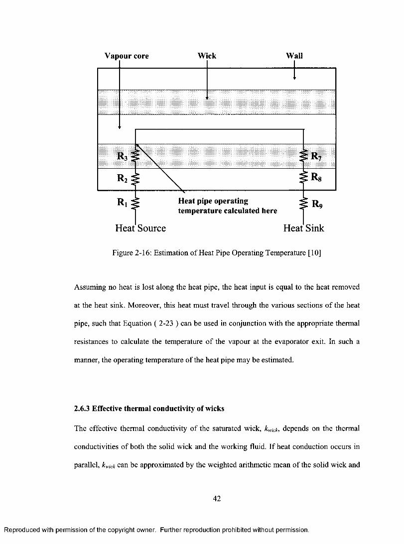
Vapour core Wick Wall

Heat pipe operating temperature calculated here

Heat SinkHeat Source

Figure 2-16: Estimation of Heat Pipe Operating Temperature [10]

Assuming no heat is lost along the heat pipe, the heat input is equal to the heat removed

at the heat sink. Moreover, this heat must travel through the various sections of the heat

pipe, such that Equation ( 2-23 ) can be used in conjunction with the appropriate thermal

resistances to calculate the temperature of the vapour at the evaporator exit. In such a

manner, the operating temperature of the heat pipe may be estimated.

2.6.3 Effective thermal conductivity of wicks

The effective thermal conductivity of the saturated wick, kwiCk, depends on the thermal

conductivities of both the solid wick and the working fluid. If heat conduction occurs in

parallel, kwick can be approximated by the weighted arithmetic mean of the solid wick and

42


the working fluid. On the other hand, if conduction is in series, kwjCk is estimated by

taking a weighted average o f the two thermal conductivities. These scenarios are

illustrated in Figure 2-17.

Direction of heat transfer

Liquid patl

Solid path


(a) Parallel case


Liquid

Solid


(b) Series case

Figure 2-17: Thermal Conductivity for Heat Transfer in (a) Parallel and (b) Series [1]

These simplest of models represent two boundary values between which the effective

thermal conductivity must lie [1]:

i Series < i < i ^w ick ~ wick ~ wick

Parallel ( 2 - 36)

Expressed mathematically:

43


k,ksA s + k, ( \ - s )

^K,ct^~e)ks+Ai\ ( 2 - 37)

Here, k\ and ks are the liquid and solid thermal conductivities and s is the wick porosity.

For unsintered wrapped screen wicks, the effective thermal conductivity is commonly

calculated using [10], [16]:

k ....._ k, [k, + ks - (1 - e)(k, - ks ) ]

(k ,+ks) + ( l - s ) ( k , - k s)(2 -38)

In the above expression, ks is the thermal conductivity of the solid portion of the wick.

Effective thermal conductivities for other common wicks are listed in Table 2-4.

Wick Structure Effective Thermal Conductivity tk,.fd Porositv

Wrapped metal screens, plain

k i [k,+ks - 0 - - £ ) ( k l - k s)\ (k ,+ks) + ( l - s ) ( k , - k s)

l 1.05 nNd 4

Wrapped metal screens, sintered

\ . k i j

1 1.05 nNd 4

Packed spherical metal powder,

plain

k,[2k,+ks - 2 ( 1 - s)(k, - k s)] 2k, +ks + ( l - e ) ( k , - k s)

Measureexperimentally

Packed spherical metal powder,

sintered

k s i 2 k s+ k i “ 2 e(ks - k , ) \2 ks +k, + e(ks - k , )

Measureexperimentally

Table 2-4: Effective Thermal Conductivities of Various Wicks [1]

44


For wrapped screen wicks, N is the Wire Number and d is the wire diameter. These

quantities, along with wick porosity, are covered in greater detail in Section 3.3.1. One

important observation can be drawn from the equations comparing sintered wicks to non

sintered wicks: the effective thermal conductivity increases by approximately one order

of magnitude. The positive effect this would have on the thermal performance is

significant. Through the sintering process, the effective thermal conductivity o f the

liquid-saturated wick would increase, and two of the largest thermal resistances in the

equivalent thermal resistance network of Figure 2-15 (R 3 and R 7) would be minimized.

Referring to Equations ( 2-32 ) to ( 2-35 ), this would reduce the axial temperature drop,

and thus the effective thermal conductivity would increase. The sintering process is

discussed further in Section 3.3.3.

45


3 Heat Pipe Design

Oftentimes, engineering design is an iterative procedure. Heat pipe design is no exception

to this, since many preliminary decisions must be made without precise knowledge of

their outcome. This section provides a brief overview of the more important aspects of

heat pipe design, focusing on the selection of working fluids, wicking structures and

containers.

3.1 Working Fluid Selection

Upon completion of the operating temperature estimate, the working fluid selection

process can begin. Several factors must be considered here. Firstly, the heat pipe

operating temperature range must be between the fluid’s melting point and critical

temperatures [10], [16]. The critical temperature of a fluid is defined as the temperature

above which a gas cannot be liquefied, or the temperature above which a substance

cannot exhibit distinct gas and liquid phases [33]. Under these criteria, Table 3-1 shows

various working fluids and their corresponding useful temperature ranges. Water,

ammonia and methanol are suitable for moderate temperature heat pipes. High

temperature heat pipes make use o f mercury, caesium, potassium and sodium at the lower

end o f the range, while lithium and silver are desirable for very high temperature

applications.

46


IncreasingHast

TransportCspafaWty

10 60 100 500 1000 5000Twnpwalura (*K)

*440 -400 -300 -200 -100 i) 100 500 1000 10000Temperature (°F)

Table 3-1: Heat Pipe Working Fluids and Their Corresponding Temperature Ranges [10]

Since the above-mentioned rule-of-thumb usually yields a number o f candidate working

fluids, optimization is commonly accomplished by considering the Liquid Transport

Factor (TV/), also called the Liquid Figure of Merit [16]:

N i = a P ih fe ( 3-1)

f t

where a is the surface tension of the fluid, pi is the liquid density, hfg is the latent heat of

vapourization of the fluid and pi is the liquid dynamic viscosity. Since these properties

change with temperature, the optimum working fluid will possess the highest Liquid

47

CRVOGEMC HEAT PIPES LOW TEMPERATURE HEAT PIPES

WGH TEMPERATURE HEAT PIPES

H i

*V>“S-

ayM<oyoo

VI.'M1-

Ml--CH.


Transport Factor in the heat pipe operating temperature range. Figure 3-1 illustrates the

variation of the Liquid Transport Factor with temperature for a few common working

fluids. Water is a desirable working fluid for lower temperature applications, while

sodium has better performance at temperatures greater than 500 K.

Na

NH,

Methanol| w

1000 1200 1400600 600200 400Temperature. K

Figure 3-1: Variation of Liquid Transport Factor with Temperature [5]

Other important factors to consider during fluid selection are vapour pressure levels,

liquid-solid wettability, liquid thermal conductivity and material compatibility.

Excessively high vapour pressures must be avoided, otherwise an excessively thick-

walled container will be required to prevent rupture [5], Conversely, if the vapour

pressure is too low, very high vapour velocities can trigger the sonic limit. The working

fluid should also have an affinity for the wick and container material [3], [10]. This is

referred to as the wettability of the fluid. If the liquid readily wets the wick and container,

the contact angle will be equal to zero and the generated capillary pressure will reach a

48


maximum value, as discussed in Section 2.1.1. Clearly, this is a favourable quality, since

the capillary limit will increase for perfectly wetting fluids.

High thermal conductivity is another favourable property, since the working fluid is

relied on to conduct heat through the saturated wick [1], [10]. Lastly, the working fluid

must be compatible with the container and wick materials. If an incompatible working

fluid is used, chemical reactions could generate non-condensable gases (NCGs) [10],

[34], which accumulate at the condenser end of the heat pipe, impeding heat flow to the

heat sink. This leads to long-term performance degradation. However, life tests with

copper-water heat pipes have yielded excellent results, with no degradation in

performance after 20000 hours [35]. A long-term test on a sodium-filled stainless steel

heat pipe also demonstrated compatibility after 9000 hours [36]. Life tests on stainless

steel/water heat pipes revealed an incompatibility between these, with hydrogen gas

generation detected within 2 hours of start-up [37], Table 3-2 summarizes the

compatibility data of various low temperature material/working fluid combinations.

49


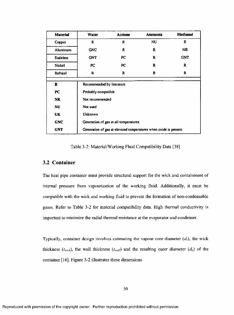
Material W ater Acetone Ammonia Methanol

Copper R R NU R

Aluminum GNC R R NR

Stainless GNT PC R GNT

Nickel PC PC R R

Refrasil R R R R

R Recommended by literature

PC Probably compatible

NR Not recommended

NU Not used

UK Unknown

GNC Generation of gas at all temperatures

GNT Generation of gas at elevated temperatures when oxide is present

Table 3-2: Material/Working Fluid Compatibility Data [38]

3.2 Container

The heat pipe container must provide structural support for the wick and containment of

internal pressure from vapourization of the working fluid. Additionally, it must be

compatible with the wick and working fluid to prevent the formation of non-condensable

gases. Refer to Table 3-2 for material compatibility data. High thermal conductivity is

important to minimize the radial thermal resistance at the evaporator and condenser.

Typically, container design involves estimating the vapour core diameter (dv), the wick

thickness (twick), the wall thickness (twau) and the resulting outer diameter (ci„) o f the

container [16]. Figure 3-2 illustrates these dimensions.

50


Figure 3-2: Heat Pipe Container and Wick Dimensions

The vapour core diameter is usually designed to avoid compressible flow, and Chi

suggests specifying a Mach Number of 0.2 for this purpose [16]:

M.. = — =-------- = 0 .2V 7id,2 - (3 -2 )

where Q is the heat transfer rate, dv is the vapour core diameter, pv is the vapour density,

hfg is the latent heat of vapourization, K ' o f Equation ( 2-16 ) is the ratio of specific heats,

Rvap is the vapour gas constant and Tv is the vapour temperature. Rearranging Equation

( 3-2 ) for dv\

51


d V

20 Q ( 3 - 3 )

y n p vh f g ^ K % J v

Preliminary estimates of the capillary limit must be determined next to obtain the internal

diameter (d,) o f the container. Referring to Equation ( 2-13 ), this step is necessary

because both the liquid and vapour pressure drop terms of the capillary limit depend on

the wick cross-sectional area. The internal diameter of the heat pipe can then be estimated

by adding twice the wick thickness (twick) to the vapour core diameter:

d = d + 2 t . . (3 '4)I V W I C K

The outside container diameter (da) can therefore be expressed as:

where twau is the wall thickness. Next, using data from candidate container materials, the

equation for hoop stress in a pressurized thin-walled cylinder can be used to estimate the

container wall thickness:

d = d + 2t „o i wall( 3 - 5 )

<T,m a x

( 3 - 6 )

52


where P is the pressure differential across the tube wall. For heat pipe design, P is taken

to be the vapour pressure of the working fluid at the maximum intended operating

temperature. Rearranging Equation ( 3-6 ) for twaii and substituting Equation ( 3-5 ) for d0:

d i^wall ' ) r r ( )

^max ^

P

The maximum allowable hoop stress, omax, is specified as being no more than 'A o f the

material’s ultimate tensile strength at the heat pipe operating temperature under the

ASME code for unfired pressure vessels [16].

Minimum end cap thicknesses must also be specified. End caps may be hemispherical,

flat or conical. For a flat, circular end cap, the maximum allowable stress is given by

[16]:

P da =

cap ( 3 - 8 )m ax

cap

where dcap is the end cap diameter and tcap is the end cap thickness. Again, omax is

equivalent to % of the material’s ultimate tensile strength. Rearranging Equation ( 3-8 )

for tc a p .

P d L Vt =cap

cap ( 3 - 9 )

53


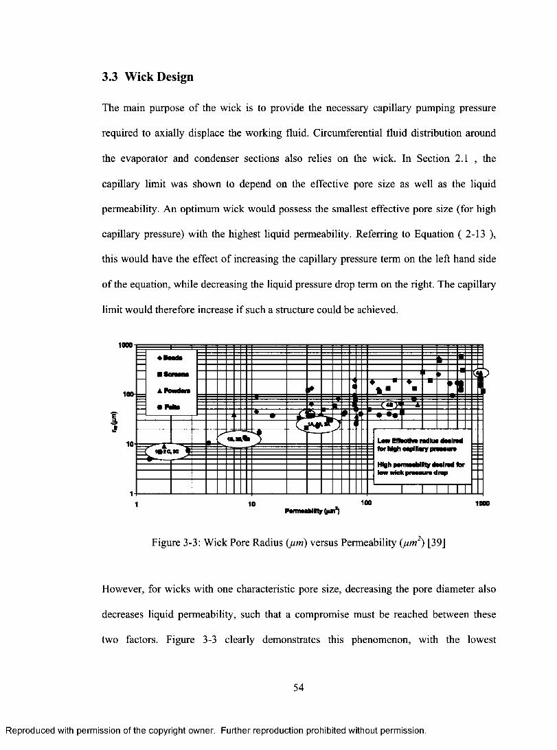
3.3 Wick Design

The main purpose of the wick is to provide the necessary capillary pumping pressure

required to axially displace the working fluid. Circumferential fluid distribution around

the evaporator and condenser sections also relies on the wick. In Section 2.1 , the

capillary limit was shown to depend on the effective pore size as well as the liquid

permeability. An optimum wick would possess the smallest effective pore size (for high

capillary pressure) with the highest liquid permeability. Referring to Equation ( 2-13 ),

this would have the effect o f increasing the capillary pressure term on the left hand side

of the equation, while decreasing the liquid pressure drop term on the right. The capillary

limit would therefore increase if such a structure could be achieved.

1000

IJ

Low Elfcullm radlut dMliwd for high eapillary praoouro

H i g h p a r m a a b J I K y d a o l r o d f o r l o w w i c k p r a o o u r o d r o p

100 1000101

Figure 3-3: Wick Pore Radius (jum) versus Permeability (jum2) [39]

However, for wicks with one characteristic pore size, decreasing the pore diameter also

decreases liquid permeability, such that a compromise must be reached between these

two factors. Figure 3-3 clearly demonstrates this phenomenon, with the lowest

54


permeability coinciding with the smallest pore radius [39], If either the liquid

permeability or the effective pore radius is inadequate, the heat pipe’s performance will

suffer. Therefore, the need for composite wicks that strike a balance between both of

these requirements is evident. Interestingly, sintered metal powders and felts cover the

largest scope, implying that they may be tailor-made for numerous applications.

Another critical aspect in high performance wick design involves evaporation heat

transfer. A number of research programs have confirmed that optimization of porous

material properties has significantly enhanced evaporation heat transfer performance.

Moreover, some researchers have conclusively shown that porous media with two

characteristic pore radii offer substantial improvements in evaporation performance over

single pore sized structures. Thus, considerations on wick selection and design involve a

discussion of conventional heat pipe wicking structures, followed by a review of relevant

studies in evaporation heat transfer in biporous media.

3.3.1 Metal screens

Metal screens are commonly used as wicks due to their widespread availability, low cost

and simplification of the heat pipe manufacturing process [16]. In their most economical

form, they consist of drawn metal wires, woven together and crimped in place using a

ram. Typically, plain carbon steels, copper, nickel and stainless steels are popular

materials for metals screens [40], Some common weave configurations for fine screens

are shown in Figure 3-4.

55


t P

Figure 3-4: Plain Wire Screen Weave (Left), Twill Screen Weave (Right) [40]

One commonly used expression for the fineness of the weave is the Mesh Number (TV).

This describes the number of apertures per linear inch of screen [41], A higher Mesh

Number indicates a finer weave. For example, a 100-mesh wire screen has 100 apertures

per linear inch while a 250-mesh screen has 250 apertures per linear inch. Typically, heat

pipe applications use 100 to 400-mesh screens. The effective pore size o f metal screens

can be theoretically calculated using [16]:

„ _ Wwire + dwire ( 3-10 )r« ~ 2

where Wwire is the wire spacing and dwire is the wire diameter, shown in Figure 3-5.

56


**wirc

f

* ^ wire *

f

Figure 3-5: Metal Screen Wick Dimensions

More commonly, the effective pore radius is expressed in terms of the Mesh Number (AO

[16], [42]:

r = — <3- U >‘s IN

Some researchers have discovered that Equation (3-11 ) overestimates the effective pore

radius of screen wicks [43]. Therefore, this gives a conservative estimate of the

maximum capillary pressure the wick can develop, and so it can safely be used in design

calculations. Liquid permeability (AO is calculated with [42], [44]:

K d l ire£ ( 3 - 12)

122(1 - £f

The porosity (e) is given by [10], [16]:

57


^ t nSNdwil 4

( 3- 13)

where S (=1.05) is the crimping factor, accounting for the fact that screens are not

crossed rods [16]. Metal screens are commonly used due to their balance between ease of

wick manufacture, fair liquid permeability and average capillary pumping performance

[1], [16]. However, because o f their limited capillary pumping ability, metal screens may

exhibit poor performance in unfavourable orientations. Furthermore, because of their low

effective thermal conductivity [1], heat pipes with metal screens suffer from relatively

high axial temperature drops.

3.3.2 Axial grooves

Another simple type of wicking structure consists of axial grooves embedded into the

container wall. This type of heat pipe is most common in aerospace applications. Cross-

sections can be trapezoidal, rectangular or triangular [11], [45], [46]. An axially grooved

heat pipe cross section is shown in Figure 3-6.

Figure 3-6: Cross-section of Heat Pipe with Rectangular Axial Grooves [45]

58


Extrusion is the most common form of manufacture [45]. In this bulk deformation

process, the work metal is forced to flow through a die opening by means of a ram, and

therefore the final part assumes the cross-sectional shape of the die [48]. Aluminium is

the material of choice because of its low weight penalty and formability [5]. Other

manufacturing processes have also been employed, especially for very fine capillary

grooves. For example, miniature heat pipes with triangular axial grooves have been

manufactured with etching processes [49], Target material removal occurs through

selective chemical attack of unprotected surfaces using an aqueous solution, while a

protective layer covers the bulk of the material [50]. Characteristic dimensions as small

as 80 pm have been achieved using this technique [10].

As previously listed in Table 2-1, the effective pore radii for rectangular and triangular

grooves can be calculated using [16]:

where w is the groove width and [i is the half-included angle of the triangular groove. The

liquid permeability for axial grooves is given by [16]:

( 3 - 14)

W ( 3 -15)

59


K =2 F T 2AbTh,l ( 3 - 16)

/ , R e ,

where r/,,/ is the hydraulic radius of the groove and fR e i is the friction factor Reynolds

Number product. For a rectangular cross-section,

W ( 3 - 17)€ = —

5

r h,l =2 wS ( 3 - 18)

w + 2 S

where s is the groove pitch and S is the groove depth. The groove pitch is defined as the

width o f one groove plus the width of the wall separating one groove from the next. For

rectangular grooves, the friction factor Reynolds Number product can be obtained from

Figure 3-7.

60


*

0 06 QJa

Figure 3-7: Friction Factor Reynolds Number Product for Rectangular Passages [16]

Typically, axially grooved wicks have the highest liquid permeability o f all wick designs,

however they are limited due to poor capillary pumping ability [1], Moreover, because

the vapour flow shear stress acts on the open-channelled liquid flow, these types of wicks

are more susceptible to the entrainment limit than others. For these reasons, axially

grooved wicks are most commonly used in zero gravity applications where vapour

velocities are not excessively high.

61


3.3.3 Sintered metal wicks

Perhaps the most versatile wicking structure, sintered metal powders and felts can be

tailored to a wide variety of requirements [51]. Highly porous structures can be achieved,

with effective pore sizes a few microns in diameter [52].

In this category, heat pipe wicks are normally fabricated using the loose powder solid-

state sintering technique. It is termed “solid-state” because powder particle bonding takes

place at temperatures significantly lower than the melting temperature of the material. In

the case o f powder metallurgy, metal powder is mixed with a cement-like binder and is

either applied onto the substrate metal (ie: the container) or formed into the desired shape

and inserted into the heat pipe container. It is then placed in a furnace with a protective

atmosphere to prevent metal oxidation, which occurs at an accelerated rate during high

temperatures [53], Oxide formation would inhibit diffusion bonding, the driving transport

mechanism behind the sintering process [53], Typical sintering environments include

methane, hydrogen and vacuum atmospheres.

Since the purpose of this operation is to produce a highly porous structure, sample

preparation, process time and temperature must be designed to achieve this result.

Therefore, there is little or no sample compaction prior to sintering. Sintering temperature

and time are instead selected with the objective of neck formation between adjacent

particles, while maintaining an open pore structure of interconnected voids. Sintering

usually takes place in three distinct phases [53]: debinding, sintering and cooling, shown

schematically in Figure 3-8. The debinding phase is necessary to expel the binder before

62


proceeding to the sintering temperature. The binder should bum off without

decomposition, since this would leave carbon residue on the wick. Then, the sintering

temperature is reached, typically 70-90% of the metal’s absolute melting temperature

[50], After sintering for the prescribed time, the cooling step begins, where the wick is

cooled to a temperature low enough to avoid oxidation. The wick is then safely removed

from the furnace.

SinteringVI-s«i-vQ.EV

Time

Figure 3-8: Phases during Sintering Process

It is generally agreed that the driving force behind the sintering process is a reduction in

surface energy [50], therefore neck growth and pore annihilation proceed with increasing

time and temperature. Accordingly, process design is essential for adequate particle

bonding, while avoiding excessive pore closure.

Solid-state sintering is a diffusion controlled process. Diffusion is defined as the transport

of material by atomic motion [54], Heated solid metal particles in contact with each other

will experience diffusion, and necks will form between them, as illustrated in Figure 3-9.

63


This phenomenon increases with temperature, so that higher diffusion rates are achieved

at higher temperatures.

Figure 3-9: Neck Formation in Sintered Bronze Powder [55]

The diffusion coefficient (D ) is the constant of proportionality between the diffusion

mass flux and the concentration gradient of Fick’s First Law, and describes the rapidity

of atomic diffusion [54], Thus, a higher diffusion coefficient is indicative o f faster

diffusion and sintering rates. Since diffusion is a thermally-activated process, it follows

an Arrhenius temperature dependence [56]. For the self-diffusion o f a pure metal, the

diffusion coefficient at a given temperature is given by [57]:

D SD = D o exp - Q .\

SD (3 - 19)

V RT /

64


where D$d is the self-diffusion coefficient, D 0 is the diffusion constant for the diffusing

species, Qsd is the activation energy for self-diffusion, R is the Universal Gas Constant,

and T is the absolute temperature. During the initial stages of sintering, it is possible to

estimate neck formation size using [56]:

f - Y Bt

D m(3-20 )

where X is the neck diameter, D is the particle diameter, t is the sintering time and n and

m are constants dependant on the mechanism of mass transport. The coefficient B

contains material properties and the diffusion coefficient [56].

Unsintered SurfaceDiffusion

VolumeDiffusion

h xHXi = Original interparticle distance

h~X2HX2 = Interparticle distance at intermediate sintering time or temperaturex2~x,

X3 = Interparticle distance at longer sintering time or higher temperatureX3<X,

Figure 3-10: Surface Diffusion versus Volume Diffusion [58]

For example, nickel powder has been shown to experience surface diffusion at

temperatures around 450°C, while at 900°C, volume diffusion is dominant [58]. During

low temperature surface diffusion, mass transport occurs along the surface of the

65


material, and the interparticle distance does not change. However, when the sintering

temperature is high enough, the interparticle distance shrinks and mass transport is

favourable through the bulk of the material during volume diffusion. These mechanisms

are shown in Figure 3-10. Under these mass transport mechanisms, n, m and B are given

in Table 3-3.

Mechanism n m B

Volume Diffusion 5 3

80 D v}Cl kT

Dv= volume diffusion coefficient y = surface energy Q = atomic volume

k = Boltzmann’s constant T = absolute temperature

Surface Diffusion 7 4

4

kT

Ds = surface diffusion constant

Table 3-3: Values for n, m and B of the Initial Stage Sintering Equation [56]

For sintered wicks, accurate predictions of the theoretical effective pore radius and liquid

permeability are usually not reliable. However, estimates based on a spherical model are

sometimes used if particle geometry is similar. For unconsolidated packed spheres, the

effective pore radius can be theoretically calculated using [10]:

66


reff = 0.2\dm ( 3 - 21)

where dav is the average particle diameter. The theoretical permeability (AT) is given by:

r - d l £ i ( 3 - 22)

where d is the particle diameter and the porosity (e), is assumed to be 0.48 [10].

Equations ( 3-21 ) and ( 3-22 ) are not accurate for the complex morphologies associated

with most sintered metal wicks. Therefore, wick properties are usually directly

determined with experimental methods.

3.3.4 Composite wicks

The above sections discussed conventional wick design, widely accepted due to their

relative ease of manufacture and predictable performance. However, these homogeneous

structures possess some shortcomings, namely their compromise between liquid

permeability and capillary pumping performance, as well as a relatively small

evaporative surface area. The anomaly between liquid permeability and capillary pressure

in homogeneous wicks was previously discussed in Section 2.1.2, with examples of

higher performing composite layered structures presented from the study conducted by

Canti et al. [20]. To review, they concluded that the presence of both fine and coarse

pores permitted a better compromise between liquid permeability and capillary pressure

67


generation. Therefore, for a higher performance heat pipe, a layered composite wick

consisting o f both coarse and fine pores should be considered during the design process.

Evaporation heat transfer can also benefit from the employment o f composite wicks. Heat

pipes function because o f phase changes. In other words, the latent heat o f vapourization

is the mechanism responsible for the very high heat transport rates characteristic of heat

pipes. Composite porous materials have been shown to increase this effect, and a few

relevant studies on evaporation heat transfer are discussed below.

When compared to planar surfaces, porous media have been shown to improve heat

transfer [59], As the working fluid evaporates, it absorbs its latent heat o f vapourization.

This process is increased due to the enhanced heat transfer that occurs in the so-called

thin film regions that exist near the contact line between liquids and solids, shown in

Figure 3-11 [60], [61].

68


Vapour

Kvaporation

Liquid

Thin-film region:I - Non evaporating regionII - Evaporating film regionIII Meniscus film region

Heat Input

Figure 3-11: Thin Film Evaporation in Porous Structures [61]

In the non-evaporating region (Region I), attractive forces at the liquid-solid interface

prevent evaporation. As the film thickness increases, these forces decrease rapidly and

evaporation is permitted in the evaporating film region (Region II). Evaporation also

takes place in the meniscus region (Region III), however the thicker liquid film produces

a higher thermal resistance to heat flow. Therefore, the most favourable heat transfer

occurs in the evaporating thin film region due to low thermal resistance coupled with

negligible attractive forces at the liquid-solid interface.

Consequently, by increasing the thin film area in an evaporator’s wick, one would expect

an improvement in heat transfer. This can be done by employing a highly porous

structure with a fine pore size [61], [62], The use of homogeneous wicks can satisfy this

69


requirement. However, heat transfer experiments with composite wicks have been shown

to further improve this effect.

Konev et al. investigated the use of composite porous sintered wicks for evaporation heat

transfer [63]. They concluded that when compared to homogeneous wicks, composite

porous media enhanced heat transfer, owing to higher effective thermal conductivities.

However, they failed to recognize the important contribution from the increased thin film

area.

North et al. conducted a similar study, where a biporous sintered nickel wick consisting

o f two characteristic pore sizes was designed to increase the density of evaporating

menisci in capillary structures [60]. Clusters o f sintered nickel powder contained the

small pores, while spaces between the clusters formed the large pores, shown in Figure

3-12. A monoporous nickel wick was also tested for comparison.

Fine Coarse pores pores Evaporation

from coarse pore menisci

9 o o o c9 O G G O9 G O O O £ogoo 90000 Z&QQ O

Evaporation from fine pore menisci

Figure 3-12: Composite Metal Powder Wick [60]

70


At low heat fluxes, heat transfer was suspected to be controlled by conduction through

the liquid saturated wick because of a linear relationship between heat flux and

temperature. As the heat flux increased, it was postulated that vapour preferentially filled

the large pores, forming menisci around the small pores. This significantly increased the

thin film evaporation area, and the heat flux increased dramatically while the temperature

difference between the heated wall and the vapour remained approximately constant. In

contrast, the homogeneous wick had a much higher temperature difference for the same

heat flux and experienced dryout much sooner. Thus, it was concluded that composite

wicks with small and large pores were desirable for heat pipes.

Wang and Catton arrived at similar conclusions based on numerical simulations. In one

o f their studies, evaporation heat transfer from triangular axial grooves was modeled with

and without a fine porous coating [46]. These configurations are shown in Figure 3-13.

m m

m

+q(a)

m

IT TIT TIT+q(b)

Figure 3-13: Triangular Grooves (a) without and (b) with Fine Pores [46]

71


While the composite wick on the right could experience mass transfer (and consequently

heat transfer) from both the menisci of the groove and the fine pores, the plain triangular

groove would only be permitted mass transfer from the large meniscus.

They concluded that evaporation heat transfer was augmented three to six times over

conventional triangular grooves by the inclusion o f a fine porous layer. This was

attributable to the extension of thin film evaporative surface area associated with the fine

pores. Figure 3-14 summarizes these findings as a plot of heat transfer coefficient {htotai)

versus increasing groove meniscus (Rm). In all instances, the composite wick

outperformed the triangular groove, with the highest performance reached at the smallest

meniscus radius. This was explained by the increased exposure o f fine pore evaporative

surface area with decreasing meniscus radius. In comparison, the standard triangular

groove only experienced modest performance gains, since there was little extension of

thin film evaporative surface area with decreasing meniscus radius.

72


E£

10

9 W ith a thin porous layer ’Without porous layers8

7

6

5

4

3

2

1

00 0.2 0 4 0.6 0.8 1 1.2 1.4 1.6

R , m m

Figure 3-14: Wang and Cation’s Results [46]

Numerous other studies support enhanced evaporation heat transfer through composite

wick design, the large pore sizes being in the 200-800 pm range with the fine pores

approximately an order of magnitude smaller [65], [66], [67]. Consequently, composite

wicks are most likely favourable over homogeneous configurations, and should be given

consideration during the heat pipe design process.

73


4 Experimental Procedure

This section covers all aspects of the experimental investigation regarding heat pipe

performance enhancement through the employment of composite wicks. Wick and

container materials are selected, along with various composite wick configurations

believed to be o f merit. Heat pipe design and manufacturing is discussed, followed by

particulars on the construction o f a heat pipe test rig used for performance validation. In

addition, test procedures are presented, including heat pipe preparation, data collection

and data manipulation.

4.1 Container and Wick Materials

Materials were chosen based on thermophysical and mechanical properties, powder

morphology, manufacturing and processing considerations and supplier availability.

Since water was chosen as the working fluid for this study due to its high Liquid

Transport Factor, compatibility considerations were also of importance.

Copper tubing was selected for the container material due to its high thermal

conductivity, its availability in a wide range of standard sizes and its common use in

moderate temperature heat pipes. A 3/8" outside diameter (O.D.) was chosen for ease of

manufacture, the smaller sizes being less accommodating towards wick insertion.

Medium pressure tubing, known as Type L Refrigeration Grade Tubing, was chosen for

its thin wall. This would ensure low thermal resistance while still providing adequate

strength. Refer to Section 4.3.1 for container design calculations. Tubing was selected in

74


5 ft. straight lengths to eliminate bending and straightening operations. This would also

provide excellent thermal contact between the wall and the wick, guaranteeing a kink-

free container. Copper tubing data is listed in Table 4-1

TvDe L Copper Tubing: Properties Value

Supplier McMaster-CarrUNS designation UNS C l2200

Composition 99.9% Cu (min.) 0.02% P (nom.)

O.D. 0.375"9.525 mm

I.D. 0.315"8 mm

Wall thickness 0.03" 0.762 mm

0.2% Yield Strength (assume fully annealed condition)

Approximately 48 MPa

Thermal conductivity (at 20°C)

340 W/m°C

Table 4-1: Copper Tubing Properties [68], [69], [70]

Copper mesh was chosen as the standard wick material. Again, this was primarily due to

its high thermal conductivity as well as its widespread use in heat pipe applications. The

springback effect o f rolled copper mesh was also considered to be very beneficial, since

this promoted reliable thermal contact between the wick and the container wall. Since

preliminary heat pipe tests demonstrated suitable performance from 100-mesh copper

screen wicks [72], it was decided to employ this standard configuration, with composite

wicks derived from this baseline. Table 4-2 lists properties for 100-mesh copper screen.

75


Copper Mesh: Properties Value

Supplier McMaster-CarrMesh number (AO 100

Wire diameter (dwire) 0.0045"114.3 pm

Effective pore radius (reg) Equation ( 3-11)

0.005" 127 pm

Pore diameter 0.01" 254 pm

Porosity (e) Equation (3-13)

62.9%

Permeability (K) Equation ( 3-12 )

193 pm2

Thermal conductivity (&) {assume pure copper at 20°C)

Approximately 400 W/m°C

Table 4-2: 100-Mesh Copper Screen Properties [1], [68]

Composite wicks would employ 100-mesh copper screen as the large pore substrate. Fine

pores were provided by metal powders applied to the screen at various locations assumed

to be favourable for enhanced heat transfer performance. Metco 55 copper powder,

shown in Figure 4-1, was chosen as one candidate, since this would not pose a

compatibility issue with the working fluid, the container and the wick. Copper powder

specifications are listed in Table 4-3.

Metco 55 Copper Powder: Properties Value

Manufacturer Sulzer-MetcoMorphology SphericalComposition Cu 99%

Particle size45 pm (min) 90 pm (max)

Table 4-3: Properties o f Metco 55 Copper Powder [71]

76


Figure 4-1: Spherical Copper Powder Morphology

INCO Type 255 nickel powder was another candidate metal powder primarily chosen for

its unique morphology, with properties listed in Table 4-4. As a result of its filamentary

nature, characteristics of this metal powder include a very fine pore size, a high surface

area to mass ratio and high porosity upon sintering. Also, because o f their high corrosion

resistance in aqueous environments, copper-nickel alloys would be desirable in heat pipes

to avoid non-condensable gas formation. Therefore, sintering nickel powder onto copper

mesh was not believed to be detrimental to heat pipe integrity, although further research

would be necessary for confirmation of this theory. Type 255 nickel powder morphology

is illustrated in Figure 4-2.

77


Figure 4-2: Filamentary Nickel Powder Morphology

TvDe 255 Nickel Powder: Properties Value

Manufacturer INCO Special ProductsMorphology FilamentaryComposition Ni 97.9%

Particle size 2.2 pm (min) 2.8 pm (max)

Table 4-4: Properties of Nickel Powder [73]

4.2 Wick Configurations

Wick configurations ranged from homogeneous copper mesh or sintered metal powders

to composite arrangements o f layered copper mesh and metal powders, sintered together.

Composite designs were selected to enhance evaporation heat transfer and increase the

capillary limit based on the previous findings from researchers presented in Sections 2.1

and 3.3 . Wick designs were assigned identification codes based on an arbitrary

78


alphanumeric naming system. The first alphabetic character identifies the specific

configuration, while the next numeric character represents sequential attempts o f the

same configuration. Since some designs were unsuccessful and not all configurations

were reported, there are omissions in the identification list. However, the list is

representative of successfully manufactured wick designs, and candidates for heat

transfer performance testing were selected from these. These codes are summarized in

Table 4-5.

Identification Configuration

A 100-mesh copper screen, unsintered

B100-mesh copper screen, liquid/vapour interface covered with nickel powder, sintered

E100-mesh copper screen, wall/wick and liquid/vapour interfaces covered with nickel powder, sintered

H100-mesh copper screen as carrier, heavily covered with nickel powder, sintered

I100-mesh copper screen, liquid/vapour interface covered with copper powder, sintered

J100-mesh copper screen, wall/wick and liquid/vapour interfaces covered with copper powder, sintered

K Copper powder, sintered

L100-mesh copper screen, lightly covered with nickel powder throughout structure, sintered

Table 4-5: Summary of Wick Identification

79


4.2.1 Homogeneous wicks

Wicks included plain unsintered copper screens and sintered metal powders. These

baseline designs represent the relatively high permeability and low capillary pressure of

mesh wicks to the high capillary pressure and low permeability of sintered metal

powders. By comparing composite wicks to these standard configurations, differences in

performance could be quantified.

Container 100-mesh copper wick

ContainerSintered metal powder wick

• • • • • • • • • • • • • • • • • • • • to

Figure 4-3: Schematics o f Configuration A (Left) and Configurations H and K (Right)

The unsintered copper screen wick shown in Figure 4-3 was named Configuration “A”,

and was formed from layers of mesh, rolled tightly around a mandrel o f appropriate size.

The wick, still wrapped around the mandrel, was then carefully inserted into the

container. Upon insertion, the mandrel was removed, leaving the unobstructed vapour

core. The heat pipe was then ready for charging and sealing.

Sintered metal powder wicks were constructed by mixing metal powder with a binder.

The mixture was poured around a centred mandrel and air dried. Alternatively, this slurry

was applied to a 100-mesh copper carrier, rolled and inserted. Upon drying, the mandrel

80


was removed, exposing the vapour core. The container and wick were then vacuum

furnace sintered, charged with working fluid and sealed. Copper powder wicks were

named Configuration “K”, while nickel powders were termed Configuration “H”.

Schematics of these configurations are shown in Figure 4-3.

4.2.2 Composite wicks

Composite wicks were designed to exploit enhanced evaporation heat transfer and to

achieve a superior compromise between liquid permeability and capillary pressure over

conventional wicks.

The first composite configuration, shown in Figure 4-4, was comprised o f layers of 100-

copper mesh, with an integral layer of metal powder at the liquid/vapour interface. This

fine pore layer would serve a twofold purpose:

• To significantly increase the number evaporating surface menisci, thereby enhancing

evaporation heat transfer.

• To increase the wick’s capillary pumping ability. This would increase the capillary

limit, greatly enhancing against gravity heat transfer performance.

The layers of copper mesh would provide a higher permeability liquid flow path, thus

ensuring a lower liquid pressure drop. This property would also increase the capillary

limit.

81


Composite nickel powder wicks following this design were assigned the name

Configuration “B”, while copper powder composite wicks with this construction were

identified as Configuration “I”. Metal powders were mixed with a binder to a liquid

consistency and applied onto the mesh.

Container 100-mesh Layer of copper metalscreen powder

IS"EI""S3"Isn«****»•*tnmnmn:numnnxx!

t W t t t i t x

1 1

100-mesh copper screen, liquid/vapour interface covered with metal powder, sintered together

Figure 4-4: Liquid/Vapour Interface Covered with Metal Powder, Configurations B and I

Another composite configuration similar to the above included an additional layer of

metal powder at the wall/wick interface, shown in Figure 4-5 . The fine pore layer at the

wall/wick interface was included because it could augment performance through an

increase in the wall/wick contact area, thus decreasing the contact resistance. This would

lower the heat pipe end-to-end temperature drop. Powder application techniques were

identical to the above. Composite nickel powder wicks with this construction were called

Configuration “E”. Similarly, copper powder composite wicks possessing this design

were named Configuration “J”.

82


Container 100-meshcopperscreen

Layers of metal

powder

100-mesh copper screen,wall/wick and liquid/vapour interfaces coveredwith metal powder, sintered together

Figure 4-5: Wall/Wick and Liquid/Vapour Interfaces Covered with Metal Powder,

Configurations E and J

The last composite configuration employed a 100-mesh copper screen, uniformly covered

with a thin layer of nickel powder. This was labelled as Configuration “L”, shown in

Figure 4-6 . A copper powder variation was not attempted due to difficulties in coverage

control, explained further in Section 4.3.4. This configuration was designed to not only

increase the number of evaporating menisci at the liquid/vapour interface, but throughout

the whole wick thickness as well. O f course, another possible benefit associated with this

fine pore microstructure was believed to be an increase in the wick’s capillary pumping

ability.

Another postulation leading to the selection of Configuration “L” was associated with

liquid recession into the wick. If a fine pore arrangement existed exclusively at the

83


liquid/vapour interface as in Configuration B, liquid could potentially recede beyond this

layer at higher heat fluxes. The evaporating menisci would then dry out, resulting in

performance degradation. The extension of evaporating menisci throughout the wick

thickness could mitigate this potential problem.

Figure 4-6: Metal Powder Applied throughout Wick Thickness, Configuration L

4.3 Heat Pipe Design and Manufacture

Because of their widespread use in electronics cooling, the focus o f this study was the

performance enhancement o f moderate temperature heat pipes. As previously mentioned,

water was chosen as the working fluid, with copper tubing selected as a container.

Copper and nickel powders, in combination with copper mesh, were chosen for wick

materials. This section details the design and manufacture of the moderate temperature

copper/water and copper/nickel/water heat pipes that were tested in this research

program.

Container 100-mesh copper screen, lightly covered with metal powder, sintered together

84


4.3.1 Design

Design calculations were based on a conventional 25 cm long (9.84"), 9.525 mm (3/8")

O.D. copper/water heat pipe with a 100-mesh copper screen wick, operating in the

horizontal position. Referring to the naming convention in Section 4.2 , this wick is

known as Configuration A. Because circular, flat end caps and solder filling would be

used for sealing, some clearance was required at each tube end. This amounted to an

additional 1.57 cm, for a total tube length of 26.57 cm. Copper tube details are listed in

Table 4-1. Complete calculations are presented in Appendix A.

Since tube dimensions were already determined, design calculations began with the

estimation of the maximum allowable vapour temperature based on the hoop stress.

Assuming a fully annealed material state with a safety factor of 3 on the yield strength of

48 MPa, the maximum allowable vapour temperature was estimated to be approximately

235°C based on the tube wall. This temperature corresponded to a vapour pressure of

approximately 3 MPa. Although it was recommended to use % of the material’s ultimate

tensile strength in Section 3.2 , the alternative use of one third the yield strength added an

even greater measure o f safety for this particular copper alloy. Moreover, because the end

caps were soldered into place and their strength was not supplied by the manufacturer, an

additional safety factor was considered here. Using Equation ( 3-8 ) with a safety factor

of 4 on the previously determined maximum allowable hoop stress, a maximum vapour

temperature o f approximately 185°C was estimated based on the end cap strength. This

corresponded to a vapour pressure of 1.2 MPa. Since the heat pipe’s thermal resistances

were not yet calculated, the maximum allowable wall temperature associated with the

85


estimated vapour temperature was unknown. Therefore, for added safety, it was decided

to keep the maximum temperature of the evaporator wall in the 150-160°C range during

testing and back-calculate the resultant vapour temperature based on this assumption.

Next, the minimum vapour core diameter was determined using Equation ( 3-3 ). The

maximum heat input and the assumed vapour temperature were estimated to assess their

effect on the vapour core diameter. Assuming a conservatively high estimate o f 300 W

for the maximum heat input and a vapour temperature of 160°C, the minimum vapour

core diameter necessary to avoid compressibility effects was calculated to be 0.75 mm, a

very small dimension. Therefore, any vapour core diameter greater than this would

ensure incompressible vapour flow. It should be mentioned that the above assumptions

led to a very conservative estimate of the minimum vapour core diameter, meaning there

was essentially no danger of encountering compressible flow with the proposed design.

The final vapour core diameter required an estimate o f the wick thickness, described

below.

The required wick thickness was calculated based on a 4-layer, 100-mesh copper design.

This configuration was chosen to accommodate one or two layers of metal powder-coated

screen on the outermost and innermost layers, sandwiching a two or three-layer metal

screen core. Referring to Table 4-2, the wire diameter was approximately 114 pm.

86


Thickness of 1layer of mesh

i i

Figure 4-7: Schematic of Mesh Weave [28]

Figure 4-7 illustrates the layout of a plain mesh weave, used to estimate the wick

thickness. The thickness o f 1 layer of 100-mesh copper screen was therefore

approximated as 228 pm. Therefore, four layers would measure 0.91 mm thick. As a

result, the final vapour core diameter was roughly 6.2 mm, much larger than the

minimum value of 0.75 mm.

Using Equations ( 2-30) and ( 2-31 ), the heat pipe operating temperature was calculated

based on evaporator and condenser wall temperatures of 160°C and 24°C respectively.

Neglecting source and sink thermal resistances, the operating temperature, defined as the

vapour temperature at the evaporator exit, was calculated to be approximately 90°C.

Then, employing this operating temperature, capillary and boiling limits were computed.

Equation ( 2-13 ) was rearranged to solve for the maximum evaporator heat input at the

capillary limit, estimated to be approximately 139 W in the horizontal orientation. The

boiling limit was calculated to be much higher at approximately 895 W. Therefore, it

appeared that the capillary limit would be encountered before the boiling limit. The

entrainment limit was not calculated since this is not usually problematic in moderate

temperature mesh-wick heat pipes. The sonic limit was indirectly considered in the

87


calculation of the minimum vapour core diameter, and it was shown that compressibility

effects were negligible.

To summarize, all heat pipes manufactured for this study would closely follow the design

specifications of the standard heat pipe described above, with some minor geometric

variations to the wick structure. For example, some composite wicks would employ

layers o f sintered metal powder. This would slightly decrease the vapour core diameter.

Specifications for the conventional, benchmarking heat pipe (ie: Configuration A) are

listed below in Table 4-6.

Conventional Heat Pine: Specifications Value

Length 10.46"26.57 cm

O.D. 3/8"9.525 mm

I.D. 0.315"8 mm

Vapour core diameter 0.244"6.2 mm

Wick 100-mesh Cu wick, 4 layersWorking fluid Water

Operating temperature =90°CSource temperature =160°CSink temperature =24°C

Capillary limit =139 WBoiling limit =894 W

Table 4-6: Conventional Heat Pipe Design Specifications

88


4.3.2 Wick cutting

Since the wick was rolled around a mandrel from a single flat sheet of mesh, length and

width dimensions were required. The wick length was selected to be 25 cm. To estimate

the width of the cut, the wick was modeled as concentric circles, shown in Figure 4-8.

The four circumferences were added, yielding a required mesh width of approximately 92

mm. A metal template 250 mm long by 92 mm wide was fabricated for wick cutting

purposes. Using the wick cutting template and a sharp utility blade on a clean, rubber

cutting mat, all wicks were cut to the same dimensions. Tools are shown in Figure 4-9.

Vapour core

Width of flat mesh sheet = Ctot = Ci + C2 + C3 + C

Figure 4-8: Model for Required Width of Mesh

89


Figure 4-9: Wick Cutting Tools

4.3.3 Degreasing and deoxidizing

Because o f the importance o f material cleanliness in heat pipe manufacturing, a

methodical procedure was developed for material preparation. These steps were followed

for all heat pipes prior to processing:

1. Immerse parts for 30 min. in ultrasonic bath consisting of a 1:1 volumetric ratio

solution of Simple Green® all-purpose cleaner and water.

2. Rinse parts with running water for 5 min.

3. Immerse parts in ultrasonic acetone bath for 20 min. Air dry.

4. Deoxidize parts in an ultrasonic acid bath consisting o f 100 ml o f phosphoric acid

(H3PO4) + 100 ml of nitric acid (HNO3) + 1800 ml of water. Copper tubes should

be etched for 30 min. Copper mesh should be etched for 20 min. Rinse parts with

running water for 5 min.

90


5. Rinse in acetone and air dry.

Following deoxidation and cleaning, the standard wick configuration was prepared for

rolling and insertion into the container. For composite wicks, additional processing steps

are described in Section 4.3.4.

4.3.4 Metal powder application

Homogeneous copper metal powder wicks (Configuration K) were formed using a slurry

mixture of metal powder and binder. A mud-like slurry consistency was selected to

ensure metal particles would remain suspended during the drying process. A 4.76 mm

(0.1875") mandrel was centred in the container using a mandrel centering end plug. The

end plugs, shown in Figure 4-10, were designed to both centre the mandrel and provide

clearance for end caps.

Figure 4-10: End Plugs

91


By means of syringe injection, the slurry was forced into the annular spacing between the

mandrel and the container wall. An additional end plug was fitted on the opposite end of

the assembly to form the slurry into the wick shape. Details are shown in Figure 4-11.

Slurry drying was accelerated using a hot air dryer for approximately 8 hours, after which

the heat pipes were prepared for vacuum furnace processing.

Figure 4-11: Homogeneous Copper Metal Powder Heat Pipe Manufacturing Assembly

Composite wicks were formed by applying a metal powder and binder slurry to a 100-

mesh copper screen. A spray application technique was employed for all nickel powder

wicks, including the homogeneous nickel powder configuration described above.

92


250 mm

-92 mm-

20.4 mmh *

25.1 mm

-92 mm-

l ~20.4 mm

Kk

Copper mesh

tletal powder m copper nesh

250 mm

Copper mesh

Metal powder on copper mesh

Configurations B (Nickel) and I (Copper)

Configurations E (Nickel) and J (Copper)

Figure 4-12: Metal Powder Application Patterns for Configurations B, E, I and J

-92 mm-

250 mm

i i m1 “■ ■ 11 1 1 ■ 11 “ 1 B

“I Z ’ z !! Z ’ z . m’ z ’ z" “■■ * ■’ z ■ * ■

a a? * ? *

z " * ’ z [. mI Z „ z 1 z z*• - * ■ * “■ a a a- * " * ■ *

1*a a . “ * * * i *'. ' H ' i ' i i f i f f i 1 1

a - . a a .“ ■

I _ »; Z ’ Z " ai "j it a.

a a a

Z ’ * -■ * ■[ z ;’ z ;1 a r * a - .

~ *a Z " “ ■* _ i 1 ma a. a I -

_ , a . »■ * ■. „ [’ „ , ' I

a a.a aa a

• ■■ “ '■ - ‘“ * ■. a a■ * a a a

M .. . .. m .« ai .; m., * a 1 a I -■ ■ ■ m - ■ ■" ■. „

a a.

z Z " ‘ \| . " ZI[ ma I a •> a. m m1 Z .. . "

" m "' mZ "" Z "" Z a 1 ’" Z"■ “ - Z a -

- a .■ - ■I ’

" “ "■ “ a - 1 m". a a

z -- Z - ZIIZ "• a a.a a a

1 T * "" m "■ * ■* m ■■ “ ■" " a a. a a aa a m

Copper mesh sprayed

y lightly with nickel powder

250 mm

92 mm

Configuration I. Configuration H

Figure 4-13: Spray Patterns for Configurations L and H

Copper mesh sprayed heavily with nickel powder

93


Figure 4-12 and Figure 4-13 illustrate spray patterns associated with the various wick

configurations. For configurations B and I, the metal powder treated portion of the wick

was sized by estimating the inner circumference of the wick. Similarly, configurations E

and J were estimated using inner and outer wick circumferences. Prior to spraying, wicks

were masked with paper to prevent unintentional overspray onto copper mesh layers.

Masking paper was not necessary for configurations L and H since the copper mesh

would be completely coated to some extent with nickel powder. Following the spraying

process, the masking paper was removed and the wicks were allowed to dry for

approximately 1 hour. At this point, the wicks were fully prepared for rolling and

insertion. Figure 4-14 shows configuration B after spraying and prior to masking paper

removal.

w e s r c o t r

Figure 4-14: Nickel Powder Sprayed Wick, Configuration B

94


Attempts were made to spray apply copper powder onto copper mesh to form

configurations I and J. However, these were unsuccessful due to clogging of the spray

gun nozzle. A powder sifting technique was therefore developed to produce

configurations I and J. For masking, the mesh was sandwiched between two cleaned

steel beam sections. Metal was used in favour o f paper masking since the binder could

saturate the paper, resulting in paper disintegration and contamination o f the wick.

Firstly, binder was applied onto unmasked portions of the copper mesh. Next, copper

powder was carefully sifted onto the binder-saturated wick using a sieve. Then, the wicks

were allowed to dry for approximately 1 hour prior to rolling and insertion.

Figure 4-15: Composite Copper Wick Manufacturing

4.3.5 Rolling and insertion

Prior to rolling and insertion of wicks into their containers, all work area surfaces coming

into contact with heat pipe components were thoroughly cleaned with soap and water,

followed by a rinse in isopropyl alcohol or acetone. Isopropyl alcohol was used to

95


decontaminate the rubber rolling mat, while acetone was used to clean end plugs and

mandrels. Rolling and insertion tools are shown in Figure 4-16.

Figure 4-16: Configuration J with Rolling Tools

A 3/16" (4.76 mm) mandrel was used to roll all wicks. The mandrel was placed on top of

the wick, and rolling was initiated by folding the leading edge of the wick over and

around the mandrel. By commencing the roll at the appropriate edge, composite layers

would be positioned correctly in the wick. Even hand pressure was applied across the

wick throughout the rolling procedure. Rolling was repeated until the wick was wrapped

tightly enough around the mandrel to initiate insertion into the container. Initial insertion

resistance was kept as high as possible to ensure good wall/wick contact.

96


Figure 4-17: Placement of End Plugs for Wick Centering

Rolling and insertion then carefully proceeded in alternate steps until the wick was

completely inserted into the container. End plugs were then slipped over the mandrel and

pushed into opposite ends o f the container to properly locate and center the wick,

demonstrated in Figure 4-17. The end plugs and mandrel were then removed from the

container. At this point, container/wick assemblies were completely prepared for

sintering.

4.3.6 Sintering

Sintering trial exercises were performed to estimate the best combination of time and

temperature prior to actual manufacturing operations. Trial runs were performed on

nickel powder samples at sintering temperatures ranging from 700°C to 980°C. Time at

the sintering temperature was varied from 0.5 to 1.5 hours. One copper powder sintering

trial was also performed at 850°C for one hour. Inadequate nickel powder bonding,

97


illustrated in Figure 4-18, was observed for trials with sintering temperatures up to 800°C

for any length of time attempted. Some copper powder bonding was observed in Figure

4-19, however to ensure sufficient strength, increased neck formation was desired.

Figure 4-18: Nickel Powder, Sintered at 800°C for 1.5 Hours

Figure 4-19: Copper Powder, Sintered at 850°C for 1 Hour


When the sintering temperature was increased to values over 900°C, significant nickel

particle bonding was observed. See Figure 4-20 for an example of an adequately sintered

porous nickel wick. Sufficient particle bonding was achieved, while still maintaining high

porosity. It was therefore decided to process all samples at the same sintering temperature

of 940°C for 1 hour, since desirable results were obtained during these trial experiments.

During sintering, container/wick assemblies were placed on a commercially-pure

titanium tray coated a surface protection agent. This would prevent unwanted diffusion

bonding between the components and the tray. Additionally, a layer of fire brick wafers

covered the tray for added safety against unwanted bonding. To prevent surface

oxidation, sintering took place in a vacuum environment using the following procedure:

Figure 4-20: Nickel Powder, Sintered at 940°C for 1 Hour

99


1. Ambient temperature: Achieve a vacuum level of at least 1x102 torr in furnace

chamber. Backfill chamber with argon. Evacuate and repeat. Achieve a vacuum

level o f at least lx l O'4 torr before activating heating elements.

2. Ambient-550°C: Ramp up temperature as quickly as possible while maintaining a

vacuum level o f at least lxlO '2 torr. Hold at 550°C for 45 min. to ensure complete

volatilization of binder.

3. 550oC-900°C: Ramp up temperature in increments o f 50°C every 10 min. while

maintaining a vacuum level of at least lx l O'4 torr.

4. 900oC-940°C: Ramp up temperature in two increments of 20°C every 4 min. to

prevent temperature overshoot.

5. 940°C: Hold for 1 hour at sintering temperature.

6. 940oC-20°C: Furnace cool to room temperature.

After furnace processing, the container/wick assemblies were removed and measured to

estimate fluid charging amounts, described in Section 4.3.7.

4.3.7 Fluid charging and sealing

For homogeneous metal powder wicks, working fluid charging amounts were estimated

by performing measurements on container/wick assemblies. From these measurements of

mass and geometric dimensions, wick porosities were calculated. Wherever 100-mesh

copper screen was employed, including for composite wicks, wick porosity was

estimated using Equation ( 3-13 ). In mm, porosity was used to estimate fluid charging

amounts using the following expression from Chi [16]:

100


m = A L,Pv + A«L,ePi (4 -1 )

where m is the mass of the fluid charge, Av is the cross-sectional area of the vapour core,

Lt is the heat pipe length, p v is the vapour density, A w is the wick cross-sectional area, e is

the wick porosity and pi is the liquid density. A slight overcharge was included as a

precautionary measure against premature dryout. See Appendix B for complete

calculations. A summary of the procedure followed for fluid charge estimation is

described below:

1. Measure outside and inside tube diameters and condenser and evaporator end cap

clearances using Vernier calipers. Measure tube lengths. From tube lengths and

end cap clearances, verify wick lengths. These should be approximately 250 mm.

2. Measure vapour core diameters using hole gauge and Vernier calipers. Weigh

post-sintered container/wick assemblies. By subtracting the cross-sectional area of

the vapour core from the cross-sectional area o f the tube I.D., the area o f the wick

is calculated.

3. For homogeneous metal powder wicks, use mass and geometry measurements to

estimate the volume o f solid wick material and the total volume o f the wick. The

porosity is calculated by subtracting the volume of solid material from the total

volume of the wick, then dividing by the total wick volume. For all other wicks,

approximate the porosity using Equation ( 3-13 ).

4. Calculate the fluid charge using Equation (4-1 ). Add a 10% fluid overcharge.

101


Fluid charging and sealing was completed using proprietary procedures at Acrolab of

Windsor, Ontario, a heat transfer engineering company specializing in heat pipe

manufacture. With the fluid charging and sealing steps completed, heat pipe

manufacturing was accomplished. Thermal performance testing, described in the

following sections, would be carried out next to evaluate improvements in heat transfer

associated with composite wick designs.

4.4 Heat Pipe Test Rig

The heat pipe test rig in this study was designed to both apply and remove heat from heat

pipes while recording all important analytical data. A band heater and copper annulus

clamped over the evaporator portion of the heat pipe, while a plastic cooling jacket

enabled liquid to flow across the condenser end. Insulation was wrapped around all

exposed areas to minimize heat losses to the ambient. Thermocouples were fastened

axially along the container to capture temperature profiles, subsequently used in effective

thermal conductivity calculations. A LabView data acquisition program recorded,

monitored and displayed information during testing. Upon test completion, data files

were generated for further analysis of thermal performance. A test rig schematic is

illustrated in Figure 4-21.

102


FlowmeterFlowmeter signal

to FieldPoint (Variacj module

Isolationtransformer

ACTo 120 V

'w all outlet

Coolingjacket

- r -H r - EE!Heat pipe

Thermocouples

O O I IChiller

□Workstation

FieldPointModules

Figure 4-21: Heat Pipe Test Rig Schematic

4.4.1 Heater and annulus

A one-piece band heater from Omega Engineering was selected for heating purposes.

This design was selected for its ability to deliver a uniform heat flux to the evaporator.

Additionally, its high clamping force would minimize the thermal contact resistance

between the band heater, the copper annulus and the heat pipe. Power was controlled

through a variable voltage power supply, connected to an isolation transformer to prevent

power fluctuations. Band heater details are listed in Table 4-7.

103


Clamp- Style Band Heater: Properties Value

Supplier Omega EngineeringModel number HBZ-12224

Diameter 2.125”5.4 cm

Heated length 2.25”5.7 cm

Maximum power 400 WVoltage 120 V

Table 4-7: Band Heater Properties

Since the diameter o f the available heater was greater than the heat pipe outside diameter,

a metallic annulus was designed to eliminate this gap. Copper was selected for its high

thermal conductivity, ensuring lower heat losses to the ambient. A split design was

selected to enable good thermal contact and space for thermocouple instrumentation, with

dimensions illustrated in Figure 4-22. Some additional clearance was designed between

annulus halves to accommodate thermocouple wiring on the evaporator section of the

heat pipe. This was manufactured by slotting the annulus from the outside diameter to the

concentric hole using a 1/8” saw. The heater and annulus assembly is shown in Figure

4-23.

104


0 2.375

0 0.375

Spacing to accommodate thermocouple wires

CNSOoo '

LTlcsfN

Figure 4-22: Dimensions of Copper Annulus Half

Figure 4-23: Heater and Annulus Assembly

105


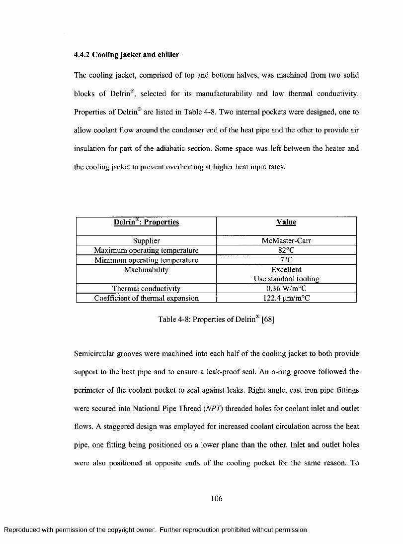
4.4.2 Cooling jacket and chiller

The cooling jacket, comprised o f top and bottom halves, was machined from two solid

blocks of Delrin®, selected for its manufacturability and low thermal conductivity.

Properties of Delrin® are listed in Table 4-8. Two internal pockets were designed, one to

allow coolant flow around the condenser end of the heat pipe and the other to provide air

insulation for part of the adiabatic section. Some space was left between the heater and

the cooling jacket to prevent overheating at higher heat input rates.

Delrin®: Properties Value

Supplier McMaster-CarrMaximum operating temperature 82°CMinimum operating temperature 7°C

Machinability Excellent Use standard tooling

Thermal conductivity 0.36 W/m°CCoefficient of thermal expansion 122.4 |im/m°C

Table 4-8: Properties of Delrin® [68]

Semicircular grooves were machined into each half of the cooling jacket to both provide

support to the heat pipe and to ensure a leak-proof seal. An o-ring groove followed the

perimeter of the coolant pocket to seal against leaks. Right angle, cast iron pipe fittings

were secured into National Pipe Thread (NPT) threaded holes for coolant inlet and outlet

flows. A staggered design was employed for increased coolant circulation across the heat

pipe, one fitting being positioned on a lower plane than the other. Inlet and outlet holes

were also positioned at opposite ends of the cooling pocket for the same reason. To

106


provide access for the condenser-end thermocouples, wires were passed through a bolt

with a concentrically drilled hole. The hole was then filled with hot-melt glue to seal

against leaks. The sealed bolt assembly was then tightened into a tapped hole through the

top half o f the cooling jacket. After inserting an instrumented heat pipe, the top and

bottom halves of the cooling jacket assembly were clamped together using twelve

through bolts. The cooling jacket is shown in Figure 4-24, while design drawings are

presented in Appendix C.

Figure 4-24: Cooling Jacket

A Cole-Parmer refrigerated recirculation chiller was selected to supply temperature-

controlled coolant to the cooling jacket. Details are listed in Table 4-9. The chiller outlet

hose connected to the cooling jacket inlet, while the chiller inlet hose connected to the

107


cooling jacket outlet. Reinforced, braided polyvinylchloride tubing with a Vi" I.D. and a

%” O.D. was selected for this purpose.

Cole-Parmer Chiller: Properties Value

Manufacturer Cole-Parmer Instrument Co.Model number 12920-10

Temperature range -5 to 40°CCooling capacity 0°C 3 5 0 W

10°C 780 W20°C 1100W

Pump pressure 5.5 psiPump flow 10 gal(US)/min

38 1/min

Table 4-9: Properties of Refrigerated Recirculation Chiller [74]

A 50/50 volumetric mixture of automotive coolant and distilled water was chosen as the

cooling fluid. Since a high coolant flow rate was not necessary, a system o f flow control

bypass valves was installed to limit this to more manageable levels. One valve controlled

bypass flow from the chiller outlet to the chiller inlet, while another valve controlled the

inlet flow to the cooling jacket. In this fashion, cooling flow was lowered from

approximately 38 1/min to 1.5 1/min.

4.4.3 Insulation

To minimize ambient heat losses, all exposed surfaces were covered with a flexible

alumina-silica based high-temperature pipe and tube wrap, as illustrated in Figure 4-25.

Most importantly, this insulation was selected because of its resistance to extreme heat, a

108


situation it could encounter in the vicinity o f the band heater during high heat inputs.

Other desirable attributes were its flexibility and low thermal conductivity. See Table

4-10 for insulation properties.

Insulation: Properties Value

Supplier McMaster-CarrMaterial Alumina and silica based ceramic fibres

Dimensions 12 ft long x 3" wide x Vi " thickTemperature range -10°C to 1260°C

Thermal conductivity 0.036 W/m°C

Table 4-10: Properties of Insulation [68]

Insulated surfaces included the band heater periphery, the ends of the copper annulus, the

exposed portion o f the heat pipe’s adiabatic section and all cooling jacket surfaces, except

for the base during horizontal heat pipe testing. Insulation was not added underneath the

base because it would upset the mechanical stability o f the cooling jacket, and heat losses

from this surface were negligible in this orientation. However during vertical tests, the

cooling jacket base was covered with insulation to minimize the expected free convection

heat losses.

109


Figure 4-25: Insulation Covering Cooling Jacket and Heater

4.4.4 Instrumentation

Test rig instrumentation included thermocouples for heat pipe temperature measurements

along with a voltmeter and an ammeter to record the power input to the heater.

Additionally, two thermistors, a flowmeter and numerous other thermocouples were

employed in an attempt to perform a heat balance on the test rig. However, since to date

this has not yet been accomplished, a brief description is included in this section for

future research purposes.

For temperature measurements in the evaporator and adiabatic sections, 30 gauge glass-

braid insulated K-type thermocouples were selected. These were ideal because of their

small size and high temperature capabilities. The condenser section employed the same

type of thermocouple, however waterproof Teflon insulation was chosen since it was

immersed in the coolant pocket. Thermocouple specifications are presented in Table

4-11. Nine thermocouples, spaced apart as shown in Figure 4-26, were fastened to each

heat pipe to record temperature profiles.

110


Thermocouples: Properties Glass Insulated Teflon Insulated

Manufacturer Omega Engineering Omega EngineeringProduct number GG-K-30 TT-K-30

Type K-type K-typeWire diameter (30 gauge) 0.01"

0.2546 mm0.01"

0.2546 mmMeasurement temperature

range-200°C to 1250°C -200°C to 1250°C

Maximum insulation operating temperature

482°C 200°C

Limits o f error (special) 1.1 °C or 0.4% of reading, whichever is greater

1.1 °C or 0.4% of reading, whichever is greater

Table 4-11: Thermocouple Properties [75]

7.9 mm

28.51t min

35.9 mm 35.9 mm 35.9 mm 35.9 mm

>4.6.5 min

1

o o o

-Evaporator- -Adiabatic-

o o o7.9 mm

-Condenser-

Figure 4-26: Thermocouple Locations on Heat Pipe

Heater input power was recorded using two Fluke 45 Dual Display Multimeters, one to

measure voltage and the other to measure current. By multiplying these two values, the

power input to the heater could be calculated [10]. This was also estimated as the

evaporator heat input (Qin):

p = V x Iin z-sin

( 4 - 2 )

111


where Pin is the input power to the heater, V is the measured voltage and I is the measured

current. Multimeter specifications are listed in Table 4-12.

Fluke 45 Multimeters: Properties Value

Manufacturer Fluke CorporationType Multifunction bench multimeter

Volts (AC) Range: 0 V to 750 V Resolution: 1 pV to 0.01 V

Accuracy: ±0.2%+100 mV (from 0-100 V)Current (AC) Range: 15pA to 10A

Resolution: 0.1 pA to 10mA Accuracy: ±2%+10 mA (from 1-10 A)

Table 4-12: Multimeter Properties [76]

Although a heat balance was attempted to account for all heat flow into and out o f the test

rig, results were not included the results of Section 5.3 since further investigation is still

required. The associated heat balance instrumentation is as follows. To measure the heat

removal rate, two high precision thermistors were inserted into drilled and tapped holes

on the inlet and outlet elbows of the cooling jacket. These elements exhibited large

changes in resistance with temperature, making them favourable for the measurement of

minute temperature changes. However, since the data acquisition system could only

record voltage or current signals, voltage divider circuits were added to each thermistor to

convert these resistances to voltages. Thermistor details are listed in Table 4-13. A

flowmeter monitored the coolant flow rate through the cooling jacket by means o f a

current signal. See Table 4-14 for flowmeter specifics.

112


Thermistors: Properties Value

Manufacturer Omega EngineeringProduct number ON-401-PP

Type Laboratory grade, waterproof, immersion type thermistor. Encased in vinyl sheath.

Resistance at 25°C 2252 QMeasurement range -80°C to 100°C

Accuracy ±0.1 °C

Table 4-13: Thermistor Properties [75]

Flowmeter: Properties Value

Manufacturer Kobold Instruments, Inc.Product number DPM-1120-N2-L443

Type Pelton wheel flow sensorMeasurement range 0.05 to 2 1/minCurrent output range 4 to 20 mA

Power 24 V (DC)Accuracy ±2.5% of full scale reading

Table 4-14: Flowmeter Properties [77]

Additional thermocouples were used as part of the heat balance instrumentation. These

were identical to the thermocouples detailed in Table 4-11 and are described next. Three

thermocouples, spaced radially 120° apart, were fastened to the outside o f the heater

insulation. Additionally, two thermocouples were placed in the vicinity o f the cooling

jacket to monitor ambient temperature. These were all employed in the heat balance to

approximate the heat lost to the ambient through natural convection. Two additional

thermocouples were taped to the outside of the cast iron elbows for an alternative

measurement of the heat removal rate.

113


4.4.5 Data acquisition system

The data acquisition system includes FieldPoint modules designed by National

Instruments, a desktop computer and a Lab View data acquisition program.

Two FieldPoint thermocouple modules were used to record all temperature signals. These

modules could record up to eight thermocouple readings each, while providing built-in 60

Hz noise filtering and voltage-to-temperature conversion for all common thermocouples.

One FieldPoint analog input module recorded the analog input signals from the

flowmeter and thermistors. The entire module assembly was powered by one FieldPoint

network module, which also communicated data to the desktop computer. FieldPoint

module properties are listed in Table 4-15, Table 4-16, and Table 4-17.

Thermocouple Modules: Properties Value

Manufacturer National Instruments CorporationProduct number FP-TC-120

Type Thermocouple moduleChannels 8

Resolution 16-bitNoise filtering 50 and 60 Hz

Supported thermocouples J,K,R,S,T,N,E,BCold-junction accuracy 0.15°C typ., 0.3°C max.

Table 4-15: Properties of Thermocouple Modules [78]

114


Analog Input Module: Properties Value

Manufacturer National Instruments CorporationProduct number FP-AI-100

Type Analog input moduleChannels 8

Resolution 12-bitCurrent input ranges 0 to 20 mA, 4 to 20 mA, ±20 mAVoltage input ranges 0 to 1 V, 0 to 5 V, 0 to 15 V, 0 to 30 V

±1 V, ±5 V, ±15 V, ±30 V

Table 4-16: Properties of Analog Input Module [79]

Network Module: Properties Value

Manufacturer National Instruments CorporationProduct number FP-1000

Type Network and power source modulePower supply range 11-30 V (DC)

Communication ports 1 RS-232 port1 RS-485 port

Table 4-17: Properties of Network Module [80]

The data acquisition program “HeatPipeDatAcq” was written with LabView, a graphical

programming language for data flow visualization. Main features of the graphical user

interface are a real-time thermocouple temperature graph, warning indicators for

excessive flow rate and overheating conditions, and data logging controls. A “Setup”

page enables the user to select temperature and flow rate limits, sampling rates, filenames

and data logging frequency. A “Monitor” page allows observation o f all measured

parameters and data capture control settings. During a test, two files are created: one file

captures all data points (full data file ) and the other only records data points during

steady-state operation (steady-state file).

115


Once the “Start” button on the “Monitor” page is depressed, the test commences and data

is logged to the full data file. Depending on data logging frequency and sampling rate,

data points are an average of all data collected between the last logged data point and the

next. For example, if a sampling rate of 10 Hz was selected with a data logging frequency

of 1 Hz, one data point would be appended to the full data file every second. This data

point would be calculated using the average of the 10 data samples taken during the last

second.

Whenever the power level is changed, the new voltage and current must be manually

recorded in the “ Voltage” and “Current” fields. Following an increase in power, the heat

pipe is allowed time to reach thermal equilibrium. Transient periods can be monitored by

means o f the real-time temperature graph on the “Monitor” page, shown as decaying

exponential curves. All thermocouple temperatures are displayed, and upon flattening of

temperature curves, steady-state operation can be distinguished from transient operation.

Here, it should be mentioned that steady-state temperature meters also indicated steady-

state operation, however these were not as reliable as the real-time graph and were not

usually employed.

When steady state is achieved, the “Take Data” button is depressed. This records data at

the prescribed sampling rate and data logging frequency, but then calculates an

arithmetically-averaged data point from all data samples taken in a one minute interval.

This steady-state data point is then added to the steady-state file. Upon test completion,

the “Stop” button is depressed, terminating data capture to the full data file. At this point,

116


the data acquisition program has created two complete Comma Separated Value (.c\sv)

files, easily manipulated by spreadsheet programs such as Excel. Depressing the “Exit

Program” button closes the program. A flowchart and screenshots o f “HeatPipeDatAcq”

are found in Appendix D.

4.5 Test Procedure

A discussion of heat pipe preparation, testing orientations, data collection and data

reduction comprise important aspects of the test procedure followed for all heat pipe

experiments.

4.5.1 Heat pipe preparation

Prior to testing, all heat pipe thermocouple locations were marked using Vernier calipers

and a scribe. See Figure 4-26 for thermocouple locations. They were then cleaned with

acetone to remove any contamination to ensure good thermocouple/container surface

adherence. Evaporator and adiabatic thermocouples were then attached to the heat pipe

outer surface with aluminium tape, shown in Figure 4-27. A small amount of Teflon tape,

shown in Figure 4-28, was wrapped around the circumferential sealing contact area of the

heat pipe. This prevented internal cooling jacket leaks between the cooling pocket and the

air pocket.

117


Figure 4-27: Thermocouple Attachment

; H.3 ”o ” (.> N" )

1 1 I h m t a p e

Figure 4-28: Teflon Tape Seal

Next, the heat pipe was placed in position over the top half of the cooling jacket for

fastening of the condenser thermocouples. For ease o f assembly, the top half of the

cooling jacket was placed vertically on the orientation pedestal, a wooden assembly used

118


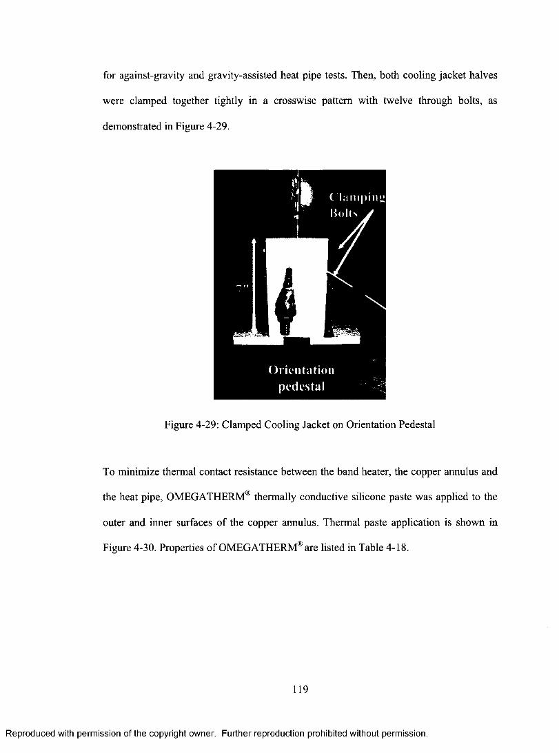
for against-gravity and gravity-assisted heat pipe tests. Then, both cooling jacket halves

were clamped together tightly in a crosswise pattern with twelve through bolts, as

demonstrated in Figure 4-29.

Orientationpedestal

Figure 4-29: Clamped Cooling Jacket on Orientation Pedestal

To minimize thermal contact resistance between the band heater, the copper annulus and

the heat pipe, OMEGATHERM® thermally conductive silicone paste was applied to the

outer and inner surfaces of the copper annulus. Thermal paste application is shown in

Figure 4-30. Properties of OMEGATHERM® are listed in Table 4-18.

119


OMEGATHERM®: Properties Value

Manufacturer Omega EngineeringProduct number OT-201

Type Thermally conductive pasteComponents Aluminum oxide

Zinc oxide Silicone resin

Thermal conductivity 2.308 W/m°CApplication temperature range 40°C to 200°C

Table 4-18: Properties of OMEGATHERM® [81]

Figure 4-30: Thermal Paste Application

The annulus was then fitted around the heat pipe evaporator, aligning the first and last

evaporator thermocouples with the two ends of the annulus. The band heater was spread

open slightly and slipped over the copper annulus halves. A nut and bolt clamped the

band heater tabs together, tightly securing the assembly to the heat pipe, shown in Figure

120


4-31. Heat pipe test preparations were completed by connecting the coolant hoses to the

cooling jacket and wrapping the assembly with insulation.

Figure 4-31: Heater Assembly Secured to Evaporator Section

4.5.2 Orientations

Each heat pipe was tested in three orientations: horizontal, gravity-assisted and against-

gravity operation. This would allow for the evaluation of different heat pipe operational

conditions and the underlying mechanisms of increased performance.

The horizontal test represented a standard operating situation, where both permeability

and capillary pressure were expected to be important. Gravity-assisted operation

corresponded to favourable conditions, where high permeability was believed to be the

dominant factor for increased performance. Finally, the most severe test was evaluated

121


during against-gravity operation, where the development o f high capillary pressure was

most likely essential. In all tests, enhanced evaporation heat transfer was also

hypothesized to manifest itself through lower axial temperature drops.

Coolant hoses were always connected to permit maximum coolant dwell time in the

cooling pocket. This positioning also coincided with the most efficient orientation for

coolant pocket air expulsion. For horizontal operation, the test assembly was positioned

in a horizontal orientation such that the evaporator and condenser sections were on the

same plane. The inlet coolant hose was connected to the lowest elbow fitting, while the

outlet hose was connected to the higher fitting. Since the band heater and copper annulus

were quite heavy and could cause heat pipe deformation, some additional insulation was

wedged under the heater assembly for support.

During gravity-assisted test preparations, the test assembly was vertically oriented such

that the heater assembly was positioned underneath the cooling jacket. This required the

use o f the orientation pedestal, shown previously in Figure 4-29. Again, coolant hoses

were connected to facilitate air egress and enhanced cooling.

Against-gravity testing was similar to gravity-assisted tests, only the assembly was

oriented with the heater assembly above the cooling jacket. Coolant hoses were

reconnected in the opposite manner to gravity-assisted tests. That is, the gravity-assisted

outlet connection was reconnected as the inlet during against-gravity tests and vice-versa.

122


4.5.3 Testing and data collection

Heat pipe test runs consisted o f temperature measurements at stepwise increasing heater

power settings. Heat inputs were approximately set in the following fashion, up to a

maximum evaporator wall temperature ranging from 150°C to 160°C:

1. From 0 W to 40 W: increments o f 10 W

2. From 40 W to 100 W: increments of 20 W

3. From 100 W to maximum: increments of 40 W

Some variations in the prescribed heat input settings were required to achieve the desired

maximum evaporator temperatures. Therefore, some of the higher heat input increments

did not exactly follow the pattern listed above. Also, if a minimum final increment o f 5

W was not estimated to be attainable without exceeding the maximum allowable

evaporator temperature, the test was ended prematurely. For example, heat pipe H3

attained a maximum heat input o f 31 W with an evaporator temperature of 143°C. Since

the previous 10 W increment (from 20 to 30 W) raised the evaporator temperature by

37°C, it was estimated that an additional increment in heat input would grossly exceed

safe operating temperatures. Therefore, the test was halted at 31 W.

Filenames were selected using the following standard:

1. The first block of characters represented the heat pipe I.D. and consisted of “HP”

plus the two character heat pipe name.

123


2. The next block of characters signified the test orientation: “horizontal” for

horizontal tests, “assistG” for gravity-assisted tests and “againstG” for against

gravity tests.

3. The final group of characters identified successive repeats of the same test. For

example, “HPB7_horizontal_runl” signified that heat pipe B7 was being tested in

the horizontal orientation for the first time.

A typical heat pipe test was performed in the following way. Typical settings are listed in

brackets, while screenshots o f “HeatPipeDatAcq" are available in Appendix D:

1. Launch data acquisition program “HeatPipeDatAcq". Click the “Setup" tab and

enter desired data logging frequency (1Hz), sampling rate (10 Hz), temperature

warning (150°C) and flow rate limit (1.6 1/min). Assign filename using previously

explained file naming convention. Choose an appropriate file path.

2. Click the “Monitor" tab. Depress “Start" button on graphical user interface to

begin taking data. Ensuring test assembly is at room temperature, take one “flow

o ff’ data point to record zero flowmeter reading (Note: this step was used in the

heat balance and is not strictly necessary for the data reduction process presented

in Section 4.5.4).

3. Start chiller and set coolant delivery temperature to 24°C to emulate room

temperature sink conditions. Manipulate coolant hoses to work air bubbles out of

cooling circuit.

124


4. When steady state is reached, take a “flow on” data point (See Note o f Step 2).

5. Turn on power to the isolation transformer and the variac.

6. Set heater power level by rotating variac control knob until desired voltage and

corresponding current to the heater is achieved (e.g.: for 10 W, typical settings

were 18.8 V X 0.54 A ~ 10 W). Record voltage and current in “ Voltage” and

“Current” fields on the “Monitor” page.

7. Monitor heat pipe thermal response using real-time temperature graph on

“Monitor” page. When temperature curves exhibit a clear flattening trend, steady-

state operation has been achieved. A steady-state data point may now be recorded.

Prior to data capture, input any changes to the power settings in the “ Voltage” and

“Current” fields. Depress the “Take Data” button. Do not adjust any settings

during steady-state data recording, indicated by the illuminated green light next to

the “Take Data” button.

8. When the “Take Data’’’ indicator turns off, increase the power level in steps

corresponding to those previously outlined above. Repeat Steps 6 and 7 until the

maximum recorded heat pipe temperature is between 150°C to 160°C. Once this

is achieved, rotate the variac knob to the “zero” position. Switch variac and

isolation transformer off. For faster heat pipe cooling, reduce coolant delivery

temperature to 0°C.

9. When heat pipe temperature is sufficiently low (e.g.: ~40°C), turn off chiller.

Depress “Stop" button on “Monitor” page to end recording of test data. Depress

“Exit Program" button to terminate program.

125


10. Retrieve data files from file path. Two files have been produced, each with the

specified filename plus a file identity extension. The full data file has a “.csv”

extension while the steady state file has a “_ss_values.csv” extension.

The steady state file was used for the data reduction of Section 4.5.4. Although the full

data file was not needed, it could be used for test event troubleshooting or for heat pipe

thermal transient response studies.

4.5.4 Data reduction program

Test data was manipulated with the MATLAB software program “thermalPerformance”,

available in Appendix E. Essentially, this program was written to calculate and plot heat

pipe effective thermal conductivities for all recorded heater power input levels.

Originally, the heat removed by the cooling circuit was to be used for effective thermal

conductivity calculations. Because of unreliable heat balance measurements, results were

based on heater input power levels instead. A general explanation o f the data reduction

procedure is described as follows.

Before data was manipulated, files were converted into a MATLAB-compatible binary

format. This was accomplished by importing the comma separated value files into the

MATLAB workspace and saving them as binary “MAT-files” with the same filenames as

the originals.

The program “thermalPerformance” was executed by passing the desired filename as a

character string to the data reduction program. The program began its routine by

126


initializing line markers, legend labels and loading file data. Evaporator, adiabatic,

condenser and total heat pipe lengths were assigned next. To avoid measurement

uncertainty in effective thermal conductivity calculations, the distance between the

central evaporator and central condenser thermocouples was approximated using the

effective length of Equation ( 2-8 ). Due to thermocouple spacing requirements, the

calculated effective length was slightly shorter than the actual effective length

measurements, however this would produce a conservative estimate of the effective

thermal conductivity. Next, a large portion of code was dedicated to heat balance

assessments, however in the context o f the current study these calculations will not be

elaborated upon.

Since the three evaporator and three condenser thermocouples were evenly spaced, the

axial heat pipe temperature drop was based on the centrally-located thermocouple of each

section. Thus, the temperature drop was calculated next by subtracting the second

condenser temperature from the second evaporator temperature. Then, knowing the cross-

sectional area of the heat pipe and employing Equation ( 2-35 ), the effective thermal

conductivity was calculated for each heater power setting. The program then concluded

with plotting routines for immediate graphical representation of test results.

127


5 Results and Discussion

In this section, experimental results are presented and discussed. A complete list of

thermal performance tests is given. Wick morphology is examined through scanning

electron microscopy and correlated with the obtained results. In support of effective

thermal conductivity behaviour, some axial temperature gradients are also presented.

Finally, the effects of biporous wicks on heat pipe thermal conductivity are graphically

illustrated.

5.1 Summary of Tests Performed

A summary of heat pipes tested is listed in Table 5-1. Most notable is the absence of any

“I” configuration heat pipes (i.e.: copper mesh with copper powder on the liquid vapour

interface). Because of poor performance from previous copper mesh/copper powder heat

pipes, it was decided this configuration would not produce any substantial performance

advantage over conventional designs. As such, these configurations were eliminated from

testing. Also of note, repeatability experiments were performed to assess both

manufacturing reproducibility and test methodology. Manufacturing reproducibility tests

were performed for configurations B, K and L. Test repeatability was accomplished by

retesting heat pipe B8 in every orientation.

128


Heat Pipe I.D. and Configuration Tests Performed

A7: 100-mesh copper screen, unsintered 1 horizontal, 1 gravity assisted, 1 against gravity

B7: 100-mesh copper screen, liquid/vapour interface covered with nickel powder, sintered

1 horizontal, 1 gravity assisted, 1 against gravity

B8: identical to B7 2 horizontal, 2 gravity assisted, 2 against gravity

E7: 100-mesh copper screen, wall/wick and liquid/vapour interfaces covered with nickel powder, sintered


H3: 100-mesh copper screen as carrier, heavily covered with nickel powder, sintered


J3: 100-mesh copper screen, wall/wick and liquid/vapour interfaces covered with copper powder, sintered


K l: Copper powder, sintered 1 horizontal, 1 gravity assisted, 1 against gravity

K2: identical to K l 1 horizontal, 1 gravity assisted, 1 against gravity

L I: 100-mesh copper screen, lightly covered with nickel powder throughout structure, sintered


L2: identical to LI 1 horizontal, 1 gravity assisted, 1 against gravity

Table 5-1: List of Heat Pipe Tests

5.2 Scanning Electron Microscopy

Scanning electron microscopy was employed to analyze wick morphology, including the

degree o f sintering and the interfacial microstructure. Samples were prepared from both

flat, unrolled wicks and sectioned heat pipes. These assessments determined the effects of

the sintering process on porous wick properties, such as adequate neck formation and

satisfactory wall/wick contact. Manufacturing techniques were also assessed through

biporous microstructure detection and evidence of increased evaporative surface area.

129


Homogeneous wick microstructures are presented first. These include Configurations A

(copper mesh), H (nickel powder) and K (copper powder). Next, composite

configurations are examined. These findings provided valuable insight into heat pipe

performance predictions.

5.2.1 Configuration A

For comparison and reference, a few micrographs were taken of this copper mesh

structure, one of which is shown in Figure 5-1. This mesh uses a plain weave

construction, employed for wick thickness calculations in Section 3.3.1. Referring to the

scale in Figure 5-1, the pore diameter seems slightly smaller than the theoretically

calculated value of 254 pm. This may have produced better than expected performance

during against gravity tests.

Figure 5-1: Configuration A

130


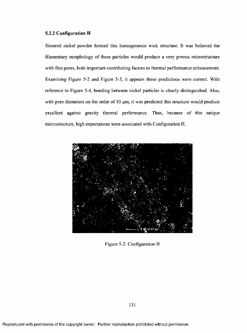
5.2.2 Configuration H

Sintered nickel powder formed this homogeneous wick structure. It was believed the

filamentary morphology of these particles would produce a very porous microstructure

with fine pores, both important contributing factors to thermal performance enhancement.

Examining Figure 5-2 and Figure 5-3, it appears these predictions were correct. With

reference to Figure 5-4, bonding between nickel particles is clearly distinguished. Also,

with pore diameters on the order of 10 pm, it was predicted this structure would produce

excellent against gravity thermal performance. Thus, because o f this unique

microstructure, high expectations were associated with Configuration H.

Figure 5-2: Configuration H

131


Figure 5-3: Configuration H, Higher Magnification

Figure 5-4: Sintering in Nickel Powder

132


5.2.3 Configuration K

For this homogeneous sintered copper powder configuration, samples were primarily

examined for adequate sintering. Figure 5-5 illustrates this microstructure. The spherical

copper particles did not seem to produce a highly porous structure in comparison to the

filamentary nickel powder. This could lead to relatively poor thermal performance due to

low liquid permeability. However, some performance advantage was still expected from

this configuration during against gravity tests due to a much finer pore size than the

copper mesh.

Figure 5-5: Configuration K

Only limited sintering was detected through modest neck formation, depicted in Figure

5-6. Comparing the preliminary observations from Figure 4-19 of Section 4.3.6 with the

present results, neck formation was not noticeably improved. Therefore, it was likely that

copper powder sintering parameters were not suitably chosen. However, increasing the

133


sintering temperature would not be an option since the melting point o f copper (1085°C)

was only marginally higher than the sintering temperature. Increasing the sintering time

could have aided particle bonding somewhat, yet it seemed the poor sintering behaviour

was largely associated with the relatively low surface area of the spherical copper

powder. This in turn probably led to a lower particle surface energy and the observed

sintering difficulties. Primarily due to the relatively low porosity, this configuration was

not expected to perform well during horizontal and gravity assisted testing. Some

sufficient performance was expected during against gravity testing due to its finer pore

size relative to Configuration A.

Neckformatior

Figure 5-6: Neck Formation in Configuration K

5.2.4 Configuration B

This configuration featured nickel powder covering the liquid/vapour interface, illustrated

in Figure 5-7. The presence o f the unobstructed large pore structure is evident. Finer

134


pores can also be identified in Figure 5-8. Therefore, it was concluded that the powder

application technique successfully produced a composite, biporous morphology. Closer

examination of the fine pore nickel powder structure in Figure 5-8 revealed a significant

increase in surface area over Configuration A, an important factor in enhanced

evaporation heat transfer.

Figure 5-7: Liquid/Vapour Interface of Configuration B

135


Figure 5-8: Increased Surface Area in Configuration B

Like Configuration H in Figure 5-4, sintering was observed between nickel powder

particles. Moreover, bonding was also detected between the nickel powder and the copper

mesh, shown in Figure 5-9. This indicated that sintering temperature and time were

appropriately selected. Because of the above properties, Configuration B appeared to be a

promising candidate for heat pipe performance enhancement.

136


Figure 5-9: Sintering between Nickel Powder and Copper Mesh

5.2.5 Configuration E

Much like Configuration B, this structure included a fine pore nickel powder arrangement

at the liquid/vapour interface in addition to a layer o f nickel powder applied at the

wall/wick interface. These two interfaces are displayed in Figure 5-10. Concerning the

wall/wick interface, generally poor contact was observed, with noticeable gaps between

the container and the wick, illustrated in Figure 5-11. These could potentially increase the

contact resistance and trap vapour, increasing the radial temperature drop and reducing

the effective thermal conductivity. However, like Configuration B, an increase in surface

area and an acceptable level of sintering was observed. Refer to Figure 5-7 and Figure

5-8 for these similarities. Therefore, this configuration also displayed promising

characteristics as a composite wick for heat pipes. Conversely, at higher heat fluxes,

decreased performance was expected due to vapour entrapment at the wall/wick interface.

137


Figure 5-10: Configuration E

Figure 5-11: Wall/Wick Interface o f Configuration E

138


5.2.6 Configuration I

A fine layer of copper powder was applied at the liquid/vapour interface in this

configuration, shown in Figure 5-12. Referring to Figure 5-13, there was little evidence

of a biporous structure, since the copper powder completely covered the larger pores of

the copper mesh. This was expected to cause poor heat transfer performance, since any

generated vapour would not be permitted an easy exit path to the vapour core. It was

therefore concluded that the sifting application technique of Section 4.3.4 was not a

completely successful composite wick fabrication method. Similar to Configuration K

shown in Figure 5-6, very little evidence of sintering was detected. For these reasons,

Configuration I was predicted to exhibit poor thermal performance.

Figure 5-12: Configuration I

139


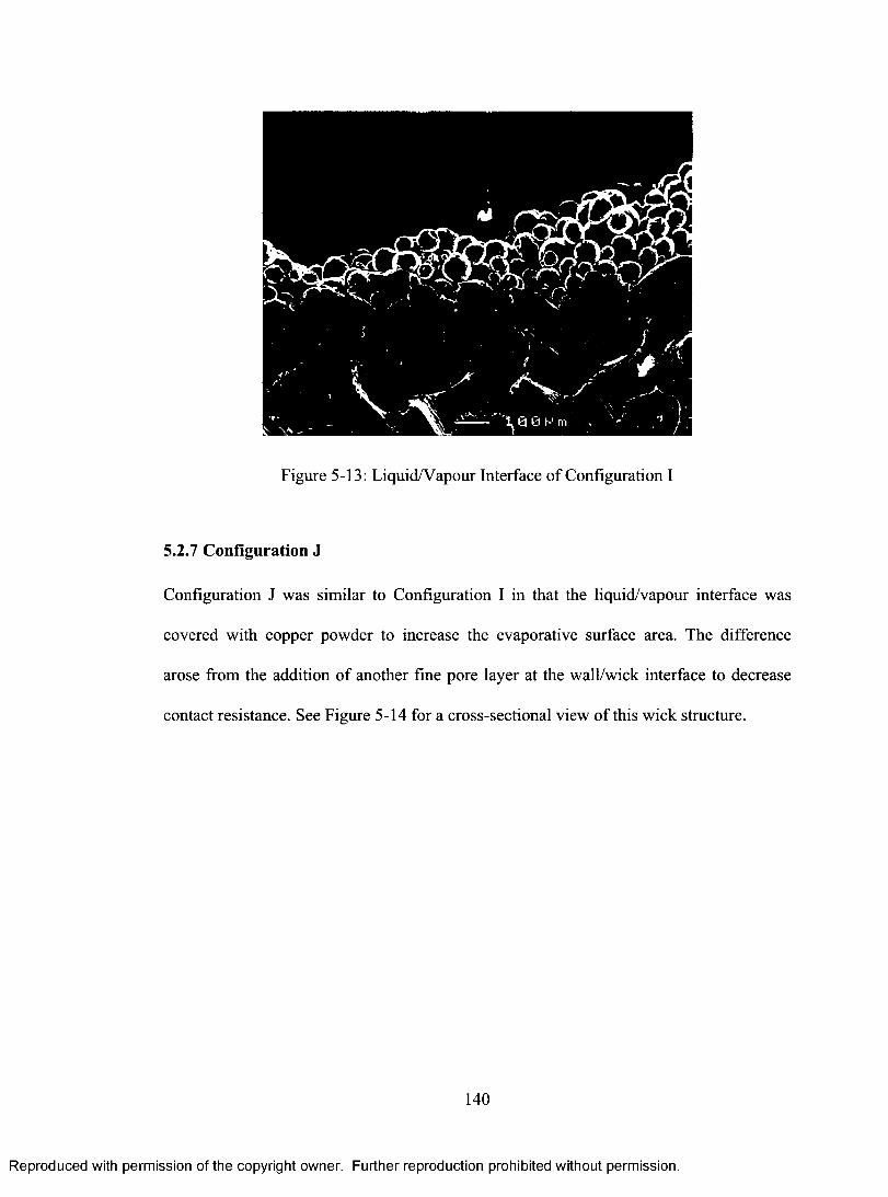
Figure 5-13: Liquid/Vapour Interface o f Configuration I

5.2.7 Configuration J

Configuration J was similar to Configuration I in that the liquid/vapour interface was

covered with copper powder to increase the evaporative surface area. The difference

arose from the addition of another fine pore layer at the wall/wick interface to decrease

contact resistance. See Figure 5-14 for a cross-sectional view of this wick structure.

140


Figure 5-14: Configuration J

Like Configuration I, this structure experienced the same difficulties in powder coverage

control and adequate sintering. Referring to Figure 5-15, the large pores at the wall/wick

interface are completely covered by copper powder. Again, this indicated the sifting

application technique could not produce the desired biporous microstructure. Another

factor contributing to large pore blockage was associated with the selected powder size

and mesh combination. The powder size was clearly too large for the 100-mesh copper

screen, and a finer powder could have produced better results. Moreover, voids and

disbondments were observed between the wall and the wick. Similar to Configuration E,

shortcomings in performance could potentially be attributed to vapour entrapment in

these voids. For these reasons, it was predicted that heat pipes with Configuration J

would exhibit reduced heat transfer performance, particularly at higher heat fluxes.

141


Figure 5-15: Wall/Wick Interface o f Configuration J

5.2.8 Configuration L

A biporous structure throughout the wick thickness was the aim of this configuration,

achieved through the spray application of nickel powder. Regrettably, since this

configuration was selected in the later stages of this research, no additional samples were

prepared in time for SEM analysis. Consequently, no preliminary results could be drawn

prior to testing. However, sample morphology was expected to closely resemble

Configuration B of Figure 5-7, only this structure would exist throughout the entire radial

thickness of the wick. It was postulated that this would enable enhanced evaporation heat

transfer throughout the full heat flux range, as well as offering superior performance

during against gravity operation from increased capillary pressure.

142


5.3 Effective Thermal Conductivity and Maximum Heat Input Rate

The best indicator of thermal performance enhancement is expressed in terms o f an

effective thermal conductivity, as discussed in Section 2.6.1. Also of great importance is

the maximum achievable heat input rate for a given orientation. A presentation o f the

heat transfer performance attained by each heat pipe configuration is discussed here.

Firstly, heat pipes containing homogeneous wick configurations are presented. These

include Configurations A (copper mesh), H (nickel powder) and K (copper powder).

Then, composite configurations are graphically compared with homogeneous wick results

to gauge whether performance increases have been achieved. For quick reference, heat

transfer performance summaries are tabulated at the end of each subsection.

The measured heat pipe temperatures were plotted versus axial position for preliminary

analysis of thermal performance. Nine thermocouples were fastened on each heat pipe at

the axial locations shown in Figure 4-26 o f Section 4.4.4. The zero axial reference

position was taken to be the evaporator end cap. Maximum evaporator temperatures and

axial temperature drops were also compared using these graphs to determine

improvements in heat transfer at various power settings. However, because of the

extensive amount of experimental data, only key results are presented here. Complete

results for axial temperature profiles are available in Appendix F, as well as any

additional effective thermal conductivity results not presented in the following sections.

One note about the line plots o f Appendix F: the heater power input labels listed in plot

legends were not exactly equal to those experienced during testing. However, since

143


variations between these were negligible, it was decided to standardize line plot labels for

clarity. On the other hand, the effective thermal conductivity calculations of the following

sections relied on the actual heater power input levels experienced during testing.

5.3.1 Configuration A

Generally, the conventional monoporous copper mesh-wick heat pipe seemed to perform

reasonably well in comparison to the composite wick heat pipes, including during against

gravity tests. In horizontal operation, no signs o f the capillary limit could be

distinguished up to approximately 140 W, detected by a sudden and continuous rise in the

evaporator wall temperature.

Moreover, this configuration achieved some of the best gravity assisted results, most

likely due to its relatively high liquid permeability. At heat inputs up to 220 W during

gravity assisted testing, A7 did not seem to reach the capillary limit. For safety, both tests

were terminated prior to dryout due to high evaporator temperatures. Figure 5-16 displays

horizontal and gravity assisted effective thermal conductivities for A7. The highest

effective thermal conductivities were achieved at the highest heat inputs, another

indicator that dryout was not encountered.

144


Effective Thermal Conductivity vs Heat Input, A7

12000 -Horizontal

Gravity Assisted10000

8000Uoe£ 6000

4000

2000 -

120 150 180 210 2400 30 60 90

Heat Input (W)

Figure 5-16: Horizontal and Gravity Assisted Effective Thermal Conductivities for A7

However, as the heat input was increased during against gravity operation, some evidence

of impending dryout was observed, particularly at levels greater than 30 W. See Figure

5-17 for axial temperature distributions demonstrating this phenomenon. Progressively

higher temperature differences between evaporator and adiabatic thermocouples were

observed here, a universally recognized sign of wick dryout. As a result, this

configuration could only function against gravity up to heat inputs of 50 W before

evaporator temperatures became excessively high. This result was most probably due to

the relatively low capillary pumping ability of the 100-mesh copper screen. The addition

of a secondary fine pore structure was expected to improve this outcome significantly.

See Figure 5-18 for against gravity effective thermal conductivity values of A7. Most

noticeable is the decrease in effective thermal conductivity after peaking at

145


approximately 30 W, attributable to the increasing axial temperature drop with heat input,

shown in Figure 5-17. All axial temperature profiles for A7 are available in Appendix F.

u

Ii - i

I<DH

Temperature vs Axial Position A7: Against Gravity Operation

180

160

140

120

60 X 5040

20

00 25050 100 150 200 300

Axial Position (mm)

Figure 5-17: Axial Temperature Distribution of A7, Against Gravity Operation

Effective Thermal Conductivity vs Heat Input, A7

1600Against Gravity

1400

1200

1000 s£ 800

3 600

400

200

0 30 40 5010 20 60

Heat Input (W)

Figure 5-18: Against Gravity Effective Thermal Conductivity Results for A7


Heat pipe A7

Maximum heat inputs tested and corresponding maximum evaporator temperatures

Horizontal: 142.9 W at 152.5°C

Gravity assisted: 218.4 W at 147.7°C

Against gravity: 51 W at 148.3°C

Maximum effective thermal conductivities

Horizontal: 5351 W/m°C at 142.9 W

Gravity assisted: 10219 W/m°C at 218.4 W

Against gravity: 1443 W/m°C at 31 W

Table 5-2: Thermal Performance Summary for A7

5.3.2 Configuration H

Configuration H was comprised o f a homogeneous, sintered nickel powder wick with

pore diameters on the order of 10 pm. It was predicted that this wick structure would

produce enhanced against gravity thermal performance.

In all instances, this configuration did not perform well when compared to the results of

Configuration A in Figure 5-16. Figure 5-19 confirms this, displaying unsatisfactory

effective thermal conductivities during horizontal and gravity assisted testing. In

particular, against gravity performance was surprisingly poor when compared to the

results o f heat pipe A7 in Figure 5-18. Configuration FI only reached an effective thermal

conductivity of 572 W/m°C at 30 W, shown in Figure 5-20. In contrast, the much coarser

pore wick of Configuration A achieved an effective thermal conductivity o f 1443 W/m°C

at 30 W, over twice the level of Configuration H. It was expected that the fine pore nickel

powder structure would outperform all other configurations in against gravity operation,

147


yet it exhibited the worst performance o f all the tested heat pipes. Referring to Figure 5-4

on page 132, sintering trials produced a highly porous microstructure with high surface

area density and pore diameters at least an order of magnitude smaller than the copper

mesh. This should have greatly increased the capillary pumping ability o f the heat pipe.

However, Figure 5-20 displays poor against gravity results, with heat pipe A7 easily

outperforming this configuration. This should not have occurred, since Configuration H

possessed a higher capillary pumping ability due to a much finer pore structure. The most

likely cause of this inadequacy could have been related to an overestimation o f the wick

porosity and fluid charge. For heat pipe H3, a porosity of 80% was estimated using the

procedure outlined in Section 4.3.7. This led to a fluid charge o f roughly 7.5 g, or about

1.8 times higher than the average liquid fill amount for all other configurations.

A fluid overcharge this excessive could have caused blockage at the condenser end,

filling the vapour passage with liquid. Axial heat transfer may have been hampered by

the presence of a high thermal resistance liquid slug at the condenser end, instead of a

negligibly low vapour thermal resistance. As a result, the effective thermal conductivity

would suffer a significant degradation in performance. Kempers et al. also concluded that

a substantial fluid overcharge would increase the heat pipe thermal resistance

significantly [82], In their study, the heat pipe with the highest fluid charging amount also

possessed the highest thermal resistance. Table 5-3 summarizes the thermal performance

results for H3.

148


Effective Thermal Conductivity vs Heat Input, H3

1200Horizontal

Gravity Assisted1000

800oo5 £it!

6

600

400

200

40 500 10 20 30

Heat Input (W)

Figure 5-19: Horizontal and Gravity Assisted Effective Thermal Conductivities for H3

Effective Thermal Conductivity vs Heat Input, H3

700Against Gravity

600

500

400

300

200

100

025 30 350 10 15 205

Heat Input (W)

Figure 5-20: Against Gravity Effective Thermal Conductivity Results for H3

149


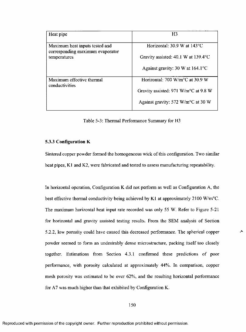
Heat pipe H3


Horizontal: 30.9 W at 143°C


Against gravity: 30 W at 164.1°C




Against gravity: 572 W/m°C at 30 W

Table 5-3: Thermal Performance Summary for H3

5.3.3 Configuration K

Sintered copper powder formed the homogeneous wick of this configuration. Two similar

heat pipes, K1 and K2, were fabricated and tested to assess manufacturing repeatability.

In horizontal operation, Configuration K did not perform as well as Configuration A, the

best effective thermal conductivity being achieved by K1 at approximately 2100 W/m°C.

The maximum horizontal heat input rate recorded was only 55 W. Refer to Figure 5-21

for horizontal and gravity assisted testing results. From the SEM analysis o f Section

5.2.2, low porosity could have caused this decreased performance. The spherical copper

powder seemed to form an undesirably dense microstructure, packing itself too closely

together. Estimations from Section 4.3.1 confirmed these predictions of poor

performance, with porosity calculated at approximately 44%. In comparison, copper

mesh porosity was estimated to be over 62%, and the resulting horizontal performance

for A7 was much higher than that exhibited by Configuration K.

150


Lower porosity would lead to a lower liquid permeability, a higher liquid pressure drop

[10], and a decrease in thermal performance. Again, the problems associated with

homogeneous wicks become evident here: although Configuration K possessed fine pores

for high capillary pressure, fluid transport was most likely reduced due to low liquid

permeability.

Effective Thermal Conductivity vs Heat Input, K1 and K27000

■ K1 Horizontal

■ - K2 Horizontal

9 K1 Gravity Assisted

• - K2 Gravity Assisted

6000

5000

U°g 4000

3000

2000

1000

21090 120 150 1800 30 60

Heat Input (W)

Figure 5-21: Horizontal and Gravity Assisted Results for Configuration K

Gravity assisted performance for Configuration K was also quite low, with K1 attaining a

best effective thermal conductivity of 6343 W/m°C at 183 W, shown above in Figure

5-21. With the comparatively high permeability wick of A7 reaching over 10000 W/m°C,

the difference can again most likely be attributed to the low porosity o f Configuration K.

In fact, the complete absence o f a wick would most probably produce the best gravity

151


assisted results, since this represents the scenario with the least resistance to liquid flow

[1], [10], [16].

Effective Thermal Conductivity vs Heat Input, K1 and K21800

A K1 Against Gravity

- A - K2 Against Gravity1600

1400

u 1200 1000

X 800

J 600

400

200

20 30 40 50 600 10

Heat Input (W)

Figure 5-22: Against Gravity Effective Thermal Conductivity Results for K1 and K2

Against gravity performance was fair, however much higher effective thermal

conductivities were expected from this configuration. The best against gravity effective

thermal conductivity was 1700 W/m°C, recorded by K1 at 30 W. The maximum heat

input rate achieved by both o f these heat pipes was approximately equivalent at 50 W,

perhaps because of the unsatisfactory compromise between high capillary pressure

generation and low liquid permeability. Referring to the capillary limit expression of

Equation ( 2-13 ), the net capillary pressure available for liquid transport would be

reduced significantly by a low permeability wick. As a result, the capillary limit may

152


have been approached much sooner than expected. Another possible cause of the

inadequate against gravity performance could be due to the greater wick thickness of this

configuration. Because of the manufacturing process outlined in Section 4.3.4, wick

thicknesses for K1 and K2 were approximately twice that of A7. This could have greatly

increased the heat pipe’s axial temperature drop. Since the liquid-saturated wick

represents the largest resistance to heat transfer in the equivalent thermal resistance

network shown in Figure 2-15, a much lower effective thermal conductivity would

therefore be expected. In comparison to A7, only modest improvements in effective

thermal conductivity were realized, and no significant gains were achieved in the

maximum heat input rate.

Temperature vs Axial Position Kl: Against Gravity Operation, Run 1

180

160

- ■ - 2 0 WA 30 W

40 W- * - 5 0 W

20

00 50 100 150 200 250 300

Axial Position (mm)

Figure 5-23: Axial Temperature Distribution for K l, Against Gravity

153


One unique characteristic of this configuration was the nearly isothermal behaviour along

the first two thirds o f the heat pipe length, displayed in Figure 5-23. The evaporator and

adiabatic sections recorded very similar temperatures, with a maximum temperature

variation of 11.5°C at 50 W. Here, Configuration K performed very well. Unfortunately,

temperatures dropped dramatically along the condenser section, leading to the relatively

low effective thermal conductivity values. One possible reason for this peculiar behaviour

could be another instance of fluid overcharging, similar to the mechanism of performance

degradation suggested for Configuration H. A liquid slug could have essentially

inactivated a portion o f the condenser end, greatly decreasing thermal performance [10].

Peterson also attributes these axial temperature characteristics to the presence of non-

condensable gases [10]. This problem would also have a similar effect on performance to

that of a liquid slug. That is, during operation, these gases would be swept towards the

condenser end where they would impede heat flow and cause a distinct decrease in the

axial temperature distribution.

Examining the effective thermal conductivity plots on pages 151 to 152, some

conclusions can be made regarding manufacturing repeatability. Overall, K l performed

slightly better than K2, except in the against gravity orientation during higher heat inputs.

Nevertheless, they still exhibit similar trends in performance. During fabrication,

geometric wick measurements, porosity estimates and the required fluid charging

amounts agreed well with each other. However, during final charging and sealing, K2

was slightly overfilled by approximately 8% in comparison to K l. This could have led to

the discrepancy in effective thermal conductivity seen in the graphs. One observation in

154


particular should be discussed: Figure 5-22 suggests that K2’s slight overfill actually

aided heat transfer performance at higher heat inputs in the against gravity orientation,

since it exhibited a higher effective thermal conductivity after approximately 30 W.

Perhaps this was a result of delayed dryout due to a higher fluid charge. In other words,

while dryout was initiated first in K l, K2 experienced dryout initiation at slightly higher

heat inputs, and thus marginally better performance was produced in this region of the

graph. Thermal performance results are listed in Table 5-4.

Heat pipe K l K2


Horizontal:54.4 W at 159.3°C


Against gravity: 49.7 W at 155.9°C



Against gravity:49.7 W at 138°C


Horizontal:2144 W/m°C at 29.6 W

Gravity assisted:6343 W/m°C at 183.2 W

Against gravity:1704 W/m°C at 20 W



Against gravity:1540 W/m°C at 30.1 W

Table 5-4: Thermal Performance Summary for K l and K2

5.3.4 Configuration B

The addition o f a sintered layer of nickel powder at the liquid/vapour interface was

shown to enhance horizontal heat transfer performance at all heat inputs. Compared to the

conventional copper mesh configuration of A7, heat pipe B8 displayed a clear

155


performance advantage, demonstrated in Figure 5-24. Heat pipe B8 reached a maximum

effective thermal conductivity o f 6374 W/m°C at 40 W. Although a slight decrease in

performance was observed after 40 W, stable operation continued at levels around 5850

W/m°C until excessive evaporator temperatures required test cessation.

Effective Thermal Conductivity vs Heat Input, B8 and A77000

B8 Horizontal, Run 16000

■ - A7 Horizontal~ 5000o

| 4000

2000

3000

1000

20 40 60 80 100 120 140 1600

Heat Input (W)

Figure 5-24: Comparison of Horizontal Thermal Performance between B8 and A7

This increased performance could have occurred due to enhanced evaporation heat

transfer from a higher density of evaporating menisci at the liquid/vapour interface, as

discussed previously in Section 3.3.4. Much like the findings of Hanlon and Ma [61],

these results seemed to provide evidence of increased thin film evaporation due to a

decrease in pore size and a higher density of evaporating menisci at the liquid/vapour

156


interface. Recalling Figure 5-8 on page 136, an increase in surface area, and hence a

much higher number of evaporating menisci, was confirmed to exist in Configuration B.

When comparing gravity assisted results, Configuration B noticeably outperformed

Configuration A at heat inputs below 180 W. Above this, the performance advantage was

essentially lost, confirmed in Figure 5-25. A maximum effective thermal conductivity of

approximately 13300 W/m°C was reached at 60 W, virtually doubling the performance of

Configuration A at the same heat input. Again, the most likely cause o f this substantial

performance gain was likely attributed towards enhanced evaporation heat transfer from

the higher density of fine pores at the liquid/vapour interface. Additionally, the presence

o f the large pores in the adjacent wick layers may have provided a low resistance liquid

flow path, approaching the permeability o f Configuration A. It seemed possible that the

slight decrease in liquid permeability due to the presence of the biporous layer could have

caused a somewhat lower maximum heat input rate (202 W) when compared to the

results for A7 (218 W).

157



♦ B8 Gravity Assisted, Run 1

- • - A7 Gravity Assisted

12000

^ 10000uo| 8000 £to

4000

6000

2000

150 200 2500 50 100

Heat Input (W)

Figure 5-25: Comparison of Gravity Assisted Thermal Performance between B8 and A7

Another important observation can be made here regarding both the gravity assisted and

horizontal operation of B8: at higher heat inputs, the performance increase over A7

diminished. It is believed this effect arose from liquid recession into the wick and

subsequent dryout of the biporous layer, with the formation o f evaporating menisci on the

monoporous copper mesh structure underneath. With solely large pores comprising the

inner wick layers, one would expect a decrease in the number o f evaporating menisci, and

hence, a decrease in the evaporative heat transfer rate. This is the effect observed in both

Figure 5-24 and Figure 5-25.

158


Wih the diminishing trend in effective thermal conductivity at higher heat inputs, it is

believed the large pores of the inner wick layers allowed continued performance at levels

equivalent to those of A7. Additionally, the biporous layer seemed to allow vapour egress

from the wick, such that a catastrophic decrease in performance was avoided. From these

results, the conceptualization of a continuous biporous wick was postulated to offer better

performance throughout the entire spectrum of heat inputs. Thus, the design and

manufacture of Configuration L was initiated and realized, with results presented in

Section 5.3.7.

In addition to promising horizontal and gravity assisted test results, impressive gains in

performance over homogeneous configurations were revealed during against gravity

testing. As illustrated in Figure 5-26, B8 clearly possessed an advantage in effective

thermal conductivity over the poorly performing H3. With its fine pore sintered structure,

H3 was expected to produce the best against gravity results, yet due to potential fluid

overcharging issues discussed in Section 5.3.2, it did not exhibit the anticipated

performance. In contrast, B8 reached a maximum effective thermal conductivity value of

3124 W/m°C at 10 W, over three times the performance o f A7 and approximately six

times that o f H3. Like the previous observations regarding horizontal and gravity assisted

tests, against gravity performance improvements tended to diminish with increasing heat

input. The most likely cause was the previously mentioned liquid recession into the

monoporous portion o f the wick.

159


Effective Thermal Conductivity vs Heat Input: B8, A7 and H3

3500—A— B8 Against

Gravity, Run 1

" A - A7 Against Gravity

—A. - H3 Against Gravity

3000

2500

fcl 1500

1000

▲ —500

0 10 20 30 40 50 60

Heat Input (W)

Figure 5-26: Against Gravity Thermal Performance Comparison between B8, A7 and H3

A maximum heat input of 56 W was achieved before evaporator temperatures became

excessive. This was 5 W higher than A7 and 26 W higher than H3. Perhaps the fine pore

layer at the liquid/vapour interface aided in the extension of the capillary limit, evidenced

by the marginal improvement in the maximum heat input rate over A7. These results also

encouraged an investigation into the effects of an increase in the number of composite

wick layers on the maximum heat input rate. In particular, it was postulated that

Configuration E would achieve even higher heat input rates due to the inclusion of two

composite pore layers, one at the liquid/vapour interface and the other at the wall/wick

interface. Moreover, because all wick layers o f Configuration L possessed fine pores, it

was assumed it would attain the best overall performance in the against gravity

160


Kef

f (W

/m°C

)

orientation. The hypothesis of capillary limit enhancement from fine pore layer additions

is further explored in Sections 5.3.5 and 5.3.7.

Effective Thermal Conductivity vs Heat Input: B8, Runs 1 and 27000

6000

5000

4000

3000

2000

1000

0

0 20 40 60 80 100 120 140 160

Heat Input (W)

Figure 5-27: Testing Repeatability for B8, Horizontal Orientation

■B8 Horizontal, Run 1

1 B8 Horizontal, Run 2

161


Kef

f(W

/m°C

) K

efF

(W/m

°C)

Effective Thermal Conductivity vs Heat Input: B8, Runs 1 and 214000

B8 Gravity Assisted, Run 112000

- • - B8 GravityAssisted, Run 210000

8000

6000

4000

2000

0 50 100 150 200 250

Heat Input (W)

Figure 5-28: Testing Repeatability for B8, Gravity Assisted Orientation

Effective Thermal Conductivity vs Heat Input: B 8 , Runs 1 and 2

3500B 8 Against Gravity, Run 13000

- A - B8 AgainstGravity, Run 2

2000

1500

1000

500

0 10 20 30 40 50 60

Heat Input (W)

Figure 5-29: Testing Repeatability for B8, Against Gravity Orientation

162


Testing repeatability was also explored with B8. For this purpose, heat pipe B8 was

completely removed, reinserted and tested using the procedures outlined in Sections 4.5.1

to 4.5.3. Horizontal testing repeatability is presented in Figure 5-27, while gravity

assisted results are found in Figure 5-28. Against gravity results are given in Figure 5-29.

Overall, retesting seemed to yield sufficient repeatability in heat pipe behaviour, allowing

some measure of confidence in the results obtained.

From the above graphs of Runs 1 and 2, a maximum difference in effective thermal

conductivity of approximately 8% was observed at 140 W during horizontal tests. During

gravity assisted testing, variation in results reached a maximum of approximately 30% at

60 W. For against gravity operation, values differed by a maximum of 15% at 20 W.

Interestingly, the two curves of Figure 5-28 display the same behaviour, with some

amount o f offset. This suggests the possibility of inadequacies in thermocouple

mounting. Perhaps the taping procedure presented in 4.5.1 led to poor thermocouple/heat

pipe contact. Another possibility is that the thermocouples measuring the axial

temperature drop used in the effective thermal conductivity calculations were not

properly positioned. One other peculiarity was noticed in reference to test repeatability:

the first runs performed for B8 all exhibited higher performance than the second runs.

The second round of tests took place from 8 to 20 days after the first. It seemed most

likely that some performance degradation was detected, possibly due to the formation of

non-condensable gases during the time period between testing. Perhaps the nickel-copper

wick combination created a galvanic cell, with hydrogen gas generation as a product of

this reaction. However, without further analysis, this speculation cannot be confirmed.

163


Additional rounds of testing could offer more insight into this potential problem.

Summarized results for B8 are given in Table 5-5.

Heat pipe B8 Run 1 B8 Run 2


Horizontal:141 W at 146.3°C




Gravity assisted:201.5 W at 149.6°C

Against gravity:54.1 W at 144.2°C




Against gravity:3124 W /m°Cat 10.1 W



Against gravity:2758 W/m°C at 9.9 W

Table 5-5: Thermal Performance Summary for Runs 1 and 2 of B8

5.3.5 Configuration E

A biporous, composite wick layer at the liquid/vapour interface was added to this

configuration for the primary purpose o f evaporation heat transfer enhancement. An

additional layer at the wall/wick interface was also coated with nickel powder with the

goal of decreasing the contact resistance. However, upon observation of results from B8,

it was also believed this layer could potentially boost the capillary limit by providing

increased liquid transport, especially against gravity.

164


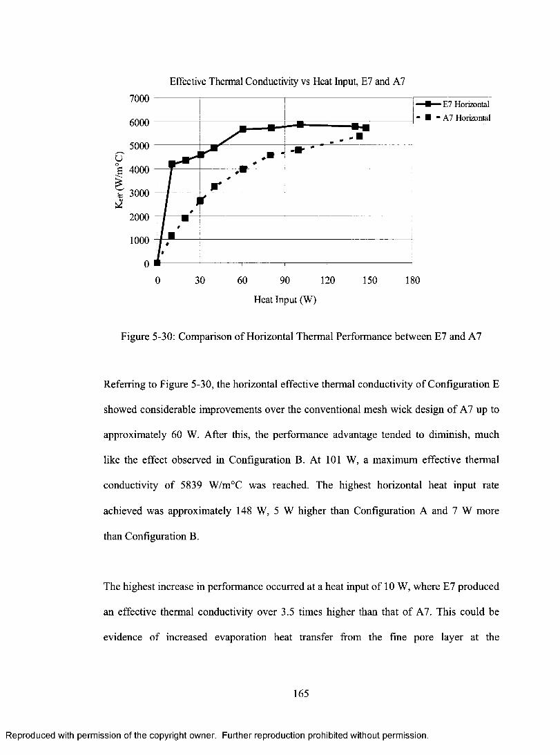
Effective Thermal Conductivity vs Heat Input, E7 and A7

7000 H E7 Horizontal

■ ■ “ A7 Horizontal6000

5000

e 4000

3000

2000

1000

0 30 60 90 120 150 180

Heat Input (W)

Figure 5-30: Comparison of Horizontal Thermal Performance between E7 and A7

Referring to Figure 5-30, the horizontal effective thermal conductivity of Configuration E

showed considerable improvements over the conventional mesh wick design of A7 up to

approximately 60 W. After this, the performance advantage tended to diminish, much

like the effect observed in Configuration B. At 101 W, a maximum effective thermal

conductivity of 5839 W/m°C was reached. The highest horizontal heat input rate

achieved was approximately 148 W, 5 W higher than Configuration A and 7 W more

than Configuration B.

The highest increase in performance occurred at a heat input of 10 W, where E7 produced

an effective thermal conductivity over 3.5 times higher than that of A7. This could be

evidence of increased evaporation heat transfer from the fine pore layer at the

165


liquid/vapour interface. The flattening of this curve could have resulted from liquid

recession into the homogeneous wick layers underneath the composite layer. However,

considering again the results from Configuration B in Figure 5-24, it is noted that E7 did

not perform as well as B8 at lower heat inputs, suggesting that perhaps the inclusion of

the fine porous layer at the wall/wick interface could have actually hindered horizontal

performance somewhat. Another explanation for this comparatively lower performance is

offered by the scanning electron microscopy results of Section 5.2.5. In Figure 5-11, gaps

are shown to exist between the wall and the wick. These would certainly decrease

performance by promoting vapour entrapment, thus increasing the contact resistance.

In Section 2.3 , the mechanisms o f the boiling limit were presented. By decreasing the

pore size in Equation ( 2-17 ), the critical superheat for boiling would also be reduced,

and hence, the boiling limit calculated by Equation ( 2-19 ) would decrease. Yet there is

no evidence of severe performance degradation, suggesting that even if Configuration E

promoted bubble generation, at least some vapour was allowed to escape through the

larger pores o f the biporous structure.

166


Effective Thermal Conductivity vs Heat Input, E7 and A712000

1 ( \ f \ f \ f \ - *E7 Gravity Assisted

• " A7 Gravity Assisted

0 50 100 150 200 250

Heat Input (W)

Figure 5-31: Comparison of Gravity Assisted Performance between E7 and A7

Comparing the gravity assisted performance in Figure 5-31, E7 only outperformed A7 at

heat inputs below 80 W. Above 80 W, Configuration A reached higher effective thermal

conductivities and a greater maximum heat input rate. The higher performance at lower

heat inputs was again believed to be attributable to enhanced evaporation heat transfer

from the fine pore composite wick layer. In comparison to B8, E7 did not perform as well

in this orientation, with a best effective thermal conductivity o f 8292 W/m°C at 62 W.

This result was almost 5000 W/m°C lower than that achieved by B8 at 60 W. Perhaps the

lower permeability wick o f Configuration E or the aforementioned suggestions regarding

the boiling limit and vapour entrapment contributed to the comparatively lower effective

thermal conductivities. However with only the present data, the exact mechanism remains

167


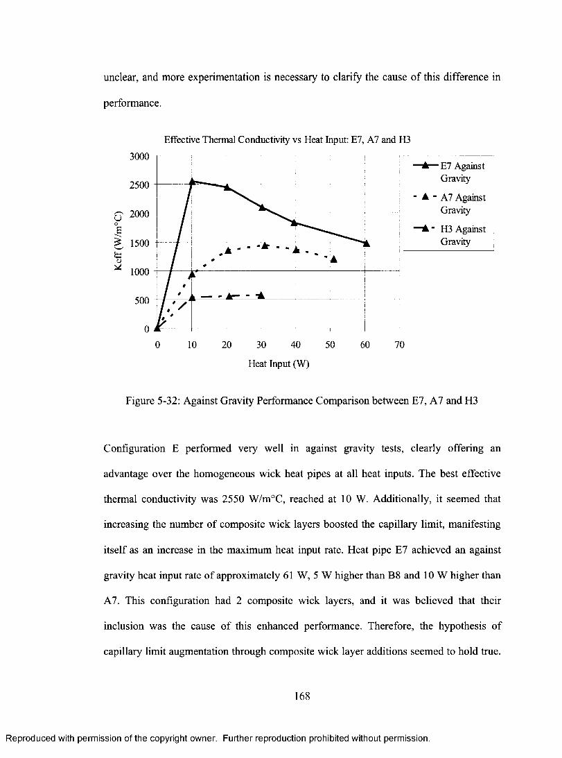
unclear, and more experimentation is necessary to clarify the cause o f this difference in

performance.

Effective Thermal Conductivity vs Heat Input: E7, A7 and H3

£ 1500

“A— E7 Against Gravity

A - A7 Against Gravity

"A " H3 Against Gravity

0 10 20 30 40 50 60 70

Heat Input (W)

Figure 5-32: Against Gravity Performance Comparison between E7, A7 and H3

Configuration E performed very well in against gravity tests, clearly offering an

advantage over the homogeneous wick heat pipes at all heat inputs. The best effective

thermal conductivity was 2550 W/m°C, reached at 10 W. Additionally, it seemed that

increasing the number of composite wick layers boosted the capillary limit, manifesting

itself as an increase in the maximum heat input rate. Heat pipe E7 achieved an against

gravity heat input rate of approximately 61 W, 5 W higher than B8 and 10 W higher than

A7. This configuration had 2 composite wick layers, and it was believed that their

inclusion was the cause of this enhanced performance. Therefore, the hypothesis of

capillary limit augmentation through composite wick layer additions seemed to hold true.

168


The study conducted by Canti et al. [20] discussed in 2.1.2 also examined heat transfer

enhancement using composite wicks. Findings suggested that a layered, composite wick

structure of both fine and coarse pores augmented heat transfer performance over

homogeneous designs [20], They attributed this to an increase in capillary pumping

ability through the fine pores, while still maintaining adequate liquid permeability with

the presence of large pores. Furthermore, when the fine pore layer was positioned against

the heat source, it performed better than if it was located at the liquid/vapour interface

[20], They explained this additional mechanism of enhanced heat transfer through an

increase in the number of nucleation sites against the heat source.

Thus, the findings of Canti et al. appeared to be verified. That is, composite layered

wicks could increase heat transfer performance through the simultaneous presence of

both fine and coarse pore layers, offering a compromise between high capillary pressure

and increased liquid permeability [20]. Conversely, no evidence was found to support the

claim of augmented heat transfer from increased nucleation sites at the wall/wick

interface, since B8 still exhibited a higher effective thermal conductivity. Also, it was

never conclusively proven that the inclusion of the fine pore layer at the wall/wick

interface decreased the thermal contact resistance, since the performance of

Configuration B was superior to that o f Configuration E.

169


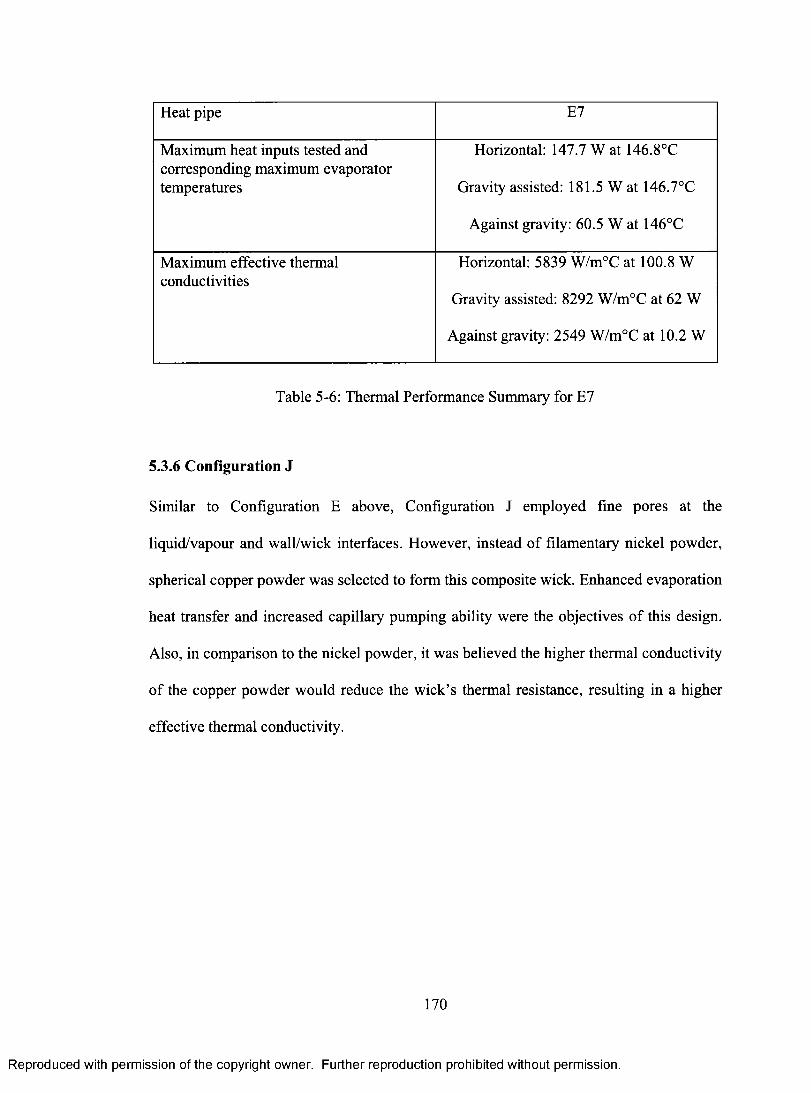
Heat pipe E7




Against gravity: 60.5 W at 146°C



Gravity assisted: 8292 W/m°C at 62 W

Against gravity: 2549 W/m°C at 10.2 W

Table 5-6: Thermal Performance Summary for E7

5.3.6 Configuration J

Similar to Configuration E above, Configuration J employed fine pores at the

liquid/vapour and wall/wick interfaces. However, instead of filamentary nickel powder,

spherical copper powder was selected to form this composite wick. Enhanced evaporation

heat transfer and increased capillary pumping ability were the objectives of this design.

Also, in comparison to the nickel powder, it was believed the higher thermal conductivity

of the copper powder would reduce the wick’s thermal resistance, resulting in a higher

effective thermal conductivity.

170


Effective Thermal Conductivity vs Heat Input, J3 and A76000

J3 HorizontalM5000

■ - A7 HorizontalU 4000o

3000is

2000

1000

0 20 40 60 80 100 120 140 160

Heat Input (W)

Figure 5-33: Comparison of Horizontal Performance between J3 and A7

In Figure 5-33, Configuration J displays some performance advantage over Configuration

A at heat inputs below 30 W. At any heat input higher than 30 W, A7 noticeably

outperforms heat pipe J3. Also, the maximum horizontal heat input achieved by J3 was

100 W, 40 W lower than that of A7. At this point, elevated evaporator temperatures

required test termination. The best performance of J3 was reached at 10 W, with an

effective thermal conductivity o f 2724 W/m°C. Performance was nearly twice that of

heat pipe A7, again supporting the argument of superior heat transfer through composite

wick design. The mechanism for this could very well be related to enhanced evaporation

heat transfer, although the effect was much less pronounced here than for Configurations

B or E.

171


Comparing scanning electron microscopy images of the sintered nickel and copper

structures, some rationale behind this performance difference is offered. The sintered

nickel powder in Figure 5-8 o f page 136 clearly shows both finer pores and a much

higher density of evaporating menisci than the copper powder in Figure 5-6 of page 134.

Recalling the thin film evaporation schematic of Figure 3-11 and the conclusions of

Hanlon and Ma [61], a finer pore size offers a greater number of evaporating menisci and

higher heat transfer performance. It logically follows that evaporation heat transfer

performance should be greater for the nickel powder composite wicks than for the copper

powder composite wicks.

Another possible cause of this modest performance could be due to the absence of a

composite structure of fine and coarse pores in the interfacial layers of the wick. North et

al. [60] found that composite structures offered substantial improvements in heat transfer

performance due to the formation of a high density of evaporating menisci. Referring

again to the SEM results of Section 5.2.7, Figure 5-15 shows that Configuration J

possesses an essentially monoporous and homogeneous structure at the liquid/vapour

interface. The copper particles seemed to completely block the larger openings of the

copper mesh. This could have affected the performance in two ways: the tight packing of

the copper particles could have impeded vapour egress at higher heat fluxes, and less

surface area was available for evaporation heat transfer due to the homogeneous nature of

this structure. These findings suggested that the application technique required

refinement. Additionally, a finer powder or a larger mesh should be used in future

attempts to achieve the desired composite microstructure.

172


Effective Thermal Conductivity vs Heat Input, J3 and A712000

J3 Gravity Assisted

10000- • ■ A7 Gravity

AssistedO 8000O

£ 6000fa

4000

2000

0 50 100 150 200 250

Heat Input (W)

Figure 5-34: Comparison of Gravity Assisted Performance between J3 and A7

Gravity assisted performance for J3 was improved over A7 for heat inputs less than 60

W, illustrated in Figure 5-34. The greatest performance advantage was measured at 20 W,

where J3 achieved an effective thermal conductivity of 4118 W/m°C, 1.7 times higher

than A l . Beyond 60 W, A7 exhibited superior performance, reaching a maximum heat

input rate of 218 W, much higher than that of J3 at 163 W.

Again, perhaps the monoporous nature o f the interfacial layers caused this poor

performance. It seems possible that the vapour generated at higher heat fluxes could have

become trapped in the central wick layers as the liquid receded beneath the liquid/vapour

interface. Fine pores and poor contact at the wall/wick interface, shown in Figure 5-15 on

173


, could have also promoted bubble nucleation, leading to the formation of a

vapour blanket and a high thermal resistance.

Effective Thermal Conductivity vs Heat Input: J3, A7 and K1

1800

1600

1400_s 1200ua 1000£

800£ 600

400

200

0

/\

v/ A- :

r // /! * *

F %% % 7 ^

/ / >

/ / */ /*j ' '

f

a -------------.-------- ..... . .

10 20 30 40

Heat Input (W)

50

-A — J3 Against Gravity


"A ■ K1 Against Gravity

60

Figure 5-35: Against Gravity Performance Comparison between J3, A7 and K1

Against gravity operation of J3 revealed a slight increase in performance over

homogeneous designs, as illustrated in Figure 5-35. Modest gains were achieved at 10 W,

where J3 attained an effective thermal conductivity o f 1391 W/m°C, 1.5 times higher

than A7 and 1.25 times better than K l. However, results were much lower than those

achieved by the nickel composite wick configurations B and E. At 21 W, J3 reached its

highest effective thermal conductivity of 1553 W/m°C, yet K l performed slightly better,

most likely due to its overall finer pore structure. The additional composite layers of

Configuration J could have aided in extending the capillary limit, suggested by an

174


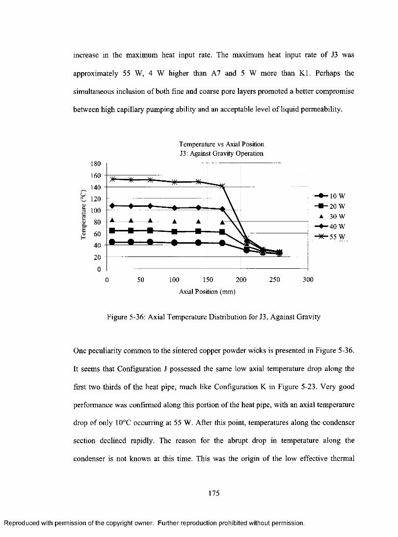
increase in the maximum heat input rate. The maximum heat input rate o f J3 was

approximately 55 W, 4 W higher than A7 and 5 W more than K l. Perhaps the

simultaneous inclusion of both fine and coarse pore layers promoted a better compromise

between high capillary pumping ability and an acceptable level o f liquid permeability.

u

OJ&£a>H

Temperature vs Axial Position J3: Against Gravity Operation

180

160

14010W 20 W

120

100

80

60

40

20

0250 300100 150 2000 50

Axial Position (mm)

Figure 5-36: Axial Temperature Distribution for J3, Against Gravity

One peculiarity common to the sintered copper powder wicks is presented in Figure 5-36.

It seems that Configuration J possessed the same low axial temperature drop along the

first two thirds o f the heat pipe, much like Configuration K in Figure 5-23. Very good

performance was confirmed along this portion of the heat pipe, with an axial temperature

drop of only 10°C occurring at 55 W. After this point, temperatures along the condenser

section declined rapidly. The reason for the abrupt drop in temperature along the

condenser is not known at this time. This was the origin of the low effective thermal

175


conductivities of this configuration. Like Configuration K, the presence of non-

condensable gases or fluid overcharging could have potentially caused this behaviour. In

addition to these factors, vapour entrapment could have also contributed to this inferior

performance, however further experimentation is required to confirm these theories.

Test results for J3 are summarized in Table 5-7. Overall, the results of this configuration

demonstrated the potential shortcomings of copper powder composite configurations in

comparison to the superiority of the nickel powder composite wicks. Since Configuration

J was tested before Configuration I and results were not promising, all “I” type heat pipes

were eliminated from further trials. It was therefore concluded that further development

and testing efforts would focus on sintered nickel powder composite wicks, or biporous

wicks comprised of finer sintered copper powder.

Heat pipe J3


Horizontal: 103 W at 152.6°C




Horizontal: 2724 W/m°C at 10 W



Table 5-7: Thermal Performance Summary for J3

176


5.3.7 Configuration L

Several key factors led to the design of this configuration. The studies conducted by

North et al. [60] and Cao et al. [67] both concluded that composite wicks comprised of

two characteristic pore sizes provided clear heat transfer performance advantages over

monoporous wick designs. A significant increase in evaporative surface area was credited

with these gains. The wicks in these studies consisted of a continuous, bimodal

distribution of fine and coarse pores, formed with sintered metal powder. Additionally,

the performance results from Configuration B and E suggested that an increase in the

number of composite wick layers would lead to an extension of the capillary limit, most

noticeable against gravity. Therefore, Configuration L was designed to exploit these

effects, with a structure comprised throughout of fine nickel powder lightly applied to a

large pore substrate of copper mesh.

177


Effective Thermal Conductivity vs Heat Input, L2 and A76000

L2 Horizontal

5000- ■ - A7 Horizontal

U 4000O

£ 3000

2000

1000

0 20 40 60 80 100 120 140 160

Heat Input (W)

Figure 5-37: Comparison of Horizontal Performance between L2 and A7

Figure 5-37 illustrates the horizontal performance o f L2 in comparison with A7. At heat

inputs lower than 80 W, L2 outperformed A7. The highest increase in performance was

achieved at a heat input of 10 W, where the effective thermal conductivity of L2 was over

3 times that o f A7. The best effective thermal conductivity was 5103 W/m°C, attained at

its maximum heat input rate of 140 W.

It appeared that the performance of L2 and A7 were equivalent above 80 W, suggesting

that at higher heat fluxes, liquid recession into the wick did not expose any additional

evaporating menisci. It was previously postulated that at higher heat fluxes, liquid

recession into the wick would activate a higher number of evaporating menisci, and

therefore heat transfer performance would increase dramatically. This theory was based

178


on the research conducted by North et al. [60] discussed in Section 3.3.4. Biporous wicks

were employed to enhance evaporation heat transfer performance. The wicks were

comprised o f clusters of powder, sintered together. The fine pores were formed in the

clusters, with the large pores residing in the spaces between the clusters. They discovered

a previously undetected heat transfer regime, where at higher heat fluxes the wall/wick-

to-vapour temperature difference remained virtually equivalent for a large range of heat

fluxes. It was reasoned that higher heat fluxes exposed more evaporating menisci, thus

encouraging better thermal performance through a significant increase in thin-film

surface area. It seemed that the clusters acted as fluid reservoirs as the liquid receded

further into the wick. With heat addition, vapour migrated into the spaces between the

clusters, so that more evaporating menisci were activated. Consequently, very high heat

transfer performance was achieved. It did not seem likely that this effect was present

here, because the augmented effective thermal conductivity trend decayed and flattened

instead of exponentially increasing, as would be the expected behaviour if this

mechanism was active. Perhaps Configuration L did not perform as expected because it

did not possess fluid reservoir clusters, since the biporous wick was formed with copper

mesh and sintered nickel powder, and not clusters o f sintered metal powder.

When results for Configuration B were reviewed in Figure 5-24, it was thought the

characteristic bump and flattening of the effective thermal conductivity curve was caused

by two phenomena. First, high evaporation heat transfer performance was encouraged by

the biporous layer. Then, as the heat flux increased, liquid recession into the monoporous

layers beneath the liquid/vapour interface produced a flattening of the effective thermal

179


conductivity curve. It was postulated that fewer evaporating menisci were present once

the biporous layer dried out. Naturally, these results suggested that increasing the number

biporous wick layers should extend the enhanced performance effect into higher heat flux

regions. Unfortunately, no evidence of this was discovered in Configuration L, yet it still

did offer substantial heat transfer advantages over the monoporous wick o f A7 at low

heat inputs.

Examining the particle sizes used in the studies from Cao et al. [67] could offer some

insight into this unexpected behaviour. A qualitative summary of their results is presented

in Table 5-8. The two monoporous samples produced the lowest heat transfer

performance, and all biporous structures outperformed them at all heat fluxes. Two

interesting observations can be deduced from this study: an optimum large pore size

produced the best performance for the selected small pore size, and both the small and

large pores from the study o f Cao et al. [67] were greater than those used for the present

study.

Overall, the pore sizes chosen in Configuration L were smaller than those of Cao et al.

[67], the large pores measuring approximately 250 pm with the fine pores estimated at 2

to 25 pm. It therefore seems possible that the pore sizes of Configuration L could have

caused this reduced performance at higher heat inputs, most likely due to vapour

entrapment difficulties. Perhaps a greater small and large pore size would have extended

the enhanced performance shown in the earlier portions of Figure 5-37 to the higher heat

input regime.

180


Sample Pore Size Perform ance Rating

1 80 pm LastMonoporous

2 800 pm FourthMonoporous

3 Small pores: 80 pm Third bestBiporous Large pores: 200 pm

4 Small pores: 80 pm BestBiporous Large pores: 400 pm

5 Small pores: 80 pm Second bestBiporous Large pores: 800 pm

Table 5-8: Summary of Findings from Cao et al. [67]

Effective Thermal Conductivity vs Heat Input, L2 and A712000

L2 Gravity Assisted

10000" • - A7 Gravity

Assisted8000

6000

4000

2000

0

0 50 100 150 200 250

Heat Input (W)

Figure 5-38: Comparison of Gravity Assisted Performance between L2 and A7

Investigating the gravity assisted performance of Configuration L in Figure 5-38, it can

be appreciated that a performance advantage again existed in the low heat input regime

below 80 W. Compared to A7, L2 performed over three times as well at 10 W. The

181


highest effective thermal conductivity measured was 8597 W/m°C at 183 W,

significantly lower than the best performance of A7. The lower liquid permeability of L2

seemed to neutralize any evaporation heat transfer improvements offered by the fine pore

structure during higher heat inputs. Overall, it appeared that the high permeability wick

structure of Configuration A was favourable to all other configurations in the gravity

assisted orientation, with the exception of Configuration B.

Effective Thermal Conductivity vs Heat Input: L2, A7 and H3

3500

3000

2500uoa 2000

te 1500£

1000

500

0

----- -

/ > I #/ . ^/ A

//> - < I #/A

1J

<1

----------------

20 40 60

Heat Input (W)

80

"A— L2 Against Gravity


"A ■ H3 Against Gravity

100

Figure 5-39: Against Gravity Performance Comparison between L2, A7 and H3

Against gravity testing, shown in Figure 5-39, revealed a significant finding: overall,

Configuration L outperformed all other wick structures by a comfortable margin. The

highest effective thermal conductivity achieved was 3096 W/m°C at 31 W, over twice

182


that o f A7. Moreover, the maximum heat input rate was 80 W. This was 50 W higher

than H3 and 29 W higher than A7.

Regarding the hypothesis suggested by the results of Configurations B and E, it did seem

likely that increasing the number of composite wick layers encouraged the extension of

the capillary limit. Table 5-9 summarizes the maximum heat input rates achieved by

Configurations A, B, E and L. The trend of increasing heat input rate with the number of

composite wick layers is evident. One can appreciate this observation by understanding

the importance of the fine pores o f the composite structure: they provide the capillary

pressure necessary to transport the fluid against the forces of gravity. If there are a greater

number of these pores, it can be reasonably assumed the capillary limit would be

extended. The presence of the large pores should have also minimized the liquid pressure

drop, as suggested in the findings o f Cao et al. [67], so that a higher net capillary pressure

would be available for liquid delivery. As for the poor performance o f Configuration H, it

is possible that although it possessed the greatest number of fine pores, its against gravity

performance was hindered by very low liquid permeability. However, as mentioned

before, this heat pipe was probably overcharged.

Configuration Composite Lavers Max. Heat Input Rate

A 0 51 WB 1 56 WE 2 61 WL 4 80 W

Table 5-9: Maximum Heat Input Rate Comparison, Against Gravity

183


It is thought that the above effects resulted in L2 achieving the highest against gravity

performance. This belief is supported by the behaviour shown in Figure 5-39: the

effective thermal conductivity curves display the same trend, yet the composite wick heat

pipe (L2) offers much higher performance. A finer pore size would both extend the

capillary limit and increase the effective thermal conductivity, provided liquid

permeability is not greatly compromised. Conversely, there was no strong evidence

supporting the mechanism of enhanced evaporation heat transfer, which is believed to

exhibit itself as a characteristic hump in the effective thermal conductivity curves, shown

in the results for Configuration B and E. Thermal performance results for Configuration

L are summarized in Table 5-10.

Heat pipe L2









Table 5-10: Thermal Performance Summary for L2

184


5.3.8 Summary of composite wicks with highest thermal performance

The graphs displayed below illustrate the best performing composite wicks in comparison

to the conventional, homogeneous configurations. All of the highest performing wicks

contained nickel powder, while the wick containing copper powder did not exhibit

favourable heat transfer characteristics and as such, it was not included in this summary.

Overall, B8 displayed the most desirable performance in horizontal and gravity assisted

orientations, while L2 was favoured during against gravity operation. These results

confirm that wick design must be tailored depending on the orientation o f the heat pipe

and the heat input, so that no solitary wick can satisfy all requirements and still offer the

very best thermal performance. However, it can be appreciated that a better compromise

in performance can be reached if a composite wick is employed over a homogeneous

design.

185


Kr

ff

(W

/m°

C)

Effective Thermal Conductivity vs Heat Input, Best Performers

7000A7 Horizontal

6000•a— B 8 Horizontal

5000E7 Horizontal

Uos 4000 ■ 1L2 Horizontal

3000

2000

1000

150 2000 50 100

Heat Input (W)

Figure 5-40: Best Performing Configurations, Horizontal Operation


14000A7 Gravity Assisted12000

'A— B8 Gravity Assisted10000

E7 Gravity Assisted

8000

6000 “ ♦ L2 Gravity Assisted

4000

2000

150 200 2500 50 100

Heat Input (W)

Figure 5-41: Best Performing Configurations, Gravity Assisted Operation

186



3500

3000

2500u0a 2000

1500uT

1000

500

020 40 60

Heat Input (W)

80

• A7 Against Gravity

"A— B8 Against Gravity

■ *“ E7 Against Gravity

♦' L2 Against Gravity

H3 Against Gravity

100

Figure 5-42: Best Performing Configurations, Against Gravity Operation

5.3.9 Uncertainty analysis

Uncertainties in the estimated effective thermal conductivities o f the previous sections

arose from measurements o f the axial temperature drop, the voltage and current readings

and the heat pipe effective length. Additionally, the tolerance on the outside diameter of

the copper tubing presented some measure o f uncertainty. An uncertainty analysis was

conducted to assess the effects of these factors on the effective thermal conductivity

calculated with Equation ( 2-35 ).

A universally accepted approach was employed for propagation of error calculations, the

governing equation given by [83], [84]:

187


^ z =f dz v

\ O X j+

r dz N

v dy a > y+.

(5-1)

where az is the error on the quantity z, — is the partial derivative o f z with respect to thedx

variable x, ax is the error on the variable x, and so on for any number of variables that z is

dependant upon. Suppose z is expressed as:

z = Axny mu-p (5 -2 )

where x, y and u are variables that z is dependant upon. Then, Equation (5 -1 ) can be

simplified to deal with error propagation in expressions involving multiplication and

division using [83]:

crz = z .* J

+r m<jy V

. y j+

v U J+ .

(5 -3 )

Expressing the effective thermal conductivity of Equation ( 2-35 ) in terms o f all of the

measured quantities, we obtain:

keff = V x / x leff x — x d 2 x AT 1Tt

(5 -4 )

For the effective thermal conductivity estimations o f Section 5.3 , the uncertainty on

Equation ( 5-4 ) was calculated with Equation ( 5-3 ), yielding:

188


where av is the error on the voltage measurement, 07 is the error on the current

measurement, oieff is the error on the measurement of the effective length, Od is the

variation on the outside diameter o f the heat pipe container, and cruris the variation on the

axial temperature drop. This last quantity was calculated with:

where aTfevaP is the error on the central evaporator temperature, and Or.cond is the variation

on the central condenser temperature. The errors employed in Equation ( 5-5 ) are

summarized in Table 5-11.

Ouantitv Error (0 )

Voltage (V) ±0.2% of voltage + 100 mVCurrent (I) ±2% of current + 1 0 mA

Effective length (lcff) ±1 mm, the smallest division on scaleTube outside diameter (d) ±0.0254 mm (tolerance from tube

manufacturer)Central evaporator temperature ( T eva p ) ±1.1°C or 0.4% of temperature reading,

whichever is greaterCentral condenser temperature (Tcond) ±1.1°C or 0.4% of temperature reading,

whichever is greater

Table 5-11: Measurement Uncertainties Used in Equation ( 5-5 )

189


As an example, effective thermal conductivity uncertainties for heat pipe B8 are

summarized in Table 5-12, while uncertainties are graphically represented in Figure 5-43

to Figure 5-45.

Test Heat InDut fWl K„ff ± Uncertaintv (W /m °C )

B8 Horizontal Runl

10.2 5169 ±155820.1 5759 ±99030.1 6156 ±76840.4 6375 ±62460.7 5889 ±37779.4 5844 ±30199.3 5878 ±260141 5825 ±209

B8 Gravity Assisted Runl

10 5764 ± 196420.3 7617 ± 170230.1 9823 ± 191140.3 11409 ±193360.7 13272 ± 175080.2 10850 ± 916102.1 9816 ±616140.2 9908 ± 488180 9904 ± 410

201.6 10464 ± 417B8 Against Gravity

Runl10.1 2758 ±46720.1 2188 ± 15730.1 1990 ± 10240.5 1704 ± 6 856.1 1381 ± 4 6

Table 5-12: Uncertainty Summary for Heat Pipe B8

190


Effective Thermal Conductivity Uncertainty vs Heat Input, B88000

B8 Horizontal, Run 17000

6000

£ 5000 j=^ 4000In^ 3000

2000

1000

20 40 60 80 100 120 140 1600

Heat Input (W)

Figure 5-43 Uncertainty for B8, Horizontal Orientation

Effective Thermal Conductivity Uncertainty vs Heat Input, B816000

B8 Gravity Assisted, Run 114000

12000

oj 10000

E 8000

6000

4000

2000

200 250100 1500 50

Heat Input (W)

Figure 5-44: Uncertainty for B8, Gravity Assisted Orientation

191


Effective Thermal Conductivity Uncertainty vs Heat Input: B8

4000B8 Against Gravity, Run 13500 -

3000 -

U 2500 t

£ 2000

^ 1500

1000

500

6010 20 30 40 500

Heat Input (W)

Figure 5-45: Uncertainty for B8, Against Gravity Orientation

Overall, it can be seen that the uncertainty tends to decrease as the heat input increases.

Also, for all heat pipes, the uncertainty on the effective thermal conductivity was

discovered to be the highest for the gravity assisted orientation, followed by the

horizontal tests and the against gravity orientations. Reviewing Equation ( 5-5 ), it is

understood why this is so: the last term in the equation is associated with the axial

temperature difference. As the temperature difference decreases, this term becomes larger

such that the overall uncertainty grows. Conversely, as the heat input is increased, the

temperature difference increases, and hence, the error contribution from the temperature

measurement decreases. Against gravity tests also tended to increase the axial

temperature difference, since there was less net capillary pressure available for liquid

delivery to the evaporator. Therefore, since gravity assisted operation tended to decrease

192


this axial temperature difference, these tests possessed the highest uncertainties at the

lowest heat inputs.

The highest measured uncertainty for all experiments occurred during gravity assisted

testing of B8. At 10 W, the estimated uncertainty was ± 34% of the calculated effective

thermal conductivity. Incidentally, this particular data point was associated with the

lowest axial temperature drop of all tests at 4.6°C. The lowest uncertainty (± 3%)

occurred during against gravity testing of Configuration L at a heat input o f 75 W.

Because o f the measurement uncertainties associated with the axial temperature drop, it

was concluded that a more accurate thermocouple with a lower temperature range should

have been used. In hindsight, T-type thermocouples would have been a more suitable

choice for temperature measurement.

193


6 Conclusions and Recommendations

From the results presented in Section 5, several important conclusions can be drawn.

Recommendations are suggested with respect to further investigations in evaporative heat

transfer performance, porous material testing and heat pipe test rig refinement. These are

given in the following sections.

6.1 Remarks on Results

The results obtained in the previous section led to the following conclusions. Firstly,

composite wicks have been shown to offer significant heat pipe performance

improvements over conventional, homogeneous structures. These thermal performance

enhancements could be primarily attributed to:

1. Enhanced evaporation heat transfer due to an increase in the evaporating

meniscus density at the liquid/vapour interface, and/or

2. An increase in the capillary pumping ability of the wick from the presence o f a

fine pore structure, while maintaining adequate liquid permeability through a

large open pore network.

It is quite possible that both of the above mechanisms played an important role in the

observed performance increases detailed in Section 5.3 . However without further testing,

it is uncertain which factor made the greater contribution. Regarding the enhancement in

capillary pumping capability, it seems reasonable to conclude that a greater number of

194


composite wick layers led to the increase in against gravity performance, particularly in

the maximum heat input rate achieved. This was probably accomplished through an

extension of the capillary limit and an augmentation of the net capillary pressure

available for liquid transport. Hence, due to the presence of both fine and coarse pores,

these biporous structures seemed to simultaneously increase the wick’s capillary pumping

capability while maintaining a high liquid permeability.

Some peculiarities in heat pipe behaviour have also been found. In particular, the decay

of effective thermal conductivity at higher heat inputs, ubiquitous to all composite wicks,

is not completely understood. This behaviour could have been caused by vapour

entrapment in the wick, possibly caused by the fineness of the 100-mesh copper screen.

Perhaps a coarser mesh would have provided larger pores for vapour escape. However,

without direct visual observation of this phenomenon, this theory cannot be fully

supported at present. Therefore, a research program should be initiated to visually

investigate evaporation heat transfer processes in homogeneous and composite porous

materials. These studies could assess:

1. The formation of evaporating menisci at increasing heat inputs,

2. The relative vapour entrapment resistances of the wicks, and

3. The associated gains in heat transfer performance of composite wicks over

homogeneous wicks.

195


Another noteworthy conclusion was the evident performance superiority o f the sintered

nickel powder composite wicks over those of the copper powder. It seems probable that

the filamentary morphology and fineness of the nickel powder observed in Section 5.2

greatly increased the thermal performance of these wicks. These results lend themselves

well to the hypothesis of evaporation heat transfer enhancement, since other researchers

have indicated a direct link between increased evaporative surface area and improved

thermal performance.

6.2 Remarks on Manufacturing

Some shortcomings in manufacturing are also worth mentioning. Performance sometimes

varied significantly between supposedly identical configurations. Also, some

configurations displayed unpredictable results. These could have been caused by

manufacturing uncertainties. Therefore, for manufacturing reproducibility, it is

recommended to:

1. Accurately dispense the required amount o f metal powder applied to the wick,

2. Automate the metal powder application phase,

3. Accurately verify wick porosity, and

4. Employ a controlled, vacuum evacuation process to minimize non-condensable

gases.

196


6.3 Remarks on Testing

There are some important recommendations associated with the heat pipe test rig and the

results obtained in Section 5.3 . Most importantly, a heat balance would provide more

accurate effective thermal conductivity estimates. Although all heat pipe performances

were essentially normalized through an identical test protocol, from an industrial

application standpoint it would be necessary to verify these values in absolute terms. That

is, these newly developed configurations would require a more rigorous validation

program to ensure adequate performance. For this purpose it is recommended to:

1. Use more accurate T-type thermocouples for axial temperature measurements,

2. Measure the coolant flow rate with a traceable, calibrated flowmeter, and

3. Record the coolant temperature differential with high precision, high accuracy

thermistors arranged in a Wheatstone bridge circuit.

The last point is probably the most important, since this arrangement is capable of

accurately measuring the small temperature difference of the flowing coolant, a

potentially large source of error in calorimetric experiments of this nature.

6.4 Concluding Words

In summary, the present research program concerning heat pipe performance

enhancement through composite wick design was successful. Heat pipe design was based

on standard procedures available in the literature. Manufacturing processes were created

to fabricate novel, composite wick heat pipes aimed at increasing the effective thermal

197


conductivity and the maximum heat transfer rate o f conventional heat pipes. These

designs were based on biporous structures offering enhanced evaporation heat transfer

and capillary limit optimization. A heat pipe test rig was conceptualized and built to

assess thermal performance improvements. Substantial gains in heat transfer performance

were achieved, with nickel powder/copper mesh composite wick heat pipes obtaining the

highest level of thermal effectiveness.

While some questions were answered by this study, many more remain to be explored.

These are associated with the precise mechanisms of heat transfer performance

enhancement in porous media and a more detailed analysis of wick characteristics. If a

more complete understanding of these phenomena are realized, even greater gains in

thermal performance can be exploited in the future.

198


Appendix A Heat Pipe Design Calculations

af Maximum allowable operating temperature: Calculate the maximum allowable

operating temperature (the vapour temperature at the evaporator exit) based on the yield

strength o f the copper tube and end caps, whichever is lower. Use a safety factor of 3 on

the tubing and an additional safety factor of 4 on the end caps.

Copper tubing container properties:

0.D: 0.375" (9.525 mm)1.D.: 0.315" (8.001mm)Wall thickness: 0.03" (0.762 mm)0.2% Yield Strength: ~48MPa, fully annealed condition Safety factor o f 3 on the Yield Strength

Copper end cap properties:

Thickness: 0.06" (1.524 mm)Diameter: 0.315" (8.001 mm)0.2% Yield Strength: ~48MPa, fully annealed conditionAdditional safety factor o f 4 on the above (due to uncertainty on the strength o f the soldered end caps)

Solve for the maximum allowable internal pressure of the container using Equation

( 3-6 ) and rearranging for P:

2 / „ 2 x 7 .62 x 1 0 ”4 m x 4 8 M P a /P = wal1 ma* = --------------------------- ^ - = 3 .05 M Pa

d a 8 .0 0 1 x 1 0 m

Now check the maximum allowable internal pressure that the end caps can sustain using

Equation (3-8 ):

199


8 / rrc a p max8 x (l .524 x 1 O'3 mf x 16M P^/

= \ . \ 6 A d P ad 2cap (8 . 0 0 1 xlO"3 /w)2

This is lower than the maximum allowable internal pressure of the container. Therefore,

the maximum operating temperature of the heat pipe will be based on this lower internal

pressure. From Moran and Shapiro [32], the maximum operating temperature associated

with this vapour pressure is:

b) Vapour core diam eter: Calculate the minimum vapour core diameter to avoid

compressibility effects.

Assume:

A heat input rate (Qin) o f 300 W A vapour temperature (Tv) of 160°C

Properties o f water at 160°C:

hfg= 2082.6x103 J/kg pv = 3.256 kg/m3 K = 1.243 Rvap = 461.38 J/kgK

From Equation ( 3-3 )

rmax = m ° C @ \ A 6 M P a

200


__________________________2 0 x 3 0 0 ^

^ x 3 . 2 5 6 ^ 3 x 2082.6xlO3 J/ x H / m / k g V

= 7.52x 10“4 m = 0.752mm

Therefore, if the vapour core diameter is larger than 0.752 mm, compressibility effects

will be avoided. With a 4-layer wick of 100-mesh copper screen chosen for the heat pipe,

the resultant vapour core is 6.18 mm, much larger than the required minimum.

c) Heat transfer rate and operating temperature: Calculate the approximate heat

transfer rate of the heat pipe at an evaporator wall temperature of 160°C and a sink

temperature of 24°C. Also, estimate the operating temperature {vapour temperature) at

this heat transfer rate.

1.243x461.38^/ ^x433.15A: / k g K

201


Ri § § r ,


Assume:

The effective thermal conductivities of the wick at the evaporator and condenser ends are determined using working fluid and copper properties at 160°C.The evaporator length (Le) is 0.05715 m, while the condenser length (Lc) is 0.0666 m. The wick thickness is 0.036" (0.9144 mm), such that the vapour core radius (rv) is 0.1575" (4 mm)

Properties of copper:

k = 390.7 W/m°C @ 160°C k = 400 W/m°C @ 24 °C

Properties of water:

k = 0.684 W/m°C @ 160°C (liquid)

Copper mesh properties:

Mesh Number: 100Wire diameter, dw: 0.0045" (0.1143 mm)

Since the wall temperature at the evaporator and condenser are assumed to be 160°C and

24°C respectively, there is no need to calculate the source and sink resistances, Ri and

R9. Equations ( 2-25 ) to ( 2-28 ) are used to calculate the thermal resistances shown in

the above network.

202


Estimating the resistance o f the container wall at the evaporator (R2) using:

/

Inf \

r, f 0.1875"0 InU J [ o . l 5 7 5 Je K a l l 2tt x 0 .0 5 7 1 5 m x 3 9 0 .7 W,

= 1.243xl0-3 ° ^ /

m°C

The liquid-saturated wick resistance at the evaporator (R3) is given by:

In

R , = —2 ”L ' k M*

First, calculate wick porosity, since it will be needed for kwjCk:

1.05/r x 100 TEEtL x 0.0045 1 .0 S * t t / ---------------------------- in ---------------------- = Q 6 2 9

Now calculate kw^:

k = ki[kl + k s - ( \ - £ ) ( k l - k s)\

WiCk +

0.684[0.684 + 390.7 - (l - 0.629X0.684 - 390.7)] W

(0.684 + 390.7)+ (l - 0.629X0.684 - 390.7) m°C

1.486——m°C

203


Therefore, R3 is equivalent to:

R ,=

In In^0.1575"A

0.1215"

2 n L ek eff 2;rx 0.05715m x 1.486^,m°C

°C= 0 .486—

W

The thermal resistance o f the liquid-saturated wick at the condenser (R7) is calculated

with:

In* V ,V'v y

In0.15750.1215"

"A

2 2/rx 0.0666 mx 1.486*^= 0.417

m°CW

The thermal resistance of the container wall at the condenser (R«) is given by:

/

In

R0 =

f \

r , f 0.1875" ^0 InVV > 7 [o . l5 7 5 J

2 ^LcKaii 2 n X 0.0666 m x 400 wy= 1 .042x10 -3 ° c

m°CW

Therefore, the overall heat transfer coefficient ( U h p ) from Equation ( 2-30) is:

1U hp =

(7?2 t R + R-j + Rg) • AHP

1

(l .243 x 10 “ 3 + 0 .4 8 6 + 0 .4 1 7 + 1 .0 4 2 x 1 0 “3)— x \ — x (9.525 x 10 “ 3 m fv v u

= 15502.2-W2 O/m C

204


The heat transfer rate (Q), is calculated with Equation (2-31 ):

' ' W < ,Q = Uhp • Ahp • AThp = 1 5 5 0 2 .2 —- — x 7 . 1 2 5 6 x l 0 m x ( 1 6 0 - 2 4 ) ° C

m °C = 150.2 W

Now, calculate the overall heat transfer coefficient of R.2 and R3, since these are the only

thermal resistances from the heat input surface to the vapour core, as explained in Section

2.6.2. Use the surface area of the evaporator, Aevap:

u = _______ !_______'■+"! (R 2 + R , ) A m v

1________________________________

( l . 2 4 3 x l0 -3 +0.486) x ^ -x 9.525x l 0 _3m x0.05715m

W= 1200.2-----------

m°C

Finally, estimate the vapour temperature (Tv). This is the approximate operating

temperature of the heat pipe:

205


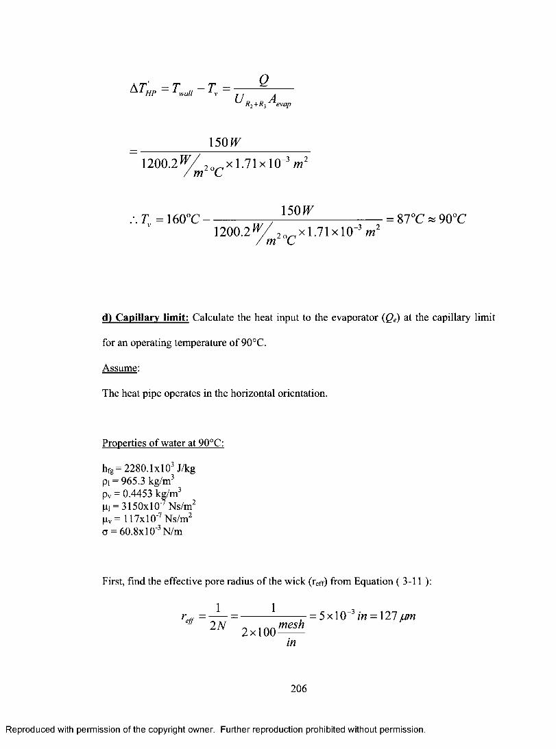
150 W

1200.2 f 2 O s~ym Cx l . 7 1 x 1 0 3 m

T = 1 6 0 ° C -150 IT

= 87°C * 90 °C1200.2 } 2 0/~im C

x 1.71 x 10 3 m

d) Capillary limit: Calculate the heat input to the evaporator (Qe) at the capillary limit

for an operating temperature of 90°C.

Assume:

The heat pipe operates in the horizontal orientation.

Properties of water at 90°C:

hfg= 2280.lx l0 3 J/kg pi = 965.3 kg/m3 pv = 0.4453 kg/m3 pi = 3150xl0'7 Ns/m2 P v = 117xlO_7Ns/m2 a = 60.8xl0~3N/m

First, find the effective pore radius of the wick (reff) from Equation (3-11 ):

206


Veff 2 N - = 5x10 3in = 127um mesh

in

The porosity was calculated above and is equal to:

s = 0 .629

The wick permeability is calculated using Equation ( 3-12 ):

K = = (U 4 3 X ' ° 4 * 0-62^ = 1 .9 3 x 10-'°122(1 - s ) 1 1 2 2 ( 1 - 0 . 6 2 9 )

Now find the wick’s cross-sectional area (Aw). From Figure 4-7, each mesh layer is twice

the wire diameter, and there are 4 layers:

d v = i u b e I . D . - 2 x t w = 8 .001 x lO 3 m - 2 x ( 2 x l , 1 4 3 x l 0 “4m x 4 layers)

d v = 6 .1 7 2 2 x 1 0 “3m

r = ^ = 3 . 0 8 6 1 x 1 0 ~3 m v 2

A = — (tubeI.D .2 - d v2)W ^ v v /

Aw = - ( ( 8 .0 0 1 x 1 0 ' 3 m f - (6 .1 7 2 2 x 1 0 ' 3 m f ) = 2 .0 3 6 x 10 5 m 2

The effective length, leff, is calculated using Equation ( 2-8 ). The length of the heat pipe

is 250.2 mm, while the lengths o f the evaporator (/e) and condenser (/c) sections are 57.15

mm and 66.6 mm respectively:

207


hff = L + e + ^ ~ {heat p ipe length ~ le ~ l c) + ^ + ^eff a ^ v *■ 1 e c / ^

^57.15 + 6 6 .6 ^= ( 2 5 0 . 2 - 5 7 . 1 5 - 6 6 . 6 ) mm +

= 188.325 mm = 0 .188325 m

mmy

From the capillary limit equation of Section 2.1.5:

2 c r p tQ elef f %pvQ J eff .1 + PjgLt sin tp>

V P , A J i f i K n p vR y hfs

The equation will be solved for the heat input to the evaporator, Qe. Since the heat pipe

horizontal, the hydrostatic pressure term is zero. This gives:

2(7

Q e = ^M i l eff + W e f f

p ,A whfgK npvRvhk

Now, solving each term on the right hand side of the above equation:

208


2 x 6 0 .8 x l0 ”3 N / = -----------------_ / » L = 957.5 p flreff 1.27x10 m

u l 3 1 5 0 x l0 '7Ay 2 x0.188325mP i 1 e f f / m

PiAwhfgK 965.3 kg/ 3 X 2 .036x l0 " 5m 2 x 2280.1 x lO 3 J/ x l.9 3 x lO “10 m 23 ykgm

= 6.84m

ft,/ I 8 x l l7 x lO “7Ay 2 x0.188325m° P v l e f f / m

nP v K hte 7t x 0.4453 kg/ , x (3 .0861xl0"3m)4 x 2280.1 xlO 3/ m v 7 / kg

= 0.061m

Substituting the above values into the equation for Qe:

Q e = 9 5 1 5 P a --------- = 139 w

6 .8 4 ^ + 0.061^- m m

el Boiling limit: Calculate the boiling limit for an operating temperature of 90°C.

Assume:

The bubble radius (/?*)is 10‘7 mThe meniscus radius (Rme„) is equal to the effective pore radius o f the wick = 127 pm Use the properties for water at 90°C listed in Part (d)The effective thermal conductivity o f the wick (kefj) is estimated to be 1.486 W/m°C

3 -3The inner container radius (i?,)= 4x10' m, the vapour space radius (7?v)=3.0861xl0' m

209


Using Equation ( 2-17 ), the critical wall-to-vapour temperature is calculated first. Recall

that the vapour temperature (Tv) must be converted to Kelvin:

A T . ^crit1 1

h f g P v V R b R men J

2 X 60.8 X 1 O' 3 N/ X (273.15 + 90)^

) . l x l 0 3 J / x 0 .4 4 5 3 ^ /2280. 1 A T-T_>J / 3kg / n r

1

1 0 -1 m 1 .2 7 x l0 “4 m1

- 4

= 434.6AT

Now calculate the boiling limit with Equation ( 2-19 ):

27iL k . .ATe wick crit2 x x x 0.05715 m x 1.486 W/ K x 434.6 K

In In4 x 1 0 3 m

v 3.0861xl0~3m y

= 893 .6W

Since the heat input due to the capillary limit (Qe = 139 W) is lower than that calculated

due to the boiling limit (Qb = 894 W), the heat pipe will be capillary limited.

210


Appendix B Fluid Charging

Calculate the fluid charge necessary for heat pipe K1 (copper powder wick). Assume the

density of copper is 8954 kg/m .

Measurements:

Post-sintered mass of heat pipe assembly: 0.09167 kg Evaporator end cap clearance: 7.09 mm Condenser end cap clearance: 7.06 mm Tube length: 265.7 mm Vapour core diameter: 4.7625 mm

a) Estim ate porosity:

First, calculate the heat pipe length (L t), equivalent to the wick length:

Lt = tube length — evaporator and condenser end cap clearances

= 2 6 5 .7 m m - 7 ,09mm - 7 ,06mm - 2 5 1 .5 5 mm

The vapour core area is:

A = - d 2 = - ( 4 . 7 6 2 5 x lO ' 3 ) 2 = 1 . 7 8 1 4 x 1 0v 4 v 4 v ’

5 m2

Next, calculate the total wick volume ( V w ic k ):

Vwick = container volume — vapour core volume

j x (8.001 x 10 ~ 3 m f x 0 .25155 mj - (l .7814 x 10 " 5 m2 x 0 .25155 m)

8 . 1 6 6x 10 “6 w 3

211


The wick mass is also required:

mwjck = heat p ipe assembly mass - tube mass

0 .0 9 1 6 7 kg - ^ x \tube O.D.2 - tube I.D.2 ] x L ( x Density o f copper

0 .0 9 1 6 7 % “

= 0 .0 4 1 7 6 %

(9 .5 2 5 x 1(T 3 m f - (8 .001 x 1 0 “3 m f x 0 .2 6 5 7 m x 8 9 5 4 ^ / 3m

With the wick mass known, we may calculate the volume o f solid wick material ( V so iid ) :

Mwck 0 .0 4 1 7 6 %V -s o l id Density o f copper 3 9 5 4 %m3

= 4 . 6 6 4 x 1 0 ~6 m 3

The difference between the total volume o f the wick and the solid volume is the pore

volume. The pore volume divided by the total volume o f the wick is the porosity:

( 8 . 1 6 6 x 1 0 - “ - 4 . 6 6 4 x 1 ( T V

8.166xl(T6 mJ43

b) Calculate the fluid charge:

First, the wick cross-sectional area is required:

212


Aw = ^ x ( tu b e I .D . 2 - < 2)= ((8-001 x lO '3 m f -(4 .7625x1 O'3 m f )

= 3.25x10 ~5 m 2

The fluid charge is calculated using Equation (4-1 ). A 10% overcharge is specified:

= \ . \ ( A vL , p v + A wL l£p)lm

= 1.11 .7 8 1 4 x l0 ”5 m 2 x 0 .2 5 1 5 5 w x 0.5974

m

+ 3 .2 5 x 10“5 m 2 x 0 .2 5 1 5 5 m x 0 .4 3 x 9 5 8 .7 7 ^ / 3 m

213


Appendix C Cooling Jacket Drawings

214

Reproduced with permission of the copyright owner. Further reproduction prohibited without permission

215


216


217


218


219


220


221


222


223


224


225


Appendix D Data Acquisition Program

End

itart] button is clicked?

itop] button is clicked?

Record the Start time

Initialization Output filename

Sam ple Frequency Data Logging Frequency

Elasped Time = Current time - Start time;

GetD ata Download data from 16

TCs, 7 Analog inputs, 1 flow m eter from FiekiPoint a s welll a s the current and

voltage inputs from heater

226


ake Data] button is click*

—N'

rate > max flow

^ - " T e m p e r a tu r e Stability C h e c K ^ \ . Is the max. difference am ong 10 readings

for each TO less than Tem perature R ange?

Append data to output file

Flow rate warning is on

S teady S tate reached

Collect the da ta for 1 minute and append the average to the S teady

S tate file

227


228


229


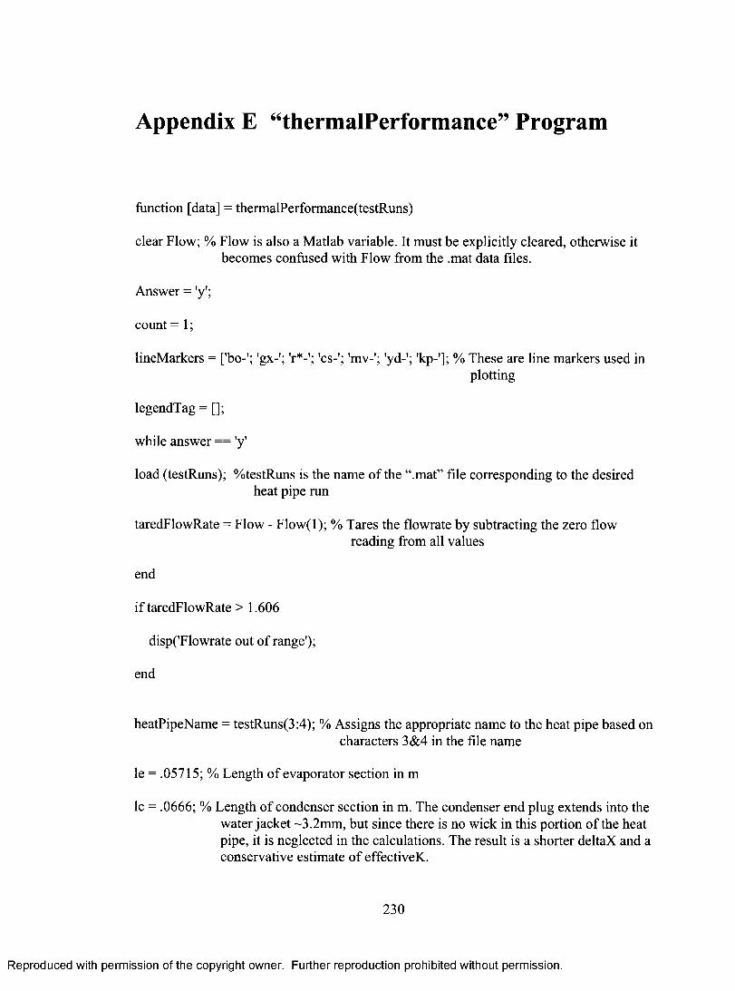
Appendix E “thermalPerformance” Program

function [data] = thermalPerformance(testRuns)

clear Flow; % Flow is also a Matlab variable. It must be explicitly cleared, otherwise it becomes confused with Flow from the .mat data files.

Answer = 'y';

count = 1;

lineMarkers = ['bo-'; 'gx-'; 'r*-'; 'cs-'; 'mv-'; 'yd-'; 'kp-']; % These are line markers used inplotting

legendTag = [];

while answer == 'y'

load (testRuns); %testRuns is the name of the “.mat” file corresponding to the desired heat pipe run

taredFlowRate = Flow - Flow(l); % Tares the flowrate by subtracting the zero flowreading from all values

end

if taredFlowRate > 1.606

disp('Flowrate out of range');

end

heatPipeName = testRuns(3:4); % Assigns the appropriate name to the heat pipe based oncharacters 3&4 in the file name

le = .05715; % Length of evaporator section in m

lc = .0666; % Length of condenser section in m. The condenser end plug extends into the water jacket ~3.2mm, but since there is no wick in this portion of the heat pipe, it is neglected in the calculations. The result is a shorter deltaX and a conservative estimate of effectiveK.

230


la = heatPipeLength - le - lc; % Length of adiabatic section (m)

deltaX = la + ((le + lc)/2); % Average effective length of heat pipe assuming evaporationand condensation occur halfway through the evaporator and condenser

heatln = Voltage.*Current;

%%%%%%CALCULATE HEAT REMOVED%%%%%%

%This entire section describes the heat balance calculations. These results were not included in Section 5.3 , however they are listed here for documentation purposes.

%%%%%%CALCULATE WATER DELTA T%%%%%%

load thermistorCal2252; % Resistance vs temperature thermistor calibration data for 2252ohm (25 C) thermistors

Vsup = 24; % Supply voltage = 24V. Voltage supplied to the voltage divider thermistor circuit.

resistor = 30050; % Resistance o f the constant resistors in the voltage divider thermistor circuits (ohms)

wtrlnletR = AIl*resistor./(Vsup - A ll); % Resistance of the water inlet thermistor in theinlet voltage divider circuit (ohms)

wtrlnletT = interpl(thermistorR, thermistorTemp, wtrlnletR); %Water inlet temperature( C )

wtrOutletR = AI2*resistor./(Vsup - AI2); % Resistance of the water outlet thermistor inthe outlet voltage divider circuit (ohms)

wtrOutletT = interpl(thermistorR, thermistorTemp, wtrOutletR);

waterDeltaT = wtrOutletT - wtrlnletT; % Temperature difference across the water jacket

%waterDeltaT = chlO - ch9;

end

231


%%%%%CALCULATE COOLANT SPECIFIC HEAT & MASS FLOWRATE%%%%

% Coolant properties from Prestone Specific Heat graph and MSDS for Extended Life Coolant. Properties for water are from Holman (Heat Transfer, 9th ed.). A 50/50 volume mixture of distilled water and coolant was used. Considering a 1 L mixture:

averageFluidTemp = (wtrlnletT + wtrOutletT)/2;

load WaterData; % Properties o f water

load specificHeatCoolant; % Contains data on the specific heat o f aqueous Prestonecoolant solutions

waterDensity = interpl(temp, density, averageFluidTemp);

% Assume a constant specific gravity for the coolant, from Prestone MSDS 410. SG = (1.07 + 1.14)/2

coolantSG = (1.07 + 1.14)/2;

% Mass of coolant (kg) per litre = volume(L) x specific gravity of coolant x density of water at cooling fluid average temperature x 1 mA3 per 1000L:

massCoolant = 0.5*coolantSG*waterDensity/1000;

massWater = 0.5*l*waterDensity/1000; % For water, same calculation as above

massPercentCoolant = massCoolant./(massCoolant + massWater)* 100;

% Interpolates to find the specific heat of the coolant/water solution at the average cooling fluid temperature:

specificHeat = interp2(xWeight, yTemp, zSpecificHeat, massPercentCoolant, averageFluidT emp) *4186.8;

coolingSolutionDensity = (massCoolant + massWater)/le-3; %in kg/mA3

massFlowrate = taredFlowRate / (60*1000) .* coolingSolutionDensity; %in kg/s

%%%%%%%%%%%%%%%%%%%%%%%%%%%%%%%%%%%%%%%%%%%

heatOut = massFlowrate.*specificHeat.*waterDeltaT; % Calculation of heat removed

232


%%%%%CALCULATE FREE CONVECTION LOSSES%%%%%

avHeaterlnsTemp = (chi 1 + chl2 + chl3)/3; % Average heater insulation temperature

avAmbientTemp = (ch i4 + chi5)/2; % Average ambient temperature

T f = (avHeaterlnsTemp + avAmbientTemp)/2 + 273.15; %Absolute film temperature (K)

load airData; %Loads air tables

beta = Tf.A-l; % (KA-1)

heaterDia = 0.09; % Approximate diameter of heater wrapped with insulation (m)

heaterLength = 0.085; % Approximate heater length with insulation (m)

% Kinematic viscosity of air at the film temperature (mA2/s):

kinematicViscosity = interpl(airTemp, airKinematicVisc, Tf);

thermalCond = interpl(airTemp, airK, Tf); %Thermal conductivity of air at the filmtemperature (W/m*C)

prandtlNo = interpl(airTemp, airPr, Tf); %Prandtl Number o f air at the film temperature

if findstr(testRuns, 'horizontal') > 0 %Estimate the heat loss to the ambient along thehorizontal heater. Assume isothermal surface, free convection

orientation = ' Horizontal';

% The Rayleigh Number:

GrPr = (9.81.*beta.*abs(avHeaterInsTemp -avAmbientTemp)*heaterDiaA3./kinematicViscosity.A2).*prandtlNo;

denominator = (1 + (0.559./prandtlNo).A(9/16)).A(16/9);

% For 10A-5 < Rayleigh No. < 10A12, Churchill and Chu (in Holman):

Nusselt = (0.6 + 0.387*(GrPr./denominator).A(l/6)).A2;

233


h = Nusselt.*(thermalCond/heaterDia); % The heat transfer coefficient in W/mA2*C

elseif (findstr(testRuns, 'assistG') > 0) % Estimate the heat loss to the ambient along thevertical heater. Assume isothermal surface, free convection

orientation = ' Gravity Assisted';


GrPr = (9.81.*beta.*abs(avHeaterInsTemp -avAmbientTemp)*heaterLengthA3./kinematicViscosity.A2).*prandtlNo;


% For 10A-1 < Rayleigh No. < 10A12:

Nusselt = (0.825 + (0.387*GrPr.A(l/6)./denominator)).A2;

h = Nusselt. *(thermalCond/heaterLength); % The heat transfer coefficient inW/mA2*C

elseif (findstr(testRuns, 'againstG') > 0) % Same equations as for 'assistG' above

orientation = ' Against Gravity';




% For 10A-1 < Rayleigh No. < 10A12:

Nusselt = (0.825 + (0.3 87*GrPr.A( 1/6)./denominator)). A2;

h = Nusselt.*(thermalCond/heaterLength); % The heat transfer coefficient in W/mA2*C

else

orientation = ' Gravity Assisted';

234


%The Rayleigh Number:



Nusselt = (0.825 + (0.387*GrPr.A(l/6)./denominator)).A2; % for 10A-1 < Rayleigh No. < 10A12

h = Nusselt.*(thermalCond/heaterLength); % The heat transfer coefficient inW/mA2*C

disp('Wrong filename');

%retum;

end

heatLoss = h.*(pi*heaterDia*heaterLength).*(avHeaterInsTemp - avAmbientTemp);

%%%%%%%%%%%%%%%%%%%%%%%%%%%%%%%%%%%%%%%%%%%

heatBalance = heatln - heatOut - heatLoss;

heatPipeDeltaT = chi - ch7; % Heat pipe temperature difference between middle ofevaporator to middle of condenser

area = pi/4*9.525e-3A2; % The cross - sectional area of the heat pipe based on the outerdiameter

effectiveK = heatIn*deltaX./(area*heatPipeDeltaT); % The effective thermal conductivityin W/mC

data = [heatln, heatOut, heatLoss, heatBalance, heatPipeDeltaT, effectiveK];

%%%%SCREEN DATA DISPLAY%%%%

disp('Pwr Input(W) Pwr Output(W) Heat Loss(W) Heat Bal.(W) Delta T (C) Keff (W/m*C)');

format bank;

235


disp(data((2: end),:));

%%%%%%%%PLOTTING%%%%%%

lineMarker = lineMarkers(count,:);

count = count + 1;

xx = linspace(min(heatln), max(heatln));

yy = interpl(heatln(2:end), effectiveK(2:end), xx, 'cubic');

%plot(heatIn, effectiveK, lineMarker, xx, yy); plot(heatIn, effectiveK, lineMarker);

hold on;

title('Effective Thermal Conductivity vs Heat Input');

xlabel('Heat Input (W)');

ylabel('K_e_f_f (W/m*C)');

grid on;

legendTag = [legendTag;strcat(heatPipeName, orientation)];

legend(legendTag, 0);

answer = input('Plot another line?');

testRuns = input('Test run?');

end

236


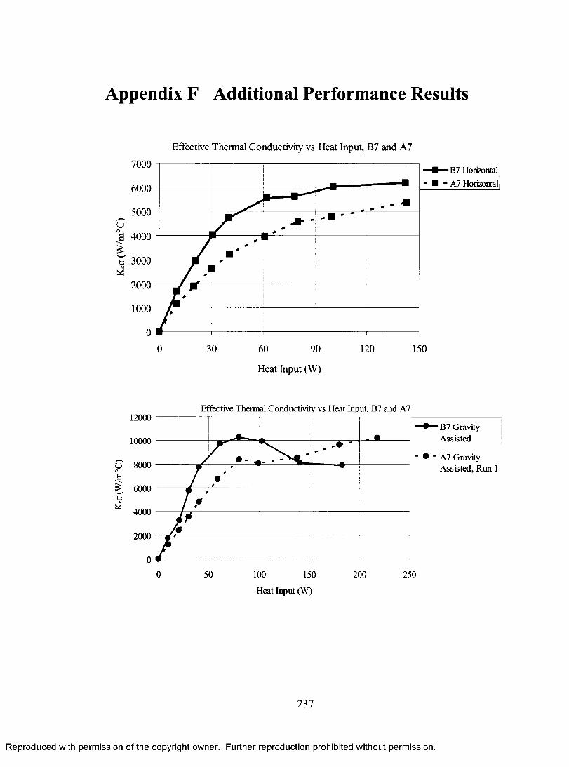
Appendix F Additional Performance Results


7000 M B7 Horizontal

- ■ - A7 Horizontal6000

5000

S 4000

3000

2000

1000

0 30 60 90 120 150

Heat Input (W)


—• “ B7 Gravity Assisted

" • " A7 GravityAssisted, Run 1

10000

U 8000o

£ 6000te

4000

2000

0 50 100 150 200 250

Heat Input (W)

237


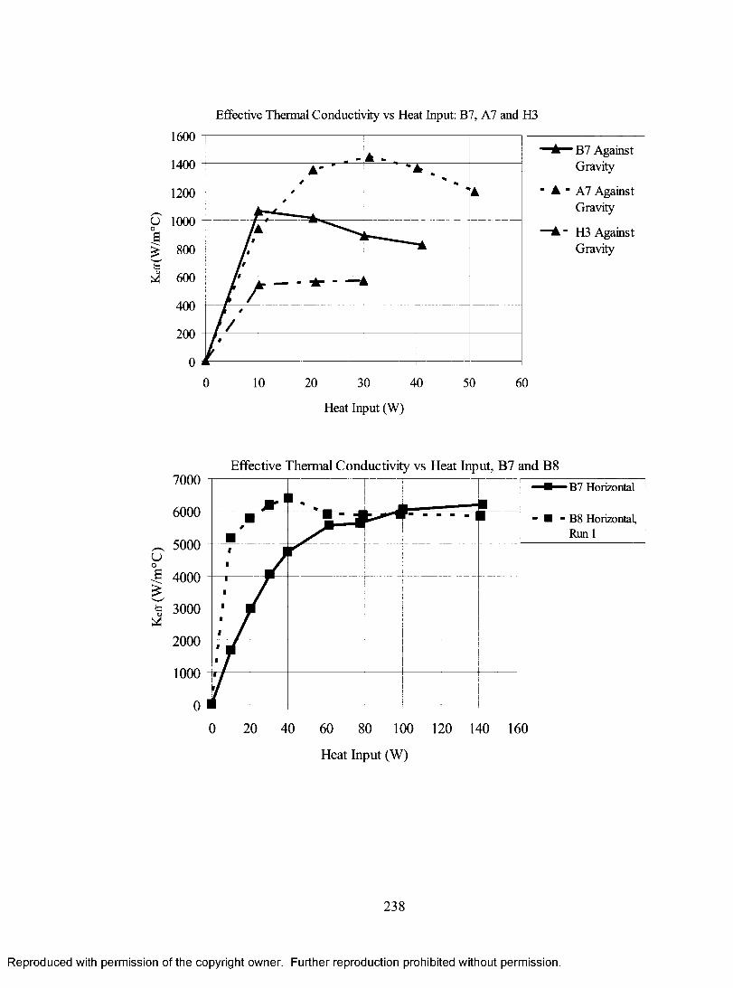
Effective Thermal Conductivity vs Heat Input: B7, A7 and H3

o 1000

"A— B7 Against Gravity


"A - H3 Against Gravity

10 20 30 40

Heat Input (W)

50 60

Effective Thermal Conductivity vs Heat Input, B7 and B87000 B7 Horizontal

6000 ■ - B8 Horizontal, Run 1

^ 5000 U-I 4000 £'ta 3000

2000

1000

0 20 40 60 80 100 120 140 160

Heat Input (W)

238


Kof

f(W/m

°C)

Keff

(W/m

°C)

Effective Thermal Conductivity vs Heat Input, B7 and B814000

B7 Gravity Assisted12000

■ • ■ B8 GravityAssisted, Run 1

10000 —

8000

6000

4000

2000 ■

2500 50 100 150 200

Heat Input (W)

Effective Thermal Conductivity vs Heat Input, B7 and B8

3500—A— B7 Against

Gravity

- ▲ - B8 AgainstGravity, Run 1

3000

2500

2000

1500

1000

500

40 50 600 10 20 30

Heat Input (W)

239


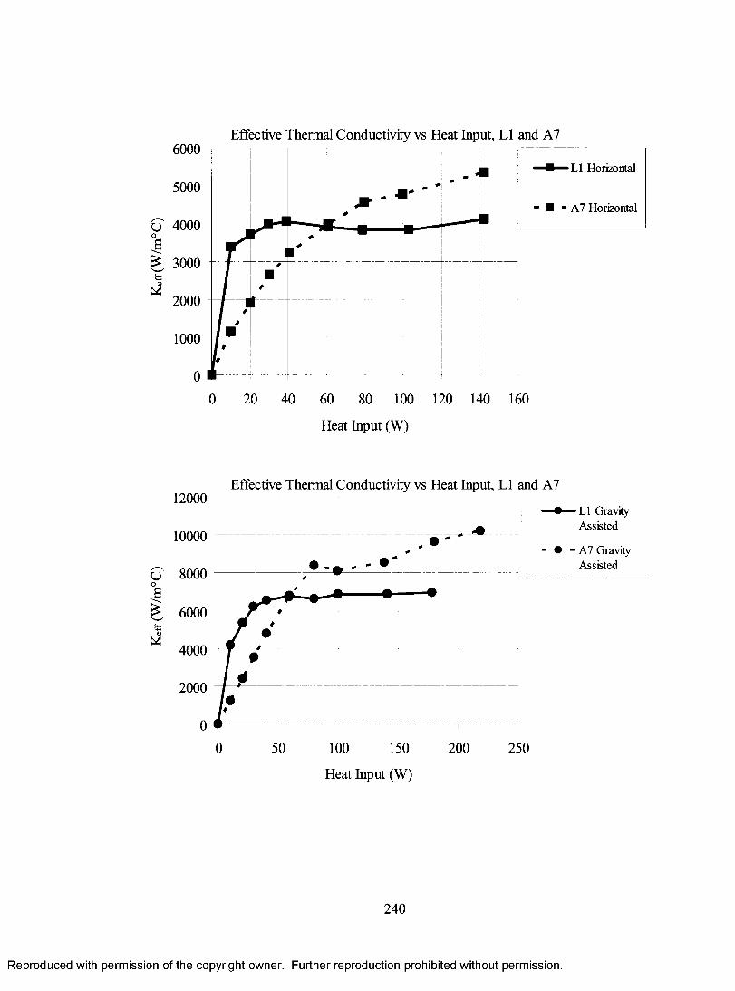
Kefr

(W/m

°C)

Kef

f(W

/m°C

)Effective Thermal Conductivity vs Heat Input, LI and A7

6000LI Horizontal

5000■ - A7 Horizontal

4000

3000

1000

0 20 40 60 80 100 120 140 160

Heat Input (W)

Effective Thermal Conductivity vs Heat Input, LI and A712000

LI Gravity Assisted

10000■ • ■ A7 Gravity

Assisted8000

6000

4000

2000

0 50 100 150 200 250

Heat Input (W)

240


Kef

f(W

/m°C

) Kcf

f (W

/m°C

)

Effective Thermal Conductivity vs Heat Input: LI, A7 and H3

3000—A— LI Against

Gravity

" A - A7 Against Gravity

—A - H3 Against Gravity

2500

2000

1500

1000

0 20 40 60 80

Heat Input (W)

Effective Thermal Conductivity vs Heat Input, LI and L26000

LI Horizontal

5000■ - L2 Horizontal

4000

3000

1000

0 20 40 60 80 100 120 140 160

Heat Input (W)

241


Kcff

(W/m

°C)

Kef

f(W

/m°C

)Effective Thermal Conductivity vs Heat Input, LI and L2

10000LI Gravity Assisted9000

8000 - • - L2 Gravity Assisted7000

6000

5000

4000

3000

20001000

2000 50 100 150

Heat Input (W)

Effective Thermal Conductivity vs Heat Input, LI and L2

3500

LI Against Gravity3000

2500L2 Against Gravity

1500

1000

500

20 40 60 80 1000

Heat Input (W)


Tem

pera

ture

(°C

) Te

mpe

ratu

re

(°C

)

Temperature vs Axial PositionA7: Horizontal Operation

1 0 W

20 W A 30 W

40 W

- * - 6 0 W 80 W 100 W 140 W

100 150 200

Axial Position (mm)

Temperature vs Axial Position A7: Gravity Assisted Operation

■ • - 1 0 W

■m -20 W A 30 W

- ♦ - 4 0 W

- * - 6 0 W

• - 8 0 W

-1— 100 W • — 140 W • — 180 W

* — 220 W

50 100 150 200

Axial Position (mm)

250 300

243


Tem

pera

ture

(°C

) Te

mpe

ratu

re

(°C

)

Temperature vs Axial PositionA7: Against Gravity Operation

180

160

140

120

100

80

60

40

200

- • - 1 0 W - ■ - 2 0 W

A 30 W

- ♦ - 4 0 W—* —50 W

50 100 150 200

Axial Position (mm)

250 300

Temperature vs Axial Position B7: Horizontal Operation

180

160

140

120

100

80

60

40

20

00 50 100 150 200 250 300

Axial Position (mm)

- • - 1 0 W - ■ - 2 0 W

A 30 W

- ♦ - 4 0 W- * - 6 0 W

- • - 8 0 W

—1— 100 W

- ♦ - 1 4 0 W

244


50

Temperature vs Axial PositionB7: Gravity Assisted Operation

10W

40 Wa 10033 - * - 6 0 W

100 W140 W180 W

100 150 200Axial Position (mm)

250 300

O

<u&e<uH

Temperature vs Axial Position B7: Against Gravity Operation

180

160

140

120

100

80

60

40

20

00 50 100 200 250 300150

■ •-10W -■—20 WA 30 W

- ♦ - 4 0 W

Axial Position (mm)

245


Tem

pera

ture

(°C

) Te

mpe

ratu

re

(°C

)

Temperature vs Axial PositionB8: Horizontal Operation, Run 1

180

160

140

120

100

80

60

40

20

050

- • - 1 0 W - ■ - 2 0 W

A 30 W

- ♦ - 4 0 W

- * - 6 0 W

- • - 8 0 W—I— 100 W

- ♦ - 1 4 0 W

100 150 200

Axial Position (mm)

250 300

Temperature vs Axial Position B 8 : Horizontal Operation, Run 2

• - 1 0 W

■ - 2 0 W A 30 W

• - 4 0 W - * - 6 0 W

• - 8 0 W

-I— 100 W ♦ - 140 W

50 100 150 200

Axial Position (mm)

250 300

246


Tem

pera

ture

(°C

) Te

mpe

ratu

re

(°C)

Temperature vs Axial PositionB8: Gravity Assisted Operation, Run 1

120 - ♦

80 -

- • - 1 0 W -■ -2 0 W

A 30 W

- ♦ - 4 0 W—* —60 W - • - 8 0 W—1— 100 W

-♦ -1 4 0 W - • - 1 8 0 W - • - 2 0 0 W

50 100 150 200

Axial Position (mm)

250 300

Temperature vs Axial Position B8: Gravity Assisted Operation, Run 2

!

- • - l o w - ■ - 2 0 W

a 30 W —♦“ 40 W- * - 6 0 W - • - 8 0 W—1— 100 W - ♦ - 1 4 0 W -A -1 8 0 W - • - 2 0 0 W

50 100 150 200

Axial Position (mm)

250 300

247


Temperature vs Axial PositionB8: Against Gravity Operation, Run 1

180

160

140Uo - • - l o w

- ■ - 2 0 WA 30 W

- ♦ - 4 0 W - * - 5 5 W

120<Dt -

5 100cd<Ua£(D

0 50 100 150 200 250 300

Axial Position (mm)

Temperature vs Axial Position B8: Against Gravity Operation, Run 2

180

160

140/*“\Uo 120e32

100(UaS<DH

0 50 100 150 200 250 300

Axial Position (mm)

248


Tem

pera

ture

(°C

) Te

mpe

ratu

re

(°C

)

Temperature vs Axial PositionE7: Horizontal Operation

80 *

• - 1 0 W

■ - 2 0 W A 30 W

- ♦ - 4 0 W- * - 6 0 W

• - 8 0 W

-1— 100 W 4 - 140 W

A — 150 W

50 100 150 200

Axial Position (mm)

250 300

Temperature vs Axial Position E7: Gravity Assisted Operation

■ - 1 0 W ■ - 2 0 W A 30 W

■ - 4 0 W

- * - 6 0 W • - 8 0 W -I— 100 W

4 - 1 4 0 W 4 —180 W

50 100 150 200

Axial Position (mm)

250 300

249


Tem

pera

ture

(°C

) Te

mpe

ratu

re

(°C

)

Temperature vs Axial PositionE7: Against Gravity Operation

180

160

140W120

100

80

60

40

20

0100 150 200 250 3000 50

Axial Position (mm)

Temperature vs Axial Position H3: Horizontal Operation

180

160

140

120

100

80

60

40

20

03000 50 100 150 200 250

Axial Position (mm)


Tem

pera

ture

(°C

) Te

mpe

ratu

re

(°C

)

Temperature vs Axial PositionH3: Gravity Assisted Operation

180

160

140

120

100

60

4020

0

-• -1 0 W - ■ - 2 0 W

A 30 W - ♦ - 4 0 W

50 100 150 200

Axial Position (mm)

250 300

Temperature vs Axial Position H3: Against Gravity Operation

180

160

140

120• - 1 0 W ■ - 2 0 W A 30 W

100

0 50 100 200 250 300150

Axial Position (mm)

251


Tem

pera

ture

(°C

) Te

mpe

ratu

re

(°C

)

Temperature vs Axial PositionJ3: Horizontal Operation

50 100 150 200

Axial Position (mm)

- * -

10W 20 W 30 W

40 W 60 W 80 W

100 W

250 300

Temperature vs Axial Position J3: Gravity Assisted Operation

■•“ 10W * - 2 0 W A 30 W

- ♦ - 4 0 W

- * - 6 0 W• - 8 0 W + - 1 0 0 W • - 1 4 0 W

* - 1 6 0 W

50 100 150 200

Axial Position (mm)

250 300

252


Temperature vs Axial PositionJ3: Against Gravity Operation

180

160

- • - 1 0 W- ■ - 2 0 W

A 30 W

- ♦ - 4 0 W- * - 5 5 W

3 100

} »S 60H

—A.

0 50 150 200 300100 250

Axial Position (mm)

Temperature vs Axial Position K l: Horizontal Operation

180

160

140

120

| 100

I 80I 60H

0 50 200100 150 250 300

Axial Position (mm)

253


Tem

pera

ture

(°C

) Te

mpe

ratu

re

(°C

)

Temperature vs Axial PositionK l: Gravity Assisted Operation

180

160

140

120

100

80

60

40

20

0

-• -1 0 W - ■ - 2 0 WA 30 W

- ♦ - 4 0 W- * - 6 0 W

• - 8 0 W

-I- 100 w♦ - 1 4 0 W A— 180 W

50 100 150 200 250 300

Axial Position (mm)

Temperature vs Axial Position K l: Against Gravity Operation

- • - 1 0 W - ■ - 2 0 W

A 30 W - ♦ - 4 0 W- * - 5 0 W

50 100 150 200

Axial Position (mm)

250 300

254


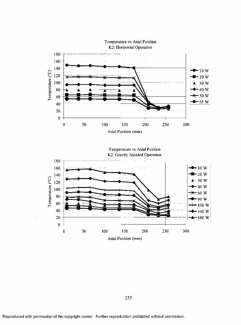
Tem

pera

ture

(°C

) Te

mpe

ratu

re

(°C

)

Temperature vs Axial PositionK2: Horizontal Operation

- • - 1 0 W - ■ - 2 0 W

A 30 W - ♦ - 4 0 W - * - 5 0 W - • - 5 5 W

50 100 150 200

Axial Position (mm)

250 300

Temperature vs Axial Position K2: Gravity Assisted Operation

180

160

140

120

100

80

60

40

20

00 50 100 150 200 250 300

Axial Position (mm)

- * -

10W 20 W

30 W 40 W

60 W 80 W 100 W 140 W

180 W

255


Temperature vs Axial PositionK2: Against Gravity Operation

180

160

_ 140

& 1 2 0--1 100 ♦

lo w20 W

<L>I<UH

250 3000 50 100 150 200

A x i a l P o s i t i o n ( m m )

T e m p e r a t u r e v s A x i a l P o s i t i o n

L I : H o r i z o n t a l O p e r a t i o n

180

160

140Oo 120tub 100<DaS<DH

100 W

H O W

0 50 100 150 200 250 300

A x i a l P o s i t i o n ( m m )

2 5 6


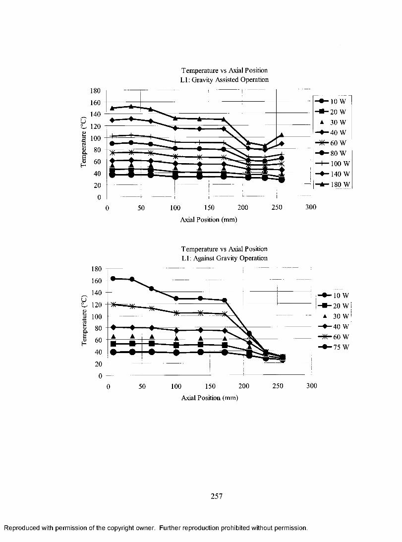
Tem

pera

ture

(°C

) Te

mpe

ratu

re

(°C

)

Temperature vs Axial PositionLI: Gravity Assisted Operation

- • -1 0 W -■—20 WA 30 W

- ♦ - 4 0 W

- * - 6 0 W • - 8 0 W -I— 100 W ♦ - 140 W

* - 1 8 0 W

50 100 150 200 250 300

Axial Position (mm)

Temperature vs Axial Position LI: Against Gravity Operation

— * — — —

wA A A

— ♦ — ▲ A N

- • - 1 0 W - ■ - 2 0 W

A 30 W

- ♦ - 4 0 W

- * - 6 0 W - • - 7 5 W

50 100 150 200

Axial Position (mm)

250 300

257


Tem

pera

ture

(°C

) Te

mpe

ratu

re

(°C

)

Temperature vs Axial PositionL2: Horizontal Operation

180

160 - • - 1 0 W - * - 2 0 W

A 30 W - ♦ - 4 0 W

-3K -60 W

140

120

100 W 140 W

300250200150100

Axial Position (mm)

Temperature vs Axial Position L2: Gravity Assisted Operation

- • - 1 0 W - ■ - 2 0 W

A 30 W

- ♦ - 4 0 W - * - 6 0 W - • - 8 0 W—I— 100 w- ♦ - 1 4 0 W

- • - 1 8 0 W

50 100 150 200

Axial Position (mm)

250 300

258


Tem

pera

ture

(°

C)

Temperature vs Axial PositionL2: Against Gravity Operation

- • - 1 0 W - ■ - 2 0 W

A 30 W

- ♦ - 4 0 W

- * - 6 0 W - • - 8 0 W

50 100 150 200

Axial Position (mm)

250 300

259


7 References

[1] Faghri, A., Heat Pipe Science and Technology, Taylor and Francis, Washington, USA, 1995.

[2] Grover G., Cotter, T., Erikson, G., Structures o f Very High Thermal Conductance, Los Alamos Scientific Laboratory, Los Alamos, New Mexico, 1964.

[3] Cotter, T.P., Theory o f Heat Pipes: Los Alamos Scientific Laboratory Report No. LA-3246-MS, Los Alamos Scientific Laboratory, Los Alamos, New Mexico,1965.

[4] Anon, Thermacore International, Inc. website, www.thermacore.com, 2004

[5] Dunn, P., Reay, D.A., Heat Pipes, Second Edition, Pergamon Press, Oxford, England, 1978.

[6] Ali, A., DeHoff, R., Grubb, K., Advanced Heat Pipe Thermal Solutions fo r Higher Power Notebook Computers, Intel Corporation, Santa Clara, California, 1999.

[7] Anon, Mobile Intel Pentium 4 Processor-MDatasheet, Intel Corporation, Santa Clara, California, 2003.

[8] Lin, S., Sefiane, K., Christy J.R.E., Prospects o f Confined Flow Boiling in Thermal Management o f Microsystems, Applied Thermal Engineering, Vol. 22, pp. 825-837, 2002.

[9] Wang, J., Catton, I., Vaporization Heat Transfer in Biporous Wicks o f Heat Pipe Evaporators, 13th International Heat Pipe Conference, Shanghai, China, pp. 1-11, 2004.

[10] Peterson, G.P., An Introduction to Heat Pipes, John Wiley and Sons, Inc., New York, N.Y., 1994.

[11] Baturkin, V., Zhuk, S., Vojta, J., Lura, F., Biering, B., Lotzke, H., Elaboration o f Thermal Control Systems on Heat Pipes fo r Microsatellites Magion 4, 5 and BIRD, Applied Thermal Engineering, Vol. 23, No. 9, pp 1109-1117, 2003.

[12] Anon, NASA Thermal Engineering Branch website, http://mscweb.gsfc.nasa.gov/545web/groups/p2/projects/glas/glaslhp.html, 2004.

[13] Waters, E.D., Heat Pipes fo r the Trans-Alaska Pipeline, Second International Heat Pipe Conference, Bologna, Italy, 1976.

[14] Anon, Alyeska Pipeline website, http://www.alyeska-pipe.com, 2004.

260


http://www.thermacore.com

http://mscweb.gsfc.nasa.gov/545web/groups/p2/projects/glas/glaslhp.html

http://www.alyeska-pipe.com

[15] Jen, T.C., Gutierrez, G., Eapen, S., Barber, G., Zhao, H., Szuba, P.S., Labataille,J., Manjunathaiah, J., Investigation o f Heat Pipe Cooling in Drilling Applications. Part I: Preliminary Numerical Analysis and Verification, International Journal of Machine Tools and Manufacture, Vol. 42, pp. 643-652, 2002.

[16] Chi, S. W., Heat Pipe Theory and Practice: A Sourcebook, McGraw-Hill Book Company, New York, N.Y., 1976.

[17] Franchi, G., Convective Heat and Mass Transfer Term Project: The Effect o f Wick Parameters on Heat Pipe Performance, Carleton University, 2005.

[18] Leon y Leon, C.A., New Perspectives in Mercury Porosimetry, Advances in Colloid and Interface Science, Vol. 76-77, pp. 341-372, 1998.

[19] Maydanik, Y. F., Fershtater, Y.G., Dimensions o f Pores o f Wicks o f “Antigravity” Heat Pipes, Heat Transfer-Soviet Research, Vol. 17, No. 4, pp. 119-126, 1985.

[20] Canti, G., Celata, G. P., Cumo, M., Furrer, M., Thermal Hydraulic Characterization o f Stainless Steel Wicks fo r Heat Pipe Applications, Revue. Gen. Thermique., Vol. 37, pp. 5-16, 1998.

[21 ] Busse, C. A., Pressure Drop in the Vapor Phase o f Long Heat Pipes, Proc. IEEEConf. o f Thermionic Conversion Specialists, Palo Alto, CA., pp. 1279-1287,1967.

[22] Levy, E.K., Theoretical Investigation o f Heat Pipes Operating at Low Vapour Pressures, Trans. Am. Soc. Mech. Engrs., Vol. 90B, p. 547, 1968.

[23] Mughal, M.P., Plumb, O.A., An Experimental Study o f Boiling on a Wicked Surface, International Journal o f Heat and Mass Transfer, Vol. 39, No. 4, pp. 771-777, 1996.

[24] Shaubach, R.M.., Dussinger, P.M., Bogart, J.E, Boiling in Heat Pipe Evaporator Wick Structures, Proceedings o f the 7th International Heat Pipe Conference,Minsk, Belarus, 1990.

[25] Gu, J., Convective Heat and Mass Transfer Course Notes: Boiling, Carleton University, Ottawa, 2005.

[26] Holman, J.P., Heat Transfer, Ninth Edition, McGraw-Hill, New York, NY, 2002.

[27] Bergles, A.E., Rohsenow, W.M., ASME Journal o f Heat Transfer, Vol. 86, p. 365-371, 1964.

[28] Brautsch, A., Kew, P., Examination and Visualization o f Heat Transfer Processes During Evaporation in Capillary Porous Structures, Applied Thermal Engineering, Vol. 22, pp. 815-824, 2002.

261


[29] Cotter, T.P., Heat Pipe Startup Dynamics, Proceedings of the 1967 Thermionic Conversion Specialist Conference, pp. 344-348, Palo Alto, California, 1967.

[30] Zuo, Z.J., Faghri, A., A Network Thermodynamic Analysis o f the Heat Pipe, International Journal of Heat and Mass Transfer, Vol. 41, No. 11, pp. 1473-1484, 1998.

[31] Abo El-Naser, A., El-Haggar, S.M., Effective Thermal Conductivity o f Heat Pipes, Heat and Mass Transfer, Vol. 32, pp. 97-101, 1996.

[32] Moran, M.J., Shapiro, H.N., Fundamentals o f Engineering Thermodynamics, 4th Edition, John Wiley and Sons, New York, N.Y., 2000.

[33] Anon, The Chemical Institute o f Canada, Hamilton Section website, http://home.nas.net/~dbc/cic_hamilton/dictionary/c.html, 2004.

[34] Tien, Chen, Non-Condensable Gases in Heat Pipes, 5th International Heat Pipe Conference, Tsukuba, Japan, 1984.

[35] Kreeb, H., Groll, M., Zimmerman, P., Life Test Investigations with Low Temperature Heat Pipes, 1st International Heat Pipe Conference, Stuttgart, 1973.

[36] Yamamoto, Tanaka, Long-Term Test o f Sodium Heat Pipe, 5th International Heat Pipe Conference, Tsukuba, Japan, 1984.

[37] Busse, C.A., Campanile, A, Loens, J . , , Hydrogen Generation in Water Heat Pipes at 250°C, 1st International Heat Pipe Conference, Stuttgart, 1973.

[38] Dunn, P., Reay, D.A., Heat Pipes, Third Edition, Pergamon Press, New York, 1982.

[39] Williams, R., Harris, D., Cross-Plane and In-Plane Porous Properties Measurements o f Thin Metal Felts: Applications in Heat Pipes, Experimental Thermal and Fluid Science, Vol. 27, pp 227-235, 2003.

[40] Anon, Cleveland Wire Cloth company website, www.wirecloth.com/rawmaterials.html, 2004.

[41] Anon, International Wire Weavers Association website, www.wire-cloth.com/reference/glossary.htm, 2004.

[42] Gupta, A., Upadhya, G., Optimization o f Heat Pipe Wick Structures fo r Low Wattage Electronics Cooling Applications, Advances in Electronics Packaging, Vol. 2, pp. 2129-2137, 1999.

[43] Imura, H., Kozai, H., Ikeda, Y., Effective Pore Radius o f Screen Wicks, Heat Transfer Engineering, Vol. 15, No. 4, pp. 24-32, 1994.

262


http://home.nas.net/~dbc/cic_hamilton/dictionary/c.html

http://www.wirecloth.com/rawmaterials.html

http://www.wire-cloth.com/reference/glossary.htm

[44] Marcus, B. D., Theory and Design o f Variable Conductance Heat Pipe, Report No. CR-2018, NASA, Washington, D.C., 1972.

[45] Hoa, C., Demolder, B., Alexandre, A., Roadmap fo r Developing Heat Pipes fo r ALCATEL SPACE’s Satellites, Applied Thermal Engineering, Vol. 23, pp. 1099- 1108,2003.

[46] Wang, J., Catton, I., Enhanced Evaporation Heat Transfer in Triangular Grooves Covered with a Thin Fine Porous Layer, Applied Thermal Engineering, Vol. 21, pp. 1721-1737, 2001.

[47] Groll, M., Schneider, M., Sartre, V., Zaghdoudi, M.C., Lallemand, M., Thermal Control o f Electronic Equipment by Heat Pipes, Revue Gen. Thermique, Vol. 37, pp 323-352, 1998.

[48] Beddoes, J., Bibby, M.J., Principles o f Metal Manufacturing Processes, JohnWiley & Sons, Inc., New York, N.Y., 1999.

[49] Peterson, G.P., Modeling, Fabrication and Testing o f Micro Heat Pipe Arrays: AnUpdate, Applied Mechanics Review, Vol. 49, No. 10, Part 2, pp. S175-S183,1996.

[50] Groover, M. P., Fundamentals o f Modern Manufacturing, Second Edition, John Wiley and Sons, Inc., New York, N.Y., 2002.

[51] Leong, K.C., Liu, C.Y., Characterization o f Sintered Copper Wicks Used in Heat Pipes, Journal of Porous Materials, Vol. 4, pp. 303-308, 1997.

[52] Reimbrecht, E.G., Wendhausen, P., Fredel, M.C., Bazzo, E., Manufacturing o f Flat Porous Structures fo r Capillary Pump Applications, Key Engineering Materials, Vols. 189-191, pp. 455-460, 2001.

[53] Dowson, G., Powder Metallurgy: The Process and its Products, IOP PublishingLtd, Bristol, England, 1990.

[54] Callister, W., Materials Science and Engineering: An Introduction, John Wiley and Sons, Inc., N.J., 2003.

[55] Banhart, J., Manufacture, Characterization and Application o f Cellular Metals and Metal Foams, Progress in Materials Science, Vol. 46, pp. 559-632, 2001.

[56] German, R. M., Powder Metallurgy Science, 2nd Edition, Metal Powder Industries Federation, Princeton N.J., 1994.

[57] Beddoes, J., MAAE 4102 Course Notes, Chapter 7: Creep, Carleton University, Ottawa, 2003.

263


[58] Tracey, V.A., Sintering o f Porous Nickel-Theoretical and Practical Considerations, Modem Developments in Powder Metalllurgy, Vol. 12, pp. 423- 438, 1981.

[59] Kajikawa, T., Takazawa, H., Heat Transfer Performance o f Metal Fiber Sintered Surfaces, Heat Transfer Engineering, Vol. 4, N o.l, pp. 57-66, 1983.

[60] North, M., Rosenfeld, R., Liquid Film Evaporation from Bidisperse Capillary Wicks in Heat Pipe Evaporators, 9th International Heat Pipe Conference, Albuquerque, NM, pp. 143-147, 1995.

[61] Hanlon, M., Ma, H., Evaporation Heat Transfer in Sintered Porous Media, Transactions of the ASME, Vol. 125, pp. 644-652, 2003.

[62] Wang, J., Merilo, E., Catton, I., Investigation o f Evaporation Heat Transfer in Porous Wicks fo r High Heat Flux Applications, Proceedings o f ASME NHTC’01 35th National Heat Transfer Conference, pp. 1063-1070, Anaheim, California, 2001 .

[63] Konev, S.K., Polasek, F., Horvat, L., Investigation o f Boiling in Capillary Structures, Heat Transfer-Soviet Research, Vol. 19, No. l,p p . 14-17, 1987.

[64] Wang, J., Catton, W., Biporous Heat Pipes fo r High Power Electronic Device Cooling, 17th IEEE SEMI-THERM Symposium, pp. 211-218, 2001.

[65] North, M., Sarraf, D., Rosenfeld, J., High Heat Flux Loop Heat Pipes, Proceedings of the 6th European Space Symposium, Noordwijk, The Netherlands, pp. 371-376, 1997.

[66] Semenic, T., Lin, Y., Catton, I., Use o f Liquid Film Evaporation in Biporous Media to Achieve High Heat Flux over Large Areas, Proceedings o f 2005 ASME Summer Heat Transfer Conference, San Francisco, CA, pp. 63-68, 2005.

[67] Cao, X.L., Cheng, P., Zhao, T.S., Experimental Study o f Evaporative Heat Transfer in Sintered Copper Bidispersed Wick Structures, Journal Of Thermophysics and Heat Transfer, Vol. 16, No. 4, 2002.

[68] Anon, McMaster-Carr website, www.mcmaster.com, 2006.

[69] Smithells, C.J., Brandes, E.A., Brook, G.B., Smithells Metals Reference Book, 7th Edition, Butterworth-Heinemann, Oxford, Boston, 1998.

[70] Anon, Copper Development Association Website, www.copper.org/resources/properties, 2006.

[71] Anon, Sulzer Metco Website, www.sulzermetco.com, 2006.

264


http://www.mcmaster.com

http://www.copper.org/resources/properties

http://www.sulzermetco.com

[72] Huang, X., Franchi, G., Hybrid Wicking Material fo r Use in High Performance Heat Pipes, US patent, 11/185,013 filed July 20, 2005 and PCT/CA 2005/00001141 filed July 20, 2005.

[73] Anon, INCO Type 255 Filamentary Nickel Powder Product Data Sheet, www.incosp.com/pdf/sp_nickelType255_en.pdf, 2006.

[74] Anon, Cole-Parmer Refrigerated Recirculation Chiller Operator’s Manual, Cole- Parmer Instrument Company, Vemon Hills, IL, 1999.

[75] Anon, The Temperature Handbook, Omega Engineering, Inc., Stamford, CT.,2003.

[76] Anon, Fluke 45 Dual Display Multimeter User’s Manual, Fluke Corporation, Everett, WA, 1999.

[77] Anon, Low Volume Rotating Vane Flowmeter Model DPM, Kobold Messring GmbH, Hofheim/Taunus, Germany, 2005.

[78] Anon, FieldPoint Operating Instructions: FP-TC-120 and cFP-TC-120 8- Channel Thermocouple Input Modules, National Instruments Corporation, Austin, TX, 2005.

[79] Anon, FieldPoint Operating Instructions: FP-AI-100 and cFP-AI-100 Eight- Channel, 12-Bit Analog Input Modules, National Instruments Corporation, Austin, TX, 2005.

[80] Anon, FieldPoint FP-1000/FP-1001 User Manual, National Instruments Corporation, Austin, TX, 2003.

[81] Anon, OMEGA THERMm Thermally Conductive Silicone Paste Instruction Sheet, Omega Engineering, Inc., Stamford, CT., 2005.

[82] Kempers, R., Robinson, A., Ching, C., Ewing, D., Effect o f Fluid Loading on the Performance o f Wicked Heat Pipes, Proceedings of the 2004 ASME Heat Transfer/Fluids Engineering Division Summer Meeting, North Carolina, U.S.A.,2004.

[83] Wadden, J., Introductory Physics o f Electromagnetism with Engineering Applications: 75.104 Lab Manual, Carleton University, Ottawa, 1999.

[84] Wheeler, A.J., Ganji, A.R., Introduction to Engineering Experimentation, Prentice-Hall, Inc., New Jersey, 1996.

265


http://www.incosp.com/pdf/sp_nickelType255_en.pdf

NOTE TO USERS - CURVE | Carleton University Research ...

Documents

Transcript of NOTE TO USERS - CURVE | Carleton University Research ...