CARLETON UNIVERSITY

SCHOOL OF

MATHEMATICS AND STATISTICS

HONOURS PROJECT

TITLE: Selected Methods of Cluster Analysis

AUTHOR: Qiang Xu

SUPERVISOR: Dr. Natalia Stepanova

DATE: May 3rd, 2021

Contents

1 Introduction 5

1.1 De�nitions . . . . . . . . . . . . . . . . . . . . . . . . . . . . . . . . . . . 5

1.2 Examples of the use of cluster analysis . . . . . . . . . . . . . . . . . . . 6

1.2.1 Astronomy . . . . . . . . . . . . . . . . . . . . . . . . . . . . . . . 6

1.2.2 Archaeology . . . . . . . . . . . . . . . . . . . . . . . . . . . . . . 7

1.2.3 Market research . . . . . . . . . . . . . . . . . . . . . . . . . . . . 8

2 Similarity Measures 8

2.1 Distances and Similarity Coe�cients for Pairs of Items . . . . . . . . . . 8

2.2 Examples . . . . . . . . . . . . . . . . . . . . . . . . . . . . . . . . . . . 11

3 Hierarchical Clustering Methods 18

3.1 Linkage Methods . . . . . . . . . . . . . . . . . . . . . . . . . . . . . . . 19

3.1.1 Single Linkage . . . . . . . . . . . . . . . . . . . . . . . . . . . . . 19

3.1.2 Complete Linkage . . . . . . . . . . . . . . . . . . . . . . . . . . . 20

3.2 Examples . . . . . . . . . . . . . . . . . . . . . . . . . . . . . . . . . . . 21

3.3 Ward's Hierarchical Clustering Method . . . . . . . . . . . . . . . . . . . 25

3.4 Final Comments on Hierarchical Procedures . . . . . . . . . . . . . . . . 26

4 Nonhierarchical Clustering Methods 27

4.1 K-means Method . . . . . . . . . . . . . . . . . . . . . . . . . . . . . . . 27

4.2 Example . . . . . . . . . . . . . . . . . . . . . . . . . . . . . . . . . . . . 27

4.3 Final Comments�Nonhierarchical Procedures . . . . . . . . . . . . . . . . 30

5 Clustering Based on Statistical Models 31

6 Correspondence Analysis 36

6.1 Algebraic Development of Correspondence Analysis . . . . . . . . . . . . 36

6.2 Inertia . . . . . . . . . . . . . . . . . . . . . . . . . . . . . . . . . . . . . 43

6.3 Interpretation of Correspondence Analysis in Two Dimensions . . . . . . 44

6.4 Example . . . . . . . . . . . . . . . . . . . . . . . . . . . . . . . . . . . . 44

7 Conclusion 46

2

8 Appendix I 50

9 Appendix II 55

3

Abstract

The goal of this honours project is to explore the basics of cluster analysis from

Applied Multivariate Statistical Analysis (6th Edition) by Richard A. Johnson and

Dean W. Wichern [7], illustrate the use of various cluster procedures by solving

selected exercises from Chapter 12, and hone the skills of writing technical papers

using LATEX2ε.

4

1 Introduction

An intelligent being cannot treat every object it sees as a unique entity unlike

anything else in the universe. It has to put objects in categories so that it

may apply its hard-won knowledge about similar objects encountered in the

past, to the object at hand.

Steven Pinker, How the Mind Works [10]

One of basic abilities of human being is grouping of similar objects to produce clas-

si�cation; the idea of sorting similar things into categories is essential to human being's

mind. For example, early man must have been able to realize that many individual

objects had certain properties such as being edible, or poisonous, etc. Classi�cation is

also fundamental to most branches of scienti�c pursues. For instance, the classi�cation

of the elements in the periodic table produced by D. I. Mendeleyev in the 1860s has

helped to understand the structure of the atom profoundly. A classi�cation represents

a convenient method for organizing a large data set so that it can be understood more

easily and information can be retrieved more e�ciently. If the data can be summarized

by a small number of groups of objects, then the group labels may provide a very con-

cise description of patterns of similarities and di�erences in the data. Because of the

growing number of large databases, the need to summarize data sets in this way and

extract useful information or knowledge is increasingly important.

1.1 De�nitions

Cluster, group, and class have been used in the statistical literature interchangeably

without formal de�nition. Many, for example, Gordon [3], attempt to de�ne what is a

cluster in terms of homogeneity (internal cohesion) and external isolation (separation);

but others, for example, Bonner [1], suggest that the criterion for evaluating the meaning

of cluster is the value judgment of the researcher, that is, if the term of cluster produces

an answer of value to the researcher, that is all that matters. This may explain why

so many attempts to di�erentiate the concepts of homogeneity and separation mathe-

matically proliferate numerous and diverse criteria, sometimes leading to confusion in

practice. The attempt to de�ne the term of cluster mathematically precise is beyond

the scope of the project, so we will leave it as it be.

Cluster analysis concerns about searching for patterns in a data set by grouping the

multivariate observations into clusters in order to �nd an optimal grouping by which

5

the observations or objects within each cluster are similar but the clusters are dissimilar

to each other. The goal of cluster analysis is to �nd the �natural groupings� in the data

set that make sense to the researcher.

Cluster analysis is also referred to as classi�cation, pattern recognition (speci�cally,

unsupervised learning), and numerical taxonomy. Classi�cation and clustering are often

used interchangeably in the literature, but we wish to di�erentiate them for the project.

In classi�cation, we assign new observations to one of several groupings, the number of

which is prede�ned. In cluster analysis, neither the number of groups nor the groups

themselves are unknown in advance.

The basic data for most applications of cluster analysis is the usual n×p multivariatedata matrix containing the variable values describing each object to be clustered. The

data matrix can be de�ned as

Y =

y>1

y>2...

y>n

=(y(1),y(2), · · ·y(p)

), (1)

where y>i is a row observation vector and y(j) is a column corresponding to a variable.

We usually wish to group ny>i 's rows into g clusters, but may also cluster the columns

y(j), j = 1, 2, . . . , p.

Many techniques employed in cluster analysis begin with similarities between all pairs

of observations. It means that the data points required to be measured similarly or at

least from which similarities can be computed. In practice, there exist time constraints

that make it almost impossible to determine the best grouping of similar objects from

a list of all possible structure. Thus, we should settle for algorithms searching for good,

but not necessarily the best, groupings.

1.2 Examples of the use of cluster analysis

Cluster analysis appears in many disciplines such as biology, botany, medicine, psychol-

ogy, geography, marketing, image processing, psychiatry, archaeology, etc. We brie�y

discuss several applications of cluster analysis.

1.2.1 Astronomy

Large multivariate astronomical data frequently contain relatively distinct groups of

objects which can be distinguished from each other. Astronomers want to know how

6

many groups of stars there exist on the some sorts of statistical criterion. Cluster analysis

can be used to classify astronomical objects and let astronomers �nd unusual objects.

For example, discoveries of high-redshift quasars, type 2 quasars, and brown dwarfs.

The Hertzsprung-Russell plot (see Figure 1: Hertzsprung-Russell-Diagram, Montmerle

[9]) of temperature vs. luminosity helps to classify stars into dwarf stars, giant stars,

and main sequence stars that develops theories of stellar evolution and forecasts the life

expectancy of the Sun.

Figure 1: Hertzsprung-Russell Diagram

1.2.2 Archaeology

In archaeology, the classi�cation of artifacts help to �nd their di�erent uses, the pe-

riods they were used and who used by. And the study of fossilized material can help

to understand how prehistoric societies lived. For example, Hodson et al. [6] applied

single linkage and average linkage clustering to brooches from the Iron Age and found

classi�cations of archaeological signi�cance; Hodson [5] used a k-means clustering tech-

nique to classify hand axes found in the British Isles, and variables used to describe the

axes included length, breadth and pointedness at the tip, which resulted in two clusters:

thin, small axes and thick, large axes used for di�erent purposes.

7

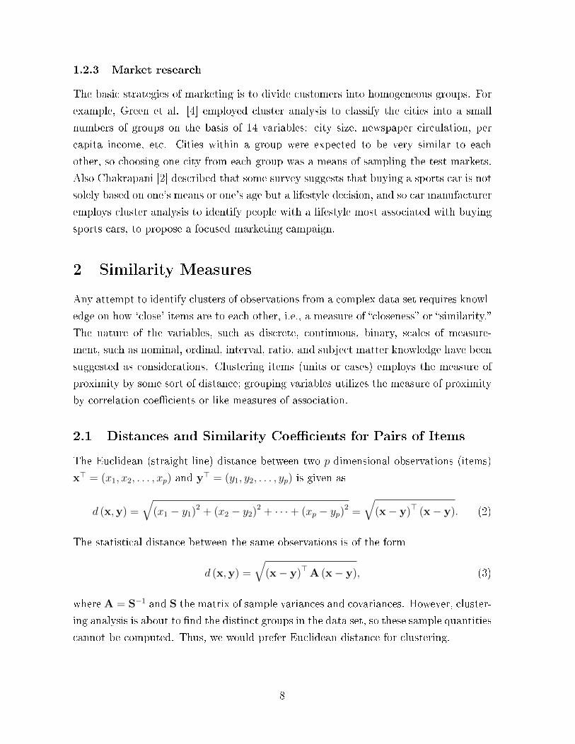
1.2.3 Market research

The basic strategies of marketing is to divide customers into homogeneous groups. For

example, Green et al. [4] employed cluster analysis to classify the cities into a small

numbers of groups on the basis of 14 variables: city size, newspaper circulation, per

capita income, etc. Cities within a group were expected to be very similar to each

other, so choosing one city from each group was a means of sampling the test markets.

Also Chakrapani [2] described that some survey suggests that buying a sports car is not

solely based on one's means or one's age but a lifestyle decision, and so car manufacturer

employs cluster analysis to identify people with a lifestyle most associated with buying

sports cars, to propose a focused marketing campaign.

2 Similarity Measures

Any attempt to identify clusters of observations from a complex data set requires knowl-

edge on how `close' items are to each other, i.e., a measure of �closeness� or �similarity.�

The nature of the variables, such as discrete, continuous, binary, scales of measure-

ment, such as nominal, ordinal, interval, ratio, and subject matter knowledge have been

suggested as considerations. Clustering items (units or cases) employs the measure of

proximity by some sort of distance; grouping variables utilizes the measure of proximity

by correlation coe�cients or like measures of association.

2.1 Distances and Similarity Coe�cients for Pairs of Items

The Euclidean (straight-line) distance between two p-dimensional observations (items)

x> = (x1, x2, . . . , xp) and y> = (y1, y2, . . . , yp) is given as

d (x,y) =

√(x1 − y1)2 + (x2 − y2)2 + · · ·+ (xp − yp)2 =

√(x− y)> (x− y). (2)

The statistical distance between the same observations is of the form

d (x,y) =

√(x− y)>A (x− y), (3)

where A = S−1 and S the matrix of sample variances and covariances. However, cluster-

ing analysis is about to �nd the distinct groups in the data set, so these sample quantities

cannot be computed. Thus, we would prefer Euclidean distance for clustering.

8

The third distance measure is the Minkowski metric

d (x,y) =

[p∑i=1

|xi − yi|m]1/m

. (4)

Two additional popular measures of �distance� are Canberra metric and the Czekanowski

coe�cient which are both de�ned for nonnegative variables. We have

Canberra metric:

d (x,y) =

p∑i=1

|xi − yi|(xi + yi)

. (5)

Czekanowski coe�cient:

d (x,y) = 1− 2∑p

i=1 min (xi, yi)∑pi=1 (xi + yi)

. (6)

Manhattan distance:

d (x,y) =

p∑i=1

|xi − yi| . (7)

It is always advisable to use �true� distances for clustering objects. However, most

clustering algorithms do accept subjectively assigned distance numbers that may not

satisfy the triangle inequality.

In situation where items cannot be accessed by meaningful p-dimensional measure-

ments, we would compare them on the basis of the presence or absence of certain charac-

teristics. The presence or absence of a characteristic can be represented mathematically

by a binary variable, which assumes the value of 1 if the characteristic is present and

the value of 0 if absent. For example, for p = 5 binary variables, the �scores� of two

items i and k might be arranged as in Table 1.

Table 1: Example

Variables1 2 3 4 5

Item i 1 0 0 1 1Item k 1 1 0 1 0

In this table, we have two 1− 1 matches, one 1− 0 mismatch, one 0− 1 mismatch,

and one 0− 0 matches.

Let xij be the score (1 or 0) of the j th binary variable on the ith item and xkj be

9

the score of the jth binary variable on the kth item, j = 1, 2, . . . , p. Therefore, if we let

(xij − xkj)2 =

0 if xij = xkj = 1 or xij = xkj = 0,

1 if xij 6= xkj,(8)

then the squared distance,∑p

j=1 (xij − xkj)2, counts the number of mismatches. A large

distance corresponds to many mismatches, or dissimilar items. The above example gives

us the following distance:

5∑j=1

(xij − xkj)2 = (1− 1)2 + (0− 1)2 + (0− 0)2 + (1− 1)2 + (1− 0)2 = 2.

The result of 2 indicates that there are two mismatches in the example.

A distance based on (7) weights the 1−1 and 0−0 matches equally. In some cases, a

1−1 match indicates a stronger similarity than a 0−0 match. For instance, in grouping

people, two persons both read Chinese is stronger support to similarity than the absence

of this ability. To di�erential treatment of the 1 − 1 matches and the 0 − 0 matches,

mathematicians have suggested several schemes for de�ning similarity coe�cients.

First, we need to arrange the frequencies of matches and mismatches for items i and

k in the form of a contingency table (see Table 2). Table 3 lists common similarity

coe�cients de�ned in terms of the frequencies in the Table 2. Coe�cients 1, 2, and 3

in Table 3 are related monotonically. For instance, coe�cient 1 is calculated for two

contingency tables, Table I and Table II; then if (aI + dI) /p > (aII + dII) /p, we also

have

2 (aI + dI) / [2 (aI + dI) + bI + cI] > 2 (aII + dII) / [2 (aII + dII) + bII + cII] ,

and coe�cient 3 will be at least as large for Table I as it is for Table II. And coe�cient

5, 6, and 7 also retain their relative orders.

Table 2: Contingency Table

Item k

1 0 Totals

Item i1 a b a+ b0 c d c+ d

Totals a+ c b+ d p = a+ b+ c+ d

Monotonicity (or maintaining relative orders) is important because certain clustering

10

algorithms are not a�ected if the de�nition of similarity is changed in a fashion that

retains the relative orderings of similarities. For instance, the single linkage and complete

linkage hierarchical procedures discussed below are not a�ected. Hence, any choice of

the coe�cients 1, 2, and 3 in Table 3 will produce the same groupings. Similarly, any

choice of the coe�cients 5, 6, and 7 will produce identical clusters.

Table 3: Similarity Coe�cients for Clustering Items*

Coe�cient Rationale

1. a+dp

Equal weights for 1− 1 matches and 0− 0 matches.

2. 2(a+d)2(a+d)+b+c

Double weight for 1− 1matches and 0− 0 matches.

3. a+da+d+2(b+c)

Double weight for unmatched pairs.

4. ap

No 0− 0 matches in numerator.

5. aa+b+c

No 0− 0 matches in numerator or denominator.

(The 0− 0 matches are treated as irrelevant.)

6. 2a2a+b+c

No 0− 0 matches in numerator or denominator.

Double weight for 1− 1 matches.

7. aa+2(b+c)

No 0− 0 matches in numerator or denominator.

Double weight for unmatched pairs.

8. ab+c

Ratio of matches to mismatches with 0− 0 matches

excluded.

*[p binary variables; see Table 2.]

2.2 Examples

Example 1 (Example 12.1 from Johnson and Wichern [7]: Calculating the

values of a similarity coe�cient). Suppose �ve individuals posses the following

characteristics:

Table 4: Characteristics of Five Individuals

Eye HairHeight Weight color color Handedness Gender

Individual 1 68 in 140 lb green blond right femaleIndividual 2 73 in 185 lb brown brown right maleIndividual 3 67 in 165 lb blue blond right maleIndividual 4 64 in 120 lb brown brown right femaleIndividual 5 76 in 210 lb brown brown left male

De�ne six binary variables X1, X2, X3, X4, X5, X6 as follows:

11

X1 =

1 height > 72 in.

0 height < 72 in.X4 =

1 blond hair

0 not blond hair

X2 =

1 weight > 150 lb

0 weight < 150 lbX5 =

1 right handed

0 left handed

X3 =

1 brown eyes

0 otherwiseX6 =

1 female

0 male

The scores for individuals 1 and 2 on the p = 6 binary variables are as in Table 5,

Table 5: Binary Variables

X1 X2 X3 X4 X5 X6

Individual 1 0 0 0 1 1 1

2 1 1 1 0 1 0

and the number of matches and mismatches are indicated in the two-way array in

Table 6.

Table 6: Two-way Array of Individual 1 and 2

Individual 2

Individual 1 1 0 Total

1 1 2 3

0 3 0 3

Total 4 2 6

Using similarity coe�cient 1, which gives equal weight to matches, we have

a+ d

p=

1 + 0

6=

1

6.

Under equal weight scheme, 1− 1 match occurs once every six times.

Example 2 (Exercise 12.1 from Johnson and Wichern [7]). Certain charac-

teristics associated with a few recent U.S. presidents are listed in Table 7.

(a) Introducing appropriate binary variables, calculate similarity coe�cient 1 in Ta-

ble 7 for pairs of presidents.

(b) Proceeding as in part (a), calculate similarity coe�cients 2 and 3 in Table 3.

Verify the monotonicity relation of coe�cient 1, 2, and 3 by displaying the order of the

15 similarities for each coe�cient.

12

Table 7: Information Concerning Six Presidents of USA

President

Birthplace

(region of

United States

Elected �rst

term?Party

Prior U.S.

congressional

experience?

Served as

vice

president?

1. R. Reagan Midwest Yes Republican No No

2. J. Carter South Yes Democrat No No

3. G. Ford Midwest No Republican Yes Yes

4. R. Nixon West Yes Republican Yes Yes

5. L. Johnson South No Democrat Yes Yes

6. J. Kennedy East Yes Democrat Yes No

Solution: (a) Introduce �ve binary variables X1, X2, X3, X4 and X5 as follows:

X1 =

1 South

0 Non-south

X2 =

1 Elected �rst term

0 Not Elected �rst term

X3 =

1 Republican party

0 Democrat party

X4 =

1 Prior U.S. congressional experience

0 Not Prior U.S. congressional experience

X5 =

1 Served as vice president

0 Not Served as vice president

For example, the score for Presidents 1 and 2 on the p = 5 binary variables is as in

the following table:

Table 8: Binary Variables of President 1 and 2

X1 X2 X3 X4 X5

President 1 0 1 1 0 0

President 2 1 1 0 0 0

The contingency table of matches and mismatches is shown in Table 9.

13

Table 9: Two-way Array of Matches and Mismatches

President 2

1 0 Total

President 1 1 1 1 2

0 1 2 3

Total 2 3 5

Coe�cient 1 from Table 3 of the pair is calculated as

a+ d

p=

1 + 2

5=

3

5.

Similarly, we can calculate coe�cient 1 for the pairs of presidents and display them

in a 6× 6 symmetric matrix as follows:

1 2 3 4 5 6

1 1 68

47

68

0 68

2 68

1 0 26

47

68

3 47

0 1 89

68

47

4 68

26

89

1 47

68

5 0 47

68

47

1 47

6 68

68

47

68

47

1

.

(b) The scores for Presidents 1 and 2 on the p = 5 binary variables are shown in

Table 10.

Table 10: Binary Variables of Presidents 1 and 2

X1 X2 X3 X4 X5

President 1 0 1 1 0 0

President 2 1 1 0 0 0

The contingency table of matches and mismatches is as displayed in Table 11.

14

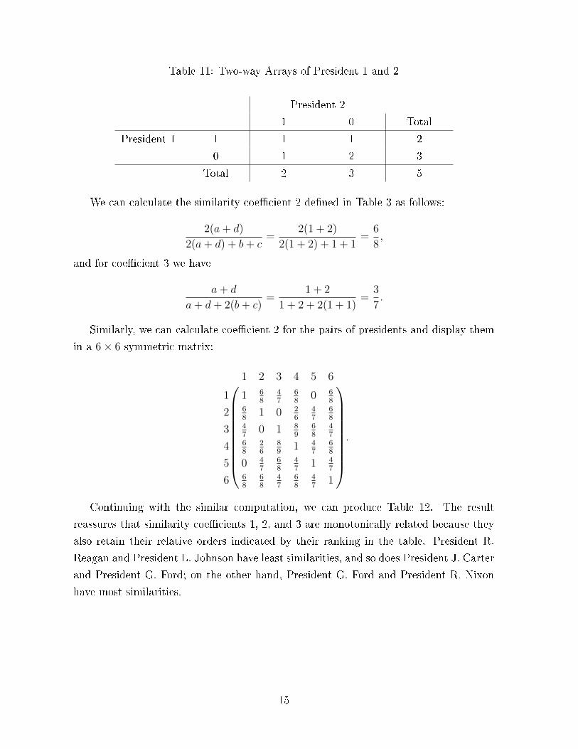
Table 11: Two-way Arrays of President 1 and 2

President 2

1 0 Total

President 1 1 1 1 2

0 1 2 3

Total 2 3 5

We can calculate the similarity coe�cient 2 de�ned in Table 3 as follows:

2(a+ d)

2(a+ d) + b+ c=

2(1 + 2)

2(1 + 2) + 1 + 1=

6

8,

and for coe�cient 3 we have

a+ d

a+ d+ 2(b+ c)=

1 + 2

1 + 2 + 2(1 + 1)=

3

7.

Similarly, we can calculate coe�cient 2 for the pairs of presidents and display them

in a 6× 6 symmetric matrix:

1 2 3 4 5 6

1 1 68

47

68

0 68

2 68

1 0 26

47

68

3 47

0 1 89

68

47

4 68

26

89

1 47

68

5 0 47

68

47

1 47

6 68

68

47

68

47

1

.

Continuing with the similar computation, we can produce Table 12. The result

reassures that similarity coe�cients 1, 2, and 3 are monotonically related because they

also retain their relative orders indicated by their ranking in the table. President R.

Reagan and President L. Johnson have least similarities, and so does President J. Carter

and President G. Ford; on the other hand, President G. Ford and President R. Nixon

have most similarities.

15

Table 12: The Results of the Example 2

Similarity Coe�cient Ranking

Pair 1 2 3 1 2 3

1-2 0.6 0.75 0.429 4.5 4.5 4.5

1-3 0.4 0.571 0.25 10 10 10

1-4 0.6 0.75 0.429 4.5 4.5 4.5

1-5 0 0 0 14.5 14.5 14.5

1-6 0.6 0.75 0.429 4.5 4.5 4.5

2-3 0 0 0 14.5 14.5 14.5

2-4 0.2 0.333 0.111 13 13 13

2-5 0.4 0.571 0.25 10 10 10

2-6 0.6 0.75 0.429 4.5 4.5 4.5

3-4 0.8 0.889 0.667 1 1 1

3-5 0.6 0.75 0.429 4.5 4.5 4.5

3-6 0.4 0.571 0.25 10 10 10

4-5 0.4 0.571 0.25 10 10 10

4-6 0.6 0.75 0.429 4.5 4.5 4.5

5-6 0.4 0.571 0.25 10 10 10

Example 3 (Exercise 12.3 from Johnson and Wichern [7]). Show that the

sample correlation coe�cient given by formula (9) can be written as

r =ad− bc

[(a+ b)(a+ c)(b+ d)(c+ d)]1/2

for two 0− 1 binary variables with the following frequencies:

Table 13: Frequencies of Variable 1 and 2

Variable 2

0 1

Variable 10 a b

1 c d

Solution: First, we form the table of binary variables as follows:

16

Table 14: Binary Values of Variables X and Y

y

1 0 Total

x1 a b a+ b

0 c d c+ d

Total a+ c b+ d p = a+ b+ c+ d

We have

x =(a+ b)

p,

y =(a+ c)

p.

The simple correlation coe�cient formula is

r =

∑ni=1 (xi − x) (yi − y)√∑n

i=1 (xi − x)2∑n

i=1 (yi − y)2, (9)

where the term∑n

i=1 (xi − x)2 can be calculated as follows:

n∑i=1

(xi − x)2 = (a+ b)

(1− (a+ b)

p

)2

+ (c+ d)

(0− (a+ b)

p

)2

=(c+ d) (a+ b)

p.

Similarly, we can write

n∑i=1

(yi − y)2 = (a+ c)

(1− (a+ c)

p

)2

+ (b+ d)

(0− (a+ c)

p

)2

=(a+ c) (b+ d)

p.

Next, we have

17

n∑i=1

(xi − x) (yi − y) = a− (a+ c) (a+ b)

p− (a+ b) (a+ c)

p− p(a+ b) (a+ c)

p2

=a (a+ b+ c+ d)− (a+ c) (a+ b)

p

=a2 + ab+ ac+ ad− a2 − ab− ac− ba

p

=ad− bc

p.

Now, we insert the above expressions into the simple correlation coe�cient formula

(9) and obtain

r =

∑ni=1 (xi − x) (yi − y)√∑n

i=1 (xi − x)2∑n

i=1 (yi − y)2

=

(ad−bcp

)[(c+d)(a+b)

p× (a+c)(b+d)

p

] 12

=ad− bc

[(a+ b) (c+ d) (a+ c) (b+ d)]12

.

Thus, the relation of interest is veri�ed. Note that variables with large negative

correlations are regarded as very dissimilar and variables with large positive correlations

are regarded as very similar.

3 Hierarchical Clustering Methods

Hierarchical clustering is conducted by either a series of successive mergers or a series of

successive divisions. Agglomerative hierarchical methods begin with the individual ob-

jects; so there are as many clusters as objects initially. They �rst group the most similar

objects, and then these groups are merged according to their similarities. Eventually, all

subgroups are merged into a single cluster. Divisive hierarchical methods initially divide

all objects into two subgroups in which the objects in one subgroup are �far from� the

objects in the other group. The subgroups are further divided into dissimilar subgroups

until each object forms a group itself. The results of both methods could be depicted

in a dendrogram that illustrates the mergers or divisions made at successive levels.

Our focus is agglomerative hierarchical procedures, and particularly, linkage methods

which are suitable for clustering items as well as variables. In turn, single linkage (min-

18

imum distance or nearest neighbor), complete linkage (maximum distance or farthest

neighbor), and average linkage (average distance) shall be discussed.

The steps in the agglomerative hierarchical clustering algorithm for grouping N

objects (items or variables) are shown below:

1. Begin with N clusters, each of which contains a single entity and an N × N

symmetric matrix of distances (or similarities) D = {dik}.

2. Find the distance matrix for the nearest pair of clusters. Suppose the distance

between the nearest clusters U and V is dUV .

3. Merge clusters U and V , and label the new cluster (UV ). Recalculate the entries

in the distance matrix by deleting the rows and columns corresponding to clusters

U and V and adding a row and column giving the distances between cluster (UV )

and the remaining clusters.

4. Follow Steps 2 and 3 a total of N − 1 times until all objects will be in a single

cluster. Make a record of the identity of clusters that are merged and the distance

at which the mergers take place.

3.1 Linkage Methods

3.1.1 Single Linkage

Distances or similarities between pairs of objects can be inputs to a single linkage algo-

rithm. Clusters are merged from the individual entities by combining nearest neighbors,

which mean the smallest distance or largest similarity.

First, we should identify the smallest distance in D = {dik} and merge the corre-

sponding objects, say, U and V , to �nd the cluster (UV ). For Step 3 in the above

algorithm, the distance between (UV ) and any other cluster W is calculated by

d(UV )W = min {dUW , dVW} . (10)

The quantities dUW and dVW are the distances between the nearest neighbours of clusters

U and W and clusters V and W , respectively.

In a typical application of hierarchical clustering, the intermediate results, where the

objects are sorted into a moderate number of clusters, are of great interest. Because

single linkage joins clusters by the shortest link between them, the method cannot

discern poorly separated clusters. Also, the method is one of a few clustering methods

that can delineate nonellipsoidal clusters. The tendency of single linkage to pick out

19

long stringlike clusters is known as chaining that can be misleading if items at opposite

ends of the chain are quite dissimilar.

The clusters formed by the method will be unchanged by any initial assignment of

distance (similarity) that gives the same relative orderings. In particular, any of a set

of similarity coe�cients from Table 3 that are monotonic to one another will produce

the same clustering in the end.

3.1.2 Complete Linkage

Complete linkage clustering is conducted in the almost same way as single linkage clus-

tering, with one important exception: at each stage, the distance between clusters is

determined by the distance between the elements, one from each cluster, that are most

distant. So, complete linkage guarantees that all items in a cluster are within some

maximum distance (or minimum similarity) of each other.

The general agglomerative algorithm starts by �nding the minimum entry in D =

{dik} and merging the corresponding objects, such as U and V , to get cluster (UV ).

For Step 3 of the above algorithm, the distance between (UV ) and any other cluster W

is computed by

d(UV )W = max {dUW , dVW} . (11)

Here dUW and dVW are the distances between the most distant members of clusters U

and W and cluster V and W , respectively.

Similar to the single linkage method, a new assignment of distances (similarities) that

have the same relative orderings as the initial distances will not change the con�guration

of the complete linkage clusters.

3.1.3 Average Linkage

Average linkage treats the distance between two clusters as the average distance between

all pairs of items where one member of a pair belongs to each cluster. The method begins

by searching the distance matrix D ={dik} to �nd the nearest (most similar) objects, for

instance, U and V . These objects are merged to form the cluster (UV ). For Step 3 of

the above algorithm, the distance between (UV ) and the other cluster W is determined

by

d(UV )W =

∑i

∑k

dik

N(UV )NW

, (12)

where dik is the distance between object i in the cluster (UV ) and object k in the cluster

W , and N(UV ) and NW are the number of items in cluster (UV ) and W , respectively.

20

For average linkage clustering, changes in the assignment of distances (similarities)

can a�ect the arrangement of the �nal cluster con�guration, but preserve relative or-

derings.

3.2 Examples

Example 4 (Exercise 12.5 from Johnson and Wichern [7]). Consider the matrix

of distances

1 2 3 4

1 0 1 11 5

2 1 0 2 3

3 11 2 0 4

4 5 3 4 0

Cluster the four items using each of the following procedures.

(a) Single linkage hierarchical procedure.

(b) Complete linkage hierarchical procedure.

(c) Average linkage hierarchical procedure.

Draw the dendrograms and compare the results in (a), (b), and (c).

Solution: (a) We treat each subject in the above matrix as cluster, apply clustering

by using single linkage, and merge the two closest items. Since

mini,k

(dik) = d21 = 1,

we merge objects 2 and 1 to form a cluster (12). To move on to the next level of

clustering, calculate the distances between the cluster (12) and the remaining objects 3

and 4. The nearest neighbour distances can be calculated as below:

d(12)3 = min{d13, d23} = min {11, 2} = 2,

and also

d(12)4 = min {d14, d24} = min {5, 3} = 3.

We now delete the rows and columns of the above matrix corresponding to objects

1 and 2, and add cluster (12) to obtain new distance matrix as below:

21

(12) 3 4

(12) 0 2 3

3 2 0 4

4 3 4 0

.The smallest distance between pairs of clusters is now d(12)3 = 2. Hence, we merge

cluster 3 with cluster (12) to get a new cluster (312). Next, we have

d(312)4 = min{d(12)4, d(34)

}= min {3, 4} = 3,

and hence, the �nal matrix is as shown below:

( (312) 4

(312) 0 3

4 3 0

).

Finally, clusters (312) and 4 are merged together to form a single cluster (1234) when

the nearest neighbour distance reaches 3. The dendrogram picturing the hierarchical

clustering using single linkage algorithm just concluded is shown below. The groupings

and the distance levels at which they occur are illustrated by the diagram.

(b) We treat each subject in the above matrix as cluster. To apply clustering by

using complete linkage, merge the two closest items. Since

maxi,k

(dik) = d21 = 2,

we merge objects 2 and 1 to form a cluster (12). To move on to the next level of

clustering, calculate the distance between the cluster (12) and the remaining objects 3

and 4.

22

The nearest neighbour distances can be calculated as follows:

d(12)3 = max {d13, d23} = max {11, 2} = 11,

and

d(12)4 = max {d14, d24} = max {5, 3} = 5.

Delete the rows and columns of the above matrix corresponding to object 1 and 2,

and add cluster (12) to obtain new distance matrix as below:

(12) 3 4

(12) 0 11 5

3 11 0 4

4 5 4 0

.At the �nal step, clusters (312) and 4 are merged together to form a single cluster

(1234) when the nearest neighbour distances reaches 11. The �nal matrix is as follows:

( (312) 4

(312) 0 11

4 11 0

).

The dendrogram picturing the hierarchical clustering using complete linkage algorithm

just concluded is shown below. The groupings and the distance levels at which they

occur are illustrated by the diagram.

(c) Due to intensive computation of average linkage procedures, we use Minitab to

cluster the �ve items instead. The dendrogram picturing the hierarchical clustering

23

using average linkage algorithm just concluded is shown below. The groupings and the

distance levels at which they occur are illustrated by the diagram.

Example 5 (Exercise 12.7 from Johnson and Wichern [7]). Sample correla-

tions for �ve stocks, rounded to two decimal places, are as given in Table 15.

Table 15: Sample correlations

JP Wells Royal Exxon

Morgan Citibank Fargo DutchShell Mobil

JP Morgan 1

Citibank .63 1

Wells Fargo .51 .57 1

Royal

DutchShell.12 .32 .18 1

Exxon

Mobil.16 .21 .15 .68 1

Treating the sample correlations as similarity measures, cluster the stocks using the

single linkage and complete linkage hierarchical procedures. Draw the dendrograms and

compare the results.

Solution: (a) We use Minitab to cluster the �ve stocks using single linkage proce-

dure.

24

(b) We use Minitab to cluster the �ve stocks using complete linkage procedure.

The above two methods produce almost the same clustering con�guration in their

�nal stage.

3.3 Ward's Hierarchical Clustering Method

J. H. Ward Jr. [11] proposed a hierarchical clustering method based on minimizing the

�loss of information� from joining two groups. This method regards an increase in an

error sum of squares, ESS, as loss of information. First, for a given cluster k, let ESSk

be the sum of the squared deviations of every item in the cluster from the cluster mean

(centroid). If there are currently K clusters, de�ne ESS as the sum of the ESSks or

ESS = ESS1 + ESS2 + . . . + ESSk. At each step, the union of every possible pair of

clusters is considered, and the two clusters whose combination results in the smallest

increase in ESS (minimum loss of information) are joined. Initially, each cluster consists

of a single item and, if there are N items, ESSk = 0, k = 1, 2, . . . , N , so ESS = 0. At

the other extreme, when all the clusters are combined in a single group of N items, the

25

value of ESS is given by

ESS =N∑j=1

(xj − x)> (xj − x) , (13)

where xj is the multivariate measurement associated with the jth item and x is the

mean of all the items. The results of Ward's method can be displayed as a dendrogram

in which the vertical axis gives the values of ESS where the mergers occur.

Ward's method is based on the assumption that the clusters of multivariate obser-

vations are expected to be roughly elliptically shaped. It is a hierarchical precursor to

nonhierarchical clustering methods that optimize some criterion for dividing data into

a given number of elliptical groups.

3.4 Final Comments on Hierarchical Procedures

Hierarchical procedures do not take sources of error and variation into account which

means that a clustering method will be sensitive to outliers, or �noise points.� Also, there

is no provision for a reallocation of objects that may have been �incorrectly� grouped at

an early stage; therefore, the �nal con�guration of clusters should be carefully examined

to see whether it is sensible or not. For a particular problem, it is a good idea to try

several clustering methods and, within a given method, a couple of di�erent ways of

assigning distances. If the outcomes from the several methods are (roughly) consistent

with one another, perhaps a case for �natural� groupings can be advanced.

The stability of a hierarchical solution can be checked by applying the clustering al-

gorithm before and after small errors (perturbations) have been added to the data units.

If the groups are fairly well distinguished, the clusterings before and after perturbation

should agree.

Common values in the similarity or distance matrix can produce multiple solutions

to a hierarchical clustering problem. This is not an inherent problem of any method;

rather, multiple solutions occur for certain kinds of data. Some data sets and hierar-

chical clustering methods can produce inversions that occur when an object joins an

existing cluster at a smaller distance (greater similarity) than that of a previous mergers.

Inversions can occur when there is no clear cluster structure and are generally associ-

ated with two hierarchical clustering algorithms known as the centroid method and the

median method.

26

4 Nonhierarchical Clustering Methods

Nonhierachical clustering methods aim to group items instead of variables into K clus-

ters, where K can be either determined beforehand or during the clustering procedure.

These methods can be utilized to much larger data sets than do hierarchical methods

because a matrix of distances (similarities) does not have to be determined, and none

of the basic data have to be stored during the computation. These methods start from

the nuclei of clusters which can be formed from either an initial partition of items into

groups or an initial set of seed points. Starting con�gurations should be chosen without

overt biases, i.e., randomly select seed points from the items or randomly partition the

items into initial groups. We will discuss the K-means method, one of the most popular

nonhierarchical procedures.

4.1 K-means Method

J. B. MacQueen [8] gives the term K-means to one of his algorithms assigning each item

to the cluster having the nearest centroid (mean). The algorithm is composed of three

steps below:

1. Divide the items into K initial clusters.

2. Assign each item in the list to the cluster whose centroid (mean) is nearest, by the

distance computed using Euclidean distance with either standardized or unstan-

dardized observations. After assignment, recalculate the centroid for the cluster

gaining the new item and for the cluster losing the item.

3. Repeat Step 2 until there is no more reassignments.

We could assign K initial centroids (seed points) and carry on Step 2 instead of parti-

tioning all items into K preliminary groups in Step 1. The �nal assignment of all items

will be in�uenced by the initial partition or the selection of centroids.

4.2 Example

Example 5 (Exercise 12.11 from Johnson and Wichern [7]). Suppose we mea-

sure two variables X1 and X2 for four items A, B, C and D. The data are collected in

Table 16.

27

Table 16: Measurements of two variables

Observations

Item x1 x2

A 5 4

B 1 −2

C −1 1

D 3 1

Use the K-means clustering technique to divide the items into K = 2 clusters. Start

with the initial groups (AB) and (CD).

Solution: We use the K-means clustering technique to divide the items into K = 2

clusters. The initial groups (AB) and (CD) are given as below:

Coordinates of the centroid

cluster x1 x2

(AB) 5+12

= 3 4−22

= 1

(CD) −1+32

= 1 1+12

= 1

Similarly, calculate the remaining clusters that are given as below:

Coordinates of the centroid

Cluster x1 x2

(AC) 2 2.5

(AD) 4 2.5

(BD) 2 −0.5

(BC) 0 −0.5

The squared distance of the centroids from �nal cluster (AD) and four items A, B,

C and D are computed as below:

d2 (A, (AD)) = (x1 − x1)2 + (x2 − x2)2

= (5− 4)2 + (4− 2.5)2

= 1 + 2.25

= 3.25,

28

d2 (B, (AD)) = (x1 − x1)2 + (x2 − x2)2

= (1− 4)2 + (−2− 2.5)2

= 9 + 20.25

= 29.25,

d2 (C, (AD)) = (x1 − x1)2 + (x2 − x2)2

= (−1− 4)2 + (1− 2.5)2

= 25 + 2.25

= 27.25,

d2 (D, (AD)) = (x1 − x1)2 + (x2 − x2)2

= (3− 4)2 + (1− 2.5)2

= 1 + 2.25

= 3.25 .

Similarly, we calculate the squared distances of the centroids from the �nal cluster (BC)

and four items A, B, C and D. The calculated distances are as follows:

d2 (A, (BC)) = (x1 − x1)2 + (x2 − x2)2

= (5− 0)2 + (4 + 0.5)2

= 25 + 20.25

= 45.25,

d2 (B, (BC)) = (x1 − x1)2 + (x2 − x2)2

= (1− 0)2 + (−2 + 0.5)2

= 1 + 2.25

= 3.25,

29

d2 (C, (BC)) = (x1 − x1)2 + (x2 − x2)2

= (−1 + 0)2 + (1 + 0.5)2

= 1 + 2.25

= 3.25,

d2 (D, (BC)) = (x1 − x1)2 + (x2 − x2)2

= (3− 0)2 + (1 + 0.5)2

= 9 + 2.25

= 11.25 .

For the �nal clusters, we have

Squared distance to group centroids

Cluster A B C D

(AD) 3.25 29.25 27.25 3.25

(BC) 45.25 3.25 3.25 11.25

Therefore, the �nal partition (AD) and (BC) is given as below:

x1 x2

(AD) 4 2.5

(BC) 0 −0.5

The coordinates of Cluster (AD)'s centroid is (4, 2.5); the ones of Cluster (BC)'s

centroid is (0,−0.5).

4.3 Final Comments�Nonhierarchical Procedures

To check the stability of the clustering procedure, we should run the algorithm with a

di�erent initial partition or centroids. Once clusters emerges, the list of items should

be rearranged so that items in the �rst cluster appear �rst, those in the second cluster

appear next, and so on. A table of the cluster centroids and within-cluster variances also

help us to �nd the di�erences between clusters. The importance of individual variables

in clustering should be evaluated from a multivariate perspective. Descriptive statistics

can be helpful in assessing the importance of individual variables and the �success� of

the clustering algorithm.

Some strong arguments for not �xing the number of clusters beforehand are:

30

1. Two or more seed points lying within a single cluster causes their resulting clusters

to be poorly di�erentiated.

2. An outlier might cause at least one cluster in which items disperse widely.

3. A sample may not contain items from the rarest group in a population. Forcing

the sample data into K groups would produce nonsensical clusters.

It is advisable to rerun the algorithm for several choices to the number of centroids.

5 Clustering Based on Statistical Models

The clustering methods discussed earlier, for instance, single linkage, complete link-

age, average linkage, Ward's method and K-means clustering, are intuitively reasonable

procedures. However, the introduction of statistical models has made major advances

in clustering techniques because statistical models explain how the collection of (p× 1)

measurements xj, from the N objects, was generated. We will discuss the most common

model where cluster k has expected proportion pk of the objects and the corresponding

measurements are generated by a probability density function fk (x). If there are K

clusters, the mixing distribution is used to model the observation vector for a single

object:

fMix (x) =K∑k=1

pk fk (x), x ∈ Rp,

where each pk ≥ 0 and∑K

k=1 pk = 1. Because the observation comes from the component

distribution fk (x) with probability pk, the distribution fMix (x) is a mixture of the K

distributions f1 (x), f2 (x), . . . , fK (x). Therefore, the collection of N observation

vectors generated from this distribution should be a mixture of observations from the

component distributions.

A mixture of multivariate normal distributions in which the kth component fk (x)

is the Np (µk,Σk) density function is the most common mixture model. The normal

mixture model for a single observation x is

fMix (x | µ1,Σ1, . . . ,µK ,ΣK) =K∑k=1

pk

(2π)p/2 | Σk |1/2exp

(−1

2(x− µk)

>Σ−1k (x− µk)

).

(14)

Clusters obtained from this model should be ellipsoidal in shape that is concentrated

heavily near the center. Inferences are based on the likelihood for N objects and a �xed

31

number of clusters K, which is given by

L (p1, ..., pK ,µ1,Σ1, ...,µk,ΣK) =N∏j=1

fMix (xj |µ1 ,Σ1, · · · ,µK ,ΣK)

=N∏j=1

(K∑k=1

P · exp (Q)

),

(15)

where the proportions p1, . . . , pk, the mean vectors µ1, . . . ,µk, and the covariance matri-

ces Σ1, . . . ,Σk are unknown, and P = pk(2π)p/2|Σk|1/2

and Q = −12

(x− µk)>Σ−1k (x− µk).

The measurements for di�erent objects are regarded as independent and identically dis-

tributed observations from the mixture distribution fMix (x).

The likelihood-based procedure under the normal mixture model with all Σk being

the same multiple of the identity matrix, ηI, under which certain conclusions can be

drawn based on a heuristic clustering method, is approximately analogues to K-means

clustering and Ward's method since these methods use the distance computed using

the Euclidean distance with either standardized or unstandardized observations. It

is a major advance that under the sequence of mixture models (12) for di�erent K,

the problems of choosing the number of clusters and an appropriate clustering method

become the one of selecting an appropriate statistical model.

The maximum likelihood estimators p1, . . . , pK , µ1, Σ1, . . . , µK , ΣK for a �xed num-

ber of clusters K must be obtained numerically using special software. The resulting

estimator

Lmax := L(p1, . . . , pK , µ1, Σ1, . . . , µK , ΣK

)provides the basis for model selection. To compare models with di�erent numbers of

parameters, a penalty is subtracted from twice the maximum of the log-likelihood to

give

−2lnLmax − Penalty ,

where the penalty depends on the number of parameters estimated and the number of

observations N . Because the probabilities pk sum up to 1, there are K − 1 probabilities

that must be estimated, K × p means and K × p (p+ 1) /2 variances and covariances.

For the Akaike information criterion (AIC), the penalty is 2N×(number of parameters)

so

AIC = 2lnLmax − 2N

(K

1

2(p+ 1) (p+ 2)− 1

). (16)

The Bayesian information criterion (BIC) uses the logarithm of the number of pa-

32

rameters in the penalty function:

BIC = 2lnLmax − 2ln (N)

(K

1

2(p+ 1) (p+ 2)− 1

). (17)

Under either AIC or BIC, the better model is indicated by the higher score using

AIC or BIC formula.

To avoid occasional di�culty with too many parameters in the mixture model, we

assume simple structures for the Σk. Namely, we allow the covariance structures as

listed in Table 17.

Table 17: BIC for Di�erent Scenarios

Assumed form Total number

for Σk of parameters BIC

Σk = η I K (p+ 1) lnLmax − 2lnNK (p+ 1)

Σk = ηk I K (p+ 2)− 1 lnLmax − 2lnN (K (p+ 2− 1))

Σk = ηk Diag (λ1, λ2, . . . , λp) K (p+ 2) + p− 1 lnLmax − 2lnN (K (p+ 2) + p− 1)

The package MCLUST available in the R software library, provides the combina-

tion of hierarchical clustering, the EM algorithm and the BIC criterion to develop an

appropriate model for clustering.

Example 6 (Example 12.13: A model based clustering of the Iris data

Johnson and Wichern [7]). For the Iris data in Table 11.5 (see Appendix I), we

use MCLUST (version 5.4.7) which provides the EM algorithm to determine the model

based on the best BIC values, using di�erent structures of the covariance matrix. As

a multivariate data set, the Iris data consists of 50 samples from each of three species

of Iris: Iris setosa, Iris virginica and Iris versicolor, totaling 150 samples; the length

and the width of the sepals and petals were measured from each sample. Thus, the

Iris data set has �ve variables: sepal length, sepal width, petal length, petal width and

species; it has three clusters: Iris setosa, Iris virginica and Iris versicolor. A matrix plot

of the clusters for pairs of variables, among sepal length, sepal width, petal length and

petal width, is as shown on Figure 7. The scatter plots of petal length and petal width

suggest certain positive correlations between the two variables.

The best BIC value is −561.7285 (VEV, 2 clusters) shown on Figure 8, where VEV is

an identi�er for covariance parameter of G+ (d− 1) +G [d (d− 1) /2], with G denoting

the number of mixture components and d denoting the dimension of the data. The EII,

33

VEE, etc. are the identi�ers for covariance parameters in MCLUST package. Figure 8

shows that the �best� model can be estimated by �tting the model with VEV covariance

parameter with 2 clusters.

The plot, located in the second row and the �rst column, and boxed in red lines, on

Figure 9, demonstrates the best model based on the above computation.

This clustering algorithm suggests that the Iris data set can be divided into two,

rather obvious, clusters: one of the clusters is Iris setosa, and the other contains both

Iris virginica and Iris vesrsicolor.

Figure 7: A scatter plot matrix for pairs of variables, where blue = setosa, red =

versicolor, green = virginica

34

Figure 8: the BIC plot with di�erent covariance parameter models, the �best� model is

the model with VEV, 2 clusters.

Figure 9: Matrix plot of di�erent models

35

6 Correspondence Analysis

A graphical procedure that represents associations in a table of frequencies is called

correspondence analysis. This project focuses on two-way table of frequencies or con-

tingency table. Suppose the contingency table has I rows and J columns, the plot is

produced by correspondence analysis containing two sets of points: a set of I points cor-

responding to the rows and a set of J points corresponding to the columns. Associations

between the points is re�ected by the positions of the points on the plot. Row points

being close together show rows having similar pro�les (conditional distributions) across

the columns; column points being close together show columns having similar pro�les

(conditional distributions) down the rows; and row points being close to column points

demonstrates combinations occurring more frequently than would be expected from an

independence mode in which the row categories are unrelated to the column categories.

The usual output from a correspondence analysis provides the �best� two-dimensional

representation of the data, the coordinates of the plotted points, and the inertia of the

amount of information retained in each dimension.

6.1 Algebraic Development of Correspondence Analysis

Let X, with elements xij, be an I × J two-way table of unscaled frequencies. We take

I > J and assume that X is of full column rank J in the table of which the rows and

columns correspond to di�erent categories of two di�erent characteristics. If n is the

total of the frequencies in the data matrix X, we should �rst construct a matrix of

proportions P = {pij} by dividing each element of X by n. Thus, we obtain

pij =xijn, i = 1, 2, . . . , I, j = 1, 2, . . . , J, or P

(I×J)=

1

nX

(I×J). (18)

The matrix P is called the correspondence matrix.

We de�ne the vector of row sums r = (r1, r2, . . . , rJ)> as follows:

ri =J∑j=1

pij =J∑j=1

xij

n, i = 1, 2, . . . , I, or r

(I×1)= P

(I×J)1J

(J×1)

and the vector of column sum c = (c1, c2, . . . , cI)> as below:

cj =I∑i=1

pij =I∑i=1

xij

n, j = 1, 2, . . . , J, or c

(J×1)= P>

(J×1)1I

(I×1)

36

where 1J is a J × 1 and 1I is a I × 1 vector of 1′s. We de�ne the diagonal matrix Dr

with the elements of r on the main diagonal:

Dr = diag (r1, r2, . . . , rI) ,

and the diagonal matrix Dc with the elements of c on the main diagonal:

Dc = diag (c1, c2, . . . , cJ) .

Also, for scaling purposes, we de�ne the square root matrices:

D1/2r = diag (

√r1,√r2, . . . ,

√rI) , (19)

D−1/2r = diag

(1√r1,

1√r2, . . . ,

1√rI

),

D1/2c = diag (

√c1,√c2, . . . ,

√cJ) , (20)

D−1/2c = diag

(1√c1,

1√c2, . . . ,

1√cJ

).

Correspondence analysis can be formulated in the form of the weighted least squares

problem to select P = {pij}, a matrix of speci�ed reduced rank, to minimize

I∑i=1

J∑j=1

(pij − pij)2

ricj= tr

[(D−1/2r

(P− P

)D−1/2c

)(D−1/2r

(P− P

)D−1/2c

)>], (21)

because(pij−pij)√

ricjis the (i, j)element of D

−1/2r

(P− P

)D−1/2c .

Before introducing Result 12.1, we will review the relevant Result 2A.15 and 2A.16

from Johnson and Wichern [7]. These are standard results of Linear Algebra.

Result 2A.15. Singular-Value Decomposition. Let A be an m × k matrix of real

numbers. Then there exist an m × m orthogonal matrix U and a k × k orthogonal

matrix V such that

A = UΛV>,

where the m × k matrix Λ has (i, i) entry λi ≥ 0 for i = 1, 2, . . . ,min (m, k) and the

other entries are zero. The positive constants λi are called the singular values of A.

The singular-value decomposition can also be expressed as a matrix expansion that

depends on the rank r of A. There exist r positive constants λ1, λ2, . . . , λr, r orthogonal

37

m× 1 unit vectors u1,u2 . . . ,ur and r orthogonal k× 1 unit vectors v1,v2, . . . ,vr, such

that

A =r∑i=1

λiuiv>i = UrΛrV

>r , (22)

where Ur = (u1,u2, . . . ,ur), Vr = (v1,v2, . . . ,vr), and Λr is an r × r diagonal matrix

with diagonal entries λi. Here AA> has eigenvalue-eigenvector pairs (λ2i ,ui), so

AA>ui = λ2iui

with λ21, λ22, . . . , λ

2r > 0 = λ2r+1, λ

2r+2, . . . , λ

2m (for m > k). Then, in view of (21), vi =

λ−1i A>ui. Alternatively, the vi are the eigenvectors of A>A with the same nonzero

eigenvalues λ2i .

The matrix expansion for the singular-value decomposition written in terms of the

full dimensional matrices U,V,Λ is

A(m×k)

= U(m×m)

Λ(m×k)

V>(k×k)

,

where U has m orthogonal eigenvectors of AA> as its columns, V has k orthogonal

eigenvectors of A>A as its columns, and Λ is speci�ed in Result 2A.15.

Result 2A.16. Error of Approximation. Let A be an m × k matrix of real numbers

with m ≥ k and singular value decomposition UΛV>. Let s < k = rank (A). Then

B =s∑i=1

λiuiv>i

is the rank s least squares approximation to A. It minimizes

tr[(A−B) (A−B)>

]over all m× k matrices B having rank no greater than s. The minimum value, or error

of approximation, is∑k

i=s+1 λ2i .

Proof. To establish this result, we use UU> = Im and VV> = Ik to write the sum of

38

squares as

tr[(A−B) (A−B)>

]= tr

[UU> (A−B) VV> (A−B)>

]= tr

[U> (A−B) VV> (A−B)>U

]= tr

[(Λ−C) (Λ−C)>

]=

m∑i=1

k∑j=1

(λij − cij)2

=m∑i=1

(λi − cij)2 +∑∑

i 6=j

c2ij,

where C = U>BV = (cij). Clearly, the minimum occurs when cij = 0 for i 6= j and

cii = λi for the s largest singular values; the other cii = 0. That is, UBV> = Λs or

B =∑s

i=1 λiuiv>i .

Result 12.1. The term rc> is common (the meaning of �common� is explained right

below the proof of this result) to the approximation P whatever the I×J correspondence

matrix P in (18).

The reduced rank s approximation to P is a minimizer of the sum of squares (21).

It is given by

P.=

s∑k=1

λk(D1/2r uk

) (D1/2c vk

)= rc> +

s∑k=2

λk(D1/2r uk

) (D1/2c vk

)>,

where the λk are the singular values and the I × 1 vectors uk and the J × 1 vectors vk

are the corresponding singular vectors of the I × J matrix D−1/2r PD−1/2c . In view of

Result 2A.16, the minimum value of (21) is∑J

k=s+1 λ2k.

The reduced rank K > 1 approximation to P− rc> is

P− rc>.=

K∑k=1

λk(D1/2r uk

) (D1/2c vk

)>,

where the λk are the singular values and the I × 1 vectors uk and the J × 1 vectors vk

are the corresponding singular vectors of the I ×J matrix D−1/2r

(P− rc>

)D−1/2c . And

λk = λk+1, uk = uk+1, and vk = vk+1 for k = 1, . . . , J − 1.

39

Proof. First we consider a scaled version B = D−1/2r PD−1/2c of the correspondence ma-

trix P. According to Result 2A.16, the best row rank = s approximation B to D−1/2r PD

−1/2c

is given by the �rst s terms in the singular-value decomposition

D−1/2r PD−1/2c =J∑k=1

λkukv>k ,

where

D−1/2r PD−1/2c vk = λkuk u>k D−1/2r PD−1/2c = λkv>k , (23)

and ∣∣∣∣(D−1/2r PD−1/2c

)(D−1/2r PD−1/2c

)>− λ2kI

∣∣∣∣ = 0 for k = 1, . . . , J.

The approximation to P is therefore given by

P = D1/2r BD

1/2

c.=

s∑k=1

λk(D1/2r uk

) (D1/2c vk

)>and, by Result 2.16, the error of approximation is

∑Jk=s+1 λ

2k.

Whatever the correspondence matrix P, the term rc>always provides the best rank

one approximation; thus, it is common to the approximation P. This corresponds to

the assumption of Independence of the rows and columns of P. Let u1 = D1/2r 1I and

v1 = D1/2c 1J , where 1I is I × 1 and J × 1 vector of 1′s. We can show that (22) holds

for these choices. Indeed, we have

u>1

(D−1/2r PD−1/2c

)=(D1/2r 1I

)> (D−1/2r PD−1/2c

)= 1>I PD−1/2c = c>D−1/2c

= (√c1, . . . ,

√cJ) =

(D1/2c 1J

)>= v>1 ,

and (D−1/2r PD−1/2c

)v1 =

(D−1/2r PD−1/2c

) (D1/2c 1J

)= D−1/2r P1J = D−1/2r r

= (√r1, . . . ,

√rI)> = D1/2

r 1I = u1.

40

That is,

(u1, v1) =(D1/2r 1I ,D

1/2c 1J

)are singular vectors associated with singular value λ1 = 1. For any correspondence

matrix P, the common term in every expansion is

D1/2r u1v

>1 D1/2

c = Dr1I1>J Dc = rc>.

Therefore, we have established the �rst approximation and (22) can always be ex-

pressed as

P = rc> +J∑k=2

λk(D1/2r uk

) (D1/2c vk

)>.

Because of the common term, the problem can be rephrased in terms of P−rc> and

its scaled version D−1/2r (P− rc′) D

−1/2c . By the orthogonality of the singular vectors of

D−1/2r PD−1/2c , we have u>k

(D

1/2r 1I

)= 0 and v>k

(D

1/2c 1J

)= 0 for k > 1, so

D−1/2r

(P− rc>

)D−1/2c =

J∑k=2

λkukv>k

is the singular-value decomposition of D−1/2r

(P− rc>

)D−1/2c in terms of the singular

values and vectors obtained from D−1/2r PD−1/2c . Converting the singular values and

vectors λk, uk, and vk from D−1/2r

(P− rc>

)D−1/2c only amounts to changing k to k−1

so λk = λk+1, uk = uk+1, and vk = vk+1 for k = 1,. . . , J − 1.

In terms of the singular value decomposition for D−1/2r

(P− rc>

)D−1/2c , the expan-

sion for P− rc> takes the form

P− rc> =J−1∑k=1

λk(D1/2r uk

) (D1/2c vk

)>.

The best rank K approximation to D−1/2r

(P− rc>

)D−1/2c is given by

∑Kk=1 λkukv

>k .

Then the best approximation to P− rc> is

P− rc>.=

K∑k=1

λk(D1/2r uk

) (D1/2c vk

)>. (24)

Remark. Note that the vectors D1/2r uk and D

1/2c vk in the expansion (24) of P − rc>

41

need not have length one but satisfy the scaling

(D1/2r uk

)>D−1r

(D1/2r uk

)= u>k uk = 1,(

D1/2c vk

)>D−1c

(D1/2c vk

)= v>k vk = 1.

Because of this scaling, the expansion in Result 12.1 is called a generalized singular-value

decomposition.

The preceding approach is called the matrix approximation method and the approach

to follow the pro�le approximation method. We will also discuss the pro�le approxima-

tion method using the row pro�les that are the rows of the matrix D−1r P. Contingency

analysis can also be de�ned as the approximation of the row pro�les by points in a low-

dimensional space. The row pro�les are the row proportions that are calculated from

the counts in the contingency table; the value of each cell in the row pro�les is the count

of the cell divided by the sum of the counts for the entire row; the row pro�les for each

row sum to approximately 1 (or 100%). Suppose the row pro�les are approximated by

the matrix P∗ =(p∗ij). Using the square-root matrices D

1/2r and D

1/2c de�ned in (19)

and (20), we have

(D−1r P−P∗

)D−1/2c = D−1/2r

(D−1/2r P−D1/2

r P∗)

D−1/2c

and, with p∗ij =pijri

the least squares criterion (20) can be written as

I∑i=1

J∑j=1

(pij − pij)2

ricj=

I∑i=1

ri

J∑j=1

(pij/ri − p∗ij

)2cj

=tr[[

(Q) D−1/2c

]D1/2r

[(Q) D−1/2r

]>],

where Q = D−1/2r P−D

1/2r P∗.

The proof of Result 12.1 deals with the minimization of the last expression for the

trace, and D−1/2r PD−1/2c has the singular-value decomposition

D−1/2r PD−1/2c =J∑k=1

λkukv>k . (25)

The best rank K approximation can be obtained by the �rst K terms of this ex-

pansion. Since D−1/2r PD−1/2c can be approximated by D

1/2r P∗D

1/2c , we can left multiply

each side of (25) by D−1/2r and right multiply each side of (24) by D

1/2c to obtain the

42

generalized singular-value decomposition

D−1r P =J∑k=1

λkD−1/2r uk

(D1/2c vk

)>,

where (u1, v1) =(D

1/2r 1I ,D

1/2c 1J

), are singular vectors associated with singular value

λ1 = 1, where 1I is a I × 1 and 1J is a J × 1 vector of 1′s. Because D−1/2r

(D

1/2r 1I

)=

1I and(D

1/2c 1J

)>D

1/2c = c>, the leading term in the above decomposition is 1Ic

>.

Therefore, in terms of the singular values and vectors from D−1/2r PD−1/2c , the reduced

rank K < J approximation of the row pro�les of D−1r P is

P∗.= 1Ic

> +K∑k=2

λkD−1/2r uk

(D1/2c vk

)>.

The above formula provides one of the mathematical foundations for statistical softwares

to carry out the algorithm of correspondence analysis. In practice, the correspondence

analysis can be conveniently implemented by using statistical software (see Example 7

below).

6.2 Inertia

Total inertia, de�ned as the weighted sum of squares below, is a measure of the variation

in the count data:

tr[D−1/2r

(P− rc>

)D−1/2c

(D−1/2r

(P− rc>

)D−1/2c

)>]=

I∑i=1

J∑j=1

(pij − ricj)2

ricj=

J−1∑k=1

λ2k,

where λk are the singular values obtained from the single-value decomposition of

D−1/2r

(P− rc>

)D−1/2c (see the proof of Result 12.1).

The inertia associated with the best reduced rank K < J approximation to the

centered matrix P−rc> (the K-dimensional solution) has inertia∑K

k=1 λ2k. The residual

inertia (variation) not accounted for by the rankK solution is equal to the sum of squares

of the remaining singular values: λ2K+1 + λ2K+2 + . . .+ λ2J−1.

The total inertia is related to the chi-square measure of association in a two-way

contingency table, χ2 =∑

i,j(Oij−Eij)

2

Eij. Here Oij = xij is the observed frequency and

Eij is the expected frequency for the (i, j)th cell. In the correspondence analysis, it is

43

assumed that the row variable is independent of the column variable, Eij = nricj, and

Total inertia =I∑i=1

J∑j=1

(pij − ricj)2

ricj=χ2

n.

The total inertia of all the rows in a contingency table is equal to the χ2 statistic

divided by n which is also known as Pearson's mean-square contingency used to assess

the quality of its graphical representation in correspondence analysis.

6.3 Interpretation of Correspondence Analysis in Two Dimen-

sions

Geometrically, we interpret a large value for the proportion(λ21+λ22)∑J−1

k=1 λ2k

as the associations

in the centered data well represented by points in a plane, and this best approximating

plane accounting for nearly all the variation in the data beyond that accounted for by

the rank 1 solution (independence model). Algebraically, the approximation can be

written as

P− rc>.= λ1u1v

>1 + λ2u2v

>2 .

6.4 Example

Example 7 (Exercise 12.20 Johnson and Wichern [7]). A sample of n = 1660

people is cross-classi�ed according to mental health status and socioeconomics status in

Table 18. Perform a correspondence analysis of these data. Interpret the results. Can

the associations in the data be well represented in one dimension?

Table 18

A B C D E

Well 121 57 72 36 21

Mild Symptoms 188 105 141 97 71

Moderate Symptoms 112 65 77 54 54

Impaired 86 60 94 78 71

Solution: To perform correspondence analysis, we use the SAS software. The ob-

tained results are shown on Figure 10.

44

Figure 10: Inertia and Chi-Square Decomposition

According to the above analysis, the singular values are 0.16132, 0.03709, and

0.00820; the principal inertia are 0.02602, 0.00138, and 0.00007. The row coordinates

and column coordinates are shown on Figure 11:

Figure 11: Row Coordinates and Column Coordinates

A correspondence analysis plot of the mental health-socioeconomic data is shown

on Figure 12 below. Hence, the lowest economic class (A and B in the plot) is located

between moderate and impaired; the lower class (C and D) is closest to impaired.

45

Figure 12: A Correspondence Analysis Plot of the Mental Health-socioeconomic Data

Correspondence analysis designed to represent associations in a low-dimensional

space is primarily a graphical technique. But it is also relevant to principal compo-

nent analysis and canonical correlation analysis.

7 Conclusion

Cluster analysis combines numerical methods of classi�cation; it appears in many disci-

plines such as biology, botany, medicine, psychology, geography, marketing, image pro-

cessing, psychiatry, archaeology, etc. Some examples of applications of cluster analysis

appeared in the Introduction of the project. Cluster analysis concerns about searching

for patterns in a data set by grouping the multivariate observations into clusters in order

to �nd an optimal grouping by which the observations or objects within each cluster are

similar but the clusters are dissimilar to each other. The goal of cluster analysis is to

�nd the �natural groupings� in the data set that make sense to the researcher. Cluster-

ing items (units or cases) employs the measure of proximity by some sort of distance;

grouping variables utilizes the measure of proximity by correlation coe�cients or like

measures of association.

46

The project has discussed some statistical theory behind several clustering methods

related to hierarchical classi�cation, nonhierachical partition, and graphical representa-

tion.

First, hierarchical clustering is conducted by either a series of successive mergers or

a series of successive divisions. Agglomerative hierarchical methods begin with the indi-

vidual objects; so there are as many clusters as objects initially. They �rst group the

most similar objects, and then these groups are merged according to their similarities.

Eventually, all subgroups are merged into a single cluster. Divisive hierarchical methods

initially divide all objects into two subgroups in which the objects in one subgroup are

�far from� the objects in the other group. The subgroups are further divided into dissim-

ilar subgroups until each object forms a group itself. The results of both methods could

be depicted in a dendrogram that illustrates the mergers or divisions made at successive

levels. Our focus was on agglomerative hierarchical procedures, and particularly, link-

age methods which are suitable for clustering items as well as variables. In turn, single

linkage (minimum distance or nearest neighbor), complete linkage (maximum distance

or farthest neighbor), and average linkage (average distance) were discussed.

Second, nonhierachical clustering methods aim to group items instead of variables

into K clusters, the number K of which can be either determined beforehand or during

the clustering procedure. Theses methods can be utilized to much larger data sets than

do hierarchical methods because a matrix of distances (similarities) does not have to

be determined, and none of the basic data have to be stored during the computation.

These methods start from the nuclei of clusters which can be formed from either an initial

partition of items into groups or an initial set of seed points. Starting con�gurations

should be chosen without overt biases, i.e., randomly select seed points from the items

or randomly partition the items into initial groups. We discuss the K-means method,

one of the most popular nonhierarchical procedures.

Third, statistical model-based classi�cation has made major advances in clustering

techniques because statistical models explain how the collection of (p× 1) measurements

xj, from the N objects, was generated. We discussed the most common model where

cluster k has expected proportion pk of the objects and the corresponding measurements

are generated by a probability density function fk (x). If there areK clusters, the mixing

distribution is used to model the observation vector for a single object:

fMix (x) =K∑k=1

pk fk (x), x ∈ Rp,

where each pk ≥ 0 and∑K

k=1 pk = 1. Because the observation comes from the com-

47

ponent distribution fk (x) with probability pk, the distribution fMix (x) is a mixture

of the K distributions f1 (x), f2 (x), . . . , fK (x). Therefore, the collection of N ob-

servation vectors generated from this distribution should be a mixture of observations

from the component distributions. Statistical model-based classi�cation involves both

hierarchical or nonhierarchinal procedures.

Finally, a graphical procedure that represents associations in a table of frequencies

is called correspondence analysis. This project has focused on two-way table of frequen-

cies or contingency table. Suppose the contingency table has I rows and J columns, the

plot is produced by correspondence analysis containing two sets of points: a set of I

points corresponding to the rows and a set of J points corresponding to the columns.

Associations between the points is re�ected by the positions of the points on the plot.

Row points being close together show rows having similar pro�les (conditional distri-

butions) across the columns; column points being close together show columns having

similar pro�les (conditional distributions) down the rows; and row points being close

to column points demonstrates combinations occurring more frequently than would be

expected from an independence mode in which the row categories are unrelated to the

column categories. The usual output from a correspondence analysis provides the �best�

two-dimensional representation of the data, the coordinates of the plotted points, and

the inertia of the amount of information retained in each dimension.

Due to the scope of the project, it does not confront the di�cult problem of cluster

analysis: cluster validation or avoiding artefactual solutions to cluster analysis. The

preceding discussion of clustering methods reveals that no one clustering method can be

judged to be the �best� in all circumstances. However, it might be advisable to apply

a number of clustering methods to the data set before reaching any conclusion. If all

produce very similar solutions, it is justi�ably concluded that the results are worthy of

further investigation; otherwise, it might be evidence against any clustering solution. In

this project, we have not only discussed in detail some common clustering techniques,

but also illustrated their use by numerical examples with real-life data sets.

References

[1] R. E. Bonner. �On Some Clustering Techniques�. In: IBM Journal of Research and

Development 8.1 (Jan. 1964), pp. 22�32.

[2] C. Chakrapani. Statistics in Market Research. London: Arnold, 2004.

48

[3] A. D. Gordon. Classi�cation. 2nd edition. Boca Raton, FL: Chapman and Hall/CRC,

1999.

[4] P. E. Green, R. E. Frank, and P. J. Robinson. �Cluster Analysis in Test Market

Selection�. In: Management Science 13.8 (1967), pp. 387�400.

[5] F. R. Hodson. Numerical typology and prehistoric archaeology. In: Mathematics

in the Archaeological and Historical Sciences. Ed. by P. A. Tautu F. R. Hodson

D. G. Kendall. Edinburgh: Edinburgh University Press, 1971.

[6] F. R. Hodson, P. H. A. Sneath, and J. E. Doran. �Some Experiments in the Nu-

merical Analysis of Archaeological Data�. In: Biometrika 53.3�4 (1966), pp. 311�

324.

[7] R. A. Johnson and D. W. Wichern. Applied Multivariate Statistical Analysis. 6th

edition. Upper Saddle River, NJ: Pearson, Mar. 2007.

[8] J. MacQueen. �Some methods for classi�cation and analysis of multivariate obser-

vations�. In: 5th Berkeley Symposium on Mathematical Statistics and Probability.

1967, pp. 281�297.

[9] T. Montmerle. �Hertzsprung Russell Diagram�. In: Berlin, Heidelberg: Springer,

2011, pp. 749�754.

[10] S. Pinker. How the Mind Works. New York, NY: W. W. Norton & Company, 2009.

[11] J. H. Ward. �Hierarchical Grouping to Optimize an Objective Function�. In: Jour-

nal of the American Statistical Association. 58.301 (1963), pp. 236�244.

49

8 Appendix I

Table 11.5: the Iris data

5.1, 3.5, 1.4, 0.2, setosa

4.9, 3.0, 1.4, 0.2, setosa

4.7, 3.2, 1.3, 0.2, setosa

4.6, 3.1, 1.5, 0.2, setosa

5.0, 3.6, 1.4, 0.2, setosa

5.4, 3.9, 1.7, 0.4, setosa

4.6, 3.4, 1.4, 0.3, setosa

5.0, 3.4, 1.5, 0.2, setosa

4.4, 2.9, 1.4, 0.2, setosa

4.9, 3.1, 1.5, 0.1, setosa

5.4, 3.7, 1.5, 0.2, setosa

4.8, 3.4, 1.6, 0.2, setosa

4.8, 3.0, 1.4, 0.1, setosa

4.3, 3.0, 1.1, 0.1, setosa

5.8, 4.0, 1.2, 0.2, setosa

5.7, 4.4, 1.5, 0.4, setosa

5.4, 3.9, 1.3, 0.4, setosa

5.1, 3.5, 1.4, 0.3, setosa

5.7, 3.8, 1.7, 0.3, setosa

5.1, 3.8, 1.5, 0.3, setosa

5.4, 3.4, 1.7, 0.2, setosa

5.1, 3.7, 1.5, 0.4, setosa

4.6, 3.6, 1.0, 0.2, setosa

5.1, 3.3, 1.7, 0.5, setosa

4.8, 3.4, 1.9, 0.2, setosa

5.0, 3.0, 1.6, 0.2, setosa

5.0, 3.4, 1.6, 0.4, setosa

5.2, 3.5, 1.5, 0.2, setosa

5.2, 3.4, 1.4, 0.2, setosa

4.7, 3.2, 1.6, 0.2, setosa

4.8, 3.1, 1.6, 0.2, setosa

5.4, 3.4, 1.5, 0.4, setosa

5.2, 4.1, 1.5, 0.1, setosa

50

5.5, 4.2, 1.4, 0.2, setosa

4.9, 3.1, 1.5, 0.1, setosa

5.0, 3.2, 1.2, 0.2, setosa

5.5, 3.5, 1.3, 0.2, setosa

4.9, 3.1, 1.5, 0.1, setosa

4.4, 3.0, 1.3, 0.2, setosa

5.1, 3.4, 1.5, 0.2, setosa

5.0, 3.5, 1.3, 0.3, setosa

4.5, 2.3, 1.3, 0.3, setosa

4.4, 3.2, 1.3, 0.2, setosa

5.0, 3.5, 1.6, 0.6, setosa

5.1, 3.8, 1.9, 0.4, setosa

4.8, 3.0, 1.4, 0.3, setosa

5.1, 3.8, 1.6, 0.2, setosa

4.6, 3.2, 1.4, 0.2, setosa

5.3, 3.7, 1.5, 0.2, setosa

5.0, 3.3, 1.4, 0.2, setosa

7.0, 3.2, 4.7, 1.4, versicolor

6.4, 3.2, 4.5, 1.5, versicolor

6.9, 3.1, 4.9, 1.5, versicolor

5.5, 2.3, 4.0, 1.3, versicolor

6.5, 2.8, 4.6, 1.5, versicolor

5.7, 2.8, 4.5, 1.3, versicolor

6.3, 3.3, 4.7, 1.6, versicolor

4.9, 2.4, 3.3, 1.0, versicolor

6.6, 2.9, 4.6, 1.3, versicolor

5.2, 2.7, 3.9, 1.4, versicolor

5.0, 2.0, 3.5, 1.0, versicolor

5.9, 3.0, 4.2, 1.5, versicolor

6.0, 2.2, 4.0, 1.0, versicolor

6.1, 2.9, 4.7, 1.4, versicolor

5.6, 2.9, 3.6, 1.3, versicolor

6.7, 3.1, 4.4, 1.4, versicolor

5.6, 3.0, 4.5, 1.5, versicolor

5.8, 2.7, 4.1, 1.0, versicolor

6.2, 2.2, 4.5, 1.5, versicolor

51

5.6, 2.5, 3.9, 1.1, versicolor

5.9, 3.2, 4.8, 1.8, versicolor

6.1, 2.8, 4.0, 1.3, versicolor

6.3, 2.5, 4.9, 1.5, versicolor

6.1, 2.8, 4.7, 1.2, versicolor

6.4, 2.9, 4.3, 1.3, versicolor

6.6, 3.0, 4.4, 1.4, versicolor

6.8, 2.8, 4.8, 1.4, versicolor

6.7, 3.0, 5.0, 1.7, versicolor

6.0, 2.9, 4.5, 1.5, versicolor

5.7, 2.6, 3.5, 1.0, versicolor

5.5, 2.4, 3.8, 1.1, versicolor

5.5, 2.4, 3.7, 1.0, versicolor

5.8, 2.7, 3.9, 1.2, versicolor

6.0, 2.7, 5.1, 1.6, versicolor

5.4, 3.0, 4.5, 1.5, versicolor

6.0, 3.4, 4.5, 1.6, versicolor

6.7, 3.1, 4.7, 1.5, versicolor

6.3, 2.3, 4.4, 1.3, versicolor

5.6, 3.0, 4.1, 1.3, versicolor

5.5, 2.5, 4.0, 1.3, versicolor

5.5, 2.6, 4.4, 1.2, versicolor

6.1, 3.0, 4.6, 1.4, versicolor

5.8, 2.6, 4.0, 1.2, versicolor

5.0, 2.3, 3.3, 1.0, versicolor

5.6, 2.7, 4.2, 1.3, versicolor

5.7, 3.0, 4.2, 1.2, versicolor

5.7, 2.9, 4.2, 1.3, versicolor

6.2, 2.9, 4.3, 1.3, versicolor

5.1, 2.5, 3.0, 1.1, versicolor

5.7, 2.8, 4.1, 1.3, versicolor

6.3, 3.3, 6.0, 2.5, virginica

5.8, 2.7, 5.1, 1.9, virginica

7.1, 3.0, 5.9, 2.1, virginica

6.3, 2.9, 5.6, 1.8, virginica

6.5, 3.0, 5.8, 2.2, virginica

52

7.6, 3.0, 6.6, 2.1, virginica

4.9, 2.5, 4.5, 1.7, virginica

7.3, 2.9, 6.3, 1.8, virginica

6.7, 2.5, 5.8, 1.8, virginica

7.2, 3.6, 6.1, 2.5, virginica

6.5, 3.2, 5.1, 2.0, virginica

6.4, 2.7, 5.3, 1.9, virginica

6.8, 3.0, 5.5, 2.1, virginica

5.7, 2.5, 5.0, 2.0, virginica

5.8, 2.8, 5.1, 2.4, virginica

6.4, 3.2, 5.3, 2.3, virginica

6.5, 3.0, 5.5, 1.8, virginica

7.7, 3.8, 6.7, 2.2, virginica

7.7, 2.6, 6.9, 2.3, virginica

6.0, 2.2, 5.0, 1.5, virginica

6.9, 3.2, 5.7, 2.3, virginica

5.6, 2.8, 4.9, 2.0, virginica

7.7, 2.8, 6.7, 2.0, virginica

6.3, 2.7, 4.9, 1.8, virginica

6.7, 3.3, 5.7, 2.1, virginica

7.2, 3.2, 6.0, 1.8, virginica

6.2, 2.8, 4.8, 1.8, virginica

6.1, 3.0, 4.9, 1.8, virginica

6.4, 2.8, 5.6, 2.1, virginica

7.2, 3.0, 5.8, 1.6, virginica

7.4, 2.8, 6.1, 1.9, virginica

7.9, 3.8, 6.4, 2.0, virginica

6.4, 2.8, 5.6, 2.2, virginica

6.3, 2.8, 5.1, 1.5, virginica

6.1, 2.6, 5.6, 1.4, virginica

7.7, 3.0, 6.1, 2.3, virginica

6.3, 3.4, 5.6, 2.4, virginica

6.4, 3.1, 5.5, 1.8, virginica

6.0, 3.0, 4.8, 1.8, virginica

6.9, 3.1, 5.4, 2.1, virginica

6.7, 3.1, 5.6, 2.4, virginica

53

6.9, 3.1, 5.1, 2.3, virginica

5.8, 2.7, 5.1, 1.9, virginica

6.8, 3.2, 5.9, 2.3, virginica

6.7, 3.3, 5.7, 2.5, virginica

6.7, 3.0, 5.2, 2.3, virginica

6.3, 2.5, 5.0, 1.9, virginica

6.5, 3.0, 5.2, 2.0, virginica

6.2, 3.4, 5.4, 2.3, virginica

5.9, 3.0, 5.1, 1.8, virginica

54

9 Appendix II

R code for Example 6:

BIC <- mclustBIC(X)

mod <- Mclust(X, x = BIC) summary(mod, parameters = TRUE)

plot(mod, what = "classi�cation")

table(class, mod$classi�cation)

plot(mod, what = "uncertainty")

SAS code for Example 7:

data T12_14;

input Mental_Health_status A B C D E;

cards;

Well 121 57 72 36 21

MildSymptoms 188 105 141 97 71

ModerateSymptoms 112 65 77 54 54

Impaired 86 60 94 78 71

run;

proc corresp data=T12_14 out=E12_14 short;

var A B C D E;

id Mental_Health_status;

run;

55