CHAPTER 3. A REVIEW OF PROBABILITY THEORY
40
McFadden, Statistical Tools, © 2000 Chapter 3-1, Page 39 ___________________________________________________________________________ CHAPTER 3. A REVIEW OF PROBABILITY THEORY 3.1. SAMPLE SPACE The starting point for probability theory is the concept of a state of Nature, which is a description of everything that has happened and will happen in the universe. In particular, this description includes the outcomes of all probability and sampling experiments. The set of all possible states of Nature is called the sample space. Let s denote a state of Nature, and S the sample space. These are abstract objects that play a conceptual rather than a practical role in the development of probability theory. Consequently, there can be considerable flexibility in thinking about what goes into the description of a state of Nature and into the specification of the sample space; the only critical restriction is that there be enough states of Nature so that distinct observations are always associated with distinct states of Nature. In elementary probability theory, it is often convenient to think of the states of Nature as corresponding to the outcomes of a particular experiment, such as flipping coins or tossing dice, and to suppress the description of everything else in the universe. Sections 3.2-3.4 in this Chapter contain a few crucial definitions, for events, probabilities, conditional probabilities, and statistical independence. They also contain a treatment of measurability, the theory of integration, and probability on product spaces that is needed mostly for more advanced topics in econometrics. Therefore, readers who do not have a good background in mathematical analysis may find it useful to concentrate on the definitions and examples in these sections, and postpone study of the more mathematical material until it is needed. 3.2. EVENT FIELDS AND INFORMATION 3.2.1. An event is a set of states of Nature with the property that one can in principle determine whether the event occurs or not. If states of Nature describe all happenings, including the outcome of a particular coin toss, then one event might be the set of states of Nature in which this coin toss comes up heads. The family of potentially observable events is denoted by F. This family is assumed to have the following properties: (i) The "anything can happen" event S is in F. (ii) If event A is in F, then the event "not A", denoted A c or S\A, is in F. (iii) If A and B are events in F, then the event "both A and B", denoted A1B, is in F. (iv) If A 1 ,A 2 ,... is a finite or countable sequence of events in F, then the event "one or more of A 1 or A 2 or ...", denoted A i , is in F. ^ i 1 A family F with these properties is called a -field (or Boolean -algebra) of subsets of S. The pair (S,F) consisting of an abstract set S and a -field F of subsets of S is called a measurable space, and the sets in F are called the measurable subsets of S. Implications of the definition of a -field are
-
Upload
khangminh22 -
Category
Documents
-
view
0 -
download
0
Transcript of CHAPTER 3. A REVIEW OF PROBABILITY THEORY

McFadden, Statistical Tools, © 2000 Chapter 3-1, Page 39 ___________________________________________________________________________
CHAPTER 3. A REVIEW OF PROBABILITY THEORY
3.1. SAMPLE SPACE
The starting point for probability theory is the concept of a state of Nature, which is a descriptionof everything that has happened and will happen in the universe. In particular, this descriptionincludes the outcomes of all probability and sampling experiments. The set of all possible states ofNature is called the sample space. Let s denote a state of Nature, and S the sample space. These areabstract objects that play a conceptual rather than a practical role in the development of probabilitytheory. Consequently, there can be considerable flexibility in thinking about what goes into thedescription of a state of Nature and into the specification of the sample space; the only criticalrestriction is that there be enough states of Nature so that distinct observations are always associatedwith distinct states of Nature. In elementary probability theory, it is often convenient to think of thestates of Nature as corresponding to the outcomes of a particular experiment, such as flipping coinsor tossing dice, and to suppress the description of everything else in the universe. Sections 3.2-3.4in this Chapter contain a few crucial definitions, for events, probabilities, conditional probabilities,and statistical independence. They also contain a treatment of measurability, the theory ofintegration, and probability on product spaces that is needed mostly for more advanced topics ineconometrics. Therefore, readers who do not have a good background in mathematical analysis mayfind it useful to concentrate on the definitions and examples in these sections, and postpone studyof the more mathematical material until it is needed.
3.2. EVENT FIELDS AND INFORMATION
3.2.1. An event is a set of states of Nature with the property that one can in principle determinewhether the event occurs or not. If states of Nature describe all happenings, including the outcomeof a particular coin toss, then one event might be the set of states of Nature in which this coin tosscomes up heads. The family of potentially observable events is denoted by F. This family isassumed to have the following properties:
(i) The "anything can happen" event S is in F.(ii) If event A is in F, then the event "not A", denoted Ac or S\A, is in F.(iii) If A and B are events in F, then the event "both A and B", denoted A1B, is in F.(iv) If A1,A2,... is a finite or countable sequence of events in F, then the event "one or more of
A1 or A2 or ...", denoted Ai, is in F.^4i'1
A family F with these properties is called a -field (or Boolean -algebra) of subsets of S. The pair(S,F) consisting of an abstract set S and a -field F of subsets of S is called a measurable space, andthe sets in F are called the measurable subsets of S. Implications of the definition of a -field are

McFadden, Statistical Tools, © 2000 Chapter 3-2, Page 40 ___________________________________________________________________________
(v) If A1,A2,... is a finite or countable sequence of events in F, then is also in F._4i'1 A i
(vi) If A1,A2,... is a countable sequence of events in F that is monotone decreasing (i.e., A1 g A2
g ...), then its limit, also denoted Ai ̀ A0, is also in F. Similarly, if a sequence in F is monotone
increasing (i.e., A1 f A2 f ...), then its limit A0 = , is also in F ^4i'1 A i
(vii) The empty event is in F.
We will use a few concrete examples of sample spaces and -fields:
Example 1. [Two coin tosses] A coin is tossed twice, and for each toss a head or tail appears.Let HT denote the state of Nature in which the first toss yields a head and the second toss yields atail. Then S = {HH,HT,TH,TT}. Let F be the class of all possible subsets of S; F has 24 members.
Example 2. [Coin toss until a tail] A coin is tossed until a tail appears. The sample space is S= {T, HT, HHT, HHHT,...}. In this example, the sample space is infinite, but countable. Let F bethe -field generated by the finite subsets of S. This -field contains events such as “At most tenheads”, and also, using the monotone closure property (vi) above, events such as "Ten or more tosseswithout a tail", and "an even number of heads before a tail". A set that is not in F will have theproperty that both the set and its complement are infinite. It is difficult to describe such a set,primarily because the language that we normally use to construct sets tends to correspond toelements in the -field. However, mathematical analysis shows that such sets must exist, becausethe cardinality of the class of all possible subsets of S is greater than the cardinality of F .
Example 3. [S&P stock index] The stock index is a number in the positive real line ß+, so S /ß+. Take the -field of events to be the Borel -field B(ß+), which is defined as the smallest familyof subsets of the real line that contains all the open intervals in ß+ and satisfies the properties (i)-(iv)of a -field. The subsets of ß+ that are in B are said to be measurable, and those not in B are saidto be non-measurable.
Example 4. [S&P stock index on successive days] The set of states of Nature is the Cartesianproduct of the set of calues on day one and the set of values on day 2, S = ß+×ß+ (also denoted ß+
2).Take the -field of events to be the product of the one-dimensional -fields, F = B1qB2, where "q"denotes an operation that forms the smallest -field containing all sets of the form A×C with A 0B1 and C 0 B2. In this example, B1 and B2 are identical copies of the Borel -field on ß+. Assumethat the index was normalized to be one at the beginning of the previous year. Examples of eventsin F are "below 1 on day 1", "at least 2 on both days", and "higher on the second day than the firstday". The operation "q" is different than the cartesian product "×", where B1×B2 is the family of all
McFadden, Statistical Tools, © 2000 Chapter 3-3, Page 41 ___________________________________________________________________________
rectangles A×C formed from A 0 B1 and C 0 B2. This family is not itself a -field, but the -fieldthat it generates is B1qB2. For example, the event "higher on the second day than the first day" isnot a rectangle, but is obtained as a monotone limit of rectangles.
In the first example, the -field consisted of all possible subsets of the sample space. This wasnot the case in the last two examples, because the Borel -field does not contain all subsets of thereal line. There are two reasons to introduce the complication of dealing with -fields that do notcontain all the subsets of the sample space, one substantive and one technical. The substantivereason is that the -field can be interpreted as the potential information that is available byobservation. If an observer is incapable of making observations that distinguish two states of Nature,then the -field cannot contain sets that include one of these states and excludes the other. Then, thespecification of the -field will depend on what is observable in an application. The technical reasonis that when the sample space contains an infinite number of states, it may be mathematicallyimpossible to define probabilities with sensible properties on all subsets of the sample space.Restricting the definition of probabilities to appropriately chosen -fields solves this problem.
3.2.2. It is possible that more than one -field of subsets is defined for a particular sample spaceS. If A is an arbitrary collection of subsets of S, then the smallest -field that contains A is said tobe the -field generated by A. It is sometimes denoted (A). If F and G are both -fields, and Gf F, then G is said to be a sub-field of F, and F is said to contain more information or refine G. Itis possible that neither F f G nor G f F. The intersection F1G of two -fields is again a -fieldthat contains the common information in F and G. Further, the intersection of an arbitrary countableor uncountable collection of -fields is again a -field. The union FcG of two -fields is notnecessarily a -field, but there is always a smallest -field that refines both F and G, which is simplythe -field (FcG) generated by the sets in the union of F and G, or put another way, the intersectionof all -fields that contain both F and G.
Example 1. (continued) Let F denote the -field of all subsets of S. Another -field is G ={ ,S,{HT,HH},{TT,TH}}, containing events with information only on the outcome of the first cointoss. Yet another -field contains the events with information only on the number of heads, but nottheir order, H = { ,S,{HH},{TT},{HT,TH},{HH,TT},{HT,TH,TT},{HH,HT,TH}}. Then, Fcontains more information than G or H. The intersection G1H is the “no information” -field{ ,S}. The union GcH is not a -field, and the -field (GcH) that it generates is F. This can beverified constructively (in this finite S case) by building up (GcH) by forming intersections andunions of members of GcH, but is also obvious since knowing the outcome of the first toss andknowing the total number of heads reveals full information on both tosses.
Example 3. (continued) Let F denote the Borel -field. Then G = { ,S,(1,4),(-4,1]} and D ={ ,S,{-4,2),[2,4)} are both -fields, the first corresponding to the ability to observe whether the
McFadden, Statistical Tools, © 2000 Chapter 3-4, Page 42 ___________________________________________________________________________
index is above 1, the second corresponding to the ability to tell whether it is above 2. For shorthand,let a = (-4,1], b = (-4,2], c = (1,+4), d = (2,+4), and e = (1,2]. Neither G or D contains the other,both are contained in F, and their intersection is the “no information” -field { ,S}. The -fieldgenerated by their union, corresponding to the ability to tell if the index is in a,e, or d, is (GcD) ={ ,S,a,b,c,d,e,acd}.
An element B in a -field G of subsets of S is an atom if the only set in G that is a proper subsetof B is the empty set . In the last example, D has atoms b and d, and the atoms of (GcD) are a,d, and e, but not b = ace or c = ecd. The atoms of the Borel -field are the individual real numbers.An economic interpretation of this concept that if the -field defining the common information oftwo economic agents contains an atom, then a contingent contract between them must have the samerealization no matter what state of Nature within this atom occurs.
3.3. PROBABILITY
3.3.1. Given a sample space S and -field of subsets F, a probability (or probability measure)is defined as a function P from F into the real line with the following properties:
(i) P(A) $ 0 for all A 0 F.(ii) P(S) = 1.(iii) [Countable Additivity] If A1, A2,... is a finite or countable sequence of events in F that are
mutually exclusive (i.e., Ai1Aj = for all i ú j), then P( Ai) = P(Ai). ^4i'1 j4
i'1
With conditions (i)-(iii), P has the following additional intuitive properties of a probability when Aand B are events in F:
(iv) P(A) + P(Ac) = 1.(v) P( ) = 0. (vi) P(AcB) = P(A) + P(B) - P(A1B).(vii) P(A) $ P(B) when B f A. (viii) If Ai in F is monotone decreasing to (denoted Ai ` ), then P(Ai) 6 0.
(ix) If Ai 0 F, not necessarily disjoint, then P( Ai) # P(Ai). ^4i'1 j4
i'1
(x) If {Ai} is a finite or countable partition of S (i.e., the events Ai 0 F are mutually exclusive
and exhaustive, or Ai1Aj = for all i ú j and Ai = S), then P(B) = P(B1Ai).^4i'1 j4
i'1

McFadden, Statistical Tools, © 2000 Chapter 3-5, Page 43 ___________________________________________________________________________
The triplet (S,F,P) consisting of a measurable space (S,F) and a probability measure P is called aprobability space.
Example 1 (continued). Consider the -field H containing information on the number of heads,but not their order. The table below gives three functions P1, P2, P3 defined on H. All satisfyproperties (i) and (ii) for a probability. Functions P2 and P3 also satisfy (iii), and are probabilities,but P1 violates (iii) since P1({HH} c{TT}) ú P1({HH}) + P 1({TT}). The probability P2 is generatedby fair coins, and the probability P3 by one fair coin and one biased coin.
S HH TT HT,TH HH,TT HT,TH,TT HH,HT,TH
P1 0 1 1/3 1/3 1/2 1/2 2/3 2/3
P2 0 1 1/4 1/4 1/2 1/2 3/4 3/4
P3 0 1 1/3 1/6 1/2 1/2 2/3 5/6
3.3.2. If A 0 F has P(A) = 1, then A is said to occur almost surely (a.s.), or with probability one(w.p.1). If A 0 F has P(A) = 0, then A is said to occur with probability zero (w.p.0). Finite orcountable intersections of events that occur almost surely again occur almost surely, and finite orcountable unions of events that occur with probability zero again occur with probability zero.
Example 2. (continued) If the coin is fair, then the probability of k-1 heads followed by a tailis 1/2k. Use the geometric series formulas in 2.1.10 to verify that the probability of “At most 3heads” is 15/16, of "Ten or more heads" is 1/210, and of "an even number of heads" is 2/3.
Example 3. (continued) Consider the function P defined on open sets (s,4) 0 ß+ by P((s,4)) =e-s/2. This function maps into the unit interval. It is then easy to show that P satisfies properties(i)-(iii) of a probability on the restricted family of open intervals, and a little work to show that whena probability is determined on this family of open intervals, then it is uniquely determined on the-field generated by these intervals. Each single point, such as {1}, is in F. Taking intervals that
shrink to this point, each single point occurs with probability zero. Then, a countable set of pointsoccurs w.p.0.
3.3.3. Often a measurable space (S,F) will have an associated measure that is a countably
additive function from F into the nonnegative real line; i.e., ( Ai) = (Ai) for any^4i'1 j4
i'1
sequence of disjoint Ai 0 F. The measure is positive if (A) $ 0 for all A 0 F; we will consider onlypositive measures. The measure is finite if * (A)* # M for some constant M and all A 0 F, and
McFadden, Statistical Tools, © 2000 Chapter 3-6, Page 44 ___________________________________________________________________________
-finite if F contains a countable partition {Ai} of S such that the measure of each partition set isfinite; i.e., (Ai) < +4. The measure may be a probability, but more commonly it is a measure of"length" or "volume". For example, it is common when the sample space S is the countable set ofpositive integers to define to be counting measure with (A) equal to the number of points in A.When the sample space S is the real line, with the Borel -field B, it is common to define to beLebesgue measure, with ((a,b)) = b - a for any open interval (a,b). Both of these examples arepositive -finite measures. A set A is said to be of -measure zero if (A) = 0. A property that holdsexcept on a set of measure zero is said to hold almost everywhere (a.e.). It will sometimes be usefulto talk about a -finite measure space (S,F,µ) where µ is positive and -finite and may either be aprobability measure or a more general counting or length measure such as Lebesgue measure.
3.3.4. Suppose f is a real-valued function on a -finite measure space (S,F,µ). This function ismeasurable if f -1(C) 0 F for each open set C in the real line. A measurable function has theproperty that its contour sets of the form {s0S|a#f(s)#c} are contained in F . This implies that if B0 F is an atom, then f(s) must be constant for all s 0 B.
The integral of measurable f on a set A 0 F, denoted f(s)@µ(ds), is defined for µ(A) < +4mA
as the limit as n 6 4 of sums of the form (k/n)@µ(Ckn), where Ckn is the set of states ofj4
k'&4
Nature in A for which f(s) is contained in the interval (k/n,(k+1)/n]. A finite limit exists
if |k/n|@µ(Ckn) < +4, in which case f is said to be integrable on A. Let {Ai} 0 F be aj4
k'4
countable partition of S with µ(Ai) < +4, guaranteed by the -finite property of µ. The function f
is integrable on a general set A 0 F if it is integrable on A1Ai for each i and if |f(s)|@µ(ds) =mA
limn64 |f(s)|@µ(ds) exists, and simply integrable if it is integrable for A = S. Injni'1 mA1Ai
general, the measure µ can have point masses (at atoms), or continuous measure, or both, so that the
notation for integration with respect to µ includes sums and mixed cases. The integral f(s)µ(ds)mA
will sometimes be denoted f(s)dµ, or in the case of Lebesgue measure, f(s)ds. mA mA
3.3.5. For a -finite measure space (S,F,µ), define Lq(S,F,µ) for 1 # q < +4 to be the set ofmeasurable real-valued functions on S with the property that |f|q is integrable, and define 2f2q =
McFadden, Statistical Tools, © 2000 Chapter 3-7, Page 45 ___________________________________________________________________________
[ *f(s)*q µ(ds)]1/q to be the norm of f. Then, Lq(S,F,µ) is a linear space, since linearmcombinations of integrable functions are again integrable. This space has many, but not all, offamiliar properties of finite-dimensional Euclidean space. The set of all linear functions on the spaceLq(S,F,µ) for q > 1 is the space Lr(S,F,µ), where 1/r = 1 - 1/q. This follows from an application ofHolder’s inequality, which generalizes from finite vector spaces to the condition
f 0 Lq(S,F,µ) and g 0 Lr(S,F,µ) with q-1 + r-1 = 1 imply *f(s)@g(s)* µ(ds) # [email protected] case q = r = 2 gives the Cauchy-Schwartz inequality in general form. This case arises often instatistics, with the functions f interpreted as random variables and the norm 2f22 interpreted as aquadratic mean or variance.
3.3.6. There are three important concepts for the limit of a sequence of functions fn 0 Lq(S,F,µ).First, there is convergence in norm, or strong convergence: f is a limit of fn if 2fn - f2q 6 0. Second,there is convergence in µ-measure: f is a limit of fn if µ({s0S* |fn(s) - f(s)| > g}) 6 0 for each g > 0.
Third, there is weak convergence: f is a limit of fn if (f n(s) - f(s))@g(s) µ(ds) 6 0 for each g 0mLr(S,F,µ) with 1/r = 1 - 1/q. The following relationship holds between these modes of convergence:
Strong Convergence ~| Weak Convergence ~| Convergence in µ-measure
An example shows that convergence in µ-measure does not in general imply weak convergence:Consider L2([0,1],B,µ) where B is the Borel -field and µ is Lebesgue measure. Consider thesequence fn(s) =@n@1(s#1/n). Then µ({s0S| |fn(s)| > g}) = 1/n, so that fn converges in µ-measure to
zero, but for g(s) = s-1/3, one has 2g22 = 31/2 and fn(s)g(s) µ(ds) = 3n1/3/2 divergent. Anothermexample shows that weak convergence does not in general imply strong convergence: Consider S= {1,2,...} endowed with the -field generated by the family of finite sets and the measure µ thatgives weight k-1/2 to point k. Consider fn(k) =@n1/4@1(k = n). Then 2fn22@= 1. If g is a function for
which fn(k)g(k)µ({k}) = g(n)@n1/4 does not converge to zero, then g(k)2 µ({k}) is boundedj4
k'1
away from zero infinitely often, implying 2g22 = g(k)2 µ({k}) = +4. Then, fn convergesj4
k'1
weakly, but not strongly, to zero. The following theorem, which is of great importance in advancedeconometrics, gives a uniformity condition under which these modes of convergence coincide.
McFadden, Statistical Tools, © 2000 Chapter 3-8, Page 46 ___________________________________________________________________________
Theorem 3.1. (Lebesgue Dominated Convergence) If g and fn for n = 1,2,... are in Lq(S,F,µ) for1 # q < +4 and a -finite measure space (S,F,µ), and if |fn(s)| # g(s) almost everywhere, then fn
converges in µ-measure to a function f if and only if f 0 Lq(S,F,µ) and 2fn - f2q 6 0.
One application of this theorem is a result for interchange of the order of integration anddifferentiation. Suppose f(@,t) 0 Lq(S,F,µ) for t in an open set T f ßn. Suppose f is differentiable,meaning that there exists a function Ltf(@,t) 0 Lq(S,F,µ) for t 0 T such that if t+h 0 T and h ú 0, thenthe remainder function r(s,t,h) = [f(s,t+h) - f(s,t) - Ltf(@,t)@h]/|h| 0 Lq(S,F,µ) converges in µ-measure
to zero as h 6 0. Define F(t) = f(s,t)µ(ds). If there exists g 0 Lq(S,F,µ) which dominates themremainder function (i.e., |r(s,t,h)| # g(s) a.e.), then Theorem 3.1 implies limh602r(@,t,h)2q = 0, and F(t)
is differentiable and satisfies LtF(t) = Ltf(s,t)µ(ds).mA finite measure P on (S,F) is absolutely continuous with respect to a measure if A 0 F and
(A) = 0 imply P(A) = 0. If P is a probability measure that is absolutely continuous with respect tothe measure , then an event of measure zero occurs w.p.0, and an event that is true almosteverywhere occurs almost surely. A fundamental result from analysis is the theorem:
Theorem 3.2. (Radon-Nikodym) If a finite measure P on a measurable space (S,F) is absolutelycontinuous with respect to a positive -finite measure on (S,F), then there exists an integrable real-valued function p 0 L1(S,F, ) such that
p(s) (ds) = P(A) for each A 0 F. mA
When P is a probability, the function p given by the theorem is nonnegative, and is called theprobability density. An implication of the Radon-Nikodym theorem is that if a measurable space(S,F) has a positive -finite measure and a probability measure P that is absolutely continuous withrespect to , then there exists a density p such that for every f 0 Lq(S,F,P) for some 1 # q < +4, one
has f(s)P(ds) = f(s)@p(s) (ds).mS mS
3.3.7. In applications where the probability space is the real line with the Borel -field, with aprobability P such that P((-4,s]) = F(s) is continuously differentiable, the fundamental theorem of
integral calculus states that p(s) = FN(s) satisfies F(A) = p(s)ds. What the Radon-NikodymmA
theorem does is extend this result to -finite measure spaces and weaken the assumption from

McFadden, Statistical Tools, © 2000 Chapter 3-9, Page 47 ___________________________________________________________________________
continuous differentiability to absolute continuity. In basic econometrics, we will often characterizeprobabilities both in terms of the probability measure (or distribution) and the density, and willusually need only the elementary calculus version of the Radon-Nikodym result. However, it isuseful in theoretical discussions to remember that the Radon-Nikodym theorem makes theconnection between probabilities and densities. We give two examples that illustrate practical useof the calculus version of the Radon-Nikodym theorem.
Example 3. (continued) Given P((s,4)) = e-s/2, one can use the differentiability of the functionin s to argue that it is absolutely continuous with respect to Lebesgue measure on the line. Verifyby integration that the density implied by the Radon-Nikodym theorem is p(s) = e-s/2/2.
Example 5. A probability that appears frequently in statistics is the normal, which is definedon (ß,B), where ß is the real line and B the Borel -field, by the density n(s-µ, ) /
, so that P(A) = . In this probability, µ and are(2 2)&1/2"e &(s&µ)2/2 2
mA(2 2)&1/2"e &(s&µ)2/2 2
ds
parameters that are interpreted as determining the location and scale of the probability, respectively.When µ = 0 and = 1, this probability is called the standard normal.
3.3.8. Consider a probability space (S,F,P), and a -field G f F. If the event B 0 G has P(B) >0, then the conditional probability of A given B is defined as P(A*B) = P(A1B)/P(B). Statedanother way, P(A*B) is a real-valued function on F×G with the property that P(A1B) = P(A*B)P(B)for all A 0 F and B 0 G. When B is a finite set, the conditional probability of A given B is the ratioof sums
P(A|B) = .js0A1B P({ s})
js0B P({ s})
Example 6. On a quiz show, a contestant is shown three doors, one of which conceals a prize,and is asked to select one. Before it is opened, the host opens one of the remaining doors which heknows does not contain the prize, and asks the contestant whether she wants to keep her originalselection or switch to the other remaining unopened door. Should the contestant switch? Designatethe contestant’s initial selection as door 1. The sample space consists of pairs of numbers ab, wherea = 1,2,3 is the number of the door containing the prize and b = 2,3 is the number of the door openedby the host, with b ú a: S = {12,13,23,32}. The probability is 1/3 that the prize is behind each door.The conditional probability of b = 2, given a = 1, is 1/2, since in this case the host opens door 2 ordoor 3 at random. However, the conditional probability of b = 2, given a = 2 is zero and theconditional probability of b = 2 given a = 3 is one. Hence, P(12) = P(13) = (1/3)@(1/2), and P(23) =P(32) = 1/3. Let A = {12,13} be the event that door 1 contains the prize and B = {12,32} be the
McFadden, Statistical Tools, © 2000 Chapter 3-10, Page 48 ___________________________________________________________________________
0
2
4
6
8
10
Sec
ond
Sto
re
0 2 4 6 8 10 First Store
Location of Fast Food Stores
event that the host opens door 2. Then the conditional probability of A given B isP(12)/(P(12)+P(32)) = (1/6)/((1/6)+(1/3)) = 1/3. Hence, the probability of receiving the prize is 1/3if the contestant stays with her original selection, 2/3 if she switches to the other unopened door.
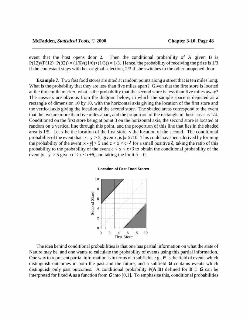
Example 7. Two fast food stores are sited at random points along a street that is ten miles long.What is the probability that they are less than five miles apart? Given that the first store is locatedat the three mile marker, what is the probability that the second store is less than five miles away?The answers are obvious from the diagram below, in which the sample space is depicted as arectangle of dimension 10 by 10, with the horizontal axis giving the location of the first store andthe vertical axis giving the location of the second store. The shaded areas correspond to the eventthat the two are more than five miles apart, and the proportion of the rectangle in these areas is 1/4.Conditioned on the first store being at point 3 on the horizontal axis, the second store is located atrandom on a vertical line through this point, and the proportion of this line that lies in the shadedarea is 1/5. Let x be the location of the first store, y the location of the second. The conditionalprobability of the event that |x - y| > 5, given x, is |x-5|/10. This could have been derived by formingthe probability of the event |x - y| > 5 and c < x < c+ for a small positive , taking the ratio of thisprobability to the probability of the event c < x < c+ to obtain the conditional probability of theevent |x - y| > 5 given c < x < c+, and taking the limit 6 0.
The idea behind conditional probabilities is that one has partial information on what the state ofNature may be, and one wants to calculate the probability of events using this partial information.One way to represent partial information is in terms of a subfield; e.g., F is the field of events whichdistinguish outcomes in both the past and the future, and a subfield G contains events whichdistinguish only past outcomes. A conditional probability P(A*B) defined for B f G can beinterpreted for fixed A as a function from G into [0,1]. To emphasize this, conditional probabilities
McFadden, Statistical Tools, © 2000 Chapter 3-11, Page 49 ___________________________________________________________________________
are sometimes written P(A*G), and G is termed the information set, or a family of events with theproperty that you know whether or not they happened at the time you are forming the conditionalprobability.
Example 1. (continued) If G = { ,S,{HT,HH},{TT,TH}}, so that events in G describe theoutcome of the first coin toss, then P(HH*{HH,HT}) = P(HH)/(P(HH)+P(HT)) = ½ is the probabilityof heads on the second toss, given heads on the first toss. In this example, the conditional probabilityof a head on the second toss equals the unconditional probability of this event. In this case, theoutcome of the first coin toss provides no information on the probabilities of heads from the secondcoin, and the two tosses are said to be statistically independent. If G ={ ,S,{HT,TH},{HH},{TT},{HH} c,{TT} c}, the family of events that determine the number of headsthat occur in two tosses without regard for order, then the conditional probability of heads on thefirst toss, given at least one head, is P({HT,HH}*{TT} c) = (P(HT)+P(HH))/(1-P(TT))= 2/3. Then,the conditional probability of heads on the first toss given at least one head is not equal to theunconditional probability of heads on the first toss.
Example 3. (continued) Suppose G = { ,S,(1,4),(-4,1]} is the -field corresponding to theevent that the index exceeds 1, and let B denote the Borel -field containing all the open intervals.The unconditional probability P((s,4)) = e-s/2 implies P((1,4)) = e-1/2 = 0.6065. The conditionalprobability of (2,4) given (1,4) satisfies P(((2,4)*(1,4)) = P((1,4)1(2,4))/P((1,4)) = e-1/e-1/2 = 0.6065> P((2,4)) = 0.3679. The conditional and unconditional probabilities are not the same, so that theconditioning event provides information on the probability of (2,4).
For a probability space (S,F,P), suppose A1,...,Ak is a finite partition of S; i.e., Ai1Aj = and
Ai = S. The partition generates a finite field G f F . From the formula P(A1B) =�ki'1
P(A*B)P(B) satisfied by conditional probabilities, one has for an event C 0 F the formula
P(C) = P(C|Ai)@P(Ai).jk
i'1
This is often useful in calculating probabilities in applications where the conditional probabilitiesare available.
3.3.9. In a probability space (S,F,P), the concept of a conditional probability P(A|B) of A 0 Fgiven an event B in a -field G f F can be extended to cases where P(B) = 0 by defining P(A*B)as the limit of P(A*Bi) for sequences Bi 0 G that satisfy P(Bi) > 0 and Bi 6 B, provided the limitexists. If we fix A, and consider P(A1B) as a measure defined for B 0 G, this measure obviouslysatisfies P(A1B) # P(B), so that it is absolutely continuous with respect to P(B). Then, Theorem 3.2
McFadden, Statistical Tools, © 2000 Chapter 3-12, Page 50 ___________________________________________________________________________
implies that there exists a function P(A|@) 0 L1(S,G,P) such that P(A1B) = P(A|s)@P(ds). WemB
have written this function as if it were a conditional probability of A given the “event” {s}, and itcan be given this interpretation. If B 0 G is an atom, then the measurability of P(A|@) with respectto G requires that it be constant for s 0 B, so that P(A1B) = P(A|s)@P(B) for any s 0 B, and we caninstead write P(A1B) = P(A|B)@P(B), satisfying the definition of conditional probability even if P(B)= 0.
Example 4. (continued) Consider F = BqB, the product Borel -field on ß+, and G =Bq{ .ß+}, the -field corresponding to having complete information on the level of the index onthe first day and no information on the second day. Suppose P((s,4)×(t,4)) = 2/(1+es+t). This is aprobability on these open intervals that extends to F; verifying this takes some work. Theconditional probability of (s,4)×(t,4) given the event (r,4)×(0,4) 0 G and s # r equals P((r,4)×(t,4))divided by P((r,4)×(0,4)), or (1+er)/(1+er+t). The conditional probability of (s,4)×(t,4) given theevent (r,r+)×(0,4) 0 G and s # r is [1/(1+er+t) - 1/(1+er+ +t)]/[1/(1+er) - 1/(1+er+ )]. The limit of thisexpression as 6 0 is er@(1+er)2/(1+er+t)2 = P((s,4)×(t,4)|{r}×(0,4)); this function of r is also theintegrand that satisfies Theorem 3.2. Note that P((s,4)×(t,4)|{r}×(0,4)) ú P((s,4)×(0,4)) = 1/(1+es),so that the conditioning event conveys information about the probability of (s,4)×(t,4).
3.4. STATISTICAL INDEPENDENCE AND REPEATED TRIALS
3.4.1. Consider a probability space (S,F,P). Events A and C in F are statistically independentif P(A1C) = P(A)"P(C). From the definition of conditional probability, if A and C are statisticallyindependent and P(A) > 0, then P(C*A) = P(A1C)/P(A) = P(C). Thus, when A and C arestatistically independent, knowing that A occurs is unhelpful in calculating the probability that Coccurs. The idea of statistical independence of events has an exact analogue in a concept ofstatistical independence of subfields. Let A = { ,A,Ac,S} and C = { ,C,Cc,S} be the subfields ofF generated by A and C, respectively. Verify as an exercise that if A and C are statisticallyindependent, then so are any pair of events AN 0 A and CN 0 C. Then, one can say that the subfieldsA and C are statistically independent. One can extend this idea and talk about statisticalindependence in a collection of subfields. Let N denote an index set, which may be finite, countable,or non-countable. Let Fi denote a -subfield of F (Fi f F) for each i 0 N. The subfields Fi are
mutually statistically independence (MSI) if and only if P( Aj) = P(Aj) for all finite K_j0K
kj0K
f N and Aj 0 Fj for j 0 K. As in the case of statistical independence between two events (subfields),the concept of MSI can be stated in terms of conditional probabilities: Fi for i 0 N are mutually
McFadden, Statistical Tools, © 2000 Chapter 3-13, Page 51 ___________________________________________________________________________
statistically independent (MSI) if, for all i 0 N, finite K f N\{i} and Aj 0 Fj for j 0 {i} cK, one has
P(Ai Aj) = P(Ai), so the conditional and unconditional probabilities are the same. _j0K
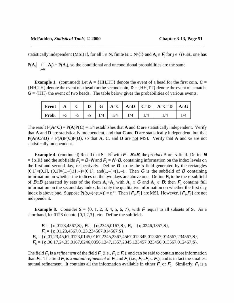
Example 1. (continued) Let A = {HH,HT} denote the event of a head for the first coin, C ={HH,TH} denote the event of a head for the second coin, D = {HH,TT} denote the event of a match,G = {HH} the event of two heads. The table below gives the probabilities of various events.
Event A C D G A1C A1D C1D A1C1D A1G
Prob. ½ ½ ½ 1/4 1/4 1/4 1/4 1/4 1/4
The result P(A1C) = P(A)P(C) = 1/4 establishes that A and C are statistically independent. Verifythat A and D are statistically independent, and that C and D are statistically independent, but thatP(A1C1D) ú P(A)P(C)P(D), so that A, C, and D are not MSI. Verify that A and G are notstatistically independent.
Example 4. (continued) Recall that S = ß2 with F = BqB, the product Borel -field. Define N= { ,ß} and the subfields F1 = B×N and F2 = N×B, containing information on the index levels onthe first and second day, respectively. Define G to be the -field generated by the rectangles(0,1]×(0,1], (0,1]×(1,4),(1,4)×(0,1], and(1,4)×(1,4). Then G is the subfield of B containinginformation on whether the indices on the two days are above one. Define F3 to be the -subfieldof BqB generated by sets of the form A1×A2 with A1 0 G and A2 0 B; then F3 contains fullinformation on the second day index, but only the qualitative information on whether the first dayindex is above one. Suppose P((s,4)×(t,4)) = e-s-t. Then {F1,F2} are MSI. However, {F1,F3} are notindependent.
Example 8. Consider S = {0, 1, 2, 3, 4, 5, 6, 7}, with F equal to all subsets of S. As ashorthand, let 0123 denote {0,1,2,3}, etc. Define the subfields
F1 = { ,0123,4567,S}, F2 = { ,2345,0167,S}, F3 = { ,0246,1357,S},F4 = { ,01,23,4567,0123,234567,014567,S},
F5 = { ,01,23,45,67,0123,0145,0167,2345,2367,4567,012345,012367,014567,234567,S}, F6 = { ,06,17,24,35,0167,0246,0356,1247,1357,2345,123457,023456,013567,012467,S}.
The field F4 is a refinement of the field F1 (i.e., F1 f F4), and can be said to contain more informationthan F1. The field F5 is a mutual refinement of F1 and F2 (i.e., F1cF2 f F5), and is in fact the smallestmutual refinement. It contains all the information available in either F1 or F2. Similarly, F6 is a

McFadden, Statistical Tools, © 2000 Chapter 3-14, Page 52 ___________________________________________________________________________
mutual refinement of F2 and F3. The intersection of F5 and F6 is the field F2; it is the commoninformation available in F5 and F6. If, for example, F5 characterized the information available to oneeconomic agent, and F6 characterized the information available to a second agent, then F2 wouldcharacterize the common information upon which they could base contingent contracts. SupposeP(i) = 1/8. Then {F1, F2, F3} are MSI. E.g., P(0123*2345) = P(0123*0246) = P(0123*234510246)= P(0123) = 1/2. However, {F1, F4} are not independent; e.g., 1 = P(0123*01) ú P(0123) = 1/2.
For M f N, let FM denote the smallest -field containing Fi for all i 0 M. Then MSI satisfies thefollowing theorem, which provides a useful criterion for determining whether a collection ofsubfields is MSI:
Theorem 3.3. If Fi are MSI for i 0 N, and M f N\{i}, then { Fi,FM} are MSI. Further, Fi for i0Nare MSI if and only if {Fi,FN\i} are MSI for all i0N.
Example 5. (continued) If M = {2,3}, then FM / F6, and P(0123 A) = ½ for each A 0 FM.
3.4.2. The idea of repeated trials is that an experiment, such as a coin toss, is replicated overand over. It is convenient to have common probability space in which to describe the outcomes oflarger and larger experiments with more and more replications. The notation for repeated trials willbe similar to that introduced in the definition of mutual statistical independence. Let N denote afinite or countable index set of trials, Si a sample space for trial i, and Gi a -field of subsets of Si.Note that (Si,Gi) may be the same for all i. Assume that (Si, Gi) is the real line with the Borel -field,or a countable set with the field of all subsets, or a pair with comparable mathematical properties(i.e., Si is a complete separable metric space and Gi is its Borel field). Let t = (s1,s2,...) = (si : i0N)
denote an ordered sequence of outcomes of trials, and SN = ×i0N Si denote the sample space of these
sequences. Let FN = qi0NGi denote the -field of subsets of SN generated by the finite rectangles
which are sets of the form (×i0K Ai)×(×i0N\K Si) with K a finite subset of N and Ai 0 Gi for i 0 K.The collection FN is called the product -field of subsets of SN.
Example 9. N = {1,2,3}, Si = {0,1}, Gi = { ,{0},{1},S} is a sample space for a coin toss, coded“1" if heads and “0" if tails. Then SN = {s1s2s3 si 0 Si} = {000, 001, 010, 011, 100, 101, 110, 111},where 000 is shorthand for the event {0}×{0}×{0}, and so forth, is the sample space for three cointosses. The field FN is the family of all subsets of SN.
For any subset K of N, define SK = ×i0K Si and GK = qi0KGi. Then, GK is the product -fieldon SK. Define FK to be the -field on SN generated by sets of the form A×SN\K for A 0 GK. Then GK
McFadden, Statistical Tools, © 2000 Chapter 3-15, Page 53 ___________________________________________________________________________
and FK contain essentially the same information, but GK is a field of subsets of SK and FK is acorresponding field of subsets of SN which contains no information on events outside of K. SupposePN is a probability on (SN, FN). The restriction of PN to (SK,GK) is a probability PK defined for A 0GK by PK(A) = PN(A×SN\K). The following result establishes a link between different restrictions:
Theorem 3.4. If M f K and PM, PK are restrictions of PN, then PM and PK satisfy thecompatibility condition that PM(A) = PK(A×SK\M) for all A 0 FM.
There is then a fundamental result that establishes that when probabilities are defined on all finitesequences of trials and are compatible, then there exists a probability defined on the infinite sequenceof trials that yields each of the probabilities for a finite sequence as a restriction.
Theorem 3.5. If PK on (SK,GK) for all finite K f N satisfy the compatibility condition, then thereexists a unique PN on (SN,FN) such that each PK is a restriction of PN.
This result guarantees that it is meaningful to make probability statements about events such as “aninfinite number of heads in repeated coin tosses"..
Suppose trials (Si,Gi,Pi) indexed by i in a countable set N are mutually statistically independent.For finite K f N, let GK denote the product -field on SK. Then MSI implies that the probability of
a set ×i0K Ai 0 GK satisfies PK(×i0K Ai) = Pj(Aj). Then, the compatibility condition inkj0K
Theorem 3.3 is satisfied, and that result implies the existence of a probability PN on (SN,FN) whoserestrictions to (SK,GK) for finite K f N are the probabilities PK.
3.4.3. The assumption of statistically independent repeated trials is a natural one for manystatistical and econometric applications where the data comes from random samples from thepopulation, such as surveys of consumers or firms. This assumption has many powerfulimplications, and will be used to get most of the results of basic econometrics. However, it is alsocommon in econometrics to work with aggregate time series data. In these data, each period ofobservation can be interpreted as a new trial. The assumption of statistical independence acrossthese trials is unlikely in many cases, because in most cases real random effects do not convenientlylimit themselves to single time periods. The question becomes whether there are weakerassumptions that time series data are likely to satisfy that are still strong enough to get some of thebasic statistical theorems. It turns out that there are quite general conditions, called mixingconditions, that are enough to yield many of the key results. The idea behind these conditions is thatusually events that are far apart in time are nearly independent, because intervening shocksoverwhelm the older history in determining the later event. This idea is formalized in Chapter 4.

McFadden, Statistical Tools, © 2000 Chapter 3-16, Page 54 ___________________________________________________________________________
5. RANDOM VARIABLES, DISTRIBUTION FUNCTIONS, AND EXPECTATIONS
3.5.1. A random variable X is a measurable real-valued function on a probability space (S,F,P).The value of the function x = X(s) for a state of Nature s that actually occurs is termed a realizationof the random variable. One can have many random variables defined on the same probability space;another measurable function y = Y(s) defines a second random variable. It is very helpful in workingwith random variables to keep in mind that the random variable itself is a function of states ofNature, and that observations are of realizations of the random variable. Thus, when one talks aboutconvergence of a sequence of random variables, one is actually talking about convergence of asequence of functions, and notions of distance and closeness need to be formulated as distance andcloseness of functions.
3.5.2. The term measurable in the definition of a random variable means that for each set A inthe Borel -field B of subsets of the real line, the inverse image X-1(A) / {s0S*X(s)0A} is in the-field F of subsets of the sample space S. The assumption of measurability is a mathematical
technicality that ensures that probability statements about the random variable are meaningful. Weshall not make any explicit reference to measurability in basic econometrics, and shall alwaysassume implicitly that the random variables we are dealing with are measurable.
3.5.3. The probability that a random variable X has a realization in a set A 0 B is given by
F(A) / P(X-1(A)) / P({s0S*X(s)0A}).
The function F is a probability on B; it is defined in particular for half-open intervals of the form A= (-4,x], in which case F((-4,x]) is abbreviated to F(x) and is called the distribution function (or,cumulative distribution function, CDF) of X. From the properties of a probability, the distributionfunction has the properties
(i) F(-4) = 0 and F(+4) = 1.(ii) F(x) is non-decreasing in x, and continuous from the right.(iii) F(x) has at most a countable number of jumps, and is continuous except at these jumps.(Points without jumps are called continuity points.)
Conversely, any function F that satisfies (i) and (ii) determines uniquely a probability F on B. Thesupport of the distribution F is the smallest closed set A 0 B such that F(A) = 1.

McFadden, Statistical Tools, © 2000 Chapter 3-17, Page 55 ___________________________________________________________________________
Example 5. (continued) The standard normal CDF is (x) = , obtained bymx
&4
(2 )&1/2"e &s 2/2ds
integrating the density n(s) = . Other examples are the CDF for the standard(2 )&1/2"e &s 2/2
exponential distribution, F(x) = 1 - e-x for x > 0, and the CDF for the logistic distribution, F(x) =
1/(1+e-x). An example of a CDF that has jumps is F(x) = 1 - e-x/2 - for x > 0.j4
k'1 1(k$x)/2k%1
3.5.4. If F is absolutely continuous with respect to a -finite measure on ß; i.e., F givesprobability zero to any set that has -measure zero, then (by the Radon-Nikodym theorem) thereexists a real-valued function f on ß, called the density (or probability density function, pdf) of X,such that
F(A) = f(x) (dx) mA
for every A 0 B. With the possible exception of a set of -measure zero, F is differentiable and thederivative of the distribution gives the density, f(x) = FN(x). When the measure is Lebesguemeasure, so that the measure of an interval is its length, it is customary to simplify the notation and
write F(A) = f(x)dx.mA
If F is absolutely continuous with respect to counting measure on a countable subset C of ß, thenit is called a discrete distribution, and there is a real-valued function f on C such that
F(A) = f(x).jx0A
Recall that the probability is itself a measure. This suggests a notation F(A) = F(dx) that coversmA
both continuous and counting cases. This is called a Lebesgue-Stieltjes integral.
3.5.5. If (ß,B,F) is the probability space associated with a random variable X, and g:ß 6 ß isa measurable function, then Y = g(X) is another random variable. The random variable Y is
integrable with respect to the probability F if *g(x)*F(dx) < +4;mß

McFadden, Statistical Tools, © 2000 Chapter 3-18, Page 56 ___________________________________________________________________________
if it is integrable, then the integral g(x)F(dx) / g"dF exists, is denoted E g(X), and ismß mßcalled the expectation of g(X). When necessary, this expectation will also be denoted EXg(X) toidentify the distribution used to form the expectation. When F is absolutely continuous with respect
to Lebesgue measure, so that F has a density f, the expectation is written E g(X) = g(x)f(x)dx.mßAlternately, for counting measure on the integers with density f(k), E g(X) = g(k)f(k).j%4
k'&4
The expectation of X, if it exists, is called the mean of X. The expectation of (X - EX)2, if itexists, is called the variance of X. Define 1(X#a) to be an indicator function that is one if X(s) #a, and zero otherwise. Then, E 1(X#a) = F(a), and the distribution function can be recovered fromthe expectations of the indicator functions.
Example 1. (continued) Define a random variable X by
X(s) =
0 if s ' TT
1 if s ' TH or HT
2 if s ' HH
Then, X is the number of heads in two coin tosses. For a fair coin, E X = 1.
Example 2. (continued) Let X be a random variable defined to equal the number of heads thatappear before a tail occurs. Then, possible values of X are the integers C = {0,1,2,...}. Then C isthe support of X. For x real, define [x] to be the largest integer k satisfying k # x. A distribution
function for X, defined on the real line, is F(x) = ; the associated density1& 2&[x%1] for 0# x
0 for 0 > x
defined on C is f(k) = 2-k-1. The expectation of X, obtained using evaluation of a special series from
2.1.10, is E X = k"2-k-1 = 1.j4
k'0
Example 3. (continued) Define a random variable X by X(s) = *s - 1*. Then, X is the magnitudeof the deviation of the index from one. The inverse image of an interval (a,b) is (1-b,1-a)c(1+a,1+b)0 F, so that X is measurable. Other examples of measurable random variables are Y defined by Y(s)= Max {1,s} and Z defined by Z(s) = s3.

McFadden, Statistical Tools, © 2000 Chapter 3-19, Page 57 ___________________________________________________________________________
3.5.6. Consider a random variable Y on (ß,B). The expectation EYk is the k-th moment of Y,and E(Y-EY)k is the k-th central moment. Sometimes moments fail to exist. However, if g(Y) iscontinuous and bounded, then Eg(Y) always exists. The expectation m(t) = EetY is termed themoment generating function (mgf) of Y; it sometimes fails to exist. Call a mgf proper if it is finitefor t in an interval around 0. When a proper mgf exists, the random variable has finite moments ofall orders. The expectation (t) = EetY, where is the square root of -1, is termed the characteristicfunction (cf) of Y. The characteristic function always exists.
Example 5. (continued) A density f(x) that is symmetric about zero, such as the standard normal,
has EXk = xkf(x)dx = xkf(-x)dx + xkf(x)dx = [1 + (-1)k]xkf(x)dx = 0 form%4
&4 m0
&4 m%4
0 m%4
0
k odd. Integration by parts yields the formula EXk = 2k xk-1 [1-F(x)]dx for k even. For them%4
0
standard normal, EX2k = = (2k-1)@EX2k-2 for k > 2 using integration2@m%4
0(2 )&1/2"x 2k&1@e &x 2/2xdx
by parts, and EX2 = = 2@ (0) = 1. Then, EX4 = 3 and EX6 = 15. The2@m%4
0(2 )&1/2@e &x 2/2xdx
moment generating function of the standard normal is m(t) = .m%4
&4
(2 )&1/2"e tx@e &x 2/2dx
Completing the square in the exponent gives m(t) = = .e t 2/2@m%4
&4
(2 )&1/2@e &(x&t)2/2dx e t 2/2
3.5.7. A measurable function X from the probability space (S,F,P) into (ßn,Bn) is termed arandom vector. (The notation B n means BqBq...qB n times, where B is the Borel -field on the
real line. This is also called the product -field, and is sometimes written B n = qi=1,...,n Bi, wherethe Bi are identical copies of B.) The random vector can also be written XN = (X1,...,Xn) , with eachcomponent Xi a random variable. The distribution function (CDF) of X is
F(x1,...,xn) = P({sgS*X i(s) # xi for i = 1,...,n}).
If A 0 B n, define F(A) = P({sgS*X(s)0A}). If F(A) = 0 for every set A of Lebesque measurezero, then there exists a probability density function (pdf) f(x1,...,xn) such that
McFadden, Statistical Tools, © 2000 Chapter 3-20, Page 58 ___________________________________________________________________________
(1) F(x1,...,xn) = f(y1,...,yn) dy1...dyn. mx1
&4mx2
&4
...mxn
&4
F and f are termed the joint or multivariate CDF and pdf, respectively, of X. The random variableX1 has a distribution that satisfies
F1(x1) / P({s0S*X1(s) # x1}) = F(x1,+4,...,+4).
This random variable is measurable with respect to the -subfield G1 containing the events whoseoccurrence is determined by X1 alone; i.e., G1 is the family generated by sets of the form A×ß×...×ßwith A 0 B. If F is absolutely continuous with respect to Lebesque measure on B n, then there areassociated densities f and f1 satisfying
(2) F1(x1) = f1(y1) dy1 mx1
y1'&4
(3) f1(x1) = f(x1,y2,...,yn)"dy2...dyn. m%4
y2'&4
@ @ @m%4
yn'&4
F1 and f1 are termed the marginal CDF and pdf, respectively, of X1.
3.5.8. Corresponding to the concept of a conditional probability, we can define a conditionaldistribution: Suppose C is an event in G1 with P(C) > 0. Then, define F(2)(x2,...,xn*C) =F({y0ßn*y10C,y2#x2,...,yn#xn})/F1(C) to be the conditional distribution of (X2,...,Xn) given X1 0 C.When F is absolutely continuous with respect to Lebesgue measure on ßn, the conditionaldistribution can be written in terms of the joint density,
F(2)(x2,...,xn*C) = .my10C m
x2
y2 '&4m
xn
yn'&4
f(y1,y2,...,yn)"dy1dy2...dyn
my10C m%4
y2 '&4m%4
yn'&4
f(y1,y2,...,yn)"dy1dy2...dyn
Taking the limit as C shrinks to a point X1 = x1, one obtains the conditional distribution of (X2,...,Xn)given X1 = x1,
F(2)(x2,...,xn*X1=x1) = ,
mx2
y2 '&4m
xn
yn'&4
f(x1,y2,...,yn)"dy1dy2...dyn
f1(x1)
provided f1(x1) > 0. Finally, associated with this conditional distribution is the conditional densityf(2)(x2,...,xn*X1=x1) = f(x1,x2,...,xn)/f1(x1). More generally, one could consider the marginaldistributions of any subset, say X1,...Xk, of the vector X, with Xk+1,...Xn integrated out; and the
McFadden, Statistical Tools, © 2000 Chapter 3-21, Page 59 ___________________________________________________________________________
conditional distributions of one or more of the variables Xk+1,...Xn given one or more of theconditions X1 = x1,...,Xk = xk.
3.5.9. Just as expectations are defined for a single random variable, it is possible to defineexpectations for a vector of random variables. For example, E(X1 - EX1)(X2-EX2) is called thecovariance of X1 and X2, and EetNX, where tN = (t1,...,tn) is a vector of constants, is a (multivariate)moment generating function for the random vector X. Here are some useful properties ofexpectations of vectors:
(a) If g(X) is a function of a random vector, then Eg(X) is the integral of g with respect to thedistribution of X. When g depends on a subvector of X, then Eg(X) is the integral of g(y) withrespect to the marginal distribution of this subvector.(b) If X and Z are random vectors of length n, and a and b are scalars, then E(aX + bZ) = aEX+ bEZ.(c) [Cauchy-Schwartz inequality] If X and Z are random vectors of length n, then (EXNZ)2 #(EXNX)(EZNZ).(d) [Minkowski Inequality] If X is a random vector of length n and r $ 1 is a scalar, then
(E* X i*r)1/r # (E*X i*
r)1/r.jni'1 jn
i'1
(e) [Loeve Inequality] If X is a random vector of length n and r > 0, then E* X i*r #jn
i'1
max(1,nr-1) E*X i*r.jn
i'1
(f) [Jensen Inequality] If X is a random vector and g(x) is a convex function, then E g(X) $g(EX). If g(x) is a concave function, the inequality is reversed.
When expectations exist, they can be used to bound the probability that a random variable takes onextreme values.
Theorem 3.6. Suppose X is a n×1 random vector and g is a positive scalar. a. [Markov bound] If maxiE*X i* < +4, then maxiPr(*X i* > g) < maxiE*X i*/g.b. [Chebyshev bound] If EXNX < +4, then Pr(2X22 > g) < EXNX/g2.c. [Chernoff bound] If EetNX exists for all vectors t in some neighborhood of zero, then for somepositive scalars and M, Pr(2X22 > g) < Me- g.
Proof: All these inequalities are established by the same technique: If r(y) is a positive non-decreasing function of y > 0, and Er(2X2) < +4, then

McFadden, Statistical Tools, © 2000 Chapter 3-22, Page 60 ___________________________________________________________________________
Pr(2X2 > g) = F(dx) # [r(2x2)/r(g)]F(dx) # Er(2X2)/r(g). m2x2>g m2x2>gTaking r(y) = y2 gives the result directly for the Chebyshev bound. In the remaining cases, first geta component-by-component inequality. For the Markov bound, Pr(*X i* > g) < E*X i*/g for each igives the result. For the Chernoff bound,
Pr(2X22 > g) # [Pr(Xi > g@n-1/2) + Pr(Xi < -g@n-1/2)]jni'1
since if the event on the left occurs, one of the events on the right must occur. Then apply theinequality Pr(*X i* > g) # Er(*X i*)/r(g) with r(y) = n-1/2@ey to each term in the right-hand-side sum.The inequality for vectors is built up from a corresponding inequality for each component. ~
3.5.10. When the expectation of a random variable is taken with respect to a conditionaldistribution, it is called a conditional expectation. If F(x*C) is the conditional distribution of arandom vector X given the event C, then the conditional expectation of a function g(X) given C isdefined as
EX*Cg(X) = g(y)F(dy*C).mAnother notation for this expectation is E(g(X)*C). When the distribution of the random variableX is absolutely continuous with respect to Lebesgue measure, so that it has a density f(x), the
conditional density can be written as , and the conditional expectationf(x|C)' f(x)@1(x0C)/mCf(s)ds
can then be written
EX*Cg(X) = = .mCg(x)@f(x|C)dx
mCg(x)@f(x)dx
mCf(x)dx
When the distribution of X is discrete, this formula becomes
EX*Cg(X) = .jk0C g(k)@f(k)
jk0C f(k)
The conditional expectation is actually a function on the -field C of conditioning events, and issometimes written EX*C g(X) or E(g(X)*C) to emphasize this dependence.
Suppose A1,...,Ak partition the domain of X. Then the distribution satisfies
McFadden, Statistical Tools, © 2000 Chapter 3-23, Page 61 ___________________________________________________________________________
F(x) = F(x|Ai)@F(Ai),jki'1
implying
Eg(X) = g(x)F(dx) = g(x)F(dx*Ai)@F(Ai) = E{g(X)|Ai} @F(Ai).m jki'1 m jk
i'1
This is called the law of iterated expectations, and is heavily used in econometrics.
Example 2. (continued) Recall that X is the number of heads that appear before a tail in asequence of coin tosses, and that the probability of X = k is 2-k-1 for k = 0,1,... . Let C be the eventof an even number of heads. Then,
EX*CX = = = 2/3,jk'0,2,4,... k@2&k&1
jk'0,2,4,... 2&k&1
jj'0,1,2,... j@4&j
jj'0,1,2,... 4&j/2
where the second ratio is obtained by substituting k = 2j, and the value is obtained using thesummation formulas for a geometric series from 2.1.10. A similar calculation for the event A of anodd number of heads yields EX*AX = 5/3. The probability of an even number of heads is
= 2/3. The law of iterated expectations then givesjk'0,2,4,... 2&k&1
E X = E{X|C)@P(C) + E{X|A)@P(A) = (2/3)(2/3) + (5/3)(1/3) = 1,
which confirms the direct calculation of E X.
The concept of a conditional expectation is very important in econometrics and in economictheory, so we will work out its properties in some detail for the case of two variables. Supposerandom variables (U,X) have a joint density f(u,x). The marginal density of X is defined by
g(x) = f(u,x)du, m%4
u'&4
and the conditional density of U given X = x is defined by f(u*x) = f(u,x)/g(x), provided g(x) > 0.The conditional expectation of a function h(U,X) satisfies E(h(U,X)*X=x) = Ih(u,x)f(u*x)du, andis a function of x. The unconditional expectation of h(U,X) satisfies
Eh(U,X) = h(u,x)f(u,x)dudx = = EXEU*Xh(U,X); mm m%4
x'&4 m4
u'&4h(u,x)f(u*x)du g(x)dx
another example of the law of iterated expectations. The conditional mean of U given X=x isMU*X(x) / EU*X=xU; by the law of iterated expectations, the conditional and unconditional mean are

McFadden, Statistical Tools, © 2000 Chapter 3-24, Page 62 ___________________________________________________________________________
related by EUU = EXEU*XU / EXMU*X(X). The conditional variance of U is defined by V(U*x) =EU*X(U - MU*X(x))2. It is related to the unconditional variance by the formula
EU(U - EUU)2 = EXEU*X(U - MU*X(X) + MU*X(X) - EUU)2
= EXEU*X(U - MU*X(X))2 + EXEU*X(MU*X(X) - EUU)2 + 2EXEU*X(U - MU*X(X))(MU*X(X) - EUU) = EXV(U*X) + EX(MU*X(X) - EUU)2 + 2EX(MU*X(X) - EUU)EU*X(U - MU*X(X)) = EXV(U*X) + EX(MU*X(X) - EUU)2
Then, the unconditional variance equals the expectation of the conditional variance plus the varianceof the conditional expectation.
Example 10: Suppose (U,X) are bivariate normal with means EU = µu and EX = µx, and secondmoments E(U-µu)
2 = u2, E(X-µx)
2 = x2, and E(U-µu)(X-µx) = ux / u x. Define
Q = ,1
1& 2@
u&µu
u
2
%x&µx
x
2
& 2@ @u&µu
u
@x&µx
x
and observe that
.Q&x&µx
x
2
'1
1& 2@
u&µu
u
& @x&µx
x
2
The bivariate normal density is f(u,x) = [2u x(1- 2)1/2] -1@exp(-Q/2). The marginal density of X isnormal with mean µx and variance x
2: n(x-µx, x) = (2 x2)-1@exp(-(x-µx)
2/2 x2) . This can be derived
from the bivariate density by completing the square for u in Q and integrating over u. Theconditional density of U given X then satisfies
f(u*x) = [2 u x(1- 2)½]-1@exp(-Q/2)/(2 x2)-1@exp(-(x-µx)
2/2 x2).
= [2 u2(1- 2)]-½@ . exp
&1
2@(1& 2)@
u&µu
u
& @x&µx
x
2
Hence the conditional distribution of U, given X = x, is normal with conditional mean E(U*X=x)= µu + u(x � µx)/ x / µu + ux(x-µx)/ x
2 and variance V(U*X=x) / E((U-E(U*X=x))2*X=x) =
u2(1- 2) / u
2 - ux2/ x
2. When U and X are joint normal random vectors with EU = µu, EX = µx,E(U-µu)(U-µu)N = uu, E(X-µx)(X-µx)N= xx, and E(U-µu)(X-µx)N = ux, then (U*X=x) is normal withE(U*X=x) = µu + ux xx
-1(x - µx) and V(U*X=x) = uu - ux xx-1
xu.

McFadden, Statistical Tools, © 2000 Chapter 3-25, Page 63 ___________________________________________________________________________
3.5.11. Conditional densities satisfy f(u,x) = f(u*x)g(x) = f(x*u)h(u), where h(u) is the marginaldensity of U, and hence f(u*x) = f(x*u) h(u)/g(x). This is called Bayes Law. When U and X areindependent, f(u,x) = h(u)"g(x), or f(u*x) = h(u) and f(x*u) = g(x). For U and X independent, andr(") and s(") any functions, one has E(r(U)*X=x) = Ir(u)f(u*x)du / Ir(u)h(u)du = Er(U), andE(r(U)s(X)) = Ir(u)s(x)f(u,x)dudx = Is(x)g(x)Ir(u)f(u*x)du dx = Is(x)g(x)Er(U*x)dx =[Es(X)][Er(U)], or cov(r(U),s(X)) = 0, provided Er(U) and Es(X) exist. If r(u) = u - EU, thenE(r(U)*X=x) = 0 and cov(U,X) = E(U-EU)X = 0. Conversely, suppose U and X are jointlydistributed. If cov(r(U),s(X)) = 0 for all functions r ("), s(") such that Er(U) and Es(X) exist, then Xand U are independent. To see this, choose r(u) = 1 for u # u*, r(u) = 0 otherwise; choose s(x) = 1for x # x*, s(x) = 0 otherwise. Then Er(U) = H(u*) and Es(X) = G(x*), where H and G are themarginal cumulative distribution functions, and 0 = cov = F(u*,x*) - H(u*)"G(x*), where F is the jointcumulative distribution function. Hence, F(u,x) = H(u)"G(x), and X, U are independent.
Note that cov (U,X) = 0 is not sufficient to imply U,X independent. For example, g(x) = ½ for-1 # x # l and f(u*x) = ½ for -1 # u-x2 # 1 is nonindependent with E(U*X=x) = x2, but cov(U,X) =EX3 = 0. Furthermore, E(U*X=x) / 0 is not sufficient to imply U,X independent. For example, g(x)= ½ for -1 # x # 1 and f(u*x)= 1/2(1 + x2) for -(1+ x2) # u # (1 + x2) is nonindependent with E(U2*x) = (1 + x2 )2 ú E U2 = 28/15, but E(U*X=x) / 0.
Example 11. Suppose monthly family income (in thousands of dollars) is a random variable Ywith a CDF F(y) = 1 - y-2 for y > 1. Suppose a random variable Z is one for home owners and zerootherwise, and that the conditional probability of the event Z = 1, given Y, is (Y-1)/Y. Theunconditional expectation of Y is 2. The joint density of Y and Z is f(y)@g(z|y) = (2y-3) (1 - y-1) for
z = 1. The unconditional probability of Z = 1 is then f(y)@g(z|y)dy = 1/3. Bayes Law givesm%4
y'1
the conditional density of Y given z = 1, f(y|z) = f(y)@g(z|y)/ f(y)@g(z|y)dy = (6y-3) (1 - y-1), som%4
y'1
that the conditional expectation of Y given z = 1 is E(Y|Z=1) = y f(y|z)dy = 3.m%4
y'1
Example 12. The problem of interpreting the results of medical tests illustrates Bayes Law. Ablood test for prostate cancer is known to yield a “positive” with probability 0.9 if cancer is present,and a false “positive” with probability of 0.2 if cancer is not present. The prevalence of the cancerin the population of males is 0.05. Then, the conditional probability of cancer, given a “positive”test result, equals the joint probability of cancer and a positive test result, (0.05)(0.9), divided by theprobability of a positive test result, (0.05)(0.9)+(0.95)(0.2), or 0.235. Thus, a “positive” test has alow probability of identifying a case of cancer, and if all “positive” tests were followed by surgery,about 75 percent of these surgeries would prove unnecessary.

McFadden, Statistical Tools, © 2000 Chapter 3-26, Page 64 ___________________________________________________________________________
3.5.12. The discussion of expectations will be concluded with a list of detailed properties ofcharacteristic functions and moment generating functions:
a. (t) = EetY / Ecos(tY) + Esin(tY).b. Z = a + bY has the cf eta (bt) and Z = f(Y) has the cf Eet@f(Y). c. If EYk exists, then (k)(t) / dk (t)/dtk exists, satisfies the bound *dk (t)/dtk* # E*Y*k, and isuniformly continuous, and EYk = (- )k (k)(0). If (k)(t) exists, then EYk exists. d. If Y has finite moments through order k, then (t) has a Taylor's expansion
(t) = j(EY j)tj/j! + [ (k)( t) - (k)(0)]tk/k! jkj'0
where is a scalar with 0 < < 1; the Taylor's expansion satisfies the bounds
* (t) - j (EY j)tj/j!* # *t*kE*Y*k/k! jk&1j'0
and
* (t) - j (EY j)tj/j!* # 2*t*kE*Y*k/k! jkj'0
If EYk exists, then the expression (t) = Ln (t), called the second characteristic function orcumulant generating function, has a Taylor's expansion
(t) = jjtj/j! + [ (k)( t) - (k)(t)], jk
j'1
where (k) / dk /dtk, and is a scalar with 0 < < 1. The expressions j are called the cumulantsof the distribution, and satisfy 1 = EY and 2 = Var(Y). The expression 3/ 2
3/2 is called theskewness, and the expression 4/ 2
2 - 3 is called the kurtosis (i.e., thickness of tails relative tocenter), of the distribution. e. If Y is normally distributed with mean µ and variance 2, then its characteristic function isexp(µt- 2t2/2). The normal has cumulants 1 = µ, 2 = 2, 3 = 4 = 0. f. Random variables X and Y have identical distribution functions if and only if they haveidentical characteristic functions. g. If Yn 6p Y (see Chap. 4.1), then the associated characteristic functions satisfy n(t) 6 (t) foreach t. Conversely, if Yn has characteristic function n(t) converging pointwise to a function (t)that is continuous at t = 0, then there exists Y such that (t) is the characteristic function of Yand Yn 6p Y. h. The characteristic function of a sum of independent random variables equals the product ofthe characteristic functions of these random variables, and the second characteristic function ofa sum of independent random variables is the sum of the second characteristic functions of thesevariables; the characteristic function of a mean of n independently identically distributed randomvariables, with characteristic function (t), is (t/n)n.
McFadden, Statistical Tools, © 2000 Chapter 3-27, Page 65 ___________________________________________________________________________
Similar properties hold for proper moment generating functions, with obvious modifications:Suppose a random variable Y has a proper mgf m(t), finite for *t* < , where is a positive constant.Then, the following properties hold:
a. m(t) = EetY for *t* < . b. Z = a + bY has the mgf etam(bt). c. EYk exists for all k > 0, and m / dkm(t)/dtk exists and is uniformly continuous for *t* < , withEYk = mY(0). d. m(t) has a Taylor's expansion (for any k) mY(t) = (EY j)tj/j! + [m( t) - m(0)]tk/k!, where isa scalar with 0 < < 1. e. If Y is normally distributed with mean µ and variance 2, then it has mgf exp(µt+2t2). f. Random variables X and Y with proper mgf have identical distribution functions if and onlyif their mgf are identical. g. If Yn 6p Y and the associated mgf are finite for *t* < , then the mgf of Yn converges pointwiseto the MGF of Y. Conversely, if Yn have proper MGF which converges pointwise to a functionm(t) that is finite for *t* < , then there exists Y such that m(t) is the mgf of Y and Yn 6p Y. h. The mgf of a sum of independent random variables equals the product of the mgf of theserandom variables; the mgf of the mean of n independently identically distributed randomvariables, each with proper mgf m(t), is m(t/n)n.
The definitions of characteristic and moment generating functions can be extended to vectors ofrandom variables. Suppose Y is a n×1 random vector, and let t be a n×1 vector of constants. Then
(t) = EetNY is the characteristic function and m(t) = EetNY is the moment generating function. Theproperties of cf and mgf listed above also hold in their multivariate versions, with obviousmodifications. For characteristic functions, two of the important properties translate to
(b’) Z = a + BY, where a is a m×1 vector and B is a m×n matrix, has cf etNa (Bt).(e’) if Y is multivariate normal with mean µ and covariance matrix G, then its characteristicfunction is exp( µNt - tNGt/2).
A useful implication of (b’) and (e’) is that a linear transformation of a multivariate normal vectoris again multivariate normal. Conditions (c) and (d) relating Taylor’s expansions and moments forunivariate cf have multivariate versions where the expansions are in terms of partial derivatives ofvarious orders. Conditions (f) through (h) are unchanged in the multivariate version.
The properties of characteristic functions and moment generating functions are discussed andestablished in C. R. Rao Linear Statistical Inference, 2b.4, and W. Feller An Introduction toProbability Theory, II, Chap. 13 and 15.
6. TRANSFORMATIONS OF RANDOM VARIABLES
McFadden, Statistical Tools, © 2000 Chapter 3-28, Page 66 ___________________________________________________________________________
6.1. Suppose X is a measurable random variable on (ß,B) with a distribution F(x) that is absolutelycontinuous with respect to Lebesgue measure, so that X has a density f(x). Consider an increasingtransformation Y = H(X); then Y is another random variable. Let h denote the inverse function ofH; i.e., y = H(x) implies x = h(y). The distribution function of Y is given by
G(y) = Pr(Y # y) = Pr(H(X) # y) = Pr(X # h(y)) = F(h(y)).
When h(y) is differentiable, with a derivative hN(y) = dh(y)/dy, the density of Y is obtained bydifferentiating, and satisfies g(y) = f(h(y))hN(y). Since y / H(h(y)), one obtains by differentiationthe formula 1 / HN(h(y))hN(y), or hN(y) = 1/HN(h(y)). Substituting this formula gives g(y) =f(h(y))/HN(h(y)).
Example 13. Suppose X has the distribution function F(x) = 1-e-x for x > 0, with F(x) = 0 forx # 0; then X is said to have an exponential distribution. Suppose Y = H(X) / log X, so that X =h(Y) / eY. Then, G(y) = 1-exp(-ey) and G(y) = exp(-ey)ey = exp(y-ey) for -4 < y < +4. This is calledan extreme value distribution. A third example is X with some distribution function F and densityf, and Y = F(X), so that for any value of X, the corresponding value of Y is the proportion of all Xthat are below this value. Let xp denote the solution to F(x) = p. The distribution function of Y isG(y) = F(xy) = y. Hence, Y has the uniform density on the unit interval.
The rule for an increasing transformation of a random variable X can be extended in severalways. If the transformation Y = H(X) is decreasing rather than increasing, then
G(y) = Pr(Y # y) = Pr(H(X) # y) = Pr(X $ h(y)) = 1-F(h(y)),
where h is the inverse function of H. Differentiating,
g(y) = f(h(y))(-hN(y)).
Then, combining cases, one has the result that for any one-to-one transformation Y = H(X) withinverse X = h(Y), the density of Y is
g(y) = f(h(y))*hN(y)* / f(h(y))/*HN(h(y)*.
An example of a decreasing transformation is X with the exponential density e-x for x > 0, and Y =1/X. Show as an exercise that G(y) = e-1/y and g(y) = e-1/y/y2.
Consider a transformation Y = H(X) that is not one-to-one. The interval (-4,y) is the image ofa set Ay of x values that may have a complicated structure. One can write
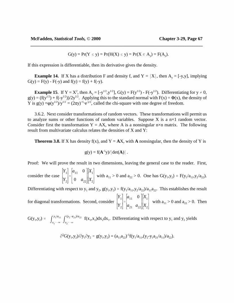
McFadden, Statistical Tools, © 2000 Chapter 3-29, Page 67 ___________________________________________________________________________
G(y) = Pr(Y # y) = Pr(H(X) # y) = Pr(X 0 Ay) = F(Ay).
If this expression is differentiable, then its derivative gives the density.
Example 14. If X has a distribution F and density f, and Y = *X*, then Ay = [-y,y], implyingG(y) = F(y) - F(-y) and f(y) = f(y) + f(-y).
Example 15. If Y = X2, then Ay = [-y1/2,y1/2], G(y) = F(y1/2) - F(-y1/2). Differentiating for y ú 0,g(y) = (f(y1/2) + f(-y1/2))/2y1/2. Applying this to the standard normal with F(x) = (x), the density ofY is g(y) =n(y1/2)/y1/2 = (2 y)-½@e-y/2, called the chi-square with one degree of freedom.
3.6.2. Next consider transformations of random vectors. These transformations will permit usto analyze sums or other functions of random variables. Suppose X is a n×1 random vector.Consider first the transformation Y = AX, where A is a nonsingular n×n matrix. The followingresult from multivariate calculus relates the densities of X and Y:
Theorem 3.8. If X has density f(x), and Y = AX, with A nonsingular, then the density of Y is
g(y) = f(A-1y)/*det(A)* .
Proof: We will prove the result in two dimensions, leaving the general case to the reader. First,
consider the case with a11 > 0 and a22 > 0. One has G(y1,y2) / F(y1/a11,y2/a22).Y1
Y2
'
a11 0
0 a22
X1
X2
Differentiating with respect to y1 and y2, g(y1,y2) / f(y1/a11,y2/a22)/a11a22. This establishes the result
for diagonal transformations. Second, consider with a11 > 0 and a22 > 0. ThenY1
Y2
'
a11 0
a21 a22
X1
X2
G(y1,y2) / f(x1,x2)dx2dx1. Differentiating with respect to y1 and y2 yields m
y1/a11
x1'&4m
(y2&a21)/a22
x2'&4
M2G(y1,y2)/My1My2 / g(y1,y2) = (a11a22)-1f(y1/a11,(y2-y1a21/a11)/a22).

McFadden, Statistical Tools, © 2000 Chapter 3-30, Page 68 ___________________________________________________________________________
This establishes the result for triangular transformations. Finally, consider the general
transformation with a11 > 0 and a11a22-a12a21 > 0. Apply the result for triangularY1
Y2
'
a11 a12
a21 a22
X1
X2
transformations first to , and second to . ThisZ1
Z2
'1 a12/a11
0 1
X1
X2
Y1
Y2
'
a11 0
a21 a22&a12a21/a11
Z1
Z2
gives the general transformation, as . The density ofa11 a12
a21 a22
'
a11 0
a21 a22&a12a21/a11
1 a12/a11
0 1
Z is h(z1,z2) = f(z1-z2a12/a11,z2), and of Y is g(y1,y2) = h(y1/a11,(y2-y1a21/a11)/(a22-a12a21/a11)).Substituting for h in the last expression and simplifying gives
g(y1,y2) = f((a22y1-a12y2)/D,(a11y2-a21y1)/D)/D,
where D = a11a22-a12a21 is the determinant of the transformation. We leave as an exercise the proof of the theorem for the density of Y = AX in the general case
with A n×n and nonsingular. First, recall that A can be factored so that A = PLDUNQN, where P andQ are permutation matrices, L and U are lower triangular with ones down the diagonal, and D is anonsingular diagonal matrix. Write Y = PLDUQNX. Then consider the series of intermediatetransformations obtained by applying each matrix in turn, constructing the densities as was donepreviously. ~
3.6.3. The extension from linear transformations to one-to-one nonlinear transformations ofvectors is straightforward. Consider Y = H(X), with an inverse transformation X = h(Y). At a pointyo and xo = h(yo), a first-order Taylor's expansion gives
y - yo = A(x - xo) + o(x - xo),
where A is the Jacobean matrix
A =
MH 1(x o)/Mx1 ... MH 1(x o)/Mxn
| |
MH n(x o)/Mx1 ... MH n(x o)/Mxn
and the notation o(z) means an expression that is small relative to z. Alternately, one has

McFadden, Statistical Tools, © 2000 Chapter 3-31, Page 69 ___________________________________________________________________________
B = A-1 = .
Mh 1(y o)/My1 ... Mh 1(y o)/Myn
| |
Mh n(x o)/My1 ... Mh n(y o)/Myn
The probability of Y in the little rectangle [yo,yo+ y] is approximately equal to the probability of Xin the little rectangle [xo,xo+A-1 y]. This is the same situation as in the linear case, except there theequality was exact. Then, the formulas for the linear case carry over directly, with the Jacobeanmatrix of the transformation replacing the linear transformation matrix A. If f(x) is the density ofX, then g(y) = f(h(y))@*det(B)* = f(h(y))/*det(A)* is the density of Y.
Example 16. Suppose a random vector (X,Z) has a density f(x,z) for x,z > 0, and consider thenonlinear transformation W = X@Z and Y = X/Z, which has the inverse transformation X = (WY)1/2
and Z = (W/Y)1/2. The Jacobean matrix is B = , and det(B) = 1/2y.W &1/2Y 1/2/2 W 1/2Y &1/2/2
W &1/2Y &1/2/2 &W 1/2Y &3/2/2
Hence, the density of (w,y) is f((wy)1/2,(w/y)1/2)/2y.
In principle, it is possible to analyze n-dimensional nonlinear transformations that are notone-to-one in the same manner as the one-dimensional case, by working with the one-to-manyinverse transformation. There are no general formulas, and each case needs to be treated separately.
Often in applications, one is interested in a transformation from a n×1 vector of random variablesX to a lower dimension. For example, one may be interested in the scalar random variable S = X1
+ ... + Xn. If one "fills out" the transformation in a one-to-one way, so that the random variables ofinterest are components of the complete transformation, then Theorem 3.6 can be applied. In thecase of S, the transformation Y1 / S filled out by Yi = Xi for i = 2,...,n is one-to-one, with
.
Y1
Y2
Y3
|
Yn
'
1 1 1 ... 1
0 1 0 ... 0
0 0 1 ... 0
| | | |
0 0 0 ... 1
X1
X2
X3
|
Xn
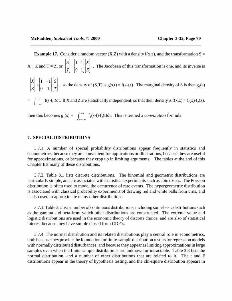
McFadden, Statistical Tools, © 2000 Chapter 3-32, Page 70 ___________________________________________________________________________
Example 17. Consider a random vector (X,Z) with a density f(x,z), and the transformation S =
X + Z and T = Z, or . The Jacobean of this transformation is one, and its inverse isS
T'
1 1
0 1
X
Z
, so the density of (S,T) is g(s,t) = f(s-t,t). The marginal density of S is then g1(s)X
Z'
1 &1
0 1
S
T
= f(s-t,t)dt. If X and Z are statistically independent, so that their density is f(x,z) = f1(x)@f2(z),m%4
t'&4
then this becomes g1(s) = f1(s-t)@f2(t)dt. This is termed a convolution formula.m%4
t'&4
7. SPECIAL DISTRIBUTIONS
3.7.1. A number of special probability distributions appear frequently in statistics andeconometrics, because they are convenient for applications or illustrations, because they are usefulfor approximations, or because they crop up in limiting arguments. The tables at the end of thisChapter list many of these distributions.
3.7.2. Table 3.1 lists discrete distributions. The binomial and geometric distributions areparticularly simple, and are associated with statistical experiments such as coin tosses. The Poissondistribution is often used to model the occurrence of rare events. The hypergeometric distributionis associated with classical probability experiments of drawing red and white balls from urns, andis also used to approximate many other distributions.
3.7.3. Table 3.2 list a number of continuous distributions, including some basic distributions suchas the gamma and beta from which other distributions are constructed. The extreme value andlogistic distributions are used in the economic theory of discrete choice, and are also of statisticalinterest because they have simple closed form CDF’s.
3.7.4. The normal distribution and its related distributions play a central role in econometrics,both because they provide the foundation for finite-sample distribution results for regression modelswith normally distributed disturbances, and because they appear as limiting approximations in largesamples even when the finite sample distributions are unknown or intractable. Table 3.3 lists thenormal distribution, and a number of other distributions that are related to it. The t and Fdistributions appear in the theory of hypothesis testing, and the chi-square distribution appears in
McFadden, Statistical Tools, © 2000 Chapter 3-33, Page 71 ___________________________________________________________________________
large-sample approximations. The non-central versions of these distributions appear in calculationsof the power of hypothesis tests.
It is a standard exercise in mathematical statistics to establish the relationships between normal,chi-square, F, and t distributions. For completeness, we state the most important result:
Theorem 3.9. Normal and chi-square random variables have the following properties:(I) If S = Y1
2 + ... + Yk2, where the Yk are independent normal random variables with means µk
and unit variances, then S has a non-central chi-square distribution with degrees of freedomparameter k and non-centrality parameter = µ1
2 + ... + µk2, denoted N2(k, ). If = 0, this is
a (central) chi-square distribution with degrees of freedom parameter k, denoted 2(k).(ii) If Y and S are independent, Y is normal with mean and unit variance, and S is chi-squarewith k degrees of freedom, then T = Y/(S/k)½ is non-central t-distributed with degrees offreedom parameter k and non-centrality parameter , denoted tN(k, ). If = 0, this is a (central)t-distribution with degrees of freedom parameter k, denoted t(k).(iii) If R and S are independent, R is non-central chi-square with degrees of freedom parameterk and non-centrality parameter , and S is central chi-square with degrees of freedom parametern, then F = nR/kS is non-central F-distributed with degrees of freedom parameters (k,n) andnon-centrality parameter , denoted FN(k,n, ). If = 0, this distribution is F-distributed withdegrees of freedom parameters (k,n), and is denoted F(k,n).(iv) T is non-central t-distributed with degrees of freedom parameter k and non-centralityparameter if and only if F = T2 is non-central F-distributed with degrees of freedomparameters (1,k) and non-centrality parameter = 2.
Proof: These results can be found in most classical texts in mathematical statistics; see particularlyRao (1973), pp. 166-167, 170-172, 181-182, Johnson & Kotz (1970), Chap. 26-31, and Graybill(1961), Chap. 4.. ~
In applied statistics, it is important to be able to calculate values x = G-1(p), where G is the CDFof the central chi-square, F, or t, distribution, and values p = G(x) where G is the CDF of the non-central chi-square, F, or t distribution. Selected points of these distributions are tabled in manybooks of mathematical and statistical tables, but it is more convenient and accurate to calculate thesevalues within a statistical or econometrics software package. Most current packages, including TSP,STATA, and SST, can provide these values.
3.7.5. One of the most heavily used distributions in econometrics is the multivariate normal. Wedescribe this distribution and summarize some of its properties. A n×1 random vector Y ismultivariate normal with a vector of means µ and a positive definite covariance matrix if it hasthe density
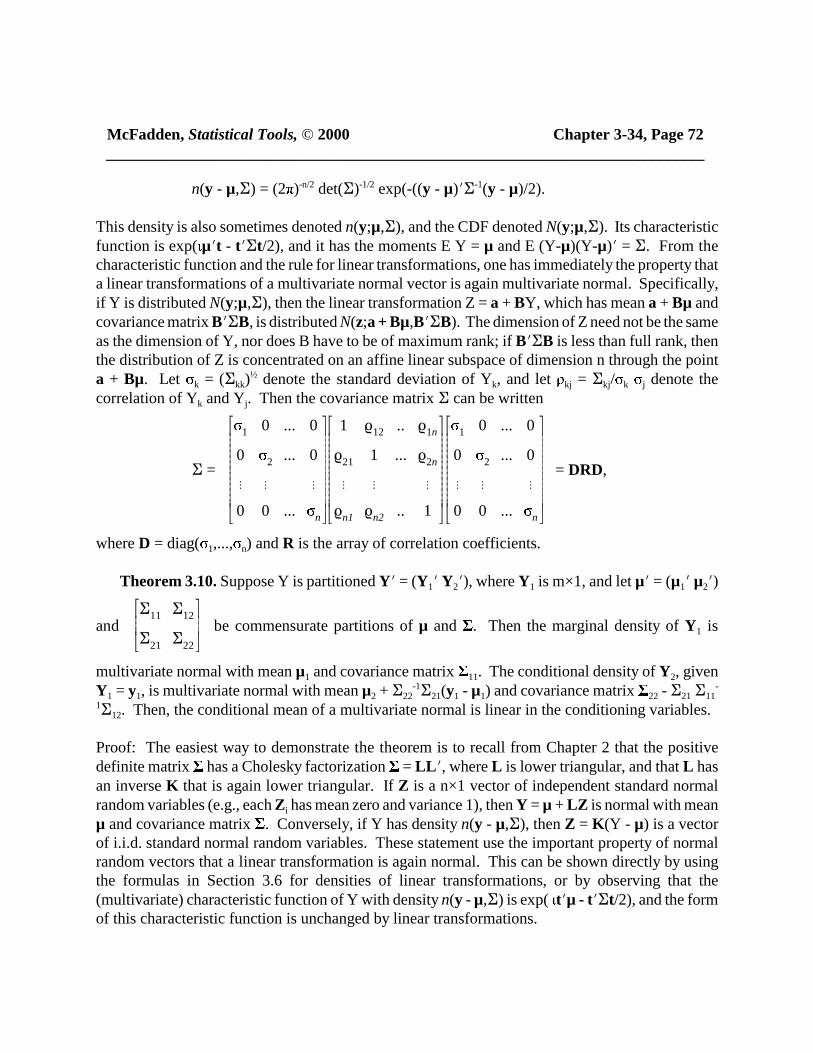
McFadden, Statistical Tools, © 2000 Chapter 3-34, Page 72 ___________________________________________________________________________
n(y - µ,G) = (2 )-n/2 det(G)-1/2 exp(-((y - µ)NG-1(y - µ)/2).
This density is also sometimes denoted n(y;µ,G), and the CDF denoted N(y;µ,G). Its characteristicfunction is exp( µNt - tNGt/2), and it has the moments E Y = µ and E (Y-µ)(Y-µ)N = G. From thecharacteristic function and the rule for linear transformations, one has immediately the property thata linear transformations of a multivariate normal vector is again multivariate normal. Specifically,if Y is distributed N(y;µ,G), then the linear transformation Z = a + BY, which has mean a + Bµ andcovariance matrix BNGB, is distributed N(z;a + Bµ,BNGB). The dimension of Z need not be the sameas the dimension of Y, nor does B have to be of maximum rank; if BNGB is less than full rank, thenthe distribution of Z is concentrated on an affine linear subspace of dimension n through the pointa + Bµ. Let k = (Gkk)
½ denote the standard deviation of Yk, and let kj = Gkj/ k j denote thecorrelation of Yk and Yj. Then the covariance matrix G can be written
G = = DRD,
1 0 ... 0
0 2 ... 0
! ! !
0 0 ... n
1 k12 .. k1n
k21 1 ... k2n
! ! !
kn1 kn2 .. 1
1 0 ... 0
0 2 ... 0
! ! !
0 0 ... n
where D = diag( 1,..., n) and R is the array of correlation coefficients.
Theorem 3.10. Suppose Y is partitioned YN = (Y1N Y2N), where Y1 is m×1, and let µN = (µ1N µ2N)
and be commensurate partitions of µ and . Then the marginal density of Y1 isG11 G12
G21 G22
multivariate normal with mean µ1 and covariance matrix 11. The conditional density of Y2, givenY1 = y1, is multivariate normal with mean µ2 + G22
-1G21(y1 - µ1) and covariance matrix 22 - G21 G11-
1G12. Then, the conditional mean of a multivariate normal is linear in the conditioning variables.
Proof: The easiest way to demonstrate the theorem is to recall from Chapter 2 that the positivedefinite matrix has a Cholesky factorization = LL N, where L is lower triangular, and that L hasan inverse K that is again lower triangular. If Z is a n×1 vector of independent standard normalrandom variables (e.g., each Zi has mean zero and variance 1), then Y = µ + LZ is normal with meanµ and covariance matrix . Conversely, if Y has density n(y - µ,G), then Z = K (Y - µ) is a vectorof i.i.d. standard normal random variables. These statement use the important property of normalrandom vectors that a linear transformation is again normal. This can be shown directly by usingthe formulas in Section 3.6 for densities of linear transformations, or by observing that the(multivariate) characteristic function of Y with density n(y - µ,G) is exp( tNµ - tNGt/2), and the formof this characteristic function is unchanged by linear transformations.
McFadden, Statistical Tools, © 2000 Chapter 3-35, Page 73 ___________________________________________________________________________
The Cholesky construction Y = µ + LZ provides an easy demonstration for the densities ofmarginal or conditional subvectors of Y. Partition L and Z commensurately with (Y1N Y2N), so that
L = and ZN = (Z1N Z2N). Then G11 = L 11L 11N, G21 = L21 L11N, G22 = L 22L 22N + L 21L 21N, andL11 0
L21 L22
hence G21G11-1 = L 21L 11
-1, implying L 22L 22N = G22 - G21G11-1G12. Then, Y1 = µ1 + L11Z1 has a marginal
multivariate normal density with mean µ1 and covariance matrix L 11L11N = G11. Also, Y2 = µ2 + L21Z1
+ L 22Z2, implying Y2 = µ2 + L21L11-1(Y1 - µ1) + L 22Z2. Conditioned on Y1 = y1, this implies Y2 = µ2
+ G21G11-1(y1 - µ1) + L 22Z2 is multivariate normal with mean µ2 - G21G11
-1µ1 and covariance matrixG22 - G21G11
-1G12. ~
The next theorem gives some additional useful properties of the multivariate normal and ofquadratic forms in normal vectors.
Theorem 3.11. Let Y be a n×1 random vector. Then,(i) If YN = (Y1N Y2N) is multivariate normal, then Y1 and Y2 are independent if and only if theyare uncorrelated. However, Y1 and Y2 can be uncorrelated and each have a marginal normaldistribution without necessarily being independent.(ii) If every linear combination cNY is normal, then Y is multivariate normal.(iii) If Y is i.i.d. standard normal and A is an idempotent n×n matrix of rank k, then YNAY isdistributed 2(k).(iv) If Y is distributed N(µ,I ) and A is an idempotent n×n matrix of rank k, then YNAY isdistributed N2(k, ) with = µNAµ.(v) If Y is i.i.d. standard normal and A and B are positive semidefinite n×n matrices, thenYNAY and YNBY are independent if and only if AB = 0.(vi) If Y is distributed N(µ,I ), and A i is an idempotent n×n matrix of rank ki for I = 1,...K, thenthe YNAi Y are mutually independent and distributed N2(ki, i) with i = µNA iµ if and only ifeither (a) A iA j = 0 for I ú j or (b) A1 + ... + AK is idempotent.(vii) If Y is distributed N(µ,I ), A is a positive semidefinite n×n matrix, B is a k×n matrix, andBA = 0, then BY and YNAY are independent.(viii) If Y is distributed N(µ,I ) and A is a positive semidefinite n×n matrix, then E YNAY =µNAµ + tr(A).
Proof: Results (i) and (ii) are proved in Anderson (1958), Thm. 2.4.2 and 2.6.2. For (iii) and (iv),write A = UUN, where this is its singular value decomposition with U a n×k column orthogonalmatrix. Then UNY is distributed N(UNµ,I k), and the result follows from Theorem 3.8. For (v), let kbe the rank of A and m the rank of B. There exists a n×k matrix U of rank k and a n×m matrix Vof rank m such that A = UUN and B = VVN. The vectors UNY and VNY are uncorrelated, hence

McFadden, Statistical Tools, © 2000 Chapter 3-36, Page 74 ___________________________________________________________________________
independent, if and only if UNV = 0. But AB = U(UNV)VN is zero if and only if UNV = 0 since U andVN are of maximum rank. For (vi), use the SVD decomposition as in (iv). For (vii), write A = UUNwith U of maximum rank as in (v). Then BA = (BU)UN = 0 implies BU = 0, so that BY and UNY areindependent by (i). For (vii), E YNAY = µNAµ + E (Y-µ)NA(Y-µ) = µNAµ + tr(E (Y-µ)NA(Y-µ)) =µNAµ +tr(A). ~
NOTES AND COMMENTS
The purpose of this chapter has been to collect the key results from probability theory that areused in econometrics. While the chapter is reasonably self-contained, it is expected that the readerwill already be familiar with most of the concepts, and can if necessary refer to one of the excellenttexts in basic probability theory and mathematical statistics, such as P. Billingsley, Probability andMeasure, Wiley, 1986; or Y. Chow and H. Teicher, Probability Theory, 1997. A classic thatprovides an accessible treatment of fields of subsets, measure, and statistical independence is J.Neveu, Mathematical Foundations of the Calculus of Probability, Holden-Day, 1965. Anotherclassic that contains many results from mathematical statistics is C. R. Rao (1973) Linear StatisticalInference and Its Applications, Wiley. A comprehensive classical text with treatment of manytopics, including characteristic functions, is W. Feller, An Introduction to Probability Theory andIts Applications, Vol. 1&2, Wiley, 1957. For special distributions, properties of distributions, andcomputation, a four-volume compendium by N. Johnson and S. Kotz, Distributions in Statistics,Houghton-Mifflin, 1970, is a good source. For the multivariate normal distribution, T. Anderson(1958) An Introduction to Multivariate Statistical Analysis, Wiley, and F. Graybill (1961) AnIntroduction to Linear Statistical Models, McGraw-Hill, are good sources. Readers who find somesections of this chapter unfamiliar or too dense may find it useful to first review an introductory textat the undergraduate level, such as K. Chung, A Course in Probability Theory, Academic Press, NewYork, or R. Larsen and M. Marx, Probability Theory, Prentice-Hall.

McFadden, Statistical Tools, © 2000 Chapter 3-37, Page 75 ___________________________________________________________________________
TABLE 3.1. SPECIAL DISCRETE DISTRIBUTIONS NAME & DOMAIN DENSITY MOMENTS CHAR. FN.1. Binomial
n
kp k(1&p)n&k
µ = np (1-p+pet)n
k = 0,1,...,n 0 < p < 1 2 = np(1-p) Note 12. Hypergeometric
÷r
k
w
n&k
r%w
n
µ = nr/(r+w) Note 2
k an integermax{0,n-w} # k& k # min{r,n}
r+w > n r,w,n positive integers 2 = "nrw
(r%w)2
r%w&nr%w&1
3. Geometric p(1-p)k µ = (1-p)/p Note 3k = 0,1,2,... 0 < p < 1 2 = (1-p)/p2
4. Poisson e- k/k! µ = exp[ (et-1)]k = 0,1,2,... > 0 2 = 2 Note 45. Negative Binomial
pr(1-p)kr%k&1
k
µ = r(1-p)/p
k = 0,1,2,... r integer, r > 0 & 0 < p < 1 2 = r(1-p)/p2 Note 5
NOTES1. µ / EX (the mean), and 2 = E(X-µ)2 (the variance). The density is often denoted b(k;n,p). The momentgenerating function is (1-p+pet)n . 2. The characteristic and moment generating functions are complicated. 3. The characteristic function is p/(1-(1-p)et) and the moment generating function is p/(1-(1-p)et), defined for t <-ln(1-p). 4. The moment generating function is exp((et-1)), defined for all t. 5. The characteristic function is pr/(1-(1-p)et)r, and the moment generating function is pr/(1-(1-p)et)r, defined fort < -ln(1-p).

McFadden, Statistical Tools, © 2000 Chapter 3-38, Page 76 ___________________________________________________________________________
TABLE 3.2. SPECIAL CONTINUOUS DISTRIBUTIONSNAME & DOMAIN DENSITY MOMENTS CHAR. FN.1. Uniform
a # x # b
1/(b-a) µ = (a+b)/22 = (b-a)2/12 e bt&e at
t(b&a)
Note 12. Triangular (1-|x|/a)/a µ = 0
21&cosat
a 2t 2|x| < a 2 = a2 /6
3. Cauchy a/(a2 + (x-µ)2) none etµ-|t |
-4 < x < +4
4. Exponential e-x/ / µ = 1/(1- t)x $ 0
2 = 2 Note 25. Pareto babx--b-1 µ = ab/(b-1) Note 3
x $ a 2 = ba2/(b-1)2(b-2)6. Gamma
x > 0 x a&1e x/b
(a)b a
µ = ab2 = ab2
(1- bt)-a
Note 4
7. Beta0 < x < 1
xa-1(1-x)b-1(a%b)(a) (b)
µ = a/(a+b)
2 = ab
(a%b)2(a%b%1)
Note 5
8. Extreme Valueexp
1b
&x&a
b& e &(x&a)/b
µ = a + 0.57721"b Note 6
-4 < x < +4 2 = ( b)2/12
9. Logistic"1
bexp((a&x)/b)
(1%exp((a&x)/b))2
µ = a Note 7
-4 < x < +4 2 = ( b)2/6
NOTES 1. The moment generating function is (ebt - eat)/(b-a)t, defined for all t. 2. The moment generating function is 1/(1 - t), defined for t < 1/ . 3. The moment generating function does not exist. The mean exists for b > 1, the variance exists for b > 2. 4. For a > 0, (a) = Io
4 x a-1e-xdx is the gamma function. If a is an integer, (a) = (a-1)!. 5. For the characteristic function, see C. R. Rao, Linear Statistical Inference, Wiley, 1973, p. 151. 6. The moment generating function is eat (1 - tb) for t < 1/b . 7. The moment generating function is eat bt/sin( bt) for *t*< 1/2b.

McFadden, Statistical Tools, © 2000 Chapter 3-39, Page 77 ___________________________________________________________________________
TABLE 3.3. THE NORMAL DISTRIBUTION AND ITS RELATIVESNAME & DOMAIN DENSITY MOMENTS CHAR. FN.
1. Normaln(x-µ, )
-4 < x < +4, > 0(2 2)-½@exp( )&(x&µ)2
2 2
µ = mean2 = variance
exp(tµ- 2t2/2)Note 1
2. Standard Normal-4 < x < +4
(x) = (2 )-½@exp(-x2/2) µ = 02 = 1
exp(-t2/2)
3. Chi-Square0 < x < +4 2(x;k) =
x (k/2)&1"e&x/2
(k/2)2k/2
µ = k2 = 2k
k = 1,2,...
(1-2 t)-k/2
Note 2
4. F-distribution0 < x < +4
F(x;k,n)k,n positive integers
µ = if n > 2
2'2n 2(k%n&2)
k(n&2)2(n&4)
if n > 4
Note 3
5. t-distribution-4 < x < +4 (
k%12
)(1%x 2/k)&(k%1)/2
k (12
) (1%2k
2)
µ = 0 if k > 12 = k/(k-2) if k > 2
Note 4
1. Noncentral 2(x;k, ) µ = k+ Note 5 Chi-Squared k pos. integer 2 = 2(k+2 )
x > 0 $ 02. Noncentral F(x;k,n,) if n > 2, µ = n(k+)/k(n-2) Note 6 F-distribution
x > 0k,n positive integers $ 0
if n > 4, 2 =
2(n/k)2(k% )2%(k%2 )(n&2)
(n&2)2(n&4)
3. Noncentralt-distribution
t(x;k, )k pos. integer µ = if k > 1
((k&1)/2)(k/2)
Note 7
2 = (1+ 2)k/(k-2) - µ2 if k > 2

McFadden, Statistical Tools, © 2000 Chapter 3-40, Page 78 ___________________________________________________________________________
NOTES TO TABLE 3.31. The density is often denoted n(x-µ, 2), and the cumulative distribution referred to as N(x-µ, 2), or simply N(µ, 2). Themoment generating function is exp(µt+2t2/2), defined for all t. The standard normal density is often denoted n(x), and thestandard normal CDF is denoted (x). The general normal and standard normal formulas are related by n(x-µ, 2) =
((x-µ)/ )/ and N(x-µ, 2) = ((x-µ)/ ). 2. The moment generating function is (1-t/2)-k/2 for t < 2. The Chi-Square distribution with parameter k (/ degrees offreedom) is the distribution of the sum of squares of k independent standard normal random variables. The Chi-Squaredensity is the same as the gamma density with b = 2 and a = k/2.3. The F-distribution is the distribution of the expression nU/kV, where U is a random variable with a Chi-squaredistribution with parameter k, and V is an independent random variable with a Chi-square distribution with parameter n.
The density is . For n # 2, the mean does not exist, and for n # 4, the variance does not exist.( k%n
2)
( k2
) ( n2
)@ k
k/2n n/2x k/2&1
(n%kx)(k%n)/2
The characteristic and moment generating functions are complicated.
4. If Y is standard normal and Z is independently Chi-squared distributed with parameter k, then Y/ has aZ/k
T-Distribution with parameter k (/ degrees of freedom). The characteristic function is complicated; the moment generatingfunction does not exist. 5. The Noncentral Chi-square is the distribution of the sum of squares of k independent normal random variables, eachwith variance one, and with means whose squares sum to . The Noncentral Chi-Square density is a Poisson mixture of
(central) Chi-square densities, [e- /2( /2)j/j!] 2(x;k+2j).j4
j'0
6. The Non-central F-distribution has a density that is a Poisson mixture of rescaled (central) F-distributed densities,
[e- /2( /2)j/j!] F( ;k+2j,n). It is the distribution of the expression nUN/kV, where UN is a Noncentralj4
j'0k
k%2jkx
k%2j
Chi-Squared random variable with parameters k and , and V is an independent central Chi-Squared distribution withparameter n.
7. If Y is standard normal and Z is independently Chi-squared distributed with parameter k, then (Y+)/ has(Z/k)
a Noncentral T-Distribution with parameters k and . The density is a Poisson mixture of scaled Beta distributed densities,
[ ( 2/2)j/j!] B( ). j4
j'0 e&2/2 xk
(k%x 2)2
k
k%x 2, k2
,1%2j2
The square of a Noncentral T-Distributed random variable has a Noncentral F-Distribution with parameters 1, k, and = 2.


![Chapter 22: Kinetic Theory of Warm Plasmas [version 1222.1.K]](https://static.fdokumen.com/doc/165x107/631d6102f7af5f2ec200e245/chapter-22-kinetic-theory-of-warm-plasmas-version-12221k.jpg)