arX

iv:0

905.

3938

v2 [

hep-

th]

9 J

un 2

009

First Order Description of D = 4

static Black Holes

and the Hamilton–Jacobi equation

L. Andrianopoli∗, R. D’Auria∗, E. Orazi∗ and M. Trigiante∗

∗ Dipartimento di Fisica, Politecnico di Torino, Corso Duca degli Abruzzi 24, I-10129 Turin, Italy and

Istituto Nazionale di Fisica Nucleare (INFN) Sezione di Torino, Italy 1

Abstract

In this note we discuss the application of the Hamilton–Jacobi formalism to the firstorder description of four dimensional spherically symmetric and static black holes. In par-ticular we show that the prepotential characterizing the flow coincides with the Hamiltonprincipal function associated with the one-dimensional effective Lagrangian. This impliesthat the prepotential can always be defined, at least locally in the radial variable and inthe moduli space, both in the extremal and non-extremal case and allows us to concludethat it is duality invariant. We also give, in this framework, a general definition of the“Weinhold metric” in terms of which a necessary condition for the existence of multipleattractors is given. The Hamilton–Jacobi formalism can be applied both to the restrictedphase space where the electromagnetic potentials have been integrated out as well asin the case where the electromagnetic potentials are dualized to scalar fields using theso-called three-dimensional Euclidean approach. We give some examples of applicationof the formalism, both for the BPS and the non-BPS black holes.

1laura.andrianopoli@polito.it;

riccardo.dauria@polito.it;

emanuele.orazi@polito.it;

mario.trigiante@polito.it.

1

1 Introduction

Recently considerable attention has been devoted to the study of black-hole solutions insupergravity theories, especially in connection with the attractor mechanism [1, 2] (see also[3] and references therein). In this respect, of particular relevance is the issue of describing thespatial evolution of the scalar fields and the metric in terms of a first order dynamical systemof equations written in terms of a prepotential, also called fake superpotential [4, 5, 6, 7]. Inthe case of four dimensional spherically symmetric black holes, if we collectively denote themetric and scalar degrees of freedom characterizing the solution by qi and the radial variableby τ , the issue has been of whether it is possible to define a prepotential W(q), function of qi

and of the quantized electric-magnetic charges, such that the radial evolution of qi is solutionto a system of equations of the following form:

qi = Gij ∂W∂qj

, (1)

Gij(q) being a suitable non-degenerate metric. Equations (1) are particularly suitable forstudying the attractor behavior [1, 2] of four dimensional black-hole solutions [8, 9] as wellas higher dimensional black-brane solutions [10]. The reason behind the interest in such aprepotential W goes beyond the simple convenience in writing the black-hole equations in afirst order form. This function seems to have a deeper physical meaning also related to thedescription of the radial evolution of the black-hole fields in terms of a dual RG flow.

So far such a description has been found for specific extremal and non-extremal staticfour dimensional black-hole solutions and the following questions have been left unanswered:

• For which solutions does the prepotential W exist?

• Is W invariant under the global symmetries (dualities) of the four dimensional theory?

• In ref. [5] it was found for the extremal case that W is a c-function, that is alwaysmonotonic in τ . Can this property be extended, whenever W exists, also to the non-extremal case?

It is a well established fact that the problem of finding a first order description of the form(1) can be recast, for static solutions, into a Hamilton–Jacobi problem in which the Wprepotential is the Hamilton’s characteristic function such that:

H(q, ∂qW) = c2 . (2)

The Hamilton–Jacobi approach to the first order description of supergravity solutions hasbeen applied to the study of RG flows “dual” to domain walls and cosmological solutions[11, 12, 13, 14] and to extremal black holes [15]. It has also been applied to the generaldescription of extended supergravity solutions in various dimensions [16].

In this note we restrict ourselves to static, spherically symmetric black holes and wishto point out some important consequences of the well known theory of the Hamilton–Jacobiequation which have never been clearly stated in the black-hole literature so far.

We first show that the prepotential, being identified with Hamilton’s characteristic func-tion, can always be given (in both the extremal (c = 0) and non-extremal (c 6= 0) case) in alocal form, in terms of the integral of the Lagrangian along a trajectory which minimizes the

2

action (characteristic trajectory). We also give, in this framework, a general definition of the“Weinhold metric” [2] in terms of which to define a necessary condition [17] for the existenceof multiple attractors in the extremal case (c = 0). Actually, the expression we find for theprepotential, eq. (14) below, generalizes the one conjectured in [5].

Of particular interest to us is the issue of whether W(q) is duality invariant. If W is to beassociated with some fundamental physical property of the black hole, just like the entropy, itought to be duality invariant, namely independent on the particular description of its degreesof freedom. The duality invariance of W is guaranteed by the fact that it can be expressedas the integral of the duality invariant Lagrangian on a characteristic trajectory.

The paper is organized as follows: in Section 2 we briefly review the Hamiltonian de-scription of four dimensional spherically symmetric and static black holes. In Section 3 weintroduce the Hamilton–Jacobi problem in D = 4 and the definition of the prepotential W. InSection 4 we write a local form for the solution to the Hamilton–Jacobi equation and discusssome of its properties. In Section 5 we prove duality invariance of W. Finally in Section 6 wegeneralize the Hamiltonian problem by extending the phase space to include the quantizedcharges and their conjugate variables, namely the electric-magnetic potentials. This extendedformulation has a natural setting in the D = 3 Euclidean theory arising from time reductionof the four dimensional one. We write the Hamilton–Jacobi equation in this enlarged phasespace and express its solution W3 in terms of the four dimensional prepotential W. We dis-cuss cases of interest in which a globally defined solution W3, and correspondingly W, of theHamilton–Jacobi equation exists.

2 Review of Static D = 4 Black Holes

Let us recall the main facts about the description of a static black hole in D = 4 as solutionof a Hamiltonian system. We start from the four dimensional bosonic action of a genericsupergravity theory, describing n scalar fields φ = (φr) coupled to nv vector fields AΛ

µ :

S4 =

∫d4x

√−g

[−1

2R +

1

2Grs(φ) ∂µφr ∂µφs + IΛΣ(φ)FΛ

µν FΣ µν+

+1

2√−g

ǫµνρσ RΛΣ(φ)FΛµν FΣ

ρσ

], (3)

where the gauge field-strength 2-form is defined as FΛ = dAΛ and IΛΣ, RΛΣ are the imaginaryand real part of the complex kinetic matrix NΛΣ(φ), with the convention that IΛΣ < 0. Thegeneral Ansatz for a spherically symmetric static black hole reads [18, 2, 3]:

ds24 = gµν dxµ dxν = e2 U dt2 − e−2 U

(c4

sinh4(c τ)dτ2 +

c2

sinh2(c τ)dΩ2

),

FΛ = mΛ sin(θ) dθ ∧ dϕ + e2 U ℓΛ(φ) dt ∧ dτ , (4)

where ℓΛ(φ) = I−1ΛΣ (eΣ − RΣΓ mΓ), eΛ, mΣ being the quantized electric and magneticcharges. The constant c is the extremality parameter which is related to the temperatureand entropy of the black hole through c = 2S T and identifies the inner and outer horizonscorresponding to r± = r0 ± c. The dependence of the evolution parameter τ on the radial

3

variable r is implicitly given by the equation c2

sinh2(c τ)= (r − r0)

2 − c2, which in the extremal

case c → 0 can be written as τ = −1/(r − r0).It is well known that the equations of motion obtained from the above Ansatz read:

d2U

dτ2≡ U = V (φ, e,m)e2U ,

D2φr

Dτ2≡ φr + Γr

stφs φt = grs(φ)

∂V (φ, e,m)

∂φse2U , (5)

together with the constraint

U2 +1

2grs(φ)

dφr

dτ

dφs

dτ− V (φ, e,m) e2U = c2 , (6)

where the positive definite geodesic potential V (φ, e,m) has the following form:

V = −1

2ΓTM(φ) Γ = −1

2ΓT

(I + R I−1 R −R I−1

−I−1 R I−1

)Γ > 0 , (7)

in terms of the vector of magnetic-electric charges Γ ≡ (mΛ, eΛ). Here the dotted quantitiesare differentiated with respect to the evolution parameter τ .

The equations of motion (5) can be associated to a one dimensional theory whose La-grangian2 is:

L = U2 +1

2Grs(φ) φr φs + e2 U V (φ) =

1

2Gij(q) qi qj + V(q) , (8)

where V(q) ≡ e2 U V (φ) and we introduced the functions qi(τ) = (U(τ), φr(τ)) together withthe metric

Gij(q) =

(2 0

0 Grs(φ)

). (9)

Once the Lagrangian is known we can proceed with an Hamiltonian approach using thephase space that stems from the qi(τ) = (U(τ), φr(τ)) variables, introducing the conjugatemomenta to qi:

pi =δLδqi

= Gij qj . (10)

In terms of the phase-space variables qi and pi the Hamiltonian H(p, q) then reads:

H(p, q) =1

2pi G

ij pj − V(q) =1

2qi Gij(q) qj − V(q) . (11)

This is consistent with the constraint (6) that acquires the meaning of “energy conservation”:

H(p, q) = c2 ⇔ 1

2qi Gij(q) qj − V(q) = c2 . (12)

2Note that here and in the following by abuse of language we adopt the terms Lagrangian and Hamiltonian

even if the evolution variable τ does not describe the temporal evolution but the radial one.

4

3 Hamilton–Jacobi Formalism and Static Black Holes

Let us recall how the solutions of the equations of motion can be obtained by applying themachinery of the Hamilton–Jacobi theory. We consider the principal Hamiltonian functionS(q, P, τ) depending on qi and on new constant momenta Pi. It is defined by the set of firstorder equations:

∂S

∂qi= pi ,

∂S

∂Pi= Qi ,

∂S

∂τ= −H , (13)

where Pi, Qi are new constant canonical variables which can be expressed in terms of theinitial values of qi and pi. From the general theory of canonical transformations, see forinstance [19], it is known that the above transformation generated by S always exists locallyin the p, q space, in a neighborhood of any point which is not critical, namely in which(∂H

∂q, ∂H

∂p) 6= (0, 0).

We shall leave the dependence of S on the constant Pi implicit and focus on its dependenceon the qi.From the last and the first equations of (13) and from the Hamiltonian constraint (12) wehave:

S(q, τ) = W(q) − c2 τ (14)

pi =∂W∂qi

, (15)

H(q, ∂qW) ≡ 1

2∂iW Gij ∂jW −V(q) = c2 , (16)

where (16) defines the Hamilton–Jacobi equation for the function W, usually called Hamiltoncharacteristic function.

From eq. (15) and eq. (10) we finally get

qi = Gij pj = Gij ∂W∂qj

. (17)

This shows that, provided a solution to the equations (14)-(16) is found, the evolution of themetric and scalar fields can be described in terms of a dynamical system of the form (1). Inthe next section we give its unique solution.

Note that the function S in eq. (14) generalizes the expression for the prepotentialconjectured in [5] for the general (non-extremal) case. To make contact with the proposal in[5], let us consider the following expression for the principal function S:

S(U, φr, τ) = 2 eUW (φr, τ) + c2 τ = W(U, φr) − c2 τ . (18)

This expression reproduces the first order equations for the prepotential as given in [4, 5]:

U = eU W , φr = 2 eU Grs ∂sW , (19)

together with the condition found in [5] for the non-extremal case: ∂τW = −c2e−U .We observe, however, that (18) is a rather restrictive Ansatz for the Hamilton’s principal

function, since the dependence of W on U may not have a factorized form, as it is apparent, forexample, in the Reissner–Nordstrom case discussed below. Actually, the present discussiongeneralizes such an Ansatz.

5

3.1 Critical points as attractors.

The first order system (17) may have critical points in the space of the qis, namely points(qi

0) in which its right hand side vanishes: ∂iW|q0= 0. From the Hamilton–Jacobi equation

it is clear that such points may exist only in the extremal case, since the right hand side ofthe equation

∂iW Gij ∂jW = 2 (c2 + e2 U V (φ)) , (20)

being V ≥ 0, may vanish only if c = 0. A critical point is an attractor [1] if at that pointthe Hessian of the geodesic potential is positive. Attractors are reached at τ → −∞, whereU(−∞) → −∞, which corresponds to the horizon, since, for c = 0, τ = −1/(r − r0).

In the extremal case we can make the Ansatz W(U, φr) = 2 eU W (φr), which correspondsto taking W in eq. (18) not to depend explicitly on τ , and the Hamilton–Jacobi equationtranslates in the following equation for W (φr):

W 2 + 2Grs ∂W

∂φr

∂W

∂φs= V (φr) . (21)

The ADM mass of the solution is given by the value of U at radial infinity (r → ∞, τ → 0−):MADM (φr

∞, e,m) = limτ→0− U , where φr∞ are the boundary values of the scalar fields at

infinity. From the first order equations (19) written in terms of W (φr, e,m), we see that,since limτ→0− eU = 1, the ADM mass of the solution coincides with the value of W as afunction of the values of φr

∞: MADM (φr∞, e,m) = W (φr

∞, e,m).

Multiple attractors For a given set of quantized electric and magnetic charges Γ =(mΛ, eΛ), extremal solutions may have more than one attractors [17, 20]. In [17] a nec-essary condition was given for the existence of multiple attractors. We want here to givea general proof of this statement for generic (not necessarily BPS) attractors. As in [2] wecan define the “Weinhold metric” as the Hessian of MADM (φr

∞, e,m) = W (φr∞, e,m) with

respect to the boundary values φr∞:

W = (Wrs) ≡(

∂2W

∂φr ∂φs

)

φ=φ∞

. (22)

We can take φr∞ to coincide with the critical point φr

0. In this case ∂rV (φr0) = ∂rW (φr

0) = 0and the scalar fields of the solution will not evolve: φr(τ) ≡ φr

0. This solution is called double

extremal. By computing the second derivatives of eq. (21) we can relate the Hessian matrix(Wrs) of W to the Hessian matrix V ≡ (∂r∂s V ) of V at a critical point as follows:

2√

V W + 4W G−1 W = V , (23)

where G−1 ≡ (Grs). The above matrix equation is solved by

W G−1 =

√V

4

(−11 +

√11 +

4

VV G−1

), (24)

where 11 ≡ (δsr). The matrix V G−1 = (∂r∂sV Gsℓ)|φ0

is the “mass squared” matrix of thefluctuations of φr around φr

0. We can consider for instance BPS black holes in N = 2

6

supergravity, described by a function W = |Z|, Z being the complex central charge of thetheory. At the corresponding extremum one can show that ∂r∂sV (φr

0) = 2V Grs(φr0) > 0 [2],

and from eq. (24) one finds

∂r∂sW (φr0) =

1

4√

V∂r∂sV (φr

0) =

√V

2Grs(φ

r0) > 0 (BPS attractor) . (25)

In general a critical point φr0 is an attractor iff V(φ0), or equivalently V G−1(φ0), are positive

definite. Eq. (24) then implies that φr0 is an attractor iff W G−1(φ0), or equivalently W(φ0),

are positive definite. If, for a given choice of the quantized charges e, m, W (or equivalentlyV ) has more than one attractor point, W must have more than one minimum and this impliesthat there should exist at least one critical point in which the Hessian of W has negativeeigenvalues. Therefore if the Weinhold metric is positive definite everywhere in the moduli

space, there can be no more than one attractor which is the statement made in [17].

4 Solution to the Hamilton–Jacobi equation

We recall that the solution of the set of differential equations (13), (16) in terms of Hamilton’sprincipal function S is formally given by (see e.g. [21])

S(q, τ) = S0 +

∫ q,τ

q0,τ0

L(q, q) dτ , (26)

where the integral is performed along the characteristic trajectory γ = qi(τ), i.e. the solutionof Hamilton’s equations, such that:

qi(τ0) = qi0 , qi(τ) = qi . (27)

Few comments here are in order. The above formula provides, in the most general case,only a local definition of S: local in τ , to avoid multivaluedness of S [21], and local in theconfiguration space with coordinates qis, being S defined only on the points (qi), for fixedqi0, τ0, for which the interpolating characteristic trajectory, satisfying (27), exists. In fact,

as pointed out in Section 3, locally, in the neighborhood of a non-critical point in the phasespace, there always exist a complete solution S(qi, Pi, τ) to the Hamilton–Jacobi equationand it has the form (26) (Pi can be seen as a complete set of integration constants). In whatfollows, we shall use eq. (26) bearing its local validity in mind.

In our problem, we can use the Hamiltonian constraint to find the expression of theprincipal function in terms of the potential, as follows:

S(q, τ) = S0 +

∫ q,τ

q0,τ0

[c2 + 2V(q)

]dτ , (28)

so that, using (8) and (12), the Hamilton’s characteristic function is given by:

W(q) = W0 +

∫ q,τ

q0,τ0

[c2 + L(q, q)

]dτ = W0 + 2

∫ q,τ

q0,τ0

[c2 + V(q)

]dτ . (29)

7

Actually, the above formula can also be derived from direct integration of eq. (16). Indeed(16) has the form of the eikonal equation for a wave front W = const. propagating in amedium of refractive index n =

√2(c2 + V):

n2 = ∂iW Gij ∂jW. (30)

From equation (17) we get that ∂iW is tangent to the “light rays” namely the characteristicsγ = (qi(τ)). Introducing the proper distance s along a characteristic:

ds =√

qi Gij(q) qj dτ =√

2(c2 + V(q)) dτ (31)

using (17) we have:

dWds

=∂Wdqi

dqi

dτ

dτ

ds= ∂iW Gij ∂jW

dτ

ds=√

2(c2 + V(q)) (32)

that is:dW =

√2(c2 + V(q)) ds = 2(c2 + V(q)) dτ. (33)

From the above equation it follows that dWdτ

along γ is positive, namely that W is a monotonicincreasing function of τ along a solution (the same is true for the principal function S, sincethe Lagrangian is non-negative).

Example Let us review the construction of W for the Reissner-Nordstrom black hole [16].The qi variables now consist of the function U alone. This is for instance a solution to N = 2pure supergravity. With respect to the only vector field of the theory (the graviphoton) thesolution can have in general an electric and a magnetic charge e, m. The geodesic potentialreads:

V(U, e, m) = e2 U Q2 , Q2 ≡ 1

2(e2 + m2) . (34)

The Hamiltonian constraint and the Hamilton–Jacobi equation read:

U2 = (∂UW)2 = c2 + e2 U Q2 . (35)

We can then readily apply eq. (29) to find, upon changing variables from τ to U :

W(U) = W0 + 2

∫ U,τ

U0,τ0

[c2 + e2 U Q2

]dτ = W0 + 2

∫ U

U0

[c2 + e2 U Q2

] dU

U=

= W0 + 2

∫ U

U0

√c2 + e2 U Q2 dU =

= W0 + 2

[√

c2 + e2 U Q2 − c

2log

(√c2 + e2 U Q2 + c√c2 + e2 U Q2 − c

)]. (36)

8

5 Duality invariance of the prepotential W.

Let us now consider an extended supergravity theory in D = 4. It is known that the globalsymmetries of the equations of motion and Bianchi identities are encoded in the isometrygroup G of the scalar manifold (if non-empty), whose action on the scalar fields is associatedwith a simultaneous linear symplectic action on the field strengths FΛ and their duals GΛ.The duality action of G is defined by an embedding D of G inside the group Sp(2nv, R):

g ∈ G :

φr → φr ′ = g ⋆ φr(FΛ

GΛ

)→ D(g) ·

(FΛ

GΛ

), (37)

where g⋆ denotes the non-linear action of g on the scalar fields and D(g) is the 2nv × 2nv

symplectic matrix associated with g.We are going to prove explicitly that the prepotential W(q) is invariant under the duality

action of G. Keeping in mind that the metric (and therefore the function U) is a dualityinvariant field, we define (g ⋆ qi) ≡ (U, g ⋆ φr). The on-shell global invariance of the fourdimensional theory under G implies that, if γ = (qi(τ)) is a characteristic trajectory of theLagrangian system (8) with charge parameters Γ = (mΛ, eΛ), then g ⋆ γ = (g ⋆ qi(τ)) is atrajectory of the Lagrangian system (8) with charge parameters D(g) · Γ.

Let us make the dependence of the geodesic potential V on the electric-magnetic chargesexplicit by writing V(q, Γ). From general properties of the symplectic matrix M(φ), definedin (7), we have:

M(g ⋆ φ) = D(g)−T M(φ)D(g)−1 . (38)

From this it follows that the potential V is duality invariant, in the sense that:

V(g ⋆ q, D(g) · Γ) = V(q, Γ) . (39)

The group G is then a global symmetry group of the one-dimensional Lagrangian L in (8)and thus of both Hamilton’s principal and characteristic functions S(q, τ ; Γ) and W(q; Γ).Indeed from (29) and (39) we have:

W(q; Γ) = W0 + 2

∫ q, τ

q0, τ0

[c2 + V(q, Γ)

]dτ = W0 + 2

∫ g⋆q, τ

g⋆q0, τ0

[c2+

+ V(g ⋆ q, D(g) · Γ)] dτ = W(g ⋆ q; D(g) · Γ) . (40)

6 The extended phase space and time-reductions to D = 3

Four-dimensional static and spherically symmetric black holes depend on a number of degreesof freedom which includes, besides the metric and scalars, also the degrees of freedom corre-sponding to the gauge potentials. The one-dimensional effective Lagrangian (8) encoding theinformation on the theory can then been formulated as a Lagrangian for a geodesic modeldescribing all the degrees of freedom, as discussed in [18],[2]. It is then natural to extendthe phase space to include as further degrees of freedom the magnetic and electric potentialstogether with their conjugate momenta. This approach was pionereed in [22], in the case ofdouble extremal black holes.

9

As it is well known, this approach is equivalent, for static black holes, to a time reductionof the four dimensional Lagrangian (3) [18].

To implement the reduction on the time direction, let us consider the following Ansatzfor the metric [18] 3:

ds24 = e2U (dt + A0

i dxi)2 − e−2U g(3)ij dxi dxj , (41)

where xi, i = 1, 2, 3, are the coordinates of the final Euclidean space. In this theory all thevectors are dualized to scalar fields so as to obtain a sigma model coupled to gravity. Let usintroduce the nv three dimensional scalars ζΛ = AΛ

0 which, together with the scalars ζΛ, dualin D = 3 to the vectors AΛ

i , form the symplectic vector of electric and magnetic potentials

ZM = (ζΛ, ζΛ). Finally we shall denote by a the axion dual in D = 3 to the Kaluza-Kleinvector A0

i . The final D = 3 action reads:

S3 =

∫d3x

√|g(3)|

(1

2R3 −

1

2GIJ(Φ) ∂iΦ

I ∂iΦJ

),

where ΦI ≡ (U, φr, a, ZM ), and the sigma model metric reads:

GIJ (Φ) dΦI dΦJ = dU2 +1

2Grs dφr dφs +

e−4 U

4ω2 +

e−2 U

2dZT M dZ ,

where MMN is the negative definite matrix defined in (7) and the one-form ω is defined asω = da − ZT

C dZ, C being the antisymmetric 2nv × 2nv Sp(2nv , R)-invariant matrix, forwhich we shall use the following form

C =

(0 −1111 0

). (42)

The scalar fields ΦI span a pseudo-Riemannian manifold M3 which contains as a submanifoldthe scalar manifold M4 of the D = 4 parent theory spanned by φr.

Spherically symmetric black-hole solutions are described by geodesics ΦI(τ) on M3 para-metrized by the radial variable τ [18]. We shall restrict ourselves to spherically symmetricsolutions with vanishing NUT charge, namely we shall take ωτ = 0. These solutions will bedescribed by the following effective Lagrangian:

L3 = U2 +1

2Grs φr φs +

e−2 U

2ZT MZ =

1

2Gαβ qα qβ .

Let us introduce the following generalized coordinates qα ≡ (U, φr, ZM ) = (qi,ZM ). Theconjugate momenta pα will read:

pα = Gαβ(qi) qα = (pi, pM ) . (43)

In terms of qα, pα we write the Hamiltonian:

H3(p, q) =1

2Gαβ pα pβ =

1

2Gij(qi) pi pj +

e2 U

2pM MMN (φr) pN = c2 ,

3This metric describes stationary solutions, in the static case A0

i = 0.

10

where MMN denotes the inverse matrix of MMN , given by: MMN = CMP

CNQ MPQ. Since

ZM are cyclic, the corresponding momenta pM are constants of motion. They are identifiedwith the quantized charges as follows: pM = −CMN ΓN . With this identification, the lastterm in H3 reads 1

2 e2 U ΓT · M · Γ = −V(qi,Γ) and H3 coincides with the Hamiltonian Hdefined in the previous sections. Therefore the resulting equations of motion for pi, qi arethe same as those discussed earlier. As far as the equation for ZM is concerned, it reads [18]:

ZM =∂H3

∂pM= −e2 U

CMN MNP ΓP . (44)

This analysis can be viewed as an extension of that given in [22] since it includes in thedefinition of the phase space also the four dimensional scalar fields.

In this enlarged Hamiltonian system we want now to define Hamilton’s characteristicfunction, to be denoted by W3(q

α, Pα). By definition this function generates the canonicaltransformation to the coordinates Qα, Pα, where Pα are constants of motion. Since also c2 isconserved, it will be a function of the Pα, c2 = c2(P ). It will indeed provide the Hamiltonianin the new coordinates. From the general theory it is known that the coordinates Qα arelinear in τ , i.e. harmonic functions:

Qα =

(∂c2

∂Pα

)τ + Qα

0 . (45)

If we choose one of the Pi to coincide with c2, then only the corresponding Qi will be linearin τ , the other Qα being constants. The function W3(q

α, Pα) satisfies the following relations:

pα =∂W3

∂qα, (46)

Qα =∂W3

∂Pα, (47)

c2 = H3(qα,

∂W3

∂qα) , (48)

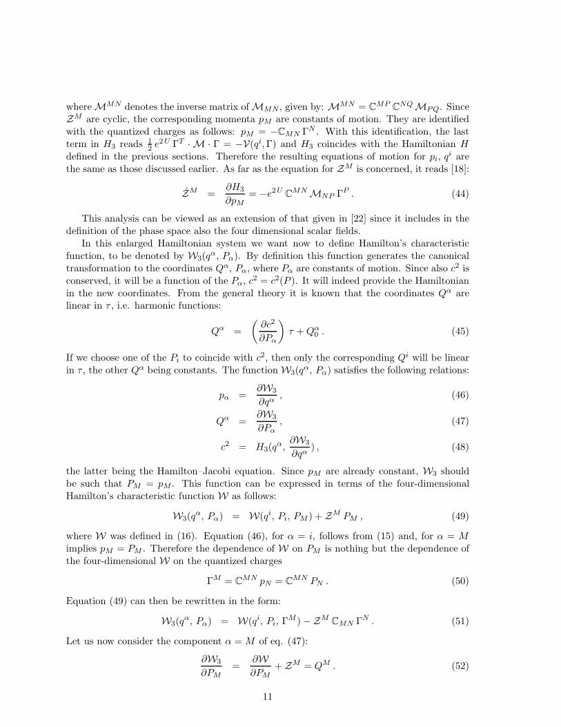
the latter being the Hamilton–Jacobi equation. Since pM are already constant, W3 shouldbe such that PM = pM . This function can be expressed in terms of the four-dimensionalHamilton’s characteristic function W as follows:

W3(qα, Pα) = W(qi, Pi, PM ) + ZM PM , (49)

where W was defined in (16). Equation (46), for α = i, follows from (15) and, for α = Mimplies pM = PM . Therefore the dependence of W on PM is nothing but the dependence ofthe four-dimensional W on the quantized charges

ΓM = CMN pN = C

MN PN . (50)

Equation (49) can then be rewritten in the form:

W3(qα, Pα) = W(qi, Pi, ΓM ) −ZM

CMN ΓN . (51)

Let us now consider the component α = M of eq. (47):

∂W3

∂PM=

∂W∂PM

+ ZM = QM . (52)

11

The above equation can also be written, using (50):

ZM − CMN ∂W

∂ΓN= QM . (53)

This is a non-trivial equation which implies that the combination on the left hand side is asymplectic vector of harmonic functions. Since the QM can be chosen to be constant, we canwrite:

ZM = CMN ∂W

∂ΓN+ const . (54)

The above equation allows to compute the electric-magnetic potentials once the W- prepo-tential is known on the solution as a function of all the quantized charges.

We shall check below eq. (54) on some specific solutions.

The BPS Solution for the N = 2 Case.

We shall refer to the usual N = 2 special geometry notations. Let zi denote the complexscalar fields on the special Kahler manifold and let V M (z, z), UM

i (z, z) be the covariantlyholomorphic symplectic section and its covariant derivative:

V M =

(LΛ

MΛ

), UM

i = DiVM =

(fΛ

i

hΛi

). (55)

The matrix M = (MMN ) is related to the above quantities as follows:

CMC = −M−1 = V VT

+ V V T + gi Ui UT + gi U UT

i . (56)

The symplectic section V M also satisfies the property: V TC V = −i.

The central charge Z is defined as follows:

Z = ΓTC V = eΛ LΛ − mΛ MΛ , (57)

The first order equations describing the spatial evolution of the BPS solution originate fromthe Killing-spinor equations and read:

U = eU |Z| , zi = 2eU gi ∂|Z| . (58)

The corresponding prepotential W has the following form W = 2 eU |Z|.We wish now to verify equation (54) for this class of solutions. To this end we show that

the derivative of the right hand side of this equation equals Z, as given from eq. (44):

d

dτ

∂W∂ΓM

= −CMN ZN = −e2 U MMN ΓN . (59)

Let us define the quantity:

T = HTC V = HΛ LΛ − HΛ MΛ , (60)

where we have introduced the symplectic vector HM of harmonic functions HM(τ) ≡ hM −√2ΓM τ . In terms of the above quantities, it was shown in [23] that the BPS solution is

defined by the following algebraic equations:

T V M − T VM

= − i√2

HM , e−U = |T | , (61)

12

with the condition that HTC H = 0. From the above relations and positions one can prove

the following properties:

Im(T Z) = 0 , T = −Z . (62)

Differentiating W = 2 eU |Z| with respect to Γ and using (54) we find

ZM = −2eU

|Z| Re(Z V M ) = −2 e2 U Re(T V M ) . (63)

Using (58) and (62) one finds:

d

dτ(T V M ) =

(V M V

N − gi UMi U

N

)CNP ΓP , (64)

and then

ZM = −4 |Z| e3 U Re(T V M ) − e2 U (V M VN

+ VM

V N − gi UMi U

N −

−g i UM UN

i ) CNP ΓP . (65)

Using (61), the first term on the right hand side of the above formula can be rewritten asfollows

− 4 |Z| e3 U Re(T V M ) = 2 e2 U (V M VN

+ VM

V N ) CNP ΓP . (66)

Finally, using (56) and the above property, equation (65) then yields equation (59).

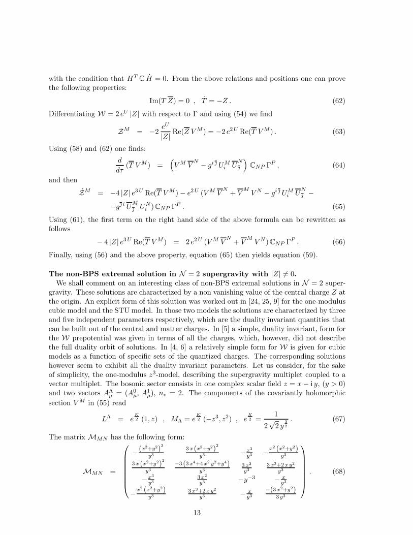
The non-BPS extremal solution in N = 2 supergravity with |Z| 6= 0.We shall comment on an interesting class of non-BPS extremal solutions in N = 2 super-

gravity. These solutions are characterized by a non vanishing value of the central charge Z atthe origin. An explicit form of this solution was worked out in [24, 25, 9] for the one-moduluscubic model and the STU model. In those two models the solutions are characterized by threeand five independent parameters respectively, which are the duality invariant quantities thatcan be built out of the central and matter charges. In [5] a simple, duality invariant, form forthe W prepotential was given in terms of all the charges, which, however, did not describethe full duality orbit of solutions. In [4, 6] a relatively simple form for W is given for cubicmodels as a function of specific sets of the quantized charges. The corresponding solutionshowever seem to exhibit all the duality invariant parameters. Let us consider, for the sakeof simplicity, the one-modulus z3-model, describing the supergravity multiplet coupled to avector multiplet. The bosonic sector consists in one complex scalar field z = x − i y, (y > 0)and two vectors AΛ

µ = (A0µ, A1

µ), nv = 2. The components of the covariantly holomorphic

section V M in (55) read

LΛ = eK

2 (1, z) , MΛ = eK

2 (−z3, z2) , eK

2 =1

2√

2 y3

2

. (67)

The matrix MMN has the following form:

MMN =

−(x2+y2)3

y3

3 x (x2+y2)2

y3 −x3

y3 −x2 (x2+y2)y3

3 x (x2+y2)2

y3

−3 (3 x4+4 x2 y2+y4)y3

3 x2

y3

3 x3+2 x y2

y3

−x3

y3

3 x2

y3 −y−3 − xy3

−x2 (x2+y2)y3

3 x3+2 x y2

y3 − xy3

−(3 x2+y2)3 y3

. (68)

13

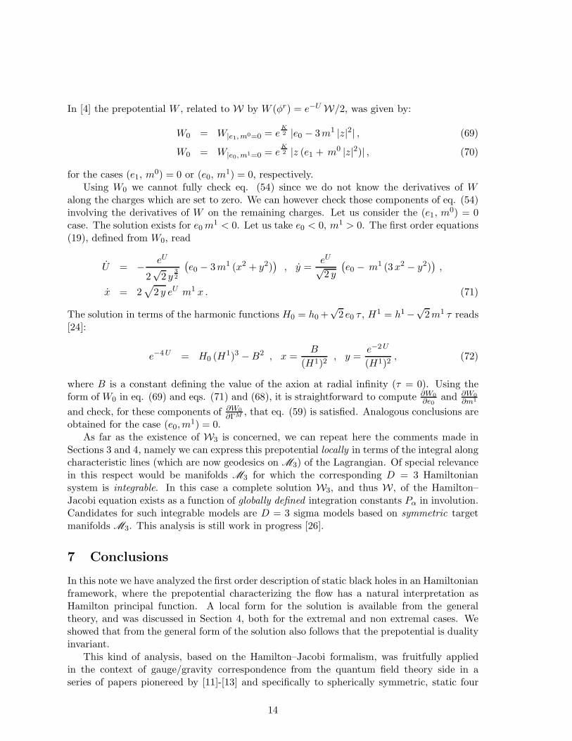
In [4] the prepotential W , related to W by W (φr) = e−U W/2, was given by:

W0 = W|e1, m0=0 = eK

2 |e0 − 3m1 |z|2| , (69)

W0 = W|e0, m1=0 = eK

2 |z (e1 + m0 |z|2)| , (70)

for the cases (e1, m0) = 0 or (e0, m1) = 0, respectively.Using W0 we cannot fully check eq. (54) since we do not know the derivatives of W

along the charges which are set to zero. We can however check those components of eq. (54)involving the derivatives of W on the remaining charges. Let us consider the (e1, m0) = 0case. The solution exists for e0 m1 < 0. Let us take e0 < 0, m1 > 0. The first order equations(19), defined from W0, read

U = − eU

2√

2 y3

2

(e0 − 3m1 (x2 + y2)

), y =

eU

√2 y

(e0 − m1 (3x2 − y2)

),

x = 2√

2 y eU m1 x . (71)

The solution in terms of the harmonic functions H0 = h0 +√

2 e0 τ , H1 = h1 −√

2m1 τ reads[24]:

e−4 U = H0 (H1)3 − B2 , x =B

(H1)2, y =

e−2 U

(H1)2, (72)

where B is a constant defining the value of the axion at radial infinity (τ = 0). Using theform of W0 in eq. (69) and eqs. (71) and (68), it is straightforward to compute ∂W0

∂e0and ∂W0

∂m1

and check, for these components of ∂W0

∂ΓM , that eq. (59) is satisfied. Analogous conclusions areobtained for the case (e0,m

1) = 0.As far as the existence of W3 is concerned, we can repeat here the comments made in

Sections 3 and 4, namely we can express this prepotential locally in terms of the integral alongcharacteristic lines (which are now geodesics on M3) of the Lagrangian. Of special relevancein this respect would be manifolds M3 for which the corresponding D = 3 Hamiltoniansystem is integrable. In this case a complete solution W3, and thus W, of the Hamilton–Jacobi equation exists as a function of globally defined integration constants Pα in involution.Candidates for such integrable models are D = 3 sigma models based on symmetric targetmanifolds M3. This analysis is still work in progress [26].

7 Conclusions

In this note we have analyzed the first order description of static black holes in an Hamiltonianframework, where the prepotential characterizing the flow has a natural interpretation asHamilton principal function. A local form for the solution is available from the generaltheory, and was discussed in Section 4, both for the extremal and non extremal cases. Weshowed that from the general form of the solution also follows that the prepotential is dualityinvariant.

This kind of analysis, based on the Hamilton–Jacobi formalism, was fruitfully appliedin the context of gauge/gravity correspondence from the quantum field theory side in aseries of papers pionereed by [11]-[13] and specifically to spherically symmetric, static four

14

dimensional black holes in [15]. From this analysis emerges the role of the prepotential W, onthe dual QFT side, as a c-function characterizing the renormalization group flow towards theconformal fixed point. The results in [15] apply to cases where the principal function doesnot depend explicitly in the evolution parameter (cut-off) corresponding, on the gravity side,to extremal solutions. It would be interesting to extended such analysis also to non-extremalcases, where no IR critical point exists, but nevertheless,the function W is defined and shouldplay a role.

It would also be interesting to extend our approach to more general settings which in-clude for instance higher derivative corrections to the supergravity Lagrangian (see [13] andreferences therein), stationary (non static) solutions and multicenter black holes.

Another relevant issue is related to the duality invariance of the most general W functionin four dimensional supergravity theories, which hints to the fact that W should be expressedonly in terms of duality invariant quantities, constructed in terms of the central and mattercharges. This was done in [5] for a broad class of extremal black holes in various supergravi-ties. Such analysis however did not encompass the five-parameter solutions found in [24, 25]and described, for specific choices of electric and magnetic charges, by the prepotentials givenin [4, 6]. The prepotentials found in those papers, however, do not exhibit manifest duality in-variance, being expressed in terms of a reduced set of charges. We expect that the completionof these prepotentials to a function of a full set of charges will exhibit manifest duality andwould be expressible in terms of central and matter charges only. Such completion could beachieved, for instance, by integrating eq. (59). An equivalent approach to the same problemis to use duality transformations on the five parameter solution to generate the remainingcharges [9].

Finally D = 3 global symmetry transformations which map static black holes into oneanother, and which are employed in the solution generating techniques [27, 28], should beviewed as canonical transformations in the extended phase space, according to our discussion,and also along the lines of [22]. We leave to a future investigation the study of the relationsbetween the various kinds of static black holes within this new framework. It would beinteresting to address, at least for symmetric scalar manifolds M3, the issue of integrability ofthe Hamiltonian system in the extended phase space. To this respect, of particular relevance,in the case of symmetric manifolds, is the Lax pair description of the geodesic equations[29, 30, 31], and the existence of a number of conserved Hamiltonians in involution, found in[32].

Acknowledgements

Work supported in part by PRIN Program 2007 of MIUR.

References

[1] S. Ferrara, R. Kallosh and A. Strominger, “N=2 extremal black holes,” Phys. Rev. D52 (1995) 5412 [arXiv:hep-th/9508072]. A. Strominger, “Macroscopic Entropy of N = 2Extremal Black Holes,” Phys. Lett. B 383 (1996) 39 [arXiv:hep-th/9602111]. S. Fer-rara and R. Kallosh, “Supersymmetry and Attractors,” Phys. Rev. D 54 (1996) 1514[arXiv:hep-th/9602136]; S. Ferrara and R. Kallosh, “Universality of Supersymmetric

15

Attractors,” Phys. Rev. D 54 (1996) 1525 [arXiv:hep-th/9603090]; R. Kallosh, “Newattractors,” JHEP 0512 (2005) 022 [arXiv:hep-th/0510024];

[2] S. Ferrara, G. W. Gibbons and R. Kallosh, “Black holes and critical points in modulispace,” Nucl. Phys. B 500, 75 (1997) [arXiv:hep-th/9702103];

[3] L. Andrianopoli, R. D’Auria, S. Ferrara and M. Trigiante, “Extremal black holes insupergravity,” Lect. Notes Phys. 737 (2008) 661 [arXiv:hep-th/0611345].

[4] A. Ceresole and G. Dall’Agata, “Flow Equations for Non-BPS Extremal Black Holes,”JHEP 0703 (2007) 110 [arXiv:hep-th/0702088].

[5] L. Andrianopoli, R. D’Auria, E. Orazi and M. Trigiante, “First Order Description ofBlack Holes in Moduli Space,” JHEP 0711, 032 (2007) [arXiv:0706.0712 [hep-th]].

[6] G. Lopes Cardoso, A. Ceresole, G. Dall’Agata, J. M. Oberreuter and J. Perz, “First-order flow equations for extremal black holes in very special geometry,” JHEP 0710

(2007) 063 [arXiv:0706.3373 [hep-th]].

[7] J. Perz, P. Smyth, T. Van Riet and B. Vercnocke, “First-order flow equations for extremaland non-extremal black holes,” JHEP 0903 (2009) 150 [arXiv:0810.1528 [hep-th]].

[8] S. Bellucci, S. Ferrara, M. Gunaydin and A. Marrani, “Charge orbits of symmetric specialgeometries and attractors,” Int. J. Mod. Phys. A 21 (2006) 5043 [arXiv:hep-th/0606209];S. Ferrara, K. Hayakawa and A. Marrani, “Lectures on Attractors and Black Holes,”Fortsch. Phys. 56 (2008) 993 [arXiv:0805.2498 [hep-th]];

[9] S. Bellucci, S. Ferrara, A. Marrani and A. Yeranyan, “stu Black Holes Unveiled,”arXiv:0807.3503 [hep-th].

[10] S. Ferrara, A. Marrani, J. F. Morales and H. Samtleben, “Intersecting Attractors,”arXiv:0812.0050 [hep-th].

[11] J. de Boer, E. P. Verlinde and H. L. Verlinde, “On the holographic renormalizationgroup,” JHEP 0008 (2000) 003 [arXiv:hep-th/9912012].

[12] E. P. Verlinde and H. L. Verlinde, “RG-flow, gravity and the cosmological constant,”JHEP 0005 (2000) 034 [arXiv:hep-th/9912018].

[13] M. Fukuma, S. Matsuura and T. Sakai, “Holographic renormalization group,” Prog.Theor. Phys. 109 (2003) 489 [arXiv:hep-th/0212314].

[14] K. Skenderis and P. K. Townsend, “Hamilton–Jacobi method for Domain Walls andCosmologies,” Phys. Rev. D 74 (2006) 125008 [arXiv:hep-th/0609056]; P. K. Townsend,“Hamilton-Jacobi Mechanics from Pseudo-Supersymmetry,” Class. Quant. Grav. 25

(2008) 045017 [arXiv:0710.5178 [hep-th]].

[15] K. Hotta, “Holographic RG flow dual to attractor flow in extremal black holes,”arXiv:0902.3529 [hep-th].

[16] B. Janssen, P. Smyth, T. Van Riet and B. Vercnocke, “A first-order formalism for timelikeand spacelike brane solutions,” JHEP 0804 (2008) 007 [arXiv:0712.2808 [hep-th]].

16

[17] G. W. Moore, “Arithmetic and attractors,” arXiv:hep-th/9807087;

[18] P. Breitenlohner, D. Maison and G. W. Gibbons, “Four-Dimensional Black Holes fromKaluza-Klein Theories,” Commun. Math. Phys. 120 (1988) 295.

[19] K. Meyer, G. Hall, “Introduction to Hamiltonian Dynamical Systems and the N-BodyProblem,” , Springer-Verlag, 1992.

[20] R. Kallosh, A. D. Linde and M. Shmakova, “Supersymmetric multiple basin attractors,”JHEP 9911 (1999) 010 [arXiv:hep-th/9910021]; S. Bellucci, S. Ferrara, A. Marrani andA. Shcherbakov, “Splitting of Attractors in 1-modulus Quantum Corrected Special Ge-ometry,” JHEP 0802 (2008) 088 [arXiv:0710.3559 [hep-th]].

[21] V. I. Arnold, “Mathematical Methods of Classical Mechanics” (Graduate Texts in Math-ematics), Springer, 1997.

[22] R. Kallosh, “From BPS to non-BPS black holes canonically,” arXiv:hep-th/0603003.

[23] K. Behrndt, G. Lopes Cardoso, B. de Wit, D. Lust, T. Mohaupt and W. A. Sabra,“Higher-Order Black-Hole Solutions in N=2 Supergravity and Calabi-Yau String Back-grounds,” Phys. Lett. B 429 (1998) 289 [arXiv:hep-th/9801081].

[24] K. Hotta and T. Kubota, “Exact Solutions and the Attractor Mechanism in Non-BPSBlack Holes,” Prog. Theor. Phys. 118 (2007) 969 [arXiv:0707.4554 [hep-th]].

[25] E. G. Gimon, F. Larsen and J. Simon, “Black Holes in Supergravity: the non-BPSBranch,” JHEP 0801 (2008) 040 [arXiv:0710.4967 [hep-th]].

[26] W. Chemissany, P. Fre, J. Rosseel, A. S. Sorin, M. Trigiante, T. Van Riet, to appear.

[27] M. Cvetic and D. Youm, “All the Static Spherically Symmetric Black Holes of HeteroticString on a Six Torus,” Nucl. Phys. B 472 (1996) 249 [arXiv:hep-th/9512127].

[28] E. Bergshoeff, W. Chemissany, A. Ploegh, M. Trigiante and T. Van Riet, “Gener-ating Geodesic Flows and Supergravity Solutions,” Nucl. Phys. B 812 (2009) 343[arXiv:0806.2310 [hep-th]].

[29] P. Fre and A. S. Sorin, “Supergravity Black Holes and Billiards and Liouville integrablestructure of dual Borel algebras,” arXiv:0903.2559 [hep-th].

[30] W. Chemissany, J. Rosseel, M. Trigiante and T. Van Riet, “The full integration of blackhole solutions to symmetric supergravity theories,” arXiv:0903.2777 [hep-th].

[31] W. Chemissany, P. Fre and A. S. Sorin, “The Integration Algorithm of Lax equation forboth Generic Lax matrices and Generic Initial Conditions,” arXiv:0904.0801 [hep-th].

[32] P. Fre and A. S. Sorin, “The Integration Algorithm for Nilpotent Orbits of G/H∗ Laxsystems: for Extremal Black Holes,” arXiv:0903.3771 [hep-th].

17