SEMIDISCRETE CENTRAL-UPWIND SCHEMES FORHYPERBOLIC CONSERVATION LAWS AND

HAMILTON–JACOBI EQUATIONS∗

ALEXANDER KURGANOV† , SEBASTIAN NOELLE‡ , AND GUERGANA PETROVA†

SIAM J. SCI. COMPUT. c© 2001 Society for Industrial and Applied MathematicsVol. 23, No. 3, pp. 707–740

Abstract. We introduce new Godunov-type semidiscrete central schemes for hyperbolic systemsof conservation laws and Hamilton–Jacobi equations. The schemes are based on the use of moreprecise information about the local speeds of propagation and can be viewed as a generalizationof the schemes from [A. Kurganov and E. Tadmor, J. Comput. Phys., 160 (2000), pp. 241–282;A. Kurganov and D. Levy, SIAM J. Sci. Comput., 22 (2000), pp. 1461–1488; A. Kurganov andG. Petrova, A third-order semidiscrete genuinely multidimensional central scheme for hyperbolicconservation laws and related problems, Numer. Math., to appear] and [A. Kurganov and E. Tadmor,J. Comput. Phys., 160 (2000), pp. 720–742].

The main advantages of the proposed central schemes are the high resolution, due to the smalleramount of the numerical dissipation, and the simplicity. There are no Riemann solvers and character-istic decomposition involved, and this makes them a universal tool for a wide variety of applications.

At the same time, the developed schemes have an upwind nature, since they respect the directionsof wave propagation by measuring the one-sided local speeds. This is why we call them central-upwindschemes.

The constructed schemes are applied to various problems, such as the Euler equations of gasdynamics, the Hamilton–Jacobi equations with convex and nonconvex Hamiltonians, and the incom-pressible Euler and Navier–Stokes equations. The incompressibility condition in the latter equationsallows us to treat them both in their conservative and transport form. We apply to these problemsthe central-upwind schemes, developed separately for each of them, and compute the correspondingnumerical solutions.

Key words. multidimensional conservation laws and Hamilton–Jacobi equations, high-resolutionsemidiscrete central schemes, compressible and incompressible Euler equations

AMS subject classifications. Primary, 65M06; Secondary, 35L65

PII. S1064827500373413

1. Introduction. We consider Godunov-type schemes for the multidimensional(multi-D) systems of conservation laws

ut +∇x · f(u) = 0, x ∈ Rd,(1.1)

and the multi-D Hamilton–Jacobi equations

ϕt +H(∇xϕ) = 0, x ∈ Rd.(1.2)

Godunov-type schemes for the system (1.1) are projection-evolution methods.Starting with cell averages at time level tn, one reconstructs a piecewise polynomialinterpolant of degree r − 1 (where r is the formal order of the scheme), which is

∗Received by the editors June 7, 2000; accepted for publication (in revised form) February 19,2001; published electronically August 15, 2001.

http://www.siam.org/journals/sisc/23-3/37341.html†Department of Mathematics, University of Michigan, Ann Arbor, MI 48109-1109 (kurganov@

math.lsa.umich.edu, petrova@math.lsa.umich.edu). The first author was supported in part by a NSFGroup Infrastructure grant and NSF grant DMS-0073631. The third author was supported by theRackham Grant and Fellowship Program, and her visit to Bonn University was sponsored by DFGgrant SFB256.

‡Institut fur Geometrie und Praktische Mathematik, RWTH Aachen, Templergraben 55, 52056Aachen, Germany (noelle@igpm.rwth-aachen.de). Part of the work of the second author was spon-sored by DFG grant SFB256.

707

708 A. KURGANOV, S. NOELLE, AND G. PETROVA

evolved to the next time level tn+1, and then it is projected onto a space of piecewiseconstants. Depending on the projection step, we distinguish two kinds of Godunov-type schemes: central and upwind. The Godunov-type central schemes are based onexact evolution and averaging over Riemann fans. In contrast to the upwind schemes,they do not employ Riemann solvers and characteristic decomposition, which makesthem simple, efficient, and universal.

In the one-dimensional (1-D) case, examples of such schemes are the first-order(staggered) Lax–Friedrichs scheme [28, 14], the second-order Nessyahu–Tadmor scheme[40], and the higher-order schemes in [39, 8, 30]. Second-order multi-D central schemeswere introduced in [3, 4, 5, 6, 19, 34], and their higher-order extensions were developedin [31, 32]. We would also like to mention the central schemes for incompressible flowsin [33, 22, 20, 21], and their applications to various systems, for example, [2, 13, 44, 49].

Unfortunately, these staggered central schemes may not provide a satisfactoryresolution when small time steps are enforced by stability restrictions, which mayoccur, for example, in the application of these schemes to convection-diffusion prob-lems. Also, they cannot be used for steady-state computations. These disadvantages

are caused by the accumulation of numerical dissipation, which is of order O( (∆x)2r

∆t ),where r is the formal order of the scheme.

The aforementioned problems have been recently resolved in [26], where newhigh-order Godunov-type central schemes are introduced. The proposed constructionis based on the use of the CFL related local speeds of propagation and on integrationover Riemann fans of variable sizes. In this way, a nonstaggered fully discrete cen-tral scheme is derived and is naturally reduced to a particularly simple semidiscreteform (for details see [26]). The same idea was used in [24] to develop a third-ordersemidiscrete central scheme, and in [25], where its genuinely multi-D extension wasintroduced.

The purpose of the first part of this paper is to present new semidiscrete centralschemes for the conservation law (1.1), which we call central-upwind schemes. Theyare based on the one-sided local speeds of propagation. For example, in the 1-D case,these one-sided local speeds are the largest and smallest eigenvalues of the Jacobian∂f∂u (in contrast to the less precise local information, used in [26, 24, 25]—the spectral

radius ρ(∂f∂u )).

The new schemes are Godunov-type central schemes, because the evolution stepemploys integration over Riemann fans and does not require a Riemann solver anda characteristic decomposition. They also have an upwind nature, since one-sidedinformation is used to estimate the width of the Riemann fans. This more preciseestimate makes our schemes less dissipative generalizations of the semidiscrete centralschemes in [26, 24, 25].

The second part of this paper is devoted to the Hamilton–Jacobi equations, (1.2),which are closely related to (scalar) conservation laws. For example, in the 1-D case,the unique viscosity solution of the Hamilton–Jacobi equation, ϕt + H(ϕx) = 0, isthe primitive of the unique entropy solution of the corresponding conservation law,ut + H(u)x = 0, where u = ϕx. However, in the multi-D case, this one-to-onecorrespondence no longer exists, but the gradient ∇xϕ satisfies (at least formally) asystem of (weakly) hyperbolic conservation laws.

This relation allows one to apply techniques, developed for conservation laws, tothe derivation of the numerical methods for Hamilton–Jacobi equations. Examples ofsuch methods can be found in [1, 10, 11, 35, 36, 42, 48]. One of the approaches [35, 36]is Godunov-type schemes. As in the case of conservation laws, they are projection-

CENTRAL-UPWIND SCHEMES 709

evolution methods. The differences are that here one starts with point values (notcell averages) at time tn, builds a continuous piecewise polynomial reconstruction ofdegree r, and evolves it to the next time level tn+1. The pointwise projection (not thecell averages) of this evolved solution is used as initial data for the next time step.

Godunov-type central schemes for Hamilton–Jacobi equations were first intro-duced in [35, 36]. Semidiscrete Godunov-type central schemes for the multi-D equa-tions (1.2) were developed in [27], where the same idea of local speeds of propagationwas used to separate between smooth and nonsmooth parts of the evolved solution.

In the second part of this work, we present a new second-order semidiscretecentral-upwind scheme for the Hamilton–Jacobi equations (1.2). It is a less dissipativegeneralization of the scheme in [27], which uses more precise one-sided information ofthe local propagation speeds.

The paper is organized as follows. In section 2, we give a brief overview of theGodunov-type central schemes for conservation laws and Hamilton–Jacobi equationsin one space dimension. We also describe the nonoscillatory piecewise quadratic re-construction from [25], which is later used in the numerical examples. Next, in section3, we introduce our new Godunov-type central-upwind schemes for the conservationlaws and Hamilton–Jacobi equations, both in one and in two spatial dimensions. Theresults of our numerical experiments are presented in section 4. We apply the proposedscheme to a variety of test problems: the one- and two-dimensional compressible Eulerequations, a 1-D Hamilton–Jacobi equation with a nonconvex Hamiltonian, the two-dimensional (2-D) eikonal equation of geometric optics. Finally, the incompressibleEuler and Navier–Stokes equations are solved using two different approaches, basedon either their conservative or transport form. The performed numerical experiments,especially in the case of incompressible flow simulations (see section 4.3), demonstratethe advantage of our new central-upwind approach.

2. Godunov-type central schemes—brief description. In this section, wereview Godunov-type central schemes in one spatial dimension. We will consider onlyuniform grids and use the following notation: let xj := j∆x, xj± 1

2:= (j ± 1/2)∆x,

tn := n∆t, unj := u(xj , t

n), ϕnj := ϕ(xj , t

n), where ∆x and ∆t are small spatial andtime scales, respectively.

2.1. Central schemes for conservation laws. The starting point for the con-struction of Godunov-type schemes for conservation laws is the equivalent integralformulation of the system (1.1),

u(x, t+∆t)

= u(x, t)− 1

∆x

[∫ t+∆t

τ=t

f

(u

(x+

∆x

2, τ

))dτ −

∫ t+∆t

τ=t

f

(u

(x− ∆x

2, τ

))dτ

],

(2.1)

where by

u(x, t) :=1

∆x

∫I(x)

u(ξ, t) dξ, I(x) =

{ξ : |ξ − x| < ∆x

2

}(2.2)

we denote the sliding averages of u(·, t) over the interval (x − ∆x2 , x + ∆x

2 ). At timelevel t = tn we consider problem (2.1) with the piecewise polynomial initial condition

u(x, tn) = pnj (x), xj− 12< x < xj+ 1

2∀j,(2.3)

710 A. KURGANOV, S. NOELLE, AND G. PETROVA

obtained from the cell averages unj := u(xj , t

n), computed at the previous time step.This piecewise polynomial reconstruction should be conservative, accurate of order r,and nonoscillatory.

Second-order schemes require a piecewise linear reconstruction (see the exam-ples in [15, 16, 23, 29, 40, 43]). Third-order schemes employ a piecewise quadraticapproximation, and one of the possibilities is to use the essentially nonoscillatory(ENO) reconstruction. In the 1-D case, we refer the reader to [16, 46]. The weightedENO interpolants are proposed in [38, 18, 30, 32], and the multi-D ENO-type recon-structions can be found in [31, 32]. The ENO-type approach employs smoothnessindicators. They require certain a priori information about the solution, which maybe unavailable and then spurious oscillations or extra smearing of discontinuities mayappear.

1-D nonoscillatory piecewise quadratic reconstructions, which do not require theuse of smoothness indicators, were proposed in [37, 39, 25]. 2-D generalizations ofthese reconstructions were presented in [25, 41].

The reconstructed piecewise polynomial u(x, tn) is then evolved exactly accordingto (2.1), and the solution at time t = tn+1 is obtained in terms of its sliding averages,u(x, tn+1). An evaluation of these sliding averages at particular grid points providesthe approximate cell averages of the solution at the next time level.

The choice of x = xj in (2.1) results in an upwind scheme. The solution then maybe nonsmooth in the neighborhood of the points {xj+ 1

2}, and the evaluation of the

flux integrals in (2.1) requires the use of a computationally expensive (approximate)Riemann solver and characteristic decomposition.

If x = xj+ 12in (2.1), we obtain Godunov-type central schemes, namely,

un+1j+ 1

2

=1

∆x

[∫ xj+ 1

2

xj

pnj (x) dx+

∫ xj+1

xj+ 1

2

pnj+1(x) dx

]

− λ

∆t

[∫ tn+1

tnf(u(xj+1, t)) dt−

∫ tn+1

tnf(u(xj , t)) dt

], λ :=

∆t

∆x.(2.4)

In contrast to the upwind framework, the solution is smooth in the neighborhood ofthe points {xj}. Therefore, a discretization of the flux integrals in (2.4) can be done,using an appropriate quadrature formula. The corresponding function values can becomputed either by Taylor expansion or by a Runge–Kutta method [39, 8].

2.2. Central schemes for Hamilton–Jacobi equations. In this section, wedescribe second-order Godunov-type central schemes for Hamilton–Jacobi equations.We follow the approach from [36] and construct a 1-D second-order staggered centralscheme.

Assume that we have computed the point values of ϕ at time t = tn. We thenstart with a continuous piecewise quadratic interpolant,

ϕ(x, tn) := ϕnj +

(∆ϕ)nj+ 1

2

∆x(x− xj) +

(∆ϕ)′j+ 1

2

2(∆x)2 (x− xj)(x− xj+1),

x ∈ [xj , xj+1],(2.5)

where

(∆ϕ)nj+ 12:= ϕn

j+1 − ϕnj .(2.6)

CENTRAL-UPWIND SCHEMES 711

Here, (∆ϕ)′j+ 1

2

/(∆x)2is an approximation to the second derivative ϕxx(xj+ 1

2, tn). An

appropriate nonlinear limiter employed in this approximation guarantees the nonoscil-latory nature of ϕ(x, tn). Examples of such limiters, developed in the context of hy-perbolic conservation laws, may be found in [15, 16, 23, 40, 43]. In this paper we usea one-parameter family of the minmod limiters [29, 15, 43]

(∆ϕ)′j+ 12= minmod

(θ[(∆ϕ)nj+ 3

2− (∆ϕ)nj+ 1

2

],1

2

[(∆ϕ)nj+ 3

2− (∆ϕ)nj− 1

2

],

θ[(∆ϕ)nj+ 1

2− (∆ϕ)nj− 1

2

]),(2.7)

where θ ∈ [1, 2], and the multivariable minmod function is defined by

minmod(x1, x2, . . .) :=

minj{xj} if xj > 0 ∀j,maxj{xj} if xj < 0 ∀j,0 otherwise.

(2.8)

Notice that larger θ’s in (2.7) correspond to less dissipative, but still nonoscillatorylimiters [29, 15, 43].

Given a reconstruction (2.5), we consider the Hamilton–Jacobi equation (1.2),subject to the initial data ϕ(x, 0) = ϕ(x, tn). Under an appropriate CFL condition,due to the finite speed of propagation, the solution of this initial value problem issmooth in the neighborhood of the line segment {(x, t) : x = xj+ 1

2, tn ≤ t ≤ tn+1}.

Therefore, from the Taylor expansion of the solution about the point (xj+ 12, tn), we

obtain

ϕn+1j+ 1

2

=ϕnj + ϕn

j+1

2−(∆ϕ)′

j+ 12

8−∆tH

((∆ϕ)n

j+ 12

∆x

)+(∆t)2

2

[H ′((∆ϕ)n

j+ 12

∆x

)]2

·(∆ϕ)′

j+ 12

(∆x)2.

(2.9)Remarks.1. The derived scheme (2.9) is different from the one in [36]. There, the evo-

lution step is executed by integration of (1.2) over [tn, tn+1], followed by theapplication of the midpoint rule to the resulting integrals. For details, see[36, 27].

2. A 2-D staggered central scheme for (1.2) can be found in [36].

3. Central-upwind semidiscrete schemes. In this section, we develop newsemidiscrete central-upwind schemes for conservation laws and Hamilton–Jacobi equa-tions, following the approach presented in [26, 24, 25] and [27], respectively.

3.1. Semidiscrete central-upwind schemes for 1-D conservation laws.We consider the 1-D system (1.1) of N strictly hyperbolic conservation laws. Westart with a piecewise polynomial reconstruction (2.3) with possible discontinuities atthe interface points {xj+ 1

2}. These discontinuities propagate with right- and left-sided

local speeds, which can be estimated by

a+j+ 1

2

:= maxω∈C

(u−j+ 1

2

,u+

j+ 12

){λN

(∂f∂u

(ω)), 0}

and

a−j+ 1

2

:= minω∈C

(u−j+ 1

2

,u+

j+ 12

){λ1

(∂f∂u

(ω)), 0},

712 A. KURGANOV, S. NOELLE, AND G. PETROVA

respectively. Here, λ1 < · · · < λN are the N eigenvalues of the Jacobian ∂f∂u , and

C(u−j+ 1

2

, u+j+ 1

2

) is the curve in the phase space that connects

u+j+ 1

2

:= pj+1(xj+ 12) and u−

j+ 12

:= pj(xj+ 12).(3.1)

For example, in the genuinely nonlinear or linearly degenerate case, we have

a+j+ 1

2

= max

{λN

(∂f∂u

(u−j+ 1

2

)), λN

(∂f∂u

(u+j+ 1

2

)), 0

},

a−j+ 1

2

= min

{λ1

(∂f∂u

(u−j+ 1

2

)), λ1

(∂f∂u

(u+j+ 1

2

)), 0

}.(3.2)

In fact, these one-sided local speeds are related to the CFL number. Note that inthe schemes from [26, 24] only the spectral radius of ∂f

∂u is used, and for its computationone actually needs to know both λ1 and λN .

Further, we utilize these one-sided local speeds of propagation in the followingway. We consider the nonequal rectangular domains

[xnj− 1

2 ,r, xn

j+ 12 ,l

]× [tn, tn+1] and [xnj+ 1

2 ,l, xn

j+ 12 ,r

]× [tn, tn+1],(3.3)

with xnj+ 1

2 ,l:= xj+ 1

2+∆ta−

j+ 12

and xnj+ 1

2 ,r:= xj+ 1

2+∆ta+

j+ 12

, where the solution of

(1.1) with the initial data u(x, tn) is smooth and nonsmooth, respectively.

The cell averages

wn+1j =

1

xnj+ 1

2 ,l− xn

j− 12 ,r

[∫ xn

j+ 12,l

xn

j− 12,r

pnj (x) dx−∫ tn+1

tn

(f(u(xn

j+ 12 ,l

, t))−f(u(xnj− 1

2 ,r, t))

)dt

],

(3.4)and

wn+1j+ 1

2

=1

xnj+ 1

2 ,r− xn

j+ 12 ,l

[∫ xj+ 1

2

xn

j+ 12,l

pnj (x) dx+

∫ xn

j+ 12,r

xj+ 1

2

pnj+1(x) dx

−∫ tn+1

tn

(f(u(xn

j+ 12 ,r

, t))− f(u(xnj+ 1

2 ,l, t))

)dt

](3.5)

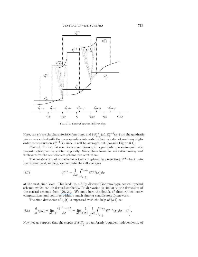
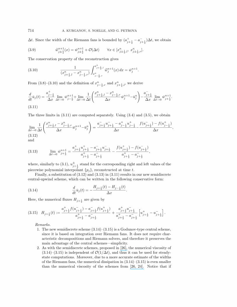
are obtained by integrating (1.1) over the corresponding domains in (3.3); see Figure3.1.

Given the polynomials {pnj }, the spatial integrals in (3.4) and (3.5) can be com-puted explicitly. To discretize the flux integrals there, one may use an appropriatequadrature formula, since the solution is smooth along the line segments (xn

j+ 12 ,l

, t),

tn ≤ t < tn+1 and (xnj+ 1

2 ,r, t), tn ≤ t < tn+1.

Next, from the cell averages, wn+1j+ 1

2

, wn+1j , given by (3.4)–(3.5), we reconstruct

a nonoscillatory, conservative, third-order, piecewise polynomial interpolant, denotedby

wn+1(x) =∑j

(wn+1

j (x)χ[xn

j− 12,r, xn

j+ 12,l

] + wn+1j+ 1

2

(x)χ[xn

j+ 12,l, xn

j+ 12,r

]).(3.6)

CENTRAL-UPWIND SCHEMES 713

x j-1 jx

nu j

n+1u j

j-1/2n+1

w

n+1j+1w

n+1j+1/2w

nj+1u

x j+3/2,ln

xnj-1/2,l

n+1jw

j-1n+1

w

x x x xj+1/2j-1/2 j+1 j+3/2

x xn n

nu

j-1/2,rj-3/2,r

j-1

nj+1/2,lx j+1/2,rx

n

Fig. 3.1. Central-upwind differencing.

Here, the χ’s are the characteristic functions, and {wn+1j+ 1

2

(x), wn+1j (x)} are the quadratic

pieces, associated with the corresponding intervals. In fact, we do not need any high-order reconstruction wn+1

j (x) since it will be averaged out (consult Figure 3.1).

Remark. Notice that even for a nonuniform grid, a particular piecewise quadraticreconstruction can be written explicitly. Since these formulae are rather messy andirrelevant for the semidiscrete scheme, we omit them.

The construction of our scheme is then completed by projecting wn+1 back ontothe original grid, namely, we compute the cell averages

un+1j =

1

∆x

∫ xj+ 1

2

xj− 1

2

wn+1(x) dx(3.7)

at the next time level. This leads to a fully discrete Godunov-type central-upwindscheme, which can be derived explicitly. Its derivation is similar to the derivation ofthe central schemes from [26, 24]. We omit here the details of these rather messycomputations and continue within a much simpler semidiscrete framework.

The time derivative of uj(t) is expressed with the help of (3.7) as

d

dtuj(t) = lim

∆t→0

un+1j − un

j

∆t= lim

∆t→0

1

∆t

[1

∆x

∫ xj+ 1

2

xj− 1

2

wn+1(x) dx− unj

].(3.8)

Now, let us suppose that the slopes of wn+1j± 1

2

are uniformly bounded, independently of

714 A. KURGANOV, S. NOELLE, AND G. PETROVA

∆t. Since the width of the Riemann fans is bounded by (a+j+ 1

2

− a−j+ 1

2

)∆t, we obtain

wn+1j± 1

2

(x) = wn+1j± 1

2

+O(∆t) ∀x ∈ [xnj± 1

2 ,l, xn

j± 12 ,r

].(3.9)

The conservation property of the reconstruction gives

1

(xnj+ 1

2 ,l− xn

j− 12 ,r

)

∫ xn

j+ 12,l

xn

j− 12,r

wn+1j (x) dx = wn+1

j .(3.10)

From (3.8)–(3.10) and the definition of xnj− 1

2 ,rand xn

j+ 12 ,l

, we derive

d

dtuj(t) =

a+j− 1

2

∆xlim

∆t→0wn+1

j− 12

+ lim∆t→0

1

∆t

(xnj+ 1

2 ,l− xn

j− 12 ,r

∆xwn+1

j −unj

)−a−j+ 1

2

∆xlim

∆t→0wn+1

j+ 12

.

(3.11)

The three limits in (3.11) are computed separately. Using (3.4) and (3.5), we obtain

lim∆t→0

1

∆t

(xnj+ 1

2 ,l− xn

j− 12 ,r

∆xwn+1

j −unj

)=

a−j+ 1

2

u−j+ 1

2

− a+j− 1

2

u+j− 1

2

∆x−f(u−

j+ 12

)− f(u+j− 1

2

)

∆x,

(3.12)and

lim∆t→0

wn+1j+ 1

2

=a+j+ 1

2

u+j+ 1

2

− a−j+ 1

2

u−j+ 1

2

a+j+ 1

2

− a−j+ 1

2

−f(u+

j+ 12

)− f(u−j+ 1

2

)

a+j+ 1

2

− a−j+ 1

2

,(3.13)

where, similarly to (3.1), u±j+ 1

2

stand for the corresponding right and left values of the

piecewise polynomial interpolant {pj}, reconstructed at time t.Finally, a substitution of (3.12) and (3.13) in (3.11) results in our new semidiscrete

central-upwind scheme, which can be written in the following conservative form:

d

dtuj(t) = −

Hj+ 12(t)−Hj− 1

2(t)

∆x.(3.14)

Here, the numerical fluxes Hj+ 12are given by

Hj+ 12(t) :=

a+j+ 1

2

f(u−j+ 1

2

)− a−j+ 1

2

f(u+j+ 1

2

)

a+j+ 1

2

− a−j+ 1

2

+a+j+ 1

2

a−j+ 1

2

a+j+ 1

2

− a−j+ 1

2

[u+j+ 1

2

− u−j+ 1

2

].(3.15)

Remarks.1. The new semidiscrete scheme (3.14)–(3.15) is a Godunov-type central scheme,

since it is based on integration over Riemann fans. It does not require char-acteristic decompositions and Riemann solvers, and therefore it preserves themain advantage of the central schemes—simplicity.

2. As with the semidiscrete schemes, proposed in [26], the numerical viscosity of(3.14)–(3.15) is independent of O(1/∆t), and thus it can be used for steady-state computations. Moreover, due to a more accurate estimate of the widthsof the Riemann fans, the numerical dissipation in (3.14)–(3.15) is even smallerthan the numerical viscosity of the schemes from [26, 24]. Notice that if

CENTRAL-UPWIND SCHEMES 715

one takes a+j+ 1

2

= −a−j+ 1

2

= aj+ 12:= maxω∈C(un−

j+ 12

,un+

j+ 12

) ρ(∂f∂u (ω)), then the

numerical flux (3.15) reduces to

Hj+ 12(t) :=

f(u+j+ 1

2

) + f(u−j+ 1

2

)

2−

aj+ 12

2

[u+j+ 1

2

− u−j+ 1

2

],

which is the numerical flux of the schemes from [26, 24].3. We would like to point out that the first-order version of our scheme is exactly

the semidiscrete version of the scheme in [17, 12]. Moreover, if the flux f ismonotone, it reduces to the standard upwind scheme. That is why we callour new schemes central-upwind. For example, if f ′(u) ≥ 0, then a−

j+ 12

= 0

∀j, and the first-order scheme simplifies to

uj(t) = −f(unj )− f(un

j−1)

∆x.

4. A fully discrete, 2-D, third-order accurate scheme using the Harten–Lax–vanLeer approximate Riemann solver [17, 12] was implemented and tested in [41].

5. It can be proved that a scalar second-order version of (3.14)–(3.15), togetherwith the minmod reconstruction,

unj (x) = un

j + snj (x− xj),

snj = minmod

(θunj − un

j−1

∆x,unj+1 − un

j−1

2∆x, θ

unj+1 − un

j

∆x

),(3.16)

is a TVD scheme (for 1 ≤ θ ≤ 2), that is, ‖u(·, t)‖BV ≤ ‖u(·, 0)‖BV . The proofis analogous to the proof of Theorem 4.1 in [26], and we leave the details tothe reader.

6. The semidiscrete scheme (3.14)–(3.15) is a system of time-dependent ODEs,which can be solved by any stable ODE solver which retains the spatial accu-racy of the semidiscrete scheme. In the numerical examples below, we haveused the TVD Runge–Kutta method, proposed in [47, 45].

7. The scheme (3.14)–(3.15) can be easily generalized and applied to convection-diffusion equations in a straightforward manner. For details, we refer thereader to [26, 24].

3.2. Semidiscrete central-upwind schemes for multi-D conservation laws.The semidiscrete central-upwind schemes, presented in section 3.1, can be generalizedto the multi-D case. Without loss of generality, we consider the 2-D system

ut + f(u)x + g(u)y = 0.(3.17)

Given the grid points xj := j∆x, yk := k∆y and the intermediate points xj± 12:=

xj ± ∆x2 , yk± 1

2:= yk ± ∆y

2 , we start at time t = tn with a conservative piecewisepolynomial reconstruction of an appropriate order:

un(x, y) :=∑j,k

pnj,k(x, y)χj,k,

where χj,k is the characteristic function of the cell [xj− 12, xj+ 1

2]× [yk− 1

2, yk+ 1

2]. In the

numerical examples in this paper, we have used the third-order piecewise quadraticreconstruction, described in [25].

716 A. KURGANOV, S. NOELLE, AND G. PETROVA

We use the notation

uj,k := pnj,k(xj , yk), uNj,k := pnj,k(xj , yk+ 1

2), uS

j,k := pnj,k(xj , yk− 12),

uEj,k := pnj,k(xj+ 1

2, yk), uW

j,k := pnj,k(xj− 12, yk), uNE

j,k := pnj,k(xj+ 12, yk+ 1

2),(3.18)

uNWj,k := pnj,k(xj− 1

2, yk+ 1

2), uSE

j,k := pnj,k(xj+ 12, yk− 1

2), uSW

j,k := pnj,k(xj− 12, yk− 1

2)

for the corresponding point values and

uj,k :=1

∆x∆y

∫ xj+ 1

2

xj− 1

2

∫ yk+ 1

2

yk− 1

2

pnj,k(x, y) dx dy

for the cell averages.The piecewise polynomial interpolant un may have discontinuities along the lines

x = xj± 12and y = yk± 1

2, which propagate with different right- and left-sided local

speeds. To estimate them is a nontrivial problem, but in practice one may use

a+j+ 1

2 ,k:= max

{λN

(∂f∂u

(uWj+1,k)

), λN

(∂f∂u

(uEj,k)

), 0},

b+j,k+ 1

2

:= max{λN

(∂g∂u

(uSj,k+1)

), λN

(∂g∂u

(uNj,k)

), 0},

a−j+ 1

2 ,k:= min

{λ1

(∂f∂u

(uWj+1,k)

), λ1

(∂f∂u

(uEj,k)

), 0},

b−j,k+ 1

2

:= min{λ1

(∂g∂u

(uSj,k+1)

), λ1

(∂g∂u

(uNj,k)

), 0},(3.19)

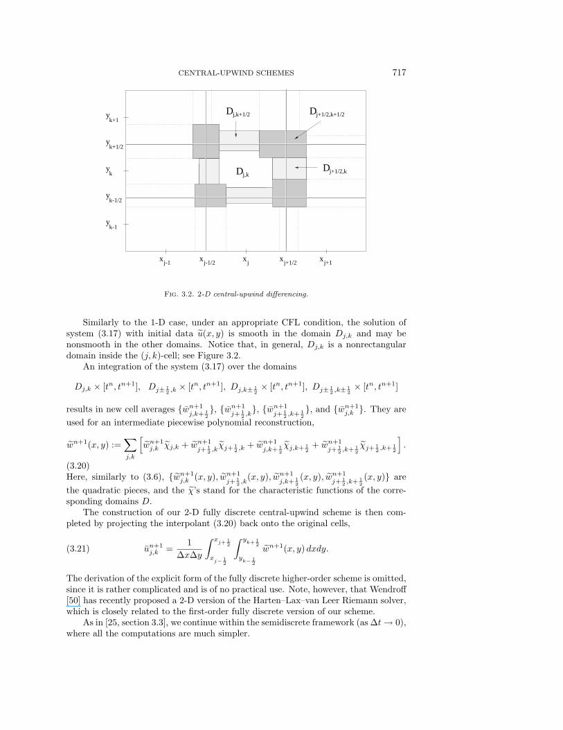
respectively. As in [25], we consider the nonuniform domains, outlined in Figure 3.2and defined by

Dj,k+ 12:= [xj− 1

2+A+

j− 12 ,k+ 1

2

∆t, xj+ 12+A−

j+ 12 ,k+ 1

2

∆t]×[yk+ 12+b−

j,k+ 12

∆t, yk+ 12+b+

j,k+ 12

∆t],

Dj+ 12 ,k

:= [xj+ 12+a−

j+ 12 ,k

∆t, xj+ 12+a+

j+ 12 ,k

∆t]×[yk− 12+B+

j+ 12 ,k− 1

2

∆t, yk+ 12+B−

j+ 12 ,k+ 1

2

∆t],

Dj+ 12 ,k+ 1

2:= [xj+ 1

2+A−

j+ 12 ,k+ 1

2

∆t, xj+ 12+A+

j+ 12 ,k+ 1

2

∆t]

×[yk+ 12+B−

j+ 12 ,k+ 1

2

∆t, yk+ 12+B+

j+ 12 ,k+ 1

2

∆t],

Dj,k := [xj− 12, xj+ 1

2]× [yk− 1

2, yk+ 1

2] \

⋃±

[Dj,k± 12∪Dj± 1

2 ,k∪Dj± 1

2 ,k± 12],

where

A+j+ 1

2 ,k+ 12

:= max{a+j+ 1

2 ,k, a+

j+ 12 ,k+1

}, B+

j+ 12 ,k+ 1

2

:= max{b+j,k+ 1

2

, b+j+1,k+ 1

2

},

A−j+ 1

2 ,k+ 12

:= min{a−j+ 1

2 ,k, a−

j+ 12 ,k+1

}, B−

j+ 12 ,k+ 1

2

:= min{b−j,k+ 1

2

, b−j+1,k+ 1

2

}.

CENTRAL-UPWIND SCHEMES 717

xj-1 x x xj-1/2 j+1/2 j+1xj

k+1/2y

y

y

y

k+1

k-1/2

k-1

yk Dj,k

D

Dj+1/2,k

j,k+1/2 Dj+1/2,k+1/2

Fig. 3.2. 2-D central-upwind differencing.

Similarly to the 1-D case, under an appropriate CFL condition, the solution ofsystem (3.17) with initial data u(x, y) is smooth in the domain Dj,k and may benonsmooth in the other domains. Notice that, in general, Dj,k is a nonrectangulardomain inside the (j, k)-cell; see Figure 3.2.

An integration of the system (3.17) over the domains

Dj,k × [tn, tn+1], Dj± 12 ,k

× [tn, tn+1], Dj,k± 12× [tn, tn+1], Dj± 1

2 ,k± 12× [tn, tn+1]

results in new cell averages {wn+1j,k+ 1

2

}, {wn+1j+ 1

2 ,k}, {wn+1

j+ 12 ,k+ 1

2

}, and {wn+1j,k }. They are

used for an intermediate piecewise polynomial reconstruction,

wn+1(x, y) :=∑j,k

[wn+1

j,k χj,k + wn+1j+ 1

2 ,kχj+ 1

2 ,k+ wn+1

j,k+ 12

χj,k+ 12+ wn+1

j+ 12 ,k+ 1

2

χj+ 12 ,k+ 1

2

].

(3.20)Here, similarly to (3.6), {wn+1

j,k (x, y), wn+1j+ 1

2 ,k(x, y), wn+1

j,k+ 12

(x, y), wn+1j+ 1

2 ,k+ 12

(x, y)} are

the quadratic pieces, and the χ’s stand for the characteristic functions of the corre-sponding domains D.

The construction of our 2-D fully discrete central-upwind scheme is then com-pleted by projecting the interpolant (3.20) back onto the original cells,

un+1j,k =

1

∆x∆y

∫ xj+ 1

2

xj− 1

2

∫ yk+ 1

2

yk− 1

2

wn+1(x, y) dxdy.(3.21)

The derivation of the explicit form of the fully discrete higher-order scheme is omitted,since it is rather complicated and is of no practical use. Note, however, that Wendroff[50] has recently proposed a 2-D version of the Harten–Lax–van Leer Riemann solver,which is closely related to the first-order fully discrete version of our scheme.

As in [25, section 3.3], we continue within the semidiscrete framework (as ∆t → 0),where all the computations are much simpler.

718 A. KURGANOV, S. NOELLE, AND G. PETROVA

We use the following notation for the intersections of the cell [xj− 12, xj+ 1

2] ×

[yk− 12, yk+ 1

2] with the domains D – Cj± 1

2 ,k± 12for the four corners, Sj± 1

2 ,k, Sj,k± 1

2

for the four side domains, and Dj,k for the center. The sizes of these domains are|C| ∼ (∆t)2 and |S| ∼ ∆t. Since we assume that the spatial derivatives of wn+1 arebounded independently of ∆t, the relation between wn+1 and wn+1 is given by∫ ∫

Cj± 1

2,k± 1

2

wn+1j± 1

2 ,k± 12

dxdy = O((∆t)2),(3.22)

∫ ∫Sj± 1

2,k

wn+1j± 1

2 ,kdxdy = |Sj± 1

2 ,k| wn+1

j± 12 ,k

+O(∆t2),(3.23)

∫ ∫Sj,k± 1

2

wn+1j,k± 1

2

dxdy = |Sj,k± 12| wn+1

j,k± 12

+O(∆t2).(3.24)

Also, the conservation property of the reconstruction wn+1 yields∫ ∫Dj,k

wn+1j,k (x, y) dxdy = |Dj,k|wn+1

j,k .(3.25)

We now use (3.21) together with (3.22)–(3.25) and obtain

d

dtuj,k(t) = lim

∆t→0

un+1j,k − un

j,k

∆t

= lim∆t→0

(∑±

|Sj,k± 12|

∆t∆x∆ywn+1

j,k± 12

+∑±

|Sj± 12 ,k

|∆t∆x∆y

wn+1j± 1

2 ,k

)

+ lim∆t→0

1

∆t

[|Dj,k|∆x∆y

wn+1j,k − un

j,k

].

(3.26)

For the first sum on the right-hand side (RHS), we apply Simpson’s quadrature for-mula to the integrals over Dj,k± 1

2in the computation of wn+1

j,k± 12

. Since |Sj,k± 12| =

∓b∓j,k± 1

2

∆t∆x+O((∆t)2), we arrive at (consult [25] for details)

lim∆t→0

|Sj,k± 12|

∆t∆x∆ywn+1

j,k± 12

≈ −b+j,k± 1

2

b−j,k± 1

2

6(b+j,k± 1

2

− b−j,k± 1

2

)∆y

[u

SW(NW)j,k±1 + 4u

S(N)j,k±1 + u

SE(NE)j,k±1

]

+

(b∓j,k± 1

2

)2

6(b+j,k± 1

2

− b−j,k± 1

2

)∆y

[u

NW(SW)j,k + 4u

N(S)j,k + u

NE(SE)j,k

]

+b∓j,k± 1

2

6(b+j,k± 1

2

− b−j,k± 1

2

)∆y

[g(u

SW(NW)j,k±1 )− g(u

NW(SW)j,k )

+ 4(g(u

S(N)j,k±1)− g(u

N(S)j,k )

)+ g(u

SE(NE)j,k±1 )− g(u

NE(SE)j,k )

].(3.27)

CENTRAL-UPWIND SCHEMES 719

The second sum on the RHS of (3.26) is treated similarly, and we obtain

lim∆t→0

|Sj± 12 ,k

|∆t∆x∆y

wn+1j± 1

2 ,k≈ −

a+j± 1

2 ,ka−j± 1

2 ,k

6(a+j± 1

2 ,k− a−

j± 12 ,k

)∆x

[u

NW(NE)j±1,k + 4u

W(E)j±1,k + u

SW(SE)j±1,k

]

+

(a∓j± 1

2 ,k

)2

6(a+j± 1

2 ,k− a−

j± 12 ,k

)∆x

[u

NE(NW)j,k + 4u

E(W)j,k + u

SE(SW)j,k

]

+a∓j± 1

2 ,k

6(a+j± 1

2 ,k− a−

j± 12 ,k

)∆x

[f(u

NW(NE)j±1,k )− f(u

NE(NW)j,k )

+ 4(f(u

W(E)j±1,k)− f(u

E(W)j,k )

)f(u

SW(SE)j±1,k )− f(u

SE(SW)j,k )

].(3.28)

Finally, we consider the last term on the RHS of (3.26). Since the domain Dj,k

becomes rectangular as ∆t → 0, up to small corners of a negligible size O((∆t)2), theintegration of (3.17) over Dj,k × [tn, tn + ∆t] and the application of Simpson’s ruleresult in

lim∆t→0

1

∆t

[|Dj,k|∆x∆y

wn+1j,k − un

j,k

]

≈a−j+ 1

2 ,k

6∆x

[uNEj,k + 4uE

j,k + uSEj,k

]−

a+j− 1

2 ,k

6∆x

[uNWj,k + 4uW

j,k + uSWj,k

]+

b−j,k+ 1

2

6∆y

[uNWj,k + 4uN

j,k + uNEj,k

]−

b+j,k− 1

2

6∆y

[uSWj,k + 4uS

j,k + uSEj,k

]− 1

6∆x

[f(uNE

j,k )− f(uNWj,k ) + 4

(f(uE

j,k)− f(uWj,k)

)+ f(uSE

j,k)− f(uSWj,k )

]− 1

6∆y

[g(uNW

j,k )− g(uSWj,k ) + 4

(g(uN

j,k)− g(uSj,k)

)+ g(uNE

j,k )− g(uSEj,k)

].(3.29)

Our 2-D semidiscrete central-upwind scheme is obtained by plugging (3.27)–(3.29)into (3.26). It can be written in the following conservative form:

d

dtuj,k(t) = −

Hxj+ 1

2 ,k(t)−Hx

j− 12 ,k

(t)

∆x−

Hy

j,k+ 12

(t)−Hy

j,k− 12

(t)

∆y,(3.30)

where the numerical fluxes are

Hxj+ 1

2 ,k:=

a+j+ 1

2 ,k

6(a+j+ 1

2 ,k− a−

j+ 12 ,k

)[f(uNEj,k ) + 4f(uE

j,k) + f(uSEj,k)

]

−a−j+ 1

2 ,k

6(a+j+ 1

2 ,k− a−

j+ 12 ,k

)[f(uNWj+1,k) + 4f(uW

j+1,k) + f(uSWj+1,k)

]

+a+j+ 1

2 ,ka−j+ 1

2 ,k

6(a+j+ 1

2 ,k− a−

j+ 12 ,k

)[uNWj+1,k − uNE

j,k + 4(uWj+1,k − uE

j,k) + uSWj+1,k − uSE

j,k

](3.31)

720 A. KURGANOV, S. NOELLE, AND G. PETROVA

and

Hy

j,k+ 12

:=b+j,k+ 1

2

6(b+j,k+ 1

2

− b−j,k+ 1

2

)[g(uNWj,k ) + 4g(uN

j,k) + g(uNEj,k )

]

−b−j,k+ 1

2

6(b+j,k+ 1

2

− b−j,k+ 1

2

)[g(uSWj,k+1) + 4g(uS

j,k+1) + g(uSEj,k+1)

]

+b+j,k+ 1

2

b−j,k+ 1

2

6(b+j,k+ 1

2

− b−j,k+ 1

2

)[uSWj,k+1 − uNW

j,k + 4(uSj,k+1 − uN

j,k) + uSEj,k+1 − uNE

j,k

].(3.32)

Here, the one-sided local speeds a±j+ 1

2 ,k, b±

j,k+ 12

are defined in (3.19), and the values

of the u’s are computed in (3.18), using the piecewise quadratic reconstruction {pj,k}at time t. In our numerical examples, we have implemented the reconstruction intro-duced in [25].

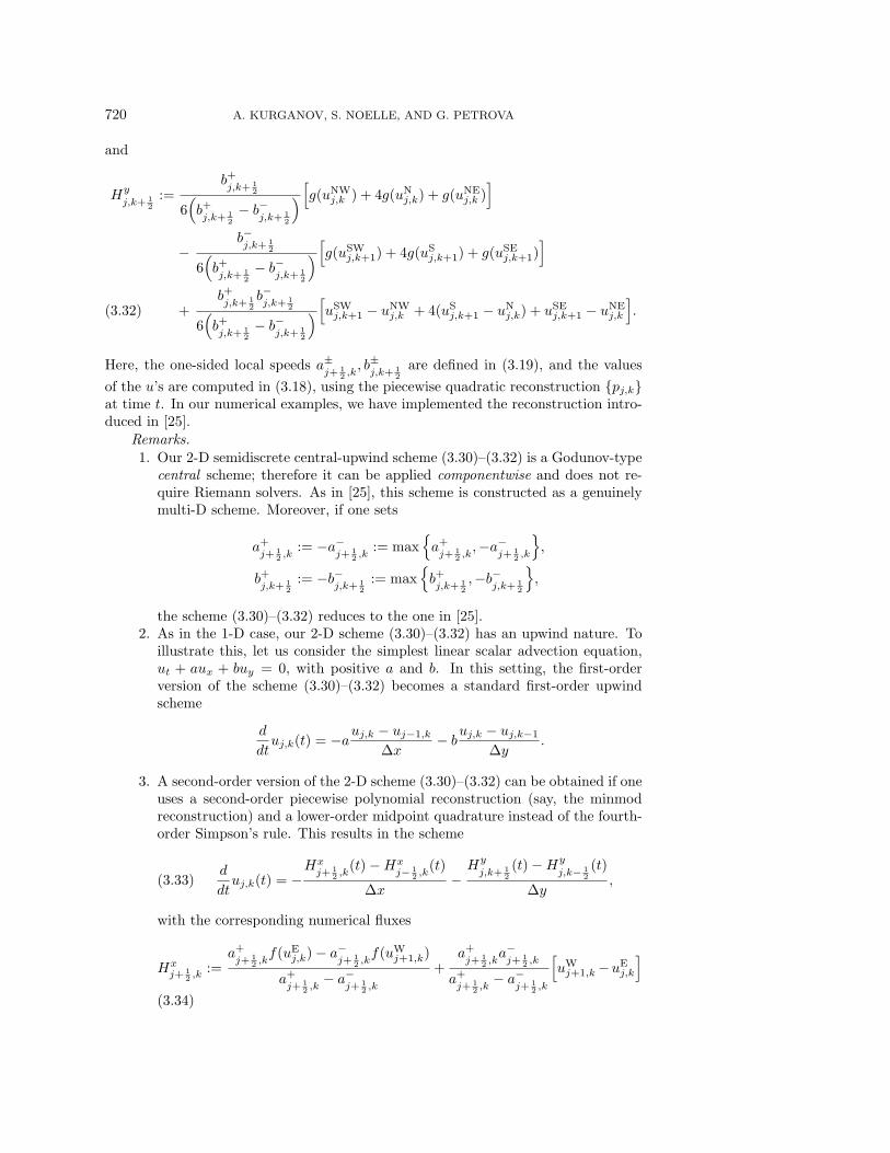
Remarks.1. Our 2-D semidiscrete central-upwind scheme (3.30)–(3.32) is a Godunov-typecentral scheme; therefore it can be applied componentwise and does not re-quire Riemann solvers. As in [25], this scheme is constructed as a genuinelymulti-D scheme. Moreover, if one sets

a+j+ 1

2 ,k:= −a−

j+ 12 ,k

:= max{a+j+ 1

2 ,k,−a−

j+ 12 ,k

},

b+j,k+ 1

2

:= −b−j,k+ 1

2

:= max{b+j,k+ 1

2

,−b−j,k+ 1

2

},

the scheme (3.30)–(3.32) reduces to the one in [25].2. As in the 1-D case, our 2-D scheme (3.30)–(3.32) has an upwind nature. To

illustrate this, let us consider the simplest linear scalar advection equation,ut + aux + buy = 0, with positive a and b. In this setting, the first-orderversion of the scheme (3.30)–(3.32) becomes a standard first-order upwindscheme

d

dtuj,k(t) = −a

uj,k − uj−1,k

∆x− b

uj,k − uj,k−1

∆y.

3. A second-order version of the 2-D scheme (3.30)–(3.32) can be obtained if oneuses a second-order piecewise polynomial reconstruction (say, the minmodreconstruction) and a lower-order midpoint quadrature instead of the fourth-order Simpson’s rule. This results in the scheme

d

dtuj,k(t) = −

Hxj+ 1

2 ,k(t)−Hx

j− 12 ,k

(t)

∆x−

Hy

j,k+ 12

(t)−Hy

j,k− 12

(t)

∆y,(3.33)

with the corresponding numerical fluxes

Hxj+ 1

2 ,k:=

a+j+ 1

2 ,kf(uE

j,k)− a−j+ 1

2 ,kf(uW

j+1,k)

a+j+ 1

2 ,k− a−

j+ 12 ,k

+a+j+ 1

2 ,ka−j+ 1

2 ,k

a+j+ 1

2 ,k− a−

j+ 12 ,k

[uWj+1,k −uE

j,k

](3.34)

CENTRAL-UPWIND SCHEMES 721

and

Hy

j,k+ 12

:=b+j,k+ 1

2

g(uNj,k)− b−

j,k+ 12

g(uSj,k+1)

b+j,k+ 1

2

− b−j,k+ 1

2

+b+j,k+ 1

2

b−j,k+ 1

2

b+j,k+ 1

2

− b−j,k+ 1

2

[uSj,k+1−uN

j,k

].

(3.35)The same scheme can also be derived by applying the 1-D numerical flux(3.15) in both x- and y-directions (this is the so-called dimension-by-dimensionapproach, used in [26]).

4. The scheme (3.30)–(3.32) can be generalized and applied to convection-diffusion equations (for details see [26, 25, 24]). Also, it can be rather easilyextended to the multi-D case, d ≥ 3.

3.2.1. Maximum principle for the second-order central-upwind scheme.We consider the 2-D second-order central-upwind scheme (3.33)–(3.35), together withthe minmod reconstruction (3.16). We solve the time-dependent ODE system (3.33),using a TVD Runge–Kutta method. Under an appropriate CFL condition, the result-ing fully discrete scheme, applied to a scalar conservation law, satisfies the maximumprinciple; see the following theorem.

Theorem 3.1 (maximum principle). Consider the scalar conservation laws(3.17). Then the second-order scheme (3.33)–(3.35), with the minmod reconstruc-tion (3.16), coupled with a TVD Runge–Kutta method [47, 45] satisfies the maximumprinciple

minj,k

{unj,k} ≤ min

j,k{un+1

j,k } ≤ maxj,k

{un+1j,k } ≤ max

j,k{un

j,k}(3.36)

under the CFL condition

max

(∆tn

∆xmaxu

|f ′(u)|, ∆tn

∆ymaxu

|g′(u)|)

≤ 1

8,(3.37)

where ∆tn is the variable time step of the Runge–Kutta method.We omit the proof since it is similar to the proof of Theorem 5.1 in [26].

3.3. Semidiscrete central-upwind scheme for Hamilton–Jacobi equa-tions. In this section, we propose a new Godunov-type central-upwind scheme forthe 1-D and 2-D Hamilton–Jacobi equations (1.2). We follow the approach in [27],but this time we utilize more precise information about the one-sided local speeds ofpropagation.

We begin with the 1-D case and start at time level t = tn with the continuouspiecewise polynomial interpolant ϕ(x, tn) and estimate the maximal one-sided localspeeds, a+

j and a−j . For example, in the convex case, they are equal to

a+j := max{H ′(ϕ+

x ), H′(ϕ−

x ), 0}, a−j := min{H ′(ϕ+x ), H

′(ϕ−x ), 0},(3.38)

where we use the notation ϕ±x := ϕx(xj±0, tn). To construct the second-order scheme

one should use the continuous piecewise quadratic polynomial (2.5), and in this case,

ϕ±x =

(∆ϕ)nj± 1

2

∆x∓

(∆ϕ)′j± 1

2

2∆x.(3.39)

Note that under an appropriate CFL-condition, the solution of the Hamilton–Jacobi equation (1.2) with the piecewise polynomial initial data ϕ(x, tn) is smooth

722 A. KURGANOV, S. NOELLE, AND G. PETROVA

x x n x nxnx

ϕ n

ϕ n+1ϕ n+1 ϕ n+1

jn

j- j j +1- j +1

j

j+1 j+1- j-

x+

x+1/2j

n+1ϕ j+ j

n+1ϕ

ϕ n+1 j+1+

+1j +

ϕ n j+1

Fig. 3.3. Central-upwind differencing—1-D.

along the line segments (xnj±, t), t

n ≤ t < tn+1, xnj± := xj + a±j ∆t; see Figure 3.3.

Therefore, one can use the Taylor expansion to compute the intermediate point valuesat the next time level:

ϕn+1j± = ϕ(xj±, tn)−∆t ·H(ϕx(x

nj±, t

n)) +O(∆t)2.(3.40)

We complete the construction of our fully discrete central-upwind scheme by pro-jecting the intermediate point values back onto the original grid. Since the distancebetween xn

j+ and xnj− is proportional to ∆t, it suffices to compute the weighted aver-

ages of ϕn+1j+ and ϕn+1

j− , that is,

ϕn+1j =

a+j

a+j − a−j

ϕn+1j− − a−j

a+j − a−j

ϕn+1j+ +O(∆t)2.(3.41)

Finally, we substitute (3.40) in (3.41), and arrive at the fully discrete scheme

ϕn+1j =

a+j

a+j − a−j

(ϕ(xj−, tn)−∆tH(ϕx(x

nj−, t

n)))

− a−ja+j − a−j

(ϕ(xj+, t

n)−∆tH(ϕx(xnj+, t

n))),(3.42)

which is high-order in space (depending on the order of the piecewise polynomialreconstruction) and only first-order in time.

A semidiscrete version of the scheme (3.42), coupled with a high-order ODEsolver, will allow us to achieve high accuracy both in space and time. To derive such

CENTRAL-UPWIND SCHEMES 723

a scheme, we first use the Taylor expansions, ϕ(xj±, tn) = ϕ(xj , tn) + ∆ta±j ϕx(xj ±

0, tn) +O(∆t)2, and rewrite the fully discrete scheme (3.42) as

ϕn+1j = ϕn

j −∆ta+j a

−j

a+j − a−j

[ϕx(xj + 0, tn)− ϕx(xj − 0, tn)

]+

∆t

a+j − a−j

[a−j H(ϕx(x

nj+, t

n))− a+j H(ϕx(x

nj−, t

n))]+O(∆t)2.(3.43)

We now let ∆t → 0, and end up with the following semidiscrete central-upwindscheme:

d

dtϕj(t) =

1

a+j − a−j

[a−j H(ϕ+

x )− a+j H(ϕ−

x )]− a+

j a−j

a+j − a−j

(ϕ+x − ϕ−

x

).(3.44)

Here, a±j are given by (3.38), and ϕ±x are the right and the left derivatives at the point

x = xj of the reconstruction ϕ(·, t) at time t.

We continue with the construction of a multi-D extension of the scheme (3.44).Without loss of generality, we consider the 2-D Hamilton–Jacobi equation,

ϕt +H(ϕx, ϕy) = 0.(3.45)

Assume that at time t = tn the discrete approximation to the point values of itssolution, {ϕn

j,k ≈ ϕ(xj , yk, tn)}, has already been computed. We then construct the

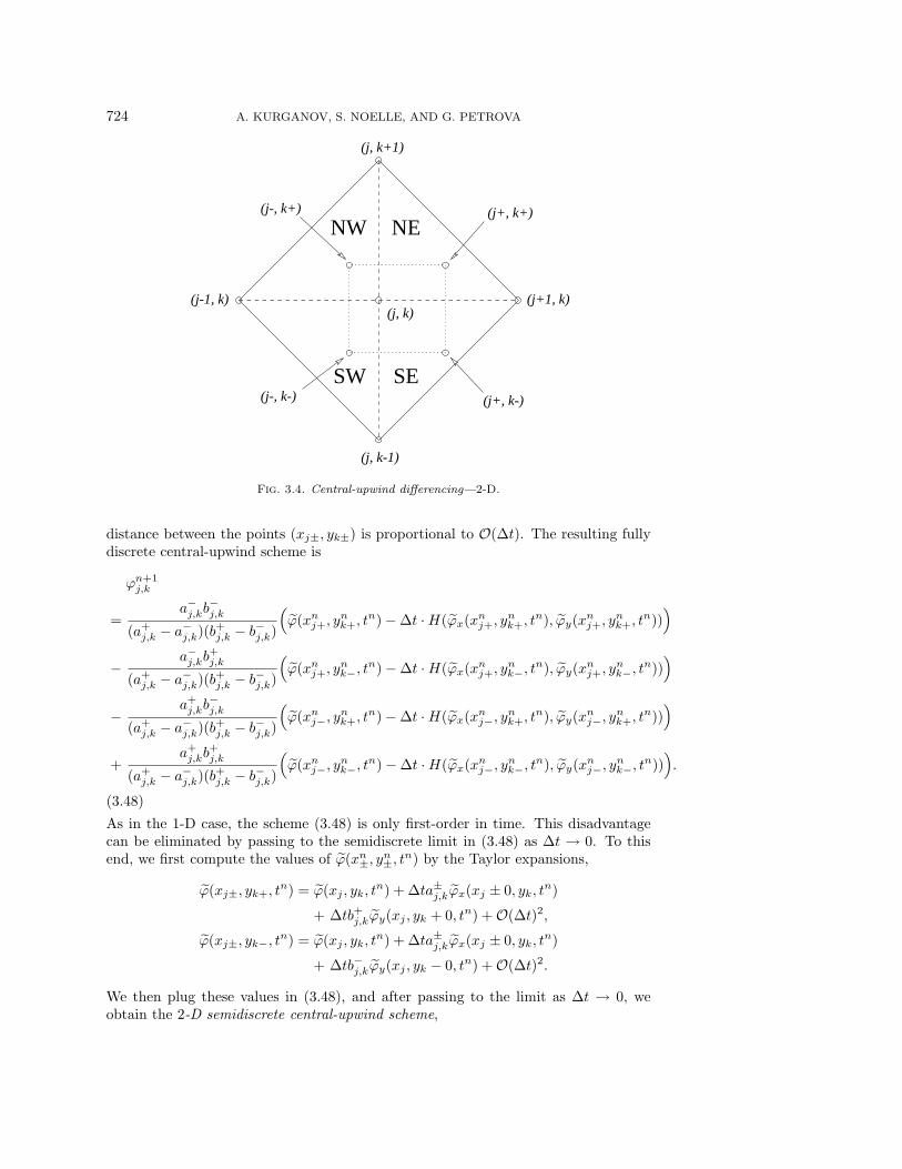
2-D continuous piecewise polynomial interpolant ϕ(x, y, tn). Such a reconstruction isdefined over the four triangles (NW, NE, SW, and SE) around each grid-point (xj , yk)(see Figure 3.4). We refer the reader to [27] for an example of a nonoscillatory second-order piecewise quadratic interpolant.

We now continue with the construction of our semidiscrete central-upwind scheme.As in the 1-D case, we use the maximal values of the one-sided local speeds of prop-agation in the x- and y-directions. These values at the grid-point (xj , yk) are givenby

a+j,k := max

Cj,k

{Hu(ϕx(x, y), ϕy(x, y))

}+, a−j,k := min

Cj,k

{Hu(ϕx(x, y), ϕy(x, y))

}−,

b+j,k := maxCj,k

{Hv(ϕx(x, y), ϕy(x, y))

}+, b−j,k := min

Cj,k

{Hv(ϕx(x, y), ϕy(x, y))

}−,

(3.46)where Cj,k := [xj− 1

2, xj+ 1

2]× [yk− 1

2, yk+ 1

2] and ( · )+ := max(·, 0), ( · )− := min(·, 0).

To compute the solution at the next time level t = tn+1, we use the intermediatevalues {ϕn+1

j±,k±}, obtained by the Taylor expansion about the points (xnj± := xj +

a±j,k∆t, ynk± := yk + b±j,k∆t),

ϕn+1j±,k± = ϕ(xn

j±, ynk±, t

n)−∆t ·H(ϕx(xnj±, y

nk±, t

n), ϕy(xnj±, y

nk±, t

n))+O(∆t)2.

(3.47)Expansion (3.47) is valid, since due to the finite speed of propagation, the solution of(3.45) with the initial data ϕ(x, y, tn) is smooth around (xn

j±, ynk±); see Figure 3.4.

Next, the computed intermediate values (3.47) are projected back onto the originalgrid. This can be done using the weighted average of the values ϕn+1

j±,k±, since the

724 A. KURGANOV, S. NOELLE, AND G. PETROVA

(j, k)(j-1, k) (j+1, k)

(j, k+1)

(j, k-1)

NW NE

SW SE(j-, k-)

(j-, k+) (j+, k+)

(j+, k-)

Fig. 3.4. Central-upwind differencing—2-D.

distance between the points (xj±, yk±) is proportional to O(∆t). The resulting fullydiscrete central-upwind scheme is

ϕn+1j,k

=a−j,kb

−j,k

(a+j,k − a−j,k)(b

+j,k − b−j,k)

(ϕ(xn

j+, ynk+, t

n)−∆t ·H(ϕx(xnj+, y

nk+, t

n), ϕy(xnj+, y

nk+, t

n)))

− a−j,kb+j,k

(a+j,k − a−j,k)(b

+j,k − b−j,k)

(ϕ(xn

j+, ynk−, t

n)−∆t ·H(ϕx(xnj+, y

nk−, t

n), ϕy(xnj+, y

nk−, t

n)))

− a+j,kb

−j,k

(a+j,k − a−j,k)(b

+j,k − b−j,k)

(ϕ(xn

j−, ynk+, t

n)−∆t ·H(ϕx(xnj−, y

nk+, t

n), ϕy(xnj−, y

nk+, t

n)))

+a+j,kb

+j,k

(a+j,k − a−j,k)(b

+j,k − b−j,k)

(ϕ(xn

j−, ynk−, t

n)−∆t ·H(ϕx(xnj−, y

nk−, t

n), ϕy(xnj−, y

nk−, t

n))).

(3.48)

As in the 1-D case, the scheme (3.48) is only first-order in time. This disadvantagecan be eliminated by passing to the semidiscrete limit in (3.48) as ∆t → 0. To thisend, we first compute the values of ϕ(xn

±, yn±, t

n) by the Taylor expansions,

ϕ(xj±, yk+, tn) = ϕ(xj , yk, t

n) + ∆ta±j,kϕx(xj ± 0, yk, tn)

+ ∆tb+j,kϕy(xj , yk + 0, tn) +O(∆t)2,

ϕ(xj±, yk−, tn) = ϕ(xj , yk, tn) + ∆ta±j,kϕx(xj ± 0, yk, t

n)

+ ∆tb−j,kϕy(xj , yk − 0, tn) +O(∆t)2.

We then plug these values in (3.48), and after passing to the limit as ∆t → 0, weobtain the 2-D semidiscrete central-upwind scheme,

CENTRAL-UPWIND SCHEMES 725

d

dtϕj,k(t)

= − a−j,kb−j,kH(ϕ+

x , ϕ+y )− a−j,kb

+j,kH(ϕ+

x , ϕ−y )− a+

j,kb−j,kH(ϕ−

x , ϕ+y ) + a+

j,kb+j,kH(ϕ−

x , ϕ−y )

(a+j,k − a−j,k)(b

+j,k − b−j,k)

− a+j,ka

−j,k

a+j,k − a−j,k

(ϕ+x − ϕ−

x

)− b+j,kb

−j,k

b+j,k − b−j,k

(ϕ+y − ϕ−

y

).

(3.49)Here, ϕ±

x := ϕx(xj ± 0, yk, t) and ϕ±y := ϕy(xj , yk ± 0, t) are the right and the left

derivatives in the x- and y-direction, respectively. The one-sided local speeds in (3.49)are given by (3.46). In practice, these speeds can be estimated in a simpler way. Forinstance, in the numerical examples, we have used

a+j,k := max±

{Hu(ϕ

±x , ϕ

±y )}

+, a−j,k := min±

{Hu(ϕ

±x , ϕ

±y )}−,

b+j,k := max±

{Hv(ϕ

±x , ϕ

±y )}

+, b−j,k := min±

{Hv(ϕ

±x , ϕ

±y )}−.

(3.50)

Finally, to obtain the same second-order accuracy in time, our semidiscrete central-upwind scheme (3.49)–(3.50) should be complemented with at least a second-orderODE solver for time discretization.

4. Numerical examples. In this section, we implement our scheme for con-servation laws and Hamilton–Jacobi equations and perform several numerical exper-iments. We test the accuracy of the scheme on problems with smooth solutions andsolve various equations which admit nonsmooth solutions. Among them are the Eu-ler equations of gas dynamics, the incompressible Euler equations, and others. Thenumerical results show that our scheme gives sharper resolution and reduces some ofthe side effects of the schemes from [27, 25].

The high-order semidiscrete methods, presented in this paper, require a timediscretization of the corresponding order. In the numerical examples, shown below,we have used the third-order TVD Runge–Kutta method, proposed in [45, 47], and thesecond-order modified Euler method. Our choice is based on the stability propertiesof these methods, each time step of which can be viewed as a convex combination ofsmall forward Euler steps.

In all the numerical experiments below, the CFL number is equal to 0.475, andthe value of θ in the generalized minmod limiter is 2.

4.1. 1-D problems.

Example 1. Burgers’ equation. We consider the initial boundary value prob-lem (IBVP) for the inviscid Burgers’ equation

ut +(u2

2

)x= 0, u(x, 0) = 0.5 + sinx, x ∈ [0, 2π],(4.1)

with periodic boundary conditions. It is known that the unique entropy solution of(4.1) develops a shock discontinuity at time t = 1. The solution at the preshock timeT = 0.5 is smooth, and this allows us to test the accuracy of the 1-D third-ordercentral-upwind scheme (3.14)–(3.15). We couple it with the basic piecewise quadraticreconstruction (for details, see [37, 39, 25]), and compute the solution using N gridpoints, N = 40, 80, . . . , 1280.

The L∞- and L1-errors are shown in Table 4.1, and they clearly demonstrate athird-order experimental convergence rate.

726 A. KURGANOV, S. NOELLE, AND G. PETROVA

Table 4.1Accuracy test for the Burgers’ equation (4.1), T = 0.5.

N L∞-error rate L1-error rate40 1.456e-03 – 1.241e-03 –80 2.177e-04 2.74 1.683e-04 2.88160 2.893e-05 2.91 2.187e-05 2.94320 3.689e-06 2.97 2.794e-06 2.97640 4.559e-07 3.02 3.484e-07 3.001280 5.720e-08 2.99 4.376e-08 2.99

0

1

2

3

4

5

6

0 0.1 0.2 0.3 0.4 0.5 0.6 0.7 0.8 0.9 1

N=1600N=400

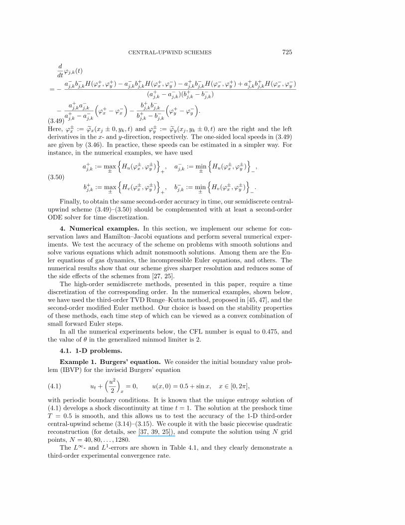
Fig. 4.1. Problem (4.2)–(4.3), density at T = 0.01.

Example 2. 1-D Euler equations of gas dynamics. We solve the 1-D Eulersystem

∂

∂t

ρmE

+∂

∂x

mρu2 + pu(E + p)

= 0, p = (γ − 1) ·(E − ρ

2u2),(4.2)

with the initial data

-u(x, 0) =

-uL = (1, 0, 2500)

T, 0 ≤ x < 0.1,

-uM = (1, 0, 0.025)T, 0.1 ≤ x < 0.9,

-uR = (1, 0, 250)T, 0.9 ≤ x < 1,

(4.3)

and solid wall boundary conditions, applied to both ends. This problem, proposed in[51], models the interaction of blast waves. Here, ρ, u, m = ρu, p , and E are thedensity, velocity, momentum, pressure, and the total energy, respectively; γ = 1.4.

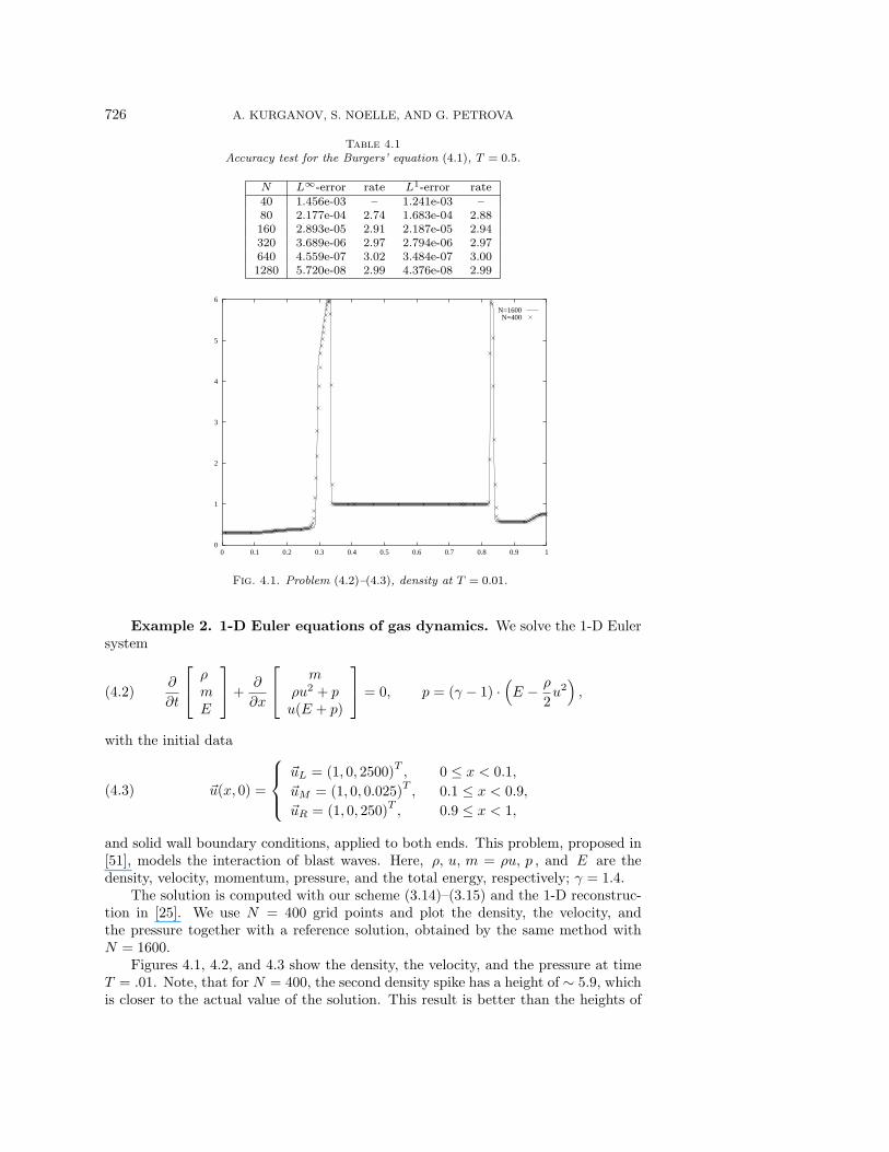
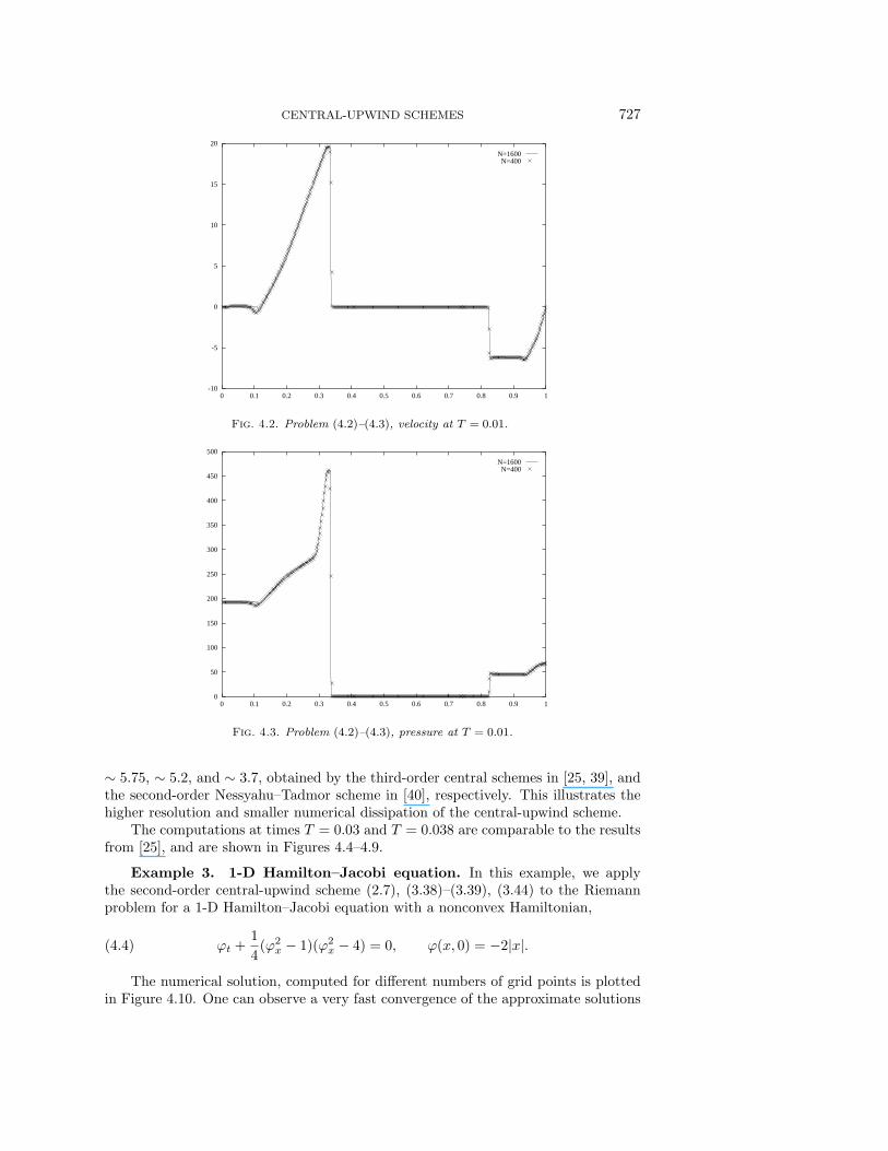
The solution is computed with our scheme (3.14)–(3.15) and the 1-D reconstruc-tion in [25]. We use N = 400 grid points and plot the density, the velocity, andthe pressure together with a reference solution, obtained by the same method withN = 1600.

Figures 4.1, 4.2, and 4.3 show the density, the velocity, and the pressure at timeT = .01. Note, that for N = 400, the second density spike has a height of ∼ 5.9, whichis closer to the actual value of the solution. This result is better than the heights of

CENTRAL-UPWIND SCHEMES 727

-10

-5

0

5

10

15

20

0 0.1 0.2 0.3 0.4 0.5 0.6 0.7 0.8 0.9 1

N=1600N=400

Fig. 4.2. Problem (4.2)–(4.3), velocity at T = 0.01.

0

50

100

150

200

250

300

350

400

450

500

0 0.1 0.2 0.3 0.4 0.5 0.6 0.7 0.8 0.9 1

N=1600N=400

Fig. 4.3. Problem (4.2)–(4.3), pressure at T = 0.01.

∼ 5.75, ∼ 5.2, and ∼ 3.7, obtained by the third-order central schemes in [25, 39], andthe second-order Nessyahu–Tadmor scheme in [40], respectively. This illustrates thehigher resolution and smaller numerical dissipation of the central-upwind scheme.

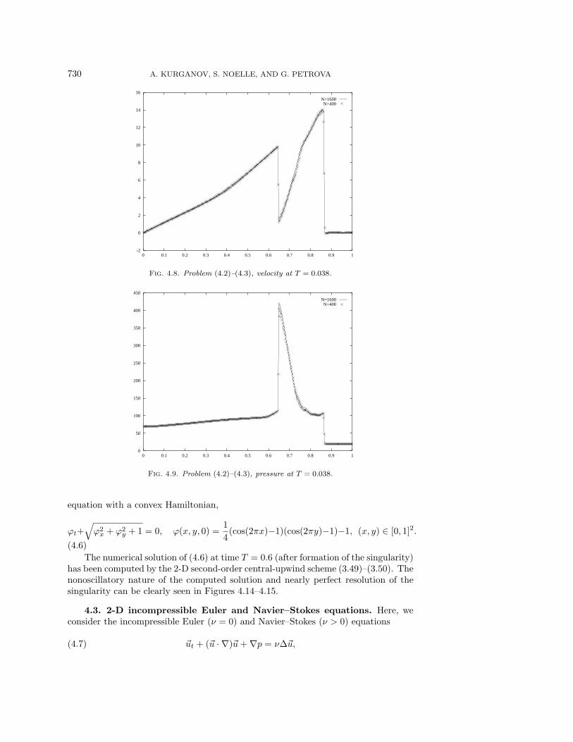
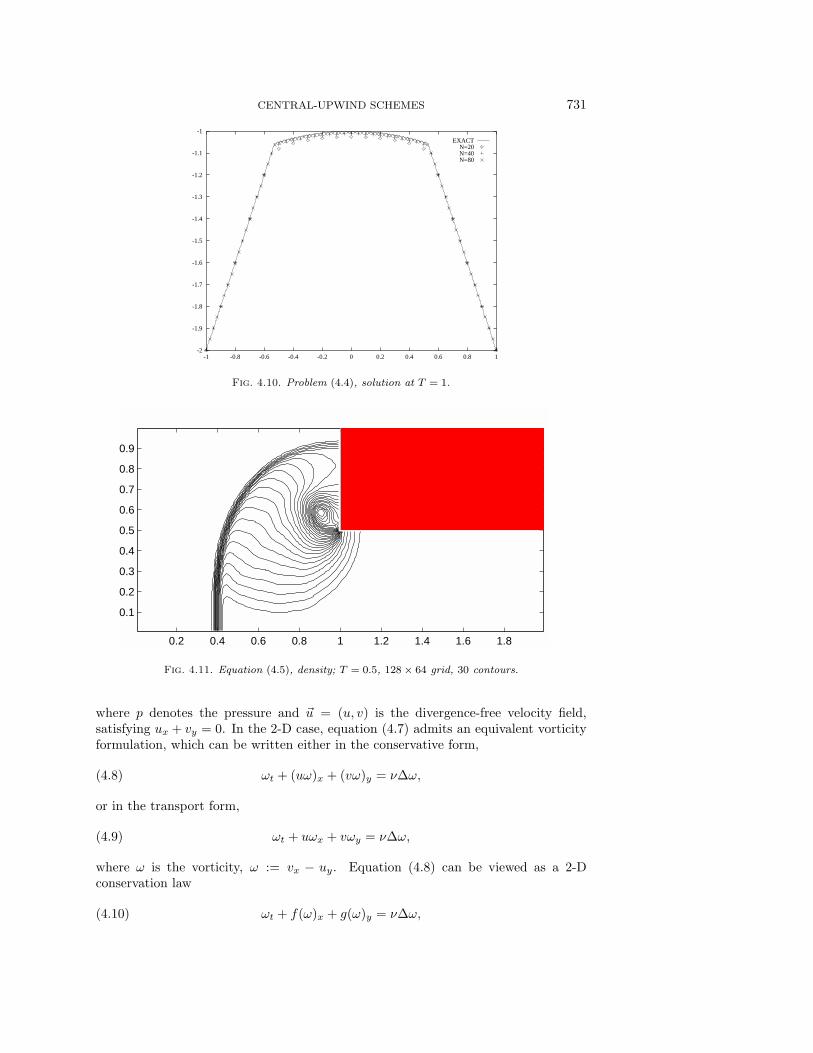
The computations at times T = 0.03 and T = 0.038 are comparable to the resultsfrom [25], and are shown in Figures 4.4–4.9.

Example 3. 1-D Hamilton–Jacobi equation. In this example, we applythe second-order central-upwind scheme (2.7), (3.38)–(3.39), (3.44) to the Riemannproblem for a 1-D Hamilton–Jacobi equation with a nonconvex Hamiltonian,

ϕt +1

4(ϕ2

x − 1)(ϕ2x − 4) = 0, ϕ(x, 0) = −2|x|.(4.4)

The numerical solution, computed for different numbers of grid points is plottedin Figure 4.10. One can observe a very fast convergence of the approximate solutions

728 A. KURGANOV, S. NOELLE, AND G. PETROVA

0

5

10

15

20

25

0 0.1 0.2 0.3 0.4 0.5 0.6 0.7 0.8 0.9 1

N=1600N=400

Fig. 4.4. Problem (4.2)–(4.3), density at T = 0.03.

-6

-4

-2

0

2

4

6

8

10

12

14

0 0.1 0.2 0.3 0.4 0.5 0.6 0.7 0.8 0.9 1

N=1600N=400

Fig. 4.5. Problem (4.2)–(4.3), velocity at T = 0.03.

toward the exact (viscosity) solution of (4.4) as the mesh is refined. The exact solutionis obtained by solving the Riemann problem for the corresponding conservation law.

4.2. 2-D problems.

Example 4. 2-D Euler equations of gas dynamics. We solve the 2-Dcompressible Euler equations

∂

∂t

ρρuρvE

+ ∂

∂x

ρu

ρu2 + pρuv

u(E + p)

+ ∂

∂y

ρvρuv

ρv2 + pv(E + p)

= 0, p = (γ−1)·[E − ρ

2(u2 + v2)

](4.5)

CENTRAL-UPWIND SCHEMES 729

0

100

200

300

400

500

600

700

800

900

0 0.1 0.2 0.3 0.4 0.5 0.6 0.7 0.8 0.9 1

N=1600N=400

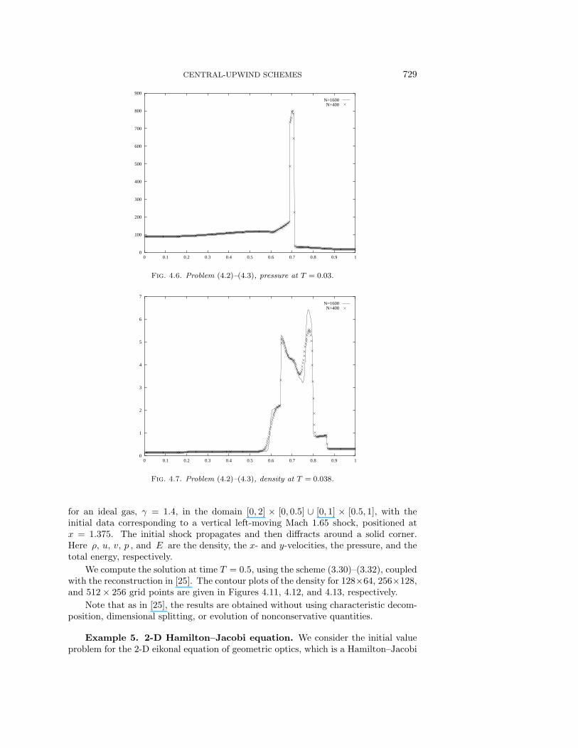
Fig. 4.6. Problem (4.2)–(4.3), pressure at T = 0.03.

0

1

2

3

4

5

6

7

0 0.1 0.2 0.3 0.4 0.5 0.6 0.7 0.8 0.9 1

N=1600N=400

Fig. 4.7. Problem (4.2)–(4.3), density at T = 0.038.

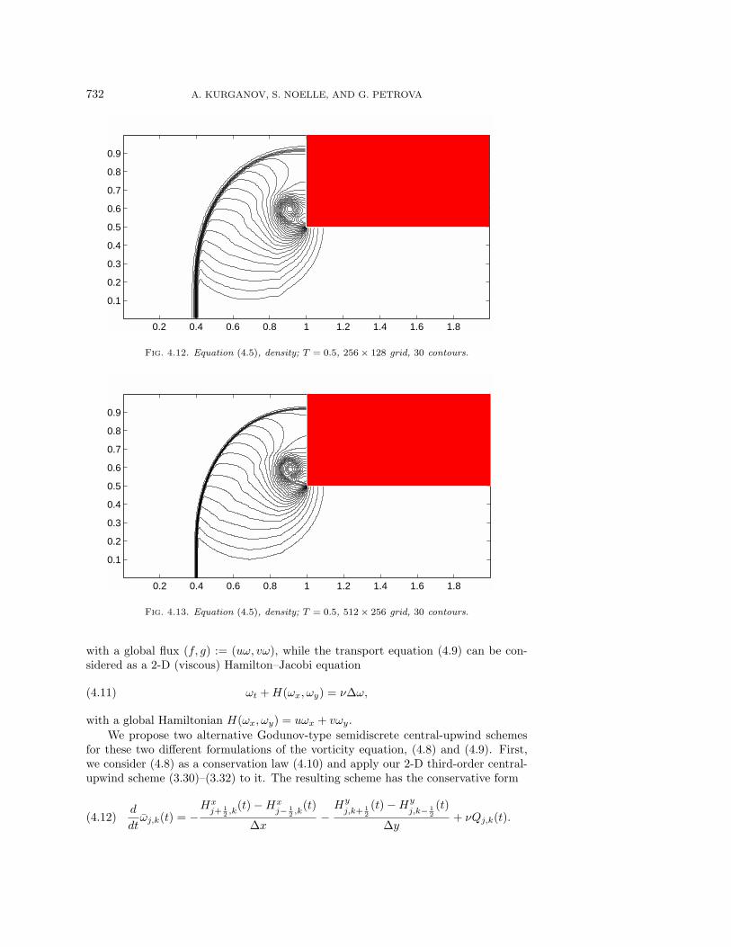
for an ideal gas, γ = 1.4, in the domain [0, 2] × [0, 0.5] ∪ [0, 1] × [0.5, 1], with theinitial data corresponding to a vertical left-moving Mach 1.65 shock, positioned atx = 1.375. The initial shock propagates and then diffracts around a solid corner.Here ρ, u, v, p , and E are the density, the x- and y-velocities, the pressure, and thetotal energy, respectively.

We compute the solution at time T = 0.5, using the scheme (3.30)–(3.32), coupledwith the reconstruction in [25]. The contour plots of the density for 128×64, 256×128,and 512× 256 grid points are given in Figures 4.11, 4.12, and 4.13, respectively.

Note that as in [25], the results are obtained without using characteristic decom-position, dimensional splitting, or evolution of nonconservative quantities.

Example 5. 2-D Hamilton–Jacobi equation. We consider the initial valueproblem for the 2-D eikonal equation of geometric optics, which is a Hamilton–Jacobi

730 A. KURGANOV, S. NOELLE, AND G. PETROVA

-2

0

2

4

6

8

10

12

14

16

0 0.1 0.2 0.3 0.4 0.5 0.6 0.7 0.8 0.9 1

N=1600N=400

Fig. 4.8. Problem (4.2)–(4.3), velocity at T = 0.038.

0

50

100

150

200

250

300

350

400

450

0 0.1 0.2 0.3 0.4 0.5 0.6 0.7 0.8 0.9 1

N=1600N=400

Fig. 4.9. Problem (4.2)–(4.3), pressure at T = 0.038.

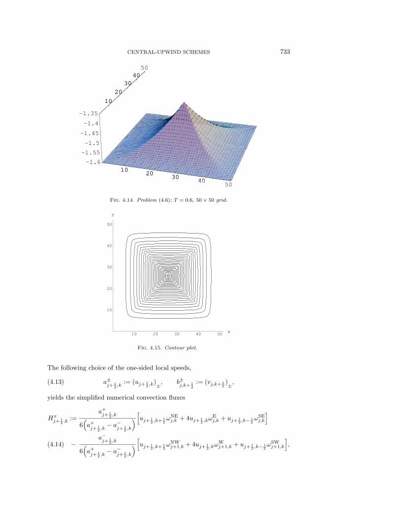
equation with a convex Hamiltonian,

ϕt+√

ϕ2x + ϕ2

y + 1 = 0, ϕ(x, y, 0) =1

4(cos(2πx)−1)(cos(2πy)−1)−1, (x, y) ∈ [0, 1]2.

(4.6)

The numerical solution of (4.6) at time T = 0.6 (after formation of the singularity)has been computed by the 2-D second-order central-upwind scheme (3.49)–(3.50). Thenonoscillatory nature of the computed solution and nearly perfect resolution of thesingularity can be clearly seen in Figures 4.14–4.15.

4.3. 2-D incompressible Euler and Navier–Stokes equations. Here, weconsider the incompressible Euler (ν = 0) and Navier–Stokes (ν > 0) equations

-ut + (-u · ∇)-u+∇p = ν∆-u,(4.7)

CENTRAL-UPWIND SCHEMES 731

-2

-1.9

-1.8

-1.7

-1.6

-1.5

-1.4

-1.3

-1.2

-1.1

-1

-1 -0.8 -0.6 -0.4 -0.2 0 0.2 0.4 0.6 0.8 1

EXACTN=20N=40N=80

Fig. 4.10. Problem (4.4), solution at T = 1.

0.2 0.4 0.6 0.8 1 1.2 1.4 1.6 1.8

0.1

0.2

0.3

0.4

0.5

0.6

0.7

0.8

0.9

Fig. 4.11. Equation (4.5), density; T = 0.5, 128× 64 grid, 30 contours.

where p denotes the pressure and -u = (u, v) is the divergence-free velocity field,satisfying ux + vy = 0. In the 2-D case, equation (4.7) admits an equivalent vorticityformulation, which can be written either in the conservative form,

ωt + (uω)x + (vω)y = ν∆ω,(4.8)

or in the transport form,

ωt + uωx + vωy = ν∆ω,(4.9)

where ω is the vorticity, ω := vx − uy. Equation (4.8) can be viewed as a 2-Dconservation law

ωt + f(ω)x + g(ω)y = ν∆ω,(4.10)

732 A. KURGANOV, S. NOELLE, AND G. PETROVA

0.2 0.4 0.6 0.8 1 1.2 1.4 1.6 1.8

0.1

0.2

0.3

0.4

0.5

0.6

0.7

0.8

0.9

Fig. 4.12. Equation (4.5), density; T = 0.5, 256× 128 grid, 30 contours.

0.2 0.4 0.6 0.8 1 1.2 1.4 1.6 1.8

0.1

0.2

0.3

0.4

0.5

0.6

0.7

0.8

0.9

Fig. 4.13. Equation (4.5), density; T = 0.5, 512× 256 grid, 30 contours.

with a global flux (f, g) := (uω, vω), while the transport equation (4.9) can be con-sidered as a 2-D (viscous) Hamilton–Jacobi equation

ωt +H(ωx, ωy) = ν∆ω,(4.11)

with a global Hamiltonian H(ωx, ωy) = uωx + vωy.

We propose two alternative Godunov-type semidiscrete central-upwind schemesfor these two different formulations of the vorticity equation, (4.8) and (4.9). First,we consider (4.8) as a conservation law (4.10) and apply our 2-D third-order central-upwind scheme (3.30)–(3.32) to it. The resulting scheme has the conservative form

d

dtωj,k(t) = −

Hxj+ 1

2 ,k(t)−Hx

j− 12 ,k

(t)

∆x−

Hy

j,k+ 12

(t)−Hy

j,k− 12

(t)

∆y+ νQj,k(t).(4.12)

CENTRAL-UPWIND SCHEMES 733

1020

3040

50

10

20

3040

50

-1.6

-1.55

-1.5

-1.45

-1.4

-1.35

1020

3040

10

20

3040

Fig. 4.14. Problem (4.6); T = 0.6, 50× 50 grid.

10 20 30 40 50x

10

20

30

40

50

y

Fig. 4.15. Contour plot.

The following choice of the one-sided local speeds,

a±j+ 1

2 ,k:= (uj+ 1

2 ,k)±, b±

j,k+ 12

:= (vj,k+ 12)±,(4.13)

yields the simplified numerical convection fluxes

Hxj+ 1

2 ,k:=

a+j+ 1

2 ,k

6(a+j+ 1

2 ,k− a−

j+ 12 ,k

)[uj+ 12 ,k+ 1

2ωNEj,k + 4uj+ 1

2 ,kωEj,k + uj+ 1

2 ,k− 12ωSEj,k

]

−a−j+ 1

2 ,k

6(a+j+ 1

2 ,k− a−

j+ 12 ,k

)[uj+ 12 ,k+ 1

2ωNWj+1,k + 4uj+ 1

2 ,kωWj+1,k + uj+ 1

2 ,k− 12ωSWj+1,k

],(4.14)

734 A. KURGANOV, S. NOELLE, AND G. PETROVA

and

Hy

j,k+ 12

:=b+j,k+ 1

2

6(b+j,k+ 1

2

− b−j,k+ 1

2

)[vj− 12 ,k+ 1

2ωNWj,k + 4vj,k+ 1

2ωNj,k + vj+ 1

2 ,k+ 12ωNEj,k

]

−b−j,k+ 1

2

6(b+j,k+ 1

2

− b−j,k+ 1

2

)[vj− 12 ,k+ 1

2ωSWj,k+1 + 4vj,k+ 1

2ωSj,k+1 + vj+ 1

2 ,k+ 12ωSEj,k+1

].(4.15)

The diffusion term in (4.12) is obtained by the fourth-order central differencing,

Qj,k =−ωj+2,k + 16ωj+1,k − 30ωj,k + 16ωj−1,k − ωj−2,k

12(∆x)2

+−ωj,k+2 + 16ωj,k+1 − 30ωj,k + 16ωj,k−1 − ωj,k−2

12(∆y)2.(4.16)

The intermediate values of the velocities, required to compute the convection fluxes(4.14) and (4.15), are approximated by the fourth-order averaging, namely,

uj+ 12 ,k

=−uj+2,k + 9uj+1,k + 9uj,k − uj−1,k

16,

vj,k+ 12=

−vj,k+2 + 9vj,k+1 + 9vj,k − vj,k−1

16.(4.17)

The velocities at the grid points, {uj,k, vj,k}, are recovered from the computed vor-ticities {ωj,k} at every time step. This is done with the help of the streamfunction ψ,such that u = ψy, v = −ψx, and ∆ψ = −ω. We solve this Poisson equation by thenine-point Laplacian approximation. Then, having the values of {ψj,k}, we computethe velocities

uj,k =−ψj,k+2 + 8ψj,k+1 − 8ψj,k−1 + ψj,k−2

12∆y,

vj,k =ψj+2,k − 8ψj+1,k + 8ψj−1,k − ψj−2,k

12∆x.(4.18)

This completes the construction of the “conservative” central-upwind scheme for theincompressible Euler and Navier–Stokes equations.

We now apply this scheme, coupled with the reconstruction in [25], to the Navier–Stokes equation (4.8) with ν = 0.05, augmented with the smooth periodic initial data

u(x, y, 0) = − cosx sin y, v(x, y, 0) = sinx cos y.(4.19)

This test problem, proposed in [9], admits the exact classical solution, given by

u(x, y, t) = −e−2νt cosx sin y, v(x, y, t) = e−2νt sinx cos y.

In this numerical experiment, we check the accuracy of our scheme. The numericalsolution is computed at time T = 2, and the errors for the vorticity, measured inthe L∞-, L1-, and L2-norms, are presented in Table 4.2. These results indicate theexpected third-order accuracy of the proposed scheme (4.12)–(4.18).

Next, we apply the scheme (4.12)–(4.18) together with the reconstruction in [25]to the Euler equation, (4.8) with ν = 0, subject to the (2π, 2π)-periodic initial data

u(x, y, 0) =

tanh( 1

ρ (y − π/2)), y ≤ π,

tanh( 1ρ (3π/2− y)), y > π,

v(x, y, 0) = δ · sinx.(4.20)

CENTRAL-UPWIND SCHEMES 735

Table 4.2Accuracy test for the third-order “conservative” scheme for the Navier–Stokes equation (4.8),

(4.19), ν = 0.05; errors at T = 2.

Nx×Ny L∞-error rate L1-error rate L2-error rate32× 32 2.103e-03 – 2.761e-02 – 5.623e-03 –64× 64 2.788e-04 2.92 3.652e-03 2.92 7.404e-04 2.92128× 128 3.548e-05 2.97 4.636e-04 2.98 9.385e-05 2.98256× 256 4.444e-06 3.00 5.811e-05 3.00 1.176e-05 3.00

x

y

20

40

60

20

40

60

-4-202

4

20

40

60(a) (b)

Fig. 4.16. Vorticity—“conservative” scheme, 64× 64.

x

y

50

100

50

100

-4-20

2

4

50

100

(a) (b)

Fig. 4.17. Vorticity—“conservative” scheme, 128× 128.

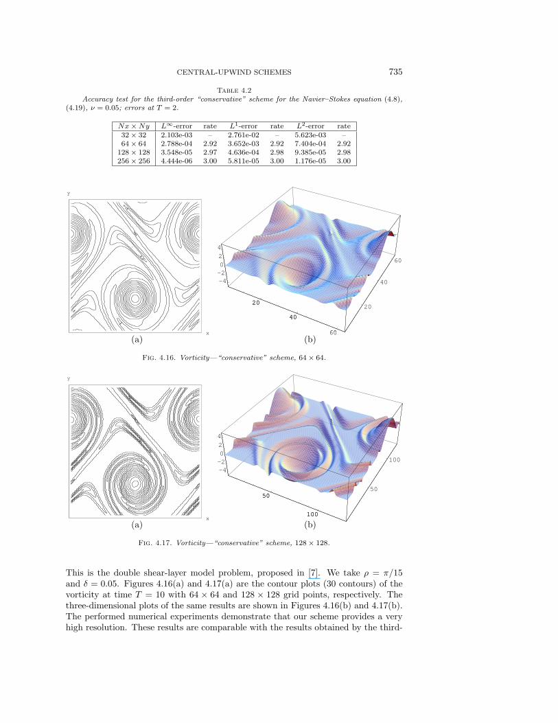
This is the double shear-layer model problem, proposed in [7]. We take ρ = π/15and δ = 0.05. Figures 4.16(a) and 4.17(a) are the contour plots (30 contours) of thevorticity at time T = 10 with 64 × 64 and 128 × 128 grid points, respectively. Thethree-dimensional plots of the same results are shown in Figures 4.16(b) and 4.17(b).The performed numerical experiments demonstrate that our scheme provides a veryhigh resolution. These results are comparable with the results obtained by the third-

736 A. KURGANOV, S. NOELLE, AND G. PETROVA

Table 4.3Accuracy test for the second-order “transport” scheme for the Navier–Stokes equation (4.9),

(4.19), ν = 0.05; errors at T = 2.

Nx×Ny L∞-error rate L1-error rate L2-error rate32× 32 5.559e-03 – 7.304e-02 – 1.492e-02 –64× 64 1.672e-03 1.73 2.265e-02 1.69 4.574e-03 1.71128× 128 4.531e-04 1.88 6.263e-03 1.85 1.250e-03 1.87256× 256 1.176e-04 1.95 1.644e-03 1.93 3.276e-04 1.93

order semidiscrete central scheme in [25].The second alternative is to solve the vorticity equation in its transport form,

(4.9), which can be viewed as a Hamilton–Jacobi equation (4.11).We choose the one-sided local speeds to be

a±j,k := (uj,k)±, b±j,k := (vj,k)±,(4.21)

and in this setting, our 2-D second-order central-upwind scheme (3.49)–(3.50) has thefollowing simple form:

d

dtωj,k(t) = −a−j,kb

−j,k(uj,kω

+x + vj,kω

+y )− a−j,kb

+j,k(uj,kω

+x + vj,kω

−y )

(a+j,k − a−j,k)(b

+j,k − b−j,k)

+a+j,kb

−j,k(uj,kω

−x + vj,kω

+y )− a+

j,kb+j,k(uj,kω

−x + vj,kω

−y )

(a+j,k − a−j,k)(b

+j,k − b−j,k)

+ νLj,k.(4.22)

Here, w±x , w

±y are the right and the left derivatives in the x- and y-directions of the

continuous piecewise polynomial reconstruction of {ωj,k}. The term Lj,k stands forthe standard central difference approximation of the linear viscous term, that is,

Lj,k =ωj+1,k − 2ωj,k + ωj−1,k

(∆x)2 +

ωj,k+1 − 2ωj,k + ωj,k−1

(∆y)2 .(4.23)

As in the “conservative” scheme, we recover the velocities {uj,k, vj,k} from the knownvalues of the vorticity {ωj,k}, using the streamfunction approach. At each time step wesolve the five-points Laplacian ∆ψj,k = −ωj,k and compute the velocities as follows:

uj,k =ψj,k+1 − ψj,k−1

2∆y, vj,k = −ψj+1,k − ψj−1,k

2∆x.(4.24)

We now apply this second-order “transport” scheme to the IBVP for the Navier–Stokes equation (4.9), (4.19) with ν = 0.05. The numerical solution of this testproblem is computed at time T = 2, and the L∞-, L1-, and L2-errors for the vorticityare presented in Table 4.3. These results indicate the second-order convergence ratemeasured in all these norms. We would also like to point out that the absolute valuesof the errors here are about 10 times smaller than the corresponding errors obtainedby the semidiscrete central scheme in [27, Table 6.1].

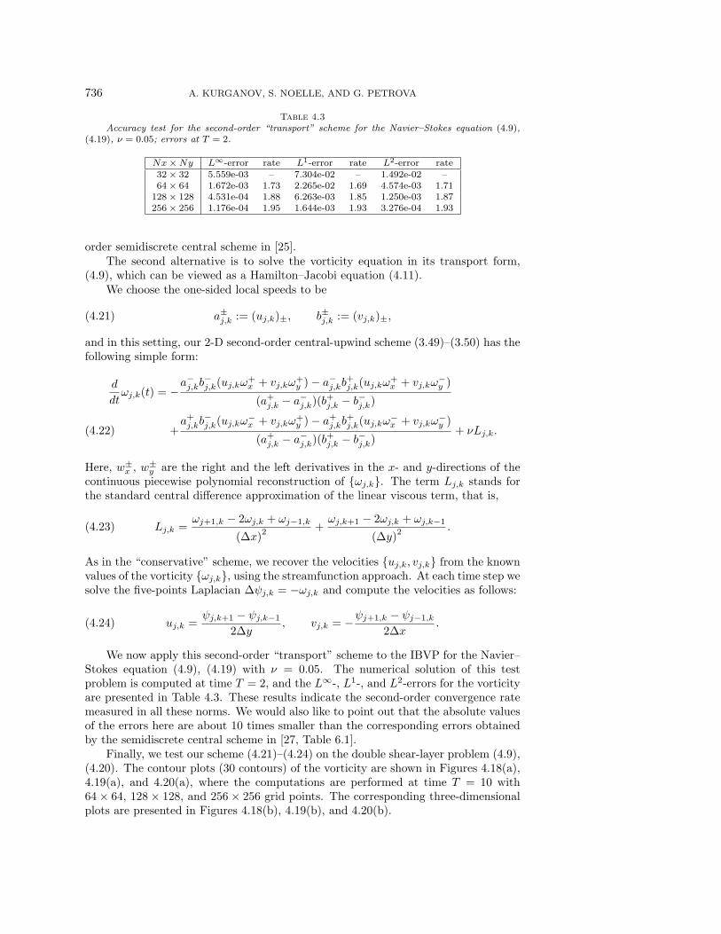
Finally, we test our scheme (4.21)–(4.24) on the double shear-layer problem (4.9),(4.20). The contour plots (30 contours) of the vorticity are shown in Figures 4.18(a),4.19(a), and 4.20(a), where the computations are performed at time T = 10 with64× 64, 128× 128, and 256× 256 grid points. The corresponding three-dimensionalplots are presented in Figures 4.18(b), 4.19(b), and 4.20(b).

CENTRAL-UPWIND SCHEMES 737

x

y

20

40

60

20

40

60

-4-202

4

20

40

60(a) (b)

Fig. 4.18. Vorticity—“transport” scheme, 64× 64.

x

y

50

100

50

100

-4-20

2

4

50

100

(a) (b)

Fig. 4.19. Vorticity—“transport” scheme, 128× 128.

x

y

100

200

100

200

-4-20

2

4

100

200

(a) (b)

Fig. 4.20. Vorticity—“transport” scheme, 256× 256.

738 A. KURGANOV, S. NOELLE, AND G. PETROVA

We would like to point out that our second-order “transport” scheme (4.21)–(4.24) has a very high resolution. The numerical experiments show that it is farsuperior to the second-order semidiscrete central scheme in [27, Figures 6.7–6.10]. Thisimprovement is attributed to the smaller numerical viscosity present in the central-upwind scheme. Moreover, the resolution of (4.21)–(4.24) is almost as good as theresolution of our third-order “conservative” scheme (Figures 4.16 and 4.17).

As in [27, Figures 6.9–6.10], our numerical solution has spurious spikes, but ofsmaller heights. Also, the consequent mesh refinements (Figures 4.18–4.20) clearlydemonstrate that the supports of these spikes diminish as the mesh size decreases.

Concluding remark. We have already mentioned the benefits of using the newcentral-upwind schemes in comparison to the central schemes in [26, 27, 24, 25].Namely, they are less dissipative, and at the same time they retain the major ad-vantages of central schemes—simplicity and efficiency.

In particular, the effect of the reduced numerical dissipation can be clearly seenwhen solving the incompressible Euler equation in its transport form. Moreover, in allof the numerical examples presented above, the achieved resolution is slightly betterthan the resolution obtained in [27, 24, 25].

The only drawback is the fact that the new schemes require the computation ofboth left and right local speeds, which increases the computational costs. However,the increase is not substantial, because as in any central scheme, our central-upwindschemes are Riemann-solver-free and do not require any computationally expensivecharacteristic decomposition.

REFERENCES

[1] R. Abgrall, Numerical discretization of first-order Hamilton-Jacobi equation on triangularmeshes, Comm. Pure Appl. Math., 49 (1996), pp. 1339–1373.

[2] A.M. Anile, V. Romano, and G. Russo, Extended hydrodynamical model of carrier transportin semiconductors, SIAM J. Appl. Math., 61 (2000), pp. 74–101.

[3] P. Arminjon and M.-C. Viallon, Generalisation du schema de Nessyahu-Tadmor pour uneequation hyperbolique a deux dimensions d’espace, C. R. Acad. Sci. Paris Ser. I Math., 320(1995), pp. 85–88.

[4] P. Arminjon, D. Stanescu, and M.-C. Viallon, A two-dimensional finite volume extension ofthe Lax-Friedrichs and Nessyahu-Tadmor schemes for compressible flows, in Proceedingsof the 6th International Symposium on Computational Fluid Dynamics, Vol. 4, Lake Tahoe,CA, M. Hafez and K. Oshima, eds., 1995, pp. 7–14.

[5] P. Arminjon, M.-C. Viallon, and A. Madrane, A finite volume extension of the Lax-Friedrichs and Nessyahu-Tadmor schemes for conservation laws on unstructured grids,Int. J. Comput. Fluid Dyn., 9 (1997), pp. 1–22.

[6] P. Arminjon and M.-C. Viallon, Convergence of a finite volume extension of the Nessyahu–Tadmor scheme on unstructured grids for a two-dimensional linear hyperbolic equation,SIAM J. Numer. Anal., 36 (1999), pp. 738–771.

[7] J.B. Bell, P. Colella, and H.M. Glaz, A second-order projection method for the incom-pressible Navier-Stokes equations, J. Comput. Phys., 85 (1989), pp. 257–283.

[8] F. Bianco, G. Puppo, and G. Russo, High-order central schemes for hyperbolic systems ofconservation laws, SIAM J. Sci. Comput., 21 (1999), pp. 294–322.

[9] A. Chorin, Numerical solution of the Navier-Stokes equations, Math. Comp., 22 (1968), pp.745–762.

[10] L. Corrias, M. Falcone, and R. Natalini, Numerical schemes for conservation laws viaHamilton-Jacobi equations, Math. Comp., 64 (1995), pp. 555–580.

[11] M.G. Crandall and P.-L. Lions, Two approximations of solutions of Hamilton-Jacobi equa-tions, Math. Comp., 43 (1984), pp. 1–19.

[12] B. Einfeldt, On Godunov-type methods for gas dynamics, SIAM J. Numer. Anal., 25 (1988),pp. 294–318.

CENTRAL-UPWIND SCHEMES 739

[13] B. Engquist and O. Runborg, Multi-phase computations in geometrical optics, J. Comput.Appl. Math., 74 (1996), pp. 175–192.

[14] K.O. Friedrichs, Symmetric hyperbolic linear differential equations, Comm. Pure Appl. Math.,7 (1954), pp. 345–392.

[15] A. Harten, High resolution schemes for hyperbolic conservation laws, J. Comput. Phys., 49(1983), pp. 357–393.

[16] A. Harten, B. Engquist, S. Osher, and S.R. Chakravarthy, Uniformly high order accurateessentially non-oscillatory schemes III, J. Comput. Phys., 71 (1987), pp. 231–303.

[17] A. Harten, P.D. Lax, and B. van Leer, On upstream differencing and Godunov-type schemesfor hyperbolic conservation laws, SIAM Rev., 25 (1983), pp. 35–61.

[18] G.-S. Jiang and C.-W. Shu, Efficient implementation of weighted ENO schemes, J. Comput.Phys., 126 (1996), pp. 202–228.

[19] G.-S. Jiang and E. Tadmor, Nonoscillatory central schemes for multidimensional hyperbolicconservation laws, SIAM J. Sci. Comput., 19 (1998), pp. 1892–1917.

[20] R. Kupferman, Simulation of viscoelastic fluids: Couette-Taylor flow, J. Comput. Phys., 147(1998), pp. 22–59.

[21] R. Kupferman, A numerical study of the axisymmetric Couette–Taylor problem using a fasthigh-resolution second-order central scheme, SIAM J. Sci. Comput., 20 (1998), pp. 858–877.

[22] R. Kupferman and E. Tadmor, A fast high-resolution second-order central scheme for in-compressible flows, Proc. Natl. Acad. Sci. USA, 94 (1997), pp. 4848–4852.

[23] A. Kurganov, Conservation Laws: Stability of Numerical Approximations and NonlinearRegularization, Ph.D. Thesis, Tel-Aviv University, Israel, 1997.

[24] A. Kurganov and D. Levy, A third-order semidiscrete central scheme for conservation lawsand convection-diffusion equations, SIAM J. Sci. Comput., 22 (2000), pp. 1461–1488.

[25] A. Kurganov and G. Petrova, A third-order semi-discrete genuinely multidimensional cen-tral scheme for hyperbolic conservation laws and related problems, Numer. Math., to ap-pear.

[26] A. Kurganov and E. Tadmor, New high-resolution central schemes for nonlinear conservationlaws and convection-diffusion equations, J. Comput. Phys., 160 (2000), pp. 241–282.

[27] A. Kurganov and E. Tadmor, New high-resolution semi-discrete central schemes forHamilton-Jacobi equations, J. Comput. Phys., 160 (2000), pp. 720–742.

[28] P.D. Lax, Weak solutions of nonlinear hyperbolic equations and their numerical computation,Comm. Pure Appl. Math., 7 (1954), pp. 159–193.

[29] B. van Leer, Towards the ultimate conservative difference scheme, V. A second order sequelto Godunov’s method, J. Comput. Phys., 32 (1979), pp. 101–136.

[30] D. Levy, G. Puppo, and G. Russo, Central WENO schemes for hyperbolic systems of con-servation laws, M2AN Math. Model. Numer. Anal., 33 (1999), pp. 547–571.

[31] D. Levy, G. Puppo, and G. Russo, A third order central WENO scheme for 2D conservationlaws, Appl. Numer. Math., 33 (2000), pp. 407–414.

[32] D. Levy, G. Puppo, and G. Russo, Compact central WENO schemes for multidimensionalconservation laws, SIAM J. Sci. Comput., 22 (2000), pp. 656–672.

[33] D. Levy and E. Tadmor, Non-oscillatory central schemes for the incompressible 2-D Eulerequations, Math. Res. Lett., 4 (1997), pp. 1–20.

[34] K.-A. Lie and S. Noelle, Remarks on High-Resolution Non-Oscillatory Central Schemes forMulti-Dimensional Systems of Conservation Laws. Part I: An Improved Quadrature Rulefor the Flux-Computation, SFB256 preprint 679, Bonn University, Germany.

[35] C.-T. Lin and E. Tadmor, L1-stability and error estimates for approximate Hamilton-Jacobisolutions, Numer. Math., 87 (2001), pp. 701–735.

[36] C.-T. Lin and E. Tadmor, High-resolution nonoscillatory central schemes for Hamilton–Jacobi equations, SIAM J. Sci. Comput., 21 (2000), pp. 2163–2186.

[37] X.-D. Liu and S. Osher, Nonoscillatory high order accurate self-similar maximum principlesatisfying shock capturing schemes. I, SIAM J. Numer. Anal., 33 (1996), pp. 760–779.

[38] X.-D. Liu, S. Osher, and T. Chan,Weighted essentially non-oscillatory schemes, J. Comput.Phys., 115 (1994), pp. 200–212.

[39] X.-D. Liu and E. Tadmor, Third order nonoscillatory central scheme for hyperbolic conser-vation laws, Numer. Math., 79 (1998), pp. 397–425.

[40] H. Nessyahu and E. Tadmor, Non-oscillatory central differencing for hyperbolic conservationlaws, J. Comput. Phys., 87 (1990), pp. 408–463.

[41] S. Noelle, A comparison of third and second order accurate finite volume schemes for thetwo-dimensional compressible Euler equations, in Proceedings of the Seventh Interna-tional Conference on Hyperbolic Problems, Zurich, 1998, Internat. Ser. Numer. Math.

740 A. KURGANOV, S. NOELLE, AND G. PETROVA

129, Birkhauser, Basel, pp. 757–766.[42] S. Osher and C.-W. Shu, High-order essentially nonoscillatory schemes for Hamilton-Jacobi

equations, SIAM J. Numer. Anal., 28 (1991), pp. 907–922.[43] S. Osher and E. Tadmor, On the convergence of difference approximations to scalar conser-

vation laws, Math. Comp., 50 (1988), pp. 19–51.[44] V. Romano and G. Russo, Numerical solution for hydrodynamical models of semiconductors,

Math. Models Methods Appl. Sci., 10 (2000), pp. 1099–1120.[45] C.-W. Shu, Total-variation-diminishing time discretizations, SIAM J. Sci. Statist. Comput., 9

(1988), pp. 1073–1084.[46] C.-W. Shu, Numerical experiments on the accuracy of ENO and modified ENO schemes, J.

Sci. Comput., 5 (1990), pp. 127–149.[47] C.-W. Shu and S. Osher, Efficient implementation of essentially non-oscillatory shock-

capturing schemes, J. Comput. Phys., 77 (1988), pp. 439–471.[48] P.E. Souganidis, Approximation schemes for viscosity solutions of Hamilton-Jacobi equations,

J. Differential Equations., 59 (1985), pp. 1–43.[49] Y.C. Tai, S. Noelle, N. Gray, and K. Hutter, Shock Capturing and Front Tracking Methods

for Granular Avalanches, SFB256 Preprint 678, Bonn University, Germany; J. Comput.Phys., to appear.

[50] B. Wendroff, Approximate Riemann solvers, Godunov schemes, and contact discontinuities,in Godunov Methods: Theory and Applications, E. F. Toro, ed., Kluwer Academic/PlenumPublishers, New York, to appear.

[51] P. Woodward and P. Colella, The numerical solution of two-dimensional fluid flow withstrong shocks, J. Comput. Phys., 54 (1988), pp. 115–173.