CAT(0) and CAT(-1) fillings of hyperbolic manifolds

arX

iv:0

901.

0056

v1 [

mat

h.G

T]

31

Dec

200

8

CAT(0) AND CAT(−1) FILLINGS OF HYPERBOLIC MANIFOLDS

KOJI FUJIWARA AND JASON FOX MANNING

Abstract. We give new examples of hyperbolic and relatively hyperbolicgroups of cohomological dimension d for all d ≥ 4 (see Theorem 2.13). Theseexamples result from applying CAT(0)/CAT(−1) filling constructions (basedon singular doubly warped products) to finite volume hyperbolic manifoldswith toral cusps.

The groups obtained have a number of interesting properties, which are es-tablished by analyzing their boundaries at infinity by a kind of Morse-theoretictechnique, related to but distinct from ordinary and combinatorial Morse the-ory (see Section 5).

Contents

1. Introduction 21.1. Outline 31.2. Acknowledgments 32. Statements of results 32.1. Cones and fillings 32.2. Main results 53. Preliminaries 73.1. Warped products 73.2. The space of directions and the tangent cone 93.3. Locally injective logarithms 104. The metric construction and proof of Theorem 2.7 114.1. A model for the singular part 114.2. Curvatures in Riemannian warped products 154.3. Gluing functions 154.4. Nonpositively curved metrics on the partial cones 184.5. Proof of Theorem 2.7 and Proposition 2.8 204.6. Isolated flats 215. Visual boundaries of fillings 225.1. The boundary as an inverse limit 225.2. Simple connectivity at infinity 306. Further questions 31References 32

December 31, 2008.

1

http://arXiv.org/abs/0901.0056v1

2 K. FUJIWARA AND J. F. MANNING

1. Introduction

In this paper we study some generalizations of the Gromov-Thurston 2π theorem[12]. Informally, the 2π theorem states that “most” Dehn fillings of a hyperbolic3–manifold with cusps admit negatively curved metrics. Moreover, these negativelycurved metrics are close approximations of the metric on the original cusped man-ifold. Group-theoretically, the fundamental groups of these fillings are relativelyhyperbolic (defined below). If all cusps of the original manifold were filled, thefundamental group of the filling is hyperbolic; if moreover the original manifoldwas finite volume, the filling is an aspherical closed 3–manifold.

In the world of coarse geometry, the correct generalizations of fundamentalgroups of hyperbolic manifolds with and without cusps are relatively hyperbolic andhyperbolic groups, respectively. These generalizations were introduced by Gromovin [21]. We give a quick review of the definitions: A metric space is δ–hyperbolicfor δ > 0 if all its geodesic triangles are δ–thin, meaning each side of the triangle iscontained in the δ–neighborhood of the other two. A space is Gromov hyperbolic ifit is δ–hyperbolic for some δ. Groups which are hyperbolic or relatively hyperbolicare those which have particular kinds of actions on Gromov hyperbolic spaces. IfG acts by isometries on a Gromov hyperbolic space X properly and cocompactly,then G is said to be hyperbolic. A geometrically finite action of a group G on aGromov hyperbolic space X is one which satisfies the following conditions:

(1) G acts properly and by isometries on X .(2) There is a family H of disjoint horoballs (sub-level sets of so-called horo-

functions), preserved by the action.(3) The action on X \

⋃

H is cocompact.(4) The quotient X/G is quasi-isometric to a wedge of rays.

(See [21] for more details.) If G acts onX geometrically finitely, then G is said to berelatively hyperbolic, relative to the peripheral subgroups, which are the stabilizersof individual horoballs. (Typically the list of peripheral subgroups is given bychoosing one such stabilizer from each conjugacy class.)

In [24] and [37], group-theoretic analogues of the 2π theorem were proved. Thesetheorems roughly state that if one begins with a relatively hyperbolic group, andkills off normal subgroups of the peripheral subgroups which contain no “short”elements, then the resulting group is also relatively hyperbolic, and “close” to theoriginal group in various ways. From this one recovers a weaker group-theoreticversion of the 2π theorem, as the fundamental group of a hyperbolic 3–manifoldis relatively hyperbolic, relative to the cusp groups; the operation of Dehn fillingacts on fundamental groups by killing the cyclic subgroups generated by the fillingslopes.

In the context of the original 2π theorem, we begin with a group which has suchan action on H

3, which is not only δ–hyperbolic, but which is actually CAT(−1).(See Section 3 for the definition of CAT(κ) for κ ∈ R. For now, just note thatCAT(−1) implies Gromov hyperbolic.) Moreover, the group acts cocompactly ona “neutered” H

3, which is CAT(0) with isolated flats. The fundamental group ofthe filled manifold acts properly and cocompactly on a CAT(−1) 3–manifold.

For κ ≤ 0, we say that a group is CAT(κ) if it acts isometrically, properly, andcocompactly on some CAT(κ) space. We will say that a group is relatively CAT(−1)if it has a geometrically finite action on a CAT(−1) space. A group is CAT(0) with

CAT(0) AND CAT(−1) FILLINGS OF HYPERBOLIC MANIFOLDS 3

isolated flats if it acts isometrically, properly, and cocompactly on some CAT(0)space with isolated flats. (It follows from a result of Hruska and Kleiner [26] thathoroballs can always be added to such a space to make it δ–hyperbolic for some δ.In particular, a group which is CAT(0) with isolated flats is relatively hyperbolic.)It is natural to wonder to what extent the main results of [24] and [37] can bestrengthened in the presence of these stronger conditions.

Question 1.1. If one performs relatively hyperbolic Dehn filling on a relativelyCAT(−1) group, is the filled group always relatively CAT(−1)?

Question 1.2. If one performs relatively hyperbolic Dehn filling on a CAT(0) withisolated flats group, is the filled group always CAT(0) with isolated flats?

These questions form a part of the motivation for this paper; we answer thempositively in some special cases. The utility of these answers is illustrated by usingthe additional CAT(0) structure of the quotient groups to obtain information aboutthe filled groups which is less accessible from the coarse geometric viewpoint.

1.1. Outline. In Section 2, we describe the main results. In Section 3, we re-call the definition of warped product metric and an important result of Alexanderand Bishop. We also discuss the space of directions and the logarithm map froma CAT(0) space to the tangent cone at a point. In Section 4, we extend origi-nal construction of the 2π theorem to our setting, using doubly warped productconstructions to give locally CAT(0) and locally CAT(−1) models for our fillings.Section 5 contains the “Morse theoretic” arguments which give information aboutthe boundary at infinity of the fundamental groups of our fillings. In Section 6, wepose some questions.

1.2. Acknowledgments. Fujiwara started working on this project during his visitat Max Planck Institute in Bonn in the fall of 2005. He has benefited from con-versation with Potyagailo. The joint project with Manning started when he visitedCaltech in April 2006. He thanks both institutions for their hospitality. He ispartially supported by Grant-in-Aid for Scientific Research (No. 19340013).

Manning thanks Ric Ancel for explaining how to prove Claim 5.22 in the proofof Proposition 5.20, and thanks Noel Brady and Daniel Groves for useful conversa-tions. He was partially supported by NSF grants DMS-0301954 and DMS-0804369.

2. Statements of results

2.1. Cones and fillings. We first establish some notation:

Definition 2.1 (Partial cone). Let N be a flat torus of dimension n, and let T bea totally geodesic k–dimensional submanifold in N , where 1 ≤ k ≤ n. The torus Nhas Euclidean universal cover E

n → N ; let T ∼= Ek be a component of the preimage

of T in N . The parallel copies of T are the leaves of a fibration En π−→ E

n−k. Thisfibration covers a fibration

Nπ−→ B

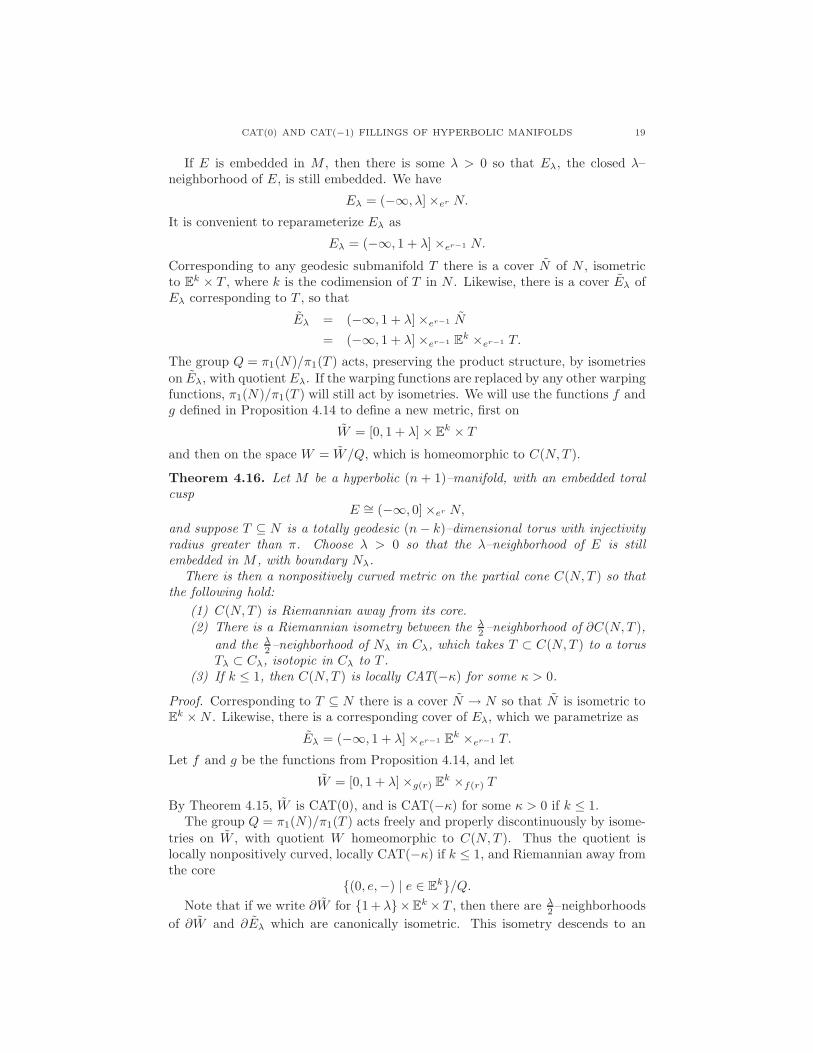
of N over some (n − k)–torus B. We define the partial cone C(N,T ) to be themapping cylinder of π, i.e.

C(N,T ) = N × [0, 1]/ ∼,

where (t1, 1) ∼ (t2, 1) if π(t1) = π(t2).


We refer to N × 0 as the boundary of C(N,T ), and to V (N,T ) := N × 1/ ∼ asthe core.

V (N,T )

C(N,T )

N

TC(T )

Figure 1. cone C(N,T )

Remark 2.2. The space C(N,N) is the cone on N . In the case that N is a metricproduct N = T × B, then C(N,T ) can be canonically identified with C(T ) ×B. (Although the identification is not canonical in general, C(N,T ) is alwayshomeomorphic to C(T )×B for some torus B of complementary dimension to that ofT . In particular, the core V (N,T ) is always homeomorphic to a torus of dimensiondim(N) − dim(T ).) The partial cone C(N,T ) is a manifold with boundary onlywhen dim(T ) = 1.

Definition 2.3. Let M be a hyperbolic (n+ 1)–manifold. A toral cusp of M is aneighborhood E of an end of M so that

(1) E is homeomorphic to the product of a torus with the interval (−∞, 0], and(2) the induced Riemannian metric on ∂E is flat.

For the rest of the section we make the following:

Standing assumption 2.4. M is a hyperbolic (n+ 1)–manifold of finite volumecontaining disjoint toral cusps E1, . . . , Em, and no other ends.

Let M ⊂M be the manifold with boundary obtained by removing the interiorsof the cusps. Let N1, . . . , Nm be the components of ∂M .

Definition 2.5 (Filling, 2π–filling). For each component Ni of ∂M choose anembedded totally geodesic torus Ti of dimension ki. Form C(Ni, Ti) as in theprevious definition. We use the canonical identification φi of ∂C(Ni, Ti) with Ni toform the space

M(T1, . . . , Tm) := M⋃

φ1⊔···⊔φm

(C(N1, T1) ⊔ · · · ⊔ C(Nm, Tm)).

We say that M(T1, . . . , Tm) is obtained from M by filling along T1, . . . , Tm. Werefer to the cores of the C(Ni, Ti) as the filling cores.

If no Ti contains a geodesic of length 2π or less, we say that M(T1, . . . , Tm) is a2π–filling of M .


Remark 2.6. The space M(T1, . . . , Tm) described above is homeomorphic to amanifold if and only if every filling core has dimension exactly n− 1. In any caseM(T1, . . . , Tm) is a pseudomanifold of dimension (n + 1), and the complement ofthe filling cores is homeomorphic to M .

On the level of fundamental groups, π1(M(T1, . . . , Tm)) is obtained from π1(M)by adjoining relations representing the generators of some direct summands of thecusp subgroups; namely, for each i ∈ 1, . . . ,m, one adjoins relations correspond-ing to the generators of π1(Ti) ⊳ π1(Ei) = π1(Ni).

2.2. Main results. Our main theorem says that under hypotheses exactly analo-gous to those used in the 2π theorem, a space obtained by filling as above can begiven a nice locally CAT(0) metric; moreover, if all the filling cores are zero or onedimensional, the metric can be chosen to be locally CAT(−1). We remind the readerthat, under the condition 2.4, M is assumed to be a hyperbolic (n + 1)–manifoldwith only toral cusps.

Theorem 2.7. Let n ≥ 2 and assume the condition 2.4.If M(T1, . . . , Tm) is a 2π–filling of M , then there is a complete path metric d on

M(T1, . . . , Tm) satisfying the following:

(1) The path metric d is the completion of a path metric induced by a negativelycurved Riemannian metric on the complement of the filling cores.

(2) The path metric d is locally CAT(0).(3) If for every i, Ti has codimension at most 1 in ∂Ei, then d is locally

CAT(−κ) for some κ > 0.

The metric constructed in Theorem 2.7 is identical to the original hyperbolicmetric, away from a neighborhood of the filling cores. We will prove the followingin the course of showing Theorem 2.7.

Proposition 2.8. Let n ≥ 2 and assume the condition 2.4, and let M(T1, . . . , Tm)be a 2π–filling of M . Let

M = M \m⋃

i=1

Ei

be as described in Definition 2.5. Choose λ > 0 so that the λ–neighborhood of⋃mi=1Ei is embedded in M . Let M

′be the complement in M of the λ

2 –neighborhood

of⋃mi=1Ei. We thus have inclusions M

′⊂M ⊂M , and M

′⊂M ⊂M(T1, . . . , Tm).

The Riemannian metric described in Theorem 2.7 is equal to the hyperbolic met-

ric, when restricted to M′.

Remark 2.9. Let G = π1(M(T1, . . . , Tm)) be the fundamental group of some 2π–filling of M . It follows from Theorem 2.7 that Hn+1(G) ∼= Hn+1(M(T1, . . . , Tm)) iscyclic. One can ask what the Gromov norm of a generator is, and define this numberto be the simplicial volume of M(T1, . . . , Tm) (or of G). In case M(T1, . . . , Tm) isa manifold, this definition is the same as Gromov’s in [20]. In the setting of theoriginal 2π theorem, both M and M(T1, . . . , Tm) are hyperbolic manifolds, and itwas shown by Thurston that the simplicial volume of M(T1, . . . , Tm) is boundedabove by the hyperbolic volume of M , divided by a constant [39]. We extendThurston’s result to higher dimensions in [19].

Remark 2.10. Special cases of Theorem 2.7 appear in


• the Gromov-Thurston 2π–theorem [12], in which n = 2 and each filling coreis a circle,• Schroeder’s generalization of the 2π theorem to n > 2, with filling cores

equal to (n− 1)–dimensional tori [38] (This is the case in which every Ti isone-dimensional, and the only case in which the filling M(T1, . . . , Tm) is amanifold.), and• Mosher and Sageev’s construction in [35] of (n+1)–dimensional hyperbolic

groups which are not aspherical manifold groups; here the filling cores arepoints.

The construction of Mosher and Sageev is based on a discussion in [22, 7.A.VI],and the examples constructed by Mosher and Sageev answered a question whichappeared in an early version of Bestvina’s problem list [9]. The new examplesof the current paper fall in some sense between those of Schroeder, and those ofMosher-Sageev.

Our construction gives the following corollary, which can be deduced from The-orem 2.7 and Proposition 4.21.

Corollary 2.11. Let n ≥ 2 and assume the condition 2.4.Let M(T1, . . . , Tm) be a 2π–filling of M , and let G be the fundamental group of

M(T1, . . . , Tm). Then G is CAT(0) with isolated flats. If each Ti has dimension nor n− 1, then G is CAT(−1).

Thus Theorem 2.7 says that given a cusped hyperbolic (n + 1)–manifold withn ≥ 2, there are many ways to fill its cusps to get a space whose universal cover isCAT(−κ) for κ > 0. If n ≥ 3, there are many ways to fill its cusps to get a spacewhose universal cover is CAT(0) with isolated flats. The following proposition saysthat different fillings generally have different fundamental groups:

Proposition 2.12. Let n ≥ 2 and assume the condition 2.4.For each i ∈ N choose a filling Mi = M(T i1, . . . , T

im) of M , and suppose that the

fillings Mi satisfy: For each 1 ≤ j ≤ m and each element γ of π1(Ej) \ 1, the seti | γ ∈ π1(T

ij ) is finite. Then for any k, there are only finitely many i ∈ N so

that π1(Mi) ∼= π1(Mk).

Proof. We argue by contradiction. The hypotheses imply that all but finitely manyfillings Mi are 2π–fillings. By passing to a subsequence we may suppose that allthe π1(Mi) are isomorphic to some fixed G. Applying Corollary 2.11 and [26,Theorem 1.2.1], G is relatively hyperbolic with respect to a collection of free abeliansubgroups. If Γ = π1(M) we have a sequence of surjections

Γφi−→ G

obtained by killing subgroups Kij of the peripheral subgroups of Γ corresponding to

the tori T ij . Since the injectivity radii of these tori are going to infinity, the length

(with respect to a fixed generating set for Γ) of a shortest nontrivial element of∪jKi

j is also going to infinity. It follows from Corollary 9.7 of [24] that the stablekernel

ker−→φi = γ ∈ Γ | φi(γ) = 1 for almost all φi

is trivial. Work of Groves then shows that Γ is either abelian or splits over anabelian group [23, Proposition 2.11]. But Γ is the fundamental group of a finite


volume hyperbolic manifold of dimension at least 3, so it cannot split over a virtuallyabelian subgroup (see, e.g. [6, Theorem 1.3.(i)]).

We will show (Corollary 5.24) that no 2π–filling of an (n+1)–dimensional hyper-bolic manifold with filling cores of dimension < n has the same fundamental groupas a closed hyperbolic manifold (or even a closed aspherical manifold) for n ≥ 3.This is in sharp contrast to the situation for hyperbolic 3–manifolds. CombiningCorollary 5.24 and Proposition 2.12 immediately yields the following:

Theorem 2.13. Let n ≥ 3 and assume the condition 2.4. There are infinitely many2π–fillings of M whose fundamental groups are non-pairwise-isomorphic, torsion-free, (n + 1)–dimensional hyperbolic groups, each of which acts geometrically onsome (n+1)–dimensional CAT(−1) space, and none of which is a closed asphericalmanifold group.

If n ≥ 4, there are infinitely many 2π–fillings of M whose fundamental groupsare non-pairwise-isomorphic, torsion-free, (n+1)–dimensional relatively hyperbolicgroups, each of which acts geometrically on some (n+1)–dimensional CAT(0) spacewith isolated flats, and none of which is a closed aspherical manifold group. Flatsof any dimension up to (n− 2) occur in infinitely many such fillings.

In [30], Januszkiewicz and Swiatkowski introduce systolic groups, in part as ameans of giving examples of non-manifold n–dimensional hyperbolic groups for alln (see [15, 29] for other approaches). Recently, Osajda has shown that systolicgroups are never simply connected at infinity [36]. It follows from our analysisof the group boundary in Section 5 that the high-dimensional groups obtained inTheorem 2.13 are simply connected at infinity whenever no filling cores are points.In particular, these groups are not systolic (Corollary 5.27).

3. Preliminaries

For general results and terminology for CAT(κ) spaces we refer to Bridson andHaefliger [13]. For convenience, we remind the reader of the definition. Let κ ∈ R,and let Sκ be the complete simply connected surface of constant curvature κ. LetRκ ≤ ∞ be the diameter of Sκ. Now let X be a length space. (See [13, 14] formore on length spaces.) If ∆ ⊂ X is a geodesic triangle in X whose perimeter isbounded above by 2Rκ, with corners x, y, and z, then there is a comparison triangle∆ ⊂ Sκ; i.e., the corners of ∆ can be labelled x, y, and z, and there is a map from∆ to ∆ which is an isometry restricted to any edge of ∆, taking x to x, and soon (See Figure 3). If this map never decreases distance on any triangle ∆ whoseperimeter is bounded above by 2Rκ, we say that X is CAT(κ). Put informally,X is CAT(κ) if its triangles are “no fatter” than the comparison triangles in Sκ.If every point in X has a neighborhood which is CAT(κ), then we say that X islocally CAT(κ). If X is locally CAT(0), then we say that X is nonpositively curved.For κ ≤ 0, the universal cover of a complete, locally CAT(κ) space is CAT(κ), bythe Cartan-Hadamard Theorem.

3.1. Warped products. We take this definition from [14, 3.6.4].

Definition 3.1. Given two complete length spaces (X, dX) and (Y, dY ), and acontinuous nonnegative f : X → [0,∞), we can define the warped product of Xwith Y , with warping function f to be the length space based on the followingmethod of measuring lengths of paths. Given any closed interval [a, b] and any


xy

z

x

y

z∆ ⊂ X ∆ ⊂ Sk

Figure 2. Comparison for CAT(k).

lipschitz path γ : I → X × Y , with γ(t) = (γ1(t), γ2(t)), the quantities |γ′1(t)| and|γ′2(t)| are well defined almost everywhere on I (see [14, 2.7.6]). Define the lengthof γ, l(γ) to be

l(γ) =

∫ b

a

√

|γ′1(t)|2 + f2(γ1(t))|γ′2(t)|

2dt.

The quotient map X × Y → X ×f Y is injective exactly when f has no zeroes.If f(x) = 0 then x × Y is identified to a point in X ×f Y .

Often we will have X ⊆ R, or X = I ×g Z for I ⊆ R, and f depending only onr ∈ I. In this case, we will usually write X ×f Y as X ×f(r) Y . For example:

• The euclidean plane is isometric to [0,∞)×r S1. The subset R× S1 is acircle of radius R.• The hyperbolic space H

n+1 is isometric to R×er En. The subset R×E

n

is a horosphere.

We will often abuse notation by using points in X × Y to refer to points inX ×f Y , even when the quotient map is not injective. For example the cone pointof the Euclidean cone [0,∞) ×r X might be referred to as (0, x) for some x ∈ X ,or just as (0,−).

In case the metrics dX and dY are induced by Riemannian metrics gX and gYand f : X → R>0 is smooth, the warped product metric on X ×f Y is equal tothe path metric induced by a Riemannian metric g, given at a point (x, y) by theformula

g = gX + f2(x)gY .

Curvature bounds on warped product spaces are studied by Alexander andBishop in [4], where quite general sufficient conditions are given for a warped prod-uct to have curvature bounded from above or below. In order to state the resultsfrom [4] which we need, we first recall some definitions.

Definition 3.2. Let K ∈ R. Let FK be the set of solutions to the differentialequation g′′ + Kg = 0. A function f satisfying f ≤ g for any function g in FKagreeing with f at two points which are sufficiently close together is said to satisfythe differential inequality f ′′ +Kf ≥ 0 in the barrier sense.

Definition 3.3. Let K ∈ R, and let B be a geodesic space. A continuous functionf : B → R is FK–convex if its composition with any unit-speed geodesic satisfiesthe differential inequality f ′′ +Kf ≥ 0 in the barrier sense.

We collect here some useful facts about FK–convexity:


Useful facts 3.4.

(1) A function is F0–convex if and only if it is convex in the usual sense.(2) A non-negative FK–convex function is also FK ′–convex for any K ′ ≥ K.(3) [3, Theorem 1.1(1A)] If B is CAT(−1) and x ∈ B, then cosh(d(·, x)) is aF(−1)–convex function on B.

(4) [3, Theorem 1.1(3A)] If A is a convex subset of a CAT(0) space B, thend(·, A) is a convex function on B.

(5) [3, Theorem 1.1(4A)] If A is a convex subset of a CAT(−1) space B, thensinh(d(·, A)) is a F(−1)–convex function on B.

We now state a special case of a more general result in [4].

Theorem 3.5. [4, Theorem 1.1] Let K ≤ 0, and let KF ∈ R. Let B and F becomplete locally compact CAT(K) and CAT(KF ) spaces, respectively. Let f : B →[0,∞) be FK–convex. Let X = f−1(0).

Suppose further that either

(1) X = ∅ and KF ≤ K(inf f)2, or(2) X is nonempty and (f σ)′(0+)2 ≥ KF whenever σ : [0, x] → B is a

shortest (among all paths starting in X) unit-speed geodesic from X to apoint b ∈ B rX.

Then the warped product B ×f F is CAT(K).

3.2. The space of directions and the tangent cone. Suppose that X is alength space, and p ∈ X . Recall that the space of directions at p is the collection ofgeodesic segments issuing from p, modulo the equivalence relation: [p, x] ∼ [p, y] ifthe Alexandroff angle between [p, x] and [p, y] at p is zero. The Alexandroff angle atp makes the space of directions, Σp(X), into a metric space. If X is a Riemannianmanifold, then Σp(X) is always a round sphere of diameter π. The tangent cone atp is the Euclidean cone on the space of directions at p:

Cp(X) ∼= [0,∞)×r Σp(X)

We will sometimes just write Σp and Cp if the space X is understood. If X is aRiemannian manifold near the point p, then the tangent cone Cp can be canonicallyidentified with the tangent space of X at p.

In our setting X will always be geodesically complete and locally compact. Withthese assumptions, if U is any open neighborhood of p ∈ X , then Cp(X) is isometricto the pointed Gromov-Hausdorff limit of spaces Un isometric to U with the metricmultiplied by factors Rn going to infinity (see for example [14, Theorem 9.1.48]).

Alexander and Bishop [4, page 1147] observe that the space of directions at apoint in a warped product is determined by the spaces of directions in the factorstogether with infinitesimal information about the warping functions. If f : B → R isa convex function and p ∈ R, then f has a well-defined “derivative” Dfp : Cp(B)→R at the point p; this derivative is linear on each ray.

Definition 3.6 (spherical join, cf. [13, I.5]). Let A and B be metric spaces. Wemay give the product [0, π2 ]×A×B a pseudometric as follows. Let x1 = (φ1, a1, b1)and x2 = (φ2, a2, b2). The distance d(x1, x2) is given by

cos (d(x1, x2)) = cos(φ1) cos(φ2) cos (dπ(a1, a2))

+ sin(φ1) sin(φ2) cos (dπ(b1, b2)) ,


where dπ(p1, p2) means minπ, d(p1, p2). The spherical join A ∗ B of A and B isthe canonical metric space quotient of [0, π2 ]×A×B with the above metric. Pointsin A ∗ B can be written as triples (φ, a, b) with φ ∈ [0, π2 ], a ∈ A and b ∈ B. Ifφ = 0, the third coordinate can be ignored, and if φ = π

2 , the second coordinatecan be ignored.

Proposition 3.7. [4] Let B, F , and f be as in Theorem 3.5. Let p ∈ B, and letφ ∈ F . If f(p) > 0, then there are isometries

C(p,φ)(B ×f F ) ∼= Cp(B) × Cφ(F )

and

Σ(p,φ)(B ×f F ) ∼= Σp(B) ∗ Σφ(F ).

If f(p) = 0, there are isometries

C(p,φ)(B ×f F ) ∼= Cp(B)×DfpF

and

Σ(p,φ)(B ×f F ) ∼= Σp(B)×DfpF.

3.3. Locally injective logarithms. Let X be a uniquely geodesic metric spaceand let p ∈ X . In general, there is no exponential map defined on the entire tangentcone Cp. However, there is a well-defined logarithm map from X to Cp [31].

Definition 3.8. Let X be a uniquely geodesic metric space, and let Cp = [0,∞)×rΣp be the tangent cone at a point p ∈ X . If x ∈ X , then logp(x) is the equivalenceclass of (d(x, p), [p, x]) in Cp.

If the metric is only locally uniquely geodesic, then the logarithm map can stillbe defined in a neighborhood of each point. The existence of a local exponentialmap is limited by the extent to which the logarithm is injective and surjective.

Definition 3.9. The log-injectivity radius at p, loginj(p), is be the supremum ofthose numbers r for which logp is well-defined and injective on the ball of radiusr about p. A neighborhood of p on which logp is injective is called a log-injectiveneighborhood of p.

Similarly, the log-surjectivity radius at p, logsurj(p), is the supremum of thosenumbers r for which [0, r]×r Σp ⊂ Cp is contained in the image of logp.

In general, neither loginj(p) nor logsurj(p) is positive. Recall that a space hasthe geodesic extension property if any locally geodesic segment terminating at y canbe extended to a longer locally geodesic segment terminating at some y′ 6= y. Acomplete CAT(0) space satisfying the geodesic extension property has logsurj(p) =∞.

Observation 3.10. If R = minlogsurj(p), loginj(p), then there is an exponentialmap

expp : [0, R)×r Σp → X

which is a homeomorphism onto the open R–neighborhood of p. More generallythere is always an exponential map

expp : logp(U)→ U ⊂ X

for any log-injective neighborhood U of p, and this map is a homeomorphism ontoits image.


Definition 3.11. A subset V of a uniquely geodesic space is convex if for anytwo points in V , the geodesic connecting them is contained in V . The subset V isstrictly convex if it is convex and if the frontier of V contains no non-degenerategeodesic segment.

Lemma 3.12. Let X be a proper uniquely geodesic space satisfying the geodesicextension property. Suppose that C is a compact strictly convex set in X containingp in its interior, and suppose that C is contained in a log-injective neighborhood ofp. It follows that the frontier of C is homeomorphic to Σp.

Proof. Since under the hypotheses both the space of directions Σp and the frontierof C (which we denote here by ∂C) are compact Hausdorff spaces, it suffices to finda continuous bijection from one to the other.

Let h : ∂C → Σp be the map which sends a point x to the equivalence class of[x, p]. Since p /∈ ∂C, this map is well-defined. Since X is a proper uniquely geodesicspace, geodesic segments vary continuously with their endpoints [13, I.3.13]. Itfollows that the map h is continuous.

We next show that h is surjective. Let θ ∈ Σp, and choose a geodesic segmentbeginning at p with direction θ. Since X satisfies the geodesic extension property,this geodesic segment can be extended to a point x not in C. Some point on thegeodesic [p, x] must be in the frontier of C, and so θ is in the image of C.

Finally we show that h is injective. Choose θ ∈ Σp, and suppose that h(x) =h(y) = θ for some x, y in ∂C. Without loss of generality, suppose that d(x, p) ≤d(y, p). Since C is strictly convex, the geodesic from x to y must be contained inC but cannot be contained entirely in ∂C. Thus there is some point z ∈ [x, y] sothat z is in the interior of C. By the hypotheses and Observation 3.10 there is anopen set U ⊂ Cp = [0,∞) ×r Σp containing logp(C) so that the exponential mapexpp is a homeomorphism from U to its image. The point logp(z) is contained insome basic open subset of U of the form (d(z, p)− ǫ, d(z, p) + ǫ)× V where V is anopen set in Σp containing θ. But since C is convex, logp(C) must also contain theunion of the segments beginning at p and ending in (d(z, p)− ǫ, d(z, p) + ǫ)× V ; inother words, logp(C) must contain (0, d(z, p)+ ǫ)×V . In particular, C contains anopen neighborhood of any point on the geodesic between p and z, and thus x mustbe an interior point of C, which is a contradiction.

4. The metric construction and proof of Theorem 2.7

In this section we prove Theorem 2.7 by constructing suitable warped productmetrics on the “partial cones” C(Ni, Ti) (see Definition 2.1) so that those metricsare compatible with the hyperbolic metric on M . The metric will be shown to beCAT(0) by applying Theorem 3.5 near the singular part, and by computing thesectional curvatures in the Riemannian part.

4.1. A model for the singular part. We first make an observation about warpedproducts, whose proof we leave to the reader.

Lemma 4.1. Let I ⊆ R be connected, and let f : I → [0,∞), and let F be ageodesic metric space. Suppose that f has a local minimum at z ∈ I.

(1) z × F is a convex subset of Z = I ×f F .(2) Let y ∈ I, and x ∈ F . The shortest path from (y, x) to z × F in Z is

[y, z]× x.


We next give some applications of Theorem 3.5.

Lemma 4.2. Let E be complete and CAT(k) for k ∈ [−1, 0]. The warped product

B = [0,∞)×cosh(r) E

is CAT(k), and (0, e) | e ∈ E ⊂ B is convex.

Proof. Since cosh(r) is F(−1) convex, it is F(k)–convex, by 3.4.(2). The zero setcosh−1(0) is empty, and infr cosh(r) = 1, so condition (1) of Theorem 3.5 is verifiedwith K = KF = k. It follows that B is CAT(k). Since the warping function cosh(r)has a minimum at 0, Lemma 4.1 implies that 0 × E is convex.

Proposition 4.3. Suppose that E is complete and CAT(k) for k ∈ −1, 0, andsuppose that F is CAT(1). The space

W = [0,∞)×cosh(r) E ×sinh(r) F

is CAT(k), and (0, e,−) | e ∈ E ⊂W is convex.

Proof. By Lemma 4.1, the set Y = 0×E is a convex subset of B = [0,∞)×cosh(r)

E. On B, the function d(r, e) = r is the distance to Y . By Lemma 4.2 and Usefulfact 3.4.(4), the function d(·, Y ) is convex on B

Suppose k = 0. The function sinh(r) is the composition of an increasing convexfunction with a convex function, hence it is convex. If k = −1, then sinh(r) isF(−1)–convex by 3.4.(5). In either case, sinh(r) is Fk–convex, and so we can tryto apply Theorem 3.5 to the warped product

W = B ×sinh(r) F.

We must verify condition (2) of Theorem 3.5, since Y = sinh−1(0) is nonempty.Let b = (z, e) ∈ B \ Y . We can apply the second part of Lemma 4.1 to see that ashortest unit speed geodesic σ from F to b is of the form σ(t) = (t, e), with domain[0, z]. We thus have (sinh σ)′(0+) = cosh(0) = 1 ≥ 1 as required.

Finally, we show that Z = (0, e,−) | e ∈ E is convex. If σ : [0, 1]→ W is anyrectifiable path with both endpoints in Z, and σ(t) = (r(t), e(t), θ(t)), we note thatσ(t) = (0, e(t),−) is a shorter path with the same endpoints. It follows that anygeodesic with both endpoints in Z must lie entirely in Z.

Using the convention that E0 is a point, the euclidean space E

k is CAT(0) forall n, and is CAT(−1) for k = 0 and k = 1. We thus have:

Corollary 4.4. Let T be a complete CAT(1) space, and let k be a nonnegativeinteger. The warped product

F = [0,∞)×cosh(r) Ek ×sinh(r) T

is complete and CAT(0). If k ≤ 1, then F is CAT(−1).

Lemma 4.5. Let T be a flat manifold. The warped product

F = [0,∞)×cosh(r) Ek ×sinh(r) T

is the metric completion of the Riemannian manifold

D = (0,∞)×cosh(r) Ek ×sinh(r) T


Proof. The manifold D is clearly dense in F , so it suffices to show that D includesisometrically in F . Let x1 = (r1, e1, t1) and x2 = (r2, e2, t2) be two points in D,and let ǫ > 0. Let γ be a lipschitz path in the product [0,∞) × E

k × T nearly

realizing the distance between x1 and x2 in F , so that the length in F of γ is atmost dF (x1, x2) + ǫ. We will replace γ by a path γ′ in D so that the length of γ′

exceeds the length of γ by at most δ(ǫ), with limǫ→0+ δ(ǫ) = 0. Letting ǫ tend tozero, the lemma will follow.

For t in the domain of γ, we have γ(t) = (r(t), e(t), θ(t)). If r(t) is positive forall t, then γ stays inside D, and there is nothing to prove. We therefore assumethat r(t) = 0 for t in a (possibly degenerate) interval [t1, t2]. By Proposition 4.3,(0, e,−) | e ∈ E

k is convex, so we have r(t) > 0 for any t /∈ [t1, t2].The coordinates of γ are uniformly continuous in t, so we can find small positive

α1 and α2 so that r(t1 − α1) = r(t2 + α2) and all the following are satisfied:

maxd(e(t1 − α1), e(t1)), d(e(t2 + α2), e(t2)) < ǫ

maxd(θ(t1 − α1), θ(t1)), d(θ(t2 + α2), θ(t2)) < ǫ

maxcosh(r(t1 − α1))− 1, sinh(r(t1 − α1)) < ǫ

Let e′ : [t1 − α1, t2 + α2] → Ek be a constant-speed geodesic from e(t1 − α1) to

e(t2 +α2), and let θ′ : [t1−α1, t2 +α2] be a constant-speed geodesic from θ(t1−α1)to θ(t2 + α2). Let γ′ be given by

γ′(t) =

γ(t) t < t1 − α1

(r(t1 − α1), e′(t), θ′(t)) t1 − α1 ≤ t ≤ t2 + α2

γ(t) t > t2 + α2

As the reader may check, the difference between the length of γ and the length ofγ′ is at most ǫ(d(θ(t1), θ(t2) + d(e(t1), e(t2)) + ǫ + 2ǫ2. Letting ǫ tend to zero, wehave established the lemma.

If T is a Riemannian manifold, the warped product from Corollary 4.4 is aRiemannian manifold in a neighborhood of any p /∈ 0 × E

k × T . It follows thatthe space of directions at p is a sphere. The next lemma describes the space ofdirections at a non-manifold point.

Lemma 4.6. Let F be as in Corollary 4.4. The space of directions Σ(0,e,−)(F ) at

a point (0, e,−) of F is isometric to the spherical join Sk−1 ∗ T .

Proof. Proposition 3.7 can be applied twice, as follows. Let B = [0,∞)×sinh(r) T ,and apply the second part of Proposition 3.7 to deduce

Σ(0,−)(B) ∼= T.

Next, since F ∼= B ×cosh r Ek, we can apply the first part of Proposition 3.7 to

deduce that

Σ(0,e,−)(F ) ∼= Σ(0,−)(B) ∗ Σe(E).

Lemma 4.7. Suppose T is a complete flat Riemannian manifold with injectivityradius bigger than π. Then F = [0,∞) ×cosh(r) E

k ×sinh(r) T has the geodesicextension property.


Proof. Since F is CAT(0) by Corollary 4.4, geodesics are the same as local geodesics.

Away from V = (0, e,−) | e ∈ Ek, the space F is Riemannian, so geodesics can

be extended in F \ V .At a point p of V , Lemma 4.6 implies that the space of directions Σp is isometric

to Sk−1 ∗ T . Suppose σ is a geodesic segment terminating at p, and let [σ] =(φ, α, θ) ∈ Σp be the direction of σ, where φ ∈ [0, π2 ], α ∈ Sk−1, and θ ∈ T . SinceT has injectivity radius bigger than π, there is some θ′ with dT (θ, θ′) = π. It isstraightforward to check that the Alexandrov angle between [σ] and (φ,−α, θ′) isπ. Letting σ′ be any geodesic segment starting at p, with direction (φ,−α, θ′), wesee that σ′ geodesically extends σ past p.

We next argue that the space F described in Corollary 4.4 has log-injectiveneighborhoods at the singular points, in the sense of Definition 3.9. It suffices toshow that geodesic segments emanating from a point in the singular set can onlymake an angle of zero if they coincide on an initial subsegment. We first find thedirection of an arbitrary geodesic segment emanating from a point in the singularset.

Lemma 4.8. Let T be a flat manifold of injectivity radius larger than π. Let p0

be a point in E = 0 × Ek ⊂ [0,∞) ×cosh(r) E

k ×sinh(r) T , and let p1 be some

other point of F ; that is, p0 = (0, a0,−) and p1 = (t1, a1, θ1) for some t1 ≥ 0, a0

and a1 ∈ E and θ1 ∈ T . Let σ be a geodesic from p0 to p1. If a1 = a0, then thedirection of σ at p0 (in the spherical join coordinates of Definition 3.6) is (π2 ,−, θ1).Otherwise let α be the direction of a geodesic in E from a0 to a1; the direction ofσ is (φ, α, θ1) where

tan(φ) =tanh(t1)

sinh(|a1 − a0|).

Proof. If a1 = a0 the Lemma is obvious. Otherwise, we identify R with a geodesicγ in E passing through a0 and a1, setting a0 = 0. The warped product W =[0,∞)×u cosh(t) R ⊂ F contains the geodesic from p0 to p1.

The map h(t, a) = eua(tanh t+isech t) takesW isometrically onto the hyperbolichalf plane in the upper half-space model consisting of points with nonnegative realpart. The map h takes p0 to i and p1 to some point of modulus at least 1. Thegeodesic γ is sent to the positive imaginary axis. It is an exercise in hyperbolicgeometry to verify that if the geodesic from h(p0) to h(p1) makes an angle of φ

with h(γ), then tan(φ) = tanh(t1)sinh(|a1−a0|)

. The lemma follows.

Corollary 4.9. Let p = (0, a,−) lie in E ⊂ F . Any open neighborhood of p islog-injective at p.

Proof. Let p1 = (t1, a1, θ1) and p2 = (t2, a2, θ2) be points of F = [0,∞) ×cosh(r)

Ek ×sinh(r) T , and suppose that log(p1) = log(p2) in the tangent cone at p. Let γi

be the unique geodesic from p to pi, for i ∈ 1, 2. Since log(p1) = log(p2), thegeodesic segments γ1 and γ2 have the same length and the same direction (φ, α, θ)as described in Lemma 4.8. In particular, the segments [a, a1] and [a, a2] in E musthave the same direction at a. The log-injectivity radius at any point in Euclideanspace is infinite, so these geodesic segments are subsets of a single line in E. As inthe proof of Lemma 4.8, the geodesics γ1 and γ2 both lie in a subset of F isometricto a hyperbolic halfplane. Since a hyperbolic half-plane has infinite log-injectivityradius, γ1 and γ2 must coincide.


Remark 4.10. If one is merely interested in nonpositive curvature, and not log-injectivity, there is more flexibility in the choice of warping functions. Suppose thatT is a flat manifold. It is not hard to show that the space

F ′ = [0,∞)×er Ek ×sinh(r) T

is CAT(0). On the other hand, F ′ does not have log-injective neighborhoods atpoints (0, e,−).

4.2. Curvatures in Riemannian warped products. The following propositioncan be proved by a simple if tedious computation involving Christoffel symbols.See [12] for a proof in case both flat factors are 1–dimensional.

Proposition 4.11. Let A1 and A2 be flat manifolds, and let I ⊆ R. Let f1, f2 bepositive smooth functions on I. The warped product manifold

W = I ×f1 A1 ×f2 A2

has sectional curvatures at (t, a1, a2) ∈ W which are convex combinations of thefollowing functions, evaluated at t:

−f ′′1

f1,−

f ′′2

f2,−

(f ′1)

2

f21

,−(f ′

2)2

f22

, and −f ′1f

′2

f1f2

Let i ∈ 1, 2. If dim(Ai) = 1, then the term −(f ′

i)2

f2i

can be ignored. If dim(Ai) = 0,

then all terms involving fi and its derivatives can be ignored.

It follows from this proposition that if f1 and f2 are positive, convex, and in-creasing, the warped product I ×f1 A×f2 B is nonpositively curved. If f1, f2, andtheir first and second derivatives are all bounded between two positive numbers

ǫ < 1 and R > 1, then the curvature of I ×f1 A ×f2 B is bounded between −R2

ǫ2,

and − ǫ2

R2 .

4.3. Gluing functions. We will construct smooth convex increasing functions fand g on [0, 1 + λ] interpolating between the exponential function er−1 near r = λ,and the functions sinh(r) and cosh(r) near r = 0. We will apply the following resultof Agol, proved in [2].

Lemma 4.12. [2, Lemma 2.5] Suppose

a(r) =

b(r) r < R,

c(r) r ≥ R,

where b(r) and c(r) are C∞ on (−∞,∞), and b(R) = c(R), b′(R) = c′(R). Thenwe may find C∞ functions aǫ on (−∞,∞) for ǫ > 0 such that

(1) there is a δ(ǫ) > 0 such that limǫ→0+

δ(ǫ) = 0 and aǫ(r) = b(r) for r ≤ R−δ(e),

aǫ(r) = c(r) for r ≥ R, and(2)

minb′′(R), c′′(R) = limǫ→0+

infR−δ(ǫ)≤r≤R

a′′ǫ (r)

≤ limǫ→0+

supR−δ(ǫ)≤r≤R

a′′ǫ (r) = maxb′′(R), c′′(R).


Agol’s lemma allows us to smoothly interpolate between functions which agreeup to first order at some point. We wish to interpolate between pairs of functions(either sinh(r) and er−1 or cosh(r) and er−1) which do not agree anywhere up tofirst order. To solve this difficulty, we introduce a third function which interpolatesbetween the pair:

Lemma 4.13. Let l1(x) = ax+ b, l2(x) = cx+ d. Suppose a < c, and let [A,B] bean interval containing b−d

c−a (where the graphs of l1 and l2 meet). There is a k > 0

and a smooth function ε on [A,B] so that:

(1) ε′(A) = a,(2) ε′(B) = c, and(3) ε′′(t) > k on [A,B].

Proof. One way to do this is to start with the circle

S = (x, y) | (x − 1)2 + (y − 1)2 = 1,

and let M : R2 → R

2 be the unique affine map taking (0, 1) to (A, l1(A)), (1, 0) to(B, l2(B)), and (0, 0) to the point of intersection of the graphs of l1 and l2. Theresulting ellipse M(S) is tangent to the graph of l1 at (A, l1(A)), and to the graphof l2 at (B, l2(B)). The part of the ellipse between these two points and closestto the union of the graphs of l1 and l2 is the graph of a function ε satisfying therequirements of the lemma. See Figure 4.3 for an illustration.

Figure 3. The curve on the right closest to the lines is a C1

interpolation between the lines.

Proposition 4.14. For any λ > 0 there is a δ > 0, k > 0, and a pair of smoothfunctions f : R+ → R+ and g : R+ → R+ satisfying:

(1) for r < δ, f(r) = sinh(r) and g(r) = cosh(r),(2) for r > 1 + λ

2 , f(r) = g(r) = er−1, and(3) for r > 0, f ′′(r) > 0, and for r ∈ R+, g′′(r) > k.

Proof. We first define C1 functions f0 and g0 with the above properties. We theninvoke Agol’s gluing lemma (Lemma 4.12) to obtain smooth functions.


Let l2 be the equation of the tangent line to h(r) = er−1 at r = 1 + λ2 , and note

that l2(λ2 ) = 0. Since h(1+ λ

2 ) = eλ2 > 1+ λ

2 , the line l2 intersects the tangent lines

at 0 to both cosh(r) and sinh(r) somewhere in the interval (0, 1+ λ2 ). By continuity,

there is some δ0 > 0 so that the tangent lines to cosh(r) and sinh(r) at r = δ0 stillhit l2 somewhere in the interval (0, 1 + λ

2 ).In particular, if l1 is the tangent line to sinh(r) at r = δ0, we may apply Lemma

4.13 to obtain a function εf on (δ0, 1 + λ2 ) with ε′f (δ0) = cosh(δ0), ε

′f (1 + λ

2 ) =

h′(1 + λ2 ), and ε′′f > kf everywhere, for some kf > 0. We define

f0(r) =

sinh(r) r ≤ δ0

εf (r) δ0 < r < 1 + λ2

er−1 r ≥ 1 + λ2

(see Figure 4). Choosing some positive ǫ < minδ0,λ2 , we may twice apply Lemma

er−1

δ0

εg(r)

εf(r)

1 + λ2

sinh(r)

cosh(r)

01 1.5 2

0

0.5

1

1.5

2

2.5

0 0.5 1 1.5 20

0.5

1

1.5

2

2.5

0 0.5 1 1.5 20

0.5

1

1.5

2

2.5

0 0.5 1 1.5 20

0.5

1

1.5

2

2.5

0 0.5 1 1.5 20

0.5

1

1.5

2

2.5

0 0.5 1 1.5 20

2.5

2

1.5

1

0.5

0.5

Figure 4. The bottom curve is f0, and the top curve is g0, forλ = 1.6 and δ0 = 0.2.

4.12 (at r = δ0 and at r = 1 + λ2 ) to obtain a smooth function f : R+ → R+

satisfying:

(1) f(r) = f0(r) outside the intervals (δ0 − ǫ, δ0) and (1 + λ2 − ǫ, 1 + λ

2 ),(2) f ′′(r) > 0.9 minsinh(δ0), ε

′′f (δ0) on (δ0 − ǫ, δ0), and

(3) f ′′(r) > 0.9 minε′′f(1 + λ2 ), e

λ2 on (1 + λ

2 − ǫ, 1 + λ2 ).

(Here 0.9 can be replaced with any number less than 1.)A similar argument can be used to construct g. Lemma 4.13 can be used to

construct a function εg on the interval (δ0, 1+ λ2 ) with ε′g(δ0) = sinh(δ0), ε

′g(1+ λ

2 ) =


eλ2 , and ε′′g > kg everywhere. We can thus assemble a C1 function:

g0(r) =

cosh(r) r ≤ δ0

εg(r) δ0 < r < 1 + λ2

er−1 r ≥ 1 + λ2 .

Applying Lemma 4.12 twice to g0 and using the same ǫ as above we obtain afunction g satisfying:

(1) g(r) = g0(r) outside the intervals (δ0 − ǫ, δ0) and (1 + λ2 − ǫ, 1 + λ

2 ),(2) g′′(r) > 0.9 mincosh(δ0), ε

′′g(δ0) on (δ0 − ǫ, δ0), and

(3) g′′(r) > 0.9 minε′′g(1 + λ2 ), e1+

λ2 on (1 + λ

2 − ǫ, 1 + λ2 ).

The functions f and g satisfy the conclusion of the proposition for δ = δ0 − ǫ, andk = min0.9kg, 1.

Theorem 4.15. Let f and g be as in Proposition 4.14, and let T be flat manifoldwith injectivity radius bigger than π. The warped product

Z = [0, 1 + λ]×g(r) Ek ×f(r) T

is Riemannian away from 0×Ek×T . The space Z is complete and CAT(0), and

is CAT(−κ) for some κ > 0 if k ≤ 1.

Proof. Since g(r) and f(r) are positive and smooth for r > 0, the space Z isRiemannian away from Ξ = 0 × E

k × T . Since f(0) = 0, the space Z is simplyconnected, so it suffices to check the curvature locally. Near the singular set Ξ, theZ is locally isometric to a subset of the space F described in Corollary 4.4. It followsthat Z is locally CAT(0) (and locally CAT(−1) if k ≤ 1) in a δ–neighborhood of Ξ.

Away from Ξ, we may estimate derivatives, and apply Proposition 4.11. Sincef , g, and their first and second derivatives are all positive and continuous on theinterval [δ, 1 + λ], there is a positive lower bound κ valid for all the quantities

f ′′

f,g′′

g,(f ′)2

f2,(g′)2

g2, and

f ′g′

fg

on this interval. Proposition 4.11 implies that the sectional curvatures are thusbounded above by −κ, away from a δ–neighborhood of Ξ.

Putting the local pictures together, Z is locally (and hence globally) CAT(−κ)if k ≤ 1, and CAT(0) otherwise.

4.4. Nonpositively curved metrics on the partial cones. If M is a hyperbolicmanifold, and E ⊂M is a closed horospherical neighborhood of a toral cusp, thenE is isometric to a warped product

E = (−∞, 0]×er N,

where N = ∂E with the induced flat Riemannian metric. (To see this, recall thatif we identify H

n+1 with R×er En, then sets of the form R × E

n are concentrichorospheres. Any discrete group P of parabolic isometries of H

n+1 can be realizedas a group preserving these horospheres. The quotient by the action is then of theform R ×er F for some flat manifold F . If P is a maximal parabolic subgroup ofa torsion-free lattice Γ, some subset of the form (−∞, t]×er F embeds in H

n+1/ΓBy rescaling F to another flat manifold F ′, this subset looks like (−∞, 0]×er F ′.)


If E is embedded in M , then there is some λ > 0 so that Eλ, the closed λ–neighborhood of E, is still embedded. We have

Eλ = (−∞, λ]×er N.

It is convenient to reparameterize Eλ as

Eλ = (−∞, 1 + λ]×er−1 N.

Corresponding to any geodesic submanifold T there is a cover N of N , isometricto E

k × T , where k is the codimension of T in N . Likewise, there is a cover Eλ ofEλ corresponding to T , so that

Eλ = (−∞, 1 + λ]×er−1 N

= (−∞, 1 + λ]×er−1 Ek ×er−1 T.

The group Q = π1(N)/π1(T ) acts, preserving the product structure, by isometries

on Eλ, with quotient Eλ. If the warping functions are replaced by any other warpingfunctions, π1(N)/π1(T ) will still act by isometries. We will use the functions f andg defined in Proposition 4.14 to define a new metric, first on

W = [0, 1 + λ]× Ek × T

and then on the space W = W/Q, which is homeomorphic to C(N,T ).

Theorem 4.16. Let M be a hyperbolic (n + 1)–manifold, with an embedded toralcusp

E ∼= (−∞, 0]×er N,

and suppose T ⊆ N is a totally geodesic (n− k)–dimensional torus with injectivityradius greater than π. Choose λ > 0 so that the λ–neighborhood of E is stillembedded in M , with boundary Nλ.

There is then a nonpositively curved metric on the partial cone C(N,T ) so thatthe following hold:

(1) C(N,T ) is Riemannian away from its core.(2) There is a Riemannian isometry between the λ

2 –neighborhood of ∂C(N,T ),

and the λ2 –neighborhood of Nλ in Cλ, which takes T ⊂ C(N,T ) to a torus

Tλ ⊂ Cλ, isotopic in Cλ to T .(3) If k ≤ 1, then C(N,T ) is locally CAT(−κ) for some κ > 0.

Proof. Corresponding to T ⊆ N there is a cover N → N so that N is isometric toEk ×N . Likewise, there is a corresponding cover of Eλ, which we parametrize as

Eλ = (−∞, 1 + λ]×er−1 Ek ×er−1 T.

Let f and g be the functions from Proposition 4.14, and let

W = [0, 1 + λ]×g(r) Ek ×f(r) T

By Theorem 4.15, W is CAT(0), and is CAT(−κ) for some κ > 0 if k ≤ 1.The group Q = π1(N)/π1(T ) acts freely and properly discontinuously by isome-

tries on W , with quotient W homeomorphic to C(N,T ). Thus the quotient islocally nonpositively curved, locally CAT(−κ) if k ≤ 1, and Riemannian away fromthe core

(0, e,−) | e ∈ Ek/Q.

Note that if we write ∂W for 1 +λ×Ek ×T , then there are λ

2 –neighborhoods

of ∂W and ∂Eλ which are canonically isometric. This isometry descends to an


isometry between λ2 –neighborhoods of ∂W and ∂Eλ, which takes T ⊂ W to Tλ as

described in the statement of the theorem.

Remark 4.17. Since we obtain a compact space with the same metric near theboundary as a cusp by this operation, this is sometimes called cusp closing (cf.[38,5, 28]). The difference in our setting is that we are not generally closing the cusp“as a manifold” or even as an orbifold. Rather, we show how to close a cusp “as apseudomanifold”, with a certain curvature control.

A reverse operation, cusp opening or “drilling”, has also been studied. (See forexample [2, 25] for applications to hyperbolic 3–manifolds.) For example, in [18] acusp is produced under a certain curvature control after removing a totally geodesiccodimension two submanifold in a closed hyperbolic manifold. This constructionalso used doubly warped products and was generalized in [1] (cf. [8, 7]).

4.5. Proof of Theorem 2.7 and Proposition 2.8. Let n ≥ 2. Suppose M isa finite volume hyperbolic (n + 1)–manifold, with horospherical cusps E1, . . . , Emembedded in M . Suppose each of those cusps is isometric to (−∞, 0]×Ni for a flattorus Ni. Choose λ > 0 so that the λ–neighborhood of

⋃n

i=1Ei is still embedded inM . For each i, let Ti be a totally geodesic torus in Ni with injectivity radius largerthan π, so that the space M(T1, . . . , Tm) from Definition 2.5 is a 2π–filling of M .

We will describe a metric on M(T1, . . . , Tm) satisfying the conclusions of Theo-rem 2.7 and 2.8.

Fix i ∈ 1, . . . ,m. The λ–neighborhood of the cusp Ei is embedded, and disjointfrom the λ–neighborhood of all the other cusps. Give C(Ni, Ti) the nonpositivelycurved metric from Theorem 4.16.

For t ∈ [0, λ], let Mt ⊂ M be the closure of the complement of the union of thet–neighborhoods of the cusps E1, . . . , Em. Thus M0 is the compact manifold Mfrom Definition 2.5. By our choice of λ, each Mt is an embedded submanifold withboundary, and each Mt is isotopic to M0. Let Di be an open λ

2 –neighborhood ofthe boundary of C(Ni, Ti). According to Theorem 4.16.(2), there is an isometry

ψi : Di −→M λ2\Mλ

for each i, so that the space

Y = M λ2

⋃

ψ1⊔···⊔ψm

(C(N1, T1) ⊔ · · · ⊔ C(Nm, Tm))

is homeomorphic to the fillingM(T1, . . . , Tm) by a homeomorphism takingM λ2⊂ Y

isometrically to M λ2⊂ M(T1, . . . , Tm). It is clear that Proposition 2.8 holds for

this metric on M(T1, . . . , Tm), and M′= M λ

2.

Conclusion (1) of Theorem 2.7 holds by construction; indeed, every non-singularpoint of Y has a neighborhood which is either isometric to a neighborhood in Mor to a neighborhood in the non-singular part of some C(N1, T1), endowed withthe metric from Theorem 4.16. This metric is Riemannian by Theorem 4.16.(1).The fact that the metric on Y is the completion of the Riemannian metric on thenon-singular part can be deduced from Lemma 4.5.

Every point in Y has a neighborhood isometric either to a neighborhood ofa point in M , which has curvature bounded above by −1 by assumption, or inC(N1, T1), which is nonpositively curved by Theorem 4.16. Conclusion (2) of The-orem 2.7 is established.


If for every i, the torus Ti has codimension at most 1 in Ni, then the spacesC(Ni, Ti) have curvature bounded above by −κ for some κ > 0, by Theorem4.16.(3). Conclusion (3) of Theorem 2.7 follows.

4.6. Isolated flats. Let M(T1, . . . , Tm) be a 2π–filling of the hyperbolic (n+ 1)–manifold M . In this section we concentrate on the case in which, for at least onei ∈ 1, . . . ,m, the torus Ti has dimension at most n − 2. In this case the metricconstructed in Theorem 2.7 is nonpositively curved but not locally CAT(−κ) forany positive κ. This is because the filling core Vi of C(Ni, Ti) is an isometricallyembedded k–torus, where k = n− dim(Ti) > 1.

The metric described in Theorem 2.7 lifts to a metric on the universal cover Xof M(T1, . . . , Tm).

Definition 4.18. A convex subset of a geodesic metric space which is isometric toEd is called a flat, if d ≥ 2.

The preimage of Vi in X is a union of k–dimensional flats. Conversely, every flatin X is in the preimage of some filling core, since the metric on M(T1, . . . , Tm) isRiemannian and negatively curved away from the cores, by Theorem 2.7.(1).

In [26], Hruska and Kleiner give a definition of isolated flats (their (IF1)), whichis easier to check than the equivalent definition from [27]. The next two definitionsare taken from [26].

Definition 4.19. Let X be a proper metric space, and let C be the set of closedsubsets of X , and let dH be the Hausdorff distance on C. Let C ∈ C, let x ∈ X ,and let r and ǫ be positive real numbers. Define

U(C, x, r, ǫ) = D ∈ C | dH(C ∩B(x, r), D ∩B(x, r)) ≤ ǫ.

The topology of Hausdorff convergence on bounded sets is the smallest topology onC so that all such sets are open.

Definition 4.20. Let X be a CAT(0) space, and let Γ act properly discontinuously,cocompactly, and isometrically on X . The space X has isolated flats if it containsa family of flats F satisfying:

• Equivariance: The set of flats F is invariant under the action of Γ.• Maximality: There is a constant B such that every flat in X is contained

in a B–neighborhood of some flat F ′ ∈ F .• Isolation: The set F is a discrete subset of Flat(X), the set of all flats inX with the topology of Hausdorff convergence on bounded sets.

We prove that our X has isolated flats.

Proposition 4.21. Let M(T1, . . . , Tm) be a 2π–filling of the hyperbolic manifoldM , endowed with the nonpositively curved metric from Theorem 2.7. If X is theuniversal cover of M(T1, . . . , Tm), then X has isolated flats.

Proof. We let F be the collection of all flats in X .Maximality and equivariance are clear. We show the isolation property. Let

F1 and F2 be elements of F . Any path from F1 to F2 must project to a pathfrom some filling core V1 to some (possibly the same) filling core V2, which passes

through M′⊂M(T1, . . . , Tm), where M

′is as in the statement of Proposition 2.8.

Such a path must have length at least 2 + λ.


Let F ∈ F , and let x ∈ F . Choose any r > 0, and let U = U(F, x, r, λ) bedefined as in Definition 4.19. Clearly F ∈ U , so U is an open neighborhood of F .On the other hand, since any path from F to another flat has length at least 2 +λ,no other flat is in U , so F is an isolated point of F . The flat F was arbitrary, so Fis discrete.

5. Visual boundaries of fillings

We suppose that Y = M(T1, . . . , Tm) is obtained by filling a hyperbolic (n+1)–manifold with m toral cusps, and that the tori Ti all satisfy the hypotheses of The-orem 2.7. It follows (Corollary 2.11) that the universal cover X of M(T1, . . . , Tm)is a CAT(0) space. In particular, since X is CAT(0), the visual boundary ∂X isa boundary for G = π1(Y ) in the sense of Bestvina [10]. The shape of such aboundary is an invariant of G [10, Proposition 1.6]. (Since X is either CAT(−1)or CAT(0) with isolated flats, the homeomorphism type of the boundary is an in-variant of G, by a result of Hruska [27].) In particular, the reduced integral Cechcohomology groups of ∂X are invariants of G, since they are shape invariants. Byanother result of Bestvina, these cohomology groups are the same as the (reduced)cohomology groups of G with ZG coefficients ([10, Proposition 1.5], cf. [11] for thecase when G is word hyperbolic). The particular results we need from [10] can besummarized:

Theorem 5.1. [10] If G is the fundamental group of a compact non-positivelycurved space Y with universal cover X, and Z is the visual boundary of X, then

Hq(Z; Z) ∼= Hq+1(G; ZG).

Moreover, if G is a Poincare duality group of dimension n, then Z is a Cechcohomology sphere of dimension n− 1.

In our setting, we do not find the homeomorphism type of Z, but we give enoughinformation to determine the shape of Z.

5.1. The boundary as an inverse limit. If X is any CAT(0) space, and x ∈ X ,then the visual boundary ofX is homeomorphic to an inverse limit of metric spheresaround x [13, II.8.5]. In order to describe the visual boundary, it therefore sufficesto describe

(1) the spheres of finite radius about a fixed point, and(2) the projection maps toward the fixed point between these spheres.

For the remainder of this subsection, we suppose that M is a hyperbolic (n + 1)–manifold, and that M(T1, . . . , Tm) is a filling satisfying the hypotheses of Theo-rem 2.7, so that F1, . . . , Fm are the filling cores. Let X be the universal cover ofM(T1, . . . , Tm).

Definition 5.2. If A is a component of the preimage in X of a filling core inM(T1, . . . , Tm), we say that A is a singular point, singular geodesic, or singularflat, depending on whether A is 0, 1, or k–dimensional for k ≥ 2. The union of allsingular points, geodesics, and flats in X is called the singular set, or Ξ.

Definition 5.3. If A is a component of the singular set, then by the constructionof Section 4, A has a regular neighborhood in X isometric to

[0, δ]×cosh(t) A×sinh(t) Tk


for some flat torus T k with injectivity radius strictly larger than π. We call this astandard neighborhood of A of radius δ.

Remark 5.4. In this section the emphasis is on filling cores which are positivedimensional, but all statements we give remain true, if the following conventionsare kept in mind:

(1) The 0–disk is a point.(2) The −1–sphere and the −1–disk are both the empty set ∅.(3) The spherical join of the empty set with any metric space (M,d) is taken

to be (M,dπ), where dπ(x, y) = minπ, d(x, y).

If all cores are assumed to be zero-dimensional, the results here merely recapitulatethose of [35].

The space X is a manifold away from the singular set Ξ. Even near the singularset, X is quite well behaved.

Lemma 5.5. There exists a constant δ so that loginj(p) ≥ δ for all p ∈ Ξ. Forp ∈ X r Ξ we have loginj(p) ≥ d(p,Ξ) > 0.

Proof. If p ∈ A for some singular component A of Ξ, and A has a standard δ–neighborhood as in Definition 5.3, then loginj(p) ≥ δ, by Corollary 4.9. Since thereare finitely many orbits of components of A in X , some δ works for all such p.

Let p ∈ X r Ξ, let ǫ > 0, and let N be an open ǫ–neighborhood of Ξ in X .The space X r N is a complete nonpositively curved manifold with boundary. Ifr < d(p,Ξ) − ǫ, then the r–ball around p lies in the interior of this manifold, andso the logarithm logp restricted to this ball is injective.

Remark 5.6. We will see in Lemma 5.16 that if p /∈ Ξ, then loginj(p) ≤ d(p,Ξ),so actually loginj(p) = d(p,Ξ).

Lemma 5.7. X has the geodesic extension property.

Proof. Away from the singular set, X is a Riemannian manifold of nonpositivecurvature, so local geodesics can be extended in X \Ξ. A local geodesic terminatingon Ξ can be extended by Lemma 4.7.

For the remainder of the section, we fix a point x0 ∈ X \Ξ, and a constant δ > 0as in Lemma 5.5.

Definition 5.8. A sphere centered at x0 is a metric sphere

Sr = x ∈ X | d(x, x0) = r

for some r > 0. We write Br for the closed ball of radius r centered at x0, and

write Br for the interior of Br.

For small enough r, Sr is homeomorphic to an ordinary sphere Sn and Br to anordinary (n+ 1)–dimensional ball. Describing the topology for larger r is the maingoal in this subsection.

Recall that an ENR, or Euclidean Neighborhood Retract, is any space homeo-morphic to a retract of an open subset of some euclidean space. Equivalently, anENR is any locally compact, metrizable, separable, finite dimensional ANR.

Lemma 5.9. Suppose that d(x0, A) 6= r for any component A of the singular setΞ. Then the metric sphere Sr is an ENR, and Sr r Ξ is an n–manifold which isopen and dense in Sr.


Proof. We first note that Sr is finite dimensional, as it is embedded in the (n+1)–dimensional space X . It is obviously locally compact, metrizable, and separable, sowe need only establish that Sr is an ANR to prove the first part of the lemma. Atheorem of Dugundji [16] states that a finite dimensional metric space is an ANRif and only if it is locally contractible. We therefore examine the local behavior ofSr. Let p ∈ Sr.

Claim 5.10. There is some q ∈ Br so that p is contained in the interior of alog-injective ball centered at q.

Proof. There are two cases, depending on whether p is in the singular set Ξ or not.Suppose first that p /∈ Ξ, and let d = d(p,Ξ). Let q 6= p be a point on the geodesicfrom p to x0, so that d(p, q) < d/3. The point q is no closer than 2

3d from Ξ, so the

log-injectivity radius at q is at least 23d < d(p, q), by Lemma 5.5. It follows that p

is in a log-injective ball about q.In the second case, p is contained in some component A of the singular set. By

the hypothesis of the lemma d(x0, A) < r; let z ∈ A satisfy d(x0, z) < r. Chooseq 6= p on the geodesic from p to z so that d(p, q) < δ, where δ is as in Lemma 5.5.Since A is convex, q ∈ A. Applying Lemma 5.5, the log-injectivity radius at q is atleast δ, and so p is contained in a log-injective ball centered at q.

Let U be the log-injective ball around q given by the claim, and let B be aslightly smaller closed ball around q so that p is still in the interior of B. Theintersection C = B ∩Br is a strictly convex set containing q in its interior, so thatC is contained in a log-injective neighborhood of U . Moreover, X has the geodesicextension property by Lemma 5.7. We can therefore apply Lemma 3.12 to obtaina homeomorphism

h : Front(C)→ Σq

from the frontier of C to the space of directions Σq at q. This space of direc-tions is always either a round n–sphere or (using Lemma 4.6) an n–pseudomanifoldisometric to the join of a sphere and a torus. In particular, it is locally contractible.

Let s be the radius of the ball B, and choose a positive ǫ < s − d(p, q). Theopen ǫ–ball around p intersects the frontier of C in a set V ⊂ Sr, which is an openneighborhood of p in Sr. Using the homeomorphism h to the locally contractiblespace Σq, we may find an open contractible V ′ ⊂ V containing p.

To see that Sr \Ξ is a manifold, note that, in the argument just made, if p /∈ Ξ,then q /∈ Ξ, and h takes a neighborhood of p in Sr to an open set in the sphere Sn.Even for p /∈ Ξ, the local description makes it clear that p is in the closure of theset of manifold points of Sr.

Definition 5.11. For any r, there is a map pr from the exterior of Sr to Sr definedby geodesic projection toward x0: If x is any point lying further than r from x0,then the geodesic from x to x0 intersects Sr in the unique point pr(x).

Definition 5.12. A shell is a set of the form

Sba = x ∈ X | a ≤ d(x, x0) ≤ b = Bb \ Ba.

A shell Sba is good if it satisfies all of the following:

(1) If δ is the constant fixed after Lemma 5.5, then b− a < δ.(2) Whenever A is an l–dimensional component of Ξ and c ∈ a, b, then A∩Sc

is either empty or a (topological) sphere of dimension l − 1.


(3) The map pa restricted to Ξ ∩ Sba is an embedding.

The following observation will be useful later.

Lemma 5.13. Suppose that a ≤ s < t ≤ b. If Sba is good, then either Sts is good,or d(x0, A) ∈ s, t for some component A of the singular set Ξ.

Components of the singular set have very nice intersections with good shells:

Lemma 5.14. Suppose Sba is a good shell. Let A be a component of the singularset of dimension l which intersects Sba nontrivially. If A intersects Sba but not Sa,then A ∩ Sba is a disk of dimension l. Otherwise A ∩ Sa is a sphere of dimensionl− 1 and there is a homeomorphism ha,b,A from A ∩ Sba to (A ∩ Sa)× I.

Proof. Distance to the basepoint d(−, x0) is a proper strictly convex function onA ∼= E

l. If A does not intersect Sa, then A ∩ Sba is a sublevel set of this strictlyconvex function, so A∩Sba is strictly convex. Since d(A, x0) < b, the set A∩Sba hasnonempty interior (as a subset of A), so it is an l–disk.

Now suppose that A intersects Sa as well as Sb. Let q be the closest point on Ato x0. We define the first coordinate of

ha,b,A : A ∩ Sba → (A ∩ Sa)× I

by geodesic projection toward q; the second coordinate is the distance to x0, affinelyrescaled to lie in [0, 1]. Explicitly,

ha,b,A(p) =

(

z,d(p, x0)− a

b − a

)

,

where z is the unique point in Sa on a geodesic from p to q. The convexity of Aand of the distance function make this map a homeomorphism.

The next lemma says that there are plenty of good shells.

Lemma 5.15. For every r > 0 there is some ǫ > 0 so that the shell Sr+ǫr−ǫ is good.

Proof. Let δ be the smallest radius of a standard neighborhood of a componentof the singular set of X . The distance between two distinct components is thusgreater than 2δ. It follows that if ǫ < δ/2, then

p := pr−ǫ|Ξ∩Sr+ǫr−ǫ

cannot send points from different singular components to the same point in Sr−ǫ.Let A be the collection of components of the singular set Ξ, and note that the

setS := s | ∃A ∈ A, d(x0, A) = s

is a discrete subset of [0,∞). We may therefore choose ǫ < minδ/2, r so thatneither r − ǫ nor r + ǫ is in S. Condition (1) is obviously satisfied for any such ǫ.We will show that (2) and (3) are as well.

Suppose A ∈ A intersects Sc nontrivially for c ∈ r+ǫ, r−ǫ, and let B = Bc∩Abe the intersection of A with the ball of radius c around x0. Since c > d(A, x0),the set B has non-empty interior (as a subset of A), and since both A and themetric are convex, B is a strictly convex subset of A. Lemma 3.12 implies that∂B = A ∩ Sc is an (l − 1)–sphere, so condition (2) of Definition 5.12 is satisfied.

Finally, suppose that that Sr+ǫr−ǫ does not satisfy condition (3) of Definition 5.12.

There is then some A ∈ A and two points x, y ∈ A ∩ Sr+ǫr−ǫ so that p(x) = p(y).


Since p(x) = p(y), the geodesics [x0, x] and [x0, y] must coincide on some (maximal)initial segment [x0, z] of length at least r − ǫ.

There are two cases:Case 1: Suppose that z ∈ x, y. Without loss of generality, suppose that z = x,and rechoose x so that x is the closest point on [x0, x] ∩ A = x. Since A isconvex, the geodesic [x, y] lies entirely in A, so [x, y] represents a point in Sn−k−1 ⊂Sn−k−1 ∗ T k = Σx. Since [x0, y] is geodesic, the geodesic sub-segments [x, y] and[x, x0] must have Alexandroff angle π at x. This implies that [x, x0] also lies inSn−k−1 ⊂ Sn−k−1 ∗ T k = Σx, but since A has a standard neighborhood, thisimplies that [x, x0], and hence x0, lies in A. But this contradicts the fact that x0

lies outside the singular set.Case 2: Suppose z /∈ x, y. The directions in Σz corresponding to [z, x] and[z, y] are both at distance π from the direction corresponding to [z, x0]. Sincethe logarithm map is injective near z, these directions are all distinct in Σz. Inparticular, Σz is not a round sphere of diameter π and so z must lie in somecomponent of the singular set A′. Since p(z) = p(x) = p(y), we must have A′ = A.Replacing either x or y by z, we may derive a contradiction as in Case 1.

This establishes condition (3).

To understand the difference between the two boundary components of a goodshell, we have to understand how geodesics can be continued through a piece of thesingular set. In a simply connected Riemannian manifold of non-positive curva-ture, geodesics (in the sense of length-minimizing paths) can always be continueduniquely. At a point in a singular space whose space of directions is not a roundsphere of diameter π (or a point which does not have a log-injective neighborhood)this uniqueness generally fails. The next lemma gives a description of the collec-tion of geodesics of a fixed length starting at a point and passing through someparticular component of the singular set.

Lemma 5.16. Let A be a component of the singular set isometric to El, and let

k = n− l. Choose R so that

d(x0, A) < R < d(x0, A) + δ.

If Z is the set of endpoints of geodesics of length R starting at x0 and meeting A,then Z is homeomorphic to Sl−1∗P k, where P k is a flat k–dimensional torus minusthe interior of a closed embedded k–dimensional ball.

Proof. By the construction of Section 4, there is a standard neighborhood of Awhich we may identify with the warped product:

[0, δ]×cosh(r) A×sinh(r) T

for some flat k–torus T whose injectivity radius is greater than π. Let a ∈ A bethe closest point to x0, and let a′ ∈ A be arbitrary. Via Proposition 3.7, we mayidentify the space of directions Σa′(X) with Σa(A) ∗ T . Let

πT : Σa′(X) r Σa′(A)→ T

be the canonical projection onto the T factor. Finally, let ψ : Z → A send a pointz ∈ Z to the unique point in A on the geodesic from z to x0.

We can then define a map φ : Z → Σa(A) ∗ T = [0, π2 ]× Σa(A)× T/ ∼ by

φ(z) =

(

π

2

d(ψ(z), z)

R− d(x0, a), [a, ψ(z)], πT ([ψ(z), z])

)

,


abusing notation in the second and third factor by writing a geodesic segment witha given direction instead of the direction itself. Because geodesics are continuousas their endpoints are varied, φ is a continuous map onto some closed subset ofΣa(A)∗T . Note here that the first two factors are essentially the polar coordinatescentered at a of ψ(z), reparametrized in the radial direction. To check injectivityof φ, we therefore only need to check injectivity of φ restricted to ψ−1(a′) fora′ ∈ A ∩ BR. If d(a′, x0) = R, there is nothing to check, so it suffices to verify thefollowing.

Claim 5.17. For a′ ∈ A with d(a′, x0) < R, φ restricted to ψ−1(a′) is an embed-ding, and ψ−1(a′) is homeomorphic to T minus an open ball of radius π.

Proof. For any z ∈ ψ−1(a′), the geodesic from x0 to z is composed of two sub-segments [a′, x0] and [a′, z]. Regarded as directions in Σa′(X), these subsegmentsmust subtend an angle of π. Conversely, any direction which is Alexandroff angleπ from [a′, x0] is the direction of the geodesic continuation of [x0, a

′] on to someunique z ∈ Z. (Uniqueness follows from log-injectivity at a′ of the δ–neighborhoodof A, in which Z is contained.) To sum up, loga′ is an embedding restricted toψ−1(a′), with image D, the set of directions whose angle with [a′, x0] is exactly π.

Identifying Σa′(X) with Σa(A) ∗ T , suppose that [a′, x0] = (φ, α, θ) in the stan-dard join coordinates. Because x0 /∈ A, φ 6= 0. Standard trigonometric iden-tities can be used to show that those (φ′, α′, θ′) which make an angle of π with[a′, x0] are exactly those with φ′ = φ, α′ = −α, and d(θ′, θ) ≥ π. It follows thatπT (loga′(ψ

−1(a′))) is T minus an open ball of radius π around θ.

It follows that the image of φ is homeomorphic to the join of Σa(A) with T minusa ball of radius π. Since φ was a homeomorphism onto its image, and Σa(A) is an(l − 1)–sphere, the lemma is proved.

Remark 5.18. The space Sl−1 ∗P k described in Lemma 5.16 is a pseudomanifoldwith boundary homeomorphic to Sl−1 ∗ Sk−1 ∼= Sn−1.

Definition 5.19. Let Y1 and Y2 be spaces containing U1 ⊆ Y1 and U2 ⊆ Y2 whichare open, connected, dense, and homeomorphic to oriented n–manifolds. Then theconnect sum Y1 # Y2 is the space obtained by choosing small closed n–ballsD1 ⊂ U1

and D2 ⊂ U2, choosing an orientation reversing homeomorphism φ : ∂D1 → ∂D2,and gluing the exteriors together thus:

Y1 # Y2 := (Y1 r D1) ∪φ (Y1 r D2).

For i, j = 1, 2 there is a (unique up to homotopy) map qYi: Y1 # Y2 → Yi

which takes Yi r Di to itself by the identity map, and sends Yj r Dj onto Di by adegree one map. We refer to qYi

as the map which pinches Yj to a point.

We remark that the operation of connect sum described in Definition 5.19 isassociative, so that the connect sum of three or more spaces is well-defined. More-over, if W = (A # B) # C ∼= A # (B # C), then the map which pinches B # Cto a point is homotopic to the composition of the map which pinches B to a pointwith the map which pinches C to a point.

Proposition 5.20. Suppose Sba is a good shell, and let A1, . . . , Ap be the compo-nents of the singular set which intersect Sba but not Sa. If the dimension of Ai is


li = n−ki for each i, then there is a homotopy equivalence φ from Sb to the connectsum Sa # J , where

(1) J =p

#i=1

Sli−1 ∗ T ki .

Moreover, the projection map pba = pa|Sbfits into a homotopy commutative triangle

Sb

pba

AA

AA

AA

A

φ// Sa # J

qSaww

wwww

www

Sa

where qSais the map which pinches J to a point.

Proof. One complicating point here is that near the components of the singularset, the projection map pba is not a local homeomorphism. This is true even ifSa and Sb intersect the same components of the singular set. To deal with thisissue, we replace Sa and Sb with homotopy equivalent quotients Qa and Qb so thatQb ∼= Qa # J , chosen so that pba induces a map pQ : Qb → Qa, and so that pQ isthe map which pinches J to a point.

The maps ha,b,A from Lemma 5.14 can be patched together to give an embeddingh : (Sa ∩Ξ)× I → Sba whose image is the union of the components of Ξ∩Sba whichintersect both boundary components of the shell. Since Sba is a good shell, the mappa restricts to an embedding of Ξ ∩ Sba, and so pa h is also an embedding.

We next give decompositions Ga and Gb of Sa and Sb into closed sets. A set in Gais either a point outside the image of pa h, or it is an arc of the form pa h(e× I)for some e ∈ Sa ∩ Ξ.

A set in Gb is either a point z so that pa(z) lies outside the image of pa h, or itis the preimage of one of the arcs of the form pa h(e× I). Arguing as in Lemma5.16, each element of Gb is either a point or homeomorphic to the cone on a closedsubset of a torus.

We leave it to the reader to check that the decompositions Ga and Gb are uppersemicontinuous. It follows that Qa and Qb are Hausdorff, and therefore compactmetric spaces.

The projection map from Sa sends elements of Gb to elements of Ga, and thusinduces a continuous map pQ from Qb to Qa. We have the following commutingsquare:

(2) Sbqb

//

pba

Qb

pQ

Saqa

// Qa

Note that the map pQ is a homeomorphism away from the image in Qa of

(pba)−1

(

pa(∪iAi ∩ Sba)

)

.

The Proposition now reduces to two claims:

Claim 5.21. The space Qb is homeomorphic to the connect sum Qa # J , and pQis homotopic to the map which pinches J to a point.

Claim 5.22. The horizontal maps in (2) are homotopy equivalences.


Proof of Claim 5.21. As noted above, pQ is a homeomorphism away from

qa(

(pba)−1(∪pi=1Ai ∩ S

ba)

)

,

where the Ai are those components of the singular set which intersect Sba but not Sa.A small regular neighborhood in Sa of each li–dimensional disk Di := pa(Ai ∩ S

ba)

is a ball Bi (again using Lemma 5.14), so this implies that Qb is homeomorphic tothe connect sum of Qa with some collection of spaces Ki | 1 ≤ i ≤ p where eachKi is equal to (pba)

−1(Bi), capped off with a ball.We must describe the topology of the spaces (pba)

−1(Bi). The topology of(pba)

−1(Di) is given in Lemma 5.16: Each such space is homeomorphic to a joinSli−1 ∗ P ki with ki + li = n and P homeomorphic to a ki–torus with a small openball removed. It follows that Ki is homeomorphic to the join of a ki–torus with an(li − 1)–sphere.

Putting the pieces together, we see that Qb is homeomorphic to a connect sumof Qa with the space J described in the statement, and projection from Qb to Qais homotopic to the map which pinches J to a point.

Proof of Claim 5.22. We first claim that the quotient spaces Qa and Qb are ENRs.Indeed, Lemma 5.9 implies that the metric spheres Sa and Sb are ENRs, so each ofQa and Qb is a quotient of an ENR by a decomposition into closed contractible (inparticular cell-like) sets. A theorem of Lacher [32, Corollary 3.3] says that if such aquotient is metrizable and finite dimensional, then it is an ENR. We have alreadyshown that Qa and Qb are metrizable. Moreover, there is an obvious decompositionof each into an open n–manifold and a union of closed annuli and disks of strictlylower dimension. (Only annuli are needed for Qa.) Applying the Addition Theoremfrom dimension theory (see, e.g. [17, 3.1.17]), we obtain the finite dimensionalityof Qa and Qb.

It now follows from another theorem of Lacher [32, Theorem 1.2] that the quo-tient maps are homotopy equivalences.

The Proposition now follows from the two claims.

Theorem 5.23. Let n ≥ 2. Let M be a hyperbolic (n + 1)–manifold with mtoral cusps E1, . . . , Em, let M be a manifold with boundary obtained from M byremoving open horospherical neighborhoods of the cusps, and let T1, . . . , Tm betotally geodesic tori in ∂M satisfying the hypotheses of Theorem 2.7. Let s be themaximum of the dimensions of T1, . . . , Tm. Let X = M(T1, . . . , Tm) be obtainedfrom M by filling along T1, . . . , Tm, and let G = π1(X).

The cohomology of G with ZG coefficients satisfies:

Hq(G; ZG) =

0 q ≤ n− s+ 1 or q > n+ 1

Z∞ n− s+ 2 ≤ q ≤ n

Z q = n+ 1.

Proof. Let Y be the universal cover of X . By Theorem 2.7, the space Y is CAT(0).As pointed out in [10], the visual boundary ∂Y is a boundary for G, and so we haveHq(G; ZG) = Hq−1(∂Y ; Z) for all q.

We thus compute the Cech cohomology of ∂Y .As at the beginning of Section 5.1, choose some x0 in Y , not in the singular set,

and write Sr for the metric sphere of radius r centered as x. As already noted, the


visual boundary of Y is homeomorphic to the inverse limit of the system of spherescentered at x, i.e.,

∂Y ∼= lim←−

Stpt

s−→ Ss | s, t ∈ R and t ≥ s

where pst is projection along geodesics toward x0. In fact, any sub-collection ofspheres Sri

| i ∈ N with limi→∞ ri =∞ determines the inverse limit. By Lemmas5.13 and 5.15, we may therefore choose the sequence ri so that each shell S

ri+1

ri

is good. Let pi = pri+1

ri . We have

∂Y ∼= lim←−

Sri+1

pi−→ Sri

| i ∈ N

,

and so

Hq(∂Y ; Z) = lim−→

Hq(Sri; Z)

p∗i−→ Hq(Sri+1; Z) | i ∈ N

.

For each i, we apply Proposition 5.20 to compute p∗i . Let Ji be the space J from theproposition, applied with b = ri+1 and a = ri, and let si be the largest dimension ofany torus Tj occurring in Ji = #pi

j=1 Sj ∗ Tj. Elementary algebraic topology shows

that p∗i is injective, and that coker(p∗i ) is free abelian of nonzero rank in dimensionj for

n− si + 1 ≤ j ≤ n− 1,

and zero in all other dimensions. Note that si = s for infinitely many i ∈ N.It follows that the (reduced) Cech cohomology of ∂G is

Hq(∂G; Z) =

0 if q ≤ n− s or q > nZ∞ if n− s+ 1 ≤ q ≤ n− 1

Z if q = n.

Applying Theorem 5.1 gives the desired result.

Corollary 5.24. Let M , T1, . . . , Tm satisfy the hypotheses of Theorem 5.23. Thegroup G = π1(M(T1, . . . , Tm)) is a Poincare duality group if and only if every Tihas dimension one.

Proof. If every Ti has dimension one, then M(T1, . . . , Tm) is a non-positively curved(and hence aspherical) closed manifold of dimension n+1, and so π1(M(T1, . . . , Tm))must be a Poincare duality group of dimension n + 1. (The special case in whichevery Ti has dimension one was already handled by Schroeder in [38].)

If some Ti has dimension different from one, then Theorem 5.23 implies that Ghas cohomological dimension n+ 1, but Hq(G; ZG) 6= 0 for some q 6= n+ 1, and soG cannot be an (n+ 1)–dimensional Poincare duality group, by the second part ofTheorem 5.1.

Remark 5.25. The proof that our examples are not manifold groups is essentiallythe same as that used in [35] for the case in which every cusp is coned off completely.The difference in our setting is that we get a wider variety of behavior at infinity.

5.2. Simple connectivity at infinity.

Proposition 5.26. Let M(T1, . . . , Tm) be a 2π–filling of an (n + 1)–dimensionalhyperbolic manifold M . Unless some Ti is n–dimensional, the universal cover X ofM(T1, . . . , Tm) is simply connected at infinity.


Proof. We retain the notation of Subsection 5.1. To show simple connectivity atinfinity, it suffices to show that for every r > 0 there is some R > r so that anyloop in X \BR is null-homotopic in X \Br.

Accordingly, let r > 0, and choose r1 < r2 < r3 < · · · as in the proof of Theorem5.23, so that each shell S

ri+1

ri is good and so that limi→∞ ri = ∞. Choose some iso that ri > r. We claim that R = ri suffices.

Let γ : S1 → X \BR be a loop. It is easy to show that X deformation retracts(holding BR fixed) to BR, so γ is homotopic in the complement of Br to a loop γ′

in SR. Induction together with Proposition 5.20 shows that SR is a connect sum ofjoins of tori and spheres. Moreover, unless some Ti is n–dimensional, each such joinis simply connected, so SR is simply connected. It follows that γ′ is null-homotopicin SR, so γ is null-homotopic in the complement of Br.

In [36], it is shown that systolic groups are never simply connected at infinity.

Corollary 5.27. Let G = π1(M(T1, . . . , Tm)), where M(T1, . . . , Tm) is a 2π–filling of an (n + 1)–dimensional hyperbolic manifold, and suppose that no Ti isn–dimensional. Then G is not systolic.

6. Further questions

Suppose we are given a group G and a collection of subgroups P = P1, . . . , Pmwith respect to which G is relatively hyperbolic. Suppose further that normalsubgroups Ni ⊳ Pi (filling kernels) are given, and K = 〈〈∪iNi〉〉G is the normalclosure in G of these subgroups. The group G(N1, . . . , Nm) := G/K is said to be ahyperbolic filling of G if

(1) the obvious map ψi : Pi/Ni → G(N1, . . . , Nm) is injective for each i, and(2) G(Ni, . . . , Nm) is hyperbolic relative to ψi(Pi/Ni) | 1 ≤ i ≤ m.

The main results of [24, 37] show that as long as every filling kernel Ni is com-posed entirely of “long” elements of Pi, the group G(N1, . . . , Nm) is always a hy-perbolic filling of G.

If G acts properly and cocompactly on a CAT(0) space with isolated flats, thenit is hyperbolic relative to the flat stabilizers [26]. These flat stabilizers are virtuallyabelian, and so there are many candidates for the filling kernels as above.

Question 6.1. If G acts properly and cocompactly on a CAT(0) space with iso-lated flats, does every hyperbolic filling of G act properly and cocompactly on someCAT(0) space with isolated flats? What can be said about the dimension of thisspace?

Question 6.2. If G acts properly and cocompactly on a CAT(0) space with isolatedflats (or geometrically finitely on a CAT(−1) space), and G′ is a hyperbolic fillingof G which is hyperbolic, does G act properly and cocompactly on some CAT(−1)space? What can be said about the dimension of this space?

In the current paper we have given answers to both of these questions in the spe-cial case that G is the fundamental group of a hyperbolic (n+1)–manifold with toralcusps and the filling kernels are direct summands of the (free abelian) peripheralsubgroups. It should be possible to appeal to Haefliger’s theory of nonpositivelycurved orbispaces and extend our results to the case in which the filling kernels arearbitrary subgroups of the peripheral subgroups.


It seems much more challenging to extend the current techniques to hyperbolicfillings of fundamental groups of finite volume complex or quaternionic hyperbolicmanifolds.

Focusing on fillings of the fundamental group G of a fixed hyperbolic manifoldM with toral cusps, other kinds of question arise. Theorem 2.13 says that there areinfinitely many isomorphism types of hyperbolic fillings of M . On the other hand,the discussion in Section 5 shows that these fillings have boundary whose shape isdetermined by the dimensions of the filling tori.

Question 6.3. Let n ≥ 2. Let M be a hyperbolic (n + 1)–manifold with toralcusps, and let A ⊆ 1, . . . , n. Let MA be the collection of fundamental groups of2π–fillings M(T1, . . . , Tm) so that

dim(Ti) | i ∈ 1, . . . ,m = A.

How many quasi-isometry types are there in MA?

The case of classical hyperbolic Dehn filling of 3–manifolds is A = 1 andn = 2. The 2π theorem together with the positive solution to the geometrizationconjecture by Perelman [33, 34] implies that, in this case, every group in MA isquasi-isometric to H

3.In Mosher and Sageev’s setting in [35], A = n and the set MA has at most

one element.In all other cases, Question 6.3 seems to be open.

References

[1] U. Abresch and V. Schroeder. Graph manifolds, ends of negatively curved spaces and thehyperbolic 120-cell space. J. Differential Geom., 35(2):299–336, 1992.

[2] I. Agol. Volume change under drilling. Geom. Topol., 6:905–916 (electronic), 2002.[3] S. Alexander and R. L. Bishop. FK-convex functions on metric spaces. Manuscripta Math.,

110(1):115–133, 2003.[4] S. B. Alexander and R. L. Bishop. Curvature bounds for warped products of metric spaces.

Geom. Funct. Anal., 14(6):1143–1181, 2004.[5] M. T. Anderson. Dehn filling and Einstein metrics in higher dimensions. J. Differential Geom.,

73(2):219–261, 2006.[6] I. Belegradek. Aspherical manifolds with relatively hyperbolic fundamental groups. Geom.

Dedicata, 129:119–144, 2007.[7] I. Belegradek. Complex hyperbolic hyperplane complements, 2007. preprint,arXiv:0711.5001.[8] I. Belegradek. Rigidity and relative hyperbolicity of real hyperbolic hyperplane complements,

2007. preprint, arXiv:0711.2324.[9] M. Bestvina. Questions in geometric group theory. available at

http://www.math.utah.edu/∼bestvina.[10] M. Bestvina. Local homology properties of boundaries of groups. Michigan Math. J.,

43(1):123–139, 1996.[11] M. Bestvina and G. Mess. The boundary of negatively curved groups. J. Amer. Math. Soc.,

4(3):469–481, 1991.[12] S. A. Bleiler and C. D. Hodgson. Spherical space forms and Dehn filling. Topology, 35:809–833,

1996.[13] M. R. Bridson and A. Haefliger. Metric Spaces of Non–Positive Curvature, volume 319 of

Grundlehren der mathematischen Wissenschaften. Springer–Verlag, Berlin, 1999.[14] D. Burago, Y. Burago, and S. Ivanov. A course in metric geometry, volume 33 of Graduate

Studies in Mathematics. American Mathematical Society, Providence, RI, 2001.[15] R. M. Charney and M. W. Davis. Strict hyperbolization. Topology, 34(2):329–350, 1995.[16] J. Dugundji. Absolute neighborhood retracts and local connectedness in arbitrary metric

spaces. Compositio Math., 13:229–246, 1958.

arXiv:0711.5001

arXiv:0711.2324

http://www.math.utah.edu/~bestvina


[17] R. Engelking. Theory of dimensions finite and infinite, volume 10 of Sigma Series in PureMathematics. Heldermann Verlag, Lemgo, 1995.

[18] K. Fujiwara. A construction of negatively curved manifolds. Proc. Japan Acad. Ser. A Math.Sci., 64(9):352–355, 1988.

[19] K. Fujiwara and J. F. Manning. Simplicial volume and fillings of hyperbolic manifolds. inpreparation.

[20] M. Gromov. Volume and bounded cohomology. Inst. Hautes Etudes Sci. Publ. Math., (56):5–99 (1983), 1982.

[21] M. Gromov. Hyperbolic groups. In Essays in group theory, volume 8 of Math. Sci. Res. Inst.Publ., pages 75–263. Springer, New York, 1987.

[22] M. Gromov. Asymptotic invariants of infinite groups. In Geometric group theory, Vol. 2(Sussex, 1991), volume 182 of London Math. Soc. Lecture Note Ser., pages 1–295. CambridgeUniv. Press, Cambridge, 1993.

[23] D. Groves. Limit groups for relatively hyperbolic groups. II. Makanin-Razborov diagrams.

Geom. Topol., 9:2319–2358 (electronic), 2005.[24] D. Groves and J. F. Manning. Dehn filling in relatively hyperbolic groups. Israel Journal of

Mathematics, 168:317–429, 2008.[25] C. D. Hodgson and S. P. Kerckhoff. Universal bounds for hyperbolic Dehn surgery. Ann. of

Math. (2), 162(1):367–421, 2005.[26] G. Hruska, B. Kleiner, and (with an appendix written jointly with M. Hindawi). Hadamard

spaces with isolated flats. Geometry and Topology, 9:1501–1538, 2005.[27] G. C. Hruska. Geometric invariants of spaces with isolated flats. Topology, 44(2):441–458,

2005.[28] C. Hummel and V. Schroeder. Cusp closing in rank one symmetric spaces. Invent. Math.,

123(2):283–307, 1996.

[29] T. Januszkiewicz and J. Swiatkowski. Hyperbolic Coxeter groups of large dimension. Com-ment. Math. Helv., 78(3):555–583, 2003.

[30] T. Januszkiewicz and J. Swiatkowski. Simplicial nonpositive curvature. Publ. Math. Inst.

Hautes Etudes Sci., 104(1):1–85, 2005.[31] B. Kleiner and B. Leeb. Rigidity of quasi-isometries for symmetric spaces and Euclidean

buildings. Inst. Hautes Etudes Sci. Publ. Math., 86:115–197 (1998), 1997.[32] R. C. Lacher. Cell-like mappings. I. Pacific J. Math., 30:717–731, 1969.[33] J. Morgan and G. Tian. Ricci flow and the Poincare conjecture, volume 3 of Clay Mathematics

Monographs. American Mathematical Society, Providence, RI, 2007.[34] J. Morgan and G. Tian. Completion of the proof of the geometrization conjecture, 2008.

preprint, arXiv:0809.4040.[35] L. Mosher and M. Sageev. Nonmanifold hyperbolic groups of high cohomological dimension,

1997. Preprint, available at http://newark.rutgers.edu/∼mosher/.[36] D. Osajda. Connectedness at infinity of systolic complexes and groups. Groups Geom. Dyn.,

1(2):183–203, 2007.[37] D. V. Osin. Peripheral fillings of relatively hyperbolic groups. Invent. Math., 167(2):295–326,

2007.[38] V. Schroeder. A cusp closing theorem. Proc. Amer. Math. Soc., 106(3):797–802, 1989.[39] W. P. Thurston. Geometry and topology of three-manifolds. Princeton lecture notes available

at http://www.msri.org/publications/books/gt3m/ , 1980.

Graduate School of Information Science, Tohoku University

E-mail address: [email protected]

Department of Mathematics, University at Buffalo, SUNY

E-mail address: [email protected]

arXiv:0809.4040

http://newark.rutgers.edu/~mosher/

http://www.msri.org/publications/books/gt3m/

CAT(0) and CAT(-1) fillings of hyperbolic manifolds

Documents

Transcript of CAT(0) and CAT(-1) fillings of hyperbolic manifolds