An entropy fix for multi-dimensional upwind residual distribution schemes

Computers & Fluids 34 (2005) 617–640www.elsevier.com/locate/compfluid

An entropy fix for multi-dimensional upwindresidual distribution schemes

K. Sermeus *, H. Deconinck

von Karman Institute for Fluid Dynamics, Waterloosesteenweg 72, B-1640 Sint-Genesius-Rode, Belgium

Received 1 August 2003; accepted 29 September 2003

Available online 30 April 2004

Abstract

The residual distribution method allows a genuinely multi-dimensional generalization of the flux dif-

ference splitting schemes that are commonly used for dimension-by-dimension upwinding in finite volume

discretization methods. Despite their many advantages, the residual distribution schemes also share an

important deficiency with the Roe-type flux difference splitting schemes: they admit expansion shocks andthus do not respect the entropy condition, i.e. the second law of thermodynamics. In this paper the entropy

condition violation of the residual distribution method is analyzed and an entropy fix is presented. By

adding the entropy fix the deficiency is cured, as demonstrated by two examples of steady supersonic Euler

flow.

� 2004 Elsevier Ltd. All rights reserved.

1. Introduction

Finite volume methods based on flux difference splitting, in particular the Roe scheme and itssecond order extension based on van Leer’s MUSCL reconstruction, are well established for thenumerical solution of one-dimensional (1D) gas dynamics problems. The extension of theseschemes to multi-dimensional problems, based on a dimension by dimension application of the1D approximate Riemann solver, is however less satisfying from a theoretical view point.Most importantly, the 1D Riemann solvers do not capture the real multi-dimensional flow

physics and the dimension by dimension first order upwinding is overly diffusive in 2D and 3D.Motivated by these drawbacks multi-dimensional upwind residual distribution (RD) schemes

have been developed since more than a decade, mainly by Roe [2], Deconinck and coworkers

* Corresponding author.

E-mail address: [email protected] (K. Sermeus).

0045-7930/$ - see front matter � 2004 Elsevier Ltd. All rights reserved.

doi:10.1016/j.compfluid.2003.09.006

mail to: [email protected]

618 K. Sermeus, H. Deconinck / Computers & Fluids 34 (2005) 617–640

[6,10], Sidilkover [12], Abgrall [11] and their coworkers. These schemes are based on a genuinelymulti-dimensional generalization of the 1D flux difference splitting (FDS) schemes and incorpo-rate ideas from both the finite volume (FV) and finite element (FE) methods. The advantages ofthe RD method are mainly:

• a first order scheme with much lower cross-diffusion than its FV counterpart, due to the gen-uinely multi-dimensional upwinding that it incorporates, and which is very similar to thestreamline upwind scheme [3],

• a positivity (or local extremum diminishing, LED) property which ensures the satisfaction of adiscrete maximum principle and consequently the absence of spurious oscillations,

• schemes with second order accuracy on compact stencils, based on a continuous finite elementapproximation space.

Despite these advantages of the multi-dimensional upwind RD schemes, they also have someflaws in common with certain FDS schemes. The most notable flaw is that they admit unphysical‘‘expansion shocks’’ and thus do not respect the entropy condition, i.e. the second law of ther-modynamics. To address this problem a multi-dimensional entropy fix has been developed for theRD schemes, which introduces a model for a continuous sonic expansion, following some ideasalready put forward by Roe in his seminal paper on the RD approach [2]. It turned out that theentropy fix is actually a multi-dimensional extension of the entropy fix proposed by Harten andHyman [4] for Roe’s flux difference splitting scheme [1]. That entropy fix is often interpreted asmerely some artificial dissipation for diffusing the expansion shock [5], but it in fact consistentlymodels the continuous sonic expansion.The paper is organized as follows. In Section 2 a brief description is given of the residual

distribution method. Then in Section 3 the mechanism of the expansion shock flaw is analyzed forthe one-dimensional case and a one-dimensional entropy fix is proposed as a remedy. Followingthe analysis in Section 4 of the shock capturing of the RD schemes in the multi-dimensionalcase, the multi-dimensional entropy fix is developed in Section 5. Section 6 shows the results fortwo examples of steady supersonic Euler flow, which allow to conclude that with the entropy fixadded, the RD schemes satisfy the entropy condition. The first results of the present entropy fixwere in fact reported in [7].

2. Multi-dimensional upwind residual distribution

In this section a brief description is given of the residual distribution (RD) method. Moredetails can be found in the overview paper by Deconinck et al. [7] and the references therein.Consider a hyperbolic system of conservation laws:

oU

otþ ~r �~F ¼ 0; ð1Þ

or transformed to quasi-linear form:

oU

otþ A‘

oU

ox‘¼ 0; ð2Þ

K. Sermeus, H. Deconinck / Computers & Fluids 34 (2005) 617–640 619

where the Jacobians A‘ ¼ oF‘=oU are in general non-commuting. The discretization assumes acontinuous, piecewise linear solution representation Uh on a P1 finite element grid (i.e. triangularor tetrahedral meshes).The cell residual or fluctuation over an element T is defined as

UT ¼IoXT

~Fh �~ndS: ð3Þ

Linearized Jacobian matrices A‘ are defined by a conservative linearization, which consists infinding on each element T an average state ~U, such that:

UT � XTA‘

oUh

ox‘; ð4Þ

with an average gradient, consistently defined by:

oUh

ox‘¼ 1

XT

ZXT

oUh

ox‘dX: ð5Þ

For the Euler equations, such a conservative linearization is obtained by a multi-dimensionalextension of Roe’s linearization [6]: assuming that Roe’s parameter vector Z is actually the un-known having linear variation on T and since both the conserved variables U and the fluxes F‘ arehomogeneous functions of degree 2 in the components of Z, the average Jacobians can be definedas A‘ ¼ A‘ðZÞ and the average gradient defined by Eq. (5) becomes

oUh

ox‘¼ oU

oZðZÞ oZ

h

ox‘; ð6Þ

where the state Z is the arithmetic average over the values of Z in the vertices of the element.Finally the cell residual is computed as

UT ¼Xi

KiUi; ð7Þ

where Ki ¼ 1d A‘ni;‘ is called the inflow Jacobian,~ni being the scaled inward normal of the element’s

face opposite to node i (see Fig. 1) and d the number of spatial dimensions.The principle of the RD method is to distribute fractions of the residual of each element T to

the vertices i of that element. The contributions of all elements surrounding a node i sum up to thenodal residual Ri. The steady state solution is then obtained by time integration of the semi-discrete system:

XidUi

dtþ Ri ¼ Xi

dUi

dtþXT

jBTi U

T|fflffl{zfflffl}�UT

i

¼ 0; ð8Þ

for i ¼ 1; . . . ;N , where N is the total number of nodes. Xi is the area (or volume in 3D) of themedian dual cell of node i. Specific residual distribution schemes are defined by the formula forthe distribution matrices jBi which can be designed to satisfy certain properties, such as up-winding, positivity and linearity preservation (a sufficient condition for second order accuracy)[7,9].

nj

nk

ni

j

i

k

Fig. 1. Scaled inward normals on P1 element.


As the system (2) is hyperbolic, the eigenvalues of each inflow Jacobian Ki are all real and theeigenvectors of Ki form a complete basis. Hence, the inflow Jacobians can be diagonalized, i.e.they can be written as

Ki ¼ RiKiLi; ð9Þ
where the columns of Ri contain the right eigenvectors, Ki is a diagonal matrix of the eigenvaluesand Li ¼ R1
i . In order to introduce multi-dimensional upwinding, matrices Kþi and K1

i are thendefined by

Kþi ¼ RiK

þi Li; K

i ¼ RiKi Li; ð10Þ

where Kþi contains the positive and K

i the negative eigenvalues.For the N (narrow) scheme, the multi-dimensional first order upwind scheme with the lowest

crosswind diffusion, the fraction of the cell residual UT distributed to node i is defined as [9]:

UT ;Ni ¼ Kþ

i

Xj

Kj

!1Xj

Kj ðUi UjÞ: ð11Þ

The N scheme is the genuinely multi-dimensional extension of Roe’s flux difference splittingscheme.

3. Residual distribution method: one-dimensional case

Before addressing the entropy condition of the multi-dimensional upwind schemes, let usconsider the one-dimensional case to make the basic ideas clear. The analysis presented here waslargely inspired by Roe’s seminal paper [2].


3.1. Scalar advection scheme

For a scalar, and possibly non-linear, conservation law:

ut þ f ðuÞx ¼ 0 or ut þ aux ¼ 0; ð12Þ
the cell residual of an element ½i; iþ 1� is defined as
/iþ12¼Z xiþ1

xi

f hx dx ¼ fiþ1 fi; ð13Þ

with fi ¼ f ðuiÞ.Upwinding is introduced by the principle that this residual is sent to ‘‘the downwind node’’. The

time evolution of the solution in node i is then given by (using forward Euler time-integration)

unþ1i ¼ uni DtDxi

/þi12

hþ /

iþ12

i; ð14Þ

where the left or right moving signals are defined as

/�i12¼ �a�ðuniþ1 uni Þ; ð15Þ

and where Dxi is the length of the median dual cell

Dxi ¼xiþ1 xi1

2: ð16Þ

With a conservative linearization, the average wave speed �a satisfies:

/iþ12¼ f n

iþ1 f ni ¼ �aðuniþ1 uni Þ: ð17Þ

To simplify notation we will drop in what follows the time index n in the right hand side.

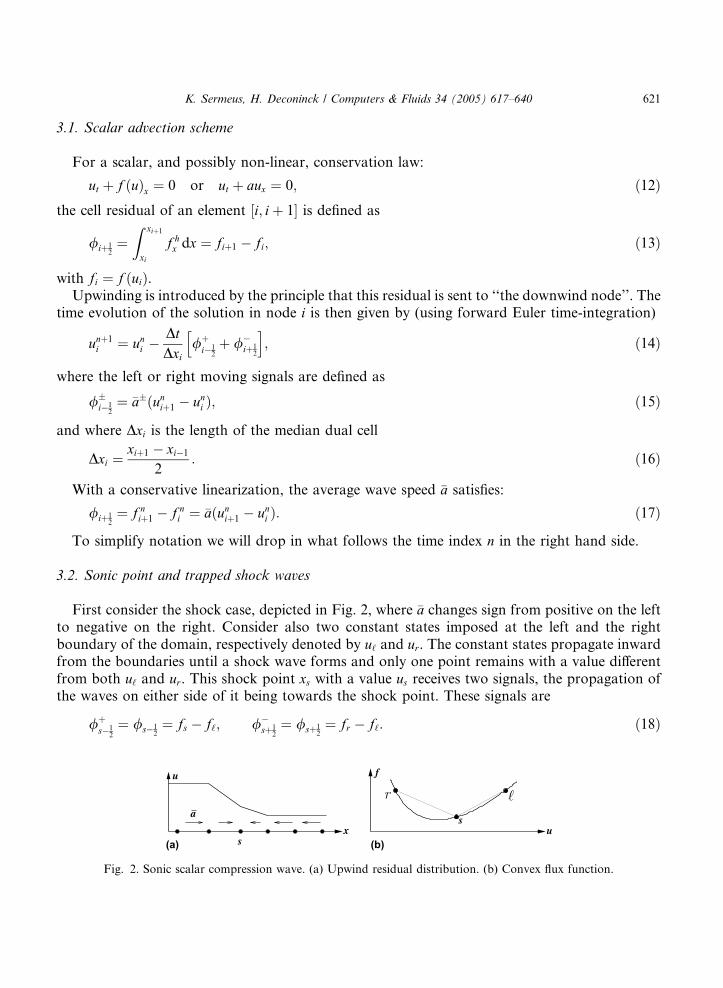
3.2. Sonic point and trapped shock waves

First consider the shock case, depicted in Fig. 2, where �a changes sign from positive on the leftto negative on the right. Consider also two constant states imposed at the left and the rightboundary of the domain, respectively denoted by u‘ and ur. The constant states propagate inwardfrom the boundaries until a shock wave forms and only one point remains with a value differentfrom both u‘ and ur. This shock point xs with a value us receives two signals, the propagation ofthe waves on either side of it being towards the shock point. These signals are

/þs12¼ /s1

2¼ fs f‘; /

sþ12¼ /sþ1

2¼ fr f‘: ð18Þ

Fig. 2. Sonic scalar compression wave. (a) Upwind residual distribution. (b) Convex flux function.


The evolution of us becomes from Eq. (14):

unþ1s ¼ uns DtDxs

ðfr f‘Þ: ð19Þ

If the left and right states are such that f ðu‘Þ ¼ f ðurÞ, a steady state is obtained with a shock at xs.Given a convex flux function f ðuÞ which satisfies Eq. (17), a steady shock solution can exist

with one intermediate shock point, which has a value us anywhere between u‘ and ur (the left andright state). This shows that a steady shock can be captured in at most 2 cells, or in other wordswith at most one intermediate shock point.Now consider the sonic expansion case, depicted in Fig. 3, where �a changes sign from negative

on the left to positive on the right. There is a point, call it xs, which receives no signals, thepropagation of the waves on either side of it being away from it. Consequently the value of us willnot change with time. The expansion or rarefaction continues, until eventually one of theneighbour nodes, xsþ1 or xs1, approaches a value for which the flux balance with f ðusÞ becomeszero, so that the corresponding cell is in equilibrium. That particular neighbour node is the one inwhich the wave speed a ¼ f 0ðuÞ has a sign opposite to aðusÞ, or in other words it is the node xsr,where we defined r ¼ signf 0ðusÞ. Once the equilibrium is reached in the sonic cell, the two regionsbecome separated by an unphysical expansion shock over that single cell. It is important to ob-serve that the strength of the ‘‘trapped’’ expansion shock is determined by the original value us atthe intermediate point.If the value of us would correspond to the sonic state, i.e. f 0ðusÞ ¼ 0, then there would in fact be

no expansion shock. In general this does not occur, unless the intermediate node has, by chance,the correct initial value. From this observation one is lead to the remedy proposed by Roe [2]:insert an extra grid point in the interval across which the wave speed changes sign. As long as thisextra grid point has a value uM in the range ½u‘; ur� of the interval, it actually does not matter atfirst what exactly this value is, nor where in the interval we put the extra grid point, because it willreceive no signals anyway. Eventually, an expansion shock will reform when one of the nodes ofthat interval has reached a value uM 0 such that f ðu0MÞ ¼ f ðuMÞ. Therefore, the best value for uM isthe sonic value.

3.3. One-dimensional entropy fix

The remedy described above can now be made more formal. Instead of really adding a gridpoint, we want of course to introduce a model of a sonic expansion fan in the residual distributionmethod. This is somewhat similar to what Harten and Hyman [4] did to remedy the expansion

a

xs

u

(b)(a)u

s

f

Fig. 3. Sonic scalar expansion fan. (a) Upwind residual distribution. (b) Convex flux function.

aa*–

x

t

i i+1

*+

M

Fig. 4. Sonic rarefaction model with an intermediate point in cell ½i; iþ 1�.


shock for Roe’s approximate Riemann solver in the flux difference splitting context. Consider acell ½i; iþ 1� with a sonic expansion, i.e. with wave speeds ai < 0 and aiþ1 > 0. The sonic expansionfan is modelled by replacing the single average wave in the residual distribution method by twomodified waves, with respectively a positive speed �aþ� and a negative speed �a� , which send signalsto both nodes of the sonic cell ½i; iþ 1�, as illustrated in Fig. 4. The signals sent to node i and tonode iþ 1 are respectively defined as

/iþ12¼ �a� ðuiþ1 uiÞ; /þ

iþ12¼ �aþ� ðui þ 1 uiÞ: ð20Þ

Conservation requires that these two signals sum up to the cell residual /iþ12, which satisfies

Eq. (17) and hence that �aþ� þ �a� ¼ �a. This condition is met if we define the modified wave speedsas

�aþ� ¼ �aþ j�aj�2

; �a� ¼ �a j�aj�2

: ð21Þ

By setting j�aj� to a non-zero value, waves are continued to be sent to the nodes of the sonic cell,even with the cell residual being zero (�a ¼ 0). This effectively breaks down the expansion shock.The question remains how to define j�aj�.A straightforward choice is to define j�aj� as follows:

j�aj� ¼ j�aj; if j�ajP �;�; if j�aj < �;

ð22Þ

with � a small constant. The value of that constant is however dependent on the specific problemand on the mesh size, making it difficult to apply in practice.To derive a better definition of j�aj�, the modelling of the sonic expansion fan should be taken a

little further. The value uM at the virtual intermediate grid point xM is determined from therequirement that the residuals of the two sub-cells ½i;M � and ½M ; iþ 1� add up to the residual ofcell ½i; iþ 1�, i.e.

�a� ðuM uiÞ þ �aþ� ðuiþ1 uMÞ ¼ �aðuiþ1 uiÞ: ð23Þ
With the modified wave speeds given by Eq. (21), this consistency requirement becomes
j�aj�ui þ uiþ12

h uM

i¼ 12�aðuiþ1 uiÞ: ð24Þ

For a cell with a sonic expansion, �a ¼ 0, this constraint is met if either j�aj� ¼ 0, i.e. the originalsituation with an expansion shock (trivial), or if:

uM ¼ ui þ uiþ12

: ð25Þ


To derive from this a formula for j�aj� we look more specifically to the case of a quadratic fluxfunction, such as the inviscid Burgers equation, i.e. Eq. (12) with f ¼ u2=2 and a ¼ f 0ðuÞ ¼ u. Byconservative linearization the average wave speed in cell ½i; iþ 1� is

�a ¼ ai þ aiþ12

¼ ui þ uiþ12

: ð26Þ

Defined consistently with the linearization, the modified average wave speeds that model thesonic expansion for a quadratic flux are

�aþ� ¼ uM þ uiþ12

; �a� ¼ ui þ uM2

: ð27Þ

With the definition in (21) it then follows:

j�aj� ¼ �aþ� �a� ¼ uiþ1 ui2

: ð28Þ

To conclude, the sonic expansion fan model is included in the residual distribution method asexpressed by Eq. (15) if the signed average wave speeds in (15) are replaced by the modified wavespeeds defined by Eq. (21), with

j�aj� ¼j�aj; if j�ajP d;d; if j�aj < d;

ð29Þ

where

�a ¼ 12maxð0; aiþ1 aiÞ:

The max function is included in the definition of d to skip the modification for the case ofcompression shocks.As it turns out, the entropy fix defined by the above equations is formally identical to the

entropy fix of Harten and Hyman [4] for the approximate Riemann solver of Roe [1]. This is nottoo surprising, since the first order upwind residual distribution scheme is formally equivalent toRoe’s approximate Riemann solver, although by principle the residual distribution method doesnot derive from the Riemann problem (see also next section). Although the entropy fix of Hartenand Hyman [4] is formally identical to (29), it was derived from a simpler model, namely one thatreplaces the sonic expansion fan in the approximate Riemann problem solution by a singleintermediate state. If however a linear transition u�ðx=tÞ for the expansion fan is introduced in theRiemann problem solution, a different entropy fix formula is obtained for Roe’s approximateRiemann solver, also due to Harten and Hyman [4]:

j�aj� ¼j�aj; if j�ajP d;12ðj�aj2=d þ dÞ; if j�aj < d;

ð30Þ

with still the same definition for d as in Eq. (29). This entropy fix formula can be applied for theRD method as well. Though there is no theoretical basis for doing so and the results are in factless satisfactory, as illustrated next.As a first example, consider the inviscid one-dimensional Burgers equation and for the initial

state at time t ¼ 0 a discontinuity defined by

Fig. 5. Sonic expansion for one-dimensional Burgers equations. Left: original residual distribution scheme. Middle:

with entropy fix of (29). Right: with entropy fix of (30).


uðx; t ¼ 0Þ ¼ 1; if x < 0;2; if xP 0:

ð31Þ

The exact solution is an expansion fan emanating from the sonic point at x ¼ 0. Fig. 5 com-pares at time t ¼ 0:4 the numerical solution on a uniform grid with 100 points with the exactsolution. The solution computed with the one-dimensional residual distribution scheme featuresan expansion shock. Adding the present entropy fix described by (29), the expansion shock isremoved completely so that the entropy condition is satisfied. With the alternative entropy fix of(30) however, the result is less satisfactory since a weak expansion shock remains in the numericalsolution.

3.4. Hyperbolic systems of conservation laws––the Euler equations

Consider a one-dimensional hyperbolic system of m conservation laws, written in conservativeform, respectively quasi-linear form, as

oU

otþ oF

ox¼ 0 or

oU

otþ A

oU

ox¼ 0: ð32Þ

Specifically for the Euler equations, we have U ¼ ðq; qu;qEÞt and F ¼ ðqu; q2u þ p; quHÞt.

The cell residual or fluctuation over a cell ½i; iþ 1� is defined as

Uiþ12 ¼

Z iþ1

i

oFh

oxdx ¼ Fiþ1 Fi: ð33Þ

The conservative linearization defined by Eq. (4) becomes in the one-dimensional case

Uiþ12 � A

oUh

oxDxiþ1

2� AðUiþ1 UiÞ; ð34Þ

where

Dxiþ12¼ xiþ1 xi ð35Þ

is the length of the cell ½i; iþ 1�. For the Euler equations this is obtained by the Roe linearizationin the parameter vector Z ¼ ð ffiffiffi

qp

;ffiffiffiffiffiffiqu

p;ffiffiffiq

pHÞt. Indeed, since both U and F are homogeneous


functions of degree 2 in the components of Z, and by assuming a linear variation of Z over P1elements, the cell residual as defined by Eq. (33) can be written as

Uiþ12 ¼

Z iþ1

i

oFh

oxdx ¼

Z iþ1

i

oF

oZ

oZh

oxdx ¼ oF

oZ

� �Z

Z iþ1

i

oZh

oxdx ð36Þ

¼ oF

oU

oU

oZ

� �Z

ðZiþ1 ZiÞ ð37Þ

¼ AZðUiþ1 UiÞ; ð38Þ

where AZ ¼ AðZÞ is the flux Jacobian oFoUevaluated at the average state Z ¼ ZiþZiþ1

2of the element

½i; iþ 1� and where Ui are nodal values of the conserved variables, defined consistently with theRoe linearization by

Uiþ1 Ui �oU

oZ

� �Z

ðZiþ1 ZiÞ: ð39Þ

As the one-dimensional system of conservation laws is hyperbolic, the Jacobian A can be di-agonalized in the basis of its eigenvectors, i.e. A ¼ RKR1, where K is a diagonal matrix con-taining the eigenvalues of A and R is the matrix of right eigenvectors. By this diagonalization thehyperbolic system can be written as

oW

otþ K

oW

ox¼ 0 ð40Þ

for characteristic variables defined by oW ¼ R1oU. By the same similarity transformation the cellresidual of Eq. (34) becomes

Uiþ12 � RZKZðcWiþ1 cWiÞ �

Xmk¼1

�kkð bW kiþ1 bW k

i Þ�rk; ð41Þ

where cWi is defined by cWi ¼ R1ðZÞUi, such that it satisfies
cWiþ1 cWi ¼ R1ðZÞðUiþ1 UiÞ: ð42Þ
This corresponds to a decomposition into m characteristic waves �rkr bW k, defined by the ei-genvectors �rk, and which travel with a speed given by the corresponding eigenvalue �kk. Theresidual can thus be decomposed into right-moving waves, with �kk > 0, and left-moving waves,with �kk < 0,

Uiþ12 �

X�kk P 0

�kðþÞk ð bW k

iþ1 bW ki Þ�rk þ

X�kk<0

�kðÞk ð bW k

iþ1 bW ki Þ�rk: ð43Þ

The upwind residual distribution method then consists in sending the different scalar wavecontributions in the cell residual to the downwind node, i.e. to node i or node iþ 1, depending onwhether the sign of �kk is negative, resp. positive. Summing contributions from cells ½i 1; i� and½i; iþ 1�, the semi-discrete equation for the solution in node i is


DxidUi

dt¼ jBi1

2i ðKÞUi1

2

hþ jBiþ1

2i ðKÞUiþ1

2

ið44Þ

� Ui12

i ðKþÞh

þ Uiþ12

i ðKÞi

ð45Þ

� X�kk P 0

�kðþÞk ðW k

i

24 W ki1Þ�rk þ

X�kk<0

�kðÞk ðW k

iþ1 W ki Þ�rk

35: ð46Þ

This one-dimensional upwind residual distribution scheme is formally equivalent to the fluxdifference splitting scheme with Roe’s approximate Riemann solver [1], although no reference wasmade here to a Riemann problem, see also [6]. The important difference is that the residual dis-tribution approach is better suited for extending to a genuinely multi-dimensional upwindingscheme.

3.5. The Lax entropy condition and expansion shocks

A discontinuity separating the states U‘ and Ur, propagating at the speed s, satisfies the Laxentropy condition [13] if there exists a characteristic field (index k) for which the k-characteristicsare impinging on the discontinuity, i.e.

kkðU‘Þ > s > kkðUrÞ; ð47Þ

while the other characteristics are crossing the discontinuity,

kjðU‘Þ < s and kjðUrÞ > s for j < k;

kjðU‘Þ < s and kjðUrÞ > s for j > k;ð48Þ

where we assumed that the eigenvalues are ordered such that k1 < k2 < � � � < km.The states U‘ and Ur of the weak solution to the system of conservation laws also satisfy the

Rankine–Hugoniot relations,

½F� ¼ s½U�; ð49Þ

where s denotes the shock speed. Since Eq. (49) represents m 1 conditions (after elimination ofs), the states Ur that can be connected to a given state U‘ by a single shock in the kth field form aone-parameter family,

Ur ¼ UðnÞ; where Uð0Þ ¼ U‘; ð50Þ

representing a so-called Hugoniot locus in the state space. The shock speed s is also a function ofthe parameter: s ¼ sðnÞ.Differentiating the Rankine–Hugoniot relation with respect to n, at n ¼ 0, and using the defi-

nition of the flux Jacobian gives

sU0 ¼ F0 ¼ oU0

oUU0 ¼ AU0; ð51Þ

which shows that (if U0 is different from zero) sð0Þ must be an eigenvalue of A ¼ AðU‘Þ, say thekth,


sð0Þ ¼ kkðU‘Þ; ð52Þ

while U0 is parallel to the corresponding right eigenvector,

U0 ¼ arkðU‘Þ: ð53Þ

It then follows that the change in the eigenvalue kk over the discontinuity is, to second order in(DU),

kkðUrÞ kkðU‘Þ ¼ kkðU‘ þ DUðnÞÞ kkðU‘Þ ¼ ðrUkk � rkÞaDn: ð54Þ

As a consequence of Eq. (54), the characteristic fields of a quasi-linear system can be classifiedin two distinct types, cf. [13]:

(1) Genuinely non-linear: If rUkk � rk 6¼ 0 for all U, the kth characteristic field is called genuinelynon-linear.

(2) Linearly degenerate: If rUkk � rk � 0 for all U, the kth characteristic field is called linearly

degenerate.

In a genuinely non-linear field the wave speed kkðUðnÞÞ varies monotonically with n, it eitherincreases or decreases, i.e. the characteristics are either expanding or compressing. Though be-cause of the Lax entropy condition, Eq. (47), only one case is admissible. For the shock to beadmissible, the wave speed must decrease in the direction of propagation of the shock, i.e. thecharacteristics must be impinging on the shock. The opposite case of an expansion shock is notadmissible by the entropy condition, only continuous expansion waves are admissible. On thecontrary, in a linearly degenerate field, the characteristics are parallel, not compressing norexpanding. Across a discontinuity in a linearly degenerate field, the wave speed kk is the same oneither side and equal to the propagation speed of the discontinuity. This is the case of a contact

discontinuity, for which the inequalities in Eq. (47) become equalities. Thus there is actually noentropy condition to be considered for the waves in a linearly degenerate field. Physically thiscorresponds to the fact that, as fluid particles do not cross a contact discontinuity, their entropydoes not change.The upwind RD method for one-dimensional hyperbolic systems of conservation laws, given by

Eq. (46), violates the entropy condition, as can be shown by an analysis of the shock capturingproperties of the RD scheme, similar to the analysis for the scalar case in Section 3.2. Consideragain a sonic expansion case, where now one of the wave speeds kk (for a genuinely non-linearfield) changes sign from negative on the left to positive on the right. Hence, as can be seen fromEq. (46), there is a node (at position xs), which receives no signals in the kth characteristic field,since

ð�kkÞs12< 0 < ð�kkÞsþ1

2: ð55Þ

Consequently, the Wk characteristic component in the state Us will not change with time, and theexpansion shock, which was initially present in the solution will not decay, but remain trapped inone cell, either left or right of node xs, depending on the initial conditions. This situation of anumerical solution with expansion shock across which the wave speed kk changes as in (55),clearly violates the Lax entropy condition (47).


3.6. Entropy fix for one-dimensional hyperbolic system

The entropy fix developed for the scalar case in Section 3.3 is now extended to the one-dimensional hyperbolic system case. As the mechanism in the RD method leading to expansionshocks is the same for a genuinely non-linear field of the hyperbolic system as for the scalar case,the extension of the entropy fix is straightforward. Consider a situation with in the cell ½i; iþ 1� asonic expansion in the kth characteristic field, i.e. ðkkÞi < 0 < ðkkÞiþ1. Introducing a model for thesonic expansion fan in the kth characteristic field, the entropy fix is formulated similarly to Eqs.(21) and (29):

�kþk ¼

�kk þ j�kkj�2

; �kk ¼

�kk j�kkj�2

; ð56Þ

j�kkj� ¼j�kkj; if j�kkjP dk;d; if j�kkj < dk;

ð57Þ

where

dk ¼ 12maxð0; ðkkÞiþ1 ðkkÞiÞ:

The model of the sonic expansion fan adopted for defining this entropy fix, assumes that thewave speed kk varies linearly with x. This assumption is in fact generally valid for any hyperbolicsystem, since the problem for which the entropy fix is intended, i.e. the breakdown of anexpansion shock into a continuous sonic expansion fan, is a Riemann problem for which the exactsolution has a linearly varying wave speed kkðxÞ. The sonic (also called ‘‘centered’’) expansion fanis a similarity solution of the Riemann problem, i.e. a solution which depends on x=t alone, givenby

Uðx; tÞ ¼U‘ x6 g‘t;Wðx=tÞ g‘t < x < grt;Ur xP grt;

8<: ð58Þ

whereWðx=tÞ is a smooth vector valued function, equal to respectively U‘ and Ur at the left andright end of the expansion fan. For the solution in the sonic expansion fan, it holds

oU

ot¼ oW

ogogot

¼ W0ðgÞ xt2; ð59Þ

oF

ox¼ oFðWðgÞÞ

oU

oWðgÞog

ogox

¼ AðWðgÞÞW0ðgÞ 1t; ð60Þ

where g ¼ x=t. Substituting these expressions in the conservation law (32), it follows that WðgÞmust satisfy, for g‘ < g < gr,

AðWðgÞÞW0ðgÞ ¼ gW0ðgÞ; ð61Þ
which implies that W0ðgÞ is a right eigenvector of A and that the corresponding eigenvalue kk isequal to g:

Fig. 6

schem


W0ðgÞ ¼ aðgÞrkðWðgÞÞ; ð62Þ

kðWðgÞÞ ¼ g: ð63Þ
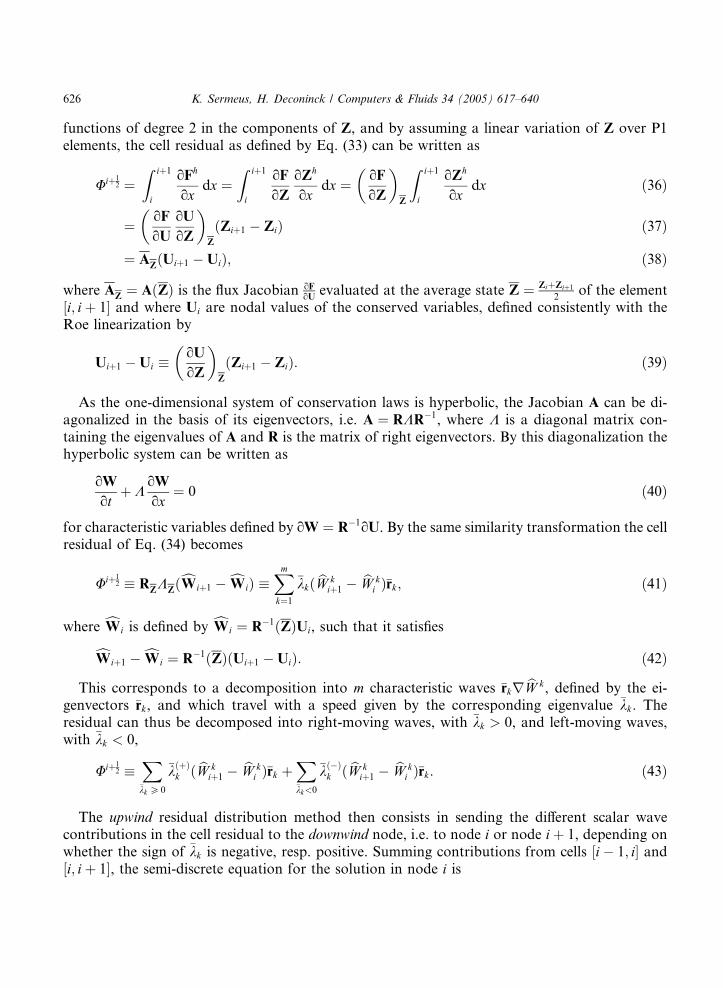
Thus, for a simple expansion wave in the kth characteristic field, the values of WðgÞ lie along
the integral curve of rk, a well known result for genuinely nonlinear fields in hyperbolic systems.The interesting point is that irrespective of the function WðgÞ and at any given time, the wavespeed kk in a sonic expansion fan varies linearly with x, as indicated by Eq. (63). This confirms theassumption of linear kkðxÞ in the definition of the entropy fix.To illustrate the entropy fix, consider the one-dimensional Euler equations of gas dynamics.

The three wave speeds are k1 ¼ u c, k2 ¼ u and k3 ¼ uþ c, where u is the velocity and c thespeed of sound. The entropy fix formulated in (57) is applied only to the two acoustic wave speedsk1 and k3. The wave speed k2 needs no entropy fix, since it corresponds to a linearly degeneratefield, in which only contact discontinuities exist.As an example, the RD method is applied to solve a Riemann problem for the Euler equations

in an ideal polytropic gas with c ¼ 1:4 (i.e. air). The initial solution is defined by the followingconstant left and right state (in SI units):

q‘ ¼ 1; p‘ ¼ 105; u‘ ¼ 0;qr ¼ 0:1317; pr ¼ 5853; ur ¼ 623:6:

ð64Þ

The exact solution of this particular Riemann problem is a transonic rarefaction wave, giving acontinuous expansion from Mach 0 to Mach 2.5. Fig. 6 compares the numerical solution and theexact solution at time t ¼ 6 ms. The solution in the left figure is computed by the RD method ofEq. (46). Clearly an expansion shock is trapped over one cell and thus the entropy condition isviolated by the RD method. With the entropy fix added the expansion shock is removed and anaccurate approximation of the continuous solution is obtained, as shown by the solution in theright figure.The present interpretation of the entropy fix of Harten and Hyman [4] for the one-dimensional

upwind RD method allows a generalization to the genuinely multi-dimensional upwind RDmethod, as discussed in Section 5.

. Sonic expansion for Euler equations computed by the upwind residual distribution method. Left: original

e. Right: with entropy fix.


4. Shock capturing analysis––the multi-dimensional case

The shock capturing properties of the multi-dimensional upwind residual distribution schemesare controlled by the linearization step, which determines the signs (and also magnitudes ofcourse) of the average wave speeds. The analysis will first look at the special case of a normalshock, i.e. a shock which is normal to the velocity of the incoming flow. As the flow velocity doesnot change direction across a normal shock, this special case is equivalent to the one-dimensionalshock problem. The second part of the analysis considers the general case of an oblique shock,which is at a given shock angle b with respect to the velocity of the incoming flow (a normal shockis an oblique shock with b ¼ 90�).

4.1. Normal shock analysis

First, consider a simple scalar 2D model corresponding to a 2D extension of the inviscidBurgers equation, in conservation law form:

ut þ f ðuÞx þ gðuÞy ¼ 0; with f ðuÞ ¼ u2

2; gðuÞ ¼ u; ð65Þ

or in quasi-linear form:

ut þ aux þ buy ¼ 0; with a ¼ f 0ðuÞ ¼ u; b ¼ g0ðuÞ ¼ 1: ð66Þ

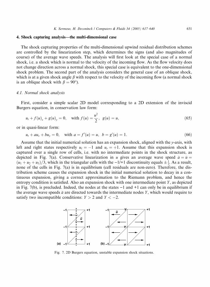
Assume that the initial numerical solution has an expansion shock, aligned with the y-axis, withleft and right states respectively u‘ ¼ 1 and ur ¼ þ1. Assume that this expansion shock iscaptured over a single row of cells, i.e. with no intermediate points in the shock structure, asdepicted in Fig. 7(a). Conservative linearization in u gives an average wave speed �a ¼ �u ¼ðu1 þ u2 þ u3Þ=3, which in the triangular cells with the )1/+1 discontinuity equals � 1

3. As a result,

none of the cells in Fig. 7(a) is in equilibrium (cell residuals are non-zero). Therefore, the dis-tribution scheme causes the expansion shock in the initial numerical solution to decay in a con-tinuous expansion, giving a correct approximation to the Riemann problem, and hence theentropy condition is satisfied. Also an expansion shock with one intermediate point Y , as depictedin Fig. 7(b), is precluded. Indeed, the nodes at the states )1 and +1 can only be in equilibrium ifthe average wave speeds �a are directed towards the intermediate nodes Y , which would require tosatisfy two incompatible conditions: Y > 2 and Y < 2.

+1

+1

+1

—1

—1

—1

—1

—1

—1

u

+1

+1

+1

uY

Y

Y

(a) (b)

Fig. 7. 2D Burgers equation, unstable expansion shock situations.


Similar results apply for the multi-dimensional Euler equations with the conservative lineari-zation in the parameter vector Z. In the one-dimensional case discussed before, when the twostates Ui and Uiþ1 satisfy the Rankine–Hugoniot jump relation, the shock propagation speed isprecisely one of the eigenvalues �kk of the average Jacobian A, given by the Roe linearization in Z(this is the so-called Property U defined by Roe [1]). Hence, if the two states satisfy the Rankine–Hugoniot jump relation for a steady shock, the average acoustic wave speed �u �c is zero. Thus, aswas shown in Fig. 6, an expansion shock can remain trapped in a single cell.In the multi-dimensional case however, the conservative linearization in Z does not satisfy this

jump property, i.e. the average eigenvalue �kk is not equal to the shock propagation speed, and thusexpansion shocks seem to be precluded in the multi-dimensional case. Assume that a steadynormal expansion shock was captured over one cell (i.e. one ‘‘row’’ of cells), as depicted in Fig. 8,i.e. the states U1 and U2 satisfy the steady Rankine–Hugoniot relation for normal shocks. Theaverage state by the linearization in Z is

Fig

Z ¼ 2Z1 þ Z2

3: ð67Þ

Substituting the Rankine–Hugoniot relations between U1 and U2 into Eq. (67), it follows thatthe average velocity �u and speed of sound �c satisfy the relation [8]

�c2 ¼ ðc þ 1Þð2þM1�Þ2 ðc 1Þð1þ 2M1�Þ2

2ð1þ 2M1�Þ2

" #�u2; ð68Þ

where M1� denotes the critical Mach number, defined by

M21� ¼

cþ12M21

1þ c12M21

ð69Þ

and c is the ratio of specific heats. Since the slow acoustic wave speed �k1 ¼ �u �c 6¼ 0 (except forthe trivial case M1� ¼ 1), this shows that the residual for a shock captured over the cell depicted inFig. 8 is non-zero and thus that this cell cannot be in equilibrium. Consequently physical normalshocks cannot be captured over a single cell (i.e. there is always an intermediate point in thenumerical shock structure) and for the same reason normal expansion shocks cannot occur either.From this analysis Paill�ere [8] concluded that the residual distribution schemes do not admit

Σ1

1

2

. 8. Steady discontinuity in one cell. States U1 and U2 are related by the Rankine–Hugoniot jump relations.


expansion shocks and thus that the entropy condition is satisfied. Nevertheless, we have observedoblique expansion shocks in many steady flow computations with the RD method, which indicatesthat generalizing the conclusions of the above normal shock analysis to oblique shocks may beinvalid.

4.2. Oblique shock analysis

Fig. 9(a) shows an oblique shock at a shock angle b trapped in a single row of cells. Assume leftand right states U1 and U2 which satisfy the Rankine–Hugoniot jump relations for a stationarydiscontinuity and then compute the average acoustic wave speed �k1 ¼ �un �c given by the con-servative linearization at the average state Z ¼ Z1þ2Z2

3(for a cell 1–2–2). Note that the actual shape

of the elements does not play a role in the conservative linearization.Because of the lengthy algebra involved, we do not derive an equation for �un �c in this case,

similar to Eq. (68). Instead we plot in Fig. 9(b), for the case b ¼ 50�, the pressure ratio p2=p1 andthe downstream normal Mach number Mn2, as a function of the upstream Mach number M1 andfor c ¼ 1:4. On the right ordinate the graph shows the average acoustic wave speed �un �c in thecells with vertices 1–2–2 and 1–1–2. As seen from the pressure ratio, for M1 < MB ¼ 1:31 thediscontinuity corresponds to an expansion. The important point to observe is that for an obliqueshock, �un �c changes sign at another value of M1, in the example at the lower value of MA ¼ 1:10for the cell 1–2–2 and at a much higher value for the cell 1–1–2. This shows that in the case of anoblique shock and for MA < M1 < MB the nodes at state U2 receive not any signal from the slowacoustic waves (speed un c), and hence the component of the solution in the correspondingcharacteristic field is not updated by the RD scheme, so that the expansion shock does not decay.The above analysis indicates that oblique expansion shocks may exist in the numerical solution,

as has been confirmed by many numerical experiments (cf. Section 6). Normal expansion shocksare precluded though, because for M1 < 1 (i.e. an expansion) the sign of the average wave speed

Fig. 9. Analysis of oblique shock trapped in one cell. (a) Sketch of a shock at angle b to the upstream flow. (b) Averageacoustic wave speed �un �c in the cells 1–1–2 and 1–2–2 for b ¼ 50�.

Fig. 10. Analysis of normal shock trapped in one cell (same as Fig. 9(b), but for b ¼ 90�). Average acoustic wave speed�un �c in the cells 1–1–2 and 1–2–2.


�u �c is always such that the discontinuity is destroyed. The normal shock case is illustrated in Fig.10, which should be compared with the similar graph in Fig. 9.

5. Multi-dimensional entropy fix

As shown in the previous section, the multi-dimensional upwind RD method is in general notfree from expansion shocks, although, being limited to oblique expansion shocks, the problem isperhaps less severe than for the dimension-by-dimension upwinding with the FDS schemes.Therefore a multi-dimensional extension of the one-dimensional entropy fix defined in Eq. (29)was developed.Generalizing the one-dimensional fix, the multi-dimensional entropy fix is introduced by

modifying the upwinding matrices defined in Eq. (10) to

K��i ¼ 1

2ðKi � jKij�Þ: ð70Þ

In the matrix

jKij� ¼ RijKij�R1i ð71Þ

the moduli of the acoustic eigenvalues are modified similarly to Eq. (29) as

j�ki;kj� ¼j�ki;kj; if j�ki;kjP dk;dk; if j�ki;kj < dk:

ð72Þ

Since the modified matrices satisfy Kþ�i þ K�

i ¼ Ki, the conservation property of the scheme ismaintained. The quantity dk remains to be defined so that it detects the sonic point where theeigenvalue ki;k changes sign.The definition of dk is based on the observation that when expansion shocks exist in the

numerical solution, they are trapped in a single row of elements, and hence they are aligned withone of the faces of the elements. Fig. 11 shows the model of an expansion shock in that situation.The vector ~nshock is defined as a unit vector parallel to the face normal ~ni of the element along

Fig. 11. Model of a trapped expansion shock. The expansion shock shows up as a constant gradient over the linear

element.


which the component of the pressure gradient is the largest. To distinguish expansion shocks fromphysical (compression) shocks, the orientation of ~nshock is defined such that it is pointing down-wind with respect to the average flow velocity in the element. In analogy to Eq. (57) d is defined bythe change of the slow acoustic wave speed k ¼ un c (subscript k dropped to simplify notation)over the element:

d ¼ 12maxð0; kdown kupÞ: ð73Þ

Assuming that k varies linearly over the element, the values in the ‘‘upwind’’ and ‘‘downwind’’point are defined on a line parallel to vector~nshock and which goes through one of the vertices ofthe element:

kup ¼P

j kj kjP

j kj

; kdown ¼P

j kþj kjP

j kþj

; ð74Þ

where kj �~nshock �~nj.This definition of d is justified by consideration of the flow field in a Prandtl–Meyer expansion

fan, i.e. the expansion of a supersonic flow over a sharp convex corner. It is especially for thisproblem, which has a singularity in the boundary conditions due to the sharp corner of the wall,that an (unphysical) oblique expansion shock can arise most easily in the numerical solution. ThePrandtl–Meyer expansion fan is a self-similar solution of steady planar supersonic flow, which iseasily derived from the conservation laws when written in polar coordinates ðr; hÞ, where r is thedistance from the corner and h is the azimuthal angle. The self-similar solution requires that noneof the dependent variables depend on r, but only on h. It then follows directly from the governingequations that

ouroh

¼ uh ¼ c: ð75Þ


The last equality shows that the radial lines from the origin (corner on the wall) are exactlyMach lines, i.e. steady characteristics for acoustic waves in supersonic flow. Indeed, as theory ofcharacteristics shows, the relative velocity component perpendicular to a Mach line equals thelocal speed of sound. Thus, the slow acoustic wave speed in the azimuthal direction of the time-dependent hyperbolic system equals zero in a Prandtl–Meyer expansion fan:

k1 ¼ uh c ¼ 0: ð76Þ
Together with the absence of any gradients in the radial direction, this is a physical argument to
justify the definition of d as in Eq. (73). If in the numerical solution of a Prandtl–Meyer expansionthis parameter d would differ from zero (or rather a small epsilon to account for discretizationerrors), it indicates the presence of an expansion shock.Note that, since an expansion shock would always be aligned with one face of the element, the

entropy fix needs to be applied only to the Jacobian Ki for which the normal~ni is parallel to~nshock.Numerical experiments support the conjecture that with the above entropy fix added the multi-

dimensional upwind residual distribution schemes satisfy the entropy condition, i.e. that thenumerical solution is free from unphysical expansion shocks.

6. Numerical tests

The effectiveness of the entropy fix developed in the previous section is illustrated for twotypical 2D supersonic flow problems. The Euler equations are discretized by the multi-dimen-sional upwind RD method described in Section 2. In particular we use the first order N schemeand the second order LDA/N blended scheme [7,10]. Actually, the second order scheme is ahybridization of the scalar PSI scheme for the entropy advection equation, which is decoupledfrom the Euler equations by similarity transformation, and the matrix LDA/N blended scheme forthe remaining subsystem of the Euler equations. The steady state solution is computed by implicittime integration using a Newton–Krylov solver [10].

6.1. Mach 3 wind tunnel with step

The first problem considered is the well known test case of inviscid flow in a Mach 3 windtunnel with forward facing step [15]. Fig. 12 shows the density isolines of the steady state solutioncomputed on a quasi-uniform unstructured grid with 17,300 nodes and 34,000 triangular ele-ments. For the first order N scheme (top figure) an expansion shock is seen to emanate from thecorner over which the flow normally expands gradually. With the second order LDA/N scheme(middle) the shocks are of course better resolved and the diffusion of the slip line is lower.Although less pronounced, an expansion shock is still clearly visible at the corner of the step.Finally the bottom figure shows, that with the entropy fix added, the expansion shock flaw iscured and hence the improved scheme satisfies the entropy condition.Note that the occurrence of expansion shocks is more likely for a regular grid, since the shock is

trapped in a single row of cells, with all cells having one face parallel to the shock. It is to beremarked though, that the oblique shock analysis of Section 4.2, which demonstrated that obliqueexpansion shocks may exist in the numerical solution, does not directly depend on the precise

Fig. 12. Inviscid Mach 3 flow with forward facing step, iso-density lines. Top: first order scheme, no entropy fix.

Middle: second order scheme, no entropy fix. Bottom: second order scheme with entropy fix.


orientation of the elements in the grid. Therefore expansion shocks cannot be excluded in theoryon very irregular grids either. Nevertheless, the large disturbances of the flux balances caused byirregular grids, might prevent expansion shocks to form in practice during the transient to asteady state. On the more or less regular grids used here, generated by the frontal Delaunaymethod [14], expansion shocks have been found to exist in many cases though. This is furtherillustrated in the next problem.

6.2. Mach 3 wind tunnel with triangular bump

The second test case is the Mach 3 flow over a triangular bump in a channel. Fig. 13 shows thedensity isolines of the steady state solution computed on a quasi-uniform unstructured grid withapproximately 7400 nodes and 14,406 triangular elements. The same observations can be made asfor the first test case. Note that in this test case, as well as in the first, the initial flow field wascompletely uniform and thus did not contain any initial expansion shock. In multi-dimensional

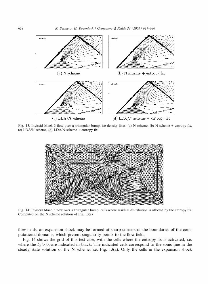
Fig. 13. Inviscid Mach 3 flow over a triangular bump, iso-density lines. (a) N scheme, (b) N scheme + entropy fix,

(c) LDA/N scheme, (d) LDA/N scheme + entropy fix.

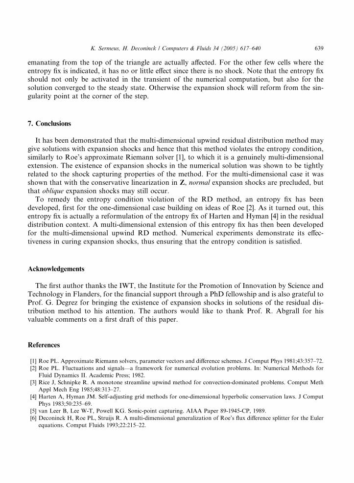
Fig. 14. Inviscid Mach 3 flow over a triangular bump, cells where residual distribution is affected by the entropy fix.

Computed on the N scheme solution of Fig. 13(a).


flow fields, an expansion shock may be formed at sharp corners of the boundaries of the com-putational domains, which present singularity points to the flow field.Fig. 14 shows the grid of this test case, with the cells where the entropy fix is activated, i.e.

where the dk > 0, are indicated in black. The indicated cells correspond to the sonic line in thesteady state solution of the N scheme, i.e. Fig. 13(a). Only the cells in the expansion shock


emanating from the top of the triangle are actually affected. For the other few cells where theentropy fix is indicated, it has no or little effect since there is no shock. Note that the entropy fixshould not only be activated in the transient of the numerical computation, but also for thesolution converged to the steady state. Otherwise the expansion shock will reform from the sin-gularity point at the corner of the step.

7. Conclusions

It has been demonstrated that the multi-dimensional upwind residual distribution method maygive solutions with expansion shocks and hence that this method violates the entropy condition,similarly to Roe’s approximate Riemann solver [1], to which it is a genuinely multi-dimensionalextension. The existence of expansion shocks in the numerical solution was shown to be tightlyrelated to the shock capturing properties of the method. For the multi-dimensional case it wasshown that with the conservative linearization in Z, normal expansion shocks are precluded, butthat oblique expansion shocks may still occur.To remedy the entropy condition violation of the RD method, an entropy fix has been

developed, first for the one-dimensional case building on ideas of Roe [2]. As it turned out, thisentropy fix is actually a reformulation of the entropy fix of Harten and Hyman [4] in the residualdistribution context. A multi-dimensional extension of this entropy fix has then been developedfor the multi-dimensional upwind RD method. Numerical experiments demonstrate its effec-tiveness in curing expansion shocks, thus ensuring that the entropy condition is satisfied.

Acknowledgements

The first author thanks the IWT, the Institute for the Promotion of Innovation by Science andTechnology in Flanders, for the financial support through a PhD fellowship and is also grateful toProf. G. Degrez for bringing the existence of expansion shocks in solutions of the residual dis-tribution method to his attention. The authors would like to thank Prof. R. Abgrall for hisvaluable comments on a first draft of this paper.

References

[1] Roe PL. Approximate Riemann solvers, parameter vectors and difference schemes. J Comput Phys 1981;43:357–72.

[2] Roe PL. Fluctuations and signals––a framework for numerical evolution problems. In: Numerical Methods for

Fluid Dynamics II. Academic Press; 1982.

[3] Rice J, Schnipke R. A monotone streamline upwind method for convection-dominated problems. Comput Meth

Appl Mech Eng 1985;48:313–27.

[4] Harten A, Hyman JM. Self-adjusting grid methods for one-dimensional hyperbolic conservation laws. J Comput

Phys 1983;50:235–69.

[5] van Leer B, Lee W-T, Powell KG. Sonic-point capturing. AIAA Paper 89-1945-CP, 1989.

[6] Deconinck H, Roe PL, Struijs R. A multi-dimensional generalization of Roe’s flux difference splitter for the Euler

equations. Comput Fluids 1993;22:215–22.


[7] Deconinck H, Sermeus K, Abgrall R. Status of multi-dimensional upwind residual distribution schemes and

applications in aeronautics. AIAA Paper 2000-2328, 2000.

[8] Paill�ere H. Multi-dimensional upwind residual distribution schemes for the Euler and Navier–Stokes equations onunstructured grids. PhD Thesis, Universit�e Libre de Bruxelles, Belgium, 1995.

[9] van der Weide E, Deconinck H. Positive matrix distribution schemes for hyperbolic systems, with application to the

Euler equations. In: Proceedings of the 3rd European CFD Conference. Paris, France: Wiley; 1996. p. 747–53.

[10] van der Weide E, Deconinck H, Issman E, Degrez G. A parallel, implicit, multi-dimensional upwind residual

distribution method for the Navier–Stokes equations on unstructured grids. Comput Mech 1999;23(2):199–208.

[11] Abgrall R. Toward the ultimate conservative scheme: following the quest. J Comput Phys 2001;167:277–315.

[12] Sidilkover D. A genuinely multi-dimensional upwind scheme and efficient multigrid solver for the compressible

Euler equations. ICASE Report 94-84, 1994.

[13] Lax PD. Hyperbolic systems of conservation laws and the mathematical theory of shock waves. SIAM

Publications; 1973.

[14] M€uller J-D. On triangles and flow. PhD Thesis, University of Michigan, USA, 1996.[15] Woodward P, Colella P. The numerical simulation of two-dimensional fluid flow with strong shocks. J Comput

Phys 1984;54:115–73.

An entropy fix for multi-dimensional upwind residual distribution schemes

Documents

Transcript of An entropy fix for multi-dimensional upwind residual distribution schemes