
Hamilton Institute - School of Computing Science
260
Hamilton Institute Making Sense of Interaction Using a Model-Based Approach by Parisa Eslambolchilar, B.Eng., M.Eng. Supervisor: Dr. Roderick Murray-Smith Doctor of Philosophy Hamilton Institute/Department of Computer Science National University of Ireland, Maynooth Ollscoil na h ´ Eireann, M´a Nuad October 2006
-
Upload
khangminh22 -
Category
Documents
-
view
1 -
download
0
Transcript of Hamilton Institute - School of Computing Science

Hamilton Institute
Making Sense of Interaction Using a
Model-Based Approach
by
Parisa Eslambolchilar, B.Eng., M.Eng.
Supervisor: Dr. Roderick Murray-Smith
Doctor of Philosophy
Hamilton Institute/Department of Computer Science
National University of Ireland, Maynooth
Ollscoil na hEireann, Ma Nuad
October 2006

Dedicated to my parents for all their love and support.
Thesis advisor AuthorDr. Roderick Murray-Smith Parisa Eslambolchilar
Making Sense of Interaction Using a Model-Based Approach
Abstract
This thesis provides a theoretical method for developing and designing hu-man computer interaction based on a continuous control process on mobile com-puting devices. This view provides a tight coupling between the user and systembased on a continuous exchange of input/output dynamic information over a per-iod of time, where continuous feedback from the display (visual/audio/haptic)influences the user’s actions as more information becomes available and changesthe user’s perception. The proper representation and modeling of conceptualmodels in the interaction -via state-space model- and the explicit analysis of hu-man behaviour and adaptability of the system to human behaviour -in the formof dynamic systems and probability theory are inherent to this framework.
This framework supports continuous interaction techniques based on tilt in-puts and multimodal outputs with handheld devices because one-handed controlrequires less visual attention and multimodality in the interaction can compensatefor the lack of the screen space. The dynamic systems approach to the design ofsuch continuous interactive interfaces allows the incorporation of analytical toolsand constructive techniques from manual and automatic control theory, proba-bilistic models–and thus many of the techniques of machine learning–into theinterface and integrating multimodality in a principled manner.
Methods are presented for displaying the state of a system(visual/audio/haptic) with appropriate representation of a pseudo-physical model, via state-space model. Specifically, the use of predictive audio/visual-feedback for audi-tory/graphical display in a period of interaction is described, and it is shownhow predictive elements can be introduced into goal directed displays, conside-ring gains and delays present in the interaction loop. The use of these techniquesin simulating the system behaviour before the actual implementation, and tuningand testing the system parameters are illustrated.
Viewing human behaviour as a control process, a general framework for sup-porting human behaviour is developed, which supports intermittent interactionby smooth and natural dynamic mode switching. This is a probabilistic approachand not only applicable on small screen devices but also in many range of com-puting appliances. It provides general design guidelines for dynamic interactivesystems based on models for the dynamic system, probabilistic language modeland a probabilistic audio feedback.
Acknowledgments
Completing this doctoral work has been a wonderful and often overwhelmingexperience. It is hard to know whether it has been grappling with the researchitself which has been the real learning experience, or grappling with how to writea paper, prepare demo, code intelligibly, recover a crashed Pocket PC, and... stayfocussed.
I have been very privileged to have undoubtedly the most intuitive, smartand supportive advisor anyone could ask for, namely Dr. Roderick Murray-Smith.Dr. Murray-Smith has an ability to cut through reams of mathematics with asingle visual explanation that I will always admire, and I have learned a great dealof control theory from him. His guidance throughout this project, his patienceand enthusiastic attitude and motivating ideas within the subject field whichhelped spark inspiration for the project is admirable. He has also given me alittle push in the forward direction when I needed it.
Throughout my three years and half, I thank the SFI, Science FoundationIreland and IRCSET BRG SC/2003/271 Continuous Gestural Interaction withMobile devices for providing my funding and the Hamilton Institute here at NUIMaynooth, specially the director of the Institute, Professor Douglas Leith, andProfessor Robert Shorten, whose efforts help to make a great research atmospherein the Institute.
In the Institute, I have benefited from discussions with Professor Bill Lei-thead, Professor Peter Wellstead, Professor Barak Pearlmutter, Professor RonanReilly, Dr. Mehmet Akar, Dr. Joe Timoney, Dr. Eric Bullinger, Dr. ThomasHermann, Dr. Oliver Mason, Dr. Mark Verwoerd, and Carlos Villegas. Also, myappreciation goes to Professor Wellstead for his moral support, fatherly adviceand being all ears for me. In this context, special thanks are due to RosemaryHunt and Kate Moriarty whose patient and kindness help with the various admi-nistrative issues that need to be dealt with the course of Ph.D, visa and residencyin Ireland have made my task considerably easier.
On the topic of positive work environment, I would like to thank my office-mate Keith Neo for being a good friend, and for making our office a relaxed andenjoyable place to work. I also enjoyed sharing ideas about mathematics andcontrol with him.
iv

Acknowledgments
Dr. Murray-Smith’s other students and post-docs, both past and present inGlasgow University and at the Hamilton Institute, comprise a superb researchgroup. The ability to bounce ideas off so many excellent minds has been priceless.My most intense collaboration has been with Dr. Andrew Crossan, Dr. JohnWilliamson, Andrew Ramsay and Steven Strachan whose clarity, persistence,ability to create novel ideas, and ability to implement the applications and demos,has taught me a lot.
My special thanks go to Dr. Frank Pollick and Sara Dalzel-Job in the Psycho-logy Department, Glasgow University, who have influenced me in audio percep-tion and model-based target sonification research and their assistance is gratefullyacknowledged.
I would like to thank Professor Stephen Brewster in the Computing ScienceDepartment, Glasgow University, Dr. Matt Jones in Department of ComputerScience, University of Wales Swansea for their comments and advice during myvisits to Glasgow University.
On a more personal level, it would be impossible for me to overstate thedebt of the gratitude that I owe to my parents and sister, who have been therethrough the most stressful of thesis days, despite the long distance. I feel I wouldhave struggled to cope without their support and advice.
In finishing, I apologise to those who I have inevitably forgotten to name inthis list. The quote in below goes towards the numerous people whose help andsupport have made this thesis possible:
The glory of friendship is not the outstretched hand, nor the kindlysmile, nor the joy of companionship; it’s the spiritual inspiration thatcomes to one when he discovers that someone else believes in him andis willing to trust him with his friend.
Ralph Waldo Emerson (1803-1882)
v

Declaration
I hereby certify that this material, which I now submit for assessment onthe program study leading to the award of Doctor of Philosophy in ComputerScience is entirely my own work and has not been taken from the work of otherssave and to the extent that such work has been cited and acknowledged withinthe text of my work.
(Parisa Eslambolchilar)
vi
Contributing Publications
Large portions of Chapter 4 have appeared in the following papers:
P. Eslambolchilar, R. Murray-Smith, A. Crossan, S. Dalzel-Job, F.Pollick . In J. Lumsden, editor, Handbook of Research on User Inter-face Design and Evaluation for Mobile Technology, chapter “Model-based Target Sonification in Small Screen Devices: Perception andAction”. Idea Group Reference, 2007. This chapter has been submit-ted in September 2006 for review.
S. Strachan, P. Eslambolchilar, and R. Murray-Smith, “GPSTunes-controlling navigation via audio feedback”. In Manfred Tscheligi, edi-tor, Proceedings of Mobile Human-Computer Interaction - MobileHCI 2005, pages 275-278, Salzburg, Austria, September 2005. ACMPress.
P. Eslambolchilar, A. Crossan, and R. Murray-Smith, “Model-basedTarget Sonification on Mobile Devices”, Bielefeld, Germany, January2004. Proceedings of Interactive Sonification Workshop.
Large part of the first half of Chapter 5 have appeared in:
P. Eslambolchilar and R. Murray-Smith,“Tilt-based Automatic Zoo-ming and Scaling in mobile devices- a state-space implementation”.In S. Brewster and M. Dunlop, editors, MobileHCI 2004: 6th In-ternational Symposium, volume 3160 of Lecture Notes in Compu-ting Science, pages 120-131, Glasgow, Scotland, September 2004.Springer-Verlag.
The second half of Chapter 5 appears in its entirety as
P. Eslambochilar, J. Williamson, and R. Murray-Smith, “MultimodalFeedback for tilt controlled Speed Dependent Automatic Zooming”.In UIST’04: Proceedings of the 17th annual ACM symposium on Userinterface software and technology, Santa Fe, New Mexico, October2004, ACM Press.
vii

Contributing Publications
Finally, most of Chapter 6 has been published as
P. Eslambolchilar and R. Murray-Smith, “Model-Based, Multimo-dal Interaction in Document Browsing”. In Invited paper, 3nd JointWorkshop on Multimodal Interaction and Related Machine LearningAlgorithms, MLMI, Washington DC., USA, May 2006.
Electronic preprints are available on the Internet at the following URL:
http://www.hamilton.ie/parisa/
viii

If our designs are failing due to the constant rain of changing
requirements, it is our designs that are at fault. We must somehow
find a way to make our designs resilient to such changes and protect
them from rotting.
Robert C. Martin,
Design Principles and Design Patterns,
objectmentor.com, 2000
Contents
List of Figures xiv
List of Tables xix
1 Introduction 11.1 Interaction with Small Screen Devices . . . . . . . . . . . . . . . 1
1.1.1 Peripheral Devices for Handheld Devices . . . . . . . . . . 31.1.2 Novel Interaction Methods . . . . . . . . . . . . . . . . . 4
1.2 Human-System Interaction Model . . . . . . . . . . . . . . . . . . 51.3 A Theory for Designing Interaction . . . . . . . . . . . . . . . . . 71.4 Thesis Aims and Contributions . . . . . . . . . . . . . . . . . . . 91.5 Thesis layout . . . . . . . . . . . . . . . . . . . . . . . . . . . . . 11
2 Purposeful Behaviour, Motor Control and Analysing Interac-tion 142.1 Introduction . . . . . . . . . . . . . . . . . . . . . . . . . . . . . . 142.2 Background . . . . . . . . . . . . . . . . . . . . . . . . . . . . . . 15
2.2.1 What is Motor Control? . . . . . . . . . . . . . . . . . . . 152.2.2 What is Control and Control Systems? . . . . . . . . . . . 152.2.3 What is Behaviour? . . . . . . . . . . . . . . . . . . . . . 16
2.3 The Control System Architecture . . . . . . . . . . . . . . . . . . 172.4 Interaction Model and Motor Control . . . . . . . . . . . . . . . 20
2.4.1 Conceptual Models . . . . . . . . . . . . . . . . . . . . . . 202.4.2 Instrumental Interaction . . . . . . . . . . . . . . . . . . . 212.4.3 Examples from HCI . . . . . . . . . . . . . . . . . . . . . 23
2.5 Modeling Perceptual-Motor Performance . . . . . . . . . . . . . . 252.5.1 Movement Time . . . . . . . . . . . . . . . . . . . . . . . 252.5.2 Fitts’ Law . . . . . . . . . . . . . . . . . . . . . . . . . . . 26
2.6 Fitts’ Law and Control Theory . . . . . . . . . . . . . . . . . . . 282.7 Conclusions and Summary . . . . . . . . . . . . . . . . . . . . . . 30
x
Contents
3 Continuous Interaction and Human Behaviour Control 323.1 Introduction . . . . . . . . . . . . . . . . . . . . . . . . . . . . . . 323.2 Manual Control . . . . . . . . . . . . . . . . . . . . . . . . . . . . 33
3.2.1 Discrete and Continuous Control . . . . . . . . . . . . . . 333.2.2 Open and Closed Loop Control . . . . . . . . . . . . . . . 343.2.3 Compensatory and Pursuit Systems . . . . . . . . . . . . 353.2.4 Gain and Time-delay . . . . . . . . . . . . . . . . . . . . . 373.2.5 Order of Control . . . . . . . . . . . . . . . . . . . . . . . 373.2.6 Quickening and Prediction . . . . . . . . . . . . . . . . . . 393.2.7 Control Order and Design Issues . . . . . . . . . . . . . . 403.2.8 Control Devices . . . . . . . . . . . . . . . . . . . . . . . . 413.2.9 State-space Modeling . . . . . . . . . . . . . . . . . . . . 423.2.10 Performance Measures . . . . . . . . . . . . . . . . . . . . 483.2.11 Conceptual Models and State-Space Modeling . . . . . . . 48
3.3 Human Operator Modeling . . . . . . . . . . . . . . . . . . . . . 493.3.1 Describing Functions in Bode Diagram . . . . . . . . . . . 513.3.2 “Bang Bang” Models of Human Controller for High-Order
Systems . . . . . . . . . . . . . . . . . . . . . . . . . . . . 543.4 Control Devices for Small Screen Devices . . . . . . . . . . . . . 55
3.4.1 Tilt Sensor: Accelerometer . . . . . . . . . . . . . . . . . 563.4.2 Calibration . . . . . . . . . . . . . . . . . . . . . . . . . . 593.4.3 Continuous Interaction via Tilt Sensor . . . . . . . . . . . 60
3.5 Conclusions and Summary . . . . . . . . . . . . . . . . . . . . . . 61
4 Model-based Target Sonification in Small Screen Devices: Per-ception and Action 624.1 Introduction . . . . . . . . . . . . . . . . . . . . . . . . . . . . . . 634.2 Background . . . . . . . . . . . . . . . . . . . . . . . . . . . . . . 64
4.2.1 Hearing and Vision . . . . . . . . . . . . . . . . . . . . . . 644.2.2 The Potential of Auditory/Tactile Interfaces . . . . . . . . 65
4.3 Model-Based Sonification . . . . . . . . . . . . . . . . . . . . . . 674.3.1 Quickening . . . . . . . . . . . . . . . . . . . . . . . . . . 684.3.2 Doppler Effect . . . . . . . . . . . . . . . . . . . . . . . . 69
4.4 Experiment . . . . . . . . . . . . . . . . . . . . . . . . . . . . . . 704.4.1 Goals . . . . . . . . . . . . . . . . . . . . . . . . . . . . . 704.4.2 Apparatus . . . . . . . . . . . . . . . . . . . . . . . . . . . 714.4.3 Experiment I . . . . . . . . . . . . . . . . . . . . . . . . . 724.4.4 Experiment II . . . . . . . . . . . . . . . . . . . . . . . . . 834.4.5 Human Operator Modeling . . . . . . . . . . . . . . . . . 93
4.5 Conclusions and Summary . . . . . . . . . . . . . . . . . . . . . . 95
xi
Contents
5 Tilt-Controlled Zooming User Interfaces on Mobile Devices 985.1 Introduction . . . . . . . . . . . . . . . . . . . . . . . . . . . . . . 985.2 Related Work . . . . . . . . . . . . . . . . . . . . . . . . . . . . . 100
5.2.1 Alternative Scrolling Techniques . . . . . . . . . . . . . . 1005.2.2 Alternative Zooming Techniques . . . . . . . . . . . . . . 1005.2.3 Alternative Visualisation Techniques . . . . . . . . . . . . 1015.2.4 Disadvantages of Current Scrolling and Zooming Techniques1015.2.5 Role of Input Devices in Scrolling and Zooming Techniques 1035.2.6 Speed Dependent Automatic Zooming . . . . . . . . . . . 1035.2.7 Applications of SDAZ on Small Screen Devices . . . . . . 1045.2.8 Viewing and Navigation . . . . . . . . . . . . . . . . . . . 105
5.3 Tilt-Controlled SDAZ on Small Screen Devices . . . . . . . . . . 1055.3.1 Tilt-Controlled SDAZ Behaviour . . . . . . . . . . . . . . 1065.3.2 Design . . . . . . . . . . . . . . . . . . . . . . . . . . . . . 1105.3.3 Simulation . . . . . . . . . . . . . . . . . . . . . . . . . . 115
5.4 Model-Based Interactive Behaviour in SDAZ . . . . . . . . . . . 1195.4.1 Control Modes in SDAZ . . . . . . . . . . . . . . . . . . . 1205.4.2 Calibration, Performance Measures and State-Space Ap-
proach . . . . . . . . . . . . . . . . . . . . . . . . . . . . . 1275.4.3 Reference Signals as Inputs . . . . . . . . . . . . . . . . . 1315.4.4 Human Operator Modeling in Tilt-Controlled SDAZ . . . 139
5.5 Example Application – Document Browser for a PDA . . . . . . 1425.5.1 Discussion . . . . . . . . . . . . . . . . . . . . . . . . . . . 143
5.6 Multimodal Feedback in a Tilt-Controlled SDAZ . . . . . . . . . 1445.6.1 Design . . . . . . . . . . . . . . . . . . . . . . . . . . . . . 1455.6.2 Sound Synthesising . . . . . . . . . . . . . . . . . . . . . . 1525.6.3 Experiment . . . . . . . . . . . . . . . . . . . . . . . . . . 153
5.7 Conclusions and Summary . . . . . . . . . . . . . . . . . . . . . . 1575.7.1 Dynamics and Modeling in Tilt-Controlled SDAZ . . . . . 1575.7.2 Augmented Control and Reference Signal . . . . . . . . . 1575.7.3 Modeling the User Behaviour . . . . . . . . . . . . . . . . 1585.7.4 Tilt Control Interaction . . . . . . . . . . . . . . . . . . . 1585.7.5 Multimodal Tilt-Controlled SDAZ . . . . . . . . . . . . . 159
6 Multimodal Motion Controlled Focus-in-Context Method: Sen-sing Complex Information 1606.1 Introduction . . . . . . . . . . . . . . . . . . . . . . . . . . . . . . 1606.2 Related Work and Background . . . . . . . . . . . . . . . . . . . 161
6.2.1 The Presentation Problem . . . . . . . . . . . . . . . . . . 1626.2.2 Why have Focus in Context methods not been widely ac-
cepted? . . . . . . . . . . . . . . . . . . . . . . . . . . . . 167
xii
Contents
6.2.3 Applications of Focus in Context Methods on Small ScreenDevices . . . . . . . . . . . . . . . . . . . . . . . . . . . . 168
6.3 Model-Based Fisheye Views . . . . . . . . . . . . . . . . . . . . . 1716.3.1 Design . . . . . . . . . . . . . . . . . . . . . . . . . . . . . 1726.3.2 Coupling between velocity and Degree-of-Magnification . 1726.3.3 Calibration and State-Space Approach . . . . . . . . . . . 180
6.4 User Behavioural Model . . . . . . . . . . . . . . . . . . . . . . . 1816.4.1 Behaviours in Text Browsing Application . . . . . . . . . 1866.4.2 Detecting state transitions . . . . . . . . . . . . . . . . . . 1866.4.3 Inputs as Reference Signals . . . . . . . . . . . . . . . . . 1916.4.4 Discussion . . . . . . . . . . . . . . . . . . . . . . . . . . . 192
6.5 Language Identification System . . . . . . . . . . . . . . . . . . . 1936.5.1 Language Prediction . . . . . . . . . . . . . . . . . . . . . 194
6.6 Language Model and Granular Synthesis Feedback . . . . . . . . 1956.7 Example Application – A Multimodal Document Browser . . . . 1966.8 Conclusions and Summary . . . . . . . . . . . . . . . . . . . . . . 205
6.8.1 Dynamics and Probability theory . . . . . . . . . . . . . . 2056.8.2 Reference Signals as Inputs . . . . . . . . . . . . . . . . . 2066.8.3 Multimodal Interaction . . . . . . . . . . . . . . . . . . . 206
7 Conclusions and Future Work 2087.1 Contributions of the Thesis . . . . . . . . . . . . . . . . . . . . . 208
7.1.1 Model–Based Target Sonification . . . . . . . . . . . . . . 2097.1.2 Tilt-Controlled Zooming User Interfaces . . . . . . . . . . 2097.1.3 Multimodal Motion Controlled Focus-in-Context Method:
Sensing Complex Information . . . . . . . . . . . . . . . . 2117.2 Outlook . . . . . . . . . . . . . . . . . . . . . . . . . . . . . . . . 2127.3 Final Remarks . . . . . . . . . . . . . . . . . . . . . . . . . . . . 214
A Matlab Simulation of the Mass-Spring-Damper Example 234
B Matlab Simulation of Following a Reference Signal 236
C Bode Diagrams of Open-Loop Transfer Function in Matlab 238
D Online Materials 240D.1 Materials . . . . . . . . . . . . . . . . . . . . . . . . . . . . . . . 240
D.1.1 Model-based Target Sonification on Small Screen Devices:Perception and Action . . . . . . . . . . . . . . . . . . . . 240
D.1.2 Tilt-Controlled Zooming User Interfaces on Mobile Devices 241D.1.3 Multimodal Motion Controlled Focus-in-Context Method:
Sensing Complex Information . . . . . . . . . . . . . . . . 241
xiii
List of Figures
1.1 Different models of portable computational appliances. . . . . . . 21.2 Human-System interaction model. Adapted from Schomaker et al.
(1995). . . . . . . . . . . . . . . . . . . . . . . . . . . . . . . . . 6
2.1 The basic control system describing any living system’s behaviour.Adapted from Powers (1989). . . . . . . . . . . . . . . . . . . . . 17
2.3 Modifications of the environment by means . . . . . . . . . . . . 22
3.1 An example of a continuous skill, steering a car. From Kelley(1968). . . . . . . . . . . . . . . . . . . . . . . . . . . . . . . . . 34
3.2 (a) A simple open-loop system, (b) A simple closed-loop system,negative/positive feedback. . . . . . . . . . . . . . . . . . . . . . 36
3.3 Effect of gain and time delay parameters on control. From Jaga-cinski and Flach (2003). . . . . . . . . . . . . . . . . . . . . . . 36
3.4 A zero-order system. . . . . . . . . . . . . . . . . . . . . . . . . . 383.5 A first-order system. Adapted from Jagacinski and Flach (2003). 383.6 A second-order system; Adapted from Jagacinski and Flach (2003).
. . . . . . . . . . . . . . . . . . . . . . . . . . . . . . . . . . . . . 383.7 A block diagram for a second-order system with a quickened display. 393.8 A dead-band (dead-zone) that can be used to insure that there is
a well-defined null position for a control device. . . . . . . . . . . 423.9 A typical hysteresis loop, increases only on the blue curve, de-
creases on the red curve. . . . . . . . . . . . . . . . . . . . . . . 433.10 A typical state space model. . . . . . . . . . . . . . . . . . . . . . 433.11 A Spring-Mass-Damper system. . . . . . . . . . . . . . . . . . . . 453.12 The Spring-Mass-Damper system behaviour (only position, y, is
shown) for different damping coefficient. In this system m = 10,b = 3, initial position is 0.5 and there is no initial velocity. Theoscillatory behaviour is generated when k is zero. When k is set to4 the system behaviour is under-damped and changing k to 8 hasgenerated critically damped behaviour. For very large dampingcoefficient, for example 20 here, over-damped behaviour is observed. 47
xiv
List of Figures
3.13 A quasi-linear model of the human operator. . . . . . . . . . . . 503.14 A typical 1D compensatory tracking task. Adapted from Jaga-
cinski and Flach (2003). . . . . . . . . . . . . . . . . . . . . . . 503.15 Top– A Bode plot representation of a first-order lag with gain k
and time delay τ . Bottom–The frequency response for a humanoperator controlling a zero-order system (Yp = 4) . . . . . . . . . 52
3.16 The schematic illustrations shows the adaptive nature of the hu-man controller. The human transfer function (amplitude ratio andphase shift) changes depending on the system being controlled.From Jagacinski and Flach (2003). . . . . . . . . . . . . . . . . . 52
3.17 A finite state controller. . . . . . . . . . . . . . . . . . . . . . . . 543.18 The ‘mass in a box’ representation of an accelerometer. . . . . . 583.19 Left: XSENS device alone, Right: The XSENS attached to an
HP5500 Pocket PC. . . . . . . . . . . . . . . . . . . . . . . . . . 583.20 MESH Input Device. . . . . . . . . . . . . . . . . . . . . . . . . . 583.21 Rotational motion of a PDA and roll, pitch and yaw tilt angles
measured by accelerometer. . . . . . . . . . . . . . . . . . . . . . 60
4.1 The geometry for the Doppler shift of a moving sound source re-lative to an observer. . . . . . . . . . . . . . . . . . . . . . . . . 70
4.2 A Pocket PC, an accelerometer and the first experiment runningon the system. . . . . . . . . . . . . . . . . . . . . . . . . . . . . 72
4.3 The cursor trace and the density contour plot of the 4th participantin the “no Doppler-no vibration” condition. . . . . . . . . . . . . 74
4.4 Hidden target positions (circles), and points selected by user 4in the “no Doppler-no vibration” condition, as the best guess(crosses). . . . . . . . . . . . . . . . . . . . . . . . . . . . . . . . 75
4.5 The traces of the cursor in different audio/haptic conditions. . . 784.6 The traces of the cursor in different audio/haptic conditions. . . 794.7 Examples of few search patterns in different conditions. . . . . . 804.8 Mean distance in pixels from target in different tasks. . . . . . . 804.9 Count of most accurately chosen songs in different conditions for
all users. . . . . . . . . . . . . . . . . . . . . . . . . . . . . . . . 814.10 Mean distance (pixels) of selected songs in all conditions for all
users. . . . . . . . . . . . . . . . . . . . . . . . . . . . . . . . . . 814.11 The audio space in the second experiment and corresponding angles. 844.12 Boxplot of distance versus audio conditions and angles. . . . . . 854.13 Average of position error in pixels for all participants in three
audio conditions. . . . . . . . . . . . . . . . . . . . . . . . . . . . 864.14 Trajectories of different subjects in three audio conditions. . . . . 88
xv
List of Figures
4.15 Percentage of the screen covered by users’ movement in differentconditions. . . . . . . . . . . . . . . . . . . . . . . . . . . . . . . . 89
4.16 Trajectories of different subjects in three audio conditions whenthey have moved from the centre to outlying active audio sources. 90
4.17 The time-series and trajectories of one of participants in the Dop-pler condition with and without predictive feedback. . . . . . . . 91
4.18 The time-series and trajectories of one of participants in the deri-vative condition with and without predictive feedback. . . . . . . 92
4.19 The trajectories of two subjects in the Doppler and derivativeconditions, without and with predictive feedback. . . . . . . . . . 95
5.1 A Pocket PC and an accelerometer attached to the serial port . . 1065.2 Zoom-To-Centre in tilt-controlled SDAZ. . . . . . . . . . . . . . . 1095.3 Zoom to zooming-window’s position in tilt-controlled SDAZ. . . . 1095.4 Zoom-Pan space diagrams displaying zoom-in trajectories. . . . . 1105.5 Simulating SDAZ as a flying mass. . . . . . . . . . . . . . . . . . 1115.6 View domain of a flying object. . . . . . . . . . . . . . . . . . . . 1125.7 Behaviour of SDAZ model to a step input. . . . . . . . . . . . . . 1155.8 Behaviour of SDAZ model to a step input. . . . . . . . . . . . . . 1165.9 An example of bad coefficients settings for tilt-controlled SDAZ. 1175.10 An example of non-linear relationship between velocity and friction.1185.11 Control modes and their controllers in tilt-controlled SDAZ. . . . 1215.12 Classification in changes in velocity and level of zoom. . . . . . . 1225.13 Mode switching and reference signals. . . . . . . . . . . . . . . . 1225.14 An example of proportional control. . . . . . . . . . . . . . . . . 1225.15 An example of velocity control mode. . . . . . . . . . . . . . . . . 1235.16 An example of diving control mode. . . . . . . . . . . . . . . . . 1245.17 Examples of simulated system behaviour to different reference si-
gnals with different coefficients settings. . . . . . . . . . . . . . . 1265.18 Simulated system’s behaviour with settings m = 10 kg, R = 10
kgs−1, R′ = 10 kgs−1, b = 3 kgs−1 and c = 3. . . . . . . . . . . . 1305.19 Real developed system’s behaviour with settings m = 10 kg, R =
10 kgs−1, R′ = 10 kgs−1, b = 3 kgs−1 and c = 3. The user wasasked to find and land on the 4th header in the document. . . . . 131
5.20 Real developed system’s behaviour with settings m = 10 kg, R =10 kgs−1, R′ = 10 kgs−1, b = 3 kgs−1 and c = 3. The user wasasked to find and land on different headers in the document. . . . 132
5.21 An example of reference signal and mode switch. . . . . . . . . . 1335.22 A user’s trajectory and position, velocity, and zoom-level data. . 1355.23 Time series and phase plots of tracking a few targets in the document.136
xvi
List of Figures
5.24 Time series and phase plots of slowing down and landing in thedocument when the eyes are closed. . . . . . . . . . . . . . . . . . 137
5.25 Phase plots of tracking task in the document. . . . . . . . . . . . 1375.26 Controller with settings m = 10 kg, R and R′ = 1 kgs−1, b = 3
kgs−1 and c = 3 or a1 = 0.1 s−1 and b1 = 0.1 kg−1. . . . . . . . . 1415.27 Controller with settings m = 10 kg, R and R′ = 5 kgs−1, b = 3
kgs−1 and c = 3 or a1 = 0.2 s−1 and b1 = 0.1 kg−1. . . . . . . . . 1465.28 Controller with settings m = 10 kg, R and R′ = 10 kgs−1, b = 3
kgs−1 and c = 3 or a1 = 1 s−1 and b1 = 0.1 kg−1. . . . . . . . . . 1475.29 Controller with settings m = 1 kg, R and R′ = 1 kgs−1, b = 3
kgs−1 and c = 0.5 or a1 = 1 s−1 and b1 = 1 kg−1. . . . . . . . . . 1485.31 The reference model for multimodality in designing interfaces.
Adapted from Card et al. (1999). . . . . . . . . . . . . . . . . . . 1505.32 A general framework of the model-based sonification system for
the document browser. . . . . . . . . . . . . . . . . . . . . . . . . 1515.33 Time series of position, velocity, zoom and tilt data in searching
for 4th header. . . . . . . . . . . . . . . . . . . . . . . . . . . . . 1535.34 Time series of position, velocity, zoom and tilt data in searching
for 5th header. . . . . . . . . . . . . . . . . . . . . . . . . . . . . 1545.35 Time series of position, velocity, zoom and tilt data in searching
for 7th header. . . . . . . . . . . . . . . . . . . . . . . . . . . . . 155
6.1 The magnification function in different coordinate systems. . . . 1646.2 A few fisheye transformations produced by EPF toolkit (Carpen-
dale, 2004). . . . . . . . . . . . . . . . . . . . . . . . . . . . . . . 1656.3 Carpendale’s EPS library uses a three-dimensional projection of a
two-dimensional image. From Carpendale (1999). . . . . . . . . 1666.4 (a) A document representation in Elastic Presentation Framework,
(b) Communication between the PDA and the laptop via BlueTooth1676.5 Motion effect of magnification: as the magnifier moves upwards,
the magnified image moves down. From Gutwin (2002). . . . . . 1696.6 The fisheye lens with Gaussian drop-off function. . . . . . . . . . 1726.7 Interpreting Fisheye Lens as a floating ball. . . . . . . . . . . . . 1746.8 Applied forces to the floating ball. . . . . . . . . . . . . . . . . . 1746.9 Behaviour of fisheye model to a step input in an implemented
model (m = 10 kg, k = 10 kgs−1, k′ = 10 kgs−1, b = 1 kgs−1 andc = 3). . . . . . . . . . . . . . . . . . . . . . . . . . . . . . . . . . 177
6.10 Behaviour of fisheye model to different step inputs in the imple-mented model (m = 10 kg, k = 10 kgs−1, k′ = 10 kgs−1, b = 1kgs−1 and c = 3). . . . . . . . . . . . . . . . . . . . . . . . . . . . 178
xvii
List of Figures
6.11 Gutwin’s speed-coupled flattening (Gutwin, 2002) and the state-space approach in the simulated system. . . . . . . . . . . . . . . 179
6.12 Four states of control mode in text-browsing example and transi-tions among them. . . . . . . . . . . . . . . . . . . . . . . . . . . 181
6.13 A general probabilistic framework of the model-based behavioursystem. . . . . . . . . . . . . . . . . . . . . . . . . . . . . . . . . 182
6.14 Visualising the user behaviour and mode transitions in the textbrowser example. . . . . . . . . . . . . . . . . . . . . . . . . . . . 183
6.15 Visualising the user and the system behaviour in the reading mode 1846.16 The reading trajectory and time-series of the velocity and the
DOM in task presented in Figure 6.15. . . . . . . . . . . . . . . . 1856.17 The user’s trace in the text browser example. . . . . . . . . . . . 1876.18 Changing from the targeting mode to the reading mode. . . . . . 1886.19 Time-series of the velocity, input and changes in the input where
the reading mode is not active. . . . . . . . . . . . . . . . . . . . 1896.20 Time-series of the velocity, input and changes in the input where
the reading mode is active. . . . . . . . . . . . . . . . . . . . . . 1906.21 The major stages of language identification system. . . . . . . . . 1946.22 The user’s browsing behaviour with different input mechanisms. . 1976.23 Changes in DOM and velocity versus time in searching for French
sections in the document using mouse and accelerometer . . . . . 1986.24 Changes in DOM versus position in searching for French sections
in the document. . . . . . . . . . . . . . . . . . . . . . . . . . . . 1996.25 Looking for a French paragraph around pixel 310 using mouse. A
user is doing the task in visual only application. . . . . . . . . . . 2006.26 Looking for a French paragraph around pixel 440 using mouse. A
user is doing the task in visual only application. . . . . . . . . . . 2016.27 Looking for a French paragraph around pixel 310 using mouse. A
user is doing the task in audio/visual application. . . . . . . . . . 2026.28 Looking for a French paragraph around pixel 440 using mouse. A
user is doing the task in audio/visual application. . . . . . . . . . 2036.29 The hunting effect appears after omitting the targeting control
mode in tilt-controlled document browser around pixel 200, 240,290 and 430. . . . . . . . . . . . . . . . . . . . . . . . . . . . . . 204
6.30 Phase plots of two users who are targeting the second French para-graph in the document blindfolded using mouse and accelerometer. 204
xviii

List of Tables
4.1 Audio sources in first experiment in all conditions . . . . . . . . . 734.2 Accuracy score for audio sources in the first experiment. . . . . . 81
5.1 Users performance in different targeting tasks using vision only,audio only and haptic only . . . . . . . . . . . . . . . . . . . . . 156
xix
Chapter 1
Introduction
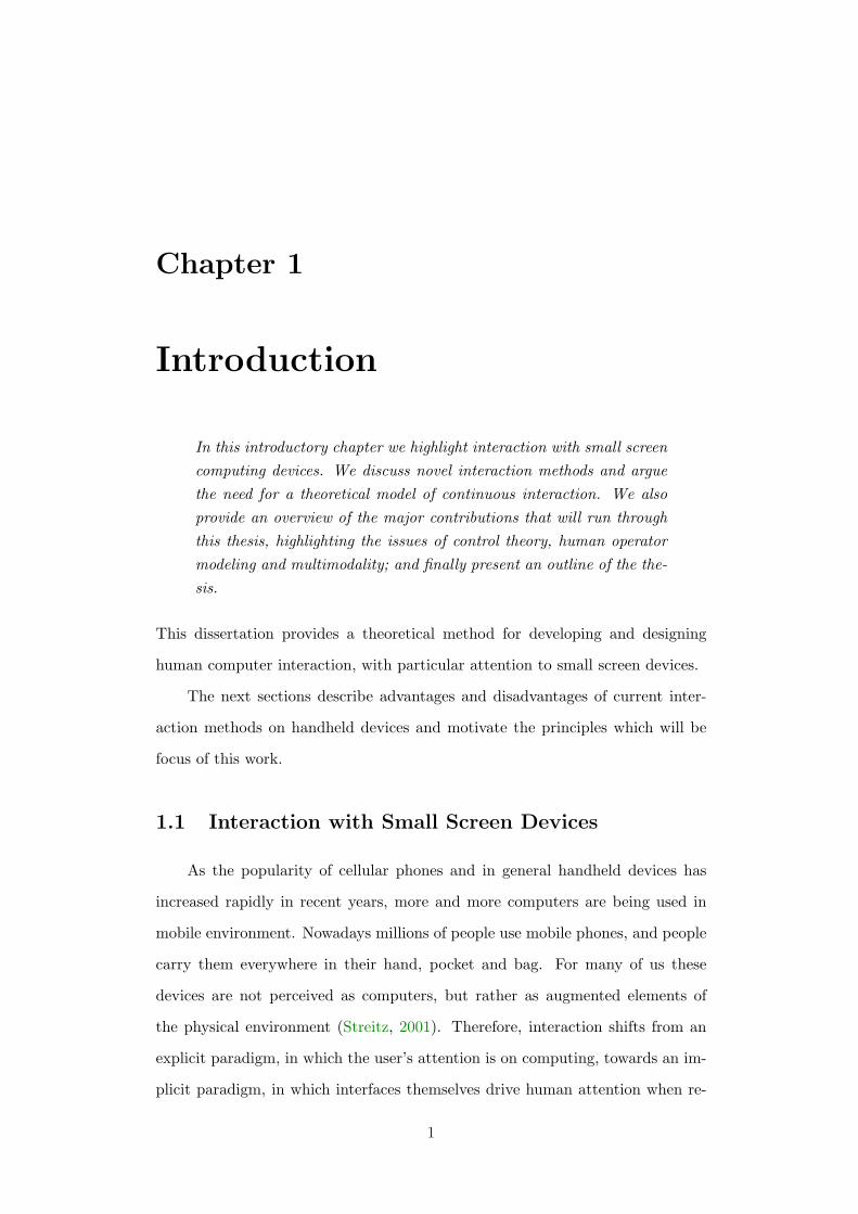
In this introductory chapter we highlight interaction with small screencomputing devices. We discuss novel interaction methods and arguethe need for a theoretical model of continuous interaction. We alsoprovide an overview of the major contributions that will run throughthis thesis, highlighting the issues of control theory, human operatormodeling and multimodality; and finally present an outline of the the-sis.
This dissertation provides a theoretical method for developing and designing
human computer interaction, with particular attention to small screen devices.
The next sections describe advantages and disadvantages of current inter-
action methods on handheld devices and motivate the principles which will be
focus of this work.
1.1 Interaction with Small Screen Devices
As the popularity of cellular phones and in general handheld devices has
increased rapidly in recent years, more and more computers are being used in
mobile environment. Nowadays millions of people use mobile phones, and people
carry them everywhere in their hand, pocket and bag. For many of us these
devices are not perceived as computers, but rather as augmented elements of
the physical environment (Streitz, 2001). Therefore, interaction shifts from an
explicit paradigm, in which the user’s attention is on computing, towards an im-
plicit paradigm, in which interfaces themselves drive human attention when re-
1
1.1 Interaction with Small Screen Devices
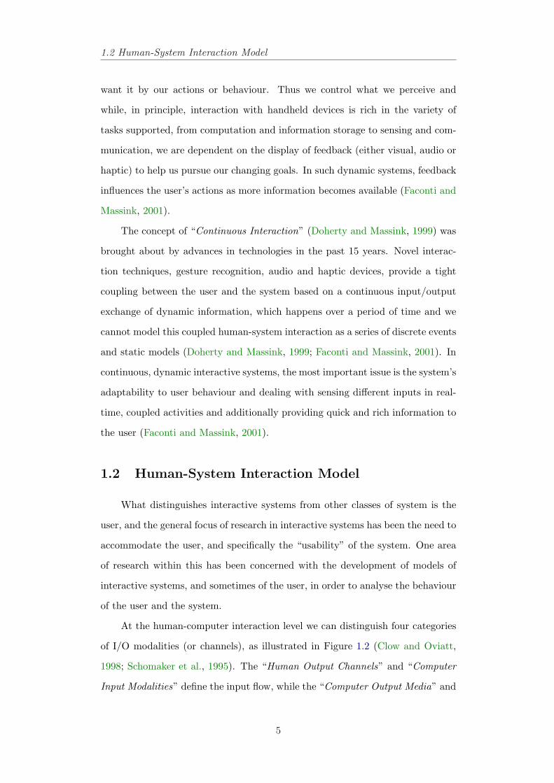
(a) Sony E-Book (b) Palm PilotTM (c) Mobile Phone
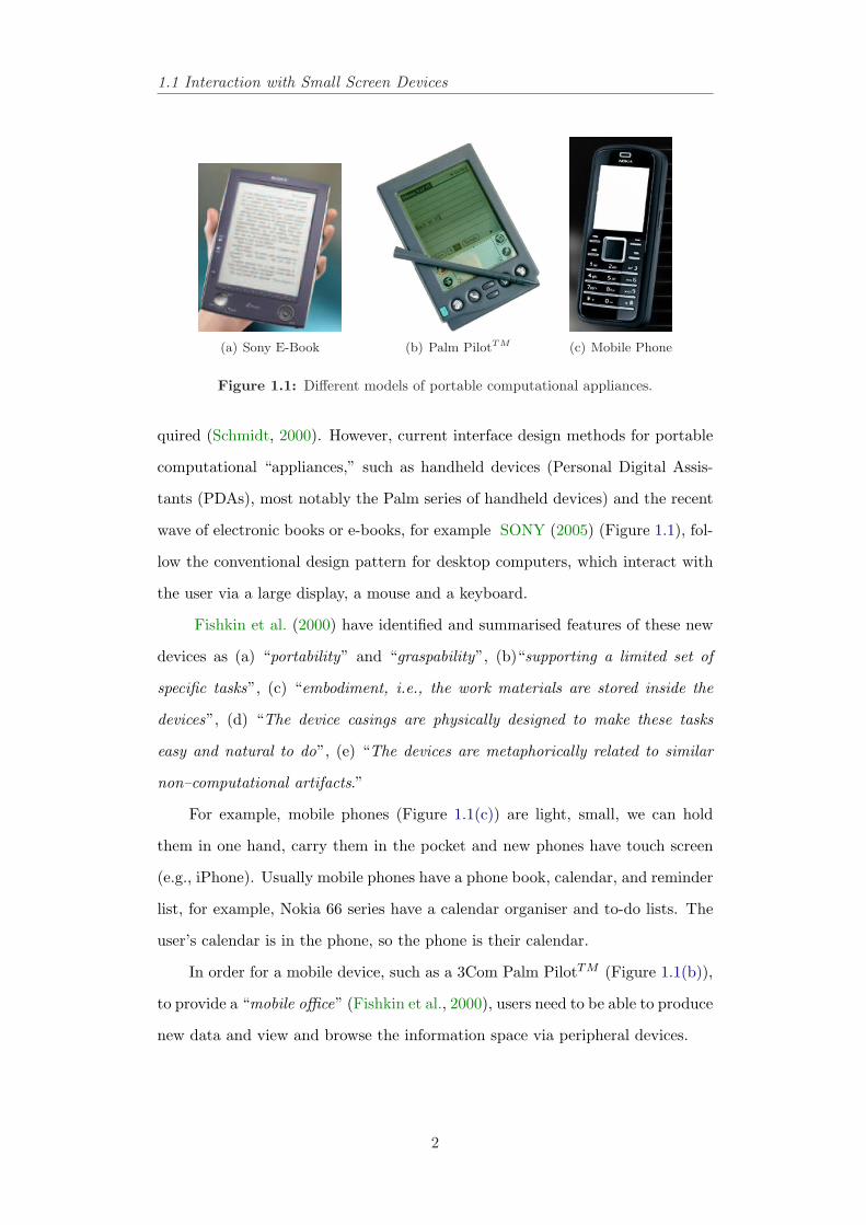
Figure 1.1: Different models of portable computational appliances.
quired (Schmidt, 2000). However, current interface design methods for portable
computational “appliances,” such as handheld devices (Personal Digital Assis-
tants (PDAs), most notably the Palm series of handheld devices) and the recent
wave of electronic books or e-books, for example SONY (2005) (Figure 1.1), fol-
low the conventional design pattern for desktop computers, which interact with
the user via a large display, a mouse and a keyboard.
Fishkin et al. (2000) have identified and summarised features of these new
devices as (a) “portability” and “graspability”, (b)“supporting a limited set of
specific tasks”, (c) “embodiment, i.e., the work materials are stored inside the
devices”, (d) “The device casings are physically designed to make these tasks
easy and natural to do”, (e) “The devices are metaphorically related to similar
non–computational artifacts.”
For example, mobile phones (Figure 1.1(c)) are light, small, we can hold
them in one hand, carry them in the pocket and new phones have touch screen
(e.g., iPhone). Usually mobile phones have a phone book, calendar, and reminder
list, for example, Nokia 66 series have a calendar organiser and to-do lists. The
user’s calendar is in the phone, so the phone is their calendar.
In order for a mobile device, such as a 3Com Palm PilotTM (Figure 1.1(b)),
to provide a “mobile office” (Fishkin et al., 2000), users need to be able to produce
new data and view and browse the information space via peripheral devices.
2
1.1 Interaction with Small Screen Devices
1.1.1 Peripheral Devices for Handheld Devices
While the computational power of portable systems increases for every new
generation being produced, there are still some concerns regarding Human-Computer
Interaction (HCI) issues on these devices. In the literature of Mobile HCI, two
main problems in the usability of mobile devices have been highlighted. First,
text entry methods (i.e., there is still no way of entering text at a reasonable
speed in these devices), second, limited screen size (Fishkin et al., 2000; Harrison
and Fishkin, 1998; Norman, 1998).
The main idea behind the design of the mobile/smart phones is that people
use them as mobile offices (Fallman, 2002b). Hence, users need to enter or edit
text data and browse through a large information space. Large screen devices,
for example desktop computers, provide enough screen space to open and handle
several documents at once, and the keyboard and mouse are used as input tools.
In comparison, small screen devices, for example HP Pocket PCs running win-
dows CE, do not have a physical keyboard and the keyboard has been replaced
by a “stylus” pen and a pressure sensitive screen, which operate a virtual key-
board. The “stylus” pen obscures the small screen, hides the information the
user wants to interact with, and engages both hands. Stylus input of characters
and text recognition algorithms, for example graffiti text entry and hand writing
recognition, are still crucial issues; because they both require the user to adapt
to the device. They are fine for entering small amounts of text in almost every
environment, but as soon as it comes to entering large amounts of text they
are not very satisfactory (Ward et al., 2000; Fallman, 2002b; Williamson and
Murray-Smith, 2005a; Partridge et al., 2002).
Automatic Speech Recognition (ASR) has become an important component
of modern Human-Computer Interface (HCI), appearing as a natural way to in-
teract with computers, improving the ergonomics of man-machine dialogues (Ris
and Couvreur, 2004). However, the integration of accurate ASR is still difficult
on small screen devices. The main problem comes from the hardware and the
processor limitations in mobile phones, which generally have low processor power
whose design rarely takes into account the real-time capabilities necessary for the
3
1.1 Interaction with Small Screen Devices
fast–running algorithms required for automatic speech recognition.
Traditional interaction design methods based on WIMP (Windows-Icon-
Menu-Pointer) for desktop computers cannot be fully employed for portable de-
vices. Therefore, these devices must be able to accept input and provide output
via other means than WIMP. Such a means of achieving this can be gestures and
audio/haptic. Thus, ways of facilitating novel interaction techniques which do
not fully rely on speech recognition or traditional interaction techniques must be
created on portable computing appliances.
1.1.2 Novel Interaction Methods
As described before, portable computing devices have been designed to be
like a mobile office (Fallman, 2002b); Fishkin et al. (2000) argued that
“The physical interaction with [mobile] devices in comparison to apaper artifact, such as a notebook, is still quite limited; we can onlywrite on these devices, but we cannot flip, thumb, bend, and crease itspages. We have highly developed dexterity, skills, and practices withsuch artifacts, none of which are brought to bear on computationaldevices. So, why cannot users manipulate devices in a variety ofways–squeeze, shake, flick, and tilt–as an integral part of using them?”
In the past ten years many researchers have focused on tilt-based inputs and
audio and haptic outputs in Mobile HCIs (Dong et al., 2005; Fallman, 2002a,b;
Harrison and Fishkin, 1998; Hinckley et al., 2005; Oakley et al., 2004; Partridge
et al., 2002; Rekimoto, 1996; Sazawal et al., 2002; Wigdor and Balakrishnan,
2003). The results of these studies have proved that one-handed control of a
small–screen device needs less visual attention than two-handed control, and that
multimodality in the interaction can compensate for the lack of screen space.
Such novel interaction techniques with computers and handheld devices are
examples of interactive dynamic systems, and the development of these systems
explores a range of possible solutions for overcoming some problems of interac-
tion design on computing devices, including the limited sources of input/output
media, adaptability, predictability, disturbances and individual differences. We
should include dynamics because we experience our environment in the way we
4
1.2 Human-System Interaction Model
want it by our actions or behaviour. Thus we control what we perceive and
while, in principle, interaction with handheld devices is rich in the variety of
tasks supported, from computation and information storage to sensing and com-
munication, we are dependent on the display of feedback (either visual, audio or
haptic) to help us pursue our changing goals. In such dynamic systems, feedback
influences the user’s actions as more information becomes available (Faconti and
Massink, 2001).
The concept of “Continuous Interaction” (Doherty and Massink, 1999) was
brought about by advances in technologies in the past 15 years. Novel interac-
tion techniques, gesture recognition, audio and haptic devices, provide a tight
coupling between the user and the system based on a continuous input/output
exchange of dynamic information, which happens over a period of time and we
cannot model this coupled human-system interaction as a series of discrete events
and static models (Doherty and Massink, 1999; Faconti and Massink, 2001). In
continuous, dynamic interactive systems, the most important issue is the system’s
adaptability to user behaviour and dealing with sensing different inputs in real-
time, coupled activities and additionally providing quick and rich information to
the user (Faconti and Massink, 2001).
1.2 Human-System Interaction Model
What distinguishes interactive systems from other classes of system is the
user, and the general focus of research in interactive systems has been the need to
accommodate the user, and specifically the “usability” of the system. One area
of research within this has been concerned with the development of models of
interactive systems, and sometimes of the user, in order to analyse the behaviour
of the user and the system.
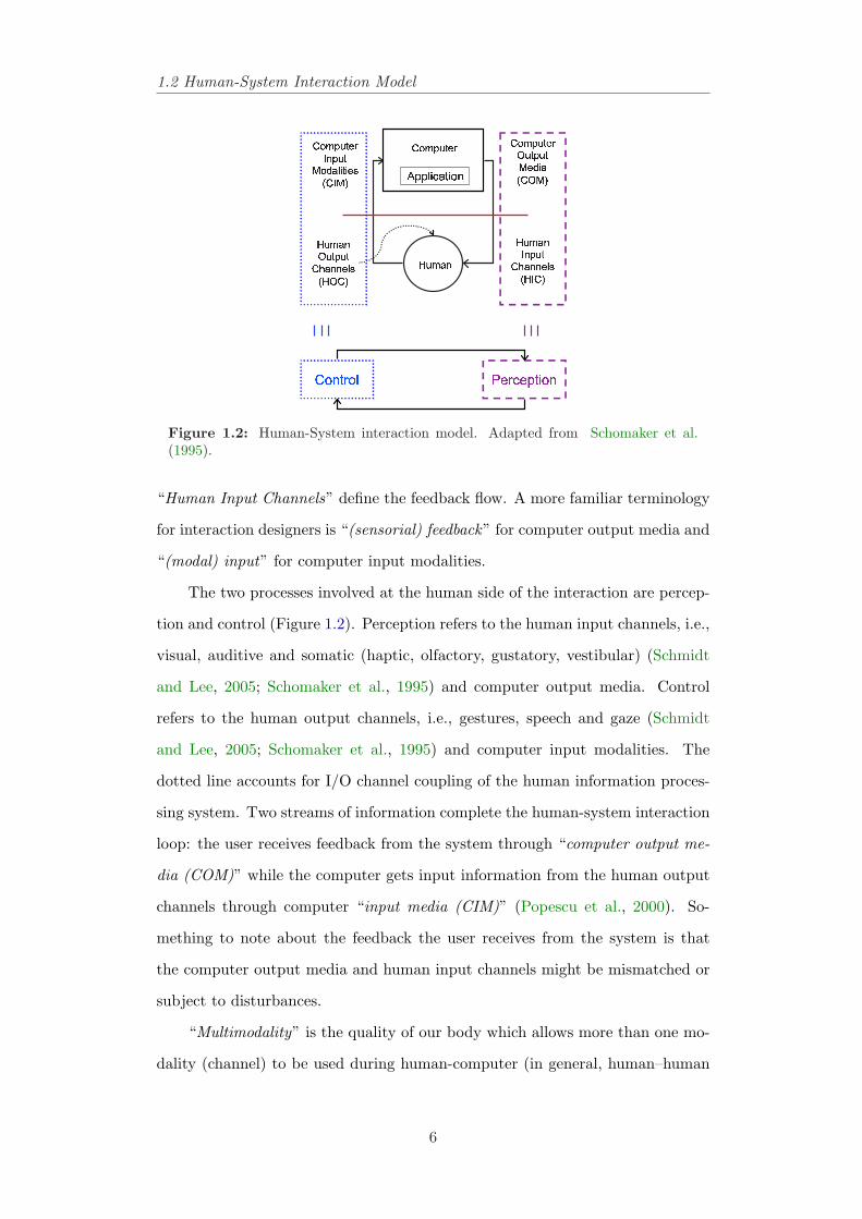
At the human-computer interaction level we can distinguish four categories
of I/O modalities (or channels), as illustrated in Figure 1.2 (Clow and Oviatt,
1998; Schomaker et al., 1995). The “Human Output Channels” and “Computer
Input Modalities” define the input flow, while the “Computer Output Media” and
5
1.2 Human-System Interaction Model
� � � � � � � � � � �
� � � � �� � � �
� � � � �� � � �
� � � �� � � �
� � � � � � �� � � �
� � � �
� � � � �
� � � �� � � �
� � � � � � �� � � �
� � � � �� � � �
� � � � � � � � �� � � �
� � ! " � # $ % " & % ' ! ( �
Figure 1.2: Human-System interaction model. Adapted from Schomaker et al.(1995).
“Human Input Channels” define the feedback flow. A more familiar terminology
for interaction designers is “(sensorial) feedback” for computer output media and
“(modal) input” for computer input modalities.
The two processes involved at the human side of the interaction are percep-
tion and control (Figure 1.2). Perception refers to the human input channels, i.e.,
visual, auditive and somatic (haptic, olfactory, gustatory, vestibular) (Schmidt
and Lee, 2005; Schomaker et al., 1995) and computer output media. Control
refers to the human output channels, i.e., gestures, speech and gaze (Schmidt
and Lee, 2005; Schomaker et al., 1995) and computer input modalities. The
dotted line accounts for I/O channel coupling of the human information proces-
sing system. Two streams of information complete the human-system interaction
loop: the user receives feedback from the system through “computer output me-
dia (COM)” while the computer gets input information from the human output
channels through computer “input media (CIM)” (Popescu et al., 2000). So-
mething to note about the feedback the user receives from the system is that
the computer output media and human input channels might be mismatched or
subject to disturbances.
“Multimodality” is the quality of our body which allows more than one mo-
dality (channel) to be used during human-computer (in general, human–human
6
1.3 A Theory for Designing Interaction
/ environment) interaction. In a multimodal computing system the user controls
and communicates with computers via several modalities such as voice, gesture,
gaze, visual, auditory, and haptic. These new environments are a great challenge
for the future of the Human Computer Interaction studies, specially in portable
computational devices. More senses (vision, hearing and touch) and more means
of expression (gesture, facial expression, eye movement, speech) can be invol-
ved in interaction from the human side with respect to traditional WIMP based
applications (Cohen, 1999; Cohen et al., 1999; Flanagan et al., 1999).
A wide variety of novel sensors, inertial sensors, light and pressure sensors
and many others, create the potential for new methods of interaction with all
range of computing devices and in different contexts. These sensors also have
different information capacities, delays, bandwidths and support different modali-
ties. Designers of interfaces which use these devices need a model to create usable
communication media (CIM and COM) as well as supporting human/device ca-
pacity and human behaviour. Current models are severely limited: for example,
Fitts’ law predicts the time required to rapidly move from a starting position to a
final target area but cannot make any predictions about human behaviour or how
to get to the target. Furthermore, this model is only applied to untrained move-
ments in a single dimension using visual display. Moreover, it is unclear whether
other communication channels, for example audio, are sufficiently similar to the
visual channel for Fitts’ Law to be applicable (Friedlander et al., 1998).
1.3 A Theory for Designing Interaction
Beaudouin-Lafon (2004) has argued:
...if we are to create the next generation of interactive environments,we must move from individual point designs to a more holistic ap-proach. We need a solid theoretical foundation that combines anunderstanding of the content of use with attention to the details ofinteraction, supported by a robust interaction architecture.
This characteristic has been described as “designing interaction” rather than
designing interfaces, which simply means “to control the quality of the inter-
7
1.3 A Theory for Designing Interaction
action between user and computer; because interfaces are the means, not the
end” (Beaudouin-Lafon, 2004).
Physics, chemistry, and in general natural sciences are established on a base
of solid and falsifiable theories to analyse, understand and control a phenome-
non (Beaudouin-Lafon, 2004). Many successful computer interfaces have been
designed and developed based on many experimental tests over a considerable
amount of time but there is no solid and falsifiable theory to generalise those expe-
rimental results even to similar interfaces (Beaudouin-Lafon, 2004; Thimbleby,
1990). Additionally there is no theory of continuous interaction for designing
and developing interfaces based on dynamic systems, continuous technologies
and multimodal integration (Faconti and Massink, 2001).
Currently, there are few theoretical frameworks for interaction. For example,
a few theories in psychology which provide insights into human behaviour have
also been applied in designing interfaces (e.g., Fitts’ law). Also, there are many
physiological models of human body motion (Schmidt and Lee, 2005). These
models are incomplete in that they only focus on the human in the interaction
while the coupling between the user and the system has not been taken into
account. However, models established based on mathematics and dynamics, for
example “control theory” have been overlooked in HCI research.
In 1970 William Powers suggested (Powers, 1989, 1992) that many kinds
of behaviour can be described as continuous control problems, and he showed
that this viewpoint provides a method for the estimation of a subject’s intention
interacting with a computing system. He gave several examples which show that
for identifying controlled variables in an interaction we can apply disturbances,
directly or otherwise, to variables which are under the user’s control. If these va-
riables are corrected by the user after applying disturbances, then those variables
are assumed to be controlled. Based on the solid evidence Powers provides in his
work he argues that “control theory is a theory of behaviour.”
A branch of control theory that is used to analyse human and system beha-
viour when operating in a tightly coupled loop is called manual control theory (Ja-
gacinski and Flach, 2003; Poulton, 1974). The theory is applicable of to a wide
8
1.4 Thesis Aims and Contributions
range of tasks involving vigilance, tracking and stability and creates a framework
for modeling dynamic systems. The general approach followed in manual control
theory is to express the dynamics of the combined human and controlled ele-
ment behaviour as a set of linear differential equations in the time domain, called
state-space modeling (Poulton, 1974). A state space representation is the mathe-
matical realisation of control theory. This representation provides a convenient
and compact way to model and analyse systems with multiple inputs and out-
puts. Also, it can incorporate sensor noise, disturbance rejection, sensor fusion,
changes in input/output devices, and calibration challenges.
Several models include human related aspects of information processing ex-
plicitly such as delays for visual process, motor-nerve latency and neuro-motor
dynamics. Control theory can be linked to Fitts’ Law (Fitts, 1954) by viewing
the pointing movements towards the target as a feedback control loop based on
visual input and the limb as a control element allowing most of Fitts’ law results
to be predicted by a simple control theory (Jagacinski and Flach, 2003).
Machine learning techniques and probability theory can potentially be cou-
pled with control theory to classify and predict user behaviour in the interac-
tion. Probability theory provides theoretical models for the classification of evi-
dence and machine learning techniques provide algorithms for inference (MacKay,
2003). For example, a probabilistic classification of the likelihood of different mo-
dels of user behaviour can be used to alter the dynamics of the controlled system,
rendering the user’s task easier.
Throughout this thesis we use dynamic system and manual control theory as
a theoretical framework for the design and analysis of interaction between human
and system, giving particular attention to instrumented handheld devices with
multimodal feedback.
1.4 Thesis Aims and Contributions
The overall aim of this research is to create an interaction metaphor and
provide a framework that designers can use to model system and user behaviour
9
1.4 Thesis Aims and Contributions
and integrate them into multimodal human-computer interfaces. Additionally,
this framework should be platform free and can be used for all computing devices
from desktop computers to PDAs. This thesis uses manual control theory as a
formal modeling approach to provide appropriate concepts to deal with issues of
continuous interaction, human operator modeling, and human performance data
analysis.
Using the continuous control dynamic system approach and manual control
theory we can simulate the model and observe the behaviour of the system.
This approach makes tuning and calibration a lot easier, especially when we use
a higher degrees of freedom input; because we can find proper settings for the
interface only by observing the behaviour of the simulated system before the
actual implementation and test its stability when coupled with a manual control
model of user behaviour. Using the theory, we can make consistent conceptual
models (Liddle, 1996) using real-world effects such as haptic feedback of springs,
viscous effects linked to motion in the liquid, or friction linked to speed of motion,
which are easy to reproduce in a dynamic system, and we can choose to explicitly
use these features to design the system to encourage interaction to fall into a
comfortable, natural rhythm.
This thus provides a few hidden real “affordances” because the presence
of feedback effects the usability and understandability of the system and lets
the user experience them. The word affordance was invented by the perceptual
psychologist Gibson (1979) to refer to the actionable properties between the world
and an actor (a person or animal). To Gibson, affordances are relationships.
They exist naturally: they do not have to be visible, known, or desirable. For
example, in a tilt-controlled visualisation application running on a PDA, the tilt
sensor allows tilting but this tilting must be a meaningful, useful action, with
a known outcome. The application presents changes in the speed of scroll and
degree of magnification according to tilt angles as a(n) audio/visual output to
the user. Presenting the current status of the controlled variables via audio,
vision or haptic to the user makes their action more clear and the design model
(i.e., how the designer understands how the system works) more visible (Norman,
10
1.5 Thesis layout
1999; Preece et al., 2002). Furthermore while there is a feedback the user can
determine the relationship (mapping) between actions and perceptions (Preece
et al., 2002). Lastly, the natural constraints of human hand motion add some
constraints to the interaction. For example, a roll tilt angle of −200◦ is not a
convenient angle for holding the PDA and looking at the screen.
The dynamic system approach has the potential to provide a very general
framework for the development, analysis and optimisation of interfaces which
induce complex, but convenient coupling among multiple states, in order to cope
with few degrees of freedom in input. This approach concurs with the argu-
ment of Norman (1986) who stated that in an ideal interactive systems three
interacting components, the design model, the system image and the user model,
should map onto each other. The dynamic system approach helps to bring these
three components close together by providing “visibility”, range of “affordances”,
“constraints”, “mappings” and most of all “feedback”.
The theme that runs through the next chapters outlines the fundamentals
of continuous control and manual control theory, and how it can be developed
and extended to multimodal interaction. In the later chapters, we support our
arguments by providing implemented examples from auditory to graphical user
interfaces on handheld devices. The implementations have been specifically cho-
sen to illuminate the most important principles to augment the more limited
approach of, demonstrating only usability that is common in HCI research.
1.5 Thesis layout
The reminder of this thesis is organised as follows:
Chapter 2 introduces a new point of view to the analysis of behaviour pro-
posed by William Powers, discusses the effect of this new definition in psychology
and computing science and some of its applications in interaction design. This
chapter will focus on perceptual control theory and its contribution to motor
control and designing interaction.
Chapter 3 introduces continuous interaction as a requirement of interactive
11
1.5 Thesis layout
systems to support natural human behaviour. The initial sections of this chap-
ter introduces the basic definitions and terms of manual control theory for the
analysis of the continuous aspects of the interface and human behaviour. Subse-
quently it addresses a framework of modeling notations and tools to drive design
decisions during the development of interactive systems. Lastly, this chapter will
consider control inputs for small screen devices.
Chapter 4 outlines model-based sonification and human perception and ac-
tion when s/he is interacting with auditory interfaces on small screen devices
using a tilt sensor. This chapter highlights the pros and cons of different audio
feedback and control strategies in browsing the audio space and one possible way
of improving performance based on models of human control behaviour in few
example applications.
Chapter 5 presents a dynamic system interpretation of the coupling of in-
ternal states involved in speed-dependent automatic zooming (SDAZ), followed
by testing of an implementation on a text browser on a Pocket PC instrumen-
ted with a tilt sensor. This approach to the design of a continuous interaction
interface allows the incorporation of analytical tools to analyse and simulate the
system behaviour before the actual implementation, calibration and tuning of
the parameters, model generalisation and stability testing of the controller when
coupled with a manual control model of user behaviour. It shows that the refe-
rence signal exists in control systems as an input and according to these reference
variables the controller switches among different modes. Also, it is shown that
a model-based sonification approach for the tilt-controlled SDAZ provides a ge-
neral design guideline to add multimodal feedback to the interaction that also
support intermittent interaction.
Chapter 6 introduces a continuous interactive system to support human
behaviour in browsing a multilingual text based on a language model, focus-in-
context method and manual control theory. It is argued that to design interaction
we need models of key aspects of the process, here for example, we need models
for the dynamic system, a probabilistic language model and a probabilistic model
of an audio feedback space as an example of a multimodal approach to sensing
12

1.5 Thesis layout
different languages in a multilingual text. This example illustrates a general fra-
mework, which brings the usefulness of quickened displays and prediction of user
behaviour and the importance of multimodality in the intermittent interaction
scenario, together along with the use of probabilistic model for classifying human
behaviour in browsing tasks.
Chapter 7 concludes the thesis, reviews its contributions and outlines pos-
sible avenues of future work.
13
Chapter 2
Purposeful Behaviour, Motor
Control and Analysing
Interaction
Behaviour is often described as the computation of a response to astimulus (Cisek, 1999). This description is incomplete in an impor-tant way because it only examines what occurs between the receptionof stimulus information and the generation of an action. Powers(1989) has described behaviour as a control process where actions areperformed in order to affect perceptions or actions are motivated byorganic needs and they affect an organism’s perception about theirneeds. This chapter will focus on perceptual control theory and itscontribution to motor control and designing interaction.
2.1 Introduction
To control movement, multi-cell organisms developed a nervous system. This
began when multi-cell organisms began to move. Movement is the only way we
have of interacting with our environment, i.e., shaking hands, eating, drinking.
We communicate with other people using speech, body gestures, and touch. From
this viewpoint, the purpose of the human brain is to use sensory representations
to determine future actions (Wolpert et al., 1999).
Movement takes many forms. Some forms can be classed as genetically defi-
14
2.2 Background
ned movements, such as the way in which people control their limbs or the rapid
eye-blink in response to a strong flashlight (Schmidt and Lee, 2005). A second
form of movements can be described as “learned”– for example, those involved in
controlling a car or operating a typewriter. These learned movements are often
termed “skills”. They are not inherited and require long periods of practice and
experience to be acquired (Schmidt and Lee, 2005). Skills are especially critical
to the study of human behaviour, as they are involved in operating machines in
industry, controlling vehicles, playing games, and so forth.
In this thesis we consider only the second category of movements or skills.
We will be concerned with how these movements are controlled and can be mo-
deled in interactive tasks with computing systems. Thus, in this chapter we look
at the definition of motor control, the theory of living systems’ behaviour as a
theory of system control and human behaviour and its contribution to perceptual
control theory. The following section provides key definitions before progressing
on to the detailed exposition of the control paradigm.
2.2 Background
This section introduces definitions for “motor control”, “control” and “be-
haviour” and their contribution to control systems.
2.2.1 What is Motor Control?
Brooks (1986) defines motor control as “the study of posture, movement
and functions of the mind and body that govern posture and movement.” Thus,
motor control models the complexity of any movement we perform for any task,
for instance how we sit down, or walk.
2.2.2 What is Control and Control Systems?
Marken (1995b) has described control as “the process of producing consistent
results in the face of unpredictable disturbances.” So any simple task, for example
keeping a car in a lane in a highway on a windy day, is a control process. Control
15
2.2 Background
refers to both a phenomenon and the theory designed to explain it.
Control systems are systems that control their actions or control what they
perceive through their sensory systems. Thus we can classify all living orga-
nisms (and some non-living artifacts, such as thermostats) in the class of control
systems (Marken, 1995b).
2.2.3 What is Behaviour?
Millikan (2002) defines behaviour as a biological function, which is “fulfilled
normally via mediation of the environment, or via resulting alterations in the
organism’s relation to the environment.” This definition distinguishes behaviour
from physiological processes and allows other ways of interaction, which does not
involve movement, to be behaviour, for example, emission of sounds, pheromone,
changes of colour and so forth. Also, if human purposes are a species of biologi-
cal purposes or proper functions, then human actions are behaviours (Millikan,
2002).
In spite of behaviour’s diversity, however, there is one obvious , and often
ignored, characteristic of most behaviour: it repeats (Marken, 2002). The events
that are labeled behaviour based on the definition presented by Millikan (2002)–
lifting, walking, eating, writing– happen over and over again: there is regularity.
Scientific psychology is built on the assumption that behaviour is output but
Powers (1989, 1992) has argued that “behaviour is not output but a controlled
consequence of input: behaviour is control.” Behaviour is control because the
events called behaviour are consistent results of continuously changing effects
produced, simultaneously, by the organism and the environment (Powers, 1989,
1992, 2005) and control theory is an explanation of the phenomenon of control,
which is now called Perceptual Control Theory (PCT). In the following section we
look at the basic structure of controlled systems and their important functions,
using riding a bicycle as an illustrative example.
16
2.3 The Control System Architecture
� � � � � � � � � � � � � � � �
� � � � � � � � � � � � � � � � �
� � � � � �
� � � � � � � �� � � � � � �
� � � � � � � � � �
� � � � � � � �
� � � � � �
� � � � � � � �
� � � � � �
� � � � � � � � � � � �
� � � �� � � � �
� � � � � � � � � �� � � � � � � � � � � � � � � �
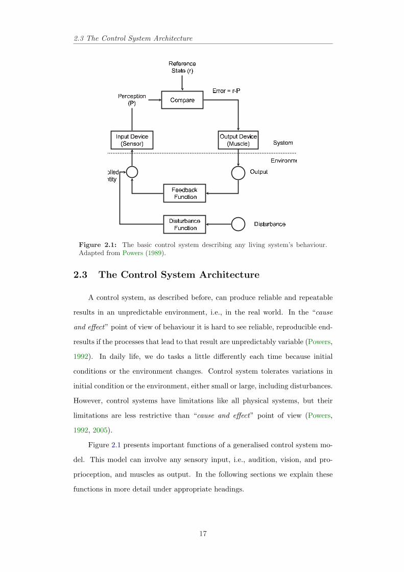
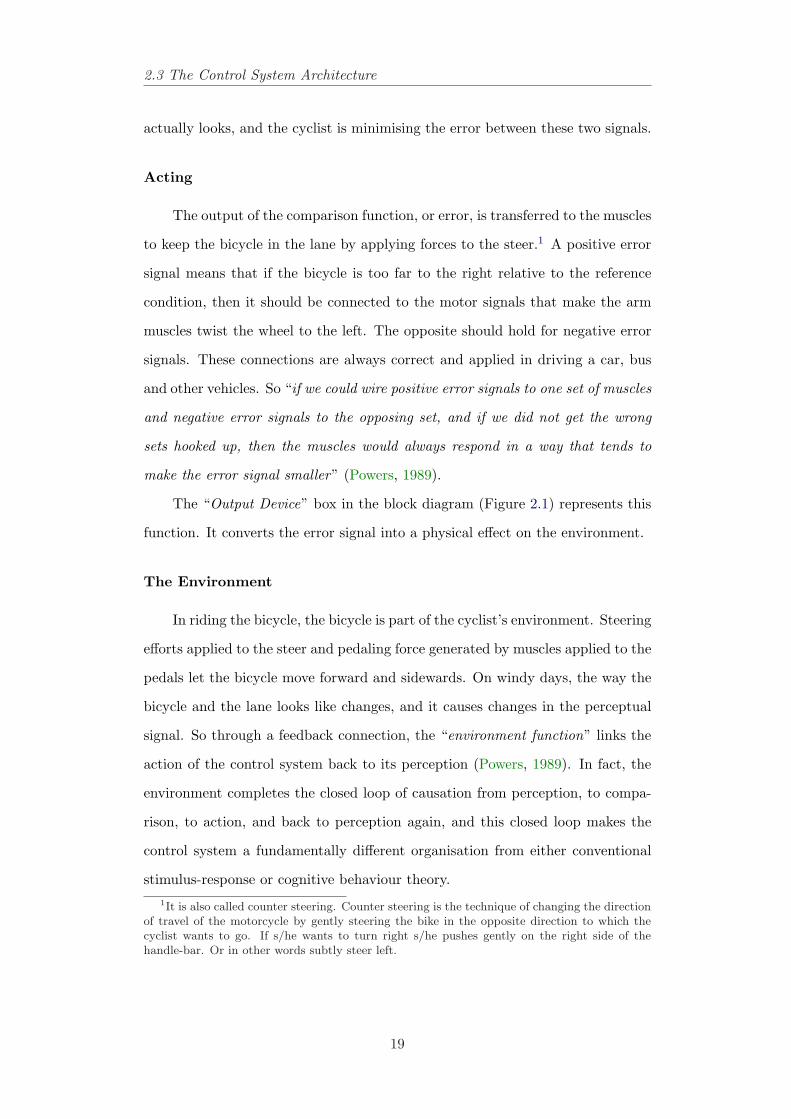
Figure 2.1: The basic control system describing any living system’s behaviour.Adapted from Powers (1989).
2.3 The Control System Architecture
A control system, as described before, can produce reliable and repeatable
results in an unpredictable environment, i.e., in the real world. In the “cause
and effect” point of view of behaviour it is hard to see reliable, reproducible end-
results if the processes that lead to that result are unpredictably variable (Powers,
1992). In daily life, we do tasks a little differently each time because initial
conditions or the environment changes. Control system tolerates variations in
initial condition or the environment, either small or large, including disturbances.
However, control systems have limitations like all physical systems, but their
limitations are less restrictive than “cause and effect” point of view (Powers,
1992, 2005).
Figure 2.1 presents important functions of a generalised control system mo-
del. This model can involve any sensory input, i.e., audition, vision, and pro-
prioception, and muscles as output. In the following sections we explain these
functions in more detail under appropriate headings.
17
2.3 The Control System Architecture
� � �
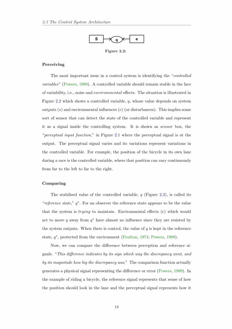
Figure 2.2:
Perceiving
The most important issue in a control system is identifying the “controlled
variables” (Powers, 1989). A controlled variable should remain stable in the face
of variability, i.e., noise and environmental effects. The situation is illustrated in
Figure 2.2 which shows a controlled variable, q, whose value depends on system
outputs (s) and environmental influences (e) (or disturbances). This implies some
sort of sensor that can detect the state of the controlled variable and represent
it as a signal inside the controlling system. It is shown as sensor box, the
“perceptual input function,” in Figure 2.1 where the perceptual signal is at the
output. The perceptual signal varies and its variations represent variations in
the controlled variable. For example, the position of the bicycle in its own lane
during a race is the controlled variable, where that position can vary continuously
from far to the left to far to the right.
Comparing
The stabilised value of the controlled variable, q (Figure 2.2), is called its
“reference state,” q∗. For an observer the reference state appears to be the value
that the system is trying to maintain. Environmental effects (e) which would
act to move q away from q∗ have almost no influence since they are resisted by
the system outputs. When there is control, the value of q is kept in the reference
state, q∗, protected from the environment (Poulton, 1974; Powers, 1989).
Now, we can compare the difference between perception and reference si-
gnals. “This difference indicates by its sign which way the discrepancy went, and
by its magnitude how big the discrepancy was.” The comparison function actually
generates a physical signal representing the difference or error (Powers, 1989). In
the example of riding a bicycle, the reference signal represents that sense of how
the position should look in the lane and the perceptual signal represents how it
18
2.3 The Control System Architecture
actually looks, and the cyclist is minimising the error between these two signals.
Acting
The output of the comparison function, or error, is transferred to the muscles
to keep the bicycle in the lane by applying forces to the steer.1 A positive error
signal means that if the bicycle is too far to the right relative to the reference
condition, then it should be connected to the motor signals that make the arm
muscles twist the wheel to the left. The opposite should hold for negative error
signals. These connections are always correct and applied in driving a car, bus
and other vehicles. So “if we could wire positive error signals to one set of muscles
and negative error signals to the opposing set, and if we did not get the wrong
sets hooked up, then the muscles would always respond in a way that tends to
make the error signal smaller” (Powers, 1989).
The “Output Device” box in the block diagram (Figure 2.1) represents this
function. It converts the error signal into a physical effect on the environment.
The Environment
In riding the bicycle, the bicycle is part of the cyclist’s environment. Steering
efforts applied to the steer and pedaling force generated by muscles applied to the
pedals let the bicycle move forward and sidewards. On windy days, the way the
bicycle and the lane looks like changes, and it causes changes in the perceptual
signal. So through a feedback connection, the “environment function” links the
action of the control system back to its perception (Powers, 1989). In fact, the
environment completes the closed loop of causation from perception, to compa-
rison, to action, and back to perception again, and this closed loop makes the
control system a fundamentally different organisation from either conventional
stimulus-response or cognitive behaviour theory.1It is also called counter steering. Counter steering is the technique of changing the direction
of travel of the motorcycle by gently steering the bike in the opposite direction to which thecyclist wants to go. If s/he wants to turn right s/he pushes gently on the right side of thehandle-bar. Or in other words subtly steer left.
19
2.4 Interaction Model and Motor Control
The Disturbance
Controlled variables are affected not only by the actions of the control system
via a closed loop of action and perception, but also by other influences. For
example, only the position of the bicycle in its lane is affected by anything that
can apply a sideward force to it, like a wind or a ramp in the road. In Figure 2.1,
the sum of all such independent effects has been presented as a single equivalent
disturbance, and it affects directly the controlled variable. “No model of a control
system is complete without a representation of the disturbance, because it is the
way actions vary in response to disturbances that provides strong evidence that
we are dealing with a control system” (Powers, 1989).
In this section we provided a general and basic structure for the controlled
systems using a bicycle as an example. This simple example can be extended to
computing devices (which will be discussed in more detail in Chapter 3). With
computers, humans are no longer exposed to the physical world governed by
the laws of physics, however we can make consistent “conceptual models” using
real-world effects based on pseudo–physical models.
2.4 Interaction Model and Motor Control
One important issue in the interaction design is that the interface should
match with the users’ capabilities or conceptual models.
2.4.1 Conceptual Models
In Chapter one we discussed a need for a solid and falsifiable methodology
for designing interaction. As Liddle has highlighted (Liddle, 1996),“the most im-
portant thing to design is the user’s conceptual model. Everything else should be
subordinated to making that model clear, obvious and substantial.” By a concep-
tual model he meant:
...a description of the proposed system in terms of a set of integratedideas and concepts about what it should do and look like, that will beunderstandable by the users in the manner intended (Preece et al.,2002).
20
2.4 Interaction Model and Motor Control
One popular way of describing conceptual models is in terms of interaction me-
taphors. By this is meant a conceptual model that has been developed to be
similar in some way to aspects of a physical entity (or entities) but that also has
its own behaviours. Such models can be based on an activity or an object or
both, for example spreadsheets and search engines (Preece et al., 2002). The
search engine tool has been designed to invite comparison with a physical object
– a mechanical engine with several parts working – together with an everyday
action – searching by looking through numerous files in many different places to
extract relevant information (Preece et al., 2002).
Dynamic control theory models the conceptual approach a user brings to an
interaction based on pseudo-physical models which are familiar to the user from
real-world effects such as the haptic feedback of springs, viscous effects linked to
motion in the liquid, friction linked to speed of motion, or weight of mass which
are easy to reproduce in a dynamic system as a set of mass-spring-damper. These
models provide a general framework for guiding designers and developers to create
interactive systems. Unlike ergonomic rules, which are not conceptual and are
often limited to post-hoc evaluation of a design, these interaction models are
usable from the early stages of the design and the final behaviour of the model
can be simulated and observed before the actual implementation and is therefore
proactive.
2.4.2 Instrumental Interaction
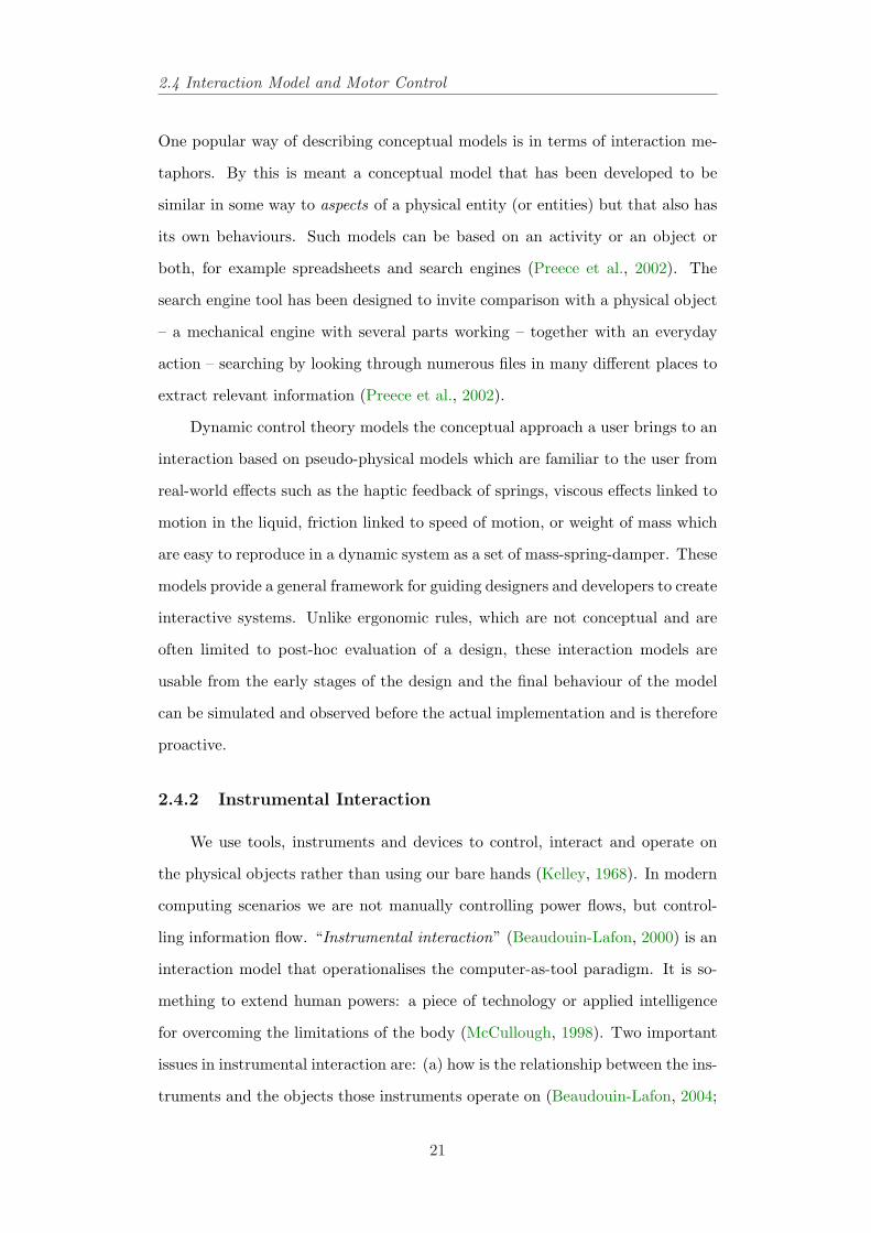
We use tools, instruments and devices to control, interact and operate on
the physical objects rather than using our bare hands (Kelley, 1968). In modern
computing scenarios we are not manually controlling power flows, but control-
ling information flow. “Instrumental interaction” (Beaudouin-Lafon, 2000) is an
interaction model that operationalises the computer-as-tool paradigm. It is so-
mething to extend human powers: a piece of technology or applied intelligence
for overcoming the limitations of the body (McCullough, 1998). Two important
issues in instrumental interaction are: (a) how is the relationship between the ins-
truments and the objects those instruments operate on (Beaudouin-Lafon, 2004;
21
2.4 Interaction Model and Motor Control
Perceptual
Information
Modulated
Power(muscular)
Man Controlled Variable
Feedback Information
Perceptual
Information
Modulated
Power(muscular)
Man Controlled Variable
Feedback Information
(a)
Man Controlled Variable
Feedback Information
ToolPerceptualInformation
Man Controlled Variable
Feedback Information
ToolPerceptualInformation
(b)
PerceptualInformation
Man
Controlled Variable
Feedback Information
ToolControl
Junction
Modulated
Power(muscular)
Power
Source
Power
Control
Signal
PerceptualInformation
Man
Controlled Variable
Feedback Information
ToolControl
Junction
Modulated
Power(muscular)
Power
Source
Power
Control
Signal
(c)
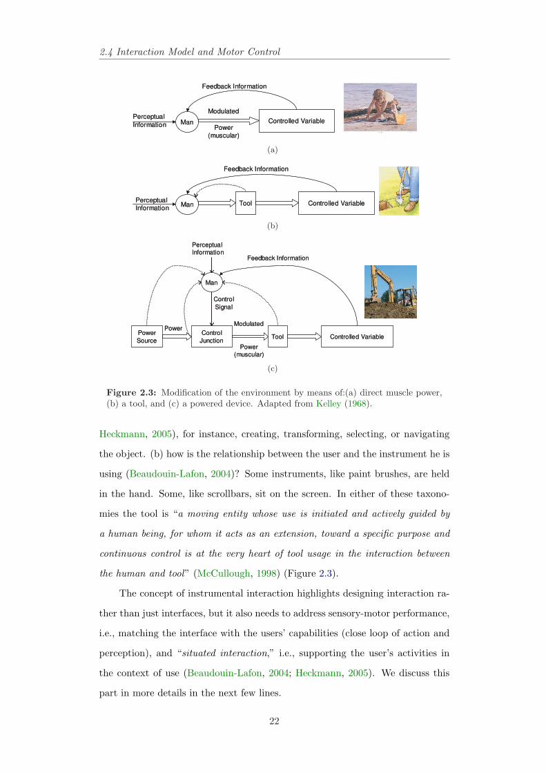
Figure 2.3: Modification of the environment by means of:(a) direct muscle power,(b) a tool, and (c) a powered device. Adapted from Kelley (1968).
Heckmann, 2005), for instance, creating, transforming, selecting, or navigating
the object. (b) how is the relationship between the user and the instrument he is
using (Beaudouin-Lafon, 2004)? Some instruments, like paint brushes, are held
in the hand. Some, like scrollbars, sit on the screen. In either of these taxono-
mies the tool is “a moving entity whose use is initiated and actively guided by
a human being, for whom it acts as an extension, toward a specific purpose and
continuous control is at the very heart of tool usage in the interaction between
the human and tool” (McCullough, 1998) (Figure 2.3).
The concept of instrumental interaction highlights designing interaction ra-
ther than just interfaces, but it also needs to address sensory-motor performance,
i.e., matching the interface with the users’ capabilities (close loop of action and
perception), and “situated interaction,” i.e., supporting the user’s activities in
the context of use (Beaudouin-Lafon, 2004; Heckmann, 2005). We discuss this
part in more details in the next few lines.
22
2.4 Interaction Model and Motor Control
Situated Interaction
The definition of situated interaction depends on the interaction model. For
example, in the desktop computing devices, a user interacts locally with a com-
puter, but in the mobile computing devices, a mostly moving user interacts with
a small portable device and has to cope with various contextual distractions, for
example ambient noise. The goal in situated interaction is to combine a range of
techniques for designing interactive systems that are better adapted (and adap-
table) to their context of use. It also provides a range of physical and perceived
affordances which can be discovered by the user via feedback and a mutual re-
lationship between the perception and action (McCullough, 2001). For example
many objects in everyday environments possess inherent degrees of freedom that
have to be actuated to perform their function. Such objects include door handles,
doors, drawers, and a large number of tools, such as scissors and pliers (Katz and
Brock, 2007; Thimbleby, 2001).
2.4.3 Examples from HCI
As discussed in Section 2.4.2, we use tools to control. A software tool gives
visible form and physical action to a logical operation. Like a physical tool it
modifies the effect of the hand, which it accomplishes by modifying the functio-
nality of the visible cursor that we operate with the physical pointing device (i.e.,
the mouse). For example, a paint software tool offers pencils, brushes, and so
forth for applying colour to a surface. This plays on the fact that a tool can be
conceptual, and indirectly controlled. Whether direct or indirect, what matters
is manipulation (Beaudouin-Lafon, 2000, 2004; McCullough, 1998).
Selection without the use of pointing is of particular interest because of
challenges faced in designing interaction with hand-held devices and wearable
computers, where input and output are often limited, or only unconventional
means of interaction are available. These devices might be instrumented with
sensors for which pointing may not be a natural method of selection, (e.g., acce-
lerometers), or may have displays (such as audio displays) that are not suited to
pointing. The display may also just be too small to allow convenient pointing.
23
2.4 Interaction Model and Motor Control
Dasher is an information-efficient text-entry interface, driven by natural conti-
nuous pointing gestures. Moreover, Dasher is a competitive text-entry system
wherever a full-size keyboard cannot be used (Ward, 2001; Ward et al., 2000).
Dasher offers a dynamic selection technique based on continuous one dimensional
movement. Dasher is a very efficient entry system, especially where control is
difficult, or the language or other structure is unfamiliar, however the dynamic
layout of letters reduces the opportunity for learning highly optimised strategies
for entry, and requires continuous attention to control.
Williamson and Murray-Smith (2004b),(Williamson, 2006; Williamson et al.,
2007) designed an example interface built on methods from perceptual control
theory and dynamic systems. They presented a method for performing selec-
tion tasks based on the continuous control of multiple, competing agents who
try to determine the user’s intentions from their control behaviour without re-
quiring an explicit, visible pointer. In this example, there are several objects
on the screen and each object has a position to which a small white noise is
added (disturbance) and the displayed position of the object is the sum of the
object’s position and the mouse position. The variance of this sum and the va-
riance of the object’s position in each time step is calculated. The probability of
each object i being selected is the ratio of the variance of the sum the object’s
position and the mouse position to the variance of the object’s position. The
object with higher probability is selected. These methods are close to those used
in perceptual control theory, proposed by Marken (1995b) and Powers (1989).
This earlier work suggested that many kinds of behaviour can be described as
continuous control problems, and Powers proposed that this viewpoint provides
an empirical method for the estimation of a subject’s intention. This can be done
by designing an experiment to identify which variables the subject is controlling,
by introducing changes (disturbances in control theory nomenclature), directly
or otherwise, to variables which are under the subject’s control. Variables for
which disturbances are corrected are assumed to be controlled by the subject.
Furthermore, there is an evidence that correct display of uncertainty lead to
appropriately regularised control behaviour in human motor control, in reaching
24
2.5 Modeling Perceptual-Motor Performance
and targeting actions. For example, Kording and Wolpert (2004) showed that
in a target acquisition task, where a disturbance was artificially added to the
user’s control input, uncertain display (Gaussian point clouds) lead to behaviour
that was consistent with Bayesian integration of the uncertain sensory inputs
and prior beliefs about the system. Modeling human operator, such as those
proposed in (Jagacinski and Flach, 2003), which incorporate Kalman filters imply
that uncertainty is modeled in user control behaviour.
2.5 Modeling Perceptual-Motor Performance
From the literature on perceptual-motor performance (Powers, 1989, 1992,
2005; Schmidt and Lee, 2005), the time taken for the user to complete a task in
response to a stimulus is divided into three components: (a) “perceptual delay,”
which is the time taken by the user to notice that the stimulus has occurred. It is
also affected by the modality, for example, audio, vision or tactile, (b) “decision
making time”, which is based on both the number of possible stimuli, and on
the possible responses to the stimulus, (c) “movement time”, which is the time
taken by the user to carry out the response which will be described later in this
section. It is this movement time which many HCI studies focus on.
2.5.1 Movement Time
“Movement time is the time from response initiation to the end of the res-
ponse”(Schmidt and Lee, 2005). Here, speed of movement becomes important.
One of important functions in the movement time is the “speed–accuracy” trade–
off function and is considered in situations in which the goal is to move a limb
(or some other effectors) as quickly as possible to achieve a target, doing so with
a minimum number of errors (Schmidt and Lee, 2005). For example, typing,
moving a mouse-driven cursor to a desktop icon, and numerous other activities
that require rapid movements to push, touch, or displace an object.
A very well known, and widely applied rule for the estimation of motor time
is Fitt’s Law:
25
2.5 Modeling Perceptual-Motor Performance
2.5.2 Fitts’ Law
Fitts’ law models human movement and predicts the time required to rapidly
move from a starting position to a final target area, as a function of the distance
to the target and the size of the target. This model was introduced by Paul Fitts
(1954), and many researches since then have been carried out in applying Fitts’
law to evaluate the human-computer interfaces.
Fitts’ law in its general form, sometimes called the Shannon formulation
(MacKenzie and Ware, 1993), states a logarithmic relationship between the mo-
vement time to the target and the ratio of the distance to the target to the size
of the target.
MT = a + b log2(D
W+ 1) (2.1)
where MT is the average time taken to complete the movement, a and b are
empirical constants, and can be determined by fitting a straight line to measured
data, D is the distance from the starting point to the centre of the target, W is
the width (size) of the target.
ID = log2(DW +1) is the index of difficulty (measured in bits), the amount of
information necessary to specify the target width (W ) relative to the distance (D)
to be covered. From the equation, we see a speed-accuracy tradeoff associated
with pointing, whereby targets that are smaller and/or further away require more
time to acquire (Jagacinski et al., 1980; MacKenzie and Ware, 1993).
Is Fitts’ Law successful in all HCI application?
Fitts’ law is a well-studied model of human psychomotor behaviour (Bootsma
et al., 2004; MacKenzie, 1991). Fitts’ law’s first HCI application was by Card
et al. (1978), who used the index of performance (IP = 1b ) to compare the perfor-
mance of different input devices, with the mouse coming out on top. Fitts’ law
has been shown to apply under a variety of conditions (a, b, and IP have different
values under each of conditions), with many different limbs (hands, feet, head-
mounted sights, eye gaze), different input devices (mouse, joystick, track-ball,
keyboard, etc), different users (young, old, and mentally disabled).
26
2.5 Modeling Perceptual-Motor Performance
Recently, several researchers have tried to “beat Fitts’ law” or obtain a
better pointing performance than in the real world. For example, McGuffin and
Balakrishnan (2002) show that when the target expands as the cursor approaches
it, the performance depends on the target’s final size even when the target only
begins expanding as late as after 90% of the distant to the target. An example
of expanding targets is MacOS dock (Apple, 2002), however Zhai et al. (2003)
show that relative motion of the targets makes targeting difficult. “Semantic
pointing” or manipulating the control-display ratio was introduced by Blanch
et al. (2004). They argued that the visual size of targets can be independent
from their size in motor space. A visually-small target can be made easier to
point to, for example, without the user even noticing the manipulation. In a joint
work Beaudouin-Lafon and Guiard (Guiard et al., 2001), have pushed the limits
of Fitts’ law even further. Pointing with one’s arm in physical space is limited
to an index of difficulty of about 10 bits (1mm at a 1m distance). However, on
a computer, and with the help of zooming, one can point to targets that are
arbitrarily small at an arbitrarily-long distance.
Fitts’ law has proven to be an invaluable tool in studying interaction as a
sensory-motor phenomenon (Beaudouin-Lafon, 2004). This model is restricted,
however, because it has been designed to evaluate pointing actions in a single
dimension of movement not in two dimensions (MacKenzie and Buxton, 1992);
Additionally tt describes untrained movements only, not skilled movements. It
is also unclear whether for auditory interfaces this communication channel is
sufficiently similar to the visual channel for Fitts’ Law to apply (Friedlander
et al., 1998). With visual feedback, the user is constantly aware of the exact
position of the target. In contrast there is no analogy in the non-visual model.
With auditory feedback, the user can only approximate the position of the target;
given the distance s/he has already moved the pointer and the speed at which
the pointer is moving (see Chapter 4).
Aside from these drawbacks, Fitts’ law remains one of the most reliable
human-computer interaction predictive models, joined more recently by the Accot-
Zhai steering law (Accot and Zhai, 1997, 1999, 2001, 2002), which is derived from
27
2.6 Fitts’ Law and Control Theory
Fitts’ law. There are other laws in interaction design, for example Hick’s law or
the Hick-Hyman law (Hick, 1952; Hyman, 1953), Moore’s law (Moore, 1965),2
Tesler’s law3 and Poka-Yoke principle (Shingo, 1986),4 but few studies have been
done to apply them in human-computer interaction.
2.6 Fitts’ Law and Control Theory
Fitts’ Law uses the logic of information theory to account for both movement
time and the associated error rates (Mackinlay et al., 1991). The speed-accuracy
tradeoff seen for continuous movements is qualitatively very similar to that seen
for reaction times (MacKenzie and Ware, 1993). This suggests that using the
information statistic taps into an invariant property of the human controller.
Also, Fitts’ model of movement time uses an information metric. This metric is
very useful for characterising the noise properties of a communication channel.
The arm is viewed as a channel through which an intention to move to a specific
location is communicated. The output variability reflects the signal-to-noise pro-
perties of the communication channel. However, the problem with this metaphor
is that it ignores kinematics. Kinematics is a branch of dynamics that deals with
aspects of motion apart from considerations of mass and force (Webster dictio-
nary definition). It provides a description of the movement, independent of the
forces that causes the movement.
Crossman and Goodeve (1983) were among the first researchers to consider
control theoretic descriptions as an alternative to Fitts’ information theoretic
model of human movements. They described a first order continuous control
system where the instantaneous velocity is proportional to the current error (i.e.,
the distance left to traverse). The settling time for this system yields Fitts’2Moore’s law is extended to wireless hardware on mobile devices. Hardware components in
such devices have been decreasing in size considerably and can nowadays be placed on smallmicrophones. As the size gets smaller the traditional interaction design techniques become moredifficult to be fully applied on small computing appliances.
3For any process there is a base level of complexity that is inherent to that process. Oncethe designer hits that base, he cannot simplify the process anymore.
4Poka-Yoke principle roughly means “mistake-proofing,” or designing constraints into pro-ducts that prevent users from making mistakes–and ultimately into influences, or approachessuch as Direct/Indirect Manipulation, Feedback/Feed-forward.
28
2.6 Fitts’ Law and Control Theory
law. Jagacinski and Flach (2003) explain and illustrate it fully with respect to
movement time. That both the limited capacity communication channel and
the first-order lag metaphors are equivalent when modeling the data from Fitts’
experiments. However the first-order lag is a stronger model, because there are
more ways to falsify it. The first-order lag predicts the time history of the
movement time. Thus, this model can be rejected if the time histories for human
movements differ in significant ways from those that would be generated by the
first-order lag. The information-processing channel metaphor does not make any
predictions about time histories.
Langolf et al. (1976) describe a second-order underdamped control system
whose settling time also corresponds to Fitts’ law. In addition, Langolf et al.
(1976) describe a discrete response model, originally developed by Crossman and
Goodeve (1983). Jagacinski and Flach (2003) (chapter 6) show the second-order
system can be used to predict Fitts’ Law and for validity checking.
Bootsma et al. (2004) compared Fitts’ law with continuous control models.
They realised changes in ID (see Section 2.5.2 on page 26) give rise to systematic
changes in the kinematics patterns that determine MT in Fitts’ law tasks. In
a reciprocal aiming task, participants produced a series of back-and-forth mo-
vements between targets with different index of difficulties (IDs). The resulting
pattern of movement had a continuous, sinusoidal form: The movement pattern
was harmonic in low IDs. When task difficulty increased, systematic deviations
from harmonicity came to the fore. Over the past few years, Bootsma et al.
(2004) explored the typical pattern of change in the kinematic forms, as found in
a variety of settings, and sought to capture its characteristics through dynami-
cal systems modeling. In their experiments averaging over (half) cycles allowed
detection of the regularities in the pattern of movements produced. They develo-
ped a method of analysis based on both qualitative inspection and quantification
of the forms produced. Portraying the data, Hooke and Phase portraits, (after
averaging over consecutive cycles) proved to be particularly useful and, Bootsma
et al. (2004) introduced them using a pure sinusoidal signal as an exemplary case.
They concluded that observation of the shape of the Hooke portrait of a signal
29
2.7 Conclusions and Summary
allows an assessment of the nature of the dynamics that may be hypothesised
to underlie the movements observed. It is with this logic that they addressed
the patterns observed in a reciprocal aiming task under different levels of task
difficulty. They showed that a limit-cycle model captures all these changes and
provided further evidence for the organising role of the informational flow in task
space by differentially manipulating task space and effector space.
These theoretical and empirical findings about the predicting the time-
histories of the movement time and the structure of the aimed movement are
also applicable to human-computer interaction to improve the efficiency of the
interface.
2.7 Conclusions and Summary
Studying interaction at the level of a sensory-motor phenomenon has led to
important advances in HCI, for example Fitts’ Law provided a scientific basis to
evaluate the performance of interaction techniques. However, these results must
be taken with care since they are easy to misuse or overgeneralise (Gibson, 1979;
Norman, 1999). Controlled experiments only simulate real situations and they
run in a restricted environment and take into account only untrained movements
in order to operationalise the phenomenon being observed.
This chapter argues that computer as a tool extends human powers and
continuous control is at the very heart of tool usage in the interaction between the
human and tool. Yet the applications of control theory in designing interaction
are still considered novel and, to some, revolutionary (Powers, 1989).
A control system can produce reliable and repeatable results in an unpre-
dictable environment. Control theory can model human information processing
and is an analytical tool for partitioning and modeling human performance (Ja-
gacinski and Flach, 2003). Consistent behaviour patterns are created by variable
acts, and generally repeat only because detailed acts change. The stimulus-
response tradition is incapable of dealing with such novel situations.
Control theoretic analysis is able to model movement time with the same ac-
curacy as information theory (Bootsma et al., 2004; Jagacinski and Flach, 2003).
30

2.7 Conclusions and Summary
However, control theory allows predictions about the space-time properties of
movements that cannot be addressed using information statistics. The language
of control theory also provides a perspective for looking at the world in a way
that enhances our appreciation and understanding of the dynamic coupling of
perception and action with biological systems. The essentials of the theory as
will be discussed in more details in the following chapter are simple but “this
does not mean control theory deals only with simple behaviour. Control theory is
a theory of behaviour” (Marken, 1995a).
31
Chapter 3
Continuous Interaction and
Human Behaviour Control
This chapter introduces continuous interaction as a requirement ofinteractive systems to support natural human behaviour. This deve-lopment requires some term definitions from manual control theoryfor the analysis of the continuous aspects of the interface and humanbehaviour. Subsequently it addresses a framework of modeling nota-tions and tools to drive design decisions during the development ofinteractive systems.
3.1 Introduction
In novel interaction techniques, i.e., gesture recognition, audio/haptic feed-
back, continuous interaction is at the heart of the interaction between the human
and system; because the human is tightly coupled to the computing system via
interaction over a period of time and exchange continuous input/output of dyna-
mic information at a relatively high speed with the system (Doherty and Massink,
1999).
In the following sections we review manual control in brief and how we may
bring ideas from manual control in novel interactions with small screen devices
and modeling human operator.
A key reference in this Chapter is (Jagacinski and Flach, 2003). We refer
to that to clarify and explain basic techniques they discuss about control theory
32
3.2 Manual Control
and human operator models in the context of design and development of Human-
Computer Interaction.
3.2 Manual Control
Manual control theory was originally developed by feedback control engi-
neers for modeling tasks such as tracking for anti-aircraft gunners, and vehicles
of all kinds, including aircraft, spacecraft (Baskett, 2000; Blakelock, 1991), au-
tomobiles (Kiencke and Nielsen, 2000), bicycles, and ships (Fossen, 1994). Ho-
wever, the theory is applicable to an even wider range of tasks such as vigilance,
tracking, and stabilising. The theory, particularly that branch developed from
control theory, has been refined to a very high degree over the years. In general
an approach that is used to analyse human and system behaviour when operating
in a tightly coupled loop is manual control (Brogan, 1991; Kelley, 1968; Poulton,
1974). The general approach followed in manual control theory is to express the
dynamics of the combined human and controlled element behaviour as a set of
linear differential equations in the time domain. In order to obtain a solution,
this set of equations is transformed into a set of linear algebraic equations in the
complex frequency domain by well-known mathematical techniques. The focus of
the approach is on the perception and transformation of signals representing, for
example, the actual and desired state of a process. Motor performance is viewed
in terms of information transmission, with inaccuracy viewed as additive noise
(this was described in Section 2.6 on page 28). The following sections will explain
the key definitions in manual control theory, which are important in designing
interaction.
3.2.1 Discrete and Continuous Control
“Discrete movements are those with a recognisable beginning and end” (Schmidt
and Lee, 2005). Kicking a ball, pressing a button, and shifting gear in a car are
examples. The end of the movement is defined by the skill in question not arbi-
trarily by the time at which an observer ceased examining it. Discrete skills can
33
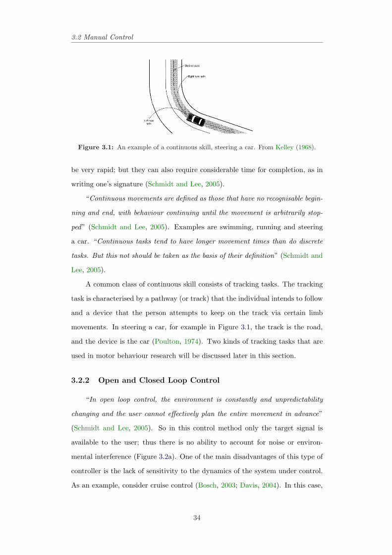
3.2 Manual Control
Figure 3.1: An example of a continuous skill, steering a car. From Kelley (1968).
be very rapid; but they can also require considerable time for completion, as in
writing one’s signature (Schmidt and Lee, 2005).
“Continuous movements are defined as those that have no recognisable begin-
ning and end, with behaviour continuing until the movement is arbitrarily stop-
ped” (Schmidt and Lee, 2005). Examples are swimming, running and steering
a car. “Continuous tasks tend to have longer movement times than do discrete
tasks. But this not should be taken as the basis of their definition” (Schmidt and
Lee, 2005).
A common class of continuous skill consists of tracking tasks. The tracking
task is characterised by a pathway (or track) that the individual intends to follow
and a device that the person attempts to keep on the track via certain limb
movements. In steering a car, for example in Figure 3.1, the track is the road,
and the device is the car (Poulton, 1974). Two kinds of tracking tasks that are
used in motor behaviour research will be discussed later in this section.
3.2.2 Open and Closed Loop Control
“In open loop control, the environment is constantly and unpredictability
changing and the user cannot effectively plan the entire movement in advance”
(Schmidt and Lee, 2005). So in this control method only the target signal is
available to the user; thus there is no ability to account for noise or environ-
mental interference (Figure 3.2a). One of the main disadvantages of this type of
controller is the lack of sensitivity to the dynamics of the system under control.
As an example, consider cruise control (Bosch, 2003; Davis, 2004). In this case,
34
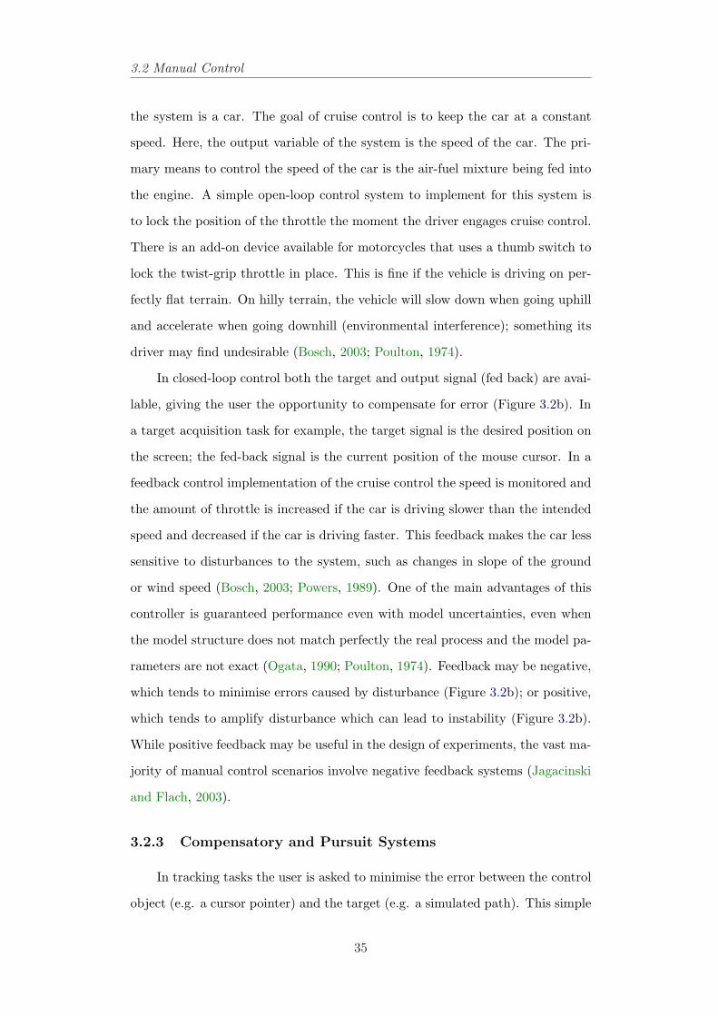
3.2 Manual Control
the system is a car. The goal of cruise control is to keep the car at a constant
speed. Here, the output variable of the system is the speed of the car. The pri-
mary means to control the speed of the car is the air-fuel mixture being fed into
the engine. A simple open-loop control system to implement for this system is
to lock the position of the throttle the moment the driver engages cruise control.
There is an add-on device available for motorcycles that uses a thumb switch to
lock the twist-grip throttle in place. This is fine if the vehicle is driving on per-
fectly flat terrain. On hilly terrain, the vehicle will slow down when going uphill
and accelerate when going downhill (environmental interference); something its
driver may find undesirable (Bosch, 2003; Poulton, 1974).
In closed-loop control both the target and output signal (fed back) are avai-
lable, giving the user the opportunity to compensate for error (Figure 3.2b). In
a target acquisition task for example, the target signal is the desired position on
the screen; the fed-back signal is the current position of the mouse cursor. In a
feedback control implementation of the cruise control the speed is monitored and
the amount of throttle is increased if the car is driving slower than the intended
speed and decreased if the car is driving faster. This feedback makes the car less
sensitive to disturbances to the system, such as changes in slope of the ground
or wind speed (Bosch, 2003; Powers, 1989). One of the main advantages of this
controller is guaranteed performance even with model uncertainties, even when
the model structure does not match perfectly the real process and the model pa-
rameters are not exact (Ogata, 1990; Poulton, 1974). Feedback may be negative,
which tends to minimise errors caused by disturbance (Figure 3.2b); or positive,
which tends to amplify disturbance which can lead to instability (Figure 3.2b).
While positive feedback may be useful in the design of experiments, the vast ma-
jority of manual control scenarios involve negative feedback systems (Jagacinski
and Flach, 2003).
3.2.3 Compensatory and Pursuit Systems
In tracking tasks the user is asked to minimise the error between the control
object (e.g. a cursor pointer) and the target (e.g. a simulated path). This simple
35
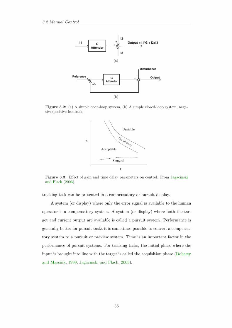
3.2 Manual Control
G
Attender
I1 ++
I2
I3
Output = I1*G + I2+I3
(a)
GAttender
Disturbance
Output+
+Reference
+
+/-
(b)
Figure 3.2: (a) A simple open-loop system, (b) A simple closed-loop system, nega-tive/positive feedback.
Figure 3.3: Effect of gain and time delay parameters on control. From Jagacinskiand Flach (2003).
tracking task can be presented in a compensatory or pursuit display.
A system (or display) where only the error signal is available to the human
operator is a compensatory system. A system (or display) where both the tar-
get and current output are available is called a pursuit system. Performance is
generally better for pursuit tasks-it is sometimes possible to convert a compensa-
tory system to a pursuit or preview system. Time is an important factor in the
performance of pursuit systems. For tracking tasks, the initial phase where the
input is brought into line with the target is called the acquisition phase (Doherty
and Massink, 1999; Jagacinski and Flach, 2003).
36
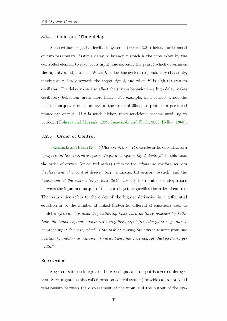
3.2 Manual Control
3.2.4 Gain and Time-delay
A closed loop negative feedback system’s (Figure 3.2b) behaviour is based
on two parameters, firstly a delay or latency τ which is the time taken by the
controlled element to react to its input, and secondly the gain K which determines
the rapidity of adjustment. When K is low the system responds very sluggishly,
moving only slowly towards the target signal, and when K is high the system
oscillates. The delay τ can also affect the system behaviour – a high delay makes
oscillatory behaviour much more likely. For example, in a concert where the
music is output, τ must be low (of the order of 20ms) to produce a perceived
immediate output. If τ is much higher, most musicians become unwilling to
perform (Doherty and Massink, 1999; Jagacinski and Flach, 2003; Kelley, 1968).
3.2.5 Order of Control
Jagacinski and Flach (2003)(Chapter 9, pp. 87) describe order of control as a
“property of the controlled system (e.g., a computer input device).” In this case,
the order of control (or control order) refers to the “dynamic relation between
displacement of a control device” (e.g. a mouse, tilt sensor, joystick) and the
“behaviour of the system being controlled.” Usually the number of integrations
between the input and output of the control system specifies the order of control.
The term order refers to the order of the highest derivative in a differential
equation or to the number of linked first-order differential equations used to
model a system. “In discrete positioning tasks such as those modeled by Fitts’
Law, the human operator produces a step-like output from the plant (e.g. mouse
or other input devices), which is the task of moving the cursor pointer from one
position to another in minimum time and with the accuracy specified by the target
width.”
Zero Order
A system with no integration between input and output is a zero-order sys-
tem. Such a system (also called position control system) provides a proportional
relationship between the displacement of the input and the output of the sys-
37
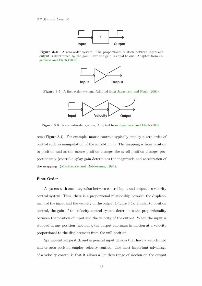
3.2 Manual Control
1
Input Output
Figure 3.4: A zero-order system. The proportional relation between input andoutput is determined by the gain. Here the gain is equal to one. Adapted from Ja-gacinski and Flach (2003).
Input Output
Figure 3.5: A first-order system. Adapted from Jagacinski and Flach (2003).
Input Velocity Output
Figure 3.6: A second-order system; Adapted from Jagacinski and Flach (2003).
tem (Figure 3.4). For example, mouse controls typically employ a zero-order of
control such as manipulation of the scroll-thumb. The mapping is from position
to position and as the mouse position changes the scroll position changes pro-
portionately (control-display gain determines the magnitude and acceleration of
the mapping) (MacKenzie and Riddersma, 1994).
First Order
A system with one integration between control input and output is a velocity
control system. Thus, there is a proportional relationship between the displace-
ment of the input and the velocity of the output (Figure 3.5). Similar to position
control, the gain of the velocity control system determines the proportionality
between the position of input and the velocity of the output. When the input is
stopped in any position (not null), the output continues in motion at a velocity
proportional to the displacement from the null position.
Spring-centred joystick and in general input devices that have a well-defined
null or zero position employ velocity control. The most important advantage
of a velocity control is that it allows a limitless range of motion on the output
38
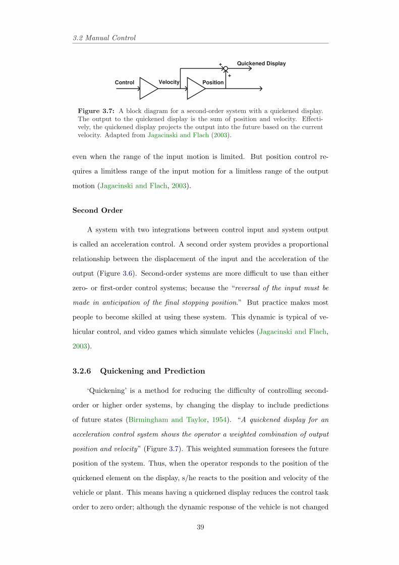
3.2 Manual Control
Control Velocity Position
+
+
Quickened Display
Figure 3.7: A block diagram for a second-order system with a quickened display.The output to the quickened display is the sum of position and velocity. Effecti-vely, the quickened display projects the output into the future based on the currentvelocity. Adapted from Jagacinski and Flach (2003).
even when the range of the input motion is limited. But position control re-
quires a limitless range of the input motion for a limitless range of the output
motion (Jagacinski and Flach, 2003).
Second Order
A system with two integrations between control input and system output
is called an acceleration control. A second order system provides a proportional
relationship between the displacement of the input and the acceleration of the
output (Figure 3.6). Second-order systems are more difficult to use than either
zero- or first-order control systems; because the “reversal of the input must be
made in anticipation of the final stopping position.” But practice makes most
people to become skilled at using these system. This dynamic is typical of ve-
hicular control, and video games which simulate vehicles (Jagacinski and Flach,
2003).
3.2.6 Quickening and Prediction
‘Quickening’ is a method for reducing the difficulty of controlling second-
order or higher order systems, by changing the display to include predictions
of future states (Birmingham and Taylor, 1954). “A quickened display for an
acceleration control system shows the operator a weighted combination of output
position and velocity” (Figure 3.7). This weighted summation foresees the future
position of the system. Thus, when the operator responds to the position of the
quickened element on the display, s/he reacts to the position and velocity of the
vehicle or plant. This means having a quickened display reduces the control task
order to zero order; although the dynamic response of the vehicle is not changed
39
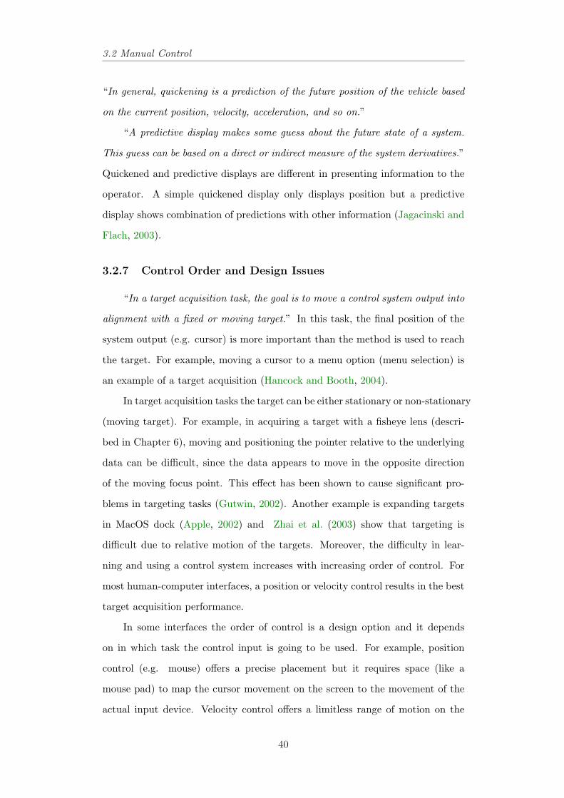
3.2 Manual Control
“In general, quickening is a prediction of the future position of the vehicle based
on the current position, velocity, acceleration, and so on.”
“A predictive display makes some guess about the future state of a system.
This guess can be based on a direct or indirect measure of the system derivatives.”
Quickened and predictive displays are different in presenting information to the
operator. A simple quickened display only displays position but a predictive
display shows combination of predictions with other information (Jagacinski and
Flach, 2003).
3.2.7 Control Order and Design Issues
“In a target acquisition task, the goal is to move a control system output into
alignment with a fixed or moving target.” In this task, the final position of the
system output (e.g. cursor) is more important than the method is used to reach
the target. For example, moving a cursor to a menu option (menu selection) is
an example of a target acquisition (Hancock and Booth, 2004).
In target acquisition tasks the target can be either stationary or non-stationary
(moving target). For example, in acquiring a target with a fisheye lens (descri-
bed in Chapter 6), moving and positioning the pointer relative to the underlying
data can be difficult, since the data appears to move in the opposite direction
of the moving focus point. This effect has been shown to cause significant pro-
blems in targeting tasks (Gutwin, 2002). Another example is expanding targets
in MacOS dock (Apple, 2002) and Zhai et al. (2003) show that targeting is
difficult due to relative motion of the targets. Moreover, the difficulty in lear-
ning and using a control system increases with increasing order of control. For
most human-computer interfaces, a position or velocity control results in the best
target acquisition performance.
In some interfaces the order of control is a design option and it depends
on in which task the control input is going to be used. For example, position
control (e.g. mouse) offers a precise placement but it requires space (like a
mouse pad) to map the cursor movement on the screen to the movement of the
actual input device. Velocity control offers a limitless range of motion on the
40
3.2 Manual Control
output even when the range of the control device is limited (Buxton et al., 2002),
and when the relative range of movement is an issue velocity control should be
considered (Jagacinski and Flach, 2003).
Scrollbars include both a position and a velocity control. Clicking on one
of the up/down arrows in the scrollbar with the mouse cursor moves the text
up or down at a constant rate, and thus is a velocity control system. Howe-
ver, the mouse cursor can be placed directly over the scroll handle, and drag
it to the desired position in the document. When the position is acquired the
handle is released and the text is then updated on the screen. This mode is a
position control. However, in browsing long documents, this position control can
become very sensitive because many pages map into a limited range of control
movement. In this case, the handle position control is commonly used for ap-
proximate positioning, and the less sensitive velocity control arrows are used for
fine positioning.
Additionally, moving target acquisition can work better with velocity control.
For example, Jagacinski et al. (1980) found that velocity control had higher per-
formance than position control in capturing small fast moving targets.
3.2.8 Control Devices
Another issue in designing systems is the type of input and control device
that is used. The prominence of the null (zero) position is one important conside-
ration for the input device, especially those who operate with velocity or higher
order control systems; “because the stick must be in this position for the output
to stop on a target”. Null position is not a problem in position control systems;
because the output stops whenever the control input stops moving. So, a mouse
is better suited for a position control system, but not a first order system. Spring-
centred joysticks are generally better suited for velocity and higher order control
systems.
“One way to make the null position more distinct is to include a nonlinear
dead-band or dead-zone in the zero region” (Figure 3.8). Rockway (1957) reports
that dead-space reduces the mean time on a target acquisition task using a spring-
41
3.2 Manual Control
Input
Output
Figure 3.8: A dead-band (dead-zone) that can be used to insure that there is awell-defined null position for a control device. In the dead-zone, the output is zerofor a range of input positions. Outside the zone, output is proportional to input.
centred joystick. A high gain reduces the range of movement required to keep
the pointer on target. The effect of dead-space is particularly determined, when
the gain of the control system is high. “The dead-space is therefore a larger
proportion of the range of movement” (Kelley, 1968).
Another common nonlinear feature of a control device is hysteresis. When
we push on something it yields and when we release it it does not spring back
completely, then it is exhibiting hysteresis. A small amount of hysteresis is
considered in the design of keys in a computer keyboard. Thus, the pressure
required to activate the key is smaller than the pressure is required to deactivate
it. So, the key remains in the active state, even if the pressure is partially released.
The advantage of this nonlinear hysteresis is that it prevents accidentally double-
clicking on the same key (Figure 3.9).
One important issue in evaluating and comparing particular control input
devices is that these devices should be tested with the same dynamics; because
dynamic aspects of the designed controller is sometimes independent from the
task they are going to be used and tested. For example, comparing a mouse with
a joystick in a target acquisition task may produce confusing results; because the
dynamics are different (Jagacinski and Flach, 2003).
3.2.9 State-space Modeling
In control engineering a state space modeling is another way of presenting
differential equations describing a dynamic system. It uses a set of first-order
42
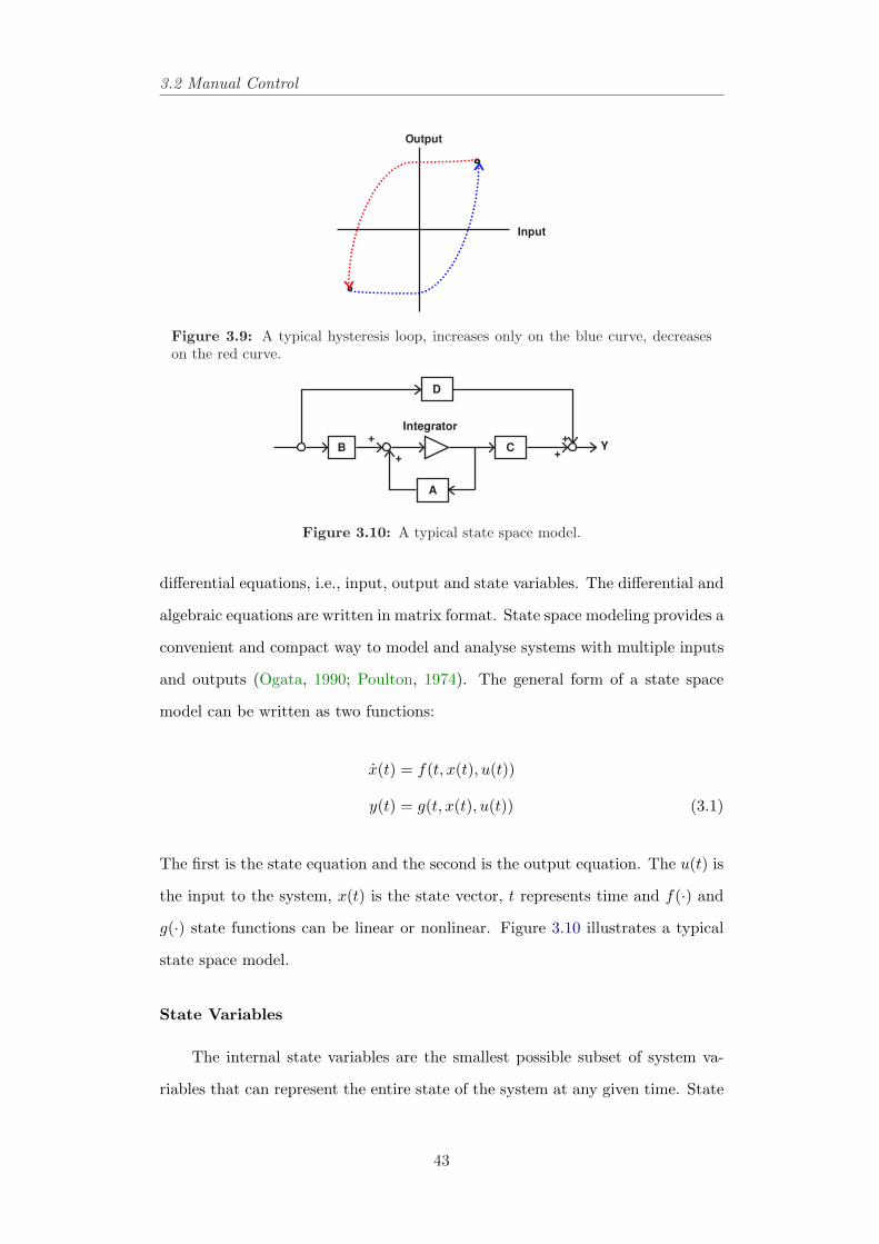
3.2 Manual Control
Input
Output
Figure 3.9: A typical hysteresis loop, increases only on the blue curve, decreaseson the red curve.
B
D
A
C Y+
+
+
+
Integrator
Figure 3.10: A typical state space model.
differential equations, i.e., input, output and state variables. The differential and
algebraic equations are written in matrix format. State space modeling provides a
convenient and compact way to model and analyse systems with multiple inputs
and outputs (Ogata, 1990; Poulton, 1974). The general form of a state space
model can be written as two functions:
x(t) = f(t, x(t), u(t))
y(t) = g(t, x(t), u(t)) (3.1)
The first is the state equation and the second is the output equation. The u(t) is
the input to the system, x(t) is the state vector, t represents time and f(·) and
g(·) state functions can be linear or nonlinear. Figure 3.10 illustrates a typical
state space model.
State Variables
The internal state variables are the smallest possible subset of system va-
riables that can represent the entire state of the system at any given time. State
43
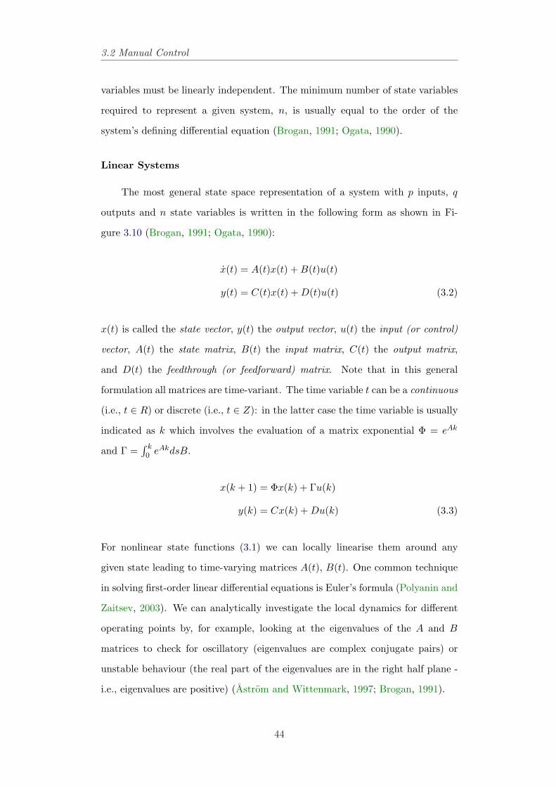
3.2 Manual Control
variables must be linearly independent. The minimum number of state variables
required to represent a given system, n, is usually equal to the order of the
system’s defining differential equation (Brogan, 1991; Ogata, 1990).
Linear Systems
The most general state space representation of a system with p inputs, q
outputs and n state variables is written in the following form as shown in Fi-
gure 3.10 (Brogan, 1991; Ogata, 1990):
x(t) = A(t)x(t) + B(t)u(t)
y(t) = C(t)x(t) + D(t)u(t) (3.2)
x(t) is called the state vector, y(t) the output vector, u(t) the input (or control)
vector, A(t) the state matrix, B(t) the input matrix, C(t) the output matrix,
and D(t) the feedthrough (or feedforward) matrix. Note that in this general
formulation all matrices are time-variant. The time variable t can be a continuous
(i.e., t ∈ R) or discrete (i.e., t ∈ Z): in the latter case the time variable is usually
indicated as k which involves the evaluation of a matrix exponential Φ = eAk
and Γ =∫ k0 eAkdsB.
x(k + 1) = Φx(k) + Γu(k)
y(k) = Cx(k) + Du(k) (3.3)
For nonlinear state functions (3.1) we can locally linearise them around any
given state leading to time-varying matrices A(t), B(t). One common technique
in solving first-order linear differential equations is Euler’s formula (Polyanin and
Zaitsev, 2003). We can analytically investigate the local dynamics for different
operating points by, for example, looking at the eigenvalues of the A and B
matrices to check for oscillatory (eigenvalues are complex conjugate pairs) or
unstable behaviour (the real part of the eigenvalues are in the right half plane -
i.e., eigenvalues are positive) (Astrom and Wittenmark, 1997; Brogan, 1991).
44
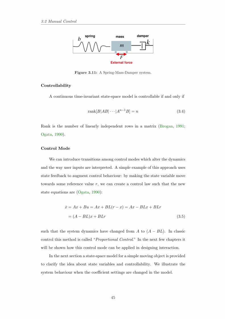
3.2 Manual Control
bspring mass damper
mk
F
External force
Figure 3.11: A Spring-Mass-Damper system.
Controllability
A continuous time-invariant state-space model is controllable if and only if
rank[B|AB| · · · |An−1B] = n (3.4)
Rank is the number of linearly independent rows in a matrix (Brogan, 1991;
Ogata, 1990).
Control Mode
We can introduce transitions among control modes which alter the dynamics
and the way user inputs are interpreted. A simple example of this approach uses
state feedback to augment control behaviour: by making the state variable move
towards some reference value r, we can create a control law such that the new
state equations are (Ogata, 1990):
x = Ax + Bu = Ax + BL(r − x) = Ax−BLx + BLr
= (A−BL)x + BLr (3.5)
such that the system dynamics have changed from A to (A − BL). In classic
control this method is called “Proportional Control.” In the next few chapters it
will be shown how this control mode can be applied in designing interaction.
In the next section a state-space model for a simple moving object is provided
to clarify the idea about state variables and controllability. We illustrate the
system behaviour when the coefficient settings are changed in the model.
45
3.2 Manual Control
Moving Object Example
A classical linear example is a one-dimensional mass moving horizontally
on a plane and attached to a wall with a spring and a damper (Figure 3.11).
Newton’s laws of motion, Cause of change = Resistance to change × Rate of
change or Force = Mass × Acceleration, for this object:
my(t) = u(t)− ky(t)− by(t) (3.6)
where
• y0 is initial position; y(t) is position; y(t) is velocity; y(t) is acceleration,
• u(t) is an applied force, F ,
• k is the damping coefficient,
• b is the spring constant,
• m is the mass of the object.
The state equation would then become
x1
x2
=
0 1
−bm
−km
x1
x2
+
0
1m
u
y(t) =(
1 0)
x1
x2
(3.7)
Where
• x1(t) represents the position of the object
• x2(t) = x1(t) is the velocity of the object,
• x2(t) = x1(t) is the acceleration of the objection,
• the output y(t) is the position of the object
Figure 3.12 presents this system’s behaviour to different damping coefficient set-
tings. In MATLAB (MathWorks, 2005) we can solve these first-order differential
46
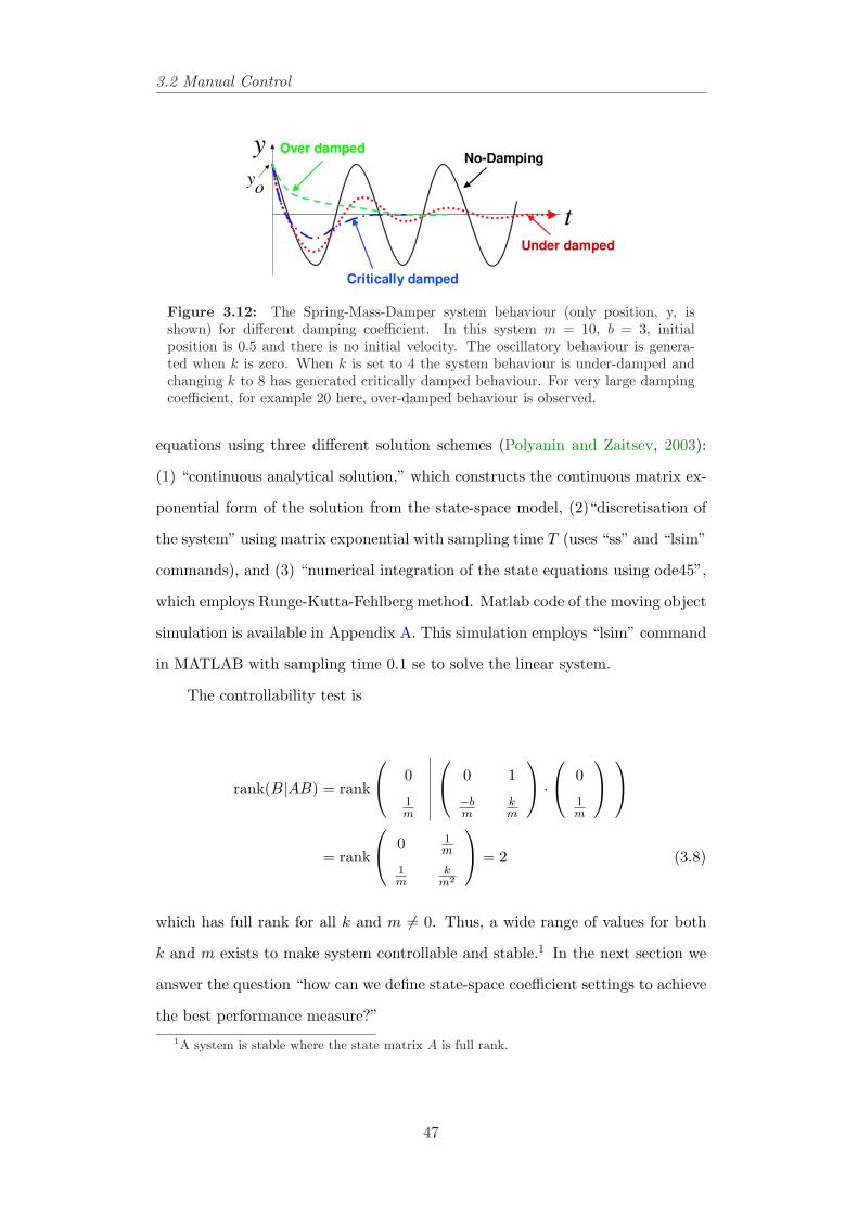
3.2 Manual Control
t
yNo-Damping
Under damped
Critically damped
Over damped
oy
Figure 3.12: The Spring-Mass-Damper system behaviour (only position, y, isshown) for different damping coefficient. In this system m = 10, b = 3, initialposition is 0.5 and there is no initial velocity. The oscillatory behaviour is genera-ted when k is zero. When k is set to 4 the system behaviour is under-damped andchanging k to 8 has generated critically damped behaviour. For very large dampingcoefficient, for example 20 here, over-damped behaviour is observed.
equations using three different solution schemes (Polyanin and Zaitsev, 2003):
(1) “continuous analytical solution,” which constructs the continuous matrix ex-
ponential form of the solution from the state-space model, (2)“discretisation of
the system” using matrix exponential with sampling time T (uses “ss” and “lsim”
commands), and (3) “numerical integration of the state equations using ode45”,
which employs Runge-Kutta-Fehlberg method. Matlab code of the moving object
simulation is available in Appendix A. This simulation employs “lsim” command
in MATLAB with sampling time 0.1 se to solve the linear system.
The controllability test is
rank(B|AB) = rank
0
1m
0 1
−bm
km
·
0
1m
= rank
0 1
m
1m
km2
= 2 (3.8)
which has full rank for all k and m 6= 0. Thus, a wide range of values for both
k and m exists to make system controllable and stable.1 In the next section we
answer the question “how can we define state-space coefficient settings to achieve
the best performance measure?”1A system is stable where the state matrix A is full rank.
47
3.2 Manual Control
3.2.10 Performance Measures
The “performance criteria” provide a value system for identifying an opti-
mal path. “The performance criteria are typically expressed as a function to be
minimised.” The differential and algebraic equations in the state-space mode can
be used to determine the path through state space (or the control law) that mi-
nimises (or maximises) the performance criterion. Typical criteria include time,
distance, or resource consumption.
In Fitts’ law experiments, the goal is to capture the target in minimum
time (refer to Section 2.5.2 on page 26). Thus, the performance in this discrete
positioning can be described as minimising the function:
J = ‖tf − t0‖ (3.9)
t0 and tf are initial and final time in Fitts’ Law task respectively.
In continuous tracking tasks, “performance is typically scored in terms of
an integrated or average mean squared error”. Thus, the performance can be
described as minimising the tracking error e1(t) as below:
J =1
tf − t0
∫ tf
t0
e21(t)dt (3.10)
A general form for the performance measure is:
J = h(x(tf ), tf ) +∫ tf
t0
g(x(t), u(t), t)dt (3.11)
The first term in this function reflects the value (or cost) of the final state and
final time. The second integral term represents a cumulative function of the
states, the control actions, and time (Brogan, 1991; Jagacinski and Flach, 2003;
Kirk, 1970; Ogata, 1990).
3.2.11 Conceptual Models and State-Space Modeling
In this section we showed that the laws of physics (e.g., Newton’s law of
motion) can be incorporated in building dynamical systems using state-space re-
48
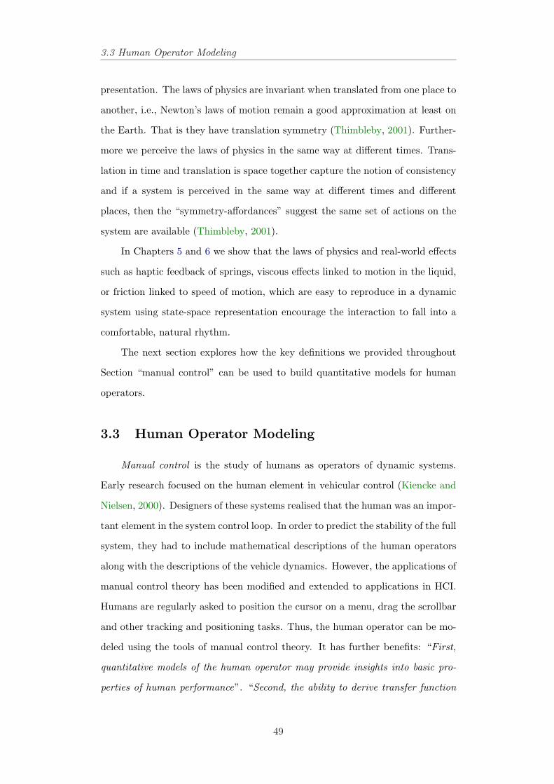
3.3 Human Operator Modeling
presentation. The laws of physics are invariant when translated from one place to
another, i.e., Newton’s laws of motion remain a good approximation at least on
the Earth. That is they have translation symmetry (Thimbleby, 2001). Further-
more we perceive the laws of physics in the same way at different times. Trans-
lation in time and translation is space together capture the notion of consistency
and if a system is perceived in the same way at different times and different
places, then the “symmetry-affordances” suggest the same set of actions on the
system are available (Thimbleby, 2001).
In Chapters 5 and 6 we show that the laws of physics and real-world effects
such as haptic feedback of springs, viscous effects linked to motion in the liquid,
or friction linked to speed of motion, which are easy to reproduce in a dynamic
system using state-space representation encourage the interaction to fall into a
comfortable, natural rhythm.
The next section explores how the key definitions we provided throughout
Section “manual control” can be used to build quantitative models for human
operators.
3.3 Human Operator Modeling
Manual control is the study of humans as operators of dynamic systems.
Early research focused on the human element in vehicular control (Kiencke and
Nielsen, 2000). Designers of these systems realised that the human was an impor-
tant element in the system control loop. In order to predict the stability of the full
system, they had to include mathematical descriptions of the human operators
along with the descriptions of the vehicle dynamics. However, the applications of
manual control theory has been modified and extended to applications in HCI.
Humans are regularly asked to position the cursor on a menu, drag the scrollbar
and other tracking and positioning tasks. Thus, the human operator can be mo-
deled using the tools of manual control theory. It has further benefits: “First,
quantitative models of the human operator may provide insights into basic pro-
perties of human performance”. “Second, the ability to derive transfer function
49
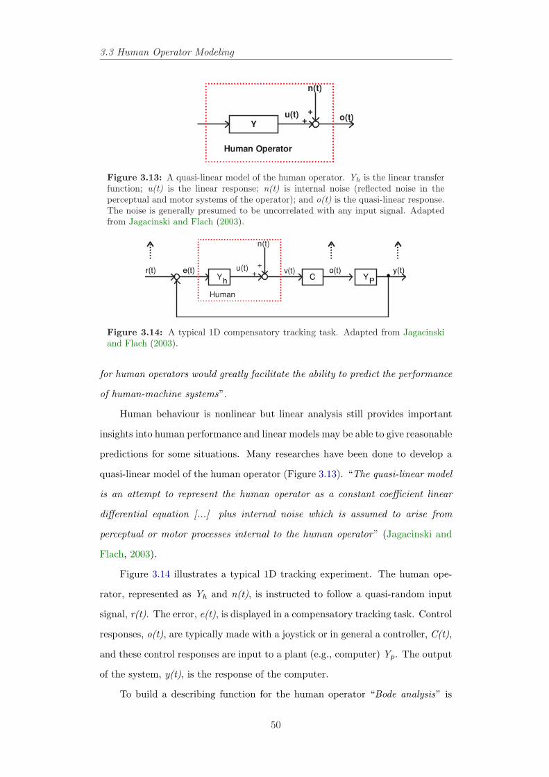
3.3 Human Operator Modeling
Y
n(t)
++
Human Operator
u(t) o(t)
Figure 3.13: A quasi-linear model of the human operator. Yh is the linear transferfunction; u(t) is the linear response; n(t) is internal noise (reflected noise in theperceptual and motor systems of the operator); and o(t) is the quasi-linear response.The noise is generally presumed to be uncorrelated with any input signal. Adaptedfrom Jagacinski and Flach (2003).
Y
n(t)
++
Human
u(t) v(t)C
o(t)e(t)r(t)Y
h P
y(t)
Figure 3.14: A typical 1D compensatory tracking task. Adapted from Jagacinskiand Flach (2003).
for human operators would greatly facilitate the ability to predict the performance
of human-machine systems”.
Human behaviour is nonlinear but linear analysis still provides important
insights into human performance and linear models may be able to give reasonable
predictions for some situations. Many researches have been done to develop a
quasi-linear model of the human operator (Figure 3.13). “The quasi-linear model
is an attempt to represent the human operator as a constant coefficient linear
differential equation [...] plus internal noise which is assumed to arise from
perceptual or motor processes internal to the human operator” (Jagacinski and
Flach, 2003).
Figure 3.14 illustrates a typical 1D tracking experiment. The human ope-
rator, represented as Yh and n(t), is instructed to follow a quasi-random input
signal, r(t). The error, e(t), is displayed in a compensatory tracking task. Control
responses, o(t), are typically made with a joystick or in general a controller, C(t),
and these control responses are input to a plant (e.g., computer) Yp. The output
of the system, y(t), is the response of the computer.
To build a describing function for the human operator “Bode analysis” is
50
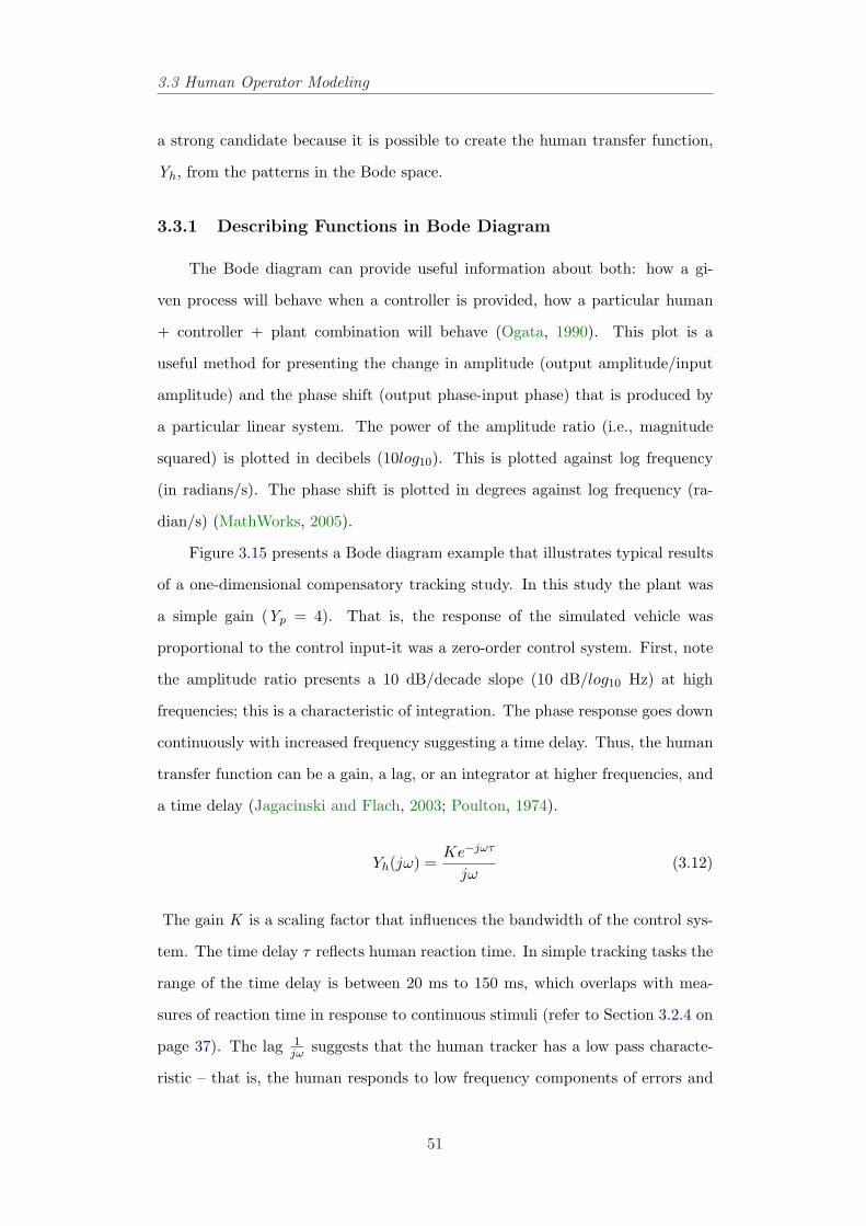
3.3 Human Operator Modeling
a strong candidate because it is possible to create the human transfer function,
Yh, from the patterns in the Bode space.
3.3.1 Describing Functions in Bode Diagram
The Bode diagram can provide useful information about both: how a gi-
ven process will behave when a controller is provided, how a particular human
+ controller + plant combination will behave (Ogata, 1990). This plot is a
useful method for presenting the change in amplitude (output amplitude/input
amplitude) and the phase shift (output phase-input phase) that is produced by
a particular linear system. The power of the amplitude ratio (i.e., magnitude
squared) is plotted in decibels (10log10). This is plotted against log frequency
(in radians/s). The phase shift is plotted in degrees against log frequency (ra-
dian/s) (MathWorks, 2005).
Figure 3.15 presents a Bode diagram example that illustrates typical results
of a one-dimensional compensatory tracking study. In this study the plant was
a simple gain (Yp = 4). That is, the response of the simulated vehicle was
proportional to the control input-it was a zero-order control system. First, note
the amplitude ratio presents a 10 dB/decade slope (10 dB/log10 Hz) at high
frequencies; this is a characteristic of integration. The phase response goes down
continuously with increased frequency suggesting a time delay. Thus, the human
transfer function can be a gain, a lag, or an integrator at higher frequencies, and
a time delay (Jagacinski and Flach, 2003; Poulton, 1974).
Yh(jω) =Ke−jωτ
jω(3.12)
The gain K is a scaling factor that influences the bandwidth of the control sys-
tem. The time delay τ reflects human reaction time. In simple tracking tasks the
range of the time delay is between 20 ms to 150 ms, which overlaps with mea-
sures of reaction time in response to continuous stimuli (refer to Section 3.2.4 on
page 37). The lag 1jω suggests that the human tracker has a low pass characte-
ristic – that is, the human responds to low frequency components of errors and
51
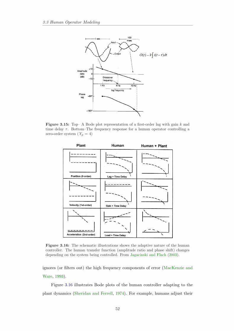
3.3 Human Operator Modeling
Figure 3.15: Top– A Bode plot representation of a first-order lag with gain k andtime delay τ . Bottom–The frequency response for a human operator controlling azero-order system (Yp = 4)
Figure 3.16: The schematic illustrations shows the adaptive nature of the humancontroller. The human transfer function (amplitude ratio and phase shift) changesdepending on the system being controlled. From Jagacinski and Flach (2003).
ignores (or filters out) the high frequency components of error (MacKenzie and
Ware, 1993).
Figure 3.16 illustrates Bode plots of the human controller adapting to the
plant dynamics (Sheridan and Ferrell, 1974). For example, humans adjust their
52
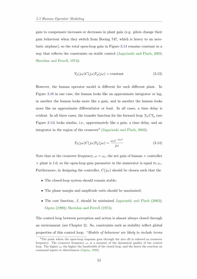
3.3 Human Operator Modeling
gain to compensate increases or decreases in plant gain (e.g. pilots change their
gain behaviour when they switch from Boeing 747, which is heavy to an aero-
batic airplane), so the total open-loop gain in Figure 3.14 remains constant in a
way that reflects the constraints on stable control (Jagacinski and Flach, 2003;
Sheridan and Ferrell, 1974):
Yh(jω)C(jω)Yp(jω) = constant (3.13)
However, the human operator model is different for each different plant. In
Figure 3.16 in one case, the human looks like an approximate integrator or lag,
in another the human looks more like a gain, and in another the human looks
more like an approximate differentiator or lead. In all cases, a time delay is
evident. In all three cases, the transfer function for the forward loop YhCYp (see
Figure 3.14) looks similar, i.e., approximately like a gain, a time delay, and an
integrator in the region of the crossover2 (Jagacinski and Flach, 2003):
Yh(jω)C(jω)Yp(jω) =ωce
−jωτ
jω(3.14)
Note that at the crossover frequency, ω = ωc, the net gain of human + controller
+ plant is 1.0, so the open-loop gain parameter in the numerator is equal to ωc.
Furthermore, in designing the controller, C(jω) should be chosen such that the
• The closed-loop system should remain stable;
• The phase margin and amplitude ratio should be maximised;
• The cost function, J , should be minimised Jagacinski and Flach (2003);
Ogata (1990); Sheridan and Ferrell (1974).
The control loop between perception and action is almost always closed through
an environment (see Chapter 2). So, constraints such as stability reflect global
properties of this control loop. “Models of behaviour are likely to include terms2The point where the open-loop response goes through the zero db is referred as crossover
frequency. The crossover frequency ωc is a measure of the dynamical quality of the controlloop. The higher ωc the higher the bandwidth of the closed loop, and the faster the reaction oncommand inputs or disturbances (Ogata, 1990).
53
3.3 Human Operator Modeling
Ta
rge
t
Distance to Goal
Accelerate
Toward Target
CoastDecelerate
vel
Figure 3.17: A finite state controller. The switching criteria are diagonal lines(constant time-to-contact). Three controllers are an acceleration toward the goal(bang), a coast (zero control input) resulting in a constant velocity, and a deceleration(bang) into the target. Adapted from Jagacinski and Flach (2003).
like the control strategy in the crossover model, whose parameters depend on
the task context. It suggests that behaviour is “situated”. Behaviour is just an
adaptive response to situation constraints” (Jagacinski and Flach, 2003).
3.3.2 “Bang Bang” Models of Human Controller for High-Order
Systems
In Fitts’ law tasks, where the user is asked to move the cursor from a starting
position to a target area, the hand is also moving from one position to another, or
in rotating the eye from one fixation to another, the human operator has to vary
the location of a mass using the force exerted by his muscles which is limited in
its maximum value. Dynamically, the hand or eye is virtually a pure mass, with
low dissipation of energy through friction, and low storage of potential energy
through spring-like behaviour. A simple servomechanism, in controlling the lo-
cation of an object, applies a force to it proportional to the deviation of the loca-
tion from the desired one, in such a direction as to reduce the deviation (Gaines,
1967b,a). Bushaw (1953) showed that the control policy of the linear servomecha-
nism was not time-optimal, in that it did not reduce the error in location to zero
54
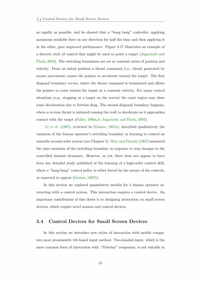
3.4 Control Devices for Small Screen Devices
as rapidly as possible, and he showed that a “bang bang” controller, applying
maximum available force in one direction for half the time and then applying it
in the other, gave improved performance. Figure 3.17 illustrates an example of
a discrete style of control that might be used to point a target (Jagacinski and
Flach, 2003). The switching boundaries are set at constant ratios of position and
velocity. From an initial position a thrust command (i.e., thrust generated by
mouse movement) causes the pointer to accelerate toward the target. The first
diagonal boundary occurs, where the thrust command is terminated and allows
the pointer to coast toward the target at a constant velocity. For many control
situations (e.g., stopping at a target on the screen) the coast region may show
some deceleration due to friction drag. The second diagonal boundary happens,
where a reverse thrust is initiated causing the craft to decelerate as it approaches
contact with the target (Fuller, 1960a,b; Jagacinski and Flach, 2003).
Li et al. (1965), reviewed in (Gaines, 1967a), described qualitatively the
variation of the human operator’s switching boundary in learning to control an
unstable second-order system (see Chapter 5). Weir and Phatak (1967) measured
the time-variation of the switching boundary in response to step changes in the
controlled element dynamics. However, as yet, there does not appear to have
been any detailed study published of the learning of a high-order control skill,
where a “bang bang” control policy is either forced by the nature of the controls,
or expected to appear (Gaines, 1967b).
In this section we explored quantitative models for a human operator in-
teracting with a control system. This interaction requires a control device. An
important contribution of this thesis is to designing interaction on small screen
devices, which require novel sensors and control devices.
3.4 Control Devices for Small Screen Devices
In this section we introduce new styles of interaction with mobile compu-
ters most prominently tilt-based input method. Two-handed input, which is the
most common form of interaction with “Palmtop” computers, is not suitable in
55
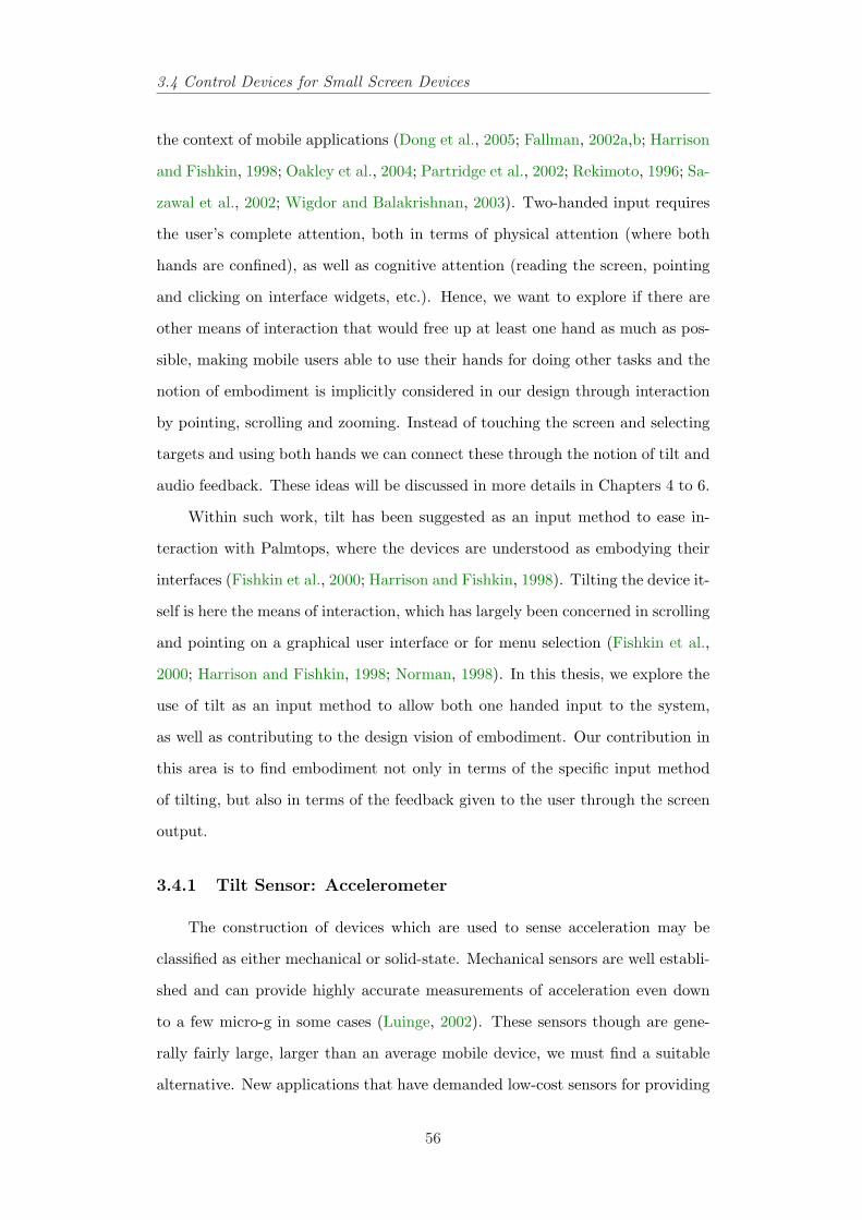
3.4 Control Devices for Small Screen Devices
the context of mobile applications (Dong et al., 2005; Fallman, 2002a,b; Harrison
and Fishkin, 1998; Oakley et al., 2004; Partridge et al., 2002; Rekimoto, 1996; Sa-
zawal et al., 2002; Wigdor and Balakrishnan, 2003). Two-handed input requires
the user’s complete attention, both in terms of physical attention (where both
hands are confined), as well as cognitive attention (reading the screen, pointing
and clicking on interface widgets, etc.). Hence, we want to explore if there are
other means of interaction that would free up at least one hand as much as pos-
sible, making mobile users able to use their hands for doing other tasks and the
notion of embodiment is implicitly considered in our design through interaction
by pointing, scrolling and zooming. Instead of touching the screen and selecting
targets and using both hands we can connect these through the notion of tilt and
audio feedback. These ideas will be discussed in more details in Chapters 4 to 6.
Within such work, tilt has been suggested as an input method to ease in-
teraction with Palmtops, where the devices are understood as embodying their
interfaces (Fishkin et al., 2000; Harrison and Fishkin, 1998). Tilting the device it-
self is here the means of interaction, which has largely been concerned in scrolling
and pointing on a graphical user interface or for menu selection (Fishkin et al.,
2000; Harrison and Fishkin, 1998; Norman, 1998). In this thesis, we explore the
use of tilt as an input method to allow both one handed input to the system,
as well as contributing to the design vision of embodiment. Our contribution in
this area is to find embodiment not only in terms of the specific input method
of tilting, but also in terms of the feedback given to the user through the screen
output.
3.4.1 Tilt Sensor: Accelerometer
The construction of devices which are used to sense acceleration may be
classified as either mechanical or solid-state. Mechanical sensors are well establi-
shed and can provide highly accurate measurements of acceleration even down
to a few micro-g in some cases (Luinge, 2002). These sensors though are gene-
rally fairly large, larger than an average mobile device, we must find a suitable
alternative. New applications that have demanded low-cost sensors for providing
56
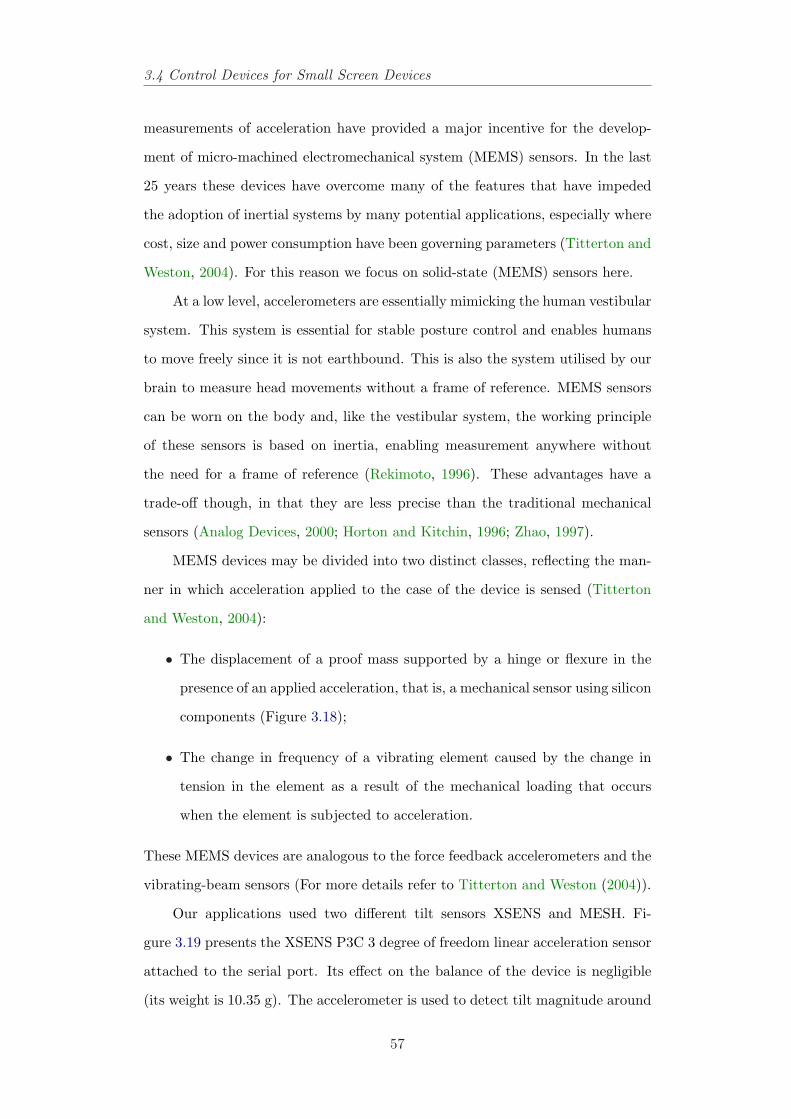
3.4 Control Devices for Small Screen Devices
measurements of acceleration have provided a major incentive for the develop-
ment of micro-machined electromechanical system (MEMS) sensors. In the last
25 years these devices have overcome many of the features that have impeded
the adoption of inertial systems by many potential applications, especially where
cost, size and power consumption have been governing parameters (Titterton and
Weston, 2004). For this reason we focus on solid-state (MEMS) sensors here.
At a low level, accelerometers are essentially mimicking the human vestibular
system. This system is essential for stable posture control and enables humans
to move freely since it is not earthbound. This is also the system utilised by our
brain to measure head movements without a frame of reference. MEMS sensors
can be worn on the body and, like the vestibular system, the working principle
of these sensors is based on inertia, enabling measurement anywhere without
the need for a frame of reference (Rekimoto, 1996). These advantages have a
trade-off though, in that they are less precise than the traditional mechanical
sensors (Analog Devices, 2000; Horton and Kitchin, 1996; Zhao, 1997).
MEMS devices may be divided into two distinct classes, reflecting the man-
ner in which acceleration applied to the case of the device is sensed (Titterton
and Weston, 2004):
• The displacement of a proof mass supported by a hinge or flexure in the
presence of an applied acceleration, that is, a mechanical sensor using silicon
components (Figure 3.18);
• The change in frequency of a vibrating element caused by the change in
tension in the element as a result of the mechanical loading that occurs
when the element is subjected to acceleration.
These MEMS devices are analogous to the force feedback accelerometers and the
vibrating-beam sensors (For more details refer to Titterton and Weston (2004)).
Our applications used two different tilt sensors XSENS and MESH. Fi-
gure 3.19 presents the XSENS P3C 3 degree of freedom linear acceleration sensor
attached to the serial port. Its effect on the balance of the device is negligible
(its weight is 10.35 g). The accelerometer is used to detect tilt magnitude around
57
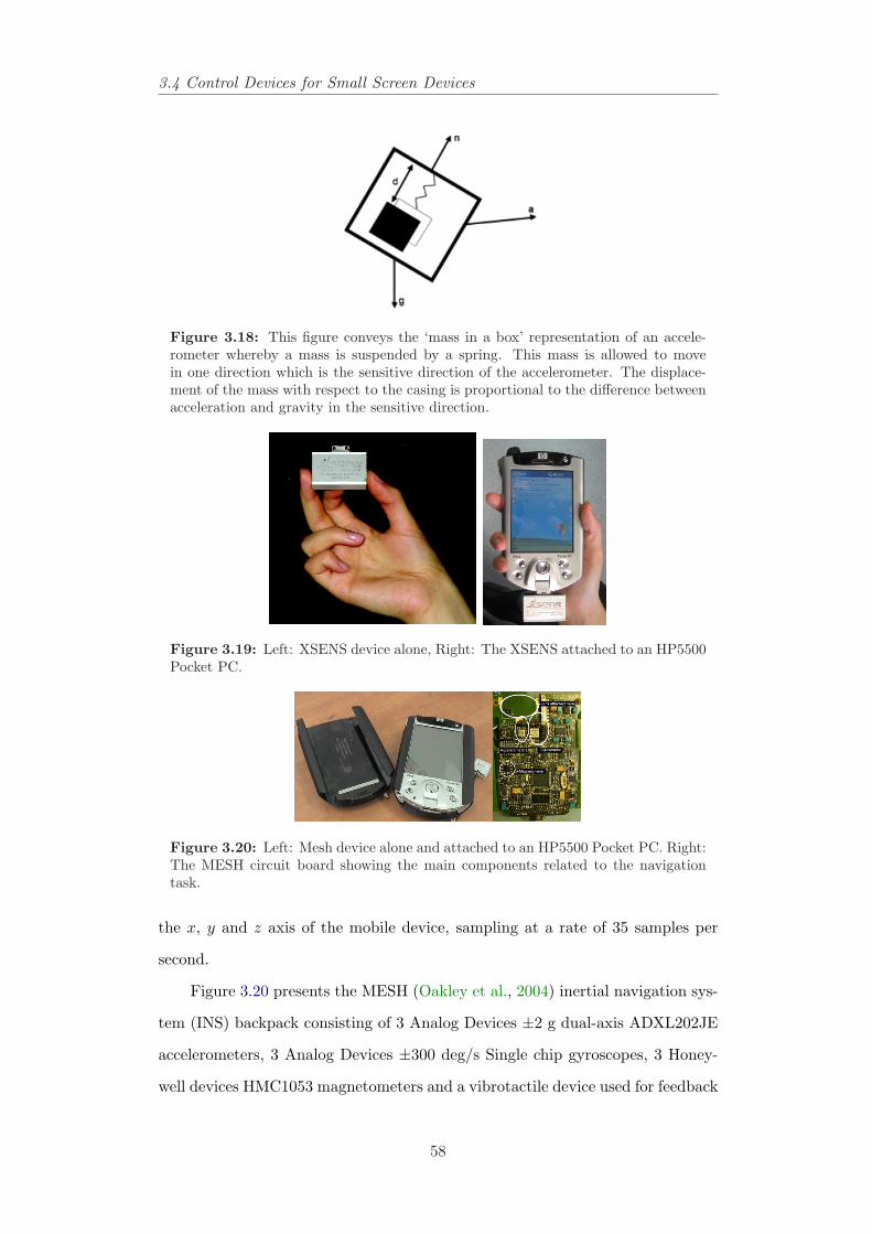
3.4 Control Devices for Small Screen Devices
Figure 3.18: This figure conveys the ‘mass in a box’ representation of an accele-rometer whereby a mass is suspended by a spring. This mass is allowed to movein one direction which is the sensitive direction of the accelerometer. The displace-ment of the mass with respect to the casing is proportional to the difference betweenacceleration and gravity in the sensitive direction.
Figure 3.19: Left: XSENS device alone, Right: The XSENS attached to an HP5500Pocket PC.
Figure 3.20: Left: Mesh device alone and attached to an HP5500 Pocket PC. Right:The MESH circuit board showing the main components related to the navigationtask.
the x, y and z axis of the mobile device, sampling at a rate of 35 samples per
second.
Figure 3.20 presents the MESH (Oakley et al., 2004) inertial navigation sys-
tem (INS) backpack consisting of 3 Analog Devices ±2 g dual-axis ADXL202JE
accelerometers, 3 Analog Devices ±300 deg/s Single chip gyroscopes, 3 Honey-
well devices HMC1053 magnetometers and a vibrotactile device used for feedback
58
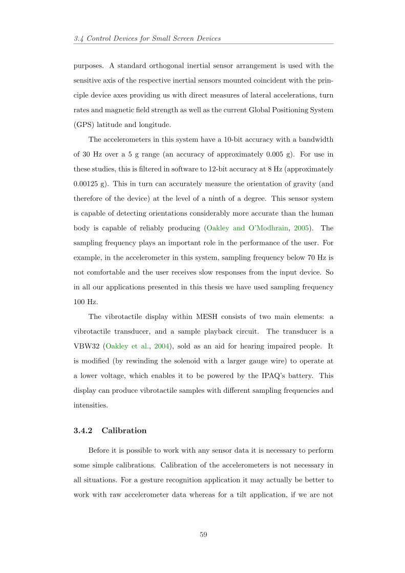
3.4 Control Devices for Small Screen Devices
purposes. A standard orthogonal inertial sensor arrangement is used with the
sensitive axis of the respective inertial sensors mounted coincident with the prin-
ciple device axes providing us with direct measures of lateral accelerations, turn
rates and magnetic field strength as well as the current Global Positioning System
(GPS) latitude and longitude.
The accelerometers in this system have a 10-bit accuracy with a bandwidth
of 30 Hz over a 5 g range (an accuracy of approximately 0.005 g). For use in
these studies, this is filtered in software to 12-bit accuracy at 8 Hz (approximately
0.00125 g). This in turn can accurately measure the orientation of gravity (and
therefore of the device) at the level of a ninth of a degree. This sensor system
is capable of detecting orientations considerably more accurate than the human
body is capable of reliably producing (Oakley and O’Modhrain, 2005). The
sampling frequency plays an important role in the performance of the user. For
example, in the accelerometer in this system, sampling frequency below 70 Hz is
not comfortable and the user receives slow responses from the input device. So
in all our applications presented in this thesis we have used sampling frequency
100 Hz.
The vibrotactile display within MESH consists of two main elements: a
vibrotactile transducer, and a sample playback circuit. The transducer is a
VBW32 (Oakley et al., 2004), sold as an aid for hearing impaired people. It
is modified (by rewinding the solenoid with a larger gauge wire) to operate at
a lower voltage, which enables it to be powered by the IPAQ’s battery. This
display can produce vibrotactile samples with different sampling frequencies and
intensities.
3.4.2 Calibration
Before it is possible to work with any sensor data it is necessary to perform
some simple calibrations. Calibration of the accelerometers is not necessary in
all situations. For a gesture recognition application it may actually be better to
work with raw accelerometer data whereas for a tilt application, if we are not
59
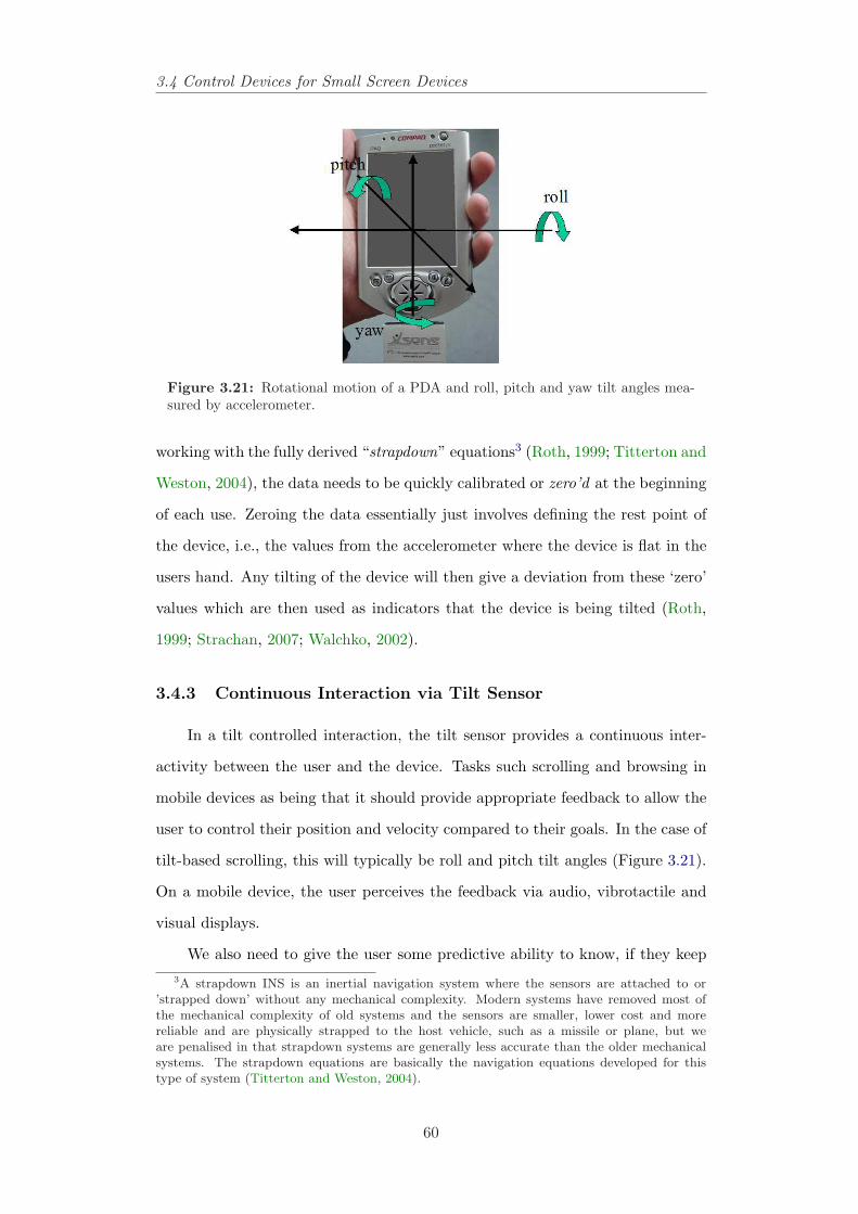
3.4 Control Devices for Small Screen Devices
Figure 3.21: Rotational motion of a PDA and roll, pitch and yaw tilt angles mea-sured by accelerometer.
working with the fully derived “strapdown” equations3 (Roth, 1999; Titterton and
Weston, 2004), the data needs to be quickly calibrated or zero’d at the beginning
of each use. Zeroing the data essentially just involves defining the rest point of
the device, i.e., the values from the accelerometer where the device is flat in the
users hand. Any tilting of the device will then give a deviation from these ‘zero’
values which are then used as indicators that the device is being tilted (Roth,
1999; Strachan, 2007; Walchko, 2002).
3.4.3 Continuous Interaction via Tilt Sensor
In a tilt controlled interaction, the tilt sensor provides a continuous inter-
activity between the user and the device. Tasks such scrolling and browsing in
mobile devices as being that it should provide appropriate feedback to allow the
user to control their position and velocity compared to their goals. In the case of
tilt-based scrolling, this will typically be roll and pitch tilt angles (Figure 3.21).
On a mobile device, the user perceives the feedback via audio, vibrotactile and
visual displays.
We also need to give the user some predictive ability to know, if they keep3A strapdown INS is an inertial navigation system where the sensors are attached to or
’strapped down’ without any mechanical complexity. Modern systems have removed most ofthe mechanical complexity of old systems and the sensors are smaller, lower cost and morereliable and are physically strapped to the host vehicle, such as a missile or plane, but weare penalised in that strapdown systems are generally less accurate than the older mechanicalsystems. The strapdown equations are basically the navigation equations developed for thistype of system (Titterton and Weston, 2004).
60
3.5 Conclusions and Summary
scrolling or browsing in a certain direction, they will get to the goal. ‘Quickening’
(or ‘predictive’) display (see Section 3.2.6 on page 39) is one method for reducing
the difficulty of controlling second-order tilt-controlled system.
3.5 Conclusions and Summary
The advent of a number of modern interaction technologies means that tech-
niques must be developed to allow designers to consider issues raised by conti-
nuous interaction between users and computer systems. In this chapter, we
reviewed the main concepts of manual control theory. This approach requires
that special consideration is given to control and feedback signals, and transfor-
mations of these signals. This approach to modeling can cope with the diverse
challenges of traditional interaction design which allows us to view the operation
of the system at many different levels, from low level device control to high level
human operator modeling and task analysis (Jagacinski and Flach, 2003). By
building on work from control theory, human behaviour modeling and interactive
systems, and developing a framework for relating analysis at different levels, we
hope to provide the designer with a richer modeling capability for continuous
interaction.
In the next chapters we will investigate the applications of this view to
interactive system design by considering systems for mobile situations. In this
context, we will look at characterisation of control the aspects of user, device and
controlled process, some of the tradeoffs involved in designing a control system,
and simple graphical representations of control system configurations.
61
Chapter 4
Model-based Target
Sonification in Small Screen
Devices: Perception and
Action
This chapter investigates the use of audio and haptic feedback to aug-ment the display of a mobile device controlled by tilt input. The ques-tions we answer in this chapter are: how do people begin searchingin unfamiliar spaces? What patterns are visible or techniques areemployed to accomplish the experimental task? What effect(s) do aprediction of the future state in the audio space and modeling humanoperator have on subjects’ behaviour? In the pilot study we study sub-jects’ navigation in a state-space with seven randomly placed audiosources, displayed via audio and vibrotactile modalities. In the mainstudy we compare only the efficiency of different forms of audio feed-back. We run these experiments on a Pocket PC instrumented withan accelerometer and a headset. The accuracy of selecting, explora-tion density and orientation of each target are measured. The resultsquantify the changes brought by predictive or ‘quickened’ sonified dis-plays in mobile, gestural interaction. Additionally they highlight sub-jects’ search pattern and the effect of a combination of independentvariables and each individual variable in the navigation patterns.
62
4.1 Introduction
4.1 Introduction
One of the main goals of interaction design is to render the interfaces as
intuitive as possible. In our everyday environments humans receive a variety
of stimuli playing upon all senses, including aural, tactile and visual, and we
respond to these stimuli. Even though hearing and vision are our two primary
senses, most interfaces are today mainly visual.
As stated in the introduction chapter, visual interfaces have crucial limi-
tations in small screen devices. These devices have a limited amount of screen
space on which to display information. Designing interfaces for mobile compu-
ters is problematic as there is a very limited amount of screen resource on which
to display information and users’ eyes are often needed on the environment ra-
ther than the interface (i.e. that they can look where they are going), therefore,
output is limited (Blattner et al., 1992; Brewster and Murray, 2000; Brewster,
1997; Johnson et al., 1998; Kramer et al., 1999; Rinott, 2004; Smith and Walker,
2005; Walker and Lindsay, 2006). Also, low graphics resolution and few colours
in these devices do not help designers to design complicated interfaces.
One way around these problems would be sonically enhanced interfaces that
require less or no visual attention, therefore the size of visual display and portable
device can be decreased. Moreover auditory interfaces potentially interfere less
in the main activity in which the user is engaged. Consequently, the user may
be able to perform more than one task at a time, such as driving a car while
using a telephone or grabbing a cup of coffee while waiting for a mobile phone
to finish downloading an image. Auditory feedback can often be a necessary
complement, but also a useful alternative to visual feedback. When designing a
mobile electronic device, it is difficult to predict all possible scenarios when it
might be used. Obviously, visual feedback is preferred in many situations such
as in noisy environments or when the user has to concentrate on a listening task.
However, as there might be numerous occasions when a user cannot look at a
display, versatile devices such as mobile phones or handheld computers benefit
from having flexible interfaces.
63
4.2 Background
Chapter 4 outlines model-based sonification and human perception and ac-
tion when s/he is interacting with auditory interfaces on small screen devices.
In Chapter 4 we investigate the usability of non-speech sounds and haptic feed-
back to augment the display of a mobile device controlled by a gesture input.
Non-speech sound has advantages over speech in that it is faster and language
independent. We use control strategies of users in browsing the audio/haptic
state space. Lastly, we explore one possible way of improving performance based
on models of human control behaviour in two example applications.
4.2 Background
4.2.1 Hearing and Vision
Vision and hearing are our two primary senses for obtaining information
about the outside world. Hearing has often been considered secondary to vision,
as it seems that in many situations we use our ears merely to tell us where to turn
our eyes (Gaver, 1997). However, it is important to emphasise that sound is a
unique medium that can provide information which vision cannot. Our eyes per-
ceive light, which is reflected from objects around us. Vision hence tells us about
the surface, size and shape of objects. Our ears, on the other hand, perceive pat-
terns of moving air that vibrating objects generate. Sound can carry information
about the consistency and hollowness of objects. Hearing can therefore provide
understanding about the interior of objects, which is a domain where vision is
limited. Another feature of sound is that it can communicate information qui-
ckly (Brewster, 1997). Sound is of a fundamentally different temporal nature to
that of visual objects; what we hear become more transitory than what we see.
In the words of Gaver (1989), “sound exists in time and over space, vision exists
in space and over time.” Spatially, sound has the advantage of not being bound
to a certain location. To see something, say a screen, we need to face it. However,
the sound from a speaker can be heard in darkness, from far away and facing any
direction. A drawback of this is that one cannot turn away from sounds. Neither
can one close one’s ears from an unpleasant sound. In our everyday lives, sound
64
4.2 Background
and vision interact smoothly. Hearing and vision complement one another in
the natural world around us and could also do so in films, multimedia and other
environments created by human beings. People prefer to communicate face to
face, being able emphasise words with facial expressions and body language. Na-
turally, almost every form of communication – e-mail, letters or even talking on
the phone – has characteristic limitations. For example, written words cannot
convey intonation as well as a spoken voice. Human-machine interaction ought
to benefit from using sound because it is central to human communication. If
the possibility of conveying information sonically were used to its full potential,
it would be a powerful complement to visual interfaces (Brewster and Murray,
2000). A strong argument against the use of sound in interfaces is that it easily
can become annoying both for the user and other people around them, since it is
more intrusive than visual impressions. It is not useful in noisy environments, for
instance, train stations, underground, so forth. However, by skilfully designing
auditory interfaces or using haptic feedback, this can be avoided.
4.2.2 The Potential of Auditory/Tactile Interfaces
The single audio output channel has been little used to improve interaction
in mobile devices. Speech sounds are, of course, used in mobile phones when
calls are being made but are not used by the telephone to aid the interaction
with the device (Blattner et al., 1992; Brewster, 2002; Gaver et al., 1991). Non-
speech sounds and vibrotactile devices are used for ringing tones or alarms but
again do not help the user interact with the system beyond this. Some signals
provide feedback that some event has been successful, such as when buttons are
pressed or devices are switched on. Selecting items with a stylus in PDAs is
often confusing for the users without tactile feedback because it is hard to know
they have hit the target or not, especially if used in a mobile setting (Brewster,
2002). In this case vibrators in mobile phones could be a good haptic feedback.
This feedback assures the user that s/he is in the target, and if the user wants
to select a target s/he can then press a key in the vibration area to select it.
If using continuous sounds as opposed to the more common brief signals,
65
4.2 Background
auditory interfaces do not need to be more transitory than visual interfaces.
However, such sounds probably benefit from being quite discreet. While, most
existing sound feedback today occurs in the foreground of the interface, subtle
background sounds can be a useful complement in advanced auditory interfaces.
Films and computer games generally make use of music and sound effects. Film
sound theorist Chion (1994) has made the following statement concerning sound
in film: there is no soundtrack. An extreme statement coming from a researcher
of sound, Chion means that there is no way to separate the auditory and visual
channels of a film. We experience them only through a unified sense which he
terms “audio-vision.” In a similar way, an interface that uses sound cleverly
can enhance the user’s immersion and improve interaction. Gaver (1997) found
that during an experimental process control task, the participants’ engagement
increased when he provided relevant sound feedback. There is now evidence
that sound can improve interaction and may be very powerful in small screen
devices (Brewster, 2002). By developing more efficient auditory interfaces, inter-
action with machines can become easier, and hopefully more pleasant.
The most advanced auditory/haptic feedback seems to exist in computer
games and multimedia products. Gaver (1997) claims that memory limitations
in the technical product is one reason why sound feedback has not been used on
a larger scale. Until quite recently it has been too expensive computationally
to use sound of good quality in computers and handheld devices. Today, only
lightweight electronic devices, such as mobile phones or handheld computers have
limited memory capacities, although this is rapidly changing with the develop-
ment of memory cards and effective compression algorithms for sound. However,
nowadays these devices give various choices of discrete audio/haptic ring tones
and alarms and to their users. The potential to use sound and haptics in small
electronics is growing fast.
66
4.3 Model-Based Sonification
4.3 Model-Based Sonification
As there are many ways in which sound can be employed in interfaces, it is
important to define the purposes of every sound at an early stage in the design
process. A sound that conveys crucial information should have different attri-
butes to one that serves as a complement to visual information. It is important
to distinguish between two very different approaches (Chion, 1994): the practical
and the naturalistic approach. The “practical” approach to auditory interfaces
deals with sound as the main feedback. This can be the case when designing in-
terfaces for visually impaired people, who must rely on sound feedback to provide
sufficient assistance in performing a task. Furthermore, sound is often the only
means of communication when using a portable hands-free device with a mobile
phone. Auditory interfaces based on a practical approach should be comprehen-
sive and simple (Brewster, 2002; Brewster and Murray, 2000; Smith and Walker,
2005; Walker and Lindsay, 2006). The drawback of this approach is sound might
be noisy and tiresome over time. The “naturalistic” view regards sound mainly as
a complement to a visual interface. A naturalistic interface combines sound and
vision in a way as similar as possible to corresponding phenomena in the natural
world. Such auditory interfaces are supposed to enhance interaction between the
user and a machine, especially in situations where the visual interface is inef-
fective on its own. Sounds that complement a visual interface can generally be
subtle background events that do not disturb. In a way, such sounds correspond
to the background music of films, since they convey information to the audience
without interfering with the main events. Sound feedback based on the natura-
listic strategy is thus very subtle and might only be recognised subconsciously.
The focus of Chapter 4 is on the “practical” approach.
Sonification is a method suggested in “practical” domain, which is defined
as the use of non-speech audio to convey information. More specifically, sonifica-
tion is the transformation of data relations into perceived relations in an acoustic
signal for the purposes of facilitating communication or interpretation (Gaver,
1989; Beaudouin-Lafon and Gaver, 1994). Many of the major current research
67
4.3 Model-Based Sonification
areas in sonification are similar in that they focus on the identification of applica-
tions for which audition provides advantages over other modalities, especially for
situations where temporal features are important or the visual modality is over-
taxed. The main issues that will move sonification research forward include (1)
mapping data onto appropriate sound features like volume, pitch, timbre, (2) un-
derstanding dynamic sound perception, (3) investigating auditory streaming, (4)
defining and categorising salience in general auditory contexts and understanding
where highly salient sonic events or patterns can surpass visual representations in
data mining, and (5) developing multimodal applications of sonification (Kramer
et al., 1999). Thus, sonification is a way to help in the exploration of complex
data. Various kinds of information can be presented using sonification, simply
by using different acoustic elements (Hermann et al., 2000).
Studies such as (Cook, 2002; Cook and Lakatos, 2003) have investigated the
human ability to perceive various physical attributes of sound sources and have
proved that feature-based synthesis is of use in studying the low-level acousti-
cal properties that human listeners use to deduce the more complex physical
attributes of a sound’s source. The generated sounds from a set of features are
correlated with the listener’s perception of, e.g., size, speed, or shape of the
source. Two methods of sonification have been used in this chapter, the Doppler
effect and derivative volume adaptation. Both of these methods create a conti-
nuous sound for each data point. Thus, the relative position to the targets is
perceived by a change of volume when passing the data point and pitch shift for
Doppler effect as well. From the data points obtained in this way, we may be
able to discover consistent relationships between acoustical and human-generated
features that can be used to predict how a sound manifesting certain acoustic
feature values will be perceived.
4.3.1 Quickening
In section 3.2.6 ‘Quickening’ was discussed. A quickened display for a tilt
controlled system like our handheld device shows the user a weighted combination
of position and velocity. This weighted summation effectively anticipates the
68
4.3 Model-Based Sonification
future position of the system. An example of this is based on the Doppler effect,
which highlights the user’s approach to a target, or a target’s movement from the
current state. Another example could be derivative of volume of sound source.
When the user is further from the audio source, the sound is quieter than when
the user is close to it. Another predictive method that has been investigated
in (Williamson et al., 2006) include Monte Carlo simulation in a tilt-controlled
navigation system.
4.3.2 Doppler Effect
The auditory system is responsible for constructing a map of the auditory
scene around us, using information from audio input. Sound localisation is the
act of using aural cues to identify the location of specific sound sources (Breg-
man, 1990; Smith, 2004). There are various types of cues that humans can use to
localise the position of a sound source. These cues can be divided into monaural
and binaural cues. The two different types of monaural cue are loudness and
Doppler shift. The loudness cue relies on the fact that when a sound source is
far away it is quieter than when it is close by. The Doppler shift corresponds to
a frequency shift associated with a sound source moving through a homogeneous
medium (Smith, 2004). Pressure wave crests emerge from the sound source at in-
tervals corresponding to the acoustic wavelength. Each crest spreads spherically
out from the point of origin at the speed of sound c (Figure 4.1). The succes-
sively generated spheres of wave crests are closer together ahead of the sound
source but farther apart behind the source. For a stationary observer, the mea-
sured frequency corresponds to the number of crests per unit time, therefore the
composite frequencies will be higher when the observer is in front of the moving
sound source and less when behind the moving sound source (Hermann et al.,
2000; Hermann and Ritter, 1999). A familiar example is the shift in frequency
of an ambulance siren as the vehicle approaches, passes, and then recedes. The
well known lawful dependence of the Doppler shifted frequency, here denoted Ψt,
69
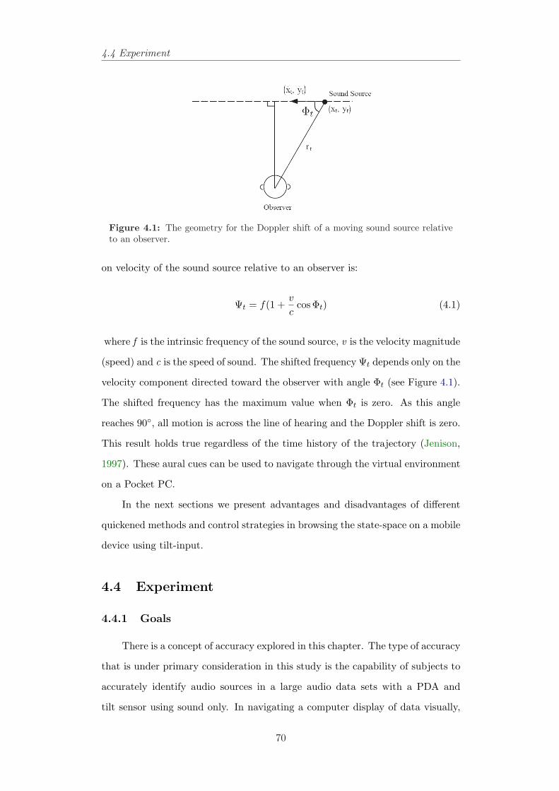
4.4 Experiment
Figure 4.1: The geometry for the Doppler shift of a moving sound source relativeto an observer.
on velocity of the sound source relative to an observer is:
Ψt = f(1 +v
ccosΦt) (4.1)
where f is the intrinsic frequency of the sound source, v is the velocity magnitude
(speed) and c is the speed of sound. The shifted frequency Ψt depends only on the
velocity component directed toward the observer with angle Φt (see Figure 4.1).
The shifted frequency has the maximum value when Φt is zero. As this angle
reaches 90◦, all motion is across the line of hearing and the Doppler shift is zero.
This result holds true regardless of the time history of the trajectory (Jenison,
1997). These aural cues can be used to navigate through the virtual environment
on a Pocket PC.
In the next sections we present advantages and disadvantages of different
quickened methods and control strategies in browsing the state-space on a mobile
device using tilt-input.
4.4 Experiment
4.4.1 Goals
There is a concept of accuracy explored in this chapter. The type of accuracy
that is under primary consideration in this study is the capability of subjects to
accurately identify audio sources in a large audio data sets with a PDA and
tilt sensor using sound only. In navigating a computer display of data visually,
70
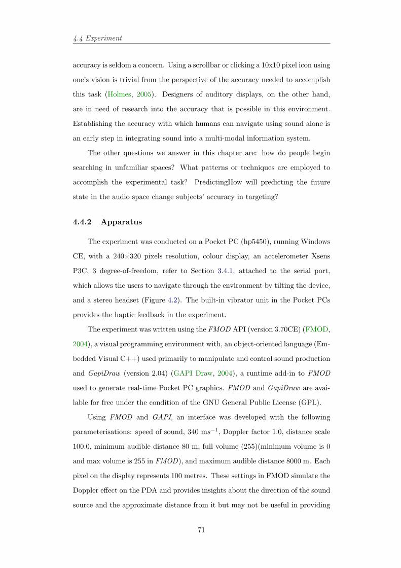
4.4 Experiment
accuracy is seldom a concern. Using a scrollbar or clicking a 10x10 pixel icon using
one’s vision is trivial from the perspective of the accuracy needed to accomplish
this task (Holmes, 2005). Designers of auditory displays, on the other hand,
are in need of research into the accuracy that is possible in this environment.
Establishing the accuracy with which humans can navigate using sound alone is
an early step in integrating sound into a multi-modal information system.
The other questions we answer in this chapter are: how do people begin
searching in unfamiliar spaces? What patterns or techniques are employed to
accomplish the experimental task? PredictingHow will predicting the future
state in the audio space change subjects’ accuracy in targeting?
4.4.2 Apparatus
The experiment was conducted on a Pocket PC (hp5450), running Windows
CE, with a 240×320 pixels resolution, colour display, an accelerometer Xsens
P3C, 3 degree-of-freedom, refer to Section 3.4.1, attached to the serial port,
which allows the users to navigate through the environment by tilting the device,
and a stereo headset (Figure 4.2). The built-in vibrator unit in the Pocket PCs
provides the haptic feedback in the experiment.
The experiment was written using the FMOD API (version 3.70CE) (FMOD,
2004), a visual programming environment with, an object-oriented language (Em-
bedded Visual C++) used primarily to manipulate and control sound production
and GapiDraw (version 2.04) (GAPI Draw, 2004), a runtime add-in to FMOD
used to generate real-time Pocket PC graphics. FMOD and GapiDraw are avai-
lable for free under the condition of the GNU General Public License (GPL).
Using FMOD and GAPI, an interface was developed with the following
parameterisations: speed of sound, 340 ms−1, Doppler factor 1.0, distance scale
100.0, minimum audible distance 80 m, full volume (255)(minimum volume is 0
and max volume is 255 in FMOD), and maximum audible distance 8000 m. Each
pixel on the display represents 100 metres. These settings in FMOD simulate the
Doppler effect on the PDA and provides insights about the direction of the sound
source and the approximate distance from it but may not be useful in providing
71
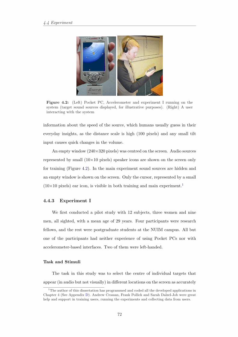
4.4 Experiment
Figure 4.2: (Left) Pocket PC, Accelerometer and experiment I running on thesystem (target sound sources displayed, for illustrative purposes). (Right) A userinteracting with the system
information about the speed of the source, which humans usually guess in their
everyday insights, as the distance scale is high (100 pixels) and any small tilt
input causes quick changes in the volume.
An empty window (240×320 pixels) was centred on the screen. Audio sources
represented by small (10×10 pixels) speaker icons are shown on the screen only
for training (Figure 4.2). In the main experiment sound sources are hidden and
an empty window is shown on the screen. Only the cursor, represented by a small
(10×10 pixels) ear icon, is visible in both training and main experiment.1
4.4.3 Experiment I
We first conducted a pilot study with 12 subjects, three women and nine
men, all sighted, with a mean age of 29 years. Four participants were research
fellows, and the rest were postgraduate students at the NUIM campus. All but
one of the participants had neither experience of using Pocket PCs nor with
accelerometer-based interfaces. Two of them were left-handed.
Task and Stimuli
The task in this study was to select the centre of individual targets that
appear (in audio but not visually) in different locations on the screen as accurately1The author of this dissertation has programmed and coded all the developed applications in
Chapter 4 (See Appendix D). Andrew Crossan, Frank Pollick and Sarah Dalzel-Job were greathelp and support in training users, running the experiments and collecting data from users.
72
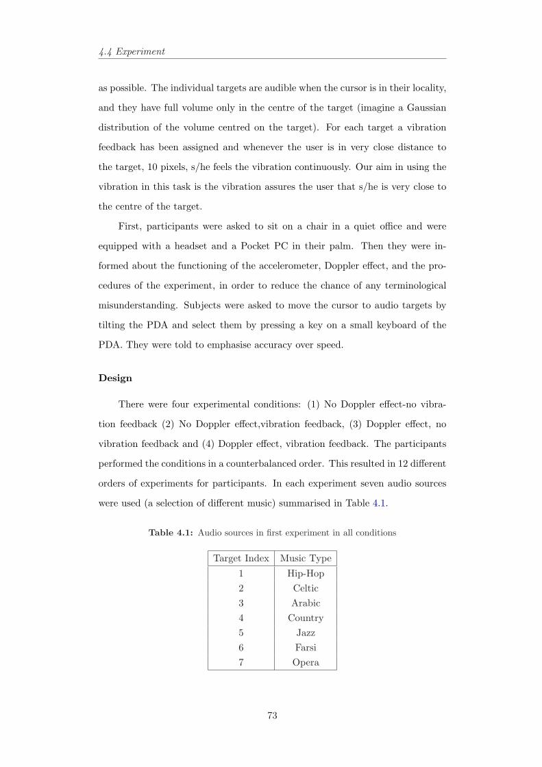
4.4 Experiment
as possible. The individual targets are audible when the cursor is in their locality,
and they have full volume only in the centre of the target (imagine a Gaussian
distribution of the volume centred on the target). For each target a vibration
feedback has been assigned and whenever the user is in very close distance to
the target, 10 pixels, s/he feels the vibration continuously. Our aim in using the
vibration in this task is the vibration assures the user that s/he is very close to
the centre of the target.
First, participants were asked to sit on a chair in a quiet office and were
equipped with a headset and a Pocket PC in their palm. Then they were in-
formed about the functioning of the accelerometer, Doppler effect, and the pro-
cedures of the experiment, in order to reduce the chance of any terminological
misunderstanding. Subjects were asked to move the cursor to audio targets by
tilting the PDA and select them by pressing a key on a small keyboard of the
PDA. They were told to emphasise accuracy over speed.
Design
There were four experimental conditions: (1) No Doppler effect-no vibra-
tion feedback (2) No Doppler effect,vibration feedback, (3) Doppler effect, no
vibration feedback and (4) Doppler effect, vibration feedback. The participants
performed the conditions in a counterbalanced order. This resulted in 12 different
orders of experiments for participants. In each experiment seven audio sources
were used (a selection of different music) summarised in Table 4.1.
Table 4.1: Audio sources in first experiment in all conditions
Target Index Music Type
1 Hip-Hop2 Celtic3 Arabic4 Country5 Jazz6 Farsi7 Opera
73
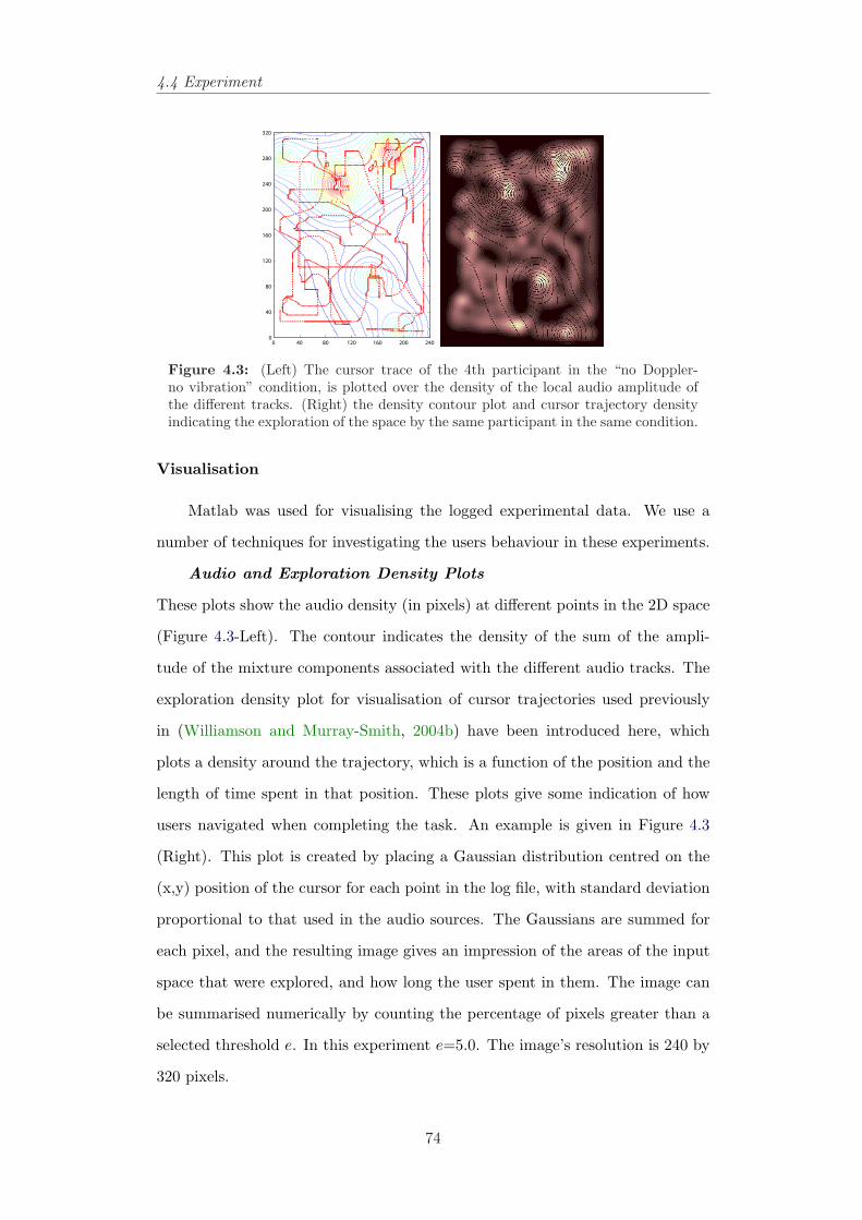
4.4 Experiment
0 40 80 120 160 200 2400
40
80
120
160
200
240
280
320
Figure 4.3: (Left) The cursor trace of the 4th participant in the “no Doppler-no vibration” condition, is plotted over the density of the local audio amplitude ofthe different tracks. (Right) the density contour plot and cursor trajectory densityindicating the exploration of the space by the same participant in the same condition.
Visualisation
Matlab was used for visualising the logged experimental data. We use a
number of techniques for investigating the users behaviour in these experiments.
Audio and Exploration Density Plots
These plots show the audio density (in pixels) at different points in the 2D space
(Figure 4.3-Left). The contour indicates the density of the sum of the ampli-
tude of the mixture components associated with the different audio tracks. The
exploration density plot for visualisation of cursor trajectories used previously
in (Williamson and Murray-Smith, 2004b) have been introduced here, which
plots a density around the trajectory, which is a function of the position and the
length of time spent in that position. These plots give some indication of how
users navigated when completing the task. An example is given in Figure 4.3
(Right). This plot is created by placing a Gaussian distribution centred on the
(x,y) position of the cursor for each point in the log file, with standard deviation
proportional to that used in the audio sources. The Gaussians are summed for
each pixel, and the resulting image gives an impression of the areas of the input
space that were explored, and how long the user spent in them. The image can
be summarised numerically by counting the percentage of pixels greater than a
selected threshold e. In this experiment e=5.0. The image’s resolution is 240 by
320 pixels.
74
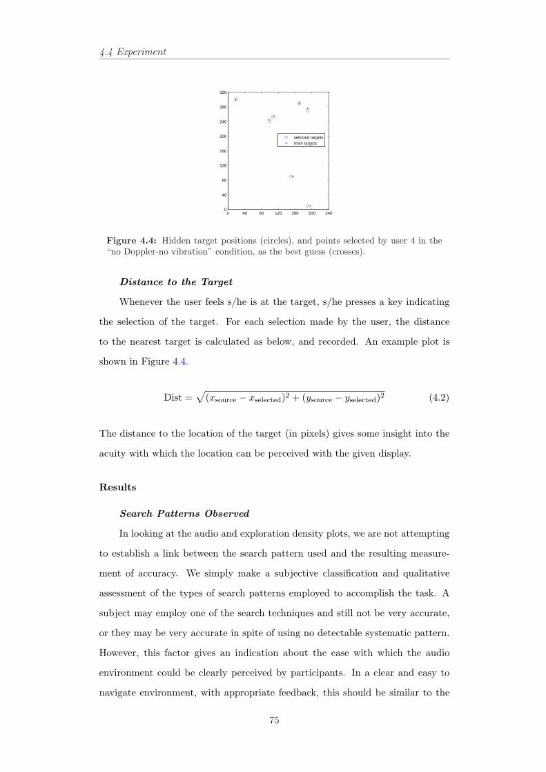
4.4 Experiment
0 40 80 120 200 200 2400
40
80
120
160
200
240
280
320
selected targetsmain targets
Figure 4.4: Hidden target positions (circles), and points selected by user 4 in the“no Doppler-no vibration” condition, as the best guess (crosses).
Distance to the Target
Whenever the user feels s/he is at the target, s/he presses a key indicating
the selection of the target. For each selection made by the user, the distance
to the nearest target is calculated as below, and recorded. An example plot is
shown in Figure 4.4.
Dist =√
(xsource − xselected)2 + (ysource − yselected)2 (4.2)
The distance to the location of the target (in pixels) gives some insight into the
acuity with which the location can be perceived with the given display.
Results
Search Patterns Observed
In looking at the audio and exploration density plots, we are not attempting
to establish a link between the search pattern used and the resulting measure-
ment of accuracy. We simply make a subjective classification and qualitative
assessment of the types of search patterns employed to accomplish the task. A
subject may employ one of the search techniques and still not be very accurate,
or they may be very accurate in spite of using no detectable systematic pattern.
However, this factor gives an indication about the ease with which the audio
environment could be clearly perceived by participants. In a clear and easy to
navigate environment, with appropriate feedback, this should be similar to the
75
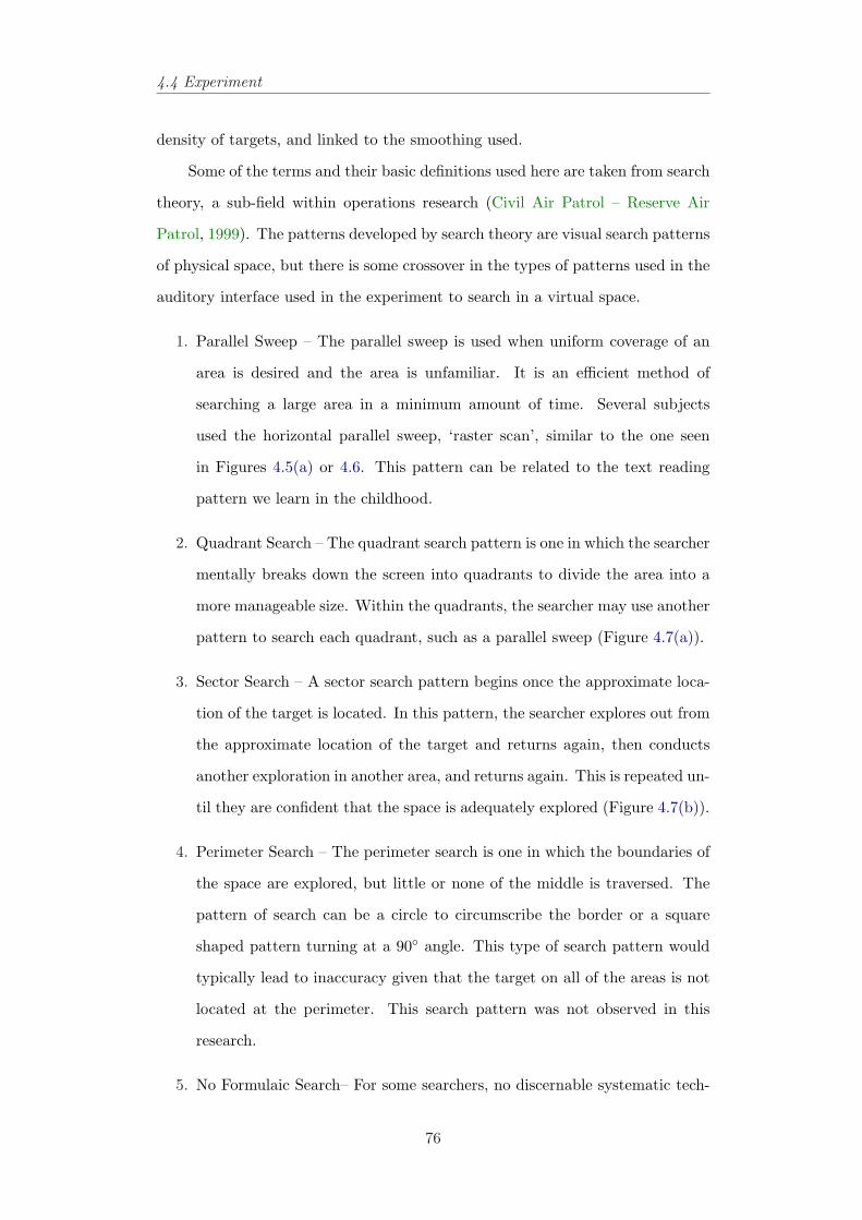
4.4 Experiment
density of targets, and linked to the smoothing used.
Some of the terms and their basic definitions used here are taken from search
theory, a sub-field within operations research (Civil Air Patrol – Reserve Air
Patrol, 1999). The patterns developed by search theory are visual search patterns
of physical space, but there is some crossover in the types of patterns used in the
auditory interface used in the experiment to search in a virtual space.
1. Parallel Sweep – The parallel sweep is used when uniform coverage of an
area is desired and the area is unfamiliar. It is an efficient method of
searching a large area in a minimum amount of time. Several subjects
used the horizontal parallel sweep, ‘raster scan’, similar to the one seen
in Figures 4.5(a) or 4.6. This pattern can be related to the text reading
pattern we learn in the childhood.
2. Quadrant Search – The quadrant search pattern is one in which the searcher
mentally breaks down the screen into quadrants to divide the area into a
more manageable size. Within the quadrants, the searcher may use another
pattern to search each quadrant, such as a parallel sweep (Figure 4.7(a)).
3. Sector Search – A sector search pattern begins once the approximate loca-
tion of the target is located. In this pattern, the searcher explores out from
the approximate location of the target and returns again, then conducts
another exploration in another area, and returns again. This is repeated un-
til they are confident that the space is adequately explored (Figure 4.7(b)).
4. Perimeter Search – The perimeter search is one in which the boundaries of
the space are explored, but little or none of the middle is traversed. The
pattern of search can be a circle to circumscribe the border or a square
shaped pattern turning at a 90◦ angle. This type of search pattern would
typically lead to inaccuracy given that the target on all of the areas is not
located at the perimeter. This search pattern was not observed in this
research.
5. No Formulaic Search– For some searchers, no discernable systematic tech-
76
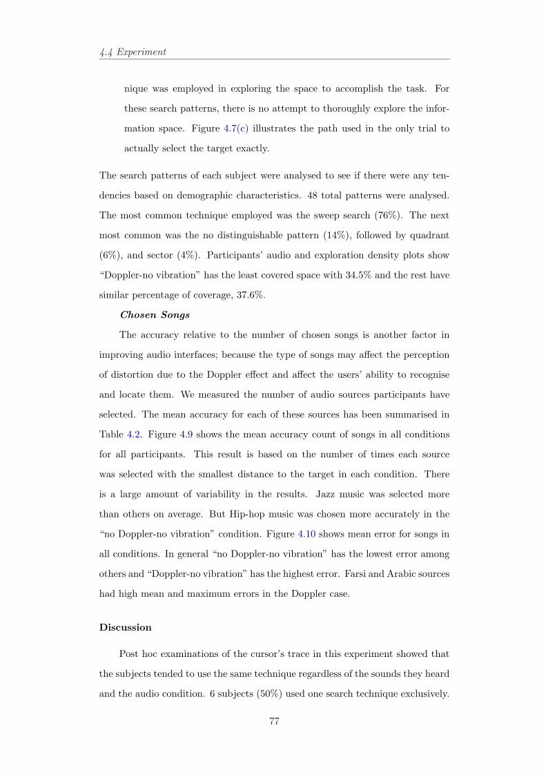
4.4 Experiment
nique was employed in exploring the space to accomplish the task. For
these search patterns, there is no attempt to thoroughly explore the infor-
mation space. Figure 4.7(c) illustrates the path used in the only trial to
actually select the target exactly.
The search patterns of each subject were analysed to see if there were any ten-
dencies based on demographic characteristics. 48 total patterns were analysed.
The most common technique employed was the sweep search (76%). The next
most common was the no distinguishable pattern (14%), followed by quadrant
(6%), and sector (4%). Participants’ audio and exploration density plots show
“Doppler-no vibration” has the least covered space with 34.5% and the rest have
similar percentage of coverage, 37.6%.
Chosen Songs
The accuracy relative to the number of chosen songs is another factor in
improving audio interfaces; because the type of songs may affect the perception
of distortion due to the Doppler effect and affect the users’ ability to recognise
and locate them. We measured the number of audio sources participants have
selected. The mean accuracy for each of these sources has been summarised in
Table 4.2. Figure 4.9 shows the mean accuracy count of songs in all conditions
for all participants. This result is based on the number of times each source
was selected with the smallest distance to the target in each condition. There
is a large amount of variability in the results. Jazz music was selected more
than others on average. But Hip-hop music was chosen more accurately in the
“no Doppler-no vibration” condition. Figure 4.10 shows mean error for songs in
all conditions. In general “no Doppler-no vibration” has the lowest error among
others and “Doppler-no vibration” has the highest error. Farsi and Arabic sources
had high mean and maximum errors in the Doppler case.
Discussion
Post hoc examinations of the cursor’s trace in this experiment showed that
the subjects tended to use the same technique regardless of the sounds they heard
and the audio condition. 6 subjects (50%) used one search technique exclusively.
77
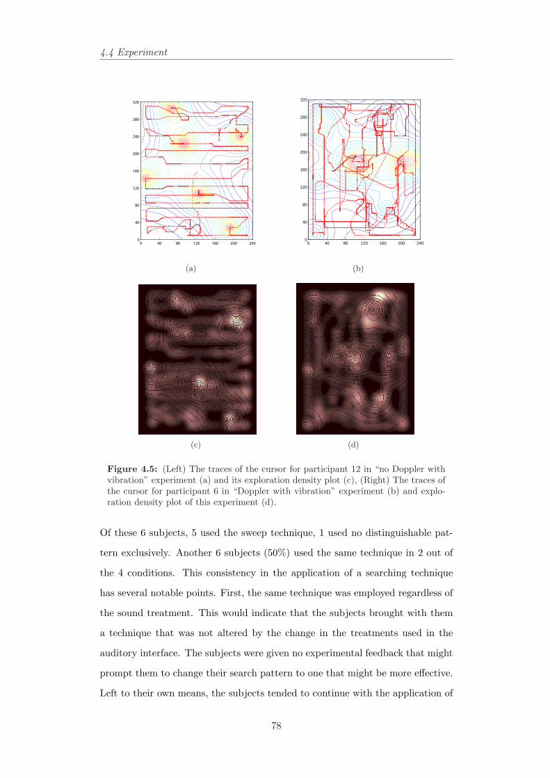
4.4 Experiment
0 40 80 120 160 200 2400
40
80
120
160
200
240
280
320
(a)
0 40 80 120 160 200 2400
40
80
120
160
200
240
280
320
(b)
(c) (d)
Figure 4.5: (Left) The traces of the cursor for participant 12 in “no Doppler withvibration” experiment (a) and its exploration density plot (c), (Right) The traces ofthe cursor for participant 6 in “Doppler with vibration” experiment (b) and explo-ration density plot of this experiment (d).
Of these 6 subjects, 5 used the sweep technique, 1 used no distinguishable pat-
tern exclusively. Another 6 subjects (50%) used the same technique in 2 out of
the 4 conditions. This consistency in the application of a searching technique
has several notable points. First, the same technique was employed regardless of
the sound treatment. This would indicate that the subjects brought with them
a technique that was not altered by the change in the treatments used in the
auditory interface. The subjects were given no experimental feedback that might
prompt them to change their search pattern to one that might be more effective.
Left to their own means, the subjects tended to continue with the application of
78
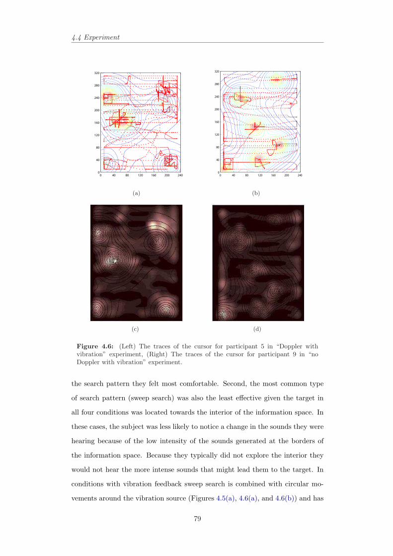
4.4 Experiment
0 40 80 120 160 200 2400
40
80
120
160
200
240
280
320
(a)
0 40 80 120 160 200 2400
40
80
120
160
200
240
280
320
(b)
(c) (d)
Figure 4.6: (Left) The traces of the cursor for participant 5 in “Doppler withvibration” experiment, (Right) The traces of the cursor for participant 9 in “noDoppler with vibration” experiment.
the search pattern they felt most comfortable. Second, the most common type
of search pattern (sweep search) was also the least effective given the target in
all four conditions was located towards the interior of the information space. In
these cases, the subject was less likely to notice a change in the sounds they were
hearing because of the low intensity of the sounds generated at the borders of
the information space. Because they typically did not explore the interior they
would not hear the more intense sounds that might lead them to the target. In
conditions with vibration feedback sweep search is combined with circular mo-
vements around the vibration source (Figures 4.5(a), 4.6(a), and 4.6(b)) and has
79
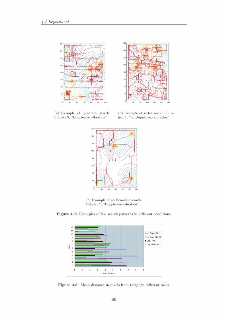
4.4 Experiment
0 40 80 120 160 200 2400
40
80
120
160
200
240
280
320
(a) Example of quadrant search:Subject 9, “Doppler-no vibration”
0 40 80 120 160 200 2400
40
80
120
160
200
240
280
320
(b) Example of sector search: Sub-ject 1, “no Doppler-no vibration”
0 40 80 120 160 200 2400
40
80
120
160
200
240
280
320
(c) Example of no formulaic search:Subject 7, “Doppler-no vibration”
Figure 4.7: Examples of few search patterns in different conditions.
0 1 2 3 4 5 6 7 8 9
1
2
3
4
5
6
7
8
9
10
11
12
Use
rs
Mean distance
No Dop - Vib
No Dop - No Vib
Dop - Vib
Dop - Non Vib
Figure 4.8: Mean distance in pixels from target in different tasks.
80
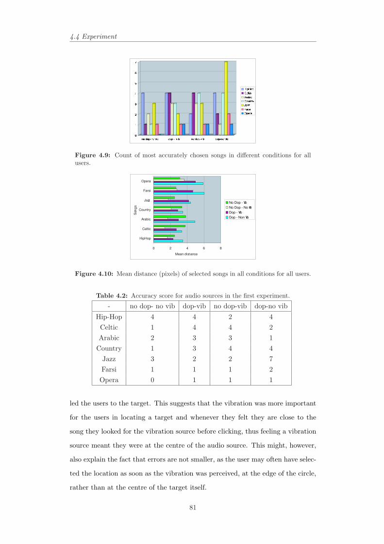
4.4 Experiment
�
�
�
�
�
�
�
�
� � � � � � � � � � � � � � � � � � � �
� � � � �� � � � � �� � � � � �� � � � � �� � � �
� � � � �� � � � �
Figure 4.9: Count of most accurately chosen songs in different conditions for allusers.
0 2 4 6 8
HipHop
Celtic
Arabic
Country
Jazz
Farsi
Opera
Son
gs
Mean distance
No Dop - Vib
No Dop - No Vib
Dop - Vib
Dop - Non Vib
Figure 4.10: Mean distance (pixels) of selected songs in all conditions for all users.
Table 4.2: Accuracy score for audio sources in the first experiment.
- no dop- no vib dop-vib no dop-vib dop-no vib
Hip-Hop 4 4 2 4Celtic 1 4 4 2Arabic 2 3 3 1
Country 1 3 4 4Jazz 3 2 2 7Farsi 1 1 1 2Opera 0 1 1 1
led the users to the target. This suggests that the vibration was more important
for the users in locating a target and whenever they felt they are close to the
song they looked for the vibration source before clicking, thus feeling a vibration
source meant they were at the centre of the audio source. This might, however,
also explain the fact that errors are not smaller, as the user may often have selec-
ted the location as soon as the vibration was perceived, at the edge of the circle,
rather than at the centre of the target itself.
81
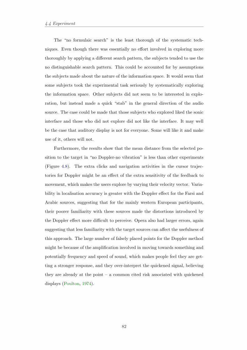
4.4 Experiment
The “no formulaic search” is the least thorough of the systematic tech-
niques. Even though there was essentially no effort involved in exploring more
thoroughly by applying a different search pattern, the subjects tended to use the
no distinguishable search pattern. This could be accounted for by assumptions
the subjects made about the nature of the information space. It would seem that
some subjects took the experimental task seriously by systematically exploring
the information space. Other subjects did not seem to be interested in explo-
ration, but instead made a quick “stab” in the general direction of the audio
source. The case could be made that those subjects who explored liked the sonic
interface and those who did not explore did not like the interface. It may well
be the case that auditory display is not for everyone. Some will like it and make
use of it, others will not.
Furthermore, the results show that the mean distance from the selected po-
sition to the target in “no Doppler-no vibration” is less than other experiments
(Figure 4.8). The extra clicks and navigation activities in the cursor trajec-
tories for Doppler might be an effect of the extra sensitivity of the feedback to
movement, which makes the users explore by varying their velocity vector. Varia-
bility in localisation accuracy is greater with the Doppler effect for the Farsi and
Arabic sources, suggesting that for the mainly western European participants,
their poorer familiarity with these sources made the distortions introduced by
the Doppler effect more difficult to perceive. Opera also had larger errors, again
suggesting that less familiarity with the target sources can affect the usefulness of
this approach. The large number of falsely placed points for the Doppler method
might be because of the amplification involved in moving towards something and
potentially frequency and speed of sound, which makes people feel they are get-
ting a stronger response, and they over-interpret the quickened signal, believing
they are already at the point – a common cited risk associated with quickened
displays (Poulton, 1974).
82
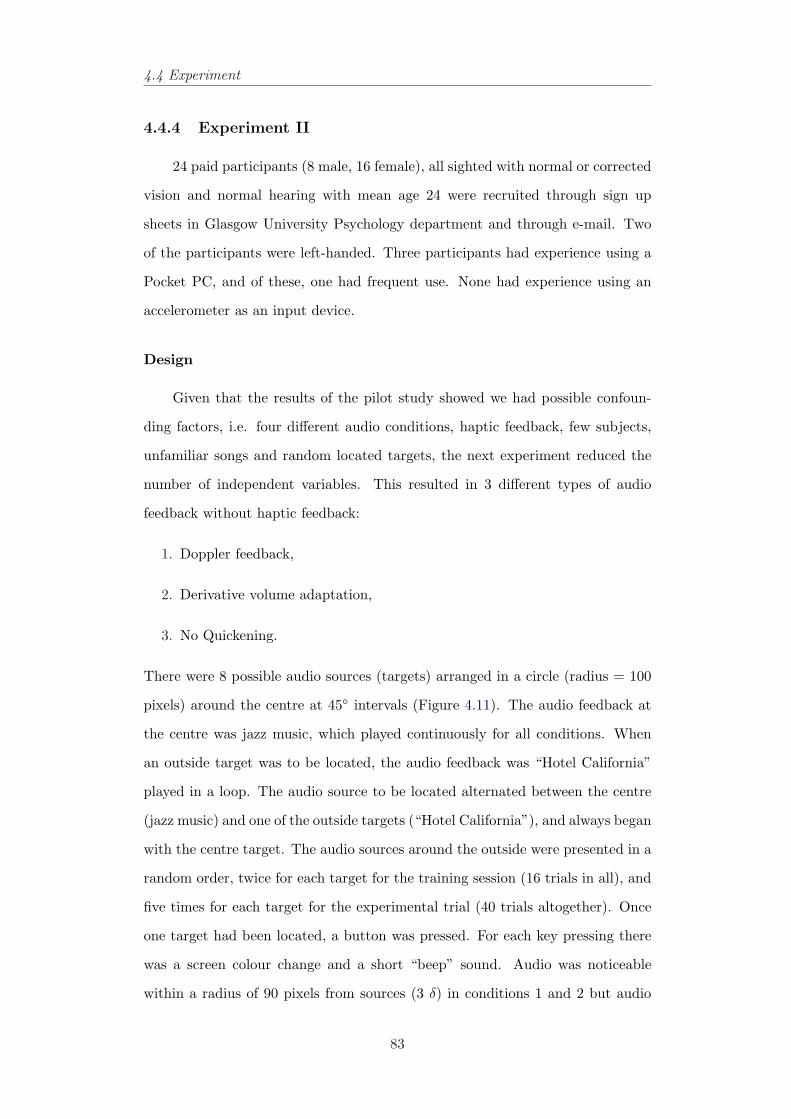
4.4 Experiment
4.4.4 Experiment II
24 paid participants (8 male, 16 female), all sighted with normal or corrected
vision and normal hearing with mean age 24 were recruited through sign up
sheets in Glasgow University Psychology department and through e-mail. Two
of the participants were left-handed. Three participants had experience using a
Pocket PC, and of these, one had frequent use. None had experience using an
accelerometer as an input device.
Design
Given that the results of the pilot study showed we had possible confoun-
ding factors, i.e. four different audio conditions, haptic feedback, few subjects,
unfamiliar songs and random located targets, the next experiment reduced the
number of independent variables. This resulted in 3 different types of audio
feedback without haptic feedback:
1. Doppler feedback,
2. Derivative volume adaptation,
3. No Quickening.
There were 8 possible audio sources (targets) arranged in a circle (radius = 100
pixels) around the centre at 45◦ intervals (Figure 4.11). The audio feedback at
the centre was jazz music, which played continuously for all conditions. When
an outside target was to be located, the audio feedback was “Hotel California”
played in a loop. The audio source to be located alternated between the centre
(jazz music) and one of the outside targets (“Hotel California”), and always began
with the centre target. The audio sources around the outside were presented in a
random order, twice for each target for the training session (16 trials in all), and
five times for each target for the experimental trial (40 trials altogether). Once
one target had been located, a button was pressed. For each key pressing there
was a screen colour change and a short “beep” sound. Audio was noticeable
within a radius of 90 pixels from sources (3 δ) in conditions 1 and 2 but audio
83
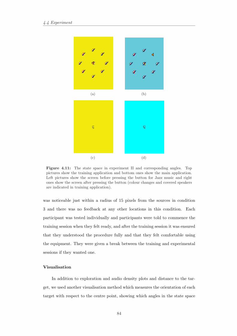
4.4 Experiment
(a) (b)
(c) (d)
Figure 4.11: The state space in experiment II and corresponding angles. Toppictures show the training application and bottom ones show the main application.Left pictures show the screen before pressing the button for Jazz music and rightones show the screen after pressing the button (colour changes and covered speakersare indicated in training application).
was noticeable just within a radius of 15 pixels from the sources in condition
3 and there was no feedback at any other locations in this condition. Each
participant was tested individually and participants were told to commence the
training session when they felt ready, and after the training session it was ensured
that they understood the procedure fully and that they felt comfortable using
the equipment. They were given a break between the training and experimental
sessions if they wanted one.
Visualisation
In addition to exploration and audio density plots and distance to the tar-
get, we used another visualisation method which measures the orientation of each
target with respect to the centre point, showing which angles in the state space
84
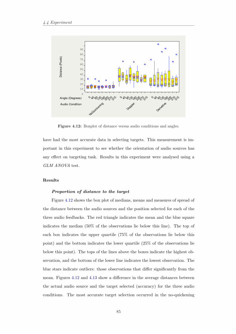
4.4 Experiment
Dis
tance (
Pix
els
)
Audio Condition
Angle (Degrees)
Deriva
tive
Doppl
er
NoQui
cken
ing
315
270
225
180
13590450
315
270
225
180
13590450
315
270
225
180
13590450
90
80
70
60
50
40
30
20
10
0
Figure 4.12: Boxplot of distance versus audio conditions and angles.
have had the most accurate data in selecting targets. This measurement is im-
portant in this experiment to see whether the orientation of audio sources has
any effect on targeting task. Results in this experiment were analysed using a
GLM ANOVA test.
Results
Proportion of distance to the target
Figure 4.12 shows the box plot of medians, means and measures of spread of
the distance between the audio sources and the position selected for each of the
three audio feedbacks. The red triangle indicates the mean and the blue square
indicates the median (50% of the observations lie below this line). The top of
each box indicates the upper quartile (75% of the observations lie below this
point) and the bottom indicates the lower quartile (25% of the observations lie
below this point). The tops of the lines above the boxes indicate the highest ob-
servation, and the bottom of the lower line indicates the lowest observation. The
blue stars indicate outliers: those observations that differ significantly from the
mean. Figures 4.12 and 4.13 show a difference in the average distances between
the actual audio source and the target selected (accuracy) for the three audio
conditions. The most accurate target selection occurred in the no-quickening
85
4.4 Experiment
0
5
10
15
20
25Angle 90
Angle 45
Angle 0
Angle 315
Angle 270
Angle 225
Angle 180
Angle 135
(a) Average of position error in theDerivative condition for all users
0
10
20
30
40
50Angle 90
Angle 45
Angle 0
Angle 315
Angle 270
Angle 225
Angle 180
Angle 135
(b) Average of position error in theDoppler condition for all users
0
2
4
6
8
10Angle 90
Angle 45
Angle 0
Angle 315
Angle 270
Angle 225
Angle 180
Angle 135
(c) Average of position error in theNo-Quickening condition for all users
Figure 4.13: Average of position error in pixels for all participants in three audioconditions.
condition, and there was little difference between the levels of accuracy for each
orientation. The spread for no quickening was very small, and the 5 outliers are
not very far away from the median, suggesting that, overall, most people in this
condition took approximately the same length of time to select a target. The
derivative condition takes longer overall than the no-quickening condition. The
spread is larger (largest of all three conditions) and the outliers further away
from the median than in the no-quickening condition. The participants in the
Doppler condition took longer on average to select the targets, compared with
those in the other two conditions. The spread in the Doppler condition is smaller
than in the derivative condition, but larger than in the no-quickening condition.
This shows that angles 90◦ and 270◦ have higher accuracy. In the GLM ANOVA
analysis it was found that there was a significant effect of audio type on the dis-
tance (F(2,21)=4.345; p<0.05). There were, however, no significant differences
between the 8 audio orientations. Post-hoc analysis using a Tukey test showed
that there was a significant difference between the estimated mean distances
86
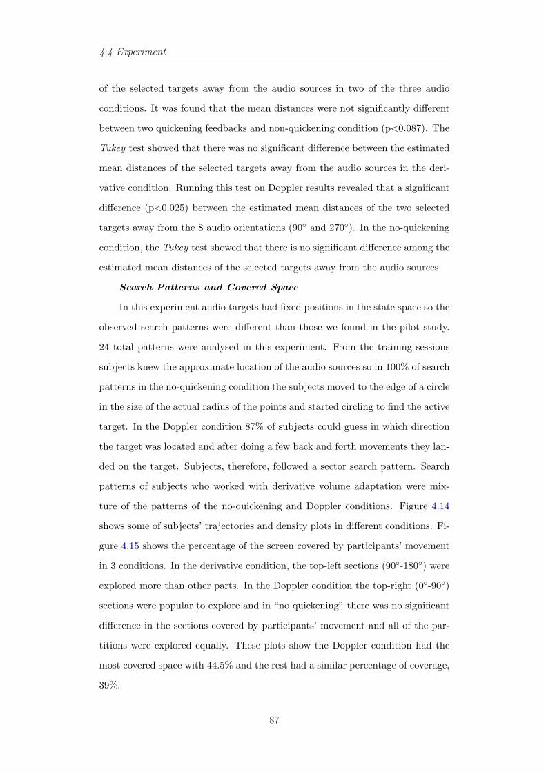
4.4 Experiment
of the selected targets away from the audio sources in two of the three audio
conditions. It was found that the mean distances were not significantly different
between two quickening feedbacks and non-quickening condition (p<0.087). The
Tukey test showed that there was no significant difference between the estimated
mean distances of the selected targets away from the audio sources in the deri-
vative condition. Running this test on Doppler results revealed that a significant
difference (p<0.025) between the estimated mean distances of the two selected
targets away from the 8 audio orientations (90◦ and 270◦). In the no-quickening
condition, the Tukey test showed that there is no significant difference among the
estimated mean distances of the selected targets away from the audio sources.
Search Patterns and Covered Space
In this experiment audio targets had fixed positions in the state space so the
observed search patterns were different than those we found in the pilot study.
24 total patterns were analysed in this experiment. From the training sessions
subjects knew the approximate location of the audio sources so in 100% of search
patterns in the no-quickening condition the subjects moved to the edge of a circle
in the size of the actual radius of the points and started circling to find the active
target. In the Doppler condition 87% of subjects could guess in which direction
the target was located and after doing a few back and forth movements they lan-
ded on the target. Subjects, therefore, followed a sector search pattern. Search
patterns of subjects who worked with derivative volume adaptation were mix-
ture of the patterns of the no-quickening and Doppler conditions. Figure 4.14
shows some of subjects’ trajectories and density plots in different conditions. Fi-
gure 4.15 shows the percentage of the screen covered by participants’ movement
in 3 conditions. In the derivative condition, the top-left sections (90◦-180◦) were
explored more than other parts. In the Doppler condition the top-right (0◦-90◦)
sections were popular to explore and in “no quickening” there was no significant
difference in the sections covered by participants’ movement and all of the par-
titions were explored equally. These plots show the Doppler condition had the
most covered space with 44.5% and the rest had a similar percentage of coverage,
39%.
87
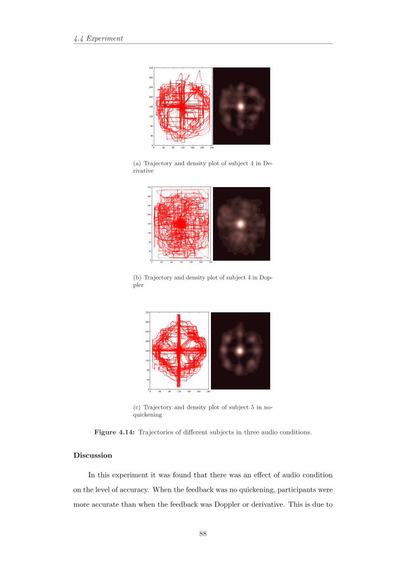
4.4 Experiment
0 40 80 120 160 200 2400
40
80
120
160
200
240
280
320
(a) Trajectory and density plot of subject 4 in De-rivative
0 40 80 120 160 200 2400
40
80
120
160
200
240
280
320
(b) Trajectory and density plot of subject 4 in Dop-pler
0 40 80 120 160 200 2400
40
80
120
160
200
240
280
320
(c) Trajectory and density plot of subject 5 in no-quickening
Figure 4.14: Trajectories of different subjects in three audio conditions.
Discussion
In this experiment it was found that there was an effect of audio condition
on the level of accuracy. When the feedback was no quickening, participants were
more accurate than when the feedback was Doppler or derivative. This is due to
88
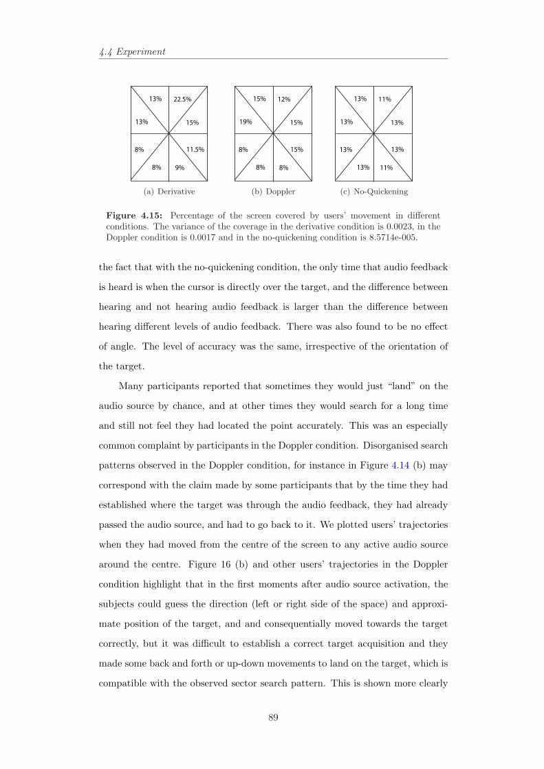
4.4 Experiment
22.5%
15%
11.5%
9%8%
8%
13%
13%
(a) Derivative
12%
15%
15%
8%8%
8%
19%
15%
(b) Doppler
11%
13%
13%
11%13%
13%
13%
13%
(c) No-Quickening
Figure 4.15: Percentage of the screen covered by users’ movement in differentconditions. The variance of the coverage in the derivative condition is 0.0023, in theDoppler condition is 0.0017 and in the no-quickening condition is 8.5714e-005.
the fact that with the no-quickening condition, the only time that audio feedback
is heard is when the cursor is directly over the target, and the difference between
hearing and not hearing audio feedback is larger than the difference between
hearing different levels of audio feedback. There was also found to be no effect
of angle. The level of accuracy was the same, irrespective of the orientation of
the target.
Many participants reported that sometimes they would just “land” on the
audio source by chance, and at other times they would search for a long time
and still not feel they had located the point accurately. This was an especially
common complaint by participants in the Doppler condition. Disorganised search
patterns observed in the Doppler condition, for instance in Figure 4.14 (b) may
correspond with the claim made by some participants that by the time they had
established where the target was through the audio feedback, they had already
passed the audio source, and had to go back to it. We plotted users’ trajectories
when they had moved from the centre of the screen to any active audio source
around the centre. Figure 16 (b) and other users’ trajectories in the Doppler
condition highlight that in the first moments after audio source activation, the
subjects could guess the direction (left or right side of the space) and approxi-
mate position of the target, and and consequentially moved towards the target
correctly, but it was difficult to establish a correct target acquisition and they
made some back and forth or up-down movements to land on the target, which is
compatible with the observed sector search pattern. This is shown more clearly
89
4.4 Experiment
0 40 120 160 240
0
40
80
120
160
200
280
80 180
240
320
(a) Trajectory and density plot ofsubject 1 in Derivative case
0 40 120 160 240
0
40
80
120
160
200
280
80 180
240
320
(b) Trajectory of subject 4 in Dopplercase
0 40 120 160 240
0
40
80
120
160
200
280
80 180
240
320
(c) Trajectory of subject 4 in No Qui-ckening case
Figure 4.16: Trajectories of different subjects in three audio conditions when theyhave moved from the centre to outlying active audio sources.
in Figure 4.17 (a-left) and the user’s trajectories as time series in Figure 4.17
(b-left) in an individual target acquisition task when the user has moved from
the centre to the target in angle 45◦, which has been activated. Figures 4.14(a)
and 4.16(a) shows a trajectory that is fairly typical for most participants in the
derivative condition. It can be seen that the trajectory is far more ordered, with
participants moving in the horizontal and vertical directions (in the directions
of 0◦, 90◦, 180◦ and 270◦), more so than in the Doppler condition. It becomes
obvious that participants moved in a circular motion that they learnt during the
training session, far more so than those in the Doppler condition. From this,
90
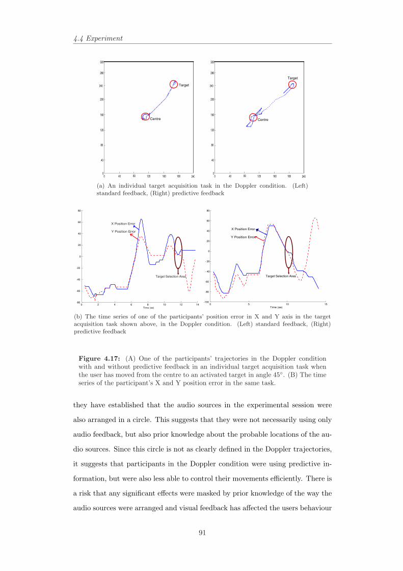
4.4 Experiment
Target
Centre
0 40 120 160 240
0
40
80
120
160
200
280
80 180
240
320
Target
Centre
0 40 120 160 240
0
40
80
120
160
200
280
80 180
240
320
(a) An individual target acquisition task in the Doppler condition. (Left)standard feedback, (Right) predictive feedback
0 2 4 6 8 10 12 14-80
-60
-40
-20
0
20
40
60
80
Time (se)
X Position E rr or
Y Position E rr or
Target Selection Area
0 5 10 15-100
-80
-60
- 40
- 20
0
20
40
60
80
Time (se)
X Position E rr or
Y Position E rr or
Target Selection Area
(b) The time series of one of the participants’ position error in X and Y axis in the targetacquisition task shown above, in the Doppler condition. (Left) standard feedback, (Right)predictive feedback
Figure 4.17: (A) One of the participants’ trajectories in the Doppler conditionwith and without predictive feedback in an individual target acquisition task whenthe user has moved from the centre to an activated target in angle 45◦. (B) The timeseries of the participant’s X and Y position error in the same task.
they have established that the audio sources in the experimental session were
also arranged in a circle. This suggests that they were not necessarily using only
audio feedback, but also prior knowledge about the probable locations of the au-
dio sources. Since this circle is not as clearly defined in the Doppler trajectories,
it suggests that participants in the Doppler condition were using predictive in-
formation, but were also less able to control their movements efficiently. There is
a risk that any significant effects were masked by prior knowledge of the way the
audio sources were arranged and visual feedback has affected the users behaviour
91
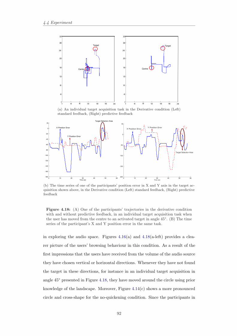
4.4 Experiment
Target
Centre
0 40 120 160 240
0
40
80
120
160
200
280
80 180
240
320
Target
Centre
0 40 120 160 240
0
40
80
120
160
200
280
80 180
240
320
(a) An individual target acquisition task in the Derivative condition (Left)standard feedback, (Right) predictive feedback
0 10 20 30 40 50 60-180
-160
-140
-120
-100
-80
-60
-40
-20
0
20
Time (se)
X Position E rr or
Y Position E rr or
Target Selection Area
0 10 20 30 40 50 60-200
-150
-100
-50
0
50
Time (se)
X Position E rr orY Position E rr or
Target Selection Area
(b) The time series of one of the participants’ position error in X and Y axis in the target ac-quisition shown above, in the Derivative condition (Left) standard feedback, (Right) predictivefeedback
Figure 4.18: (A) One of the participants’ trajectories in the derivative conditionwith and without predictive feedback, in an individual target acquisition task whenthe user has moved from the centre to an activated target in angle 45◦. (B) The timeseries of the participant’s X and Y position error in the same task.
in exploring the audio space. Figures 4.16(a) and 4.18(a-left) provides a clea-
rer picture of the users’ browsing behaviour in this condition. As a result of the
first impressions that the users have received from the volume of the audio source
they have chosen vertical or horizontal directions. Whenever they have not found
the target in these directions, for instance in an individual target acquisition in
angle 45◦ presented in Figure 4.18, they have moved around the circle using prior
knowledge of the landscape. Moreover, Figure 4.14(c) shows a more pronounced
circle and cross-shape for the no-quickening condition. Since the participants in
92
4.4 Experiment
the no-quickening condition were presented with no aural feedback except when
directly over the target, it is, most likely that they were relying on the circu-
lar target distribution previously seen in the training. This led to a systematic
search strategy, less ‘browsing around’ because of the lack of predictive ability
without quickening. All users who participated in this condition claimed that
this was not an exciting method of exploring the auditory space.
4.4.5 Human Operator Modeling
Interaction with auditory interfaces is an example of continuous interaction
which was discussed in Section 3.3.1. In these systems which rely heavily on the
tracking of hand in a simulated environment the pretence of reality requires a
tight coupling between the user’s view and hearing of the environment and the
actions, hand motions, that set the view and hearing. Thus the performance is
adversely affected when the feedback is subject to delay or lag (Jagacinski and
Flach, 2003; MacKenzie and Ware, 1993).
Using the platform in the previous experiment, we carried out a prelimi-
nary investigation to measure and model the accuracy, and bandwidth of human
motor-sensory performance in interactive tasks subject to lag. We kept the same
format of the second experiment but instead of providing audio feedback to the
user’s current position we provided feedback to the user’s predicted position cal-
culated according to equation ( 3.12) in Section 3.3.1:
Xt+τ = Xt + V τ (4.3)
The volume of the audio source, which provides feedback about the target’s
position, is a function of the user’s current velocity and position. Here, Xt+τ
and Xt are the user’s position at time t + τ and t or current position and next
possible position respectively. τ is the human’s time-delay or reflection time
(refer to Section 3.3.1 on page 51), which becomes our ‘prediction horizon’ for
the predictive model, and V is the user’s speed of motion in the audio space. This
has the effect that, as the user moves toward the target s/he feels him/herself in
93
4.4 Experiment
the position predicted to be reached at time t + τ .
Design
In the second experimental setup we added a smooth drop-off in the time
horizon of the prediction, as the target is approached. The fall off began at
radius 15 pixels, and once the user was within 5 pixels of the source the feedback
reverted to standard feedback with no predictive element.
In a pilot study we ran the application for three participants familiar with the
Pocket PCs and accelerometer. Neither felt any difference in the two derivative
conditions, with and without prediction. In Figures 4.18(a) and 4.19(b) we see
one of the participant’s trajectories when he has moved from the centre to any
active target. Providing feedback to the user’s future position in the derivative
condition has not much changed the user’s exploratory behaviour. But users
reported a great difference between Doppler with the predictive model-based
feedback and Doppler with no predictive feedback. They said it felt they were
able to acquire the direction of the audio source more quickly in the predictive
case, but that it was a more difficult to land on the source. In the standard
model with no predictive element they felt it was slower to find the direction
but easier to land. Despite their perceptions, the trajectories in Figures 4.17(a-
right) and 4.19(a) suggest the opposite case, that they performed fewer oscillatory
movements around the target in the predictive model, compared to the standard
case.
Prediction in the Doppler case allowed the users to converge more rapidly
and directly to the target, but it seemed less helpful very close to the target.
In the derivative condition predictive feedback seems to have smoothed the be-
haviour, but has not improved the initial target localisation. These preliminary
explorations suggest that a more detailed investigation of incorporating the pre-
dictive element in the feedback system would be of interest.
94
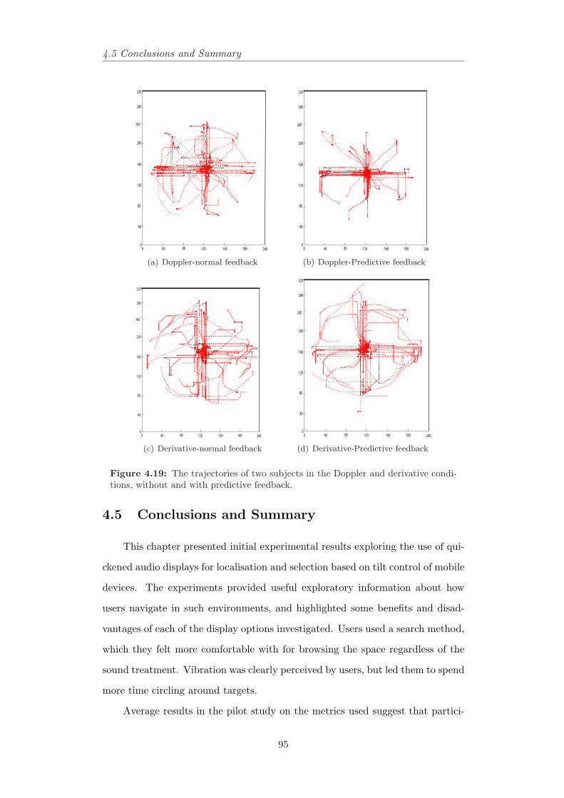
4.5 Conclusions and Summary
0 40 120 160 240
0
40
80
120
160
200
280
80 180
240
320
(a) Doppler-normal feedback
0 40 120 160 240
0
40
80
120
160
200
280
80 180
240
320
(b) Doppler-Predictive feedback
0 40 120 160 240
0
40
80
120
160
200
280
80 180
240
320
(c) Derivative-normal feedback
0 40 120 160 240
0
40
80
120
160
200
280
80 180
240
320
(d) Derivative-Predictive feedback
Figure 4.19: The trajectories of two subjects in the Doppler and derivative condi-tions, without and with predictive feedback.
4.5 Conclusions and Summary
This chapter presented initial experimental results exploring the use of qui-
ckened audio displays for localisation and selection based on tilt control of mobile
devices. The experiments provided useful exploratory information about how
users navigate in such environments, and highlighted some benefits and disad-
vantages of each of the display options investigated. Users used a search method,
which they felt more comfortable with for browsing the space regardless of the
sound treatment. Vibration was clearly perceived by users, but led them to spend
more time circling around targets.
Average results in the pilot study on the metrics used suggest that partici-
95
4.5 Conclusions and Summary
pants were more accurate in target selection in the “no Doppler-no vibration”
than other conditions. The results do not suggest that the use of Doppler or
vibration brought consistently improved accuracy, but some people did very well
with Doppler and most stated that they found the vibration feedback useful. Lon-
ger studies might show different use in real-life tasks once users had familiarised
themselves with the system.
The main study represented a more focused investigation, with fewer confoun-
ding factors. We increased the number of participants, placed all the targets at
equal distances from the starting point (centre of the screen), did not include
haptic feedback, chose western pop music which was familiar to all users, and
specified more time for allowing users to learn how to use the specific interface,
which was new to all. We investigated whether quickening was more useful to
users searching for targets in state-space than no quickening audio feedback. We
also investigated if there was any advantage of using Doppler feedback over deri-
vative, and if there was an effect of orientation in either Doppler, derivative or no
quickening, and therefore to find out if the results of the first experiment could
have been masked by an interaction with the orientation of the targets. It was
also found that there was no effect of the angle at which the audio source was
located.
In a preliminary investigation to better understanding the results and to
guide future work, we performed an explanatory experiment with predictive
model-based feedback. The model is based on human operator modeling in
continuous tracking tasks, and it could take human response delays and lags
into account (not considered in this Chapter). Using this predictive model, we
could improve the users’ performance in the Doppler condition and reduce their
overshoots during landing on the target just by providing audio feedback about
the user’s predicted position instead of their current position. This suggests that
further research to investigate the benefits of explicitly incorporating models of
human behaviour in the design of feedback methods. More studies need to be
done to find out how much does this method improve the users’ performance in
the audio/haptic interfaces? Does this method reduce the user’s overshoots when
96
4.5 Conclusions and Summary
they are targeting just by providing the multimodal feedback about the user’s
predicted position instead of his/her current position?
As discussed earlier in Chapter 2, Fitts’ law has not been successful in audi-
tory interfaces but it would be interesting to study Hick’s law, or the Hick-Hyman
law (Hick, 1952; Hyman, 1953) in auditory/haptic interfaces where targets are
located or activated randomly similar to the application described in this chap-
ter. This study may answer questions, for example, how long do users need to
familiarised themselves with the system?
The results in this chapter are a useful starting point for further investiga-
tion into the types of feedback that are most useful and informative in assisting
users of a tilt-controlled Pocket PC and sonified interface. Further development
of the techniques and experimental design employed in this study will allow ma-
nufacturers of such devices to incorporate the most effective type of feedback into
their products.
In the following chapters we focus more on tilt-controlled interfaces, models
of human behaviour in the design of audio/visual feedback methods and human
response delays.
97
Chapter 5
Tilt-Controlled Zooming User
Interfaces on Mobile Devices
This chapter provides a dynamic system interpretation of the couplingof internal states involved in speed-dependent automatic zooming, andwe test our implementation on a text browser on a Pocket PC ins-trumented with an accelerometer. The dynamic systems approach tothe design of such continuous interaction interfaces allows to simulateand use analytical tools to analyse the behaviour and stability of thecontrolled system alone and when it is coupled with a manual controlmodel of user behaviour and calibrate and tune the parameters of thesystem before the actual implementation. Furthermore, it is shownthat browsing and targeting can be facilitated by using a model-basedsonification approach to generate audio/vibrotactile feedback about do-cument structure, in the proposed interface for a text-browser. Weshow examples of audio/vibrotactile feedback and illustrate that mul-timodal feedback provides valuable information, supporting intermit-tent interaction, i.e., allowing movement-based interaction techniquesto continue for a blindfolded user.
5.1 Introduction
Navigation techniques such as scrolling (or panning) and zooming are essen-
tial components of mobile device applications such as map browsing and reading
text documents, allowing the user to access to a larger information space than
can be viewed on the small screen. Scrolling allows the user to move to different
98
5.1 Introduction
locations, while zooming allows the user to view a target at different scales.
However, the restrictions in screen space on mobile devices make it difficult to
browse a large document efficiently. Using the traditional scroll bar, the user
must move back and forth between the document and the scroll bar, which can
increase the effort required to use the interface. In addition, in a long document,
a small movement of the handle can cause a sudden jump to a distant location,
resulting in disorientation and frustration (Brewster et al., 1994).
Speed-dependent automatic zooming is a relatively new navigation tech-
nique (Cockburn et al., 2003; Cockburn and Savage, 2003; Igarashi and Hinckely,
2000; Savage, 2004; Wallace, 2003; Wallace et al., 2004) that unifies rate-based
scrolling and zooming to overcome these limitations. The user controls the scrol-
ling speed only, and the system automatically adjusts the zoom level so that the
speed of visual flow across the screen remains constant. Using this technique, the
user can smoothly locate a distant target in a large document without having
to manually interweave zooming and scrolling, and without becoming disorien-
ted by extreme visual flow. In this chapter we demonstrate that, as suggested
by Igarashi and Hinckely (2000), speed-dependent automatic zooming (SDAZ) is
well suited to implementation on mobile devices instrumented with tilt sensors,
which can then be comfortably controlled in a single-handed fashion. We also
describe an alternative stylus-controlled implementation for the Pocket PC. A
further contribution is the use of a state-space formulation of speed dependent
zooming, which we believe is a promising reformulation of the technique, which
opens the path to the use of analytic tools from optimal and manual control
theory.
Next, we show that browsing and targeting can be facilitated by using a
model-based sonification approach to generate audio feedback about document
structure in the text browser interface. This supports intermittent interaction
and allows movement-based interaction to continue while the user is simulta-
neously involved with other tasks.
99
5.2 Related Work
5.2 Related Work
5.2.1 Alternative Scrolling Techniques
Several alternations to traditional scroll bars have been proposed. They
allow the user to control scrolling speed, enabling fine positioning in large docu-
ments. The AlphaSlider (Ahlberg and Shneiderman, 1994) and FineSlider (Ma-
sui et al., 1995) are two alternative scrolling techniques for precise selection in
large lists. The essential components of these techniques are the same as those
of a drop-down list-box. There is a slider area, a slider thumb and left/right ar-
row keys. The AlphaSlider functions identically to a drop-down list-box, except
for its vertical orientation. This method is very efficient in its screen space use
but it allows less use of context in searching. The FineSlider is based upon the
AlphaSlider but uses an elastic technique based on a rubber band metaphor. A
control object such as a scroll bar is moved by pulling the object with a rubber
band between the object and the mouse cursor.
LensBar (Masui, 1998) combines these techniques with interactive filtering
and semantic zooming, and also provides explicit control of zooming via hori-
zontal motion of the mouse cursor. A rate-based scrolling interface is described
in (Zhai et al., 1997) that maps displacement of the input device to the velocity
of scrolling.
Another technique is called Stretch Button Scrollbar (Smith and Henning,
1996). The scroll handle is modified with two extra buttons, one on either side.
These buttons allow fine movements similar to that provided by the arrow mo-
vement buttons on traditional scroll bars.
5.2.2 Alternative Zooming Techniques
Zoomable user interfaces, such as Pad and Pad++ (Bederson et al., 1994;
Perlin and Fox, 1993), use continuous zooming as a central navigation tool. The
objects are spatially organised in an infinite two-dimensional information space,
and the user accesses a target object using panning and zooming operations. A
notable problem with the original zoomable interfaces is that they require explicit
100
5.2 Related Work
control of both panning and zooming, and it is sometimes difficult for the user
to coordinate them. The user can get lost in the infinite information space (Jul
and Furnas, 1998). Bimanual approaches also exist, such as that of Guiard et al.
(2001) where a joystick in one hand controlled zoom level, and a mouse in the
other hand provided navigation. They showed that by using zooming interfaces,
bit rates far beyond those possible in physical selection tasks become possible.
Van Wijk derived an optimal trajectory for panning and zooming (Wijk and Nuij,
2003), for known start and end points.
5.2.3 Alternative Visualisation Techniques
Information visualisation techniques, such as Fisheye Views (Furnas, 1986;
Gutwin, 2002), Perspective Wall (Mackinlay et al., 1991), and the Document
Lens (Perlin and Fox, 1993) also address the problem of information overload
by distorting the view of documents. The focused area is magnified, while the
non-focused areas are squashed but remain in spatial context. The user specifies
the next focal point by clicking or panning. These methods can cause several
problems for users. One of these is focus-targeting, where a user moves the focus
to a new location. Magnification makes focus-targeting difficult because objects
appear to move as the focus point approaches them. One solution to this problem
is speed-coupled flattening (SCF) (Gutwin, 2002). This technique reduces the
distortion level of the focus, based on pointer velocity and acceleration. SCF was
proven to significantly reduce both targeting time and targeting errors in fisheye
environments. Another technique to solve focus-targeting problem is state-space
modeling which will be described in Chapter 6.
5.2.4 Disadvantages of Current Scrolling and Zooming Techniques
Scrolling, panning and zooming techniques have their own limitations. Iga-
rashi and Hinckely (2000) identified the additional overhead involved with the
user’s attention moving back and forth between the scroll bars and the docu-
ment. To scroll the user must first acquire the scroll handle, which is sometimes
very small (i.e., in long documents) and difficult to target, by moving the mouse
101
5.2 Related Work
cursor or stylus pointer to the handle and clicking the mouse button or tapping
on the screen. Then the user goes back to the updated text in the document.
In long documents scroll handle manipulation is more difficult because a small
movement can cause a large jump in the information space, which can cause
disorientation and confusion (Brewster et al., 1994).
Changing the magnification level affects the user’s speed. In zoomed-out do-
cument the user moves quickly to avoid frustration but in zoomed-in document
s/he moves slowly to avoid disorientation. Furthemore, these non-smooth tran-
sitions may cause users to lose context when zooming in and out of a document;
because when they are zoomed out to get an overview from the document, there
is not enough detail to target and when they are zoomed in to see the detail, the
context is lost (Brewster et al., 1994; Cockburn et al., 2005). To improve this
problem, multiple windows, each with pan and zoom capability can be provided.
But, this method may cause usability problems on small screen devices due to
lack of screen space and window overlap. An alternative solution is to have one
window containing a small overview, while a second window shows a large more
detailed view (Beard and Walker, 1990; Furnas and Bederson, 1995). The small
overview contains a rectangle that can be moved and resized, and its contents
are shown at a larger scale in the large view. This strategy, however, requires
extra space for the overview and the user should mentally integrate the detail
and context views. An operational overhead is also required, because the user
must regularly move the mouse between the detail and context windows.
The most important problem with panning is that constant mouse movement
is required to scroll. One solution is a rate-based scrolling interface (first-order
control devices, see Section 3.2.5 on page 38) (Zhai et al., 1993). Rate-based
scrolling maps the displacement of the cursor to the scrolling velocity. In a study
of different input devices for scrolling and pointing tasks, Zhai et al. (1993) used
an isometric joystick which maps the force exerted to velocity in the document.
For this study they used the IBM ScrollPoint IITM , which is a mouse with a small
joystick in place of the scroll wheel, commonly used for rate-based scrolling. In
this study Zhai et al. compared rate-based scrolling with scrollbars. They found
102
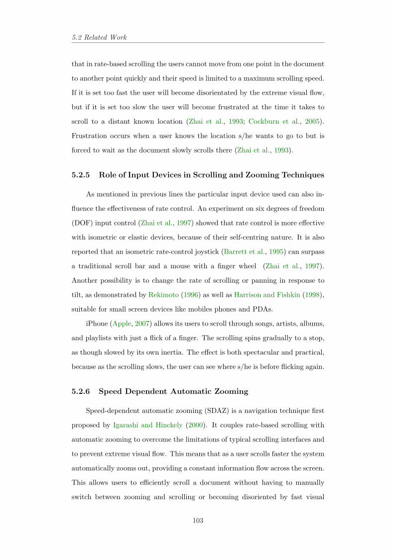
5.2 Related Work
that in rate-based scrolling the users cannot move from one point in the document
to another point quickly and their speed is limited to a maximum scrolling speed.
If it is set too fast the user will become disorientated by the extreme visual flow,
but if it is set too slow the user will become frustrated at the time it takes to
scroll to a distant known location (Zhai et al., 1993; Cockburn et al., 2005).
Frustration occurs when a user knows the location s/he wants to go to but is
forced to wait as the document slowly scrolls there (Zhai et al., 1993).
5.2.5 Role of Input Devices in Scrolling and Zooming Techniques
As mentioned in previous lines the particular input device used can also in-
fluence the effectiveness of rate control. An experiment on six degrees of freedom
(DOF) input control (Zhai et al., 1997) showed that rate control is more effective
with isometric or elastic devices, because of their self-centring nature. It is also
reported that an isometric rate-control joystick (Barrett et al., 1995) can surpass
a traditional scroll bar and a mouse with a finger wheel (Zhai et al., 1997).
Another possibility is to change the rate of scrolling or panning in response to
tilt, as demonstrated by Rekimoto (1996) as well as Harrison and Fishkin (1998),
suitable for small screen devices like mobiles phones and PDAs.
iPhone (Apple, 2007) allows its users to scroll through songs, artists, albums,
and playlists with just a flick of a finger. The scrolling spins gradually to a stop,
as though slowed by its own inertia. The effect is both spectacular and practical,
because as the scrolling slows, the user can see where s/he is before flicking again.
5.2.6 Speed Dependent Automatic Zooming
Speed-dependent automatic zooming (SDAZ) is a navigation technique first
proposed by Igarashi and Hinckely (2000). It couples rate-based scrolling with
automatic zooming to overcome the limitations of typical scrolling interfaces and
to prevent extreme visual flow. This means that as a user scrolls faster the system
automatically zooms out, providing a constant information flow across the screen.
This allows users to efficiently scroll a document without having to manually
switch between zooming and scrolling or becoming disoriented by fast visual
103
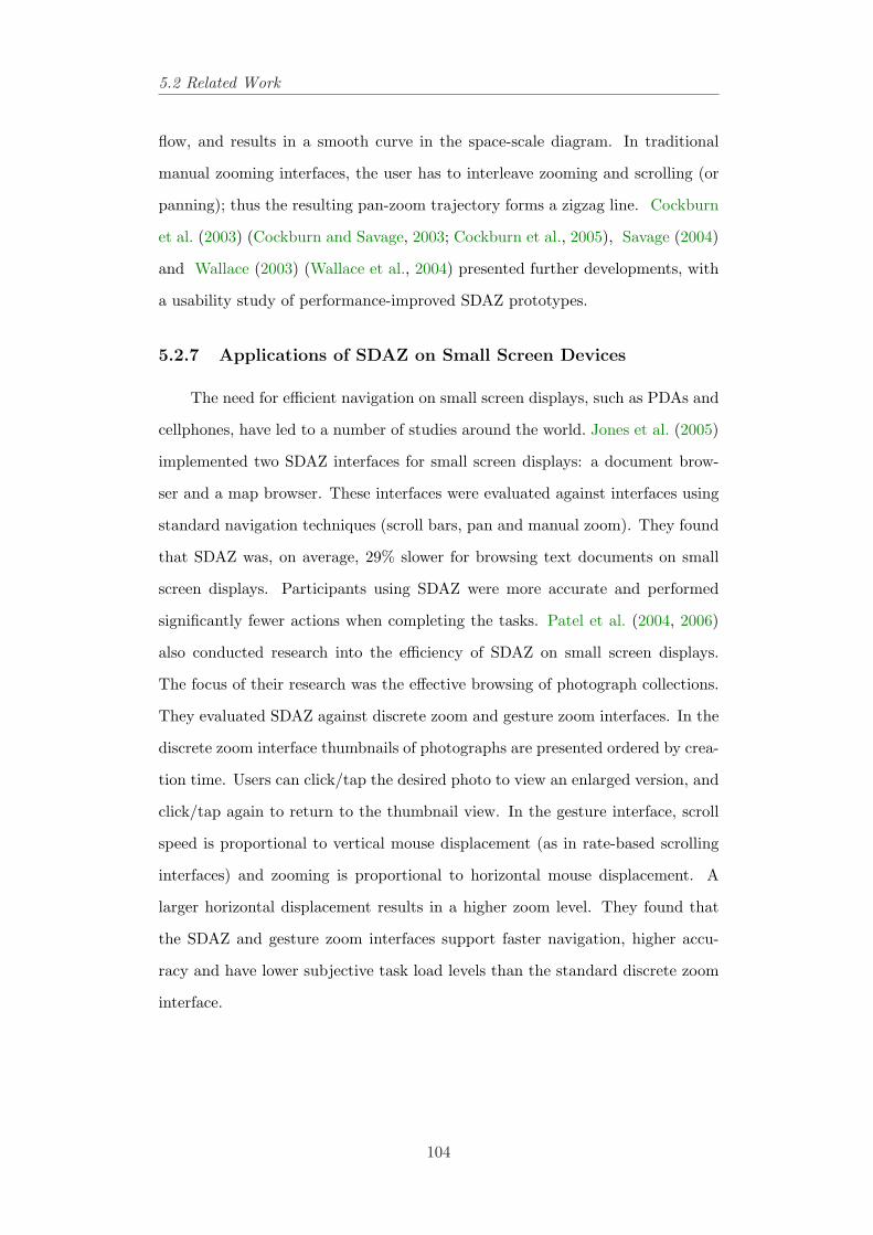
5.2 Related Work
flow, and results in a smooth curve in the space-scale diagram. In traditional
manual zooming interfaces, the user has to interleave zooming and scrolling (or
panning); thus the resulting pan-zoom trajectory forms a zigzag line. Cockburn
et al. (2003) (Cockburn and Savage, 2003; Cockburn et al., 2005), Savage (2004)
and Wallace (2003) (Wallace et al., 2004) presented further developments, with
a usability study of performance-improved SDAZ prototypes.
5.2.7 Applications of SDAZ on Small Screen Devices
The need for efficient navigation on small screen displays, such as PDAs and
cellphones, have led to a number of studies around the world. Jones et al. (2005)
implemented two SDAZ interfaces for small screen displays: a document brow-
ser and a map browser. These interfaces were evaluated against interfaces using
standard navigation techniques (scroll bars, pan and manual zoom). They found
that SDAZ was, on average, 29% slower for browsing text documents on small
screen displays. Participants using SDAZ were more accurate and performed
significantly fewer actions when completing the tasks. Patel et al. (2004, 2006)
also conducted research into the efficiency of SDAZ on small screen displays.
The focus of their research was the effective browsing of photograph collections.
They evaluated SDAZ against discrete zoom and gesture zoom interfaces. In the
discrete zoom interface thumbnails of photographs are presented ordered by crea-
tion time. Users can click/tap the desired photo to view an enlarged version, and
click/tap again to return to the thumbnail view. In the gesture interface, scroll
speed is proportional to vertical mouse displacement (as in rate-based scrolling
interfaces) and zooming is proportional to horizontal mouse displacement. A
larger horizontal displacement results in a higher zoom level. They found that
the SDAZ and gesture zoom interfaces support faster navigation, higher accu-
racy and have lower subjective task load levels than the standard discrete zoom
interface.
104
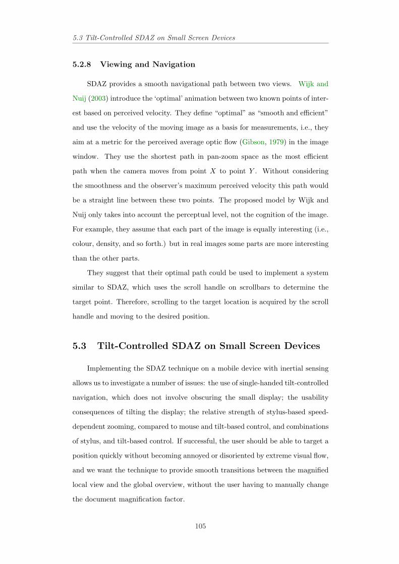
5.3 Tilt-Controlled SDAZ on Small Screen Devices
5.2.8 Viewing and Navigation
SDAZ provides a smooth navigational path between two views. Wijk and
Nuij (2003) introduce the ‘optimal’ animation between two known points of inter-
est based on perceived velocity. They define “optimal” as “smooth and efficient”
and use the velocity of the moving image as a basis for measurements, i.e., they
aim at a metric for the perceived average optic flow (Gibson, 1979) in the image
window. They use the shortest path in pan-zoom space as the most efficient
path when the camera moves from point X to point Y . Without considering
the smoothness and the observer’s maximum perceived velocity this path would
be a straight line between these two points. The proposed model by Wijk and
Nuij only takes into account the perceptual level, not the cognition of the image.
For example, they assume that each part of the image is equally interesting (i.e.,
colour, density, and so forth.) but in real images some parts are more interesting
than the other parts.
They suggest that their optimal path could be used to implement a system
similar to SDAZ, which uses the scroll handle on scrollbars to determine the
target point. Therefore, scrolling to the target location is acquired by the scroll
handle and moving to the desired position.
5.3 Tilt-Controlled SDAZ on Small Screen Devices
Implementing the SDAZ technique on a mobile device with inertial sensing
allows us to investigate a number of issues: the use of single-handed tilt-controlled
navigation, which does not involve obscuring the small display; the usability
consequences of tilting the display; the relative strength of stylus-based speed-
dependent zooming, compared to mouse and tilt-based control, and combinations
of stylus, and tilt-based control. If successful, the user should be able to target a
position quickly without becoming annoyed or disoriented by extreme visual flow,
and we want the technique to provide smooth transitions between the magnified
local view and the global overview, without the user having to manually change
the document magnification factor.
105
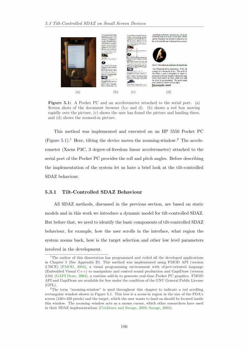
5.3 Tilt-Controlled SDAZ on Small Screen Devices
(a) (b) (c) (d)
Figure 5.1: A Pocket PC and an accelerometer attached to the serial port. (a)Screen shots of the document browser (b,c and d). (b) shows a red box movingrapidly over the picture, (c) shows the user has found the picture and landing there,and (d) shows the zoomed-in picture.
This method was implemented and executed on an HP 5550 Pocket PC
(Figure 5.1).1 Here, tilting the device moves the zooming-window.2 The accele-
rometer (Xsens P3C, 3 degree-of-freedom linear accelerometer) attached to the
serial port of the Pocket PC provides the roll and pitch angles. Before describing
the implementation of the system let us have a brief look at the tilt-controlled
SDAZ behaviour.
5.3.1 Tilt-Controlled SDAZ Behaviour
All SDAZ methods, discussed in the previous section, are based on static
models and in this work we introduce a dynamic model for tilt-controlled SDAZ.
But before that, we need to identify the basic components of tilt-controlled SDAZ
behaviour, for example, how the user scrolls in the interface, what region the
system zooms back, how is the target selection and other low level parameters
involved in the development.1The author of this dissertation has programmed and coded all the developed applications
in Chapter 5 (See Appendix D). This method was implemented using FMOD API (version3.70CE) (FMOD, 2004), a visual programming environment with object-oriented language(Embedded Visual C++) to manipulate and control sound production and GapiDraw (version2.04) (GAPI Draw, 2004), a runtime add-in to generate real-time Pocket PC graphics. FMODAPI and GapiDraw are available for free under the condition of the GNU General Public License(GPL).
2The term “zooming-window” is used throughout this chapter to indicate a red scrollingrectangular window shown in Figure 5.1. This box is a zoom-in region in the size of the PDA’sscreen (240×320 pixels) and the target, which the user wants to land on should be located insidethis window. The zooming–window acts as a mouse cursor, which other researchers have usedin their SDAZ implementations (Cockburn and Savage, 2003; Savage, 2004).
106
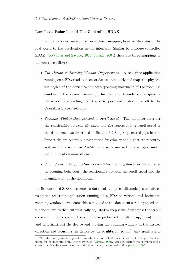
5.3 Tilt-Controlled SDAZ on Small Screen Devices
Low Level Behaviour of Tilt-Controlled SDAZ
Using an accelerometer provides a direct mapping from acceleration in the
real world to the acceleration in the interface. Similar to a mouse-controlled
SDAZ (Cockburn and Savage, 2003; Savage, 2004) there are three mappings in
tilt-controlled SDAZ:
• Tilt Motion to Zooming-Window Displacement – A real-time application
running on a PDA reads tilt sensor data continuously and maps the physical
tilt angles of the device to the corresponding movement of the zooming-
window on the screen. Generally, this mapping depends on the speed of
tilt sensor data reading from the serial port and it should be left to the
Operating System settings.
• Zooming-Window Displacement to Scroll Speed – This mapping describes
the relationship between tilt angle and the corresponding scroll speed in
the document. As described in Section 3.2.8, spring-centred joysticks or
force sticks are generally better suited for velocity and higher order control
systems and a nonlinear dead-band or dead-zone in the zero region makes
the null position more distinct.
• Scroll Speed to Magnification Level – This mapping describes the automa-
tic zooming behaviour: the relationship between the scroll speed and the
magnification of the document.
In tilt-controlled SDAZ acceleration data (roll and pitch tilt angles) is translated
using the real-time application running on a PDA to vertical and horizontal
zooming-window movements, this is mapped to the document scrolling speed and
the zoom level is then automatically adjusted to keep visual flow across the screen
constant. In this system the scrolling is performed by tilting up/down(pitch)
and left/right(roll) the device and moving the zooming-window in the desired
direction and returning the device to the equilibrium point.3 Any great lateral3Equilibrium point is a point from which a controlled variable will not change. Another
name for equilibrium point is steady state (Ogata, 1990). An equilibrium point represents astate in which the system can be maintained using the defined action (Ogata, 1995).
107
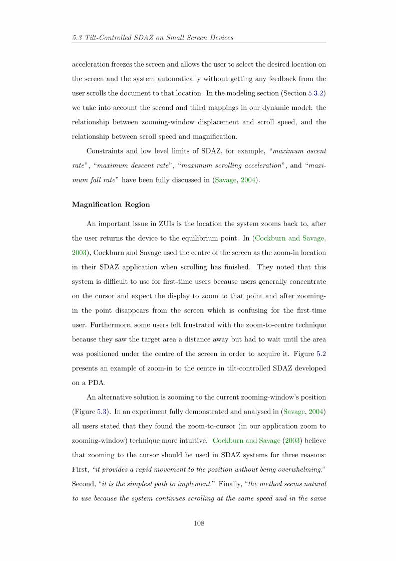
5.3 Tilt-Controlled SDAZ on Small Screen Devices
acceleration freezes the screen and allows the user to select the desired location on
the screen and the system automatically without getting any feedback from the
user scrolls the document to that location. In the modeling section (Section 5.3.2)
we take into account the second and third mappings in our dynamic model: the
relationship between zooming-window displacement and scroll speed, and the
relationship between scroll speed and magnification.
Constraints and low level limits of SDAZ, for example, “maximum ascent
rate”, “maximum descent rate”, “maximum scrolling acceleration”, and “maxi-
mum fall rate” have been fully discussed in (Savage, 2004).
Magnification Region
An important issue in ZUIs is the location the system zooms back to, after
the user returns the device to the equilibrium point. In (Cockburn and Savage,
2003), Cockburn and Savage used the centre of the screen as the zoom-in location
in their SDAZ application when scrolling has finished. They noted that this
system is difficult to use for first-time users because users generally concentrate
on the cursor and expect the display to zoom to that point and after zooming-
in the point disappears from the screen which is confusing for the first-time
user. Furthermore, some users felt frustrated with the zoom-to-centre technique
because they saw the target area a distance away but had to wait until the area
was positioned under the centre of the screen in order to acquire it. Figure 5.2
presents an example of zoom-in to the centre in tilt-controlled SDAZ developed
on a PDA.
An alternative solution is zooming to the current zooming-window’s position
(Figure 5.3). In an experiment fully demonstrated and analysed in (Savage, 2004)
all users stated that they found the zoom-to-cursor (in our application zoom to
zooming-window) technique more intuitive. Cockburn and Savage (2003) believe
that zooming to the cursor should be used in SDAZ systems for three reasons:
First, “it provides a rapid movement to the position without being overwhelming.”
Second, “it is the simplest path to implement.” Finally, “the method seems natural
to use because the system continues scrolling at the same speed and in the same
108
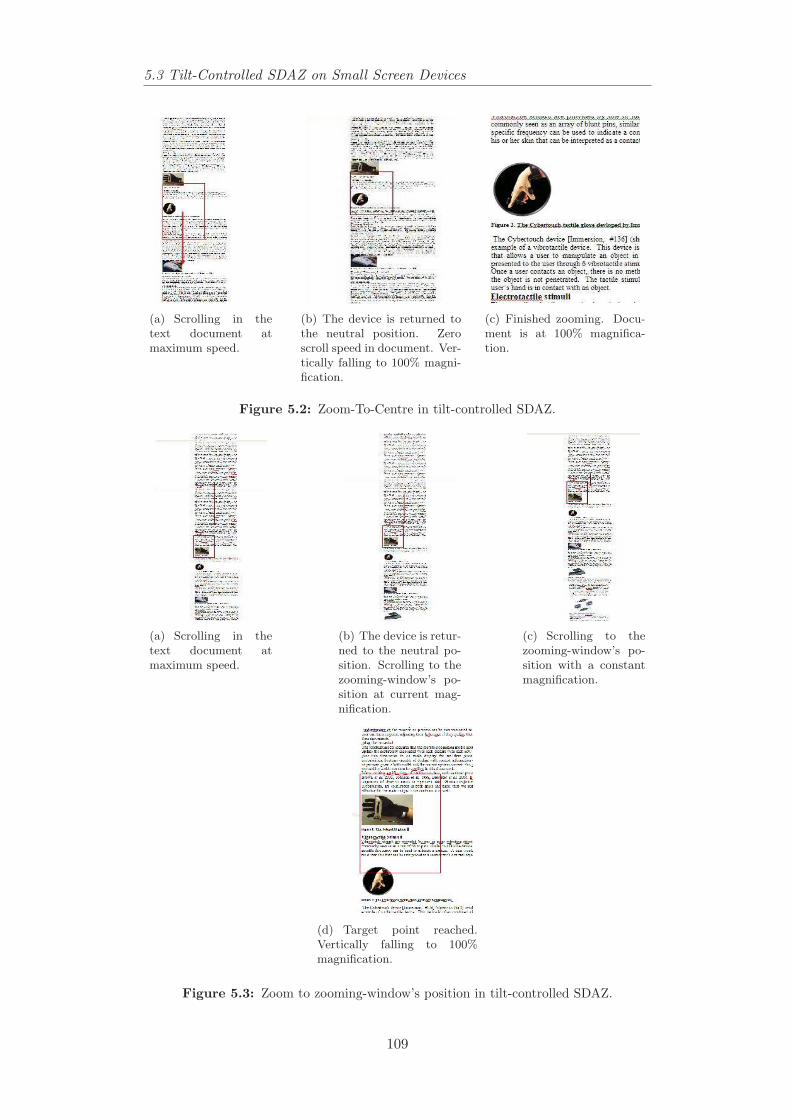
5.3 Tilt-Controlled SDAZ on Small Screen Devices
(a) Scrolling in thetext document atmaximum speed.
(b) The device is returned tothe neutral position. Zeroscroll speed in document. Ver-tically falling to 100% magni-fication.
(c) Finished zooming. Docu-ment is at 100% magnifica-tion.
Figure 5.2: Zoom-To-Centre in tilt-controlled SDAZ.
(a) Scrolling in thetext document atmaximum speed.
(b) The device is retur-ned to the neutral po-sition. Scrolling to thezooming-window’s po-sition at current mag-nification.
(c) Scrolling to thezooming-window’s po-sition with a constantmagnification.
(d) Target point reached.Vertically falling to 100%magnification.
Figure 5.3: Zoom to zooming-window’s position in tilt-controlled SDAZ.
109
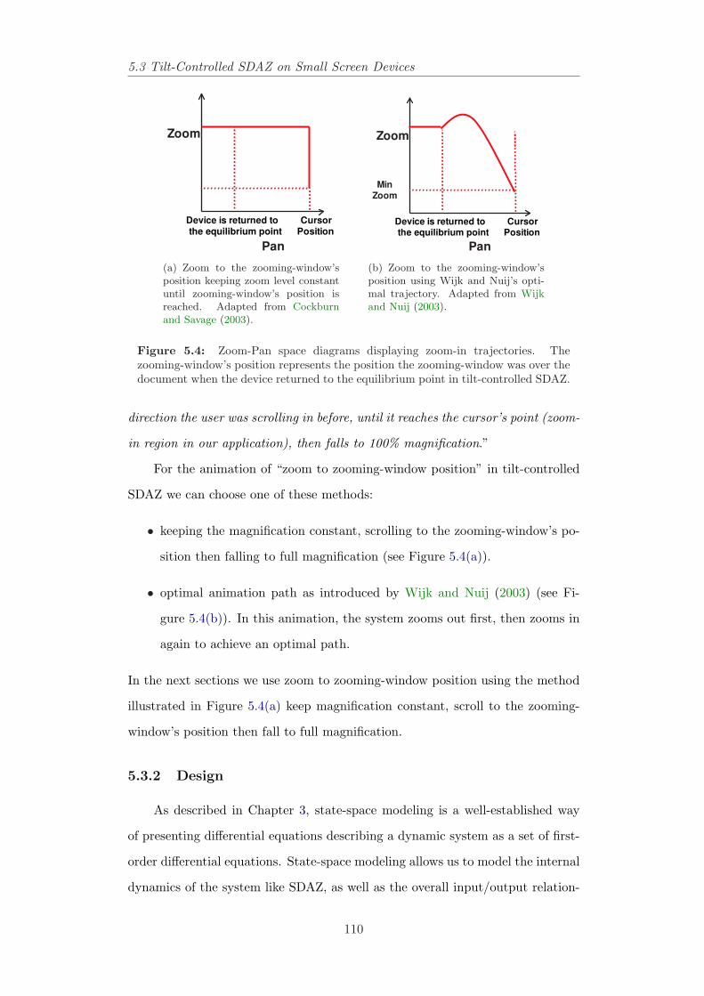
5.3 Tilt-Controlled SDAZ on Small Screen Devices
Pan
Zoom
Device is returned tothe equilibrium point
CursorPosition
(a) Zoom to the zooming-window’sposition keeping zoom level constantuntil zooming-window’s position isreached. Adapted from Cockburnand Savage (2003).
Pan
Zoom
MinZoom
Device is returned tothe equilibrium point
CursorPosition
(b) Zoom to the zooming-window’sposition using Wijk and Nuij’s opti-mal trajectory. Adapted from Wijkand Nuij (2003).
Figure 5.4: Zoom-Pan space diagrams displaying zoom-in trajectories. Thezooming-window’s position represents the position the zooming-window was over thedocument when the device returned to the equilibrium point in tilt-controlled SDAZ.
direction the user was scrolling in before, until it reaches the cursor’s point (zoom-
in region in our application), then falls to 100% magnification.”
For the animation of “zoom to zooming-window position” in tilt-controlled
SDAZ we can choose one of these methods:
• keeping the magnification constant, scrolling to the zooming-window’s po-
sition then falling to full magnification (see Figure 5.4(a)).
• optimal animation path as introduced by Wijk and Nuij (2003) (see Fi-
gure 5.4(b)). In this animation, the system zooms out first, then zooms in
again to achieve an optimal path.
In the next sections we use zoom to zooming-window position using the method
illustrated in Figure 5.4(a) keep magnification constant, scroll to the zooming-
window’s position then fall to full magnification.
5.3.2 Design
As described in Chapter 3, state-space modeling is a well-established way
of presenting differential equations describing a dynamic system as a set of first-
order differential equations. State-space modeling allows us to model the internal
dynamics of the system like SDAZ, as well as the overall input/output relation-
110
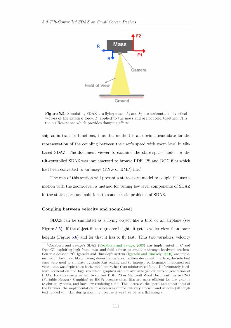
5.3 Tilt-Controlled SDAZ on Small Screen Devices
Figure 5.5: Simulating SDAZ as a flying mass. F1 and F2 are horizontal and verticalvectors of the external force, F applied to the mass and are coupled together. R isthe air Resistance which provides damping effects.
ship as in transfer functions, thus this method is an obvious candidate for the
representation of the coupling between the user’s speed with zoom level in tilt-
based SDAZ. The document viewer to examine the state-space model for the
tilt-controlled SDAZ was implemented to browse PDF, PS and DOC files which
had been converted to an image (PNG or BMP) file.4
The rest of this section will present a state-space model to couple the user’s
motion with the zoom-level, a method for tuning low level components of SDAZ
in the state-space and solutions to some classic problems of SDAZ.
Coupling between velocity and zoom-level
SDAZ can be simulated as a flying object like a bird or an airplane (see
Figure 5.5). If the object flies to greater heights it gets a wider view than lower
heights (Figure 5.6) and for that it has to fly fast. Thus two variables, velocity4Cockburn and Savage’s SDAZ (Cockburn and Savage, 2003) was implemented in C and
OpenGL exploiting high frame-rates and fluid animation available through hardware accelera-tion in a desktop PC. Igarashi and Hinckley’s system (Igarashi and Hinckely, 2000) was imple-mented in Java most likely having slower frame-rates. In their document interface, discrete fontsizes were used to simulate dynamic font scaling and to improve performance in zoomed-outviews, text was depicted as horizontal lines rather than miniaturised fonts. Unfortunately hard-ware acceleration and high resolution graphics are not available yet on current generation ofPDAs. For this reason we had to convert PDF, PS or Microsoft Word Document files to PNG(Portable Network Graphics) or BMP; because these files are more efficient for low graphicresolution systems, and have low rendering time. This increases the speed and smoothness ofthe browser, the implementation of which was simple but very efficient and smooth (althoughtext tended to flicker during zooming because it was treated as a flat image).
111
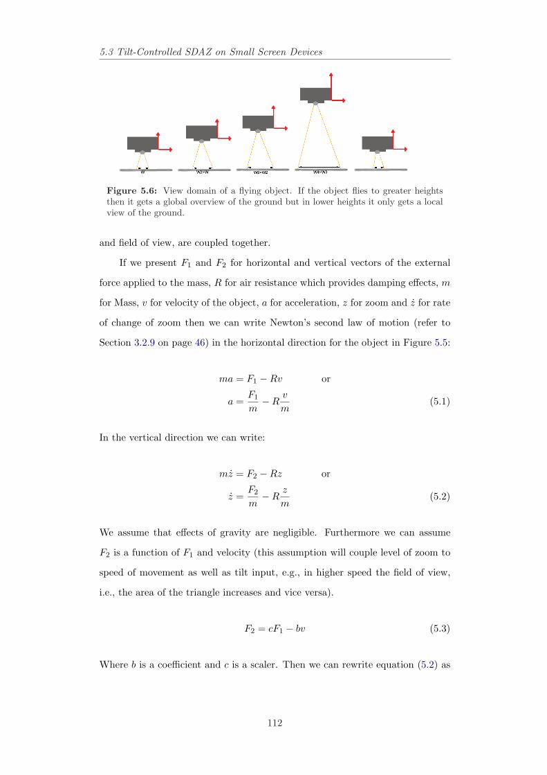
5.3 Tilt-Controlled SDAZ on Small Screen Devices
Figure 5.6: View domain of a flying object. If the object flies to greater heightsthen it gets a global overview of the ground but in lower heights it only gets a localview of the ground.
and field of view, are coupled together.
If we present F1 and F2 for horizontal and vertical vectors of the external
force applied to the mass, R for air resistance which provides damping effects, m
for Mass, v for velocity of the object, a for acceleration, z for zoom and z for rate
of change of zoom then we can write Newton’s second law of motion (refer to
Section 3.2.9 on page 46) in the horizontal direction for the object in Figure 5.5:
ma = F1 −Rv or
a =F1
m−R
v
m(5.1)
In the vertical direction we can write:
mz = F2 −Rz or
z =F2
m−R
z
m(5.2)
We assume that effects of gravity are negligible. Furthermore we can assume
F2 is a function of F1 and velocity (this assumption will couple level of zoom to
speed of movement as well as tilt input, e.g., in higher speed the field of view,
i.e., the area of the triangle increases and vice versa).
F2 = cF1 − bv (5.3)
Where b is a coefficient and c is a scaler. Then we can rewrite equation (5.2) as
112
5.3 Tilt-Controlled SDAZ on Small Screen Devices
below:
z = cF1
m− b
v
m−R
z
m(5.4)
Friction in Control
Friction causes delays. Poulton (1974) discusses about the effect of friction
in spring-centred control devices, for example, joysticks or tilt sensors. He shows
that for tracking in two dimensions, a single spring-centred input device is likely
to be an advantage when the task in the two dimensions are similar. Then he
argues to prevent accidental operation while the user is tracking in a vehicle,
which vibrates we may use different frictions in the vertical and horizontal di-
rections. This idea can be applied to tilt-controlled SDAZ and we can consider
two different frictions in different directions; R for horizontal direction and R′
for vertical direction. Then the equation (5.4) can be rewritten as below:
z = cF1
m− b
v
m−R′ z
m(5.5)
The inputs to the system can be the tilting angles measured using an accelerome-
ter attached to the serial port of PDA, or the stylus position on the PDA’s touch
screen. The state variables chosen are x1(t) for position of zooming-window,
x2(t) for speed of scroll and x3(t) for zoom. u represents input, F1 (pitch tilting
angle), and the state equations are:
x2(t) = v = x1 (5.6)
x3(t) = z = f(x1, x2, u) (5.7)
Thus the zoom-level is a function of position, velocity and pitch tilting angle, u.
An initial suggestion is to reproduce the standard second-order dynamics of
a mass-spring-damper system and give the scrolling movement and zoom level
some inertia to provide a physically intuitive interface. The first time-derivative
of the state equations given in equations (5.1) to (5.4) can be rewritten as below,
113
5.3 Tilt-Controlled SDAZ on Small Screen Devices
as a linearisation of the system at a given velocity and zoom:
x1(t) = v = x2(t) (5.8)
x2(t) = a = v =−R
mx2(t) +
1m
u(t) (5.9)
x3(t) = z(t) =−b
mx2(t)− R′
mx3(t) +
c
mu(t) (5.10)
The standard matrix format of these equations is (refer Section 3.2.9):
x1
x2
x3
=
0 1 0
0 −Rm 0
0 −bm
−R′m
x1
x2
x3
+
0
1m
cm
u (5.11)
This shows how a single-degree of freedom input can control both velocity and
zoom-level. The non-zero off-diagonal elements of the A matrix indicate coupling
among states, and the B matrix indicates how the inputs affect each state. This
example could be represented as having zoom as an output equation, rather than
state, and the coupling between zoom and speed comes only primarily the B
matrix, which is not particularly satisfying.
The next step is finding suitable values for R, R′, m, b and c coefficients in
the state-space model to make the system controllable (refer to Section 3.2.9 on
page 45). We can write the controllability matrix as below:
rank[B|AB|A2B] = rank
0 1m
−Rm2
1m
−Rm2
R2
m3
cm
−b−R′cm2
bR+bR′+cR′2m3
(5.12)
which has a full rank for all R, R′, m 6= 0, b 6= 0 and c. This suggests a wide
range of possible coefficient settings for the model. One way to choose the right
settings is observing the simulated system’s behaviour.
114
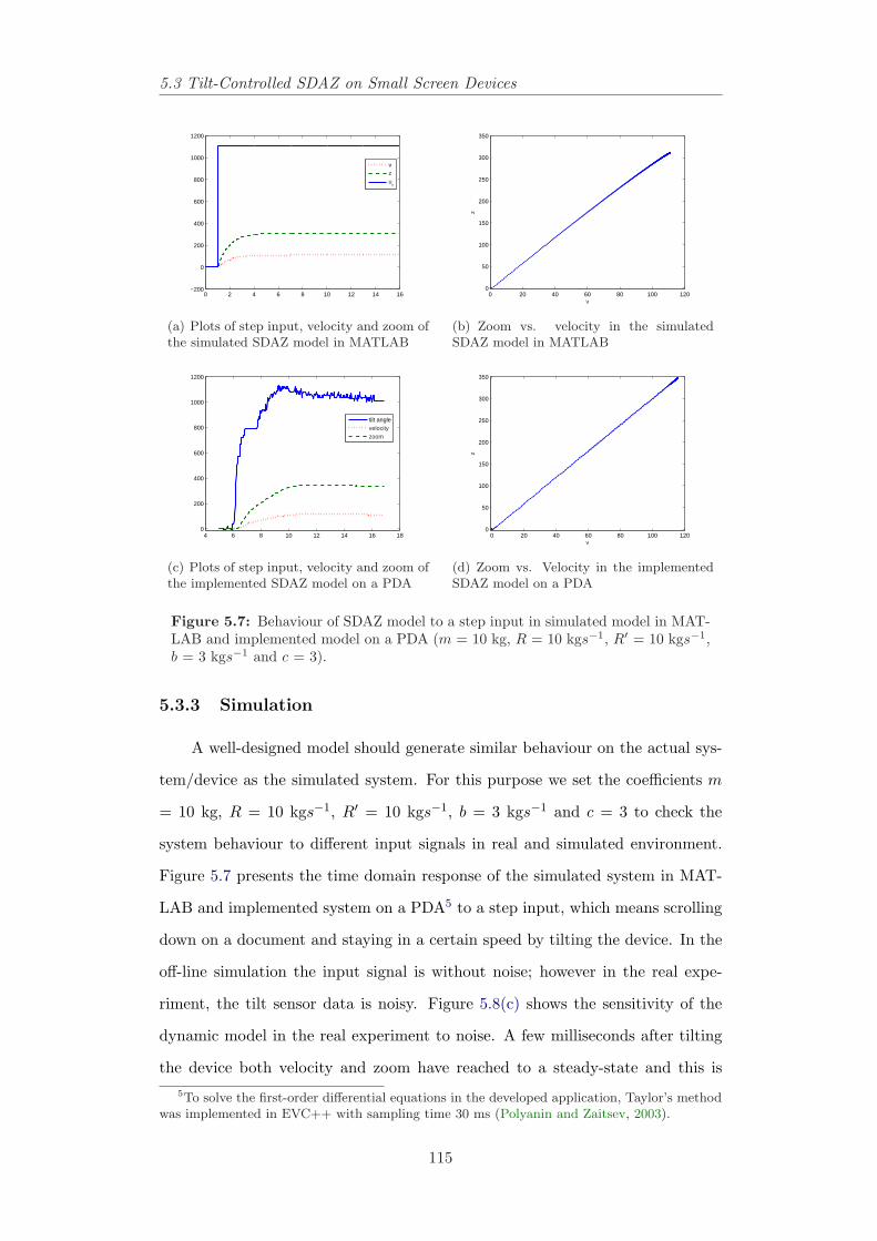
5.3 Tilt-Controlled SDAZ on Small Screen Devices
0 2 4 6 8 10 12 14 16−200
0
200
400
600
800
1000
1200
vzu
r
(a) Plots of step input, velocity and zoom ofthe simulated SDAZ model in MATLAB
0 20 40 60 80 100 1200
50
100
150
200
250
300
350
v
z
(b) Zoom vs. velocity in the simulatedSDAZ model in MATLAB
4 6 8 10 12 14 16 180
200
400
600
800
1000
1200
tilt anglevelocityzoom
(c) Plots of step input, velocity and zoom ofthe implemented SDAZ model on a PDA
0 20 40 60 80 100 1200
50
100
150
200
250
300
350
v
z
(d) Zoom vs. Velocity in the implementedSDAZ model on a PDA
Figure 5.7: Behaviour of SDAZ model to a step input in simulated model in MAT-LAB and implemented model on a PDA (m = 10 kg, R = 10 kgs−1, R′ = 10 kgs−1,b = 3 kgs−1 and c = 3).
5.3.3 Simulation
A well-designed model should generate similar behaviour on the actual sys-
tem/device as the simulated system. For this purpose we set the coefficients m
= 10 kg, R = 10 kgs−1, R′ = 10 kgs−1, b = 3 kgs−1 and c = 3 to check the
system behaviour to different input signals in real and simulated environment.
Figure 5.7 presents the time domain response of the simulated system in MAT-
LAB and implemented system on a PDA5 to a step input, which means scrolling
down on a document and staying in a certain speed by tilting the device. In the
off-line simulation the input signal is without noise; however in the real expe-
riment, the tilt sensor data is noisy. Figure 5.8(c) shows the sensitivity of the
dynamic model in the real experiment to noise. A few milliseconds after tilting
the device both velocity and zoom have reached to a steady-state and this is5To solve the first-order differential equations in the developed application, Taylor’s method
was implemented in EVC++ with sampling time 30 ms (Polyanin and Zaitsev, 2003).
115
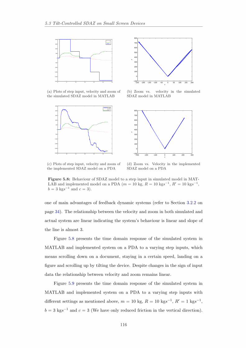
5.3 Tilt-Controlled SDAZ on Small Screen Devices
0 5 10 15 20 25 30−2500
−2000
−1500
−1000
−500
0
500
1000
1500
2000
vzu
r
(a) Plots of step input, velocity and zoom ofthe simulated SDAZ model in MATLAB
−250 −200 −150 −100 −50 0 50 100 150 200−100
0
100
200
300
400
500
600
700
800
v
z
(b) Zoom vs. velocity in the simulatedSDAZ model in MATLAB
5 10 15 20 25 30 35−2500
−2000
−1500
−1000
−500
0
500
1000
1500
2000
2500
tilt anglevelocityzoom
(c) Plots of step input, velocity and zoom ofthe implemented SDAZ model on a PDA
−300 −200 −100 0 100 200 300−100
0
100
200
300
400
500
600
700
800
v
z
(d) Zoom vs. Velocity in the implementedSDAZ model on a PDA
Figure 5.8: Behaviour of SDAZ model to a step input in simulated model in MAT-LAB and implemented model on a PDA (m = 10 kg, R = 10 kgs−1, R′ = 10 kgs−1,b = 3 kgs−1 and c = 3).
one of main advantages of feedback dynamic systems (refer to Section 3.2.2 on
page 34). The relationship between the velocity and zoom in both simulated and
actual system are linear indicating the system’s behaviour is linear and slope of
the line is almost 3.
Figure 5.8 presents the time domain response of the simulated system in
MATLAB and implemented system on a PDA to a varying step inputs, which
means scrolling down on a document, staying in a certain speed, landing on a
figure and scrolling up by tilting the device. Despite changes in the sign of input
data the relationship between velocity and zoom remains linear.
Figure 5.9 presents the time domain response of the simulated system in
MATLAB and implemented system on a PDA to a varying step inputs with
different settings as mentioned above, m = 10 kg, R = 10 kgs−1, R′ = 1 kgs−1,
b = 3 kgs−1 and c = 3 (We have only reduced friction in the vertical direction).
116
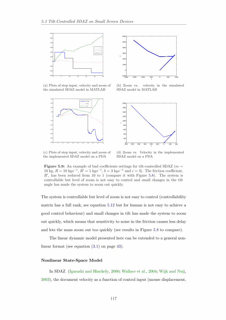
5.3 Tilt-Controlled SDAZ on Small Screen Devices
0 5 10 15 20 25 30−3000
−2000
−1000
0
1000
2000
3000
4000
5000
6000
v
z
ur
(a) Plots of step input, velocity and zoom ofthe simulated SDAZ model in MATLAB
−2000 −1500 −1000 −500 0 500 1000−1000
0
1000
2000
3000
4000
5000
6000
v
z
(b) Zoom vs. velocity in the simulatedSDAZ model in MATLAB
4 6 8 10 12 14 16 18 20 22 24−3000
−2500
−2000
−1500
−1000
−500
0
500
1000
1500
2000
tilt angle
velocity
zoom
(c) Plots of step input, velocity and zoom ofthe implemented SDAZ model on a PDA
−600 −500 −400 −300 −200 −100 0 100 2000
200
400
600
800
1000
1200
1400
1600
1800
v
z
(d) Zoom vs. Velocity in the implementedSDAZ model on a PDA
Figure 5.9: An example of bad coefficients settings for tilt-controlled SDAZ (m =10 kg, R = 10 kgs−1, R′ = 1 kgs−1, b = 3 kgs−1 and c = 3). The friction coefficient,R′, has been reduced from 10 to 1 (compare it with Figure 5.8). The system iscontrollable but level of zoom is not easy to control and small changes in the tiltangle has made the system to zoom out quickly.
The system is controllable but level of zoom is not easy to control (controllability
matrix has a full rank, see equation 5.12 but for human is not easy to achieve a
good control behaviour) and small changes in tilt has made the system to zoom
out quickly, which means that sensitivity to noise in the friction causes less delay
and lets the mass zoom out too quickly (see results in Figure 5.8 to compare).
The linear dynamic model presented here can be extended to a general non-
linear format (see equation (3.1) on page 43).
Nonlinear State-Space Model
In SDAZ (Igarashi and Hinckely, 2000; Wallace et al., 2004; Wijk and Nuij,
2003), the document velocity as a function of control input (mouse displacement,
117
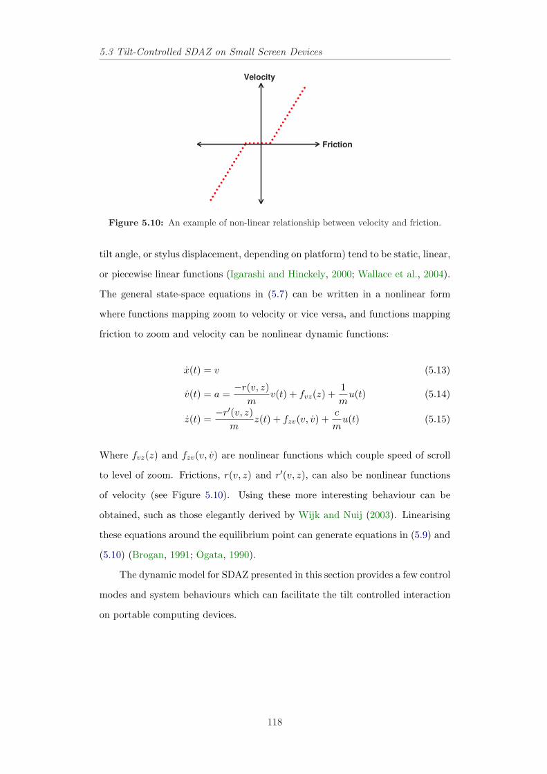
5.3 Tilt-Controlled SDAZ on Small Screen Devices
Friction
Velocity
Figure 5.10: An example of non-linear relationship between velocity and friction.
tilt angle, or stylus displacement, depending on platform) tend to be static, linear,
or piecewise linear functions (Igarashi and Hinckely, 2000; Wallace et al., 2004).
The general state-space equations in (5.7) can be written in a nonlinear form
where functions mapping zoom to velocity or vice versa, and functions mapping
friction to zoom and velocity can be nonlinear dynamic functions:
x(t) = v (5.13)
v(t) = a =−r(v, z)
mv(t) + fvz(z) +
1m
u(t) (5.14)
z(t) =−r′(v, z)
mz(t) + fzv(v, v) +
c
mu(t) (5.15)
Where fvz(z) and fzv(v, v) are nonlinear functions which couple speed of scroll
to level of zoom. Frictions, r(v, z) and r′(v, z), can also be nonlinear functions
of velocity (see Figure 5.10). Using these more interesting behaviour can be
obtained, such as those elegantly derived by Wijk and Nuij (2003). Linearising
these equations around the equilibrium point can generate equations in (5.9) and
(5.10) (Brogan, 1991; Ogata, 1990).
The dynamic model for SDAZ presented in this section provides a few control
modes and system behaviours which can facilitate the tilt controlled interaction
on portable computing devices.
118
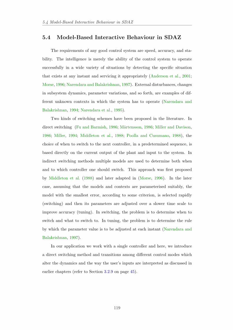
5.4 Model-Based Interactive Behaviour in SDAZ
5.4 Model-Based Interactive Behaviour in SDAZ
The requirements of any good control system are speed, accuracy, and sta-
bility. The intelligence is merely the ability of the control system to operate
successfully in a wide variety of situations by detecting the specific situation
that exists at any instant and servicing it appropriately (Anderson et al., 2001;
Morse, 1996; Narendara and Balakrishnan, 1997). External disturbances, changes
in subsystem dynamics, parameter variations, and so forth, are examples of dif-
ferent unknown contexts in which the system has to operate (Narendara and
Balakrishnan, 1994; Narendara et al., 1995).
Two kinds of switching schemes have been proposed in the literature. In
direct switching (Fu and Barmish, 1986; Martensson, 1986; Miller and Davison,
1986; Miller, 1994; Middleton et al., 1988; Poolla and Cusumano, 1988), the
choice of when to switch to the next controller, in a predetermined sequence, is
based directly on the current output of the plant and input to the system. In
indirect switching methods multiple models are used to determine both when
and to which controller one should switch. This approach was first proposed
by Middleton et al. (1988) and later adapted in (Morse, 1996). In the later
case, assuming that the models and contexts are parameterised suitably, the
model with the smallest error, according to some criterion, is selected rapidly
(switching) and then its parameters are adjusted over a slower time scale to
improve accuracy (tuning). In switching, the problem is to determine when to
switch and what to switch to. In tuning, the problem is to determine the rule
by which the parameter value is to be adjusted at each instant (Narendara and
Balakrishnan, 1997).
In our application we work with a single controller and here, we introduce
a direct switching method and transitions among different control modes which
alter the dynamics and the way the user’s inputs are interpreted as discussed in
earlier chapters (refer to Section 3.2.9 on page 45).
119
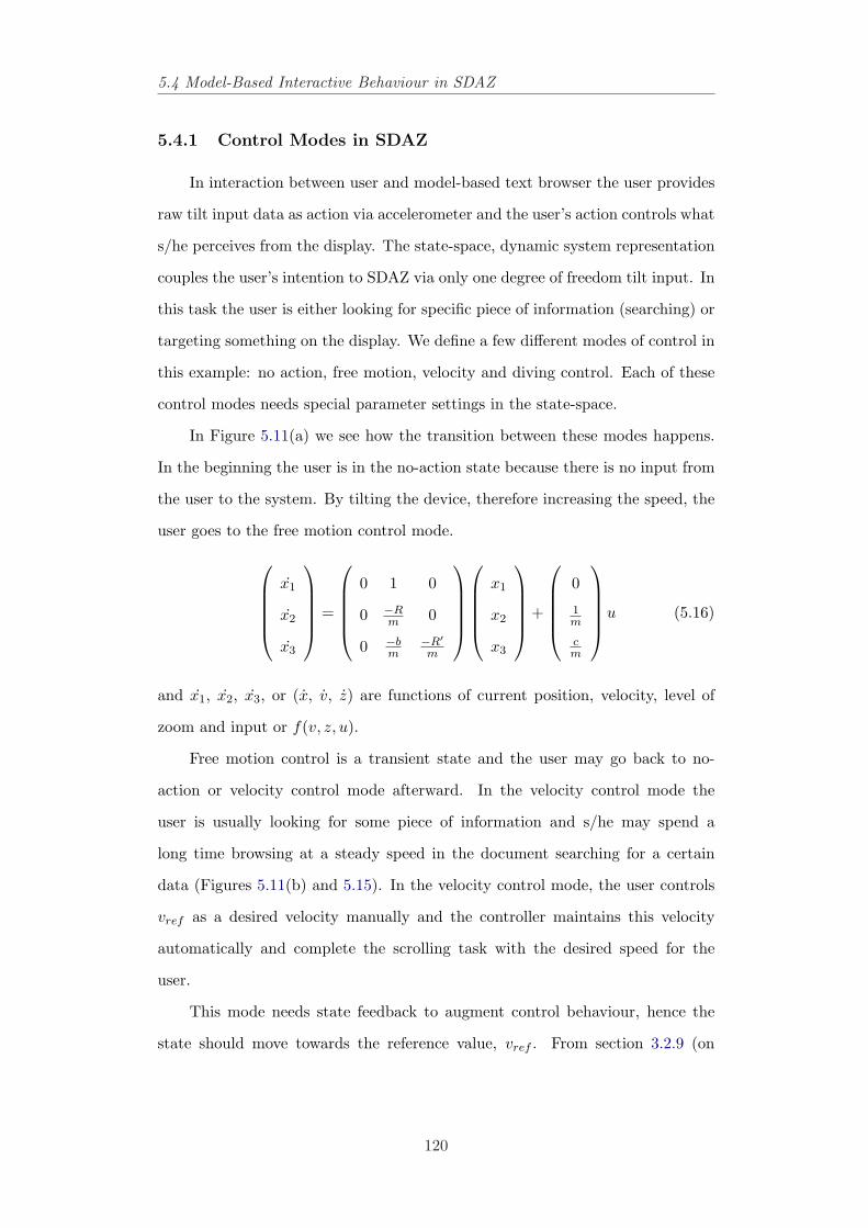
5.4 Model-Based Interactive Behaviour in SDAZ
5.4.1 Control Modes in SDAZ
In interaction between user and model-based text browser the user provides
raw tilt input data as action via accelerometer and the user’s action controls what
s/he perceives from the display. The state-space, dynamic system representation
couples the user’s intention to SDAZ via only one degree of freedom tilt input. In
this task the user is either looking for specific piece of information (searching) or
targeting something on the display. We define a few different modes of control in
this example: no action, free motion, velocity and diving control. Each of these
control modes needs special parameter settings in the state-space.
In Figure 5.11(a) we see how the transition between these modes happens.
In the beginning the user is in the no-action state because there is no input from
the user to the system. By tilting the device, therefore increasing the speed, the
user goes to the free motion control mode.
x1
x2
x3
=
0 1 0
0 −Rm 0
0 −bm
−R′m
x1
x2
x3
+
0
1m
cm
u (5.16)
and x1, x2, x3, or (x, v, z) are functions of current position, velocity, level of
zoom and input or f(v, z, u).
Free motion control is a transient state and the user may go back to no-
action or velocity control mode afterward. In the velocity control mode the
user is usually looking for some piece of information and s/he may spend a
long time browsing at a steady speed in the document searching for a certain
data (Figures 5.11(b) and 5.15). In the velocity control mode, the user controls
vref as a desired velocity manually and the controller maintains this velocity
automatically and complete the scrolling task with the desired speed for the
user.
This mode needs state feedback to augment control behaviour, hence the
state should move towards the reference value, vref . From section 3.2.9 (on
120
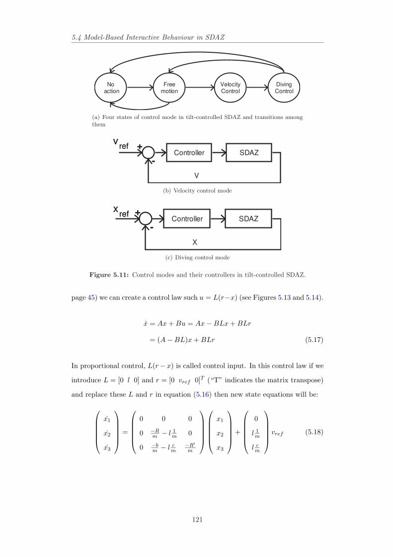
5.4 Model-Based Interactive Behaviour in SDAZ
Noaction
Freemotion
VelocityControl
DivingControl
(a) Four states of control mode in tilt-controlled SDAZ and transitions amongthem
V
Controller SDAZ
vref
vref +
-
(b) Velocity control mode
X
Controller SDAZ
xref
xref +
-
(c) Diving control mode
Figure 5.11: Control modes and their controllers in tilt-controlled SDAZ.
page 45) we can create a control law such u = L(r−x) (see Figures 5.13 and 5.14).
x = Ax + Bu = Ax−BLx + BLr
= (A−BL)x + BLr (5.17)
In proportional control, L(r−x) is called control input. In this control law if we
introduce L = [0 l 0] and r = [0 vref 0]T (“T” indicates the matrix transpose)
and replace these L and r in equation (5.16) then new state equations will be:
x1
x2
x3
=
0 0 0
0 −Rm − l 1
m 0
0 −bm − l c
m−R′m
x1
x2
x3
+
0
l 1m
l cm
vref (5.18)
121
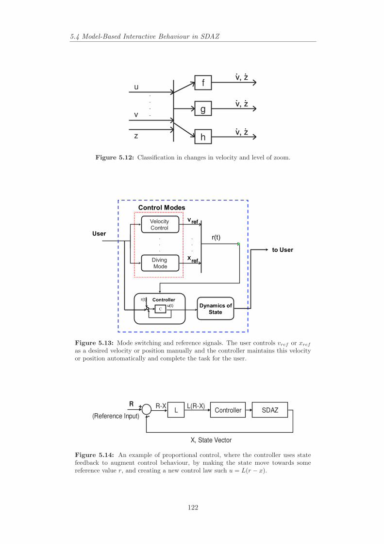
5.4 Model-Based Interactive Behaviour in SDAZ
.
.
.
.
f
g
h
u
v
z
v, z. .v, z. .
v, z. .v, z. .
v, z. .v, z. .
Figure 5.12: Classification in changes in velocity and level of zoom.
Velocity
Control
Diving
Mode
.
.
.
Controller
Cu(t)
r(t)
Dynamics of
State
User
xref
xref
.
.
.
Control Modes
to User
ref v ref v
r(t)
Figure 5.13: Mode switching and reference signals. The user controls vref or xref
as a desired velocity or position manually and the controller maintains this velocityor position automatically and complete the task for the user.
R
(Reference Input)
X, State Vector
Controller SDAZL+
-
R-X L(R-X)
Figure 5.14: An example of proportional control, where the controller uses statefeedback to augment control behaviour, by making the state move towards somereference value r, and creating a new control law such u = L(r − x).
122
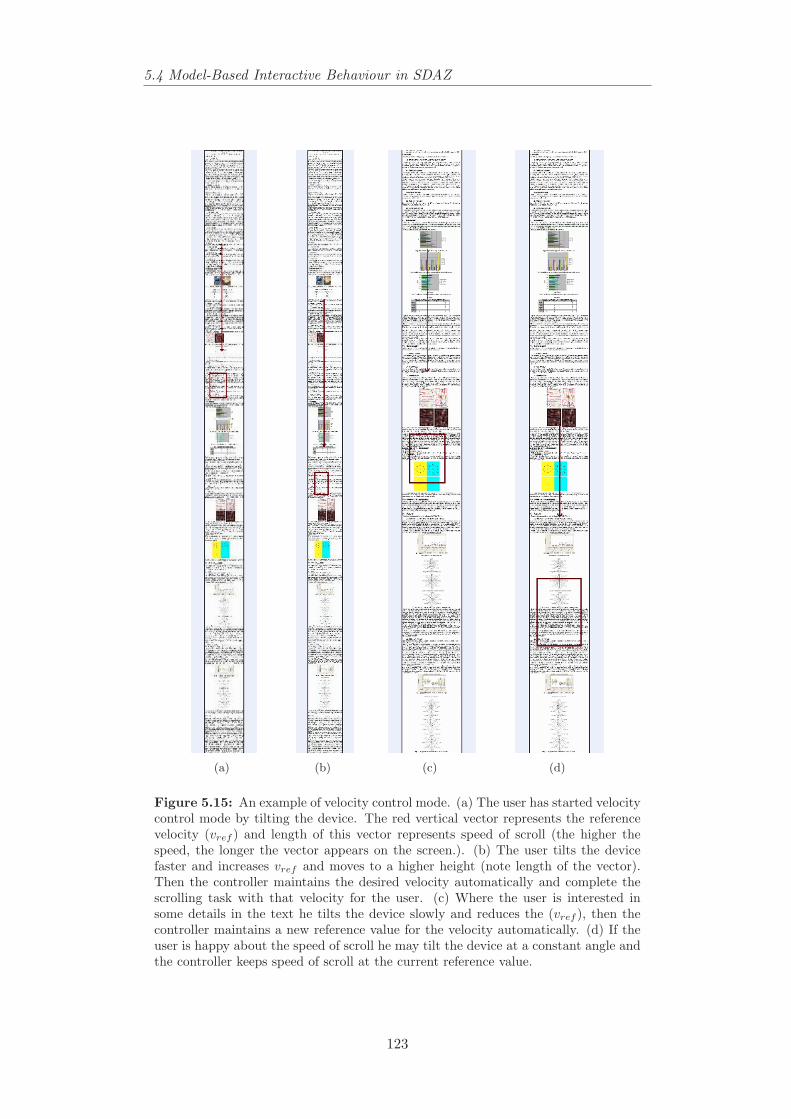
5.4 Model-Based Interactive Behaviour in SDAZ
(a) (b) (c) (d)
Figure 5.15: An example of velocity control mode. (a) The user has started velocitycontrol mode by tilting the device. The red vertical vector represents the referencevelocity (vref ) and length of this vector represents speed of scroll (the higher thespeed, the longer the vector appears on the screen.). (b) The user tilts the devicefaster and increases vref and moves to a higher height (note length of the vector).Then the controller maintains the desired velocity automatically and complete thescrolling task with that velocity for the user. (c) Where the user is interested insome details in the text he tilts the device slowly and reduces the (vref ), then thecontroller maintains a new reference value for the velocity automatically. (d) If theuser is happy about the speed of scroll he may tilt the device at a constant angle andthe controller keeps speed of scroll at the current reference value.
123
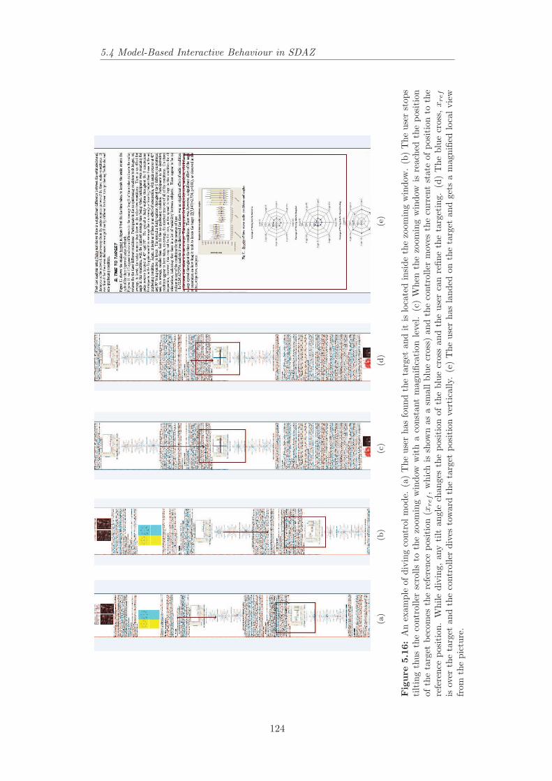
5.4 Model-Based Interactive Behaviour in SDAZ
(a)
(b)
(c)
(d)
(e)
Fig
ure
5.16
:A
nex
ampl
eof
divi
ngco
ntro
lmod
e.(a
)T
heus
erha
sfo
und
the
targ
etan
dit
islo
cate
din
side
the
zoom
ing
win
dow
.(b
)T
heus
erst
ops
tilt
ing
thus
the
cont
rolle
rsc
rolls
toth
ezo
omin
gw
indo
ww
ith
aco
nsta
ntm
agni
ficat
ion
leve
l.(c
)W
hen
the
zoom
ing
win
dow
isre
ache
dth
epo
siti
onof
the
targ
etbe
com
esth
ere
fere
nce
posi
tion
(xref,w
hich
issh
own
asa
smal
lbl
uecr
oss)
and
the
cont
rolle
rm
oves
the
curr
ent
stat
eof
posi
tion
toth
ere
fere
nce
posi
tion
.W
hile
divi
ng,an
yti
ltan
gle
chan
ges
the
posi
tion
ofth
ebl
uecr
oss
and
the
user
can
refin
eth
eta
rget
ing.
(d)
The
blue
cros
s,x
ref
isov
erth
eta
rget
and
the
cont
rolle
rdi
ves
tow
ard
the
targ
etpo
siti
onve
rtic
ally
.(e
)T
heus
erha
sla
nded
onth
eta
rget
and
gets
am
agni
fied
loca
lvi
ewfr
omth
epi
ctur
e.
124
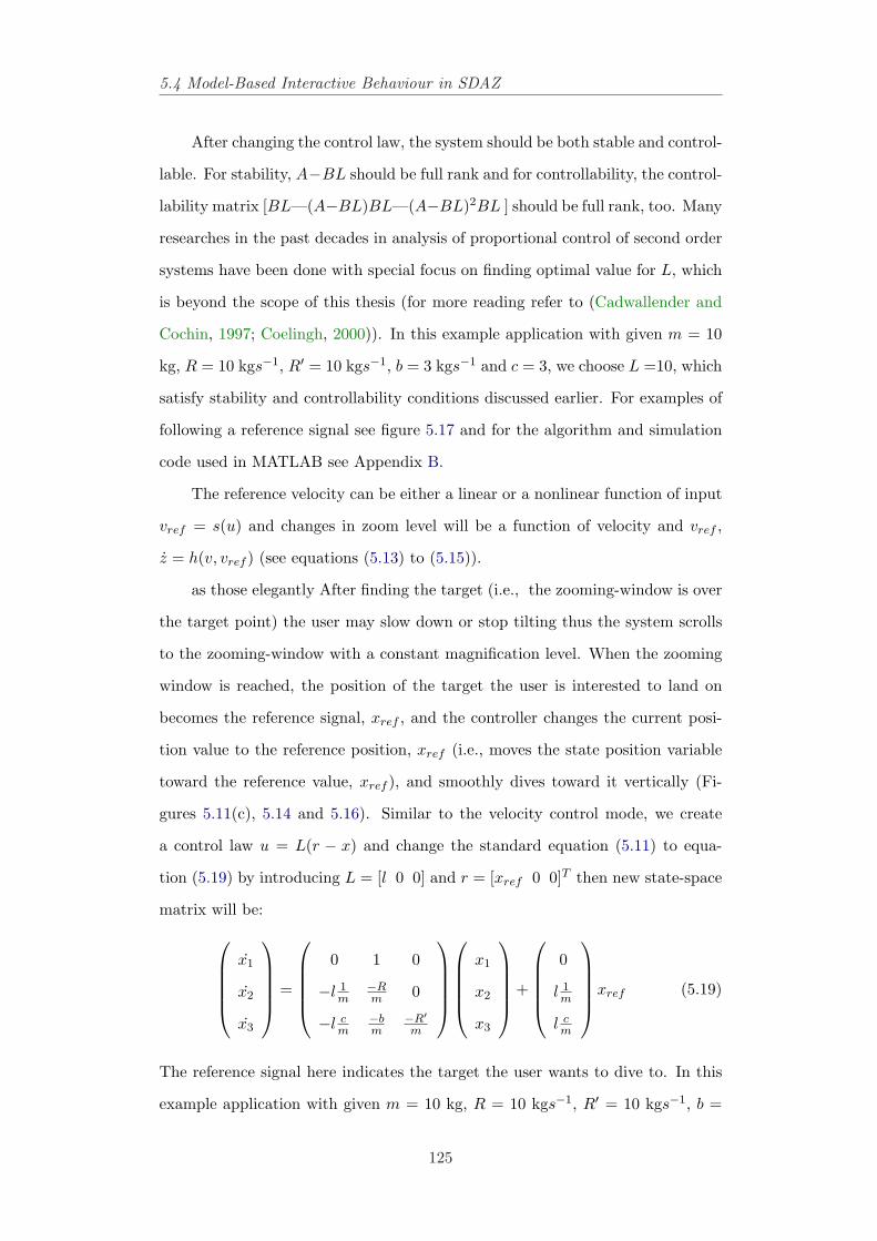
5.4 Model-Based Interactive Behaviour in SDAZ
After changing the control law, the system should be both stable and control-
lable. For stability, A−BL should be full rank and for controllability, the control-
lability matrix [BL—(A−BL)BL—(A−BL)2BL ] should be full rank, too. Many
researches in the past decades in analysis of proportional control of second order
systems have been done with special focus on finding optimal value for L, which
is beyond the scope of this thesis (for more reading refer to (Cadwallender and
Cochin, 1997; Coelingh, 2000)). In this example application with given m = 10
kg, R = 10 kgs−1, R′ = 10 kgs−1, b = 3 kgs−1 and c = 3, we choose L =10, which
satisfy stability and controllability conditions discussed earlier. For examples of
following a reference signal see figure 5.17 and for the algorithm and simulation
code used in MATLAB see Appendix B.
The reference velocity can be either a linear or a nonlinear function of input
vref = s(u) and changes in zoom level will be a function of velocity and vref ,
z = h(v, vref ) (see equations (5.13) to (5.15)).
as those elegantly After finding the target (i.e., the zooming-window is over
the target point) the user may slow down or stop tilting thus the system scrolls
to the zooming-window with a constant magnification level. When the zooming
window is reached, the position of the target the user is interested to land on
becomes the reference signal, xref , and the controller changes the current posi-
tion value to the reference position, xref (i.e., moves the state position variable
toward the reference value, xref ), and smoothly dives toward it vertically (Fi-
gures 5.11(c), 5.14 and 5.16). Similar to the velocity control mode, we create
a control law u = L(r − x) and change the standard equation (5.11) to equa-
tion (5.19) by introducing L = [l 0 0] and r = [xref 0 0]T then new state-space
matrix will be:
x1
x2
x3
=
0 1 0
−l 1m
−Rm 0
−l cm
−bm
−R′m
x1
x2
x3
+
0
l 1m
l cm
xref (5.19)
The reference signal here indicates the target the user wants to dive to. In this
example application with given m = 10 kg, R = 10 kgs−1, R′ = 10 kgs−1, b =
125
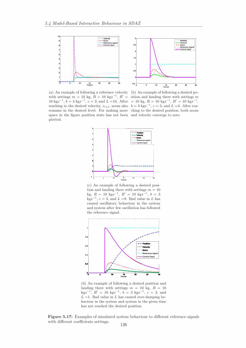
5.4 Model-Based Interactive Behaviour in SDAZ
0 5 10 15 20 25 300
1
2
3
4
5
6
7
8
9
10
Time(se)
Velocity
Zoom
Reference signal
Control Input
(a) An example of following a reference velocitywith settings m = 10 kg, R = 10 kgs−1, R′ =10 kgs−1, b = 3 kgs−1, c = 3, and L =10. Afterreaching to the desired velocity, vref , zoom alsoremains in the desired level. For making morespace in the figure position state has not beenplotted.
0 5 10 15 20 25 300.5
0
0.5
1
1.5
2
2.5
3
Time(se)
Position
Velocity
Zoom
Reference signal
Control Input
(b) An example of following a desired po-sition and landing there with settings m= 10 kg, R = 10 kgs−1, R′ = 10 kgs−1,b = 3 kgs−1, c = 3, and L =3. After rea-ching to the desired position, both zoomand velocity converge to zero.
0 5 10 15 20 25 30
3
4
5
6
7
8
Time(se)
Reference signal
Control Input
(c) An example of following a desired posi-tion and landing there with settings m = 10kg, R = 10 kgs−1, R′ = 10 kgs−1, b = 3kgs−1, c = 3, and L =8. Bad value in L hascaused oscillatory behaviour in the systemand system after few oscillation has followedthe reference signal.
0.4
0.6
0.8
1
Time(se)
Reference signal
Control Input
(d) An example of following a desired position andlanding there with settings m = 10 kg, R = 10kgs−1, R′ = 10 kgs−1, b = 3 kgs−1, c = 3, andL =1. Bad value in L has caused over-damping be-haviour in the system and system in the given timehas not reached the desired position.
Figure 5.17: Examples of simulated system behaviour to different reference signalswith different coefficients settings.
126
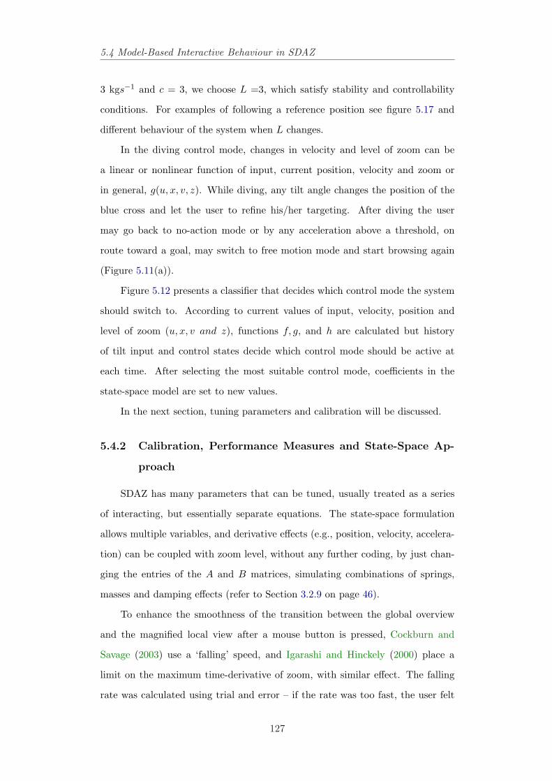
5.4 Model-Based Interactive Behaviour in SDAZ
3 kgs−1 and c = 3, we choose L =3, which satisfy stability and controllability
conditions. For examples of following a reference position see figure 5.17 and
different behaviour of the system when L changes.
In the diving control mode, changes in velocity and level of zoom can be
a linear or nonlinear function of input, current position, velocity and zoom or
in general, g(u, x, v, z). While diving, any tilt angle changes the position of the
blue cross and let the user to refine his/her targeting. After diving the user
may go back to no-action mode or by any acceleration above a threshold, on
route toward a goal, may switch to free motion mode and start browsing again
(Figure 5.11(a)).
Figure 5.12 presents a classifier that decides which control mode the system
should switch to. According to current values of input, velocity, position and
level of zoom (u, x, v and z), functions f, g, and h are calculated but history
of tilt input and control states decide which control mode should be active at
each time. After selecting the most suitable control mode, coefficients in the
state-space model are set to new values.
In the next section, tuning parameters and calibration will be discussed.
5.4.2 Calibration, Performance Measures and State-Space Ap-
proach
SDAZ has many parameters that can be tuned, usually treated as a series
of interacting, but essentially separate equations. The state-space formulation
allows multiple variables, and derivative effects (e.g., position, velocity, accelera-
tion) can be coupled with zoom level, without any further coding, by just chan-
ging the entries of the A and B matrices, simulating combinations of springs,
masses and damping effects (refer to Section 3.2.9 on page 46).
To enhance the smoothness of the transition between the global overview
and the magnified local view after a mouse button is pressed, Cockburn and
Savage (2003) use a ‘falling’ speed, and Igarashi and Hinckely (2000) place a
limit on the maximum time-derivative of zoom, with similar effect. The falling
rate was calculated using trial and error – if the rate was too fast, the user felt
127
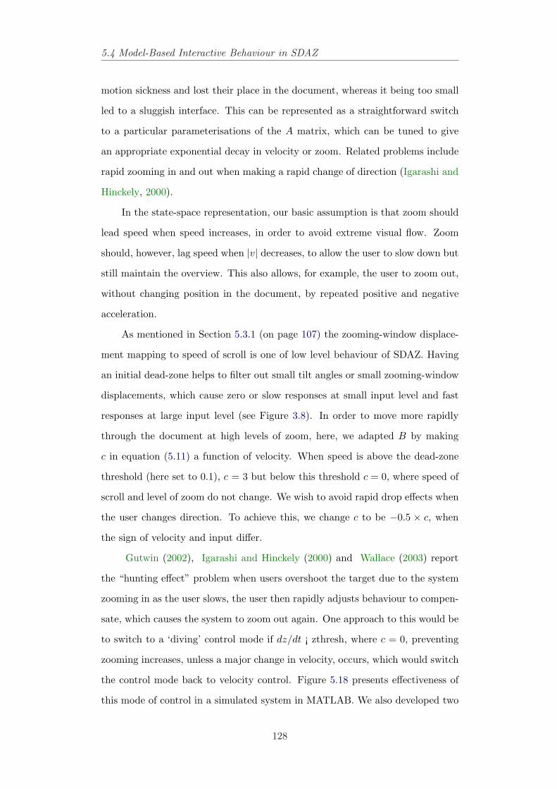
5.4 Model-Based Interactive Behaviour in SDAZ
motion sickness and lost their place in the document, whereas it being too small
led to a sluggish interface. This can be represented as a straightforward switch
to a particular parameterisations of the A matrix, which can be tuned to give
an appropriate exponential decay in velocity or zoom. Related problems include
rapid zooming in and out when making a rapid change of direction (Igarashi and
Hinckely, 2000).
In the state-space representation, our basic assumption is that zoom should
lead speed when speed increases, in order to avoid extreme visual flow. Zoom
should, however, lag speed when |v| decreases, to allow the user to slow down but
still maintain the overview. This also allows, for example, the user to zoom out,
without changing position in the document, by repeated positive and negative
acceleration.
As mentioned in Section 5.3.1 (on page 107) the zooming-window displace-
ment mapping to speed of scroll is one of low level behaviour of SDAZ. Having
an initial dead-zone helps to filter out small tilt angles or small zooming-window
displacements, which cause zero or slow responses at small input level and fast
responses at large input level (see Figure 3.8). In order to move more rapidly
through the document at high levels of zoom, here, we adapted B by making
c in equation (5.11) a function of velocity. When speed is above the dead-zone
threshold (here set to 0.1), c = 3 but below this threshold c = 0, where speed of
scroll and level of zoom do not change. We wish to avoid rapid drop effects when
the user changes direction. To achieve this, we change c to be −0.5 × c, when
the sign of velocity and input differ.
Gutwin (2002), Igarashi and Hinckely (2000) and Wallace (2003) report
the “hunting effect” problem when users overshoot the target due to the system
zooming in as the user slows, the user then rapidly adjusts behaviour to compen-
sate, which causes the system to zoom out again. One approach to this would be
to switch to a ‘diving’ control mode if dz/dt ¡ zthresh, where c = 0, preventing
zooming increases, unless a major change in velocity, occurs, which would switch
the control mode back to velocity control. Figure 5.18 presents effectiveness of
this mode of control in a simulated system in MATLAB. We also developed two
128
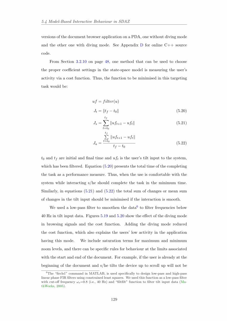
5.4 Model-Based Interactive Behaviour in SDAZ
versions of the document browser application on a PDA, one without diving mode
and the other one with diving mode. See Appendix D for online C++ source
code.
From Section 3.2.10 on page 48, one method that can be used to choose
the proper coefficient settings in the state-space model is measuring the user’s
activity via a cost function. Thus, the function to be minimised in this targeting
task would be:
uf = filter(u)
Jt = ‖tf − t0‖ (5.20)
Js =tf∑
t=t0
‖uft+1 − uft‖ (5.21)
Ja =
tf∑t=t0
‖uft+1 − uft‖
tf − t0(5.22)
t0 and tf are initial and final time and uft is the user’s tilt input to the system,
which has been filtered. Equation (5.20) presents the total time of the completing
the task as a performance measure. Thus, when the use is comfortable with the
system while interacting s/he should complete the task in the minimum time.
Similarly, in equations (5.21) and (5.22) the total sum of changes or mean sum
of changes in the tilt input should be minimised if the interaction is smooth.
We used a low-pass filter to smoothen the data6 to filter frequencies below
40 Hz in tilt input data. Figures 5.19 and 5.20 show the effect of the diving mode
in browsing signals and the cost function. Adding the diving mode reduced
the cost function, which also explains the users’ low activity in the application
having this mode. We include saturation terms for maximum and minimum
zoom levels, and there can be specific rules for behaviour at the limits associated
with the start and end of the document. For example, if the user is already at the
beginning of the document and s/he tilts the device up to scroll up will not be6The “fircls1” command in MATLAB, is used specifically to design low-pass and high-pass
linear phase FIR filters using constrained least squares. We used this function as a low-pass filterwith cut-off frequency ωo=0.8 (i.e., 40 Hz) and “filtfilt” function to filter tilt input data (Ma-thWorks, 2005).
129
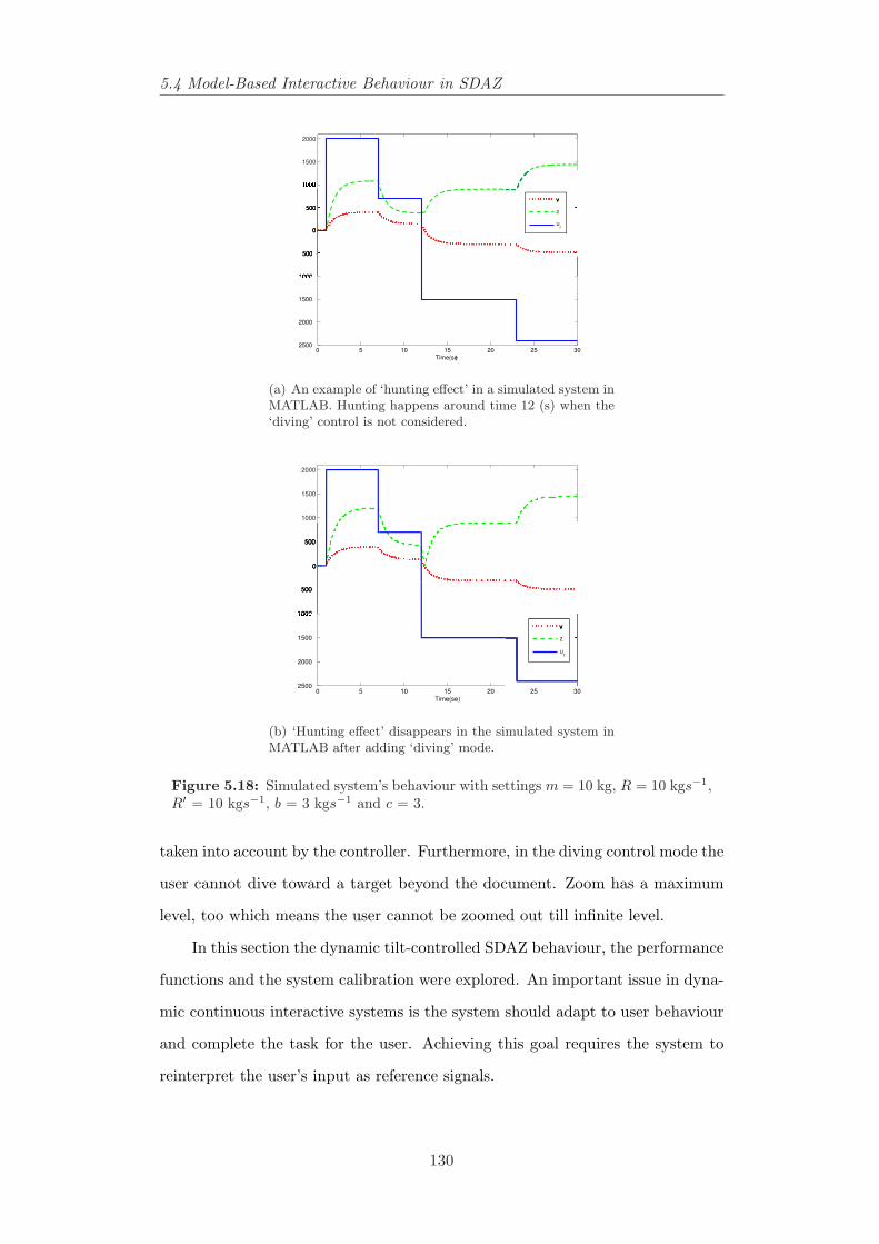
5.4 Model-Based Interactive Behaviour in SDAZ
0 5 10 15 20 25 302500
2000
1500
1500
2000
Time(se)
z
ur
(a) An example of ‘hunting effect’ in a simulated system inMATLAB. Hunting happens around time 12 (s) when the‘diving’ control is not considered.
0 5 10 15 20 25 302500
2000
1500
1000
1500
2000
Time(se)
z
ur
(b) ‘Hunting effect’ disappears in the simulated system inMATLAB after adding ‘diving’ mode.
Figure 5.18: Simulated system’s behaviour with settings m = 10 kg, R = 10 kgs−1,R′ = 10 kgs−1, b = 3 kgs−1 and c = 3.
taken into account by the controller. Furthermore, in the diving control mode the
user cannot dive toward a target beyond the document. Zoom has a maximum
level, too which means the user cannot be zoomed out till infinite level.
In this section the dynamic tilt-controlled SDAZ behaviour, the performance
functions and the system calibration were explored. An important issue in dyna-
mic continuous interactive systems is the system should adapt to user behaviour
and complete the task for the user. Achieving this goal requires the system to
reinterpret the user’s input as reference signals.
130
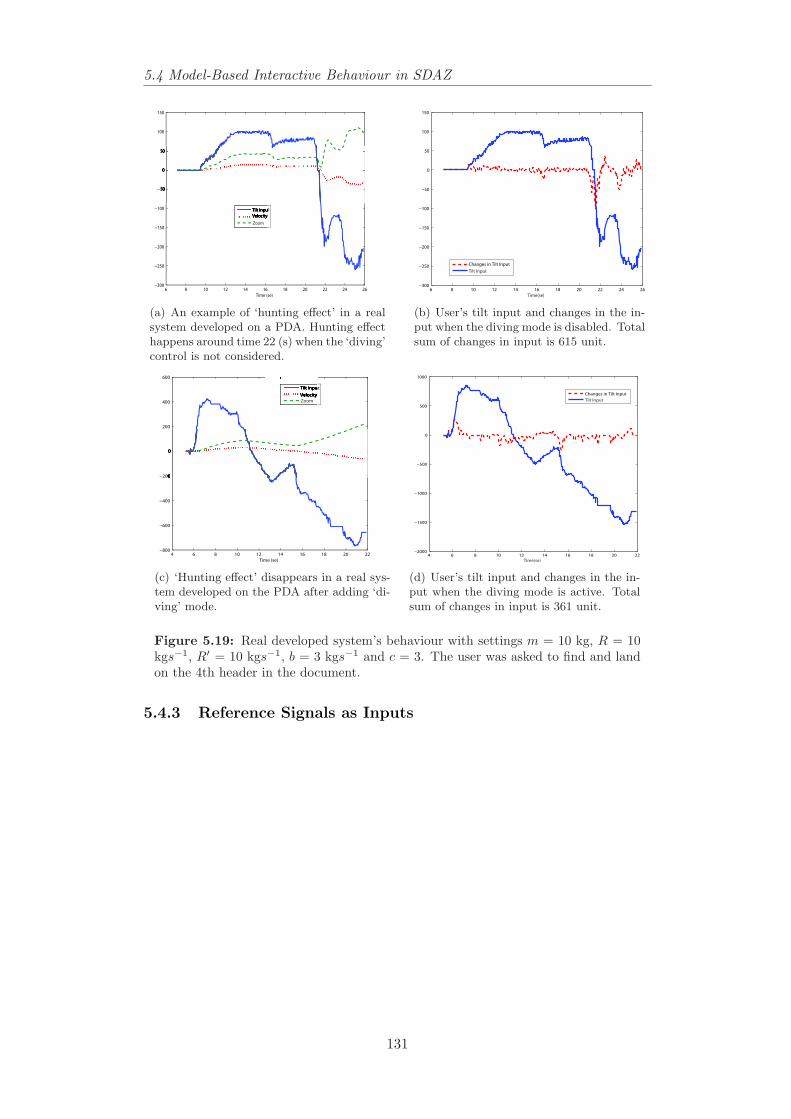
5.4 Model-Based Interactive Behaviour in SDAZ
6 8 10 12 14 16 18 20 22 24 26−300
−250
−200
−150
−100
−50
0
50
100
150
Time (se)
Tilt input
Velocity
Zoom
(a) An example of ‘hunting effect’ in a realsystem developed on a PDA. Hunting effecthappens around time 22 (s) when the ‘diving’control is not considered.
6 8 10 12 14 16 18 20 22 24 26−300
−250
−200
−150
−100
−50
0
50
100
150
Time(se)
Changes in Tilt Input
Tilt Input
(b) User’s tilt input and changes in the in-put when the diving mode is disabled. Totalsum of changes in input is 615 unit.
4 6 8 10 12 14 16 18 20 22−800
−600
−400
−200
0
200
400
600
Time (se)
Tilt input
Velocity
Zoom
(c) ‘Hunting effect’ disappears in a real sys-tem developed on the PDA after adding ‘di-ving’ mode.
4 6 8 10 12 14 16 18 20 22−2000
−1500
−1000
−500
0
500
1000
Time(se)
Changes in Tilt Input
Tilt Input
(d) User’s tilt input and changes in the in-put when the diving mode is active. Totalsum of changes in input is 361 unit.
Figure 5.19: Real developed system’s behaviour with settings m = 10 kg, R = 10kgs−1, R′ = 10 kgs−1, b = 3 kgs−1 and c = 3. The user was asked to find and landon the 4th header in the document.
5.4.3 Reference Signals as Inputs
131
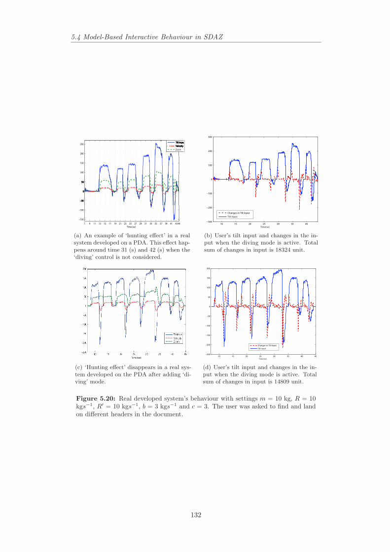
5.4 Model-Based Interactive Behaviour in SDAZ
7 9 11 13 15 17 19 21 23 25 27 29 31 33 35 37 39 41 4344
−150
−100
−50
0
50
100
150
200
250
Time (se)
Tilt input
Velocity
Zoom
(a) An example of ‘hunting effect’ in a realsystem developed on a PDA. This effect hap-pens around time 31 (s) and 42 (s) when the‘diving’ control is not considered.
10 15 20 25 30 35 40−300
−200
−100
0
100
200
300
Time(se)
Changes in Tilt Input
Tilt Input
(b) User’s tilt input and changes in the in-put when the diving mode is active. Totalsum of changes in input is 18324 unit.
(c) ‘Hunting effect’ disappears in a real sys-tem developed on the PDA after adding ‘di-ving’ mode.
10 15 20 25 30 35 40 45−250
−200
−150
−100
−50
0
50
100
150
200
Time(se)
Changes in Tilt Input
Tilt Input
(d) User’s tilt input and changes in the in-put when the diving mode is active. Totalsum of changes in input is 14809 unit.
Figure 5.20: Real developed system’s behaviour with settings m = 10 kg, R = 10kgs−1, R′ = 10 kgs−1, b = 3 kgs−1 and c = 3. The user was asked to find and landon different headers in the document.
132
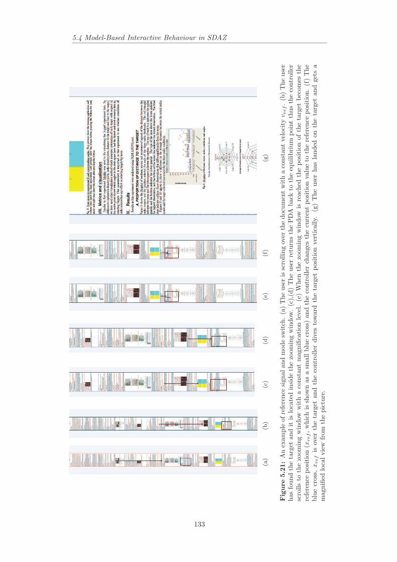
5.4 Model-Based Interactive Behaviour in SDAZ
(a)
(b)
(c)
(d)
(e)
(f)
(g)
Fig
ure
5.21
:A
nex
ampl
eof
refe
renc
esi
gnal
and
mod
esw
itch
.(a
)T
heus
eris
scro
lling
over
the
docu
men
tw
ith
aco
nsta
ntve
loci
tyv r
ef.
(b)
The
user
has
foun
dth
eta
rget
and
itis
loca
ted
insi
deth
ezo
omin
gw
indo
w.
(c),
(d)
The
user
retu
rns
the
PD
Aba
ckto
the
equi
libri
umpo
int
thus
the
cont
rolle
rsc
rolls
toth
ezo
omin
gw
indo
ww
ith
aco
nsta
ntm
agni
ficat
ion
leve
l.(e
)W
hen
the
zoom
ing
win
dow
isre
ache
dth
epo
siti
onof
the
targ
etbe
com
esth
ere
fere
nce
posi
tion
(xref,w
hich
issh
own
asa
smal
lbl
uecr
oss)
and
the
cont
rolle
rch
ange
sth
ecu
rren
tpo
siti
onva
lue
toth
ere
fere
nce
posi
tion
.(f
)T
hebl
uecr
oss,
xref
isov
erth
eta
rget
and
the
cont
rolle
rdi
ves
tow
ard
the
targ
etpo
siti
onve
rtic
ally
.(g
)T
heus
erha
sla
nded
onth
eta
rget
and
gets
am
agni
fied
loca
lvi
ewfr
omth
epi
ctur
e.
133
5.4 Model-Based Interactive Behaviour in SDAZ
From Section 2.3 and Figure 2.1 we know the reference signal is a goal
or a target the user is aiming to reach. The attempt to design systems that
could keep variables in reference states led to development of control theory in
the first place (Jagacinski et al., 1980). In control engineering, engineers design
systems to control variables with respect to reference signals, and they plan to
be able to manipulate the references (inputs) when they want to get the system
to control a variable at a different level (as when we change the setting on the
thermostat) (Brogan, 1991; Ogata, 1990).
Control systems and Reference Signals
In control systems the controller may support the user to complete the task
with less effort by changing the interpretation of the inputs to being reference
values, rather than control commands. In modern aircraft controllers there are
different interpretations of aircraft controls depending on flight mode (e.g., take
off, altitude-hold and so forth.) and blend seamlessly between modes (See (Ti-
schler, 1994) for examples). For example, in tilt-controlled SDAZ we have two
variables the user is aiming to reach: a desirable speed of scroll for browsing,
which is also coupled to the level of zoom, and a target that the user is trying
to land on. For these two variables we have two individual reference signals, vref
and xref and these signals give an example of an intuitive mode transitions.
To show the effect of the reference signal in mode transition we ran a few
examples. We asked the user to track a position in the document in cruising
mode by holding the cross-hair over the target. Tracking has been started from
top of the document. We logged the time series of the zooming-window posi-
tion, velocity and level of zoom. As an example of tracking, 10th header in the
document and its time series of data and phase plot is shown in Figures 5.21
and 5.22. In this example, while the user tilts the sensor at a constant angle, the
controller maintains the desired velocity automatically, e.g., vref and completes
the scrolling task with the velocity the user wants to achieve, rather than the
user having to do this. Any change in the tilt angle for the controller means the
user wants to change the vref (see Figure 5.15).
134
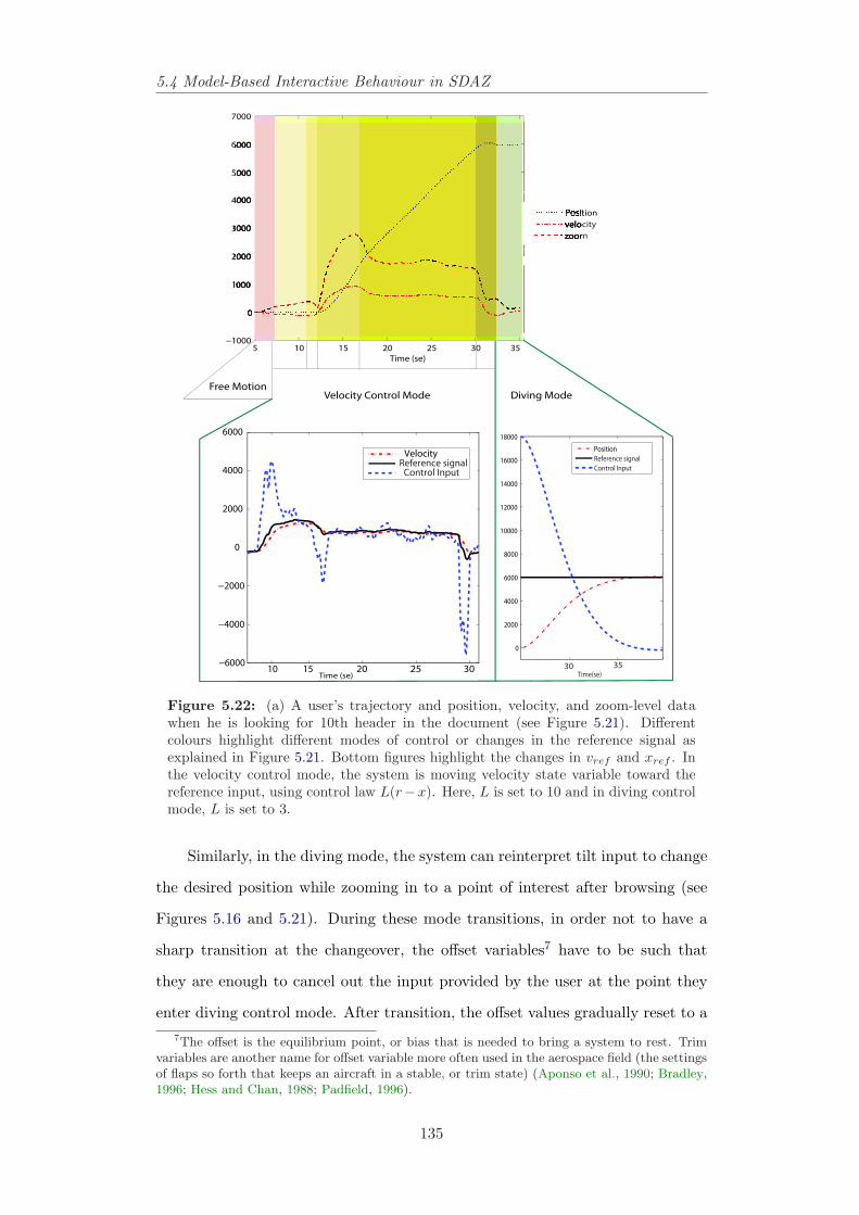
5.4 Model-Based Interactive Behaviour in SDAZ
5 10 15 20 25 30 35−1000
0
1000
2000
3000
4000
5000
6000
7000
Time (se)
Free MotionVelocity Control Mode Diving Mode
Position
velocity
zoom
Time (se)10 15 20 25 30
−6000
−4000
−2000
0
2000
4000
6000
VelocityReference signalControl Input
0
2000
4000
6000
8000
10000
12000
14000
16000
18000
Time(se)
Position
Reference signal
Control Input
30 35
Figure 5.22: (a) A user’s trajectory and position, velocity, and zoom-level datawhen he is looking for 10th header in the document (see Figure 5.21). Differentcolours highlight different modes of control or changes in the reference signal asexplained in Figure 5.21. Bottom figures highlight the changes in vref and xref . Inthe velocity control mode, the system is moving velocity state variable toward thereference input, using control law L(r−x). Here, L is set to 10 and in diving controlmode, L is set to 3.
Similarly, in the diving mode, the system can reinterpret tilt input to change
the desired position while zooming in to a point of interest after browsing (see
Figures 5.16 and 5.21). During these mode transitions, in order not to have a
sharp transition at the changeover, the offset variables7 have to be such that
they are enough to cancel out the input provided by the user at the point they
enter diving control mode. After transition, the offset values gradually reset to a7The offset is the equilibrium point, or bias that is needed to bring a system to rest. Trim
variables are another name for offset variable more often used in the aerospace field (the settingsof flaps so forth that keeps an aircraft in a stable, or trim state) (Aponso et al., 1990; Bradley,1996; Hess and Chan, 1988; Padfield, 1996).
135
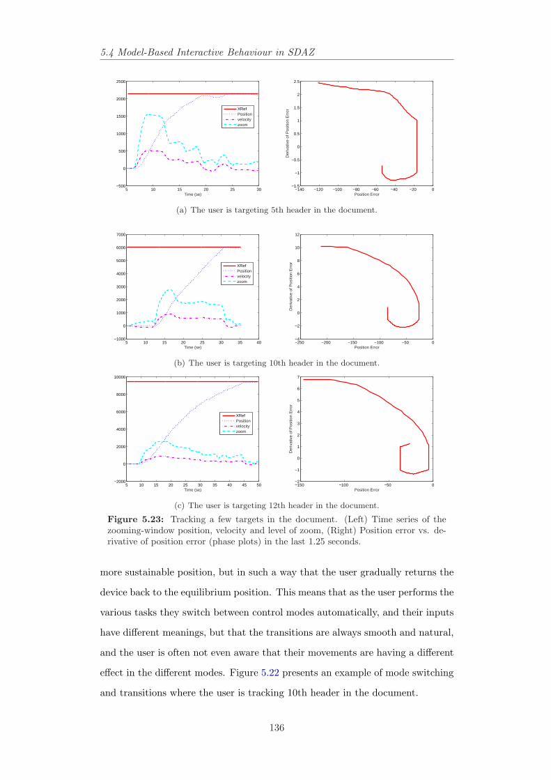
5.4 Model-Based Interactive Behaviour in SDAZ
5 10 15 20 25 30−500
0
500
1000
1500
2000
2500
Time (se)
XRefPositionvelocityzoom
−140 −120 −100 −80 −60 −40 −20 0−1.5
−1
−0.5
0
0.5
1
1.5
2
2.5
Position Error
Der
ivat
ive
of P
ositi
on E
rror
(a) The user is targeting 5th header in the document.
5 10 15 20 25 30 35 40−1000
0
1000
2000
3000
4000
5000
6000
7000
Time (se)
XRefPositionvelocityzoom
−250 −200 −150 −100 −50 0−4
−2
0
2
4
6
8
10
12
Position Error
Der
ivat
ive
of P
ositi
on E
rror
(b) The user is targeting 10th header in the document.
5 10 15 20 25 30 35 40 45 50−2000
0
2000
4000
6000
8000
10000
Time (se)
XRefPositionvelocityzoom
−150 −100 −50 0−2
−1
0
1
2
3
4
5
6
7
Position Error
Der
ivat
ive
of P
ositi
on E
rror
(c) The user is targeting 12th header in the document.
Figure 5.23: Tracking a few targets in the document. (Left) Time series of thezooming-window position, velocity and level of zoom, (Right) Position error vs. de-rivative of position error (phase plots) in the last 1.25 seconds.
more sustainable position, but in such a way that the user gradually returns the
device back to the equilibrium position. This means that as the user performs the
various tasks they switch between control modes automatically, and their inputs
have different meanings, but that the transitions are always smooth and natural,
and the user is often not even aware that their movements are having a different
effect in the different modes. Figure 5.22 presents an example of mode switching
and transitions where the user is tracking 10th header in the document.
136
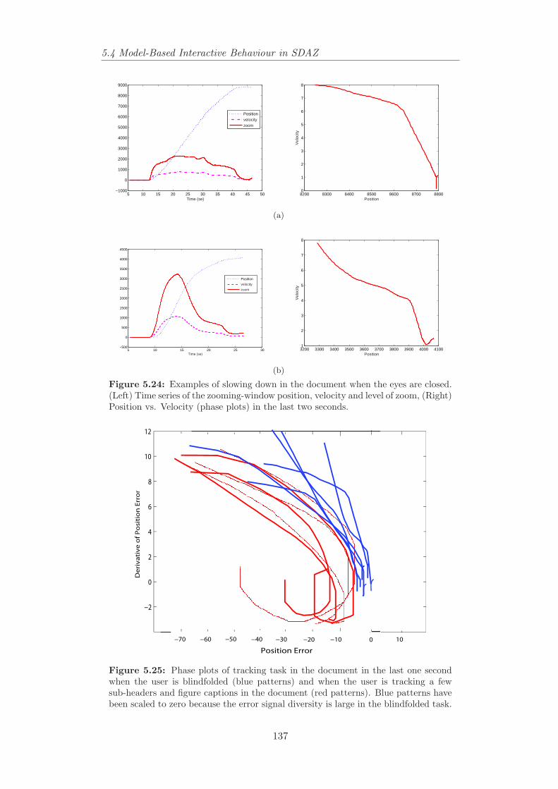
5.4 Model-Based Interactive Behaviour in SDAZ
5 10 15 20 25 30 35 40 45 50−1000
0
1000
2000
3000
4000
5000
6000
7000
8000
9000
Time (se)
Positionvelocityzoom
8200 8300 8400 8500 8600 8700 88000
1
2
3
4
5
6
7
8
Position
Vel
ocity
(a)
5 10 15 20 25 30−500
0
500
1000
1500
2000
2500
3000
3500
4000
4500
Time (se)
Position
velocity
zoom
3200 3300 3400 3500 3600 3700 3800 3900 4000 41001
2
3
4
5
6
7
8
Position
Vel
ocity
(b)
Figure 5.24: Examples of slowing down in the document when the eyes are closed.(Left) Time series of the zooming-window position, velocity and level of zoom, (Right)Position vs. Velocity (phase plots) in the last two seconds.
−2
0
2
4
6
8
10
12
Position Error
De
riv
ativ
e o
f P
osit
ion
Erro
r
−40 −30 −20 −10 100−50−60−70
Figure 5.25: Phase plots of tracking task in the document in the last one secondwhen the user is blindfolded (blue patterns) and when the user is tracking a fewsub-headers and figure captions in the document (red patterns). Blue patterns havebeen scaled to zero because the error signal diversity is large in the blindfolded task.
137
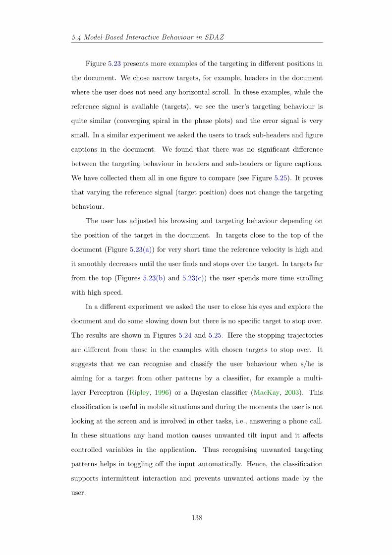
5.4 Model-Based Interactive Behaviour in SDAZ
Figure 5.23 presents more examples of the targeting in different positions in
the document. We chose narrow targets, for example, headers in the document
where the user does not need any horizontal scroll. In these examples, while the
reference signal is available (targets), we see the user’s targeting behaviour is
quite similar (converging spiral in the phase plots) and the error signal is very
small. In a similar experiment we asked the users to track sub-headers and figure
captions in the document. We found that there was no significant difference
between the targeting behaviour in headers and sub-headers or figure captions.
We have collected them all in one figure to compare (see Figure 5.25). It proves
that varying the reference signal (target position) does not change the targeting
behaviour.
The user has adjusted his browsing and targeting behaviour depending on
the position of the target in the document. In targets close to the top of the
document (Figure 5.23(a)) for very short time the reference velocity is high and
it smoothly decreases until the user finds and stops over the target. In targets far
from the top (Figures 5.23(b) and 5.23(c)) the user spends more time scrolling
with high speed.
In a different experiment we asked the user to close his eyes and explore the
document and do some slowing down but there is no specific target to stop over.
The results are shown in Figures 5.24 and 5.25. Here the stopping trajectories
are different from those in the examples with chosen targets to stop over. It
suggests that we can recognise and classify the user behaviour when s/he is
aiming for a target from other patterns by a classifier, for example a multi-
layer Perceptron (Ripley, 1996) or a Bayesian classifier (MacKay, 2003). This
classification is useful in mobile situations and during the moments the user is not
looking at the screen and is involved in other tasks, i.e., answering a phone call.
In these situations any hand motion causes unwanted tilt input and it affects
controlled variables in the application. Thus recognising unwanted targeting
patterns helps in toggling off the input automatically. Hence, the classification
supports intermittent interaction and prevents unwanted actions made by the
user.
138
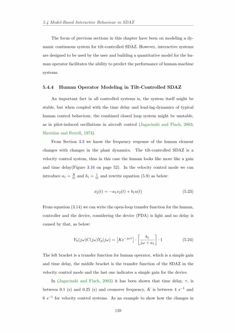
5.4 Model-Based Interactive Behaviour in SDAZ
The focus of previous sections in this chapter have been on modeling a dy-
namic continuous system for tilt-controlled SDAZ. However, interactive systems
are designed to be used by the user and building a quantitative model for the hu-
man operator facilitates the ability to predict the performance of human-machine
systems.
5.4.4 Human Operator Modeling in Tilt-Controlled SDAZ
An important fact in all controlled systems is, the system itself might be
stable, but when coupled with the time delay and lead-lag-dynamics of typical
human control behaviour, the combined closed loop system might be unstable,
as in pilot-induced oscillations in aircraft control (Jagacinski and Flach, 2003;
Sheridan and Ferrell, 1974).
From Section 3.3 we know the frequency response of the human element
changes with changes in the plant dynamics. The tilt-controlled SDAZ is a
velocity control system, thus in this case the human looks like more like a gain
and time delay(Figure 3.16 on page 52). In the velocity control mode we can
introduce a1 = Rm and b1 = 1
m and rewrite equation (5.9) as below:
x2(t) = −a1x2(t) + b1u(t) (5.23)
From equation (3.14) we can write the open-loop transfer function for the human,
controller and the device, considering the device (PDA) is light and no delay is
caused by that, as below:
Yh(jω)C(jω)Yp(jω) =[Ke−jωτ
] ·[
b1
jω + a1
]· 1 (5.24)
The left bracket is a transfer function for human operator, which is a simple gain
and time delay, the middle bracket is the transfer function of the SDAZ in the
velocity control mode and the last one indicates a simple gain for the device.
In (Jagacinski and Flach, 2003) it has been shown that time delay, τ , is
between 0.1 (s) and 0.25 (s) and crossover frequency, K is between 4 s−1 and
6 s−1 for velocity control systems. As an example to show how the changes in
139
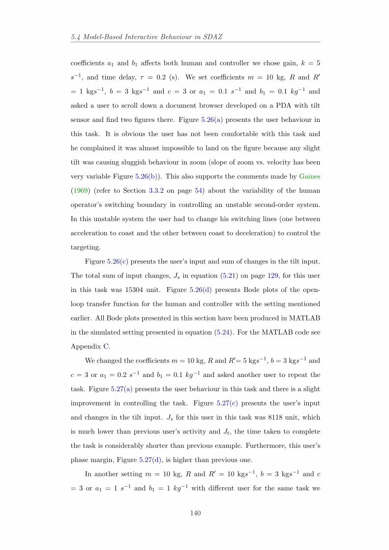
5.4 Model-Based Interactive Behaviour in SDAZ
coefficients a1 and b1 affects both human and controller we chose gain, k = 5
s−1, and time delay, τ = 0.2 (s). We set coefficients m = 10 kg, R and R′
= 1 kgs−1, b = 3 kgs−1 and c = 3 or a1 = 0.1 s−1 and b1 = 0.1 kg−1 and
asked a user to scroll down a document browser developed on a PDA with tilt
sensor and find two figures there. Figure 5.26(a) presents the user behaviour in
this task. It is obvious the user has not been comfortable with this task and
he complained it was almost impossible to land on the figure because any slight
tilt was causing sluggish behaviour in zoom (slope of zoom vs. velocity has been
very variable Figure 5.26(b)). This also supports the comments made by Gaines
(1969) (refer to Section 3.3.2 on page 54) about the variability of the human
operator’s switching boundary in controlling an unstable second-order system.
In this unstable system the user had to change his switching lines (one between
acceleration to coast and the other between coast to deceleration) to control the
targeting.
Figure 5.26(c) presents the user’s input and sum of changes in the tilt input.
The total sum of input changes, Js in equation (5.21) on page 129, for this user
in this task was 15304 unit. Figure 5.26(d) presents Bode plots of the open-
loop transfer function for the human and controller with the setting mentioned
earlier. All Bode plots presented in this section have been produced in MATLAB
in the simulated setting presented in equation (5.24). For the MATLAB code see
Appendix C.
We changed the coefficients m = 10 kg, R and R′= 5 kgs−1, b = 3 kgs−1 and
c = 3 or a1 = 0.2 s−1 and b1 = 0.1 kg−1 and asked another user to repeat the
task. Figure 5.27(a) presents the user behaviour in this task and there is a slight
improvement in controlling the task. Figure 5.27(c) presents the user’s input
and changes in the tilt input. Js for this user in this task was 8118 unit, which
is much lower than previous user’s activity and Jt, the time taken to complete
the task is considerably shorter than previous example. Furthermore, this user’s
phase margin, Figure 5.27(d), is higher than previous one.
In another setting m = 10 kg, R and R′ = 10 kgs−1, b = 3 kgs−1 and c
= 3 or a1 = 1 s−1 and b1 = 1 kg−1 with different user for the same task we
140
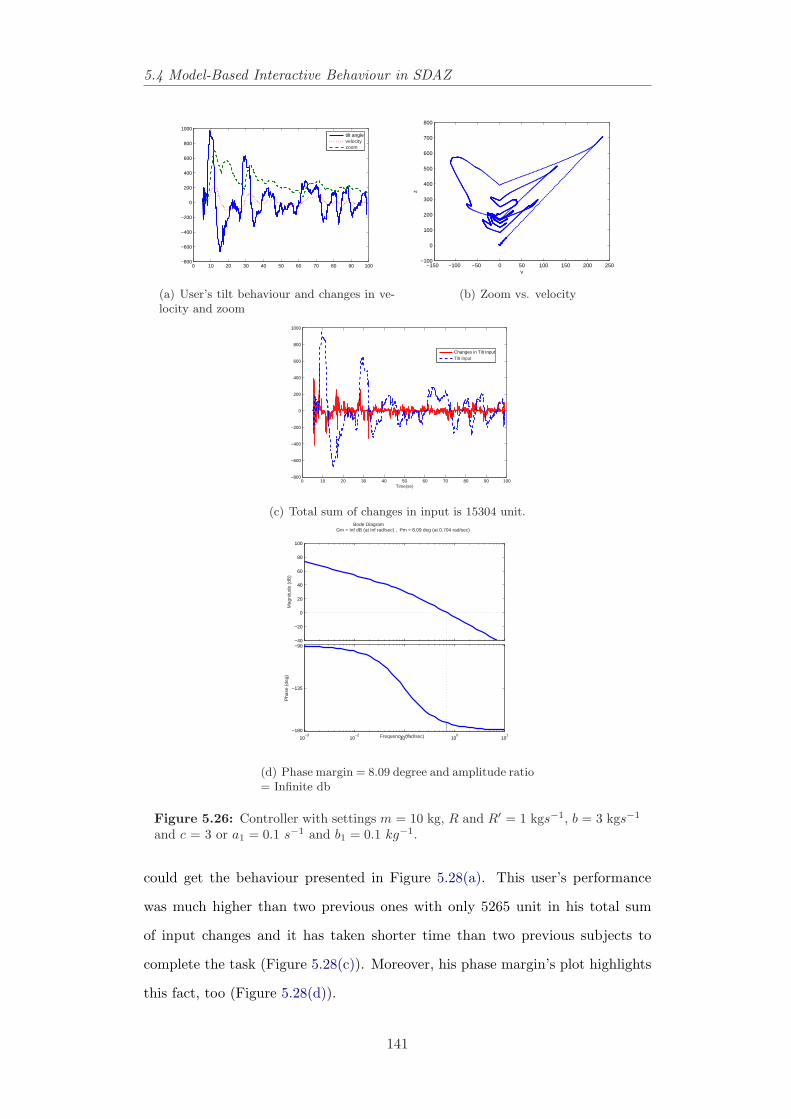
5.4 Model-Based Interactive Behaviour in SDAZ
0 10 20 30 40 50 60 70 80 90 100−800
−600
−400
−200
0
200
400
600
800
1000tilt anglevelocityzoom
(a) User’s tilt behaviour and changes in ve-locity and zoom
−150 −100 −50 0 50 100 150 200 250−100
0
100
200
300
400
500
600
700
800
v
z
(b) Zoom vs. velocity
0 10 20 30 40 50 60 70 80 90 100−800
−600
−400
−200
0
200
400
600
800
1000
Time(se)
Changes in Tilt InputTilt Input
(c) Total sum of changes in input is 15304 unit.
−40
−20
0
20
40
60
80
100
Mag
nitu
de (
dB)
10−3
10−2
10−1
100
101
−180
−135
−90
Pha
se (
deg)
Bode Diagram Gm = Inf dB (at Inf rad/sec) , Pm = 8.09 deg (at 0.704 rad/sec)
Frequency (rad/sec)
(d) Phase margin = 8.09 degree and amplitude ratio= Infinite db
Figure 5.26: Controller with settings m = 10 kg, R and R′ = 1 kgs−1, b = 3 kgs−1
and c = 3 or a1 = 0.1 s−1 and b1 = 0.1 kg−1.
could get the behaviour presented in Figure 5.28(a). This user’s performance
was much higher than two previous ones with only 5265 unit in his total sum
of input changes and it has taken shorter time than two previous subjects to
complete the task (Figure 5.28(c)). Moreover, his phase margin’s plot highlights
this fact, too (Figure 5.28(d)).
141
5.5 Example Application – Document Browser for a PDA
Other settings for this system could not bring the cost down or maximise the
phase margin more than settings, a1 = 1 and b1 = 0.1 (Figure 5.29). Thus this
simple example shows, first, the controller with settings m = 1 kg, R and R′ =
10 kgs−1, b = 3 kgs−1 and c = 3 is stable; second, a quasi-linear model of human
operator (first-order system, equation (5.24)) is a suitable model for our task;
third, phase margin and amplitude ratio of the open-loop transfer function for
the human and controller is maximised for this setting; fourth, the cost function
(either the time required to complete the task, equation (5.20) or total sum of
changes in the input, equation (5.21)) is minimised for this setting. For these
reasons and for later research we kept these setting for the controller to compare
its efficiency with other input methods, which will be discussed in later sections
in this chapter.
The next section presents an example application for browsing a document
developed on a PDA to highlight a few effects of calibration by taking into account
the results in the previous sections.
5.5 Example Application – Document Browser for a
PDA
We implemented a touch-screen version of the tilt-controlled SDAZ for brow-
sing the same document used in previous examples to compare with the tilt-
controlled version. The state-space settings for the touch-screen one was the
most stable setting in previous section, m = 1 kg, R and R′ = 10 kgs−1, b = 3
kgs−1 and c = 3.
Users found the touch-screen-based mechanism intuitive and easy to use for
browsing. Figure 5.30 presents the system’s inputs in three SDAZ applications
to find the same paragraph used in scroll bar browser for tilt-based and touch-
screen-controlled SDAZ. Additionally this figure presents an example run with
tilt-based SDAZ, with augmented velocity control, as described in Section 3.2.9,
to browse the document to find 7 main headings. For comparison, the central
plots in Figure 5.30 show tilt-based SDAZ without augmented velocity control
142
5.5 Example Application – Document Browser for a PDA
on the same task, where fluctuations indicate that controlling the zoom level was
difficult, and hunting behaviour appears when users tried to land on the targets
(e.g., t=20, 40, 85 seconds in Figure 5.30(b)).
5.5.1 Discussion
We asked five users from our research lab to work with the document brow-
ser using tilt-based SDAZ and touch-screen-controlled SDAZ with and without
augmented velocity control. Users who did the experiment without augmented
velocity control suggested that adding a control option or a switch to control
the zoom-level with velocity and tilting angles will make the system more com-
fortable to use. Most of them proposed if they could control level of zoom by
tapping on the screen or pressing a key on the PDA, the application would be
easier to use.
In contrast, the users who did their experiments with augmented velocity
control were satisfied with the application in both tilt-based and touch-screen-
controlled modes; because they commented they could easily land in on the goal
without tilting back and forth to adjust their targeting. Some users complained
that with tilt input, they had to tilt the device to angles which caused irritating
reflections from the Pocket PC screen. We could improve this by calibrating the
interface to the starting tilt-angle in the user’s palm.
Users in both groups, with and without augmented control, commented that
if they were involved with other tasks, (answering the phone, showing a figure on
the PDA to someone, and so forth) they would prefer the touch-screen-controlled
SDAZ because they imagined it would be difficult to stay in the desired position in
the document with a tilt-based SDAZ. This is one of the significant disadvantages
of using motion as an input in a handheld device. Motion as an input in a
handheld scenario limits the usefulness of the visual display for the duration of
the input; as the user is moving the device, s/he is unable to clearly see its
screen (Oakley et al., 2004). Using a classifier suggested in Section 5.4.3 would
be one solution to filter out unwanted movements. A more complex controller
that responds to only intended angles of tilt and filters unintended angles or a
143
5.6 Multimodal Feedback in a Tilt-Controlled SDAZ
controller that senses different contexts and locations the user is in and toggles
on suitable inputs are other solutions for this problem.
Furthermore the real physical model of the system (e.g., a flying object)
provided a clearer understanding about the tilt-controlled SDAZ. Users who were
told about this model could improve their actions quickly and commented that
after explaining the actual physical model the interaction made more sense.
In the next section we use multimodality as a possible solution for this
problem in tilt-controller SDAZ and its application in browsing a document.
5.6 Multimodal Feedback in a Tilt-Controlled SDAZ
Earlier in this chapter it was shown how interaction models and state-space
design can help create interactive systems. This design focuses on the lower level
of sensory-motor phenomenon and here we show how this method may help in
higher level of context of use.
Using motion as an input in a handheld device reduces the quality of the
visual display for the duration of the input, due to reflections from the screen
and difficulty in concentrating on a rapidly moving screen (Oakley et al., 2004).
Consequently, we believe that non-visual feedback will be an essential component
of movement-based interaction techniques. Audio/vibrotactile feedback in par-
ticular seems suitable for this role as it can be discretely presented directly to a
user’s ears/hand, and is already prevalent in mobile devices. Audio or vibrotac-
tile feedback may be crucial to support tasks or functionality on mobile devices
that must continue even while the user is not looking at the display (Hinckley
et al., 2000).
There are several stages in the process that produces audio/haptic repre-
sentations out of raw, abstract data. A general method which has been used in
our application is presented in Figure 5.31. The starting point in adding mul-
timodality is the raw data. This data, for example, Microsoft document, is in
“Data Tables” format. Data tables can describe many types of data, header, sub-
header, paragraph, table, figure, variables, and so forth in multiple dimensions.
144
5.6 Multimodal Feedback in a Tilt-Controlled SDAZ
Data tables are transformed into visual/audio/haptic structures by applying vi-
sual/audio/haptic mappings. In our application visual structures are transferred
to an image format, BMP or PNG. Audio/Haptic mappings will be discussed in
more details in the next section.
5.6.1 Design
We have used two mechanisms by which we can support tilt-controlled SDAZ
with audio feedback for rate of scrolling and structural information, to highlight
specific information that is currently on the screen.
As an intuitive model of the sonification process, we can imagine the text
on the screen to be embossed on the surface. This embossed type excites some
resonating object (elastic band or guitar string, for example) as it is dragged over
the text. This physically motivated model is similar in nature to the model-based
sonifications described by Hermann and Ritter (1999).
145
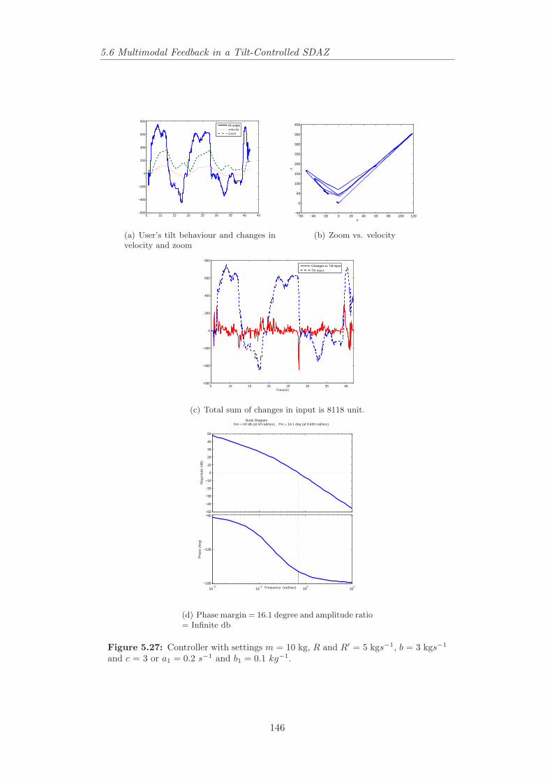
5.6 Multimodal Feedback in a Tilt-Controlled SDAZ
5 10 15 20 25 30 35 40 45−600
−400
−200
0
200
400
600
800tilt anglevelocityzoom
(a) User’s tilt behaviour and changes invelocity and zoom
−60 −40 −20 0 20 40 60 80 100 120−50
0
50
100
150
200
250
300
350
400
v
z
(b) Zoom vs. velocity
5 10 15 20 25 30 35 40−600
−400
−200
0
200
400
600
800
Time(se)
Changes in Tilt InputTilt Input
(c) Total sum of changes in input is 8118 unit.
−50
−40
−30
−20
−10
0
10
20
30
40
50
Mag
nitu
de (
dB)
10−2
10−1
100
101
−180
−135
−90
Pha
se (
deg)
Bode Diagram Gm = Inf dB (at Inf rad/sec) , Pm = 16.1 deg (at 0.693 rad/sec)
Frequency (rad/sec)
(d) Phase margin = 16.1 degree and amplitude ratio= Infinite db
Figure 5.27: Controller with settings m = 10 kg, R and R′ = 5 kgs−1, b = 3 kgs−1
and c = 3 or a1 = 0.2 s−1 and b1 = 0.1 kg−1.
146
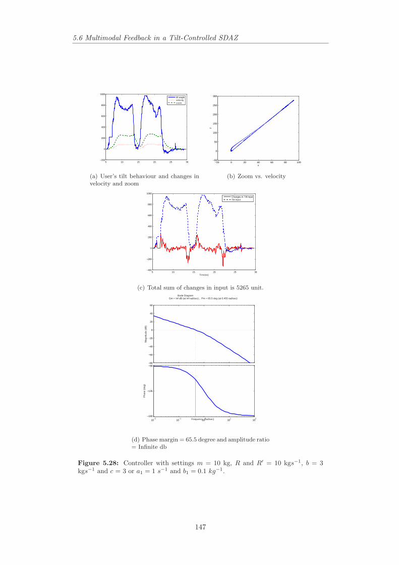
5.6 Multimodal Feedback in a Tilt-Controlled SDAZ
5 10 15 20 25 30−200
0
200
400
600
800
1000tilt anglevelocityzoom
(a) User’s tilt behaviour and changes invelocity and zoom
−20 0 20 40 60 80 100−50
0
50
100
150
200
250
300
v
z
(b) Zoom vs. velocity
5 10 15 20 25 30−400
−200
0
200
400
600
800
1000
Time(se)
Changes in Tilt InputTilt Input
(c) Total sum of changes in input is 5265 unit.
−80
−60
−40
−20
0
20
40
60
Mag
nitu
de (
dB)
10−2
10−1
100
101
102
−180
−135
−90
Pha
se (
deg)
Bode Diagram Gm = Inf dB (at Inf rad/sec) , Pm = 65.5 deg (at 0.455 rad/sec)
Frequency (rad/sec)
(d) Phase margin = 65.5 degree and amplitude ratio= Infinite db
Figure 5.28: Controller with settings m = 10 kg, R and R′ = 10 kgs−1, b = 3kgs−1 and c = 3 or a1 = 1 s−1 and b1 = 0.1 kg−1.
147
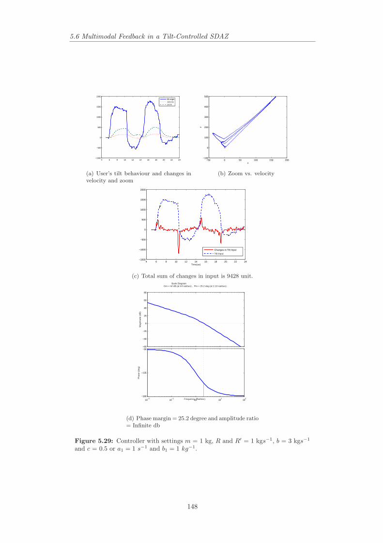
5.6 Multimodal Feedback in a Tilt-Controlled SDAZ
4 6 8 10 12 14 16 18 20 22 24−1000
−500
0
500
1000
1500
2000tilt anglevelocityzoom
(a) User’s tilt behaviour and changes invelocity and zoom
−50 0 50 100 150 200−100
0
100
200
300
400
500
v
z
(b) Zoom vs. velocity
4 6 8 10 12 14 16 18 20 22 24−1500
−1000
−500
0
500
1000
1500
2000
Time(se)
Changes in Tilt Input
Tilt Input
(c) Total sum of changes in input is 9428 unit.
−60
−40
−20
0
20
40
60
80
Mag
nitu
de (
dB)
10−2
10−1
100
101
102
−180
−135
−90
Pha
se (
deg)
Bode Diagram Gm = Inf dB (at Inf rad/sec) , Pm = 25.2 deg (at 2.13 rad/sec)
Frequency (rad/sec)
(d) Phase margin = 25.2 degree and amplitude ratio= Infinite db
Figure 5.29: Controller with settings m = 1 kg, R and R′ = 1 kgs−1, b = 3 kgs−1
and c = 0.5 or a1 = 1 s−1 and b1 = 1 kg−1.
148
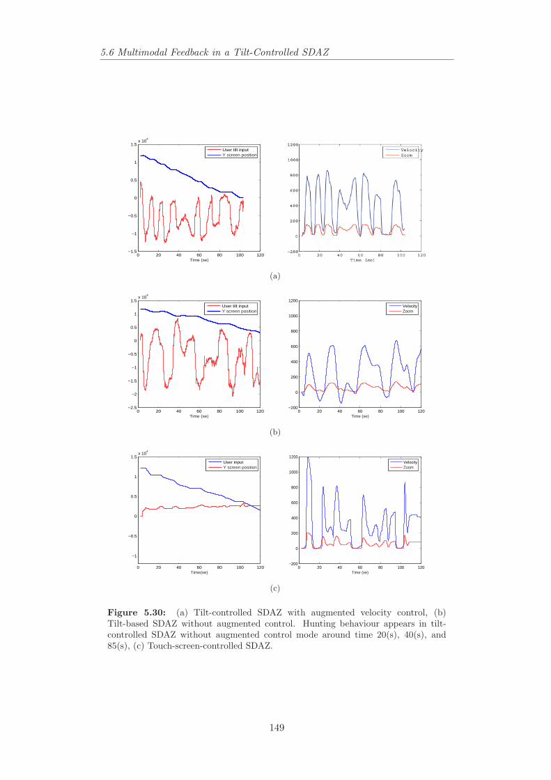
5.6 Multimodal Feedback in a Tilt-Controlled SDAZ
0 20 40 60 80 100 120−1.5
−1
−0.5
0
0.5
1
1.5x 10
4
Time (se)
User tilt inputY screen position
(a)
0 20 40 60 80 100 120−2.5
−2
−1.5
−1
−0.5
0
0.5
1
1.5x 10
4
Time (se)
User tilt inputY screen position
0 20 40 60 80 100 120−200
0
200
400
600
800
1000
1200
Time (se)
VelocityZoom
(b)
0 20 40 60 80 100 120
−1
−0.5
0
0.5
1
1.5x 10
4
Time(se)
User inputY screen position
0 20 40 60 80 100 120−200
0
200
400
600
800
1000
1200
Time (se)
VelocityZoom
(c)
Figure 5.30: (a) Tilt-controlled SDAZ with augmented velocity control, (b)Tilt-based SDAZ without augmented control. Hunting behaviour appears in tilt-controlled SDAZ without augmented control mode around time 20(s), 40(s), and85(s), (c) Touch-screen-controlled SDAZ.
149
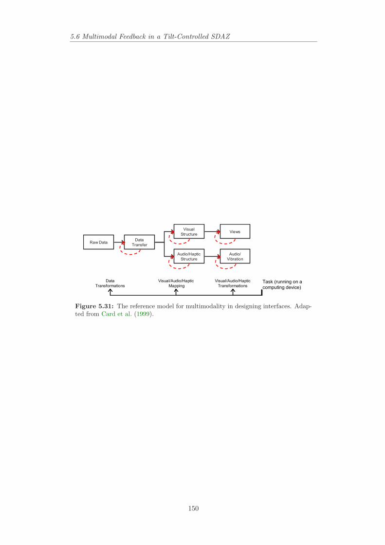
5.6 Multimodal Feedback in a Tilt-Controlled SDAZ
Raw DataData
Transfer
Visual
Structure
Audio/Haptic
Structure
Views
Audio/
Vibration
Task (running on a
computing device)
Data
Transformations
Visual/Audio/Haptic
Mapping
Visual/Audio/Haptic
Transformations
Figure 5.31: The reference model for multimodality in designing interfaces. Adap-ted from Card et al. (1999).
150
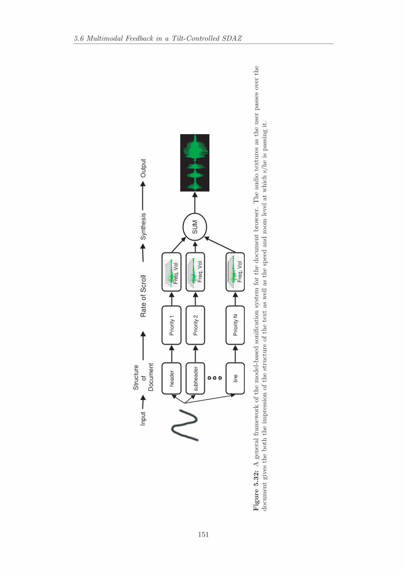
5.6 Multimodal Feedback in a Tilt-Controlled SDAZ
Inp
ut
Str
uctu
re
of
Docum
ent
Ra
te o
f S
cro
llS
ynth
esis
Outp
ut
he
ad
er
sub
he
ad
er
line
SU
M
Pri
ori
ty 1
Pri
ori
ty 2
Pri
ori
ty N
Fre
q, V
ol
Fre
q, V
ol
Fre
q, V
ol
Fig
ure
5.32
:A
gene
ralfr
amew
ork
ofth
em
odel
-bas
edso
nific
atio
nsy
stem
for
the
docu
men
tbr
owse
r.T
heau
dio
text
ures
asth
eus
erpa
sses
over
the
docu
men
tgi
ves
the
both
the
impr
essi
onof
the
stru
ctur
eof
the
text
asw
ellas
the
spee
dan
dzo
omle
velat
whi
chs/
heis
pass
ing
it.
151
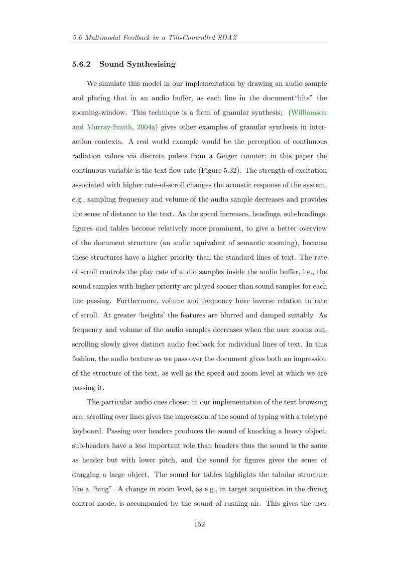
5.6 Multimodal Feedback in a Tilt-Controlled SDAZ
5.6.2 Sound Synthesising
We simulate this model in our implementation by drawing an audio sample
and placing that in an audio buffer, as each line in the document“hits” the
zooming-window. This technique is a form of granular synthesis; (Williamson
and Murray-Smith, 2004a) gives other examples of granular synthesis in inter-
action contexts. A real world example would be the perception of continuous
radiation values via discrete pulses from a Geiger counter; in this paper the
continuous variable is the text flow rate (Figure 5.32). The strength of excitation
associated with higher rate-of-scroll changes the acoustic response of the system,
e.g., sampling frequency and volume of the audio sample decreases and provides
the sense of distance to the text. As the speed increases, headings, sub-headings,
figures and tables become relatively more prominent, to give a better overview
of the document structure (an audio equivalent of semantic zooming), because
these structures have a higher priority than the standard lines of text. The rate
of scroll controls the play rate of audio samples inside the audio buffer, i.e., the
sound samples with higher priority are played sooner than sound samples for each
line passing. Furthermore, volume and frequency have inverse relation to rate
of scroll. At greater ‘heights’ the features are blurred and damped suitably. As
frequency and volume of the audio samples decreases when the user zooms out,
scrolling slowly gives distinct audio feedback for individual lines of text. In this
fashion, the audio texture as we pass over the document gives both an impression
of the structure of the text, as well as the speed and zoom level at which we are
passing it.
The particular audio cues chosen in our implementation of the text browsing
are: scrolling over lines gives the impression of the sound of typing with a teletype
keyboard. Passing over headers produces the sound of knocking a heavy object;
sub-headers have a less important role than headers thus the sound is the same
as header but with lower pitch, and the sound for figures gives the sense of
dragging a large object. The sound for tables highlights the tabular structure
like a “bing”. A change in zoom level, as e.g., in target acquisition in the diving
control mode, is accompanied by the sound of rushing air. This gives the user
152
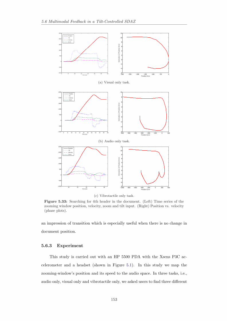
5.6 Multimodal Feedback in a Tilt-Controlled SDAZ
6 8 10 12 14 16 18 20−1000
−500
0
500
1000
1500
2000
2500
Time (se)
Position
Tilt
Velocity
Zoom
−300 −250 −200 −150 −100 −50 0−6
−4
−2
0
2
4
6
8
10
12
Position Error
De
riva
tive
of
Po
sitio
n E
rro
r
(a) Visual only task.
6 8 10 12 14 16 18 20 22 24 26 28−1000
−500
0
500
1000
1500
2000
2500
Time (se)
Position
Tilt
Velocity
Zoom
−600 −500 −400 −300 −200 −100 0 100−6
−4
−2
0
2
4
6
8
10
Position Error
De
riva
tive
of
Po
sitio
n E
rro
r
(b) Audio only task.
10 15 20 25 30−1000
−500
0
500
1000
1500
2000
2500
Time (se)
Position
Tilt
Velocity
Zoom
−1000 −800 −600 −400 −200 0 200 400−8
−6
−4
−2
0
2
4
6
8
10
12
Position Error
De
riva
tive
of
Po
sitio
n E
rro
r
(c) Vibrotactile only task.
Figure 5.33: Searching for 4th header in the document. (Left) Time series of thezooming window position, velocity, zoom and tilt input. (Right) Position vs. velocity(phase plots).
an impression of transition which is especially useful when there is no change in
document position.
5.6.3 Experiment
This study is carried out with an HP 5500 PDA with the Xsens P3C ac-
celerometer and a headset (shown in Figure 5.1). In this study we map the
zooming-window’s position and its speed to the audio space. In three tasks, i.e.,
audio only, visual only and vibrotactile only, we asked users to find three different
153
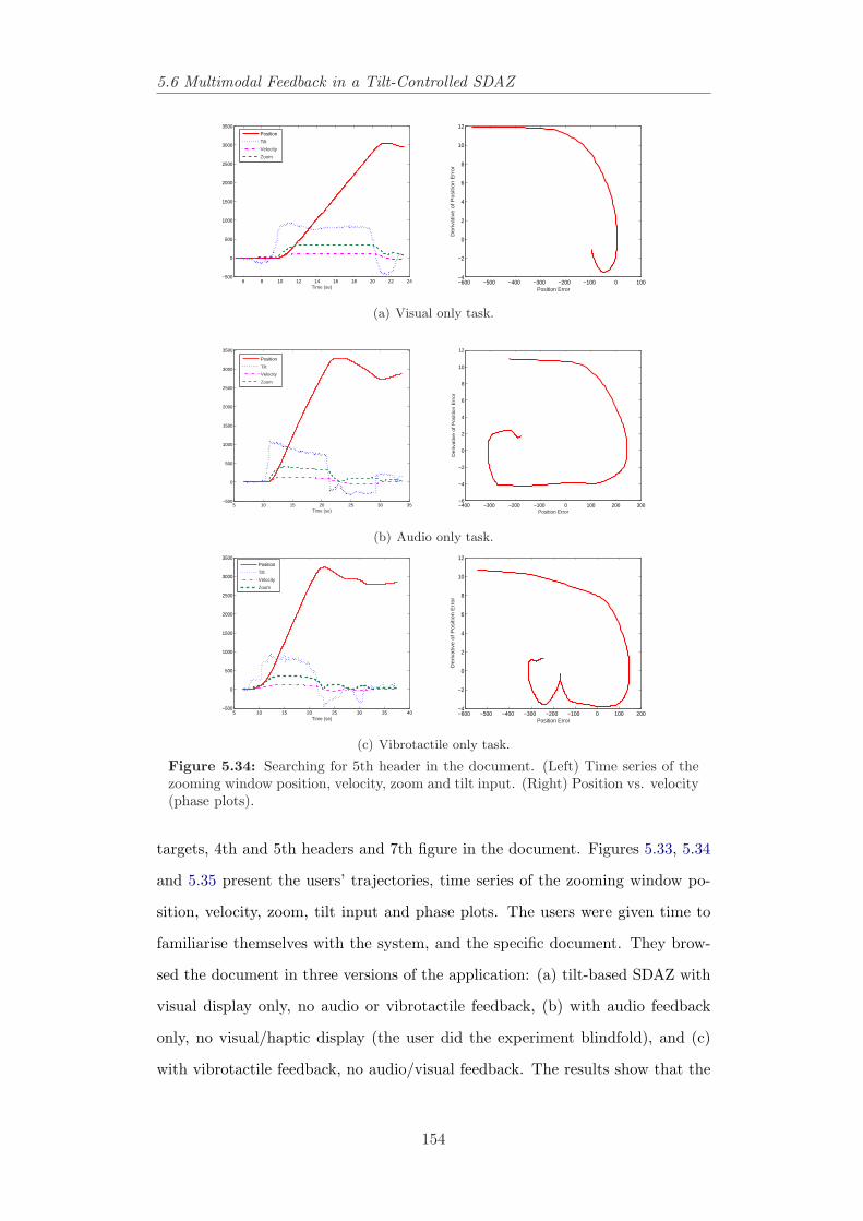
5.6 Multimodal Feedback in a Tilt-Controlled SDAZ
6 8 10 12 14 16 18 20 22 24−500
0
500
1000
1500
2000
2500
3000
3500
Time (se)
Position
Tilt
Velocity
Zoom
−600 −500 −400 −300 −200 −100 0 100−4
−2
0
2
4
6
8
10
12
Position Error
De
riva
tive
of
Po
sitio
n E
rro
r
(a) Visual only task.
5 10 15 20 25 30 35−500
0
500
1000
1500
2000
2500
3000
3500
Time (se)
Position
Tilt
Velocity
Zoom
−400 −300 −200 −100 0 100 200 300−6
−4
−2
0
2
4
6
8
10
12
Position Error
De
riva
tive
of P
osi
tion
Err
or
(b) Audio only task.
5 10 15 20 25 30 35 40−500
0
500
1000
1500
2000
2500
3000
3500
Time (se)
Position
Tilt
Velocity
Zoom
−600 −500 −400 −300 −200 −100 0 100 200−4
−2
0
2
4
6
8
10
12
Position Error
De
riva
tive
of
Po
sitio
n E
rro
r
(c) Vibrotactile only task.
Figure 5.34: Searching for 5th header in the document. (Left) Time series of thezooming window position, velocity, zoom and tilt input. (Right) Position vs. velocity(phase plots).
targets, 4th and 5th headers and 7th figure in the document. Figures 5.33, 5.34
and 5.35 present the users’ trajectories, time series of the zooming window po-
sition, velocity, zoom, tilt input and phase plots. The users were given time to
familiarise themselves with the system, and the specific document. They brow-
sed the document in three versions of the application: (a) tilt-based SDAZ with
visual display only, no audio or vibrotactile feedback, (b) with audio feedback
only, no visual/haptic display (the user did the experiment blindfold), and (c)
with vibrotactile feedback, no audio/visual feedback. The results show that the
154
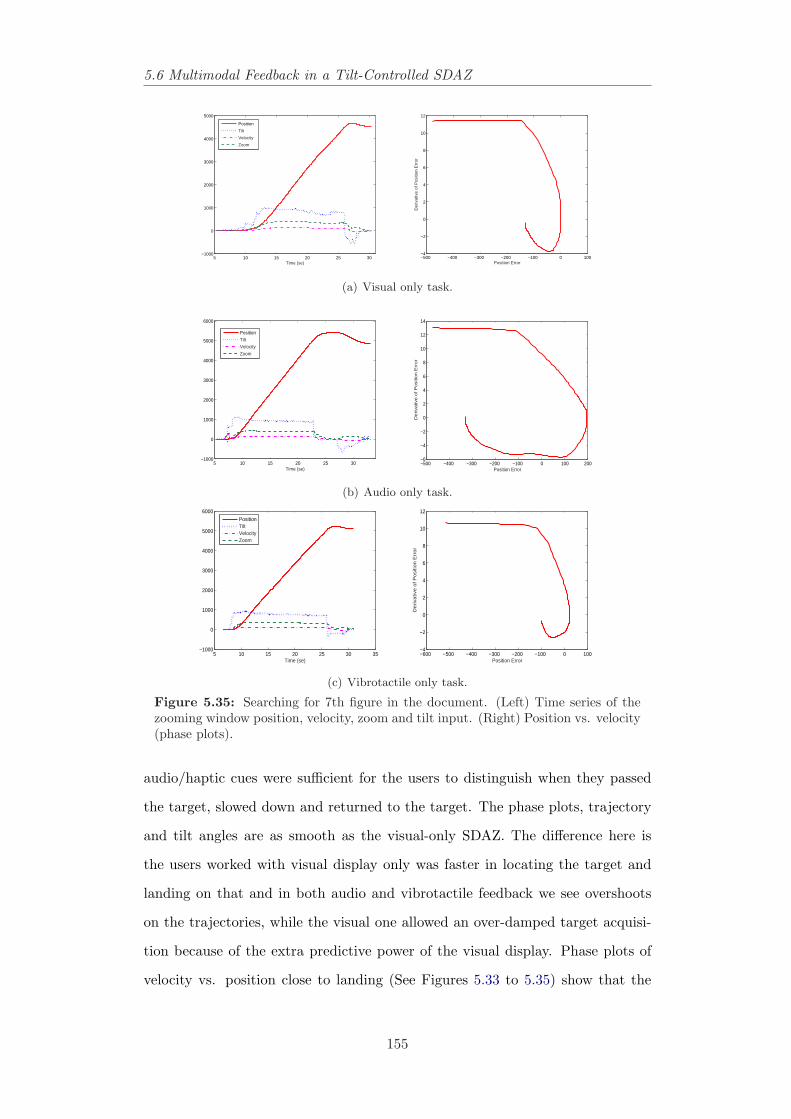
5.6 Multimodal Feedback in a Tilt-Controlled SDAZ
5 10 15 20 25 30−1000
0
1000
2000
3000
4000
5000
Time (se)
Position
Tilt
Velocity
Zoom
−500 −400 −300 −200 −100 0 100−4
−2
0
2
4
6
8
10
12
Position Error
Der
ivat
ive
of P
ositi
on E
rror
(a) Visual only task.
5 10 15 20 25 30−1000
0
1000
2000
3000
4000
5000
6000
Time (se)
Position
Tilt
Velocity
Zoom
−500 −400 −300 −200 −100 0 100 200−6
−4
−2
0
2
4
6
8
10
12
14
Position Error
De
riva
tive
of P
osi
tion
Err
or
(b) Audio only task.
5 10 15 20 25 30 35−1000
0
1000
2000
3000
4000
5000
6000
Time (se)
PositionTiltVelocityZoom
−600 −500 −400 −300 −200 −100 0 100−4
−2
0
2
4
6
8
10
12
Position Error
De
riva
tive
of
Po
sitio
n E
rro
r
(c) Vibrotactile only task.
Figure 5.35: Searching for 7th figure in the document. (Left) Time series of thezooming window position, velocity, zoom and tilt input. (Right) Position vs. velocity(phase plots).
audio/haptic cues were sufficient for the users to distinguish when they passed
the target, slowed down and returned to the target. The phase plots, trajectory
and tilt angles are as smooth as the visual-only SDAZ. The difference here is
the users worked with visual display only was faster in locating the target and
landing on that and in both audio and vibrotactile feedback we see overshoots
on the trajectories, while the visual one allowed an over-damped target acquisi-
tion because of the extra predictive power of the visual display. Phase plots of
velocity vs. position close to landing (See Figures 5.33 to 5.35) show that the
155
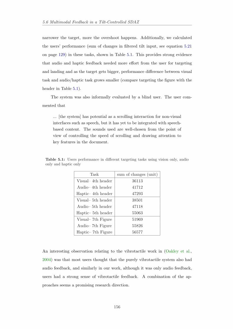
5.6 Multimodal Feedback in a Tilt-Controlled SDAZ
narrower the target, more the overshoot happens. Additionally, we calculated
the users’ performance (sum of changes in filtered tilt input, see equation 5.21
on page 129) in these tasks, shown in Table 5.1. This provides strong evidence
that audio and haptic feedback needed more effort from the user for targeting
and landing and as the target gets bigger, performance difference between visual
task and audio/haptic task grows smaller (compare targeting the figure with the
header in Table 5.1).
The system was also informally evaluated by a blind user. The user com-
mented that
... [the system] has potential as a scrolling interaction for non-visualinterfaces such as speech, but it has yet to be integrated with speech-based content. The sounds used are well-chosen from the point ofview of controlling the speed of scrolling and drawing attention tokey features in the document.
Table 5.1: Users performance in different targeting tasks using vision only, audioonly and haptic only
Task sum of changes (unit)
Visual– 4th header 36113Audio– 4th header 41712Haptic– 4th header 47293
Visual– 5th header 38501Audio– 5th header 47118Haptic– 5th header 55063
Visual– 7th Figure 51969Audio– 7th Figure 55826Haptic– 7th Figure 56577
An interesting observation relating to the vibrotactile work in (Oakley et al.,
2004) was that most users thought that the purely vibrotactile system also had
audio feedback, and similarly in our work, although it was only audio feedback,
users had a strong sense of vibrotactile feedback. A combination of the ap-
proaches seems a promising research direction.
156
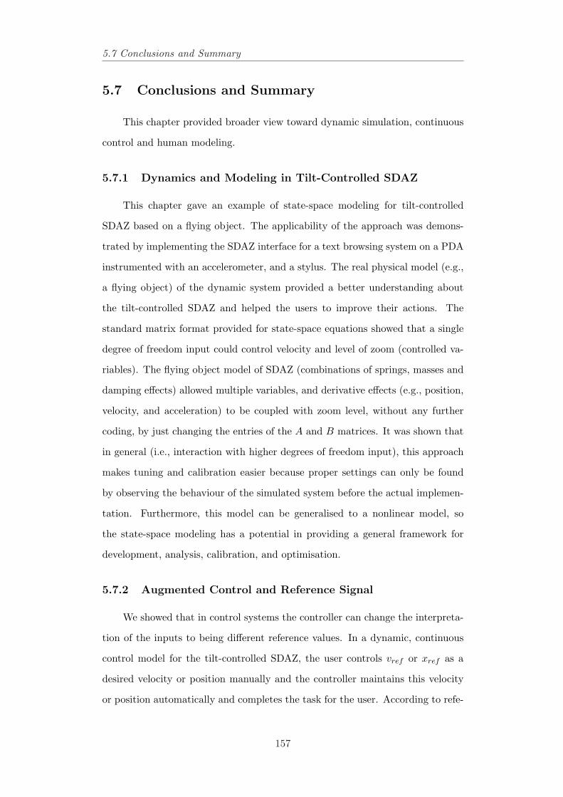
5.7 Conclusions and Summary
5.7 Conclusions and Summary
This chapter provided broader view toward dynamic simulation, continuous
control and human modeling.
5.7.1 Dynamics and Modeling in Tilt-Controlled SDAZ
This chapter gave an example of state-space modeling for tilt-controlled
SDAZ based on a flying object. The applicability of the approach was demons-
trated by implementing the SDAZ interface for a text browsing system on a PDA
instrumented with an accelerometer, and a stylus. The real physical model (e.g.,
a flying object) of the dynamic system provided a better understanding about
the tilt-controlled SDAZ and helped the users to improve their actions. The
standard matrix format provided for state-space equations showed that a single
degree of freedom input could control velocity and level of zoom (controlled va-
riables). The flying object model of SDAZ (combinations of springs, masses and
damping effects) allowed multiple variables, and derivative effects (e.g., position,
velocity, and acceleration) to be coupled with zoom level, without any further
coding, by just changing the entries of the A and B matrices. It was shown that
in general (i.e., interaction with higher degrees of freedom input), this approach
makes tuning and calibration easier because proper settings can only be found
by observing the behaviour of the simulated system before the actual implemen-
tation. Furthermore, this model can be generalised to a nonlinear model, so
the state-space modeling has a potential in providing a general framework for
development, analysis, calibration, and optimisation.
5.7.2 Augmented Control and Reference Signal
We showed that in control systems the controller can change the interpreta-
tion of the inputs to being different reference values. In a dynamic, continuous
control model for the tilt-controlled SDAZ, the user controls vref or xref as a
desired velocity or position manually and the controller maintains this velocity
or position automatically and completes the task for the user. According to refe-
157
5.7 Conclusions and Summary
rence variables xref and vref , the controller switches among four discrete states,
no action, free motion (i.e., basic acceleration mode), velocity and diving control
modes. During mode transitions, in order not to have a sharp transition at the
changeover, the offset variables change such that to cancel out the input provi-
ded by the user at the point they enter a new control mode. After transition the
offset values gradually reset to a more sustainable position, but in such a way
that the user gradually returns the device back to the equilibrium position, so
the transition is smooth and natural, and the user is often not even aware that
their movements are having a different effect in different modes. Moreover, users
commented that with augmented velocity control the application was easier to
control during landing; because the controller’s setting is adapted to the task
the user tends to do and makes that task easier to control for the user and it
improves hunting behaviour.
5.7.3 Modeling the User Behaviour
A number of examples were presented to show that, the controlled system it-
self might be stable, but when coupled with the time delay and lead-lag-dynamics
of typical human control behaviour, the combined closed loop system might be
unstable. It proves control theory can support design of closed-loop interaction
between human and system. We modeled human operator like a gain and time
delay, plotted the Bode plots of the open-loop transfer function for the human
and controller and calculated the activity of the user using a performance func-
tion with different settings for the controller and human. It helped us to choose
settings that suit both the system and the user and made the controlled system
stable when coupled with user model.
5.7.4 Tilt Control Interaction
The tilt-controlled version has its own pros and cons. The tilt input applica-
tion can be controlled in a single-handed manner, without obscuring the screen.
Users preferred the stylus, as there were no reflections from the screen and they
could stop interacting by taking the stylus off the screen. In the tilt-controlled
158
5.7 Conclusions and Summary
version users have to tilt the device to angles, which caused irritating reflections
from the Pocket PC screen. We improved this by calibrating the interface to
the starting tilt-angle in the user’s palm as an equilibrium point. Furthermore,
users commented that if they were involved with other tasks, i.e., answering the
phone, and so forth they would prefer the touch-screen-controlled SDAZ because
it would be difficult to stay in the desired position in the document, with a
tilt-based SDAZ. Recognising targeting patterns as discussed before may help in
toggling on/off the input automatically.
5.7.5 Multimodal Tilt-Controlled SDAZ
Next, we presented an audio/haptic feedback representation of the speed-
zoom coupling involved in speed-dependent automatic zooming. The applicabi-
lity of the approach was demonstrated by implementing the SDAZ interface for
a text browser system on the PDA instrumented with the tilt sensor. Sonifying
each piece of structural information in the document was easy to understand by
users and they could feel different textures in the document even blind people.
The results showed that the audio/haptic cue is sufficient for the blindfolded
users to distinguish where the target is but when they start to land they have
already passed the target, so they have to adjust the tilt and go back to the
target. Additionally, the users’ activities in the audio and haptic only interface
were higher than the visual only, most likely because the vision is leading sense
(this will be discussed in the next chapter). Providing audio feedback about the
user’s predicted position instead of their current position may solve this problem
(see Chapter 4). Multimodal SDAZ can also support intermittent interaction.
In the next chapter we introduce a similar approach in designing interfaces
to multimodal SDAZ, for a focus-in-context method and extend that to support
human behaviour in browsing a document, and feedback its contents visually and
in non-speech audio based on a language model and prediction.
159
Chapter 6
Multimodal Motion Controlled
Focus-in-Context Method:
Sensing Complex Information
This chapter introduces a dynamic system approach to the coupling ofinternal states involved in a focus-in-context visualisation. We use anexample, where we support human behaviour in browsing a document,and feedback its contents visually using the focus-in-context methodand in non-speech audio based on a language model. We alter thedynamics of movement in the document as a function of the interpre-ted behaviour. It is argued that to design interaction we need modelsof key aspects of the process. Here for example, we need models forthe dynamic system, a probabilistic language model and a probabilis-tic audio feedback as an example of a multimodal approach to sensingdifferent languages in a multilingual text. We demonstrate that howthe user’s intention is coupled to the visualisation technique via thedynamic model, and how the focus-in-context method couples detailsin context to audio samples via the language identification system.
6.1 Introduction
As mentioned in the preceding chapters the unique challenge in the computer-
as-tool paradigm (see Section 2.4.2 on page 21) is to create new tools that both
augment and complement human capabilities. One important area of research in
160
6.2 Related Work and Background
this chapter is presenting multimodal information on the display. Thus, we utilise
focus in context techniques, which apply complex algorithms to data and human
perceptual abilities to extract patterns, to facilitate the visual presentation issue.
Psychology’s gestalt theory deals with issues regarding details and context,
stating that details have more meaning when presented within their context.
Specifically, Wertheimer (1938) states that, “there are wholes, the behaviour of
which is not determined by that of their individual elements, but where the part-
processes are themselves determined by the intrinsic nature of the whole.” Furnas
(1986) illustrates an efficient way of embedding a specific piece of information
within its larger context. He represents those portions of the context that are
closer to the immediate area of interest in greater detail while including only
some major landmarks of the context further away. His method suggests that
such views (he called them ‘fisheye views’) might be useful for the computer
display of large information structures like programs, data bases, online text,
and so forth (Furnas, 1986) and for large steering tasks (Gutwin and Skopik,
2003).
In this chapter, we extend this issue to the multimodality and the human
interaction with multimodal interfaces. We introduce browsing and sensing mul-
tilingual texts as an example of a continuous interactive system and present a
model-based interactive method for searching a particular language based on a
language model, sonification, a focus-in-context method and continuous interac-
tion interface, which can be linked to a wide range of inputs and feedback/display
mechanisms.
6.2 Related Work and Background
In this section we explore the presentation problems and its possible solu-
tions.
161
6.2 Related Work and Background
6.2.1 The Presentation Problem
Providing both detailed and contextual information in the same view is a
crucial issue, especially on displays with constrained view, for instance, mobile
phones. In the past 20 years many researches on the information visualisation ha
been done in solving this problem. Spence (2001) categorises these solutions into:
(1) focus + context, (2) suppression of information, (3) magic lenses, (4) browsing,
(5) effective views, and (6) zoom and pan. Focus-in-context and suppression of
information will be focus of the research in this chapter, thus we explore their
principles in brief in this section.
Focus+Context Techniques
Card et al. (1999) and Carpendale and Montagnese (2001) suggest three
premises for focus + context techniques: “First of all, both the context and the
detailed information must be available simultaneously. Second, the type of infor-
mation shown in the detailed view and context may be different from one another.
Third, these two types of information should be combined into one display.”
Generally distortion in focus + context techniques is controlled by a visual
transformation function, which distorts the visualisations through stretching and
compression, in order to give the focal portion of the visualisation more visual
detail. The shape of the transformation, that is how the magnification factor
changes across the visualisation, is expressed by a magnification function that is
a derivative of the visual transformation function (Carpendale and Montagnese,
2001).
Leung and Apperley (1994) presented a thorough review of focus + context
techniques. In this review they divided transformation functions into two catego-
ries: step functions and continuous transformation functions. They define step
functions as functions, which change the values discontinuously from one constant
to the next, causing discrete levels of magnification and continuous transforma-
tion functions as functions, which scale the values in a continuous manner, causing
smooth magnification. Continuous transformation functions will be discussed in
suppression techniques. The step magnification function can be constant (as in
162
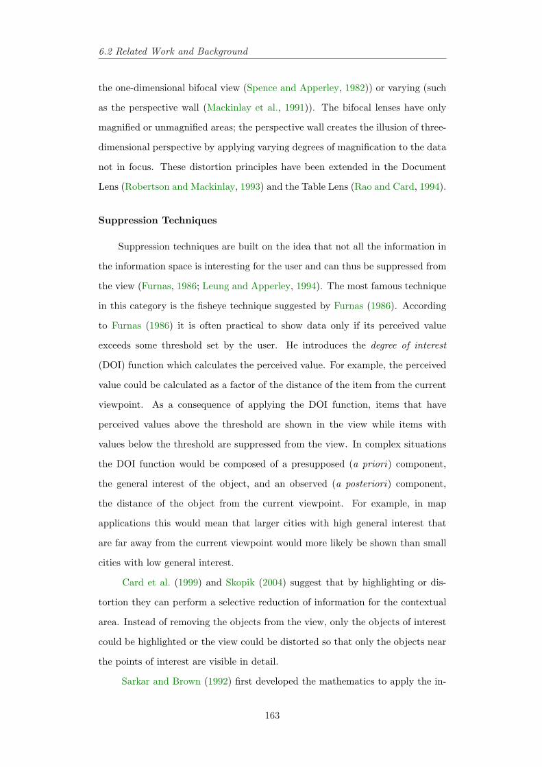
6.2 Related Work and Background
the one-dimensional bifocal view (Spence and Apperley, 1982)) or varying (such
as the perspective wall (Mackinlay et al., 1991)). The bifocal lenses have only
magnified or unmagnified areas; the perspective wall creates the illusion of three-
dimensional perspective by applying varying degrees of magnification to the data
not in focus. These distortion principles have been extended in the Document
Lens (Robertson and Mackinlay, 1993) and the Table Lens (Rao and Card, 1994).
Suppression Techniques
Suppression techniques are built on the idea that not all the information in
the information space is interesting for the user and can thus be suppressed from
the view (Furnas, 1986; Leung and Apperley, 1994). The most famous technique
in this category is the fisheye technique suggested by Furnas (1986). According
to Furnas (1986) it is often practical to show data only if its perceived value
exceeds some threshold set by the user. He introduces the degree of interest
(DOI) function which calculates the perceived value. For example, the perceived
value could be calculated as a factor of the distance of the item from the current
viewpoint. As a consequence of applying the DOI function, items that have
perceived values above the threshold are shown in the view while items with
values below the threshold are suppressed from the view. In complex situations
the DOI function would be composed of a presupposed (a priori) component,
the general interest of the object, and an observed (a posteriori) component,
the distance of the object from the current viewpoint. For example, in map
applications this would mean that larger cities with high general interest that
are far away from the current viewpoint would more likely be shown than small
cities with low general interest.
Card et al. (1999) and Skopik (2004) suggest that by highlighting or dis-
tortion they can perform a selective reduction of information for the contextual
area. Instead of removing the objects from the view, only the objects of interest
could be highlighted or the view could be distorted so that only the objects near
the points of interest are visible in detail.
Sarkar and Brown (1992) first developed the mathematics to apply the in-
163
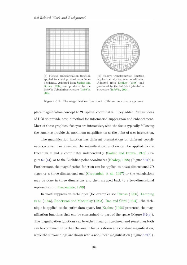
6.2 Related Work and Background
(a) Fisheye transformation functionapplied to x and y coordinates inde-pendently. Adapted from Sarkar andBrown (1992) and produced by theInfoVis CyberInfrastructure (InfoVis,2004).
(b) Fisheye transformation functionapplied radially to polar coordinates.Adapted from Keahey (1998) andproduced by the InfoVis CyberInfra-structure (InfoVis, 2004).
Figure 6.1: The magnification function in different coordinate systems.
place magnification concept to 2D spatial coordinates. They added Furnas’ ideas
of DOI to provide both a method for information suppression and enhancement.
Most of these graphical fisheyes are interactive, with the focus typically following
the cursor to provide the maximum magnification at the point of user interaction.
The magnification function has different presentations on different coordi-
nate systems. For example, the magnification function can be applied to the
Euclidian x and y coordinates independently (Sarkar and Brown, 1992) (Fi-
gure 6.1(a)), or to the Euclidian polar coordinates (Keahey, 1998) (Figure 6.1(b)).
Furthermore, the magnification function can be applied to a two-dimensional 2D
space or a three-dimensional one (Carpendale et al., 1997) or the calculations
may be done in three dimensions and then mapped back to a two-dimensional
representation (Carpendale, 1999).
In most suppression techniques (for examples see Furnas (1986), Lamping
et al. (1995), Robertson and Mackinlay (1993), Rao and Card (1994)), the tech-
nique is applied to the entire data space, but Keahey (1998) presented the mag-
nification functions that can be constrained to part of the space (Figure 6.2(a)).
The magnification functions can be either linear or non-linear and sometimes both
can be combined, thus that the area in focus is shown at a constant magnification,
while the surroundings are shown with a non-linear magnification (Figure 6.2(b)).
164
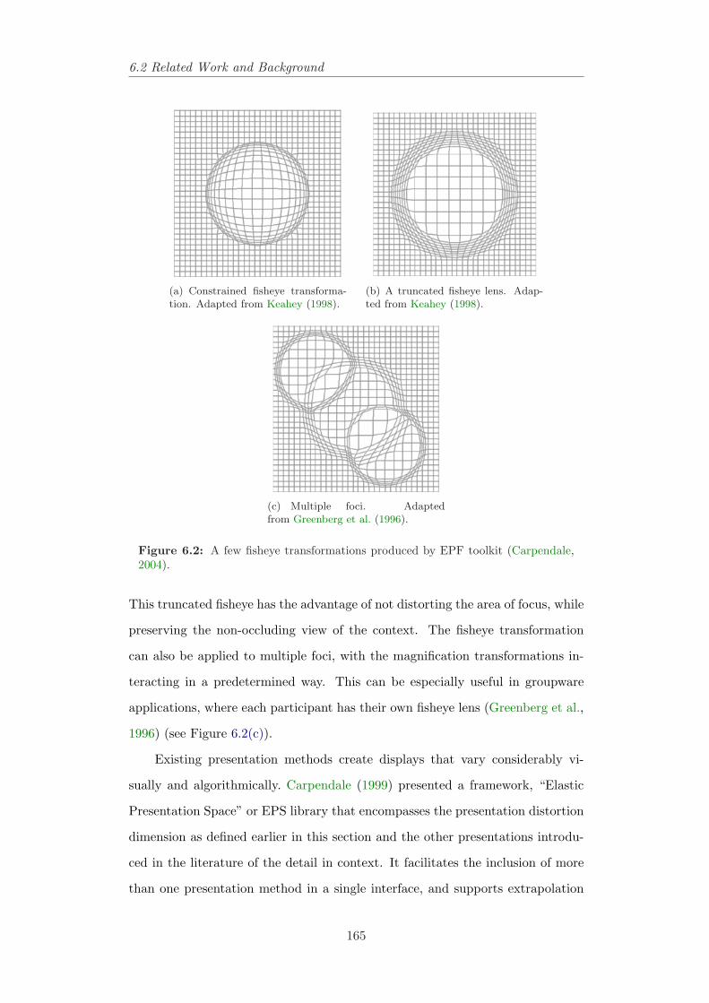
6.2 Related Work and Background
(a) Constrained fisheye transforma-tion. Adapted from Keahey (1998).
(b) A truncated fisheye lens. Adap-ted from Keahey (1998).
(c) Multiple foci. Adaptedfrom Greenberg et al. (1996).
Figure 6.2: A few fisheye transformations produced by EPF toolkit (Carpendale,2004).
This truncated fisheye has the advantage of not distorting the area of focus, while
preserving the non-occluding view of the context. The fisheye transformation
can also be applied to multiple foci, with the magnification transformations in-
teracting in a predetermined way. This can be especially useful in groupware
applications, where each participant has their own fisheye lens (Greenberg et al.,
1996) (see Figure 6.2(c)).
Existing presentation methods create displays that vary considerably vi-
sually and algorithmically. Carpendale (1999) presented a framework, “Elastic
Presentation Space” or EPS library that encompasses the presentation distortion
dimension as defined earlier in this section and the other presentations introdu-
ced in the literature of the detail in context. It facilitates the inclusion of more
than one presentation method in a single interface, and supports extrapolation
165
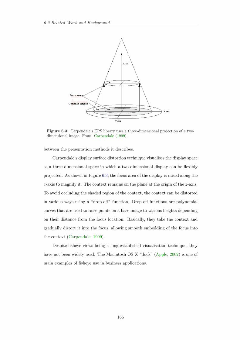
6.2 Related Work and Background
Figure 6.3: Carpendale’s EPS library uses a three-dimensional projection of a two-dimensional image. From Carpendale (1999).
between the presentation methods it describes.
Carpendale’s display surface distortion technique visualises the display space
as a three dimensional space in which a two dimensional display can be flexibly
projected. As shown in Figure 6.3, the focus area of the display is raised along the
z-axis to magnify it. The context remains on the plane at the origin of the z-axis.
To avoid occluding the shaded region of the context, the context can be distorted
in various ways using a “drop-off” function. Drop-off functions are polynomial
curves that are used to raise points on a base image to various heights depending
on their distance from the focus location. Basically, they take the context and
gradually distort it into the focus, allowing smooth embedding of the focus into
the context (Carpendale, 1999).
Despite fisheye views being a long-established visualisation technique, they
have not been widely used. The Macintosh OS X “dock” (Apple, 2002) is one of
main examples of fisheye use in business applications.
166
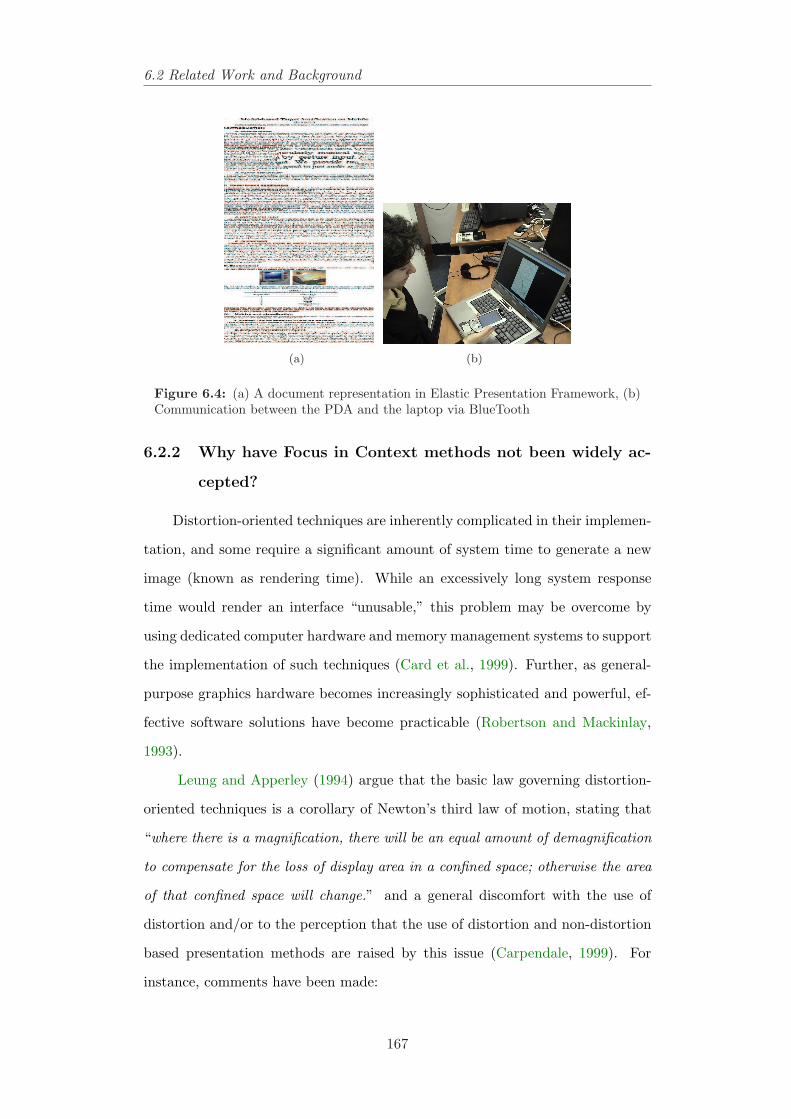
6.2 Related Work and Background
(a) (b)
Figure 6.4: (a) A document representation in Elastic Presentation Framework, (b)Communication between the PDA and the laptop via BlueTooth
6.2.2 Why have Focus in Context methods not been widely ac-
cepted?
Distortion-oriented techniques are inherently complicated in their implemen-
tation, and some require a significant amount of system time to generate a new
image (known as rendering time). While an excessively long system response
time would render an interface “unusable,” this problem may be overcome by
using dedicated computer hardware and memory management systems to support
the implementation of such techniques (Card et al., 1999). Further, as general-
purpose graphics hardware becomes increasingly sophisticated and powerful, ef-
fective software solutions have become practicable (Robertson and Mackinlay,
1993).
Leung and Apperley (1994) argue that the basic law governing distortion-
oriented techniques is a corollary of Newton’s third law of motion, stating that
“where there is a magnification, there will be an equal amount of demagnification
to compensate for the loss of display area in a confined space; otherwise the area
of that confined space will change.” and a general discomfort with the use of
distortion and/or to the perception that the use of distortion and non-distortion
based presentation methods are raised by this issue (Carpendale, 1999). For
instance, comments have been made:
167
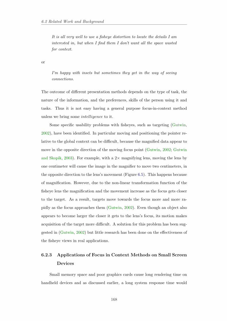
6.2 Related Work and Background
It is all very well to use a fisheye distortion to locate the details I aminterested in, but when I find them I don’t want all the space wastedfor context.
or
I’m happy with insets but sometimes they get in the way of seeingconnections.
The outcome of different presentation methods depends on the type of task, the
nature of the information, and the preferences, skills of the person using it and
tasks. Thus it is not easy having a general purpose focus-in-context method
unless we bring some intelligence to it.
Some specific usability problems with fisheyes, such as targeting (Gutwin,
2002), have been identified. In particular moving and positioning the pointer re-
lative to the global context can be difficult, because the magnified data appear to
move in the opposite direction of the moving focus point (Gutwin, 2002; Gutwin
and Skopik, 2003). For example, with a 2× magnifying lens, moving the lens by
one centimeter will cause the image in the magnifier to move two centimeters, in
the opposite direction to the lens’s movement (Figure 6.5). This happens because
of magnification. However, due to the non-linear transformation function of the
fisheye lens the magnification and the movement increase as the focus gets closer
to the target. As a result, targets move towards the focus more and more ra-
pidly as the focus approaches them (Gutwin, 2002). Even though an object also
appears to become larger the closer it gets to the lens’s focus, its motion makes
acquisition of the target more difficult. A solution for this problem has been sug-
gested in (Gutwin, 2002) but little research has been done on the effectiveness of
the fisheye views in real applications.
6.2.3 Applications of Focus in Context Methods on Small Screen
Devices
Small memory space and poor graphics cards cause long rendering time on
handheld devices and as discussed earlier, a long system response time would
168
6.2 Related Work and Background
Figure 6.5: Motion effect of magnification: as the magnifier moves upwards, themagnified image moves down. From Gutwin (2002).
make the interface “unusable,” thus not many focus-in-context applications have
been implemented and tested on these devices.
Holmquist et al. (1999) demonstrated the “flip zoom” technique embodied
in a palmtop display, to function as a Web browser (The Zoom Browser). Users
navigated through a data set by flipping between the individual pieces, just like
flipping among pages in a book. When an entry is to be examined in detail, it is
selected by clicking on the representation of the item. This zoomed the image of
the item to a readable size, and the surrounding items are reduced in size and re-
arranged to accommodate the expanded focus image. The main advantage with
this technique was that the computational demand of the graphics was quite low
which, at the time, was very important. The main problem was the scalability.
When viewing a large number of pages, the thumbnails got very small they could
not show any useful information.
Rauschenbach (2002) presented the “Rectangular FishEye View” as a solu-
tion for the problem of screen space on mobile devices. He rendered the user’s
point of view (the focus) at high detail, and downscaled the surrounding context
to save display space. He implemented this idea on a Siemens tablet computer.
In 2003, Bederson et al. (2003) published an article on a ZUI for calendars
in PDAs. They implemented a zoomable calendar for the Pocket PC called the
DateLens. Their studies showed that a ZUI can be very useful when trying to
access a large amount of information, and accessing data deeper in the dataset
at the same time as keeping an overview. Later, in 2003, Karstens et al. (2003)
proposed a technique to visualise hierarchical structures on mobile devices. They
adapted the “magic eye view,” and integrated the interaction paradigm “event
169
6.2 Related Work and Background
horizon” and discussed concepts for browsing the Web via handhelds.
Baudisch et al. (2004) introduced “Fishnet,” a web browser that always
displays web pages in their entirety, independent of their size on small screen
devices. Fishnet accomplishes this by using a fisheye views, i.e., by showing a
focus region at readable scale while spatially compressing page content above and
below that region.
In 2004, Lank and Phan (2004) presented the first fisheye lens for sketching
data on a Pocket PC using Elastic Presentation framework (Carpendale and
Montagnese, 2001). This technique allowed users to sketch in a high-resolution
focus area, while still seeing the focus area in context with the rest of the drawing.
To prevent long rendering time they pre-computed the distortion matrix off-line
and added the distortion values to points to get an acceptable frame-rate.
Heimonen (2002) introduced and evaluated a number of information visua-
lisation techniques as solutions to the presentation problem on handheld devices,
as well as devices on which the techniques could be used. The framework pre-
sented in this work drew together the visualisation techniques and devices by
comparing their corresponding properties for the first time for mobile phones
and handheld computers and found out that only one third of the proposed so-
lutions are suitable for use on mobile phones. The situation is reversed in the
context of high-end display devices (handheld computers). In their case only one
third of the techniques are found unsuitable for use.
Gutwin and Fedak (2004) compared three techniques for using large inter-
faces on small screens: a panning system similar to what is in current use, a
two-level zoom system, and a fisheye views. They found that people were able
to carry out a web navigation task significantly faster with the fisheye views,
that the two-level zoom was significantly better for a monitoring task, and that
people were slowest with the panning system. However, their real experiments
were never conducted on a handheld and they just employed a small monitor
connected to a normal PC running Windows XP.
170
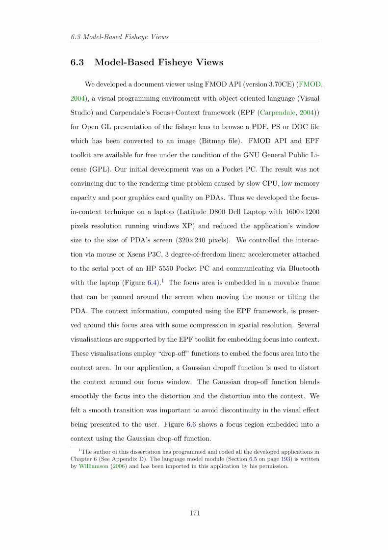
6.3 Model-Based Fisheye Views
6.3 Model-Based Fisheye Views
We developed a document viewer using FMOD API (version 3.70CE) (FMOD,
2004), a visual programming environment with object-oriented language (Visual
Studio) and Carpendale’s Focus+Context framework (EPF (Carpendale, 2004))
for Open GL presentation of the fisheye lens to browse a PDF, PS or DOC file
which has been converted to an image (Bitmap file). FMOD API and EPF
toolkit are available for free under the condition of the GNU General Public Li-
cense (GPL). Our initial development was on a Pocket PC. The result was not
convincing due to the rendering time problem caused by slow CPU, low memory
capacity and poor graphics card quality on PDAs. Thus we developed the focus-
in-context technique on a laptop (Latitude D800 Dell Laptop with 1600×1200
pixels resolution running windows XP) and reduced the application’s window
size to the size of PDA’s screen (320×240 pixels). We controlled the interac-
tion via mouse or Xsens P3C, 3 degree-of-freedom linear accelerometer attached
to the serial port of an HP 5550 Pocket PC and communicating via Bluetooth
with the laptop (Figure 6.4).1 The focus area is embedded in a movable frame
that can be panned around the screen when moving the mouse or tilting the
PDA. The context information, computed using the EPF framework, is preser-
ved around this focus area with some compression in spatial resolution. Several
visualisations are supported by the EPF toolkit for embedding focus into context.
These visualisations employ “drop-off” functions to embed the focus area into the
context area. In our application, a Gaussian dropoff function is used to distort
the context around our focus window. The Gaussian drop-off function blends
smoothly the focus into the distortion and the distortion into the context. We
felt a smooth transition was important to avoid discontinuity in the visual effect
being presented to the user. Figure 6.6 shows a focus region embedded into a
context using the Gaussian drop-off function.1The author of this dissertation has programmed and coded all the developed applications in
Chapter 6 (See Appendix D). The language model module (Section 6.5 on page 193) is writtenby Williamson (2006) and has been imported in this application by his permission.
171
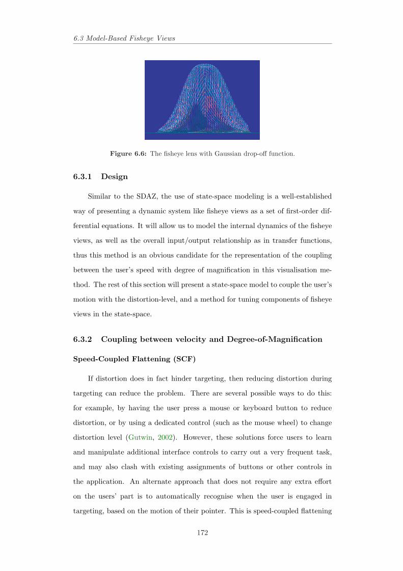
6.3 Model-Based Fisheye Views
Figure 6.6: The fisheye lens with Gaussian drop-off function.
6.3.1 Design
Similar to the SDAZ, the use of state-space modeling is a well-established
way of presenting a dynamic system like fisheye views as a set of first-order dif-
ferential equations. It will allow us to model the internal dynamics of the fisheye
views, as well as the overall input/output relationship as in transfer functions,
thus this method is an obvious candidate for the representation of the coupling
between the user’s speed with degree of magnification in this visualisation me-
thod. The rest of this section will present a state-space model to couple the user’s
motion with the distortion-level, and a method for tuning components of fisheye
views in the state-space.
6.3.2 Coupling between velocity and Degree-of-Magnification
Speed-Coupled Flattening (SCF)
If distortion does in fact hinder targeting, then reducing distortion during
targeting can reduce the problem. There are several possible ways to do this:
for example, by having the user press a mouse or keyboard button to reduce
distortion, or by using a dedicated control (such as the mouse wheel) to change
distortion level (Gutwin, 2002). However, these solutions force users to learn
and manipulate additional interface controls to carry out a very frequent task,
and may also clash with existing assignments of buttons or other controls in
the application. An alternate approach that does not require any extra effort
on the users’ part is to automatically recognise when the user is engaged in
targeting, based on the motion of their pointer. This is speed-coupled flattening
172
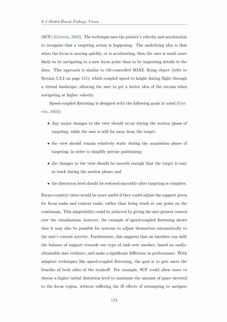
6.3 Model-Based Fisheye Views
(SCF) (Gutwin, 2002). The technique uses the pointer’s velocity and acceleration
to recognise that a targeting action is happening. The underlying idea is that
when the focus is moving quickly, or is accelerating, then the user is much more
likely to be navigating to a new focus point than to be inspecting details in the
data. This approach is similar to tilt-controlled SDAZ, flying object (refer to
Section 5.3.2 on page 111), which coupled speed to height during flight through
a virtual landscape, allowing the user to get a better idea of the terrain when
navigating at higher velocity.
Speed-coupled flattening is designed with the following goals in mind (Gut-
win, 2002):
• Any major changes to the view should occur during the motion phase of
targeting, while the user is still far away from the target;
• the view should remain relatively static during the acquisition phase of
targeting, in order to simplify precise positioning;
• the changes to the view should be smooth enough that the target is easy
to track during the motion phase; and
• the distortion level should be restored smoothly after targeting is complete.
Focus+context views would be more useful if they could adjust the support given
for focus tasks and context tasks, rather than being stuck at one point on the
continuum. This adaptability could be achieved by giving the user greater control
over the visualisation; however, the example of speed-coupled flattening shows
that it may also be possible for systems to adjust themselves automatically to
the user’s current activity. Furthermore, this suggests that an interface can shift
the balance of support towards one type of task over another, based on easily-
obtainable user evidence, and make a significant difference in performance. With
adaptive techniques like speed-coupled flattening, the goal is to give users the
benefits of both sides of the tradeoff. For example, SCF could allow users to
choose a higher initial distortion level to maximise the amount of space devoted
to the focus region, without suffering the ill effects of attempting to navigate
173
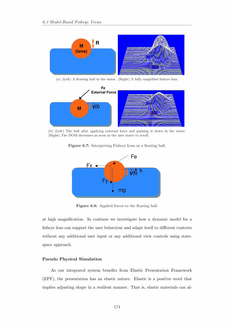
6.3 Model-Based Fisheye Views
M
(lens)
R
(a) (Left) A floating ball in the water. (Right) A fully magnified fisheye lens.
M
Fe
External Force
y(t).
(b) (Left) The ball after applying external force and pushing it down in the water.(Right) The DOM decreases as soon as the user starts to scroll.
Figure 6.7: Interpreting Fisheye Lens as a floating ball.
mg
Fe
Fy
Fxky(t)
.
Figure 6.8: Applied forces to the floating ball.
at high magnification. In continue we investigate how a dynamic model for a
fisheye lens can support the user behaviour and adapt itself to different contexts
without any additional user input or any additional view controls using state-
space approach.
Pseudo Physical Simulation
As our integrated system benefits from Elastic Presentation Framework
(EPF), the presentation has an elastic nature. Elastic is a positive word that
implies adjusting shape in a resilient manner. That is, elastic materials can al-
174
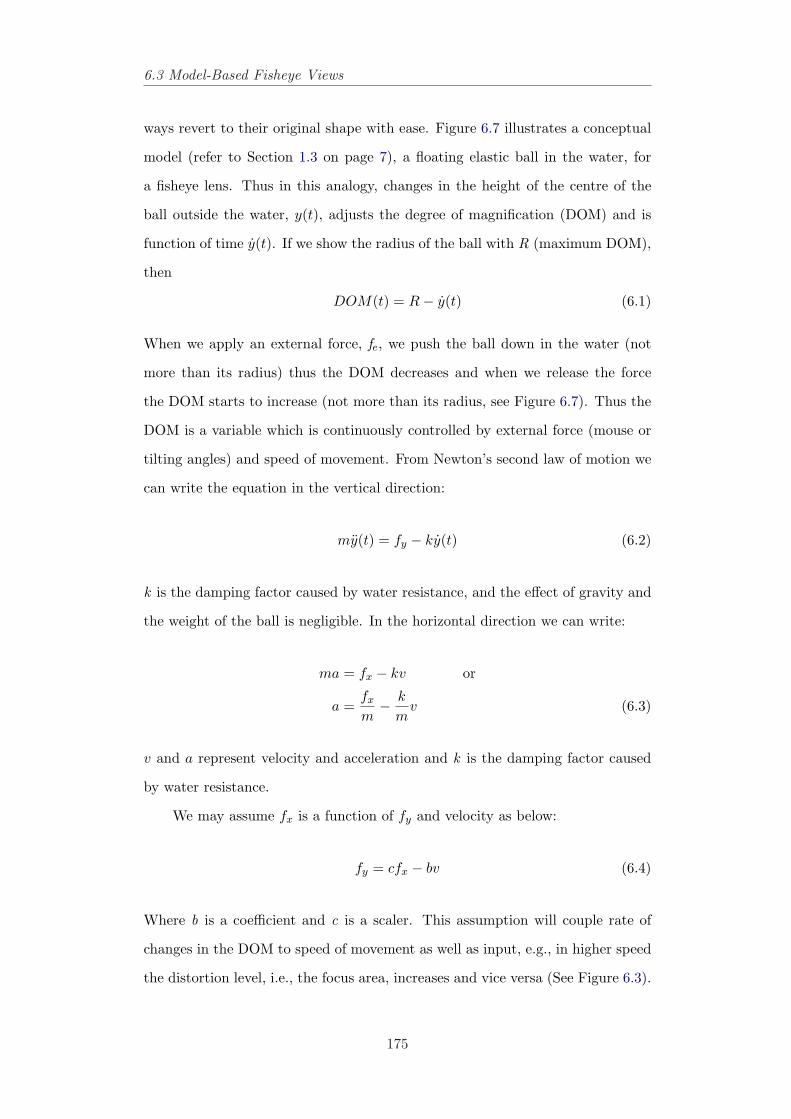
6.3 Model-Based Fisheye Views
ways revert to their original shape with ease. Figure 6.7 illustrates a conceptual
model (refer to Section 1.3 on page 7), a floating elastic ball in the water, for
a fisheye lens. Thus in this analogy, changes in the height of the centre of the
ball outside the water, y(t), adjusts the degree of magnification (DOM) and is
function of time y(t). If we show the radius of the ball with R (maximum DOM),
then
DOM(t) = R− y(t) (6.1)
When we apply an external force, fe, we push the ball down in the water (not
more than its radius) thus the DOM decreases and when we release the force
the DOM starts to increase (not more than its radius, see Figure 6.7). Thus the
DOM is a variable which is continuously controlled by external force (mouse or
tilting angles) and speed of movement. From Newton’s second law of motion we
can write the equation in the vertical direction:
my(t) = fy − ky(t) (6.2)
k is the damping factor caused by water resistance, and the effect of gravity and
the weight of the ball is negligible. In the horizontal direction we can write:
ma = fx − kv or
a =fx
m− k
mv (6.3)
v and a represent velocity and acceleration and k is the damping factor caused
by water resistance.
We may assume fx is a function of fy and velocity as below:
fy = cfx − bv (6.4)
Where b is a coefficient and c is a scaler. This assumption will couple rate of
changes in the DOM to speed of movement as well as input, e.g., in higher speed
the distortion level, i.e., the focus area, increases and vice versa (See Figure 6.3).
175
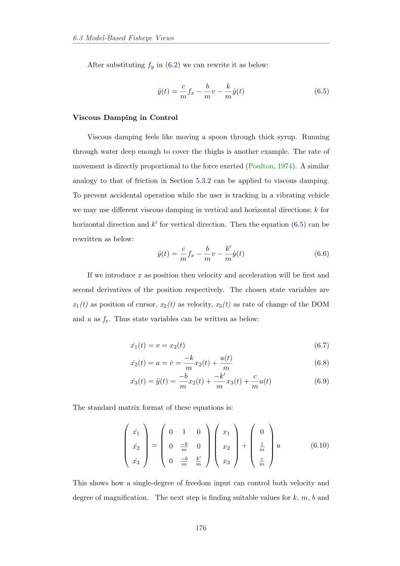
6.3 Model-Based Fisheye Views
After substituting fy in (6.2) we can rewrite it as below:
y(t) =c
mfx − b
mv − k
my(t) (6.5)
Viscous Damping in Control
Viscous damping feels like moving a spoon through thick syrup. Running
through water deep enough to cover the thighs is another example. The rate of
movement is directly proportional to the force exerted (Poulton, 1974). A similar
analogy to that of friction in Section 5.3.2 can be applied to viscous damping.
To prevent accidental operation while the user is tracking in a vibrating vehicle
we may use different viscous damping in vertical and horizontal directions; k for
horizontal direction and k′ for vertical direction. Then the equation (6.5) can be
rewritten as below:
y(t) =c
mfx − b
mv − k′
my(t) (6.6)
If we introduce x as position then velocity and acceleration will be first and
second derivatives of the position respectively. The chosen state variables are
x1(t) as position of cursor, x2(t) as velocity, x3(t) as rate of change of the DOM
and u as fx. Thus state variables can be written as below:
x1(t) = v = x2(t) (6.7)
x2(t) = a = v =−k
mx2(t) +
u(t)m
(6.8)
x3(t) = y(t) =−b
mx2(t) +
−k′
mx3(t) +
c
mu(t) (6.9)
The standard matrix format of these equations is:
x1
x2
x3
=
0 1 0
0 −km 0
0 −bm
k′m
x1
x2
x3
+
0
1m
cm
u (6.10)
This shows how a single-degree of freedom input can control both velocity and
degree of magnification. The next step is finding suitable values for k, m, b and
176
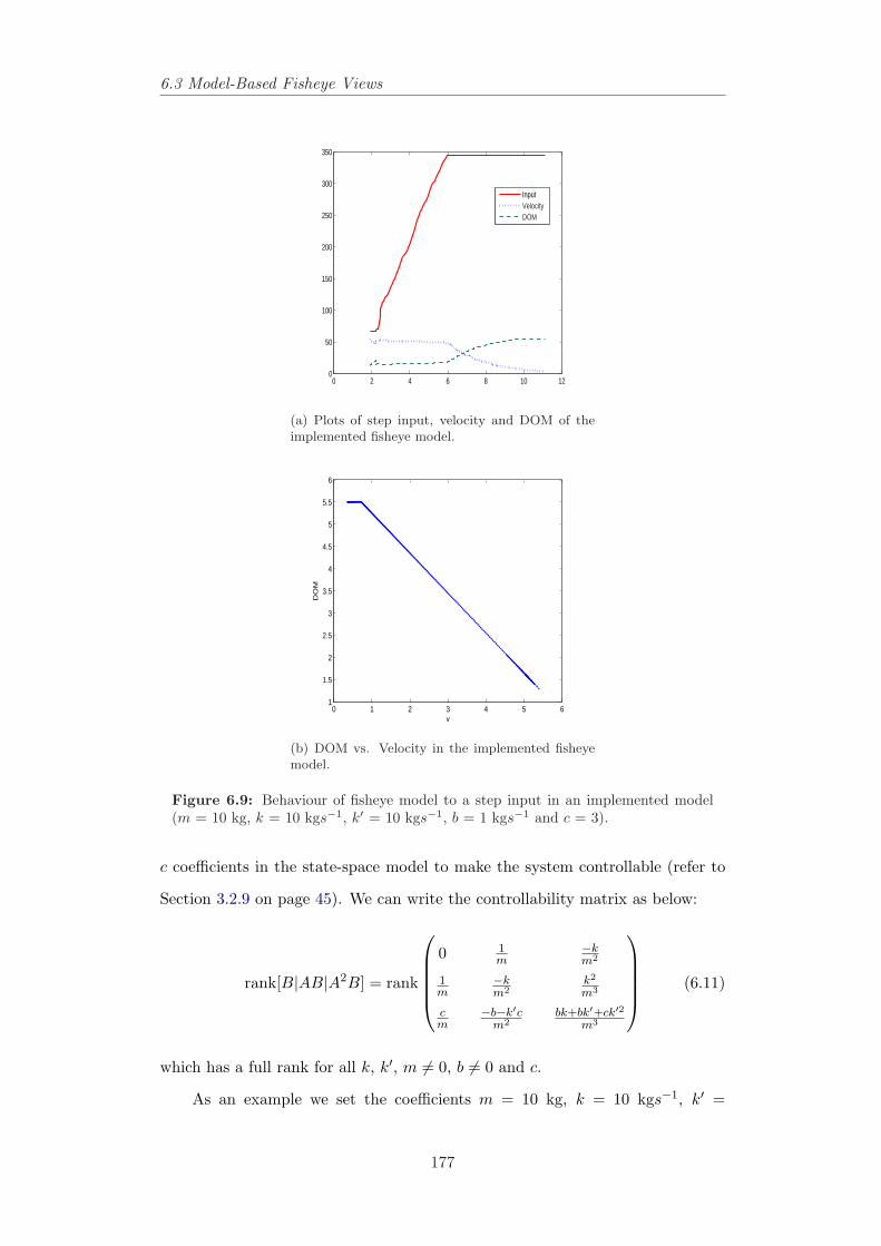
6.3 Model-Based Fisheye Views
0 2 4 6 8 10 120
50
100
150
200
250
300
350
InputVelocityDOM
(a) Plots of step input, velocity and DOM of theimplemented fisheye model.
0 1 2 3 4 5 61
1.5
2
2.5
3
3.5
4
4.5
5
5.5
6
v
DO
M
(b) DOM vs. Velocity in the implemented fisheyemodel.
Figure 6.9: Behaviour of fisheye model to a step input in an implemented model(m = 10 kg, k = 10 kgs−1, k′ = 10 kgs−1, b = 1 kgs−1 and c = 3).
c coefficients in the state-space model to make the system controllable (refer to
Section 3.2.9 on page 45). We can write the controllability matrix as below:
rank[B|AB|A2B] = rank
0 1m
−km2
1m
−km2
k2
m3
cm
−b−k′cm2
bk+bk′+ck′2m3
(6.11)
which has a full rank for all k, k′, m 6= 0, b 6= 0 and c.
As an example we set the coefficients m = 10 kg, k = 10 kgs−1, k′ =
177
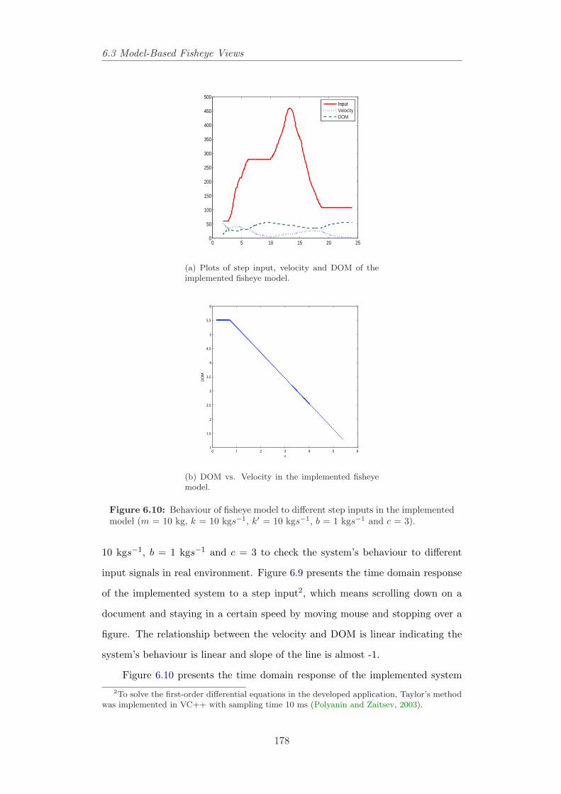
6.3 Model-Based Fisheye Views
0 5 10 15 20 250
50
100
150
200
250
300
350
400
450
500InputVelocityDOM
(a) Plots of step input, velocity and DOM of theimplemented fisheye model.
0 1 2 3 4 5 61
1.5
2
2.5
3
3.5
4
4.5
5
5.5
6
v
DOM
(b) DOM vs. Velocity in the implemented fisheyemodel.
Figure 6.10: Behaviour of fisheye model to different step inputs in the implementedmodel (m = 10 kg, k = 10 kgs−1, k′ = 10 kgs−1, b = 1 kgs−1 and c = 3).
10 kgs−1, b = 1 kgs−1 and c = 3 to check the system’s behaviour to different
input signals in real environment. Figure 6.9 presents the time domain response
of the implemented system to a step input2, which means scrolling down on a
document and staying in a certain speed by moving mouse and stopping over a
figure. The relationship between the velocity and DOM is linear indicating the
system’s behaviour is linear and slope of the line is almost -1.
Figure 6.10 presents the time domain response of the implemented system2To solve the first-order differential equations in the developed application, Taylor’s method
was implemented in VC++ with sampling time 10 ms (Polyanin and Zaitsev, 2003).
178
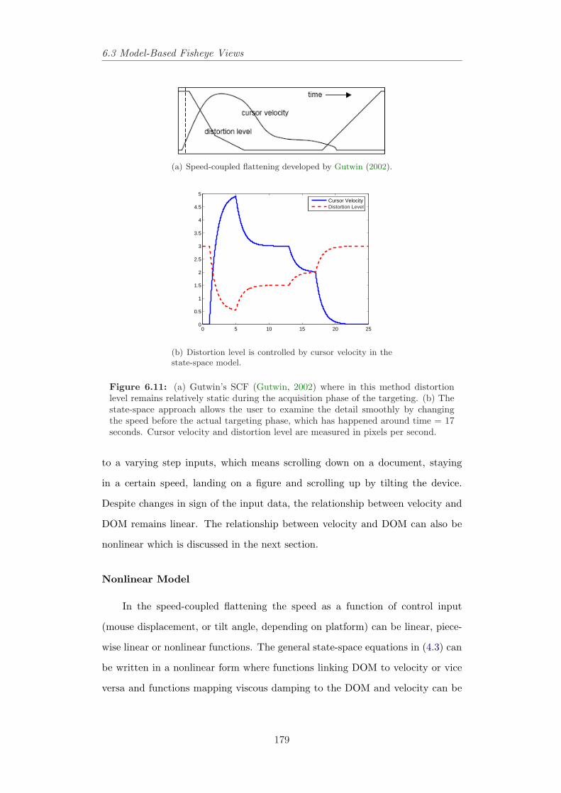
6.3 Model-Based Fisheye Views
(a) Speed-coupled flattening developed by Gutwin (2002).
0 5 10 15 20 250
0.5
1
1.5
2
2.5
3
3.5
4
4.5
5Cursor VelocityDistortion Level
(b) Distortion level is controlled by cursor velocity in thestate-space model.
Figure 6.11: (a) Gutwin’s SCF (Gutwin, 2002) where in this method distortionlevel remains relatively static during the acquisition phase of the targeting. (b) Thestate-space approach allows the user to examine the detail smoothly by changingthe speed before the actual targeting phase, which has happened around time = 17seconds. Cursor velocity and distortion level are measured in pixels per second.
to a varying step inputs, which means scrolling down on a document, staying
in a certain speed, landing on a figure and scrolling up by tilting the device.
Despite changes in sign of the input data, the relationship between velocity and
DOM remains linear. The relationship between velocity and DOM can also be
nonlinear which is discussed in the next section.
Nonlinear Model
In the speed-coupled flattening the speed as a function of control input
(mouse displacement, or tilt angle, depending on platform) can be linear, piece-
wise linear or nonlinear functions. The general state-space equations in (4.3) can
be written in a nonlinear form where functions linking DOM to velocity or vice
versa and functions mapping viscous damping to the DOM and velocity can be
179
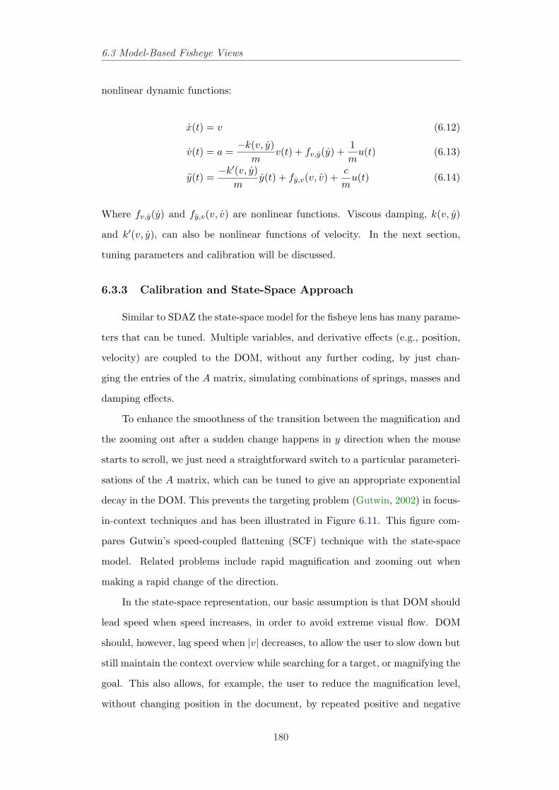
6.3 Model-Based Fisheye Views
nonlinear dynamic functions:
x(t) = v (6.12)
v(t) = a =−k(v, y)
mv(t) + fv,y(y) +
1m
u(t) (6.13)
y(t) =−k′(v, y)
my(t) + fy,v(v, v) +
c
mu(t) (6.14)
Where fv,y(y) and fy,v(v, v) are nonlinear functions. Viscous damping, k(v, y)
and k′(v, y), can also be nonlinear functions of velocity. In the next section,
tuning parameters and calibration will be discussed.
6.3.3 Calibration and State-Space Approach
Similar to SDAZ the state-space model for the fisheye lens has many parame-
ters that can be tuned. Multiple variables, and derivative effects (e.g., position,
velocity) are coupled to the DOM, without any further coding, by just chan-
ging the entries of the A matrix, simulating combinations of springs, masses and
damping effects.
To enhance the smoothness of the transition between the magnification and
the zooming out after a sudden change happens in y direction when the mouse
starts to scroll, we just need a straightforward switch to a particular parameteri-
sations of the A matrix, which can be tuned to give an appropriate exponential
decay in the DOM. This prevents the targeting problem (Gutwin, 2002) in focus-
in-context techniques and has been illustrated in Figure 6.11. This figure com-
pares Gutwin’s speed-coupled flattening (SCF) technique with the state-space
model. Related problems include rapid magnification and zooming out when
making a rapid change of the direction.
In the state-space representation, our basic assumption is that DOM should
lead speed when speed increases, in order to avoid extreme visual flow. DOM
should, however, lag speed when |v| decreases, to allow the user to slow down but
still maintain the context overview while searching for a target, or magnifying the
goal. This also allows, for example, the user to reduce the magnification level,
without changing position in the document, by repeated positive and negative
180
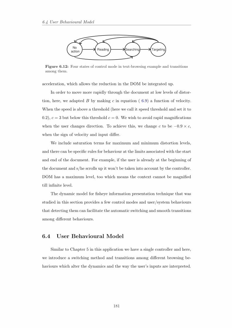
6.4 User Behavioural Model
Noaction
Reading Searching Targeting
Figure 6.12: Four states of control mode in text-browsing example and transitionsamong them.
acceleration, which allows the reduction in the DOM be integrated up.
In order to move more rapidly through the document at low levels of distor-
tion, here, we adapted B by making c in equation ( 6.9) a function of velocity.
When the speed is above a threshold (here we call it speed threshold and set it to
0.2), c = 3 but below this threshold c = 0. We wish to avoid rapid magnifications
when the user changes direction. To achieve this, we change c to be −0.9 × c,
when the sign of velocity and input differ.
We include saturation terms for maximum and minimum distortion levels,
and there can be specific rules for behaviour at the limits associated with the start
and end of the document. For example, if the user is already at the beginning of
the document and s/he scrolls up it won’t be taken into account by the controller.
DOM has a maximum level, too which means the context cannot be magnified
till infinite level.
The dynamic model for fisheye information presentation technique that was
studied in this section provides a few control modes and user/system behaviours
that detecting them can facilitate the automatic switching and smooth transitions
among different behaviours.
6.4 User Behavioural Model
Similar to Chapter 5 in this application we have a single controller and here,
we introduce a switching method and transitions among different browsing be-
haviours which alter the dynamics and the way the user’s inputs are interpreted.
181
6.4 User Behavioural Model
Dynamics(S1)
Focus-in-Context (S2)
LanguageModel (S3)
Sonification (S4)
User
Document
(a)
S1
.
.
.
Classifier
Controller
Cu(t)
r(t)Dynamics of
State
to S2
User
(b)
.
.
.
From S1
S2
To S3
To User
(c)
From S2
S3
French
English
Other
Languages
to S4
(d)
From S3
S4
to UserSUM
(e)
Figure 6.13: (a) A general probabilistic framework of the model-based behavioursystem. (b) A Bayesian classifier classifies the user’s input. Its output and the user’sinput come to the controller and change the dynamics (state variables). (c) Statevariables coupled to the focus-in-context change the size and shape of lens. (d),(e)Language identification method infers the most probable language inside the windowaround the lens and its output probabilities are fed to the audio synthesis algorithm.
182
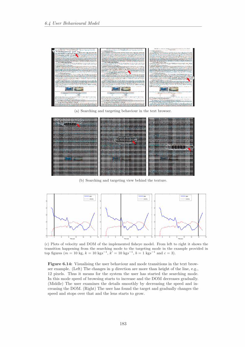
6.4 User Behavioural Model
(a) Searching and targeting behaviour in the text browser.
(b) Searching and targeting view behind the texture.
2 4 6 8 10 12 14 160
1
2
3
4
5
Time (se)
dom
velocity
2 4 6 8 10 12 14 160
1
2
3
4
5
Time (se)
dom
velocity
2 4 6 8 10 12 14 160
1
2
3
4
5
Time (se )
dom
velocity
(c) Plots of velocity and DOM of the implemented fisheye model. From left to right it shows thetransition happening from the searching mode to the targeting mode in the example provided intop figures (m = 10 kg, k = 10 kgs−1, k′ = 10 kgs−1, b = 1 kgs−1 and c = 3).
Figure 6.14: Visualising the user behaviour and mode transitions in the text brow-ser example. (Left) The changes in y direction are more than height of the line, e.g.,12 pixels. Thus it means for the system the user has started the searching mode.In this mode speed of browsing starts to increase and the DOM decreases gradually.(Middle) The user examines the details smoothly by decreasing the speed and in-creasing the DOM. (Right) The user has found the target and gradually changes thespeed and stops over that and the lens starts to grow.
183
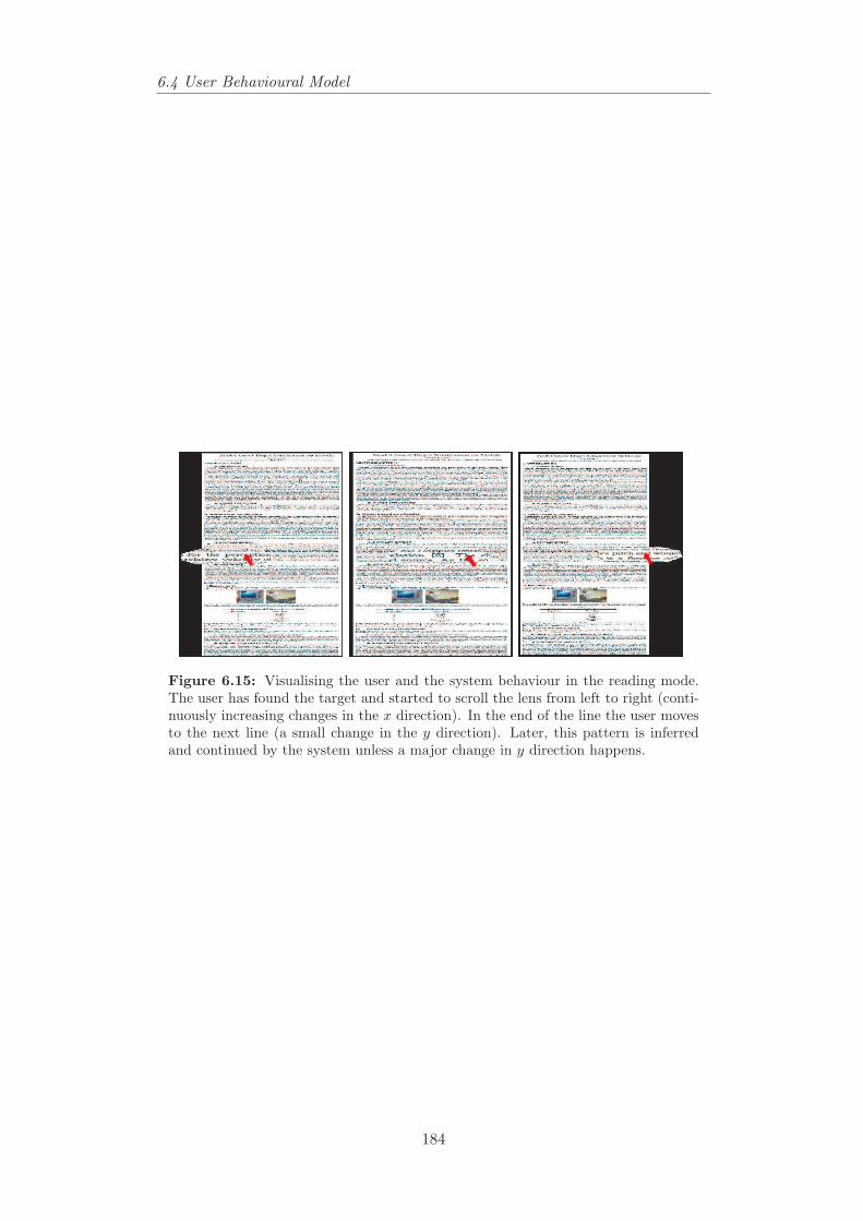
6.4 User Behavioural Model
Figure 6.15: Visualising the user and the system behaviour in the reading mode.The user has found the target and started to scroll the lens from left to right (conti-nuously increasing changes in the x direction). In the end of the line the user movesto the next line (a small change in the y direction). Later, this pattern is inferredand continued by the system unless a major change in y direction happens.
184
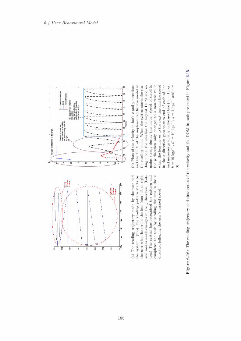
6.4 User Behavioural Model
(a)
The
readin
gtr
aje
ctory
made
by
the
use
rand
the
syst
em.
(top)
The
readin
gpatt
ern
start
sby
the
use
rw
hen
he
scro
lls
the
lens
from
left
tori
ght
and
makes
small
changes
inth
ey
dir
ecti
on.
(bot-
tom
)T
he
syst
emhas
reco
gnis
edth
epatt
ern
and
com
ple
tes
the
task
by
scro
llin
gth
ele
ns
inth
ex
dir
ecti
on
follow
ing
the
use
r’s
des
ired
spee
d.
510
1520
2530
3540
4550
5560
0
0.51
1.52
2.53
3.54
4.55
Tim
e(se
)
Ho
rizo
nta
l Vel
oci
ty
DO
M
Ver
tica
l Vel
oci
ty
The
user
is a
ctiv
e an
dre
ads
the
text
by
scro
lling
the
lens
man
ually
from
left
to r
ight
.
Th
e sy
stem
has
infe
rred
the
pat
tern
and
scr
olls
th
e le
ns
auto
mat
ical
ly t
hu
s th
eu
ser
is n
ot
acti
ve.
The
user
scr
olls
dow
n to
the
targ
et.
(b)
Plo
tsofth
evel
oci
tyin
both
xand
ydir
ecti
ons
and
the
DO
Mofth
eim
ple
men
ted
fish
eye
model
inth
ere
adin
gm
ode.
When
the
syst
emst
art
sth
ere
a-
din
gm
ode,
the
lens
has
the
hig
hes
tD
OM
and
re-
main
sst
eady
duri
ng
this
mode.
Spee
dof
scro
llin
the
ydir
ecti
on
only
changes
toa
non-z
ero
valu
ew
hen
the
lens
mov
esto
the
nex
tline
and
the
spee
din
the
xdir
ecti
on
goes
toze
roen
dof
each
of
line
and
incr
ease
sgra
dually
inth
enex
tline
(m=
10
kg,
k=
10
kgs−
1,k′=
10
kgs−
1,b
=1
kgs−
1and
c=
3).
Fig
ure
6.16
:T
here
adin
gtr
ajec
tory
and
tim
e-se
ries
ofth
eve
loci
tyan
dth
eD
OM
inta
skpr
esen
ted
inFig
ure
6.15
.
185
6.4 User Behavioural Model
6.4.1 Behaviours in Text Browsing Application
In the model-based text browser example, the user’s input, mouse data,
controls what s/he perceives via visual/audio/haptic display. In this example
we assume the user is acting in one of four different modes: no-action, reading,
searching and targeting.
Figure 6.13 illustrates the general framework. Figure 6.13(b) shows the
classification of the user behaviour being used to switch the control mode. This
mode is then coupled to the visualisation parameters, as shown in Figure 6.13(c),
where the control mode changes the size and shape of the lens, and the controller
provides the DOM, position and speed of the lens. For example, in the rea-
ding mode the controller adjusts the DOM to stay in the maximum level, but
as a long horizontal lens, while if the user ‘breaks out’ into general searching,
the DOM is decreased smoothly to a lower level. This prevents the targeting
problem (Gutwin, 2002) in focus-in-context techniques.
6.4.2 Detecting state transitions
Figure 6.12 illustrates the possible state transitions. Initially, the user is in
the no-action state. Depending on the input behaviour, the user can either go
to the reading or the searching mode. A qualitative description of the automa-
tic mode transitions is given below: In the reading mode, the user is making
continuous increasing changes in x direction (left-to-right) and small changes in
y direction (not more than height of a line) and at the end of the line makes
a sudden change from right-to-left in x direction. If the changes in y direction
are more than height of the line the system switches the mode to the searching
mode. After finding the target, the user slows down or stops scrolling until the
lens is over the target point (targeting mode), or can return to the no-action
mode directly (see Figures 6.14, 6.15 and 6.16).
A general technique for implementing this is to use a probabilistic classifica-
tion of the likelihood of being in one of these four browsing behaviours according
to the joint probability of the input and output time-series. From Bayes’ law, we
186
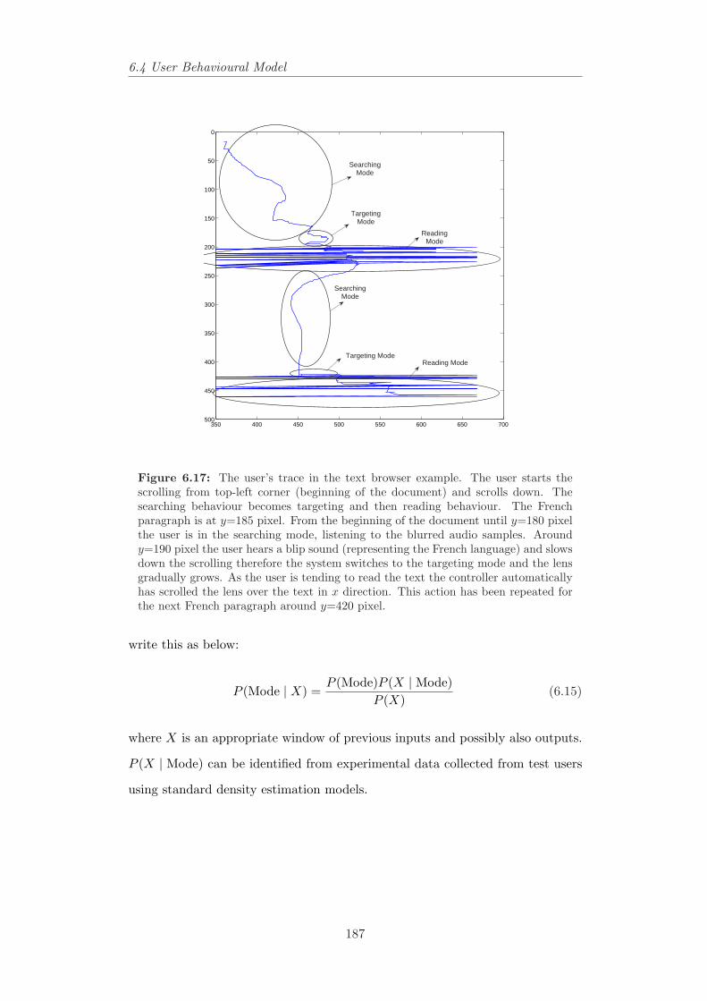
6.4 User Behavioural Model
350 400 450 500 550 600 650 700
0
50
100
150
200
250
300
350
400
450
500
SearchingMode
TargetingMode
Targeting Mode
SearchingMode
ReadingMode
Reading Mode
Figure 6.17: The user’s trace in the text browser example. The user starts thescrolling from top-left corner (beginning of the document) and scrolls down. Thesearching behaviour becomes targeting and then reading behaviour. The Frenchparagraph is at y=185 pixel. From the beginning of the document until y=180 pixelthe user is in the searching mode, listening to the blurred audio samples. Aroundy=190 pixel the user hears a blip sound (representing the French language) and slowsdown the scrolling therefore the system switches to the targeting mode and the lensgradually grows. As the user is tending to read the text the controller automaticallyhas scrolled the lens over the text in x direction. This action has been repeated forthe next French paragraph around y=420 pixel.
write this as below:
P (Mode | X) =P (Mode)P (X | Mode)
P (X)(6.15)
where X is an appropriate window of previous inputs and possibly also outputs.
P (X | Mode) can be identified from experimental data collected from test users
using standard density estimation models.
187
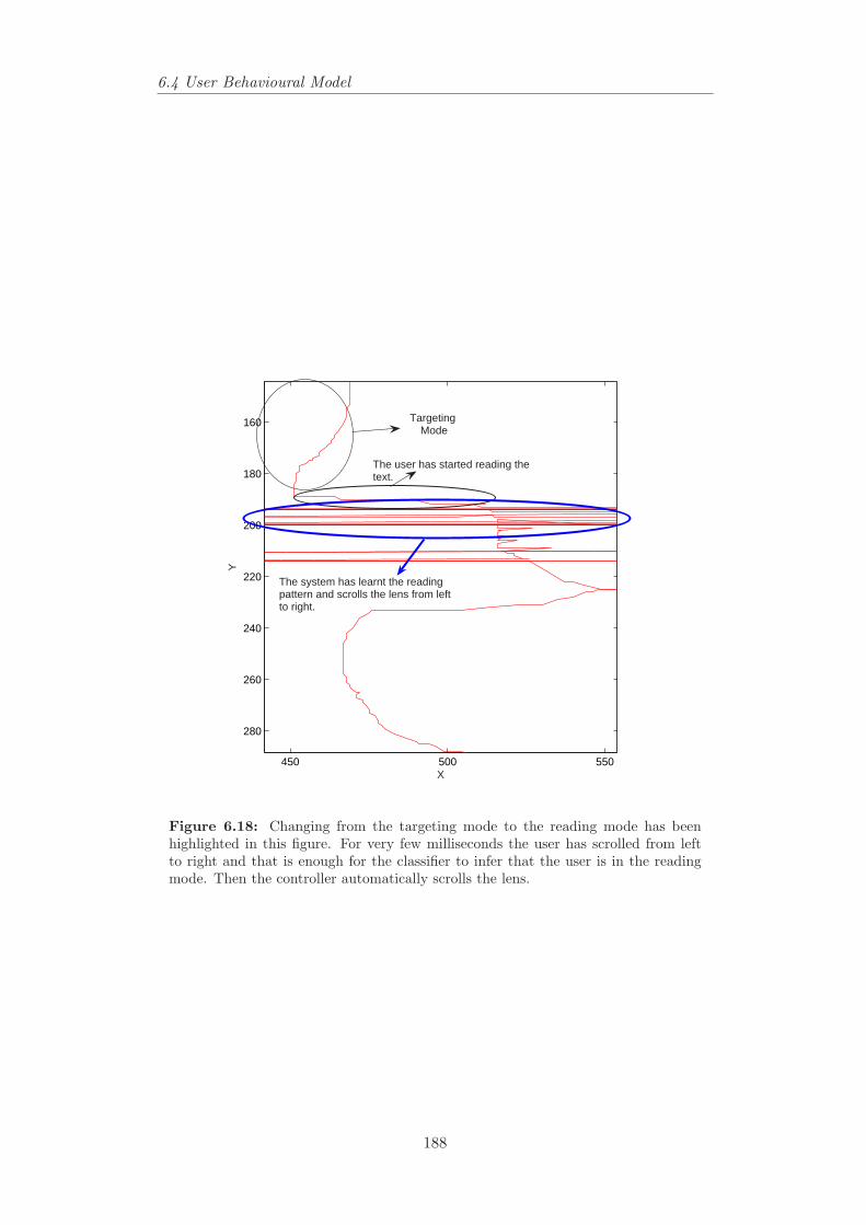
6.4 User Behavioural Model
450 500 550
160
180
200
220
240
260
280
X
Y
Targeting Mode
The user has started reading thetext.
The system has learnt the readingpattern and scrolls the lens from leftto right.
Figure 6.18: Changing from the targeting mode to the reading mode has beenhighlighted in this figure. For very few milliseconds the user has scrolled from leftto right and that is enough for the classifier to infer that the user is in the readingmode. Then the controller automatically scrolls the lens.
188
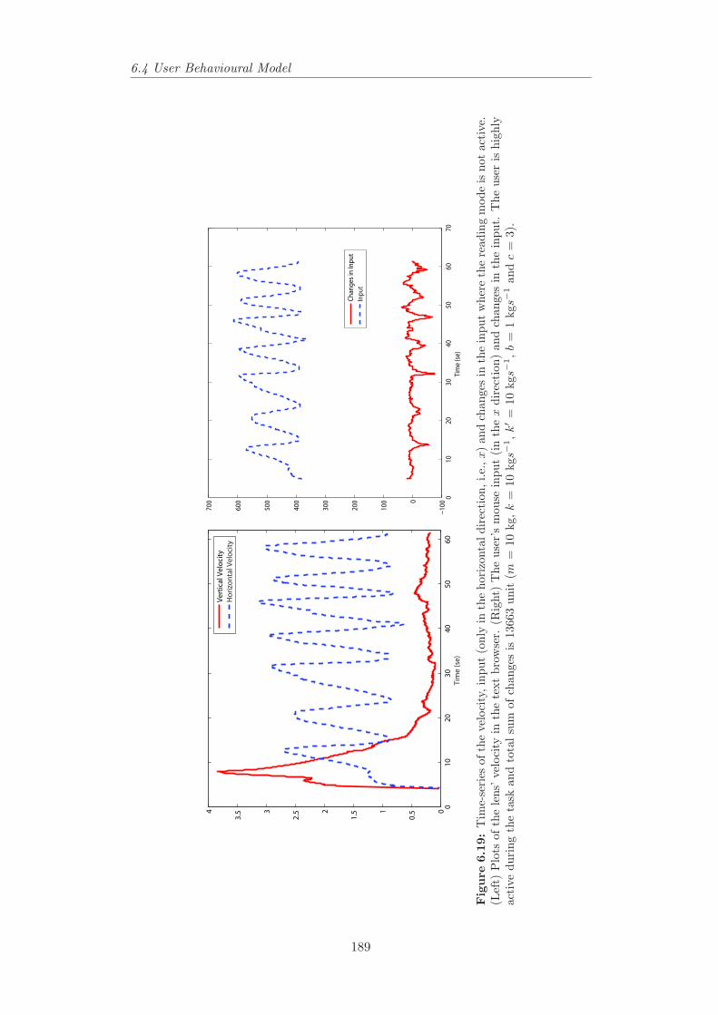
6.4 User Behavioural Model
01
02
03
04
05
06
00
0.51
1.52
2.53
3.54
Tim
e (
se)
Ve
rtic
al V
elo
city
Ho
rizo
nta
l Ve
loci
ty
01
02
03
04
05
06
07
0−
10
00
10
0
20
0
30
0
40
0
50
0
60
0
70
0
Tim
e (s
e)
Ch
ang
es in
Inp
ut
Inp
ut
Fig
ure
6.19
:T
ime-
seri
esof
the
velo
city
,inp
ut(o
nly
inth
eho
rizo
ntal
dire
ctio
n,i.e
.,x)
and
chan
ges
inth
ein
put
whe
reth
ere
adin
gm
ode
isno
tac
tive
.(L
eft)
Plo
tsof
the
lens
’vel
ocity
inth
ete
xtbr
owse
r.(R
ight
)T
heus
er’s
mou
sein
put
(in
the
xdi
rect
ion)
and
chan
ges
inth
ein
put.
The
user
ishi
ghly
acti
vedu
ring
the
task
and
tota
lsu
mof
chan
ges
is13
663
unit
(m=
10kg
,k
=10
kgs−
1,k′=
10kg
s−1,b
=1
kgs−
1an
dc
=3)
.
189
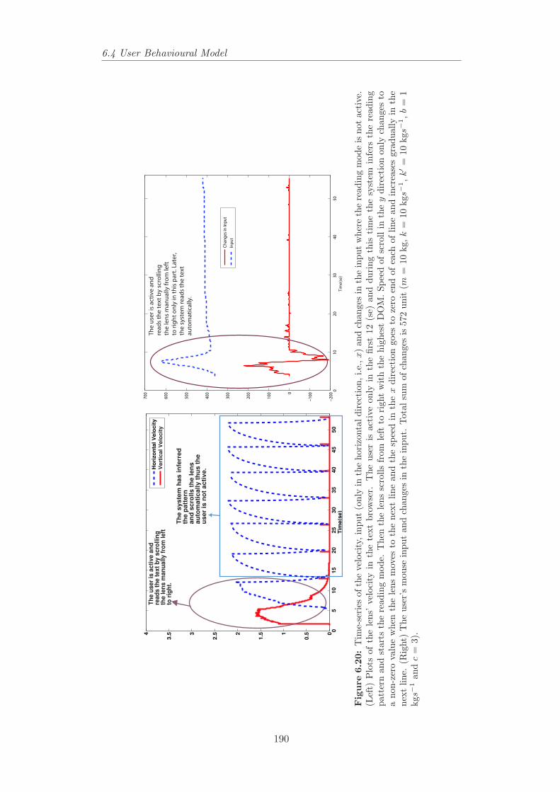
6.4 User Behavioural Model
05
10
15
20
25
30
35
40
45
50
0
0.51
1.52
2.53
3.54
Tim
e(s
e)
Ho
rizo
nta
l V
elo
cit
y
Ve
rtic
al
Ve
loc
ity
Th
e u
ser
is a
cti
ve a
nd
read
s t
he t
ext
by s
cro
llin
gth
e len
s m
an
ually f
rom
left
to r
igh
t.
Th
e s
yste
m h
as
in
ferr
ed
the p
att
ern
an
d s
cro
lls t
he
len
sau
tom
ati
cally t
hu
s t
he
user
is n
ot
acti
ve
.
01
02
03
04
05
0−
20
0
−1
000
10
0
20
0
30
0
40
0
50
0
60
0
70
0
Tim
e(s
e)
Ch
ang
es
in In
pu
t
Inp
ut
Th
e u
ser
is a
ctiv
e a
nd
rea
ds
the
te
xt
by
scr
oll
ing
the
len
s m
an
ua
lly
fro
m le
ft
to r
igh
t o
nly
in t
his
pa
rt. L
ate
r,
the
sy
ste
m r
ea
ds
the
te
xt
au
tom
ati
call
y.
Fig
ure
6.20
:T
ime-
seri
esof
the
velo
city
,inp
ut(o
nly
inth
eho
rizo
ntal
dire
ctio
n,i.e
.,x)
and
chan
ges
inth
ein
put
whe
reth
ere
adin
gm
ode
isno
tac
tive
.(L
eft)
Plo
tsof
the
lens
’ve
loci
tyin
the
text
brow
ser.
The
user
isac
tive
only
inth
efir
st12
(se)
and
duri
ngth
isti
me
the
syst
emin
fers
the
read
ing
patt
ern
and
star
tsth
ere
adin
gm
ode.
The
nth
ele
nssc
rolls
from
left
tori
ght
wit
hth
ehi
ghes
tD
OM
.Spe
edof
scro
llin
the
ydi
rect
ion
only
chan
ges
toa
non-
zero
valu
ew
hen
the
lens
mov
esto
the
next
line
and
the
spee
din
the
xdi
rect
ion
goes
toze
roen
dof
each
oflin
ean
din
crea
ses
grad
ually
inth
ene
xtlin
e.(R
ight
)T
heus
er’s
mou
sein
put
and
chan
ges
inth
ein
put.
Tot
alsu
mof
chan
ges
is57
2un
it(m
=10
kg,k
=10
kgs−
1,k
′=
10kg
s−1,b
=1
kgs−
1an
dc
=3)
.
190
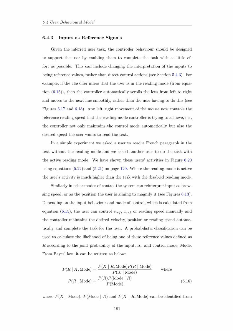
6.4 User Behavioural Model
6.4.3 Inputs as Reference Signals
Given the inferred user task, the controller behaviour should be designed
to support the user by enabling them to complete the task with as little ef-
fort as possible. This can include changing the interpretation of the inputs to
being reference values, rather than direct control actions (see Section 5.4.3). For
example, if the classifier infers that the user is in the reading mode (from equa-
tion (6.15)), then the controller automatically scrolls the lens from left to right
and moves to the next line smoothly, rather than the user having to do this (see
Figures 6.17 and 6.18). Any left–right movement of the mouse now controls the
reference reading speed that the reading mode controller is trying to achieve, i.e.,
the controller not only maintains the control mode automatically but also the
desired speed the user wants to read the text.
In a simple experiment we asked a user to read a French paragraph in the
text without the reading mode and we asked another user to do the task with
the active reading mode. We have shown these users’ activities in Figure 6.20
using equations (5.22) and (5.21) on page 129. Where the reading mode is active
the user’s activity is much higher than the task with the disabled reading mode.
Similarly in other modes of control the system can reinterpret input as brow-
sing speed, or as the position the user is aiming to magnify it (see Figures 6.13).
Depending on the input behaviour and mode of control, which is calculated from
equation (6.15), the user can control vref , xref or reading speed manually and
the controller maintains the desired velocity, position or reading speed automa-
tically and complete the task for the user. A probabilistic classification can be
used to calculate the likelihood of being one of these reference values defined as
R according to the joint probability of the input, X, and control mode, Mode.
From Bayes’ law, it can be written as below:
P (R | X, Mode) =P (X | R, Mode)P (R | Mode)
P (X | Mode)where
P (R | Mode) =P (R)P (Mode | R)
P (Mode)(6.16)
where P (X | Mode), P (Mode | R) and P (X | R, Mode) can be identified from
191
6.4 User Behavioural Model
experimental data from test users. Then, the controller in mode switching uses
state feedback to augment control behaviour, by making the state to move to-
wards the reference value R.
While the user performs the various tasks, his/her inputs, have different
meanings (interpreted as different reference inputs) and s/he switches between
control modes automatically, but that the transitions are always smooth and
natural and the user is often not even aware that his/her movements are having
a different effect in the different modes; because the offset variables are set such
that to cancel out the input provided by the user at the point they enter new
control mode and after transition the offset values gradually reset to a more
sustainable position.
6.4.4 Discussion
The advent of new virtual media and visualisation means that technology
offers not only new tools but also the prospect of entirely new ways of developing
work in virtual space. McCullough (1998) states
what good are computers, except perhaps for mundane documentation,if you cannot even touch your work? The fact that traditional craftendures at all is because it satisfies some deep need for direct expe-rience and most computers are not yet providing that experience.
An applied artists’ instinctive grasp of constructing and visualising in three di-
mensions, their spatial thinking and sense of touch are integral to their process
of creativity. Makers combine all their sensory modalities, such as sight, hand
motions and gestures, and sound both to explore and bring intended qualities
to the object they are making. The process is open and evolving: results can
only be achieved through ongoing dialogue between the maker, materials and pro-
cess (Dormer, 1994).
A significant disadvantage of focus-in-context techniques is for the user, it
is impossible to see or feel the context before magnifying it; because the context
is too small and far from the viewpoint. This lack of knowledge about detail
of context before targeting limits the usefulness of the visual display for the
192
6.5 Language Identification System
duration of the input; as the user is moving the pointer, s/he is unable to clearly
see its detail. In the next section we use multimodality as a possible solution
for this problem in searching and feeling a particular language in a multilingual
document.
6.5 Language Identification System
Language classification consists of two major stages. From Figure 6.21 we see
at the top we have the modeling stage. During this stage, the language-specific
features of a text are learned and stored in a model. First, as can be seen on
the upper left-hand side in this figure, the distinctive features for each language
in a multi-lingual corpus are determined and stored in a language model. Later,
seen on the upper right-hand side, the features of a specific text are determined
and stored in a document model. In this application a language model based on
partial predictive matching (Bell et al., 1990) is used to calculate the probability
of the letter, l, through a conditional probability distribution P(letter | prefix),
which specifies the view about future possible value of l, conditional upon the
truth of that particular description prefix on a per-word basis. Then a tree with
probability information is generated from a corpus (Williamson and Murray-
Smith, 2005a). In our application these trees are built from short texts collected
from BBC and Le Monde news web-sites in English and French (only a few
paragraphs). For simplicity no grammar or word-level model is used, although
this would be likely to improve performance significantly (Lesher and Rinkus,
2002).
At the bottom of the Figure 6.21, the classification stage is shown. During
this stage, a word (the user is pointing to) of an untrained text in a document
is compared to these trained language models. The language model which is the
most similar to the language of this word is then selected, and represents the
language of the word the user has pointed to. The actual comparison method
depends on the classification technique used.
193
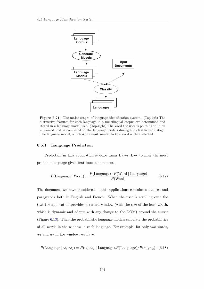
6.5 Language Identification System
Language
Corpus
Input
Documents
Language
Models
Languages
Generate
Models
Classify
Figure 6.21: The major stages of language identification system. (Top-left) Thedistinctive features for each language in a multilingual corpus are determined andstored in a language model tree. (Top-right) The word the user is pointing to in anuntrained text is compared to the language models during the classification stage.The language model, which is the most similar to this word is then selected.
6.5.1 Language Prediction
Prediction in this application is done using Bayes’ Law to infer the most
probable language given text from a document.
P (Language | Word) =P (Language) · P (Word | Language)
P (Word)(6.17)
The document we have considered in this applications contains sentences and
paragraphs both in English and French. When the user is scrolling over the
text the application provides a virtual window (with the size of the lens’ width,
which is dynamic and adapts with any change to the DOM) around the cursor
(Figure 6.13). Then the probabilistic language models calculate the probabilities
of all words in the window in each language. For example, for only two words,
w1 and w2 in the window, we have:
P (Language | w1, w2) = P (w1, w2 | Language).P (Language)/P (w1, w2) (6.18)
194
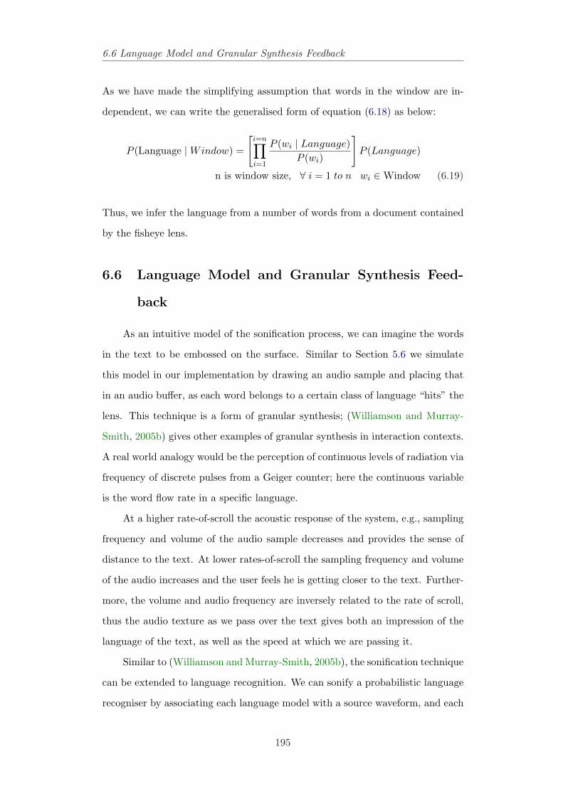
6.6 Language Model and Granular Synthesis Feedback
As we have made the simplifying assumption that words in the window are in-
dependent, we can write the generalised form of equation (6.18) as below:
P (Language | Window) =
[i=n∏
i=1
P (wi | Language)P (wi)
]P (Language)
n is window size, ∀ i = 1 to n wi ∈ Window (6.19)
Thus, we infer the language from a number of words from a document contained
by the fisheye lens.
6.6 Language Model and Granular Synthesis Feed-
back
As an intuitive model of the sonification process, we can imagine the words
in the text to be embossed on the surface. Similar to Section 5.6 we simulate
this model in our implementation by drawing an audio sample and placing that
in an audio buffer, as each word belongs to a certain class of language “hits” the
lens. This technique is a form of granular synthesis; (Williamson and Murray-
Smith, 2005b) gives other examples of granular synthesis in interaction contexts.
A real world analogy would be the perception of continuous levels of radiation via
frequency of discrete pulses from a Geiger counter; here the continuous variable
is the word flow rate in a specific language.
At a higher rate-of-scroll the acoustic response of the system, e.g., sampling
frequency and volume of the audio sample decreases and provides the sense of
distance to the text. At lower rates-of-scroll the sampling frequency and volume
of the audio increases and the user feels he is getting closer to the text. Further-
more, the volume and audio frequency are inversely related to the rate of scroll,
thus the audio texture as we pass over the text gives both an impression of the
language of the text, as well as the speed at which we are passing it.
Similar to (Williamson and Murray-Smith, 2005b), the sonification technique
can be extended to language recognition. We can sonify a probabilistic language
recogniser by associating each language model with a source waveform, and each
195
6.7 Example Application – A Multimodal Document Browser
model’s output probability then directly maps to the probability of drawing a
grain from the source corresponding to that model (Figures 6.13(d) and 6.13(e)).
The temporal distribution of grains inside the source waveforms maps to the
probability of the language of the words inside the virtual window. The overall
grain density is dynamic throughout the sonification when the user scrolls over
the text. In practice, during the searching mode this produces a sound that’s
unclear when text features are blurred and the DOM is in the minimum level, and
it means the information entropy inside the virtual window around the cursor is
high. These features resolve to a clear, distinct sound as system’s mode switches
to the targeting. The sonification’s primary effect is to display the current goal
distribution’s entropy, i.e., language, audio and text content.
The concept of entropy in information theory describes the level of uncer-
tainty of a random variable. An alternative way to look at this is to talk about
how much information is carried by the signal. For example, in an English text,
encoded as a string of letters, spaces, and punctuation the signal is a string of
characters. The letter frequency for different characters is different, and we can-
not perfectly predict what the next character will be in the string: it is, to some
degree, ‘random’. Entropy is a measure of this randomness and was suggested
by Shannon (1948).
Thus model-based behaviour in this task couples the user’s input (speed of
scroll) to the visualisation technique via the dynamics and the focus-in-context
method couples detail-in-context to audio samples via the language identification
system (Figure 6.13(a)). The next section presents an example application for
browsing a document to highlight the ideas discussed and explored in the previous
sections.
6.7 Example Application – A Multimodal Document
Browser
We presented a 5 page scientific document in English and a paragraph, a
Figure caption and few sentences in French. The object study was conducted
196
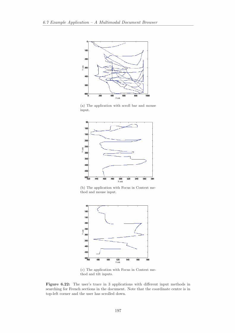
6.7 Example Application – A Multimodal Document Browser
X axis
Y a
xis
(a) The application with scroll bar and mouseinput.
580
X axis
Y a
xis
(b) The application with Focus in Context me-thod and mouse input.
X axis
Y a
xis
(c) The application with Focus in Context me-thod and tilt inputs.
Figure 6.22: The user’s trace in 3 applications with different input methods insearching for French sections in the document. Note that the coordinate centre is intop-left corner and the user has scrolled down.
197
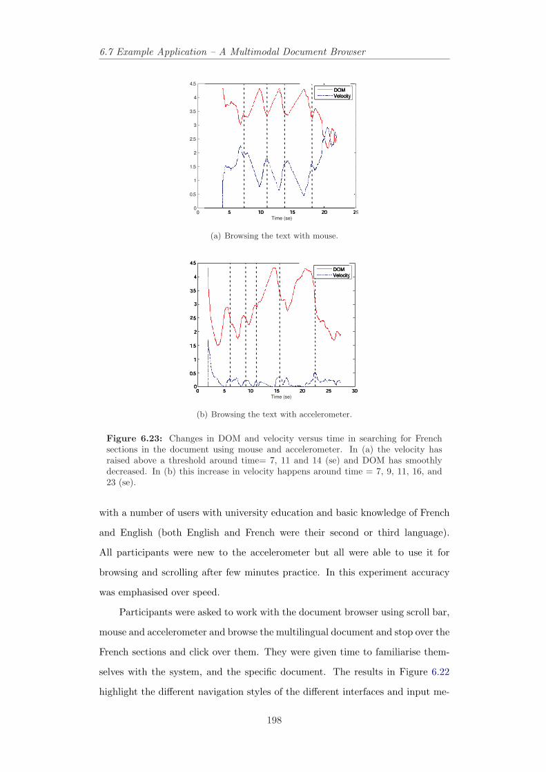
6.7 Example Application – A Multimodal Document Browser
0 250
0.5
1
1.5
2
2.5
3
3.5
4
4.5
Time (se)
(a) Browsing the text with mouse.
0.
2.
3.
4.
Time (se)
(b) Browsing the text with accelerometer.
Figure 6.23: Changes in DOM and velocity versus time in searching for Frenchsections in the document using mouse and accelerometer. In (a) the velocity hasraised above a threshold around time= 7, 11 and 14 (se) and DOM has smoothlydecreased. In (b) this increase in velocity happens around time = 7, 9, 11, 16, and23 (se).
with a number of users with university education and basic knowledge of French
and English (both English and French were their second or third language).
All participants were new to the accelerometer but all were able to use it for
browsing and scrolling after few minutes practice. In this experiment accuracy
was emphasised over speed.
Participants were asked to work with the document browser using scroll bar,
mouse and accelerometer and browse the multilingual document and stop over the
French sections and click over them. They were given time to familiarise them-
selves with the system, and the specific document. The results in Figure 6.22
highlight the different navigation styles of the different interfaces and input me-
198
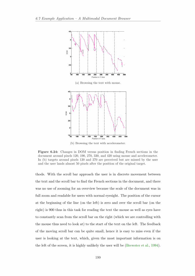
6.7 Example Application – A Multimodal Document Browser
Position in Y Axis
DO
M
(a) Browsing the text with mouse.
50 100 150 200 250 300 350 400 450 500
Position in Y axis
DO
M
(b) Browsing the text with accelerometer.
Figure 6.24: Changes in DOM versus position in finding French sections in thedocument around pixels 120, 190, 270, 330, and 420 using mouse and accelerometer.In (b) targets around pixels 120 and 270 are perceived but are missed by the userand the user lands almost 50 pixels after the position of the original target.
thods. With the scroll bar approach the user is in discrete movement between
the text and the scroll bar to find the French sections in the document, and there
was no use of zooming for an overview because the scale of the document was in
full zoom and readable for users with normal eyesight. The position of the cursor
at the beginning of the line (on the left) is zero and over the scroll bar (on the
right) is 900 thus in this task for reading the text the mouse as well as eyes have
to constantly scan from the scroll bar on the right (which we are controlling with
the mouse thus need to look at) to the start of the text on the left. The feedback
of the moving scroll bar can be quite small, hence it is easy to miss even if the
user is looking at the text, which, given the most important information is on
the left of the screen, it is highly unlikely the user will be (Brewster et al., 1994).
199
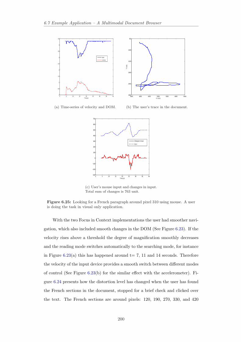
6.7 Example Application – A Multimodal Document Browser
0 5 10 15 20 25 30 35 400
0.5
1
1.5
2
2.5
3
3.5
4
4.5
Time(se)
dom
velocity
(a) Time-series of velocity and DOM.
350 400 450 500 550 600 650
50
100
150
200
250
300
X Axis
Y A
xis
(b) The user’s trace in the document.
0 5 10 15 20 25 30 35 40−300
−200
−100
0
100
200
300
400
500
600
700
Time(se)
Changes in Input
Input
(c) User’s mouse input and changes in input.Total sum of changes is 763 unit.
Figure 6.25: Looking for a French paragraph around pixel 310 using mouse. A useris doing the task in visual only application.
With the two Focus in Context implementations the user had smoother navi-
gation, which also included smooth changes in the DOM (See Figure 6.23). If the
velocity rises above a threshold the degree of magnification smoothly decreases
and the reading mode switches automatically to the searching mode, for instance
in Figure 6.23(a) this has happened around t= 7, 11 and 14 seconds. Therefore
the velocity of the input device provides a smooth switch between different modes
of control (See Figure 6.23(b) for the similar effect with the accelerometer). Fi-
gure 6.24 presents how the distortion level has changed when the user has found
the French sections in the document, stopped for a brief check and clicked over
the text. The French sections are around pixels: 120, 190, 270, 330, and 420
200
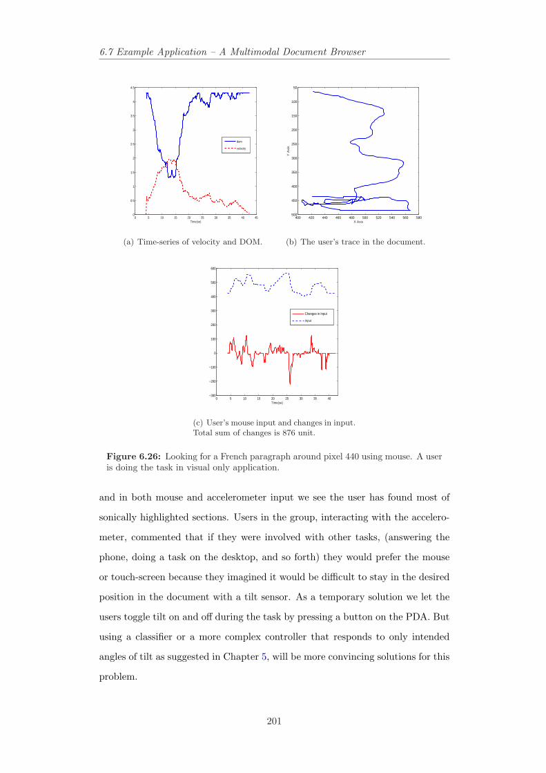
6.7 Example Application – A Multimodal Document Browser
0 5 10 15 20 25 30 35 40 450
0.5
1
1.5
2
2.5
3
3.5
4
4.5
Time(se)
dom
velocity
(a) Time-series of velocity and DOM.
400 420 440 460 480 500 520 540 560 580
50
100
150
200
250
300
350
400
450
500
X Axis
Y A
xis
(b) The user’s trace in the document.
0 5 10 15 20 25 30 35 40−300
−200
−100
0
100
200
300
400
500
600
Time(se)
Changes in Input
Input
(c) User’s mouse input and changes in input.Total sum of changes is 876 unit.
Figure 6.26: Looking for a French paragraph around pixel 440 using mouse. A useris doing the task in visual only application.
and in both mouse and accelerometer input we see the user has found most of
sonically highlighted sections. Users in the group, interacting with the accelero-
meter, commented that if they were involved with other tasks, (answering the
phone, doing a task on the desktop, and so forth) they would prefer the mouse
or touch-screen because they imagined it would be difficult to stay in the desired
position in the document with a tilt sensor. As a temporary solution we let the
users toggle tilt on and off during the task by pressing a button on the PDA. But
using a classifier or a more complex controller that responds to only intended
angles of tilt as suggested in Chapter 5, will be more convincing solutions for this
problem.
201
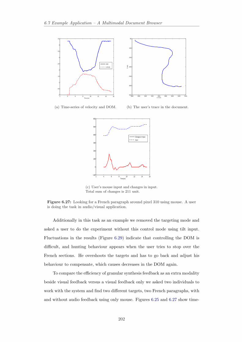
6.7 Example Application – A Multimodal Document Browser
2 4 6 8 10 12 14 160
0.5
1
1.5
2
2.5
3
3.5
4
4.5
Time (se)
dom
velocity
(a) Time-series of velocity and DOM.
380 400 420 440 460 480 500 520 540
50
100
150
200
250
300
350
X Axis
Y Ax
is
(b) The user’s trace in the document.
2 4 6 8 10 12 14 16−100
0
100
200
300
400
500
600
Time(se)
Changes in Input
Input
(c) User’s mouse input and changes in input.Total sum of changes is 211 unit.
Figure 6.27: Looking for a French paragraph around pixel 310 using mouse. A useris doing the task in audio/visual application.
Additionally in this task as an example we removed the targeting mode and
asked a user to do the experiment without this control mode using tilt input.
Fluctuations in the results (Figure 6.29) indicate that controlling the DOM is
difficult, and hunting behaviour appears when the user tries to stop over the
French sections. He overshoots the targets and has to go back and adjust his
behaviour to compensate, which causes decreases in the DOM again.
To compare the efficiency of granular synthesis feedback as an extra modality
beside visual feedback versus a visual feedback only we asked two individuals to
work with the system and find two different targets, two French paragraphs, with
and without audio feedback using only mouse. Figures 6.25 and 6.27 show time-
202
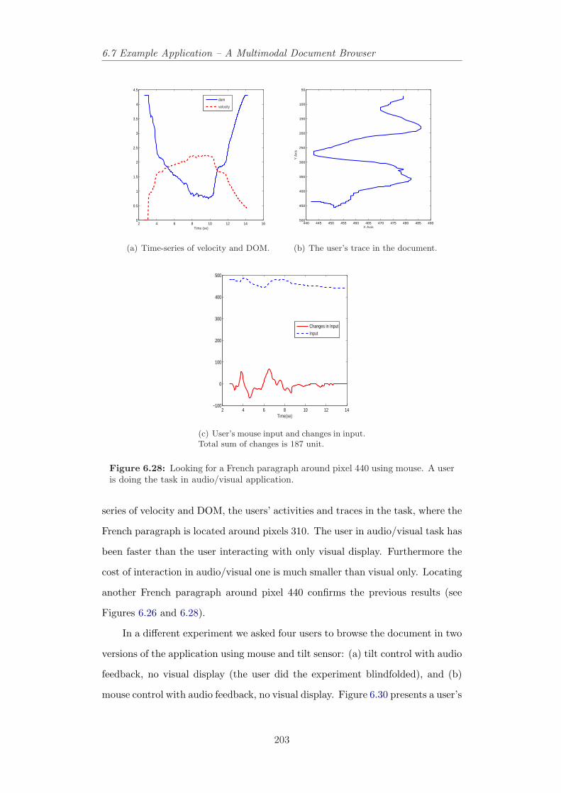
6.7 Example Application – A Multimodal Document Browser
2 4 6 8 10 12 14 160
0.5
1
1.5
2
2.5
3
3.5
4
4.5
Time (se)
dom
velocity
(a) Time-series of velocity and DOM.
440 445 450 455 460 465 470 475 480 485 490
50
100
150
200
250
300
350
400
450
500
X Axis
Y A
xis
(b) The user’s trace in the document.
2 4 6 8 10 12 14−100
0
100
200
300
400
500
Time(se)
Changes in InputInput
(c) User’s mouse input and changes in input.Total sum of changes is 187 unit.
Figure 6.28: Looking for a French paragraph around pixel 440 using mouse. A useris doing the task in audio/visual application.
series of velocity and DOM, the users’ activities and traces in the task, where the
French paragraph is located around pixels 310. The user in audio/visual task has
been faster than the user interacting with only visual display. Furthermore the
cost of interaction in audio/visual one is much smaller than visual only. Locating
another French paragraph around pixel 440 confirms the previous results (see
Figures 6.26 and 6.28).
In a different experiment we asked four users to browse the document in two
versions of the application using mouse and tilt sensor: (a) tilt control with audio
feedback, no visual display (the user did the experiment blindfolded), and (b)
mouse control with audio feedback, no visual display. Figure 6.30 presents a user’s
203
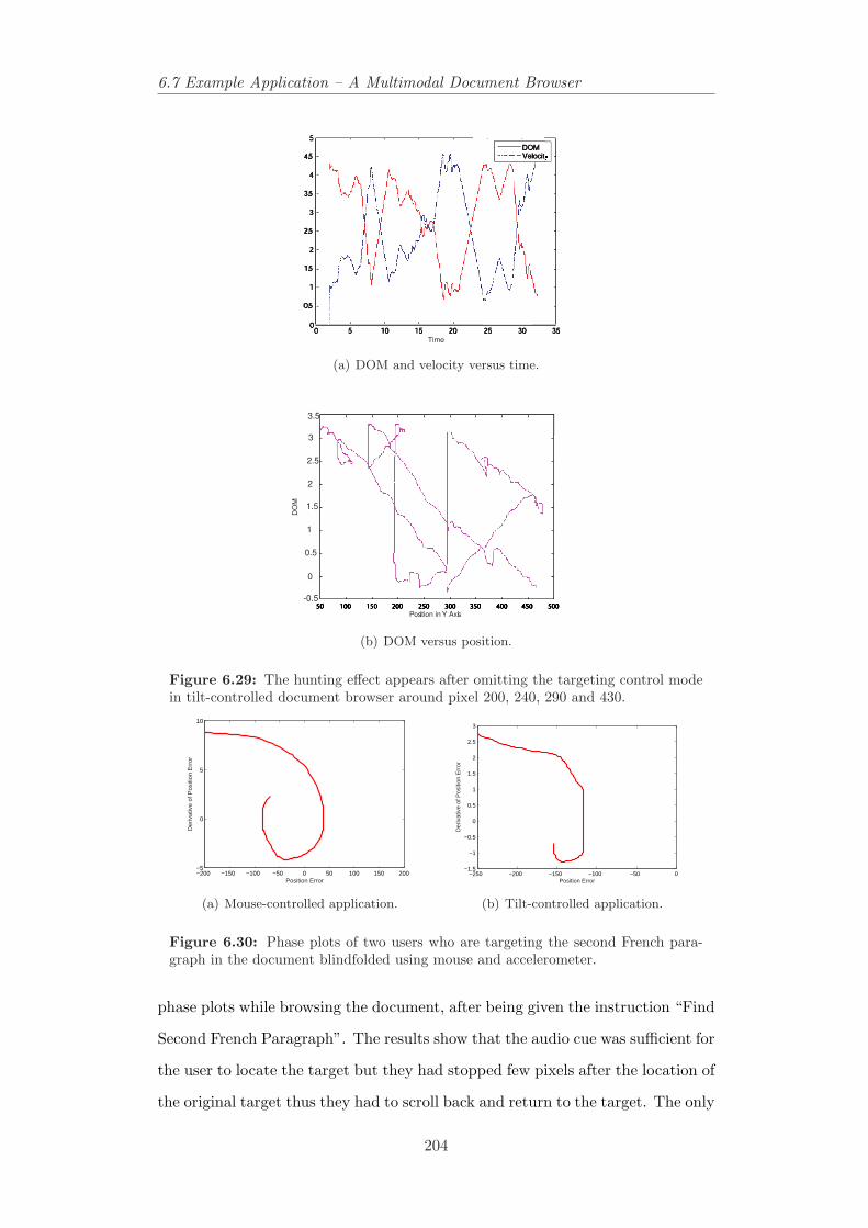
6.7 Example Application – A Multimodal Document Browser
Time
(a) DOM and velocity versus time.
50 100 150 200 250 300 350 400 450 500
Position in Y Axis
DO
M
-0.5
0
0.5
1
1.5
2
2.5
3
3.5
(b) DOM versus position.
Figure 6.29: The hunting effect appears after omitting the targeting control modein tilt-controlled document browser around pixel 200, 240, 290 and 430.
−200 −150 −100 −50 0 50 100 150 200−5
0
5
10
Position Error
Der
ivat
ive
of P
ositi
on E
rror
(a) Mouse-controlled application.
−250 −200 −150 −100 −50 0−1.5
−1
−0.5
0
0.5
1
1.5
2
2.5
3
Position Error
Der
ivat
ive
of P
ositi
on E
rror
(b) Tilt-controlled application.
Figure 6.30: Phase plots of two users who are targeting the second French para-graph in the document blindfolded using mouse and accelerometer.
phase plots while browsing the document, after being given the instruction “Find
Second French Paragraph”. The results show that the audio cue was sufficient for
the user to locate the target but they had stopped few pixels after the location of
the original target thus they had to scroll back and return to the target. The only
204
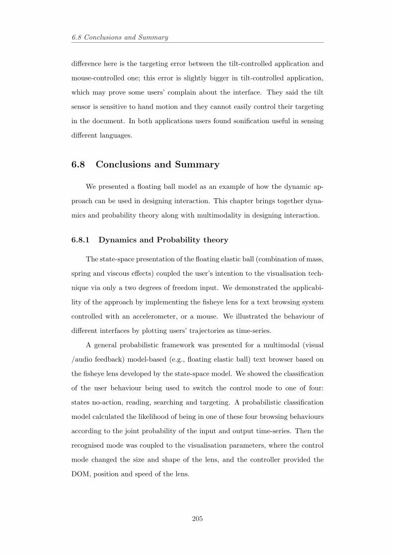
6.8 Conclusions and Summary
difference here is the targeting error between the tilt-controlled application and
mouse-controlled one; this error is slightly bigger in tilt-controlled application,
which may prove some users’ complain about the interface. They said the tilt
sensor is sensitive to hand motion and they cannot easily control their targeting
in the document. In both applications users found sonification useful in sensing
different languages.
6.8 Conclusions and Summary
We presented a floating ball model as an example of how the dynamic ap-
proach can be used in designing interaction. This chapter brings together dyna-
mics and probability theory along with multimodality in designing interaction.
6.8.1 Dynamics and Probability theory
The state-space presentation of the floating elastic ball (combination of mass,
spring and viscous effects) coupled the user’s intention to the visualisation tech-
nique via only a two degrees of freedom input. We demonstrated the applicabi-
lity of the approach by implementing the fisheye lens for a text browsing system
controlled with an accelerometer, or a mouse. We illustrated the behaviour of
different interfaces by plotting users’ trajectories as time-series.
A general probabilistic framework was presented for a multimodal (visual
/audio feedback) model-based (e.g., floating elastic ball) text browser based on
the fisheye lens developed by the state-space model. We showed the classification
of the user behaviour being used to switch the control mode to one of four:
states no-action, reading, searching and targeting. A probabilistic classification
model calculated the likelihood of being in one of these four browsing behaviours
according to the joint probability of the input and output time-series. Then the
recognised mode was coupled to the visualisation parameters, where the control
mode changed the size and shape of the lens, and the controller provided the
DOM, position and speed of the lens.
205
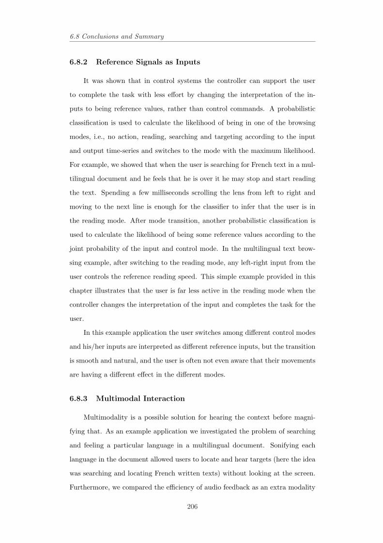
6.8 Conclusions and Summary
6.8.2 Reference Signals as Inputs
It was shown that in control systems the controller can support the user
to complete the task with less effort by changing the interpretation of the in-
puts to being reference values, rather than control commands. A probabilistic
classification is used to calculate the likelihood of being in one of the browsing
modes, i.e., no action, reading, searching and targeting according to the input
and output time-series and switches to the mode with the maximum likelihood.
For example, we showed that when the user is searching for French text in a mul-
tilingual document and he feels that he is over it he may stop and start reading
the text. Spending a few milliseconds scrolling the lens from left to right and
moving to the next line is enough for the classifier to infer that the user is in
the reading mode. After mode transition, another probabilistic classification is
used to calculate the likelihood of being some reference values according to the
joint probability of the input and control mode. In the multilingual text brow-
sing example, after switching to the reading mode, any left-right input from the
user controls the reference reading speed. This simple example provided in this
chapter illustrates that the user is far less active in the reading mode when the
controller changes the interpretation of the input and completes the task for the
user.
In this example application the user switches among different control modes
and his/her inputs are interpreted as different reference inputs, but the transition
is smooth and natural, and the user is often not even aware that their movements
are having a different effect in the different modes.
6.8.3 Multimodal Interaction
Multimodality is a possible solution for hearing the context before magni-
fying that. As an example application we investigated the problem of searching
and feeling a particular language in a multilingual document. Sonifying each
language in the document allowed users to locate and hear targets (here the idea
was searching and locating French written texts) without looking at the screen.
Furthermore, we compared the efficiency of audio feedback as an extra modality
206
6.8 Conclusions and Summary
beside visual feedback versus visual feedback only system. The users’ activities in
the multimodal system were lower than unimodal system. It suggests that trans-
ferring information sonically will be a powerful complement to visual interfaces
and supports intermittent interaction where the motion limits the usefulness of
the small screen for the duration of input and the user carries on with other
activities. Thus there would be an application for this system in mobile phones,
small screen computing devices and shared displays, too.
The general probabilistic framework presented in this chapter brings the re-
sults in chapter 4, usefulness of quickened displays and predicting the user beha-
viour, and chapter 5, importance of multimodality in the intermittent interaction,
together along with the probabilistic model for classifying human behaviour in
browsing tasks suggested in this chapter.
In the next chapter we present a general overview of the thesis and summarise
the work.
207

Chapter 7
Conclusions and Future Work
“The reward for work well done is the opportunity to do more work.”Jonas Salk, MD
In this final Chapter we present a summary and discussion of thecontributions of this dissertation, concluding remarks and note somepotential avenues for future work.
In this thesis our focus has been on setting out a theoretical basis for the design
of interactive systems on portable computing devices. This work has presen-
ted a general framework to achieve this goal as well as exploring novel areas in
portable computational appliances. Concrete techniques, developed real working
interfaces allowed us to collect detailed real data from users testing the prototype
we developed in the thesis.
7.1 Contributions of the Thesis
This thesis addresses a theoretical basis for the design of interactive sys-
tems on small, portable computing devices. This framework includes current
human-computer interfaces; it also reveals a number of unexplored areas in this
context and human–mobile device interaction. Concrete techniques for applying
the concepts have been discussed for example applications, in both auditory and
graphical user interfaces. Working interfaces which embody these novel interac-
tion concepts can be created with these techniques. We view this approach in
208
7.1 Contributions of the Thesis
terms of a framework for specification and analysis, rather than a set of predefined
techniques.
7.1.1 Model–Based Target Sonification
In Chapter 4, the major contribution made to the auditory displays and
localisation and selection on mobile devices using tilt sensor. The experiments
in this Chapter provide better understanding about users’ navigation and search
behaviour in audio displays. For example, in conditions where the vibration
(haptic) feedback is included, the sweep search pattern is combined with circular
movements around the vibration source. In these conditions where the audio
feedback guides the user toward the target, and he feels that he is close enough
to the target, then he starts looking for the vibration source; because a clear
on/off feedback at the edge of the vibration indicates that the target has been
achieved. Also, results in this Chapter show that while the interaction lacks
enough feedback information the user uses his/her prior knowledge learnt from
training session or from other activities, for example, left-right reading patterns
and it affects their browsing behaviour.
Next, results in this Chapter provide evidence on usefulness of quickened
displays and advantages and disadvantages of different audio/haptic patterns.
It is highlighted that over-interpreting the quickened signal, especially in the
Doppler condition is a common risk associated with quickened displays. Also,
this Chapter is concerned with the predictive feedback based on human operator
modeling in continuous tracking tasks, to tie together feedback mechanism of
interactive auditory displays.
7.1.2 Tilt-Controlled Zooming User Interfaces
The importance of continuous control and modeling, which emerges to an
extent in Chapter 4 is the main focus of Chapters 5 and 6, which investigate the
dynamic systems approach to the design of continuous interaction interfaces. The
contribution Chapter 5 makes is the development one of the first tilt controlled
speed-dependent automatic zooming (SDAZ) on a PDA. Tilt-controlled SDAZ
209
7.1 Contributions of the Thesis
is used for browsing long documents based on a state-space implementation of
a flying object metaphor (combinations of springs, masses and damping effects)
with pseudo autopilot modes. We suggest that the state-space approach has the
potential to provide a general framework for development, analysis and optimisa-
tion of interfaces which induce complex, but convenient coupling among multiple
states, in order to cope with one degree of freedom input.
In the general approach (i.e., interaction with higher degrees of freedom in-
put and many controlled variables) this model makes tuning and calibration a
lot easier for the system itself or when the system is coupled with the time de-
lay and lag-lead-dynamics of human control behaviour; because proper settings,
which make the closed-loop system-human stable, can only be found by obser-
ving the behaviour of the simulated system before the actual implementation.
For example, by modeling the human operator like a gain and delay, plotting the
Bode plots and calculating the activity of the user using a performance function,
we find the most satisfying setting for the user and the system and this sug-
gests that control model supports closed-loop dynamics. We show that having
augmented velocity and position control help the user to perform more accurate
browsing and landing over the targets. Interpreting inputs as reference values
provides switching among different control modes, but the mode transition is
designed to be smooth and natural and the user is not aware that their hand
movements have different effects in different modes.
The tilt-controlled SDAZ has its own pros and cons. It facilitates single-
handed control of the application without obscuring the screen, however it may
cause irritating reflections from the screen. This does not happen in the touch-
screen version. Thus the user can stop interaction with the device by simply
taking the stylus off the screen. We improve this by auto–calibrating the device
according to the comfortable starting angle (equilibrium point) of the tilt-sensor
in the user’s palm.
The audio/haptic feedback representation of the speed-zoom coupling invol-
ved in speed-dependent automatic zooming is the other contribution this Chapter
makes. We implement and demonstrate the multimodal tilt-controlled SDAZ in-
210
7.1 Contributions of the Thesis
terface for a text browser system on the PDA instrumented with the tilt sensor.
Sonifying each piece of structural information in the document lets the blindfol-
ded users feel and sense different textures. The results show that the audio/haptic
cue is sufficient for the blindfolded users to distinguish where the target is, but
the users’ activities in the audio and haptic only interface were higher than the vi-
sual only, most likely because the vision is leading sense. This provides a general
design guideline for developers to add multimodal feedback, which is an essential
component of movement-based interaction techniques and supports intermittent
interaction.
7.1.3 Multimodal Motion Controlled Focus-in-Context Method:
Sensing Complex Information
We developed a motion controlled focus-in-context visualisation method ba-
sed on a pseudo-physical metaphor (a floating ball) and a state-space implemen-
tation, which also presents a general framework of how dynamic system simula-
tion and continuous control method can be linked to multimodal feedback and
probabilistic language model and support human behaviour.
Supporting the user input and completing the task automatically for the
user by changing the interpretation of the inputs to being reference values, ra-
ther than control commands has been shown in a few examples in this Chapter.
A probabilistic classification is used to calculate the likelihood of being in one of
the browsing modes, i.e no action, reading, searching and targeting according to
the input and output time-series and switches to the mode with the maximum
likelihood. After mode transition another probabilistic classification is used to
calculate the likelihood of being some reference values according to the joint pro-
bability of the input and control mode. As an example, we provide a multilingual
text browser and how the controller supports the user input and completes the
reading task the user is interested and changes interpretation of inputs after mode
transition. In this example application the user switches among different control
modes, but the transition is smooth and natural, and the user is often not even
aware that their movements are having a different effect in the different modes.
211
7.2 Outlook
A significant disadvantage of focus-in-context techniques is the user’s know-
ledge about the context, for example, the language of the text is very limited
when the degree of the magnification is low; because the context is too small
and far from the viewpoint. In this Chapter we suggest that multimodality is a
possible solution for this problem. As an example application we investigate the
problem of searching and feeling a particular language in a multilingual docu-
ment. Sonifying each language in the document allows users to hear and locate
targets without looking at the screen. In a simple example we compare the ef-
ficiency of audio feedback as an extra modality beside visual feedback versus a
visual feedback only system. The performance measure indicates that the mul-
timodal system decreases the cost more than the unimodal system and suggests
that audio/haptic feedback will be a powerful complement to visual interfaces and
supports intermittent interaction, where the user can spend varying amounts of
attention on interaction while carrying on with other activities.
The general probabilistic framework presented in this Chapter brings the
results in Chapter 4, usefulness of quickened displays and predicting the user’s
behaviour, and Chapter 5, importance of multimodality in the intermittent in-
teraction, together along with the probabilistic model for classifying human be-
haviour combined with audio/visual feedback in browsing tasks suggested in this
Chapter.
7.2 Outlook
A more thorough exploitation of the continuous control and dynamic system
approach presents a promising theoretical framework for interaction models and
design principles and help create better interactive systems not only on portable
computing devices but also on all range of computing systems. The availability
of this solid theory for use in interactive systems, allow the incorporation of
analytical tools and constructive techniques from manual and automatic control
theory, probabilistic models, and machine learning techniques into the interface
and integrating multimodality in a principled manner. Thus, this concrete theory
212
7.2 Outlook
provides a wide range of possibilities for future work.
In this thesis, we provided a number of examples, where the system relies
on a tight coupling between the user’s perception and the action. Providing pre-
dictive feedback based on human operator modeling and taking human response
delays and lags into account is one of important issues in multimodal interfaces.
It provides important insight about human performance or activity in the interac-
tion with multimodal systems, for example model-based sonification application
in Chapter 4 or multimodal, model-based text browser application in Chapter 6.
In continuous dynamic interactive systems the trend is that the system is
adapting to the complexity of the user behaviour rather than the user adapting
himself to a system’s interface. We presented a few examples of this adaptability
in Chapters 5 and 6, where the controller changes the interpretation of user
inputs to being reference values, rather than control commands, switches among
different control modes smoothly according to these reference values without
being noticed by the user and completes the task without too much effort from
the user. An interesting application of control systems, which adapt themselves
to the user behaviour will be interactive systems whose users have different range
of expertise in the interaction with the system, novice, intermediate or expert.
The objective, consequently, is to determine the most appropriate parameter
settings for the dynamic system model, which make the closed-loop interaction
between the system and user stable. As the user learns how to interact with the
system, i.e lags and delays in muscles decrease, the system switches to the model
and the controller which suits the parameters of that user more.
Chapter 6 provided a number of examples of coupling between probability
theory and control theory to classify and predict user behaviour in the interaction.
Probability theory gives theoretical models for the combination and classification
of evidence. For example, a probabilistic classification of the likelihood of dif-
ferent modes of control is used to change the dynamics of the controlled system,
which makes the user’s task easier. The idea of probabilistic classification can be
used in classifying and recognising misinterpreted and unintended inputs as we
show a few examples of these inputs in Chapter 5. Implementing such a classifier
213
7.3 Final Remarks
is an important step forward in designing continuous tilt-controlled interfaces
and supporting intermittent interaction.
The core of this dissertation is building prototypes and addressing a theo-
retical basis for the design of interactive systems, which help designers to build
their own interfaces based on these prototypes and run usability experiments.
7.3 Final Remarks
Research in the area of designing continuous interaction is still in its infancy.
The dynamic theory driven approach to the design of interactive systems on por-
table computing appliances allows us to utilise the concrete analytical tools and
constructive techniques from manual and automatic control theory in augmen-
ting and complementing human capabilities in the interaction and integration
of multimodality in a principled manner. From this basis, this dissertation has
provided a number of contributions to the research on interaction with portable
computing devices, tilt-controlled applications, audio/haptic interfaces, multimo-
dal zooming user interfaces, and probability theory.
214
Bibliography
Accot, J. and Zhai, S. (1997). Beyond Fitts’ Law: Models for Trajectory-BasedHCI Taks. In Proceedings of the ACM Conference on Human Factors in Com-puting Systems, CHI’97, pages 295–302, Atlanta, Georgia, United States. ACMPress.
Accot, J. and Zhai, S. (1999). Performance Evaluation of Input Devices inTrajectory-Based Tasks: An Application of the Steering Law. In Proceedingsof the SIGCHI conference on Human factors in computing systems: CHI’99,pages 466–472, Pittsburgh, Pennsylvania, USA. ACM Press.
Accot, J. and Zhai, S. (2001). Scale Effects in Steering Law Tasks: Do DeviceSize and Different Motor Joints Matter? In Proceedings of the ACM Confe-rence on Human Factors in Computing Systems, CHI’01, pages 1–8, Seattle,Washington, USA. ACM Press.
Accot, J. and Zhai, S. (2002). More than dotting the i’s – Foundations forcrossing-based interfaces. In Proceedings of the SIGCHI Conference on Hu-man Factors in Computing Systems, Changing our world, changing ourselves,Session: Input: Smooth Moves, CHI’02, pages 73–80, Minneapolis, Minnesota,USA. ACM Press.
Ahlberg, C. and Shneiderman, B. (1994). The Alphaslider: A Compact andRapid Selector. In Proceedings of the ACM Conference on Human Factorsin Computing Systems, CHI’94, pages 365–371, Boston, Massachusetts, USA.ACM Press.
Analog Devices (2000). Adxl202especifications. http://www.analog.com.
Anderson, B., Brinsmead, T., Liberzon, D., and Morse, A. (2001). Multiple modeladaptive control with safe switching. In International Journal of AdaptiveControl and Signal Processing, volume 15, pages 445–470. John Wiley & Sons.
Aponso, B. L., Mitchell, D. G., and Hoh, R. H. (1990). Simulation investigationof the effects of helicopter hovering dynamics on pilot performance. Journal ofGuidance, Control and Dynamics, 13(1):8–15.
215
Bibliography
Apple (2002). The Macintosh Operating system. Website: http://www.apple.com/macosx/theater/dock.html.
Apple (2007). iPhone. Website: http://www.apple.com/iphone/ipod/.
Astrom, J. K. and Wittenmark, B. (1997). Computer controlled systems, Theoryand Design. 3rd ed. NJ: Prentice Hall.
Barrett, R. C., Sleker, E. J., Rutledge, J. D., and Olyha, R. S. (1995). The Nega-tive Inertia: A dynamic pointing function. In Proceedings of the ACM Confe-rence on Human Factors in Computing Systems, CHI’95, conference compa-nion, pages 316–317, Denver, Colorado, USA. ACM Press.
Baskett, B. (2000). Aeronautical design standard performance specification hand-ling qualities requirements for military rotorcraft. Technical report, US ArmyAviation and Missile Command Aviation Engineering Directorate, Alabama.
Baudisch, P., Lee, B., and Hanna, L. (2004). Fishnet, a Fisheye Web Browserwith Search Term Popouts: a Comparative Evaluation with Overview andLinear View. In AVI ’04: Proceedings of the working conference on Advancedvisual interfaces, pages 133–140, Gallipoli, Italy. ACM Press.
Beard, D. and Walker, J. (1990). Navigational techniques to improve the displayof large two-dimensional spaces. In Behaviour Information and Technology,volume 9, pages 451–466.
Beaudouin-Lafon, M. (2000). Instrumental Interaction: An Interaction Model forDesigning Post-WIMP User Interfaces. In Proceedings of the ACM Conferenceon Human Factors in Computing Systems, CHI’00, CHI Letters, volume 2,pages 446–453, The Hague, The Netherlands. ACM Press.
Beaudouin-Lafon, M. (2004). Designing Interaction, not Interfaces. In AVI’04:Proceedings of the working conference on Advanced visual interfaces, pages15–22, Gallipoli, Italy. ACM Press.
Beaudouin-Lafon, M. and Gaver, W. (1994). ENO: synthesizing structured soundspaces. In Proceedings of the 7th annual ACM symposium on User interfacesoftware and technology , pages 49–57, Marina del Rey, California, UnitedStates. ACM Press.
Bederson, B., Hollan, J., Perlin, K., Meyer, J., Bacon, D., and Furnas, G. (1994).Pad++: A Zoomable Graphical Sketchpad for Exploring Alternate InterfacePhysics. In UIST’94: Proceedings of the 7th annual ACM symposium on Userinterface software and technology, pages 17–26, Marina del Rey, California,USA. ACM Press.
216
Bibliography
Bederson, B. B., Clamage, A., Czerwinski, M. P., and Robertson, G. G. (2003).A fisheye calendar interface for PDAs: providing overviews for small displays.In Conference on Human Factors in Computing Systems, CHI’03 extendedabstracts on Human factors in computing systems, pages 618–619, Florida,USA. ACM Press.
Bell, T. C., Cleary, J. G., and Witten, I. H. (1990). Text Compression. PrenticeHall Advanced Reference Series. Prentice Hall.
Birmingham, H. P. and Taylor, F. V. (1954). A design philosophy for man-machine control systems. In Proceedings of the Institute of Radio Engineers,pages 1748–1758.
Blakelock, J. H. (1991). Automatic Control of Aircraft and Missiles. John Wiley.
Blanch, R., Guiard, Y., and Beaudouin-Lafon, M. (2004). Semantic Pointing:Improving target acquisition with Control-Display ratio adaptation. In ACMConference on Human Factors in Computing Systems, CHI’04, pages 519–526,Vienna, Austria. ACM Press.
Blattner, M., Papp, A., and Glinert, E. (1992). Sonic enhancements of two dimen-sional graphic displays. In Proceedings of International Conference on AuditoryDisplay,ICAD’92, pages 447–470, Santa Fe, NM, USA. Addison-Wesley.
Bootsma, R. J., Fernandez, L., and Mottet, D. (2004). Behind Fitts’ law: kinema-tic patterns in goal-directed movements. In International Journal of Human-Computer studies, IJHCS, volume 61, pages 811–821, NY, New York. ElsevierScience Publishing.
Bosch, R. (2003). ACC Adaptive Cruise Control. Automative Technology.
Bradley, R. (1996). The flying brick exposed: Non-linear control of a basichelicopter model. Technical report, Dept. of Mathematics, Glasgow CaledonianUniversity.
Bregman, A. S. (1990). Auditory Scene Analysis: The Perceptual Organisationof Sound. MIT Press, Cambridge, Massachusetts.
Brewster, S., Wright, P., and Edwards, A. (1994). The Design and Evaluation ofan Auditory-Enhanced Scrollbar. In Proceedings of the SIGCHI Conference onHuman Factors in Computing Systems: Celebrating Interdependence, CHI’94,pages 173–179, Boston, Massachusetts, USA.
Brewster, S. A. (1997). Using Non-Speech Sound to Overcome Information Over-load. In Special Issue on Multimedia Displays, volume 17, pages 179–189.
217
Bibliography
Brewster, S. A. (2002). Overcoming the Lack of Screen Space on Mobile Com-puters. Proceedings of Personal and Ubiquitous Computing, 6(3):188–205.
Brewster, S. A. and Murray, R. (2000). Presenting dynamic information onmobile computers. In Personal Technologies, pages 209–212. Springer-Verlag.
Brogan, W. L. (1991). Modern Control Theory. Prentice Hall.
Brooks, V. (1986). The Neural Basis of Motor Control. New York:Oxford Uni-versity Press.
Bushaw, D. W. (1953). Differential Equations with Discontinuous Forcing Terms.Stevens Tech. Inst., N.J. USA. Rep. 469.
Buxton, B., Billinghurst, M., Guiard, Y., Sellen, A., and Zhai, S. (2002). Hu-man Input to Computer Systems: Theories, Techniques and Technology. Un-published manuscript available on the web. http://www.billbuxton.com/
inputManuscript.html.
Cadwallender, W. and Cochin, I. (1997). Analysis and Design of Dynamic Sys-tems, 3rd Edition. Prentice Hall.
Card, S. K., English, W. K., and Burr, B. J. (1978). Evaluation of mouse, rate-controlled isometric joystick, step keys, and text keys for text selection on aCRT. In Ergonomics, volume 21, pages 601–613.
Card, S. K., Mackinlay, J. D., and Shneiderman, B. (1999). Readings in Infor-mation Visualization: Using Vision to Think. Morgan Kaufmann Publishers.
Carpendale, M. S. T. (1999). A Framework for Elastic Presentation Space. PhDthesis, Department of Computing Science, Simon Fraser University, Canada.
Carpendale, M. S. T., Cowperthwaite, D., and Fracchia, F. (1997). Extendingdistortion viewing from 2D to 3D. In Computer Graphics and Applications,volume 17, pages 45–51. IEEE Computer Society Press, Los Alamitos, CA,USA.
Carpendale, S. (2004). Elastic Presentation Framework (EPF) Library. http:
//innovis.cpsc.ucalgary.ca/epfDistribution/install.html.
Carpendale, S. and Montagnese, C. (2001). A Framework for Unifying Presen-tation Space. In UIST’01: Proceedings of ACM User Interface Software andTechnology, pages 82–92, Orlando, Florida, USA. ACM Press.
Chion, M. (1994). Audio-Vision. New York: Columbia University Press.
Cisek, P. (1999). Beyond the Computer Metaphor: Behaviour as Interaction. InJournal of Consciousness Studies, volume 6, pages 125–142.
218
Bibliography
Civil Air Patrol – Reserve Air Patrol (1999). Mission Observer Course Manual.Civil Air Patrol.
Clow, J. and Oviatt, S. (1998). STAMP: A suite of tools for analyzing multimo-dal system processing. In Proceedings of International Conference in SpokenLanguage Processing, volume 2, pages 277–280, Sydney. ASSTA Inc.
Cockburn, A., Looser, J., and Savage, J. (2003). Around the World in Secondswith Speed-Dependent Automatic Zooming. In ACM Conference on HumanFactors in Computing Systems, Vancouver, Canada, pages 35–36.
Cockburn, A. and Savage, J. (2003). Comparing Speed-Dependent AutomaticZooming with Traditional Scroll, Pan, and Zoom Methods. In People andComputers XVII: British Computer Society Conference on Human ComputerInteraction, Bath, England, pages 87–102.
Cockburn, A., Savage, J., and Wallace, A. (2005). Tuning and testing scrolling in-terfaces that automatically zoom. In Proceedings of the SIGCHI conference onHuman factors in computing systems, CHI’05, pages 71–80, Portland, Oregon,USA. ACM Press.
Coelingh, H. J. (2000). Design Support for Motion Control Systems – A Mecha-tronic Approach. PhD thesis, Faculty of Electrical Engineering, University ofTwente, The Netherlands.
Cohen, C. (1999). A brief overview of gesture recognition. On-line resource: http://www/dai.ed.ac.uk/cvonline/LOCAL COPIES/COHEN/
gesture overview.html.
Cohen, P. R., McGee, D., Oviatt, S. L., Wu, L., Clow, J., King, R., Julier, S.,and Rosenblum, L. (July/August 1999). Multimodal interactions for 2d and3d environments. In IEEE Computer Graphics and Applications, volume 4,pages 10–13, Washington D.C., USA. IEEE.
Cook, P. R. (2002). Real Sound Synthesis for Interactive Applications. Peters, AK, Limited.
Cook, P. R. and Lakatos, S. (2003). Using Dsp-based Parametric Physical Syn-thesis Models to Study Human Sound Perception. In Applications of SignalProcessing to Audio and Acoustics, pages 75–78. IEEE Workshop.
Crossman, E. R. F. W. and Goodeve, P. J. (1983). Feedback control of hand-movement and Fitts’ law. In Quarterly Journal of Experimental Psychology,(Original work presented at the meeting of the Experimental Psychology So-ciety, Oxford, England, July 1963), volume 35A, pages 251–278.
219
Bibliography
Davis, L. C. (2004). Effect of Adaptive Cruise Control Systems on Traffic Flow.In Physical Review Letters, volume 69.
Doherty, G. and Massink, M. (1999). Continuous Interaction and Human Control.In Alty, J., editor, Proceedings of the XVIII European Annual Conference onHuman Decision Making and Manual Control, pages 80–96, Group-D Publica-tions, Loughborough.
Dong, L., Watters, C., and Duffy, J. (2005). Comparing Two One-handed AccessMethods on a PDA. In Proceedings of the MobileHCI05, Salzburg, Austria,pages 291–295. Springer-Verlag.
Dormer, P. (1994). The Art of the Maker. Thames & Hudson.
Faconti, G. and Massink, M. (2001). Continuous interaction with computers:Issues and Requirements. In C.Stephanidis, editor, Proceedings of UniversalAccess in HCI, Universal Access in HCI - HCI International 2001, volume 3,pages 301–304, New Orleans. Lawrence Erlbaum Associates, Inc.
Fallman, D. (2002a). An Interface with Weight: Taking Interaction by Tiltbeyond Disembodied Metaphors. In Proceedings of the 4th International Sym-posium on Mobile Human-Computer Interaction, pages 291–295. Springer-Verlag.
Fallman, D. (2002b). Wear, point and tilt. In Proceedings of the conference onDesigning interactive systems: processes, practices, methods, and techniques,pages 293–302. ACM Press.
Fishkin, K. P., Gujar, A., Harrison, B., Moran, T., and Want, R. (2000). Embo-died user interfaces for really direct manipulation. In Communications of theACM, volume 43, pages 74–80. ACM Press.
Fitts, P. M. (1954). The Information Capacity of the Human Motor system inControlling the Amplitude of Movement. In Journal of Experimental Psycho-logy, volume 47, pages 381–391.
Flanagan, J., Kulikovski, C., Marsic, I., Burdea, G., Wilder, J., and Meer, P.(1999). Synergistic multimodal communication in collaborative multiuser en-vironments. In NSF-STIMULATE Annual Report.
FMOD (2004). Music and sound effect system. www.fmod.org.
Fossen, T. I. (1994). Guidance and control of ocean vehicles. Chichester:Wiley.
Friedlander, N., Schlueter, K., and Mantei, M. (1998). Bullseye! When Fitts’Law Doesn’t Fit. In Proceedings of the SIGCHI conference on Human factorsin computing systems ,CHI’98, pages 257–264, Los Angeles, California, USA.ACM Press/Addison-Wesley Publishing Co.
220
Bibliography
Fu, M. and Barmish, B. R. (1986). Adaptive stabilization of linear systems viaswitching control. In IEEE Transaction on Automatic Control, volume 31,pages 1097–1103.
Fuller, A. T. (1960a). Phase space in the theory of optimum control. In Journalof Electron, volume 8. Control.
Fuller, A. T. (1960b). Relay control systems optimized for various performancecriteria. In Proceedings of the First International IFAC World Congress, vo-lume 1, pages 510–519. Butterworth & Co., Ltd. London.
Furnas, G. (1986). Generalized Fisheye Views. In Proceedings of the ACM Confe-rence on Human Factors in Computing Systems, CHI’86, pages 16–23, Boston,Massachusetts, USA. ACM Press.
Furnas, G. and Bederson, B. (1995). Space-Scale Diagrams: Understanding Mul-tiscale Interfaces. In Proceedings of the ACM Conference on Human Factorsin Computing Systems, CHI’95, pages 234–241, Denver, Colorado, USA. ACMPress.
Gaines, B. R. (1967a). Automated Feedback Trainers for Perceptual-Motor Skills.Final report ministry of defence contract, Department of Electrical EngineeringScience, University of Essex, Colchester, England.
Gaines, B. R. (1967b). Teaching Machines for Perceptual-Motor Skills. In Aspectsof Educational Technology, volume 1.
Gaines, B. R. (1969). Linear and Nonlinear Models of the Human Controller. InInternational Journal of Man-Machine Studies, volume 1, pages 333–360.
GAPI Draw (2004). Graphic api draw. www.gapi.org.
Gaver, W. (1989). The Sonic Finder. In Human-Computer Interaction 4:1, pages67–94, NY, New York. Elsevier Science Publishing.
Gaver, W., Smith, R., and O’Shea, T. (1991). Effective sounds in complexsystems:The ARKola simulation. In Proceedings of the ACM Conference onHuman Factors in Computing Systems CHI’91, pages 471–498. ACM press,Addison-Wesley.
Gaver, W. W. (1997). Auditory Interfaces. Handbook of Human-ComputerInteraction, 2nd edition.
Gibson, J. J. (1979). The Ecological Approach to Visual Perception. Boston:Houghton Mifflin.
221
Bibliography
Greenberg, S., Gutwin, C., and Cockburn, A. (1996). Using distortion-orienteddisplays to support workspace awareness. In People and Computers XI (Pro-ceedings of the HCI’96), volume August.
Guiard, Y., Bourgeois, F., Mottet, D., and Beaudouin-Lafon, M. (2001). Beyondthe 10-Bit Barrier: Fitts’ Law in Multiscale Electronic Worlds. In Proceedingsof IHM-HCI, pages 573–587.
Gutwin, C. (2002). Improving Focus Targeting in Interactive Fisheye Views.In Proceeding of ACM Conference on Human Factors in Computing Systems,CHI’02, pages 267–274, Minneapolis, Minnesota, USA. ACM Press.
Gutwin, C. and Fedak, C. (2004). Interacting with Big Interfaces on SmallScreens: a Comparison of Fisheye, Zoom, and Panning Techniques. In Procee-ding of ACM Conference Proceedings of the 2004 conference on Graphics inter-face, pages 145–152, London, Ontario, Canada. Canadian Human-ComputerCommunications Society School of Computer Science, University of Waterloo,Waterloo, Ontario, Canada.
Gutwin, C. and Skopik, A. (2003). Fisheye Views are Good for Large SteeringTasks. In Proceedings of the ACM Conference on Human Factors in ComputingSystems, CHI’03 , volume 5, pages 201–208, Ft. Lauderdale, Florida, USA.ACM Press.
Hancock, M. S. and Booth, K. S. (2004). Improving menu placement strategiesfor pen input. In Proceedings of the 2004 conference on Graphics interface,volume 62, pages 221–230, Ontario, Canada. ACM Press.
Harrison, B. and Fishkin, K. P. (1998). Squeeze Me, Hold Me, Tilt Me! An Explo-ration of Manipulative User Interfaces. In Proceedings of the ACM Conferenceon Human Factors in Computing Systems, CHI’98, pages 17–24, Los Angeles,California, USA. ACM Press/Addison-Wesley Publishing Co.
Heckmann, D. (2005). Ubiquitous User Modeling. PhD thesis, Faculty of Engi-neering, Saarland University, Germany.
Heimonen, T. (2002). Information visualization on small display devices. Mas-ter’s thesis, University of Tampere, Department of Computer and InformationSciences.
Hermann, T., Hansen, M., and Ritter, H. (2000). Principal curve sonification.In Proceedings of International Conference on Auditory Displays, ICAD’00,pages 81–86, USA.
Hermann, T. and Ritter, H. (1999). Listen to your data: Model-based sonificationfor data analysis. In Lasker, G. E., editor, intelligent computing and multimediasystems, pages 189–194, Baden-Baden, Germany.
222
Bibliography
Hess, R. A. and Chan, K. K. (1988). Preview control pilot model for near-earthmanoeuvring helicopter flight. J. Guidance Control and Dynamics, 11:146–152.
Hick, W. E. (1952). On the rate of gain of information. In Quarterly Journal ofExperimental Psychology, volume 4, pages 11–26.
Hinckley, K., Pierce, J., Horvitz, E., and Sinclair, M. (2005). Foreground andbackground interaction with sensor-enhanced mobile devices. In ACM Tran-sactions on Computer-Human Interaction (TOCHI), volume 12, pages 31–52.ACM Press.
Hinckley, K., Pierce, J., Sinclair, M., and Horvitz, E. (2000). Sensing Techniquesfor Mobile Interaction. In UIST’00: Proceedings of the 13th annual ACM sym-posium on User interface software and technology, pages 91–100, San Diego,CA, USA. ACM Press.
Holmes, J. (2005). Interacting with an information space using sound: accuracyand patterns. In Proceedings of ICAD 05-Eleventh Meeting of the InternationalConference on Auditory Display, pages 69–76, Limerick, Ireland.
Holmquist, L. E., Redstrom, J., Bretan, I., Danielsson, R., Karlgren, J., andFranzen, K. (1999). WEST: A Web Browser for Small Terminals. In UIST’99:Proceedings of the 12th annual ACM symposium on User interface software andtechnology, volume 1, pages 187–196, Asheville, North Carolina. ACM Press.
Horton, M. and Kitchin, C. (1996). A dual axis tilt sensor based on micromachi-ned accelerometers. Sensors, (April 1996).
Hyman, R. (1953). Stimulus information as a determinant of reaction time. InJournal of Experimental Psychology, volume 45, pages 188–196.
Igarashi, T. and Hinckely, K. (2000). Automatic Speed-Dependent Zooming forBrowsing Large Documents. In UIST’00: 13th Annual Symposium on UserInterface Software and Technology, pages 139–148, San Diego, CA, USA. ACMPress.
InfoVis (2004). Infovis cyberinfrastructure toolkit. http://iv.slis.indiana.
edu.
Jagacinski, R. J. and Flach, J. M. (2003). Control Theory for Humans: Quan-titative approaches to modeling performance. Lawrence Erlbaum Associates,Inc., Mahwah, New Jersey.
Jagacinski, R. J., Repperger, D., Moran, M., Ward, S., and Glass, B. (1980).Fitts’ law and the microstructure of rapid discrete movements, volume 6. Ame-rican Psychological Association, Mahwah, New Jersey.
223
Bibliography
Jenison, R. L. (1997). On acoustic information for motion. In Ecological Psycho-logy, volume 9, pages 131–151.
Johnson, C., Brewster, S., Leplatre, G., and Crease, M. (1998). Using Non-SpeechSounds in Mobile Computing Devices. In Proceedings of the First Workshop onHuman Computer Interaction with Mobile Devices, pages 26–29, Departmentof Computing Science, University of Glasgow, Glasgow, UK.
Jones, S., Jones, M., Marsden, G., Patel, D., and Cockburn, A. (2005). An eva-luation of integrated zooming and scrolling on small-screens. In InternationalJournal of Human-Computer Studies, volume 63, pages 271–303. ACM Press.
Jul, S. and Furnas, G. (1998). Critical Zones in Desert Fog: Aids to MultiscaleNavigation. In UIST’98: Proceedings of the 11th annual ACM symposium onUser interface software and technology, pages 97–106, San Francisco, Califor-nia, USA. ACM Press.
Karstens, B., Rosenbaum, R., and Schumann, H. (2003). Information presenta-tion on mobile handhelds. In 14th IRMA International Conference, Philadel-phia, PA, USA.
Katz, D. and Brock, O. (2007). Interactive Perception: Closing the Gap BetweenAction and Perception. In From features to actions - Unifying perspectivesin computational and robot vision at the IEEE International Conference onRobotics and Automation, Workshop, Rome, Italy.
Keahey, T. A. (1998). The Generalized Detail-In-Context Problem. In Procee-dings of the IEEE Symposium on Information Visualization, IEEE Visualiza-tion, volume October.
Kelley, C. R. (1968). Manual and Automatic Control. John Wiley and Sons, Inc.,New York.
Kiencke, U. and Nielsen, L. (2000). Automotive Control System For Engine,Driveline, and Vehicle. Springer-Verlag.
Kirk, D. E. (1970). Optimal Control Theory. Prentice-Hall, INC.
Kording, K. P. and Wolpert, D. (2004). Bayesian integration in sensorimotorlearning. In Nature, volume 427, pages 244–247.
Kramer, G., Walker, B., Bonebright, T., Cook, P., and J. Flowers, N. Miner, J. N.(1999). Using non-speech sound to overcome information overload. Reportprepared for the National Science Foundation by members of the InternationalCommunity for Auditory Display.
224
Bibliography
Lamping, J., Rao, R., and Pirolli, P. (1995). A focus+context technique basedon hyperbolic geometry for visualizing large hierarchies. In Proceedings of theSIGCHI conference on Human factors in computing systems, CHI’95, pages401–408, Denver, Colorado, USA. ACM Press.
Langolf, G. D., Chaffin, D. B., and Foulke, J. A. (1976). An investigation ofFitts’ Law using a wide range of movement amplitudes. In Journal of MotorBehaviour, volume 8, pages 113–128.
Lank, E. and Phan, S. (2004). Focus+Context Sketching on a Pocket PC. InProceedings of the SIGCHI conference on Human factors in computing systems,CHI’04, pages 1275–1278, Vienna, Austria. ACM Press.
Lesher, G. and Rinkus, G. (2002). Leveraging word prediction to improve cha-racter prediction in a scanning configuration. In In Proceedings of the 25thAnnual Conference on Rehabilitation Engineering, Washington, DC. USA. RE-SNA Press.
Leung, Y. K. and Apperley, M. D. (1994). A review and taxonomy of distortion-oriented presentation tech. In ACM Transactions on Computer-Human Inter-action (TOCHI), volume 1, pages 126–160.
Li, Y. T., Young, L. R., and Meiry, J. L. (1965). Adaptive functions of man invehicle control systems. In Hammond, P. H., editor, Proceedings of the SecondIFAC Symposium on the Theory of Self-adaptive Control Systems held, pages43–56. Instrument Society of America. Library of Congress Catalog Card No.66-12631. TJ212.I617.
Liddle, D. (1996). Design of the conceptual model, In T. Wingrad, (ed.) BringingDesign to Software. MA: Addison-Wesley.
Luinge, H. J. (2002). Inertial Sensing Of Human Movement. PhD thesis, Uni-versity Of Twente, The Netherlands.
MacKay, D. J. C. (2003). Information Theory, Inference, and Learning Algo-rithms. Cambridge University Press.
MacKenzie, I. and Ware, C. (1993). Lag as a determinant of human performancein interactive systems. In Proceedings of the ACM Conference on HumanFactors in Computing Systems–INTERCHI ’93, pages 488–493, Amsterdam,The Netherlands. IOS Press.
MacKenzie, I. S. (1991). Fitts’ Law as a Performance Model in Human-ComputerInteraction. PhD thesis, University of Toronto, Toronto, Ontario, Canada.
225
Bibliography
MacKenzie, I. S. and Buxton, W. (1992). Extending Fitts’ law to two-dimensionaltasks. In Proceedings of the ACM Conference on Human Factors in ComputingSystems - CHI’92, pages 219–226, Monterey, CA, USA. ACM Press.
MacKenzie, I. S. and Riddersma, S. (1994). Effects of output display and control-display gain on human performance in interactive systems. In Behaviour andInformation Technology, volume 13, pages 328–337.
Mackinlay, J. D., Robertson, G. G., and Card, C. K. (1991). The PerspectiveWall: Detail and Context Smoothly Integrated. In Proceedings of the ACMConference on Human Factors in Computing Systems, CHI’91, pages 173–179,New Orleans, Louisiana, USA. ACM Press.
Marken, R. S. (1995a). Behaviour in the First Degree. In Marken, R. S., editor,Mind Readings: Experimental Studies of Purpose. The Control Systems GroupBook.
Marken, R. S. (1995b). Mind Readings: Experimental Studies of Purpose. TheControl Systems Group Book.
Marken, R. S. (2002). More Mind Readings: Methods and Models in the Studyof Purpose. NewView, St. Louis, MO.
Martensson, B. (1986). Adaptive stabilization. PhD thesis, Lund Institute ofTechnology, Lund, Sweden.
Masui, T. (1998). LensBar - Visualization for Browsing and Filtering LargeLists of Data. In Proceedings of the International Conference in InformationVisualization, InfoVis’98, pages 113–120.
Masui, T., Kashiwagi, K., and Borden, G. R. (1995). Elastic graphical inter-faces for precise data manipulation. In Proceedings of the ACM Conferenceon Human Factors in Computing Systems, CHI’95, pages 143–144, Denver,Colorado, USA. ACM Press.
MathWorks (2005). Signal Processing Toolbox. http://www.mathworks.com/
access/helpdesk/help/toolbox/signal/.
McCullough, M. (1998). Abstract Craft: Practical Digital Hand. The MIT Press.
McCullough, M. (2001). On Typologies of Situated Interaction. In Human-Computer Interaction, pages 337–349. Lawrence Erlbaum Associates, Inc.
McGuffin, M. and Balakrishnan, R. (2002). Acquisition of expanding targets. InCompanion Proceedings of the ACM Conference on Human Factors in Com-puting Systems - CHI’02, pages 113–114, Minneapolis, Minnesota, USA. ACMPress.
226
Bibliography
Middleton, R. H., Goodwin, G. C., Hill, D. J., and Mayne, D. Q. (1988). Designissues in adaptive control. In IEEE Transaction on Automatic Control, volumeAC-33, pages 50–58.
Miller, D. E. (1994). Adaptive stabilization using a nonlinear time-varyingcontroller. In IEEE Transaction on Automatic Control, volume 39, pages 1347–1359.
Miller, D. E. and Davison, E. J. (1986). An adaptive controller which providesLyapunov stability. In IEEE Transaction on Automatic Control, volume 34,pages 599–609.
Millikan, R. G. (2002). Varieties of Meaning. The MIT Press.
Moore, G. E. (1965). Cramming more components onto integrated circuits. Elec-tronics, 38(8).
Morse, A. S. (1996). Supervisory Control of Families of Linear Set-PointControllers-Part I:Exact Matching. In IEEE Transaction on AutomaticControl, volume 41, pages 1413–1431.
Narendara, K. and Balakrishnan, J. (1994). Improving Transient Response ofAdaptive Control Systems Using Multiple Models. In IEEE Transaction onAutomatic Control, volume 39, pages 1861–1866.
Narendara, K. and Balakrishnan, J. (1997). Adaptive Control Using MultipleModels. In IEEE Transaction on Automatic Control, volume 42, pages 171–187.
Narendara, K. S., Balakrishnan, J., and Ciliz, M. K. (1995). Adaptation andLearning Using Multiple Models, Switching, and Tuning. In IEEE Transactionon Control Systems, pages 37–51.
Norman, D. (1986). Cognitive Engineering. Hillsdale, NJ:Erlbaum.
Norman, D. A. (1998). The Invisible Computer. MIT Press, Cambridge MA.
Norman, D. A. (1999). Affordances, conventions and design. In Interactions,volume 6, pages 38–43. ACM Press.
Oakley, I., Angesleva, J., Hughes, S., and O’Modhrain, S. (2004). Tilt and feel:Scrolling with vibrotactile display. In Proceedings of Eurohaptics 2004, MunichGermany.
Oakley, I. and O’Modhrain, S. (2005). Tilt to scroll: Evaluating a motion basedvibrotactile mobile interface. In Proceedings of the First Joint EurohapticsConference and Symposium on Haptic Interfaces for Virtual Environment andTeleoperator Systems, WHC’05, pages 40–49.
227
Bibliography
Ogata, K. (1990). Modern Control Engineering. Englewood Cliffs, NJ: PrenticeHall.
Ogata, K. (1995). Discrete-Time Control Systems, 2nd Edition. Prentice Hall.
Padfield, G. D. (1996). Helicopter Flight Dynamics: the Theory and Applicationof Flying Qualities and Simulation Modeling. American Institute of Aeronau-tics.
Partridge, K., Chatterjee, S., Sazawal, V., Borriello, G., and Want, R. (2002).TiltType: Accelerometer-Supported Text Entry for Very Small Devices. InUIST’02: Proceedings of the 15th annual ACM symposium on User interfacesoftware and technology, pages 201–204, Paris, France. ACM Press.
Patel, D., Marsden, G., Jones, M., and Jones, S. (2006). Improving PhotoSearching Interfaces for Small-Screen Mobile Computers. In Proceeding of the8th International Conference on Mobile Human-Computer Interaction, MobileHCI’06, pages 149–156, Espoo, Finland. ACM.
Patel, D., Marsden, G., Jones, S., and Jones, M. (2004). An evaluation oftechniques for browsing photograph collections on small displays. In MobileHuman-Computer Interaction–Mobile HCI 2004, Lecture Notes in ComputerScience, pages 271–303, Glasgow, Scotland. Springer.
Perlin, K. and Fox, D. (1993). Pad: An Alternative Approach to the ComputerInterface. In Proceedings of the 20th Annual Conference on Computer Graphicsand Interactive Technology, pages 57–64. ACM Press.
Polyanin, A. D. and Zaitsev, V. F. (2003). Handbook of Exact Solutions forOrdinary Differential Equations (2nd edition). Chapman & Hall/CRC Press.
Poolla, K. and Cusumano, S. J. (1988). A new approach to adaptive robustcontrolParts I and II. Technical report, Coordinated Science Laboratory, Univ.Illinois, Urbana, Technical Report.
Popescu, V. G., Burdea, G., and Trefftz, H. (2000). The Handbook of VirtualEnvironments Technology, chapter Multimodal Interaction Modeling, Chapter25. Lawrence Erlbaum Associates, Inc.
Poulton, E. C. (1974). Tracking skill and manual control. Academic press.
Powers, W. T. (1989). Living Control Systems: Selected papers of William T.Powers. The Control Systems Group Book.
Powers, W. T. (1992). Living Control Systems II: Selected papers of William T.Powers. The Control Systems Group Book.
228
Bibliography
Powers, W. T. (2005). Behaviour: The Control of Perception. Benchmark Pu-blications, New Canaan, Connecticut, USA.
Preece, J., Rogers, Y., and Sharp, H. (2002). Interaction Design: Beyond HumanComputer Interaction. John Willey.
Rao, R. and Card, S. (1994). The table lens: Merging graphical and symbolicrepresentations in an interactive focus+context visualization for tabular infor-mation. In Proceedings of the SIGCHI conference on Human factors in com-puting systems, CHI’94, pages 318–322, Boston, Massachusetts, USA. ACMPress.
Rauschenbach, U. (2002). Fisheye-views fur den mobilen zugriff auf prozeßbil-der. In Erschienen in VDI-Bericht, number 1678, pages 337–342, Darmstadt,Germany.
Rekimoto, J. (1996). Tilting Operations for Small Screen Interfaces. In UIST’96:Proceedings of the 9th annual ACM symposium on User interface software andtechnology, pages 167–168, Seattle, Washington, USA. ACM Press.
Rinott, M. (2004). Sonified Interactions with Mobile Devices. In Hermann, T. andHunt, A., editors, Proceedings of the International Workshop on InteractiveSonification, Bielefeld, Germany.
Ripley, B. D. (1996). Pattern Recognition and Neural Networks. CambridgeUniversity Press, New York.
Ris, C. and Couvreur, L. (2004). Improving ASR performance on PDA by Conta-mination of Training Data. In Proceedings of SPECOM 2004, 9th InternationalConference on Speech and Computer, pages 236–243, St. Petersburg. ISCA.
Robertson, G. G. and Mackinlay, J. D. (1993). The Document Lens. In UIST’93:Proceedings of the 6th annual ACM symposium on User interface software andtechnology, pages 101–108, Atlanta, Georgia, USA. ACM Press.
Rockway, M. R. (1957). Effects of variations in control deadspace and gain on tra-cking performance. Technical Report 57-326, USAF Wright Air DevelopmentCentre, Wright-Patterson Air Force Base, Ohio, USA.
Roth, F. (1999). Strapdown inertial navigation for ground penetrating radardata acquisition: Theory and experiments. Master’s thesis, Colorado Schoolof Mines, USA.
Sarkar, M. and Brown, M. H. (1992). Graphical Fisheye Views of Graphs. InBauersfeld, P., Bennett, J., and Lynch, G., editors, Human Factors in Com-puting Systems, CHI’92 Conference Proceedings: Striking A Balance, pages83–91. ACM Press.
229
Bibliography
Savage, J. (2004). The calibration and evaluation of speed-dependent automaticzooming interfaces. Master’s thesis, Computer Science Department, Universityof Canterbury, New Zealand.
Sazawal, V., Want, R., and Borriello, G. (2002). The Unigesture Approach,One-Handed Text Entry for Small Devices. In Proceedings of Mobile Human-Computer Interaction - Mobile HCI’02, pages 256–270. ACM Press.
Schmidt, A. (2000). Implicit Human Computer Interaction Through Context. InPersonal Technologies, volume 4, pages 191–199. Springer-Verlag.
Schmidt, R. A. and Lee, T. (2005). Motor Control and Learning-4th Edition - ABehaviourial Emphasis. Human Kinetics.
Schomaker, L., Nijtmans, J., Camurri, A., Lavagetto, F., Morasso, P., Benoit,C., Guiard-Marigny, T., Goff, B. L., Robert-Ribes, J., Adjoudani, A., Defee,I., Munch, S., Hartung, K., and Blauert., J. (1995). A Taxonomy of Multimo-dal Interaction in the Human Information Processing System. In MultimodalIntegration for Advanced Multimedia Interfaces (MIAMI), ESPRIT III, BasicResearch Project 8579.
Shannon, D. (1948). A mathematical theory of communication. In Bell SystemTechnical Journal, volume 27. Bell Labs. http://cm.bell-labs.com/cm/ms/what/shannonday/paper.html.
Sheridan, T. B. and Ferrell, W. R. (1974). Man-Machine Systems: Information,Control, and Decision Models of Human Performance. MIT press.
Shingo, S. (1986). Zero quality control: source inspection and the poka-yokesystem. Productivity Press, Portland, Oregon.
Skopik, A. C. (2004). Improving Memorability in Fisheye Views. Master’s the-sis, The College of Graduate Studies and Research, Department of ComputerScience University of Saskatchewan Saskatoon, Canada.
Smith, D. J. and Henning, R. A. (1996). Stretch button scrollbar. In Proceedingsof the ACM Conference on Human Factors in Computing Systems, CHI’96,pages 301–302. ACM Press.
Smith, D. R. and Walker, B. N. (2005). Effects of auditory context cues andtraining on performance of a point estimation sonification task. In AppliedCognitive Psychology, volume 19, pages 1065–1087.
Smith, N. (2004). Localisation and auditory scene analysis. http://www.psych.mcmaster.ca/nsmith/2e03/lecture8localization.pdf.
SONY (2005). Sony E-Book. http://products.sel.sony.com/pa/PRS/.
230
Bibliography
Spence, R. (2001). Information Visualization. ACM Press Books, Addison-Wesley.
Spence, R. and Apperley, M. D. (1982). Data Base Navigation: An Office En-vironment for the Professional. In Behaviour and Information Technology,volume 1, pages 43–54.
Strachan, S. (2007). Multimodal, Embodied and Location-Aware Interaction. PhDthesis, Department of Computing Science, National University of Ireland, May-nooth, CoKildare, Ireland.
Streitz, N. A. (2001). Mental vs. Physical Disappearance: The Challenge ofInteracting with Disappearing Computers. In Workshop Proceedings “Distri-buted and Disappearing User Interfaces in Ubiquitous Computing”, Seattle,WA. ACM CHI’01.
Thimbleby, H. (1990). User Interface Design. ACM Press.
Thimbleby, H. (2001). Affordance and Symmetry. In Lecture Notes in Com-puter Science, Proceedings of the 8th International Workshop on InteractiveSystems: Design, Specification, and Verification-Revised Papers, volume 2220,pages 199–218. Springer-Verlag.
Tischler, M. B. (1994). Advances in Aircraft flight Control. Taylor & Francis.
Titterton, D. H. and Weston, J. L. (2004). Strapdown Inertial Navigation Tech-nology, 2nd Edition. The Institution of Electrical Engineers.
Walchko, K. J. (2002). Low cost inertial navigation: learning to integrate noiseand find your way. Master’s thesis, University of Florida.
Walker, B. N. and Lindsay, J. (2006). Navigation performance with a virtualauditory display: Effects of beacon sound, capture radius, and practice. InHuman Factors, volume 48, pages 265–278.
Wallace, A. (2003). The Calibration and Optimization of Speed-Dependent Au-tomatic Zooming. Honours Report, University of Canterbury, Christchurch,New Zealand.
Wallace, A., Savage, J., and Cockburn, A. (2004). Rapid Visual Flow: HowFast is Too Fast? In Proceedings of the Fifth Australasian User InterfaceConference (AUIC2004), pages 117–122, Dunedin, New Zealand. AustralianComputer Society, Inc., Darlinghurst, Australia.
Ward, D. J. (2001). Adaptive Computer Interfaces. PhD thesis, Churchill College,Cambridge, England.
231
Bibliography
Ward, D. J., Blackwell, A. F., and MacKay, D. J. C. (2000). Dasher – A DataEntry Interface Using Continuous Gestures and Language Models. In UIST’00:The 13th Annual ACM Symposium on User Interface Software and Technology,pages 129–137, San Diego, CA, USA. ACM Press.
Weir, D. H. and Phatak, A. V. (1967). Model of human operator response tostep transitions in controlled element dynamics. NASA CR-671.
Wertheimer, M. (1938). Source Book of Gestalt Psychology. Harcourt Brace, NewYork.
Wigdor, D. and Balakrishnan, R. (2003). TiltText: Using Tilt for Text Input toMobile Phones. In UIST’03: Proceedings of the 16th annual ACM symposiumon User interface software and technology, pages 81–90, Vancouver, Canada.ACM Press.
Wijk, J. J. V. and Nuij, W. (2003). Smooth and efficient zooming and pan-ning. In Munzner, T. and North, S., editors, Proceedings IEEE Symposium onInformation Visualization (InfoVis’2003), pages 15–23, Seattle, Washington,USA.
Williamson, J. (2006). Continuous Uncertain Interaction. PhD thesis, De-partment of Computing Science, Faculty of Information and MathematicalSciences, Glasgow, Sctoland, UK.
Williamson, J. and Murray-Smith, R. (2004a). Granular synthesis for displayof time-varying probability densities. In Hunt, A. and Hermann, T., editors,International Workshop on Interactive Sonification (Human Interaction withAuditory Displays). Bielefeld University, Germany.
Williamson, J. and Murray-Smith, R. (2004b). Pointing without a pointer. InProceedings of the ACM Conference on Human Factors in Computing Systems,CHI’04, pages 1407–1410, Vienna, Austria. ACM Press.
Williamson, J. and Murray-Smith, R. (2005a). Dynamics and probabilistic textentry. In Murray-Smith, R. and Shorten, R., editors, Hamilton Summer Schoolon Switching and Learning in Feedback systems, volume 3355 of Lecture Notesin Computing Science, pages 333–342. Springer-Verlag.
Williamson, J. and Murray-Smith, R. (2005b). Sonification of probabilistic feed-back through granular synthesis. In Hermann, T. and Hunt, A., editors, IEEEMultimedia, volume 12, pages 45–52. IEEE.
Williamson, J., Murray-Smith, R., and Hughes, S. (2007). Shoogle: MultimodalExcitatory Interaction on Mobile Devices. In Proceedings of ACM SIG CHIConference.
232
Bibliography
Williamson, J., Strachan, S., and Murray-Smith, R. (2006). It’s a long way toMonte Carlo: Probabilistic display in GPS navigation. In Proceeding of the8th International Conference on Mobile Human-Computer Interaction, MobileHCI’06, pages 89–96, Espoo, Finland. ACM.
Wolpert, D., Doya, K., and Kawato, M. (1999). Computational motor control.In M. Gazzaniga, (Ed.). The Cognitive Neurosciences. Cambridge, MA: MITPress.
Zhai, S., Conversy, S., Beaudoin-lafon, M., and Guiard, Y. (2003). Human On-line Response to Target Expansion. In Proceedings of the SIGCHI Conferenceon Human Factors in Computing Systems, CHI’03, pages 177–184, Ft. Lau-derdale, Florida, USA. ACM Press.
Zhai, S., Smith, B., and Selker, T. (1993). Improving browsing performance: Astudy of four input devices for scrolling and pointing tasks. In Proceedingsof the ACM Conference on Human Factors in Computing Systems, CHI’93,pages 123–125, Amsterdam, Netherlands. ACM Press.
Zhai, S., Smith, B. A., and Selker, T. (1997). Improving Browsing Performance:A Study of Four Input Devices for Scrolling and Pointing Tasks. In Proceedingsof INTERACT’97, pages 286–292.
Zhao, Y. (1997). Vehicle location and navigation systems. Norwood, MA: ArtechHouse, Inc. Chapter 3.
233
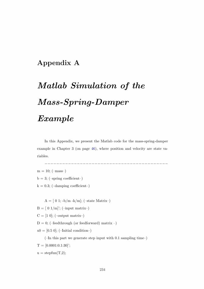
Appendix A
Matlab Simulation of the
Mass-Spring-Damper
Example
In this Appendix, we present the Matlab code for the mass-spring-damper
example in Chapter 3 (on page 46), where position and velocity are state va-
riables.
−−−−−−−−−−−−−−−−−−−−−−−−−−−−−−−−−−−−−−−−−−m = 10; (–mass–)
b = 3; (–spring coefficient–)
k = 0.3; (–damping coefficient–)
A = [ 0 1; -b/m -k/m]; (–state Matrix–)
B = [ 0 1/m]’; (–input matrix–)
C = [1 0]; (–output matrix–)
D = 0; (–feedthrough (or feedforward) matrix –)
x0 = [0.5 0]; (–Initial condition–)
(–In this part we generate step input with 0.1 sampling time–)
T = [0.0001:0.1:30]’;
u = stepfun(T,2);
234

(–Here we use lsim Matlab command to simulate the linear state-space model
and plot the results.–)
[z,x] = lsim(A,B,C,D,u,T,x0);
figure(1)
plot(T,[x(:,1) x(:,2) u])
legend(’position’, ’velocity’, ’Input’);
235
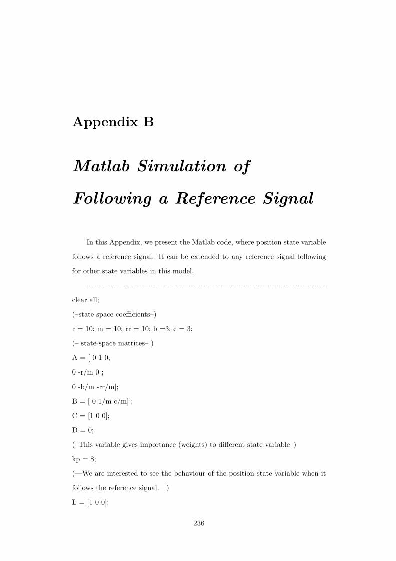
Appendix B
Matlab Simulation of
Following a Reference Signal
In this Appendix, we present the Matlab code, where position state variable
follows a reference signal. It can be extended to any reference signal following
for other state variables in this model.
−−−−−−−−−−−−−−−−−−−−−−−−−−−−−−−−−−−−−−−−−−clear all;
(–state space coefficients–)
r = 10; m = 10; rr = 10; b =3; c = 3;
(– state-space matrices– )
A = [ 0 1 0;
0 -r/m 0 ;
0 -b/m -rr/m];
B = [ 0 1/m c/m]’;
C = [1 0 0];
D = 0;
(–This variable gives importance (weights) to different state variable–)
kp = 8;
(—We are interested to see the behaviour of the position state variable when it
follows the reference signal.—)
L = [1 0 0];
236
AA = A - kp*B*L; (–state Matrix–)
BB = kp*B; (–input matrix–)
CC = C; (–output matrix–)
DD = D; (–feedthrough (or feedforward) matrix –)
(–In this part we generate step input with 0.1 sampling time–)
T = [0.0001:0.1:30]’;
u = stepfun(T,2);
(–Here we use lsim Matlab command to simulate the linear state-space mo-
del. –)
[y,x] = lsim(AA,BB,CC,DD,u,T);
(–Here we plot the state variables, control input and reference signal–)
figure(1)
plot(T,[x(:,1) x(:,2) x(:,3) u kp*(u-y)])
legend(’Position’,’Velocity’,’Zoom’, ’Reference signal’, ’Control Input’);
237
Appendix C
Bode Diagrams of Open-Loop
Transfer Function in Matlab
In this Appendix, we present the Matlab code, to plot Bode plots of the open-
loop transfer function for the human and controller with the setting mentioned
in Section 5.4.4 (on page 139).
−−−−−−−−−−−−−−−−−−−−−−−−−−−−−−−−−−−−−−−−−−clear all;
kdok=[]; gmm=0; pmm=0; K=5; D=1
(– Human model transfer function, K is the gain and D is the delay–)
Gh=tf([K],[1,D]);
(– Controller transfer function, a1 and b1 are coefficients in the state-space
model–)
a1 = 1;
b1 = 0.01;
Gc=tf([b1],[1 a1]);
(–Open loop transfer function for human operator and controller–)
Gopenloop=Gh*Gc;
238
(–Phase and Gain margins are calculated and plotted–)
[Gm,Pm, Wcg,Wcp] = margin(Gopenloop);
margin(Gopenloop);
GmdB=20*log 10(Gm);
[ GmdB Pm Wcg/(2 ∗ pi) Wcp/(2 ∗ pi) ];
if GmdB >0 & Pm > 0
kdok=[kdok; [a1 b1]];
if GmdB >= gmm & Pm >= pmm
kc=[a1 b1];
gmm=GmdB;
pmm=Pm;
end;
end;
239
Appendix D
Online Materials
Online materials which accompany this thesis are briefly listed below. The
up-to-date videos, publications, source codes, and the electronic version of this
thesis are available online at http://www.hamilton.ie/parisa/.
D.1 Materials
D.1.1 Model-based Target Sonification on Small Screen Devices:
Perception and Action
• Experiment I:
C++ source code for this experiment, which include training and main
applications in four different audio conditions is available at
http://www.hamilton.ie/parisa/Parisa files/Experiment I.zip
• Experiment II:
C++ source code for this experiment, which include training and main
applications in three different audio conditions is available at
http://www.hamilton.ie/parisa/Parisa files/Experiment II.zip
240
D.1 Materials
D.1.2 Tilt-Controlled Zooming User Interfaces on Mobile De-
vices
• Tilt-controlled Speed Dependent Automatic Zooming:
C++ source code for this application is available directly at
http://www.hamilton.ie/parisa/Parisa files/SDAZ-Tilt.zip
• Multimodal Tilt-controlled Speed Dependent Automatic Zooming:
C++ source code for this application is available directly at
http://www.hamilton.ie/parisa/Parisa files/SDAZ-Tilt-Sound.zip
• Stylus-controlled Speed Dependent Automatic Zooming:
C++ source code for this application is available directly at
http://www.hamilton.ie/parisa/Parisa files/SDAZ-Touch.zip
D.1.3 Multimodal Motion Controlled Focus-in-Context Method:
Sensing Complex Information
C++ source code for this application is available directly at
http://www.hamilton.ie/parisa/Parisa files/F+C(language,sound).zip
241