Parallel Jacobi-type algorithms for the singular and ... - CORE
130
Faculty of Science Department of Mathematics Vedran Novaković Parallel Jacobi-type algorithms for the singular and the generalized singular value decomposition DOCTORAL THESIS Zagreb, 2017
-
Upload
khangminh22 -
Category
Documents
-
view
1 -
download
0
Transcript of Parallel Jacobi-type algorithms for the singular and ... - CORE

Faculty of ScienceDepartment of Mathematics
Vedran Novaković
Parallel Jacobi-type algorithms for thesingular and the generalized singular
value decomposition
DOCTORAL THESIS
Zagreb, 2017


Faculty of ScienceDepartment of Mathematics
Vedran Novaković
Parallel Jacobi-type algorithms for thesingular and the generalized singular
value decomposition
DOCTORAL THESIS
Supervisor: prof. Sanja Singer, PhD
Zagreb, 2017


Prirodoslovno–matematički fakultetMatematički odsjek
Vedran Novaković
Paralelni algoritmi Jacobijeva tipa zasingularnu i generaliziranu singularnu
dekompoziciju
DOKTORSKI RAD
Mentor: prof. dr. sc. Sanja Singer
Zagreb, 2017.


A note on the supervisor and thecommittees (O mentoru i komisijama)
Sanja Singer was born in Zagreb on December 27th, 1963, where she earned BSc.(1986), MSc. (1993) and PhD. (1997) in mathematics at the University of Zagreb,Faculty of Science, Department of Mathematics.
From December 1987 to September 1989 she was employed as a junior assistantat the University of Zagreb, Faculty of Economics. Since September 1989 she hasbeen affiliated with the University of Zagreb, Faculty of Mechanical Engineeringand Naval Architecture, first as a research assistant, then assistant professor (2001–2007), associate professor (2007–2013) and full professor (2013–).
She has co-authored 27 papers, 17 of them published in journals. Her researchinterests are the algorithms for the dense matrix factorizations, eigenvalues andsingular values, and efficient parallelization of those algorithms.
Sanja Singer rođena je u Zagrebu 27. prosinca 1963., gdje je diplomirala (1986.),magistrirala (1993.) i doktorirala (1997.) na Matematičkom odsjeku Prirodoslovno–matematičkog fakulteta Sveučilišta u Zagrebu.
Od prosinca 1987. do rujna 1989. bila je zaposlena kao asistentica pripravnicana Ekonomskom fakultetu Sveučilišta u Zagrebu. Od rujna 1989. zaposlena je naFakultetu strojarstva i brodogradnje Sveučilišta u Zagrebu, prvo kao znanstvenanovakinja, a zatim kao docentica (2001.–2007.), izvanredna (2007.–2013.) i redovitaprofesorica (2013.–).
Koautorica je 27 znanstvenih radova, od kojih je 17 objavljeno u časopisima. Nje-zin znanstveni interes su algoritmi za računanje matričnih faktorizacija, svojstvenihi singularnih vrijednosti, te njihova efikasna paralelizacija.
The evaluationE and defenseD committees (komisije za ocjenuE i obranuD rada):
1. E,D Vjeran Hari, University of Zagreb (PMF-MO), full professor, chairman
2. E,D Enrique S. Quintana Ortí, Universitat Jaume I, Spain, full professor
3. E Zvonimir Bujanović, University of Zagreb (PMF-MO), assistant professor
4. D Sanja Singer, University of Zagreb (FSB), full professor, supervisor
This thesis was submitted on September 4th, 2017, to the Council of Department ofMathematics, Faculty of Science, University of Zagreb. Following a positive reviewby the evaluation committee, approved by the Council on November 8th (at its 2nd
session in academic year 2017/18), and after the submission of the thesis in itspresent (revised) form, the public defense was held on December 15th, 2017.


Acknowledgments
I would like to express my gratitude and dedicate this work to Sanja Singer, for tryingand succeeding to be a proactive, but at the same time not too active supervisor,
For drawing many of the figures shown here with METAPOST from handmadesketches, helping when all hope seemed to be lost while debugging the code, sortingout the bureaucratic hurdles, financing herself the research efforts when there wasno other way, and encouraging me for many years to finish this manuscript,
But also for stepping aside when it was best for me to discover, learn, and do thingsthe hard way myself, knowing that such experience does not fade with time,
And for being a friend in times when friendship was scarce.
This work has been supported in part by Croatian Science Foundation under theproject IP-2014-09-3670 (“Matrix Factorizations and Block Diagonalization Algo-rithms” – MFBDA); by grant 037–1193086–2771 (“Numerical methods in geophysi-cal models”) from Ministry of Science, Education and Sports, Republic of Croatia;by an NVIDIA’s Academic Partnership Program hardware donation (arranged byZlatko Drmač) to a research group from University of Zagreb, Croatia; and by thetravel grants from Swiss National Science Foundation, Universitat Jaume I, Spain,and The University of Manchester, United Kingdom.
The completion of this work would not be possible without the author havinggenerously been granted allocation of the computing resources and administrativesupport from Department of Mathematics, Faculty of Science, and from Faculty ofMechanical Engineering and Naval Architecture (by Hrvoje Jasak), University ofZagreb, Croatia; from Universitat Jaume I, Spain (by Enrique S. Quintana Ortí);and by the Hartree Centre and its staff at the Daresbury Laboratory of the Scienceand Technology Facilities Council, United Kingdom.
I am indebted to Saša Singer for fruitful advice, and for proofreading and cor-recting the manuscripts of the papers leading to this dissertation, alongside withNeven Krajina; and to Zvonimir Bujanović for GPU-related and Vjeran Hari formathematical discussions, all of University of Zagreb. Norbert Juffa of NVIDIA haskindly provided an experimental CUDA implementation of the rsqrt routine.
The people of NLAFET Horizon 2020 project and others who happened to be inmy vicinity should be thanked for bearing with me while finishing this manuscript.
“Hope. . . is not the conviction that something will turn out well, but the certaintythat something makes sense, regardless of how it turns out .” — Václav Havel


Abstract
In this thesis, a hierarchically blocked one-sided Jacobi algorithm for the singularvalue decomposition (SVD) is presented. The algorithm targets both single andmultiple graphics processing units (GPUs). The blocking structure reflects the levelsof the GPU’s memory hierarchy. To this end, a family of parallel pivot strategies onthe GPU’s shared address space has been developed, but the strategies are applicableto inter-node communication as well, with GPU nodes, CPU nodes, or, in general,any NUMA nodes. Unlike common hybrid approaches, the presented algorithm ina single-GPU setting needs a CPU for the controlling purposes only, while utilizingthe GPU’s resources to the fullest extent permitted by the hardware. When requiredby the problem size, the algorithm, in principle, scales to an arbitrary number ofGPU nodes. The scalability is demonstrated by more than twofold speedup forsufficiently large matrices on a four-GPU system vs. a single GPU.
The subsequent part of the thesis describes how to modify the two-sided Hari–Zimmermann algorithm for computation of the generalized eigendecomposition of asymmetric matrix pair (A,B), where B is positive definite, to an implicit algorithmthat computes the generalized singular value decomposition (GSVD) of a pair (F,G).In addition, blocking and parallelization techniques for accelerating both the CPUand the GPU computation are presented, with the GPU approach following theJacobi SVD algorithm from the first part of the thesis.
For triangular matrix pairs of a moderate size, numerical tests show that thedouble precision sequential pointwise algorithm is several times faster than the es-tablished DTGSJA algorithm in LAPACK, while the accuracy is slightly better, espe-cially for the small generalized singular values. Cache-aware blocking increases theperformance even further. As with the one-sided Jacobi-type (G)SVD algorithmsin general, the presented algorithm is almost perfectly parallelizable and scalableon the shared memory machines, where the speedup almost solely depends on thenumber of cores used. A distributed memory variant, intended for huge matricesthat do not fit into a single NUMA node, as well as a GPU variant, are also sketched.
The thesis concludes with the affirmative answer to a question whether the one-sided Jacobi-type algorithms can be an efficient and scalable choice for computingthe (G)SVD of dense matrices on the massively parallel CPU and GPU architectures.
Unless otherwise noted by the inline citations or implied by the context, thisthesis is an overview of the original research results, most of which has already beenpublished in [55, 58]. The author’s contributions are the one-sided Jacobi-type GPUalgorithms for the ordinary and the generalized SVD, of which the latter has not yetbeen published, as well as the parallelization technique and some implementationdetails of the one-sided Hari–Zimmermann CPU algorithm for the GSVD. The restis joint work with Sanja and Saša Singer.
Key words: one-sided Jacobi-type algorithms, (generalized) singular value decom-position, parallel pivot strategies, graphics processing units, (generalized) eigenvalueproblem, cache-aware blocking, (hybrid) parallelization.


Sažetak (prošireni)
Singularna dekompozicija, katkad zvana prema engleskom originalu i dekom-pozicija singularnih vrijednosti, ili kraće SVD, jedna je od najkorisnijih matričnihdekompozicija, kako za teorijske, tako i za praktične svrhe. Svaka matrica G ∈ Cm×n
(zbog jednostavnijeg zapisa, uobičajeno se smatra da je m ≥ n; u protivnom, tražise SVD matrice G∗) može se rastaviti u produkt tri matrice
G = UΣV ∗,
gdje su U ∈ Cm×m i V ∈ Cn×n unitarne, a Σ ∈ Rm×n je ‘dijagonalna’ s nenegativnimdijagonalnim elementima. Osim ovog oblika dekompozicije, koristi se i skraćeni oblik
G = U ′Σ′V ∗,
pri čemu je U ′ ∈ Cm×n matrica s ortonormiranim stupcima, a Σ′ = diag(σ1, . . . , σn),σi ≥ 0 za i = 0, . . . , n, je sada stvarno dijagonalna.
Izvan matematike, u ‘stvarnom’ životu, SVD se koristi u procesiranju slika (re-konstrukciji, sažimanju, izoštravanju) i signala, s primjenama u medicini (CT, tj.kompjuterizirana tomografija; MR, tj. magnetna rezonancija), geoznanostima, zna-nosti o materijalima, kristalografiji, sigurnosti (prepoznavanje lica), izvlačenja infor-macija iz velike količine podataka (na primjer, LSI, tj. latent semantic indexing), alii drugdje. Većina primjena koristi svojstvo da se iz SVD-a lako čita najbolja aprok-simacija dane matrice matricom fiksnog (niskog) ranga. Čini se da je lakše rećigdje se SVD ne koristi, nego gdje se koristi, stoga se SVD često naziva i “švicarskimnožićem matričnih dekompozicija”.1
Prvi počeci razvoja SVD-a sežu u 19. stoljeće, kad su poznati matematičari Euge-nio Beltrami, Camille Jordan, James Joseph Sylvester, Erhard Schmidt i HermanWeyl pokazali njezinu egzistenciju i osnovna svojstva (za detalje pogledati [74]).
Pioniri u numeričkom računanju SVD-a su Ervand George Kogbetliantz, te GeneGolub i William Kahan, koji su razvili algoritam za računanje (bidijagonalni QR),koji je dvadeset i pet godina vladao scenom numeričkog računanja SVD-a. U tovrijeme, sveučilište Stanford (gdje je Gene Golub radio) bilo je ‘glavno sjedište’ zarazvoj primjena SVD-a.
Početkom devedesetih godina, ‘sjedište SVD-a’ preseljeno je u Europu, nakonobjave članka [21] o relativnoj točnosti računanja svojstvenih vrijednosti simetrič-nih pozitivno definitnih matrica korištenjem Jacobijeve metode. Naime, problemračunanja svojstvene dekompozicije pozitivno definitne matrice i problem računa-nja SVD-a usko su vezani. Ako je poznata dekompozicija singularnih vrijednostimatrice G punog stupčanog ranga, G ∈ Cm×n = UΣV ∗, pri čemu je G faktormatrice A, A = G∗G, onda je A simetrična i pozitivno definitna i vrijedi
A = G∗G = V ΣTU∗UΣV ∗ = V diag(σ21, . . . , σ
2m)V ∗.
1Diane O’Leary, 2006.

Matrica V je matrica svojstvenih vektora, a svojstvene vrijednosti su kvadrati sin-gularnih vrijednosti. Stoga se algoritmi za računanje svojstvenih vrijednosti, kodkojih se transformacija vrši dvostranim (i slijeva i zdesna) djelovanjem na matricuA, mogu napisati implicitno, tako da se transformacija vrši ili zdesna na faktor Gili slijeva na faktor G∗.
U svojoj doktorskoj disertaciji Drmač [24] je napravio daljnju analizu, ne samosingularne dekompozicije računate Jacobijevim algoritmom, nego i generaliziranesingularne dekompozicije (GSVD). Temeljem tih istraživanja, SVD baziran na Ja-cobijevim rotacijama ušao je i u numeričku biblioteku LAPACK.
U međuvremenu, gotovo sva računala postala su višejezgrena, a moderni klasteriračunala za znanstveno računanje sastoje se od nekoliko tisuća do nekoliko stotinatisuća višejezgrenih procesora2, pa standardni sekvencijalni algoritmi nipošto višenisu primjereni za numeričko računanje. Stoga se ubrzano razvijaju paralelni al-goritmi koji poštuju i hijerarhijsku memorijsku strukturu odgovarajućih računala,težeći iskoristiti brzu cache memoriju za procesiranje potproblema u blokovima, nakoje je moguće primijeniti BLAS-3 operacije. Ideja blokiranja je u primjeni što više(tipično, kubično u dimenziji matrice) numeričkih operacija nad podacima u brzojmemoriji. Nadalje, pojavom grafičkih procesnih jedinica namijenjenih znanstvenomračunanju, kao i drugih visokoparalelnih numeričkih akceleratora (npr. Intel XeonPhi), otvorio se novi segment istraživanja, koji poštuje njihov masivni paralelizam,s pojedinačno slabašnom snagom svake dretve u odnosu na središnji procesor.
Generaliziranu singularnu dekompoziciju (GSVD) uveli su Van Loan [77], tePaige i Saunders [62]. Definicija GSVD-a nešto je manje poznata. Ako su zadanematrice F ∈ Cm×n i G ∈ Cp×n, za koje vrijedi
K =
[FG
], k = rank(K),
tad postoje unitarne matrice U ∈ Cm×m, V ∈ Cp×p, i matrica X ∈ Ck×n, takve daje
F = UΣFX, G = V ΣGX, ΣF ∈ Rm×k, ΣG ∈ Rp×k.
Elementi matrica ΣF i ΣG su nula, osim dijagonalnih elemenata, koji su realni inenegativni. Nadalje, ΣF i ΣG zadovoljavaju
ΣTFΣF + ΣT
GΣG = I.
Omjeri (ΣF )ii/(ΣG)ii su generalizirane singularne vrijednosti para (F,G). Ako jeG punog stupčanog ranga, tada je rank(K) = n i generalizirane singularne vrijed-nosti su konačni brojevi. Ako je par (F,G) realan, onda su realne sve matrice udekompoziciji. Odavde nadalje, zbog jednostavnoti pretpostavlja se da je par realan.
Može se pokazati da, ako je k = n, tada se relacija između GSVD-a i reduciraneforme CS (kosinus-sinus) dekompozicije (vidjeti, na primjer, [26]) može iskoristiti zanjezino računanje (pogledati, na primjer članke Stewarta [72, 73] i Suttona [75]).
Slično kao i SVD, generalizirana singularna dekompozicija ima primjene u mno-gim područjima, kao što je usporedna analiza podataka vezanih uz genome [1],
2https://www.top500.org
viii
nepotpuna singularna metoda rubnih elemeneata [47], ionosferna tomografija [9], alii mnogo drugih.
GSVD para matrica (F,G) blisko je vezana s hermitskim generaliziranim svoj-stvenim problemom za par (A,B) := (F ∗F,G∗G), tako da se metode za istovremenudijagonalizaciju para (A,B) mogu modificirati za računanje GSVD-a para (F,G).U ovoj radnji razvijen je brzi i efikasan algoritam za računanje generalizirane sin-gularne dekompozicije realnog para (F,G).
Metoda razvijena u radnji bazirana je na algoritmu za računanje generaliziranesvojstvene dekompozicije,
Ax = λBx, x 6= 0, (1)
gdje su A i B simetrične matrice, a par je definitan, tj. postoji realna konstanta µtakva da je matrica A−µB pozitivno definitna. Članke s metodom objavili su 1960.Falk i Langemeyer [31, 32] u slabo poznatom priručniku. Kad je paralelna verzijametode testirana, pokazalo se da pati zbog problema rastuće skale stupaca matricetijekom procesa ortogonalizacije. Treba još primijetiti da pozitivna definitnost ma-trice B odmah znači da je definitan i par (A,B).
Gotovo desetljeće nakon Falka i Langemeyera, Katharina Zimmermann je u svo-joj doktorskoj disertaciji [81] grubo skicirala metodu za rješavanje generaliziranogsvojstvenog problema (1) ako je B pozitivno definitna. Gose [34] je predložio op-timalnu ne-cikličku pivotnu strategiju i dokazao globalnu konvergenciju originalnemetode. Hari je u svojoj disertaciji [37], potaknut Zimmermanninom skicom me-tode, izveo algoritam i pokazao njegovu globalnu i kvadratičnu konvergenciju uzcikličke pivotne strategije.
Kvadratičnu konvergenciju originalne Falk–Langemeyerove metode dokazao je1988. Slapničar u svojem magisteriju, četiri godine nakon dokaza konvergencijeHari–Zimmermann metode. Hari je u [37] pokazao ključnu vezu između Hari–Zimmermannine i Falk–Langemeyerove varijante algoritma. Ako je matrica B obos-trano skalirana dijagonalnom matricom D, tako da su joj dijagonalni elementi jed-naki 1 prije svakog koraka poništavanja u Falk–Langemeyerovoj metodi, dobiva seHari–Zimmermannina metoda. Dakle, nova metoda imala je ključno svojstvo nor-miranosti stupaca barem jedne matrice, što se pokazalo iznimno bitnim za uspjehalgoritma (izbjegavanje skaliranja matrica tijekom procesa ortogonalizacije).
Treba reći da se GSVD može računati i na druge načine. Drmač je u [26] iz-veo algoritam za računanje GSVD-a para (F,G), kad je G punog stupčanog ranga.Algoritam transformira problem na samo jednu matricu, a nakon toga primjenjujejednostrani Jacobijev SVD algoritam. Taj algoritam računa generalizirane singu-larne vrijednosti s malom relativnom greškom. Algoritam svođenja na jednu matricusastoji se od tri koraka: skaliranje stupaca matrica F i G, QR faktorizacije sa stup-čanim pivotiranjem već skalirane matrice G, i konačno, rješavanjem trokutastoglinearnog sustava s k desnih strana. Posljednja dva koraka su sekvencijalna i vrloih je teško paralelizirati.
Sama ideja korištenja implicitne (tj. jednostrane) Falk–Langemeyerove metodeza GSVD para (F,G), s G punog stupčanog ranga, sreće se u disertaciji AnnetteDeichmöller [17], međutim, tamo se ne spominju usporedbe te metode s drugimmetodama.
ix

S druge strane, algoritam za računanje GSVD-a u biblioteci LAPACK (potpro-gram xGGSVD), je modificirani Kogbetliantzov algoritam (vidjeti Paige [61]) s obvez-nim pretprocesiranjem (vidjeti Bai i Demmel [5]). Algoritam pretprocesiranja [6]transformira zadani matrični par (F0, G0) u par (F,G), takav da su F i G gornje-trokutaste, a G je i nesingularna. Ako se unaprijed zna da je G punog stupčanogranga, i implicitna Falk–Langemeyerova i implicitna Hari–Zimmermannina metodaće raditi i bez pretprocesiranja. Ako su F i G vitke (engl. “tall and skinny”), QRfactorizacija obje matrice će ubrzati ortogonalizaciju. Ako G nije punog ranga, ondatreba koristiti isto pretprocesiranje kao u LAPACK-u, budući da puni stupčani rangmatrice G garantira pozitivnu definitnost matrice B := GTG.
∗ ∗ ∗
U ovoj radnji razvijen je i hijerarhijski, blokirani jednostrani algoritam za raču-nanje SVD-a. Opisani algoritam može raditi na višeprocesorskom računalu, računal-nim klasterima, jednoj ili više grafičkih procesnih jedinica. Princip rada algoritmana svim arhitekturama je sličan. Posebno je opisan algoritam koji radi na grafičkimprocesnim jedinicama. Struktura blokiranja reflektira razine memorijske strukturegrafičke procesne jedninice. Da bi se to postiglo, razvijene su familije paralelnihpivotnih strategija za dijeljenu (engl. shared) memoriju grafičkih procesnih jedinica.Uz dodatak rasporeda po procesima, strategije se mogu koristiti i kao strategijeza komuniciranje među računalnim čvorovima (bili oni grafičke procesne jedinice,jezgre procesora ili tzv. NUMA čvorovi).
Razvijeni algoritam nije hibridni, tj. centralnu procesnu jedinicu koristi samo zakontrolne svrhe, a cjelokupno računanje odvija se na grafičkoj procesnoj jedinici.Kad je zbog veličine problema potrebno, algoritam se može rasprostrijeti (skalirati)na proizvoljan broj grafičkih procesnih jedinica. Na dovoljno velikim matricama,skalabilnost je pokazana ubrzanjem od preko dva puta na četiri grafičke procesnejedinice, obzirom na jednu.
U drugom dijelu radnje opisuje se jedan način modifikacije dvostranog Hari–Zimmermanninog algoritma za računanje generalizirane svojstvene dekompozicijematričnog para (A,B), gdje su obje matrice simetrične, a B je pozitivno definitna.Implicitni algoritam računa GSVD para (F,G), pri čemu je (A,B) := (F TF,GTG).Nadalje, pokazuje se kako treba blokirati algoritam, te kako ga paralelizirati, i uslučaju standardnih, i u slučaju grafičkih procesora.
Za trokutaste matrične parove srednje velikih dimenzija (približno 5 000), poka-zano je da je već sekvencijalni, neblokirani algoritam u dvostrukoj točnosti, predlo-žen u radnji, nekoliko desetaka puta brži no što je to LAPACK potprogram DTGSJAi pritom ima nešto bolju točnost, posebno za male generalizirane singularne vri-jednosti. Blokiranje algoritma koje odgovara cacheima znatno ubrzava algoritam.Pokazuje se da je i ovaj algoritam, slično kao jednostrani Jacobijev algoritam zaSVD, gotovo idealno paralelizabilan i skalabilan na računalima s dijeljenom memo-rijom, te da njegovo ubrzanje gotovo isključivo ovisi o broju korištenih jezgara. Uvrijeme testiranja, pokazalo se da je paralelizirani i blokirani Hari–Zimmermanninalgoritam preko sto puta brži od LAPACK potprograma DTGESJA s višedretvenimBLAS potprogramima. Varijanta algoritma za razdijeljenu (engl. distributed) me-moriju namijenjena je ogromnim matricama koje ne stanu u jedan NUMA čvor.
x

Također, skicirana je i GPU varijanta algoritma, koja je vrlo slična jednostranomJacobijevom algoritmu za SVD.
Disertacija završava zaključkom da su ovi algoritmi Jacobijevog tipa efikasni iskalabilni i izvrstan su izbor za računanje (G)SVD-a punih matrica na masivnoparalelnim standardnim arhitekturama i na grafičkim procesnim jedinicama.
Ova doktorska disertacija bazirana je na originalnim znanstvenim radovima [55,58], te proširena nekim novim rezultatima. Autorov doprinos u ovoj disertacijisu novi paralelni algoritmi za (G)SVD za grafičke procesne jedinice, tehnike para-lelizacije, te detalji implementacije jednostranog Hari–Zimmermannina algoritma.Ostatak je zajednički rad sa Sanjom Singer i Sašom Singerom.
Ključne riječi: jednostrani algoritmi Jacobijeva tipa, (generalizirana) dekompozi-cija singularnih vrijednosti, paralelne pivotne strategije, grafičke procesne jedinice,(generalizirani) problem svojstvenih vrijednosti, blokiranje obzirom na cache me-moriju, (hibridna) paralelizacija.
xi


Contents
1. Introduction . . . . . . . . . . . . . . . . . . . . . . . . . . . . . . . . . . . . 1
2. The Jacobi-type multilevel (H)SVD algorithm for the GPU(s) . . . . 82.1. Jacobi–type SVD algorithm . . . . . . . . . . . . . . . . . . . . . . . . . 82.2. Parallel pivot strategies . . . . . . . . . . . . . . . . . . . . . . . . . . . 11
2.2.1. Generating the Jacobi p-strategies . . . . . . . . . . . . . . . . . 162.3. A single-GPU algorithm . . . . . . . . . . . . . . . . . . . . . . . . . . . 31
2.3.1. The Cholesky factorization . . . . . . . . . . . . . . . . . . . . . . 332.3.2. The QR factorization . . . . . . . . . . . . . . . . . . . . . . . . . 352.3.3. The orthogonalization . . . . . . . . . . . . . . . . . . . . . . . . 362.3.4. The Jacobi rotations . . . . . . . . . . . . . . . . . . . . . . . . . 402.3.5. The postmultiplication . . . . . . . . . . . . . . . . . . . . . . . . 422.3.6. A GPU-wide convergence criterion . . . . . . . . . . . . . . . . . 422.3.7. An illustration of the algorithm’s execution . . . . . . . . . . . . 45
2.4. A multi-GPU algorithm . . . . . . . . . . . . . . . . . . . . . . . . . . . 462.5. Numerical testing . . . . . . . . . . . . . . . . . . . . . . . . . . . . . . . 50
2.5.1. Modern CUDA on modern hardware . . . . . . . . . . . . . . . . 562.6. Parallel norm computation . . . . . . . . . . . . . . . . . . . . . . . . . . 58
3. The implicit Hari–Zimmermann algorithm for the GSVD . . . . . . . 613.1. The Jacobi–type sequential algorithms for GEP . . . . . . . . . . . . . . 61
3.1.1. The Falk–Langemeyer algorithm . . . . . . . . . . . . . . . . . . 613.1.2. The Hari–Zimmermann algorithm . . . . . . . . . . . . . . . . . . 62
3.2. The Jacobi–type algorithms for GSVD . . . . . . . . . . . . . . . . . . . 663.2.1. The implicit Hari–Zimmermann algorithm . . . . . . . . . . . . . 663.2.2. Blocking in the one-sided algorithm . . . . . . . . . . . . . . . . . 70
3.3. The parallel algorithms . . . . . . . . . . . . . . . . . . . . . . . . . . . . 773.3.1. A shared memory algorithm . . . . . . . . . . . . . . . . . . . . . 773.3.2. A distributed memory algorithm . . . . . . . . . . . . . . . . . . 80
3.4. Numerical testing . . . . . . . . . . . . . . . . . . . . . . . . . . . . . . . 823.5. An implicit Hari–Zimmermann algorithm for the GPU(s) . . . . . . . . . 88
4. Conclusions and future work . . . . . . . . . . . . . . . . . . . . . . . . . 924.1. Conclusions . . . . . . . . . . . . . . . . . . . . . . . . . . . . . . . . . . 924.2. A work in progress . . . . . . . . . . . . . . . . . . . . . . . . . . . . . . 93
4.2.1. A new hierarchy for the Jacobi-type processes . . . . . . . . . . . 934.3. A note on the figures and the software . . . . . . . . . . . . . . . . . . . 99
5. Bibliography . . . . . . . . . . . . . . . . . . . . . . . . . . . . . . . . . . . 100
6. Biography . . . . . . . . . . . . . . . . . . . . . . . . . . . . . . . . . . . . . 109


1. Introduction
Why this thesis? Apart to fulfill one of the requirements for a doctoral degree, ofcourse. . . ? Out of a conviction that the results it summarizes are useful to a diverseaudience that tries to compute the large singular value decompositions (SVDs) andthe generalized singular value decompositions (GSVDs), or many small, similar-sizedones, arising from a plethora of the real-life problems, as fast as possible, and/oras accurately as possible, on a wide range of dense matrices, on almost any modernhigh performance computing hardware.
The main part and contribution of the thesis is contained in chapters 2 and 3, inwhich the one-sided Jacobi-type SVD algorithm for the graphics processing units,and the implicit Hari–Zimmermann method for the GSVD, respectively, are devel-oped. In the following, after a short overview of the singular value decomposition,those chapters are independently introduced, while each chapter on its own startswith a summary of its contents.
The thesis concludes with some directions for the future work on fully utilizingthe vectorization capabilities of the CPUs for the Jacobi-type (G)SVD algorithms.
About the singular value decomposition
The SVD is one of the most useful matrix decompositions, for theoretical as wellas practical considerations. Any matrix G ∈ Cm×n (to simplify the notation, assumem ≥ n; otheriwse, take the SVD of G∗ instead) can be decomposed as a product ofthree matrices
G = UΣV ∗,
where U ∈ Cm×m and V ∈ Cn×n are unitary, and Σ ∈ Rm×n is a ‘diagonal’ matrix,with the non-negative diagonal elements. Apart from this form of the decomposition,a ‘truncated’ form
G = U ′Σ′V ∗
is also widely used, where U ′ ∈ Cm×n is a matrix with the orthonormal columns,and Σ′ = diag(σ1, . . . , σn), σi ≥ 0 for i = 0, . . . , n, is now truly diagonal.
It is often repeated that the “SVD is the Swiss Army knife of matrix decomposi-tions”.1 And indeed, it would be easier to enumerate the applications of numericallinear algebra as such that do not benefit from the SVD either directly or indirectly,than to list those that do.
Outside of the realm of mathematics, in the ‘real-life’ domains, the SVD is usedin image (reconstruction, compression, deblurring) and signal processing, with appli-cations in medicine (CT, i.e., computed tomography; MRI, i.e., magnetic resonanceimaging), geosciences, material science, crystallography, security applications (facialrecognition), information retrieval from big datasets (e.g., LSI, i.e., latent semantic
1Diane O’Leary, 2006.

1. Introduction
indexing), and elsewhere. Most applications rely on a property that the SVD pro-vides an easy method of computing the best approximation of a given matrix by amatrix of the fixed (low) rank.
The first developments of a concept of the SVD date back to the 19th century,when the well-known mathematicians Eugenio Beltrami, Camille Jordan, JamesJoseph Sylvester, Erhard Schmidt, and Herman Weyl showed the decomposition’sexistence and some of its basic properties (see [74] for details).
Alongside Ervand George Kogbetliantz, the pioneers of the numerical compu-tation of the SVD were Gene Golub and William Kahan, who had developed aneffective algorithm (the bidiagonal QR), which dominated the computational scenefor twenty five years. At that time, the Stanford University (where Gene Golub wasteaching) was the ‘headquarters’ for development of the SVD’s applications.
At the begining of 1990s, the ‘SVD headquarters’ moved to Europe, after thepaper [21] had been published, concerning the relative accuracy of the computationof the eigenvalues of Hermitian positive definite matrices by the Jacobi method.
Computation of the eigenvalue decomposition (EVD) of a positive definite matrixand computation of the SVD are closely related. If the SVD of a matrix G of thefull column rank is given, G ∈ Cm×n = UΣV ∗, where G is a factor of the matrix A,A = G∗G, then A is a Hermitian positive definite matrix, and it holds that
A = G∗G = V ΣTU∗UΣV ∗ = V diag(σ21, . . . , σ
2m)V ∗.
The eigenvalues here are the squares of the singular values, and the eigenvectorsare the columns of the matrix V . Therefore, the eigendecomposition algorithms,which transform the matrix A from both the left and the right side (the “two-sided”approach), can also be rewritten in an ‘implicit’ way (the “one-sided” approach),such that either the factor G (i.e., its columns) is transformed from the right side,or the factor G∗ (i.e., its rows) is transformed from the left side, only.
In his doctoral thesis Drmač [24] has provided a more detailed analysis, not onlyof the SVD computed by the Jacobi algorithm, but also of the generalized singularvalue decomposition (GSVD). Following that research, the SVD based on the Jacobirotations has been included in the LAPACK numerical subroutine library.
In the meantime, almost all processors have started to be designed as multicoreones, while the modern clusters for high performance computing contain from acouple of thousands up to several hundreds of thousands of multicore CPUs2.
Therefore, the standard sequential algorithms are no longer adequate for numer-ical computing. Such a trend has spurred the development of the parallel algorithmsthat respect and follow the hierarchical structure of the computers’ memory architec-ture, with an intent to utilize the fast cache memory for processing the subproblemsin blocks, to which the BLAS-3 operations can be applied.
The blocking idea stems from the desire to apply as many (e.g., cubically interms of the matrix dimension) floating-point operations over the data as possible,while it resides in the fast memory. Furthermore, the recent advent of the graphicalprocessing units specifically designed for scientific computing, and other kinds of thehighly parallel numerical accelerators (e.g., Intel Xeon Phi), a whole new segment
2https://www.top500.org
2

of research has been opened, that targets that massive parallelism while bearing inmind a relatively weak computational power of each thread, compared to a typicalCPU.
The one-sided Jacobi-type SVD for the GPU(s)
Graphics processing units (GPUs) have become a widely accepted tool of par-allel scientific computing, but many of the established algorithms still need to beredesigned with massive parallelism in mind. Instead of multiple CPU cores, whichare fully capable of simultaneously processing different operations, GPUs are essen-tially limited to many concurrent instructions of the same kind—a paradigm knownas SIMT (single-instruction, multiple-threads) parallelism.
The SIMT type of parallelism is not the only reason for the redesign. Mod-ern CPU algorithms rely on (mostly automatic) multilevel cache management forspeedup. GPUs instead offer a complex memory hierarchy, with different accessspeeds and patterns, and both automatically and programmatically managed caches.Even more so than in the CPU world, a (less) careful hardware-adapted blocking ofa GPU algorithm is the key technique by which considerable speedups are gained(or lost).
The introductory paper [56] proposed a non-blocked (i.e., pointwise) single-GPUone-sided Jacobi SVD algorithm. In this thesis a family of the full block [40] andthe block-oriented [39] one-sided Jacobi-type algorithm variants for the ordinary sin-gular value decomposition (SVD) and the hyperbolic singular value decomposition(HSVD) of a matrix is presented, targeting both a single GPU and multiple GPUs.The blocking of the algorithm follows the levels of the GPU memory hierarchy;namely, the innermost level of blocking tries to maximize the amount of compu-tation done inside the fastest (and smallest) memory of the registers and manualcaches. The GPU’s global RAM and caches are considered by the midlevel, whileinter-GPU communication and synchronization are among the issues addressed bythe outermost level of blocking.
At each blocking level an instance of either the block-oriented or the full blockJacobi (H)SVD is run, orthogonalizing pivot columns or block-columns by concep-tually the same algorithm at the lower level. Thus, the overall structure of thealgorithm is hierarchical (or recursive) in nature and ready to fit not only the cur-rent GPUs, but also various other memory and communication hierarchies, providedthat efficient, hardware-tuned implementations at each level are available.
The Jacobi method is an easy and elegant way to find the eigenvalues and eigen-vectors of a symmetric matrix. In 1958 Hestenes [41] developed the one-sided JacobiSVD method: an implicit diagonalization is performed by orthogonalizing a factorof a symmetric positive definite matrix. But, after discovery of the QR algorithmin 1961–62 by Francis and Kublanovskaya, the Jacobi algorithm seemed to have nofuture, at least in the sequential processing world, due to its perceived slowness [30].
However, a new hope for the algorithm has been found in its amenability to par-allelization (including vectorization, as a way of computing multiple transformationsat once), in its proven high relative accuracy [21], and, finally, in the emergence ofthe fast Jacobi SVD implementation in LAPACK, due to Drmač and Veselić [28, 29].
3

1. Introduction
In the beginning of the 1970s Sameh in [65] developed two strategies for parallelexecution of the Jacobi method on Illiac IV. The first of those, the modulus strategy,is still in use, and it is one of the very rare parallel strategies for which a proof ofconvergence exists [50].
In the mid 1980s, Brent and Luk designed another parallel strategy [12], knownby the names of its creators. The same authors, together with Van Loan [13],described several parallel one-sided Jacobi and Kogbetliantz (also known as “thetwo-sided Jacobi”) algorithms. The parallel block Kogbetliantz method is developedin [78].
In 1987 Eberlein [30] proposed two strategies, the round-robin strategy, andanother one that depends on the parity of a sweep. A new efficient recursive divide-exchange parallel strategy, specially designed for the hypercube topologies (and,consequently, matrices of order 2n) is given in [33]. This strategy is later refined byMantharam and Eberlein in [51] to the block-recursive (BR) strategy.
Two papers by Luk and Park [50, 49] published in 1989 established equivalencebetween numerous strategies, showing that if one of them is convergent, then allequivalent strategies are convergent. In the same year Shroff and Schreiber [66]showed convergence for a family of strategies called the wavefront ordering, anddiscussed the parallel orderings weakly equivalent to the wavefront ordering, andthus convergent.
One of the first attempts to implement a parallel SVD on a GPU was a hybridone, by Lahabar and Narayanan [48]. It is based on the Golub–Reinsch algorithm,with bidiagonalization and updating of the singular vectors performed on a GPU,while the rest of the bidiagonal QR algorithm is computed on a CPU. In MAGMA3,a GPU library of the LAPACK-style routines, DGESVD algorithm is also hybrid, withbidiagonalization (DGEBRD) parallelized on a GPU [76], while for the bidiagonal QR,LAPACK routine DBDSQR is used.
In two previous papers [69, 68] the parallel one-sided Jacobi algorithms for the(H)SVD were discussed, with two and three levels of blocking, respectively. Theoutermost level is mapped to a ring of CPUs which communicate according to aslightly modified modulus strategy, while the inner two (in the three-level case) aresequential and correspond to the “fast” (L1) and “slow” (L2 and higher) cache levels.
At first glance a choice of the parallel strategy might seem like a technical detail,but the tests at the outermost level have shown that the modified modulus strategycan be two times faster than the round-robin strategy. That was a motivation toexplore if and how even faster strategies could be constructed that preserve theaccuracy of the algorithm. A class of parallel strategies is presented here, designedaround a conceptually simple but computationally difficult notion of a metric ona set of strategies of the same order. These new strategies can be regarded asgeneralizations of the Mantharam–Eberlein BR strategy to all even matrix orders,outperforming the Brent and Luk and modified modulus strategies in the GPUalgorithm.
However, a parallel strategy alone is not sufficient to achieve decent GPU per-formance. The standard routines that constitute a block Jacobi algorithm, like the
3Matrix Algebra on GPU and Multicore Architectures, http://icl.utk.edu/magma/
4
Gram matrix formation, the Cholesky (or the QR) factorization, and the point-wise one-sided Jacobi algorithm itself, have to be mapped to the fast, but in manyways limited, shared memory of a GPU, and to the peculiar way the computationalthreads are grouped and synchronized. Even the primitives that are usually takenfor granted, like the numerically robust calculation of a vector’s 2-norm, presenta challenge on a SIMT architecture. Combined with the problems inherent in theblock Jacobi algorithms, whether sequential or parallel, like the reliable convergencecriterion, a successful design of the Jacobi-type GPU (H)SVD is far from trivial.
This thesis aims to show that such GPU-centric design is possible and that theJacobi-type algorithms for a single GPU and multiple GPUs compare favorably tothe present state of the art in the GPU-assisted computation of the (H)SVD. Sinceall computational work is offloaded to a GPU, there is no need for a significantamount of CPU ↔ GPU communication, or for complex synchronization of theirtasks. This facilitates scaling to a large number of GPUs, while keeping their load inbalance and communication simple and predictable. While many questions remainopen, the algorithms presented here might prove themselves to be a valuable choiceto consider when computing the (H)SVD on the GPUs.
The implicit Hari–Zimmermann method for the GSVD
The singular value decomposition (SVD) is a widely used tool in many applica-tions. Similarly, a generalization of the SVD for a matrix pair (F,G), the gener-alized SVD (GSVD), has applications in many areas, such as comparative analysisof the genome-scale expression data sets [1], incomplete singular boundary elementmethod [47], ionospheric tomography [9], and many others.
The GSVD of a pair (F,G) is closely related to the Hermitian generalized eigen-value problem (GEP) of a pair (A,B) := (F ∗F,G∗G), so the methods for simulta-neous diagonalization of (A,B) can be modified to compute the GSVD of (F,G).The aim is to develop a fast and efficient parallel algorithm for the real pair (F,G).
The definition of the GSVD (see, for example, [62]), in its full generality, is asfollows: for given matrices F ∈ Cm×n and G ∈ Cp×n, where
K =
[FG
], k = rank(K),
there exist unitary matrices U ∈ Cm×m, V ∈ Cp×p, and a matrix X ∈ Ck×n, suchthat
F = UΣFX, G = V ΣGX, ΣF ∈ Rm×k, ΣG ∈ Rp×k. (1.1)
The elements of ΣF and ΣG are zeros, except for the diagonal entries, which are realand nonnegative. Furthermore, ΣF and ΣG satisfy
ΣTFΣF + ΣT
GΣG = I.
The ratios (ΣF )ii/(ΣG)ii are called the generalized singular values of the pair (F,G).If G is of full column rank, then rank(K) = n, and the generalized singular valuesare finite numbers. If the pair (F,G) is real, then all matrices in (1.1) are real. Fromnow on, it is assumed that all matrices are real.
5

1. Introduction
In 1960, Falk and Langemeyer published two papers [31, 32] on the computationof the GEP,
Ax = λBx, x 6= 0, (1.2)
where A and B are symmetric matrices and B is positive definite. Their methodwas shown in 1991 by Slapničar and Hari [71] to work for definite matrix pairs. Thepair (A,B) is definite if there exists a real constant µ such that the matrix A− µBis positive definite.
Note that, if B is positive definite, then the pair (A,B) is definite. This can beproved easily by using the Weyl theorem (see, for example, [43, Theorem 4.3.1, page181]). In this case,
λi(A+ (−µ)B) ≥ λi(A) + λmin(−µB) = λi(A)− µλmax(B), (1.3)
where λi(·) denotes the i-th smallest eigenvalue of a matrix. If A is positive definite,any µ ≤ 0 will make the pair definite. If A is indefinite, or negative definite, itsuffices to choose µ < 0 in (1.3) of such magnitude that λmin(A) − µλmax(B) > 0holds.
Almost a decade after Falk and Langemeyer, Zimmermann in her Ph.D. the-sis [81] briefly sketched a new method for the problem (1.2) if B is positive definite.Gose [34] proposed some optimal non-cyclic pivot strategies and proved the globalconvergence of the original method. Hari in his Ph.D. thesis [37] filled in the miss-ing details of the method of Zimmermann, and proved its global and quadraticconvergence under the cyclic pivot strategies.
The quadratic convergence of the original Falk–Langemeyer method was provedin 1988, by Slapničar in his MS thesis, four years after the proof of the convergenceof the Hari–Zimmermann method, and the results were extended afterwards andpublished in [71]. In the same paper, Slapničar and Hari also showed the followingconnection between the Hari–Zimmermann and the Falk–Langemeyer variants of themethod. If the matrix B is scaled (from both sides) so that its diagonal elementsare equal to 1, before each annihilation step in the Falk–Langemeyer method, thenthe Hari–Zimmermann method is obtained.
The GSVD was introduced by Van Loan [77] and Paige and Saunders [62]. Ifk = n in (1.1), then the relation between the GSVD and the reduced form ofthe CS (cosine-sine) decomposition (see, for example, [26]) could be used for thecomputation of the GSVD; see the papers by Stewart [72, 73] and Sutton [75].
Drmač in [26] derived an algorithm for the computation of the GSVD of a pair(F,G), with G of full column rank. This algorithm transforms the problem to asingle matrix, and then applies the ordinary Jacobi SVD algorithm. The algorithmproduces the generalized singular values with small relative errors. The part ofthe algorithm that reduces the problem to a single matrix consists of three steps: ascaling of the columns of both matrices F and G, the QR factorization with pivotingof the already scaled G, and, finally, a solution of a triangular linear system with kright-hand sides. The last two steps are inherently sequential and, therefore, hardto parallelize.
The idea of using an implicit (i.e., one-sided) version of the Falk–Langemeyermethod for the GSVD of a pair (F,G), with G of full column rank, can be found in
6

the Ph.D. thesis of Deichmöller [17], but there is no comment on how this methodperforms in comparison with the other methods.
On the other hand, the state of the art algorithm xGGSVD for computing theGSVD in LAPACK, is a Kogbetliantz-based variation of the Paige algorithm [61] byBai and Demmel [5], with preprocessing. The preprocessing algorithm [6] transformsa given matrix pair (F0, G0) to a pair (F,G), such that F and G are upper triangularand G is nonsingular. If it is known in advance that G is of full column rank,both implicit methods, the Falk–Langemeyer and the Hari–Zimmermann methodwill work without preprocessing. But, if F and G are tall and skinny, the QRfactorization of both matrices will speed up the orthogonalization. If G is not offull column rank, the same preprocessing technique (as in LAPACK) should be usedby the implicit algorithm, since a full column rank G guarantees that B := GTG ispositive definite.
Finally, a prototype of the implicit blocked Hari–Zimmermann method has beendeveloped for the GPU(s), along the same lines (so much that many routines havesimply been reused) as the one-sided Jacobi-type SVD algorithm from the previouschapter, and briefly sketched at the end of the main part of the thesis.
A comparison with the published work
The second chapter of the thesis is based on [55] and (unless stated by thecitations otherwise or implied by the context) is a sole contribution of the candidate.The published material has been expanded, namely, by the additional considerationswith regard to the parallel strategies, and by some implementation suggestions andnew test results on the modern GPUs.
The third chapter is based on [58], where the published version has been ex-panded, most notably by an algorithm variant that targets the GPUs. That algo-rithm variant, as well as all software implementations (save for the modified modulusstrategy and the first-level block-partitioning), the parallelization and column sort-ing techniques, and most of the numerical testing results are a sole contribution ofthe candidate, while the rest of the chapter’s material has been prepared in collab-oration with Sanja and Saša Singer.
7

2. The Jacobi-type multilevel (H)SVDalgorithm for the GPU(s)
This chapter is organized as follows. In section 2.1. a brief summary of the one-sided Jacobi-type (H)SVD block algorithm variants is given. In section 2.2. newparallel Jacobi strategies are developed: nearest to row-cyclic and nearest to column-cyclic. The main part is contained in section 2.3., where a detailed implementationof a single-GPU Jacobi (H)SVD algorithm is described. In section 2.4., a proof-of-concept implementation on multiple GPUs is presented. In section 2.5., results ofthe numerical testing are given. Section 2.6. completes the chapter with a parallel,numerically stable procedure for computing the 2-norm of a vector.
2.1. Jacobi–type SVD algorithm
Suppose that a matrix G ∈ Fm×n, where F denotes the real (R) or the complex(C) field, is given. Without loss of generality, it may be assumed that m ≥ n. Ifnot, instead of G, the algorithm will transform G∗.
Ifm� n, or if the column rank of G is less than n, then the first step of the SVDis to preprocess G by the QR factorization with column pivoting [25] and, possibly,row pivoting or row presorting,
G = PrQRPc = PrQ
[R0
0
]Pc, (2.1)
where Q is unitary, R0 ∈ Fk×n is upper trapezoidal with the full row rank k, whilePr and Pc are permutations. If k < n, then R0 should be factored by the LQfactorization,
R0 = P ′rLQ′P ′c = P ′r
[L0 0
]Q′P ′c. (2.2)
Finally, L0 ∈ Fk×k is a lower triangular matrix of full rank. From the SVD of L0,by (2.1) and (2.2), it is easy to compute the SVD of G. Thus, it can be assumedthat the initial G is square and of full rank n, with n ≥ 2.
The one-sided Jacobi SVD algorithm for G can be viewed as the implicit two-sided Jacobi algorithm which diagonalizes either G∗G or GG∗. Let, e.g., H := G∗G.Stepwise, a suitably chosen pair of pivot columns gp and gq of G is orthogonal-ized by postmultiplying the matrix
[gp gq
]by a Jacobi plane rotation Vpq, which
diagonalizes the 2× 2 pivot matrix Hpq,
Hpq =
[hpp hpqh∗pq hqq
]=
[g∗pgp g
∗pgq
g∗qgp g∗qgq
]=
[g∗pg∗q
] [gp gq
], (2.3)
such thatV ∗pqHpqVpq = diag(λp, λq). (2.4)

2.1. Jacobi–type SVD algorithm
In case of convergence, after a number of steps, the product of transformationmatrices will approach the set of eigenvector matrices. Let V be an eigenvectormatrix of H. Then
Λ = V ∗HV = (V ∗G∗)(GV ), Λ = diag(λ1, λ2, . . . , λn).
The resulting matrix GV has orthogonal columns and can be written as
GV = UΣ, (2.5)
where U is unitary and Σ = Λ1/2 is a diagonal matrix of the column norms of GV .The matrix U of the left singular vectors results from scaling the columns of GV
by Λ−1/2, so only the right singular vectors V have to be obtained, either by accu-mulation of the Jacobi rotations applied to G, or by solving the linear system (2.5)for V , with the initial G preserved. The system (2.5) is usually triangular, since Gis either preprocessed in such a form, or already given as a Cholesky factor. Solving(2.5) is therefore faster than accumulation of V , but it needs more memory and maybe less accurate if G is not well-conditioned (see [27]).
The choice of pivot indices p, q in successive steps is essential for possible paral-lelization of the algorithm. Let the two pairs of indices, (p, q) and (p′, q′), be calleddisjoint , or non-colliding , if p 6= q, p′ 6= q′, and {p, q} ∩ {p′, q′} = ∅. Otherwise, thepairs are called colliding . These definitions are naturally extended to an arbitrarynumber of pairs. The pairs of indexed objects (e.g., the pairs of matrix columns) aredisjoint or (non)colliding if such are the corresponding pairs of the objects’ indices.
The one-sided Jacobi approach is better suited for parallelization than the two-sided one, since it can simultaneously process disjoint pairs of columns. This is stillnot enough to make a respectful parallel algorithm. In the presence of a memoryhierarchy, the columns of G and V should be grouped together into block-columns,
G =[G1 G2 · · · Gb
], V =
[V1 V2 · · · Vb
]. (2.6)
In order to balance the workload, the block-columns should be (almost) equallysized.
Usually, a parallel task processes two block-columns Gp and Gq, indexed by a sin-gle pivot block-pair, either by forming the pivot block-matrix Hpq and its Choleskyfactor Rpq,
Hpq =
[G∗pGp G∗pGq
G∗qGp G∗qGq
]=
[G∗pG∗q
] [Gp Gq
], P ∗HpqP = R∗pqRpq, (2.7)
or by shortening the block-columns[Gp Gq
]directly, by the QR factorization,
[Gp Gq
]P = Qpq
[Rpq
0
]. (2.8)
When it is easy from the context to disambiguate a reference to the (block-)columnsfrom a one to their (block-)indices, in what follows “the (block-)columns indexed bya pivot (block-)pair” expression will be shortened to “a (block-)pivot pair”.
9

2. The Jacobi-type multilevel (H)SVD algorithm for the GPU(s)
The diagonal pivoting in the Cholesky factorization, or analogously, the columnpivoting in the QR factorization should be employed, if possible (see [69] for furtherdiscussion, involving also the HSVD case). However, the pivoting in factorizations(2.7) or (2.8) may be detrimental to performance of the parallel implementationsof the respective factorizations, so the factorizations’ nonpivoted counterparts haveto be used in those cases (with P = I). Either way, a square pivot factor Rpq isobtained. Note that the unitary matrix Qpq in the QR factorization is not neededfor the rest of the Jacobi process, and it consequently does not have to be computed.
Further processing of Rpq is determined by a variant of the Jacobi algorithm.The following variants are advisable: block-oriented variant (see [39]), in whichthe communication (or memory access) overhead between the tasks is negligiblecompared to the computational costs, and full block variant (see [40]) otherwise.
In both variants, Rpq is processed by an inner one-sided Jacobi method. In theblock-oriented variant, exactly one (quasi-)sweep of the inner (quasi-)cyclic1 Jacobimethod is allowed. Therefore, Rpq is transformed to R′pq = RpqVpq, with Vpq beinga product of the rotations applied in the (quasi-)sweep. In the full block variant,the inner Jacobi method computes the SVD of Rpq, i.e., RpqVpq = UpqΣpq. Let V ′pqdenote the transformation matrix, either Vpq from the former, or Vpq from the lattervariant.
Especially for the full block variant, the width of the block-columns should bechosen such that Rpq and V ′pq jointly saturate, without being evicted from, the fastlocal memory (e.g., the private caches) of a processing unit to which the block-columns
[Gp Gq
]are assigned. This also allows efficient blocking of the matrix
computations in (2.7) (or (2.8)) and (2.9), as illustrated in subsections 2.3.1. and2.3.5.
Having computed V ′pq, the block-columns of G (and, optionally, V ) are updated,[G′p G′q
]=[Gp Gq
]V ′pq,
[V ′p V ′q
]=[Vp Vq
]V ′pq. (2.9)
The tasks processing disjoint pairs of block-columns may compute concurrently withrespect to each other, up to the local completions of updates (2.9). A task thenreplaces (at least) one of its updated block-columns of G by (at least) one updatedblock-column of G from another task(s). Optionally, the same replacement patternis repeated for the corresponding updated block-column(s) of V . The block-columnreplacements entail a synchronization of the tasks. The replacements are performedby communication or, on shared-memory systems, by assigning a new pivot block-pair to each of the tasks.
The inner Jacobi method of both variants may itself be blocked, i.e., may divideRpq into block-columns of an appropriate width for the next (usually faster butsmaller) memory hierarchy level. This recursive blocking principle terminates atthe pointwise (nonblocked) Jacobi method, when no advantages in performancecould be gained by further blocking. In that way a hierarchical (or multilevel)blocking algorithm is created, with each blocking level corresponding to a distinctcommunication or memory domain (see [68]).
1See section 2.2. for the relevant definitions.
10

2.2. Parallel pivot strategies
For example, in the case of a multi-GPU system, access to the global memory(RAM) of a GPU could be identified as slow compared to the shared memory andregister access, and data exchange with another GPU could be identified as slowcompared to access to the local RAM. This suggests the two-level blocking for asingle-GPU algorithm, and the three-level for a multi-GPU one.
The inner Jacobi method, whether blocked or not, may be sequential or parallel.Both a single-GPU and a multi-GPU algorithm are examples of a nested parallelism.
Similar ideas hold also for the HSVD. If G ∈ Fm×n, m ≥ n, and rank(G) =rank(GJG∗), where J = diag(±1), with the number of positive signs in J alreadygiven (e.g., by the symmetric indefinite factorization with complete pivoting [70]),then the HSVD of G is (see [60, 80])
G = U
[Σ0
]V ∗, Σ = diag(σ1, . . . , σn), σ1 ≥ σ2 ≥ · · ·σn ≥ 0. (2.10)
Here, U is a unitary matrix of order m, while V is J-unitary (i.e., V ∗JV = J) oforder n. The HSVD in (2.10) can be computed by orthogonalization of either theof columns of G∗ by trigonometric rotations [23], or the columns of G by hyperbolicrotations [79].
A diagonalization method for the symmetric definite (or indefinite) matricesrequires only the partial SVD (or HSVD), i.e., the matrix V is not needed. Withthe former algorithm, the eigenvector matrix U should be accumulated, but withthe latter, it is easily obtainable by scaling the columns of the final G. Thus, thehyperbolic algorithm is advantageous for the eigenproblem applications, as shownin [69]. From the HSVD of G, as in (2.10), it immediately follows the EVD ofA := GJG∗, since (consider the case with m = n, for simplicity)
AU = (GJG∗)U = (UΣV ∗JV ΣU∗)U = UΣ2J(U∗U) = UΣ2J,
with the columns of U being the eigenvectors, and Σ2J being the eigenvalues of A.In the following it is assumed that F = R, but everything, save the computation
of the Jacobi rotations and the hardware-imposed block sizes, is valid also for F = C.
2.2. Parallel pivot strategies
In each step of the classical, two-sided Jacobi (eigenvalue) algorithm, the pivotstrategy seeks and annihilates an off-diagonal element hpq with the largest magni-tude. This approach has been generalized for the parallel two-sided block-Jacobimethods [7]. However, the one-sided Jacobi algorithms would suffer from a pro-hibitive overhead of forming and searching through the elements of H = G∗G. Inthe parallel algorithm there is an additional problem of finding bn/2c off-diagonalelements with large magnitudes, that can be simultaneously annihilated. Therefore,a cyclic pivot strategy—a repetitive, fixed order of annihilation of all off-diagonalelements of H—is more appropriate for the one-sided algorithms.
More precisely, let Pn be the set {(i, j) | 1 ≤ i < j ≤ n} of all pivot pairs, i.e.,pairs of indices of the elements in the strictly upper triangle of a matrix of order
11

2. The Jacobi-type multilevel (H)SVD algorithm for the GPU(s)
n, and let τ = |Pn| be the cardinality of Pn. Obviously, τ = n(n − 1)/2. A pivotstrategy of order n is a function Pn : N→ Pn that associates with each step k ≥ 1 apivot pair (p(k), q(k)).
If Pn is a periodic function, with the fundamental period υ, then, for all i ≥ 1,the pivot sequences Ci(υ) = (Pn(k) | (i−1)υ+1 ≤ k ≤ iυ), of length υ, are identical.Consider a case where such a sequence contains all the pivot pairs from Pn. Then, ifυ = τ , Pn is called a cyclic strategy and Ci(υ) is its i-th sweep. Otherwise, if υ > τ ,Pn is called a quasi-cyclic strategy and Ci(υ) is its i-th quasi-sweep. It follows thata (quasi-)cyclic strategy is completely defined by specifying its (quasi-)sweep as apivot sequence (also called a pivot ordering , since it establishes a total order on Pn),the properties of which are described above. Therefore, a (quasi-)cyclic strategy (afunction) can be identified with such a pivot ordering (a finite sequence).
A Jacobi method is called (quasi-)cyclic if its pivot strategy is (quasi-)cyclic. Inthe (quasi-)cyclic method the pivot pair therefore runs through all elements of Pnexactly (at least) once in a (quasi-)sweep, and repeats the same sequence until theconvergence criterion is met.
The reader is referred to the standard terminology of equivalent, shift-equivalentand weakly equivalent strategies [66]. In what follows, a (quasi-)cyclic pivot strategywill be identified with its first (quasi-)sweep to facilitate applications of the existingresults for finite sequences to the infinite but periodic ones.
A cyclic Jacobi strategy is perfectly parallel (p-strategy) if it allows simultaneousannihilation of as many elements of H as possible. More precisely, let
t =⌊n
2
⌋, s =
{n− 1, n even,n, n odd,
(2.11)
and then exactly t disjoint pivot pairs can be simultaneously processed in each of thes parallel steps (p-steps). As the p-strategies for an even n admit more parallelismwithin a p-step, i.e., one parallel task more than the p-strategies for n− 1, with thesame number of p-steps in both cases, it is assumed that n is even.
A definition of a p-strategy closest to a given sequential strategy is now pro-vided. The motivation was to explore whether a heuristic based on such a notioncould prove valuable in producing fast p-strategies from the well-known row- andcolumn-cyclic sequential strategies. The numerical testing (see section 2.5.) stronglysupports an affirmative answer.
Let O be the pivot ordering2 of a cyclic strategy of order n. Then, for eachpivot pair (i, j) ∈ Pn there exists an integer k such that (i, j) = (p(k), q(k)), where(p(k), q(k)) ∈ O. For any cyclic strategy O′, and for each (p′(k), q′(k)) ∈ O′, thereis (p(`(k)), q(`(k))) ∈ O, such that
(p′(k), q′(k)) = (p(`(k)), q(`(k))). (2.12)
For 1 ≤ k ≤ τ , the values `(k) are all distinct, and lie between 1 and τ , inclusive.For a fixed strategy O, this induces a one-to-one mapping IO, from the set of all
2In what follows, when talking about the (quasi-)cyclic pivot strategies, their correspondingpivot orderings will be meant instead.
12

2.2. Parallel pivot strategies
cyclic strategies on matrices of order n to the symmetric group Sym(τ), as
IO(O′) = (`(1), `(2), . . . , `(k), . . . , `(τ)) ∈ Sym(τ),
with `(k) defined as in (2.12). For example, IO(O) = (1, 2, . . . , k, . . . , τ), i.e., theidentity permutation.
Definition 2.1. For any two cyclic strategies, O1 and O2, let it be said that O1 iscloser to O than O2, and let that be denoted by O1 �O O2, if IO(O1) � IO(O2), where� stands for the lexicographic ordering of permutations.
The relation “strictly closer to O”, denoted by ≺O, is defined similarly. Notethat �O is a total order on the finite set of all cyclic strategies with a fixed n,and therefore, each non-empty subset (e.g., a subset of all p-strategies) has a leastelement. Now, take O ∈ {Rn,Cn}, where Rn and Cn are the row-cyclic and thecolumn-cyclic strategies, respectively. Then there exists a unique p-strategy R
‖n
(resp. C‖n) that is closest to Rn (resp. Cn).Interpreted in the graph-theoretical setting, a task of finding the closest p-
strategy amounts to a recursive application of an algorithm for generating all max-imal independent sets (MIS) in lexicographic order (see, e.g., [45]). Let G be asimple graph with the vertices enumerated from 1 to τ , representing pivot pairsfrom a prescribed cyclic strategy On, and the edges denoting that two pivot pairscollide (share an index). Note that |MIS(G)| ≤ t, where t is defined by (2.11). Thena MIS(G) with t vertices is an admissible p-step, and vice versa. The same holdsfor the graph G′ = G \ S, where S is any admissible p-step.
Since any permutation of pivot pairs in a p-step generates an equivalent (calledstep-equivalent) p-strategy, the vertices in each MIS can be assumed to be sortedin ascending order. With a routine next_lex, returning the lexicographically nextMIS with t vertices (or ∅ if no such sets are left), Algorithm 1 always produces O‖n,the p-strategy closest to On. Note that, at the suitable recursion depths, next_lexcould prepare further candidates in parallel with the rest of the search, and parallelsearches could also be launched (or possibly canceled) on the waiting candidates.
Algorithm 1, however optimized, might still not be feasible even for the off-linestrategy generation, with n sufficiently large. However, there are two remedies:first, no large sizes are needed due to the multi-level blocking, and, second, it willbe shown in what follows that it might suffice to generate R‖n (or C‖n) only for n = 2o,with o odd.
Lemma 2.2. For all even n, the sequence of pivot pairs
S(1)n = ((2k − 1, 2k) | 1 ≤ k ≤ n/2)
is the first p-step of R‖n and C‖n.
Proof. Note that S(1)n is an admissible p-step, i.e., there exists a p-strategy having
S(1)n as one of its p-steps. For example, the Brent and Luk strategy starts with it.The first pivot pair in Rn and Cn is (1, 2), i.e., (2k− 1, 2k) for k = 1. If all pivot
pairs in Rn or Cn containing indices 1 or 2 are removed, the first pivot pair in the
13

2. The Jacobi-type multilevel (H)SVD algorithm for the GPU(s)
Algorithm 1: MIS-based generation of the p-strategy O‖n closest to On.
Description: Input: the graph G induced by On. Output: O‖n (initially ∅).boolean gen_strat(in G);begin
if G = ∅ then return true; // no more pivot pairs (success)begin loop
S ← next_lex(G); // take a lexicographically next MIS...if S = ∅ then return false; // ...but there are none; fail
append S to O‖n; // ...else, S is a new p-step candidate
if gen_strat(G \ S) then return true; // try recursively...
remove S from the back of O‖n; // ...and backtrack if failedend loop;
end
remaining sequence is (3, 4), i.e., (2k − 1, 2k) for k = 2. Inductively, after selectingthe pivot pair (2`− 1, 2`), with ` < n/2, and removing all pivot pairs that contain2k − 1 or 2k, for all 1 ≤ k ≤ `, the first remaining pivot pair is (2`′ − 1, 2`′) for`′ = `+ 1.
A matrix of order 2n can be regarded at the same time as a block matrix of ordern with 2× 2 blocks (see Figure 2.1). As a consequence of Lemma 2.2, after the firstp-step of either R
‖2n or C
‖2n (i.e., S(1)
2n ), the diagonal 2 × 2 blocks are diagonalized,and the off-diagonal blocks are yet to be annihilated.
Once the diagonal blocks have been diagonalized, it is easy to construct the clos-est block p-strategy O
‖2n from O
‖n, since each pivot pair of O‖n corresponds uniquely
to an off-diagonal 2× 2 block. A p-step of O‖n is expanded to two successive p-stepsof O‖2n. The expansion procedure is given by Algorithm 2, for On ∈ {Rn,Cn}, andillustrated, for n = 6 and On = Rn, with Figure 2.1. Note that a pivot pair of O‖ncontributes two pairs, (nw, se) and either (ne, sw) or (sw,ne), of non-collidingand locally closest pivot pairs in its corresponding block.
It is trivial to show that, with O‖n given, the p-strategy O
‖2n generated by Al-
gorithm 2 is indeed the closest block p-strategy; any other such S‖2n ≺O O
‖2n would
induce, by the block-to-pivot correspondence, a strategy S‖n ≺O O
‖n, which is im-
possible. Moreover, it has been verified that, for n ≤ 18 and both Rn and Cnstrategies, O‖2n = O
‖2n, and although lacking a rigorous proof, it can be claimed that
the same holds for all even n. Therefore, as a tentative corrolary, to construct O‖m,for Om ∈ {Rm,Cm} and m = 2ko, with k > 1 and o odd, it would suffice to constructO‖n, n = 2o, and apply, k − 1 times, Algorithm 2.For example, a three-level blocking algorithm for four GPUs and a matrix of order
15 · 1024 requires O‖8, O‖240, and O
‖32 strategies. To find O
‖240, it suffices to construct
O‖30, and expand (i.e., duplicate) it 3 times, since 240 = 23 · (2 · 15). Thus, the
O‖m strategies should be pretabulated once, for the small, computationally feasible
orders m, and stored into a code library for future use. The expansion procedure
14

2.2. Parallel pivot strategies
Algorithm 2: Expansion of O‖n to O‖2n for On ∈ {Rn,Cn}.
Description: Input: O‖n, On ∈ {Rn,Cn}. Output: O‖2n.S(i)n is the i-th p-step of O‖n, and S
(i)2n is the i-th p-step of O‖2n.
S(1)2n ← ((2k − 1, 2k) | 1 ≤ k ≤ n);
for i← 2 to 2n− 1 do // construct S(i)2n
S(i)2n = ∅;
foreach (p, q) ∈ S(idiv 2)n do
if even(i) thennw = (2p− 1, 2q − 1); se = (2p, 2q); append (nw, se) to S(i)
2n ;else
ne = (2p− 1, 2q); sw = (2p, 2q − 1);if On = Rn then append (ne, sw) to S(i)
2n else append (sw,ne) to S(i)2n ;
end ifend foreach
end for
1
2
3
4
5
6
7
8
9
10
11
12
1
2
3
4
5
6
7
8
9
10
11
12
1
2
3
4
5
6
7
8
9
10
11
12
1
2
3
4
5
6
7
8
9
10
11
12
1
2
3
4
5
6
7
8
9
10
11
12
1
2
3
4
5
6
7
8
9
10
11
12
Figure 2.1: Expansion of R‖6 to R‖12, according to Algorithm 2. From left to right:
the black disks represent the odd p-steps, while the black squares stand for the evenp-steps.
can be performed at run-time, when the size of input is known.The strategies just described progress from the diagonal of a matrix outwards.
However, if the magnitudes of the off-diagonal elements in the final sweeps of thetwo-sided Jacobi method are depicted, a typical picture [29, page 1349] shows thatthe magnitudes rise towards the ridge on the diagonal. That was a motivation
15

2. The Jacobi-type multilevel (H)SVD algorithm for the GPU(s)
to explore whether a faster decay of the off-diagonal elements far away from thediagonal could be reached by annihilating them first, and the near-diagonal elementslast. This change of annihilation order is easily done by reverting the order of pivotpairs in a sweep of R‖n and C
‖n. Formally, a reverse of the strategy On is the strategy3
On, given byOn := ((p(τ − k + 1), q(τ − k + 1)) | 1 ≤ k ≤ τ),
where On = ((p(k), q(k)) | 1 ≤ k ≤ τ). Thus, R‖n and C‖n progress inwards, endingwith S(1)
n reversed. The reverses of both R‖n and R
‖n (resp. C‖n and C
‖n) are tentatively
denoted by the same symbol.For m = 2k, both R
‖m and C
‖m can be generated efficiently by Algorithm 1, since
(as an empirical, but not yet proven or well understood fact) no backtracking occurs.In this special case it holds that R‖m = R
‖m, C‖m = C
‖m, and R
‖m is step-equivalent to
C‖m. The former claims are verified for k ≤ 14.The respective reverses, R‖m and C‖m, operate in the same block-recursive fashion
(preserved by Algorithm 2) of the Mantharam–Eberlein BR strategy [51], i.e., pro-cessing first the off-diagonal block, and then simultaneously the diagonal blocks ofa matrix. It follows that all three strategies are step-equivalent. Thus, R‖n and C‖ncan be regarded as the generalizations of the BR strategy to an arbitrary even ordern, albeit lacking a simple communication pattern. Conversely, for the power-of-twoorders, R‖m and C‖m might be replaced by the BR strategy with a hypercube-basedcommunication.
2.2.1. Generating the Jacobi p-strategies
Finding a single new class of p-strategies is an extremely difficult task. It requiressome ingenuity and a lot of luck, since there is no recipe for even starting to tacklethe problem. Ideally, such a new class should be easy to generate, should preserveor enhance both the speed and the accuracy of the algorithms that employ it, andshould be provably convergent.
The closest semblances of a recipe are contained in two papers [54, 66], byNazareth and Shroff and Schreiber, respectively. The former one gives an effectivealgorithm for creating a family of the similar classes of the Jacobi strategies, butonly the sequential ones. The latter offers a way to prove convergence of a parallelstrategy, by reducing it to a wavefront ordering by a series of the equivalence rela-tions, i.e., the convergence-preserving transformations of the Jacobi orderings. Butboth papers stop short of giving an effective procedure for generating a yet unseenp-strategy, or for proving convergence of a strategy that is not weakly equivalent toa wavefront one.
Let it first be shown that the Nazareth’s algorithm [54, Procedure P] generatesonly the sequential strategies for a nontrivial matrix order.
Proposition 2.3. For a matrix order n > 3, the procedure P from [54] generatesonly the sequential Jacobi strategies.
3Here, the reverse is denoted by a mirror image of the strategy’s symbol, but it is also commonto denote the reverse of O by O← or O←.
16

2.2. Parallel pivot strategies
Proof. In the step B of the procedure P, the two nonempty sets of consecutiveindices, G1 = {k, k+ 1, . . . , `} and G2 = {`+ 1, . . . ,m− 1,m}, are obtained. Then,in the step C, a list of pairs L is formed by picking any member of G1 and pairingit with every member of G2 (taken in any order), or vice versa.
If either µ = |G1| > 1 or ν = |G2| > 1, the list L will contain a sublist, L’, of thecolliding consecutive pairs of the form (p, q1), (p, q2), . . . , (p, qν) (or (p, qµ)), whichcannot be present in the same p-step. Note that n > 3 implies that µ > 1 or ν > 1in the first level of a recursive call to P. Also, it is implied that either µ > 2 orν > 2, since µ+ ν = n > 3. Therefore, more than 2 elements will exist in L’, whichentails that L’ cannot be split such that the first part of it belongs to one p-step,and the rest to the following p-step.
Now, a question could be made if the following principle might lead to a devel-opment of a “decent” parallel strategy: take a provably convergent, sequential one,and start applying all equivalence transformations known. After each transforma-tion having been applied, check if the new strategy is perfectly parallel; if not, keepon trying.
But leaving the sheer combinatorial complexity of such an approach asside, forall but the very small matrix orders, a question on generalization still remains: givena p-strategy for order n, how to efficiently generate a p-strategy for order m 6= n,that operates in a fashion similar enough to the given one that they both may beconsidered to belong to the same class? Therefore, a complementary set of tools isneeded; not only a number of equivalence transformations for an arbitrary, albeitfixed matrix order, but a set of prinicples that can “expand” or “contract” a givenconvergent (p-)strategy, and still obtain a convergent (p-)strategy as a result. Thearsenal might include, e.g., the duplication principle from Algorithm 2, if it can beproven to posses such a property.
Note that the duplication principle will leave a lot of matrix orders uncovered. Away of “interpolating” between them, e.g., generating a p-strategy for even n, where2k < n < 2k+1, from the ones for orders 2k and 2k+1, would instantly generalize theMantharam–Eberlein p-strategies to any even order.
For now, let those aims remain labeled as the future work, and let the generationof the “closest-to” p-strategies from the previous section be explained in more detail.
The MIS-based generation of R‖
For illustration of the graph-based approach, via maximal independent sets, togenerate R‖ (similarly for C‖), take the first nontrivial even matrix order, n = 4 (forn = 2, there is only one Jacobi strategy, which is both R
‖2 and C
‖2).
Then, form a collide graph G4 for R4, whose vertices are the pivot pairs takenfrom R4, enumerated in order of their appearance in the serial strategy. Note thatthere are n(n−1)/2 vertices for a cyclic strategy of order n. There exists an edge inG4 between a vertex (p, q) = v and a vertex (p′, q′) = v′ 6= v if and only if the pivotpairs v and v′ collide (i.e., share an index). The first subfigure of Figure 2.2 showsG4 with zero-based indexing of both the vertices and the matrix rows/columns.
17

2. The Jacobi-type multilevel (H)SVD algorithm for the GPU(s)
0[0,1]
1[0,2]
2[0,3]
3[1,2]
4[1,3]
5[2,3]
0[0,1]
1[0,2]
2[0,3]
3[1,2]
4[1,3]
5[2,3]
0[0,1]
1[0,2]
2[0,3]
3[1,2]
4[1,3]
5[2,3]
0[0,1]
1[0,2]
2[0,3]
3[1,2]
4[1,3]
5[2,3]
Figure 2.2: Generating the parallel steps of R‖4; left to right, top to bottom.
In general, the graph density of Gn does not depend on the underlying cyclicJacobi strategy. To show that, consider the following Proposition 2.4.
Proposition 2.4. Given a matrix of order n, and a pivot pair (p, q), with p < q,the number of pivot pairs colliding with (and including) (p, q), denoted by CP (n),does not depend on either p or q, and is equal to 2(n− 1)− 1.
Proof. Take a set of all the elements of the matrix that have either p or q or bothas at least one of their indices. That set comprises of (and only of) the rows p andq, and the columns p and q. There are n elements in each row and in each column,which makes for 4n elements, but the ones that are in the intersections of the row por q with the column p or q, i.e., (p, p), (p, q), (q, p), (q, q), are thus counted twice,so the total number of elements indexed by either p or q is 4n− 4.
As those elements on the diagonal, i.e., (p, p) and (q, q), are of no interest here,there remain (4n− 4)− 2 elements, evenly distributed in the strictly upper and inthe strictly lower triangle of the matrix. If only those elements in the strictly uppertriangle are counted, that leaves us with (4(n− 1)− 2)/2 = 2(n− 1)− 1 pivot pairs,as claimed.
From that it immediately follows that all vertices of Gn have the same degree,
18

2.2. Parallel pivot strategies
that depends on n only, as shown in Corollary 2.5.
Corollary 2.5. The degree of a vertex of Gn is equal to δn := CP (n)−1 = 2(n−2).
Proof. For an arbitrary vertex of Gn, take it out of the set of the pivot pairs collidingwith it and apply Proposition 2.4.
For example, δ4 = 4, as it can be seen on Figure 2.2; δ6 = 8, as on Figure 2.3;and δ10 = 16, as on Figure 2.8. Corollary 2.6 ends these observations, and it will beused in the optimized generation procedure shown in Listing 1.
00[0,1]
01[0,2]
02[0,3]
03[0,4]
04[0,5]
05[1,2]
06[1,3]
07[1,4]
08[1,5]
09[2,3]
10[2,4]
11[2,5]
12[3,4]
13[3,5]
14[4,5]
Figure 2.3: Generating the first parallel step of R‖6.
Corollary 2.6. Given a matrix of order n, and a pivot pair (p, q), with p < q,the number of pivot pairs non-colliding with (p, q), denoted by NCP (n), is equal ton(n− 1)/2− (2(n− 1)− 1).
19

2. The Jacobi-type multilevel (H)SVD algorithm for the GPU(s)
00[0,1]
01[0,2]
02[0,3]
03[0,4]
04[0,5]
05[1,2]
06[1,3]
07[1,4]
08[1,5]
09[2,3]
10[2,4]
11[2,5]
12[3,4]
13[3,5]
14[4,5]
Figure 2.4: Generating the second parallel step of R‖6.
Proof. The number of pivot pairs for a matrix of order n is a number of elementsin the strictly upper triangle of the matrix, which is n(n− 1)/2. Subtracting fromthat the number of pivot pairs colliding with (p, q), as per Proposition 2.4 above,concludes the proof.
The Figures 2.2, 2.3, 2.4, 2.5, 2.6, and 2.7 should be interpreted as follows. Thevertices with a black border and a white background are “inactive” ones, that areout of consideration in a particular step of Algorithm 1. The vertices with a redborder and a yellow background are the “active” ones, that are to form the nextmaximal independent set (i.e., a p-step). The edges incident to them are coloredblue instead of black, and are to be removed, alongside the vertices, to progress tothe next step. The vertices and edges of a very pale color are those already removedin some of the previous steps. Finally, the vertices with a pink background are theones where the algorithm “backtracked”. They were considered to form a p-step,
20

2.2. Parallel pivot strategies
00[0,1]
01[0,2]
02[0,3]
03[0,4]
04[0,5]
05[1,2]
06[1,3]
07[1,4]
08[1,5]
09[2,3]
10[2,4]
11[2,5]
12[3,4]
13[3,5]
14[4,5]
Figure 2.5: Generating the third parallel step of R‖6.
but such a choice would lead to a MIS with less than n/2 pivot pairs, and thereforehad to be discarded, as it will be detailed below.
For n = 4, Figure 2.2 shows that the vertices 0 and 5 form the first MIS. Startingfrom the vertex 0, i.e., from the pivot pair (0, 1), the first independent vertex is 5,i.e., the first non-colliding pivot pair is (2, 3). After the vertices 0 and 5 have beenremoved, from the reduced graph the vertex 1 is taken and paired with the firstindependent vertex 4. Finally, after the vertices 1 and 4 have also been removed,there are vertices 2 and 3 left, without any edges, so they can form the last p-step.Here, there is no backtracking involved, i.e., a “greedy” approach to choosing thevertices to complete a MIS works in every step. It seems that the greedy methodalso works for n being any power of 2, since no backtracking has been observed inall such instances tested.
A more difficult situation happens with n = 6, and all other non-power-of-2instances tried. Generating the first p-step, as shown on Figure 2.3, proceeds as
21

2. The Jacobi-type multilevel (H)SVD algorithm for the GPU(s)
00[0,1]
01[0,2]
02[0,3]
03[0,4]
04[0,5]
05[1,2]
06[1,3]
07[1,4]
08[1,5]
09[2,3]
10[2,4]
11[2,5]
12[3,4]
13[3,5]
14[4,5]
Figure 2.6: Generating the fourth parallel step of R‖6.
explained, starting from the vertex 0 and greedily adding the independent vertices.But a backtrack is needed in the second step (see Figure 2.4). After taking thevertex 1, the next candidate should be the vertex 6. But if so, then all the indices0, 1, 2, and 3 would be exhausted, and there would be no non-colliding pivot left tocomplete a MIS with three vertices. Therefore, the vertex 7 is chosen instead, andthat suffices to proceed as usual.
Should no MIS have been completed in a particular step (not a case here), thewhole step should be aborted by backtracking. Then, the previous MIS would haveto be replaced by a lexicographically greater one, if possible. If not, the backtrackingwould propagate yet another step back, and so on. The procedure cannot ultimatelyfail, though, since the p-strategy sought for exists and will be found eventually.
The backtracking happens again in generation of the third p-step (see Figure 2.5).Here, starting from the vertex 2, the next candidate is the vertex 5, but it has tobe discarded for reasons similar to above. However, the vertex 6 collides with the
22

2.2. Parallel pivot strategies
00[0,1]
01[0,2]
02[0,3]
03[0,4]
04[0,5]
05[1,2]
06[1,3]
07[1,4]
08[1,5]
09[2,3]
10[2,4]
11[2,5]
12[3,4]
13[3,5]
14[4,5]
Figure 2.7: Generating the fifth (last) parallel step of R‖6.
vertex 2, and the vertex 7 has already been removed, so the next candidate is thevertex 8, from where the usual procedure succeeds.
A similar situation occurs for the fourth p-step (see Figure 2.6). Here, startingfrom the vertex 3, the next candidate (the vertex 5) has to be discarded, but thevertex 6 can be chosen to proceed as usual.
Finally, the last p-step of R‖6 is completed without backtracking, as shown inFigure 2.7. Even more complex situation would occur with R
‖10, so only the initial
G10 is shown in Figure 2.8.
The optimized generation of R‖
Implementing Algorithm 1 as an efficient computer program is far from trivial,and has to resort to any and all optimizations possible to be able to generate allp-strategies for n up to 42 (n = 46 is out of reach, at least without a heavy paral-
23

2. The Jacobi-type multilevel (H)SVD algorithm for the GPU(s)
lelization and vectorization). A subset of such optimizations relies on the propertiesof the underlying row-cyclic strategy, so the implementation presented in Listing 1is not as general as Algorithm 1 itself.
The code is thoroughly commented and should be self-explanatory. One mayargue that the set operations (intersection, difference) could be implemented usingbit sets (as they frequently are elsewhere), where bits of a vector register (or a coupleof registers) indicate presence or absence of a particular element from the set, andthe vector operations (bitwise ands and andnots, respectively) on those registers.
Another important operation is computing the cardinalities of sets represented insuch a way. On many modern machines there exists a “population count” instruction,that returns a number of bits set in a word, for one or more words at once.
Such code should then be manually tuned or rewritten for each CPU architecture.However, with 512-bit vector architectures already available, and the ones with evenwider registers on the horizon, the vectorization should be the first thing to try forspeeding up the code.
24

2.2. Parallel pivot strategies
Figure 2.8: A collide graph for the row-cyclic strategy of order 10.
25

2. The Jacobi-type multilevel (H)SVD algorithm for the GPU(s)
Listing 1: R‖ generation
1 #include <algor ithm>2 #include <cs td l i b >3 using namespace std ;4 // Define N s.t. 2 ≤ N ≤ 254 and N is even!5 // # of pivots in a parallel step6 #define P ( (N) >> 1u) // P = N/27 // # of parallel steps in a sweep8 #define S ( (N) − 1u) // S = N − 19 // # of entries in the strictly upper triangle of an N ×N matrix10 #define E ( (P) ∗ (S ) ) // E = P · S11 #define N_1 ( (N) − 1u)12 #define P_1 ( (P) − 1u)13 #define E_1 ( (E) − 1u)14 // # of the pivots not colliding with a given one15 #define NCP ( (E) − ( ( (N_1) << 1u) − 1u ) ) // NCP = E − (2(N − 1)− 1)16 typedef unsigned char uchar ;17 // Initial (here: row-cyclic) strategy is created in in_strat , as18 // an array of (row,column), 0 ≤ row < column < N , pivot pairs.19 stat ic struct pivot { uchar r , c ; } in_st rat [E ] ;20 typedef unsigned short ushort ;21 // For a pivot pair from in_strat , there is a set of pivots that22 // are independent from (i.e., non-colliding with) the chosen one.23 // Only those pivots that come after the chosen one (let it be i)24 // are stored in indep_set[i], while the size of such a set (at25 // most NCP, but can be as low as 0) is recorded in indep_cnts[i].26 stat ic ushort indep_sets [E_1 ] [NCP] ; // Ij := indep_sets[j]27 // Active set of a given pivot is a set from which the candidates28 // for the pivot’s successor in a step being generated are chosen.29 // Active set of the first pivot in a step is the independent30 // set of that pivot, without the pivots already put in used_set.31 // Once a candidate j has been chosen from the active set of its32 // predecessor i, the j’s active set is formed from those pivots33 // following j in the active set of i that are independent from j.34 stat ic ushort ac t i v e_se t s [E_1 ] [NCP] ; // Aj := active_sets[j]35 stat ic ushort indep_cnts [E_1 ] ; // |Ij | := indep_cnts[j]36 stat ic ushort act ive_cnts [E_1 ] ; // |Aj | := active_cnts[j]37 // Keeps track of the pivots used so far to construct the partial38 // parallel strategy. Initially empty, the set’s actual size is39 // stored in used_cnt; it grows by speculatively appending , and40 // shrinks by removing one pivot at the end of the set at a time.41 stat ic ushort used_set [E ] ; // U := used_set42 // A buffer , when a sorted copy of used_set is needed , since the43 // STL’s set algorithms require the elements in ascending order.44 stat ic ushort tmp_set [E ] ; // U ′ := tmp_set45 stat ic ushort used_cnt ; // |U |, initially 046 stat ic unsigned long long btrack ; // # of ‘backtracks’47 // .. EXECUTABLE CODE ..
26

2.2. Parallel pivot strategies
48 void make_pairs_and_indep_sets ( ) // data initialization49 {50 // Generating pivot pairs...51 ushort i = 0u ;52 for ( uchar r = 0u ; r < N_1; ++r ) {53 for ( uchar c = r + 1u ; c < N; ++c ) {54 p ivot &pvt = in_strat [ i ++];55 pvt . r = r ; pvt . c = c ;56 }57 }5859 // Building independent sets...60 // Note that only indices of the pivots in in_strat are stored!61 for ( i = 0u ; i < E_1; ++i )62 for ( ushort j = i + 1u ; j < E; ++j )63 i f ( ( in_st rat [ i ] . r != in_strat [ j ] . r ) &&64 ( in_strat [ i ] . r != in_strat [ j ] . c ) &&65 ( in_strat [ i ] . c != in_strat [ j ] . r ) &&66 ( in_strat [ i ] . c != in_strat [ j ] . c ) )67 indep_sets [ i ] [ indep_cnts [ i ]++] = j ;6869 // Asserting monotonically non-increasing cardinalities...70 // Where it holds (e.g., for row-cyclic strategy), this property71 // shall be used to speed up the early pruning of the unfeasible72 // branches. It may not hold for an arbitrary initial strategy!73 for ( i = 1u ; i < E_1; ++i )74 i f ( indep_cnts [ i ] > indep_cnts [ i − 1u ] )75 e x i t (EXIT_FAILURE) ;76 }7778 bool next_pivot ( ) // a recursive routine that generates R
‖N
79 {80 // Determine if a new parallel step should begin (rem = 0), or81 // if the current one should be expanded by another pivot...82 const div_t qr = div ( int ( used_cnt ) , int (P ) ) ;83 i f ( qr . rem) { // expanding the current partial parallel step84 // take the index of the last pivot candidate from U85 const ushort prev_ix = used_set [ used_cnt − 1u ] ;86 // How many more pivots are needed to complete this step, not87 // counting the one that is about to be candidated in this call?88 const ushort needed = P_1 − ushort ( qr . rem ) ;89 i f ( needed ) { // at least one more pivot is needed90 // Ppix counts the number of indices NOT used so far in this step:91 // to form rem pivots , rem distinct rows and the same number of92 // distinct columns , different from rows, is needed , i.e., twice93 // that in total, leaving N − 2 · rem = 2(P − rem) indices available.94 const ushort P_pix = (P − ushort ( qr . rem ) ) << 1u ;95 const ushort prev_cnt = act ive_cnts [ prev_ix ] ; // |Aprev_ix|
27

2. The Jacobi-type multilevel (H)SVD algorithm for the GPU(s)
96 // (Over -)estimation of the length of a leading part of Aprev_ix
97 // that contains the viable candidates for the next pivot;98 // first estimate: |Aprev_ix|, less the needed count.99 ushort j , prev_cnt_ = prev_cnt − needed ;100 // refine (shorten) the length of a leading part of Aprev_ix
101 for ( j = 0u ; j < prev_cnt_ ; ++j ) {102 // a potential candidate from Aprev_ix
103 const ushort my_ix = ac t i v e_se t s [ prev_ix ] [ j ] ;104 // If a candidate starts in row r, then it and its successors can105 // only contain indices that are not less than r, since the column106 // indices have to be greater than the corresponding row ones,107 // and the row index of a pivot has to be greater than in any108 // predecessor in the same step. So, there are at most N − r109 // indices available to generate the pivots; if that is less than110 // Ppix, the candidate is not viable , since not all indices could111 // be covered if it were chosen. Stop iterating any further.112 i f ( (N − i n_st rat [my_ix ] . r ) < P_pix )113 break ;114 const ushort mync_cnt = indep_cnts [my_ix ] ;115 // "Fast" break, but only if |Ij | monotonically116 // non-increasing w.r.t. j. Otherwise , continue.117 i f (mync_cnt < needed )118 break ;119 }120 i f ( j < prev_cnt_ ) // shorten on early exit121 prev_cnt_ = j ;122123 const ushort ∗const prev_end = // one-past-last of Aprev_ix
124 &(ac t i v e_se t s [ prev_ix ] [ prev_cnt ] ) ;125126 // iterate over Aprev_ix, testing the pivot candidates in turn127 for ( ushort i = 0u ; i < prev_cnt_ ; ++i ) {128 // the candidate: my_ix := Aprev_ix[i]129 const ushort my_ix = ac t i v e_se t s [ prev_ix ] [ i ] ;130 // the candidate’s independent -pivot-list size, |Imy_ix|131 const ushort mync_cnt = indep_cnts [my_ix ] ;132 const ushort ∗const prev_beg = // start of the tail133 &(ac t i v e_se t s [ prev_ix ] [ i + 1u ] ) ; // of Aprev_ix, after i134 const ushort ∗const mync_beg = // start of Imy_ix
135 &( indep_sets [my_ix ] [ 0 u ] ) ;136 const ushort ∗const mync_end = // one-past-last of Imy_ix
137 &( indep_sets [my_ix ] [ mync_cnt ] ) ;138 // about to generate Amy_ix
139 ushort ∗const my_dst = &(ac t i v e_se t s [my_ix ] [ 0 u ] ) ;140 // Amy_ix = Aprev_ix[i+ 1: ] ∩ Imy_ix
141 act ive_cnts [my_ix ] = ushort ( s e t_ i n t e r s e c t i o n (142 prev_beg , prev_end , mync_beg , mync_end , my_dst)143 − my_dst ) ;
28

2.2. Parallel pivot strategies
144 // If Amy_ix has enough pivots , there is a chance of completing145 // this step; otherwise , cycle and try with the next candidate.146 i f ( act ive_cnts [my_ix ] >= needed ) {147 used_set [ used_cnt++] = my_ix ;148 i f ( next_pivot ( ) )149 return true ;150 −−used_cnt ; // discard the candidate151 ++btrack ; // backtrack152 }153 else // ‘backtrack’ (a kind of)154 ++btrack ;155 }156 }157 else { // choose a candidate for the last pivot in the step158 // So far, P − 1 pivots have been chosen , i.e., P − 1 distinct rows159 // and P − 1 distinct columns , different from rows. It means that160 // 2(P − 1) = N − 2 indices have been used, so there is exactly one161 // pivot candidate left (i.e., no need to iterate over Aprev_ix).162 // take the first (and only) pivot from Aprev_ix
163 used_set [ used_cnt++] = ac t i v e_se t s [ prev_ix ] [ 0 u ] ;164 // try to progress into the next step, backtrack on failure165 i f ( next_pivot ( ) )166 return true ;167 −−used_cnt ; // discard the candidate168 ++btrack ; // backtrack169 }170 }171 else i f ( used_cnt == E) // All available pivots used: SUCCESS!172 return true ; // propagates up to stop the recursion173 else {// a new parallel step’s head (first pivot) is sought for174 // Which parallel step should be created?175 const ushort i x = ushort ( qr . quot ) ;176 i f ( i x ) { // not the first one, so used_set is not empty177 // copy used_set to tmp_set178 copy ( used_set , used_set + used_cnt , tmp_set ) ;179 // sort tmp_set ascendingly180 s o r t ( tmp_set , tmp_set + used_cnt ) ;181 }182183 // The parallel steps are internally sorted , ascendingly w.r.t.184 // the order that the pivots have in row-cyclic strategy. The185 // first row-cyclic pivot therefore has to be at a head of some186 // parallel step, the second pivot of another (since the first187 // pivot collides with the second), and so on. The first paral-188 // lel step has to begin with the first row-cyclic pivot; other-189 // wise, by exchanging order of the steps (i.e., swapping the190 // first step and the one which starts with the first pivot), a191 // lexicographically closer parallel strategy would emerge. The
29

2. The Jacobi-type multilevel (H)SVD algorithm for the GPU(s)
192 // second parallel step has to start with the second row-cyclic193 // pivot, the third step with the third pivot, and so on, follow -194 // ing a similar argument. Therefore , step ix starts with pivot ix.195196 // If there are not enough non-colliding pivots available when the197 // head is fixed, there is a global FAILURE (not just backtrack)!198 i f ( indep_cnts [ i x ] < P_1)199 return fa l se ;200 // Aix consists of all the pivots that are non-colliding with201 // ix (i.e., of Iix), without those already used: Aix = Iix\U ′.202 // If Aix does not contain enough pivot candidates to complete203 // this step, there is a global FAILURE (not just backtrack)!204 ushort ∗const dst = &(ac t i v e_se t s [ i x ] [ 0 u ] ) ;205 i f ( ( act ive_cnts [ i x ] = ushort ( s e t_d i f f e r e n c e (206 &( indep_sets [ i x ] [ 0 u ] ) ,207 &( indep_sets [ i x ] [ indep_cnts [ i x ] ] ) ,208 tmp_set , tmp_set + used_cnt , dst )209 − dst )210 ) < P_1)211 return fa l se ;212 // Fix the head to ix and try recursively to complete the213 // strategy. Backtrack on failure to the previous step.214 used_set [ used_cnt++] = ix ;215 i f ( next_pivot ( ) )216 return true ;217 −−used_cnt ; // discard the candidate218 ++btrack ; // backtrack219 // Discard is needed even though ix is the correct choice here,220 // but some of the previous candidates in U have to get discarded221 // as well. On all future attempts of creating this step, ix will222 // be chosen as its head again, but with a different state of U.223 }224 return fa l se ;225 }226227 int main ( ) // initialize the data and start the recursive search228 {229 make_pairs_and_indep_sets ( ) ;230 i f ( next_pivot ( ) ) {231 // Print out the parallel strategy recorded as a sequence of232 // pivot indices in used_set: in_strat[used_set[i]], 0 ≤ i < E.233 return EXIT_SUCCESS;234 }235 else // Should never happen!236 return EXIT_FAILURE;237 }238 // specify N when compiling; e.g., ‘c++ -DN=42u this_code.cpp‘239 // tested with: g++ (GNU), clang++ (Apple), cl.exe (Microsoft)
30

2.3. A single-GPU algorithm
On Figure 2.9 the performance of the code in Listing 1 is shown, alongside withthe number of backtracks needed for a particular strategy order. Please bear inmind that the user time axis is in log10 scale! An older machine, with about 2/3performance peak than the one used to get the timings, struggled for weeks togenerate R
‖46 and R
‖50, and had to be shut down before completion.
2 4 6 8 10 12 14 16 18 20 22 24 26 28 30 32 34 36 38 40 42
0.001
0.01
0.1
1
10
100
1000
10000
100000• Timing and backtrack count for generation ofthe closest-to-row-cyclic parallel Jacobi strategy.
◦ The same as •, but probably unnecessary torun, due to the strategy duplication principle. . .
• • • • •
•
•
•
•
•
•
0 3 24 1,995
1,178
113,388
109,471,663
851,097,325,284
28,828,567
3,096,415,405
21,240,701,818
◦ ◦ ◦ ◦
◦
◦
◦
◦
◦
◦
0 0 121 0
10,549
766,763
9,377,984,290
0
746,562,946
366,208,768,760
matrix/strategy order
usertime[s](log
10scale)
Figure 2.9: The user part of the execution time, as reported by time utility, ofR‖ generation, with a number of pivot candidates discarded (i.e., the algorithm’s“backtracks” counted as in Listing 1) per each strategy/matrix order, on an IntelCore i5-4570 CPU @ 3.20GHz with clang-703.0.31 C++ compiler (macOS Sierra).
2.3. A single-GPU algorithm
In this section the two-level blocked Jacobi (H)SVD algorithm for a single GPUis described. The algorithm is designed and implemented with NVIDIA CUDA [59]technology, but is also applicable to OpenCL, and—at least conceptually—to theother massively parallel accelerator platforms.
It is assumed that the following CUDA operations are correctly rounded, asper IEEE standard 754-2008 [44]: +, −, ∗, /,
√x, fma(x, y, z) = x · y + z, and
rcp(x) = 1/x. The round to nearest (tie to even) rounding is also assumed, unlessstated otherwise. Under those assumptions, the algorithm may work in any floating-point precision available, but is tested in double precision only, on Fermi and KeplerGPU architectures.
The algorithm performs all computation on a GPU, and consists of three kernels:
31

2. The Jacobi-type multilevel (H)SVD algorithm for the GPU(s)
1. initV – optional initialization of the matrix V to In, if the full (H)SVD isrequested (for the HSVD, V −T = JV J will be accumulated instead of V );
2. pStep – invoked once for each p-step in a block-sweep;3. Sigma – a final singular value extraction (σi = ‖g′i‖2).
The CPU is responsible only for the main control flow, i.e., kernel invocations andtesting of the stopping criterion. Besides a simple statistics from each pStep call,there is no other CPU ↔ GPU data transfer. It is assumed that the input factor Gis preloaded onto a GPU. The matrix J is kept partitioned as J = diag(I,−I) andrepresent it with a parameter n+, where n+ denotes the number of positive signs inJ . The output data remaining on the GPU are G′ = UΣ (overwrites G), Σ, and(optionally) V .
Data layout (i.e., array order) is column-major (as in Fortran), to be compatiblewith (cu)BLAS and other numerical libraries, like MAGMA. The one-based arrayindices will be written in parentheses, and zero-based ones in square brackets.
The matrices G and V are partitioned into b = n/16 block-columns, as in (2.6).To simplify the algorithm, n must be divisible by 16 and b must be even. Otherwise,if n is not divisible by 32, G has to be bordered as in [56, eq. (4.1)]. The reason liesin the hardware constraints on the GPU shared memory configurations and a fixedwarp size (32 threads), as explained in what follows.
The main focus will be on pStep kernel, since the other two are straightforward.An execution grid for pStep comprises b/2 thread blocks, i.e., one thread block per apivot block-pair. Each 2-dimensional thread block is assigned 32×16 = 512 threads,and 16 kB of the GPU shared memory. That imposes a theoretical limit of 3 threadblocks per multiprocessor, 100% occupancy on a Fermi, and 75% occupancy on aKepler GPU.
A chosen block p-strategy Sb is preloaded in the constant or global GPU memoryin a form of an O(1) lookup table Sb. A thread block t in a pStep invocation s duringa block-sweep r obtains from Sb the indices p and q, 1 ≤ p < q ≤ b, of the block-columns t is about to process. In other words, a mapping (r, s, t) 7→ (p, q) ∈ Sb
establishes a correspondence between the thread blocks and the pivot block-pairs.A thread block behavior is uniquely determined by the block indices p and q,
since the thread blocks in every pStep invocation are mutually independent. Com-putation in a thread block proceeds in the three major phases:
1. factorize – shortens the pivot block-pair[Gp Gq
], according to (2.7) or
(2.8), into the triangular factor Rpq of order 32, and initializes V ′pq = I32;2. orthogonalize – orthogonalizes Rpq by the inner pointwise Jacobi method,
according to the block-oriented or the full block variant of the Jacobi (H)SVDalgorithm (see section 2.1.), accumulating the applied rotations into V ′pq;
3. postmultiply – postmultiplies[Gp Gq
], and optionally
[Vp Vq
], by V ′pq, ac-
cording to (2.9).
The matrices Rpq and V ′pq reside in the shared memory and together occupy 16 kB.The entire allocated shared memory can also be regarded as a 64× 32 double preci-sion matrix, named Gpq, of which Rpq aliases the lower half and V ′pq the upper half.
32

2.3. A single-GPU algorithm
There is no shared memory configuration that can hold two square double pre-cision matrices of order that is a larger multiple of the warp size than 32. It istherefore optimal to use the smallest shared memory configuration (16 kB), leavingthe highest amount (48 kB) of the L1 cache available. Also, since Rpq and V ′pq haveto be preserved between the phases, all phases need to be completed in the samekernel invocation. That creates a heavy register pressure, which is the sole reasonwhy only one thread block (instead of three) can be active on a multiprocessor.
In the complex case (F = C), the shared memory configuration would be 48 kB(suboptimal, 16 kB unutilized) or 32 kB, for a Fermi or a Kepler GPU, respectively.
The two approaches for factorize will be presented. The Cholesky factoriza-tion of the Gram matrix Hpq, as in (2.7), is described in subsection 2.3.1. in twosubphases, and the QR factorization (2.8) is discussed in subsection 2.3.2.
2.3.1. The Cholesky factorization
The first subphase of factorize loads the successive 64×32 chunks of[Gp Gq
]into Gpq. For a thread with the Cartesian indices [x, y] in a particular thread block,x is its lane ID, and y its warp ID. Let y′ = y + 16 onwards. After a chunk isloaded, the thread [x, y] then updates Hpq[x, y] and Hpq[x, y
′] (kept in its registersand being initially 0),
Hpq[x, y] +=Gpq[:, x]TGpq[:, y],
Hpq[x, y′] +=Gpq[:, x]TGpq[:, y
′].
Finally, when all the chunks are processed, Hpq is written into Rpq, and V ′pq is setto I32. Note that data in the GPU RAM are accessed only once. No symmetrizationis needed for Hpq, since only its lower triangle is taken as an input for the Choleskyfactorization. For details of this subphase see Algorithm 3.
On a Kepler GPU, with 8-byte-wide shared memory banks, each thread in awarp can access a different bank. Due to column-major data layout, each of 32consecutive (modulo 64) rows of Gpq belongs to a separate bank. Therefore, themodular row addressing of Algorithm 3 guarantees bank-conflict-free operation ona Kepler GPU, and generates two-way bank conflicts on a Fermi GPU, with 4-byte-wide banks.
The next subphase consists of the in-place, forward-looking Cholesky factor-ization of Hpq without pivoting, i.e., Hpq = LpqL
Tpq. The factorization proceeds
columnwise to avoid bank conflicts. After the factorization, the upper triangle ofRpq is set to LTpq, and the strict lower triangle to zero. This transposition is theonly part of the entire algorithm that necessarily incurs the bank conflicts. Thefactorization has 32 steps. The step k, for 0 ≤ k < 32, transforms Hpq[k:, k:] (wherethis notation indicates a range of all rows from—and including—the k-th, and of allcolumns from—and including—the k-th, onwards) in two or three stages as follows:
(a) Compute Lpq[k:, k], overwriting Hpq[k:, k] (see Figure 2.10(a)). Only one warpis active. The thread [x, y] performs the following operations:• If x = y = k, then Lpq[k, k] =
√Hpq[k, k];
33

2. The Jacobi-type multilevel (H)SVD algorithm for the GPU(s)
Algorithm 3: Device function that computes the Gram matrix Hpq.Description: Input:
[Gp Gq
]. Output: Hpq. Thread ID: [x, y].
x′ = x+ 32; y′ = y + 16; hxy = hxy′ = 0; //Hpq elements kept in registersfor (i = x; i < n; i+=64) // process the next chunk of
[Gp Gq
]Gpq[x, y] = Gp[i, y]; Gpq[x, y
′] = Gq[i, y]; //load the first 32 chunk rowsif (i′ = i+ 32) < n then // load the remaining chunk rows
Gpq[x′, y] = Gp[i
′, y]; Gpq[x′, y′] = Gq[i
′, y];else // border Gpq with zeros
Gpq[x′, y] = 0; Gpq[x
′, y′] = 0;end if__syncthreads(); // the shared memory writes must take effectunrolled for (j = 0; j < 64; ++j) // compute the partial dot-products
j′ = (x+ j) mod 64; // modular row indexing, avoid bank conflictsgj′x = Gpq[j
′, x]; gj′y = Gpq[j′, y]; gj′y′ = Gpq[j
′, y′];hxy = fma(gj′x, gj′y, hxy); // update Hpq[x, y]hxy′ = fma(gj′x, gj′y′ , hxy′); // update Hpq[x, y
′]
endfor__syncthreads(); // ensure that Gpq is free to be overwritten
endforRpq[x, y] = hxy; Rpq[x, y
′] = hxy′ ; // store (unsymmetrized) Hpq to Rpq
__syncthreads(); // ensure the shared memory writes have taken effect
• else, if x > y = k, then Lpq[x, k] = Hpq[x, k]/√Hpq[k, k];4
• else, the thread is dormant, i.e., does nothing.
(b) Update at most 16 subsequent columns of Hpq. Let j = (k + 1) + y. Ifx ≥ j and j < 32, then Hpq[x, j] = fma(−Lpq[x, k], Lpq[j, k], Hpq[x, j]), else donothing (see Figure 2.10(b)).
(c) If there are more columns remaining, let j′ = (k + 1) + y′. If x ≥ j′ andj′ < 32, then Hpq[x, j
′] = fma(−Lpq[x, k], Lpq[j′, k], Hpq[x, j
′]), else do nothing(see Figure 2.10(c)).
After each stage, a thread-block-wide synchronization (__syncthreads) is necessary.
L L L
︷ ︸︸ ︷16
︷ ︸︸ ︷16
(a) (b) (c)
Figure 2.10: The forward-looking Cholesky factorization Hpq = LpqLTpq.
4Could possibly be faster if implemented as Lpq[x, k] = Hpq[x, k] ∗ rsqrt(Hpq[k, k]).
34

2.3. A single-GPU algorithm
2.3.2. The QR factorization
When the input matrix G is badly scaled, the QR factorization (2.8) is requiredat all blocking levels, since the input columns of too large (resp. too small) normcould cause overflow (resp. underflow) while forming the Gram matrices. If the QRfactorization employs the Householder reflectors, the column norm computationsshould be carried out carefully, as detailed in section 2.6.
The tall-and-skinny in-GPU QR factorization is described in [3]. It is applicablewhen a single QR factorization per p-step is to be performed on a GPU, e.g., in theshortening phase of a multi-GPU algorithm. On the shared memory blocking level,each thread block has to perform its own QR factorization. Therefore, an algorithmfor the batched tall-and-skinny QRs is needed in this case.
Ideally, such an algorithm should access the GPU RAM as few times as possibleand be comparable in speed to the Cholesky factorization approach. The algorithmcan be made to access
[Gp Gq
]exactly once, as it will be shown, but the latter
remains difficult to accomplish.Let A(i)
0 and A(i)1 be the 32× 32 matrices that alias the lower half and the upper
half of Gpq, i.e., Rpq and V ′pq, respectively. The first 32 × 32 chunk of[Gp Gq
]is
loaded into A(0)0 and factorized as A(0)
0 = Q(0)0 R
(0)0 . The factorization is performed
by 31 successive applications of the Householder reflectors, in a pattern similar toFigure 2.10(b),(c). A reflector is simultaneously computed in all active warps beforethe update, but is not preserved, and Q(0)
0 is not (explicitly or implicitly) formed.More precisely, for 0 ≤ k < 31, let Hk be the reflector annihilating the subdiag-
onal of the k-th column,Hk = I32 − τkwkwTk ,
where wk =[0 1 vk
]T (0 is a vector of k zeros). In a thread with the row indexx, Hk is represented by τk and wk[x]. When the reflector is found, the warp y
transforms A(0)0 [`:, `], where ` = k+y. Let z` be the scalar product z` = wT` A
(0)0 [:, `],
computed by warp-level shared memory reduction (on Fermi), or by warp shufflereduction (on Kepler, see Listing 2). Then, the update by Hk is
A(0)0 [x, `]′ = fma(−τ` · z`, w`[x], A
(0)0 [x, `]).
The transformation is then repeated for `′ = k+ y′ (see Listing 3 for the implemen-tation, up to the choice of the norm computation algorithm dNRM2_32).
After R(0)0 is formed, the second chunk of
[Gp Gq
]is loaded into A(0)
1 and simi-larly factored as A(0)
1 = Q(0)1 R
(0)1 .
The factors R(0)0 and R
(0)1 are combined into R
(1)0 by a “peel-off” procedure,
illustrated in Figure 2.11. The procedure peels off one by one (super)diagonal of R(0)1
by the independent Givens rotations, until (after 32 stages) R(0)1 is reduced to a zero
matrix. In the stage k, the row x of R(0)0 and the row x− k of R(0)
1 are transformedby a rotation determined from R
(0)0 [x, x] and R(0)
1 [x− k, x] to annihilate the latter.This is the main conceptual difference from the tall-and-skinny QR, described, e.g.,in [18, 19], where the combining is performed by the structure-aware Householder
35

2. The Jacobi-type multilevel (H)SVD algorithm for the GPU(s)
Listing 2: Sum-reduction across a warp by the warp shuffle Kepler instructions1 // Kepler warp shuffle +-reduction of x2 __device__ double dSum32( const double x ) {3 // my lane’s value, broken into 2 x 4 bytes4 int lo_my , hi_my ;5 // the other lane’s value, broken into 2 x 4 bytes6 int lo_his , hi_his ;7 // my lane’s and the other lane’s values8 double x_my = x , x_his ;910 // the following loop is unrolled log2 32 = 5 times11 for ( int i = 16 ; i > 0 ; i >>= 1) {12 // x[my_id] += x[my_id XOR i]13 lo_my = __double2loint (x_my) ;14 hi_my = __double2hiint (x_my) ;15 lo_his = __shfl_xor( lo_my , i ) ;16 hi_his = __shfl_xor(hi_my , i ) ;17 x_his = __hiloint2double ( hi_his , lo_his ) ;18 x_my += x_his ;19 }2021 // get the value of x[0] to x_his22 lo_my = __double2loint (x_my) ;23 hi_my = __double2hiint (x_my) ;24 lo_his = __shfl( lo_my , 0 ) ;25 hi_his = __shfl(hi_my , 0 ) ;26 x_his = __hiloint2double ( hi_his , lo_his ) ;2728 return x_his ;29 }
reflectors. The Givens rotations are chosen to avoid the expensive column normcomputations.
Each remaining chunk of[Gp Gq
]is loaded into A(i)
1 , factored as A(i)1 = Q
(i)1 R
(i)1 ,
and combined with R(i)0 to obtain R(i+1)
0 . After the final Rpq = R(n/32−1)0 is formed,
V ′pq is set to I32.Unfortunately, this approach is not recommendable when efficiency matters. For
example, on matrices of order 3072, the QR factorization is 12–15 times slower thanthe Cholesky factorization, depending on the column norm computation algorithm.
2.3.3. The orthogonalization
In this phase, the inner pointwise Jacobi (H)SVD method is run on Rpq. Aconstant memory parameter Ms, representing the maximal number of inner sweeps,decides whether the block-oriented (Ms = 1) or the full block variant (Ms > 1,usually Ms = 30) should be performed.
36

2.3. A single-GPU algorithm
Listing 3: The 32× 32 QR factorization as a CUDA device function1 __device__ void dQR32( // compute R = qr(A), with 32x32 double A2 volat i le double ∗const A, // shared mem, to be overwritten by R3 // in the upper triangle , and 0s in the strictly lower triangle4 const unsigned x , // lane ID [ 0..31], row index5 const unsigned y0 , // warp ID [ 0..15], column index6 const unsigned y1 ) { // warp ID + 16 [16..31], column index7 for (unsigned k = 0u ; k < 31u ; ++k) { // unrolled loop8 double nrm2 = 0 . 0 , Axk , Axk_, beta , alpha_beta , tau ;9 // compute the Householer reflector , see LAPACK’s DLARFG10 const unsigned l 0 = k + y0 ;11 i f ( l 0 < 32u) { // A[(row,col)] := A[32 * col + row]12 Axk = A[ ( x , k ) ] ; Axk_ = (( x >= k) ? Axk : 0 . 0 ) ;13 // compute ||A[k:, k]||2 using the warp shuffles14 nrm2 = dNRM2_32(Axk_) ; // `2-norm computation15 i f (nrm2 > 0 . 0 ) { // __ddiv_rn(x,y): intrinsic for x�RN y16 const double alpha = A[ ( k , k ) ] ;17 beta = copys ign (nrm2 , alpha ) ;18 alpha_beta = alpha + beta ;19 tau = __ddiv_rn( alpha_beta , beta ) ;20 } // end if nrm2...21 } // end if l0...22 __syncthreads ( ) ;2324 i f (nrm2 > 0 . 0 ) { // apply the Householder reflector25 i f ( l 0 == k) // set A[k, k] = −β and annihilate A[k + 1:, k]26 A[ ( x , k ) ] = ( ( x == k) ? −beta : ( ( x > k) ? 0 .0 : Axk ) ) ;27 else { // __fma_rn(x,y,z): Fused-Multiply -Add (x ∗ y + z)RN
28 const double Axy = A[ ( x , l 0 ) ] ;29 const double Wxk = (( x == k) ? 1 .0 :30 ( ( x > k) ? __ddiv_rn(Axk_, alpha_beta ) : 0 . 0 ) ) ;31 const double z l 0 = dSum32(Wxk ∗ Axy ) ;32 const double _tz = −(tau ∗ z l 0 ) ;33 A[ ( x , l 0 ) ] = __fma_rn(_tz , Wxk, Axy ) ;34 } // end else35 const unsigned l 1 = k + y1 ;36 i f ( l 1 < 32u) { // _rn: round-to-nearest(even) in � and FMA37 const double Axy = A[ ( x , l 1 ) ] ;38 const double Wxk = (( x == k) ? 1 .0 :39 ( ( x > k) ? __ddiv_rn(Axk_, alpha_beta ) : 0 . 0 ) ) ;40 const double z l 1 = dSum32(Wxk ∗ Axy ) ;41 const double _tz = −(tau ∗ z l 1 ) ;42 A[ ( x , l 1 ) ] = __fma_rn(_tz , Wxk, Axy ) ;43 } // end if l1...44 } // end if nrm2...45 __syncthreads ( ) ;46 } // end for47 } // end dQR32
37

2. The Jacobi-type multilevel (H)SVD algorithm for the GPU(s)
R(i)0
R(i)1
R(i+1)0
0
Figure 2.11: A parallel “peel-off” procedure on 4×4 matrices, in 4 stages. The rowswith the same symbol are transformed in a stage independently of each other bythe Givens rotations computed from the dark-colored diagonal elements. The finalelements of R(i+1)
0 are fully shaded.
The inner p-strategy S′32 is encoded into a constant memory lookup table S ′32.In principle, S′32 need not be of the same type of p-strategies as Sb. For example,S′32 may be of the Brent and Luk type, and Sb may be of the Matharam–Eberleintype, but usually a choice of the p-strategies is uniform, with only a single type forall levels.
In each p-step s of an inner sweep r, the warp y is assigned the pivot pair(p, q) = S ′32(r, s)[y], i.e., the pair of columns
[gp gq
]of Rpq, and the pair of columns[
vp vq]of V ′pq. Then, the following subphases are executed:
1. The 2 × 2 pivot matrix Hpq from (2.3) is computed. As explained in subsec-tion 2.3.4., three dot products (for hpq, hpp, and hqq) are needed when therotation formulas from [25] are not used. The elements gp[x], gq[x], vp[x], andvq[x] are preloaded into registers of a thread with lane ID x, so, e.g., V ′pq maybe overwritten as a scratch space for warp-level reductions on Fermi GPUs.
2. The relative orthogonality criterion for gp and gq is fulfilled if
|hpq| < c(ε)√hpp√hqq = c(ε)‖gp‖2‖gq‖2,
where c(ε) = ε√n, and n is the matrix order (here, n = 32). If gp and gq
are relatively orthogonal, then set an indicator ρs that determines whethera rotation should be applied, to ρs = 0, else set ρs = 1. Note that ρs is aper-thread variable, but has the same value across a warp.
3. Let as be a thread-block-wide number of warps about to perform the rotations.A warp has 32 threads, so as = (Σρs)/32, where the sum ranges over all threadsin the thread block. Compute as as __syncthreads_count(ρs)/32. Since thepointwise Jacobi process stops if no rotations occurred in a sweep, a per-sweepcounter of rotations, Ar, has to be increased by as. The counters as and Arare kept per thread, but have the same value in the thread block.
4. Let the pivot indices p and q correspond to the columns k and `, respectively,of the input factor G. If k ≤ n+ < `, then compute the transformation Vpqfrom (2.4) as a hyperbolic rotation (2.14), else as a trigonometric one (2.13),
38
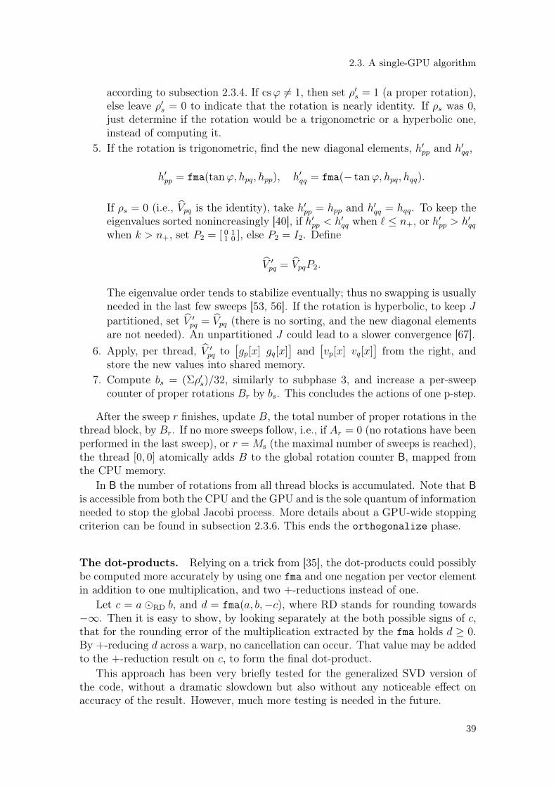
2.3. A single-GPU algorithm
according to subsection 2.3.4. If csϕ 6= 1, then set ρ′s = 1 (a proper rotation),else leave ρ′s = 0 to indicate that the rotation is nearly identity. If ρs was 0,just determine if the rotation would be a trigonometric or a hyperbolic one,instead of computing it.
5. If the rotation is trigonometric, find the new diagonal elements, h′pp and h′qq,
h′pp = fma(tanϕ, hpq, hpp), h′qq = fma(− tanϕ, hpq, hqq).
If ρs = 0 (i.e., Vpq is the identity), take h′pp = hpp and h′qq = hqq. To keep theeigenvalues sorted nonincreasingly [40], if h′pp < h′qq when ` ≤ n+, or h′pp > h′qqwhen k > n+, set P2 = [ 0 1
1 0 ], else P2 = I2. Define
V ′pq = VpqP2.
The eigenvalue order tends to stabilize eventually; thus no swapping is usuallyneeded in the last few sweeps [53, 56]. If the rotation is hyperbolic, to keep Jpartitioned, set V ′pq = Vpq (there is no sorting, and the new diagonal elementsare not needed). An unpartitioned J could lead to a slower convergence [67].
6. Apply, per thread, V ′pq to[gp[x] gq[x]
]and
[vp[x] vq[x]
]from the right, and
store the new values into shared memory.7. Compute bs = (Σρ′s)/32, similarly to subphase 3, and increase a per-sweep
counter of proper rotations Br by bs. This concludes the actions of one p-step.
After the sweep r finishes, update B, the total number of proper rotations in thethread block, by Br. If no more sweeps follow, i.e., if Ar = 0 (no rotations have beenperformed in the last sweep), or r = Ms (the maximal number of sweeps is reached),the thread [0, 0] atomically adds B to the global rotation counter B, mapped fromthe CPU memory.
In B the number of rotations from all thread blocks is accumulated. Note that Bis accessible from both the CPU and the GPU and is the sole quantum of informationneeded to stop the global Jacobi process. More details about a GPU-wide stoppingcriterion can be found in subsection 2.3.6. This ends the orthogonalize phase.
The dot-products. Relying on a trick from [35], the dot-products could possiblybe computed more accurately by using one fma and one negation per vector elementin addition to one multiplication, and two +-reductions instead of one.
Let c = a �RD b, and d = fma(a, b,−c), where RD stands for rounding towards−∞. Then it is easy to show, by looking separately at the both possible signs of c,that for the rounding error of the multiplication extracted by the fma holds d ≥ 0.By +-reducing d across a warp, no cancellation can occur. That value may be addedto the +-reduction result on c, to form the final dot-product.
This approach has been very briefly tested for the generalized SVD version ofthe code, without a dramatic slowdown but also without any noticeable effect onaccuracy of the result. However, much more testing is needed in the future.
39

2. The Jacobi-type multilevel (H)SVD algorithm for the GPU(s)
2.3.4. The Jacobi rotations
The numerically stable, state-of-the-art procedure of computing the trigonomet-ric Jacobi rotations is described in [25]. The procedure relies on computing thecolumn norms reliably, as described in section 2.6.
The rest of the computation from [25] is straightforward to implement. Sincethe entire shared memory per thread block is occupied, storing and updating thecolumn scales, as in [2], is not possible without changing the shared memory config-uration and reducing the L1 cache. The memory traffic that would thus be incurredoverweights the two additional multiplications by a cosine per GPU thread. There-fore, rotations in the following form (fma followed by a multiplication, if cosϕ 6= 1)are chosen, [
g′p g′q
]= cosϕ
[gp gq
] [ 1 tanϕ− tanϕ 1
]. (2.13)
The hyperbolic rotations may be computed similarly to the trigonometric ones, byadapting the ideas from [25], in the form
[g′p g
′q
]= coshϕ
[gp gq
] [ 1 tanhϕtanhϕ 1
]. (2.14)
Let DDRJAC be a procedure that computes, as in [25], the trigonometric rotationsin form (2.13) from the column norms it obtains by calling DRDSSQ (see section 2.6.).On a Fermi GPU (matrix order 6144), DDRJAC is only 14% slower than a simple pro-cedure discusses in the following. However, the protection from the input columnsof too large (or too small) a norm that DDRJAC offers has to be complemented bythe QR factorization at all blocking levels, which is extremely expensive.
Assume instead that the Gram matrix formation, the ordinary scalar products,and the induced norm computations never overflow. By using only correctly roundedarithmetic, cosϕ and tanϕ of (2.13), or coshϕ and tanhϕ of (2.14), may be com-puted as in (2.15)–(2.18) (an adapted version of the Rutishauser’s formulas [64]):
h = hqq − t · hpp; ct 2ϕ = t · h
2hpq; (2.15)
| ctϕ| = | ct 2ϕ|+√fma(ct 2ϕ, ct 2ϕ, t); (2.16)
tnϕ = sign(ct 2ϕ) · rcp(| ctϕ|); (2.17)
cs1 ϕ = rcp(√fma(t · tnϕ, tnϕ, 1)); cs2 ϕ =
| ctϕ|√fma(| ctϕ|, | ctϕ|, t)
. (2.18)
Formulas (2.15)–(2.18), for t = 1, produce the parameters of a trigonometricrotation (ct = cot, tn = tan, cs = cos), and for t = −1, of a hyperbolic rotation(ct = coth, tn = tanh, cs = cosh). If, numerically, | coth 2ϕ| = 1, it is substitutedby 5/4 (see [79]). In all other hyperbolic cases | tanhϕ| < 1 holds.
If | cot 2ϕ| <√ε, then
√fma(cot 2ϕ, cot 2ϕ, 1) = 1, and (2.16) in the trigono-
metric case simplifies to | cotϕ| = | cot 2ϕ| + 1. If | ct 2ϕ| ≥√
2/ε, then (barringan overflow)
√fma(ct 2ϕ, ct 2ϕ, t) = | ct 2ϕ|, with (2.16) and (2.18) simplifying to
40

2.3. A single-GPU algorithm
| ctϕ| = 2 · | ct 2ϕ| and csϕ = 1, respectively. These simplifications avoid takingsquare roots and a possible overflow of ct2 2ϕ, at a price of at most three floating-point comparisons. If | ct 2ϕ| ≤ ν/4, with ν being the largest positive normalizedfloating-point number, then tn is normalized.
If rsqrt(x) = 1/√x were correctly rounded in CUDA, cs1 ϕ could be written as
cs′1 ϕ = rsqrt(fma(t · tnϕ, tnϕ, 1)). (2.19)
Although (2.19) has only one iterative operation (rsqrt) instead of two (rcp and√x), and thus has a potential to be faster than (2.18), while also improving the
orthogonality of V , (2.19) has been omitted from the final testing due to a slowdownof about 1%, using a correctly rounded-to-nearest rsqrt prototype implementation5,that could be expected to vanish with the subsequent implementations of rsqrt.
In (2.18) and (2.19) there are three mathematically (but not numerically) equiv-alent expressions, cs1 ϕ, cs′1 ϕ, and cs2 ϕ, which compute the cosine. By a similaranalysis as above, | ctϕ| ≥
√2/ε implies cs2 ϕ = 1, tnϕ ≤
√ε/2, and therefore
cs1 ϕ = 1 and cs′1 ϕ = 1. Testing that condition also avoids an overflow of ct2 ϕ.
A choice of the rotation formulas
In the block Jacobi algorithms, it is vital to preserve (J-)orthogonality of theaccumulated V . In the hyperbolic case, the perturbation of the hyperbolic singularvalues also depends on the condition number of V [40, Proposition 4.4]. A simpleattempt would be to try to compute each rotation as (J-)orthogonal as possible,without sacrificing performance.
Departure from a single rotation’s (J-)orthogonality should be checked in a suf-ficiently high (e.g., 128-bit quadruple) precision, as dt = |(cos2 ϕ + sin2 ϕ) − 1|,or as dh = |(coshϕ − sinhϕ)(coshϕ + sinhϕ) − 1|, with sinϕ = cosϕ ∗ tanϕ, orsinhϕ = coshϕ ∗ tanhϕ. For each binary exponent −53 ≤ e ≤ 53, 224 uniformlydistributed pseudorandom 52-bit integers mi had been generated on a CPU, to form| ct 2ϕ|i with the exponent e and the non-implied bits of the significand equal to mi.From | ct 2ϕ|i and (2.16)–(2.18), (tnϕ)i, (cs1 ϕ)i, and (cs2 ϕ)i had been computedin double precision. In the Fortran’s quadruple arithmetic the corresponding dtand dh were then found and averaged, over all tested exponents. The results aresummarized in Table 2.1.
Table 2.1: The average departures from (J-)orthogonality of the rotations givenby (2.16)–(2.18).
trigonometric rotations hyperbolic rotationsdt with cos1 ϕ dt with cos2 ϕ dh with cosh1 ϕ dh with cosh2 ϕ
8.270887 · 10−17 8.335956 · 10−17 7.575893 · 10−17 6.586691 · 10−17
5Courtesy of Norbert Juffa of NVIDIA.
41

2. The Jacobi-type multilevel (H)SVD algorithm for the GPU(s)
Table 2.1 indicates that cosh2 ϕ produces, on average, more J-orthogonal hy-perbolic rotations than cosh1 ϕ. In the trigonometric case it is the opposite, butwith a far smaller difference. Orthogonality of the final V was comparable in thetests for both trigonometric versions, often slightly better (by a fraction of the orderof magnitude) using cos2 ϕ. Therefore, cs2 ϕ formulas were chosen for a full-scaletesting.
It is still far from conclusive which formulas from (2.18) or (2.19), and for whichranges of ct 2ϕ, should be used. However, cs2 ϕ or cs′1 ϕ formulas might be analternative to the established cs1 ϕ ones. A deeper analysis is left for future work.
2.3.5. The postmultiplication
This phase postmultiplies[Gp Gq
]and, optionally,
[Vp Vq
]by V ′pq only if the
rotation counter from orthogonalize is nonzero, i.e., if V ′pq 6= I32. Let Apq alias thefirst half of Gpq (i.e., Rpq). The procedure, detailed in Algorithm 4, is based on theCannon parallel matrix multiplication algorithm [15].
Algorithm 4: Pseudocode for Cannon-like postmultiplication by V ′pq.
Description: Input:[Ap Aq
], A ∈ {G,V }. Output:
[A′p A′q
]=[Ap Aq
]V ′pq.
for (i = x; i < n; i+=32) // multiply the next chunk of[Ap Aq
]by V ′pq
Apq[x, y] = Ap[i, y]; Apq[x, y′] = Aq[i, y]; // load the RAM chunk into Apq
__syncthreads(); // the shared memory writes must take effectaxy = axy′ = 0; //
[A′p A′q
]elements kept in registers
j = (y + x) mod 32; j′ = (y′ + x) mod 32; // initial skew modulo 32unrolled for (k = 0; k < 32; ++k) // multiply-and-cyclic-shift
axy = fma(Apq[x, j], V′pq[j, y], axy); // update A′p[i, y]
axy′ = fma(Apq[x, j′], V ′pq[j
′, y′], axy′); // update A′q[i, y]
j = (j + 1) mod 32; j′ = (j′ + 1) mod 32; // cyclic shift modulo 32
endfor__syncthreads(); // ensure that Apq is free to be overwrittenA′p[i, y] = axy; A′q[i, y] = axy′ ; // store the product in the RAM chunk
endfor
Finally, Figure 2.12 summarizes the entire pStep kernel, from the perspective ofthe shared memory state transitions per thread block. The GPU RAM is accessedby one read (when no rotations occur), or by two reads and one write per element ofG (and, optionally, at most one read and write per element of V ), with all operationsfully coalesced. The only additional global memory traffic are the atomic reductionsnecessary for the convergence criterion in orthogonalize.
2.3.6. A GPU-wide convergence criterion
Contrary to the pointwise Jacobi algorithm, which is considered to convergewhen no rotations have been performed in a sweep, stopping of the block algorithmsfor large inputs is more complicated than observing no rotations in a block-sweep.
42

2.3. A single-GPU algorithm
16 16
32
32
RAM
RAM RAM
RAM RAM
G ∗
C
ho
l
T
∗ ∗
Ja
c
GTG
V0 = I I
L
?
I
0
R0
Ri+1
= RiV
Vi+1
= ViV
RN
= UΣ
VN
G
VN
V
VN
(a) (b) (c) (d)
(e) (f) (g) (h)
Figure 2.12: An overview of pStep kernel per thread block, the full block variant.Each subfigure depicts the state of the shared memory, the computation subphaseperformed, and the data transfer in or out of the GPU RAM. Subfigures (a)–(d) illustrate factorize with the Cholesky factorization, (e) and (f) belong toorthogonalize, and (g) and (h) to postmultiply phase.
There has to be an additional, more relaxed stopping criterion at the block level(motivated in what follows), while keeping the one at the inner (32 × 32) levelunchanged.
The columns addressed by a pivot block-pair should be relatively orthogonalafter completion of the pStep call in the full-block variant, but instead they mayhave departed from orthogonality, because (see [40, 69])
1. the accumulated rotations are not perfectly (J-)orthogonal, and2. the postmultiplication introduces rounding errors.
Independently from that, in all variants, even the numerically orthogonal columns,when subjected to factorize (and its rounding errors), may result in the shortenedones that fail the relative orthogonality criterion.
If an orthogonality failure results from the first two causes, the ensuing rotationsmight be justified. However, if the failure is caused only by the rounding errors of thefactorization process, the spurious rotations needlessly spoil the overall convergence.
To overcome this problem, a simple heuristics has been devised to avoid excessiveblock-sweeps with just a few rotations. These rotations are expected not to beproper, i.e., to have very small angles. Let B be a counter in the CPU RAM,mapped to the GPU RAM. The counter is reset at the beginning of each block-sweep and is updated from the pStep calls as described in subsection 2.3.3. Atthe end of a block-sweep, B contains the total number of proper rotations in that
43

2. The Jacobi-type multilevel (H)SVD algorithm for the GPU(s)
sweep. If B = 0, or the maximal number of block-sweeps has been reached withoutconvergence, the process stops.
This heuristics may skip over a relatively small number of legitimate rotations,but nevertheless produces reasonable relative errors in the computed singular values(see section 2.5.). A reliable way of telling (or avoiding) the exact cause of theorthogonality failures is strongly needed in that respect.
An alternative stopping criterion
The same software infrastructure (i.e., the allocated counters and their handling)herein described can also be used for another kind of convergence criterion. Inessence, the new criterion substitutes a counter of transformations with nontrivialeffects for a counter of “proper” (in the sense of having cosϕ 6= 1) rotations.
More formally, let V ′ be a union of V ′pq over all block pairs (p, q), let vp[x] be anelement of V ′ to be transformed by a rotation, and let v′p[x] be the transformed valuein that inner step. Note that both values can be simultaneously held in registerson an architecture with a large register file (e.g., Pascal). Then, compare vp[x]and v′p[x]; if they are not equal (i.e., a nontrivial change has occured), then set thecounter variable to 1, else keep the counter unchanged. Repeat the same for vq[x]and v′q[x]. If only swapping of vp[x] and vq[x] has occured, treat that case as atrivial change. At the start of each block-sweep, reset the counter to 0. In all otheraspects, treat the counter in the same way as it would be handled for the previouslydescribed criterion, where the counter is set to 1 if cosϕ 6= 1, and to 0 otherwise.
The motivation behind such a criterion is an observation that V ′, once it doesnot change in a particular block-sweep, i.e., does not accumulate any rotations, bethey proper or not, it is hardly conceivable that it should start changing at somelater block-sweep, at least not significantly enough to warrant a few extra block-sweeps at the end of the process. Note that such heuristics does not imply anythingabout (non)orthogonality of the columns of G′.
Complementary to looking at V ′, the “standard” stopping criterion in an innersweep, based on relative orthogonality of the columns of Rpq, can be augmentedby checking whether the elements gp[x] and g′p[x] (resp. gq[x] and g′q[x]) differ aftera transformation has been applied. The transformation still shall not be appliedif the relative orthogonality criterion has been satisfied. However, if and when theelements are transformed, even by a proper rotation, there might be a chance (purelyhypothetical, perhaps) that they have not actually changed. If the columns havenot changed at all during the entire inner sweep, the standard criterion might notbe satisfied, but then it will be impossible ever to reach convergence, and the onlyreasonable option would be to stop the inner process at that point. Such a situationdoes not preclude a possibility that the whole process will eventually converge;however, if there are no changes to G′ during the entire block-sweep, what can bededuced from aggregating (i.e., +-reducing) the inner sweep change counters, thewhole process should be terminated at once.
It is important to note that no transformations are ever skipped in any innersweep due to this criterion in place that would not have been skipped otherwise, orthat would have had no effect. Only the number of block-sweeps required to reach
44

2.3. A single-GPU algorithm
overall convergence may change, and thus, indirectly, some transformations at theend of the process, that would have been applied under the previously proposedcriterion’s regime, might never be performed.
Carefully implementing and testing the new criterion is left for future work.
2.3.7. An illustration of the algorithm’s execution
As an illustration of the execution of the block-oriented algorithm’s variant underR‖ strategies, Figures 2.13, 2.14, 2.15, 2.16, and 2.17 depict, for an input matrix G
of order 1024, the initial range of values of a non-negative symmetric matrix |H|,where H = GTG, and the subsequent values of |H|, computed at the end of eachblock-sweep from the matrix G, by forming H and taking log2 |Hij| whenever thelogarithm’s argument is a positive normalized number, or −∞ otherwise (whichhas never happend with the particular input). The colorbar at the right side ofFigure 2.17 shows the ranges of the actual values of |H| covered by the correspondingranges of colors.
It can be seen from the Figures that the largest drop in the magnitudes of theoff-diagonal elements happens in the block-sweeps 3 to 7. After that, H is almostdiagonal, but still needs two more block-sweeps to clean the remaining unconvergedregions close to the diagonal, while the majority of the pivot block-pairs (corre-sponding to the regions far away from the diagonal) require no transformations atall. That is the major drawback of any one-sided Jacobi-type SVD which blindlycycles through all pivot (block-)pairs, instead of trying to reduce the bandwidtharound the diagonal from which the (block-)pivots for the last (block-)sweeps aretaken when the quadratic convergence regime has been in effect, and detected (e.g.,by a quadratical drop in the number of rotations performed in a (block-)sweep,compared to the previous ones).
Figure 2.13: The initial |GTG|, and |GTG| after block-sweep 1.
45

2. The Jacobi-type multilevel (H)SVD algorithm for the GPU(s)
Figure 2.14: |GTG| after block-sweeps 2 and 3.
Figure 2.15: |GTG| after block-sweeps 4 and 5.
2.4. A multi-GPU algorithm
In this section the same blocking principles are applied one level up the hierar-chy, to the case of multiple GPUs. As a proof-of-concept, the algorithm is developedon a 4-GPU Tesla S2050 system, and implemented as a single CPU process with4 threads, where the thread 0, . . . , 3 controls the same-numbered GPU. Were theGPUs connected to multiple machines, on each machine the setup could be simi-lar, with a CPU process and an adequate number of threads. Multiple processeson different machines could communicate via the CUDA-optimized message pass-ing interface (MPI) subsystem. Except replacing the inter-GPU communication
46

2.4. A multi-GPU algorithm
Figure 2.16: |GTG| after block-sweeps 6 and 7.
Figure 2.17: |GTG| after block-sweep 8. The heatmap corresponding to |GTG| afterthe last (9th) block-sweep is omitted because it is hardly distinguishable from theone for the 8th block-sweep. A colorbar, with the value ranges for |GTG| in log2
scale, is shown instead.
application programming interfaces (APIs), the algorithm would stay the same.Each of g GPUs holds two block-columns addressed by a pivot block-pair with
a total of n = n/g columns. For simplicity, it is assumed that n mod g = 0. Afteran outer block step, a single block-column on a GPU i is sent to a GPU j, andreplaced by the one received from a GPU k, where j may or may not be equal tok, according to a block-column mapping S ′′2g. For the outer p-strategy S′′2g, a block-column mapping has to be chosen such that the communication rules implied by
47

2. The Jacobi-type multilevel (H)SVD algorithm for the GPU(s)
the mapping are (nearly) optimal for the given network topology.For example, in a test system with g = 4, a GPU i communicates with a GPU
j, j = i xor 1, faster than with the others. The amount of fast exchanges hasbeen maximized within an outer block-sweep for R
‖8 (equivalent to Mantharam–
Eberlein BR on a 2-dimensional hypercube) to 3 by choosing which pivot block-pairis assigned to which GPU in each block step. The result is a block-column mappingshown in Figure 2.18.
0 1
23
F
F
S SS S
0 1
23
0 1
23
4 5 3 6
2 71 8
0 1
23
4 6 3 5
2 81 7
0 1
23
4 7 3 8
2 51 6
*
*
0 1
23
4 8 3 7
2 61 5
0 1
23
5 8 2 3
6 71 4
*
*
0 1
23
6 8 2 4
5 71 3
*
*
0 1
23
5 6 3 4
7 81 2
Figure 2.18: The block-column mapping in a single block-sweep of a p-strategyequivalent to Mantharam–Eberlein BR to GPUs 0, . . . , 3. The fast (F) communica-tions for column exchanges between GPU peers are denoted by dashed curves, andthe slow (S) exchanges by solid lines. Two-speed communication is defined on thetop left subfigure. The (logical) column swaps needed to maintain p < q are shownby an asterisk.
Besides the two outer block-columns of G (and, optionally, V ), stored in GA
and VA regions of the GPU RAM, respectively, an additional buffer space of thesame size, GB and VB, has to be allocated to facilitate the BLAS-3-style matrixmultiplications and the full-duplex asynchronous communication between GPUs.Also, for the shortening and the single-GPU Jacobi phases, two n × n matrices, Xand Y , are needed. With a small auxiliary space AUX for the final singular valueextraction, the total memory requirements are at most m× 5n double elements pera GPU.
In an outer block step the following operations are performed (see Figure 2.19):
(0) form the Gram matrix GTAGA in X by cublasDsyrk;
(1) factorize GTAGA = RTR by the Cholesky factorization (the hybrid MAGMA’s
dpotrf_gpu has been chosen, and this is the only place where a CPU is usedfor computation, which may be circumvented by a GPU-only implementation);
(2a) case (acc.): if accumulation of the product V of the Jacobi rotations is de-sired, call a full SVD single-GPU Jacobi variant (full block, block-oriented, orhybrid) from section 2.3. on X, storing V in Y ; else
48

2.4. A multi-GPU algorithm
(2b) case (solve): copy R from X to Y , call a partial SVD single-GPU Jacobivariant on Y , and solve the triangular linear system RV = UΣ for V bycublasDtrsm, with the original R in X and V overwriting UΣ in Y ;
(3) postmultiply GA and VA by V , using two cublasDgemm calls running in theirown CUDA streams, and store the updated block-columns in GB and VB;
(4) ensure that all GPUs have completed the local updates by a device-wide syn-chronization (cudaDeviceSynchronize), followed by a process-wide threadsynchronization (wait on a common barrier), and a suitable MPI collectiveoperation (e.g., MPI_Barrier) in the multiprocess case;
(5) start, via CUDA streams, the asynchronous sends of one block-column fromGB and the corresponding one from VB to another GPU, and start the asyn-chronous copies of the other column of GB and the corresponding one of VBto either the first or the second block-column of GA and VA, according to theblock-column mapping rules for transition to the subsequent block step;
(6) wait for the outstanding asynchronous operations to finish by the same syn-chronization procedure as in (4), after which a block step is completed.
At the end of an outer block-sweep, the threads (and processes, where applicable)+-reduce their local counters Bi of proper rotations (cf. subsection 2.3.6.) to thesystem-wide number
∑i Bi of proper rotations performed in all block steps in that
sweep. If the result is 0, or the limit on the number block-sweeps has been reached,the iteration stops and the final singular values are extracted.
The full block variant of phases (2a) and (2b) usually has a 30-sweep limit forboth the inner blocking and the pointwise, shared-memory Jacobi level. The block-oriented variant has both limits set to 1. Between them many hybrid variants maybe interpolated.
Observe that phase (4) forces all GPUs to wait for the slowest one, in termsof the execution of phase (2a) or (2b). The full block variant exhibits the largestdifferences in running times between GPUs, depending on how orthogonal the block-columns are in the current block step. Although the full block variant is the fastestchoice for a single-GPU algorithm (see section 2.5.), it may be up to 35% slowerin a multi-GPU algorithm than the block-oriented variant, which has a predictable,balanced running time on all GPUs.
A reasonable hybrid variant might try to keep the running times balanced. ACPU thread that first completes the full block variant of (2a) or (2b) immediatelyinforms other threads before proceeding to phase (4). The other threads then stoptheir inner block-sweeps loops in (2a) or (2b) when the running iteration is finished.
The wall-clock execution times of such an approach may be even lower thanthe block-oriented variant, but on the average are 10% higher. Moreover, both thefull block and its hybrid variant induce the larger relative errors in Σ than theblock-oriented variant. Such effect may be partially explained, as in section 2.5., bythe same reasons valid for the single-GPU case (more rotations applied), but thelarger differences in the multi-GPU case require further attention. Therefore, thenumerical tests are presented for the block-oriented multi-GPU variant only.
49

2. The Jacobi-type multilevel (H)SVD algorithm for the GPU(s)
GA
VA
GB
VB
GT
AG
A
V
AUX
or or or or
Cholesky
Jacobi
GB = GA · V
VB = VA · V
receive send
one column locally ‖ one column remotely
(1)
(2)
(3)
(3)
(5) (5)
synchronize (4, 6)
Figure 2.19: Schematics of a GPU’s memory organization and the outer blockstep phases. Operations with the same number may be performed concurrently,in streams, if the hardware allows that.
2.5. Numerical testing
In this section the testing data is defined, the hardware is described, and thespeed and accuracy results for both the single-GPU and the multi-GPU implementa-tions are presented. By these results the p-strategies ( R‖ and C‖)6 from section 2.2.are also confirmed as a reliable choice for implementing the fast Jacobi algorithmson the various parallel architectures.
Let norm and unif be the double precision pseudorandom number generators,such that norm(µ, σ) returns the nonzero samples from normal distribution N(µ, σ),and unif(S) returns the samples from the continuous uniform distribution U overS. The following pseudorandom spectra, for k = 1, . . . , 16, have been generated:
1. Λ(1)k (1:16) = 0.5; Λ
(1)k (17:1024k) = norm(0, 0.1),
2. Λ(2)k = 1 + Λ
(1)k (verified to be greater than zero),
3. Λ(3)k (1:1024k) = ± unif(〈10−7, 10k〉), where a positive or a negative sign for
each Λ(3)k (i) is chosen independently for 1 ≤ i ≤ 1024k with equal probability,
4. Λ(4)k (1:1024k) = unif(〈10−7, 10k〉).
These arrays have been cast to the Fortran’s quadruple precision type and denotedby Λ
(1)k to Λ
(4)k . By a modified LAPACK xLAGSY routine, working in quadruple
precision, a set of symmetric matrices A(j)k = U
(j)k Λ
(j)k [U
(j)k ]T has been generated,
for j = 1, . . . , 4, by pre- and postmultiplying Λ(j)k with a product U
(j)k of the random
Householder reflectors. The matrices A(j)k have then been factored by the symmetric
6Throughout this section, the subscripts indicating the matrix order on the p-strategies’ symbolsare omitted. For each occurrence of a particular symbol, the matrix order is implied by the context.
50

2.5. Numerical testing
indefinite factorization with the complete pivoting [70] in quadruple precision:
P(j)k A
(j)k [P
(j)k ]T = G
(j)k P
(j)k [P
(j)k ]T J
(j)k P
(j)k [P
(j)k ]T [G
(j)k ]T = G
(j)k J
(j)k [G
(j)k ]T .
The inner permutation P (j)k brings J (j)
k into J (j)k = diag(I,−I) form. For j ∈ {2, 4}
the symmetric indefinite factorization is equivalent to the Cholesky factorizationwith diagonal pivoting (J (j)
k = I). Finally, G(j)k have been rounded back to double
precision, and stored as the input factors G(j)k , along with Λ
(j)k and J (j)
k .7Since one of the important applications of the (H)SVD is the eigensystem com-
putation of the symmetric (in)definite matrices, the procedure just described hasbeen designed to minimize, as much as is computationally feasible, the effect ofthe rounding errors in the factorization part. Therefore, the relative errors of thecomputed Σ2J (from G = UΣV T , and let ji = Jii) have been measured versus thegiven Λ
(j)k (with the elements denoted λi, for 1 ≤ i ≤ n), i.e.,
maxi=1,...,n
| f`(σi)2ji − λi||λi|
. (2.20)
It may be more natural and reliable to compute the (H)SVD of G(j)k in quadruple
precision and compare the obtained singular values with the ones produced by thedouble precision algorithms. For an extremely badly conditioned A,
√|Λ| may not
approximate the singular values of G well; e.g., if, by the same procedure as above, A(definite or indefinite) is generated, with n = 4096 and κ2(A) ≥ 1024, the resultingG may have the singular values (found by the quadruple Jacobi algorithm) differingin at least 4–5 least significant double precision digits from the prescribed singularvalues
√|Λ|. However, for a larger n, the quadruple precision SVD computation
is infeasible. Therefore, accuracy of the algorithms has been verified as in (2.20),but with the modestly conditioned test matrices generated, to avoid the problemsdescribed.
The NVIDIA graphics testing hardware, with accompanying CPUs, consists ofthe following:
A. Tesla C2070 (Fermi) GPU and Intel Core i7–950 CPU (4 cores),B. Tesla K20c (Kepler) GPU and Intel Core i7–4820K CPU (4 cores),C. Tesla S2050 (Fermi) 4 GPUs and two Intel Xeon E5620 CPUs (2× 4 cores).
The software used is CUDA 5.5 (nvcc and cuBLAS) under 64-bit Windows andLinux, and MAGMA 1.3.0 (with sequential and parallel Intel MKL 11.1) under64-bit Linux.
As shown in Table 2.2, the sequential Jacobi algorithm DGESVJ, with the parallelMKL BLAS-1 operations, on machine C runs approximately 16 times slower than asingle-GPU (Fermi) algorithm for the large enough inputs.
In Table 2.3 the differences in the execution times of the R‖ p-strategy on Fermiand Kepler are given. There are the three main reasons, outlined in section 2.3.,why the Kepler implementation is much faster than the Fermi one. In order ofimportance:
7The test matrices are available at http://euridika.math.hr:1846/Jacobi/ for download.
51

2. The Jacobi-type multilevel (H)SVD algorithm for the GPU(s)
Table 2.2: The ratio of the wall-clock running times of DGESVJ on machine C versusa single GPU (Fermi) for the Cholesky factors of the matrices of order n = 1024k
with spectra Λ(2)k .
k DGESVJ/ R‖
1 5.572 8.613 11.754 11.83
k DGESVJ/ R‖
5 12.346 13.477 13.628 13.58
k DGESVJ/ R‖
9 14.8910 15.4511 15.6212 16.14
k DGESVJ/ R‖
13 16.4914 16.4615 16.1916 16.00
(i) 8-byte-wide shared memory banks on Kepler versus 4-byte-wide on Fermi—the profiler reports 99.8% shared memory efficiency on Kepler versus 49.8%on Fermi;
(ii) warp shuffle reductions on Kepler (the warp-level reductions do not need theshared memory workspace); and
(iii) no register spillage on Kepler, due to the larger register file.
The other profiler metrics are also encouraging: the global memory loads and storesare more than 99% efficient, and the warp execution efficiency on Fermi is about96.5%, which confirms that the presented algorithms are almost perfectly parallel.
Table 2.3: The wall-clock running times (in seconds) of a Fermi (F ) versus a Kepler(K) GPU for the full SVD of the Cholesky factors of the matrices of order n = 1024k
with spectra Λ(2)k , the full block variant.
k Kepler [s] Fermi [s] K/F [%]
1 1.413099 2.376498 59.52 7.206334 12.438532 57.93 22.980686 35.783290 64.24 46.357804 84.466500 54.95 95.828870 160.382859 59.86 154.643361 261.917934 59.07 246.114488 403.150779 61.08 346.689433 621.341377 55.8
k Kepler [s] Fermi [s] K/F [%]
9 506.365598 850.279539 59.610 682.577101 1153.337956 59.211 904.212224 1545.451594 58.512 1148.881987 1970.591570 58.313 1439.391787 2500.931105 57.614 1809.888207 3158.116986 57.315 2196.755474 3820.551746 57.516 2625.642659 4662.748709 56.3
Even though the instruction and thread block execution partial orders may varyacross the hardware architectures, the presented algorithms are observably deter-ministic. Combined with a strong IEEE floating-point standard adherence of boththe Fermi and the Kepler GPUs, that ensures the numerical results on one architec-ture are bitwise identical to the results on the other. This numerical reproducibilityproperty should likewise be preserved on any future, standards-compliant hardware.
52

2.5. Numerical testing
In the following, it is shown that R‖ and C‖ p-strategies are superior in terms ofspeed to R‖, C‖, the Brent and Luk (B), and modified modulus (M) strategies, inboth the definite and the indefinite case. By abuse of notation, let R
‖b stand for the
block-oriented variant (otherwise, the full block variant is measured), and let R‖4b
be used for its 4-GPU implementation. Figures 2.20 and 2.21 depict the wall-clocktime ratios of the other strategies versus R‖. Except B and C‖, the other strategiesare consistently about 14–21% slower than R‖, while C‖ is almost equally fast as R‖.Therefore, in what follows only R‖ has been timed.
2 4 6 8 10 12 14 16
0.5
1.0
1.5
2.0
2.5
3.0
3.5
matrix dimension / 1024
timeratio
‖/ ‖C R
(R‖≈ C
‖)/ ‖R
M/ ‖R
B/ ‖R
‖b/ ‖R R
Figure 2.20: The wall-clock time ratio of the various parallel strategies on a singleGPU (Fermi). The test spectra are Λ
(2)k .
2 4 6 8 10 12 14 16
0.5
1.0
1.5
2.0
2.5
3.0
3.5
matrix dimension / 1024
timeratio
‖/ ‖C R
(R‖≈ C
‖)/ ‖R
M/ ‖R
B/ ‖R
‖b/ ‖R R
Figure 2.21: The wall-clock time ratio of the various parallel strategies on a singleGPU (Fermi). The test spectra are Λ
(1)k .
The standard counter-example that shows nonconvergence of the Jacobi methodunder the Brent and Luk strategy for matrices of even orders (first constructedby Hansen in [36], and later used in [50]), is actually not a counter-example in the
53

2. The Jacobi-type multilevel (H)SVD algorithm for the GPU(s)
usual diagonalization procedure which skips the rotations with the very small angles,because there is no need for diagonalization of an already diagonal matrix of order2. On the contrary, the standard algorithm will diagonalize this matrix in only one(second) step of the first sweep.
However, this still does not mean that no serious issues exist regarding conver-gence of the Jacobi method under B. Figures 2.20 and 2.21 indicate that a furtherinvestigation into the causes of the extremely slow convergence (approaching 30block-sweeps) under B may be justified.
The block-oriented variant has more block-sweeps and, while slightly faster forthe smaller matrices, is about 7% slower for the larger matrices than the full blockvariant. It may be more accurate in certain cases (see Figures 2.22 and 2.23), dueto the considerably smaller total number of the rotations performed, as shown inTable 2.4. The strategies M and B are far less accurate than the new p-strategies.
2 4 6 8 10 12 14 16
matrix dimension / 1024
1
3
5
7
9
11
13
15
max
imal
relativeerror·10
13
‖R
‖R
M
B
‖bR
Figure 2.22: The relative accuracy of the various parallel strategies on a single GPU.The test spectra are Λ
(2)k .
Table 2.4: The number of block-sweeps and the average ratios (with small variance)of the total number of rotations of the full block versus the block-oriented variant,per four spectrum types on a single GPU.
Spectrum type 1 2 3 4
average ratio of the number of rotations R‖/ R‖b 2.29 2.10 2.30 2.08
range of the number of block-sweeps R‖ 8–12 8–9 8–11 7–9range of the number of block-sweeps R
‖b 10–14 9–12 9–14 9–12
MAGMA’s dgesvd routine has been tested with the sequential (seq.) and theparallel (par.) (four threads) MKL library on machine A. The relative accuracy isidentical in both cases. Compared with the single-GPU Fermi algorithm, MAGMA
54

2.5. Numerical testing
2 4 6 8 10 12 14 16
matrix dimension / 1024
0.5
1.0
1.5
2.0
2.5
3.0
3.5
4.0
max
imal
relativeerror·10
13
‖R
‖R
M
B
‖bR
Figure 2.23: The relative accuracy of the various parallel strategies on a single GPU.The test spectra are Λ
(1)k .
(seq.) is 1.5–3 times slower, and MAGMA (par.) is up to 2 times faster. On the otherhand, MAGMA (par.) is, on average, 30% slower, and for the larger matrix sizes,more than 45% slower than the block-oriented 4-GPU Fermi (solve) implementa-tion. The (acc.) implementation is about 35% slower than (solve) (see Figures 2.24and 2.25), and only marginally more accurate (see Figures 2.26 and 2.27). For thematrix orders of at least 4096, the fastest Jacobi implementation on 4 GPUs is about2.7 times faster than the fastest one on 1 GPU.
MAGMA’s accuracy is comparable to a single-GPU algorithm for the well-conditioned test matrices, and better than a multi-GPU algorithm, but in the (sep-arately tested) case of matrices with badly scaled columns (κ2 ≈ 1012), the relativeerrors of MAGMA could be more than 20 times worse than the Jacobi ones.
2 4 6 8 10 12 14 16
0.5
1.0
1.5
2.0
2.5
3.0
matrix dimension / 1024
timeratio
‖4b(solve)/ ‖
R R
‖4b(acc.)/ ‖
R R
MAGMA (seq.)/ ‖R
MAGMA (par.)/ ‖R
Figure 2.24: The wall-clock time ratio of the block-oriented 4-GPU Fermi imple-mentations and MAGMA versus a single GPU. The test spectra are Λ
(2)k .
55

2. The Jacobi-type multilevel (H)SVD algorithm for the GPU(s)
2 4 6 8 10 12 14 16
0.5
1.0
1.5
2.0
2.5
3.0
matrix dimension / 1024
timeratio
‖4b(solve)/ ‖
R R
‖4b(acc.)/ ‖
R R
MAGMA (seq.)/ ‖R
MAGMA (par.)/ ‖R
Figure 2.25: The wall-clock time ratio of the block-oriented 4-GPU Fermi imple-mentations and MAGMA versus a single GPU. The test spectra are Λ
(4)k .
2 4 6 8 10 12 14 16
matrix dimension / 1024
1
2
3
4
5
6
7
max
imal
relativeerror·10
13
‖bR
‖4b(solve)R
‖4b(acc.)R
MAGMA (seq., par.)
Figure 2.26: The relative accuracy of the block-oriented 1- and 4-GPU Fermi im-plementations and MAGMA. The test spectra are Λ
(2)k .
Unlike MAGMA, the Jacobi GPU algorithms are perfectly scalable to an arbi-trary number of GPUs, when the matrix order is a growing function of the numberof assigned GPUs. That makes the Jacobi-type algorithms readily applicable on thecontemporary large-scale parallel computing machinery, which needs to leverage thepotential of a substantial amount of numerical accelerators.
2.5.1. Modern CUDA on modern hardware
While the GPU hardware and the CUDA software constantly evolve, the previ-ously shown results do not reflect the latest performance gains, made possible byhaving the GPUs with more registers available per thread, and with faster clocks.
The source code required virtually no change to be compiled with CUDA 8.0,
56

2.5. Numerical testing
2 4 6 8 10 12 14 16
matrix dimension / 1024
2 4 6 8 10 12 14 16
matrix dimension / 1024
1
2
3
4
5
6
7max
imal
relativeerror·10
13
‖bR
‖4b(solve)R
‖4b(acc.)R
MAGMA (seq., par.)
Figure 2.27: The relative accuracy of the block-oriented 1- and 4-GPU Fermi im-plementations and MAGMA. The test spectra are Λ
(4)k .
and only some syntactical changes for the warp shuffles with (as of now not officiallyreleased) CUDA 9.0.
Though the latest NVIDA GPUs released are based on the Volta architecture,only the ones based on the penultimate architecture, Pascal, have been available fortesting, in an IBM POWER8NVL (“Minsky”) system with two CPUs, two pairs ofNVLink-connected P100 GPUs, and CUDA 8.0 software stack.
Some numerical results on the Pascal GPU architecture with CUDA 8
Table 2.5 contains the wall-clock time results on a P100 GPU. The ratio B/F ,also shown, is given normalized per block-sweep, i.e.,
B
F=
(wall-clock time of B.O.)/(number of block-sweeps)(wall-clock time of F.B.)/(number of block-sweeps)
· 100%,
in order to demonstrate the time needed to prepare and execute one inner sweep(the B.O., i.e., block-oriented variant), versus preparing and executing a number ofinner sweeps until convergence (the F.B., i.e., full block variant). The results havebeen obtained by using the correctly rounded rsqrt prototype code.
Such a huge performance gain compared to the Kepler results might be explainedby having no register spillage at all (the compiler managed to fit all per-thread datain at most 127 registers), and by having all the hardware elements running fasterthan in the Kepler era, as well.
The Kogbetliantz-type (two-sided) SVD in CUDA 9
CUDA 9.0 has not yet been publicly released at the time of completing this thesis,but it should be noted that the cuSOLVER library might offer a GPU SVD algorithmthat seems to be an implementation of the two-sided Kogbetliantz procedure [46],even though it bears Jacobi’s name in the documentation. In its “early access”
57

2. The Jacobi-type multilevel (H)SVD algorithm for the GPU(s)
Table 2.5: The wall-clock running times (in seconds) of the full block (F ) versus theblock-oriented (B) variant on a single P100 Pascal GPU with CUDA 8 for the fullSVD of the Cholesky factors of order n = 1024k, with spectra Λ
(2)k .
k F.B. [s] B.O. [s] B/F [%]
1 0.339778 0.301851 78.972 1.850578 1.930034 83.433 4.152033 4.460573 85.944 10.162217 10.928215 86.035 17.116205 18.860442 90.166 30.998928 33.845042 89.337 43.047102 45.027426 94.148 67.491073 73.790574 89.45
k F.B. [s] B.O. [s] B/F [%]
9 100.458574 110.667394 90.1310 127.070338 140.527818 90.4811 174.411275 192.535960 90.3212 209.581525 240.855742 86.1913 277.494765 307.191926 90.5714 326.804596 360.364868 90.2215 414.276624 458.707541 90.5916 514.069278 561.758535 89.41
version, the routine has shown promising performance on small matrices (from 1024to 3072) on a consumer Kepler GPU, albeit lower than the algorithm proposed here.
2.6. Parallel norm computation
An essential prerequisite for computing the Householder reflectors and the Ja-cobi rotations [25] is obtaining the column norms (effectively, the sums of squares)reliably, avoiding the possible underflows and overflows of an ordinary scalar prod-uct. However, a strictly sequential nature of LAPACK’s DLASSQ is unsuitable forparallel processing. Therefore, an alternative procedure, DRDSSQ, is proposed here,based on the parallel reduction concept.
The proposed procedure is one of the many approaches to compute a sum ofsquares of the floating-point numbers, but those approaches differ in their assump-tions and in their ultimate goals. An assumption might be that the elements of avector should be accessed only once (which will not hold for DRDSSQ), or that thefloating-point arithmetic does not necessarily adhere to the standard [44] (here, suchadherence is required).
The goal may be only to avoid the overflows and the underflows by scaling(as in [10]), or to compute the result as accurately as possible (as in [35]), withthe overflow and underflow protection and/or vectorization as a bonus, or to seekreproducibility under various assumptions [20], etc.
Here, the goal is not the best possible accuracy or reproducibility as such (eventhough it is achieved on all current CUDA architectures as a consequence of thealgorithm’s design), but a high degree of paralellism under the SIMT computingmodel, the certainity of the overflows and the underflows being avoided, and anefficient way of utilizing the reductions, on the warp level and beyond.
Let µ be the smallest and ν the largest positive normalized floating-point number,ε the maximal relative roundoff error (ε = 2−53 for double with rounding to nearest),
58

2.6. Parallel norm computation
γ = 1−ε, δ = 1+ε, and x a vector of length n, with no special values (±∞, NaNs) forits components. A floating-point approximation of an exact quantity ξ is denotedby rn(ξ), ru(ξ), or rz(ξ), for rounding to nearest, to +∞, or to 0, respectively.
Find M := maxi |xi|. If M = 0, x is a zero vector. Else, there exists the smallestnonzero |xi|, which can be computed as m := mini |x′i|, where x′i = xi for |xi| > 0,and x′i = ν otherwise. Provided enough workspace for holding, or another techniquefor exchanging the partial results (such as the warp shuffle primitives of the KeplerGPU architecture), M and m could be found by a parallel min/max-reduction of x.
If the floating-point subnormals and infinity are supported, inexpensive, and safeto compute with (i.e., no exceptions are raised, or the non-stop exception handlingis in effect), a sum of x2i might also be computed. If the sum does not overflow, anda satisfactory accuracy is found to be maintained (e.g., the underflows could nothave happened if rn(m2) ≥ µ), DRDSSQ stops here.
Otherwise, note that the depth of a reduction tree for the summation of x2i isdlg ne, and at each tree level (the first one being level 0) at most δ relative error isaccumulated. Inductively, it follows that if, for some s = 2`,
2dlgne(sM)2δ(1+dlgne) ≤ ν,
then the sum of (sxi)2 cannot overflow. Also, if (sm)2γ ≥ µ, for some s = 2k, then
no (sxi)2 can underflow. If some j could be substituted for both k and `, it would
define a scaling factor that simultaneously protects from the potential overflows andunderflows. When the range of values of x does not permit a single scaling, theindependent scalings of too large and too small values of x should be performed.
Such a scaling of xi by s in the binary floating-point arithmetic introduces norounding errors and amounts to a fast integer addition of the exponents of xi ands. Instead of the scale factors themselves, only their exponents need to be storedand manipulated as machine integers. For clarity, the scales remain written hereinas the integer powers of 2. A pair (s, y) thus represents a number with the sameprecision as y, but with the exponent equal to a sum of the exponents of s and y.
As motivated above, define the safe, inclusive bounds µ (lower) and ν (upper)for the values of x for which no overflow nor underflow can happen, as
µ =√µ/γ, δn = 2dlgneδ(1+dlgne), ν =
√ν/δn.
Consider the following computations over a partition of the set of values of x:
• if [m,M ] ∩ [µ, ν] 6= ∅, set s1 = 1 = 20 (no scaling needed), and compute
σ21 =
n∑i=1
x2i , xi =
{xi, µ ≤ |xi| ≤ ν,
0, otherwise,
• if M > ν, take the largest s such that sM ≤ ν, denote it by s2, and compute
σ22 =
n∑i=1
(s2xi)2, xi =
{xi, |xi| > ν,
0, otherwise,
59

2. The Jacobi-type multilevel (H)SVD algorithm for the GPU(s)
• if m < µ, take the smallest s such that sm ≥ µ, denote it by s0, and compute
σ20 =
n∑i=1
(s0xi)2, xi =
{xi, |xi| < µ,
0, otherwise.
From m, M , µ, ν it is known in advance which partial sums are necessarily 0, andthe procedure should be simplified accordingly. If, e.g., m ≥ µ, then σ2
0 = 0.A C/C++ implementation of finding s0 = 2k or s2 = 2` is remarkably simple.
An expression y = frexp(x, &e) breaks x into 0.5 ≤ y < 1 and e such that 2ey = x.Let f = m, t = ru(µ), j = k for s0, or f = M , t = rz(ν), j = ` for s2. Also, letfy = frexp(f, &fe) and ty = frexp(t, &te). Then j is returned by a code fragment:
j = (f <= t) ? (te - fe) + (fy < ty) : (te - fe) - (fy > ty).
If there is more than one nonzero partial sum of squares, such (s−2i , σ2i ) are
expressed in a “common form”, (s−2i , σ2i ), where 0.5 ≤ σ2
i < 2, and the scales’exponents remain even. Let (s−2i , σ2
i ) = (2j, 2my), where y is a significand of σ2i .
Since σ2i is normalized by construction, 1 ≤ y < 2. Define m′ = −(m mod 2) and
j′ = j +m−m′. Then m′ ∈ {−1, 0}, j′ remains even, and (s−2i , σ2i ) = (2j
′, 2m
′y).
The common form makes ordering the pairs by their magnitudes equivalent toordering them lexicographically. First, find the two (out of at most three) partialsums which are the smallest by magnitude. Then add these partial sums together,such that the addend smaller by magnitude is rescaled to match the scale of thelarger one. Let (s−2+ , σ2
+) = (s−2≤ , σ2≤) + (s−2> , σ2
>), with (s−2≤ , σ2≤) ≤ (s−2> , σ2
>). Thens−2+ = s−2> , s−2− = s−2≤ /s
−2> , and σ2
+ = s−2− σ2≤ + σ2
>.If one more addition is needed, (s−2+ , σ2
+) has to be brought into the commonform (s−2+ , σ2
+), and summed with the remaining addend by the above procedure.However, both (s−22 , σ2
2) and (s−20 , σ20) have to be computed only when nµ2 ≈ εν2.
Such large n seldom occurs. In either case, accuracy of the final result is maintainedby accumulating the partial sums in the nondecreasing order of their magnitudes.
The result of DRDSSQ is (s−2, σ2), and the norm of x is ‖x‖2 =√σ2/s. If ‖x‖2
overflows or underflows for x a column of G, the input factor should be initiallyrescaled (if possible). A procedure similar to DRDSSQ is implementable wherever theparallel reduction is a choice (e.g., with MPI_Allreduce operation).
By itself, DRDSSQ does not guarantee numerical reproducibility, if the underlyingparallel reductions do not possess such guarantees. The ideas from [20] might beuseful in that respect.
60

3. The implicit Hari–Zimmermannalgorithm for the GSVD
This chapter is organized as follows. Section 3.1. contains a description of twopointwise Jacobi-type algorithms for the GEP: the Falk–Langemeyer and the Hari–Zimmermann algorithm. The one-sided analogue of the Hari–Zimmermann algo-rithm for the GSVD is presented at the beginning of section 3.2. Then the algo-rithms are described that orthogonalize a matrix pair block-by-block, to maximizethe efficiency on hierarchical memory architectures. The parallel algorithms on theshared and distributed memory architectures are detailed in section 3.3. The re-sults of numerical testing are presented and discussed in section 3.4., and a GPUimplementation of the implicit Hari–Zimermann is sketched in section 3.5.
3.1. The Jacobi–type sequential algorithms for GEP
3.1.1. The Falk–Langemeyer algorithm
The Falk–Langemeyer method solves the GEP (1.2) for a symmetric and definitematrix pair (A,B). The method constructs a sequence of matrix pairs (A(`), B(`)),
A(`+1) = CT` A
(`)C`, B(`+1) = CT` B
(`)C`, ` ∈ N, (3.1)
where A(1) := A, and B(1) := B, according to some pivot strategy that selects theorder in which the off-diagonal elements are annihilated. If the transformation ma-trix C` is nonsingular, the two consecutive pairs are congruent, so their eigenvaluesare equal [63]. A matrix that diagonalizes the pair is computed by accumulatingthe transformations
C(1) = I, C(`+1) = C(`)C`, ` = 1, 2, . . . . (3.2)
The matrix C` resembles a scaled plane rotation: it is the identity matrix, exceptfor its (i, j)-restriction C`, where it has two parameters, α` and β`
C` =
[1 α`−β` 1
]. (3.3)
The parameters α` and β` in (3.3) are determined so that the transformations in (3.1)diagonalize the pivot submatrices
A(`) =
[a(`)ii a
(`)ij
a(`)ij a
(`)jj
], B(`) =
[b(`)ii b
(`)ij
b(`)ij b
(`)jj
]. (3.4)

3. The implicit Hari–Zimmermann algorithm for the GSVD
The annihilation equations are[1 −β`α` 1
][a(`)ii a
(`)ij
a(`)ij a
(`)jj
][1 α`
−β` 1
]=
[a(`+1)ii 0
0 a(`+1)jj
],
[1 −β`α` 1
][b(`)ii b
(`)ij
b(`)ij b
(`)jj
][1 α`
−β` 1
]=
[b(`+1)ii 0
0 b(`+1)jj
].
(3.5)
In terms of α` and β`, the equations (3.5) reduce to
α`a(`)ii + (1− α`β`)a
(`)ij − β`a
(`)jj = 0,
α`b(`)ii + (1− α`β`)b
(`)ij − β`b
(`)jj = 0,
and the solution can be written as
α` =I(`)j
ν`, β` =
I(`)i
ν`,
where
I(`)i = a
(`)ii b
(`)ij − a
(`)ij b
(`)ii ,
I(`)j = a
(`)jj b
(`)ij − a
(`)ij b
(`)jj ,
I(`)ij = a
(`)ii b
(`)jj − a
(`)jj b
(`)ii ,
I(`) = (I(`)ij )2 + 4I
(`)i I
(`)j ,
ν` =1
2sign(I
(`)ij )(|I(`)ij |+
√I(`)).
If I(`) = 0, then a special set of formulas is used (for details, see [71, Algorithm 4]).Now suppose that the matrices in (3.1) are computed according to the IEEE 754–
2008 standard [44] for floating–point arithmetic. Unfortunately, for large matrices,after a certain number of transformations, the elements of both A(`) and B(`) canbecome huge in magnitude (represented as floating-point infinites). A solution tothis problem is an occasional rescaling, but how often that needs to be done, dependson the dimension of the pair, the size of its elements, and the chosen pivot strategy.
3.1.2. The Hari–Zimmermann algorithm
If B is positive definite, the initial pair (A,B) can be scaled so that the diagonalelements of B are all equal to one. By taking
D = diag
(1√b11,
1√b22, . . . ,
1√bkk
),
and making the congruence transformations
A(1) := DAD, B(1) := DBD,
a new pair (A(1), B(1)) is obtained, which is congruent to the original pair.
62

3.1. The Jacobi–type sequential algorithms for GEP
The idea behind this modification of the Falk–Langemeyer algorithm is: when Bis the identity matrix, the transformations are the ordinary Jacobi rotations. Themethod constructs a sequence of matrix pairs
A(`+1) = ZT` A
(`)Z`, B(`+1) = ZT` B
(`)Z`, ` ∈ N, (3.6)
such that the diagonal elements of B(`) remain ones after each transformation. Thematrices Z` in (3.6) are chosen to annihilate the elements at positions (i, j) (and(j, i)), and to keep ones as the diagonal elements of B(`). If the matrix that diag-onalizes the pair is needed, the accumulation procedure is given by (3.2), with Creplaced by Z.
The matrix Z` is the identity matrix, except in the plane (i, j), where its restric-tion Z` is equal to
Z` =1√
1−(b(`)ij
)2[
cosϕ` sinϕ`− sinψ` cosψ`
], (3.7)
withcosϕ` = cosϑ` + ξ`(sinϑ` − η` cosϑ`),
sinϕ` = sinϑ` − ξ`(cosϑ` + η` sinϑ`),
cosψ` = cosϑ` − ξ`(sinϑ` + η` cosϑ`),
sinψ` = sinϑ` + ξ`(cosϑ` − η` sinϑ`),
ξ` =b(`)ij√
1 + b(`)ij +
√1− b(`)ij
,
η` =b(`)ij(
1 +√
1 + b(`)ij
)(1 +
√1− b(`)ij
) ,
tan(2ϑ`) =2a
(`)ij −
(a(`)ii + a
(`)jj
)b(`)ij(
a(`)jj − a
(`)ii
)√1−
(b(`)ij
)2 , −π4< ϑ` ≤
π
4.
(3.8)
If a(`)ij = b(`)ij = 0, set ϑ` = 0. Else, if a(`)ii = a
(`)jj , and 2a
(`)ij =
(a(`)ii + a
(`)jj
)b(`)ij , then the
matrices A(`) and B(`) are proportional. Hence, set ϑ` = π4.
To justify the notation, in the following it is proven that the quantities definedin (3.8) are indeed trigonometric functions of certain angles. Note that ϑ` in thespecified range is always uniquely defined by tan(2ϑ`).
Proposition 3.1. The quantities cosϕ`, sinϕ`, cosψ`, and sinψ` represent thestated trigonometric functions of certain angles ϕ`, and ψ`, respectively.
Proof. It is sufficient to prove that cos2 ϕ` + sin2 ϕ` = 1, and cos2 ψ` + sin2 ψ` = 1.From the first two lines of (3.8) it follows that
cos2 ϕ` + sin2 ϕ` = cos2 ψ` + sin2 ψ` = (1− ξ`η`)2 + ξ2` = 1 + ξ`(−2η` + ξ`η2` + ξ`).
63

3. The implicit Hari–Zimmermann algorithm for the GSVD
To prove the claim, it is sufficient to show that
ξ`(−2η` + ξ`η2` + ξ`) = 0.
If ξ` = 0, the conclusion is obvious. Otherwise, the result is obtained by substitutionof ξ` and η` from (3.8) as the functions of b(`)ij , followed by simplification of thisexpression.
Hari in his Ph.D. thesis proved [37, Proposition 2.4] that
min{cosϕ`, cosψ`} > 0,
and−1 < tanϕ` tanψ` ≤ 1,
with tanϕ` tanψ` = 1, if and only if ϑ` = π4. Hence, Z` is nonsingular. More
precisely,
det(Z`) =1
1−(b(`)ij
)2 (cosϕ` cosψ` + sinϕ` sinψ`) =1
1−(b(`)ij
)2 (1− 2ξ2` )
=1
1−(b(`)ij
)21−
(b(`)ij
)21 +
√1−
(b(`)ij
)2 =
1√1−
(b(`)ij
)2 .The transformations applied on B are congruences, and consequently, they pre-
serve the inertia of B. Therefore, all matrices B(`) are positive definite. Since theirdiagonal elements are ones, the absolute value of all the other elements is smallerthan one, i.e., the elements of B(`) cannot overflow. For the elements of A(`), thesituation is slightly more complicated.
Proposition 3.2. The elements of the matrix A(`+1) = ZT` A
(`)Z` are bounded interms of the elements of A(`), and the pivot element b(`)ij of B(`). They are equalto the elements of A(`), except in the columns (and, due to symmetry, rows) withindices i and j, where a(`+1)
ij = 0, and
max{|a(`+1)ii |, |a(`+1)
jj |}≤
4 max{|a(`)ii |, |a
(`)ij |, |a
(`)jj |}
1−(b(`)ij
)2 ,
max{|a(`+1)pi |, |a(`+1)
pj |}≤
2 max{|a(`)pi |, |a
(`)pj |}
√1−
(b(`)ij
)2 , p = 1, . . . , k.
Moreover, if A is positive definite, the bound for the diagonal elements of A(`+1) canbe written as
max{a(`+1)ii , a
(`+1)jj
}≤
4 max{a(`)ii , a
(`)jj
}1−
(b(`)ij
)2 .
64

3.1. The Jacobi–type sequential algorithms for GEP
Proof. From the structure of Z` it follows that the elements of A(`+1) are equal to theelements of A(`), except in the pivot rows and columns, i.e., the rows and columnswith indices i and j. Therefore,
a(`+1)ii =
cos2 ϕ`a(`)ii − 2 cosϕ` sinψ`a
(`)ij + sin2 ψ`a
(`)jj
1−(b(`)ij
)2 ,
a(`+1)pi = a
(`+1)ip =
a(`)pi cosϕ` − a(`)pj sinψ`√
1−(b(`)ij
)2 , p 6= i, j,
a(`+1)pj = a
(`+1)jp =
a(`)pi sinϕ` + a
(`)pj cosψ`√
1−(b(`)ij
)2 , p 6= i, j,
a(`+1)jj =
sin2 ϕ`a(`)ii + 2 sinϕ` cosψ`a
(`)ij + cos2 ψ`a
(`)jj
1−(b(`)ij
)2 ,
(3.9)
and a(`+1)ij = a
(`+1)ji = 0. From (3.9), for s = i, j and p 6= s, it follows
|a(`+1)ps | = |a(`+1)
sp | ≤|a(`)pi |+ |a
(`)pj |√
1−(b(`)ij
)2 ≤ 2 max{|a(`)pi |, |a
(`)pj |}
√1−
(b(`)ij
)2 ,
and
|a(`+1)ss | ≤
|a(`)ii |+ 2|a(`)ij |+ |a(`)jj |
1−(b(`)ij
)2 ≤4 max
{|a(`)ii |, |a
(`)ij |, |a
(`)jj |}
1−(b(`)ij
)2 .
The bound for positive definite matrices A follows from the fact that all matricesA(`) are positive definite, and all principal minors of order 2 in A(`) are positive, i.e.,|a(`)ij | ≤
√a(`)ii a
(`)jj ≤ max
{a(`)ii , a
(`)jj
}.
Note that if B = I, then ξ` = η` = 0 for all ` in (3.8), and ϑ` is the anglefrom the ordinary Jacobi method for a single symmetric matrix A. In this case, Z`in (3.7) is the ordinary plane rotation for the angle ϑ`. A similar situation occursnear the end of the diagonalization process, when B is close to I, and the matricesZ` defined by (3.7) tend to the ordinary rotations. This reasoning is justified by thefollowing convergence theorem, proved in [37].
Theorem 3.3 (Hari). If B is positive definite, the row- and the column-cyclic Hari–Zimmermann method is globally convergent. There exists a permutation π of thegeneralized eigenvalues λ1 ≤ · · · ≤ λk of the pair (A,B), such that
lim`→∞
A(`) = diag(λπ(k), . . . , λπ(1)), lim`→∞
B(`) = I.
Since the elements of A(`+1) are bounded, and the algorithm is convergent, it canbe expected that the elements of A(`), for all `, will not overflow, provided that theinitial matrix B is not severely ill-conditioned.
65

3. The implicit Hari–Zimmermann algorithm for the GSVD
3.2. The Jacobi–type algorithms for GSVD
3.2.1. The implicit Hari–Zimmermann algorithm
In the GSVD problem, two matrices F0 ∈ Rm×n and G0 ∈ Rp×n are given. If G0
is not of full column rank, then after the preprocessing step from [6], a matrix pairof two square matrices (F,G) is obtained, with G of full rank k.
For such F and G, since GTG is a positive definite matrix, the pair (F TF,GTG)in the corresponding GEP is symmetric and definite. There exist many nonsingularmatrices Z that simultaneously diagonalize the pair (F TF,GTG) by congruences [63,Theorem 15.3.2, p. 344],
ZTF TFZ = ΛF , ZTGTGZ = ΛG, (3.10)
where ΛF and ΛG are diagonal matrices such that (ΛF )ii ≥ 0 and (ΛG)ii > 0, fori = 1, . . . , k. Since ZTGTGZΛ−1G = I, the problem (3.10) can be rewritten as
(F TF )Z = Z−T · I · ΛF = Z−T (ZTGTGZΛ−1G )ΛF = (GTG)Z(Λ−1G ΛF ),
and the eigenvalues of the pair (F TF,GTG) are the diagonal elements of the matrixΛ−1G ΛF , while the generalized eigenvectors are the columns of the matrix Z.
First note that the congruence transformations by Z in (3.10) can be written asone-sided transformations from the right-hand side on F and G, with transformationparameters computed from F TF and GTG. Moreover, the final matrices ΛF andΛG are diagonal, so the columns of FZ and GZ are orthogonal (not orthonormal),with the column norms equal to the square roots of the diagonal elements of ΛF
and ΛG, respectively. Hence, (3.10) can be written as
FZ = UΛ1/2F , GZ = V Λ
1/2G , (3.11)
where U and V are orthogonal matrices, and ( )1/2 denotes the principal square rootof a matrix (see [42, Section 1.7]). Finally, if ΛF + ΛG 6= I, then define the diagonalscaling
S = (ΛF + ΛG)1/2. (3.12)
By settingX := SZ−1, ΣF := Λ
1/2F S−1, ΣG := Λ
1/2G S−1, (3.13)
the relation (3.11) becomes (1.1), i.e., the GSVD of the pair (F,G). If only thegeneralized singular values are sought for, this rescaling is not necessary, and thegeneralized singular values are simply σi = (Λ
−1/2G Λ
1/2F )ii, for i = 1, . . . , k.
Now it is easy to establish a connection between the two-sided GEP algorithmand the one-sided GSVD algorithm. Suppose that the algorithm works in sweeps.Each sweep annihilates all pivot pairs (i, j), for 1 ≤ i < j ≤ k, only once, insome prescribed cyclic order (for example, row- or column-cyclic). To determine theannihilation parameters from (3.7)–(3.8), the elements of the matrices A(`) and B(`)
from (3.4) should be computed. If the pivot columns of F (`) and G(`) are denoted
66

3.2. The Jacobi–type algorithms for GSVD
by f (`)i , f (`)
j , g(`)i , and g(`)j , then the elements of A(`) and B(`) are the inner productsof pivot columns of F (`) and G(`), respectively,
a(`)ii = (f
(`)i )Tf
(`)i ,
b(`)ii = (g
(`)i )Tg
(`)i ,
a(`)ij = (f
(`)i )Tf
(`)j ,
b(`)ij = (g
(`)i )Tg
(`)j ,
a(`)jj = (f
(`)j )Tf
(`)j ,
b(`)jj = (g
(`)j )Tg
(`)j .
(3.14)
The rest of the one-sided or the implicit algorithm consists of computing the elementsof the transformation matrix from (3.8), and updating of the corresponding columnsin F (`) and G(`), as described in Algorithm 5.
Note that Algorithm HZ_Orthog works in sweeps, where max_sw is the maximalnumber of allowed sweeps. The step index ` is omitted, and the pivot submatricesare denoted by hat. After completion of the algorithm, Finalize computes all thematrices in the GSVD of the pair (F,G). The matrices U and V are stored in Fand G, respectively. If acc is set to true in HZ_GSVD, the transformation matrixZ = X−1S is accumulated, and X is obtained by solving the linear system
ZTXT = diag(S11, . . . , Skk).
The maximal value of 50 sweeps in HZ_GSVD is set provisionally, because numericaltesting shows that HZ_Orthog terminates much sooner than that. No transforma-tions in this sweep means that all the transformations have been computed as theidentity matrices.
In principle, the GSVD of a given pair (F,G) can be computed by solving theGEP for the pair (F TF,GTG). The first step is to compute the products A = F TFand B = GTG. Unfortunately, the conditions of A and B are squares of the originalconditions of F and G. For example, since A is symmetric and positive definite,
κ(A) =λmax(A)
λmin(A)=σ2max(F )
σ2min(F )
= κ2(F ),
and, similarly, for B and G. As a consequence, the computed generalized eigenvaluesmay suffer a significant loss of accuracy with respect to the computed solutionof the original GSVD problem. In addition, the GEP algorithm uses two-sidedtransformations, which are not cache-aware and are hard to parallelize. The one-sided transformations do not suffer from any of these drawbacks, so the GSVDalgorithm turns out to be much faster and more stable.
From the practical point of view, it is better to solve the GEP by reducing it tothe GSVD, than the other way around. The original two-sided Hari–Zimmermannalgorithm for the GEP can be replaced by a two-step algorithm. When A is posi-tive definite, the first step is the Cholesky factorization (preferably, with diagonalpivoting [69]) of A,
A = P TF TFP, i.e., PAP T = F TF,
followed by the Cholesky factorization of PBP T (with P as above), i.e.,
PBP T = GTG.
67

3. The implicit Hari–Zimmermann algorithm for the GSVD
Algorithm 5: Implicit cyclic Hari–Zimmermann algorithm for the GSVD.HZ_Orthog(inout ::F , G, Z, in :: k, acc, max_sw);begin
if acc then Z = I;it = 0;repeat // sweep loop
it = it+ 1;for all pairs (i, j), 1 ≤ i < j ≤ k do
compute A and B from (3.14);compute the elements of Z by using (3.8);// transform F and G
[fi, fj] = [fi, fj] · Z;[gi, gj] = [gi, gj] · Z;// if needed, accumulate Z
if acc then [zi, zj] = [zi, zj] · Z;end for
until (no transf. in this sweep) or (it ≥ max_sw);end
Finalize(inout ::F , G, in ::Z, k, acc, out ::ΣF , ΣG, X);begin
for i = 1 to k doSii =
√‖fi‖22 + ‖gi‖22;
(ΣF )ii = ‖fi‖2/Sii;(ΣG)ii = ‖gi‖2/Sii;fi = fi/‖fi‖2;gi = gi/‖gi‖2;
end forif acc then
solve the linear system ZTXT = S to obtain X;end if
end
HZ_GSVD(inout ::F , G, in :: k, out ::Z, ΣF , ΣG, X);begin
set acc; max_sw = 50;call HZ_Orthog(F , G, Z, k, acc, max_sw);call Finalize(F , G, Z, k, acc, ΣF , ΣG, X);
end
If no pivoting is employed (i.e., if P = I), then the Cholesky factorizations of bothmatrices can be performed concurrently.
In either case, in the second step the implicit Hari–Zimmermann method is ap-plied to the two triangular matrices, F and G, resulting from the previous step.
68

3.2. The Jacobi–type algorithms for GSVD
Since the iterative part of the algorithm is one-sided, only the transformations ofcolumns are performed, which are considerably faster (when the data is stored andaccessed in the column-major array order, as in Fortran) than the two-sided trans-formations in the original algorithm.
When A is symmetric and indefinite, and B is symmetric positive definite, analgorithm similar to Algorithm 5 can also be used as the second step in solving theGEP for the pair (A,B).
In such an algorithm, the first step should be a slightly modified symmetric indef-inite factorization [70] of A (preferably, with complete pivoting [14]), that producesthe signs of the eigenvalues,
A = P TF TJFP, i.e., PAP T = F TJF,
where P is a permutation, F is block upper triangular with diagonal blocks of order1 or 2, and J is a diagonal matrix with ±1 on its diagonal.
For easier computation, J should be partitioned in a way that all positive signsprecede all negative ones along its diagonal. If it is not already so, an additionalsymmetric permutation Q is needed to establish that partitioning,
A = P TF TQTJQFP, i.e., P TAP = F TQJFQ,
where FQ := QF . In what follows, substitute FQ for F in such a case, and assumethat J is partitioned as above.
Then, G is computed from the Cholesky factorization of the matrix
PBP T = GTG.
However, the second step should employ a modification of Algorithm 5, as follows.First, note that now it is the pair (F TJF,GTG) that is being simultaneously
diagonalized,ZTF TJFZ = ΛF , ZTGTGZ = ΛG,
where ΛF has some negative diagonal elements. Therefore, (3.14) has to be modifiedto take into account the signature matrix J ,
a(`)ii = (f
(`)i )TJf
(`)i , a
(`)ij = (f
(`)i )TJf
(`)j , a
(`)jj = (f
(`)j )TJf
(`)j .
Also, no postprocessing with Finalize in Algorithm 5 is needed for the GEP,regardless of whether A is positive definite or indefinite. In both cases it holds that
PAP TZ = PBP TZ(Λ−1G ΛF ). (3.15)
Multiplying (3.15) by P T from the left, and denoting the generalized eigenvaluesΛ−1G ΛF by Λ, it follows that
AP TZ = BP TZΛ.
The generalized eigenvectors of the pair (A,B) are the columns of the matrix P TZ.After establishing the connection between one-sided and two-sided Hari–Zimmer-
mann algorithms, the global convergence of the one-sided algorithm follows directlyfrom Theorem 3.3.
69

3. The implicit Hari–Zimmermann algorithm for the GSVD
Theorem 3.4. If G is of full column rank, the row- and the column-cyclic implicitHari–Zimmermann method for the GSVD of the pair (F,G) is globally convergent.
Proof. Let A = F TF and B = GTG. Since G is of full column rank, the matrixB is positive definite. According to Theorem 3.3, the two-sided Hari–Zimmermannalgorithm for the GEP of the pair (A,B) is globally convergent. There exists apermutation π of the generalized eigenvalues λ1 ≤ · · · ≤ λk of the pair (A,B), i.e.,a permutation of the generalized singular values σi =
√λi, i = 1, . . . , k, of the pair
(F,G), such that
lim`→∞
A(`) = diag(λπ(k), . . . , λπ(1)) = diag(σ2π(k), . . . , σ
2π(1)),
lim`→∞
B(`) = diag(1, . . . , 1) = I.
The relationship (3.14) between the elements of A and B, and the columns of Fand G, shows that in the limit, when ` → ∞, the matrices F (`) tend to a matrixwith orthogonal (but not orthonormal) columns, while the matrices G(`) tend toan orthogonal matrix. Finally, the postprocessing by the one-sided scaling S−1 in(3.12)–(3.13) has no influence on the convergence.
3.2.2. Blocking in the one-sided algorithm
The main motivation for blocking of the algorithm is an efficient utilization ofthe cache memory. To this end, the columns of F and G are grouped into nbblock-columns, denoted by Fi and Gi, respectively, with an almost equal number ofcolumns ki ≈ k/nb in each block
F = [F1, F2, . . . , Fnb], G = [G1, G2, . . . , Gnb]. (3.16)
A blocked algorithm works with the block-columns in a similar way as the non-blocked algorithm works with the individual columns. The notation remains thesame, but now it is used at the level of blocks, instead of columns.
A chosen block-pivot strategy in block-step ` selects a pair of block-columns(i, j), where 1 ≤ i < j ≤ nb, as the pivot pair. That generates the following pair ofpivot submatrices
(A(`)ij , B
(`)ij ) :=
((F
(`)ij )TF
(`)ij , (G
(`)ij )TG
(`)ij
),
whereF
(`)ij = [F
(`)i , F
(`)j ], G
(`)ij = [G
(`)i , G
(`)j ], (3.17)
and
A(`)ij := (F
(`)ij )TF
(`)ij =
[(F
(`)i )TF
(`)i (F
(`)i )TF
(`)j
(F(`)j )TF
(`)i (F
(`)j )TF
(`)j
],
B(`)ij := (G
(`)ij )TG
(`)ij =
[(G
(`)i )TG
(`)i (G
(`)i )TG
(`)j
(G(`)j )TG
(`)i (G
(`)j )TG
(`)j
].
(3.18)
70

3.2. The Jacobi–type algorithms for GSVD
The order of pivot matrices in (3.18), i.e., the number of columns in the so-calledpivot blocks F (`)
ij and G(`)ij in (3.17), is ki +kj. The blocked algorithm then performs
a one-sided transformation of both pivot blocks to obtain a new pair of blocks
F(`+1)ij = F
(`)ij Z
(`)ij , G
(`+1)ij = G
(`)ij Z
(`)ij , (3.19)
where Z(`)ij is a nonsingular matrix of order ki + kj. This transformation matrix is a
blocked analogue of the pointwise Hari–Zimmermann transformation Z` from (3.7).If these transformations have to be accumulated as in (3.2), the global transforma-tion matrix Z(`) of order k is partitioned in the same way as the columns of F andG, and only the block-columns Z(`)
i and Z(`)j need to be updated. By putting
Z(`)ij = [Z
(`)i , Z
(`)j ],
the block-column update can be written as
Z(`+1)ij = Z
(`)ij · Z
(`)ij . (3.20)
The matrix Z(`)ij in (3.19) is taken as a product, or a sequence of a certain
number of pointwise transformations, all of which have the same form as in (3.7).Each pointwise transformation orthogonalizes a pair of pivot columns, and the wholesequence of such transformations in a blocked algorithm is chosen to accomplish asimilar task on the block-level, i.e., to make all the columns in both pivot blocks moreorthogonal than before. Since ki + kj is, generally, greater than 2, the non-blocked(pointwise) algorithm can now be mimicked in two different ways—both pivot blockscan be “fully” orthogonalized, or just a single sweep of pointwise transformationscan be applied.
1. If the block-sizes are chosen to be sufficiently small, most of the required dataresides in cache, and the pivot pair (A
(`)ij , B
(`)ij ) can be diagonalized efficiently
by the non-blocked two-sided Hari–Zimmermann algorithm. In the one-sidedterminology, the columns of pivot blocks F (`)
ij and G(`)ij are orthogonalized. This
approach is called the full block algorithm.2. The offdiagonal elements of the pair (A
(`)ij , B
(`)ij ) can be annihilated exactly once,
i.e., only one sweep of the transformations is applied to the right-hand side ofF
(`)ij and G(`)
ij . If the block-sizes are chosen to be moderate, this, the so-calledblock-oriented algorithm, is a powerful alternative to the full block algorithm.
The one-sided transformations of block-columns can be applied from the right-handside on (F
(`)ij , G
(`)ij ) in (3.17), or from the left-hand side on
((F
(`)ij )T , (G
(`)ij )T
). The
choice of the side depends on the programming language. For example, Fortranstores matrices by columns, and the right-handed transformations are suitable, whileC keeps matrices by rows, and the left-handed transformations are more appropriate.
Both blocked versions of the Hari–Zimmermann algorithm are recursive in na-ture, as they use the pointwise algorithm at the bottom (or the inner) level, tocompute the transformations at the block-level. It is a well-known fact that theinner one-sided Jacobi-type algorithms are most efficient when applied to square
71

3. The implicit Hari–Zimmermann algorithm for the GSVD
matrices, because the columns that appear in inner products (3.14) and columnupdates (Algorithm 5) are as short as possible. Because the block-columns F (`)
ij andG
(`)ij are “tall-and-skinny” matrices, suitable square matrices R(`)
F and R(`)G (pivot
indices ij are omitted to keep the notation readable) can be computed either
1. from (3.17), by the QR factorization of F (`)ij and G(`)
ij , or
2. from (3.18), by the Cholesky factorization of A(`)ij and B(`)
ij .
Since the original F (`)ij and G
(`)ij are needed in the algorithm for the block-column
updates (3.19), they should be copied and saved before the QR factorization, becausethe QR factorization of a given matrix is performed in-place, i.e., it destroys theoriginal matrix. In the second alternative, this extra copying of tall blocks is notneeded. An additional storage is required only for the small square pivot submatricesto store the matrix multiply results, and the Cholesky factorization is performed in-place on these results. Besides, the “multiply + in-place Cholesky” approach turnsout to be much faster in practice, so it is used in all blocked algorithms to computeR
(`)F and R(`)
G .Regardless of the choice, the use of pivoting is desirable in both approaches, to
improve the numerical stability and the speed of convergence of the blocked algo-rithm. Since the pivoting must be the same for both matrices, a direct application ofthe LAPACK routines for the pivoted QR or the pivoted Cholesky factorization ofeach matrix, as in [69], is not possible. Instead of using pivoting in the factorizationalgorithms, which becomes quite complicated when multiple levels of blocking arepresent, the pivoting is incorporated directly into the (pointwise) orthogonalizationat the bottom level of the algorithm, i.e., into the inner loop of HZ_Orthog fromAlgorithm 5.
One way to do this is similarly as de Rijk [16] incorporated pivoting in theordinary Jacobi SVD computation. In that algorithm, each sweep orthogonalizes kcolumns of a given matrix R in a row-cyclic manner. To ensure that all pairs of theoriginal columns are indeed transformed, a sweep is implemented like the selectionsort algorithm over the columns of the current working matrix (initially R), in thedecreasing order of their norms (see Algorithm 6, where the sweep with pivoting isimplemented in-place—on the working matrix denoted by R). The sweep is dividedinto k − 1 subsweeps. In each subsweep, the first pivot column is the one with thelargest norm among the remaining columns, and then all the remaining pairs aretransformed, which changes the norms of the transformed columns. The number ofnecessary column interchanges in each sweep is at most k − 1.
Explicit interchanges of columns can cause a significant slowdown of the innerorthogonalization algorithm, so they should be avoided, if possible. Such a trickis used by Novaković [55] for the Jacobi SVD on graphics processing units (seeAlgorithm 7, again written in-place, on the working matrix R). Since this strategyis strictly local, i.e., it compares only a pair of columns to be transformed, it issuitable for parallel algorithms—any prescribed ordering of pairs (i, j) in a sweepcan be used, not just a cyclic one.
More importantly, in the local pivoting strategy there are no column interchanges
72

3.2. The Jacobi–type algorithms for GSVD
Algorithm 6: Pivoting strategies for the SVD: sequential de Rijk [16]for i = 1 to k − 1 do
find a column rmax such that ‖rmax‖2 = maxj=i,...,k
‖rj‖2;
interchange the columns ri and rmax;for j = i+ 1 to k do
orthogonalize the columns ri and rj;end for
end for
Algorithm 7: Pivoting strategies for the SVD: local Novaković [55]for each pair (i, j) in a sweep do
compute a 2× 2 rotation that orthogonalizes ri, rj;compute ‖r′i‖2 and ‖r′j‖2 as they would be after the transformation \(but without applying it);
if ‖r′i‖2 < ‖r′j‖2 thenswap the columns of the computed 2× 2 rotation;
end ifapply the rotation to ri and rj to obtain r′i and r′j;
end for
before the transformation, and the actual ordering is achieved by permuting thepointwise transformation itself, when required. In contrast to de Rijk’s sequentialstrategy, which begins with a “sorted” pair of columns (with respect to their norms),the local reordering strategy ends with a “sorted” pair of columns after each pointwisetransformation.
In the GSVD algorithm, the same pivoting has to be applied on two matrices R(`)F
and R(`)G , instead of only to one matrix R in the ordinary SVD algorithm. To describe
the modified reordering strategy, that is suitable for the GSVD computation, it issufficient to consider the state before and after one pointwise transformation. Forsimplicity, the pointwise transformation index is omitted in the discussion below,and the following convention is adopted: all quantities without a prime refer to thestate before the transformation, while all primed quantities refer to the state afterthe transformation.
The GSVD pivoting is designed in such a fashion that the ratio between thenorms of the pivot columns from RF and RG is decreasing after the transformation,i.e.,
‖(R′F )i‖2‖(R′G)i‖2
≥ ‖(R′F )j‖2
‖(R′G)j‖2, i < j.
Additionally, in the one-sided Hari–Zimmermann algorithm, the norms of all com-puted columns in R′G are equal to 1, so it is sufficient to compare the norms of thecomputed pivot columns in R′F .
To accomplish the desired ordering, the sweep phase of Algorithm 5 should be
73

3. The implicit Hari–Zimmermann algorithm for the GSVD
modified so that the pivot submatrices [fi, fj], [gi, gj], and [zi, zj] are multipliedeither by Z or by ZP , where
P =
[0 11 0
],
depending on the sizes of ‖f ′s‖2 = ‖(R′F )s‖2, for s = i, j. These two norms can becomputed very quickly (with a reasonable accuracy) before the actual transforma-tion. The elements of pivot submatrices from (3.4) are already at our disposal, asthey are needed in the computation of tan(2ϑ) in (3.8). Then it is easy to comparethe scaled squares of norms
a′′ss :=(1− b2ij
)a′ss =
(1− b2ij
)‖(R′F )s‖22, s = i, j,
where a′′ii and a′′jj are computed as
a′′ii = cos2 ϕaii − 2 cosϕ sinψ aij + sin2 ψ ajj,
a′′jj = sin2 ϕaii + 2 sinϕ cosψ aij + cos2 ψ ajj.
In the later stages of the orthogonalization, it can be expected that the columns arealready sorted in such a way, so that the permutations do not occur any more, andthe algorithm will produce the generalized singular values in the decreasing order.
Subsequently, it is assumed that HZ_Orthog in Algorithm 5 incorporates the localreordering of pivot columns as in Algorithm 7, combined with any chosen pointwisepivoting strategy. Such a modification brings an additional speedup of up to 20%.
In any blocked version of the algorithm, the matrix Z(`)ij that transforms the
columns of R(`)F and R
(`)G can be computed in several different ways (see [39, 40]).
Numerical tests show that the explicit accumulation of all used transformations isthe best option regarding the accuracy, while the solution of one of the linear systems
R(`)F Z
(`)ij = R
(`+1)F , R
(`)G Z
(`)ij = R
(`+1)G , (3.21)
after all transformations, is the best option regarding the speed (about 20% fasterfor sequential execution of blocked algorithms), with a negligible loss of accuracy(see [27] for details). The first system in (3.21) can be singular, while the secondone is certainly not, since G is of full column rank.
When the multiple levels of blocking are present, the decision which option isbetter may vary from level to level. For instance, if the blocks are spread over adistributed memory, then local matrix multiplication in each process (executed inparallel), is much faster than the parallel solution of a distributed linear system.
Both blocked versions of the one-sided Hari–Zimmermann algorithm are givenin Algorithm 8.
Algorithm HZ_BOrthog_Lvn transforms F and G by one of the blocked algo-rithms. The step index ` is omitted. To accommodate multiple levels of blocking,the algorithm is recursive in nature—each pivot block is transformed by the callingessentially the same algorithm HZ_BOrthog_Lvn−1 at the next level of blocking. Atthe bottom level, HZ_BOrthog_Lv0 is the pointwise algorithm HZ_Orthog.
74

3.2. The Jacobi–type algorithms for GSVD
Algorithm 8: Implicit blockedHari–Zimmermann algorithm for theGSVD.HZ_BOrthog_Lvn(inout ::F , G, Z, in :: k, accn, max_swn);
beginpartition matrices F , G, and (if needed) Z, as in (3.16);set accn−1 to true, if Zij will be accumulated,
or to false, if Zij will be obtained by solving the linear system;it = 0;if algorithm is full block then
max_swn−1 = 50;else if algorithm is block-oriented then
max_swn−1 = 1;end ifrepeat // sweep loop
it = it+ 1;choose a block pivot strategy block_piv;for ∀ (i, j) in a block-sweep, according to block_piv (parallel) do
// block-transformation: in parallel implementation,// a thread or a process jobcompute the factors RF and RG of
the submatrices Aij and Bij, respectively;if accn−1 then
Zij = I;else
save RF to TF , or RG to TG;end ifcall HZ_BOrthog_Lvn−1(RF , RG, Zij, ki + kj, accn−1,max_swn−1);if not accn−1 then
solve the linear system TF Zij = RF , or TGZij = RG
end if// transform the pivot blocks of F and G
Fij = Fij · Zij; Gij = Gij · Zij;// if needed, accumulate Z
if accn then Zij = Zij · Zij;end for
until (no transf. in this sweep) or (it ≥ max_swn);end
The driver routine HZ_GSVD is the same as in Algorithm 5, except that it now callsthe topmost blocked algorithm HZ_BOrthog_Lvn, instead of the pointwise algorithmHZ_Orthog.
The general blocked algorithm HZ_BOrthog_Lvn, at a certain level n, can beimplemented either sequentially or in parallel, depending on the choice of the block-
75

3. The implicit Hari–Zimmermann algorithm for the GSVD
pivot strategy.The hierarchy of blocking levels in Algorithm 8 corresponds to the memory hier-
archy in modern computer architectures. In that respect, level 1 (the bottom level oftrue blocking) is, usually, the sequential blocked algorithm, aimed at exploiting thelocal cache hierarchy of a single processing unit. The next two levels of blocking cor-respond to the shared and distributed memory parallelism, respectively. The choiceof the topmost level depends on the size of the pair and the available hardware.
In a multi-level blocked algorithm, only the topmost level “sees” the block-columns of the original square matrices F and G, while the lower levels “see” onlythe shortened square matrices R(`)
F and R(`)G , resulting from some pivot blocks at the
level above.Note that the bottom pointwise level HZ_BOrthog_Lv0 = HZ_Orthog can be
implemented in a similar fashion as all the blocked levels. However, for pivot blockswith only two columns, it is much faster to implement the transformations directly(as in Algorithm 5), without a reduction to square matrices of order 2.
The most time-consuming part of the blocked algorithm is the update of bothpivot blocks (3.19), and the update of the transformation matrix (3.20), if it isaccumulated. All updates are done by the BLAS-3 routine xGEMM. Since the originalmatrices cannot be overwritten by xGEMM, a temporary k × 2k0 matrix is needed,where
k0 = maxi=1,...,nb
ki. (3.22)
This is sufficient for the sequential blocked algorithms (level 1). If these two orthree updates are to be performed in parallel (at higher levels), then the requiredtemporary storage is k × 2k0 per update, times the maximal number of concurrentupdates to be performed.
For example, on an Intel Xeon Phi 7210 (Knights Landing) machine, for thematrices of order 8000 in MCDRAM, with 32 OpenMP threads and the sequentialMKL routine calls in P-HZ-BO-50 (see section 3.4.), the DGEMMs take about 36.4%,while the scalar products take about 28.9%, and the DSYRKs (in the Gram matrixformation part of shortening phase) take about 13% of the total CPU time.
At parallel blocked levels of the algorithm, the number of blocks nb is determinedby the number of cores or processes available (seesection 3.3.), which determines thevalue of k0 in (3.22).
For the sequential blocked algorithms, the optimal value of k0 very much dependson the cache hierarchy, but also on the fine implementation details of the algorithmitself. Therefore, the optimal k0 in (3.22) can be determined only by extensivenumerical testing. Generally, the performance of each algorithm is almost constantfor a reasonably wide range of nearly optimal block-sizes. In the full block algorithm,this range is narrower and covers smaller values of k0, than in the block-orientedalgorithm. Moreover, the range width decreases as the matrix order k grows. Forexample, for moderately sized matrices of order 5000, the nearly optimal range is16–40 for the full block, and 32–128 for the block-oriented algorithm. On the otherhand, for smaller matrices of order 2000, the difference between the ranges of nearlyoptimal block-sizes is minimal (see Figure 3.1).
76

3.3. The parallel algorithms
8 16 24 32 40 48 56 64 72 80 88 96
100
200
300
400
500
600
700
800
time(s)
block-size
full block algorithmblock-oriented algorithm
Figure 3.1: Effect of the chosen block-size k0 for the sequential block-oriented andfull block algorithms on a matrix of order 2000, with threaded MKL routines on 12cores.
3.3. The parallel algorithms
It is well known that the one-sided Jacobi type algorithms are easy to parallelize,because independent (disjoint) pivot blocks can be transformed simultaneously. Thisis implemented by choosing one of the so-called parallel pivoting strategies at theappropriate level of blocking, or even at the pointwise level of the algorithm.
3.3.1. A shared memory algorithm
To maximize the efficiency on multicore computers, the blocked algorithmsshould be parallelized adequately. The aim here is to exploit the shared mem-ory parallelism—available on almost any modern computing architecture. To thisend, the OpenMP interface in the Fortran routines is used.
The basic principle of a parallel blocked algorithm is to divide the columns of Fand G into blocks, as in (3.16), such that nb = 2p, where p is the number of availablecores. For simplicity, it is assumed that each core runs (at most) one computationalOpenMP thread. In each step, every thread transforms two block-columns of F ,and two block-columns of G, with the same indices for both pairs of block-columns.These block-columns are regarded as “pivots” in each thread (as in (3.17)), and thesequential algorithm can be used to transform them.
However, if, for example, 6 threads are available, with two matrices of order12000, then each thread would work on two 12000×2000 pivot blocks F (`)
ij and G(`)ij ,
and they would be shortened to square matrices R(`)F and R
(`)G of order 2000. De-
pending on the cache memory available for each thread, these blocks can be too largefor an efficient execution of the pointwise Hari–Zimmermann algorithm HZ_Orthog.Therefore, the matrices R(`)
F and R(`)G should be subdivided into a second level of
blocking and transformed by the sequential blocked algorithm HZ_BOrthog_Lv1. Fi-nally, the transformation matrix is applied from the right-hand side on both pivot
77

3. The implicit Hari–Zimmermann algorithm for the GSVD
blocks. So, the topmost parallel shared memory algorithm is actually given byHZ_BOrthog_Lv2.
The main difference between the sequential blocked algorithms and the parallelshared memory algorithms is the choice of pivot blocks. In the parallel case, eachthread (among p of them) transforms a block assigned to it. By choosing an appro-priate parallel pivot strategy, that maps disjoint pivot blocks to the computationalthreads in each parallel step, the block-transformation in Algorithm 8 is the taskperformed by each thread. If max_sw 1 = 1, then HZ_BOrthog_Lv2 is the block-oriented algorithm, otherwise, for sufficiently large max_sw 1, it is the full blockalgorithm.
For HZ_BOrthog_Lv1 in each thread, again it is sufficient to use a nearly optimalblock-size k0 in (3.22), because the differences in performance are not essential forany block-size in the nearly optimal range. Figure 3.1 shows that for matrices oforder 12000, and 6 available threads, the computation time of the block-oriented andthe full block parallel algorithm are almost constant if k0 is chosen in the commonrange 24–40 for both algorithms. On machines with different cache configurations,the conclusion about the flexible range of (nearly) optimal k0 values remains thesame, even though there may be a significantly different time ratio between thesetwo variants of the algorithm.
Up until now the discussion of pivot strategies has been omitted, i.e., the orderin which cores choose the pivot pairs. The ideal parallel algorithm would simulta-neously transform nb = 2p pivot blocks by using some parallel block-strategy, whileperforming the transformation of columns inside the block by using some sequentialstrategy, usually, row- or column-wise.
Parallel strategies can be classified as either pointwise or blockwise. As of now,the convergence results mostly exist for the pointwise strategies, and they are basedon proving their weak equivalence (see [38] for the definition) to the ordinary row-or column-cyclic strategies. Formal proofs of convergence for blockwise strategieshave started to appear very recently [40], but only for the standard Jacobi algorithmthat diagonalizes a single symmetric matrix.
The pointwise modulus strategy, described in [50], simultaneously annihilatesthe elements of A and B on each antidiagonal. This parallel strategy is known tobe globally convergent.
Theorem 3.5. If G is of full column rank, the implicit Hari–Zimmermann methodfor the pair (F,G), under the modulus strategy, is globally convergent.
Proof. It suffices to prove that the modulus strategy is weakly equivalent to the row-cyclic strategy, and thus convergent. This proof can be found in [56, Appendix].
If the order k of matrices A and B is even, the pointwise modulus strategy is notoptimal, in the sense that it annihilates the maximal possible number of elements(k/2) only on one half of the antidiagonals, and one element less (k/2 − 1) onthe other half of the antidiagonals. This nonoptimality is illustrated in Figure 3.2,left, where an additional element that can be annihilated is presented in a lighterhue. The strategy that annihilates these additional elements, as well, is called themodified modulus strategy.
78

3.3. The parallel algorithms
The same principle is used for the corresponding block-strategy that operateson blocks, with a slight modification to include the diagonal blocks (see Figure 3.2,right), thus providing a pivot pair for all cores at every parallel step. A completedescription of the block-layout per core in each parallel step, and all the necessarydata transfer (when needed) is given in [69, Algorithm 3.1]. The Send_Receive partof Algorithm 3.1 from [69] is not needed for the shared memory algorithms, but willbe used in the MPI version of the algorithm.
3 4 k 1
2
3
k−2
k−1
k−2
3 4 k 1
2
3
k−1
Figure 3.2: Left: modified pointwise modulus strategy on A (and B), right: modifiedblock-modulus strategy on A (and B).
This block-strategy, combined with the row-cyclic inner strategy, is weakly equiv-alent to the row-cyclic block-strategy (with the same inner strategy). Therefore, itcan be expected that the proof of convergence of these blocked algorithms is similarto the proofs for the ordinary block-Jacobi method [39, 40]. A mathematical tech-nique suitable for the proofs of convergence of block-processes is developed in [38].
A halting criterion for the sequential algorithms is that the algorithm stops ifno transformations have been performed in any block during the sweep, i.e., theoff-diagonal elements in every pivot submatrix (3.4) are negligible, relative to thediagonal ones. This strong criterion can lead to unnecessary block-sweeps in the fi-nal phase of the parallel blocked algorithm, where only a few blocks are acted uponin the concluding block-sweeps, with only a few transformations per block. Thesetransformations are caused by small rounding errors in factorizations and postmul-tiplications of the pivot blocks, but they do not alter the computed generalizedsingular values.
To prevent unnecessary transformations to incur extraneous sweeps, the sharedmemory and distributed memory parallel algorithms are terminated when a sweep(at the highest level of blocking) has had all its transformations with their cosinescomputed as 1. A similar heuristics is applied in subsection 2.3.6. for the multi-level blocked SVD. Note that the corresponding sines might still be different from0 in such a case; in fact, their magnitudes may be of order
√ε at most. Then, as
79

3. The implicit Hari–Zimmermann algorithm for the GSVD
suggested by Vjeran Hari1, one extra sweep might be beneficial for the accuracy ofthe singular vectors. It would cost about 5–10% of the execution time shown inthe timing results here. In Table 3.1 the total number of pointwise transformationsin block-sweeps of the full block parallel algorithm is compared to the number oftransformations with their cosines different from 1.
The number of block-sweeps depends on the size of the pivot blocks A(`)ij and B(`)
ij
in (3.18), as well as the cuts between the generalized singular values induced by theblock-partition (3.16). This causes a slight variation in the number of block-sweeps,when the block-size is changed.
Table 3.1: Number of transformations per sweep for the full block parallel algorithmon a matrix of order 5000 with 4 cores.
sweep number of all number of transformationsnumber transformations with cosines different from 1
1 480628807 2949970402 358157606 2078354773 263922745 1431141734 154679964 714012185 61192932 206565856 15891242 23178207 1139311 0
3.3.2. A distributed memory algorithm
The parallel shared memory algorithms presented here can also be used as thebuilding blocks in a hybrid MPI/OpenMP algorithm for the GSVD, that wouldtarget machines with the distributed, multi-level memory hierarchy and many CPUcores per machine.
The main principle is similar to the shared memory algorithm, i.e., the columnsof F , G, and Z (if needed) are divided into blocks, as in (3.16), such that nb = 2pm,where pm is the number of available MPI processes. Therefore, each MPI process, asin all blocked variants of the algorithm so far (sequential and thread-parallel ones),requires memory storage for four block-columns per matrix (F , G, and Z), and theauxiliary storage for the block-factors R(`)
F , R(`)G , and the transformation matrix Z(`)
ij .Two block-columns hold the input data, and also serve as a receive buffer in thecommunication phase of the algorithm, and the other two block-columns store thepostmultiplied (updated) data, and also serve as a send buffer in the communicationphase.
The only conceptual difference between HZ_BOrthog_Lv3 (the distributed mem-ory algorithm) and HZ_BOrthog_Lv2 (the shared memory algorithm) is that the
1private communication while reviewing this thesis
80

3.3. The parallel algorithms
updated block-columns have to be exchanged among the MPI processes after com-pleting one step of the algorithm, according to the chosen parallel pivot strategy,while with the threaded algorithm the new pairs of block-columns are readily avail-able in the shared memory. The exchange is achieved by a single MPI_SENDRECVoperation per block-column on the Cartesian topology of the one-dimensional torusof processes, according to the modified modulus pivot strategy. The communicationpattern is the same as in the three-level MPI-parallel Jacobi-type SVD computation,described in [68, 69], so it is omitted here for brevity.
To eliminate the need for communication among the processes residing on thesame computational node, there should be only one process allocated per node—either a physical one, or a NUMA domain. Here, the latter has been chosen. Typi-cally, in either case, an MPI process has several CPU cores available for execution,and it is assumed there is an even number p of them. In the setup, there is a singleCPU with p = 12 cores per process available.
Note that the block-factors R(`)F and R
(`)G may be computed concurrently, each
in its own thread, under each MPI process. Such a thread may further employthe threaded BLAS interface with p/2 threads, if nested parallelism is available, toutilize fully all the cores available.
When the block-factors have been computed, the thread-parallel blocked algo-rithm HZ_BOrthog_Lv2 with p threads is called—either the block-oriented or thefull block one. In order to have a balanced execution time among the processes, theblock-oriented variant is preferable. After that, the block-columns F (`)
ij , G(`)ij , and
Z(`)ij are postmultiplied by Z(`)
ij , using the threaded BLAS with p threads. Finally, asingle block-column of each matrix is exchanged with the neighboring processes inthe communication ring, creating an implicit synchronization point of the (other-wise concurrent) MPI processes, which concludes the actions of a single step of thedistributed memory algorithm.
Table 3.2 shows the actual levels of blocking used in the implementations ofthe one-sided Hari–Zimmermann algorithm, as described in Algorithm 8. The tablealso specifies the pivoting strategy used at each level, and the corresponding value ofaccn that selects the method of computing the transformation matrix (accumulationor solution of a linear system). The choice accn = true at all levels is motivatedby the fact that the Jacobi-type methods are known for their high accuracy of thecomputed results, so accuracy, rather than speed, has been targeted.
Table 3.2: Levels of blocking for the one-sided Hari–Zimmermann algorithm.
blocking pivoting transformationslevel n type of the algorithm strategy comm. accn
3 distributed (MPI) modified modulus yes true2 shared memory parallel modified modulus no true1 sequential blocked row-cyclic – true0 pointwise row-cyclic – true
81

3. The implicit Hari–Zimmermann algorithm for the GSVD
3.4. Numerical testing
Numerical testing has been performed on a cluster with InfiniBand interconnect,and with the nodes consisting of two Intel Xeon E5-2697 v2 CPUs, running at2.7 GHz. Each CPU is equipped with 12 cores. The cores share 30 MB of level-3cache. Each core has 256 kB of private instruction/data level-2 cache, and 32+32 kBof private level-1 data and instruction caches. Each CPU belongs to a separateNUMA domain with 64 GB of RAM.
The software stack consists of Intel Composer XE 2015.1.133 with the Fortrancompiler under 64-bit Linux, and the BLAS and LAPACK routines from Intel MKLlibrary, in the sequential and thread-parallel modes.
The test matrices2 were generated in the following manner: the diagonal matri-ces ΣF and ΣG were generated with uniformly distributed values from [10−5, 103],giving the generalized singular values from 10−5 to 104. Afterwards, these diagonalmatrices were multiplied by random orthogonal matrices U and V , and a non-singular, reasonably well-conditioned matrix X, as in (1.1), resulting in relativelyill-conditioned matrices F0 and G0.
To alleviate possible round-off errors, all multiplications of matrices were carriedout in Intel’s extended floating-point type with 80 bits, and only the final matricesF0 and G0 were rounded to double precision.
Since LAPACK’s DTGSJA Kogbetliantz-based routine requires triangular startingmatrices, F0 and G0 are preprocessed by LAPACK’s DGGSVP to obtain the startingmatrices F and G for all algorithms. The time needed for this step is not measured.
First, the non-blocked and blocked sequential versions of the Hari–Zimmermannalgorithm have been compared to DTGSJA (see Table 3.3, left). In all cases, thethreaded BLAS interface with 12 computational threads was used. Since the differ-ences between the execution times of the proposed routines and DTGSJA are alreadyevident for matrices of order 5000, further comparisons with DTGSJA were not per-formed, because DTGSJA is too slow for larger matrices.
The threaded BLAS routines, however, do not guarantee the maximum perfor-mance on the multi-core hardware. Therefore, the parallel versions of the algorithmshave been developed and tested, to see if a further speedup is possible. The right-hand side of Table 3.3 shows the execution times for the parallel (shared memory)versions of blocked routines.
To demonstrate the value of explicit parallelization, the fastest sequential routineHZ-BO-32 with threaded MKL on 12 cores is compared to the shared memory parallelroutines on p = 2, . . . , 12 cores (with p even). Figures 3.3 and 3.4 show that theblock-oriented parallel algorithm outperforms the fastest sequential routine whenp ≥ 6, and the full block algorithm does the same when p ≥ 10.
It is interesting to observe that the fastest sequential routine is more than 15times faster than the pointwise routine, both running in the same environment (withthreaded BLAS on 12 cores). Likewise, the 2p-core parallel algorithm is more than2 times faster than the p-core algorithm. These superlinear speedups are caused bymore efficient exploitation of the available memory hierarchy. The exact relationship
2Available for download at http://euridika.math.hr:1846/Jacobi/FLdata/
82
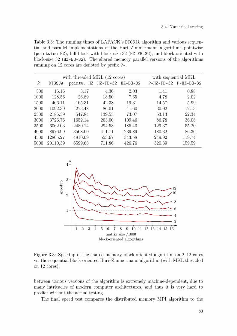
3.4. Numerical testing
Table 3.3: The running times of LAPACK’s DTGSJA algorithm and various sequen-tial and parallel implementations of the Hari–Zimmermann algorithm: pointwise(pointwise HZ), full block with block-size 32 (HZ-FB-32), and block-oriented withblock-size 32 (HZ-BO-32). The shared memory parallel versions of the algorithmsrunning on 12 cores are denoted by prefix P-.
with threaded MKL (12 cores) with sequential MKLk DTGSJA pointw. HZ HZ-FB-32 HZ-BO-32 P-HZ-FB-32 P-HZ-BO-32
500 16.16 3.17 4.36 2.03 1.41 0.881000 128.56 26.89 18.50 7.65 4.78 2.021500 466.11 105.31 42.38 19.31 14.57 5.992000 1092.39 273.48 86.01 41.60 30.02 12.132500 2186.39 547.84 139.53 73.07 53.13 22.343000 3726.76 1652.14 203.00 109.46 86.78 36.083500 6062.03 2480.14 294.58 186.40 129.37 55.204000 8976.99 3568.00 411.71 239.89 180.32 86.364500 12805.27 4910.09 553.67 343.58 249.92 119.745000 20110.39 6599.68 711.86 426.76 320.39 159.59
1 2 3 4 5 6 7 8 9 10 11 12 13 14 15 16
1
2
3
4
speedup
matrix size /1000block-oriented algorithms
2
4
6
8
10
12
Figure 3.3: Speedup of the shared memory block-oriented algorithm on 2–12 coresvs. the sequential block-oriented Hari–Zimmermann algorithm (with MKL threadedon 12 cores).
between various versions of the algorithm is extremely machine-dependent, due tomany intricacies of modern computer architectures, and thus it is very hard topredict without the actual testing.
The final speed test compares the distributed memory MPI algorithm to the
83

3. The implicit Hari–Zimmermann algorithm for the GSVD
1 2 3 4 5 6 7 8 9 10 11 12 13 14 15 16
0.5
1.0
1.5
speedup
matrix size /1000full block algorithms
seq.
2
4
6
8
10
12
Figure 3.4: Speedup of the shared memory full block algorithm on 2–12 cores vs. thesequential block-oriented Hari–Zimmermann algorithm (with MKL threaded on 12cores). An additional curve (denoted by seq.) shows the “speedup” of the sequentialfull block algorithm vs. the block-oriented algorithm. A few missing values for 2cores are caused by the limit of execution time on the cluster (12 hours).
Table 3.4: Left table: the running times of the hybrid MPI/OpenMP version of theHari–Zimmermann algorithm for a matrix pair of order 16000. Each MPI processexecutes the OpenMP algorithm with 12 threads. Each thread performs the block-oriented algorithm with the inner block-size of 32. Right table: the running timesfor the full block and block-oriented shared memory algorithms for the same matrix.
number of timeMPI processes cores MPI-HZ-BO-32
2 24 15323.724 48 8229.326 72 6049.778 96 4276.6510 120 3448.9012 144 3003.3914 168 2565.2916 192 2231.71
number of timecores P-HZ-FB-32 P-HZ-BO-32
2 – 42906.934 35168.73 18096.726 21473.00 10936.108 13745.17 7651.8610 9901.96 5599.2512 8177.90 4925.56
shared memory algorithms. Based on the results of earlier tests, the topmost (dis-tributed memory) level of the algorithm executes the block-oriented algorithm, withthe modified modulus strategy, on a collection of MPI processes. On the second
84

3.4. Numerical testing
(shared memory) level, each MPI process executes the block-oriented thread-parallelalgorithm, with the same strategy, on the given block-columns of F and G.
This comparison was carried out only for the largest matrix size of 16000, andthe results are given in Table 3.4. Because the communication between the MPIprocesses is relatively slow (compared to everything else), the MPI algorithm be-comes faster than the shared memory block-oriented algorithm when the number ofprocesses pm is at least 8. At this point the number of cores used is 96, which ishuge in comparison to only 12 cores used by the shared memory algorithm. There-fore, the MPI algorithm is designed for really huge matrices, that cannot fit intothe shared memory, or the parts of matrices given to a single thread are too big forefficient orthogonalization.
Finally, the accuracy of algorithms has been measured, by comparing the com-puted generalized singular values with the original ones, set at the beginning of thematrix generation. The test was carried out on a matrix pair of order 5000, which isthe largest size that could be tested on all algorithms, including DTGSJA. This par-ticular pair is moderately ill-conditioned, with a condition measure maxσi/minσi ≈6.32 · 105. The relative errors (see Figures 3.5–3.8) are U-shaped over the orderingof values (displayed in the logarithmic scale)—the largest errors occur at both endsof the range, which is understandable, since either (ΣF )ii or (ΣG)ii is small there.
10−3 10−2 10−1 100 101 102 103
2
4
6
8
10
12
14
16
18
relativeerrors
·1014
generalized singular values
DTGSJA
Figure 3.5: Relative errors in the computed generalized singular values for a matrixpair of order 5000 by DTGSJA.
Quite unexpectedly for the Jacobi-type methods, the pointwise algorithm, whichis usually more accurate than any of the blocked algorithms, turns out to be slightlyless accurate here. The sequential blocked algorithms are a bit more accurate thanthe parallel ones, as expected, while the differences in accuracy between the block-oriented and the full block versions are negligible. Maximal relative errors, andaverage relative errors for different routines are given in Table 3.5. Note that theaverage relative error for DTGSJA is about 5 times larger than for the blocked Hari–Zimmermann algorithms.
85

3. The implicit Hari–Zimmermann algorithm for the GSVD
10−3 10−2 10−1 100 101 102 103
2
4
6
8
10
12
14
16
18
relativeerrors
·1014
generalized singular values
pointwise HZ
Figure 3.6: Relative errors in the computed generalized singular values for a matrixpair of order 5000 by pointwise HZ.
The maximal relative errors grow with the condition of the problem, and veryslightly with the matrix size. For a matrix pair of order 16000 with maxσi/minσi ≈4.51 · 108, the maximal and average relative errors are given in Table 3.6. Only thefirst few and the last few generalized singular values are responsible for the maximalrelative error in all algorithms (the average values are much smaller). If the 5smallest and the 5 largest generalized singular values are ignored, the ratio betweenthe largest and the smallest σi drops to 2.41 ·106, and the obtained errors are similarto those in Table 3.5.
10−3 10−2 10−1 100 101 102 103
2
4
6
8
10
12
14
16
18
relativeerrors
·1014
generalized singular values
HZ-BO-32
Figure 3.7: Relative errors in the computed generalized singular values for a matrixpair of order 5000 by HZ-BO-32.
86

3.4. Numerical testing
10−3 10−2 10−1 100 101 102 103
2
4
6
8
10
12
14
16
18
relativeerrors
·1014
generalized singular values
P-HZ-BO-32
Figure 3.8: Relative errors in the computed generalized singular values for a matrixpair of order 5000 by P-HZ-BO-32.
Table 3.5: Maximal relative errors, and average relative errors for a matrix pair oforder 5000.
DTGSJA pointwise HZ HZ-BO-32 P-HZ-BO-32
max_rel 1.79666 · 10−13 1.77529 · 10−13 1.44462 · 10−13 1.46348 · 10−13
avg_rel 1.92500 · 10−14 1.25585 · 10−14 3.50042 · 10−15 4.07475 · 10−15
Note that DTGSJA is unable to handle such large matrices in any reasonabletime. On the largest matrices that can be used for comparison, the fastest sequen-tial threaded routine HZ-BO-32 is more than 47 times faster than LAPACK’s (on
Table 3.6: Maximal relative errors, and average relative errors for a matrix pairof order 16000. If the 5 smallest and the 5 largest generalized singular values areignored, the respective values are denoted by (6 : 15995).
HZ-BO-32 P-HZ-BO-32 MPI-HZ-BO-32
max_rel 1.45480 · 10−11 1.45499 · 10−11 1.45576 · 10−11
avg_rel 7.91808 · 10−15 7.30987 · 10−15 7.62689 · 10−15
max_rel (6 : 15995) 2.70628 · 10−13 2.64252 · 10−13 2.65734 · 10−13
avg_rel (6 : 15995) 6.35910 · 10−15 5.75219 · 10−15 6.06843 · 10−15
87

3. The implicit Hari–Zimmermann algorithm for the GSVD
this particular architecture), and more accurate, as well. For the fastest explicitlyparallel shared memory algorithm P-HZ-BO-32, the speedup factor is 126!
Bear in mind that, these speedup factors do not include the time required fortriangularization of both matrices, which is mandatory for DTGSJA, but not necessaryfor the Hari–Zimmermann method, when G is of full column rank.
The tests conducted on several different architectures give similar results, onlythe speedup factors are somewhat different, due to differences in architecture.
3.5. An implicit Hari–Zimmermann algorithm forthe GPU(s)
The blocked, parallel, implicit Hari–Zimmermann algorithm can be implementedon the GPU(s) much along the same lines as the blocked one-sided Jacobi SVD hasalready been detailed in chapter 2.
For brevity, only the full GSVD algorithm for a single GPU will be sketchedhere, and only the differences from the Jacobi SVD will be highlighted. The GSVDalgorithm performs all computation on a GPU, and consists of three kernels:
1. initZ – acts as if it sets Z to Ik, computes ||gi||2 for each 1 ≤ i ≤ k, andscales the columns fi of F , gi of G, and zi of Z, by 1/||gi||2;
2. pStep – invoked once for each p-step in a block-sweep;3. Sigma – rescales Z after each block-sweep, and optionally rescales F and G
and extracts the generalized singular values at the end of computation, as per(3.10), (3.11), and (3.12).
The pStep kernel is similar to the one for the Jacobi SVD. The thread blocks haveto operate on three 32× 32 matrices in the shared memory, roughly correspondingto F , G, and Z, which makes for 24 kB in the case of F = R, or for 48 kB the caseof F = C (both in double precision). The strategy tables and the mapped CPUmemory for the convergence statistics stay the same. Computation in a thread blockproceeds in the three major phases:
1. factorize – shortens the pivot block-pairs[Fp Fq
]and
[Gp Gq
], according
to (3.17) and (3.18), either by forming the Gram matrices and by factorizingthem using the Cholesky factorizations, or by the QR factorizations of theblock-columns, into the triangular factors Fpq and Gpq of order 32, initializesZpq = I32 ·diag (1/||g1||2, . . . , 1/||g32||2), and scales the columns of Fpq and Gpq
by the same inverses of the column norms of Gpq used for Zpq, i.e., by 1/||gi||2,with 1 ≤ i ≤ 32;
2. orthogonalize – orthogonalizes Fpq and Gpq by the pointwise implicit Hari-Zimmermann method, according to the block-oriented or the full block variantof the algorithm, accumulating the applied transformations into Zpq. After oneinner sweep (the block-oriented variant), or as many inner sweeps as neededuntil the local convergence (the full block variant), Zpq is rescaled accordingto (3.11) and (3.12), into Z ′pq. The singular value extraction and rescaling of
88

3.5. An implicit Hari–Zimmermann algorithm for the GPU(s)
Fpq and Gpq is not needed, since those matrices are discarded anyway;3. postmultiply – postmultiplies
[Fp Fq
],[Gp Gq
], and
[Zp Zq
], by Z ′pq, ac-
cording to (3.19) and (3.20).
Figure 3.9 summarizes the pStep kernel from a perspective of data placement andmovement. Subfigures (a) to (f) show the factorize phase, subfigures (g) and (h)show the orthogonalize phase, and subfigures (i) to (k) show the postmultiplyphase. RAM refers to the GPU’s main memory, and * to the matrix multiplication.
Note that on subfigure (a) the last 32×32 shared memory block is unused. Thatis a deficiency of the prototype code, that reuses the Gram matrix formation fromAlgorithm 3, i.e., for performing ATA operation on the 64 × 32 chunks. Anotherprocedure should be written for 96×32 chunks, to fully utilize all the shared memoryavailable. A similar remark relates to subfigures (i) to (k), where the postmultiplyphase currently reuses the 32×32 Cannon-like multiplication of Algorithm 4, insteadof performing (64×32)×(32×32) multiplication, to fully exploit the shared memory.
A transformation of a pivot pair will be computed and applied if
|gTp gq| ≥ ε√
32 or |fTp fq| ≥ ||fp||2||fq||2ε√
32,
with ε being the machine unit roundoff for the datatype. The convergence criterionlooks for the absolute values of the scaled cosines, i.e., the absolute values on thediagonal of a 2×2 transformation matrix Z, to differ from one (at least one of thoseelements), in order to mark a transformation as the “proper” one. Apart from that,handling the convergence information is exactly the same as in the SVD algorithm.
A recent GPU card (Pascal or newer) was not available at the time of writingthe code to perform a comparative numerical test against the CPU algorithm. Witha consumer Kepler GPU (GeForce GT 750M)3, CUDA 9.0 RC4, R‖ p-strategy, anda 1024×1024 matrix pair, the block-oriented variant takes 26.176350 seconds for 14block-sweeps, and the full block variant takes 30.792716 seconds for 12 block-sweeps.The block-oriented variant seems to be the faster one on the GPUs, as well as onthe CPUs (cf. Table 3.3), but further testing on newer GPUs is certainly warranted.
A multi-GPU implicit Hari-Zimmermann GSVD algorithm should be a straight-forward generalization of the one-sided multi-GPU Jacobi SVD and the single-GPUimplicit Hari-Zimmermann GSVD algorithms. It has not been implemented yet,but it makes a reasonable and attainable target for the short-term future work.
A note on the floating-point issues. Computing the dot-products and thevector (i.e., column) norms here suffers from the same issues as in the one-sidedJacobi SVD algorithm, and the same remedies apply. Also, to compute the scalingS from (3.11), a quantity
√||fi||22 + ||gi||22, and its reciprocal one, are needed. If
the squares of the column norms, or their sum, may overflow, it is advisable touse the hypot operation, which has to protect from the overflow, albeit possiblyintroducing the rounding error of a couple of ulps. But if no overflow is expected,
3With such GPUs, in double precision, at most 1/24 of single precision performace is achievable.4Release Candidate, not publicly available, so any results may change with the future versions.
89

3. The implicit Hari–Zimmermann algorithm for the GSVD
16 16
32
32
32
RAM
RAM RAM RAM
RAM RAM RAM
F
?
∗
∗
FTF
G
FTF
GTG
?
}C
h
o
l
e
s
k
yC
h
o
l
e
s
k
y
GTG
}
?
F0
0
F0
0
G0
0
?
F0
0
G0
0
Z0 =I
‖gp‖2
Fi+1
= FiZ
Gi+1
= GiZ
Zi+1
= ZiZ
}
}
}
H
Z
t
r
a
n
s
f
o
r
m
FN
= UΣF
GN
= V ΣG
Z ′N = ZN
(rescaled)
f
i
n
a
l
s
t
a
t
e
F
Z ′N
G
Z ′N
Z
Z ′N
∗ ∗ ∗
(a) (b) (c) (d)
(e) (f) (g) (h)
(i) (j) (k)
Figure 3.9: A single-GPU implicit Hari–Zimmermann algorithm, pStep kernel.
and the squares of the norms are already available, it may be faster to sum themand compute the square root or the reciprocal square root (rsqrt) directly.
Generally speaking, for both the SVD and the GSVD algorithms, a balancebetween the guaranteed correctness in all cases (i.e., even with a badly scaled input)
90

3.5. An implicit Hari–Zimmermann algorithm for the GPU(s)
and the decent performace can be struck as follows: run the faster version of thealgorithm (the one that uses the Cholesky factorizations, does not protect fromthe possible overflows induced by the dot-product based computation of the vectornorms, etc.) and check from time to time if any overflow or an invalid operation issignalled. If so, restart the whole computation with the original input (preserved ina backup workspace), but with a more careful variant of the algorithm (the one thatuses the QR factorization, protects from the avoidable overflows and underflows,etc.). For this approach to be facilitated, the floating-point operations have to setthe corresponding exception flags in the status register. Unlike the CPUs, that is notpossible on the GPUs for now, but a check for a non-finite floating-point quantityduring the computation should not be too expensive.
91

4. Conclusions and future work
4.1. Conclusions
In this thesis a set of new parallel Jacobi strategies has been developed, bothfaster and more accurate than the widely used ones. The new strategies may beseen as the generalizations of the Mantharam–Eberlein block-recursive strategy [51]to all even matrix orders. These new strategies are combined with the multi-levelblocking and parallelization techniques explored in [39, 40, 69, 68, 56], to deliver theJacobi-type (H)SVD algorithms for the graphics processing unit(s), competitive withthe leading hybrid (CPU+GPU) alternatives, like MAGMA. The new algorithmsare carefully designed to use a CPU primarily as a controlling unit. To this end,a collection of the auxiliary shared-memory routines for the concurrent formationof the Gram matrices, the Cholesky and QR factorizations, and the numericallyrobust vector 2-norm computations are proposed. The numerical results confirmthat in the massively parallel GPU case the Jacobi-type methods retain all theknown advantages [28, 29], while exhibiting noteworthy performance.
In the following part of the thesis the implicit Hari–Zimmermann method hasbeen developed, for computation of the generalized singular values of matrix pairs,where one of the matrices is of full column rank. The method is backward stable,and, if the matrices permit, computes the generalized singular values with smallrelative errors. Moreover, it is easy to parallelize. A part of the work is motivatedby the fact that the current alternatives for the GSVD computation—the best knownis DGGSVD from LAPACK, are extremely slow for larger matrices.
Unlike the triangular routine DTGSJA from LAPACK, which is Kogbetliantz-based, the Hari–Zimmermann method needs no preprocessing to make both matricestriangular. Even when the matrices are preprocessed to a triangular form, thesequential pointwise Hari–Zimmermann method is, for matrices of a moderate size,significantly faster than DTGSJA. On a particular hardware, where threaded MKL(on 12 cores) is used, the pointwise Hari–Zimmermann method is about 3 timesfaster than DTGSJA, and the computed generalized singular values have, on average,smaller relative errors.
A significant speedup is obtained by blocking of the algorithm, to exploit theefficiency of BLAS-3 operations. For example, the sequential block-oriented versionof the algorithm, in the same hardware/software environment, is 15 times faster andeven more accurate than the pointwise version, for matrices of order 5000.
Further gains in speed are obtained by explicit shared memory parallelizationof blocked algorithms, now with the sequential MKL. The shared memory block-oriented algorithm gives an additional speedup factor of about 2.5, even for muchlarger matrices. A distributed memory MPI version of the algorithm has also beendeveloped, which has been designed for really huge matrices that do not fit into theavailable shared memory, as well as a GPU version, as an extension of the GPUSVD Jacobi-type algorithm from the first part of the thesis.

4.2. A work in progress
The thesis contains several theoretical results about the implicit Hari–Zimmer-mann method. The convergence of the pointwise algorithm with the row-cyclic,column-cyclic, and modulus strategies follows from the results in [37] for the two-sided generalized eigenproblem algorithm. An extension of these results for blockedalgorithms is an open problem. The proofs of convergence for various blocked ver-sions of the algorithm are under development, by using the techniques from [38].
4.2. A work in progress
In this section the ongoing and possible future work is briefly described, withan emphasis on the benefits of, and programming for, the vector extensions to theCPU architectures, in the context of the Jacobi-type SVD processes.
4.2.1. A new hierarchy for the Jacobi-type processes
As the hardware architectures become ever more complex, it seems necessary torevisit, from time to time, the assumptions about the appropriate number of theblocking levels for the Jacobi-type algorithms.
Driven by the many levels of caches present in a typical modern CPU, alongsideSIMD (vectorization) capabilities, and the (still shared but) non-uniform memoryarchitectures (NUMA), where also a distinction between a cache level and the RAMis blurred by the advent of the large memory buffers (like MCDRAM for the IntelKNLs), it may be required for an optimal design of a Jacobi-type algorithm toconsider three to four memory hierarchy levels, as follows.
Level 0
Let V be the largest vector length for a given datatype (e.g., for double, it is 8for Intel KNL, and 2 for IBM POWER8), and 1 ≤ v ≤ V a chosen vector length.Let Cd1 be the level-1 data (L1d) cache line size, counted in number of elements ofthe datatype that fit into a cache line. For double, Cd1 = 8 on KNL, and Cd1 = 16on POWER8. Then, Cd1/v is a number of vectors that fit into a cache line. LetVc = Cd1/V, and assume v = V. The Level 0 algorithm should process exactly kVc,k ≥ 1, pairs of columns, to keep full vectorization for computing the rotations’parameters. Being the innermost level, it should avoid as much argument checkingand branching as possible. Therefore, the input matrix should have 2kVc columns,or be bordered (i.e., expanded by an identity matrix in the lower right corner, andby zeroes elsewhere) up to that size.
A parameter k should be chosen to maximize L1d cache utilization, bearing inmind that two “small” matrices, G and V (or three matrices: F , G, and Z, in theGSVD case), and a couple of vectors holding the temporary results, as well as thesines (or tangents) and the cosines, have to fit into L1d cache. One should be awareof the cache associativity, false sharing, and similar hidden dangers, also!
It is worth exploring if hyperthreading [52] (or a similar non-Intel technologyfor running more than one thread per core) with h > 1 threads per core, where h
93

4. Conclusions and future work
divides k, improves instruction throughput versus no hyperthreading (i.e., h = 1).Hyperthreading should split k tasks among h threads, but the overhead of threadingmight be to high for such an approach to be viable.
To demonstrate that manual vectorization pays off, the following example com-pares the performance of a simple, hand-written (using Intel’s AVX2 compiler in-trinsics1, that closely resemble the actual machine instructions generated) vectorizedversion of the pointwise one-sided Jacobi SVD in double (v = V = 4) to the perfor-mance of the MKL’s optimized single-threaded DGESVJ routine from LAPACK.
In the hand-written code, contrary to DGESVJ, there is no final computationof the column norms (to extract the singular values) nor there is rescaling (i.e.,normalizing) of the columns, since only the matrix of the accumulated rotations issought for, in an expectation that it will be used further up the blocking hierarchy.
That final postprocessing requires only a quadratic number of operations in termsof the matrix order, and should not affect much the time ratios shown in Figure 4.1.
8 24 40 56 72 88 104 120 136 152 16816 32 48 64 80 96 112 128 144 160 176
0
0.004
0.007
0.011
0.014
0.018
0.021
0.025
0.028
0.032
0.036• Manually vectorized code with AVX2 and FMA intrinsics (with # of sweeps)
◦ DGESVJ(´G´,´N´,´V´,. . . ), Intel MKL, sequential (with # of sweeps)
Time (ratios) for the small orders n:
n • time [µs] ◦ time [µs] ◦/• ratio8 5.860 77.855 13.28616 29.956 119.462 3.98824 90.559 267.920 2.95932 192.610 496.162 2.57640 364.998 795.039 2.178
• • • • ••
••
•
•
•
•
•
•
•
•
•
•
•
•
•
•
6 7 8 8 8 8 9 99
99
9
10
9
9
9
10
10
10
10
11
10
◦ ◦ ◦ ◦ ◦◦
◦◦
◦◦
◦
◦
◦
◦
◦
◦
◦
◦
◦
◦
◦
◦
6 8 8 9 9 10 9 9 99
99
99
109
9
9
9
9
9
10
input matrix order
timeuntilconvergence
[s]
Figure 4.1: Execution times and sweep counts of the manually vectorized Jacobi codewith AVX2 and FMA intrinsics, vs. DGESVJ from Intel MKL 2017.2.163 (sequential),on Intel Core i7-4850HQ CPU @ 2.30GHz, with macOS 10.12.4 and clang-802.0.38.Measured with CLOCK_THREAD_CPUTIME_ID POSIX clock, per run, and averagedover 100 runs; see https://github.com/venovako/JACSD/tree/master/test for more.
As can be seen on Figure 4.1, the effort of avoiding any argument checking, thefunction calls inside the algorithm, and non-vectorized code as much as possible,gives a speedup of several times for the very small matrix orders (where all data is
1See the Intel Intrinsics Guide: https://software.intel.com/sites/landingpage/IntrinsicsGuide/
94

4.2. A work in progress
expected to fit into L1d cache), although any speedup is lost for the “larger” matrixorders (104 and beyond, in this case). It is therefore advisable to pay the mostattention to the innermost blocking level of the Jacobi-type processes.
So, how to perform the vectorization of the pointwise one-sided Jacobi SVD?In effect, the SIMD vector architecture can be seen as a very restricted parallelmachine, where any and all parallelism comes from the scalar operations performedsimultaneously on all elements (also called “lanes”) of one, two, or three vectorregisters, or on a subset (defined by a bitmask) of the elements thereof.
In the present architectures, the operations within the same lane across theregisters involved (i.e., “vertical” instructions) are readily available, but the intra-register, inter-lane (i.e., “horizontal”) operations are either not supported, or (wherethey are) may be more expensive and less versatile than the vertical ones. That canbe compared to the thread warps on a GPU, where the operations across threads ina warp require manual shuffling of data between threads, as opposed to the scalaroperations within each warp lane.
Therefore, a similar parallelization approach as with the inner level of blockingon a GPU is required. Ignoring the technical details, there are three importantphases in the pointwise Jacobi SVD: the dot-product computation, the calculationof the Jacobi rotations, and their application to the matrices G (and V ).
First, the pivot pairs are chosen from the current p-step of the chosen p-strategy.There should be as many independent pivot pairs as there are vector lanes available(e.g., 4 for the doubles on the AVX2 architecture). If the matrix order n is equal to8, then all pivot pairs from a p-step can be processed as it is described below. If n issmaller, the uppermost vector lanes will be unutilized during the computation of therotations, and in the processing of the final chunk of rows during the dot-productand transformation phases. Else, if n > 8, then a p-step should be sliced intodn/(2Vc)e batches of pivot pairs, where each batch is processed as to be described.The batches can be iterated over sequentially, or they can be partitioned among thehyperthreads (where available and enabled) for parallel execution.
Obviously, it pays off to process matrices of orders which are the exact multiplesof 8 (for AVX2, or 16 for AVX-512). Otherwise, a special code path is required forloading and storing a part of a vector from memory at the end of the loops over thematrix rows, and for masking the unused lanes elsewhere in the computation.
The pointwise algorithm vectorized. For each pivot pair (in sequential, i.e.,one pivot pair after another), three dot-products are computed. Here, the vector-ization is not used to handle the pivot pairs simultaneously, but to compute, e.g.,4 scalar fmas (updates of the 4 partial sums) in one go, one chunk of 4 consecutiverow indices in the columns of G at a time. Once a chunk of gp and gq is loaded in thevector registers, three vector fmas are enough to update the partial sums of gTp gp,gTp gq, and gTq gq, each in its own vector register. So, e.g., one register will hold thepartial sums for gTp gq, where the lane i will accumulate the products of the elementsof gp with the elements of gq, with the row indices equal to i mod 4, for 0 ≤ i ≤ 3.
The tricky part, as with the GPUs, is how to reduce the partial sums, held in eachof the three aforementioned registers. Here, the “horizontal” reductions are needed,
95

4. Conclusions and future work
either readily available as an instruction or an intrinsic, or manually implemented.For the AVX2 architecture, Listing 4 shows the entire computation, with one
possible realization of the +-reduction. For each pivot pair, one vector containingthe three dot products, and additionally |gTp gq|, is obtained.
Those vectors have to be rearranged for the second phase. There, each lane willbe in charge of computing the Jacobi rotation’s parameters for a particular pivotpair. The idea is to get the parameters analogously to the scalar case, but for allthe pivot pairs simultaneously. That effectively means to compute 4 tangents and4 cosines for (about) the price of one each. For that, all 4 values of gTp gp have tobe in the same vector, occupying a lane associated with their pivot pair. The samegoes for gTp gq, gTq gq, and |gTp gq|.
Such a rearrangement comes with a price. In the prototype implementation, ithas been realized by storing the dot-product vectors back to memory, and vector-gathering their pieces into the new variables described above. Once that is done, it isdecided whether all the columns are relatively orthogonal. If so, no transformationis needed. If not, it does not hurt at all to proceed with computing the rotations evenfor the lanes (i.e., the pivot pairs) where the columns are relatively orthogonal, sincethe vector operations will take the same (or similar) amount of time, regardless ofthe number of the “active” lanes. Those results can (and will) be discarded anyway.
It is however assumed that any possible floating-point exceptions occurring in theoperations over those lanes will not affect the execution flow of the code. If that wasnot the case, a careful masking of the “offending” lanes should be considered beforeproceeding to the computation of the rotations’ parameters, shown in Listing 5.
The rotations’ parameters of the pivot pairs whose columns are nor relativelyorthogonal have to be reshuffled again. For each such tangent, it has to be spreadout (“broadcast”) over the whole new register (i.e., in 4 copies, one in each lane), inorder to be ready for vector multiplication with 4 consecutive rows of G (and V ).The same holds for each such cosine.
Finally, applying the rotations is done in a conceptually similar way to computingthe dot-products, one pivot pair (i.e., one rotation) a time (if the transformation isneeded), but with 4 elements of G (and V ) transformed at once.
Level 1
An input matrix is split into block columns, with approximately kVc columnsper a block column. The input should be sized in accordance to the level-2 cachesize (L2), i.e., two same-size matrices, G and V , and a workspace, should fit into L2cache. The workspace has to contain “small” blocks and vectors for the Level 0.
Hyperthreading might prove more beneficial at this level than at the level below,but then for each thread there should be its private input, output, and workspacememory for Level 0 set aside, as described. So, each thread t would need a “small”Gt, Vt, and Wt (workspace) arrays, while all such arrays, for all threads on a core,should simultaneously be present in L1d cache. Therefore, hyperthreading mightpush k down, close to 1, which means that k itself is a varying parameter to theLevel 0 algorithm, not a constant deducible at compile-time.
96

4.2. A work in progress
Listing 4: Computing the dot products with Intel AVX2 & FMA intrinsics1 stat ic inl ine __m256d avx2_fma_ddots ( const unsigned m,2 const double ∗const r e s t r i c t Gp, const double ∗const r e s t r i c t Gq)3 { // to be called for each pivot pair (p, q) in sequence45 // The data has to be aligned in memory to addresses that are6 // a multiple of the vector size (32 B), for faster load/store.7 register const double ∗const Gp_i = // start of Gp8 ( const double∗) __builtin_assume_aligned (Gp, 3 2 ) ;9 register const double ∗const Gq_i = // start of Gq10 ( const double∗) __builtin_assume_aligned (Gq, 3 2 ) ;1112 register __m256d Gpp = _mm256_setzero_pd ( ) ;13 register __m256d Gqq = _mm256_setzero_pd ( ) ;14 register __m256d Gpq = _mm256_setzero_pd ( ) ;1516 for ( register unsigned i = 0u ; i < m; i += 4u) {17 // load the next chunk of Gp and the next chunk of Gq18 register const __m256d Gpi = _mm256_load_pd(Gp_i + i ) ;19 register const __m256d Gqi = _mm256_load_pd(Gq_i + i ) ;20 // update the partial sums21 Gpp = _mm256_fmadd_pd(Gpi , Gpi , Gpp ) ;22 Gqq = _mm256_fmadd_pd(Gqi , Gqi , Gqq ) ;23 Gpq = _mm256_fmadd_pd(Gpi , Gqi , Gpq ) ;24 }2526 // horizontal +-reductions , with a twist to get |Gpq| as well2728 // (Gpq[2]+Gpq[3], Gpp[2]+Gpp[3], Gpq[0]+Gpq[1], Gpp[0]+Gpp[1])29 register const __m256d GppGpq = _mm256_hadd_pd(Gpp, Gpq ) ;30 // (Gpq[2]+Gpq[3], Gqq[2]+Gqq[3], Gpq[0]+Gpq[1], Gqq[0]+Gqq[1])31 register const __m256d GqqGpq = _mm256_hadd_pd(Gqq , Gpq ) ;32 // (Gpq[2]+Gpq[3], Gpq[0]+Gpq[1], Gpp[2]+Gpp[3], Gpp[0]+Gpp[1])33 register const __m256d GppGpq_ = // swap the middle lanes34 _mm256_permute4x64_pd(GppGpq, 0xD8 ) ;35 // (Gpq[2]+Gpq[3], Gpq[0]+Gpq[1], Gqq[2]+Gqq[3], Gqq[0]+Gqq[1])36 register const __m256d GqqGpq_ = // swap the middle lanes37 _mm256_permute4x64_pd(GqqGpq , 0xD8 ) ;38 // (Gpq, Gpq, Gqq, Gpp)39 register const __m256d intm = _mm256_hadd_pd(GppGpq_, GqqGpq_) ;40 // a bit of sign-masking (taking abs) needed for |Gpq|41 // x &~ -0.0 clears the sign bit, ~(-0.0): all-1s, leading 042 register const __m256d mask = // 0.0 negated: all-1s43 _mm256_set_pd(−0.0 , 0 . 0 , −0.0 , −0.0) ;4445 // out[0] = Gpp; out[1] = Gqq; out[2] = Gpq; out[3] = |Gpq|;46 return _mm256_andnot_pd(mask , intm ) ;47 }
97

4. Conclusions and future work
Listing 5: Computing the Jacobi rotations with Intel AVX2 & FMA intrinsics1 __m256d ones = _mm256_set_pd( 1 . 0 , 1 . 0 , 1 . 0 , 1 . 0 ) ;2 __m256d twos = _mm256_set_pd( 2 . 0 , 2 . 0 , 2 . 0 , 2 . 0 ) ;3 __m256d neg0 = _mm256_set_pd(−0.0 ,−0.0 ,−0.0 ,−0.0);4 // ||G~q||22 − ||G~p||22, if the squares of the norms are available5 __m256d Gq_p = _mm256_sub_pd(Gqq , Gpp ) ;6 // else, with the norms, (||G~q||2 − ||G~p||2)(||G~q||2 + ||G~p||2)7 [[ _mm256_mul_pd(_mm256_sub_pd(Gq_,Gp_) ,_mm256_add_pd(Gq_,Gp_) ) ; ]]8 // cot 2~ϕ = (||G~q||22 − ||G~p||22)/(2 ·GT~pG~q); where available and if faster ,9 // replace multiplication by 2 with a scalbn()-like instruction10 __m256d Ctg2 = _mm256_div_pd(Gq_p, _mm256_mul_pd(Gpq , twos ) ) ;11 //
√cot2 2~ϕ+ 1; only two roundings due to FMA
12 __m256d tmp0 = _mm256_sqrt_pd(_mm256_fmadd_pd(Ctg2 , Ctg2 , ones ) ) ;13 // extract the sign bit from each of the cotangents of 2~ϕ14 __m256d sgnb = _mm256_and_pd(Ctg2 , neg0 ) ;15 // transfer the sign bits onto the square roots; their sign bits16 // being 0, it is enough to bitwise -OR them with the desired ones17 __m256d tmp1 = _mm256_or_pd(tmp0 , sgnb ) ;18 // cot ~ϕ = cot 2~ϕ+ sign(
√cot2 2~ϕ+ 1, cot 2~ϕ)
19 __m256d Ctg = _mm256_add_pd(Ctg2 , tmp1 ) ;20 // tan ~ϕ = 1/ cot ~ϕ; here, a ‘reciprocal’ instruction would be useful21 __m256d Tan = _mm256_div_pd( ones , Ctg ) ;22 //
√tan2 ~ϕ+ 1; only two roundings due to FMA
23 __m256d tmp2 = _mm256_sqrt_pd(_mm256_fmadd_pd(Tan , Tan , ones ) ) ;24 // cos ~ϕ = 1/
√tan2 ~ϕ+ 1; here, there is 1 division (or reciprocal),
25 // and 1 square root; it would be beneficial to have CORRECTLY26 // ROUNDED ‘rsqrt’, x−1/2, instruction , to halve the number of ex-27 // pensive operations to 1, and have only 2 roundings altogether.28 __m256d Cos = _mm256_div_pd( ones , tmp2 ) ;29 // new ~p-th diagonal entries of GTG: ||G′~p||
22 = ||G~p||22 + tan ~ϕ · (GT~pG~q)
30 Gpp = _mm256_fmadd_pd(Tan , Gpq , Gpp ) ;31 // new ~q-th diagonal entries of GTG: ||G′~q||
22 = ||G~q||22 − tan ~ϕ · (GT~pG~q)
32 Gqq = _mm256_fnmadd_pd(Tan , Gpq , Gqq ) ;
Level 2
At this level the algorithm becomes thread-parallel (e.g., using OpenMP), if notalready so due to the hyperthreading. The threads are bound to cores, one-to-one, ina single NUMA domain. Usually, that would be one CPU socket in an SMP machineand its associated memory, but it may get more complicated with the KNLs.
This is also the most appropriate level for introducing any kind of hybrid process-ing (e.g., CPU&GPU, CPU&MIC, CPU&FPGA, . . . ), since the attached devicesshare a NUMA domain with their neighboring CPU, but what part(s), if any, ofthe entire computation to offload to a coprocessing device still remains a separateresearch topic.
98

4.3. A note on the figures and the software
Level 3
At this level the algorithm operates in the “classical” MPI data exchange regime,and can span multiple NUMA domains (still with shared memory), or multipleSMP nodes in a cluster (with distributed memory). Each MPI process is threaded,in accordance to Level 2.
Alternatively, a single OpenMP-threaded process can be in charge for all NUMAdomains (and, optionally, coprocessing devices) within a single node, by carefullysetting thread affinities and allocating/using the memory local to a domain through-out execution, save for the column exchanges at the end of each block-sweep. Such aprocess should still employ MPI to communicate to other nodes in a cluster, though.That approach might be considered to be Level 2.5.
NUMA and the network (i.e., cluster) topologies may also be the drivers forthe new classes of the parallel strategies, as it has been in the past (e.g., with theMantharam-Eberlein strategy for the hypercube topologies, or with the modifiedmodulus strategy for the one-dimensional torus), to minimize the wall-clock time ofthe data exchange phases.
4.3. A note on the figures and the software
Figures 2.2, 2.3, 2.4, 2.5, 2.6, and 2.7 have been generated by circo tool ofGraphviz2 2.40.1, Figures 2.9 and 4.1 by METAPOST
3 1.9991, as well as Figures2.1, 2.10, 2.11, 2.12, 2.18, 2.19, and 3.9, which have been drawn by Sanja Singerfrom the author’s sketches. The graphs and schematics in Figures 2.20, 2.21, 2.22,2.23, 2.24, 2.25, 2.26, 2.27, 3.1, 3.2, 3.3, 3.4, 3.5, 3.6, 3.7, and 3.8 have also beenplotted by her. Figure 2.8 has been generated by Wolfram Mathematica4 10.4.1.The matrix heatmaps of Figures 2.13, 2.14, 2.15, 2.16, and 2.17 have been createdmanually5, as bitmaps, as well as the colorbar6. The rest of the thesis has beenprepared with LATEX. The final version will be available at http://venovako.eu site.
The prototype software implementations of the algorithms described in this the-sis (and some related ones) can be found on https://github.com/venovako GitHub,under repositories GPUJACHx (a single-GPU CUDA-based one-sided Jacobi SVD,HSVD, and the Hari-Zimmermann GSVD code), hz-gsvd (an OpenMP shared-memory code for the Hari-Zimmermann GSVD), JACSD (a collection of multi-levelOpenMP codes for the one-sided Jacobi SVD and a lot of support routines), andJKogb (a Kogbetliantz-like, i.e., two-sided experimental code for the HSVD).
2http://www.graphviz.org3https://www.tug.org/metapost.html4http://www.wolfram.com/mathematica/5See, in https://github.com/venovako/JACSD repository, vn library’s tools for bitmap (bmp)
generation and matrix visualization.6The colormap is based on Matlab’s jet, with the first and the last color not shown and reserved
for −∞ and +∞ (or NaNs), respectively (of which neither are present in the plotted data).
99

5. Bibliography
[1] O. Alter, P. O. Brown, and D. Botstein, Generalized singular valuedecomposition for comparative analysis of genome-scale expression data sets oftwo different organisms, P. Natl. Acad. Sci. USA, 100 (2003), pp. 3351–3356.
[2] A. A. Anda and H. Park, Fast plane rotations with dynamic scaling, SIAMJ. Matrix Anal. Appl., 15 (1994), pp. 162–174.
[3] M. Anderson, G. Ballard, J. W. Demmel, and K. Keutzer,Communication-avoiding QR decomposition for GPUs, in Proceedings of the25th IEEE International Parallel & Distributed Processing Symposium (IPDPS2011), Anchorage, AK, USA, May 2011, pp. 48–58.
[4] M. Ashworth, J. Meng, V. Novaković, and S. Siso, Early applica-tion performance at the Hartree Centre with the OpenPOWER architecture,in High Performance Computing, M. Taufer, B. Mohr, and J. M. Kunkel, eds.,vol. 9945 of Lecture Notes in Computer Science, Frankfurt, Germany, June2016, Springer, pp. 173–187.
[5] Z. Bai and J. W. Demmel, Computing the generalized singular value decom-position, SIAM J. Sci. Comput., 14 (1993), pp. 1464–1486.
[6] Z. Bai and H. Zha, A new preprocessing algorithm for the computation ofthe generalized singular value decomposition, SIAM J. Sci. Comput., 14 (1993),pp. 1007–1012.
[7] M. Bečka, G. Okša, and M. Vajteršic, Dynamic ordering for a parallelblock–Jacobi SVD algorithm, Parallel Comput., 28 (2002), pp. 243–262.
[8] P. Benner, V. Novaković, A. Plaza, E. S. Quintana-Ortí, andA. Remón, Fast and reliable noise estimation for hyperspectral subspace iden-tification, IEEE Geosci. Remote Sens. Lett., 12 (2015), pp. 1199–1203.
[9] K. Bhuyan, S. B. Singh, and P. K. Bhuyan, Application of generalizedsingular value decomposition to ionospheric tomography, Ann. Geophys., 22(2004), pp. 3437–3444.
[10] J. L. Blue, A portable fortran program to find the Euclidean norm of a vector,ACM Trans. Math. Software, 4 (1978), pp. 15–23.
[11] M. Botinčan and V. Novaković, Model-based testing of the ConferenceProtocol with Spec Explorer, in 9th International Conference on Telecommuni-cations, Zagreb, Croatia, June 2007, IEEE, pp. 131–138.
[12] R. P. Brent and F. T. Luk, The solution of singular-value and symmetriceigenvalue problems on multiprocessor arrays, SIAM J. Sci. Statist. Comput.,6 (1985), pp. 69–84.

Bibliography
[13] R. P. Brent, F. T. Luk, and C. F. Van Loan, Computation of the singularvalue decomposition using mesh–connected processors, J. VLSI Comput. Syst.,1 (1985), pp. 242–270.
[14] J. R. Bunch and B. N. Parlett, Direct methods for solving symmetricindefinite systems of linear equations, SIAM J. Numer. Anal., 8 (1971), pp. 639–655.
[15] L. E. Cannon, A Cellular Computer to Implement the Kalman Filter Algo-rithm, PhD thesis, Montana State University, Bozeman, MT, USA, 1969.
[16] P. P. M. de Rijk, A one–sided Jacobi algorithm for computing the singularvalue decomposition on a vector computer, SIAM J. Sci. Statist. Comput., 10(1989), pp. 359–371.
[17] A. Deichmöller, Über die Berechnung verallgemeinerter singularerWerte mittels Jacobi-ähnlicher Verfahren, PhD thesis, FernUniversität–Gesamthochschule, Hagen, 1990.
[18] J. W. Demmel, L. Grigori, M. F. Hoemmen, and J. Langou,Communication–optimal parallel and sequential QR and LU factorizations,Technical Report UCB/EECS–2008–89, Electrical Engineering and ComputerSciences University of California at Berkeley, Aug. 2008.
[19] , Communication–optimal parallel and sequential QR and LU factoriza-tions, SIAM J. Sci. Comput., 34 (2012), pp. A206–A239.
[20] J. W. Demmel and H. D. Nguyen, Fast reproducible floating-point sum-mation, in Proceedings of the 21st IEEE Symposium on Computer Arithmetic(ARITH), Austin, TX, USA, April 2013, pp. 163–172.
[21] J. W. Demmel and K. Veselić, Jacobi’s method is more accurate than QR,SIAM J. Matrix Anal. Appl., 13 (1992), pp. 1204–1245.
[22] M. Doko and V. Novaković, Izračunljivost i apstraktni strojevi, Hrvatskimatematički elektronski časopis math.e, 9 (2006).
[23] F. M. Dopico, P. Koev, and J. M. Molera, Implicit standard Jacobi giveshigh relative accuracy, Numer. Math., 113 (2009), pp. 519–553.
[24] Z. Drmač, Computing the Singular and the Generalized Singular Values, PhDthesis, FernUniversität–Gesamthochschule, Hagen, 1994.
[25] , Implementation of Jacobi rotations for accurate singular value computa-tion in floating point arithmetic, SIAM J. Sci. Comput., 18 (1997), pp. 1200–1222.
[26] , A tangent algorithm for computing the generalized singular value decom-position, SIAM J. Numer. Anal., 35 (1998), pp. 1804–1832.
101
Bibliography
[27] , A posteriori computation of the singular vectors in a preconditioned JacobiSVD algorithm, IMA J. Numer. Anal., 19 (1999), pp. 191–213.
[28] Z. Drmač and K. Veselić, New fast and accurate Jacobi SVD algorithm. I,SIAM J. Matrix Anal. Appl., 29 (2008), pp. 1322–1342.
[29] , New fast and accurate Jacobi SVD algorithm. II, SIAM J. Matrix Anal.Appl., 29 (2008), pp. 1343–1362.
[30] P. J. Eberlein, A one–sided Jacobi methods for parallel computation, SIAMJ. Alg. Disc. Meth., 8 (1987), pp. 790–796.
[31] S. Falk and P. Langemeyer, Das Jacobische Rotationsverfahren fur reel-symmetrische Matrizenpaare I, in Elektronische Datenverarbeitung Folge 7,H. K. Schuff, ed., Friedr. Vieweg & Sohn, Braunschweig, 1960, pp. 30–34.
[32] , Das Jacobische Rotationsverfahren fur reelsymmetrische MatrizenpaareII, in Elektronische Datenverarbeitung Folge 8, H. K. Schuff, ed., Friedr. Vieweg& Sohn, Braunschweig, 1960, pp. 35–43.
[33] G. R. Gao and S. J. Thomas, An optimal parallel Jacobi–like solution methodfor the singular value decomposition, in Proceedings of the 1988 InternationalConference on Parallel Processing, St. Charles, IL, USA, vol. 3, August 1988,pp. 47–53.
[34] G. Gose, Das Jacobi–Verfahren für Ax = λBx, Z. Angew. Math. Mech., 59(1979), pp. 93–101.
[35] S. Graillat, C. Lauter, P. T. P. Tang, N. Yamanaka, and S. Oishi,Efficient calculations of faithfully rounded l2-norms of n-vectors, ACM Trans.Math. Software, 41 (2015), p. Article 24.
[36] E. R. Hansen, On cyclic Jacobi methods, J. Soc. Indust. Appl. Math., 11(1963), pp. 448–459.
[37] V. Hari, On Cyclic Jacobi Methods for the Positive Definite Generalized Eigen-value Problem, PhD thesis, FernUniversität–Gesamthochschule, Hagen, 1984.
[38] , Convergence to diagonal form of block Jacobi-type methods, Numer.Math., 129 (2015), pp. 449–481.
[39] V. Hari, S. Singer, and S. Singer, Block-oriented J-Jacobi methods forHermitian matrices, Linear Algebra Appl., 433 (2010), pp. 1491–1512.
[40] , Full block J-Jacobi methods for Hermitian matrices, Linear AlgebraAppl., 444 (2014), pp. 1–27.
[41] M. R. Hestenes, Inversion of matrices by biorthonalization and related re-sults, J. Soc. Indust. Appl. Math., 6 (1958), pp. 51–90.
102

Bibliography
[42] N. J. Higham, Functions of Matrices: Theory and Computation, SIAM,Philadelphia, 2008.
[43] R. A. Horn and C. R. Johnson, Matrix Analysis, Cambridge UniversityPress, Cambridge, 1985.
[44] IEEE 754-2008, Standard for Floating-Point Arithmetic, New York, NY, USA,Aug. 2008.
[45] D. S. Johnson, M. Yannakakis, and C. H. Papadimitriou, On generat-ing all maximal independent sets, Inform. Process. Lett., 27 (1988), pp. 119–123.
[46] E. G. Kogbetliantz, Solution of linear equations by diagonalization of coef-ficients matrix, Quart. Appl. Math., 13 (1955), pp. 123–132.
[47] S. R. Kuo, W. Yeih, and Y. C. Wu, Applications of the generalized singular-value decomposition method on the eigenproblem using the incomplete boundaryelement formulation, J. Sound. Vib., 235 (2000), pp. 813–845.
[48] S. Lahabar and P. J. Narayanan, Singular value decomposition on GPUusing CUDA, in Proceedings of the 23rd IEEE International Symposium onParallel & Distributed Processing (IPDPS 2009), Rome, Italy, May 2009.
[49] F. T. Luk and H. Park, On parallel Jacobi orderings, SIAM J. Sci. Statist.Comput., 10 (1989), pp. 18–26.
[50] , A proof of convergence for two parallel Jacobi SVD algorithms, IEEETrans. Comput., C–38 (1989), pp. 806–811.
[51] M. Mantharam and P. J. Eberlein, Block recursive algorithm to generateJacobi–sets, Parallel Comput., 19 (1993), pp. 481–496.
[52] D. T. Marr, F. Binns, D. L. Hill, G. Hinton, D. A. Koufaty, J. A.Miller, and M. Upton, Hyper-threading technology architecture and mi-croarchitecture, Intel Technology Journal, 6 (2002), pp. 4–15.
[53] W. F. Mascarenhas, On the convergence of the Jacobi method for arbitraryorderings, SIAM J. Matrix Anal. Appl., 16 (1995), pp. 1197–1209.
[54] L. Nazareth, On the convergence of the cyclic Jacobi method, Linear AlgebraAppl., 12 (1975), pp. 151–164.
[55] V. Novaković, A hierarchically blocked Jacobi SVD algorithm for single andmultiple graphics processing units, SIAM J. Sci. Comput., 37 (2015), pp. C1–C30.
[56] V. Novaković and S. Singer, A GPU-based hyperbolic SVD algorithm, BIT,51 (2011), pp. 1009–1030.
103

Bibliography
[57] V. Novaković, S. Singer, and S. Singer, Estimates for the spectral con-dition number of cardinal B-spline collocation matrices, Math. Commun., 15(2010), pp. 503–519.
[58] , Blocking and parallelization of the Hari–Zimmermann variant of the Falk–Langemeyer algorithm for the generalized SVD, Parallel Comput., 49 (2015),pp. 136–152.
[59] NVIDIA, CUDA C Programming Guide 5.5, July 2013.
[60] R. Onn, A. O. Steinhardt, and A. Bojanczyk, The hyperbolic singularvalue decomposition and applications, IEEE Trans. Signal Process., 39 (1991),pp. 1575–1588.
[61] C. C. Paige, Computing the generalized singular value decomposition, SIAMJ. Sci. Statist. Comput., 7 (1986), pp. 1126–1146.
[62] C. C. Paige and M. A. Saunders, Towards a generalized singular valuedecomposition, SIAM J. Numer. Anal., 18 (1981), pp. 398–405.
[63] B. N. Parlett, The Symmetric Eigenvalue Problem, no. 20 in Classics inApplied Mathematics, SIAM, Philadelphia, 1998.
[64] H. Rutishauser, The Jacobi method for real symmetric matrices, Numer.Math., 9 (1966), pp. 1–10.
[65] A. H. Sameh, On Jacobi and Jacobi–like algorithms for a parallel computer,Math. Comp., 25 (1971), pp. 579–590.
[66] G. Shroff and R. S. Schreiber, On the convergence of the cyclic Jacobimethod for parallel block orderings, SIAM J. Matrix Anal. Appl., 10 (1989),pp. 326–346.
[67] S. Singer, S. Singer, V. Hari, K. Bokulić, D. Davidović, M. Jurešić,and A. Ušćumlić, Advances in speedup of the indefinite one-sided block Jacobimethod, in AIP Conf. Proc. – Volume 936 Numerical Analysis and AppliedMathematics, T. E. Simos, G. Psihoyios, and C. Tsitouras, eds., Melville, NewYork, 2007, AIP, pp. 519–522.
[68] S. Singer, S. Singer, V. Novaković, D. Davidović, K. Bokulić, andA. Ušćumlić, Three-level parallel J-Jacobi algorithms for Hermitian matrices,Appl. Math. Comput., 218 (2012), pp. 5704–5725.
[69] S. Singer, S. Singer, V. Novaković, A. Ušćumlić, and V. Dunjko,Novel modifications of parallel Jacobi algorithms, Numer. Alg., 59 (2012), pp. 1–27.
[70] I. Slapničar, Componentwise analysis of direct factorization of real symmetricand Hermitian matrices, Linear Algebra Appl., 272 (1998), pp. 227–275.
104

Bibliography
[71] I. Slapničar and V. Hari, On the quadratic convergence of the Falk–Langemeyer method, SIAM J. Math. Anal., 12 (1991), pp. 84–114.
[72] G. W. Stewart, Computing the CS decomposition of a partitioned orthogonalmatrix, Numer. Math., 40 (1982), pp. 297–306.
[73] , Computing the CS and the generalized singular value decompositions,Numer. Math., 46 (1985), pp. 479–491.
[74] , On the early history of the singular value decomposition, SIAM Rev., 35(1993), pp. 551–566.
[75] B. D. Sutton, Stable computation of the CS decomposition: Simultaneousbidiagonalization, SIAM J. Matrix Anal. Appl., 33 (2012), pp. 1–21.
[76] S. Tomov, R. Nath, and J. Dongarra, Accelerating the reduction to up-per Hessenberg, tridiagonal, and bidiagonal forms through hybrid GPU-basedcomputing, Parallel Comput., 36 (2010), pp. 645–654.
[77] C. F. Van Loan, Generalizing the singular value decomposition, SIAM J.Numer. Anal., 13 (1976), pp. 76–83.
[78] , The block Jacobi method for computing the singular value decomposition,in Computational and combinatorial methods in systems theory, Sel. Pap. 7thInt. Symp. Math. Theory Networks Syst., Stockholm 1985, 1986, pp. 245–255.
[79] K. Veselić, A Jacobi eigenreduction algorithm for definite matrix pairs, Nu-mer. Math., 64 (1993), pp. 241–269.
[80] H. Zha, A note on the existence of the hyperbolic singular value decomposition,Linear Algebra Appl., 240 (1996), pp. 199–205.
[81] K. Zimmermann, Zur Konvergenz eines Jacobiverfahren für gewönliche undverallgemeinerte Eigenwertprobleme, dissertation no. 4305, ETH, Zürich, 1969.
105


IZJAVA O IZVORNOSTI RADA
Ja, ____________________________________, student/ica Prirodoslovno-matematičkog
fakulteta Sveučilišta u Zagrebu, s prebivalištem na adresi
____________________________________________________________,OIB _________________________,
JMBAG ________________________________, ovim putem izjavljujem pod materijalnom i kaznenom
odgovornošću da je moj završni/diplomski/doktorski rad pod naslovom:
___________________________________________________________________________________________
___________________________________________________________________________________________
____________________________________________________, isključivo moje autorsko djelo, koje je u
potpunosti samostalno napisano uz naznaku izvora drugih autora i dokumenata korištenih u radu.
U Zagrebu, __________________________
_________________________________
Potpis
VEDRAN NOVAKOVIĆ
II. Maksimirsko naselje 15, HR-10000 Zagreb
1191004541
Parallel Jacobi-type algorithms for the singular and the generalized singular value decomposition
(Paralelni algoritmi Jacobijeva tipa za singularnu i generaliziranu singularnu dekompoziciju)
1. prosinca 2017.


6. Biography
Vedran Novaković was born on October 10th, 1982 in Zagreb, Croatia, where heattended XV Gymnasium and afterwards obtained a diploma from Department ofMathematics, Faculty of Science, University of Zagreb (the equivalent of Master ofinformatics and mathematics in present-day terms) in May 2006.
From July to December 2006 he was employed as a technical associate at De-partment of Mathematics, working on the “CRO-GRID Applications” project. FromJanuary 2007 to November 2007 he was a technical associate at Chair of Mathe-matics, Faculty of Mechanical Engineering and Naval Architecture, working on acollaborative project with industry, implementing a Java-based Open Mobile Al-liance Digital Rights Management solution. From December 2007 to November2014 he was a teaching assistant at the Faculty for the mathematical courses, whilealso working as a honorary teaching assistant at Department of Mathematics for theC programming labs and the parallel computing courses, as well as a researcher onthe “Numerical methods in geophysical models” project of the science ministry.
From February 2015 to October 2017 he was employed as a computational sci-entist at Daresbury Laboratory of the Science and Technology Facilities Council,United Kingdom, for the “Square Kilometre Array” and “Numerical Linear Algebrafor Exascale” (Horizon 2020) projects. He also participates in the “Matrix Fac-torizations and Block Diagonalization Algorithms” project of the Croatian ScienceFoundation.
He has coauthored 7 research papers in SCIE-indexed journals [57, 56, 69, 68,55, 8, 58], 2 in conference proceedings [4, 11], and 1 professional paper [22].

Životopis
Vedran Novaković rođen je 10. 10. 1982. u Zagrebu, Hrvatska, gdje je pohađaoXV. gimnaziju, a potom je stekao diplomu na Matematičkom odsjeku Prirodoslov-no-matematičkog fakulteta Sveučilišta u Zagrebu (ekvivalent današnjeg magistraračunarstva i matematike) u svibnju 2006.
Od srpnja do prosinca 2006. bio je zaposlen kao stručni suradnik na Matema-tičkom odsjeku, gdje jer radio na tehnološkom projektu “CRO-GRID Aplikacije”.Od siječnja do studenog 2007. bio je stručni suradnik na Katedri za matematikuFakulteta strojarstva i brodogradnje, radeći na suradnom projektu s industrijom zaimplementaciju Open Mobile Alliance Digital Rights Management rješenja u jezikuJava. Od prosinca 2007. do studenog 2014. imao je poziciju asistenta za matema-tičku grupu predmeta na Fakultetu, radeći ujedno kao honorarni asistent na Mate-matičkom odsjeku za Programiranje (C) i kolegije o paralelnom računanju, te kaoistraživač na znanstvenom projektu “Numeričke metode u geofizičkim modelima”.
Od veljače 2015. do listopada 2017. bio je zaposlen kao računalni znanstvenik uDaresbury Laboratory, Science and Technology Facilities Council, Ujedinjeno Kra-ljevstvo, na projektima “Square Kilometre Array” i “Numerical Linear Algebra forExascale” (Obzor 2020). Također je vanjski suradnik na projektu “Matrične fakto-rizacije i blok dijagonalizacijski algoritmi” Hrvatske zaklade za znanost.
Koautor je 7 znanstvenih radova u časopisima indeksiranima u SCIE [57, 56, 69,68, 55, 8, 58], 2 rada u zbornicima konferencija [4, 11], i jednog stručnog rada [22].