Optim Eng (2011) 12: 153–174DOI 10.1007/s11081-009-9093-3

Compressor scheduling in oil fieldsPiecewise-linear formulation, valid inequalities,and computational analysis

Eduardo Camponogara ·Melissa Pereira de Castro · Agustinho Plucenio ·Daniel Juan Pagano

Received: 29 October 2008 / Accepted: 12 October 2009 / Published online: 23 October 2009© Springer Science+Business Media, LLC 2009

Abstract In gas-lifted oil fields, high pressure gas is injected at the bottom of theproduction tubing of the wells to artificially lift oil to the surface. Lift-gas shouldenter each well at a certain mass flow and pressure, giving rise to the problem ofdeciding which compressors (facilities) should be installed and how they supply thedemands of the wells (clients). This compressor scheduling is a mixed-integer, non-convex, nonlinear programming problem that generalizes the standard facility loca-tion problem. By piecewise-linearizing the performance curve of each compressor—a function relating output mass flow and discharge pressure, the problem is recast as amixed-integer linear program. This paper presents this linear reformulation, proposesfamilies of valid inequalities, and reports on results from the application of theseinequalities to solve representative instances of the compressor scheduling problem.

Keywords Oil industry · Piecewise linearization · Nonlinear programming · Integerprogramming

1 Introduction

Petroleum reservoirs usually start with a formation pressure high enough to forcecrude oil from the bottom of the wells to the surface facilities. However, that pres-sure declines over time leading to a reduction in production. In such oil fields, it iscommon practice to use artificial lift methods to keep oil flowing from the reservoir

This work was supported in part by Agência Nacional do Petróleo, Gás Natural e Biocombustíveis(ANP) under grant PRH-34/aciPG/ANP and by Conselho Nacional de Desenvolvimento Científico eTecnológico (CNPq) under grants 479157/2006-5 and 473841/2007-0.

E. Camponogara (�) · M.P. de Castro · A. Plucenio · D.J. PaganoDepartment of Automation and Systems Engineering, Santa Catarina Federal University, Cx.P. 476,Florianópolis, SC 88040-900, Brazile-mail: camponog@das.ufsc.br

154 E. Camponogara et al.

to the surface. Continuous gas-lift is one of the most popular techniques to a greatextent because it is relatively inexpensive, has a wide range of operating conditions,and is simple to install and operate (Jahn et al. 2003). The process basically involvesthe injection of high-pressure gas at the bottom of the well production tubing, therebyreducing density and forcing the oil to rise to surface facilities (Nakashima and Cam-ponogara 2006).

Each well has an optimal gas injection rate and pressure that require a specificlevel of compression. Based on these levels it is decided which compressors shouldbe installed. The standard practice makes a conservative choice that accounts foran increasing compression demand to counter the decrease in the reservoir pressureover time. However, such approach can be far from optimal since the installation ofa higher capacity compressor requires pressure drops to precisely meet the needs ofthe wells, invariably resulting in energy loss. The efficient design and operation ofgas-lift systems motivates the study of the compressor scheduling problem (CSP),which consists of deciding which compressors (facilities) and operational levels willbe scheduled to the wells (clients), while keeping installation and operating costs toa minimum.

Despite being considered the most expensive part of a gas-lift system, the com-pressor scheduling problem has not been formally addressed in the scientific liter-ature, lacking models and algorithms that can yield an optimal design and opera-tion. Some works address the mechanical set up of compressors (An et al. 2003),a phase that follows compressor scheduling, while others ignore discrete decisionsor treat the problem marginally (Dutta-Roy et al. 1997; Nadar and McKie 2004;Smith et al. 1998). To this end, this article presents a mixed-integer nonlinear pro-gramming (MINLP) formulation and a mixed-integer linear programming (MILP)reformulation obtained from piecewise-linearization of the compressor performancecurves (Camponogara et al. 2007), which relate output mass flow and discharge pres-sure. Families of valid inequalities are presented and results from computational ex-periments assessing the effectiveness of these inequalities are reported. Conclusionsare drawn from these experiments and directions are suggested for future research.

2 Problem definition

The compressor scheduling problem can be viewed as a generalized facility loca-tion problem (Camponogara et al. 2006), in which facilities are compressors whereasclients model oil wells. A well i (client) requires injection of a lift-gas rate qw

i at apressure pw

i . A compressor j (facility) outputs a lift-gas rate qcj at a pressure pc

j (qcj )

modeled as a nonlinear function of the rate. The problem solution defines which fa-cilities are installed and how they service the clients, whereby each client is servicedby precisely one facility, while minimizing the installation and operating costs al-together. The output pressure yielded by a facility must be greater than the highestpressure demanded by any of its clients plus the pressure loss in the gas pipeline.Further, a facility’s output rate should exceed the total rate consumed by all of itsclients. CSP is cast as a mathematical program:

P : minxij ,yj ,qc

j

f =∑

j∈N

cjyj +∑

i∈M

∑

j∈Ni

cij xij +∑

j∈N

djqcjp

cj

(qcj

)(1a)

Compressor scheduling in oil fields 155

subject to:xij ≤ yj , i ∈ M, j ∈ Ni (1b)∑

j∈Ni

xij = 1, i ∈ M (1c)

pcj

(qcj

) ≥ (pw

i + lij)xij , i ∈ M, j ∈ Ni (1d)

qc,minj yj ≤ qc

j ≤ qc,maxj yj , j ∈ N (1e)

∑

i∈Mj

qwi xij ≤ qc

j , j ∈ N (1f)

yj ∈ {0,1}, j ∈ N (1g)

xij ∈ {0,1}, i ∈ M, j ∈ Ni (1h)

with the following decision variables:

– qcj is facility j ’s output rate of compressed lift-gas

– xij takes on value 1 if facility j services client i, otherwise it assumes value 0– yj takes on value 1 if facility j is installed (or operates) or else it assumes value 0

and with the following input parameters and functions:

– pcj (q

cj ) is a function that gives the pressure output of facility j at the given rate qc

j

– [qc,minj , q

c,maxj ] defines the feasible range of the output rate for facility j

– cj is the cost to install facility j , dj is the per unit cost of energy, and cij is theinstallation/maintenance cost of a gas pipeline connecting facility j to client i

– N = {1, . . . , n} is the set of facilities and M = {1, . . . ,m} is the set of clients– pw

i is the pressure and qwi is the rate of the lift-gas injected into well i

– lij is the pressure drop along the gas pipeline connecting facility j to client i it iscalculated based on the properties of the pipeline (e.g., length, diameter, roughness,and others) and the fixed input rate qw

i into well i; the length of the pipeline variesfrom a few meters up to a few kilometers, depending on the type of operation(on-shore or off-shore) and the completion (dry or wet) and

– Ni ⊆ N is the set of facilities that may service client i, while Mj ⊆ M is the set ofclients that may be serviced by facility j ; notice that j ∈ Ni if and only if i ∈ Mj

In the formulation above, constraint (1b) means that client i can be serviced by fa-cility j only if the facility is installed. Constraint (1c) ensures that exactly one facilityservices each client. Constraint (1d) ensures that the pressure output of facility j , incase it services client i, is above client i’s pressure plus the pressure drop throughthe pipeline. Constraint (1e) dictates that the output rate of a facility is between itsminimum and maximum rate. Constraint (1f) specifies that the total lift-gas rate dis-tributed by facility j must not surpass its output rate. The excess is sent to a flare oran exportation line. Constraints (1g) and (1h) express the discrete nature of variablesyj and xij .

156 E. Camponogara et al.

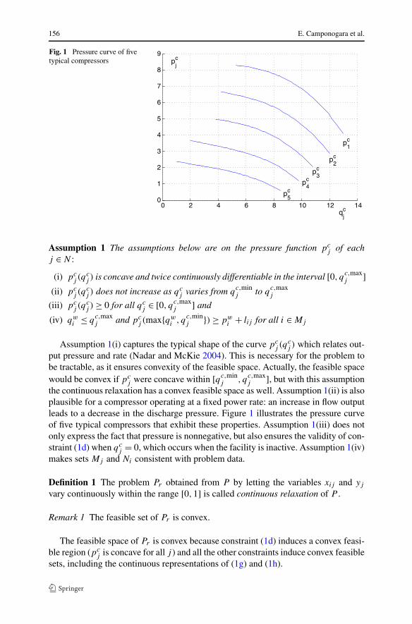
Fig. 1 Pressure curve of fivetypical compressors

Assumption 1 The assumptions below are on the pressure function pcj of each

j ∈ N :

(i) pcj (q

cj ) is concave and twice continuously differentiable in the interval [0, q

c,maxj ]

(ii) pcj (q

cj ) does not increase as qc

j varies from qc,minj to q

c,maxj

(iii) pcj (q

cj ) ≥ 0 for all qc

j ∈ [0, qc,maxj ] and

(iv) qwi ≤ q

c,maxj and pc

j (max{qwi , q

c,minj }) ≥ pw

i + lij for all i ∈ Mj

Assumption 1(i) captures the typical shape of the curve pcj (q

cj ) which relates out-

put pressure and rate (Nadar and McKie 2004). This is necessary for the problem tobe tractable, as it ensures convexity of the feasible space. Actually, the feasible spacewould be convex if pc

j were concave within [qc,minj , q

c,maxj ], but with this assumption

the continuous relaxation has a convex feasible space as well. Assumption 1(ii) is alsoplausible for a compressor operating at a fixed power rate: an increase in flow outputleads to a decrease in the discharge pressure. Figure 1 illustrates the pressure curveof five typical compressors that exhibit these properties. Assumption 1(iii) does notonly express the fact that pressure is nonnegative, but also ensures the validity of con-straint (1d) when qc

j = 0, which occurs when the facility is inactive. Assumption 1(iv)makes sets Mj and Ni consistent with problem data.

Definition 1 The problem Pr obtained from P by letting the variables xij and yj

vary continuously within the range [0,1] is called continuous relaxation of P .

Remark 1 The feasible set of Pr is convex.

The feasible space of Pr is convex because constraint (1d) induces a convex feasi-ble region (pc

j is concave for all j ) and all the other constraints induce convex feasiblesets, including the continuous representations of (1g) and (1h).

Compressor scheduling in oil fields 157

Table 1 Compressor data

j cj dj qc,minj

qc,maxj

α0,j α1,j α2,j α3,j α4,j

1 8 3 5.3 13.0 8.36900 −0.502034 0.0651919 −0.00497000 0.814770

2 6 5 4.2 12.0 7.11148 −0.602903 0.0680301 −0.00507334 0.766603

3 10 1 3.8 10.8 5.30343 −0.309098 0.0401807 −0.00427144 0.324494

4 4 7 2.0 9.8 3.49652 −1.215010 0.1236120 −0.00741996 1.978650

5 6 4 1.0 8.5 2.45413 −0.356522 0.0361532 −0.00363706 0.347968

Table 2 Well datai qw

ipw

iNi

1 3 5 {1,2}2 4 5 {1,2}3 2 4 {1,2,3}4 4 3 {1,2,3,4}5 5 1.5 {1,2,3,4,5}6 2 1 {1,2,3,4,5}

Remark 2 Function hj (qcj ) = qc

jpcj (q

cj ) is concave for qc

j ∈ [qc,minj , q

c,maxj ].

Notice that h′′j = 2pc′

j + qcjp

c′′j ≤ 0 because pc′

j (qcj ) ≤ 0 (Assumption 1(ii)),

qcj ≥ 0, and pc′′

j (qcj ) ≤ 0 as pc

j is concave for qcj ∈ [qc,min

j , qc,maxj ].

Because CSP inherits the same structure of the capacitated facility location prob-lem (Cornuéjols et al. 1991), it is a computationally hard problem (Garey and Johnson1979) as stated by the proposition below, which can be shown via a reduction fromthe knapsack problem.

Proposition 1 Problem P is NP-Hard.

2.1 Sample instance

In the illustrative scenario, the pressure curves are of the form pcj (q

cj ) = α0,j +

α1,j qcj + α2,j (q

cj )

2 + α3,j (qcj )

3 + α4,j ln(1 + qcj ) for its good fitting to vendor data.1

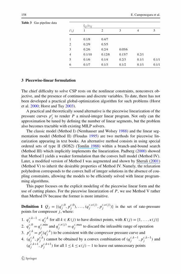
There are n = 5 facilities with properties and pressure curves given in Table 1. Thedata of m = 6 clients appear in Table 2. Table 3 gives pressure drops in and mainte-nance costs of the pipelines. It is worth remarking that the illustrative instance meetsthe conditions of Assumption 1.

1http://www.atlascopco.com.br.

158 E. Camponogara et al.

Table 3 Gas pipeline datalij /cij

i\j 1 2 3 4 5

1 0.1/8 0.4/7

2 0.2/9 0.5/5

3 0.2/6 0.2/4 0.05/6

4 0.1/10 0.12/8 0.15/7 0.2/1

5 0.1/6 0.1/4 0.2/3 0.1/1 0.1/1

6 0.1/7 0.1/3 0.1/2 0.1/1 0.1/1

3 Piecewise-linear formulation

The chief difficulty to solve CSP rests on the nonlinear constraints, nonconvex ob-jective, and the presence of continuous and discrete variables. To date, there has notbeen developed a practical global-optimization algorithm for such problems (Horstet al. 2000; Horst and Tuy 2003).

A practical and theoretically sound alternative is the piecewise linearization of thepressure curves pc

j to render P a mixed-integer linear program. Not only can theapproximation be tuned by defining the number of linear segments, but the problemalso becomes tractable with existing MILP solvers.

The classic model (Method I) (Nemhauser and Wolsey 1988) and the linear seg-mentation model (Method II) (Floudas 1995) are two methods for piecewise lin-earization appearing in text books. An alternative method consists in using specialordered sets of type II (SOS2) (Tomlin 1988) within a branch-and-bound search(Method III) which implicitly implements the linearization. Padberg (2000) showedthat Method I yields a weaker formulation than the convex hull model (Method IV).Later, a modified version of Method I was augmented and shown by Sherali (2001)(Method V) to inherit the desirable properties of Method IV. Namely, the relaxationpolyhedron corresponds to the convex hull of integer solutions in the absence of cou-pling constraints, allowing the models to be efficiently solved with linear program-ming algorithms.

This paper focuses on the explicit modeling of the piecewise linear form and theuse of cutting planes. For the piecewise linearization of P , we use Method V ratherthan Method IV because the former is more intuitive.

Definition 1 Qj = {(qc,0j ,p

c,0j ), . . . , (q

c,κ(j)j ,p

c,κ(j)j )} is the set of rate-pressure

points for compressor j , where:

1. qc,k−1j < q

c,kj for all k ∈ K(j) to have distinct points, with K(j) = {1, . . . , κ(j)}

2. qc,0j = q

c,minj and q

c,κ(j)j = q

c,maxj to discard the infeasible range of operation

3. pc,kj = pc

j (qc,kj ) to be consistent with the compressor pressure curve and

4. (qc,kj ,p

c,kj ) cannot be obtained by a convex combination of (q

c,k−1j ,p

c,k−1j ) and

(qc,k+1j ,p

c,k+1j ) for all 1 ≤ k ≤ κ(j) − 1 to leave out unnecessary points

Compressor scheduling in oil fields 159

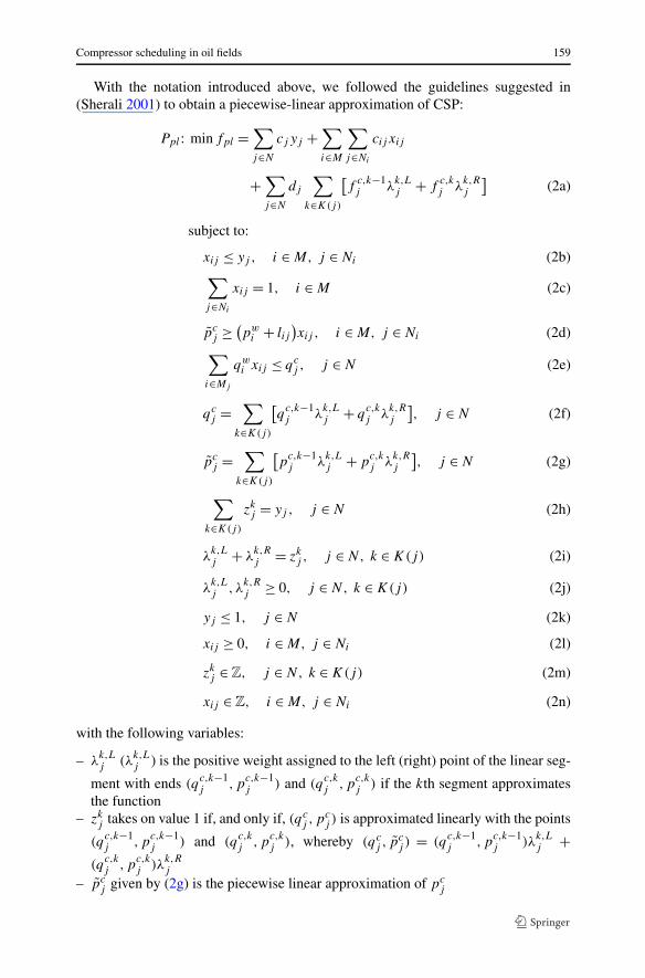
With the notation introduced above, we followed the guidelines suggested in(Sherali 2001) to obtain a piecewise-linear approximation of CSP:

Ppl : minfpl =∑

j∈N

cjyj +∑

i∈M

∑

j∈Ni

cij xij

+∑

j∈N

dj

∑

k∈K(j)

[f

c,k−1j λ

k,Lj + f

c,kj λ

k,Rj

](2a)

subject to:xij ≤ yj , i ∈ M, j ∈ Ni (2b)∑

j∈Ni

xij = 1, i ∈ M (2c)

pcj ≥ (

pwi + lij

)xij , i ∈ M, j ∈ Ni (2d)

∑

i∈Mj

qwi xij ≤ qc

j , j ∈ N (2e)

qcj =

∑

k∈K(j)

[q

c,k−1j λ

k,Lj + q

c,kj λ

k,Rj

], j ∈ N (2f)

pcj =

∑

k∈K(j)

[p

c,k−1j λ

k,Lj + p

c,kj λ

k,Rj

], j ∈ N (2g)

∑

k∈K(j)

zkj = yj , j ∈ N (2h)

λk,Lj + λ

k,Rj = zk

j , j ∈ N, k ∈ K(j) (2i)

λk,Lj , λ

k,Rj ≥ 0, j ∈ N, k ∈ K(j) (2j)

yj ≤ 1, j ∈ N (2k)

xij ≥ 0, i ∈ M, j ∈ Ni (2l)

zkj ∈ Z, j ∈ N, k ∈ K(j) (2m)

xij ∈ Z, i ∈ M, j ∈ Ni (2n)

with the following variables:

– λk,Lj (λk,L

j ) is the positive weight assigned to the left (right) point of the linear seg-

ment with ends (qc,k−1j ,p

c,k−1j ) and (q

c,kj ,p

c,kj ) if the kth segment approximates

the function– zk

j takes on value 1 if, and only if, (qcj ,p

cj ) is approximated linearly with the points

(qc,k−1j ,p

c,k−1j ) and (q

c,kj ,p

c,kj ), whereby (qc

j , pcj ) = (q

c,k−1j ,p

c,k−1j )λ

k,Lj +

(qc,kj ,p

c,kj )λ

k,Rj

– pcj given by (2g) is the piecewise linear approximation of pc

j

160 E. Camponogara et al.

– yj , qcj , and xij as in P

and having as parameters:

– fc,kj = q

c,kj p

c,kj defines the objective points according to the piecewise linear form

of function pcj (q

cj )

– and all the other parameters defined for P

Some remarks about the piecewise-linear formulation Ppl are immediate:(i) yj ≥ 0 is implicitly imposed by constraints (2b) and (2l); (ii) xij ≤ 1 is imposedby constraints (2b) and (2k); (iii) 0 ≤ zk

j ≤ 1 is enforced by constraints (2i) and (2j),and by constraints (2h) and (2k), respectively; and (iv) the integrality of yj is ensuredby (2h) and (2m). This formulation first appeared in Camponogara et al. (2007).

Notice that pcj (q) ≤ pc

j (q) for all q ∈ [qc,minj , q

c,maxj ] since pc

j is concave ac-cording to Assumption 1. The approximation error can be evaluated in a numberof ways. One way is to calculate the area between the true and approximate curve,

namely∫ q

c,maxj

q=qc,minj

|pcj (q) − pc

j (q)|dq which is easily computed or obtained analyti-

cally as pcj (q) ≥ pc

j (q). Another way to assess the approximation quality is by cal-

culating the maximum error, that is, max{|pcj (q) − pc

j (q)| : q ∈ [qc,minj , q

c,maxj ]} =

max{max{pcj (q) − pc

j (q) : q ∈ [qc,k−1j , q

c,kj ]} : k ∈ K(j)} which is obtained by solv-

ing κ(j) concave maximization problems, given that pcj is concave and pc

j is linear

within [qc,k−1j , q

c,kj ].

Let X denote the feasible set for Ppl and let P = {w = (x, y, z, q,p,λL,λR) ∈R

n : w meets constraints (2b) through (2l)} be the polyhedron of the continuousrelaxation of Ppl , where nI = ∑

i∈M |Ni | + |N | + ∑j∈N κ(j) and nC = 2|N | +

2∑

j∈N κ(j) are the number of discrete and continuous variables, respectively, and

n = nI + nC . Notice that P is a formulation to Ppl since X = P ∩ (ZnI × RnC ).

Proposition 2 Any feasible solution w = (x, y, z, q, p, λL,λR) for Ppl induces afeasible solution w′ = (x, y, q, p) for P such that fpl(w) ≤ f (w′).

Proof Take any w ∈ X . Constraints (2b), (2c), and (2e) hold and thereby w′ meets(1b), (1c), and (1f). The discharge pressures of the compressors in Ppl underesti-mate the actual discharge pressures in P , pc

j (q) ≤ pcj (q), ensuring that w′ meets (1d)

because w meets (2d). Since qc,0j = q

c,minj and q

c,κ(j)j = q

c,maxj , constraint (1e) is im-

plicitly satisfied by w and hence by w′. Further, (1g) and (1h) are obviously satisfiedby w and w′. This shows that w′ is feasible for P .

The objectives f and fpl differ in the third term. Since dj ≥ 0 and hj (qcj ) =

qcjp

cj (q

cj ) is concave as shown in Remark 1, djhj (q

cj ) is concave and its piecewise-

linear form underestimates the actual cost. Consequently, fpl(w) ≤ f (w′). �

Despite the proposition above, an optimal solution to Ppl or the relaxation of thispiecewise-linear form does not necessarily induce a lower bound for f . There couldexist feasible solutions for P that are infeasible for Ppl because pc

j underestimates

Compressor scheduling in oil fields 161

Fig. 2 Piecewise-linear formulation and upper envelope for a compressor performance curve

Table 4 Piecewise-linear data

(qc,kj

,pc,kj

)

k\j j = 1 j = 2 j = 3 j = 4 j = 5

k = 0 (5.3000, 8.2992) (4.2000, 6.6673) (3.8000, 4.9837) (2.0000, 3.6754) (1.0000, 2.3713)

k = 1 (6.8400, 8.0725) (5.7600, 6.3913) (5.2000, 4.7741) (3.5600, 3.4052) (2.5000, 2.1679)

k = 2 (8.3800, 7.6392) (7.3200, 5.9777) (6.6000, 4.4438) (5.1200, 3.1046) (4.0000, 1.9338)

k = 3 (9.9200, 6.9002) (8.8800, 5.3256) (8.0000, 3.9282) (6.6800, 2.7181) (5.5000, 1.6331)

k = 4 (11.4600, 5.7526) (10.4400, 4.3274) (9.4000, 3.1604) (8.2400, 2.1261) (7.0000, 1.2061)

k = 5 (13.0000, 4.0911) (12.0000, 2.8725) (10.8000, 2.0719) (9.8000, 1.1858) (8.5000, 0.5855)

pcj . A lower bound is induced by modifying the way pc

j is linearized while preservingthe piecewise-linear form of the objective function. To that end, in (2d) and (2g), theupper envelope pc

j would be used instead of pcj as illustrated in Fig. 2. The upper

envelope pcj is obtained from linear approximations with the Taylor series expansion

at a number of points and by defining the intercepts of these lines as the articulationpoints of pc

j . However, the piecewise-linear form of the objective function remains

the same with fc,kj = q

c,kj pc

j (qc,kj ).

Table 4 gives the sets Qj with the rate-pressure data inducing the piecewise-linearformulation for the sample instance. This data will be handy further in the text toillustrate valid inequalities for the piecewise-linear formulation.

The piecewise-linear formulation Ppl can be expressed in a modeling languagefor mathematical programming (Fourer et al. 2002) and fed to an MILP solver, suchas ILOG CPLEX, GLP (GNU Linear Programming Kit), and Xpress-MP. However,it is meaningful to exploit the structure of the formulation and design more effectivealgorithms to cope with large instances and solve problems expeditiously. The useof valid inequalities for the convex hull of feasible solutions, in cutting plane andbranch-and-cut procedures, has been very effective and embedded in state-of-the-artsolvers.

162 E. Camponogara et al.

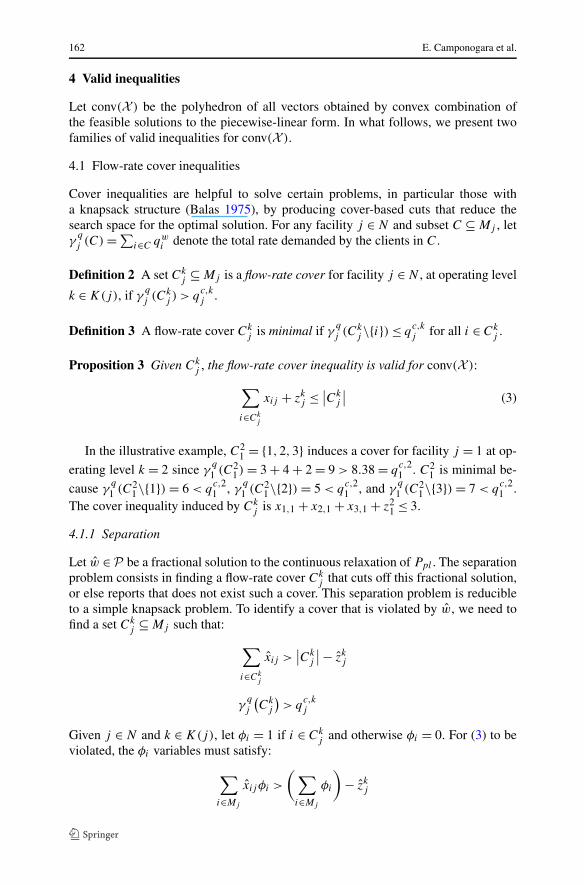
4 Valid inequalities

Let conv(X ) be the polyhedron of all vectors obtained by convex combination ofthe feasible solutions to the piecewise-linear form. In what follows, we present twofamilies of valid inequalities for conv(X ).

4.1 Flow-rate cover inequalities

Cover inequalities are helpful to solve certain problems, in particular those witha knapsack structure (Balas 1975), by producing cover-based cuts that reduce thesearch space for the optimal solution. For any facility j ∈ N and subset C ⊆ Mj , letγ

qj (C) = ∑

i∈C qwi denote the total rate demanded by the clients in C.

Definition 2 A set Ckj ⊆ Mj is a flow-rate cover for facility j ∈ N , at operating level

k ∈ K(j), if γqj (Ck

j ) > qc,kj .

Definition 3 A flow-rate cover Ckj is minimal if γ

qj (Ck

j \{i}) ≤ qc,kj for all i ∈ Ck

j .

Proposition 3 Given Ckj , the flow-rate cover inequality is valid for conv(X ):

∑

i∈Ckj

xij + zkj ≤ ∣∣Ck

j

∣∣ (3)

In the illustrative example, C21 = {1,2,3} induces a cover for facility j = 1 at op-

erating level k = 2 since γq

1 (C21) = 3 + 4 + 2 = 9 > 8.38 = q

c,21 . C2

1 is minimal be-

cause γq

1 (C21\{1}) = 6 < q

c,21 , γ

q

1 (C21\{2}) = 5 < q

c,21 , and γ

q

1 (C21\{3}) = 7 < q

c,21 .

The cover inequality induced by Ckj is x1,1 + x2,1 + x3,1 + z2

1 ≤ 3.

4.1.1 Separation

Let w ∈ P be a fractional solution to the continuous relaxation of Ppl . The separationproblem consists in finding a flow-rate cover Ck

j that cuts off this fractional solution,or else reports that does not exist such a cover. This separation problem is reducibleto a simple knapsack problem. To identify a cover that is violated by w, we need tofind a set Ck

j ⊆ Mj such that:

∑

i∈Ckj

xij >∣∣Ck

j

∣∣ − zkj

γqj

(Ck

j

)> q

c,kj

Given j ∈ N and k ∈ K(j), let φi = 1 if i ∈ Ckj and otherwise φi = 0. For (3) to be

violated, the φi variables must satisfy:

∑

i∈Mj

xijφi >

( ∑

i∈Mj

φi

)− zk

j

Compressor scheduling in oil fields 163

∑

i∈Mj

qwi φi > q

c,kj

The first constraint is expressed as (∑

i∈Mj(1− xij )φi < zk

j ), leading to the followingformulation for finding the most violated flow-rate cover inequality:

Skj : ϕk

j = minφi

∑

i∈Mj

(1 − xij )φi − zkj

subject to:∑

i∈Mj

qwi φi ≥ q

c,kj + ε, φi ∈ {0,1}, i ∈ Mj

for sufficiently small ε > 0. A violated cover Ckj = {i : φi = 1, i ∈ Mj } is found for

facility j if ϕkj < 0 for some k ∈ K(j).

As an illustration, let w be the solution to the relaxation of Ppl for the CSP instancegiven in Sect. 2.1. Among all j and k, only the separation problem S1

1 produced aflow cover inequality violated by w with ϕ1

1 = −0.406218 < 0. The relevant datais x1,1 = 1, x2,1 = 1, x3,1 = x4,1 = x5,1 = 0, z1

1 = 0.406218, z21 = z3

1 = z41 = 0, and

z51 = 0.593782. The solution to S1

1 yielded the cover C11 = {1,2} where γ

q

1 (C11) =

3 + 4 = 7 > 6.84 = qc,11 . The inequality x1,1 + x2,1 < 2 − z1

1 cuts off w as x1,1 +x2,1 = 2 �< 1.593782 = 2 − z1

1. Notice that ϕ11 = (1 − x1,1) + (1 − x2,1) − z1

1 = 2 −x1,1 − x2,1 − z1

1 = −0.406218 < 0.

4.1.2 Exact lifting

Inequality (3) can be lifted2 (Nemhauser and Wolsey 1988; Balas and Zemel 1978)to obtain a stronger inequality for conv(X ):

∑

i∈Ckj

xij + zkj +

∑

i∈Mj \Ckj

αij xij +∑

t∈K(j)\{k}βt

j ztj ≤ ∣∣Ck

j

∣∣ (4)

where αij and βtj are the lifting factors which depend as much on Ck

j as on the lifting

order of the variables xij (i ∈ Mj\Ckj ) and zt

j (t ∈ K(j)\{k}). The order in which the

variables are lifted is given by a sequence (X(l),Z(l)), l = 0, . . . ,L, such that:

1. X(0) = ∅ and Z(0) = ∅2. L = |Mj | + |K(j)| − |Ck

j | − 1 is the number of variables to be lifted

3. X(l) ⊆ Mj\Ckj and Z(l) ⊆ K(j)\{k} for all l

4. X(l) ⊆ X(l+1), Z(l) ⊆ Z(l+1), and |X(l)|+ |Z(l)|+ 1 = |X(l+1)|+ |Z(l+1)|, ∀l < L

2The reader may consult Chap. II.2 of Nemhauser and Wolsey (1988) for a thorough presentation of theprinciples underlying the lifting procedure.

164 E. Camponogara et al.

5. for all l > 0 and i ∈ X(l)\X(l−1), there exist t ∈ Z(l) ∪ {k} and qcj ∈ [qc,t−1

j , qc,tj ]

such that qwi ≤ q

c,tj and pw

i + lij ≤ pcj (q

cj )

A lifting sequence for the cover C21 = {1,2,3} of the example is X(1) = {4},

X(2) = {4,5}, X(3) = {4,5,6}, Z(4) = {1}, Z(5) = {1,3}, Z(6) = {1,3,4}, and Z(7) ={1,3,4,5} where L = 7.

The series of lifting problems Ll (l = 1, . . . ,L) is defined by:

Ll : ξl = max∑

i∈Ckj

xij + zkj +

∑

i∈X(l−1)

αij xij +∑

t∈Z(l−1)

βtj z

tj (5a)

subject to:pc

j ≥ (pw

i + lij)xij , i ∈ Ck

j ∪ X(l) (5b)∑

i∈Ckj ∪X(l)

qwi xij ≤ qc

j (5c)

(qcj , p

cj

) =∑

t∈{k}∪Z(l)

[(q

c,t−1j ,p

c,t−1j

)λ

t,Lj + (

qc,tj ,p

c,tj

)λ

t,Rj

](5d)

∑

t∈{k}∪Z(l)

ztj = 1 (5e)

{xij = 1, i ∈ X(l)\X(l−1)

ztj = 1, t ∈ Z(l)\Z(l−1)

(5f)

λt,Lj + λ

t,Rj = zt

j , t ∈ {k} ∪ Z(l) (5g)

λt,Lj , λ

t,Rj ≥ 0, t ∈ {k} ∪ Z(l) (5h)

xij ≥ 0, i ∈ Ckj ∪ X(l) (5i)

ztj ∈ Z, t ∈ {k} ∪ Z(l) (5j)

xij ∈ Z, i ∈ Ckj ∪ X(l) (5k)

where αij = |Ckj | − ξl for i ∈ X(l)\X(l−1) if |X(l)| > |X(l−1)|, or else βt

j = |Ckj | − ξl

for t ∈ Z(l)\Z(l−1). The optimization is over the variables xij , ztj , λ

t,Lj , λ

t,Rj , qc

j , andpc

j . The lifting problem is a restricted version of CSP in which only facility j canservice a subset of the clients, possibly leaving some without supply. Notice that theconditions satisfied by 〈(X(l),Z(l))〉 ensure that Ll is feasible for all l which, in turn,make the lifting factors well defined.

Proposition 4 Given a sequence 〈(X(l),Z(l)) : l = 0, . . . ,L〉, the lifted flow-ratecover inequality (4) obtained by solving 〈Ll : l = 1, . . . ,L〉 is valid for conv(X ).

Compressor scheduling in oil fields 165

Proof (By induction in l) The basis l = 0 is obviously valid as (4) reduces to thecover inequality (3). The induction step (l ≥ 1) has two cases. Case 1 occurs when|X(l)| > |X(l−1)|. Let i be the sole element of X(l)\X(l−1) and consider any solutionw ∈ X . If x

ij= 0 in w, then (4) is valid by induction. If x

ij= 1 in w, then

∣∣Ckj

∣∣ − ξl = ∣∣Ckj

∣∣ − max

{∑

i∈Ckj

xij + zkj +

∑

i∈X(l−1)

αij xij +∑

t∈Z(l−1)

βtj z

tj :

xij , ztj , λ

t,Lj , λ

t,Rj , qc

j , pcj meet (5b)–(5k)

}

≤ ∣∣Ckj

∣∣ −(∑

i∈Ckj

xij + zkj +

∑

i∈X(l−1)

αij xij +∑

t∈Z(l−1)

βtj z

tj

)

(xij , zt

j given by w)

and, in turn,

∣∣Ckj

∣∣ ≥∑

i∈Ckj

xij + zkj +

∑

i∈X(l−1)

αij xij +∑

t∈Z(l−1)

βtj z

tj + (∣∣Ck

j

∣∣ − ξl

)

=∑

i∈Ckj

xij + zkj +

∑

i∈X(l−1)

αij xij +∑

t∈Z(l−1)

βtj z

tj + α

ijxij

=∑

i∈Ckj

xij + zkj +

∑

i∈X(l)

αij xij +∑

t∈Z(l)

βtj z

tj

which implies that (4) is valid for l.Case 2, when |Z(l)| > |Z(l−1)|, can be shown in a similar manner. �

Lifting problem Ll remains an MILP problem but its low dimension may enablethe lifting of flow covers to be embedded in a cutting-plane procedure. Applying thelifting procedure to the flow-cover example, and following the lifting sequence above,produces ξ1 = 2 (α4,1 = 1), ξ2 = 2 (α5,1 = 1), ξ3 = 3 (α6,1 = 0), ξ4 = 2 (β1

1 = 1),ξ5 = 3 (β3

1 = 0), ξ6 = 3 (β41 = 0), ξ7 = 3 (β5

1 = 0). So the lifted flow-cover inequalityis x1,1 + x2,1 + x3,1 + x4,1 + x5,1 + z1

1 + z21 ≤ 3.

The dimension of the polyhedron obtained from conv(X ) by removing linear de-pendencies was established in Camponogara et al. (2007). The full dimensionality ofthis compact formulation simplifies the identification of the dimension of flow-coverinequalities as in Camponogara and Nakashima (2006) and Camponogara and Conto(2009). However, this course of research was not followed due to the intricacy ofthe constraint structure of compressor scheduling, which is far more complex thanthe structure of the generalized knapsack problem appearing in Camponogara andNakashima (2006).

166 E. Camponogara et al.

4.1.3 Approximate lifting

Because the computation of exact lifting factors is considerable, approximate liftingfactors αij and βt

j are proposed below.

Definition 4 Given a flow-rate cover Ckj , its extension is E(Ck

j ) = {i ∈ Mj\Ckj :

qwi ≥ qw

t , ∀t ∈ Ckj }.

Proposition 5 Given a flow-rate cover Ckj , the extended flow-cover inequality

∑

i∈Ckj

xij + zkj +

∑

i∈E(Ckj )

αij xij +∑

t∈K(j)\{k}βt

j ztj ≤ ∣∣Ck

j

∣∣ (6)

is valid for conv(X ) if:

– αij = max{h : qwi ≥ γ

qj (S), ∀S ⊆ Ck

j , |S| = h} for i ∈ E(Ckj )

– βtj = |Ck

j | − max{h : qc,tj ≥ γ

qj (S), ∃S ⊆ Ck

j , |S| = h} for t < k

– βtj = |Ck

j | − max{h : qc,tj ≥ γ

qj (S),∃S ⊆ Ck

j , |S| = h}, where Ckj =

Ckj

⋃i∈E(Ck

j ){the αij lightest elements of Ckj }, for t > k

Proof Suppose there exists w ∈ X that violates (6). Let C1 = {i ∈ Ckj : xij = 1} and

Sh = {i ∈ E(Ckj ) : xij = 1, αij = h}. And let γ

q,hj (Ck

j ) denote the sum of the h heav-

iest elements of Ckj . There are three cases.

Case 1: zkj = 1 for k < k. Because w violates (6),

∑i∈Ck

jxij + zk

j +∑

i∈E(Ckj ) αij xij + ∑

t∈K(j)\{k} βtj z

tj = |C1| + ∑|Ck

j |h=1 h|Sh| + β k

j > |Ckj | =⇒ β k

j >

|Ckj | − (|C1| + ∑|Ck

j |h=1 h|Sh|). But q

c,kj ≥ ∑

i∈Mjqwi xij ≥ γ

qj (C1) + ∑|Ck

j |h=1 γ

qj (Sh) ≥

γqj (C1)+∑|Ck

j |h=1 γ

q,hj (Ck

j )|Sh| ≥ γqj (C1)+γ

q,h′j (Ck

j ) where h′ = ∑|Ckj |

h=1 h|Sh|, which

implies that β kj ≤ |Ck

j | − (|C1| + ∑|Ckj |

h=1 h|Sh|), contradicting the hypothesis.

Case 2: zkj = 1. Since w violates (6),

∑i∈Ck

jxij + zk

j + ∑i∈E(Ck

j ) αij xij +∑

t∈K(j)\{k} βtj z

tj = |C1| + 1 + ∑|Ck

j |h=1 h|Sh| > |Ck

j |. But∑

i∈Mjqwi xij ≥ γ

qj (C1) +

∑|Ckj |

h=1 γqj (Sh) ≥ γ

qj (C1) + ∑|Ck

j |h=1 γ

q,hj (Ck

j )|Sh| ≥ γqj (C1) + γ

q,h′j (Ck

j ) ≥ γqj (Ck

j ) >

qc,kj [because |C1| + h′ ≥ |Ck

j |], contradicting the hypothesis.

Case 3: zkj = 1 for k > k. Since w violates (6),

∑i∈Ck

jxij +zk

j +∑i∈E(Ck

j ) αij xij +∑

t∈K(j)\{k} βtj z

tj = |C1| + ∑|Ck

j |h=1 h|Sh| + β k

j > |Ckj | =⇒ β k

j > |Ckj | − (|C1| +

∑|Ckj |

h=1 h|Sh|). But qc,kj ≥ ∑

i∈Mjqwi xij ≥ γ

qj (C1) + ∑|Ck

j |h=1 γ

qj (Sh) ≥ γ

qj (C1) +

Compressor scheduling in oil fields 167

∑|Ckj |

h=1 γq,hj (Ck

j )|Sh| ≥ γqj (C1) + γ

q,h′j (Ck

j ) =⇒ β kj ≤ |Ck

j | − (|C1| + ∑|Ckj |

h=1 h|Sh|)which contradicts the hypothesis. �

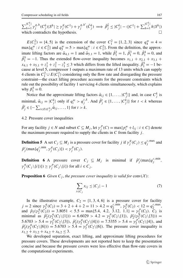
E(C21) = {4,5} is the extension of the cover C2

1 = {1,2,3} since qw4 = 4 =

max{qwi : i ∈ C2

1} and qw5 = 5 > max{qw

i : i ∈ C21}. From the definition, the approx-

imate lifting factors are α4,1 = 1 and α5,1 = 1, while β11 = 1, β3

1 = 0, β41 = 0, and

β51 = −1. Thus the extended flow-cover inequality becomes x1,1 + x2,1 + x3,1 +

x4,1 + x5,1 + z11 + z2

1 − z51 ≤ 3 which differs from the lifted inequality. β5

1 = −1 be-cause at level 5, compressor 1 outputs a maximum rate of 13 units which can supply4 clients in C2

1 ∪ E(C21) considering only the flow rate and disregarding the pressure

constraint—the exact lifting procedure accounts for the pressure constraints whichrule out the possibility of facility 1 servicing 4 clients simultaneously, which explainswhy β5

1 = 0.Notice that the approximate lifting factors αij ∈ {1, . . . , |Ck

j |} and, in case Ckj is

minimal, αij = |Ckj | only if qw

i > qc,kj . And βt

j ∈ {1, . . . , |Ckj |} for t < k whereas

βtj ∈ {−∑

i∈E(Ckj ) αij , . . . ,1} for t > k.

4.2 Pressure cover inequalities

For any facility j ∈ N and subset C ⊆ Mj , let γpj (C) = max{pw

i + lij : i ∈ C} denotethe maximum pressure required to supply the clients in C from facility j .

Definition 5 A set Cj ⊆ Mj is a pressure cover for facility j if γqj (Cj ) ≤ q

c,maxj and

pcj (max{qc,min

j , γqj (Cj )}) < γ

pj (Cj ).

Definition 6 A pressure cover Cj ⊆ Mj is minimal if pcj (max{qc,min

j ,

γqj (Cj\{i})}) ≥ γ

pj (Cj\{i}) for all i ∈ Cj .

Proposition 6 Given Cj , the pressure cover inequality is valid for conv(X ):

∑

i∈Cj

xij ≤ |Cj | − 1 (7)

In the illustrative example, C2 = {1,3,4,6} is a pressure cover for facilityj = 2 since γ

q

2 (C2) = 3 + 2 + 4 + 2 = 11 > 4.2 = qc,min2 , γ

q

2 (C2) < 12 = qc,max2 ,

and p2(γq

2 (C2)) = 3.8051 < 5.5 = max{5.4, 4.2, 3.12, 1.1} = γp

2 (C2). C2 isminimal as pc

2(γq

2 (C2\{1})) = 6.6029 > 4.2 = γp

2 (C2\{1}), pc2(γ

q

2 (C2\{3})) =5.6703 > 5.4 = γ

p

2 (C2\{3}), pc2(γ

q

2 (C2\{4})) = 7.5355 > 5.4 = γp

2 (C2\{4}), andpc

2(γq

2 (C2\{6})) = 5.6703 > 5.4 = γp

2 (C2\{6}). The pressure cover inequality isx1,2 + x3,2 + x4,2 + x6,2 ≤ 3.

We developed separation, exact lifting, and approximate lifting procedures forpressure covers. These developments are not reported here to keep the presentationconcise and because the pressure covers were less effective than flow-rate covers inthe computational experiments.

168 E. Camponogara et al.

5 Computational analysis

This section reports computational results obtained with a cut-and-branch procedurefor solving the piecewise-linear form of representative instances of the compressorscheduling problem. The purpose of the computational analysis is twofold. It aims toinvestigate the computational hardness of solving such instances and assess the effec-tiveness of the cover-based cuts (flow-rate and pressure covers) in expediting solutiontime. Preliminary results of the use of cover-based cuts appeared in Camponogara andCastro (2008).

5.1 Impact of cover-based cutting planes

The CSP instances are representative of vendor compression equipment and mirrorthe characteristics of typical oil fields. The data meet the consistency conditions statedin Assumption 1. There are three instances: instance I1 encompasses n = 7 compres-sors and m = 16 wells; I2 has n = 9 compressors and m = 14 wells; and I3 has n = 8compressors and m = 18 wells. The size of the instances is increasing, with the sizeof I1 being nm = 112, I2 being nm = 126, and I3 being nm = 144.

The cut-and-branch procedure has two phases. First, it iteratively solves the con-tinuous relaxation of Ppl introducing valid inequalities that cut off the fractional,incumbent solution until a cover-based cutting plane cannot be found. Second,a branch-and-bound algorithm solves the integer formulation augmented with thecutting planes.

An effective heuristic was designed and implemented for cover separation, ratherthan solving integer programs. The outline of the separation heuristic for flow-coverinequalities follows below:

1. Select at random a facility j which is active in the incumbent solution.2. Identify the level k for which q

c,k−1j ≤ qc

j ≤ qc,kj .

3. Let M1j = {i ∈ Mj : xij > 0} be the set of assignments of facility j to clients.

4. Let Ckj = ∅.

5. While Ckj does not induce a flow-cover and for at most T steps do:

(a) Pick an element i ∈ M1j \Ck

j at random and let Ckj ← Ck

j ∪ {i}.6. If Ck

j is not a flow-cover, then repeat step 5 but this time taking elements from

Mj\Ckj , rather than from M1

j \Ckj .

7. Report a failure if Ckj is not a flow-cover.

8. If Ckj is a flow-cover then:

(a) If Ckj is not minimal, then systematically remove elements from Ck

j until itbecomes a minimal cover.

(b) Compute the extension E(Ckj ).

(c) Compute the approximate lifting factors αij for all i ∈ E(Ckj ), βt

j for all t < k,

and βtj for all t > k according to Proposition 5.

(d) If the extended flow-cover inequality (6) cuts off the incumbent solution, thenintroduce the cutting-plane, otherwise report a failure.

Compressor scheduling in oil fields 169

Table 5 Impact of flow covers—instance I1 (n = 7 and m = 16)

Without cuts With cuts Gain (%)

κ Iter. Nodes CPU Iter. Nodes CPU Iter. Nodes CPU

10 358,357 81,773 55.12 199,960 48,231 29.53 44.20 41.02 46.43

15 644,091 126,760 97.58 1,150,180 192,785 172.02 −78.57 −52.09 −76.29

20 2,551,838 2,551,838 419.29 1,193,357 214,669 202.75 53.24 91.59 51.64

25 2,977,635 629,972 628.22 3,824,795 628,570 746.73 −28.45 0.22 −18.86

30 6,265,976 6,265,976 1292.16 3,305,001 556,327 662.41 47.25 91.12 48.74

35 18,214,289 2,579,022 3636.83 2,788,688 508,042 599.61 84.69 80.30 83.51

40 9,756,719 1,662,602 2720.00 7,892,430 1,807,651 2399.09 19.11 −8.72 11.80

40,768,905 13,897,943 8849.20 20,354,411 3,956,275 4812.14 50.07 71.53 45.62

Table 6 Impact of flow covers—instance I2 (n = 9 and m = 14)

Without cuts With cuts Gain (%)

κ Iter. Nodes CPU Iter. Nodes CPU Iter. Nodes CPU

10 96,626 17,987 11.18 74,515 15,024 11.21 22.88 16.47 −0.27

15 245,498 245,498 38.57 263,194 39,509 38.44 −7.21 83.91 0.34

20 231,218 34,347 34.77 82,694 16,091 16.69 64.24 53.15 52.00

25 538,546 93,924 110.17 423,491 423,491 79.81 21.36 −350.89 27.56

30 380,584 66,279 81.86 185,889 36,814 49.05 51.16 44.46 40.08

35 510,478 66,137 100.39 510,478 66,137 100.39 −11.87 −6.66 −20.11

40 1,085,965 145,528 231.94 387,408 68,411 113.42 64.33 52.99 51.10

3,088,915 669,700 608.88 1,988,254 669,883 429.2 35.63 −0.03 29.51

At each step of the cutting-plane procedure, the heuristic is applied at most T =nm times to find a cutting plane for the incumbent solution. If a cut is not found, theprocedure halts and outputs an improved formulation which is fed to a branch-and-bound procedure. Otherwise, the linear programming relaxation is resolved and theprocess repeated until a maximum number of cuts is reached. The separation heuristicfor pressure-cover inequalities inherits the same structure of the heuristic above.

The cutting-plane procedure and the heuristics were implemented in C/C++ usingILOG CPLEX Concert Libraries version 9.0 (ILOG Incorporated 2003). The work-station ran GNU Linux, had 1 Gb of RAM, and an Intel Pentium IV Processor witha 2.5 GHz clock. The cut-and-branch procedure, whereby cover-based cuts are gen-erated in the first phase and ILOG CPLEX solves the improved formulation in thesecond phase, was applied to the three CSP instances. The pressure-cover cuts pro-duced mixed results, sometimes reducing the computational time and resources sub-stantially, but other times slowing down the baseline solver. For this reason, cutting-planes were obtained only from flow-rate covers.

Tables 5, 6, and 7 report the results obtained for instance I1, I2, and I3 respectively.Gain is defined as (value-without-cuts− value-with-cuts)/value-with-cuts. Thus, gain

170 E. Camponogara et al.

Tabl

e7

Impa

ctof

flow

cove

rs—

inst

ance

I 3(n

=8

and

m=

18)

With

outc

uts

With

cuts

Gai

n(%

)

κIt

er.

Nod

esC

PUIt

er.

Nod

esC

PUIt

er.

Nod

esC

PU

107,

510,

496

1,29

7,44

910

37.8

46,

066,

498

685,

674

572.

7019

.23

47.1

544

.82

158,

891,

926

1,81

3,10

915

57.8

39,

763,

866

1,27

3,76

912

22.6

4−9

.81

29.7

521

.52

2011

8,30

9,44

517

,697

,880

20,2

54.2

23,2

28,1

872,

519,

350

2999

.95

80.3

785

.76

85.1

9

2515

,855

,466

2,46

9,19

029

67.6

343

,518

,833

5,28

3,11

980

32.8

9−1

74.4

7−1

13.9

6−1

70.6

8

3021

,330

,701

2,64

4,71

736

07.8

820

,115

,548

2,36

8,96

136

44.4

85.

7010

.43

−1.0

1

3594

,894

,630

11,6

99,2

3518

,344

.60

53,3

01,2

807,

330,

831

11,7

36.1

43.8

337

.34

36.0

2

4019

,838

,377

2,05

5,10

837

39.7

513

,590

,803

1,56

3,10

527

16.4

331

.49

23.9

427

.36

286,

631,

041

39,6

76,6

8851

,509

.73

169,

585,

015

21,0

24,8

0930

,925

.19

40.8

447

.01

39.9

6

Compressor scheduling in oil fields 171

Table 8 Quality of thepiecewise-linear approximation κ ε(I1, κ) ε(I2, κ) ε(I3, κ)

10 0.0925% 0.0816% 0.0728%

15 0.0411% 0.0363% 0.0323%

20 0.0231% 0.0204% 0.0182%

25 0.0148% 0.0130% 0.0116%

30 0.0102% 0.0090% 0.0080%

35 0.0075% 0.0066% 0.0059%

40 0.0057% 0.0051% 0.0045%

is positive when cutting planes reduce CPU time, number of iterations (LP pivotingoperations), or the number of branch-and-bound nodes. Gain is negative when thecuts are detrimental. Overall, the results show that flow-cover cuts improve perfor-mance of the baseline solver.

5.2 Comparison between piecewise-linear and nonlinear models

This section presents a comparison between the local optimum for the nonlinearmodel P and the global optimum for the piecewise-linear model Ppl . The nonlin-ear models were specified in AMPL (Fourer et al. 2002) and fed to three mixed-integer, nonlinear programming solvers. The solvers are BONMIN (Bonami et al.2005), FILMINT (Abhishek et al. 2008), and MINLP (Leyffer 1998; Holmström etal. 2007) which are available from NEOS Servers at Argonne National Lab. Actu-ally, they are frameworks that rely on preprocessing procedures, existing algorithmsfor MILP, cutting-plane procedures, and outer approximations of the MINLP pro-gram. BONMIN uses CBC for solving MILPs and IPOPT for solving NLPs, whereasFILMINT uses MINTO and FILTER-SQP for solving such problems. While BONMIN

is a hybrid between a branch-and-bound solver based on nonlinear relaxations andone based on polyhedral outer approximation, FILMINT relies solely on linear un-derestimators. This main difference between BONMIN and FILMINT, as explained byAbhishek et al. (2008), explains why FILMINT tends to outperform BONMIN. It isimportant to mention that such solvers were designed to solve convex MINLP pro-grams, but can be applied as powerful heuristics to nonconvex MINLP programs.

Table 8 reports the values

ε(I, κ) = 1

n

∑

j∈N

∫ qc,maxj

qc,minj

∣∣pcj (q) − pc

j (q)∣∣dq

/∫ qc,maxj

qc,minj

pcj (q) dq

for each instance I and piecewise-linear form pcj given by κ(j) = κ segments. The

error value ε(I, κ) measures the quality of the piecewise-linear approximation. Theerror is relatively small and decreases with the increase of the discretization parame-ter κ .

Given a solution w to Ppl , the corresponding piecewise-linear objective fpl(w)

and nonlinear objective f (w) are calculated. The results of the experiments appear

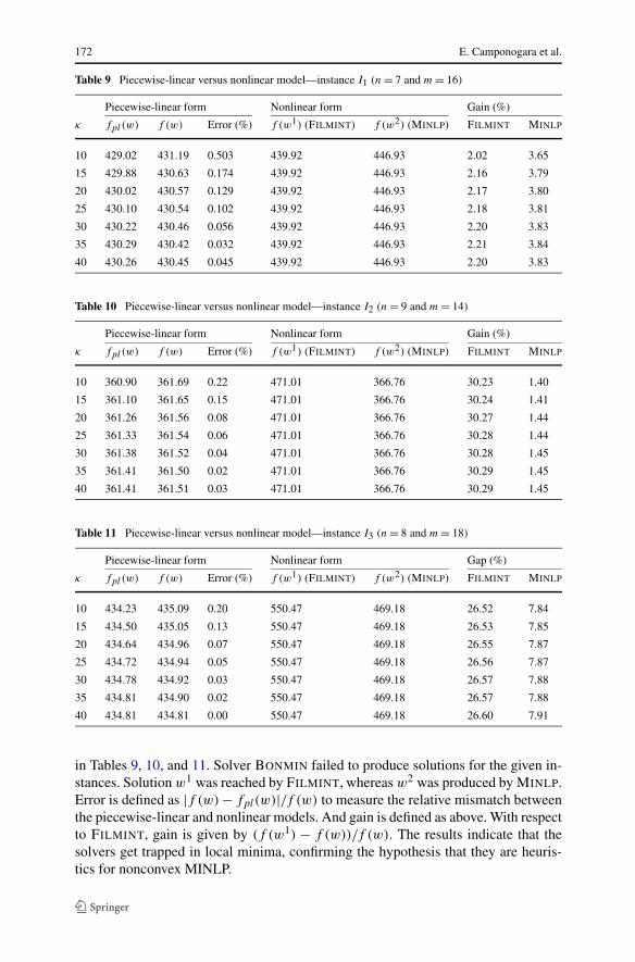
172 E. Camponogara et al.

Table 9 Piecewise-linear versus nonlinear model—instance I1 (n = 7 and m = 16)

Piecewise-linear form Nonlinear form Gain (%)

κ fpl(w) f (w) Error (%) f (w1) (FILMINT) f (w2) (MINLP) FILMINT MINLP

10 429.02 431.19 0.503 439.92 446.93 2.02 3.65

15 429.88 430.63 0.174 439.92 446.93 2.16 3.79

20 430.02 430.57 0.129 439.92 446.93 2.17 3.80

25 430.10 430.54 0.102 439.92 446.93 2.18 3.81

30 430.22 430.46 0.056 439.92 446.93 2.20 3.83

35 430.29 430.42 0.032 439.92 446.93 2.21 3.84

40 430.26 430.45 0.045 439.92 446.93 2.20 3.83

Table 10 Piecewise-linear versus nonlinear model—instance I2 (n = 9 and m = 14)

Piecewise-linear form Nonlinear form Gain (%)

κ fpl(w) f (w) Error (%) f (w1) (FILMINT) f (w2) (MINLP) FILMINT MINLP

10 360.90 361.69 0.22 471.01 366.76 30.23 1.40

15 361.10 361.65 0.15 471.01 366.76 30.24 1.41

20 361.26 361.56 0.08 471.01 366.76 30.27 1.44

25 361.33 361.54 0.06 471.01 366.76 30.28 1.44

30 361.38 361.52 0.04 471.01 366.76 30.28 1.45

35 361.41 361.50 0.02 471.01 366.76 30.29 1.45

40 361.41 361.51 0.03 471.01 366.76 30.29 1.45

Table 11 Piecewise-linear versus nonlinear model—instance I3 (n = 8 and m = 18)

Piecewise-linear form Nonlinear form Gap (%)

κ fpl(w) f (w) Error (%) f (w1) (FILMINT) f (w2) (MINLP) FILMINT MINLP

10 434.23 435.09 0.20 550.47 469.18 26.52 7.84

15 434.50 435.05 0.13 550.47 469.18 26.53 7.85

20 434.64 434.96 0.07 550.47 469.18 26.55 7.87

25 434.72 434.94 0.05 550.47 469.18 26.56 7.87

30 434.78 434.92 0.03 550.47 469.18 26.57 7.88

35 434.81 434.90 0.02 550.47 469.18 26.57 7.88

40 434.81 434.81 0.00 550.47 469.18 26.60 7.91

in Tables 9, 10, and 11. Solver BONMIN failed to produce solutions for the given in-stances. Solution w1 was reached by FILMINT, whereas w2 was produced by MINLP.Error is defined as |f (w) − fpl(w)|/f (w) to measure the relative mismatch betweenthe piecewise-linear and nonlinear models. And gain is defined as above. With respectto FILMINT, gain is given by (f (w1) − f (w))/f (w). The results indicate that thesolvers get trapped in local minima, confirming the hypothesis that they are heuris-tics for nonconvex MINLP.

Compressor scheduling in oil fields 173

6 Summary and future work

Smart Fields technology (Murray et al. 2006; Yeten et al. 2004) advocates the useof downhole sensors and flow control devices to operate a reservoir more efficiently,reduce the intervention of human operators, and ultimately increase oil recovery. Onthe one hand, the industry is implementing pilot projects to gain insights and demon-strate its potential, while academia is developing models and algorithms to furtherthis technology. This paper contributes to Smart Fields technology by addressing theproblem of scheduling compressors to oil wells, which plays an important role in theoperation of gas-lifted oil fields.

The compressor scheduling problem was introduced as a mixed-integer, non-convex, nonlinear program and reformulated as a mixed-integer linear program bypiecewise-linearizing the compressor performance curves. An analysis of the convexhull of the feasible solutions led to the synthesis of two families of valid inequalities,both based on the concept of covers with one applied to the compressor flow-rate andthe other applied to the compressor discharge pressure. Exact and approximate liftingprocedures were developed to obtain higher dimensional faces. Separation heuristicswere designed and implemented to produce cuts from these families of inequalities.A two-phase solution procedure was implemented: the first phase generates cuts fromthe proposed inequalities to improve the baseline formulation; the second phase ap-plies an MILP solver to the improved formulation. Computational results show thatthe cover-based cuts reduce computational time and memory usage. The results alsoindicate that operating costs are reduced by using the piecewise-linear form in placeof the nonlinear model.

Future work will progress along theoretical and applied directions. The theoreticaldirection will extend valid inequalities of the capacitated facility location problem,develop Fenchel cuts (Leung and Magnanti 1989; Boyd 1994), and investigate the useof a linear representation of the minimum pressure constraint. The applied directionwill be geared towards integrating compressor scheduling with a gas-lift automationsystem (Camponogara et al. 2008), which coordinates identification of well perfor-mance curves, pressure control of the gas-lift manifold, and constraint handling forlift-gas and separation capacity.

Acknowledgement We are indebted to Eng. Alex Teixeira from Petrobras Research Center (CENPES)for his support to the research on optimization and control of lift-gas systems. And we also thank theanonymous referees for their insightful comments.

References

Abhishek K, Leyffer S, Linderoth JT (March 2008) FilMINT: An outer-approximation-based solverfor nonlinear mixed integer programs. Technical Report ANL/MCS-P1374-0906, Mathematics andComputer Science Division, Argonne National Laboratory

An S, Li Q, Gedra TW (September 2003) Natural gas and electricity optimal power flow. In: Proceedingsof the IEEE/PES transmission and distribution conference, Dallas, TX, pp. 138–143

Balas E (1975) Facets of the knapsack polytope. Math Program 8(1):146–164Balas E, Zemel E (1978) Facets of the knapsack polytope from minimal covers. SIAM J Appl Math

34(1):119–148

174 E. Camponogara et al.

Bonami P, Biegler LT, Conn AR, Cornuéjols G, Grossmann IE, Laird CD, Lee J, Lodi A, Margot F,Sawaya N, Waechter A (October 2005) An algorithmic framework for convex mixed integer nonlinearprograms. Technical Report RC23771, IBM Research Division

Boyd EA (1994) Fenchel cutting planes for integer programs. Oper Res 42(1):53–64Camponogara E, de Castro MP (June 2008) Cover-based cutting planes for a compressor scheduling prob-

lem: a computational study. In: Proceedings of the international conference on engineering optimiza-tion, Rio de Janeiro, Brazil

Camponogara E, de Castro MP, Plucenio A (2006) The facility location problem: model, algorithm, andapplication to compressor allocation. In: Proceedings of the IFAC international symposium on ad-vanced control of chemical processes. Elsevier, Amsterdam

Camponogara E, de Castro MP, Plucenio A (September 2007) Compressor scheduling in oil fields: apiecewise-linear formulation. In: Proceedings of the IEEE conference on automation science andengineering, Scottsdale, AZ, pp 436–441

Camponogara E, de Conto AM (2009) Lift-gas allocation under precedence constraints: MILP formulationand computational analysis. IEEE Trans Automa Sci Eng 6(3):544–551

Camponogara E, Nakashima PHR (2006) Optimizing gas-lift production of oil wells: piecewise linearformulation and computational analysis. IIE Trans 38(2):173–182

Camponogara E, Plucenio A, Teixeira AF, Campos SRV (2008) An automation system for gas-lifted oilwells: model identification, control, and optimization. J Petrol Sci Eng (submitted)

Cornuéjols G, Sridharan R, Thizy J-M (1991) A comparison of heuristics and relaxations for the capaci-tated plant location problem. Eur J Oper Res 50:280–297

Dutta-Roy K, Barua S, Heiba A (March 1997) Computer-aided gas field planning and optimization. In:Proceedings of the SPE production operations symposium, Oklahoma City

Floudas CA (1995) Nonlinear and mixed-integer optimization: fundamentals and applications. OxfordUniversity Press, New York

Fourer R, Gay DM, Kernighan BW (2002) AMPL: A modeling language for mathematical programming.Duxbury, N. Scituate

Garey MR, Johnson DS (1979) Computers and intractability: a guide to the theory of NP-completeness.Freeman, New York

Holmström K, Göran AO, Edvall MM (February 2007) User’s guide for TOMLAB/MINLP. Technicalreport, Tomlab Optimization Inc., San Diego, CA

Horst R, Pardalos PM, Van Thoai N (2000) Introduction to global optimization (nonconvex optimizationand its applications). Springer, Berlin

Horst R, Tuy H (2003) Global optimization: deterministic approaches. Springer, BerlinILOG Incorporated, Mountain View, CA. ILOG CPLEX 9.0: Getting Started 2003Jahn F, Cook M, Graham M (2003) Hydrocarbon exploration and production. Elsevier, AmsterdamLeung JM, Magnanti TL (1989) Valid inequalities and facets of the capacitated plant location problem.

Math Program 44(1–3):271–291Leyffer S (1998) User manual for MINLP-BB. Technical report, University of Dundee, 1998Murray R, Edwards C, Gibbons K, Jakeman S, de Jonge G, Kimminau S, Ormerod L, Roy C, Vachon G

(April 2006) Making our mature fields smarter—an industry wide position paper from the 2005 SPEforum. In: Proc of the SPE intelligent energy conference and exhibition, Amsterdam, The Nether-lands. Paper SPE 100024

Nadar MS, McKie C (June 2004) Benefits of detailed compressor modelling in optimising production fromgas-lifted fields. In: Proceedings of the 2nd Middle East artificial lift forum, Dubai, pp 46–47

Nakashima PHR, Camponogara E (2006) Optimization of lift-gas allocation using dynamic programming.IEEE Trans Syst Man Cybernet Part A 36(2):407–414

Nemhauser GL, Wolsey LA (1988) Integer and combinatorial optimization. Wiley, New YorkPadberg M (2000) Approximating separable nonlinear functions via mixed zero-one programs. Oper Res

Lett 27(1):1–5Sherali HD (2001) On mixed-integer zero-one representations for separable lower-semicontinuous

piecewise-linear functions. Oper Res Lett 28(4):155–160Smith A, Law F, Sillner R (1998) Scheduling, maintenance software helps reduce pipeline costs, downtime.

Oil Gas J 96(43):69–74Tomlin J (1988) Special ordered sets and an application to gas supply operations planning. Math Program

42(1–3):69–84Yeten B, Brouwer DR, Durlofsky LJ, Aziz K (2004) Decision analysis under uncertainty for smart well

deployment. J Petrol Sci Eng 44(1–2):183–199