Centrifugal Compressor Polytropic Performance—Improved ...
43
Turbomachinery Propulsion and Power International Journal of Article Centrifugal Compressor Polytropic Performance—Improved Rapid Calculation Results—Cubic Polynomial Methods Matt Taher 1, * and Fred Evans 2 Citation: Taher, M.; Evans, F. Centrifugal Compressor Polytropic Performance—Improved Rapid Calculation Results—Cubic Polynomial Methods. Int. J. Turbomach. Propuls. Power 2021, 6, 15. https://doi.org/10.3390/ijtpp6020015 Academic Editors: Francesco Martelli and Marcello Manna Received: 31 December 2020 Accepted: 21 May 2021 Published: 28 May 2021 Publisher’s Note: MDPI stays neutral with regard to jurisdictional claims in published maps and institutional affil- iations. Copyright: © 2021 by the authors. Licensee MDPI, Basel, Switzerland. This article is an open access article distributed under the terms and conditions of the Creative Commons Attribution (CC BY-NC-ND) license (https://creativecommons.org/ licenses/by-nc-nd/4.0/). 1 Principal Engineer, LNG Technology Center, Bechtel Energy, Houston, TX 77056, USA 2 Independent Researcher, Canyon Lake, TX 78133, USA; [email protected] * Correspondence: [email protected] or [email protected] Abstract: This paper presents a new improved approach to calculation of polytropic performance of centrifugal compressors. This rapid solution technique is based upon a constant efficiency, temperature-entropy polytropic path represented by cubic polynomials. New thermodynamic path slope constraints have been developed that yield highly accurate results while requiring fewer computing resources and reducing computing elapsed time. Applying this thermodynamically sound cubic polynomial model would improve accuracy and shorten compressor performance test duration at a vendor’s shop. A broad range of example case results verify the accuracy and ease of use of the method. The example cases confirm the cubic polynomial methods result in lower calculation uncertainty than other methods. Keywords: polytropic process; compressor performance test; ASME PTC-10; piecewise cubic polyno- mial approximation; real gas; temperature-entropy; polytropic path 1. Introduction A highly accurate centrifugal compressor polytropic performance approximation method has been developed that is easy to employ. This real gas method is based upon a constant efficiency, temperature-entropy polytropic path. The elegance of this method is its exceedingly simple way of calculating polytropic efficiency with sufficiently high precision as required for compressor performance testing, while providing the polytropic compression path on T-s and h-s diagrams to a high degree of accuracy. A constant effi- ciency polytropic path can be modeled as either a single or several sequential piecewise cubic polynomial segments affording solutions that allow for determining thermodynamic state variables along a continuous path [1,2]. New analytic terms have been developed for slope and curvature of temperature versus entropy along the constant efficiency polytropic path [1]. Furthermore, a new screening method has been developed to assist in determining how many cubic polynomial segments are required to provide sufficient accuracy for a given application. Example cases are reported that demonstrate accuracy and compar- isons to other polytropic performance calculation methods as well as a review of results documented by Evans [3]. Cubic polynomial endpoint path methods are demonstrated to achieve better accuracy than any other endpoint polytropic efficiency calculation method. Cubic polynomial sequential segment path methods are shown to be superior to other multi-point numerical methods described in available literature. The Taher–Evans Cubic Polynomial method (TE-CP) provides not only overall poly- tropic compression performance results but has the ability to predict fluid state parameters at any arbitrary point along the polytropic compression path. The analysis is based upon an inlet flange to discharge flange constant efficiency polytropic path for a single, uncooled, compressor section that may contain multiple impellers. Thermodynamic state parameters used in the calculations are based upon total conditions at inlet and discharge measurement locations. Typically, these are pressure and temperature measurements. An Equation of State (EOS) provides all other necessary thermodynamic state parameters based upon Int. J. Turbomach. Propuls. Power 2021, 6, 15. https://doi.org/10.3390/ijtpp6020015 https://www.mdpi.com/journal/ijtpp
-
Upload
khangminh22 -
Category
Documents
-
view
1 -
download
0
Transcript of Centrifugal Compressor Polytropic Performance—Improved ...

Turbomachinery Propulsion and Power
International Journal of
Article
Centrifugal Compressor Polytropic Performance—ImprovedRapid Calculation Results—Cubic Polynomial Methods
Matt Taher 1,* and Fred Evans 2
�����������������
Citation: Taher, M.; Evans, F.
Centrifugal Compressor Polytropic
Performance—Improved Rapid
Calculation Results—Cubic
Polynomial Methods. Int. J.
Turbomach. Propuls. Power 2021, 6, 15.
https://doi.org/10.3390/ijtpp6020015
Academic Editors: Francesco Martelli
and Marcello Manna
Received: 31 December 2020
Accepted: 21 May 2021
Published: 28 May 2021
Publisher’s Note: MDPI stays neutral
with regard to jurisdictional claims in
published maps and institutional affil-
iations.
Copyright: © 2021 by the authors.
Licensee MDPI, Basel, Switzerland.
This article is an open access article
distributed under the terms and
conditions of the Creative Commons
Attribution (CC BY-NC-ND) license
(https://creativecommons.org/
licenses/by-nc-nd/4.0/).
1 Principal Engineer, LNG Technology Center, Bechtel Energy, Houston, TX 77056, USA2 Independent Researcher, Canyon Lake, TX 78133, USA; [email protected]* Correspondence: [email protected] or [email protected]
Abstract: This paper presents a new improved approach to calculation of polytropic performanceof centrifugal compressors. This rapid solution technique is based upon a constant efficiency,temperature-entropy polytropic path represented by cubic polynomials. New thermodynamicpath slope constraints have been developed that yield highly accurate results while requiring fewercomputing resources and reducing computing elapsed time. Applying this thermodynamicallysound cubic polynomial model would improve accuracy and shorten compressor performance testduration at a vendor’s shop. A broad range of example case results verify the accuracy and easeof use of the method. The example cases confirm the cubic polynomial methods result in lowercalculation uncertainty than other methods.
Keywords: polytropic process; compressor performance test; ASME PTC-10; piecewise cubic polyno-mial approximation; real gas; temperature-entropy; polytropic path
1. Introduction
A highly accurate centrifugal compressor polytropic performance approximationmethod has been developed that is easy to employ. This real gas method is based upona constant efficiency, temperature-entropy polytropic path. The elegance of this methodis its exceedingly simple way of calculating polytropic efficiency with sufficiently highprecision as required for compressor performance testing, while providing the polytropiccompression path on T-s and h-s diagrams to a high degree of accuracy. A constant effi-ciency polytropic path can be modeled as either a single or several sequential piecewisecubic polynomial segments affording solutions that allow for determining thermodynamicstate variables along a continuous path [1,2]. New analytic terms have been developed forslope and curvature of temperature versus entropy along the constant efficiency polytropicpath [1]. Furthermore, a new screening method has been developed to assist in determininghow many cubic polynomial segments are required to provide sufficient accuracy for agiven application. Example cases are reported that demonstrate accuracy and compar-isons to other polytropic performance calculation methods as well as a review of resultsdocumented by Evans [3]. Cubic polynomial endpoint path methods are demonstrated toachieve better accuracy than any other endpoint polytropic efficiency calculation method.Cubic polynomial sequential segment path methods are shown to be superior to othermulti-point numerical methods described in available literature.
The Taher–Evans Cubic Polynomial method (TE-CP) provides not only overall poly-tropic compression performance results but has the ability to predict fluid state parametersat any arbitrary point along the polytropic compression path. The analysis is based uponan inlet flange to discharge flange constant efficiency polytropic path for a single, uncooled,compressor section that may contain multiple impellers. Thermodynamic state parametersused in the calculations are based upon total conditions at inlet and discharge measurementlocations. Typically, these are pressure and temperature measurements. An Equation ofState (EOS) provides all other necessary thermodynamic state parameters based upon
Int. J. Turbomach. Propuls. Power 2021, 6, 15. https://doi.org/10.3390/ijtpp6020015 https://www.mdpi.com/journal/ijtpp
Int. J. Turbomach. Propuls. Power 2021, 6, 15 2 of 43
known fluid composition, total pressures and total temperatures. These guiding principlesalign the TE-CP calculation method with requirements of the ASME PTC-10 [4].
1.1. Polytropic History
A compressor polytropic performance calculation method was first documented inthe 1860′s by Zeuner as discussed in the 1906 English version of his thermodynamicsbook [5]. In the 1960’s, Schultz [6] documented an expanded version of Zeuner’s workand added a correction factor to acknowledge that fluids were neither perfect nor ideal.These polytropic analysis methods were included in the ASME PTC 10 version publishedin 1965 [7], resulting in the industry accepted vernacular label of “Schultz Methods”. The1997 version of ASME PTC 10 [4], retained the basic Schultz methods but changed the pathdefinition model from constant efficiency dictated by [6,8], to constant polytropic exponent,which is an incorrect definition for the polytropic process of real gas compression. Whileuseful for some applications, Schultz’s methods have been shown to provide results thatare less accurate than required, especially near a fluid’s critical point and in the dense phaseregion [9].
Since Schultz’s methods were first codified by ASME, analysts have publishedsuggested refinements, improvements and alternatives. Some notable references are,Kent [10]; Mallen and Saville [9]; Nathoo and Gottenberg [11,12]; Huntington [13,14];Hunseid, et al. [15]; Oldrich [16]; Sandberg and Colby [17]; Taher [18]; Wettstein [19];Plano [20]; Evans and Huble [21,22]; Sandberg [23]; Taher [1]. The variations includedthe use of several different polytropic path equations as well as a plethora of numericalintegration techniques. Evans and Huble [21] provided concise reviews of several of thesemethods while a tutorial by Evans and Huble [22] provided implementation details forsome of them.
It is important for the reader to keep in mind that any calculated polytropic path is anapproximation based upon an assumed model of the actual thermodynamic process ratherthan an absolute knowledge of the exact path. However, in much of the currently availabletechnical literature on the subject, Schultz’s methods have been described as an almostuniversal default definition for “polytropic performance”. Evans and Huble [22], pointed outthe error of assuming that Schultz’s formulas represent “a fundamental truth instead of a modelused for convenience”. George Box, a statistician, said “Remember that all models are wrong; thepractical question is how wrong do they have to be to not be useful” [24]. While Schultz’s methodsare acceptable for introducing polytropic concepts in a classroom, their limitations must alsobe taught. When using any mathematical model of a constant efficiency polytropic path, ananalyst must understand the limitations of the model and take care not to apply it outsideof its useful boundaries. This paper thoroughly documents the thermodynamic soundnessand superior features of the Taher–Evans Cubic Polynomial methods for calculation ofpolytropic efficiency to satisfy the requirements of ASME PTC-10 [4].
In the quest to provide improved calculation methods for the PTC-10 code, the re-ality of how OEMs operate compressor test stands was taken into account. Real timeperformance analyses and results can be provided by existing, dedicated, data acquisitionssystems, which can significantly shorten testing duration and thus, lower costs. Thisimposes two competing requirements on polytropic efficiency calculations within thecomputing systems; namely: (1) high accuracy and (2) rapid solutions.
Many publications have documented that numerical methods satisfy the first require-ment. However, numerical solutions typically involve significant resources and computingelapsed time. The Taher–Evans Cubic Polynomial methods described in this paper havebeen shown to uniquely satisfy both requirements stated above as well as provide athermodynamically sound documentation of the theory behind the solutions.
Int. J. Turbomach. Propuls. Power 2021, 6, 15 3 of 43
1.2. Polytropic Process
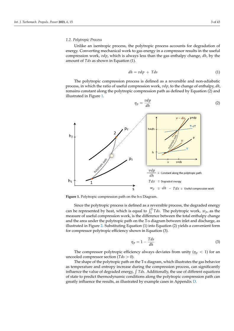
Unlike an isentropic process, the polytropic process accounts for degradation ofenergy. Converting mechanical work to gas energy in a compressor results in the usefulcompression work, vdp, which is always less than the gas enthalpy change, dh, by theamount of Tds as shown in Equation (1).
dh = vdp + Tds (1)
The polytropic compression process is defined as a reversible and non-adiabaticprocess, in which the ratio of useful compression work, vdp, to the change of enthalpy, dh,remains constant along the polytropic compression path as defined by Equation (2) andillustrated in Figure 1.
ηp =vdpdh
(2)
Int. J. Turbomach. Propuls. Power 2021, 6, x FOR PEER REVIEW 3 of 45
work, 𝑣𝑑𝑝, which is always less than the gas enthalpy change, 𝑑ℎ, by the amount of 𝑇𝑑𝑠 as shown in Equation (1). 𝑑ℎ = 𝑣𝑑𝑝 + 𝑇𝑑𝑠 (1)
The polytropic compression process is defined as a reversible and non-adiabatic process, in which the ratio of useful compression work, 𝑣𝑑𝑝, to the change of enthalpy, 𝑑ℎ, remains constant along the polytropic compression path as defined by Equation (2) and illustrated in Figure 1.
Figure 1. Polytropic compression path on the h-s Diagram.
𝜂 = 𝑣𝑑𝑝𝑑ℎ (2)
Since the polytropic process is defined as a reversible process, the degraded energy can be represented by heat, which is equal to 𝑇𝑑𝑠. The polytropic work, 𝑤 , as the measure of useful compression work, is the difference between the total enthalpy change and the area under the polytropic path on the T-s diagram between inlet and discharge, as illustrated in Figure 2. Substituting Equation (1) into Equation (2) yields a convenient form for compressor polytropic efficiency shown in Equation (3).
𝜂 = 1 − 𝑇𝑑𝑠𝑑ℎ (3)
The compressor polytropic efficiency always deviates from unity (𝜂 < 1) for an un-cooled compressor section (𝑇𝑑𝑠 > 0).
The shape of the polytropic path on the T-s diagram, which illustrates the gas behavior as temperature and entropy increase during the compression process, can significantly influ-ence the value of degraded energy, 𝑇𝑑𝑠. Additionally, the use of different equations of state to predict thermodynamic conditions along the polytropic compression path can greatly in-fluence the results, as illustrated by example cases in Appendix D.
Figure 1. Polytropic compression path on the h-s Diagram.
Since the polytropic process is defined as a reversible process, the degraded energycan be represented by heat, which is equal to
∫ 21 Tds. The polytropic work, wp, as the
measure of useful compression work, is the difference between the total enthalpy changeand the area under the polytropic path on the T-s diagram between inlet and discharge, asillustrated in Figure 2. Substituting Equation (1) into Equation (2) yields a convenient formfor compressor polytropic efficiency shown in Equation (3).
ηp = 1− Tdsdh
(3)
The compressor polytropic efficiency always deviates from unity (ηp < 1) for anuncooled compressor section (Tds > 0).
The shape of the polytropic path on the T-s diagram, which illustrates the gas behavioras temperature and entropy increase during the compression process, can significantlyinfluence the value of degraded energy,
∫Tds. Additionally, the use of different equations
of state to predict thermodynamic conditions along the polytropic compression path cangreatly influence the results, as illustrated by example cases in Appendix D.

Int. J. Turbomach. Propuls. Power 2021, 6, 15 4 of 43Int. J. Turbomach. Propuls. Power 2021, 6, x FOR PEER REVIEW 4 of 45
Figure 2. Area under the polytropic path on the T-s diagram represents degradation of energy in a polytropic compression process. Additionally, see Figure 10 for different possible curve shapes of the polytropic path between endpoints.
2. Polytropic Path: Polynomial Approximation Methods The constant efficiency polytropic path on the T-s diagram is a continuous real-valued
function of entropy defined on a bounded interval 𝑠 , 𝑠 . This actual polytropic path can be approximated to a high degree of accuracy using a single polynomial or a series of sequen-tial piecewise segment polynomials. The concept is to accurately estimate the actual un-known temperature function, T(s), by an approximating function that is simple but accurate enough (i.e., within acceptably small error tolerances) to calculate 𝑇𝑑𝑠, which is the de-graded part of energy transfer in the polytropic compression process. Taher [1], documented the mathematics of applying sequential piecewise cubic polynomials to approximate a con-stant efficiency temperature-entropy polytropic path.
The temperature-entropy relationship along the polytropic path can be approximated using a single polynomial for the entire range from inlet to discharge. This is referred to as an “Endpoint” method since the thermodynamic state variables at both compressor inlet and discharge are required inputs and are known from testing. For some applications, when a single polynomial cannot provide sufficient accuracy, a series of sequential steps or segments of polynomials can be employed. The following sections will discuss and compare first- and third-degree polynomial approximants as used to calculate 𝑇𝑑𝑠. First degree polynomials are described as using “steps” while third degree polynomials are described as using “seg-ments.” This distinction is due to the discontinuity of path slope change for linear steps whereas sequential piecewise cubic segments possess a continuous slope change. It will be shown that this continuity of slope at the knots gives rise to increased accuracy while using fewer segments to achieve the desired accuracy.
2.1. Temperature-Entropy Polytropic Path Approximation: Linear Polynomial Endpoint Method A linear straight-line approximation between inlet and discharge conditions has been
used by Kent [10] and Sandberg [23] to approximate the actual polytopic path on the T-s diagram. Neither Kent nor Sandberg explicitly mentioned employing a linear approximation for the polytropic path on the T-s diagram, but in fact a straight-line approximation of tem-perature, T, as a function of entropy, s, is used in their linear approximation method. Since pressure and temperature are known at both endpoints, all other thermodynamic properties at inlet and discharge can be determined by an equation of state.
Equation (4) represents temperature as a function of entropy connecting compressor section inlet and discharge points on a T-s diagram. The form of the function is a classic straight line.
Figure 2. Area under the polytropic path on the T-s diagram represents degradation of energy in apolytropic compression process. Additionally, see Figure 10 for different possible curve shapes of thepolytropic path between endpoints.
2. Polytropic Path: Polynomial Approximation Methods
The constant efficiency polytropic path on the T-s diagram is a continuous real-valuedfunction of entropy defined on a bounded interval [s1, s2]. This actual polytropic pathcan be approximated to a high degree of accuracy using a single polynomial or a seriesof sequential piecewise segment polynomials. The concept is to accurately estimate theactual unknown temperature function, T(s), by an approximating function that is simplebut accurate enough (i.e., within acceptably small error tolerances) to calculate
∫ 21 Tds,
which is the degraded part of energy transfer in the polytropic compression process.Taher [1], documented the mathematics of applying sequential piecewise cubic polynomialsto approximate a constant efficiency temperature-entropy polytropic path.
The temperature-entropy relationship along the polytropic path can be approximatedusing a single polynomial for the entire range from inlet to discharge. This is referred to asan “Endpoint” method since the thermodynamic state variables at both compressor inletand discharge are required inputs and are known from testing. For some applications,when a single polynomial cannot provide sufficient accuracy, a series of sequential stepsor segments of polynomials can be employed. The following sections will discuss andcompare first- and third-degree polynomial approximants as used to calculate
∫ 21 Tds. First
degree polynomials are described as using “steps” while third degree polynomials aredescribed as using “segments”. This distinction is due to the discontinuity of path slopechange for linear steps whereas sequential piecewise cubic segments possess a continuousslope change. It will be shown that this continuity of slope at the knots gives rise toincreased accuracy while using fewer segments to achieve the desired accuracy.
2.1. Temperature-Entropy Polytropic Path Approximation: Linear Polynomial Endpoint Method
A linear straight-line approximation between inlet and discharge conditions has beenused by Kent [10] and Sandberg [23] to approximate the actual polytopic path on the T-sdiagram. Neither Kent nor Sandberg explicitly mentioned employing a linear approxima-tion for the polytropic path on the T-s diagram, but in fact a straight-line approximation oftemperature, T, as a function of entropy, s, is used in their linear approximation method.Since pressure and temperature are known at both endpoints, all other thermodynamicproperties at inlet and discharge can be determined by an equation of state.
Equation (4) represents temperature as a function of entropy connecting compressorsection inlet and discharge points on a T-s diagram. The form of the function is a classicstraight line.
(1)1T(s) = ms + b (4)
Int. J. Turbomach. Propuls. Power 2021, 6, 15 5 of 43
The constraints applied to Equation (4) are shown in Equations (5) and (6).
T(s1) = T1 (5)
T(s2) = T2 (6)
Equations (7) and (8) show the analytically derived values for the slope and interceptof the straight-line approximant. These values are constant and only dependent upon thethermodynamic parameters at the compression endpoints.
m =T2 − T1
s2 − s1=
∆T∆s
(7)
b =s2T1 − s1T2
s2 − s1(8)
Substituting Equations (7) and (8) into Equation (4) yields Equation (9), (1)1T(s), whichis a first-degree polynomial that approximates the actual polytropic path T(s).
(1)1T(s) ∼=
(T2 − T1
s2 − s1
)s +
s2T1 − s1T2
s2 − s1(9)
The deviation of the approximated temperature from the actual temperature valueusing a linear approximant is represented by the error function (1)
1ErT(S) in Equation (10).
T(s) = (1)1T(s) + (1)
1ErT(s) (10)
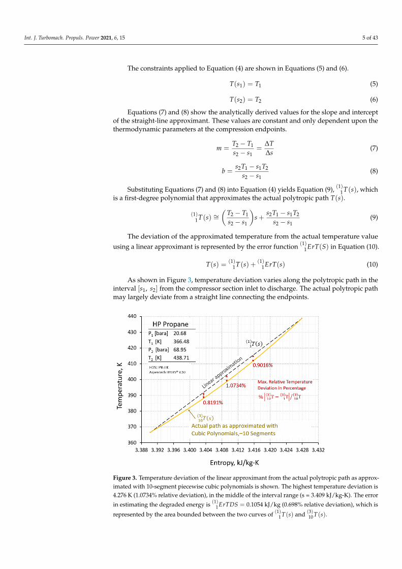
As shown in Figure 3, temperature deviation varies along the polytropic path in theinterval [s1, s2] from the compressor section inlet to discharge. The actual polytropic pathmay largely deviate from a straight line connecting the endpoints.
Int. J. Turbomach. Propuls. Power 2021, 6, x FOR PEER REVIEW 5 of 45
𝑇( ) (𝑠) = 𝑚𝑠 + 𝑏 (4)
The constraints applied to Equation (4) are shown in Equations (5) and (6). 𝑇(𝑠 ) = 𝑇 (5)
𝑇(𝑠 ) = 𝑇 (6)
Equations (7) and (8) show the analytically derived values for the slope and intercept of the straight-line approximant. These values are constant and only dependent upon the ther-modynamic parameters at the compression endpoints. 𝑚 = 𝑇 − 𝑇𝑠 − 𝑠 = ∆𝑇∆𝑠 (7)
𝑏 = 𝑠 𝑇 − 𝑠 𝑇𝑠 − 𝑠 (8)
Substituting Equations (7) and (8) into Equation (4) yields Equation (9), 𝑇( ) (𝑠), which is a first-degree polynomial that approximates the actual polytropic path 𝑇(𝑠). 𝑇( ) (𝑠) ≅ 𝑇 − 𝑇𝑠 − 𝑠 𝑠 + 𝑠 𝑇 − 𝑠 𝑇𝑠 − 𝑠 (9)
The deviation of the approximated temperature from the actual temperature value using a linear approximant is represented by the error function 𝐸𝑟𝑇( ) (𝑠) in Equation (10). 𝑇(𝑠) = 𝑇( ) (𝑠) + 𝐸𝑟( ) 𝑇(𝑠) (10)
As shown in Figure 3, temperature deviation varies along the polytropic path in the interval 𝑠 , 𝑠 from the compressor section inlet to discharge. The actual polytropic path may largely deviate from a straight line connecting the endpoints.
Figure 3. Temperature deviation of the linear approximant from the actual polytropic path as approx-imated with 10-segment piecewise cubic polynomials is shown. The highest temperature deviation is 4.276 K (1.0734% relative deviation), in the middle of the interval range (s = 3.409 kJ/kg-K). The error in estimating the degraded energy is 𝐸𝑟( ) 𝑇𝐷𝑆 = 0.1054 kJ/kg (0.698% relative deviation), which is represented by the area bounded between the two curves of 𝑇( ) (𝑠) and 𝑇( ) (𝑠).
Figure 3. Temperature deviation of the linear approximant from the actual polytropic path as approx-imated with 10-segment piecewise cubic polynomials is shown. The highest temperature deviation is4.276 K (1.0734% relative deviation), in the middle of the interval range (s = 3.409 kJ/kg-K). The error
in estimating the degraded energy is (1)1ErTDS = 0.1054 kJ/kg (0.698% relative deviation), which is
represented by the area bounded between the two curves of (1)1T(s) and (3)
10T(s).
Int. J. Turbomach. Propuls. Power 2021, 6, 15 6 of 43
The term (1)1ErTDS in Equation (11) shows the error in calculating
∫ 21 Tds using a
linear approximation for the temperature-entropy relationship between endpoints of thepolytropic compression path.∫ 2
1Tds =
(T1 + T2)
2(S2 − S1) +
(1)1ErTDS (11)
The (1)1ErTDS error can only be estimated by comparing the result against a more
accurate approximation for the polytropic path. In this paper, a 10-segment cubic polyno-mial method (i.e., using (3)
10T(s) approximants) is used as the basis of evaluation. (SeeAppendix B for confirmation of the accuracy of the multi-segment cubic polynomialmethod as applied with 10 segments).
Employing a straight line as the approximant to model the actual polytropic path onthe T-s diagram overly simplifies the actual compression path resulting in reduced accuracyof the calculation for the
∫ 21 Tds and thus the resulting polytopic efficiency rendering the
polytropic work values less accurate. For example, as illustrated in Figure 3, a linearapproximation for the polytropic path on T-s diagram overestimates the degraded energy(i.e., (1)1ErTDS = 0.1054 kJ/kg) by the bounded area between the linear approximant andthe actual path as estimated with the cubic polynomial method. A linear approximant isinherently limited to a fixed constant slope along the entire polytropic path. This is a majorfactor in estimating the
∫ 21 Tds with large errors using a linear endpoint approximant.
2.2. Temperature-Entropy Polytropic Path Approximation: Cubic Polynomial Endpoint Method
The desire to improve the accuracy of approximating the actual polytropic path onthe T-s diagram has led to employing the approximant function as a cubic polynomial.Polynomials of the first degree and second degree are limited since they cannot account forpath slope changes and concavity of the actual polytropic path respectively. A polynomialof the third degree is the simplest form of a polynomial approximant, which allowsthe model to account for these two important features. As explained later in this paper(see Section 4), the slope and concavity of the polytropic path on the T-s diagram revealsignificant thermodynamic insight about the behavior of fluids during the compressionprocess and must be carefully studied.
Using Equation (12), the actual temperature that increases with entropy, T(s), alongthe polytropic path of a compressor section can be approximated using the third-degreepolynomial (3)1T(s).
(3)1T(s) = As3 + Bs2 + Cs + D (12)
Since thermodynamic conditions at endpoints are known, the constraints applied toEquation (12) are shown in Equations (13)–(16).
T(s1) = T1 (13)
T(s2) = T2 (14)(dTds
)η,1
= E1 =T1
Cp1
(1 + ηp X1
1− ηp
)(15)
(dTds
)η,2
= E2 =T2
Cp2
(1 + ηp X2
1− ηp
)(16)
Relationships (15) and (16) determine values of the slope of the temperature-entropycurve at endpoints of the polytropic path. For details on how these equations are derivedfrom thermodynamic relationships, see Appendix A.

Int. J. Turbomach. Propuls. Power 2021, 6, 15 7 of 43
Coefficients A, B, C and D of the third order polynomial (3)1T(s) in Equation (12)
are “analytically” derived from the known conditions above. The results are shown inEquations (17)–(20).
A =2
(s2 − s1)2
(E1 + E2
2− T2 − T1
s2 − s1
)(17)
B =12
(E2 − E1
s2 − s1
)− 3(s1 + s2)
2A (18)
C =E1 + E2
2− 3
2A(
s22 + s2
1
)− B(s1 + s2) (19)
D =(T1 + T2)
2− A
2
(s3
1 + s32
)− B
2
(s2
1 + s22
)− C
2(s1 + s2) (20)
Coefficient A accounts for the deviation of the average value of the slope at the end-points,
(E1+E2
2
), from that of the straight line, which connects the endpoints, ( ∆T
∆s = T2−T1S2−S1
).Coefficient B accounts for the change of slope along the polytropic path. When the polytopicpath on the T-s diagram approaches to a straight line that connects the endpoints, (e.g., in thecase of compressing an ideal gas) coefficients A and B approach zero and coefficients C and Drepresent the slope and the intercept of the straight line as shown in relationships (7) and (8).
The deviation of the temperature approximated using a cubic polynomial approximantfrom the actual temperature value is shown by the error function (3)
1ErT(s) in Equation (21).The temperature deviation varies along the polytropic path in the interval [s1, s2] from thecompressor inlet to discharge.
T(s) = (3)1T(s) + (3)
1ErT(s) (21)
As illustrated in Figure 4, the deviation of approximated temperature from the actualtemperature shows significant improvement for the cubic polynomial approximation overthe linear version, which is expected since (3)
1ErT(s)� (1)1ErT(s).
Int. J. Turbomach. Propuls. Power 2021, 6, x FOR PEER REVIEW 7 of 45
Coefficients A, B, C and D of the third order polynomial 𝑇( ) (𝑠) in Equation (12) are “analytically” derived from the known conditions above. The results are shown in Equations (17)–(20). 𝐴 = 2(𝑠 − 𝑠 ) 𝐸 + 𝐸2 − 𝑇 − 𝑇𝑠 − 𝑠 (17)
𝐵 = 12 𝐸 − 𝐸𝑠 − 𝑠 − 3(𝑠 + 𝑠 )2 𝐴 (18)
𝐶 = 𝐸 + 𝐸2 − 32 𝐴(𝑠 + 𝑠 ) − 𝐵(𝑠 + 𝑠 ) (19)
𝐷 = (𝑇 + 𝑇 )2 − 𝐴2 (𝑠 + 𝑠 ) − 𝐵2 (𝑠 + 𝑠 ) − 𝐶2 (𝑠 + 𝑠 ) (20)
Coefficient A accounts for the deviation of the average value of the slope at the end-points, , from that of the straight line, which connects the endpoints, (∆∆ = ). Co-efficient B accounts for the change of slope along the polytropic path. When the polytopic path on the T-s diagram approaches to a straight line that connects the endpoints, (e.g., in the case of compressing an ideal gas) coefficients A and B approach zero and coefficients C and D represent the slope and the intercept of the straight line as shown in relationships (7) and (8).
The deviation of the temperature approximated using a cubic polynomial approximant from the actual temperature value is shown by the error function 𝐸𝑟𝑇( ) (𝑠) in Equation (21). The temperature deviation varies along the polytropic path in the interval 𝑠 , 𝑠 from the compressor inlet to discharge. 𝑇(𝑠) = 𝑇( ) (𝑠) + 𝐸𝑟( ) 𝑇(𝑠) (21)
As illustrated in Figure 4, the deviation of approximated temperature from the actual temperature shows significant improvement for the cubic polynomial approximation over the linear version, which is expected since 𝐸𝑟𝑇( ) (𝑠) ≪ 𝐸𝑟𝑇( ) (𝑠).
Figure 4. Temperature deviation of the cubic polynomial endpoint method from the actual polytropicpath as approximated with 10-segment piecewise cubic polynomial approximants is shown. Thehighest temperature deviation is 1.185 K (0.289% relative deviation), at s = 3.414 kJ/kg-K. The error
in estimating the degraded energy is (1)1ErTDS = 0.0237 kJ/kg (0.157% relative deviation), which is
represented by the area bounded between the two curves of (3)1T(s) and (3)
10T(s).

Int. J. Turbomach. Propuls. Power 2021, 6, 15 8 of 43
Figure 5 compares the temperature deviation of the linear, (1)1T(s), and cubic poly-
nomial, (3)1T(s), endpoint approximants from the highly accurate polytropic path as ap-
proximated with a 10-segment piecewise cubic polynomials, (3)10T(s), for the high pressurepropane case with the endpoint conditions shown on the figure. The cubic polynomialendpoint approximant provides a maximum temperature deviation that is less than a thirdof that of the linear endpoint approximant.
Int. J. Turbomach. Propuls. Power 2021, 6, x FOR PEER REVIEW 8 of 45
Figure 4. Temperature deviation of the cubic polynomial endpoint method from the actual polytropic path as approximated with 10-segment piecewise cubic polynomial approximants is shown. The high-est temperature deviation is 1.185 K (0.289% relative deviation), at s = 3.414 kJ/kg·K. The error in esti-mating the degraded energy is 𝐸𝑟( ) 𝑇𝐷𝑆 = 0.0237 kJ/kg (0.157% relative deviation), which is repre-sented by the area bounded between the two curves of 𝑇( ) (𝑠) 𝑎𝑛𝑑 𝑇( ) (𝑠).
Figure 5 compares the temperature deviation of the linear, 𝑇( ) (𝑠), and cubic polyno-mial, 𝑇( ) (𝑠), endpoint approximants from the highly accurate polytropic path as approxi-mated with a 10-segment piecewise cubic polynomials, 𝑇( ) (𝑠), for the high pressure pro-pane case with the endpoint conditions shown on the figure. The cubic polynomial endpoint approximant provides a maximum temperature deviation that is less than a third of that of the linear endpoint approximant.
Figure 5. Distribution of temperature deviation shows the maximum error of cubic polynomial end-point approximant is less than one third of the linear endpoint approximation.
The term 𝐸𝑟( ) 𝑇𝐷𝑆 in Equation (22) shows the error in calculating 𝑇𝑑𝑠 using the cu-bic polynomial endpoint approximation. 𝑇𝑑𝑠 = (𝑇 + 𝑇 )2 (𝑠 − 𝑠 ) − (𝐸 − 𝐸 )12 (𝑠 − 𝑠 ) + 𝐸𝑟( ) 𝑇𝐷𝑆 (22)
The improved accuracy of calculating 𝑇𝑑𝑠 using the cubic polynomial endpoint ap-proximant, 𝑇( ) (𝑠), as compared to the linear approximant, 𝑇( ) (𝑠), can be calculated using Equation (23). 𝐸𝑟( ) 𝑇𝐷𝑆 − 𝐸𝑟( ) 𝑇𝐷𝑆 = − (𝐸 − 𝐸 )12 (𝑠 − 𝑠 ) (23)
Equation (23) shows that the accuracy of the cubic polynomial approximant as com-pared to a linear approximant increases for compression applications with a large difference between the slopes at the endpoints. As explained in the next section of this paper, this ana-lytical relationship conveniently provides a means to evaluate accuracy of the linear endpoint method.
3. Polytropic Efficiency Calculation
Figure 5. Distribution of temperature deviation shows the maximum error of cubic polynomialendpoint approximant is less than one third of the linear endpoint approximation.
The term (3)1ErTDS in Equation (22) shows the error in calculating
∫ 21 Tds using the
cubic polynomial endpoint approximation.∫ 2
1Tds =
(T1 + T2)
2(s2 − s1)−
(E2 − E1)
12(s2 − s1)
2 +(3)
1ErTDS (22)
The improved accuracy of calculating∫ 2
1 Tds using the cubic polynomial endpoint
approximant, (3)1T(s), as compared to the linear approximant, (1)1T(s), can be calculatedusing Equation (23).
(1)1ErTDS− (3)
1ErTDS = − (E2 − E1)
12(s2 − s1)
2 (23)
Equation (23) shows that the accuracy of the cubic polynomial approximant as com-pared to a linear approximant increases for compression applications with a large differencebetween the slopes at the endpoints. As explained in the next section of this paper, thisanalytical relationship conveniently provides a means to evaluate accuracy of the linearendpoint method.
3. Polytropic Efficiency Calculation
Since the late 19th century, various calculation methods have been proposed to esti-mate polytropic efficiency. The polytropic efficiency can only be estimated. The accuracy ofthe estimation depends upon the calculation method and the accuracy of thermodynamicproperties used in the calculation. As shown in this paper, different equations of state for afixed method can result in variation of polytropic efficiency values, which may be evenlarger than the effect of measurement uncertainties. It is important to ensure that the same

Int. J. Turbomach. Propuls. Power 2021, 6, 15 9 of 43
equation of state as used for calculating expected performance is used when calculatingpolytropic efficiency based on equipment test results.
Regardless of which calculation method is used, usually five significant digits canwell serve the purpose for any compressor performance evaluation. Accuracy of measuredinlet and discharge conditions as well as of the equation of state and test data used toobtain thermodynamic properties for the calculation method may impose to reduce thenumber of significant digits. The identification of significant digits is only possible throughknowledge of the circumstances [25]. However, in this paper, the intended precisionof polytropic efficiency is chosen as five significant digits in order to evaluate differentpolytropic efficiency calculation methods.
A novel approach is used in this paper to differentiate between the actual polytropicefficiency (for a fixed calculation method and EOS) from the calculated polytropic efficiencyby using an error function, Erη. This is believed to help clarify that regardless of thecalculation method, the actual polytropic efficiency, ηp, can only be estimated with someacceptable error, Erη, as compared to a more accurate reference method. In this paper, theTaher–Evans Cubic Polynomial 10-segment method is used as the basis to compare theaccuracy of other methods.
3.1. Polytropic Efficiency Calculation: Linear Polynomial Endpoint Method
In the simplest case, the polytropic path can be approximated using a linear approxi-mant, which connects the endpoints (i.e., one step) as follows:
(1)1T(s) = ms + b (24)
The degraded energy in the polytropic compression process,∫ 2
1 Tds, is approximated
using the linear endpoint approximant (1)1T(s):
∫ 2
1Tds =
∫ 2
1
(1)1T(s) ds + (1)
1ErTDS (25)
By replacing (1)1T(s) from (24) and analytically performing the integral
∫ 21
(1)1T(s) ds using
the relationship (9), the relationship (26) emerges:∫ 2
1Tds =
(T1 + T2)
2(s2 − s1) +
(1)1ErTDS (26)
Using the relationships (2) and (26), the polytopic efficiency, (1)1η , as approximatedwith the linear endpoint approximation method is developed as follows:
(1)1η = 1−
∫ 21
(1)1T(s) ds∫ 21 dh
= 1−(
s2 − s1
h2 − h1
)[T1 + T2
2
](27)
The deviation of the approximated endpoint polytropic efficiency, (1)1η , from the actual
polytropic efficiency, ηp, using the linear endpoint approximant, (1)1T(s), is represented by
the error function (1)1Erη in Equation (28).
ηp =(1)
1η +(1)
1Erη (28)
A similar relationship to (27) for calculating the polytropic efficiency was suggestedby Stepanoff [26] in 1955.

Int. J. Turbomach. Propuls. Power 2021, 6, 15 10 of 43
3.2. Polytropic Efficiency Calculation: Taher–Evans Cubic Polynomial Endpoint Method
In a more accurate case, the polytropic path can be approximated using a cubicpolynomial, which connects the endpoints (i.e., one segment) as follows:
(3)1T(s) = As3 + Bs2 + Cs + D (29)
The degraded energy in the polytropic compression process,∫ 2
1 Tds, can be approxi-
mated using the cubic polynomial endpoint approximant, (3)1T(s):
∫ 2
1Tds =
∫ 2
1
(3)1T(s) ds + (3)
1ErTDS (30)
By replacing (3)1T(s) from (29) and analytically performing the integral,
∫ 21
(3)1T(s) ds,
using relationships (17)–(20), the relationship (31) emerges:∫ 2
1Tds =
(T1 + T2)
2(s2 − s1)−
(E2 − E1)
12(s2 − s1)
2 +(3)
1ErTDS (31)
Using the relationships (2) and (31), the polytopic efficiency, (3)1η , as approximatedwith the cubic polynomial endpoint approximation method is developed as follows:
(3)1η = 1−
∫ 21
(3)1T(s) ds∫ 21 dh
= 1−(
s2 − s1
h2 − h1
)[T1 + T2
2−(
E2 − E1
12
)(s2 − s1)
](32)
Equation (32) can be solved recursively by assuming an initial value for the efficiencyto calculate endpoint slopes E1 and E2, calculating the resulting efficiency from (32), andminimizing the difference between assumed and calculated efficiency.
The deviation of the approximated endpoint polytropic efficiency, (3)1η , from the actualpolytropic efficiency, ηp, using Taher–Evans cubic polynomial endpoint approximant(3)
1T(s), is represented by the error function (3)1Erη in Equation (33).
ηp =(3)
1η +(3)
1Erη (33)
By comparing relationships (27) and (32) the efficiency deviation between the linearand cubic polynomial endpoint methods can be developed as follows:
(3)1Erη − (1)
1Erη = − 112
(E2 − E1
h2 − h1
)(s2 − s1)
2 (34)
As shown by the relationship (34), the deviation linearly increases with the change ofslopes, (E2 − E1), at endpoints. This analytical relationship conveniently provides a meansto evaluate accuracy of the linear methods as applied to endpoints.
Once the polytropic efficiency, (3)1η is determined, coefficients A, B, C, and D are
calculated, and the polytopic path model on T-s and h-s diagrams can be graphicallyrepresented using relationships (29) and (51).
Figure 6 compares the efficiency deviation of the linear endpoint and cubic polynomialendpoint methods from the highly accurate 10-segment cubic polytropic efficiency, (3)10η ,using different equations of state for the high pressure propane case with the condi-tions shown on the figure. Evidently, the linear endpoint method involves significantlylarger deviations for the polytropic efficiency as compared with the cubic polynomialendpoint method.

Int. J. Turbomach. Propuls. Power 2021, 6, 15 11 of 43
Using illustrative examples in Appendix B, it is shown that Taher–Evans cubic polyno-mial endpoint method provides the highest accuracy among all other endpoint methods.
Int. J. Turbomach. Propuls. Power 2021, 6, x FOR PEER REVIEW 11 of 45
Figure 6. Percentage deviation of polytropic efficiency of the linear, 𝜂( ) , and cubic polynomial, 𝜂( ) , endpoint methods from the highly accurate 10-segment cubic polynomials polytropic efficiency, 𝜂( ) , as calculated using different equation of states.
3.3. Polytropic Efficiency Calculation: Linear Multistep Method
As illustrated in Figures 3 and 6, the linear approximant, 𝑇( ) (𝑠), when applied to end-points may introduce large deviations from the actual T-s polytropic path resulting in re-duced accuracy for the calculated polytropic efficiency, 𝜂( ) . By applying the composite trap-ezoidal rule, the integral 𝑇𝑑𝑠 is approximated by employing piecewise linear polynomial approximants that cover the entire path in multiple steps with smaller subintervals 𝑠 , 𝑠 .
In the linear multi-step method, temperature deviation along the polytropic path re-duces as the number of steps, j, which approximate the entropy interval 𝑠 , 𝑠 increases.
𝑇(𝑠) = 𝑇( ) (𝑠) + 𝐸𝑟( ) 𝑇 (𝑠) (35)
where for the 𝑖th step, 𝑇( ) (𝑠) is defined in the sub-interval 𝑠 , 𝑠 .
As shown in Figure 7, maximum temperature deviation along the polytropic path re-duces as the number of steps increases. As expected, linear approximation involves larger deviation as compared with cubic polynomial approximation for the same number of steps or segments. As reviewed in Appendix C, a maximum of five cubic polynomial segments has been documented to provide sufficient accuracy for a broad range of example cases by Evans [3].
The degraded energy in the polytropic compression process, 𝑇𝑑𝑠 , is approximated by dividing the path into j-steps and using a linear approximant for each step.
𝑇𝑑𝑠 = 𝑇( ) (𝑠) 𝑑𝑠 + 𝐸𝑟( ) 𝑇𝐷𝑆 (36)
where 𝐸𝑟( ) 𝑇𝐷𝑆 shows the error in approximating the integral, 𝑇(𝑠) 𝑑𝑠, by using the linear approximant 𝑇( ) (𝑠) in the subinterval 𝑠𝑖 , 𝑠𝑖+1 . By summing up errors of all j-steps, the total error for approximating the integral 𝑇𝑑𝑠, with linear approximants using j-steps is developed:
Figure 6. Percentage deviation of polytropic efficiency of the linear, (1)1η , and cubic polynomial, (3)1η ,
endpoint methods from the highly accurate 10-segment cubic polynomials polytropic efficiency, (3)10η ,as calculated using different equation of states.
3.3. Polytropic Efficiency Calculation: Linear Multistep Method
As illustrated in Figures 3 and 6, the linear approximant, (1)1T(s), when applied to
endpoints may introduce large deviations from the actual T-s polytropic path resulting inreduced accuracy for the calculated polytropic efficiency, (1)1η . By applying the compos-ite trapezoidal rule, the integral
∫ 21 Tds is approximated by employing piecewise linear
polynomial approximants that cover the entire path in multiple steps with smaller subin-tervals [si, si+1].
In the linear multi-step method, temperature deviation along the polytropic pathreduces as the number of steps, j, which approximate the entropy interval [s1, s2] increases.
T(s) =j
∑i=1
((1)
j T i(s) +(1)
j ErTi(s))
(35)
where for the ith step, (1)j T i(s) is defined in the sub-interval [si, si+1].As shown in Figure 7, maximum temperature deviation along the polytropic path
reduces as the number of steps increases. As expected, linear approximation involveslarger deviation as compared with cubic polynomial approximation for the same numberof steps or segments. As reviewed in Appendix C, a maximum of five cubic polynomialsegments has been documented to provide sufficient accuracy for a broad range of examplecases by Evans [3].

Int. J. Turbomach. Propuls. Power 2021, 6, 15 12 of 43
The degraded energy in the polytropic compression process,∫ 2
1 Tds , is approximatedby dividing the path into j-steps and using a linear approximant for each step.
∫ 2
1Tds =
j
∑i=1
∫ i+1
i
(1)j T i(s) ds + (1)
j EriTDS (36)
where (1)j EriTDS shows the error in approximating the integral,
∫ i+1i T(s) ds, by using
the linear approximant (1)j T i(s) in the subinterval [si, si+1]. By summing up errors of all
j-steps, the total error for approximating the integral∫ 2
1 Tds, with linear approximantsusing j-steps is developed:
(1)j ErTDS =
j
∑i=1
(1)j EriTDS (37)
Int. J. Turbomach. Propuls. Power 2021, 6, x FOR PEER REVIEW 12 of 45
𝐸𝑟( ) 𝑇𝐷𝑆 = 𝐸𝑟( ) 𝑇𝐷𝑆 (37)
Figure 7. Maximum temperature deviation along the polytropic path for the example case 14. See Table A1 in Appendix B for gas compositions and compressor inlet and discharge conditions.
By applying the relationship (26) for each step, and using the composite trapezoidal rule, the integral, 𝑇𝑑𝑠, is approximated as follows:
𝑇𝑑𝑠 = (𝑇𝑖 + 𝑇𝑖+1)2 (𝑠𝑖+1 − 𝑠𝑖)𝑗𝑖=1 + 𝐸𝑟( ) 𝑇𝐷𝑆 (38)
Using the relationships (2) and (38), the polytopic efficiency, 𝜂( ) , is developed as fol-lows: 𝜂( ) = 1 − 𝑠 − 𝑠ℎ − ℎ 𝑇𝑖 + 𝑇𝑖+12 (39)
The deviation of the approximated polytropic efficiency, 𝜂( ) , from the actual polytropic efficiency, 𝜂 using linear approximants, 𝑇( ) (𝑠), at each step is represented by the error function, 𝐸𝑟𝜂( ) , in Equation (40). 𝜂 = 𝜂( ) + 𝐸𝑟𝜂( ) (40)
Because the linear method ignores the change in slope and concavity along the compres-sion path, a large number of steps are needed to achieve the desired accuracy. Sandberg [23] provided no criteria to determine the required number of linear steps to approximate 𝑇𝑑𝑠. The uncertainty about the required number of steps in the linear multi-step method could possibly be overcome by applying a large number of linear steps (50 to 100+ steps) to ensure sufficient accuracy. However, pre-selecting 50 or 100+ linear polynomial steps has been shown to be inefficient, (see Figure 11). Utilizing a large number of linear steps significantly increases the calculation time due to the required nested iteration loops. Figure A3b docu-ments a comparison of elapsed time measurements for the supercritical propane example case.
3.4. Polytropic Efficiency Calculation: Taher–Evans Cubic Polynomial Multi-Segment Method
Figure 7. Maximum temperature deviation along the polytropic path for the example case 14. SeeTable A1 in Appendix B for gas compositions and compressor inlet and discharge conditions.
By applying the relationship (26) for each step, and using the composite trapezoidalrule, the integral,
∫ 21 Tds, is approximated as follows:
∫ 2
1Tds =
(j
∑i=1
(Ti + Ti+1)
2(si+1 − si)
)+
(1)j ErTDS (38)
Using the relationships (2) and (38), the polytopic efficiency, (1)j η , is developed as follows:
(1)j η = 1−
j
∑i=1
(si+1 − sihi+1 − hi
)[Ti + Ti+1
2
](39)
The deviation of the approximated polytropic efficiency, (1)j η , from the actual poly-
tropic efficiency, ηp using linear approximants, (1)j T i(s), at each step is represented by the
error function, (1)j Erη, in Equation (40).
ηp =(1)
j η +(1)
j Erη (40)

Int. J. Turbomach. Propuls. Power 2021, 6, 15 13 of 43
Because the linear method ignores the change in slope and concavity along the com-pression path, a large number of steps are needed to achieve the desired accuracy. Sand-berg [23] provided no criteria to determine the required number of linear steps to approxi-mate
∫ 21 Tds. The uncertainty about the required number of steps in the linear multi-step
method could possibly be overcome by applying a large number of linear steps (50 to 100+steps) to ensure sufficient accuracy. However, pre-selecting 50 or 100+ linear polynomialsteps has been shown to be inefficient, (see Figure 11). Utilizing a large number of linearsteps significantly increases the calculation time due to the required nested iteration loops.Figure A3b documents a comparison of elapsed time measurements for the supercriticalpropane example case.
3.4. Polytropic Efficiency Calculation: Taher–Evans Cubic Polynomial Multi-Segment Method
The T-s polytropic path can be accurately approximated with a set of piecewisethermodynamically coupled cubic polynomials. The T-s polytropic path is divided into “j”segments over the entropy range, [s1, s2], from compressor section inlet to discharge.Each subinterval [si, si+1] of the actual path, T(s), is approximated by a cubic polynomialapproximant, (3)j T i(s), which allows the temperature as well as T-s polytropic path slope,(dT/ds), to be matched at endpoints of adjacent segments, thus increasing accuracy whilesmoothing the overall path. The key factor in the accuracy of cubic polynomial multi-segment method as compared with the linear multistep method is taking advantage ofapplying the thermodynamic constraint, dT
ds , at each intermediate point (knot) to enablesmooth transition from one to the following segment.
The relationship (41) shows the actual temperature-entropy path, T(s), as approx-imated with a set of “j” cubic polynomial approximants, (3)
j T i(s), and the temperature
deviation at each segment, (3)j ErTi(s) :
T(s) =j
∑i=1
((3)
j T i(s) +(3)
j ErTi(s))
(41)
where (3)j T i(s) at each segment is determined by:
T(s) = Ais3 + Bis2 + Cis + Di si ≤ s ≤ si+1T(si) = TiT(si+1) = Ti+1(
dTds
)i= Ei =
TiCpi
(1+(3)
j η Xi
1−(3)j η
)(
dTds
)i+1
= Ei+1 =Ti+1
Cpi+1
(1+(3)
j η Xi+1
1−(3)j η
) (42)
The coefficients (Ai, Bi, Ci, Di), of each cubic polynomial approximant are calculatedusing the relationships (17) to (20), where subscripts 1 and 2 are replaced with endpointconditions of the ith segment.
Similar to relationships (30) and (31), the degraded energy is calculated,∫ i+1
i(3)
j T i(s) ds
and its related error, (3)j EriTDS, at each segment are defined. The total error for approximat-
ing the integral∫ 2
1 Tds, using cubic polynomial approximants is determined by summingup errors of each segment.
(3)j ErTDS =
j
∑i=1
(3)j EriTDS (43)

Int. J. Turbomach. Propuls. Power 2021, 6, 15 14 of 43
By applying the relationship (32) for each segment, the integral,∫ 2
1 Tds, is approxi-mated as follows:
∫ 2
1Tds =
(j
∑i=1
(Ti + Ti+1)
2(si+1 − si)−
(Ei+1 − Ei)
12(si+1 − si)
2
)+
(3)j ErTDS (44)
Using the relationships (2) and (44), the polytopic efficiency (3)j η is developed as follows:
(3)j η = 1−
j
∑i=1
(si+1 − sihi+1 − hi
)[Ti + Ti+1
2− (Ei+1 − Ei)
12(si+1 − si)
](45)
The deviation of the approximated polytropic efficiency (3)j η from the actual polytropic
efficiency, ηp using cubic polynomial approximants (3)j T i(s) at each step is represented by
the error function (3)j Erη in Equation (46).
ηp =(3)
j η +(3)
j Erη (46)
3.4.1. Polytropic Efficiency Calculation Procedure: Taher–Evans Cubic PolynomialMulti-Segment Method
The solution requires an initial estimate of efficiency and then recursive solutionsfor segment discharge temperature. Equation (45) is solved recursively by assuming aninitial value for the efficiency, (3)
j η to calculate endpoint slopes E1 and E2, calculatingthe resulting efficiency from (45), and minimizing the difference between assumed andcalculated efficiency. The step-by-step procedure is explained as follows:
Note: inlet and discharge pressures and temperatures discussed below are assumedto be for total conditions at a given compressor section.
(1) Determine an initial estimate of polytropic efficiency by assuming (E2 = E1) in therelationship (45) for the cubic polynomial endpoint method.Note: for the purpose of compressor performance testing, the initial value of theefficiency is the expected efficiency provided by the compressor manufacturer.
(2) Select the number of segments (j).There are different ways to select intermediate knots. In this paper, the overall pressureratio is divided across the number of segments (j) to determine equal pressure ratiosteps as shown in the next step.
(3) Use “j” number of equal pressure ratio segments.(
pr = j√
p2p1
).
(4) Use Equation (29) to estimate the initial value of segment outlet temperature. (Thisrequires a solution to the cubic polynomial endpoint method).Note: steps 1 through 4 are only required for the initialization of the solution algorithm.
(5) Calculate segment temperature rise, (∆Ti = Ti+1 − Ti)(6) Calculate the segment polytropic efficiency using the relationship (45).(7) Calculate efficiency deviation from the initially estimated polytropic efficiency from
step 1.(8) Iterate segment outlet temperature to match assumed efficiency.
Note: different root finding algorithms may be used to optimize iterations for segmentoutlet temperature.Note: the acceptable efficiency convergence should be set less than 1E−6.
(9) Move to next segment using outlet conditions of previous segment as inlet conditions.

Int. J. Turbomach. Propuls. Power 2021, 6, 15 15 of 43
(10) Repeat steps 5 through 9 for each segment.(11) Compare final discharge temperature with the given value, Td(12) If step 11 result is not within a small tolerance, iterate efficiency and determine new
values for coefficients A, B, C and D.(13) Repeat steps 5 through 11 until agreement is reached within the tolerance.
Note: the acceptable convergence from the given discharge temperature should be setless than 1E−8.
In the Taher–Evans Cubic Polynomial method, intermediate points are determined bysetting one thermodynamic variable (such as pressure or entropy) at each end of a segmentand calculating other thermodynamic variables to force the segment endpoint to lie on aconstant efficiency path via nested recursive algorithms (within a small error tolerance).Using cubic polynomial approximants, the polytropic path slope can be accurately calcu-lated since the first derivative of each segmental polynomial can be determined at eachintermediate point (see Ei and Ei+1 in Equation (42)).
The difference between final segment calculated discharge temperature and the knowndischarge temperature, Td, can be minimized by iterating efficiency. These nested itera-tions of efficiency (inner loop) and the final segment discharge temperatures (outer loop)converge quickly.
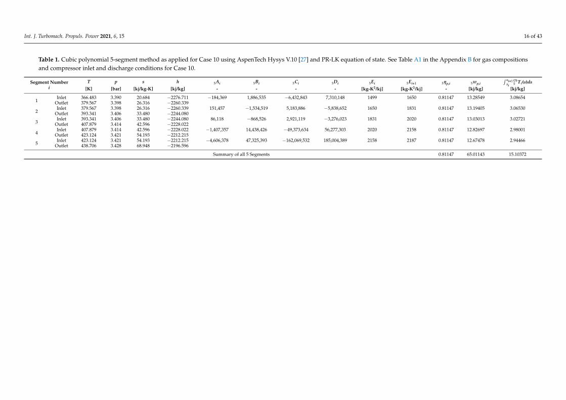
When a final efficiency is determined, summations of enthalpy changes and Tds lossescan be performed for the entire set of segments. The cubic polynomial multi-segmentmethod provides intermediate points along the constant efficiency temperature-entropypath that have been forced to coincide with the actual path. Additionally, the path slope ateach intermediate point is equal at the end of the ith segment and the beginning of the i+1segment. See Table 1.
3.4.2. Distinction between Cubic Interpolation and Approximation
As the final point in this section, it should be noted that the approximation of functionsis different from interpolation. In the case of interpolation, at certain intermediate points,the value of an unknown function is given (such as measured values at intermediate points),but the function itself is not known. Interpolating cubic splines are used to interpolatebetween known intermediate points, which is irrelevant in the problem of approximatingan unknown function without any given intermediate point. Accordingly, the descriptor“spline” is not applied in this paper as it usually is thought of as being used to approximatea curve passing through previously known knots.
Int. J. Turbomach. Propuls. Power 2021, 6, 15 16 of 43
Table 1. Cubic polynomial 5-segment method as applied for Case 10 using AspenTech Hysys V.10 [27] and PR-LK equation of state. See Table A1 in the Appendix B for gas compositionsand compressor inlet and discharge conditions for Case 10.
Segment Numberi
T p s h 5Ai 5Bi 5Ci 5Di 5Ei 5Ei+1 5ηp,i 5wp,i∫ si+1
si(3)5 T i(s)ds
[K] [bar] [kj/kg-K] [kj/kg] - - - - [kg-K2/kj] [kg-K2/kj] - [kj/kg] [kj/kg]
1Inlet 366.483 3.390 20.684 −2276.711 −184,369 1,886,535 −6,432,843 7,310,148 1499 1650 0.81147 13.28549 3.08654
Outlet 379.567 3.398 26.316 −2260.339
2Inlet 379.567 3.398 26.316 −2260.339 151,457 −1,534,519 5,183,886 −5,838,652 1650 1831 0.81147 13.19405 3.06530
Outlet 393.341 3.406 33.480 −2244.080
3Inlet 393.341 3.406 33.480 −2244.080 86,118 −868,526 2,921,119 −3,276,023 1831 2020 0.81147 13.03013 3.02721
Outlet 407.879 3.414 42.596 −2228.022
4Inlet 407.879 3.414 42.596 −2228.022 −1,407,357 14,438,426 −49,373,634 56,277,303 2020 2158 0.81147 12.82697 2.98001
Outlet 423.124 3.421 54.193 −2212.215
5Inlet 423.124 3.421 54.193 −2212.215 −4,606,378 47,325,393 −162,069,532 185,004,389 2158 2187 0.81147 12.67478 2.94466
Outlet 438.706 3.428 68.948 −2196.596
Summary of all 5 Segments 0.81147 65.01143 15.10372

Int. J. Turbomach. Propuls. Power 2021, 6, 15 17 of 43
4. Polytropic Path on Temperature-Entropy Diagram
For an uncooled compressor section, entropy increases along the polytropic path.The rate of change of temperature with entropy at each point along the polytropic path isdetermined with the relationship (A10) from Appendix A.(
dTds
)ηp
= E =Tcp
(1 + ηpX1− ηp
)(A10)
The change of temperature with entropy from the compressor section inlet to dischargevaries as temperature, specific heat, cp, and compressibility function, X, change at eachpoint along the compression path. At conditions near to the critical point, the rate of changeof cp and X is usually large. This has significant impact on the change of temperature withentropy as the relationship (A10) suggests. The supercritical propane example case hasinlet conditions extremely close to the critical point and the thermodynamic propertiesare varying rapidly as compression begins. Figures 8 and 9 illustrate the variation ofspecific heat, cp, and compressibility function, X, respectively, in the vicinity of the criticalpoint. Each isobar has a distinct peak. The inlet conditions lie in an area on the flank of apeak while discharge conditions (not shown) are far removed from the critical area peaks.Equations (15) and (16) would show a large difference in slope of the T-s path betweeninlet, E1, and discharge, E2, as documented in Table A2. These large differences are oneindicator of the difficulty of a compression case.
Int. J. Turbomach. Propuls. Power 2021, 6, x FOR PEER REVIEW 17 of 45
3.4.2 Distinction Between Cubic Interpolation and Approximation As the final point in this section, it should be noted that the approximation of functions
is different from interpolation. In the case of interpolation, at certain intermediate points, the value of an unknown function is given (such as measured values at intermediate points), but the function itself is not known. Interpolating cubic splines are used to interpolate between known intermediate points, which is irrelevant in the problem of approximating an unknown function without any given intermediate point. Accordingly, the descriptor “spline” is not applied in this paper as it usually is thought of as being used to approximate a curve passing through previously known knots.
4. Polytropic Path on Temperature-Entropy Diagram For an uncooled compressor section, entropy increases along the polytropic path. The
rate of change of temperature with entropy at each point along the polytropic path is deter-mined with the relationship (A10) from Appendix A. 𝑑𝑇𝑑𝑠 = 𝐸 = 𝑇𝑐 1 + 𝜂 𝑋1 − 𝜂 (A10)
The change of temperature with entropy from the compressor section inlet to discharge varies as temperature, specific heat, 𝑐 , and compressibility function, 𝑋, change at each point along the compression path. At conditions near to the critical point, the rate of change of 𝑐 and 𝑋 is usually large. This has significant impact on the change of temperature with en-tropy as the relationship (A10) suggests. The supercritical propane example case has inlet conditions extremely close to the critical point and the thermodynamic properties are varying rapidly as compression begins. Figures 8 and 9 illustrate the variation of specific heat, 𝑐 , and compressibility function, 𝑋, respectively, in the vicinity of the critical point. Each isobar has a distinct peak. The inlet conditions lie in an area on the flank of a peak while discharge conditions (not shown) are far removed from the critical area peaks. Equations (15) and (16) would show a large difference in slope of the T-s path between inlet, 𝐸 , and discharge, 𝐸 , as documented in Table A2. These large differences are one indicator of the difficulty of a compression case.
Figure 8. Change of specific heat, cp, along the polytropic path for supercritical propane example.Moreover, the change of specific heat, cp, with temperature at different inlet pressures is shown.

Int. J. Turbomach. Propuls. Power 2021, 6, 15 18 of 43
Int. J. Turbomach. Propuls. Power 2021, 6, x FOR PEER REVIEW 18 of 45
Figure 8. Change of specific heat, 𝑐 , along the polytropic path for supercritical propane example. Moreover, the change of specific heat, 𝑐 , with temperature at different inlet pressures is shown.
Figure 9. Change of compressibility function, 𝑋, along the polytropic path for supercritical propane example. Furthermore, the change of compressibility function, 𝑋, with temperature at different inlet pressures is shown.
While the change of temperature with entropy along the compression path of an un-cooled compressor section is always positive ( > 0), the curvature of the polytropic path on the T-s diagram may change sign (from concave upward to downward or vice versa). A change in sign happens when equals to zero at any point along the compression path which indicates a change of curvature (as seen in the case of HP Ethylene in Appendix B).
The cubic polynomial endpoint method can be used to approximate the concavity of the actual T-s polytropic path. No other endpoint methods can provide such a mathematical and thermodynamic insight about the behavior of the actual T-s polytropic path from known thermodynamic conditions at the inlet and discharge of the compressor section.
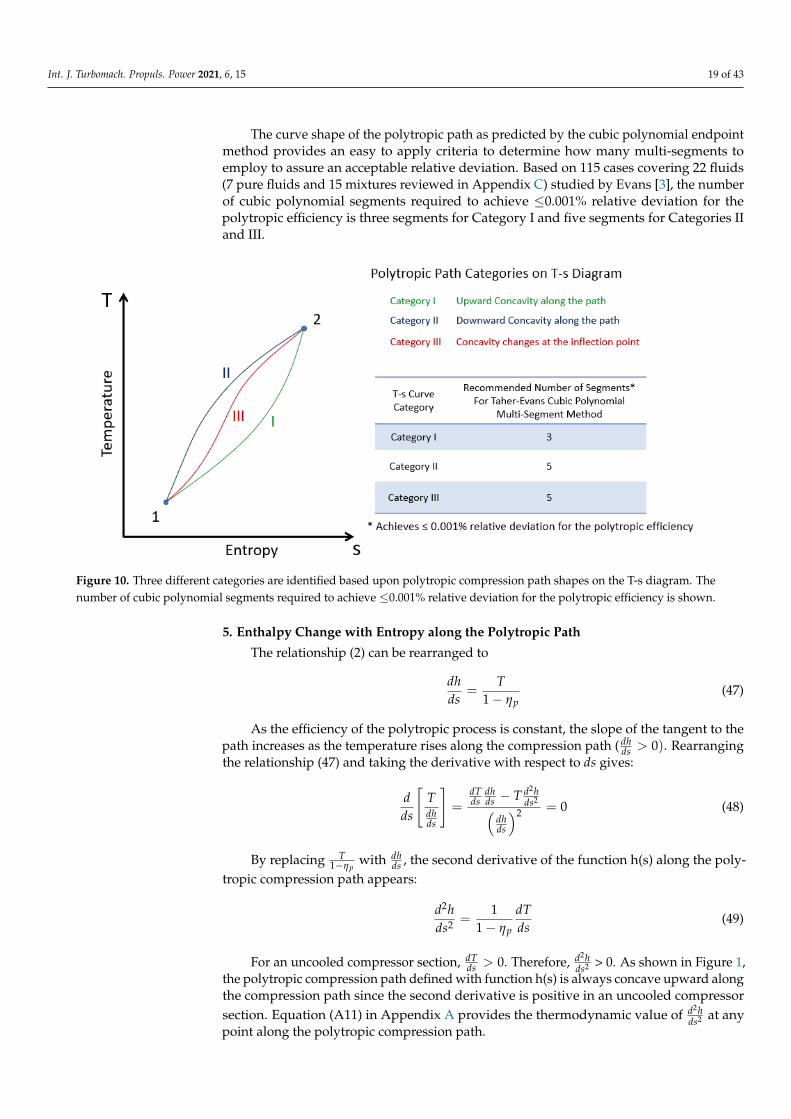
The concavity of the polynomial approximant can be examined using the second deriv-ative test of the path equation with the following criteria: • If (−𝐵 3𝐴⁄ ) 𝑖𝑠 out of the range of 𝑠 , 𝑠 and 3𝐴𝑠 + 𝐵 > 0 the upward concavity of
the cubic polynomial approximant, 𝑇( ) (𝑠), is unchanged along the path. See Figure 10 curve I.
• If (−𝐵 3𝐴⁄ ) is out of the range of 𝑠 , 𝑠 and 3𝐴𝑠 + 𝐵 < 0 the downward concavity of the cubic polytropic approximant, 𝑇( ) (𝑠), is unchanged along the path. See Figure 10 curve II.
• If 𝑠 < (−𝐵 3𝐴⁄ ) < 𝑠 the concavity of the cubic polytropic approximant, 𝑇( ) (𝑠), changes at the inflection point 𝑠( ) = (−𝐵 3𝐴⁄ ). See Figure 10 curve III.
Downward concavity is an indication of increased difficulty for the compression case as shown and confirmed by example cases in Appendix B. See Appendix B for several compres-sion cases evaluated.
Figure 9. Change of compressibility function, X, along the polytropic path for supercritical propaneexample. Furthermore, the change of compressibility function, X, with temperature at different inletpressures is shown.
While the change of temperature with entropy along the compression path of an un-cooled compressor section is always positive ( dT
ds > 0), the curvature of the polytropic pathon the T-s diagram may change sign (from concave upward to downward or vice versa). Achange in sign happens when d2T
ds2 equals to zero at any point along the compression pathwhich indicates a change of curvature (as seen in the case of HP Ethylene in Appendix B).
The cubic polynomial endpoint method can be used to approximate the concavity ofthe actual T-s polytropic path. No other endpoint methods can provide such a mathematicaland thermodynamic insight about the behavior of the actual T-s polytropic path fromknown thermodynamic conditions at the inlet and discharge of the compressor section.
The concavity of the polynomial approximant can be examined using the secondderivative test of the path equation with the following criteria:
• If (−B/3A) is out of the range of [s1, s2] and 3As1 + B > 0 the upward concavity of
the cubic polynomial approximant,(3)1T(s), is unchanged along the path. See Figure 10curve I.
• If (−B/3A) is out of the range of [s1, s2] and 3As1 + B < 0 the downward concavity of
the cubic polytropic approximant,(3)1T(s), is unchanged along the path. See Figure 10curve II.
• If s1 < (−B/3A) < s2 the concavity of the cubic polytropic approximant,(3)1T(s),
changes at the inflection point (3)j s in f = (−B/3A). See Figure 10 curve III.
Downward concavity is an indication of increased difficulty for the compression caseas shown and confirmed by example cases in Appendix B. See Appendix B for severalcompression cases evaluated.
The actual location of the inflection point on the T-s polytropic path can be moreprecisely approximated by applying the cubic polynomial multi-segment method.
The rate of change of dTds with entropy can be considered as a screening criterion to
determine the difficulty of a compression case.
Int. J. Turbomach. Propuls. Power 2021, 6, 15 19 of 43
The curve shape of the polytropic path as predicted by the cubic polynomial endpointmethod provides an easy to apply criteria to determine how many multi-segments toemploy to assure an acceptable relative deviation. Based on 115 cases covering 22 fluids(7 pure fluids and 15 mixtures reviewed in Appendix C) studied by Evans [3], the numberof cubic polynomial segments required to achieve ≤0.001% relative deviation for thepolytropic efficiency is three segments for Category I and five segments for Categories IIand III.
Int. J. Turbomach. Propuls. Power 2021, 6, x FOR PEER REVIEW 19 of 45
Figure 10. Three different categories are identified based upon polytropic compression path shapes on the T-s diagram. The number of cubic polynomial segments required to achieve ≤0.001% relative deviation for the polytropic efficiency is shown.
The actual location of the inflection point on the T-s polytropic path can be more pre-cisely approximated by applying the cubic polynomial multi-segment method.
The rate of change of with entropy can be considered as a screening criterion to de-termine the difficulty of a compression case.
The curve shape of the polytropic path as predicted by the cubic polynomial endpoint method provides an easy to apply criteria to determine how many multi-segments to employ to assure an acceptable relative deviation. Based on 115 cases covering 22 fluids (7 pure fluids and 15 mixtures reviewed in Appendix C) studied by Evans [3], the number of cubic polyno-mial segments required to achieve ≤0.001% relative deviation for the polytropic efficiency is three segments for Category I and five segments for Categories II and III.
5. Enthalpy Change with Entropy along the Polytropic Path The relationship (2) can be rearranged to 𝑑ℎ𝑑𝑠 = 𝑇1 − 𝜂 (47)
As the efficiency of the polytropic process is constant, the slope of the tangent to the path increases as the temperature rises along the compression path ( > 0). Rearranging the relationship (47) and taking the derivative with respect to 𝑑𝑠 gives:
𝑑𝑑𝑠 𝑇𝑑ℎ𝑑𝑠 = 𝑑𝑇𝑑𝑠 𝑑ℎ𝑑𝑠 − 𝑇 𝑑 ℎ𝑑𝑠𝑑ℎ𝑑𝑠 = 0 (48)
By replacing with , the second derivative of the function h(s) along the poly-
tropic compression path appears: 𝑑 ℎ𝑑𝑠 = 11 − 𝜂 𝑑𝑇𝑑𝑠 (49)
For an uncooled compressor section, > 0. Therefore, > 0. As shown in Figure 1, the polytropic compression path defined with function h(s) is always concave upward along
Figure 10. Three different categories are identified based upon polytropic compression path shapes on the T-s diagram. Thenumber of cubic polynomial segments required to achieve ≤0.001% relative deviation for the polytropic efficiency is shown.
5. Enthalpy Change with Entropy along the Polytropic Path
The relationship (2) can be rearranged to
dhds
=T
1− ηp(47)
As the efficiency of the polytropic process is constant, the slope of the tangent to thepath increases as the temperature rises along the compression path ( dh
ds > 0). Rearrangingthe relationship (47) and taking the derivative with respect to ds gives:
dds
[Tdhds
]=
dTds
dhds − T d2h
ds2(dhds
)2 = 0 (48)
By replacing T1−ηp
with dhds , the second derivative of the function h(s) along the poly-
tropic compression path appears:
d2hds2 =
11− ηp
dTds
(49)
For an uncooled compressor section, dTds > 0. Therefore, d2h
ds2 > 0. As shown in Figure 1,the polytropic compression path defined with function h(s) is always concave upward alongthe compression path since the second derivative is positive in an uncooled compressorsection. Equation (A11) in Appendix A provides the thermodynamic value of d2h
ds2 at anypoint along the polytropic compression path.
Int. J. Turbomach. Propuls. Power 2021, 6, 15 20 of 43
The change of enthalpy with entropy at any point along the polytropic path can beapproximated by substituting the relationship of temperature from (12) to (47):
dhds
=As3 + Bs2 + Cs + D
1− ηp(50)
By integrating (50), the relationship of enthalpy and entropy can be approximated atany point along the polytropic path:
h(s) = h1 +A4(s4 − s4
1)+ B
3(s3 − s3
1)+ C
2(s2 − s2
1)+ D(s− s1)
1− ηp(51)
where, s represents any entropy value between compressor section inlet, s1 and sectiondischarge, s2.
6. Comparison of Cubic and Linear Polynomial Results
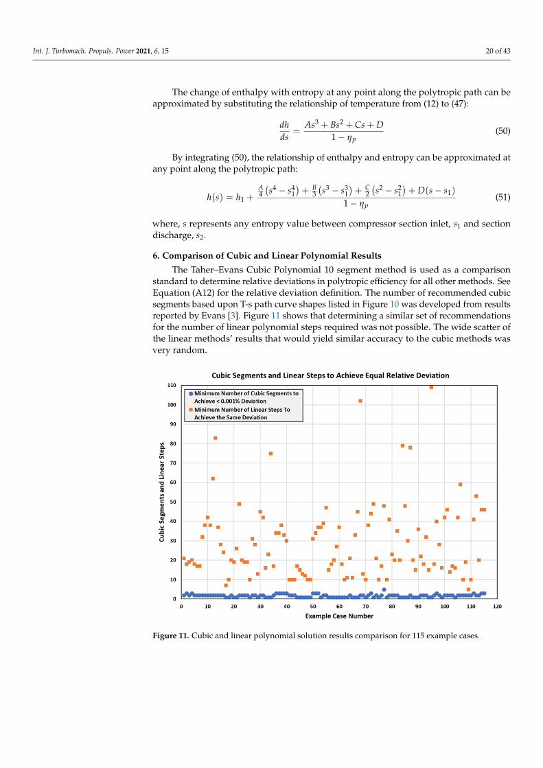
The Taher–Evans Cubic Polynomial 10 segment method is used as a comparisonstandard to determine relative deviations in polytropic efficiency for all other methods. SeeEquation (A12) for the relative deviation definition. The number of recommended cubicsegments based upon T-s path curve shapes listed in Figure 10 was developed from resultsreported by Evans [3]. Figure 11 shows that determining a similar set of recommendationsfor the number of linear polynomial steps required was not possible. The wide scatter ofthe linear methods’ results that would yield similar accuracy to the cubic methods wasvery random.
Int. J. Turbomach. Propuls. Power 2021, 6, x FOR PEER REVIEW 20 of 45
the compression path since the second derivative is positive in an uncooled compressor sec-tion. Equation (A11) in Appendix A provides the thermodynamic value of at any point along the polytropic compression path.
The change of enthalpy with entropy at any point along the polytropic path can be ap-proximated by substituting the relationship of temperature from (12) to (47): 𝑑ℎ𝑑𝑠 = 𝐴𝑠 + 𝐵𝑠 + 𝐶𝑠 + 𝐷1 − 𝜂 (50)
By integrating (50), the relationship of enthalpy and entropy can be approximated at any point along the polytropic path:
ℎ(𝑠) = ℎ1 + 𝐴4 (𝑠4 − 𝑠14) + 𝐵3 (𝑠3 − 𝑠13) + 𝐶2 (𝑠2 − 𝑠12) + 𝐷(𝑠 − 𝑠1)1 − 𝜂 (51)
where, 𝑠 represents any entropy value between compressor section inlet, 𝑠 and section dis-charge, 𝑠 .
6. Comparison of Cubic and Linear Polynomial Results The Taher–Evans Cubic Polynomial 10 segment method is used as a comparison
standard to determine relative deviations in polytropic efficiency for all other methods. See Equation (A12) for the relative deviation definition. The number of recommended cubic seg-ments based upon T-s path curve shapes listed in Figure 10 was developed from results re-ported by Evans [3]. Figure 11 shows that determining a similar set of recommendations for the number of linear polynomial steps required was not possible. The wide scatter of the linear methods’ results that would yield similar accuracy to the cubic methods was very random.
Figure 11. Cubic and linear polynomial solution results comparison for 115 example cases. Figure 11. Cubic and linear polynomial solution results comparison for 115 example cases.
Int. J. Turbomach. Propuls. Power 2021, 6, 15 21 of 43
Appendices B and C discuss example cases and compare various polytropic calculationmethods. The 19 example cases in Appendix B were selected for illustration of a rangeof relatively easy and difficult polytropic efficiency calculation applications. Several ofthese are used to show various characteristics of the calculation results. Appendix C is areview of 115 example cases studied by Evans [3], and includes the 19 example cases fromAppendix B. This larger population further confirms and documents the trends discoveredwhen applying the multi-segment cubic and multi-step linear polynomial methods.
7. Conclusions
• The Taher–Evans Cubic Polynomial method (TE-CP), defined, described and testedherein, illustrates that a highly accurate calculation method for real gas centrifugalcompressor polytropic performance efficiency has been developed and implementedthat employs a temperature—entropy cubic polynomial path function.
# Both endpoint and sequential segment versions are described and tested.# Previously published polytropic efficiency calculation methods including first
degree linear polynomial methods are shown to be less accurate and/or slowerto achieve a solution than Taher–Evans Cubic Polynomial methods.
# The TE-CP methods’ superior results are due to the cubic polynomial pathhaving additional thermodynamic constraints applied to more accurately ap-proximate the actual path slope at any point along the path. Determinationof path slope at the compression endpoints is independent of performancecalculation method.
# T-s polytropic path curve shapes can be determined from derivatives of thecubic polynomial path equation and are indicative of calculation relative diffi-culty. The curve shape is used as a criterion to select the required number ofcubic segments. No other polytropic method can provide such a mathematicaland thermodynamic insight into the fluid compression process.
# The number of T-s path cubic polynomial segments required to achieve an ac-ceptable relative deviation ≤0.001% for polytropic efficiency is three segmentsfor category I and five segments for categories II and III curve shapes.
# As shown in Figure A10, the cubic polynomial methods provide low uncer-tainty with only a few cubic segments. Uncertainty is based upon polytropicefficiency relative deviation, and its magnitude is related to the size of thestatistical population.
# Cubic polynomial methods provide continuous equations to plot the polytropicpath on T-s and h-s diagrams. This is a very unique feature of the cubicpolynomial method that enables visualizing the polytropic path.
# The cubic path coefficients (A, B, C, and D) in Equation (12) provide mean-ingful insights about the behavior of the polytropic path on the temperature-entropy diagram.
# The Taher–Evans Cubic Polynomial methods are highly suitable for applicationto compressor performance testing according to ASME PTC 10 [4].
• Cubic and linear polynomial calculation methods have been extensively documentedand compared.
# Polytropic efficiency calculations have been reviewed for 17 methods across115 example cases yielding a total of 1955 independent calculations that validatesuperior results are achieved when using both endpoint and sequential segmentTaher–Evans Cubic Polynomial (TE-CP) polytropic path methods. A total of22 fluids were employed including seven pure fluids and 15 fluid mixtures tocover wide ranges of mole weight and critical pressures and temperatures.

Int. J. Turbomach. Propuls. Power 2021, 6, 15 22 of 43
# Cubic polynomial endpoint path methods were demonstrated to achieve betteraccuracy than any other endpoint polytropic efficiency calculation method.
# Cubic polynomial sequential segment path methods were demonstrated toachieve high accuracy acceptable polytropic efficiency results significantlyfaster with fewer segments required than linear polynomial path methodsbased upon 115 compression example cases.
# For all 115 example cases, T-s polytropic paths agreed between 10 cubic seg-ments and 100 linear steps which confirmed the validity of using the result of10-segment cubic polynomial approximants as the standard for comparison forpolytropic efficiency relative deviation and uncertainty.
# Cubic polynomial path methods show that the required number of segmentsto achieve an acceptable result remains within a maximum of five segmentsor less for all the cases studied. For the linear polynomial path method, therequired number of steps did not follow a regular pattern as shown in Figure11. No rule or algorithm can be determined for the required number of linearpolynomial steps to achieve an acceptable result.
# While both cubic and linear polynomial methods can reach acceptable results,the cubic methods require fewer repetitive iterations and are completed muchfaster. Sequential segment cubic polynomial method calculations are typicallyat least an order of magnitude faster than sequential step linear polynomialmethods. This is a clear advantage for cubic methods when processing com-pressor performance test data in real time.
# The cubic polynomial methods provide an order of magnitude lower uncer-tainty with significantly fewer cubic segments than linear polynomial methods.(See Figure A10).
# The cubic polynomial methods’ uncertainty rapidly decreases as the numberof segments increases while the linear polynomial methods illustrate a muchmore gradual decrease in uncertainty as they approach an asymptote. Thelinear polynomial methods uncertainty asymptote appears to be more than anorder of magnitude greater than the cubic methods.
• Identical calculations for selected example cases using several different equations ofstate to obtain thermodynamic state point data for application of cubic and linearpolynomial methods revealed significant differences in results for efficiency can occurbased upon the chosen EOS. See Appendix D for selective examples.
Recommendations
• When rapid, highly accurate, low uncertainty, centrifugal compressor polytropicefficiency calculations are required, the Taher–Evans Cubic Polynomial methods (TE-CP) should be used.
• Due to significant differences found between results when employing various equa-tions of state, it is recommended that a project use the same equation of state through-out the project timeline to avoid potential discrepancies.
Author Contributions: Conceptualization and methodology, M.T.; software, validation, formalanalysis, writing—original draft preparation, writing—review and editing, M.T. and F.E.; All authorshave read and agreed to the published version of the manuscript.
Funding: This research received no external funding.
Institutional Review Board Statement: Not applicable.
Informed Consent Statement: Not applicable.
Data Availability Statement: Not applicable.
Conflicts of Interest: The authors declare no conflict of interest.
Int. J. Turbomach. Propuls. Power 2021, 6, 15 23 of 43
Nomenclature
A Polynomial approximant coefficientB Polynomial approximant coefficientb Linear approximant coefficient
β Isobaric expansivity, = 1υ
(∂v∂T
)p
BWRS Benedict–Webb–Rubin EOS as modified by K. E. StarlingC Polynomial approximant coefficientCH4 MethaneCO2 Carbon DioxideC3H8 PropaneCP Cubic PolynomialCp heat capacity at constant pressureD Polynomial approximant coefficient
E Slope of the polytropic path on the T-s diagram,(
dTds
)ηp
EOS Equation of StateErη Deviation of polytropic efficiencyErT Deviation of approximated temperatureErTDS Deviation of approximated
∫Tds
EOS Equation of Stateh Specific enthalpyHP High pressureOEM Original Equipment ManufacturerPR Peng-Robinson EOS
PR-LKPPeng-Robinson EOS and the Lee-Kesler EOS for the calculationof enthalpies
LP Linear Polynomial, or Low PressureLKP Lee-Kesler-Plöcker EOSm Linear approximant coefficientMP Medium Pressuren Schultz [6] polytropic volume exponent as applied in pvn = cT TemperatureTE-CP Taher–Evans Cubic PolynomialREFPROP Reference properties EOS softwares Specific entropySC Supercriticalv Specific volumeX Compressibility function, = βT − 1XY Schultz method using compressibility functions X and Yηp Polytropic efficiency
Subscripts and Superscripts(q)
j T i(s)i indicates the ith segmentj total number of segmentsq degree of the polynomial approximant
Example: (3)10T6(s) indicates the cubic polynomial approximant, which is
used to approximate the segment number 6 of a polytropic path that isdivided into 10 segments.This symbology provides a clear way to compare different methodsdiscussed in this paper.
inf inflectionp Polytropic, or pressurer ratiod compressor section discharge (measured)1 compressor section inlet2 compressor section discharge

Int. J. Turbomach. Propuls. Power 2021, 6, 15 24 of 43
Appendix A. Temperature Change with Entropy along the Polytropic Path
Derivation of the following two important relationships, dTds and d2h
ds2 along the poly-tropic compression path is explained in this appendix.
Choose the entropy to be a function of temperature and pressure. Writing the differen-tial of s = s(T, P) gives:
ds =(
∂s∂T
)P
dT +
(∂s∂P
)T
dP (A1)
The first partial derivative in (A1) can be written as follows:
(∂s∂T
)P=
(∂h∂T
)P(
∂h∂s
)P
=cp
T(A2)
where(
∂h∂T
)P= cP and
(∂h∂s
)P= T from the first partial derivate of the Gibbs relationship
dh = Tds + vdP.The second partial derivative in (A1) is one of the Maxwell relations:(
∂s∂P
)T= −
(∂v∂T
)P
(A3)
Substituting the first and second partial derivatives in (A1) from (A2) and (A3) yields:
ds =cp
TdT −
(∂v∂T
)P
dP (A4)
Using the definition of isobaric expansivity β = 1υ
(∂v∂T
)p
for the second partial deriva-
tive gives:
ds =cp
TdT − βvdP (A5)
Employing the Gibbs relationship dh = Tds + vdP for a polytropic process andsubstituting dh with vdP
ηpgives:
vdP =Tds
1ηp− 1
(A6)
Substituting vdP from (A5) to (A4) yields:
ds =cp
TdT − βTds
1ηp− 1
(A7)
This can be further simplified to1 +βT
1ηp− 1
ds =cp
TdT (A8)
From (A8) the slope of the polytropic path on a T-s diagram is determined:
dTds
=Tcp
(1 + ηp(βT − 1)
1− ηp
)(A9)
Substituting (βT − 1) with the Schultz compressibility function X gives:
dTds
=Tcp
(1 + ηpX1− ηp
)(A10)

Int. J. Turbomach. Propuls. Power 2021, 6, 15 25 of 43
By replacing dTds from (A10) to (47) gives:
d2hds2 =
Tcp
(1 + ηpX
)(1− ηp
)2 (A11)
The relationships (A10) and (A11) were developed and presented for the first time byTaher [1].
The relationship (A11) shows that the polytropic path on the enthalpy-entropy dia-gram is concave upward since the second derivative is positive in an uncooled compres-sor section.
Appendix B. Comparative Numeric Examples of Application of the Taher–EvansCubic Polynomial Methods
The Taher–Evans Cubic Polynomial method for calculation of centrifugal compressorpolytropic performance has been applied to 19 compression example cases which are com-prised of five pure fluids and four hydrocarbon fluid mixtures. Eight cases are consideredlow pressure while eleven cases are considered medium or high pressure. Input data forten cases came from existing literature references while nine cases are new. All cases werechosen based upon the desire to explore a wide range of process conditions for fluidscommon to the hydrocarbon industry.
The fluids and process conditions selected represent a combination of relatively easyand difficult calculations for centrifugal compressor polytropic performance. Table A1lists input data for the 19 cases. The “easy cases” are found by the results listed below tobe low pressure versions for CO2, C3H8 and CH4/C3H8/CO2. The most difficult case issupercritical propane due to inlet conditions.
Using results of the above referenced analyses, this appendix will review polytropicefficiency calculation method comparisons for following three categories:
• Endpoint methods
# Schultz (two variations) [6];# Mallen Saville [9];# Cubic Polynomial;# Linear polynomial.
• Three point methods
# Cubic Polynomial two segment;# Huntington’s three point [13].
• Multi-step and multi-segment methods
# Cubic Polynomial—sequential segments (2 through 10 segments);# Linear Polynomial—sequential steps (10, 20, 50, 90 and 100 steps).
The Taher–Evans Cubic Polynomial 10 segment method is used as a comparisonstandard to determine relative deviations in polytropic efficiency for all other methods.The validity of using this standard is confirmed below. Equation (A12) documents therelative deviation calculation.
Relative Deviation, % = 100×∣∣ηTE-CP 10 Segment − ηp
∣∣ηTE-CP 10 Segment
(A12)
Industry standardized compressor data sheets document operating conditions andperformance characteristics with polytropic efficiency shown as a percentage, typicallywith two decimal places of accuracy, such as 68.25%. One criterion applied in the examplecases below is that the deviation should be known to be less than 0.001% of an acceptablestandard. Since all polytropic efficiency calculation methods are approximations, a standarddetermines the magnitude of the difference between two calculations.

Int. J. Turbomach. Propuls. Power 2021, 6, 15 26 of 43
As mentioned in the paper (see also Appendix D), polytropic performance resultscan be impacted by the choice of an equation of state (EOS). The REFPROP (version 10)software package [28] produced by the National Institute of Science and Technology (NIST)was employed for calculations in this appendix. REFPROP provides reference quality,multi parameter, real gas equations of state for thermodynamic and transport properties ofindividual fluids. REFPROP applies optimized binary interaction parameters via mixingrules to determine mixture properties.
When using the REFPROP software package, all example case inlet and discharge statepoint phases are single phase and either superheated or supercritical. For some examplecases, the close proximity of inlet conditions to a fluid’s critical point yielded two phaseor liquid phases for some other equations of state used in Appendix D. The polytropicperformance methods discussed in this paper are neither designed nor recommended fortwo phase flows. The impact of equation of state choices will be reviewed in Appendix D.
Table A1. Example case input data.
Case Number 1 2 3 4 5 6 7 8 9 10 11
Case Name
Schu
ltz
R12
LPEt
hyle
ne
HP
Ethy
lene
SCEt
hane
PTC
10C
O2
LPC
O2
MP
CO
2
HP
CO
2
LPPr
opan
e
HP
Prop
ane
SCPr
opan
e
Com
posi
tion
,mol
%
Ethane 1.0000
Propane 1.0000 1.0000 1.0000
CarbonDioxide 1.0000 1.0000 1.0000 1.0000
Ethylene 1.0000 1.0000
R12 1.0000
Com
pres
sion
Con
diti
ons
p1 , psia 10 360 362.5 750 300.01 400 500 1100.1 17.99 300 650
p1 , bara 0.689 24.821 24.993 51.710 20.685 27.579 34.474 75.849 1.240 20.684 44.816
T1 , ◦F −10 50 98.3 110 100 100 75 98.3 −31.36 200 210
T1 , ◦C −23.33 10 36.833 43.333 37.778 37.778 23.88 36.833 −35.2 93.333 98.889
p2 , psia 130 1000 7250 3500 487.76 1200 3000 6000.3 60 1000 3500
p2 , bara 8.963 68.948 499.870 241.316 33.630 82.737 206.843 413.706 4.137 68.948 241.316
T2 , ◦F 210 195 566.3 285 201.59 325 400 368.3 60 330 300
T2 , ◦C 98.889 90.556 296.833 140.556 94.217 162.778 204.444 186.833 15.556 165.556 148.889
Case Number 12 13 14 15 16 17 18 19
Case Name
LPC
H4/
C3H
8/C
O2
MP
CH
4/C
3H8/
CO
2
HP
CH
4/C
3H8/
CO
2
LPC
H4/
CO
2
HP
CH
4/C
O2
LPH
eavy
NG
HP
Hea
vyN
G
PTC
10H
PNG
Com
posi
tion
,mol
%
Methane 0.30294 0.30294 0.30294 0.256274 0.256274 0.688671 0.688671 0.8600
Ethane 0.03748 0.03748 0.03748 0.022871 0.022871 0.119957 0.119957 0.1125
Propane 0.43533 0.43533 0.43533 0.005691 0.005691 0.102964 0.102964 0.0075
isoButane 0.00222 0.00222 0.00222 0.000001 0.000001 0.031432 0.031432
Butane 0.00218 0.00218 0.00218 0.000001 0.000001 0.027541 0.027541
isoPentane 0.000001 0.000001 0.008927 0.008927
Pentane 0.000001 0.000001 0.005563 0.005563
Hexane 0.000175 0.000175
Nitrogen 0.00399 0.00399 0.00399 0.002629 0.002629 0.002477 0.002477 0.0040
CarbonDioxide 0.21586 0.21586 0.21586 0.712356 0.712356 0.012468 0.012468 0.0160
Com
pres
sion
Con
diti
ons
p1 , psia 650 2071 2071 500 1649.7 500 1750 2520.6
p1 , bara 44.816 142.790 142.790 34.474 113.743 34.474 120.658 173.789
T1 , ◦F 115 160 160 50 101.2 100 50 100
T1 , ◦C 46.111 71.111 71.111 10 38.444 37.778 10 37.778
p2 , psia 2200 10,025.70 11,010.80 1700 8189.70 1800 4375 6500
p2 , bara 151.685 691.248 759.168 117.211 564.660 124.106 301.646 448.159
T2 , ◦F 270 291.9 301.5 250 316.2 295 125 280

Int. J. Turbomach. Propuls. Power 2021, 6, 15 27 of 43
Appendix B.1. Endpoint Methods
Schultz [6] described several alternative versions of his methodology in his originalASME paper all of which applied a path equation of pvn = c. The variations involvedcalculating his “polytropic head factor”, f , in various ways as well as multiple methods ofaveraging his “polytropic volume exponent”, n. For the comparisons below, the followingtwo variations of Schultz’s method are included for examination since they were includedin the 1997 version of ASME PTC10 [4].
• Schulzn—with n based upon the endpoints of compression
# n = ln(p2/p1)ln(v2/v1)
• Schultz XY average n—with n averaged based upon individual calculations at inletand discharge
# n = n1+n22
Mallen and Saville [9] employed a path equation of TdsdT = c. Path equations are
described above in this paper for the liner and cubic polynomial methods.Figure A1a–e illustrate polytropic efficiency relative deviation results for endpoint
methods for the 19 example cases. The Taher–Evans endpoint method provides superiorresults compared to the other endpoint methods for all example cases. Example casesPTC10 CO2, LP CO2, LP propane and LP CH4/C3H8/CO2 are considered easy casessince the Taher–Evans Cubic Polynomial endpoint method achieves deviations from the10-segment method of less than 0.001%. Thus, using multi-segment analyses would notbe required for these cases. The two Schultz based methods show significant errors forsome example cases and do not exhibit a consistent pattern. Figure A1f directly comparestwo related cases in that the PTC10 CO2 case represents a Type 2 test designed for theHPNG example case. The PTC10 CO2 case is a low-pressure case and deviations are seento be smaller than for the HPNG case as expected. However, the Taher–Evans endpointmethod provides better accuracy for the PTC 10 HPNG case. The HPNG case requiresmore segments to achieve less than a 0.001% deviation level.
Notable comparisons for endpoint methods:
• Figure A1a
# HP ethylene; Mallen and Saville [9] highlighted their improvements overSchultz’s method for high pressure, but still have an approximate 1% deviation;
# LP and HP ethylene; typical and expected patterns for cubic and lin-ear polynomials.
• Figure A1b,c
# CO2 and propane; as pressure increases accuracy decreases is a typical pattern
• Figure A1d
# CH4/C3H8/CO2; medium and high pressure cases are very similar sincedischarge conditions are close
• Figure A1f
# PTC10; the HPNG case will require more cubic segments to achieve sufficientaccuracy than the Type 2 test design using CO2

Int. J. Turbomach. Propuls. Power 2021, 6, 15 28 of 43
Int. J. Turbomach. Propuls. Power 2021, 6, x FOR PEER REVIEW 29 of 45
Figure A1. (a–f) Summary comparison of relative deviation results for endpoint methods.
Table A2 lists the T-s path inlet and discharge slope and curve category for the 19 exam-ple cases. Five cases show that an inflection point in curvature exists along the path. For these five cases, endpoint analyses do not provide sufficient polytropic efficiency accuracy and multi-segment analyses are recommended. Changes in path slope and curvature can be used as criteria for determining how many cubic segments are needed to provide sufficient accu-racy (See Section 4, Figure 10 and Appendix C).
Figure A1. (a–f) Summary comparison of relative deviation results for endpoint methods.
Table A2 lists the T-s path inlet and discharge slope and curve category for the 19example cases. Five cases show that an inflection point in curvature exists along the path.For these five cases, endpoint analyses do not provide sufficient polytropic efficiencyaccuracy and multi-segment analyses are recommended. Changes in path slope andcurvature can be used as criteria for determining how many cubic segments are needed toprovide sufficient accuracy (See Section 4, Figure 10 and Appendix C).

Int. J. Turbomach. Propuls. Power 2021, 6, 15 29 of 43
Table A2. Taher–Evans Cubic Polynomial endpoint method T-s path slope and curvature.
Case Number Case 1 Case 2 Case 3 Case 4 Case 5
T-s Slope at Inlet, E1, lbm.R2/BTU 14,168 10,442 9383 14,537 7026T-s Slope at Discharge, E2, lbm.R2/BTU 19,822 12,253 8302 7946 7881T-s Slope Change, % 39.90 17.34 −11.52 −45.34 12.17T-s Curve Shape Category I I III II IEntropy at Inflection Point, BTU/lbm.R - - 0.65070 - -Temperature at Inflection Point, ◦F - - 304.71 - -
Case Number Case 6 Case 7 Case 8 Case 9 Case 10
T-s Slope at Inlet, E1, lbm.R2/BTU 8551 15,181 10,553 7178 10,330T-s Slope at Discharge, E2, lbm.R2/BTU 10,744 19,708 8887 8151 15,523T-s Slope Change, % 25.66 29.82 −15.79 13.57 50.28T-s Curve Shape Category I I II I IEntropy at Inflection Point, BTU/lbm.R - - - - -Temperature at Inflection Point, ◦F - - - - -
Case Number Case 11 Case 12 Case 13 Case 14 Case 15
T-s Slope at Inlet, E1, lbm.R2/BTU 14,053 10,664 11,513 11,509 13,135T-s Slope at Discharge, E2, lbm.R2/BTU 3773 9986 5526 5352 16,183T-s Slope Change, % −73.15 −6.36 −52.01 −53.50 23.20T-s Curve Shape Category III III III III IEntropy at Inflection Point, BTU/lbm.R 0.48820 0.64410 0.55540 0.55670 -Temperature at Inflection Point, ◦F 288.95 176.68 286.75 294.07 -
Case Number Case 16 Case 17 Case 18 Case 19
T-s Slope at Inlet, E1, lbm.R2/BTU 18,783 5147 4601 2786T-s Slope at Discharge, E2, lbm.R2/BTU 12,049 5762 3362 2632T-s Slope Change, % −35.85 11.94 −26.94 −5.53T-s Curve Shape Category II I II IIEntropy at Inflection Point, BTU/lbm.R - - - -Temperature at Inflection Point, ◦F - - - -
Appendix B.2. Three Point Methods
Figure A2a–e provide a summary of the polytropic efficiency deviation results compar-ing the Taher–Evans Cubic Polynomial 2 segment method with Huntington’s three-pointmethod [13]. The two-segment cubic polynomial method shows sufficient accuracy for 13of 19 example cases while Huntington’s three-point method shows sufficient accuracy foronly 7 of 19 example cases based upon the 0.001% requirement. In all example cases, thecubic polynomial method is more accurate than Huntington’s method. Figure A2f com-pares PTC10 CO2 and HPNG cases. Both cubic and the Huntington’s three-point methodare sufficient for the low-pressure test case but only the cubic polynomial is sufficient forthe HPNG case.
Appendix B.3. Multi-Step and Multi-Segment Methods
Table A3 lists the polytropic efficiency calculated for Taher–Evans Cubic Polynomial 2through 10 multi-segment methods, and linear polynomial 10, 20, 50, 90 and 100 multi-stepmethods. The general trend is that using more segments or steps yields higher accuracy. Inmany example cases, as more segments or steps are applied, the efficiency only changesbeyond the fourth decimal place as highlighted in the table by the outlined values. Theresults are shown to have “stabilized” to four decimal places for additional segments orsteps. In all example cases, the highest accuracy shown agrees between cubic and linearmethods, but the linear method requires many more steps before “stabilizing”. The generaltrend of higher-pressure cases requiring more segments or steps to stabilize is confirmed.
For the supercritical ethane example case, the cubic method demonstrates a polytropicefficiency of 79.9519% for three segments and remains at that value for the four decimal

Int. J. Turbomach. Propuls. Power 2021, 6, 15 30 of 43
places shown as the number of segments is increased. The linear method needs between 50and 90 steps to reach the same accuracy for efficiency. In other words, the linear methodapproaches an asymptote much more slowly than the cubic method at the cost of increasedcomputing resources and elapsed time to reach a solution. This illustrates the usefulnessof the cubic method in being able to take advantage of matching the slope of the T-s pathbetween sequential segments. Both the cubic and linear methods are approximants thatcan reach essentially the same level of approximation, but the cubic method employs morethermodynamic constraints to achieve the resulting polytropic efficiency much quicker.
It is not necessary to reach a “stabilized” polytropic efficiency to satisfy the maximumallowable deviation requirement of 0.001% as compared to the Taher–Evans Cubic Polyno-mial 10 segment results. Deviations are less than 0.001% for 13 of 19 example cases using2 cubic segments while only 4 of 19 are less than 0.001% for 10 linear steps.
Int. J. Turbomach. Propuls. Power 2021, 6, x FOR PEER REVIEW 31 of 45
Figure A2. (a–f) Summary comparison of relative deviation results for three point methods.
Appendix B.3. Multi-Step and Multi-Segment Methods Table A3 lists the polytropic efficiency calculated for Taher–Evans Cubic Polynomial 2
through 10 multi-segment methods, and linear polynomial 10, 20, 50, 90 and 100 multi-step methods. The general trend is that using more segments or steps yields higher accuracy. In many example cases, as more segments or steps are applied, the efficiency only changes be-yond the fourth decimal place as highlighted in the table by the outlined values. The results are shown to have “stabilized” to four decimal places for additional segments or steps. In all example cases, the highest accuracy shown agrees between cubic and linear methods, but the linear method requires many more steps before “stabilizing.” The general trend of higher-pressure cases requiring more segments or steps to stabilize is confirmed.
Figure A2. (a–f) Summary comparison of relative deviation results for three point methods.

Int. J. Turbomach. Propuls. Power 2021, 6, 15 31 of 43
Table A3. Summary comparison of polytropic efficiency results for linear multi-step and cubic polynomial multi-segment methods.
Case Number Case 1 Case 2 Case 3 Case 4 Case 5 Case 6 Case 7Cubic Polynomial 2 Segment 75.0442 81.9199 80.6174 79.9531 59.4118 65.2211 78.4933Cubic Polynomial 3 Segment 75.0437 81.9200 80.6148 79.9521 59.4118 65.2211 78.4938Cubic Polynomial 4 Segment 75.0436 81.9200 80.6146 79.9519 59.4118 65.2211 78.4939Cubic Polynomial 5 Segment 75.0435 81.9200 80.6145 79.9519 59.4118 65.2211 78.4939Cubic Polynomial 6 Segment 75.0435 81.9200 80.6145 79.9519 59.4118 65.2211 78.4939Cubic Polynomial 7 Segment 75.0435 81.9200 80.6145 79.9519 59.4118 65.2211 78.4939Cubic Polynomial 8 Segment 75.0435 81.9200 80.6145 79.9519 59.4118 65.2211 78.4939Cubic Polynomial 9 Segment 75.0435 81.9200 80.6145 79.9519 59.4118 65.2211 78.4939Cubic Polynomial 10 Segment 75.0435 81.9200 80.6145 79.9519 59.4118 65.2211 78.4939
Linear Polynomial 10 step 75.0408 81.9194 80.6153 79.9544 59.4111 65.2189 78.4916Linear Polynomial 20 step 75.0428 81.9198 80.6147 79.9525 59.4116 65.2205 78.4933Linear Polynomial 50 step 75.0434 81.9200 80.6145 79.9520 59.4118 65.2210 78.4938Linear Polynomial 90 step 75.0435 81.9200 80.6145 79.9519 59.4118 65.2211 78.4939Linear Polynomial 100 step 75.0435 81.9200 80.6145 79.9519 59.4118 65.2211 78.4939
Case Number Case 8 Case 9 Case 10 Case 11 Case 12 Case 13 Case 14Cubic Polynomial 2 Segment 64.3513 81.0248 79.4381 67.7882 76.7610 82.0678 82.0695Cubic Polynomial 3 Segment 64.3497 81.0247 79.4386 67.7984 76.7610 82.0692 82.0712Cubic Polynomial 4 Segment 64.3493 81.0247 79.4387 67.8002 76.7610 82.0694 82.0714Cubic Polynomial 5 Segment 64.3492 81.0247 79.4387 67.8007 76.7610 82.0695 82.0715Cubic Polynomial 6 Segment 64.3491 81.0247 79.4387 67.8009 76.7610 82.0695 82.0715Cubic Polynomial 7 Segment 64.3491 81.0247 79.4387 67.8010 76.7610 82.0695 82.0716Cubic Polynomial 8 Segment 64.3491 81.0247 79.4387 67.8010 76.7610 82.0695 82.0716Cubic Polynomial 9 Segment 64.3491 81.0247 79.4387 67.8011 76.7610 82.0695 82.0716Cubic Polynomial 10 Segment 64.3491 81.0247 79.4387 67.8011 76.7610 82.0695 82.0716
Linear Polynomial 10 step 64.3512 81.0243 79.4375 67.8050 76.7612 82.0715 82.0738Linear Polynomial 20 step 64.3496 81.0246 79.4384 67.8021 76.7610 82.0700 82.0721Linear Polynomial 50 step 64.3491 81.0247 79.4387 67.8013 76.7610 82.0696 82.0717Linear Polynomial 90 step 64.3491 81.0247 79.4387 67.8012 76.7610 82.0695 82.0716Linear Polynomial 100 step 64.3491 81.0247 79.4387 67.8011 76.7610 82.0695 82.0716
Case Number Case 15 Case 16 Case 17 Case 18 Case 19Cubic Polynomial 2 Segment 80.3316 82.1055 72.1215 71.3151 59.2985Cubic Polynomial 3 Segment 80.3317 82.1052 72.1216 71.3153 59.2984Cubic Polynomial 4 Segment 80.3317 82.1052 72.1217 71.3154 59.2984Cubic Polynomial 5 Segment 80.3317 82.1052 72.1217 71.3154 59.2984Cubic Polynomial 6 Segment 80.3317 82.1052 72.1217 71.3154 59.2984Cubic Polynomial 7 Segment 80.3317 82.1052 72.1217 71.3154 59.2984Cubic Polynomial 8 Segment 80.3317 82.1052 72.1217 71.3154 59.2984Cubic Polynomial 9 Segment 80.3317 82.1052 72.1217 71.3154 59.2984Cubic Polynomial 10 Segment 80.3317 82.1052 72.1217 71.3154 59.2984Linear Polynomial 10 step 80.3306 82.1073 72.1209 71.3164 59.2990Linear Polynomial 20 step 80.3315 82.1057 72.1215 71.3156 59.2986Linear Polynomial 50 step 80.3317 82.1053 72.1216 71.3154 59.2984Linear Polynomial 90 step 80.3317 82.1052 72.1217 71.3154 59.2984Linear Polynomial 100 step 80.3317 82.1052 72.1217 71.3154 59.2984
Figure A3a illustrates polytropic efficiency relative deviation results for all cubic multi-segment methods and linear multi-step methods for the supercritical propane examplecase. The more difficult an example case is, the more segments or steps it takes to achievea relative deviation of 0.001% or less. This most difficult case achieves this target with5 segments for the cubic polynomial method while it would take 44 steps for the linearpolynomial method to reach the same deviation value as the 5 cubic segment method. Thecubic polynomial method does not suffer from the requirement of a small step size for eachsegment as does the linear polynomial method.
Figure A3b shows the elapsed calculation times for 5 cubic segments and 44 linearsteps are approximately 3.5 s and 55.8 s, respectively. Thus, the linear method takes 16 timeslonger to reach the same level of accuracy for this very difficult example case. For the sixexample cases that required more than 2 cubic segments to reach a deviation less of than0.001%, the elapsed time ratio varied from 5 to 16 times longer for the linear method.

Int. J. Turbomach. Propuls. Power 2021, 6, 15 32 of 43
The elapsed time to reach a solution is dependent upon the algorithm employed toresolve the inner and outer nested, recursive loops for discharge temperature and efficiency.The algorithm used for both cubic and linear method results in this appendix is identical.Thus, while another algorithm might reach solutions faster or slower, the ratio betweencubic and linear method elapsed times should remain approximately the same for a givenexample case.
Int. J. Turbomach. Propuls. Power 2021, 6, x FOR PEER REVIEW 33 of 45
and 90 steps to reach the same accuracy for efficiency. In other words, the linear method approaches an asymptote much more slowly than the cubic method at the cost of increased computing resources and elapsed time to reach a solution. This illustrates the usefulness of the cubic method in being able to take advantage of matching the slope of the T-s path be-tween sequential segments. Both the cubic and linear methods are approximants that can reach essentially the same level of approximation, but the cubic method employs more ther-modynamic constraints to achieve the resulting polytropic efficiency much quicker.
It is not necessary to reach a “stabilized” polytropic efficiency to satisfy the maximum allowable deviation requirement of 0.001% as compared to the Taher–Evans Cubic Polyno-mial 10 segment results. Deviations are less than 0.001% for 13 of 19 example cases using 2 cubic segments while only 4 of 19 are less than 0.001% for 10 linear steps.
Figure A3a illustrates polytropic efficiency relative deviation results for all cubic multi-segment methods and linear multi-step methods for the supercritical propane example case. The more difficult an example case is, the more segments or steps it takes to achieve a relative deviation of 0.001% or less. This most difficult case achieves this target with 5 segments for the cubic polynomial method while it would take 44 steps for the linear polynomial method to reach the same deviation value as the 5 cubic segment method. The cubic polynomial method does not suffer from the requirement of a small step size for each segment as does the linear polynomial method.
Figure A3b shows the elapsed calculation times for 5 cubic segments and 44 linear steps are approximately 3.5 s and 55.8 s, respectively. Thus, the linear method takes 16 times longer to reach the same level of accuracy for this very difficult example case. For the six example cases that required more than 2 cubic segments to reach a deviation less of than 0.001%, the elapsed time ratio varied from 5 to 16 times longer for the linear method.
The elapsed time to reach a solution is dependent upon the algorithm employed to re-solve the inner and outer nested, recursive loops for discharge temperature and efficiency. The algorithm used for both cubic and linear method results in this appendix is identical. Thus, while another algorithm might reach solutions faster or slower, the ratio between cubic and linear method elapsed times should remain approximately the same for a given example case.
(a)
Int. J. Turbomach. Propuls. Power 2021, 6, x FOR PEER REVIEW 34 of 45
(b)
Figure A3. (a) Polytropic efficiency relative deviations for supercritical propane example. (b) elapsed time for supercritical propane example.
Figures A4a–e illustrate polytropic efficiency relative deviation results for all cubic multi-segment methods and linear multi-step methods for the 19 example cases. The 10 cubic segment results are used as the standard for comparison. For each case, fewer cubic segments are needed than linear steps to achieve the 0.001% required accuracy. Figure A4f directly compares the HPNG case and the PTC10 CO2 Type 2 performance test designed to prove the compressor should meet the design requirements within the tolerances allowed by the ASME PTC10 code [4].
Figure A3. (a) Polytropic efficiency relative deviations for supercritical propane example. (b) elapsedtime for supercritical propane example.

Int. J. Turbomach. Propuls. Power 2021, 6, 15 33 of 43
Figure A4a–e illustrate polytropic efficiency relative deviation results for all cubicmulti-segment methods and linear multi-step methods for the 19 example cases. The10 cubic segment results are used as the standard for comparison. For each case, fewercubic segments are needed than linear steps to achieve the 0.001% required accuracy.Figure A4f directly compares the HPNG case and the PTC10 CO2 Type 2 performancetest designed to prove the compressor should meet the design requirements within thetolerances allowed by the ASME PTC10 code [4].
Int. J. Turbomach. Propuls. Power 2021, 6, x FOR PEER REVIEW 35 of 45
Figure A4. (a–f) Summary comparison of results for linear multi-step and cubic polynomial multi-segment methods.
Appendix B.4. High Pressure Ethylene Example This example was first created by Mallen and Saville [9] to demonstrate differences be-
tween their polytropic work calculation method and Schultz’s method [6] at higher pressures. Since then, it has been used by many authors as a strong test of other methods due to its large pressure and temperature ranges. The high compression ratio and extreme discharge tem-perature for this case illustrate it would likely not be feasible to build a single section com-pressor to accomplish this application. However, its use as an example to test calculation methods has been documented.
Ethylene has been described as an unruly fluid by Brown, [29]. Evans and Huble, [22], postulated Brown’s comment could be due to the proximity of ethylene’s critical temperature to usual inlet temperature ranges for common applications causing rapid, large changes in specific heat, 𝑐 , and especially density with small inlet temperature changes. In the vicinity of the critical point, large changes in inlet density can occur due to small changes in inlet temperature causing a centrifugal compressor’s operating point to move from one side of its performance map to the other without any process operator control changes.
Figure A4. (a–f) Summary comparison of results for linear multi-step and cubic polynomial multi-segment methods.
Appendix B.4. High Pressure Ethylene Example
This example was first created by Mallen and Saville [9] to demonstrate differencesbetween their polytropic work calculation method and Schultz’s method [6] at higherpressures. Since then, it has been used by many authors as a strong test of other methodsdue to its large pressure and temperature ranges. The high compression ratio and extremedischarge temperature for this case illustrate it would likely not be feasible to build a single

Int. J. Turbomach. Propuls. Power 2021, 6, 15 34 of 43
section compressor to accomplish this application. However, its use as an example to testcalculation methods has been documented.
Ethylene has been described as an unruly fluid by Brown, [29]. Evans and Huble, [22],postulated Brown’s comment could be due to the proximity of ethylene’s critical tem-perature to usual inlet temperature ranges for common applications causing rapid, largechanges in specific heat, cp, and especially density with small inlet temperature changes. Inthe vicinity of the critical point, large changes in inlet density can occur due to small changesin inlet temperature causing a centrifugal compressor’s operating point to move from oneside of its performance map to the other without any process operator control changes.
The Taher–Evans Cubic Polynomial method provides the ability to calculate andgraphically display the T-s values at any point along the constant polytropic efficiencypath between inlet and discharge. The HP ethylene example case serves to demon-strate the method’s usefulness to visualize the path, its curvature and an inflection point.Figure A5a shows paths for 1 and 10 segment cubic polynomial methods and 1 and 100 steplinear polynomial methods. The 100-step linear method’s orange markers are seen to lie ontop of the solid blue 10-segment cubic path. The one segment cubic dotted blue line showsan inflection point near the center of the graph. The 10-segment cubic polynomial pathbegins with an upward concavity that transitions to downward at the inflection point. The100 step linear markers follow this pattern illustrating the accuracy of the cubic polynomialmethod’s path.
Figure A5b shows an expanded view of the area outlined by a black box in Figure A5a.The inflection point of the 10-segment cubic polynomial path is shown to occur at a slightlyhigher temperature for the more refined calculation. The 10-segment cubic polynomialbegins with 5 upward concave segments, and ends with 4 downward concave segments.The 6th segment is “s” shaped since it starts out concave upward and shifts at the inflectionpoint to concave downward. The curvature of the cubic segments is determined by valuesof the derivatives of the T-s path equation. The point where the blue 10-segment curvecrosses the orange dotted linear endpoint line is not an inflection point, but rather just acrossing of the upward concave segments of the 10-segment cubic method path.
Int. J. Turbomach. Propuls. Power 2021, 6, x FOR PEER REVIEW 36 of 45
The Taher–Evans Cubic Polynomial method provides the ability to calculate and graph-ically display the T-s values at any point along the constant polytropic efficiency path be-tween inlet and discharge. The HP ethylene example case serves to demonstrate the method’s usefulness to visualize the path, its curvature and an inflection point. Figure A5a shows paths for 1 and 10 segment cubic polynomial methods and 1 and 100 step linear polynomial meth-ods. The 100-step linear method’s orange markers are seen to lie on top of the solid blue 10-segment cubic path. The one segment cubic dotted blue line shows an inflection point near the center of the graph. The 10-segment cubic polynomial path begins with an upward con-cavity that transitions to downward at the inflection point. The 100 step linear markers follow this pattern illustrating the accuracy of the cubic polynomial method’s path.
Figure A5b shows an expanded view of the area outlined by a black box in Figure A5a. The inflection point of the 10-segment cubic polynomial path is shown to occur at a slightly higher temperature for the more refined calculation. The 10-segment cubic polynomial be-gins with 5 upward concave segments, and ends with 4 downward concave segments. The 6th segment is “s” shaped since it starts out concave upward and shifts at the inflection point to concave downward. The curvature of the cubic segments is determined by values of the derivatives of the T-s path equation. The point where the blue 10-segment curve crosses the orange dotted linear endpoint line is not an inflection point, but rather just a crossing of the upward concave segments of the 10-segment cubic method path.
(a)
Figure A5. Cont.

Int. J. Turbomach. Propuls. Power 2021, 6, 15 35 of 43Int. J. Turbomach. Propuls. Power 2021, 6, x FOR PEER REVIEW 37 of 45
(b)
Figure A5. (a) T-s compression paths for HP ethylene example case. (b) the location of inflection point on T-s compression polytropic path is compared for different methods—HP ethylene example case.
Appendix B.5. Supercritical Propane Example The results shown in Table A3 illustrated that the supercritical propane example case is
the most difficult. The following discussion uses this case to shed light upon reasons perfor-mance calculations are more difficult for certain applications. Figures A6a,b are pressure-temperature and pressure-enthalpy diagrams for this example. Figure A6a shows inlet con-ditions are very near the critical point such that the reduced pressure and reduced tempera-ture are very near 1.0. While these inlet conditions might not be recommended in normal compression industry practice, the example serves as an “acid test” for polytropic calculation methods. Figure A6b shows isotherms in the dense phase region are nearly horizontal at inlet but are nearly vertical at discharge. For the cubic polynomial compression curve shown in the figure, near the inlet, pressure changes are more rapid than enthalpy changes while the opposite is true near discharge conditions giving the path its shape. Near discharge, one value of enthalpy could be associated with two values of pressure at the same temperature making an EOS root finding algorithm more difficult to converge.
Figures 8 and 9 in the main body of the paper illustrate the rapid variation of thermo-dynamic properties 𝑐 and 𝑋 in the vicinity of the critical point for this application. This causes large differences of path slope between the inlet and discharge (𝐸 and 𝐸 ).
Figure A5. (a) T-s compression paths for HP ethylene example case. (b) the location of inflection pointon T-s compression polytropic path is compared for different methods—HP ethylene example case.
Appendix B.5. Supercritical Propane Example
The results shown in Table A4 illustrated that the supercritical propane examplecase is the most difficult. The following discussion uses this case to shed light uponreasons performance calculations are more difficult for certain applications. Figure A6a,bare pressure-temperature and pressure-enthalpy diagrams for this example. Figure A6ashows inlet conditions are very near the critical point such that the reduced pressureand reduced temperature are very near 1.0. While these inlet conditions might not berecommended in normal compression industry practice, the example serves as an “acid test”for polytropic calculation methods. Figure A6b shows isotherms in the dense phase regionare nearly horizontal at inlet but are nearly vertical at discharge. For the cubic polynomialcompression curve shown in the figure, near the inlet, pressure changes are more rapidthan enthalpy changes while the opposite is true near discharge conditions giving the pathits shape. Near discharge, one value of enthalpy could be associated with two values ofpressure at the same temperature making an EOS root finding algorithm more difficultto converge.
Figures 8 and 9 in the main body of the paper illustrate the rapid variation of thermo-dynamic properties cp and X in the vicinity of the critical point for this application. Thiscauses large differences of path slope between the inlet and discharge (E1 and E2).

Int. J. Turbomach. Propuls. Power 2021, 6, 15 36 of 43Int. J. Turbomach. Propuls. Power 2021, 6, x FOR PEER REVIEW 38 of 45
(a)
(b)
Figure A6. (a) Pressure-temperature diagram for supercritical propane example. (b) pressure-enthalpy diagram for super-critical propane example.
Figure A6. (a) Pressure-temperature diagram for supercritical propane example. (b) pressure-enthalpy diagram forsupercritical propane example.

Int. J. Turbomach. Propuls. Power 2021, 6, 15 37 of 43
Figure A7 illustrates the T-s path determined by four methods for the supercriticalpropane example case. The cubic and linear polynomial endpoint methods are shown withdotted lines. The 10 segment Taher–Evans Cubic Polynomial method is shown with a solidblue line. The 100-step linear method is shown with markers which lay on top of the cubicpolynomial line. The endpoint methods clearly do not provide a sufficiently accurate pathfor this example case. The 10-segment cubic polynomial and the 100-step linear polynomialagree on the path.
Int. J. Turbomach. Propuls. Power 2021, 6, x FOR PEER REVIEW 39 of 45
Figure A7 illustrates the T-s path determined by four methods for the supercritical pro-pane example case. The cubic and linear polynomial endpoint methods are shown with dot-ted lines. The 10 segment Taher–Evans Cubic Polynomial method is shown with a solid blue line. The 100-step linear method is shown with markers which lay on top of the cubic poly-nomial line. The endpoint methods clearly do not provide a sufficiently accurate path for this example case. The 10-segment cubic polynomial and the 100-step linear polynomial agree on the path.
Figure A7. Linear and cubic polytropic compression methods comparisons for supercritical propane.
The supercritical propane example case serves to illustrate the accuracy of the 10 seg-ment Taher–Evans Cubic Polynomial method even when inlet conditions are near the critical point of a fluid.
Appendix C. Overview of 115 Example Case Results Evans [3] provided a broad set of 115 example cases that compares endpoint and multi-
step linear polynomial solutions to endpoint and multi-segment cubic polynomial solutions. This set covers 22 fluids (7 pure fluids and 15 mixtures) with a wide range of mole weight and critical point properties. The 19 example cases discussed in Appendix B above were in-cluded in the 115 example cases. Seventeen polytropic efficiency calculation methods were included which yielded a total of 1955 independent calculations. This effort is sufficient to document the validity of the results for the polytropic performance methods employed and gives a robust comparison basis for the conclusions and recommendations included in this paper.
One consistent result for all 115 example cases matches the trend shown in Figure A7 above in that the 10 segment cubic polynomial temperature-entropy based polytropic path and the 100 step linear polynomial path are matched. If fact, these two methods agreed to four decimal places for polytropic efficiency. The figures and tables below summarize the
Figure A7. Linear and cubic polytropic compression methods comparisons for supercritical propane.
The supercritical propane example case serves to illustrate the accuracy of the 10 seg-ment Taher–Evans Cubic Polynomial method even when inlet conditions are near thecritical point of a fluid.
Appendix C. Overview of 115 Example Case Results
Evans [3] provided a broad set of 115 example cases that compares endpoint andmulti-step linear polynomial solutions to endpoint and multi-segment cubic polynomialsolutions. This set covers 22 fluids (7 pure fluids and 15 mixtures) with a wide range ofmole weight and critical point properties. The 19 example cases discussed in Appendix Babove were included in the 115 example cases. Seventeen polytropic efficiency calculationmethods were included which yielded a total of 1955 independent calculations. This effortis sufficient to document the validity of the results for the polytropic performance methodsemployed and gives a robust comparison basis for the conclusions and recommendationsincluded in this paper.
One consistent result for all 115 example cases matches the trend shown in Figure A7above in that the 10 segment cubic polynomial temperature-entropy based polytropic pathand the 100 step linear polynomial path are matched. If fact, these two methods agreed tofour decimal places for polytropic efficiency. The figures and tables below summarize the

Int. J. Turbomach. Propuls. Power 2021, 6, 15 38 of 43
superior results provided by the cubic polynomial methods for all of the 115 example casesdue to much more rapid solutions requiring fewer computing resources.
Figure A8 illustrates that the cubic multi-segment and linear multi-step methodsboth approach an asymptote as the number of segments and steps increase. The cubicpolynomial methods approach the asymptote much more rapidly yielding an acceptablesolution in less than 10 segments while the linear polynomial methods would require morethan 50 steps to provide an equivalent solution. The cubic and linear methods approachthe asymptote from opposite directions for this methane, propane, and carbon dioxidemixture example case.
Int. J. Turbomach. Propuls. Power 2021, 6, x FOR PEER REVIEW 40 of 45
superior results provided by the cubic polynomial methods for all of the 115 example cases due to much more rapid solutions requiring fewer computing resources.
Figure A8 illustrates that the cubic multi-segment and linear multi-step methods both approach an asymptote as the number of segments and steps increase. The cubic polynomial methods approach the asymptote much more rapidly yielding an acceptable solution in less than 10 segments while the linear polynomial methods would require more than 50 steps to provide an equivalent solution. The cubic and linear methods approach the asymptote from opposite directions for this methane, propane, and carbon dioxide mixture example case.
Figure A8. Asymptotic approach to a solution.
For the 115 example cases, 114 reached an acceptable relative deviation of ≤0.001% in three or less cubic polynomial segments as documented in Table A3. Only one example case required 5 cubic segments due to inlet conditions being extremely close to the critical point, which is unlikely to occur in reality. Based upon an analysis of these results, the recom-mended number of segments required for a particular application can be related to the path categories defined in Figure 10 above. • Category I: 3 cubic polynomial segments required; • Category II: 5 cubic polynomial segments required; • Category III: 5 cubic polynomial segments required.
Table A3. Cubic polynomial solution segments required versus polytropic path curve category for 115 example cases.
T-s Path Category Number of Cubic Polynomial Segments Required
Totals 1 Segment 2 Segments 3 Segments 4 Segments 5 Segments
I 28 16 44 II 10 28 8 1 47 III 4 13 7 24
Totals 42 57 15 0 1 115
Figure A8. Asymptotic approach to a solution.
For the 115 example cases, 114 reached an acceptable relative deviation of ≤0.001% inthree or less cubic polynomial segments as documented in Table A4. Only one examplecase required 5 cubic segments due to inlet conditions being extremely close to the criticalpoint, which is unlikely to occur in reality. Based upon an analysis of these results, therecommended number of segments required for a particular application can be related tothe path categories defined in Figure 10 above.
• Category I: 3 cubic polynomial segments required;• Category II: 5 cubic polynomial segments required;• Category III: 5 cubic polynomial segments required.
Recall that Figure 11 shows that determining a similar set of recommendations forthe number of linear polynomial steps required was not possible. The wide scatter of thelinear methods results that would yield similar accuracy results to the cubic methods wasvery random.

Int. J. Turbomach. Propuls. Power 2021, 6, 15 39 of 43
Table A4. Cubic polynomial solution segments required versus polytropic path curve category for115 example cases.
T-s PathCategory
Number of Cubic Polynomial Segments RequiredTotals
1 Segment 2 Segments 3 Segments 4 Segments 5 Segments
I 28 16 44II 10 28 8 1 47III 4 13 7 24
Totals 42 57 15 0 1 115
Figure A9 shows dissimilar patterns for average elapsed calculation time betweencubic segments and linear steps. The cubic polynomial solutions average time per seg-ment decreases with an increasing number of segments. However, the linear polynomialsolutions pattern shows an increasing time per step as the number of steps increases. Theaverages are over all 115 example cases.
Int. J. Turbomach. Propuls. Power 2021, 6, x FOR PEER REVIEW 41 of 45
Recall that Figure 11 shows that determining a similar set of recommendations for the number of linear polynomial steps required was not possible. The wide scatter of the linear methods results that would yield similar accuracy results to the cubic methods was very ran-dom.
Figure A9 shows dissimilar patterns for average elapsed calculation time between cubic segments and linear steps. The cubic polynomial solutions average time per segment de-creases with an increasing number of segments. However, the linear polynomial solutions pattern shows an increasing time per step as the number of steps increases. The averages are over all 115 example cases.
Figure A9. Average elapsed calculation time per cubic segment and linear step for 115 example cases.
Figures A8 and A9 combined show that the Taher–Evans Cubic Polynomial polytropic path methods are superior. While both cubic and linear polynomial methods can reach ac-ceptable results, the cubic methods require fewer repetitive iterations and are completed much faster. This is a clear advantage when processing test data in real time.
Figure A10 compares polytropic efficiency calculation uncertainty for cubic and linear polynomial methods. Both exhibit decreasing uncertainty with an increase in cubic segments or linear steps. However, the cubic polynomial methods uncertainty rapidly decreases as the number of segments increases while the linear polynomial methods illustrate a much more gradual decrease as they approach an asymptote. The linear methods uncertainty asymptote appears to be more than an order of magnitude greater than the uncertainty of the 9-segment cubic method. A comparison of uncertainty between 115 and 19 example case statistical pop-ulations revealed that uncertainty decreased with a larger population for both cubic and lin-ear polynomial methods. However, cubic methods had lower uncertainty than linear meth-ods for both population sizes.
Figure A9. Average elapsed calculation time per cubic segment and linear step for 115 example cases.
Figures A8 and A9 combined show that the Taher–Evans Cubic Polynomial polytropicpath methods are superior. While both cubic and linear polynomial methods can reachacceptable results, the cubic methods require fewer repetitive iterations and are completedmuch faster. This is a clear advantage when processing test data in real time.
Figure A10 compares polytropic efficiency calculation uncertainty for cubic and lin-ear polynomial methods. Both exhibit decreasing uncertainty with an increase in cubicsegments or linear steps. However, the cubic polynomial methods uncertainty rapidlydecreases as the number of segments increases while the linear polynomial methods illus-trate a much more gradual decrease as they approach an asymptote. The linear methodsuncertainty asymptote appears to be more than an order of magnitude greater than theuncertainty of the 9-segment cubic method. A comparison of uncertainty between 115 and19 example case statistical populations revealed that uncertainty decreased with a largerpopulation for both cubic and linear polynomial methods. However, cubic methods hadlower uncertainty than linear methods for both population sizes.

Int. J. Turbomach. Propuls. Power 2021, 6, 15 40 of 43Int. J. Turbomach. Propuls. Power 2021, 6, x FOR PEER REVIEW 42 of 45
Figure A10. Calculation uncertainty comparison for 115 example cases.
Appendix D. Equation of State Impact on Polytropic Efficiency When a compression application is first designed by a user, it typically involves a pro-
cess simulator that has many equations of state available. One is selected from those available within a specific simulator software package based upon the overall project Type. When var-ious vendors receive an inquiry for a compressor containing the necessary inlet and discharge state point operating conditions and other pertinent details, each vendor may select a differ-ent equation of state for their detailed compressor design according to individual experience. Using different equations of state can yield variations in predicted performance. The same holds true for analyzing compressor test data to verify conformance to testing codes and/or contractual guarantees.
A user is encouraged to require the use of a consistent equation of state throughout a project by all parties involved from inception to final testing and operation to minimize or avoid EOS related discrepancies. It should be pointed out that variations exist in the imple-mentation of similarly named equations of state across various software platforms. Should these variations cause issues, they should be investigated and documented.
All polytropic efficiency calculation results shown in this Appendix D were performed with the Taher–Evans Cubic Polynomial endpoint method. These results are influenced by thermodynamic state point parameters calculated by the various equations of state. From the main text of this paper, the required equations are (15), (16) and (32).
For given inputs of fluid composition, total pressure and total temperature at inlet and discharge the parameters required to be calculated by an EOS to determine polytropic effi-ciency are: • Enthalpy, ℎ; • Entropy, 𝑠; • Specific heat at constant pressure, 𝐶 ; • Compressibility function, 𝑋.
Figure A10. Calculation uncertainty comparison for 115 example cases.
Appendix D. Equation of State Impact on Polytropic Efficiency
When a compression application is first designed by a user, it typically involves aprocess simulator that has many equations of state available. One is selected from thoseavailable within a specific simulator software package based upon the overall project Type.When various vendors receive an inquiry for a compressor containing the necessary inletand discharge state point operating conditions and other pertinent details, each vendormay select a different equation of state for their detailed compressor design according toindividual experience. Using different equations of state can yield variations in predictedperformance. The same holds true for analyzing compressor test data to verify conformanceto testing codes and/or contractual guarantees.
A user is encouraged to require the use of a consistent equation of state throughout aproject by all parties involved from inception to final testing and operation to minimizeor avoid EOS related discrepancies. It should be pointed out that variations exist in theimplementation of similarly named equations of state across various software platforms.Should these variations cause issues, they should be investigated and documented.
All polytropic efficiency calculation results shown in this Appendix D were performedwith the Taher–Evans Cubic Polynomial endpoint method. These results are influenced bythermodynamic state point parameters calculated by the various equations of state. Fromthe main text of this paper, the required equations are (15), (16) and (32).
For given inputs of fluid composition, total pressure and total temperature at inletand discharge the parameters required to be calculated by an EOS to determine polytropicefficiency are:
• Enthalpy, h;• Entropy, s;• Specific heat at constant pressure, Cp;• Compressibility function, X.
Even though various EOS may use different reference states for enthalpy and entropy,it is the change in these parameters that are used in Equation (32), therefore differences inindividual reference states for different EOS is not an issue for the purpose of this study.
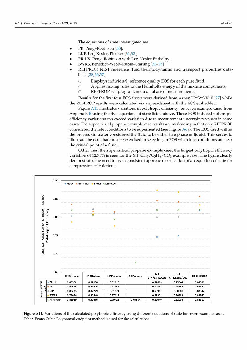
Int. J. Turbomach. Propuls. Power 2021, 6, 15 41 of 43
The equations of state investigated are:
• PR, Peng–Robinson [30];• LKP, Lee, Kesler, Plöcker [31,32];• PR-LK, Peng–Robinson with Lee–Kesler Enthalpy;• BWRS, Benedict–Webb–Rubin–Starling [33–35]• REFPROP, NIST reference fluid thermodynamic and transport properties data-
base [28,36,37]
# Employs individual, reference quality EOS for each pure fluid;# Applies mixing rules to the Helmholtz energy of the mixture components;# REFPROP is a program, not a database of measurements.
Results for the first four EOS above were derived from Aspen HYSYS V.10 [27] whilethe REFPROP results were calculated via a spreadsheet with the EOS embedded.
Figure A11 illustrates variations in polytropic efficiency for seven example cases fromAppendix B using the five equations of state listed above. These EOS induced polytropicefficiency variations can exceed variation due to measurement uncertainty values in somecases. The supercritical propane example case results are misleading in that only REFPROPconsidered the inlet conditions to be superheated (see Figure A6a). The EOS used withinthe process simulator considered the fluid to be either two phase or liquid. This serves toillustrate the care that must be exercised in selecting an EOS when inlet conditions are nearthe critical point of a fluid.
Other than the supercritical propane example case, the largest polytropic efficiencyvariation of 12.75% is seen for the MP CH4/C3H8/CO2 example case. The figure clearlydemonstrates the need to use a consistent approach to selection of an equation of state forcompression calculations.
Int. J. Turbomach. Propuls. Power 2021, 6, x FOR PEER REVIEW 43 of 45
Even though various EOS may use different reference states for enthalpy and entropy, it is the change in these parameters that are used in Equation (32), therefore differences in individual reference states for different EOS is not an issue for the purpose of this study.
The equations of state investigated are: • PR, Peng–Robinson [30]; • LKP, Lee, Kesler, Plöcker [31,32]; • PR-LK, Peng–Robinson with Lee–Kesler Enthalpy; • BWRS, Benedict–Webb–Rubin–Starling [33–35] • REFPROP, NIST reference fluid thermodynamic and transport properties database
[28,36,37] o Employs individual, reference quality EOS for each pure fluid; o Applies mixing rules to the Helmholtz energy of the mixture components; o REFPROP is a program, not a database of measurements. Results for the first four EOS above were derived from Aspen HYSYS V.10 [27] while
the REFPROP results were calculated via a spreadsheet with the EOS embedded. Figure A11 illustrates variations in polytropic efficiency for seven example cases from
Appendix B using the five equations of state listed above. These EOS induced polytropic efficiency variations can exceed variation due to measurement uncertainty values in some cases. The supercritical propane example case results are misleading in that only REFPROP considered the inlet conditions to be superheated (see Figure A6a). The EOS used within the process simulator considered the fluid to be either two phase or liquid. This serves to illus-trate the care that must be exercised in selecting an EOS when inlet conditions are near the critical point of a fluid.
Other than the supercritical propane example case, the largest polytropic efficiency var-iation of 12.75% is seen for the MP CH4/C3H8/CO2 example case. The figure clearly demon-strates the need to use a consistent approach to selection of an equation of state for compres-sion calculations.
Figure A11. Variations of the calculated polytropic efficiency using different equations of state for seven example cases.Taher–Evans Cubic Polynomial endpoint method is used for the calculations.

Int. J. Turbomach. Propuls. Power 2021, 6, 15 42 of 43
To explore the efficiency variations shown in Figure A11, the EOS supplied parametersthat are used by the Taher–Evans Cubic Polynomial method are compared.
References1. Taher, M. Mathematical Modeling of the Polytropic Process Using the Sequential Cubic Polynomial Approximation. In Proceed-
ings of the ASME GT2021, ASME Turbo Expo 2021, Virtual, Online, 7–11 June 2021. Paper Number GT2021-59715.2. Taher, M.; Evans, B.F. Centrifugal Compressor Polytropic Performance Evaluation Using Cubic Polynomial Approximation for
the Temperature-Entropy Polytropic Path. In Proceedings of the ASME GT2021, ASME Turbo Expo 2021, Virtual, Online, 7–11June 2021. Paper Number GT2021-59678.
3. Evans, B.F. Centrifugal Compressor Polytropic Efficiency—Cubic and Linear Polynomial Solution Methods Comparing 115 Example CaseCalculations; Technology Report; ResearchGate: Berlin, Germany, 2020. [CrossRef]
4. ASME PTC 10. Performance Test Code on Compressors and Exhausters; American Society of Mechanical Engineers: New York, NY,USA, 1997.
5. Zeuner, G.A. Fundamental Laws of Thermodynamics Theory of Gases. In Technical Thermodynamics; D. Van Nostrand Company:New York, NY, USA, 1906; Volume 1.
6. Schultz, J.M. The Polytropic Analysis of Centrifugal Compressors. ASME J. Eng. Power 1962, 84, 69–82. [CrossRef]7. ASME PTC 10. Compressors and Exhausters Power Test Code 10; American Society of Mechanical Engineers: New York, NY,
USA, 1965.8. ASME PTC 10. Compressors and Exhausters Power Test Code 10; reaffirmed of the 1965 edition; American Society of Mechanical
Engineers: New York, NY, USA, 1992.9. Mallen, M.; Saville, G. Polytropic Processes in the Performance Prediction of Centrifugal Compressors; Institution of Mechanical
Engineers Conference Publications C183/77; Institution of Mechanical Engineers: London, UK, 1977; pp. 89–96.10. Kent, R.G. Application of Basic Thermodynamics to Compressor Cycle Analysis. In Proceedings of the International Compressor
Engineering Conference, West Lafayette, IN, USA, 10–12 July 1974. Paper 135.11. Nathoo, N.S.; Gottenberg, W.G. Measuring the Thermodynamic Performance of Multistage Compressors Operating on Mixed
Hydrocarbon Gases. In Proceedings of the Tenth Turbomachinery Symposium; Turbomachinery Laboratory, Texas A&M University:College Station, TX, USA, 1981; pp. 15–23.
12. Nathoo, N.S.; Gottenberg, W.G. A New Look at Performance Analysis of Centrifugal Compressors Operating with MixedHydrocarbon Gases. ASME J. Eng. Power 1983, 105, 920–926. [CrossRef]
13. Huntington, R.A. Evaluation of Polytropic Calculation Methods for Turbomachinery Performance. ASME Trans. J. Eng. GasTurbines Power 1985, 107, 872–879. [CrossRef]
14. Huntington, R. Limitations of the Schultz Calculation for Polytropic Head—A Proposal for Revision of PTC-10; Technology Report;ResearchGate: Berlin, Germany, 1997. [CrossRef]
15. Hundseid, O.; Bakken, L.E.; Helde, T. A Revised Compressor Polytropic Performance Analysis. In Proceedings of the ASMEGT2006, ASME Turbo Expo 2006, Barcelona, Spain, 8–11 May 2006. Paper Number 91033.
16. Oldrich, J. Advanced Polytropic Calculation Method of Centrifugal Compressor. In Proceedings of the ASME IMECE2010, theASME International Mechanical Engineering Congress and Exposition 2010, Vancouver, BC, Canada, 12–18 November 2010.Paper Number 40931.
17. Sandberg, M.R.; Colby, G.M. Limitations of ASME PTC 10 in Accurately Evaluating Centrifugal Compressor ThermodynamicPerformance. In Proceedings of the 42nd Turbomachinery Symposium, Houston, TX, USA, 1–3 October 2013; TurbomachineryLaboratory, Texas A&M University: College Station, TX, USA, 2013.
18. Taher, M. ASME PTC-10 Performance Testing of Centrifugal Compressors—The Real Gas Calculation Method. In Proceedings ofthe ASME GT2014, ASME Turbo Expo 2014, Düsseldorf, Germany, 16–20 June 2014. Paper Number GT2014-26411.
19. Wettstein, H.E. Polytropic Change of State Calculations. In Proceedings of the ASME IMECE2014, the ASME InternationalMechanical Engineering Congress and Exposition 2014, Montreal, QC, Canada, 14–20 November 2014. Paper Number 36202.
20. Plano, M. Evaluation of Thermodynamic Models used for Wet Gas Compressor Design. Master’s Thesis, Innovative SustainableEnergy Engineering, Norwegian University of Science and Technology, Trondheim, Norway, June 2014.
21. Evans, B.F.; Huble, S.R. Centrifugal Compressor Polytropic Performance: Consistently Accurate Results from Improved RealGas Calculations. In Proceedings of the ASME GT2017, ASME Turbo Expo 2017, Charlotte, NC, USA, 26–30 June 2017. PaperNumber GT2017-65235.
22. Evans, B.F.; Huble, S.R. Tutorial, ‘Centrifugal Compressor Performance: Making Enlightened Analysis Decisions. In Proceedingsof the 46th Turbomachinery Symposium, Houston, TX, USA, 11–14 December 2017; Turbomachinery Laboratory, Texas A&MUniversity: College Station, TX, USA, 2017.
23. Sandberg, M.R. A More Detailed Explanation of the Sandberg-Colby Method for the Evaluation of Centrifugal Compressor ThermodynamicPerformance; ResearchGate: Berlin, Germany, 2020. [CrossRef]
24. Box, G.E.; Draper, N.R. Empirical Model-Building and Response Surfaces; Wiley: Hoboken, NJ, USA, 1987.25. IEEE/ASTM SI 10-2016—American National Standard for Metric Practice; Institute of Electrical and Electronics Engineers:
Washington, DC, USA, 2016.

Int. J. Turbomach. Propuls. Power 2021, 6, 15 43 of 43
26. Stepanoff, A.J. Turboblowers: Theory, Design, and Application of Centrifugal and Axial Flow Compressors and Fans; John Wiley and Sons:New York, NY, USA, 1955.
27. HYSYS; Aspentech: Bedford, MA, USA, 2020.28. Lemmon, E.W.; Bell, I.H.; Huber, M.L.; McLinden, M.O. NIST Standard Reference Database 23: Reference Fluid Thermodynamic and
Transport Properties-REFPROP, Version 10.0; Standard Reference Data Program; National Institute of Standards and Technology:Gaithersburg, MD, USA, 2018.
29. Brown, R.N. Compressors Selection and Sizing, 2nd ed.; Butterworth-Heinemann: Woburn, MA, USA, 1997.30. Peng, D.Y.; Robinson, D.B. A New Two-Constant Equation of State. Ind. Eng. Chem. Fundam. 1976, 15, 59–64. [CrossRef]31. Lee, B.I.; Kesler, M.G. A Generalized Thermodynamic Correlation Based on Three-Parameter Corresponding States. AIChE J.
1975, 21, 510–527. [CrossRef]32. Plöcker, U.; Knapp, H.; Prausnitz, J. Calculation of High-Pressure Vapor-Liquid Equilibria from a Corresponding States Correlation
with Emphasis on Asymmetric Mixtures. Ind. Chem. Process Des. Dev. 1978, 17, 324–332. [CrossRef]33. Benedict, M.; Webb, G.B.; Rubin, L.C. An Empirical Equation for Thermodynamic Properties of Light Hydrocarbons and their
Mixtures. J. Chem. Phys. 1940, 8, 334–345. [CrossRef]34. Benedict, M.; Webb, G.B.; Rubin, L.C. An Empirical Equation for Thermodynamic Properties of Light Hydrocarbons and their
Mixtures II. Mixtures of Methane, Ethane, Propane, and n-Butane. J. Chem. Phys. 1942, 10, 757–758. [CrossRef]35. Starling, K.E. Fluid Thermodynamic Properties for Light Petroleum Systems; Gulf Publishing: Houston, TX, USA, 1973.36. Span, R. Multiparameter Equations of State: An Accurate Source of Thermodynamic Property Data; Springer: New York, NY, USA, 2000.37. Span, R.; Wagner, W. A New Equation of State for Carbon Dioxide Covering the Fluid Region from the Triple-Point Temperature
to 1100 K at Pressures up to 800 MPa. J. Phys. Chem. Ref. Data 1996, 25, 1509–1596. [CrossRef]