Parallel progressive multiple sequence alignment on reconfigurable meshes

RESEARCH Open Access

Parallel progressive multiple sequence alignmenton reconfigurable meshesKen D Nguyen1, Yi Pan2*, Ge Nong3

From BIOCOMP 2010. The 2010 International Conference on Bioinformatics and Computational BiologyLas Vegas, NV, USA. 12-15 July 2010

Abstract

Background: One of the most fundamental and challenging tasks in bio-informatics is to identify related sequencesand their hidden biological significance. The most popular and proven best practice method to accomplish this taskis aligning multiple sequences together. However, multiple sequence alignment is a computing extensive task. Inaddition, the advancement in DNA/RNA and Protein sequencing techniques has created a vast amount of sequencesto be analyzed that exceeding the capability of traditional computing models. Therefore, an effective parallel multiplesequence alignment model capable of resolving these issues is in a great demand.

Results: We design O(1) run-time solutions for both local and global dynamic programming pair-wise alignmentalgorithms on reconfigurable mesh computing model. To align m sequences with max length n, we combiningthe parallel pair-wise dynamic programming solutions with newly designed parallel components. We successfullyreduce the progressive multiple sequence alignment algorithm’s run-time complexity from O(m × n4) to O(m)using O(m × n3) processing units for scoring schemes that use three distinct values for match/mismatch/gap-extension. The general solution to multiple sequence alignment algorithm takes O(m × n4) processing units andcompletes in O(m) time.

Conclusions: To our knowledge, this is the first time the progressive multiple sequence alignment algorithm iscompletely parallelized with O(m) run-time. We also provide a new parallel algorithm for the Longest CommonSubsequence (LCS) with O(1) run-time using O(n3) processing units. This is a big improvement over the currentbest constant-time algorithm that uses O(n4) processing units.

BackgroundThe advancement of DNA/RNA and protein sequencingand sequence identification has created numerous data-bases of sequences. One of the most fundamental andchallenging tasks in bio-informatics is to identify relatedsequences and their hidden biological significance.Aligning multiple sequences together provides research-ers with one of the best solutions to this task. In gen-eral, multiple sequence alignment can be defined as:Definition 1Given: m sequences, (s1, s2,..., sm), over an alphabet ∑,

where each sequence contains up to n symbols from ∑; a

scoring function h:∑

×∑

×· · · ×∑

→ �; and a gap

cost function. Multiple sequence alignment is a techniqueto transform (s1, s2, ..., sm) to

(s′1, s′2, · · · , s′m

), where s′iis si

∪ ‘-’ [gap insertions], that optimizes the matching scoresbetween the residues across all sequence columns [1].However, multiple sequence alignment is an NP-Com-plete problem [2]; therefore, it is often solved by heuris-tic techniques. Progressive multiple sequence alignmentis one of the most popular multiple sequence alignmenttechniques, in which the pair-wise symbol matchingscores can be derived from any scoring scheme orobtained from a substitution scoring matrix such asPAM [3] or BLOSUM [4]. There are many implementa-tions of progressive multiple sequence alignment as seenin [5-8]. In general, progressive multiple sequence align-ment algorithm follows three steps:

* Correspondence: [email protected] of Computer Science, Georgia State University, Atlanta, GA30303, USAFull list of author information is available at the end of the article

Nguyen et al. BMC Genomics 2011, 12(Suppl 5):S4http://www.biomedcentral.com/1471-2164/12/S5/S4

© 2011 Nguyen et al. licensee BioMed Central Ltd This is an open access article distributed under the terms of the Creative CommonsAttribution License (http://creativecommons.org/licenses/by/2.0), which permits unrestricted use, distribution, and reproduction inany medium, provided the original work is properly cited.

mailto:[email protected]

http://creativecommons.org/licenses/by/2.0

(i) Perform all pair-wise alignments of the inputsequences.(ii) Compute a dendrogram indicating the order in

which the sequences to be aligned.(iii) Pair-wise align two sequences (or two pre-aligned

groups of sequences) following the dendrogram startingfrom the leaves to the root of the dendrogram.Figure 1 shows an example of these steps, where (a)

represents the input sequences, (b) represents an align-ment of step (i), (c) shows the dendrogram obtainedfrom step (ii), and (d) shows a pair-wise group-align-ment in step (iii).Step (i) can be optimally solve by Dynamic Program-

ming (DP) algorithm. There are two versions of DP: theSmith-Waterman’s [9] is used to find the optimallyaligned segment between two sequences (local DP), andthe Needleman-Wunsch’s [10] is used to find the globaloptimal overall sequence pair-wise alignment (globalDP). The two algorithms are very similar and will bedescribed in more details in the next section. Thedynamic programming algorithms take O(n2) time tocomplete, including the back-tracking steps. Thus, withm(m−1)

2unique pairs of the input sequences, the run-time

complexity of step (i) is O(m2 n2) or O(n4) if n and mare asymptotically equivalent.

To generate a dendrogram from the distances betweenthe sequences (or the scores generated from step (i)),either UPGMA [11] or Neighbor Joining (NJ) [12] hier-archical clustering is used. These algorithms yield O(m3)run-time complexity.In the worst case, step (iii) performs (m - 1) pair-wise

alignments in-order following the dendrogram hierarchy.Similar to step (i), dynamic programming for pair-wisealignment is used, however, each of these pair-wisegroup alignment yields an order of O(n4) via dynamicprogramming (O(n2)) and sum-of-pair scoring function[13](O(n2)). This scoring function is required to evaluateevery all possible residue matchings of the sequences.As a result, the run-time complexity of step (iii) is O(m× n4) ≈ O(n5), which is the overall run-time complexityof progressive multiple sequence alignment algorithm.

Optimal pair-wise sequence alignment by dynamicprogrammingGiven two sequences x and y each contains up to n resi-due symbols. The optimal alignment of these sequencescan be found by calculating an (n + 1) × (n + 1)dynamic programming (DP) matrix containing all possi-ble pair-wise matching scores of residue symbols in thesequences. Initially, the first row and column of thematrix cells are set to 0, i.e.

c0,j = 0,

ci,0 = 0.

The recursive formula to compute the DP matrix forthe Longest Common Subsequence (LCS) as seen in[14] is:

ci,j ={

ci−1,j−1 + 1 if xi = yj

max{(ci−1,j), (ci,j−1)} if xi �= yj

Similarly, the Needleman-Wunsch’s algorithm [10]uses the following formula to complete the DP matrix:

ci,j = max

⎧⎨⎩

ci−1,j−1 + s(xi, yj) symbol matchingci−1,j + g gap insertionci,j−1 + g gap insertion

where s(xi, yj) is the pair-wise symbol matching scoreof the two symbols xi and yj from sequences x and y,respectively; and g is the gap cost for extending asequence by inserting a gap, i.e. gap insertion/deletion(indel).Smith and Waterman [9] modified the above formula as:

ci,j = max

⎧⎪⎪⎨⎪⎪⎩

0ci−1,j−1 + s(xi, yj) symbol matchingci−1,j + g gap insertionci,j−1 + g gap insertion

Figure 1 A progressive multiple sequence alignment . Anexample of progressive Multiple Sequence Alignment. (a) representsthree input sequences (S1, S2, S3); (b) shows the pair-wise dynamicprogramming alignment of two sequences; (c) shows the order ofthe sequences to be aligned, where the leaves on right hand-sideare the input sequences, the internal nodes represent thetheoretical ancestors from which the sequences are derived, andthe characters on the tree branches represent the missing/mutatedresidues; and (d) shows the pair-wise dynamic programming of twopre-aligned groups of sequences.


of 14

The alignment can be obtained from the DP matrix bystarting from cell cn, n, (or the cell containing the maxvalue in the matrix as in the Smith-Waterman’s algo-rithm), and tracking back to the top of the matrix, i.e.cell c0,0, by following neighboring cells with the largestvalue.

Existing parallel implementationsProgressive multiple sequence alignment algorithms arewidely parallelized, mostly because they perform m(m−1)

2independent pair-wise alignments as in step (i). Theseindividual pair-wise alignments can be designated to dif-ferent processing units for computation as in [15-24].These implementations are across many computingarchitectures and platforms. For example, [17] imple-mented a DP algorithm on Field-Programmable GateArray (FPGA). Similarly, Oliver et al. [23,24] distributedthe pair-wise alignment of the first step in the progres-sive alignment, where all pair-wise alignments are com-puted, on FPGA. Liu et al. [18] computed DP viaGraphic Processing Units (GPUs) using CUDA platform,[22] used CRCW PRAM neural-networks, [15] usedClusters, [16] used 2D r-mesh, [20] used Network mesh,or [21] used 2D Pr-mesh computing model.The two most notable parallel versions of dynamic

programming algorithm are proposed by Huang [25]and Huang et al. and Aluru [15,26]. Huang’s algorithmexploits the independency between the cells on the anti-diagonals of the DP matrix, where they can be calcu-lated simultaneously. There are 2n + 1 anti-diagonals ona matrix of size (n + 1 × n+1). Thus, this parallel DPalgorithm takes O(n) processing units and completes inO(n) time.Independently, Huang et al. [15] and Aluru et al. [26]

propose similar algorithms to partition the DP matrixcolumn-wise and assign each partition to a processor.Next, all processors are synchronized to calculate theirpartitions one row at a time. For this algorithm to per-form properly, each processor must hold a copy of thesequence that mapped to the rows of the matrix. Sincethese calculations are performed row-wise, the valuesfrom cells ci-1, j-1 and ci-1, j are available before the cal-culation of cell ci,j. The value of ci, j-1 can be obtainedby performing prefix-sum across all cells in row ith.Thus, with n processors, the computation time of eachrow is dominated by the prefix-sum calculations, whichis O(logn) time on PRAM models. Therefore, the DPmatrix can be completed in O(nlogn) time using O(n)processors. Recently, Sarkar, et al. [19] implement bothof these parallel DP algorithms [25,26] on a Network-on-Chip computing platform [27].In addition, the construction of a dendrogram can be

parallelized as in [18] using n Graphics Processing Units(GPUs) and completing in O(n3) time.

Furthermore, there are attempts to parallelize the pro-gressive alignment step [step (iii)] as in [28] and [29]. In[28], the independent pre-aligned pairs along the den-drogram are aligned simultaneously. This techniquegains some speed-up, however, the time complexity ofthe algorithm remains unchanged since all the pair-wisealignments eventually must be merged together.Another attempt is seen in [29], where Huang’s algo-rithm [25] is used. When an anti-diagonal of a DP align-ment matrix in lower tree level in step (iii) is completed,it is distributed immediately to other processors forcomputing the pair-wise alignment of a higher treelevel. This technique can lead to an incorrect resultsince the actual pair-wise alignment of the lower branchis still uncertain.Overall, the major speedups achieved from these

implementations come from two parallel tasks: perform-ing m(m−1)

2initial pair-wise alignments in step (i) simul-

taneously and calculating the dynamic programmingmatrix anti-diagonally (or in blocks). These tasks poten-tially can lower the run-time complexity of step (i) fromO(m2n2) to O(n) and step (iii) from O(mn4) to O(m3n) ≈O(n4), [or O(m4) if n <m]. The overall run-time com-plexity of the original progressive multiple sequencealignment algorithm is still dominated by step (iii) withan order of O(m3n) regardless of how many processingunits are used. The bottle-neck is the pair-wise groupalignments must be done in order dictated by the den-drogram (O(m)), and each alignment requires all thecolumn pair-wise scores be calculated (O(m2)). Toaddress these issues, we design our parallel progressivemultiple sequence alignment on a reconfigurable mesh(r-mesh) computing model similar to the ones used in[16,23,24]. Following is the detailed description of the r-mesh model.

Reconfigurable-mesh computing models - (r-mesh)A Reconfigurable mesh (r-mesh) computing, first pro-posed by Miller et al [30], is a two-dimensional grid ofprocessing units (PUs), in which each processing unitcontains 4 ports: North, South, East, and West (N, S, E,W). These ports can be fused or defused in any order toconnect one node of the grid to its neighboring nodes.These configurations are shown in Figure 2. Each pro-cessing unit has its own local memory, can perform sim-ple arithmetic operations, and can configure its ports inO(1) time.There are many reconfigurable computing models

such as Linear r-mesh (Lr-mesh), Processor Array withReconfigurable Bus System (PARBS), Pipedlined r-mesh(Pr-mesh), Field-programmable Gate Array (FPGA), etc.These models are different in many ways from construc-tion to operation run-time complexities. For example,the Pr-mesh model does not function properly with


of 14

configurations containing cycles, while many other mod-els do. However, there are many algorithms to simulatethe operations of one reconfigurable model ontoanother in constant time as seen in [31-36].In the scope of this study, we will use a simple elec-

trical r-mesh system, where each processing unit, orprocessing element (PU or PE), contains four portsand can perform basic routing and arithmetic opera-tions. Most reconfiguration computing models utilizethe representation of the data to parallelize theiroperations; and there are various proposed formats[37]. Commonly, data in one format can be convertedto another in O(1) time [37]. The unary representationformat is used this study, which is denoted as 1UN,and is defined as:Definition 2Given an integer x Î [0, n - 1], the unary 1UN presen-

tation of x in n-bit is: x = (b0, b1, ..., bn-1), where bi = 1for all i ≤ x and bi = 0 for all i > x [37].For example, a number 3 is represented as 11110000

in 8-bit 1UN representation.In addition to the 1UN unary format, we will be utiliz-

ing the following theorem for some of the operations:Theorem 1:The prefix-sum of n value in range [0, nc] can be found

in O(c) time on an n × n r-mesh [37].In terms of multiple sequence alignment, the number

of bits used in the 1UN notation is correlated to themaximum length of the input sequences. In the nextSection, we will describe the designs of r-meshcompo-nents to use in dynamic programming algorithms.

Parallel pair-wise dynamic programmingalgorithmsThis section begins with the description of several con-figurations of r-mesh needed to compute various opera-tions in pair-wise dynamic programming algorithm.Following the r-mesh constructions is a new constant-time parallel dynamic programming algorithm for

Needleman-Wunsch’s, Smith-Waterman, and the Long-est Common Subsequence (LCS) algorithms.

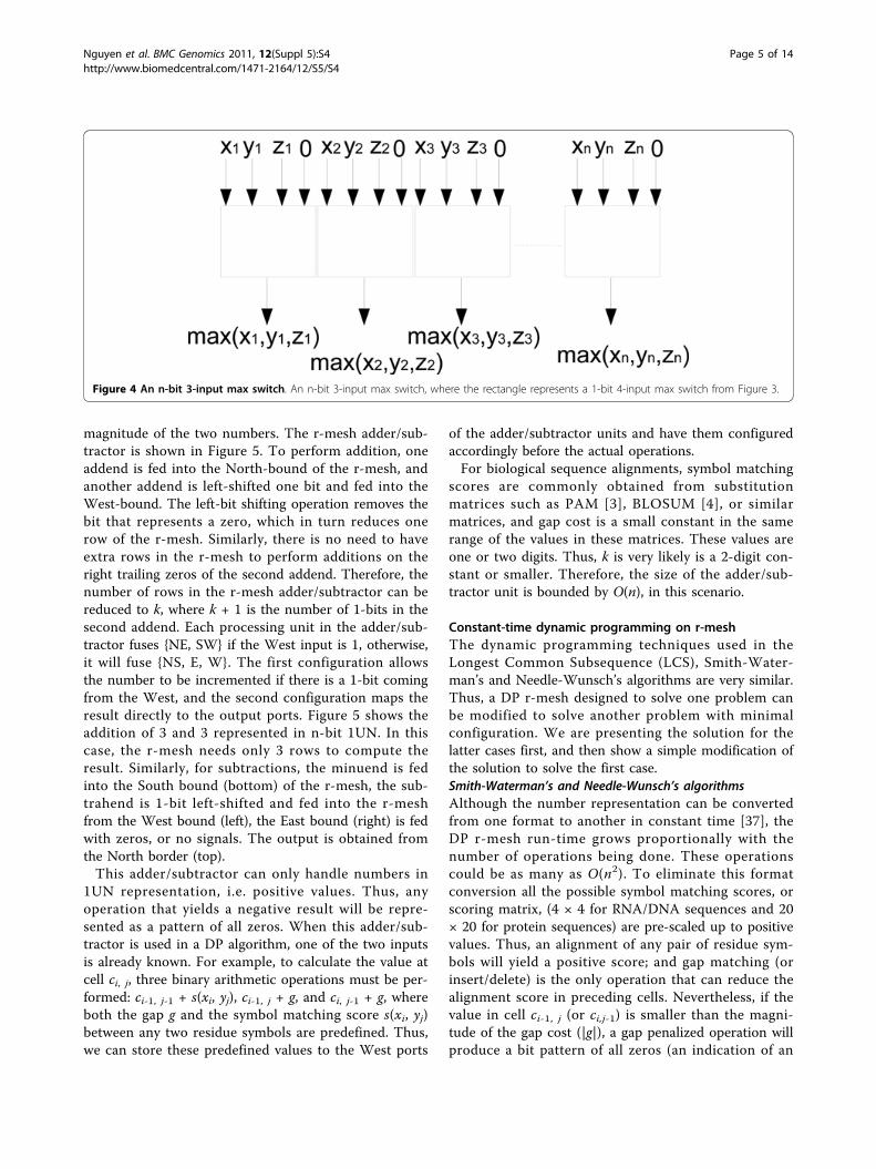
R-mesh max switchesOne of the operations in the dynamic programmingalgorithm requires the capability to select the largestvalue from a set of input numbers. Following is thedesign of an r-mesh switch that can select the maximumvalue from an input triplet in the same broadcastingstep. For 1-bit data, the switch can be built as in Figure3(a) using one processing unit, (introduced by Bertossi[14]). The unit configures its ports as {NSEW}, wherethe North and West are input ports and the others areoutput ports. When a signal (or 1) comes through theswitch, the max bit will propagate through the outputports. Similarly, a switch for finding a maximum valueof four input bits can be built using 4 processing unitswith configurations: {NSW,E}, {NSE,W}, {NE,S,W}, and{NSW,E} as in Figure 3(b). To simulate a 3-input maxswitch on positive numbers, one of the input ports loadsin a zero value. These switches can be combinedtogether to handle the max of three n-bit values as inFigure 4. This n-bit max switch takes 4 × n, (i.e. O(n))processing units and can handle 3 to 4 n-bit input num-bers. All of these max switches allow data to flowdirectly through them in exactly one broadcasting step.They will be used in the design of our algorithm,described latter.

R-mesh adder/subtractorSimilarly, to get a constant time dynamic programmingalgorithm we have to be able to perform a series ofadditions and subtractions in one broadcasting step.Exploiting the properties of 1UN representation, we arepresenting an adder/subtractor that can perform anaddition or a subtraction of two n-bit numbers in 1UNrepresentation in one broadcasting time. The adder/sub-tractor is a k × n r-mesh, where k is the smaller

Figure 2 Port configurations on reconfigurable computingmodel. Allowable configurations on 4 port processing units; (a)shows the ports directions; (b) shows the 15 possible portconnections, where the last five port configurations in curly bracesare not allowed in Linear r-mesh (Lr-mesh) models.

Figure 3 1-bit max switches. Two 1-bit max switches. (a)- fusing{NSEW} to find the max of two inputs from North and West ports;(b)- construction of a 1-bit 4-input max switch.


of 14

magnitude of the two numbers. The r-mesh adder/sub-tractor is shown in Figure 5. To perform addition, oneaddend is fed into the North-bound of the r-mesh, andanother addend is left-shifted one bit and fed into theWest-bound. The left-bit shifting operation removes thebit that represents a zero, which in turn reduces onerow of the r-mesh. Similarly, there is no need to haveextra rows in the r-mesh to perform additions on theright trailing zeros of the second addend. Therefore, thenumber of rows in the r-mesh adder/subtractor can bereduced to k, where k + 1 is the number of 1-bits in thesecond addend. Each processing unit in the adder/sub-tractor fuses {NE, SW} if the West input is 1, otherwise,it will fuse {NS, E, W}. The first configuration allowsthe number to be incremented if there is a 1-bit comingfrom the West, and the second configuration maps theresult directly to the output ports. Figure 5 shows theaddition of 3 and 3 represented in n-bit 1UN. In thiscase, the r-mesh needs only 3 rows to compute theresult. Similarly, for subtractions, the minuend is fedinto the South bound (bottom) of the r-mesh, the sub-trahend is 1-bit left-shifted and fed into the r-meshfrom the West bound (left), the East bound (right) is fedwith zeros, or no signals. The output is obtained fromthe North border (top).This adder/subtractor can only handle numbers in

1UN representation, i.e. positive values. Thus, anyoperation that yields a negative result will be repre-sented as a pattern of all zeros. When this adder/sub-tractor is used in a DP algorithm, one of the two inputsis already known. For example, to calculate the value atcell ci, j, three binary arithmetic operations must be per-formed: ci-1, j-1 + s(xi, yj), ci-1, j + g, and ci, j-1 + g, whereboth the gap g and the symbol matching score s(xi, yj)between any two residue symbols are predefined. Thus,we can store these predefined values to the West ports

of the adder/subtractor units and have them configuredaccordingly before the actual operations.For biological sequence alignments, symbol matching

scores are commonly obtained from substitutionmatrices such as PAM [3], BLOSUM [4], or similarmatrices, and gap cost is a small constant in the samerange of the values in these matrices. These values areone or two digits. Thus, k is very likely is a 2-digit con-stant or smaller. Therefore, the size of the adder/sub-tractor unit is bounded by O(n), in this scenario.

Constant-time dynamic programming on r-meshThe dynamic programming techniques used in theLongest Common Subsequence (LCS), Smith-Water-man’s and Needle-Wunsch’s algorithms are very similar.Thus, a DP r-mesh designed to solve one problem canbe modified to solve another problem with minimalconfiguration. We are presenting the solution for thelatter cases first, and then show a simple modification ofthe solution to solve the first case.Smith-Waterman’s and Needle-Wunsch’s algorithmsAlthough the number representation can be convertedfrom one format to another in constant time [37], theDP r-mesh run-time grows proportionally with thenumber of operations being done. These operationscould be as many as O(n2). To eliminate this formatconversion all the possible symbol matching scores, orscoring matrix, (4 × 4 for RNA/DNA sequences and 20× 20 for protein sequences) are pre-scaled up to positivevalues. Thus, an alignment of any pair of residue sym-bols will yield a positive score; and gap matching (orinsert/delete) is the only operation that can reduce thealignment score in preceding cells. Nevertheless, if thevalue in cell ci-1, j (or ci,j-1) is smaller than the magni-tude of the gap cost (|g|), a gap penalized operation willproduce a bit pattern of all zeros (an indication of an

Figure 4 An n-bit 3-input max switch. An n-bit 3-input max switch, where the rectangle represents a 1-bit 4-input max switch from Figure 3.


of 14

underflow or negative value). This value will not appearin cell ci,j since the addition of the positive value in cellci-1, j-1 and the positive symbol matching score s(xi, yi) isalways greater than or equal to zero.In general, we do not have to perform this scale-up

operation for DNA since DNA/RNA scoring schemesthat generally use only two values: a positive integervalue for match and the same cost for both mismatchand gap.Unlike DNA, scoring protein residue alignment is

often based on scoring scoring/substitution/mutationmatrices such as that in [3,4]. These matrices are log-odd values of the probabilities of residues being mutated(or substituted) into other residues. The differencebetween the matrices are the way the probabilities beingderived. The smaller the probability, the less likely amutation happens. Thus, the smallest alignment valuebetween any two residues, including the gap is at least

zero. To avoid the complication of small positive frac-tional numbers in calculations, log-odd is applied onthese probabilities. The log-odd score or substitution

score in [3] is calculated as s(i, j) = 1λlog

(Qij

PiPj

), where s(i,

j) is the substitution score between residues i and j, l isa positive scaling factor, Qij is the frequency or the per-centage of residue i correspond to residue j in an accu-rate alignment, and Pi and Pj are backgroundprobabilities which residues i and j occur. These prob-abilities and the log-odd function to generate thematrices are publicly available via The National Centerfor Biotechnology Information’s web-site (http://www.ncbi.nlm.nih.gov) along with the substitution matricesthemselves. With any given gap cost, the probability of aresidue aligned with a gap can be calculated proportion-ally from a given gap cost and other values from theun-scaled scoring matrices by taking anti-log of the log-

Figure 5 An n-bit adder/subtractor. An n-bit adder/subtractor that can perform addition or subtraction between two 1UN numbers during abroadcasting time. For additions the inputs are on the North and West borders and the output is on the South border. For subtractions, theinputs are on the West and South borders and the output is on the North border. The number on the West bound is 1-bit left-shifted. Thedotted lines represent the omitted processing units that are the same as the ones in the last rows. This figure shows the addition of 3 and 3.Note: the leading 1 bit of input number on the West-bound (left) has been shifted off. The right border is fed with zero (or no signal) duringthe subtract operation.


of 14

http://www.ncbi.nlm.nih.gov

http://www.ncbi.nlm.nih.gov

odd values or score matrix. Thus, when a positive num-ber b is added to the scores in these scoring matrices, itis equivalent to multiply the original probabilities by ab,where a is the log-based used in the log-odd function.A simple mechanism to obtain a scaled-up version of

a scoring matrix is: (a) taking the antilog of the scoringmatrix and g, where g is the gap costs, i.e. the equivalentlog-odd of a gap matching probability; (b) multiplyingthese antilog values by b factor such that their mini-mum log-odd value should be greater than or equal tozero; (c) performing log-odd operation on these scaled-up values.When these scaled-up scoring matrices are used, the

Smith-Waterman’s algorithm must be modified.Instead of setting sub-alignment scores to zeros when

they become negative, these scores are set to b whenthey fall below the scaled-up factor (b).Using scaled-up scoring matrices will eliminate the

need for signed number representation in our followingalgorithm designs. However, if there is a need to obtainthe alignment score based on the original scoringmatrices, the score can be calculated as follows: (i) loadthe original score matrix and gap cost to each cell on anr-mesh as similar to the one described in Section; (ii)configure cells on the diagonal path to use their

corresponding matching score from the matrix andother cells representing gap insertions or deletions touse gap cost; (iii) calculate the prefix-sum of all the cellson the path representing the alignment using Theorem1.Having the adder/subtrator units and the switches

ready, the dynamic programming r-mesh, (DP r-mesh),can be constructed with each cell ci,j in the DP matrixcontaining 3 adder/subtractor units and a 3-input maxswitch allowing it to propagate the max value of cells ci-1, j-1, ci-1, j and ci, j-1 to cell ci, j in the same broadcastingstep. Figure 6 shows the dynamic programming r-meshconstruction. The adder/subtrator units are representedas “+” or “-” corresponding to their functions.A 1 × n adder/subtractor unit can perform increments

and decrements in the range of [-1,0,1]. As a result, aDP r-mesh can be built with 1-bit input components tohandle all pair-wise alignments using constant scoringschemes that can be converted to [-1,0,1] range. Forinstance, the scoring scheme for the longest commonsubsequence rewards 1 for a match and zero for mis-match and gap extension.To align two sequences, ci, j loads or computes its

symbol matching score for the symbol pair at row i col-umn j, initially. The next step is to configure all the

Figure 6 A dynamic programming r-mesh. Each cell ci, j is a combination of a 3-input max switch and three adder/subtractor units. The “+”and “-” represent the actual functions of the adder/subtractor units in the configuration.


of 14

adder/subtractor units based on the loaded values andthe gap cost g. Finally, a signal is broadcasted from c0,0to its neighboring cells c0,1, c1,0, and c1,1 to activate theDP algorithm on the r-mesh. The values coming fromcells ci-1, j and ci, j-1 are subtracted with the gap costs.The value coming from ci-1, j-1 is added with the initialsymbol matching score in ci, j. These values will flowthrough the DP r-mesh in one broadcasting step, andcell cn, n will receive the correct value of the alignment.In term of time complexity, this dynamic programming

r-mesh takes a constant time to initialize the DP r-meshand one broadcasting time to compute the alignment.Thus, its run-time complexity is O(1). Each cell uses 10nprocessing units (4n for the 1-bit max switch and 2n foreach of the three adder/subtrator units). These processingunits are bounded by O(n). Therefore, the n × n dynamicprogramming r-mesh uses O(n3) processing units.To handle all other scoring schemes, k × n adder/sub-

tractor r-meshes and n × n max switches must be used.In addition, to avoid overflow (or underflow) all pre-defined pair-wise symbol matching scores may have tobe scaled up (or down) so that the possible smallest (orlargest) number can fit in the 1UN representation. Withthis configuration, the dynamic programming r-meshtakes O(n4) processing units.Longest common subsequence (LCS)The complication of signed numbers does not exist inthe longest common subsequence problem. The arith-metic operation in LCS is a simple addition of 1 if thereis a match. The same dynamic programming r-mesh asseen in Figure 6 can be used, where the two subtractorsunits are removed or the gap cost is set to zero (g = 0).To find the longest common subsequence between

two sequences x and y, each max switch in the DP r-mesh is configured as in Figure 7. The value from cellci-1, j-1 is fed into the North-West processing unit, andthe other values are fed into the North-East unit. Then,ci, j loads in its symbols and fuses the South-East pro-cessing unit (in bold) as NS,E,W if the symbols at row iand column j are different; otherwise, it loads 1 into theadder unit and fuses N,E,SW. These configurationsallow either the value from cell ci-1, j-1 or the max valueof cells ci-1, j and ci, j-1 to pass through. These are theonly changes for the DP r-mesh to solve the LCSproblems.This modified constant-time DP r-mesh used O(n3)

processing units. However, this is an order of reductioncomparing the current best constant parallel DP algo-rithm that uses an r-mesh of size O(n2) × O(n2) [14] tosolve the same problem.

Affine gap costAffine gap cost (or penalty) is a technique where theopening gap has different cost from an extending gap

[38]. This technique discourages multiple and disjoinedgap insertion blocks unless their inclusion greatlyimproves the pair-wise alignment score. The gap cost iscalculated as p = o + g(l - 1), where o is the openinggap cost, g is the extending gap cost, and l is the lengthof the gap block. Traditionally, Gotoh use three matricesto track these values; however, it is not intercessory inthe reconfigurable mesh computing model since eachcell in the matrix is a processing node with localmemory.To handle affine gap cost, we need to extend the

representation of the number by 1 bit (right most bit).This bit indicates whether a value coming from ci-1, j orci, j-1 to ci, j is an opening gap or not. If the incomingvalue has been gap-penalized, its right most bit is 1, andit will not be charged with an opening gap again; other-wise, an opening gap will be applied. The original “-”units must be modified to accommodate affine gaps.Figure 8 shows the modification of the “-” unit. Theoutput from the original “-” unit is piped into an n × n+ 1 r-mesh on/off switch (described in Section ), anadder/subtractor, and a max switch. When a numberflows through the “-” unit, an extending gap is applied.If the incoming value has not been charged with gap tobegin with, its right most bit (i.e. selector bit denoted as“s”) remains zero, which keeps the switch in off position.Therefore, the value with extra charge on the adder/sub-tractor is allowed to flow through; otherwise, the switchwill be on, and the larger value will be selected by themax switch. A value that is not from diagonal cells musthave its selector bit set to 1 (right most bit) after a gap

Figure 7 A 4-way max switch. A configuration of a 4-way maxswitch to solve the longest common subsequence (lcs). The South-East processing unit (in bold) configures {NS,E,W} if the symbols atrow i and column j are different; otherwise, it configures{N,E,SW}.This figure show a configuration when the two symbols aredifferent.


of 14

cost is applied to prevent multiple charges of an open-ing gap.The modification of the dynamic programming r-mesh

to handle affine gap cost requires additional 2 adder/subtractor units, 2 on/off switches, and one 2-input maxswitch. Asymptotically, the amount of processing unitsused is still bounded by O(n4) and the run-time com-plexity remains O(1).

R-mesh on/off switchesTo handle affine gap cost in dynamic programming, weneed a switch that can select, i.e. turns on or off, theoutput ports of a data flow. The on/off r-mesh switchcan be configured as in Figure 9, where the inputvalue is mapped into the North-bound (top). The right

most bit of the input is served as a selector bit. The r-mesh size is n × n+1, where column i fuses with row n- i to form an L-shape path that allows the input datafrom the Northbound to flow to the output port onthe Eastbound. The processors on the last column willfuse the East-West ports allowing the input to flowthrough only if they receive a value of 1 from theinput (Northern ports). Since the selector bit travels ashorter distance than all the other input bits, it willarrive in time to activate the opening or closing of theoutput ports.This r-mesh configuration uses (n × n + 1), i.e., O(n2),

processing units to turn off the flow of an n-bit input ina broadcasting time.

Dynamic programming back-tracking on r-meshThe pair-wise alignment is obtained by following thepath leading to the overall optimal alignment score, orthe end of the alignment. In the case of the Needleman-Wunsch’s algorithm, cell cn, n holds this value; and inthe case of the Smith-Waterman’s algorithm, cell ci, j

with the maximum alignment score is the end point.The cell with the largest value can be located in O(1)time on a 3-dimension n × n × n r-mesh through thesesteps:1. Initially, the DP matrix with calculated values are

stored in the first slice of the r-mesh cube, i.e. in cells ci,j,0, 0 <i, j ≤ n.2. ci, j,0 sends its value to ci, j, i, 0 ≤ i, j ≤ n, to propa-

gate each column of the matrix to the 2D r-meshes onthe third dimension.3. ci, j, i sends its value to c0, j, k, i.e. to move the solu-

tion values to the first row of each 2D r-mesh slice.4. Each 2D r-mesh slice finds its max value c0, r, k

where r is the column of the max value in slice k5. c0, r, k sends r to ck,0,0, i.e. each 2D r-mesh slice

sends its max value column number m to the first 2D r-mesh slice. This value is the column index of the maxvalue on row k in the first slice.6. The first 2D r-mesh slice, ci, j,0, finds the max value

of n DP r-mesh cells whose row index is i and columnindex is ci0,0 (i.e. value r received from the previousstep). The row and column indices of the max valuefound in this step is the location of the max value in theoriginal DP r-mesh.These above steps rely on the capability to find the

max value from n given numbers on an n × n r-mesh.This operation can be done in O(1) time as follows:1. initially, the values are stored in the first row of the

r-mesh.2. c0, j broadcasts its value, namely aj, to ci, j, (column-

wise broadcasting).3. ci, i broadcasts its value, namely ai, to ci, j (row-wise

broadcasting).

Figure 8 A configuration for selecting a min value. Aconfiguration to select one of the two inputs in 1UN notation usingthe right most bit as a selector s. When s = 1 the switch is turnedon to allow the data to flow through and get selected by the maxswitch. When the selector s = 0, the on/off switch produces zerosand the other data flow will be selected. ε = o - g, o ≥ g, is thedifference between opening gap cost o and extending gap cost g.


of 14

4. ci, j sets a flag bit f(i, j) to 1 if and only if ai >aj;otherwise sets f(i, j) to 0.5. c0, j is holding the max value if f(0, j), f(1, j),..., f(n -

1, j) are 0. This step can be performed in O(1) time byORing the flag bits in each column.The location of the max value in the DP r-mesh can

be obtained in O(1) time because each step in the pro-cess takes O(1) time to complete.To trace back the path leading to the optimal align-

ment, we start with the end point cell ce, d found aboveand following these steps:1. ci, j, (i ≤ e, i ≤ d), sends its value to ci, j+1, ci+ 1, j, ci

+1, j+i. Thus, each cell can receive up to three valuescoming from its Noth, West, and Northwest borders.2. ci, j finds the max of the inputs and fuses its port to

the neighbor cell that sent the max value in the previousstep. If there are more than one port to be fused, (thishappens when there are multiple optimal alignments), ci,j randomly selects one.3. ce, d sends a signal to its fused port. The optimal

pair-wise alignment is the ordered list of cells wherethis signal travels through.Each operation in the back-tracking process takes O(1)

time to complete, and there are no iterative operations.

Therefore, the back-tracking steps requires n3 proces-sing units and takes O(1) time.

Progressive multiple sequence alignment onr-meshIn this section, we start by describing a parallel algo-rithm to generate a dendrogram, or guiding tree, repre-senting the order in which the input sequences shouldbe aligned. Then we will show a reworked version ofsum-of-pair scoring method that can be performed inconstant time on a 2D r-mesh. Finally, we will describeour parallel progressive multiple sequence alignmentalgorithm on r-mesh along with its complexity analysis.

Hierarchical clustering on r-meshThe parallel neighbor-joining (NJ) [12] clusteringmethod on r-mesh is described here; other hierarchicalclustering mechanisms can be done in a similar fashion.The neighbor-joining takes a distance matrix betweenall the pairs of sequences and represents it as a star-likeconnected tree, where each sequence is an externalnode (leaf) on the tree. NJ then finds the shortest dis-tance pair of nodes and replaces it with a new node.This process is repeated until all the nodes are merged.

Figure 9 An n × n + 1 n-bit on/off switch. By default, all processing units on the last column (column n + 1) configure {NS,E,W}, and fuse{NSEW} when a signal (i.e. 1) travels through them. All cells on the main anti-diagonal cells of the first n rows and columns fuse {NE,S,W}, cellsabove the main anti-diagonal fuse {NS,E,W}, and cells below the main anti-diagonal fuse {N,S,EW}. Figure 9(a) shows the r-mesh configuration ona selector bit of 1 (s = 1) and Figure 9(b) shows the r-mesh configuration on a selector bit of 0 (s = 0).


of 14

Followings are the actual steps to build thedendrogram:1. Initially, all the pair-wise distances are given in form

of a matrix D of size m × m, where m is the number ofnodes (or input sequences).2. Calculate the average distance from node i to all the

other nodes by ri =∑m

1 Dij

m−2.

3. The pair of nodes with the shortest distance (i, j) isa pair that gives minimal value of Mij, where Mij = Dij -ri - rj.4. A new node u is created for shortest pair (i,j), and

the distances from u to i and j are: diu = Dij

2 + (ri−rj)2

, anddj,u = dij-diu.5. The distance matrix D is updated with the new

node u to replace the shortest distance pair (i,j), and thedistances from all the other nodes to u is calculated asDvu = Div + djv - Dij.These steps are repeated for m - 1 iterations to reduce

distance matrix D to one pair of nodes. The last pairdoes not have to be merged, unless the actual locationof the root node is needed.Step 1 and 4 are constant time operations on an m ×

m r-mesh, where each processing unit stores a corre-sponding value from the distance matrix. Since the pro-gressive multiple sequence alignment algorithm onlyuses the dendrogram as a guiding tree to select the clo-sest pair of sequences (or two groups of sequences), theactual distance values between the nodes on the finaldendrogram mostly are insignificant. Consequently, thevalues in distance matrix D can be scaled down withoutchanging the order of the nodes in the dendrogram. Inaddition, if these values are not to be preserved, the cal-culations in step 4 can be skipped.Before proceeding to step 2, we should reexamine

some facts. First, the maximum alignment score from allthe pair-wise DP sequence alignments are bounded byb2, where b is the max pair-wise score between any tworesidue symbols. An alignment score of b2 occurs only ifwe align a sequence of these symbols to itself. b+1 ≤ nis the number of bits being used to represent this valuein 1UN. Similarly, the maximum value in distancematrix D generated from these alignment scores are alsobounded by b2. Thus, the sum of n of these distancevalues are bounded by b4. These facts allow us to calcu-late the sums in step 2 in O(c) time using an n × n r-mesh as in Theorem 1. In this case, c is constant, (c =4). There are n summations to calculate, so the entirecalculation requires n such r-meshes, or n3 processingunits, to complete in O(1) time.In step 3, each processing unit computes value Mij

locally. The max value can be found using the sametechnique described in Section in constant time.Similarly, step 5 is performed locally by the processing

units in the r-mesh in O(1) time. Since this procedure

terminates after m - 1 iterations, the overall run-timecomplexity to build a dendrogram, (or guiding tree), forany given pair-wise distance matrix of size m × m is O(m) using O(m3) processing units.

Constant run-time sum-of-pair scoring methodThe third step [step (iii)] of the progressive MSA algo-rithm is following the dendrogram, built in the earlierstep, to perform pair-wise dynamic programming align-ment on two pre-aligned groups of sequences. Thedynamic programming alignment algorithm in this stepis exactly the same as the one in step (i); however, quan-tifying a match between two columns of residues are nolonger a simple constant look-up, unless the hierarchicalexpected probability (HEP) matching scoring scheme isused [39]. The most popular quantifying method is thesum-of-pair (SP) method [40], or its variations as seenin [5-7,41]. This quantification is the sum of all pair-wise matching scores between the residue symbols,where each paired-score is obtained either from a sub-stitution matrix or from any scoring scheme discussedearlier. The alignment at the root of the tree gets n resi-dues for every pair of columns to be quantified. Thus,

there are m(m−1)2

lookups per column quantification,

i.e. m(m−1)2

lookups or each DP matrix cell calculation.

The sum-of-pair is formally defined as:

sp(f , g) =|f |∑i=1

|g|∑j=i+1

s(fi, gj) (1)

where f is a column from one pre-aligned group ofsequences and g is a column from the other pre-alignedgroup of sequences. fi and gj are residue symbols fromcolumns f and g, respectively, and s(fi, gj) is the matchingscore between these two symbols fi and gj. For example,to calculate the sum-of-pair of the following two col-umns f and g:

Column f :

⎧⎨⎩

ACT

⎫⎬⎭

and

Column g :

⎧⎨⎩

GTT

⎫⎬⎭

we will have to score 15 residue pairs:(A,C), (A,T), (A,G), (A,T), (A,T), (C,T), (C,G), (C,T), (C,T), (T,G), (T,T),(T,T), (G,T), (G,T), (T,T). Since the matching betweenresidue a to residue b is the same as the matchingbetween residue b to residue a, these pairs become (A,C), 3(A,T), (A,G), 3(C,T), (C,G), 3(G,T), 3(T,T). These


of 14

redundancies occur since the set of symbols represent-ing the residues is small (1 for gap plus 20 for protein[or 4 for DNA/RNA]). Thus, if we combine the two col-umn symbols with their number of occurrences, thesum-of-pair method can be transformed into a countingproblem and can be defined as:

sp(f , g) =T∑

i=1

ni(ni − 1)2

s(i, i) + ni

T∑j=i+1

nj × s(i, j) (2)

where f, g are the two columns, T is the number ofdifferent residue symbols (T = 4 for DNA/RNA and T =20 for proteins), s(i,j) is the pair-wise matching score, orsubstitution score, between two residue symbols i and j,and ni and nj are the total count of symbols/types i andj (i.e. the occurrences of residue symbols/types i and j),respectively. Since residues from both column f and gare merged, there is no distinction in which column theresidue are from. Since T is constant, the summationsin Equation remain constant, regardless how manysequences are involved.Thus, the sum-of-pair score of the two columns given

above will be:

3(3−1)2 s(T, T) + [s(A,C) + s(A,G) + 3s(A,T) + s(C,G) + 3s(C,T) + 3s(G,T)]

This scoring function can be implemented on an arrayof m processing units as follows. First, map each residuesymbol into a numeric value from 1 to T. Next, m resi-dues from any two aligning columns are assigned to mprocessing units. Any processing unit holding a residuesends a 1 to processing unit pk, where k is the numberrepresents the residue symbol it is holding. pk sums the1’s it receives. The sum-of-pair score can be computedbetween the pairs of processing units containing a sumlarger than 0 calculated from previous steps. All of these

steps are carried out in constant time. There are n2 pos-sible pair-wise column arrangements of two pre-alignedgroups of sequences of max length n. Thus, the sum-of-pair column pair-wise matching scores for two pre-aligned groups of sequences can be done in O(1) usingm × n2 processing units.

Parallel progressive MSA algorithm and its complexityanalysisProgressive multiple sequence alignment algorithm is aheuristic alignment technique that builds up a final mul-tiple sequence alignment by combining pair-wise align-ments starting with the most similar pair andprogressing to the most distant pair. The distancebetween the sequences can be calculated by dynamicprogramming algorithms such as Smith-Waterman’s orNeedle-Wunsch’s algorithms (step i). The order inwhich the sequences should be aligned are representedas a guiding and can be calculated via hierarchical clus-tering algorithms similar to the one described in Section(step ii). After the guiding tree is completed, the inputsequences can be pair-wise aligned following the orderspecified in the tree (step iii). In the previous Sections,we have described and designed several r-meshes tohandle individual operations in the progressive multiplealignment algorithm. Finally, a progressive multiplesequence alignment r-mesh configuration can be con-structed. First, the input sequences are pair-wise alignedusing the dynamic programming r-mesh described pre-viously in Section. These m(m−1)

2pair-wise alignments

can be done in O(1) using m(m−1)2

dynamic programmingr-meshes, or in O(m) time using O(m) r-meshes. Thelatter is preferred since the dendrogram [step (ii)] andthe progressive alignment [step (iii)] each takes O(m)time to complete. Then, a dendrogram is built, usingthe parallel neighbor-joining clustering algorithm

Table 1 Summary of progressive multiple sequence alignment components

Component input size processors run-time

2-input max switch 1 - bit 1 1 broadcast

4-input max switch 1 - bit 4 1 broadcast

2-input max switch n - bit n 1 broadcast

4-input max switch n - bit 4n 1 broadcast

on/off switch n - bit n ×n +1 1 broadcast

adder/subtractor n k ×n, k ≤ n 1 broadcast

DP(const. scoring) 2 sequences, max length = n O(n3) 1 broadcast

DP (general scoring) 2 sequences, max length = n O(kn3), k ≤ n 1 broadcast

DP back-tracking n × n n × n × n O(1)

Neighbor-Joining m × m O(m3) O(m)

Sum-of-pair 2 pre-aligned groups of m sequences m × n2 O(1)

MSA(const. scoring) m sequences, max length = n O(m × n3) O(m)

MSA m sequences, max length = n O(m × n4) O(m)

This Table summarizes all the parallel components developed in this study along with their time and CPU complexity.


of 14

described earlier, from all the pair-wise DP alignmentscores from step (i). Lastly, [step (iii)], for each pair ofpre-aligned groups of sequences along the dendrogram,the sum-of-pair column matching scores are pre-calcu-lated for the DP r-mesh initialization before proceedingwith the dynamic programming alignment. There are m- 1 branches in the dendrogram leading to m - 1 pair-wise group alignments to be performed. In terms ofcomplexity, the progressive multiple sequence alignmenttakes O(m) time using O(n) DP r-meshes to completeall the pair-wise sequence alignments [step (i)] - (or O(1) time using m(m−1)

2DP r-meshes). Its consequence

step, [step (ii)], to build the sequence dendrogram takesO(m) time using O(m3) processing units. Finally, theprogressive step, [step (iii)], takes O(m) time using a DPr-mesh. Therefore, the overall run-time complexity ofthis parallel progressive multiple sequence alignment isO(m). The number of processing units utilized in thisparallel algorithm is bounded by the number of DP r-meshes used and their sizes. The general DP r-meshuses O(n4) processing units to handle all scoringschemes with affine gap cost. And step (i) needs m ofsuch DP r-meshes resulting in O(mn4) ≈ O(n5) proces-sing units used.For alignment problems that use constant scoring

schemes without affine gap cost, this parallel progressivemultiple sequence alignment algorithm only needs O(mn3) ≈ O(n4) processing units to complete in O(m) time.Table 1 summarizes the r-mesh size and the run-time

complexity of various components in this study, wherethe components with “broadcast” run-time can finishtheir operations in one broadcasting time. The “DP” r-mesh is designed to handle all the Needleman-wunsch’s[10], Smith-Waterman’s [9], and Longest Common Sub-sequence algorithms.

ConclusionsIn this study, we have designed various r-mesh compo-nents that can run in one broadcasting step, whichenabling us to effectively parallelize the progressive mul-tiple sequence alignment paradigm. to align msequences with max length n, we are able to reduce thealgorithm run-time complexity from O(m × n4) to O(m)using O(m × n4) processing units. For a scoring schemethat rewards 1 for a match, 0 for a mismatch, and -1 fora gap insertion/deletion, our algorithm uses only O(m ×n3) processing units. Moreover, to our knowledge, weare the first to propose an O(1) run-time dynamic pro-gramming pair-wise alignment algorithm using only O(n3) processing units.

AcknowledgementsThis study is supported by the Molecular Basis of Disease (MBD) at GeorgiaState University.

This research was also supported in part by CCF-0514750, CCF-0646102, andthe National Institutes of Health (NIH) under Grants R01 GM34766-17S1, andP20 GM065762-01A1.The research of Nong was supported in part by the National Natural ScienceFoundation of China under Grant 60873056 and the Fundamental ResearchFunds for the Central Universities of China under Grant 11lgzd04.

Author details1Department of Information Technology, Clayton State University, Morrow,GA 30260, USA. 2Department of Computer Science, Georgia State University,Atlanta, GA 30303, USA. 3Department of Computer Science, Sun Yat-senUniversity, P.R.C.

Authors’ contributionsKN designed parallel models used in this study. YP and GN participated indesigning and criticizing the parallel models and their analysis. All authorsread and approved the final manuscript.

Competing interestsThe authors declare that they have no competing interests.

Published: 23 December 2011

References1. Rosenberg MS, (Ed): Sequence alignment - methods, models, concepts, and

strategies University of California Press; 2009.2. Wang L, Jiang T: On the complexity of multiple sequence alignment. J

Comput Biol 1994, 1(4):337-48.3. Dayhoff MO, Schwartz RM, Orcutt BC: A model of evolutionary change in

proteins: matrices for detecting distant relationships. Atlas of ProteinSequence and Structure 1978, 5(Suppl 3):345-358.

4. Henikoff S, Henikoff JG: Amino acid substitution matrices from proteinblocks. Proceedings of the National Academy of Sciences 1992,89(22):10915-10919.

5. Thompson J, Higgins D, Gibson T, et al: CLUSTAL W: improving thesensitivity of progressive multiple sequence alignment throughsequence weighting, position-specific gap penalties and weight matrixchoice. Nucleic Acids Res 1994, 22(22):4673-4680.

6. Do C, Mahabhashyam M, Brudno M, Batzoglou S: ProbCons: probabilisticconsistency-based multiple sequence alignment. Genome Res 2005,15:330-340.

7. Notredame C, Higgins D, Heringa J: T-Coffee: a novel method for fast andaccurate multiple sequence alignment. J Mol Biol 2000, 302:205-217.

8. Nguyen KD, Pan Y: Multiple sequence alignment based on dynamicweighted guidance tree. International Journal of Bioinformatics Researchand Applications 2011, 7(2):168-182.

9. Smith TF, Waterman MS: Identification of common molecularsubsequences. Journal of Molecular Biology 1981, 147:195-197.

10. Needleman SB, Wunsch CD: A general method applicable to the searchfor similarities in the amino acid sequence of two proteins. J Mol Biol1970, 48(3):443-53.

11. Sneath PHA, Sokal RR: Numerical taxonomy. The principles and practiceof numerical classification. Freeman, San Francisco; 1973, 573.

12. Saitou N, Nei M: The neighbor-joining method: a new method forreconstructing phylogenetic trees. Oxford University Press; 1987:4:406-425.

13. Lipman D, Altschul S, Kececioglu J: A Tool for multiple sequencealignment. Proceedings of the National Academy of Sciences 1989,86(12):4412-4415.

14. Bertossi AA, Mei A: Constant time dynamic programming on directedreconfigurable networks. IEEE Transactions on Parallel and DistributedSystems 2000, 11:529-536.

15. Huang CH, Biswas R: Parallel pattern identification in biologicalsequences on clusters. Cluster Computing, IEEE International Conference on2002, 0:127.

16. Lee HC, Ercal F: R-mesh algorithms for parallel string matching. ThirdInternational Symposium on Parallel Architectures, Algorithms, and Networks, I-SPAN ‘97 Proceedings 1997, 223-226.

17. Lima CRE, Lopes HS, Moroz MR, Menezes RM: Multiple sequencealignment using reconfigurable computing. ARC’07: Proceedings of the 3rdinternational conference on Reconfigurable computing Berlin, Heidelberg:Springer-Verlag; 2007, 379-384.


of 14

http://www.ncbi.nlm.nih.gov/pubmed/8790475?dopt=Abstract

















18. Liu Y, Schmidt B, Maskell DL: MSA-CUDA: multiple sequence alignmenton graphics processing units with CUDA. Application-Specific Systems,Architectures and Processors, IEEE International Conference on 2009, 0:121-128.

19. Sarkar S, Kulkarni GR, Pande PP, Kalyanaraman A: Network-on-Chiphardware accelerators for biological sequence alignment. IEEETransactions on Computers 2010, 59:29-41.

20. Raju VS, Vinayababu A: Optimal parallel algorithm for string matching onmesh network structure. International Journal of Applied MathematicalSciences 2006, 3:167-175.

21. Raju VS, Vinayababu A: Parallel algorithms for string matching problemon single and two-dimensional reconfigurable pipelined bus systems.Journal of Computer Science 2007, 3:754-759.

22. Takefuji Y, Tanaka T, Lee K: A parallel string search algorithm. Systems,Man and Cybernetics, IEEE Transactions on 1992, 22(2):332-336.

23. Oliver T, Schmidt B, Nathan D, Clemens R, Maskell D: Using reconfigurablehardware to accelerate multiple sequence alignment with ClustalW.Bioinformatics 2005, 21(16):3431-3432[http://bioinformatics.oxfordjournals.org/content/21/16/3431.abstract].

24. Oliver T, Schmidt B, Maskell D, Nathan D, Clemens R: High-speed multiplesequence alignment on a reconfigurable platform. Int J Bioinformatics ResAppl 2006, 2:394-406[http://portal.acm.org/citation.cfm?id=1356527.1356532].

25. Huang X: A space-efficient parallel sequence comparison algorithm for amessage-passing multiprocessor. Int J Parallel Program 1990,18(3):223-239.

26. Aluru S, Futamura N, Mehrotra K: Parallel biological sequence comparisonusing prefix computations. Journal of Parallel and Distributed Computing2003, 63(3):264-272[http://www.sciencedirect.com/science/article/B6WKJ-48CFNBJ-3/2/e9cbdc3abeab30a9b1912cd5d7802331].

27. Dally W, Towles B: Route packets, not wires: on-chip interconnectionnetworks. Journal of Parallel and Distributed Computing 2001, 684-689.

28. Tan G, Feng S, Sun N: Parallel multiple sequences alignment in SMPcluster. HPCASIA ‘05: Proceedings of the Eighth International Conference onHigh-Performance Computing in Asia-Pacific Region IEEE Computer Society;2005, 426.

29. Luo J, Ahmad I, Ahmed M, Paul R: Parallel multiple sequence alignmentwith dynamic scheduling. In ITCC ‘05: Proceedings of the InternationalConference on Information Technology: Coding and Computing (ITCC’05).Volume I. Washington, DC, USA: IEEE Computer Society; 2005:8-13.

30. Miller R, Prasanna VK, Reisis DI, Stout QF: IEEE Trans. Computers Parallelcomputations on reconfigurable meshes.

31. Shi H, Ritter GX, Wilson JN: Simulations between two reconfigurablemesh models. Information Processing Letters 1995, 55(3):137-142[http://www.sciencedirect.com/science/article/B6V0F-3YYTDS7-15/2/1443b1ec225f2536c578ed52f1143cfa].

32. Pan Y, Li K, Hamdi M: An improved constant-time algorithm forcomputing the Radon and Hough transforms on a reconfigurable mesh.Systems, Man and Cybernetics, Part A: Systems and Humans, IEEE Transactionson 1999, 29(4):417-421.

33. Bourgeois AG, Trahan JL: Relating two-dimensional reconfigurablemeshes with optically pipelined buses. Parallel and Distributed ProcessingSymposium, International 2000, 0:747.

34. Trahan JL, Bourgeois AG, Pan Y, Vaidyanathan R: Optimally scalingpermutation routing on reconfigurable linear arrays with optical buses.Journal of Parallel and Distributed Computing 2000, 60(9):1125-1136[http://www.sciencedirect.com/science/article/B6WKJ-45F4YHC-X/2/7749ae137af49ed1a8b374762b7d0d67].

35. Nguyen KD, Bourgeois AG: Ant colony optimal algorithm: fast ants on theoptical pipelined r-mesh. International Conference on Parallel Processing(ICPP’06) 2006, 347-354.

36. Cordova-Flores CA, Fernandez-Zepeda JA, Bourgeois AG: Constant timesimulation of an r-mesh on an lr-mesh. Parallel and Distributed ProcessingSymposium, International 2007, 0:269.

37. Vaidyanathan R, Trahan JL: Dynamic reconfiguration: architectures andalgorithms. Kluwer Academic/Plenum Publishers; 2004.

38. Gotoh O: An improved algorithm for matching biological sequences.Journal of Molecular Biology 1982, 162(3):705-708[http://www.sciencedirect.com/science/article/pii/0022283682903989].

39. Nguyen KD, Pan Y: A reliable metric for quantifying multiple sequencealignment. Proceedings of the 7th IEEE international conference onBioinformatics and Bioengineering (BIBE 2007) 2007, 788-795.

40. Carillo H, Lipman D: The multiple sequence alignment problem inbiology. SIAM Journal of Applied Math 1988, 48(5):1073-1082.

41. Katoh K, Misawa K, Kuma K, Miyata T: MAFFT: a novel method for rapidmultiple sequence alignment based on fast Fourier transform. NucleicAcids Research 2002, 30(14):3059-3066.

doi:10.1186/1471-2164-12-S5-S4Cite this article as: Nguyen et al.: Parallel progressive multiple sequencealignment on reconfigurable meshes. BMC Genomics 2011 12(Suppl 5):S4.

Submit your next manuscript to BioMed Centraland take full advantage of:

• Convenient online submission

• Thorough peer review

• No space constraints or color figure charges

• Immediate publication on acceptance

• Inclusion in PubMed, CAS, Scopus and Google Scholar

• Research which is freely available for redistribution

Submit your manuscript at www.biomedcentral.com/submit


of 14



http://bioinformatics.oxfordjournals.org/content/21/16/3431.abstract

http://bioinformatics.oxfordjournals.org/content/21/16/3431.abstract

http://portal.acm.org/citation.cfm?id=1356527.1356532

http://www.sciencedirect.com/science/article/B6WKJ-48CFNBJ-3/2/e9cbdc3abeab30a9b1912cd5d7802331

http://www.sciencedirect.com/science/article/B6WKJ-48CFNBJ-3/2/e9cbdc3abeab30a9b1912cd5d7802331



http://www.sciencedirect.com/science/article/B6V0F-3YYTDS7-15/2/1443b1ec225f2536c578ed52f1143cfa



http://www.sciencedirect.com/science/article/B6WKJ-45F4YHC-X/2/7749ae137af49ed1a8b374762b7d0d67




http://www.sciencedirect.com/science/article/pii/0022283682903989

http://www.sciencedirect.com/science/article/pii/0022283682903989



Parallel progressive multiple sequence alignment on reconfigurable meshes

Documents

Transcript of Parallel progressive multiple sequence alignment on reconfigurable meshes